Predicting snow density using meteorological data

METEOROLOGICAL APPLICATIONSMeteorol. Appl. 14: 413–423 (2007)Published online in Wiley InterScience(www.interscience.wiley.com) DOI: 10.1002/met.40

Review

Predicting snow density using meteorological data

Vivian Meløysund,a,b*Bernt Leira,c Karl V. Høisethb and Kim Robert Lisøa,d

a SINTEF Building and Infrastructure, PO Box 124, Blindern, NO-0314 Oslo, Norwayb Norwegian University of Science and Technology (NTNU), Department of Structural Engineering, NO-7491 Trondheim, Norway

c NTNU, Department of Marine Technology, NO-7491 Trondheim, Norwayd NTNU, Department of Civil and Transport Engineering, NO-7491 Trondheim, Norway

ABSTRACT: This paper presents a simple method for predicting snow density by use of weather data. Six hundred andeight snow density (bulk weight density) measurements from the period 1967–1986 are used in a multiple regressionanalysis. The measurements are performed at 105 sites in the As area situated in Akershus County in southeast Norway.The area has a relatively stable winter climate. Weather data from an observing station with three registrations a day areused in the analyses. The distance between the measurement sites and the meteorological station varied between 0.6 and14 km. A clear correlation is found between the observed climate and the measured snow density. A multiple regressionequation is developed with a coefficient of determination equal to 70% and a standard deviation equal to 24 kgm−3. Snowdensity values suggested in the Norwegian code NS 3491-3 is in most cases overestimated. Expressions given in an annexto the international regulations for snow loading on roofs (ISO 4355) are less applicable to prescribing snow densityfor climate studied in this investigation. Still, they can be used as simple and rough estimates. Copyright 2007 RoyalMeteorological Society

KEY WORDS buildings; density measurements; Norway; meteorological data; snow; snow loads; structural design

Received 26 October 2006; Revised 31 August 2007; Accepted 26 September 2007

1. Introduction

1.1. Principal objectives and scope

The principal objective of the current paper is to describea methodology for the prediction of snow density (bulkweight density) by means of weather data. In Norway, thesnow depth is measured at 540 meteorological stationsduring winter, typically by the use of a yardstick. Theassociated snow load, on the ground, is then calculated bymeans of a simple assumption of snow density (Table I).Snow loads on ground are used as a basis to estimatesnow loads on roofs, according to the Norwegian codeNS 3491-3 ‘Design of structures - Design actions - Part3: Snow loads’ (Standards Norway, 2001). The codecontains the recommended values for snow load on theground for all municipalities in the country.

Because of the extreme differences in local climateand topography, a large variation in snow loads on theground can be observed within short distances in Norway.NS 3491-3 does not take this variability into account.As a result, many buildings are designed with a doubt-ful estimation of characteristic snow load on the ground.Adequate equipment for surveillance of snow depths, in

* Correspondence to: Vivian Meløysund, SINTEF Building and Infras-tructure, PO Box 124, Blindern, NO-0314 Oslo, Norway.E-mail: [email protected]

combination with more advanced calculation methods,should be used to improve the national maps for snowload on the ground. This will require detailed informa-tion of snow density depending on geographical loca-tion and climate during the period of snow accumula-tion.

Advanced calculation models that have been developedin geophysics and hydrology can be used to calculatesnow density and the associated loading with a higherdegree of accuracy than the method proposed in this paper(for instance, multi-layered models; Loth and Graf, 1998;Xue et al., 2003). The use of advanced models demandsa thorough knowledge of the weather and geophysicalprocesses in order to calculate realistic time series ofsnow loads during the winter season. The objective ofthe current study is to develop a method for predict-ing characteristic snow density based on simple weatherparameters. The method should provide sufficiently accu-rate results for structural engineering purposes, withoutthe use of advanced software.

Scenarios for future climate change indicate bothincreased winter precipitation and increased temperatures(McCarthy et al., 2001; Karl and Trenberth, 2003; reg-clim.met.no; Benestad, 2005). A realistic estimation ofcharacteristic loads is, therefore, even more importantthan before. In addition, predicting snow density by useof weather data makes it possible to evaluate also the

Copyright 2007 Royal Meteorological Society

414 V. MELØYSUND ET AL.

Table I. Bulk weight density of snow according to EN 1991-1-3and NS 3491-3 (settled snow is measured several hours or daysafter its fall; old snow several weeks or months after its fall).

Type ofsnow

Bulk weightdensity (kg m−3)

Fresh 100Settled 200Old 250–350Wet 400

effects of climate changes with respect to roof snow loadsin different parts of the country.

The focus on climate has increased the interest in mete-orological monitoring that should be used for predictingsnow loads. The Norwegian Water Resources and EnergyDirectorate (NVE) and the Norwegian MeteorologicalInstitute, for instance, are developing geographic infor-mation system (GIS) based snow maps of snow waterequivalent (percentage of normal, millimetres and rank)for Norway (Engeset et al., 2004). In their calculations,spatial estimation of temperature and precipitation is usedin combination with observations from the Norwegianmeteorological network. A snow model with 1 × 1 km2

and one-day resolution is used. Maps are produced dailyand presented to users by web- and GIS-based interfaces.In addition, an archive of daily grid data from the winterof 1962 is available (www.met.no).

In the Norwegian code, NS 3491-3, the snow load ona roof, s (kg m−2), is defined as:

s = µ × Ce × Ct × sk (1)

where sk (kg m−2) is the snow load on the ground, µ

represents the snow load shape coefficient accounting forundrifted and drifted snow load arrangements dependingon the roof shape, Ce is the exposure coefficient, whichconcerns reduction or increase of snow load as a fractionof ground snow load due to wind exposure and Ct isthe thermal coefficient defining the reduction of snowload as a function of heat flux through the roof. Anequivalent expression can be found in ISO 4355 ‘Basesfor design of structures – Determination of snow loadson roofs’ (International Organization for Standardization,1998). In NS 3491-3, snow loads on the ground (50-year return period) are specified for the centres of all 434municipalities in Norway. Rules are given for increasingthese values depending on the height of the ground abovesea level at a building site compared with that of themunicipal centre. In particular cases, the code allows forusing other reliable sources to assess the ground snowload, for instance, when the snow load has been measurednear the building site for at least 20 years.

In this paper, snow density and snow depth measure-ments performed by Professor Halvor Høibø at the formerAgricultural University of Norway (now the NorwegianUniversity of Life Sciences, UMB) during the period1966–1986 are used. These measurements have not been

previously published and were included in his workrelated to shape coefficients for roof snow loads (Høibø,1988). The work of Høibø supported the changes inshape coefficients for pitched roofs given in EN 1991-1-1‘Eurocode 1 – Actions on structures – Part 1–3: Generalactions – Snow loads’ (European Committee for Stan-dardization, 2003), on which the equivalent Norwegiancode NS 3491-3 (Standards Norway, 2001) is based.

1.2. Background

If the temperature during snowfall is well below the freez-ing point, the snow typically has a rather low density.Snow falling at higher temperatures usually has a consid-erably higher density. After a snowfall, metamorphism,compaction and wind action will increase the density.The process when water condenses in the cold outerlayer of the snow cover and causes snow crystals to growis called temperature gradient metamorphism. Equitem-perature metamorphism is a result of local differencesin vapour pressure due to crystal geometry and causesgrowth of ice bonds by sintering and strong cohesionbetween crystals. Gravitation forces compact the snowcover; i.e. the larger the depth, the higher the compaction.Strong winds will make snow crystals divide and thesnow cover becomes more densely packed. See Som-merfeld and LaChapelle (1970); Langham (1981) andPomeroy et al. (1998) for further information on theseprocesses.

The mean density of snow, as given in NS 3491-3 andEN 1991-1-3 (European Committee for Standardization,2003), is shown in Table I. The table shows that the timesince snowfall has a major impact on the density. Inaddition, the density of wet snow is given.

In an informative annexe to ISO 4355 ‘Bases for designof structures – Determination of snow loads on roofs’(International Organization for Standardization, 1998),two alternative methods for calculating snow density areproposed. These are based on formulae from the formerUSSR and Japan. In the former USSR the followingexpression was used to calculate the density of snow,ρ (kg m−3):

ρ = (90 + 130√

d)(1.5 + 0.17 × 3√

T )(1 + 0.1√

v)

(2)

where d is the snow depth (m), T is the mean temperature(°C) during the period of snow accumulation and ν is theaverage wind velocity (ms−1) in the same period. Anotherformula for the snow density (kg m−3), which is derivedfrom empirical investigations in Japan reads:

ρ = A√

d + B (3)

where d is the snow depth (m). A and B are constantsinfluenced by the mean temperature of the snow zoneduring the accumulation season.

ISO 4355 also describes a relationship between snowload (50-year return period) and snow depth used in theUSA:

s50 = 1.91(d50)1.33 (4)

Copyright 2007 Royal Meteorological Society Meteorol. Appl. 14: 413–423 (2007)DOI: 10.1002/met

https://www.researchgate.net/publication/268279960_SNOW_MAP_SYSTEM_FOR_NORWAY?el=1_x_8&enrichId=rgreq-775addab-862d-4ca0-afaf-7e036814b064&enrichSource=Y292ZXJQYWdlOzIyOTcwMDEwNTtBUzoxNjEyNDM0ODI1NjY2NTZAMTQxNTQ1NDg1MDEwOQ==

PREDICTING SNOW DENSITY USING METEOROLOGICAL DATA 415

where s50 is the snow load (kPa) on the ground and d50

is the snow depth (m) on the ground, both with returnperiods of 50 years. Equation (4) takes into account thatthe maximum ground snow load does not necessarilyoccur on the same day as the maximum ground snowdepth (according to ISO 4355).

In Pomeroy et al. (1998) recommendations are givenwith respect to density of new and aged snow. Forfresh snow, the expression developed by Hedstrom andPomeroy (1998) is recommended:

ρs = 67.9 + 51.3eT/2.6 (5)

where T is the temperature (°C). For aged wind-blownsnow covers with snow depths above 60 cm, Pomeroyet al. (1998) recommend an expression for the densityon the basis of investigations of Shook and Gray (1994)and Tabler et al. (1990):

ρs = 450 + 20 470

d(1 − e−d/67.3) (6)

where ρs is the mean snow density (kg m−3) and d issnow depth (cm). For smaller snow depths, Pomeroyet al. (1998) report a small covariance between depth anddensity (Shook and Gray, 1994).

2. Measurements

In the period 1966–1986, Professor Halvor Høibø atUMB performed depth and density measurements ofsnow on ground at 105 sites in the area of As (As issituated in Akershus County in the southeast of Norway).The distances between the measurement sites and themeteorological station in the area vary between 0.6 and14 km. The area has a relatively stable winter climate(moist mid-latitude climate with cold winters accordingto the Koppen Climate Classification System). The meantemperatures, mean wind velocities, total precipitationamounts and maximum snow depths (as registered at themeteorological station in the area) are given in Table II.In addition, the table contains monthly mean temperatureand maximum precipitation amount for January in thereference period 1961–1990. There are large variationsin maximum snow depths, precipitation amounts andmean temperatures for winter seasons. Owing to the hillytopography in the As area, both precipitation amounts andwind velocities may have large local variations. Largeweather systems from the south-east and the simultaneouslow atmospheric pressure often result in snowfall andwind in this area. The highest wind velocities arenormally in the north-west direction, but these are seldomaccompanied by snowfall (Nordli, 2000).

The measurements of Høibø were carried out at thetime of maximum snow depths. The registrations werenot done at exactly the same time every year; however,most of the data were usually collected in mid-February(earliest measurement in week no. 3 and latest in weekno. 12). A total of 608 measurements were carried out

Table II. Mean temperatures, mean wind velocities, total pre-cipitation amounts and maximum snow depths in January inthe area of As for the measurement period 1967–1986 and the

reference 30-year period 1961–1990.

Year Temperature(°C)

Windvelocity(m s−1)

Precipitation(mm)

Snowdepth(cm)

1968 −7.7 1.6 33 631969 −3.5 1.7 93 741970 −8.2 1.3 24 281971 −2.6 1.4 56 31972 −6.8 1.5 19 181977 −5.0 1.6 70 511978 −2.3 2.0 54 471980 −7.6 1.3 24 341981 −3.7 1.5 13 111982 −9.2 1.8 24 561984 −5.2 2.6 89 281985 −9.6 1.4 41 401986 −7.7 2.2 62 481961–1990 −4.8 – 49 –

(Table III). No measurement was done in winters withmaximum snow loads on ground below approximately40 kg m−2. Snow density measurements were done byusing a sharp-edged tube with internal cross-section of80 cm2. The snow inside the tube was weighed and thedensity was calculated. Verification tests showed that themeasurements were accurate within ±1% (Høibø, 1988).

Weather observations and measurements are performedby the Norwegian Meteorological Institute three times aday [local time 0800, 1300 and 1900 {coordinated univer-sal time (UTC) +1}] at a meteorological station (climateweather station) in As. Air temperatures are measured2 m above the ground with an accuracy of 0.1 °C. Inaddition, minimum, maximum and mean temperatures

Table III. Number of snow density measurements in eachmeasurement year.

Winterseason

No. ofmeasurements

1967–1968 1001968–1969 1151969–1970 1501970–1971 61971–1972 351976–1977 701977–1978 531979–1980 101980–1981 31981–1982 291983–1984 61984–1985 131985–1986 18Sum 608


https://www.researchgate.net/publication/229667799_An_evaluation_of_snow_processes_for_land_surface_modelling?el=1_x_8&enrichId=rgreq-775addab-862d-4ca0-afaf-7e036814b064&enrichSource=Y292ZXJQYWdlOzIyOTcwMDEwNTtBUzoxNjEyNDM0ODI1NjY2NTZAMTQxNTQ1NDg1MDEwOQ==

https://www.researchgate.net/publication/229667799_An_evaluation_of_snow_processes_for_land_surface_modelling?el=1_x_8&enrichId=rgreq-775addab-862d-4ca0-afaf-7e036814b064&enrichSource=Y292ZXJQYWdlOzIyOTcwMDEwNTtBUzoxNjEyNDM0ODI1NjY2NTZAMTQxNTQ1NDg1MDEwOQ==


between the observations are registered at the meteo-rological station. At each observation time, the 10-minmean wind velocity, v, is measured 10 m above theground, together with the average wind direction. Asshown in Section 3, the wind velocities (three observa-tions a day) are used to calculate mean wind velocitiesfor the snow cover. Precipitation (mm water equivalent)is measured once a day (local time 0800, UTC + 1).The accuracy of the precipitation measurements (e.g. dueto catchment errors) is not evaluated. Relative humid-ity (RH) and air pressure, p, are measured three timesper day. Air pressure was measured with an accuracy of0.1 hPa. Snow depth, d , was measured by use of a yard-stick once per day (local time 0800, UTC + 1). This isa measure of the accumulated snow depth (not only pre-cipitation as snow since last measurement). The weatherat the observation time and between observations is alsoregistered three times per day. The meteorological dataare obtained from www.met.no

3. Analyses

Multiple regression analyses are suitable in order topredict snow density by use of weather data. The analysesare based on a function of the following type:

y = β0 + β1x1 + β2x2 + . . . . + βkxk (7)

where y is the response, in this case snow density. xk arethe predictors and βk are the regression coefficients. Aregression analysis examines the relation of the responseto the predictors. The selected predictors in the analysisare parameters assumed to be of importance for determin-ing the response. The analysis searches for the combi-nation of predictors xk (including regression coefficientsβk) resulting in a response, y, with a high coefficientof determination, R2. The coefficient of determinationis the proportion of variability in the data set that isaccounted for by the statistical model. For a good model,R2 should be close to unity. The parameters investigatedas predictors in this study are those expected to be ofsignificance, considering knowledge from the literatureand the authors’ own experience from earlier investiga-tions. The analyses are performed by use of the statisticalsoftware program MINITAB.

For the parameters representing the frequency, or sum,of a specific observation, the values reflect the diurnalnumber of observations at the meteorological station. Atthe station in As, there are three observations per day. Ifa snow cover has an age, t , of 120, it means that therehave been 120 observations since the snow cover wasestablished. Hence, the age of the snow cover is 40 days.

Two parameters describe the climate during snow-falls. vsnow is a measure of wind velocities during snow-falls, while RHsnow summarizes the observed relative airhumidity for all periods with snowfall. As seen in Equa-tions (8) and (9), vsnow and RHsnow are scaled in orderto account for the amount of precipitation at each snow-fall. Thus, the climate during large snowfalls contributes

more to the total value of the parameters than the climateduring small snowfalls.

vsnow =∑

t

Psnow × vprec (8)

RHsnow =∑

t

Psnow × RH (9)

where Psnow is the amount of precipitation as snow(in mm water equivalent), t is the age of the snowcover (total number of observations) and RH is therelative air humidity (in %). vprec is the mean windvelocity in the observation period (in m s−1) when it issimultaneously snowing. The threshold temperature forwhether the precipitation falls as rain or snow is set to1.4 °C, according to Skaugen (1998).

Between snowfalls many climate parameters influencethe density of the snow. At high wind velocities snowparticles are drifting: fdrift is defined as the number oftimes the wind velocity, v, has exceeded 4 m s−1 and thesnow is in such a condition that it may drift:

fdrift = f (v > 4 m s−1) (10)

where f is the number, or frequency, of wind velocities,v, above the limit (10 min wind velocity recorded threetimes per day). The parameter, vmean, represents the meanvelocity for each snow cover:

vmean = 1

t

∑

t

v (11)

where v is the 10 min mean wind velocity (in m s−1,recorded three times per day) and t is the age of thesnow cover (total number of observations).

tsun represents the amount of solar energy absorbed bythe snow cover:

tsun =∑

t

s × (1 − a) (12)

The parameter s is the daily sun hours, and the albedo,a, accounts for the amount of radiation reflected by thesnow cover. The variation of albedo with summation ofdaily maximum temperatures since the last snowfall isfound in Harstveit (1984), referring to U.S. Army Corpsof Engineers (1956).

In order to describe the effects of high air temperatures,two parameters are defined. Theat is calculated by summa-rizing the observed temperatures, T , above the freezingpoint in the accumulation period:

Theat =∑

t

T when T > 0 °C (13)

where T is the observed air temperature (in °C, obser-vations three times per day). The mean temperature foreach snow cover is represented by Tmean:

Tmean = 1

t

∑

t

T (14)



where T is the observed temperature (in °C, observationsthree times per day) and t is the age of the snow cover(total number of observations).

ptot summarizes the atmospheric pressures observed inthe accumulation period of the snow cover:

ptot =∑

t

p (15)

where p is the observed atmospheric pressure (in hPa,observations three times per day). Other parametersused in the analyses are the observed snow depth d

(in cm) taking into account the effect of compaction,the parameter t which is the age of the snow cover(accounting for the effects of metamorphism) and Rp

summarizing the total amount of precipitation as rain (inmm) experienced by the snow cover:

Rp =∑

t

Prain (16)

The snow density ρ is finally expected to be a functionof:

ρ = f (X) where X = (d fdrift ptot vmean vsnow

× Rp RHsnow t tsun Theat Tmean) (17)

4. Results

Multiple regression analyses are performed with theparameters in Equation (17). The standard error (SE ), t-value (T ) and p-value (P ) of each regression coefficientare calculated and used to exclude the least significantparameters. The standard error SE is defined as:

SE =√

(X′X)−1s2 (18)

where s is the estimated standard deviation of the errorterm in the regression model and X is the matrix ofpredictors.

The t-value (T ) is defined as:

T = βk

SE(19)

The t-value for a predictor can be used to test whetherthe response is accurately predicted. The larger theabsolute value of the t-value, the more likely it is thatthe predictor is significant.

If the model is overfitted, i.e. too many predictorsare included in the analysis in relation to the numberof observations, a too high coefficient of determination,R2, can be achieved. A model with high R2 may not beuseful if there are no significant effects present. One wayto determine whether the observed relationship betweenthe response and a specific predictor is significant isto test the null hypothesis. The null hypothesis (H0)is explicitly formulated here as follows: for a specific

parameter, xk, there is no influence on the response, y,(i.e. the coefficient βk is equal to zero).

If the p-value P is lower than the α-level, the associ-ation between the response and predictor is statisticallysignificant. The α-level is the probability of rejecting thenull hypothesis when the null hypothesis is really true,i.e. finding a significant association when one does notreally exist. The smaller the p-value, the smaller is theprobability for making a mistake by rejecting the nullhypothesis. If the p-value is higher than the α-level, thepredictor may be excluded. A commonly used α-level is0.05 (corresponding to 95% confidence level).

Evident correlation is found between the observedclimate and the measured snow density. Equation (20)is the result of the regression analysis with the sixmost significant parameters, i.e. the combination of sixparameters from Equation (17) with highest coefficientof determination (R2). The coefficient of determinationis 70% and the standard deviation is 24 kg m−3.

ρ = 230 + 0.0167RHsnow + 2.23fdrift − 1.84d

− 4.66 × 10−4ptot + 2.4tsun − 1.89Rp (20)

where ρ is the snow density in kg m−3. The snow densityis an average for the whole snow layer. RHsnow (sumof relative air humidity in percentage, see Equation (9))describes the climate during snowfall. The parametersptot (sum of atmospheric pressure for the snow cover inhPa, see Equation (15)), fdrift (number of times with windvelocity above 4 m s−1 and simultaneous snow able todrift, see Equation (10)), tsun (a measure of the amount ofsunlight absorbed by the snow cover, see Equation (12))and Rp (the amount of rain experienced by the snow coverin milli metres, see Equation (16)) describe the climatein the whole accumulation period. In addition, the snowdepth d (in centimetres) is an important parameter.

Measurements with standardized residuals (ratio ofthe residuals, ei, to the standard error of estimate, Sy.x)above an absolute value of 3 are expected to be outliers(statistical observation that is markedly different in valuefrom others in the sample). Twelve such outliers havebeen eliminated. The SE, t-value and p-value of eachregression coefficient are listed in Table IV.

The parameters in the regression model interact, andit is difficult to show the effect of a single parametergraphically. In Figure 1, the observed values for someparameters are compared with the calculated valuesusing Equation (20) (solved with respect of the studiedparameter and where the measured density is set as ρ).As can be seen, there is some scatter.

Considering the physical interpretation of Equation(20), the constant of 230 can be seen as a start (orinitial) density. The predictors of the regression equationincrease or decrease the density depending on the sign ofthe regression coefficient. Parameters found to increasethe density are RHsnow, fdrift and tsun. Parameters foundto decrease the density are d , ptot and Rp.

Equation (20) clearly indicates that the snow densitydecreases with increasing sum of atmospheric pressure



Table IV. Regression coefficients with standard error of coefficient (SE coeff.); t-value, T (estimated coefficient divided on SEcoefficient); and p-value, P (probability of obtaining a test statistic that is at least as extreme as the actual calculated value, ifthe null hypothesis is true). P < 0.05 means that the association between the response and predictor is statistically significant.

T = βk SE−1. The larger the absolute value of T , the more likely it is that the predictor, xk, is significant.

Predictorxk

Coefficientβk

Standarerror SE

t-valueT

p-valueP

Stepwise coeff. ofdetermination R2 (%)a

Constant 230 5.27 43.62 0.000RHsnow 0.0167 5.64 × 10−4 29.55 0.000 33fdrift 2.23 0.15 15.22 0.000 40d −1.84 0.10 −18.00 0.000 44ptot −4.66 × 10−4 2.8 × 10−5 −16.46 0.000 53tsun 2.40 0.15 16.15 0.000 62Rp −1.89 0.16 −11.62 0.000 70

a Regression analysis where parameters are added one by one. The method adds the predictor that results in largest increase of R2.

180001600014000120001000080006000400020000

16000

8000

0

Calculated value (all measurements summarized, in %)

Ob

serv

ed v

alu

e (s

um

, %)

100806040200

90

60

30

Calculated value (cm)

Ob

serv

ed v

alu

e (c

m)

706050403020100-10-20

40

20

0

Calculated value (no. of occurences)

Obs

erve

d va

lue

(no.

of o

cc.)

Relative humidity RH_snow

Depth d

Frequency of wind allowing snow drift f_drift

Figure 1. Calculated values using the regression model (Equation (20)) versus the observed values. This figure is available in colour online atwww.interscience.wiley.com/ma

ptot. High pressure in the winter season normally meanscold weather, and no precipitation while low pressurenormally means higher temperatures and precipitation.The sum of the atmospheric pressures over the wholeaccumulation period provides information on both meantemperatures and precipitation amounts. High tempera-tures result in increased snow densities. Large precipita-tion amounts lead to compaction of the snow layer andincreases the snow density.

A high sum of relative air humidity during snowfalls(RHsnow) may also indicate the temperature. A snowcover with a high value of RHsnow has experienced highertemperatures (and thereby more wet snow) than a snow

cover with a lower value of RHsnow. These results areconsequently as expected.

High wind velocities enable the snow to drift. Drift-ing snow gives smaller snow crystals and compaction ofthe snow cover, and therefore the snow density increases.A windswept snow cover is expected to be more denselypacked than a less windswept snow cover. There is a ten-dency towards increasing density with increasing snow-drift (fdrift), as can be seen in Equation (20). Figure 1indicates that there may be a better description of thiseffect than a linear relationship, but the physical pro-cesses are complex and it is hard to find a simple expres-sion that could give a better correlation.



One could expect higher average snow densities forlarge snow depths, due to compaction. This is alsotrue when the influence of the snow depth is studiedseparately, as can be seen in Figure 2. However, inEquation (20), where several effects are combined, theregression coefficient for d has a negative sign, whichmeans that large snow depths tend to decrease thedensity. This tendency can also be seen in Figure 2 forsnow covers that have experienced a certain amount oftemperatures above the freezing point. For large snowdepths, the external climate influences the density to alesser degree than smaller snow depths. Only the upperpart of the snow cover is exposed, and for large snowdepths this area constitutes only a small part of the totalsnow cover. Thus, the snow depth, d , can be seen as acorrective term for the other external climate parameters.

The analyses show that the density increases withincreasing amount of solar radiation (tsun). Solar radiationsupplies energy and consequently increases the temper-ature in the snow layer, which leads to compaction andincreased snow density. The analyses also show that thedensity decreases with increasing amount of precipitationas rain (Rp). Snow cover may absorb rain, and the snow’sdensity increases. Repeated rainfalls, on the other hand,demolish the ice structure and reduce the snow cover’sability to absorb water. As a result, the snow densitydecreases.

The authors expected temperature parameters to bemore significant than the predictors in Equation (20). Thevalues of the parameters RHsnow, ptot, tsun and Rp dependon the temperatures experienced by the snow cover.

These parameters are better predictors than temperatureparameters alone because they also provide informationon other conditions. ptot, for instance, is a better predictorthan temperature parameters because it correlates withboth temperatures and amount of precipitation.

The weather data are not in a continuous time seriesand the measurements do not record all variations inthe climate (hourly data are only available for a smallnumber of meteorological stations in Norway). Localadjustments at each measurement site could be necessarywhen evaluating precipitation rates and effects of wind.

5. Discussion and further work

Snow depth, mean wind and mean temperature are themost important parameters in the expressions for snowdensity in ISO 4355 (Equations (1)–(3)). Combinationsof these parameters (

√d , 3

√T mean and

√vmean) are inves-

tigated without achieving sufficient correlation. Theseresults are not included in this paper. As can be seen inTable IV, the parameter with highest coefficient of deter-mination (R2) in a simple regression analysis, is RHsnow

where R2 equals 33%. If two parameters are combined ina multiple regression analysis, the combination RHsnow

and fdrift gives the highest coefficient of determination(40%). In a simple regression analysis, the snow depth,d , has a coefficient of determination equal to 5%.

According to NS 3491-3, old snow (several weeks ormonths after snowfall) has a density between 250 and350 kg m−3 (Table I). Of the measured snow densitiesin this investigation, 64% are below 250 kg m−3 and

300

250

200

150

100

Den

sity

(kg

m-3

)

1009080706050403020Depth (cm)

300

250

200

150

100

Den

sity

(kg

m-3

)

1009080706050403020Depth (cm)

Figure 2. Density as a function of snow depth. In the upper part of the figure black circles are measurements with values of Theat below 10, greysquares are measurements with values of Theat between 10 and 75 while triangles are measurements with values of Theat above 75. This figure

is available in colour online at www.interscience.wiley.com/ma



350300250200150100500

350

300

250

200

150

100

Age (days x 3)

Den

sity

(kg

m-3

)

250

200

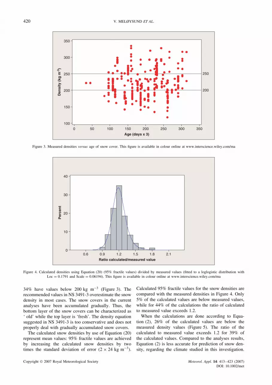
Figure 3. Measured densities versus age of snow cover. This figure is available in colour online at www.interscience.wiley.com/ma

2.11.81.51.20.90.6

40

30

20

10

0

Ratio calculated/measured value

Per

cen

t

Figure 4. Calculated densities using Equation (20) (95% fractile values) divided by measured values (fitted to a loglogistic distribution withLoc = 0.1791 and Scale = 0.06194). This figure is available in colour online at www.interscience.wiley.com/ma

34% have values below 200 kg m−3 (Figure 3). Therecommended values in NS 3491-3 overestimate the snowdensity in most cases. The snow covers in the currentanalyses have been accumulated gradually. Thus, thebottom layer of the snow covers can be characterized as‘ old’ while the top layer is ‘fresh’. The density equationsuggested in NS 3491-3 is too conservative and does notproperly deal with gradually accumulated snow covers.

The calculated snow densities by use of Equation (20)represent mean values: 95% fractile values are achievedby increasing the calculated snow densities by twotimes the standard deviation of error (2 × 24 kg m−3).

Calculated 95% fractile values for the snow densities arecompared with the measured densities in Figure 4. Only5% of the calculated values are below measured values,while for 44% of the calculations the ratio of calculatedto measured value exceeds 1.2.

When the calculations are done according to Equa-tion (2), 26% of the calculated values are below themeasured density values (Figure 5). The ratio of thecalculated to measured value exceeds 1.2 for 39% ofthe calculated values. Compared to the analyses results,Equation (2) is less accurate for prediction of snow den-sity, regarding the climate studied in this investigation.



2.11.81.51.20.90.6

40

30

20

10

0

Ratio calculated value/measured value

Per

cen

t

Figure 5. Calculated values according to Equation (2) divided by measured values (fitted to a loglogistic distribution with Loc = 0.1202 andScale = 0.1038). This figure is available in colour online at www.interscience.wiley.com/ma

2.11.81.51.20.90.6

40

30

20

10

0

Ratio calculated value/measured value

Per

cen

t

Figure 6. Calculated values according to Equation (4) divided by measured values (fitted to a loglogistic distribution with Loc = −0.3535 andScale = 0.1078). This figure is available in colour online at www.interscience.wiley.com/ma

This is because Equation (2) underestimates the snowdensity in many cases. The equation is nevertheless usefulfor simple and rough estimates.

When calculating snow density by use of Equation (4),almost all (97%) calculated densities are below the mea-sured values (Figure 6). The equation is less applicablefor an occasional/arbitrary period in a climate as studiedin this investigation. Equation (4) is meant to be usedfor snow depths with a 50-year return period. A compar-ison between measured snow densities and calculationsby use of Equations (2), (4) and (20) is summarized inTable V.

The density measurements were done within a smallarea in Norway and combined with data from one meteo-rological station. Further work should aim at investigatingthe results in view of data from other parts of the country.Possible measurement uncertainties in conjunction withthe used meteorological station could then be reduced.The capability of the proposed empirical formula to esti-mate snow density in different climates would then alsobe demonstrated.

The current investigation will be used as input to ongo-ing studies within the Norwegian research and develop-ment programme ‘Climate 2000’ (Lisø et al., 2005). In



Table V. Comparison of measured snow density and calculated snow density (in kg m−3) using Equations (2), (4) and (20) (95%fractile values). Statistical data for the ratio ‘calculated value/measured value’.

Densityequation

Mean Standarddeviation

No. of occurrencesbelow 1.0 (%)

No. of occurrencesabove 1.2 (%)

Figureno.

Equation (2) 1.14 0.21 26 39 5Equation (4) 0.71 0.14 97 1 6Equation (20) (new method) 1.21 0.14 5 44 4

‘Climate 2000’, the relationship between snow loads onroof and wind exposure is subjected to further investi-gations (Meløysund et al., 2006, 2007). The significanceof the magnitude of roof snow load according to totalbuilding costs will also be addressed. Will society profitfrom a more detailed prediction of roof snow loads? Theadvantage of a built-in safety margin accounting for afuture change in wind exposure and climate will mostlikely be beneficial.

In recent years, methods to refine the design processwith respect to snow load have been developed. However,advanced tools and data processing are required. Thesetools are often not available for structural engineers, andhigh qualifications within meteorological and geophysicalprocesses are required. The risk that advanced methodswill be used in an unintended manner is thereforepresent. Further work should focus on developing toolsfor geographic differentiation of snow loads, includinglocal topography and climate variations.

6. Conclusions

A clear correlation is found between observed climate andmeasured snow density. A multiple regression equationfor prediction of snow density is developed. The resultsare promising, with a coefficient of determination equalto 70% and a standard deviation equal to 24 kg m−3

compared to measured values.The suggested equation has six predictors and one

constant. The most important predictor RHsnow (sum ofrelative air humidity when snowing) concerns the climateduring snowfalls. Other important parameters reflect theclimate in the whole accumulation period, such as tsun

(the amount of solar radiation) and fdrift (frequency ofhigh wind velocity and simultaneous snow which isable to drift). The parameters RHsnow, fdrift and tsun arefound to increase the density. The parameters d (snowdepth), ptot (sum of atmospheric pressure) and Rp (sumof precipitation as rain) are found to decrease the density.

The most important parameters in density equationspresented in an informative annexe of ISO 4355 are snowdepth, mean wind and mean temperature. Combinationsof these parameters are investigated without achievingsatisfactory correlation. These results are not included inthis paper.

Snow density values calculated by use of the Nor-wegian code NS 3491-3 will in most cases be overes-timated. The expressions in ISO 4355 are less applicable

to prescribe snow density for a climate as studied in thisinvestigation. Still, they can be used as simple and roughestimates.

Acknowledgements

This paper has been written as part of the ongoingSINTEF research and development programme ‘Climate2000–Building constructions in a more severe climate’(2000–2007), strategic institute project ‘Impact of cli-mate change on the built environment’. The authors grate-fully acknowledge all construction industry partners andthe Research Council of Norway. A special thanks to Pro-fessor emeritus Halvor Høibø and Professor Egil Bergeat the Norwegian University of Life Sciences (UMB) forallowing use of their measurements, and to Dr Hans OlavHygen (Norwegian Meteorological Institute) for valuablecomments on the text.

References

Benestad RE. 2005. Climate change scenarios for northern Europe frommulti-model IPCC AR4 climate simulations. Geophysical ResearchLetters 32: L17704.

Engeset R, Tveito OE, Alfnes E, Mengistu Z, Udnæs HC, Isaksen K,Førland EJ. 2004. Snow map system for Norway. In Proceedings,XXIII Nordic Hydrological Conference 2004 , Tallinn.

European Committee for Standardization. 2003. EN 1991-1-1: Eurocode 1 – Actions on Structures – Part 1–3: GeneralActions – Snow Loads. European Committee for Standardization:Brussels.

Harstveit K. 1984. Snowmelt modelling and energy exchange betweenthe atmoshere and a melting snow cover, PhD thesis, GeophysicalInstitute, Meteorological Division, University of Bergen, Norway.

Hedstrom N, Pomeroy JW. 1998. Intercepted snow in the boreal forest:measurement and modelling. Journal of Hydrological Processes 12:1611–1625.

Høibø H. 1988. Snow load on gable roofs. Results from snow loadmeasurements on farm buildings in Norway. In Proceedings, theFirst International Conference on Snow Engineering. CRREL SpecialReport 89-6 , Santa Barbara, 95–104.

International Organization for Standardization. 1998. ISO 4355 Basesfor design on structures – Determination of snow loads on roofs. InInternational Organization for Standardization , Geneve.

Karl TR, Trenberth KE. 2003. Modern global climate change. Science302: 1719–1723.

Langham EJ. 1981. Physics and properties of snow cover. In Handbookof Snow: Principles, Processes, Management and Use, Gray DM,Male DH (eds). Pergamon Press; New York 275–337.

Lisø KR, Kvande T, Thue JV. 2005. Climate 2000 – buildingenclosure performance in a more severe climate. Proceedings, the7th Symposium on Building Physics in the Nordic Countries. TheIcelandic Building Research Institute: Reykjavik; 1195–1202.

Loth B, Graf H. 1998. Modeling the snow cover in climate studies.1. Long-term integrations under different climatic conditions usinga multilayered snow-cover model. Journal of Geophysical Research103: 11 313–11 327.



McCarthy JJ, Canziani OF, Leary NA, Dokken DJ, White KS (eds.).2001. Climate Change 2001: Impacts, Adaptation and Vulnerability.Cambridge University Press: Cambridge.

Meløysund V, Lisø KR, Siem J, Apeland K. 2006. Increased snowloads and wind actions on existing buildings: reliability ofthe Norwegian building stock. Journal of Structural Engineering132(10): 1813–1820.

Meløysund V, Lisø KR, Hygen HO, Høiseth KV, Leira B. 2007.Effects of wind exposure on roof snow loads. Building andEnvironment 42(10): 3726–3736.

Nordli O. 2000. Fjellet i snø, vind, sol og t ake. Dannevigs Fjellbok(in Norwegian). Det Norske Samlaget, Oslo.

Pomeroy JW, Gray DM, Shook KR, Toth B, Essery RLH, Pietron-iro A, Hedstrom N. 1998. An evaluation of snow accumulation andablation processes for land surface modelling. Hydrological Pro-cesses 12: 2339–2367.

Shook D, Gray DM. 1994. Determining the snow water equivalent ofshallow prairie snowcovers. In Proceedings, 51st Annual MeetingEastern Snow Conference, Dearborn, 89–95.

Skaugen T. 1998. Studie av skilletemperatur for snø ved hjelp avsamlokalisert snøpute, nedbør- og temperaturdata (in Norwegian).Rapport nr. 11. NVE – Norges Vassdrags- og Energiverk, Oslo.

Sommerfeld RA, LaChapelle E. 1970. The classification of snowmetamorphism. Journal of Glaciology 9(55): 3–17.

Standards Norway. 2001. NS 3491-3: Design of structures – Designactions – Part 3: Snow loads (in Norwegian). Standards Norway,Oslo.

Tabler RD, Pomeroy JW, Santana BW. 1990. Drifting snow. In ColdRegions Hydrology and Hydraulics, Ryan WL, Crissman RD (eds).ASME: New York, USA; 95–146.

U.S. Army Corps of Engineers. 1956. Snow Hydrology: SummaryReport of the Snow Investigations. U. S. Army Corps of Engineers,North Pacific Division: Portland, OR.

Xue Y, Sun S, Kahan DS, Jiao Y. 2003. Impact of parameterizationsin snow physics and interface processes on the simulation of snowcover and runoff at several cold regions sites. Journal of GeophysicalResearch 108(D22): 8859.


Documents

Predicting snow density using meteorological data