Embed Size (px)
Citation preview
ENVIRONMENTAL CONSULTING amp MANAGEMENT
ROUX ASSOCIATES INC 12 Gill Street Suite 4700 Woburn Massachusetts 01801 TEL 781-569-4000 FAX 781-569-4001
January 20 2014
Mr William Lovely Office of Site Remediation amp Restoration USEPA - Region 1 5 Post Office Square Suite 100 Boston Massachusetts 02109-3912
Re Tinkham Garage Proposed Bedrock Investigation Work Plan
Dear Mr Lovely
Roux Associates has developed the following Work Plan to assess the long-term protectiveness of the groundwater monitoring program at the Tinkhamrsquos Garage Site (the Site) located in Londonderry New Hampshire (Figure 1) It is intended that the results of this work will address issue no 5 of the 2009 Five Year Review Report which states
5 Many of the wells are antiquated and are open borehole and do not provide detailed information about contaminated fracture zones Concentrations remain high especially at FW21D Given that this is an open borehole well it is possible that there is a highly contaminated fracture that is averaged out and that a full understanding of the extent of the plume is not entirely understood
This Work Plan has been developed based upon extensive discussions with the US Environmental Protection Agency (EPA) and the New Hampshire Department of Environmental Services (NHDES) as well as a detailed review of existing data generated over 30 years of investigation remediation and monitoring
Background
The PRPs were asked by EPA and NHDES to assess the long-term protectiveness of the groundwater monitoring program In particular the EPA and NHDES request focused on whether the open-hole bedrock well monitoring is representative of contaminant concentrations in the bedrock aquifer The concern is that unimpacted or relatively clean water from some fracture zones may be diluting the contaminant concentrations in other fracture zones and thus current monitoring in open boreholes may not provide sufficient data to support Site closure
Currently the bi-annual monitoring program includes seven bedrock monitoring wells with either long open intervals or long well screens that may intersect multiple fracture zones
Work Plan
The following Work Plan will provide additional data to address the concerns of EPA and NHDES The Work Plan described below is intended to identify and monitor the significant water bearing fractures in several key monitoring wells representative of Site conditions for water quality and hydraulics Specifically the Work Plan is designed to
CSG11170001M000150WPREV1
Mr William Lovely January 10 2014 Page 2
1 Assess vertical flow within the selected key open hole bedrock wells
2 Assess the hydraulics and water quality of up to three fractures within each of the selected key open hole bedrock wells
3 Determine facture-specific contaminate flux rates and well-specific mass discharge rates and
4 Evaluate and recommend the most appropriate open borehole intervals to demonstrate the long-term protectiveness of the remedy and thereby support Site closure
The wells identified for this investigation were chosen based on a detailed review of
The boring logs for the bedrock monitoring wells installed at the Site to identify significant water bearing fracturesfracture zones
The results of the geophysical testing performed on 11 bedrock monitoring wells in 1984 that were intended to support the identification of significant water bearing fracturesfracture zones
The results of the pumping test completed in 1983 that demonstrated a very strong northeast-southwest flow pattern in the bedrock with little to no perpendicular flow and
The results of over ten years of bi-annual groundwater monitoring
Given the findings of this review the monitoring well locations to be investigated include one source area well (FW11D) one downgradient well within the main northeast-southwest fracture zone (FW21D) and one Groundwater Management Zone (GMZ) compliance well (FW28D) (Figure 2) Monitoring wells FW21D and FW28D are open borehole wells Monitoring well FW11D is an open borehole completed with a 15-inch diameter PVC well screened from approximately 10-feet below the top of bedrock to 98 feet below ground surface (55 feet) The boring logs are included in Attachment A
These locations were selected to provide a good aerial distribution across the Site and measure contaminant concentrations at important Site locations to assess the long-term protectiveness of the remedy The investigation will include geophysical profiling and discrete zone sampling Based on this information the Work Plan includes three primary tasks
1 Replace existing monitoring well FW11D with a larger diameter open borehole bedrock well so that individual fractures can be assessed
2 Complete downhole geophysical testing to identify water producing fracture zones within the new FW11D as well as existing wells FW21D and FW28D and
3 Collection of up to nine discrete groundwater samples from up to three water producing fracture zones identified in new FW11D FW21D and FW28D and testing for VOC and 14-dioxane analyses
ROUX ASSOCIATES INC CSG11170001M000150WPREV1
Mr William Lovely January 10 2014 Page 3
The details for each of these tasks are provided below
Task 1 FW11D Replacement As shown on the boring log FW11D is an open hole bedrock monitoring well that was completed with an 15-inch diameter PVC well screened from approximately 10-feet below the top of bedrock to 98 feet below ground surface (55 feet) Because the current well construction will not allow for downhole geophysics or discrete zone sampling FW11D must be drilled out and reconstructed
The following steps will be followed to complete this task
Step 1 ndash Remove the existing 15-inch diameter PVC monitoring well by over-drilling FW11D with 3 78-inch diameter air hammer style rotary drilling rig to a depth of 103 feet below grade to remove the existing PVC casing well screen sand pack grout and bentonite seals from the existing three-inch diameter borehole
Investigation derived waste (IDW) which will primarily consist of soil and rock waste as well as screen casing and well construction materials removed from FW11D will be containerized and characterized for appropriate off-site disposal
Step 2 ndash Install and grout a four-inch diameter steel isolation casing from grade to three feet into the top of bedrock (approximately 34 feet below ground surface) The isolation casing will extend two-feet above grade and be equipped with a locking cover The annular space between the borehole wall and the steel isolation casing will be sealed with a cement-bentonite grout consisting of Type I Portland cement (ie lsquoneat cementrsquo) mixed with approximately 5 bentonite The addition of bentonite will require additional water to hydrolyze the Portland cement Care will be taken not to over-hydrolyze the mixture in order to minimize shrinkage The recommend mixture is as follows
5 pounds bentonite
94 pounds Portland cement (ie one sack) and
65 gallons water
Step 3 ndash Develop the newly installed open hole well using the pump and surge method to remove any drilling materials that may have entered the new well It is intended that development will continue until groundwater is visibly clear
Development water generated will be discharged to the ground to the south of FW11D
Task 2 Downhole Geophysical Survey
Downhole geophysics were completed on eleven bedrock monitoring wells (including FW28D) as part of the Remedial Investigation (RI) completed in 1985 The objectives of the RIrsquos geophysical investigations were to characterize the bedrock fracture system across the Site including the water-bearing fractures and aid in the location and design of additional monitoring well locations Four logging functions were run during the RI Caliper Single Point Resistance Spontaneous Potential and Natural Gamma
ROUX ASSOCIATES INC CSG11170001M000150WPREV1
Mr William Lovely January 10 2014 Page 4
Based upon the geophysical work and the other RI investigations EPA concluded that the principal water-bearing fractures were encountered at relatively shallow depths (generally less than 80 feet below ground surface)
To expand upon the knowledge and conclusions about bedrock fractures at the Site this task will include the four logging functions previously performed by EPA and will add high-resolution flow profiling using either Heat-pulse flowmeter1 or Electromagnetic flowmeter2 depending on expected flow rates in FW11D and FW21D Additionally flow profiling will also be conducted in existing bedrock monitoring well FW28D Downhole geophysical logging will be accomplished as follows
Step 1 ndash Decontaminate downhole cable and geophysical logging tools with an Alconox or equivalent wash prior to deployment at each monitoring well
Step 2 ndash Complete the following logs (order of logging and logging speeds will be at the discretion of the geophysical subcontractor based on site conditions and available equipment) in new FW11D and existing well FW21D Caliper Probe Natural Gamma Single Point Resistance Spontaneous Potential and Heat-pulse or electromagnetic flowmeter (ambient and induced) Complete flow profiling in FW28D using Heat-pulse or electromagnetic flowmeter (ambient and induced) Each geophysical tool including the caliper probe shall be calibrated according to manufacturerrsquos specifications consistent with procedures outlined in the United States Geological Survey publication titled Application of Borehole Geophysics to Water-Resources Investigations3 Daily calibration logs will be maintained by the geophysical subcontractor and provided along with the raw and interpreted data at the conclusion of the field task
The intended outcome of Task 2 will be to determine hydraulically active fractures quantity vertical flow rates and identify up to three zones in each bore hole for discrete groundwater sampling (Task 3) Data collected during this task will also be used estimate fracture transmissivities and hydraulic heads
Task 3 Collection of Discrete Groundwater Samples
The results of the RI indicate that the principal water bearing zones in the bedrock are relatively shallow (less than 80 feet below ground surface) and that there are generally two to three water bearing fractures This information in addition to the data gathered in Task 2 will be used to identify up to three discrete fracture zones in FW11D FW21D and FW28D for sampling
Up to three discrete groundwater samples will be collected from new FW11D FW21D and FW28D using inflatable pneumatic packers to isolate up to three ten-foot long intervals within each well as detailed in the steps below
1 Heat-pulse flowmeters can measure flow between 001 to 15 galmin 2 Electromagnetic flowmeters can measure flow between 01 to 15 galmin (higher flow measurements are
possible with modifications) 3 United States Department of the Interior 1990 Application of Borehole Geophysics To Water-
Resources Investigations Techniques of Water-Resources Investigations Book 2 Chapter E1
ROUX ASSOCIATES INC CSG11170001M000150WPREV1
Mr William Lovely January 10 2014 Page 5
Step 1 ndash Decontaminate downhole cables tubes pipes pumps and packer assemblies with an Alconox or equivalent wash prior to deployment at each location
Step 2 ndash Set Packers by slowly lowering the pneumatic straddle packer assembly to the predetermined depth and slowly inflate the packers isolate the sampling interval Packers will be of a diameter compatible with the borehole diameter so the sampling zone can be properly isolated (ie sealed off from other depth intervals in the boring) Pressure transducers located within the packer interval and above and below the packer assembly (or depth to water gauging above the top packer) will be monitored during sampling to ensure that a proper seal has been achieved Following inflation of the isolation packers the sufficiency of the seal shall be checked by recording the pressures above below and within the isolated interval for two minutes4 If the pressures remain unchanged then the seal shall be deemed adequate If not the packers will be reset to achieve a better seal Additionally if the hydrostatic pressure above or below the isolation packers changes in response to groundwater sample collection within the isolated interval the packers will be reset to ensure a suitable seal is achieved
Unless data collected during the geophysical phase of this work plan suggests otherwise samples shall be collected first from the shallowest zone followed by the intermediate and then deepest zones
Step 3 ndash Collect groundwater samples from the isolated interval from the perforated pipe located between the isolation packers Prior to implementing sample collection procedures a minimum of three packer interval volumes will be removed Following purging groundwater samples will be collected in general accordance with EPA low-flow protocol and placed in appropriate pre-cleaned and preserved sample containers
Step 4 ndash Remove packer and sampling assembles from the borehole decontaminate as described in Step 1 and or replace disposable sampling equipment with clean components and deploy assembling to the next sampling interval Collect the next groundwater sample as described above The procedure described above will be repeated at each of the three wells to be tested
Groundwater samples will be analyzed for VOCs using method 8260B and 14-dioxane using modified method 16792 consistent with the bi-annual monitoring events The testing results from each interval will be compared within each location and with the results generated from the routine groundwater monitoring of the entire open borehole
Purge water derived during Task 3 and decontamination fluids will be discharged to the ground in the vicinity of the monitoring well
4 Inflation pressures shall be determined according to manufacturerrsquos specifications and using procedures outlined in United States Bureau of Reclamation report USBR 7310 found in United States Department of the Interior 1990 Earth Manual Part 2
ROUX ASSOCIATES INC CSG11170001M000150WPREV1
Mr William Lovely January 10 2014 Page 6
Task 4 Data Evaluation and Report
Following completion of Tasks 1 through 3 the data will be analyzed to assess the yields and the contaminant mass of each fracture zone The hydraulic properties of the target zones will be estimated using a procedure and computer tools developed by the United States Geologic Survey that uses the ambient and induced flowmeter data described in Task 2 above to calculate both fracture transmissivities as well as hydraulic heads as described in a 2011 paper titled A Computer Program for Flow-Log Analysis of Single Holes (FLASH) (Attachment B)5
It is anticipated that the investigation report will include a summary of the investigation procedures and results (including any deviations from the work plan) conclusions based upon the results and the observations and measurements made in the field including
1 Identification of hydraulically active zones within each borehole
2 Evaluation of the vertical flow within each borehole and groundwater flux at hydraulically active factures
3 Contaminant concentrations for each of the sampled fracture zones
4 Flow weighted contaminant flux for each sampled fracture
5 Comparison of sampling results (ie open bore hole sampling completed during routine monitoring) with fracture flow weighted interval sampling and
6 Recommendations for appropriate borehole completion and future monitoring protocols to demonstrate the long-term protectiveness of the remedy and to support Site closure
Sincerely
Attachments
cc Kenneth A Richards New Hampshire Department of Environmental Services Joseph Guarnaccia BASF Michael Walters
5 Day-Lewis et al 2011 A computer program for flow-log analysis of single holes (FLASH) Ground Water doi 101111 j 1745-6584201100798a
ROUX ASSOCIATES INC CSG11170001M000150WPREV1
FIGURES
N
PR
OJE
CT
SC
AN
NO
NS
111
Lo
nd
on
de
ryN
HC
SG
01
M1
40
CS
G7
011
40
01
cd
r
SITE LOCATION
QUADRANGLE LOCATION
SOURCE USGS Windham New Hampshire 75 Minute Topographic Quadrangle
NH
SITE LOCATION MAP
CANNONS ENGINEERING - SITE TECHNICAL COMMITTEE TINKHAM GARAGE SITE LONDONDERRY NEW HAMPSHIRE
Title
Prepared for
CANNONS ENGINEERING
ROUX ASSOCIATES INC Environmental Consulting
amp Management
Compiled by KS 121812Date FIGURE
1 Prepared by CC Scale NTS
Project Mgr IP MAOffice
File No CSG70114001 Project No 111701M
Reed St
TGISCannonsTINKHAMS GARAGE11170001M00150111715002mxd
FW21D
NevinsD
r
Hud
son-
Der
ry R
d
McA
llist
erR
d
Mercury
Dr
ConstitutionDr
Orc
hard
Vie
w D
r
Haley C
t
Eay
ers
Ran
ge R
d
Nas
hua
Rd
C a p
i t o
l H i ll
D r
Winding Pond Rd
e
FW11D
Ross Dr
M o
rr i s o n
D r
Toka nel Rd
P a s t or D r
Wel
sley
Dr
P l u
m m
e r
D r
MableDr
D a v e n p o r t D r
Procto
r Dr
Albany Av
H a r
r i e
t C
t
No
Nam
e
FW28D
sup3
1 inch = 300 feet
0 300 600 900 1200150 Feet
SOURCES -2010 NEW HAMPSHIRE STATEWIDE 1-FOOT COLOR ORTHOPHOTO LAYER -FIGURE 3 MONITORING LOCATIONS AND TOTAL VOLATILE ORGANIC COMPOUND CONCENTRATIONS MAY 2008 FROM THE ANNUAL WATER QUALITY MONITORING REPORT FOR 2008
MONITORING WELL LOCATIONS TO BE INVESTIGATED
GROUNDWATER MANAGEMENT ZONE
MONITORING WELL LOCATIONS TO BE INVESTIGATED
CANNONS ENGINEERING - TINKHAM GARAGE SITE LONDONDERRY NH
Title
CANNONS ENGINEERING
Prepared For
ROUX ASSOCIATES INC Environmental Consulting
amp Management
ROUX Compiled By MH Date 1613
2
FIGURE
Prepared By CC Scale AS SHOWN
Project Mgr KS Office MA
File No111715002 Project11170001M00
ATTACHMENTS
ATTACHMENT A
Boring Logs
ROUX ASSOCIATES INC CSG11170001M000150ATTA
I
I i
il
II
bull
- ITDO No I SHEET HOLE No
Tinkhams Garage 8211-11 1 of 1 FW-11
PROJECT
NUSrmiddot bull middot middot -middotmiddotr I -- ~- middot aA=CAATCN
LOCATION IANGLE FROM HORIZ
Behind garage at Southeast corner of open field 90deg
ICOMPLETEol-ORILLER DRILL MAKE a MODEL IHOLpound OIA OVERBuRDEN IROCK 1111 llOTAL DEPTH
New England Boring (ft) 5-24-83 5- 24-B3 Contractors Inc Mobile B47 3 24 NA 24
BEGUN
CORE RECOVERY (ft) CORE BXS ISAMPLES IELTOPol CAStlGj GROUNO ELjDEPTH to GWTIME IDEPTH to TOP of ROCK
NIA NA 5 I 282 57 I 23077 I O 5-24-83 NA SAMPLE HAMMER WEIGHT FALL CASING LEFT in HOLE =DIALENGTH INUS INSPECTOR
14nt30 l 5 26 J Plunkett
x ROCKE ~ ~ COREREC ROD o a lin)
ss-1
5
ssshy
- -- shy
gt---middot
10
--shy
SOIL PENREC OE~~
( in )middot IN1fi ymiddotshy ELONS6
4114 0-2 l 112-3-18
--- shy
d 11 R S-7 12=ZQ~
-shy
middot shy2414__ 10-11_ 16-1822-31
STRATUM DESCRIPTION
middot
m to c SANO
- shy - shy - ---middotshy - ---- --middot --shy ----+---------- - ---middotmiddot- middot----- shy ----shy --- --- shy ---1
l 5+--+--+---+---+--+-----1 s-4 4114 15-17 lA -11-34-41
TILL
1---+- ---t shy - - - ---middot - - - shy - -- shy
20+--t----+----t----t----1----~ ~s_-_s+-_ __ _ __~1~8~1~2--1~2~0~-2~1-l--~34~-~4~7--9~0~
DETAILED DESCRIPTION
Topso il Dark brown sand and humus
light brown medium-coarse sand little silt little fine gravel
light brown-gray med ium sand little silt 1ittl e clay trace fine grave l
gray finebullmedium sand l ittle silt l i ttle clay trace fi ne gravel
gray fine-medium sand little silt little clay trace fi ne ~ravel trace cobble
gray fine -medium sand little silt little cl ay t race f ine gravel t race cobb le
(compacted till)
5 z
2
l---+---~----+----t-----1-----~-------+--------------------3 25+-----------+---+------1
GRANULAR SOILS COHESIVE SOILS REMARKS
BLOWSFT DENSITY 810WSFT OENSITI
0middot4 V LOOSE lt z V Ubull I
4 middot10 LOOSE Z-4 SOFT
4middot8 STIFF 10middot 3 0 DENSE B-15 STIFI
J0middot50 DENSE 15 shy JO STIFF
gt50 V DENSE gtJO HARO
Bottom of Bor i ng 24 lnstal led
-Screen f rom 24 to 4 -6 riser -Ottawa sand backfill from 24 to 3 - Benton i te from 3 to 1 - Cased cemented and locked
-middot r -middot
l) SS-3 first Indication of contamination shy 5 ppm methane equivalent on OVA
2) SS-4 5 ppm methane equ ivalent on OVA 3) Drilled to 25 sand blew in hol e to 24 bull
PROJECT TOO No SHEET
r_-middot r NUS Ti nkham s Gara e LOCATION
8211-11 1 of 3 ANGLE FROM HORIZ L-7_1 cxFPORATON
Behind the garage sout heas t corner o f open field 5 wes t of FW- 11 90deg
BEGUN COMPLETED j)RILLER DRILL MAKE S MODEL HOLEOIA OVERBURDEN R00lt(11) (11)
6-8-83 6-13-83 New England Boring
Co nt rac to rs Inc Mobi l e B4 7 3 34
CORE RECOVERY (f1) CORE BXS SAMPES ELTOPolCASNG ~EL DEPTH to GW TIME
63 3 2B2 B2 28 1 17 SAMPLE HAMMER WEIGHT FALL
140 30
CASING LEFT in HOLE = DIA LENGTH
1 5100
c ROCK 5 l ~ CORfREC R 0 0 O ( on )
PENREC (1 n )
SOIL DEPTH
INT t
-shy -- -shy __________
15 -1---11-----1----1gt-----+---+------lt
20 -1---1----1----1----+--shy -+------lt
25 +--1---+---1---+---+-------1 s s - 66 25-25 5 11 76
s s shy 12 12 30-31 61-74
STRATUM
DESCRIPTION
Re fer to 1 og for we 11 FW -11
middot
TI LL
1--+- - -+---+---+---+-shy- ---1 Oecomposed Pock
5 60 56 64 t Fractured SCHI ST GRANULAR SOILS COHESIVE SOILS REMARKS
BLOWS FT DENSITY BLOWSFT DENS
0-4 V LOOSE lt V
LOOSE 2-4 SOFT
4- 10 4 - 8 M STIFF
10-30 M OENSE 8 -15 STIFF
30-50 DENSE 15 - 30 V STIFF gt 50 V DENSE gtJO HARO
0 6shy13-B3 NUS INSPECTOR
J Plu nkett
DETAILED DESCRIPTION
Re fer t o log we ll FW- 11
l i ght brown-gray fi ne-med i um sand l i ttl e silt and clay t r ace f i ne gravel heavily compac t ed (comp acted t ill)
compacted t 11
Run 11 34 -39 (fr ac t ured ra schi s t)
I
i
bull ltt i i I
l
I
PROJECT HOLE No
NUS TOD No l SHEET 1
1---IiDkham s GaUU1e__________8_2_11_-_1_1____l2__0_1_3_ ___F_w_-1_1_0_ LOCATION
CCAPCgtRATION
5 west of FW-11~~---------------J____ ----shymiddot---shy
r ROCK SOIL ~ ioL---c-RE-C~-------E-C~-O~EP~T-H~-----Je ~ z c~ ROO PEN R ERlltIL e S60 A lbulln) (o n) IN1T11i LOW
--shy ---1----------1---1------l
40 -1---+-4_8 4_4____7_6-+----+--~-----1
---shy-
45deg1---11-----1----1---4-----1------1
middotmiddotmiddotmiddot-shy ----shyL---1- ----middot ---shy
--middot-shy-shy __6~~~ SOX
-middot-- --shy -50+--+---+---1----1------l------l
--- -middot-middotshy middot- middot -middot-- --middotmiddot-middot shy
-6060 44t
55+--+---+---+----+---+------l
90
60+--+---+---+----+---+------l
middot--shy -shy
60 60 96-65+--+---+---1----+-----l------l
-- shy -shy ----l
middot shy ----shy middot----~---~---
70+---+---+---1----+---4---~
-middot--shy middotmiddot--shy
L-_ - --middot middotmiddot-shy6060 74
75
STRATUM
DESCRIPTION
middot
Frac tured Bedrock
(SCHIST)
REMARKS 1) Washwater 1 taken at 38 2) WW-2 at 42 3) WW-3 at 44 4) WW-4 at 49 5) WW-5 at 53
DETAILED DESCRIPTION
Run Z 39-43
fractu red gray schi st
Run 13 43-48
fra ctured gray schist
Run 4 48-53
fractured gray schist
Run f5 53-58
fractured gray schist
Run 16 58-63
fracture~ gray schist with quartzite
Run 7 63 -68
fractured gray schist with quartz i te vein
Run 8 68-73
light gray quartz i te (ve i n) slightly fractured
Run 19 73deg-78 fractured gray schist with quartzite vein
6) WW-6 at 58 7) WW-7 at 636 8) WW-8 at 68 9) WW-9 at 73
6
8
9
--
---
--- --------
--- --- - ---
--- ---- - - - -------
I PROJECT TOO No SHEET HOLE No- I ~
Tinkhams Ga rage 8211- 11 1 3 of 3 FW- 11 Dl - ~NUS LOCATIONl _ _J caPCAATON
5 wes t ofFW- 11 shymiddot~ ~ROCK SOILz STRATUM It 0poundPTH DETAILED DESCRIPTION 0 COii~ PENRECw 0z RQO BLOWS6 DESCRIPTIONI~0 (1 n ) zlin)
middot middot bullbull l)o ilt
middot-- ~ t4Run 10 78 -83 706059
fra ~ture d gray schis t wi th qua r t zite ve i n shy80
-10 middot Run 11 83 -88 806060
fractured gray schi s t j~85 Bedrock
( SCH ISl)
___ 6060 Run 11 2 88 - 93 54
hea vily frac tured gr ay schi st wi th quart z 90 ve in I
11
_- shyRu n 113 93 - 986060 60 middot-- shy
12 95
fractured gra y sch i s t
middot-middot ----middotmiddotmiddot-- shy
Bottom o f Boring 98middot------shy- Ins tall ed 00 -Screen f rom 98 to 43
- 45 r iser - --middotshy middot---middot-- shy -Otta wa sand backfill from 98 to 34 - Be ntoni te f rom 34 to 24 -Natura1 backfill t o surface - Cased cemen t ed and loc ked
middot-middotshy --- shy
-- ------middot shy
gt
REMARKS 10 ) WW-10 a t 836 11) WW- 11 at 91 I 12) WW-12 a t 95
middot
I I I I I I I I I I I
bullbullbull
I II I STRATIJMI 11middot -ishybullbullbullbull 1lbullntUi-- I ___ _ OEVRIPTLt
I f1eJ l~f
1
r
l 10 tl-~1r----ilr----lr----~11~ 1
---+ll-----lI tri2lcqls I qei I i I I I i I I I I I I I I I I I I I I I I I I I I l I I 11 11e I I I I II1 bii I I
111
11 1
I I~ I I I I I ~~t qQ ill jI I lf I I II I I I I I I I I II I I I I I 1 I I I I I I I I 12~J 11 r 11 I PI I I 1I I I I I II I I I I I i I I I I I I I I I I I I I I I I I I
1 1
11 I
1-l I I j JI 11 rc 1 1 1 1 1
I I I I I I I I I I I I t I 1 I II I J I I I I I I I I I 11 11 1 I 1
1
1 I I I 11111I I I I I
J I 1 1- l I 1
1
1
I I I I middot I I I I I I
r I I I I
GIUHllM sou CDCStoC SlU
CCbullSTl ~ shy ll~KSbull~middot~f~==-1 ~ -
1
II I 1 I 1bull1 I I I I I I I I I I I I I I I I I Z I
I
bullbull _bullbullbull 10 bullbullbull bullMO -
deg -middot-middot
tlXI)bull Qio1cnlt -~~~ iia (ir plf~ (~~)
CIU $1 ~ ~ o-imiddot 2-Ltb ~ ~J ~ ~ rK
I I I~ I
I f$
~ f--41~-+----+---i---+--~~ri
i I f-Z
r r i r s i i T
Lshyi r r I r ~
L r 11 I I I I I rlO
I I I
I I II 1 2I I I l
11~F 1 I I If J I ~Jr
I I 1 1 I1r-~--ili---+---1-I~-~---iL ~1-+---~111
1
~-f~-=~l-middot---11--~---i~bull 1 1 bull I I 1
1r rt1- -+--+---t--=--i1--1-----iIJWl I II I I I I I -middot I I I I I -I I I I
I I I 1
i i 111~1 I I I II = 1 11 I I I Ir
II r I r ~
lrf I r IrIV I ir - I I I
I I r I 2-1I I i r I I I I i r shy~ ICLS COCSM --bull llOtUIQkOoln OlllSTT ~-middot middot- shy4bull10 1bull4
bullbullbull 0middot)0 gtIMO
1~~~ euli~ ~ bulldeg -middot
ri bull
f
r
I I I I ~ j~ampJ- I Ir fT -n ~ ___ r II r I I I I
lrnJ ~ -~ Pt~ I I _-- - bull oAamp I middotk_ I I
I - - lto(J-i --I ~ I I I I
I ~ I Ienmiddotmiddot I II1i_shy
f
l
~ aW-- ~bullbullbulle 441l~
- r ciJ I
(R I ro
~r~+-~-t~~-+o~~-+~~+-~~~-1
I SOIL i_1~1I ftbullbull I -rmiddotm-1 ~f af ~~lo i~~ I bull
I ~01CCiI ---1ifi~ I - -
I LN
r-~
CeuroTAALED tSC-PTOH
I cu~
IFW-210
~
I I I I I I I I I I I I I I I I I I I I I I I I
L__l_ - _I -
[ I I l
I
I I
--
1
- I
1shy
REMARKS
I middot a IC11 bull CAJLIJilITM I __I I _ _
I iJk I --- ___ f I t1 n_J __ 1 - 1 r~ ~~1
I bull 1 l ROCX I SOIL i- i f r
j
I i 1 f I t 11 I JJmiddot1 J r I I - I 1
11
I I I 1
11
omiddotbull bull bull
I l l I I_
1middot4 _bullmiddotbullO middot- bullbull bullbullbull oOmiddotIO ODa ~ ~ N_41i bull oocr -middot
~
j ~O poundCT
I hnc--w-r~ ~
l1Ba+6MHoorJc iOO ~ I bull 1 ~r
f iz14 ~I
J SOii
Il~_=lkJi
I -q1--1tlbullI
I I I I I I II I I I I I III I I I I I I II l
j2COf1---+~_f--~+-~~+-~-+~~~~I
1middot I
1 ~j~+-~--if--~-t-~~-t-~~i--~~---1
L
I I
II L_ I
I I I I I II II II I I
I I I I I
I I I
I I I
I I
bull I I II I
I I I
I I I I l I I II ~ I I I I I II I I I I I
l I I II I I I I I I I II I I
I I II I I I I I II I
I I I I I II I I I I I I II I I I I I II I I I I
I I I I I I I IT
~ I I I I I
REMAllKS
SM(pound r 1 oL _ 1 x - _ I_ I
IFl~ -z_-z IRi1-ZB o I - - ---or ftlJ-Z ~ ~r~ ~ ~ I
1
I I I I I I I I
I I I I I I I
ATTACHMENT B
Guidance Documents
ROUX ASSOCIATES INC CSG11170001M000150ATTA
UNITED STATES DEPARTMENT OF THE INTERIOR BUREAU OF RECLAMATION
USBR 7310-89 PROCEDURE FOR
CONSTANT HEAD HYDRAULIC CONDUCTIVITY TESTS IN SINGLE DRILL HOLES
INTRODUCTION
This procedure is under the jurisdiction of the Georechnical Services Branch code D-3760 Research and Laboratory Services Division Denver Office Denver Colorado The procedure is issued under the fixed designarion USBR 7) 10 The number immediately following the designation indicates the year of acceptance or the year of lase revision
Although rhe term permeability was used in all ocher procedures in this manual percammg co che capacity of rock or soil co conduce a liquid the similar term hydraulic conquctiviry is used throughout chis procedure (See designation USBR 3900 for differences in meaning of rhe two cerms)
Since geologic and hydrologic conditions encountered during drilling are nor always predictable and may nor be ideal variations from chis procedure may be necessary to suit the particular purpose of the resc and conditions at the test sice Much of the information for this procedure was taken from references LI l through L5 l which contain additional information on fielq hydraulic conductivity resting
1 Scope
11 This designation outlines the procedure for pershyforming rests to determine an approximate value of hydraulic conductivity (permeability) of soil or rock in an isolated vertical or inclined interval of a drill hole (boreshyhole) either above or below the water table Usually the rests are performed as a part of the drilling program This procedure can be used in holes of various diameters if suitable equipment is available but N-size L3-in (76-mm)] nominal diameter drill holes are most commonly used2
l2 The constant head single drill hole rest is based on the same theories as the sready-srare or Theim-type aquifer rest and the same assumptions are made These assumptions are ( 1) the aquifer is homogeneous isotropic and of uniform thickness (2) the well (rest interval) fully penetrates the aquifer and receives or delivers water to the entire thickness (3) discharge or inflow is cons rant and has continued for a sufficient duration for the hydraulic system to reach a steady state and (4) flow co or from the well is horizontal radial and laminar Field conditions may not meet all of these assumptions Equations and other factors affecting the rest are given in paragraph 14 Calculations This procedure should nor be used for resting roxic waste containment that requires a very low loss of liquid
13 Constant head hydraulic conductivity rests should be considered scientific tests Grear care should be exercised by chose conducting the rests to eliminate as much error as possible
1 Number in brackets refers co the reference Hereafter referred mas N-size holes
2 Auxiliary Tests
21 The soil or rock penetrated by the drill hole should be identified described and classified from samples taken during the drilling operation Soil can be sampled in accordance with USBR 7010 7015 or 7105 and classified in accordance with USBR 5000 Rock cores or cuttings should be examined and appropriate description and classification made Dara obtained from the drill hole should be entered on appropriate log forms
3 Applicable Documents
31 USBR Procedures USBR 1040 Calibrating Pressure Gauges USBR 1050 Calibrating Pressure Transducers USBR 3900 Standard Definitions of Terms and Symbols Relating to Soil Mechanics USBR 5000 Determining Unified Soil Classification (Laboratory Method) USBR 5005 Determining Unified Soil Classification (Visual Method) USBR 5600 Determining Permeability and Settlement of-Soils [8-in (203-mm) Diameter Cylinder] USBR 5605 Determining Permeability and Serrlement of Soils Containing Gravel USBR 7010 Performing Disturbed Soil Sampling Using Auger Boring Method USBR 7015 Performing Penetration Resistance Testing and Sampling of Soil USBR 7105 Performing Undisturbed Soil Sampling by Mechanical Drilling Methods USBR 7300 Performing Field Permeability Testing by the Well Permeameter Method
1245
2
USBR 7310
32 USER Document 321 Geology for Designs and Specifications by the
Bureau of Reclamation (This document covers both soil and rock)
4 Summary of Method
41 Pump-In Test-Water is injected into an isolated interval of a drill hole in soil or rock and the volume of water injected is determined for a measured period of time The injection pressure is a constant gravity head with or without added pressure head provided by a hydraulic pump The hydraulic conductivity is calculated from the flow rate length and radius of test interval in the drill hole and effective head
42 Artesian Test-Where water under artesian pressure flows out of the drill hole the effective (shutshyin) head at the test interval is measured and the hydraulic conductivity calculated from the flow rate the length and radius of the well and the effective head
5 Significance and Use
51 Hydraulic conductivity tests are made to obtain daca related to (a) identifying seepage potential and dewatering requirements (b) drainage problems (c) ground-water supply investigations and (d) grouting requirements The tests yield approximate values of hydraulic conductivity that are suitable for many engineering purposes Reliability of the values obtained depends primarily on (a) homogeneity of the strata tested (b) suitability of rest equipment used for a given condition (c) care taken in performing the test and ( d) adherence to requirements for proper use of the equations The test is also used in formulating geologic descriptions and interpretation of material properties particularly where there is poor sample recovery
52 Where tests are performed in fractured rock results could reflect secondary conductivity rates which would not represent primary conductivity of the intact mass When the test is performed in fractured brittle swelling clay or rock or where fractures contain loose material hydraulic conductivity may be reduced and judgment should be used in applying results
53 Generally this procedure is suitable for materials in which the hydraulic conductivity ranges between 5 and 100000 ftyr (5 X 10⁻⁶ and 1 X 10⁻¹ cms) and where results are to be used for engineering purposes The procedure is not applicable in materials of lower permeability particularly for purposes such as investigashytions for containment of toxic wastes
6 Terminology
61 Definitions are in accordance with USBR 3900 Some definitions are from Glossary of Geology [6]
62 Terms not included in USBR 3900 specific to this designation are
62 l DnJJ Hole-A circular hole made by drilling
622 Feed Pipe (conductor pipe injection pipe riser pipe drop pipe)-The main pipe (or rod) which conducts water from the collar of the hole into the test interval in the drill hole for the hydraulic conductivity test
623 Baifer-A cylindrical container with a valve on the bortom for admission of fluid attached to a line and used for recovering and removing water cuttings and mud from a drill hole
624 Walking Beam-An oscillating rigid lever balanced on a fulcrum used to activate the cable in cableshytool drilling by alternating up and down motion
625 Aquifer-A water-bearing bed or stratum of earth gravel or porous rock with interconnected openings or pores through which water can move
626 Packer-A short expansible device deliberately set in a drill hole to prevent upward or downward fluid movement generally for temporary use The expansible part of the packer is called the gland Straddle packers are two packers separated by a length of perforated pipe to span or straddle a test interval
627 Artesian-An adjective referring to ground water under hydrostatic pressure ie an artesian aquifer is a confined aquifer Artesian ground water rises above the confining layer in the drill hole and may or may not flow at ground surface
628 Ground W1ter-That part of the subsurface water that is in the zone of saturation
629 W1ter Tizble-The surface between the zone of saturation and the zone of aeration that surface of a body of unconfined ground water at which the pressure is equal to that of the atmosphere
6210 Perched Water Table-A water cable usually of limited area maintained above the normal free water elevation by the presence of an intervening relatively impervious confining stratum
6211 Gauge Saver-A vessel with a pressure gauge filled with glycerin or oil to protect the gauge from direct contact with fluid in the pressure line (see fig 1)
6212 Holding Pressure (applicable primarily for grouting) -The gauge pressure after the water-pumping system has been shut off at the valve ahead of the gauge and backflow is prevented
6213 Back Pressure (applicable primarily for grouting)-The gauge pressure in the system after the holding pressure has dissipated as determined by opening a valve and allowing the gauge ro drop ro zero and then reclosing the valve
6214 Backflow(applicable primarily for grouring)shyThe reverse movement of water out of the drill hole when the holding andor back pressure below the packers exceeds the pressure of the water column in the hole
7 Interferences
71 During drilling it is important ro minimize movement of fines [minus No 200 sieve-size material (75 microm)] into the material being tested and to remove any accumulation of fines from the wall of the drill hole during preparation for the test so as to avoid obtaining test values
1246
USBR 7310
Heov1 Out1 Pressure Gouge
poundLpoundVATON SECTION
TOP VpoundW BOTTOM VIEW
Figure I - Gauge saver device for protecting pressure gauge 40-D-4287
lower than the actual hydraulic conductivity of the material being tested Drilling using clear water without additives is preferred Bentoniticmiddotmuds should nor be used in holes where hydraulic conductivity testing is to be performed Biodegradable additives may be used if necessary but only if the test interval is adequately cleaned before testing The drilling procedure should be documented on the log form
72 Test results can be adversely affected by injecting water containing sediment which would tend to plug voids in the material being tested
73 The temperature of the injected water should be equal to or warmer than that of the ground or ground water This reduces the tendency of air dissolved in the water to become entrapped in the voids of the material be ing tested and co cause low values of _hydraulic conductivity In most areas not affected by artesian conditions the temperature at a depth of about 25 feet (8 m) below the ground surface remains relatively constant at the annual mean air temperature for the region At significantly greater depths temperature rises about l degF (06 degC) for each 500 to 1000 feet (150 to 300 m) of depth The temperature of the injected water especially if it is known to be colder than the ground-water temperature should be recorded on a geologic log or the hydraulic conductivity cesc daca forms (see subpar 812 for suitable temperature measuring devices)
74 It is possible that dissolved minerals in the wacer used for a rest may react chemically wich substances in the material being reseed to cause a change in the hydraulic conductivity Therefore it is desirable to use wacer for the test chat is similar in quality co that expec~ed to permeate che ground when che project is in operation
8 Apparatus
81 Drill Rigs (see fig 2) ~1 ~ Rotary Drilling-A drilling method resulting m grinding a hole with a hard-toothed drill bic at che end of a rocacing drill rod (pipe) The equipment consists essentially of a power unit hoisting or rugging unit controlled-feed rotary drill head and mounting frame masc or tripod and circulating pump The rig should have various accessory drilling andsampling equipment (rods bits core barrels augers) as required for drill hole advancement sampling and testing
812 Cable Tool Drilling-A method of drilling in which the material at the bottom of the hole is broken up by a steel bic with a blunt chisel-shaped cutting edge The drilling equipment consists essentially of a mast a sering of drill tools (casing tubing or pipe of one size) chat is alternately lifted and dropped by a hoist with a power unit and a walking beam A bailer is always used with a cable tool rig Normally a cable tool drilled hole is noc satisfactory for hydraulic conductivity testing with packers
82 Injecrion Pump-A centrifugal or helical screw type pump providing a constant water flow is required This may require a special pump separate from that used for drilling operations Although there may be conditions where a larger or smaller pump may be required highshy
quality pumps having a capacity of 40 galjmin (150 L min) at a pressure of 120 bf in2 (830 kPa) (such as Moriyo model 3L-8 manufactured by the Robbins and Myers Company Springfield Ohio or equivalent) are adequate for most hydraulic conductivity tests The pump should provide the required flow at the required constant pressure with maximum allowable pressure fluctuation-due co pumping pulsations-of plusmn5 percent of the test gauge pressure A surge chamber is required for all testing chis minimizes pulsations which can affect the injection race in the test interval Also ic makes readings more accurate and protects che pressure gauges against damage from sudden pressure changes
83 Feed P1pe- The feed pipe should be of adequate diameter to minimize head losses and have adequate tensile strength to withstand pumping pressures and stresses during hoisting or tugging The feed pipe is commonly a threaded and coupled assembly of pipe or tubing having a uniform inside diameter Drill rods generally of N-size can be used wichouc seriously affecting reliability of rest data if che flow rate to the test interval does nor exceed about 15 galmin (57 Lmin) and the depth co che top of che interval does noc exceed 50 feet (15 m)
NOTE 1-Use of drill rods as feed pipe should be permitted only after the assembled drill rod string has been pressure reseed ro cali_brare head losses ar anricipared flows If seals or sealing marenals are used during calibrarion the same type of seals or sealing materials (not oils or wax) should be used during hydraulic conductivity resting
84 Flowmecers-One or more calibrated flowmecers are required the capacity of each meter should be specified
1247
USBR 7310
- Byooss votve Surgechomber~
Wotermettr-
Observation oost see Detail A
SCHEMATIC ARRANGEMENT OF EQUIPMENT
(Water meter
~==it=======t(k=====- For wottr tes t ing middotWell cas1n9
Press1Jre gouge
-=====bull===========~-For drilling DETAIL A OBSERVATION POST FOR
OPTIONAL EQUIPMENT ARRANGEMENT FOR DETAILS 8 AND C
WATER TESTING ANO DRILLING FROM SECTION X-X TO WELL
DETAIL D GRAVITY TEST
DETAIL B DETAIL C DOUBLE PACKER TEST SINGLE PACKER TEST
Figure 2 - Schematic arrangement of hydraulic conductivity equipment 801-D-l I I
For flows up to 50 galmin (200 Lmin) a 1-inch (25- 851 Pneumatic Piezometers-A down-hole pneushymm) diameter disk-type meter may be used For higher matic piezomerer system has been developed [7] flows a 2- or 2-12-inch (50- or 65-mm) diameter impellershy Descriptions of the equipment and procedure as used ar type meter is recommended two damsites are presented in appendix XL
841 A straight uninterrupted section of pipe having 852 Electrical Transducers-Electrical transducers an inside diameter equal to the rated size of the meter have been used as down-hole pressure sensors by other and a minimum length 10 times the inside diameter of agencies [8) particularly for very low hydraulic conducshythe pipe should be provided upstream of the meter tivities [below 1 ftyr (1 X 10⁻⁶ cms)] The USBR has Manufacturers commonly recommend pipe lengths of one used electrical down-hole sensors in preliminary trials tO two times the inside diameter of straight pipe Electrical transducers measure pressures more accurately downstream from the meter than pneumatic piezometers and can be connected tO a
85 Pressure Sensors-Where required calibrated strip-chart recorder for a continuous record However pneumatic piezometers or electrical transducers can be used transducers are considered less rugged for field use and as down-hole sensors tO measure pressures at the rest require more maintenance and experienced personnel tO
interval during a hydraulic conductivity rest Down-hole operate than do pneumatic piezometers sensors are preferred over the method of calibrating the 86 Pressure Gauges-When down-hole pressure piping system for head loss between a pressure gauge on sensors are not available or sensors are not working the surface and the test interval However an above-ground properly calibrated pressure gauges can be used t0 estimate pressure measurement can provide a check of the pressure effective pressure in rhe rest interval after correcting for sensor friction loss through the feed pipe and packer All pressure
1248
USBR 7310
gauges used in water resting should be high-quality stainless steel glycerin or oil filled wich pressure indicated in both lbfin2 and kPa (such as manufactured by Marsh Instrument Company a unic of General Signal P 0 Box 1011 Skokie Illinois or equal) Pressure gauge ranges should be compatible wich middot cescing requirements chey should be sized so char che gauge capacity does not exceed two co three rimes che maximum desired pumping pressure for each respective pumping stage Gauges should have the smallest graduations possible and an accuracy of plusmn25 percent over che coral range of the gauge If a gauge saver is used wich che gauge calibration should be made wich the gauge saver in place Accuracy of che gauges should be checked before use and periodically during the resting program (see subpar 112 for additional information)
861 One or more pressure gauges should be located downstream of che flowmecer and downstream of any valves ac che cop of che feed pipe This location for pressure measurement can be used by inserting a sub (adaptor or shore piece of pipe) wirh che gauge - installed on che cop of rhe feed pipe
862 Ac least one additional calibrated replacement gauge should be available ar che resr sire
87 Swivel-During che hydraulic conductivity cesc ic is preferable co eliminate the swivel and use a direct connection co the feed pipe If a swivel muse be used in che water line during resting ic should be of che nonconscriccing type and calibrated for head loss Significant friction loss can result from use of che constricting type
88 Packers-One or two (straddle) packers are required for che rest Packers may be either bottom-set mechanical screw set mechanical pneumatic inflatable or liquid inflatable The pneumatic inflatable packer is the preferable type for general use and is usually che only one suitable for use in soft rock and soil The gland of this packer is longer and more flexible chan the ocher types and will form a tighter seal in an irregular drill hole A leather cup type of packer should noc be used To ensure a eight water seal che length of contact between each expanded packer and che drill hole wall should noc be less than three rimes the drill hole diameter
NOfE 2-More than one type of packer may be required to test the complete length of a drill hole The type of packer used depends upon many factors eg rock type drill hole roughness spacing and width of rock joints and test pressures
881 Inflatable Packers-Inflatable packers with an expansible gland and a floating head (see app fig Xl2) should be designed for anticipated drill hole diameters and pressure conditions For normal hydraulic conductivity cescing a reasonable maximum recommended working pressure inside and outside of che packer is 300 lbf in2
(2070 kPa) [8] Inside pressure should be increased in water-filled holes proportionally co che sracic head For drill holes wich sharp projections in the walls a wireshyreinforced packer gland having a higher working pressure [7] may be required The pressure in che packer should not be high enough to fracture the material being reseed
The pressure required to form a cighr seal ac che ends of a cesr interval depends on the flexibility of rhe gland the friction of the floating head and che drill hole roughness The minimum differential pressure between che packer and the cesc interval can be derermined by res ring packers in a pipe slighrly larger rhan rhe nominal diameter of rhe drill hole in order co simulate possible enlargement of rhe drill hole during drilling For a given resr interval pressure che packer pressure is increased until ir provides a waterrighc seal between the packer and the material with which ic is in contact The pressure in rhe packer should range approximately berween 30 and 300 lbfin2 (210 ro 2100 kPa) greater chan char in che cesc interval with 100 lbfin2 (690 kPa) being normal Pneumatic inflatable packers can be inflated with compressed air or compressed nitrogen
882 Special pneumatic packers are available for use in wireline drilling operations Because che packers must be able co pass through che wireline bit and then expand co completely seal che hole ac che cesc interval special materials are needed for che packer gland A special packer assembly-consisting of cwo packers in tandem-is used with the upper packer being expanded inside che drill rod just above che bic and che lower packer expanded against che wall of the hole just below che bit The two packers on the assembly can be positioned properly-relative co the bit-by a sec of lugs or a ring located on the assembly Special seals or connections are needed co attach che water supply co che wire-line drill pipe at the surface
883 A minimum of two secs of replacement packers andor spare glands should be available at the test sire
89 Perforated Pipe Sections-Lengths of perforated steel pipe corresponding ro the lengths of rest intervals are required between packers to admit water inco che rest intervals The coral area of all perforations should be greater than five rimes che inside cross-sectional area of che pipe These perforated pipe sections should be calibrated for head loss
810 Well Screen-Well screen or slotted pipe may be required for cescing in granular unstable materials chat require support [9] As a general rule the maximum size of sloe width should be approximately equal to che 50shypercent size of che particles around the drill hole (see subpar 114)
811 Water Level Measuring Device 8111 Although there are ocher types of water level
indicacors che electrical probe indicator is most commonly used Essentially ic consists of (1) a flexible insulated conduit marked in linear units and enclosing cwo wires each insulated except ac che tips (2) a low-voltage electrical source and (3) a light or ocher means of indicating a closed circuit which occurs when che rips contact che water surface Different brands of electric wacer level indicacors and even different models of the same brand ofren have their own unique operating characteristics Before using any electric water level indicacor it should first be reseed at the surface in a bucket of water
8112 For approximate measurements of the water level when ic is within about 100 feet (30 m) of the ground
1249
USBR 7310
surface a cloth tape with a popper can be used A popper can be made from a short pipe nipple (or length of tubing) by screwing a plug attached to a graduated tape intu one end of the nipple and leaving the other end of the nipple open When the popper is lowered in the drill hole and the open end of the pipe nipple strikes a water surface it makes a popping sound and the depth to water can be measured by the tape
8113 An accurate measuremenr of the water level can be made by chalking the lower end of the steel tape After contacting the water level the tape should be lowered about L more foot before retrieving it Measurement is then made to the wet line on the tape
812 Temperacuie Measuring Device-Equipment for measuring ground-water temperature is available from commercial sources or can be made from a thermistor two-conductor cable reel Wheatstone bridge and a lowshyvoltage electrical source A maximum-minimum type thermometer is acceptable
9 Regents and Materials
91 ~71ter (See subpars 72 73 and 74)-The clear water supply should be sufficient tO perform the hydraulic conductivity test without interrruption and to maintain the required pressure throughout the test period
92 Swd or Gravel Backfill-Where a granular backfill is used t0 prevent sloughing of the drill hole wall it should be a clean coarse sand or fine gravel Laboratory permeability tests (USBR 5600 or 5605) should be made on the backfill material to make sure that it has a coefficient of permeability greater than one order of magnitude higher than that expected of the in situ material being rested
10 Precautions
L01 Safety Precautions L011 This procedure may involve hazardous
materials operations and equipment lO l2 Use normal precautions for drilling [ 10 11] L013 Precautions should be taken during calibration
pressure testing of equipment particularly testing of packers with compressed air or nitrogen (never use oxygen) to avoid injuries from a sudden packer or hose rupture
L02 Technical Prernutions 102 l As a general rule total pressure (static head
plus gauge pressure) applied in the drill hole should nor exceed 1 lbfin2 per foot (226 kPam) of rock and soil overburden at the center of the test interval if the test interval is 10 feet (3 m) long or less If the rest interval exceeds 10 feet pressure should not exceed 1 lbfin 2 per foot of overburden at the top of the interval In layered or fractured material or for drill holes near steep abutments or slopes 05 lbf in2 per foot ( 113 kPa m) of material to the nearest free surface is an appropriate maximum pressure Higher pressures than these may fracture the materials
1022 If there is excessive or complete loss of water when the hole is being drilled drilling should be sropped before cuttings fill the voids and a hydraulic conductivity rest completed on a shorter than normal length rest interval
1023 Hydraulic conductivity rest equipment should be considered and treated as precision testing equipment Gauges thermometers ere should have their own protective cases they should not be carried with drill tools or be tossed around They should be calibrated frequently Ir is recommended that all test equipment needed for hydraulic conductivity resting be kept separate from drilling equipment
11 Calibration
111 For Measurment ofEffeaive Head 11 l l Pressure Sensurs-Calibrate down-hole
pressure sensors by the methods and at frequencies prescribed by USBR LOSO
ll12 Friction Loss Estimates-Where down-hole pressure sensors are nor used estimates of effective head at the rest interval are made by subtracting friction loss from the applied head measured at the ground surface The friction loss should be determined for all components of the piping system from the pressure gauge to the test interval
1112 I Calibrate friction loss in parts or sections of the piping systems including ( L) the swivel (if used) (2) feed pipe (per unit length) and (3) the packer assembly Record the data with references to the particular parts calibrated in tabular or graphical form so the accumulative friction loss can be totaled for determination of effective head at the test interval The calibration procedure is as follows
I l l211 Lay out the individual or joined parts to be calibrated on a horizontal surface with calibrated pressure gauges at each end
l L 12 12 Pump water through the system at incremental increasing flow rares to the maximum flow rare expected to be used in the test allow the flow to stabilize between incremental flows
L 112 L3 Record the pressure at each gauge for each incremental flow rate
11 l 2 L4 Calculate the friction head loss for each incremental flow rare
2f = 23 l ( p ~I p ) (I )
where f = friction head loss in feet of head per linear foot
of pipe ftft or mm P1 = upstream pressure bf in 2 or kPa P2 = downstream pressure lbfin2 or kPa d = pipe length fr or m (d = l for swivel or packer
assembly) 23 l = converts from pressure in bf in2 to head in feet
or 0102 converts from pressure in kPa to head in meters
Example assume
P1 = 186 lbfin2 or 128 kPa P2 = 132 lbfin2 or 910 kPa d = 100 ft or 305 m
1250
USBR 7310
Inch-pound application
f = 231 ( 18 ~~-~3 2) 125 ftfr
SI application
f = 0 102( 128
- 9 tO) = 124 mm 305
l l l215 Plot friction head loss versus flow rare Figure 3 is an example of a plot of friction head loss (f) at relatively low flow races for a 10-foor (33-m) length of 1-14-inch (32-mm) diameter pipe Since head loss in pipe at turbulent flow is approximately related to velocity squared a plot of friction head loss versus the square of the flow rate is nearly a straight line (see fig 4)
NOfE 3-There are srandard rabies and charcs which provide unit friction losses for various sizes of pipe elbows cees reducers ere for clean and ruscy conditions Although such informacion is sometimes used it is preferable to determine friction losses in che piping syscem and packers accually used for che hydraulic conductivity rest
111216 To calibrate a packer inflate the packer in a shore length of casing or pipe in which amiddotvalve and pressure gauge have been installed A pressure gauge is also installed in the rods immediately ahead of the packer assembly Pump water into the rods at incremental increases (or decreases) of flow rate-allowing the system to stabilize after each incremental change-until the highest anticipated flow rate is reached
NOfE 4-For packers smaller than N-size such as the B-size used in wireline equipmentmiddot there are significant head losses and relatively low flow races must be maintained This requires water meters and pressure gauges capable of accurately measuring the low flows and small changes in pressures
112 Pressure Gauges-Calibrate each pressure gauge (see USBR 1040) by comparing it with a test or master
FLOW RATE IN LITERS PER MINUTE
o
I _ I_ I I I II
I I I I I loI I I I I I rI
I I I )I
I I I I I v I I I I I I I I I I lr II
I I
I I I I 11deg II i j~ I I I -~-----1 -- I I I I i
JO deg HOW RATE IN GALLONS PEA MINOT[
Figure 3 - Head loss due ro friction at increasing flow rates for a I 0shy
foot (3-m) 1-14-inch (32-mm) diameter iron pipe
gauge The master gauge should not be used during drilling or hydraulic conductivity testing Calibrate each gauge at the start of a res ring program plus one additional calibration per week during rests of long duration
113 Flowmeters-Calibrate a flowmerer by flowing water into a container of known volume the container used for the volume check should be commensurate in size with the flowmeter size and graduations From these data flow rares can be calculated for comparison with meter readings All flowmeters should be calibrated to an accuracy of plusmn1 percent Calibration should be done at the stare of the resting program plus one additional calibration per week during rests of long duration
NOfE 5-Some impeller-type flowmeters have an accuracy range significantly less than indicated by the dial Minimum and maximum races should be esrablished
114 Well Screens and Perforated or Slotted Pipe Sections-From manufacturers dara or by calibration determine the head losses in expected flow ranges to ensure there is no restriction of flow into the material being tested
12 Conditioning
12 l Nor applicable special conditioning requirements are not needed for this procedure
13 Procedure
13l Cleaning ofDnll Hole 13l1 Remove any accumulation of fine particles
(smear mud cake compaction caused by driving casing etc) from the drill hole wall Such accumulation significantly restricts the flow of water into or from the hole Exercise good judgment in cleaning the hole since excess cleaning may be detrimental If there is a question as to whether or not drill holes in particular materials need cleaning hydraulic conductivity tests can be performed in holes with cleaning and others without cleaning If cleaning does not significantly change rest results at a sire cleaning of additional intervals in the same materials may not be necessary
131 l1 When the rest interval is above the water table it may be possible to brush or scratch the drill hole wall to break up accumulated fines For unstable materials which require use of a well screen materials which cavemiddot against the screen may break up the accumulation of fines on the wall Mild surging with a bailer while adding water also may help break up a disturbed or compacced zone but this may stir up fines which then plug the voids in the material co be rested Mild jetting-followed immediately by bailing or pumping-also is a possibility
13 l l2 When the test interval is below the water table-in materials chat are rock-like and self-supporcingshyuse of a water jet in the hole (preferably accompanied with pumping to induce flow into the borehole) is one of the best methods to clean the hole After jetting bail or pump the sediment-laden water from the rest interval Jetting can also be used through a screen below the water
1251
tJ
I I 0 GO-GI I GO-G2 0 GI -G2
~
I
I
v
v p-shy~ -shyl--~ L--shy
-shy
v
0
middot 005 =0 00005 100
-shy~--~ 0 middot 0025 =0 00005
I 50 I
~ --shy = 0 00005
50
I
t - A
v -
-
[] --shy shy--shy0 -
4--l_-E
-
16
-shy-shy-8 --shyl---shy~ - 2
~ ~---shy z 3 4 5 6 7 8 9
FLOW RATE SQUARED (q 2 )(10001
s of oalmin ) 2
Figu re 4 - Plot of feed p_ipe ca libra tion data - example
USBR 7310
2FLOW RATE SQUARED (q2)( 1000degs of L min)
10 15 20 25 - 30 35
50
40
r w w LL
z
~ 30 0 J Cl ltgt w I
z 0 20 r S a LL
10
0
cable in unstable materials For soft rock flushing che sides of che drill hole by running che bit or a bailer up and down the hole may enlarge the hole by erosion or ocherwise change the characceriscics of the fracture systems
13113 Finally clean the drill hole by pumping or bailing water from the bottom upward with the pumping continued until the return fluid is clear without cuttings or sediment Record the method used in cleaning the hole on the log of drill ho le or on a special testing form
132 Length of Test Interval 1321 The length of the test interval depends on
(1) purpose of the test (2) stratigraphic interval and (3) flow rate Where materials are relatively uniform use a test interval of about 10 feet (3 m) Where flow rates are high shorten the test interval co locate high flow race zones where races are very low the interval may be lengthened if desired
133 Ground-Water Level Determination 13 31 Depth co ground-water level muse be
determined before calculating hydraulic conductivity Measure depths to water levels with an electrical probe or o ther suitable equipment (see subpar 811)
1332 Auger Holes-ln power auger or other types of holes to which water is not added as pare of the drilling process report the presence or absence of a water level depth to water level and dace of initial and final water level measurement In materials of low hydraulic
14
12Cll a w r w
101 z () Vgt 0
8 J
Cl ltgt w I
Sz 0 r u a
4 IL
conduccivicy several days to several weeks may be required for a water level to stabilize in the hole Report evidence of moisture in the cuttings and if a perched water level was observed
1333 Rotary or Cable Tool Holes-For drill holes in which addition of water to the hole is an integral part of the drilling process
13331 Bail or pump the hole dry or to a stable wa ter level at the close of the last shift each day and record level
13332 Report the presence or absence of water and depth to water at the beginning of the first shift each day Additional readings are desirable whenever water level in the hole has nor been disturbed for an appreciable period of time
13333 Report changes in water level detected as the hole is drilled deeper Record faccors that affect the water level such as depth of casing andor cemented intervals These data may be helpful in recognizing perched or confined (artesian) conditions
13334 Upon completion of the hole the water must be bailed down to the extent practicable the water level measured and the dace recorded of hole completion Measure the water level for a period of days or weeks until equilibrium is reached
NOfE 6-At times exceptions must be made to the requirement for conrinuation of water level readings Such is the case when
1252
USBR 7310
state or local laws require chat the hole be filled continuousiy from bottom to cop immediately upon hole completion and before the drill crew leaves the sire In ocher instances landowners may allow right-of-entry for only a limited time for measurements
1334 Perched and Artesian Aquifers-lc is imporshytant tO recognize perched and artesian aquifers especially those under sufficient pressure tO raise the water level above the confining layer but nor tO the ground surface (see (5 ]) They must be distinguished from water table aquifers (those which continue in depth) If perched water table or artesian aquifers-separated by dry or less permeable strata-are encountered in the same drill hole the resulting water level in the hole is a composite therefore conclusions and interpretations based on such data are misleading If a perched water table is recognized (or suspected) during drilling water levels must be determined for each zone for calculation of hydraulic conductivity This might require completion of the drill hole with a watertight seal set at a suitable horizon tO
separate two water table conditions In this type installarion two strings of pipe or conduit are required one extending down to the portion of the hole immediately above the packer and a second string extending through the packer to a point near the bottom of the hole Water-level measurements provide the basis for determining a perched condition or if the lower water table is under artesian pressure
13 35 Mulriple Water-Level Measurements-In some instances it is desirable tO install multiple conduits and packers or plugs in a drill hole so that ground-water levels (or pressure heads) in several water-bearing horizons can be measured over an extended period of time (see [5] pp 7-14)
134 Pressure Tests With Packers 134 l The recommended arrangement of typical
equipment for packer pressure tests without a pressure sensor is shown on figure 2 (See app fig Xl l for equipment with a pressure sensor) Beginning at the source of warer the general arrangement is clean water source suction line pump discharge line tO srorage andor settling tank suction line water-supply pump surge chamber line ro bypass valve junction water meter gate or plug valve tee with sub for pressure gauge short length of pipe on which the pressure gauge is attached tee and off-line bleeder valve for evaluating back andor holding pressure flexible 1-14-inch (32-mm) diameter hose and 1-14shyinch-diameter feed pipe ro packer or packers in drill hole which isolate the rest interval All connections should be tight and as short and straight as possible with minimum change in diameter of hose and pipe Friction loss decreases as the pipe diameter is increased
1342 When the material is subject co caving and casing andor grout is needed to support the walls of the drill hole the hole should be water rested as it is advanced Other hole conditions may make this procedure desirable or necessary The following procedure is commonly used
1342 l After the hole has been drilled to the top of the interval to be tested it may be desirable tO remove
the drill string from rhe hole and advance casing or grout ro rhe bonom of the hole
13422 Advance the hole 5 to lO feet ( 15 to 3 m) into the material to be rested
13423 Remove the drill string from rhe hole 13424 Clean the interval to be tested and record
the depth tO the warer table if present If a composite water level is suspected the warer level affecting rhe rest should be determined by measurements through the feed pipe after rhe packer has been seated and the water level has stabilized
13425 If rhe hole will stand open sear a single packer ar the top of rhe test interval Record the type of packer irs depth and packer pressure if it is rhe inflatable type
13426 Pump water into the interval ar a rate to develop a suitable pressure The pressure to be used depends upon testing depths and ground water levels or pressures Materials subject to deformation or heaving such as by separation of bedding planes or joints or materials at shallow depths must nor be subjecred to high pressures (see subpar 102 l ) For comparison of flow rates in different pares of a single foundation and with results from other foundations some of the following pressures are commonly used 25 50 75 and LOO lbfin 2 (170 350 520 and 690 kPa)
NorE 7-At test pressures less than 25 lbfin2 errors in measurement of pressure and volume of water may increase unless special low pressure gauges are used Gravity tests provide more accurate results under these conditions At pressures higher than 10 lbfin2 difficulties in securing a right packer seal and the likelihood of leakage increase rapidly However under artesian pressures or in deep holes the water pressure-as registered on a surface gauge-will need to be sufficient to overcome the effeccive head at the test interval and firmly seal the packer
NillE 8-Where the hole is subject to caving a pump-down wire-line system has been developed rhar can be used to eliminate removal of the drill string from the hole With this system the hole is drilled to the bottom of the interval tO be tested and the drill rod is raised so the end of the rod is at the top of the test interval The tandem packer (see subpar 882) is then lowered through the drill rod and expanded to seal both inside the rod and against the wall of the hole at the cop of the test interval Models of this equipment are available which have transducers below the packer for measuring water pressures at the test interval
13427 For determining effective head artesian heads encountered in the drill hole are treated the same as water table conditions ie the depth from the pressure gauge or the water level maintained during the test to
the stabilized water level is used as the gravity head If the artesian head stabilizes above the ground surface the gravity component of the effective head is negative and is measured between rhe stabilized level and the pressure gauge height If a flow-type rest is used the effective head is the difference between rhe stabilized water level and rhe level maintained during the flow period
1253
USBR 7310
13428 Afrer pressures are selected based on ground-water conditions and the purpose of the test perform a test at each pressure Usually a 5-cycle procedure is used three increas ing steps to the maximum pressure and then two decreasing steps to the starting pressure This cycling allows a more derailed evaluation of rest results than testing at a single pressure and commonly allows extrapolation to ascertain at what pressures the following may occur (1) laminar flow (2) turbulent flow (3) dilation of fractures ( 4) washouts (5) void filling or (6) hydraulic fracturing However the equations normally used to ca lculate hydraulic conductivity are based on laminar flow conditions
NOfE 9-ln some insrances on ly a single water pressure test at a given interval in the drill ho le may be required For example if geologic conditions are known and there is no need ro perform the seeps in subparagraphs 13422 through 13426 a single value of hydraulic conductivity with a relatively low application of pressure may suffice
13429 During each test continue pumping water to the test interval at the required pressure until the flow rate becomes stable As a general guide maintain flow rares during three or more 5-minute intervals during which l-minute readings of flow are made and recorded In tests above the water table water should be applied to the test interval until the flow rate stabilizes before starting the 5-minuce measurement intervals Where tests are below the water table flow rates usually stabilize faster than for the tests above the water table and the time period before the 5-minure test intervals may be shorter These rime periods may need to be varied particularly when rests to determine grouting requirements are made
134210 Determine and record the presence of back pressure and decay of holding pressure Afrer the rest deflate the packer and remove it from the drill hole
134211 Advance the drill hole and if necessary the casing repeat the procedure in subparagraphs 13423 through 134210 until the required depth of drill hole is reached When casing is used in a drill hole always set the packer in the material below the casing
1343 If the hole will stay open without casing it can be drilled to final depth and after cleaning the hole hydraulic conductivity rests can be performed from the bottom of the hole upward using straddle (double) packers Although a single packer can be used to test the bottom interval of the hole starting at the bottom with double packers will cause loss of borehole testing of only about the length of the bottom packer and will save one complete trip in and out of the hole with the drill string assembly co change the packers After the test for the bottom interval is completed straddle packers are used for successive test intervals up the drill hole See subparagraph 1342 where caving or other hole conditions will not allow this procedure
135 Gra vity Tests 135 1 Constant-head gravity tests are usually
performed without packers above or below the water table with drill holes of N-size or larger (see fig 2 derail D)
This type of test is often made in reasonably stable-walled drill ho les up to 25 feet (76 m) depth where water pressure at the test interval needs to be kept low The test is usually performed in successive 5- or 10-foot (l5- or 3-m) intervals as the drill hole is advanced The upper end of each test interval is normally determined by the bottom depth of tightly reamed or driven casing If the casing is not believed
middotto be tight appropriate entries should be recorded on the log form If the wall of the drill hole is stable the test can be performed in the unsupported hole If the wall needs to be supported use a well screen (see subpar 114 for calibration) inserted through the casing It may be necessary to ream or drive the casing to the bottom of the interval set the screen and then pull back the casing to expose the screen Afrer the test the screen is removed and the casing reamed or driven to the bottom of the hole
NOfE lO-Clean coarse sa nd or fine gravel backfill (see subpar 92) may be used instead of a well scree n Ream or drive rhe casing ro the borrom of the inrerval dean ir our and add rhe backfill as rhe rnsing is pulled back ro expose rhe resr interva l Record use of rhis procedure on the log form
l 35l l If the drill hole is self-supporting clean and prepare it in rhe normal n1anner (see subpar 13l)
l35 l2 If the drill hole is not self-supporting lower the well screen and casing into the hole
135 l3 For test intervals above the water table maintain a constant head of water _within 02 foot (60 mm)] at the top of the test interval by injecting water through a small diameter rube extending below the water level maintained during the test For rest intervals below the water table or influenced by artesian conditions maintain a constant head a short distance above the measured static water level
Monitor the water level with a water-level indicato r If the water-level indicator is inserted in a small diameter pipe in the casing the wave or ripple action on the water surface will be dampened and permit more accurate watershylevel measurements
NOfE l l-When rhe flow rare is very low rhe consranr wa rer level c1n be maintained by pouring warer in rhe hole from a graduated container
135 l4 Record the flow rate at wne intervals until a constanc flow rare is reached
135 l5 Repeat the procedure of subparagraphs 135 l3 and 135 14 at one or more different water levels
13516 This rest is essentially the same as desigshynation USBR 7300 (see also L3] p 74) the instructions in USBR 7300 for performing the rest and calculating hydraulic conductivity apply to this procedure also
14 Calculations
14 l For pressure or constant gravity head hydraulic conductivity rests calculace the hydraulic conductivity of
1254
USBR 7310
rhe soil or rock by rhe following equation (expressed m consisrent unirs) [4]
k = ~ In ~ where L ~ lOr (2)
or
k = ~ sinh-1 r where lOr~ L ~ r (3)
where k = hydraulic conducrivity fryr or cms q = consrant race of flow into che rest interval
ft3yr or cm3s L = length of the test interval ft or cm
H = differential head of wacer ac rest interval fr or cm
r= radius of the borehole ft or cm In= natural logarithm loge
inv~rse hyperbolic sin~ smh- 1 x In (x + -yx2 + 1)
142 An example calculation for a single packer test _ in the botrom of a borehole belovt the wacer table follows
Example assume
r = 18 in or 015 ft= 46 cm q - 22 galmin or 83 Lmin q = 15 X 10 ft3yr = 140 cm3s L 30 ft = 91 cm
Hg gravity = disrance from ground-water level co pressure gauge = 102 ft = 311 cm
Hp pressure 5 lbf in2 X 231 ftwater (lbf in2)
116 ft = 3 54 cm of water H = Hg+ Hp= 218 ft= 664 cm
~ = ~lo = 20 hence use equation (2) 5 k = _9_ In]
2rrLH r k = 15 X 10 ft3 yr In 30 ft
2rr (30 ft) 218 ft 015 ft k = 11X103 ftyr = 11 X lQ-3 cms
NafE 12-These equations are most applicable and reliable where the length of test interval is at lease 5 r and the interval is below che water table The equations are based on laminar flow of fluid through porous media Flow races high enough co cause turbulent flow invalidate the results in all types of material In fractured material the calculated value should be considered an apparent hydraulic conductivity even under laminar flow conditions
143 For pressure resrs when rhe resr interval is below the water table H is the distance from rhe water table to the elevation of che pressure gauge plus applied pressure converted to linear units of water head
Where the rest interval is above the water table His rhe distance from rhe midpoint of the isolated rest interval to che elevation of the pressure gauge plus the applied pressure converted to linear units of water head
For gravity rests above che water table H is che distance between che boccom of the tesc interval and che water level maintained during the test
For gravity rests below the water cable His che distance between the pretest stabilized wacer level in the drill hole and the water level maintained during the rest
144 If chere is artesian pressure an additional pressure muse be applied to overcome che artesian pressure co provide an effective rest pressure For example if there is an artesian pressure of 5 lbfin2 (34 kPa) ac che pressure gauge 15 lbfin2 (103 kPa) could be applied chen che effecrive pressure would be 15 lbfin2 minus 5 lbfin2 which equals 10 lbfin2 (69 kPa)
145 The calculations can be done conveniently by (1) a nomograph [12] (2) a hand calculator with che proper functions or (3) a com purer For repeared tests ic is convenient to prepare a table for one or more diameter drill holes and lengths of resc intervals and combine che terms on che right side of the equations other than q and H into a coefficient
NafE 13-The lugeon (lugeon unit lugeon coefficient) [ 13 14 15 16] has been used as an index of hydraulic conductivity in connection with cyclic rests and for grouting purposes
15 Report
151 Record field test data on a daily driller s report and or on rhe log of the drill hole or on a special reporting form designed for the specific project Record the following
1511 Log of the drill hole 1512 Elevations of the ground surface the water
cable and che top and bortom of the rest interval 1513 Diameter of the drill hole at test interval 1514 Method of cleaning the drill hole 1515 Size of the feed pipe and any well screen 1516 Water pressure andor gravity head and flow
rare for each rime interval 1517 Tora[ amount of warer used per resr 1518 Average temperature of ground warer and
water used in the rest 1519 Packer inflation pressures 1511 Capacity of pump supplying water to the
rest interval 15111 All head loss calibrarion dara 15112 Nore any comments considered necessary to
help evaluate che rest results
15 References
[ l] Permeability Tests Using Drill Holes and Wells Bureau of Reclamation Geology Report No G-97 Denver ColoradoJanuary 3 1951
[2] Ground Warer Manual lst ed rev reprint Bureau of Reclamation US Government Printing Office Washington DC 1981
1255
USBR 7310
[3] Drainage Manual lsc ed 2d princ Bureau of Reclamacion U S Governmenc Princing Office Washingcon DC 1981 1984
[4] Zangar Carl N Theory and Problems of Water Percolation Engineering Monograph No 8 Bureau of Reclamation Denver Colorado 1953
[5] Drill Hole Water Tests Technical lnstructionsshyProvisional Engineering Geology Bureau of Reclamation July 1970 (unpublished)
[6] Glossary of Geology 2d ed American Geological lnscitute Falls Church Virginia 1980
[7] Haccher R C High Pressure Inflacable Packer with Pneumatic Piezometer Bureau of Reclamation Reporc GR-10-75 Denver Colorado October 1975
[8] Bennett R D and R F Anderson New Pressure Test for Determining Coefficient of Permeability of Rock Masses Technical Reporc GL-82-3 US Army Engineer Waterways Experiment Station Vicksburg Mississippi 1982
[9] Ground Water and Wells A Reference Book for the Water-well Industry 1st ed published by Edward E Johnson Inc Saint Paul Minnesota 1966
[10] Drillers Safety Manual 1st ed reprint Bureau of Reclamation Denver Colorado 1982
[11] Acker W L III Basic Procedures for Soil Sampling and Core Drilling published by the Acker Drilling Company Scranton Pennsylvania 1974
[12] Underground Mining Methods Handbook No 580 W-88 Society of Mining Engineers Littlecon Colorado p 62 1982
[13] Lugeon M Barrages et Geologie Dunod Paris 1933
[14] Houlsby A C Routine Interpretation of the Lugeon Water-Test Quarterly Journal Engineering Geology vol 9 pp 303-313 1976
[15] Heitfeld K H and L Krapp The Problem of Water Permeability in Dam Geology Bull International Association of Engineering Geology No 23 pp 79-83 1981
[16] Pearson R and M S Money Improvements in the Lugeon or Packer Permeability Test Quarcerly Journal Engineering Geology vol 10 the Netherlands pp 221shy239 1977
1256
USBR 7310
APPENDIX
XL PROCEDURE USING A PNEUMATIC PIEZOMETER WITH TWO PACKERS ISOLATING THE TEST INTERVAL
Xl l Equipment Assembly (Refer to figs Xll and X l2) -A complete straddle packer unit is assembled as follows
X 11 l Co nnect a predetermined length of perforated injection (feed) pipe to the lower packer (The length of perforated pipe is determined by the thickness of the zone to be rested) Connect the inflation tubing to the lower packer and lower the sliding head end of the packer into the drill hole (See subpar l l l216 for calibration of packers)
Xl l2 Clamp the top of the perforated injection pipe at the hole collar and connecr the upper packer with the sliding head already down the hole
Xl l3 Provide approximately 12 inches (300 mm) of slack in the inflation tubing between the two packers to allow for retraction of the upper packer sliding head Connecr the tubing to the upper packer
Xl l4 Install the pneumatic piezometer piezomerer tubing packer inflation tubing and sealed lengths of injecrion pipe to the head adaptor
X ll5 Lower the entire unit into the drill hole adding lengths of sealed injection pipe as necessary to reach the
( Storoqf Settling ton
interval to be tested As the unit 1s lowered che packer inflation cubing and che piezomecer tubing is unreeled into che hole and caped to che sealed injection pipe at approximately 10-fooc intervals
Xll6 Upon reaching the rest depth lock both the inflation cubing reel and rhe piezomecer cubing reel connecr the inflation tubing by quick-connecr couplings co a nitrogen or compressed air boccie equipped with a high pressure regulator connecr the piezomecer cubing by quick-connect couplings co the readout box and connect the injection pipe co the water pressure source The cesc is now ready to begin
Xl2 Test Procedure
X 12 l After the unit has been lowered to the rest interval and before infacing the packers any water head above the cesc interval must be determined This head will sho w as pressure on the pneumatic piezomecer gauge and can be verified by running a water level indicator into che hole to measure the deprh co the water cable The piezometer will register water pressure chat can be converted to head of water This water head should be
Compressed 01r or nitrogen bot tie Regulator_
Poc~er air lin e- I
P1nometer ln1ec t1on oioe head adaptor
Lo er ooc~er inflation tubmr
Figure X 1 1 - Schematic arrongemem of drill hole packer and pressure monimring equipment 801-0-180
1257
USBR 7310
------=--From compressed air or nitrogen boltle
From piezometer
_To
PRESSURE READOUT BOX
Packer inflation tubing From wafer source From air or Water injection pipe ring seals
PIEZOMETER TUBING REEL
Pressure seals Wire reinforced rubber gland clomps
nitrogen ~~i==-=~==t~f=lil~~~jii~9ll~~~~~sect9ll~sect~sectsect~~~sectl~iilf~f--- To per for o t e d ~~~ze=zzzoCzzzze=zzze=plusmnzz~EZio~~~~21p~
To pressuresource~~~~~~~~~~~~~~~readout box
Piezometer
~~~~~~~~~~~~~~~~---
Inflation chamber Floating packer head Packer inflation lubing
UPPER DRILL HOLE PACKER AND PRESSURE MONITORING EQUIPMENT FOR N X HOLE
Figure X 12 - Upper Jrill hole packer anJ pressure monitoring equipment for NX hole
used to determine the minimum inflation pressure to be applied co the packers by the following equation
SH+ PP+ PE = minimum inflation pressure
where SH = static pressure at the midpoint elevation of the
test interval lbf in2 or kPa PP = gauge pressure to be maintained during the test
lbfin2 or kPa PE = pressure needed to expand packer to hole
diameter as determined before insertion in the drill hole by expanding the packer in a length of pipe having a diameter similar to the hole diameter lbfin 2 or kPa
Inflation pressure gauge is in units of lbf in2 (kPa) The static water level measured before the packers are
inflated might be a composite water level (see subpar 1334)
Xl22 Inflate the packers and determine water head for the rest interval This is the static head to be used for calculation of hydraulic conductivity If rhe static head is significantly different from the composite measured
before the packers were inflated recalculation of packer inflation pressure may be required The final packer inflation pressure should be the lowest practical pressure to seal the test interval against the maximum injection pressure to avoid fracturing of the material being tested
Xl2 3 After the inflation pressures have been determined deflate the packers fill and flush the system with water until all entrapped air has been removed This is accomplished by filling the injection pipe under a gravity head and leaving the air-release valve open ar the top of the injection pipe tee at an elevation higher than the injection hose The valve must remain open until all air has been removed and water runs freely indicating a filled system At this point water is flowing around the deflated packer system and is completely filling the annulus between the drillhole and the packers In the case of an interval with a high injection rate it may be necessary to keep the air valve closed to keep from entraining air into the test interval
X 124 Close the air release valve at the top of the injection pipe and slowly inflate the packers to the predetermined inflation pressure
Xl2 5 Lock in the inflation pressure by closing the pressure valve in the packer cubing If the pressure gauge
1258
USBR 7310
on the closed system remains steady it verifies a sealed system At this point water injecced under gravity head approaches a constant flow rate
X 126 Record the piezometer pressure after packer inflation For an interval of very low injection rate this is equal to che height of the injeccion standpipe plus che pressure recorded at the hole collar gauge For a test interval with a high injection rate the readout would show the same value less any friction from water flow through the injeccion pipe
X 127 Proceed with the test by applying the selected pressures ac the test interval and moniroring the flow rate and pressure on the pneumatic piezometer
X 128 To accurately compute hydraulic conduetivity rhe down-hole pressure muse remain constant A zone with a high injection rate must be monirored more closely than a zone with a small injection rate and adjustments made to hold the down-hole pressure constant To accomplish
this che injeccion pressure shown on che collar gauge must be adjusted in order co maintain che down-hole pressure constant
NOfE X 1-For example a pressure srage is scarred with the collar gauge reading 35 lbfin2 (241 kPa) and the down-hole piezomerer reading 200 lbf in2 ( 1380 kPa) As rhe flow increases rhe down -hole pressure may drop to 150 lbfin2 (1034 kPa) because fricrion loss in the injection pipe and the collar gauge would have to be adjusted to bring the down-hole pressure gauge back up co 200 lbfin2bull When the flow decreases from a fast to a slow rare the collar gauge pressure would have to be decreased
Xl29 The cesc is completed following one or more stages of pressure increases and pressure decreases Following the last stage deflate the packers and close the injection line The system is now ready to move to the next test interval for repetition of this procedure
1259
Methods Note
A Computer Program for Flow-Log Analysis of Single Holes (FLASH) by Frederick D Day-Lewis1 Carole D Johnson2 Frederick L Paillet3 and Keith J Halford4
Abstract A new computer program FLASH (Flow-Log Analysis of Single Holes) is presented for the analysis of
borehole vertical flow logs The code is based on an analytical solution for steady-state multilayer radial flow to a borehole The code includes options for (1) discrete fractures and (2) multilayer aquifers Given vertical flow profiles collected under both ambient and stressed (pumping or injection) conditions the user can estimate fracture (or layer) transmissivities and far-field hydraulic heads FLASH is coded in Microsoft Excel5 with Visual Basic for Applications routines The code supports manual and automated model calibration
Introduction Flowmeters provide means to infer the flow into or
out of boreholes connected to transmissive aquifer units or fractures In the past the relative inaccuracy and difficult operating procedures for spinner flowmeters limited the use of borehole flow measurements With the advent of heat-pulse (Paillet et al 1996) and electromagnetic (Molz et al 1994) instruments measurements of vertical flow as small as 005 Lmin became practicable and borehole flowmeter logging is becoming routine New modeling and analysis tools are needed to achieve the full potential of these measurements
1Corresponding author US Geological Survey Office of Groundwater Branch of Geophysics 11 Sherman Place Unit 5015 Storrs CT 06269 (860) 487-7402 ext 21 fax (860) 487-8802 daylewisusgsgov
2US Geological Survey Office of Groundwater Branch of Geophysics 11 Sherman Place Unit 5015 Storrs CT 06269
3Office of Groundwater Branch of Geophysics (Emeritus) US Geological Survey 11 Sherman Place Unit 5015 Storrs CT 06269
4US Geological Survey Nevada Water Science Center 2730 N Deer Run Rd Carson City NV 89703
5Any use of trade product or firm names is for descriptive purposes only and does not imply endorsement by the US government
Received April 2010 accepted December 2010 copy 2011 The Author(s) Ground Water copy 2011 National Ground Water Association doi 101111j1745-6584201100798x
Calibration of a borehole flow model to flowmeter data can produce estimates of transmissivity and heads for one or more flow zones (aquifer layers or fractures) Here we briefly review approaches for analysis of flowmeter logs and introduce a new computer program which supports manual and automated calibration of an analytical borehole flow model
Approach Single-hole flowmeter data can be analyzed to
estimate transmissivity profiles along boreholes and characterize aquifer compartmentalization (Molz et al 1989 Kabala 1994 Paillet 1998) Analysis of single-hole flowmeter data is commonly based on the Thiem Equation (Thiem 1906) which written for confined radial flow from a single flow zone (ie aquifer layer or fracture) to a screened or open well is
2πTi(hw minus hi)Qi = minus (1)
ln(r0rw)
where Qi is the volumetric flow into the well from flow zone i [L3Tminus1] hw and hi are respectively the hydraulic head [L] at the radius of the well rw and at radial distance r0 commonly taken as the radius of influence where heads do not change as a result of pumping in which
926 Vol 49 No 6ndashGROUND WATERndashNovember-December 2011 (pages 926ndash931) NGWAorg
case hi is the connected far-field head for zone i and Ti
is the transmissivity of flow zone i [L2Tminus1] A number of approaches to flowmeter analysis have
been proposed and demonstrated for different sets of assumptions (eg no ambient flow in boreholes) and data requirements (eg flow profiles collected under both ambient and stressed conditions) based either on Equation 1 (Molz et al 1989) or quasi-steady flow approximations (Paillet 1998) We refer the interested reader to Williams et al (2008) for additional background on flowmeter logs and focus the following discussion on the approach of Paillet (1998 2001) which is adapted here
Paillet (1998) formulated flowmeter log analysis as a model-calibration procedure involving flow profiles collected under both ambient and stressed (pumping or injection) conditions Consideration of the two conditions allows for the estimation of the transmissivities and also far-field heads of flow zones The latter is critical for the interpretation of water samples from wells that intersect multiple fractures or layers with different hydraulic head (Johnson et al 2005) Applying Equation 1 to an ambient condition (condition a) and a stressed condition (condition s) gives
factorT total(ha minus h02πTi )w iQa = minus (2)i ln(r0rw) factorT total(hs minus h02πTi )w iQs = minus (3)i ln(r0rw)
where T factor i is the fraction of the boreholersquos transmisshy
sivity contributed by flow zone i [ndash] T total is the total transmissivity of the flow zones intersected by the bore-hole [L2Tminus1] ha hs are the ambient and stressed water w w levels in the well respectively [L] h0 is the far-field head i in flow zone i [L]
For both ambient and stressed conditions the water level in the borehole is assumed to be constant in
time and the water level in the far-field of each zone is assumed to be the natural condition that is hi
0 In a field experiment (Figure 1) rw would be known and the flow rates and water levels in the well would be measured Radius of influence can be inferred experimentally based on head data at observation wells in which case r0 can be constrained during calibration or else it can be approximated (Bear 1979 306) Estimates of transmissivity are not strongly sensitive to the value assumed for r0 because it appears inside the logarithm in Equations 2 and 3 For example a change in r0rw
from 10 to 100 yields a change in the estimated Ti of only a factor of 2 and order-of-magnitude estimates of transmissivity are acceptable for many problems In cases where knowledge of r0 is unavailable but the boreholersquos total transmissivity is known from specific-capacity or slug-test results it is possible to estimate r0 in the calibration procedure We note that the forward model (Equations 2 and 3) produces twice as many independent equations as there are flow zones with an additional equation requiring T factor values to sum to 1 The number of parameters being estimated is twice the number of flow zones (T factor and h0 for all i) plus one parameter for either i i T total 0or r i
Model calibration involves changing the model parameters such that the flows predicted by Equations 2 and 3 match the interpreted flow profiles Following Paillet (1998 2001) calibration is to the interpreted profile and not individual data This formulation allows the user to incorporate additional insight (eg from other logs) to identify the number and locations of flow zones and elimshyinates the need for weighting measurements differently according to variable measurement errors and the spatial distribution of measurements along the borehole
Calibration can be implemented by manual trial-andshyerror or automated using nonlinear regression Whether manual or automated the goal for calibration is to identify the set of parameters that minimize a measure
Figure 1 Schematic of flowmeter experiment in a fractured-rock aquifer with (a) flow-log profiles for ambient (blue) and stressed (dashed red) conditions and conceptual cross sections of flow system for (b) ambient condition and (c) stressed condition In this example two flow zones (fractures) intersect a well Under ambient conditions flow enters the well from fracture 1 and exits from fracture 3 Under pumping conditions flow enters the well from fractures 1 and 2 The far-field head of zone 2 is equal to the ambient water level thus there is no flow tofrom zone 2 under ambient conditions The far-field head of zone 3 is equal to the stressed water level thus there is no flow tofrom zone 3 under pumping conditions
NGWAorg FD Day-Lewis et al GROUND WATER 49 no 6 926ndash931 927
of combined data misfit and model misfit Considerashytion of model misfit criteria commonly referred to as regularization is useful when multiple models can match the data equally well or within measurement errors Here the data misfit is formulated based on squared differshyences between the predicted and interpreted flow profiles such that multiple measurements may be collected in a single borehole interval The model misfit could be forshymulated in different ways but we use criteria based on the differences between the water level in the borehole under ambient conditions and the far-field heads Thus the objective function F consists of two terms (1) the mean squared error (MSE) between interpreted and preshydicted flow profiles with equal weights for all cumulative flows (ambient and stressed) and (2) the sum of squared differences (h) between the boreholersquos water level and far-field heads
n1 2ssim sintmin F = Q minus Qi i n
i=1
n asim aint 2+
Q minus Q
2 + α (hi) (4)i i i=1
subject to constraints
factor factorT ge T for all i andi min
ABS(haw minus h0
i ) le hmax for all i
aintwhere Qi Qi sint are the interpreted flow profiles (ie
cumulative flow above zones) for zone i under ambishyasiment and stressed conditions respectively [L3Tminus1] Qi
ssimQi are the simulated flow profiles (ie cumulative flow above zones) for zone i under ambient and stressed conditions respectively [L3Tminus1] α weights the regushylarization relative to the data misfit [L4Tminus2] T factor ismin
T factorthe user-specified minimum for any flow zone which can ensure nonnegative T factor hmax is the user-specified maximum absolute difference between the ambishyent water level and the far-field head of any flow zone and n is the number of flow zones
Without regularization F reduces to the MSE between simulated and interpreted flows The trade-off parameter α is set by the user with larger values more strongly penalizing large head differences Commonly small α values (less than 0001) are sufficient to obtain good results In selecting α the user should be guided by the goal of regularization which is to identify the ldquosimplestrdquo explanation of the data while minimizing the data misfit
Using FLASH FLASH (Flow-Log Analysis of Single Holes) is writshy
ten in Excel with Visual Basic for Applications (VBA) The spreadsheet includes a toggle (INPUTS worksheet cell A20) to choose between analysis for (1) fractures or fracture zones that intersect a well at discrete locations
and (2) aquifer layers in porous media The first is indishycated for cases where flow profiles are characterized by step increasesdecreases and the second for cases where flow profiles show approximately linear change over each layer Up to 10 fractures or layers can be modeled
The FLASH spreadsheet includes four worksheets INTRODUCTION INPUTS FIELD_DATA and PLOTshyTING INTRODUCTION provides information about the program and input parameters On the INPUTS workshysheet the user enters information about the flow zones transmissivities and heads Note that the user must intershypret flow profiles from the flowmeter data for both the ambient and stressed conditions The flow measurements are entered in FIELD_DATA and the interpreted proshyfiles are entered in INPUTS The interpreted profiles plot as dashed lines the data as points and the simulated proshyfiles as solid lines (Figure 2) Line and marker styles can be modified using standard Excel tools Flows are positive upward and negative downward PLOTTING is used by the program and does not require the userrsquos attention
In the INPUTS worksheet input parameters are entered in the cells with light blue and bright aquamarine backgrounds The former include specifications of the experiment setup (eg borehole diameter and water level) and the latter include calibration parameters Manual calibration is performed by adjusting the values of
ldquoT factorrdquothe cells and ldquohrdquo which are respectively T factor and the difference between the flow zonersquos far-i field head and the ambient water level in the borehole As parameters are adjusted the simulated flow profiles update automatically thus guiding the user toward best-fit parameters The MSE between simulated and observed flows is calculated in cell B36 on the INPUTS worksheet
Although the principle calibration parameters are Ti
factor and h the radius of influence r0 and total transshymissivity T total also are possible calibration parameters as explained above and indicated by aquamarine highshylighting By inspection of Equations 2 and 3 it is not possible to estimate unique values for both radius of influshyence and total transmissivity but only the ratio of total transmissivity divided by ln(r0rw) In general the user will have more information about total transmissivity than radius of influence Total transmissivity is estimated readshyily using an open-hole slug test or specific-capacity test Indeed the drawdown and pumping rate under stressed conditions could serve as data to estimate a total transshymissivity for the borehole In rare cases however the estimated total transmissivity may be considered unrelishyable for example in the presence of ambiguous slug-test data or discrepancy between the volumes over which the slug test and flowmeter analysis measure In such cases it may be useful to allow the T factor values to sum to a value other than 1 FLASH assumes a uniform radius of influence for all flow zones In reality the effective radius of influence may vary between zones according to their transmissivities and distances to boundaries Data to supshyport variable radius of influence however is commonly unavailable furthermore transmissivity estimates are not
928 FD Day-Lewis et al GROUND WATER 49 no 6 926ndash931 NGWAorg
Figure 2 The INPUTS worksheet after execution of the Solver with options ldquoEstimate ROIrdquo and ldquoSolve with regularizationrdquo for example On this worksheet the user enters the well and flow-log specifications and performs model calibration Data (points) and interpreted profiles (dashed lines) Simulated profiles (solid lines) are for an arbitrarily selected starting model
a strong function of the assumed radius of influence as explained previously
Automated model calibration is implemented using the Excel Solver an optimization tool based on a Genshyeralized Reduced Gradient algorithm (Lasdon and Smith 1992) The Solver is invoked using VBA ldquocontrol butshytonsrdquo on the INPUTS worksheet Radio buttons allow for selections of (1) the parameters to be estimated (Estishymate ROI [radius of influence] or Estimate Transmissivshyity) and (2) regularization (Solve without Regularization or Solve with Regularization) Under the option Estimate
T factorROI the Solver estimates the values of i for all i and the single radius of influence Under the option Estimate Transmissivity radius of influence is assumed known the parameters for estimation are T factor for all ii such that total transmissivity is allowed to vary Users are encouraged to perform manual calibration before attemptshying automated calibration Manual calibration provides insight into the sensitivity of flows to parameters and helps to identify a good starting model for automated calshyibration As for any nonlinear optimization the algorithm may get ldquostuckrdquo in local minima and fail to identify the globally optimal parameter values Consideration of mulshytiple starting models is advised Additional information
and the FLASH spreadsheet are available online as noted under Supporting Information at the end of this article
Example FLASH is demonstrated for a simple data set from
a fractured-rock aquifer (Figure 2) Johnson et al (2005) provide additional details for this data set for which additional borehole logs were used to identify fractures and select locations for flow measurements
Under ambient conditions the deeper fractures 1 and 2 experience inflow to the borehole which indicates the far-field heads for each of these fractures is greater than the head in the borehole thus producing upward flow (Figure 1) Under ambient conditions upflowing water exits the borehole at fracture 3 indicating the far-field head is lower than the head in the borehole Under low-rate pumping conditions water continues to enter the borehole at fracture 1 additional water enters at fracture 2 indicating the far-field heads for fractures 1 and 2 are higher than the quasi-steady state open-hole water level under pumping conditions The uppermost fracture (3) no longer shows outflow indicating the far-field head is equal to the pumping water level In this example
NGWAorg FD Day-Lewis et al GROUND WATER 49 no 6 926ndash931 929
fracture 2 has a far-field head similar to the ambient water level in the well and therefore does not result in a substantial change in borehole flow under ambient conditions Similarly fracture 3 has a far-field head similar to the stressed water level in the well and does not produce a measurable change in borehole flow under stressed conditions This field example underscores the importance of collecting both ambient and stressed flow profilesmdashwith only ambient data fracture 2 could not be identified and with only stressed data fracture 3 could not be identified
To induce flow from a given fracture to enter the borehole the h for that fracture must be positive Conversely to induce flow from the borehole to the fracture the h must be negative The rate of flow is determined by the magnitude of a given flow zonersquos h and transmissivity Thus manual calibration entails for each zone (1) adjustment of a h (cells F21F30) to control whether flow enters or exits the borehole from that zone and (2) adjustment of a T factor to control the rate of flow A final solution can be obtained with the manual fit or after a starting model is generated manually the Solver can be applied For the example here automated calibration produces an excellent match to the data (Figure 2) using options ldquoEstimate ROI rdquo and ldquoEstimate with Regularizationrdquo
Discussion and Conclusions We present a new tool to aid in flowmeter log
analysis a computer code named FLASH We follow a model-calibration strategy similar to that of Paillet (1998) with a simple analytical model for borehole flow based on the Thiem Equation (Thiem 1906) which has been used extensively in previous analyses of flowmeter logs It is important to note that FLASH assumes a borehole flow model that neglects head losses in the borehole or across the well screen and these losses are important in some data sets (Zlotnik and Zurbuchen 2003) We also note the limitations inherent to flowmeter methods primarily that they not as sensitive as straddle-packer hydraulic testing Flowmeter methods consistently identify transmissivities within 15 to 2 orders of magnitude of the most transmissive zone in a borehole depending on the resolution of the flowmeter itself (Williams et al 2008) but straddle-packer tests can see features 6 orders of magnitude less transmissive than is possible with flowmeter (Paillet 1998 Day-Lewis et al 2000 Shapiro 2001) Despite the limited resolution of flowmeter measurements flowmeter modeling results can reproduce packer-test estimates to within an order of magnitude and far-field head values determined with flowmeter methods commonly compare well with packer-test results and discrete-interval water-level monitoring (Johnson et al 2005 Williams et al 2008)
FLASH provides a graphical user interface for calshyibration of an analytical borehole flow model and estishymation of flow-zone transmissivities and far-field heads The program supports manual and automated calibration
with and without regularization FLASH is highly cusshytomizable Experienced Excel users may prefer to invoke the Solver outside of FLASHrsquos VBA routines or to use alternative objective functions or regularization criteria or variable weighting for ambient vs stressed flows Future extensions may include tools for analysis of crosshole flowmeter data and evaluation of estimation uncertainty
Acknowledgments This work was supported by the US Environmental
Protection Agency Region 1 the US Geological Survey Groundwater Resources Program and Toxic Substances Hydrology Program The authors are grateful for review comments from Tom Reilly Allen Shapiro Tom Burbey John Williams Roger Morin Landis West and Mary Anderson
Supporting Information Additional Supporting Information may be found in
the online version of this article
Supplemental material available online include (1) the FLASH spreadsheet which also can be downloaded from httpwaterusgsgovogwflash and (2) a README file with information for installation and troubleshooting
Please note Wiley-Blackwell is not responsible for the content or functionality of any supporting information supplied by the authors Any queries (other than missing material) should be directed to the corresponding author for the article
References Bear J 1979 Hydraulics of Groundwater New York McGraw-
Hill Inc Day-Lewis FD PA Hsieh and SM Gorelick 2000 Idenshy
tifying fracture-zone geometry using simulated annealing and hydraulic-connection data Water Resources Research 36 no 7 1707ndash1721
Johnson CD CK Kochiss and CB Dawson 2005 Use of discrete-zone monitoring systems for hydraulic charshyacterization of a fractured-rock aquifer at the Univershysity of Connecticut landfill Storrs Connecticut 1999 to 2002 Water-Resources Investigations Report 03-4338 105 Reston Virginia USGS
Kabala ZJ 1994 Measuring distributions of hydraulic conducshytivity and storativity by the double flowmeter test Water Resources Research 3 685ndash690
Lasdon LS and S Smith 1992 Solving large sparse nonlinear programs using GRG ORSA Journal on Computing 4 no 1 2ndash15
Molz FJ GK Bowman SC Young and WR Waldrop 1994 Borehole flowmetersmdashfield application and data analysis Journal of Hydrology 163 no 3ndash4 347ndash371
Molz FJ RH Morin AE Hess JG Melville and O Guven 1989 The impeller meter for measuring aquifer permeabilshyity variations evaluations and comparison with other tests Water Resources Research 25 no 7 1677ndash1683
Paillet FL 2001 Hydraulic head applications of flow logs in the study of heterogeneous aquifers Ground Water 39 no 5 667ndash675
930 FD Day-Lewis et al GROUND WATER 49 no 6 926ndash931 NGWAorg
Paillet FL 1998 Flow modeling and permeability estimation using borehole flow logs in heterogeneous fractured formashytions Water Resources Research 34 no 5 997ndash1010
Paillet FL RE Crowder and AE Hess 1996 High-resolution flowmeter logging applications with the heat-pulse flowmeter Journal of Environmental and Engineering Geophysics 1 no 1 1ndash14
Shapiro AM 2001 Effective matrix diffusion in kilometer-scale transport in fractured crystalline rock Water Resources Research 37 no 3 507ndash522
Thiem G 1906 Hydologische methoden 56 Leipzig JM Gebhardt
Williams JH 2008 Flow-log analysis for hydraulic characshyterization of selected test wells at the Indian Point Energy Center Buchanan New York Open-File Report 2008-1123 31 Reston Virginia USGS
Zlotnik VA and BR Zurbuchen 2003 Estimation of hydraulic conductivity from borehole flowmeter tests conshysidering head losses Journal of Hydrology 281 no 1ndash2 115ndash128
NGWAorg FD Day-Lewis et al GROUND WATER 49 no 6 926ndash931 931
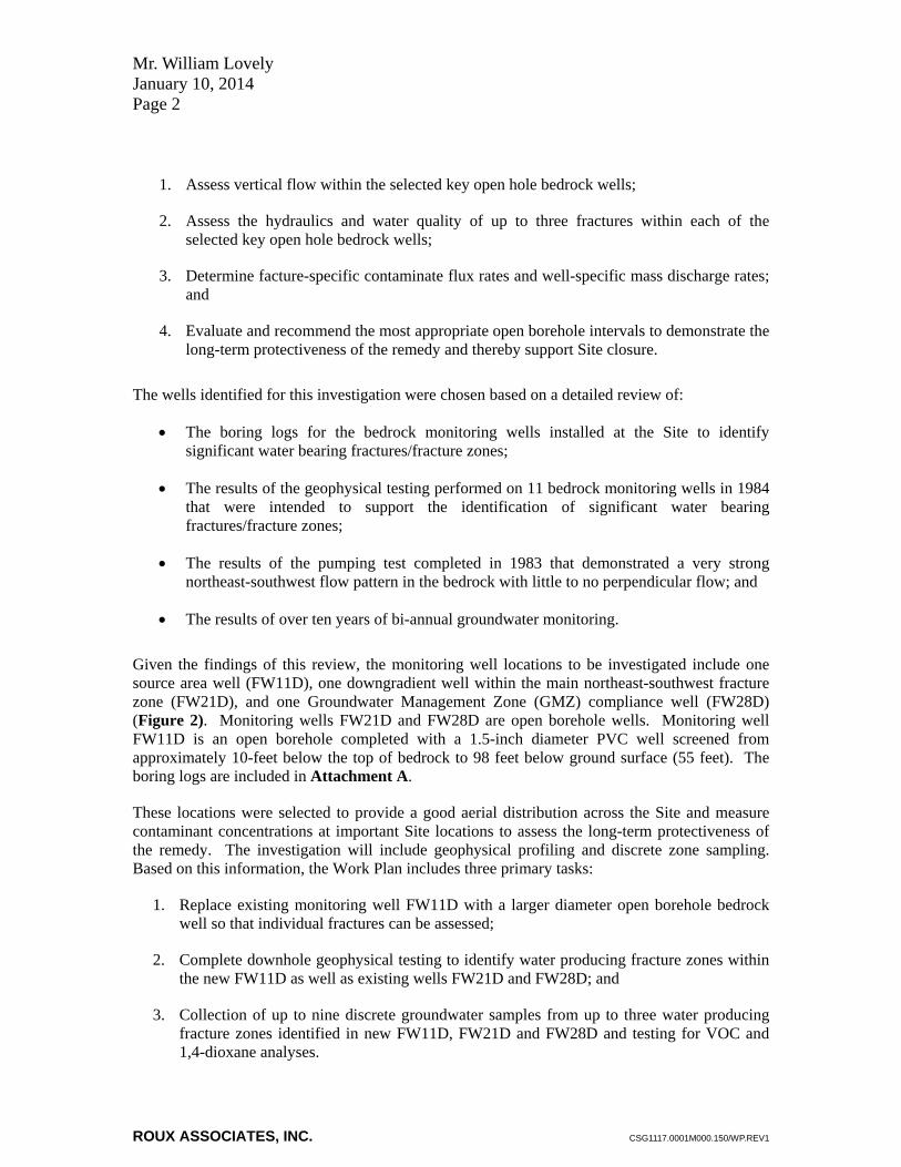
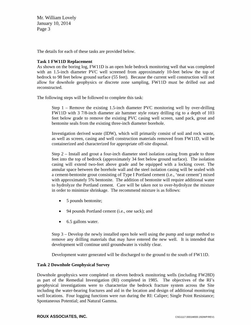
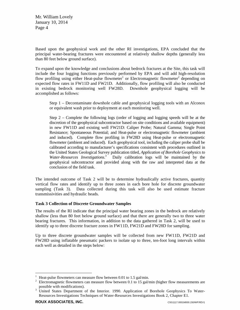
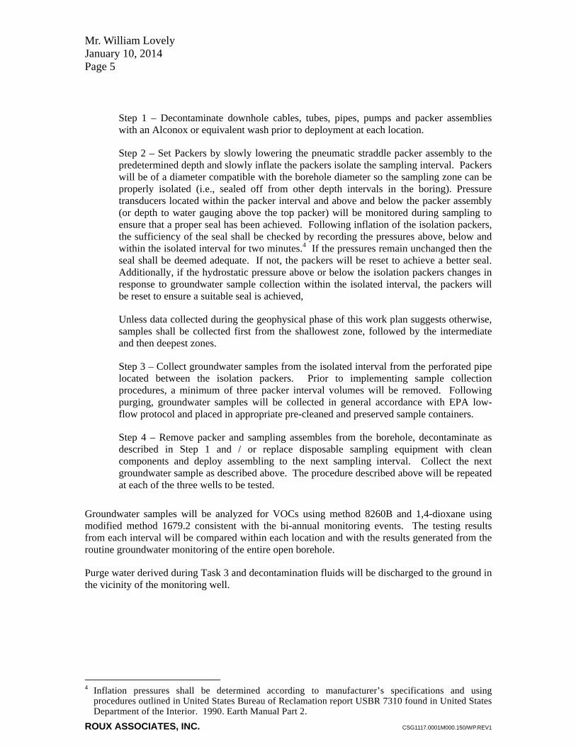
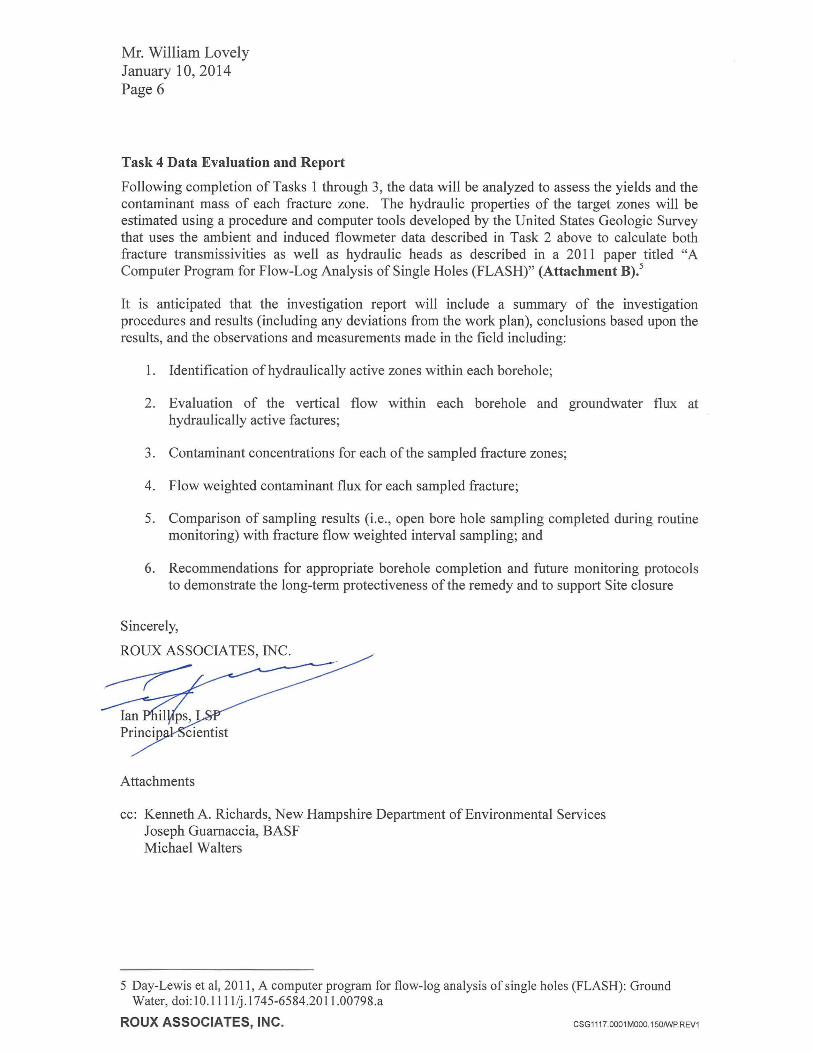
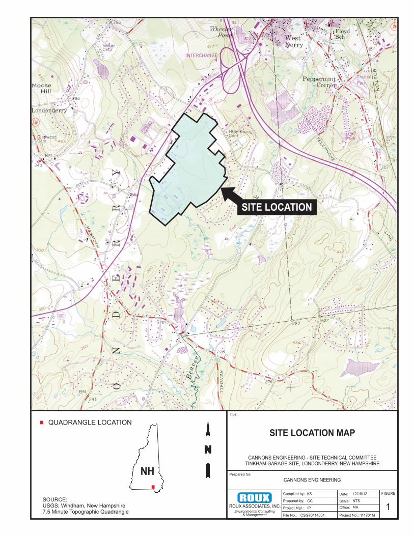
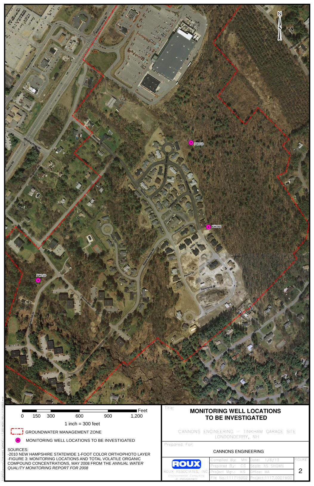
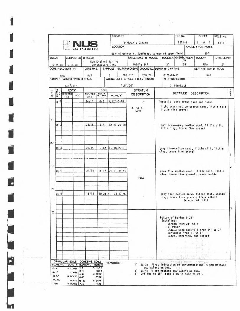
I
I i
il
II
bull
- ITDO No I SHEET HOLE No
Tinkhams Garage 8211-11 1 of 1 FW-11
PROJECT
NUSrmiddot bull middot middot -middotmiddotr I -- ~- middot aA=CAATCN
LOCATION IANGLE FROM HORIZ
Behind garage at Southeast corner of open field 90deg
ICOMPLETEol-ORILLER DRILL MAKE a MODEL IHOLpound OIA OVERBuRDEN IROCK 1111 llOTAL DEPTH
New England Boring (ft) 5-24-83 5- 24-B3 Contractors Inc Mobile B47 3 24 NA 24
BEGUN
CORE RECOVERY (ft) CORE BXS ISAMPLES IELTOPol CAStlGj GROUNO ELjDEPTH to GWTIME IDEPTH to TOP of ROCK
NIA NA 5 I 282 57 I 23077 I O 5-24-83 NA SAMPLE HAMMER WEIGHT FALL CASING LEFT in HOLE =DIALENGTH INUS INSPECTOR
14nt30 l 5 26 J Plunkett
x ROCKE ~ ~ COREREC ROD o a lin)
ss-1
5
ssshy
- -- shy
gt---middot
10
--shy
SOIL PENREC OE~~
( in )middot IN1fi ymiddotshy ELONS6
4114 0-2 l 112-3-18
--- shy
d 11 R S-7 12=ZQ~
-shy
middot shy2414__ 10-11_ 16-1822-31
STRATUM DESCRIPTION
middot
m to c SANO
- shy - shy - ---middotshy - ---- --middot --shy ----+---------- - ---middotmiddot- middot----- shy ----shy --- --- shy ---1
l 5+--+--+---+---+--+-----1 s-4 4114 15-17 lA -11-34-41
TILL
1---+- ---t shy - - - ---middot - - - shy - -- shy
20+--t----+----t----t----1----~ ~s_-_s+-_ __ _ __~1~8~1~2--1~2~0~-2~1-l--~34~-~4~7--9~0~
DETAILED DESCRIPTION
Topso il Dark brown sand and humus
light brown medium-coarse sand little silt little fine gravel
light brown-gray med ium sand little silt 1ittl e clay trace fine grave l
gray finebullmedium sand l ittle silt l i ttle clay trace fi ne gravel
gray fine-medium sand little silt little clay trace fi ne ~ravel trace cobble
gray fine -medium sand little silt little cl ay t race f ine gravel t race cobb le
(compacted till)
5 z
2
l---+---~----+----t-----1-----~-------+--------------------3 25+-----------+---+------1
GRANULAR SOILS COHESIVE SOILS REMARKS
BLOWSFT DENSITY 810WSFT OENSITI
0middot4 V LOOSE lt z V Ubull I
4 middot10 LOOSE Z-4 SOFT
4middot8 STIFF 10middot 3 0 DENSE B-15 STIFI
J0middot50 DENSE 15 shy JO STIFF
gt50 V DENSE gtJO HARO
Bottom of Bor i ng 24 lnstal led
-Screen f rom 24 to 4 -6 riser -Ottawa sand backfill from 24 to 3 - Benton i te from 3 to 1 - Cased cemented and locked
-middot r -middot
l) SS-3 first Indication of contamination shy 5 ppm methane equivalent on OVA
2) SS-4 5 ppm methane equ ivalent on OVA 3) Drilled to 25 sand blew in hol e to 24 bull
PROJECT TOO No SHEET
r_-middot r NUS Ti nkham s Gara e LOCATION
8211-11 1 of 3 ANGLE FROM HORIZ L-7_1 cxFPORATON
Behind the garage sout heas t corner o f open field 5 wes t of FW- 11 90deg
BEGUN COMPLETED j)RILLER DRILL MAKE S MODEL HOLEOIA OVERBURDEN R00lt(11) (11)
6-8-83 6-13-83 New England Boring
Co nt rac to rs Inc Mobi l e B4 7 3 34
CORE RECOVERY (f1) CORE BXS SAMPES ELTOPolCASNG ~EL DEPTH to GW TIME
63 3 2B2 B2 28 1 17 SAMPLE HAMMER WEIGHT FALL
140 30
CASING LEFT in HOLE = DIA LENGTH
1 5100
c ROCK 5 l ~ CORfREC R 0 0 O ( on )
PENREC (1 n )
SOIL DEPTH
INT t
-shy -- -shy __________
15 -1---11-----1----1gt-----+---+------lt
20 -1---1----1----1----+--shy -+------lt
25 +--1---+---1---+---+-------1 s s - 66 25-25 5 11 76
s s shy 12 12 30-31 61-74
STRATUM
DESCRIPTION
Re fer to 1 og for we 11 FW -11
middot
TI LL
1--+- - -+---+---+---+-shy- ---1 Oecomposed Pock
5 60 56 64 t Fractured SCHI ST GRANULAR SOILS COHESIVE SOILS REMARKS
BLOWS FT DENSITY BLOWSFT DENS
0-4 V LOOSE lt V
LOOSE 2-4 SOFT
4- 10 4 - 8 M STIFF
10-30 M OENSE 8 -15 STIFF
30-50 DENSE 15 - 30 V STIFF gt 50 V DENSE gtJO HARO
0 6shy13-B3 NUS INSPECTOR
J Plu nkett
DETAILED DESCRIPTION
Re fer t o log we ll FW- 11
l i ght brown-gray fi ne-med i um sand l i ttl e silt and clay t r ace f i ne gravel heavily compac t ed (comp acted t ill)
compacted t 11
Run 11 34 -39 (fr ac t ured ra schi s t)
I
i
bull ltt i i I
l
I
PROJECT HOLE No
NUS TOD No l SHEET 1
1---IiDkham s GaUU1e__________8_2_11_-_1_1____l2__0_1_3_ ___F_w_-1_1_0_ LOCATION
CCAPCgtRATION
5 west of FW-11~~---------------J____ ----shymiddot---shy
r ROCK SOIL ~ ioL---c-RE-C~-------E-C~-O~EP~T-H~-----Je ~ z c~ ROO PEN R ERlltIL e S60 A lbulln) (o n) IN1T11i LOW
--shy ---1----------1---1------l
40 -1---+-4_8 4_4____7_6-+----+--~-----1
---shy-
45deg1---11-----1----1---4-----1------1
middotmiddotmiddotmiddot-shy ----shyL---1- ----middot ---shy
--middot-shy-shy __6~~~ SOX
-middot-- --shy -50+--+---+---1----1------l------l
--- -middot-middotshy middot- middot -middot-- --middotmiddot-middot shy
-6060 44t
55+--+---+---+----+---+------l
90
60+--+---+---+----+---+------l
middot--shy -shy
60 60 96-65+--+---+---1----+-----l------l
-- shy -shy ----l
middot shy ----shy middot----~---~---
70+---+---+---1----+---4---~
-middot--shy middotmiddot--shy
L-_ - --middot middotmiddot-shy6060 74
75
STRATUM
DESCRIPTION
middot
Frac tured Bedrock
(SCHIST)
REMARKS 1) Washwater 1 taken at 38 2) WW-2 at 42 3) WW-3 at 44 4) WW-4 at 49 5) WW-5 at 53
DETAILED DESCRIPTION
Run Z 39-43
fractu red gray schi st
Run 13 43-48
fra ctured gray schist
Run 4 48-53
fractured gray schist
Run f5 53-58
fractured gray schist
Run 16 58-63
fracture~ gray schist with quartzite
Run 7 63 -68
fractured gray schist with quartz i te vein
Run 8 68-73
light gray quartz i te (ve i n) slightly fractured
Run 19 73deg-78 fractured gray schist with quartzite vein
6) WW-6 at 58 7) WW-7 at 636 8) WW-8 at 68 9) WW-9 at 73
6
8
9
--
---
--- --------
--- --- - ---
--- ---- - - - -------
I PROJECT TOO No SHEET HOLE No- I ~
Tinkhams Ga rage 8211- 11 1 3 of 3 FW- 11 Dl - ~NUS LOCATIONl _ _J caPCAATON
5 wes t ofFW- 11 shymiddot~ ~ROCK SOILz STRATUM It 0poundPTH DETAILED DESCRIPTION 0 COii~ PENRECw 0z RQO BLOWS6 DESCRIPTIONI~0 (1 n ) zlin)
middot middot bullbull l)o ilt
middot-- ~ t4Run 10 78 -83 706059
fra ~ture d gray schis t wi th qua r t zite ve i n shy80
-10 middot Run 11 83 -88 806060
fractured gray schi s t j~85 Bedrock
( SCH ISl)
___ 6060 Run 11 2 88 - 93 54
hea vily frac tured gr ay schi st wi th quart z 90 ve in I
11
_- shyRu n 113 93 - 986060 60 middot-- shy
12 95
fractured gra y sch i s t
middot-middot ----middotmiddotmiddot-- shy
Bottom o f Boring 98middot------shy- Ins tall ed 00 -Screen f rom 98 to 43
- 45 r iser - --middotshy middot---middot-- shy -Otta wa sand backfill from 98 to 34 - Be ntoni te f rom 34 to 24 -Natura1 backfill t o surface - Cased cemen t ed and loc ked
middot-middotshy --- shy
-- ------middot shy
gt
REMARKS 10 ) WW-10 a t 836 11) WW- 11 at 91 I 12) WW-12 a t 95
middot
I I I I I I I I I I I
bullbullbull
I II I STRATIJMI 11middot -ishybullbullbullbull 1lbullntUi-- I ___ _ OEVRIPTLt
I f1eJ l~f
1
r
l 10 tl-~1r----ilr----lr----~11~ 1
---+ll-----lI tri2lcqls I qei I i I I I i I I I I I I I I I I I I I I I I I I I I l I I 11 11e I I I I II1 bii I I
111
11 1
I I~ I I I I I ~~t qQ ill jI I lf I I II I I I I I I I I II I I I I I 1 I I I I I I I I 12~J 11 r 11 I PI I I 1I I I I I II I I I I I i I I I I I I I I I I I I I I I I I I
1 1
11 I
1-l I I j JI 11 rc 1 1 1 1 1
I I I I I I I I I I I I t I 1 I II I J I I I I I I I I I 11 11 1 I 1
1
1 I I I 11111I I I I I
J I 1 1- l I 1
1
1
I I I I middot I I I I I I
r I I I I
GIUHllM sou CDCStoC SlU
CCbullSTl ~ shy ll~KSbull~middot~f~==-1 ~ -
1
II I 1 I 1bull1 I I I I I I I I I I I I I I I I I Z I
I
bullbull _bullbullbull 10 bullbullbull bullMO -
deg -middot-middot
tlXI)bull Qio1cnlt -~~~ iia (ir plf~ (~~)
CIU $1 ~ ~ o-imiddot 2-Ltb ~ ~J ~ ~ rK
I I I~ I
I f$
~ f--41~-+----+---i---+--~~ri
i I f-Z
r r i r s i i T
Lshyi r r I r ~
L r 11 I I I I I rlO
I I I
I I II 1 2I I I l
11~F 1 I I If J I ~Jr
I I 1 1 I1r-~--ili---+---1-I~-~---iL ~1-+---~111
1
~-f~-=~l-middot---11--~---i~bull 1 1 bull I I 1
1r rt1- -+--+---t--=--i1--1-----iIJWl I II I I I I I -middot I I I I I -I I I I
I I I 1
i i 111~1 I I I II = 1 11 I I I Ir
II r I r ~
lrf I r IrIV I ir - I I I
I I r I 2-1I I i r I I I I i r shy~ ICLS COCSM --bull llOtUIQkOoln OlllSTT ~-middot middot- shy4bull10 1bull4
bullbullbull 0middot)0 gtIMO
1~~~ euli~ ~ bulldeg -middot
ri bull
f
r
I I I I ~ j~ampJ- I Ir fT -n ~ ___ r II r I I I I
lrnJ ~ -~ Pt~ I I _-- - bull oAamp I middotk_ I I
I - - lto(J-i --I ~ I I I I
I ~ I Ienmiddotmiddot I II1i_shy
f
l
~ aW-- ~bullbullbulle 441l~
- r ciJ I
(R I ro
~r~+-~-t~~-+o~~-+~~+-~~~-1
I SOIL i_1~1I ftbullbull I -rmiddotm-1 ~f af ~~lo i~~ I bull
I ~01CCiI ---1ifi~ I - -
I LN
r-~
CeuroTAALED tSC-PTOH
I cu~
IFW-210
~
I I I I I I I I I I I I I I I I I I I I I I I I
L__l_ - _I -
[ I I l
I
I I
--
1
- I
1shy
REMARKS
I middot a IC11 bull CAJLIJilITM I __I I _ _
I iJk I --- ___ f I t1 n_J __ 1 - 1 r~ ~~1
I bull 1 l ROCX I SOIL i- i f r
j
I i 1 f I t 11 I JJmiddot1 J r I I - I 1
11
I I I 1
11
omiddotbull bull bull
I l l I I_
1middot4 _bullmiddotbullO middot- bullbull bullbullbull oOmiddotIO ODa ~ ~ N_41i bull oocr -middot
~
j ~O poundCT
I hnc--w-r~ ~
l1Ba+6MHoorJc iOO ~ I bull 1 ~r
f iz14 ~I
J SOii
Il~_=lkJi
I -q1--1tlbullI
I I I I I I II I I I I I III I I I I I I II l
j2COf1---+~_f--~+-~~+-~-+~~~~I
1middot I
1 ~j~+-~--if--~-t-~~-t-~~i--~~---1
L
I I
II L_ I
I I I I I II II II I I
I I I I I
I I I
I I I
I I
bull I I II I
I I I
I I I I l I I II ~ I I I I I II I I I I I
l I I II I I I I I I I II I I
I I II I I I I I II I
I I I I I II I I I I I I II I I I I I II I I I I
I I I I I I I IT
~ I I I I I
REMAllKS
SM(pound r 1 oL _ 1 x - _ I_ I
IFl~ -z_-z IRi1-ZB o I - - ---or ftlJ-Z ~ ~r~ ~ ~ I
1
I I I I I I I I
I I I I I I I
ATTACHMENT B
Guidance Documents
ROUX ASSOCIATES INC CSG11170001M000150ATTA
UNITED STATES DEPARTMENT OF THE INTERIOR BUREAU OF RECLAMATION
USBR 7310-89 PROCEDURE FOR
CONSTANT HEAD HYDRAULIC CONDUCTIVITY TESTS IN SINGLE DRILL HOLES
INTRODUCTION
This procedure is under the jurisdiction of the Georechnical Services Branch code D-3760 Research and Laboratory Services Division Denver Office Denver Colorado The procedure is issued under the fixed designarion USBR 7) 10 The number immediately following the designation indicates the year of acceptance or the year of lase revision
Although rhe term permeability was used in all ocher procedures in this manual percammg co che capacity of rock or soil co conduce a liquid the similar term hydraulic conquctiviry is used throughout chis procedure (See designation USBR 3900 for differences in meaning of rhe two cerms)
Since geologic and hydrologic conditions encountered during drilling are nor always predictable and may nor be ideal variations from chis procedure may be necessary to suit the particular purpose of the resc and conditions at the test sice Much of the information for this procedure was taken from references LI l through L5 l which contain additional information on fielq hydraulic conductivity resting
1 Scope
11 This designation outlines the procedure for pershyforming rests to determine an approximate value of hydraulic conductivity (permeability) of soil or rock in an isolated vertical or inclined interval of a drill hole (boreshyhole) either above or below the water table Usually the rests are performed as a part of the drilling program This procedure can be used in holes of various diameters if suitable equipment is available but N-size L3-in (76-mm)] nominal diameter drill holes are most commonly used2
l2 The constant head single drill hole rest is based on the same theories as the sready-srare or Theim-type aquifer rest and the same assumptions are made These assumptions are ( 1) the aquifer is homogeneous isotropic and of uniform thickness (2) the well (rest interval) fully penetrates the aquifer and receives or delivers water to the entire thickness (3) discharge or inflow is cons rant and has continued for a sufficient duration for the hydraulic system to reach a steady state and (4) flow co or from the well is horizontal radial and laminar Field conditions may not meet all of these assumptions Equations and other factors affecting the rest are given in paragraph 14 Calculations This procedure should nor be used for resting roxic waste containment that requires a very low loss of liquid
13 Constant head hydraulic conductivity rests should be considered scientific tests Grear care should be exercised by chose conducting the rests to eliminate as much error as possible
1 Number in brackets refers co the reference Hereafter referred mas N-size holes
2 Auxiliary Tests
21 The soil or rock penetrated by the drill hole should be identified described and classified from samples taken during the drilling operation Soil can be sampled in accordance with USBR 7010 7015 or 7105 and classified in accordance with USBR 5000 Rock cores or cuttings should be examined and appropriate description and classification made Dara obtained from the drill hole should be entered on appropriate log forms
3 Applicable Documents
31 USBR Procedures USBR 1040 Calibrating Pressure Gauges USBR 1050 Calibrating Pressure Transducers USBR 3900 Standard Definitions of Terms and Symbols Relating to Soil Mechanics USBR 5000 Determining Unified Soil Classification (Laboratory Method) USBR 5005 Determining Unified Soil Classification (Visual Method) USBR 5600 Determining Permeability and Settlement of-Soils [8-in (203-mm) Diameter Cylinder] USBR 5605 Determining Permeability and Serrlement of Soils Containing Gravel USBR 7010 Performing Disturbed Soil Sampling Using Auger Boring Method USBR 7015 Performing Penetration Resistance Testing and Sampling of Soil USBR 7105 Performing Undisturbed Soil Sampling by Mechanical Drilling Methods USBR 7300 Performing Field Permeability Testing by the Well Permeameter Method
1245
2
USBR 7310
32 USER Document 321 Geology for Designs and Specifications by the
Bureau of Reclamation (This document covers both soil and rock)
4 Summary of Method
41 Pump-In Test-Water is injected into an isolated interval of a drill hole in soil or rock and the volume of water injected is determined for a measured period of time The injection pressure is a constant gravity head with or without added pressure head provided by a hydraulic pump The hydraulic conductivity is calculated from the flow rate length and radius of test interval in the drill hole and effective head
42 Artesian Test-Where water under artesian pressure flows out of the drill hole the effective (shutshyin) head at the test interval is measured and the hydraulic conductivity calculated from the flow rate the length and radius of the well and the effective head
5 Significance and Use
51 Hydraulic conductivity tests are made to obtain daca related to (a) identifying seepage potential and dewatering requirements (b) drainage problems (c) ground-water supply investigations and (d) grouting requirements The tests yield approximate values of hydraulic conductivity that are suitable for many engineering purposes Reliability of the values obtained depends primarily on (a) homogeneity of the strata tested (b) suitability of rest equipment used for a given condition (c) care taken in performing the test and ( d) adherence to requirements for proper use of the equations The test is also used in formulating geologic descriptions and interpretation of material properties particularly where there is poor sample recovery
52 Where tests are performed in fractured rock results could reflect secondary conductivity rates which would not represent primary conductivity of the intact mass When the test is performed in fractured brittle swelling clay or rock or where fractures contain loose material hydraulic conductivity may be reduced and judgment should be used in applying results
53 Generally this procedure is suitable for materials in which the hydraulic conductivity ranges between 5 and 100000 ftyr (5 X 10⁻⁶ and 1 X 10⁻¹ cms) and where results are to be used for engineering purposes The procedure is not applicable in materials of lower permeability particularly for purposes such as investigashytions for containment of toxic wastes
6 Terminology
61 Definitions are in accordance with USBR 3900 Some definitions are from Glossary of Geology [6]
62 Terms not included in USBR 3900 specific to this designation are
62 l DnJJ Hole-A circular hole made by drilling
622 Feed Pipe (conductor pipe injection pipe riser pipe drop pipe)-The main pipe (or rod) which conducts water from the collar of the hole into the test interval in the drill hole for the hydraulic conductivity test
623 Baifer-A cylindrical container with a valve on the bortom for admission of fluid attached to a line and used for recovering and removing water cuttings and mud from a drill hole
624 Walking Beam-An oscillating rigid lever balanced on a fulcrum used to activate the cable in cableshytool drilling by alternating up and down motion
625 Aquifer-A water-bearing bed or stratum of earth gravel or porous rock with interconnected openings or pores through which water can move
626 Packer-A short expansible device deliberately set in a drill hole to prevent upward or downward fluid movement generally for temporary use The expansible part of the packer is called the gland Straddle packers are two packers separated by a length of perforated pipe to span or straddle a test interval
627 Artesian-An adjective referring to ground water under hydrostatic pressure ie an artesian aquifer is a confined aquifer Artesian ground water rises above the confining layer in the drill hole and may or may not flow at ground surface
628 Ground W1ter-That part of the subsurface water that is in the zone of saturation
629 W1ter Tizble-The surface between the zone of saturation and the zone of aeration that surface of a body of unconfined ground water at which the pressure is equal to that of the atmosphere
6210 Perched Water Table-A water cable usually of limited area maintained above the normal free water elevation by the presence of an intervening relatively impervious confining stratum
6211 Gauge Saver-A vessel with a pressure gauge filled with glycerin or oil to protect the gauge from direct contact with fluid in the pressure line (see fig 1)
6212 Holding Pressure (applicable primarily for grouting) -The gauge pressure after the water-pumping system has been shut off at the valve ahead of the gauge and backflow is prevented
6213 Back Pressure (applicable primarily for grouting)-The gauge pressure in the system after the holding pressure has dissipated as determined by opening a valve and allowing the gauge ro drop ro zero and then reclosing the valve
6214 Backflow(applicable primarily for grouring)shyThe reverse movement of water out of the drill hole when the holding andor back pressure below the packers exceeds the pressure of the water column in the hole
7 Interferences
71 During drilling it is important ro minimize movement of fines [minus No 200 sieve-size material (75 microm)] into the material being tested and to remove any accumulation of fines from the wall of the drill hole during preparation for the test so as to avoid obtaining test values
1246
USBR 7310
Heov1 Out1 Pressure Gouge
poundLpoundVATON SECTION
TOP VpoundW BOTTOM VIEW
Figure I - Gauge saver device for protecting pressure gauge 40-D-4287
lower than the actual hydraulic conductivity of the material being tested Drilling using clear water without additives is preferred Bentoniticmiddotmuds should nor be used in holes where hydraulic conductivity testing is to be performed Biodegradable additives may be used if necessary but only if the test interval is adequately cleaned before testing The drilling procedure should be documented on the log form
72 Test results can be adversely affected by injecting water containing sediment which would tend to plug voids in the material being tested
73 The temperature of the injected water should be equal to or warmer than that of the ground or ground water This reduces the tendency of air dissolved in the water to become entrapped in the voids of the material be ing tested and co cause low values of _hydraulic conductivity In most areas not affected by artesian conditions the temperature at a depth of about 25 feet (8 m) below the ground surface remains relatively constant at the annual mean air temperature for the region At significantly greater depths temperature rises about l degF (06 degC) for each 500 to 1000 feet (150 to 300 m) of depth The temperature of the injected water especially if it is known to be colder than the ground-water temperature should be recorded on a geologic log or the hydraulic conductivity cesc daca forms (see subpar 812 for suitable temperature measuring devices)
74 It is possible that dissolved minerals in the wacer used for a rest may react chemically wich substances in the material being reseed to cause a change in the hydraulic conductivity Therefore it is desirable to use wacer for the test chat is similar in quality co that expec~ed to permeate che ground when che project is in operation
8 Apparatus
81 Drill Rigs (see fig 2) ~1 ~ Rotary Drilling-A drilling method resulting m grinding a hole with a hard-toothed drill bic at che end of a rocacing drill rod (pipe) The equipment consists essentially of a power unit hoisting or rugging unit controlled-feed rotary drill head and mounting frame masc or tripod and circulating pump The rig should have various accessory drilling andsampling equipment (rods bits core barrels augers) as required for drill hole advancement sampling and testing
812 Cable Tool Drilling-A method of drilling in which the material at the bottom of the hole is broken up by a steel bic with a blunt chisel-shaped cutting edge The drilling equipment consists essentially of a mast a sering of drill tools (casing tubing or pipe of one size) chat is alternately lifted and dropped by a hoist with a power unit and a walking beam A bailer is always used with a cable tool rig Normally a cable tool drilled hole is noc satisfactory for hydraulic conductivity testing with packers
82 Injecrion Pump-A centrifugal or helical screw type pump providing a constant water flow is required This may require a special pump separate from that used for drilling operations Although there may be conditions where a larger or smaller pump may be required highshy
quality pumps having a capacity of 40 galjmin (150 L min) at a pressure of 120 bf in2 (830 kPa) (such as Moriyo model 3L-8 manufactured by the Robbins and Myers Company Springfield Ohio or equivalent) are adequate for most hydraulic conductivity tests The pump should provide the required flow at the required constant pressure with maximum allowable pressure fluctuation-due co pumping pulsations-of plusmn5 percent of the test gauge pressure A surge chamber is required for all testing chis minimizes pulsations which can affect the injection race in the test interval Also ic makes readings more accurate and protects che pressure gauges against damage from sudden pressure changes
83 Feed P1pe- The feed pipe should be of adequate diameter to minimize head losses and have adequate tensile strength to withstand pumping pressures and stresses during hoisting or tugging The feed pipe is commonly a threaded and coupled assembly of pipe or tubing having a uniform inside diameter Drill rods generally of N-size can be used wichouc seriously affecting reliability of rest data if che flow rate to the test interval does nor exceed about 15 galmin (57 Lmin) and the depth co che top of che interval does noc exceed 50 feet (15 m)
NOTE 1-Use of drill rods as feed pipe should be permitted only after the assembled drill rod string has been pressure reseed ro cali_brare head losses ar anricipared flows If seals or sealing marenals are used during calibrarion the same type of seals or sealing materials (not oils or wax) should be used during hydraulic conductivity resting
84 Flowmecers-One or more calibrated flowmecers are required the capacity of each meter should be specified
1247
USBR 7310
- Byooss votve Surgechomber~
Wotermettr-
Observation oost see Detail A
SCHEMATIC ARRANGEMENT OF EQUIPMENT
(Water meter
~==it=======t(k=====- For wottr tes t ing middotWell cas1n9
Press1Jre gouge
-=====bull===========~-For drilling DETAIL A OBSERVATION POST FOR
OPTIONAL EQUIPMENT ARRANGEMENT FOR DETAILS 8 AND C
WATER TESTING ANO DRILLING FROM SECTION X-X TO WELL
DETAIL D GRAVITY TEST
DETAIL B DETAIL C DOUBLE PACKER TEST SINGLE PACKER TEST
Figure 2 - Schematic arrangement of hydraulic conductivity equipment 801-D-l I I
For flows up to 50 galmin (200 Lmin) a 1-inch (25- 851 Pneumatic Piezometers-A down-hole pneushymm) diameter disk-type meter may be used For higher matic piezomerer system has been developed [7] flows a 2- or 2-12-inch (50- or 65-mm) diameter impellershy Descriptions of the equipment and procedure as used ar type meter is recommended two damsites are presented in appendix XL
841 A straight uninterrupted section of pipe having 852 Electrical Transducers-Electrical transducers an inside diameter equal to the rated size of the meter have been used as down-hole pressure sensors by other and a minimum length 10 times the inside diameter of agencies [8) particularly for very low hydraulic conducshythe pipe should be provided upstream of the meter tivities [below 1 ftyr (1 X 10⁻⁶ cms)] The USBR has Manufacturers commonly recommend pipe lengths of one used electrical down-hole sensors in preliminary trials tO two times the inside diameter of straight pipe Electrical transducers measure pressures more accurately downstream from the meter than pneumatic piezometers and can be connected tO a
85 Pressure Sensors-Where required calibrated strip-chart recorder for a continuous record However pneumatic piezometers or electrical transducers can be used transducers are considered less rugged for field use and as down-hole sensors tO measure pressures at the rest require more maintenance and experienced personnel tO
interval during a hydraulic conductivity rest Down-hole operate than do pneumatic piezometers sensors are preferred over the method of calibrating the 86 Pressure Gauges-When down-hole pressure piping system for head loss between a pressure gauge on sensors are not available or sensors are not working the surface and the test interval However an above-ground properly calibrated pressure gauges can be used t0 estimate pressure measurement can provide a check of the pressure effective pressure in rhe rest interval after correcting for sensor friction loss through the feed pipe and packer All pressure
1248
USBR 7310
gauges used in water resting should be high-quality stainless steel glycerin or oil filled wich pressure indicated in both lbfin2 and kPa (such as manufactured by Marsh Instrument Company a unic of General Signal P 0 Box 1011 Skokie Illinois or equal) Pressure gauge ranges should be compatible wich middot cescing requirements chey should be sized so char che gauge capacity does not exceed two co three rimes che maximum desired pumping pressure for each respective pumping stage Gauges should have the smallest graduations possible and an accuracy of plusmn25 percent over che coral range of the gauge If a gauge saver is used wich che gauge calibration should be made wich the gauge saver in place Accuracy of che gauges should be checked before use and periodically during the resting program (see subpar 112 for additional information)
861 One or more pressure gauges should be located downstream of che flowmecer and downstream of any valves ac che cop of che feed pipe This location for pressure measurement can be used by inserting a sub (adaptor or shore piece of pipe) wirh che gauge - installed on che cop of rhe feed pipe
862 Ac least one additional calibrated replacement gauge should be available ar che resr sire
87 Swivel-During che hydraulic conductivity cesc ic is preferable co eliminate the swivel and use a direct connection co the feed pipe If a swivel muse be used in che water line during resting ic should be of che nonconscriccing type and calibrated for head loss Significant friction loss can result from use of che constricting type
88 Packers-One or two (straddle) packers are required for che rest Packers may be either bottom-set mechanical screw set mechanical pneumatic inflatable or liquid inflatable The pneumatic inflatable packer is the preferable type for general use and is usually che only one suitable for use in soft rock and soil The gland of this packer is longer and more flexible chan the ocher types and will form a tighter seal in an irregular drill hole A leather cup type of packer should noc be used To ensure a eight water seal che length of contact between each expanded packer and che drill hole wall should noc be less than three rimes the drill hole diameter
NOfE 2-More than one type of packer may be required to test the complete length of a drill hole The type of packer used depends upon many factors eg rock type drill hole roughness spacing and width of rock joints and test pressures
881 Inflatable Packers-Inflatable packers with an expansible gland and a floating head (see app fig Xl2) should be designed for anticipated drill hole diameters and pressure conditions For normal hydraulic conductivity cescing a reasonable maximum recommended working pressure inside and outside of che packer is 300 lbf in2
(2070 kPa) [8] Inside pressure should be increased in water-filled holes proportionally co che sracic head For drill holes wich sharp projections in the walls a wireshyreinforced packer gland having a higher working pressure [7] may be required The pressure in che packer should not be high enough to fracture the material being reseed
The pressure required to form a cighr seal ac che ends of a cesr interval depends on the flexibility of rhe gland the friction of the floating head and che drill hole roughness The minimum differential pressure between che packer and the cesc interval can be derermined by res ring packers in a pipe slighrly larger rhan rhe nominal diameter of rhe drill hole in order co simulate possible enlargement of rhe drill hole during drilling For a given resr interval pressure che packer pressure is increased until ir provides a waterrighc seal between the packer and the material with which ic is in contact The pressure in rhe packer should range approximately berween 30 and 300 lbfin2 (210 ro 2100 kPa) greater chan char in che cesc interval with 100 lbfin2 (690 kPa) being normal Pneumatic inflatable packers can be inflated with compressed air or compressed nitrogen
882 Special pneumatic packers are available for use in wireline drilling operations Because che packers must be able co pass through che wireline bit and then expand co completely seal che hole ac che cesc interval special materials are needed for che packer gland A special packer assembly-consisting of cwo packers in tandem-is used with the upper packer being expanded inside che drill rod just above che bic and che lower packer expanded against che wall of the hole just below che bit The two packers on the assembly can be positioned properly-relative co the bit-by a sec of lugs or a ring located on the assembly Special seals or connections are needed co attach che water supply co che wire-line drill pipe at the surface
883 A minimum of two secs of replacement packers andor spare glands should be available at the test sire
89 Perforated Pipe Sections-Lengths of perforated steel pipe corresponding ro the lengths of rest intervals are required between packers to admit water inco che rest intervals The coral area of all perforations should be greater than five rimes che inside cross-sectional area of che pipe These perforated pipe sections should be calibrated for head loss
810 Well Screen-Well screen or slotted pipe may be required for cescing in granular unstable materials chat require support [9] As a general rule the maximum size of sloe width should be approximately equal to che 50shypercent size of che particles around the drill hole (see subpar 114)
811 Water Level Measuring Device 8111 Although there are ocher types of water level
indicacors che electrical probe indicator is most commonly used Essentially ic consists of (1) a flexible insulated conduit marked in linear units and enclosing cwo wires each insulated except ac che tips (2) a low-voltage electrical source and (3) a light or ocher means of indicating a closed circuit which occurs when che rips contact che water surface Different brands of electric wacer level indicacors and even different models of the same brand ofren have their own unique operating characteristics Before using any electric water level indicacor it should first be reseed at the surface in a bucket of water
8112 For approximate measurements of the water level when ic is within about 100 feet (30 m) of the ground
1249
USBR 7310
surface a cloth tape with a popper can be used A popper can be made from a short pipe nipple (or length of tubing) by screwing a plug attached to a graduated tape intu one end of the nipple and leaving the other end of the nipple open When the popper is lowered in the drill hole and the open end of the pipe nipple strikes a water surface it makes a popping sound and the depth to water can be measured by the tape
8113 An accurate measuremenr of the water level can be made by chalking the lower end of the steel tape After contacting the water level the tape should be lowered about L more foot before retrieving it Measurement is then made to the wet line on the tape
812 Temperacuie Measuring Device-Equipment for measuring ground-water temperature is available from commercial sources or can be made from a thermistor two-conductor cable reel Wheatstone bridge and a lowshyvoltage electrical source A maximum-minimum type thermometer is acceptable
9 Regents and Materials
91 ~71ter (See subpars 72 73 and 74)-The clear water supply should be sufficient tO perform the hydraulic conductivity test without interrruption and to maintain the required pressure throughout the test period
92 Swd or Gravel Backfill-Where a granular backfill is used t0 prevent sloughing of the drill hole wall it should be a clean coarse sand or fine gravel Laboratory permeability tests (USBR 5600 or 5605) should be made on the backfill material to make sure that it has a coefficient of permeability greater than one order of magnitude higher than that expected of the in situ material being rested
10 Precautions
L01 Safety Precautions L011 This procedure may involve hazardous
materials operations and equipment lO l2 Use normal precautions for drilling [ 10 11] L013 Precautions should be taken during calibration
pressure testing of equipment particularly testing of packers with compressed air or nitrogen (never use oxygen) to avoid injuries from a sudden packer or hose rupture
L02 Technical Prernutions 102 l As a general rule total pressure (static head
plus gauge pressure) applied in the drill hole should nor exceed 1 lbfin2 per foot (226 kPam) of rock and soil overburden at the center of the test interval if the test interval is 10 feet (3 m) long or less If the rest interval exceeds 10 feet pressure should not exceed 1 lbfin 2 per foot of overburden at the top of the interval In layered or fractured material or for drill holes near steep abutments or slopes 05 lbf in2 per foot ( 113 kPa m) of material to the nearest free surface is an appropriate maximum pressure Higher pressures than these may fracture the materials
1022 If there is excessive or complete loss of water when the hole is being drilled drilling should be sropped before cuttings fill the voids and a hydraulic conductivity rest completed on a shorter than normal length rest interval
1023 Hydraulic conductivity rest equipment should be considered and treated as precision testing equipment Gauges thermometers ere should have their own protective cases they should not be carried with drill tools or be tossed around They should be calibrated frequently Ir is recommended that all test equipment needed for hydraulic conductivity resting be kept separate from drilling equipment
11 Calibration
111 For Measurment ofEffeaive Head 11 l l Pressure Sensurs-Calibrate down-hole
pressure sensors by the methods and at frequencies prescribed by USBR LOSO
ll12 Friction Loss Estimates-Where down-hole pressure sensors are nor used estimates of effective head at the rest interval are made by subtracting friction loss from the applied head measured at the ground surface The friction loss should be determined for all components of the piping system from the pressure gauge to the test interval
1112 I Calibrate friction loss in parts or sections of the piping systems including ( L) the swivel (if used) (2) feed pipe (per unit length) and (3) the packer assembly Record the data with references to the particular parts calibrated in tabular or graphical form so the accumulative friction loss can be totaled for determination of effective head at the test interval The calibration procedure is as follows
I l l211 Lay out the individual or joined parts to be calibrated on a horizontal surface with calibrated pressure gauges at each end
l L 12 12 Pump water through the system at incremental increasing flow rares to the maximum flow rare expected to be used in the test allow the flow to stabilize between incremental flows
L 112 L3 Record the pressure at each gauge for each incremental flow rate
11 l 2 L4 Calculate the friction head loss for each incremental flow rare
2f = 23 l ( p ~I p ) (I )
where f = friction head loss in feet of head per linear foot
of pipe ftft or mm P1 = upstream pressure bf in 2 or kPa P2 = downstream pressure lbfin2 or kPa d = pipe length fr or m (d = l for swivel or packer
assembly) 23 l = converts from pressure in bf in2 to head in feet
or 0102 converts from pressure in kPa to head in meters
Example assume
P1 = 186 lbfin2 or 128 kPa P2 = 132 lbfin2 or 910 kPa d = 100 ft or 305 m
1250
USBR 7310
Inch-pound application
f = 231 ( 18 ~~-~3 2) 125 ftfr
SI application
f = 0 102( 128
- 9 tO) = 124 mm 305
l l l215 Plot friction head loss versus flow rare Figure 3 is an example of a plot of friction head loss (f) at relatively low flow races for a 10-foor (33-m) length of 1-14-inch (32-mm) diameter pipe Since head loss in pipe at turbulent flow is approximately related to velocity squared a plot of friction head loss versus the square of the flow rate is nearly a straight line (see fig 4)
NOfE 3-There are srandard rabies and charcs which provide unit friction losses for various sizes of pipe elbows cees reducers ere for clean and ruscy conditions Although such informacion is sometimes used it is preferable to determine friction losses in che piping syscem and packers accually used for che hydraulic conductivity rest
111216 To calibrate a packer inflate the packer in a shore length of casing or pipe in which amiddotvalve and pressure gauge have been installed A pressure gauge is also installed in the rods immediately ahead of the packer assembly Pump water into the rods at incremental increases (or decreases) of flow rate-allowing the system to stabilize after each incremental change-until the highest anticipated flow rate is reached
NOfE 4-For packers smaller than N-size such as the B-size used in wireline equipmentmiddot there are significant head losses and relatively low flow races must be maintained This requires water meters and pressure gauges capable of accurately measuring the low flows and small changes in pressures
112 Pressure Gauges-Calibrate each pressure gauge (see USBR 1040) by comparing it with a test or master
FLOW RATE IN LITERS PER MINUTE
o
I _ I_ I I I II
I I I I I loI I I I I I rI
I I I )I
I I I I I v I I I I I I I I I I lr II
I I
I I I I 11deg II i j~ I I I -~-----1 -- I I I I i
JO deg HOW RATE IN GALLONS PEA MINOT[
Figure 3 - Head loss due ro friction at increasing flow rates for a I 0shy
foot (3-m) 1-14-inch (32-mm) diameter iron pipe
gauge The master gauge should not be used during drilling or hydraulic conductivity testing Calibrate each gauge at the start of a res ring program plus one additional calibration per week during rests of long duration
113 Flowmeters-Calibrate a flowmerer by flowing water into a container of known volume the container used for the volume check should be commensurate in size with the flowmeter size and graduations From these data flow rares can be calculated for comparison with meter readings All flowmeters should be calibrated to an accuracy of plusmn1 percent Calibration should be done at the stare of the resting program plus one additional calibration per week during rests of long duration
NOfE 5-Some impeller-type flowmeters have an accuracy range significantly less than indicated by the dial Minimum and maximum races should be esrablished
114 Well Screens and Perforated or Slotted Pipe Sections-From manufacturers dara or by calibration determine the head losses in expected flow ranges to ensure there is no restriction of flow into the material being tested
12 Conditioning
12 l Nor applicable special conditioning requirements are not needed for this procedure
13 Procedure
13l Cleaning ofDnll Hole 13l1 Remove any accumulation of fine particles
(smear mud cake compaction caused by driving casing etc) from the drill hole wall Such accumulation significantly restricts the flow of water into or from the hole Exercise good judgment in cleaning the hole since excess cleaning may be detrimental If there is a question as to whether or not drill holes in particular materials need cleaning hydraulic conductivity tests can be performed in holes with cleaning and others without cleaning If cleaning does not significantly change rest results at a sire cleaning of additional intervals in the same materials may not be necessary
131 l1 When the rest interval is above the water table it may be possible to brush or scratch the drill hole wall to break up accumulated fines For unstable materials which require use of a well screen materials which cavemiddot against the screen may break up the accumulation of fines on the wall Mild surging with a bailer while adding water also may help break up a disturbed or compacced zone but this may stir up fines which then plug the voids in the material co be rested Mild jetting-followed immediately by bailing or pumping-also is a possibility
13 l l2 When the test interval is below the water table-in materials chat are rock-like and self-supporcingshyuse of a water jet in the hole (preferably accompanied with pumping to induce flow into the borehole) is one of the best methods to clean the hole After jetting bail or pump the sediment-laden water from the rest interval Jetting can also be used through a screen below the water
1251
tJ
I I 0 GO-GI I GO-G2 0 GI -G2
~
I
I
v
v p-shy~ -shyl--~ L--shy
-shy
v
0
middot 005 =0 00005 100
-shy~--~ 0 middot 0025 =0 00005
I 50 I
~ --shy = 0 00005
50
I
t - A
v -
-
[] --shy shy--shy0 -
4--l_-E
-
16
-shy-shy-8 --shyl---shy~ - 2
~ ~---shy z 3 4 5 6 7 8 9
FLOW RATE SQUARED (q 2 )(10001
s of oalmin ) 2
Figu re 4 - Plot of feed p_ipe ca libra tion data - example
USBR 7310
2FLOW RATE SQUARED (q2)( 1000degs of L min)
10 15 20 25 - 30 35
50
40
r w w LL
z
~ 30 0 J Cl ltgt w I
z 0 20 r S a LL
10
0
cable in unstable materials For soft rock flushing che sides of che drill hole by running che bit or a bailer up and down the hole may enlarge the hole by erosion or ocherwise change the characceriscics of the fracture systems
13113 Finally clean the drill hole by pumping or bailing water from the bottom upward with the pumping continued until the return fluid is clear without cuttings or sediment Record the method used in cleaning the hole on the log of drill ho le or on a special testing form
132 Length of Test Interval 1321 The length of the test interval depends on
(1) purpose of the test (2) stratigraphic interval and (3) flow rate Where materials are relatively uniform use a test interval of about 10 feet (3 m) Where flow rates are high shorten the test interval co locate high flow race zones where races are very low the interval may be lengthened if desired
133 Ground-Water Level Determination 13 31 Depth co ground-water level muse be
determined before calculating hydraulic conductivity Measure depths to water levels with an electrical probe or o ther suitable equipment (see subpar 811)
1332 Auger Holes-ln power auger or other types of holes to which water is not added as pare of the drilling process report the presence or absence of a water level depth to water level and dace of initial and final water level measurement In materials of low hydraulic
14
12Cll a w r w
101 z () Vgt 0
8 J
Cl ltgt w I
Sz 0 r u a
4 IL
conduccivicy several days to several weeks may be required for a water level to stabilize in the hole Report evidence of moisture in the cuttings and if a perched water level was observed
1333 Rotary or Cable Tool Holes-For drill holes in which addition of water to the hole is an integral part of the drilling process
13331 Bail or pump the hole dry or to a stable wa ter level at the close of the last shift each day and record level
13332 Report the presence or absence of water and depth to water at the beginning of the first shift each day Additional readings are desirable whenever water level in the hole has nor been disturbed for an appreciable period of time
13333 Report changes in water level detected as the hole is drilled deeper Record faccors that affect the water level such as depth of casing andor cemented intervals These data may be helpful in recognizing perched or confined (artesian) conditions
13334 Upon completion of the hole the water must be bailed down to the extent practicable the water level measured and the dace recorded of hole completion Measure the water level for a period of days or weeks until equilibrium is reached
NOfE 6-At times exceptions must be made to the requirement for conrinuation of water level readings Such is the case when
1252
USBR 7310
state or local laws require chat the hole be filled continuousiy from bottom to cop immediately upon hole completion and before the drill crew leaves the sire In ocher instances landowners may allow right-of-entry for only a limited time for measurements
1334 Perched and Artesian Aquifers-lc is imporshytant tO recognize perched and artesian aquifers especially those under sufficient pressure tO raise the water level above the confining layer but nor tO the ground surface (see (5 ]) They must be distinguished from water table aquifers (those which continue in depth) If perched water table or artesian aquifers-separated by dry or less permeable strata-are encountered in the same drill hole the resulting water level in the hole is a composite therefore conclusions and interpretations based on such data are misleading If a perched water table is recognized (or suspected) during drilling water levels must be determined for each zone for calculation of hydraulic conductivity This might require completion of the drill hole with a watertight seal set at a suitable horizon tO
separate two water table conditions In this type installarion two strings of pipe or conduit are required one extending down to the portion of the hole immediately above the packer and a second string extending through the packer to a point near the bottom of the hole Water-level measurements provide the basis for determining a perched condition or if the lower water table is under artesian pressure
13 35 Mulriple Water-Level Measurements-In some instances it is desirable tO install multiple conduits and packers or plugs in a drill hole so that ground-water levels (or pressure heads) in several water-bearing horizons can be measured over an extended period of time (see [5] pp 7-14)
134 Pressure Tests With Packers 134 l The recommended arrangement of typical
equipment for packer pressure tests without a pressure sensor is shown on figure 2 (See app fig Xl l for equipment with a pressure sensor) Beginning at the source of warer the general arrangement is clean water source suction line pump discharge line tO srorage andor settling tank suction line water-supply pump surge chamber line ro bypass valve junction water meter gate or plug valve tee with sub for pressure gauge short length of pipe on which the pressure gauge is attached tee and off-line bleeder valve for evaluating back andor holding pressure flexible 1-14-inch (32-mm) diameter hose and 1-14shyinch-diameter feed pipe ro packer or packers in drill hole which isolate the rest interval All connections should be tight and as short and straight as possible with minimum change in diameter of hose and pipe Friction loss decreases as the pipe diameter is increased
1342 When the material is subject co caving and casing andor grout is needed to support the walls of the drill hole the hole should be water rested as it is advanced Other hole conditions may make this procedure desirable or necessary The following procedure is commonly used
1342 l After the hole has been drilled to the top of the interval to be tested it may be desirable tO remove
the drill string from rhe hole and advance casing or grout ro rhe bonom of the hole
13422 Advance the hole 5 to lO feet ( 15 to 3 m) into the material to be rested
13423 Remove the drill string from rhe hole 13424 Clean the interval to be tested and record
the depth tO the warer table if present If a composite water level is suspected the warer level affecting rhe rest should be determined by measurements through the feed pipe after rhe packer has been seated and the water level has stabilized
13425 If rhe hole will stand open sear a single packer ar the top of rhe test interval Record the type of packer irs depth and packer pressure if it is rhe inflatable type
13426 Pump water into the interval ar a rate to develop a suitable pressure The pressure to be used depends upon testing depths and ground water levels or pressures Materials subject to deformation or heaving such as by separation of bedding planes or joints or materials at shallow depths must nor be subjecred to high pressures (see subpar 102 l ) For comparison of flow rates in different pares of a single foundation and with results from other foundations some of the following pressures are commonly used 25 50 75 and LOO lbfin 2 (170 350 520 and 690 kPa)
NorE 7-At test pressures less than 25 lbfin2 errors in measurement of pressure and volume of water may increase unless special low pressure gauges are used Gravity tests provide more accurate results under these conditions At pressures higher than 10 lbfin2 difficulties in securing a right packer seal and the likelihood of leakage increase rapidly However under artesian pressures or in deep holes the water pressure-as registered on a surface gauge-will need to be sufficient to overcome the effeccive head at the test interval and firmly seal the packer
NillE 8-Where the hole is subject to caving a pump-down wire-line system has been developed rhar can be used to eliminate removal of the drill string from the hole With this system the hole is drilled to the bottom of the interval tO be tested and the drill rod is raised so the end of the rod is at the top of the test interval The tandem packer (see subpar 882) is then lowered through the drill rod and expanded to seal both inside the rod and against the wall of the hole at the cop of the test interval Models of this equipment are available which have transducers below the packer for measuring water pressures at the test interval
13427 For determining effective head artesian heads encountered in the drill hole are treated the same as water table conditions ie the depth from the pressure gauge or the water level maintained during the test to
the stabilized water level is used as the gravity head If the artesian head stabilizes above the ground surface the gravity component of the effective head is negative and is measured between rhe stabilized level and the pressure gauge height If a flow-type rest is used the effective head is the difference between rhe stabilized water level and rhe level maintained during the flow period
1253
USBR 7310
13428 Afrer pressures are selected based on ground-water conditions and the purpose of the test perform a test at each pressure Usually a 5-cycle procedure is used three increas ing steps to the maximum pressure and then two decreasing steps to the starting pressure This cycling allows a more derailed evaluation of rest results than testing at a single pressure and commonly allows extrapolation to ascertain at what pressures the following may occur (1) laminar flow (2) turbulent flow (3) dilation of fractures ( 4) washouts (5) void filling or (6) hydraulic fracturing However the equations normally used to ca lculate hydraulic conductivity are based on laminar flow conditions
NOfE 9-ln some insrances on ly a single water pressure test at a given interval in the drill ho le may be required For example if geologic conditions are known and there is no need ro perform the seeps in subparagraphs 13422 through 13426 a single value of hydraulic conductivity with a relatively low application of pressure may suffice
13429 During each test continue pumping water to the test interval at the required pressure until the flow rate becomes stable As a general guide maintain flow rares during three or more 5-minute intervals during which l-minute readings of flow are made and recorded In tests above the water table water should be applied to the test interval until the flow rate stabilizes before starting the 5-minuce measurement intervals Where tests are below the water table flow rates usually stabilize faster than for the tests above the water table and the time period before the 5-minure test intervals may be shorter These rime periods may need to be varied particularly when rests to determine grouting requirements are made
134210 Determine and record the presence of back pressure and decay of holding pressure Afrer the rest deflate the packer and remove it from the drill hole
134211 Advance the drill hole and if necessary the casing repeat the procedure in subparagraphs 13423 through 134210 until the required depth of drill hole is reached When casing is used in a drill hole always set the packer in the material below the casing
1343 If the hole will stay open without casing it can be drilled to final depth and after cleaning the hole hydraulic conductivity rests can be performed from the bottom of the hole upward using straddle (double) packers Although a single packer can be used to test the bottom interval of the hole starting at the bottom with double packers will cause loss of borehole testing of only about the length of the bottom packer and will save one complete trip in and out of the hole with the drill string assembly co change the packers After the test for the bottom interval is completed straddle packers are used for successive test intervals up the drill hole See subparagraph 1342 where caving or other hole conditions will not allow this procedure
135 Gra vity Tests 135 1 Constant-head gravity tests are usually
performed without packers above or below the water table with drill holes of N-size or larger (see fig 2 derail D)
This type of test is often made in reasonably stable-walled drill ho les up to 25 feet (76 m) depth where water pressure at the test interval needs to be kept low The test is usually performed in successive 5- or 10-foot (l5- or 3-m) intervals as the drill hole is advanced The upper end of each test interval is normally determined by the bottom depth of tightly reamed or driven casing If the casing is not believed
middotto be tight appropriate entries should be recorded on the log form If the wall of the drill hole is stable the test can be performed in the unsupported hole If the wall needs to be supported use a well screen (see subpar 114 for calibration) inserted through the casing It may be necessary to ream or drive the casing to the bottom of the interval set the screen and then pull back the casing to expose the screen Afrer the test the screen is removed and the casing reamed or driven to the bottom of the hole
NOfE lO-Clean coarse sa nd or fine gravel backfill (see subpar 92) may be used instead of a well scree n Ream or drive rhe casing ro the borrom of the inrerval dean ir our and add rhe backfill as rhe rnsing is pulled back ro expose rhe resr interva l Record use of rhis procedure on the log form
l 35l l If the drill hole is self-supporting clean and prepare it in rhe normal n1anner (see subpar 13l)
l35 l2 If the drill hole is not self-supporting lower the well screen and casing into the hole
135 l3 For test intervals above the water table maintain a constant head of water _within 02 foot (60 mm)] at the top of the test interval by injecting water through a small diameter rube extending below the water level maintained during the test For rest intervals below the water table or influenced by artesian conditions maintain a constant head a short distance above the measured static water level
Monitor the water level with a water-level indicato r If the water-level indicator is inserted in a small diameter pipe in the casing the wave or ripple action on the water surface will be dampened and permit more accurate watershylevel measurements
NOfE l l-When rhe flow rare is very low rhe consranr wa rer level c1n be maintained by pouring warer in rhe hole from a graduated container
135 l4 Record the flow rate at wne intervals until a constanc flow rare is reached
135 l5 Repeat the procedure of subparagraphs 135 l3 and 135 14 at one or more different water levels
13516 This rest is essentially the same as desigshynation USBR 7300 (see also L3] p 74) the instructions in USBR 7300 for performing the rest and calculating hydraulic conductivity apply to this procedure also
14 Calculations
14 l For pressure or constant gravity head hydraulic conductivity rests calculace the hydraulic conductivity of
1254
USBR 7310
rhe soil or rock by rhe following equation (expressed m consisrent unirs) [4]
k = ~ In ~ where L ~ lOr (2)
or
k = ~ sinh-1 r where lOr~ L ~ r (3)
where k = hydraulic conducrivity fryr or cms q = consrant race of flow into che rest interval
ft3yr or cm3s L = length of the test interval ft or cm
H = differential head of wacer ac rest interval fr or cm
r= radius of the borehole ft or cm In= natural logarithm loge
inv~rse hyperbolic sin~ smh- 1 x In (x + -yx2 + 1)
142 An example calculation for a single packer test _ in the botrom of a borehole belovt the wacer table follows
Example assume
r = 18 in or 015 ft= 46 cm q - 22 galmin or 83 Lmin q = 15 X 10 ft3yr = 140 cm3s L 30 ft = 91 cm
Hg gravity = disrance from ground-water level co pressure gauge = 102 ft = 311 cm
Hp pressure 5 lbf in2 X 231 ftwater (lbf in2)
116 ft = 3 54 cm of water H = Hg+ Hp= 218 ft= 664 cm
~ = ~lo = 20 hence use equation (2) 5 k = _9_ In]
2rrLH r k = 15 X 10 ft3 yr In 30 ft
2rr (30 ft) 218 ft 015 ft k = 11X103 ftyr = 11 X lQ-3 cms
NafE 12-These equations are most applicable and reliable where the length of test interval is at lease 5 r and the interval is below che water table The equations are based on laminar flow of fluid through porous media Flow races high enough co cause turbulent flow invalidate the results in all types of material In fractured material the calculated value should be considered an apparent hydraulic conductivity even under laminar flow conditions
143 For pressure resrs when rhe resr interval is below the water table H is the distance from rhe water table to the elevation of che pressure gauge plus applied pressure converted to linear units of water head
Where the rest interval is above the water table His rhe distance from rhe midpoint of the isolated rest interval to che elevation of the pressure gauge plus the applied pressure converted to linear units of water head
For gravity rests above che water table H is che distance between che boccom of the tesc interval and che water level maintained during the test
For gravity rests below the water cable His che distance between the pretest stabilized wacer level in the drill hole and the water level maintained during the rest
144 If chere is artesian pressure an additional pressure muse be applied to overcome che artesian pressure co provide an effective rest pressure For example if there is an artesian pressure of 5 lbfin2 (34 kPa) ac che pressure gauge 15 lbfin2 (103 kPa) could be applied chen che effecrive pressure would be 15 lbfin2 minus 5 lbfin2 which equals 10 lbfin2 (69 kPa)
145 The calculations can be done conveniently by (1) a nomograph [12] (2) a hand calculator with che proper functions or (3) a com purer For repeared tests ic is convenient to prepare a table for one or more diameter drill holes and lengths of resc intervals and combine che terms on che right side of the equations other than q and H into a coefficient
NafE 13-The lugeon (lugeon unit lugeon coefficient) [ 13 14 15 16] has been used as an index of hydraulic conductivity in connection with cyclic rests and for grouting purposes
15 Report
151 Record field test data on a daily driller s report and or on rhe log of the drill hole or on a special reporting form designed for the specific project Record the following
1511 Log of the drill hole 1512 Elevations of the ground surface the water
cable and che top and bortom of the rest interval 1513 Diameter of the drill hole at test interval 1514 Method of cleaning the drill hole 1515 Size of the feed pipe and any well screen 1516 Water pressure andor gravity head and flow
rare for each rime interval 1517 Tora[ amount of warer used per resr 1518 Average temperature of ground warer and
water used in the rest 1519 Packer inflation pressures 1511 Capacity of pump supplying water to the
rest interval 15111 All head loss calibrarion dara 15112 Nore any comments considered necessary to
help evaluate che rest results
15 References
[ l] Permeability Tests Using Drill Holes and Wells Bureau of Reclamation Geology Report No G-97 Denver ColoradoJanuary 3 1951
[2] Ground Warer Manual lst ed rev reprint Bureau of Reclamation US Government Printing Office Washington DC 1981
1255
USBR 7310
[3] Drainage Manual lsc ed 2d princ Bureau of Reclamacion U S Governmenc Princing Office Washingcon DC 1981 1984
[4] Zangar Carl N Theory and Problems of Water Percolation Engineering Monograph No 8 Bureau of Reclamation Denver Colorado 1953
[5] Drill Hole Water Tests Technical lnstructionsshyProvisional Engineering Geology Bureau of Reclamation July 1970 (unpublished)
[6] Glossary of Geology 2d ed American Geological lnscitute Falls Church Virginia 1980
[7] Haccher R C High Pressure Inflacable Packer with Pneumatic Piezometer Bureau of Reclamation Reporc GR-10-75 Denver Colorado October 1975
[8] Bennett R D and R F Anderson New Pressure Test for Determining Coefficient of Permeability of Rock Masses Technical Reporc GL-82-3 US Army Engineer Waterways Experiment Station Vicksburg Mississippi 1982
[9] Ground Water and Wells A Reference Book for the Water-well Industry 1st ed published by Edward E Johnson Inc Saint Paul Minnesota 1966
[10] Drillers Safety Manual 1st ed reprint Bureau of Reclamation Denver Colorado 1982
[11] Acker W L III Basic Procedures for Soil Sampling and Core Drilling published by the Acker Drilling Company Scranton Pennsylvania 1974
[12] Underground Mining Methods Handbook No 580 W-88 Society of Mining Engineers Littlecon Colorado p 62 1982
[13] Lugeon M Barrages et Geologie Dunod Paris 1933
[14] Houlsby A C Routine Interpretation of the Lugeon Water-Test Quarterly Journal Engineering Geology vol 9 pp 303-313 1976
[15] Heitfeld K H and L Krapp The Problem of Water Permeability in Dam Geology Bull International Association of Engineering Geology No 23 pp 79-83 1981
[16] Pearson R and M S Money Improvements in the Lugeon or Packer Permeability Test Quarcerly Journal Engineering Geology vol 10 the Netherlands pp 221shy239 1977
1256
USBR 7310
APPENDIX
XL PROCEDURE USING A PNEUMATIC PIEZOMETER WITH TWO PACKERS ISOLATING THE TEST INTERVAL
Xl l Equipment Assembly (Refer to figs Xll and X l2) -A complete straddle packer unit is assembled as follows
X 11 l Co nnect a predetermined length of perforated injection (feed) pipe to the lower packer (The length of perforated pipe is determined by the thickness of the zone to be rested) Connect the inflation tubing to the lower packer and lower the sliding head end of the packer into the drill hole (See subpar l l l216 for calibration of packers)
Xl l2 Clamp the top of the perforated injection pipe at the hole collar and connecr the upper packer with the sliding head already down the hole
Xl l3 Provide approximately 12 inches (300 mm) of slack in the inflation tubing between the two packers to allow for retraction of the upper packer sliding head Connecr the tubing to the upper packer
Xl l4 Install the pneumatic piezometer piezomerer tubing packer inflation tubing and sealed lengths of injecrion pipe to the head adaptor
X ll5 Lower the entire unit into the drill hole adding lengths of sealed injection pipe as necessary to reach the
( Storoqf Settling ton
interval to be tested As the unit 1s lowered che packer inflation cubing and che piezomecer tubing is unreeled into che hole and caped to che sealed injection pipe at approximately 10-fooc intervals
Xll6 Upon reaching the rest depth lock both the inflation cubing reel and rhe piezomecer cubing reel connecr the inflation tubing by quick-connecr couplings co a nitrogen or compressed air boccie equipped with a high pressure regulator connecr the piezomecer cubing by quick-connect couplings co the readout box and connect the injection pipe co the water pressure source The cesc is now ready to begin
Xl2 Test Procedure
X 12 l After the unit has been lowered to the rest interval and before infacing the packers any water head above the cesc interval must be determined This head will sho w as pressure on the pneumatic piezomecer gauge and can be verified by running a water level indicator into che hole to measure the deprh co the water cable The piezometer will register water pressure chat can be converted to head of water This water head should be
Compressed 01r or nitrogen bot tie Regulator_
Poc~er air lin e- I
P1nometer ln1ec t1on oioe head adaptor
Lo er ooc~er inflation tubmr
Figure X 1 1 - Schematic arrongemem of drill hole packer and pressure monimring equipment 801-0-180
1257
USBR 7310
------=--From compressed air or nitrogen boltle
From piezometer
_To
PRESSURE READOUT BOX
Packer inflation tubing From wafer source From air or Water injection pipe ring seals
PIEZOMETER TUBING REEL
Pressure seals Wire reinforced rubber gland clomps
nitrogen ~~i==-=~==t~f=lil~~~jii~9ll~~~~~sect9ll~sect~sectsect~~~sectl~iilf~f--- To per for o t e d ~~~ze=zzzoCzzzze=zzze=plusmnzz~EZio~~~~21p~
To pressuresource~~~~~~~~~~~~~~~readout box
Piezometer
~~~~~~~~~~~~~~~~---
Inflation chamber Floating packer head Packer inflation lubing
UPPER DRILL HOLE PACKER AND PRESSURE MONITORING EQUIPMENT FOR N X HOLE
Figure X 12 - Upper Jrill hole packer anJ pressure monitoring equipment for NX hole
used to determine the minimum inflation pressure to be applied co the packers by the following equation
SH+ PP+ PE = minimum inflation pressure
where SH = static pressure at the midpoint elevation of the
test interval lbf in2 or kPa PP = gauge pressure to be maintained during the test
lbfin2 or kPa PE = pressure needed to expand packer to hole
diameter as determined before insertion in the drill hole by expanding the packer in a length of pipe having a diameter similar to the hole diameter lbfin 2 or kPa
Inflation pressure gauge is in units of lbf in2 (kPa) The static water level measured before the packers are
inflated might be a composite water level (see subpar 1334)
Xl22 Inflate the packers and determine water head for the rest interval This is the static head to be used for calculation of hydraulic conductivity If rhe static head is significantly different from the composite measured
before the packers were inflated recalculation of packer inflation pressure may be required The final packer inflation pressure should be the lowest practical pressure to seal the test interval against the maximum injection pressure to avoid fracturing of the material being tested
Xl2 3 After the inflation pressures have been determined deflate the packers fill and flush the system with water until all entrapped air has been removed This is accomplished by filling the injection pipe under a gravity head and leaving the air-release valve open ar the top of the injection pipe tee at an elevation higher than the injection hose The valve must remain open until all air has been removed and water runs freely indicating a filled system At this point water is flowing around the deflated packer system and is completely filling the annulus between the drillhole and the packers In the case of an interval with a high injection rate it may be necessary to keep the air valve closed to keep from entraining air into the test interval
X 124 Close the air release valve at the top of the injection pipe and slowly inflate the packers to the predetermined inflation pressure
Xl2 5 Lock in the inflation pressure by closing the pressure valve in the packer cubing If the pressure gauge
1258
USBR 7310
on the closed system remains steady it verifies a sealed system At this point water injecced under gravity head approaches a constant flow rate
X 126 Record the piezometer pressure after packer inflation For an interval of very low injection rate this is equal to che height of the injeccion standpipe plus che pressure recorded at the hole collar gauge For a test interval with a high injection rate the readout would show the same value less any friction from water flow through the injeccion pipe
X 127 Proceed with the test by applying the selected pressures ac the test interval and moniroring the flow rate and pressure on the pneumatic piezometer
X 128 To accurately compute hydraulic conduetivity rhe down-hole pressure muse remain constant A zone with a high injection rate must be monirored more closely than a zone with a small injection rate and adjustments made to hold the down-hole pressure constant To accomplish
this che injeccion pressure shown on che collar gauge must be adjusted in order co maintain che down-hole pressure constant
NOfE X 1-For example a pressure srage is scarred with the collar gauge reading 35 lbfin2 (241 kPa) and the down-hole piezomerer reading 200 lbf in2 ( 1380 kPa) As rhe flow increases rhe down -hole pressure may drop to 150 lbfin2 (1034 kPa) because fricrion loss in the injection pipe and the collar gauge would have to be adjusted to bring the down-hole pressure gauge back up co 200 lbfin2bull When the flow decreases from a fast to a slow rare the collar gauge pressure would have to be decreased
Xl29 The cesc is completed following one or more stages of pressure increases and pressure decreases Following the last stage deflate the packers and close the injection line The system is now ready to move to the next test interval for repetition of this procedure
1259
Methods Note
A Computer Program for Flow-Log Analysis of Single Holes (FLASH) by Frederick D Day-Lewis1 Carole D Johnson2 Frederick L Paillet3 and Keith J Halford4
Abstract A new computer program FLASH (Flow-Log Analysis of Single Holes) is presented for the analysis of
borehole vertical flow logs The code is based on an analytical solution for steady-state multilayer radial flow to a borehole The code includes options for (1) discrete fractures and (2) multilayer aquifers Given vertical flow profiles collected under both ambient and stressed (pumping or injection) conditions the user can estimate fracture (or layer) transmissivities and far-field hydraulic heads FLASH is coded in Microsoft Excel5 with Visual Basic for Applications routines The code supports manual and automated model calibration
Introduction Flowmeters provide means to infer the flow into or
out of boreholes connected to transmissive aquifer units or fractures In the past the relative inaccuracy and difficult operating procedures for spinner flowmeters limited the use of borehole flow measurements With the advent of heat-pulse (Paillet et al 1996) and electromagnetic (Molz et al 1994) instruments measurements of vertical flow as small as 005 Lmin became practicable and borehole flowmeter logging is becoming routine New modeling and analysis tools are needed to achieve the full potential of these measurements
1Corresponding author US Geological Survey Office of Groundwater Branch of Geophysics 11 Sherman Place Unit 5015 Storrs CT 06269 (860) 487-7402 ext 21 fax (860) 487-8802 daylewisusgsgov
2US Geological Survey Office of Groundwater Branch of Geophysics 11 Sherman Place Unit 5015 Storrs CT 06269
3Office of Groundwater Branch of Geophysics (Emeritus) US Geological Survey 11 Sherman Place Unit 5015 Storrs CT 06269
4US Geological Survey Nevada Water Science Center 2730 N Deer Run Rd Carson City NV 89703
5Any use of trade product or firm names is for descriptive purposes only and does not imply endorsement by the US government
Received April 2010 accepted December 2010 copy 2011 The Author(s) Ground Water copy 2011 National Ground Water Association doi 101111j1745-6584201100798x
Calibration of a borehole flow model to flowmeter data can produce estimates of transmissivity and heads for one or more flow zones (aquifer layers or fractures) Here we briefly review approaches for analysis of flowmeter logs and introduce a new computer program which supports manual and automated calibration of an analytical borehole flow model
Approach Single-hole flowmeter data can be analyzed to
estimate transmissivity profiles along boreholes and characterize aquifer compartmentalization (Molz et al 1989 Kabala 1994 Paillet 1998) Analysis of single-hole flowmeter data is commonly based on the Thiem Equation (Thiem 1906) which written for confined radial flow from a single flow zone (ie aquifer layer or fracture) to a screened or open well is
2πTi(hw minus hi)Qi = minus (1)
ln(r0rw)
where Qi is the volumetric flow into the well from flow zone i [L3Tminus1] hw and hi are respectively the hydraulic head [L] at the radius of the well rw and at radial distance r0 commonly taken as the radius of influence where heads do not change as a result of pumping in which
926 Vol 49 No 6ndashGROUND WATERndashNovember-December 2011 (pages 926ndash931) NGWAorg
case hi is the connected far-field head for zone i and Ti
is the transmissivity of flow zone i [L2Tminus1] A number of approaches to flowmeter analysis have
been proposed and demonstrated for different sets of assumptions (eg no ambient flow in boreholes) and data requirements (eg flow profiles collected under both ambient and stressed conditions) based either on Equation 1 (Molz et al 1989) or quasi-steady flow approximations (Paillet 1998) We refer the interested reader to Williams et al (2008) for additional background on flowmeter logs and focus the following discussion on the approach of Paillet (1998 2001) which is adapted here
Paillet (1998) formulated flowmeter log analysis as a model-calibration procedure involving flow profiles collected under both ambient and stressed (pumping or injection) conditions Consideration of the two conditions allows for the estimation of the transmissivities and also far-field heads of flow zones The latter is critical for the interpretation of water samples from wells that intersect multiple fractures or layers with different hydraulic head (Johnson et al 2005) Applying Equation 1 to an ambient condition (condition a) and a stressed condition (condition s) gives
factorT total(ha minus h02πTi )w iQa = minus (2)i ln(r0rw) factorT total(hs minus h02πTi )w iQs = minus (3)i ln(r0rw)
where T factor i is the fraction of the boreholersquos transmisshy
sivity contributed by flow zone i [ndash] T total is the total transmissivity of the flow zones intersected by the bore-hole [L2Tminus1] ha hs are the ambient and stressed water w w levels in the well respectively [L] h0 is the far-field head i in flow zone i [L]
For both ambient and stressed conditions the water level in the borehole is assumed to be constant in
time and the water level in the far-field of each zone is assumed to be the natural condition that is hi
0 In a field experiment (Figure 1) rw would be known and the flow rates and water levels in the well would be measured Radius of influence can be inferred experimentally based on head data at observation wells in which case r0 can be constrained during calibration or else it can be approximated (Bear 1979 306) Estimates of transmissivity are not strongly sensitive to the value assumed for r0 because it appears inside the logarithm in Equations 2 and 3 For example a change in r0rw
from 10 to 100 yields a change in the estimated Ti of only a factor of 2 and order-of-magnitude estimates of transmissivity are acceptable for many problems In cases where knowledge of r0 is unavailable but the boreholersquos total transmissivity is known from specific-capacity or slug-test results it is possible to estimate r0 in the calibration procedure We note that the forward model (Equations 2 and 3) produces twice as many independent equations as there are flow zones with an additional equation requiring T factor values to sum to 1 The number of parameters being estimated is twice the number of flow zones (T factor and h0 for all i) plus one parameter for either i i T total 0or r i
Model calibration involves changing the model parameters such that the flows predicted by Equations 2 and 3 match the interpreted flow profiles Following Paillet (1998 2001) calibration is to the interpreted profile and not individual data This formulation allows the user to incorporate additional insight (eg from other logs) to identify the number and locations of flow zones and elimshyinates the need for weighting measurements differently according to variable measurement errors and the spatial distribution of measurements along the borehole
Calibration can be implemented by manual trial-andshyerror or automated using nonlinear regression Whether manual or automated the goal for calibration is to identify the set of parameters that minimize a measure
Figure 1 Schematic of flowmeter experiment in a fractured-rock aquifer with (a) flow-log profiles for ambient (blue) and stressed (dashed red) conditions and conceptual cross sections of flow system for (b) ambient condition and (c) stressed condition In this example two flow zones (fractures) intersect a well Under ambient conditions flow enters the well from fracture 1 and exits from fracture 3 Under pumping conditions flow enters the well from fractures 1 and 2 The far-field head of zone 2 is equal to the ambient water level thus there is no flow tofrom zone 2 under ambient conditions The far-field head of zone 3 is equal to the stressed water level thus there is no flow tofrom zone 3 under pumping conditions
NGWAorg FD Day-Lewis et al GROUND WATER 49 no 6 926ndash931 927
of combined data misfit and model misfit Considerashytion of model misfit criteria commonly referred to as regularization is useful when multiple models can match the data equally well or within measurement errors Here the data misfit is formulated based on squared differshyences between the predicted and interpreted flow profiles such that multiple measurements may be collected in a single borehole interval The model misfit could be forshymulated in different ways but we use criteria based on the differences between the water level in the borehole under ambient conditions and the far-field heads Thus the objective function F consists of two terms (1) the mean squared error (MSE) between interpreted and preshydicted flow profiles with equal weights for all cumulative flows (ambient and stressed) and (2) the sum of squared differences (h) between the boreholersquos water level and far-field heads
n1 2ssim sintmin F = Q minus Qi i n
i=1
n asim aint 2+
Q minus Q
2 + α (hi) (4)i i i=1
subject to constraints
factor factorT ge T for all i andi min
ABS(haw minus h0
i ) le hmax for all i
aintwhere Qi Qi sint are the interpreted flow profiles (ie
cumulative flow above zones) for zone i under ambishyasiment and stressed conditions respectively [L3Tminus1] Qi
ssimQi are the simulated flow profiles (ie cumulative flow above zones) for zone i under ambient and stressed conditions respectively [L3Tminus1] α weights the regushylarization relative to the data misfit [L4Tminus2] T factor ismin
T factorthe user-specified minimum for any flow zone which can ensure nonnegative T factor hmax is the user-specified maximum absolute difference between the ambishyent water level and the far-field head of any flow zone and n is the number of flow zones
Without regularization F reduces to the MSE between simulated and interpreted flows The trade-off parameter α is set by the user with larger values more strongly penalizing large head differences Commonly small α values (less than 0001) are sufficient to obtain good results In selecting α the user should be guided by the goal of regularization which is to identify the ldquosimplestrdquo explanation of the data while minimizing the data misfit
Using FLASH FLASH (Flow-Log Analysis of Single Holes) is writshy
ten in Excel with Visual Basic for Applications (VBA) The spreadsheet includes a toggle (INPUTS worksheet cell A20) to choose between analysis for (1) fractures or fracture zones that intersect a well at discrete locations
and (2) aquifer layers in porous media The first is indishycated for cases where flow profiles are characterized by step increasesdecreases and the second for cases where flow profiles show approximately linear change over each layer Up to 10 fractures or layers can be modeled
The FLASH spreadsheet includes four worksheets INTRODUCTION INPUTS FIELD_DATA and PLOTshyTING INTRODUCTION provides information about the program and input parameters On the INPUTS workshysheet the user enters information about the flow zones transmissivities and heads Note that the user must intershypret flow profiles from the flowmeter data for both the ambient and stressed conditions The flow measurements are entered in FIELD_DATA and the interpreted proshyfiles are entered in INPUTS The interpreted profiles plot as dashed lines the data as points and the simulated proshyfiles as solid lines (Figure 2) Line and marker styles can be modified using standard Excel tools Flows are positive upward and negative downward PLOTTING is used by the program and does not require the userrsquos attention
In the INPUTS worksheet input parameters are entered in the cells with light blue and bright aquamarine backgrounds The former include specifications of the experiment setup (eg borehole diameter and water level) and the latter include calibration parameters Manual calibration is performed by adjusting the values of
ldquoT factorrdquothe cells and ldquohrdquo which are respectively T factor and the difference between the flow zonersquos far-i field head and the ambient water level in the borehole As parameters are adjusted the simulated flow profiles update automatically thus guiding the user toward best-fit parameters The MSE between simulated and observed flows is calculated in cell B36 on the INPUTS worksheet
Although the principle calibration parameters are Ti
factor and h the radius of influence r0 and total transshymissivity T total also are possible calibration parameters as explained above and indicated by aquamarine highshylighting By inspection of Equations 2 and 3 it is not possible to estimate unique values for both radius of influshyence and total transmissivity but only the ratio of total transmissivity divided by ln(r0rw) In general the user will have more information about total transmissivity than radius of influence Total transmissivity is estimated readshyily using an open-hole slug test or specific-capacity test Indeed the drawdown and pumping rate under stressed conditions could serve as data to estimate a total transshymissivity for the borehole In rare cases however the estimated total transmissivity may be considered unrelishyable for example in the presence of ambiguous slug-test data or discrepancy between the volumes over which the slug test and flowmeter analysis measure In such cases it may be useful to allow the T factor values to sum to a value other than 1 FLASH assumes a uniform radius of influence for all flow zones In reality the effective radius of influence may vary between zones according to their transmissivities and distances to boundaries Data to supshyport variable radius of influence however is commonly unavailable furthermore transmissivity estimates are not
928 FD Day-Lewis et al GROUND WATER 49 no 6 926ndash931 NGWAorg
Figure 2 The INPUTS worksheet after execution of the Solver with options ldquoEstimate ROIrdquo and ldquoSolve with regularizationrdquo for example On this worksheet the user enters the well and flow-log specifications and performs model calibration Data (points) and interpreted profiles (dashed lines) Simulated profiles (solid lines) are for an arbitrarily selected starting model
a strong function of the assumed radius of influence as explained previously
Automated model calibration is implemented using the Excel Solver an optimization tool based on a Genshyeralized Reduced Gradient algorithm (Lasdon and Smith 1992) The Solver is invoked using VBA ldquocontrol butshytonsrdquo on the INPUTS worksheet Radio buttons allow for selections of (1) the parameters to be estimated (Estishymate ROI [radius of influence] or Estimate Transmissivshyity) and (2) regularization (Solve without Regularization or Solve with Regularization) Under the option Estimate
T factorROI the Solver estimates the values of i for all i and the single radius of influence Under the option Estimate Transmissivity radius of influence is assumed known the parameters for estimation are T factor for all ii such that total transmissivity is allowed to vary Users are encouraged to perform manual calibration before attemptshying automated calibration Manual calibration provides insight into the sensitivity of flows to parameters and helps to identify a good starting model for automated calshyibration As for any nonlinear optimization the algorithm may get ldquostuckrdquo in local minima and fail to identify the globally optimal parameter values Consideration of mulshytiple starting models is advised Additional information
and the FLASH spreadsheet are available online as noted under Supporting Information at the end of this article
Example FLASH is demonstrated for a simple data set from
a fractured-rock aquifer (Figure 2) Johnson et al (2005) provide additional details for this data set for which additional borehole logs were used to identify fractures and select locations for flow measurements
Under ambient conditions the deeper fractures 1 and 2 experience inflow to the borehole which indicates the far-field heads for each of these fractures is greater than the head in the borehole thus producing upward flow (Figure 1) Under ambient conditions upflowing water exits the borehole at fracture 3 indicating the far-field head is lower than the head in the borehole Under low-rate pumping conditions water continues to enter the borehole at fracture 1 additional water enters at fracture 2 indicating the far-field heads for fractures 1 and 2 are higher than the quasi-steady state open-hole water level under pumping conditions The uppermost fracture (3) no longer shows outflow indicating the far-field head is equal to the pumping water level In this example
NGWAorg FD Day-Lewis et al GROUND WATER 49 no 6 926ndash931 929
fracture 2 has a far-field head similar to the ambient water level in the well and therefore does not result in a substantial change in borehole flow under ambient conditions Similarly fracture 3 has a far-field head similar to the stressed water level in the well and does not produce a measurable change in borehole flow under stressed conditions This field example underscores the importance of collecting both ambient and stressed flow profilesmdashwith only ambient data fracture 2 could not be identified and with only stressed data fracture 3 could not be identified
To induce flow from a given fracture to enter the borehole the h for that fracture must be positive Conversely to induce flow from the borehole to the fracture the h must be negative The rate of flow is determined by the magnitude of a given flow zonersquos h and transmissivity Thus manual calibration entails for each zone (1) adjustment of a h (cells F21F30) to control whether flow enters or exits the borehole from that zone and (2) adjustment of a T factor to control the rate of flow A final solution can be obtained with the manual fit or after a starting model is generated manually the Solver can be applied For the example here automated calibration produces an excellent match to the data (Figure 2) using options ldquoEstimate ROI rdquo and ldquoEstimate with Regularizationrdquo
Discussion and Conclusions We present a new tool to aid in flowmeter log
analysis a computer code named FLASH We follow a model-calibration strategy similar to that of Paillet (1998) with a simple analytical model for borehole flow based on the Thiem Equation (Thiem 1906) which has been used extensively in previous analyses of flowmeter logs It is important to note that FLASH assumes a borehole flow model that neglects head losses in the borehole or across the well screen and these losses are important in some data sets (Zlotnik and Zurbuchen 2003) We also note the limitations inherent to flowmeter methods primarily that they not as sensitive as straddle-packer hydraulic testing Flowmeter methods consistently identify transmissivities within 15 to 2 orders of magnitude of the most transmissive zone in a borehole depending on the resolution of the flowmeter itself (Williams et al 2008) but straddle-packer tests can see features 6 orders of magnitude less transmissive than is possible with flowmeter (Paillet 1998 Day-Lewis et al 2000 Shapiro 2001) Despite the limited resolution of flowmeter measurements flowmeter modeling results can reproduce packer-test estimates to within an order of magnitude and far-field head values determined with flowmeter methods commonly compare well with packer-test results and discrete-interval water-level monitoring (Johnson et al 2005 Williams et al 2008)
FLASH provides a graphical user interface for calshyibration of an analytical borehole flow model and estishymation of flow-zone transmissivities and far-field heads The program supports manual and automated calibration
with and without regularization FLASH is highly cusshytomizable Experienced Excel users may prefer to invoke the Solver outside of FLASHrsquos VBA routines or to use alternative objective functions or regularization criteria or variable weighting for ambient vs stressed flows Future extensions may include tools for analysis of crosshole flowmeter data and evaluation of estimation uncertainty
Acknowledgments This work was supported by the US Environmental
Protection Agency Region 1 the US Geological Survey Groundwater Resources Program and Toxic Substances Hydrology Program The authors are grateful for review comments from Tom Reilly Allen Shapiro Tom Burbey John Williams Roger Morin Landis West and Mary Anderson
Supporting Information Additional Supporting Information may be found in
the online version of this article
Supplemental material available online include (1) the FLASH spreadsheet which also can be downloaded from httpwaterusgsgovogwflash and (2) a README file with information for installation and troubleshooting
Please note Wiley-Blackwell is not responsible for the content or functionality of any supporting information supplied by the authors Any queries (other than missing material) should be directed to the corresponding author for the article
References Bear J 1979 Hydraulics of Groundwater New York McGraw-
Hill Inc Day-Lewis FD PA Hsieh and SM Gorelick 2000 Idenshy
tifying fracture-zone geometry using simulated annealing and hydraulic-connection data Water Resources Research 36 no 7 1707ndash1721
Johnson CD CK Kochiss and CB Dawson 2005 Use of discrete-zone monitoring systems for hydraulic charshyacterization of a fractured-rock aquifer at the Univershysity of Connecticut landfill Storrs Connecticut 1999 to 2002 Water-Resources Investigations Report 03-4338 105 Reston Virginia USGS
Kabala ZJ 1994 Measuring distributions of hydraulic conducshytivity and storativity by the double flowmeter test Water Resources Research 3 685ndash690
Lasdon LS and S Smith 1992 Solving large sparse nonlinear programs using GRG ORSA Journal on Computing 4 no 1 2ndash15
Molz FJ GK Bowman SC Young and WR Waldrop 1994 Borehole flowmetersmdashfield application and data analysis Journal of Hydrology 163 no 3ndash4 347ndash371
Molz FJ RH Morin AE Hess JG Melville and O Guven 1989 The impeller meter for measuring aquifer permeabilshyity variations evaluations and comparison with other tests Water Resources Research 25 no 7 1677ndash1683
Paillet FL 2001 Hydraulic head applications of flow logs in the study of heterogeneous aquifers Ground Water 39 no 5 667ndash675
930 FD Day-Lewis et al GROUND WATER 49 no 6 926ndash931 NGWAorg
Paillet FL 1998 Flow modeling and permeability estimation using borehole flow logs in heterogeneous fractured formashytions Water Resources Research 34 no 5 997ndash1010
Paillet FL RE Crowder and AE Hess 1996 High-resolution flowmeter logging applications with the heat-pulse flowmeter Journal of Environmental and Engineering Geophysics 1 no 1 1ndash14
Shapiro AM 2001 Effective matrix diffusion in kilometer-scale transport in fractured crystalline rock Water Resources Research 37 no 3 507ndash522
Thiem G 1906 Hydologische methoden 56 Leipzig JM Gebhardt
Williams JH 2008 Flow-log analysis for hydraulic characshyterization of selected test wells at the Indian Point Energy Center Buchanan New York Open-File Report 2008-1123 31 Reston Virginia USGS
Zlotnik VA and BR Zurbuchen 2003 Estimation of hydraulic conductivity from borehole flowmeter tests conshysidering head losses Journal of Hydrology 281 no 1ndash2 115ndash128
NGWAorg FD Day-Lewis et al GROUND WATER 49 no 6 926ndash931 931
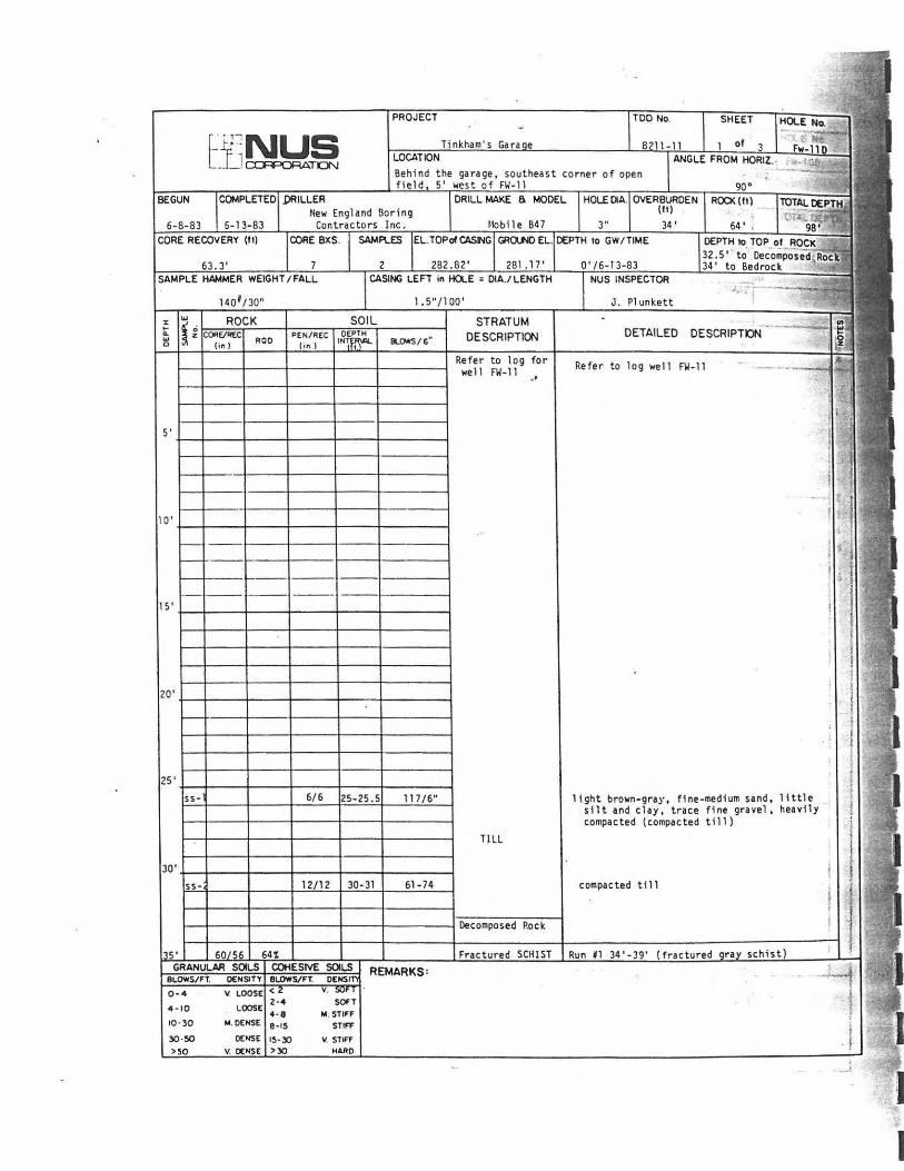
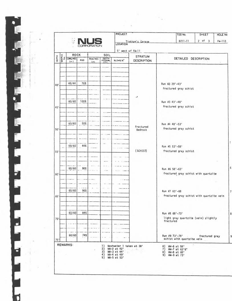
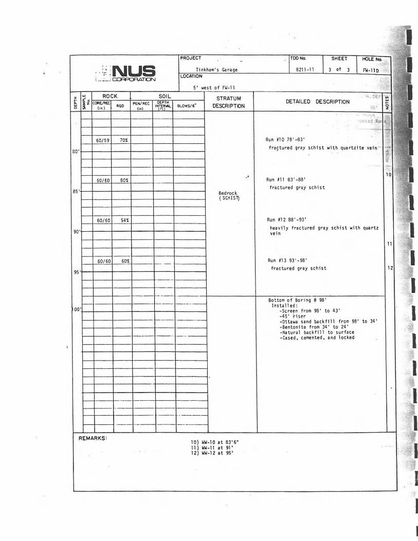
--
---
--- --------
--- --- - ---
--- ---- - - - -------
I PROJECT TOO No SHEET HOLE No- I ~
Tinkhams Ga rage 8211- 11 1 3 of 3 FW- 11 Dl - ~NUS LOCATIONl _ _J caPCAATON
5 wes t ofFW- 11 shymiddot~ ~ROCK SOILz STRATUM It 0poundPTH DETAILED DESCRIPTION 0 COii~ PENRECw 0z RQO BLOWS6 DESCRIPTIONI~0 (1 n ) zlin)
middot middot bullbull l)o ilt
middot-- ~ t4Run 10 78 -83 706059
fra ~ture d gray schis t wi th qua r t zite ve i n shy80
-10 middot Run 11 83 -88 806060
fractured gray schi s t j~85 Bedrock
( SCH ISl)
___ 6060 Run 11 2 88 - 93 54
hea vily frac tured gr ay schi st wi th quart z 90 ve in I
11
_- shyRu n 113 93 - 986060 60 middot-- shy
12 95
fractured gra y sch i s t
middot-middot ----middotmiddotmiddot-- shy
Bottom o f Boring 98middot------shy- Ins tall ed 00 -Screen f rom 98 to 43
- 45 r iser - --middotshy middot---middot-- shy -Otta wa sand backfill from 98 to 34 - Be ntoni te f rom 34 to 24 -Natura1 backfill t o surface - Cased cemen t ed and loc ked
middot-middotshy --- shy
-- ------middot shy
gt
REMARKS 10 ) WW-10 a t 836 11) WW- 11 at 91 I 12) WW-12 a t 95
middot
I I I I I I I I I I I
bullbullbull
I II I STRATIJMI 11middot -ishybullbullbullbull 1lbullntUi-- I ___ _ OEVRIPTLt
I f1eJ l~f
1
r
l 10 tl-~1r----ilr----lr----~11~ 1
---+ll-----lI tri2lcqls I qei I i I I I i I I I I I I I I I I I I I I I I I I I I l I I 11 11e I I I I II1 bii I I
111
11 1
I I~ I I I I I ~~t qQ ill jI I lf I I II I I I I I I I I II I I I I I 1 I I I I I I I I 12~J 11 r 11 I PI I I 1I I I I I II I I I I I i I I I I I I I I I I I I I I I I I I
1 1
11 I
1-l I I j JI 11 rc 1 1 1 1 1
I I I I I I I I I I I I t I 1 I II I J I I I I I I I I I 11 11 1 I 1
1
1 I I I 11111I I I I I
J I 1 1- l I 1
1
1
I I I I middot I I I I I I
r I I I I
GIUHllM sou CDCStoC SlU
CCbullSTl ~ shy ll~KSbull~middot~f~==-1 ~ -
1
II I 1 I 1bull1 I I I I I I I I I I I I I I I I I Z I
I
bullbull _bullbullbull 10 bullbullbull bullMO -
deg -middot-middot
tlXI)bull Qio1cnlt -~~~ iia (ir plf~ (~~)
CIU $1 ~ ~ o-imiddot 2-Ltb ~ ~J ~ ~ rK
I I I~ I
I f$
~ f--41~-+----+---i---+--~~ri
i I f-Z
r r i r s i i T
Lshyi r r I r ~
L r 11 I I I I I rlO
I I I
I I II 1 2I I I l
11~F 1 I I If J I ~Jr
I I 1 1 I1r-~--ili---+---1-I~-~---iL ~1-+---~111
1
~-f~-=~l-middot---11--~---i~bull 1 1 bull I I 1
1r rt1- -+--+---t--=--i1--1-----iIJWl I II I I I I I -middot I I I I I -I I I I
I I I 1
i i 111~1 I I I II = 1 11 I I I Ir
II r I r ~
lrf I r IrIV I ir - I I I
I I r I 2-1I I i r I I I I i r shy~ ICLS COCSM --bull llOtUIQkOoln OlllSTT ~-middot middot- shy4bull10 1bull4
bullbullbull 0middot)0 gtIMO
1~~~ euli~ ~ bulldeg -middot
ri bull
f
r
I I I I ~ j~ampJ- I Ir fT -n ~ ___ r II r I I I I
lrnJ ~ -~ Pt~ I I _-- - bull oAamp I middotk_ I I
I - - lto(J-i --I ~ I I I I
I ~ I Ienmiddotmiddot I II1i_shy
f
l
~ aW-- ~bullbullbulle 441l~
- r ciJ I
(R I ro
~r~+-~-t~~-+o~~-+~~+-~~~-1
I SOIL i_1~1I ftbullbull I -rmiddotm-1 ~f af ~~lo i~~ I bull
I ~01CCiI ---1ifi~ I - -
I LN
r-~
CeuroTAALED tSC-PTOH
I cu~
IFW-210
~
I I I I I I I I I I I I I I I I I I I I I I I I
L__l_ - _I -
[ I I l
I
I I
--
1
- I
1shy
REMARKS
I middot a IC11 bull CAJLIJilITM I __I I _ _
I iJk I --- ___ f I t1 n_J __ 1 - 1 r~ ~~1
I bull 1 l ROCX I SOIL i- i f r
j
I i 1 f I t 11 I JJmiddot1 J r I I - I 1
11
I I I 1
11
omiddotbull bull bull
I l l I I_
1middot4 _bullmiddotbullO middot- bullbull bullbullbull oOmiddotIO ODa ~ ~ N_41i bull oocr -middot
~
j ~O poundCT
I hnc--w-r~ ~
l1Ba+6MHoorJc iOO ~ I bull 1 ~r
f iz14 ~I
J SOii
Il~_=lkJi
I -q1--1tlbullI
I I I I I I II I I I I I III I I I I I I II l
j2COf1---+~_f--~+-~~+-~-+~~~~I
1middot I
1 ~j~+-~--if--~-t-~~-t-~~i--~~---1
L
I I
II L_ I
I I I I I II II II I I
I I I I I
I I I
I I I
I I
bull I I II I
I I I
I I I I l I I II ~ I I I I I II I I I I I
l I I II I I I I I I I II I I
I I II I I I I I II I
I I I I I II I I I I I I II I I I I I II I I I I
I I I I I I I IT
~ I I I I I
REMAllKS
SM(pound r 1 oL _ 1 x - _ I_ I
IFl~ -z_-z IRi1-ZB o I - - ---or ftlJ-Z ~ ~r~ ~ ~ I
1
I I I I I I I I
I I I I I I I
ATTACHMENT B
Guidance Documents
ROUX ASSOCIATES INC CSG11170001M000150ATTA
UNITED STATES DEPARTMENT OF THE INTERIOR BUREAU OF RECLAMATION
USBR 7310-89 PROCEDURE FOR
CONSTANT HEAD HYDRAULIC CONDUCTIVITY TESTS IN SINGLE DRILL HOLES
INTRODUCTION
This procedure is under the jurisdiction of the Georechnical Services Branch code D-3760 Research and Laboratory Services Division Denver Office Denver Colorado The procedure is issued under the fixed designarion USBR 7) 10 The number immediately following the designation indicates the year of acceptance or the year of lase revision
Although rhe term permeability was used in all ocher procedures in this manual percammg co che capacity of rock or soil co conduce a liquid the similar term hydraulic conquctiviry is used throughout chis procedure (See designation USBR 3900 for differences in meaning of rhe two cerms)
Since geologic and hydrologic conditions encountered during drilling are nor always predictable and may nor be ideal variations from chis procedure may be necessary to suit the particular purpose of the resc and conditions at the test sice Much of the information for this procedure was taken from references LI l through L5 l which contain additional information on fielq hydraulic conductivity resting
1 Scope
11 This designation outlines the procedure for pershyforming rests to determine an approximate value of hydraulic conductivity (permeability) of soil or rock in an isolated vertical or inclined interval of a drill hole (boreshyhole) either above or below the water table Usually the rests are performed as a part of the drilling program This procedure can be used in holes of various diameters if suitable equipment is available but N-size L3-in (76-mm)] nominal diameter drill holes are most commonly used2
l2 The constant head single drill hole rest is based on the same theories as the sready-srare or Theim-type aquifer rest and the same assumptions are made These assumptions are ( 1) the aquifer is homogeneous isotropic and of uniform thickness (2) the well (rest interval) fully penetrates the aquifer and receives or delivers water to the entire thickness (3) discharge or inflow is cons rant and has continued for a sufficient duration for the hydraulic system to reach a steady state and (4) flow co or from the well is horizontal radial and laminar Field conditions may not meet all of these assumptions Equations and other factors affecting the rest are given in paragraph 14 Calculations This procedure should nor be used for resting roxic waste containment that requires a very low loss of liquid
13 Constant head hydraulic conductivity rests should be considered scientific tests Grear care should be exercised by chose conducting the rests to eliminate as much error as possible
1 Number in brackets refers co the reference Hereafter referred mas N-size holes
2 Auxiliary Tests
21 The soil or rock penetrated by the drill hole should be identified described and classified from samples taken during the drilling operation Soil can be sampled in accordance with USBR 7010 7015 or 7105 and classified in accordance with USBR 5000 Rock cores or cuttings should be examined and appropriate description and classification made Dara obtained from the drill hole should be entered on appropriate log forms
3 Applicable Documents
31 USBR Procedures USBR 1040 Calibrating Pressure Gauges USBR 1050 Calibrating Pressure Transducers USBR 3900 Standard Definitions of Terms and Symbols Relating to Soil Mechanics USBR 5000 Determining Unified Soil Classification (Laboratory Method) USBR 5005 Determining Unified Soil Classification (Visual Method) USBR 5600 Determining Permeability and Settlement of-Soils [8-in (203-mm) Diameter Cylinder] USBR 5605 Determining Permeability and Serrlement of Soils Containing Gravel USBR 7010 Performing Disturbed Soil Sampling Using Auger Boring Method USBR 7015 Performing Penetration Resistance Testing and Sampling of Soil USBR 7105 Performing Undisturbed Soil Sampling by Mechanical Drilling Methods USBR 7300 Performing Field Permeability Testing by the Well Permeameter Method
1245
2
USBR 7310
32 USER Document 321 Geology for Designs and Specifications by the
Bureau of Reclamation (This document covers both soil and rock)
4 Summary of Method
41 Pump-In Test-Water is injected into an isolated interval of a drill hole in soil or rock and the volume of water injected is determined for a measured period of time The injection pressure is a constant gravity head with or without added pressure head provided by a hydraulic pump The hydraulic conductivity is calculated from the flow rate length and radius of test interval in the drill hole and effective head
42 Artesian Test-Where water under artesian pressure flows out of the drill hole the effective (shutshyin) head at the test interval is measured and the hydraulic conductivity calculated from the flow rate the length and radius of the well and the effective head
5 Significance and Use
51 Hydraulic conductivity tests are made to obtain daca related to (a) identifying seepage potential and dewatering requirements (b) drainage problems (c) ground-water supply investigations and (d) grouting requirements The tests yield approximate values of hydraulic conductivity that are suitable for many engineering purposes Reliability of the values obtained depends primarily on (a) homogeneity of the strata tested (b) suitability of rest equipment used for a given condition (c) care taken in performing the test and ( d) adherence to requirements for proper use of the equations The test is also used in formulating geologic descriptions and interpretation of material properties particularly where there is poor sample recovery
52 Where tests are performed in fractured rock results could reflect secondary conductivity rates which would not represent primary conductivity of the intact mass When the test is performed in fractured brittle swelling clay or rock or where fractures contain loose material hydraulic conductivity may be reduced and judgment should be used in applying results
53 Generally this procedure is suitable for materials in which the hydraulic conductivity ranges between 5 and 100000 ftyr (5 X 10⁻⁶ and 1 X 10⁻¹ cms) and where results are to be used for engineering purposes The procedure is not applicable in materials of lower permeability particularly for purposes such as investigashytions for containment of toxic wastes
6 Terminology
61 Definitions are in accordance with USBR 3900 Some definitions are from Glossary of Geology [6]
62 Terms not included in USBR 3900 specific to this designation are
62 l DnJJ Hole-A circular hole made by drilling
622 Feed Pipe (conductor pipe injection pipe riser pipe drop pipe)-The main pipe (or rod) which conducts water from the collar of the hole into the test interval in the drill hole for the hydraulic conductivity test
623 Baifer-A cylindrical container with a valve on the bortom for admission of fluid attached to a line and used for recovering and removing water cuttings and mud from a drill hole
624 Walking Beam-An oscillating rigid lever balanced on a fulcrum used to activate the cable in cableshytool drilling by alternating up and down motion
625 Aquifer-A water-bearing bed or stratum of earth gravel or porous rock with interconnected openings or pores through which water can move
626 Packer-A short expansible device deliberately set in a drill hole to prevent upward or downward fluid movement generally for temporary use The expansible part of the packer is called the gland Straddle packers are two packers separated by a length of perforated pipe to span or straddle a test interval
627 Artesian-An adjective referring to ground water under hydrostatic pressure ie an artesian aquifer is a confined aquifer Artesian ground water rises above the confining layer in the drill hole and may or may not flow at ground surface
628 Ground W1ter-That part of the subsurface water that is in the zone of saturation
629 W1ter Tizble-The surface between the zone of saturation and the zone of aeration that surface of a body of unconfined ground water at which the pressure is equal to that of the atmosphere
6210 Perched Water Table-A water cable usually of limited area maintained above the normal free water elevation by the presence of an intervening relatively impervious confining stratum
6211 Gauge Saver-A vessel with a pressure gauge filled with glycerin or oil to protect the gauge from direct contact with fluid in the pressure line (see fig 1)
6212 Holding Pressure (applicable primarily for grouting) -The gauge pressure after the water-pumping system has been shut off at the valve ahead of the gauge and backflow is prevented
6213 Back Pressure (applicable primarily for grouting)-The gauge pressure in the system after the holding pressure has dissipated as determined by opening a valve and allowing the gauge ro drop ro zero and then reclosing the valve
6214 Backflow(applicable primarily for grouring)shyThe reverse movement of water out of the drill hole when the holding andor back pressure below the packers exceeds the pressure of the water column in the hole
7 Interferences
71 During drilling it is important ro minimize movement of fines [minus No 200 sieve-size material (75 microm)] into the material being tested and to remove any accumulation of fines from the wall of the drill hole during preparation for the test so as to avoid obtaining test values
1246
USBR 7310
Heov1 Out1 Pressure Gouge
poundLpoundVATON SECTION
TOP VpoundW BOTTOM VIEW
Figure I - Gauge saver device for protecting pressure gauge 40-D-4287
lower than the actual hydraulic conductivity of the material being tested Drilling using clear water without additives is preferred Bentoniticmiddotmuds should nor be used in holes where hydraulic conductivity testing is to be performed Biodegradable additives may be used if necessary but only if the test interval is adequately cleaned before testing The drilling procedure should be documented on the log form
72 Test results can be adversely affected by injecting water containing sediment which would tend to plug voids in the material being tested
73 The temperature of the injected water should be equal to or warmer than that of the ground or ground water This reduces the tendency of air dissolved in the water to become entrapped in the voids of the material be ing tested and co cause low values of _hydraulic conductivity In most areas not affected by artesian conditions the temperature at a depth of about 25 feet (8 m) below the ground surface remains relatively constant at the annual mean air temperature for the region At significantly greater depths temperature rises about l degF (06 degC) for each 500 to 1000 feet (150 to 300 m) of depth The temperature of the injected water especially if it is known to be colder than the ground-water temperature should be recorded on a geologic log or the hydraulic conductivity cesc daca forms (see subpar 812 for suitable temperature measuring devices)
74 It is possible that dissolved minerals in the wacer used for a rest may react chemically wich substances in the material being reseed to cause a change in the hydraulic conductivity Therefore it is desirable to use wacer for the test chat is similar in quality co that expec~ed to permeate che ground when che project is in operation
8 Apparatus
81 Drill Rigs (see fig 2) ~1 ~ Rotary Drilling-A drilling method resulting m grinding a hole with a hard-toothed drill bic at che end of a rocacing drill rod (pipe) The equipment consists essentially of a power unit hoisting or rugging unit controlled-feed rotary drill head and mounting frame masc or tripod and circulating pump The rig should have various accessory drilling andsampling equipment (rods bits core barrels augers) as required for drill hole advancement sampling and testing
812 Cable Tool Drilling-A method of drilling in which the material at the bottom of the hole is broken up by a steel bic with a blunt chisel-shaped cutting edge The drilling equipment consists essentially of a mast a sering of drill tools (casing tubing or pipe of one size) chat is alternately lifted and dropped by a hoist with a power unit and a walking beam A bailer is always used with a cable tool rig Normally a cable tool drilled hole is noc satisfactory for hydraulic conductivity testing with packers
82 Injecrion Pump-A centrifugal or helical screw type pump providing a constant water flow is required This may require a special pump separate from that used for drilling operations Although there may be conditions where a larger or smaller pump may be required highshy
quality pumps having a capacity of 40 galjmin (150 L min) at a pressure of 120 bf in2 (830 kPa) (such as Moriyo model 3L-8 manufactured by the Robbins and Myers Company Springfield Ohio or equivalent) are adequate for most hydraulic conductivity tests The pump should provide the required flow at the required constant pressure with maximum allowable pressure fluctuation-due co pumping pulsations-of plusmn5 percent of the test gauge pressure A surge chamber is required for all testing chis minimizes pulsations which can affect the injection race in the test interval Also ic makes readings more accurate and protects che pressure gauges against damage from sudden pressure changes
83 Feed P1pe- The feed pipe should be of adequate diameter to minimize head losses and have adequate tensile strength to withstand pumping pressures and stresses during hoisting or tugging The feed pipe is commonly a threaded and coupled assembly of pipe or tubing having a uniform inside diameter Drill rods generally of N-size can be used wichouc seriously affecting reliability of rest data if che flow rate to the test interval does nor exceed about 15 galmin (57 Lmin) and the depth co che top of che interval does noc exceed 50 feet (15 m)
NOTE 1-Use of drill rods as feed pipe should be permitted only after the assembled drill rod string has been pressure reseed ro cali_brare head losses ar anricipared flows If seals or sealing marenals are used during calibrarion the same type of seals or sealing materials (not oils or wax) should be used during hydraulic conductivity resting
84 Flowmecers-One or more calibrated flowmecers are required the capacity of each meter should be specified
1247
USBR 7310
- Byooss votve Surgechomber~
Wotermettr-
Observation oost see Detail A
SCHEMATIC ARRANGEMENT OF EQUIPMENT
(Water meter
~==it=======t(k=====- For wottr tes t ing middotWell cas1n9
Press1Jre gouge
-=====bull===========~-For drilling DETAIL A OBSERVATION POST FOR
OPTIONAL EQUIPMENT ARRANGEMENT FOR DETAILS 8 AND C
WATER TESTING ANO DRILLING FROM SECTION X-X TO WELL
DETAIL D GRAVITY TEST
DETAIL B DETAIL C DOUBLE PACKER TEST SINGLE PACKER TEST
Figure 2 - Schematic arrangement of hydraulic conductivity equipment 801-D-l I I
For flows up to 50 galmin (200 Lmin) a 1-inch (25- 851 Pneumatic Piezometers-A down-hole pneushymm) diameter disk-type meter may be used For higher matic piezomerer system has been developed [7] flows a 2- or 2-12-inch (50- or 65-mm) diameter impellershy Descriptions of the equipment and procedure as used ar type meter is recommended two damsites are presented in appendix XL
841 A straight uninterrupted section of pipe having 852 Electrical Transducers-Electrical transducers an inside diameter equal to the rated size of the meter have been used as down-hole pressure sensors by other and a minimum length 10 times the inside diameter of agencies [8) particularly for very low hydraulic conducshythe pipe should be provided upstream of the meter tivities [below 1 ftyr (1 X 10⁻⁶ cms)] The USBR has Manufacturers commonly recommend pipe lengths of one used electrical down-hole sensors in preliminary trials tO two times the inside diameter of straight pipe Electrical transducers measure pressures more accurately downstream from the meter than pneumatic piezometers and can be connected tO a
85 Pressure Sensors-Where required calibrated strip-chart recorder for a continuous record However pneumatic piezometers or electrical transducers can be used transducers are considered less rugged for field use and as down-hole sensors tO measure pressures at the rest require more maintenance and experienced personnel tO
interval during a hydraulic conductivity rest Down-hole operate than do pneumatic piezometers sensors are preferred over the method of calibrating the 86 Pressure Gauges-When down-hole pressure piping system for head loss between a pressure gauge on sensors are not available or sensors are not working the surface and the test interval However an above-ground properly calibrated pressure gauges can be used t0 estimate pressure measurement can provide a check of the pressure effective pressure in rhe rest interval after correcting for sensor friction loss through the feed pipe and packer All pressure
1248
USBR 7310
gauges used in water resting should be high-quality stainless steel glycerin or oil filled wich pressure indicated in both lbfin2 and kPa (such as manufactured by Marsh Instrument Company a unic of General Signal P 0 Box 1011 Skokie Illinois or equal) Pressure gauge ranges should be compatible wich middot cescing requirements chey should be sized so char che gauge capacity does not exceed two co three rimes che maximum desired pumping pressure for each respective pumping stage Gauges should have the smallest graduations possible and an accuracy of plusmn25 percent over che coral range of the gauge If a gauge saver is used wich che gauge calibration should be made wich the gauge saver in place Accuracy of che gauges should be checked before use and periodically during the resting program (see subpar 112 for additional information)
861 One or more pressure gauges should be located downstream of che flowmecer and downstream of any valves ac che cop of che feed pipe This location for pressure measurement can be used by inserting a sub (adaptor or shore piece of pipe) wirh che gauge - installed on che cop of rhe feed pipe
862 Ac least one additional calibrated replacement gauge should be available ar che resr sire
87 Swivel-During che hydraulic conductivity cesc ic is preferable co eliminate the swivel and use a direct connection co the feed pipe If a swivel muse be used in che water line during resting ic should be of che nonconscriccing type and calibrated for head loss Significant friction loss can result from use of che constricting type
88 Packers-One or two (straddle) packers are required for che rest Packers may be either bottom-set mechanical screw set mechanical pneumatic inflatable or liquid inflatable The pneumatic inflatable packer is the preferable type for general use and is usually che only one suitable for use in soft rock and soil The gland of this packer is longer and more flexible chan the ocher types and will form a tighter seal in an irregular drill hole A leather cup type of packer should noc be used To ensure a eight water seal che length of contact between each expanded packer and che drill hole wall should noc be less than three rimes the drill hole diameter
NOfE 2-More than one type of packer may be required to test the complete length of a drill hole The type of packer used depends upon many factors eg rock type drill hole roughness spacing and width of rock joints and test pressures
881 Inflatable Packers-Inflatable packers with an expansible gland and a floating head (see app fig Xl2) should be designed for anticipated drill hole diameters and pressure conditions For normal hydraulic conductivity cescing a reasonable maximum recommended working pressure inside and outside of che packer is 300 lbf in2
(2070 kPa) [8] Inside pressure should be increased in water-filled holes proportionally co che sracic head For drill holes wich sharp projections in the walls a wireshyreinforced packer gland having a higher working pressure [7] may be required The pressure in che packer should not be high enough to fracture the material being reseed
The pressure required to form a cighr seal ac che ends of a cesr interval depends on the flexibility of rhe gland the friction of the floating head and che drill hole roughness The minimum differential pressure between che packer and the cesc interval can be derermined by res ring packers in a pipe slighrly larger rhan rhe nominal diameter of rhe drill hole in order co simulate possible enlargement of rhe drill hole during drilling For a given resr interval pressure che packer pressure is increased until ir provides a waterrighc seal between the packer and the material with which ic is in contact The pressure in rhe packer should range approximately berween 30 and 300 lbfin2 (210 ro 2100 kPa) greater chan char in che cesc interval with 100 lbfin2 (690 kPa) being normal Pneumatic inflatable packers can be inflated with compressed air or compressed nitrogen
882 Special pneumatic packers are available for use in wireline drilling operations Because che packers must be able co pass through che wireline bit and then expand co completely seal che hole ac che cesc interval special materials are needed for che packer gland A special packer assembly-consisting of cwo packers in tandem-is used with the upper packer being expanded inside che drill rod just above che bic and che lower packer expanded against che wall of the hole just below che bit The two packers on the assembly can be positioned properly-relative co the bit-by a sec of lugs or a ring located on the assembly Special seals or connections are needed co attach che water supply co che wire-line drill pipe at the surface
883 A minimum of two secs of replacement packers andor spare glands should be available at the test sire
89 Perforated Pipe Sections-Lengths of perforated steel pipe corresponding ro the lengths of rest intervals are required between packers to admit water inco che rest intervals The coral area of all perforations should be greater than five rimes che inside cross-sectional area of che pipe These perforated pipe sections should be calibrated for head loss
810 Well Screen-Well screen or slotted pipe may be required for cescing in granular unstable materials chat require support [9] As a general rule the maximum size of sloe width should be approximately equal to che 50shypercent size of che particles around the drill hole (see subpar 114)
811 Water Level Measuring Device 8111 Although there are ocher types of water level
indicacors che electrical probe indicator is most commonly used Essentially ic consists of (1) a flexible insulated conduit marked in linear units and enclosing cwo wires each insulated except ac che tips (2) a low-voltage electrical source and (3) a light or ocher means of indicating a closed circuit which occurs when che rips contact che water surface Different brands of electric wacer level indicacors and even different models of the same brand ofren have their own unique operating characteristics Before using any electric water level indicacor it should first be reseed at the surface in a bucket of water
8112 For approximate measurements of the water level when ic is within about 100 feet (30 m) of the ground
1249
USBR 7310
surface a cloth tape with a popper can be used A popper can be made from a short pipe nipple (or length of tubing) by screwing a plug attached to a graduated tape intu one end of the nipple and leaving the other end of the nipple open When the popper is lowered in the drill hole and the open end of the pipe nipple strikes a water surface it makes a popping sound and the depth to water can be measured by the tape
8113 An accurate measuremenr of the water level can be made by chalking the lower end of the steel tape After contacting the water level the tape should be lowered about L more foot before retrieving it Measurement is then made to the wet line on the tape
812 Temperacuie Measuring Device-Equipment for measuring ground-water temperature is available from commercial sources or can be made from a thermistor two-conductor cable reel Wheatstone bridge and a lowshyvoltage electrical source A maximum-minimum type thermometer is acceptable
9 Regents and Materials
91 ~71ter (See subpars 72 73 and 74)-The clear water supply should be sufficient tO perform the hydraulic conductivity test without interrruption and to maintain the required pressure throughout the test period
92 Swd or Gravel Backfill-Where a granular backfill is used t0 prevent sloughing of the drill hole wall it should be a clean coarse sand or fine gravel Laboratory permeability tests (USBR 5600 or 5605) should be made on the backfill material to make sure that it has a coefficient of permeability greater than one order of magnitude higher than that expected of the in situ material being rested
10 Precautions
L01 Safety Precautions L011 This procedure may involve hazardous
materials operations and equipment lO l2 Use normal precautions for drilling [ 10 11] L013 Precautions should be taken during calibration
pressure testing of equipment particularly testing of packers with compressed air or nitrogen (never use oxygen) to avoid injuries from a sudden packer or hose rupture
L02 Technical Prernutions 102 l As a general rule total pressure (static head
plus gauge pressure) applied in the drill hole should nor exceed 1 lbfin2 per foot (226 kPam) of rock and soil overburden at the center of the test interval if the test interval is 10 feet (3 m) long or less If the rest interval exceeds 10 feet pressure should not exceed 1 lbfin 2 per foot of overburden at the top of the interval In layered or fractured material or for drill holes near steep abutments or slopes 05 lbf in2 per foot ( 113 kPa m) of material to the nearest free surface is an appropriate maximum pressure Higher pressures than these may fracture the materials
1022 If there is excessive or complete loss of water when the hole is being drilled drilling should be sropped before cuttings fill the voids and a hydraulic conductivity rest completed on a shorter than normal length rest interval
1023 Hydraulic conductivity rest equipment should be considered and treated as precision testing equipment Gauges thermometers ere should have their own protective cases they should not be carried with drill tools or be tossed around They should be calibrated frequently Ir is recommended that all test equipment needed for hydraulic conductivity resting be kept separate from drilling equipment
11 Calibration
111 For Measurment ofEffeaive Head 11 l l Pressure Sensurs-Calibrate down-hole
pressure sensors by the methods and at frequencies prescribed by USBR LOSO
ll12 Friction Loss Estimates-Where down-hole pressure sensors are nor used estimates of effective head at the rest interval are made by subtracting friction loss from the applied head measured at the ground surface The friction loss should be determined for all components of the piping system from the pressure gauge to the test interval
1112 I Calibrate friction loss in parts or sections of the piping systems including ( L) the swivel (if used) (2) feed pipe (per unit length) and (3) the packer assembly Record the data with references to the particular parts calibrated in tabular or graphical form so the accumulative friction loss can be totaled for determination of effective head at the test interval The calibration procedure is as follows
I l l211 Lay out the individual or joined parts to be calibrated on a horizontal surface with calibrated pressure gauges at each end
l L 12 12 Pump water through the system at incremental increasing flow rares to the maximum flow rare expected to be used in the test allow the flow to stabilize between incremental flows
L 112 L3 Record the pressure at each gauge for each incremental flow rate
11 l 2 L4 Calculate the friction head loss for each incremental flow rare
2f = 23 l ( p ~I p ) (I )
where f = friction head loss in feet of head per linear foot
of pipe ftft or mm P1 = upstream pressure bf in 2 or kPa P2 = downstream pressure lbfin2 or kPa d = pipe length fr or m (d = l for swivel or packer
assembly) 23 l = converts from pressure in bf in2 to head in feet
or 0102 converts from pressure in kPa to head in meters
Example assume
P1 = 186 lbfin2 or 128 kPa P2 = 132 lbfin2 or 910 kPa d = 100 ft or 305 m
1250
USBR 7310
Inch-pound application
f = 231 ( 18 ~~-~3 2) 125 ftfr
SI application
f = 0 102( 128
- 9 tO) = 124 mm 305
l l l215 Plot friction head loss versus flow rare Figure 3 is an example of a plot of friction head loss (f) at relatively low flow races for a 10-foor (33-m) length of 1-14-inch (32-mm) diameter pipe Since head loss in pipe at turbulent flow is approximately related to velocity squared a plot of friction head loss versus the square of the flow rate is nearly a straight line (see fig 4)
NOfE 3-There are srandard rabies and charcs which provide unit friction losses for various sizes of pipe elbows cees reducers ere for clean and ruscy conditions Although such informacion is sometimes used it is preferable to determine friction losses in che piping syscem and packers accually used for che hydraulic conductivity rest
111216 To calibrate a packer inflate the packer in a shore length of casing or pipe in which amiddotvalve and pressure gauge have been installed A pressure gauge is also installed in the rods immediately ahead of the packer assembly Pump water into the rods at incremental increases (or decreases) of flow rate-allowing the system to stabilize after each incremental change-until the highest anticipated flow rate is reached
NOfE 4-For packers smaller than N-size such as the B-size used in wireline equipmentmiddot there are significant head losses and relatively low flow races must be maintained This requires water meters and pressure gauges capable of accurately measuring the low flows and small changes in pressures
112 Pressure Gauges-Calibrate each pressure gauge (see USBR 1040) by comparing it with a test or master
FLOW RATE IN LITERS PER MINUTE
o
I _ I_ I I I II
I I I I I loI I I I I I rI
I I I )I
I I I I I v I I I I I I I I I I lr II
I I
I I I I 11deg II i j~ I I I -~-----1 -- I I I I i
JO deg HOW RATE IN GALLONS PEA MINOT[
Figure 3 - Head loss due ro friction at increasing flow rates for a I 0shy
foot (3-m) 1-14-inch (32-mm) diameter iron pipe
gauge The master gauge should not be used during drilling or hydraulic conductivity testing Calibrate each gauge at the start of a res ring program plus one additional calibration per week during rests of long duration
113 Flowmeters-Calibrate a flowmerer by flowing water into a container of known volume the container used for the volume check should be commensurate in size with the flowmeter size and graduations From these data flow rares can be calculated for comparison with meter readings All flowmeters should be calibrated to an accuracy of plusmn1 percent Calibration should be done at the stare of the resting program plus one additional calibration per week during rests of long duration
NOfE 5-Some impeller-type flowmeters have an accuracy range significantly less than indicated by the dial Minimum and maximum races should be esrablished
114 Well Screens and Perforated or Slotted Pipe Sections-From manufacturers dara or by calibration determine the head losses in expected flow ranges to ensure there is no restriction of flow into the material being tested
12 Conditioning
12 l Nor applicable special conditioning requirements are not needed for this procedure
13 Procedure
13l Cleaning ofDnll Hole 13l1 Remove any accumulation of fine particles
(smear mud cake compaction caused by driving casing etc) from the drill hole wall Such accumulation significantly restricts the flow of water into or from the hole Exercise good judgment in cleaning the hole since excess cleaning may be detrimental If there is a question as to whether or not drill holes in particular materials need cleaning hydraulic conductivity tests can be performed in holes with cleaning and others without cleaning If cleaning does not significantly change rest results at a sire cleaning of additional intervals in the same materials may not be necessary
131 l1 When the rest interval is above the water table it may be possible to brush or scratch the drill hole wall to break up accumulated fines For unstable materials which require use of a well screen materials which cavemiddot against the screen may break up the accumulation of fines on the wall Mild surging with a bailer while adding water also may help break up a disturbed or compacced zone but this may stir up fines which then plug the voids in the material co be rested Mild jetting-followed immediately by bailing or pumping-also is a possibility
13 l l2 When the test interval is below the water table-in materials chat are rock-like and self-supporcingshyuse of a water jet in the hole (preferably accompanied with pumping to induce flow into the borehole) is one of the best methods to clean the hole After jetting bail or pump the sediment-laden water from the rest interval Jetting can also be used through a screen below the water
1251
tJ
I I 0 GO-GI I GO-G2 0 GI -G2
~
I
I
v
v p-shy~ -shyl--~ L--shy
-shy
v
0
middot 005 =0 00005 100
-shy~--~ 0 middot 0025 =0 00005
I 50 I
~ --shy = 0 00005
50
I
t - A
v -
-
[] --shy shy--shy0 -
4--l_-E
-
16
-shy-shy-8 --shyl---shy~ - 2
~ ~---shy z 3 4 5 6 7 8 9
FLOW RATE SQUARED (q 2 )(10001
s of oalmin ) 2
Figu re 4 - Plot of feed p_ipe ca libra tion data - example
USBR 7310
2FLOW RATE SQUARED (q2)( 1000degs of L min)
10 15 20 25 - 30 35
50
40
r w w LL
z
~ 30 0 J Cl ltgt w I
z 0 20 r S a LL
10
0
cable in unstable materials For soft rock flushing che sides of che drill hole by running che bit or a bailer up and down the hole may enlarge the hole by erosion or ocherwise change the characceriscics of the fracture systems
13113 Finally clean the drill hole by pumping or bailing water from the bottom upward with the pumping continued until the return fluid is clear without cuttings or sediment Record the method used in cleaning the hole on the log of drill ho le or on a special testing form
132 Length of Test Interval 1321 The length of the test interval depends on
(1) purpose of the test (2) stratigraphic interval and (3) flow rate Where materials are relatively uniform use a test interval of about 10 feet (3 m) Where flow rates are high shorten the test interval co locate high flow race zones where races are very low the interval may be lengthened if desired
133 Ground-Water Level Determination 13 31 Depth co ground-water level muse be
determined before calculating hydraulic conductivity Measure depths to water levels with an electrical probe or o ther suitable equipment (see subpar 811)
1332 Auger Holes-ln power auger or other types of holes to which water is not added as pare of the drilling process report the presence or absence of a water level depth to water level and dace of initial and final water level measurement In materials of low hydraulic
14
12Cll a w r w
101 z () Vgt 0
8 J
Cl ltgt w I
Sz 0 r u a
4 IL
conduccivicy several days to several weeks may be required for a water level to stabilize in the hole Report evidence of moisture in the cuttings and if a perched water level was observed
1333 Rotary or Cable Tool Holes-For drill holes in which addition of water to the hole is an integral part of the drilling process
13331 Bail or pump the hole dry or to a stable wa ter level at the close of the last shift each day and record level
13332 Report the presence or absence of water and depth to water at the beginning of the first shift each day Additional readings are desirable whenever water level in the hole has nor been disturbed for an appreciable period of time
13333 Report changes in water level detected as the hole is drilled deeper Record faccors that affect the water level such as depth of casing andor cemented intervals These data may be helpful in recognizing perched or confined (artesian) conditions
13334 Upon completion of the hole the water must be bailed down to the extent practicable the water level measured and the dace recorded of hole completion Measure the water level for a period of days or weeks until equilibrium is reached
NOfE 6-At times exceptions must be made to the requirement for conrinuation of water level readings Such is the case when
1252
USBR 7310
state or local laws require chat the hole be filled continuousiy from bottom to cop immediately upon hole completion and before the drill crew leaves the sire In ocher instances landowners may allow right-of-entry for only a limited time for measurements
1334 Perched and Artesian Aquifers-lc is imporshytant tO recognize perched and artesian aquifers especially those under sufficient pressure tO raise the water level above the confining layer but nor tO the ground surface (see (5 ]) They must be distinguished from water table aquifers (those which continue in depth) If perched water table or artesian aquifers-separated by dry or less permeable strata-are encountered in the same drill hole the resulting water level in the hole is a composite therefore conclusions and interpretations based on such data are misleading If a perched water table is recognized (or suspected) during drilling water levels must be determined for each zone for calculation of hydraulic conductivity This might require completion of the drill hole with a watertight seal set at a suitable horizon tO
separate two water table conditions In this type installarion two strings of pipe or conduit are required one extending down to the portion of the hole immediately above the packer and a second string extending through the packer to a point near the bottom of the hole Water-level measurements provide the basis for determining a perched condition or if the lower water table is under artesian pressure
13 35 Mulriple Water-Level Measurements-In some instances it is desirable tO install multiple conduits and packers or plugs in a drill hole so that ground-water levels (or pressure heads) in several water-bearing horizons can be measured over an extended period of time (see [5] pp 7-14)
134 Pressure Tests With Packers 134 l The recommended arrangement of typical
equipment for packer pressure tests without a pressure sensor is shown on figure 2 (See app fig Xl l for equipment with a pressure sensor) Beginning at the source of warer the general arrangement is clean water source suction line pump discharge line tO srorage andor settling tank suction line water-supply pump surge chamber line ro bypass valve junction water meter gate or plug valve tee with sub for pressure gauge short length of pipe on which the pressure gauge is attached tee and off-line bleeder valve for evaluating back andor holding pressure flexible 1-14-inch (32-mm) diameter hose and 1-14shyinch-diameter feed pipe ro packer or packers in drill hole which isolate the rest interval All connections should be tight and as short and straight as possible with minimum change in diameter of hose and pipe Friction loss decreases as the pipe diameter is increased
1342 When the material is subject co caving and casing andor grout is needed to support the walls of the drill hole the hole should be water rested as it is advanced Other hole conditions may make this procedure desirable or necessary The following procedure is commonly used
1342 l After the hole has been drilled to the top of the interval to be tested it may be desirable tO remove
the drill string from rhe hole and advance casing or grout ro rhe bonom of the hole
13422 Advance the hole 5 to lO feet ( 15 to 3 m) into the material to be rested
13423 Remove the drill string from rhe hole 13424 Clean the interval to be tested and record
the depth tO the warer table if present If a composite water level is suspected the warer level affecting rhe rest should be determined by measurements through the feed pipe after rhe packer has been seated and the water level has stabilized
13425 If rhe hole will stand open sear a single packer ar the top of rhe test interval Record the type of packer irs depth and packer pressure if it is rhe inflatable type
13426 Pump water into the interval ar a rate to develop a suitable pressure The pressure to be used depends upon testing depths and ground water levels or pressures Materials subject to deformation or heaving such as by separation of bedding planes or joints or materials at shallow depths must nor be subjecred to high pressures (see subpar 102 l ) For comparison of flow rates in different pares of a single foundation and with results from other foundations some of the following pressures are commonly used 25 50 75 and LOO lbfin 2 (170 350 520 and 690 kPa)
NorE 7-At test pressures less than 25 lbfin2 errors in measurement of pressure and volume of water may increase unless special low pressure gauges are used Gravity tests provide more accurate results under these conditions At pressures higher than 10 lbfin2 difficulties in securing a right packer seal and the likelihood of leakage increase rapidly However under artesian pressures or in deep holes the water pressure-as registered on a surface gauge-will need to be sufficient to overcome the effeccive head at the test interval and firmly seal the packer
NillE 8-Where the hole is subject to caving a pump-down wire-line system has been developed rhar can be used to eliminate removal of the drill string from the hole With this system the hole is drilled to the bottom of the interval tO be tested and the drill rod is raised so the end of the rod is at the top of the test interval The tandem packer (see subpar 882) is then lowered through the drill rod and expanded to seal both inside the rod and against the wall of the hole at the cop of the test interval Models of this equipment are available which have transducers below the packer for measuring water pressures at the test interval
13427 For determining effective head artesian heads encountered in the drill hole are treated the same as water table conditions ie the depth from the pressure gauge or the water level maintained during the test to
the stabilized water level is used as the gravity head If the artesian head stabilizes above the ground surface the gravity component of the effective head is negative and is measured between rhe stabilized level and the pressure gauge height If a flow-type rest is used the effective head is the difference between rhe stabilized water level and rhe level maintained during the flow period
1253
USBR 7310
13428 Afrer pressures are selected based on ground-water conditions and the purpose of the test perform a test at each pressure Usually a 5-cycle procedure is used three increas ing steps to the maximum pressure and then two decreasing steps to the starting pressure This cycling allows a more derailed evaluation of rest results than testing at a single pressure and commonly allows extrapolation to ascertain at what pressures the following may occur (1) laminar flow (2) turbulent flow (3) dilation of fractures ( 4) washouts (5) void filling or (6) hydraulic fracturing However the equations normally used to ca lculate hydraulic conductivity are based on laminar flow conditions
NOfE 9-ln some insrances on ly a single water pressure test at a given interval in the drill ho le may be required For example if geologic conditions are known and there is no need ro perform the seeps in subparagraphs 13422 through 13426 a single value of hydraulic conductivity with a relatively low application of pressure may suffice
13429 During each test continue pumping water to the test interval at the required pressure until the flow rate becomes stable As a general guide maintain flow rares during three or more 5-minute intervals during which l-minute readings of flow are made and recorded In tests above the water table water should be applied to the test interval until the flow rate stabilizes before starting the 5-minuce measurement intervals Where tests are below the water table flow rates usually stabilize faster than for the tests above the water table and the time period before the 5-minure test intervals may be shorter These rime periods may need to be varied particularly when rests to determine grouting requirements are made
134210 Determine and record the presence of back pressure and decay of holding pressure Afrer the rest deflate the packer and remove it from the drill hole
134211 Advance the drill hole and if necessary the casing repeat the procedure in subparagraphs 13423 through 134210 until the required depth of drill hole is reached When casing is used in a drill hole always set the packer in the material below the casing
1343 If the hole will stay open without casing it can be drilled to final depth and after cleaning the hole hydraulic conductivity rests can be performed from the bottom of the hole upward using straddle (double) packers Although a single packer can be used to test the bottom interval of the hole starting at the bottom with double packers will cause loss of borehole testing of only about the length of the bottom packer and will save one complete trip in and out of the hole with the drill string assembly co change the packers After the test for the bottom interval is completed straddle packers are used for successive test intervals up the drill hole See subparagraph 1342 where caving or other hole conditions will not allow this procedure
135 Gra vity Tests 135 1 Constant-head gravity tests are usually
performed without packers above or below the water table with drill holes of N-size or larger (see fig 2 derail D)
This type of test is often made in reasonably stable-walled drill ho les up to 25 feet (76 m) depth where water pressure at the test interval needs to be kept low The test is usually performed in successive 5- or 10-foot (l5- or 3-m) intervals as the drill hole is advanced The upper end of each test interval is normally determined by the bottom depth of tightly reamed or driven casing If the casing is not believed
middotto be tight appropriate entries should be recorded on the log form If the wall of the drill hole is stable the test can be performed in the unsupported hole If the wall needs to be supported use a well screen (see subpar 114 for calibration) inserted through the casing It may be necessary to ream or drive the casing to the bottom of the interval set the screen and then pull back the casing to expose the screen Afrer the test the screen is removed and the casing reamed or driven to the bottom of the hole
NOfE lO-Clean coarse sa nd or fine gravel backfill (see subpar 92) may be used instead of a well scree n Ream or drive rhe casing ro the borrom of the inrerval dean ir our and add rhe backfill as rhe rnsing is pulled back ro expose rhe resr interva l Record use of rhis procedure on the log form
l 35l l If the drill hole is self-supporting clean and prepare it in rhe normal n1anner (see subpar 13l)
l35 l2 If the drill hole is not self-supporting lower the well screen and casing into the hole
135 l3 For test intervals above the water table maintain a constant head of water _within 02 foot (60 mm)] at the top of the test interval by injecting water through a small diameter rube extending below the water level maintained during the test For rest intervals below the water table or influenced by artesian conditions maintain a constant head a short distance above the measured static water level
Monitor the water level with a water-level indicato r If the water-level indicator is inserted in a small diameter pipe in the casing the wave or ripple action on the water surface will be dampened and permit more accurate watershylevel measurements
NOfE l l-When rhe flow rare is very low rhe consranr wa rer level c1n be maintained by pouring warer in rhe hole from a graduated container
135 l4 Record the flow rate at wne intervals until a constanc flow rare is reached
135 l5 Repeat the procedure of subparagraphs 135 l3 and 135 14 at one or more different water levels
13516 This rest is essentially the same as desigshynation USBR 7300 (see also L3] p 74) the instructions in USBR 7300 for performing the rest and calculating hydraulic conductivity apply to this procedure also
14 Calculations
14 l For pressure or constant gravity head hydraulic conductivity rests calculace the hydraulic conductivity of
1254
USBR 7310
rhe soil or rock by rhe following equation (expressed m consisrent unirs) [4]
k = ~ In ~ where L ~ lOr (2)
or
k = ~ sinh-1 r where lOr~ L ~ r (3)
where k = hydraulic conducrivity fryr or cms q = consrant race of flow into che rest interval
ft3yr or cm3s L = length of the test interval ft or cm
H = differential head of wacer ac rest interval fr or cm
r= radius of the borehole ft or cm In= natural logarithm loge
inv~rse hyperbolic sin~ smh- 1 x In (x + -yx2 + 1)
142 An example calculation for a single packer test _ in the botrom of a borehole belovt the wacer table follows
Example assume
r = 18 in or 015 ft= 46 cm q - 22 galmin or 83 Lmin q = 15 X 10 ft3yr = 140 cm3s L 30 ft = 91 cm
Hg gravity = disrance from ground-water level co pressure gauge = 102 ft = 311 cm
Hp pressure 5 lbf in2 X 231 ftwater (lbf in2)
116 ft = 3 54 cm of water H = Hg+ Hp= 218 ft= 664 cm
~ = ~lo = 20 hence use equation (2) 5 k = _9_ In]
2rrLH r k = 15 X 10 ft3 yr In 30 ft
2rr (30 ft) 218 ft 015 ft k = 11X103 ftyr = 11 X lQ-3 cms
NafE 12-These equations are most applicable and reliable where the length of test interval is at lease 5 r and the interval is below che water table The equations are based on laminar flow of fluid through porous media Flow races high enough co cause turbulent flow invalidate the results in all types of material In fractured material the calculated value should be considered an apparent hydraulic conductivity even under laminar flow conditions
143 For pressure resrs when rhe resr interval is below the water table H is the distance from rhe water table to the elevation of che pressure gauge plus applied pressure converted to linear units of water head
Where the rest interval is above the water table His rhe distance from rhe midpoint of the isolated rest interval to che elevation of the pressure gauge plus the applied pressure converted to linear units of water head
For gravity rests above che water table H is che distance between che boccom of the tesc interval and che water level maintained during the test
For gravity rests below the water cable His che distance between the pretest stabilized wacer level in the drill hole and the water level maintained during the rest
144 If chere is artesian pressure an additional pressure muse be applied to overcome che artesian pressure co provide an effective rest pressure For example if there is an artesian pressure of 5 lbfin2 (34 kPa) ac che pressure gauge 15 lbfin2 (103 kPa) could be applied chen che effecrive pressure would be 15 lbfin2 minus 5 lbfin2 which equals 10 lbfin2 (69 kPa)
145 The calculations can be done conveniently by (1) a nomograph [12] (2) a hand calculator with che proper functions or (3) a com purer For repeared tests ic is convenient to prepare a table for one or more diameter drill holes and lengths of resc intervals and combine che terms on che right side of the equations other than q and H into a coefficient
NafE 13-The lugeon (lugeon unit lugeon coefficient) [ 13 14 15 16] has been used as an index of hydraulic conductivity in connection with cyclic rests and for grouting purposes
15 Report
151 Record field test data on a daily driller s report and or on rhe log of the drill hole or on a special reporting form designed for the specific project Record the following
1511 Log of the drill hole 1512 Elevations of the ground surface the water
cable and che top and bortom of the rest interval 1513 Diameter of the drill hole at test interval 1514 Method of cleaning the drill hole 1515 Size of the feed pipe and any well screen 1516 Water pressure andor gravity head and flow
rare for each rime interval 1517 Tora[ amount of warer used per resr 1518 Average temperature of ground warer and
water used in the rest 1519 Packer inflation pressures 1511 Capacity of pump supplying water to the
rest interval 15111 All head loss calibrarion dara 15112 Nore any comments considered necessary to
help evaluate che rest results
15 References
[ l] Permeability Tests Using Drill Holes and Wells Bureau of Reclamation Geology Report No G-97 Denver ColoradoJanuary 3 1951
[2] Ground Warer Manual lst ed rev reprint Bureau of Reclamation US Government Printing Office Washington DC 1981
1255
USBR 7310
[3] Drainage Manual lsc ed 2d princ Bureau of Reclamacion U S Governmenc Princing Office Washingcon DC 1981 1984
[4] Zangar Carl N Theory and Problems of Water Percolation Engineering Monograph No 8 Bureau of Reclamation Denver Colorado 1953
[5] Drill Hole Water Tests Technical lnstructionsshyProvisional Engineering Geology Bureau of Reclamation July 1970 (unpublished)
[6] Glossary of Geology 2d ed American Geological lnscitute Falls Church Virginia 1980
[7] Haccher R C High Pressure Inflacable Packer with Pneumatic Piezometer Bureau of Reclamation Reporc GR-10-75 Denver Colorado October 1975
[8] Bennett R D and R F Anderson New Pressure Test for Determining Coefficient of Permeability of Rock Masses Technical Reporc GL-82-3 US Army Engineer Waterways Experiment Station Vicksburg Mississippi 1982
[9] Ground Water and Wells A Reference Book for the Water-well Industry 1st ed published by Edward E Johnson Inc Saint Paul Minnesota 1966
[10] Drillers Safety Manual 1st ed reprint Bureau of Reclamation Denver Colorado 1982
[11] Acker W L III Basic Procedures for Soil Sampling and Core Drilling published by the Acker Drilling Company Scranton Pennsylvania 1974
[12] Underground Mining Methods Handbook No 580 W-88 Society of Mining Engineers Littlecon Colorado p 62 1982
[13] Lugeon M Barrages et Geologie Dunod Paris 1933
[14] Houlsby A C Routine Interpretation of the Lugeon Water-Test Quarterly Journal Engineering Geology vol 9 pp 303-313 1976
[15] Heitfeld K H and L Krapp The Problem of Water Permeability in Dam Geology Bull International Association of Engineering Geology No 23 pp 79-83 1981
[16] Pearson R and M S Money Improvements in the Lugeon or Packer Permeability Test Quarcerly Journal Engineering Geology vol 10 the Netherlands pp 221shy239 1977
1256
USBR 7310
APPENDIX
XL PROCEDURE USING A PNEUMATIC PIEZOMETER WITH TWO PACKERS ISOLATING THE TEST INTERVAL
Xl l Equipment Assembly (Refer to figs Xll and X l2) -A complete straddle packer unit is assembled as follows
X 11 l Co nnect a predetermined length of perforated injection (feed) pipe to the lower packer (The length of perforated pipe is determined by the thickness of the zone to be rested) Connect the inflation tubing to the lower packer and lower the sliding head end of the packer into the drill hole (See subpar l l l216 for calibration of packers)
Xl l2 Clamp the top of the perforated injection pipe at the hole collar and connecr the upper packer with the sliding head already down the hole
Xl l3 Provide approximately 12 inches (300 mm) of slack in the inflation tubing between the two packers to allow for retraction of the upper packer sliding head Connecr the tubing to the upper packer
Xl l4 Install the pneumatic piezometer piezomerer tubing packer inflation tubing and sealed lengths of injecrion pipe to the head adaptor
X ll5 Lower the entire unit into the drill hole adding lengths of sealed injection pipe as necessary to reach the
( Storoqf Settling ton
interval to be tested As the unit 1s lowered che packer inflation cubing and che piezomecer tubing is unreeled into che hole and caped to che sealed injection pipe at approximately 10-fooc intervals
Xll6 Upon reaching the rest depth lock both the inflation cubing reel and rhe piezomecer cubing reel connecr the inflation tubing by quick-connecr couplings co a nitrogen or compressed air boccie equipped with a high pressure regulator connecr the piezomecer cubing by quick-connect couplings co the readout box and connect the injection pipe co the water pressure source The cesc is now ready to begin
Xl2 Test Procedure
X 12 l After the unit has been lowered to the rest interval and before infacing the packers any water head above the cesc interval must be determined This head will sho w as pressure on the pneumatic piezomecer gauge and can be verified by running a water level indicator into che hole to measure the deprh co the water cable The piezometer will register water pressure chat can be converted to head of water This water head should be
Compressed 01r or nitrogen bot tie Regulator_
Poc~er air lin e- I
P1nometer ln1ec t1on oioe head adaptor
Lo er ooc~er inflation tubmr
Figure X 1 1 - Schematic arrongemem of drill hole packer and pressure monimring equipment 801-0-180
1257
USBR 7310
------=--From compressed air or nitrogen boltle
From piezometer
_To
PRESSURE READOUT BOX
Packer inflation tubing From wafer source From air or Water injection pipe ring seals
PIEZOMETER TUBING REEL
Pressure seals Wire reinforced rubber gland clomps
nitrogen ~~i==-=~==t~f=lil~~~jii~9ll~~~~~sect9ll~sect~sectsect~~~sectl~iilf~f--- To per for o t e d ~~~ze=zzzoCzzzze=zzze=plusmnzz~EZio~~~~21p~
To pressuresource~~~~~~~~~~~~~~~readout box
Piezometer
~~~~~~~~~~~~~~~~---
Inflation chamber Floating packer head Packer inflation lubing
UPPER DRILL HOLE PACKER AND PRESSURE MONITORING EQUIPMENT FOR N X HOLE
Figure X 12 - Upper Jrill hole packer anJ pressure monitoring equipment for NX hole
used to determine the minimum inflation pressure to be applied co the packers by the following equation
SH+ PP+ PE = minimum inflation pressure
where SH = static pressure at the midpoint elevation of the
test interval lbf in2 or kPa PP = gauge pressure to be maintained during the test
lbfin2 or kPa PE = pressure needed to expand packer to hole
diameter as determined before insertion in the drill hole by expanding the packer in a length of pipe having a diameter similar to the hole diameter lbfin 2 or kPa
Inflation pressure gauge is in units of lbf in2 (kPa) The static water level measured before the packers are
inflated might be a composite water level (see subpar 1334)
Xl22 Inflate the packers and determine water head for the rest interval This is the static head to be used for calculation of hydraulic conductivity If rhe static head is significantly different from the composite measured
before the packers were inflated recalculation of packer inflation pressure may be required The final packer inflation pressure should be the lowest practical pressure to seal the test interval against the maximum injection pressure to avoid fracturing of the material being tested
Xl2 3 After the inflation pressures have been determined deflate the packers fill and flush the system with water until all entrapped air has been removed This is accomplished by filling the injection pipe under a gravity head and leaving the air-release valve open ar the top of the injection pipe tee at an elevation higher than the injection hose The valve must remain open until all air has been removed and water runs freely indicating a filled system At this point water is flowing around the deflated packer system and is completely filling the annulus between the drillhole and the packers In the case of an interval with a high injection rate it may be necessary to keep the air valve closed to keep from entraining air into the test interval
X 124 Close the air release valve at the top of the injection pipe and slowly inflate the packers to the predetermined inflation pressure
Xl2 5 Lock in the inflation pressure by closing the pressure valve in the packer cubing If the pressure gauge
1258
USBR 7310
on the closed system remains steady it verifies a sealed system At this point water injecced under gravity head approaches a constant flow rate
X 126 Record the piezometer pressure after packer inflation For an interval of very low injection rate this is equal to che height of the injeccion standpipe plus che pressure recorded at the hole collar gauge For a test interval with a high injection rate the readout would show the same value less any friction from water flow through the injeccion pipe
X 127 Proceed with the test by applying the selected pressures ac the test interval and moniroring the flow rate and pressure on the pneumatic piezometer
X 128 To accurately compute hydraulic conduetivity rhe down-hole pressure muse remain constant A zone with a high injection rate must be monirored more closely than a zone with a small injection rate and adjustments made to hold the down-hole pressure constant To accomplish
this che injeccion pressure shown on che collar gauge must be adjusted in order co maintain che down-hole pressure constant
NOfE X 1-For example a pressure srage is scarred with the collar gauge reading 35 lbfin2 (241 kPa) and the down-hole piezomerer reading 200 lbf in2 ( 1380 kPa) As rhe flow increases rhe down -hole pressure may drop to 150 lbfin2 (1034 kPa) because fricrion loss in the injection pipe and the collar gauge would have to be adjusted to bring the down-hole pressure gauge back up co 200 lbfin2bull When the flow decreases from a fast to a slow rare the collar gauge pressure would have to be decreased
Xl29 The cesc is completed following one or more stages of pressure increases and pressure decreases Following the last stage deflate the packers and close the injection line The system is now ready to move to the next test interval for repetition of this procedure
1259
Methods Note
A Computer Program for Flow-Log Analysis of Single Holes (FLASH) by Frederick D Day-Lewis1 Carole D Johnson2 Frederick L Paillet3 and Keith J Halford4
Abstract A new computer program FLASH (Flow-Log Analysis of Single Holes) is presented for the analysis of
borehole vertical flow logs The code is based on an analytical solution for steady-state multilayer radial flow to a borehole The code includes options for (1) discrete fractures and (2) multilayer aquifers Given vertical flow profiles collected under both ambient and stressed (pumping or injection) conditions the user can estimate fracture (or layer) transmissivities and far-field hydraulic heads FLASH is coded in Microsoft Excel5 with Visual Basic for Applications routines The code supports manual and automated model calibration
Introduction Flowmeters provide means to infer the flow into or
out of boreholes connected to transmissive aquifer units or fractures In the past the relative inaccuracy and difficult operating procedures for spinner flowmeters limited the use of borehole flow measurements With the advent of heat-pulse (Paillet et al 1996) and electromagnetic (Molz et al 1994) instruments measurements of vertical flow as small as 005 Lmin became practicable and borehole flowmeter logging is becoming routine New modeling and analysis tools are needed to achieve the full potential of these measurements
1Corresponding author US Geological Survey Office of Groundwater Branch of Geophysics 11 Sherman Place Unit 5015 Storrs CT 06269 (860) 487-7402 ext 21 fax (860) 487-8802 daylewisusgsgov
2US Geological Survey Office of Groundwater Branch of Geophysics 11 Sherman Place Unit 5015 Storrs CT 06269
3Office of Groundwater Branch of Geophysics (Emeritus) US Geological Survey 11 Sherman Place Unit 5015 Storrs CT 06269
4US Geological Survey Nevada Water Science Center 2730 N Deer Run Rd Carson City NV 89703
5Any use of trade product or firm names is for descriptive purposes only and does not imply endorsement by the US government
Received April 2010 accepted December 2010 copy 2011 The Author(s) Ground Water copy 2011 National Ground Water Association doi 101111j1745-6584201100798x
Calibration of a borehole flow model to flowmeter data can produce estimates of transmissivity and heads for one or more flow zones (aquifer layers or fractures) Here we briefly review approaches for analysis of flowmeter logs and introduce a new computer program which supports manual and automated calibration of an analytical borehole flow model
Approach Single-hole flowmeter data can be analyzed to
estimate transmissivity profiles along boreholes and characterize aquifer compartmentalization (Molz et al 1989 Kabala 1994 Paillet 1998) Analysis of single-hole flowmeter data is commonly based on the Thiem Equation (Thiem 1906) which written for confined radial flow from a single flow zone (ie aquifer layer or fracture) to a screened or open well is
2πTi(hw minus hi)Qi = minus (1)
ln(r0rw)
where Qi is the volumetric flow into the well from flow zone i [L3Tminus1] hw and hi are respectively the hydraulic head [L] at the radius of the well rw and at radial distance r0 commonly taken as the radius of influence where heads do not change as a result of pumping in which
926 Vol 49 No 6ndashGROUND WATERndashNovember-December 2011 (pages 926ndash931) NGWAorg
case hi is the connected far-field head for zone i and Ti
is the transmissivity of flow zone i [L2Tminus1] A number of approaches to flowmeter analysis have
been proposed and demonstrated for different sets of assumptions (eg no ambient flow in boreholes) and data requirements (eg flow profiles collected under both ambient and stressed conditions) based either on Equation 1 (Molz et al 1989) or quasi-steady flow approximations (Paillet 1998) We refer the interested reader to Williams et al (2008) for additional background on flowmeter logs and focus the following discussion on the approach of Paillet (1998 2001) which is adapted here
Paillet (1998) formulated flowmeter log analysis as a model-calibration procedure involving flow profiles collected under both ambient and stressed (pumping or injection) conditions Consideration of the two conditions allows for the estimation of the transmissivities and also far-field heads of flow zones The latter is critical for the interpretation of water samples from wells that intersect multiple fractures or layers with different hydraulic head (Johnson et al 2005) Applying Equation 1 to an ambient condition (condition a) and a stressed condition (condition s) gives
factorT total(ha minus h02πTi )w iQa = minus (2)i ln(r0rw) factorT total(hs minus h02πTi )w iQs = minus (3)i ln(r0rw)
where T factor i is the fraction of the boreholersquos transmisshy
sivity contributed by flow zone i [ndash] T total is the total transmissivity of the flow zones intersected by the bore-hole [L2Tminus1] ha hs are the ambient and stressed water w w levels in the well respectively [L] h0 is the far-field head i in flow zone i [L]
For both ambient and stressed conditions the water level in the borehole is assumed to be constant in
time and the water level in the far-field of each zone is assumed to be the natural condition that is hi
0 In a field experiment (Figure 1) rw would be known and the flow rates and water levels in the well would be measured Radius of influence can be inferred experimentally based on head data at observation wells in which case r0 can be constrained during calibration or else it can be approximated (Bear 1979 306) Estimates of transmissivity are not strongly sensitive to the value assumed for r0 because it appears inside the logarithm in Equations 2 and 3 For example a change in r0rw
from 10 to 100 yields a change in the estimated Ti of only a factor of 2 and order-of-magnitude estimates of transmissivity are acceptable for many problems In cases where knowledge of r0 is unavailable but the boreholersquos total transmissivity is known from specific-capacity or slug-test results it is possible to estimate r0 in the calibration procedure We note that the forward model (Equations 2 and 3) produces twice as many independent equations as there are flow zones with an additional equation requiring T factor values to sum to 1 The number of parameters being estimated is twice the number of flow zones (T factor and h0 for all i) plus one parameter for either i i T total 0or r i
Model calibration involves changing the model parameters such that the flows predicted by Equations 2 and 3 match the interpreted flow profiles Following Paillet (1998 2001) calibration is to the interpreted profile and not individual data This formulation allows the user to incorporate additional insight (eg from other logs) to identify the number and locations of flow zones and elimshyinates the need for weighting measurements differently according to variable measurement errors and the spatial distribution of measurements along the borehole
Calibration can be implemented by manual trial-andshyerror or automated using nonlinear regression Whether manual or automated the goal for calibration is to identify the set of parameters that minimize a measure
Figure 1 Schematic of flowmeter experiment in a fractured-rock aquifer with (a) flow-log profiles for ambient (blue) and stressed (dashed red) conditions and conceptual cross sections of flow system for (b) ambient condition and (c) stressed condition In this example two flow zones (fractures) intersect a well Under ambient conditions flow enters the well from fracture 1 and exits from fracture 3 Under pumping conditions flow enters the well from fractures 1 and 2 The far-field head of zone 2 is equal to the ambient water level thus there is no flow tofrom zone 2 under ambient conditions The far-field head of zone 3 is equal to the stressed water level thus there is no flow tofrom zone 3 under pumping conditions
NGWAorg FD Day-Lewis et al GROUND WATER 49 no 6 926ndash931 927
of combined data misfit and model misfit Considerashytion of model misfit criteria commonly referred to as regularization is useful when multiple models can match the data equally well or within measurement errors Here the data misfit is formulated based on squared differshyences between the predicted and interpreted flow profiles such that multiple measurements may be collected in a single borehole interval The model misfit could be forshymulated in different ways but we use criteria based on the differences between the water level in the borehole under ambient conditions and the far-field heads Thus the objective function F consists of two terms (1) the mean squared error (MSE) between interpreted and preshydicted flow profiles with equal weights for all cumulative flows (ambient and stressed) and (2) the sum of squared differences (h) between the boreholersquos water level and far-field heads
n1 2ssim sintmin F = Q minus Qi i n
i=1
n asim aint 2+
Q minus Q
2 + α (hi) (4)i i i=1
subject to constraints
factor factorT ge T for all i andi min
ABS(haw minus h0
i ) le hmax for all i
aintwhere Qi Qi sint are the interpreted flow profiles (ie
cumulative flow above zones) for zone i under ambishyasiment and stressed conditions respectively [L3Tminus1] Qi
ssimQi are the simulated flow profiles (ie cumulative flow above zones) for zone i under ambient and stressed conditions respectively [L3Tminus1] α weights the regushylarization relative to the data misfit [L4Tminus2] T factor ismin
T factorthe user-specified minimum for any flow zone which can ensure nonnegative T factor hmax is the user-specified maximum absolute difference between the ambishyent water level and the far-field head of any flow zone and n is the number of flow zones
Without regularization F reduces to the MSE between simulated and interpreted flows The trade-off parameter α is set by the user with larger values more strongly penalizing large head differences Commonly small α values (less than 0001) are sufficient to obtain good results In selecting α the user should be guided by the goal of regularization which is to identify the ldquosimplestrdquo explanation of the data while minimizing the data misfit
Using FLASH FLASH (Flow-Log Analysis of Single Holes) is writshy
ten in Excel with Visual Basic for Applications (VBA) The spreadsheet includes a toggle (INPUTS worksheet cell A20) to choose between analysis for (1) fractures or fracture zones that intersect a well at discrete locations
and (2) aquifer layers in porous media The first is indishycated for cases where flow profiles are characterized by step increasesdecreases and the second for cases where flow profiles show approximately linear change over each layer Up to 10 fractures or layers can be modeled
The FLASH spreadsheet includes four worksheets INTRODUCTION INPUTS FIELD_DATA and PLOTshyTING INTRODUCTION provides information about the program and input parameters On the INPUTS workshysheet the user enters information about the flow zones transmissivities and heads Note that the user must intershypret flow profiles from the flowmeter data for both the ambient and stressed conditions The flow measurements are entered in FIELD_DATA and the interpreted proshyfiles are entered in INPUTS The interpreted profiles plot as dashed lines the data as points and the simulated proshyfiles as solid lines (Figure 2) Line and marker styles can be modified using standard Excel tools Flows are positive upward and negative downward PLOTTING is used by the program and does not require the userrsquos attention
In the INPUTS worksheet input parameters are entered in the cells with light blue and bright aquamarine backgrounds The former include specifications of the experiment setup (eg borehole diameter and water level) and the latter include calibration parameters Manual calibration is performed by adjusting the values of
ldquoT factorrdquothe cells and ldquohrdquo which are respectively T factor and the difference between the flow zonersquos far-i field head and the ambient water level in the borehole As parameters are adjusted the simulated flow profiles update automatically thus guiding the user toward best-fit parameters The MSE between simulated and observed flows is calculated in cell B36 on the INPUTS worksheet
Although the principle calibration parameters are Ti
factor and h the radius of influence r0 and total transshymissivity T total also are possible calibration parameters as explained above and indicated by aquamarine highshylighting By inspection of Equations 2 and 3 it is not possible to estimate unique values for both radius of influshyence and total transmissivity but only the ratio of total transmissivity divided by ln(r0rw) In general the user will have more information about total transmissivity than radius of influence Total transmissivity is estimated readshyily using an open-hole slug test or specific-capacity test Indeed the drawdown and pumping rate under stressed conditions could serve as data to estimate a total transshymissivity for the borehole In rare cases however the estimated total transmissivity may be considered unrelishyable for example in the presence of ambiguous slug-test data or discrepancy between the volumes over which the slug test and flowmeter analysis measure In such cases it may be useful to allow the T factor values to sum to a value other than 1 FLASH assumes a uniform radius of influence for all flow zones In reality the effective radius of influence may vary between zones according to their transmissivities and distances to boundaries Data to supshyport variable radius of influence however is commonly unavailable furthermore transmissivity estimates are not
928 FD Day-Lewis et al GROUND WATER 49 no 6 926ndash931 NGWAorg
Figure 2 The INPUTS worksheet after execution of the Solver with options ldquoEstimate ROIrdquo and ldquoSolve with regularizationrdquo for example On this worksheet the user enters the well and flow-log specifications and performs model calibration Data (points) and interpreted profiles (dashed lines) Simulated profiles (solid lines) are for an arbitrarily selected starting model
a strong function of the assumed radius of influence as explained previously
Automated model calibration is implemented using the Excel Solver an optimization tool based on a Genshyeralized Reduced Gradient algorithm (Lasdon and Smith 1992) The Solver is invoked using VBA ldquocontrol butshytonsrdquo on the INPUTS worksheet Radio buttons allow for selections of (1) the parameters to be estimated (Estishymate ROI [radius of influence] or Estimate Transmissivshyity) and (2) regularization (Solve without Regularization or Solve with Regularization) Under the option Estimate
T factorROI the Solver estimates the values of i for all i and the single radius of influence Under the option Estimate Transmissivity radius of influence is assumed known the parameters for estimation are T factor for all ii such that total transmissivity is allowed to vary Users are encouraged to perform manual calibration before attemptshying automated calibration Manual calibration provides insight into the sensitivity of flows to parameters and helps to identify a good starting model for automated calshyibration As for any nonlinear optimization the algorithm may get ldquostuckrdquo in local minima and fail to identify the globally optimal parameter values Consideration of mulshytiple starting models is advised Additional information
and the FLASH spreadsheet are available online as noted under Supporting Information at the end of this article
Example FLASH is demonstrated for a simple data set from
a fractured-rock aquifer (Figure 2) Johnson et al (2005) provide additional details for this data set for which additional borehole logs were used to identify fractures and select locations for flow measurements
Under ambient conditions the deeper fractures 1 and 2 experience inflow to the borehole which indicates the far-field heads for each of these fractures is greater than the head in the borehole thus producing upward flow (Figure 1) Under ambient conditions upflowing water exits the borehole at fracture 3 indicating the far-field head is lower than the head in the borehole Under low-rate pumping conditions water continues to enter the borehole at fracture 1 additional water enters at fracture 2 indicating the far-field heads for fractures 1 and 2 are higher than the quasi-steady state open-hole water level under pumping conditions The uppermost fracture (3) no longer shows outflow indicating the far-field head is equal to the pumping water level In this example
NGWAorg FD Day-Lewis et al GROUND WATER 49 no 6 926ndash931 929
fracture 2 has a far-field head similar to the ambient water level in the well and therefore does not result in a substantial change in borehole flow under ambient conditions Similarly fracture 3 has a far-field head similar to the stressed water level in the well and does not produce a measurable change in borehole flow under stressed conditions This field example underscores the importance of collecting both ambient and stressed flow profilesmdashwith only ambient data fracture 2 could not be identified and with only stressed data fracture 3 could not be identified
To induce flow from a given fracture to enter the borehole the h for that fracture must be positive Conversely to induce flow from the borehole to the fracture the h must be negative The rate of flow is determined by the magnitude of a given flow zonersquos h and transmissivity Thus manual calibration entails for each zone (1) adjustment of a h (cells F21F30) to control whether flow enters or exits the borehole from that zone and (2) adjustment of a T factor to control the rate of flow A final solution can be obtained with the manual fit or after a starting model is generated manually the Solver can be applied For the example here automated calibration produces an excellent match to the data (Figure 2) using options ldquoEstimate ROI rdquo and ldquoEstimate with Regularizationrdquo
Discussion and Conclusions We present a new tool to aid in flowmeter log
analysis a computer code named FLASH We follow a model-calibration strategy similar to that of Paillet (1998) with a simple analytical model for borehole flow based on the Thiem Equation (Thiem 1906) which has been used extensively in previous analyses of flowmeter logs It is important to note that FLASH assumes a borehole flow model that neglects head losses in the borehole or across the well screen and these losses are important in some data sets (Zlotnik and Zurbuchen 2003) We also note the limitations inherent to flowmeter methods primarily that they not as sensitive as straddle-packer hydraulic testing Flowmeter methods consistently identify transmissivities within 15 to 2 orders of magnitude of the most transmissive zone in a borehole depending on the resolution of the flowmeter itself (Williams et al 2008) but straddle-packer tests can see features 6 orders of magnitude less transmissive than is possible with flowmeter (Paillet 1998 Day-Lewis et al 2000 Shapiro 2001) Despite the limited resolution of flowmeter measurements flowmeter modeling results can reproduce packer-test estimates to within an order of magnitude and far-field head values determined with flowmeter methods commonly compare well with packer-test results and discrete-interval water-level monitoring (Johnson et al 2005 Williams et al 2008)
FLASH provides a graphical user interface for calshyibration of an analytical borehole flow model and estishymation of flow-zone transmissivities and far-field heads The program supports manual and automated calibration
with and without regularization FLASH is highly cusshytomizable Experienced Excel users may prefer to invoke the Solver outside of FLASHrsquos VBA routines or to use alternative objective functions or regularization criteria or variable weighting for ambient vs stressed flows Future extensions may include tools for analysis of crosshole flowmeter data and evaluation of estimation uncertainty
Acknowledgments This work was supported by the US Environmental
Protection Agency Region 1 the US Geological Survey Groundwater Resources Program and Toxic Substances Hydrology Program The authors are grateful for review comments from Tom Reilly Allen Shapiro Tom Burbey John Williams Roger Morin Landis West and Mary Anderson
Supporting Information Additional Supporting Information may be found in
the online version of this article
Supplemental material available online include (1) the FLASH spreadsheet which also can be downloaded from httpwaterusgsgovogwflash and (2) a README file with information for installation and troubleshooting
Please note Wiley-Blackwell is not responsible for the content or functionality of any supporting information supplied by the authors Any queries (other than missing material) should be directed to the corresponding author for the article
References Bear J 1979 Hydraulics of Groundwater New York McGraw-
Hill Inc Day-Lewis FD PA Hsieh and SM Gorelick 2000 Idenshy
tifying fracture-zone geometry using simulated annealing and hydraulic-connection data Water Resources Research 36 no 7 1707ndash1721
Johnson CD CK Kochiss and CB Dawson 2005 Use of discrete-zone monitoring systems for hydraulic charshyacterization of a fractured-rock aquifer at the Univershysity of Connecticut landfill Storrs Connecticut 1999 to 2002 Water-Resources Investigations Report 03-4338 105 Reston Virginia USGS
Kabala ZJ 1994 Measuring distributions of hydraulic conducshytivity and storativity by the double flowmeter test Water Resources Research 3 685ndash690
Lasdon LS and S Smith 1992 Solving large sparse nonlinear programs using GRG ORSA Journal on Computing 4 no 1 2ndash15
Molz FJ GK Bowman SC Young and WR Waldrop 1994 Borehole flowmetersmdashfield application and data analysis Journal of Hydrology 163 no 3ndash4 347ndash371
Molz FJ RH Morin AE Hess JG Melville and O Guven 1989 The impeller meter for measuring aquifer permeabilshyity variations evaluations and comparison with other tests Water Resources Research 25 no 7 1677ndash1683
Paillet FL 2001 Hydraulic head applications of flow logs in the study of heterogeneous aquifers Ground Water 39 no 5 667ndash675
930 FD Day-Lewis et al GROUND WATER 49 no 6 926ndash931 NGWAorg
Paillet FL 1998 Flow modeling and permeability estimation using borehole flow logs in heterogeneous fractured formashytions Water Resources Research 34 no 5 997ndash1010
Paillet FL RE Crowder and AE Hess 1996 High-resolution flowmeter logging applications with the heat-pulse flowmeter Journal of Environmental and Engineering Geophysics 1 no 1 1ndash14
Shapiro AM 2001 Effective matrix diffusion in kilometer-scale transport in fractured crystalline rock Water Resources Research 37 no 3 507ndash522
Thiem G 1906 Hydologische methoden 56 Leipzig JM Gebhardt
Williams JH 2008 Flow-log analysis for hydraulic characshyterization of selected test wells at the Indian Point Energy Center Buchanan New York Open-File Report 2008-1123 31 Reston Virginia USGS
Zlotnik VA and BR Zurbuchen 2003 Estimation of hydraulic conductivity from borehole flowmeter tests conshysidering head losses Journal of Hydrology 281 no 1ndash2 115ndash128
NGWAorg FD Day-Lewis et al GROUND WATER 49 no 6 926ndash931 931
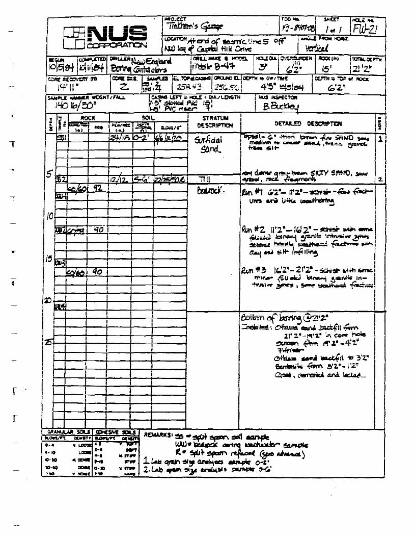
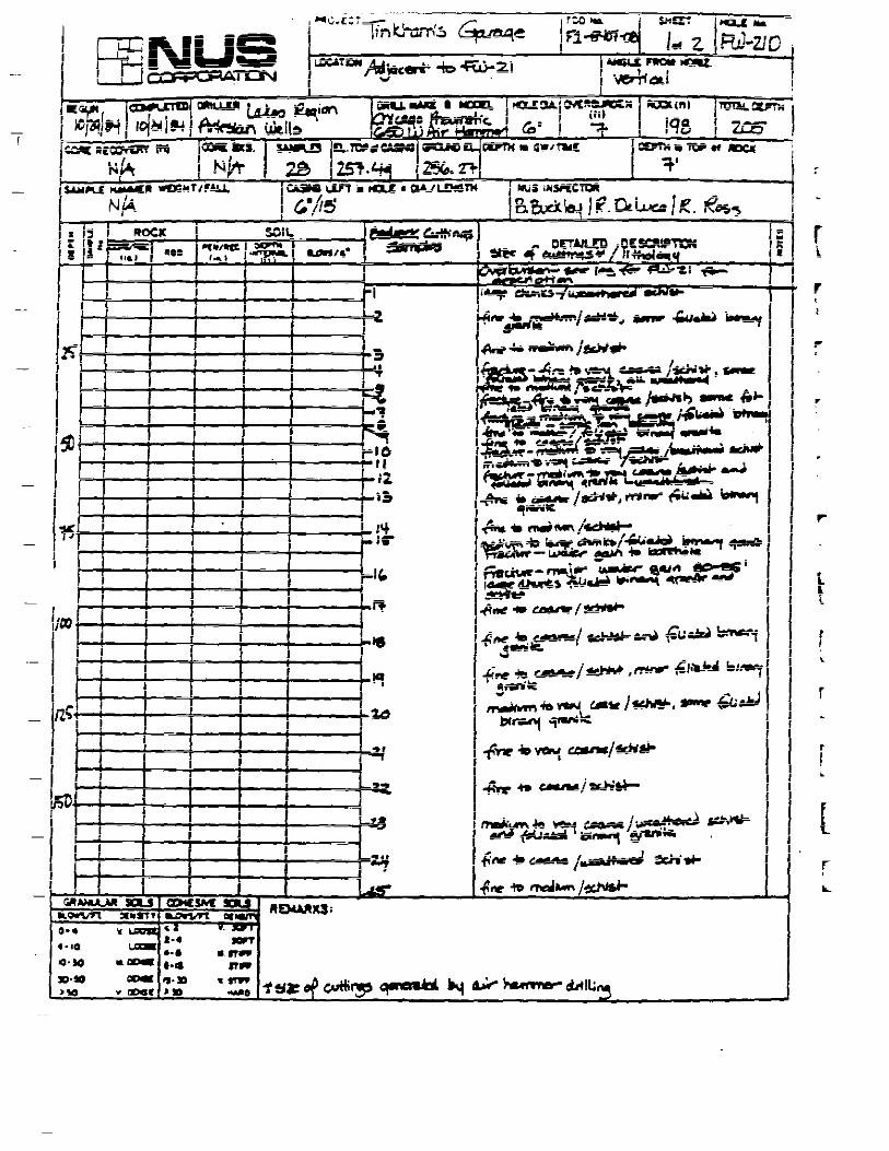
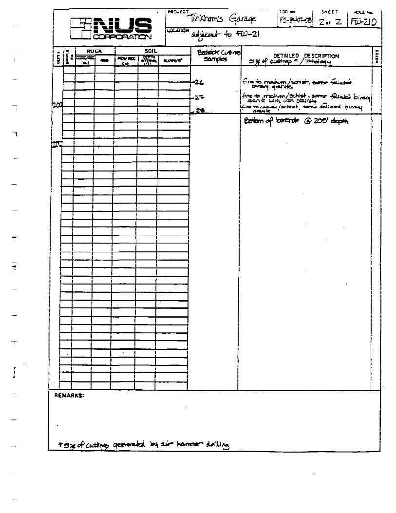
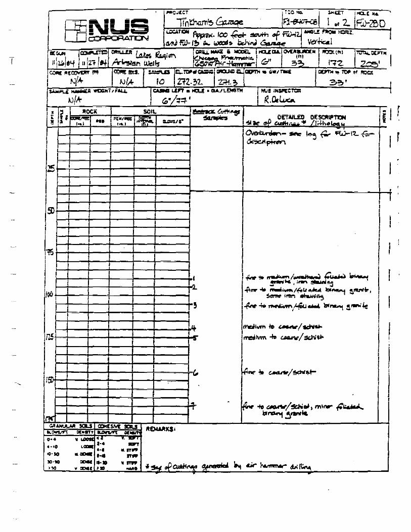
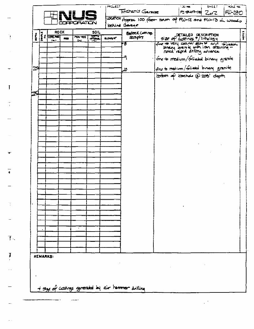
~
j ~O poundCT
I hnc--w-r~ ~
l1Ba+6MHoorJc iOO ~ I bull 1 ~r
f iz14 ~I
J SOii
Il~_=lkJi
I -q1--1tlbullI
I I I I I I II I I I I I III I I I I I I II l
j2COf1---+~_f--~+-~~+-~-+~~~~I
1middot I
1 ~j~+-~--if--~-t-~~-t-~~i--~~---1
L
I I
II L_ I
I I I I I II II II I I
I I I I I
I I I
I I I
I I
bull I I II I
I I I
I I I I l I I II ~ I I I I I II I I I I I
l I I II I I I I I I I II I I
I I II I I I I I II I
I I I I I II I I I I I I II I I I I I II I I I I
I I I I I I I IT
~ I I I I I
REMAllKS
SM(pound r 1 oL _ 1 x - _ I_ I
IFl~ -z_-z IRi1-ZB o I - - ---or ftlJ-Z ~ ~r~ ~ ~ I
1
I I I I I I I I
I I I I I I I
ATTACHMENT B
Guidance Documents
ROUX ASSOCIATES INC CSG11170001M000150ATTA
UNITED STATES DEPARTMENT OF THE INTERIOR BUREAU OF RECLAMATION
USBR 7310-89 PROCEDURE FOR
CONSTANT HEAD HYDRAULIC CONDUCTIVITY TESTS IN SINGLE DRILL HOLES
INTRODUCTION
This procedure is under the jurisdiction of the Georechnical Services Branch code D-3760 Research and Laboratory Services Division Denver Office Denver Colorado The procedure is issued under the fixed designarion USBR 7) 10 The number immediately following the designation indicates the year of acceptance or the year of lase revision
Although rhe term permeability was used in all ocher procedures in this manual percammg co che capacity of rock or soil co conduce a liquid the similar term hydraulic conquctiviry is used throughout chis procedure (See designation USBR 3900 for differences in meaning of rhe two cerms)
Since geologic and hydrologic conditions encountered during drilling are nor always predictable and may nor be ideal variations from chis procedure may be necessary to suit the particular purpose of the resc and conditions at the test sice Much of the information for this procedure was taken from references LI l through L5 l which contain additional information on fielq hydraulic conductivity resting
1 Scope
11 This designation outlines the procedure for pershyforming rests to determine an approximate value of hydraulic conductivity (permeability) of soil or rock in an isolated vertical or inclined interval of a drill hole (boreshyhole) either above or below the water table Usually the rests are performed as a part of the drilling program This procedure can be used in holes of various diameters if suitable equipment is available but N-size L3-in (76-mm)] nominal diameter drill holes are most commonly used2
l2 The constant head single drill hole rest is based on the same theories as the sready-srare or Theim-type aquifer rest and the same assumptions are made These assumptions are ( 1) the aquifer is homogeneous isotropic and of uniform thickness (2) the well (rest interval) fully penetrates the aquifer and receives or delivers water to the entire thickness (3) discharge or inflow is cons rant and has continued for a sufficient duration for the hydraulic system to reach a steady state and (4) flow co or from the well is horizontal radial and laminar Field conditions may not meet all of these assumptions Equations and other factors affecting the rest are given in paragraph 14 Calculations This procedure should nor be used for resting roxic waste containment that requires a very low loss of liquid
13 Constant head hydraulic conductivity rests should be considered scientific tests Grear care should be exercised by chose conducting the rests to eliminate as much error as possible
1 Number in brackets refers co the reference Hereafter referred mas N-size holes
2 Auxiliary Tests
21 The soil or rock penetrated by the drill hole should be identified described and classified from samples taken during the drilling operation Soil can be sampled in accordance with USBR 7010 7015 or 7105 and classified in accordance with USBR 5000 Rock cores or cuttings should be examined and appropriate description and classification made Dara obtained from the drill hole should be entered on appropriate log forms
3 Applicable Documents
31 USBR Procedures USBR 1040 Calibrating Pressure Gauges USBR 1050 Calibrating Pressure Transducers USBR 3900 Standard Definitions of Terms and Symbols Relating to Soil Mechanics USBR 5000 Determining Unified Soil Classification (Laboratory Method) USBR 5005 Determining Unified Soil Classification (Visual Method) USBR 5600 Determining Permeability and Settlement of-Soils [8-in (203-mm) Diameter Cylinder] USBR 5605 Determining Permeability and Serrlement of Soils Containing Gravel USBR 7010 Performing Disturbed Soil Sampling Using Auger Boring Method USBR 7015 Performing Penetration Resistance Testing and Sampling of Soil USBR 7105 Performing Undisturbed Soil Sampling by Mechanical Drilling Methods USBR 7300 Performing Field Permeability Testing by the Well Permeameter Method
1245
2
USBR 7310
32 USER Document 321 Geology for Designs and Specifications by the
Bureau of Reclamation (This document covers both soil and rock)
4 Summary of Method
41 Pump-In Test-Water is injected into an isolated interval of a drill hole in soil or rock and the volume of water injected is determined for a measured period of time The injection pressure is a constant gravity head with or without added pressure head provided by a hydraulic pump The hydraulic conductivity is calculated from the flow rate length and radius of test interval in the drill hole and effective head
42 Artesian Test-Where water under artesian pressure flows out of the drill hole the effective (shutshyin) head at the test interval is measured and the hydraulic conductivity calculated from the flow rate the length and radius of the well and the effective head
5 Significance and Use
51 Hydraulic conductivity tests are made to obtain daca related to (a) identifying seepage potential and dewatering requirements (b) drainage problems (c) ground-water supply investigations and (d) grouting requirements The tests yield approximate values of hydraulic conductivity that are suitable for many engineering purposes Reliability of the values obtained depends primarily on (a) homogeneity of the strata tested (b) suitability of rest equipment used for a given condition (c) care taken in performing the test and ( d) adherence to requirements for proper use of the equations The test is also used in formulating geologic descriptions and interpretation of material properties particularly where there is poor sample recovery
52 Where tests are performed in fractured rock results could reflect secondary conductivity rates which would not represent primary conductivity of the intact mass When the test is performed in fractured brittle swelling clay or rock or where fractures contain loose material hydraulic conductivity may be reduced and judgment should be used in applying results
53 Generally this procedure is suitable for materials in which the hydraulic conductivity ranges between 5 and 100000 ftyr (5 X 10⁻⁶ and 1 X 10⁻¹ cms) and where results are to be used for engineering purposes The procedure is not applicable in materials of lower permeability particularly for purposes such as investigashytions for containment of toxic wastes
6 Terminology
61 Definitions are in accordance with USBR 3900 Some definitions are from Glossary of Geology [6]
62 Terms not included in USBR 3900 specific to this designation are
62 l DnJJ Hole-A circular hole made by drilling
622 Feed Pipe (conductor pipe injection pipe riser pipe drop pipe)-The main pipe (or rod) which conducts water from the collar of the hole into the test interval in the drill hole for the hydraulic conductivity test
623 Baifer-A cylindrical container with a valve on the bortom for admission of fluid attached to a line and used for recovering and removing water cuttings and mud from a drill hole
624 Walking Beam-An oscillating rigid lever balanced on a fulcrum used to activate the cable in cableshytool drilling by alternating up and down motion
625 Aquifer-A water-bearing bed or stratum of earth gravel or porous rock with interconnected openings or pores through which water can move
626 Packer-A short expansible device deliberately set in a drill hole to prevent upward or downward fluid movement generally for temporary use The expansible part of the packer is called the gland Straddle packers are two packers separated by a length of perforated pipe to span or straddle a test interval
627 Artesian-An adjective referring to ground water under hydrostatic pressure ie an artesian aquifer is a confined aquifer Artesian ground water rises above the confining layer in the drill hole and may or may not flow at ground surface
628 Ground W1ter-That part of the subsurface water that is in the zone of saturation
629 W1ter Tizble-The surface between the zone of saturation and the zone of aeration that surface of a body of unconfined ground water at which the pressure is equal to that of the atmosphere
6210 Perched Water Table-A water cable usually of limited area maintained above the normal free water elevation by the presence of an intervening relatively impervious confining stratum
6211 Gauge Saver-A vessel with a pressure gauge filled with glycerin or oil to protect the gauge from direct contact with fluid in the pressure line (see fig 1)
6212 Holding Pressure (applicable primarily for grouting) -The gauge pressure after the water-pumping system has been shut off at the valve ahead of the gauge and backflow is prevented
6213 Back Pressure (applicable primarily for grouting)-The gauge pressure in the system after the holding pressure has dissipated as determined by opening a valve and allowing the gauge ro drop ro zero and then reclosing the valve
6214 Backflow(applicable primarily for grouring)shyThe reverse movement of water out of the drill hole when the holding andor back pressure below the packers exceeds the pressure of the water column in the hole
7 Interferences
71 During drilling it is important ro minimize movement of fines [minus No 200 sieve-size material (75 microm)] into the material being tested and to remove any accumulation of fines from the wall of the drill hole during preparation for the test so as to avoid obtaining test values
1246
USBR 7310
Heov1 Out1 Pressure Gouge
poundLpoundVATON SECTION
TOP VpoundW BOTTOM VIEW
Figure I - Gauge saver device for protecting pressure gauge 40-D-4287
lower than the actual hydraulic conductivity of the material being tested Drilling using clear water without additives is preferred Bentoniticmiddotmuds should nor be used in holes where hydraulic conductivity testing is to be performed Biodegradable additives may be used if necessary but only if the test interval is adequately cleaned before testing The drilling procedure should be documented on the log form
72 Test results can be adversely affected by injecting water containing sediment which would tend to plug voids in the material being tested
73 The temperature of the injected water should be equal to or warmer than that of the ground or ground water This reduces the tendency of air dissolved in the water to become entrapped in the voids of the material be ing tested and co cause low values of _hydraulic conductivity In most areas not affected by artesian conditions the temperature at a depth of about 25 feet (8 m) below the ground surface remains relatively constant at the annual mean air temperature for the region At significantly greater depths temperature rises about l degF (06 degC) for each 500 to 1000 feet (150 to 300 m) of depth The temperature of the injected water especially if it is known to be colder than the ground-water temperature should be recorded on a geologic log or the hydraulic conductivity cesc daca forms (see subpar 812 for suitable temperature measuring devices)
74 It is possible that dissolved minerals in the wacer used for a rest may react chemically wich substances in the material being reseed to cause a change in the hydraulic conductivity Therefore it is desirable to use wacer for the test chat is similar in quality co that expec~ed to permeate che ground when che project is in operation
8 Apparatus
81 Drill Rigs (see fig 2) ~1 ~ Rotary Drilling-A drilling method resulting m grinding a hole with a hard-toothed drill bic at che end of a rocacing drill rod (pipe) The equipment consists essentially of a power unit hoisting or rugging unit controlled-feed rotary drill head and mounting frame masc or tripod and circulating pump The rig should have various accessory drilling andsampling equipment (rods bits core barrels augers) as required for drill hole advancement sampling and testing
812 Cable Tool Drilling-A method of drilling in which the material at the bottom of the hole is broken up by a steel bic with a blunt chisel-shaped cutting edge The drilling equipment consists essentially of a mast a sering of drill tools (casing tubing or pipe of one size) chat is alternately lifted and dropped by a hoist with a power unit and a walking beam A bailer is always used with a cable tool rig Normally a cable tool drilled hole is noc satisfactory for hydraulic conductivity testing with packers
82 Injecrion Pump-A centrifugal or helical screw type pump providing a constant water flow is required This may require a special pump separate from that used for drilling operations Although there may be conditions where a larger or smaller pump may be required highshy
quality pumps having a capacity of 40 galjmin (150 L min) at a pressure of 120 bf in2 (830 kPa) (such as Moriyo model 3L-8 manufactured by the Robbins and Myers Company Springfield Ohio or equivalent) are adequate for most hydraulic conductivity tests The pump should provide the required flow at the required constant pressure with maximum allowable pressure fluctuation-due co pumping pulsations-of plusmn5 percent of the test gauge pressure A surge chamber is required for all testing chis minimizes pulsations which can affect the injection race in the test interval Also ic makes readings more accurate and protects che pressure gauges against damage from sudden pressure changes
83 Feed P1pe- The feed pipe should be of adequate diameter to minimize head losses and have adequate tensile strength to withstand pumping pressures and stresses during hoisting or tugging The feed pipe is commonly a threaded and coupled assembly of pipe or tubing having a uniform inside diameter Drill rods generally of N-size can be used wichouc seriously affecting reliability of rest data if che flow rate to the test interval does nor exceed about 15 galmin (57 Lmin) and the depth co che top of che interval does noc exceed 50 feet (15 m)
NOTE 1-Use of drill rods as feed pipe should be permitted only after the assembled drill rod string has been pressure reseed ro cali_brare head losses ar anricipared flows If seals or sealing marenals are used during calibrarion the same type of seals or sealing materials (not oils or wax) should be used during hydraulic conductivity resting
84 Flowmecers-One or more calibrated flowmecers are required the capacity of each meter should be specified
1247
USBR 7310
- Byooss votve Surgechomber~
Wotermettr-
Observation oost see Detail A
SCHEMATIC ARRANGEMENT OF EQUIPMENT
(Water meter
~==it=======t(k=====- For wottr tes t ing middotWell cas1n9
Press1Jre gouge
-=====bull===========~-For drilling DETAIL A OBSERVATION POST FOR
OPTIONAL EQUIPMENT ARRANGEMENT FOR DETAILS 8 AND C
WATER TESTING ANO DRILLING FROM SECTION X-X TO WELL
DETAIL D GRAVITY TEST
DETAIL B DETAIL C DOUBLE PACKER TEST SINGLE PACKER TEST
Figure 2 - Schematic arrangement of hydraulic conductivity equipment 801-D-l I I
For flows up to 50 galmin (200 Lmin) a 1-inch (25- 851 Pneumatic Piezometers-A down-hole pneushymm) diameter disk-type meter may be used For higher matic piezomerer system has been developed [7] flows a 2- or 2-12-inch (50- or 65-mm) diameter impellershy Descriptions of the equipment and procedure as used ar type meter is recommended two damsites are presented in appendix XL
841 A straight uninterrupted section of pipe having 852 Electrical Transducers-Electrical transducers an inside diameter equal to the rated size of the meter have been used as down-hole pressure sensors by other and a minimum length 10 times the inside diameter of agencies [8) particularly for very low hydraulic conducshythe pipe should be provided upstream of the meter tivities [below 1 ftyr (1 X 10⁻⁶ cms)] The USBR has Manufacturers commonly recommend pipe lengths of one used electrical down-hole sensors in preliminary trials tO two times the inside diameter of straight pipe Electrical transducers measure pressures more accurately downstream from the meter than pneumatic piezometers and can be connected tO a
85 Pressure Sensors-Where required calibrated strip-chart recorder for a continuous record However pneumatic piezometers or electrical transducers can be used transducers are considered less rugged for field use and as down-hole sensors tO measure pressures at the rest require more maintenance and experienced personnel tO
interval during a hydraulic conductivity rest Down-hole operate than do pneumatic piezometers sensors are preferred over the method of calibrating the 86 Pressure Gauges-When down-hole pressure piping system for head loss between a pressure gauge on sensors are not available or sensors are not working the surface and the test interval However an above-ground properly calibrated pressure gauges can be used t0 estimate pressure measurement can provide a check of the pressure effective pressure in rhe rest interval after correcting for sensor friction loss through the feed pipe and packer All pressure
1248
USBR 7310
gauges used in water resting should be high-quality stainless steel glycerin or oil filled wich pressure indicated in both lbfin2 and kPa (such as manufactured by Marsh Instrument Company a unic of General Signal P 0 Box 1011 Skokie Illinois or equal) Pressure gauge ranges should be compatible wich middot cescing requirements chey should be sized so char che gauge capacity does not exceed two co three rimes che maximum desired pumping pressure for each respective pumping stage Gauges should have the smallest graduations possible and an accuracy of plusmn25 percent over che coral range of the gauge If a gauge saver is used wich che gauge calibration should be made wich the gauge saver in place Accuracy of che gauges should be checked before use and periodically during the resting program (see subpar 112 for additional information)
861 One or more pressure gauges should be located downstream of che flowmecer and downstream of any valves ac che cop of che feed pipe This location for pressure measurement can be used by inserting a sub (adaptor or shore piece of pipe) wirh che gauge - installed on che cop of rhe feed pipe
862 Ac least one additional calibrated replacement gauge should be available ar che resr sire
87 Swivel-During che hydraulic conductivity cesc ic is preferable co eliminate the swivel and use a direct connection co the feed pipe If a swivel muse be used in che water line during resting ic should be of che nonconscriccing type and calibrated for head loss Significant friction loss can result from use of che constricting type
88 Packers-One or two (straddle) packers are required for che rest Packers may be either bottom-set mechanical screw set mechanical pneumatic inflatable or liquid inflatable The pneumatic inflatable packer is the preferable type for general use and is usually che only one suitable for use in soft rock and soil The gland of this packer is longer and more flexible chan the ocher types and will form a tighter seal in an irregular drill hole A leather cup type of packer should noc be used To ensure a eight water seal che length of contact between each expanded packer and che drill hole wall should noc be less than three rimes the drill hole diameter
NOfE 2-More than one type of packer may be required to test the complete length of a drill hole The type of packer used depends upon many factors eg rock type drill hole roughness spacing and width of rock joints and test pressures
881 Inflatable Packers-Inflatable packers with an expansible gland and a floating head (see app fig Xl2) should be designed for anticipated drill hole diameters and pressure conditions For normal hydraulic conductivity cescing a reasonable maximum recommended working pressure inside and outside of che packer is 300 lbf in2
(2070 kPa) [8] Inside pressure should be increased in water-filled holes proportionally co che sracic head For drill holes wich sharp projections in the walls a wireshyreinforced packer gland having a higher working pressure [7] may be required The pressure in che packer should not be high enough to fracture the material being reseed
The pressure required to form a cighr seal ac che ends of a cesr interval depends on the flexibility of rhe gland the friction of the floating head and che drill hole roughness The minimum differential pressure between che packer and the cesc interval can be derermined by res ring packers in a pipe slighrly larger rhan rhe nominal diameter of rhe drill hole in order co simulate possible enlargement of rhe drill hole during drilling For a given resr interval pressure che packer pressure is increased until ir provides a waterrighc seal between the packer and the material with which ic is in contact The pressure in rhe packer should range approximately berween 30 and 300 lbfin2 (210 ro 2100 kPa) greater chan char in che cesc interval with 100 lbfin2 (690 kPa) being normal Pneumatic inflatable packers can be inflated with compressed air or compressed nitrogen
882 Special pneumatic packers are available for use in wireline drilling operations Because che packers must be able co pass through che wireline bit and then expand co completely seal che hole ac che cesc interval special materials are needed for che packer gland A special packer assembly-consisting of cwo packers in tandem-is used with the upper packer being expanded inside che drill rod just above che bic and che lower packer expanded against che wall of the hole just below che bit The two packers on the assembly can be positioned properly-relative co the bit-by a sec of lugs or a ring located on the assembly Special seals or connections are needed co attach che water supply co che wire-line drill pipe at the surface
883 A minimum of two secs of replacement packers andor spare glands should be available at the test sire
89 Perforated Pipe Sections-Lengths of perforated steel pipe corresponding ro the lengths of rest intervals are required between packers to admit water inco che rest intervals The coral area of all perforations should be greater than five rimes che inside cross-sectional area of che pipe These perforated pipe sections should be calibrated for head loss
810 Well Screen-Well screen or slotted pipe may be required for cescing in granular unstable materials chat require support [9] As a general rule the maximum size of sloe width should be approximately equal to che 50shypercent size of che particles around the drill hole (see subpar 114)
811 Water Level Measuring Device 8111 Although there are ocher types of water level
indicacors che electrical probe indicator is most commonly used Essentially ic consists of (1) a flexible insulated conduit marked in linear units and enclosing cwo wires each insulated except ac che tips (2) a low-voltage electrical source and (3) a light or ocher means of indicating a closed circuit which occurs when che rips contact che water surface Different brands of electric wacer level indicacors and even different models of the same brand ofren have their own unique operating characteristics Before using any electric water level indicacor it should first be reseed at the surface in a bucket of water
8112 For approximate measurements of the water level when ic is within about 100 feet (30 m) of the ground
1249
USBR 7310
surface a cloth tape with a popper can be used A popper can be made from a short pipe nipple (or length of tubing) by screwing a plug attached to a graduated tape intu one end of the nipple and leaving the other end of the nipple open When the popper is lowered in the drill hole and the open end of the pipe nipple strikes a water surface it makes a popping sound and the depth to water can be measured by the tape
8113 An accurate measuremenr of the water level can be made by chalking the lower end of the steel tape After contacting the water level the tape should be lowered about L more foot before retrieving it Measurement is then made to the wet line on the tape
812 Temperacuie Measuring Device-Equipment for measuring ground-water temperature is available from commercial sources or can be made from a thermistor two-conductor cable reel Wheatstone bridge and a lowshyvoltage electrical source A maximum-minimum type thermometer is acceptable
9 Regents and Materials
91 ~71ter (See subpars 72 73 and 74)-The clear water supply should be sufficient tO perform the hydraulic conductivity test without interrruption and to maintain the required pressure throughout the test period
92 Swd or Gravel Backfill-Where a granular backfill is used t0 prevent sloughing of the drill hole wall it should be a clean coarse sand or fine gravel Laboratory permeability tests (USBR 5600 or 5605) should be made on the backfill material to make sure that it has a coefficient of permeability greater than one order of magnitude higher than that expected of the in situ material being rested
10 Precautions
L01 Safety Precautions L011 This procedure may involve hazardous
materials operations and equipment lO l2 Use normal precautions for drilling [ 10 11] L013 Precautions should be taken during calibration
pressure testing of equipment particularly testing of packers with compressed air or nitrogen (never use oxygen) to avoid injuries from a sudden packer or hose rupture
L02 Technical Prernutions 102 l As a general rule total pressure (static head
plus gauge pressure) applied in the drill hole should nor exceed 1 lbfin2 per foot (226 kPam) of rock and soil overburden at the center of the test interval if the test interval is 10 feet (3 m) long or less If the rest interval exceeds 10 feet pressure should not exceed 1 lbfin 2 per foot of overburden at the top of the interval In layered or fractured material or for drill holes near steep abutments or slopes 05 lbf in2 per foot ( 113 kPa m) of material to the nearest free surface is an appropriate maximum pressure Higher pressures than these may fracture the materials
1022 If there is excessive or complete loss of water when the hole is being drilled drilling should be sropped before cuttings fill the voids and a hydraulic conductivity rest completed on a shorter than normal length rest interval
1023 Hydraulic conductivity rest equipment should be considered and treated as precision testing equipment Gauges thermometers ere should have their own protective cases they should not be carried with drill tools or be tossed around They should be calibrated frequently Ir is recommended that all test equipment needed for hydraulic conductivity resting be kept separate from drilling equipment
11 Calibration
111 For Measurment ofEffeaive Head 11 l l Pressure Sensurs-Calibrate down-hole
pressure sensors by the methods and at frequencies prescribed by USBR LOSO
ll12 Friction Loss Estimates-Where down-hole pressure sensors are nor used estimates of effective head at the rest interval are made by subtracting friction loss from the applied head measured at the ground surface The friction loss should be determined for all components of the piping system from the pressure gauge to the test interval
1112 I Calibrate friction loss in parts or sections of the piping systems including ( L) the swivel (if used) (2) feed pipe (per unit length) and (3) the packer assembly Record the data with references to the particular parts calibrated in tabular or graphical form so the accumulative friction loss can be totaled for determination of effective head at the test interval The calibration procedure is as follows
I l l211 Lay out the individual or joined parts to be calibrated on a horizontal surface with calibrated pressure gauges at each end
l L 12 12 Pump water through the system at incremental increasing flow rares to the maximum flow rare expected to be used in the test allow the flow to stabilize between incremental flows
L 112 L3 Record the pressure at each gauge for each incremental flow rate
11 l 2 L4 Calculate the friction head loss for each incremental flow rare
2f = 23 l ( p ~I p ) (I )
where f = friction head loss in feet of head per linear foot
of pipe ftft or mm P1 = upstream pressure bf in 2 or kPa P2 = downstream pressure lbfin2 or kPa d = pipe length fr or m (d = l for swivel or packer
assembly) 23 l = converts from pressure in bf in2 to head in feet
or 0102 converts from pressure in kPa to head in meters
Example assume
P1 = 186 lbfin2 or 128 kPa P2 = 132 lbfin2 or 910 kPa d = 100 ft or 305 m
1250
USBR 7310
Inch-pound application
f = 231 ( 18 ~~-~3 2) 125 ftfr
SI application
f = 0 102( 128
- 9 tO) = 124 mm 305
l l l215 Plot friction head loss versus flow rare Figure 3 is an example of a plot of friction head loss (f) at relatively low flow races for a 10-foor (33-m) length of 1-14-inch (32-mm) diameter pipe Since head loss in pipe at turbulent flow is approximately related to velocity squared a plot of friction head loss versus the square of the flow rate is nearly a straight line (see fig 4)
NOfE 3-There are srandard rabies and charcs which provide unit friction losses for various sizes of pipe elbows cees reducers ere for clean and ruscy conditions Although such informacion is sometimes used it is preferable to determine friction losses in che piping syscem and packers accually used for che hydraulic conductivity rest
111216 To calibrate a packer inflate the packer in a shore length of casing or pipe in which amiddotvalve and pressure gauge have been installed A pressure gauge is also installed in the rods immediately ahead of the packer assembly Pump water into the rods at incremental increases (or decreases) of flow rate-allowing the system to stabilize after each incremental change-until the highest anticipated flow rate is reached
NOfE 4-For packers smaller than N-size such as the B-size used in wireline equipmentmiddot there are significant head losses and relatively low flow races must be maintained This requires water meters and pressure gauges capable of accurately measuring the low flows and small changes in pressures
112 Pressure Gauges-Calibrate each pressure gauge (see USBR 1040) by comparing it with a test or master
FLOW RATE IN LITERS PER MINUTE
o
I _ I_ I I I II
I I I I I loI I I I I I rI
I I I )I
I I I I I v I I I I I I I I I I lr II
I I
I I I I 11deg II i j~ I I I -~-----1 -- I I I I i
JO deg HOW RATE IN GALLONS PEA MINOT[
Figure 3 - Head loss due ro friction at increasing flow rates for a I 0shy
foot (3-m) 1-14-inch (32-mm) diameter iron pipe
gauge The master gauge should not be used during drilling or hydraulic conductivity testing Calibrate each gauge at the start of a res ring program plus one additional calibration per week during rests of long duration
113 Flowmeters-Calibrate a flowmerer by flowing water into a container of known volume the container used for the volume check should be commensurate in size with the flowmeter size and graduations From these data flow rares can be calculated for comparison with meter readings All flowmeters should be calibrated to an accuracy of plusmn1 percent Calibration should be done at the stare of the resting program plus one additional calibration per week during rests of long duration
NOfE 5-Some impeller-type flowmeters have an accuracy range significantly less than indicated by the dial Minimum and maximum races should be esrablished
114 Well Screens and Perforated or Slotted Pipe Sections-From manufacturers dara or by calibration determine the head losses in expected flow ranges to ensure there is no restriction of flow into the material being tested
12 Conditioning
12 l Nor applicable special conditioning requirements are not needed for this procedure
13 Procedure
13l Cleaning ofDnll Hole 13l1 Remove any accumulation of fine particles
(smear mud cake compaction caused by driving casing etc) from the drill hole wall Such accumulation significantly restricts the flow of water into or from the hole Exercise good judgment in cleaning the hole since excess cleaning may be detrimental If there is a question as to whether or not drill holes in particular materials need cleaning hydraulic conductivity tests can be performed in holes with cleaning and others without cleaning If cleaning does not significantly change rest results at a sire cleaning of additional intervals in the same materials may not be necessary
131 l1 When the rest interval is above the water table it may be possible to brush or scratch the drill hole wall to break up accumulated fines For unstable materials which require use of a well screen materials which cavemiddot against the screen may break up the accumulation of fines on the wall Mild surging with a bailer while adding water also may help break up a disturbed or compacced zone but this may stir up fines which then plug the voids in the material co be rested Mild jetting-followed immediately by bailing or pumping-also is a possibility
13 l l2 When the test interval is below the water table-in materials chat are rock-like and self-supporcingshyuse of a water jet in the hole (preferably accompanied with pumping to induce flow into the borehole) is one of the best methods to clean the hole After jetting bail or pump the sediment-laden water from the rest interval Jetting can also be used through a screen below the water
1251
tJ
I I 0 GO-GI I GO-G2 0 GI -G2
~
I
I
v
v p-shy~ -shyl--~ L--shy
-shy
v
0
middot 005 =0 00005 100
-shy~--~ 0 middot 0025 =0 00005
I 50 I
~ --shy = 0 00005
50
I
t - A
v -
-
[] --shy shy--shy0 -
4--l_-E
-
16
-shy-shy-8 --shyl---shy~ - 2
~ ~---shy z 3 4 5 6 7 8 9
FLOW RATE SQUARED (q 2 )(10001
s of oalmin ) 2
Figu re 4 - Plot of feed p_ipe ca libra tion data - example
USBR 7310
2FLOW RATE SQUARED (q2)( 1000degs of L min)
10 15 20 25 - 30 35
50
40
r w w LL
z
~ 30 0 J Cl ltgt w I
z 0 20 r S a LL
10
0
cable in unstable materials For soft rock flushing che sides of che drill hole by running che bit or a bailer up and down the hole may enlarge the hole by erosion or ocherwise change the characceriscics of the fracture systems
13113 Finally clean the drill hole by pumping or bailing water from the bottom upward with the pumping continued until the return fluid is clear without cuttings or sediment Record the method used in cleaning the hole on the log of drill ho le or on a special testing form
132 Length of Test Interval 1321 The length of the test interval depends on
(1) purpose of the test (2) stratigraphic interval and (3) flow rate Where materials are relatively uniform use a test interval of about 10 feet (3 m) Where flow rates are high shorten the test interval co locate high flow race zones where races are very low the interval may be lengthened if desired
133 Ground-Water Level Determination 13 31 Depth co ground-water level muse be
determined before calculating hydraulic conductivity Measure depths to water levels with an electrical probe or o ther suitable equipment (see subpar 811)
1332 Auger Holes-ln power auger or other types of holes to which water is not added as pare of the drilling process report the presence or absence of a water level depth to water level and dace of initial and final water level measurement In materials of low hydraulic
14
12Cll a w r w
101 z () Vgt 0
8 J
Cl ltgt w I
Sz 0 r u a
4 IL
conduccivicy several days to several weeks may be required for a water level to stabilize in the hole Report evidence of moisture in the cuttings and if a perched water level was observed
1333 Rotary or Cable Tool Holes-For drill holes in which addition of water to the hole is an integral part of the drilling process
13331 Bail or pump the hole dry or to a stable wa ter level at the close of the last shift each day and record level
13332 Report the presence or absence of water and depth to water at the beginning of the first shift each day Additional readings are desirable whenever water level in the hole has nor been disturbed for an appreciable period of time
13333 Report changes in water level detected as the hole is drilled deeper Record faccors that affect the water level such as depth of casing andor cemented intervals These data may be helpful in recognizing perched or confined (artesian) conditions
13334 Upon completion of the hole the water must be bailed down to the extent practicable the water level measured and the dace recorded of hole completion Measure the water level for a period of days or weeks until equilibrium is reached
NOfE 6-At times exceptions must be made to the requirement for conrinuation of water level readings Such is the case when
1252
USBR 7310
state or local laws require chat the hole be filled continuousiy from bottom to cop immediately upon hole completion and before the drill crew leaves the sire In ocher instances landowners may allow right-of-entry for only a limited time for measurements
1334 Perched and Artesian Aquifers-lc is imporshytant tO recognize perched and artesian aquifers especially those under sufficient pressure tO raise the water level above the confining layer but nor tO the ground surface (see (5 ]) They must be distinguished from water table aquifers (those which continue in depth) If perched water table or artesian aquifers-separated by dry or less permeable strata-are encountered in the same drill hole the resulting water level in the hole is a composite therefore conclusions and interpretations based on such data are misleading If a perched water table is recognized (or suspected) during drilling water levels must be determined for each zone for calculation of hydraulic conductivity This might require completion of the drill hole with a watertight seal set at a suitable horizon tO
separate two water table conditions In this type installarion two strings of pipe or conduit are required one extending down to the portion of the hole immediately above the packer and a second string extending through the packer to a point near the bottom of the hole Water-level measurements provide the basis for determining a perched condition or if the lower water table is under artesian pressure
13 35 Mulriple Water-Level Measurements-In some instances it is desirable tO install multiple conduits and packers or plugs in a drill hole so that ground-water levels (or pressure heads) in several water-bearing horizons can be measured over an extended period of time (see [5] pp 7-14)
134 Pressure Tests With Packers 134 l The recommended arrangement of typical
equipment for packer pressure tests without a pressure sensor is shown on figure 2 (See app fig Xl l for equipment with a pressure sensor) Beginning at the source of warer the general arrangement is clean water source suction line pump discharge line tO srorage andor settling tank suction line water-supply pump surge chamber line ro bypass valve junction water meter gate or plug valve tee with sub for pressure gauge short length of pipe on which the pressure gauge is attached tee and off-line bleeder valve for evaluating back andor holding pressure flexible 1-14-inch (32-mm) diameter hose and 1-14shyinch-diameter feed pipe ro packer or packers in drill hole which isolate the rest interval All connections should be tight and as short and straight as possible with minimum change in diameter of hose and pipe Friction loss decreases as the pipe diameter is increased
1342 When the material is subject co caving and casing andor grout is needed to support the walls of the drill hole the hole should be water rested as it is advanced Other hole conditions may make this procedure desirable or necessary The following procedure is commonly used
1342 l After the hole has been drilled to the top of the interval to be tested it may be desirable tO remove
the drill string from rhe hole and advance casing or grout ro rhe bonom of the hole
13422 Advance the hole 5 to lO feet ( 15 to 3 m) into the material to be rested
13423 Remove the drill string from rhe hole 13424 Clean the interval to be tested and record
the depth tO the warer table if present If a composite water level is suspected the warer level affecting rhe rest should be determined by measurements through the feed pipe after rhe packer has been seated and the water level has stabilized
13425 If rhe hole will stand open sear a single packer ar the top of rhe test interval Record the type of packer irs depth and packer pressure if it is rhe inflatable type
13426 Pump water into the interval ar a rate to develop a suitable pressure The pressure to be used depends upon testing depths and ground water levels or pressures Materials subject to deformation or heaving such as by separation of bedding planes or joints or materials at shallow depths must nor be subjecred to high pressures (see subpar 102 l ) For comparison of flow rates in different pares of a single foundation and with results from other foundations some of the following pressures are commonly used 25 50 75 and LOO lbfin 2 (170 350 520 and 690 kPa)
NorE 7-At test pressures less than 25 lbfin2 errors in measurement of pressure and volume of water may increase unless special low pressure gauges are used Gravity tests provide more accurate results under these conditions At pressures higher than 10 lbfin2 difficulties in securing a right packer seal and the likelihood of leakage increase rapidly However under artesian pressures or in deep holes the water pressure-as registered on a surface gauge-will need to be sufficient to overcome the effeccive head at the test interval and firmly seal the packer
NillE 8-Where the hole is subject to caving a pump-down wire-line system has been developed rhar can be used to eliminate removal of the drill string from the hole With this system the hole is drilled to the bottom of the interval tO be tested and the drill rod is raised so the end of the rod is at the top of the test interval The tandem packer (see subpar 882) is then lowered through the drill rod and expanded to seal both inside the rod and against the wall of the hole at the cop of the test interval Models of this equipment are available which have transducers below the packer for measuring water pressures at the test interval
13427 For determining effective head artesian heads encountered in the drill hole are treated the same as water table conditions ie the depth from the pressure gauge or the water level maintained during the test to
the stabilized water level is used as the gravity head If the artesian head stabilizes above the ground surface the gravity component of the effective head is negative and is measured between rhe stabilized level and the pressure gauge height If a flow-type rest is used the effective head is the difference between rhe stabilized water level and rhe level maintained during the flow period
1253
USBR 7310
13428 Afrer pressures are selected based on ground-water conditions and the purpose of the test perform a test at each pressure Usually a 5-cycle procedure is used three increas ing steps to the maximum pressure and then two decreasing steps to the starting pressure This cycling allows a more derailed evaluation of rest results than testing at a single pressure and commonly allows extrapolation to ascertain at what pressures the following may occur (1) laminar flow (2) turbulent flow (3) dilation of fractures ( 4) washouts (5) void filling or (6) hydraulic fracturing However the equations normally used to ca lculate hydraulic conductivity are based on laminar flow conditions
NOfE 9-ln some insrances on ly a single water pressure test at a given interval in the drill ho le may be required For example if geologic conditions are known and there is no need ro perform the seeps in subparagraphs 13422 through 13426 a single value of hydraulic conductivity with a relatively low application of pressure may suffice
13429 During each test continue pumping water to the test interval at the required pressure until the flow rate becomes stable As a general guide maintain flow rares during three or more 5-minute intervals during which l-minute readings of flow are made and recorded In tests above the water table water should be applied to the test interval until the flow rate stabilizes before starting the 5-minuce measurement intervals Where tests are below the water table flow rates usually stabilize faster than for the tests above the water table and the time period before the 5-minure test intervals may be shorter These rime periods may need to be varied particularly when rests to determine grouting requirements are made
134210 Determine and record the presence of back pressure and decay of holding pressure Afrer the rest deflate the packer and remove it from the drill hole
134211 Advance the drill hole and if necessary the casing repeat the procedure in subparagraphs 13423 through 134210 until the required depth of drill hole is reached When casing is used in a drill hole always set the packer in the material below the casing
1343 If the hole will stay open without casing it can be drilled to final depth and after cleaning the hole hydraulic conductivity rests can be performed from the bottom of the hole upward using straddle (double) packers Although a single packer can be used to test the bottom interval of the hole starting at the bottom with double packers will cause loss of borehole testing of only about the length of the bottom packer and will save one complete trip in and out of the hole with the drill string assembly co change the packers After the test for the bottom interval is completed straddle packers are used for successive test intervals up the drill hole See subparagraph 1342 where caving or other hole conditions will not allow this procedure
135 Gra vity Tests 135 1 Constant-head gravity tests are usually
performed without packers above or below the water table with drill holes of N-size or larger (see fig 2 derail D)
This type of test is often made in reasonably stable-walled drill ho les up to 25 feet (76 m) depth where water pressure at the test interval needs to be kept low The test is usually performed in successive 5- or 10-foot (l5- or 3-m) intervals as the drill hole is advanced The upper end of each test interval is normally determined by the bottom depth of tightly reamed or driven casing If the casing is not believed
middotto be tight appropriate entries should be recorded on the log form If the wall of the drill hole is stable the test can be performed in the unsupported hole If the wall needs to be supported use a well screen (see subpar 114 for calibration) inserted through the casing It may be necessary to ream or drive the casing to the bottom of the interval set the screen and then pull back the casing to expose the screen Afrer the test the screen is removed and the casing reamed or driven to the bottom of the hole
NOfE lO-Clean coarse sa nd or fine gravel backfill (see subpar 92) may be used instead of a well scree n Ream or drive rhe casing ro the borrom of the inrerval dean ir our and add rhe backfill as rhe rnsing is pulled back ro expose rhe resr interva l Record use of rhis procedure on the log form
l 35l l If the drill hole is self-supporting clean and prepare it in rhe normal n1anner (see subpar 13l)
l35 l2 If the drill hole is not self-supporting lower the well screen and casing into the hole
135 l3 For test intervals above the water table maintain a constant head of water _within 02 foot (60 mm)] at the top of the test interval by injecting water through a small diameter rube extending below the water level maintained during the test For rest intervals below the water table or influenced by artesian conditions maintain a constant head a short distance above the measured static water level
Monitor the water level with a water-level indicato r If the water-level indicator is inserted in a small diameter pipe in the casing the wave or ripple action on the water surface will be dampened and permit more accurate watershylevel measurements
NOfE l l-When rhe flow rare is very low rhe consranr wa rer level c1n be maintained by pouring warer in rhe hole from a graduated container
135 l4 Record the flow rate at wne intervals until a constanc flow rare is reached
135 l5 Repeat the procedure of subparagraphs 135 l3 and 135 14 at one or more different water levels
13516 This rest is essentially the same as desigshynation USBR 7300 (see also L3] p 74) the instructions in USBR 7300 for performing the rest and calculating hydraulic conductivity apply to this procedure also
14 Calculations
14 l For pressure or constant gravity head hydraulic conductivity rests calculace the hydraulic conductivity of
1254
USBR 7310
rhe soil or rock by rhe following equation (expressed m consisrent unirs) [4]
k = ~ In ~ where L ~ lOr (2)
or
k = ~ sinh-1 r where lOr~ L ~ r (3)
where k = hydraulic conducrivity fryr or cms q = consrant race of flow into che rest interval
ft3yr or cm3s L = length of the test interval ft or cm
H = differential head of wacer ac rest interval fr or cm
r= radius of the borehole ft or cm In= natural logarithm loge
inv~rse hyperbolic sin~ smh- 1 x In (x + -yx2 + 1)
142 An example calculation for a single packer test _ in the botrom of a borehole belovt the wacer table follows
Example assume
r = 18 in or 015 ft= 46 cm q - 22 galmin or 83 Lmin q = 15 X 10 ft3yr = 140 cm3s L 30 ft = 91 cm
Hg gravity = disrance from ground-water level co pressure gauge = 102 ft = 311 cm
Hp pressure 5 lbf in2 X 231 ftwater (lbf in2)
116 ft = 3 54 cm of water H = Hg+ Hp= 218 ft= 664 cm
~ = ~lo = 20 hence use equation (2) 5 k = _9_ In]
2rrLH r k = 15 X 10 ft3 yr In 30 ft
2rr (30 ft) 218 ft 015 ft k = 11X103 ftyr = 11 X lQ-3 cms
NafE 12-These equations are most applicable and reliable where the length of test interval is at lease 5 r and the interval is below che water table The equations are based on laminar flow of fluid through porous media Flow races high enough co cause turbulent flow invalidate the results in all types of material In fractured material the calculated value should be considered an apparent hydraulic conductivity even under laminar flow conditions
143 For pressure resrs when rhe resr interval is below the water table H is the distance from rhe water table to the elevation of che pressure gauge plus applied pressure converted to linear units of water head
Where the rest interval is above the water table His rhe distance from rhe midpoint of the isolated rest interval to che elevation of the pressure gauge plus the applied pressure converted to linear units of water head
For gravity rests above che water table H is che distance between che boccom of the tesc interval and che water level maintained during the test
For gravity rests below the water cable His che distance between the pretest stabilized wacer level in the drill hole and the water level maintained during the rest
144 If chere is artesian pressure an additional pressure muse be applied to overcome che artesian pressure co provide an effective rest pressure For example if there is an artesian pressure of 5 lbfin2 (34 kPa) ac che pressure gauge 15 lbfin2 (103 kPa) could be applied chen che effecrive pressure would be 15 lbfin2 minus 5 lbfin2 which equals 10 lbfin2 (69 kPa)
145 The calculations can be done conveniently by (1) a nomograph [12] (2) a hand calculator with che proper functions or (3) a com purer For repeared tests ic is convenient to prepare a table for one or more diameter drill holes and lengths of resc intervals and combine che terms on che right side of the equations other than q and H into a coefficient
NafE 13-The lugeon (lugeon unit lugeon coefficient) [ 13 14 15 16] has been used as an index of hydraulic conductivity in connection with cyclic rests and for grouting purposes
15 Report
151 Record field test data on a daily driller s report and or on rhe log of the drill hole or on a special reporting form designed for the specific project Record the following
1511 Log of the drill hole 1512 Elevations of the ground surface the water
cable and che top and bortom of the rest interval 1513 Diameter of the drill hole at test interval 1514 Method of cleaning the drill hole 1515 Size of the feed pipe and any well screen 1516 Water pressure andor gravity head and flow
rare for each rime interval 1517 Tora[ amount of warer used per resr 1518 Average temperature of ground warer and
water used in the rest 1519 Packer inflation pressures 1511 Capacity of pump supplying water to the
rest interval 15111 All head loss calibrarion dara 15112 Nore any comments considered necessary to
help evaluate che rest results
15 References
[ l] Permeability Tests Using Drill Holes and Wells Bureau of Reclamation Geology Report No G-97 Denver ColoradoJanuary 3 1951
[2] Ground Warer Manual lst ed rev reprint Bureau of Reclamation US Government Printing Office Washington DC 1981
1255
USBR 7310
[3] Drainage Manual lsc ed 2d princ Bureau of Reclamacion U S Governmenc Princing Office Washingcon DC 1981 1984
[4] Zangar Carl N Theory and Problems of Water Percolation Engineering Monograph No 8 Bureau of Reclamation Denver Colorado 1953
[5] Drill Hole Water Tests Technical lnstructionsshyProvisional Engineering Geology Bureau of Reclamation July 1970 (unpublished)
[6] Glossary of Geology 2d ed American Geological lnscitute Falls Church Virginia 1980
[7] Haccher R C High Pressure Inflacable Packer with Pneumatic Piezometer Bureau of Reclamation Reporc GR-10-75 Denver Colorado October 1975
[8] Bennett R D and R F Anderson New Pressure Test for Determining Coefficient of Permeability of Rock Masses Technical Reporc GL-82-3 US Army Engineer Waterways Experiment Station Vicksburg Mississippi 1982
[9] Ground Water and Wells A Reference Book for the Water-well Industry 1st ed published by Edward E Johnson Inc Saint Paul Minnesota 1966
[10] Drillers Safety Manual 1st ed reprint Bureau of Reclamation Denver Colorado 1982
[11] Acker W L III Basic Procedures for Soil Sampling and Core Drilling published by the Acker Drilling Company Scranton Pennsylvania 1974
[12] Underground Mining Methods Handbook No 580 W-88 Society of Mining Engineers Littlecon Colorado p 62 1982
[13] Lugeon M Barrages et Geologie Dunod Paris 1933
[14] Houlsby A C Routine Interpretation of the Lugeon Water-Test Quarterly Journal Engineering Geology vol 9 pp 303-313 1976
[15] Heitfeld K H and L Krapp The Problem of Water Permeability in Dam Geology Bull International Association of Engineering Geology No 23 pp 79-83 1981
[16] Pearson R and M S Money Improvements in the Lugeon or Packer Permeability Test Quarcerly Journal Engineering Geology vol 10 the Netherlands pp 221shy239 1977
1256
USBR 7310
APPENDIX
XL PROCEDURE USING A PNEUMATIC PIEZOMETER WITH TWO PACKERS ISOLATING THE TEST INTERVAL
Xl l Equipment Assembly (Refer to figs Xll and X l2) -A complete straddle packer unit is assembled as follows
X 11 l Co nnect a predetermined length of perforated injection (feed) pipe to the lower packer (The length of perforated pipe is determined by the thickness of the zone to be rested) Connect the inflation tubing to the lower packer and lower the sliding head end of the packer into the drill hole (See subpar l l l216 for calibration of packers)
Xl l2 Clamp the top of the perforated injection pipe at the hole collar and connecr the upper packer with the sliding head already down the hole
Xl l3 Provide approximately 12 inches (300 mm) of slack in the inflation tubing between the two packers to allow for retraction of the upper packer sliding head Connecr the tubing to the upper packer
Xl l4 Install the pneumatic piezometer piezomerer tubing packer inflation tubing and sealed lengths of injecrion pipe to the head adaptor
X ll5 Lower the entire unit into the drill hole adding lengths of sealed injection pipe as necessary to reach the
( Storoqf Settling ton
interval to be tested As the unit 1s lowered che packer inflation cubing and che piezomecer tubing is unreeled into che hole and caped to che sealed injection pipe at approximately 10-fooc intervals
Xll6 Upon reaching the rest depth lock both the inflation cubing reel and rhe piezomecer cubing reel connecr the inflation tubing by quick-connecr couplings co a nitrogen or compressed air boccie equipped with a high pressure regulator connecr the piezomecer cubing by quick-connect couplings co the readout box and connect the injection pipe co the water pressure source The cesc is now ready to begin
Xl2 Test Procedure
X 12 l After the unit has been lowered to the rest interval and before infacing the packers any water head above the cesc interval must be determined This head will sho w as pressure on the pneumatic piezomecer gauge and can be verified by running a water level indicator into che hole to measure the deprh co the water cable The piezometer will register water pressure chat can be converted to head of water This water head should be
Compressed 01r or nitrogen bot tie Regulator_
Poc~er air lin e- I
P1nometer ln1ec t1on oioe head adaptor
Lo er ooc~er inflation tubmr
Figure X 1 1 - Schematic arrongemem of drill hole packer and pressure monimring equipment 801-0-180
1257
USBR 7310
------=--From compressed air or nitrogen boltle
From piezometer
_To
PRESSURE READOUT BOX
Packer inflation tubing From wafer source From air or Water injection pipe ring seals
PIEZOMETER TUBING REEL
Pressure seals Wire reinforced rubber gland clomps
nitrogen ~~i==-=~==t~f=lil~~~jii~9ll~~~~~sect9ll~sect~sectsect~~~sectl~iilf~f--- To per for o t e d ~~~ze=zzzoCzzzze=zzze=plusmnzz~EZio~~~~21p~
To pressuresource~~~~~~~~~~~~~~~readout box
Piezometer
~~~~~~~~~~~~~~~~---
Inflation chamber Floating packer head Packer inflation lubing
UPPER DRILL HOLE PACKER AND PRESSURE MONITORING EQUIPMENT FOR N X HOLE
Figure X 12 - Upper Jrill hole packer anJ pressure monitoring equipment for NX hole
used to determine the minimum inflation pressure to be applied co the packers by the following equation
SH+ PP+ PE = minimum inflation pressure
where SH = static pressure at the midpoint elevation of the
test interval lbf in2 or kPa PP = gauge pressure to be maintained during the test
lbfin2 or kPa PE = pressure needed to expand packer to hole
diameter as determined before insertion in the drill hole by expanding the packer in a length of pipe having a diameter similar to the hole diameter lbfin 2 or kPa
Inflation pressure gauge is in units of lbf in2 (kPa) The static water level measured before the packers are
inflated might be a composite water level (see subpar 1334)
Xl22 Inflate the packers and determine water head for the rest interval This is the static head to be used for calculation of hydraulic conductivity If rhe static head is significantly different from the composite measured
before the packers were inflated recalculation of packer inflation pressure may be required The final packer inflation pressure should be the lowest practical pressure to seal the test interval against the maximum injection pressure to avoid fracturing of the material being tested
Xl2 3 After the inflation pressures have been determined deflate the packers fill and flush the system with water until all entrapped air has been removed This is accomplished by filling the injection pipe under a gravity head and leaving the air-release valve open ar the top of the injection pipe tee at an elevation higher than the injection hose The valve must remain open until all air has been removed and water runs freely indicating a filled system At this point water is flowing around the deflated packer system and is completely filling the annulus between the drillhole and the packers In the case of an interval with a high injection rate it may be necessary to keep the air valve closed to keep from entraining air into the test interval
X 124 Close the air release valve at the top of the injection pipe and slowly inflate the packers to the predetermined inflation pressure
Xl2 5 Lock in the inflation pressure by closing the pressure valve in the packer cubing If the pressure gauge
1258
USBR 7310
on the closed system remains steady it verifies a sealed system At this point water injecced under gravity head approaches a constant flow rate
X 126 Record the piezometer pressure after packer inflation For an interval of very low injection rate this is equal to che height of the injeccion standpipe plus che pressure recorded at the hole collar gauge For a test interval with a high injection rate the readout would show the same value less any friction from water flow through the injeccion pipe
X 127 Proceed with the test by applying the selected pressures ac the test interval and moniroring the flow rate and pressure on the pneumatic piezometer
X 128 To accurately compute hydraulic conduetivity rhe down-hole pressure muse remain constant A zone with a high injection rate must be monirored more closely than a zone with a small injection rate and adjustments made to hold the down-hole pressure constant To accomplish
this che injeccion pressure shown on che collar gauge must be adjusted in order co maintain che down-hole pressure constant
NOfE X 1-For example a pressure srage is scarred with the collar gauge reading 35 lbfin2 (241 kPa) and the down-hole piezomerer reading 200 lbf in2 ( 1380 kPa) As rhe flow increases rhe down -hole pressure may drop to 150 lbfin2 (1034 kPa) because fricrion loss in the injection pipe and the collar gauge would have to be adjusted to bring the down-hole pressure gauge back up co 200 lbfin2bull When the flow decreases from a fast to a slow rare the collar gauge pressure would have to be decreased
Xl29 The cesc is completed following one or more stages of pressure increases and pressure decreases Following the last stage deflate the packers and close the injection line The system is now ready to move to the next test interval for repetition of this procedure
1259
Methods Note
A Computer Program for Flow-Log Analysis of Single Holes (FLASH) by Frederick D Day-Lewis1 Carole D Johnson2 Frederick L Paillet3 and Keith J Halford4
Abstract A new computer program FLASH (Flow-Log Analysis of Single Holes) is presented for the analysis of
borehole vertical flow logs The code is based on an analytical solution for steady-state multilayer radial flow to a borehole The code includes options for (1) discrete fractures and (2) multilayer aquifers Given vertical flow profiles collected under both ambient and stressed (pumping or injection) conditions the user can estimate fracture (or layer) transmissivities and far-field hydraulic heads FLASH is coded in Microsoft Excel5 with Visual Basic for Applications routines The code supports manual and automated model calibration
Introduction Flowmeters provide means to infer the flow into or
out of boreholes connected to transmissive aquifer units or fractures In the past the relative inaccuracy and difficult operating procedures for spinner flowmeters limited the use of borehole flow measurements With the advent of heat-pulse (Paillet et al 1996) and electromagnetic (Molz et al 1994) instruments measurements of vertical flow as small as 005 Lmin became practicable and borehole flowmeter logging is becoming routine New modeling and analysis tools are needed to achieve the full potential of these measurements
1Corresponding author US Geological Survey Office of Groundwater Branch of Geophysics 11 Sherman Place Unit 5015 Storrs CT 06269 (860) 487-7402 ext 21 fax (860) 487-8802 daylewisusgsgov
2US Geological Survey Office of Groundwater Branch of Geophysics 11 Sherman Place Unit 5015 Storrs CT 06269
3Office of Groundwater Branch of Geophysics (Emeritus) US Geological Survey 11 Sherman Place Unit 5015 Storrs CT 06269
4US Geological Survey Nevada Water Science Center 2730 N Deer Run Rd Carson City NV 89703
5Any use of trade product or firm names is for descriptive purposes only and does not imply endorsement by the US government
Received April 2010 accepted December 2010 copy 2011 The Author(s) Ground Water copy 2011 National Ground Water Association doi 101111j1745-6584201100798x
Calibration of a borehole flow model to flowmeter data can produce estimates of transmissivity and heads for one or more flow zones (aquifer layers or fractures) Here we briefly review approaches for analysis of flowmeter logs and introduce a new computer program which supports manual and automated calibration of an analytical borehole flow model
Approach Single-hole flowmeter data can be analyzed to
estimate transmissivity profiles along boreholes and characterize aquifer compartmentalization (Molz et al 1989 Kabala 1994 Paillet 1998) Analysis of single-hole flowmeter data is commonly based on the Thiem Equation (Thiem 1906) which written for confined radial flow from a single flow zone (ie aquifer layer or fracture) to a screened or open well is
2πTi(hw minus hi)Qi = minus (1)
ln(r0rw)
where Qi is the volumetric flow into the well from flow zone i [L3Tminus1] hw and hi are respectively the hydraulic head [L] at the radius of the well rw and at radial distance r0 commonly taken as the radius of influence where heads do not change as a result of pumping in which
926 Vol 49 No 6ndashGROUND WATERndashNovember-December 2011 (pages 926ndash931) NGWAorg
case hi is the connected far-field head for zone i and Ti
is the transmissivity of flow zone i [L2Tminus1] A number of approaches to flowmeter analysis have
been proposed and demonstrated for different sets of assumptions (eg no ambient flow in boreholes) and data requirements (eg flow profiles collected under both ambient and stressed conditions) based either on Equation 1 (Molz et al 1989) or quasi-steady flow approximations (Paillet 1998) We refer the interested reader to Williams et al (2008) for additional background on flowmeter logs and focus the following discussion on the approach of Paillet (1998 2001) which is adapted here
Paillet (1998) formulated flowmeter log analysis as a model-calibration procedure involving flow profiles collected under both ambient and stressed (pumping or injection) conditions Consideration of the two conditions allows for the estimation of the transmissivities and also far-field heads of flow zones The latter is critical for the interpretation of water samples from wells that intersect multiple fractures or layers with different hydraulic head (Johnson et al 2005) Applying Equation 1 to an ambient condition (condition a) and a stressed condition (condition s) gives
factorT total(ha minus h02πTi )w iQa = minus (2)i ln(r0rw) factorT total(hs minus h02πTi )w iQs = minus (3)i ln(r0rw)
where T factor i is the fraction of the boreholersquos transmisshy
sivity contributed by flow zone i [ndash] T total is the total transmissivity of the flow zones intersected by the bore-hole [L2Tminus1] ha hs are the ambient and stressed water w w levels in the well respectively [L] h0 is the far-field head i in flow zone i [L]
For both ambient and stressed conditions the water level in the borehole is assumed to be constant in
time and the water level in the far-field of each zone is assumed to be the natural condition that is hi
0 In a field experiment (Figure 1) rw would be known and the flow rates and water levels in the well would be measured Radius of influence can be inferred experimentally based on head data at observation wells in which case r0 can be constrained during calibration or else it can be approximated (Bear 1979 306) Estimates of transmissivity are not strongly sensitive to the value assumed for r0 because it appears inside the logarithm in Equations 2 and 3 For example a change in r0rw
from 10 to 100 yields a change in the estimated Ti of only a factor of 2 and order-of-magnitude estimates of transmissivity are acceptable for many problems In cases where knowledge of r0 is unavailable but the boreholersquos total transmissivity is known from specific-capacity or slug-test results it is possible to estimate r0 in the calibration procedure We note that the forward model (Equations 2 and 3) produces twice as many independent equations as there are flow zones with an additional equation requiring T factor values to sum to 1 The number of parameters being estimated is twice the number of flow zones (T factor and h0 for all i) plus one parameter for either i i T total 0or r i
Model calibration involves changing the model parameters such that the flows predicted by Equations 2 and 3 match the interpreted flow profiles Following Paillet (1998 2001) calibration is to the interpreted profile and not individual data This formulation allows the user to incorporate additional insight (eg from other logs) to identify the number and locations of flow zones and elimshyinates the need for weighting measurements differently according to variable measurement errors and the spatial distribution of measurements along the borehole
Calibration can be implemented by manual trial-andshyerror or automated using nonlinear regression Whether manual or automated the goal for calibration is to identify the set of parameters that minimize a measure
Figure 1 Schematic of flowmeter experiment in a fractured-rock aquifer with (a) flow-log profiles for ambient (blue) and stressed (dashed red) conditions and conceptual cross sections of flow system for (b) ambient condition and (c) stressed condition In this example two flow zones (fractures) intersect a well Under ambient conditions flow enters the well from fracture 1 and exits from fracture 3 Under pumping conditions flow enters the well from fractures 1 and 2 The far-field head of zone 2 is equal to the ambient water level thus there is no flow tofrom zone 2 under ambient conditions The far-field head of zone 3 is equal to the stressed water level thus there is no flow tofrom zone 3 under pumping conditions
NGWAorg FD Day-Lewis et al GROUND WATER 49 no 6 926ndash931 927
of combined data misfit and model misfit Considerashytion of model misfit criteria commonly referred to as regularization is useful when multiple models can match the data equally well or within measurement errors Here the data misfit is formulated based on squared differshyences between the predicted and interpreted flow profiles such that multiple measurements may be collected in a single borehole interval The model misfit could be forshymulated in different ways but we use criteria based on the differences between the water level in the borehole under ambient conditions and the far-field heads Thus the objective function F consists of two terms (1) the mean squared error (MSE) between interpreted and preshydicted flow profiles with equal weights for all cumulative flows (ambient and stressed) and (2) the sum of squared differences (h) between the boreholersquos water level and far-field heads
n1 2ssim sintmin F = Q minus Qi i n
i=1
n asim aint 2+
Q minus Q
2 + α (hi) (4)i i i=1
subject to constraints
factor factorT ge T for all i andi min
ABS(haw minus h0
i ) le hmax for all i
aintwhere Qi Qi sint are the interpreted flow profiles (ie
cumulative flow above zones) for zone i under ambishyasiment and stressed conditions respectively [L3Tminus1] Qi
ssimQi are the simulated flow profiles (ie cumulative flow above zones) for zone i under ambient and stressed conditions respectively [L3Tminus1] α weights the regushylarization relative to the data misfit [L4Tminus2] T factor ismin
T factorthe user-specified minimum for any flow zone which can ensure nonnegative T factor hmax is the user-specified maximum absolute difference between the ambishyent water level and the far-field head of any flow zone and n is the number of flow zones
Without regularization F reduces to the MSE between simulated and interpreted flows The trade-off parameter α is set by the user with larger values more strongly penalizing large head differences Commonly small α values (less than 0001) are sufficient to obtain good results In selecting α the user should be guided by the goal of regularization which is to identify the ldquosimplestrdquo explanation of the data while minimizing the data misfit
Using FLASH FLASH (Flow-Log Analysis of Single Holes) is writshy
ten in Excel with Visual Basic for Applications (VBA) The spreadsheet includes a toggle (INPUTS worksheet cell A20) to choose between analysis for (1) fractures or fracture zones that intersect a well at discrete locations
and (2) aquifer layers in porous media The first is indishycated for cases where flow profiles are characterized by step increasesdecreases and the second for cases where flow profiles show approximately linear change over each layer Up to 10 fractures or layers can be modeled
The FLASH spreadsheet includes four worksheets INTRODUCTION INPUTS FIELD_DATA and PLOTshyTING INTRODUCTION provides information about the program and input parameters On the INPUTS workshysheet the user enters information about the flow zones transmissivities and heads Note that the user must intershypret flow profiles from the flowmeter data for both the ambient and stressed conditions The flow measurements are entered in FIELD_DATA and the interpreted proshyfiles are entered in INPUTS The interpreted profiles plot as dashed lines the data as points and the simulated proshyfiles as solid lines (Figure 2) Line and marker styles can be modified using standard Excel tools Flows are positive upward and negative downward PLOTTING is used by the program and does not require the userrsquos attention
In the INPUTS worksheet input parameters are entered in the cells with light blue and bright aquamarine backgrounds The former include specifications of the experiment setup (eg borehole diameter and water level) and the latter include calibration parameters Manual calibration is performed by adjusting the values of
ldquoT factorrdquothe cells and ldquohrdquo which are respectively T factor and the difference between the flow zonersquos far-i field head and the ambient water level in the borehole As parameters are adjusted the simulated flow profiles update automatically thus guiding the user toward best-fit parameters The MSE between simulated and observed flows is calculated in cell B36 on the INPUTS worksheet
Although the principle calibration parameters are Ti
factor and h the radius of influence r0 and total transshymissivity T total also are possible calibration parameters as explained above and indicated by aquamarine highshylighting By inspection of Equations 2 and 3 it is not possible to estimate unique values for both radius of influshyence and total transmissivity but only the ratio of total transmissivity divided by ln(r0rw) In general the user will have more information about total transmissivity than radius of influence Total transmissivity is estimated readshyily using an open-hole slug test or specific-capacity test Indeed the drawdown and pumping rate under stressed conditions could serve as data to estimate a total transshymissivity for the borehole In rare cases however the estimated total transmissivity may be considered unrelishyable for example in the presence of ambiguous slug-test data or discrepancy between the volumes over which the slug test and flowmeter analysis measure In such cases it may be useful to allow the T factor values to sum to a value other than 1 FLASH assumes a uniform radius of influence for all flow zones In reality the effective radius of influence may vary between zones according to their transmissivities and distances to boundaries Data to supshyport variable radius of influence however is commonly unavailable furthermore transmissivity estimates are not
928 FD Day-Lewis et al GROUND WATER 49 no 6 926ndash931 NGWAorg
Figure 2 The INPUTS worksheet after execution of the Solver with options ldquoEstimate ROIrdquo and ldquoSolve with regularizationrdquo for example On this worksheet the user enters the well and flow-log specifications and performs model calibration Data (points) and interpreted profiles (dashed lines) Simulated profiles (solid lines) are for an arbitrarily selected starting model
a strong function of the assumed radius of influence as explained previously
Automated model calibration is implemented using the Excel Solver an optimization tool based on a Genshyeralized Reduced Gradient algorithm (Lasdon and Smith 1992) The Solver is invoked using VBA ldquocontrol butshytonsrdquo on the INPUTS worksheet Radio buttons allow for selections of (1) the parameters to be estimated (Estishymate ROI [radius of influence] or Estimate Transmissivshyity) and (2) regularization (Solve without Regularization or Solve with Regularization) Under the option Estimate
T factorROI the Solver estimates the values of i for all i and the single radius of influence Under the option Estimate Transmissivity radius of influence is assumed known the parameters for estimation are T factor for all ii such that total transmissivity is allowed to vary Users are encouraged to perform manual calibration before attemptshying automated calibration Manual calibration provides insight into the sensitivity of flows to parameters and helps to identify a good starting model for automated calshyibration As for any nonlinear optimization the algorithm may get ldquostuckrdquo in local minima and fail to identify the globally optimal parameter values Consideration of mulshytiple starting models is advised Additional information
and the FLASH spreadsheet are available online as noted under Supporting Information at the end of this article
Example FLASH is demonstrated for a simple data set from
a fractured-rock aquifer (Figure 2) Johnson et al (2005) provide additional details for this data set for which additional borehole logs were used to identify fractures and select locations for flow measurements
Under ambient conditions the deeper fractures 1 and 2 experience inflow to the borehole which indicates the far-field heads for each of these fractures is greater than the head in the borehole thus producing upward flow (Figure 1) Under ambient conditions upflowing water exits the borehole at fracture 3 indicating the far-field head is lower than the head in the borehole Under low-rate pumping conditions water continues to enter the borehole at fracture 1 additional water enters at fracture 2 indicating the far-field heads for fractures 1 and 2 are higher than the quasi-steady state open-hole water level under pumping conditions The uppermost fracture (3) no longer shows outflow indicating the far-field head is equal to the pumping water level In this example
NGWAorg FD Day-Lewis et al GROUND WATER 49 no 6 926ndash931 929
fracture 2 has a far-field head similar to the ambient water level in the well and therefore does not result in a substantial change in borehole flow under ambient conditions Similarly fracture 3 has a far-field head similar to the stressed water level in the well and does not produce a measurable change in borehole flow under stressed conditions This field example underscores the importance of collecting both ambient and stressed flow profilesmdashwith only ambient data fracture 2 could not be identified and with only stressed data fracture 3 could not be identified
To induce flow from a given fracture to enter the borehole the h for that fracture must be positive Conversely to induce flow from the borehole to the fracture the h must be negative The rate of flow is determined by the magnitude of a given flow zonersquos h and transmissivity Thus manual calibration entails for each zone (1) adjustment of a h (cells F21F30) to control whether flow enters or exits the borehole from that zone and (2) adjustment of a T factor to control the rate of flow A final solution can be obtained with the manual fit or after a starting model is generated manually the Solver can be applied For the example here automated calibration produces an excellent match to the data (Figure 2) using options ldquoEstimate ROI rdquo and ldquoEstimate with Regularizationrdquo
Discussion and Conclusions We present a new tool to aid in flowmeter log
analysis a computer code named FLASH We follow a model-calibration strategy similar to that of Paillet (1998) with a simple analytical model for borehole flow based on the Thiem Equation (Thiem 1906) which has been used extensively in previous analyses of flowmeter logs It is important to note that FLASH assumes a borehole flow model that neglects head losses in the borehole or across the well screen and these losses are important in some data sets (Zlotnik and Zurbuchen 2003) We also note the limitations inherent to flowmeter methods primarily that they not as sensitive as straddle-packer hydraulic testing Flowmeter methods consistently identify transmissivities within 15 to 2 orders of magnitude of the most transmissive zone in a borehole depending on the resolution of the flowmeter itself (Williams et al 2008) but straddle-packer tests can see features 6 orders of magnitude less transmissive than is possible with flowmeter (Paillet 1998 Day-Lewis et al 2000 Shapiro 2001) Despite the limited resolution of flowmeter measurements flowmeter modeling results can reproduce packer-test estimates to within an order of magnitude and far-field head values determined with flowmeter methods commonly compare well with packer-test results and discrete-interval water-level monitoring (Johnson et al 2005 Williams et al 2008)
FLASH provides a graphical user interface for calshyibration of an analytical borehole flow model and estishymation of flow-zone transmissivities and far-field heads The program supports manual and automated calibration
with and without regularization FLASH is highly cusshytomizable Experienced Excel users may prefer to invoke the Solver outside of FLASHrsquos VBA routines or to use alternative objective functions or regularization criteria or variable weighting for ambient vs stressed flows Future extensions may include tools for analysis of crosshole flowmeter data and evaluation of estimation uncertainty
Acknowledgments This work was supported by the US Environmental
Protection Agency Region 1 the US Geological Survey Groundwater Resources Program and Toxic Substances Hydrology Program The authors are grateful for review comments from Tom Reilly Allen Shapiro Tom Burbey John Williams Roger Morin Landis West and Mary Anderson
Supporting Information Additional Supporting Information may be found in
the online version of this article
Supplemental material available online include (1) the FLASH spreadsheet which also can be downloaded from httpwaterusgsgovogwflash and (2) a README file with information for installation and troubleshooting
Please note Wiley-Blackwell is not responsible for the content or functionality of any supporting information supplied by the authors Any queries (other than missing material) should be directed to the corresponding author for the article
References Bear J 1979 Hydraulics of Groundwater New York McGraw-
Hill Inc Day-Lewis FD PA Hsieh and SM Gorelick 2000 Idenshy
tifying fracture-zone geometry using simulated annealing and hydraulic-connection data Water Resources Research 36 no 7 1707ndash1721
Johnson CD CK Kochiss and CB Dawson 2005 Use of discrete-zone monitoring systems for hydraulic charshyacterization of a fractured-rock aquifer at the Univershysity of Connecticut landfill Storrs Connecticut 1999 to 2002 Water-Resources Investigations Report 03-4338 105 Reston Virginia USGS
Kabala ZJ 1994 Measuring distributions of hydraulic conducshytivity and storativity by the double flowmeter test Water Resources Research 3 685ndash690
Lasdon LS and S Smith 1992 Solving large sparse nonlinear programs using GRG ORSA Journal on Computing 4 no 1 2ndash15
Molz FJ GK Bowman SC Young and WR Waldrop 1994 Borehole flowmetersmdashfield application and data analysis Journal of Hydrology 163 no 3ndash4 347ndash371
Molz FJ RH Morin AE Hess JG Melville and O Guven 1989 The impeller meter for measuring aquifer permeabilshyity variations evaluations and comparison with other tests Water Resources Research 25 no 7 1677ndash1683
Paillet FL 2001 Hydraulic head applications of flow logs in the study of heterogeneous aquifers Ground Water 39 no 5 667ndash675
930 FD Day-Lewis et al GROUND WATER 49 no 6 926ndash931 NGWAorg
Paillet FL 1998 Flow modeling and permeability estimation using borehole flow logs in heterogeneous fractured formashytions Water Resources Research 34 no 5 997ndash1010
Paillet FL RE Crowder and AE Hess 1996 High-resolution flowmeter logging applications with the heat-pulse flowmeter Journal of Environmental and Engineering Geophysics 1 no 1 1ndash14
Shapiro AM 2001 Effective matrix diffusion in kilometer-scale transport in fractured crystalline rock Water Resources Research 37 no 3 507ndash522
Thiem G 1906 Hydologische methoden 56 Leipzig JM Gebhardt
Williams JH 2008 Flow-log analysis for hydraulic characshyterization of selected test wells at the Indian Point Energy Center Buchanan New York Open-File Report 2008-1123 31 Reston Virginia USGS
Zlotnik VA and BR Zurbuchen 2003 Estimation of hydraulic conductivity from borehole flowmeter tests conshysidering head losses Journal of Hydrology 281 no 1ndash2 115ndash128
NGWAorg FD Day-Lewis et al GROUND WATER 49 no 6 926ndash931 931
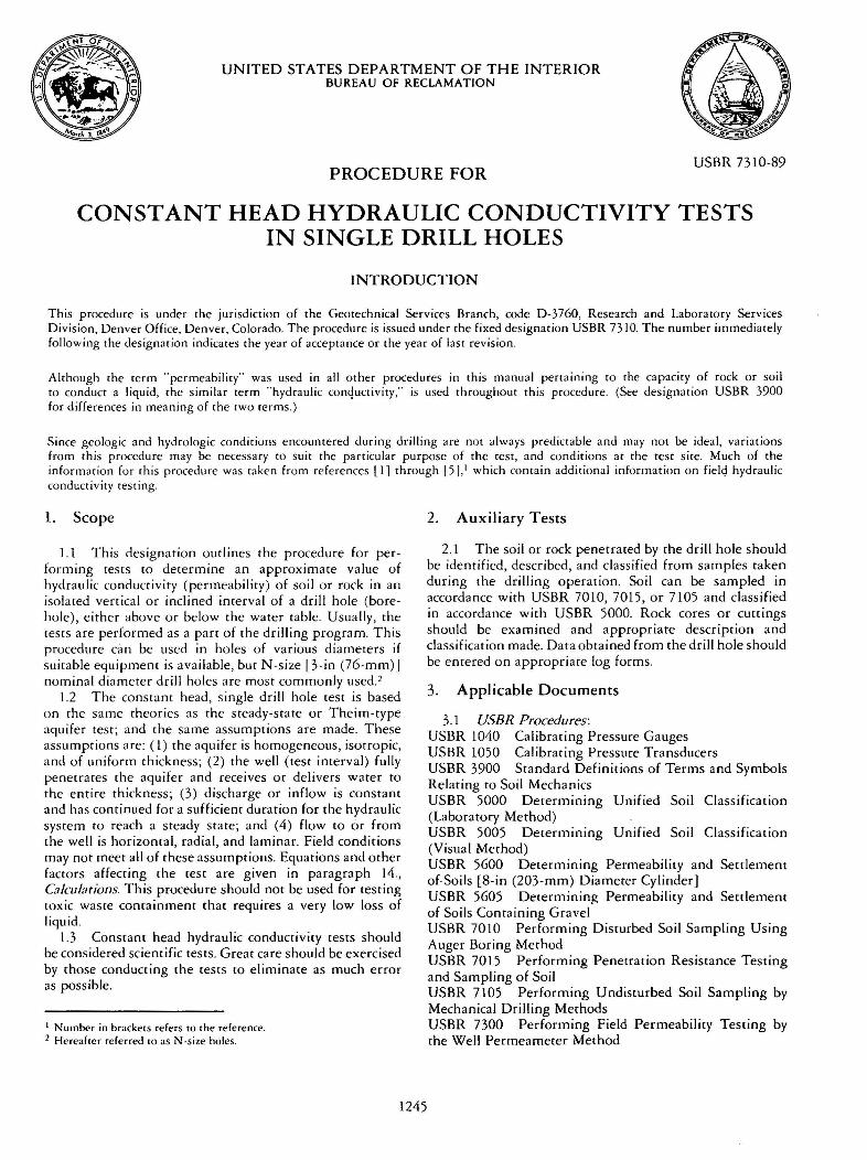
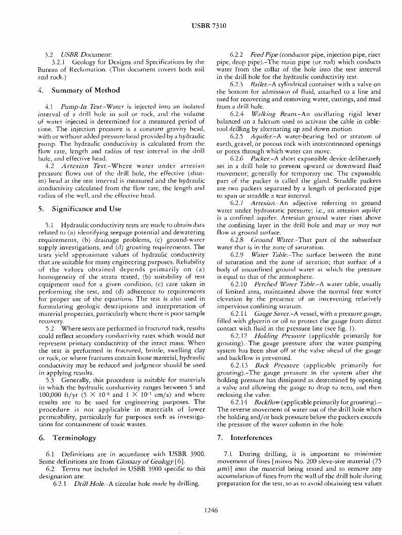
USBR 7310
32 USER Document 321 Geology for Designs and Specifications by the
Bureau of Reclamation (This document covers both soil and rock)
4 Summary of Method
41 Pump-In Test-Water is injected into an isolated interval of a drill hole in soil or rock and the volume of water injected is determined for a measured period of time The injection pressure is a constant gravity head with or without added pressure head provided by a hydraulic pump The hydraulic conductivity is calculated from the flow rate length and radius of test interval in the drill hole and effective head
42 Artesian Test-Where water under artesian pressure flows out of the drill hole the effective (shutshyin) head at the test interval is measured and the hydraulic conductivity calculated from the flow rate the length and radius of the well and the effective head
5 Significance and Use
51 Hydraulic conductivity tests are made to obtain daca related to (a) identifying seepage potential and dewatering requirements (b) drainage problems (c) ground-water supply investigations and (d) grouting requirements The tests yield approximate values of hydraulic conductivity that are suitable for many engineering purposes Reliability of the values obtained depends primarily on (a) homogeneity of the strata tested (b) suitability of rest equipment used for a given condition (c) care taken in performing the test and ( d) adherence to requirements for proper use of the equations The test is also used in formulating geologic descriptions and interpretation of material properties particularly where there is poor sample recovery
52 Where tests are performed in fractured rock results could reflect secondary conductivity rates which would not represent primary conductivity of the intact mass When the test is performed in fractured brittle swelling clay or rock or where fractures contain loose material hydraulic conductivity may be reduced and judgment should be used in applying results
53 Generally this procedure is suitable for materials in which the hydraulic conductivity ranges between 5 and 100000 ftyr (5 X 10⁻⁶ and 1 X 10⁻¹ cms) and where results are to be used for engineering purposes The procedure is not applicable in materials of lower permeability particularly for purposes such as investigashytions for containment of toxic wastes
6 Terminology
61 Definitions are in accordance with USBR 3900 Some definitions are from Glossary of Geology [6]
62 Terms not included in USBR 3900 specific to this designation are
62 l DnJJ Hole-A circular hole made by drilling
622 Feed Pipe (conductor pipe injection pipe riser pipe drop pipe)-The main pipe (or rod) which conducts water from the collar of the hole into the test interval in the drill hole for the hydraulic conductivity test
623 Baifer-A cylindrical container with a valve on the bortom for admission of fluid attached to a line and used for recovering and removing water cuttings and mud from a drill hole
624 Walking Beam-An oscillating rigid lever balanced on a fulcrum used to activate the cable in cableshytool drilling by alternating up and down motion
625 Aquifer-A water-bearing bed or stratum of earth gravel or porous rock with interconnected openings or pores through which water can move
626 Packer-A short expansible device deliberately set in a drill hole to prevent upward or downward fluid movement generally for temporary use The expansible part of the packer is called the gland Straddle packers are two packers separated by a length of perforated pipe to span or straddle a test interval
627 Artesian-An adjective referring to ground water under hydrostatic pressure ie an artesian aquifer is a confined aquifer Artesian ground water rises above the confining layer in the drill hole and may or may not flow at ground surface
628 Ground W1ter-That part of the subsurface water that is in the zone of saturation
629 W1ter Tizble-The surface between the zone of saturation and the zone of aeration that surface of a body of unconfined ground water at which the pressure is equal to that of the atmosphere
6210 Perched Water Table-A water cable usually of limited area maintained above the normal free water elevation by the presence of an intervening relatively impervious confining stratum
6211 Gauge Saver-A vessel with a pressure gauge filled with glycerin or oil to protect the gauge from direct contact with fluid in the pressure line (see fig 1)
6212 Holding Pressure (applicable primarily for grouting) -The gauge pressure after the water-pumping system has been shut off at the valve ahead of the gauge and backflow is prevented
6213 Back Pressure (applicable primarily for grouting)-The gauge pressure in the system after the holding pressure has dissipated as determined by opening a valve and allowing the gauge ro drop ro zero and then reclosing the valve
6214 Backflow(applicable primarily for grouring)shyThe reverse movement of water out of the drill hole when the holding andor back pressure below the packers exceeds the pressure of the water column in the hole
7 Interferences
71 During drilling it is important ro minimize movement of fines [minus No 200 sieve-size material (75 microm)] into the material being tested and to remove any accumulation of fines from the wall of the drill hole during preparation for the test so as to avoid obtaining test values
1246
USBR 7310
Heov1 Out1 Pressure Gouge
poundLpoundVATON SECTION
TOP VpoundW BOTTOM VIEW
Figure I - Gauge saver device for protecting pressure gauge 40-D-4287
lower than the actual hydraulic conductivity of the material being tested Drilling using clear water without additives is preferred Bentoniticmiddotmuds should nor be used in holes where hydraulic conductivity testing is to be performed Biodegradable additives may be used if necessary but only if the test interval is adequately cleaned before testing The drilling procedure should be documented on the log form
72 Test results can be adversely affected by injecting water containing sediment which would tend to plug voids in the material being tested
73 The temperature of the injected water should be equal to or warmer than that of the ground or ground water This reduces the tendency of air dissolved in the water to become entrapped in the voids of the material be ing tested and co cause low values of _hydraulic conductivity In most areas not affected by artesian conditions the temperature at a depth of about 25 feet (8 m) below the ground surface remains relatively constant at the annual mean air temperature for the region At significantly greater depths temperature rises about l degF (06 degC) for each 500 to 1000 feet (150 to 300 m) of depth The temperature of the injected water especially if it is known to be colder than the ground-water temperature should be recorded on a geologic log or the hydraulic conductivity cesc daca forms (see subpar 812 for suitable temperature measuring devices)
74 It is possible that dissolved minerals in the wacer used for a rest may react chemically wich substances in the material being reseed to cause a change in the hydraulic conductivity Therefore it is desirable to use wacer for the test chat is similar in quality co that expec~ed to permeate che ground when che project is in operation
8 Apparatus
81 Drill Rigs (see fig 2) ~1 ~ Rotary Drilling-A drilling method resulting m grinding a hole with a hard-toothed drill bic at che end of a rocacing drill rod (pipe) The equipment consists essentially of a power unit hoisting or rugging unit controlled-feed rotary drill head and mounting frame masc or tripod and circulating pump The rig should have various accessory drilling andsampling equipment (rods bits core barrels augers) as required for drill hole advancement sampling and testing
812 Cable Tool Drilling-A method of drilling in which the material at the bottom of the hole is broken up by a steel bic with a blunt chisel-shaped cutting edge The drilling equipment consists essentially of a mast a sering of drill tools (casing tubing or pipe of one size) chat is alternately lifted and dropped by a hoist with a power unit and a walking beam A bailer is always used with a cable tool rig Normally a cable tool drilled hole is noc satisfactory for hydraulic conductivity testing with packers
82 Injecrion Pump-A centrifugal or helical screw type pump providing a constant water flow is required This may require a special pump separate from that used for drilling operations Although there may be conditions where a larger or smaller pump may be required highshy
quality pumps having a capacity of 40 galjmin (150 L min) at a pressure of 120 bf in2 (830 kPa) (such as Moriyo model 3L-8 manufactured by the Robbins and Myers Company Springfield Ohio or equivalent) are adequate for most hydraulic conductivity tests The pump should provide the required flow at the required constant pressure with maximum allowable pressure fluctuation-due co pumping pulsations-of plusmn5 percent of the test gauge pressure A surge chamber is required for all testing chis minimizes pulsations which can affect the injection race in the test interval Also ic makes readings more accurate and protects che pressure gauges against damage from sudden pressure changes
83 Feed P1pe- The feed pipe should be of adequate diameter to minimize head losses and have adequate tensile strength to withstand pumping pressures and stresses during hoisting or tugging The feed pipe is commonly a threaded and coupled assembly of pipe or tubing having a uniform inside diameter Drill rods generally of N-size can be used wichouc seriously affecting reliability of rest data if che flow rate to the test interval does nor exceed about 15 galmin (57 Lmin) and the depth co che top of che interval does noc exceed 50 feet (15 m)
NOTE 1-Use of drill rods as feed pipe should be permitted only after the assembled drill rod string has been pressure reseed ro cali_brare head losses ar anricipared flows If seals or sealing marenals are used during calibrarion the same type of seals or sealing materials (not oils or wax) should be used during hydraulic conductivity resting
84 Flowmecers-One or more calibrated flowmecers are required the capacity of each meter should be specified
1247
USBR 7310
- Byooss votve Surgechomber~
Wotermettr-
Observation oost see Detail A
SCHEMATIC ARRANGEMENT OF EQUIPMENT
(Water meter
~==it=======t(k=====- For wottr tes t ing middotWell cas1n9
Press1Jre gouge
-=====bull===========~-For drilling DETAIL A OBSERVATION POST FOR
OPTIONAL EQUIPMENT ARRANGEMENT FOR DETAILS 8 AND C
WATER TESTING ANO DRILLING FROM SECTION X-X TO WELL
DETAIL D GRAVITY TEST
DETAIL B DETAIL C DOUBLE PACKER TEST SINGLE PACKER TEST
Figure 2 - Schematic arrangement of hydraulic conductivity equipment 801-D-l I I
For flows up to 50 galmin (200 Lmin) a 1-inch (25- 851 Pneumatic Piezometers-A down-hole pneushymm) diameter disk-type meter may be used For higher matic piezomerer system has been developed [7] flows a 2- or 2-12-inch (50- or 65-mm) diameter impellershy Descriptions of the equipment and procedure as used ar type meter is recommended two damsites are presented in appendix XL
841 A straight uninterrupted section of pipe having 852 Electrical Transducers-Electrical transducers an inside diameter equal to the rated size of the meter have been used as down-hole pressure sensors by other and a minimum length 10 times the inside diameter of agencies [8) particularly for very low hydraulic conducshythe pipe should be provided upstream of the meter tivities [below 1 ftyr (1 X 10⁻⁶ cms)] The USBR has Manufacturers commonly recommend pipe lengths of one used electrical down-hole sensors in preliminary trials tO two times the inside diameter of straight pipe Electrical transducers measure pressures more accurately downstream from the meter than pneumatic piezometers and can be connected tO a
85 Pressure Sensors-Where required calibrated strip-chart recorder for a continuous record However pneumatic piezometers or electrical transducers can be used transducers are considered less rugged for field use and as down-hole sensors tO measure pressures at the rest require more maintenance and experienced personnel tO
interval during a hydraulic conductivity rest Down-hole operate than do pneumatic piezometers sensors are preferred over the method of calibrating the 86 Pressure Gauges-When down-hole pressure piping system for head loss between a pressure gauge on sensors are not available or sensors are not working the surface and the test interval However an above-ground properly calibrated pressure gauges can be used t0 estimate pressure measurement can provide a check of the pressure effective pressure in rhe rest interval after correcting for sensor friction loss through the feed pipe and packer All pressure
1248
USBR 7310
gauges used in water resting should be high-quality stainless steel glycerin or oil filled wich pressure indicated in both lbfin2 and kPa (such as manufactured by Marsh Instrument Company a unic of General Signal P 0 Box 1011 Skokie Illinois or equal) Pressure gauge ranges should be compatible wich middot cescing requirements chey should be sized so char che gauge capacity does not exceed two co three rimes che maximum desired pumping pressure for each respective pumping stage Gauges should have the smallest graduations possible and an accuracy of plusmn25 percent over che coral range of the gauge If a gauge saver is used wich che gauge calibration should be made wich the gauge saver in place Accuracy of che gauges should be checked before use and periodically during the resting program (see subpar 112 for additional information)
861 One or more pressure gauges should be located downstream of che flowmecer and downstream of any valves ac che cop of che feed pipe This location for pressure measurement can be used by inserting a sub (adaptor or shore piece of pipe) wirh che gauge - installed on che cop of rhe feed pipe
862 Ac least one additional calibrated replacement gauge should be available ar che resr sire
87 Swivel-During che hydraulic conductivity cesc ic is preferable co eliminate the swivel and use a direct connection co the feed pipe If a swivel muse be used in che water line during resting ic should be of che nonconscriccing type and calibrated for head loss Significant friction loss can result from use of che constricting type
88 Packers-One or two (straddle) packers are required for che rest Packers may be either bottom-set mechanical screw set mechanical pneumatic inflatable or liquid inflatable The pneumatic inflatable packer is the preferable type for general use and is usually che only one suitable for use in soft rock and soil The gland of this packer is longer and more flexible chan the ocher types and will form a tighter seal in an irregular drill hole A leather cup type of packer should noc be used To ensure a eight water seal che length of contact between each expanded packer and che drill hole wall should noc be less than three rimes the drill hole diameter
NOfE 2-More than one type of packer may be required to test the complete length of a drill hole The type of packer used depends upon many factors eg rock type drill hole roughness spacing and width of rock joints and test pressures
881 Inflatable Packers-Inflatable packers with an expansible gland and a floating head (see app fig Xl2) should be designed for anticipated drill hole diameters and pressure conditions For normal hydraulic conductivity cescing a reasonable maximum recommended working pressure inside and outside of che packer is 300 lbf in2
(2070 kPa) [8] Inside pressure should be increased in water-filled holes proportionally co che sracic head For drill holes wich sharp projections in the walls a wireshyreinforced packer gland having a higher working pressure [7] may be required The pressure in che packer should not be high enough to fracture the material being reseed
The pressure required to form a cighr seal ac che ends of a cesr interval depends on the flexibility of rhe gland the friction of the floating head and che drill hole roughness The minimum differential pressure between che packer and the cesc interval can be derermined by res ring packers in a pipe slighrly larger rhan rhe nominal diameter of rhe drill hole in order co simulate possible enlargement of rhe drill hole during drilling For a given resr interval pressure che packer pressure is increased until ir provides a waterrighc seal between the packer and the material with which ic is in contact The pressure in rhe packer should range approximately berween 30 and 300 lbfin2 (210 ro 2100 kPa) greater chan char in che cesc interval with 100 lbfin2 (690 kPa) being normal Pneumatic inflatable packers can be inflated with compressed air or compressed nitrogen
882 Special pneumatic packers are available for use in wireline drilling operations Because che packers must be able co pass through che wireline bit and then expand co completely seal che hole ac che cesc interval special materials are needed for che packer gland A special packer assembly-consisting of cwo packers in tandem-is used with the upper packer being expanded inside che drill rod just above che bic and che lower packer expanded against che wall of the hole just below che bit The two packers on the assembly can be positioned properly-relative co the bit-by a sec of lugs or a ring located on the assembly Special seals or connections are needed co attach che water supply co che wire-line drill pipe at the surface
883 A minimum of two secs of replacement packers andor spare glands should be available at the test sire
89 Perforated Pipe Sections-Lengths of perforated steel pipe corresponding ro the lengths of rest intervals are required between packers to admit water inco che rest intervals The coral area of all perforations should be greater than five rimes che inside cross-sectional area of che pipe These perforated pipe sections should be calibrated for head loss
810 Well Screen-Well screen or slotted pipe may be required for cescing in granular unstable materials chat require support [9] As a general rule the maximum size of sloe width should be approximately equal to che 50shypercent size of che particles around the drill hole (see subpar 114)
811 Water Level Measuring Device 8111 Although there are ocher types of water level
indicacors che electrical probe indicator is most commonly used Essentially ic consists of (1) a flexible insulated conduit marked in linear units and enclosing cwo wires each insulated except ac che tips (2) a low-voltage electrical source and (3) a light or ocher means of indicating a closed circuit which occurs when che rips contact che water surface Different brands of electric wacer level indicacors and even different models of the same brand ofren have their own unique operating characteristics Before using any electric water level indicacor it should first be reseed at the surface in a bucket of water
8112 For approximate measurements of the water level when ic is within about 100 feet (30 m) of the ground
1249
USBR 7310
surface a cloth tape with a popper can be used A popper can be made from a short pipe nipple (or length of tubing) by screwing a plug attached to a graduated tape intu one end of the nipple and leaving the other end of the nipple open When the popper is lowered in the drill hole and the open end of the pipe nipple strikes a water surface it makes a popping sound and the depth to water can be measured by the tape
8113 An accurate measuremenr of the water level can be made by chalking the lower end of the steel tape After contacting the water level the tape should be lowered about L more foot before retrieving it Measurement is then made to the wet line on the tape
812 Temperacuie Measuring Device-Equipment for measuring ground-water temperature is available from commercial sources or can be made from a thermistor two-conductor cable reel Wheatstone bridge and a lowshyvoltage electrical source A maximum-minimum type thermometer is acceptable
9 Regents and Materials
91 ~71ter (See subpars 72 73 and 74)-The clear water supply should be sufficient tO perform the hydraulic conductivity test without interrruption and to maintain the required pressure throughout the test period
92 Swd or Gravel Backfill-Where a granular backfill is used t0 prevent sloughing of the drill hole wall it should be a clean coarse sand or fine gravel Laboratory permeability tests (USBR 5600 or 5605) should be made on the backfill material to make sure that it has a coefficient of permeability greater than one order of magnitude higher than that expected of the in situ material being rested
10 Precautions
L01 Safety Precautions L011 This procedure may involve hazardous
materials operations and equipment lO l2 Use normal precautions for drilling [ 10 11] L013 Precautions should be taken during calibration
pressure testing of equipment particularly testing of packers with compressed air or nitrogen (never use oxygen) to avoid injuries from a sudden packer or hose rupture
L02 Technical Prernutions 102 l As a general rule total pressure (static head
plus gauge pressure) applied in the drill hole should nor exceed 1 lbfin2 per foot (226 kPam) of rock and soil overburden at the center of the test interval if the test interval is 10 feet (3 m) long or less If the rest interval exceeds 10 feet pressure should not exceed 1 lbfin 2 per foot of overburden at the top of the interval In layered or fractured material or for drill holes near steep abutments or slopes 05 lbf in2 per foot ( 113 kPa m) of material to the nearest free surface is an appropriate maximum pressure Higher pressures than these may fracture the materials
1022 If there is excessive or complete loss of water when the hole is being drilled drilling should be sropped before cuttings fill the voids and a hydraulic conductivity rest completed on a shorter than normal length rest interval
1023 Hydraulic conductivity rest equipment should be considered and treated as precision testing equipment Gauges thermometers ere should have their own protective cases they should not be carried with drill tools or be tossed around They should be calibrated frequently Ir is recommended that all test equipment needed for hydraulic conductivity resting be kept separate from drilling equipment
11 Calibration
111 For Measurment ofEffeaive Head 11 l l Pressure Sensurs-Calibrate down-hole
pressure sensors by the methods and at frequencies prescribed by USBR LOSO
ll12 Friction Loss Estimates-Where down-hole pressure sensors are nor used estimates of effective head at the rest interval are made by subtracting friction loss from the applied head measured at the ground surface The friction loss should be determined for all components of the piping system from the pressure gauge to the test interval
1112 I Calibrate friction loss in parts or sections of the piping systems including ( L) the swivel (if used) (2) feed pipe (per unit length) and (3) the packer assembly Record the data with references to the particular parts calibrated in tabular or graphical form so the accumulative friction loss can be totaled for determination of effective head at the test interval The calibration procedure is as follows
I l l211 Lay out the individual or joined parts to be calibrated on a horizontal surface with calibrated pressure gauges at each end
l L 12 12 Pump water through the system at incremental increasing flow rares to the maximum flow rare expected to be used in the test allow the flow to stabilize between incremental flows
L 112 L3 Record the pressure at each gauge for each incremental flow rate
11 l 2 L4 Calculate the friction head loss for each incremental flow rare
2f = 23 l ( p ~I p ) (I )
where f = friction head loss in feet of head per linear foot
of pipe ftft or mm P1 = upstream pressure bf in 2 or kPa P2 = downstream pressure lbfin2 or kPa d = pipe length fr or m (d = l for swivel or packer
assembly) 23 l = converts from pressure in bf in2 to head in feet
or 0102 converts from pressure in kPa to head in meters
Example assume
P1 = 186 lbfin2 or 128 kPa P2 = 132 lbfin2 or 910 kPa d = 100 ft or 305 m
1250
USBR 7310
Inch-pound application
f = 231 ( 18 ~~-~3 2) 125 ftfr
SI application
f = 0 102( 128
- 9 tO) = 124 mm 305
l l l215 Plot friction head loss versus flow rare Figure 3 is an example of a plot of friction head loss (f) at relatively low flow races for a 10-foor (33-m) length of 1-14-inch (32-mm) diameter pipe Since head loss in pipe at turbulent flow is approximately related to velocity squared a plot of friction head loss versus the square of the flow rate is nearly a straight line (see fig 4)
NOfE 3-There are srandard rabies and charcs which provide unit friction losses for various sizes of pipe elbows cees reducers ere for clean and ruscy conditions Although such informacion is sometimes used it is preferable to determine friction losses in che piping syscem and packers accually used for che hydraulic conductivity rest
111216 To calibrate a packer inflate the packer in a shore length of casing or pipe in which amiddotvalve and pressure gauge have been installed A pressure gauge is also installed in the rods immediately ahead of the packer assembly Pump water into the rods at incremental increases (or decreases) of flow rate-allowing the system to stabilize after each incremental change-until the highest anticipated flow rate is reached
NOfE 4-For packers smaller than N-size such as the B-size used in wireline equipmentmiddot there are significant head losses and relatively low flow races must be maintained This requires water meters and pressure gauges capable of accurately measuring the low flows and small changes in pressures
112 Pressure Gauges-Calibrate each pressure gauge (see USBR 1040) by comparing it with a test or master
FLOW RATE IN LITERS PER MINUTE
o
I _ I_ I I I II
I I I I I loI I I I I I rI
I I I )I
I I I I I v I I I I I I I I I I lr II
I I
I I I I 11deg II i j~ I I I -~-----1 -- I I I I i
JO deg HOW RATE IN GALLONS PEA MINOT[
Figure 3 - Head loss due ro friction at increasing flow rates for a I 0shy
foot (3-m) 1-14-inch (32-mm) diameter iron pipe
gauge The master gauge should not be used during drilling or hydraulic conductivity testing Calibrate each gauge at the start of a res ring program plus one additional calibration per week during rests of long duration
113 Flowmeters-Calibrate a flowmerer by flowing water into a container of known volume the container used for the volume check should be commensurate in size with the flowmeter size and graduations From these data flow rares can be calculated for comparison with meter readings All flowmeters should be calibrated to an accuracy of plusmn1 percent Calibration should be done at the stare of the resting program plus one additional calibration per week during rests of long duration
NOfE 5-Some impeller-type flowmeters have an accuracy range significantly less than indicated by the dial Minimum and maximum races should be esrablished
114 Well Screens and Perforated or Slotted Pipe Sections-From manufacturers dara or by calibration determine the head losses in expected flow ranges to ensure there is no restriction of flow into the material being tested
12 Conditioning
12 l Nor applicable special conditioning requirements are not needed for this procedure
13 Procedure
13l Cleaning ofDnll Hole 13l1 Remove any accumulation of fine particles
(smear mud cake compaction caused by driving casing etc) from the drill hole wall Such accumulation significantly restricts the flow of water into or from the hole Exercise good judgment in cleaning the hole since excess cleaning may be detrimental If there is a question as to whether or not drill holes in particular materials need cleaning hydraulic conductivity tests can be performed in holes with cleaning and others without cleaning If cleaning does not significantly change rest results at a sire cleaning of additional intervals in the same materials may not be necessary
131 l1 When the rest interval is above the water table it may be possible to brush or scratch the drill hole wall to break up accumulated fines For unstable materials which require use of a well screen materials which cavemiddot against the screen may break up the accumulation of fines on the wall Mild surging with a bailer while adding water also may help break up a disturbed or compacced zone but this may stir up fines which then plug the voids in the material co be rested Mild jetting-followed immediately by bailing or pumping-also is a possibility
13 l l2 When the test interval is below the water table-in materials chat are rock-like and self-supporcingshyuse of a water jet in the hole (preferably accompanied with pumping to induce flow into the borehole) is one of the best methods to clean the hole After jetting bail or pump the sediment-laden water from the rest interval Jetting can also be used through a screen below the water
1251
tJ
I I 0 GO-GI I GO-G2 0 GI -G2
~
I
I
v
v p-shy~ -shyl--~ L--shy
-shy
v
0
middot 005 =0 00005 100
-shy~--~ 0 middot 0025 =0 00005
I 50 I
~ --shy = 0 00005
50
I
t - A
v -
-
[] --shy shy--shy0 -
4--l_-E
-
16
-shy-shy-8 --shyl---shy~ - 2
~ ~---shy z 3 4 5 6 7 8 9
FLOW RATE SQUARED (q 2 )(10001
s of oalmin ) 2
Figu re 4 - Plot of feed p_ipe ca libra tion data - example
USBR 7310
2FLOW RATE SQUARED (q2)( 1000degs of L min)
10 15 20 25 - 30 35
50
40
r w w LL
z
~ 30 0 J Cl ltgt w I
z 0 20 r S a LL
10
0
cable in unstable materials For soft rock flushing che sides of che drill hole by running che bit or a bailer up and down the hole may enlarge the hole by erosion or ocherwise change the characceriscics of the fracture systems
13113 Finally clean the drill hole by pumping or bailing water from the bottom upward with the pumping continued until the return fluid is clear without cuttings or sediment Record the method used in cleaning the hole on the log of drill ho le or on a special testing form
132 Length of Test Interval 1321 The length of the test interval depends on
(1) purpose of the test (2) stratigraphic interval and (3) flow rate Where materials are relatively uniform use a test interval of about 10 feet (3 m) Where flow rates are high shorten the test interval co locate high flow race zones where races are very low the interval may be lengthened if desired
133 Ground-Water Level Determination 13 31 Depth co ground-water level muse be
determined before calculating hydraulic conductivity Measure depths to water levels with an electrical probe or o ther suitable equipment (see subpar 811)
1332 Auger Holes-ln power auger or other types of holes to which water is not added as pare of the drilling process report the presence or absence of a water level depth to water level and dace of initial and final water level measurement In materials of low hydraulic
14
12Cll a w r w
101 z () Vgt 0
8 J
Cl ltgt w I
Sz 0 r u a
4 IL
conduccivicy several days to several weeks may be required for a water level to stabilize in the hole Report evidence of moisture in the cuttings and if a perched water level was observed
1333 Rotary or Cable Tool Holes-For drill holes in which addition of water to the hole is an integral part of the drilling process
13331 Bail or pump the hole dry or to a stable wa ter level at the close of the last shift each day and record level
13332 Report the presence or absence of water and depth to water at the beginning of the first shift each day Additional readings are desirable whenever water level in the hole has nor been disturbed for an appreciable period of time
13333 Report changes in water level detected as the hole is drilled deeper Record faccors that affect the water level such as depth of casing andor cemented intervals These data may be helpful in recognizing perched or confined (artesian) conditions
13334 Upon completion of the hole the water must be bailed down to the extent practicable the water level measured and the dace recorded of hole completion Measure the water level for a period of days or weeks until equilibrium is reached
NOfE 6-At times exceptions must be made to the requirement for conrinuation of water level readings Such is the case when
1252
USBR 7310
state or local laws require chat the hole be filled continuousiy from bottom to cop immediately upon hole completion and before the drill crew leaves the sire In ocher instances landowners may allow right-of-entry for only a limited time for measurements
1334 Perched and Artesian Aquifers-lc is imporshytant tO recognize perched and artesian aquifers especially those under sufficient pressure tO raise the water level above the confining layer but nor tO the ground surface (see (5 ]) They must be distinguished from water table aquifers (those which continue in depth) If perched water table or artesian aquifers-separated by dry or less permeable strata-are encountered in the same drill hole the resulting water level in the hole is a composite therefore conclusions and interpretations based on such data are misleading If a perched water table is recognized (or suspected) during drilling water levels must be determined for each zone for calculation of hydraulic conductivity This might require completion of the drill hole with a watertight seal set at a suitable horizon tO
separate two water table conditions In this type installarion two strings of pipe or conduit are required one extending down to the portion of the hole immediately above the packer and a second string extending through the packer to a point near the bottom of the hole Water-level measurements provide the basis for determining a perched condition or if the lower water table is under artesian pressure
13 35 Mulriple Water-Level Measurements-In some instances it is desirable tO install multiple conduits and packers or plugs in a drill hole so that ground-water levels (or pressure heads) in several water-bearing horizons can be measured over an extended period of time (see [5] pp 7-14)
134 Pressure Tests With Packers 134 l The recommended arrangement of typical
equipment for packer pressure tests without a pressure sensor is shown on figure 2 (See app fig Xl l for equipment with a pressure sensor) Beginning at the source of warer the general arrangement is clean water source suction line pump discharge line tO srorage andor settling tank suction line water-supply pump surge chamber line ro bypass valve junction water meter gate or plug valve tee with sub for pressure gauge short length of pipe on which the pressure gauge is attached tee and off-line bleeder valve for evaluating back andor holding pressure flexible 1-14-inch (32-mm) diameter hose and 1-14shyinch-diameter feed pipe ro packer or packers in drill hole which isolate the rest interval All connections should be tight and as short and straight as possible with minimum change in diameter of hose and pipe Friction loss decreases as the pipe diameter is increased
1342 When the material is subject co caving and casing andor grout is needed to support the walls of the drill hole the hole should be water rested as it is advanced Other hole conditions may make this procedure desirable or necessary The following procedure is commonly used
1342 l After the hole has been drilled to the top of the interval to be tested it may be desirable tO remove
the drill string from rhe hole and advance casing or grout ro rhe bonom of the hole
13422 Advance the hole 5 to lO feet ( 15 to 3 m) into the material to be rested
13423 Remove the drill string from rhe hole 13424 Clean the interval to be tested and record
the depth tO the warer table if present If a composite water level is suspected the warer level affecting rhe rest should be determined by measurements through the feed pipe after rhe packer has been seated and the water level has stabilized
13425 If rhe hole will stand open sear a single packer ar the top of rhe test interval Record the type of packer irs depth and packer pressure if it is rhe inflatable type
13426 Pump water into the interval ar a rate to develop a suitable pressure The pressure to be used depends upon testing depths and ground water levels or pressures Materials subject to deformation or heaving such as by separation of bedding planes or joints or materials at shallow depths must nor be subjecred to high pressures (see subpar 102 l ) For comparison of flow rates in different pares of a single foundation and with results from other foundations some of the following pressures are commonly used 25 50 75 and LOO lbfin 2 (170 350 520 and 690 kPa)
NorE 7-At test pressures less than 25 lbfin2 errors in measurement of pressure and volume of water may increase unless special low pressure gauges are used Gravity tests provide more accurate results under these conditions At pressures higher than 10 lbfin2 difficulties in securing a right packer seal and the likelihood of leakage increase rapidly However under artesian pressures or in deep holes the water pressure-as registered on a surface gauge-will need to be sufficient to overcome the effeccive head at the test interval and firmly seal the packer
NillE 8-Where the hole is subject to caving a pump-down wire-line system has been developed rhar can be used to eliminate removal of the drill string from the hole With this system the hole is drilled to the bottom of the interval tO be tested and the drill rod is raised so the end of the rod is at the top of the test interval The tandem packer (see subpar 882) is then lowered through the drill rod and expanded to seal both inside the rod and against the wall of the hole at the cop of the test interval Models of this equipment are available which have transducers below the packer for measuring water pressures at the test interval
13427 For determining effective head artesian heads encountered in the drill hole are treated the same as water table conditions ie the depth from the pressure gauge or the water level maintained during the test to
the stabilized water level is used as the gravity head If the artesian head stabilizes above the ground surface the gravity component of the effective head is negative and is measured between rhe stabilized level and the pressure gauge height If a flow-type rest is used the effective head is the difference between rhe stabilized water level and rhe level maintained during the flow period
1253
USBR 7310
13428 Afrer pressures are selected based on ground-water conditions and the purpose of the test perform a test at each pressure Usually a 5-cycle procedure is used three increas ing steps to the maximum pressure and then two decreasing steps to the starting pressure This cycling allows a more derailed evaluation of rest results than testing at a single pressure and commonly allows extrapolation to ascertain at what pressures the following may occur (1) laminar flow (2) turbulent flow (3) dilation of fractures ( 4) washouts (5) void filling or (6) hydraulic fracturing However the equations normally used to ca lculate hydraulic conductivity are based on laminar flow conditions
NOfE 9-ln some insrances on ly a single water pressure test at a given interval in the drill ho le may be required For example if geologic conditions are known and there is no need ro perform the seeps in subparagraphs 13422 through 13426 a single value of hydraulic conductivity with a relatively low application of pressure may suffice
13429 During each test continue pumping water to the test interval at the required pressure until the flow rate becomes stable As a general guide maintain flow rares during three or more 5-minute intervals during which l-minute readings of flow are made and recorded In tests above the water table water should be applied to the test interval until the flow rate stabilizes before starting the 5-minuce measurement intervals Where tests are below the water table flow rates usually stabilize faster than for the tests above the water table and the time period before the 5-minure test intervals may be shorter These rime periods may need to be varied particularly when rests to determine grouting requirements are made
134210 Determine and record the presence of back pressure and decay of holding pressure Afrer the rest deflate the packer and remove it from the drill hole
134211 Advance the drill hole and if necessary the casing repeat the procedure in subparagraphs 13423 through 134210 until the required depth of drill hole is reached When casing is used in a drill hole always set the packer in the material below the casing
1343 If the hole will stay open without casing it can be drilled to final depth and after cleaning the hole hydraulic conductivity rests can be performed from the bottom of the hole upward using straddle (double) packers Although a single packer can be used to test the bottom interval of the hole starting at the bottom with double packers will cause loss of borehole testing of only about the length of the bottom packer and will save one complete trip in and out of the hole with the drill string assembly co change the packers After the test for the bottom interval is completed straddle packers are used for successive test intervals up the drill hole See subparagraph 1342 where caving or other hole conditions will not allow this procedure
135 Gra vity Tests 135 1 Constant-head gravity tests are usually
performed without packers above or below the water table with drill holes of N-size or larger (see fig 2 derail D)
This type of test is often made in reasonably stable-walled drill ho les up to 25 feet (76 m) depth where water pressure at the test interval needs to be kept low The test is usually performed in successive 5- or 10-foot (l5- or 3-m) intervals as the drill hole is advanced The upper end of each test interval is normally determined by the bottom depth of tightly reamed or driven casing If the casing is not believed
middotto be tight appropriate entries should be recorded on the log form If the wall of the drill hole is stable the test can be performed in the unsupported hole If the wall needs to be supported use a well screen (see subpar 114 for calibration) inserted through the casing It may be necessary to ream or drive the casing to the bottom of the interval set the screen and then pull back the casing to expose the screen Afrer the test the screen is removed and the casing reamed or driven to the bottom of the hole
NOfE lO-Clean coarse sa nd or fine gravel backfill (see subpar 92) may be used instead of a well scree n Ream or drive rhe casing ro the borrom of the inrerval dean ir our and add rhe backfill as rhe rnsing is pulled back ro expose rhe resr interva l Record use of rhis procedure on the log form
l 35l l If the drill hole is self-supporting clean and prepare it in rhe normal n1anner (see subpar 13l)
l35 l2 If the drill hole is not self-supporting lower the well screen and casing into the hole
135 l3 For test intervals above the water table maintain a constant head of water _within 02 foot (60 mm)] at the top of the test interval by injecting water through a small diameter rube extending below the water level maintained during the test For rest intervals below the water table or influenced by artesian conditions maintain a constant head a short distance above the measured static water level
Monitor the water level with a water-level indicato r If the water-level indicator is inserted in a small diameter pipe in the casing the wave or ripple action on the water surface will be dampened and permit more accurate watershylevel measurements
NOfE l l-When rhe flow rare is very low rhe consranr wa rer level c1n be maintained by pouring warer in rhe hole from a graduated container
135 l4 Record the flow rate at wne intervals until a constanc flow rare is reached
135 l5 Repeat the procedure of subparagraphs 135 l3 and 135 14 at one or more different water levels
13516 This rest is essentially the same as desigshynation USBR 7300 (see also L3] p 74) the instructions in USBR 7300 for performing the rest and calculating hydraulic conductivity apply to this procedure also
14 Calculations
14 l For pressure or constant gravity head hydraulic conductivity rests calculace the hydraulic conductivity of
1254
USBR 7310
rhe soil or rock by rhe following equation (expressed m consisrent unirs) [4]
k = ~ In ~ where L ~ lOr (2)
or
k = ~ sinh-1 r where lOr~ L ~ r (3)
where k = hydraulic conducrivity fryr or cms q = consrant race of flow into che rest interval
ft3yr or cm3s L = length of the test interval ft or cm
H = differential head of wacer ac rest interval fr or cm
r= radius of the borehole ft or cm In= natural logarithm loge
inv~rse hyperbolic sin~ smh- 1 x In (x + -yx2 + 1)
142 An example calculation for a single packer test _ in the botrom of a borehole belovt the wacer table follows
Example assume
r = 18 in or 015 ft= 46 cm q - 22 galmin or 83 Lmin q = 15 X 10 ft3yr = 140 cm3s L 30 ft = 91 cm
Hg gravity = disrance from ground-water level co pressure gauge = 102 ft = 311 cm
Hp pressure 5 lbf in2 X 231 ftwater (lbf in2)
116 ft = 3 54 cm of water H = Hg+ Hp= 218 ft= 664 cm
~ = ~lo = 20 hence use equation (2) 5 k = _9_ In]
2rrLH r k = 15 X 10 ft3 yr In 30 ft
2rr (30 ft) 218 ft 015 ft k = 11X103 ftyr = 11 X lQ-3 cms
NafE 12-These equations are most applicable and reliable where the length of test interval is at lease 5 r and the interval is below che water table The equations are based on laminar flow of fluid through porous media Flow races high enough co cause turbulent flow invalidate the results in all types of material In fractured material the calculated value should be considered an apparent hydraulic conductivity even under laminar flow conditions
143 For pressure resrs when rhe resr interval is below the water table H is the distance from rhe water table to the elevation of che pressure gauge plus applied pressure converted to linear units of water head
Where the rest interval is above the water table His rhe distance from rhe midpoint of the isolated rest interval to che elevation of the pressure gauge plus the applied pressure converted to linear units of water head
For gravity rests above che water table H is che distance between che boccom of the tesc interval and che water level maintained during the test
For gravity rests below the water cable His che distance between the pretest stabilized wacer level in the drill hole and the water level maintained during the rest
144 If chere is artesian pressure an additional pressure muse be applied to overcome che artesian pressure co provide an effective rest pressure For example if there is an artesian pressure of 5 lbfin2 (34 kPa) ac che pressure gauge 15 lbfin2 (103 kPa) could be applied chen che effecrive pressure would be 15 lbfin2 minus 5 lbfin2 which equals 10 lbfin2 (69 kPa)
145 The calculations can be done conveniently by (1) a nomograph [12] (2) a hand calculator with che proper functions or (3) a com purer For repeared tests ic is convenient to prepare a table for one or more diameter drill holes and lengths of resc intervals and combine che terms on che right side of the equations other than q and H into a coefficient
NafE 13-The lugeon (lugeon unit lugeon coefficient) [ 13 14 15 16] has been used as an index of hydraulic conductivity in connection with cyclic rests and for grouting purposes
15 Report
151 Record field test data on a daily driller s report and or on rhe log of the drill hole or on a special reporting form designed for the specific project Record the following
1511 Log of the drill hole 1512 Elevations of the ground surface the water
cable and che top and bortom of the rest interval 1513 Diameter of the drill hole at test interval 1514 Method of cleaning the drill hole 1515 Size of the feed pipe and any well screen 1516 Water pressure andor gravity head and flow
rare for each rime interval 1517 Tora[ amount of warer used per resr 1518 Average temperature of ground warer and
water used in the rest 1519 Packer inflation pressures 1511 Capacity of pump supplying water to the
rest interval 15111 All head loss calibrarion dara 15112 Nore any comments considered necessary to
help evaluate che rest results
15 References
[ l] Permeability Tests Using Drill Holes and Wells Bureau of Reclamation Geology Report No G-97 Denver ColoradoJanuary 3 1951
[2] Ground Warer Manual lst ed rev reprint Bureau of Reclamation US Government Printing Office Washington DC 1981
1255
USBR 7310
[3] Drainage Manual lsc ed 2d princ Bureau of Reclamacion U S Governmenc Princing Office Washingcon DC 1981 1984
[4] Zangar Carl N Theory and Problems of Water Percolation Engineering Monograph No 8 Bureau of Reclamation Denver Colorado 1953
[5] Drill Hole Water Tests Technical lnstructionsshyProvisional Engineering Geology Bureau of Reclamation July 1970 (unpublished)
[6] Glossary of Geology 2d ed American Geological lnscitute Falls Church Virginia 1980
[7] Haccher R C High Pressure Inflacable Packer with Pneumatic Piezometer Bureau of Reclamation Reporc GR-10-75 Denver Colorado October 1975
[8] Bennett R D and R F Anderson New Pressure Test for Determining Coefficient of Permeability of Rock Masses Technical Reporc GL-82-3 US Army Engineer Waterways Experiment Station Vicksburg Mississippi 1982
[9] Ground Water and Wells A Reference Book for the Water-well Industry 1st ed published by Edward E Johnson Inc Saint Paul Minnesota 1966
[10] Drillers Safety Manual 1st ed reprint Bureau of Reclamation Denver Colorado 1982
[11] Acker W L III Basic Procedures for Soil Sampling and Core Drilling published by the Acker Drilling Company Scranton Pennsylvania 1974
[12] Underground Mining Methods Handbook No 580 W-88 Society of Mining Engineers Littlecon Colorado p 62 1982
[13] Lugeon M Barrages et Geologie Dunod Paris 1933
[14] Houlsby A C Routine Interpretation of the Lugeon Water-Test Quarterly Journal Engineering Geology vol 9 pp 303-313 1976
[15] Heitfeld K H and L Krapp The Problem of Water Permeability in Dam Geology Bull International Association of Engineering Geology No 23 pp 79-83 1981
[16] Pearson R and M S Money Improvements in the Lugeon or Packer Permeability Test Quarcerly Journal Engineering Geology vol 10 the Netherlands pp 221shy239 1977
1256
USBR 7310
APPENDIX
XL PROCEDURE USING A PNEUMATIC PIEZOMETER WITH TWO PACKERS ISOLATING THE TEST INTERVAL
Xl l Equipment Assembly (Refer to figs Xll and X l2) -A complete straddle packer unit is assembled as follows
X 11 l Co nnect a predetermined length of perforated injection (feed) pipe to the lower packer (The length of perforated pipe is determined by the thickness of the zone to be rested) Connect the inflation tubing to the lower packer and lower the sliding head end of the packer into the drill hole (See subpar l l l216 for calibration of packers)
Xl l2 Clamp the top of the perforated injection pipe at the hole collar and connecr the upper packer with the sliding head already down the hole
Xl l3 Provide approximately 12 inches (300 mm) of slack in the inflation tubing between the two packers to allow for retraction of the upper packer sliding head Connecr the tubing to the upper packer
Xl l4 Install the pneumatic piezometer piezomerer tubing packer inflation tubing and sealed lengths of injecrion pipe to the head adaptor
X ll5 Lower the entire unit into the drill hole adding lengths of sealed injection pipe as necessary to reach the
( Storoqf Settling ton
interval to be tested As the unit 1s lowered che packer inflation cubing and che piezomecer tubing is unreeled into che hole and caped to che sealed injection pipe at approximately 10-fooc intervals
Xll6 Upon reaching the rest depth lock both the inflation cubing reel and rhe piezomecer cubing reel connecr the inflation tubing by quick-connecr couplings co a nitrogen or compressed air boccie equipped with a high pressure regulator connecr the piezomecer cubing by quick-connect couplings co the readout box and connect the injection pipe co the water pressure source The cesc is now ready to begin
Xl2 Test Procedure
X 12 l After the unit has been lowered to the rest interval and before infacing the packers any water head above the cesc interval must be determined This head will sho w as pressure on the pneumatic piezomecer gauge and can be verified by running a water level indicator into che hole to measure the deprh co the water cable The piezometer will register water pressure chat can be converted to head of water This water head should be
Compressed 01r or nitrogen bot tie Regulator_
Poc~er air lin e- I
P1nometer ln1ec t1on oioe head adaptor
Lo er ooc~er inflation tubmr
Figure X 1 1 - Schematic arrongemem of drill hole packer and pressure monimring equipment 801-0-180
1257
USBR 7310
------=--From compressed air or nitrogen boltle
From piezometer
_To
PRESSURE READOUT BOX
Packer inflation tubing From wafer source From air or Water injection pipe ring seals
PIEZOMETER TUBING REEL
Pressure seals Wire reinforced rubber gland clomps
nitrogen ~~i==-=~==t~f=lil~~~jii~9ll~~~~~sect9ll~sect~sectsect~~~sectl~iilf~f--- To per for o t e d ~~~ze=zzzoCzzzze=zzze=plusmnzz~EZio~~~~21p~
To pressuresource~~~~~~~~~~~~~~~readout box
Piezometer
~~~~~~~~~~~~~~~~---
Inflation chamber Floating packer head Packer inflation lubing
UPPER DRILL HOLE PACKER AND PRESSURE MONITORING EQUIPMENT FOR N X HOLE
Figure X 12 - Upper Jrill hole packer anJ pressure monitoring equipment for NX hole
used to determine the minimum inflation pressure to be applied co the packers by the following equation
SH+ PP+ PE = minimum inflation pressure
where SH = static pressure at the midpoint elevation of the
test interval lbf in2 or kPa PP = gauge pressure to be maintained during the test
lbfin2 or kPa PE = pressure needed to expand packer to hole
diameter as determined before insertion in the drill hole by expanding the packer in a length of pipe having a diameter similar to the hole diameter lbfin 2 or kPa
Inflation pressure gauge is in units of lbf in2 (kPa) The static water level measured before the packers are
inflated might be a composite water level (see subpar 1334)
Xl22 Inflate the packers and determine water head for the rest interval This is the static head to be used for calculation of hydraulic conductivity If rhe static head is significantly different from the composite measured
before the packers were inflated recalculation of packer inflation pressure may be required The final packer inflation pressure should be the lowest practical pressure to seal the test interval against the maximum injection pressure to avoid fracturing of the material being tested
Xl2 3 After the inflation pressures have been determined deflate the packers fill and flush the system with water until all entrapped air has been removed This is accomplished by filling the injection pipe under a gravity head and leaving the air-release valve open ar the top of the injection pipe tee at an elevation higher than the injection hose The valve must remain open until all air has been removed and water runs freely indicating a filled system At this point water is flowing around the deflated packer system and is completely filling the annulus between the drillhole and the packers In the case of an interval with a high injection rate it may be necessary to keep the air valve closed to keep from entraining air into the test interval
X 124 Close the air release valve at the top of the injection pipe and slowly inflate the packers to the predetermined inflation pressure
Xl2 5 Lock in the inflation pressure by closing the pressure valve in the packer cubing If the pressure gauge
1258
USBR 7310
on the closed system remains steady it verifies a sealed system At this point water injecced under gravity head approaches a constant flow rate
X 126 Record the piezometer pressure after packer inflation For an interval of very low injection rate this is equal to che height of the injeccion standpipe plus che pressure recorded at the hole collar gauge For a test interval with a high injection rate the readout would show the same value less any friction from water flow through the injeccion pipe
X 127 Proceed with the test by applying the selected pressures ac the test interval and moniroring the flow rate and pressure on the pneumatic piezometer
X 128 To accurately compute hydraulic conduetivity rhe down-hole pressure muse remain constant A zone with a high injection rate must be monirored more closely than a zone with a small injection rate and adjustments made to hold the down-hole pressure constant To accomplish
this che injeccion pressure shown on che collar gauge must be adjusted in order co maintain che down-hole pressure constant
NOfE X 1-For example a pressure srage is scarred with the collar gauge reading 35 lbfin2 (241 kPa) and the down-hole piezomerer reading 200 lbf in2 ( 1380 kPa) As rhe flow increases rhe down -hole pressure may drop to 150 lbfin2 (1034 kPa) because fricrion loss in the injection pipe and the collar gauge would have to be adjusted to bring the down-hole pressure gauge back up co 200 lbfin2bull When the flow decreases from a fast to a slow rare the collar gauge pressure would have to be decreased
Xl29 The cesc is completed following one or more stages of pressure increases and pressure decreases Following the last stage deflate the packers and close the injection line The system is now ready to move to the next test interval for repetition of this procedure
1259
Methods Note
A Computer Program for Flow-Log Analysis of Single Holes (FLASH) by Frederick D Day-Lewis1 Carole D Johnson2 Frederick L Paillet3 and Keith J Halford4
Abstract A new computer program FLASH (Flow-Log Analysis of Single Holes) is presented for the analysis of
borehole vertical flow logs The code is based on an analytical solution for steady-state multilayer radial flow to a borehole The code includes options for (1) discrete fractures and (2) multilayer aquifers Given vertical flow profiles collected under both ambient and stressed (pumping or injection) conditions the user can estimate fracture (or layer) transmissivities and far-field hydraulic heads FLASH is coded in Microsoft Excel5 with Visual Basic for Applications routines The code supports manual and automated model calibration
Introduction Flowmeters provide means to infer the flow into or
out of boreholes connected to transmissive aquifer units or fractures In the past the relative inaccuracy and difficult operating procedures for spinner flowmeters limited the use of borehole flow measurements With the advent of heat-pulse (Paillet et al 1996) and electromagnetic (Molz et al 1994) instruments measurements of vertical flow as small as 005 Lmin became practicable and borehole flowmeter logging is becoming routine New modeling and analysis tools are needed to achieve the full potential of these measurements
1Corresponding author US Geological Survey Office of Groundwater Branch of Geophysics 11 Sherman Place Unit 5015 Storrs CT 06269 (860) 487-7402 ext 21 fax (860) 487-8802 daylewisusgsgov
2US Geological Survey Office of Groundwater Branch of Geophysics 11 Sherman Place Unit 5015 Storrs CT 06269
3Office of Groundwater Branch of Geophysics (Emeritus) US Geological Survey 11 Sherman Place Unit 5015 Storrs CT 06269
4US Geological Survey Nevada Water Science Center 2730 N Deer Run Rd Carson City NV 89703
5Any use of trade product or firm names is for descriptive purposes only and does not imply endorsement by the US government
Received April 2010 accepted December 2010 copy 2011 The Author(s) Ground Water copy 2011 National Ground Water Association doi 101111j1745-6584201100798x
Calibration of a borehole flow model to flowmeter data can produce estimates of transmissivity and heads for one or more flow zones (aquifer layers or fractures) Here we briefly review approaches for analysis of flowmeter logs and introduce a new computer program which supports manual and automated calibration of an analytical borehole flow model
Approach Single-hole flowmeter data can be analyzed to
estimate transmissivity profiles along boreholes and characterize aquifer compartmentalization (Molz et al 1989 Kabala 1994 Paillet 1998) Analysis of single-hole flowmeter data is commonly based on the Thiem Equation (Thiem 1906) which written for confined radial flow from a single flow zone (ie aquifer layer or fracture) to a screened or open well is
2πTi(hw minus hi)Qi = minus (1)
ln(r0rw)
where Qi is the volumetric flow into the well from flow zone i [L3Tminus1] hw and hi are respectively the hydraulic head [L] at the radius of the well rw and at radial distance r0 commonly taken as the radius of influence where heads do not change as a result of pumping in which
926 Vol 49 No 6ndashGROUND WATERndashNovember-December 2011 (pages 926ndash931) NGWAorg
case hi is the connected far-field head for zone i and Ti
is the transmissivity of flow zone i [L2Tminus1] A number of approaches to flowmeter analysis have
been proposed and demonstrated for different sets of assumptions (eg no ambient flow in boreholes) and data requirements (eg flow profiles collected under both ambient and stressed conditions) based either on Equation 1 (Molz et al 1989) or quasi-steady flow approximations (Paillet 1998) We refer the interested reader to Williams et al (2008) for additional background on flowmeter logs and focus the following discussion on the approach of Paillet (1998 2001) which is adapted here
Paillet (1998) formulated flowmeter log analysis as a model-calibration procedure involving flow profiles collected under both ambient and stressed (pumping or injection) conditions Consideration of the two conditions allows for the estimation of the transmissivities and also far-field heads of flow zones The latter is critical for the interpretation of water samples from wells that intersect multiple fractures or layers with different hydraulic head (Johnson et al 2005) Applying Equation 1 to an ambient condition (condition a) and a stressed condition (condition s) gives
factorT total(ha minus h02πTi )w iQa = minus (2)i ln(r0rw) factorT total(hs minus h02πTi )w iQs = minus (3)i ln(r0rw)
where T factor i is the fraction of the boreholersquos transmisshy
sivity contributed by flow zone i [ndash] T total is the total transmissivity of the flow zones intersected by the bore-hole [L2Tminus1] ha hs are the ambient and stressed water w w levels in the well respectively [L] h0 is the far-field head i in flow zone i [L]
For both ambient and stressed conditions the water level in the borehole is assumed to be constant in
time and the water level in the far-field of each zone is assumed to be the natural condition that is hi
0 In a field experiment (Figure 1) rw would be known and the flow rates and water levels in the well would be measured Radius of influence can be inferred experimentally based on head data at observation wells in which case r0 can be constrained during calibration or else it can be approximated (Bear 1979 306) Estimates of transmissivity are not strongly sensitive to the value assumed for r0 because it appears inside the logarithm in Equations 2 and 3 For example a change in r0rw
from 10 to 100 yields a change in the estimated Ti of only a factor of 2 and order-of-magnitude estimates of transmissivity are acceptable for many problems In cases where knowledge of r0 is unavailable but the boreholersquos total transmissivity is known from specific-capacity or slug-test results it is possible to estimate r0 in the calibration procedure We note that the forward model (Equations 2 and 3) produces twice as many independent equations as there are flow zones with an additional equation requiring T factor values to sum to 1 The number of parameters being estimated is twice the number of flow zones (T factor and h0 for all i) plus one parameter for either i i T total 0or r i
Model calibration involves changing the model parameters such that the flows predicted by Equations 2 and 3 match the interpreted flow profiles Following Paillet (1998 2001) calibration is to the interpreted profile and not individual data This formulation allows the user to incorporate additional insight (eg from other logs) to identify the number and locations of flow zones and elimshyinates the need for weighting measurements differently according to variable measurement errors and the spatial distribution of measurements along the borehole
Calibration can be implemented by manual trial-andshyerror or automated using nonlinear regression Whether manual or automated the goal for calibration is to identify the set of parameters that minimize a measure
Figure 1 Schematic of flowmeter experiment in a fractured-rock aquifer with (a) flow-log profiles for ambient (blue) and stressed (dashed red) conditions and conceptual cross sections of flow system for (b) ambient condition and (c) stressed condition In this example two flow zones (fractures) intersect a well Under ambient conditions flow enters the well from fracture 1 and exits from fracture 3 Under pumping conditions flow enters the well from fractures 1 and 2 The far-field head of zone 2 is equal to the ambient water level thus there is no flow tofrom zone 2 under ambient conditions The far-field head of zone 3 is equal to the stressed water level thus there is no flow tofrom zone 3 under pumping conditions
NGWAorg FD Day-Lewis et al GROUND WATER 49 no 6 926ndash931 927
of combined data misfit and model misfit Considerashytion of model misfit criteria commonly referred to as regularization is useful when multiple models can match the data equally well or within measurement errors Here the data misfit is formulated based on squared differshyences between the predicted and interpreted flow profiles such that multiple measurements may be collected in a single borehole interval The model misfit could be forshymulated in different ways but we use criteria based on the differences between the water level in the borehole under ambient conditions and the far-field heads Thus the objective function F consists of two terms (1) the mean squared error (MSE) between interpreted and preshydicted flow profiles with equal weights for all cumulative flows (ambient and stressed) and (2) the sum of squared differences (h) between the boreholersquos water level and far-field heads
n1 2ssim sintmin F = Q minus Qi i n
i=1
n asim aint 2+
Q minus Q
2 + α (hi) (4)i i i=1
subject to constraints
factor factorT ge T for all i andi min
ABS(haw minus h0
i ) le hmax for all i
aintwhere Qi Qi sint are the interpreted flow profiles (ie
cumulative flow above zones) for zone i under ambishyasiment and stressed conditions respectively [L3Tminus1] Qi
ssimQi are the simulated flow profiles (ie cumulative flow above zones) for zone i under ambient and stressed conditions respectively [L3Tminus1] α weights the regushylarization relative to the data misfit [L4Tminus2] T factor ismin
T factorthe user-specified minimum for any flow zone which can ensure nonnegative T factor hmax is the user-specified maximum absolute difference between the ambishyent water level and the far-field head of any flow zone and n is the number of flow zones
Without regularization F reduces to the MSE between simulated and interpreted flows The trade-off parameter α is set by the user with larger values more strongly penalizing large head differences Commonly small α values (less than 0001) are sufficient to obtain good results In selecting α the user should be guided by the goal of regularization which is to identify the ldquosimplestrdquo explanation of the data while minimizing the data misfit
Using FLASH FLASH (Flow-Log Analysis of Single Holes) is writshy
ten in Excel with Visual Basic for Applications (VBA) The spreadsheet includes a toggle (INPUTS worksheet cell A20) to choose between analysis for (1) fractures or fracture zones that intersect a well at discrete locations
and (2) aquifer layers in porous media The first is indishycated for cases where flow profiles are characterized by step increasesdecreases and the second for cases where flow profiles show approximately linear change over each layer Up to 10 fractures or layers can be modeled
The FLASH spreadsheet includes four worksheets INTRODUCTION INPUTS FIELD_DATA and PLOTshyTING INTRODUCTION provides information about the program and input parameters On the INPUTS workshysheet the user enters information about the flow zones transmissivities and heads Note that the user must intershypret flow profiles from the flowmeter data for both the ambient and stressed conditions The flow measurements are entered in FIELD_DATA and the interpreted proshyfiles are entered in INPUTS The interpreted profiles plot as dashed lines the data as points and the simulated proshyfiles as solid lines (Figure 2) Line and marker styles can be modified using standard Excel tools Flows are positive upward and negative downward PLOTTING is used by the program and does not require the userrsquos attention
In the INPUTS worksheet input parameters are entered in the cells with light blue and bright aquamarine backgrounds The former include specifications of the experiment setup (eg borehole diameter and water level) and the latter include calibration parameters Manual calibration is performed by adjusting the values of
ldquoT factorrdquothe cells and ldquohrdquo which are respectively T factor and the difference between the flow zonersquos far-i field head and the ambient water level in the borehole As parameters are adjusted the simulated flow profiles update automatically thus guiding the user toward best-fit parameters The MSE between simulated and observed flows is calculated in cell B36 on the INPUTS worksheet
Although the principle calibration parameters are Ti
factor and h the radius of influence r0 and total transshymissivity T total also are possible calibration parameters as explained above and indicated by aquamarine highshylighting By inspection of Equations 2 and 3 it is not possible to estimate unique values for both radius of influshyence and total transmissivity but only the ratio of total transmissivity divided by ln(r0rw) In general the user will have more information about total transmissivity than radius of influence Total transmissivity is estimated readshyily using an open-hole slug test or specific-capacity test Indeed the drawdown and pumping rate under stressed conditions could serve as data to estimate a total transshymissivity for the borehole In rare cases however the estimated total transmissivity may be considered unrelishyable for example in the presence of ambiguous slug-test data or discrepancy between the volumes over which the slug test and flowmeter analysis measure In such cases it may be useful to allow the T factor values to sum to a value other than 1 FLASH assumes a uniform radius of influence for all flow zones In reality the effective radius of influence may vary between zones according to their transmissivities and distances to boundaries Data to supshyport variable radius of influence however is commonly unavailable furthermore transmissivity estimates are not
928 FD Day-Lewis et al GROUND WATER 49 no 6 926ndash931 NGWAorg
Figure 2 The INPUTS worksheet after execution of the Solver with options ldquoEstimate ROIrdquo and ldquoSolve with regularizationrdquo for example On this worksheet the user enters the well and flow-log specifications and performs model calibration Data (points) and interpreted profiles (dashed lines) Simulated profiles (solid lines) are for an arbitrarily selected starting model
a strong function of the assumed radius of influence as explained previously
Automated model calibration is implemented using the Excel Solver an optimization tool based on a Genshyeralized Reduced Gradient algorithm (Lasdon and Smith 1992) The Solver is invoked using VBA ldquocontrol butshytonsrdquo on the INPUTS worksheet Radio buttons allow for selections of (1) the parameters to be estimated (Estishymate ROI [radius of influence] or Estimate Transmissivshyity) and (2) regularization (Solve without Regularization or Solve with Regularization) Under the option Estimate
T factorROI the Solver estimates the values of i for all i and the single radius of influence Under the option Estimate Transmissivity radius of influence is assumed known the parameters for estimation are T factor for all ii such that total transmissivity is allowed to vary Users are encouraged to perform manual calibration before attemptshying automated calibration Manual calibration provides insight into the sensitivity of flows to parameters and helps to identify a good starting model for automated calshyibration As for any nonlinear optimization the algorithm may get ldquostuckrdquo in local minima and fail to identify the globally optimal parameter values Consideration of mulshytiple starting models is advised Additional information
and the FLASH spreadsheet are available online as noted under Supporting Information at the end of this article
Example FLASH is demonstrated for a simple data set from
a fractured-rock aquifer (Figure 2) Johnson et al (2005) provide additional details for this data set for which additional borehole logs were used to identify fractures and select locations for flow measurements
Under ambient conditions the deeper fractures 1 and 2 experience inflow to the borehole which indicates the far-field heads for each of these fractures is greater than the head in the borehole thus producing upward flow (Figure 1) Under ambient conditions upflowing water exits the borehole at fracture 3 indicating the far-field head is lower than the head in the borehole Under low-rate pumping conditions water continues to enter the borehole at fracture 1 additional water enters at fracture 2 indicating the far-field heads for fractures 1 and 2 are higher than the quasi-steady state open-hole water level under pumping conditions The uppermost fracture (3) no longer shows outflow indicating the far-field head is equal to the pumping water level In this example
NGWAorg FD Day-Lewis et al GROUND WATER 49 no 6 926ndash931 929
fracture 2 has a far-field head similar to the ambient water level in the well and therefore does not result in a substantial change in borehole flow under ambient conditions Similarly fracture 3 has a far-field head similar to the stressed water level in the well and does not produce a measurable change in borehole flow under stressed conditions This field example underscores the importance of collecting both ambient and stressed flow profilesmdashwith only ambient data fracture 2 could not be identified and with only stressed data fracture 3 could not be identified
To induce flow from a given fracture to enter the borehole the h for that fracture must be positive Conversely to induce flow from the borehole to the fracture the h must be negative The rate of flow is determined by the magnitude of a given flow zonersquos h and transmissivity Thus manual calibration entails for each zone (1) adjustment of a h (cells F21F30) to control whether flow enters or exits the borehole from that zone and (2) adjustment of a T factor to control the rate of flow A final solution can be obtained with the manual fit or after a starting model is generated manually the Solver can be applied For the example here automated calibration produces an excellent match to the data (Figure 2) using options ldquoEstimate ROI rdquo and ldquoEstimate with Regularizationrdquo
Discussion and Conclusions We present a new tool to aid in flowmeter log
analysis a computer code named FLASH We follow a model-calibration strategy similar to that of Paillet (1998) with a simple analytical model for borehole flow based on the Thiem Equation (Thiem 1906) which has been used extensively in previous analyses of flowmeter logs It is important to note that FLASH assumes a borehole flow model that neglects head losses in the borehole or across the well screen and these losses are important in some data sets (Zlotnik and Zurbuchen 2003) We also note the limitations inherent to flowmeter methods primarily that they not as sensitive as straddle-packer hydraulic testing Flowmeter methods consistently identify transmissivities within 15 to 2 orders of magnitude of the most transmissive zone in a borehole depending on the resolution of the flowmeter itself (Williams et al 2008) but straddle-packer tests can see features 6 orders of magnitude less transmissive than is possible with flowmeter (Paillet 1998 Day-Lewis et al 2000 Shapiro 2001) Despite the limited resolution of flowmeter measurements flowmeter modeling results can reproduce packer-test estimates to within an order of magnitude and far-field head values determined with flowmeter methods commonly compare well with packer-test results and discrete-interval water-level monitoring (Johnson et al 2005 Williams et al 2008)
FLASH provides a graphical user interface for calshyibration of an analytical borehole flow model and estishymation of flow-zone transmissivities and far-field heads The program supports manual and automated calibration
with and without regularization FLASH is highly cusshytomizable Experienced Excel users may prefer to invoke the Solver outside of FLASHrsquos VBA routines or to use alternative objective functions or regularization criteria or variable weighting for ambient vs stressed flows Future extensions may include tools for analysis of crosshole flowmeter data and evaluation of estimation uncertainty
Acknowledgments This work was supported by the US Environmental
Protection Agency Region 1 the US Geological Survey Groundwater Resources Program and Toxic Substances Hydrology Program The authors are grateful for review comments from Tom Reilly Allen Shapiro Tom Burbey John Williams Roger Morin Landis West and Mary Anderson
Supporting Information Additional Supporting Information may be found in
the online version of this article
Supplemental material available online include (1) the FLASH spreadsheet which also can be downloaded from httpwaterusgsgovogwflash and (2) a README file with information for installation and troubleshooting
Please note Wiley-Blackwell is not responsible for the content or functionality of any supporting information supplied by the authors Any queries (other than missing material) should be directed to the corresponding author for the article
References Bear J 1979 Hydraulics of Groundwater New York McGraw-
Hill Inc Day-Lewis FD PA Hsieh and SM Gorelick 2000 Idenshy
tifying fracture-zone geometry using simulated annealing and hydraulic-connection data Water Resources Research 36 no 7 1707ndash1721
Johnson CD CK Kochiss and CB Dawson 2005 Use of discrete-zone monitoring systems for hydraulic charshyacterization of a fractured-rock aquifer at the Univershysity of Connecticut landfill Storrs Connecticut 1999 to 2002 Water-Resources Investigations Report 03-4338 105 Reston Virginia USGS
Kabala ZJ 1994 Measuring distributions of hydraulic conducshytivity and storativity by the double flowmeter test Water Resources Research 3 685ndash690
Lasdon LS and S Smith 1992 Solving large sparse nonlinear programs using GRG ORSA Journal on Computing 4 no 1 2ndash15
Molz FJ GK Bowman SC Young and WR Waldrop 1994 Borehole flowmetersmdashfield application and data analysis Journal of Hydrology 163 no 3ndash4 347ndash371
Molz FJ RH Morin AE Hess JG Melville and O Guven 1989 The impeller meter for measuring aquifer permeabilshyity variations evaluations and comparison with other tests Water Resources Research 25 no 7 1677ndash1683
Paillet FL 2001 Hydraulic head applications of flow logs in the study of heterogeneous aquifers Ground Water 39 no 5 667ndash675
930 FD Day-Lewis et al GROUND WATER 49 no 6 926ndash931 NGWAorg
Paillet FL 1998 Flow modeling and permeability estimation using borehole flow logs in heterogeneous fractured formashytions Water Resources Research 34 no 5 997ndash1010
Paillet FL RE Crowder and AE Hess 1996 High-resolution flowmeter logging applications with the heat-pulse flowmeter Journal of Environmental and Engineering Geophysics 1 no 1 1ndash14
Shapiro AM 2001 Effective matrix diffusion in kilometer-scale transport in fractured crystalline rock Water Resources Research 37 no 3 507ndash522
Thiem G 1906 Hydologische methoden 56 Leipzig JM Gebhardt
Williams JH 2008 Flow-log analysis for hydraulic characshyterization of selected test wells at the Indian Point Energy Center Buchanan New York Open-File Report 2008-1123 31 Reston Virginia USGS
Zlotnik VA and BR Zurbuchen 2003 Estimation of hydraulic conductivity from borehole flowmeter tests conshysidering head losses Journal of Hydrology 281 no 1ndash2 115ndash128
NGWAorg FD Day-Lewis et al GROUND WATER 49 no 6 926ndash931 931
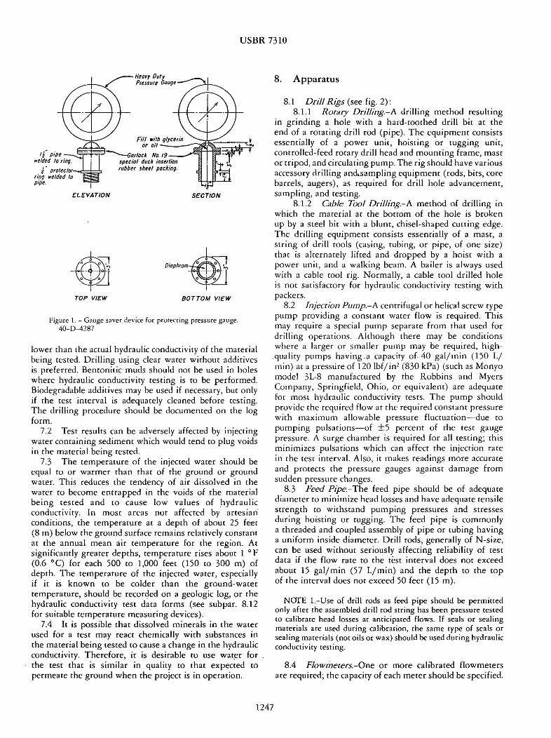
USBR 7310
Heov1 Out1 Pressure Gouge
poundLpoundVATON SECTION
TOP VpoundW BOTTOM VIEW
Figure I - Gauge saver device for protecting pressure gauge 40-D-4287
lower than the actual hydraulic conductivity of the material being tested Drilling using clear water without additives is preferred Bentoniticmiddotmuds should nor be used in holes where hydraulic conductivity testing is to be performed Biodegradable additives may be used if necessary but only if the test interval is adequately cleaned before testing The drilling procedure should be documented on the log form
72 Test results can be adversely affected by injecting water containing sediment which would tend to plug voids in the material being tested
73 The temperature of the injected water should be equal to or warmer than that of the ground or ground water This reduces the tendency of air dissolved in the water to become entrapped in the voids of the material be ing tested and co cause low values of _hydraulic conductivity In most areas not affected by artesian conditions the temperature at a depth of about 25 feet (8 m) below the ground surface remains relatively constant at the annual mean air temperature for the region At significantly greater depths temperature rises about l degF (06 degC) for each 500 to 1000 feet (150 to 300 m) of depth The temperature of the injected water especially if it is known to be colder than the ground-water temperature should be recorded on a geologic log or the hydraulic conductivity cesc daca forms (see subpar 812 for suitable temperature measuring devices)
74 It is possible that dissolved minerals in the wacer used for a rest may react chemically wich substances in the material being reseed to cause a change in the hydraulic conductivity Therefore it is desirable to use wacer for the test chat is similar in quality co that expec~ed to permeate che ground when che project is in operation
8 Apparatus
81 Drill Rigs (see fig 2) ~1 ~ Rotary Drilling-A drilling method resulting m grinding a hole with a hard-toothed drill bic at che end of a rocacing drill rod (pipe) The equipment consists essentially of a power unit hoisting or rugging unit controlled-feed rotary drill head and mounting frame masc or tripod and circulating pump The rig should have various accessory drilling andsampling equipment (rods bits core barrels augers) as required for drill hole advancement sampling and testing
812 Cable Tool Drilling-A method of drilling in which the material at the bottom of the hole is broken up by a steel bic with a blunt chisel-shaped cutting edge The drilling equipment consists essentially of a mast a sering of drill tools (casing tubing or pipe of one size) chat is alternately lifted and dropped by a hoist with a power unit and a walking beam A bailer is always used with a cable tool rig Normally a cable tool drilled hole is noc satisfactory for hydraulic conductivity testing with packers
82 Injecrion Pump-A centrifugal or helical screw type pump providing a constant water flow is required This may require a special pump separate from that used for drilling operations Although there may be conditions where a larger or smaller pump may be required highshy
quality pumps having a capacity of 40 galjmin (150 L min) at a pressure of 120 bf in2 (830 kPa) (such as Moriyo model 3L-8 manufactured by the Robbins and Myers Company Springfield Ohio or equivalent) are adequate for most hydraulic conductivity tests The pump should provide the required flow at the required constant pressure with maximum allowable pressure fluctuation-due co pumping pulsations-of plusmn5 percent of the test gauge pressure A surge chamber is required for all testing chis minimizes pulsations which can affect the injection race in the test interval Also ic makes readings more accurate and protects che pressure gauges against damage from sudden pressure changes
83 Feed P1pe- The feed pipe should be of adequate diameter to minimize head losses and have adequate tensile strength to withstand pumping pressures and stresses during hoisting or tugging The feed pipe is commonly a threaded and coupled assembly of pipe or tubing having a uniform inside diameter Drill rods generally of N-size can be used wichouc seriously affecting reliability of rest data if che flow rate to the test interval does nor exceed about 15 galmin (57 Lmin) and the depth co che top of che interval does noc exceed 50 feet (15 m)
NOTE 1-Use of drill rods as feed pipe should be permitted only after the assembled drill rod string has been pressure reseed ro cali_brare head losses ar anricipared flows If seals or sealing marenals are used during calibrarion the same type of seals or sealing materials (not oils or wax) should be used during hydraulic conductivity resting
84 Flowmecers-One or more calibrated flowmecers are required the capacity of each meter should be specified
1247
USBR 7310
- Byooss votve Surgechomber~
Wotermettr-
Observation oost see Detail A
SCHEMATIC ARRANGEMENT OF EQUIPMENT
(Water meter
~==it=======t(k=====- For wottr tes t ing middotWell cas1n9
Press1Jre gouge
-=====bull===========~-For drilling DETAIL A OBSERVATION POST FOR
OPTIONAL EQUIPMENT ARRANGEMENT FOR DETAILS 8 AND C
WATER TESTING ANO DRILLING FROM SECTION X-X TO WELL
DETAIL D GRAVITY TEST
DETAIL B DETAIL C DOUBLE PACKER TEST SINGLE PACKER TEST
Figure 2 - Schematic arrangement of hydraulic conductivity equipment 801-D-l I I
For flows up to 50 galmin (200 Lmin) a 1-inch (25- 851 Pneumatic Piezometers-A down-hole pneushymm) diameter disk-type meter may be used For higher matic piezomerer system has been developed [7] flows a 2- or 2-12-inch (50- or 65-mm) diameter impellershy Descriptions of the equipment and procedure as used ar type meter is recommended two damsites are presented in appendix XL
841 A straight uninterrupted section of pipe having 852 Electrical Transducers-Electrical transducers an inside diameter equal to the rated size of the meter have been used as down-hole pressure sensors by other and a minimum length 10 times the inside diameter of agencies [8) particularly for very low hydraulic conducshythe pipe should be provided upstream of the meter tivities [below 1 ftyr (1 X 10⁻⁶ cms)] The USBR has Manufacturers commonly recommend pipe lengths of one used electrical down-hole sensors in preliminary trials tO two times the inside diameter of straight pipe Electrical transducers measure pressures more accurately downstream from the meter than pneumatic piezometers and can be connected tO a
85 Pressure Sensors-Where required calibrated strip-chart recorder for a continuous record However pneumatic piezometers or electrical transducers can be used transducers are considered less rugged for field use and as down-hole sensors tO measure pressures at the rest require more maintenance and experienced personnel tO
interval during a hydraulic conductivity rest Down-hole operate than do pneumatic piezometers sensors are preferred over the method of calibrating the 86 Pressure Gauges-When down-hole pressure piping system for head loss between a pressure gauge on sensors are not available or sensors are not working the surface and the test interval However an above-ground properly calibrated pressure gauges can be used t0 estimate pressure measurement can provide a check of the pressure effective pressure in rhe rest interval after correcting for sensor friction loss through the feed pipe and packer All pressure
1248
USBR 7310
gauges used in water resting should be high-quality stainless steel glycerin or oil filled wich pressure indicated in both lbfin2 and kPa (such as manufactured by Marsh Instrument Company a unic of General Signal P 0 Box 1011 Skokie Illinois or equal) Pressure gauge ranges should be compatible wich middot cescing requirements chey should be sized so char che gauge capacity does not exceed two co three rimes che maximum desired pumping pressure for each respective pumping stage Gauges should have the smallest graduations possible and an accuracy of plusmn25 percent over che coral range of the gauge If a gauge saver is used wich che gauge calibration should be made wich the gauge saver in place Accuracy of che gauges should be checked before use and periodically during the resting program (see subpar 112 for additional information)
861 One or more pressure gauges should be located downstream of che flowmecer and downstream of any valves ac che cop of che feed pipe This location for pressure measurement can be used by inserting a sub (adaptor or shore piece of pipe) wirh che gauge - installed on che cop of rhe feed pipe
862 Ac least one additional calibrated replacement gauge should be available ar che resr sire
87 Swivel-During che hydraulic conductivity cesc ic is preferable co eliminate the swivel and use a direct connection co the feed pipe If a swivel muse be used in che water line during resting ic should be of che nonconscriccing type and calibrated for head loss Significant friction loss can result from use of che constricting type
88 Packers-One or two (straddle) packers are required for che rest Packers may be either bottom-set mechanical screw set mechanical pneumatic inflatable or liquid inflatable The pneumatic inflatable packer is the preferable type for general use and is usually che only one suitable for use in soft rock and soil The gland of this packer is longer and more flexible chan the ocher types and will form a tighter seal in an irregular drill hole A leather cup type of packer should noc be used To ensure a eight water seal che length of contact between each expanded packer and che drill hole wall should noc be less than three rimes the drill hole diameter
NOfE 2-More than one type of packer may be required to test the complete length of a drill hole The type of packer used depends upon many factors eg rock type drill hole roughness spacing and width of rock joints and test pressures
881 Inflatable Packers-Inflatable packers with an expansible gland and a floating head (see app fig Xl2) should be designed for anticipated drill hole diameters and pressure conditions For normal hydraulic conductivity cescing a reasonable maximum recommended working pressure inside and outside of che packer is 300 lbf in2
(2070 kPa) [8] Inside pressure should be increased in water-filled holes proportionally co che sracic head For drill holes wich sharp projections in the walls a wireshyreinforced packer gland having a higher working pressure [7] may be required The pressure in che packer should not be high enough to fracture the material being reseed
The pressure required to form a cighr seal ac che ends of a cesr interval depends on the flexibility of rhe gland the friction of the floating head and che drill hole roughness The minimum differential pressure between che packer and the cesc interval can be derermined by res ring packers in a pipe slighrly larger rhan rhe nominal diameter of rhe drill hole in order co simulate possible enlargement of rhe drill hole during drilling For a given resr interval pressure che packer pressure is increased until ir provides a waterrighc seal between the packer and the material with which ic is in contact The pressure in rhe packer should range approximately berween 30 and 300 lbfin2 (210 ro 2100 kPa) greater chan char in che cesc interval with 100 lbfin2 (690 kPa) being normal Pneumatic inflatable packers can be inflated with compressed air or compressed nitrogen
882 Special pneumatic packers are available for use in wireline drilling operations Because che packers must be able co pass through che wireline bit and then expand co completely seal che hole ac che cesc interval special materials are needed for che packer gland A special packer assembly-consisting of cwo packers in tandem-is used with the upper packer being expanded inside che drill rod just above che bic and che lower packer expanded against che wall of the hole just below che bit The two packers on the assembly can be positioned properly-relative co the bit-by a sec of lugs or a ring located on the assembly Special seals or connections are needed co attach che water supply co che wire-line drill pipe at the surface
883 A minimum of two secs of replacement packers andor spare glands should be available at the test sire
89 Perforated Pipe Sections-Lengths of perforated steel pipe corresponding ro the lengths of rest intervals are required between packers to admit water inco che rest intervals The coral area of all perforations should be greater than five rimes che inside cross-sectional area of che pipe These perforated pipe sections should be calibrated for head loss
810 Well Screen-Well screen or slotted pipe may be required for cescing in granular unstable materials chat require support [9] As a general rule the maximum size of sloe width should be approximately equal to che 50shypercent size of che particles around the drill hole (see subpar 114)
811 Water Level Measuring Device 8111 Although there are ocher types of water level
indicacors che electrical probe indicator is most commonly used Essentially ic consists of (1) a flexible insulated conduit marked in linear units and enclosing cwo wires each insulated except ac che tips (2) a low-voltage electrical source and (3) a light or ocher means of indicating a closed circuit which occurs when che rips contact che water surface Different brands of electric wacer level indicacors and even different models of the same brand ofren have their own unique operating characteristics Before using any electric water level indicacor it should first be reseed at the surface in a bucket of water
8112 For approximate measurements of the water level when ic is within about 100 feet (30 m) of the ground
1249
USBR 7310
surface a cloth tape with a popper can be used A popper can be made from a short pipe nipple (or length of tubing) by screwing a plug attached to a graduated tape intu one end of the nipple and leaving the other end of the nipple open When the popper is lowered in the drill hole and the open end of the pipe nipple strikes a water surface it makes a popping sound and the depth to water can be measured by the tape
8113 An accurate measuremenr of the water level can be made by chalking the lower end of the steel tape After contacting the water level the tape should be lowered about L more foot before retrieving it Measurement is then made to the wet line on the tape
812 Temperacuie Measuring Device-Equipment for measuring ground-water temperature is available from commercial sources or can be made from a thermistor two-conductor cable reel Wheatstone bridge and a lowshyvoltage electrical source A maximum-minimum type thermometer is acceptable
9 Regents and Materials
91 ~71ter (See subpars 72 73 and 74)-The clear water supply should be sufficient tO perform the hydraulic conductivity test without interrruption and to maintain the required pressure throughout the test period
92 Swd or Gravel Backfill-Where a granular backfill is used t0 prevent sloughing of the drill hole wall it should be a clean coarse sand or fine gravel Laboratory permeability tests (USBR 5600 or 5605) should be made on the backfill material to make sure that it has a coefficient of permeability greater than one order of magnitude higher than that expected of the in situ material being rested
10 Precautions
L01 Safety Precautions L011 This procedure may involve hazardous
materials operations and equipment lO l2 Use normal precautions for drilling [ 10 11] L013 Precautions should be taken during calibration
pressure testing of equipment particularly testing of packers with compressed air or nitrogen (never use oxygen) to avoid injuries from a sudden packer or hose rupture
L02 Technical Prernutions 102 l As a general rule total pressure (static head
plus gauge pressure) applied in the drill hole should nor exceed 1 lbfin2 per foot (226 kPam) of rock and soil overburden at the center of the test interval if the test interval is 10 feet (3 m) long or less If the rest interval exceeds 10 feet pressure should not exceed 1 lbfin 2 per foot of overburden at the top of the interval In layered or fractured material or for drill holes near steep abutments or slopes 05 lbf in2 per foot ( 113 kPa m) of material to the nearest free surface is an appropriate maximum pressure Higher pressures than these may fracture the materials
1022 If there is excessive or complete loss of water when the hole is being drilled drilling should be sropped before cuttings fill the voids and a hydraulic conductivity rest completed on a shorter than normal length rest interval
1023 Hydraulic conductivity rest equipment should be considered and treated as precision testing equipment Gauges thermometers ere should have their own protective cases they should not be carried with drill tools or be tossed around They should be calibrated frequently Ir is recommended that all test equipment needed for hydraulic conductivity resting be kept separate from drilling equipment
11 Calibration
111 For Measurment ofEffeaive Head 11 l l Pressure Sensurs-Calibrate down-hole
pressure sensors by the methods and at frequencies prescribed by USBR LOSO
ll12 Friction Loss Estimates-Where down-hole pressure sensors are nor used estimates of effective head at the rest interval are made by subtracting friction loss from the applied head measured at the ground surface The friction loss should be determined for all components of the piping system from the pressure gauge to the test interval
1112 I Calibrate friction loss in parts or sections of the piping systems including ( L) the swivel (if used) (2) feed pipe (per unit length) and (3) the packer assembly Record the data with references to the particular parts calibrated in tabular or graphical form so the accumulative friction loss can be totaled for determination of effective head at the test interval The calibration procedure is as follows
I l l211 Lay out the individual or joined parts to be calibrated on a horizontal surface with calibrated pressure gauges at each end
l L 12 12 Pump water through the system at incremental increasing flow rares to the maximum flow rare expected to be used in the test allow the flow to stabilize between incremental flows
L 112 L3 Record the pressure at each gauge for each incremental flow rate
11 l 2 L4 Calculate the friction head loss for each incremental flow rare
2f = 23 l ( p ~I p ) (I )
where f = friction head loss in feet of head per linear foot
of pipe ftft or mm P1 = upstream pressure bf in 2 or kPa P2 = downstream pressure lbfin2 or kPa d = pipe length fr or m (d = l for swivel or packer
assembly) 23 l = converts from pressure in bf in2 to head in feet
or 0102 converts from pressure in kPa to head in meters
Example assume
P1 = 186 lbfin2 or 128 kPa P2 = 132 lbfin2 or 910 kPa d = 100 ft or 305 m
1250
USBR 7310
Inch-pound application
f = 231 ( 18 ~~-~3 2) 125 ftfr
SI application
f = 0 102( 128
- 9 tO) = 124 mm 305
l l l215 Plot friction head loss versus flow rare Figure 3 is an example of a plot of friction head loss (f) at relatively low flow races for a 10-foor (33-m) length of 1-14-inch (32-mm) diameter pipe Since head loss in pipe at turbulent flow is approximately related to velocity squared a plot of friction head loss versus the square of the flow rate is nearly a straight line (see fig 4)
NOfE 3-There are srandard rabies and charcs which provide unit friction losses for various sizes of pipe elbows cees reducers ere for clean and ruscy conditions Although such informacion is sometimes used it is preferable to determine friction losses in che piping syscem and packers accually used for che hydraulic conductivity rest
111216 To calibrate a packer inflate the packer in a shore length of casing or pipe in which amiddotvalve and pressure gauge have been installed A pressure gauge is also installed in the rods immediately ahead of the packer assembly Pump water into the rods at incremental increases (or decreases) of flow rate-allowing the system to stabilize after each incremental change-until the highest anticipated flow rate is reached
NOfE 4-For packers smaller than N-size such as the B-size used in wireline equipmentmiddot there are significant head losses and relatively low flow races must be maintained This requires water meters and pressure gauges capable of accurately measuring the low flows and small changes in pressures
112 Pressure Gauges-Calibrate each pressure gauge (see USBR 1040) by comparing it with a test or master
FLOW RATE IN LITERS PER MINUTE
o
I _ I_ I I I II
I I I I I loI I I I I I rI
I I I )I
I I I I I v I I I I I I I I I I lr II
I I
I I I I 11deg II i j~ I I I -~-----1 -- I I I I i
JO deg HOW RATE IN GALLONS PEA MINOT[
Figure 3 - Head loss due ro friction at increasing flow rates for a I 0shy
foot (3-m) 1-14-inch (32-mm) diameter iron pipe
gauge The master gauge should not be used during drilling or hydraulic conductivity testing Calibrate each gauge at the start of a res ring program plus one additional calibration per week during rests of long duration
113 Flowmeters-Calibrate a flowmerer by flowing water into a container of known volume the container used for the volume check should be commensurate in size with the flowmeter size and graduations From these data flow rares can be calculated for comparison with meter readings All flowmeters should be calibrated to an accuracy of plusmn1 percent Calibration should be done at the stare of the resting program plus one additional calibration per week during rests of long duration
NOfE 5-Some impeller-type flowmeters have an accuracy range significantly less than indicated by the dial Minimum and maximum races should be esrablished
114 Well Screens and Perforated or Slotted Pipe Sections-From manufacturers dara or by calibration determine the head losses in expected flow ranges to ensure there is no restriction of flow into the material being tested
12 Conditioning
12 l Nor applicable special conditioning requirements are not needed for this procedure
13 Procedure
13l Cleaning ofDnll Hole 13l1 Remove any accumulation of fine particles
(smear mud cake compaction caused by driving casing etc) from the drill hole wall Such accumulation significantly restricts the flow of water into or from the hole Exercise good judgment in cleaning the hole since excess cleaning may be detrimental If there is a question as to whether or not drill holes in particular materials need cleaning hydraulic conductivity tests can be performed in holes with cleaning and others without cleaning If cleaning does not significantly change rest results at a sire cleaning of additional intervals in the same materials may not be necessary
131 l1 When the rest interval is above the water table it may be possible to brush or scratch the drill hole wall to break up accumulated fines For unstable materials which require use of a well screen materials which cavemiddot against the screen may break up the accumulation of fines on the wall Mild surging with a bailer while adding water also may help break up a disturbed or compacced zone but this may stir up fines which then plug the voids in the material co be rested Mild jetting-followed immediately by bailing or pumping-also is a possibility
13 l l2 When the test interval is below the water table-in materials chat are rock-like and self-supporcingshyuse of a water jet in the hole (preferably accompanied with pumping to induce flow into the borehole) is one of the best methods to clean the hole After jetting bail or pump the sediment-laden water from the rest interval Jetting can also be used through a screen below the water
1251
tJ
I I 0 GO-GI I GO-G2 0 GI -G2
~
I
I
v
v p-shy~ -shyl--~ L--shy
-shy
v
0
middot 005 =0 00005 100
-shy~--~ 0 middot 0025 =0 00005
I 50 I
~ --shy = 0 00005
50
I
t - A
v -
-
[] --shy shy--shy0 -
4--l_-E
-
16
-shy-shy-8 --shyl---shy~ - 2
~ ~---shy z 3 4 5 6 7 8 9
FLOW RATE SQUARED (q 2 )(10001
s of oalmin ) 2
Figu re 4 - Plot of feed p_ipe ca libra tion data - example
USBR 7310
2FLOW RATE SQUARED (q2)( 1000degs of L min)
10 15 20 25 - 30 35
50
40
r w w LL
z
~ 30 0 J Cl ltgt w I
z 0 20 r S a LL
10
0
cable in unstable materials For soft rock flushing che sides of che drill hole by running che bit or a bailer up and down the hole may enlarge the hole by erosion or ocherwise change the characceriscics of the fracture systems
13113 Finally clean the drill hole by pumping or bailing water from the bottom upward with the pumping continued until the return fluid is clear without cuttings or sediment Record the method used in cleaning the hole on the log of drill ho le or on a special testing form
132 Length of Test Interval 1321 The length of the test interval depends on
(1) purpose of the test (2) stratigraphic interval and (3) flow rate Where materials are relatively uniform use a test interval of about 10 feet (3 m) Where flow rates are high shorten the test interval co locate high flow race zones where races are very low the interval may be lengthened if desired
133 Ground-Water Level Determination 13 31 Depth co ground-water level muse be
determined before calculating hydraulic conductivity Measure depths to water levels with an electrical probe or o ther suitable equipment (see subpar 811)
1332 Auger Holes-ln power auger or other types of holes to which water is not added as pare of the drilling process report the presence or absence of a water level depth to water level and dace of initial and final water level measurement In materials of low hydraulic
14
12Cll a w r w
101 z () Vgt 0
8 J
Cl ltgt w I
Sz 0 r u a
4 IL
conduccivicy several days to several weeks may be required for a water level to stabilize in the hole Report evidence of moisture in the cuttings and if a perched water level was observed
1333 Rotary or Cable Tool Holes-For drill holes in which addition of water to the hole is an integral part of the drilling process
13331 Bail or pump the hole dry or to a stable wa ter level at the close of the last shift each day and record level
13332 Report the presence or absence of water and depth to water at the beginning of the first shift each day Additional readings are desirable whenever water level in the hole has nor been disturbed for an appreciable period of time
13333 Report changes in water level detected as the hole is drilled deeper Record faccors that affect the water level such as depth of casing andor cemented intervals These data may be helpful in recognizing perched or confined (artesian) conditions
13334 Upon completion of the hole the water must be bailed down to the extent practicable the water level measured and the dace recorded of hole completion Measure the water level for a period of days or weeks until equilibrium is reached
NOfE 6-At times exceptions must be made to the requirement for conrinuation of water level readings Such is the case when
1252
USBR 7310
state or local laws require chat the hole be filled continuousiy from bottom to cop immediately upon hole completion and before the drill crew leaves the sire In ocher instances landowners may allow right-of-entry for only a limited time for measurements
1334 Perched and Artesian Aquifers-lc is imporshytant tO recognize perched and artesian aquifers especially those under sufficient pressure tO raise the water level above the confining layer but nor tO the ground surface (see (5 ]) They must be distinguished from water table aquifers (those which continue in depth) If perched water table or artesian aquifers-separated by dry or less permeable strata-are encountered in the same drill hole the resulting water level in the hole is a composite therefore conclusions and interpretations based on such data are misleading If a perched water table is recognized (or suspected) during drilling water levels must be determined for each zone for calculation of hydraulic conductivity This might require completion of the drill hole with a watertight seal set at a suitable horizon tO
separate two water table conditions In this type installarion two strings of pipe or conduit are required one extending down to the portion of the hole immediately above the packer and a second string extending through the packer to a point near the bottom of the hole Water-level measurements provide the basis for determining a perched condition or if the lower water table is under artesian pressure
13 35 Mulriple Water-Level Measurements-In some instances it is desirable tO install multiple conduits and packers or plugs in a drill hole so that ground-water levels (or pressure heads) in several water-bearing horizons can be measured over an extended period of time (see [5] pp 7-14)
134 Pressure Tests With Packers 134 l The recommended arrangement of typical
equipment for packer pressure tests without a pressure sensor is shown on figure 2 (See app fig Xl l for equipment with a pressure sensor) Beginning at the source of warer the general arrangement is clean water source suction line pump discharge line tO srorage andor settling tank suction line water-supply pump surge chamber line ro bypass valve junction water meter gate or plug valve tee with sub for pressure gauge short length of pipe on which the pressure gauge is attached tee and off-line bleeder valve for evaluating back andor holding pressure flexible 1-14-inch (32-mm) diameter hose and 1-14shyinch-diameter feed pipe ro packer or packers in drill hole which isolate the rest interval All connections should be tight and as short and straight as possible with minimum change in diameter of hose and pipe Friction loss decreases as the pipe diameter is increased
1342 When the material is subject co caving and casing andor grout is needed to support the walls of the drill hole the hole should be water rested as it is advanced Other hole conditions may make this procedure desirable or necessary The following procedure is commonly used
1342 l After the hole has been drilled to the top of the interval to be tested it may be desirable tO remove
the drill string from rhe hole and advance casing or grout ro rhe bonom of the hole
13422 Advance the hole 5 to lO feet ( 15 to 3 m) into the material to be rested
13423 Remove the drill string from rhe hole 13424 Clean the interval to be tested and record
the depth tO the warer table if present If a composite water level is suspected the warer level affecting rhe rest should be determined by measurements through the feed pipe after rhe packer has been seated and the water level has stabilized
13425 If rhe hole will stand open sear a single packer ar the top of rhe test interval Record the type of packer irs depth and packer pressure if it is rhe inflatable type
13426 Pump water into the interval ar a rate to develop a suitable pressure The pressure to be used depends upon testing depths and ground water levels or pressures Materials subject to deformation or heaving such as by separation of bedding planes or joints or materials at shallow depths must nor be subjecred to high pressures (see subpar 102 l ) For comparison of flow rates in different pares of a single foundation and with results from other foundations some of the following pressures are commonly used 25 50 75 and LOO lbfin 2 (170 350 520 and 690 kPa)
NorE 7-At test pressures less than 25 lbfin2 errors in measurement of pressure and volume of water may increase unless special low pressure gauges are used Gravity tests provide more accurate results under these conditions At pressures higher than 10 lbfin2 difficulties in securing a right packer seal and the likelihood of leakage increase rapidly However under artesian pressures or in deep holes the water pressure-as registered on a surface gauge-will need to be sufficient to overcome the effeccive head at the test interval and firmly seal the packer
NillE 8-Where the hole is subject to caving a pump-down wire-line system has been developed rhar can be used to eliminate removal of the drill string from the hole With this system the hole is drilled to the bottom of the interval tO be tested and the drill rod is raised so the end of the rod is at the top of the test interval The tandem packer (see subpar 882) is then lowered through the drill rod and expanded to seal both inside the rod and against the wall of the hole at the cop of the test interval Models of this equipment are available which have transducers below the packer for measuring water pressures at the test interval
13427 For determining effective head artesian heads encountered in the drill hole are treated the same as water table conditions ie the depth from the pressure gauge or the water level maintained during the test to
the stabilized water level is used as the gravity head If the artesian head stabilizes above the ground surface the gravity component of the effective head is negative and is measured between rhe stabilized level and the pressure gauge height If a flow-type rest is used the effective head is the difference between rhe stabilized water level and rhe level maintained during the flow period
1253
USBR 7310
13428 Afrer pressures are selected based on ground-water conditions and the purpose of the test perform a test at each pressure Usually a 5-cycle procedure is used three increas ing steps to the maximum pressure and then two decreasing steps to the starting pressure This cycling allows a more derailed evaluation of rest results than testing at a single pressure and commonly allows extrapolation to ascertain at what pressures the following may occur (1) laminar flow (2) turbulent flow (3) dilation of fractures ( 4) washouts (5) void filling or (6) hydraulic fracturing However the equations normally used to ca lculate hydraulic conductivity are based on laminar flow conditions
NOfE 9-ln some insrances on ly a single water pressure test at a given interval in the drill ho le may be required For example if geologic conditions are known and there is no need ro perform the seeps in subparagraphs 13422 through 13426 a single value of hydraulic conductivity with a relatively low application of pressure may suffice
13429 During each test continue pumping water to the test interval at the required pressure until the flow rate becomes stable As a general guide maintain flow rares during three or more 5-minute intervals during which l-minute readings of flow are made and recorded In tests above the water table water should be applied to the test interval until the flow rate stabilizes before starting the 5-minuce measurement intervals Where tests are below the water table flow rates usually stabilize faster than for the tests above the water table and the time period before the 5-minure test intervals may be shorter These rime periods may need to be varied particularly when rests to determine grouting requirements are made
134210 Determine and record the presence of back pressure and decay of holding pressure Afrer the rest deflate the packer and remove it from the drill hole
134211 Advance the drill hole and if necessary the casing repeat the procedure in subparagraphs 13423 through 134210 until the required depth of drill hole is reached When casing is used in a drill hole always set the packer in the material below the casing
1343 If the hole will stay open without casing it can be drilled to final depth and after cleaning the hole hydraulic conductivity rests can be performed from the bottom of the hole upward using straddle (double) packers Although a single packer can be used to test the bottom interval of the hole starting at the bottom with double packers will cause loss of borehole testing of only about the length of the bottom packer and will save one complete trip in and out of the hole with the drill string assembly co change the packers After the test for the bottom interval is completed straddle packers are used for successive test intervals up the drill hole See subparagraph 1342 where caving or other hole conditions will not allow this procedure
135 Gra vity Tests 135 1 Constant-head gravity tests are usually
performed without packers above or below the water table with drill holes of N-size or larger (see fig 2 derail D)
This type of test is often made in reasonably stable-walled drill ho les up to 25 feet (76 m) depth where water pressure at the test interval needs to be kept low The test is usually performed in successive 5- or 10-foot (l5- or 3-m) intervals as the drill hole is advanced The upper end of each test interval is normally determined by the bottom depth of tightly reamed or driven casing If the casing is not believed
middotto be tight appropriate entries should be recorded on the log form If the wall of the drill hole is stable the test can be performed in the unsupported hole If the wall needs to be supported use a well screen (see subpar 114 for calibration) inserted through the casing It may be necessary to ream or drive the casing to the bottom of the interval set the screen and then pull back the casing to expose the screen Afrer the test the screen is removed and the casing reamed or driven to the bottom of the hole
NOfE lO-Clean coarse sa nd or fine gravel backfill (see subpar 92) may be used instead of a well scree n Ream or drive rhe casing ro the borrom of the inrerval dean ir our and add rhe backfill as rhe rnsing is pulled back ro expose rhe resr interva l Record use of rhis procedure on the log form
l 35l l If the drill hole is self-supporting clean and prepare it in rhe normal n1anner (see subpar 13l)
l35 l2 If the drill hole is not self-supporting lower the well screen and casing into the hole
135 l3 For test intervals above the water table maintain a constant head of water _within 02 foot (60 mm)] at the top of the test interval by injecting water through a small diameter rube extending below the water level maintained during the test For rest intervals below the water table or influenced by artesian conditions maintain a constant head a short distance above the measured static water level
Monitor the water level with a water-level indicato r If the water-level indicator is inserted in a small diameter pipe in the casing the wave or ripple action on the water surface will be dampened and permit more accurate watershylevel measurements
NOfE l l-When rhe flow rare is very low rhe consranr wa rer level c1n be maintained by pouring warer in rhe hole from a graduated container
135 l4 Record the flow rate at wne intervals until a constanc flow rare is reached
135 l5 Repeat the procedure of subparagraphs 135 l3 and 135 14 at one or more different water levels
13516 This rest is essentially the same as desigshynation USBR 7300 (see also L3] p 74) the instructions in USBR 7300 for performing the rest and calculating hydraulic conductivity apply to this procedure also
14 Calculations
14 l For pressure or constant gravity head hydraulic conductivity rests calculace the hydraulic conductivity of
1254
USBR 7310
rhe soil or rock by rhe following equation (expressed m consisrent unirs) [4]
k = ~ In ~ where L ~ lOr (2)
or
k = ~ sinh-1 r where lOr~ L ~ r (3)
where k = hydraulic conducrivity fryr or cms q = consrant race of flow into che rest interval
ft3yr or cm3s L = length of the test interval ft or cm
H = differential head of wacer ac rest interval fr or cm
r= radius of the borehole ft or cm In= natural logarithm loge
inv~rse hyperbolic sin~ smh- 1 x In (x + -yx2 + 1)
142 An example calculation for a single packer test _ in the botrom of a borehole belovt the wacer table follows
Example assume
r = 18 in or 015 ft= 46 cm q - 22 galmin or 83 Lmin q = 15 X 10 ft3yr = 140 cm3s L 30 ft = 91 cm
Hg gravity = disrance from ground-water level co pressure gauge = 102 ft = 311 cm
Hp pressure 5 lbf in2 X 231 ftwater (lbf in2)
116 ft = 3 54 cm of water H = Hg+ Hp= 218 ft= 664 cm
~ = ~lo = 20 hence use equation (2) 5 k = _9_ In]
2rrLH r k = 15 X 10 ft3 yr In 30 ft
2rr (30 ft) 218 ft 015 ft k = 11X103 ftyr = 11 X lQ-3 cms
NafE 12-These equations are most applicable and reliable where the length of test interval is at lease 5 r and the interval is below che water table The equations are based on laminar flow of fluid through porous media Flow races high enough co cause turbulent flow invalidate the results in all types of material In fractured material the calculated value should be considered an apparent hydraulic conductivity even under laminar flow conditions
143 For pressure resrs when rhe resr interval is below the water table H is the distance from rhe water table to the elevation of che pressure gauge plus applied pressure converted to linear units of water head
Where the rest interval is above the water table His rhe distance from rhe midpoint of the isolated rest interval to che elevation of the pressure gauge plus the applied pressure converted to linear units of water head
For gravity rests above che water table H is che distance between che boccom of the tesc interval and che water level maintained during the test
For gravity rests below the water cable His che distance between the pretest stabilized wacer level in the drill hole and the water level maintained during the rest
144 If chere is artesian pressure an additional pressure muse be applied to overcome che artesian pressure co provide an effective rest pressure For example if there is an artesian pressure of 5 lbfin2 (34 kPa) ac che pressure gauge 15 lbfin2 (103 kPa) could be applied chen che effecrive pressure would be 15 lbfin2 minus 5 lbfin2 which equals 10 lbfin2 (69 kPa)
145 The calculations can be done conveniently by (1) a nomograph [12] (2) a hand calculator with che proper functions or (3) a com purer For repeared tests ic is convenient to prepare a table for one or more diameter drill holes and lengths of resc intervals and combine che terms on che right side of the equations other than q and H into a coefficient
NafE 13-The lugeon (lugeon unit lugeon coefficient) [ 13 14 15 16] has been used as an index of hydraulic conductivity in connection with cyclic rests and for grouting purposes
15 Report
151 Record field test data on a daily driller s report and or on rhe log of the drill hole or on a special reporting form designed for the specific project Record the following
1511 Log of the drill hole 1512 Elevations of the ground surface the water
cable and che top and bortom of the rest interval 1513 Diameter of the drill hole at test interval 1514 Method of cleaning the drill hole 1515 Size of the feed pipe and any well screen 1516 Water pressure andor gravity head and flow
rare for each rime interval 1517 Tora[ amount of warer used per resr 1518 Average temperature of ground warer and
water used in the rest 1519 Packer inflation pressures 1511 Capacity of pump supplying water to the
rest interval 15111 All head loss calibrarion dara 15112 Nore any comments considered necessary to
help evaluate che rest results
15 References
[ l] Permeability Tests Using Drill Holes and Wells Bureau of Reclamation Geology Report No G-97 Denver ColoradoJanuary 3 1951
[2] Ground Warer Manual lst ed rev reprint Bureau of Reclamation US Government Printing Office Washington DC 1981
1255
USBR 7310
[3] Drainage Manual lsc ed 2d princ Bureau of Reclamacion U S Governmenc Princing Office Washingcon DC 1981 1984
[4] Zangar Carl N Theory and Problems of Water Percolation Engineering Monograph No 8 Bureau of Reclamation Denver Colorado 1953
[5] Drill Hole Water Tests Technical lnstructionsshyProvisional Engineering Geology Bureau of Reclamation July 1970 (unpublished)
[6] Glossary of Geology 2d ed American Geological lnscitute Falls Church Virginia 1980
[7] Haccher R C High Pressure Inflacable Packer with Pneumatic Piezometer Bureau of Reclamation Reporc GR-10-75 Denver Colorado October 1975
[8] Bennett R D and R F Anderson New Pressure Test for Determining Coefficient of Permeability of Rock Masses Technical Reporc GL-82-3 US Army Engineer Waterways Experiment Station Vicksburg Mississippi 1982
[9] Ground Water and Wells A Reference Book for the Water-well Industry 1st ed published by Edward E Johnson Inc Saint Paul Minnesota 1966
[10] Drillers Safety Manual 1st ed reprint Bureau of Reclamation Denver Colorado 1982
[11] Acker W L III Basic Procedures for Soil Sampling and Core Drilling published by the Acker Drilling Company Scranton Pennsylvania 1974
[12] Underground Mining Methods Handbook No 580 W-88 Society of Mining Engineers Littlecon Colorado p 62 1982
[13] Lugeon M Barrages et Geologie Dunod Paris 1933
[14] Houlsby A C Routine Interpretation of the Lugeon Water-Test Quarterly Journal Engineering Geology vol 9 pp 303-313 1976
[15] Heitfeld K H and L Krapp The Problem of Water Permeability in Dam Geology Bull International Association of Engineering Geology No 23 pp 79-83 1981
[16] Pearson R and M S Money Improvements in the Lugeon or Packer Permeability Test Quarcerly Journal Engineering Geology vol 10 the Netherlands pp 221shy239 1977
1256
USBR 7310
APPENDIX
XL PROCEDURE USING A PNEUMATIC PIEZOMETER WITH TWO PACKERS ISOLATING THE TEST INTERVAL
Xl l Equipment Assembly (Refer to figs Xll and X l2) -A complete straddle packer unit is assembled as follows
X 11 l Co nnect a predetermined length of perforated injection (feed) pipe to the lower packer (The length of perforated pipe is determined by the thickness of the zone to be rested) Connect the inflation tubing to the lower packer and lower the sliding head end of the packer into the drill hole (See subpar l l l216 for calibration of packers)
Xl l2 Clamp the top of the perforated injection pipe at the hole collar and connecr the upper packer with the sliding head already down the hole
Xl l3 Provide approximately 12 inches (300 mm) of slack in the inflation tubing between the two packers to allow for retraction of the upper packer sliding head Connecr the tubing to the upper packer
Xl l4 Install the pneumatic piezometer piezomerer tubing packer inflation tubing and sealed lengths of injecrion pipe to the head adaptor
X ll5 Lower the entire unit into the drill hole adding lengths of sealed injection pipe as necessary to reach the
( Storoqf Settling ton
interval to be tested As the unit 1s lowered che packer inflation cubing and che piezomecer tubing is unreeled into che hole and caped to che sealed injection pipe at approximately 10-fooc intervals
Xll6 Upon reaching the rest depth lock both the inflation cubing reel and rhe piezomecer cubing reel connecr the inflation tubing by quick-connecr couplings co a nitrogen or compressed air boccie equipped with a high pressure regulator connecr the piezomecer cubing by quick-connect couplings co the readout box and connect the injection pipe co the water pressure source The cesc is now ready to begin
Xl2 Test Procedure
X 12 l After the unit has been lowered to the rest interval and before infacing the packers any water head above the cesc interval must be determined This head will sho w as pressure on the pneumatic piezomecer gauge and can be verified by running a water level indicator into che hole to measure the deprh co the water cable The piezometer will register water pressure chat can be converted to head of water This water head should be
Compressed 01r or nitrogen bot tie Regulator_
Poc~er air lin e- I
P1nometer ln1ec t1on oioe head adaptor
Lo er ooc~er inflation tubmr
Figure X 1 1 - Schematic arrongemem of drill hole packer and pressure monimring equipment 801-0-180
1257
USBR 7310
------=--From compressed air or nitrogen boltle
From piezometer
_To
PRESSURE READOUT BOX
Packer inflation tubing From wafer source From air or Water injection pipe ring seals
PIEZOMETER TUBING REEL
Pressure seals Wire reinforced rubber gland clomps
nitrogen ~~i==-=~==t~f=lil~~~jii~9ll~~~~~sect9ll~sect~sectsect~~~sectl~iilf~f--- To per for o t e d ~~~ze=zzzoCzzzze=zzze=plusmnzz~EZio~~~~21p~
To pressuresource~~~~~~~~~~~~~~~readout box
Piezometer
~~~~~~~~~~~~~~~~---
Inflation chamber Floating packer head Packer inflation lubing
UPPER DRILL HOLE PACKER AND PRESSURE MONITORING EQUIPMENT FOR N X HOLE
Figure X 12 - Upper Jrill hole packer anJ pressure monitoring equipment for NX hole
used to determine the minimum inflation pressure to be applied co the packers by the following equation
SH+ PP+ PE = minimum inflation pressure
where SH = static pressure at the midpoint elevation of the
test interval lbf in2 or kPa PP = gauge pressure to be maintained during the test
lbfin2 or kPa PE = pressure needed to expand packer to hole
diameter as determined before insertion in the drill hole by expanding the packer in a length of pipe having a diameter similar to the hole diameter lbfin 2 or kPa
Inflation pressure gauge is in units of lbf in2 (kPa) The static water level measured before the packers are
inflated might be a composite water level (see subpar 1334)
Xl22 Inflate the packers and determine water head for the rest interval This is the static head to be used for calculation of hydraulic conductivity If rhe static head is significantly different from the composite measured
before the packers were inflated recalculation of packer inflation pressure may be required The final packer inflation pressure should be the lowest practical pressure to seal the test interval against the maximum injection pressure to avoid fracturing of the material being tested
Xl2 3 After the inflation pressures have been determined deflate the packers fill and flush the system with water until all entrapped air has been removed This is accomplished by filling the injection pipe under a gravity head and leaving the air-release valve open ar the top of the injection pipe tee at an elevation higher than the injection hose The valve must remain open until all air has been removed and water runs freely indicating a filled system At this point water is flowing around the deflated packer system and is completely filling the annulus between the drillhole and the packers In the case of an interval with a high injection rate it may be necessary to keep the air valve closed to keep from entraining air into the test interval
X 124 Close the air release valve at the top of the injection pipe and slowly inflate the packers to the predetermined inflation pressure
Xl2 5 Lock in the inflation pressure by closing the pressure valve in the packer cubing If the pressure gauge
1258
USBR 7310
on the closed system remains steady it verifies a sealed system At this point water injecced under gravity head approaches a constant flow rate
X 126 Record the piezometer pressure after packer inflation For an interval of very low injection rate this is equal to che height of the injeccion standpipe plus che pressure recorded at the hole collar gauge For a test interval with a high injection rate the readout would show the same value less any friction from water flow through the injeccion pipe
X 127 Proceed with the test by applying the selected pressures ac the test interval and moniroring the flow rate and pressure on the pneumatic piezometer
X 128 To accurately compute hydraulic conduetivity rhe down-hole pressure muse remain constant A zone with a high injection rate must be monirored more closely than a zone with a small injection rate and adjustments made to hold the down-hole pressure constant To accomplish
this che injeccion pressure shown on che collar gauge must be adjusted in order co maintain che down-hole pressure constant
NOfE X 1-For example a pressure srage is scarred with the collar gauge reading 35 lbfin2 (241 kPa) and the down-hole piezomerer reading 200 lbf in2 ( 1380 kPa) As rhe flow increases rhe down -hole pressure may drop to 150 lbfin2 (1034 kPa) because fricrion loss in the injection pipe and the collar gauge would have to be adjusted to bring the down-hole pressure gauge back up co 200 lbfin2bull When the flow decreases from a fast to a slow rare the collar gauge pressure would have to be decreased
Xl29 The cesc is completed following one or more stages of pressure increases and pressure decreases Following the last stage deflate the packers and close the injection line The system is now ready to move to the next test interval for repetition of this procedure
1259
Methods Note
A Computer Program for Flow-Log Analysis of Single Holes (FLASH) by Frederick D Day-Lewis1 Carole D Johnson2 Frederick L Paillet3 and Keith J Halford4
Abstract A new computer program FLASH (Flow-Log Analysis of Single Holes) is presented for the analysis of
borehole vertical flow logs The code is based on an analytical solution for steady-state multilayer radial flow to a borehole The code includes options for (1) discrete fractures and (2) multilayer aquifers Given vertical flow profiles collected under both ambient and stressed (pumping or injection) conditions the user can estimate fracture (or layer) transmissivities and far-field hydraulic heads FLASH is coded in Microsoft Excel5 with Visual Basic for Applications routines The code supports manual and automated model calibration
Introduction Flowmeters provide means to infer the flow into or
out of boreholes connected to transmissive aquifer units or fractures In the past the relative inaccuracy and difficult operating procedures for spinner flowmeters limited the use of borehole flow measurements With the advent of heat-pulse (Paillet et al 1996) and electromagnetic (Molz et al 1994) instruments measurements of vertical flow as small as 005 Lmin became practicable and borehole flowmeter logging is becoming routine New modeling and analysis tools are needed to achieve the full potential of these measurements
1Corresponding author US Geological Survey Office of Groundwater Branch of Geophysics 11 Sherman Place Unit 5015 Storrs CT 06269 (860) 487-7402 ext 21 fax (860) 487-8802 daylewisusgsgov
2US Geological Survey Office of Groundwater Branch of Geophysics 11 Sherman Place Unit 5015 Storrs CT 06269
3Office of Groundwater Branch of Geophysics (Emeritus) US Geological Survey 11 Sherman Place Unit 5015 Storrs CT 06269
4US Geological Survey Nevada Water Science Center 2730 N Deer Run Rd Carson City NV 89703
5Any use of trade product or firm names is for descriptive purposes only and does not imply endorsement by the US government
Received April 2010 accepted December 2010 copy 2011 The Author(s) Ground Water copy 2011 National Ground Water Association doi 101111j1745-6584201100798x
Calibration of a borehole flow model to flowmeter data can produce estimates of transmissivity and heads for one or more flow zones (aquifer layers or fractures) Here we briefly review approaches for analysis of flowmeter logs and introduce a new computer program which supports manual and automated calibration of an analytical borehole flow model
Approach Single-hole flowmeter data can be analyzed to
estimate transmissivity profiles along boreholes and characterize aquifer compartmentalization (Molz et al 1989 Kabala 1994 Paillet 1998) Analysis of single-hole flowmeter data is commonly based on the Thiem Equation (Thiem 1906) which written for confined radial flow from a single flow zone (ie aquifer layer or fracture) to a screened or open well is
2πTi(hw minus hi)Qi = minus (1)
ln(r0rw)
where Qi is the volumetric flow into the well from flow zone i [L3Tminus1] hw and hi are respectively the hydraulic head [L] at the radius of the well rw and at radial distance r0 commonly taken as the radius of influence where heads do not change as a result of pumping in which
926 Vol 49 No 6ndashGROUND WATERndashNovember-December 2011 (pages 926ndash931) NGWAorg
case hi is the connected far-field head for zone i and Ti
is the transmissivity of flow zone i [L2Tminus1] A number of approaches to flowmeter analysis have
been proposed and demonstrated for different sets of assumptions (eg no ambient flow in boreholes) and data requirements (eg flow profiles collected under both ambient and stressed conditions) based either on Equation 1 (Molz et al 1989) or quasi-steady flow approximations (Paillet 1998) We refer the interested reader to Williams et al (2008) for additional background on flowmeter logs and focus the following discussion on the approach of Paillet (1998 2001) which is adapted here
Paillet (1998) formulated flowmeter log analysis as a model-calibration procedure involving flow profiles collected under both ambient and stressed (pumping or injection) conditions Consideration of the two conditions allows for the estimation of the transmissivities and also far-field heads of flow zones The latter is critical for the interpretation of water samples from wells that intersect multiple fractures or layers with different hydraulic head (Johnson et al 2005) Applying Equation 1 to an ambient condition (condition a) and a stressed condition (condition s) gives
factorT total(ha minus h02πTi )w iQa = minus (2)i ln(r0rw) factorT total(hs minus h02πTi )w iQs = minus (3)i ln(r0rw)
where T factor i is the fraction of the boreholersquos transmisshy
sivity contributed by flow zone i [ndash] T total is the total transmissivity of the flow zones intersected by the bore-hole [L2Tminus1] ha hs are the ambient and stressed water w w levels in the well respectively [L] h0 is the far-field head i in flow zone i [L]
For both ambient and stressed conditions the water level in the borehole is assumed to be constant in
time and the water level in the far-field of each zone is assumed to be the natural condition that is hi
0 In a field experiment (Figure 1) rw would be known and the flow rates and water levels in the well would be measured Radius of influence can be inferred experimentally based on head data at observation wells in which case r0 can be constrained during calibration or else it can be approximated (Bear 1979 306) Estimates of transmissivity are not strongly sensitive to the value assumed for r0 because it appears inside the logarithm in Equations 2 and 3 For example a change in r0rw
from 10 to 100 yields a change in the estimated Ti of only a factor of 2 and order-of-magnitude estimates of transmissivity are acceptable for many problems In cases where knowledge of r0 is unavailable but the boreholersquos total transmissivity is known from specific-capacity or slug-test results it is possible to estimate r0 in the calibration procedure We note that the forward model (Equations 2 and 3) produces twice as many independent equations as there are flow zones with an additional equation requiring T factor values to sum to 1 The number of parameters being estimated is twice the number of flow zones (T factor and h0 for all i) plus one parameter for either i i T total 0or r i
Model calibration involves changing the model parameters such that the flows predicted by Equations 2 and 3 match the interpreted flow profiles Following Paillet (1998 2001) calibration is to the interpreted profile and not individual data This formulation allows the user to incorporate additional insight (eg from other logs) to identify the number and locations of flow zones and elimshyinates the need for weighting measurements differently according to variable measurement errors and the spatial distribution of measurements along the borehole
Calibration can be implemented by manual trial-andshyerror or automated using nonlinear regression Whether manual or automated the goal for calibration is to identify the set of parameters that minimize a measure
Figure 1 Schematic of flowmeter experiment in a fractured-rock aquifer with (a) flow-log profiles for ambient (blue) and stressed (dashed red) conditions and conceptual cross sections of flow system for (b) ambient condition and (c) stressed condition In this example two flow zones (fractures) intersect a well Under ambient conditions flow enters the well from fracture 1 and exits from fracture 3 Under pumping conditions flow enters the well from fractures 1 and 2 The far-field head of zone 2 is equal to the ambient water level thus there is no flow tofrom zone 2 under ambient conditions The far-field head of zone 3 is equal to the stressed water level thus there is no flow tofrom zone 3 under pumping conditions
NGWAorg FD Day-Lewis et al GROUND WATER 49 no 6 926ndash931 927
of combined data misfit and model misfit Considerashytion of model misfit criteria commonly referred to as regularization is useful when multiple models can match the data equally well or within measurement errors Here the data misfit is formulated based on squared differshyences between the predicted and interpreted flow profiles such that multiple measurements may be collected in a single borehole interval The model misfit could be forshymulated in different ways but we use criteria based on the differences between the water level in the borehole under ambient conditions and the far-field heads Thus the objective function F consists of two terms (1) the mean squared error (MSE) between interpreted and preshydicted flow profiles with equal weights for all cumulative flows (ambient and stressed) and (2) the sum of squared differences (h) between the boreholersquos water level and far-field heads
n1 2ssim sintmin F = Q minus Qi i n
i=1
n asim aint 2+
Q minus Q
2 + α (hi) (4)i i i=1
subject to constraints
factor factorT ge T for all i andi min
ABS(haw minus h0
i ) le hmax for all i
aintwhere Qi Qi sint are the interpreted flow profiles (ie
cumulative flow above zones) for zone i under ambishyasiment and stressed conditions respectively [L3Tminus1] Qi
ssimQi are the simulated flow profiles (ie cumulative flow above zones) for zone i under ambient and stressed conditions respectively [L3Tminus1] α weights the regushylarization relative to the data misfit [L4Tminus2] T factor ismin
T factorthe user-specified minimum for any flow zone which can ensure nonnegative T factor hmax is the user-specified maximum absolute difference between the ambishyent water level and the far-field head of any flow zone and n is the number of flow zones
Without regularization F reduces to the MSE between simulated and interpreted flows The trade-off parameter α is set by the user with larger values more strongly penalizing large head differences Commonly small α values (less than 0001) are sufficient to obtain good results In selecting α the user should be guided by the goal of regularization which is to identify the ldquosimplestrdquo explanation of the data while minimizing the data misfit
Using FLASH FLASH (Flow-Log Analysis of Single Holes) is writshy
ten in Excel with Visual Basic for Applications (VBA) The spreadsheet includes a toggle (INPUTS worksheet cell A20) to choose between analysis for (1) fractures or fracture zones that intersect a well at discrete locations
and (2) aquifer layers in porous media The first is indishycated for cases where flow profiles are characterized by step increasesdecreases and the second for cases where flow profiles show approximately linear change over each layer Up to 10 fractures or layers can be modeled
The FLASH spreadsheet includes four worksheets INTRODUCTION INPUTS FIELD_DATA and PLOTshyTING INTRODUCTION provides information about the program and input parameters On the INPUTS workshysheet the user enters information about the flow zones transmissivities and heads Note that the user must intershypret flow profiles from the flowmeter data for both the ambient and stressed conditions The flow measurements are entered in FIELD_DATA and the interpreted proshyfiles are entered in INPUTS The interpreted profiles plot as dashed lines the data as points and the simulated proshyfiles as solid lines (Figure 2) Line and marker styles can be modified using standard Excel tools Flows are positive upward and negative downward PLOTTING is used by the program and does not require the userrsquos attention
In the INPUTS worksheet input parameters are entered in the cells with light blue and bright aquamarine backgrounds The former include specifications of the experiment setup (eg borehole diameter and water level) and the latter include calibration parameters Manual calibration is performed by adjusting the values of
ldquoT factorrdquothe cells and ldquohrdquo which are respectively T factor and the difference between the flow zonersquos far-i field head and the ambient water level in the borehole As parameters are adjusted the simulated flow profiles update automatically thus guiding the user toward best-fit parameters The MSE between simulated and observed flows is calculated in cell B36 on the INPUTS worksheet
Although the principle calibration parameters are Ti
factor and h the radius of influence r0 and total transshymissivity T total also are possible calibration parameters as explained above and indicated by aquamarine highshylighting By inspection of Equations 2 and 3 it is not possible to estimate unique values for both radius of influshyence and total transmissivity but only the ratio of total transmissivity divided by ln(r0rw) In general the user will have more information about total transmissivity than radius of influence Total transmissivity is estimated readshyily using an open-hole slug test or specific-capacity test Indeed the drawdown and pumping rate under stressed conditions could serve as data to estimate a total transshymissivity for the borehole In rare cases however the estimated total transmissivity may be considered unrelishyable for example in the presence of ambiguous slug-test data or discrepancy between the volumes over which the slug test and flowmeter analysis measure In such cases it may be useful to allow the T factor values to sum to a value other than 1 FLASH assumes a uniform radius of influence for all flow zones In reality the effective radius of influence may vary between zones according to their transmissivities and distances to boundaries Data to supshyport variable radius of influence however is commonly unavailable furthermore transmissivity estimates are not
928 FD Day-Lewis et al GROUND WATER 49 no 6 926ndash931 NGWAorg
Figure 2 The INPUTS worksheet after execution of the Solver with options ldquoEstimate ROIrdquo and ldquoSolve with regularizationrdquo for example On this worksheet the user enters the well and flow-log specifications and performs model calibration Data (points) and interpreted profiles (dashed lines) Simulated profiles (solid lines) are for an arbitrarily selected starting model
a strong function of the assumed radius of influence as explained previously
Automated model calibration is implemented using the Excel Solver an optimization tool based on a Genshyeralized Reduced Gradient algorithm (Lasdon and Smith 1992) The Solver is invoked using VBA ldquocontrol butshytonsrdquo on the INPUTS worksheet Radio buttons allow for selections of (1) the parameters to be estimated (Estishymate ROI [radius of influence] or Estimate Transmissivshyity) and (2) regularization (Solve without Regularization or Solve with Regularization) Under the option Estimate
T factorROI the Solver estimates the values of i for all i and the single radius of influence Under the option Estimate Transmissivity radius of influence is assumed known the parameters for estimation are T factor for all ii such that total transmissivity is allowed to vary Users are encouraged to perform manual calibration before attemptshying automated calibration Manual calibration provides insight into the sensitivity of flows to parameters and helps to identify a good starting model for automated calshyibration As for any nonlinear optimization the algorithm may get ldquostuckrdquo in local minima and fail to identify the globally optimal parameter values Consideration of mulshytiple starting models is advised Additional information
and the FLASH spreadsheet are available online as noted under Supporting Information at the end of this article
Example FLASH is demonstrated for a simple data set from
a fractured-rock aquifer (Figure 2) Johnson et al (2005) provide additional details for this data set for which additional borehole logs were used to identify fractures and select locations for flow measurements
Under ambient conditions the deeper fractures 1 and 2 experience inflow to the borehole which indicates the far-field heads for each of these fractures is greater than the head in the borehole thus producing upward flow (Figure 1) Under ambient conditions upflowing water exits the borehole at fracture 3 indicating the far-field head is lower than the head in the borehole Under low-rate pumping conditions water continues to enter the borehole at fracture 1 additional water enters at fracture 2 indicating the far-field heads for fractures 1 and 2 are higher than the quasi-steady state open-hole water level under pumping conditions The uppermost fracture (3) no longer shows outflow indicating the far-field head is equal to the pumping water level In this example
NGWAorg FD Day-Lewis et al GROUND WATER 49 no 6 926ndash931 929
fracture 2 has a far-field head similar to the ambient water level in the well and therefore does not result in a substantial change in borehole flow under ambient conditions Similarly fracture 3 has a far-field head similar to the stressed water level in the well and does not produce a measurable change in borehole flow under stressed conditions This field example underscores the importance of collecting both ambient and stressed flow profilesmdashwith only ambient data fracture 2 could not be identified and with only stressed data fracture 3 could not be identified
To induce flow from a given fracture to enter the borehole the h for that fracture must be positive Conversely to induce flow from the borehole to the fracture the h must be negative The rate of flow is determined by the magnitude of a given flow zonersquos h and transmissivity Thus manual calibration entails for each zone (1) adjustment of a h (cells F21F30) to control whether flow enters or exits the borehole from that zone and (2) adjustment of a T factor to control the rate of flow A final solution can be obtained with the manual fit or after a starting model is generated manually the Solver can be applied For the example here automated calibration produces an excellent match to the data (Figure 2) using options ldquoEstimate ROI rdquo and ldquoEstimate with Regularizationrdquo
Discussion and Conclusions We present a new tool to aid in flowmeter log
analysis a computer code named FLASH We follow a model-calibration strategy similar to that of Paillet (1998) with a simple analytical model for borehole flow based on the Thiem Equation (Thiem 1906) which has been used extensively in previous analyses of flowmeter logs It is important to note that FLASH assumes a borehole flow model that neglects head losses in the borehole or across the well screen and these losses are important in some data sets (Zlotnik and Zurbuchen 2003) We also note the limitations inherent to flowmeter methods primarily that they not as sensitive as straddle-packer hydraulic testing Flowmeter methods consistently identify transmissivities within 15 to 2 orders of magnitude of the most transmissive zone in a borehole depending on the resolution of the flowmeter itself (Williams et al 2008) but straddle-packer tests can see features 6 orders of magnitude less transmissive than is possible with flowmeter (Paillet 1998 Day-Lewis et al 2000 Shapiro 2001) Despite the limited resolution of flowmeter measurements flowmeter modeling results can reproduce packer-test estimates to within an order of magnitude and far-field head values determined with flowmeter methods commonly compare well with packer-test results and discrete-interval water-level monitoring (Johnson et al 2005 Williams et al 2008)
FLASH provides a graphical user interface for calshyibration of an analytical borehole flow model and estishymation of flow-zone transmissivities and far-field heads The program supports manual and automated calibration
with and without regularization FLASH is highly cusshytomizable Experienced Excel users may prefer to invoke the Solver outside of FLASHrsquos VBA routines or to use alternative objective functions or regularization criteria or variable weighting for ambient vs stressed flows Future extensions may include tools for analysis of crosshole flowmeter data and evaluation of estimation uncertainty
Acknowledgments This work was supported by the US Environmental
Protection Agency Region 1 the US Geological Survey Groundwater Resources Program and Toxic Substances Hydrology Program The authors are grateful for review comments from Tom Reilly Allen Shapiro Tom Burbey John Williams Roger Morin Landis West and Mary Anderson
Supporting Information Additional Supporting Information may be found in
the online version of this article
Supplemental material available online include (1) the FLASH spreadsheet which also can be downloaded from httpwaterusgsgovogwflash and (2) a README file with information for installation and troubleshooting
Please note Wiley-Blackwell is not responsible for the content or functionality of any supporting information supplied by the authors Any queries (other than missing material) should be directed to the corresponding author for the article
References Bear J 1979 Hydraulics of Groundwater New York McGraw-
Hill Inc Day-Lewis FD PA Hsieh and SM Gorelick 2000 Idenshy
tifying fracture-zone geometry using simulated annealing and hydraulic-connection data Water Resources Research 36 no 7 1707ndash1721
Johnson CD CK Kochiss and CB Dawson 2005 Use of discrete-zone monitoring systems for hydraulic charshyacterization of a fractured-rock aquifer at the Univershysity of Connecticut landfill Storrs Connecticut 1999 to 2002 Water-Resources Investigations Report 03-4338 105 Reston Virginia USGS
Kabala ZJ 1994 Measuring distributions of hydraulic conducshytivity and storativity by the double flowmeter test Water Resources Research 3 685ndash690
Lasdon LS and S Smith 1992 Solving large sparse nonlinear programs using GRG ORSA Journal on Computing 4 no 1 2ndash15
Molz FJ GK Bowman SC Young and WR Waldrop 1994 Borehole flowmetersmdashfield application and data analysis Journal of Hydrology 163 no 3ndash4 347ndash371
Molz FJ RH Morin AE Hess JG Melville and O Guven 1989 The impeller meter for measuring aquifer permeabilshyity variations evaluations and comparison with other tests Water Resources Research 25 no 7 1677ndash1683
Paillet FL 2001 Hydraulic head applications of flow logs in the study of heterogeneous aquifers Ground Water 39 no 5 667ndash675
930 FD Day-Lewis et al GROUND WATER 49 no 6 926ndash931 NGWAorg
Paillet FL 1998 Flow modeling and permeability estimation using borehole flow logs in heterogeneous fractured formashytions Water Resources Research 34 no 5 997ndash1010
Paillet FL RE Crowder and AE Hess 1996 High-resolution flowmeter logging applications with the heat-pulse flowmeter Journal of Environmental and Engineering Geophysics 1 no 1 1ndash14
Shapiro AM 2001 Effective matrix diffusion in kilometer-scale transport in fractured crystalline rock Water Resources Research 37 no 3 507ndash522
Thiem G 1906 Hydologische methoden 56 Leipzig JM Gebhardt
Williams JH 2008 Flow-log analysis for hydraulic characshyterization of selected test wells at the Indian Point Energy Center Buchanan New York Open-File Report 2008-1123 31 Reston Virginia USGS
Zlotnik VA and BR Zurbuchen 2003 Estimation of hydraulic conductivity from borehole flowmeter tests conshysidering head losses Journal of Hydrology 281 no 1ndash2 115ndash128
NGWAorg FD Day-Lewis et al GROUND WATER 49 no 6 926ndash931 931
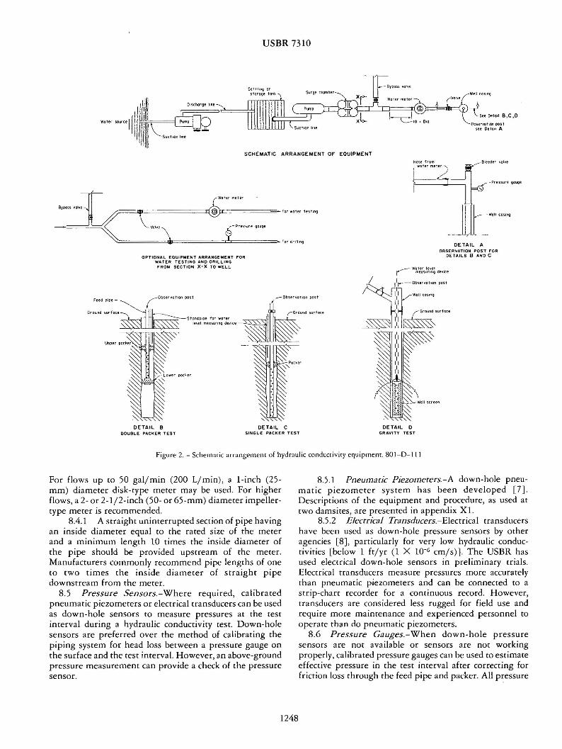
USBR 7310
- Byooss votve Surgechomber~
Wotermettr-
Observation oost see Detail A
SCHEMATIC ARRANGEMENT OF EQUIPMENT
(Water meter
~==it=======t(k=====- For wottr tes t ing middotWell cas1n9
Press1Jre gouge
-=====bull===========~-For drilling DETAIL A OBSERVATION POST FOR
OPTIONAL EQUIPMENT ARRANGEMENT FOR DETAILS 8 AND C
WATER TESTING ANO DRILLING FROM SECTION X-X TO WELL
DETAIL D GRAVITY TEST
DETAIL B DETAIL C DOUBLE PACKER TEST SINGLE PACKER TEST
Figure 2 - Schematic arrangement of hydraulic conductivity equipment 801-D-l I I
For flows up to 50 galmin (200 Lmin) a 1-inch (25- 851 Pneumatic Piezometers-A down-hole pneushymm) diameter disk-type meter may be used For higher matic piezomerer system has been developed [7] flows a 2- or 2-12-inch (50- or 65-mm) diameter impellershy Descriptions of the equipment and procedure as used ar type meter is recommended two damsites are presented in appendix XL
841 A straight uninterrupted section of pipe having 852 Electrical Transducers-Electrical transducers an inside diameter equal to the rated size of the meter have been used as down-hole pressure sensors by other and a minimum length 10 times the inside diameter of agencies [8) particularly for very low hydraulic conducshythe pipe should be provided upstream of the meter tivities [below 1 ftyr (1 X 10⁻⁶ cms)] The USBR has Manufacturers commonly recommend pipe lengths of one used electrical down-hole sensors in preliminary trials tO two times the inside diameter of straight pipe Electrical transducers measure pressures more accurately downstream from the meter than pneumatic piezometers and can be connected tO a
85 Pressure Sensors-Where required calibrated strip-chart recorder for a continuous record However pneumatic piezometers or electrical transducers can be used transducers are considered less rugged for field use and as down-hole sensors tO measure pressures at the rest require more maintenance and experienced personnel tO
interval during a hydraulic conductivity rest Down-hole operate than do pneumatic piezometers sensors are preferred over the method of calibrating the 86 Pressure Gauges-When down-hole pressure piping system for head loss between a pressure gauge on sensors are not available or sensors are not working the surface and the test interval However an above-ground properly calibrated pressure gauges can be used t0 estimate pressure measurement can provide a check of the pressure effective pressure in rhe rest interval after correcting for sensor friction loss through the feed pipe and packer All pressure
1248
USBR 7310
gauges used in water resting should be high-quality stainless steel glycerin or oil filled wich pressure indicated in both lbfin2 and kPa (such as manufactured by Marsh Instrument Company a unic of General Signal P 0 Box 1011 Skokie Illinois or equal) Pressure gauge ranges should be compatible wich middot cescing requirements chey should be sized so char che gauge capacity does not exceed two co three rimes che maximum desired pumping pressure for each respective pumping stage Gauges should have the smallest graduations possible and an accuracy of plusmn25 percent over che coral range of the gauge If a gauge saver is used wich che gauge calibration should be made wich the gauge saver in place Accuracy of che gauges should be checked before use and periodically during the resting program (see subpar 112 for additional information)
861 One or more pressure gauges should be located downstream of che flowmecer and downstream of any valves ac che cop of che feed pipe This location for pressure measurement can be used by inserting a sub (adaptor or shore piece of pipe) wirh che gauge - installed on che cop of rhe feed pipe
862 Ac least one additional calibrated replacement gauge should be available ar che resr sire
87 Swivel-During che hydraulic conductivity cesc ic is preferable co eliminate the swivel and use a direct connection co the feed pipe If a swivel muse be used in che water line during resting ic should be of che nonconscriccing type and calibrated for head loss Significant friction loss can result from use of che constricting type
88 Packers-One or two (straddle) packers are required for che rest Packers may be either bottom-set mechanical screw set mechanical pneumatic inflatable or liquid inflatable The pneumatic inflatable packer is the preferable type for general use and is usually che only one suitable for use in soft rock and soil The gland of this packer is longer and more flexible chan the ocher types and will form a tighter seal in an irregular drill hole A leather cup type of packer should noc be used To ensure a eight water seal che length of contact between each expanded packer and che drill hole wall should noc be less than three rimes the drill hole diameter
NOfE 2-More than one type of packer may be required to test the complete length of a drill hole The type of packer used depends upon many factors eg rock type drill hole roughness spacing and width of rock joints and test pressures
881 Inflatable Packers-Inflatable packers with an expansible gland and a floating head (see app fig Xl2) should be designed for anticipated drill hole diameters and pressure conditions For normal hydraulic conductivity cescing a reasonable maximum recommended working pressure inside and outside of che packer is 300 lbf in2
(2070 kPa) [8] Inside pressure should be increased in water-filled holes proportionally co che sracic head For drill holes wich sharp projections in the walls a wireshyreinforced packer gland having a higher working pressure [7] may be required The pressure in che packer should not be high enough to fracture the material being reseed
The pressure required to form a cighr seal ac che ends of a cesr interval depends on the flexibility of rhe gland the friction of the floating head and che drill hole roughness The minimum differential pressure between che packer and the cesc interval can be derermined by res ring packers in a pipe slighrly larger rhan rhe nominal diameter of rhe drill hole in order co simulate possible enlargement of rhe drill hole during drilling For a given resr interval pressure che packer pressure is increased until ir provides a waterrighc seal between the packer and the material with which ic is in contact The pressure in rhe packer should range approximately berween 30 and 300 lbfin2 (210 ro 2100 kPa) greater chan char in che cesc interval with 100 lbfin2 (690 kPa) being normal Pneumatic inflatable packers can be inflated with compressed air or compressed nitrogen
882 Special pneumatic packers are available for use in wireline drilling operations Because che packers must be able co pass through che wireline bit and then expand co completely seal che hole ac che cesc interval special materials are needed for che packer gland A special packer assembly-consisting of cwo packers in tandem-is used with the upper packer being expanded inside che drill rod just above che bic and che lower packer expanded against che wall of the hole just below che bit The two packers on the assembly can be positioned properly-relative co the bit-by a sec of lugs or a ring located on the assembly Special seals or connections are needed co attach che water supply co che wire-line drill pipe at the surface
883 A minimum of two secs of replacement packers andor spare glands should be available at the test sire
89 Perforated Pipe Sections-Lengths of perforated steel pipe corresponding ro the lengths of rest intervals are required between packers to admit water inco che rest intervals The coral area of all perforations should be greater than five rimes che inside cross-sectional area of che pipe These perforated pipe sections should be calibrated for head loss
810 Well Screen-Well screen or slotted pipe may be required for cescing in granular unstable materials chat require support [9] As a general rule the maximum size of sloe width should be approximately equal to che 50shypercent size of che particles around the drill hole (see subpar 114)
811 Water Level Measuring Device 8111 Although there are ocher types of water level
indicacors che electrical probe indicator is most commonly used Essentially ic consists of (1) a flexible insulated conduit marked in linear units and enclosing cwo wires each insulated except ac che tips (2) a low-voltage electrical source and (3) a light or ocher means of indicating a closed circuit which occurs when che rips contact che water surface Different brands of electric wacer level indicacors and even different models of the same brand ofren have their own unique operating characteristics Before using any electric water level indicacor it should first be reseed at the surface in a bucket of water
8112 For approximate measurements of the water level when ic is within about 100 feet (30 m) of the ground
1249
USBR 7310
surface a cloth tape with a popper can be used A popper can be made from a short pipe nipple (or length of tubing) by screwing a plug attached to a graduated tape intu one end of the nipple and leaving the other end of the nipple open When the popper is lowered in the drill hole and the open end of the pipe nipple strikes a water surface it makes a popping sound and the depth to water can be measured by the tape
8113 An accurate measuremenr of the water level can be made by chalking the lower end of the steel tape After contacting the water level the tape should be lowered about L more foot before retrieving it Measurement is then made to the wet line on the tape
812 Temperacuie Measuring Device-Equipment for measuring ground-water temperature is available from commercial sources or can be made from a thermistor two-conductor cable reel Wheatstone bridge and a lowshyvoltage electrical source A maximum-minimum type thermometer is acceptable
9 Regents and Materials
91 ~71ter (See subpars 72 73 and 74)-The clear water supply should be sufficient tO perform the hydraulic conductivity test without interrruption and to maintain the required pressure throughout the test period
92 Swd or Gravel Backfill-Where a granular backfill is used t0 prevent sloughing of the drill hole wall it should be a clean coarse sand or fine gravel Laboratory permeability tests (USBR 5600 or 5605) should be made on the backfill material to make sure that it has a coefficient of permeability greater than one order of magnitude higher than that expected of the in situ material being rested
10 Precautions
L01 Safety Precautions L011 This procedure may involve hazardous
materials operations and equipment lO l2 Use normal precautions for drilling [ 10 11] L013 Precautions should be taken during calibration
pressure testing of equipment particularly testing of packers with compressed air or nitrogen (never use oxygen) to avoid injuries from a sudden packer or hose rupture
L02 Technical Prernutions 102 l As a general rule total pressure (static head
plus gauge pressure) applied in the drill hole should nor exceed 1 lbfin2 per foot (226 kPam) of rock and soil overburden at the center of the test interval if the test interval is 10 feet (3 m) long or less If the rest interval exceeds 10 feet pressure should not exceed 1 lbfin 2 per foot of overburden at the top of the interval In layered or fractured material or for drill holes near steep abutments or slopes 05 lbf in2 per foot ( 113 kPa m) of material to the nearest free surface is an appropriate maximum pressure Higher pressures than these may fracture the materials
1022 If there is excessive or complete loss of water when the hole is being drilled drilling should be sropped before cuttings fill the voids and a hydraulic conductivity rest completed on a shorter than normal length rest interval
1023 Hydraulic conductivity rest equipment should be considered and treated as precision testing equipment Gauges thermometers ere should have their own protective cases they should not be carried with drill tools or be tossed around They should be calibrated frequently Ir is recommended that all test equipment needed for hydraulic conductivity resting be kept separate from drilling equipment
11 Calibration
111 For Measurment ofEffeaive Head 11 l l Pressure Sensurs-Calibrate down-hole
pressure sensors by the methods and at frequencies prescribed by USBR LOSO
ll12 Friction Loss Estimates-Where down-hole pressure sensors are nor used estimates of effective head at the rest interval are made by subtracting friction loss from the applied head measured at the ground surface The friction loss should be determined for all components of the piping system from the pressure gauge to the test interval
1112 I Calibrate friction loss in parts or sections of the piping systems including ( L) the swivel (if used) (2) feed pipe (per unit length) and (3) the packer assembly Record the data with references to the particular parts calibrated in tabular or graphical form so the accumulative friction loss can be totaled for determination of effective head at the test interval The calibration procedure is as follows
I l l211 Lay out the individual or joined parts to be calibrated on a horizontal surface with calibrated pressure gauges at each end
l L 12 12 Pump water through the system at incremental increasing flow rares to the maximum flow rare expected to be used in the test allow the flow to stabilize between incremental flows
L 112 L3 Record the pressure at each gauge for each incremental flow rate
11 l 2 L4 Calculate the friction head loss for each incremental flow rare
2f = 23 l ( p ~I p ) (I )
where f = friction head loss in feet of head per linear foot
of pipe ftft or mm P1 = upstream pressure bf in 2 or kPa P2 = downstream pressure lbfin2 or kPa d = pipe length fr or m (d = l for swivel or packer
assembly) 23 l = converts from pressure in bf in2 to head in feet
or 0102 converts from pressure in kPa to head in meters
Example assume
P1 = 186 lbfin2 or 128 kPa P2 = 132 lbfin2 or 910 kPa d = 100 ft or 305 m
1250
USBR 7310
Inch-pound application
f = 231 ( 18 ~~-~3 2) 125 ftfr
SI application
f = 0 102( 128
- 9 tO) = 124 mm 305
l l l215 Plot friction head loss versus flow rare Figure 3 is an example of a plot of friction head loss (f) at relatively low flow races for a 10-foor (33-m) length of 1-14-inch (32-mm) diameter pipe Since head loss in pipe at turbulent flow is approximately related to velocity squared a plot of friction head loss versus the square of the flow rate is nearly a straight line (see fig 4)
NOfE 3-There are srandard rabies and charcs which provide unit friction losses for various sizes of pipe elbows cees reducers ere for clean and ruscy conditions Although such informacion is sometimes used it is preferable to determine friction losses in che piping syscem and packers accually used for che hydraulic conductivity rest
111216 To calibrate a packer inflate the packer in a shore length of casing or pipe in which amiddotvalve and pressure gauge have been installed A pressure gauge is also installed in the rods immediately ahead of the packer assembly Pump water into the rods at incremental increases (or decreases) of flow rate-allowing the system to stabilize after each incremental change-until the highest anticipated flow rate is reached
NOfE 4-For packers smaller than N-size such as the B-size used in wireline equipmentmiddot there are significant head losses and relatively low flow races must be maintained This requires water meters and pressure gauges capable of accurately measuring the low flows and small changes in pressures
112 Pressure Gauges-Calibrate each pressure gauge (see USBR 1040) by comparing it with a test or master
FLOW RATE IN LITERS PER MINUTE
o
I _ I_ I I I II
I I I I I loI I I I I I rI
I I I )I
I I I I I v I I I I I I I I I I lr II
I I
I I I I 11deg II i j~ I I I -~-----1 -- I I I I i
JO deg HOW RATE IN GALLONS PEA MINOT[
Figure 3 - Head loss due ro friction at increasing flow rates for a I 0shy
foot (3-m) 1-14-inch (32-mm) diameter iron pipe
gauge The master gauge should not be used during drilling or hydraulic conductivity testing Calibrate each gauge at the start of a res ring program plus one additional calibration per week during rests of long duration
113 Flowmeters-Calibrate a flowmerer by flowing water into a container of known volume the container used for the volume check should be commensurate in size with the flowmeter size and graduations From these data flow rares can be calculated for comparison with meter readings All flowmeters should be calibrated to an accuracy of plusmn1 percent Calibration should be done at the stare of the resting program plus one additional calibration per week during rests of long duration
NOfE 5-Some impeller-type flowmeters have an accuracy range significantly less than indicated by the dial Minimum and maximum races should be esrablished
114 Well Screens and Perforated or Slotted Pipe Sections-From manufacturers dara or by calibration determine the head losses in expected flow ranges to ensure there is no restriction of flow into the material being tested
12 Conditioning
12 l Nor applicable special conditioning requirements are not needed for this procedure
13 Procedure
13l Cleaning ofDnll Hole 13l1 Remove any accumulation of fine particles
(smear mud cake compaction caused by driving casing etc) from the drill hole wall Such accumulation significantly restricts the flow of water into or from the hole Exercise good judgment in cleaning the hole since excess cleaning may be detrimental If there is a question as to whether or not drill holes in particular materials need cleaning hydraulic conductivity tests can be performed in holes with cleaning and others without cleaning If cleaning does not significantly change rest results at a sire cleaning of additional intervals in the same materials may not be necessary
131 l1 When the rest interval is above the water table it may be possible to brush or scratch the drill hole wall to break up accumulated fines For unstable materials which require use of a well screen materials which cavemiddot against the screen may break up the accumulation of fines on the wall Mild surging with a bailer while adding water also may help break up a disturbed or compacced zone but this may stir up fines which then plug the voids in the material co be rested Mild jetting-followed immediately by bailing or pumping-also is a possibility
13 l l2 When the test interval is below the water table-in materials chat are rock-like and self-supporcingshyuse of a water jet in the hole (preferably accompanied with pumping to induce flow into the borehole) is one of the best methods to clean the hole After jetting bail or pump the sediment-laden water from the rest interval Jetting can also be used through a screen below the water
1251
tJ
I I 0 GO-GI I GO-G2 0 GI -G2
~
I
I
v
v p-shy~ -shyl--~ L--shy
-shy
v
0
middot 005 =0 00005 100
-shy~--~ 0 middot 0025 =0 00005
I 50 I
~ --shy = 0 00005
50
I
t - A
v -
-
[] --shy shy--shy0 -
4--l_-E
-
16
-shy-shy-8 --shyl---shy~ - 2
~ ~---shy z 3 4 5 6 7 8 9
FLOW RATE SQUARED (q 2 )(10001
s of oalmin ) 2
Figu re 4 - Plot of feed p_ipe ca libra tion data - example
USBR 7310
2FLOW RATE SQUARED (q2)( 1000degs of L min)
10 15 20 25 - 30 35
50
40
r w w LL
z
~ 30 0 J Cl ltgt w I
z 0 20 r S a LL
10
0
cable in unstable materials For soft rock flushing che sides of che drill hole by running che bit or a bailer up and down the hole may enlarge the hole by erosion or ocherwise change the characceriscics of the fracture systems
13113 Finally clean the drill hole by pumping or bailing water from the bottom upward with the pumping continued until the return fluid is clear without cuttings or sediment Record the method used in cleaning the hole on the log of drill ho le or on a special testing form
132 Length of Test Interval 1321 The length of the test interval depends on
(1) purpose of the test (2) stratigraphic interval and (3) flow rate Where materials are relatively uniform use a test interval of about 10 feet (3 m) Where flow rates are high shorten the test interval co locate high flow race zones where races are very low the interval may be lengthened if desired
133 Ground-Water Level Determination 13 31 Depth co ground-water level muse be
determined before calculating hydraulic conductivity Measure depths to water levels with an electrical probe or o ther suitable equipment (see subpar 811)
1332 Auger Holes-ln power auger or other types of holes to which water is not added as pare of the drilling process report the presence or absence of a water level depth to water level and dace of initial and final water level measurement In materials of low hydraulic
14
12Cll a w r w
101 z () Vgt 0
8 J
Cl ltgt w I
Sz 0 r u a
4 IL
conduccivicy several days to several weeks may be required for a water level to stabilize in the hole Report evidence of moisture in the cuttings and if a perched water level was observed
1333 Rotary or Cable Tool Holes-For drill holes in which addition of water to the hole is an integral part of the drilling process
13331 Bail or pump the hole dry or to a stable wa ter level at the close of the last shift each day and record level
13332 Report the presence or absence of water and depth to water at the beginning of the first shift each day Additional readings are desirable whenever water level in the hole has nor been disturbed for an appreciable period of time
13333 Report changes in water level detected as the hole is drilled deeper Record faccors that affect the water level such as depth of casing andor cemented intervals These data may be helpful in recognizing perched or confined (artesian) conditions
13334 Upon completion of the hole the water must be bailed down to the extent practicable the water level measured and the dace recorded of hole completion Measure the water level for a period of days or weeks until equilibrium is reached
NOfE 6-At times exceptions must be made to the requirement for conrinuation of water level readings Such is the case when
1252
USBR 7310
state or local laws require chat the hole be filled continuousiy from bottom to cop immediately upon hole completion and before the drill crew leaves the sire In ocher instances landowners may allow right-of-entry for only a limited time for measurements
1334 Perched and Artesian Aquifers-lc is imporshytant tO recognize perched and artesian aquifers especially those under sufficient pressure tO raise the water level above the confining layer but nor tO the ground surface (see (5 ]) They must be distinguished from water table aquifers (those which continue in depth) If perched water table or artesian aquifers-separated by dry or less permeable strata-are encountered in the same drill hole the resulting water level in the hole is a composite therefore conclusions and interpretations based on such data are misleading If a perched water table is recognized (or suspected) during drilling water levels must be determined for each zone for calculation of hydraulic conductivity This might require completion of the drill hole with a watertight seal set at a suitable horizon tO
separate two water table conditions In this type installarion two strings of pipe or conduit are required one extending down to the portion of the hole immediately above the packer and a second string extending through the packer to a point near the bottom of the hole Water-level measurements provide the basis for determining a perched condition or if the lower water table is under artesian pressure
13 35 Mulriple Water-Level Measurements-In some instances it is desirable tO install multiple conduits and packers or plugs in a drill hole so that ground-water levels (or pressure heads) in several water-bearing horizons can be measured over an extended period of time (see [5] pp 7-14)
134 Pressure Tests With Packers 134 l The recommended arrangement of typical
equipment for packer pressure tests without a pressure sensor is shown on figure 2 (See app fig Xl l for equipment with a pressure sensor) Beginning at the source of warer the general arrangement is clean water source suction line pump discharge line tO srorage andor settling tank suction line water-supply pump surge chamber line ro bypass valve junction water meter gate or plug valve tee with sub for pressure gauge short length of pipe on which the pressure gauge is attached tee and off-line bleeder valve for evaluating back andor holding pressure flexible 1-14-inch (32-mm) diameter hose and 1-14shyinch-diameter feed pipe ro packer or packers in drill hole which isolate the rest interval All connections should be tight and as short and straight as possible with minimum change in diameter of hose and pipe Friction loss decreases as the pipe diameter is increased
1342 When the material is subject co caving and casing andor grout is needed to support the walls of the drill hole the hole should be water rested as it is advanced Other hole conditions may make this procedure desirable or necessary The following procedure is commonly used
1342 l After the hole has been drilled to the top of the interval to be tested it may be desirable tO remove
the drill string from rhe hole and advance casing or grout ro rhe bonom of the hole
13422 Advance the hole 5 to lO feet ( 15 to 3 m) into the material to be rested
13423 Remove the drill string from rhe hole 13424 Clean the interval to be tested and record
the depth tO the warer table if present If a composite water level is suspected the warer level affecting rhe rest should be determined by measurements through the feed pipe after rhe packer has been seated and the water level has stabilized
13425 If rhe hole will stand open sear a single packer ar the top of rhe test interval Record the type of packer irs depth and packer pressure if it is rhe inflatable type
13426 Pump water into the interval ar a rate to develop a suitable pressure The pressure to be used depends upon testing depths and ground water levels or pressures Materials subject to deformation or heaving such as by separation of bedding planes or joints or materials at shallow depths must nor be subjecred to high pressures (see subpar 102 l ) For comparison of flow rates in different pares of a single foundation and with results from other foundations some of the following pressures are commonly used 25 50 75 and LOO lbfin 2 (170 350 520 and 690 kPa)
NorE 7-At test pressures less than 25 lbfin2 errors in measurement of pressure and volume of water may increase unless special low pressure gauges are used Gravity tests provide more accurate results under these conditions At pressures higher than 10 lbfin2 difficulties in securing a right packer seal and the likelihood of leakage increase rapidly However under artesian pressures or in deep holes the water pressure-as registered on a surface gauge-will need to be sufficient to overcome the effeccive head at the test interval and firmly seal the packer
NillE 8-Where the hole is subject to caving a pump-down wire-line system has been developed rhar can be used to eliminate removal of the drill string from the hole With this system the hole is drilled to the bottom of the interval tO be tested and the drill rod is raised so the end of the rod is at the top of the test interval The tandem packer (see subpar 882) is then lowered through the drill rod and expanded to seal both inside the rod and against the wall of the hole at the cop of the test interval Models of this equipment are available which have transducers below the packer for measuring water pressures at the test interval
13427 For determining effective head artesian heads encountered in the drill hole are treated the same as water table conditions ie the depth from the pressure gauge or the water level maintained during the test to
the stabilized water level is used as the gravity head If the artesian head stabilizes above the ground surface the gravity component of the effective head is negative and is measured between rhe stabilized level and the pressure gauge height If a flow-type rest is used the effective head is the difference between rhe stabilized water level and rhe level maintained during the flow period
1253
USBR 7310
13428 Afrer pressures are selected based on ground-water conditions and the purpose of the test perform a test at each pressure Usually a 5-cycle procedure is used three increas ing steps to the maximum pressure and then two decreasing steps to the starting pressure This cycling allows a more derailed evaluation of rest results than testing at a single pressure and commonly allows extrapolation to ascertain at what pressures the following may occur (1) laminar flow (2) turbulent flow (3) dilation of fractures ( 4) washouts (5) void filling or (6) hydraulic fracturing However the equations normally used to ca lculate hydraulic conductivity are based on laminar flow conditions
NOfE 9-ln some insrances on ly a single water pressure test at a given interval in the drill ho le may be required For example if geologic conditions are known and there is no need ro perform the seeps in subparagraphs 13422 through 13426 a single value of hydraulic conductivity with a relatively low application of pressure may suffice
13429 During each test continue pumping water to the test interval at the required pressure until the flow rate becomes stable As a general guide maintain flow rares during three or more 5-minute intervals during which l-minute readings of flow are made and recorded In tests above the water table water should be applied to the test interval until the flow rate stabilizes before starting the 5-minuce measurement intervals Where tests are below the water table flow rates usually stabilize faster than for the tests above the water table and the time period before the 5-minure test intervals may be shorter These rime periods may need to be varied particularly when rests to determine grouting requirements are made
134210 Determine and record the presence of back pressure and decay of holding pressure Afrer the rest deflate the packer and remove it from the drill hole
134211 Advance the drill hole and if necessary the casing repeat the procedure in subparagraphs 13423 through 134210 until the required depth of drill hole is reached When casing is used in a drill hole always set the packer in the material below the casing
1343 If the hole will stay open without casing it can be drilled to final depth and after cleaning the hole hydraulic conductivity rests can be performed from the bottom of the hole upward using straddle (double) packers Although a single packer can be used to test the bottom interval of the hole starting at the bottom with double packers will cause loss of borehole testing of only about the length of the bottom packer and will save one complete trip in and out of the hole with the drill string assembly co change the packers After the test for the bottom interval is completed straddle packers are used for successive test intervals up the drill hole See subparagraph 1342 where caving or other hole conditions will not allow this procedure
135 Gra vity Tests 135 1 Constant-head gravity tests are usually
performed without packers above or below the water table with drill holes of N-size or larger (see fig 2 derail D)
This type of test is often made in reasonably stable-walled drill ho les up to 25 feet (76 m) depth where water pressure at the test interval needs to be kept low The test is usually performed in successive 5- or 10-foot (l5- or 3-m) intervals as the drill hole is advanced The upper end of each test interval is normally determined by the bottom depth of tightly reamed or driven casing If the casing is not believed
middotto be tight appropriate entries should be recorded on the log form If the wall of the drill hole is stable the test can be performed in the unsupported hole If the wall needs to be supported use a well screen (see subpar 114 for calibration) inserted through the casing It may be necessary to ream or drive the casing to the bottom of the interval set the screen and then pull back the casing to expose the screen Afrer the test the screen is removed and the casing reamed or driven to the bottom of the hole
NOfE lO-Clean coarse sa nd or fine gravel backfill (see subpar 92) may be used instead of a well scree n Ream or drive rhe casing ro the borrom of the inrerval dean ir our and add rhe backfill as rhe rnsing is pulled back ro expose rhe resr interva l Record use of rhis procedure on the log form
l 35l l If the drill hole is self-supporting clean and prepare it in rhe normal n1anner (see subpar 13l)
l35 l2 If the drill hole is not self-supporting lower the well screen and casing into the hole
135 l3 For test intervals above the water table maintain a constant head of water _within 02 foot (60 mm)] at the top of the test interval by injecting water through a small diameter rube extending below the water level maintained during the test For rest intervals below the water table or influenced by artesian conditions maintain a constant head a short distance above the measured static water level
Monitor the water level with a water-level indicato r If the water-level indicator is inserted in a small diameter pipe in the casing the wave or ripple action on the water surface will be dampened and permit more accurate watershylevel measurements
NOfE l l-When rhe flow rare is very low rhe consranr wa rer level c1n be maintained by pouring warer in rhe hole from a graduated container
135 l4 Record the flow rate at wne intervals until a constanc flow rare is reached
135 l5 Repeat the procedure of subparagraphs 135 l3 and 135 14 at one or more different water levels
13516 This rest is essentially the same as desigshynation USBR 7300 (see also L3] p 74) the instructions in USBR 7300 for performing the rest and calculating hydraulic conductivity apply to this procedure also
14 Calculations
14 l For pressure or constant gravity head hydraulic conductivity rests calculace the hydraulic conductivity of
1254
USBR 7310
rhe soil or rock by rhe following equation (expressed m consisrent unirs) [4]
k = ~ In ~ where L ~ lOr (2)
or
k = ~ sinh-1 r where lOr~ L ~ r (3)
where k = hydraulic conducrivity fryr or cms q = consrant race of flow into che rest interval
ft3yr or cm3s L = length of the test interval ft or cm
H = differential head of wacer ac rest interval fr or cm
r= radius of the borehole ft or cm In= natural logarithm loge
inv~rse hyperbolic sin~ smh- 1 x In (x + -yx2 + 1)
142 An example calculation for a single packer test _ in the botrom of a borehole belovt the wacer table follows
Example assume
r = 18 in or 015 ft= 46 cm q - 22 galmin or 83 Lmin q = 15 X 10 ft3yr = 140 cm3s L 30 ft = 91 cm
Hg gravity = disrance from ground-water level co pressure gauge = 102 ft = 311 cm
Hp pressure 5 lbf in2 X 231 ftwater (lbf in2)
116 ft = 3 54 cm of water H = Hg+ Hp= 218 ft= 664 cm
~ = ~lo = 20 hence use equation (2) 5 k = _9_ In]
2rrLH r k = 15 X 10 ft3 yr In 30 ft
2rr (30 ft) 218 ft 015 ft k = 11X103 ftyr = 11 X lQ-3 cms
NafE 12-These equations are most applicable and reliable where the length of test interval is at lease 5 r and the interval is below che water table The equations are based on laminar flow of fluid through porous media Flow races high enough co cause turbulent flow invalidate the results in all types of material In fractured material the calculated value should be considered an apparent hydraulic conductivity even under laminar flow conditions
143 For pressure resrs when rhe resr interval is below the water table H is the distance from rhe water table to the elevation of che pressure gauge plus applied pressure converted to linear units of water head
Where the rest interval is above the water table His rhe distance from rhe midpoint of the isolated rest interval to che elevation of the pressure gauge plus the applied pressure converted to linear units of water head
For gravity rests above che water table H is che distance between che boccom of the tesc interval and che water level maintained during the test
For gravity rests below the water cable His che distance between the pretest stabilized wacer level in the drill hole and the water level maintained during the rest
144 If chere is artesian pressure an additional pressure muse be applied to overcome che artesian pressure co provide an effective rest pressure For example if there is an artesian pressure of 5 lbfin2 (34 kPa) ac che pressure gauge 15 lbfin2 (103 kPa) could be applied chen che effecrive pressure would be 15 lbfin2 minus 5 lbfin2 which equals 10 lbfin2 (69 kPa)
145 The calculations can be done conveniently by (1) a nomograph [12] (2) a hand calculator with che proper functions or (3) a com purer For repeared tests ic is convenient to prepare a table for one or more diameter drill holes and lengths of resc intervals and combine che terms on che right side of the equations other than q and H into a coefficient
NafE 13-The lugeon (lugeon unit lugeon coefficient) [ 13 14 15 16] has been used as an index of hydraulic conductivity in connection with cyclic rests and for grouting purposes
15 Report
151 Record field test data on a daily driller s report and or on rhe log of the drill hole or on a special reporting form designed for the specific project Record the following
1511 Log of the drill hole 1512 Elevations of the ground surface the water
cable and che top and bortom of the rest interval 1513 Diameter of the drill hole at test interval 1514 Method of cleaning the drill hole 1515 Size of the feed pipe and any well screen 1516 Water pressure andor gravity head and flow
rare for each rime interval 1517 Tora[ amount of warer used per resr 1518 Average temperature of ground warer and
water used in the rest 1519 Packer inflation pressures 1511 Capacity of pump supplying water to the
rest interval 15111 All head loss calibrarion dara 15112 Nore any comments considered necessary to
help evaluate che rest results
15 References
[ l] Permeability Tests Using Drill Holes and Wells Bureau of Reclamation Geology Report No G-97 Denver ColoradoJanuary 3 1951
[2] Ground Warer Manual lst ed rev reprint Bureau of Reclamation US Government Printing Office Washington DC 1981
1255
USBR 7310
[3] Drainage Manual lsc ed 2d princ Bureau of Reclamacion U S Governmenc Princing Office Washingcon DC 1981 1984
[4] Zangar Carl N Theory and Problems of Water Percolation Engineering Monograph No 8 Bureau of Reclamation Denver Colorado 1953
[5] Drill Hole Water Tests Technical lnstructionsshyProvisional Engineering Geology Bureau of Reclamation July 1970 (unpublished)
[6] Glossary of Geology 2d ed American Geological lnscitute Falls Church Virginia 1980
[7] Haccher R C High Pressure Inflacable Packer with Pneumatic Piezometer Bureau of Reclamation Reporc GR-10-75 Denver Colorado October 1975
[8] Bennett R D and R F Anderson New Pressure Test for Determining Coefficient of Permeability of Rock Masses Technical Reporc GL-82-3 US Army Engineer Waterways Experiment Station Vicksburg Mississippi 1982
[9] Ground Water and Wells A Reference Book for the Water-well Industry 1st ed published by Edward E Johnson Inc Saint Paul Minnesota 1966
[10] Drillers Safety Manual 1st ed reprint Bureau of Reclamation Denver Colorado 1982
[11] Acker W L III Basic Procedures for Soil Sampling and Core Drilling published by the Acker Drilling Company Scranton Pennsylvania 1974
[12] Underground Mining Methods Handbook No 580 W-88 Society of Mining Engineers Littlecon Colorado p 62 1982
[13] Lugeon M Barrages et Geologie Dunod Paris 1933
[14] Houlsby A C Routine Interpretation of the Lugeon Water-Test Quarterly Journal Engineering Geology vol 9 pp 303-313 1976
[15] Heitfeld K H and L Krapp The Problem of Water Permeability in Dam Geology Bull International Association of Engineering Geology No 23 pp 79-83 1981
[16] Pearson R and M S Money Improvements in the Lugeon or Packer Permeability Test Quarcerly Journal Engineering Geology vol 10 the Netherlands pp 221shy239 1977
1256
USBR 7310
APPENDIX
XL PROCEDURE USING A PNEUMATIC PIEZOMETER WITH TWO PACKERS ISOLATING THE TEST INTERVAL
Xl l Equipment Assembly (Refer to figs Xll and X l2) -A complete straddle packer unit is assembled as follows
X 11 l Co nnect a predetermined length of perforated injection (feed) pipe to the lower packer (The length of perforated pipe is determined by the thickness of the zone to be rested) Connect the inflation tubing to the lower packer and lower the sliding head end of the packer into the drill hole (See subpar l l l216 for calibration of packers)
Xl l2 Clamp the top of the perforated injection pipe at the hole collar and connecr the upper packer with the sliding head already down the hole
Xl l3 Provide approximately 12 inches (300 mm) of slack in the inflation tubing between the two packers to allow for retraction of the upper packer sliding head Connecr the tubing to the upper packer
Xl l4 Install the pneumatic piezometer piezomerer tubing packer inflation tubing and sealed lengths of injecrion pipe to the head adaptor
X ll5 Lower the entire unit into the drill hole adding lengths of sealed injection pipe as necessary to reach the
( Storoqf Settling ton
interval to be tested As the unit 1s lowered che packer inflation cubing and che piezomecer tubing is unreeled into che hole and caped to che sealed injection pipe at approximately 10-fooc intervals
Xll6 Upon reaching the rest depth lock both the inflation cubing reel and rhe piezomecer cubing reel connecr the inflation tubing by quick-connecr couplings co a nitrogen or compressed air boccie equipped with a high pressure regulator connecr the piezomecer cubing by quick-connect couplings co the readout box and connect the injection pipe co the water pressure source The cesc is now ready to begin
Xl2 Test Procedure
X 12 l After the unit has been lowered to the rest interval and before infacing the packers any water head above the cesc interval must be determined This head will sho w as pressure on the pneumatic piezomecer gauge and can be verified by running a water level indicator into che hole to measure the deprh co the water cable The piezometer will register water pressure chat can be converted to head of water This water head should be
Compressed 01r or nitrogen bot tie Regulator_
Poc~er air lin e- I
P1nometer ln1ec t1on oioe head adaptor
Lo er ooc~er inflation tubmr
Figure X 1 1 - Schematic arrongemem of drill hole packer and pressure monimring equipment 801-0-180
1257
USBR 7310
------=--From compressed air or nitrogen boltle
From piezometer
_To
PRESSURE READOUT BOX
Packer inflation tubing From wafer source From air or Water injection pipe ring seals
PIEZOMETER TUBING REEL
Pressure seals Wire reinforced rubber gland clomps
nitrogen ~~i==-=~==t~f=lil~~~jii~9ll~~~~~sect9ll~sect~sectsect~~~sectl~iilf~f--- To per for o t e d ~~~ze=zzzoCzzzze=zzze=plusmnzz~EZio~~~~21p~
To pressuresource~~~~~~~~~~~~~~~readout box
Piezometer
~~~~~~~~~~~~~~~~---
Inflation chamber Floating packer head Packer inflation lubing
UPPER DRILL HOLE PACKER AND PRESSURE MONITORING EQUIPMENT FOR N X HOLE
Figure X 12 - Upper Jrill hole packer anJ pressure monitoring equipment for NX hole
used to determine the minimum inflation pressure to be applied co the packers by the following equation
SH+ PP+ PE = minimum inflation pressure
where SH = static pressure at the midpoint elevation of the
test interval lbf in2 or kPa PP = gauge pressure to be maintained during the test
lbfin2 or kPa PE = pressure needed to expand packer to hole
diameter as determined before insertion in the drill hole by expanding the packer in a length of pipe having a diameter similar to the hole diameter lbfin 2 or kPa
Inflation pressure gauge is in units of lbf in2 (kPa) The static water level measured before the packers are
inflated might be a composite water level (see subpar 1334)
Xl22 Inflate the packers and determine water head for the rest interval This is the static head to be used for calculation of hydraulic conductivity If rhe static head is significantly different from the composite measured
before the packers were inflated recalculation of packer inflation pressure may be required The final packer inflation pressure should be the lowest practical pressure to seal the test interval against the maximum injection pressure to avoid fracturing of the material being tested
Xl2 3 After the inflation pressures have been determined deflate the packers fill and flush the system with water until all entrapped air has been removed This is accomplished by filling the injection pipe under a gravity head and leaving the air-release valve open ar the top of the injection pipe tee at an elevation higher than the injection hose The valve must remain open until all air has been removed and water runs freely indicating a filled system At this point water is flowing around the deflated packer system and is completely filling the annulus between the drillhole and the packers In the case of an interval with a high injection rate it may be necessary to keep the air valve closed to keep from entraining air into the test interval
X 124 Close the air release valve at the top of the injection pipe and slowly inflate the packers to the predetermined inflation pressure
Xl2 5 Lock in the inflation pressure by closing the pressure valve in the packer cubing If the pressure gauge
1258
USBR 7310
on the closed system remains steady it verifies a sealed system At this point water injecced under gravity head approaches a constant flow rate
X 126 Record the piezometer pressure after packer inflation For an interval of very low injection rate this is equal to che height of the injeccion standpipe plus che pressure recorded at the hole collar gauge For a test interval with a high injection rate the readout would show the same value less any friction from water flow through the injeccion pipe
X 127 Proceed with the test by applying the selected pressures ac the test interval and moniroring the flow rate and pressure on the pneumatic piezometer
X 128 To accurately compute hydraulic conduetivity rhe down-hole pressure muse remain constant A zone with a high injection rate must be monirored more closely than a zone with a small injection rate and adjustments made to hold the down-hole pressure constant To accomplish
this che injeccion pressure shown on che collar gauge must be adjusted in order co maintain che down-hole pressure constant
NOfE X 1-For example a pressure srage is scarred with the collar gauge reading 35 lbfin2 (241 kPa) and the down-hole piezomerer reading 200 lbf in2 ( 1380 kPa) As rhe flow increases rhe down -hole pressure may drop to 150 lbfin2 (1034 kPa) because fricrion loss in the injection pipe and the collar gauge would have to be adjusted to bring the down-hole pressure gauge back up co 200 lbfin2bull When the flow decreases from a fast to a slow rare the collar gauge pressure would have to be decreased
Xl29 The cesc is completed following one or more stages of pressure increases and pressure decreases Following the last stage deflate the packers and close the injection line The system is now ready to move to the next test interval for repetition of this procedure
1259
Methods Note
A Computer Program for Flow-Log Analysis of Single Holes (FLASH) by Frederick D Day-Lewis1 Carole D Johnson2 Frederick L Paillet3 and Keith J Halford4
Abstract A new computer program FLASH (Flow-Log Analysis of Single Holes) is presented for the analysis of
borehole vertical flow logs The code is based on an analytical solution for steady-state multilayer radial flow to a borehole The code includes options for (1) discrete fractures and (2) multilayer aquifers Given vertical flow profiles collected under both ambient and stressed (pumping or injection) conditions the user can estimate fracture (or layer) transmissivities and far-field hydraulic heads FLASH is coded in Microsoft Excel5 with Visual Basic for Applications routines The code supports manual and automated model calibration
Introduction Flowmeters provide means to infer the flow into or
out of boreholes connected to transmissive aquifer units or fractures In the past the relative inaccuracy and difficult operating procedures for spinner flowmeters limited the use of borehole flow measurements With the advent of heat-pulse (Paillet et al 1996) and electromagnetic (Molz et al 1994) instruments measurements of vertical flow as small as 005 Lmin became practicable and borehole flowmeter logging is becoming routine New modeling and analysis tools are needed to achieve the full potential of these measurements
1Corresponding author US Geological Survey Office of Groundwater Branch of Geophysics 11 Sherman Place Unit 5015 Storrs CT 06269 (860) 487-7402 ext 21 fax (860) 487-8802 daylewisusgsgov
2US Geological Survey Office of Groundwater Branch of Geophysics 11 Sherman Place Unit 5015 Storrs CT 06269
3Office of Groundwater Branch of Geophysics (Emeritus) US Geological Survey 11 Sherman Place Unit 5015 Storrs CT 06269
4US Geological Survey Nevada Water Science Center 2730 N Deer Run Rd Carson City NV 89703
5Any use of trade product or firm names is for descriptive purposes only and does not imply endorsement by the US government
Received April 2010 accepted December 2010 copy 2011 The Author(s) Ground Water copy 2011 National Ground Water Association doi 101111j1745-6584201100798x
Calibration of a borehole flow model to flowmeter data can produce estimates of transmissivity and heads for one or more flow zones (aquifer layers or fractures) Here we briefly review approaches for analysis of flowmeter logs and introduce a new computer program which supports manual and automated calibration of an analytical borehole flow model
Approach Single-hole flowmeter data can be analyzed to
estimate transmissivity profiles along boreholes and characterize aquifer compartmentalization (Molz et al 1989 Kabala 1994 Paillet 1998) Analysis of single-hole flowmeter data is commonly based on the Thiem Equation (Thiem 1906) which written for confined radial flow from a single flow zone (ie aquifer layer or fracture) to a screened or open well is
2πTi(hw minus hi)Qi = minus (1)
ln(r0rw)
where Qi is the volumetric flow into the well from flow zone i [L3Tminus1] hw and hi are respectively the hydraulic head [L] at the radius of the well rw and at radial distance r0 commonly taken as the radius of influence where heads do not change as a result of pumping in which
926 Vol 49 No 6ndashGROUND WATERndashNovember-December 2011 (pages 926ndash931) NGWAorg
case hi is the connected far-field head for zone i and Ti
is the transmissivity of flow zone i [L2Tminus1] A number of approaches to flowmeter analysis have
been proposed and demonstrated for different sets of assumptions (eg no ambient flow in boreholes) and data requirements (eg flow profiles collected under both ambient and stressed conditions) based either on Equation 1 (Molz et al 1989) or quasi-steady flow approximations (Paillet 1998) We refer the interested reader to Williams et al (2008) for additional background on flowmeter logs and focus the following discussion on the approach of Paillet (1998 2001) which is adapted here
Paillet (1998) formulated flowmeter log analysis as a model-calibration procedure involving flow profiles collected under both ambient and stressed (pumping or injection) conditions Consideration of the two conditions allows for the estimation of the transmissivities and also far-field heads of flow zones The latter is critical for the interpretation of water samples from wells that intersect multiple fractures or layers with different hydraulic head (Johnson et al 2005) Applying Equation 1 to an ambient condition (condition a) and a stressed condition (condition s) gives
factorT total(ha minus h02πTi )w iQa = minus (2)i ln(r0rw) factorT total(hs minus h02πTi )w iQs = minus (3)i ln(r0rw)
where T factor i is the fraction of the boreholersquos transmisshy
sivity contributed by flow zone i [ndash] T total is the total transmissivity of the flow zones intersected by the bore-hole [L2Tminus1] ha hs are the ambient and stressed water w w levels in the well respectively [L] h0 is the far-field head i in flow zone i [L]
For both ambient and stressed conditions the water level in the borehole is assumed to be constant in
time and the water level in the far-field of each zone is assumed to be the natural condition that is hi
0 In a field experiment (Figure 1) rw would be known and the flow rates and water levels in the well would be measured Radius of influence can be inferred experimentally based on head data at observation wells in which case r0 can be constrained during calibration or else it can be approximated (Bear 1979 306) Estimates of transmissivity are not strongly sensitive to the value assumed for r0 because it appears inside the logarithm in Equations 2 and 3 For example a change in r0rw
from 10 to 100 yields a change in the estimated Ti of only a factor of 2 and order-of-magnitude estimates of transmissivity are acceptable for many problems In cases where knowledge of r0 is unavailable but the boreholersquos total transmissivity is known from specific-capacity or slug-test results it is possible to estimate r0 in the calibration procedure We note that the forward model (Equations 2 and 3) produces twice as many independent equations as there are flow zones with an additional equation requiring T factor values to sum to 1 The number of parameters being estimated is twice the number of flow zones (T factor and h0 for all i) plus one parameter for either i i T total 0or r i
Model calibration involves changing the model parameters such that the flows predicted by Equations 2 and 3 match the interpreted flow profiles Following Paillet (1998 2001) calibration is to the interpreted profile and not individual data This formulation allows the user to incorporate additional insight (eg from other logs) to identify the number and locations of flow zones and elimshyinates the need for weighting measurements differently according to variable measurement errors and the spatial distribution of measurements along the borehole
Calibration can be implemented by manual trial-andshyerror or automated using nonlinear regression Whether manual or automated the goal for calibration is to identify the set of parameters that minimize a measure
Figure 1 Schematic of flowmeter experiment in a fractured-rock aquifer with (a) flow-log profiles for ambient (blue) and stressed (dashed red) conditions and conceptual cross sections of flow system for (b) ambient condition and (c) stressed condition In this example two flow zones (fractures) intersect a well Under ambient conditions flow enters the well from fracture 1 and exits from fracture 3 Under pumping conditions flow enters the well from fractures 1 and 2 The far-field head of zone 2 is equal to the ambient water level thus there is no flow tofrom zone 2 under ambient conditions The far-field head of zone 3 is equal to the stressed water level thus there is no flow tofrom zone 3 under pumping conditions
NGWAorg FD Day-Lewis et al GROUND WATER 49 no 6 926ndash931 927
of combined data misfit and model misfit Considerashytion of model misfit criteria commonly referred to as regularization is useful when multiple models can match the data equally well or within measurement errors Here the data misfit is formulated based on squared differshyences between the predicted and interpreted flow profiles such that multiple measurements may be collected in a single borehole interval The model misfit could be forshymulated in different ways but we use criteria based on the differences between the water level in the borehole under ambient conditions and the far-field heads Thus the objective function F consists of two terms (1) the mean squared error (MSE) between interpreted and preshydicted flow profiles with equal weights for all cumulative flows (ambient and stressed) and (2) the sum of squared differences (h) between the boreholersquos water level and far-field heads
n1 2ssim sintmin F = Q minus Qi i n
i=1
n asim aint 2+
Q minus Q
2 + α (hi) (4)i i i=1
subject to constraints
factor factorT ge T for all i andi min
ABS(haw minus h0
i ) le hmax for all i
aintwhere Qi Qi sint are the interpreted flow profiles (ie
cumulative flow above zones) for zone i under ambishyasiment and stressed conditions respectively [L3Tminus1] Qi
ssimQi are the simulated flow profiles (ie cumulative flow above zones) for zone i under ambient and stressed conditions respectively [L3Tminus1] α weights the regushylarization relative to the data misfit [L4Tminus2] T factor ismin
T factorthe user-specified minimum for any flow zone which can ensure nonnegative T factor hmax is the user-specified maximum absolute difference between the ambishyent water level and the far-field head of any flow zone and n is the number of flow zones
Without regularization F reduces to the MSE between simulated and interpreted flows The trade-off parameter α is set by the user with larger values more strongly penalizing large head differences Commonly small α values (less than 0001) are sufficient to obtain good results In selecting α the user should be guided by the goal of regularization which is to identify the ldquosimplestrdquo explanation of the data while minimizing the data misfit
Using FLASH FLASH (Flow-Log Analysis of Single Holes) is writshy
ten in Excel with Visual Basic for Applications (VBA) The spreadsheet includes a toggle (INPUTS worksheet cell A20) to choose between analysis for (1) fractures or fracture zones that intersect a well at discrete locations
and (2) aquifer layers in porous media The first is indishycated for cases where flow profiles are characterized by step increasesdecreases and the second for cases where flow profiles show approximately linear change over each layer Up to 10 fractures or layers can be modeled
The FLASH spreadsheet includes four worksheets INTRODUCTION INPUTS FIELD_DATA and PLOTshyTING INTRODUCTION provides information about the program and input parameters On the INPUTS workshysheet the user enters information about the flow zones transmissivities and heads Note that the user must intershypret flow profiles from the flowmeter data for both the ambient and stressed conditions The flow measurements are entered in FIELD_DATA and the interpreted proshyfiles are entered in INPUTS The interpreted profiles plot as dashed lines the data as points and the simulated proshyfiles as solid lines (Figure 2) Line and marker styles can be modified using standard Excel tools Flows are positive upward and negative downward PLOTTING is used by the program and does not require the userrsquos attention
In the INPUTS worksheet input parameters are entered in the cells with light blue and bright aquamarine backgrounds The former include specifications of the experiment setup (eg borehole diameter and water level) and the latter include calibration parameters Manual calibration is performed by adjusting the values of
ldquoT factorrdquothe cells and ldquohrdquo which are respectively T factor and the difference between the flow zonersquos far-i field head and the ambient water level in the borehole As parameters are adjusted the simulated flow profiles update automatically thus guiding the user toward best-fit parameters The MSE between simulated and observed flows is calculated in cell B36 on the INPUTS worksheet
Although the principle calibration parameters are Ti
factor and h the radius of influence r0 and total transshymissivity T total also are possible calibration parameters as explained above and indicated by aquamarine highshylighting By inspection of Equations 2 and 3 it is not possible to estimate unique values for both radius of influshyence and total transmissivity but only the ratio of total transmissivity divided by ln(r0rw) In general the user will have more information about total transmissivity than radius of influence Total transmissivity is estimated readshyily using an open-hole slug test or specific-capacity test Indeed the drawdown and pumping rate under stressed conditions could serve as data to estimate a total transshymissivity for the borehole In rare cases however the estimated total transmissivity may be considered unrelishyable for example in the presence of ambiguous slug-test data or discrepancy between the volumes over which the slug test and flowmeter analysis measure In such cases it may be useful to allow the T factor values to sum to a value other than 1 FLASH assumes a uniform radius of influence for all flow zones In reality the effective radius of influence may vary between zones according to their transmissivities and distances to boundaries Data to supshyport variable radius of influence however is commonly unavailable furthermore transmissivity estimates are not
928 FD Day-Lewis et al GROUND WATER 49 no 6 926ndash931 NGWAorg
Figure 2 The INPUTS worksheet after execution of the Solver with options ldquoEstimate ROIrdquo and ldquoSolve with regularizationrdquo for example On this worksheet the user enters the well and flow-log specifications and performs model calibration Data (points) and interpreted profiles (dashed lines) Simulated profiles (solid lines) are for an arbitrarily selected starting model
a strong function of the assumed radius of influence as explained previously
Automated model calibration is implemented using the Excel Solver an optimization tool based on a Genshyeralized Reduced Gradient algorithm (Lasdon and Smith 1992) The Solver is invoked using VBA ldquocontrol butshytonsrdquo on the INPUTS worksheet Radio buttons allow for selections of (1) the parameters to be estimated (Estishymate ROI [radius of influence] or Estimate Transmissivshyity) and (2) regularization (Solve without Regularization or Solve with Regularization) Under the option Estimate
T factorROI the Solver estimates the values of i for all i and the single radius of influence Under the option Estimate Transmissivity radius of influence is assumed known the parameters for estimation are T factor for all ii such that total transmissivity is allowed to vary Users are encouraged to perform manual calibration before attemptshying automated calibration Manual calibration provides insight into the sensitivity of flows to parameters and helps to identify a good starting model for automated calshyibration As for any nonlinear optimization the algorithm may get ldquostuckrdquo in local minima and fail to identify the globally optimal parameter values Consideration of mulshytiple starting models is advised Additional information
and the FLASH spreadsheet are available online as noted under Supporting Information at the end of this article
Example FLASH is demonstrated for a simple data set from
a fractured-rock aquifer (Figure 2) Johnson et al (2005) provide additional details for this data set for which additional borehole logs were used to identify fractures and select locations for flow measurements
Under ambient conditions the deeper fractures 1 and 2 experience inflow to the borehole which indicates the far-field heads for each of these fractures is greater than the head in the borehole thus producing upward flow (Figure 1) Under ambient conditions upflowing water exits the borehole at fracture 3 indicating the far-field head is lower than the head in the borehole Under low-rate pumping conditions water continues to enter the borehole at fracture 1 additional water enters at fracture 2 indicating the far-field heads for fractures 1 and 2 are higher than the quasi-steady state open-hole water level under pumping conditions The uppermost fracture (3) no longer shows outflow indicating the far-field head is equal to the pumping water level In this example
NGWAorg FD Day-Lewis et al GROUND WATER 49 no 6 926ndash931 929
fracture 2 has a far-field head similar to the ambient water level in the well and therefore does not result in a substantial change in borehole flow under ambient conditions Similarly fracture 3 has a far-field head similar to the stressed water level in the well and does not produce a measurable change in borehole flow under stressed conditions This field example underscores the importance of collecting both ambient and stressed flow profilesmdashwith only ambient data fracture 2 could not be identified and with only stressed data fracture 3 could not be identified
To induce flow from a given fracture to enter the borehole the h for that fracture must be positive Conversely to induce flow from the borehole to the fracture the h must be negative The rate of flow is determined by the magnitude of a given flow zonersquos h and transmissivity Thus manual calibration entails for each zone (1) adjustment of a h (cells F21F30) to control whether flow enters or exits the borehole from that zone and (2) adjustment of a T factor to control the rate of flow A final solution can be obtained with the manual fit or after a starting model is generated manually the Solver can be applied For the example here automated calibration produces an excellent match to the data (Figure 2) using options ldquoEstimate ROI rdquo and ldquoEstimate with Regularizationrdquo
Discussion and Conclusions We present a new tool to aid in flowmeter log
analysis a computer code named FLASH We follow a model-calibration strategy similar to that of Paillet (1998) with a simple analytical model for borehole flow based on the Thiem Equation (Thiem 1906) which has been used extensively in previous analyses of flowmeter logs It is important to note that FLASH assumes a borehole flow model that neglects head losses in the borehole or across the well screen and these losses are important in some data sets (Zlotnik and Zurbuchen 2003) We also note the limitations inherent to flowmeter methods primarily that they not as sensitive as straddle-packer hydraulic testing Flowmeter methods consistently identify transmissivities within 15 to 2 orders of magnitude of the most transmissive zone in a borehole depending on the resolution of the flowmeter itself (Williams et al 2008) but straddle-packer tests can see features 6 orders of magnitude less transmissive than is possible with flowmeter (Paillet 1998 Day-Lewis et al 2000 Shapiro 2001) Despite the limited resolution of flowmeter measurements flowmeter modeling results can reproduce packer-test estimates to within an order of magnitude and far-field head values determined with flowmeter methods commonly compare well with packer-test results and discrete-interval water-level monitoring (Johnson et al 2005 Williams et al 2008)
FLASH provides a graphical user interface for calshyibration of an analytical borehole flow model and estishymation of flow-zone transmissivities and far-field heads The program supports manual and automated calibration
with and without regularization FLASH is highly cusshytomizable Experienced Excel users may prefer to invoke the Solver outside of FLASHrsquos VBA routines or to use alternative objective functions or regularization criteria or variable weighting for ambient vs stressed flows Future extensions may include tools for analysis of crosshole flowmeter data and evaluation of estimation uncertainty
Acknowledgments This work was supported by the US Environmental
Protection Agency Region 1 the US Geological Survey Groundwater Resources Program and Toxic Substances Hydrology Program The authors are grateful for review comments from Tom Reilly Allen Shapiro Tom Burbey John Williams Roger Morin Landis West and Mary Anderson
Supporting Information Additional Supporting Information may be found in
the online version of this article
Supplemental material available online include (1) the FLASH spreadsheet which also can be downloaded from httpwaterusgsgovogwflash and (2) a README file with information for installation and troubleshooting
Please note Wiley-Blackwell is not responsible for the content or functionality of any supporting information supplied by the authors Any queries (other than missing material) should be directed to the corresponding author for the article
References Bear J 1979 Hydraulics of Groundwater New York McGraw-
Hill Inc Day-Lewis FD PA Hsieh and SM Gorelick 2000 Idenshy
tifying fracture-zone geometry using simulated annealing and hydraulic-connection data Water Resources Research 36 no 7 1707ndash1721
Johnson CD CK Kochiss and CB Dawson 2005 Use of discrete-zone monitoring systems for hydraulic charshyacterization of a fractured-rock aquifer at the Univershysity of Connecticut landfill Storrs Connecticut 1999 to 2002 Water-Resources Investigations Report 03-4338 105 Reston Virginia USGS
Kabala ZJ 1994 Measuring distributions of hydraulic conducshytivity and storativity by the double flowmeter test Water Resources Research 3 685ndash690
Lasdon LS and S Smith 1992 Solving large sparse nonlinear programs using GRG ORSA Journal on Computing 4 no 1 2ndash15
Molz FJ GK Bowman SC Young and WR Waldrop 1994 Borehole flowmetersmdashfield application and data analysis Journal of Hydrology 163 no 3ndash4 347ndash371
Molz FJ RH Morin AE Hess JG Melville and O Guven 1989 The impeller meter for measuring aquifer permeabilshyity variations evaluations and comparison with other tests Water Resources Research 25 no 7 1677ndash1683
Paillet FL 2001 Hydraulic head applications of flow logs in the study of heterogeneous aquifers Ground Water 39 no 5 667ndash675
930 FD Day-Lewis et al GROUND WATER 49 no 6 926ndash931 NGWAorg
Paillet FL 1998 Flow modeling and permeability estimation using borehole flow logs in heterogeneous fractured formashytions Water Resources Research 34 no 5 997ndash1010
Paillet FL RE Crowder and AE Hess 1996 High-resolution flowmeter logging applications with the heat-pulse flowmeter Journal of Environmental and Engineering Geophysics 1 no 1 1ndash14
Shapiro AM 2001 Effective matrix diffusion in kilometer-scale transport in fractured crystalline rock Water Resources Research 37 no 3 507ndash522
Thiem G 1906 Hydologische methoden 56 Leipzig JM Gebhardt
Williams JH 2008 Flow-log analysis for hydraulic characshyterization of selected test wells at the Indian Point Energy Center Buchanan New York Open-File Report 2008-1123 31 Reston Virginia USGS
Zlotnik VA and BR Zurbuchen 2003 Estimation of hydraulic conductivity from borehole flowmeter tests conshysidering head losses Journal of Hydrology 281 no 1ndash2 115ndash128
NGWAorg FD Day-Lewis et al GROUND WATER 49 no 6 926ndash931 931
USBR 7310
surface a cloth tape with a popper can be used A popper can be made from a short pipe nipple (or length of tubing) by screwing a plug attached to a graduated tape intu one end of the nipple and leaving the other end of the nipple open When the popper is lowered in the drill hole and the open end of the pipe nipple strikes a water surface it makes a popping sound and the depth to water can be measured by the tape
8113 An accurate measuremenr of the water level can be made by chalking the lower end of the steel tape After contacting the water level the tape should be lowered about L more foot before retrieving it Measurement is then made to the wet line on the tape
812 Temperacuie Measuring Device-Equipment for measuring ground-water temperature is available from commercial sources or can be made from a thermistor two-conductor cable reel Wheatstone bridge and a lowshyvoltage electrical source A maximum-minimum type thermometer is acceptable
9 Regents and Materials
91 ~71ter (See subpars 72 73 and 74)-The clear water supply should be sufficient tO perform the hydraulic conductivity test without interrruption and to maintain the required pressure throughout the test period
92 Swd or Gravel Backfill-Where a granular backfill is used t0 prevent sloughing of the drill hole wall it should be a clean coarse sand or fine gravel Laboratory permeability tests (USBR 5600 or 5605) should be made on the backfill material to make sure that it has a coefficient of permeability greater than one order of magnitude higher than that expected of the in situ material being rested
10 Precautions
L01 Safety Precautions L011 This procedure may involve hazardous
materials operations and equipment lO l2 Use normal precautions for drilling [ 10 11] L013 Precautions should be taken during calibration
pressure testing of equipment particularly testing of packers with compressed air or nitrogen (never use oxygen) to avoid injuries from a sudden packer or hose rupture
L02 Technical Prernutions 102 l As a general rule total pressure (static head
plus gauge pressure) applied in the drill hole should nor exceed 1 lbfin2 per foot (226 kPam) of rock and soil overburden at the center of the test interval if the test interval is 10 feet (3 m) long or less If the rest interval exceeds 10 feet pressure should not exceed 1 lbfin 2 per foot of overburden at the top of the interval In layered or fractured material or for drill holes near steep abutments or slopes 05 lbf in2 per foot ( 113 kPa m) of material to the nearest free surface is an appropriate maximum pressure Higher pressures than these may fracture the materials
1022 If there is excessive or complete loss of water when the hole is being drilled drilling should be sropped before cuttings fill the voids and a hydraulic conductivity rest completed on a shorter than normal length rest interval
1023 Hydraulic conductivity rest equipment should be considered and treated as precision testing equipment Gauges thermometers ere should have their own protective cases they should not be carried with drill tools or be tossed around They should be calibrated frequently Ir is recommended that all test equipment needed for hydraulic conductivity resting be kept separate from drilling equipment
11 Calibration
111 For Measurment ofEffeaive Head 11 l l Pressure Sensurs-Calibrate down-hole
pressure sensors by the methods and at frequencies prescribed by USBR LOSO
ll12 Friction Loss Estimates-Where down-hole pressure sensors are nor used estimates of effective head at the rest interval are made by subtracting friction loss from the applied head measured at the ground surface The friction loss should be determined for all components of the piping system from the pressure gauge to the test interval
1112 I Calibrate friction loss in parts or sections of the piping systems including ( L) the swivel (if used) (2) feed pipe (per unit length) and (3) the packer assembly Record the data with references to the particular parts calibrated in tabular or graphical form so the accumulative friction loss can be totaled for determination of effective head at the test interval The calibration procedure is as follows
I l l211 Lay out the individual or joined parts to be calibrated on a horizontal surface with calibrated pressure gauges at each end
l L 12 12 Pump water through the system at incremental increasing flow rares to the maximum flow rare expected to be used in the test allow the flow to stabilize between incremental flows
L 112 L3 Record the pressure at each gauge for each incremental flow rate
11 l 2 L4 Calculate the friction head loss for each incremental flow rare
2f = 23 l ( p ~I p ) (I )
where f = friction head loss in feet of head per linear foot
of pipe ftft or mm P1 = upstream pressure bf in 2 or kPa P2 = downstream pressure lbfin2 or kPa d = pipe length fr or m (d = l for swivel or packer
assembly) 23 l = converts from pressure in bf in2 to head in feet
or 0102 converts from pressure in kPa to head in meters
Example assume
P1 = 186 lbfin2 or 128 kPa P2 = 132 lbfin2 or 910 kPa d = 100 ft or 305 m
1250
USBR 7310
Inch-pound application
f = 231 ( 18 ~~-~3 2) 125 ftfr
SI application
f = 0 102( 128
- 9 tO) = 124 mm 305
l l l215 Plot friction head loss versus flow rare Figure 3 is an example of a plot of friction head loss (f) at relatively low flow races for a 10-foor (33-m) length of 1-14-inch (32-mm) diameter pipe Since head loss in pipe at turbulent flow is approximately related to velocity squared a plot of friction head loss versus the square of the flow rate is nearly a straight line (see fig 4)
NOfE 3-There are srandard rabies and charcs which provide unit friction losses for various sizes of pipe elbows cees reducers ere for clean and ruscy conditions Although such informacion is sometimes used it is preferable to determine friction losses in che piping syscem and packers accually used for che hydraulic conductivity rest
111216 To calibrate a packer inflate the packer in a shore length of casing or pipe in which amiddotvalve and pressure gauge have been installed A pressure gauge is also installed in the rods immediately ahead of the packer assembly Pump water into the rods at incremental increases (or decreases) of flow rate-allowing the system to stabilize after each incremental change-until the highest anticipated flow rate is reached
NOfE 4-For packers smaller than N-size such as the B-size used in wireline equipmentmiddot there are significant head losses and relatively low flow races must be maintained This requires water meters and pressure gauges capable of accurately measuring the low flows and small changes in pressures
112 Pressure Gauges-Calibrate each pressure gauge (see USBR 1040) by comparing it with a test or master
FLOW RATE IN LITERS PER MINUTE
o
I _ I_ I I I II
I I I I I loI I I I I I rI
I I I )I
I I I I I v I I I I I I I I I I lr II
I I
I I I I 11deg II i j~ I I I -~-----1 -- I I I I i
JO deg HOW RATE IN GALLONS PEA MINOT[
Figure 3 - Head loss due ro friction at increasing flow rates for a I 0shy
foot (3-m) 1-14-inch (32-mm) diameter iron pipe
gauge The master gauge should not be used during drilling or hydraulic conductivity testing Calibrate each gauge at the start of a res ring program plus one additional calibration per week during rests of long duration
113 Flowmeters-Calibrate a flowmerer by flowing water into a container of known volume the container used for the volume check should be commensurate in size with the flowmeter size and graduations From these data flow rares can be calculated for comparison with meter readings All flowmeters should be calibrated to an accuracy of plusmn1 percent Calibration should be done at the stare of the resting program plus one additional calibration per week during rests of long duration
NOfE 5-Some impeller-type flowmeters have an accuracy range significantly less than indicated by the dial Minimum and maximum races should be esrablished
114 Well Screens and Perforated or Slotted Pipe Sections-From manufacturers dara or by calibration determine the head losses in expected flow ranges to ensure there is no restriction of flow into the material being tested
12 Conditioning
12 l Nor applicable special conditioning requirements are not needed for this procedure
13 Procedure
13l Cleaning ofDnll Hole 13l1 Remove any accumulation of fine particles
(smear mud cake compaction caused by driving casing etc) from the drill hole wall Such accumulation significantly restricts the flow of water into or from the hole Exercise good judgment in cleaning the hole since excess cleaning may be detrimental If there is a question as to whether or not drill holes in particular materials need cleaning hydraulic conductivity tests can be performed in holes with cleaning and others without cleaning If cleaning does not significantly change rest results at a sire cleaning of additional intervals in the same materials may not be necessary
131 l1 When the rest interval is above the water table it may be possible to brush or scratch the drill hole wall to break up accumulated fines For unstable materials which require use of a well screen materials which cavemiddot against the screen may break up the accumulation of fines on the wall Mild surging with a bailer while adding water also may help break up a disturbed or compacced zone but this may stir up fines which then plug the voids in the material co be rested Mild jetting-followed immediately by bailing or pumping-also is a possibility
13 l l2 When the test interval is below the water table-in materials chat are rock-like and self-supporcingshyuse of a water jet in the hole (preferably accompanied with pumping to induce flow into the borehole) is one of the best methods to clean the hole After jetting bail or pump the sediment-laden water from the rest interval Jetting can also be used through a screen below the water
1251
tJ
I I 0 GO-GI I GO-G2 0 GI -G2
~
I
I
v
v p-shy~ -shyl--~ L--shy
-shy
v
0
middot 005 =0 00005 100
-shy~--~ 0 middot 0025 =0 00005
I 50 I
~ --shy = 0 00005
50
I
t - A
v -
-
[] --shy shy--shy0 -
4--l_-E
-
16
-shy-shy-8 --shyl---shy~ - 2
~ ~---shy z 3 4 5 6 7 8 9
FLOW RATE SQUARED (q 2 )(10001
s of oalmin ) 2
Figu re 4 - Plot of feed p_ipe ca libra tion data - example
USBR 7310
2FLOW RATE SQUARED (q2)( 1000degs of L min)
10 15 20 25 - 30 35
50
40
r w w LL
z
~ 30 0 J Cl ltgt w I
z 0 20 r S a LL
10
0
cable in unstable materials For soft rock flushing che sides of che drill hole by running che bit or a bailer up and down the hole may enlarge the hole by erosion or ocherwise change the characceriscics of the fracture systems
13113 Finally clean the drill hole by pumping or bailing water from the bottom upward with the pumping continued until the return fluid is clear without cuttings or sediment Record the method used in cleaning the hole on the log of drill ho le or on a special testing form
132 Length of Test Interval 1321 The length of the test interval depends on
(1) purpose of the test (2) stratigraphic interval and (3) flow rate Where materials are relatively uniform use a test interval of about 10 feet (3 m) Where flow rates are high shorten the test interval co locate high flow race zones where races are very low the interval may be lengthened if desired
133 Ground-Water Level Determination 13 31 Depth co ground-water level muse be
determined before calculating hydraulic conductivity Measure depths to water levels with an electrical probe or o ther suitable equipment (see subpar 811)
1332 Auger Holes-ln power auger or other types of holes to which water is not added as pare of the drilling process report the presence or absence of a water level depth to water level and dace of initial and final water level measurement In materials of low hydraulic
14
12Cll a w r w
101 z () Vgt 0
8 J
Cl ltgt w I
Sz 0 r u a
4 IL
conduccivicy several days to several weeks may be required for a water level to stabilize in the hole Report evidence of moisture in the cuttings and if a perched water level was observed
1333 Rotary or Cable Tool Holes-For drill holes in which addition of water to the hole is an integral part of the drilling process
13331 Bail or pump the hole dry or to a stable wa ter level at the close of the last shift each day and record level
13332 Report the presence or absence of water and depth to water at the beginning of the first shift each day Additional readings are desirable whenever water level in the hole has nor been disturbed for an appreciable period of time
13333 Report changes in water level detected as the hole is drilled deeper Record faccors that affect the water level such as depth of casing andor cemented intervals These data may be helpful in recognizing perched or confined (artesian) conditions
13334 Upon completion of the hole the water must be bailed down to the extent practicable the water level measured and the dace recorded of hole completion Measure the water level for a period of days or weeks until equilibrium is reached
NOfE 6-At times exceptions must be made to the requirement for conrinuation of water level readings Such is the case when
1252
USBR 7310
state or local laws require chat the hole be filled continuousiy from bottom to cop immediately upon hole completion and before the drill crew leaves the sire In ocher instances landowners may allow right-of-entry for only a limited time for measurements
1334 Perched and Artesian Aquifers-lc is imporshytant tO recognize perched and artesian aquifers especially those under sufficient pressure tO raise the water level above the confining layer but nor tO the ground surface (see (5 ]) They must be distinguished from water table aquifers (those which continue in depth) If perched water table or artesian aquifers-separated by dry or less permeable strata-are encountered in the same drill hole the resulting water level in the hole is a composite therefore conclusions and interpretations based on such data are misleading If a perched water table is recognized (or suspected) during drilling water levels must be determined for each zone for calculation of hydraulic conductivity This might require completion of the drill hole with a watertight seal set at a suitable horizon tO
separate two water table conditions In this type installarion two strings of pipe or conduit are required one extending down to the portion of the hole immediately above the packer and a second string extending through the packer to a point near the bottom of the hole Water-level measurements provide the basis for determining a perched condition or if the lower water table is under artesian pressure
13 35 Mulriple Water-Level Measurements-In some instances it is desirable tO install multiple conduits and packers or plugs in a drill hole so that ground-water levels (or pressure heads) in several water-bearing horizons can be measured over an extended period of time (see [5] pp 7-14)
134 Pressure Tests With Packers 134 l The recommended arrangement of typical
equipment for packer pressure tests without a pressure sensor is shown on figure 2 (See app fig Xl l for equipment with a pressure sensor) Beginning at the source of warer the general arrangement is clean water source suction line pump discharge line tO srorage andor settling tank suction line water-supply pump surge chamber line ro bypass valve junction water meter gate or plug valve tee with sub for pressure gauge short length of pipe on which the pressure gauge is attached tee and off-line bleeder valve for evaluating back andor holding pressure flexible 1-14-inch (32-mm) diameter hose and 1-14shyinch-diameter feed pipe ro packer or packers in drill hole which isolate the rest interval All connections should be tight and as short and straight as possible with minimum change in diameter of hose and pipe Friction loss decreases as the pipe diameter is increased
1342 When the material is subject co caving and casing andor grout is needed to support the walls of the drill hole the hole should be water rested as it is advanced Other hole conditions may make this procedure desirable or necessary The following procedure is commonly used
1342 l After the hole has been drilled to the top of the interval to be tested it may be desirable tO remove
the drill string from rhe hole and advance casing or grout ro rhe bonom of the hole
13422 Advance the hole 5 to lO feet ( 15 to 3 m) into the material to be rested
13423 Remove the drill string from rhe hole 13424 Clean the interval to be tested and record
the depth tO the warer table if present If a composite water level is suspected the warer level affecting rhe rest should be determined by measurements through the feed pipe after rhe packer has been seated and the water level has stabilized
13425 If rhe hole will stand open sear a single packer ar the top of rhe test interval Record the type of packer irs depth and packer pressure if it is rhe inflatable type
13426 Pump water into the interval ar a rate to develop a suitable pressure The pressure to be used depends upon testing depths and ground water levels or pressures Materials subject to deformation or heaving such as by separation of bedding planes or joints or materials at shallow depths must nor be subjecred to high pressures (see subpar 102 l ) For comparison of flow rates in different pares of a single foundation and with results from other foundations some of the following pressures are commonly used 25 50 75 and LOO lbfin 2 (170 350 520 and 690 kPa)
NorE 7-At test pressures less than 25 lbfin2 errors in measurement of pressure and volume of water may increase unless special low pressure gauges are used Gravity tests provide more accurate results under these conditions At pressures higher than 10 lbfin2 difficulties in securing a right packer seal and the likelihood of leakage increase rapidly However under artesian pressures or in deep holes the water pressure-as registered on a surface gauge-will need to be sufficient to overcome the effeccive head at the test interval and firmly seal the packer
NillE 8-Where the hole is subject to caving a pump-down wire-line system has been developed rhar can be used to eliminate removal of the drill string from the hole With this system the hole is drilled to the bottom of the interval tO be tested and the drill rod is raised so the end of the rod is at the top of the test interval The tandem packer (see subpar 882) is then lowered through the drill rod and expanded to seal both inside the rod and against the wall of the hole at the cop of the test interval Models of this equipment are available which have transducers below the packer for measuring water pressures at the test interval
13427 For determining effective head artesian heads encountered in the drill hole are treated the same as water table conditions ie the depth from the pressure gauge or the water level maintained during the test to
the stabilized water level is used as the gravity head If the artesian head stabilizes above the ground surface the gravity component of the effective head is negative and is measured between rhe stabilized level and the pressure gauge height If a flow-type rest is used the effective head is the difference between rhe stabilized water level and rhe level maintained during the flow period
1253
USBR 7310
13428 Afrer pressures are selected based on ground-water conditions and the purpose of the test perform a test at each pressure Usually a 5-cycle procedure is used three increas ing steps to the maximum pressure and then two decreasing steps to the starting pressure This cycling allows a more derailed evaluation of rest results than testing at a single pressure and commonly allows extrapolation to ascertain at what pressures the following may occur (1) laminar flow (2) turbulent flow (3) dilation of fractures ( 4) washouts (5) void filling or (6) hydraulic fracturing However the equations normally used to ca lculate hydraulic conductivity are based on laminar flow conditions
NOfE 9-ln some insrances on ly a single water pressure test at a given interval in the drill ho le may be required For example if geologic conditions are known and there is no need ro perform the seeps in subparagraphs 13422 through 13426 a single value of hydraulic conductivity with a relatively low application of pressure may suffice
13429 During each test continue pumping water to the test interval at the required pressure until the flow rate becomes stable As a general guide maintain flow rares during three or more 5-minute intervals during which l-minute readings of flow are made and recorded In tests above the water table water should be applied to the test interval until the flow rate stabilizes before starting the 5-minuce measurement intervals Where tests are below the water table flow rates usually stabilize faster than for the tests above the water table and the time period before the 5-minure test intervals may be shorter These rime periods may need to be varied particularly when rests to determine grouting requirements are made
134210 Determine and record the presence of back pressure and decay of holding pressure Afrer the rest deflate the packer and remove it from the drill hole
134211 Advance the drill hole and if necessary the casing repeat the procedure in subparagraphs 13423 through 134210 until the required depth of drill hole is reached When casing is used in a drill hole always set the packer in the material below the casing
1343 If the hole will stay open without casing it can be drilled to final depth and after cleaning the hole hydraulic conductivity rests can be performed from the bottom of the hole upward using straddle (double) packers Although a single packer can be used to test the bottom interval of the hole starting at the bottom with double packers will cause loss of borehole testing of only about the length of the bottom packer and will save one complete trip in and out of the hole with the drill string assembly co change the packers After the test for the bottom interval is completed straddle packers are used for successive test intervals up the drill hole See subparagraph 1342 where caving or other hole conditions will not allow this procedure
135 Gra vity Tests 135 1 Constant-head gravity tests are usually
performed without packers above or below the water table with drill holes of N-size or larger (see fig 2 derail D)
This type of test is often made in reasonably stable-walled drill ho les up to 25 feet (76 m) depth where water pressure at the test interval needs to be kept low The test is usually performed in successive 5- or 10-foot (l5- or 3-m) intervals as the drill hole is advanced The upper end of each test interval is normally determined by the bottom depth of tightly reamed or driven casing If the casing is not believed
middotto be tight appropriate entries should be recorded on the log form If the wall of the drill hole is stable the test can be performed in the unsupported hole If the wall needs to be supported use a well screen (see subpar 114 for calibration) inserted through the casing It may be necessary to ream or drive the casing to the bottom of the interval set the screen and then pull back the casing to expose the screen Afrer the test the screen is removed and the casing reamed or driven to the bottom of the hole
NOfE lO-Clean coarse sa nd or fine gravel backfill (see subpar 92) may be used instead of a well scree n Ream or drive rhe casing ro the borrom of the inrerval dean ir our and add rhe backfill as rhe rnsing is pulled back ro expose rhe resr interva l Record use of rhis procedure on the log form
l 35l l If the drill hole is self-supporting clean and prepare it in rhe normal n1anner (see subpar 13l)
l35 l2 If the drill hole is not self-supporting lower the well screen and casing into the hole
135 l3 For test intervals above the water table maintain a constant head of water _within 02 foot (60 mm)] at the top of the test interval by injecting water through a small diameter rube extending below the water level maintained during the test For rest intervals below the water table or influenced by artesian conditions maintain a constant head a short distance above the measured static water level
Monitor the water level with a water-level indicato r If the water-level indicator is inserted in a small diameter pipe in the casing the wave or ripple action on the water surface will be dampened and permit more accurate watershylevel measurements
NOfE l l-When rhe flow rare is very low rhe consranr wa rer level c1n be maintained by pouring warer in rhe hole from a graduated container
135 l4 Record the flow rate at wne intervals until a constanc flow rare is reached
135 l5 Repeat the procedure of subparagraphs 135 l3 and 135 14 at one or more different water levels
13516 This rest is essentially the same as desigshynation USBR 7300 (see also L3] p 74) the instructions in USBR 7300 for performing the rest and calculating hydraulic conductivity apply to this procedure also
14 Calculations
14 l For pressure or constant gravity head hydraulic conductivity rests calculace the hydraulic conductivity of
1254
USBR 7310
rhe soil or rock by rhe following equation (expressed m consisrent unirs) [4]
k = ~ In ~ where L ~ lOr (2)
or
k = ~ sinh-1 r where lOr~ L ~ r (3)
where k = hydraulic conducrivity fryr or cms q = consrant race of flow into che rest interval
ft3yr or cm3s L = length of the test interval ft or cm
H = differential head of wacer ac rest interval fr or cm
r= radius of the borehole ft or cm In= natural logarithm loge
inv~rse hyperbolic sin~ smh- 1 x In (x + -yx2 + 1)
142 An example calculation for a single packer test _ in the botrom of a borehole belovt the wacer table follows
Example assume
r = 18 in or 015 ft= 46 cm q - 22 galmin or 83 Lmin q = 15 X 10 ft3yr = 140 cm3s L 30 ft = 91 cm
Hg gravity = disrance from ground-water level co pressure gauge = 102 ft = 311 cm
Hp pressure 5 lbf in2 X 231 ftwater (lbf in2)
116 ft = 3 54 cm of water H = Hg+ Hp= 218 ft= 664 cm
~ = ~lo = 20 hence use equation (2) 5 k = _9_ In]
2rrLH r k = 15 X 10 ft3 yr In 30 ft
2rr (30 ft) 218 ft 015 ft k = 11X103 ftyr = 11 X lQ-3 cms
NafE 12-These equations are most applicable and reliable where the length of test interval is at lease 5 r and the interval is below che water table The equations are based on laminar flow of fluid through porous media Flow races high enough co cause turbulent flow invalidate the results in all types of material In fractured material the calculated value should be considered an apparent hydraulic conductivity even under laminar flow conditions
143 For pressure resrs when rhe resr interval is below the water table H is the distance from rhe water table to the elevation of che pressure gauge plus applied pressure converted to linear units of water head
Where the rest interval is above the water table His rhe distance from rhe midpoint of the isolated rest interval to che elevation of the pressure gauge plus the applied pressure converted to linear units of water head
For gravity rests above che water table H is che distance between che boccom of the tesc interval and che water level maintained during the test
For gravity rests below the water cable His che distance between the pretest stabilized wacer level in the drill hole and the water level maintained during the rest
144 If chere is artesian pressure an additional pressure muse be applied to overcome che artesian pressure co provide an effective rest pressure For example if there is an artesian pressure of 5 lbfin2 (34 kPa) ac che pressure gauge 15 lbfin2 (103 kPa) could be applied chen che effecrive pressure would be 15 lbfin2 minus 5 lbfin2 which equals 10 lbfin2 (69 kPa)
145 The calculations can be done conveniently by (1) a nomograph [12] (2) a hand calculator with che proper functions or (3) a com purer For repeared tests ic is convenient to prepare a table for one or more diameter drill holes and lengths of resc intervals and combine che terms on che right side of the equations other than q and H into a coefficient
NafE 13-The lugeon (lugeon unit lugeon coefficient) [ 13 14 15 16] has been used as an index of hydraulic conductivity in connection with cyclic rests and for grouting purposes
15 Report
151 Record field test data on a daily driller s report and or on rhe log of the drill hole or on a special reporting form designed for the specific project Record the following
1511 Log of the drill hole 1512 Elevations of the ground surface the water
cable and che top and bortom of the rest interval 1513 Diameter of the drill hole at test interval 1514 Method of cleaning the drill hole 1515 Size of the feed pipe and any well screen 1516 Water pressure andor gravity head and flow
rare for each rime interval 1517 Tora[ amount of warer used per resr 1518 Average temperature of ground warer and
water used in the rest 1519 Packer inflation pressures 1511 Capacity of pump supplying water to the
rest interval 15111 All head loss calibrarion dara 15112 Nore any comments considered necessary to
help evaluate che rest results
15 References
[ l] Permeability Tests Using Drill Holes and Wells Bureau of Reclamation Geology Report No G-97 Denver ColoradoJanuary 3 1951
[2] Ground Warer Manual lst ed rev reprint Bureau of Reclamation US Government Printing Office Washington DC 1981
1255
USBR 7310
[3] Drainage Manual lsc ed 2d princ Bureau of Reclamacion U S Governmenc Princing Office Washingcon DC 1981 1984
[4] Zangar Carl N Theory and Problems of Water Percolation Engineering Monograph No 8 Bureau of Reclamation Denver Colorado 1953
[5] Drill Hole Water Tests Technical lnstructionsshyProvisional Engineering Geology Bureau of Reclamation July 1970 (unpublished)
[6] Glossary of Geology 2d ed American Geological lnscitute Falls Church Virginia 1980
[7] Haccher R C High Pressure Inflacable Packer with Pneumatic Piezometer Bureau of Reclamation Reporc GR-10-75 Denver Colorado October 1975
[8] Bennett R D and R F Anderson New Pressure Test for Determining Coefficient of Permeability of Rock Masses Technical Reporc GL-82-3 US Army Engineer Waterways Experiment Station Vicksburg Mississippi 1982
[9] Ground Water and Wells A Reference Book for the Water-well Industry 1st ed published by Edward E Johnson Inc Saint Paul Minnesota 1966
[10] Drillers Safety Manual 1st ed reprint Bureau of Reclamation Denver Colorado 1982
[11] Acker W L III Basic Procedures for Soil Sampling and Core Drilling published by the Acker Drilling Company Scranton Pennsylvania 1974
[12] Underground Mining Methods Handbook No 580 W-88 Society of Mining Engineers Littlecon Colorado p 62 1982
[13] Lugeon M Barrages et Geologie Dunod Paris 1933
[14] Houlsby A C Routine Interpretation of the Lugeon Water-Test Quarterly Journal Engineering Geology vol 9 pp 303-313 1976
[15] Heitfeld K H and L Krapp The Problem of Water Permeability in Dam Geology Bull International Association of Engineering Geology No 23 pp 79-83 1981
[16] Pearson R and M S Money Improvements in the Lugeon or Packer Permeability Test Quarcerly Journal Engineering Geology vol 10 the Netherlands pp 221shy239 1977
1256
USBR 7310
APPENDIX
XL PROCEDURE USING A PNEUMATIC PIEZOMETER WITH TWO PACKERS ISOLATING THE TEST INTERVAL
Xl l Equipment Assembly (Refer to figs Xll and X l2) -A complete straddle packer unit is assembled as follows
X 11 l Co nnect a predetermined length of perforated injection (feed) pipe to the lower packer (The length of perforated pipe is determined by the thickness of the zone to be rested) Connect the inflation tubing to the lower packer and lower the sliding head end of the packer into the drill hole (See subpar l l l216 for calibration of packers)
Xl l2 Clamp the top of the perforated injection pipe at the hole collar and connecr the upper packer with the sliding head already down the hole
Xl l3 Provide approximately 12 inches (300 mm) of slack in the inflation tubing between the two packers to allow for retraction of the upper packer sliding head Connecr the tubing to the upper packer
Xl l4 Install the pneumatic piezometer piezomerer tubing packer inflation tubing and sealed lengths of injecrion pipe to the head adaptor
X ll5 Lower the entire unit into the drill hole adding lengths of sealed injection pipe as necessary to reach the
( Storoqf Settling ton
interval to be tested As the unit 1s lowered che packer inflation cubing and che piezomecer tubing is unreeled into che hole and caped to che sealed injection pipe at approximately 10-fooc intervals
Xll6 Upon reaching the rest depth lock both the inflation cubing reel and rhe piezomecer cubing reel connecr the inflation tubing by quick-connecr couplings co a nitrogen or compressed air boccie equipped with a high pressure regulator connecr the piezomecer cubing by quick-connect couplings co the readout box and connect the injection pipe co the water pressure source The cesc is now ready to begin
Xl2 Test Procedure
X 12 l After the unit has been lowered to the rest interval and before infacing the packers any water head above the cesc interval must be determined This head will sho w as pressure on the pneumatic piezomecer gauge and can be verified by running a water level indicator into che hole to measure the deprh co the water cable The piezometer will register water pressure chat can be converted to head of water This water head should be
Compressed 01r or nitrogen bot tie Regulator_
Poc~er air lin e- I
P1nometer ln1ec t1on oioe head adaptor
Lo er ooc~er inflation tubmr
Figure X 1 1 - Schematic arrongemem of drill hole packer and pressure monimring equipment 801-0-180
1257
USBR 7310
------=--From compressed air or nitrogen boltle
From piezometer
_To
PRESSURE READOUT BOX
Packer inflation tubing From wafer source From air or Water injection pipe ring seals
PIEZOMETER TUBING REEL
Pressure seals Wire reinforced rubber gland clomps
nitrogen ~~i==-=~==t~f=lil~~~jii~9ll~~~~~sect9ll~sect~sectsect~~~sectl~iilf~f--- To per for o t e d ~~~ze=zzzoCzzzze=zzze=plusmnzz~EZio~~~~21p~
To pressuresource~~~~~~~~~~~~~~~readout box
Piezometer
~~~~~~~~~~~~~~~~---
Inflation chamber Floating packer head Packer inflation lubing
UPPER DRILL HOLE PACKER AND PRESSURE MONITORING EQUIPMENT FOR N X HOLE
Figure X 12 - Upper Jrill hole packer anJ pressure monitoring equipment for NX hole
used to determine the minimum inflation pressure to be applied co the packers by the following equation
SH+ PP+ PE = minimum inflation pressure
where SH = static pressure at the midpoint elevation of the
test interval lbf in2 or kPa PP = gauge pressure to be maintained during the test
lbfin2 or kPa PE = pressure needed to expand packer to hole
diameter as determined before insertion in the drill hole by expanding the packer in a length of pipe having a diameter similar to the hole diameter lbfin 2 or kPa
Inflation pressure gauge is in units of lbf in2 (kPa) The static water level measured before the packers are
inflated might be a composite water level (see subpar 1334)
Xl22 Inflate the packers and determine water head for the rest interval This is the static head to be used for calculation of hydraulic conductivity If rhe static head is significantly different from the composite measured
before the packers were inflated recalculation of packer inflation pressure may be required The final packer inflation pressure should be the lowest practical pressure to seal the test interval against the maximum injection pressure to avoid fracturing of the material being tested
Xl2 3 After the inflation pressures have been determined deflate the packers fill and flush the system with water until all entrapped air has been removed This is accomplished by filling the injection pipe under a gravity head and leaving the air-release valve open ar the top of the injection pipe tee at an elevation higher than the injection hose The valve must remain open until all air has been removed and water runs freely indicating a filled system At this point water is flowing around the deflated packer system and is completely filling the annulus between the drillhole and the packers In the case of an interval with a high injection rate it may be necessary to keep the air valve closed to keep from entraining air into the test interval
X 124 Close the air release valve at the top of the injection pipe and slowly inflate the packers to the predetermined inflation pressure
Xl2 5 Lock in the inflation pressure by closing the pressure valve in the packer cubing If the pressure gauge
1258
USBR 7310
on the closed system remains steady it verifies a sealed system At this point water injecced under gravity head approaches a constant flow rate
X 126 Record the piezometer pressure after packer inflation For an interval of very low injection rate this is equal to che height of the injeccion standpipe plus che pressure recorded at the hole collar gauge For a test interval with a high injection rate the readout would show the same value less any friction from water flow through the injeccion pipe
X 127 Proceed with the test by applying the selected pressures ac the test interval and moniroring the flow rate and pressure on the pneumatic piezometer
X 128 To accurately compute hydraulic conduetivity rhe down-hole pressure muse remain constant A zone with a high injection rate must be monirored more closely than a zone with a small injection rate and adjustments made to hold the down-hole pressure constant To accomplish
this che injeccion pressure shown on che collar gauge must be adjusted in order co maintain che down-hole pressure constant
NOfE X 1-For example a pressure srage is scarred with the collar gauge reading 35 lbfin2 (241 kPa) and the down-hole piezomerer reading 200 lbf in2 ( 1380 kPa) As rhe flow increases rhe down -hole pressure may drop to 150 lbfin2 (1034 kPa) because fricrion loss in the injection pipe and the collar gauge would have to be adjusted to bring the down-hole pressure gauge back up co 200 lbfin2bull When the flow decreases from a fast to a slow rare the collar gauge pressure would have to be decreased
Xl29 The cesc is completed following one or more stages of pressure increases and pressure decreases Following the last stage deflate the packers and close the injection line The system is now ready to move to the next test interval for repetition of this procedure
1259
Methods Note
A Computer Program for Flow-Log Analysis of Single Holes (FLASH) by Frederick D Day-Lewis1 Carole D Johnson2 Frederick L Paillet3 and Keith J Halford4
Abstract A new computer program FLASH (Flow-Log Analysis of Single Holes) is presented for the analysis of
borehole vertical flow logs The code is based on an analytical solution for steady-state multilayer radial flow to a borehole The code includes options for (1) discrete fractures and (2) multilayer aquifers Given vertical flow profiles collected under both ambient and stressed (pumping or injection) conditions the user can estimate fracture (or layer) transmissivities and far-field hydraulic heads FLASH is coded in Microsoft Excel5 with Visual Basic for Applications routines The code supports manual and automated model calibration
Introduction Flowmeters provide means to infer the flow into or
out of boreholes connected to transmissive aquifer units or fractures In the past the relative inaccuracy and difficult operating procedures for spinner flowmeters limited the use of borehole flow measurements With the advent of heat-pulse (Paillet et al 1996) and electromagnetic (Molz et al 1994) instruments measurements of vertical flow as small as 005 Lmin became practicable and borehole flowmeter logging is becoming routine New modeling and analysis tools are needed to achieve the full potential of these measurements
1Corresponding author US Geological Survey Office of Groundwater Branch of Geophysics 11 Sherman Place Unit 5015 Storrs CT 06269 (860) 487-7402 ext 21 fax (860) 487-8802 daylewisusgsgov
2US Geological Survey Office of Groundwater Branch of Geophysics 11 Sherman Place Unit 5015 Storrs CT 06269
3Office of Groundwater Branch of Geophysics (Emeritus) US Geological Survey 11 Sherman Place Unit 5015 Storrs CT 06269
4US Geological Survey Nevada Water Science Center 2730 N Deer Run Rd Carson City NV 89703
5Any use of trade product or firm names is for descriptive purposes only and does not imply endorsement by the US government
Received April 2010 accepted December 2010 copy 2011 The Author(s) Ground Water copy 2011 National Ground Water Association doi 101111j1745-6584201100798x
Calibration of a borehole flow model to flowmeter data can produce estimates of transmissivity and heads for one or more flow zones (aquifer layers or fractures) Here we briefly review approaches for analysis of flowmeter logs and introduce a new computer program which supports manual and automated calibration of an analytical borehole flow model
Approach Single-hole flowmeter data can be analyzed to
estimate transmissivity profiles along boreholes and characterize aquifer compartmentalization (Molz et al 1989 Kabala 1994 Paillet 1998) Analysis of single-hole flowmeter data is commonly based on the Thiem Equation (Thiem 1906) which written for confined radial flow from a single flow zone (ie aquifer layer or fracture) to a screened or open well is
2πTi(hw minus hi)Qi = minus (1)
ln(r0rw)
where Qi is the volumetric flow into the well from flow zone i [L3Tminus1] hw and hi are respectively the hydraulic head [L] at the radius of the well rw and at radial distance r0 commonly taken as the radius of influence where heads do not change as a result of pumping in which
926 Vol 49 No 6ndashGROUND WATERndashNovember-December 2011 (pages 926ndash931) NGWAorg
case hi is the connected far-field head for zone i and Ti
is the transmissivity of flow zone i [L2Tminus1] A number of approaches to flowmeter analysis have
been proposed and demonstrated for different sets of assumptions (eg no ambient flow in boreholes) and data requirements (eg flow profiles collected under both ambient and stressed conditions) based either on Equation 1 (Molz et al 1989) or quasi-steady flow approximations (Paillet 1998) We refer the interested reader to Williams et al (2008) for additional background on flowmeter logs and focus the following discussion on the approach of Paillet (1998 2001) which is adapted here
Paillet (1998) formulated flowmeter log analysis as a model-calibration procedure involving flow profiles collected under both ambient and stressed (pumping or injection) conditions Consideration of the two conditions allows for the estimation of the transmissivities and also far-field heads of flow zones The latter is critical for the interpretation of water samples from wells that intersect multiple fractures or layers with different hydraulic head (Johnson et al 2005) Applying Equation 1 to an ambient condition (condition a) and a stressed condition (condition s) gives
factorT total(ha minus h02πTi )w iQa = minus (2)i ln(r0rw) factorT total(hs minus h02πTi )w iQs = minus (3)i ln(r0rw)
where T factor i is the fraction of the boreholersquos transmisshy
sivity contributed by flow zone i [ndash] T total is the total transmissivity of the flow zones intersected by the bore-hole [L2Tminus1] ha hs are the ambient and stressed water w w levels in the well respectively [L] h0 is the far-field head i in flow zone i [L]
For both ambient and stressed conditions the water level in the borehole is assumed to be constant in
time and the water level in the far-field of each zone is assumed to be the natural condition that is hi
0 In a field experiment (Figure 1) rw would be known and the flow rates and water levels in the well would be measured Radius of influence can be inferred experimentally based on head data at observation wells in which case r0 can be constrained during calibration or else it can be approximated (Bear 1979 306) Estimates of transmissivity are not strongly sensitive to the value assumed for r0 because it appears inside the logarithm in Equations 2 and 3 For example a change in r0rw
from 10 to 100 yields a change in the estimated Ti of only a factor of 2 and order-of-magnitude estimates of transmissivity are acceptable for many problems In cases where knowledge of r0 is unavailable but the boreholersquos total transmissivity is known from specific-capacity or slug-test results it is possible to estimate r0 in the calibration procedure We note that the forward model (Equations 2 and 3) produces twice as many independent equations as there are flow zones with an additional equation requiring T factor values to sum to 1 The number of parameters being estimated is twice the number of flow zones (T factor and h0 for all i) plus one parameter for either i i T total 0or r i
Model calibration involves changing the model parameters such that the flows predicted by Equations 2 and 3 match the interpreted flow profiles Following Paillet (1998 2001) calibration is to the interpreted profile and not individual data This formulation allows the user to incorporate additional insight (eg from other logs) to identify the number and locations of flow zones and elimshyinates the need for weighting measurements differently according to variable measurement errors and the spatial distribution of measurements along the borehole
Calibration can be implemented by manual trial-andshyerror or automated using nonlinear regression Whether manual or automated the goal for calibration is to identify the set of parameters that minimize a measure
Figure 1 Schematic of flowmeter experiment in a fractured-rock aquifer with (a) flow-log profiles for ambient (blue) and stressed (dashed red) conditions and conceptual cross sections of flow system for (b) ambient condition and (c) stressed condition In this example two flow zones (fractures) intersect a well Under ambient conditions flow enters the well from fracture 1 and exits from fracture 3 Under pumping conditions flow enters the well from fractures 1 and 2 The far-field head of zone 2 is equal to the ambient water level thus there is no flow tofrom zone 2 under ambient conditions The far-field head of zone 3 is equal to the stressed water level thus there is no flow tofrom zone 3 under pumping conditions
NGWAorg FD Day-Lewis et al GROUND WATER 49 no 6 926ndash931 927
of combined data misfit and model misfit Considerashytion of model misfit criteria commonly referred to as regularization is useful when multiple models can match the data equally well or within measurement errors Here the data misfit is formulated based on squared differshyences between the predicted and interpreted flow profiles such that multiple measurements may be collected in a single borehole interval The model misfit could be forshymulated in different ways but we use criteria based on the differences between the water level in the borehole under ambient conditions and the far-field heads Thus the objective function F consists of two terms (1) the mean squared error (MSE) between interpreted and preshydicted flow profiles with equal weights for all cumulative flows (ambient and stressed) and (2) the sum of squared differences (h) between the boreholersquos water level and far-field heads
n1 2ssim sintmin F = Q minus Qi i n
i=1
n asim aint 2+
Q minus Q
2 + α (hi) (4)i i i=1
subject to constraints
factor factorT ge T for all i andi min
ABS(haw minus h0
i ) le hmax for all i
aintwhere Qi Qi sint are the interpreted flow profiles (ie
cumulative flow above zones) for zone i under ambishyasiment and stressed conditions respectively [L3Tminus1] Qi
ssimQi are the simulated flow profiles (ie cumulative flow above zones) for zone i under ambient and stressed conditions respectively [L3Tminus1] α weights the regushylarization relative to the data misfit [L4Tminus2] T factor ismin
T factorthe user-specified minimum for any flow zone which can ensure nonnegative T factor hmax is the user-specified maximum absolute difference between the ambishyent water level and the far-field head of any flow zone and n is the number of flow zones
Without regularization F reduces to the MSE between simulated and interpreted flows The trade-off parameter α is set by the user with larger values more strongly penalizing large head differences Commonly small α values (less than 0001) are sufficient to obtain good results In selecting α the user should be guided by the goal of regularization which is to identify the ldquosimplestrdquo explanation of the data while minimizing the data misfit
Using FLASH FLASH (Flow-Log Analysis of Single Holes) is writshy
ten in Excel with Visual Basic for Applications (VBA) The spreadsheet includes a toggle (INPUTS worksheet cell A20) to choose between analysis for (1) fractures or fracture zones that intersect a well at discrete locations
and (2) aquifer layers in porous media The first is indishycated for cases where flow profiles are characterized by step increasesdecreases and the second for cases where flow profiles show approximately linear change over each layer Up to 10 fractures or layers can be modeled
The FLASH spreadsheet includes four worksheets INTRODUCTION INPUTS FIELD_DATA and PLOTshyTING INTRODUCTION provides information about the program and input parameters On the INPUTS workshysheet the user enters information about the flow zones transmissivities and heads Note that the user must intershypret flow profiles from the flowmeter data for both the ambient and stressed conditions The flow measurements are entered in FIELD_DATA and the interpreted proshyfiles are entered in INPUTS The interpreted profiles plot as dashed lines the data as points and the simulated proshyfiles as solid lines (Figure 2) Line and marker styles can be modified using standard Excel tools Flows are positive upward and negative downward PLOTTING is used by the program and does not require the userrsquos attention
In the INPUTS worksheet input parameters are entered in the cells with light blue and bright aquamarine backgrounds The former include specifications of the experiment setup (eg borehole diameter and water level) and the latter include calibration parameters Manual calibration is performed by adjusting the values of
ldquoT factorrdquothe cells and ldquohrdquo which are respectively T factor and the difference between the flow zonersquos far-i field head and the ambient water level in the borehole As parameters are adjusted the simulated flow profiles update automatically thus guiding the user toward best-fit parameters The MSE between simulated and observed flows is calculated in cell B36 on the INPUTS worksheet
Although the principle calibration parameters are Ti
factor and h the radius of influence r0 and total transshymissivity T total also are possible calibration parameters as explained above and indicated by aquamarine highshylighting By inspection of Equations 2 and 3 it is not possible to estimate unique values for both radius of influshyence and total transmissivity but only the ratio of total transmissivity divided by ln(r0rw) In general the user will have more information about total transmissivity than radius of influence Total transmissivity is estimated readshyily using an open-hole slug test or specific-capacity test Indeed the drawdown and pumping rate under stressed conditions could serve as data to estimate a total transshymissivity for the borehole In rare cases however the estimated total transmissivity may be considered unrelishyable for example in the presence of ambiguous slug-test data or discrepancy between the volumes over which the slug test and flowmeter analysis measure In such cases it may be useful to allow the T factor values to sum to a value other than 1 FLASH assumes a uniform radius of influence for all flow zones In reality the effective radius of influence may vary between zones according to their transmissivities and distances to boundaries Data to supshyport variable radius of influence however is commonly unavailable furthermore transmissivity estimates are not
928 FD Day-Lewis et al GROUND WATER 49 no 6 926ndash931 NGWAorg
Figure 2 The INPUTS worksheet after execution of the Solver with options ldquoEstimate ROIrdquo and ldquoSolve with regularizationrdquo for example On this worksheet the user enters the well and flow-log specifications and performs model calibration Data (points) and interpreted profiles (dashed lines) Simulated profiles (solid lines) are for an arbitrarily selected starting model
a strong function of the assumed radius of influence as explained previously
Automated model calibration is implemented using the Excel Solver an optimization tool based on a Genshyeralized Reduced Gradient algorithm (Lasdon and Smith 1992) The Solver is invoked using VBA ldquocontrol butshytonsrdquo on the INPUTS worksheet Radio buttons allow for selections of (1) the parameters to be estimated (Estishymate ROI [radius of influence] or Estimate Transmissivshyity) and (2) regularization (Solve without Regularization or Solve with Regularization) Under the option Estimate
T factorROI the Solver estimates the values of i for all i and the single radius of influence Under the option Estimate Transmissivity radius of influence is assumed known the parameters for estimation are T factor for all ii such that total transmissivity is allowed to vary Users are encouraged to perform manual calibration before attemptshying automated calibration Manual calibration provides insight into the sensitivity of flows to parameters and helps to identify a good starting model for automated calshyibration As for any nonlinear optimization the algorithm may get ldquostuckrdquo in local minima and fail to identify the globally optimal parameter values Consideration of mulshytiple starting models is advised Additional information
and the FLASH spreadsheet are available online as noted under Supporting Information at the end of this article
Example FLASH is demonstrated for a simple data set from
a fractured-rock aquifer (Figure 2) Johnson et al (2005) provide additional details for this data set for which additional borehole logs were used to identify fractures and select locations for flow measurements
Under ambient conditions the deeper fractures 1 and 2 experience inflow to the borehole which indicates the far-field heads for each of these fractures is greater than the head in the borehole thus producing upward flow (Figure 1) Under ambient conditions upflowing water exits the borehole at fracture 3 indicating the far-field head is lower than the head in the borehole Under low-rate pumping conditions water continues to enter the borehole at fracture 1 additional water enters at fracture 2 indicating the far-field heads for fractures 1 and 2 are higher than the quasi-steady state open-hole water level under pumping conditions The uppermost fracture (3) no longer shows outflow indicating the far-field head is equal to the pumping water level In this example
NGWAorg FD Day-Lewis et al GROUND WATER 49 no 6 926ndash931 929
fracture 2 has a far-field head similar to the ambient water level in the well and therefore does not result in a substantial change in borehole flow under ambient conditions Similarly fracture 3 has a far-field head similar to the stressed water level in the well and does not produce a measurable change in borehole flow under stressed conditions This field example underscores the importance of collecting both ambient and stressed flow profilesmdashwith only ambient data fracture 2 could not be identified and with only stressed data fracture 3 could not be identified
To induce flow from a given fracture to enter the borehole the h for that fracture must be positive Conversely to induce flow from the borehole to the fracture the h must be negative The rate of flow is determined by the magnitude of a given flow zonersquos h and transmissivity Thus manual calibration entails for each zone (1) adjustment of a h (cells F21F30) to control whether flow enters or exits the borehole from that zone and (2) adjustment of a T factor to control the rate of flow A final solution can be obtained with the manual fit or after a starting model is generated manually the Solver can be applied For the example here automated calibration produces an excellent match to the data (Figure 2) using options ldquoEstimate ROI rdquo and ldquoEstimate with Regularizationrdquo
Discussion and Conclusions We present a new tool to aid in flowmeter log
analysis a computer code named FLASH We follow a model-calibration strategy similar to that of Paillet (1998) with a simple analytical model for borehole flow based on the Thiem Equation (Thiem 1906) which has been used extensively in previous analyses of flowmeter logs It is important to note that FLASH assumes a borehole flow model that neglects head losses in the borehole or across the well screen and these losses are important in some data sets (Zlotnik and Zurbuchen 2003) We also note the limitations inherent to flowmeter methods primarily that they not as sensitive as straddle-packer hydraulic testing Flowmeter methods consistently identify transmissivities within 15 to 2 orders of magnitude of the most transmissive zone in a borehole depending on the resolution of the flowmeter itself (Williams et al 2008) but straddle-packer tests can see features 6 orders of magnitude less transmissive than is possible with flowmeter (Paillet 1998 Day-Lewis et al 2000 Shapiro 2001) Despite the limited resolution of flowmeter measurements flowmeter modeling results can reproduce packer-test estimates to within an order of magnitude and far-field head values determined with flowmeter methods commonly compare well with packer-test results and discrete-interval water-level monitoring (Johnson et al 2005 Williams et al 2008)
FLASH provides a graphical user interface for calshyibration of an analytical borehole flow model and estishymation of flow-zone transmissivities and far-field heads The program supports manual and automated calibration
with and without regularization FLASH is highly cusshytomizable Experienced Excel users may prefer to invoke the Solver outside of FLASHrsquos VBA routines or to use alternative objective functions or regularization criteria or variable weighting for ambient vs stressed flows Future extensions may include tools for analysis of crosshole flowmeter data and evaluation of estimation uncertainty
Acknowledgments This work was supported by the US Environmental
Protection Agency Region 1 the US Geological Survey Groundwater Resources Program and Toxic Substances Hydrology Program The authors are grateful for review comments from Tom Reilly Allen Shapiro Tom Burbey John Williams Roger Morin Landis West and Mary Anderson
Supporting Information Additional Supporting Information may be found in
the online version of this article
Supplemental material available online include (1) the FLASH spreadsheet which also can be downloaded from httpwaterusgsgovogwflash and (2) a README file with information for installation and troubleshooting
Please note Wiley-Blackwell is not responsible for the content or functionality of any supporting information supplied by the authors Any queries (other than missing material) should be directed to the corresponding author for the article
References Bear J 1979 Hydraulics of Groundwater New York McGraw-
Hill Inc Day-Lewis FD PA Hsieh and SM Gorelick 2000 Idenshy
tifying fracture-zone geometry using simulated annealing and hydraulic-connection data Water Resources Research 36 no 7 1707ndash1721
Johnson CD CK Kochiss and CB Dawson 2005 Use of discrete-zone monitoring systems for hydraulic charshyacterization of a fractured-rock aquifer at the Univershysity of Connecticut landfill Storrs Connecticut 1999 to 2002 Water-Resources Investigations Report 03-4338 105 Reston Virginia USGS
Kabala ZJ 1994 Measuring distributions of hydraulic conducshytivity and storativity by the double flowmeter test Water Resources Research 3 685ndash690
Lasdon LS and S Smith 1992 Solving large sparse nonlinear programs using GRG ORSA Journal on Computing 4 no 1 2ndash15
Molz FJ GK Bowman SC Young and WR Waldrop 1994 Borehole flowmetersmdashfield application and data analysis Journal of Hydrology 163 no 3ndash4 347ndash371
Molz FJ RH Morin AE Hess JG Melville and O Guven 1989 The impeller meter for measuring aquifer permeabilshyity variations evaluations and comparison with other tests Water Resources Research 25 no 7 1677ndash1683
Paillet FL 2001 Hydraulic head applications of flow logs in the study of heterogeneous aquifers Ground Water 39 no 5 667ndash675
930 FD Day-Lewis et al GROUND WATER 49 no 6 926ndash931 NGWAorg
Paillet FL 1998 Flow modeling and permeability estimation using borehole flow logs in heterogeneous fractured formashytions Water Resources Research 34 no 5 997ndash1010
Paillet FL RE Crowder and AE Hess 1996 High-resolution flowmeter logging applications with the heat-pulse flowmeter Journal of Environmental and Engineering Geophysics 1 no 1 1ndash14
Shapiro AM 2001 Effective matrix diffusion in kilometer-scale transport in fractured crystalline rock Water Resources Research 37 no 3 507ndash522
Thiem G 1906 Hydologische methoden 56 Leipzig JM Gebhardt
Williams JH 2008 Flow-log analysis for hydraulic characshyterization of selected test wells at the Indian Point Energy Center Buchanan New York Open-File Report 2008-1123 31 Reston Virginia USGS
Zlotnik VA and BR Zurbuchen 2003 Estimation of hydraulic conductivity from borehole flowmeter tests conshysidering head losses Journal of Hydrology 281 no 1ndash2 115ndash128
NGWAorg FD Day-Lewis et al GROUND WATER 49 no 6 926ndash931 931
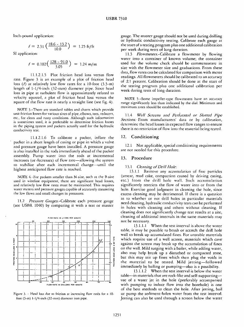
USBR 7310
Inch-pound application
f = 231 ( 18 ~~-~3 2) 125 ftfr
SI application
f = 0 102( 128
- 9 tO) = 124 mm 305
l l l215 Plot friction head loss versus flow rare Figure 3 is an example of a plot of friction head loss (f) at relatively low flow races for a 10-foor (33-m) length of 1-14-inch (32-mm) diameter pipe Since head loss in pipe at turbulent flow is approximately related to velocity squared a plot of friction head loss versus the square of the flow rate is nearly a straight line (see fig 4)
NOfE 3-There are srandard rabies and charcs which provide unit friction losses for various sizes of pipe elbows cees reducers ere for clean and ruscy conditions Although such informacion is sometimes used it is preferable to determine friction losses in che piping syscem and packers accually used for che hydraulic conductivity rest
111216 To calibrate a packer inflate the packer in a shore length of casing or pipe in which amiddotvalve and pressure gauge have been installed A pressure gauge is also installed in the rods immediately ahead of the packer assembly Pump water into the rods at incremental increases (or decreases) of flow rate-allowing the system to stabilize after each incremental change-until the highest anticipated flow rate is reached
NOfE 4-For packers smaller than N-size such as the B-size used in wireline equipmentmiddot there are significant head losses and relatively low flow races must be maintained This requires water meters and pressure gauges capable of accurately measuring the low flows and small changes in pressures
112 Pressure Gauges-Calibrate each pressure gauge (see USBR 1040) by comparing it with a test or master
FLOW RATE IN LITERS PER MINUTE
o
I _ I_ I I I II
I I I I I loI I I I I I rI
I I I )I
I I I I I v I I I I I I I I I I lr II
I I
I I I I 11deg II i j~ I I I -~-----1 -- I I I I i
JO deg HOW RATE IN GALLONS PEA MINOT[
Figure 3 - Head loss due ro friction at increasing flow rates for a I 0shy
foot (3-m) 1-14-inch (32-mm) diameter iron pipe
gauge The master gauge should not be used during drilling or hydraulic conductivity testing Calibrate each gauge at the start of a res ring program plus one additional calibration per week during rests of long duration
113 Flowmeters-Calibrate a flowmerer by flowing water into a container of known volume the container used for the volume check should be commensurate in size with the flowmeter size and graduations From these data flow rares can be calculated for comparison with meter readings All flowmeters should be calibrated to an accuracy of plusmn1 percent Calibration should be done at the stare of the resting program plus one additional calibration per week during rests of long duration
NOfE 5-Some impeller-type flowmeters have an accuracy range significantly less than indicated by the dial Minimum and maximum races should be esrablished
114 Well Screens and Perforated or Slotted Pipe Sections-From manufacturers dara or by calibration determine the head losses in expected flow ranges to ensure there is no restriction of flow into the material being tested
12 Conditioning
12 l Nor applicable special conditioning requirements are not needed for this procedure
13 Procedure
13l Cleaning ofDnll Hole 13l1 Remove any accumulation of fine particles
(smear mud cake compaction caused by driving casing etc) from the drill hole wall Such accumulation significantly restricts the flow of water into or from the hole Exercise good judgment in cleaning the hole since excess cleaning may be detrimental If there is a question as to whether or not drill holes in particular materials need cleaning hydraulic conductivity tests can be performed in holes with cleaning and others without cleaning If cleaning does not significantly change rest results at a sire cleaning of additional intervals in the same materials may not be necessary
131 l1 When the rest interval is above the water table it may be possible to brush or scratch the drill hole wall to break up accumulated fines For unstable materials which require use of a well screen materials which cavemiddot against the screen may break up the accumulation of fines on the wall Mild surging with a bailer while adding water also may help break up a disturbed or compacced zone but this may stir up fines which then plug the voids in the material co be rested Mild jetting-followed immediately by bailing or pumping-also is a possibility
13 l l2 When the test interval is below the water table-in materials chat are rock-like and self-supporcingshyuse of a water jet in the hole (preferably accompanied with pumping to induce flow into the borehole) is one of the best methods to clean the hole After jetting bail or pump the sediment-laden water from the rest interval Jetting can also be used through a screen below the water
1251
tJ
I I 0 GO-GI I GO-G2 0 GI -G2
~
I
I
v
v p-shy~ -shyl--~ L--shy
-shy
v
0
middot 005 =0 00005 100
-shy~--~ 0 middot 0025 =0 00005
I 50 I
~ --shy = 0 00005
50
I
t - A
v -
-
[] --shy shy--shy0 -
4--l_-E
-
16
-shy-shy-8 --shyl---shy~ - 2
~ ~---shy z 3 4 5 6 7 8 9
FLOW RATE SQUARED (q 2 )(10001
s of oalmin ) 2
Figu re 4 - Plot of feed p_ipe ca libra tion data - example
USBR 7310
2FLOW RATE SQUARED (q2)( 1000degs of L min)
10 15 20 25 - 30 35
50
40
r w w LL
z
~ 30 0 J Cl ltgt w I
z 0 20 r S a LL
10
0
cable in unstable materials For soft rock flushing che sides of che drill hole by running che bit or a bailer up and down the hole may enlarge the hole by erosion or ocherwise change the characceriscics of the fracture systems
13113 Finally clean the drill hole by pumping or bailing water from the bottom upward with the pumping continued until the return fluid is clear without cuttings or sediment Record the method used in cleaning the hole on the log of drill ho le or on a special testing form
132 Length of Test Interval 1321 The length of the test interval depends on
(1) purpose of the test (2) stratigraphic interval and (3) flow rate Where materials are relatively uniform use a test interval of about 10 feet (3 m) Where flow rates are high shorten the test interval co locate high flow race zones where races are very low the interval may be lengthened if desired
133 Ground-Water Level Determination 13 31 Depth co ground-water level muse be
determined before calculating hydraulic conductivity Measure depths to water levels with an electrical probe or o ther suitable equipment (see subpar 811)
1332 Auger Holes-ln power auger or other types of holes to which water is not added as pare of the drilling process report the presence or absence of a water level depth to water level and dace of initial and final water level measurement In materials of low hydraulic
14
12Cll a w r w
101 z () Vgt 0
8 J
Cl ltgt w I
Sz 0 r u a
4 IL
conduccivicy several days to several weeks may be required for a water level to stabilize in the hole Report evidence of moisture in the cuttings and if a perched water level was observed
1333 Rotary or Cable Tool Holes-For drill holes in which addition of water to the hole is an integral part of the drilling process
13331 Bail or pump the hole dry or to a stable wa ter level at the close of the last shift each day and record level
13332 Report the presence or absence of water and depth to water at the beginning of the first shift each day Additional readings are desirable whenever water level in the hole has nor been disturbed for an appreciable period of time
13333 Report changes in water level detected as the hole is drilled deeper Record faccors that affect the water level such as depth of casing andor cemented intervals These data may be helpful in recognizing perched or confined (artesian) conditions
13334 Upon completion of the hole the water must be bailed down to the extent practicable the water level measured and the dace recorded of hole completion Measure the water level for a period of days or weeks until equilibrium is reached
NOfE 6-At times exceptions must be made to the requirement for conrinuation of water level readings Such is the case when
1252
USBR 7310
state or local laws require chat the hole be filled continuousiy from bottom to cop immediately upon hole completion and before the drill crew leaves the sire In ocher instances landowners may allow right-of-entry for only a limited time for measurements
1334 Perched and Artesian Aquifers-lc is imporshytant tO recognize perched and artesian aquifers especially those under sufficient pressure tO raise the water level above the confining layer but nor tO the ground surface (see (5 ]) They must be distinguished from water table aquifers (those which continue in depth) If perched water table or artesian aquifers-separated by dry or less permeable strata-are encountered in the same drill hole the resulting water level in the hole is a composite therefore conclusions and interpretations based on such data are misleading If a perched water table is recognized (or suspected) during drilling water levels must be determined for each zone for calculation of hydraulic conductivity This might require completion of the drill hole with a watertight seal set at a suitable horizon tO
separate two water table conditions In this type installarion two strings of pipe or conduit are required one extending down to the portion of the hole immediately above the packer and a second string extending through the packer to a point near the bottom of the hole Water-level measurements provide the basis for determining a perched condition or if the lower water table is under artesian pressure
13 35 Mulriple Water-Level Measurements-In some instances it is desirable tO install multiple conduits and packers or plugs in a drill hole so that ground-water levels (or pressure heads) in several water-bearing horizons can be measured over an extended period of time (see [5] pp 7-14)
134 Pressure Tests With Packers 134 l The recommended arrangement of typical
equipment for packer pressure tests without a pressure sensor is shown on figure 2 (See app fig Xl l for equipment with a pressure sensor) Beginning at the source of warer the general arrangement is clean water source suction line pump discharge line tO srorage andor settling tank suction line water-supply pump surge chamber line ro bypass valve junction water meter gate or plug valve tee with sub for pressure gauge short length of pipe on which the pressure gauge is attached tee and off-line bleeder valve for evaluating back andor holding pressure flexible 1-14-inch (32-mm) diameter hose and 1-14shyinch-diameter feed pipe ro packer or packers in drill hole which isolate the rest interval All connections should be tight and as short and straight as possible with minimum change in diameter of hose and pipe Friction loss decreases as the pipe diameter is increased
1342 When the material is subject co caving and casing andor grout is needed to support the walls of the drill hole the hole should be water rested as it is advanced Other hole conditions may make this procedure desirable or necessary The following procedure is commonly used
1342 l After the hole has been drilled to the top of the interval to be tested it may be desirable tO remove
the drill string from rhe hole and advance casing or grout ro rhe bonom of the hole
13422 Advance the hole 5 to lO feet ( 15 to 3 m) into the material to be rested
13423 Remove the drill string from rhe hole 13424 Clean the interval to be tested and record
the depth tO the warer table if present If a composite water level is suspected the warer level affecting rhe rest should be determined by measurements through the feed pipe after rhe packer has been seated and the water level has stabilized
13425 If rhe hole will stand open sear a single packer ar the top of rhe test interval Record the type of packer irs depth and packer pressure if it is rhe inflatable type
13426 Pump water into the interval ar a rate to develop a suitable pressure The pressure to be used depends upon testing depths and ground water levels or pressures Materials subject to deformation or heaving such as by separation of bedding planes or joints or materials at shallow depths must nor be subjecred to high pressures (see subpar 102 l ) For comparison of flow rates in different pares of a single foundation and with results from other foundations some of the following pressures are commonly used 25 50 75 and LOO lbfin 2 (170 350 520 and 690 kPa)
NorE 7-At test pressures less than 25 lbfin2 errors in measurement of pressure and volume of water may increase unless special low pressure gauges are used Gravity tests provide more accurate results under these conditions At pressures higher than 10 lbfin2 difficulties in securing a right packer seal and the likelihood of leakage increase rapidly However under artesian pressures or in deep holes the water pressure-as registered on a surface gauge-will need to be sufficient to overcome the effeccive head at the test interval and firmly seal the packer
NillE 8-Where the hole is subject to caving a pump-down wire-line system has been developed rhar can be used to eliminate removal of the drill string from the hole With this system the hole is drilled to the bottom of the interval tO be tested and the drill rod is raised so the end of the rod is at the top of the test interval The tandem packer (see subpar 882) is then lowered through the drill rod and expanded to seal both inside the rod and against the wall of the hole at the cop of the test interval Models of this equipment are available which have transducers below the packer for measuring water pressures at the test interval
13427 For determining effective head artesian heads encountered in the drill hole are treated the same as water table conditions ie the depth from the pressure gauge or the water level maintained during the test to
the stabilized water level is used as the gravity head If the artesian head stabilizes above the ground surface the gravity component of the effective head is negative and is measured between rhe stabilized level and the pressure gauge height If a flow-type rest is used the effective head is the difference between rhe stabilized water level and rhe level maintained during the flow period
1253
USBR 7310
13428 Afrer pressures are selected based on ground-water conditions and the purpose of the test perform a test at each pressure Usually a 5-cycle procedure is used three increas ing steps to the maximum pressure and then two decreasing steps to the starting pressure This cycling allows a more derailed evaluation of rest results than testing at a single pressure and commonly allows extrapolation to ascertain at what pressures the following may occur (1) laminar flow (2) turbulent flow (3) dilation of fractures ( 4) washouts (5) void filling or (6) hydraulic fracturing However the equations normally used to ca lculate hydraulic conductivity are based on laminar flow conditions
NOfE 9-ln some insrances on ly a single water pressure test at a given interval in the drill ho le may be required For example if geologic conditions are known and there is no need ro perform the seeps in subparagraphs 13422 through 13426 a single value of hydraulic conductivity with a relatively low application of pressure may suffice
13429 During each test continue pumping water to the test interval at the required pressure until the flow rate becomes stable As a general guide maintain flow rares during three or more 5-minute intervals during which l-minute readings of flow are made and recorded In tests above the water table water should be applied to the test interval until the flow rate stabilizes before starting the 5-minuce measurement intervals Where tests are below the water table flow rates usually stabilize faster than for the tests above the water table and the time period before the 5-minure test intervals may be shorter These rime periods may need to be varied particularly when rests to determine grouting requirements are made
134210 Determine and record the presence of back pressure and decay of holding pressure Afrer the rest deflate the packer and remove it from the drill hole
134211 Advance the drill hole and if necessary the casing repeat the procedure in subparagraphs 13423 through 134210 until the required depth of drill hole is reached When casing is used in a drill hole always set the packer in the material below the casing
1343 If the hole will stay open without casing it can be drilled to final depth and after cleaning the hole hydraulic conductivity rests can be performed from the bottom of the hole upward using straddle (double) packers Although a single packer can be used to test the bottom interval of the hole starting at the bottom with double packers will cause loss of borehole testing of only about the length of the bottom packer and will save one complete trip in and out of the hole with the drill string assembly co change the packers After the test for the bottom interval is completed straddle packers are used for successive test intervals up the drill hole See subparagraph 1342 where caving or other hole conditions will not allow this procedure
135 Gra vity Tests 135 1 Constant-head gravity tests are usually
performed without packers above or below the water table with drill holes of N-size or larger (see fig 2 derail D)
This type of test is often made in reasonably stable-walled drill ho les up to 25 feet (76 m) depth where water pressure at the test interval needs to be kept low The test is usually performed in successive 5- or 10-foot (l5- or 3-m) intervals as the drill hole is advanced The upper end of each test interval is normally determined by the bottom depth of tightly reamed or driven casing If the casing is not believed
middotto be tight appropriate entries should be recorded on the log form If the wall of the drill hole is stable the test can be performed in the unsupported hole If the wall needs to be supported use a well screen (see subpar 114 for calibration) inserted through the casing It may be necessary to ream or drive the casing to the bottom of the interval set the screen and then pull back the casing to expose the screen Afrer the test the screen is removed and the casing reamed or driven to the bottom of the hole
NOfE lO-Clean coarse sa nd or fine gravel backfill (see subpar 92) may be used instead of a well scree n Ream or drive rhe casing ro the borrom of the inrerval dean ir our and add rhe backfill as rhe rnsing is pulled back ro expose rhe resr interva l Record use of rhis procedure on the log form
l 35l l If the drill hole is self-supporting clean and prepare it in rhe normal n1anner (see subpar 13l)
l35 l2 If the drill hole is not self-supporting lower the well screen and casing into the hole
135 l3 For test intervals above the water table maintain a constant head of water _within 02 foot (60 mm)] at the top of the test interval by injecting water through a small diameter rube extending below the water level maintained during the test For rest intervals below the water table or influenced by artesian conditions maintain a constant head a short distance above the measured static water level
Monitor the water level with a water-level indicato r If the water-level indicator is inserted in a small diameter pipe in the casing the wave or ripple action on the water surface will be dampened and permit more accurate watershylevel measurements
NOfE l l-When rhe flow rare is very low rhe consranr wa rer level c1n be maintained by pouring warer in rhe hole from a graduated container
135 l4 Record the flow rate at wne intervals until a constanc flow rare is reached
135 l5 Repeat the procedure of subparagraphs 135 l3 and 135 14 at one or more different water levels
13516 This rest is essentially the same as desigshynation USBR 7300 (see also L3] p 74) the instructions in USBR 7300 for performing the rest and calculating hydraulic conductivity apply to this procedure also
14 Calculations
14 l For pressure or constant gravity head hydraulic conductivity rests calculace the hydraulic conductivity of
1254
USBR 7310
rhe soil or rock by rhe following equation (expressed m consisrent unirs) [4]
k = ~ In ~ where L ~ lOr (2)
or
k = ~ sinh-1 r where lOr~ L ~ r (3)
where k = hydraulic conducrivity fryr or cms q = consrant race of flow into che rest interval
ft3yr or cm3s L = length of the test interval ft or cm
H = differential head of wacer ac rest interval fr or cm
r= radius of the borehole ft or cm In= natural logarithm loge
inv~rse hyperbolic sin~ smh- 1 x In (x + -yx2 + 1)
142 An example calculation for a single packer test _ in the botrom of a borehole belovt the wacer table follows
Example assume
r = 18 in or 015 ft= 46 cm q - 22 galmin or 83 Lmin q = 15 X 10 ft3yr = 140 cm3s L 30 ft = 91 cm
Hg gravity = disrance from ground-water level co pressure gauge = 102 ft = 311 cm
Hp pressure 5 lbf in2 X 231 ftwater (lbf in2)
116 ft = 3 54 cm of water H = Hg+ Hp= 218 ft= 664 cm
~ = ~lo = 20 hence use equation (2) 5 k = _9_ In]
2rrLH r k = 15 X 10 ft3 yr In 30 ft
2rr (30 ft) 218 ft 015 ft k = 11X103 ftyr = 11 X lQ-3 cms
NafE 12-These equations are most applicable and reliable where the length of test interval is at lease 5 r and the interval is below che water table The equations are based on laminar flow of fluid through porous media Flow races high enough co cause turbulent flow invalidate the results in all types of material In fractured material the calculated value should be considered an apparent hydraulic conductivity even under laminar flow conditions
143 For pressure resrs when rhe resr interval is below the water table H is the distance from rhe water table to the elevation of che pressure gauge plus applied pressure converted to linear units of water head
Where the rest interval is above the water table His rhe distance from rhe midpoint of the isolated rest interval to che elevation of the pressure gauge plus the applied pressure converted to linear units of water head
For gravity rests above che water table H is che distance between che boccom of the tesc interval and che water level maintained during the test
For gravity rests below the water cable His che distance between the pretest stabilized wacer level in the drill hole and the water level maintained during the rest
144 If chere is artesian pressure an additional pressure muse be applied to overcome che artesian pressure co provide an effective rest pressure For example if there is an artesian pressure of 5 lbfin2 (34 kPa) ac che pressure gauge 15 lbfin2 (103 kPa) could be applied chen che effecrive pressure would be 15 lbfin2 minus 5 lbfin2 which equals 10 lbfin2 (69 kPa)
145 The calculations can be done conveniently by (1) a nomograph [12] (2) a hand calculator with che proper functions or (3) a com purer For repeared tests ic is convenient to prepare a table for one or more diameter drill holes and lengths of resc intervals and combine che terms on che right side of the equations other than q and H into a coefficient
NafE 13-The lugeon (lugeon unit lugeon coefficient) [ 13 14 15 16] has been used as an index of hydraulic conductivity in connection with cyclic rests and for grouting purposes
15 Report
151 Record field test data on a daily driller s report and or on rhe log of the drill hole or on a special reporting form designed for the specific project Record the following
1511 Log of the drill hole 1512 Elevations of the ground surface the water
cable and che top and bortom of the rest interval 1513 Diameter of the drill hole at test interval 1514 Method of cleaning the drill hole 1515 Size of the feed pipe and any well screen 1516 Water pressure andor gravity head and flow
rare for each rime interval 1517 Tora[ amount of warer used per resr 1518 Average temperature of ground warer and
water used in the rest 1519 Packer inflation pressures 1511 Capacity of pump supplying water to the
rest interval 15111 All head loss calibrarion dara 15112 Nore any comments considered necessary to
help evaluate che rest results
15 References
[ l] Permeability Tests Using Drill Holes and Wells Bureau of Reclamation Geology Report No G-97 Denver ColoradoJanuary 3 1951
[2] Ground Warer Manual lst ed rev reprint Bureau of Reclamation US Government Printing Office Washington DC 1981
1255
USBR 7310
[3] Drainage Manual lsc ed 2d princ Bureau of Reclamacion U S Governmenc Princing Office Washingcon DC 1981 1984
[4] Zangar Carl N Theory and Problems of Water Percolation Engineering Monograph No 8 Bureau of Reclamation Denver Colorado 1953
[5] Drill Hole Water Tests Technical lnstructionsshyProvisional Engineering Geology Bureau of Reclamation July 1970 (unpublished)
[6] Glossary of Geology 2d ed American Geological lnscitute Falls Church Virginia 1980
[7] Haccher R C High Pressure Inflacable Packer with Pneumatic Piezometer Bureau of Reclamation Reporc GR-10-75 Denver Colorado October 1975
[8] Bennett R D and R F Anderson New Pressure Test for Determining Coefficient of Permeability of Rock Masses Technical Reporc GL-82-3 US Army Engineer Waterways Experiment Station Vicksburg Mississippi 1982
[9] Ground Water and Wells A Reference Book for the Water-well Industry 1st ed published by Edward E Johnson Inc Saint Paul Minnesota 1966
[10] Drillers Safety Manual 1st ed reprint Bureau of Reclamation Denver Colorado 1982
[11] Acker W L III Basic Procedures for Soil Sampling and Core Drilling published by the Acker Drilling Company Scranton Pennsylvania 1974
[12] Underground Mining Methods Handbook No 580 W-88 Society of Mining Engineers Littlecon Colorado p 62 1982
[13] Lugeon M Barrages et Geologie Dunod Paris 1933
[14] Houlsby A C Routine Interpretation of the Lugeon Water-Test Quarterly Journal Engineering Geology vol 9 pp 303-313 1976
[15] Heitfeld K H and L Krapp The Problem of Water Permeability in Dam Geology Bull International Association of Engineering Geology No 23 pp 79-83 1981
[16] Pearson R and M S Money Improvements in the Lugeon or Packer Permeability Test Quarcerly Journal Engineering Geology vol 10 the Netherlands pp 221shy239 1977
1256
USBR 7310
APPENDIX
XL PROCEDURE USING A PNEUMATIC PIEZOMETER WITH TWO PACKERS ISOLATING THE TEST INTERVAL
Xl l Equipment Assembly (Refer to figs Xll and X l2) -A complete straddle packer unit is assembled as follows
X 11 l Co nnect a predetermined length of perforated injection (feed) pipe to the lower packer (The length of perforated pipe is determined by the thickness of the zone to be rested) Connect the inflation tubing to the lower packer and lower the sliding head end of the packer into the drill hole (See subpar l l l216 for calibration of packers)
Xl l2 Clamp the top of the perforated injection pipe at the hole collar and connecr the upper packer with the sliding head already down the hole
Xl l3 Provide approximately 12 inches (300 mm) of slack in the inflation tubing between the two packers to allow for retraction of the upper packer sliding head Connecr the tubing to the upper packer
Xl l4 Install the pneumatic piezometer piezomerer tubing packer inflation tubing and sealed lengths of injecrion pipe to the head adaptor
X ll5 Lower the entire unit into the drill hole adding lengths of sealed injection pipe as necessary to reach the
( Storoqf Settling ton
interval to be tested As the unit 1s lowered che packer inflation cubing and che piezomecer tubing is unreeled into che hole and caped to che sealed injection pipe at approximately 10-fooc intervals
Xll6 Upon reaching the rest depth lock both the inflation cubing reel and rhe piezomecer cubing reel connecr the inflation tubing by quick-connecr couplings co a nitrogen or compressed air boccie equipped with a high pressure regulator connecr the piezomecer cubing by quick-connect couplings co the readout box and connect the injection pipe co the water pressure source The cesc is now ready to begin
Xl2 Test Procedure
X 12 l After the unit has been lowered to the rest interval and before infacing the packers any water head above the cesc interval must be determined This head will sho w as pressure on the pneumatic piezomecer gauge and can be verified by running a water level indicator into che hole to measure the deprh co the water cable The piezometer will register water pressure chat can be converted to head of water This water head should be
Compressed 01r or nitrogen bot tie Regulator_
Poc~er air lin e- I
P1nometer ln1ec t1on oioe head adaptor
Lo er ooc~er inflation tubmr
Figure X 1 1 - Schematic arrongemem of drill hole packer and pressure monimring equipment 801-0-180
1257
USBR 7310
------=--From compressed air or nitrogen boltle
From piezometer
_To
PRESSURE READOUT BOX
Packer inflation tubing From wafer source From air or Water injection pipe ring seals
PIEZOMETER TUBING REEL
Pressure seals Wire reinforced rubber gland clomps
nitrogen ~~i==-=~==t~f=lil~~~jii~9ll~~~~~sect9ll~sect~sectsect~~~sectl~iilf~f--- To per for o t e d ~~~ze=zzzoCzzzze=zzze=plusmnzz~EZio~~~~21p~
To pressuresource~~~~~~~~~~~~~~~readout box
Piezometer
~~~~~~~~~~~~~~~~---
Inflation chamber Floating packer head Packer inflation lubing
UPPER DRILL HOLE PACKER AND PRESSURE MONITORING EQUIPMENT FOR N X HOLE
Figure X 12 - Upper Jrill hole packer anJ pressure monitoring equipment for NX hole
used to determine the minimum inflation pressure to be applied co the packers by the following equation
SH+ PP+ PE = minimum inflation pressure
where SH = static pressure at the midpoint elevation of the
test interval lbf in2 or kPa PP = gauge pressure to be maintained during the test
lbfin2 or kPa PE = pressure needed to expand packer to hole
diameter as determined before insertion in the drill hole by expanding the packer in a length of pipe having a diameter similar to the hole diameter lbfin 2 or kPa
Inflation pressure gauge is in units of lbf in2 (kPa) The static water level measured before the packers are
inflated might be a composite water level (see subpar 1334)
Xl22 Inflate the packers and determine water head for the rest interval This is the static head to be used for calculation of hydraulic conductivity If rhe static head is significantly different from the composite measured
before the packers were inflated recalculation of packer inflation pressure may be required The final packer inflation pressure should be the lowest practical pressure to seal the test interval against the maximum injection pressure to avoid fracturing of the material being tested
Xl2 3 After the inflation pressures have been determined deflate the packers fill and flush the system with water until all entrapped air has been removed This is accomplished by filling the injection pipe under a gravity head and leaving the air-release valve open ar the top of the injection pipe tee at an elevation higher than the injection hose The valve must remain open until all air has been removed and water runs freely indicating a filled system At this point water is flowing around the deflated packer system and is completely filling the annulus between the drillhole and the packers In the case of an interval with a high injection rate it may be necessary to keep the air valve closed to keep from entraining air into the test interval
X 124 Close the air release valve at the top of the injection pipe and slowly inflate the packers to the predetermined inflation pressure
Xl2 5 Lock in the inflation pressure by closing the pressure valve in the packer cubing If the pressure gauge
1258
USBR 7310
on the closed system remains steady it verifies a sealed system At this point water injecced under gravity head approaches a constant flow rate
X 126 Record the piezometer pressure after packer inflation For an interval of very low injection rate this is equal to che height of the injeccion standpipe plus che pressure recorded at the hole collar gauge For a test interval with a high injection rate the readout would show the same value less any friction from water flow through the injeccion pipe
X 127 Proceed with the test by applying the selected pressures ac the test interval and moniroring the flow rate and pressure on the pneumatic piezometer
X 128 To accurately compute hydraulic conduetivity rhe down-hole pressure muse remain constant A zone with a high injection rate must be monirored more closely than a zone with a small injection rate and adjustments made to hold the down-hole pressure constant To accomplish
this che injeccion pressure shown on che collar gauge must be adjusted in order co maintain che down-hole pressure constant
NOfE X 1-For example a pressure srage is scarred with the collar gauge reading 35 lbfin2 (241 kPa) and the down-hole piezomerer reading 200 lbf in2 ( 1380 kPa) As rhe flow increases rhe down -hole pressure may drop to 150 lbfin2 (1034 kPa) because fricrion loss in the injection pipe and the collar gauge would have to be adjusted to bring the down-hole pressure gauge back up co 200 lbfin2bull When the flow decreases from a fast to a slow rare the collar gauge pressure would have to be decreased
Xl29 The cesc is completed following one or more stages of pressure increases and pressure decreases Following the last stage deflate the packers and close the injection line The system is now ready to move to the next test interval for repetition of this procedure
1259
Methods Note
A Computer Program for Flow-Log Analysis of Single Holes (FLASH) by Frederick D Day-Lewis1 Carole D Johnson2 Frederick L Paillet3 and Keith J Halford4
Abstract A new computer program FLASH (Flow-Log Analysis of Single Holes) is presented for the analysis of
borehole vertical flow logs The code is based on an analytical solution for steady-state multilayer radial flow to a borehole The code includes options for (1) discrete fractures and (2) multilayer aquifers Given vertical flow profiles collected under both ambient and stressed (pumping or injection) conditions the user can estimate fracture (or layer) transmissivities and far-field hydraulic heads FLASH is coded in Microsoft Excel5 with Visual Basic for Applications routines The code supports manual and automated model calibration
Introduction Flowmeters provide means to infer the flow into or
out of boreholes connected to transmissive aquifer units or fractures In the past the relative inaccuracy and difficult operating procedures for spinner flowmeters limited the use of borehole flow measurements With the advent of heat-pulse (Paillet et al 1996) and electromagnetic (Molz et al 1994) instruments measurements of vertical flow as small as 005 Lmin became practicable and borehole flowmeter logging is becoming routine New modeling and analysis tools are needed to achieve the full potential of these measurements
1Corresponding author US Geological Survey Office of Groundwater Branch of Geophysics 11 Sherman Place Unit 5015 Storrs CT 06269 (860) 487-7402 ext 21 fax (860) 487-8802 daylewisusgsgov
2US Geological Survey Office of Groundwater Branch of Geophysics 11 Sherman Place Unit 5015 Storrs CT 06269
3Office of Groundwater Branch of Geophysics (Emeritus) US Geological Survey 11 Sherman Place Unit 5015 Storrs CT 06269
4US Geological Survey Nevada Water Science Center 2730 N Deer Run Rd Carson City NV 89703
5Any use of trade product or firm names is for descriptive purposes only and does not imply endorsement by the US government
Received April 2010 accepted December 2010 copy 2011 The Author(s) Ground Water copy 2011 National Ground Water Association doi 101111j1745-6584201100798x
Calibration of a borehole flow model to flowmeter data can produce estimates of transmissivity and heads for one or more flow zones (aquifer layers or fractures) Here we briefly review approaches for analysis of flowmeter logs and introduce a new computer program which supports manual and automated calibration of an analytical borehole flow model
Approach Single-hole flowmeter data can be analyzed to
estimate transmissivity profiles along boreholes and characterize aquifer compartmentalization (Molz et al 1989 Kabala 1994 Paillet 1998) Analysis of single-hole flowmeter data is commonly based on the Thiem Equation (Thiem 1906) which written for confined radial flow from a single flow zone (ie aquifer layer or fracture) to a screened or open well is
2πTi(hw minus hi)Qi = minus (1)
ln(r0rw)
where Qi is the volumetric flow into the well from flow zone i [L3Tminus1] hw and hi are respectively the hydraulic head [L] at the radius of the well rw and at radial distance r0 commonly taken as the radius of influence where heads do not change as a result of pumping in which
926 Vol 49 No 6ndashGROUND WATERndashNovember-December 2011 (pages 926ndash931) NGWAorg
case hi is the connected far-field head for zone i and Ti
is the transmissivity of flow zone i [L2Tminus1] A number of approaches to flowmeter analysis have
been proposed and demonstrated for different sets of assumptions (eg no ambient flow in boreholes) and data requirements (eg flow profiles collected under both ambient and stressed conditions) based either on Equation 1 (Molz et al 1989) or quasi-steady flow approximations (Paillet 1998) We refer the interested reader to Williams et al (2008) for additional background on flowmeter logs and focus the following discussion on the approach of Paillet (1998 2001) which is adapted here
Paillet (1998) formulated flowmeter log analysis as a model-calibration procedure involving flow profiles collected under both ambient and stressed (pumping or injection) conditions Consideration of the two conditions allows for the estimation of the transmissivities and also far-field heads of flow zones The latter is critical for the interpretation of water samples from wells that intersect multiple fractures or layers with different hydraulic head (Johnson et al 2005) Applying Equation 1 to an ambient condition (condition a) and a stressed condition (condition s) gives
factorT total(ha minus h02πTi )w iQa = minus (2)i ln(r0rw) factorT total(hs minus h02πTi )w iQs = minus (3)i ln(r0rw)
where T factor i is the fraction of the boreholersquos transmisshy
sivity contributed by flow zone i [ndash] T total is the total transmissivity of the flow zones intersected by the bore-hole [L2Tminus1] ha hs are the ambient and stressed water w w levels in the well respectively [L] h0 is the far-field head i in flow zone i [L]
For both ambient and stressed conditions the water level in the borehole is assumed to be constant in
time and the water level in the far-field of each zone is assumed to be the natural condition that is hi
0 In a field experiment (Figure 1) rw would be known and the flow rates and water levels in the well would be measured Radius of influence can be inferred experimentally based on head data at observation wells in which case r0 can be constrained during calibration or else it can be approximated (Bear 1979 306) Estimates of transmissivity are not strongly sensitive to the value assumed for r0 because it appears inside the logarithm in Equations 2 and 3 For example a change in r0rw
from 10 to 100 yields a change in the estimated Ti of only a factor of 2 and order-of-magnitude estimates of transmissivity are acceptable for many problems In cases where knowledge of r0 is unavailable but the boreholersquos total transmissivity is known from specific-capacity or slug-test results it is possible to estimate r0 in the calibration procedure We note that the forward model (Equations 2 and 3) produces twice as many independent equations as there are flow zones with an additional equation requiring T factor values to sum to 1 The number of parameters being estimated is twice the number of flow zones (T factor and h0 for all i) plus one parameter for either i i T total 0or r i
Model calibration involves changing the model parameters such that the flows predicted by Equations 2 and 3 match the interpreted flow profiles Following Paillet (1998 2001) calibration is to the interpreted profile and not individual data This formulation allows the user to incorporate additional insight (eg from other logs) to identify the number and locations of flow zones and elimshyinates the need for weighting measurements differently according to variable measurement errors and the spatial distribution of measurements along the borehole
Calibration can be implemented by manual trial-andshyerror or automated using nonlinear regression Whether manual or automated the goal for calibration is to identify the set of parameters that minimize a measure
Figure 1 Schematic of flowmeter experiment in a fractured-rock aquifer with (a) flow-log profiles for ambient (blue) and stressed (dashed red) conditions and conceptual cross sections of flow system for (b) ambient condition and (c) stressed condition In this example two flow zones (fractures) intersect a well Under ambient conditions flow enters the well from fracture 1 and exits from fracture 3 Under pumping conditions flow enters the well from fractures 1 and 2 The far-field head of zone 2 is equal to the ambient water level thus there is no flow tofrom zone 2 under ambient conditions The far-field head of zone 3 is equal to the stressed water level thus there is no flow tofrom zone 3 under pumping conditions
NGWAorg FD Day-Lewis et al GROUND WATER 49 no 6 926ndash931 927
of combined data misfit and model misfit Considerashytion of model misfit criteria commonly referred to as regularization is useful when multiple models can match the data equally well or within measurement errors Here the data misfit is formulated based on squared differshyences between the predicted and interpreted flow profiles such that multiple measurements may be collected in a single borehole interval The model misfit could be forshymulated in different ways but we use criteria based on the differences between the water level in the borehole under ambient conditions and the far-field heads Thus the objective function F consists of two terms (1) the mean squared error (MSE) between interpreted and preshydicted flow profiles with equal weights for all cumulative flows (ambient and stressed) and (2) the sum of squared differences (h) between the boreholersquos water level and far-field heads
n1 2ssim sintmin F = Q minus Qi i n
i=1
n asim aint 2+
Q minus Q
2 + α (hi) (4)i i i=1
subject to constraints
factor factorT ge T for all i andi min
ABS(haw minus h0
i ) le hmax for all i
aintwhere Qi Qi sint are the interpreted flow profiles (ie
cumulative flow above zones) for zone i under ambishyasiment and stressed conditions respectively [L3Tminus1] Qi
ssimQi are the simulated flow profiles (ie cumulative flow above zones) for zone i under ambient and stressed conditions respectively [L3Tminus1] α weights the regushylarization relative to the data misfit [L4Tminus2] T factor ismin
T factorthe user-specified minimum for any flow zone which can ensure nonnegative T factor hmax is the user-specified maximum absolute difference between the ambishyent water level and the far-field head of any flow zone and n is the number of flow zones
Without regularization F reduces to the MSE between simulated and interpreted flows The trade-off parameter α is set by the user with larger values more strongly penalizing large head differences Commonly small α values (less than 0001) are sufficient to obtain good results In selecting α the user should be guided by the goal of regularization which is to identify the ldquosimplestrdquo explanation of the data while minimizing the data misfit
Using FLASH FLASH (Flow-Log Analysis of Single Holes) is writshy
ten in Excel with Visual Basic for Applications (VBA) The spreadsheet includes a toggle (INPUTS worksheet cell A20) to choose between analysis for (1) fractures or fracture zones that intersect a well at discrete locations
and (2) aquifer layers in porous media The first is indishycated for cases where flow profiles are characterized by step increasesdecreases and the second for cases where flow profiles show approximately linear change over each layer Up to 10 fractures or layers can be modeled
The FLASH spreadsheet includes four worksheets INTRODUCTION INPUTS FIELD_DATA and PLOTshyTING INTRODUCTION provides information about the program and input parameters On the INPUTS workshysheet the user enters information about the flow zones transmissivities and heads Note that the user must intershypret flow profiles from the flowmeter data for both the ambient and stressed conditions The flow measurements are entered in FIELD_DATA and the interpreted proshyfiles are entered in INPUTS The interpreted profiles plot as dashed lines the data as points and the simulated proshyfiles as solid lines (Figure 2) Line and marker styles can be modified using standard Excel tools Flows are positive upward and negative downward PLOTTING is used by the program and does not require the userrsquos attention
In the INPUTS worksheet input parameters are entered in the cells with light blue and bright aquamarine backgrounds The former include specifications of the experiment setup (eg borehole diameter and water level) and the latter include calibration parameters Manual calibration is performed by adjusting the values of
ldquoT factorrdquothe cells and ldquohrdquo which are respectively T factor and the difference between the flow zonersquos far-i field head and the ambient water level in the borehole As parameters are adjusted the simulated flow profiles update automatically thus guiding the user toward best-fit parameters The MSE between simulated and observed flows is calculated in cell B36 on the INPUTS worksheet
Although the principle calibration parameters are Ti
factor and h the radius of influence r0 and total transshymissivity T total also are possible calibration parameters as explained above and indicated by aquamarine highshylighting By inspection of Equations 2 and 3 it is not possible to estimate unique values for both radius of influshyence and total transmissivity but only the ratio of total transmissivity divided by ln(r0rw) In general the user will have more information about total transmissivity than radius of influence Total transmissivity is estimated readshyily using an open-hole slug test or specific-capacity test Indeed the drawdown and pumping rate under stressed conditions could serve as data to estimate a total transshymissivity for the borehole In rare cases however the estimated total transmissivity may be considered unrelishyable for example in the presence of ambiguous slug-test data or discrepancy between the volumes over which the slug test and flowmeter analysis measure In such cases it may be useful to allow the T factor values to sum to a value other than 1 FLASH assumes a uniform radius of influence for all flow zones In reality the effective radius of influence may vary between zones according to their transmissivities and distances to boundaries Data to supshyport variable radius of influence however is commonly unavailable furthermore transmissivity estimates are not
928 FD Day-Lewis et al GROUND WATER 49 no 6 926ndash931 NGWAorg
Figure 2 The INPUTS worksheet after execution of the Solver with options ldquoEstimate ROIrdquo and ldquoSolve with regularizationrdquo for example On this worksheet the user enters the well and flow-log specifications and performs model calibration Data (points) and interpreted profiles (dashed lines) Simulated profiles (solid lines) are for an arbitrarily selected starting model
a strong function of the assumed radius of influence as explained previously
Automated model calibration is implemented using the Excel Solver an optimization tool based on a Genshyeralized Reduced Gradient algorithm (Lasdon and Smith 1992) The Solver is invoked using VBA ldquocontrol butshytonsrdquo on the INPUTS worksheet Radio buttons allow for selections of (1) the parameters to be estimated (Estishymate ROI [radius of influence] or Estimate Transmissivshyity) and (2) regularization (Solve without Regularization or Solve with Regularization) Under the option Estimate
T factorROI the Solver estimates the values of i for all i and the single radius of influence Under the option Estimate Transmissivity radius of influence is assumed known the parameters for estimation are T factor for all ii such that total transmissivity is allowed to vary Users are encouraged to perform manual calibration before attemptshying automated calibration Manual calibration provides insight into the sensitivity of flows to parameters and helps to identify a good starting model for automated calshyibration As for any nonlinear optimization the algorithm may get ldquostuckrdquo in local minima and fail to identify the globally optimal parameter values Consideration of mulshytiple starting models is advised Additional information
and the FLASH spreadsheet are available online as noted under Supporting Information at the end of this article
Example FLASH is demonstrated for a simple data set from
a fractured-rock aquifer (Figure 2) Johnson et al (2005) provide additional details for this data set for which additional borehole logs were used to identify fractures and select locations for flow measurements
Under ambient conditions the deeper fractures 1 and 2 experience inflow to the borehole which indicates the far-field heads for each of these fractures is greater than the head in the borehole thus producing upward flow (Figure 1) Under ambient conditions upflowing water exits the borehole at fracture 3 indicating the far-field head is lower than the head in the borehole Under low-rate pumping conditions water continues to enter the borehole at fracture 1 additional water enters at fracture 2 indicating the far-field heads for fractures 1 and 2 are higher than the quasi-steady state open-hole water level under pumping conditions The uppermost fracture (3) no longer shows outflow indicating the far-field head is equal to the pumping water level In this example
NGWAorg FD Day-Lewis et al GROUND WATER 49 no 6 926ndash931 929
fracture 2 has a far-field head similar to the ambient water level in the well and therefore does not result in a substantial change in borehole flow under ambient conditions Similarly fracture 3 has a far-field head similar to the stressed water level in the well and does not produce a measurable change in borehole flow under stressed conditions This field example underscores the importance of collecting both ambient and stressed flow profilesmdashwith only ambient data fracture 2 could not be identified and with only stressed data fracture 3 could not be identified
To induce flow from a given fracture to enter the borehole the h for that fracture must be positive Conversely to induce flow from the borehole to the fracture the h must be negative The rate of flow is determined by the magnitude of a given flow zonersquos h and transmissivity Thus manual calibration entails for each zone (1) adjustment of a h (cells F21F30) to control whether flow enters or exits the borehole from that zone and (2) adjustment of a T factor to control the rate of flow A final solution can be obtained with the manual fit or after a starting model is generated manually the Solver can be applied For the example here automated calibration produces an excellent match to the data (Figure 2) using options ldquoEstimate ROI rdquo and ldquoEstimate with Regularizationrdquo
Discussion and Conclusions We present a new tool to aid in flowmeter log
analysis a computer code named FLASH We follow a model-calibration strategy similar to that of Paillet (1998) with a simple analytical model for borehole flow based on the Thiem Equation (Thiem 1906) which has been used extensively in previous analyses of flowmeter logs It is important to note that FLASH assumes a borehole flow model that neglects head losses in the borehole or across the well screen and these losses are important in some data sets (Zlotnik and Zurbuchen 2003) We also note the limitations inherent to flowmeter methods primarily that they not as sensitive as straddle-packer hydraulic testing Flowmeter methods consistently identify transmissivities within 15 to 2 orders of magnitude of the most transmissive zone in a borehole depending on the resolution of the flowmeter itself (Williams et al 2008) but straddle-packer tests can see features 6 orders of magnitude less transmissive than is possible with flowmeter (Paillet 1998 Day-Lewis et al 2000 Shapiro 2001) Despite the limited resolution of flowmeter measurements flowmeter modeling results can reproduce packer-test estimates to within an order of magnitude and far-field head values determined with flowmeter methods commonly compare well with packer-test results and discrete-interval water-level monitoring (Johnson et al 2005 Williams et al 2008)
FLASH provides a graphical user interface for calshyibration of an analytical borehole flow model and estishymation of flow-zone transmissivities and far-field heads The program supports manual and automated calibration
with and without regularization FLASH is highly cusshytomizable Experienced Excel users may prefer to invoke the Solver outside of FLASHrsquos VBA routines or to use alternative objective functions or regularization criteria or variable weighting for ambient vs stressed flows Future extensions may include tools for analysis of crosshole flowmeter data and evaluation of estimation uncertainty
Acknowledgments This work was supported by the US Environmental
Protection Agency Region 1 the US Geological Survey Groundwater Resources Program and Toxic Substances Hydrology Program The authors are grateful for review comments from Tom Reilly Allen Shapiro Tom Burbey John Williams Roger Morin Landis West and Mary Anderson
Supporting Information Additional Supporting Information may be found in
the online version of this article
Supplemental material available online include (1) the FLASH spreadsheet which also can be downloaded from httpwaterusgsgovogwflash and (2) a README file with information for installation and troubleshooting
Please note Wiley-Blackwell is not responsible for the content or functionality of any supporting information supplied by the authors Any queries (other than missing material) should be directed to the corresponding author for the article
References Bear J 1979 Hydraulics of Groundwater New York McGraw-
Hill Inc Day-Lewis FD PA Hsieh and SM Gorelick 2000 Idenshy
tifying fracture-zone geometry using simulated annealing and hydraulic-connection data Water Resources Research 36 no 7 1707ndash1721
Johnson CD CK Kochiss and CB Dawson 2005 Use of discrete-zone monitoring systems for hydraulic charshyacterization of a fractured-rock aquifer at the Univershysity of Connecticut landfill Storrs Connecticut 1999 to 2002 Water-Resources Investigations Report 03-4338 105 Reston Virginia USGS
Kabala ZJ 1994 Measuring distributions of hydraulic conducshytivity and storativity by the double flowmeter test Water Resources Research 3 685ndash690
Lasdon LS and S Smith 1992 Solving large sparse nonlinear programs using GRG ORSA Journal on Computing 4 no 1 2ndash15
Molz FJ GK Bowman SC Young and WR Waldrop 1994 Borehole flowmetersmdashfield application and data analysis Journal of Hydrology 163 no 3ndash4 347ndash371
Molz FJ RH Morin AE Hess JG Melville and O Guven 1989 The impeller meter for measuring aquifer permeabilshyity variations evaluations and comparison with other tests Water Resources Research 25 no 7 1677ndash1683
Paillet FL 2001 Hydraulic head applications of flow logs in the study of heterogeneous aquifers Ground Water 39 no 5 667ndash675
930 FD Day-Lewis et al GROUND WATER 49 no 6 926ndash931 NGWAorg
Paillet FL 1998 Flow modeling and permeability estimation using borehole flow logs in heterogeneous fractured formashytions Water Resources Research 34 no 5 997ndash1010
Paillet FL RE Crowder and AE Hess 1996 High-resolution flowmeter logging applications with the heat-pulse flowmeter Journal of Environmental and Engineering Geophysics 1 no 1 1ndash14
Shapiro AM 2001 Effective matrix diffusion in kilometer-scale transport in fractured crystalline rock Water Resources Research 37 no 3 507ndash522
Thiem G 1906 Hydologische methoden 56 Leipzig JM Gebhardt
Williams JH 2008 Flow-log analysis for hydraulic characshyterization of selected test wells at the Indian Point Energy Center Buchanan New York Open-File Report 2008-1123 31 Reston Virginia USGS
Zlotnik VA and BR Zurbuchen 2003 Estimation of hydraulic conductivity from borehole flowmeter tests conshysidering head losses Journal of Hydrology 281 no 1ndash2 115ndash128
NGWAorg FD Day-Lewis et al GROUND WATER 49 no 6 926ndash931 931
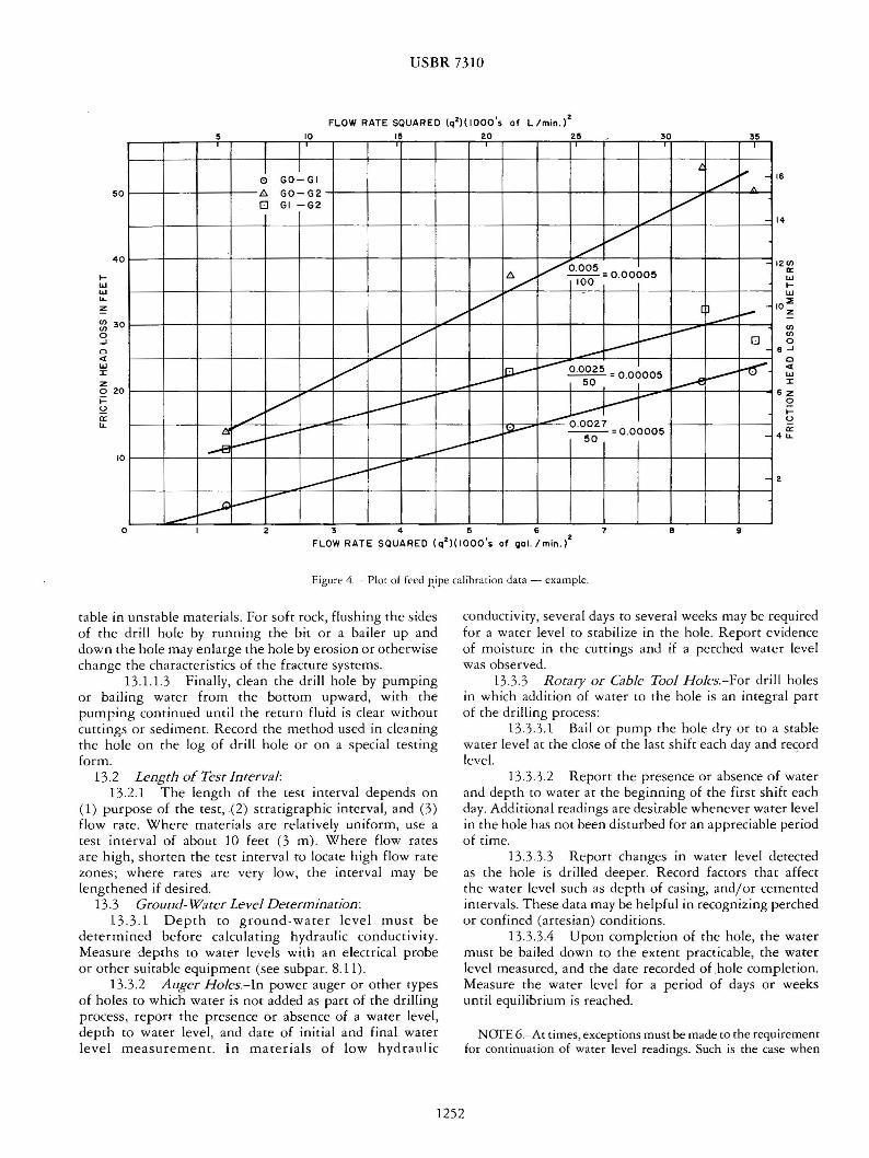
USBR 7310
13428 Afrer pressures are selected based on ground-water conditions and the purpose of the test perform a test at each pressure Usually a 5-cycle procedure is used three increas ing steps to the maximum pressure and then two decreasing steps to the starting pressure This cycling allows a more derailed evaluation of rest results than testing at a single pressure and commonly allows extrapolation to ascertain at what pressures the following may occur (1) laminar flow (2) turbulent flow (3) dilation of fractures ( 4) washouts (5) void filling or (6) hydraulic fracturing However the equations normally used to ca lculate hydraulic conductivity are based on laminar flow conditions
NOfE 9-ln some insrances on ly a single water pressure test at a given interval in the drill ho le may be required For example if geologic conditions are known and there is no need ro perform the seeps in subparagraphs 13422 through 13426 a single value of hydraulic conductivity with a relatively low application of pressure may suffice
13429 During each test continue pumping water to the test interval at the required pressure until the flow rate becomes stable As a general guide maintain flow rares during three or more 5-minute intervals during which l-minute readings of flow are made and recorded In tests above the water table water should be applied to the test interval until the flow rate stabilizes before starting the 5-minuce measurement intervals Where tests are below the water table flow rates usually stabilize faster than for the tests above the water table and the time period before the 5-minure test intervals may be shorter These rime periods may need to be varied particularly when rests to determine grouting requirements are made
134210 Determine and record the presence of back pressure and decay of holding pressure Afrer the rest deflate the packer and remove it from the drill hole
134211 Advance the drill hole and if necessary the casing repeat the procedure in subparagraphs 13423 through 134210 until the required depth of drill hole is reached When casing is used in a drill hole always set the packer in the material below the casing
1343 If the hole will stay open without casing it can be drilled to final depth and after cleaning the hole hydraulic conductivity rests can be performed from the bottom of the hole upward using straddle (double) packers Although a single packer can be used to test the bottom interval of the hole starting at the bottom with double packers will cause loss of borehole testing of only about the length of the bottom packer and will save one complete trip in and out of the hole with the drill string assembly co change the packers After the test for the bottom interval is completed straddle packers are used for successive test intervals up the drill hole See subparagraph 1342 where caving or other hole conditions will not allow this procedure
135 Gra vity Tests 135 1 Constant-head gravity tests are usually
performed without packers above or below the water table with drill holes of N-size or larger (see fig 2 derail D)
This type of test is often made in reasonably stable-walled drill ho les up to 25 feet (76 m) depth where water pressure at the test interval needs to be kept low The test is usually performed in successive 5- or 10-foot (l5- or 3-m) intervals as the drill hole is advanced The upper end of each test interval is normally determined by the bottom depth of tightly reamed or driven casing If the casing is not believed
middotto be tight appropriate entries should be recorded on the log form If the wall of the drill hole is stable the test can be performed in the unsupported hole If the wall needs to be supported use a well screen (see subpar 114 for calibration) inserted through the casing It may be necessary to ream or drive the casing to the bottom of the interval set the screen and then pull back the casing to expose the screen Afrer the test the screen is removed and the casing reamed or driven to the bottom of the hole
NOfE lO-Clean coarse sa nd or fine gravel backfill (see subpar 92) may be used instead of a well scree n Ream or drive rhe casing ro the borrom of the inrerval dean ir our and add rhe backfill as rhe rnsing is pulled back ro expose rhe resr interva l Record use of rhis procedure on the log form
l 35l l If the drill hole is self-supporting clean and prepare it in rhe normal n1anner (see subpar 13l)
l35 l2 If the drill hole is not self-supporting lower the well screen and casing into the hole
135 l3 For test intervals above the water table maintain a constant head of water _within 02 foot (60 mm)] at the top of the test interval by injecting water through a small diameter rube extending below the water level maintained during the test For rest intervals below the water table or influenced by artesian conditions maintain a constant head a short distance above the measured static water level
Monitor the water level with a water-level indicato r If the water-level indicator is inserted in a small diameter pipe in the casing the wave or ripple action on the water surface will be dampened and permit more accurate watershylevel measurements
NOfE l l-When rhe flow rare is very low rhe consranr wa rer level c1n be maintained by pouring warer in rhe hole from a graduated container
135 l4 Record the flow rate at wne intervals until a constanc flow rare is reached
135 l5 Repeat the procedure of subparagraphs 135 l3 and 135 14 at one or more different water levels
13516 This rest is essentially the same as desigshynation USBR 7300 (see also L3] p 74) the instructions in USBR 7300 for performing the rest and calculating hydraulic conductivity apply to this procedure also
14 Calculations
14 l For pressure or constant gravity head hydraulic conductivity rests calculace the hydraulic conductivity of
1254
USBR 7310
rhe soil or rock by rhe following equation (expressed m consisrent unirs) [4]
k = ~ In ~ where L ~ lOr (2)
or
k = ~ sinh-1 r where lOr~ L ~ r (3)
where k = hydraulic conducrivity fryr or cms q = consrant race of flow into che rest interval
ft3yr or cm3s L = length of the test interval ft or cm
H = differential head of wacer ac rest interval fr or cm
r= radius of the borehole ft or cm In= natural logarithm loge
inv~rse hyperbolic sin~ smh- 1 x In (x + -yx2 + 1)
142 An example calculation for a single packer test _ in the botrom of a borehole belovt the wacer table follows
Example assume
r = 18 in or 015 ft= 46 cm q - 22 galmin or 83 Lmin q = 15 X 10 ft3yr = 140 cm3s L 30 ft = 91 cm
Hg gravity = disrance from ground-water level co pressure gauge = 102 ft = 311 cm
Hp pressure 5 lbf in2 X 231 ftwater (lbf in2)
116 ft = 3 54 cm of water H = Hg+ Hp= 218 ft= 664 cm
~ = ~lo = 20 hence use equation (2) 5 k = _9_ In]
2rrLH r k = 15 X 10 ft3 yr In 30 ft
2rr (30 ft) 218 ft 015 ft k = 11X103 ftyr = 11 X lQ-3 cms
NafE 12-These equations are most applicable and reliable where the length of test interval is at lease 5 r and the interval is below che water table The equations are based on laminar flow of fluid through porous media Flow races high enough co cause turbulent flow invalidate the results in all types of material In fractured material the calculated value should be considered an apparent hydraulic conductivity even under laminar flow conditions
143 For pressure resrs when rhe resr interval is below the water table H is the distance from rhe water table to the elevation of che pressure gauge plus applied pressure converted to linear units of water head
Where the rest interval is above the water table His rhe distance from rhe midpoint of the isolated rest interval to che elevation of the pressure gauge plus the applied pressure converted to linear units of water head
For gravity rests above che water table H is che distance between che boccom of the tesc interval and che water level maintained during the test
For gravity rests below the water cable His che distance between the pretest stabilized wacer level in the drill hole and the water level maintained during the rest
144 If chere is artesian pressure an additional pressure muse be applied to overcome che artesian pressure co provide an effective rest pressure For example if there is an artesian pressure of 5 lbfin2 (34 kPa) ac che pressure gauge 15 lbfin2 (103 kPa) could be applied chen che effecrive pressure would be 15 lbfin2 minus 5 lbfin2 which equals 10 lbfin2 (69 kPa)
145 The calculations can be done conveniently by (1) a nomograph [12] (2) a hand calculator with che proper functions or (3) a com purer For repeared tests ic is convenient to prepare a table for one or more diameter drill holes and lengths of resc intervals and combine che terms on che right side of the equations other than q and H into a coefficient
NafE 13-The lugeon (lugeon unit lugeon coefficient) [ 13 14 15 16] has been used as an index of hydraulic conductivity in connection with cyclic rests and for grouting purposes
15 Report
151 Record field test data on a daily driller s report and or on rhe log of the drill hole or on a special reporting form designed for the specific project Record the following
1511 Log of the drill hole 1512 Elevations of the ground surface the water
cable and che top and bortom of the rest interval 1513 Diameter of the drill hole at test interval 1514 Method of cleaning the drill hole 1515 Size of the feed pipe and any well screen 1516 Water pressure andor gravity head and flow
rare for each rime interval 1517 Tora[ amount of warer used per resr 1518 Average temperature of ground warer and
water used in the rest 1519 Packer inflation pressures 1511 Capacity of pump supplying water to the
rest interval 15111 All head loss calibrarion dara 15112 Nore any comments considered necessary to
help evaluate che rest results
15 References
[ l] Permeability Tests Using Drill Holes and Wells Bureau of Reclamation Geology Report No G-97 Denver ColoradoJanuary 3 1951
[2] Ground Warer Manual lst ed rev reprint Bureau of Reclamation US Government Printing Office Washington DC 1981
1255
USBR 7310
[3] Drainage Manual lsc ed 2d princ Bureau of Reclamacion U S Governmenc Princing Office Washingcon DC 1981 1984
[4] Zangar Carl N Theory and Problems of Water Percolation Engineering Monograph No 8 Bureau of Reclamation Denver Colorado 1953
[5] Drill Hole Water Tests Technical lnstructionsshyProvisional Engineering Geology Bureau of Reclamation July 1970 (unpublished)
[6] Glossary of Geology 2d ed American Geological lnscitute Falls Church Virginia 1980
[7] Haccher R C High Pressure Inflacable Packer with Pneumatic Piezometer Bureau of Reclamation Reporc GR-10-75 Denver Colorado October 1975
[8] Bennett R D and R F Anderson New Pressure Test for Determining Coefficient of Permeability of Rock Masses Technical Reporc GL-82-3 US Army Engineer Waterways Experiment Station Vicksburg Mississippi 1982
[9] Ground Water and Wells A Reference Book for the Water-well Industry 1st ed published by Edward E Johnson Inc Saint Paul Minnesota 1966
[10] Drillers Safety Manual 1st ed reprint Bureau of Reclamation Denver Colorado 1982
[11] Acker W L III Basic Procedures for Soil Sampling and Core Drilling published by the Acker Drilling Company Scranton Pennsylvania 1974
[12] Underground Mining Methods Handbook No 580 W-88 Society of Mining Engineers Littlecon Colorado p 62 1982
[13] Lugeon M Barrages et Geologie Dunod Paris 1933
[14] Houlsby A C Routine Interpretation of the Lugeon Water-Test Quarterly Journal Engineering Geology vol 9 pp 303-313 1976
[15] Heitfeld K H and L Krapp The Problem of Water Permeability in Dam Geology Bull International Association of Engineering Geology No 23 pp 79-83 1981
[16] Pearson R and M S Money Improvements in the Lugeon or Packer Permeability Test Quarcerly Journal Engineering Geology vol 10 the Netherlands pp 221shy239 1977
1256
USBR 7310
APPENDIX
XL PROCEDURE USING A PNEUMATIC PIEZOMETER WITH TWO PACKERS ISOLATING THE TEST INTERVAL
Xl l Equipment Assembly (Refer to figs Xll and X l2) -A complete straddle packer unit is assembled as follows
X 11 l Co nnect a predetermined length of perforated injection (feed) pipe to the lower packer (The length of perforated pipe is determined by the thickness of the zone to be rested) Connect the inflation tubing to the lower packer and lower the sliding head end of the packer into the drill hole (See subpar l l l216 for calibration of packers)
Xl l2 Clamp the top of the perforated injection pipe at the hole collar and connecr the upper packer with the sliding head already down the hole
Xl l3 Provide approximately 12 inches (300 mm) of slack in the inflation tubing between the two packers to allow for retraction of the upper packer sliding head Connecr the tubing to the upper packer
Xl l4 Install the pneumatic piezometer piezomerer tubing packer inflation tubing and sealed lengths of injecrion pipe to the head adaptor
X ll5 Lower the entire unit into the drill hole adding lengths of sealed injection pipe as necessary to reach the
( Storoqf Settling ton
interval to be tested As the unit 1s lowered che packer inflation cubing and che piezomecer tubing is unreeled into che hole and caped to che sealed injection pipe at approximately 10-fooc intervals
Xll6 Upon reaching the rest depth lock both the inflation cubing reel and rhe piezomecer cubing reel connecr the inflation tubing by quick-connecr couplings co a nitrogen or compressed air boccie equipped with a high pressure regulator connecr the piezomecer cubing by quick-connect couplings co the readout box and connect the injection pipe co the water pressure source The cesc is now ready to begin
Xl2 Test Procedure
X 12 l After the unit has been lowered to the rest interval and before infacing the packers any water head above the cesc interval must be determined This head will sho w as pressure on the pneumatic piezomecer gauge and can be verified by running a water level indicator into che hole to measure the deprh co the water cable The piezometer will register water pressure chat can be converted to head of water This water head should be
Compressed 01r or nitrogen bot tie Regulator_
Poc~er air lin e- I
P1nometer ln1ec t1on oioe head adaptor
Lo er ooc~er inflation tubmr
Figure X 1 1 - Schematic arrongemem of drill hole packer and pressure monimring equipment 801-0-180
1257
USBR 7310
------=--From compressed air or nitrogen boltle
From piezometer
_To
PRESSURE READOUT BOX
Packer inflation tubing From wafer source From air or Water injection pipe ring seals
PIEZOMETER TUBING REEL
Pressure seals Wire reinforced rubber gland clomps
nitrogen ~~i==-=~==t~f=lil~~~jii~9ll~~~~~sect9ll~sect~sectsect~~~sectl~iilf~f--- To per for o t e d ~~~ze=zzzoCzzzze=zzze=plusmnzz~EZio~~~~21p~
To pressuresource~~~~~~~~~~~~~~~readout box
Piezometer
~~~~~~~~~~~~~~~~---
Inflation chamber Floating packer head Packer inflation lubing
UPPER DRILL HOLE PACKER AND PRESSURE MONITORING EQUIPMENT FOR N X HOLE
Figure X 12 - Upper Jrill hole packer anJ pressure monitoring equipment for NX hole
used to determine the minimum inflation pressure to be applied co the packers by the following equation
SH+ PP+ PE = minimum inflation pressure
where SH = static pressure at the midpoint elevation of the
test interval lbf in2 or kPa PP = gauge pressure to be maintained during the test
lbfin2 or kPa PE = pressure needed to expand packer to hole
diameter as determined before insertion in the drill hole by expanding the packer in a length of pipe having a diameter similar to the hole diameter lbfin 2 or kPa
Inflation pressure gauge is in units of lbf in2 (kPa) The static water level measured before the packers are
inflated might be a composite water level (see subpar 1334)
Xl22 Inflate the packers and determine water head for the rest interval This is the static head to be used for calculation of hydraulic conductivity If rhe static head is significantly different from the composite measured
before the packers were inflated recalculation of packer inflation pressure may be required The final packer inflation pressure should be the lowest practical pressure to seal the test interval against the maximum injection pressure to avoid fracturing of the material being tested
Xl2 3 After the inflation pressures have been determined deflate the packers fill and flush the system with water until all entrapped air has been removed This is accomplished by filling the injection pipe under a gravity head and leaving the air-release valve open ar the top of the injection pipe tee at an elevation higher than the injection hose The valve must remain open until all air has been removed and water runs freely indicating a filled system At this point water is flowing around the deflated packer system and is completely filling the annulus between the drillhole and the packers In the case of an interval with a high injection rate it may be necessary to keep the air valve closed to keep from entraining air into the test interval
X 124 Close the air release valve at the top of the injection pipe and slowly inflate the packers to the predetermined inflation pressure
Xl2 5 Lock in the inflation pressure by closing the pressure valve in the packer cubing If the pressure gauge
1258
USBR 7310
on the closed system remains steady it verifies a sealed system At this point water injecced under gravity head approaches a constant flow rate
X 126 Record the piezometer pressure after packer inflation For an interval of very low injection rate this is equal to che height of the injeccion standpipe plus che pressure recorded at the hole collar gauge For a test interval with a high injection rate the readout would show the same value less any friction from water flow through the injeccion pipe
X 127 Proceed with the test by applying the selected pressures ac the test interval and moniroring the flow rate and pressure on the pneumatic piezometer
X 128 To accurately compute hydraulic conduetivity rhe down-hole pressure muse remain constant A zone with a high injection rate must be monirored more closely than a zone with a small injection rate and adjustments made to hold the down-hole pressure constant To accomplish
this che injeccion pressure shown on che collar gauge must be adjusted in order co maintain che down-hole pressure constant
NOfE X 1-For example a pressure srage is scarred with the collar gauge reading 35 lbfin2 (241 kPa) and the down-hole piezomerer reading 200 lbf in2 ( 1380 kPa) As rhe flow increases rhe down -hole pressure may drop to 150 lbfin2 (1034 kPa) because fricrion loss in the injection pipe and the collar gauge would have to be adjusted to bring the down-hole pressure gauge back up co 200 lbfin2bull When the flow decreases from a fast to a slow rare the collar gauge pressure would have to be decreased
Xl29 The cesc is completed following one or more stages of pressure increases and pressure decreases Following the last stage deflate the packers and close the injection line The system is now ready to move to the next test interval for repetition of this procedure
1259
Methods Note
A Computer Program for Flow-Log Analysis of Single Holes (FLASH) by Frederick D Day-Lewis1 Carole D Johnson2 Frederick L Paillet3 and Keith J Halford4
Abstract A new computer program FLASH (Flow-Log Analysis of Single Holes) is presented for the analysis of
borehole vertical flow logs The code is based on an analytical solution for steady-state multilayer radial flow to a borehole The code includes options for (1) discrete fractures and (2) multilayer aquifers Given vertical flow profiles collected under both ambient and stressed (pumping or injection) conditions the user can estimate fracture (or layer) transmissivities and far-field hydraulic heads FLASH is coded in Microsoft Excel5 with Visual Basic for Applications routines The code supports manual and automated model calibration
Introduction Flowmeters provide means to infer the flow into or
out of boreholes connected to transmissive aquifer units or fractures In the past the relative inaccuracy and difficult operating procedures for spinner flowmeters limited the use of borehole flow measurements With the advent of heat-pulse (Paillet et al 1996) and electromagnetic (Molz et al 1994) instruments measurements of vertical flow as small as 005 Lmin became practicable and borehole flowmeter logging is becoming routine New modeling and analysis tools are needed to achieve the full potential of these measurements
1Corresponding author US Geological Survey Office of Groundwater Branch of Geophysics 11 Sherman Place Unit 5015 Storrs CT 06269 (860) 487-7402 ext 21 fax (860) 487-8802 daylewisusgsgov
2US Geological Survey Office of Groundwater Branch of Geophysics 11 Sherman Place Unit 5015 Storrs CT 06269
3Office of Groundwater Branch of Geophysics (Emeritus) US Geological Survey 11 Sherman Place Unit 5015 Storrs CT 06269
4US Geological Survey Nevada Water Science Center 2730 N Deer Run Rd Carson City NV 89703
5Any use of trade product or firm names is for descriptive purposes only and does not imply endorsement by the US government
Received April 2010 accepted December 2010 copy 2011 The Author(s) Ground Water copy 2011 National Ground Water Association doi 101111j1745-6584201100798x
Calibration of a borehole flow model to flowmeter data can produce estimates of transmissivity and heads for one or more flow zones (aquifer layers or fractures) Here we briefly review approaches for analysis of flowmeter logs and introduce a new computer program which supports manual and automated calibration of an analytical borehole flow model
Approach Single-hole flowmeter data can be analyzed to
estimate transmissivity profiles along boreholes and characterize aquifer compartmentalization (Molz et al 1989 Kabala 1994 Paillet 1998) Analysis of single-hole flowmeter data is commonly based on the Thiem Equation (Thiem 1906) which written for confined radial flow from a single flow zone (ie aquifer layer or fracture) to a screened or open well is
2πTi(hw minus hi)Qi = minus (1)
ln(r0rw)
where Qi is the volumetric flow into the well from flow zone i [L3Tminus1] hw and hi are respectively the hydraulic head [L] at the radius of the well rw and at radial distance r0 commonly taken as the radius of influence where heads do not change as a result of pumping in which
926 Vol 49 No 6ndashGROUND WATERndashNovember-December 2011 (pages 926ndash931) NGWAorg
case hi is the connected far-field head for zone i and Ti
is the transmissivity of flow zone i [L2Tminus1] A number of approaches to flowmeter analysis have
been proposed and demonstrated for different sets of assumptions (eg no ambient flow in boreholes) and data requirements (eg flow profiles collected under both ambient and stressed conditions) based either on Equation 1 (Molz et al 1989) or quasi-steady flow approximations (Paillet 1998) We refer the interested reader to Williams et al (2008) for additional background on flowmeter logs and focus the following discussion on the approach of Paillet (1998 2001) which is adapted here
Paillet (1998) formulated flowmeter log analysis as a model-calibration procedure involving flow profiles collected under both ambient and stressed (pumping or injection) conditions Consideration of the two conditions allows for the estimation of the transmissivities and also far-field heads of flow zones The latter is critical for the interpretation of water samples from wells that intersect multiple fractures or layers with different hydraulic head (Johnson et al 2005) Applying Equation 1 to an ambient condition (condition a) and a stressed condition (condition s) gives
factorT total(ha minus h02πTi )w iQa = minus (2)i ln(r0rw) factorT total(hs minus h02πTi )w iQs = minus (3)i ln(r0rw)
where T factor i is the fraction of the boreholersquos transmisshy
sivity contributed by flow zone i [ndash] T total is the total transmissivity of the flow zones intersected by the bore-hole [L2Tminus1] ha hs are the ambient and stressed water w w levels in the well respectively [L] h0 is the far-field head i in flow zone i [L]
For both ambient and stressed conditions the water level in the borehole is assumed to be constant in
time and the water level in the far-field of each zone is assumed to be the natural condition that is hi
0 In a field experiment (Figure 1) rw would be known and the flow rates and water levels in the well would be measured Radius of influence can be inferred experimentally based on head data at observation wells in which case r0 can be constrained during calibration or else it can be approximated (Bear 1979 306) Estimates of transmissivity are not strongly sensitive to the value assumed for r0 because it appears inside the logarithm in Equations 2 and 3 For example a change in r0rw
from 10 to 100 yields a change in the estimated Ti of only a factor of 2 and order-of-magnitude estimates of transmissivity are acceptable for many problems In cases where knowledge of r0 is unavailable but the boreholersquos total transmissivity is known from specific-capacity or slug-test results it is possible to estimate r0 in the calibration procedure We note that the forward model (Equations 2 and 3) produces twice as many independent equations as there are flow zones with an additional equation requiring T factor values to sum to 1 The number of parameters being estimated is twice the number of flow zones (T factor and h0 for all i) plus one parameter for either i i T total 0or r i
Model calibration involves changing the model parameters such that the flows predicted by Equations 2 and 3 match the interpreted flow profiles Following Paillet (1998 2001) calibration is to the interpreted profile and not individual data This formulation allows the user to incorporate additional insight (eg from other logs) to identify the number and locations of flow zones and elimshyinates the need for weighting measurements differently according to variable measurement errors and the spatial distribution of measurements along the borehole
Calibration can be implemented by manual trial-andshyerror or automated using nonlinear regression Whether manual or automated the goal for calibration is to identify the set of parameters that minimize a measure
Figure 1 Schematic of flowmeter experiment in a fractured-rock aquifer with (a) flow-log profiles for ambient (blue) and stressed (dashed red) conditions and conceptual cross sections of flow system for (b) ambient condition and (c) stressed condition In this example two flow zones (fractures) intersect a well Under ambient conditions flow enters the well from fracture 1 and exits from fracture 3 Under pumping conditions flow enters the well from fractures 1 and 2 The far-field head of zone 2 is equal to the ambient water level thus there is no flow tofrom zone 2 under ambient conditions The far-field head of zone 3 is equal to the stressed water level thus there is no flow tofrom zone 3 under pumping conditions
NGWAorg FD Day-Lewis et al GROUND WATER 49 no 6 926ndash931 927
of combined data misfit and model misfit Considerashytion of model misfit criteria commonly referred to as regularization is useful when multiple models can match the data equally well or within measurement errors Here the data misfit is formulated based on squared differshyences between the predicted and interpreted flow profiles such that multiple measurements may be collected in a single borehole interval The model misfit could be forshymulated in different ways but we use criteria based on the differences between the water level in the borehole under ambient conditions and the far-field heads Thus the objective function F consists of two terms (1) the mean squared error (MSE) between interpreted and preshydicted flow profiles with equal weights for all cumulative flows (ambient and stressed) and (2) the sum of squared differences (h) between the boreholersquos water level and far-field heads
n1 2ssim sintmin F = Q minus Qi i n
i=1
n asim aint 2+
Q minus Q
2 + α (hi) (4)i i i=1
subject to constraints
factor factorT ge T for all i andi min
ABS(haw minus h0
i ) le hmax for all i
aintwhere Qi Qi sint are the interpreted flow profiles (ie
cumulative flow above zones) for zone i under ambishyasiment and stressed conditions respectively [L3Tminus1] Qi
ssimQi are the simulated flow profiles (ie cumulative flow above zones) for zone i under ambient and stressed conditions respectively [L3Tminus1] α weights the regushylarization relative to the data misfit [L4Tminus2] T factor ismin
T factorthe user-specified minimum for any flow zone which can ensure nonnegative T factor hmax is the user-specified maximum absolute difference between the ambishyent water level and the far-field head of any flow zone and n is the number of flow zones
Without regularization F reduces to the MSE between simulated and interpreted flows The trade-off parameter α is set by the user with larger values more strongly penalizing large head differences Commonly small α values (less than 0001) are sufficient to obtain good results In selecting α the user should be guided by the goal of regularization which is to identify the ldquosimplestrdquo explanation of the data while minimizing the data misfit
Using FLASH FLASH (Flow-Log Analysis of Single Holes) is writshy
ten in Excel with Visual Basic for Applications (VBA) The spreadsheet includes a toggle (INPUTS worksheet cell A20) to choose between analysis for (1) fractures or fracture zones that intersect a well at discrete locations
and (2) aquifer layers in porous media The first is indishycated for cases where flow profiles are characterized by step increasesdecreases and the second for cases where flow profiles show approximately linear change over each layer Up to 10 fractures or layers can be modeled
The FLASH spreadsheet includes four worksheets INTRODUCTION INPUTS FIELD_DATA and PLOTshyTING INTRODUCTION provides information about the program and input parameters On the INPUTS workshysheet the user enters information about the flow zones transmissivities and heads Note that the user must intershypret flow profiles from the flowmeter data for both the ambient and stressed conditions The flow measurements are entered in FIELD_DATA and the interpreted proshyfiles are entered in INPUTS The interpreted profiles plot as dashed lines the data as points and the simulated proshyfiles as solid lines (Figure 2) Line and marker styles can be modified using standard Excel tools Flows are positive upward and negative downward PLOTTING is used by the program and does not require the userrsquos attention
In the INPUTS worksheet input parameters are entered in the cells with light blue and bright aquamarine backgrounds The former include specifications of the experiment setup (eg borehole diameter and water level) and the latter include calibration parameters Manual calibration is performed by adjusting the values of
ldquoT factorrdquothe cells and ldquohrdquo which are respectively T factor and the difference between the flow zonersquos far-i field head and the ambient water level in the borehole As parameters are adjusted the simulated flow profiles update automatically thus guiding the user toward best-fit parameters The MSE between simulated and observed flows is calculated in cell B36 on the INPUTS worksheet
Although the principle calibration parameters are Ti
factor and h the radius of influence r0 and total transshymissivity T total also are possible calibration parameters as explained above and indicated by aquamarine highshylighting By inspection of Equations 2 and 3 it is not possible to estimate unique values for both radius of influshyence and total transmissivity but only the ratio of total transmissivity divided by ln(r0rw) In general the user will have more information about total transmissivity than radius of influence Total transmissivity is estimated readshyily using an open-hole slug test or specific-capacity test Indeed the drawdown and pumping rate under stressed conditions could serve as data to estimate a total transshymissivity for the borehole In rare cases however the estimated total transmissivity may be considered unrelishyable for example in the presence of ambiguous slug-test data or discrepancy between the volumes over which the slug test and flowmeter analysis measure In such cases it may be useful to allow the T factor values to sum to a value other than 1 FLASH assumes a uniform radius of influence for all flow zones In reality the effective radius of influence may vary between zones according to their transmissivities and distances to boundaries Data to supshyport variable radius of influence however is commonly unavailable furthermore transmissivity estimates are not
928 FD Day-Lewis et al GROUND WATER 49 no 6 926ndash931 NGWAorg
Figure 2 The INPUTS worksheet after execution of the Solver with options ldquoEstimate ROIrdquo and ldquoSolve with regularizationrdquo for example On this worksheet the user enters the well and flow-log specifications and performs model calibration Data (points) and interpreted profiles (dashed lines) Simulated profiles (solid lines) are for an arbitrarily selected starting model
a strong function of the assumed radius of influence as explained previously
Automated model calibration is implemented using the Excel Solver an optimization tool based on a Genshyeralized Reduced Gradient algorithm (Lasdon and Smith 1992) The Solver is invoked using VBA ldquocontrol butshytonsrdquo on the INPUTS worksheet Radio buttons allow for selections of (1) the parameters to be estimated (Estishymate ROI [radius of influence] or Estimate Transmissivshyity) and (2) regularization (Solve without Regularization or Solve with Regularization) Under the option Estimate
T factorROI the Solver estimates the values of i for all i and the single radius of influence Under the option Estimate Transmissivity radius of influence is assumed known the parameters for estimation are T factor for all ii such that total transmissivity is allowed to vary Users are encouraged to perform manual calibration before attemptshying automated calibration Manual calibration provides insight into the sensitivity of flows to parameters and helps to identify a good starting model for automated calshyibration As for any nonlinear optimization the algorithm may get ldquostuckrdquo in local minima and fail to identify the globally optimal parameter values Consideration of mulshytiple starting models is advised Additional information
and the FLASH spreadsheet are available online as noted under Supporting Information at the end of this article
Example FLASH is demonstrated for a simple data set from
a fractured-rock aquifer (Figure 2) Johnson et al (2005) provide additional details for this data set for which additional borehole logs were used to identify fractures and select locations for flow measurements
Under ambient conditions the deeper fractures 1 and 2 experience inflow to the borehole which indicates the far-field heads for each of these fractures is greater than the head in the borehole thus producing upward flow (Figure 1) Under ambient conditions upflowing water exits the borehole at fracture 3 indicating the far-field head is lower than the head in the borehole Under low-rate pumping conditions water continues to enter the borehole at fracture 1 additional water enters at fracture 2 indicating the far-field heads for fractures 1 and 2 are higher than the quasi-steady state open-hole water level under pumping conditions The uppermost fracture (3) no longer shows outflow indicating the far-field head is equal to the pumping water level In this example
NGWAorg FD Day-Lewis et al GROUND WATER 49 no 6 926ndash931 929
fracture 2 has a far-field head similar to the ambient water level in the well and therefore does not result in a substantial change in borehole flow under ambient conditions Similarly fracture 3 has a far-field head similar to the stressed water level in the well and does not produce a measurable change in borehole flow under stressed conditions This field example underscores the importance of collecting both ambient and stressed flow profilesmdashwith only ambient data fracture 2 could not be identified and with only stressed data fracture 3 could not be identified
To induce flow from a given fracture to enter the borehole the h for that fracture must be positive Conversely to induce flow from the borehole to the fracture the h must be negative The rate of flow is determined by the magnitude of a given flow zonersquos h and transmissivity Thus manual calibration entails for each zone (1) adjustment of a h (cells F21F30) to control whether flow enters or exits the borehole from that zone and (2) adjustment of a T factor to control the rate of flow A final solution can be obtained with the manual fit or after a starting model is generated manually the Solver can be applied For the example here automated calibration produces an excellent match to the data (Figure 2) using options ldquoEstimate ROI rdquo and ldquoEstimate with Regularizationrdquo
Discussion and Conclusions We present a new tool to aid in flowmeter log
analysis a computer code named FLASH We follow a model-calibration strategy similar to that of Paillet (1998) with a simple analytical model for borehole flow based on the Thiem Equation (Thiem 1906) which has been used extensively in previous analyses of flowmeter logs It is important to note that FLASH assumes a borehole flow model that neglects head losses in the borehole or across the well screen and these losses are important in some data sets (Zlotnik and Zurbuchen 2003) We also note the limitations inherent to flowmeter methods primarily that they not as sensitive as straddle-packer hydraulic testing Flowmeter methods consistently identify transmissivities within 15 to 2 orders of magnitude of the most transmissive zone in a borehole depending on the resolution of the flowmeter itself (Williams et al 2008) but straddle-packer tests can see features 6 orders of magnitude less transmissive than is possible with flowmeter (Paillet 1998 Day-Lewis et al 2000 Shapiro 2001) Despite the limited resolution of flowmeter measurements flowmeter modeling results can reproduce packer-test estimates to within an order of magnitude and far-field head values determined with flowmeter methods commonly compare well with packer-test results and discrete-interval water-level monitoring (Johnson et al 2005 Williams et al 2008)
FLASH provides a graphical user interface for calshyibration of an analytical borehole flow model and estishymation of flow-zone transmissivities and far-field heads The program supports manual and automated calibration
with and without regularization FLASH is highly cusshytomizable Experienced Excel users may prefer to invoke the Solver outside of FLASHrsquos VBA routines or to use alternative objective functions or regularization criteria or variable weighting for ambient vs stressed flows Future extensions may include tools for analysis of crosshole flowmeter data and evaluation of estimation uncertainty
Acknowledgments This work was supported by the US Environmental
Protection Agency Region 1 the US Geological Survey Groundwater Resources Program and Toxic Substances Hydrology Program The authors are grateful for review comments from Tom Reilly Allen Shapiro Tom Burbey John Williams Roger Morin Landis West and Mary Anderson
Supporting Information Additional Supporting Information may be found in
the online version of this article
Supplemental material available online include (1) the FLASH spreadsheet which also can be downloaded from httpwaterusgsgovogwflash and (2) a README file with information for installation and troubleshooting
Please note Wiley-Blackwell is not responsible for the content or functionality of any supporting information supplied by the authors Any queries (other than missing material) should be directed to the corresponding author for the article
References Bear J 1979 Hydraulics of Groundwater New York McGraw-
Hill Inc Day-Lewis FD PA Hsieh and SM Gorelick 2000 Idenshy
tifying fracture-zone geometry using simulated annealing and hydraulic-connection data Water Resources Research 36 no 7 1707ndash1721
Johnson CD CK Kochiss and CB Dawson 2005 Use of discrete-zone monitoring systems for hydraulic charshyacterization of a fractured-rock aquifer at the Univershysity of Connecticut landfill Storrs Connecticut 1999 to 2002 Water-Resources Investigations Report 03-4338 105 Reston Virginia USGS
Kabala ZJ 1994 Measuring distributions of hydraulic conducshytivity and storativity by the double flowmeter test Water Resources Research 3 685ndash690
Lasdon LS and S Smith 1992 Solving large sparse nonlinear programs using GRG ORSA Journal on Computing 4 no 1 2ndash15
Molz FJ GK Bowman SC Young and WR Waldrop 1994 Borehole flowmetersmdashfield application and data analysis Journal of Hydrology 163 no 3ndash4 347ndash371
Molz FJ RH Morin AE Hess JG Melville and O Guven 1989 The impeller meter for measuring aquifer permeabilshyity variations evaluations and comparison with other tests Water Resources Research 25 no 7 1677ndash1683
Paillet FL 2001 Hydraulic head applications of flow logs in the study of heterogeneous aquifers Ground Water 39 no 5 667ndash675
930 FD Day-Lewis et al GROUND WATER 49 no 6 926ndash931 NGWAorg
Paillet FL 1998 Flow modeling and permeability estimation using borehole flow logs in heterogeneous fractured formashytions Water Resources Research 34 no 5 997ndash1010
Paillet FL RE Crowder and AE Hess 1996 High-resolution flowmeter logging applications with the heat-pulse flowmeter Journal of Environmental and Engineering Geophysics 1 no 1 1ndash14
Shapiro AM 2001 Effective matrix diffusion in kilometer-scale transport in fractured crystalline rock Water Resources Research 37 no 3 507ndash522
Thiem G 1906 Hydologische methoden 56 Leipzig JM Gebhardt
Williams JH 2008 Flow-log analysis for hydraulic characshyterization of selected test wells at the Indian Point Energy Center Buchanan New York Open-File Report 2008-1123 31 Reston Virginia USGS
Zlotnik VA and BR Zurbuchen 2003 Estimation of hydraulic conductivity from borehole flowmeter tests conshysidering head losses Journal of Hydrology 281 no 1ndash2 115ndash128
NGWAorg FD Day-Lewis et al GROUND WATER 49 no 6 926ndash931 931
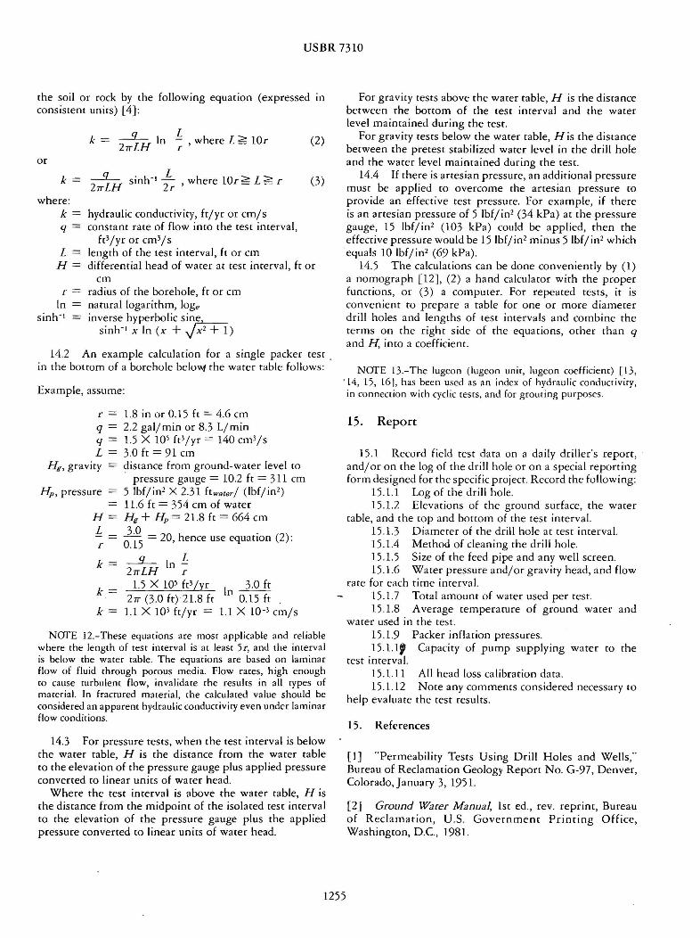
USBR 7310
rhe soil or rock by rhe following equation (expressed m consisrent unirs) [4]
k = ~ In ~ where L ~ lOr (2)
or
k = ~ sinh-1 r where lOr~ L ~ r (3)
where k = hydraulic conducrivity fryr or cms q = consrant race of flow into che rest interval
ft3yr or cm3s L = length of the test interval ft or cm
H = differential head of wacer ac rest interval fr or cm
r= radius of the borehole ft or cm In= natural logarithm loge
inv~rse hyperbolic sin~ smh- 1 x In (x + -yx2 + 1)
142 An example calculation for a single packer test _ in the botrom of a borehole belovt the wacer table follows
Example assume
r = 18 in or 015 ft= 46 cm q - 22 galmin or 83 Lmin q = 15 X 10 ft3yr = 140 cm3s L 30 ft = 91 cm
Hg gravity = disrance from ground-water level co pressure gauge = 102 ft = 311 cm
Hp pressure 5 lbf in2 X 231 ftwater (lbf in2)
116 ft = 3 54 cm of water H = Hg+ Hp= 218 ft= 664 cm
~ = ~lo = 20 hence use equation (2) 5 k = _9_ In]
2rrLH r k = 15 X 10 ft3 yr In 30 ft
2rr (30 ft) 218 ft 015 ft k = 11X103 ftyr = 11 X lQ-3 cms
NafE 12-These equations are most applicable and reliable where the length of test interval is at lease 5 r and the interval is below che water table The equations are based on laminar flow of fluid through porous media Flow races high enough co cause turbulent flow invalidate the results in all types of material In fractured material the calculated value should be considered an apparent hydraulic conductivity even under laminar flow conditions
143 For pressure resrs when rhe resr interval is below the water table H is the distance from rhe water table to the elevation of che pressure gauge plus applied pressure converted to linear units of water head
Where the rest interval is above the water table His rhe distance from rhe midpoint of the isolated rest interval to che elevation of the pressure gauge plus the applied pressure converted to linear units of water head
For gravity rests above che water table H is che distance between che boccom of the tesc interval and che water level maintained during the test
For gravity rests below the water cable His che distance between the pretest stabilized wacer level in the drill hole and the water level maintained during the rest
144 If chere is artesian pressure an additional pressure muse be applied to overcome che artesian pressure co provide an effective rest pressure For example if there is an artesian pressure of 5 lbfin2 (34 kPa) ac che pressure gauge 15 lbfin2 (103 kPa) could be applied chen che effecrive pressure would be 15 lbfin2 minus 5 lbfin2 which equals 10 lbfin2 (69 kPa)
145 The calculations can be done conveniently by (1) a nomograph [12] (2) a hand calculator with che proper functions or (3) a com purer For repeared tests ic is convenient to prepare a table for one or more diameter drill holes and lengths of resc intervals and combine che terms on che right side of the equations other than q and H into a coefficient
NafE 13-The lugeon (lugeon unit lugeon coefficient) [ 13 14 15 16] has been used as an index of hydraulic conductivity in connection with cyclic rests and for grouting purposes
15 Report
151 Record field test data on a daily driller s report and or on rhe log of the drill hole or on a special reporting form designed for the specific project Record the following
1511 Log of the drill hole 1512 Elevations of the ground surface the water
cable and che top and bortom of the rest interval 1513 Diameter of the drill hole at test interval 1514 Method of cleaning the drill hole 1515 Size of the feed pipe and any well screen 1516 Water pressure andor gravity head and flow
rare for each rime interval 1517 Tora[ amount of warer used per resr 1518 Average temperature of ground warer and
water used in the rest 1519 Packer inflation pressures 1511 Capacity of pump supplying water to the
rest interval 15111 All head loss calibrarion dara 15112 Nore any comments considered necessary to
help evaluate che rest results
15 References
[ l] Permeability Tests Using Drill Holes and Wells Bureau of Reclamation Geology Report No G-97 Denver ColoradoJanuary 3 1951
[2] Ground Warer Manual lst ed rev reprint Bureau of Reclamation US Government Printing Office Washington DC 1981
1255
USBR 7310
[3] Drainage Manual lsc ed 2d princ Bureau of Reclamacion U S Governmenc Princing Office Washingcon DC 1981 1984
[4] Zangar Carl N Theory and Problems of Water Percolation Engineering Monograph No 8 Bureau of Reclamation Denver Colorado 1953
[5] Drill Hole Water Tests Technical lnstructionsshyProvisional Engineering Geology Bureau of Reclamation July 1970 (unpublished)
[6] Glossary of Geology 2d ed American Geological lnscitute Falls Church Virginia 1980
[7] Haccher R C High Pressure Inflacable Packer with Pneumatic Piezometer Bureau of Reclamation Reporc GR-10-75 Denver Colorado October 1975
[8] Bennett R D and R F Anderson New Pressure Test for Determining Coefficient of Permeability of Rock Masses Technical Reporc GL-82-3 US Army Engineer Waterways Experiment Station Vicksburg Mississippi 1982
[9] Ground Water and Wells A Reference Book for the Water-well Industry 1st ed published by Edward E Johnson Inc Saint Paul Minnesota 1966
[10] Drillers Safety Manual 1st ed reprint Bureau of Reclamation Denver Colorado 1982
[11] Acker W L III Basic Procedures for Soil Sampling and Core Drilling published by the Acker Drilling Company Scranton Pennsylvania 1974
[12] Underground Mining Methods Handbook No 580 W-88 Society of Mining Engineers Littlecon Colorado p 62 1982
[13] Lugeon M Barrages et Geologie Dunod Paris 1933
[14] Houlsby A C Routine Interpretation of the Lugeon Water-Test Quarterly Journal Engineering Geology vol 9 pp 303-313 1976
[15] Heitfeld K H and L Krapp The Problem of Water Permeability in Dam Geology Bull International Association of Engineering Geology No 23 pp 79-83 1981
[16] Pearson R and M S Money Improvements in the Lugeon or Packer Permeability Test Quarcerly Journal Engineering Geology vol 10 the Netherlands pp 221shy239 1977
1256
USBR 7310
APPENDIX
XL PROCEDURE USING A PNEUMATIC PIEZOMETER WITH TWO PACKERS ISOLATING THE TEST INTERVAL
Xl l Equipment Assembly (Refer to figs Xll and X l2) -A complete straddle packer unit is assembled as follows
X 11 l Co nnect a predetermined length of perforated injection (feed) pipe to the lower packer (The length of perforated pipe is determined by the thickness of the zone to be rested) Connect the inflation tubing to the lower packer and lower the sliding head end of the packer into the drill hole (See subpar l l l216 for calibration of packers)
Xl l2 Clamp the top of the perforated injection pipe at the hole collar and connecr the upper packer with the sliding head already down the hole
Xl l3 Provide approximately 12 inches (300 mm) of slack in the inflation tubing between the two packers to allow for retraction of the upper packer sliding head Connecr the tubing to the upper packer
Xl l4 Install the pneumatic piezometer piezomerer tubing packer inflation tubing and sealed lengths of injecrion pipe to the head adaptor
X ll5 Lower the entire unit into the drill hole adding lengths of sealed injection pipe as necessary to reach the
( Storoqf Settling ton
interval to be tested As the unit 1s lowered che packer inflation cubing and che piezomecer tubing is unreeled into che hole and caped to che sealed injection pipe at approximately 10-fooc intervals
Xll6 Upon reaching the rest depth lock both the inflation cubing reel and rhe piezomecer cubing reel connecr the inflation tubing by quick-connecr couplings co a nitrogen or compressed air boccie equipped with a high pressure regulator connecr the piezomecer cubing by quick-connect couplings co the readout box and connect the injection pipe co the water pressure source The cesc is now ready to begin
Xl2 Test Procedure
X 12 l After the unit has been lowered to the rest interval and before infacing the packers any water head above the cesc interval must be determined This head will sho w as pressure on the pneumatic piezomecer gauge and can be verified by running a water level indicator into che hole to measure the deprh co the water cable The piezometer will register water pressure chat can be converted to head of water This water head should be
Compressed 01r or nitrogen bot tie Regulator_
Poc~er air lin e- I
P1nometer ln1ec t1on oioe head adaptor
Lo er ooc~er inflation tubmr
Figure X 1 1 - Schematic arrongemem of drill hole packer and pressure monimring equipment 801-0-180
1257
USBR 7310
------=--From compressed air or nitrogen boltle
From piezometer
_To
PRESSURE READOUT BOX
Packer inflation tubing From wafer source From air or Water injection pipe ring seals
PIEZOMETER TUBING REEL
Pressure seals Wire reinforced rubber gland clomps
nitrogen ~~i==-=~==t~f=lil~~~jii~9ll~~~~~sect9ll~sect~sectsect~~~sectl~iilf~f--- To per for o t e d ~~~ze=zzzoCzzzze=zzze=plusmnzz~EZio~~~~21p~
To pressuresource~~~~~~~~~~~~~~~readout box
Piezometer
~~~~~~~~~~~~~~~~---
Inflation chamber Floating packer head Packer inflation lubing
UPPER DRILL HOLE PACKER AND PRESSURE MONITORING EQUIPMENT FOR N X HOLE
Figure X 12 - Upper Jrill hole packer anJ pressure monitoring equipment for NX hole
used to determine the minimum inflation pressure to be applied co the packers by the following equation
SH+ PP+ PE = minimum inflation pressure
where SH = static pressure at the midpoint elevation of the
test interval lbf in2 or kPa PP = gauge pressure to be maintained during the test
lbfin2 or kPa PE = pressure needed to expand packer to hole
diameter as determined before insertion in the drill hole by expanding the packer in a length of pipe having a diameter similar to the hole diameter lbfin 2 or kPa
Inflation pressure gauge is in units of lbf in2 (kPa) The static water level measured before the packers are
inflated might be a composite water level (see subpar 1334)
Xl22 Inflate the packers and determine water head for the rest interval This is the static head to be used for calculation of hydraulic conductivity If rhe static head is significantly different from the composite measured
before the packers were inflated recalculation of packer inflation pressure may be required The final packer inflation pressure should be the lowest practical pressure to seal the test interval against the maximum injection pressure to avoid fracturing of the material being tested
Xl2 3 After the inflation pressures have been determined deflate the packers fill and flush the system with water until all entrapped air has been removed This is accomplished by filling the injection pipe under a gravity head and leaving the air-release valve open ar the top of the injection pipe tee at an elevation higher than the injection hose The valve must remain open until all air has been removed and water runs freely indicating a filled system At this point water is flowing around the deflated packer system and is completely filling the annulus between the drillhole and the packers In the case of an interval with a high injection rate it may be necessary to keep the air valve closed to keep from entraining air into the test interval
X 124 Close the air release valve at the top of the injection pipe and slowly inflate the packers to the predetermined inflation pressure
Xl2 5 Lock in the inflation pressure by closing the pressure valve in the packer cubing If the pressure gauge
1258
USBR 7310
on the closed system remains steady it verifies a sealed system At this point water injecced under gravity head approaches a constant flow rate
X 126 Record the piezometer pressure after packer inflation For an interval of very low injection rate this is equal to che height of the injeccion standpipe plus che pressure recorded at the hole collar gauge For a test interval with a high injection rate the readout would show the same value less any friction from water flow through the injeccion pipe
X 127 Proceed with the test by applying the selected pressures ac the test interval and moniroring the flow rate and pressure on the pneumatic piezometer
X 128 To accurately compute hydraulic conduetivity rhe down-hole pressure muse remain constant A zone with a high injection rate must be monirored more closely than a zone with a small injection rate and adjustments made to hold the down-hole pressure constant To accomplish
this che injeccion pressure shown on che collar gauge must be adjusted in order co maintain che down-hole pressure constant
NOfE X 1-For example a pressure srage is scarred with the collar gauge reading 35 lbfin2 (241 kPa) and the down-hole piezomerer reading 200 lbf in2 ( 1380 kPa) As rhe flow increases rhe down -hole pressure may drop to 150 lbfin2 (1034 kPa) because fricrion loss in the injection pipe and the collar gauge would have to be adjusted to bring the down-hole pressure gauge back up co 200 lbfin2bull When the flow decreases from a fast to a slow rare the collar gauge pressure would have to be decreased
Xl29 The cesc is completed following one or more stages of pressure increases and pressure decreases Following the last stage deflate the packers and close the injection line The system is now ready to move to the next test interval for repetition of this procedure
1259
Methods Note
A Computer Program for Flow-Log Analysis of Single Holes (FLASH) by Frederick D Day-Lewis1 Carole D Johnson2 Frederick L Paillet3 and Keith J Halford4
Abstract A new computer program FLASH (Flow-Log Analysis of Single Holes) is presented for the analysis of
borehole vertical flow logs The code is based on an analytical solution for steady-state multilayer radial flow to a borehole The code includes options for (1) discrete fractures and (2) multilayer aquifers Given vertical flow profiles collected under both ambient and stressed (pumping or injection) conditions the user can estimate fracture (or layer) transmissivities and far-field hydraulic heads FLASH is coded in Microsoft Excel5 with Visual Basic for Applications routines The code supports manual and automated model calibration
Introduction Flowmeters provide means to infer the flow into or
out of boreholes connected to transmissive aquifer units or fractures In the past the relative inaccuracy and difficult operating procedures for spinner flowmeters limited the use of borehole flow measurements With the advent of heat-pulse (Paillet et al 1996) and electromagnetic (Molz et al 1994) instruments measurements of vertical flow as small as 005 Lmin became practicable and borehole flowmeter logging is becoming routine New modeling and analysis tools are needed to achieve the full potential of these measurements
1Corresponding author US Geological Survey Office of Groundwater Branch of Geophysics 11 Sherman Place Unit 5015 Storrs CT 06269 (860) 487-7402 ext 21 fax (860) 487-8802 daylewisusgsgov
2US Geological Survey Office of Groundwater Branch of Geophysics 11 Sherman Place Unit 5015 Storrs CT 06269
3Office of Groundwater Branch of Geophysics (Emeritus) US Geological Survey 11 Sherman Place Unit 5015 Storrs CT 06269
4US Geological Survey Nevada Water Science Center 2730 N Deer Run Rd Carson City NV 89703
5Any use of trade product or firm names is for descriptive purposes only and does not imply endorsement by the US government
Received April 2010 accepted December 2010 copy 2011 The Author(s) Ground Water copy 2011 National Ground Water Association doi 101111j1745-6584201100798x
Calibration of a borehole flow model to flowmeter data can produce estimates of transmissivity and heads for one or more flow zones (aquifer layers or fractures) Here we briefly review approaches for analysis of flowmeter logs and introduce a new computer program which supports manual and automated calibration of an analytical borehole flow model
Approach Single-hole flowmeter data can be analyzed to
estimate transmissivity profiles along boreholes and characterize aquifer compartmentalization (Molz et al 1989 Kabala 1994 Paillet 1998) Analysis of single-hole flowmeter data is commonly based on the Thiem Equation (Thiem 1906) which written for confined radial flow from a single flow zone (ie aquifer layer or fracture) to a screened or open well is
2πTi(hw minus hi)Qi = minus (1)
ln(r0rw)
where Qi is the volumetric flow into the well from flow zone i [L3Tminus1] hw and hi are respectively the hydraulic head [L] at the radius of the well rw and at radial distance r0 commonly taken as the radius of influence where heads do not change as a result of pumping in which
926 Vol 49 No 6ndashGROUND WATERndashNovember-December 2011 (pages 926ndash931) NGWAorg
case hi is the connected far-field head for zone i and Ti
is the transmissivity of flow zone i [L2Tminus1] A number of approaches to flowmeter analysis have
been proposed and demonstrated for different sets of assumptions (eg no ambient flow in boreholes) and data requirements (eg flow profiles collected under both ambient and stressed conditions) based either on Equation 1 (Molz et al 1989) or quasi-steady flow approximations (Paillet 1998) We refer the interested reader to Williams et al (2008) for additional background on flowmeter logs and focus the following discussion on the approach of Paillet (1998 2001) which is adapted here
Paillet (1998) formulated flowmeter log analysis as a model-calibration procedure involving flow profiles collected under both ambient and stressed (pumping or injection) conditions Consideration of the two conditions allows for the estimation of the transmissivities and also far-field heads of flow zones The latter is critical for the interpretation of water samples from wells that intersect multiple fractures or layers with different hydraulic head (Johnson et al 2005) Applying Equation 1 to an ambient condition (condition a) and a stressed condition (condition s) gives
factorT total(ha minus h02πTi )w iQa = minus (2)i ln(r0rw) factorT total(hs minus h02πTi )w iQs = minus (3)i ln(r0rw)
where T factor i is the fraction of the boreholersquos transmisshy
sivity contributed by flow zone i [ndash] T total is the total transmissivity of the flow zones intersected by the bore-hole [L2Tminus1] ha hs are the ambient and stressed water w w levels in the well respectively [L] h0 is the far-field head i in flow zone i [L]
For both ambient and stressed conditions the water level in the borehole is assumed to be constant in
time and the water level in the far-field of each zone is assumed to be the natural condition that is hi
0 In a field experiment (Figure 1) rw would be known and the flow rates and water levels in the well would be measured Radius of influence can be inferred experimentally based on head data at observation wells in which case r0 can be constrained during calibration or else it can be approximated (Bear 1979 306) Estimates of transmissivity are not strongly sensitive to the value assumed for r0 because it appears inside the logarithm in Equations 2 and 3 For example a change in r0rw
from 10 to 100 yields a change in the estimated Ti of only a factor of 2 and order-of-magnitude estimates of transmissivity are acceptable for many problems In cases where knowledge of r0 is unavailable but the boreholersquos total transmissivity is known from specific-capacity or slug-test results it is possible to estimate r0 in the calibration procedure We note that the forward model (Equations 2 and 3) produces twice as many independent equations as there are flow zones with an additional equation requiring T factor values to sum to 1 The number of parameters being estimated is twice the number of flow zones (T factor and h0 for all i) plus one parameter for either i i T total 0or r i
Model calibration involves changing the model parameters such that the flows predicted by Equations 2 and 3 match the interpreted flow profiles Following Paillet (1998 2001) calibration is to the interpreted profile and not individual data This formulation allows the user to incorporate additional insight (eg from other logs) to identify the number and locations of flow zones and elimshyinates the need for weighting measurements differently according to variable measurement errors and the spatial distribution of measurements along the borehole
Calibration can be implemented by manual trial-andshyerror or automated using nonlinear regression Whether manual or automated the goal for calibration is to identify the set of parameters that minimize a measure
Figure 1 Schematic of flowmeter experiment in a fractured-rock aquifer with (a) flow-log profiles for ambient (blue) and stressed (dashed red) conditions and conceptual cross sections of flow system for (b) ambient condition and (c) stressed condition In this example two flow zones (fractures) intersect a well Under ambient conditions flow enters the well from fracture 1 and exits from fracture 3 Under pumping conditions flow enters the well from fractures 1 and 2 The far-field head of zone 2 is equal to the ambient water level thus there is no flow tofrom zone 2 under ambient conditions The far-field head of zone 3 is equal to the stressed water level thus there is no flow tofrom zone 3 under pumping conditions
NGWAorg FD Day-Lewis et al GROUND WATER 49 no 6 926ndash931 927
of combined data misfit and model misfit Considerashytion of model misfit criteria commonly referred to as regularization is useful when multiple models can match the data equally well or within measurement errors Here the data misfit is formulated based on squared differshyences between the predicted and interpreted flow profiles such that multiple measurements may be collected in a single borehole interval The model misfit could be forshymulated in different ways but we use criteria based on the differences between the water level in the borehole under ambient conditions and the far-field heads Thus the objective function F consists of two terms (1) the mean squared error (MSE) between interpreted and preshydicted flow profiles with equal weights for all cumulative flows (ambient and stressed) and (2) the sum of squared differences (h) between the boreholersquos water level and far-field heads
n1 2ssim sintmin F = Q minus Qi i n
i=1
n asim aint 2+
Q minus Q
2 + α (hi) (4)i i i=1
subject to constraints
factor factorT ge T for all i andi min
ABS(haw minus h0
i ) le hmax for all i
aintwhere Qi Qi sint are the interpreted flow profiles (ie
cumulative flow above zones) for zone i under ambishyasiment and stressed conditions respectively [L3Tminus1] Qi
ssimQi are the simulated flow profiles (ie cumulative flow above zones) for zone i under ambient and stressed conditions respectively [L3Tminus1] α weights the regushylarization relative to the data misfit [L4Tminus2] T factor ismin
T factorthe user-specified minimum for any flow zone which can ensure nonnegative T factor hmax is the user-specified maximum absolute difference between the ambishyent water level and the far-field head of any flow zone and n is the number of flow zones
Without regularization F reduces to the MSE between simulated and interpreted flows The trade-off parameter α is set by the user with larger values more strongly penalizing large head differences Commonly small α values (less than 0001) are sufficient to obtain good results In selecting α the user should be guided by the goal of regularization which is to identify the ldquosimplestrdquo explanation of the data while minimizing the data misfit
Using FLASH FLASH (Flow-Log Analysis of Single Holes) is writshy
ten in Excel with Visual Basic for Applications (VBA) The spreadsheet includes a toggle (INPUTS worksheet cell A20) to choose between analysis for (1) fractures or fracture zones that intersect a well at discrete locations
and (2) aquifer layers in porous media The first is indishycated for cases where flow profiles are characterized by step increasesdecreases and the second for cases where flow profiles show approximately linear change over each layer Up to 10 fractures or layers can be modeled
The FLASH spreadsheet includes four worksheets INTRODUCTION INPUTS FIELD_DATA and PLOTshyTING INTRODUCTION provides information about the program and input parameters On the INPUTS workshysheet the user enters information about the flow zones transmissivities and heads Note that the user must intershypret flow profiles from the flowmeter data for both the ambient and stressed conditions The flow measurements are entered in FIELD_DATA and the interpreted proshyfiles are entered in INPUTS The interpreted profiles plot as dashed lines the data as points and the simulated proshyfiles as solid lines (Figure 2) Line and marker styles can be modified using standard Excel tools Flows are positive upward and negative downward PLOTTING is used by the program and does not require the userrsquos attention
In the INPUTS worksheet input parameters are entered in the cells with light blue and bright aquamarine backgrounds The former include specifications of the experiment setup (eg borehole diameter and water level) and the latter include calibration parameters Manual calibration is performed by adjusting the values of
ldquoT factorrdquothe cells and ldquohrdquo which are respectively T factor and the difference between the flow zonersquos far-i field head and the ambient water level in the borehole As parameters are adjusted the simulated flow profiles update automatically thus guiding the user toward best-fit parameters The MSE between simulated and observed flows is calculated in cell B36 on the INPUTS worksheet
Although the principle calibration parameters are Ti
factor and h the radius of influence r0 and total transshymissivity T total also are possible calibration parameters as explained above and indicated by aquamarine highshylighting By inspection of Equations 2 and 3 it is not possible to estimate unique values for both radius of influshyence and total transmissivity but only the ratio of total transmissivity divided by ln(r0rw) In general the user will have more information about total transmissivity than radius of influence Total transmissivity is estimated readshyily using an open-hole slug test or specific-capacity test Indeed the drawdown and pumping rate under stressed conditions could serve as data to estimate a total transshymissivity for the borehole In rare cases however the estimated total transmissivity may be considered unrelishyable for example in the presence of ambiguous slug-test data or discrepancy between the volumes over which the slug test and flowmeter analysis measure In such cases it may be useful to allow the T factor values to sum to a value other than 1 FLASH assumes a uniform radius of influence for all flow zones In reality the effective radius of influence may vary between zones according to their transmissivities and distances to boundaries Data to supshyport variable radius of influence however is commonly unavailable furthermore transmissivity estimates are not
928 FD Day-Lewis et al GROUND WATER 49 no 6 926ndash931 NGWAorg
Figure 2 The INPUTS worksheet after execution of the Solver with options ldquoEstimate ROIrdquo and ldquoSolve with regularizationrdquo for example On this worksheet the user enters the well and flow-log specifications and performs model calibration Data (points) and interpreted profiles (dashed lines) Simulated profiles (solid lines) are for an arbitrarily selected starting model
a strong function of the assumed radius of influence as explained previously
Automated model calibration is implemented using the Excel Solver an optimization tool based on a Genshyeralized Reduced Gradient algorithm (Lasdon and Smith 1992) The Solver is invoked using VBA ldquocontrol butshytonsrdquo on the INPUTS worksheet Radio buttons allow for selections of (1) the parameters to be estimated (Estishymate ROI [radius of influence] or Estimate Transmissivshyity) and (2) regularization (Solve without Regularization or Solve with Regularization) Under the option Estimate
T factorROI the Solver estimates the values of i for all i and the single radius of influence Under the option Estimate Transmissivity radius of influence is assumed known the parameters for estimation are T factor for all ii such that total transmissivity is allowed to vary Users are encouraged to perform manual calibration before attemptshying automated calibration Manual calibration provides insight into the sensitivity of flows to parameters and helps to identify a good starting model for automated calshyibration As for any nonlinear optimization the algorithm may get ldquostuckrdquo in local minima and fail to identify the globally optimal parameter values Consideration of mulshytiple starting models is advised Additional information
and the FLASH spreadsheet are available online as noted under Supporting Information at the end of this article
Example FLASH is demonstrated for a simple data set from
a fractured-rock aquifer (Figure 2) Johnson et al (2005) provide additional details for this data set for which additional borehole logs were used to identify fractures and select locations for flow measurements
Under ambient conditions the deeper fractures 1 and 2 experience inflow to the borehole which indicates the far-field heads for each of these fractures is greater than the head in the borehole thus producing upward flow (Figure 1) Under ambient conditions upflowing water exits the borehole at fracture 3 indicating the far-field head is lower than the head in the borehole Under low-rate pumping conditions water continues to enter the borehole at fracture 1 additional water enters at fracture 2 indicating the far-field heads for fractures 1 and 2 are higher than the quasi-steady state open-hole water level under pumping conditions The uppermost fracture (3) no longer shows outflow indicating the far-field head is equal to the pumping water level In this example
NGWAorg FD Day-Lewis et al GROUND WATER 49 no 6 926ndash931 929
fracture 2 has a far-field head similar to the ambient water level in the well and therefore does not result in a substantial change in borehole flow under ambient conditions Similarly fracture 3 has a far-field head similar to the stressed water level in the well and does not produce a measurable change in borehole flow under stressed conditions This field example underscores the importance of collecting both ambient and stressed flow profilesmdashwith only ambient data fracture 2 could not be identified and with only stressed data fracture 3 could not be identified
To induce flow from a given fracture to enter the borehole the h for that fracture must be positive Conversely to induce flow from the borehole to the fracture the h must be negative The rate of flow is determined by the magnitude of a given flow zonersquos h and transmissivity Thus manual calibration entails for each zone (1) adjustment of a h (cells F21F30) to control whether flow enters or exits the borehole from that zone and (2) adjustment of a T factor to control the rate of flow A final solution can be obtained with the manual fit or after a starting model is generated manually the Solver can be applied For the example here automated calibration produces an excellent match to the data (Figure 2) using options ldquoEstimate ROI rdquo and ldquoEstimate with Regularizationrdquo
Discussion and Conclusions We present a new tool to aid in flowmeter log
analysis a computer code named FLASH We follow a model-calibration strategy similar to that of Paillet (1998) with a simple analytical model for borehole flow based on the Thiem Equation (Thiem 1906) which has been used extensively in previous analyses of flowmeter logs It is important to note that FLASH assumes a borehole flow model that neglects head losses in the borehole or across the well screen and these losses are important in some data sets (Zlotnik and Zurbuchen 2003) We also note the limitations inherent to flowmeter methods primarily that they not as sensitive as straddle-packer hydraulic testing Flowmeter methods consistently identify transmissivities within 15 to 2 orders of magnitude of the most transmissive zone in a borehole depending on the resolution of the flowmeter itself (Williams et al 2008) but straddle-packer tests can see features 6 orders of magnitude less transmissive than is possible with flowmeter (Paillet 1998 Day-Lewis et al 2000 Shapiro 2001) Despite the limited resolution of flowmeter measurements flowmeter modeling results can reproduce packer-test estimates to within an order of magnitude and far-field head values determined with flowmeter methods commonly compare well with packer-test results and discrete-interval water-level monitoring (Johnson et al 2005 Williams et al 2008)
FLASH provides a graphical user interface for calshyibration of an analytical borehole flow model and estishymation of flow-zone transmissivities and far-field heads The program supports manual and automated calibration
with and without regularization FLASH is highly cusshytomizable Experienced Excel users may prefer to invoke the Solver outside of FLASHrsquos VBA routines or to use alternative objective functions or regularization criteria or variable weighting for ambient vs stressed flows Future extensions may include tools for analysis of crosshole flowmeter data and evaluation of estimation uncertainty
Acknowledgments This work was supported by the US Environmental
Protection Agency Region 1 the US Geological Survey Groundwater Resources Program and Toxic Substances Hydrology Program The authors are grateful for review comments from Tom Reilly Allen Shapiro Tom Burbey John Williams Roger Morin Landis West and Mary Anderson
Supporting Information Additional Supporting Information may be found in
the online version of this article
Supplemental material available online include (1) the FLASH spreadsheet which also can be downloaded from httpwaterusgsgovogwflash and (2) a README file with information for installation and troubleshooting
Please note Wiley-Blackwell is not responsible for the content or functionality of any supporting information supplied by the authors Any queries (other than missing material) should be directed to the corresponding author for the article
References Bear J 1979 Hydraulics of Groundwater New York McGraw-
Hill Inc Day-Lewis FD PA Hsieh and SM Gorelick 2000 Idenshy
tifying fracture-zone geometry using simulated annealing and hydraulic-connection data Water Resources Research 36 no 7 1707ndash1721
Johnson CD CK Kochiss and CB Dawson 2005 Use of discrete-zone monitoring systems for hydraulic charshyacterization of a fractured-rock aquifer at the Univershysity of Connecticut landfill Storrs Connecticut 1999 to 2002 Water-Resources Investigations Report 03-4338 105 Reston Virginia USGS
Kabala ZJ 1994 Measuring distributions of hydraulic conducshytivity and storativity by the double flowmeter test Water Resources Research 3 685ndash690
Lasdon LS and S Smith 1992 Solving large sparse nonlinear programs using GRG ORSA Journal on Computing 4 no 1 2ndash15
Molz FJ GK Bowman SC Young and WR Waldrop 1994 Borehole flowmetersmdashfield application and data analysis Journal of Hydrology 163 no 3ndash4 347ndash371
Molz FJ RH Morin AE Hess JG Melville and O Guven 1989 The impeller meter for measuring aquifer permeabilshyity variations evaluations and comparison with other tests Water Resources Research 25 no 7 1677ndash1683
Paillet FL 2001 Hydraulic head applications of flow logs in the study of heterogeneous aquifers Ground Water 39 no 5 667ndash675
930 FD Day-Lewis et al GROUND WATER 49 no 6 926ndash931 NGWAorg
Paillet FL 1998 Flow modeling and permeability estimation using borehole flow logs in heterogeneous fractured formashytions Water Resources Research 34 no 5 997ndash1010
Paillet FL RE Crowder and AE Hess 1996 High-resolution flowmeter logging applications with the heat-pulse flowmeter Journal of Environmental and Engineering Geophysics 1 no 1 1ndash14
Shapiro AM 2001 Effective matrix diffusion in kilometer-scale transport in fractured crystalline rock Water Resources Research 37 no 3 507ndash522
Thiem G 1906 Hydologische methoden 56 Leipzig JM Gebhardt
Williams JH 2008 Flow-log analysis for hydraulic characshyterization of selected test wells at the Indian Point Energy Center Buchanan New York Open-File Report 2008-1123 31 Reston Virginia USGS
Zlotnik VA and BR Zurbuchen 2003 Estimation of hydraulic conductivity from borehole flowmeter tests conshysidering head losses Journal of Hydrology 281 no 1ndash2 115ndash128
NGWAorg FD Day-Lewis et al GROUND WATER 49 no 6 926ndash931 931
USBR 7310
[3] Drainage Manual lsc ed 2d princ Bureau of Reclamacion U S Governmenc Princing Office Washingcon DC 1981 1984
[4] Zangar Carl N Theory and Problems of Water Percolation Engineering Monograph No 8 Bureau of Reclamation Denver Colorado 1953
[5] Drill Hole Water Tests Technical lnstructionsshyProvisional Engineering Geology Bureau of Reclamation July 1970 (unpublished)
[6] Glossary of Geology 2d ed American Geological lnscitute Falls Church Virginia 1980
[7] Haccher R C High Pressure Inflacable Packer with Pneumatic Piezometer Bureau of Reclamation Reporc GR-10-75 Denver Colorado October 1975
[8] Bennett R D and R F Anderson New Pressure Test for Determining Coefficient of Permeability of Rock Masses Technical Reporc GL-82-3 US Army Engineer Waterways Experiment Station Vicksburg Mississippi 1982
[9] Ground Water and Wells A Reference Book for the Water-well Industry 1st ed published by Edward E Johnson Inc Saint Paul Minnesota 1966
[10] Drillers Safety Manual 1st ed reprint Bureau of Reclamation Denver Colorado 1982
[11] Acker W L III Basic Procedures for Soil Sampling and Core Drilling published by the Acker Drilling Company Scranton Pennsylvania 1974
[12] Underground Mining Methods Handbook No 580 W-88 Society of Mining Engineers Littlecon Colorado p 62 1982
[13] Lugeon M Barrages et Geologie Dunod Paris 1933
[14] Houlsby A C Routine Interpretation of the Lugeon Water-Test Quarterly Journal Engineering Geology vol 9 pp 303-313 1976
[15] Heitfeld K H and L Krapp The Problem of Water Permeability in Dam Geology Bull International Association of Engineering Geology No 23 pp 79-83 1981
[16] Pearson R and M S Money Improvements in the Lugeon or Packer Permeability Test Quarcerly Journal Engineering Geology vol 10 the Netherlands pp 221shy239 1977
1256
USBR 7310
APPENDIX
XL PROCEDURE USING A PNEUMATIC PIEZOMETER WITH TWO PACKERS ISOLATING THE TEST INTERVAL
Xl l Equipment Assembly (Refer to figs Xll and X l2) -A complete straddle packer unit is assembled as follows
X 11 l Co nnect a predetermined length of perforated injection (feed) pipe to the lower packer (The length of perforated pipe is determined by the thickness of the zone to be rested) Connect the inflation tubing to the lower packer and lower the sliding head end of the packer into the drill hole (See subpar l l l216 for calibration of packers)
Xl l2 Clamp the top of the perforated injection pipe at the hole collar and connecr the upper packer with the sliding head already down the hole
Xl l3 Provide approximately 12 inches (300 mm) of slack in the inflation tubing between the two packers to allow for retraction of the upper packer sliding head Connecr the tubing to the upper packer
Xl l4 Install the pneumatic piezometer piezomerer tubing packer inflation tubing and sealed lengths of injecrion pipe to the head adaptor
X ll5 Lower the entire unit into the drill hole adding lengths of sealed injection pipe as necessary to reach the
( Storoqf Settling ton
interval to be tested As the unit 1s lowered che packer inflation cubing and che piezomecer tubing is unreeled into che hole and caped to che sealed injection pipe at approximately 10-fooc intervals
Xll6 Upon reaching the rest depth lock both the inflation cubing reel and rhe piezomecer cubing reel connecr the inflation tubing by quick-connecr couplings co a nitrogen or compressed air boccie equipped with a high pressure regulator connecr the piezomecer cubing by quick-connect couplings co the readout box and connect the injection pipe co the water pressure source The cesc is now ready to begin
Xl2 Test Procedure
X 12 l After the unit has been lowered to the rest interval and before infacing the packers any water head above the cesc interval must be determined This head will sho w as pressure on the pneumatic piezomecer gauge and can be verified by running a water level indicator into che hole to measure the deprh co the water cable The piezometer will register water pressure chat can be converted to head of water This water head should be
Compressed 01r or nitrogen bot tie Regulator_
Poc~er air lin e- I
P1nometer ln1ec t1on oioe head adaptor
Lo er ooc~er inflation tubmr
Figure X 1 1 - Schematic arrongemem of drill hole packer and pressure monimring equipment 801-0-180
1257
USBR 7310
------=--From compressed air or nitrogen boltle
From piezometer
_To
PRESSURE READOUT BOX
Packer inflation tubing From wafer source From air or Water injection pipe ring seals
PIEZOMETER TUBING REEL
Pressure seals Wire reinforced rubber gland clomps
nitrogen ~~i==-=~==t~f=lil~~~jii~9ll~~~~~sect9ll~sect~sectsect~~~sectl~iilf~f--- To per for o t e d ~~~ze=zzzoCzzzze=zzze=plusmnzz~EZio~~~~21p~
To pressuresource~~~~~~~~~~~~~~~readout box
Piezometer
~~~~~~~~~~~~~~~~---
Inflation chamber Floating packer head Packer inflation lubing
UPPER DRILL HOLE PACKER AND PRESSURE MONITORING EQUIPMENT FOR N X HOLE
Figure X 12 - Upper Jrill hole packer anJ pressure monitoring equipment for NX hole
used to determine the minimum inflation pressure to be applied co the packers by the following equation
SH+ PP+ PE = minimum inflation pressure
where SH = static pressure at the midpoint elevation of the
test interval lbf in2 or kPa PP = gauge pressure to be maintained during the test
lbfin2 or kPa PE = pressure needed to expand packer to hole
diameter as determined before insertion in the drill hole by expanding the packer in a length of pipe having a diameter similar to the hole diameter lbfin 2 or kPa
Inflation pressure gauge is in units of lbf in2 (kPa) The static water level measured before the packers are
inflated might be a composite water level (see subpar 1334)
Xl22 Inflate the packers and determine water head for the rest interval This is the static head to be used for calculation of hydraulic conductivity If rhe static head is significantly different from the composite measured
before the packers were inflated recalculation of packer inflation pressure may be required The final packer inflation pressure should be the lowest practical pressure to seal the test interval against the maximum injection pressure to avoid fracturing of the material being tested
Xl2 3 After the inflation pressures have been determined deflate the packers fill and flush the system with water until all entrapped air has been removed This is accomplished by filling the injection pipe under a gravity head and leaving the air-release valve open ar the top of the injection pipe tee at an elevation higher than the injection hose The valve must remain open until all air has been removed and water runs freely indicating a filled system At this point water is flowing around the deflated packer system and is completely filling the annulus between the drillhole and the packers In the case of an interval with a high injection rate it may be necessary to keep the air valve closed to keep from entraining air into the test interval
X 124 Close the air release valve at the top of the injection pipe and slowly inflate the packers to the predetermined inflation pressure
Xl2 5 Lock in the inflation pressure by closing the pressure valve in the packer cubing If the pressure gauge
1258
USBR 7310
on the closed system remains steady it verifies a sealed system At this point water injecced under gravity head approaches a constant flow rate
X 126 Record the piezometer pressure after packer inflation For an interval of very low injection rate this is equal to che height of the injeccion standpipe plus che pressure recorded at the hole collar gauge For a test interval with a high injection rate the readout would show the same value less any friction from water flow through the injeccion pipe
X 127 Proceed with the test by applying the selected pressures ac the test interval and moniroring the flow rate and pressure on the pneumatic piezometer
X 128 To accurately compute hydraulic conduetivity rhe down-hole pressure muse remain constant A zone with a high injection rate must be monirored more closely than a zone with a small injection rate and adjustments made to hold the down-hole pressure constant To accomplish
this che injeccion pressure shown on che collar gauge must be adjusted in order co maintain che down-hole pressure constant
NOfE X 1-For example a pressure srage is scarred with the collar gauge reading 35 lbfin2 (241 kPa) and the down-hole piezomerer reading 200 lbf in2 ( 1380 kPa) As rhe flow increases rhe down -hole pressure may drop to 150 lbfin2 (1034 kPa) because fricrion loss in the injection pipe and the collar gauge would have to be adjusted to bring the down-hole pressure gauge back up co 200 lbfin2bull When the flow decreases from a fast to a slow rare the collar gauge pressure would have to be decreased
Xl29 The cesc is completed following one or more stages of pressure increases and pressure decreases Following the last stage deflate the packers and close the injection line The system is now ready to move to the next test interval for repetition of this procedure
1259
Methods Note
A Computer Program for Flow-Log Analysis of Single Holes (FLASH) by Frederick D Day-Lewis1 Carole D Johnson2 Frederick L Paillet3 and Keith J Halford4
Abstract A new computer program FLASH (Flow-Log Analysis of Single Holes) is presented for the analysis of
borehole vertical flow logs The code is based on an analytical solution for steady-state multilayer radial flow to a borehole The code includes options for (1) discrete fractures and (2) multilayer aquifers Given vertical flow profiles collected under both ambient and stressed (pumping or injection) conditions the user can estimate fracture (or layer) transmissivities and far-field hydraulic heads FLASH is coded in Microsoft Excel5 with Visual Basic for Applications routines The code supports manual and automated model calibration
Introduction Flowmeters provide means to infer the flow into or
out of boreholes connected to transmissive aquifer units or fractures In the past the relative inaccuracy and difficult operating procedures for spinner flowmeters limited the use of borehole flow measurements With the advent of heat-pulse (Paillet et al 1996) and electromagnetic (Molz et al 1994) instruments measurements of vertical flow as small as 005 Lmin became practicable and borehole flowmeter logging is becoming routine New modeling and analysis tools are needed to achieve the full potential of these measurements
1Corresponding author US Geological Survey Office of Groundwater Branch of Geophysics 11 Sherman Place Unit 5015 Storrs CT 06269 (860) 487-7402 ext 21 fax (860) 487-8802 daylewisusgsgov
2US Geological Survey Office of Groundwater Branch of Geophysics 11 Sherman Place Unit 5015 Storrs CT 06269
3Office of Groundwater Branch of Geophysics (Emeritus) US Geological Survey 11 Sherman Place Unit 5015 Storrs CT 06269
4US Geological Survey Nevada Water Science Center 2730 N Deer Run Rd Carson City NV 89703
5Any use of trade product or firm names is for descriptive purposes only and does not imply endorsement by the US government
Received April 2010 accepted December 2010 copy 2011 The Author(s) Ground Water copy 2011 National Ground Water Association doi 101111j1745-6584201100798x
Calibration of a borehole flow model to flowmeter data can produce estimates of transmissivity and heads for one or more flow zones (aquifer layers or fractures) Here we briefly review approaches for analysis of flowmeter logs and introduce a new computer program which supports manual and automated calibration of an analytical borehole flow model
Approach Single-hole flowmeter data can be analyzed to
estimate transmissivity profiles along boreholes and characterize aquifer compartmentalization (Molz et al 1989 Kabala 1994 Paillet 1998) Analysis of single-hole flowmeter data is commonly based on the Thiem Equation (Thiem 1906) which written for confined radial flow from a single flow zone (ie aquifer layer or fracture) to a screened or open well is
2πTi(hw minus hi)Qi = minus (1)
ln(r0rw)
where Qi is the volumetric flow into the well from flow zone i [L3Tminus1] hw and hi are respectively the hydraulic head [L] at the radius of the well rw and at radial distance r0 commonly taken as the radius of influence where heads do not change as a result of pumping in which
926 Vol 49 No 6ndashGROUND WATERndashNovember-December 2011 (pages 926ndash931) NGWAorg
case hi is the connected far-field head for zone i and Ti
is the transmissivity of flow zone i [L2Tminus1] A number of approaches to flowmeter analysis have
been proposed and demonstrated for different sets of assumptions (eg no ambient flow in boreholes) and data requirements (eg flow profiles collected under both ambient and stressed conditions) based either on Equation 1 (Molz et al 1989) or quasi-steady flow approximations (Paillet 1998) We refer the interested reader to Williams et al (2008) for additional background on flowmeter logs and focus the following discussion on the approach of Paillet (1998 2001) which is adapted here
Paillet (1998) formulated flowmeter log analysis as a model-calibration procedure involving flow profiles collected under both ambient and stressed (pumping or injection) conditions Consideration of the two conditions allows for the estimation of the transmissivities and also far-field heads of flow zones The latter is critical for the interpretation of water samples from wells that intersect multiple fractures or layers with different hydraulic head (Johnson et al 2005) Applying Equation 1 to an ambient condition (condition a) and a stressed condition (condition s) gives
factorT total(ha minus h02πTi )w iQa = minus (2)i ln(r0rw) factorT total(hs minus h02πTi )w iQs = minus (3)i ln(r0rw)
where T factor i is the fraction of the boreholersquos transmisshy
sivity contributed by flow zone i [ndash] T total is the total transmissivity of the flow zones intersected by the bore-hole [L2Tminus1] ha hs are the ambient and stressed water w w levels in the well respectively [L] h0 is the far-field head i in flow zone i [L]
For both ambient and stressed conditions the water level in the borehole is assumed to be constant in
time and the water level in the far-field of each zone is assumed to be the natural condition that is hi
0 In a field experiment (Figure 1) rw would be known and the flow rates and water levels in the well would be measured Radius of influence can be inferred experimentally based on head data at observation wells in which case r0 can be constrained during calibration or else it can be approximated (Bear 1979 306) Estimates of transmissivity are not strongly sensitive to the value assumed for r0 because it appears inside the logarithm in Equations 2 and 3 For example a change in r0rw
from 10 to 100 yields a change in the estimated Ti of only a factor of 2 and order-of-magnitude estimates of transmissivity are acceptable for many problems In cases where knowledge of r0 is unavailable but the boreholersquos total transmissivity is known from specific-capacity or slug-test results it is possible to estimate r0 in the calibration procedure We note that the forward model (Equations 2 and 3) produces twice as many independent equations as there are flow zones with an additional equation requiring T factor values to sum to 1 The number of parameters being estimated is twice the number of flow zones (T factor and h0 for all i) plus one parameter for either i i T total 0or r i
Model calibration involves changing the model parameters such that the flows predicted by Equations 2 and 3 match the interpreted flow profiles Following Paillet (1998 2001) calibration is to the interpreted profile and not individual data This formulation allows the user to incorporate additional insight (eg from other logs) to identify the number and locations of flow zones and elimshyinates the need for weighting measurements differently according to variable measurement errors and the spatial distribution of measurements along the borehole
Calibration can be implemented by manual trial-andshyerror or automated using nonlinear regression Whether manual or automated the goal for calibration is to identify the set of parameters that minimize a measure
Figure 1 Schematic of flowmeter experiment in a fractured-rock aquifer with (a) flow-log profiles for ambient (blue) and stressed (dashed red) conditions and conceptual cross sections of flow system for (b) ambient condition and (c) stressed condition In this example two flow zones (fractures) intersect a well Under ambient conditions flow enters the well from fracture 1 and exits from fracture 3 Under pumping conditions flow enters the well from fractures 1 and 2 The far-field head of zone 2 is equal to the ambient water level thus there is no flow tofrom zone 2 under ambient conditions The far-field head of zone 3 is equal to the stressed water level thus there is no flow tofrom zone 3 under pumping conditions
NGWAorg FD Day-Lewis et al GROUND WATER 49 no 6 926ndash931 927
of combined data misfit and model misfit Considerashytion of model misfit criteria commonly referred to as regularization is useful when multiple models can match the data equally well or within measurement errors Here the data misfit is formulated based on squared differshyences between the predicted and interpreted flow profiles such that multiple measurements may be collected in a single borehole interval The model misfit could be forshymulated in different ways but we use criteria based on the differences between the water level in the borehole under ambient conditions and the far-field heads Thus the objective function F consists of two terms (1) the mean squared error (MSE) between interpreted and preshydicted flow profiles with equal weights for all cumulative flows (ambient and stressed) and (2) the sum of squared differences (h) between the boreholersquos water level and far-field heads
n1 2ssim sintmin F = Q minus Qi i n
i=1
n asim aint 2+
Q minus Q
2 + α (hi) (4)i i i=1
subject to constraints
factor factorT ge T for all i andi min
ABS(haw minus h0
i ) le hmax for all i
aintwhere Qi Qi sint are the interpreted flow profiles (ie
cumulative flow above zones) for zone i under ambishyasiment and stressed conditions respectively [L3Tminus1] Qi
ssimQi are the simulated flow profiles (ie cumulative flow above zones) for zone i under ambient and stressed conditions respectively [L3Tminus1] α weights the regushylarization relative to the data misfit [L4Tminus2] T factor ismin
T factorthe user-specified minimum for any flow zone which can ensure nonnegative T factor hmax is the user-specified maximum absolute difference between the ambishyent water level and the far-field head of any flow zone and n is the number of flow zones
Without regularization F reduces to the MSE between simulated and interpreted flows The trade-off parameter α is set by the user with larger values more strongly penalizing large head differences Commonly small α values (less than 0001) are sufficient to obtain good results In selecting α the user should be guided by the goal of regularization which is to identify the ldquosimplestrdquo explanation of the data while minimizing the data misfit
Using FLASH FLASH (Flow-Log Analysis of Single Holes) is writshy
ten in Excel with Visual Basic for Applications (VBA) The spreadsheet includes a toggle (INPUTS worksheet cell A20) to choose between analysis for (1) fractures or fracture zones that intersect a well at discrete locations
and (2) aquifer layers in porous media The first is indishycated for cases where flow profiles are characterized by step increasesdecreases and the second for cases where flow profiles show approximately linear change over each layer Up to 10 fractures or layers can be modeled
The FLASH spreadsheet includes four worksheets INTRODUCTION INPUTS FIELD_DATA and PLOTshyTING INTRODUCTION provides information about the program and input parameters On the INPUTS workshysheet the user enters information about the flow zones transmissivities and heads Note that the user must intershypret flow profiles from the flowmeter data for both the ambient and stressed conditions The flow measurements are entered in FIELD_DATA and the interpreted proshyfiles are entered in INPUTS The interpreted profiles plot as dashed lines the data as points and the simulated proshyfiles as solid lines (Figure 2) Line and marker styles can be modified using standard Excel tools Flows are positive upward and negative downward PLOTTING is used by the program and does not require the userrsquos attention
In the INPUTS worksheet input parameters are entered in the cells with light blue and bright aquamarine backgrounds The former include specifications of the experiment setup (eg borehole diameter and water level) and the latter include calibration parameters Manual calibration is performed by adjusting the values of
ldquoT factorrdquothe cells and ldquohrdquo which are respectively T factor and the difference between the flow zonersquos far-i field head and the ambient water level in the borehole As parameters are adjusted the simulated flow profiles update automatically thus guiding the user toward best-fit parameters The MSE between simulated and observed flows is calculated in cell B36 on the INPUTS worksheet
Although the principle calibration parameters are Ti
factor and h the radius of influence r0 and total transshymissivity T total also are possible calibration parameters as explained above and indicated by aquamarine highshylighting By inspection of Equations 2 and 3 it is not possible to estimate unique values for both radius of influshyence and total transmissivity but only the ratio of total transmissivity divided by ln(r0rw) In general the user will have more information about total transmissivity than radius of influence Total transmissivity is estimated readshyily using an open-hole slug test or specific-capacity test Indeed the drawdown and pumping rate under stressed conditions could serve as data to estimate a total transshymissivity for the borehole In rare cases however the estimated total transmissivity may be considered unrelishyable for example in the presence of ambiguous slug-test data or discrepancy between the volumes over which the slug test and flowmeter analysis measure In such cases it may be useful to allow the T factor values to sum to a value other than 1 FLASH assumes a uniform radius of influence for all flow zones In reality the effective radius of influence may vary between zones according to their transmissivities and distances to boundaries Data to supshyport variable radius of influence however is commonly unavailable furthermore transmissivity estimates are not
928 FD Day-Lewis et al GROUND WATER 49 no 6 926ndash931 NGWAorg
Figure 2 The INPUTS worksheet after execution of the Solver with options ldquoEstimate ROIrdquo and ldquoSolve with regularizationrdquo for example On this worksheet the user enters the well and flow-log specifications and performs model calibration Data (points) and interpreted profiles (dashed lines) Simulated profiles (solid lines) are for an arbitrarily selected starting model
a strong function of the assumed radius of influence as explained previously
Automated model calibration is implemented using the Excel Solver an optimization tool based on a Genshyeralized Reduced Gradient algorithm (Lasdon and Smith 1992) The Solver is invoked using VBA ldquocontrol butshytonsrdquo on the INPUTS worksheet Radio buttons allow for selections of (1) the parameters to be estimated (Estishymate ROI [radius of influence] or Estimate Transmissivshyity) and (2) regularization (Solve without Regularization or Solve with Regularization) Under the option Estimate
T factorROI the Solver estimates the values of i for all i and the single radius of influence Under the option Estimate Transmissivity radius of influence is assumed known the parameters for estimation are T factor for all ii such that total transmissivity is allowed to vary Users are encouraged to perform manual calibration before attemptshying automated calibration Manual calibration provides insight into the sensitivity of flows to parameters and helps to identify a good starting model for automated calshyibration As for any nonlinear optimization the algorithm may get ldquostuckrdquo in local minima and fail to identify the globally optimal parameter values Consideration of mulshytiple starting models is advised Additional information
and the FLASH spreadsheet are available online as noted under Supporting Information at the end of this article
Example FLASH is demonstrated for a simple data set from
a fractured-rock aquifer (Figure 2) Johnson et al (2005) provide additional details for this data set for which additional borehole logs were used to identify fractures and select locations for flow measurements
Under ambient conditions the deeper fractures 1 and 2 experience inflow to the borehole which indicates the far-field heads for each of these fractures is greater than the head in the borehole thus producing upward flow (Figure 1) Under ambient conditions upflowing water exits the borehole at fracture 3 indicating the far-field head is lower than the head in the borehole Under low-rate pumping conditions water continues to enter the borehole at fracture 1 additional water enters at fracture 2 indicating the far-field heads for fractures 1 and 2 are higher than the quasi-steady state open-hole water level under pumping conditions The uppermost fracture (3) no longer shows outflow indicating the far-field head is equal to the pumping water level In this example
NGWAorg FD Day-Lewis et al GROUND WATER 49 no 6 926ndash931 929
fracture 2 has a far-field head similar to the ambient water level in the well and therefore does not result in a substantial change in borehole flow under ambient conditions Similarly fracture 3 has a far-field head similar to the stressed water level in the well and does not produce a measurable change in borehole flow under stressed conditions This field example underscores the importance of collecting both ambient and stressed flow profilesmdashwith only ambient data fracture 2 could not be identified and with only stressed data fracture 3 could not be identified
To induce flow from a given fracture to enter the borehole the h for that fracture must be positive Conversely to induce flow from the borehole to the fracture the h must be negative The rate of flow is determined by the magnitude of a given flow zonersquos h and transmissivity Thus manual calibration entails for each zone (1) adjustment of a h (cells F21F30) to control whether flow enters or exits the borehole from that zone and (2) adjustment of a T factor to control the rate of flow A final solution can be obtained with the manual fit or after a starting model is generated manually the Solver can be applied For the example here automated calibration produces an excellent match to the data (Figure 2) using options ldquoEstimate ROI rdquo and ldquoEstimate with Regularizationrdquo
Discussion and Conclusions We present a new tool to aid in flowmeter log
analysis a computer code named FLASH We follow a model-calibration strategy similar to that of Paillet (1998) with a simple analytical model for borehole flow based on the Thiem Equation (Thiem 1906) which has been used extensively in previous analyses of flowmeter logs It is important to note that FLASH assumes a borehole flow model that neglects head losses in the borehole or across the well screen and these losses are important in some data sets (Zlotnik and Zurbuchen 2003) We also note the limitations inherent to flowmeter methods primarily that they not as sensitive as straddle-packer hydraulic testing Flowmeter methods consistently identify transmissivities within 15 to 2 orders of magnitude of the most transmissive zone in a borehole depending on the resolution of the flowmeter itself (Williams et al 2008) but straddle-packer tests can see features 6 orders of magnitude less transmissive than is possible with flowmeter (Paillet 1998 Day-Lewis et al 2000 Shapiro 2001) Despite the limited resolution of flowmeter measurements flowmeter modeling results can reproduce packer-test estimates to within an order of magnitude and far-field head values determined with flowmeter methods commonly compare well with packer-test results and discrete-interval water-level monitoring (Johnson et al 2005 Williams et al 2008)
FLASH provides a graphical user interface for calshyibration of an analytical borehole flow model and estishymation of flow-zone transmissivities and far-field heads The program supports manual and automated calibration
with and without regularization FLASH is highly cusshytomizable Experienced Excel users may prefer to invoke the Solver outside of FLASHrsquos VBA routines or to use alternative objective functions or regularization criteria or variable weighting for ambient vs stressed flows Future extensions may include tools for analysis of crosshole flowmeter data and evaluation of estimation uncertainty
Acknowledgments This work was supported by the US Environmental
Protection Agency Region 1 the US Geological Survey Groundwater Resources Program and Toxic Substances Hydrology Program The authors are grateful for review comments from Tom Reilly Allen Shapiro Tom Burbey John Williams Roger Morin Landis West and Mary Anderson
Supporting Information Additional Supporting Information may be found in
the online version of this article
Supplemental material available online include (1) the FLASH spreadsheet which also can be downloaded from httpwaterusgsgovogwflash and (2) a README file with information for installation and troubleshooting
Please note Wiley-Blackwell is not responsible for the content or functionality of any supporting information supplied by the authors Any queries (other than missing material) should be directed to the corresponding author for the article
References Bear J 1979 Hydraulics of Groundwater New York McGraw-
Hill Inc Day-Lewis FD PA Hsieh and SM Gorelick 2000 Idenshy
tifying fracture-zone geometry using simulated annealing and hydraulic-connection data Water Resources Research 36 no 7 1707ndash1721
Johnson CD CK Kochiss and CB Dawson 2005 Use of discrete-zone monitoring systems for hydraulic charshyacterization of a fractured-rock aquifer at the Univershysity of Connecticut landfill Storrs Connecticut 1999 to 2002 Water-Resources Investigations Report 03-4338 105 Reston Virginia USGS
Kabala ZJ 1994 Measuring distributions of hydraulic conducshytivity and storativity by the double flowmeter test Water Resources Research 3 685ndash690
Lasdon LS and S Smith 1992 Solving large sparse nonlinear programs using GRG ORSA Journal on Computing 4 no 1 2ndash15
Molz FJ GK Bowman SC Young and WR Waldrop 1994 Borehole flowmetersmdashfield application and data analysis Journal of Hydrology 163 no 3ndash4 347ndash371
Molz FJ RH Morin AE Hess JG Melville and O Guven 1989 The impeller meter for measuring aquifer permeabilshyity variations evaluations and comparison with other tests Water Resources Research 25 no 7 1677ndash1683
Paillet FL 2001 Hydraulic head applications of flow logs in the study of heterogeneous aquifers Ground Water 39 no 5 667ndash675
930 FD Day-Lewis et al GROUND WATER 49 no 6 926ndash931 NGWAorg
Paillet FL 1998 Flow modeling and permeability estimation using borehole flow logs in heterogeneous fractured formashytions Water Resources Research 34 no 5 997ndash1010
Paillet FL RE Crowder and AE Hess 1996 High-resolution flowmeter logging applications with the heat-pulse flowmeter Journal of Environmental and Engineering Geophysics 1 no 1 1ndash14
Shapiro AM 2001 Effective matrix diffusion in kilometer-scale transport in fractured crystalline rock Water Resources Research 37 no 3 507ndash522
Thiem G 1906 Hydologische methoden 56 Leipzig JM Gebhardt
Williams JH 2008 Flow-log analysis for hydraulic characshyterization of selected test wells at the Indian Point Energy Center Buchanan New York Open-File Report 2008-1123 31 Reston Virginia USGS
Zlotnik VA and BR Zurbuchen 2003 Estimation of hydraulic conductivity from borehole flowmeter tests conshysidering head losses Journal of Hydrology 281 no 1ndash2 115ndash128
NGWAorg FD Day-Lewis et al GROUND WATER 49 no 6 926ndash931 931
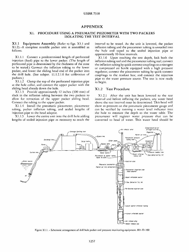
USBR 7310
APPENDIX
XL PROCEDURE USING A PNEUMATIC PIEZOMETER WITH TWO PACKERS ISOLATING THE TEST INTERVAL
Xl l Equipment Assembly (Refer to figs Xll and X l2) -A complete straddle packer unit is assembled as follows
X 11 l Co nnect a predetermined length of perforated injection (feed) pipe to the lower packer (The length of perforated pipe is determined by the thickness of the zone to be rested) Connect the inflation tubing to the lower packer and lower the sliding head end of the packer into the drill hole (See subpar l l l216 for calibration of packers)
Xl l2 Clamp the top of the perforated injection pipe at the hole collar and connecr the upper packer with the sliding head already down the hole
Xl l3 Provide approximately 12 inches (300 mm) of slack in the inflation tubing between the two packers to allow for retraction of the upper packer sliding head Connecr the tubing to the upper packer
Xl l4 Install the pneumatic piezometer piezomerer tubing packer inflation tubing and sealed lengths of injecrion pipe to the head adaptor
X ll5 Lower the entire unit into the drill hole adding lengths of sealed injection pipe as necessary to reach the
( Storoqf Settling ton
interval to be tested As the unit 1s lowered che packer inflation cubing and che piezomecer tubing is unreeled into che hole and caped to che sealed injection pipe at approximately 10-fooc intervals
Xll6 Upon reaching the rest depth lock both the inflation cubing reel and rhe piezomecer cubing reel connecr the inflation tubing by quick-connecr couplings co a nitrogen or compressed air boccie equipped with a high pressure regulator connecr the piezomecer cubing by quick-connect couplings co the readout box and connect the injection pipe co the water pressure source The cesc is now ready to begin
Xl2 Test Procedure
X 12 l After the unit has been lowered to the rest interval and before infacing the packers any water head above the cesc interval must be determined This head will sho w as pressure on the pneumatic piezomecer gauge and can be verified by running a water level indicator into che hole to measure the deprh co the water cable The piezometer will register water pressure chat can be converted to head of water This water head should be
Compressed 01r or nitrogen bot tie Regulator_
Poc~er air lin e- I
P1nometer ln1ec t1on oioe head adaptor
Lo er ooc~er inflation tubmr
Figure X 1 1 - Schematic arrongemem of drill hole packer and pressure monimring equipment 801-0-180
1257
USBR 7310
------=--From compressed air or nitrogen boltle
From piezometer
_To
PRESSURE READOUT BOX
Packer inflation tubing From wafer source From air or Water injection pipe ring seals
PIEZOMETER TUBING REEL
Pressure seals Wire reinforced rubber gland clomps
nitrogen ~~i==-=~==t~f=lil~~~jii~9ll~~~~~sect9ll~sect~sectsect~~~sectl~iilf~f--- To per for o t e d ~~~ze=zzzoCzzzze=zzze=plusmnzz~EZio~~~~21p~
To pressuresource~~~~~~~~~~~~~~~readout box
Piezometer
~~~~~~~~~~~~~~~~---
Inflation chamber Floating packer head Packer inflation lubing
UPPER DRILL HOLE PACKER AND PRESSURE MONITORING EQUIPMENT FOR N X HOLE
Figure X 12 - Upper Jrill hole packer anJ pressure monitoring equipment for NX hole
used to determine the minimum inflation pressure to be applied co the packers by the following equation
SH+ PP+ PE = minimum inflation pressure
where SH = static pressure at the midpoint elevation of the
test interval lbf in2 or kPa PP = gauge pressure to be maintained during the test
lbfin2 or kPa PE = pressure needed to expand packer to hole
diameter as determined before insertion in the drill hole by expanding the packer in a length of pipe having a diameter similar to the hole diameter lbfin 2 or kPa
Inflation pressure gauge is in units of lbf in2 (kPa) The static water level measured before the packers are
inflated might be a composite water level (see subpar 1334)
Xl22 Inflate the packers and determine water head for the rest interval This is the static head to be used for calculation of hydraulic conductivity If rhe static head is significantly different from the composite measured
before the packers were inflated recalculation of packer inflation pressure may be required The final packer inflation pressure should be the lowest practical pressure to seal the test interval against the maximum injection pressure to avoid fracturing of the material being tested
Xl2 3 After the inflation pressures have been determined deflate the packers fill and flush the system with water until all entrapped air has been removed This is accomplished by filling the injection pipe under a gravity head and leaving the air-release valve open ar the top of the injection pipe tee at an elevation higher than the injection hose The valve must remain open until all air has been removed and water runs freely indicating a filled system At this point water is flowing around the deflated packer system and is completely filling the annulus between the drillhole and the packers In the case of an interval with a high injection rate it may be necessary to keep the air valve closed to keep from entraining air into the test interval
X 124 Close the air release valve at the top of the injection pipe and slowly inflate the packers to the predetermined inflation pressure
Xl2 5 Lock in the inflation pressure by closing the pressure valve in the packer cubing If the pressure gauge
1258
USBR 7310
on the closed system remains steady it verifies a sealed system At this point water injecced under gravity head approaches a constant flow rate
X 126 Record the piezometer pressure after packer inflation For an interval of very low injection rate this is equal to che height of the injeccion standpipe plus che pressure recorded at the hole collar gauge For a test interval with a high injection rate the readout would show the same value less any friction from water flow through the injeccion pipe
X 127 Proceed with the test by applying the selected pressures ac the test interval and moniroring the flow rate and pressure on the pneumatic piezometer
X 128 To accurately compute hydraulic conduetivity rhe down-hole pressure muse remain constant A zone with a high injection rate must be monirored more closely than a zone with a small injection rate and adjustments made to hold the down-hole pressure constant To accomplish
this che injeccion pressure shown on che collar gauge must be adjusted in order co maintain che down-hole pressure constant
NOfE X 1-For example a pressure srage is scarred with the collar gauge reading 35 lbfin2 (241 kPa) and the down-hole piezomerer reading 200 lbf in2 ( 1380 kPa) As rhe flow increases rhe down -hole pressure may drop to 150 lbfin2 (1034 kPa) because fricrion loss in the injection pipe and the collar gauge would have to be adjusted to bring the down-hole pressure gauge back up co 200 lbfin2bull When the flow decreases from a fast to a slow rare the collar gauge pressure would have to be decreased
Xl29 The cesc is completed following one or more stages of pressure increases and pressure decreases Following the last stage deflate the packers and close the injection line The system is now ready to move to the next test interval for repetition of this procedure
1259
Methods Note
A Computer Program for Flow-Log Analysis of Single Holes (FLASH) by Frederick D Day-Lewis1 Carole D Johnson2 Frederick L Paillet3 and Keith J Halford4
Abstract A new computer program FLASH (Flow-Log Analysis of Single Holes) is presented for the analysis of
borehole vertical flow logs The code is based on an analytical solution for steady-state multilayer radial flow to a borehole The code includes options for (1) discrete fractures and (2) multilayer aquifers Given vertical flow profiles collected under both ambient and stressed (pumping or injection) conditions the user can estimate fracture (or layer) transmissivities and far-field hydraulic heads FLASH is coded in Microsoft Excel5 with Visual Basic for Applications routines The code supports manual and automated model calibration
Introduction Flowmeters provide means to infer the flow into or
out of boreholes connected to transmissive aquifer units or fractures In the past the relative inaccuracy and difficult operating procedures for spinner flowmeters limited the use of borehole flow measurements With the advent of heat-pulse (Paillet et al 1996) and electromagnetic (Molz et al 1994) instruments measurements of vertical flow as small as 005 Lmin became practicable and borehole flowmeter logging is becoming routine New modeling and analysis tools are needed to achieve the full potential of these measurements
1Corresponding author US Geological Survey Office of Groundwater Branch of Geophysics 11 Sherman Place Unit 5015 Storrs CT 06269 (860) 487-7402 ext 21 fax (860) 487-8802 daylewisusgsgov
2US Geological Survey Office of Groundwater Branch of Geophysics 11 Sherman Place Unit 5015 Storrs CT 06269
3Office of Groundwater Branch of Geophysics (Emeritus) US Geological Survey 11 Sherman Place Unit 5015 Storrs CT 06269
4US Geological Survey Nevada Water Science Center 2730 N Deer Run Rd Carson City NV 89703
5Any use of trade product or firm names is for descriptive purposes only and does not imply endorsement by the US government
Received April 2010 accepted December 2010 copy 2011 The Author(s) Ground Water copy 2011 National Ground Water Association doi 101111j1745-6584201100798x
Calibration of a borehole flow model to flowmeter data can produce estimates of transmissivity and heads for one or more flow zones (aquifer layers or fractures) Here we briefly review approaches for analysis of flowmeter logs and introduce a new computer program which supports manual and automated calibration of an analytical borehole flow model
Approach Single-hole flowmeter data can be analyzed to
estimate transmissivity profiles along boreholes and characterize aquifer compartmentalization (Molz et al 1989 Kabala 1994 Paillet 1998) Analysis of single-hole flowmeter data is commonly based on the Thiem Equation (Thiem 1906) which written for confined radial flow from a single flow zone (ie aquifer layer or fracture) to a screened or open well is
2πTi(hw minus hi)Qi = minus (1)
ln(r0rw)
where Qi is the volumetric flow into the well from flow zone i [L3Tminus1] hw and hi are respectively the hydraulic head [L] at the radius of the well rw and at radial distance r0 commonly taken as the radius of influence where heads do not change as a result of pumping in which
926 Vol 49 No 6ndashGROUND WATERndashNovember-December 2011 (pages 926ndash931) NGWAorg
case hi is the connected far-field head for zone i and Ti
is the transmissivity of flow zone i [L2Tminus1] A number of approaches to flowmeter analysis have
been proposed and demonstrated for different sets of assumptions (eg no ambient flow in boreholes) and data requirements (eg flow profiles collected under both ambient and stressed conditions) based either on Equation 1 (Molz et al 1989) or quasi-steady flow approximations (Paillet 1998) We refer the interested reader to Williams et al (2008) for additional background on flowmeter logs and focus the following discussion on the approach of Paillet (1998 2001) which is adapted here
Paillet (1998) formulated flowmeter log analysis as a model-calibration procedure involving flow profiles collected under both ambient and stressed (pumping or injection) conditions Consideration of the two conditions allows for the estimation of the transmissivities and also far-field heads of flow zones The latter is critical for the interpretation of water samples from wells that intersect multiple fractures or layers with different hydraulic head (Johnson et al 2005) Applying Equation 1 to an ambient condition (condition a) and a stressed condition (condition s) gives
factorT total(ha minus h02πTi )w iQa = minus (2)i ln(r0rw) factorT total(hs minus h02πTi )w iQs = minus (3)i ln(r0rw)
where T factor i is the fraction of the boreholersquos transmisshy
sivity contributed by flow zone i [ndash] T total is the total transmissivity of the flow zones intersected by the bore-hole [L2Tminus1] ha hs are the ambient and stressed water w w levels in the well respectively [L] h0 is the far-field head i in flow zone i [L]
For both ambient and stressed conditions the water level in the borehole is assumed to be constant in
time and the water level in the far-field of each zone is assumed to be the natural condition that is hi
0 In a field experiment (Figure 1) rw would be known and the flow rates and water levels in the well would be measured Radius of influence can be inferred experimentally based on head data at observation wells in which case r0 can be constrained during calibration or else it can be approximated (Bear 1979 306) Estimates of transmissivity are not strongly sensitive to the value assumed for r0 because it appears inside the logarithm in Equations 2 and 3 For example a change in r0rw
from 10 to 100 yields a change in the estimated Ti of only a factor of 2 and order-of-magnitude estimates of transmissivity are acceptable for many problems In cases where knowledge of r0 is unavailable but the boreholersquos total transmissivity is known from specific-capacity or slug-test results it is possible to estimate r0 in the calibration procedure We note that the forward model (Equations 2 and 3) produces twice as many independent equations as there are flow zones with an additional equation requiring T factor values to sum to 1 The number of parameters being estimated is twice the number of flow zones (T factor and h0 for all i) plus one parameter for either i i T total 0or r i
Model calibration involves changing the model parameters such that the flows predicted by Equations 2 and 3 match the interpreted flow profiles Following Paillet (1998 2001) calibration is to the interpreted profile and not individual data This formulation allows the user to incorporate additional insight (eg from other logs) to identify the number and locations of flow zones and elimshyinates the need for weighting measurements differently according to variable measurement errors and the spatial distribution of measurements along the borehole
Calibration can be implemented by manual trial-andshyerror or automated using nonlinear regression Whether manual or automated the goal for calibration is to identify the set of parameters that minimize a measure
Figure 1 Schematic of flowmeter experiment in a fractured-rock aquifer with (a) flow-log profiles for ambient (blue) and stressed (dashed red) conditions and conceptual cross sections of flow system for (b) ambient condition and (c) stressed condition In this example two flow zones (fractures) intersect a well Under ambient conditions flow enters the well from fracture 1 and exits from fracture 3 Under pumping conditions flow enters the well from fractures 1 and 2 The far-field head of zone 2 is equal to the ambient water level thus there is no flow tofrom zone 2 under ambient conditions The far-field head of zone 3 is equal to the stressed water level thus there is no flow tofrom zone 3 under pumping conditions
NGWAorg FD Day-Lewis et al GROUND WATER 49 no 6 926ndash931 927
of combined data misfit and model misfit Considerashytion of model misfit criteria commonly referred to as regularization is useful when multiple models can match the data equally well or within measurement errors Here the data misfit is formulated based on squared differshyences between the predicted and interpreted flow profiles such that multiple measurements may be collected in a single borehole interval The model misfit could be forshymulated in different ways but we use criteria based on the differences between the water level in the borehole under ambient conditions and the far-field heads Thus the objective function F consists of two terms (1) the mean squared error (MSE) between interpreted and preshydicted flow profiles with equal weights for all cumulative flows (ambient and stressed) and (2) the sum of squared differences (h) between the boreholersquos water level and far-field heads
n1 2ssim sintmin F = Q minus Qi i n
i=1
n asim aint 2+
Q minus Q
2 + α (hi) (4)i i i=1
subject to constraints
factor factorT ge T for all i andi min
ABS(haw minus h0
i ) le hmax for all i
aintwhere Qi Qi sint are the interpreted flow profiles (ie
cumulative flow above zones) for zone i under ambishyasiment and stressed conditions respectively [L3Tminus1] Qi
ssimQi are the simulated flow profiles (ie cumulative flow above zones) for zone i under ambient and stressed conditions respectively [L3Tminus1] α weights the regushylarization relative to the data misfit [L4Tminus2] T factor ismin
T factorthe user-specified minimum for any flow zone which can ensure nonnegative T factor hmax is the user-specified maximum absolute difference between the ambishyent water level and the far-field head of any flow zone and n is the number of flow zones
Without regularization F reduces to the MSE between simulated and interpreted flows The trade-off parameter α is set by the user with larger values more strongly penalizing large head differences Commonly small α values (less than 0001) are sufficient to obtain good results In selecting α the user should be guided by the goal of regularization which is to identify the ldquosimplestrdquo explanation of the data while minimizing the data misfit
Using FLASH FLASH (Flow-Log Analysis of Single Holes) is writshy
ten in Excel with Visual Basic for Applications (VBA) The spreadsheet includes a toggle (INPUTS worksheet cell A20) to choose between analysis for (1) fractures or fracture zones that intersect a well at discrete locations
and (2) aquifer layers in porous media The first is indishycated for cases where flow profiles are characterized by step increasesdecreases and the second for cases where flow profiles show approximately linear change over each layer Up to 10 fractures or layers can be modeled
The FLASH spreadsheet includes four worksheets INTRODUCTION INPUTS FIELD_DATA and PLOTshyTING INTRODUCTION provides information about the program and input parameters On the INPUTS workshysheet the user enters information about the flow zones transmissivities and heads Note that the user must intershypret flow profiles from the flowmeter data for both the ambient and stressed conditions The flow measurements are entered in FIELD_DATA and the interpreted proshyfiles are entered in INPUTS The interpreted profiles plot as dashed lines the data as points and the simulated proshyfiles as solid lines (Figure 2) Line and marker styles can be modified using standard Excel tools Flows are positive upward and negative downward PLOTTING is used by the program and does not require the userrsquos attention
In the INPUTS worksheet input parameters are entered in the cells with light blue and bright aquamarine backgrounds The former include specifications of the experiment setup (eg borehole diameter and water level) and the latter include calibration parameters Manual calibration is performed by adjusting the values of
ldquoT factorrdquothe cells and ldquohrdquo which are respectively T factor and the difference between the flow zonersquos far-i field head and the ambient water level in the borehole As parameters are adjusted the simulated flow profiles update automatically thus guiding the user toward best-fit parameters The MSE between simulated and observed flows is calculated in cell B36 on the INPUTS worksheet
Although the principle calibration parameters are Ti
factor and h the radius of influence r0 and total transshymissivity T total also are possible calibration parameters as explained above and indicated by aquamarine highshylighting By inspection of Equations 2 and 3 it is not possible to estimate unique values for both radius of influshyence and total transmissivity but only the ratio of total transmissivity divided by ln(r0rw) In general the user will have more information about total transmissivity than radius of influence Total transmissivity is estimated readshyily using an open-hole slug test or specific-capacity test Indeed the drawdown and pumping rate under stressed conditions could serve as data to estimate a total transshymissivity for the borehole In rare cases however the estimated total transmissivity may be considered unrelishyable for example in the presence of ambiguous slug-test data or discrepancy between the volumes over which the slug test and flowmeter analysis measure In such cases it may be useful to allow the T factor values to sum to a value other than 1 FLASH assumes a uniform radius of influence for all flow zones In reality the effective radius of influence may vary between zones according to their transmissivities and distances to boundaries Data to supshyport variable radius of influence however is commonly unavailable furthermore transmissivity estimates are not
928 FD Day-Lewis et al GROUND WATER 49 no 6 926ndash931 NGWAorg
Figure 2 The INPUTS worksheet after execution of the Solver with options ldquoEstimate ROIrdquo and ldquoSolve with regularizationrdquo for example On this worksheet the user enters the well and flow-log specifications and performs model calibration Data (points) and interpreted profiles (dashed lines) Simulated profiles (solid lines) are for an arbitrarily selected starting model
a strong function of the assumed radius of influence as explained previously
Automated model calibration is implemented using the Excel Solver an optimization tool based on a Genshyeralized Reduced Gradient algorithm (Lasdon and Smith 1992) The Solver is invoked using VBA ldquocontrol butshytonsrdquo on the INPUTS worksheet Radio buttons allow for selections of (1) the parameters to be estimated (Estishymate ROI [radius of influence] or Estimate Transmissivshyity) and (2) regularization (Solve without Regularization or Solve with Regularization) Under the option Estimate
T factorROI the Solver estimates the values of i for all i and the single radius of influence Under the option Estimate Transmissivity radius of influence is assumed known the parameters for estimation are T factor for all ii such that total transmissivity is allowed to vary Users are encouraged to perform manual calibration before attemptshying automated calibration Manual calibration provides insight into the sensitivity of flows to parameters and helps to identify a good starting model for automated calshyibration As for any nonlinear optimization the algorithm may get ldquostuckrdquo in local minima and fail to identify the globally optimal parameter values Consideration of mulshytiple starting models is advised Additional information
and the FLASH spreadsheet are available online as noted under Supporting Information at the end of this article
Example FLASH is demonstrated for a simple data set from
a fractured-rock aquifer (Figure 2) Johnson et al (2005) provide additional details for this data set for which additional borehole logs were used to identify fractures and select locations for flow measurements
Under ambient conditions the deeper fractures 1 and 2 experience inflow to the borehole which indicates the far-field heads for each of these fractures is greater than the head in the borehole thus producing upward flow (Figure 1) Under ambient conditions upflowing water exits the borehole at fracture 3 indicating the far-field head is lower than the head in the borehole Under low-rate pumping conditions water continues to enter the borehole at fracture 1 additional water enters at fracture 2 indicating the far-field heads for fractures 1 and 2 are higher than the quasi-steady state open-hole water level under pumping conditions The uppermost fracture (3) no longer shows outflow indicating the far-field head is equal to the pumping water level In this example
NGWAorg FD Day-Lewis et al GROUND WATER 49 no 6 926ndash931 929
fracture 2 has a far-field head similar to the ambient water level in the well and therefore does not result in a substantial change in borehole flow under ambient conditions Similarly fracture 3 has a far-field head similar to the stressed water level in the well and does not produce a measurable change in borehole flow under stressed conditions This field example underscores the importance of collecting both ambient and stressed flow profilesmdashwith only ambient data fracture 2 could not be identified and with only stressed data fracture 3 could not be identified
To induce flow from a given fracture to enter the borehole the h for that fracture must be positive Conversely to induce flow from the borehole to the fracture the h must be negative The rate of flow is determined by the magnitude of a given flow zonersquos h and transmissivity Thus manual calibration entails for each zone (1) adjustment of a h (cells F21F30) to control whether flow enters or exits the borehole from that zone and (2) adjustment of a T factor to control the rate of flow A final solution can be obtained with the manual fit or after a starting model is generated manually the Solver can be applied For the example here automated calibration produces an excellent match to the data (Figure 2) using options ldquoEstimate ROI rdquo and ldquoEstimate with Regularizationrdquo
Discussion and Conclusions We present a new tool to aid in flowmeter log
analysis a computer code named FLASH We follow a model-calibration strategy similar to that of Paillet (1998) with a simple analytical model for borehole flow based on the Thiem Equation (Thiem 1906) which has been used extensively in previous analyses of flowmeter logs It is important to note that FLASH assumes a borehole flow model that neglects head losses in the borehole or across the well screen and these losses are important in some data sets (Zlotnik and Zurbuchen 2003) We also note the limitations inherent to flowmeter methods primarily that they not as sensitive as straddle-packer hydraulic testing Flowmeter methods consistently identify transmissivities within 15 to 2 orders of magnitude of the most transmissive zone in a borehole depending on the resolution of the flowmeter itself (Williams et al 2008) but straddle-packer tests can see features 6 orders of magnitude less transmissive than is possible with flowmeter (Paillet 1998 Day-Lewis et al 2000 Shapiro 2001) Despite the limited resolution of flowmeter measurements flowmeter modeling results can reproduce packer-test estimates to within an order of magnitude and far-field head values determined with flowmeter methods commonly compare well with packer-test results and discrete-interval water-level monitoring (Johnson et al 2005 Williams et al 2008)
FLASH provides a graphical user interface for calshyibration of an analytical borehole flow model and estishymation of flow-zone transmissivities and far-field heads The program supports manual and automated calibration
with and without regularization FLASH is highly cusshytomizable Experienced Excel users may prefer to invoke the Solver outside of FLASHrsquos VBA routines or to use alternative objective functions or regularization criteria or variable weighting for ambient vs stressed flows Future extensions may include tools for analysis of crosshole flowmeter data and evaluation of estimation uncertainty
Acknowledgments This work was supported by the US Environmental
Protection Agency Region 1 the US Geological Survey Groundwater Resources Program and Toxic Substances Hydrology Program The authors are grateful for review comments from Tom Reilly Allen Shapiro Tom Burbey John Williams Roger Morin Landis West and Mary Anderson
Supporting Information Additional Supporting Information may be found in
the online version of this article
Supplemental material available online include (1) the FLASH spreadsheet which also can be downloaded from httpwaterusgsgovogwflash and (2) a README file with information for installation and troubleshooting
Please note Wiley-Blackwell is not responsible for the content or functionality of any supporting information supplied by the authors Any queries (other than missing material) should be directed to the corresponding author for the article
References Bear J 1979 Hydraulics of Groundwater New York McGraw-
Hill Inc Day-Lewis FD PA Hsieh and SM Gorelick 2000 Idenshy
tifying fracture-zone geometry using simulated annealing and hydraulic-connection data Water Resources Research 36 no 7 1707ndash1721
Johnson CD CK Kochiss and CB Dawson 2005 Use of discrete-zone monitoring systems for hydraulic charshyacterization of a fractured-rock aquifer at the Univershysity of Connecticut landfill Storrs Connecticut 1999 to 2002 Water-Resources Investigations Report 03-4338 105 Reston Virginia USGS
Kabala ZJ 1994 Measuring distributions of hydraulic conducshytivity and storativity by the double flowmeter test Water Resources Research 3 685ndash690
Lasdon LS and S Smith 1992 Solving large sparse nonlinear programs using GRG ORSA Journal on Computing 4 no 1 2ndash15
Molz FJ GK Bowman SC Young and WR Waldrop 1994 Borehole flowmetersmdashfield application and data analysis Journal of Hydrology 163 no 3ndash4 347ndash371
Molz FJ RH Morin AE Hess JG Melville and O Guven 1989 The impeller meter for measuring aquifer permeabilshyity variations evaluations and comparison with other tests Water Resources Research 25 no 7 1677ndash1683
Paillet FL 2001 Hydraulic head applications of flow logs in the study of heterogeneous aquifers Ground Water 39 no 5 667ndash675
930 FD Day-Lewis et al GROUND WATER 49 no 6 926ndash931 NGWAorg
Paillet FL 1998 Flow modeling and permeability estimation using borehole flow logs in heterogeneous fractured formashytions Water Resources Research 34 no 5 997ndash1010
Paillet FL RE Crowder and AE Hess 1996 High-resolution flowmeter logging applications with the heat-pulse flowmeter Journal of Environmental and Engineering Geophysics 1 no 1 1ndash14
Shapiro AM 2001 Effective matrix diffusion in kilometer-scale transport in fractured crystalline rock Water Resources Research 37 no 3 507ndash522
Thiem G 1906 Hydologische methoden 56 Leipzig JM Gebhardt
Williams JH 2008 Flow-log analysis for hydraulic characshyterization of selected test wells at the Indian Point Energy Center Buchanan New York Open-File Report 2008-1123 31 Reston Virginia USGS
Zlotnik VA and BR Zurbuchen 2003 Estimation of hydraulic conductivity from borehole flowmeter tests conshysidering head losses Journal of Hydrology 281 no 1ndash2 115ndash128
NGWAorg FD Day-Lewis et al GROUND WATER 49 no 6 926ndash931 931
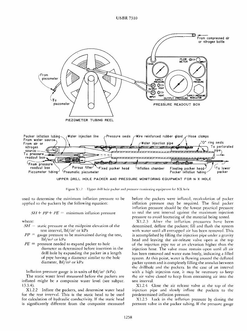
USBR 7310
------=--From compressed air or nitrogen boltle
From piezometer
_To
PRESSURE READOUT BOX
Packer inflation tubing From wafer source From air or Water injection pipe ring seals
PIEZOMETER TUBING REEL
Pressure seals Wire reinforced rubber gland clomps
nitrogen ~~i==-=~==t~f=lil~~~jii~9ll~~~~~sect9ll~sect~sectsect~~~sectl~iilf~f--- To per for o t e d ~~~ze=zzzoCzzzze=zzze=plusmnzz~EZio~~~~21p~
To pressuresource~~~~~~~~~~~~~~~readout box
Piezometer
~~~~~~~~~~~~~~~~---
Inflation chamber Floating packer head Packer inflation lubing
UPPER DRILL HOLE PACKER AND PRESSURE MONITORING EQUIPMENT FOR N X HOLE
Figure X 12 - Upper Jrill hole packer anJ pressure monitoring equipment for NX hole
used to determine the minimum inflation pressure to be applied co the packers by the following equation
SH+ PP+ PE = minimum inflation pressure
where SH = static pressure at the midpoint elevation of the
test interval lbf in2 or kPa PP = gauge pressure to be maintained during the test
lbfin2 or kPa PE = pressure needed to expand packer to hole
diameter as determined before insertion in the drill hole by expanding the packer in a length of pipe having a diameter similar to the hole diameter lbfin 2 or kPa
Inflation pressure gauge is in units of lbf in2 (kPa) The static water level measured before the packers are
inflated might be a composite water level (see subpar 1334)
Xl22 Inflate the packers and determine water head for the rest interval This is the static head to be used for calculation of hydraulic conductivity If rhe static head is significantly different from the composite measured
before the packers were inflated recalculation of packer inflation pressure may be required The final packer inflation pressure should be the lowest practical pressure to seal the test interval against the maximum injection pressure to avoid fracturing of the material being tested
Xl2 3 After the inflation pressures have been determined deflate the packers fill and flush the system with water until all entrapped air has been removed This is accomplished by filling the injection pipe under a gravity head and leaving the air-release valve open ar the top of the injection pipe tee at an elevation higher than the injection hose The valve must remain open until all air has been removed and water runs freely indicating a filled system At this point water is flowing around the deflated packer system and is completely filling the annulus between the drillhole and the packers In the case of an interval with a high injection rate it may be necessary to keep the air valve closed to keep from entraining air into the test interval
X 124 Close the air release valve at the top of the injection pipe and slowly inflate the packers to the predetermined inflation pressure
Xl2 5 Lock in the inflation pressure by closing the pressure valve in the packer cubing If the pressure gauge
1258
USBR 7310
on the closed system remains steady it verifies a sealed system At this point water injecced under gravity head approaches a constant flow rate
X 126 Record the piezometer pressure after packer inflation For an interval of very low injection rate this is equal to che height of the injeccion standpipe plus che pressure recorded at the hole collar gauge For a test interval with a high injection rate the readout would show the same value less any friction from water flow through the injeccion pipe
X 127 Proceed with the test by applying the selected pressures ac the test interval and moniroring the flow rate and pressure on the pneumatic piezometer
X 128 To accurately compute hydraulic conduetivity rhe down-hole pressure muse remain constant A zone with a high injection rate must be monirored more closely than a zone with a small injection rate and adjustments made to hold the down-hole pressure constant To accomplish
this che injeccion pressure shown on che collar gauge must be adjusted in order co maintain che down-hole pressure constant
NOfE X 1-For example a pressure srage is scarred with the collar gauge reading 35 lbfin2 (241 kPa) and the down-hole piezomerer reading 200 lbf in2 ( 1380 kPa) As rhe flow increases rhe down -hole pressure may drop to 150 lbfin2 (1034 kPa) because fricrion loss in the injection pipe and the collar gauge would have to be adjusted to bring the down-hole pressure gauge back up co 200 lbfin2bull When the flow decreases from a fast to a slow rare the collar gauge pressure would have to be decreased
Xl29 The cesc is completed following one or more stages of pressure increases and pressure decreases Following the last stage deflate the packers and close the injection line The system is now ready to move to the next test interval for repetition of this procedure
1259
Methods Note
A Computer Program for Flow-Log Analysis of Single Holes (FLASH) by Frederick D Day-Lewis1 Carole D Johnson2 Frederick L Paillet3 and Keith J Halford4
Abstract A new computer program FLASH (Flow-Log Analysis of Single Holes) is presented for the analysis of
borehole vertical flow logs The code is based on an analytical solution for steady-state multilayer radial flow to a borehole The code includes options for (1) discrete fractures and (2) multilayer aquifers Given vertical flow profiles collected under both ambient and stressed (pumping or injection) conditions the user can estimate fracture (or layer) transmissivities and far-field hydraulic heads FLASH is coded in Microsoft Excel5 with Visual Basic for Applications routines The code supports manual and automated model calibration
Introduction Flowmeters provide means to infer the flow into or
out of boreholes connected to transmissive aquifer units or fractures In the past the relative inaccuracy and difficult operating procedures for spinner flowmeters limited the use of borehole flow measurements With the advent of heat-pulse (Paillet et al 1996) and electromagnetic (Molz et al 1994) instruments measurements of vertical flow as small as 005 Lmin became practicable and borehole flowmeter logging is becoming routine New modeling and analysis tools are needed to achieve the full potential of these measurements
1Corresponding author US Geological Survey Office of Groundwater Branch of Geophysics 11 Sherman Place Unit 5015 Storrs CT 06269 (860) 487-7402 ext 21 fax (860) 487-8802 daylewisusgsgov
2US Geological Survey Office of Groundwater Branch of Geophysics 11 Sherman Place Unit 5015 Storrs CT 06269
3Office of Groundwater Branch of Geophysics (Emeritus) US Geological Survey 11 Sherman Place Unit 5015 Storrs CT 06269
4US Geological Survey Nevada Water Science Center 2730 N Deer Run Rd Carson City NV 89703
5Any use of trade product or firm names is for descriptive purposes only and does not imply endorsement by the US government
Received April 2010 accepted December 2010 copy 2011 The Author(s) Ground Water copy 2011 National Ground Water Association doi 101111j1745-6584201100798x
Calibration of a borehole flow model to flowmeter data can produce estimates of transmissivity and heads for one or more flow zones (aquifer layers or fractures) Here we briefly review approaches for analysis of flowmeter logs and introduce a new computer program which supports manual and automated calibration of an analytical borehole flow model
Approach Single-hole flowmeter data can be analyzed to
estimate transmissivity profiles along boreholes and characterize aquifer compartmentalization (Molz et al 1989 Kabala 1994 Paillet 1998) Analysis of single-hole flowmeter data is commonly based on the Thiem Equation (Thiem 1906) which written for confined radial flow from a single flow zone (ie aquifer layer or fracture) to a screened or open well is
2πTi(hw minus hi)Qi = minus (1)
ln(r0rw)
where Qi is the volumetric flow into the well from flow zone i [L3Tminus1] hw and hi are respectively the hydraulic head [L] at the radius of the well rw and at radial distance r0 commonly taken as the radius of influence where heads do not change as a result of pumping in which
926 Vol 49 No 6ndashGROUND WATERndashNovember-December 2011 (pages 926ndash931) NGWAorg
case hi is the connected far-field head for zone i and Ti
is the transmissivity of flow zone i [L2Tminus1] A number of approaches to flowmeter analysis have
been proposed and demonstrated for different sets of assumptions (eg no ambient flow in boreholes) and data requirements (eg flow profiles collected under both ambient and stressed conditions) based either on Equation 1 (Molz et al 1989) or quasi-steady flow approximations (Paillet 1998) We refer the interested reader to Williams et al (2008) for additional background on flowmeter logs and focus the following discussion on the approach of Paillet (1998 2001) which is adapted here
Paillet (1998) formulated flowmeter log analysis as a model-calibration procedure involving flow profiles collected under both ambient and stressed (pumping or injection) conditions Consideration of the two conditions allows for the estimation of the transmissivities and also far-field heads of flow zones The latter is critical for the interpretation of water samples from wells that intersect multiple fractures or layers with different hydraulic head (Johnson et al 2005) Applying Equation 1 to an ambient condition (condition a) and a stressed condition (condition s) gives
factorT total(ha minus h02πTi )w iQa = minus (2)i ln(r0rw) factorT total(hs minus h02πTi )w iQs = minus (3)i ln(r0rw)
where T factor i is the fraction of the boreholersquos transmisshy
sivity contributed by flow zone i [ndash] T total is the total transmissivity of the flow zones intersected by the bore-hole [L2Tminus1] ha hs are the ambient and stressed water w w levels in the well respectively [L] h0 is the far-field head i in flow zone i [L]
For both ambient and stressed conditions the water level in the borehole is assumed to be constant in
time and the water level in the far-field of each zone is assumed to be the natural condition that is hi
0 In a field experiment (Figure 1) rw would be known and the flow rates and water levels in the well would be measured Radius of influence can be inferred experimentally based on head data at observation wells in which case r0 can be constrained during calibration or else it can be approximated (Bear 1979 306) Estimates of transmissivity are not strongly sensitive to the value assumed for r0 because it appears inside the logarithm in Equations 2 and 3 For example a change in r0rw
from 10 to 100 yields a change in the estimated Ti of only a factor of 2 and order-of-magnitude estimates of transmissivity are acceptable for many problems In cases where knowledge of r0 is unavailable but the boreholersquos total transmissivity is known from specific-capacity or slug-test results it is possible to estimate r0 in the calibration procedure We note that the forward model (Equations 2 and 3) produces twice as many independent equations as there are flow zones with an additional equation requiring T factor values to sum to 1 The number of parameters being estimated is twice the number of flow zones (T factor and h0 for all i) plus one parameter for either i i T total 0or r i
Model calibration involves changing the model parameters such that the flows predicted by Equations 2 and 3 match the interpreted flow profiles Following Paillet (1998 2001) calibration is to the interpreted profile and not individual data This formulation allows the user to incorporate additional insight (eg from other logs) to identify the number and locations of flow zones and elimshyinates the need for weighting measurements differently according to variable measurement errors and the spatial distribution of measurements along the borehole
Calibration can be implemented by manual trial-andshyerror or automated using nonlinear regression Whether manual or automated the goal for calibration is to identify the set of parameters that minimize a measure
Figure 1 Schematic of flowmeter experiment in a fractured-rock aquifer with (a) flow-log profiles for ambient (blue) and stressed (dashed red) conditions and conceptual cross sections of flow system for (b) ambient condition and (c) stressed condition In this example two flow zones (fractures) intersect a well Under ambient conditions flow enters the well from fracture 1 and exits from fracture 3 Under pumping conditions flow enters the well from fractures 1 and 2 The far-field head of zone 2 is equal to the ambient water level thus there is no flow tofrom zone 2 under ambient conditions The far-field head of zone 3 is equal to the stressed water level thus there is no flow tofrom zone 3 under pumping conditions
NGWAorg FD Day-Lewis et al GROUND WATER 49 no 6 926ndash931 927
of combined data misfit and model misfit Considerashytion of model misfit criteria commonly referred to as regularization is useful when multiple models can match the data equally well or within measurement errors Here the data misfit is formulated based on squared differshyences between the predicted and interpreted flow profiles such that multiple measurements may be collected in a single borehole interval The model misfit could be forshymulated in different ways but we use criteria based on the differences between the water level in the borehole under ambient conditions and the far-field heads Thus the objective function F consists of two terms (1) the mean squared error (MSE) between interpreted and preshydicted flow profiles with equal weights for all cumulative flows (ambient and stressed) and (2) the sum of squared differences (h) between the boreholersquos water level and far-field heads
n1 2ssim sintmin F = Q minus Qi i n
i=1
n asim aint 2+
Q minus Q
2 + α (hi) (4)i i i=1
subject to constraints
factor factorT ge T for all i andi min
ABS(haw minus h0
i ) le hmax for all i
aintwhere Qi Qi sint are the interpreted flow profiles (ie
cumulative flow above zones) for zone i under ambishyasiment and stressed conditions respectively [L3Tminus1] Qi
ssimQi are the simulated flow profiles (ie cumulative flow above zones) for zone i under ambient and stressed conditions respectively [L3Tminus1] α weights the regushylarization relative to the data misfit [L4Tminus2] T factor ismin
T factorthe user-specified minimum for any flow zone which can ensure nonnegative T factor hmax is the user-specified maximum absolute difference between the ambishyent water level and the far-field head of any flow zone and n is the number of flow zones
Without regularization F reduces to the MSE between simulated and interpreted flows The trade-off parameter α is set by the user with larger values more strongly penalizing large head differences Commonly small α values (less than 0001) are sufficient to obtain good results In selecting α the user should be guided by the goal of regularization which is to identify the ldquosimplestrdquo explanation of the data while minimizing the data misfit
Using FLASH FLASH (Flow-Log Analysis of Single Holes) is writshy
ten in Excel with Visual Basic for Applications (VBA) The spreadsheet includes a toggle (INPUTS worksheet cell A20) to choose between analysis for (1) fractures or fracture zones that intersect a well at discrete locations
and (2) aquifer layers in porous media The first is indishycated for cases where flow profiles are characterized by step increasesdecreases and the second for cases where flow profiles show approximately linear change over each layer Up to 10 fractures or layers can be modeled
The FLASH spreadsheet includes four worksheets INTRODUCTION INPUTS FIELD_DATA and PLOTshyTING INTRODUCTION provides information about the program and input parameters On the INPUTS workshysheet the user enters information about the flow zones transmissivities and heads Note that the user must intershypret flow profiles from the flowmeter data for both the ambient and stressed conditions The flow measurements are entered in FIELD_DATA and the interpreted proshyfiles are entered in INPUTS The interpreted profiles plot as dashed lines the data as points and the simulated proshyfiles as solid lines (Figure 2) Line and marker styles can be modified using standard Excel tools Flows are positive upward and negative downward PLOTTING is used by the program and does not require the userrsquos attention
In the INPUTS worksheet input parameters are entered in the cells with light blue and bright aquamarine backgrounds The former include specifications of the experiment setup (eg borehole diameter and water level) and the latter include calibration parameters Manual calibration is performed by adjusting the values of
ldquoT factorrdquothe cells and ldquohrdquo which are respectively T factor and the difference between the flow zonersquos far-i field head and the ambient water level in the borehole As parameters are adjusted the simulated flow profiles update automatically thus guiding the user toward best-fit parameters The MSE between simulated and observed flows is calculated in cell B36 on the INPUTS worksheet
Although the principle calibration parameters are Ti
factor and h the radius of influence r0 and total transshymissivity T total also are possible calibration parameters as explained above and indicated by aquamarine highshylighting By inspection of Equations 2 and 3 it is not possible to estimate unique values for both radius of influshyence and total transmissivity but only the ratio of total transmissivity divided by ln(r0rw) In general the user will have more information about total transmissivity than radius of influence Total transmissivity is estimated readshyily using an open-hole slug test or specific-capacity test Indeed the drawdown and pumping rate under stressed conditions could serve as data to estimate a total transshymissivity for the borehole In rare cases however the estimated total transmissivity may be considered unrelishyable for example in the presence of ambiguous slug-test data or discrepancy between the volumes over which the slug test and flowmeter analysis measure In such cases it may be useful to allow the T factor values to sum to a value other than 1 FLASH assumes a uniform radius of influence for all flow zones In reality the effective radius of influence may vary between zones according to their transmissivities and distances to boundaries Data to supshyport variable radius of influence however is commonly unavailable furthermore transmissivity estimates are not
928 FD Day-Lewis et al GROUND WATER 49 no 6 926ndash931 NGWAorg
Figure 2 The INPUTS worksheet after execution of the Solver with options ldquoEstimate ROIrdquo and ldquoSolve with regularizationrdquo for example On this worksheet the user enters the well and flow-log specifications and performs model calibration Data (points) and interpreted profiles (dashed lines) Simulated profiles (solid lines) are for an arbitrarily selected starting model
a strong function of the assumed radius of influence as explained previously
Automated model calibration is implemented using the Excel Solver an optimization tool based on a Genshyeralized Reduced Gradient algorithm (Lasdon and Smith 1992) The Solver is invoked using VBA ldquocontrol butshytonsrdquo on the INPUTS worksheet Radio buttons allow for selections of (1) the parameters to be estimated (Estishymate ROI [radius of influence] or Estimate Transmissivshyity) and (2) regularization (Solve without Regularization or Solve with Regularization) Under the option Estimate
T factorROI the Solver estimates the values of i for all i and the single radius of influence Under the option Estimate Transmissivity radius of influence is assumed known the parameters for estimation are T factor for all ii such that total transmissivity is allowed to vary Users are encouraged to perform manual calibration before attemptshying automated calibration Manual calibration provides insight into the sensitivity of flows to parameters and helps to identify a good starting model for automated calshyibration As for any nonlinear optimization the algorithm may get ldquostuckrdquo in local minima and fail to identify the globally optimal parameter values Consideration of mulshytiple starting models is advised Additional information
and the FLASH spreadsheet are available online as noted under Supporting Information at the end of this article
Example FLASH is demonstrated for a simple data set from
a fractured-rock aquifer (Figure 2) Johnson et al (2005) provide additional details for this data set for which additional borehole logs were used to identify fractures and select locations for flow measurements
Under ambient conditions the deeper fractures 1 and 2 experience inflow to the borehole which indicates the far-field heads for each of these fractures is greater than the head in the borehole thus producing upward flow (Figure 1) Under ambient conditions upflowing water exits the borehole at fracture 3 indicating the far-field head is lower than the head in the borehole Under low-rate pumping conditions water continues to enter the borehole at fracture 1 additional water enters at fracture 2 indicating the far-field heads for fractures 1 and 2 are higher than the quasi-steady state open-hole water level under pumping conditions The uppermost fracture (3) no longer shows outflow indicating the far-field head is equal to the pumping water level In this example
NGWAorg FD Day-Lewis et al GROUND WATER 49 no 6 926ndash931 929
fracture 2 has a far-field head similar to the ambient water level in the well and therefore does not result in a substantial change in borehole flow under ambient conditions Similarly fracture 3 has a far-field head similar to the stressed water level in the well and does not produce a measurable change in borehole flow under stressed conditions This field example underscores the importance of collecting both ambient and stressed flow profilesmdashwith only ambient data fracture 2 could not be identified and with only stressed data fracture 3 could not be identified
To induce flow from a given fracture to enter the borehole the h for that fracture must be positive Conversely to induce flow from the borehole to the fracture the h must be negative The rate of flow is determined by the magnitude of a given flow zonersquos h and transmissivity Thus manual calibration entails for each zone (1) adjustment of a h (cells F21F30) to control whether flow enters or exits the borehole from that zone and (2) adjustment of a T factor to control the rate of flow A final solution can be obtained with the manual fit or after a starting model is generated manually the Solver can be applied For the example here automated calibration produces an excellent match to the data (Figure 2) using options ldquoEstimate ROI rdquo and ldquoEstimate with Regularizationrdquo
Discussion and Conclusions We present a new tool to aid in flowmeter log
analysis a computer code named FLASH We follow a model-calibration strategy similar to that of Paillet (1998) with a simple analytical model for borehole flow based on the Thiem Equation (Thiem 1906) which has been used extensively in previous analyses of flowmeter logs It is important to note that FLASH assumes a borehole flow model that neglects head losses in the borehole or across the well screen and these losses are important in some data sets (Zlotnik and Zurbuchen 2003) We also note the limitations inherent to flowmeter methods primarily that they not as sensitive as straddle-packer hydraulic testing Flowmeter methods consistently identify transmissivities within 15 to 2 orders of magnitude of the most transmissive zone in a borehole depending on the resolution of the flowmeter itself (Williams et al 2008) but straddle-packer tests can see features 6 orders of magnitude less transmissive than is possible with flowmeter (Paillet 1998 Day-Lewis et al 2000 Shapiro 2001) Despite the limited resolution of flowmeter measurements flowmeter modeling results can reproduce packer-test estimates to within an order of magnitude and far-field head values determined with flowmeter methods commonly compare well with packer-test results and discrete-interval water-level monitoring (Johnson et al 2005 Williams et al 2008)
FLASH provides a graphical user interface for calshyibration of an analytical borehole flow model and estishymation of flow-zone transmissivities and far-field heads The program supports manual and automated calibration
with and without regularization FLASH is highly cusshytomizable Experienced Excel users may prefer to invoke the Solver outside of FLASHrsquos VBA routines or to use alternative objective functions or regularization criteria or variable weighting for ambient vs stressed flows Future extensions may include tools for analysis of crosshole flowmeter data and evaluation of estimation uncertainty
Acknowledgments This work was supported by the US Environmental
Protection Agency Region 1 the US Geological Survey Groundwater Resources Program and Toxic Substances Hydrology Program The authors are grateful for review comments from Tom Reilly Allen Shapiro Tom Burbey John Williams Roger Morin Landis West and Mary Anderson
Supporting Information Additional Supporting Information may be found in
the online version of this article
Supplemental material available online include (1) the FLASH spreadsheet which also can be downloaded from httpwaterusgsgovogwflash and (2) a README file with information for installation and troubleshooting
Please note Wiley-Blackwell is not responsible for the content or functionality of any supporting information supplied by the authors Any queries (other than missing material) should be directed to the corresponding author for the article
References Bear J 1979 Hydraulics of Groundwater New York McGraw-
Hill Inc Day-Lewis FD PA Hsieh and SM Gorelick 2000 Idenshy
tifying fracture-zone geometry using simulated annealing and hydraulic-connection data Water Resources Research 36 no 7 1707ndash1721
Johnson CD CK Kochiss and CB Dawson 2005 Use of discrete-zone monitoring systems for hydraulic charshyacterization of a fractured-rock aquifer at the Univershysity of Connecticut landfill Storrs Connecticut 1999 to 2002 Water-Resources Investigations Report 03-4338 105 Reston Virginia USGS
Kabala ZJ 1994 Measuring distributions of hydraulic conducshytivity and storativity by the double flowmeter test Water Resources Research 3 685ndash690
Lasdon LS and S Smith 1992 Solving large sparse nonlinear programs using GRG ORSA Journal on Computing 4 no 1 2ndash15
Molz FJ GK Bowman SC Young and WR Waldrop 1994 Borehole flowmetersmdashfield application and data analysis Journal of Hydrology 163 no 3ndash4 347ndash371
Molz FJ RH Morin AE Hess JG Melville and O Guven 1989 The impeller meter for measuring aquifer permeabilshyity variations evaluations and comparison with other tests Water Resources Research 25 no 7 1677ndash1683
Paillet FL 2001 Hydraulic head applications of flow logs in the study of heterogeneous aquifers Ground Water 39 no 5 667ndash675
930 FD Day-Lewis et al GROUND WATER 49 no 6 926ndash931 NGWAorg
Paillet FL 1998 Flow modeling and permeability estimation using borehole flow logs in heterogeneous fractured formashytions Water Resources Research 34 no 5 997ndash1010
Paillet FL RE Crowder and AE Hess 1996 High-resolution flowmeter logging applications with the heat-pulse flowmeter Journal of Environmental and Engineering Geophysics 1 no 1 1ndash14
Shapiro AM 2001 Effective matrix diffusion in kilometer-scale transport in fractured crystalline rock Water Resources Research 37 no 3 507ndash522
Thiem G 1906 Hydologische methoden 56 Leipzig JM Gebhardt
Williams JH 2008 Flow-log analysis for hydraulic characshyterization of selected test wells at the Indian Point Energy Center Buchanan New York Open-File Report 2008-1123 31 Reston Virginia USGS
Zlotnik VA and BR Zurbuchen 2003 Estimation of hydraulic conductivity from borehole flowmeter tests conshysidering head losses Journal of Hydrology 281 no 1ndash2 115ndash128
NGWAorg FD Day-Lewis et al GROUND WATER 49 no 6 926ndash931 931
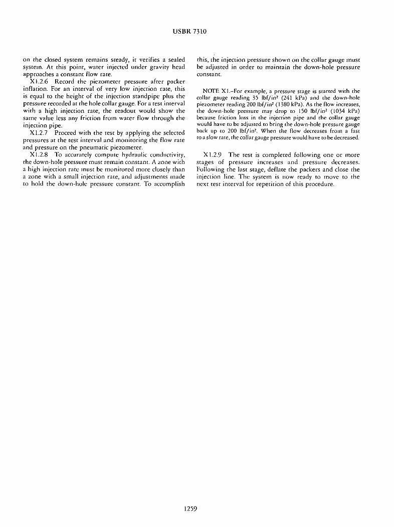
USBR 7310
on the closed system remains steady it verifies a sealed system At this point water injecced under gravity head approaches a constant flow rate
X 126 Record the piezometer pressure after packer inflation For an interval of very low injection rate this is equal to che height of the injeccion standpipe plus che pressure recorded at the hole collar gauge For a test interval with a high injection rate the readout would show the same value less any friction from water flow through the injeccion pipe
X 127 Proceed with the test by applying the selected pressures ac the test interval and moniroring the flow rate and pressure on the pneumatic piezometer
X 128 To accurately compute hydraulic conduetivity rhe down-hole pressure muse remain constant A zone with a high injection rate must be monirored more closely than a zone with a small injection rate and adjustments made to hold the down-hole pressure constant To accomplish
this che injeccion pressure shown on che collar gauge must be adjusted in order co maintain che down-hole pressure constant
NOfE X 1-For example a pressure srage is scarred with the collar gauge reading 35 lbfin2 (241 kPa) and the down-hole piezomerer reading 200 lbf in2 ( 1380 kPa) As rhe flow increases rhe down -hole pressure may drop to 150 lbfin2 (1034 kPa) because fricrion loss in the injection pipe and the collar gauge would have to be adjusted to bring the down-hole pressure gauge back up co 200 lbfin2bull When the flow decreases from a fast to a slow rare the collar gauge pressure would have to be decreased
Xl29 The cesc is completed following one or more stages of pressure increases and pressure decreases Following the last stage deflate the packers and close the injection line The system is now ready to move to the next test interval for repetition of this procedure
1259
Methods Note
A Computer Program for Flow-Log Analysis of Single Holes (FLASH) by Frederick D Day-Lewis1 Carole D Johnson2 Frederick L Paillet3 and Keith J Halford4
Abstract A new computer program FLASH (Flow-Log Analysis of Single Holes) is presented for the analysis of
borehole vertical flow logs The code is based on an analytical solution for steady-state multilayer radial flow to a borehole The code includes options for (1) discrete fractures and (2) multilayer aquifers Given vertical flow profiles collected under both ambient and stressed (pumping or injection) conditions the user can estimate fracture (or layer) transmissivities and far-field hydraulic heads FLASH is coded in Microsoft Excel5 with Visual Basic for Applications routines The code supports manual and automated model calibration
Introduction Flowmeters provide means to infer the flow into or
out of boreholes connected to transmissive aquifer units or fractures In the past the relative inaccuracy and difficult operating procedures for spinner flowmeters limited the use of borehole flow measurements With the advent of heat-pulse (Paillet et al 1996) and electromagnetic (Molz et al 1994) instruments measurements of vertical flow as small as 005 Lmin became practicable and borehole flowmeter logging is becoming routine New modeling and analysis tools are needed to achieve the full potential of these measurements
1Corresponding author US Geological Survey Office of Groundwater Branch of Geophysics 11 Sherman Place Unit 5015 Storrs CT 06269 (860) 487-7402 ext 21 fax (860) 487-8802 daylewisusgsgov
2US Geological Survey Office of Groundwater Branch of Geophysics 11 Sherman Place Unit 5015 Storrs CT 06269
3Office of Groundwater Branch of Geophysics (Emeritus) US Geological Survey 11 Sherman Place Unit 5015 Storrs CT 06269
4US Geological Survey Nevada Water Science Center 2730 N Deer Run Rd Carson City NV 89703
5Any use of trade product or firm names is for descriptive purposes only and does not imply endorsement by the US government
Received April 2010 accepted December 2010 copy 2011 The Author(s) Ground Water copy 2011 National Ground Water Association doi 101111j1745-6584201100798x
Calibration of a borehole flow model to flowmeter data can produce estimates of transmissivity and heads for one or more flow zones (aquifer layers or fractures) Here we briefly review approaches for analysis of flowmeter logs and introduce a new computer program which supports manual and automated calibration of an analytical borehole flow model
Approach Single-hole flowmeter data can be analyzed to
estimate transmissivity profiles along boreholes and characterize aquifer compartmentalization (Molz et al 1989 Kabala 1994 Paillet 1998) Analysis of single-hole flowmeter data is commonly based on the Thiem Equation (Thiem 1906) which written for confined radial flow from a single flow zone (ie aquifer layer or fracture) to a screened or open well is
2πTi(hw minus hi)Qi = minus (1)
ln(r0rw)
where Qi is the volumetric flow into the well from flow zone i [L3Tminus1] hw and hi are respectively the hydraulic head [L] at the radius of the well rw and at radial distance r0 commonly taken as the radius of influence where heads do not change as a result of pumping in which
926 Vol 49 No 6ndashGROUND WATERndashNovember-December 2011 (pages 926ndash931) NGWAorg
case hi is the connected far-field head for zone i and Ti
is the transmissivity of flow zone i [L2Tminus1] A number of approaches to flowmeter analysis have
been proposed and demonstrated for different sets of assumptions (eg no ambient flow in boreholes) and data requirements (eg flow profiles collected under both ambient and stressed conditions) based either on Equation 1 (Molz et al 1989) or quasi-steady flow approximations (Paillet 1998) We refer the interested reader to Williams et al (2008) for additional background on flowmeter logs and focus the following discussion on the approach of Paillet (1998 2001) which is adapted here
Paillet (1998) formulated flowmeter log analysis as a model-calibration procedure involving flow profiles collected under both ambient and stressed (pumping or injection) conditions Consideration of the two conditions allows for the estimation of the transmissivities and also far-field heads of flow zones The latter is critical for the interpretation of water samples from wells that intersect multiple fractures or layers with different hydraulic head (Johnson et al 2005) Applying Equation 1 to an ambient condition (condition a) and a stressed condition (condition s) gives
factorT total(ha minus h02πTi )w iQa = minus (2)i ln(r0rw) factorT total(hs minus h02πTi )w iQs = minus (3)i ln(r0rw)
where T factor i is the fraction of the boreholersquos transmisshy
sivity contributed by flow zone i [ndash] T total is the total transmissivity of the flow zones intersected by the bore-hole [L2Tminus1] ha hs are the ambient and stressed water w w levels in the well respectively [L] h0 is the far-field head i in flow zone i [L]
For both ambient and stressed conditions the water level in the borehole is assumed to be constant in
time and the water level in the far-field of each zone is assumed to be the natural condition that is hi
0 In a field experiment (Figure 1) rw would be known and the flow rates and water levels in the well would be measured Radius of influence can be inferred experimentally based on head data at observation wells in which case r0 can be constrained during calibration or else it can be approximated (Bear 1979 306) Estimates of transmissivity are not strongly sensitive to the value assumed for r0 because it appears inside the logarithm in Equations 2 and 3 For example a change in r0rw
from 10 to 100 yields a change in the estimated Ti of only a factor of 2 and order-of-magnitude estimates of transmissivity are acceptable for many problems In cases where knowledge of r0 is unavailable but the boreholersquos total transmissivity is known from specific-capacity or slug-test results it is possible to estimate r0 in the calibration procedure We note that the forward model (Equations 2 and 3) produces twice as many independent equations as there are flow zones with an additional equation requiring T factor values to sum to 1 The number of parameters being estimated is twice the number of flow zones (T factor and h0 for all i) plus one parameter for either i i T total 0or r i
Model calibration involves changing the model parameters such that the flows predicted by Equations 2 and 3 match the interpreted flow profiles Following Paillet (1998 2001) calibration is to the interpreted profile and not individual data This formulation allows the user to incorporate additional insight (eg from other logs) to identify the number and locations of flow zones and elimshyinates the need for weighting measurements differently according to variable measurement errors and the spatial distribution of measurements along the borehole
Calibration can be implemented by manual trial-andshyerror or automated using nonlinear regression Whether manual or automated the goal for calibration is to identify the set of parameters that minimize a measure
Figure 1 Schematic of flowmeter experiment in a fractured-rock aquifer with (a) flow-log profiles for ambient (blue) and stressed (dashed red) conditions and conceptual cross sections of flow system for (b) ambient condition and (c) stressed condition In this example two flow zones (fractures) intersect a well Under ambient conditions flow enters the well from fracture 1 and exits from fracture 3 Under pumping conditions flow enters the well from fractures 1 and 2 The far-field head of zone 2 is equal to the ambient water level thus there is no flow tofrom zone 2 under ambient conditions The far-field head of zone 3 is equal to the stressed water level thus there is no flow tofrom zone 3 under pumping conditions
NGWAorg FD Day-Lewis et al GROUND WATER 49 no 6 926ndash931 927
of combined data misfit and model misfit Considerashytion of model misfit criteria commonly referred to as regularization is useful when multiple models can match the data equally well or within measurement errors Here the data misfit is formulated based on squared differshyences between the predicted and interpreted flow profiles such that multiple measurements may be collected in a single borehole interval The model misfit could be forshymulated in different ways but we use criteria based on the differences between the water level in the borehole under ambient conditions and the far-field heads Thus the objective function F consists of two terms (1) the mean squared error (MSE) between interpreted and preshydicted flow profiles with equal weights for all cumulative flows (ambient and stressed) and (2) the sum of squared differences (h) between the boreholersquos water level and far-field heads
n1 2ssim sintmin F = Q minus Qi i n
i=1
n asim aint 2+
Q minus Q
2 + α (hi) (4)i i i=1
subject to constraints
factor factorT ge T for all i andi min
ABS(haw minus h0
i ) le hmax for all i
aintwhere Qi Qi sint are the interpreted flow profiles (ie
cumulative flow above zones) for zone i under ambishyasiment and stressed conditions respectively [L3Tminus1] Qi
ssimQi are the simulated flow profiles (ie cumulative flow above zones) for zone i under ambient and stressed conditions respectively [L3Tminus1] α weights the regushylarization relative to the data misfit [L4Tminus2] T factor ismin
T factorthe user-specified minimum for any flow zone which can ensure nonnegative T factor hmax is the user-specified maximum absolute difference between the ambishyent water level and the far-field head of any flow zone and n is the number of flow zones
Without regularization F reduces to the MSE between simulated and interpreted flows The trade-off parameter α is set by the user with larger values more strongly penalizing large head differences Commonly small α values (less than 0001) are sufficient to obtain good results In selecting α the user should be guided by the goal of regularization which is to identify the ldquosimplestrdquo explanation of the data while minimizing the data misfit
Using FLASH FLASH (Flow-Log Analysis of Single Holes) is writshy
ten in Excel with Visual Basic for Applications (VBA) The spreadsheet includes a toggle (INPUTS worksheet cell A20) to choose between analysis for (1) fractures or fracture zones that intersect a well at discrete locations
and (2) aquifer layers in porous media The first is indishycated for cases where flow profiles are characterized by step increasesdecreases and the second for cases where flow profiles show approximately linear change over each layer Up to 10 fractures or layers can be modeled
The FLASH spreadsheet includes four worksheets INTRODUCTION INPUTS FIELD_DATA and PLOTshyTING INTRODUCTION provides information about the program and input parameters On the INPUTS workshysheet the user enters information about the flow zones transmissivities and heads Note that the user must intershypret flow profiles from the flowmeter data for both the ambient and stressed conditions The flow measurements are entered in FIELD_DATA and the interpreted proshyfiles are entered in INPUTS The interpreted profiles plot as dashed lines the data as points and the simulated proshyfiles as solid lines (Figure 2) Line and marker styles can be modified using standard Excel tools Flows are positive upward and negative downward PLOTTING is used by the program and does not require the userrsquos attention
In the INPUTS worksheet input parameters are entered in the cells with light blue and bright aquamarine backgrounds The former include specifications of the experiment setup (eg borehole diameter and water level) and the latter include calibration parameters Manual calibration is performed by adjusting the values of
ldquoT factorrdquothe cells and ldquohrdquo which are respectively T factor and the difference between the flow zonersquos far-i field head and the ambient water level in the borehole As parameters are adjusted the simulated flow profiles update automatically thus guiding the user toward best-fit parameters The MSE between simulated and observed flows is calculated in cell B36 on the INPUTS worksheet
Although the principle calibration parameters are Ti
factor and h the radius of influence r0 and total transshymissivity T total also are possible calibration parameters as explained above and indicated by aquamarine highshylighting By inspection of Equations 2 and 3 it is not possible to estimate unique values for both radius of influshyence and total transmissivity but only the ratio of total transmissivity divided by ln(r0rw) In general the user will have more information about total transmissivity than radius of influence Total transmissivity is estimated readshyily using an open-hole slug test or specific-capacity test Indeed the drawdown and pumping rate under stressed conditions could serve as data to estimate a total transshymissivity for the borehole In rare cases however the estimated total transmissivity may be considered unrelishyable for example in the presence of ambiguous slug-test data or discrepancy between the volumes over which the slug test and flowmeter analysis measure In such cases it may be useful to allow the T factor values to sum to a value other than 1 FLASH assumes a uniform radius of influence for all flow zones In reality the effective radius of influence may vary between zones according to their transmissivities and distances to boundaries Data to supshyport variable radius of influence however is commonly unavailable furthermore transmissivity estimates are not
928 FD Day-Lewis et al GROUND WATER 49 no 6 926ndash931 NGWAorg
Figure 2 The INPUTS worksheet after execution of the Solver with options ldquoEstimate ROIrdquo and ldquoSolve with regularizationrdquo for example On this worksheet the user enters the well and flow-log specifications and performs model calibration Data (points) and interpreted profiles (dashed lines) Simulated profiles (solid lines) are for an arbitrarily selected starting model
a strong function of the assumed radius of influence as explained previously
Automated model calibration is implemented using the Excel Solver an optimization tool based on a Genshyeralized Reduced Gradient algorithm (Lasdon and Smith 1992) The Solver is invoked using VBA ldquocontrol butshytonsrdquo on the INPUTS worksheet Radio buttons allow for selections of (1) the parameters to be estimated (Estishymate ROI [radius of influence] or Estimate Transmissivshyity) and (2) regularization (Solve without Regularization or Solve with Regularization) Under the option Estimate
T factorROI the Solver estimates the values of i for all i and the single radius of influence Under the option Estimate Transmissivity radius of influence is assumed known the parameters for estimation are T factor for all ii such that total transmissivity is allowed to vary Users are encouraged to perform manual calibration before attemptshying automated calibration Manual calibration provides insight into the sensitivity of flows to parameters and helps to identify a good starting model for automated calshyibration As for any nonlinear optimization the algorithm may get ldquostuckrdquo in local minima and fail to identify the globally optimal parameter values Consideration of mulshytiple starting models is advised Additional information
and the FLASH spreadsheet are available online as noted under Supporting Information at the end of this article
Example FLASH is demonstrated for a simple data set from
a fractured-rock aquifer (Figure 2) Johnson et al (2005) provide additional details for this data set for which additional borehole logs were used to identify fractures and select locations for flow measurements
Under ambient conditions the deeper fractures 1 and 2 experience inflow to the borehole which indicates the far-field heads for each of these fractures is greater than the head in the borehole thus producing upward flow (Figure 1) Under ambient conditions upflowing water exits the borehole at fracture 3 indicating the far-field head is lower than the head in the borehole Under low-rate pumping conditions water continues to enter the borehole at fracture 1 additional water enters at fracture 2 indicating the far-field heads for fractures 1 and 2 are higher than the quasi-steady state open-hole water level under pumping conditions The uppermost fracture (3) no longer shows outflow indicating the far-field head is equal to the pumping water level In this example
NGWAorg FD Day-Lewis et al GROUND WATER 49 no 6 926ndash931 929
fracture 2 has a far-field head similar to the ambient water level in the well and therefore does not result in a substantial change in borehole flow under ambient conditions Similarly fracture 3 has a far-field head similar to the stressed water level in the well and does not produce a measurable change in borehole flow under stressed conditions This field example underscores the importance of collecting both ambient and stressed flow profilesmdashwith only ambient data fracture 2 could not be identified and with only stressed data fracture 3 could not be identified
To induce flow from a given fracture to enter the borehole the h for that fracture must be positive Conversely to induce flow from the borehole to the fracture the h must be negative The rate of flow is determined by the magnitude of a given flow zonersquos h and transmissivity Thus manual calibration entails for each zone (1) adjustment of a h (cells F21F30) to control whether flow enters or exits the borehole from that zone and (2) adjustment of a T factor to control the rate of flow A final solution can be obtained with the manual fit or after a starting model is generated manually the Solver can be applied For the example here automated calibration produces an excellent match to the data (Figure 2) using options ldquoEstimate ROI rdquo and ldquoEstimate with Regularizationrdquo
Discussion and Conclusions We present a new tool to aid in flowmeter log
analysis a computer code named FLASH We follow a model-calibration strategy similar to that of Paillet (1998) with a simple analytical model for borehole flow based on the Thiem Equation (Thiem 1906) which has been used extensively in previous analyses of flowmeter logs It is important to note that FLASH assumes a borehole flow model that neglects head losses in the borehole or across the well screen and these losses are important in some data sets (Zlotnik and Zurbuchen 2003) We also note the limitations inherent to flowmeter methods primarily that they not as sensitive as straddle-packer hydraulic testing Flowmeter methods consistently identify transmissivities within 15 to 2 orders of magnitude of the most transmissive zone in a borehole depending on the resolution of the flowmeter itself (Williams et al 2008) but straddle-packer tests can see features 6 orders of magnitude less transmissive than is possible with flowmeter (Paillet 1998 Day-Lewis et al 2000 Shapiro 2001) Despite the limited resolution of flowmeter measurements flowmeter modeling results can reproduce packer-test estimates to within an order of magnitude and far-field head values determined with flowmeter methods commonly compare well with packer-test results and discrete-interval water-level monitoring (Johnson et al 2005 Williams et al 2008)
FLASH provides a graphical user interface for calshyibration of an analytical borehole flow model and estishymation of flow-zone transmissivities and far-field heads The program supports manual and automated calibration
with and without regularization FLASH is highly cusshytomizable Experienced Excel users may prefer to invoke the Solver outside of FLASHrsquos VBA routines or to use alternative objective functions or regularization criteria or variable weighting for ambient vs stressed flows Future extensions may include tools for analysis of crosshole flowmeter data and evaluation of estimation uncertainty
Acknowledgments This work was supported by the US Environmental
Protection Agency Region 1 the US Geological Survey Groundwater Resources Program and Toxic Substances Hydrology Program The authors are grateful for review comments from Tom Reilly Allen Shapiro Tom Burbey John Williams Roger Morin Landis West and Mary Anderson
Supporting Information Additional Supporting Information may be found in
the online version of this article
Supplemental material available online include (1) the FLASH spreadsheet which also can be downloaded from httpwaterusgsgovogwflash and (2) a README file with information for installation and troubleshooting
Please note Wiley-Blackwell is not responsible for the content or functionality of any supporting information supplied by the authors Any queries (other than missing material) should be directed to the corresponding author for the article
References Bear J 1979 Hydraulics of Groundwater New York McGraw-
Hill Inc Day-Lewis FD PA Hsieh and SM Gorelick 2000 Idenshy
tifying fracture-zone geometry using simulated annealing and hydraulic-connection data Water Resources Research 36 no 7 1707ndash1721
Johnson CD CK Kochiss and CB Dawson 2005 Use of discrete-zone monitoring systems for hydraulic charshyacterization of a fractured-rock aquifer at the Univershysity of Connecticut landfill Storrs Connecticut 1999 to 2002 Water-Resources Investigations Report 03-4338 105 Reston Virginia USGS
Kabala ZJ 1994 Measuring distributions of hydraulic conducshytivity and storativity by the double flowmeter test Water Resources Research 3 685ndash690
Lasdon LS and S Smith 1992 Solving large sparse nonlinear programs using GRG ORSA Journal on Computing 4 no 1 2ndash15
Molz FJ GK Bowman SC Young and WR Waldrop 1994 Borehole flowmetersmdashfield application and data analysis Journal of Hydrology 163 no 3ndash4 347ndash371
Molz FJ RH Morin AE Hess JG Melville and O Guven 1989 The impeller meter for measuring aquifer permeabilshyity variations evaluations and comparison with other tests Water Resources Research 25 no 7 1677ndash1683
Paillet FL 2001 Hydraulic head applications of flow logs in the study of heterogeneous aquifers Ground Water 39 no 5 667ndash675
930 FD Day-Lewis et al GROUND WATER 49 no 6 926ndash931 NGWAorg
Paillet FL 1998 Flow modeling and permeability estimation using borehole flow logs in heterogeneous fractured formashytions Water Resources Research 34 no 5 997ndash1010
Paillet FL RE Crowder and AE Hess 1996 High-resolution flowmeter logging applications with the heat-pulse flowmeter Journal of Environmental and Engineering Geophysics 1 no 1 1ndash14
Shapiro AM 2001 Effective matrix diffusion in kilometer-scale transport in fractured crystalline rock Water Resources Research 37 no 3 507ndash522
Thiem G 1906 Hydologische methoden 56 Leipzig JM Gebhardt
Williams JH 2008 Flow-log analysis for hydraulic characshyterization of selected test wells at the Indian Point Energy Center Buchanan New York Open-File Report 2008-1123 31 Reston Virginia USGS
Zlotnik VA and BR Zurbuchen 2003 Estimation of hydraulic conductivity from borehole flowmeter tests conshysidering head losses Journal of Hydrology 281 no 1ndash2 115ndash128
NGWAorg FD Day-Lewis et al GROUND WATER 49 no 6 926ndash931 931
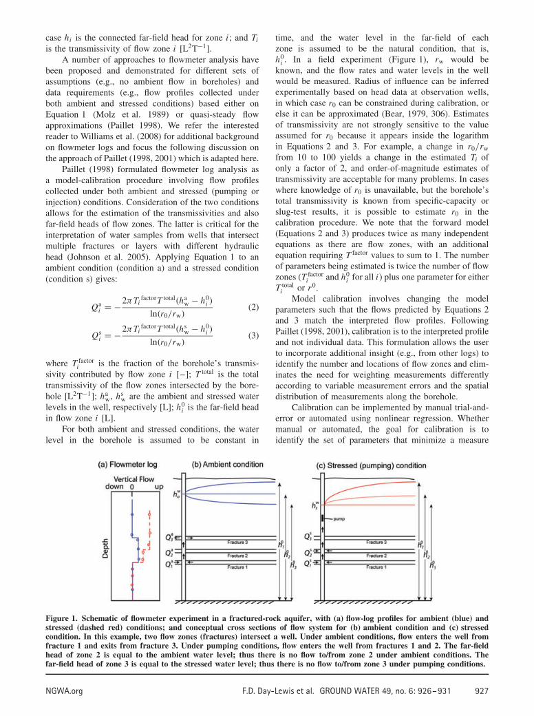
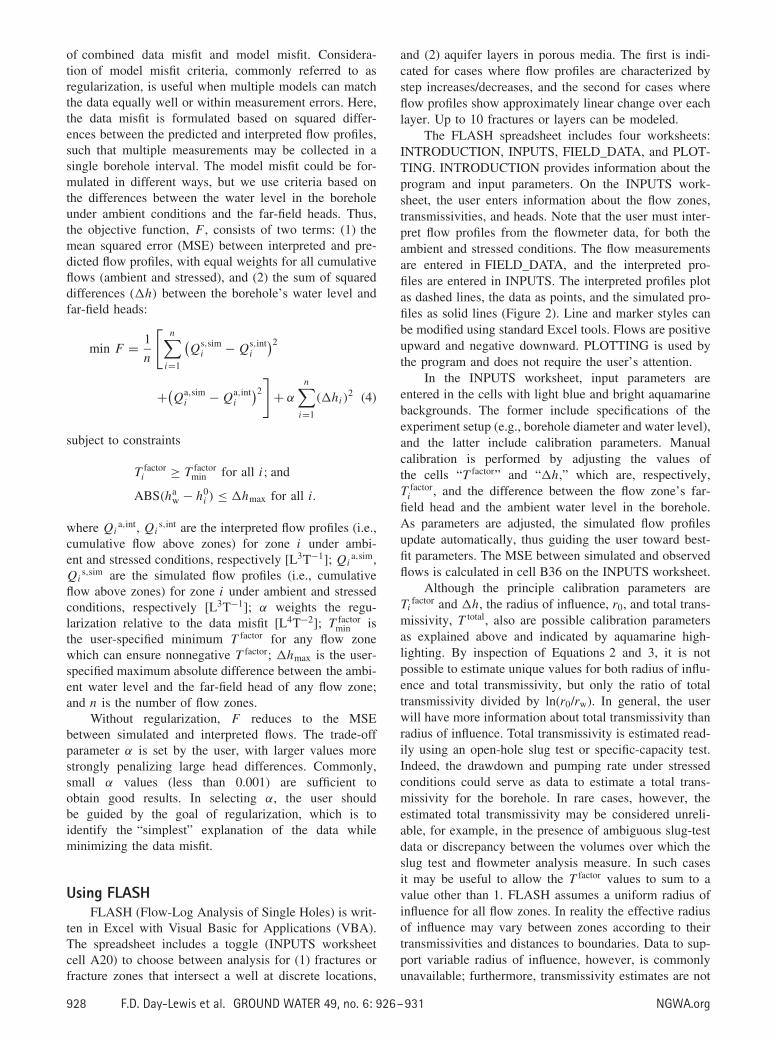
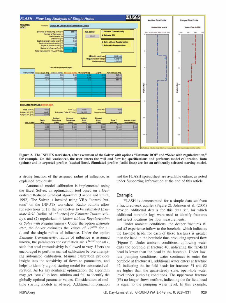
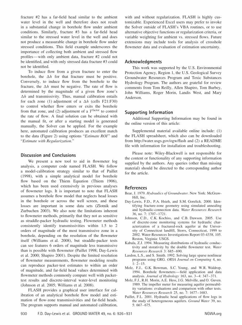