Embed Size (px)
Citation preview
Western Michigan University Western Michigan University
ScholarWorks at WMU ScholarWorks at WMU
Master's Theses Graduate College
12-1999
Quantifying a Key Injection Molding Attribute Defect Quantifying a Key Injection Molding Attribute Defect
Kristopher Bryan Horton
Follow this and additional works at: https://scholarworks.wmich.edu/masters_theses
Part of the Industrial Engineering Commons
Recommended Citation Recommended Citation Horton, Kristopher Bryan, "Quantifying a Key Injection Molding Attribute Defect" (1999). Master's Theses. 4891. https://scholarworks.wmich.edu/masters_theses/4891
This Masters Thesis-Open Access is brought to you for free and open access by the Graduate College at ScholarWorks at WMU. It has been accepted for inclusion in Master's Theses by an authorized administrator of ScholarWorks at WMU. For more information, please contact [email protected].
QUANTIFYING A KEY INJECTION MOLDING ATTRIBUTE DEFECT
by
Kristopher Bryan Horton
A Thesis
Submitted to the
Faculty of The Graduate College
in partial fulfillment of the
requirements for the
Degree of Master of Science
Department of Industrial and
Manufacturing Engineering
Western Michigan University
Kalamazoo, Michigan
December 1999

Copyright by Kristopher Bryan Horton
1999

ACKNOWLEDGMENTS
I want to thank my advisor and committee chairperson, Dr. Paul Engelmann
for believing in me and giving his full support for the topic I selected for this thesis.
On several occasions we felt like we may have taken on more than we could handle.
In the long run it was the leadership, guidance and make or break deadlines of
Dr. Engelmann that kept me on track to completion of my graduate work. I want to
express sincere thanks to my graduate committee members, Mr. Mike Monfore,
Dr. David Lyth and Dr. Mitchel Keil, for sharing with me their time and expertise.
Mr. Monfore taught me how to properly analyze the statistical data from my
experimentation. Dr. Lyth's leadership in the realm of quality control was
instrumental in helping me develop a methodology for the visual evaluation of sink
marks. Dr. Keil helped me to analyze the coordinate measurement machine data used
for quantifying sink marks.
I want to thank Johnson Controls, Inc. of Holland, Michigan for allowing me
access to their metrology center, MacBeth SpectraLight equipment, injection molding
presses and employees for my experimentation. My thesis work would not have been
possible without Johnson Controls commitment and financial investment. A special
thanks goes out to Mr. JeffVanderKolk, Mr. Mike Seymour and Ms. Shelly Bangma
of the metrology center. They spent countless hours helping measure parts with sink
11

Acknowledgments-Continued
marks on the coordinate measurement machine. I want to thank Mr. Wayne
Boomsma for helping me to systematically produce parts with various levels of sink
marks on an injection molding press. In addition, I want to thank the one hundred
and eleven Prince employees who agreed to participate in the visual evaluation phase
of my experimentation.
Finally, I want to thank my wife, Lisa. Her commitment to my work and to
me was unfailing. On numerous occasions she spurred me on and encouraged me
when I was just about to give up. Her reward is the thrill of knowing her husband is
finished with his master's degree and can spend more time with her.
Kristopher Bryan Horton
iii
QUANTIFYING A KEY INJECTION MOLDING ATTRIBUTE DEFECT
Kristopher Bryan Horton, M.S.
Western Michigan University, 1999
A mounting demand for high quality, low cost plastic injection molded
products brings with it goals such as low or even zero defects. In order to ac�ieve
these types of "world class" expectations, resources are used to monitor and control
variable data such as cycle time, part weight or dimensions. Despite this emphasis on
variable data, parts are often rejected based on attribute molding defects such as sink
marks or splay that are measured by subjective criteria and therefore difficult to
control. Appearance of a part once considered acceptable may no longer be, due to
changing expectations or subjective interpretation of an agreed upon standard.
Sink marks on each part were measured using a coordinate measurement
machine (CMM) and quantified using statistical software. Experimentation was
conducted to identify the level at which a majority of human observers were not able
to visually perceive the sink marks. This threshold could be used to develop an
acceptance standard for the part used in the experimentation. Quantifying an attribute
defect is not intended to be a substitute for preventing defect formation via robust part
design, mold design, choice of polymer, or selection of processing conditions.
TABLE OF CONTENTS
ACKNOWLEDGMENTS ......................................................................................... ii
LIST OF TABLES ..................................................................................................... viii
LIST OF FIGURES ................................................................................................... lX
CHAPTER
I. INTRODUCTION . .. . .. .. .. .. . .. .. . .. . .. .. .. .. .. .. . . . .. .. ... . . ... .. .. . . . . . . .. . ... .. .. . .. .. .. . ... .. . .. . .. . . 1
Background........................................................................................... 1
Problem Statement and Significance .. .. .. .... .. .. .. .. .. .... .. .. .. .... .. .. .... .. .... .. . 1
Summary ............................................................................................... 4
II. REVIEW OF LITERATURE .. .. .. ...... .. ...... .. .... ...... .. ...... .. .. .. .. .. .. ...... .. .... .. ...... 5
Overview............................................................................................... 5
Approaches to Defect Management...................................................... 5
Part Design................................................................................... 7
Mold Design................................................................................. 9
Choice of Polynier ....................................................................... 11
Processing Conditions .................................................................. 11
Masking ........................................................................................ 13
Inspection..................................................................................... 14
Key Elements for Developing Test Methodology ................................ 15
The First Phase: Quantifying Sink Marks ................................... 16
lV
CHAPTER
Table of Contents-Continued
Phase II: Visual Evaluation of Sink Marks................................. 22
Summary of Literature Review............................................................. 30
III. METHODOLOGY ........................................................................................ 32
Introduction........................................................................................... 32
Production of Parts With Sink Marks .. .. .. .. ... .. ... .. . . . .. .. .. .. .. .. ... .. .. .. 32
Visual Evaluation Pilot Tests ....................................................... 36
Production of Parts to Expand the Range of Sink Mark Treatments.................................................................................... 42
Quantification of Sink Marks on Non-Painted Parts ................... 42
Full-Scale Visual Evaluation of Sink Marks on Non-Painted Parts ........................................................................ 46
Production of Painted GDO Doors .............................................. 51
Full-Scale Visual Evaluation of Sink Marks on Painted Parts .... 52
Quantification of Sink Marks on Painted Parts:........................... 52
Analysis of Data........................................................................... 53
Summary of the Methodology.............................................................. 60
IV. EXPERIMENTALRESULTS ....................................................................... 61
Introduction ........................................................................................... 61
Sink Mark Quantification Results ......................................................... 61
CMM Measurement Results ...... .. ..... .. .. .. ..... .. ... ... .. .. .......... ....... .. . 61
Gauge R & R Results................................................................... 66
V
Table of Contents-Continued
CHAPTER
Visual Evaluation Results ..................................................................... 69
Test Population Attributes ........................................................... 71
Visual Evaluation Pilot Test Results ........................................... 73
Visual Evaluation Results -Painted GDO Doors ........................ 80
Visual Evaluation Results - Non-Painted GDO Doors ............... 83
Summary of Results.............................................................................. 84
V. CONCLUSIONS AND RECOMMENDATIONS ........................................ 86
Conclusions ........................................................................................... 86
Conclusions From the CMM Studies........................................... 87
Conclusions From Visual Evaluation Studies . . . . . . . .. . . .. . . .. .. . . . .. . . . . . 89
Recommendations................................................................................. 90
APPENDICES
Expansion of This Study.............................................................. 90
Implementation in the Manufacturing Environment.................... 93
A. Effron Visual Acuity Wall Chart ................................................................... 96
B. Digital Pictures of Fixture Used for Coordinate Measurement Machine ...... 98
C. Proposal and Forms Submitted to the Human Subjects Review Boardat Western Michigan University .................................................................... 101
D. Surface Scans From Third Measurement Series (Painted and Non-PaintedParts) on Coordinate Measurement Machine ................................................. 110
VI
Table of Contents-Continued
APPENDICES
E. Surface Scans From First Measurement Series (Non-Painted Parts) onCoordinate Measurement Machine ................................................................ 131
F. Surface Scans From Second Measurement Series (Non-Painted Parts) onCoordinate Measurement Machine ................................................................ 150
G. Overlaid Surface Scans Based Upon Z-axis Values and Residual Valuesfor Parts Measured During Repeatability and Reproducibility Tests ............ 169
H. Results From Visual Evaluation Experimentation for Painted &Non-Painted Parts .......................................................................................... 173
I. Results From Pilot Tests for Visual Evaluation of Sink Marks ..................... 177
BIBLIOGRAPHY ...................................................................................................... 181
vu

LIST OF TABLES
1. Results of Gauge R & R Based Upon Z-axis Values..................................... 68
2. Result of Gauge R & R Based Upon Residual Values .. . . . . .. . . .. .. . . . .. . . . . . . . . . .. . .. . 68
3. Age Ranges of Observers Included in Visual Evaluation Test Population ... 72
4. Overview of Eyesight Status for Observers Included in Test Population ..... 73
5. Number of Years Each Observer Worked in Plastics Industry ...................... 74
6. Occupation for Observers Included in Test Population ................................. 74
7. Results From Observer #1 -Hand Held Observation ................................... 75
8. Results From Rank Order Test by Groupings of Three ................................. 78
9. Results From Rank Order Test by Grouping of Eleven ................................. 79
Vlll

LIST OF FIGURES
1. Primacy of Defect Prevention (Software Quality Assurance, 1998) ............. 6
2. Product Cost Throughout Design Cycle (Savantage, 1998) .......................... 6
3. Rib and Boss Design (General Electric Plastics, 1996)................................. 8
4. Coring (General Electric Plastics, 1991) ....................................................... 9
5. Interference From Division of Wavefront (McGraw-Hill, 1997) .................. 17
6. Interference From Division of Amplitude (McGraw-Hill, 1997) .................. 17
7. Basic Arrangement of a Photoacoustic Microscope (Hoshimiya et al.) . .. .. .. . 19
8. Components of the Loria Laser Gauge (Product News, 1988) ...................... 20
9. Surface Defect Analyzer (NASA, 1997, paragraph 4) .................................. 21
10. Vergence Representation (Lehar, 1998, paragraph 1) ................................... 23
11. Overlapping Opaque Squares .... .. ..... ... .. ............... ............... .... .......... ............ 25
12. GDO Door With Five Sink Mark Areas ........................................................ 34
13. Overhead Assembly With Installed GDO Door ............................................ 34
14. Viewing Fixture Used During Pilot Test #1 .................................................. 38
15. 13-Inch Viewing Slot Fixture ........................................................................ 39
16. Four-Inch Viewing Slot Fixture ..................................................................... 40
17. Surface Scan With the Five Sink Mark Areas . .............. ............. ................... 43
18. Fixture Used During CMM Measurements ................................................... 44
19. Section of Research Questionnaire ................................................................ 48
IX
List of Figures-Continued
20. Surface Scan and Regression Line................................................................. 55
21. Overlaid Surface Scans Based Upon Z-axis Values...................................... 5 5
22. Overlaid Surface Scans Based Upon Residual Values.................................. 56
23. Painted Part Depth Values for Sink Mark Areas 1-5 (ThirdMeasurement Series)...................................................................................... 63
24. Surface Scan Profile for Pack Pressure of 200 psi From ThirdMeasurement Series....................................................................................... 64
25. Surface Scan Comparison Between First and Second Measurement Seriesfor Part Produced With Pack Pressure of 100 psi.......................................... 66
26. Average Measurements Based Upon Z -axis Values ...................................... 70
27. Average Measurements Based Upon Residual Values .................................. 70
28. Results of the Painted Parts Study for Sink Areas #1, #2, #4 & #5 ............... 81
29. Results of the Painted Parts Study Comparing Sink Area #3 to SinkAreas #1, #2, #4 & #5 .................................................................................... 82
30. Results of the Non-Painted Parts Study Comparing Sink Area #3 to SinkAreas #1, #2, #4 & #5 .................................................................................... 83
X

CHAPTER I
INTRODUCTION
Background
Plastics companies are faced with the problem of defective products that do
not meet customer expectations. Many efforts have been made to reduce the impact
of these products. Typical options for their disposition may include reworking,
recycling or negotiating a waiver with the customer. Disposition is usually a
straightforward process as long as there is no question the product is defective.
Problems arise, however, when a defect is on the borderline of what is considered
acceptable. Often these challenges are compounded when dealing with attribute
defects. Attribute defects are characteristics such as appearance that are often
difficult to directly measure. Since they are difficult to measure, the determination of
acceptability is sometimes considered subjective. Regarding attribute defects, Chang
and Tsuar (1995) state that "shrinkage, warpage, and sink marks are the most
important problems of plastic injection molding products" (p. 1222).
Problem Statement and Significance
Attribute defects are often defined with subjective criteria. When subjective
standards are used to determine part acceptability, it is difficult to effectively monitor
1

and control these defects. Many of the monitoring efforts used to detect defective
products are focused on variable data. Measurable characteristics such as time,
dimensions or weight are considered variable data (Muccio, 1991). Leaders in the
field of quality management agree that with such a large emphasis on variables,
attribute analysis may be overlooked.
Unfortunately, it is common to focus monitoring activities on data that are easily gathered rather than important or to concentrate on 'objective' measures that are easily defended at the expense of softer, more subjective data that may be more valuable for control (Meredith & Martel, 1995, p. 446).
Examples of injection molding attribute defects include flash, sink marks,
underfill, burn marks, contamination, splay, or streaking of the surface (Muccio,
1991). Attribute data includes characteristics that are sometimes difficult to directly
quantify. This does not mean that attribute data is synonymous with subjectivity. In
fact, there are several ways to measure attribute data such as rating scales, boundary
samples and go/no-go gauges. Variation is usually not allowed outside of an agreed
upon acceptance standard. But one of the most difficult aspects of dealing with
attribute data is establishing a clearly defined acceptance standard that everyone
understands and interprets the same way.
Attribute defects on injection molded parts may develop during any stage of
the molding process. It is essential to investigate all aspects of the molding process to
accurately identify their root cause. Part design, mold design, process parameters and
material selection should all be considered when analyzing the source of defects. In
some situations, finding the root cause may be difficult. Then it may be necessary to
2
implement an inspection system to contain defective parts. This strategy, while
expensive, is used to lower or eliminate the possibility of sending defective product to
the customer.
There are many consequences ofrelying on subjective acceptance standards
for attribute defects. Customer and supplier may not fully agree on the specific
requirements for what is considered an acceptable product. Requirements
communicated to employees producing the product may be misinterpreted. Rejection
criteria may change throughout the duration of the product's life cycle. This may
lead to increased quality costs due to potential increases in rejection rates at the
customer and supplier's facilities. Additional costs may be incurred through
transporting, inspecting, recycling and replacing the defective product.
One attribute defect, sink marks, was selected for this study because it occurs
frequently and can lead to significant aesthetic and dimensional problems on a part. A
sink mark is "a shallow depression or dimple on the surface of a finished part"
(Ashland Chemical, 1997, paragraph 65). This research was used to establish a
methodology to quantify sink marks and determine a level of sink marks on a
production part below which no observers could see the defect. This quantified sink
mark level could be utilized as a standard of acceptability for the part used in the
studies. The part used in this study was a painted garage door opener (GDO) door.
3

Summary
In summary, an injection molding attribute defect called sink marks was
selected so that a methodology could be developed to quantify the defect. A visual
evaluation was planned to determine the ability of human observers to see sink marks.
The goal was to determine if a quantified level of sink marks could be identified
below which observers could not visually detect the defect. Then an acceptable
standard for the defect on the GDO door could be established.
The chapters that follow describe this study. Chapter II is a review of
applicable literature used to develop the methodology detailed in Chapter III. In
Chapter IV, the results are presented from the studies involving objective
quantification and visual evaluation of sink marks. Conclusions and
recommendations are discussed in Chapter V.
4

CHAPTER II
REVIEW OF LITERATURE
Overview
Literature related to injection molding was investigated to determine what
approaches have been used to resolve attribute defects, sink marks in particular.
Research also revealed key elements that could be used to develop a methodology for
quantifying sink marks. The methodology for this thesis included objective
measurement and subjective evaluation of sink marks. Before presenting literature on
specific injection molding defects, an overview is given below on different
approaches often used to manage defects.
Approaches to Defect Management
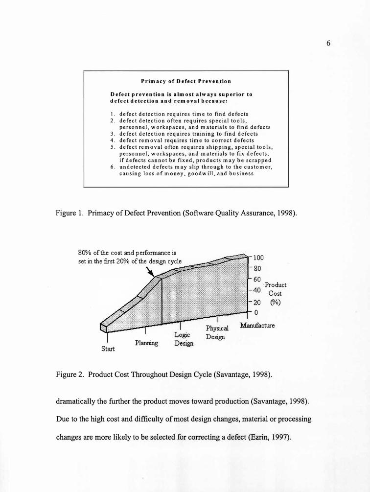
Research confirmed that defect prevention (Figure 1) is the optimum approach
for dealing with attribute or variable defects (Software Quality Assurance, 1998). To
be successful at this approach when designing products, engineers need to investigate
areas that could potentially lead to formation of surface defects. If engineers
overlook these areas, it could result in a poorly designed part or mold. Then efforts
may be necessary to eliminate the defect during a later, more costly design or
production stage. Research shows (Figure 2) the costs of design changes rise
5
, ..
Primacy of Defect Prevention
Defect prevention is almost always superior to
defect detection and removal because:
I. defect detection requires time to find defects2. defect detection often requires special tools,
personnel, workspaces, and materials to find defects3. defect detection requires training to find defects4. defect removal requires time to correct defects5. defect removal often requires shipping, special tools,
personnel, workspaces, and materials to fix defects;if defects cannot be fixed, products may be scrapped
6. undetected defects may slip through to the customer,causing loss of money, goodwill, and business
Figure 1. Primacy of Defect Prevention (Software Quality Assurance, 1998).
80% of the cost and performance is set in the first 20% of the design cycle
�
Start Planning
Physical Design
•V -1008060
·Product-4o Cost
(°lo)
Figure 2. Product Cost Throughout Design Cycle (Savantage, 1998).
dramatically the further the product moves toward production (Savantage, 1998).
Due to the high cost and difficulty of most design changes, material or processing
changes are more likely to be selected for correcting a defect (Ezrin, 1997).
6
Logic Design

However, eliminating a defect entirely may not be possible during the latter stages of
a product's design. Then reducing the size or moving the location of the defect may
be the only viable option that remains.
Considerations to prevent, eliminate, or reduce injection molding attribute
defects include part design, mold design, choice of polymer, and processing
conditions (Chang and Tsaur, 1995). In addition, techniques for inspecting or
masking the defect may be employed.
Part Design
Part design features such as ribs, bosses, coring, increased wall thickness and
others are often used to improve a part's strength or functionality. In addition, good
part design can significantly lower the possibility of visual defects forming on the
finished product. Each design feature must be selected and designed carefully for
each product. If basic design standards are violated when designing products, surface
defects could result. For example, sink marks in particular can develop opposite ribs,
bosses or any other design feature if not designed properly (Griffing and Whitaker,
1993).
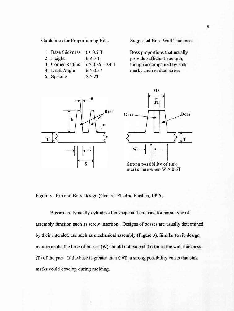
Ribs are thin walls of plastic used to reinforce a part's strength and reduce
wall thickness. Proper design of ribs can help prevent the formation of appearance
defects such as sink marks (Figure 3). As shown, if the base thickness (t) of a rib is
more than 0.5 times the wall thickness (T), sink marks can develop.
7
Guidelines for Proportioning Ribs
1. Base thickness
2 . Height
3. Comer Radius
4. Draft Angle
5. Spacing
t � 0.5 T
h�3T
r � 0.25 - 0.4 T
0 � 0.5°
S �2T
Suggested Boss Wall Thickness
Boss proportions that usually
provide sufficient strength,
though accompanied by sink
marks and residual stress.
2D
rm
Strong possibility of sink
marks here when W > 0.6T
Figure 3. Rib and Boss Design (General Electric Plastics, 1996 ).
Bosses are typically cylindrical in shape and are used for some type of
assembly function such as screw insertion. Designs of bosses are usually determined
by their intended use such as mechanical assembly (Figure 3). Similar to rib design
requirements, the base of bosses (W) should not exceed 0.6 times the wall thickness
(T) of the part. If the base is greater than 0.6T, a strong possibility exists that sink
marks could develop during molding.
8
0
oss
.______?, ._________, 4~ w4rr-r
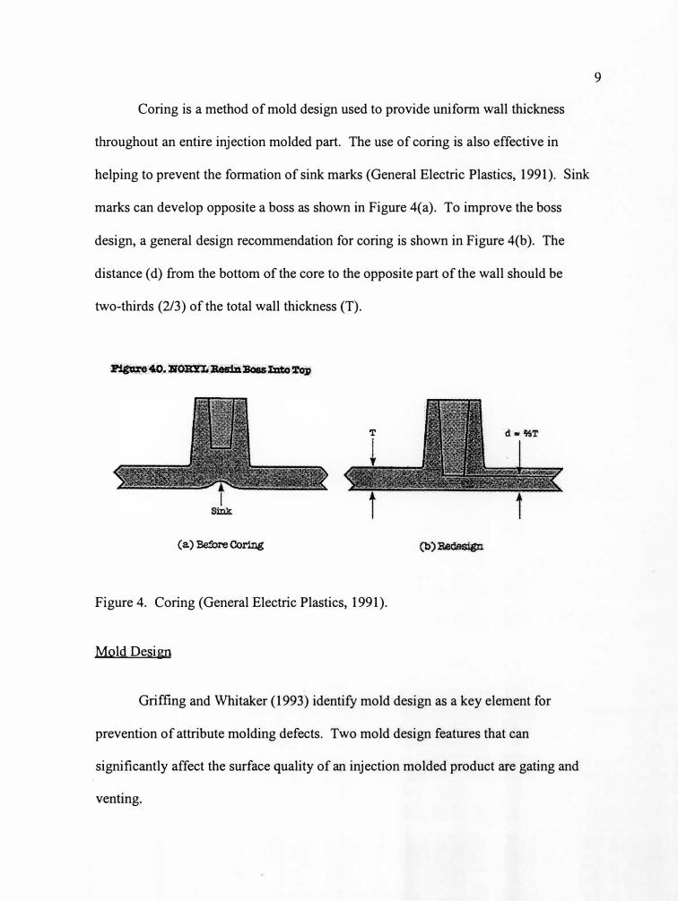
Coring is a method of mold design used to provide uniform wall thickness
throughout an entire injection molded part. The use of coring is also effective in
helping to prevent the formation of sink marks (General Electric Plastics, 1991 ). Sink
marks can develop opposite a boss as shown in Figure 4(a). To improve the boss
design, a general design recommendation for coring is shown in Figure 4(b ). The
distance ( d) from the bottom of the core to the opposite part of the wall should be
two-thirds (2/3) of the total wall thickness (T).
(a) Before Coring
Figure 4. Coring (General Electric Plastics, 1991).
Mold Design
Griffing and Whitaker (1993) identify mold design as a key element for
prevention of attribute molding defects. Two mold design features that can
significantly affect the surface quality of an injection molded product are gating and
venting.
9
(b)Bedasign

Gating is an opening in the mold where the liquid resin flows into the cavity
of the mold (Ashland Chemical, 1997, paragraph 28). Proper location of gates is
important to prevent or minimize the formation of visual defects. Gate related defects
such as jetting, splay, gate blush or other visual defects could be minimized by
locating the gate at a right angle to the runner. In situations where changing gate size
is unsuccessful, gates may be relocated so resultant defects are located on an area of
the part where surface quality is not critical. Another defect impacted by gate
location is weld lines. Weld lines are created when two flow fronts of plastic meet
and join together in the mold cavity. To reduce the size of weld line formation, gates
should be located in such a way as to allow flow of resin from thick to thin sections
within the mold (General Electric Plastics, 1994).
Venting allows gas built up during packing to escape from the mold cavity.
This gas, if not properly vented, can lead to the formation of surface imperfections
(Filbert and Roder, 1963). If vents are too large, flash may develop at the vent where
the two mold halves separate. If vents are too small, the gas trapped inside the mold
cavity could cause plastic degradation during molding of the part. The resulting
defect, burn marks, is usually seen on the surface of the part and is brown or black in
color. Using properly designed vents along the parting line (where the two mold
halves join during molding) can prevent these types of surface defects.
10
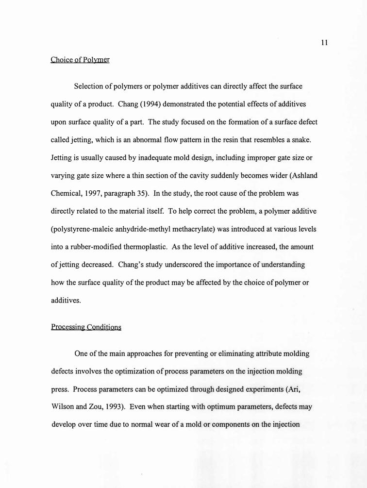
Choice of Polymer
Selection of polymers or polymer additives can directly affect the surface
quality of a product. Chang (1994) demonstrated the potential effects of additives
upon surface quality of a part. The study focused on the formation of a surface defect
called jetting, which is an abnormal flow pattern in the resin that resembles a snake.
Jetting is usually caused by inadequate mold design, including improper gate size or
varying gate size where a thin section of the cavity suddenly becomes wider (Ashland
Chemical, 1997, paragraph 35). In the study, the root cause of the problem was
directly related to the material itself. To help correct the problem, a polymer additive
(polystyrene-maleic anhydride-methyl methacrylate) was introduced at various levels
into a rubber-modified thermoplastic. As the level of additive increased, the amount
of jetting decreased. Chang's study underscored the importance of understanding
how the surface quality of the product may be affected by the choice of polymer or
additives.
Processinfi Conditions
One of the main approaches for preventing or eliminating attribute molding
defects involves the optimization of process parameters on the injection molding
press. Process parameters can be optimized through designed experiments (Ari,
Wilson and Zou, 1993). Even when starting with optimum parameters, defects may
develop over time due to normal wear of a mold or components on the injection
11
molding press. Therefore, on-going optimization may be necessary to eliminate any
defect formation.
If elimination of the defect is not possible, then the goal of process
optimization should be to minimize the size or move the location of the defect. In
some cases, the defect can be moved to an area that is less visible on the end product.
This approach may not address the root cause of a defect but can serve as a temporary
means of dealing with the symptom until a permanent solution is implemented. The
following examples show how injection molders have used processing conditions to
address various injection molding defects.
Ari et al. (1993) investigated an injection molding attribute defect called short
shots. Short shots result when the cavities inside the mold are not completely filled
with plastic during the molding cycle (Ashland Chemical, 1997, paragraph 59). The
short shot problem developed into a serious one when the defect rate reached five
percent and the company had to dedicate one employee to 100% inspection. The
company was subsequently able to establish a robust process by selecting the level of
cut-off pressure that actually prevented the formation of short shots.
Jan and O'Brien (1992) discussed how a company used a system to reduce
surface defects during the injection molding of plastic products. The system was
based on a software program that asks the operator a series of questions about the
current operating parameters and the resultant surface quality of the product. Based
upon these inputs, the system gave recommendations for process adjustments in order
to improve the surface defects on the part. The software was not designed to quantify
12
the attribute defects that appeared on the parts produced. Instead, the operator based
adjustments to the process upon subjective evaluation of the product. This system did
appear to be effective at eliminating or reducing a defect after it had developed.
Masking
One of the most common ways of masking attribute defects, especially when
dealing with automotive interior trim, is to paint the part. The primary reasons for
painting plastic parts for an automotive interior are to achieve consistent color and
gloss levels. Additional advantages include the ability to mask or cover over
common surface defects such as splay, flow lines, or blush on the molded part.
Despite these advantages, there are some defects such as sink marks that cannot be
masked with paint. In addition, in order to lower costs, the industry is beginning to
eliminate the painting of many plastic interior parts. Therefore, painting to mask a
defect's impact has become a less attractive option. This has placed greater pressure
on injection molders to understand their processes in order to produce defect-free
products.
Another method used to mask surface defects is texturing. Griffing and
Whitaker (1993) explained how the use of texture improves overall surface
appearance when used to mask weld lines and gate blush. In addition, sink marks
were evaluated on parts that had both a textured and non-textured half. The sink
marks were less visible on the side with the textured half. This study confirmed that
texturing can be an effective method for masking surface defects.
13
Inspection
In cases where surface defects cannot be prevented, eliminated or reduced,
some method of inspection may be necessary to avoid sending defective products to
the customer. In order to detect defective products, criteria must be established to
reveal what is an acceptable part. Once the suitable criteria are established, they can
be used to sort out nonconforming parts.
Establishin& Inspection Criteria
Inspection criteria can be defined as a set of standards or rules that determine
if a defect, such as sink marks, is acceptable. Inspection criteria can be established
using several different methods. The following are a few of the common methods
used.
Rating scales are used to assign a numerical value to an observable defect.
Griffing and Whittaker (1993) demonstrated an example ofthis in which five color
and appearance experts evaluated sink marks. After viewing parts with varying
degrees of sink marks, the evaluators rated the sink marks using a scale of one to five.
A rating of five represented a part with no visible sink marks. A rating of one
represented a part with highly visible sink marks. This procedure provided the
evaluators a method to make an informed decision on which parts were acceptable.
14
Boundary samples provide a way to visually show the minimum and
maximum limits of what is an acceptable part. This method is widely used in the
automotive industry for injection molded parts.
Go/no-go gauges may involve a pin gauge that has a minimum dimension at
one end and the maximum dimension at the other. Another go/no-go gauge used in
industry is sight lines. Minimum/maximum sight lines are etched into the metal of a
fixture and typically following the expected profile of a part. If the profile of the part
does not fall within the minimum and maximum sight lines, the part is rejected.
The two inspection methods used in this thesis study to evaluate sink marks
were: (1) an objective measurement system, and (2) visual evaluation by observers.
Both of these methods are discussed in the next section called Key Elements for
Developing Test Methodology, which is focused on research of key elements and
equipment for establishing a systematic approach for quantifying sink marks.
Key Elements for Developing Test Methodology
Whelan and Goff (1996) stated that when dealing with defects, "a logical and
systematic method of dealing with faults is most desirable" (p. 102). Based on this
statement, a review of applicable literature was conducted in order to establish a
systematic methodology to study sink marks. The test methodology for this thesis
consisted of two different phases.
The first phase, quantifying sink marks, involved using an existing
measurement system to measure sink marks on the surface of a plastic injection
15
molded part. Research for the first phase included various measurement systems that
could potentially be used to quantify sink marks. The second phase included
exploration of key elements such as eyesight cues, lighting, and distance of
observation that might impact the test methodology.
The First Phase: Quantifying Sink Marks
Six different objective, instrument-based measurement systems or devices
were researched to determine their usefulness to quantify sink marks: (1)
interferometers, (2) optical comparators, (3) photoacoustic microscopes, (4) laser
gauges, (5) def�ct analyzers, and (6) coordinate measurement machines. The six
systems evaluated are described below.
1. An interferometer is an instrument that can be used to measure
deformation, vibration, and contour measurements of diffuse objects (McGraw-Hill,
1997). There are several types of interferometers that can be used for wide range of
applications including surface measurements and determining the distance between
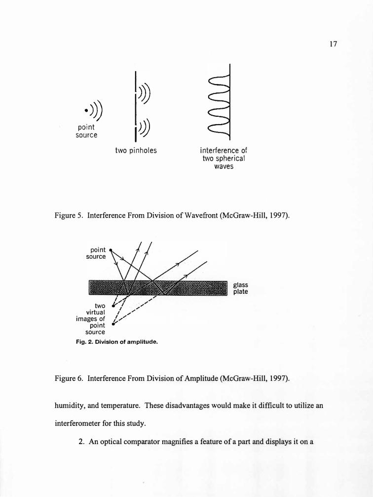
stars. Interferometers fall into two categories: (1) division of wavefront (Figure 5),
and (2) division of amplitude (Figure 6). One advantage of using an interferometer to
measure sink marks is its ability to detect surface change. Advanced equipment is
capable of measuring surface roughness with a resolution of about one nanometer ( 40
billionths of an inch). This high resolution was not required for measuring sink
marks. There were some disadvantages of using an interferometer to quantify sink
marks. For example, the equipment is sensitive to air currents, acoustic noise,
16
· )))point
source I� two pinholes interference of
two spherical waves
Figure 5. Interference From Division of Wavefront (McGraw-Hill, 1997).
two virtual
images of point
source
Fig. 2. Division of amplitude.
glass plate
Figure 6. Interference From Division of Amplitude (McGraw-Hill, 1997).
humidity, and temperature. These disadvantages would make it difficult to utilize an
interferometer for this study.
2. An optical comparator magnifies a feature of a part and displays it on a
17
viewing screen for comparison to a master outline of a desirable part. The shadow of
the part being measured must fall within specification limits in order to pass
inspection. It is typically used to compare contours or dimensions (Wortman, 1995).
Optical comparators are one of the most reliable and accurate measurement tools for
manufactured parts (Kendrick, 1994). Because the system is based upon a visual
comparison to a master part, the optical comparator is not ideal for producing a
quantitative measurement of sink marks. Also, the optical comparator does not have
the necessary measurement discrimination to quantify sink marks.
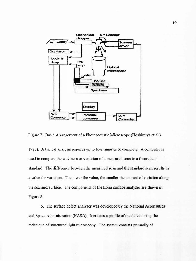
3. A photoacoustic microscope uses an Ar-ion laser beam along with optical
scanners to obtain amplitude and phase images. These images are used to produce
precise, quantitative shape and depth measurements of surface defects (Hoshimiya,
Endoh and Hiwatashi, 1996). The basic arrangement of a photoacoustic microscope
is shown in Figure 7. One advantage in using a photoacoustic is its ability to identify
both the location and shape of a defect on the surface of a part. However, most
systems are only capable of qualitative analysis. Therefore, a photoacoustic
microscope is not the optimum equipment for quantifying sink marks.
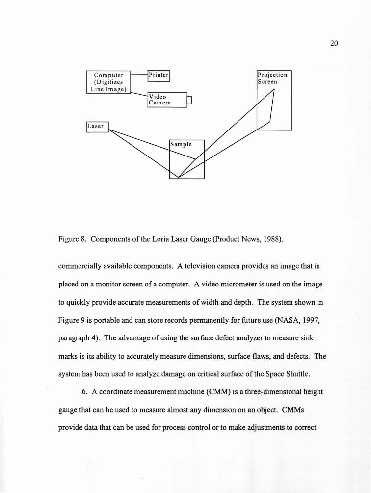
4. A laser gauge, the Loria analyzer, was developed by Ashland Chemical to
check Class A surfaces and produce a quantitative rating of the surface quality. An
advantage of using the laser gauge for measuring sink marks is its ability to detect
and quantify surface defects. A helium-neon laser beam scans the surface area. The
laser beam measurements are reflected onto a projection screen. It is recorded by a
high-resolution video camera and analyzed by the system's computer (Product News,
18
Oscillator
Lock-in Amp
A/D Converter
Mechanical X-Y Scanner
Display
Personal com uter
'-=�---tScanner -----1driver
t----Jl-.t D/A Converter
Figure 7. Basic Arrangement of a Photoacoustic Microscope (Hoshimiya et al.).
1988). A typical analysis requires up to four minutes to complete. A computer is
used to compare the waviness or variation of a measured scan to a theoretical
standard. The difference between the measured scan and the standard scan results in
a value for variation. The lower the value, the smaller the amount of variation along
the scanned surface. The components of the Loria surface analyzer are shown in
Figure 8.
5. The surface defect analyzer was developed by the National Aeronautics
and Space Administration (NASA). It creates a profile of the defect using the
technique of structured light microscopy. The system consists primarily of
19
Computer (Digitizes
Line Image)
Laser
Printer
Video Camera
Projection Screen
Figure 8. Components of the Loria Laser Gauge (Product News, 1988).
commercially available components. A television camera provides an image that is
placed on a monitor screen of a computer. A video micrometer is used on the image
to quickly provide accurate measurements of width and depth. The system shown in
Figure 9 is portable and can store records permanently for future use (NASA, 1997,
paragraph 4). The advantage of using the surface defect analyzer to measure sink
marks is its ability to accurately measure dimensions, surface flaws, and defects. The
system has been used to analyze damage on critical surface of the Space Shuttle.
6. A coordinate measurement machine (CMM) is a three-dimensional height
gauge that can be used to measure almost any dimension on an object. CMMs
provide data that can be used for process control or to make adjustments to correct
20
.....__~ I p
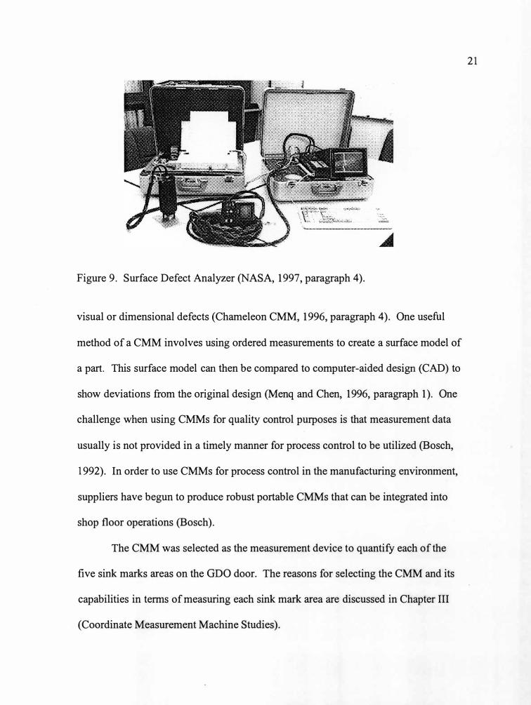
Figure 9. Surface Defect Analyzer (NASA, 1997, paragraph 4).
visual or dimensional defects (Chameleon CMM, 1996, paragraph 4). One useful
method of a CMM involves using ordered measurements to create a surface model of
a part. This surface model can then be compared to computer-aided design (CAD) to
show deviations from the original design (Menq and Chen, 1996, paragraph 1 ). One
challenge when using CMMs for quality control purposes is that measurement data
usually is not provided in a timely manner for process control to be utilized (Bosch,
1992). In order to use CMMs for process control in the manufacturing environment,
suppliers have begun to produce robust portable CMMs that can be integrated into
shop floor operations (Bosch).
The CMM was selected as the measurement device to quantify each of the
five sink marks areas on the GDO door. The reasons for selecting the CMM and its
capabilities in terms of measuring each sink mark area are discussed in Chapter III
(Coordinate Measurement Machine Studies).
21

Phase II: Visual Evaluation of Sink Marks
During this study, visual evaluation of sink marks by humans was categorized
into two areas: (1) eyesight factors, and (2) preference and discrimination
procedures. The goal of the research was to pinpoint the elements that should be
included during visual evaluation of sink marks, in order to reduce subjectivity.
Eyesight Factors
Research was conducted to determine the eyesight factors that might influence
an observer's ability to perceive sink marks. Three eyesight factors were
investigated: (1) depth perception, (2) visual acuity, and (3) external factors.
Depth Perception. During the investigation, binocular (two eye) cues were
determined to influence a person's ability to perceive depth (Depth Perception, 1996,
paragraph 2). Binocular vision relates to the coordinated use of both eyes to focus at
a common target. Three binocular cues investigated in the research were: (1)
vergence, (2) stereopsis, and (3) depth judgment.
Vergence is the only binocular cue that gives absolute depth information.
Vergence consists of the "muscular feedback from effort to converge or diverge
which gives information about depth" (Depth Perception, 1997, paragraph 2). In
other words, it is the angle ofvergence between the two eyes when an object is at a
22
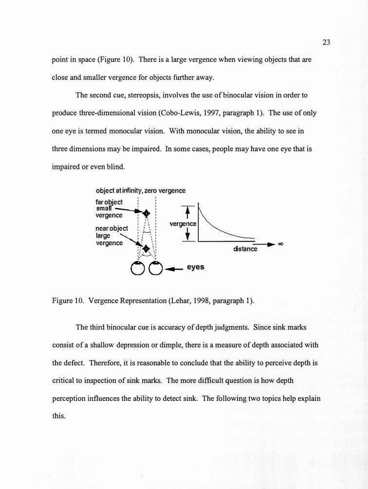
point in space (Figure 10). There is a large vergence when viewing objects that are
close and smaller vergence for objects further away.
The second cue, stereopsis, involves the use of binocular vision in order to
produce three-dimensional vision (Cobo-Lewis, 1997, paragraph 1). The use of only
one eye is termed monocular vision. With monocular vision, the ability to see in
three dimensions may be impaired. In some cases, people may have one eye that is
impaired or even blind.
object at infinity, zero vergencefar o�ect : small ---...., vergence : ♦
' " , '
near object : ! \ large '-...._ : r--\ vergence � \.
1' , \ ••
�,:,'--..-,>
.. �
oo�eyes
distance
Figure 10. Vergence Representation (Lehar, 1998, paragraph 1).
► 0()
The third binocular cue is accuracy of depth judgments. Since sink marks
consist of a shallow depression or dimple, there is a measure of depth associated with
the defect. Therefore, it is reasonable to conclude that the ability to perceive depth is
critical to inspection of sink marks. The more difficult question is how depth
perception influences the ability to detect sink. The following two topics help explain
this.
23

Autostereograms are related to depth perception and involve the viewing of 3-
D stereograms. "In 1994, America became addicted to autostereograms - those
swatches of psychedelic wallpaper that dissolve into three dimensional images when
you stare at them long enough" (Zimmer, 1995, paragraph 1). Scientists have
realized that depth perception arises from the way the brain compares signals from
the two eyes, which see an object from slightly different angles (Zimmer, paragraph
2). This involves what is known as binocular disparity. Binocular disparity refers to
how each eye perceives an object from different viewpoints. "Thus, the images
projected onto the retinas are slightly different. The brain uses assumptions of depth
to reconcile the disparity" (Murray, 1997, paragraph 15). The balance of disparity
between two eyes is disrupted when one eye is more dominant than the other.
Gestalt principles are also related to depth perception and reveal the "tendency
to seek organization and closure, recognize patterns, and so on" (Murray, 1997,
paragraph 10). For example, when observers view a drawing of two partially
overlapping opaque squares where one obscures a comer of the other such as in
Figure 11, it will be seen as overlap and not as an L-shape abutted to the edge of a
square (Murray, paragraph 10).
Gestalt principles were investigated because the possibility exists that an
observer evaluating sink marks may have a tendency to overlook the defect due to the
Gestalt tendency to seek organization and closure. In 1960, Bela Julesz concluded
"that depth perception is one of the first things the brain extracts from the visual
signal, by comparing the left-eye and right-eye images dot by dot. Object recognition
24
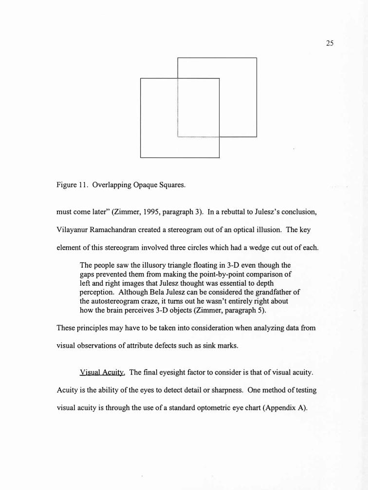
Figure 11. Overlapping Opaque Squares.
must come later" (Zimmer, 1995, paragraph 3). In a rebuttal to Julesz's conclusion,
Vilayanur Ramachandran created a stereogram out of an optical illusion. The key
element of this stereogram involved three circles which had a wedge cut out of each.
The people saw the illusory triangle floating in 3-D even though the gaps prevented them from making the point-by-point comparison of left and right images that Julesz thought was essential to depth perception. Although Bela Julesz can be considered the grandfather of the autostereogram craze, it turns out he wasn't entirely right about how the brain perceives 3-D objects (Zimmer, paragraph 5).
These principles may have to be taken into consideration when analyzing data from
visual observations of attribute defects such as sink marks.
Visual Acuity. The final eyesight factor to consider is that of visual acuity.
Acuity is the ability of the eyes to detect detail or sharpness. One method of testing
visual acuity is through the use of a standard optometric eye chart (Appendix A).
25

This method was used to categorize people into different levels of eyesight for the
visual evaluation of sink marks.
External Factors. Two external factors were included in the visual evaluation
of sink marks: (1) lighting environment, and (2) distance from the observer to the
object. A consistent lighting environment was established to minimize variability
during visual evaluation of sink marks. With respect to distance, Nakayama and
Shimojo (1992, paragraph 21) confirmed that viewing distance from observer to
object affects the observer's ability to perceive visual surfaces. Surfaces appear
flatter when viewed from greater distances.
Preference and Discrimination Procedures
For sensory related research, several different types of discrimination and
preference testing procedures are available (Johnson, 1996), including but not limited
to: (a) paired comparison, (b) triangle, (c) repeat pair, (d) double pair, (e) triad, and
(f) dual triad. When discrimination and preference types of testing procedures are
used, there can be several objectives: (a) measurement of product preference, (b)
determination of the reason for product preference, and ( c) assessment of the extent to
which individuals can actually tell the difference between products. The criteria that
were required for this thesis involved the ability to discriminate between various
levels of sink marks. The procedure selected for the visual evaluation study was a
26

simple complete block design. The following are explanations of preference
procedures and complete block designs.
Paired Comparison Procedure. When using this procedure, observers are
given two parts to observe in order to determine which one is preferred. The
procedure does not provide detailed information on discrimination. If one part is
picked more strongly, then it can be concluded that some of the observers are able to
tell the difference between the two parts (Johnson, 1996). The only discrimination
information provided is if one part is strongly preferred. This procedure is not
designed for use with more than two parts (Johnson). Accordingly it could not be
used for this research project.
Triangle Procedure. In the triangle procedure the observer is given three
parts. Two of the three are the same. The observer is asked to select which of the
three parts is different from the others. The observers can then be divided into two
groups: (1) those who correctly choose the unique part, and (2) those who incorrectly
choose one of the parts that are the same. (Johnson, 1996). The triangle procedure
does not indicate observer preference, but is used to determine to what extent the
respondents are able to tell the difference between parts. This procedure is typically
used for two treatments and therefore was not the best choice for this study.
Repeat Pair Procedure. In the repeat pair procedure observers are asked to
view two parts and choose which one they prefer. Next, the observers are given two
27

more parts, identical to the first set of parts, and asked to choose which they prefer.
Three categories ofresponse result: (1) those who select the same part in both tests,
(2) those who prefer the other part in both tests, and (3) those who choose different
parts in each test. (Johnson, 1996). An indication of both preference and
discrimination result from the use of the repeat pair procedure. This procedure is also
used for two treatments.
Double Pair Procedure. The double pair procedure involves observation of
four parts simultaneously. The four parts are actually two pairs of parts identical to
each other. The observer, not knowing that any of the parts are identical, evaluates all
four parts simultaneously and is asked to choose the two most preferred. Observers
are grouped into three categories: (1) Those who choose the first set of identical parts,
(2) those who choose the second set of identical parts, and (3) those who choose two
different parts (Johnson, 1996). The double pair procedure also provides information
on both preference and discrimination. This procedure is also used for two
treatments.
Triad Procedure. The triad procedure provides both discrimination and
preference information. Three parts are given to the observers. Two of the three
parts are identical. Respondents are asked to rank the three parts in order of
preference. The observers are again grouped into three categories: (1) those who
truly prefer the identical parts who will rank both of them higher than the unique part,
(2) those who truly prefer the unique part who will rank it above the identical parts,
28

and (3) those who cannot discriminate and rank the unique part second of the three
(Johnson, 1996). This procedure is also used for two treatments.
Dual Triad Procedure. The dual triad procedure involves two sets of the triad
procedure described above. However, the unique part in the first triad becomes the
identical pair in the second triad, and vice versa. Observers are again categorized into
three groups: (1) those who truly prefer the identical pair in the first triad and the
unique part in the second triad, (2) those who truly prefer the unique part in the first
triad and the identical pair in the second triad, and (3) those who respond randomly.
The benefit of the dual triad over the single triad procedure is that those with firm
preferences are more clearly distinguished. However, it is less convenient to
administrate than the single triad method (Johnson, 1996). This procedure is also
used for two treatments.
Simple Corrwlete Block Design. A simple complete block design involves
presenting each subject with treatments usually in random order (Gill, 1978). An
example of a treatment would be presenting human observers plastic parts with
varying levels of defects for observation. Complete block designs help to conserve
resources ( e.g. the number of people tested or expense of the testing) and reduce
experimental error while maintaining the sensitivity of an experiment (Gill). This
design can be used for more than two treatments and thus a good choice for this
research project.
29

When these types of experiments are used, it is sometimes necessary to
remove possible nuisance variables. The concept of a nuisance variable can be
illustrated through the example of various observers in different lighting conditions
viewing plastic parts with surface defects. Some observers may be able to see the
defects while others may not. The nuisance variable in this example is an
inconsistent lighting environment in which the parts were observed. Requiring all
observers to view the plastic parts using the same lighting environment would
eliminate the nuisance variable of inconsistent lighting. If the nuisance variable was
inadequate lighting, a test could be conducted using various lighting conditions to
determine which light source enabled observers to optimally see the defect.
Summary of Literature Review
The review of literature confirmed that defect prevention is a better approach
than elimination or reduction of the defect after it appears. If prevention is
economically or otherwise unfeasible, then elimination or reduction of the defect may
be needed. Elimination and reduction efforts often involve a change in part design,
mold design, choice of polymer or optimization of process parameters. Sometimes
these options may not eliminate the defect but only reduce its size or location. If the
defect can not be eliminated, then methods to mask over the defect ( e.g. painting the
part) are sometimes used. During efforts to eliminate or reduce the defect, inspection
of the molded product may be needed to prevent defects from being sent to the
30

customer. When inspection is needed, then it becomes necessary to clearly define the
inspection criteria so that an objective acceptance standard is established.
31

CHAPTER III
METHODOLOGY
Introduction
There were two phases involved in the methodology of this study. The
purpose of the first phase was to develop a method to objectively measure sink marks.
The second phase investigated the subjective human component of visual evaluation
to determine if observers were able to reliably detect different levels of sink marks.
The methodology for both phases consisted of the following nine elements:
(1) production of parts with sink marks, (2) visual evaluation pilot tests, (3)
production of parts to expand the range of sink mark treatments, ( 4) quantification of
sink marks on non-painted parts, (5) full-scale visual evaluation of sink marks on
non-painted parts, (6) production of painted GDO doors, (7) full-scale visual
evaluation of sink marks on painted parts, (8) quantification of sink marks on painted
parts, and (9) analysis of data.
Production of Parts With Sink Marks
An injection molding press produced plastic parts with various levels of sink
marks. Before parts could be produced, several elements of the methodology had to
be addressed. These elements included: (a) part selection, (b) production equipment,
32

( c) independent process variable, ( d) part production, and ( e) part labeling and
packaging.
Part Selection
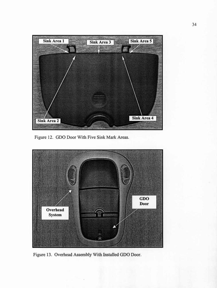
A garage door opener (GDO) door (Figure 12) met these requirements and
was selected for the study on the basis of the following factors. It could be produced
with a level of sink marks that could be detected by the measurement system used in
the study and the human eye. It also could be produced with no visible sink marks by
manipulating process parameters. It had a textured surface common to those used on
many interior automotive parts. The garage door opener is installed behind the GDO
door. The customer pushes on the GDO door to make physical contact with the
garage door opener and initiate the electronic sequence required open a garage door.
The GDO door is assembled into an overhead system (Figure 13) before being
installed into the overhead of the vehicle. Five potential sink mark areas are shown
on the GDO door in Figure 12.
After part selection was completed, the next step was to identify the
production equipment needed to produce GDO doors with various levels of sink
marks.
Production Equipment
The production equipment used to mold the product was a 220-ton hydraulic
clamp Cincinnati injection molding press. The press had a 20-ounce capacity
33
34
Figure 12. GDO Door With Five Sink Mark Areas.
Figure 13. Overhead Assembly With Installed GDO Door.
capacity injection unit, fluid drive screw motor, eagle mixing screw, an LID ratio of
20: 1, intensification ratio of 9: 1, compression ratio of 2.5: 1 and a maximum hydraulic
pressure of 2,500 psi.
After identifying the production equipment, the next step was to identify the
independent process variable that would significantly affect sink mark formation.
Selection of the independent process variable is described in the next section.
Independent Process Variable
One independent variable, pack pressure was selected for the study. Through
research, pack pressure was identified as a significant contributor for controlling sink
marks (Celstran, 1997) as one of the primary injection molding parameters used to
troubleshoot sink marks. Pack pressure is the amount of pressure used to fill out the
mold cavity after first stage injection is complete (Groleau, 1996). The only issue to
determine was the level of pack pressure at which sink marks began to appear on the
surface of the product. Since this level was not completely identified, a preliminary
study was conducted to determine it.
Part Production
Pack pressure was initially set at the top level of 1750 psi so that acceptable
parts with no apparent sink marks were produced. The process was allowed to
stabilize before parts were collected. Two consecutive parts were collected, labeled
and allowed to cool. The pack pressure was then lowered 50 psi to the next level and
35
the procedure repeated. Thirty-six parts (within a pack pressure range of zero psi to
1750 psi by increments of 50 psi) were initially produced for the visual evaluation
study.
Product Labeling and Packaging
During each level, the two consecutive parts produced by the press were
labeled with the level of pack pressure, followed by a hyphen, followed by the part
number within that level (e.g. 50-1, 50-2, 1000-1, 1000-2 ... ). The parts were labeled
on the backside to avoid contamination of the show surface of the part.
The show surface was the textured side of the part that would be visible to the
customer after installation into a vehicle. All parts were allowed to cool for at least
fourteen days to assure that the majority of shrinkage had taken place. All parts for
each level were packaged in foam padding and placed in a cardboard box to protect
their surfaces from damage prior to visual evaluation of the sink marks.
Visual Evaluation Pilot Tests
In order to prepare for a visual evaluation of parts with sink marks, three pilot
tests were conducted. All three pilot tested were completed using non-painted GDO
doors. The first two pilot tests were completed to determine whether observers
should view parts while holding them in their hands or within a viewing fixture.
During the third pilot test, two different tests were used to evaluate how observers
ranked the parts in order of preference (no visible sink to worst visible sink).
36

Pilot Test #1
The first pilot test consisted of two different methods for presenting parts to
observers: (1) hand-held observation, and (2) observation of parts in a viewing
fixture. During the testing using both methods, observers were presented eleven non
painted parts, one at a time, for observation of sink marks. The testing information
specific to each method is presented below.
Hand-held Observation. The hand-held method was evaluated because it
represented how parts are normally observed in production. Observers were asked to
view the parts in a hand-held position and record on the check sheet (Appendix C)
whether they could see sink marks on the parts. They could pick up the parts and
observe them at any angle. They were not allowed to feel the sink marks on the parts
with their fingers. All observers responded favorably to the option of being able to
pick up the parts and visually evaluate them.
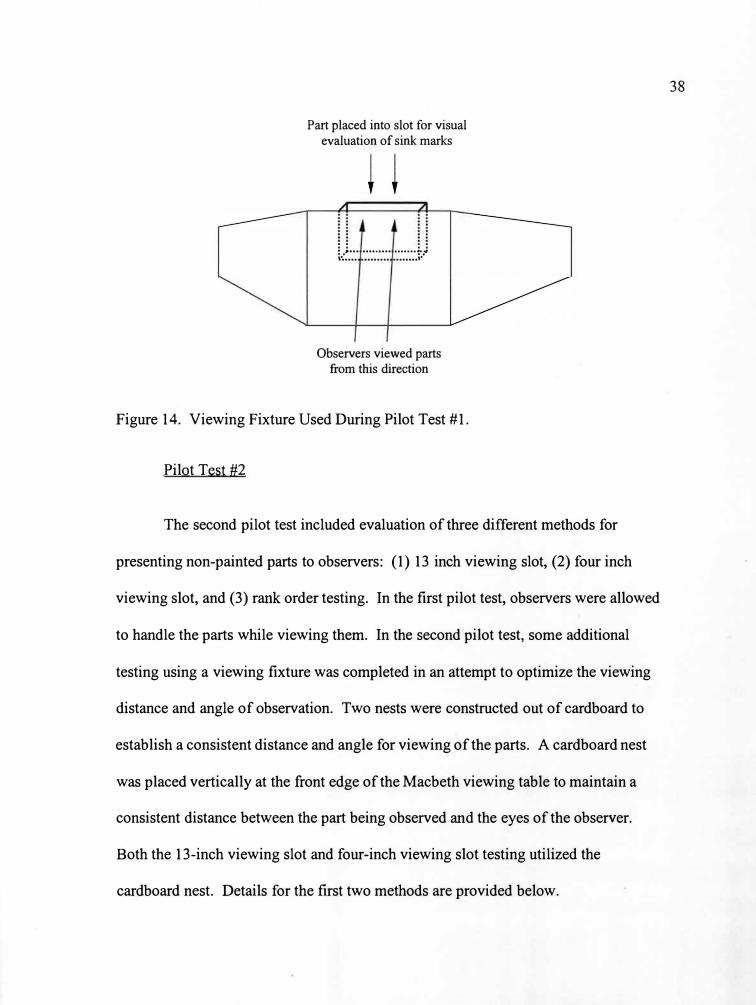
Observation Using a Viewing Fixture. This method involved using a fixture
to nest the part (Figure 14). The fixture was used to reduce the amount of variation in
how observers viewed the parts by controlling the distance and angle of observation.
During evaluation by observers, each of the eleven parts were placed into the slot for
viewing. A small section of the part where the sink marks were located was still
visible to the observers. A part was placed into the fixture and viewed by observers
without picking it up with their hands.
37
Part placed into slot for visual evaluation of sink marks
. .
. . . . : .,. ... ......... ·······�·:', ...... ........ ........ ,.
Observers viewed parts from this direction
Figure 14. Viewing Fixture Used During Pilot Test #1.
Pilot Test #2
The second pilot test included evaluation of three different methods for
presenting non-painted parts to observers: (1) 13 inch viewing slot, (2) four inch
viewing slot, and (3) rank order testing. In the first pilot test, observers were allowed
to handle the parts while viewing them. In the second pilot test, some additional
testing using a viewing fixture was completed in an attempt to optimize the viewing
distance and angle of observation. Two nests were constructed out of cardboard to
establish a consistent distance and angle for viewing of the parts. A cardboard nest
was placed vertically at the front edge of the Macbeth viewing table to maintain a
consistent distance between the part being observed and the eyes of the observer.
Both the 13-inch viewing slot and four-inch viewing slot testing utilized the
cardboard nest. Details for the first two methods are provided below.
38
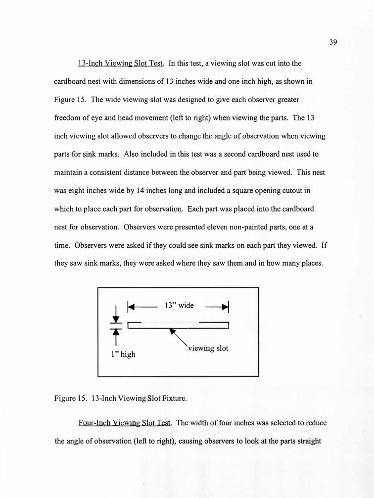
13-Inch Viewing Slot Test. In this test, a viewing slot was cut into the
cardboard nest with dimensions of 13 inches wide and one inch high, as shown in
Figure 15. The wide viewing slot was designed to give each observer greater
freedom of eye and head movement (left to right) when viewing the parts. The 13
inch viewing slot allowed observers to change the angle of observation when viewing
parts for sink marks. Also included in this test was a second cardboard nest used to
maintain a consistent distance between the observer and part being viewed. This nest
was eight inches wide by 14 inches long and included a square opening cutout in
which to place each part for observation. Each part was placed into the cardboard
nest for observation. Observers were presented eleven non-painted parts, one at a
time. Observers were asked if they could see sink marks on each part they viewed. If
they saw sink marks, they were asked where they saw them and in how many places.
13" wide ----+J j.__ I◄
T .---, , . -. -..1 I viewmg s ot 1" high
Figure 15. 13-Inch Viewing Slot Fixture.
Four-Inch Viewing Slot Test. The width of four inches was selected to reduce
the angle of observation (left to right), causing observers to look at the parts straight
39
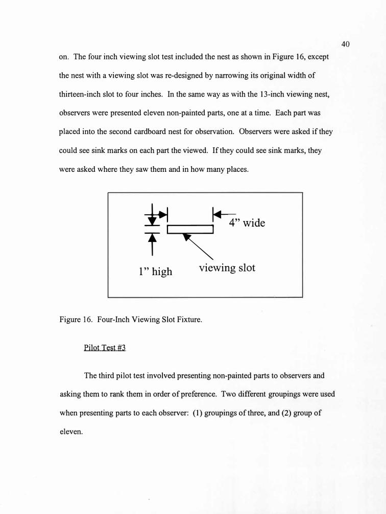
on. The four inch viewing slot test included the nest as shown in Figure 16, except
the nest with a viewing slot was re-designed by narrowing its original width of
thirteen-inch slot to four inches. In the same way as with the 13-inch viewing nest,
observers were presented eleven non-painted parts, one at a time. Each part was
placed into the second cardboard nest for observation. Observers were asked if they
could see sink marks on each part the viewed. If they could see sink marks, they
were asked where they saw them and in how many places.
i--1 �'wide
T� 1" high viewing slot
Figure 16. Four-Inch Viewing Slot Fixture.
Pilot Test #3
The third pilot test involved presenting non-painted parts to observers and
asking them to rank them in order of preference. Two different groupings were used
when presenting parts to each observer: (1) groupings of three, and (2) group of
eleven.
40
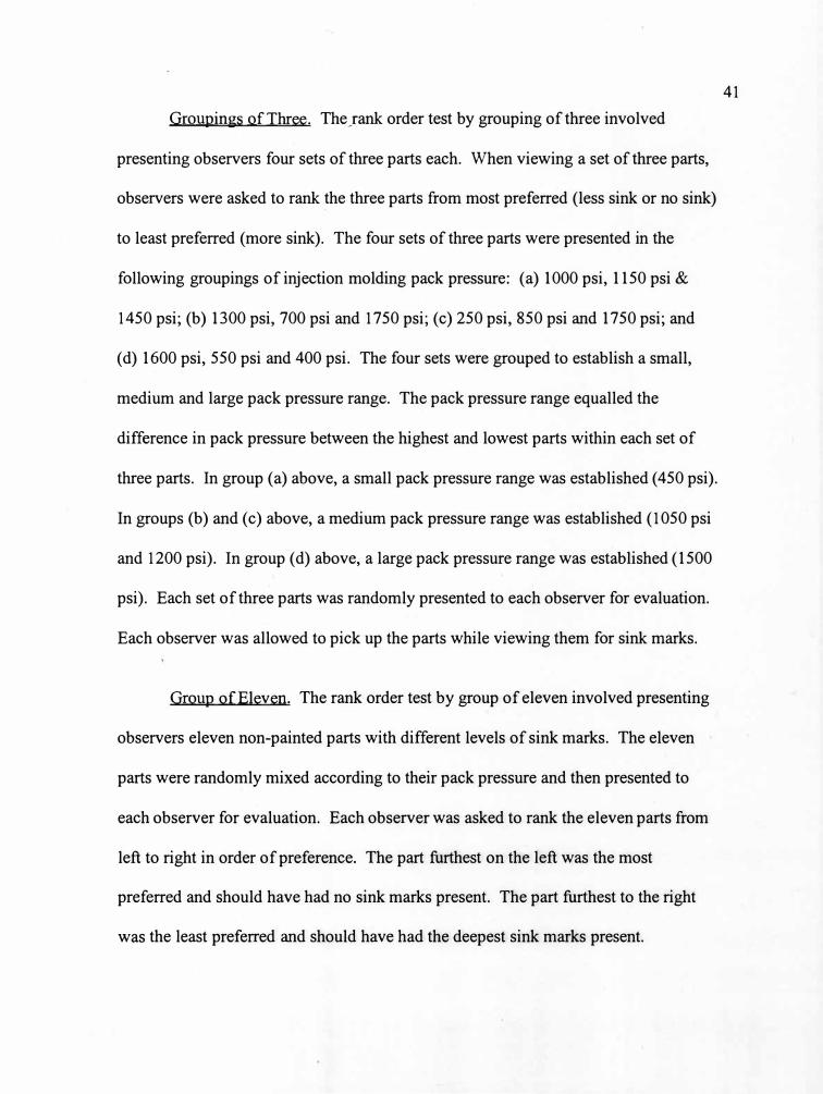
Groupings of Three. The 1ank order test by grouping of three involved
presenting observers four sets of three parts each. When viewing a set of three parts,
observers were asked to rank the three parts from most preferred (less sink or no sink)
to least preferred (more sink). The four sets of three parts were presented in the
following groupings of injection molding pack pressure: (a) 1000 psi, 1150 psi &
1450 psi; (b) 1300 psi, 700 psi and 1750 psi; (c) 250 psi, 850 psi and 1750 psi; and
(d) 1600 psi, 550 psi and 400 psi. The four sets were grouped to establish a small,
medium and large pack pressure range. The pack pressure range equalled the
difference in pack pressure between the highest and lowest parts within each set of
three parts. In group (a) above, a small pack pressure range was established (450 psi).
In groups (b) and (c) above, a medium pack pressure range was established (1050 psi
and 1200 psi). In group (d) above, a large pack pressure range was established (1500
psi). Each set of three parts was randomly presented to each observer for evaluation.
Each observer was allowed to pick up the parts while viewing them for sink marks.
Group of Eleven. The rank order test by group of eleven involved presenting
observers eleven non-painted parts with different levels of sink marks. The eleven
parts were randomly mixed according to their pack pressure and then presented to
each observer for evaluation. Each observer was asked to rank the eleven parts from
left to right in order of preference. The part furthest on the left was the most
preferred and should have had no sink marks present. The part furthest to the right
was the least preferred and should have had the deepest sink marks present.
41
•

Production of Parts to Expand the Range of Sink Mark Treatments
During the three pilot tests, it was discovered that a majority of observers
could see sink marks on the parts produced within the pack pressure range of 150 psi
to 1750 psi. In order to address this issue, additional non-painted GDO doors were
produced at pack pressures of: 1900 psi, 2050 psi, 2200 psi, and 2350 psi. An
attempt was made to produce GDO doors at pack pressures higher than 2350 psi but a
defect called flash began to appear along the parting line edges of the parts. These
parts were produced to provide additional sink mark treatments at the lowest
measurable levels. The goal was to produce parts with no visible sink marks for
inclusion in the full-scale visual evaluation study.
Quantification of Sink Marks on Non-Painted Parts
In order to quantify sink marks, several studies were completed, including:
(a) coordinate measurement machine (CMM) studies, (b) a gauge repeatability and
reproducibility (gauge R & R) study, and (c) statistical analysis of CMM data.
Coordinate Measurement Machine Studies
The system used for measurement of sink marks was a Mitutoyo CHN 1000
. coordinate measurement machine (CNC CMM, No Date). The CMM was selected
for its capability to conduct a series of repeatable measurements across the surface of
a part (surface scan). The profile of a surface scan with the five sink mark areas is
42
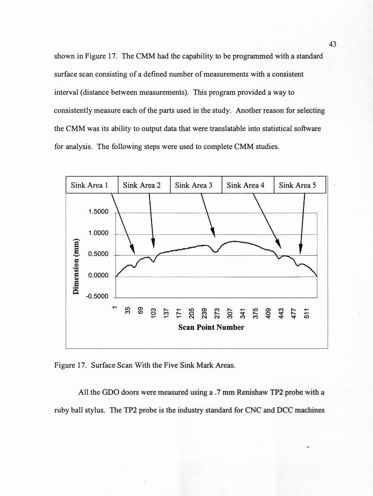
shown in Figure 17. The CMM had the capability to be programmed with a standard
surface scan consisting of a defined number of measurements with a consistent
interval (distance between measurements). This program provided a way to
consistently measure each of the parts used in the study. Another reason for selecting
the CMM was its ability to output data that were translatable into statistical software
for analysis. The following steps were used to complete CMM studies.
Sink Area 1
1.5000
1.0000
S 0.5000
=
....
5 0.0000
-0.5000
Sink Area 3 Sink Area4
Scan Point Number
Figure 17. Surface Scan With the Five Sink Mark Areas.
Sink Area 5
All the GDO doors were measured using a . 7 mm Renishaw TP2 probe with a
ruby ball stylus. The TP2 probe is the industry standard for CNC and DCC machines
43
1
35
69
103
137
171
205
239
273
307
341
375
409
443
477
511
Dim
so
m
)
(Probing for Productivity, 1998). According to Renishaw, ruby ball stylus are
suitable for most standard measurement applications.
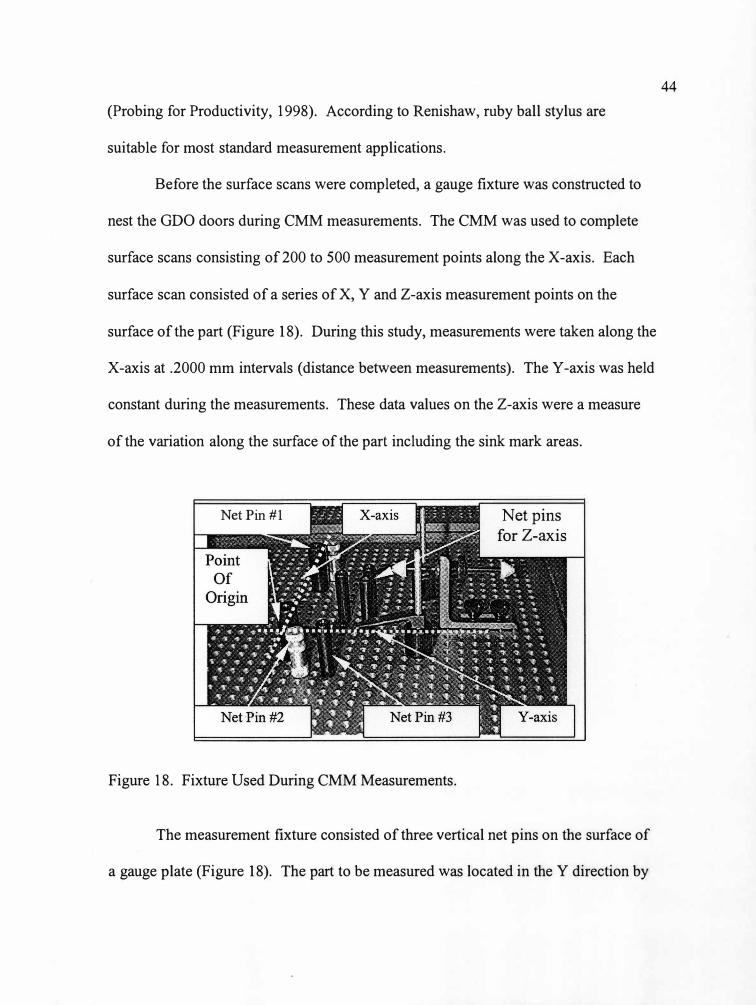
Before the surface scans were completed, a gauge fixture was constructed to
nest the GDO doors during CMM measurements. The CMM was used to complete
surface scans consisting of200 to 500 measurement points along the X-axis. Each
surface scan consisted of a series of X, Y and Z-axis measurement points on the
surface of the part (Figure 18). During this study, measurements were taken along the
X-axis at .2000 mm intervals (distance between measurements). The Y-axis was held
constant during the measurements. These data values on the Z-axis were a measure
of the variation along the surface of the part including the sink mark areas.
Net Pin #1
Figure 18. Fixture Used During CMM Measurements.
Net pins
for Z-axis
The measurement fixture consisted of three vertical net pins on the surface of
a gauge plate (Figure 18). The part to be measured was located in the Y direction by
44
Point Of
Origin
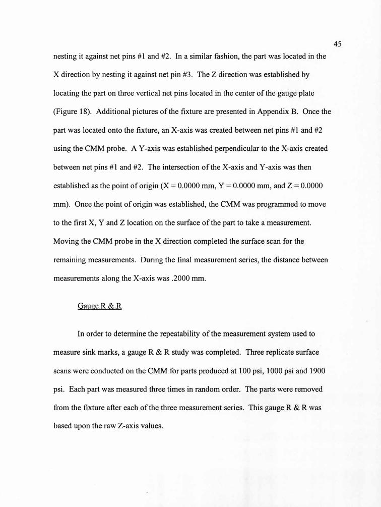
nesting it against net pins #1 and #2. In a similar fashion, the part was located in the
X direction by nesting it against net pin #3. The Z direction was established by
locating the part on three vertical net pins located in the center of the gauge plate
(Figure 18). Additional pictures of the fixture are presented in Appendix B. Once the
part was located onto the fixture, an X-axis was created between net pins # 1 and #2
using the CMM probe. A Y-axis was established perpendicular to the X-axis created
between net pins #1 and #2. The intersection of the X-axis and Y-axis was then
established as the point of origin (X = 0.0000 mm, Y = 0.0000 mm, and Z = 0.0000
mm). Once the point of origin was established, the CMM was programmed to move
to the first X, Y and Z location on the surface of the part to take a measurement.
Moving the CMM probe in the X direction completed the surface scan for the
remaining measurements. During the final measurement series, the distance between
measurements along the X-axis was .2000 mm.
GaugeR&R
In order to determine the repeatability of the measurement system used to
measure sink marks, a gauge R & R study was completed. Three replicate surface
scans were conducted on the CMM for parts produced at 100 psi, 1000 psi and 1900
psi. Each part was measured three times in random order. The parts were removed
from the fixture after each of the three measurement series. This gauge R & R was
based upon the raw Z-axis values.
45

During the initial gauge R & R, three sources of measurement related
variation were identified: (1) variation caused by the amount of pack pressure used to
produce each of the parts (hereafter called change in pack pressure), (2) variation in
how the parts were relocated onto the fixture during each of the three measurement
series (hereafter called fixture locating), and (3) variation due to change in the X-axis
value or the variation measured as the CMM probe traveled along the X-axis between
each measurement point (hereafter called change in X-axis values). The variation
along the X-axis was also determined to result from two major sources, including:
(1) variation due to the curvature of the part, and (2) variation due to part surface
irregularities such as texture and sink marks. Based upon results from this initial
gauge R & R, the research team explored opportunities to reduce the contribution of
variation due to part curvature and part relocating within the measurement fixture.
This included the use of regression analysis. A detailed discussion of this approach is
presented in the Analysis of Data section of this chapter.
Full-Scale Visual Evaluation of Sink Marks on Non-Painted Parts
Once the visual evaluation pilot tests were completed and all sink marks
quantified, full-scale visual evaluation study was conducted. The study consisted
involved seven different aspects: (1) visual evaluation methodology, (2) test
population sample size, (3) selecting the observers, (4) visual evaluation of non
painted GDO doors, (5) production of painted GDO doors, (6) visual evaluation of
painted GDO doors, and (7) CMM measurement of painted GDO doors.
46
Visual Evaluation Methodolo&y
During the full-scale visual evaluation study, observers were initially
presented fourteen non-painted GDO doors with various levels of sink marks. These
fourteen parts were produced at pack pressures of: 2350 psi, 2200 psi, 2050 psi, 1900
psi, 1750 psi, 1500 psi, 1350 psi, 1200 psi, 900 psi, 600 psi, 500 psi, 400 psi, 300 psi,
and 150 psi. A follow-up study was conducted using the same fourteen parts with
paint on them to eliminate a nuisance variable detected during the study with non
painted parts. In both studies, each observer completed a series of steps designed to
maintain consistency throughout the study.
Each observer was read the research script explaining the visual evaluation
study (Appendix C). An opportunity was given for observers to ask any questions
about the visual evaluation study. It was explained they could contact the Human
Subjects Review Board at Western Michigan University or the Principal Investigator
if they had further questions that were unable to be answered by the researcher.
Observers then read and filled out the research questionnaire, partially shown
in Figure 19. The questionnaire requested basic information such as eyesight status
(e.g., glasses, contacts, etc.), educational backgrounds and age (Appendix C).
The Effron visual acuity test was then given to each observer (Appendix A).
Observers were instructed to stand at a distance of twenty feet from the visual acuity
chart. In separate test, observers were instructed to cover one eye, look at the acuity
47

4. Do you -wear co rrective lenses? (circle one) yes, no
5. If" yes to #4, do you -wear contacts, KJasses or both? (circle one) contacts, Kl.asses, both
6. If" yes to #4, -what corrective lenses do you -wear at-work? (circle one) contacts, passes, both
7. If" yes to #4, -w-hat corrective lenses do you -wear at home? (circle one) contacts, & l asses, both
8. If" yes to #4, are you near-si&hted or far-si&hted? (circle one) near
si&hted, far-si&hted
9. Do you have color blindness? (circle one) yes, no
Figure 19. Section of Research Questionnaire.
chart, and read the lowest line of letters they could. This step was repeated for each
eye. Results were notated on the lower part of the research questionnaire.
The GDO doors were evaluated using a certified Macbeth SpectraLight II
lighting system. The system was color-balanced using four selectable light sources:
(1) simulated daylight, (2) cool white fluorescent (office or store lighting), (3) horizon
sunlight (simulating early morning sunrise or afternoon sunset), and (4) illuminant A
(incandescent home lighting). The simulated daylight setting was used because it was
recommended by the International Commission on Illumination for visual appraisal of
colors (ASTM, 1996). Observers evaluated the specimens while in a vertical stand up
position. The distance between specimen and observer varied depending on the
height of each observer. The SpectraLight H's four light sources are only 31 inches
+/- two inches away from the observation table.
48

In the MacBeth SpectraLight light booth with a daylight setting, observers
were presented a total of fourteen parts (or treatments) in non-random order, one at a
time. In the non-random sequence, the observers initially did not know where the
sink marks would occur (moving from parts with no sink to parts with the most sink).
Some parts had obvious sink marks that could easily be seen. Other parts were less
conspicuous. Observers were allowed to hold each part in their hands and view it at
any angle. They could not touch the surface of the part with their fingers. Each
observer was given approximately one minute to view each part and notate his or her
response on the sheet provided.
The non-random sequence was used to measure discrimination levels for each
observer and consisted of presenting parts in decreasing order of pack pressure
starting with the highest level of 2350 psi (i.e. least apparent sink marks) and
finishing with the lowest level of 150 psi (i.e. most apparent sink marks). A
randomized order would have sensitized the observers to the sink marks located on
each part, possibly leading to false positives. If observers saw what the sink marks
looked like before testing, they may have tried to read too much into the testing and
say they saw sink marks that were actually not visible on the part.
Test Population Sample Size
A determination of the total number of people required for the evaluation of
sink marks was based upon standard statistical methods (Steel and Torrie, 1980). The
formula for calculating the number of observations per sample was:
49

r � 2( Za12 + Zp)2 ( cr/0)2
Where: "r" represented the number of observations required. a/2 represented type I
error rate for a two-tailed test. The p represented type II error rate. cr represented the
standard deviation of the system. o represented the magnitude of the difference to be
detected. Given these definitions, Za12 was 1.96 for an a of 0.05 and Zp was .84 for
a P of 0.2. The desired difference to be detected in the system was one quarter the
size of the standard deviation. Using this formula, a total number of observers was
determined. To detect a difference one quarter the size of the standard deviation of
the measurement method, a sample population size of no less than sixty observers
was required. Since o was unknown before the study, the o of .25cr was chosen in an
attempt to maximize sensitivity.
Selection of Observers
Ninety-three observers were randomly selected for inclusion in the visual
evaluation study. The test population included observers with and without experience
in the plastics industry. Observers were selected from the following categories:
(a) consumers, (b) assembly operators, (c) molding operators, (d) engineers,
( e) technicians, ( f) managers, (g) team leaders, (h) maintenance personnel, and
(i) production trainers. Approximately a week after initial communication,
appointments were scheduled with those observers willing to participate in the visual
50
evaluation study. No observer who volunteered to participate in the study was
excluded because of age, experience, educational or eyesight status.
All observers signed a consent form before they participated in the study. The
protocol for this study was approved by the Human Subjects Institutional Review
Board (HSIRB) at Western Michigan University (Appendix C). The main role of the
HSIRB is to protect the rights and welfare of human research participants (Western
Michigan University, 1996).
Production of Painted GDO Doors
During the visual evaluation pilot tests, it was discovered that some observers
may have confused sink marks with another defect called witness lines. This issue
was also seen during the full-scale visual evaluation study using non-painted parts.
Based upon preliminary observations from the pilot and full-scale studies, it was
determined that an additional treatment of paint applied to the GDO doors was
needed to mask over the witness line defect. The goal of masking the defect was to
prevent observers from confusing it with sink marks. Below is an overview of the
type of paint used on the GDO doors and how the additional painted parts were
produced.
The identical fourteen GDO doors used during the non-painted parts study
were painted for inclusion in the visual evaluation study of painted parts. To prepare
the parts for painting, they were cleaned with isopropyl alcohol. The parts were then
placed onto a paint rack used in normal production operations. The GDO doors were
51
then spray coated with a water base, Chrysler approved production paint. The paint
was black in color with a four-gloss level. All painted parts were stored using the
methodology described above in the section Product Labeling and Packaging.
Full-Scale Visual Evaluation of Sink Marks on Painted Parts
A follow-up visual evaluation study was completed using fourteen painted
parts. This study was completed using the same methodology as described above in
the section Full-Scale Visual Evaluation of Sink Marks on Non-Painted Parts. The
main difference of the painted part study compared to the non-painted part study was
the addition of paint as a treatment. Another difference between the two studies was
the number of observers. During the non-painted part study over sixty-eight
observers were used to visually evaluate the GDO doors and identify the sink mark
treatments. Thirty-three observers were used during the painted part study.
Quantification of Sink Marks on Painted Parts
CMM surface scans were not conducted on the painted parts until completion
of the visual evaluation. It was determined the CMM probe would leave visible
marks on the painted surface of the GDO doors as each measurement was taken. By
completing the measurements after the visual evaluation was completed, it prevented
observers from seeing the probe marks on the surface of the painted parts. All surface
scans completed on the painted parts were conducted using the methodology
explained above in the section titled Coordinate Measurement Machine Studies.
52
Analysis of Data
Data analysis was categorized into two main components: (1) analysis of
CMM measurement data, and (2) analysis of visual evaluation data. The details of
the methodology used to analyze each of the components are presented below.
Analysis of CMM Measurement Data
Data from each of the surface scans completed during CMM measurements
were analyzed using the statistical software package STATISTICA ® (StatSoft, Inc.,
1996). STATISTICA ® is an extensive software package that offers a variety of
methods for statistical analysis. The X, Y and Z-axis values from the CMM could not
be directly imported into STATISTICA ®. These data had to be translated into the
proper format for STATISTICA ® using two different software packages. The
original CMM data was downloaded into files ( one file for each part measured) using
AutoCAD® software (AutoDesk, Inc., 1993). AutoCAD® is a computer-aided design
(CAD) software used to generate two-dimensional drawings and. three-dimensional
models. The AutoCAD® files were then translated into CATIA ® so that a text files
could be created for each part consisting of the X, Y and Z-axis values (Dassault
Systemes, 1996). CATIA ® software includes CAD, computer-aided manufacturing
and engineering capabilities. Once the data was imported into CATIA ®, the X, Y and
Z-axis values were translated into text files ( one text file for each part measured).
These text files were then imported into ST A TIS TICA® software for final analysis.
53
Initially each scan was displayed on a two-dimensional line plot graph to
verify that no data errors were present. The profile of each surface scan was curved
reflecting the contour of the part. After viewing the data, a multi step procedure was
used to calculate various statistical output values. These steps are presented below:
Using STATISTICA ®, two separate CMM data files were created to store the
X and Z-axis values (CMM data for all parts produced by different pack pressures)
for painted and non-painted parts. The Y-axis was held constant during CMM
measurements. Therefore, Y-axis values were not needed to compute the following
statistical values. These data files consisted of separate columns for the X and Z-axis
values (for each pack pressure, e.g. X50, Z50, ... Xl000, ZlO00, ... ). These CMM
data files were used as the source to compute the following statistical values.
Using standard least squares regression techniques, each of the forty surface
scans were fitted with a second order polynomial regression line (Figure 20). There
were two reasons for fitting the surface scan data to the regression line: (1) eliminate
a nesting problem experienced during the CMM measurements, and (2) remove the
nuisance variable of variation due to curvature designed into the part. During the
gauge R & R, the 100-psi pack pressure part was measured three different times.
Figure 21 shows that surface scans for each of the three measurement series did not
line up directly on top of each other. This variation was caused each time the part
was relocated into the CMM measurement fixture. In order to eliminate this
variation, the statistical software was used to fit a second order polynomial regression
line and to calculate residual values ( distance from each surface scan data point to the
54
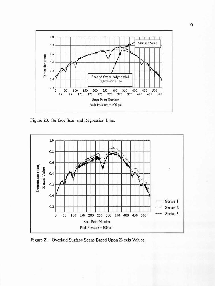
1.0 I
0.8 .t...,., Surface Scan �
6 0.6
E 0.4�
.8
� 0.2E 0.0
-� i..,i;; ..... I '
� •
� LI _,... J n, I V �
n. I I V
� Second Order Polynomial Regression Line
-0.20 50 100 150 200 250 300 350 400 450 500
25 75 125 175 225 275 325 375 425 475 525
Scan Point Number
Pack Pressure = I 00 psi
Figure 20. Surface Scan and Regression Line.
1.0
_,. , ... 0.8
,-... 0.6
s (I.)
s ;:I
';;'� 0.4
.8 "' "' -�(I.) �
.. .. -·, ,,._
�
� � ri; ·" if � .
.. �-. , .. . .
j I � �
1:.
( ,.U
""
�- y•
\ . --y
.
"
' . . . 0.2
sI
..... I
V
, ..0.0 l
;
-0.2
0 50 100 150 200 250 300 350 400 450 500
Scan Point Number
Pack Pressure = 100 psi
Figure 21. Overlaid Surface Scans Based Upon Z-axis Values.
Series 1
Series 2
Series 3
55
I I - - 7 I _L
... r---,i-,c -------- ::.-... ---. -- ' Ir- h _ .,,
.....,, L-- '"~ " t ,_ "'
0 -
i5 :'l
-
--•-
•
• • I
!I - IA- l----lliJ4+-+-++-t+ttttrn· A
N
1,
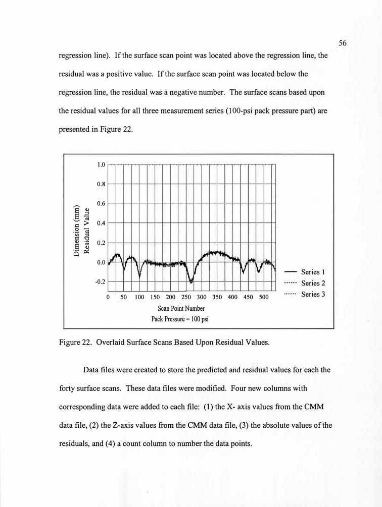
regression line). If the surface scan point was located above the regression line, the
residual was a positive value. If the surface scan point was located below the
regression line, the residual was a negative number. The surface scans based upon
the residual values for all three measurement series (100-psi pack pressure part) are
presented in Figure 22.
1.0
0.8
0.0
-0.2
....... .... � ; ,/''
•,T "' � 1W,'\. "- - � .,. I � I .. r V V ·�·,
,., ...
.,..
0 50 100 150 200 250 300 350 400 450 500
Scan Point Number
Pack Pressure = 100 psi
Figure 22. Overlaid Surface Scans Based Upon Residual Values.
Series 1
Series 2
Series 3
Data files were created to store the predicted and residual values for each the
forty surface scans. These data files were modified. Four new columns with
corresponding data were added to each file: (1) the X-axis values from the CMM
data file, (2) the Z-axis values from the CMM data file, (3) the absolute values of the
residuals, and (4) a count column to number the data points.
56
Dim
ensi
on (m
m)
Res
idua
l Val
ue
1'.. j...
0 iv
0 °'

The residual values in the sink data files were used to generate two
dimensional line plot graphs. These graphs were used to evaluate the width of each
of the five sink mark areas. After examination of scans across the range of parts, the
boundary of each sink mark area was determined. The boundary points were
generally apparent at the point where the slope of the line rapidly changed in the
transition from the sink area to the "flats" between the sinks areas. A standard width
for each sink mark area was used for all of the forty surface scans.
Once the boundaries were established for each of the five sink areas, a group
column was created in each of the sink data files (for each pack pressure). This
column was used to specify where sink areas one through five began and ended in the
data set. For example, the number one was entered into the group column for all data
points included in sink area #1. Numbers two through five were used for the
corresponding sink areas two through five. The number zero was entered into the
group column to specify which data points were not included in any of sink areas one
through five. The group column was used to identify the data for each of the five sink
areas when conducting statistical analysis.
For each of the five sink mark areas (on all surface scans), a number of
different statistics (range, minimum value, maximum value and total sum variation)
were calculated to explore which one would be the best indicator for quantifying sink
marks. For each surface scan (and sink mark area), the range, minimum value and
maximum value were calculated from the residual value data. The range for each of
the five sink mark areas (using the surface scan points located within the boundary
57
points established in step four) was calculated by subtracting the lowest residual value
(minimum value) from the highest residual value (maximum value). The total sum
variation was calculated by summing the absolute values of the residuals.
All of the statistical values and visual evaluation data were then merged into
one database so that additional statistical analyses could be completed on the
complete set of pressure data. Scatter plot diagrams were generated showing the
visual data (proportion who saw sink marks) on the Y-axis and each of the statistical
values (range, minimum value, maximum value and total sum variation) on the X
axis. Based upon visual analysis of these scatter plot diagrams, a determination was
made that the range value had the best correlation to the visual evaluation data. The
range value was considered an indicator of the depth of each sink mark area. The
nomenclature describing the range is referred to as depth or depth value throughout
the remainder of this thesis.
Analysis of Visual Evaluation Data
Analysis of the visual evaluation data was categorized into two areas: (1) data
from pilot tests, and (2) data from full-scale visual evaluation studies (non-painted
and painted parts).
Analysis of Data from Pilot Tests. During the pilot tests, a research
questionnaire was used to gather basic information about each observer. The primary
purpose of using the questionnaire during the pilot tests was to evaluate observer
58
responses to the questions. This helped to determine whether some questions needed
to be reworded, so they would be clearly understood by all observers.
The primary data gathered during the pilot tests were observer responses
(yes/no) as to whether they could see sink marks on any of the GDO doors presented
to them. These data were evaluated using summary tables. These tables provided a
measure of the consistency of each observer's responses for each part evaluated.
Analysis of Data From Full-Scale Visual Evaluation Studies. For the data
from the visual evaluation pilot studies, a number of summary statistics describing the
test population were generated and presented in tabular format. Information such as
age, eyesight status, occupation, and number of years working in the plastics industry
was gathered from observers using a research questionnaire (Appendix C). The
questionnaire was a modified version of the one used during the visual evaluation
pilot studies.
As in the pilot tests, the primary data gathered during the full-scale visual
evaluation studies were observer responses (yes/no) as to whether they could see sink
marks on any of the GDO doors presented to them. These data were evaluated using
the same type of summary tables that were used in the pilot tests. The only difference
was the addition of three more GDO doors (for a total of fourteen) in the column
designated for pack pressure.
During the full-scale visual evaluation studies, the relationship between the
visual data and CMM data were also analyzed using various scatterplot graphs.
59
Within these graphs, distance-weighted least squares analysis was used to help
evaluate trends in the data.
Summary of the Methodology
The methodology used during this study consisted of a objective measurement
phase and a visual evaluation phase. In the first phase, plastic parts with various
levels of sink marks or treatment values were systematically produced on an injection
molding machine. Measurement scans were completed on the surface of each part
using a CMM. Data from these surface scans were analyzed using statistical software
in order to quantify the depth of each sink mark area present on all GDO doors. In
the second phase, some of these parts were used to conduct two visual evaluation
pilot tests to determine the optimal test method for presenting parts to observers.
During the visual evaluation study, observers evaluated fourteen non-painted GDO
doors to determine whether they could visually perceive sink marks. A follow up
study using painted parts was conducted in order eliminate a nuisance variable
detected during the initial study. The results of the methodology described in this
chapter are presented in Chapter IV.
60
CHAPTER IV
EXPERIMENT AL RESULTS
Introduction
The results of the sink mark quantification and visual evaluation studies are
presented in this chapter. These results are based upon the methodology discussed in
Chapter III.
Sink Mark Quantification Results
The next two sections present the results of the CMM measurement studies
and gauge R & R studies. Three separate measurement series were conducted on a
CMM to gather X, Y and Z-axis values. These data values were analyzed in
statistical software to quantify each of the five sink mark areas. Results from the
gauge R & R studies helped to determine the repeatability of the measurement system
used to measure the GDO doors on the CMM.
CMM Measurement Results
Using a CMM, the goal of quantifying sink marks was achieved. Three
different measurement series were conducted before a quantified value for each sink
61
mark could be obtained. Some difficulties, explained below, arose during the first
and second measurement series. It was not until the third measurement series that
accurate depth values could be calculated for each sink mark evaluated in the study.
The third measurement series depth value results for all five sink mark areas
on the fourteen painted parts are presented below in Figure 23. The first observation
from the line plot graph is that on the part produced at a pack pressure of 150 psi,
Sink 2 is the deepest sink with a depth value of .220 mm. The next deepest sink mark
is Sink 3 with a depth value of .209 mm followed by Sink 4 (.155 mm), Sink 1 (.146
mm) and Sink 5 (.129 mm). The range between the deepest sink mark (Sink 2) on the
part produced with 150 psi and the shallowest (Sink 5) is .091 mm. This range of
.091 mm on the part produced with 150 psi is much greater than the range between
the deepest and shallowest sink marks on the part produced with a pack pressure of
2200 psi (depth value of .005 mm). Another observation from the line plot graph is
the shallowest sink mark measured on any of the fourteen parts is Sink 5 on the part
produced with a pack pressure of 2350 psi (depth value of .029 mm). These depth
value results were used in conjunction with the visual evaluation results to help
determine if a depth value could be identified below which none of the observers
could visually see sink marks.
Before depth values could be calculated, results from CMM surface scans had
to be compiled. During the third measurement series, surface scans consisting of 497
measurements were conducted on thirty-six parts with various levels of sink marks.
62
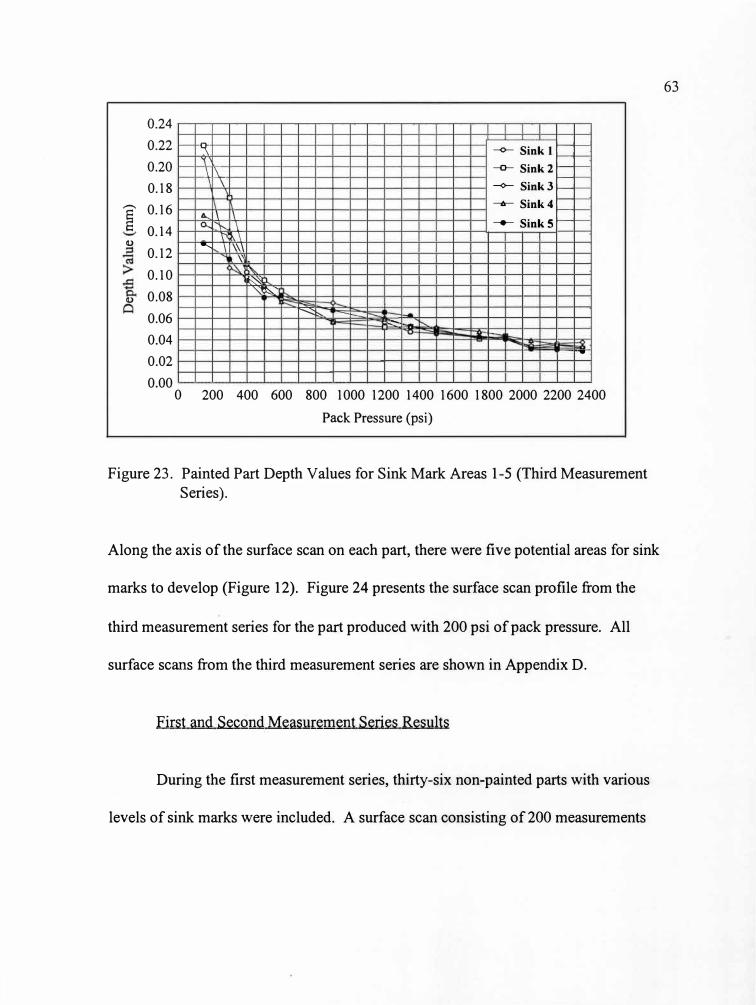
0.24
0.22
0.20
0.18
i0.16
0.14 0
0.12
0.10
0.08 0
0.06
0.04
0.02
0.00
- � � \ -o-- Sink 1
L--L--
I I\ -o- Sink 2 L--L--
� � I \ -o- Sink3 L--L--
-1,- Sink4 � � L--L--
A. I I 0... L'\--._ I -- Sink5
� �
f \--- I 1\\1
\'
�o. ' ��
r---::: ..... -....__'----
�
-
0 200 400 600 800 1000 1200 1400 1600 1800 2000 2200 2400
Pack Pressure (psi)
Figure 23. Painted Part Depth Values for Sink Mark Areas 1-5 (Third Measurement
Series).
Along the axis of the surface scan on each part, there were five potential areas for sink
marks to develop (Figure 12). Figure 24 presents the surface scan profile from the
third measurement series for the part produced with 200 psi of pack pressure. All
surface scans from the third measurement series are shown in Appendix D.
First and Second Measurement Series Results
During the first measurement series, thirty-six non-painted parts with various
levels of sink marks were included. A surface scan consisting of 200 measurements
63
-f--
- u - -
I\
....
--
- ' -
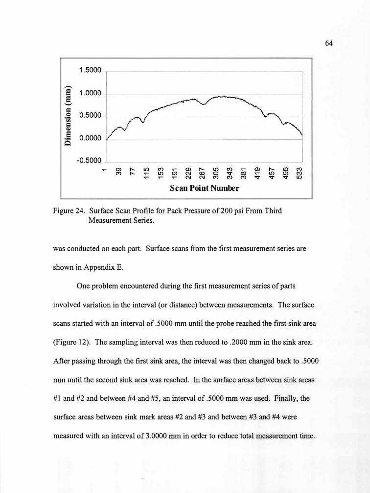
e e
= 0 ·-
= QJ
e·-
..... LO .....
.....
C") LO .....
..- O> r,,... LO 0) "' (0 0 ..... "' "' C")
Scan Point Number
.....
c:o C")
Figure 24. Surface Scan Profile for Pack Pressure of200 psi From Third
Measurement Series.
was conducted on each part. Surface scans from the first measurement series are
shown in Appendix E.
One problem encountered during the first measurement series of parts
involved variation in the interval ( or distance) between measurements. The surface
scans started with an interval of .5000 mm until the probe reached the first sink area
(Figure 12). The sampling interval was then reduced to .2000 mm in the sink area.
After passing through the first sink area, the interval was then changed back to .5000
mm until the second sink area was reached. In the surface areas between sink areas
#1 and #2 and between #4 and #5, an interval of .5000 mm was used. Finally, the
surface areas between sink mark areas #2 and #3 and between #3 and #4 were
measured with an interval of 3.0000 mm in order to reduce total measurement time.
64
39
77
343
419
457
495
533
D
I 0 0
01
0 0
0 0
0 0
0
s (
) 0
.......
.......
01
0 01
0
0 0
0 0
0 0
0 0
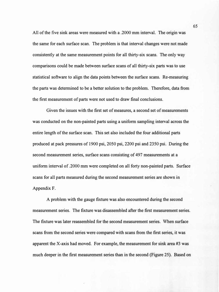
All of the five sink areas were measured with a .2000 mm interval. The origin was
the same for each surface scan. The problem is that interval changes were not made
consistently at the same measurement points for all thirty-six scans. The only way
comparisons could be made between surface scans of all thirty-six parts was to use
statistical software to align the data points between the surface scans. Re-measuring
the parts was determined to be a better solution to the problem. Therefore, data from
the first measurement of parts were not used to draw final conclusions.
Given the issues with the first set of measures, a second set of measurements
was conducted on the non-painted parts using a uniform sampling interval across the
entire length of the surface scan. This set also included the four additional parts
produced at pack pressures of 1900 psi, 2050 psi, 2200 psi and 2350 psi. During the
second measurement series, surface scans consisting of 497 measurements at a
uniform interval of .2000 mm were completed on all forty non-painted parts. Surface
scans for all parts measured during the second measurement series are shown in
Appendix F.
A problem with the gauge fixture was also encountered during the second
measurement series. The fixture was disassembled after the first measurement series.
The fixture was later reassembled for the second measurement series. When surface
scans from the second series were compared with scans from the first series, it was
apparent the X-axis had moved. For example, the measurement for sink area #3 was
much deeper in the first measurement series than in the second (Figure 25). Based on
65
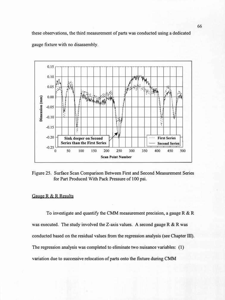
these observations, the third measurement of parts was conducted using a dedicated
gauge fixture with no disassembly.
0.15
0.10
0.05
,....._ 0.00 e e = -0.05.s=
-0.10i5
·"
� I � l
� , ..... 'J •�. ., · . .. . ...
r, -r::-: :- ,: .... 1
�ifrf :-�. . _:,,..,._ . ·: ·::,�.:-::1�
-. ·".'-\, ·.�.t�. ..
, • [1!"1,'
.. . �,:_. ' '·· . . ··: \ :'::i. ::·:·. f• •· r. . \ • E
1 ••1� WMr
� �'"-rf.
J 1 ;J
\ r�:{ ' •
:�} I
\1 :v.... .,. " .. ,,, .. -0.15
-0.20 IJf\ Sink deeper on Second I First Series . IV
1= Series than the First Series Second Series -0.25
0 50 100 150 200 250 300 350 400 450 500 Scan Point Number
Figure 25. Surface Scan Comparison Between First and Second Measurement Series
for Part Produced With Pack Pressure of 100 psi.
Gauge R & R Results
To investigate and quantify the CMM measurement precision, a gauge R & R
was executed. The study involved the Z-axis values. A second gauge R & R was
conducted based on the residual values from the regression analysis (see Chapter 111).
The regression analysis was completed to eliminate two nuisance variables: (1)
variation due to successive relocation of parts onto the fixture during CMM
66
.,, "' e
I.-
f
-
..... -~ I- I -
I r I 1
~ ···
[ J
1 1 I I
- I. l . . , . r f
I I I l lf
l ,__
I
. _ l I ..
- r-, .
·1 l ·1 I
- - - · - ...........
-~
I 1 I I .· I
I I I -
-I -~ - =-
measurements, and (2) variation due to the curvature designed into the profile of the
GDO door.
The results of the gauge R & R based upon the Z-axis values are presented in
Table 1. The largest variation in the Z-axis values during measurements was due to
change in the X-axis values. This accounted for 99.5% (estimated variance = .0452)
of the total variation observed in the measurement system. This variation was due to
several factors: (a) curvature of the part, (b) texture variation, and (c) the five sink
mark areas. The second largest source of variation was due to the change in pack
pressure treatment (100 psi, 1000 psi, and 1900 psi). This accounted for 0.5%
(estimated variance = .0002) of the total variation observed in the measurement
system. The third source of variation isolated in the analysis was attributed to
locating each part onto the fixture during CMM measurements (Figure 18). This
accounted for 0.2% (estimated variance = .0001) of the total variation within the
measurement system. Compared to the total variation within the measurement
system, the variation attributed to locating each part onto the fixture was relatively
small. The final source of variation, the interaction between the change in pressure
and change due to locating the parts in the fixture, was not a factor (0.0% - based
upon % of Total).
The results of the gauge R & R analysis of the residual values (presented in
Table 2) showed the percent of total values for each of the sources of variation were
similar to those in the gauge R & R based upon the raw Z-axis values. This second
67
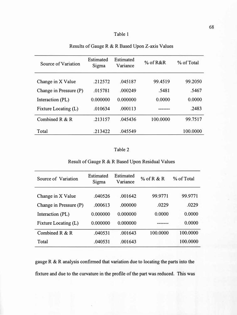
Table 1
Results of Gauge R & R Based Upon Z-axis Values
Estimated Estimated ¾ofR&R % of Total Source of Variation Sigma Variance
Change in X Value .212572 .045187 99.4519 99.2050
Change in Pressure (P) .015781 .000249 .5481 .5467
Interaction (PL) 0.000000 0.000000 0.0000 0.0000
Fixture Locating (L) .010634 .000113 .2483
Combined R & R .213157 .045436 100.0000 99.7517
Total .213422 .045549 100.0000
Table 2
Result of Gauge R & R Based Upon Residual Values
Source of Variation Estimated Estimated
¾ofR & R % of Total Sigma Variance
Change in X Value .040526 .001642 99.9771 99.9771
Change in Pressure (P) .000613 .000000 .0229 .0229
Interaction (PL) 0.000000 0.000000 0.0000 0.0000
Fixture Locating (L) 0.000000 0.000000 0.0000
Combined R & R .040531 .001643 100.0000 100.0000
Total .040531 .001643 100.0000
gauge R & R analysis confirmed that variation due to locating the parts into the
fixture and due to the curvature in the profile of the part was reduced. This was
68
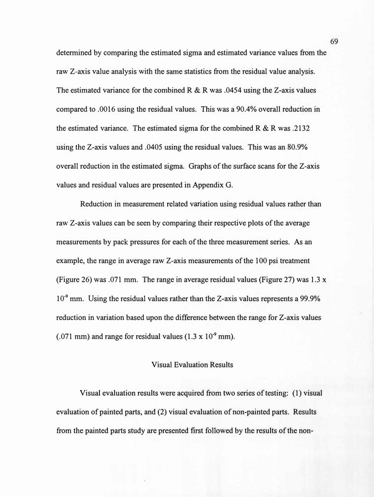
determined by comparing the estimated sigma and estimated variance values from the
raw Z-axis value analysis with the same statistics from the residual value analysis.
The estimated variance for the combined R & R was .0454 using the Z-axis values
compared to .0016 using the residual values. This was a 90.4% overall reduction in
the estimated variance. The estimated sigma for the combined R & R was .2132
using the Z-axis values and .0405 using the residual values. This was an 80.9%
overall reduction in the estimated sigma. Graphs of the surface scans for the Z-axis
values and residual values are presented in Appendix G.
Reduction in measurement related variation using residual values rather than
raw Z-axis values can be seen by comparing their respective plots of the average
measurements by pack pressures for each of the three measurement series. As an
example, the range in average raw Z-axis measurements of the 100 psi treatment
(Figure 26) was .071 mm. The range in average residual values (Figure 27) was 1.3 x
10·9 mm. Using the residual values rather than the Z-axis values represents a 99.9%
reduction in variation based upon the difference between the range for Z-axis values
(.071 mm) and range for residual values (1.3 x 10·9 mm).
Visual Evaluation Results
Visual evaluation results were acquired from two series of testing: (1) visual
evaluation of painted parts, and (2) visual evaluation of non-painted parts. Results
from the painted parts study are presented first followed by the results of the non-
69
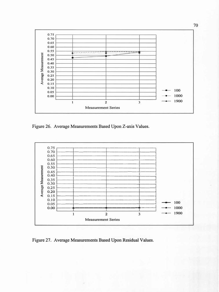
0.75
0.70
0.65
0.60
0.55
0.50 0
0.45 0
0.40
0.35 0
0.30 0
0.25
0 0.20
0.15
0.10
0.05
0.00
-►··'· !. �. �- �- : •.... • .... _. _ _._ .• .. : .: ..... ·491'· -�
2 Measurement Series
3
Figure 26. Average Measurements Based Upon Z-axis Values.
0.75 �--�-------�------�--� 0. 70 f------+-------+---------+----10.65 t------+-------+--------+-----1
0.60 1-----+---------+-------,1-----1
0.55 >------+--------+--------+------<
0.50 f------+-------+---------+----1 0.45 f------+-------+---------+----1 0.40 f------+-------+---------+----1 0.35 >------+-------+--------+------<
0.30 t------+--------+--------+------<
� 0.25 f------+-------+---------+----1 ] 0.20 ....., 0.15 f------+-------+---------+----1
0.10 t------+-------+--------+-----1
0.05 f------+-------+---------+----1 0.00 1---------------------1-----J
1 2 Measurement Series
3
Figure 27. Average Measurements Based Upon Residual Values.
- 100• 1000
.......... 1900
- 100···•··· 1000.......... 1900
70
e M
easu
rem
ent
Av
rag
M a
sur
m n
t
I
' 1·

painted parts study. Information that defines the test population is also presented
followed by results acquired during the visual evaluation pilot tests.
Test Population Attributes
The test population for the combined non-painted and painted part studies
consisted of a combined total of ninety-three observers. During the studies, the
observers filled out a research questionnaire that provided specific information that
helped define the attributes of the test population. Some of the attributes were basic
information such as age and educational status. Most of the questions on the
questionnaire were focused on the eyesight status of each observer.
In order to give an overview of the attributes of the test population, a series of
tables are presented. Table 3 shows an overview of the age ranges for all the
observers included in the population for the study. The majority of observers
participating in the study were within the age range of26 to 35 years. Over 90% of
the observers were below the age of 45 years.
Eyesight status of the observers is presented in Table 4 and includes visual
acuity for right and left eyes, visual aberrations such as near-sightedness or far
sightedness, and any visual enhancement such as glasses or contacts. The majority of
observers had left and right eye visual acuity's of 20120. Approximately 54% of the
observers wore corrective lenses (contacts, glasses or both at different times) during
working hours. At home, 44% of the observers wore contacts, glasses or both at
71

Table 3
Age Ranges of Observers Included in Visual Evaluation Test Population
Range (years)
18-25
26-35
36-45
46-55
56-65
Number in Range
29
42
14
5
3
different times. Regarding visual aberrations, 47% of the observers were near
sighted, 7% were far-sighted and 39% were neither near nor far-sighted.
An additional question asked on the research questionnaire was how many
years each observer worked within the plastics industry (Table 5). There were nine
observers who had no experience in the industry. The majority of observers had
between one and two years of experience working with plastics.
The final question for the test population included what position of work they
held at the time of the visual testing (Table 6). The majority of observers (35 total)
were operators who worked within the injection molding environment. The next
highest group of observers (22 total) was the assembly operators who assembled the
GDO door into the final assembly. The third highest group of observers (10 total)
consisted of engineers ( e.g. process engineers and quality engineers).
72

Table 4
Overview of Eyesight Status for Observers Included in Test Population
Visual Acuity Visual Aberrations Vision Enhancement
Level Number of Number Number
of Left Right
Type People
Type Who Who
Acuity Eye Eye with Use at Use at
Aberration Home Work
20/13 2 2 Near-sighted 44 Contacts 11 18
20/15 5 7 Far-sighted 7 Glasses 30 28
20/20 29 26 Bi-focal 6 Both 12 4
20/25 26 18 None 36 Neither 40 43
20/30 14 11 Color Blind 4
20/40 8 14 Not Color
89 Blind
20/50 6 12
20/70 2 2
20/100 1 1
Visual Evaluation Pilot Test Results
The following results were acquired from two visual evaluation pilot tests
where observers viewed GDO doors for sink marks. For details of the methodology
used during each test, see Chapter III.
73

74
Table 5
Number of Years Each Observer Worked in Plastics Industry
Number of Years Number of Observers
0 9
1 25
2 20
3 9
4 6
5 2
6-10 15
11-15 6
16-20 1
Table 6
Occupation for Observers Included in Test Population
Occupation Number of
Observers
Molding Operator 35
Assembly Operator 22
Engineer 10
Technician 7
Paint Operator 6
Consumers 4
Team Leader 3
Materials 2
Manager 2
Trainer 1
Maintenance 1
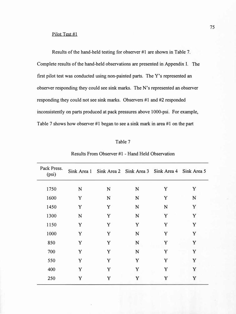
Pilot Test #1
Results of the hand-held testing for observer #1 are shown in Table 7.
Complete results of the hand-held observations are presented in Appendix I. The
first pilot test was conducted using non-painted parts. The Y's represented an
observer responding they could see sink marks. The N's represented an observer
responding they could not see sink marks. Observers #1 and #2 responded
inconsistently on parts produced at pack pressures above 1000-psi. For example,
Table 7 shows how observer #1 began to see a sink mark in area #1 on the part
Table 7
Results From Observer #1 - Hand Held Observation
Pack Press. Sink Area 1 Sink Area 2 Sink Area 3 Sink Area4 Sink Area 5
(psi)
1750 N N N y y
1600 y N N y N
1450 y y N N y
1300 N y N y y
1150 y y y y y
1000 y y N y y
850 y y N y y
700 y y N y y
550 y y y y y
400 y y y y y
250 y y y y y
75

produced at a pack pressure of 1600 psi. The observer also saw the sink in area #1 on
the 1450 psi pack pressure part. When viewing sink area #1 on the 1300 psi pack
pressure part, observer #1 said they did not see the sink mark. Similar responses were
seen for sink mark areas #4 and #5.
Pilot Test #2
Three different methods were used to present non-painted parts to observers
during the second pilot test: (1) 13 inch viewing slot, (2) four inch viewing slot, and
(3) rank order tests. Results from the 13 inch viewing slot (Appendix I) and four inch
viewing slot (Appendix I) tests involved observers viewing part through a cardboard
viewing slot to control the angle of observation. Results from the rank order tests
involved presenting observers parts in groupings of three and eleven. Results are
discussed below.
13-Inch Viewin& Slot Test. During this test, observers were presented eleven
parts in random order and asked to evaluate them for sink marks in five different
areas. A wide width of viewing slot in the cardboard nest allowed each observer to
change the angle of observation when viewing each part. Results of the 13-inch
viewing slot test are presented in Appendix I. Two out of the five observers (40%)
tested said they saw sink marks at the highest pack pressure of 1750 psi. In addition,
four out of the five observers (80%) said they saw sink marks at the second highest
pack pressure of 1650 psi.
76
Four-Inch Viewing Slot Test. During this test, observers were again presented
eleven parts in random order and asked to evaluate them for sink marks in five
different areas. The reduced width of the viewing slot limited each observer's ability
to change the angle of observation when viewing each part. The results of the four
inch viewing slot test are shown in Appendix I. Three observers were tested using the
four-inch viewing slot. Two of the three observers began to see sink marks on the
part produced with a 1300 psi pack pressure, which is 450 psi lower than the point at
which sink was seen in the 13 inch viewing slot test. All three observers had
difficulty seeing the sink marks. This may have been the result of the limited angle of
observation created by the 4" viewing slot.
Rank Order Tests. The third test in the second pilot involved presenting non
painted parts to observers and asking them to rank them in order of preference. Two
different groupings were used when presenting parts to each observer: (1) groupings
of three, and (2) group of eleven.
Groupings of Three. During the rank order test by groupings of three, one
observer ranked correctly one, two & three for all four sets of three parts. Two
observers ranked all sets correctly, except for the group with 1000 psi, 1150 psi and
1450 psi. In this group, the two observers preferred the 1000 psi part over the 1150
psi part. The results of each observer were recorded in Table 8 by ranking order of
77
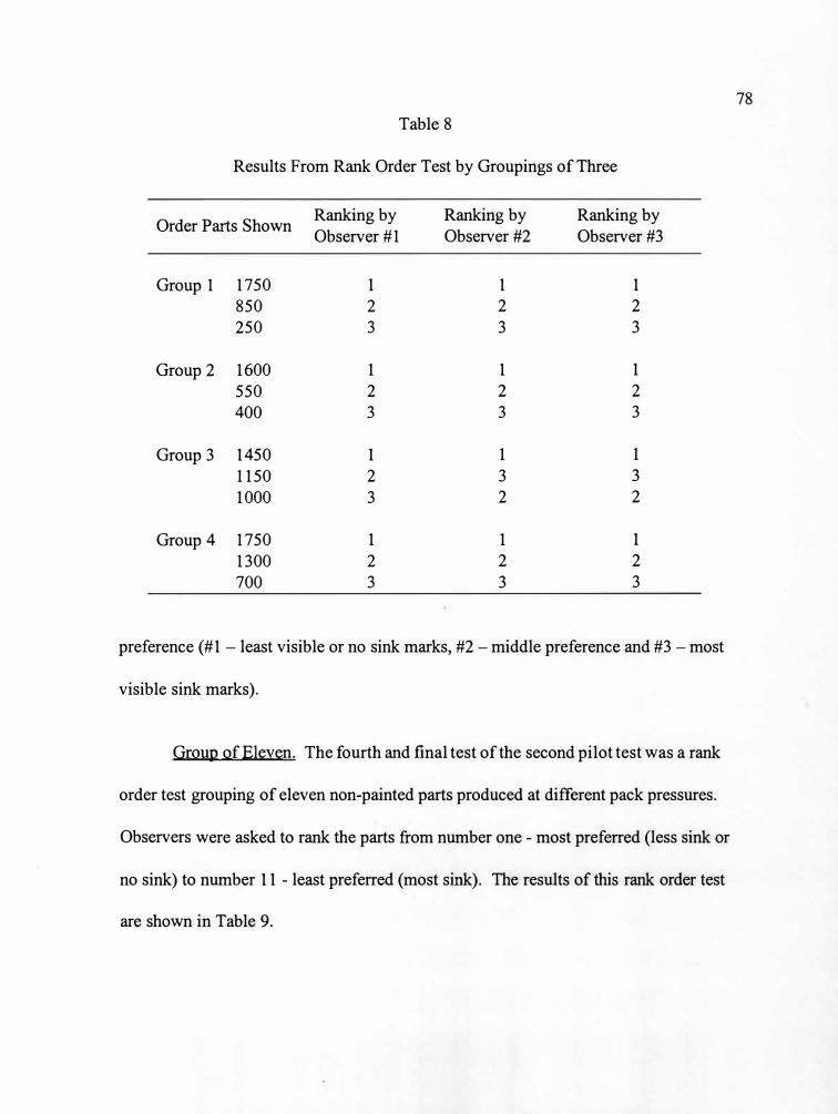
Table 8
Results From Rank Order Test by Groupings of Three
Order Parts Shown Ranking by Ranking by Ranking by Observer #1 Observer #2 Observer #3
Group 1 1750 1 1 1 850 2 2 2 250 3 3 3
Group 2 1600 1 1 1 550 2 2 2 400 3 3 3
Group 3 1450 1 1 1 1150 2 3 3 1000 3 2 2
Group 4 1750 1 1 1 1300 2 2 2 700 3 3 3
preference (#1 - least visible or no sink marks, #2 - middle preference and #3 - most
visible sink marks).
Group of Eleven. The fourth and final test of the second pilot test was a rank
order test grouping of eleven non-painted parts produced at different pack pressures.
Observers were asked to rank the parts from number one - most preferred (less sink or
no sink) to number 11 - least preferred (most sink). The results of this rank order test
are shown in Table 9.
78
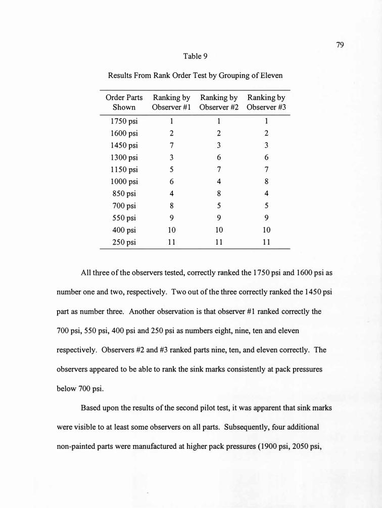
Table 9
Results From Rank Order Test by Grouping of Eleven
Order Parts Ranking by Ranking by Ranking by
Shown Observer #1 Observer#2 Observer #3
1750 psi 1 1 1
1600 psi 2 2 2
1450 psi 7 3 3
1300 psi 3 6 6
1150 psi 5 7 7
1000 psi 6 4 8
850 psi 4 8 4
700 psi 8 5 5
550 psi 9 9 9
400 psi 10 10 10
250 psi 11 11 11
All three of the observers tested, correctly ranked the 1750 psi and 1600 psi as
number one and two, respectively. Two out of the three correctly ranked the 1450 psi
part as number three. Another observation is that observer #1 ranked correctly the
700 psi, 550 psi, 400 psi and 250 psi as numbers eight, nine, ten and eleven
respectively. Observers #2 and #3 ranked parts nine, ten, and eleven correctly. The
observers appeared to be able to rank the sink marks consistently at pack pressures
below 700 psi.
Based upon the results of the second pilot test, it was apparent that sink marks
were visible to at least some observers on all parts. Subsequently, four additional
non-painted parts were manufactured at higher pack pressures (1900 psi, 2050 psi,
79
2200 psi and 2350 psi), in an attempt to further reduce the apparent sink marks.
CMM surface scans were also conducted on these parts. With the addition of these
four pack pressures, the total number of parts with different treatments (levels of sink
marks) used in the visual evaluation study was increased to fourteen.
Visual Evaluation Results - Painted GDO Doors
The visual evaluation results from the painted parts study revealed that a depth
value existed below which no observer could see sink marks. This threshold depth
value or "visual limit" was identified using scatter plot graphs which showed the
proportion of observers who saw sink marks at various depth values. Figure 28
shows the results of the painted parts study for sink mark areas #1, #2, #4 and #5.
Several observations were made based upon these results. First, observers could not
see sink marks below a depth value of .040 mm. Therefore, for these four sink areas,
the depth value of .040 mm was identified as the visual limit of an observer's ability
to see sink marks. Secondly, the visual results showed that all observers were able to
see sink marks with depth values greater than .075 mm. There were nineteen sink
marks observed with depth values greater than .075 mm. Every observer who
participated in the painted parts study detected all nineteen. Another observation was
that each observer's ability to detect sink marks in areas #1, #2, #4 and #5 increased
significantly when viewing areas with depth values greater than .050 mm. This result
suggested that observers were able to detect a distinct change in the visual appearance
80
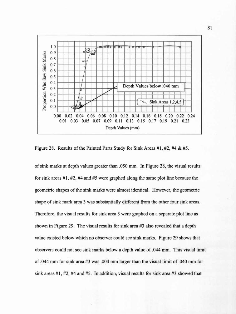
�
(I)
0
� 0 ·-e0
0
1.0 0.9 0.8 0.7
��a /2 -
I00
oof
0.6 0.5 0.4 0.3 0.2 0.1 0.0
I I /_ u Depth Values below .040 mm �-b
I/ VI
/ bo
./ I 'a.___ Sink Areas 1,2,4,5 I -I ) Vn..,. ... ,.�
0.00 0.02 0.04 0.06 0.08 0.10 0.12 0.14 0.16 0.18 0.20 0.22 0.24 0.ot 0.03 0.05 0.07 0.09 0.11 0.13 0.15 0.17 0.19 0.21 0.23
Depth Values (mm)
Figure 28. Results of the Painted Parts Study for Sink Areas #1, #2, #4 & #5.
of sink marks at depth values greater than .050 mm. In Figure 28, the visual results
for sink areas #1, #2, #4 and #5 were graphed along the same plot line because the
geometric shapes of the sink marks were almost identical. However, the geometric
shape of sink mark area 3 was substantially different from the other four sink areas.
Therefore, the visual results for sink area 3 were graphed on a separate plot line as
shown in Figure 29. The visual results for sink area #3 also revealed that a depth
value existed below which no observer could see sink marks. Figure 29 shows that
observers could not see sink marks below a depth value of .044 mm. This visual limit
of .044 mm for sink area #3 was .004 mm larger than the visual limit of .040 mm for
sink areas #1, #2, #4 and #5. In addition, visual results for sink area #3 showed that
81
'
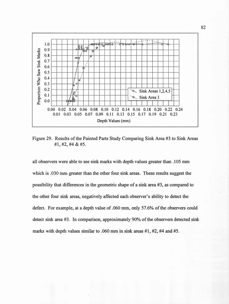
Cl)
� u3
0
� t:: 0
'€
0
.. . . ·-.... 1.0
0.9
0.8
0.7
� i� /2 p •'[]
I00 9
oof.u
C
0.6
0.5
0.4
0.3
I 9
I I - �-b
0.2
0.1
0.0
'o..___ f--
I cf· Sink Areas 1,2,4,5
I�
Sink Area 3 f--
7 ••
0.00 0.02 0.04 0.06 0.08 0.10 0.12 0.14 0.16 0.18 0.20 0.22 0.24 0.01 0.03 0.05 0.07 0.09 0.11 0.13 0.15 0.17 0.19 0.21 0.23
Depth Values (mm)
Figure 29. Results of the Painted Parts Study Comparing Sink Area #3 to Sink Areas
#1, #2, #4 & #5.
all observers were able to see sink marks with depth values greater than .105 mm
which is .030 mm greater than the other four sink areas. These results suggest the
possibility that differences in the geometric shape of a sink area #3, as compared to
the other four sink areas, negatively affected each observer's ability to detect the
defect. For example, at a depth value of .060 mm, only 57.6% of the observers could
detect sink area #3. In comparison, approximately 90% of the observers detected sink
marks with depth values similar to .060 mm in sink areas #1, #2, #4 and #5.
82
0 p. 1J, D
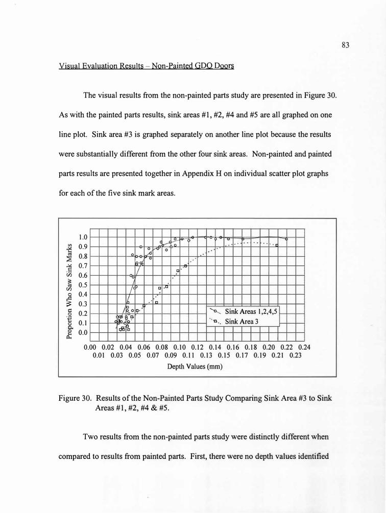
Visual Evaluation Results - Non-Painted GDO Doors
The visual results from the non-painted parts study are presented in Figure 30.
As with the painted parts results, sink areas #1, #2, #4 and #5 are all graphed on one
line plot. Sink area #3 is graphed separately on another line plot because the results
were substantially different from the other four sink areas. Non-painted and painted
parts results are presented together in Appendix H on individual scatter plot graphs
for each of the five sink mark areas.
Vl
] Cl)
Cl)
0
� i:= 0
·-e0
1.0
0.9
0.8
Cl.---' - 0 vv 0 n
0.7
0.6
R'il
I� 0.5
0.4
0.3
0.2
0.1
0.0
/v □ ,u
/, ,· n
/� 0 □•.
r� o·i:Rit
� -◄) - )
0
---□·
'a--.. u
... . . .. • •. • E
Sink Areas 1,2,4,5
Sink Area 3
I
0.00 0.02 0.04 0.06 0.08 0.10 0.12 0.14 0.16 0.18 0.20 0.22 0.24 0.01 0.03 0.05 0.07 0.09 0.11 0.13 0.15 0.17 0.19 0.21 0.23
Depth Values (mm)
Figure 30. Results of the Non-Painted Parts Study Comparing Sink Area #3 to Sink Areas #1, #2, #4 & #5.
Two results from the non-painted parts study were distinctly different when
compared to results from painted parts. First, there were no depth values identified
83
Prop
aw
M
ark
_ ___
_,,,,
--
·hx
,, l-
--+
---1
1--
-'tl
-.l-
-l--
-+--
·-:::
.....:
-
C 0
.
,_
--
l+--
-ll-
--'-
+--
--1
1--
-'-+
-I--
-'-+
-,_
--
C
--
--
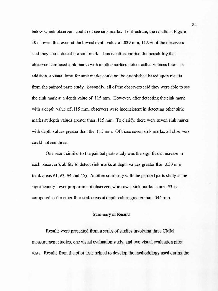
below which observers could not see sink marks. To illustrate, the results in Figure
30 showed that even at the lowest depth value of .029 mm, 11.9% of the observers
said they could detect the sink mark. This result supported the possibility that
observers confused sink marks with another surface defect called witness lines. In
addition, a visual limit for sink marks could not be established based upon results
from the painted parts study. Secondly, all of the observers said they were able to see
the sink mark at a depth value of .115 mm. However, after detecting the sink mark
with a depth value of .115 mm, observers were inconsistent in detecting other sink
marks at depth values greater than .115 mm. To clarify, there were seven sink marks
with depth values greater than the .115 mm. Of those seven sink marks, all observers
could not see three.
One result similar to the painted parts study was the significant increase in
each observer's ability to detect sink marks at depth values greater than .050 mm
(sink areas #1, #2, #4 and #5). Another similarity with the painted parts study is the
significantly lower proportion of observers who saw a sink marks in area #3 as
compared to the other four sink areas at depth values greater than .045 mm.
Summary of Results
Results were presented from a series of studies involving three CMM
measurement studies, one visual evaluation study, and two visual evaluation pilot
tests. Results from the pilot tests helped to develop the methodology used during the
84

visual evaluation study. The CMM studies produced results where the depth of each
sink mark area was quantified. The depth values were used in conjunction with the
results of the visual evaluation study to determine the depth level of sink marks below
which no observers could see the defect. Results from the guage R & R study showed
that data based upon residual values considerably reduced variation within the
measurement system. The initial study during visual evaluation was conducted using
non-painted parts. During the study it was discovered that observers may have
confused another surface defect, witness lines, with sink marks. A follow-up study
was conducted using painted parts to mask over the witness lines. The results from
the painted parts study showed there was a depth level of sink marks on the GDO
doorts below which no observers could see sink marks. The visual studies also
illustrated the difficulty of acquiring reproducible repsonses between observers when
relying on subjective visual analysis.
85
CHAPTERV
CONCLUSIONS AND RECOMMENDATIONS
Conclusions
The two main purposes of this thesis work were to determine if sink marks
could be objectively quantified and to determine ifthere was a level at which all
observers in the study were not able to see the sink marks.
Based upon the results of the coordinate measurement machine studies it was
concluded that sink marks could be objectively quantified. Quantifying sink marks
was achieved using statistical software to analyze CMM surface scan data for each
sink mark area evaluated. This methodology confirms that the attribute can be
objectively measured. Every part used in this study had measurable sink marks.
Based upon the comparison of results between the CMM and visual
evaluation studies (painted parts), a depth value of .040 mm was identified below
which no observers could see sink marks on any of the areas evaluated. This means
that for the part used in the study, sink marks do not have to be completely
eliminated. Furthermore, it may be possible to replace the subjective measurement
currently used to evaluate the GDO doors with the methodology developed in this
thesis.
86

Conclusions From the CMM Studies
In order for the CMM data to be reliable, it was concluded that major sources
of abnormal variation within the measurement system had to be reduced. Major
sources of variation were reduced in order to obtain accurate depth values for each
sink mark area. The curvature of the GDO door, part surface irregularities (texturing)
and relocation of the GDO doors into the measurement fixture caused the major
sources of measurement variation.
To address CMM surface scan variation, it was determined that a
programmable measurement set-up was required. The following issues had to be
addressed when the programmable set-up was developed:
1. A consistent point of origin had to be established for each surface scan that
was performed using a CMM. Without a consistent point of origin, data from one
surface scan could not be compared with data from another surface scan. By
establishing the programmable measurement set-up, a consistent point of origin was
maintained for each surface scan completed.
2. A consistent distance between each measurement point had to be
maintained when measuring every part used in the study. Ideally, the interval should
be held constant between all measurement points within a surface scan. If the interval
must be changed to reduce the time required to complete each surface scan, the exact
location of the interval change must be programmed into the CCM so it can be
repeated for all additional surface scans within a study.
87
3. A gauge R & R had to be completed to assess the repeatability of the CMM
when measuring all data points within each surface scan. Assessment of
reproducibility was necessary to determine the ability of the CMM to duplicate the
same surface scan measurements on all parts used in the study. After all major
sources of variation within the measurement system (discussed below) were
addressed, the gauge R & R verified the CMM was capable of completing a
repeatable surface scan on each of the parts used in the study. To address variation
due to the measurement fixture, it was concluded that a dedicated fixture should be
used throughout the study.
4. There could be no disassembling of the fixture between measurement
senes. Each time the fixture was reassembled, surface scans from the previous
measurement series could not be duplicated. Only when the fixture was dedicated
could repeatable surface scans be completed.
5. The curved contour of the GDO door made it difficult to nest it repeatedly
in the measurement fixture. Initial attempts to improve repeatability by modifying
the measurement fixture were unsuccessful. The variation caused by the contoured
surface of the GDO door could not be physically altered. Therefore it became
necessary to correct for this variation mathematically using least squares regression
techniques. Based upon the gauge R & R, the CMM data corrected in the manner
were determined to be reliable.
88

Conclusions From Visual Evaluation Studies
The following conclusions are based upon the data related to sink mark areas
1, 2, 4 and 5. The correlation between the CMM and visual evaluation data for the
painted parts used in this study revealed there were three distinct groupings of data.
The first group of data consisted of the depth values greater than .075 mm, where all
observers were able to see the sink marks. The second group of data consisted of the
depth values less than .040 mm, where all observers were not able to see sink marks.
The third group of data consisted of depth values between .041 and .074 mm, where
observers were inconsistent in their ability to detect the sink marks. These data
suggested the correlation between the CMM and visual evaluation data was decidedly
non-linear. This was evidenced by a depth value threshold below which no observers
could see sink marks.
Because no observer could see sink marks below this threshold, the possibility
exists that a standard could be established for acceptable levels of sink marks on the
part used in this study. There was another depth level threshold above which all
observers could see sink marks. This suggested that at higher depth levels, visual
measurement was a viable option for sink mark detection. However, there was
considerable variation in the ability of different observers to see sink marks with
depth values that fell in between the two thresholds stated above. This is the type of
variation in visual measurement that can lead to acceptable parts being rejected or
89
visa versa. These inconsistencies underscore the need to improve visual measurement
by developing objective measurement methodology for attribute defects.
In addition to the conclusions already discussed from the visual evaluation
studies, it was concluded that painting the parts appeared to be effective in masking
over the witness lines and other surface flaws. This eliminated the possibility of
observers confusing them with sink marks and enabled them to more clearly
distinguish the sink marks than when evaluating non-painted parts.
During the study using non-painted parts, some observers said they could see
the sink marks on every part presented. These results suggested the possibility that
some observers confused sink marks with another defect called witness lines. The
difficulty of trying to determine whether observers actually saw sink marks at the
lower depth values made it impossible to determine if a level existed at which all
observers were unable to see sink marks for non-painted parts.
Recommendations
Below are several recommendations based on the results and conclusions of
this thesis. These recommendations are divided into expansion of the work in this
thesis study, and implementation of this study in a manufacturing environment.
ExPansion of This Study
There are at least three areas into which further study is recommended: (1)
expansion of the acceptance standard developed for sink marks, (2) investigation into
90
the effects of different materials on sink mark formation, and (3) application of the
methodologies in this study to other attribute defects.
Additional studies should be conducted to determine if a standard depth level
for non-visible sink marks could be established for all plastic parts. The study could
be completed using one plastic resin for all parts studied to minimize the number of
variables. Selecting different sizes of products with various design features and
surface textures would help in assessing if non-visible sink marks on these parts have
similar depth values. Using the methods developed for this thesis, the different levels
of sink marks on each type of part could be quantified. The quantified sink marks
from each type of part could be grouped based upon similar depth values. Then a
visual evaluation study could be conducted for each part to determine the depth value
at which no observers can see the sink marks. Once depth values for non-visible sink
marks are established for each part used in the study, they would be compared to
determine if they are similar. If the depth values between the different parts were
significantly different, follow-up studies would need to be conducted to determine
what led to the differences.
If a standard depth level for non-visible sink marks can not be established for
all plastic parts, in the study discussed above, additional measurement systems should
be evaluated to determine whether sink marks can be quantified based upon area,
volume or shape. During the thesis work, depth values were calculated based upon a
cross-section of each sink mark. Other measurement systems may have the
capabilities to quantify the entire volume of each sink mark analyzed. If sink marks
91

were quantified based upon volume or area, a stronger correlation than in this study
may exist between the new measurement technique and observers' ability to see
them.
Another study recommended is to evaluate the effect of different materials on
sink mark formation. Changing the material after each injection molding run would
be completed in order to produce the same part consisting of different materials.
Materials could be selected based upon various shrink rates, types of additives and
other material characteristics. During each run of a selected material, the pack
pressure would be systematically manipulated to produce parts with varying depth
values of sink marks. Using the methodology from thesis work, parts would be
measured on a CMM and analyzed with statistical software to calculate depth values
for each sink mark. Depth values of sink marks on the parts consisting of different
materials would be compared for differences. Additional comparisons of data would
include overlaying the surface scans of the various parts produced with different
materials. The results of this type of study would help determine what type of effect
different materials have on sink mark formation.
Finally, various attribute defects such as splay, scratches, marring and other
types of surface defects should be evaluated to determine if they could be quantified
using similar methods to those used in this sink mark study. Other measurement
systems should also be investigated to develop new methods of quantifying different
attribute defects.
92
Implementation in the Manufacturing Environment
The main purpose of implementing the type of methodology conducted in the
thesis was to improve upon subjective visual defect analysis by replacing it with or
using it in conjunction with objective measurement methodology. Using objective
measures for defects that have traditionally been evaluated visually can aid in the
process of establishing clearly defined part acceptance standards with customers.
These objective acceptance standards can then be communicated to operators who
regularly produce the product to avoid any uncertainties. Below are some
recommendations for implementing into the manufacturing environment the
methodology described in this thesis.
Since quantifying sink marks using a CMM can be time consuming,
implementation of this study in a manufacturing environment can best be achieved
through incorporation into a design of experiments. Using the depth value as a
measure of sink marks during a designed experiment would enable a molder to
evaluate a new or existing injection mold to determine if parts can be produced with
an acceptable depth of sink marks. It is recommended this type of study should be
conducted on new or existing injection molds that are considered to have a high
potential for the development of sink marks in visible areas on the part surface. If the
designed experiment helps determine a process set-up of parameters that consistently
produces acceptable levels of sink marks, then process control could be used to
maintain that set-up over time. If the experiment shows the optimized set-up is
93
unable to produce parts with acceptable levels of sink marks, then this could be used
as a justification for changing the part or mold design. Once this study has been
completed on a given mold, a baseline could be agreed upon with the customer as to
what depth value and tolerance for sink marks is acceptable. This depth value could
be integrated into a product control plan and monitored by conducting process control
on the optimized process parameters established through the DOE.
Since the thesis work validated human observers' ability to visually detect
sink marks, it is recommended that a panel of observers be used in conjunction with
the DOE stated above. The variation among viewers it this thesis study suggests it
would be best to use larger numbers of evaluators, probably in a proper DOE. This
panel of observers would be used to evaluate the parts produced from various process
set-ups to help determine an acceptable depth for sink marks on the part produced
during the DOE. It is also recommended that the observers evaluate the parts in a
controlled environment, such as a light booth, to reduce possible nuisance variables.
Once the acceptable depth value for the sink marks has been established, the
observers could be used to detect unacceptable parts during production.
Finally, an injection mold usually goes through a series of preliminary tests
before it is released into production. Typical elements of mold tryouts involve
establishing the initial set-up of process parameters along with visual and dimensional
verification of parts. Sink mark analysis could be incorporated as another element
into mold tryout procedures. During dimensional verification, any sink marks on the
94

surface of the part could be measured to determine if there is a depth value at which
no observers can see the sink marks for use as acceptance criteria.
95

Appendix A
Effron Visual Acuity Wall Chart
96

97
Effron Visual Acuity Wall Chart
1
F p 2
T 0 z 3
L p E D 4
PECFD 5
EDFC2P 6
FELOPZD 7
fJ:E:FFOTEC 8
LCFODP CI" 9
!'DPLI"CCO 1 □
?J:TOLCrT:D 11

Appendix B
Digital Pictures of Fixture Used for Coordinate Measurement Machine
98
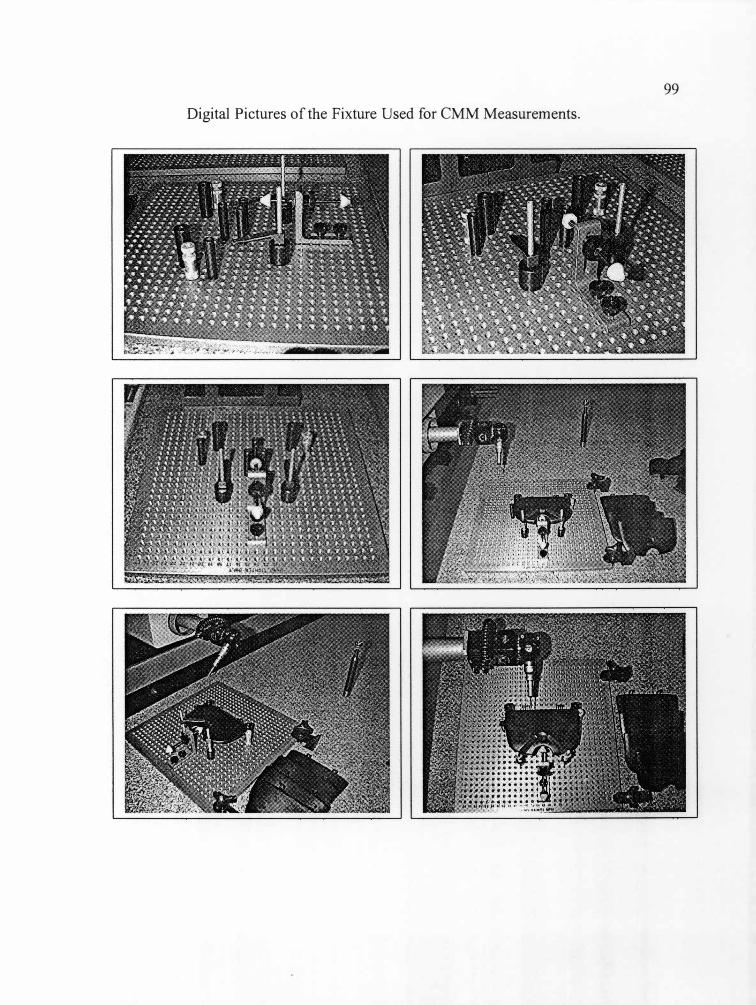
99
Digital Pictures of the Fixture Used for CMM Measurements.
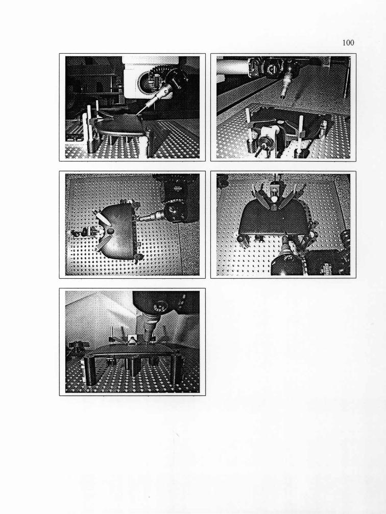
100

Appendix C
Proposal and Forms Submitted to the Human Subjects Review Board
at Western Michigan University
101

W estem Michigan University
Human Subjects Institutional Review Board (HSIRB) Proposal for Thesis Experimentation:
Quantifying a Key Injection Molding Attribute Defect
PROJECT DESCRIPTION
102
The purpose of this research is to quantify a key injection molding attribute defect called sink marks. Sink marks are a shallow depression or dimple on the surface of a finished plastic part due to shrinkage or low fill of the mold cavity. Human observers will evaluate a series of injection molded parts that have various levels of sink marks. The project will take place at Prince Corporation in Holland, Michigan. Human observers will view parts under a Macbeth SpectraLight Color viewing booth at the Prince-Maplewood
plant. The duration of the project for each observer will be approximately one half hour.
During the literature review of this thesis, it was determined that depth perception and
visual acuity are two key factors in determining a human observers ability to perceive sink marks. Therefore, during research, human observers will be asked to participate in the Stereo Fly Stereopsis Test and Effron Wall Chart visual acuity test. The stereopsis test is a universally known and understood vision test where human observers view a picture of a fly in booklet form. If the image of the fly is only viewed using one eye, the fly will appear as an ordinary flat photograph. If both eyes are functioning properly, the response
of the observer will be the ability to see the fly in three dimensions. The second test,
visual acuity, will involve asking human observers to view the Effron Wall Chart at a specified distance. They will then be asked to cover one eye and read the smallest line of numbers they are able to see. Then they will be asked to uncover the first eye and then cover up the second eye and repeat the process. If they are able to read the bottom line on the chart, the observer has 20/20 vision.
After completing the depth perception and visual acuity tests, observers will be asked to view a series of plastic parts with various levels of sink marks. The research design to be
used is called the paired comparison procedure. When using this procedure, human observers are given two parts to observe in order to determine which one is preferred. If one part is picked more strongly, then it can be concluded that some of the observers are
able to tell the difference between the two parts. The only discrimination information provided is if one part is strongly preferred. It simply means that observers are able to tell the difference between the two parts. This procedure is not designed for use with more than two parts. This procedure will be repeated for each of ten levels of sink marks.

103
BENEFITS OF RESEARCH
The short-term benefits of this research involve a determination of what level a majority
of observers are able to see sink marks. This level will be quantified in order to reduce
the subjectivity when viewing the defect. This will also translate into long term benefits
by providing a higher confidence level for human observers whose work requires them to visually detect sink marks. The minimum-maximum levels of a defect, such as sink marks, are sometimes changed throughout the life cycle of a plastic part. This fluctuation
may confuse human observers when viewing sink marks, especially when sink marks are at a level that a majority of observers are unable to visually detect.
SUBJECT SELECTION
Subjects will be selected based upon their response to a distributed pamphlet that invites
them to participate in the research. The invitation pamphlet is basically a reduced portion
of the attached consent form. The Principle Investigator's, Student Investigator's, Chair of Human Subjects Institutional Review Board's, and Vice President for Research's
phone numbers will be provided in the pamphlet. Potential subjects will be informed in the pamphlet that they can contact any of these people to ask questions about the research. Once the subjects have verbally agreed to participate in the research, an appointment will be set-up. During this appointment, they will be presented the attached Consent Form and Research Questionnaire. No subjects will participate in the research until they have read, understood and signed the Consent Form. Then subjects will
participate in visual acuity and depth perception tests before visually examining plastic
parts with various levels of sink marks.
RISKS TO SUBJECTS
One potential risk may involve discomfort to the eyes of human observers from viewing a number of plastic parts. Each observer will view ten sets of two, or twenty total plastic parts. Since the evaluation will take place using a universally accepted Macbeth
SpectraLight color booth, the known risks are minimal.
PROTECTION FOR SUBJECTS
Subjects will be informed of the potential for discomfort to their eyes. Prior to the test, they will be informed via the attached Consent Form that they can rest their eyes at
anytime during the evaluation. Most observers working in a plastic's company evaluate

104
parts at the molding press for eight hours. They usually take two breaks and then a lunch period to help provide the rest they need. Since the viewing of parts will only take about
ten minutes, the risk of discomfort to observers' eyes will be minimal.
CONFIDENTIALITY OF DATA
All the information collected during the project will be confidential. That means that
names will not appear on any papers where information is recorded. All forms will be coded to achieve confidentiality. The attached master list will help correlate the names of
participants to the corresponding code numbers. Once the data are collected and analyzed, the master list will be destroyed. All other forms will be retained for three years in a locked file in the principal investigator's office.
INSTRUMENTATION
This session will involve completing a questionnaire, depth perception test and a visual acuity test. Once these tests are complete, observers will view plastic parts with different levels of sink marks. The attached questionnaire will be used to provide general
information about human observers such as age, level of education and employment status. Also attached is a brochure explaining the Stereo Fly Stereopsis Test. This test will be used to determine each observer's ability to see depth. The final test is the
attached Effron Wall Chart to determine an observer's visual acuity. All documents will
be kept confidential using the attached coding sheet.
INFORMED CONSENT
Please see the attached informed consent form that will be given to all human observers prior to their participation in the project.

105
Text Read to Human Subjects
You are invited to participate in a research project entitled "Quantifying a Key
Injection Molding Attribute Defect." This research is intended to study how human
subjects are able to visual perceive an injection molding defect called sink marks. Sink
marks are a shallow depression or dimple on the surface of a finished plastic part due to shrinkage or low fill of the mold cavity. This project is Kris Horton's thesis project.
Participation in this project will involve a one half-hour session with Kris Horton
in the Prince-Maplewood plant color viewing room. This session will involve
completing one questionnaire for general information, visual acuity test and a viewing of plastic parts with different levels of sink marks.
If you decide to participate in the project, you may quit at any time without
penalty. If you have questions or concerns about this study, you may contact either Dr.
Paul Engelmann at 616-387-6527 or Kris Horton at 616-394-6679. You may also contact Western Michigan University and speak with the Chair of Human Subjects Institutional Review Board of Western Michigan University at 616-387-8293 or the Vice President for Research at 616-387-8298 with any concerns that you have.

College of Engineering and Applied Sciences
Department of Industrial and Manufacturing Engineering
Kalamazoo. Michigan 49008-5045
616387
FAX 616
4,o'/J J., N A; 106 rov :' 7 �V/fc
eC/ 1or • S ly1G Use . / '."ltv U
WESTERN MICHIGAN UNIVERSITY Or-,
10r 0n� /?. ;1v�frsQ u5-c .z ,. } ear fr% �I/is 1,
Principal Investigator: Dr. Paul Engelmann � ;f 9? cr,1/e_. Research Associate: Kris Horton lfslJ?s '-(. �
I h b . . d . . . h . · l d "Q 'fy' 01zqjh 1-(. ave een mv1te to part1c1pate m a researc project entlt e uantl mg a Key Injection<-<
Molding Attribute Defect." I understand that this research is intended to study how human subjects are able to visual perceive an injection molding defect called sink marks. Sink marks are a shallow depression or dimple on the surface of a finished plastic part due to shrinkage or low fill of the mold cavity. I further understand that this project is Kris Horton's thesis project.
My consent to participate in this project indicates that I will be asked to attend one, half hour session with Kris Horton. I will be asked to meet Kris Horton for these sessions at Prince Corporation in the Maplewood Color viewing room. This session will involve completing one questionnaire, a depth perception test , a visual acuity test and a viewing of plastic parts with different levels of sink marks. I will also provide general information about myself such as my age, level of education and employment status.
As in all research, there may be unforeseen risks to the participant. If an accidental injury occurs, appropriate emergency measures will be taken; however, no compensation or treatment will be made available to me except as otherwise stated in this consent form. I understand that one potential risk of my participation may involve discomfort to the eyes from viewing a number of plastic parts. I understand the Kris Horton is prepared to provide an opportunity for me to stop and rest my eyes at any time during the session.
I understand that all of the information collected from me is confidential. That means that my name will not appear on any papers on which this information is recorded. The forms will all be coded, and Kris Horton will keep a separate master list with the names of participants and the corresponding code numbers. Once the data are collected and analyzed, the master list will be destroyed. All other forms will be retained for three years in a locked file in the principal investigator's office.
I understand that I may refuse to participate or quit at any time during the study without it affecting my employment at Prince Corporation. Ifl have any questions or concerns about this study, I may contact either Dr. Paul Engelmann at 616-387-6527 or Kris Horton at 616-394-6679. I may also contact the Chair of Human Subjects Institutional Review Board at616-387-8293 or the Vice President for Research at 616-387-8298 with any concern that I have.My signature below indicates that I understand the purpose and requirements of the study andthat I agree to participate.
Signature Date
107
CODING SHEET FOR
HUMAN EVALUATION OF SINK MARKS
CODE ( on questionnaire) NAME
1
2
3
4
5
6
7
8
9
10
11
12
13
14
15
16
17
18
19
20
21
22
23
24
25

Research Questionnaire Quantifying a Key Injection Molding Attribute Defect
What is your age range? 18-25yrs. 26-35yrs. 36-45yrs. 46-55yrs. 56-65yrs. ( circle one)
How many years of education have you completed?: ( circle one)
K 1 2 3 4 5 6 7 8 9 10 11 12, GED , 1 2 3 4 5 , 1 2 3 4 undergrad graduate college
college
3. Number of years working on plastic products:
Do you wear corrective lenses? (circle one) Yes, No
If yes to #4, do you wear contacts, glasses or both?(circle one) contacts, glasses, both
If yes to #4, what corrective lenses do you wear at work? (circle one) contacts, glasses, both
108
□
If yes to #4, what corrective lenses do you wear at home? (circle one) contacts, glasses, both
If yes to #4, are you near-sighted or far-sighted? (circle one) near-sighted, far-sighted
9. Do you have color blindness? (circle one) yes, no
Visual Acuity Score = Left Eye ____ _ Right Eye ____ _

109
Check Sheet D
Part Number Area-1 Area-2 Area-3 Area-4 Area-5
2350
. 2200
2050
1900
1750
1500
1350
1200
900
600
500
400
300
150
Appendix D
Surface Scans From Third Measurement Series (Painted and Non-Painted Parts)
on Coordinate Measurement Machine
110
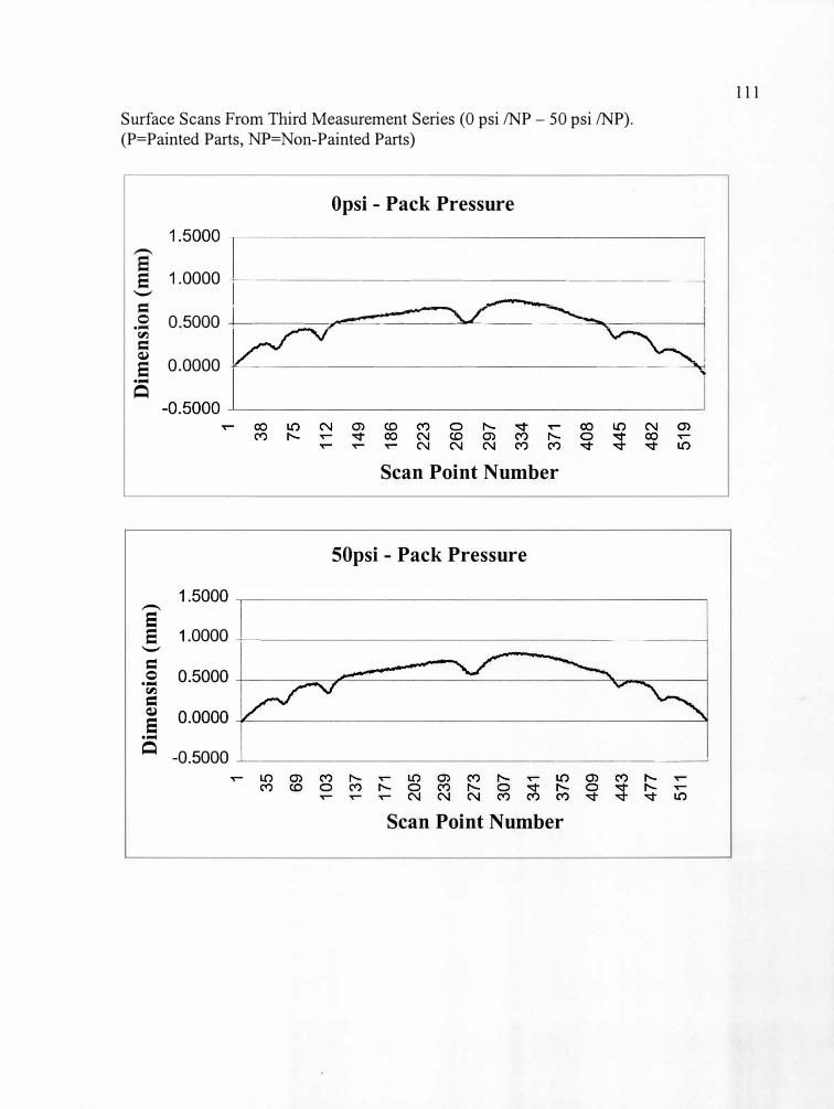
Surface Scans From Third Measurement Series (0 psi /NP - 50 psi /NP). (P=Painted Parts, NP=Non-Painted Parts)
Opsi - Pack Pressure
S 1.0000 -r--- - ---- --- - ----------<
--
.; 0.5000 i- ---------:���:::�,J__=-_--=��-- -� c:,:i
=
S 0.0000 _______ ______ _ _ _____ _______, ....
Q
Scan Point Number
50psi - Pack Pressure
--
s S 1.0000 +------------ ------------<
--
= 0 ....
c:,:i
= �
s ....
Q -0.5000 �-----------------�
Scan Point Number
111
m)
I 0 ......
0
0 ......
C.1
1 C.1
1 0
01
01
0 0
0 0
0 0
0 0
0 0
0 0
0 0
0 1
1 35
38
69
75
103
112
137
149
171
186
205
223
239
260
273
297
307
341
334
371
375
409
408
443
445
; 47
7 48
2 51
1 51
9
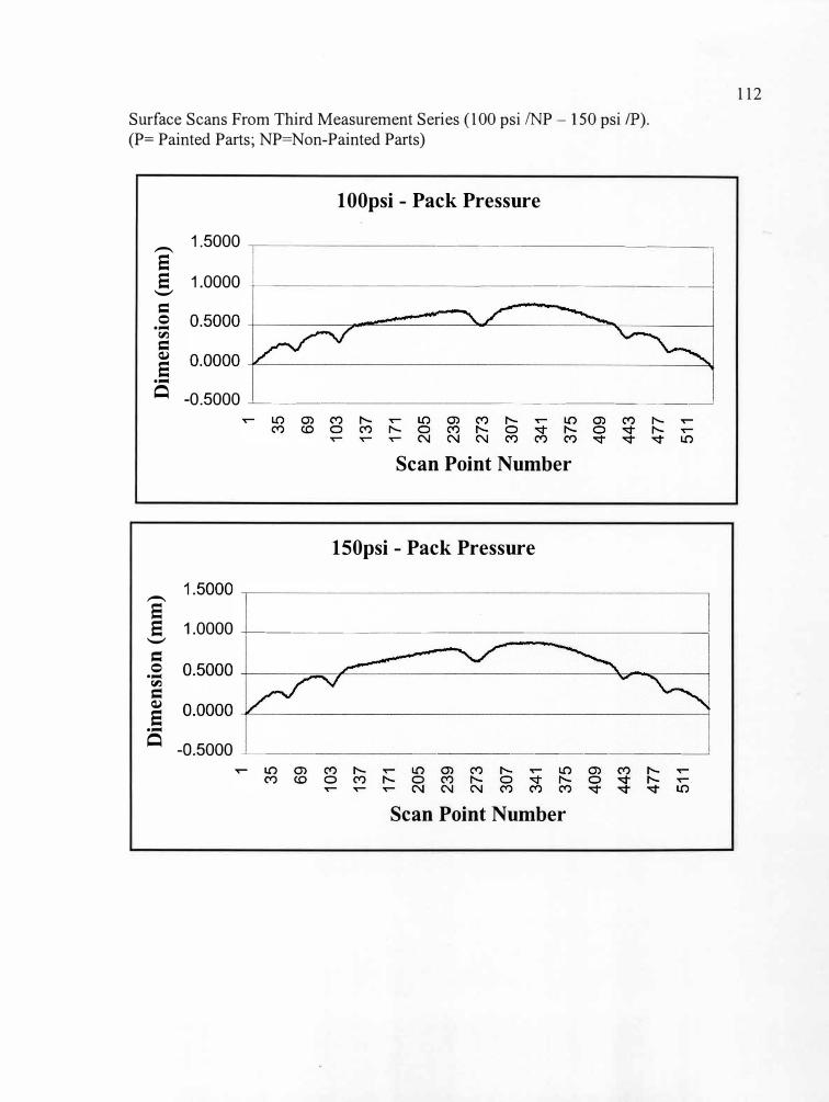
Surface Scans From Third Measurement Series (100 psi /NP - 150 psi IP).
(P= Painted Parts; NP=Non-Painted Parts)
1 00psi - Pack Pressure
,_ 1.5000 ,---- --- - - - - ------ - - - --------,8 8 1.0000 -j- --------- --------------,
--
= 0 ....
t,.)
= QI
8 ....
� -0.5000 �-----------------�
Scan Point Number
150psi - Pack Pressure
e 8 1.0000 -+-------------------
--
= 0 ....
t,.)
= QI
8 ....
� -0.5000 �--- - - --- - ------- -�
Scan Point Number
112
0 0
-"
0 0
0 01
01
0
01
0 0
0 0
0 0
0 0
0 0
0 0
0 0
0 1
1 35
35
69
69
10
3 10
3 13
7 13
7 17
1 17
1 20
5 20
5 23
9 23
9 27
3 27
3 30
7 30
7 34
1 34
1 37
5 37
5 40
9 40
9 44
3 44
3 47
7 47
7 51
1 51
1
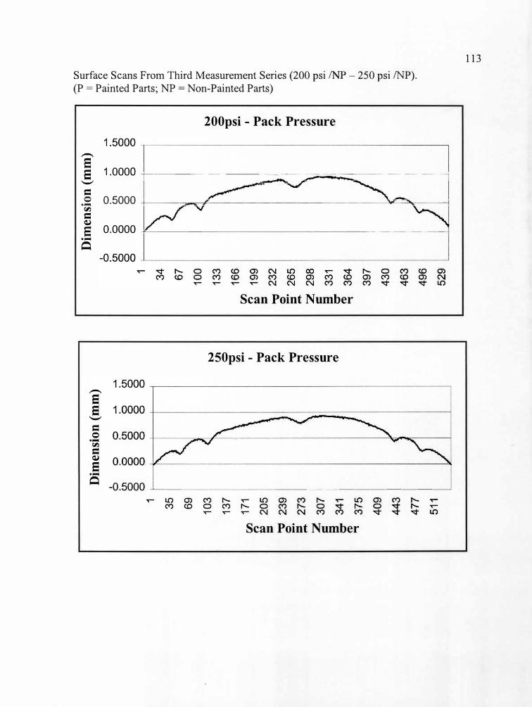
Surface Scans From Third Measurement Series (200 psi /NP - 250 psi /NP). (P = Painted Parts; NP= Non-Painted Parts)
200psi - Pack Pressure
-
£ 1.0000 -r----- --=::.�-��;;;;;::::::-------1=
.s 0.5000 +---�...-,f'----------------'¥'--�,--------1 t:l.l
=
e 0.0000 _________ _ _ _ _ _________ _ ·-
�
= 0 ·-
t:l.l
=�e·-
Scan Point Number
250psi - Pack Pressure
� -0.5000 �-- - - - - ---------- -�
Scan Point Number
113
1 35
69
103
137
171
205
239
273
307
341
375
409
443
I 41
1 I
511
0 0 0 0 0
0 01
0 0 0
(mm
) ......
......
0
01
0 0
0 0
0 0
1 34
67
100
133
166
199
232
265
298
331
364
397
430
463
496
529
6 01
0 0 0
\ ) )
J__
......
01
0 0 0
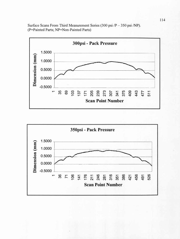
Surface Scans From Third Measurement Series (300 psi IP - 350 psi /NP).
(P=Painted Parts; NP=Non-Painted Parts)
= 0 ....
r,:i
= �
e ....
300psi - Pack Pressure
� -0.5000 �------------------
Scan Point Number
350psi - Pack Pressure
e 1.5000
_§, 1.0000 -r- --------:-�::;;;;;;;;��;;;:;;;;;;:;;::=-------, =
.s 0.5000 +-----,.___ ___________ -3-_,_------1
r,:i
5 0.0000 --------------- - - - - -e ....
� -0.5000 �-- ---------------
Scan Point Number
114
(mm
) p
0 ......
......
0
c.n
0 c.n
0
0 0
0 0
0 0
0 0
0 0
0 1
~-I
36
1
71
35
69
106
141
\1
103
I
176
137
171
211
205
246
239
281
273
316
307
351
341
386
J 42
1 37
5 40
9 45
6 44
3 49
1 ~/
52
6 47
7 51
1
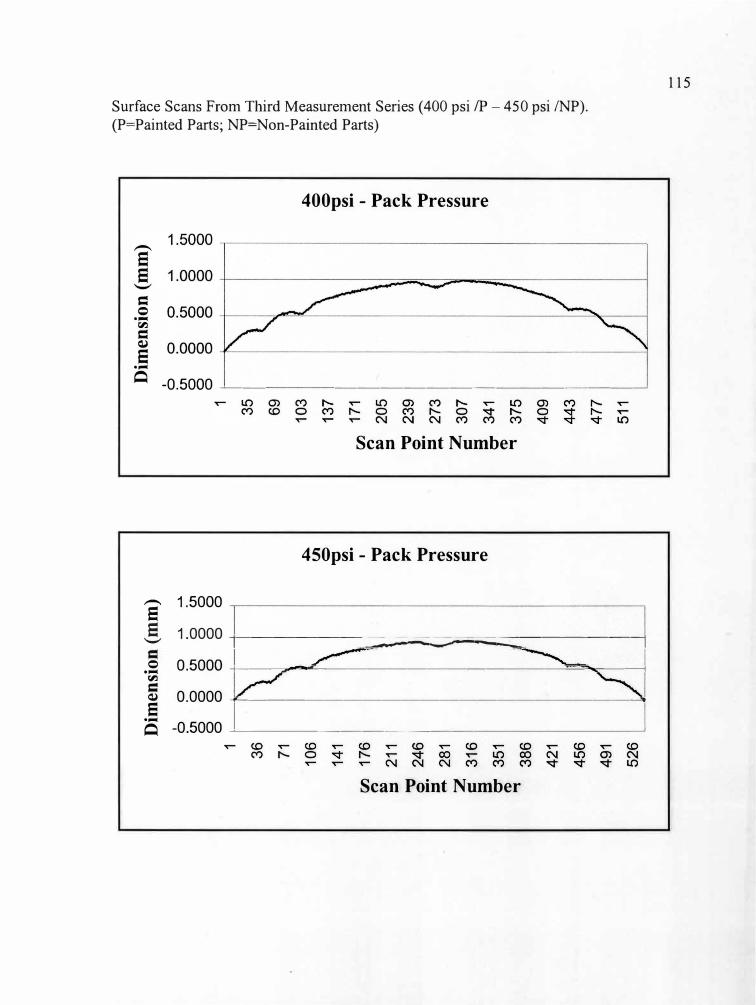
Surface Scans From Third Measurement Series ( 400 psi IP - 450 psi /NP). (P=Painted Parts; NP=Non-Painted Parts)
= 0 ...
r,.i
= Q)
e ...
400psi - Pack Pressure
Q -0.5000 --- - --------------�
Scan Point Number
450psi - Pack Pressure
S 1.5000
! 1.0000 r------=::;�;;;;;;;::;::;::;;;;;;=;;;;;;;;;;;:::::=------,
.s 0.5000 +--�-"'--------- -----=,.,,.__--------j r,.i
5 0.0000 +------------------------"'
e ...
Q -0.5000 �-----------------�
Scan Point Number
115
n (m
m)
...>.
...
>.
0 01
0
01
0 0
0 0
0 0
0 0
0 0
0 0
1
\-36
1
71
35
69
106
141
\ 10
3
176
137
171
211
205
246
239
281
273
316
307
351
341
386
/ 42
1
375
456
409
443
491 _
j 52
6
477
511
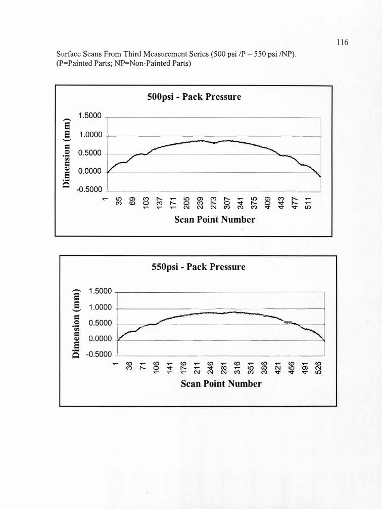
Surface Scans From Third Measurement Series (500 psi IP - 550 psi /NP).
(P=Painted Parts; NP=Non-Painted Parts)
500psi - Pack Pressure
-
e _§, 1.0000 +-- ----- -----------------< = 0 ...
r:l.l
= QJ
e ...
� -0.5000 �-----------------�
Scan Point Number
550psi - Pack Pressure
e 1.5000
E, 1.0000 +-------==;:;:::::;:;;:;::::;;;;��:::::==--------1
.s 0.5000 +----=-�-------------=-....------1 r:l.l
5 0.0000 - -- --------------- - ------"'\ e Q -0.5000 �------ ------------�
Scan Point Number
116
1 36
71
106
141
I 17
6
211
I 24
6
281
I 31
6 35
1 38
6 42
1 45
6 49
1 52
6
n \ \ ! _)
1 35
69
103
I 13
7 I
171
205
239
273
307
341
375
409
443
477
I 51
1
0 0
0 c.,,
0
0 0
0 0
0
_.,
c.,,
0 0 0
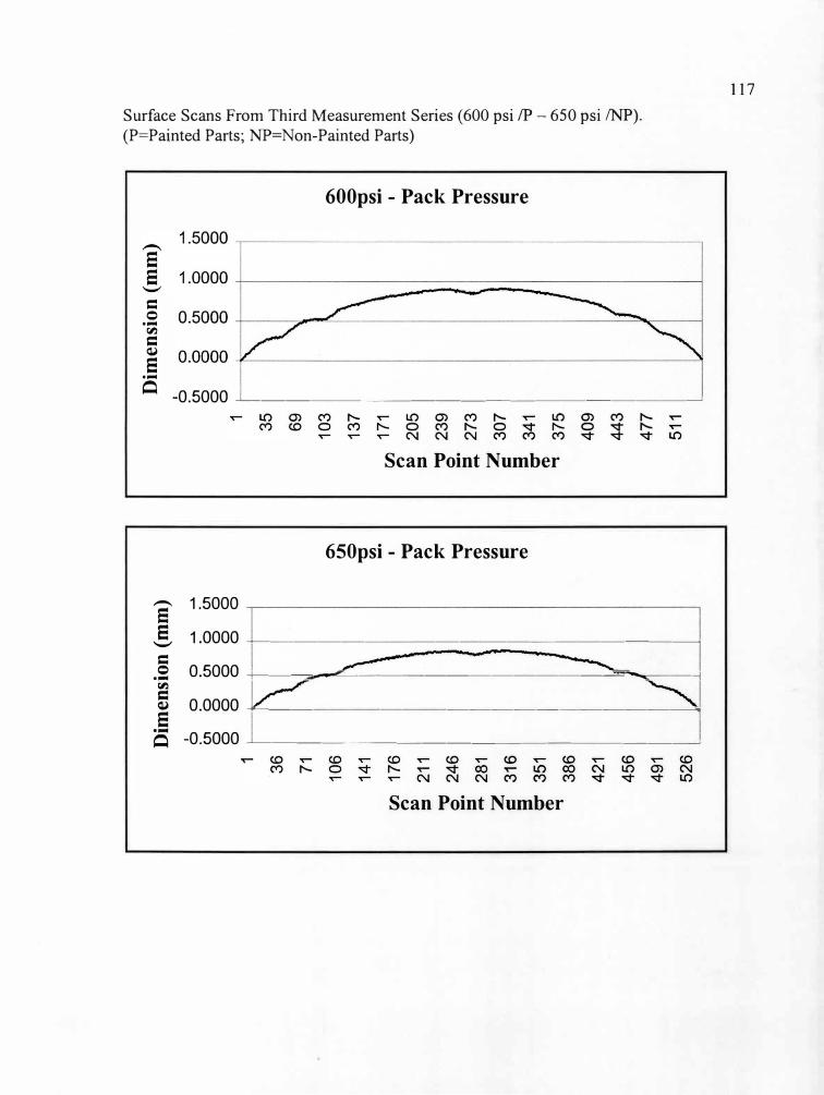
Surface Scans From Third Measurement Series (600 psi IP - 650 psi /NP).
(P=Painted Parts; NP=Non-Painted Parts)
= 0 ....
c:,:i
= Q)
8 ....
600psi - Pack Pressure
� -0.5000 �------------------
Scan Point Number
650psi - Pack Pressure
S 1.5000
,.S 1.0000 -+---- ----- ------------
= .s 0.5000 +------:::aa.--""---------------=�:------,
c:,:i
5 0.0000 ----- - --- ------------8 S -0.5000 �----------------�
Scan Point Number
117
1 36
71
106
141
176
211
246
281
316
351
386
421
456
491
526
\ _)
1 35
69
103
137
171
205
239
273
307
341
375
409
I
443
477
511
(mm
) ......
......
0
(J'1
0
(J'1
0
0 0
0 0
0 0
0 0
0 0
0
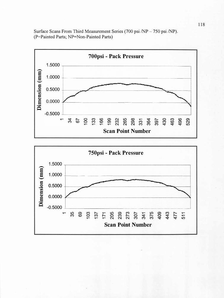
Surface Scans From Third Measurement Series (700 psi /NP - 750 psi /NP).
(P=Painted Parts; NP=Non-Painted Parts)
700psi - Pack Pressure
-
� 1.0000 +---- - - - - - - - - ------�
'-'
=
.s 0.5000 ---i--------=---------------------=-,,.---,,-----------------1
c,.i
= <l)
e 0.0000 ---f'--------------- - -�r--<
....
�
Scan Point Number
750psi - Pack Pressure
-
e e 1.0000 ------------ - - -------1
'-'
= 0 ....
c,.i
= <l)
e ....
� -0.5000 __,.___ ___ _ _ ____________ ___,
Scan Point Number
118
I 0 -"
0,
-"
0,
0 0
0 0,
0
0 0,
0
0 0
0 0
0 0
0 0
0 1
\ 0
0 0
1 34
35
67
69
10
3 10
0
137
133
171
166
205
199
239
232
273
265
307
298
341
331
375
364
409
397
430
/1
443
463
477
496
511
529
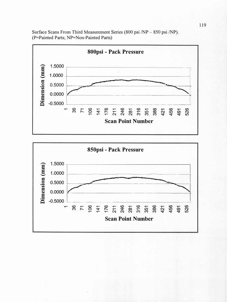
Surface Scans From Third Measurement Series (800 psi /NP - 850 psi /NP).
(P=Painted Parts; NP=Non-Painted Parts)
800psi - Pack Pressure
e 1.5000 � -- - - - - - - - -- - -----�
e '-'
=
.s 0.5000 +- ------=-"""--- ---------------'-..,..,---------i
(I)
5 0.0000 -------- --------- - -----------,,;
S -0.5000 -+----- - ---------------�
Scan Point Number
850psi - Pack Pressure
e 1.5000
S 1.0000 -+------ ----- -------------<
= .s 0.5000 +-----;;;a--�- -----------="'"""'.:-------!
(I)
5 0.0000 --- ---- -- ----------- -------'!
S -0.5000 -+------------- - - - ----�
Scan Point Number
119
m
m
_..
0 0 0 0 1
1 --
-1\-
36
36
71
71
106
106
141
141
I I
176
176
211
211
I 24
6 24
6 28
1 28
1 31
6 31
6 35
1 35
1 38
6 38
6 42
1 42
1 45
6
_IL_
456
491
491
I 1;
526
526 --
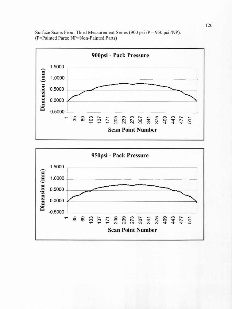
Surface Scans From Third Measurement Series (900 psi IP - 950 psi /NP).
(P=Painted Parts; NP=Non-Painted Parts)
900psi - Pack Pressure
-
e _§, 1.0000 -+---------- ---- ---- --------<
= 0 ....
�
= �
e ....
� -0.5000 ...,__ ___ _________ _____ �
Scan Point Number
950psi - Pack Pressure
-
e e 1.0000 +---- - ----------------,
-
= 0 ....
�
= �
e ....
� -0.5000 ...,__ _________________ �
Scan Point Number
120
0 0
_._
0 0
_._
0 01
0,
0
0,
0,
0 0
0 0
0 0
0 0
0 0
0 0
0 0
0 0
0 0
1 1
35
35
69
69
103
103
137
137
171
171
205
205
239
239
273
273
307
307
341
341
375
375
409
409
443
443
477
477
511
511
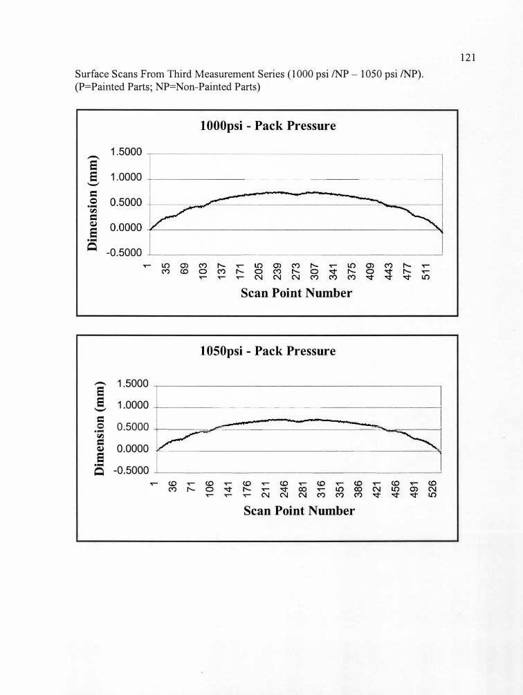
Surface Scans From Third Measurement Series (1000 psi /NP - 1050 psi /NP).(P=Painted Parts; NP=Non-Painted Parts)
l000psi - Pack Pressure
-
e e 1.0000 -+-- -- - - ------- ----------<
'-'
= 0 ...
�
= Cl)
e ...
Q -0.5000 --- ---------------�
Scan Point Number
1050psi - Pack Pressure
a 1.5000
,,S 1.0000 +--- ------------- ---------,
= .s 0.5000 +-----=�-----------�--.=,-----------,�
� 0.0000 ------------------ -----...
Q -0.5000 -+------------ ------�
Scan Point Number
121
1 36
71
106
141
176
I 21
1
246
281
316
351
386
421
456 ::: ~
/
1 35
69
103
137
171
205
239
273
307
341
375
409
I
443
477
511
0 0 0 0
u,
0 0 0
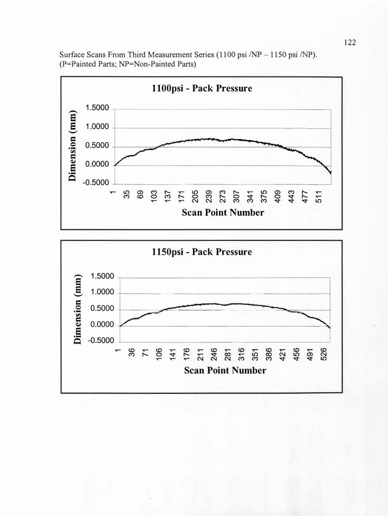
Surface Scans From Third Measurement Series (1100 psi /NP - 1150 psi /NP). (P=Painted Parts; NP=Non-Painted Parts)
11 00psi - Pack Pressure
e e 1.0000 ------- - - --- ------� --
= 0 ....
i:,J
= Cl)
e ....
� -0.5000 -+-------------------�
Scan Point Number
1150psi - Pack Pressure
5 1.5000
'5 1.0000 -+----------------------;
= .s o.5000 L----=,,I"'��:::=:::::==::::��"'-'="""--�
i:,J
5 0.0000 ------ -----------------'\,I
e S -0.5000 -+------ -------------�
Scan Point Number
122
0 0
->,.
0 01
01
0
0 0
0 0
0 0
0 0
1 1
36
\ 35
71
69
106
103
141
I
137
176
171
211
205
246
239
281
273
316
307
351
341
386
375
421
I 40
9
456
) 44
3
491
477
526
511
I ~
-
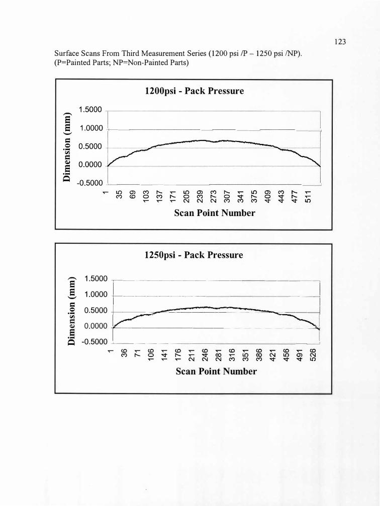
Surface Scans From Third Measurement Series (1200 psi IP - 1250 psi /NP). (P=Painted Parts; NP=Non-Painted Parts)
1200psi - Pack Pressure
-
e e 1.0000 -+---- - - - - --- ---- - -------1 --
= 0 ...
�
= �
e ...Q
-0.5000 �- -------- - - - - - - --�
Scan Point Number
1250psi - Pack Pressure
S 1.5000 -,-------------- -------,
E, 1.0000 -+------------ ---------,
=
.s 0.5000 j_ __ ����-::::::::::�==���.....,..._--____j �
5 0.0000 ---- --- - - - ----------------""d
... Q -0.5000 _,____ _________ _ _ _ _ _ __ �
Scan Point Number
123
m
..... 0
(.11
0 0
0 0
0 0
1 1
\ 36
71
35
106
69
103
141
137
176
211
I 17
1 20
5
246
239
281
273
316
307
351
341
386
375
421
409
456
~)
491
443
526
477
511
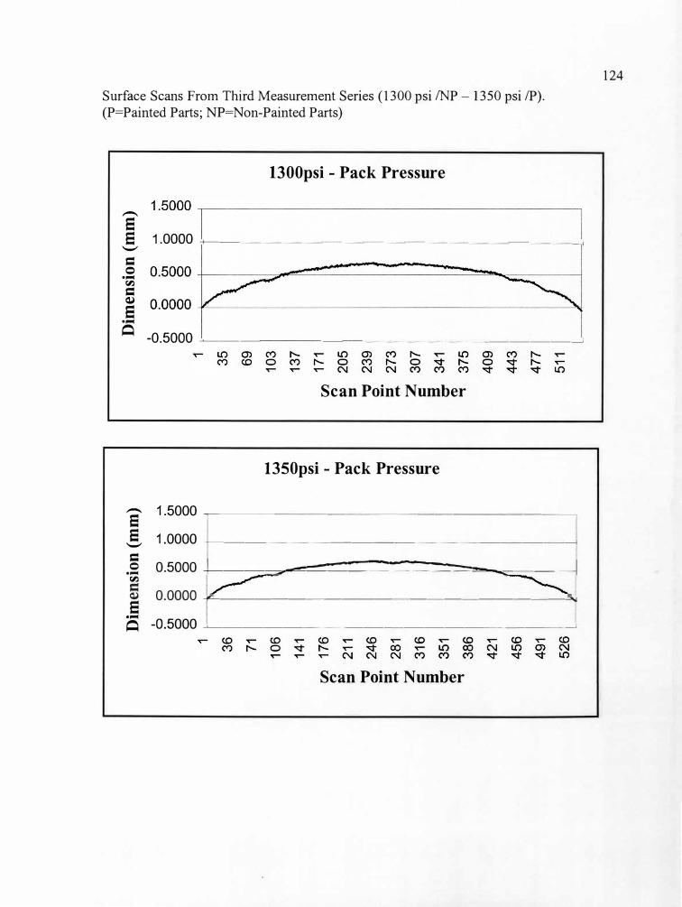
Surface Scans From Third Measurement Series (1300 psi /NP - 1350 psi IP).
(P=Painted Parts; NP=Non-Painted Parts)
1300psi - Pack Pressure
-
e e 1.0000 +----------------------j --
= 0 ·-
c-,}
=Q)
e·-
Q-0.5000 �--- - -------------�
Scan Point Number
1350psi - Pack Pressure
a 1.5000 -r----- - -------- -- - -----,
-5, 1.0000 +---------------------j
= .s 0 .5000 -l----���::::::::::::::::::::::::::::::�--..:------� c-,}
5 0.0000 -------------- -- ------�e ·-
Q -0.5000 ---'-----------------------�
Scan Point Number
124
r
......
0 (J
'I (J
'I 0
0 0
0 0
0 0
0 0
1 1
,\ 36
71
35
106
69
103
141
137
176
211
171
246
205
I I
239
I 28
1 27
3
316
307
351
341
386
375
421
409
456
)1 49
1
443
526
477
511
I. I
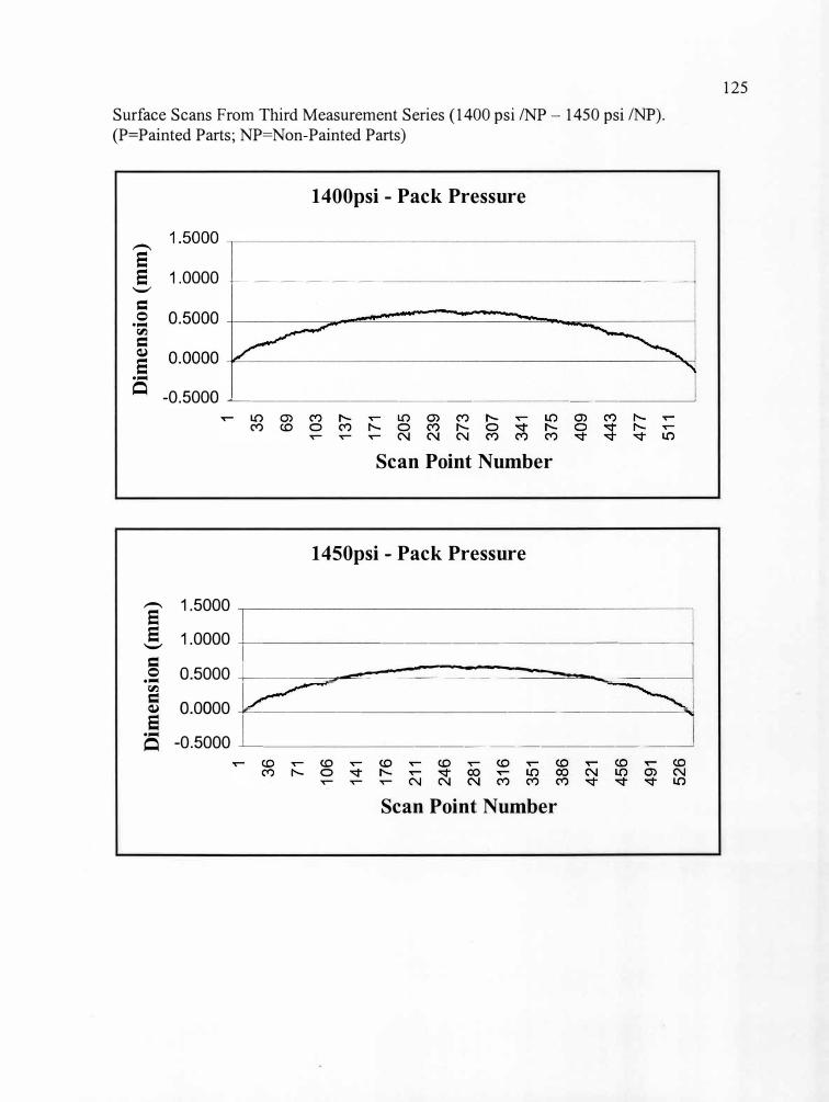
Surface Scans From Third Measurement Series (1400 psi /NP - 1450 psi /NP).(P=Painted Parts; NP=Non-Painted Parts)
1400psi - Pack Pressure
-
e e 1.0000 -+-------- - - - - - - - - ---------<
._,
= 0 ....
�
= Q)
e ....
� -0.5000 -'--------- --- - - -----�
Scan Point Number
1450psi - Pack Pressure
S 1.5000
E, 1.0000 -+-- -- - - -------------
= .s o.5000 L----��:::::=:::::::::��--=---_____j�
� 0.0000 �----- - - -----------"'\;!....
� -0.5000 -'-- -- - - - -----------�
Scan Point Number
125
1 36
71
106
141
176
211
246
281
316
351
386
421
456
491
526
\ ~)
1 35
69
103
137
171
205
239
273
307
341
375
409
443
477
511
p 0 0 0 0
p 01
0 0 0
......
01
0 0 0
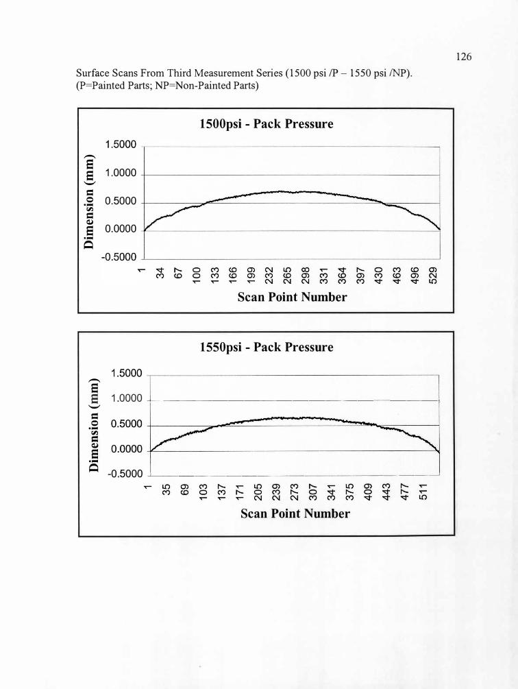
Surface Scans From Third Measurement Series (1500 psi IP - 1550 psi /NP). (P=Painted Parts; NP=Non-Painted Parts)
1500psi - Pack Pressure
,_
e 1.0000
e --
= 0 0.5000 ...
�
= Q)
0.0000e ...
Q
Scan Point Number
1550psi - Pack Pressure
,_
e e 1.0000 +----------------------,
--
= 0 ...
�
= Q)
e ...
Q -0.5000 __,___ _ _________ _ ______ �
Scan Point Number
126
I 0 .....
0 .....
0 0
, c.,,
0
, 0
, 0
0 0
0 0
0 0
0 0
0 0
0 0
0 0
1 1
35
34
69
67
103
100
137
133
171
166
205
199
239
232
273
265
307
298
341
331
375
364
409
397
443
430
477
463
496
511
529
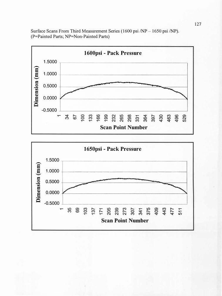
Surface Scans From Third Measurement Series (1600 psi /NP - 1650 psi /NP).
(P=Painted Parts; NP=Non-Painted Parts)
1600psi - Pack Pressure
1.5000 -
6 1.0000 6 '-'
= 0 0.5000 ....
c,:i
= Q)
6 0.0000 ....
�
Scan Point Number
1650psi - Pack Pressure
-
a 6 1.0000 -+-------------------
'-'
= 0 ....
c,:i
= Q)
6 ....
� -0.5000 �-----------------�
Scan Point Number
127
I 0 0
0 _,,_
0
01
01
01
0 0
0 0
0 0
0 0
0 0
0 0
1 1
35
34
69
67
103
100
137
133
171
166
205
199
239
232
273
265
307
298
341
331
375
364
409
397
443
430
477
463
496
511
529
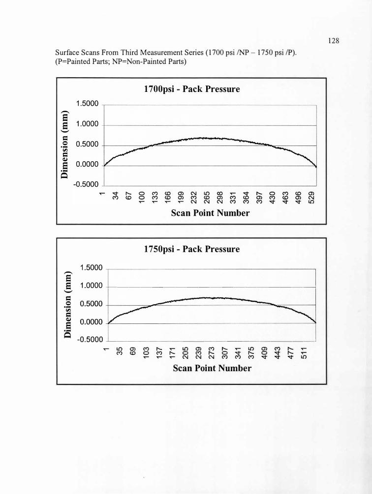
Surface Scans From Third Measurement Series (1700 psi /NP - 1750 psi IP).
(P=Painted Parts; NP=Non-Painted Parts)
1700psi - Pack Pressure
--
e 1.0000 e -
= 0 0.5000 ....
r,')
= �
e 0.0000 ....
�
Scan Point Number
1750psi - Pack Pressure
--
e e 1.0000 +------------------------,
-
= 0 ....
r,')
= � e ....
� -0.5000 -'------------- --------'
Scan Point Number
128
I 0 --
" !='
0
--"
0 CJ'1
CJ'1
CJ'1
CJ'1
0
0 0
0 0
0 0
0 0
0 0
0 0
0 0
1 1
35
34
69
67
103
100
137
133
171
166
205
199
239
232
273
265
307
298
341
331
375
364
409
397
443
430
477
463
511
496
529
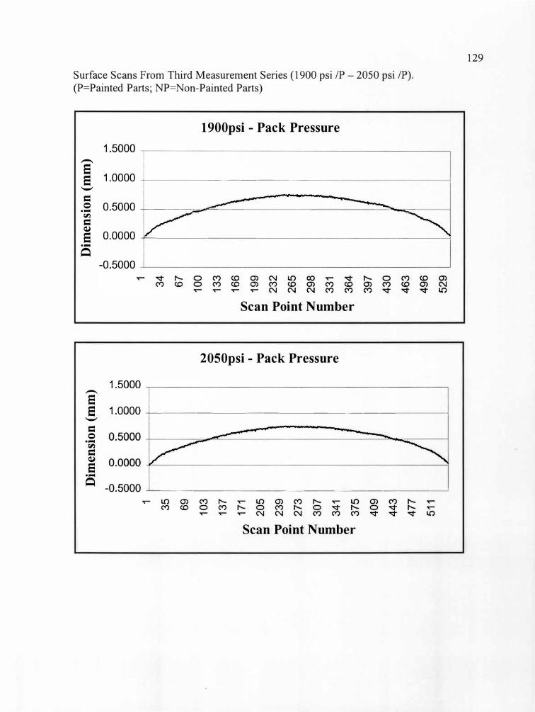
Surface Scans From Third Measurement Series (1900 psi IP- 2050 psi IP).
(P=Painted Parts; NP=Non-Painted Parts)
1900psi - Pack Pressure
e 9 1.0000 -+-------------- - - -------l
'-"
=
.s 0.5000 +------,="',,,=.--------- --- -------'-�---j
rl:l
= <l)
9 0.0000 ----- - ----------------l
..... �
Scan Point Number
2050psi - Pack Pressure
--
e e 1.0000 -+--------------------1
'-"
= 0..... rl:l
= <l)
a .....
� -0.5000 -'--------------------�
Scan Point Number
129
I 0 ...
.lo.
01
....lo
. 01
0
0 0
01
0 0
01
0 0
0 0
0 0
0 0
0 0
1 0
\ 0
0 1
34
35
67
69
100
103
137
133
171
166
205
199
239
232
273
265
307
298
341
331
375
364
409
397
443
430
463
j__
477
496
511
529
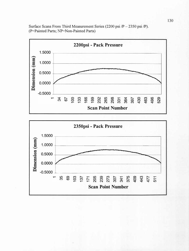
Surface Scans From Third Measurement Series (2200 psi IP - 2350 psi IP).
(P=Painted Parts; NP=Non-Painted Parts)
2200psi - Pack Pressure
-
e 1.0000 e ,_,
= 0 0.5000 ·-
� = �
e 0.0000 ·-
�
Scan Point Number
2350psi - Pack Pressure
-
e e 1.0000 -+-- ----- ---------------<
,_,
= 0 ·-
� = � e ·-
� -0.5000 -'------------- ---------'
Scan Point Number
130
I 0 ......
0
0 ......
01
01
0
01
01
0 0
0 0
0 0
0 0
0 0
0 0
0 0
1 0
1
35
34
69
67
103
100
137
133
171
166
205
199
239
232
273
265
307
I 29
8
341
331
375
364
409
397
443
430
477
463
511
496
529

Appendix E
Surface Scans From First Measurement Series (Non-Painted Parts) on Coordinate
Measurement Machine
131
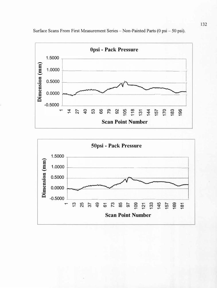
Surface Scans From First Measurement Series - Non-Painted Parts (0 psi - 50 psi).
Opsi - Pack Pressure
-
� 1.0000 -+---------------------l
--
= .s 0.5000 -+----- -- -----��- -- ------�� = �
e 0.0000 -p,,,,,......_..,,,__ ___ ____________ _.:.._---1
....
�
Scan Point Number
50psi - Pack Pressure
-
e e 1.0000 -+------------------,
--
= 0 ....
� = �
e ....
� -0.5000 �------------ -----�
Scan Point Number
132
I 0 ......
.
9 0
.......
(JI
0 01
(J
I 0
01
0 0 0
0 0
0 0
0 0
0 0
0 0
0 1
,~-
1 13
14
~· 27
25
40
37
53
49
66
61
79
73
92
85
97
10
5
109
118
121
131
133
144
145
157
157
170
169
183
181
196
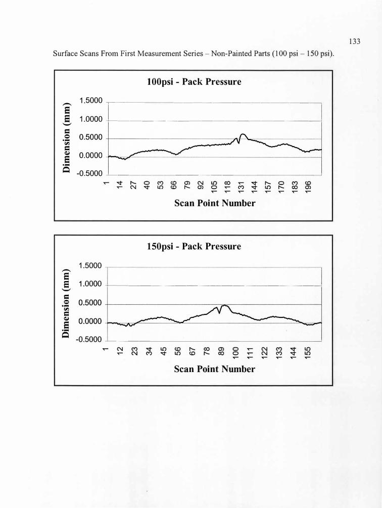
Surface Scans From First Measurement Series - Non-Painted Parts (100 psi - 150 psi).
1 OOpsi - Pack Pressure
-. 1.5000 ,------ - ---------------------,
s S 1.0000 +----------------------1
'-'
= 0 ...
C'-l
= cu
s ...
� -0.5000 � ------------- - - - ---'
Scan Point Number
l SOpsi - Pack Pressure
-
s S 1.0000 -+---------------------<
'-'
= 0 ...
C'-l
= cu
s ...
� -0.5000 �-----------------�
Scan Point Number
133
0 0
_._
0 0
0 CJ1
CJ1
0
CJ1
0 0
0 0
0 0
0 0
0 0
0 0
0 0
0 1
1 12
14
23
27
34
40
45
53
56
66
67
79
92
78
105
89
118
100
131
111
144
122
157
133
170
144
183
155
196
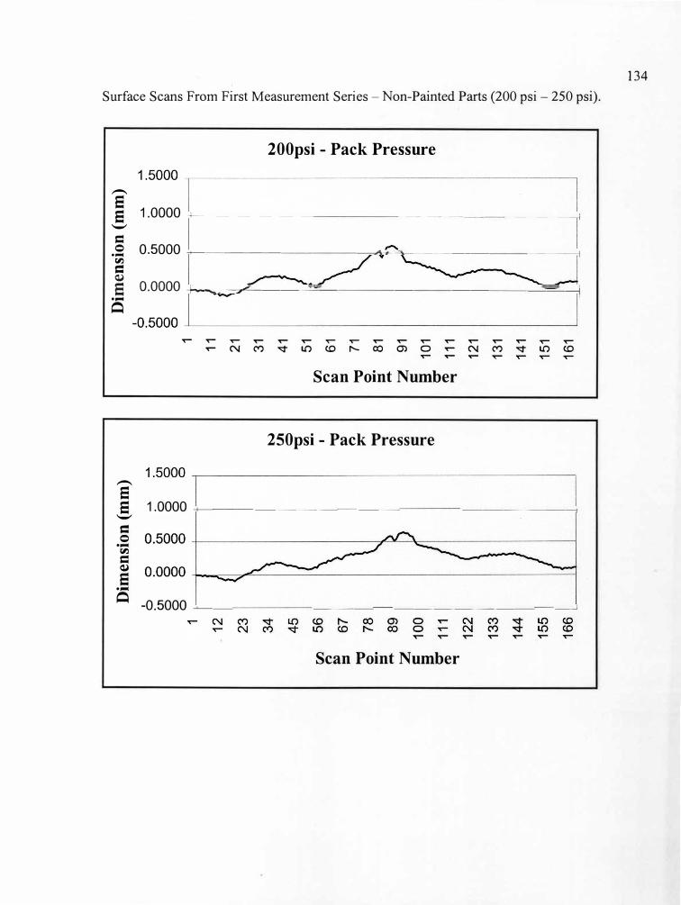
Surface Scans From First Measurement Series - Non-Painted Parts (200 psi - 250 psi).
200psi - Pack Pressure
e 8 1.0000 -+-------- - -------------,
_,
=
.s 0.5000 -+-- ----- - - -�,._,_-______ ___ _
rl.l
=
8 0.0000 --+-���---..:...==---- - --- ---- ------==--------, ...
�
� � 'T""9 � � � "t"- sir- � � � � � � � � �
� N M � � � � ro m O � N M � � �
Scan Point Number
250psi - Pack Pressure
-
8 8 1.0000 -t- ---------- - ------------1
_,
= 0 ...
rl.l
= Cl)
8 ...
� -0.5000 �-- - - -------------�
Scan Point Number
134
1 12
23
34
45
56
67
78
89
100
111
122
133
144
155
166
0 0
o 01
0
0 0
0 0
0
_._
01
0 0 0
1 1 1 1 1 1 1
I 0 01
0 0 0
0,
0 0 0
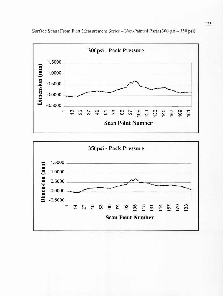
Surface Scans From First Measurement Series - Non-Painted Parts (300 psi - 350 psi).
300psi - Pack Pressure
e e 1.0000 ----------------- ------{ --
= 0..... �
= �
e..... � -0.5000 �-----------------�
Scan Point Number
350psi - Pack Pressure
e 1.5000
_§, 1.0000 -+-----------------------,
= .s 0.5000 +------- - - ----.-___.,--=---- ------, �
5 0.0000 +--�---------------------1 e S -0.5000 -'-----------------------'
Scan Point Number
135
0 0
......
0 u,
u,
0
0 0
0 0
0 0
0 0
1 1
14
13
25
27
37
40
49
53
61
66
73
79
85
92
97 I
10
5 I
) 10
9 11
8 12
1 13
1 13
3 14
4 14
5 15
7 15
7 I
170
169
183
181
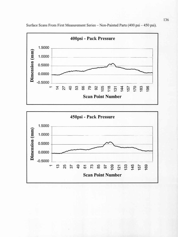
Surface Scans From First Measurement Series - Non-Painted Parts (400 psi- 450 psi).
400psi - Pack Pressure
-
e e 1.0000 -+-------- ---- -------------<
._,
= 0
•.-1 r'-l
= �
e •.-1
Q -0.5000 � ---- -- -----------�
Scan Point Number
450psi - Pack Pressure
-
e e 1.0000 +--------------- ---------;
._,
= 0
•.-1 r'-l
= �
e •.-1
Q -0.5000 --'--------- -- - --------�
Scan Point Number
136
0 0
...>.
0
0 ...
>.
0 C.1
1 C.1
1 0
01
01
0 0
0 0
0 0
0 0
0 0
0 0
0 0
0 0
0 0
1 1
13
14
25
27
37
40
49
53
61
66
73
79
85
92
105
97
118
109
131
121
144
133
157
145
170
157
183
169
196
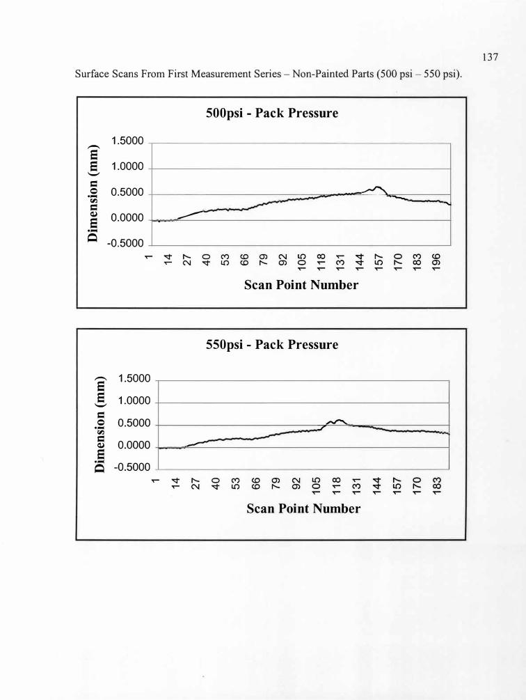
137
Surface Scans From First Measurement Series - Non-Painted Parts (500 psi - 550 psi).
500psi - Pack Pressure
1.5000 -
= = 1.0000 _,
= 0 0.5000 ....
f.f.l
=
� ---�
-....
QJ 0.0000
= -----
....
� -0.5000
Scan Point Number
550psi - Pack Pressure
- 1.5000= = 1.0000 _,
= 0 0.5000 ....
� _,
f.f.l --
= 0.0000 QJ
= -
....
-0.5000�
Scan Point Number
1 14
27
40
53
66
79
92
105
118
131
144
157
170
183
1
I
1 14
27
40
53
66
79
92
105
118
131
144
157
170
183
196
I
, \ I J I
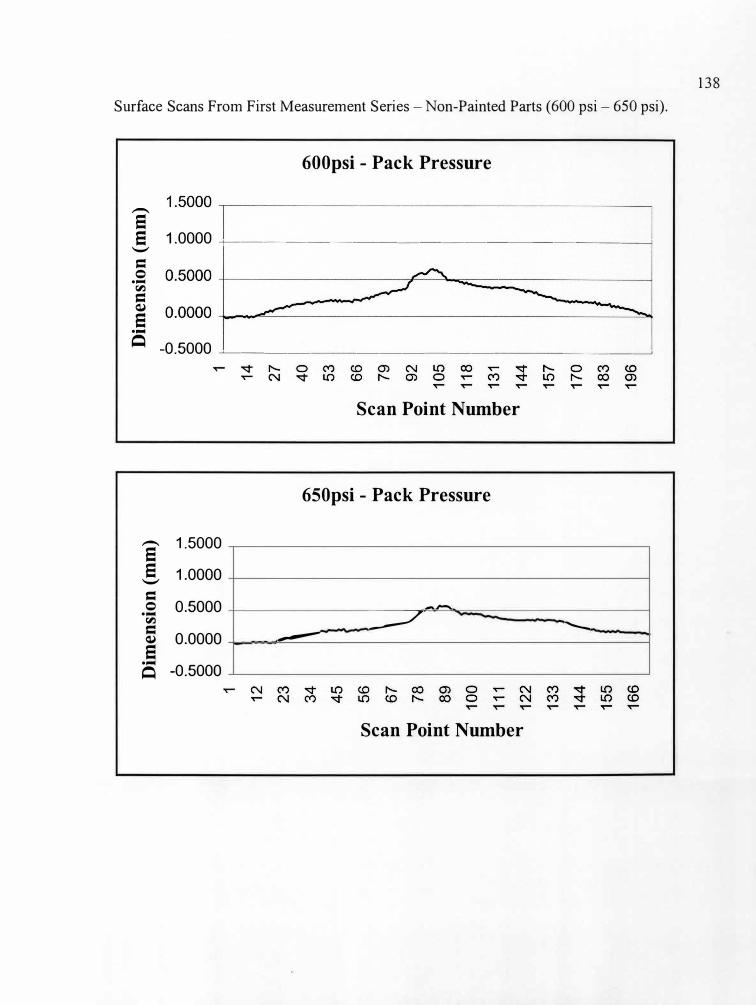
Surface Scans From First Measurement Series - Non-Painted Parts (600 psi- 650 psi).
600psi - Pack Pressure
e e 1.0000 -t-------- ---------------j
'-'
= 0 .....
VJ
= <l)
e .....
� -0.5000 �---- -------- - ---------'
Scan Point Number
650psi - Pack Pressure
- 1.5000e e 1.0000
'-'
= 0 0.5000 .....
VJ
= 0.0000 <l)
e
--
____./ ------
.....
-0.5000 �
Scan Point Number
138
1 12
23
34
45
56
67
78
89
100
111
122
133
144
155
166
\ I
1 14
27
40
53
66
79
92
105
I 11
8 13
1 14
4 15
7 17
0 18
3 19
6
0 !='
.....
0 CJ
1 CJ
1 0
0 0
0 0
0 0
0 0
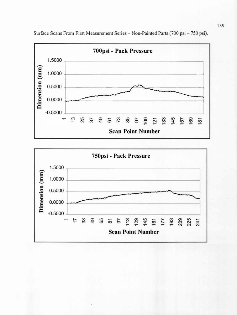
Surface Scans From First Measurement Series - Non-Painted Parts (700 psi - 750 psi).
700psi - Pack Pressure
--
� 1.0000 ---t------- - ---- - - - - - -------1
'-'
=
.s 0.5000 -i----- - - -----__,._---"'==-----------------1 {I}
= Q)
5 0.0000 ---i.--,-c..___----- - - - - --- - - - --------1
....
Q
Scan Point Number
7 SO psi - Pack Pressure
1.5000 --
e e 1.0000
'-'
= 0 0.5000 ....
{I}
=
--
---�
Q) 0.0000e
�-
....
Q -0.5000
Scan Point Number
139
1 17
33
49
65
81
97
113
129
145
161
177
193
209
225
241
'
1 1
1 13
25
37
49
61
73
85
97
109
121
133
145
157
169
181
I 0 ->
,.
01
01
0 0
0 0
0 0
---- )
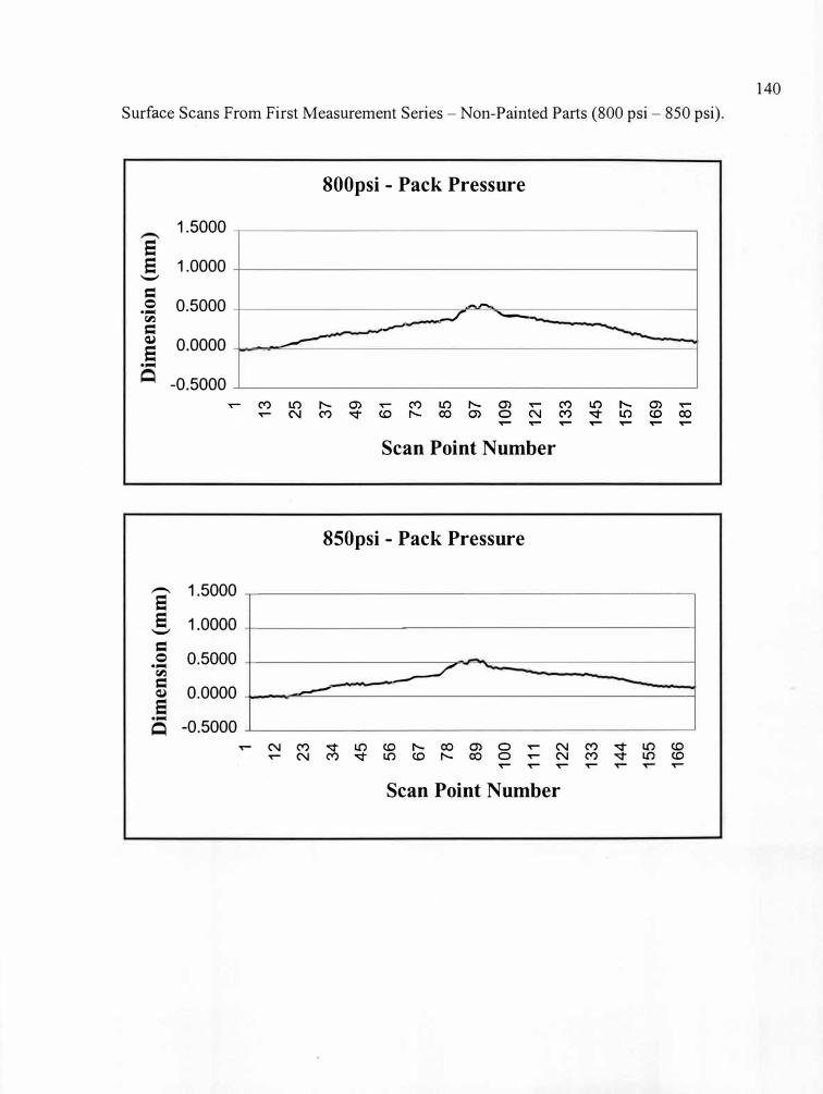
140
Surface Scans From First Measurement Series - Non-Painted Parts (800 psi - 850 psi).
800psi - Pack Pressure
1.5000
e e 1.0000 __, = 0 0.5000 ... �
--
_f --= �
<l) 0.0000
e -----
...
-0.5000
Scan Point Number
850psi - Pack Pressure
- 1.5000a e 1.0000 __, = 0 0.5000 ...
__./' �
= 0.0000 -
e ...
-0.5000Q ..- N C') s::f" I.(') (.D r-- ro 0) 0 ..- N C') s::f" I.(') (.D
..- N C') s::f" I.(') (.D r-- ro 0 ..- N C') s::f" I.(') (.D ..- ..- ..- ..- ..- ..- ..-
Scan Point Number
e \ I
1 13
25
37
49
61
73
85
97
109
121
133
145
157
169
181
D
)
\ \ '
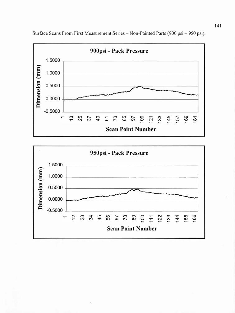
Surface Scans From First Measurement Series - Non-Painted Parts (900 psi - 950 psi).
900psi - Pack Pressure
1.5000 -
8 1.0000 8 _,
= 0 0.5000 ...
ti}
-'----
= -<l)
0.0000 8
-_,..,,--
...
� -0.5000
Scan Point Number
950psi - Pack Pressure
-
8 8 1.0000 +--- - - - - - ---- - - - --------,
_,
= 0 ...
ti}
= <l)
8 ...
� -0.5000 -'-------- ------- - - -�
Scan Point Number
141
0 0
.......
0 (J
I 0
, 0
0 0
0 0
0 0
0 0
1 1 12
13
23
25
34
37
45
49
56
61
\ 67
73
78
85
89
97
J \ 10
0 10
9
111
121
122
133
133
145
144
157
155
169
166
181
j
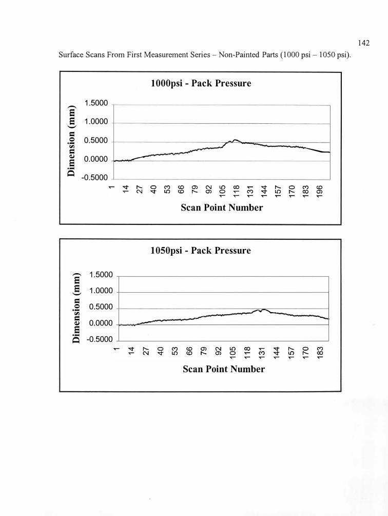
142
Surface Scans From First Measurement Series - Non-Painted Parts (1000 psi - 1050 psi).
1 000psi - Pack Pressure
-1.5000
s s 1.0000 ..._,
= 0 0.5000 ...
(;l.l
-
_/ = -
-.____
-
a)0.0000
s -----
...
� -0.5000
Scan Point Number
1050psi - Pack Pressure
- 1.5000s s 1.0000 ..._,
= 0 0.5000 ...
(;l.l �...,,......___
= 0.0000a)
- � �
s ...
-0.5000�
Scan Point Number
1 14
27
4 5 6 7 92 0 3 6 9
105
118
131
144
157
170
183
I
'
i 1
l
1 14
27
40
5 6 7 9 3 6 9 2 10
5 11
8
131
144
157
170
183
196
\ ) \ \ I I l
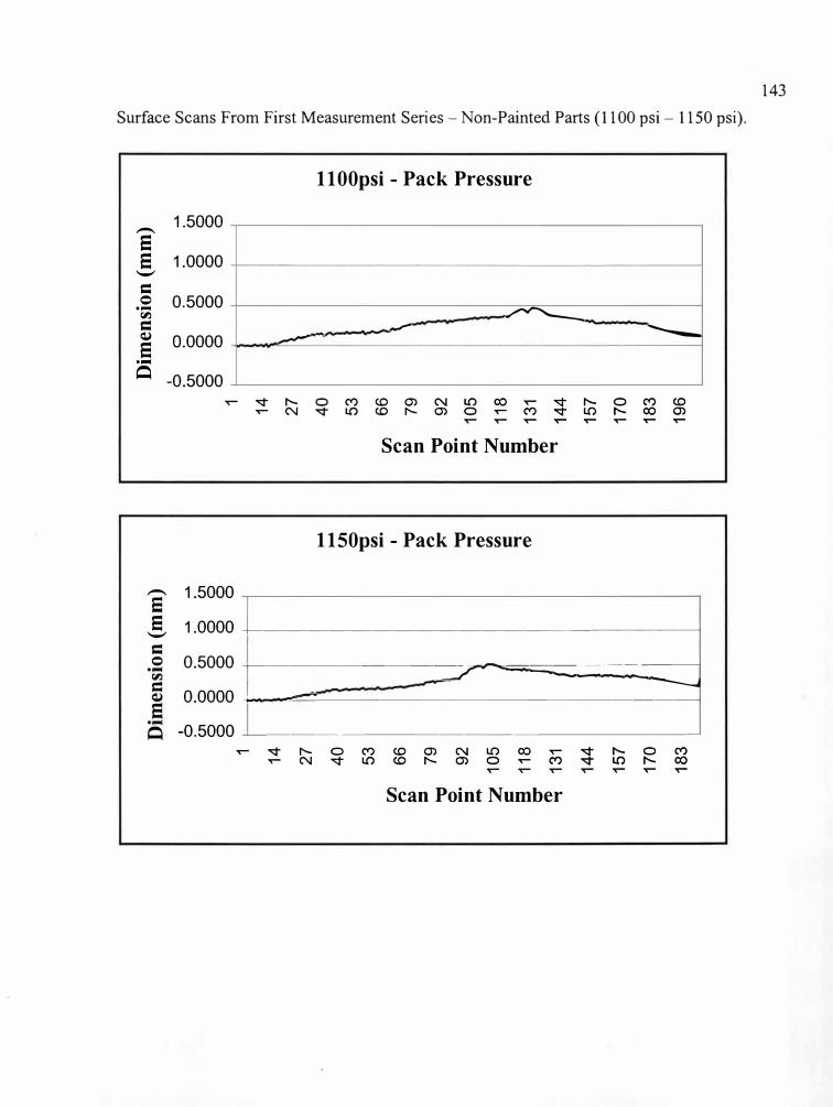
Surface Scans From First Measurement Series - Non-Painted Parts (1100 psi- 1150 psi).
11 00psi - Pack Pressure
-1.5000
e e 1.0000
'-' = 0 0.5000•...C r,:i
= Q) 0.0000e
� - � ----
•...C
� -0.5000
Scan Point Number
1150psi - Pack Pressure
a 1.5000
-8, 1.0000 -+----------------------1
=
-� 0.5000 r------- -=7-�;;;;;;::;:;:::::==::::=1
5 0.0000 �----==-------------------------1e
•...C � -0.5000 �-----------------�
Scan Point Number
143
1 1 ----
14
14
27
27
• 40
40
53
53
66
' 66
79
I
79
92
92
105
105
118
. 11
8 13
1 13
1 14
4 14
4 15
7 15
7 17
0 17
0 18
3 i
183
196
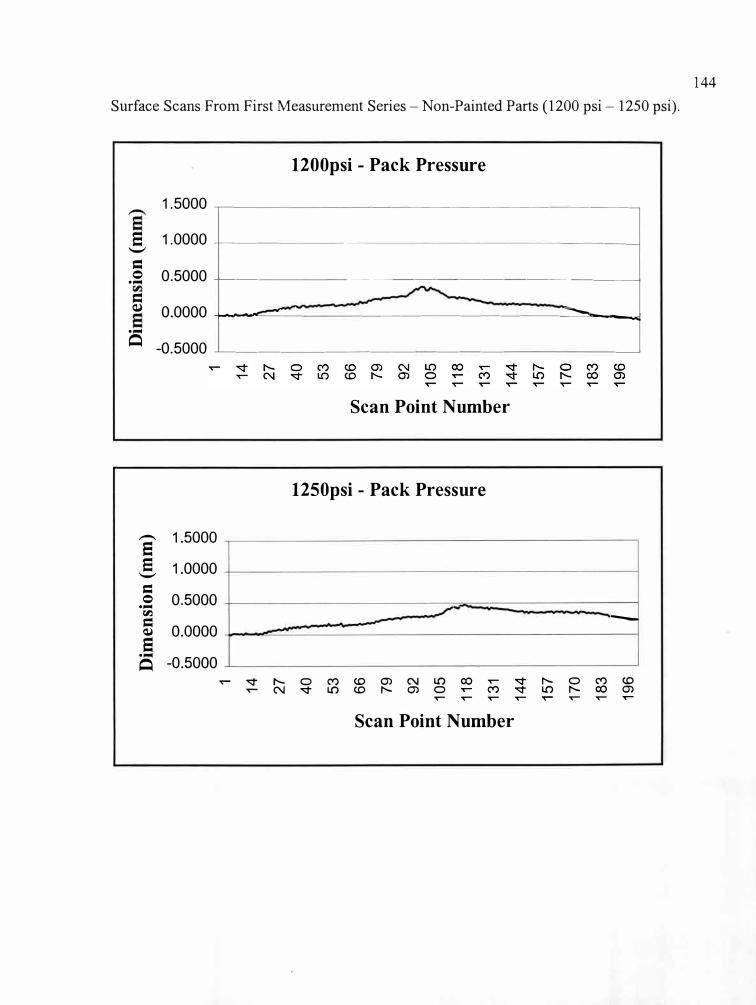
Surface Scans From First Measurement Series - Non-Painted Parts (1200 psi - 1250 psi).
1200psi - Pack Pressure
1.5000 ---,--- -- - - - - --------------�
E, 1.0000 +--- -- -- -- -- - - - - - - ---------j
= 0 ...
= a)
...
0.5000 --+----- - - ------------------<
0.0000 +-,.......-:=:--=------ - ---- ------ -----=---.1
� -0.5000 ---'----- -- -------- -- -- - - -�
Scan Point Number
1250psi - Pack Pressure
-- 1.5000 e e 1.0000
'-'
= 0 0.5000 ... -
Cl.l
= -
a) 0.0000e ...
-0.5000� ..... -.::;I- r--.. 0 C") (0 0) N LO co ..... -.::;I- r--.. 0 C") (0
..... N -.::;I- LO (0 r--.. 0) 0 ..... C") -.::;I- LO r--.. co 0) ..... ..... ..... ..... ..... ..... ..... .....
Scan Point Number
144
' \ '
1 14
I
27
40
53
66
79
92
105
I 11
8 I
131
144
157
170
183
196
m
s m
)

145
Surface Scans From First Measurement Series - Non-Painted Parts (1300 psi - 1350 psi).
1300psi - Pack Pressure
1.5000
e e 1.0000 __,
= 0 0.5000 .... � = Q)
0.0000e
� ---
....
� -0.5000
Scan Point Number
1350psi - Pack Pressure
-- 1.5000 e e 1.0000 __,
= 0 0.5000 ....
_,____ t:l'.l
= � Q) 0.0000
e ....
-0.5000� ....-- co ....-- co ....-- co ....-- co ....-- co ....-- co ....-- co ....-- co
....-- C") "'-t" co t- 0) 0 N C") LO co 00 0) ....-- N ....-- ....-- ....-- ....-- ....-- ....-- ....-- N N
Scan Point Number
s )
1 '
14
27
40
53
66
79
\ 92
10
5 11
8 13
1 14
4 '
f 15
7 17
0 18
3 19
6 l
l l
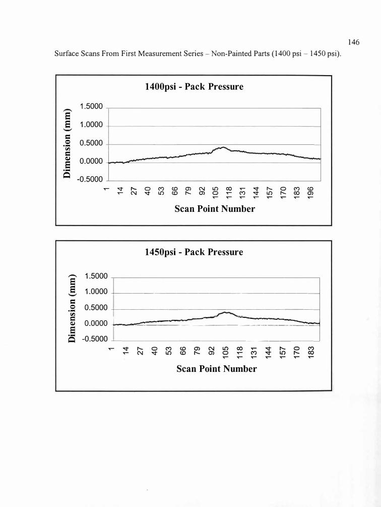
Surface Scans From First Measurement Series - Non-Painted Parts (1400 psi - 1450 psi).
1400psi - Pack Pressure
1.5000 e e 1.0000 _,
= 0 0.5000 ....
(l.l
= -� 0.0000 e ....
� -0.5000..- -.;t- r-- 0 C') (0 (j) N LO co ..- -.;t- r-- 0 C') (0
..- N '<;f" LO (0 r-- (j) 0 ..- C') -.;t- LO r-- co (j) ..- ..- ..- ..- ..- ..- ..- ..-
Scan Point Number
1450psi - Pack Pressure
a 1.5000
S 1.0000 -+--------------------------1
=
.s 0.5000 +------------------- ----1
(l.l
f 0.0000 L-�::'.'.::'.:::::::=:::::::=�__:_====:::::�d e....
� -0.5000 �------ -----------�
Scan Point Number
146
)
1 ---
14
27
40
53
66
' 79
92
! 10
5 11
8 (
131
144
157
170
i 18
3
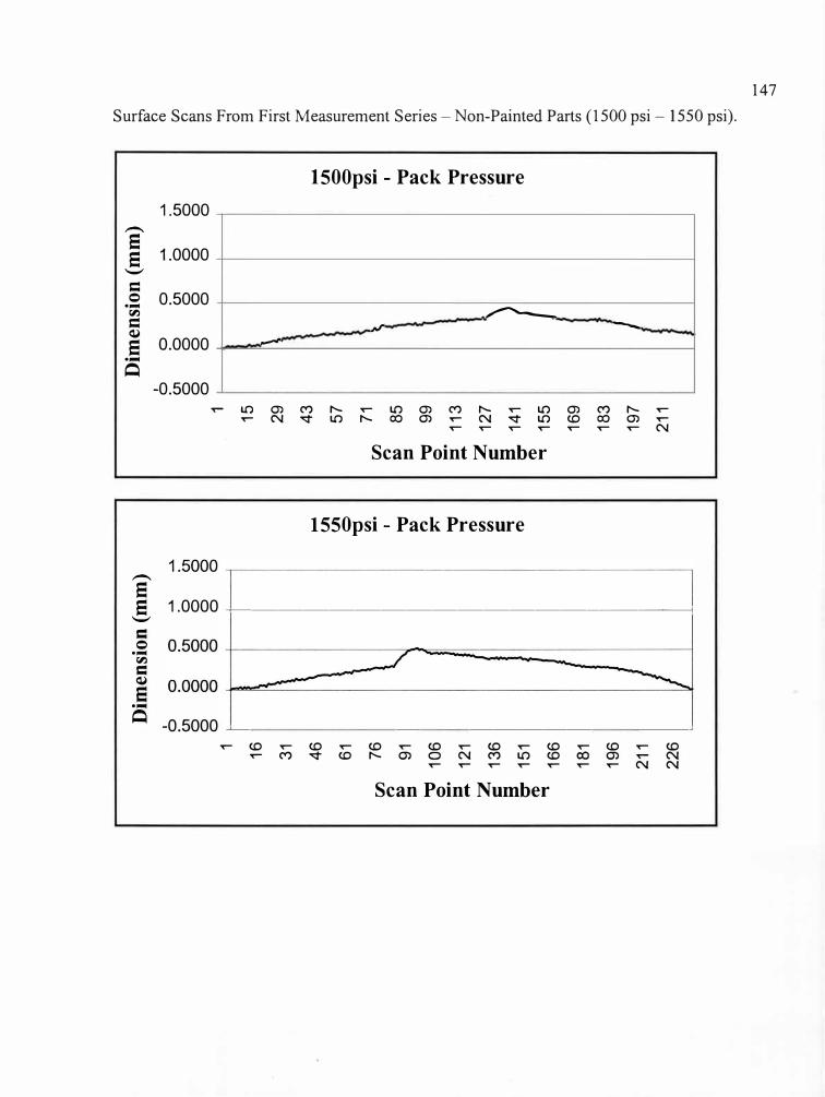
Surface Scans From First Measurement Series - Non-Painted Parts (1500 psi - 1550 psi).
1.5000 -
e 1.0000 e
'-'
= 0 0.5000 ....
VJ
= Q)
e 0.0000 ....
Q -0.5000
-
e
1500psi - Pack Pressure
-�Al ----
-
� � m M � � � m M � � � m M � � � N � � � ro m � N � � ID ro m �
.,- .,- .,- � .,- .,- .,- N
Scan Point Number
1550psi - Pack Pressure
e 1.0000 __________________ _ '-'
= 0 ....
VJ
= Q)
e ....
Q -0.5000 -'-- -- - - - --- ------- -----'� ID � ID � ID � ID � ID � ID � ID � ID
� M � ID � m O N M � ID 00 m � N � � � � � � � N N
Scan Point Number
147
.. -
1.5000 ~------------------
0.5000 r---_-_ -__:.~~r-=.;;;;;;;:::::;:::::;::::::=:==~7 0.0000 ..i-,.~=-----------------~
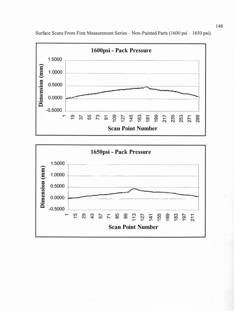
Surface Scans From First Measurement Series - Non-Painted Parts (1600 psi - 1650 psi).
1600psi - Pack Pressure
,_
� 1.0000 ---t----- - - - -------- -------i
..._,
= .s 0.5000 ---i-------------------==--------------1v.i
= Cl)
9 0.0000 --l-"""'=----- - ------ -----------1
...
�
Scan Point Number
1650psi - Pack Pressure
1.5000 �----------- ---- - - --,_
e e 1.0000 +---------- - - - ----------j ..._,
= 0 ...
v.i
= Cl)
e ...
0.5000 -+--------------------------,
0.0000 L��::::==:::==---�==:::::::::::::-� -0.5000 ..L._ _________________ �
Scan Point Number
148
I 0 ......
. 0,
01
0
0 0
0 0
0
1 1
15
19
29
37
43
55
57
73
71
91
85
109
99
127
113
145
127
163
141
181
155
199
169
217
183
235
197
253
211
271
289
L
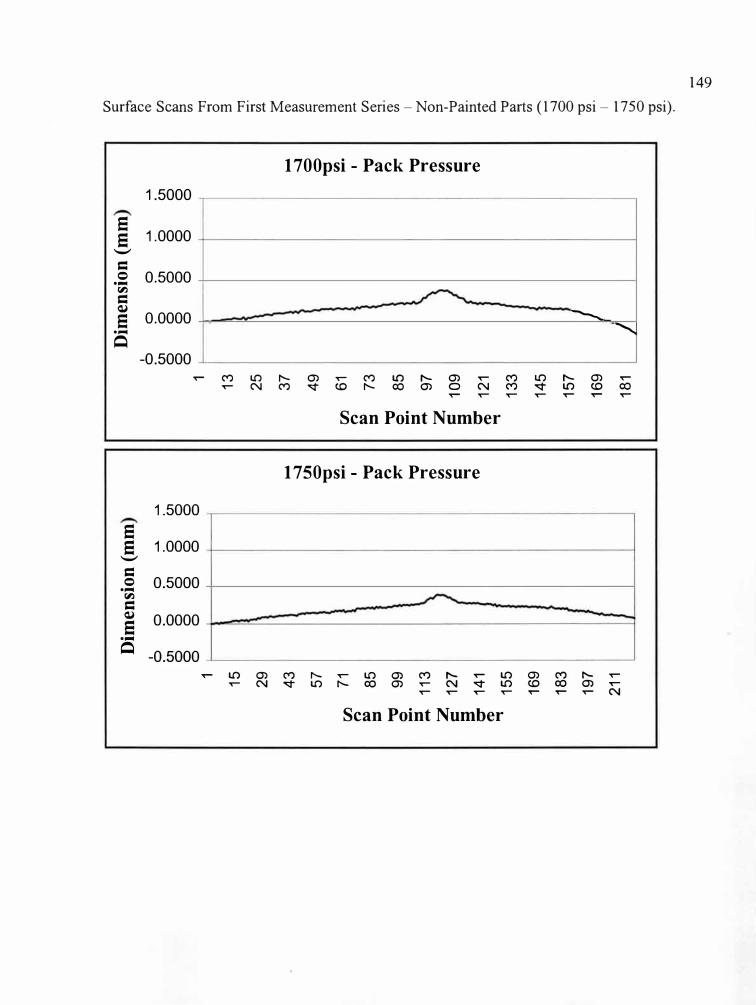
149
Surface Scans From First Measurement Series - Non-Painted Parts (1700 psi - 1750 psi).
1700psi - Pack Pressure
1.5000
a 1.0000 a --
= 0 0.5000 ....
fl:)
= Q)
0.0000 � a .... -........ �
-0.5000
..- C"') L{) r-- 0) ..- C"') L{) r-- 0) ..- C"') L{) r-- 0) ..-..- N C"') -.;t- (0 r-- co 0) 0 N C"') -.;t- L{) (0 co
..- ..- ..- ..- ..- ..- ..-
Scan Point Number
1750psi - Pack Pressure
1.5000
a a 1.0000 --
= 0 0.5000 ....
fl:)
= Q)
0.0000a ....
� -0.5000
..- L{) 0) C"') r-- ..- L{) 0) C"') r-- ..- L{) 0) C"') r-- ..-..- N -.;t- L{) r-- co 0) ..- N -.;t- L{) (0 co 0) ..-
..- ..- ..- ..- ..- ..- ..- N
Scan Point Number

Appendix F
Surface Scans From Second Measurement Series (Non-Painted Parts) on Coordinate
Measurement Machine
150
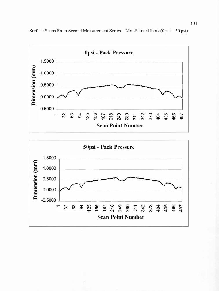
Surface Scans From Second Measurement Series - Non-Painted Parts (0 psi - 50 psi).
Opsi - Pack Pressure
-
� 1.0000 ---+--------------- - - -----<
__,
=
-� 0.5000 -j---------:�;;;;;;;;--��;;;;;;;
��-....... ;;;;;;:::=-------j= Cl)
9 0.0000 --l"<--=-----------------�----""'\
...
�
Scan Point Number
SOpsi - Pack Pressure
-
e e 1.0000 ---+---------------- ------< __,
= 0 ...
c-,.i
= Cl)
e ...
� -0.5000 ---+-------------------�
Scan Point Number
151
I 0 .....
0 0
..... u,
u,
0
()1
()1
0 0
0 0
0 0
0 0
0 0
0 0
0 0
0 1
1 >
32
32
63
63
94
94
125
125
156
156
187
187
218
218
249
249
280
280
311
311
342
342
373
373
5 40
4 40
4 43
5 43
5 46
6 46
6 49
7 49
7
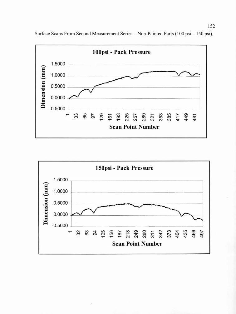
152
Surface Scans From Second Measurement Series - Non-Painted Parts (100 psi- 150 psi).
1 00psi - Pack Pressure
__ 1.5000 � ---- ------------- - ---� e e 1.0000 +-- ---- - - -=---:------:-:-F----- -----"e.____----"",._____, .._,
= 0 ....
�
= Q)
e ....
Q -0.5000 �-------- - --- - - ---�
Scan Point Number
150psi - Pack Pressure
--
e e 1.0000 +------------- ----------1
.._,
= 0 ....
�
= Q)
e ....
Q -0.5000 -'---- ----------------�
Scan Point Number
0 0
0 0
->.
o 0,
0
0,
0,
0 0
0 0
0 0
0 0
0 0
0 0
0 0
0 1
1 32
33
63
65
94
97
125
129
156
161
187
193
218
225
249
257
280
289
311
321
342
353
373
385
404
417
435
449
) 46
6 48
1 L
497
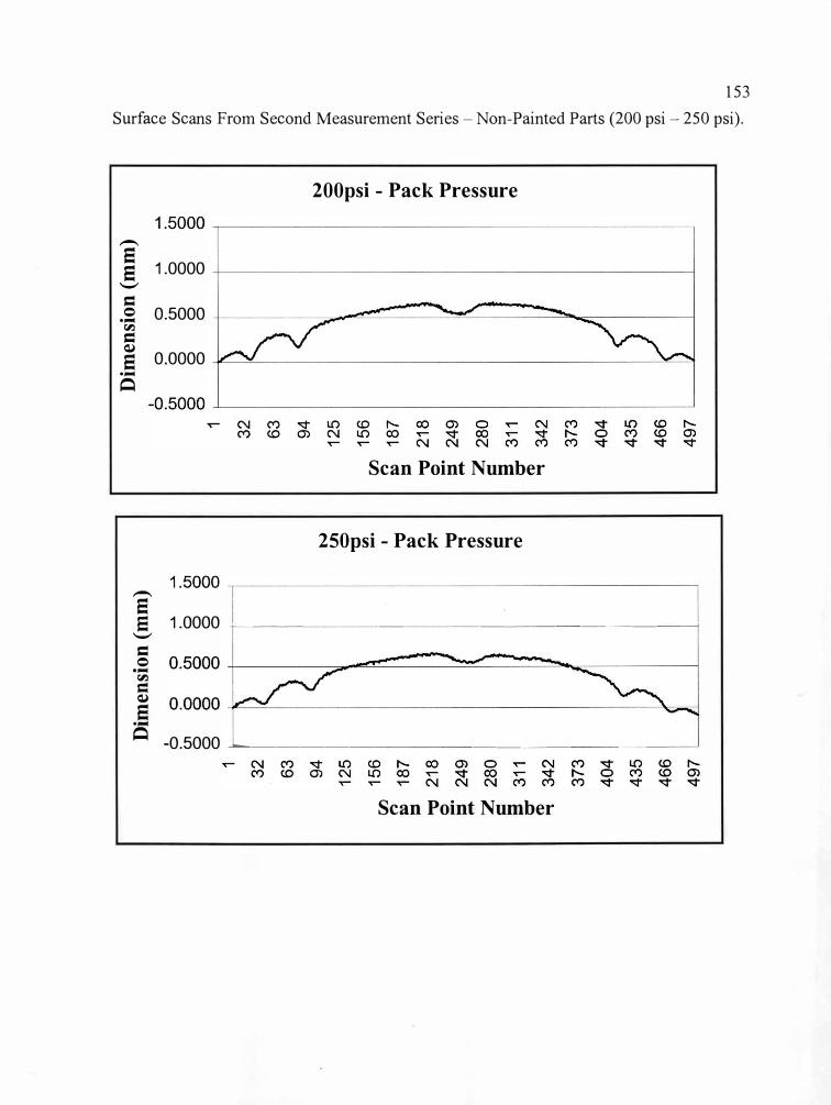
153
Surface Scans From Second Measurement Series - Non-Painted Parts (200 psi - 250 psi).
200psi - Pack Pressure
-
e 1.0000e --
= 0 0.5000 ...
� = �
0.0000e ...
Q
Scan Point Number
250psi - Pack Pressure
-
e e 1.0000 -l----- - --- - --------------l
--
= 0 ...
� = �
e ...
Q -0.5000 -'-------- - - - ------ ----
Scan Point Number
I 0 ...
.lo.
!='
0 ...
.lo.
01
0,
01
0 01
0
0 0
0 0
0 0
0 0
0 0
0 0
0 0
1 1
32
32
63
63
94
94
125
125
156
156
187
187
218
218
249
249
280
280
311
311
342
342
373
373
404
404
435
435
466
466
497
497
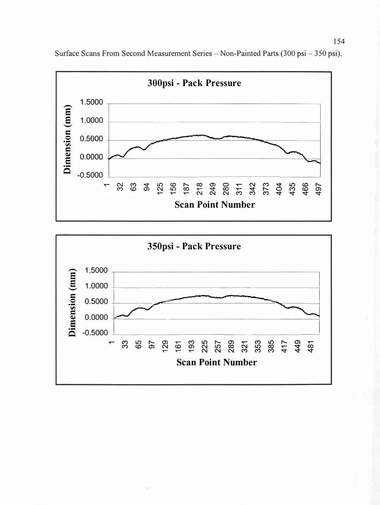
154
Surface Scans From Second Measurement Series - Non-Painted Parts (300 psi - 350 psi).
300psi - Pack Pressure
-
e e 1.0000 +----- ------------------1
--
= 0 ....
l:"'-l
= Cl)
e....
� -0.5000 ------- -----------�
Scan Point Number
350psi - Pack Pressure
8 1.5000
-$ 1.0000 +------------------------,
= .s 0.5000 -1----__,,..=--------- ---=......,.-------j
l:"'-l
� 0.0000 -f"----------- - - --------1
S -0.5000 �-----------------�
Scan Point Number
0 0
..... 0
CJ'I
CJ'I
0 0
0 0
0 0
0 0
0
1 1
33
\ 32
65
63
97
94
129
125
161
I 15
6
193
187
225
218
257
249
289
280
321
311
353
342
385
373
417
/_
404
449
435
481
I_
_ 46
6 49
7
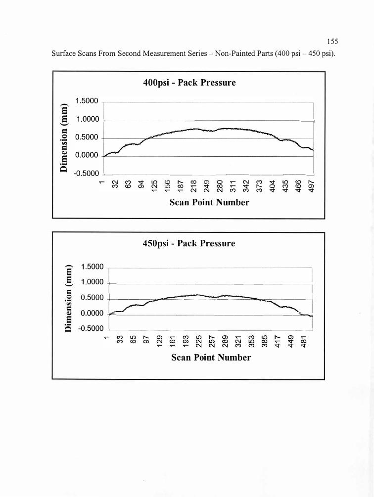
155
Surface Scans From Second Measurement Series - Non-Painted Parts ( 400 psi - 450 psi).
400psi - Pack Pressure
a e 1.0000 ---------- - - - - - - - --------, ..._,,
= 0 ·
(:I}
=�
e·-
� -0.5000 � -- - - ------- ----- -�
Scan Point Number
450psi - Pack Pressure
9 1.5000
-5, 1.0000 +---------- -- - ----- -------1
= .s 0.5000 -L-----���'.'.'::::���:::"'.:�-....-=-----�
(:I}
5 0.0000 -40=-------- ---------------'"� e Q -0.5000 �---------- - - - ----�
Scan Point Number
0 0
..... 0
01
01
0 0
0 0
0 0
0 0
0
1 1
33
32
65
63
97
94
129
125
161
156
193
187
225
218
257
249
289
280
321
311
353
342
373
385
1/i I
404
417
435
449
466
481
_J_
-
497
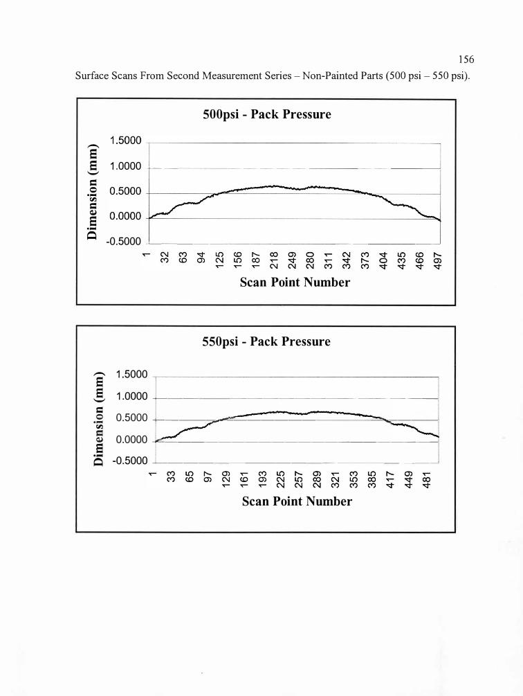
156 Surface Scans From Second Measurement Series - Non-Painted Parts (500 psi - 550 psi).
500psi - Pack Pressure
-
e e 1.0000 ---t---- - ------- - ---- ---------1
_,
= 0 ....
�
= Q)
e ....
� -0.5000 � ----- - --- - ---- - ---
Scan Point Number
550psi - Pack Pressure
S 1.5000
-5, 1.0000 -+----- -------------
= .s 0.5000 +----�-=------- - - -�....----�
5 0.0000 ---ir=---- ---------------------
9 Q -0.5000 -------------------
Scan Point Number
1 33
65
97
129
I 16
1
193
225
257
289
I 32
1
353
385
411
I 44
9 48
1
1 32 I
63
94
125
156
187
218
249
280
311
342
373
404
435
466
497
0 0 0 0
01
0 0 0
.....,,.
01
0 0 0
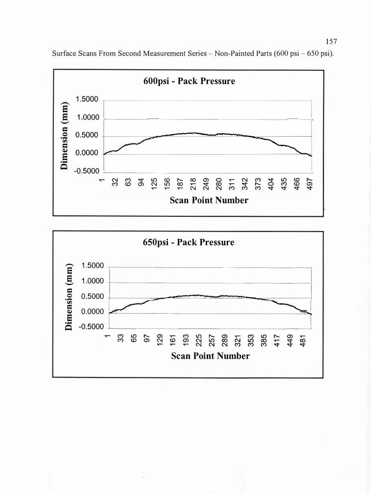
157
Surface Scans From Second Measurement Series - Non-Painted Parts (600 psi - 650 psi).
600psi - Pack Pressure
-
e e 1.0000 -+--------------------------i --
= 0 ....
r,.i
= Q)
e ....
Q -0.5000 -'--------------------------'
Scan Point Number
650psi - Pack Pressure
8 1.5000 -,-------------------------,
-5, 1.0000 --+--- ---- -------------------,
= .s 0.5000 -t-----�-�������----.....=-----ir,.i
� 0.0000 -..-=:---------------------==-.
i5 -0.5000 ...,___ __________________ ___,
Scan Point Number
0 0
..... 0
u, u,
0 0
0 0
0 0
0 0
0
1 1
33
32
65
63
97
94
129
125
161
156
193
187
225
218
257
249
289
280
321
311
353
342
385
373
I
404
417
I 43
5 44
9 46
6 48
1 49
7
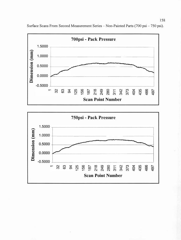
158
Surface Scans From Second Measurement Series - Non-Painted Parts (700 psi - 750 psi).
700psi - Pack Pressure
-
§ 1.0000 +------- -----------------1
--
=
.s 0.5000 +----�--=------------�"""""
:----l
� = � e 0.0000 -f"------ ------ - - ------------,
·-
�
Scan Point Number
7 SO psi - Pack Pressure
-
e e 1.0000 -+------- ---------- - -----1 --
= 0 ·-
� = � e ·-
� -0.5000 -'---------------------'
Scan Point Number
I 0 _,.
0
0 _,
. 01
(J
l 0
(Jl
01
0 0
0 0
0 0
0 0
0 0
0 0
0 0
0 1
1 32
32
63
63
94
94
125
125
156
156
187
187
218
218
249
249
280
280
311
311
342
342
373
373
404
404
435
435
-~ •• 46
6 46
6 j_
_ 49
7 49
7
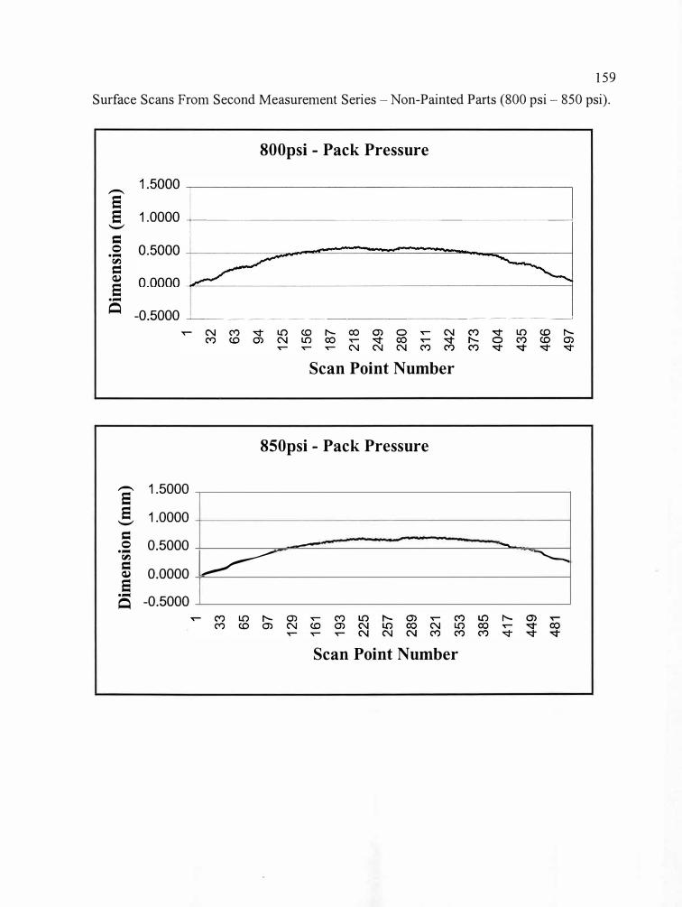
159
Surface Scans From Second Measurement Series - Non-Painted Parts (800 psi - 850 psi).
800psi - Pack Pressure
-
a a 1.0000 -+--------- - - - --- - - ---------<
'-'
= 0 ...
� = Cl)
a ...
� -0.5000 ---'------------- --- ------�
Scan Point Number
850psi - Pack Pressure
- 1.5000a s 1.0000
'-'
= 0 0.5000 ...
� = 0.0000 Cl)
s
� -
I� ·---....
... -0.5000�
Scan Point Number
0 0
......
0 u
, u
, 0
0 0
0 0
0 0
0 0
1 1
33
32
65
63
97
94
129
125
161
156
193
187
225
218
257
249
289
280
321
311
353
342
385
373
417
404
449
435
481
466
II 49
7
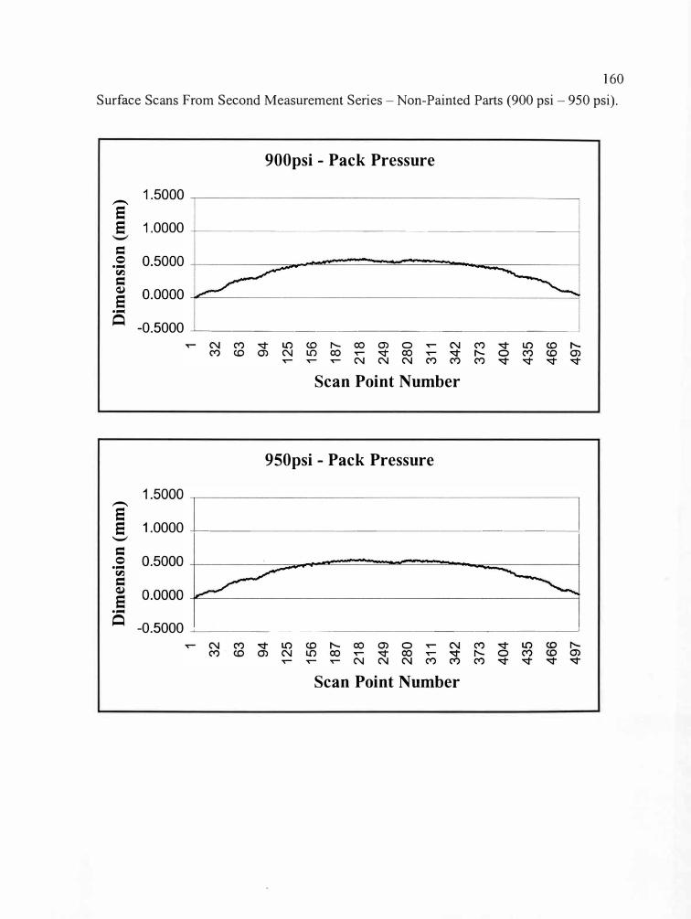
160
Surface Scans From Second Measurement Series - Non-Painted Parts (900 psi - 950 psi).
900psi - Pack Pressure
-
e e 1.0000 -t------- -------------------1
= 0 ...
r,i
= �
e ...
� -0.5000 --'-------------------�
Scan Point Number
950psi - Pack Pressure
-
e e 1.0000 -+----------------- -------,
._,
= 0 ...
r,i
= �
e ...
� -0.5000 ...,__ _________________ �
Scan Point Number
1 32
63
94
125
156
187
218
249
280
311
342
373
404
435
466
497
0 0
0 CJ1
0
0 0
0 0
0
......
CJ1
0 0 0 1 32
63
94
125
156
187
218
249
280
311
342
373
404
435
466
497
0 0
0 CJ1
0
0 0
0 0
0
( ......
CJ
1 0 0 0

161
Surface Scans From Second Measurement Series - Non-Painted Parts (1000 psi- 1050 psi).
1 000psi - Pack Pressure
e e 1.0000 -+---------------------<
_,
= 0 ....
r,.i
= �
e ....
Q -0.5000 ---'------ - - --------------'
Scan Point Number
1 0S0psi - Pack Pressure
- 1.5000e e 1.0000 _,= 0 0.5000 ....
r,.i
= 0.0000 �
e �
-�
....
-0.5000Q
Scan Point Number
0 0
.......
0 (J
I c.n
0
0 0
0 0
0 0
0 0
1 1
33
32
65
63
97
94
129
: 12
5
161
156
193
187
225
218
257
249
289
280
321
311
353
342
385
373
417
404
449
435
481
466
497
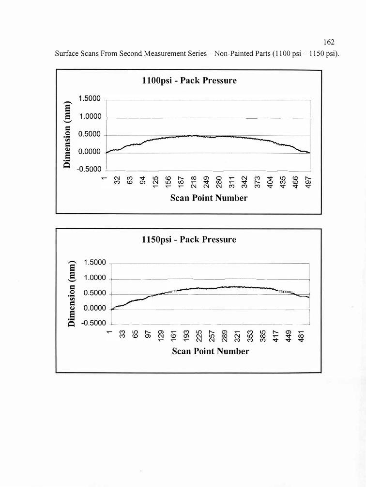
162
Surface Scans From Second Measurement Series - Non-Painted Parts (1100 psi- 1150 psi).
11 00psi - Pack Pressure
-
a a 1.0000 ---j-------- - - - - - ----------1
..._,
= 0 ...
�
= Q)
a ...
� -0.5000 -'--- ---- -- - - --- - - -----------'
Scan Point Number
1150psi - Pack Pressure
S 1.5000
!, 1.0000 +----- - - ----- - ------------1
= .s 0.5000 +----��=--------- ----------'-:::::e,,,,,,-=:-1 �
� 0.0000 --f'L-------- ------- - ------------,
a Q -0.5000 ---'---------------- -----�
Scan Point Number
0 0
..... 0
0,
0,
0 0
0 0
0 0
0 0
0
1 1
\ 32
I 33
63
65
94
97
12
5 12
9 I
156
161
193
187
225
218
257
249
289
280
321
311
342
353
1 37
3 38
5 40
4 41
7 I
435
449
I 46
6 48
1 _J
_ 49
7
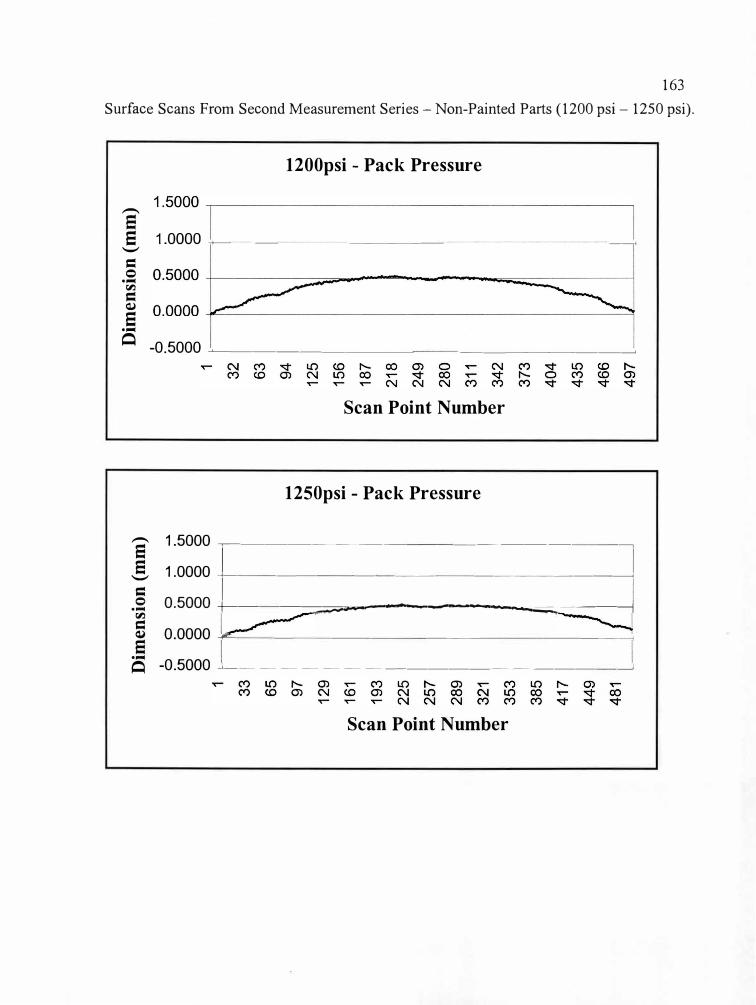
163
Surface Scans From Second Measurement Series - Non-Painted Parts (1200 psi - 1250 psi).
1200psi - Pack Pressure
e e 1.0000 -+-- -- -- ------ - - -- - ---------<
._,
= 0
•.-C r,.i
= cu
e •.-C
� -0.5000 ---'-------------- ------------'
Scan Point Number
1250psi - Pack Pressure
5 1.5000 ,----------- -------- -------,
-$ 1.0000 +-- ----- ------ -------------,
= .s 0.5000 +---------===---------==----------i
r,.i
5 0.0000 --f'L--- ---- ---- - ------ -------,
e S -0.5000 -'--------------------�
Scan Point Number
0 0
-"
0 u,
01
0
0 0
0 0
0 0
0 0
1 1
33
32
65
63
97
94
129
125
161
156
193
187
225
218
257
249
289
280
321
311
353
I 34
2
385
373
417
404
«9
L
435
481
I_
466
--
497
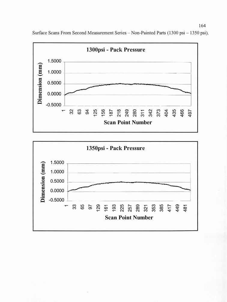
164
Surface Scans From Second Measurement Series - Non-Painted Parts (1300 psi- 1350 psi).
1300psi - Pack Pressure
-
8 8 1.0000 ---t-------- - - - - - - --------1
,,_,
= 0 ...
r,.i
= Q)
8 ...
� -0.5000 �--------------- ---
Scan Point Number
1350psi - Pack Pressure
S 1.5000
E, 1.0000 -+--- --------- - -------
.s 0.5000 ,-----=:;;;;;;;;;;;....-------......._;;;.;;;;;;;�- -r,.i
5 0.0000 �------------- - - - - - --8 S -0.5000 -'-------------- - - - ------�
Scan Point Number
n 0
0 ->
,.
0 CJ
1 CJ
1 0
0 0
0 0
0 0
0 0
1 ~
-1
33
32
65
63
97
94
129
125
161
156
193
187
225
218
257
249
289
280
321
311
353
342
385
373
417
404
449
435
481
466
497
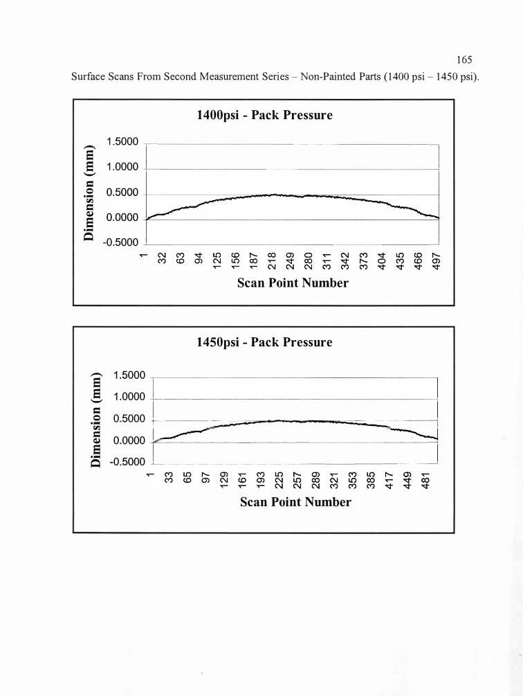
165 Surface Scans From Second Measurement Series - Non-Painted Parts (1400 psi - 1450 psi).
1400psi - Pack Pressure
-1.5000 � -- - - - - - - ----- - - - - -�
5 _§, 1.0000 +-- -- - - - - ---- - - - - - - ------1
= 0 .... �
= Q)
5 .... Q -0.5000 �-- - - - - - - - - ----- - -----'
Scan Point Number
1450psi - Pack Pressure
9 1.5000
E, 1.0000 +---- -- -- ---- - - - - - - - --------j
=
-� 0.5000 ,---=::;;;;;;;;;;;;.;.a----------;;;;;;;:;::::=---1
� 0.0000 ---l'=-----------------------1
Q -0.5000 -'-------------- --------'
Scan Point Number
0 0
0 C.1
1 0
0 0
0 0
0 1
1 -
33
32
65
63
97
94
129
125
161
156
193
187
225
218
257
249
289
280
321
311
353
342
385
373
404
417
l 43
5 44
9 46
6 48
1 49
7
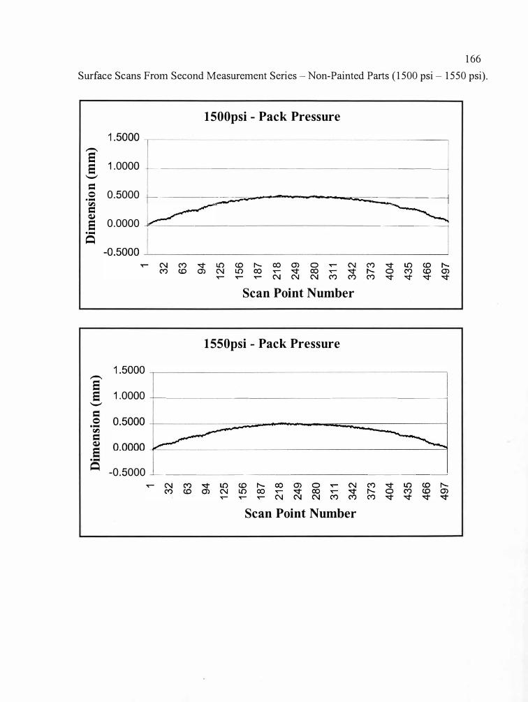
166
Surface Scans From Second Measurement Series - Non-Painted Parts (1500 psi - 1550 psi).
1500psi - Pack Pressure
-
� 1.0000 -i----- --- ------- - --------,
...._,
=
-� 0.5000 -i----- -------:-:::;;;;;;;;,..,-,------........ ...;;;;;;;::::=------j
= �
e 0.0000 � -- ---- - - - - - ----------,.....Q
Scan Point Number
1550psi - Pack Pressure
-
e e 1.0000 -+-------- - ---- - - --------,
...._,
= 0 ..... �
= �
e ..... Q -0.5000 �--- ----- -- - - -----�
Scan Point Number
I 0 ......
0
0 ......
01
01
0
01
01
0 0
0 0
0 0
0 0
0 0
0 0
0 0
0 1
1 32
32
63
63
94
94
125
125
156
156
187
187
218
218
249
249
280
280
311
311
342
342
373
373
404
404
435
435
466
466
497
497
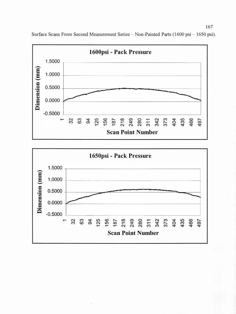
167
Surface Scans From Second Measurement Series - Non-Painted Parts (1600 psi - 1650 psi).
1600psi - Pack Pressure
1.5000 -..
e 1.0000 e '-'
= 0 0.5000 .....
r,:i
= �
0.0000 e .....
�
Scan Point Number
1650psi - Pack Pressure
e e 1.0000 +-------- - - - ------ ------,
'-'
= 0 .....
r,:i
= � e .....
� -0.5000 �-----------------�
Scan Point Number
I 0 0
0 .....
CJ1
0 C.1
1 C.1
1 0
0 0
0 0
0 0
0 0
0 0
0 1
1 32
32
63
63
94
94
125
125
156
156
187
187
218
218
249
249
280
280
311
311
342
342
373
373
404
404
435
435
466
466
497
497
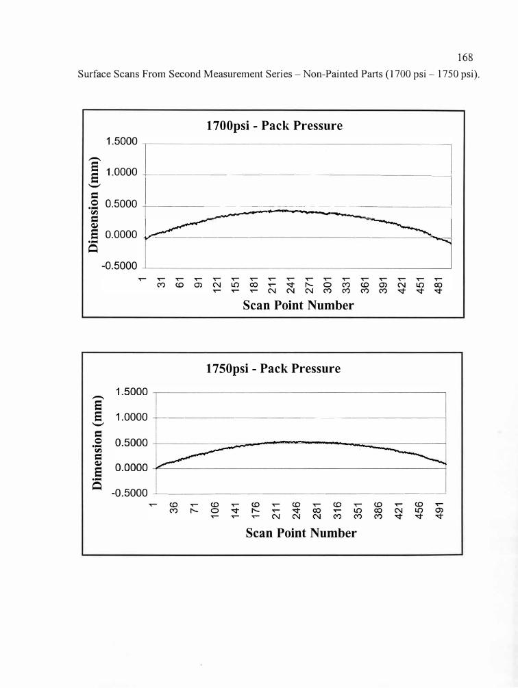
168
Surface Scans From Second Measurement Series - Non-Painted Parts (1700 psi - 1750 psi).
1700psi - Pack Pressure
-
§ 1.0000 +------------- - -----------!
'-'
=
-� o.5000 r----=:::::::;::;;::;::;;;::;:�::::::::::::=----- -7
= Cl)
5 0.0000 -vc------- -- - -- ---------'� -� Q
Scan Point Number
1750psi - Pack Pressure
-
s 5 1.0000 -+---- - ----------------1
'-'
= 0 -�
r,'l
=Cl)
s-�Q
-0.5000 �------- ---- -------
Scan Point Number
I 0 .....
0 0
..... 01
01
0
0 0
01
01
0 0
0 0
0 0
0 0
0 0
1 0
0 0
---
1 31
36
61
71
91
10
6 12
1 14
1 15
1
176
181
211
211
246
241
281
271
301
316
331
351
361
386
391
421
421
456
451
491
481

Appendix G
Overlaid Surface Scans Based Upon Z-axis Values and Residual Values for Parts Measured During
Repeatability and Reproducibility Tests
169
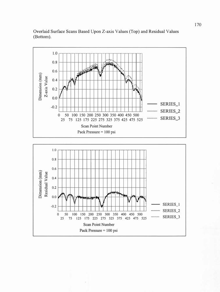
Overlaid Surface Scans Based Upon Z-axis Values (Top) and Residual Values (Bottom).
1.0
0.8
0.6
§ g'-';;;§ >
0.4
·;;; [/)
0.2i::: -� .§
0.0 Cl
-0.2
1.0
0.8
0.6
I .2 ';;' >
0.4
.9 � � .§ 0.2 Q.) ·-
s � 6 0::: 0.0
-0.2
,. .. , .... _..,,
f� ffi [li -
� �-- 'l\. .. ...... "" -j 11'1' ', �-
/1 . ..
I.L -
r y ,.
� · ... I
.,,, ,.
0 50 100 150 200 250 300 350 400 450 500 25 75 125 175 225 275 325 375 425 475 525
Scan Point Number
Pack Pressure = 100 psi
i.u..i....
� ,..� �"' ' r..., M.. 1 ....
'I ,,, .. '" I V V ·�-�
0 50 100 150 200 250 300 350 400 450 500
25 75 125 175 225 275 325 375 425 475 525
Scan Point Number
Pack Pressure = 100 psi
SERlES_l
SER1ES_2
SER1ES_3
SERIES_l
SERIES_2
SERIES_3
170
.. ' . ,
., ,, -~ .... I- ', ,-1~ I I I --
l l ........ .........
-
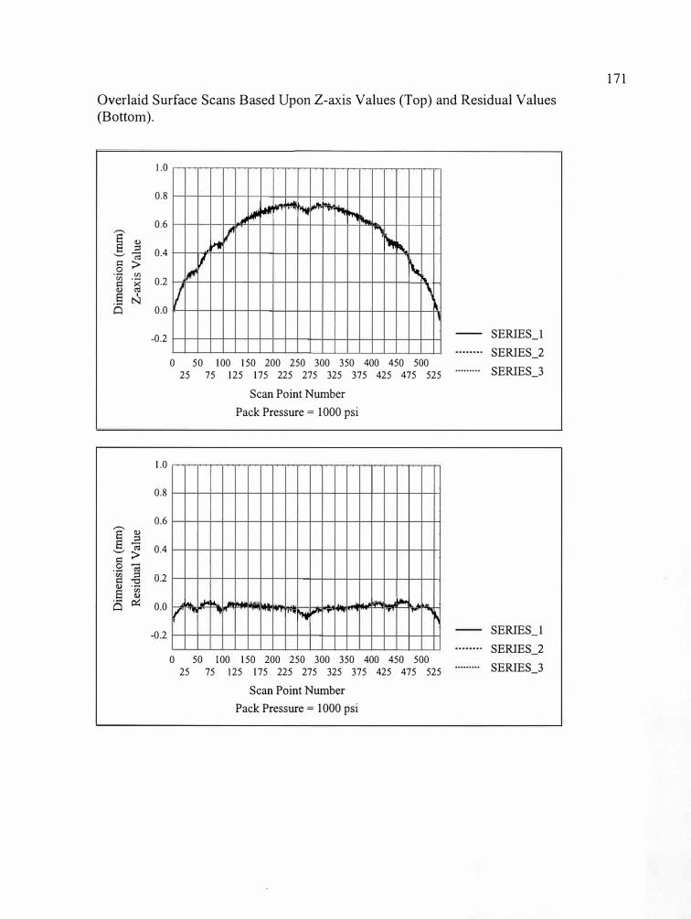
Overlaid Surface Scans Based Upon Z-axis Values (Top) and Residual Values (Bottom).
1.0
0.8
0.6
§ � 0.4 '-'.;l i::: > .9 "' "' '>< 0.2i::: �
i5 0.0
-0.2
1.0
0.8
0.6
]' .a 0.4 .._, �i::: >.9
;:l 0.2 i::: Q.) ·.;; .§ Q.)
Ci �
0.0
-0.2
i.... ........ .. !" liitfl' ... ., "' •. r'I �
,..,
.. � "' � I/
I\..,'
'
0 50 100 150 200 250 300 350 400 450 500
25 75 125 175 225 275 325 375 425 475 525
Scan Point Number
Pack Pressure = 1000 psi
la., "" .... ., .. , ,.� , .... -,r· " . , 1•·� ..,. ... ... .. ...
0 50 100 150 200 250 300 350 400 450 500
25 75 125 175 225 275 325 375 425 475 525
Scan Point Number
Pack Pressure = 1000 psi
SERIES_l
SERIES_2
SERIES_3
SERIES_!
SERIES_2
SERIES_3
171
--
I ,...., ,·-. ~,.,_.
"'--' I ,-.
I
Jl,f Q.)
·~ r s N
------·· --·······
-
-'I
- I . . ' '" " .,, r ..
I I
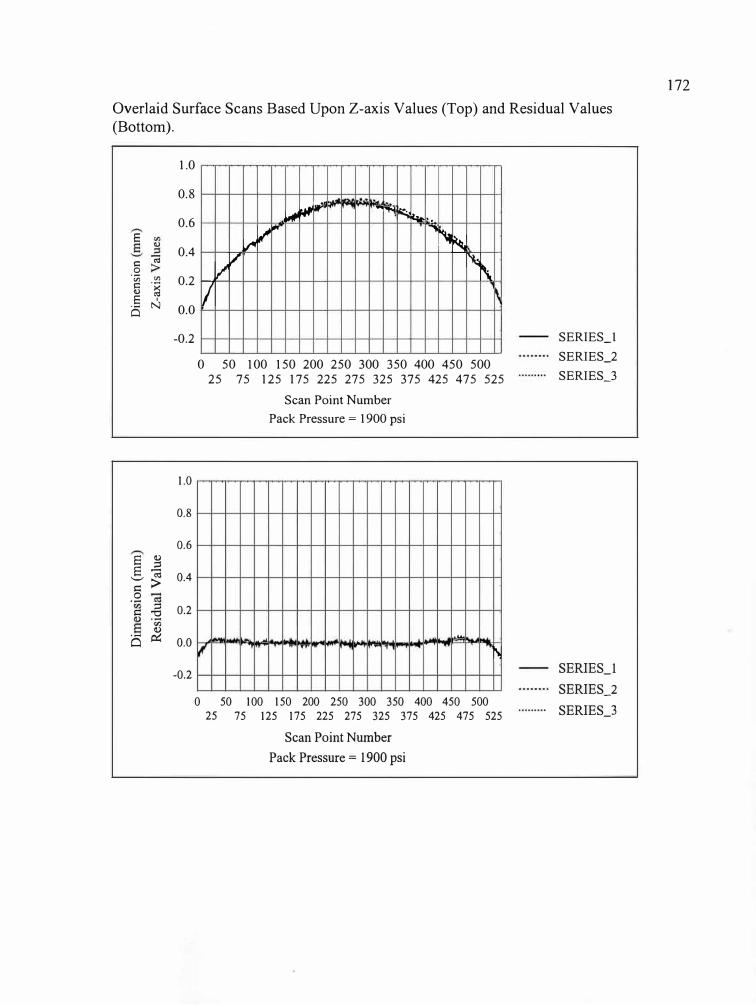
Overlaid Surface Scans Based Upon Z-axis Values (Top) and Residual Values
(Bottom).
E 0
i:: -; 0
·;;; en
i:: ·;;;0 (,:I
E N i5
§ .2 .._, ro i::: >.s
;::l i::: :"9 rJ)
cS �
1.0
0.8
0.6
0.4
0.2
0.0
-0.2
1.0
0.8
0.6
0.4
0.2
0.0
-0.2
� ,,,� -� � �-.
l/41 �,..- �� �
v V �
�
I
0 50 100 150 200 250 300 350 400 450 500 25 75 125 175 225 275 325 375 425 475 525
Scan Point Number Pack Pressure = 1900 psi
- J ....
" ... " .. , r--
0 50 100 150 200 250 300 350 400 450 500
25 75 125 175 225 275 325 375 425 475 525
Scan Point Number Pack Pressure = 1900 psi
SERIES_l SERIES_2 SERIES_3
SERIES_! SERIES_2 SERIES_3
172
l I ··-
.,,
U_j_W++-+++-t-+tiH--i-1--r--i-n-··
ti)
..
I ·1r , '"' ...

Appendix H
Results From Visual Evaluation Experimentation
for Painted & Non-Painted Parts
173
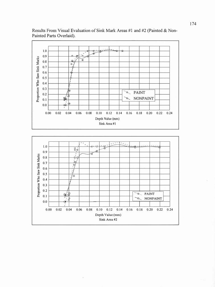
Results From Visual Evaluation of Sink Mark Areas #1 and #2 (Painted & Non
Painted Parts Overlaid).
Vl
:E .,.:
0
i:: 0
"€0
0
Cll 0
� i:: 0
"€ 0
0 11..
1.0 0.9 0.8 0.7 0.6 0.5 0.4
� .,.. .. · ....
n."/ ______,.-□
o.J
J T I
0.3 0.2 0.1
/□ J,. l
0.0 D
... �ru
. ...
·o. PAINT
'n.___ NONPAINT
0.00 0.02 0.04 0.06 0.08 0.10 0.12 0.14 0.16 0.18 0.20 0.22 0.24 Depth Value (mm)
..
1.0 o· 00
0.9 /
0.8 0.7 0.6 0.5 0.4
--·
-:7 .oj
:/
-1□
0.3 0.2 0.1 J:
I • )
0.0 _. ( -
Sink Area#l
. .. - •A . -,,.: .
� l.,..----0'"
...-
-
I .. ·o. ..
I --a.____
.... . . .
PAINT � NONPAINT
0.00 0.02 0.04 0.06 0.08 0. 10 0.12 0.14 0.16 0.18 0.20 0.22 0.24 Depth Value (mm)
Sink Area #2
174
r p
h aw
Sin
k M
arks
Pr
p
Wh
Saw
Sin
ar
k
•• _
1 ,.
_ h
, ....
,_ "~
--..
L
----
-,
--t-
.L"-
t---
---"
t--,
.s:!
--+-
--+-
+---
+--+
--1-
--l
", f-
-+-+
--+
---1
---1
--+
----
1--
--1
--1
-"11
--->
--
I ,\
'
C
( r '
', I ! I ll
,._
_
~-
>--
>--
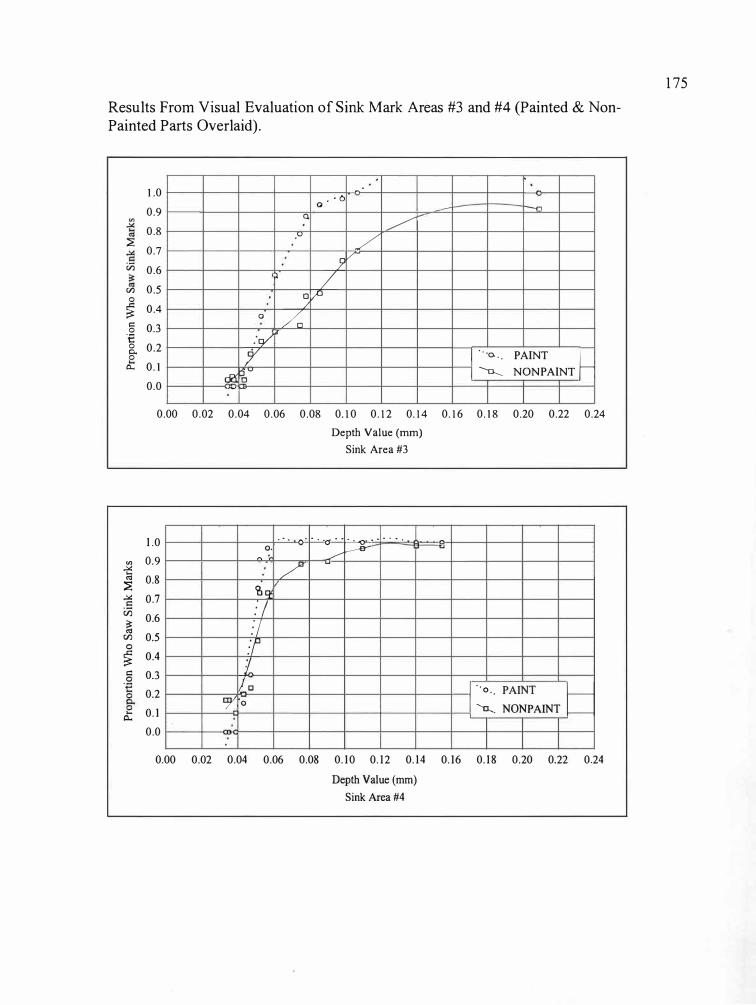
Results From Visual Evaluation of Sink Mark Areas #3 and #4 (Painted & Non
Painted Parts Overlaid).
�
:::E
in
Cl)
0
� i::: 0
"€ 0 0. 0
i:,..
"' .!><: @ � .!><: .5 Cl)
� Cl)
0
� i::: 0 "€ 0
0 .... i:,..
1.0 -·• • 0
0.9
0.8
0.7
0.6
0.5
- ___,.., Q �v
,v
_/r
7 i /
□,P0.4
0.3
0.2
0.1
0.0
/
0 /4 :c:y''
:r I - - '(> PAINT
� - .
c£ (i_ V
I "-o...__ NONPAINT D --
0.00 0.02 0.04 0.06 0.08 0.10 0.12 0.14 0.16 0.18 0.20 0.22 0.24 Depth Value (mm)
Sink Area #3
1.0 0.9 0.8
-·· -· .. ·- .. .. - . ... .. -0,
-__.a- V
- _,,/
/ -
0.7
0.6
0.5 0.4 0.3 0.2 0.1
<2iQ ,:; _:; :t 1
�□ I ··o .. PAINT
C3/ 0 I u... NONPAINT
0.0
0.00 0.02 0.04 0.06 0.08 0.10 0.12 0.14 0.16 0.18 0.20 0.22 0.24
Depth Value (mm) Sink Area #4
175
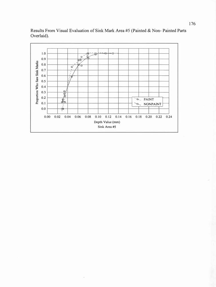
Results From Visual Evaluation of Sink Mark Area #5 (Painted & Non- Painted Parts
Overlaid).
Cl'.)
0
::! i:: 0
"€ 0
i:i...
1.0
0.9
0.8
0.7
0.6
0.5
0.4
. . ·- ..
� - -
o·)
. . o/ Q
I u
:;
I/
0.3
0.2
0.1
nf
t� 1 ···o PAINT � •,
I --=.__ NONPAINT 0.0
0.00 0.02 0.04 0.06 0.08 0.10 0.12 0.14 0.16 0.18 0.20 0.22 0.24
Depth Value (mm)
Sink Area #5
176
rop
h aw
Sin
k M
arks
..
- - -

Appendix I
Results From Pilot Tests for Visual
Evaluation of Sink Marks
177
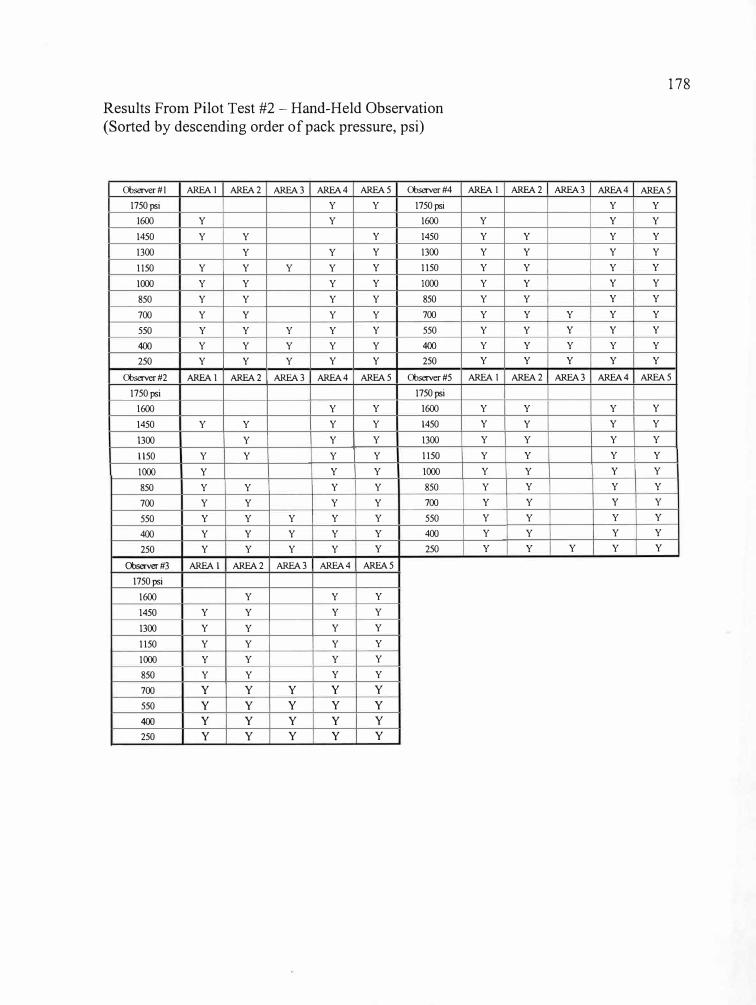
Results From Pilot Test #2 - Hand-Held Observation
(Sorted by descending order of pack pressure, psi)
Observer#! ARFAI ARFA2 ARFA3 ARFA4 ARFA5 Observer#4
1750 psi y y 1750 psi
1600 y y 1600
1450 y y y 1450
1300 y y y 1300
1150 y y y y y 1150
1000 y y y y 1000
850 y y y y 850
700 y y y y 700
550 y y y y y 550
400 y y y y y 400
250 y y y y y 250
Observer#2 ARFAl ARFA2 ARFA3 ARFA4 ARFA5 Observer#5
1750psi 1750psi
1600 y y 1600
1450 y y y y 1450
1300 y y y 1300
1150 y y y y 1150
1000 y y y 1000
850 y y y y 850
700 y y y y 700
550 y y y y y 550
400 y y y y y 400
250 y y y y y 250
Observer#) ARFAl ARFA2 ARFA3 ARFA4 ARFA5
1750psi
1600 y y y
1450 y y y y
1300 y y y y
1150 y y y y
1000 y y y y
850 y y y y
700 y y y y y
550 y y y y y
400 y y y y y
250 y y y y y
178
ARFAI ARFA2 ARFA3 ARFA4 ARFA5
y y
y y y
y y y y
y y y y
y y y y
y y y y
y y y y
y y y y y
y y y y y
y y y y y
y y y y y
ARFAI ARFA2 ARFA3 ARFA4 ARFA5
y y y y
y y y y
y y y y
y y y y
y y y y
y y y y
y y y y
y y y y
y y y y
y y y y y
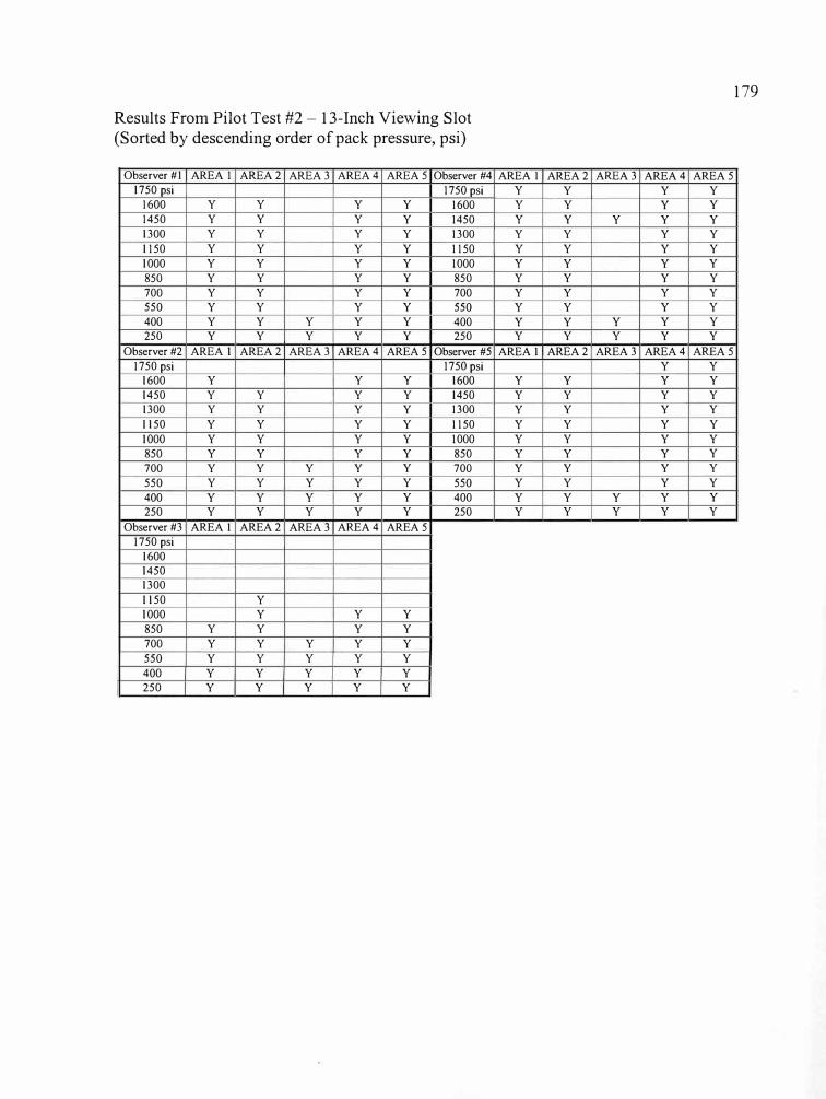
Results From Pilot Test #2 - 13-Inch Viewing Slot (Sorted by descending order of pack pressure, psi)
Observer #I AREA I AREA2 AREA3 AREA4 AREAS Observer #4
1750 psi 1750 psi
1600 y y y y 1600
1450 y y y y 1450
1300 y y y y 1300
1150 y y y y 1150
l000 y y y y l000
850 y y y y 850
700 y y y y 700
550 y y y y 550
400 y y y y y 400
250 y y y y y 250
Observer #2 AREAi AREA2 AREA3 AREA4 AREAS Observer #5
1750 psi 1750 psi
1600 y y y 1600
1450 y y y y 1450
1300 y y y y 1300
1150 y y y y 1150
l000 y y y y l000
850 y y y y 850
700 y y y y y 700
550 y y y y y 550
400 y y y y y 400
250 y y y y y 250
Observer #3 AREA I AREA2 AREA3 AREA4 AREAS
1750 psi
1600
1450
1300
1150 y
l000 y y y
850 y y y y
700 y y y y y
550 y y y y y
400 y y y y y
250 y y y y y
179
AREAi AREA2 AREA3 AREA4 AREAS
y y y y
y y y y
y y y y y
y y y y
y y y y
y y y y
y y y y
y y y y
y y y y
y y y y y
y y y y y
AREA I AREA2 AREA3 AREA4 AREAS
y y
y y y y
y y y y
y y y y
y y y y
y y y y
y y y y
y y y y
y y y y
y y y y y
y y y y y
I
I
I I
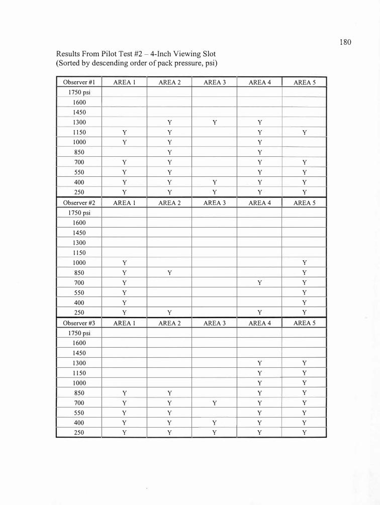
Results From Pilot Test #2 - 4-Inch Viewing Slot (Sorted by descending order of pack pressure, psi)
Observer #1 AREA 1 AREA2 AREA3
1750 psi
1600
1450
1300 y y
1150 y y
1000 y y
850 y
700 y y
550 y y
400 y y y
250 y y y
Observer #2 AREA 1 AREA2 AREA3
1750 psi
1600
1450
1300
1150
1000 y
850 y y
700 y
550 y
400 y
250 y y
Observer#3 AREA 1 AREA2 AREA3
1750 psi
1600
1450
1300
1150
1000
850 y y
700 y y y
550 y y
400 y y y
250 y y y
180
AREA4 AREAS
y
y y
y
y
y y
y y
y y
y y
AREA4 AREAS
y
y
y y
y
y
y y
AREA4 AREAS
y y
y y
y y
y y
y y
y y
y y
y y
I

BIBLIOGRAPHY
American Society for Testing and Materials (1996). Visual appraisal of colors and color differences of diffusely-illuminated opaque materials. Designation: D
1729-96.
Ari, G., Wilson, J., & Zou, Q. (1993). A systematic approach for solving an injection molding problem. Technical Papers, 39, 130-134.
Ashland Chemical (1997). Glossary. In GP Thermoplastic: Glossary [Online]. Available: http://www.ashchem.com/GP/trouble/61.html [1997, January 12].
AutoCad Release 12 for Windows Instant Reference (1993). (Chapter 1, p. 19). AutoDesk, Inc.
Beauregard, M., Greco, T., & Henricks, S. (1988). Inter company use of design of experiments to improve part quality. Technical Papers, 34, 1654-1656.
Bosch, J.A. (1992, November). The changing roles of coordinate measuring machines. Industrial Engineering, 24(11), 46.
Bozzelli, J., Furches, B., Bujanowski, R., & Little, J. (1992). Translating plastic variables to machine mold monitoring: how to track a perfect part. Technical Papers,�. 2198-2201.
Celstran® (1997, September 16). Sinks and voids. In Trouble Shooting Guide[Online]. Available: http://polymercomposites.com/tech/molding/3-10.htm [ 1997, January 12].
Chameleon CMM. (1996, September). Article 4. In Modern Machine Shop [Online] Vol. 69, n4 p164. Available: http://sbweb3.med.iacnet.com/infotrac/session/ 640/875/6610879 [1997, October 3].
Chang, M.C.O. (1994). On the study of surface defects in the injection molding of rubber-modified thermoplastics. Technical Papers, 360-367.
Chang, R.Y., & Tsaur, B. D. (1995, mid-August). Experimental and theoretical studies of shrinkage, warpage, and sink marks of crystalline polymer injection molded parts. Polymer Engineering and Science, .32(15), 1222 - 1230).
181
Chou, C. J., Hiltner, A., & Baer, E. (1985). The role of surface effects in the deformation of hard elastic polypropylene. Technical Papers, 31, 565-569.
Chudnovsky, A., & Moet, A. (1985). A theory for crack layer propagation in polymers. Technical Papers, .11, 586-587.
CNC CMM - CHNl000-1200 series (Manual No. 4467). (No Date). Tokyo, Japan: Mitutoyo Corporation.
Cobo-Lewis, A.B. (1997). What is stereopsis? In Alan B. Cobo-Lewis explains
stereopsis to you [Online]. Available: http://www.psy.miami.edu/Psychology/ Child/ACobo-Lewis/noframes/whatisstereo.html [1997, September 13].
Dassault Systemes 1996 Annual Report. (1997, May). Suresnes Cedex, France: Communication Division of Dassault Systemes.
Depth Perception. (1996, May). In Depth Perception [Online]. Available: http://psych.hanover.edu/ classes/hfnotes2/ sld02 l .html [ 1997, January 3].
Ezrin, M. (1997, April). Some effects of design in part failure. Plastics World, 55(4), 19.
Filbert, W. C., Roder, T. M., Plastics Department E.I. duPont deNemours & Company (Inc.). (1963). Improved surface of acetal moldings. Technical Papers, 2, Section IX, 1-6.
General Electric Plastics. (1991, March). Noryl® Resin. Design Guide. (pp. 28-31).
General Electric Plastics. (1994, March). Noryl® Resin. Injection Molding. (pp. 11-14).
General Electric Plastics. (1996, September). Cycoloy® Resin. Design Guide. (pp. 27-29).
Gill J. L. (1978). Design and analysis of experiments in the animal and medical sciences, (Vol. 2). Ames, IA: The Iowa State University Press.
Giragosian, S. E., Freygang, G. G., Rohm & Haas Co., Inc. (1960). Some causes and cures of splash defects in acrylic molding. Technical Papers, .Q, 44-1 - 44-3.
182
Griffing, J. S., & Whitaker, K. M. (1993). Investigation of material, process, and design effects on color and appearance of injection molded aircraft parts. Technical Papers, 3.2, 570-572.
Groleau, R. J. (1996, January). Injection molding hydraulics. RJG Seminars. Rochester Hills, MI: Vickers.
Hoshimiya, T., Endoh, H., & Hiwatashi, Y. (1996, May). Observation of surface Defects using photoacoustic microscope and quantitative evaluation of the defect depth. Japanese Journal of Applied Physics, .3..5_(5B), 2916-2920).
Jan, T. C., & O'Brien, K. T. (1992). Reducing surface defects in the injection molding of thermoplastics using a hybrid expert system. Technical Papers, 18., 2214-2217.
Johnson, R.M. (1996). Research on research. Chicago: Market Facts.
Jong, W.R., & Wang, K. K. (1990). Automatic interpretation of weld lines and air trays in injection molding by synthesizing deterministic and heuristic knowledge. Technical Papers, 36, 197-202.
Kendrick, J. J. (1994, Feb). Optical comparator outlook steady. Quality, 33(2), 54.
Lehar, S. (1998). Plato's Cave: The Vergence Representation [Online]. Available: http://ens-alumni.bu.edu/pub/slehar/webstuff/pcave/vergence.html [ 1998, July 23].
McGraw-Hill Encyclopedia of Science and Technology (8th ed.). (1997). (Vol. 9, p. 327). New York: McGraw-Hill.
Menq, C., & Chen, F. L. (1996, April). Curve and surface approximation from CMM measurement data. Computers & Industrial Engineering [Online], Vol.
30., n2 p211(15). Available: http://sbweb3.med.iacnet.com/infotrac/ session/640/875/6610879/5?xm_9 [1997, October 3].
Meredith, J. R. & Mantel, S. J., Jr. (1995). Project management (3rd ed.). New York: John Wiley & Sons, Inc.
Muccio, E. A. (1991). Plastic part design, technology, and quality. Plastic Part Technology, pp. 191-196.
Murray, J. (1993). Visual cues to depth perception. [Online]. Available: http://nswt.tuwien.ac.at: 8000/hci/deph _perception.html [ 1997, February 3].
183
Nakayama, K, Shinsuke, S. (1992, September 4). Experiencing and perceiving visiual surfaces. In Science [Online]. Available: http://sbweb3.med.iacnet.com/ infotrac/session/807/892/5743952/13?xm_5 [1997, September 16)
NASA. Surface Defect Analyzer (SURDA). In Technology Opportunity [Online]. Available: http:/ /technoogy.ksc.nasa.gov/WWW access/Opport/05 .htm [ 1997, September 1 O].
Probing for productivity (ref. CMM (UK) 5K 288 Part No. H/1000/4020). (1988). U.S.A.: Renishaw.
Product News. (1988, February). Laser gauge qualifies Class A surfaces. Plastics .wm:ld, (p. 92.)
Savantage. (1998). Savantage: Corporate Background. The Problem We Solve, [Online]. Available: http://www.savantage.com/ savantage/ corp info I .html [1998, July 30).
Software Quality Assurance (1998). Primacy of Defect Prevention [Online]. Available: http://www.cs.jmu.edu/users/foxcj/cs555/Unit10/SQA/tsld007.htm [1998, July 31).
StatSoft, Inc. (1996). STATISTICA for Windows [Computer program manual]. Tulsa, OK: StatSoft, Inc., 2300 East 14th Street, Tulsa, OK 74104,
Steel, R. G.D., & Torrie, J. H. (1980). Principles and procedures of statistics. (2nd
ed.) New York: McGraw-Hill.
Western Michigan University. (1996). What is the Human Subjects Institutional Review Board. Graduate Student Survival Kit. (p. 33).
Whelan, T. & Goff, J. (1996). The Dynisco injection molders handbook. (1st ed.).
Copyright Tony Whelan and John Goff.
Wortman, B. (1995). The Quality Engineering Primer. West Terre Haute, IN: The Quality Council of Indiana.
Zimmer, C. (1995, January). Wallpaper for the mind. 1994 - the Year in Science, 16(1), 80 .
184