Radiation hydrodynamics integrated in the code PLUTO

Astronomy & Astrophysics manuscript no. paper c© ESO 2013September 23, 2013

Radiation hydrodynamics integrated in the code PLUTOStefan M. Kolb1, Matthias Stute1, Wilhelm Kley1, and Andrea Mignone2

1 Institute for Astronomy and Astrophysics, Section Computational Physics, Eberhard Karls Universitat Tubingen, Auf derMorgenstelle 10, D-72076 Tubingen, Germanye-mail: [email protected], [email protected], [email protected]

2 Dipartimento di Fisica, Universita degli Studi di Torino, via Pietro Giuria 1, 10125 Torino, Italy

Received ; accepted 9. September 2013

ABSTRACT

Aims. The transport of energy through radiation is very important in many astrophysical phenomena. In dynamical problems the time-dependent equations of radiation hydrodynamics have to be solved. We present a newly developed radiation-hydrodynamics modulespecifically designed for the versatile MHD code PLUTO .Methods. The solver is based on the flux-limited diffusion approximation in the two-temperature approach. All equations are solvedin the co-moving frame in the frequency independent (grey) approximation. The hydrodynamics is solved by the different Godunovschemes implemented in PLUTO , and for the radiation transport we use a fully implicit scheme. The resulting system of linearequations is solved either using the successive over-relaxation (SOR) method (for testing purposes), or matrix solvers that are availablein the PETSc library. We state in detail the methodology and describe several test cases in order to verify the correctness of ourimplementation. The solver works in standard coordinate systems, such as Cartesian, cylindrical and spherical, and also for non-equidistant grids.Results. We have presented a new radiation-hydrodynamics solver coupled to the MHD-code PLUTO that is a modern, versatile andefficient new module for treating complex radiation hydrodynamical problems in astrophysics. As test cases, either purely radiativesituations, or full radiation-hydrodynamical setups (including radiative shocks and convection in accretion discs) have been studiedsuccessfully. The new module scales very well on parallel computers using MPI. For problems in star or planet formation, we haveadded the possibility of irradiation by a central source.

Key words. radiation transport – irradiation – hydrodynamics – accretion disc

1. Introduction

Radiative effects play a very important role in nearly all astro-physical fluid flows, ranging from planet and star formation tothe largest structures in the universe. Coupling the equations ofradiation transport to those of (magneto-)hydrodynamics (MHD)has been studied for decades, and comprehensive treatments canbe found for example in text books by Mihalas & Mihalas (1984)or Pomraning (1973). The numerical implementation of two-temperature radiation hydrodynamics (in the diffusion approx-imation) into multi-dimensional MHD/HD-codes has been donealready over twenty years ago in various implementations, forexample by Eggum et al. (1988), Kley (1989), in the ZEUS-code(Stone et al. 1992), and later by Turner & Stone (2001).

In order to study, for example, the dynamics and character-istics of stellar atmospheres together with convection, more ac-curate solvers for the radiation transport based on the method ofshort characteristics have been developed, see Davis et al. (2012)and Freytag et al. (2012) for the present status. This can thenbe coupled to the hydrodynamics using the Variable EddingtonTensor method (Jiang et al. 2012). Another approach is the M1closure model where the radiative moment equations are closedat a higher level (Gonzalez et al. 2007; Aubert & Teyssier 2008).Despite this progress it is still useful and desirable to have amethod at hand which solves the interaction of matter and radi-ation primarily within the bulk part of the matter which may beoptically thick. In such type of applications, the method of flux-limited diffusion (FLD, see Levermore & Pomraning (1981))

has its clear merits and is still implemented into existing MHD-codes, for example in NIRVANA (Kley et al. 2009) to study theplanet formation process, in RAMSES (Commercon et al. 2011)for protostellar collapse simulations, and in combination with amulti-frequency irradiation tool into PLUTO (Kuiper et al. 2010)for massive star formation.

Since the 3D-MHD code PLUTO (Mignone et al. 2007) isbecoming increasingly popular within the computational as-trophysics community, we added a publicly available radia-tion module, which is based on the two-temperature FLD-approximation, as described by Commercon et al. (2011).PLUTO solves the equations of hydrodynamics and magnetohy-drodynamics including the non-ideal effects of viscosity, ther-mal conduction and resistivity by means of shock-capturingGodunov-type methods. Several Riemann solvers, several timestepping methods and interpolation schemes can be chosen.Additionally, we added a ray-tracing routine that allows for ad-ditional irradiation by a point source in the center. Treating theirradiation in a ray-tracing approach, guarantees the long-rangecharacter of the radiation better than FLD (Kuiper et al. 2012;Kuiper & Klessen 2013).

The paper is organized as follows. In section 2.1, we brieflyintroduce the equations of hydrodynamics including radiationtransport. Additionally we describe the general idea behind theflux limited diffusion approximation. In section 3, we presentthe discretization of the equations and the solver of the result-ing matrix equation, and present our numerical implementationof irradiation. In section 4, we present six different test cases

1

arX

iv:1

309.

5231

v1 [

astr

o-ph

.EP]

20

Sep

2013

Stefan M. Kolb et al.: Radiation hydrodynamics integrated in the code PLUTO

to show the correctness of the implemented equations: four testcases with an analytical solution (section 4.1 to 4.4) and twoothers in which our results are compared with those from othercodes (section 4.5 and 4.6). We end with a summary and conclu-sions.

2. Radiation hydrodynamics

2.1. The equations

Even though the PLUTO-environment includes the full MHD-equations and non-ideal effects such as viscosity, we restrictourselves here to the Euler equations of ideal hydrodynamics.Radiation effects are included in the two-temperature approxi-mation, which implies an additional equation for the radiationenergy. In order to follow the transport of radiation, we applythe flux-limited diffusion approximation and treat the exchangeof energy and momentum between the gas and the radiation fieldwith additional terms in the gas momentum and energy equa-tions. The system of equations then read:

∂

∂tρ + ∇ · (ρv) = 0 (1)

∂

∂tρv + ∇ · (ρv ⊗ v) + ∇p = +ρ(aext + arad) (2)

∂

∂te + ∇ ·

[(e + p) v

]= +ρv · (aext + arad) (3)

− κPρc(aRT 4 − E)∂

∂tE + ∇ · F = κPρc

(aRT 4 − E

)(4)

The first three equations (1-3) describe the evolution of the gasmotion, where ρ is the gas density, p the thermal pressure, v thevelocity, e = ρ ε + 1/2 ρ v2 the total energy density (i.e., the sumof internal and kinetic) of the gas without radiation, and aext anacceleration caused by external forces (e.g. gravity), not inducedby the radiation field (see below). This system of equations isclosed by the ideal gas relation

p = (γ − 1) ρ ε = ρkB TµmH

, (5)

where γ is the ratio of specific heats, T the gas temperature, kBthe Boltzmann constant, µ the mean molecular weight, and mHthe mass of hydrogen. The specific internal energy can be writtenas ε = cV T , with the specific heat capacity given by

cV =kB

(γ − 1)µmH. (6)

Here, we assume constant γ and µ, which also implies a constantcV.

The evolution of the radiation energy density E is given byeq. (4), where F denotes the radiative flux, κP the Planck meanopacity, c the speed of light and aR the radiation constant. Thefluid is influenced by the radiation in two different ways. First,the radiation may be absorbed or emitted by the fluid leading tovariation of its energy density. This variation is given by the ex-pression κPρc

(aRT 4 − E

), see right hand side of equation (3) and

(4). The second effect is that of radiation pressure. We includethis term as an additional acceleration to the momentum equa-tion, arad = κR

c F. The present implementation does not include

the advective transport terms for the radiation energy and radia-tive pressure work in eqs. (3) and (4). For the relatively low tem-perature protoplanetary disk application that we consider herethese terms are of minor importance. If required, these terms canbe treated in our implementation straightforwardly within PLUTOby adding additional source terms.

2.2. The flux-limited diffusion approximation

The system of equations shown cannot be solved without furtherassumptions for the radiative flux F. Here we use the flux limiteddiffusion approximation (FLD) where the radiation flux is givenby a diffusion approximation

F = −λcκR ρ∇E , (7)

with the Rosseland mean opacity κR. The flux-limiter λ describesapproximately the transition from very optically thick regionswith λ = 1/3 to optically thin regimes, where F → −cE ∇E

|∇E| .This leads to the formal definition of the flux-limiter which is afunction of the dimensionless quantity

R =|∇E|κRρE

, (8)

with the following behaviour:

λ(R) =

13 , R→ 01R , R→ ∞

(9)

Physically sensible flux-limiters thus have to fulfil the equation(9) in the given limits and describe the behaviour between thelimits approximately. We have implemented three different flux-limiters:

λ(R) =1R

(coth R −

1R

)(10)

λ(R) =

23+√

9+12R20 ≤ R ≤ 3

21

1+R+√

1+2R32 < R ≤ ∞

(11)

λ(R) =

23+√

9+10R20 ≤ R ≤ 2

1010R+9+

√180R+81

2 < R ≤ ∞(12)

from Levermore & Pomraning (1981), Minerbo (1978), andKley (1989), respectively. A comparison of them is presentedin Kley (1989).

In general it is necessary to solve the equations for each fre-quency which appears in the physical problem. However, herewe use the grey approximation in which all radiative quantitiesincluding the opacities are integrated over all frequencies. In ourtreatment scattering is not accounted for directly, but it is in-cluded in the effective isotropic absorption and emission coeffi-cients.

3. Solving the radiation part

3.1. Reformulation of the equations

Instead of solving system of equations (1-4) directly as a whole,the problem is split into two steps. In the first step, PLUTO isused to solve the equations of fluid dynamics with the additionalforce caused by the radiation. This corresponds to the equations(1) to (3) with the additional acceleration, arad, but without theinteraction term between the matter and radiation (last term in

2


eq. 3). By using PLUTO for solving the non-radiative part of theequations, we are not limited to the Euler equations, but are ableto use the full capabilities of PLUTO for solving the equations ofhydrodynamics or magnetohydrodynamics, including the effectsof viscosity and magnetic resistivity.

In a second, additional step we solve the radiation energyequation (4) and for the corresponding heating-cooling term inthe internal energy of the fluid:

∂

∂tE − ∇ ·

(cλκRρ∇E

)= κPρc

(aRT 4 − E

)∂

∂tρε = −κPρc

(aRT 4 − E

) (13)

In order to obtain the radiation energy density, we solvethe system of coupled equations (13). Within one time stepPLUTO advances the hydrodynamical quantities, i.e. the densityρ, the velocity v and a temporary pressure p from time tn to thetime tn+1, where the time step, ∆t = tn+1 − tn, is determinedby PLUTO using the CFL conditions, presently without includ-ing the radiation pressure. These depend on the used time step-ping method in PLUTO , for more information see Mignone et al.(2007) and the userguide of PLUTO .

The physical process of radiation transport takes place ontime scales much shorter than the one in hydrodynamics. In or-der to use the same time step for hydrodynamics and the radi-ation transport, we apply an implicit scheme to handle the ra-diation diffusion and the coupling between matter and radiationdescribed by equation (13). Because of the coupling of the equa-tions, the method will update T and E simultaneously, whichleads formally to a nonlinear set of coupled equations. As out-lined below, the system is solved for the radiation energy densityE. From the new values for E, we compute the new fluid temper-ature (see eq. 17 below) and update the fluid pressure by usingthe ideal gas relation from equation (5). This is then used withinPLUTO to calculate a new total gas energy e.

3.2. Discretization

In order to discretize the equations (13), we apply a finite vol-ume method. For that purpose we integrate over the volume ofa grid cell and transform the divergence into a surface integral.Furthermore, we replace the gradient of E by finite differences,and apply an implicit scheme. The discretization scheme hasbeen implemented in 3D for Cartesian, cylindrical and spheri-cal polar coordinates including all the necessary geometry termsfor the divergence and gradient. Since the density has been up-dated already in the hydrodynamical part of the solver, we canreplace ∂ρε

∂t with ρ cV∂T∂t , which is valid for a constant heat ca-

pacity. Then the resulting discretized equations for the radiativepart can be written as

En+1i, j,k − En

i, j,k

∆t

= Grx1Kn

i+ 12 , j,k

En+1i+1, j,k − En+1

i, j,k

∆x1i+ 12

−Glx1Kn

i− 12 , j,k

En+1i, j,k − En+1

i−1, j,k

∆x1i− 12

+ Grx2Kn

i, j+ 12 ,k

En+1i, j+1,k − En+1

i, j,k

∆x2 j+ 12

−Glx2Kn

i, j− 12 ,k

En+1i, j,k − En+1

i, j−1,k

∆x2 j− 12

+ Grx3Kn

i, j,k+ 12

En+1i, j,k+1 − En+1

i, j,k

∆x3k+ 12

−Glx3Kn

i, j,k− 12

En+1i, j,k − En+1

i, j,k−1

∆x3k− 12

+ κnPi, j,k ρ

ni, j,kc

(aR(T n+1

i, j,k )4 − En+1i, j,k

), (14)

and for the thermal energy (or temperature, respectively)

T n+1i, j,k − T n

i, j,k

∆t= −

κPni, j,k c

cV

(aR

(T n+1

i, j,k

)4− En+1

i, j,k

). (15)

Here, the superscript n refers to the values of all variablesafter the most recent update from the hydrodynamical step. Inorder to simplify the notation for the separate radiation module,we assume the update takes place from time n to n + 1. The sub-scripts i, j, k refer to the 3 spatial directions of the computationalgrid, where all variables are located at the cell centers. Half-integer indices refer to cell interfaces. The physical sizes (properlength) of each cell in the 3 spatial directions m (m = 1, 2, 3) aregiven by ∆xm, where we additionally allow for non-equidistantgrids. The effective radiative diffusion coefficient (defined at cellcenters) is given by

Kni, j,k =

cλ(Ri, j,k)κR

ni, j,k ρ

ni, j,k

,

where Ri, j,k is calculated from eq. (8) by central differencing.Values at cell interfaces are obtained by linear interpolation. Thefactors Gl,r

xm are geometrical terms defined, respectively, as theleft and right surface areas divided by the cell volume in thedirection given by m = 1, 2, 3. In the recent work by Bitsch et al.(2013b) the difference equations have been written out in moredetail for Cartesian, equidistant grids. The required opacities areevaluated using the values of ρ and T after the hydrodynamicalupdate at time tn.

As mentioned before, equations (13) constitute a set of cou-pled nonlinear equations. The non-linear term (T n+1

i, j,k )4 that ap-pears in equation (15) is linearised using the method outlined inCommercon et al. (2011)

(T n+1i, j,k )4 = (T n

i, j,k)4

1 +T n+1

i, j,k − T ni, j,k

T ni, j,k

4

≈ 4(T ni, j,k)3T n+1

i, j,k−3(T ni, j,k)4 .

(16)Using this approximation, we obtain an equation for computingthe new temperature in terms of the new radiation energy density,En+1

i, j,k , and the old temperatures, T ni, j,k

T n+1i, j,k =

κPni, j,kc

(3aR(T n

i, j,k)4 + En+1i, j,k

)∆t + cVT n

i, j,k

cV + 4κPni, j,kcaR(T n

i, j,k)3∆t. (17)

The expression can be substituted into eq. (14) to obtain a lin-ear system of equations for the new radiation energies En+1

i, j,k , thatcan be solved using standard matrix solvers, see section 3.4. Thenew temperature can then be calculated from eq. (17). We im-plemented several boundary conditions for the radiation energydensity including periodic, symmetric and fixed value.

3.3. Irradiation

In order to couple possible irradiation to the radiation transportequations, a new source term, S , has to be added to the righthand side of the thermal energy equation in system (13)

∂ρε

∂t= −κPρc(aRT 4 − E) + S . (18)

This results in an additional term, S i, j,k/(ρi, j,kcV), in Eq. 15, cor-respondingly in equation (17), and in a modification of the righthand side of the resulting matrix equation for En+1

i, j,k .

3


For the present implementation, we assume that the irradiat-ing source is located at the centre of a spherical coordinate sys-tem. Therefore it is straightforward to compute the optical depthτi, j,k even for simulations using parallel computers. Assumingthat a ray of light travels along the radial direction from the ori-gin to the grid cell i, j, k under consideration, the optical depthfrom the inner radius r0 to the ith grid cell with radius ri can besimply expressed as the integral along the radial coordinate,

τi, j,k =

∫ ri

r0

κ?ρ(r) dr ≈i∑

n=0

κ?n, j,k ρn, j,k∆rn (19)

where ∆rn is the radial length of the nth grid cell, and κ? theopacity used for irradiation. For the sake of readability, we writeτi instead of τi, j,k in the following. We use κ? = κP in the test casewith irradiation presented in section 4.3. Additionally κ? can bedefined by the user as well as the other opacities. Re-emission ofthe photons which were absorbed in the cell volume is handledin our treatment by the heating-cooling term see equation (13).

The luminosity of the source is given by

L? = 4πR2?σT 4

? , (20)

where σ denotes the Stefan-Boltzmann constant, T? is the tem-perature of the star and R? its radius. In order to compute theamount of irradiated energy which is absorbed by a specific gridcell we have to know the surface area A of a grid cell orientedperpendicular to the radiation from the star and the flux f at theradius r. This surface area A is given by the expression

Ai, j,k =

θ j+1∫θ j

φk+1∫φk

dA = r2i (φk+1 − φk)(cos θ j − cos θ j+1) , (21)

where θ is the azimuthal and φ the polar angle in the sphericalcoordinate system. Without absorption the flux f is given by theexpression

f =L?

4πr2 = σT 4?

(R?

r

)2

. (22)

The amount of energy per time which arrives at the surface ofthe grid cell (i, j, k) is

Hi, j,k = Ai, j,k f = (φk+1 − φk)(cos θ j − cos θ j+1)σT 4?R2

? , (23)

again without absorption. If the irradiated energy is partlyabsorbed, the remaining amount of energy per time is thenHi, j,ke−τi, j,k . Using these results, we can compute the energy den-sity per time, S , which is absorbed by one grid cell (i, j, k)

S i, j,k =Hi, j,ke−τi − Hi, j,ke−τi+1

Vi, j,k=

Hi, j,k (e−τi − e−τi+1 )Vi, j,k

=3σT 4

?R2? (e−τi − e−τi+1 )

(r3i+1 − r3

i ), (24)

with the volume of a grid cell

Vi, j,k =

ri+1∫ri

θ j+1∫θ j

φk+1∫φk

r2sinθ dr dθ dφ

=13

(r3i+1 − r3

i )(cos θ j − cos θ j+1)(φk+1 − φk) . (25)

The absorbed energy density per time, S i, j,k, is computed foreach grid cell before solving the matrix equation. A similar treat-ment of irradiation has been described recently by Bitsch et al.(2013b), for a multi-frequency implementation see Kuiper et al.(2010).

3.4. The matrix solver

We implemented two different solvers for the matrix equa-tion. The first one uses the method of successive over-relaxation (SOR), and as a faster and more flexible solverwe use the PETSc1 library. From the PETSc library we usethe Krylov subspace iterative method and a preconditioner tosolve the matrix equation. For all test cases described we usedgmres (Generalized Minimal Residual) as iterative methode andbjacobi (Block Jacobi) as preconditioner. Beside others the con-vergence of the SOR algorithm and the PETSc library can beestimated using the following criteria∥∥∥r(k)

∥∥∥ < max(εr · ‖b‖ , εa) (26)

where b is the right hand side of the matrix equation Ax = b,r(k) = b − Ax(k) is the residual vector for the k-th iteration ofthe solver and x is the solution vector (here the radiation energydensity). As norm we used here the L2 norm. The quantities εrand εa are the relative and absolute tolerance, respectively, andare problem dependent, with a common value of 10−50 for εa. Forthe test cases in section 4 we use relative tolerances εr between10−5 and 10−8. The criterion (26) is the default one used by thePETSc library. For more information about the convergence testin PETSc the reader should refer to section 4.3.2. of Balay et al.(2012). The solver performance in a parallel environment is de-scribed in section 4.6.4.

4. Test cases

In order to verify the implemented method, we simulated severaltest problems and compared the results with either correspond-ing analytical solutions or calculations done with different nu-merical codes. Most of the tests correspond to one-dimensionalproblems. In order to model those, we have used quasi one-dimensional domains, with a very long cuboid that has the heighth, width w and a length l. The length l is much larger than thewidth or height, and for simplicity we use w = h. We performedsome of the tests in all three implemented coordinate systems(Cartesian, cylindrical and spherical) and in three different align-ments of the cuboid along each coordinate direction. This is doneto check whether the geometry factors are correct. In the case ofa non-Cartesian coordinate system we placed the cuboid at largedistances r from the origin such that the domain approximatelydescribes a Cartesian setup.

We use for all test cases the solver based on the PETSclibrary with the default iterative solver gmres and the pre-conditioner bjacobi.

4.1. Linear diffusion test

The following test is adapted from Commercon et al. (2011). Theinitial profile of the radiation energy density is set to a delta func-tion which is then evolved in time and compared to the analyti-cal one dimensional solution. We perform this test in all imple-mented coordinate systems (Cartesian, cylindrical and sphericalcoordinates) as described above, which results in nine differentsimulations. The used domain is quasi one-dimensional and theequations of hydrodynamics are not solved in this test. Only theradiation diffusion equation

∂

∂tE = ∇ ·

(cλκRρ∇E

)(27)

1 For more information visit the website http://www.mcs.anl.gov/petsc or have a look at Balay et al. (2012).

4

http://www.mcs.anl.gov/petsc

http://www.mcs.anl.gov/petsc


−1.5 −1.0 −0.5 0.0 0.5 1.0 1.5x [cm]

100

101

102

103

104

105

106E

[erg

cm3]

10−4

10−3

10−2

∣ ∣ ∣En−Ea

Ea

∣ ∣ ∣Fig. 1. Linear diffusion test at the time t = 4.2 · 10−12 s. Thesimulated (read dots) and the analytical (black line) solution isplotted. We also plot the solution with the absolute value of therelative error (blue dashed line) which belongs to the axis on theright.

0.0 0.5 1.0 1.5 2.0 2.5 3.0 3.5 4.0 4.5t [s] ×10−12

100

101

102

103

104

105

106

E[er

gcm

3]

10−9

10−8

10−7

10−6

10−5

10−4

10−3

10−2

10−1

100

101

∣ ∣ ∣En−Ea

Ea

∣ ∣ ∣

Fig. 2. Time evolution for the linear diffusion test from timet = 0 s to 4.2 · 10−12 s at three different positions at x = 0 cm(black lines), at x = 0.5 cm (blue lines) and at x = 1.0 cm (redlines). The dotted lines for each position belong to the simulatedsolution, the solid lines to the analytical solution and the dashedlines show the relative error which belong to the axis on the right.

is solved which we obtain from equations (13) by setting κP = 0.An analytical solution to equation (27) can be calculated in theone dimensional case with a constant flux-limiter λ = 1

3 and aconstant product of the Rosseland opacity and density, here weset κRρ = 1 cm−1. The equation to solve is then given by

∂

∂tE(x, t) =

c3∂2

∂x2 E(x, t) (28)

with solution

E(x, t) =E0√43 cπt

e−3x24ct , (29)

where E0 is the integral over the initial profile of the energy den-sity, E(x, t = 0). Note that in the quasi one-dimensional case(using a stretched 3D domain) E0 has the units erg cm−2.

4.1.1. Setup

The domain is a cuboid with a length of 4 cm and a width andheight of 0.04 cm. We used here 301 × 3 × 3 grid cells. Theinitial profile of the radiation energy density in the quasi one-dimensional case is set by

Ei =

1 ergcm3 , i = 1, 2, . . . ,N with i , N

2

E0∆x , i = N

2

(30)

where ∆x is the length of a grid cell. For numerical reasons,we have set Ei for i , N

2 to the value 1 erg cm−3 instead of0 erg cm−3. This choice is not problematic, since E0/∆x 1 erg cm−3 for our chosen value of E0 = 105 erg cm−2. The ini-tial values for pressure and density are p = 1 g cm−1 s−2 andρ = 1 g cm−3. Furthermore we use κR = 1 cm2 g−1 for theRosseland opacity. All boundary conditions are set to periodicexcept for the boundary conditions at the beginning and end ofthe quasi one-dimensional domain, which are set to outflow. Forthe matrix solver we used a relative tolerance of εr = 10−8.The simulation starts at t = 0 s with an constant time step of∆t = 1 · 10−14 s and stops at t = 4.2 · 10−12 s.

4.1.2. Results

The numerical solution En and the analytical solution Ea fromequation (29) are plotted in the figures 1 and 2 together withthe absolute value of the relative error. In figure 1 the radia-tion energy density is plotted against the position at the timet = 4.2 · 10−12 s. The relative error in the relevant range from−1 cm to 1 cm is always below one percent. In figure 2 the timeevolution from t = 0 s to 4.2 · 10−12 s is shown for the positionsx = 0, 0.5, 1.0 cm coded in the colors black, blue and red, re-spectively. The results shown in this figure depend strongly onthe position. For the position x = 0 cm the error is, for all timeslater than t = 4 · 10−13 s, below one percent and decreases withtime. For the other positions, the behaviour is different. The rela-tive error rises and after a while it decreases. This behaviour canbe explained by looking at figure 1. The error is higher at the dif-fusion front. This region moves with time and causes the effectfor the other positions. The test shows that the time evolutionof the radiation energy density is reproduced correctly. As de-scribed, this test was performed in different coordinate systemsand orientations, with the same results.

4.2. Coupling test

The purpose of this test from Turner & Stone (2001) is to checkthe coupling between radiation and the fluid. For this purposewe simulate a stationary fluid which is initially out of thermalequilibrium. In this simulation the radiation energy density isthe dominant energy which is constant over the whole simula-tion. The system of equations (13) decouples in this case and, inaddition, it is not necessary to solve the matrix equation for E.By setting σP = κPρ and T =

pρµmHkB

from eq. (5) with the as-sumption that σP and ρ are constant, we can rewrite the thermal

5


10−19 10−17 10−15 10−13 10−11 10−9 10−7 10−5

t [s]

101

102

103

104

105

106

107

108

109

1010

1011

e[er

gcm

3]

Fig. 3. Coupling test from t = 10−20 s to t = 10−4 s with three dif-ferent initial gas energy densities. The reference solution (blacklines) and the simulated results for the initial energy densitye0 = 1010 erg cm−3 (red dots), e0 = 106 erg cm−3 (blue dots) ande0 = 102 erg cm−3 (green dots) are plotted.

energy equation of the system (13) as

dedt

= cσPE︸︷︷︸C1

− cσPaR

(γ − 1ρ

µmH

kB

)4

︸︷︷︸C2

e4 . (31)

With the used approximations, the coefficients C1 and C2 areconstant. The solution to Eq. (31) can be calculated analyticallyin terms of an algebraic equation which would have to be solvediteratively. Hence, we integrate Eq. (31) numerically using aRunge Kutta solver of 4-th order scheme with adaptive step size.In the following we refer to this solution as the reference solu-tion.

Information on the expected behaviour of the solution can beobtained directly from the differential equation. It is clear that inthe final equilibrium state (with de

dt = 0) the gas temperature has

to be equal to the radiation temperature T = 4√

EaR

, thus the finalgas energy density will be

efinal =

(C1

C2

) 14

. (32)

If the initial gas energy density e0 is much lower than efinal, wecan neglect the second term in eq. (31) at the beginning, thuse(t) = C1 t + e0. The corresponding coupling time can be esti-mated to

τ =efinal − e0

C1. (33)

On the other hand, if e0 efinal, we can neglect the first term ineq. (31) and derive

e(t) ∝ (C2 t)−13 and τ =

1e3

final C2. (34)

10−7 10−6 10−5 10−4 10−3 10−2 10−1 100 101 102 103

t [s]

101

102

103

104

105

106

107

108

e[er

gcm

3]

Fig. 4. Coupling test with enabled irradiation from t = 10−7 s tot = 103 s at three different distances d from the inner boundaryof the domain. The reference solution (black lines) and the sim-ulated results for the energy density e = 102 erg cm−3 are plottedat distance d = 0 cm (red dots), d = 3 · 104 cm (blue dots) andd = 3 · 105 cm (green dots).

4.2.1. Setup

The computational domain is identical to that of the linear diffu-sion test in section 4.1. For the grid we use a resolution of 25×3×3 grid cells. As before we do not solve the equations of hydrody-namics and the boundary conditions are quite simple. All bound-aries are set to periodic boundary conditions. The constants weused are set to: radiation energy density E = 1012 erg cm−3, den-sity ρ = 10−7 g cm−3, opacity σP = 4 · 10−8 cm−1, mean molec-ular weight µ = 0.6 and the ratio of specific heats γ = 5/3.The simulations starts at t = 0 s with an initial time step of∆t = 10−20 s and evolves until t = 10−4 s. After each step thetime step is increased by 1% in order to speed-up the compu-tation. The simulation is done with three different initial gasenergy densities, e0 = 1010 erg cm−3, e0 = 106 erg cm−3 ande0 = 102 erg cm−3.

4.2.2. Results

Figure 3 shows the numerical gas energy density and the refer-ence solution plotted against time for the three different initialvalues of e. The agreement of both results is excellent for allinitial values. From the figure we see that in the limit of smalland large initial e0, we find exactly the behaviour as predictedby the estimates for eq. (31). The analytic estimates for the cou-pling time τ from equation (33) agrees very well with our results.The estimate for e0 = 102 erg cm−3 is τ = 5.88 · 10−8 s and fore0 = 106 erg cm−3 we calculated τ = 5.78 ·10−8 s. In the case thatefinal < e0 the estimate in eq. (34) is approximate τ = 5.88·10−8 s.We have to mention here that this test verifies primarily the cor-rectness of equation (17). As in the linear diffusion test, this testwas performed in three different coordinate systems in differentorientations, with the same results.

6


0 50000 100000 150000 200000 250000 300000d [cm] +9×108

102

103

104

105

106

107

e[er

gcm

3]

Fig. 5. Radial dependency of the gas energy density for the cou-pling test with enabled irradiation. The gas energy density isplotted at different times, t = 1.12 · 10−4 s (red dots), t =1.62 · 10−2 s (blue dots), t = 1.43 s (green dots), t = 1.72 · 101 s(yellow dots) and t = 9.18 ·102 s (magenta dots). The dots repre-sent the numerical solution and the solid black lines the referencesolution. The position d is again measured relative to the innerboundary of the quasi one-dimensional domain.

4.3. Coupling test with irradiation

This test is in its basic setup the same as that from section 4.2,but with irradiation enabled, i.e. equation (18) is solved insteadof the second equation in (13). As described in section 3.3, irra-diation is limited to spherical coordinates, which we use for thistest. With the same assumptions as in section 4.2 , i.e., that σPand ρ are constant and with the definitions for σP, e, p as well asfor T , it is possible to rewrite S from equation (24) to

S (r) =3σT 4

?R2?e−σP(r−r0)

(1 − e−σP∆r

)(r + ∆r)3 − r3

, (35)

and obtain for equation (18)

dedt

= S (r) + cσPE︸︷︷︸C1(r)

− cσPaR

(γ − 1ρ

µmH

kB

)4

︸︷︷︸C2

e4 . (36)

The reference solution is computed in the same way as before al-though it now depends on the distance r from the star. The quasione-dimensional domain starts at r = 9000 · 105 cm and ends atr = 9003 · 105 cm and we use 300 × 3 × 3 grid cells. The do-main size in θ and φ direction was chosen in a way such that thegrid cells are nearly quadratic. For the simulation we use a con-stant radiation energy density of E = 10−2 erg cm−3, a density ofρ = 10−5 g cm−3 , a Rosseland opacity of κR = 10 cm2 g−1 and aPlanck opacity of κP = κR which corresponds toσP = 10−4 cm−1.The opacity for the irradiation κ? is set to κP. For the star,the temperature was set to T? = 6000 K and the radius toR? = 8.1 · 108 cm. Additionally we make the assumption thatthere is no absorption in the region between the surface of thestar and the inner boundary of the computation domain. Figure4 shows the gas energy density plotted against time with an ini-tial gas energy of e = 102 erg cm−3 at three different positionsd = 0 cm, d = 3 · 104 cm and d = 3 · 105 cm where d is mea-sured relative to the inner boundary of the quasi one-dimensional

0.5 1.0 1.5 2.0 2.5 3.0 3.5τeff

0.02

0.04

0.06

0.08

0.10

0.12

0.14

E[er

gcm

3]

10−6

10−5

10−4

10−3

10−2

∣ ∣ ∣En−Ea

Ea

∣ ∣ ∣

Fig. 6. Comparison between the numerical (red dots) and theanalytical (black line) solution of the steady state test aftert = 1200 s. In addition the absolute value of the relative error(blue dashed line) is plotted related to the axis on the right side.Note this axis is logarithmic.

domain. In figure 5 the radial dependency of the gas energy den-sity is plotted for the same simulation at five different times. Asexpected, the results show that the gas energy density at a timelater than t = 102 s becomes constant and depends on the dis-tance from the star. The simulated and reference solution show aexcellent agreement.

4.4. A steady state test

The original version of this test was published in Flaig (2011).We consider a one-dimensional stationary setup with a givendensity stratification. In the steady state, the time derivatives inthe equations (13) vanish and the system is reduced to the fol-lowing equation for the radiation energy density

0 = ∇ ·

(cλκRρ∇E

). (37)

A further reduction is obtained when we rewrite this equationin one dimension along the z-axis in Cartesian coordinates. Theequation is then much simpler and can be written as

ddz

(cλκRρ

ddz

E)

= 0 . (38)

In general the expression cλκRρ

is not known analytically for re-alistic opacities. In order to circumvent this problem, we definethe effective optical depth τeff =

∫dτeff =

∫ za

zbκeffρ dz where

za and zb are the lower and upper boundaries of the quasi one-dimensional domain, respectively, and κeff is the effective opacitygiven by κeff = 1

3κRλ

. By using dτeff = κeffρ dz, equation (38) canbe rewritten as:

ddz

ddτeff

E = 0 . (39)

The solution of this equation is then given by

E = (E(τeff = 1) − E(τeff = 0)) τeff + E(τeff = 0) (40)

where E(τeff = 0) and E(τeff = 1) are the radiation energy den-sity at the position where the effective optical depth has the val-ues zero or one, respectively. Thus, in the static case the radiation

7


energy has a linear dependence on the optical depth τeff for allopacity laws.

4.4.1. Initial setup

The domain was chosen to have an arbitrary length of 300 cmand a width and height of 3 cm and 300 × 3 × 3 grid cells wereused. This test is performed without solving the hydrodynami-cal equations, instead we solved equations (13) for a fixed den-sity and opacity law, and evolved the solution, until a stationarystate has been reached. For the radiation boundary conditions,we used boundary conditions with fixed values of E at the lowerand upper boundary of the domain. At the lower boundary wehave chosen E = aRT 4 with a temperature of T = 2000 K.

Because the stratification is optically thin at the upper bound-ary we want to allow the radiation to escape freely from the do-main. For this reason we simply set the temperature to a verysmall value at the upper boundary, here T = 10 K.

All other boundary conditions have been set to periodic. Thedensity stratification is given by

ρ(z) = ρ0e12

(z−za

0.46·(zb−za)

)2

. (41)

The initial temperature profile can be chosen randomly in prin-ciple, but in order to speed up the computation we used a lineartemperature profile starting at za with T = 2000 K and endingat zb with T = 10 K. From this temperature profile we assignedpressure values using equation (5). The radiation energy den-sity E inside the domain is also set using the gas temperatureprofile and E = aRT 4. The ratio of specific heats and the meanmolecular weight are set to γ = 1.43 and µ = 0.6, respectively.As flux-limiter we have chosen equation (11), for the Rosselandmean opacity κR we use data from Lin & Papaloizou (1985), andthe Planck mean opacity is set to κP = κR. The initial time stepis ∆t = 0.3 s and it is increased slightly with time in order tospeed-up the computation and to keep the number of iterationsdone by the matrix solver nearly constant. This simulation waspreformed with a relative tolerance of εr = 10−6 for the matrixsolver.

4.4.2. Results

A steady state is reached approximately after t = 1200 s. In fig-ure 6, we plot the radiation energy density against the effectiveoptical depth τeff from our numerical solution (red dots) togetherwith the analytical solution from equation (40). The parametersE(τeff = 1) − E(τeff = 0) and E(τeff = 0) have been obtainedby fitting equation (40) to the numerical solution. We have tonote here that E(τeff = 0) is determined by interpolation betweenghost cells and active cells near the upper boundary zb. Hence,the radiation temperature in the active region can be much largerthan 10 K, a value was specifically chosen to be very small. Wealso plot the absolute value of the relative error |(En − Ea)/Ea|.The results from the simulation agree very well with the analyti-cal prediction. As we can see from figure 6, the largest deviationfrom the analytical solution is at small values of τeff with an rel-ative error around one percent. As the linear diffusion and thecoupling test, this test was performed in all three coordinate sys-tems and in different orientations, with the same results.

4.5. Radiation shock

In this section we extend the previous tests and solve nowthe full equations of hydrodynamics and radiation trans-

2.0 2.5 3.0 3.5 4.0 4.5 5.0s [cm] ×1010

0

200

400

600

800

1000

1200

T[K

]

(a) Subcritical shock

1 2 3 4 5 6 7s [cm] ×1010

0

1000

2000

3000

4000

5000

6000

7000

T[K

]

(b) Supercritical shock

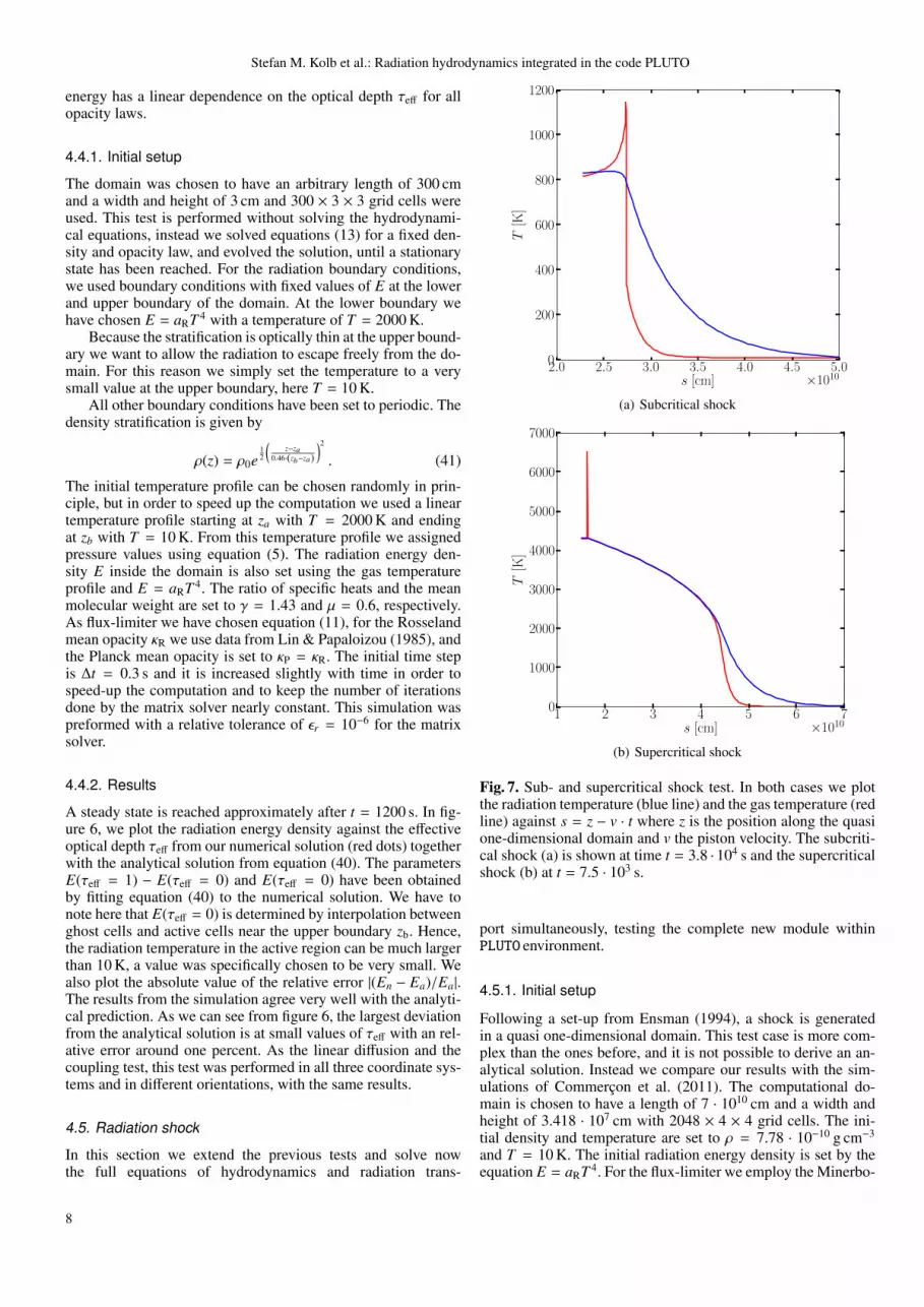
Fig. 7. Sub- and supercritical shock test. In both cases we plotthe radiation temperature (blue line) and the gas temperature (redline) against s = z − v · t where z is the position along the quasione-dimensional domain and v the piston velocity. The subcriti-cal shock (a) is shown at time t = 3.8 · 104 s and the supercriticalshock (b) at t = 7.5 · 103 s.

port simultaneously, testing the complete new module withinPLUTO environment.

4.5.1. Initial setup

Following a set-up from Ensman (1994), a shock is generatedin a quasi one-dimensional domain. This test case is more com-plex than the ones before, and it is not possible to derive an an-alytical solution. Instead we compare our results with the sim-ulations of Commercon et al. (2011). The computational do-main is chosen to have a length of 7 · 1010 cm and a width andheight of 3.418 · 107 cm with 2048 × 4 × 4 grid cells. The ini-tial density and temperature are set to ρ = 7.78 · 10−10 g cm−3

and T = 10 K. The initial radiation energy density is set by theequation E = aRT 4. For the flux-limiter we employ the Minerbo-

8


formulation according to eq. (11), and for the opacity we useκR · ρ = κP · ρ = 3.1 · 10−10 cm−1. Furthermore the ratio of spe-cific heats is set to γ = 7/5 and the mean molecular weight toµ = 1, in analogy to Commercon et al. (2011). The time stepis computed through the CFL condition of PLUTO for wich weassume a value of 0.4. For the solver we took the not so accuratebut robust tvdlf which uses a simple Lax-Friedrichs scheme. Forgenerating the radiative shock, the following boundary condi-tions are used: in the direction of the shock propagation, we em-ploy a reflective boundary condition at the lower boundary and azero-gradient at the upper boundary of the domain. The remain-ing boundaries are set to periodic. For the relative tolerance usedby the matrix solver we have chosen a value of εr = 10−5. Theshock is generated by applying an initial velocity v to the gas.The velocity is directed towards the reflecting boundary condi-tion which acts as a wall. The shock propagates then from thewall back into the domain. Depending on the velocity, the shockis sub- or supercritical, i.e., the temperature behind the shockfront is larger or equal than the temperature upstream (in frontof the shock front), respectively. In this test we simulate bothcases: the subcritical shock with a velocity of v = 6 · 105 cm s−1

and the supercritical shock with v = 20 · 105 cm s−1.

4.5.2. Results

For a better comparison with the results of simulations, wherethe material is at rest and a moving piston causes the shock,we introduce the quantity s. This quantity is given by the re-lation s = z − v · t where z is the position along the quasione-dimensional domain. Note that this quantity is called z inCommercon et al. (2011). Fig. 7 shows the radiation temperature(blue line) and the gas temperature (red line) against the previ-ously defined quantity s for both the subcritical (at t = 3.8 ·104 s)and supercritical case (at t = 7.5 · 103 s). In the supercritical casethe pre- and post-shock gas temperature are equal, as expected.In the subcritical case these temperatures can be estimated ana-lytically (Ensman 1994; Mihalas & Mihalas 1984; Commerconet al. 2011). In table 1, the analytical estimates and the numeri-cal values from our simulations and the results from Commerconet al. (2011) are shown together. Here T2 is the post-shock tem-perature, T− the pre-shock temperature and T+ the spike temper-ature. In the equations, RG = kB

µmHis the perfect gas constant,

σSB = caR4 the Stefan-Boltzmann constant, and u is the velocity

of the shock relative to the upstream material (or vice versa) inour case u = 7.19 · 105 cm s−1.

analyticalestimate

numericalsolution

Commerconet al.

T2 ≈2(γ−1)u2

RG(γ+1)2 ∼ 865 K 816.6 K 825 K

T− ≈γ−1ρuRG

2σSBT 42√

3∼ 315 K 331.9 K 275 K

T+ ≈ T2 +3−γγ+1 T− ∼ 1075 K 1147.1 K 1038 K

Table 1. Comparison of the results from the radiation shock testwith analytical estimates and the results from Commercon et al.(2011) for the pre-shock T− and post-shock T2 gas temperatureas well as the spike temperature T+.

The results agree in general with the analytical estimates andthe results from Commercon et al. (2011). The analytical esti-mate for the post-shock temperature is higher than the numericalresults with both codes. We have to note here that the analyti-

cal estimate depends on u and differs therefore from the valuesgiven in Commercon et al. (2011). The pre-shock and spike tem-peratures agree reasonably well with the analytical estimates inour simulations but are higher than the results from Commerconet al. (2011). The differences of our numerical solution to theanalytical estimates might due to the fact that we ignored the ad-vective terms in the radiation energy density in eq. (4) that mayplay a role in this dynamic situation. Additionally, it is notewor-thy that the position of the shock front is very well reproduced.This test was performed in Cartesian coordinates.

4.6. Accretion disc

The goal of this last test is to compare the results of differentcodes on a more complex two-dimensional physical problemthat involves the onset of convective motions. For this purposewe model a section of an internally heated, viscous accretiondisc in spherical coordinates (r, θ, φ) where r is the distance tothe centre of the coordinate system, θ the polar angle measuredfrom the z-axis in cylindrical coordinates and φ the azimuth an-gle. The setup follows the standard disc model used in Kley et al.(2009). The tests proceed in two steps. In a first setup we reducethe complexity of the problem and consider a static problem,i.e., without solving the equations of hydrodynamics. This willdemonstrate that the equilibrium between viscous heating andradiative cooling is treated correctly in our implementation. Inthe second setup we consider the full hydrodynamic problemand study the onset of convection in discs.

4.6.1. The initial setup

For both, the static and the dynamical case we use the same ini-tial setup. The radial extent ranges from rmin = 0.4 to rmax = 2.5,where all lengths are given in units of the semi-major axis ofJupiter ajup = 5.2 AU. In the vertical direction the domain ex-tends from θmin = 83 to θmax = 90 and in φ direction fromφmin = 0 to φmax = 360 . In the three coordinate directions(r, θ, φ) we use 256 × 32 × 4 grid cells. The disc aspect ratio his set to h = H

s = 0.05 where s = r sin θ describes the (radial)distance from the z-axis in cylindrical coordinates, and H is thedisc’s vertical scale height. The viscosity ν is set to a value ofν = 1015 cm2 s−1, and the mean molecular weight to µ = 2.3 .For the ratio of specific heats we have used different values, asspecified below. The density stratification can be obtained fromvertical hydrostatic equilibrium, assuming a temperature that isconstant on cylinders, T = T (s). It follows (Masset et al. 2006)

ρ(r, θ) = ρ0 · s−1.5 exp(

sin θ − 1h2

)(42)

where the quantity ρ0 was chosen such that the total mass of thedisc is Mdisc = 0.01 · M?, where M? is the mass of the centralstar of the system which is set to the mass of the sun, M? =M. The mass within the computational domain is then 1/2Mdiscbecause we only compute the upper half of the disc. The radialvariation leads to a surface density profile of Σ ∝ r−1/2, which isthe equilibrium profile for constant viscosity, and vanishing massflux through the disc. The pressure p is set by the isothermalrelation p = ρc2

s , with the speed of sound cs = HΩK and theKeplerian angular velocity

ΩK =

√GM?

s3 ,

9


with the gravitational constant G. The temperature can be com-puted through equation (5) and results in T =

µmHkB

pρ. The initial

velocities are set to zero except for the angular velocity vφ whichis set to

vφ =

√(1 − 2h2)GM?

s.

For the Rosseland mean opacity κR we use data from Lin &Papaloizou (1985), and the Planck mean opacity is set to κP = κR.The displayed simulations have been performed in the rotatingframe in which the coordinate system rotates with the constantangular velocity of ΩK at ajup, but for non-rotating systems iden-tical results are obtained. As before the radiation energy densityis initialised to E = aRT 4.

For density, pressure and radial velocity we apply reflectiveradial boundary conditions and the angular velocity is set to theKeplerian values. In the azimuthal direction periodic boundaryconditions are used for all variables. In the vertical direction weapply an equatorial symmetry and reflective boundary conditionfor θmin. The radiation boundary conditions are set to reflectivefor the r direction (both lower and upper), in θ-direction we usea fixed value of E = aRT 4 with T = 5 K at θmin (which denotesthe disc surface), and a symmetric boundary condition holds atthe disc’s midplane θmax. For the φ-direction we use periodicboundary conditions.

In both cases we used for the matrix solver a relative toler-ance of εr = 10−8. In the simulation with hydrodynamics we usethe Riemann-solver hllc2.

4.6.2. The static case

In this test case only the radiative equations are solved withoutthe hydrodynamics. In order to account for the viscous heatingin this case, we add an additional dissipation contribution, D,to the right hand side of the internal energy equation in (13).We consider standard viscous heating, and include only the maincontribution due to the approximately Keplerian shear flow. Atthe individual grid points the dissipation is then given by

Di, j,k = r2i ρi, j,kν

(∂Ωi, j,k

∂ri

)2

, (43)

where ν is the constant viscosity and Ωi, j,k the angular velocity atthe individual grid points. In summary we solve the same equa-tions as in the case with irradiation, when we substitute S i, j,kwith Di, j,k.

In the steady state, the time derivatives in the equations (13)vanish and the system is reduced to the following equation forthe radiation energy density

∇ ·

(cλκRρ∇E

)= D. (44)

In optically thick regions, E = aRT 4 and eq. (44) determines thetemperature stratification within the disc.

The simulation starts at t = 0 orbits and is evolved untilt = 100 orbits are reached, where one orbit corresponds to theKeplerian orbital period at the distance of ajup which is givenhere by 3.732 · 108 s. The initial and overall time step was cho-sen as ∆t = 10−3 orbits = 3.732 · 105 s. The results for the staticcase are shown in figure 8 using here a value of γ = 7/5 for

2 Harten, Lax, Van Leer approximate Riemann Solver with the con-tact discontinuity

0.5 1.0 1.5 2.0 2.5r [ajup]

0

50

100

150

200

250

T[K

]

10−4

10−3

∣ ∣ ∣TP

LU

TO−T

RH

2D

TR

H2D

∣ ∣ ∣

(a) t = 10 orbits

0.5 1.0 1.5 2.0 2.5r [ajup]

0

50

100

150

200

250

T[K

]

10−4

10−3

10−2

∣ ∣ ∣TP

LU

TO−T

RH

2D

TR

H2D

∣ ∣ ∣

(b) t = 100 orbits

Fig. 8. Radial mid-plane temperature profile in the simulationswith PLUTO (red dots) and with the code RH2D (black line) aftert = 10 orbits (a) and t = 100 orbits (b), together with the absolutevalue of the relative error (blue dashed line) which belongs to thelog axis on the right.

the adiabatic index. The plots show the radial temperature pro-file of the accretion disc in the mid-plane for the simulationsafter 10 orbits (top panel) and after 100 orbits (bottom panel).We display results of two different simulations, one done withthe code PLUTO (red dots) using the described methods, and thesecond (black lines) run with the code RH2D (Kley 1989). Theresult from both codes are nearly identical. Even after 100 orbitsthe absolute value of the relative error is always less than 2%.The test shows that the time-scale of the radiative evolution, aswell as the equilibrium state is captured correctly. We note thatthe code RH2D uses the one-temperature approach of radiationtransport in this case.

4.6.3. The dynamical case

The final equilibrium of the described static case does not de-pend on the magnitude of γ, because the viscous heating is in-dependent of it, see eq. (44). The situation is different, however,

10


Fig. 10. Vertical slice of the disc temperature at t = 100 orbits in the dynamical case with γ = 1.1 showing convection cells. Alsoplotted in the inset is the enlarged region from r = 0.4 ajup to 0.6 ajup with the velocity field in the r − θ plane (black arrows).

for the dynamical cases, where the hydrodynamical evolution ofthe flow is taken into account. Since the time scale of the radia-tive transport depends on γ (through eq. 6), one might expectthe possibility of convective instability, see for example the re-cent work by Bitsch et al. (2013a). This is indeed the case forsmall enough values of γ. In order to demonstrate the correct-ness of our implementation also for the full dynamical problem,we modelled two discs, one with γ = 5/3 which clearly shows noconvection, and the other with γ = 1.1 which shows strong con-vection. The initial setup was identical to that described before,but now we solve the equations of viscous hydrodynamics withradiation transport, but without irradiation and explicit dissipa-tion. Please note that for viscous flows the energy generation dueto viscous dissipation is automatically included in the total en-ergy equation. The equations (1) to (3) are solved by PLUTO , andthe system of equations (13) are solved as described in section 3.Since this setup is very dynamical and requires a more complexinterplay of hydrodynamics and radiative transport, we use anadditional third code, NIRVANA, for comparison. The NIRVANAcode has been used in Kley et al. (2009) and Bitsch et al. (2013a)on very similar setups. The results of the two cases are shown inFig. 9. In the top panel (a) we display the result for the γ = 5/3case which is not convective. Here, the agreement between thecodes is excellent with the maximum deviation in the percent-age range. In the lower panel (b) we display the results for theγ = 1.1 case. Here the radiative transport time-scale is enhancedwhich leads to a strongly convective situation, which can be seenin the raggedness of the curves. In this simulation we doubledthe spatial resolution, compared with the γ = 5/3 case, such thatthe convection cells are reasonably well resolved, see figure 10.The agreement between the three different codes is very good,despite of the very different solution methods for the hydrody-namics equations: PLUTO uses the total energy equation with aRiemann-solver while RH2D and NIRVANA use a second-orderupwind scheme and the thermal energy equation. Additionally,the latter two codes use the full dissipation function and the one-temperature approach.

4.6.4. Parallel scaling

In order to test the parallel scaling of our new implementation,we used the same setup as in section 4.6.3 and increased thenumber of grid cells to 1024× 64× 256. The computations wereonly run until t = 5 orbits, and we used the solver PETSc. Sowe were able to run the test on 64 up to 1024 processor coreswithin a reasonable time. The simulations were run on clustersof the BWGrid which are equipped with Intel Xeon E5440 cpusand have a low latency InfiniBand network. In figure 11 we showthe results of the simulations performed with full hydrodynamicsand radiation transport. The run-time increases nearly by a fac-tor of two when doubling the number of cores. With this setup,solving the hydrodynamics equations needs between 40% and50% of the computation time and the radiation transport theremaining 60% to 50%, however, these numbers are stronglyproblem-dependent. Therefore even up to 1024 cores, we seegood agreement with ideal scaling. According to Amdahl’s lawthe full code, including the original part of PLUTO and our im-plementation of the radiation transport, is well parallelised.

5. Summary and conclusions

We described the implementation of a new radiation module tothe PLUTO code. The module solves for the flux-limited diffu-sion approximation in the two-temperature approach. For dis-cretisation the finite volume method is used, and the resultingdifference equations couple the updates of the temperature andradiation energy density. Due to possibly severe time step limi-tations, the set of equations is solved implicitly. For treating thenon-linearity of the temperature in the matter-radiation couplingterm, we utilize the method of Commercon et al. (2011).

The accuracy of the implementation has been verified us-ing different physical and numerical setups. The first set of testsdeals with purely radiative problems that include the purely dif-fusive evolution towards an equilibrium, and special setups totest the coupling terms between radiative and thermal energy. Anewly developed setup checks for the correct inclusion of the ir-radiation from a central source in a spherical coordinate system.

In the second test suite we study the full simultaneous evo-lution of hydrodynamics and radiation. First, sub- and super-

11


0.5 1.0 1.5 2.0 2.5r [ajup]

0

50

100

150

200

250

T[K

]

(a) γ = 5/3

0.5 1.0 1.5 2.0 2.5r [ajup]

20

40

60

80

100

120

140

160

180

T[K

]

(b) γ = 1.1

Fig. 9. Radial mid-plane temperature profile in the simulationwith PLUTO (red line), RH2D (black line) and NIRVANA (blue line)in the quasi-equilibrium state after 100 orbits in the case withγ = 5/3 without convection (a) and in the strongly convectivecase with γ = 1.1 (b). Additionally we added the results of asimulation performed with PLUTOwhere we use a logarithmicgrid in r-direction (green line).

critical radiative shock simulations are performed and their out-comes agree very well with published results of identical setups.Finally, we study the onset of convection in internally heated vis-cous discs, and find very good agreement between 3 different, in-dependent hydrodynamical codes. This last test also allowed usto test the correct implementation in a spherical coordinate sys-tem and a non-equidistant logarithmic grid. Our numerical per-formance tests indicate excellent parallel scaling, up to at least1024 processors.

The current version of the radiation module comes with rou-tines for the Rosseland mean opacity from Lin & Papaloizou(1985) and Bell & Lin (1994). Additionally it is possible to usethe Rosseland and Planck mean opacities from Semenov et al.(2003).

0 200 400 600 800 1000 1200procs

0

2

4

6

8

10

12

14

16

t 64

t N

Fig. 11. Parallel scaling benchmark results for the static accre-tion disc test case. We plot here the number of processor coresagainst t64

tNwhere tN is the runtime used on N processors accord-

ingly for t64. The used run-times with full hydrodynamics andradiation transport for 64, 128, 256, 512 and 1024 cpu cores (redcrosses) are shown together with the ideal case (black dashedline).

The described radiation module can be easily used within thePLUTO -environment. It can be found on the webpage 3 as a patchfor the version 4.0 of PLUTO .

Acknowledgements. We gratefully thank the bwGRiD project4 for the com-putational resources. We gratefully acknowledges support through the GermanResearch Foundation (DFG) through grant KL 650/11 within the CollaborativeResearch Group FOR 759: The formation of Planets: The Critical First GrowthPhase. We thank Rolf Kuiper for many stimulating discussions, either physicalor technical.

ReferencesAubert, D. & Teyssier, R. 2008, MNRAS, 387, 295Balay, S., Brown, J., , et al. 2012, PETSc Users Manual, Tech. Rep. ANL-95/11

- Revision 3.3, Argonne National LaboratoryBell, K. R. & Lin, D. N. C. 1994, ApJ, 427, 987Bitsch, B., Boley, A., & Kley, W. 2013a, A&A, 550, A52Bitsch, B., Crida, A., Morbidelli, A., Kley, W., & Dobbs-Dixon, I. 2013b, A&A,

549, A124Commercon, B., Teyssier, R., Audit, E., Hennebelle, P., & Chabrier, G. 2011,

A&A, 529, A35Davis, S. W., Stone, J. M., & Jiang, Y.-F. 2012, ApJS, 199, 9Eggum, G. E., Coroniti, F. V., & Katz, J. I. 1988, ApJ, 330, 142Ensman, L. 1994, ApJ, 424, 275Flaig, M. 2011, PhD thesis, Universitat TubingenFreytag, B., Steffen, M., Ludwig, H.-G., et al. 2012, Journal of Computational

Physics, 231, 919Gonzalez, M., Audit, E., & Huynh, P. 2007, A&A, 464, 429Jiang, Y.-F., Stone, J. M., & Davis, S. W. 2012, ApJS, 199, 14Kley, W. 1989, A&A, 208, 98Kley, W., Bitsch, B., & Klahr, H. 2009, A&A, 506, 971Kuiper, R., Klahr, H., Beuther, H., & Henning, T. 2012, A&A, 537, A122Kuiper, R., Klahr, H., Dullemond, C., Kley, W., & Henning, T. 2010, A&A, 511,

A81

3 http://www.tat.physik.uni-tuebingen.de/˜pluto/pluto_radiation/

4 bwGRiD (http://www.bw-grid.de), member of the German D-Grid initiative, funded by the Ministry for Education and Research(Bundesministerium fur Bildung und Forschung) and the Ministryfor Science, Research and Arts Baden-Wurttemberg (Ministerium furWissenschaft, Forschung und Kunst Baden-Wurttemberg).

12

http://www.tat.physik.uni-tuebingen.de/~pluto/pluto_radiation/

http://www.tat.physik.uni-tuebingen.de/~pluto/pluto_radiation/


Kuiper, R. & Klessen, R. S. 2013, A&A, 555, A7Levermore, C. D. & Pomraning, G. C. 1981, ApJ, 248, 321Lin, D. N. C. & Papaloizou, J. 1985, in Protostars and Planets II, ed. D. C. Black

& M. S. Matthews, 981–1072Masset, F. S., D’Angelo, G., & Kley, W. 2006, ApJ, 652, 730Mignone, A., Bodo, G., Massaglia, S., et al. 2007, ApJS, 170, 228Mihalas, D. & Mihalas, B. W. 1984, Foundations of radiation hydrodynamicsMinerbo, G. N. 1978, J. Quant. Spec. Radiat. Transf., 20, 541Pomraning, G. C. 1973, The equations of radiation hydrodynamicsSemenov, D., Henning, T., Helling, C., Ilgner, M., & Sedlmayr, E. 2003, A&A,

410, 611Stone, J. M., Mihalas, D., & Norman, M. L. 1992, ApJS, 80, 819Turner, N. J. & Stone, J. M. 2001, ApJS, 135, 95

13

Documents

Radiation hydrodynamics integrated in the code PLUTO