Embed Size (px)
Citation preview

Hamming CodeHamming Code
Richard Hamming, in 1950, published thedescription of a class of error correction codes thatdescription of a class of error correction codes thathave subsequently become widely used. Hammingcodes may be viewed as an extension of simply
i d i h l i l i h k biparity codes in that multiple parity or check bits areemployed. Each check bit is defined over a subsetof the information bits in a word. The subsetsof the information bits in a word. The subsetsoverlap in such a manner that each information-bitis in at least two subsets. Their first application wasin error control for long-distance telephony.
Hamming Code 1

(n, k) Hamming Code(n, k) Hamming CodeThe performance parameters for the family of binary Hamming codesare typically expressed as a function of a single integer , where is thenumber of parity bitsnumber of parity bits.
(7, 4) Hamming code32 1 ; 2 1 7mn n= − = − =
Codeword length, nNumber of information bits, kNumber of parity bits, mError correcting capability t
3
2 1 ; 2 1 72 1 ; 2 3 1 4
; 7 4 3Di t 2 1
m
n nk m km n k m
= − = − =
= − − = − − == − = − =
Error correcting capability, t
Note: The Hamming distance is illustrated in a later slide.
minDistance 2 1t= × −
e.g. (7, 4) Hamming code: n = 7, k = 4, ⇒ m = 7 − 4 = 3
Hamming Code 2
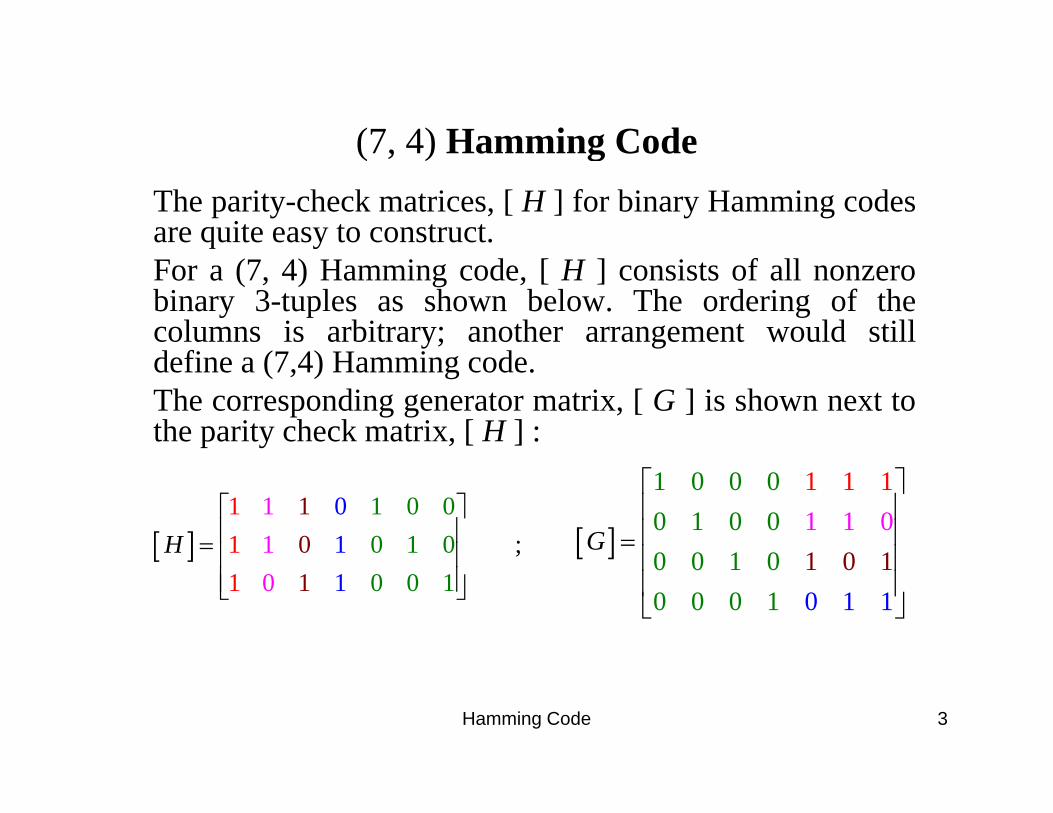
(7, 4) Hamming Code(7, 4) Hamming CodeThe parity-check matrices, [ H ] for binary Hamming codesare quite easy to construct.For a (7, 4) Hamming code, [ H ] consists of all nonzerobinary 3-tuples as shown below. The ordering of thecolumns is arbitrary; another arrangement would stilld fi (7 4) H i ddefine a (7,4) Hamming code.The corresponding generator matrix, [ G ] is shown next tothe parity check matrix, [ H ] :
[ ]11
10
1 0 00 1 0
1 01 ;1H
⎡ ⎤⎢ ⎥= ⎢ ⎥ [ ]
1 0 1
1 0 0 00 1 0 00 0 1 0
1 1 01 11
G
⎡ ⎤⎢ ⎥⎢ ⎥=⎢ ⎥[ ]
0 1 01 11 0⎢ ⎥⎢ ⎥⎣ ⎦
1 0 10 0 1 00 0 1 10 0 1⎢ ⎥⎢ ⎥⎣ ⎦
Hamming Code 3
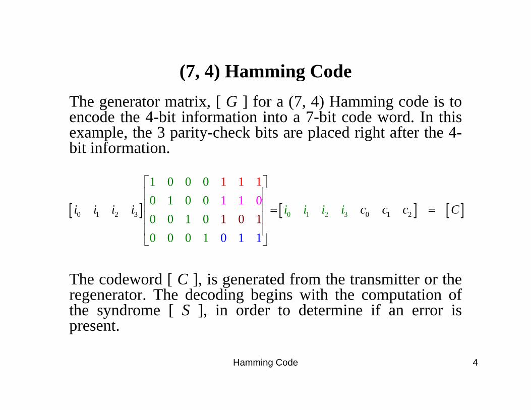
(7, 4) Hamming Code(7, 4) Hamming CodeThe generator matrix, [ G ] for a (7, 4) Hamming code is toencode the 4-bit information into a 7-bit code word. In this
l h 3 i h k bi l d i h f h 4example, the 3 parity-check bits are placed right after the 4-bit information.
1 0 0 0 1 1 1⎡ ⎤
[ ] [ ] [ ]0 1 20 1 2 3 0 1 23
1 0 0 00 1 0 00 0 1 0 1 0 1
1 1 01 1 1
i i i i ci i c Ci i c
⎡ ⎤⎢ ⎥⎢ ⎥ = =⎢ ⎥⎢ ⎥
The codeword [ C ] is generated from the transmitter or the
0 0 0 1 0 1 1⎢ ⎥⎣ ⎦
The codeword [ C ], is generated from the transmitter or theregenerator. The decoding begins with the computation ofthe syndrome [ S ], in order to determine if an error ispresent.
Hamming Code 4
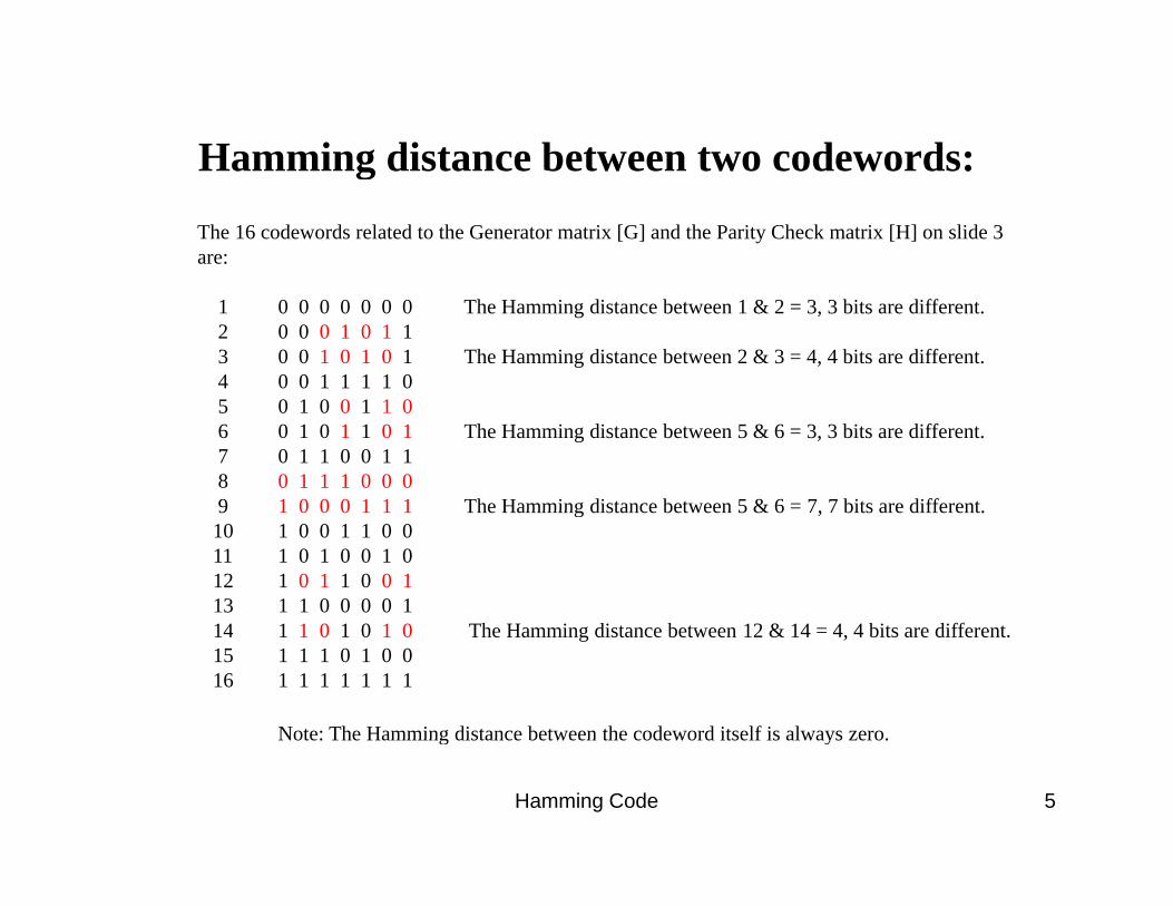
Hamming distance between two codewords:Hamming distance between two codewords:The 16 codewords related to the Generator matrix [G] and the Parity Check matrix [H] on slide 3 are:
1 0 0 0 0 0 0 0 The Hamming distance between 1 & 2 = 3, 3 bits are different.2 0 0 0 1 0 1 1 3 0 0 1 0 1 0 1 The Hamming distance between 2 & 3 = 4, 4 bits are different.4 0 0 1 1 1 1 0 5 0 1 0 0 1 1 06 0 1 0 1 1 0 1 The Hamming distance between 5 & 6 = 3, 3 bits are different.7 0 1 1 0 0 1 1 8 0 1 1 1 0 0 0 9 1 0 0 0 1 1 1 The Hamming distance between 5 & 6 = 7 7 bits are different9 1 0 0 0 1 1 1 The Hamming distance between 5 & 6 7, 7 bits are different.10 1 0 0 1 1 0 0 11 1 0 1 0 0 1 0 12 1 0 1 1 0 0 1 13 1 1 0 0 0 0 1 14 1 1 0 1 0 1 0 Th H i di b 12 & 14 4 4 bi diff14 1 1 0 1 0 1 0 The Hamming distance between 12 & 14 = 4, 4 bits are different.15 1 1 1 0 1 0 0 16 1 1 1 1 1 1 1
Note: The Hamming distance between the codeword itself is always zero.
Hamming Code 5
Note: The Hamming distance between the codeword itself is always zero.
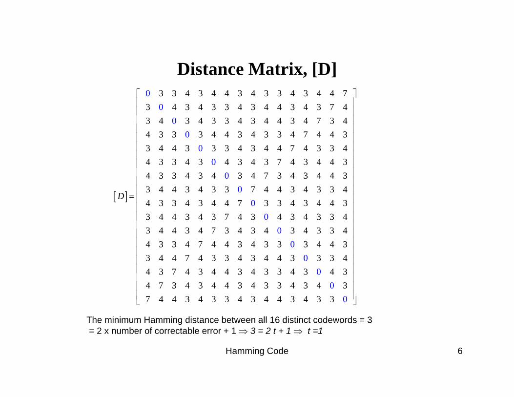
Distance Matrix, [D]Distance Matrix, [D]3 3 4 3 4 4 3 4 3 3 4 3 4 4 7
3 4 3 4 3 3 4 3 4 4 3 4 3 7 43 4 3 4 3 3 4 3 4 4 3 4 7 3 4
00
0
⎡ ⎤⎢ ⎥⎢ ⎥⎢ ⎥3 4 3 4 3 3 4 3 4 4 3 4 7 3 4
4 3 3 3 4 4 3 4 3 3 4 7 4 4 33 4 4 3 3 3 4 3 4 4 7 4 3 3 44 3 3 4 3 4 3 4 3 7 4 3 4 4 34 3 3 4 3 4 3 4 7 3 4 3 4 4 3
00
00
0
⎢ ⎥⎢ ⎥⎢ ⎥⎢ ⎥⎢ ⎥⎢ ⎥⎢ ⎥
[ ]
4 3 3 4 3 4 3 4 7 3 4 3 4 4 33 4 4 3 4 3 3 7 4 4 3 4 3 3 44 3 3 4 3 4 4 7 3 3 4 3 4 4 33 4 4 3 4 3 7 4 3 4 3 4 3 3 4
00
00
D =
⎢ ⎥⎢ ⎥⎢ ⎥⎢ ⎥⎢ ⎥⎢ ⎥⎢ ⎥3 4 4 3 4 7 3 4 3 4 3 4 3 3 4
4 3 3 4 7 4 4 3 4 30
03 3 4 4 33 4 4 7 4 3 3 4 3 4 4 3 3 3 44 3 7 4 3 4 4 3 4 3 3 4 3 4 3
00
⎢ ⎥⎢ ⎥⎢ ⎥⎢ ⎥⎢ ⎥⎢ ⎥⎢ ⎥
4 3 7 4 3 4 4 3 4 3 3 4 3 4 34 7 3 4 3 4 4 3 4 3 3 4 3 4 37 4 4 3 4 3 3 4 3 4 4 3 4
00
3 3 0
⎢ ⎥⎢ ⎥⎢ ⎥⎣ ⎦
The minimum Hamming distance between all 16 distinct codewords = 3
Hamming Code 6
g= 2 x number of correctable error + 1 ⇒ 3 = 2 t + 1 ⇒ t =1
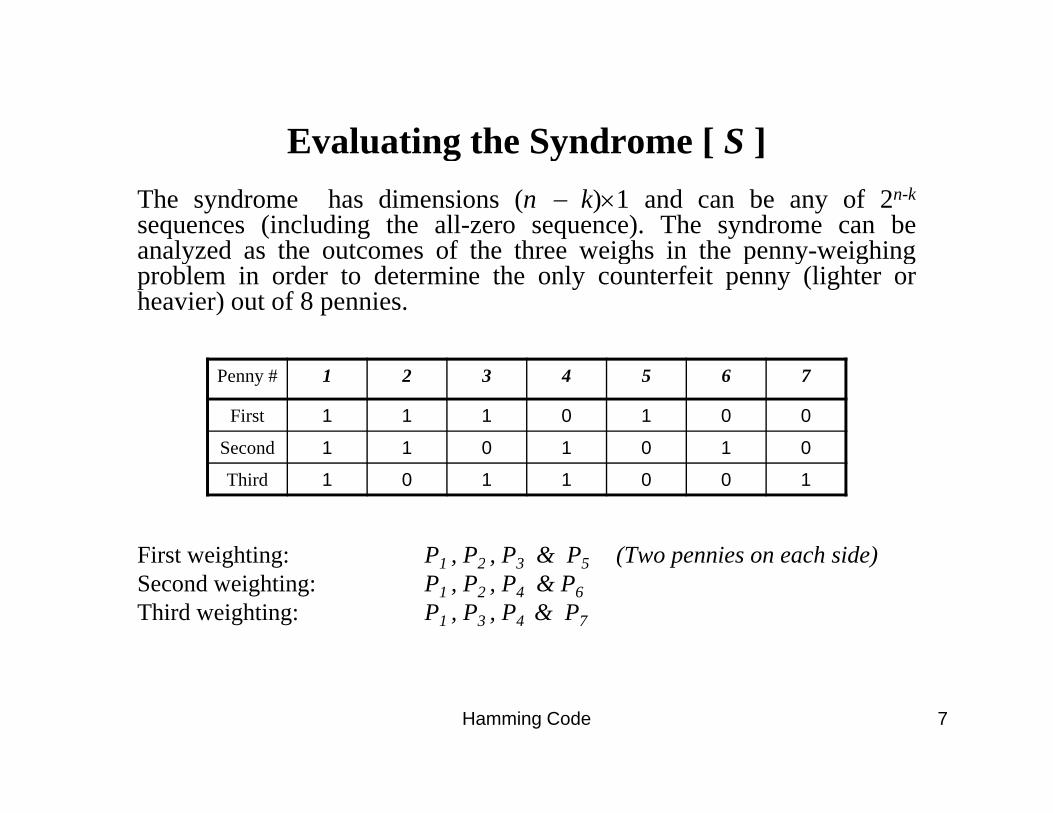
Evaluating the Syndrome [ S ]Evaluating the Syndrome [ S ]The syndrome has dimensions (n − k)×1 and can be any of 2n-k
sequences (including the all-zero sequence). The syndrome can beanalyzed as the outcomes of the three weighs in the penny-weighinganalyzed as the outcomes of the three weighs in the penny-weighingproblem in order to determine the only counterfeit penny (lighter orheavier) out of 8 pennies.
Penny # 1 2 3 4 5 6 7
First 1 1 1 0 1 0 0
Second 1 1 0 1 0 1 0
First weighting: P1 , P2 , P3 & P5 (Two pennies on each side)
Third 1 0 1 1 0 0 1
First weighting: P1 , P2 , P3 & P5 (Two pennies on each side)Second weighting: P1 , P2 , P4 & P6Third weighting: P1 , P3 , P4 & P7
Hamming Code 7

Evaluating the Syndrome [ S ]Evaluating the Syndrome [ S ]The above table represents the selected pennies for eachweighing. That is also the parity-check matrix [ H ] . The top
f h bl b l h h f i f hrow of the table below shows the counterfeit penny from theoutcomes of all three weighs. That is also the syndrome [ S ].Penny # 7 is not used in the above table, but there is asyndrome [ 0 0 0 ] T for penny # 7 in the table below Thatsyndrome [ 0 0 0 ] for penny # 7 in the table below. Thatis also the syndrome for no error.
P P P P P P P PP8 P7 P6 P5 P4 P3 P2 P1
√ √ √ √ × × × ×
√ √ × × √ √ × ×
√ × √ × √ × √ ×
Note: √ stands for balance on the scale× stands for off-balance on the scale
√ × √ × √ × √ ×
Hamming Code 8

Evaluating the Syndrome [ S ]Evaluating the Syndrome [ S ]The syndrome [ S ] , for the received codeword can bedetermined by the following:If the received codeword [ R ] = [ 0 0 1 1 1 1 0 ] T, then
0⎡ ⎤⎢ ⎥
[ ][ ] [ ]
00101
1 0 00 1 0
1 10
11
011H R S
⎢ ⎥⎢ ⎥⎢ ⎥⎡ ⎤ ⎡ ⎤⎢ ⎥⎢ ⎥ ⎢ ⎥= = =⎢ ⎥⎢ ⎥ ⎢ ⎥[ ][ ] [ ]
011
0 0 110
0
11⎢ ⎥⎢ ⎥ ⎢ ⎥⎢ ⎥⎢ ⎥ ⎢ ⎥⎣ ⎦ ⎣ ⎦⎢ ⎥⎢ ⎥⎢ ⎥⎣ ⎦
[ S ] is an all-zero sequence, it represents no error in the [ R ].
0⎣ ⎦
Hamming Code 9

Evaluating the Syndrome [ S ]Evaluating the Syndrome [ S ]If the received codeword [ R ] = [ 0 0 1 1 1 1 1 ]T , then
⎡ ⎤00
011 0 01 11 0
⎡ ⎤⎢ ⎥⎢ ⎥⎢ ⎥⎡ ⎤ ⎡ ⎤⎢ ⎥⎢ ⎥ ⎢ ⎥[ ][ ] [ ]01
111
0 1 00 0 1
01
10
11
11
H R S⎢ ⎥⎢ ⎥ ⎢ ⎥= = =⎢ ⎥⎢ ⎥ ⎢ ⎥⎢ ⎥⎢ ⎥ ⎢ ⎥⎣ ⎦ ⎣ ⎦⎢ ⎥⎢ ⎥
[ S ] is equivalent to the 7th column of [ H ], that means the 7th
1⎢ ⎥⎢ ⎥⎣ ⎦
[ ] q [ ],bit is in error. The received 7th bit is a 1 and is in error, thenthe corrected bit should be 0.The corrected codeword: [ C ] = [ 0 0 1 1 1 1 0 ]
Hamming Code 10
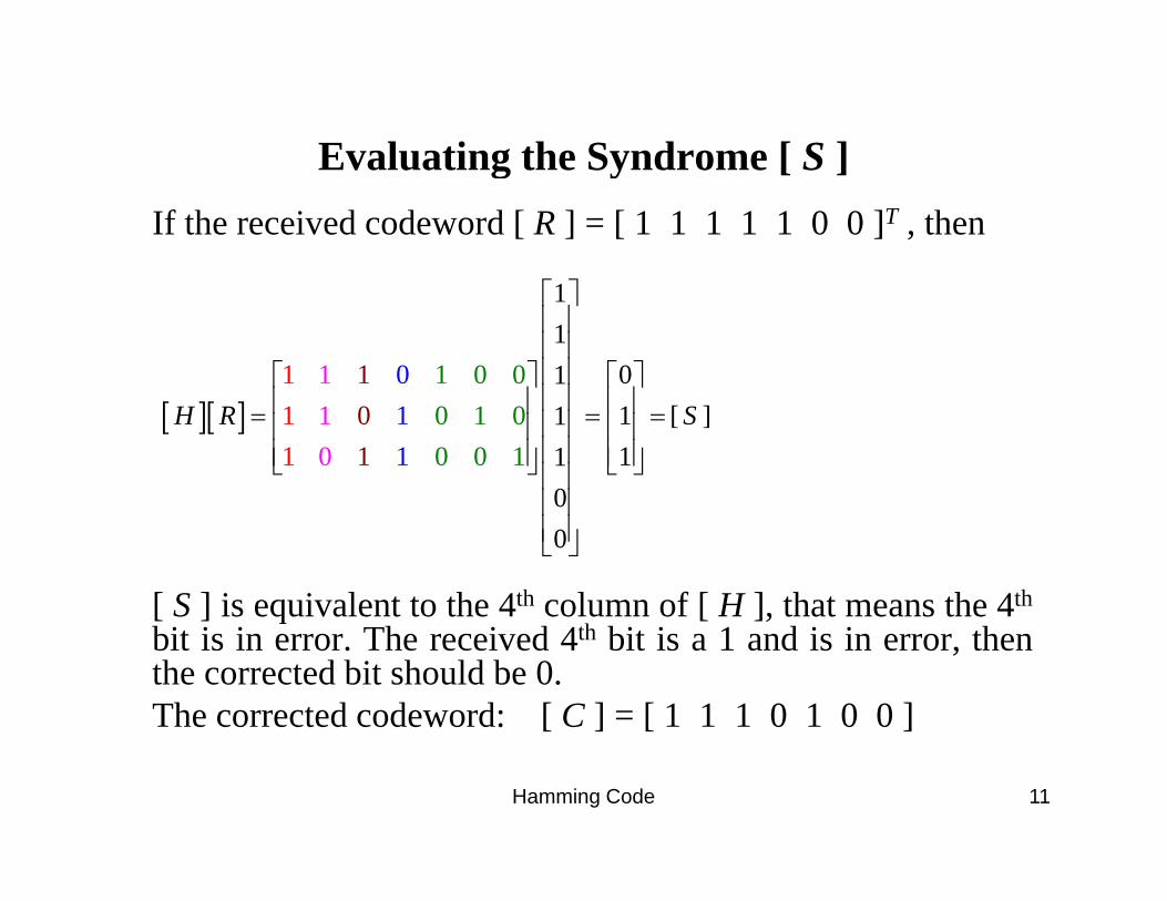
Evaluating the Syndrome [ S ]Evaluating the Syndrome [ S ]If the received codeword [ R ] = [ 1 1 1 1 1 0 0 ]T , then
⎡ ⎤11
011 1 0 001 1
⎡ ⎤⎢ ⎥⎢ ⎥⎢ ⎥⎡ ⎤ ⎡ ⎤⎢ ⎥⎢ ⎥ ⎢ ⎥[ ][ ] 1 [ ]1
110
0 1 00 0 1
1 1101
1 01
H R S⎢ ⎥⎢ ⎥ ⎢ ⎥= = =⎢ ⎥⎢ ⎥ ⎢ ⎥⎢ ⎥⎢ ⎥ ⎢ ⎥⎣ ⎦ ⎣ ⎦⎢ ⎥⎢ ⎥
[ S ] is equivalent to the 4th column of [ H ], that means the 4th
0⎢ ⎥⎢ ⎥⎣ ⎦
[ ] q [ ],bit is in error. The received 4th bit is a 1 and is in error, thenthe corrected bit should be 0.The corrected codeword: [ C ] = [ 1 1 1 0 1 0 0 ]
Hamming Code 11
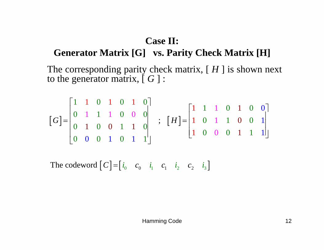
Case II: Generator Matrix [G] vs. Parity Check Matrix [H]
The corresponding parity check matrix, [ H ] is shown nextto the generator matrix [ G ] :to the generator matrix, [ G ] :
1 1 11 0
1 0 0 01 0 011
⎡ ⎤⎡ ⎤⎢ ⎥
[ ] [ ]11
01
1
1 0 00 1 0 0
0 1 00 0 1 0
0
10
1 0 11
11 1 0
10 0 1 1
;
0 1 0 1100
G H⎡ ⎤⎢ ⎥⎢ ⎥⎢ ⎥= = ⎢ ⎥⎢ ⎥⎢ ⎥⎢ ⎥ ⎣ ⎦
⎣ ⎦
[ ] [ ]1 30 20 21The codeword
0 1 0 1100
C c c ci i i i
⎣ ⎦
=
Hamming Code 12
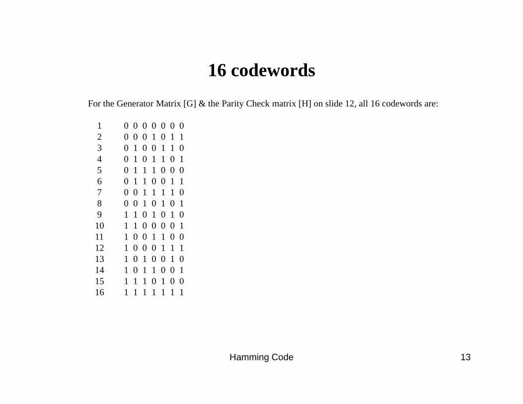
16 codewords16 codewordsFor the Generator Matrix [G] & the Parity Check matrix [H] on slide 12, all 16 codewords are:
1 0 0 0 0 0 0 01 0 0 0 0 0 0 0 2 0 0 0 1 0 1 13 0 1 0 0 1 1 0 4 0 1 0 1 1 0 1 5 0 1 1 1 0 0 0 6 0 1 1 0 0 1 1 7 0 0 1 1 1 1 08 0 0 1 0 1 0 19 1 1 0 1 0 1 0 10 1 1 0 0 0 0 110 1 1 0 0 0 0 1 11 1 0 0 1 1 0 0 12 1 0 0 0 1 1 113 1 0 1 0 0 1 014 1 0 1 1 0 0 115 1 1 1 0 1 0 015 1 1 1 0 1 0 0 16 1 1 1 1 1 1 1
Hamming Code 13
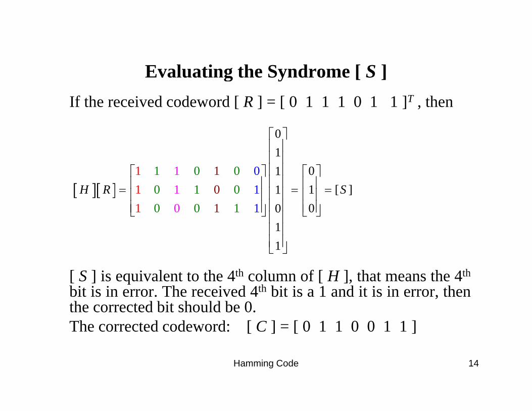
Evaluating the Syndrome [ S ]Evaluating the Syndrome [ S ]If the received codeword [ R ] = [ 0 1 1 1 0 1 1 ]T , then
⎡ ⎤01
011 01 0 011
⎡ ⎤⎢ ⎥⎢ ⎥⎢ ⎥⎡ ⎤ ⎡ ⎤⎢ ⎥⎢ ⎥ ⎢ ⎥[ ][ ] 1 [ ]1
001
11
011
0 1 00 0 1
101
H R S⎢ ⎥⎢ ⎥ ⎢ ⎥= = =⎢ ⎥⎢ ⎥ ⎢ ⎥⎢ ⎥⎢ ⎥ ⎢ ⎥⎣ ⎦ ⎣ ⎦⎢ ⎥⎢ ⎥
[ S ] is equivalent to the 4th column of [ H ], that means the 4th
1⎢ ⎥⎢ ⎥⎣ ⎦
[ ] q [ ],bit is in error. The received 4th bit is a 1 and it is in error, thenthe corrected bit should be 0.The corrected codeword: [ C ] = [ 0 1 1 0 0 1 1 ]
Hamming Code 14

Evaluating the Syndrome [ S ]Evaluating the Syndrome [ S ]If the received codeword [ R ] = [ 1 1 1 1 0 0 0 ]T , then
11
111 01 0 011
⎡ ⎤⎢ ⎥⎢ ⎥⎢ ⎥⎡ ⎤ ⎡ ⎤⎢ ⎥[ ][ ] 1 [ ]1
100
11
011
0 1 00 0 1
101
H R S⎡ ⎤ ⎡ ⎤
⎢ ⎥⎢ ⎥ ⎢ ⎥= = =⎢ ⎥⎢ ⎥ ⎢ ⎥⎢ ⎥⎢ ⎥ ⎢ ⎥⎣ ⎦ ⎣ ⎦⎢ ⎥⎢ ⎥
[ S ] is equivalent to the 1st column of [ H ], that means the 1st
00⎢ ⎥⎢ ⎥⎣ ⎦
[ ] q [ ],bit is in error. The received 1st bit is a 1 and is in error, thenthe corrected bit should be 0.The corrected codeword: [ C ] = [ 0 1 1 1 0 0 0 ]
Hamming Code 15

Case IIIG M i [G] P i Ch k M i [H]Generator Matrix [G] vs. Parity Check Matrix [H]
The corresponding parity check matrix, [ H ] is shown nextto the generator matrix [ G ] :to the generator matrix, [ G ] :
1 1 11 01
1 0 0 01 0 0 1
⎡ ⎤⎡ ⎤⎢ ⎥
[ ] [ ]11
01
1
11 1 0
10
1 0 00 1 0 0
0 1 00 0 1 0
0 0 1
10
1 0 11 1
0 1 1
;
0 0 10
G H⎡ ⎤⎢ ⎥⎢ ⎥⎢ ⎥= = ⎢ ⎥⎢ ⎥⎢ ⎥⎢ ⎥ ⎣ ⎦
⎣ ⎦
[ ] [ ]0 2 31 20 1
0 1 1
The codeword
0 0 1
0
i iC c c ic i
⎣ ⎦
=
Hamming Code 16

16 Codewords16 CodewordsFor the Generator Matrix [G] & the Parity Check matrix [H] on slide 16, all 16 codewords are:
1 0 0 0 0 0 0 01 0 0 0 0 0 0 0 2 0 0 0 1 1 0 13 0 0 1 0 1 1 0 4 0 0 1 1 0 1 1 5 0 1 1 1 0 0 0 6 0 1 1 0 1 0 1 7 0 1 0 1 1 1 08 0 1 0 0 0 1 19 1 0 1 1 1 0 0 10 1 0 1 0 0 0 110 1 0 1 0 0 0 1 11 1 0 0 1 0 1 0 12 1 0 0 0 1 1 113 1 1 0 0 1 0 014 1 1 0 1 0 0 115 1 1 1 0 0 1 015 1 1 1 0 0 1 0 16 1 1 1 1 1 1 1
Hamming Code 17
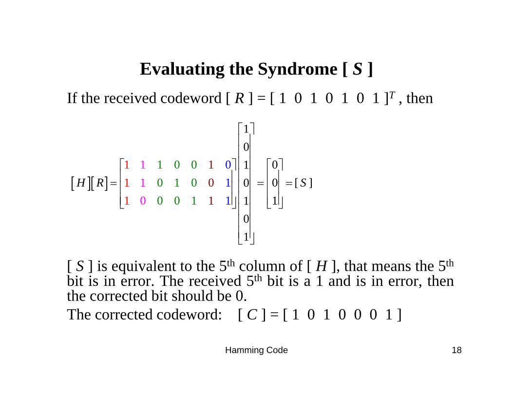
Evaluating the Syndrome [ S ]Evaluating the Syndrome [ S ]If the received codeword [ R ] = [ 1 0 1 0 1 0 1 ]T , then
⎡ ⎤10
011 011 0 01
⎡ ⎤⎢ ⎥⎢ ⎥⎢ ⎥⎡ ⎤ ⎡ ⎤⎢ ⎥⎢ ⎥ ⎢ ⎥[ ][ ] 0 [ ]0
110
11
00 1 01
1101 10 0
H R S⎢ ⎥⎢ ⎥ ⎢ ⎥= = =⎢ ⎥⎢ ⎥ ⎢ ⎥⎢ ⎥⎢ ⎥ ⎢ ⎥⎣ ⎦ ⎣ ⎦⎢ ⎥⎢ ⎥
[ S ] is equivalent to the 5th column of [ H ], that means the 5th
1⎢ ⎥⎢ ⎥⎣ ⎦
[ ] q [ ],bit is in error. The received 5th bit is a 1 and is in error, thenthe corrected bit should be 0.The corrected codeword: [ C ] = [ 1 0 1 0 0 0 1 ]
Hamming Code 18
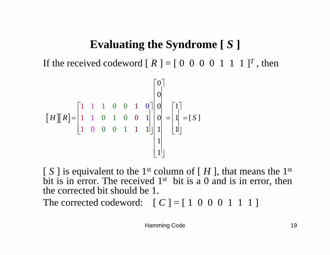
Evaluating the Syndrome [ S ]Evaluating the Syndrome [ S ]If the received codeword [ R ] = [ 0 0 0 0 1 1 1 ]T , then
⎡ ⎤00
101 011 0 01
⎡ ⎤⎢ ⎥⎢ ⎥⎢ ⎥⎡ ⎤ ⎡ ⎤⎢ ⎥⎢ ⎥ ⎢ ⎥[ ][ ] 1 [ ]0
111
11
00 1 01
1101 10 0
H R S⎢ ⎥⎢ ⎥ ⎢ ⎥= = =⎢ ⎥⎢ ⎥ ⎢ ⎥⎢ ⎥⎢ ⎥ ⎢ ⎥⎣ ⎦ ⎣ ⎦⎢ ⎥⎢ ⎥
[ S ] is equivalent to the 1st column of [ H ], that means the 1st
1⎢ ⎥⎢ ⎥⎣ ⎦
[ ] q [ ],bit is in error. The received 1st bit is a 0 and is in error, thenthe corrected bit should be 1.The corrected codeword: [ C ] = [ 1 0 0 0 1 1 1 ]
Hamming Code 19
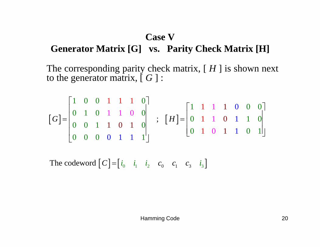
Case VG M i [G] P i Ch k M i [H]Generator Matrix [G] vs. Parity Check Matrix [H]
The corresponding parity check matrix, [ H ] is shown nextto the generator matrix [ G ] :to the generator matrix, [ G ] :
1 0 0 01 0 01 01
1 1 11
⎡ ⎤⎡ ⎤⎢ ⎥
[ ] [ ]1 0 0
0 1 0 00
10
1 0 11
1 00 0 1 0
0 0 1
011
00 0 0
11 1 0
10
111
;
11 1
G H⎡ ⎤⎢ ⎥⎢ ⎥⎢ ⎥= = ⎢ ⎥⎢ ⎥⎢ ⎥⎢ ⎥ ⎣ ⎦
⎣ ⎦
[ ] [ ]00 1 2 31 3
00 0 0
The codewor
1
d
1 1
i i i iC c c c
⎣ ⎦
=
Hamming Code 20

16 Codewords16 CodewordsFor the Generator Matrix [G] & the Parity Check matrix [H] on slide 20, all 16 codewords are:
1 0 0 0 0 0 0 01 0 0 0 0 0 0 0 2 0 0 0 0 1 1 13 0 0 1 1 0 1 0 4 0 0 1 1 1 0 1 5 0 1 0 1 1 0 0 6 0 1 0 1 0 1 1 7 0 1 1 0 1 1 08 0 1 1 0 0 0 19 1 0 0 1 1 1 0 10 1 0 0 1 0 0 110 1 0 0 1 0 0 1 11 1 0 1 0 1 0 012 1 0 1 0 0 1 113 1 1 0 0 0 1 014 1 1 0 0 1 0 115 1 1 1 1 0 0 015 1 1 1 1 0 0 0 16 1 1 1 1 1 1 1
Hamming Code 21

Evaluating the Syndrome [ S ]Evaluating the Syndrome [ S ]If the received codeword [ R ] = [ 1 0 1 1 1 1 0 ]T , then
⎡ ⎤10
111 0 001 11
⎡ ⎤⎢ ⎥⎢ ⎥⎢ ⎥⎡ ⎤ ⎡ ⎤⎢ ⎥⎢ ⎥ ⎢ ⎥[ ][ ] 1 [ ]1
011
0 1 00 0 1
1101 1
01
1H R S⎢ ⎥⎢ ⎥ ⎢ ⎥= = =⎢ ⎥⎢ ⎥ ⎢ ⎥⎢ ⎥⎢ ⎥ ⎢ ⎥⎣ ⎦ ⎣ ⎦⎢ ⎥⎢ ⎥
[ S ] is equivalent to the 3rd column of [ H ], that means the 3rd
0⎢ ⎥⎢ ⎥⎣ ⎦
[ ] q [ ],bit is in error. The received 3rd bit is a 1 and is in error, thenthe corrected bit should be 0.The corrected codeword: [ C ] = [ 1 0 0 1 1 1 0 ]
Hamming Code 22
The corrected codeword: [ C ] [ 1 0 0 1 1 1 0 ]
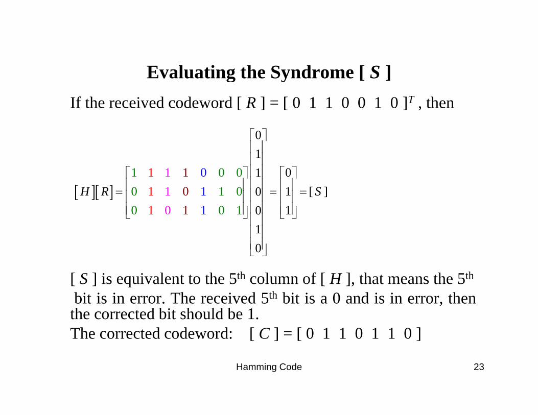
Evaluating the Syndrome [ S ]Evaluating the Syndrome [ S ]If the received codeword [ R ] = [ 0 1 1 0 0 1 0 ]T , then
⎡ ⎤01
011 0 001 11
⎡ ⎤⎢ ⎥⎢ ⎥⎢ ⎥⎡ ⎤ ⎡ ⎤⎢ ⎥⎢ ⎥ ⎢ ⎥[ ][ ] 1 [ ]0
101
0 1 00 0 1
1101 1
01
1H R S⎢ ⎥⎢ ⎥ ⎢ ⎥= = =⎢ ⎥⎢ ⎥ ⎢ ⎥⎢ ⎥⎢ ⎥ ⎢ ⎥⎣ ⎦ ⎣ ⎦⎢ ⎥⎢ ⎥
[ S ] is equivalent to the 5th column of [ H ], that means the 5th
0⎢ ⎥⎢ ⎥⎣ ⎦
[ ] q [ ],bit is in error. The received 5th bit is a 0 and is in error, thenthe corrected bit should be 1.The corrected codeword: [ C ] = [ 0 1 1 0 1 1 0 ]
Hamming Code 23
The corrected codeword: [ C ] [ 0 1 1 0 1 1 0 ]
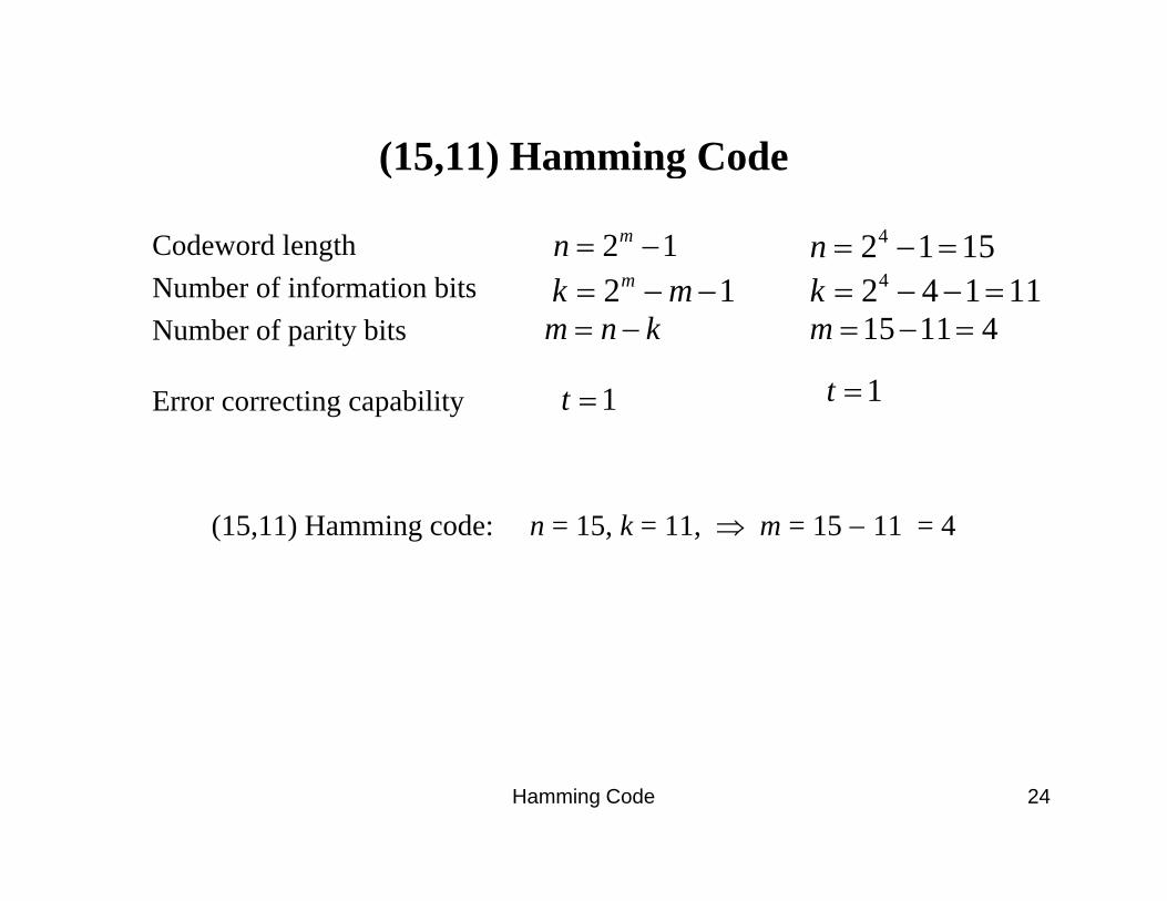
(15,11) Hamming Code(15,11) Hamming Code
Codeword lengthN b f i f ti bit
2 1mn = − 42 1 15n = − =2 1mk 42 4 1 11kNumber of information bits
Number of parity bits
E ti bilit
2 1mk m= − − 42 4 1 11k = − − =m n k= − 15 11 4m = − =
1t 1t =Error correcting capability 1t = 1t =
(15,11) Hamming code: n = 15, k = 11, ⇒ m = 15 − 11 = 4
Hamming Code 24
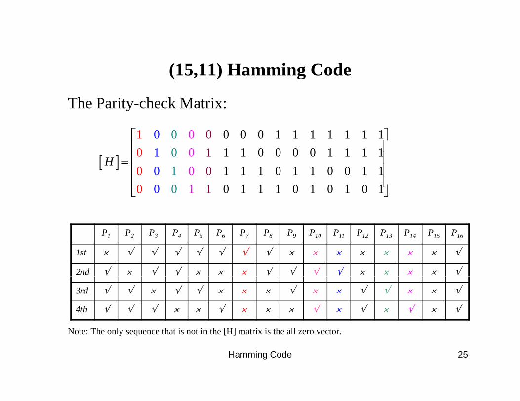
(15,11) Hamming Code(15,11) Hamming Code
The Parity-check Matrix:
[ ]
0 0 0 1 1 1 1 1 1 11 1 0 0 0 0 1 1 1 11
100
001
010 1 1 0 1 1 0 0 1 1
010
00
0H
⎡ ⎤⎢ ⎥⎢ ⎥=⎢ ⎥⎢ ⎥0 0 1 0 1 1 1 0 1 0 10 11 0⎢ ⎥⎣ ⎦
P1 P2 P3 P4 P5 P6 P7 P8 P9 P10 P11 P12 P13 P14 P15 P16
1st × √ √ √ √ √ √ √ × × × × × × × √
2nd √ × √ √ × × × √ √ √ √ × × × × √
3rd √ √ × √ √ × × × √ × × √ √ × × √
4th √ √ √ × × √ × × × √ × √ × √ × √
Hamming Code 25
Note: The only sequence that is not in the [H] matrix is the all zero vector.
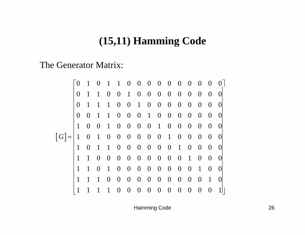
(15,11) Hamming Code(15,11) Hamming Code
The Generator Matrix:
0 1 0 1 1 0 0 0 0 0 0 0 0 0 00 1 1 0 0 1 0 0 0 0 0 0 0 0 00 1 1 1 0 0 1 0 0 0 0 0 0 0 0
⎡ ⎤⎢ ⎥⎢ ⎥⎢ ⎥0 1 1 1 0 0 1 0 0 0 0 0 0 0 00 0 1 1 0 0 0 1 0 0 0 0 0 0 01 0 0 1 0 0 0 0 1 0 0 0 0 0 0
⎢ ⎥⎢ ⎥⎢ ⎥⎢ ⎥⎢ ⎥[ ] 1 0 1 0 0 0 0 0 0 1 0 0 0 0 01 0 1 1 0 0 0 0 0 0 1 0 0 0 01 1 0 0 0 0 0 0 0 0 0 1 0 0 0
G⎢ ⎥
= ⎢ ⎥⎢ ⎥⎢ ⎥⎢ ⎥⎢ ⎥1 1 0 1 0 0 0 0 0 0 0 0 1 0 01 1 1 0 0 0 0 0 0 0 0 0 0 1 01 1 1 1 0 0 0 0 0 0 0 0 0 0 1
⎢ ⎥⎢ ⎥⎢⎢⎢⎣ ⎦
⎥⎥⎥
Hamming Code 26
1 1 1 1 0 0 0 0 0 0 0 0 0 0 1⎢⎣ ⎦⎥

![Implementation of [7,4]-Hamming Code Surya Ganesh P (15VL17F) Siddhartha Sankar Das (15VL23F) Vishnuprasath J (15VL27F](https://img.pdfslide.net/doc/110x75/6360e8ad1bb572d28603335f/implementation-of-74-hamming-code-surya-ganesh-p-15vl17f-siddhartha-sankar.jpg)