Reconcillation and Rectification of Process Flow and Inventory Data

Ind. Eng. Chem., Process Des. Dev., Vol. 15, No. 1, 1976 175

Reconciliation and Rectification of Process Flow and Inventory Data

Richard S. Mah, Gregory M. Stanley*, and Dennis M. Downing

Northwestern University, Evanston, Illinois 60201

This paper shows how information inherent in the process constraints and measurement statistics can be used to

enhance flow and inventory data. Two important graph-theoretic results are derived and used to simplify the

reconciliation of conflicting data and the estimation of unmeasured process streams. The scheme was implemented

and evaluated on a CDC-6400 computer. For a 32-node 61-stream problem, the results indicate a 42 to 60 %

reduction in total absolute errors, for the three cases in which the number of measured streams were 36, 50, and

61 respectively. A gross error detection criterion based on nodal imbalances is proposed. This criterion can be

evaluated prior to any reconciliation calculations and appeared to be effective for errors of 20 % or more for the

simulation cases studied. A logically consistent scheme for identifying the error sources was developed using this

criterion. Such a scheme could be used as a diagnostic aid in process analysis.

Introduction

Process data is the foundation upon which all control

and evaluation of process performance are based.

Because of the integrated nature of modern process

plants, ramifications of process decisions are often broad

and difficult to foresee. Inaccurate process data can

easily lead to poor decisions, which will adversely affect

many parts of the process. Many process control and

optimization activities are also based on small

improvements in process performance; errors in process

data or arbitrary methods of resolving them can easily

exceed and mask actual changes in process performance.

Moreover, because of the immense scale of operation, the impact

of any error is greatly magnified in absolute terms.

In recent years many digital computers have been installed

within refineries and chemical complexes. These installations are

usually justified on the basis of specific applications such as

process control or gasoline blending. The introduction of digital

computers in the operational environment brought forth many

beneficial side effects, not the least of which is the increasing

availability of process data. Certain data, which were not

previously collected or recorded, are now acquired and stored

because of computer applications. Other data, which were

previously scattered

176 Ind. Eng. Chem., Process Des. Dev., Vol. 15, No. 1, 1976

in different sources and appeared in various formats, are now

concentrated in computer files in forms which are highly

accessible. Moreover, improved process instrumentation makes it

feasible to acquire such data on a frequent and regular basis. With

these advances in data acquisition and data processing capabilities

the stage is set for developing a comprehensive and systematic

basis for process analysis.

In this paper we shall consider process flow rates measured at a

given instant in time and address the techniques of enhancing the

information content of these measurements through the use of

network and statistical information. It is convenient to discuss this

data enhancement in terms of three separate but related problems.

Morphologically, the simplest situation is one in which all streams

are measured and all measurements are subject to normal mea-

surement errors only. The problem is how to extract best estimates

of stream and process conditions from apparently conflicting

observations. This is the problem of data reconciliation. In most

operating processes, not all of the variables are measured, but we

may want to estimate the unmeasured process variables in terms of

the measured process data. This problem may be termed

coaptation. Finally, gross errors may be incurred as a result of

defective measurements or out-of-tune instruments, and leaks,

evaporation, deposition, etc. may result in physical losses. Isolation

and identification of such gross errors will be valuable not only in

monitoring process performance but also in scheduling equipment

and instrument maintenance. The problem is addressed in fault

detection and rectification.

The Process Graph

The interdependence of flow and inventory data in a process is

most naturally expressed in terms of the material balances. In order

to explore the network characteristics of the process, it is

convenient to define a process graph, P, which exhibits the following characteristics.

1. It is a directed graph (digraph). The directions of its arcs are

the same as those of the streams in the process flow sheet, which

are usually determined by processing requirements.

2. The nodes in the process graph generally correspond to the

units, tanks, and junctions in the process flow sheet. But since, at

any given instant of time, only a subset of process units and tanks

may be activated, the process graph may only contain a subset of

such nodes.

3. The process graph always contains an environment node. The

process receives its feeds (including utilities)

from the “environment” and supplies its products to the

“environment”. The environment node may thus be perceived as

the complement of the process.

4. With the inclusion of the environment node, the process

graph is always cyclic. Every node (vertex) is in at least one cycle

and the degree of each vertex is at least two.

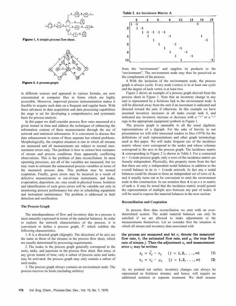
Figure 2 shows an example of a process graph derived from the

process sheet in Figure 1. Note that an inventory change in any

unit is represented by a fictitious link to the environment node. It

will be directed away from the unit if an increment is indicated and

directed toward the unit, if otherwise. In this example we have

assumed inventory increases in all tanks except tank 4, and

indicated any inventory increase or decrease with a “+“ or a “-“

sign in the appropriate equipment symbols in Figure 1.

The process graph is amenable to all the usual algebraic

representations of a digraph. For the sake of brevity in our

presentation we will refer interested readers to Deo (1974) for the

definitions of such representations and other graph terminology

used in this paper. We will make frequent use of the incidence

matrix whose rows correspond to the nodes and whose columns

correspond to the arcs in the process graph. The incidence matrix

A corresponding to Figure 2 is shown in Table I. For a connected

(n + 1)-node process graph, only n rows of the incidence matrix are

linearly independent. Physically, this property stems from the fact

that there are only n independent nodal balances in addition to the

overall balance in an (n + 1)-node network. In fact any n nodal

balances could be chosen to form an independent set of rows of A,

and it usually turns out to be convenient to omit the environment

node in this construction. In our notation then A is an n x m matrix

of rank n. It may be noted that the incidence matrix would permit

the representation of multiple arcs between any pair of nodes. It

will be used to express the material balances in the next section.

Reconciliation and Coaptation

In process flow data reconciliation we start with an over-

determined system. The nodal material balances can only be

satisfied if we are allowed to make adjustments to the

measurements themselves. Let us consider first the situation in

which all stream and inventory data associated with

As we pointed out earlier, inventory changes can always be

represented as fictitious streams, and hence, will require no

additional notation or separate treatment. We shall assume


that the measurement errors are normally distributed random

variables with zero mean and positive definite covariance matrix,

Q. The least-squares estimation for this problem is given by

subject to the material conservation constraints

Under our statistical assumption, this will be equivalent to the

maximum likelihood and minimum variance unbiased estimation.

The solution to this problem, as given by Kuehn and Davidson

(1961), is

More commonly, only some of the process streams are measured

and we wish to estimate the values of the unmeasured variables as

well as reconcile the values of the measured variables. There are

now two incidence matrices: an n x (m - s) matrix A1 corresponding

to the measured streams, v and an n x s matrix A2 corresponding to

the unmeasured streams, u. A similar development of the least-

squares estimation leads to

subject to the constraints

This estimation problem can, of course, be solved as it stands. But

a much more efficient strategy can be developed based on two

important graph-theoretic results. We shall now state these results

and refer the readers to Appendix A for the proofs. (1)

Reconciliation with missing measurements can be resolved into

two disjoint problems: reconciliation on a graph which is formed

by pairwise aggregation of the nodes linked by arcs of unmeasured

flows, and the estimation of unmeasured flows in the tree arcs of

the process graph. (2) Missing flow measurements can be

determined uniquely, if and only if the unmeasured arcs form an

acyclic graph (i.e., trees).

The first result leads to a reduction of the dimensions of the

computational problems. When two nodes are aggregated, the arcs

external to the two nodes are preserved, but all internal links (arcs)

between them are obliterated. The reverse process takes place when

the flow rate of a hitherto unmonitored stream is measured. The

impact of measurements on the problem structure of process flow

data reconciliation and coaptation is delineated by the first graph-

theoretic result.

The second result pinpoints the unmeasured streams whose flow

rates can be uniquely determined and other unmeasured streams

whose flow rates cannot be determined. Note that a process graph

may contain both categories of unmeasured arcs. In coaptation the

unmeasured streams are expressed in terms of the reconciled flows

of the aggregated graph and measured streams that are internal to

the aggregated nodes. Because the arcs form an acyclic graph,

coaptation can always be performed sequentially.

Computer Implementation

A flow reconciliation-coaptation scheme using the foregoing

graph-theoretic results was implemented on a CDC6400 computer.

The input to this program (RECON) consists of the following

items: (1) dimensions of the process graph: the total number of

measured streams, the number of nodes and their labels;

(2) information on the measured streams: measured values and

variances; (3) structure of the process graph in terms of a stream-

node connection table. In this implementation we confine ourselves to the situations in

which there is no statistical interaction between measured values.

In other words, the program provides for diagonal covariance

matrices only.

After checking over the consistency of the input, the in-

formation is used to construct: (a) an (n — q) x (m — s) incidence

matrix B1 which represents a maximal digraph generated from the

process graph by node aggregation such that all streams of B1 are

measured; we shall refer to this as the reconciliation graph; (b) a

q x q incidence matrix B2 representing a maximal acyclic subgraph

(or trees) of unmeasured arcs; the nodes spanned by these trees

may form a part of the aggregated nodes of B1, but they are not

individually represented in the reconciliation graph; (c) a q x

(m — s) incidence matrix B12 which delineates the adjacency of the

measured streams with the nodes on the maximal unmeasured

trees; (d) a list of unmeasured streams whose flow rates can

assume arbitrary values. These streams form loops with other

unmeasured streams. Their flow rates will be set to zero for the

purpose of our computation. Note that both B1 and B12 contain

columns for all the measured streams of the process graph.

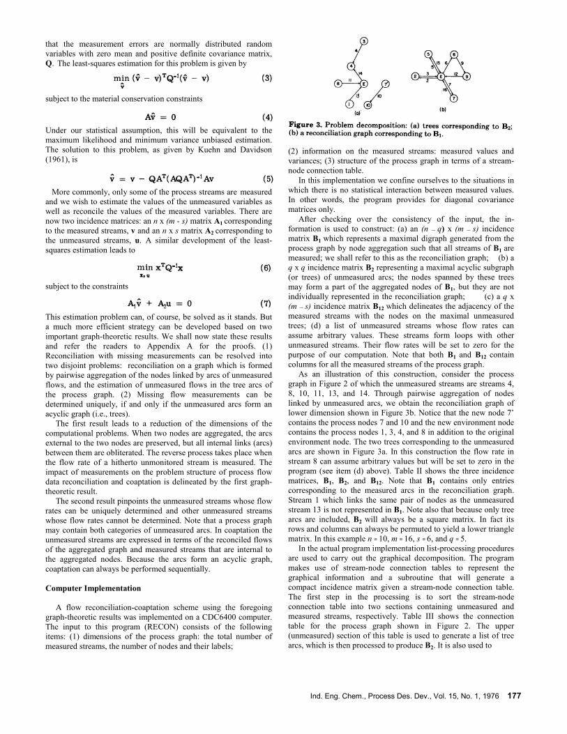
As an illustration of this construction, consider the process

graph in Figure 2 of which the unmeasured streams are streams 4,

8, 10, 11, 13, and 14. Through pairwise aggregation of nodes

linked by unmeasured arcs, we obtain the reconciliation graph of

lower dimension shown in Figure 3b. Notice that the new node 7’

contains the process nodes 7 and 10 and the new environment node

contains the process nodes 1, 3, 4, and 8 in addition to the original

environment node. The two trees corresponding to the unmeasured

arcs are shown in Figure 3a. In this construction the flow rate in

stream 8 can assume arbitrary values but will be set to zero in the

program (see item (d) above). Table II shows the three incidence

matrices, B1, B2, and B12. Note that B1 contains only entries

corresponding to the measured arcs in the reconciliation graph.

Stream 1 which links the same pair of nodes as the unmeasured

stream 13 is not represented in B1. Note also that because only tree

arcs are included, B2 will always be a square matrix. In fact its

rows and columns can always be permuted to yield a lower triangle

matrix. In this example n = 10, m = 16, s = 6, and q = 5.

In the actual program implementation list-processing procedures

are used to carry out the graphical decomposition. The program

makes use of stream-node connection tables to represent the

graphical information and a subroutine that will generate a

compact incidence matrix given a stream-node connection table.

The first step in the processing is to sort the stream-node

connection table into two sections containing unmeasured and

measured streams, respectively. Table III shows the connection

table for the process graph shown in Figure 2. The upper

(unmeasured) section of this table is used to generate a list of tree

arcs, which is then processed to produce B2. It is also used to


generate a node replacement list which is in turn used to modify

the lower (measured) section of the connection table from which

B1 is generated. Finally, B12 is constructed from the measured

streams and the nodes linked by unmeasured streams.

Since there are no unmeasured streams in the reconciliation

graph, the solution to the reconciliation problem is

Note that the solution for all measured streams is given here. But

the measured streams that are internal to the aggregated nodes are

not adjusted nor do they contribute to the reconciliation of other

measured streams, since the corresponding columns of B1 contain

only zeros.

The estimates of the unmeasured flows are given by

A derivation of this equation may be found in Appendix B.

Because u1 is a linear combination of the measured flows v,

we can apply the Addition Theorem for the normally distributed

random variables (Hald, 1952) to obtain the variances for the

estimated values of the unmeasured streams. Let p be the vector of

these variances. Then we have

The reader should be cautioned against the use of eq 10 if the

constraints are incorrect (e.g., on account of leaks), since additional

errors will be introduced to the estimates.

Simulation of Flow Reconciliation

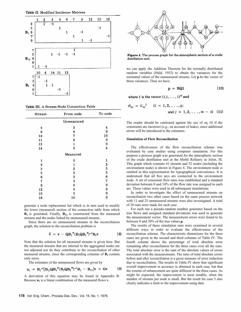
The effectiveness of the flow reconciliation scheme was

evaluated by case studies using computer simulation. For this

purpose a process graph was generated for the atmospheric section

of the crude distillation unit at the Mobil Refinery in Joliet, Ill.

This graph which contains 61 streams and 32 nodes (including the

environment node) is shown in Figure 4. The environment node is

omitted in this representation for typographical convenience. It is

understood that all free arcs are connected to the environment

node. A set of consistent flow rates was established and a standard

deviation between 0 and 10% of the flow rate was assigned to each

arc. These values were used in all subsequent simulations.

In order to investigate the effect of unmeasured streams on

reconciliation two other cases based on the same process network

with 11 and 25 unmeasured streams were also investigated. A total

of 20 runs were made for each case.

For each run a pseudo-random number generator based on the

true flows and assigned standard deviations was used to generate

the measurement vector. The measurement errors were found to lie

between 0 and 30% of the true values µµµµ.

The results of these simulation runs were examined in several

different ways in order to evaluate the effectiveness of the

reconciliation scheme. The characteristic dimensions for the three

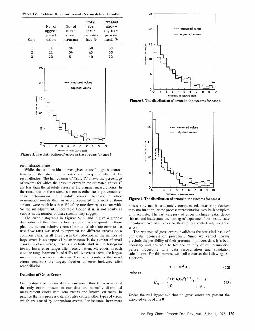
cases are given in the second and third columns of Table IV. The

fourth column shows the percentage of total absolute error

remaining after reconciliation for the three cases over all the runs.

The total absolute error is the sum of the absolute values of errors

associated with the measurements. The ratio of total absolute errors

before and after reconciliation is a gross measure of error reduction

due to reconciliation. The results in Table IV show that significant

overall improvement in accuracy is obtained in each case, but that

the extents of enhancement are quite different in the three cases. As

might be expected, the improvement is most notable, when the

number of streams per node is small. But the result for case 3 also

clearly indicates a limit to the improvement using data


reconciliation alone.

While the total residual error gives a useful gross charac-

terization, the stream flow rates are unequally affected by

reconciliation. The last column of Table IV shows the percentage

of streams for which the absolute errors in the estimated values v^

are less than the absolute errors in the original measurements. In

the remainder of these streams there is either no improvement or

some deterioration in absolute errors. However, a close

examination reveals that the errors associated with most of these

streams were much less than 1% of the true flow rates to start with.

So the maladjustment, undesirable though it is, is not nearly as

serious as the number of these streams may suggest.

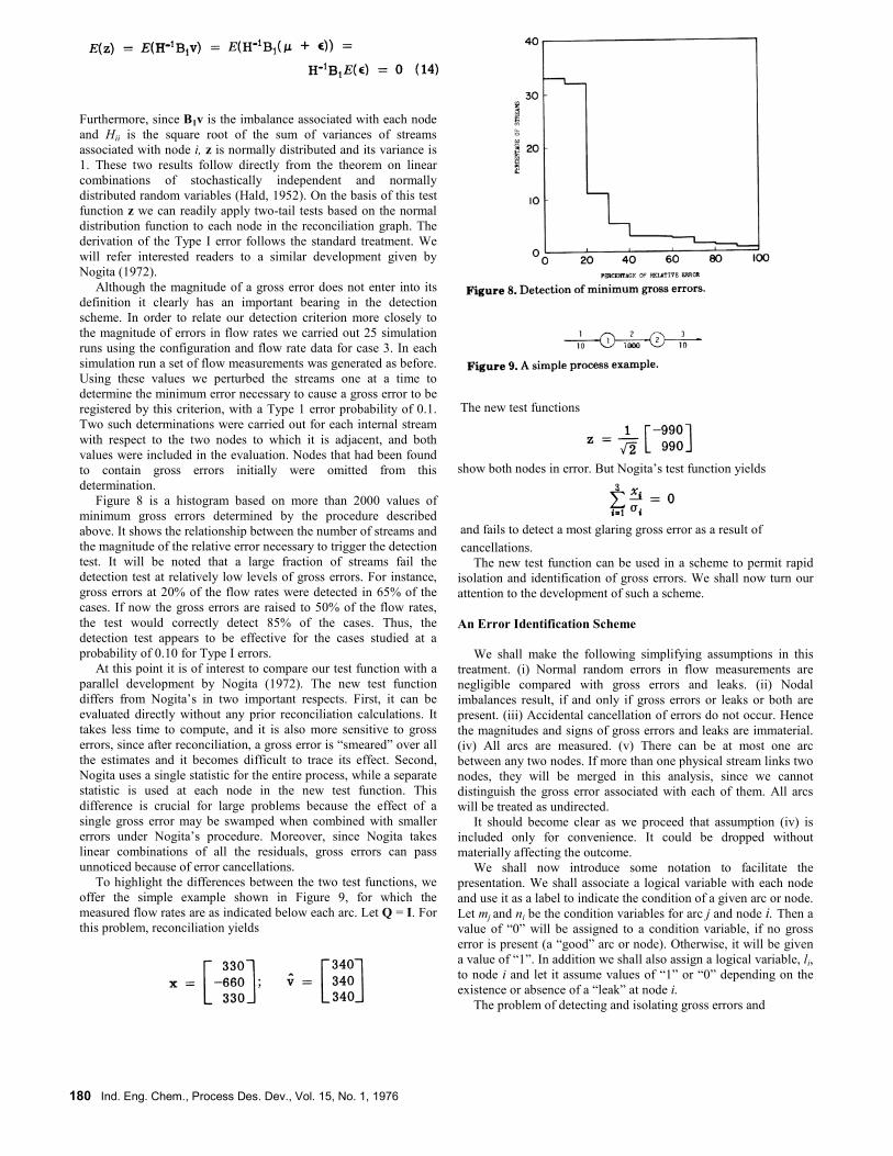
The error histograms in Figures 5, 6, and 7 give a graphic

description of the situation from yet another viewpoint. In these

plots the percent relative errors (the ratio of absolute error to the

true flow rate) was used to represent the different streams on a

common basis. In all three cases the reduction in the number of

large errors is accompanied by an increase in the number of small

errors. In other words, there is a definite shift in the histogram

toward lower error ranges after reconciliation. Moreover, in each

case the range between 0 and 0.5% relative errors shows the largest

increase in the number of streams. These results indicate that small

errors constitute the largest fraction of error incidence after

reconciliation.

Detection of Gross Errors

Our treatment of process data enhancement thus far assumes that

the only errors present in our data are normally distributed

measurement errors with zero means and known variances. In

practice the raw process data may also contain other types of errors

which are caused by nonrandom events. For instance, instrument

biases may not be adequately compensated, measuring devices

may malfunction, or the process representation may be incomplete

or inaccurate. The last category of errors includes leaks, depo-

sitions, and inadequate accounting of departures from steady-state

operations. We shall refer to these errors collectively as gross

errors.

The presence of gross errors invalidates the statistical basis of

our data reconciliation procedure. Since we cannot always

preclude the possibility of their presence in process data, it is both

necessary and desirable to test the validity of our assumption

before proceeding with data reconciliation and coaptation

calculations. For this purpose we shall construct the following test

functions

Under the null hypothesis that no gross errors are present the

expected value of z is 0


Furthermore, since B1v is the imbalance associated with each node

and Hii is the square root of the sum of variances of streams

associated with node i, z is normally distributed and its variance is

1. These two results follow directly from the theorem on linear

combinations of stochastically independent and normally

distributed random variables (Hald, 1952). On the basis of this test

function z we can readily apply two-tail tests based on the normal

distribution function to each node in the reconciliation graph. The

derivation of the Type I error follows the standard treatment. We

will refer interested readers to a similar development given by

Nogita (1972).

Although the magnitude of a gross error does not enter into its

definition it clearly has an important bearing in the detection

scheme. In order to relate our detection criterion more closely to

the magnitude of errors in flow rates we carried out 25 simulation

runs using the configuration and flow rate data for case 3. In each

simulation run a set of flow measurements was generated as before.

Using these values we perturbed the streams one at a time to

determine the minimum error necessary to cause a gross error to be

registered by this criterion, with a Type 1 error probability of 0.1.

Two such determinations were carried out for each internal stream

with respect to the two nodes to which it is adjacent, and both

values were included in the evaluation. Nodes that had been found

to contain gross errors initially were omitted from this

determination.

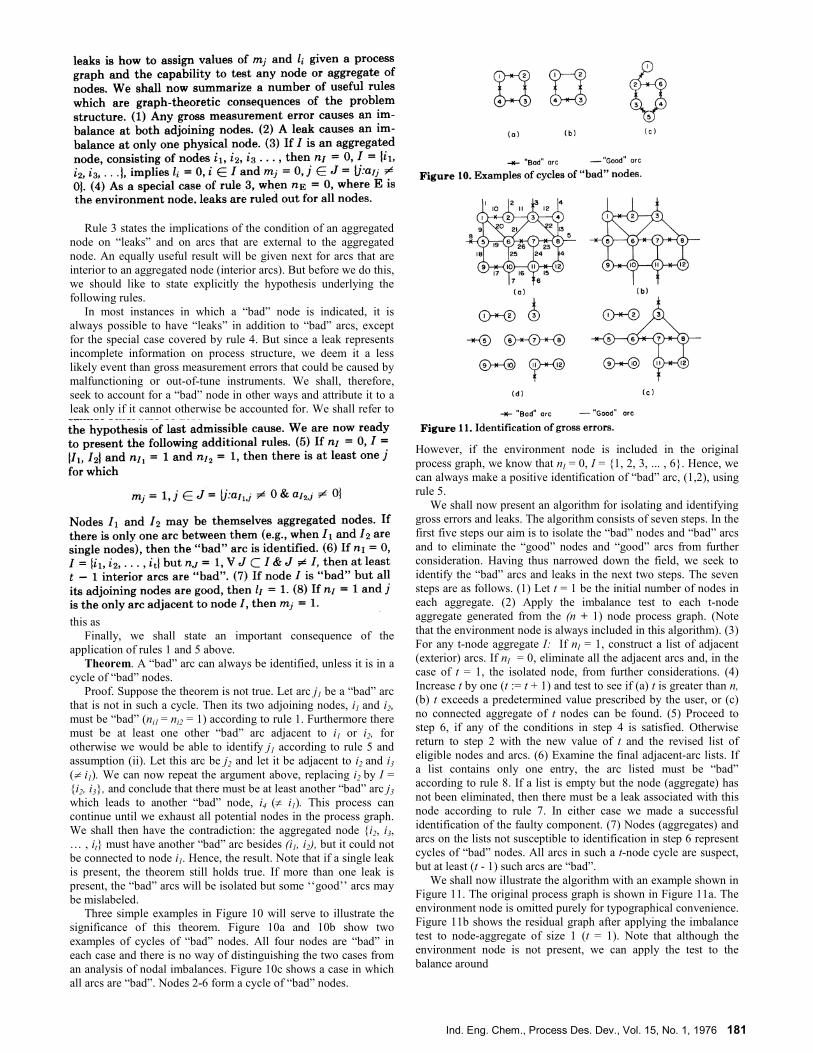
Figure 8 is a histogram based on more than 2000 values of

minimum gross errors determined by the procedure described

above. It shows the relationship between the number of streams and

the magnitude of the relative error necessary to trigger the detection

test. It will be noted that a large fraction of streams fail the

detection test at relatively low levels of gross errors. For instance,

gross errors at 20% of the flow rates were detected in 65% of the

cases. If now the gross errors are raised to 50% of the flow rates,

the test would correctly detect 85% of the cases. Thus, the

detection test appears to be effective for the cases studied at a

probability of 0.10 for Type I errors.

At this point it is of interest to compare our test function with a

parallel development by Nogita (1972). The new test function

differs from Nogita’s in two important respects. First, it can be

evaluated directly without any prior reconciliation calculations. It

takes less time to compute, and it is also more sensitive to gross

errors, since after reconciliation, a gross error is “smeared” over all

the estimates and it becomes difficult to trace its effect. Second,

Nogita uses a single statistic for the entire process, while a separate

statistic is used at each node in the new test function. This

difference is crucial for large problems because the effect of a

single gross error may be swamped when combined with smaller

errors under Nogita’s procedure. Moreover, since Nogita takes

linear combinations of all the residuals, gross errors can pass

unnoticed because of error cancellations.

To highlight the differences between the two test functions, we

offer the simple example shown in Figure 9, for which the

measured flow rates are as indicated below each arc. Let Q = I. For

this problem, reconciliation yields

cancellations.

The new test function can be used in a scheme to permit rapid

isolation and identification of gross errors. We shall now turn our

attention to the development of such a scheme.

An Error Identification Scheme

We shall make the following simplifying assumptions in this

treatment. (i) Normal random errors in flow measurements are

negligible compared with gross errors and leaks. (ii) Nodal

imbalances result, if and only if gross errors or leaks or both are

present. (iii) Accidental cancellation of errors do not occur. Hence

the magnitudes and signs of gross errors and leaks are immaterial.

(iv) All arcs are measured. (v) There can be at most one arc

between any two nodes. If more than one physical stream links two

nodes, they will be merged in this analysis, since we cannot

distinguish the gross error associated with each of them. All arcs

will be treated as undirected.

It should become clear as we proceed that assumption (iv) is

included only for convenience. It could be dropped without

materially affecting the outcome.

We shall now introduce some notation to facilitate the

presentation. We shall associate a logical variable with each node

and use it as a label to indicate the condition of a given arc or node.

Let mj and ni be the condition variables for arc j and node i. Then a value of “0” will be assigned to a condition variable, if no gross

error is present (a “good” arc or node). Otherwise, it will be given

a value of “1”. In addition we shall also assign a logical variable, li,

to node i and let it assume values of “1” or “0” depending on the

existence or absence of a “leak” at node i. The problem of detecting and isolating gross errors and

The new test functions

show both nodes in error. But Nogita’s test function yields

and fails to detect a most glaring gross error as a result of


Rule 3 states the implications of the condition of an aggregated

node on “leaks” and on arcs that are external to the aggregated

node. An equally useful result will be given next for arcs that are

interior to an aggregated node (interior arcs). But before we do this,

we should like to state explicitly the hypothesis underlying the

following rules.

In most instances in which a “bad” node is indicated, it is

always possible to have “leaks” in addition to “bad” arcs, except

for the special case covered by rule 4. But since a leak represents

incomplete information on process structure, we deem it a less

likely event than gross measurement errors that could be caused by

malfunctioning or out-of-tune instruments. We shall, therefore,

seek to account for a “bad” node in other ways and attribute it to a

leak only if it cannot otherwise be accounted for. We shall refer to

this as

Finally, we shall state an important consequence of the

application of rules 1 and 5 above.

Theorem. A “bad” arc can always be identified, unless it is in a

cycle of “bad” nodes.

Proof. Suppose the theorem is not true. Let arc j1 be a “bad” arc

that is not in such a cycle. Then its two adjoining nodes, i1 and i2, must be “bad” (ni1 = ni2 = 1) according to rule 1. Furthermore there

must be at least one other “bad” arc adjacent to i1 or i2, for

otherwise we would be able to identify j1 according to rule 5 and

assumption (ii). Let this arc be j2 and let it be adjacent to i2 and i3 (≠ i1). We can now repeat the argument above, replacing i2 by I =

{i2, i3}, and conclude that there must be at least another “bad” arc j3

which leads to another “bad” node, i4 (≠ i1). This process can

continue until we exhaust all potential nodes in the process graph.

We shall then have the contradiction: the aggregated node {i2, i3,

… , it} must have another “bad” arc besides (i1, i2), but it could not

be connected to node i1. Hence, the result. Note that if a single leak

is present, the theorem still holds true. If more than one leak is

present, the “bad” arcs will be isolated but some ‘‘good’’ arcs may

be mislabeled.

Three simple examples in Figure 10 will serve to illustrate the

significance of this theorem. Figure 10a and 10b show two

examples of cycles of “bad” nodes. All four nodes are “bad” in

each case and there is no way of distinguishing the two cases from

an analysis of nodal imbalances. Figure 10c shows a case in which

all arcs are “bad”. Nodes 2-6 form a cycle of “bad” nodes.

However, if the environment node is included in the original

process graph, we know that nI = 0, I = {1, 2, 3, ... , 6}. Hence, we

can always make a positive identification of “bad” arc, (1,2), using

rule 5. We shall now present an algorithm for isolating and identifying

gross errors and leaks. The algorithm consists of seven steps. In the

first five steps our aim is to isolate the “bad” nodes and “bad” arcs

and to eliminate the “good” nodes and “good” arcs from further

consideration. Having thus narrowed down the field, we seek to

identify the “bad” arcs and leaks in the next two steps. The seven

steps are as follows. (1) Let t = 1 be the initial number of nodes in

each aggregate. (2) Apply the imbalance test to each t-node

aggregate generated from the (n + 1) node process graph. (Note

that the environment node is always included in this algorithm). (3) For any t-node aggregate I: If nI = 1, construct a list of adjacent

(exterior) arcs. If nI = 0, eliminate all the adjacent arcs and, in the

case of t = 1, the isolated node, from further considerations. (4)

Increase t by one (t := t + 1) and test to see if (a) t is greater than n,

(b) t exceeds a predetermined value prescribed by the user, or (c)

no connected aggregate of t nodes can be found. (5) Proceed to

step 6, if any of the conditions in step 4 is satisfied. Otherwise

return to step 2 with the new value of t and the revised list of

eligible nodes and arcs. (6) Examine the final adjacent-arc lists. If

a list contains only one entry, the arc listed must be “bad”

according to rule 8. If a list is empty but the node (aggregate) has

not been eliminated, then there must be a leak associated with this

node according to rule 7. In either case we made a successful

identification of the faulty component. (7) Nodes (aggregates) and

arcs on the lists not susceptible to identification in step 6 represent

cycles of “bad” nodes. All arcs in such a t-node cycle are suspect,

but at least (t - 1) such arcs are “bad”.

We shall now illustrate the algorithm with an example shown in

Figure 11. The original process graph is shown in Figure 11a. The

environment node is omitted purely for typographical convenience.

Figure 11b shows the residual graph after applying the imbalance

test to node-aggregate of size 1 (t = 1). Note that although the

environment node is not present, we can apply the test to the

balance around


the aggregate of nodes 1, 2,... , 12, which is the same as the balance

around the environment node. A zero value of the condition

variable for the environment variable would rule out any leaks. In

this case, since the value is one, we cannot draw any positive

conclusion about leaks. Similarly, Figure 11c and Figure 11d show

the outcome of applying imbalance tests with t = 2 and t = 3. In this

case, no connected aggregate of 4 or more nodes can be found. So

we proceed to step 6.

Referring to Figure 11d, arcs 3 and 8 are identified as “bad” arcs

by rule 8. Application of rule 5 leads to the identification of “bad”

arcs 10, 17, 23, and 26. The imbalance around the aggregate of

nodes 11 and 12 identifies arc 6 as a “bad” arc (rule 8), and finally

arc 15 being the only arc adjacent to the “bad” node 12 is clearly

“bad” also. Notice that as an alternative we could have used rule 5

in this last situation by viewing it as a linear chain consisting of the

environment node, nodes 11 and 12.

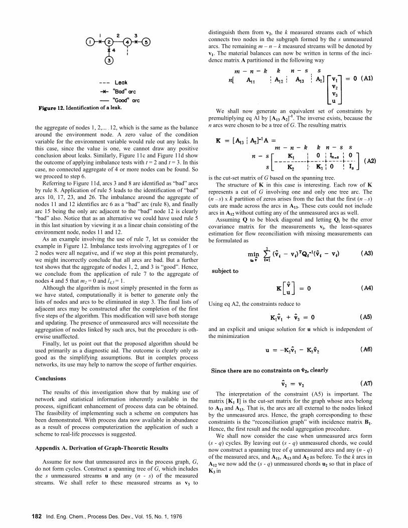
As an example involving the use of rule 7, let us consider the

example in Figure 12. Imbalance tests involving aggregates of 1 or

2 nodes were all negative, and if we stop at this point prematurely,

we might incorrectly conclude that all arcs are bad. But a further

test shows that the aggregate of nodes 1, 2, and 3 is “good”. Hence,

we conclude from the application of rule 7 to the aggregate of

nodes 4 and 5 that m2 = 0 and l4,5 = 1.

Although the algorithm is most simply presented in the form as

we have stated, computationally it is better to generate only the

lists of nodes and arcs to be eliminated in step 3. The final lists of

adjacent arcs may be constructed after the completion of the first

five steps of the algorithm. This modification will save both storage

and updating. The presence of unmeasured arcs will necessitate the

aggregation of nodes linked by such arcs, but the procedure is oth-

erwise unaffected.

Finally, let us point out that the proposed algorithm should be

used primarily as a diagnostic aid. The outcome is clearly only as

good as the simplifying assumptions. But in complex process

networks, its use may help to narrow the scope of further enquiries.

Conclusions

The results of this investigation show that by making use of

network and statistical information inherently available in the

process, significant enhancement of process data can be obtained.

The feasibility of implementing such a scheme on computers has

been demonstrated. With process data now available in abundance

as a result of process computerization the application of such a

scheme to real-life processes is suggested.

Appendix A. Derivation of Graph-Theoretic Results

Assume for now that unmeasured arcs in the process graph, G,

do not form cycles. Construct a spanning tree of G, which includes

the s unmeasured streams u and any (n - s) of the measured

streams. We shall refer to these measured streams as v3 to

distinguish them from v2, the k measured streams each of which

connects two nodes in the subgraph formed by the s unmeasured

arcs. The remaining m – n – k measured streams will be denoted by

v1. The material balances can now be written in terms of the inci-

dence matrix A partitioned in the following way

We shall now generate an equivalent set of constraints by

premultiplying eq Al by [A13 A2]-1. The inverse exists, because the

n arcs were chosen to be a tree of G. The resulting matrix

is the cut-set matrix of G based on the spanning tree.

The structure of K in this case is interesting. Each row of K

represents a cut of G involving one and only one tree arc. The

(n — s) x k partition of zeros arises from the fact that the first (n — s)

cuts are made across the arcs in A13. These cuts could not include

arcs in A12 without cutting any of the unmeasured arcs as well.

Assuming Q to be block diagonal and letting Qi be the error

covariance matrix for the measurements vi, the least-squares

estimation for flow reconciliation with missing measurements can

be formulated as

Using eq A2, the constraints reduce to

and an explicit and unique solution for u which is independent of

the minimization

The interpretation of the constraint (A5) is important. The

matrix [K1 I] is the cut-set matrix for the graph whose arcs belong

to A11 and A13. That is, the arcs are all external to the nodes linked

by the unmeasured arcs. Hence, the graph corresponding to these

constraints is the “reconciliation graph” with incidence matrix B1.

Hence, the first result and the nodal aggregation procedure.

We shall now consider the case when unmeasured arcs form

(s - q) cycles. By leaving out (s - q) unmeasured chords, we could

now construct a spanning tree of q unmeasured arcs and any (n - q)

of the measured arcs, and A11, A13 and A2 as before. To the k arcs in

A12 we now add the (s - q) unmeasured chords u2 so that in place of

K3 in


eq A2, we now have K3 and K4. The development for v proceeds as

before, but a term is now added to (A6), making it

The upshot is that the unmeasured streams in the (s - q) cycles can no

longer be uniquely determined. Their estimated values now depend on

the values assigned to u2. Hence the second result.

The notion of node aggregation in data reconciliation was first

pointed out by Vaclavek (1969). By introducing the concept of a

process graph we have found it possible to remove certain

unnecessary assumptions (e.g., the rank of the incidence matrix) and

simplify the treatment (e.g., eliminating the distinction between

“internal” and “external” arcs). The treatment has also been extended

with reference to inventory changes and unmeasured streams. Finally,

we offer, for the first time, a rigorous proof of the principal graph-

theoretic results that clear the way for computer implementation.

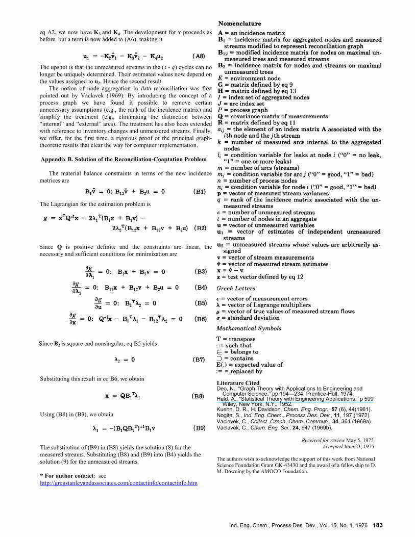
Appendix B. Solution of the Reconciliation-Coaptation Problem

The material balance constraints in terms of the new incidence

matrices are

The Lagrangian for the estimation problem is

Since Q is positive definite and the constraints are linear, the

necessary and sufficient conditions for minimization are

Substituting this result in eq B6, we obtain

Using (B8) in (B3), we obtain

The substitution of (B9) in (B8) yields the solution (8) for the

measured streams. Substituting (B8) and (B9) into (B4) yields the

solution (9) for the unmeasured streams.

* For author contact: see

http://gregstanleyandassociates.com/contactinfo/contactinfo.htm

Literature Cited Deo, N., “Graph Theory with Applications to Engineering and Computer Science,” pp 194—234, Prentice-Hall, 1974.

Hald, A., “Statistical Theory with Engineering Applications,” p 599 Wiley, New York, N.Y., 1952.

Kuehn, D. R., H. Davidson, Chem. Eng. Progr., 57 (6), 44(1961). Nogita, S., Ind. Eng. Chem., Process Des. Dev., 11, 197 (1972). Vaclavek, C., Collect. Czech. Chem. Commun., 34, 364 (1969a). Vaclavek, C., Chem. Eng. Sci., 24, 947 (1969b).

Received for review May 5, 1975

Accepted June 23, 1975

The authors wish to acknowledge the support of this work from National Science Foundation Grant GK-43430 and the award of a fellowship to D. M. Downing by the AMOCO Foundation.

Since B2 is square and nonsingular, eq B5 yields

https://www.researchgate.net/publication/44561950_Statistical_Theory_With_Engineering_Applications?el=1_x_8&enrichId=rgreq-0704cf9d69a6019116f1ae48c8cd240f-XXX&enrichSource=Y292ZXJQYWdlOzIzMTI5NjYwMztBUzo5OTU3NzI5NDIyOTUwNUAxNDAwNzUyNDg1Mjcy

Documents

Reconcillation and Rectification of Process Flow and Inventory Data