Remote reference magnetotelluric impedance estimation of wideband data using hybrid algorithm

Remote reference magnetotelluric impedance estimation

of wideband data using hybrid algorithm

Shalivahan,1 Rajib K. Sinharay,2 and Bimalendu B. Bhattacharya3

Received 6 February 2006; revised 16 June 2006; accepted 15 August 2006; published 11 November 2006.

[1] Precise and accurate determination of the magnetotelluric (MT) impedance isfundamental to valid interpretation. This paper deals with the results of hybrid processingschemes in conjunction with the remote reference (RR), for a typical site out of severalsites collected over the wide band data (�103 to 10�3 Hz). The standard practice of MTimpedance estimation is the use of robust processing in conjunction with the remotereferencing. The estimation by robust technique helps in reducing the effect of outliers inthe electric field but is often not sensitive to the exceptional predictor (magnetic field)data, which are called leverage points. The data processed with robust M estimation(RME) exacerbated the bias problem in the dead band. The application of hybrid(coherence weighted estimation (CWE) + RME, rho-variance weighting + RME) andextra hybrid (CWE + rho variance + RME) approach helps in reducing the influence ofboth the outliers in the electric field and the leverage points. These two approachesperform considerably better than either data weighting scheme by itself.

Citation: Shalivahan, R. K. Sinharay, and B. B. Bhattacharya (2006), Remote reference magnetotelluric impedance estimation of

wideband data using hybrid algorithm, J. Geophys. Res., 111, B11103, doi:10.1029/2006JB004330.

1. Introduction

[2] The interpretation of magnetotelluric (MT) datarequires estimation of tensor impedance elements from theelectric (E) and magnetic (H) vector field measurementsassuming them to be a plane wave. There exists a linearstatistical model in the frequency domain which relates theN � 1 vector E of observations of the response (also calledas dependent) variable to the NX2, rank 2 matrix H ofpredictors (explanatory variables), Z is the solution 2 vector,and assuming a homogenous plane wave, as

E ¼ ZHþM ð1Þ

where M is an N � 1 vector of random errors, and N is thenumber of observations (i.e., N Fourier transform of Nindependent data sections at a given frequency). The leastsquares (LS) solution for model (1) is

Z ¼ HHH� ��1

HHE� �

ð2Þ

where the superscript H denotes the Hermitian (complexconjugate) transpose. The terms within parenthesis are theaverage estimates of autopower and cross-power spectrabased on available data. The predicted values of the

response from the regression are derived from the observedvalues by

E ¼ PE ð3Þ

Where the N � N matrix P is called the prediction or hatmatrix as it transforms the observed vector E into its LSusing equation (3). It is given by

P ¼ H HHH� ��1

HH ð4Þ

or

E ¼ HZ ð5Þ

The predictor matrix P is idempotent (PP = P) andsymmetric (PH = P). The regression residuals r is thedifferences between the measured values of the responsevariables E and predicted E (equation (5)). These serves asan estimate on the random errors. The classical Gauss-Markov theorem gives following condition for the linearregression to yield the best linear unbiased estimate:[3] 1. The error term, on average, has no effect on the

dependent variable.[4] 2. Explanatory variable(s) are determined indepen-

dently of the values of the error term (and, therefore, thedependent variable).[5] 3. The error term has a constant variance; the obser-

vations of the error term are assumed to be drawn contin-ually from identical distributions.[6] 4. The observations of the error term are uncorrelated

with each other.[7] The complex tensor impedance Z can be estimated by

Fourier transformation of time series and using the LS

JOURNAL OF GEOPHYSICAL RESEARCH, VOL. 111, B11103, doi:10.1029/2006JB004330, 2006

1Department of Applied Geophysics, Indian School of Mines, Dhanbad,India.

2Central Water and Power Research Station, Khadakwasla, Pune, India.3S. N. Bose National Centre for Basic Sciences, Salt Lake, Kolkata,

India.

Copyright 2006 by the American Geophysical Union.0148-0227/06/2006JB004330$09.00

B11103 1 of 10

method to obtain the possible fit to equation (1) [Sims et al.,1971]. However, for noisy data, this approach fails, seeEgbert and Livelybrooks [1996]:[8] Equation (1) is appropriate to the case where noise is

restricted to the output or the ‘‘predicted’’ electric fieldchannels, while the input magnetic field is observed withouterror. Thus the violation of this assumption would result inLS estimated impedance to be biased downward [Sims etal., 1971].[9] It is, usually, necessary to estimate the response

function Z from data corresponding to large residuals,which are usually called outliers. The common types ofoutliers are: point defects and local nonstationarity. Pointdefects are isolated outliers, which are independent of theassumed linear statistical model (equation (1)). Some exam-ples of point defects are transient instrumental errors andspike noise due to natural phenomena (e.g., nearby light-ning). Local nonstationarities in geophysical problems areseen in observations of the time-varying fields (Ex, Ey, Hx,and Hy): most of the time the data statistics are approxi-mately constant i.e., coming close in satisfying equation (1),but this stationary process is interrupted sporadically bybrief but intense disturbances such as magnetic storms withmarkedly different characteristics [Chave et al., 1987], andthese are non-Gaussian in nature. Even severe bias could beproduced by auroral substorm source fields of a short spatialscale [Garcia et al., 1997]. Some types of midlatitudesources have short and temporally variable spatial scales,which can also alter MT responses [Egbert et al., 2000].Because of marked nonstationarity, departures from thelinear statistical model that produce very large residuals inthe data are more likely than ‘‘normal’’ or ‘‘expected’’ andsuch residuals are heavy-tailed or very long tailed with aGaussian center. Therefore the conventional LS approach isbeset with problems.[10] Thus there are basically two types of statistical errors

inherent in the estimation of response function: random andbias errors due to E and/or H field noise. The statisticalerrors are due to all errors normal or nonnormal. Thevariance gives a quantitative measure of the precision ofan estimate. A precise estimate may still be inaccuratebecause of bias error due to E and/or H field noise.[11] To tackle the bias errors due to noise, remote

reference (RR) measurements of MT was suggested aboutthree decades back [Goubau et al., 1978a, 1978b; Gambleet al., 1979a, 1979b; Goubau et al., 1984]. The equation ofestimating RR MT impedance in terms of power spectraldensities for magnetic field reference is given by [Vozoff,1996]

Zxy ¼ExR

*y

D EHxR

*x

D E� ExR

*x

D EHxR

*y

D E

HyR*y

D EHxR*y

D E� HyR*x

D EHyR*x

D E ð6Þ

where Rx and Ry are the remote magnetic field components.The field components in asterisk indicate complex conjugate.Schultz et al. [1993] andGarcia et al. [1997] have shown thatthe RR can give severe bias in the auroral substorm sourcefields of a short spatial scale. MTestimates even get distortedfrom DC electric rail system [Junge, 1996].[12] A number of MT processing methods have been

proposed on the basis of some sort of coherence weighted

estimates (CWE) [Stodt, 1983; Jones and Jodicke, 1984]and apparent resistivity variance (rho-var) weighting esti-mates [Stodt, 1983, also J. A. Stodt, Computation of MTparameters and their error estimates, unpublished reportsubmitted to Phoenix Geophysics Ltd., 1980, hereinafterreferred to as J. A. Stodt, unpublished report, 1980].Subsequently, the robust M estimates (RME) [Huber,1981; Rousseeuw and Leroy, 1987] have been applied toestimate the impedance functions [Egbert and Booker,1986; Chave et al., 1987; Chave and Thompson, 1989;Jones et al., 1989; Larsen, 1989; Sutarno and Vozoff, 1989,1991; Larsen et al., 1996; Egbert and Livelybrooks,1996; Egbert, 1997; Shalivahan and Bhattacharya, 2002;Smirnov, 2003]. Banks [1998] has studied the effect ofnonstationary noise on electromagnetic response estimatesin the frequency range of 0.05–0.000167 Hz. RME process-ing has long been used for very low frequency (<0.1 Hz) MTandmagnetovariational data due to its easy availability. Joneset al. [1989] have demonstrated the superiority of the RMEprocessing for low-frequency MT data and further suggestedthat RR measurements, wherever possible, should be made.[13] The RME methods tackle the noise on the electric

field but are often not sensitive to exceptional predictor(magnetic field) data called as leverage point [Chave andThompson, 2004]. This happens particularly in the dead band5 Hz to 0.05 Hz and the MT impedance estimates by RMEprocessing are severely biased [Egbert and Livelybrooks,1996]. This happens because RME is sensitive to data, whichproduce statistically unusual residuals. Such data may or maynot correspond to all of the influential data in a data set. Somesuggested methodologies for tackling the outliers and lever-age points have been suggested by Egbert and Livelybrooks[1996], Shalivahan [2000], Garcia and Jones [2002], Jonesand Spratt [2002], and Chave and Thompson [2004]. Egbertand Livelybrooks [1996] have used for the first time, a hybridapproach, i.e., combination of CWE with RME only forsingle site MT impedance estimation over a wide band totackle the problems associated with the RME particularly inthe dead band (5–0.05 Hz). Shalivahan [2000] has used twohybrid approaches, i.e., combination of CWE with RME aswell as rho-var weighting with RME in conjunction with RRfor improving the data quality for the entire frequency rangeincluding the dead band. Garcia and Jones [2002] presortedAMT data based on the power in the magnetic field channels,selecting only those values, which exceed the known instru-ment noise level by a specified amount. Jones and Spratt[2002] preselected data segments whose vertical field powerwas below a threshold value to minimize auroral source fieldbias in high-latitude MT data.[14] In this paper we compare different processing

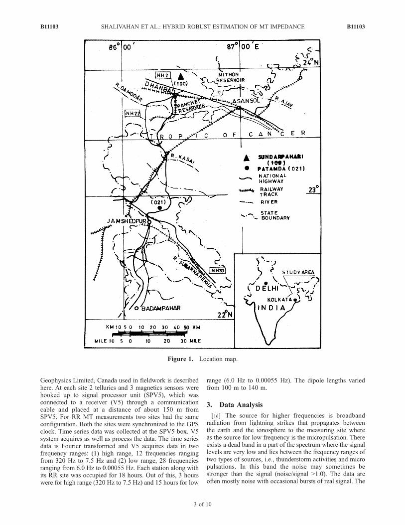
schemes, i.e., CWE, rho-var weighting, RME, hybridapproaches, i.e., the combinations of CWE with RME aswell as rho-var weighting with RME and extra hybridapproach (CWE+rho-var weighting+RME), in the estima-tion of RR MT impedance over a wide band (�103 Hz to10�3 Hz) for a representative site out of 44 sites ofDhanbad-Badampahar transect (Figure 1).

2. Data Acquisition

[15] A brief account ofMT data acquisition and processingsystem of V5-16 multiple geophysical receiver of Phoenix

B11103 SHALIVAHAN ET AL.: HYBRID ROBUST ESTIMATION OF MT IMPEDANCE

2 of 10

B11103

Geophysics Limited, Canada used in fieldwork is describedhere. At each site 2 tellurics and 3 magnetics sensors werehooked up to signal processor unit (SPV5), which wasconnected to a receiver (V5) through a communicationcable and placed at a distance of about 150 m fromSPV5. For RR MT measurements two sites had the sameconfiguration. Both the sites were synchronized to the GPSclock. Time series data was collected at the SPV5 box. V5system acquires as well as process the data. The time seriesdata is Fourier transformed and V5 acquires data in twofrequency ranges: (1) high range, 12 frequencies rangingfrom 320 Hz to 7.5 Hz and (2) low range, 28 frequenciesranging from 6.0 Hz to 0.00055 Hz. Each station along withits RR site was occupied for 18 hours. Out of this, 3 hourswere for high range (320 Hz to 7.5 Hz) and 15 hours for low

range (6.0 Hz to 0.00055 Hz). The dipole lengths variedfrom 100 m to 140 m.

3. Data Analysis

[16] The source for higher frequencies is broadbandradiation from lightning strikes that propagates betweenthe earth and the ionosphere to the measuring site whereas the source for low frequency is the micropulsation. Thereexists a dead band in a part of the spectrum where the signallevels are very low and lies between the frequency ranges oftwo types of sources, i.e., thunderstorm activities and micropulsations. In this band the noise may sometimes bestronger than the signal (noise/signal >1.0). The data areoften mostly noise with occasional bursts of real signal. The

Figure 1. Location map.


3 of 10

B11103

data noise may also remain a problem for the low-frequencysignals.[17] Following MT processing methods has been used:

(1) coherency weighted estimation (CWE), (2) apparentresistivity variance (rho-var) weighting, (3) robust M esti-mation (RME), (4) hybrid approach, and (5) extra hybridapproach to remove the statistical errors. The data processingbegins by dividing the time series into a sequence of shortdata segments and each is Fourier-transformed. This whencombined with frequency band averaging gives a series of Lcomplex data vectors for a given frequency w. The tensorimpedance Z (w) for that frequency is then estimated byminimizing weighted-residual sums of squares. The weighteddeviation for the x component electric field is given as

XLi¼1

wi Exi � ZxxHxi þ ZxyHyi

� �� 2 ð7Þ

The weights wi are estimated from the data. The CWE, rho-var and RME choose weights to emphasize the best qualitydata.

3.1. Coherency Weighted Estimation

[18] In CWE the sequence of L Fourier coefficient vectors[Egbert and Livelybrooks, 1996] are divided into q tempo-rary contiguous groups. Generally, the coefficients for groupq typically correspond to all data collected in one of a seriesof ‘‘runs’’ at the measuring site. Then for each group thestandard multiple coherence (gq

2) between the x componentof electric field and the magnetic field is computed. Thishelps in determining the weights as a function of gq

2. Thedata with higher value of gq

2 is given higher weight and viceversa. For RR estimation of the tensor impedance, ordinaryand multiple coherences between local and remote fieldscan also be computed [Stodt, 1983, also unpublished report,1980] to assess correlations between sites and determine thebest reference pair. For a RR the generalized multiplesquared coherence between the observed electric field Eand its predicted value E with magnetic field (R) as areference and the local magnetic field as H is given as[Chave and Thompson, 2004]

g2EE

¼SER SRHð Þ�1

SRE��

SEESHRE SHRHð Þ�1

SHH SHRHð Þ�1SRE

ð8Þ

where Sxy is a cross power between vector variables x and y.It is a complex quantity whose amplitude is analogous to thestandard multiple coherence and its phase is a measure ofthe similarity of the local and remote reference variables.The minimum value of squared coherency (gq

2) is set andonly those data segments meeting this minimum are used inthe estimation of the impedance. The coherence weight inthis instance consists of zeros and ones. J. A. Stodt(unpublished report, 1980) and Egbert and Livelybrooks[1996] have shown that CWE tends to increase the signal/noise ratio.

3.2. Apparent Resistivity Variance (rho-var)Weighting Estimation

[19] The expressions of variance are given by Gamble etal. [1979b]. The variance in each element of ZR (impedanceestimation using RR) can be expressed in terms of knownaverage powers, if it is assumed that the noise is indepen-

dent of signals, and the noise is stationary. The variancesdecrease as the number of measurements contained in theaverage power increases. In this case this number has beenfixed at 20 (J. A. Stodt, unpublished report, 1980). Here thevariances of apparent resistivities (rho) in conjunction withthe remote referencing computed from principle impedanceelements have been used. These are first averaged to obtaina minimum variance estimate.[20] Let us assume that the base field noises are uncor-

related with reference field noise so that the estimates ZR

are unbiased by correlated noise powers. The aim is toobtain a weighted average of the four stable estimates,which has the property that it is the minimum varianceunbiased estimate obtainable. This estimate is given by[Gamble et al., 1979a, 1979b; J. A. Stodt, unpublishedreport, 1980]

Zij ¼XMk¼1

WkZijk ð9Þ

where k indicates a sum over the weighted individualestimates and M is the four possible reference pairs, Ex

REyR,

HxRHy

R, ExRHx

R, and EyRHy

R used for the impedance estimates.The weights take the form

Wk ¼1=Var Zijk

� �PMk¼1

1=VarZijk

ð10Þ

For the impedance estimate to be unbiased the sum of the

weights should be equal to 1.0, i.e.,P41

Wi = 1. It is important

to average the real and imaginary parts of the ZijR, rather than

their magnitudes and phase, in order to avoid introducingother bias error. If the individual Zk are unbiased and if wehave accurate estimates of the Var Zk, then equation (10)will give an unbiased estimate with the minimum possiblevariance. If the Var Zk are not estimated accurately, then tooequation (10) gives an unbiased estimate but not with aminimum possible variance. The variance of the averageestimate Zij

R is given as (J. A. Stodt, unpublished report,1980)

VarZR

ij ¼X4k¼1

W 2k VarZ

R

ijkþ 2

X3k¼1

X4l¼2

WkWlCov ZRijk;ZR

ijl

� ð11Þ

If the variance estimates are accurate, then VarZijk

R will besmaller than any of the VarZijk. Gamble et al. [1979b]defined Var Zij as

VarZRij ¼

rij j2 Aj

�� 2N Dj j2

ð12Þ

where

Dj j2¼ HxRx*HyRy

*� HxRy*HyRx

*��

r ¼ E� E

A*x ¼ R*x HyR*y � R*y HyR*x

A*y ¼ R*y HxR*x � R*x HxR*y

Aj

�� 2¼ AjAj*


4 of 10

B11103

N is the number of independent determinations of eachfield. For large value of N, one can replace jrij2 in equation(12) as

rPij j2¼ Ei

�� 2 � 2 Re ZRixHxEi*þ ZR

iyHyEi

h* � ZR

ixZRiy*HxHy*

i

þ jZRixj

2jHxj2jZRiyj

2jHyj2

where Re(x) is the real part of x. N is the number of averagesin spectral estimates, i = x, y and j = x, y.[21] When the individual estimates Zk are obtained

from disjoint sets of spectra, then the variance of Zij is

VarZij ¼XMk¼1

W 2k VarZijk ð13Þ

If equation (10) is substituted into equation (13), ZRij

VarZRij ¼

1

Pk

1=VarZijk

�

and the variance of rho is (0.2T)2 Var (Zij).[22] The use of inverse variance as weights not only

incorporates the signal criteria but also down weights theevents for high coherence between the orthogonal compo-nents of magnetic field and down weights events for lowmultiple coherence between the output electric field and theinput magnetic components [Jones et al., 1989].[23] Variance of ZijR is correctly defined by the equation

(13) only if (1) R is uncorrelated with the noise in E and H,(2) the noises in E and H are independent of the signals, and(3) the noises are stationary. The purpose of RR technique isto ensure that the first condition is satisfied. The secondassumption is likely to be well satisfied if the noises aregenerated locally. On the other hand, if the noises arise frominhomogeneous atmospheric source, both assumptions 1and 2 may be violated. Assumption 2 may also be violatedif the measuring equipment produces errors that are pro-portional to the signal [Gamble et al., 1979b]. The require-ment of noise stationarity is not particularly restrictive. Herewe do not need to assume that the signals are stationarity. ZR

and errors in ZR involve only the ratios of average crosspowers and since the electric and magnetic fields (both fromlocal and remote) are causally related, these ratios do notdepend on the statistics of the field. Stodt [1983] has shownthat the scheme tends to increase signal/noise ratio.

3.3. Robust M Estimation

[24] Robustness signifies some level of insensitivity to asmall number of outliers in the data. For MT data, robust Mestimation (RME) are used [Egbert and Booker, 1986;Chave et al., 1987; Chave and Thompson, 1989; Joneset al., 1989; Larsen, 1989; Sutarno and Vozoff, 1989,1991; Egbert and Livelybrooks, 1996; Bhattacharya andShalivahan, 1999]. The impedance estimates by RME arerobust against violations of distributional assumption andthus are resistant to outliers. The weights in this case are

determined iteratively from the normalized residuals (r).The Huber weights as used by Egbert and Booker [1986],Chave et al. [1987], and Egbert and Livelybrooks [1996] aregiven as

wi ¼1 rij j 1:5

1:5= rij j rij j > 1:5

8<: ð14Þ

and

ri ¼Exi � ZxxHxi þ ZxyHyi

� �� s

Here s is the estimate of the scale of the error in theimpedance estimation and determines which of theresiduals are to be regarded as large. The medianabsolute deviation from median (MAD) gives one ofthe most robust estimates of scale. The sample value of itis given as:

SMAD ¼ r � r0j j Nþ1ð Þ=2 ð15Þ

Where N is the total number of values quantity r0 is themedian of r. The theoretical MAD is the solution sMAD

of

F m0 þ sMADð Þ � F ~m0 � sMAD

� �¼ 1=2 ð16Þ

Where m0 is the theoretical median and F denotes the targetcumulative distribution function. Robust processing pro-ceeds as follows: the LS approach determines the initialestimate of the impedance at each frequency, and is furtherused to compute the residuals r in (1) and s from the ratio ofequations (15) and (16). An iterative procedure is thenapplied with the weights as in (14) where the residuals fromthe previous iteration are used to get scale and weights. Thisprocess is repeated until convergence is reached. Huber[1981] has proved that the weights as used in equation (14)converge.[25] The RME can be even severely biased than the least

squares when typical signal/noise ratios are low (in deadband). It is also worth noting that the generalized RME,which down weights leverage points which may actuallydown weight or throw away the real data with the best signal-to-noise ratio exacerbating the bias problem.

3.4. Hybrid Approach

[26] The problem of affecting estimates when workingwith low signal data (in dead band) have been dealt by Park[1991] and Larsen et al. [1996] by reanalyzing all of the timeseries points each time a new estimate is made. This way, thepotential bias from the a few bad transfer functions estimatesis quickly identified and eliminated.[27] In order to overcome the problem of estimates in the

dead band we apply hybrid RME. The data recorded duringthe periods of high signal power are weighted more heavilyand then RME is applied. The weights are determined usingCWE and rho-var, and subsequently, RME is applied:(1) CWE plus RME, as CWE tends to improve the S/N ratio


5 of 10

B11103

and hence can decrease the bias effect; subsequently, theRME is applied to this CWE data [Egbert and Livelybrooks,1996]; and (2) rho-var weighting plus RME, as rho-var tendsto improve the signal/noise ratio and hence decreases the biaseffect due to the low signal data. Using rho-var, we weightmore heavily the data recorded during the periods of high

signal power. The RME is then applied to this rho-varweighted data (J. A. Stodt, unpublished report, 1980).

3.5. Extra Hybrid Approach (CWE Plusrho-var Weighting Plus RME)

[28] The extra hybrid scheme works in three stages. First,it weights according to the coherences of the induced

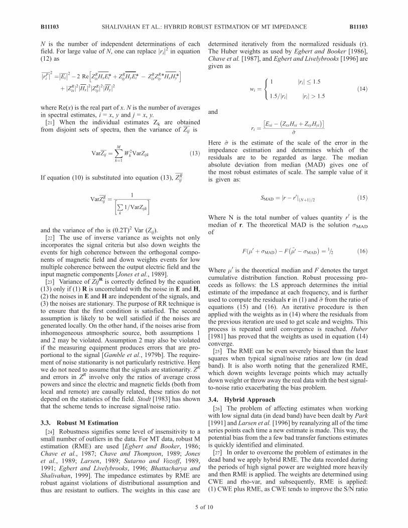
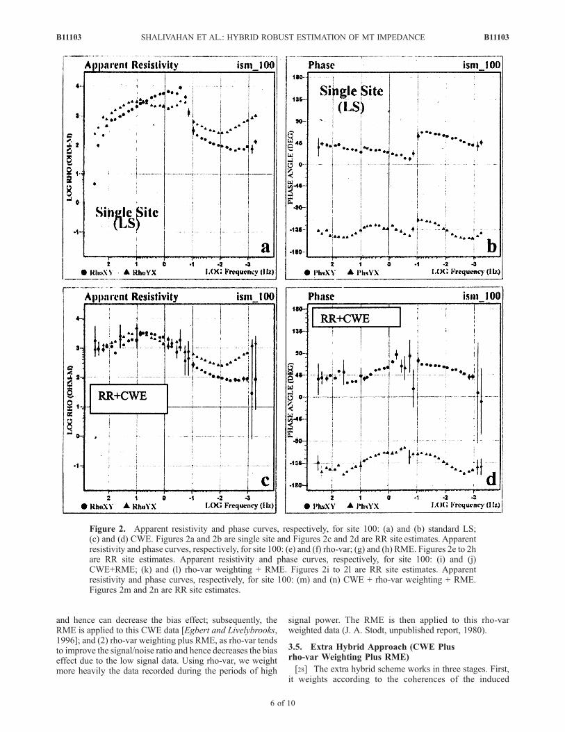
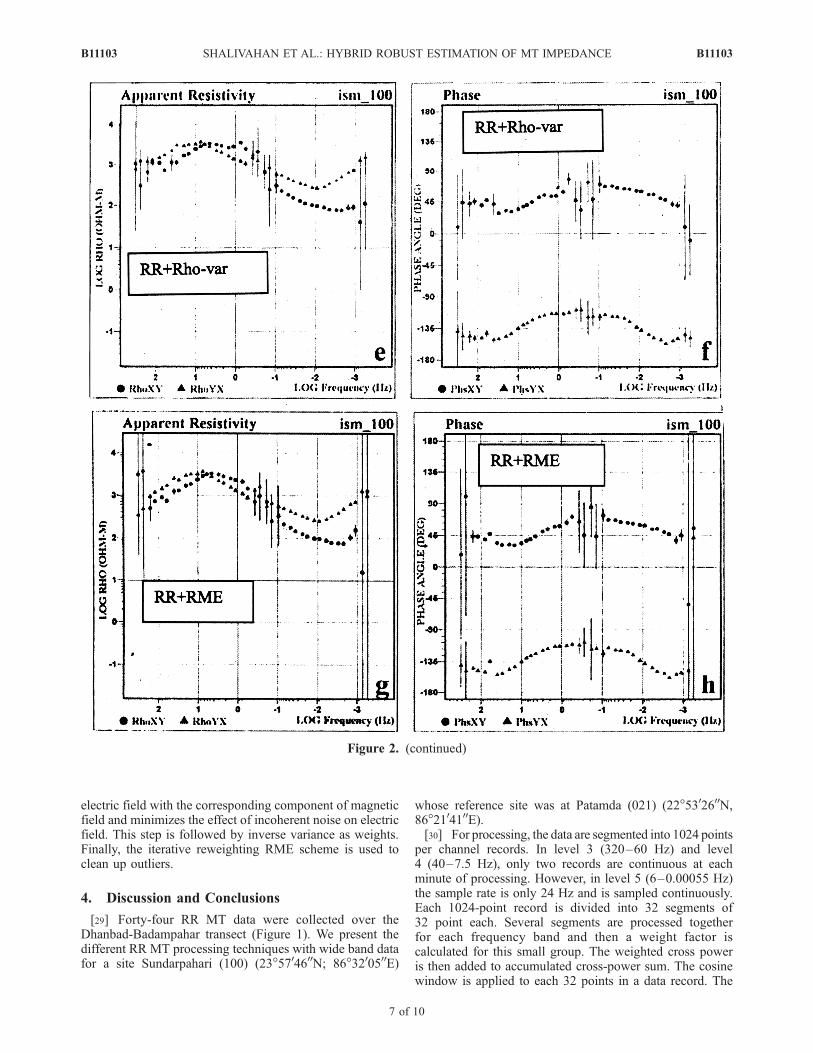
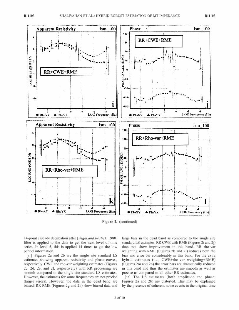
Figure 2. Apparent resistivity and phase curves, respectively, for site 100: (a) and (b) standard LS;(c) and (d) CWE. Figures 2a and 2b are single site and Figures 2c and 2d are RR site estimates. Apparentresistivity and phase curves, respectively, for site 100: (e) and (f) rho-var; (g) and (h) RME. Figures 2e to 2hare RR site estimates. Apparent resistivity and phase curves, respectively, for site 100: (i) and (j)CWE+RME; (k) and (l) rho-var weighting + RME. Figures 2i to 2l are RR site estimates. Apparentresistivity and phase curves, respectively, for site 100: (m) and (n) CWE + rho-var weighting + RME.Figures 2m and 2n are RR site estimates.


6 of 10

B11103

electric field with the corresponding component of magneticfield and minimizes the effect of incoherent noise on electricfield. This step is followed by inverse variance as weights.Finally, the iterative reweighting RME scheme is used toclean up outliers.

4. Discussion and Conclusions

[29] Forty-four RR MT data were collected over theDhanbad-Badampahar transect (Figure 1). We present thedifferent RR MT processing techniques with wide band datafor a site Sundarpahari (100) (23�5704600N; 86�3200500E)

whose reference site was at Patamda (021) (22�5302600N,86�2104100E).[30] For processing, the data are segmented into 1024 points

per channel records. In level 3 (320–60 Hz) and level4 (40–7.5 Hz), only two records are continuous at eachminute of processing. However, in level 5 (6–0.00055 Hz)the sample rate is only 24 Hz and is sampled continuously.Each 1024-point record is divided into 32 segments of32 point each. Several segments are processed togetherfor each frequency band and then a weight factor iscalculated for this small group. The weighted cross poweris then added to accumulated cross-power sum. The cosinewindow is applied to each 32 points in a data record. The

Figure 2. (continued)


7 of 10

B11103

14-point cascade decimation after [Wight and Bostick, 1980]filter is applied to the data to get the next level of timeseries. In level 5, this is applied 14 times to get the lowperiod information.[31] Figures 2a and 2b are the single site standard LS

estimates showing apparent resistivity and phase curves,respectively. CWE and rho-var weighting estimates (Figures2c, 2d, 2e, and 2f, respectively) with RR processing aresmooth compared to the single site standard LS estimates.However, the estimates for some frequencies are not precise(larger errors). However, the data in the dead band arebiased. RR RME (Figures 2g and 2h) show biased data and

large bars in the dead band as compared to the single sitestandard LS estimates. RR CWE with RME (Figures 2i and 2j)does not show improvement in this band. RR rho-varweighting with RME (Figures 2k and 2l) reduces both thebias and error bar considerably in this band. For the extrahybrid estimates (i.e., CWE+rho-var weighting+RME)(Figures 2m and 2n) the error bars are dramatically reducedin this band and thus the estimates are smooth as well asprecise as compared to all other RR estimates.[32] The LS estimates (both amplitude and phase;

Figures 2a and 2b) are distorted. This may be explainedby the presence of coherent noise events in the original time



8 of 10

B11103

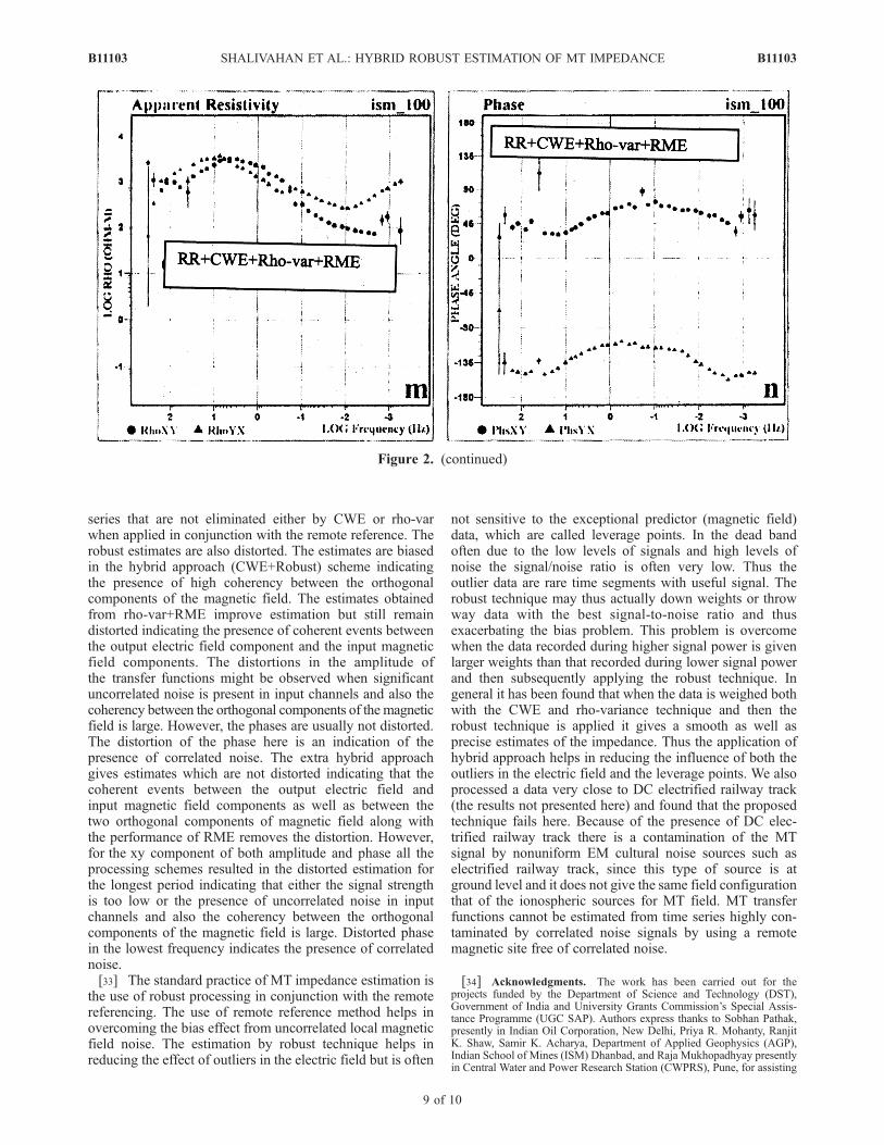
series that are not eliminated either by CWE or rho-varwhen applied in conjunction with the remote reference. Therobust estimates are also distorted. The estimates are biasedin the hybrid approach (CWE+Robust) scheme indicatingthe presence of high coherency between the orthogonalcomponents of the magnetic field. The estimates obtainedfrom rho-var+RME improve estimation but still remaindistorted indicating the presence of coherent events betweenthe output electric field component and the input magneticfield components. The distortions in the amplitude ofthe transfer functions might be observed when significantuncorrelated noise is present in input channels and also thecoherency between the orthogonal components of the magneticfield is large. However, the phases are usually not distorted.The distortion of the phase here is an indication of thepresence of correlated noise. The extra hybrid approachgives estimates which are not distorted indicating that thecoherent events between the output electric field andinput magnetic field components as well as between thetwo orthogonal components of magnetic field along withthe performance of RME removes the distortion. However,for the xy component of both amplitude and phase all theprocessing schemes resulted in the distorted estimation forthe longest period indicating that either the signal strengthis too low or the presence of uncorrelated noise in inputchannels and also the coherency between the orthogonalcomponents of the magnetic field is large. Distorted phasein the lowest frequency indicates the presence of correlatednoise.[33] The standard practice of MT impedance estimation is

the use of robust processing in conjunction with the remotereferencing. The use of remote reference method helps inovercoming the bias effect from uncorrelated local magneticfield noise. The estimation by robust technique helps inreducing the effect of outliers in the electric field but is often

not sensitive to the exceptional predictor (magnetic field)data, which are called leverage points. In the dead bandoften due to the low levels of signals and high levels ofnoise the signal/noise ratio is often very low. Thus theoutlier data are rare time segments with useful signal. Therobust technique may thus actually down weights or throwway data with the best signal-to-noise ratio and thusexacerbating the bias problem. This problem is overcomewhen the data recorded during higher signal power is givenlarger weights than that recorded during lower signal powerand then subsequently applying the robust technique. Ingeneral it has been found that when the data is weighed bothwith the CWE and rho-variance technique and then therobust technique is applied it gives a smooth as well asprecise estimates of the impedance. Thus the application ofhybrid approach helps in reducing the influence of both theoutliers in the electric field and the leverage points. We alsoprocessed a data very close to DC electrified railway track(the results not presented here) and found that the proposedtechnique fails here. Because of the presence of DC elec-trified railway track there is a contamination of the MTsignal by nonuniform EM cultural noise sources such aselectrified railway track, since this type of source is atground level and it does not give the same field configurationthat of the ionospheric sources for MT field. MT transferfunctions cannot be estimated from time series highly con-taminated by correlated noise signals by using a remotemagnetic site free of correlated noise.

[34] Acknowledgments. The work has been carried out for theprojects funded by the Department of Science and Technology (DST),Government of India and University Grants Commission’s Special Assis-tance Programme (UGC SAP). Authors express thanks to Sobhan Pathak,presently in Indian Oil Corporation, New Delhi, Priya R. Mohanty, RanjitK. Shaw, Samir K. Acharya, Department of Applied Geophysics (AGP),Indian School of Mines (ISM) Dhanbad, and Raja Mukhopadhyay presentlyin Central Water and Power Research Station (CWPRS), Pune, for assisting



9 of 10

B11103

in collecting data. All the computations were carried out in the computercentre of UGC SAP of AGP, ISM. R.K.S. also thanks CWPRS. The lastauthor (B.B.B.) thanks Council of Scientific and Industrial Research (CSIR)and National Academy of Engineers (INAE) for their support.

ReferencesBanks, R. J. (1998), The effects of non-stationary noise on electromagneticresponse estimates, Geophys. J. Int., 135, 553–563.

Bhattacharya, B. B., and Shalivahan (1999), Application of robust processingof MT data using single and remote sites, Current Sci., 76, 1108–1113.

Chave, A. D., and D. J. Thompson (1989), Some comments on magneto-telluric response function estimation, J. Geophys. Res., 94, 14,215–14,226.

Chave, A. D., and D. J. Thompson (2004), Bounded influence magneto-telluric response function estimation, Geophys. J. Int., 157, 988–1006.

Chave, A. D., D. J. Thompson, and M. E. Ander (1987), On the robustestimation of power spectra coherences and transfer functions, J. Geo-phys. Res., 92, 633–648.

Egbert, D. G. (1997), Robust multiple-station magnetotelluric data proces-sing, Geophys. J. Int., 130, 475–496.

Egbert, G., and J. R. Booker (1986), Robust estimation of geomagnetictransfer functions, Geophys. J. R. Astron. Soc., 87, 173–194.

Egbert, G., and D. W. Livelybrooks (1996), Single station magnetotelluricimpedance estimation: Coherence weighting and the regressionM-estimate, Geophysics, 61, 964 – 970.

Egbert, G. D., M. Eisel, O. S. Boyd, and H. F. Morrison (2000), DC trainsand Pc3s: Source effects in mid-latitude geomagnetic transfer functions,Geophys. Res. Lett., 27, 25–28.

Gamble, T. D., W. M. Goubau, and J. Clarke (1979a), Magnetotelluricswith a remote reference, Geophysics, 44, 53–68.

Gamble, T. D., W. M. Goubau, and J. Clarke (1979b), Error analysis forremote reference magnetotellurics, Geophysics, 44, 959–968.

Garcia, X., and A. G. Jones (2002), Atmospheric sources for audiomagne-totelluric (AMT) soundings, Geophysics, 67, 448–458.

Garcia, X., A. D. Chave, and A. G. Jones (1997), Robust processing ofmagnetotelluric data from the auroral zone, J. Geomagn. Geolectr., 49,1451–1468.

Goubau, W. M., T. D. Gamble, and J. Clarke (1978a), Magnetotelluricsusing loch-in signal detection, Geophys. Res. Lett., 5, 543–546.

Goubau, W. M., T. D. Gamble, and J. Clarke (1978b), Magnetotelluric dataanalysis. removal of bias, Geophysics, 43, 1157–1166.

Goubau, W. M., P. M. Moxton, R. H. Koch, and J. Clarke (1984), Noisecorrelation lengths in remote reference magnetotellurics, Geophysics, 49,432–438.

Huber, P. J. (1981), Robust Statistics, John Wiley, Hoboken, N. J.Jones, A. G., and H. Jodicke (1984), Magnetotelluric transfer functionestimation improvement by a coherence based rejection, paper presentedat 54thAnnual InternationalMeeting, Soc. ofExplor.Geophys.,Atlanta,Ga.

Jones, A. G., and J. Spratt (2002), A simple method for deriving the uni-form field MT response in auroral zones, Earth Planets Space, 54, 443–450.

Jones, A. G., A. D. Chave, G. D. Egbert, D. Auld, and K. Bahr (1989), Acomparison of techniques for magnetotelluric response function estima-tion, J. Geophys. Res., 94, 14,201–14,214.

Junge, A. (1996), Characterization and correction for cultural noise, Surv.Geophys., 17, 361–391.

Larsen, J. C. (1989), Transfer functions: Smooth robust estimates by LSsand remote reference methods, Geophys. J. Int., 99, 655–663.

Larsen, J. C., R. L. Mackie, A. Mazella, A. Fiordelisi, and S. Rieven(1996), Robust smooth magnetotelluric transfer functions, Geophys. J.Int., 124, 801–819.

Park, S. K. (1991), Monitoring resistivity changes prior to earthquakes inParkfield, California with telluric array, J. Geophys. Res., 96, 14,211–14,237.

Rousseeuw, P. J., and A. M. Leroy (1987), Robust Regression and OutlierDetection, John Wiley, Hoboken, N. J.

Schultz, A., R. D. Kurtz, A. D. Chave, and A. G. Jones (1993), Conduc-tivity discontinuities in the upper mantle beneath a stable craton, Geo-phys. Res. Lett., 20, 2941–2944.

Shalivahan (2000), Nonlinear inversion of electrical and magnetotelluricdata using very fast simulated annealing, Ph.D. thesis, Indian School ofMines, Dhanbad, India.

Shalivahan, and B. B. Bhattacharya (2002), How remote can the far remotereference site for magnetotelluric measurements?, J. Geophys. Res.,107(B6), 2105, doi:10.1029/2000JB000119.

Sims, W. E., F. X. Bostick, and H. W. Smith (1971), The estimation ofmagnetotelluric impedance tensor elements from measured data, Geophy-sics, 36, 938–942.

Smirnov, M. Y. (2003), Magnetotelluric data processing with a robust sta-tistical procedure having a high breakdown point, Geophys. J. Int., 152,1–7.

Stodt, J. A. (1983), Noise analysis for conventional and remote referencemagnetotellurics, Ph.D. thesis, Univ. of Utah, Salt Lake City.

Sutarno, D., and K. Vozoff (1989), Robust M-estimation of magnetotelluricimpedance tensor, Explor. Geophys., 20, 383–398.

Sutarno, D., and K. Vozoff (1991), Phase-smoothed robust M-estimation ofmagnetotelluric impedance functions, Geophysics, 56, 1999–2007.

Vozoff, K. (1996), The magnetotelluric method, in Electromagnetic Meth-ods in Applied Geophysics, edited by M. N. Nabighian, pp. 641–711,Soc. of Explor. Geophys., Tulsa, Okla.

Wight, D. E., and F. X. Bostick (1980), Cascade decimation—A techniquefor real time estimation of power spectrum, paper presented at IEEEInternational Conference on Acoustic, Speech Signal Processing, Denver,Colo., 9–11 April.

��B. B. Bhattacharya, S. N. Bose National Centre for Basic Sciences,

Sector-III, Block-JD, Salt Lake, Kolkata -700 098, India.Shalivahan, Department of Applied Geophysics, Indian School of Mines,

Dhanbad 826 004, India. ([email protected])R. K. Sinharay, Central Water and Power Research Station, Khadakwasla,

Pune, 411 024, India.


10 of 10

B11103

Documents

Remote reference magnetotelluric impedance estimation of wideband data using hybrid algorithm