Embed Size (px)
Citation preview
arX
ivh
ep-t
h07
0206
8v1
9 F
eb 2
007
Renormalisationof non-13ommutative eld theoriesVin13ent RivasseaualowastFabien Vignes-TourneretbFebruary 2 2008aLaboratoire de Physique Theacuteorique Bacirct 210Universiteacute Paris XI F-91405 Orsay Cedex Fran13ee-mail rivassthu-psudfr
bIHEacuteS Le Bois-Marie 35 route de Chartres F-91440 Bures-sur-Yvette Fran13ee-mail vignesihesfrAbstra13tThe rst renormalisable quantum eld theories on non-13ommutative spa13e havebeen found re13ently We review this rapidly growing subje13tContents1 Introdu13tion 211 The Quantum Hall ee13t 412 String Theory in ba13kground eld 52 Non-13ommutative eld theory 621 Field theory on Moyal spa13e 6211 The Moyal spa13e RDθ 6212 The φ4-theory on R4
θ 9213 UVIR mixing 922 The Grosse-Wulkenhaar breakthrough 1023 The non-13ommutative Gross-Neveu model 123 Multi-s13ale analysis in the matrix basis 1431 A dynami13al matrix model 14311 From the dire13t spa13e to the matrix basis 14312 Topology of ribbon graphs 1532 Multi-s13ale analysis 15321 Bounds on the propagator 16322 Power 13ounting 17lowastThis review follows le13tures given by VR at the workshop Renormalisation et theacuteories de GaloisLuminy Mar13h 2006 1
33 Propagators on non-13ommutative spa13e 19331 Bosoni13 kernel 19332 Fermioni13 kernel 20333 Bounds 2234 Propagators and renormalisability 224 Dire13t spa13e 2341 Short and long variables 2442 Routing Filk moves 25421 Oriented graphs 25422 Position routing 25423 Filk moves and rosettes 26424 Rosette fa13tor 2743 Renormalisation 28431 Four-point fun13tion 28432 Two-point fun13tion 29433 The Langmann-Szabo-Zarembo model 30434 Criti13al models 3044 Non-13ommutative hyperboli13 polynomials 3245 Con13lusion 361 Introdu13tionGeneral relativity and ordinary dierential geometry should be repla13ed by non-13ommutativegeometry at some point between the 13urrently a1313essible energies of about 1 - 10 Tev (af-ter starting the Large Hadron Collider (LHC) at CERN) and the Plan13k s13ale whi13h is1015 times higher where spa13e-time and gravity should be quantizedThis 13ould o1313ur either at the Plan13k s13ale or below Quantum eld theory on a non-13ommutative spa13e-time (NCQF) 13ould very well be an intermediate theory relevant forphysi13s at energies between the LHC and the Plan13k s13ale It 13ertainly looks intermediatein stru13ture between ordinary quantum eld theory on 13ommutative R4 and string theorythe 13urrent leading 13andidate for a more fundamental theory in13luding quantized gravityNCQFT in fa13t appears as an ee13tive model for 13ertain limits of string theory [1 2In joint work with R Gurau J Magnen and F Vignes-Tourneret [3 using dire13tspa13e methods we provided re13ently a new proof that the Grosse-Wulkenhaar s13alar Φ4
4theory on the Moyal spa13e R4 is renormalisable to all orders in perturbation theoryThe Grosse-Wulkenhaar breakthrough [4 5 was to realize that the right propagatorin non-13ommutative eld theory is not the ordinary 13ommutative propagator but has tobe modied to obey Langmann-Szabo duality [6 5 Grosse and Wulkenhaar were ableto 13ompute the 13orresponding propagator in the so 13alled matrix base whi13h transformsthe Moyal produ13t into a matrix produ13t This is a real tour de for13e They use thisrepresentation to prove perturbative renormalisability of the theory up to some estimateswhi13h were nally proven in [7Our dire13t spa13e method builds upon the previous works of Filk and Chepelev-Roiban[8 9 These works however remained in13on13lusive [10 sin13e these authors used the right2
intera13tion but not the right propagator hen13e the problem of ultravioletinfrared mixingprevented them from obtaining a nite renormalised perturbation seriesWe also extend the Grosse-Wulkenhaar results to more general models with 13ovari-ant derivatives in a xed magneti13 eld [11 Our proof relies on a multis13ale analysisanalogous to [7 but in dire13t spa13eNon-13ommutative eld theories (for a general review see [12) deserve a thoroughand systemati13 investigation not only be13ause they may be relevant for physi13s beyondthe standard model but also (although this is often less emphasized) be13ause they 13andes13ribe ee13tive physi13s in our ordinary standard world but with non-lo13al intera13tionsIn this 13ase there is an interesting reversal of the initial Grosse-Wulkenhaar problem-ati13 In the Φ44 theory on the Moyal spa13e R4 the vertex is sort of God-given by the Moyalstru13ture and it is LS invariant The 13hallenge was to over13ome uvir mixing and to ndthe right propagator whi13h makes the theory renormalisable This propagator turned outto have LS duality The harmoni13 potential introdu13ed by Grosse and Wulkenhaar 13anbe interpreted as a pie13e of 13ovariant derivatives in a 13onstant magneti13 eldNow to explain the (fra13tional) quantum Hall ee13t whi13h is a bulk ee13t whose un-derstanding requires ele13tron intera13tions we 13an almost invert this logi13 The propagatoris known sin13e it 13orresponds to non-relativisti13 ele13trons in two dimensions in a 13onstantmagneti13 eld It has LS duality But the intera13tion is un13lear and 13annot be lo13al sin13eat strong magneti13 eld the spins should align with the magneti13 eld hen13e by Pauliprin13iple lo13al intera13tions among ele13trons in the rst Landau level should vanishWe 13an argue that among all possible non-lo13al intera13tions a few renormalisationgroup steps should sele13t the only ones whi13h form a renormalisable theory with the 13orre-sponding propagator In the 13ommutative 13ase (ie zero magneti13 eld) lo13al intera13tionssu13h as those of the Hubbard model are just renormalisable in any dimension be13ause ofthe extended nature of the Fermi-surfa13e singularity Sin13e the non-13ommutative ele13tronpropagator (ie in non zero magneti13 eld) looks very similar to the Grosse-Wulkenhaarpropagator (it is in fa13t a generalization of the Langmann-Szabo-Zarembo propagator)we 13an 13onje13ture that the renormalisable intera13tion 13orresponding to this propagatorshould be given by a Moyal produ13t Thats why we hope that non-13ommutative eldtheory is the 13orre13t framework for a mi13ros13opi13 ab initio understanding of the fra13tionalquantum Hall ee13t whi13h is 13urrently la13kingEven for regular 13ommutative eld theory su13h as non-Abelian gauge theory thestrong 13oupling or non-perturbative regimes may be studied fruitfully through their non-13ommutative (ie non lo13al) 13ounterparts This point of view is for13efully suggested in[2 where a mapping is proposed between ordinary and non-13ommutative gauge eldswhi13h do not preserve the gauge groups but preserve the gauge equivalent 13lasses We13an at least remark that the ee13tive physi13s of 13onnement should be governed by anon-lo13al intera13tion as is the 13ase in ee13tive strings or bags modelsIn other words we propose to base physi13s upon the renormalisability prin13iple morethan any other axiom Renormalisability means generi13ity only renormalisable intera13-tions survive a few RG steps hen13e only them should be used to des13ribe generi13 ee13tivephysi13s of any kind The sear13h for renormalisabilty 13ould be the powerful prin13iple onwhi13h to orient ourselves in the jungle of all possible non-lo13al intera13tionsRenormalisability has also attra13ted 13onsiderable interest in the re13ent years as apure mathemati13al stru13ture The work of Kreimer and Connes [13 14 15 re13asts the3
re13ursive BPHZ forest formula of perturbative renormalisation in a ni13e Hopf algebrastru13ture The renormalisation group ambiguity reminds mathemati13ians of the Galoisgroup ambiguity for roots of algebrai13 equations Finding new renormalisable theoriesmay therefore be important for the future of pure mathemati13s as well as for physi13sThat was for13efully argued during the Luminy workshop Renormalisation and GaloisTheory Main open 13onje13tures in pure mathemati13s su13h as the Riemann hypothesis[16 17 or the Ja13obian 13onje13ture [18 may benet from the quantum eld theory andrenormalisation group approa13hConsidering that most of the Connes-Kreimer works uses dimensional regularizationand the minimal dimensional renormalisation s13heme it is interesting to develop the para-metri13 representation whi13h generalize S13hwingers parametri13 representation of Feynmanamplitudes to the non 13ommutative 13ontext It involves hyperboli13 generalizations of theordinary topologi13al polynomials whi13h mathemati13ians 13all Kir13ho polynomials andphysi13ist 13all Symanzik polynomials in the quantum eld theory 13ontext [19 We planalso to work out the 13orresponding regularization and minimal dimensional renormalisa-tion s13heme and to re13ast it in a Hopf algebra stru13ture The 13orresponding stru13turesseem ri13her than in ordinary eld theory sin13e they involve ribbon graphs and invariantswhi13h 13ontain information about the genus of the surfa13e on whi13h these graphs liveA 13riti13al goal to enlarge the 13lass of renormalisable non-13ommutative eld theories andto atta13k the Quantum Hall ee13t problem is to extend the results of Grosse-Wulkenhaarto Fermioni13 theories The simplest theory the two-dimensional Gross-Neveu model 13anbe shown renormalisable to all orders in their Langmann-Szabo 13ovariant versions usingeither the matrix basis [20 or the dire13t spa13e version developed here [21 However thex-spa13e version seems the most promising for a 13omplete non-perturbative 13onstru13tionusing Paulis prin13iple to 13ontroll the apparent (fake) divergen13es of perturbation theoryIn the 13ase of φ4
4 re13all that although the 13ommutative version is until now fatallyawed due to the famous Landau ghost there is hope that the non-13ommutative eldtheory treated at the perturbative level in this paper may also exist at the 13onstru13tivelevel Indeed a non trivial xed point of the renormalization group develops at highenergy where the Grosse-Wulkenhaar parameter Ω tends to 1 so that Langmann-Szaboduality be13ome exa13t and the beta fun13tion vanishes This s13enario has been 13he13kedexpli13itly to all orders of perturbation theory [22 23 24 This was done using the matrixversion of the theory again an x-spa13e version of renormalisation might be better for afuture rigorous non-perturbative investigation of this xed point and a full 13onstru13tiveversion of the modelFinally let us 13on13lude this short introdu13tion by reminding that a very important anddi13ult goal is to also extend the Grosse-Wulkenhaar breakthrough to gauge theories11 The Quantum Hall ee13tOne 13onsiders free ele13trons H0 = 12m
(p+eA)2 = π2
2mwhere p = mrminuseA is the 13anoni13al13onjugate of rThe moment and position p and r have 13ommutators
[pi pj] = 0 [ri rj] = 0 [pi rj ] = ı~δij (11)4
The moments π = mr = p + eA have 13ommutators[πi πj] = minusı~ǫijeB [ri rj ] = 0 [πi rj] = ı~δij (12)One 13an also introdu13e 13oordinates Rx Ry 13orresponding to the 13enters of the 13lassi13altraje13tories
Rx = xminus 1
eBπy Ry = y +
1
eBπx (13)whi13h do not 13ommute
[Ri Rj ] = ı~ǫij1
eB [πi Rj ] = 0 (14)This means that there exist Heisenberg-like relations between quantum positions12 String Theory in ba13kground eldOne 13onsiders the string a13tion in a generalized ba13kground
S =1
4παprime
int
Σ
(gmicroνpartaXmicropartaXνminus2πiαprimeBmicroνǫ
abpartaXmicropartbX
ν) (15)=
1
4παprime
int
Σ
gmicroνpartaXmicropartaXν minus i
2
int
partΣ
BmicroνXmicroparttX
ν (16)where Σ is the string worldsheet partt is a tangential derivative along the worldsheet bound-ary partΣ and Bmicroν is an antisymmetri13 ba13kground tensor The equations of motion deter-mine the boundary 13onditionsgmicroνpartnX
micro + 2πiαprimeBmicroνparttXmicro|partΣ = 0 (17)Boundary 13onditions for 13oordinates 13an be Neumann (B rarr 0) or Diri13hlet (g rarr 013orresponding to branes)After 13onformal mapping of the string worldsheet onto the upper half-plane the stringpropagator in ba13kground eld is
lt Xmicro(z)Xν(zprime) gt = minusαprime[gmicroν(log |z minus zprime| log |z minus zprime|)
+Gmicroν log |z minus zprime|2 + θmicroν log|z minus zprime||z minus zprime| + 13onst] (18)for some 13onstant symmetri13 and antisymmetri13 tensors G and θEvaluated at boundary points on the worldsheet this propagator is
lt Xmicro(τ)Xν(τ prime) gt= minusαprimeGmicroν log(τ minus τ prime)2 +i
2θmicroνǫ(τ minus τ prime) (19)where the θ term simply 13omes from the dis13ontinuity of the logarithm a13ross its 13utInterpreting τ as time one nds
[Xmicro Xν ] = iθmicroν (110)whi13h means that string 13oordinates lie in a non-13ommutative Moyal spa13e with parameterθ There is an equivalent argument inspired byM theory a rotation sandwi13hed betweentwo T dualities generates the same 13onstant 13ommutator for string 13oordinates5
2 Non-13ommutative eld theory21 Field theory on Moyal spa13eThe re13ent progresses 13on13erning the renormalisation of non-13ommutative eld theoryhave been obtained on a very simple non-13ommutative spa13e namely the Moyal spa13eFrom the point of view of quantum eld theory it is 13ertainly the most studied spa13eLet us start with its pre13ise denition211 The Moyal spa13e RDθLet us dene E = xmicro micro isin J1 DK and C〈E〉 the free algebra generated by E Let Θa D timesD non-degenerate skew-symmetri13 matrix (wi13h requires D even) and I the idealof C〈E〉 generated by the elements xmicroxν minus xνxmicro minus ıΘmicroν The Moyal algebra AΘ is thequotient C〈E〉I Ea13h element in AΘ is a formal power series in the xmicros for whi13h therelation [xmicro xν ] = ıΘmicroν holdsUsually one puts the matrix Θ into its 13anoni13al form
Θ =
0 θ1minusθ1 0
(0) (0)
0 θD2
minusθD2 0
(21)Sometimes one even set θ = θ1 = middot middot middot = θD2 The pre13eeding algebrai13 denition whereasshort and pre13ise may be too abstra13t to perform real 13omputations One then needsa more analyti13al denition A representation of the algebra AΘ is given by some setof fun13tions on R
d equipped with a non-13ommutative produ13t the Groenwald-Moyalprodu13t What follows is based on [25The Algebra AΘ The Moyal algebra AΘ is the linear spa13e of smooth and rapidlyde13reasing fun13tions S(RD) equipped with the non-13ommutative produ13t dened byforallf g isin SD
def= S(RD)(f ⋆Θ g)(x) =
int
RD
dDk
(2π)DdDy f(x+ 1
2Θ middot k)g(x+ y)eıkmiddoty (22)
=1
πD |det Θ|
int
RD
dDydDz f(x+ y)g(x+ z)eminus2ıyΘminus1z (23)This algebra may be 13onsidered as the fun13tions on the Moyal spa13e RDθ In the followingwe will write f ⋆ g instead of f ⋆Θ g and use forallf g isin SD forallj isin J1 2NK
(Ff)(x) =
intf(t)eminusıtxdt (24)for the Fourier transform and
(f ⋄ g)(x) =
intf(xminus t)g(t)e2ıxΘminus1tdt (25)6
for the twisted 13onvolution As on RD the Fourier transform ex13hange produ13t and13onvolutionF (f ⋆ g) =F (f) ⋄ F (g) (26)F (f ⋄ g) =F (f) ⋆F (g) (27)One also shows that the Moyal produ13t and the twisted 13onvolution are asso13iative
((f ⋄ g) ⋄ h)(x) =
intf(xminus tminus s)g(s)h(t)e2ı(xΘminus1t+(xminust)Θminus1s)ds dt (28)
=
intf(uminus v)g(v minus t)h(t)e2ı(xΘminus1vminustΘminus1v)dt dv
=(f ⋄ (g ⋄ h))(x) (29)Using (27) we show the asso13iativity of the ⋆-produit The 13omplex 13onjugation isinvolutive in AΘ
f ⋆Θ g =g ⋆Θ f (210)One also havef ⋆Θ g =g ⋆minusΘ f (211)Proposition 21 (Tra13e) For all f g isin SD
intdx (f ⋆ g)(x) =
intdx f(x)g(x) =
intdx (g ⋆ f)(x) (212)Proof
intdx (f ⋆ g)(x) =F (f ⋆ g)(0) = (Ff ⋄ Fg)(0) (213)
=
intFf(minust)Fg(t)dt = (Ff lowast Fg)(0) = F (fg)(0)
=
intf(x)g(x)dxwhere lowast is the ordinary 13onvolutionIn the following se13tions we will need lemma 22 to 13ompute the intera13tion terms forthe Φ4
4 and Gross-Neveu models We write x and y def= 2xΘminus1yLemma 22 For all j isin J1 2n+ 1K let fj isin AΘ Then
(f1 ⋆Θ middot middot middot ⋆Θ f2n) (x) =1
π2D det2 Θ
int 2nprod
j=1
dxjfj(xj) eminusıxand
P2ni=1(minus1)i+1xi eminusıϕ2n (214)
(f1 ⋆Θ middot middot middot ⋆Θ f2n+1) (x) =1
πD det Θ
int 2n+1prod
j=1
dxjfj(xj) δ(xminus
2n+1sum
i=1
(minus1)i+1xi
)eminusıϕ2n+1 (215)
forallp isin N ϕp =
psum
iltj=1
(minus1)i+j+1xi and xj (216)7
Corollary 23 For all j isin J1 2n+ 1K let fj isin AΘ Thenintdx (f1 ⋆Θ middot middot middot ⋆Θ f2n) (x) =
1
πD det Θ
int 2nprod
j=1
dxjfj(xj) δ( 2nsum
i=1
(minus1)i+1xi
)eminusıϕ2n (217)
intdx (f1 ⋆Θ middot middot middot ⋆Θ f2n+1) (x) =
1
πD det Θ
int 2n+1prod
j=1
dxjfj(xj) eminusıϕ2n+1 (218)
forallp isin N ϕp =
psum
iltj=1
(minus1)i+j+1xi and xj (219)The 13y13li13ity of the produ13t inherited from proposition 21 implies forallf g h isin SD〈f ⋆ g h〉 =〈f g ⋆ h〉 = 〈g h ⋆ f〉 (220)and allows to extend the Moyal algebra by duality into an algebra of tempered distribu-tionsExtension by Duality Let us rst 13onsider the produ13t of a tempered distributionwith a S13hwartz-13lass fun13tion Let T isin S prime
D and h isin SD We dene 〈T h〉 def= T (h) and
〈T lowast h〉 = 〈T h〉Denition 21 Let T isin S primeD f h isin SD we dene T ⋆ f and f ⋆ T by
〈T ⋆ f h〉 =〈T f ⋆ h〉 (221)〈f ⋆ T h〉 =〈T h ⋆ f〉 (222)For example the identity 1 as an element of S prime
D is the unity for the ⋆-produit forallf h isinSD
〈1 ⋆ f h〉 =〈1 f ⋆ h〉 (223)=
int(f ⋆ h)(x)dx =
intf(x)h(x)dx
=〈f h〉We are now ready to dene the linear spa13e M as the interse13tion of two sub-spa13es MLand MR of S primeDDenition 22 (Multipliers algebra)
ML = S isin S primeD forallf isin SD S ⋆ f isin SD (224)
MR = R isin S primeD forallf isin SD f ⋆ R isin SD (225)
M =ML capMR (226)One 13an show that M is an asso13iative lowast-algebra It 13ontains among others theidentity the polynomials the δ distribution and its derivatives Then the relation[xmicro xν ] =ıΘmicroν (227)often given as a denition of the Moyal spa13e holds in M (but not in AΘ)8
212 The φ4-theory on R4θThe simplest non-13ommutative model one may 13onsider is the φ4-theory on the four-dimensional Moyal spa13e Its Lagrangian is the usual (13ommutative) one where thepointwise produ13t is repla13ed by the Moyal one
S[φ] =
intd4x(minus 1
2partmicroφ ⋆ part
microφ+1
2m2 φ ⋆ φ+
λ
4φ ⋆ φ ⋆ φ ⋆ φ
)(x) (228)Thanks to the formula (23) this a13tion 13an be expli13itly 13omputed The intera13tion partis given by the 13orollary 23
intdxφ⋆4(x) =
int 4prod
i=1
dxi φ(xi) δ(x1 minus x2 + x3 minus x4)eıϕ (229)
ϕ =4sum
iltj=1
(minus1)i+j+1xi and xj The main 13hara13teristi13 of the Moyal produ13t is its non-lo13ality But its non-13ommutativityimplies that the vertex of the model (228) is only invariant under 13y13li13 permutation ofthe elds This restri13ted invarian13e in13ites to represent the asso13iated Feynman graphswith ribbon graphs One 13an then make a 13lear distin13tion between planar and non-planargraphs This will be detailed in se13tion 3Thanks to the delta fun13tion in (229) the os13illation may be written in dierent waysδ(x1 minus x2 + x3 minus x4)e
ıϕ =δ(x1 minus x2 + x3 minus x4)eıx1andx2+ıx3andx4 (230a)
=δ(x1 minus x2 + x3 minus x4)eıx4andx1+ıx2andx3 (230b)
=δ(x1 minus x2 + x3 minus x4) exp ı(x1 minus x2) and (x2 minus x3) (23013)The intera13tion is real and positive1int 4prod
i=1
dxiφ(xi) δ(x1 minus x2 + x3 minus x4)eıϕ (231)
=
intdk
(intdxdy φ(x)φ(y)eık(xminusy)+ıxandy
)2
isin R+It is also translation invariant as shows equation (23013)The property 21 implies that the propagator is the usual one C(p) = 1(p2 +m2)213 UVIR mixingThe non-lo13ality of the ⋆-produ13t allows to understand the dis13overy of Minwalla VanRaamsdonk and Seiberg [26 They showed that not only the model (228) isnt nitein the UV but also it exhibits a new type of divergen13es making it non-renormalisableIn the arti13le [8 Filk 13omputed the Feynman rules 13orresponding to (228) He showed1Another way to prove it is from (210) φ⋆4 = φ⋆49
that the planar amplitudes equal the 13ommutative ones whereas the non-planar ones giverise to os13illations 13oupling the internal and external legs A typi13al example is the thenon-planar tadpole=
λ
12
intd4k
(2π)4
eipmicrokνΘmicroν
k2 +m2
=λ
48π2
radicm2
(Θp)2K1(
radicm2(Θp)2) ≃
prarr0pminus2 (232)If p 6= 0 this amplitude is nite but for small p it diverges like pminus2 In other words ifwe put an ultraviolet 13ut-o Λ to the k-integral the two limits Λ rarr infin and prarr 0 do not13ommute This is the UVIR mixing phenomena A 13hain of non-planar tadpoles insertedin bigger graphs makes divergent any fun13tion (with six points or more for example) Butthis divergen13e is not lo13al and 13ant be absorbed in a mass redenition This is whatmakes the model non-renormalisable We will see in se13tions 34 and 4 that the UVIRmixing results in a 13oupling of the dierent s13ales of the theory We will also note thatwe should distinguish dierent types of mixingThe UVIR mixing was studied by several groups First Chepelev and Roiban [9gave a power 13ounting for dierent s13alr models They were able to identify the divergentgraphs and to 13lassify the divergen13es of the theories thanks to the topologi13al data ofthe graphs Then V Gayral [27 showed that UVIR mixing is present on all isospe13-tral deformations (they 13onsist in 13urved generalisations of the Moyal spa13e and of thenon-13ommutative torus) For this he 13onsidered a s13alar model (228) and dis13overed13ontributions to the ee13tive a13tion whi13h diverge when the external momenta vanishThe UVIR mixing is then a general 13hara13teristi13 of the non-13ommutative theories atleast on the deformations22 The Grosse-Wulkenhaar breakthroughThe situation remained so until H Grosse and R Wulkenhaar dis13overed a way to denea renormalisable non-13ommutative model We will detail their result in se13tion 3 but themain message is the following By adding an harmoni13 term to the Lagrangian (228)
S[φ] =
intd4x(minus 1
2partmicroφ ⋆ part
microφ+Ω2
2(xmicroφ) ⋆ (xmicroφ) +
1
2m2 φ ⋆ φ+
λ
4φ ⋆ φ ⋆ φ ⋆ φ
)(x)(233)where x = 2Θminus1x and the metri13 is Eu13lidean the model in four dimensions is renor-malisable at all orders of perturbation [5 We will see in se13tion 4 that this additionalterm give rise to an infrared 13ut-o and allows to de13ouple the dierent s13ales of thetheory The new model (233) we 13all it Φ4
4 do not exhibit any mixing This resultis very important be13ause it opens the way towards other non-13ommutative eld the-ories In the following we will 13all vul13anisation2 the pro13edure 13onsisting in adding a2TECHNOL Opeacuteration 13onsistant agrave traiter le 13aout13hou13 naturel ou syntheacutetique par addition desoufre pour en ameacuteliorer les proprieacuteteacutes meacute13aniques et la reacutesistan13e aux variations de tempeacuterature Treacutesorde la Langue Franccedilaise informatiseacute httpwwwlexilogos13om10
new term to a Lagrangian of a non-13ommutative theory in order to make it renormalisableThe propagator C of this Φ4 theory is the kernel of the inverse operatorminus∆+Ω2x2+m2It is known as the Mehler kernel [28 20C(x y) =
Ω2
θ2π2
int infin
0
dt
sinh2(2Ωt)eminus
eΩ2
coth(2eΩt)(xminusy)2minuseΩ2
tanh(2eΩt)(x+y)2minusm2t (234)Langmann and Szabo remarked that the quarti13 intera13tion with Moyal produ13t is in-variant under a duality transformation It is a symmetry between momentum and dire13tspa13e The intera13tion part of the model (233) is (see equation (217))Sint[φ] =
intd4x
λ
4(φ ⋆ φ ⋆ φ ⋆ φ)(x) (235)
=
int 4prod
a=1
d4xa φ(xa)V (x1 x2 x3 x4) (236)=
int 4prod
a=1
d4pa
(2π)4φ(pa) V (p1 p2 p3 p4) (237)with
V (x1 x2 x3 x4) =λ
4
1
π4 det Θδ(x1 minus x2 + x3 minus x4) cos(2(Θminus1)microν(x
micro1x
ν2 + xmicro
3xν4))
V (p1 p2 p3 p4) =λ
4(2π)4δ(p1 minus p2 + p3 minus p4) cos(
1
2Θmicroν(p1microp2ν + p3microp4ν))where we used a 13y13li13 Fourier transform φ(pa) =
intdx e(minus1)aıpaxaφ(xa) The transforma-tion
φ(p) harr π2radic
| detΘ|φ(x) pmicro harr xmicro (238)ex13hanges (236) and (237) In addition the free part of the model (228) isnt 13ovariantunder this duality The vul13anisation adds a term to the Lagrangian whi13h restores thesymmetry The theory (233) is then 13ovariant under the Langmann-Szabo dualityS[φmλΩ] 7rarrΩ2 S[φ
m
Ωλ
Ω2
1
Ω] (239)By symmetry the parameter Ω is 13onned in [0 1] Let us note that for Ω = 1 the modelis invariantThe interpretation of that harmoni13 term is not yet 13lear But the vul13anisation pro-13edure already allowed to prove the renormalisability of several other models on Moyalspa13es su13h that φ4
2 [29 φ324 [30 31 and the LSZ models [11 32 33 These last are ofthe type
S[φ] =
intdnx(1
2φ ⋆ (minuspartmicro + xmicro +m)2φ+
λ
4φ ⋆ φ ⋆ φ ⋆ φ
)(x) (240)11
By 13omparison with (233) one notes that here the additional term is formally equivalentto a xed magneti13 ba13kground Deep is the temptation to interpret it as su13h Thismodel is invariant under the above duality and is exa13tly soluble Let us remark thatthe 13omplex intera13tion in (240) makes the Langmann-Szabo duality more natural Itdoesnt need a 13y13li13 Fourier transform The φ3 have been studied at Ω = 1 where theyalso exhibit a soluble stru13ture23 The non-13ommutative Gross-Neveu modelApart from the Φ44 the modied Bosoni13 LSZ model [3 and supersymmetri13 theories wenow know several renormalizable non-13ommutative eld theories Nevertheless they eitherare super-renormalizable (Φ4
2 [29) or (and) studied at a spe13ial point in the parameterspa13e where they are solvable (Φ32Φ
34 [30 31 the LSZ models [11 32 33) Although onlylogarithmi13ally divergent for parity reasons the non-13ommutative Gross-Neveu model isa just renormalizable quantum eld theory as Φ4
4 One of its main interesting features isthat it 13an be interpreted as a non-lo13al Fermioni13 eld theory in a 13onstant magneti13ba13kground Then apart from strengthening the vul13anization pro13edure to get renor-malizable non-13ommutative eld theories the Gross-Neveu model may also be useful forthe study of the quantum Hall ee13t It is also a good rst 13andidate for a 13onstru13tivestudy [34 of a non-13ommutative eld theory as Fermioni13 models are usually easier to13onstru13t Moreover its 13ommutative 13ounterpart being asymptoti13ally free and exhibit-ing dynami13al mass generation [35 36 37 a study of the physi13s of this model would beinterestingThe non-13ommutative Gross-Neveu model (GN2Θ) is a Fermioni13 quarti13ally intera13tingquantum eld theory on the Moyal plane R2
θ The skew-symmetri13 matrix Θ isΘ =
(0 minusθθ 0
) (241)The a13tion is
S[ψ ψ] =
intdx(ψ(minusıpart + Ωx+m+ micro γ5
)ψ + Vo(ψ ψ) + Vno(ψ ψ)
)(x) (242)where x = 2Θminus1x γ5 = ıγ0γ1 and V = Vo + Vno is the intera13tion part given hereafterThe micro-term appears at two-loop order We use a Eu13lidean metri13 and the Feynman13onvention a = γmicroamicro The γ0 and γ1 matri13es form a two-dimensional representationof the Cliord algebra γmicro γν = minus2δmicroν Let us remark that the γmicros are then skew-Hermitian γmicrodagger = minusγmicroPropagator The propagator 13orresponding to the a13tion (242) is given by the followinglemma
12
Lemma 24 (Propagator [20) The propagator of the Gross-Neveu model isC(x y) =
intdmicroC(ψ ψ)ψ(x)ψ(y) =
(minusıpart + Ωx+m
)minus1(x y) (243)
=
int infin
0
dtC(t x y)
C(t x y) = minus Ω
θπ
eminustm2
sinh(2Ωt)eminus
eΩ2
coth(2eΩt)(xminusy)2+ıΩxandy (244)timesıΩ coth(2Ωt)(xminus y) + Ω(xminus y) minusm
eminus2ıΩtγΘminus1γwith Ω = 2Ω
θet x and y = 2xΘminus1yWe also have eminus2ıΩtγΘminus1γ = cosh(2Ωt)12 minus ıθ
2sinh(2Ωt)γΘminus1γIf we want to study a N -13olor model we 13an 13onsider a propagator diagonal in these13olor indi13esIntera13tions Con13erning the intera13tion part V re13all that (see 13orollary 23) for any
f1 f2 f3 f4 in AΘintdx (f1 ⋆ f2 ⋆ f3 ⋆ f4) (x) =
1
π2 det Θ
int 4prod
j=1
dxjfj(xj) δ(x1 minus x2 + x3 minus x4)eminusıϕ (245)
ϕ =4sum
iltj=1
(minus1)i+j+1xi and xj (246)This produ13t is non-lo13al and only invraiant under 13y13li13 permutations of the elds Then13ontrary to the 13ommutative Gross-Neveu model for whi13h there exits only one spinorialintera13tion the GN2Θ model has at least six dierent intera13itons the orientable ones
Vo =λ1
4
intdx(ψ ⋆ ψ ⋆ ψ ⋆ ψ
)(x) (247a)
+λ2
4
intdx(ψ ⋆ γmicroψ ⋆ ψ ⋆ γmicroψ
)(x) (247b)
+λ3
4
intdx(ψ ⋆ γ5ψ ⋆ ψ ⋆ γ5ψ
)(x) (24713)where ψs and ψs alternate and the non-orientable ones
Vno =λ4
4
intdx(ψ ⋆ ψ ⋆ ψ ⋆ ψ
)(x) (248a)
+λ5
4
intdx(ψ ⋆ γmicroψ ⋆ ψ ⋆ γmicroψ
)(x) (248b)
+λ6
4
intdx(ψ ⋆ γ5ψ ⋆ ψ ⋆ γ5ψ
)(x) (24813)All these intera13tions have the same x kernel thanks to the equation (245) The reasonfor whi13h we 13all these intera13tions orientable or not will be 13lear in se13tion 413
3 Multi-s13ale analysis in the matrix basisThe matrix basis is a basis for S13hwartz-13lass fun13tions In this basis the Moyal produ13tbe13omes a simple matrix produ13t Ea13h eld is then represented by an innite matrix[25 29 3831 A dynami13al matrix model311 From the dire13t spa13e to the matrix basisIn the matrix basis the a13tion (233) takes the formS[φ] =(2π)D2
radicdet Θ
(1
2φ∆φ+
λ
4Trφ4
) (31)where φ = φmn m n isin ND2 and
∆mnkl =
D2sum
i=1
(micro2
0 +2
θ(mi + ni + 1)
)δmlδnk (32)
minus 2
θ(1 minus Ω2)
(radic(mi + 1)(ni + 1) δmi+1liδni+1ki
+radicmini δmiminus1liδniminus1ki
)prod
j 6=i
δmj ljδnjkjThe (four-dimensional) matrix ∆ represents the quadrati13 part of the Lagragian Therst di13ulty to study the matrix model (31) is the 13omputation of its propagator Gdened as the inverse of ∆
sum
rsisinND2
∆mnrsGsrkl =sum
rsisinND2
Gmnrs∆srkl = δmlδnk (33)Fortunately the a13tion is invariant under SO(2)D2 thanks to the form (21) of the Θmatrix It implies a 13onservation law∆mnkl =0 lArrrArr m+ k 6= n + l (34)The result is [5 29
Gmm+hl+hl =θ
8Ω
int 1
0
dα(1 minus α)
micro20θ
8Ω+(D
4minus1)
(1 + Cα)D2
D2prod
s=1
G(α)msms+hsls+hsls (35)
G(α)mm+hl+hl =
(radic1 minus α
1 + Cα
)m+l+h min(ml)sum
u=max(0minush)
A(m l h u)
(Cα(1 + Ω)radic1 minus α (1 minus Ω)
)m+lminus2u
where A(m l h u) =radic(
mmminusu
)(m+hmminusu
)(l
lminusu
)(l+hlminusu
) and C is a fun13tion in Ω C(Ω) = (1minusΩ)2
4ΩThe main advantage of the matrix basis is that it simplies the intera13tion part φ⋆4be13omes Trφ4 But the propagator be13omes very 13omplli13atedLet us remark that the matrix model (31) is dynami13al its quadrati13 part is nottrivial Usually matrix models are lo13al 14
Denition 31 A matrix model is 13alled lo13al if Gmnkl = G(mn)δmlδnk and non-lo13alotherwiseIn the matrix theories the Feynman graphs are ribbon graphs The propagator Gmnklis then represented by the Figure 1 In a lo13al matrix model the propagator preservesFigure 1 Matrix Propagatorthe index values along the traje13tories (simple lines)312 Topology of ribbon graphsThe power 13ounting of a matrix model depends on the topologi13al data of its graphs Thegure 2 gives two examples of ribbon graphs Ea13h ribbon graph may be drawn on a
(a) Planar (b) Non-planarFigure 2 Ribbon Graphstwo-dimensional manifold A13tually ea13h graph denes the surfa13e on whi13h it is drawnLet a graph G with V verti13es I internal propagators (double lines) and F fa13es (madeof simple lines) The Euler 13hara13teristi13χ =2 minus 2g = V minus I + F (36)gives the genus g of the manifold One 13an make this 13lear by passing to the dual graphThe dual of a given graph G is obtained by ex13hanging fa13es and verti13es The dual graphsof the Φ4 theory are tesselations of the surfa13es on whi13h they are drawn Moreover ea13hdire13t fa13e broken by exernal legs be13omes in the dual graph a pun13ture If amongthe F fa13es of a graph B are broken this graph may be drawn on a surfa13e of genus
g = 1 minus 12(V minus I + F ) with B pun13tures The gure 3 gives the topologi13al data of thegraphs of the gure 232 Multi-s13ale analysisIn [7 V R R Wulkenhaar and F V-T used the multi-s13ale analysis to reprove thepower 13ounting of the non-13ommutative Φ4 theory15
=rArrV=3I=3F=2B=2 =rArr g = 0
=rArrV=2I=3F=1B=1 =rArr g = 1Figure 3 Topologi13al Data of Ribbon Graphs321 Bounds on the propagatorLet G a ribbon graph of the Φ4
4 theory with N external legs V verti13es I internal linesand F fa13es Its genus is then g = 1 minus 12(V minus I + F ) Four indi13es mn k l isin N2 areasso13iated to ea13h internal line of the graph and two indi13es to ea13h external line thatis to say 4I + 2N = 8V indi13es But at ea13h vertex the left index of a ribbon equalsthe right one of the neighbour ribbon This gives rise to 4V independant identi13ationswhi13h allows to write ea13h index in terms of a set I made of 4V indi13es four per vertexfor example the left index of ea13h half-ribbonThe graph amplitude is then
AG =sum
I
prod
δisinG
Gmδ(I)nδ(I)kδ(I)lδ(I) δmδminuslδnδminuskδ (37)where the four indi13es of the propagator G of the line δ are fun13tion of I and written
mδ(I) nδ(I) kδ(I) lδ(I) We de13ompose ea13h propagator given by (35)G =
infinsum
i=0
Gi thanks to int 1
0
dα =infinsum
i=1
int Mminus2(iminus1)
Mminus2i
dα M gt 1 (38)We have an asso13iated de13omposition for ea13h amplitudeAG =
sum
micro
AGmicro (39)AGmicro =
sum
I
prod
δisinG
Giδmδ(I)nδ(I)kδ(I)lδ(I) δmδ(I)minuslδ(I)nδ(I)minuskδ(I) (310)where micro = iδ runs over the all possible assignements of a positive integer iδ to ea13h line
δ We proved the following four propositionsProposition 31 For M large enough there exists a 13onstant K su13h that for Ω isin[05 1] we have the uniform bound
Gimm+hl+hl 6 KMminus2ieminus
Ω3
Mminus2im+l+h (311)16
Proposition 32 For M large enough there exists two 13onstants K and K1 su13h thatfor Ω isin [05 1] we have the uniform boundGi
mm+hl+hl
6 KMminus2ieminusΩ4
Mminus2im+l+h
D2prod
s=1
min
1
(K1 min(ms ls ms + hs ls + hs)
M2i
)|msminusls|2
(312)This bound allows to prove that the only diverging graphs have either a 13onstant indexalong the traje13tories or a total jump of 2Proposition 33 ForM large enough there exists a 13onstant K su13h that for Ω isin [2
3 1]we have the uniform bound
psum
l=minusm
Gimpminuslpm+l 6 KMminus2i eminus
Ω4
Mminus2i(p+m) (313)This bound shows that the propagator is almost lo13al in the following sense with mxed the sum over l doesnt 13ost anything (see Figure 1) Nevertheless the sums wellhave to perform are entangled (a given index may enter dierent propagators) so that weneed the following propositionProposition 34 ForM large enough there exists a 13onstant K su13h that for Ω isin [23 1]we have the uniform bound
infinsum
l=minusm
maxpgtmax(l0)
Gimpminuslpm+l 6 KMminus2ieminus
Ω36
Mminus2im (314)We refer to [7 for the proofs of these four propositions322 Power 13ountingAbout half of the 4V indi13es initially asso13iated to a graph is determined by the externalindi13es and the delta fun13tions in (37) The other indi13es are summation indi13es Thepower 13ounting 13onsists in nding whi13h sums 13ost M2i and whi13h 13ost O(1) thanks to(313) The M2i fa13tor 13omes from (311) after a summation over an index3 m isin N2infinsum
m1m2=0
eminuscMminus2i(m1+m2) =1
(1 minus eminuscMminus2i)2=M4i
c2(1 + O(Mminus2i)) (315)We rst use the delta fun13tions as mu13h as possible to redu13e the set I to a trueminimal set I prime of independant indi13es For this it is 13onvenient to use the dual graphswhere the resolution of the delta fun13tions is equivalent to a usual momentum routing3Re13all that ea13h index is in fa13t made of two indi13es one for ea13h symple13ti13 pair of R4
θ17
The dual graph is made of the same propagators than the dire13t graph ex13ept theposition of their indi13es Whereas in the original graph we have Gmnkl = theposition of the indi13es in a dual propagator isGmnkl = (316)The 13onservation δlminusmminus(nminusk) in (37) implies that the dieren13e l minusm is 13onserved alongthe propagator These dieren13es behave like an angular momentum and the 13onservationof the dieren13es ℓ = l minusm and minusℓ = nminus k is nothing else than the 13onservation of theangular momentum thanks to the symmetry SO(2) times SO(2) of the a13tion (31)
l = m+ ℓ n = k + (minusℓ) (317)The 13y13li13ity of the verti13es implies the vanishing of the sum of the angular momentaentering a vertex Thus the angular momentum in the dual graph behaves exa13tly likethe usual momentum in ordinary Feynman graphsWe know that the number of independent momenta is exa13tly the number Lprime (=I minus V prime + 1 for a 13onne13ted graph) of loops in the dual graph Ea13h index at a (dual)vertex is then given by a unique referen13e index and a sum of momenta If the dual ver-tex under 13onsideration is an external one we 13hoose an external index for the referen13eindex The referen13e indi13es in the dual graph 13orrespond to the loop indi13es in the dire13tgraph The number of summation indi13es is then V prime minusB +Lprime = I + (1minusB) where B gt 0is the number of broken fa13es of the dire13t graph or the number of external verti13es inthe dual graphBy using a well-13hosen order on the lines an optimized tree and a L1minusLinfin bound one13an prove that the summation over the angular momenta does not 13ost anything thanksto (313) Re13all that a 13onne13ted 13omponent is a subgraph for whi13h all internal lineshave indi13es greater than all its external ones The power 13ounting is then
AG 6K primeVsum
micro
prod
ik
Mω(Gik) (318)with ω(Gi
k) =4(V primeik minus Bik) minus 2Iik = 4(Fik minusBik) minus 2Iik (319)
=(4 minusNik) minus 4(2gik +Bik minus 1)and Nik Vik Iik = 2Vik minus Nik
2 Fik and Bik are respe13tively the numbers of externallegs of verti13es of (internal) propagators of fa13es and broken fa13es of the 13onne13ted13omponent Gi
k gik = 1 minus 12(Vik minus Iik + Fik) is its genus We haveTheorem 35 The sum over the s13ales attributions micro 13onverges if foralli k ω(Gi
k) lt 0We re13over the power 13ounting obtained in [4From this point on renormalisability of φ44 13an pro13eed (however remark that it re-mains limited to Ω isin [05 1] by the te13hni13al estimates su13h as (311) this limitation isover13ome in the dire13t spa13e method below)The multis13ale analysis allows to dene the so-13alled ee13tive expansion in betweenthe bare and the renormalized expansion whi13h is optimal both for physi13al and for18
13onstru13tive purposes [34 In this ee13tive expansion only the sub13ontributions with allinternal s13ales higher than all external s13ales have to be renormalised by 13ounterterms ofthe form of the initial LagrangianIn fa13t only planar su13h sub13ontributions with a single external fa13e must be renor-malised by su13h 13ounterterms This follows simply from the the Grosse-Wulkenhaar movesdened in [4 These moves translate the external legs along the outer border of the planargraph up to irrelevant 13orre13tions until they all merge together into a term of the properMoyal form whi13h is then absorbed in the ee13tive 13onstants denition This requiresonly the estimates (311)-(314) whi13h were 13he13ked numeri13ally in [4In this way the relevant and marginal 13ounterterms 13an be shown to be of the Moyaltype namely renormalise the parameters λ m and Ω4Noti13e that in the multis13ale analysis there is no need for the relatively 13ompli13ated useof Pol13hinskis equation [39 made in [4 Pol13hinskis method although undoubtedly veryelegant for proving perturbative renormalisability does not seem dire13tly suited to 13on-stru13tive purposes even in the 13ase of simple Fermioni13 models su13h as the 13ommutativeGross Neveu model see eg [40The BPHZ theorem itself for the renormalised expansion follows from niteness of theee13tive expansion by developing the 13ounterterms still hidden in the ee13tive 13ouplingsIts own niteness 13an be 13he13ked eg through the standard 13lassi13ation of forests [34Let us however re13all on13e again that in our opinion the ee13tive expansion not therenormalised one is the more fundamental obje13t both to des13ribe the physi13s and toatta13k deeper mathemati13al problems su13h as those of 13onstru13tive theory [34 41The matrix base simples very mu13h at Ω = 1 where the matrix propagator be13omesdiagonal ie 13onserves exa13tly indi13es This property has been used for the general proofthat the beta fun13tion of the theory vanishes in the ultraviolet regime [24 leading to theex13iting perspe13tive of a full non-perturbative 13onstru13tion of the model33 Propagators on non-13ommutative spa13eWe give here the results we get in [20 In this arti13le we 13omputed the x-spa13e andmatrix basis kernels of operators whi13h generalize the Mehler kernel (234) Then wepro13eeded to a study of the s13aling behaviours of these kernels in the matrix basis Thiswork is useful to study the non-13ommutative Gross-Neveu model in the matrix basis331 Bosoni13 kernelThe following lemma generalizes the Mehler kernel [28Lemma 36 Let H the operatorH =
1
2
(minus ∆ + Ω2x2 minus 2ıB(x0part1 minus x1part0)
) (320)The x-spa13e kernel of eminustH is
eminustH(x xprime) =Ω
2π sinh ΩteminusA (321)4The wave fun13tion renormalisation ie renormalisation of the partmicroφ ⋆ partmicroφ term 13an be absorbed in ares13aling of the eld 13alled eld strength renromalization19
A =Ω cosh Ωt
2 sinh Ωt(x2 + xprime2) minus Ω coshBt
sinh Ωtx middot xprime minus ı
Ω sinhBt
sinh Ωtx and xprime (322)Remark The Mehler kernel 13orresponds to B = 0 The limit Ω = B rarr 0 gives the usualheat kernelLemma 37 Let H be given by (320) with Ω(B) rarr 2Ωθ(2Bθ) Its inverse in the matrixbasis is
Hminus1mm+hl+hl =
θ
8Ω
int 1
0
dα(1 minus α)
micro20θ
8Ω+(D
4minus1)
(1 + Cα)D2
(1 minus α)minus4B8Ω
h
D2prod
s=1
G(α)msms+hsls+hsls (323)
G(α)mm+hl+hl =
(radic1 minus α
1 + Cα
)m+l+h min(ml)sum
u=max(0minush)
A(m l h u)
(Cα(1 + Ω)radic1 minus α (1 minus Ω)
)m+lminus2u
where A(m l h u) =radic(
mmminusu
)(m+hmminusu
)(l
lminusu
)(l+hlminusu
) and C is a fun13tion of Ω C(Ω) = (1minusΩ)2
4Ω332 Fermioni13 kernelOn the Moyal spa13e we modied the 13ommutative Gross-Neveu model by adding a xterm (see lemma 24) We have
G(x y) = minus Ω
θπ
int infin
0
dt
sinh(2Ωt)eminus
eΩ2
coth(2eΩt)(xminusy)2+ıeΩxandy (324)ıΩ coth(2Ωt)(xminus y) + Ω(xminus y) minus micro
eminus2ıeΩtγ0γ1
eminustmicro2
It will be useful to express G in terms of 13ommutatorsG(x y) = minus Ω
θπ
int infin
0
dtıΩ coth(2Ωt)
[xΓt
](x y)
+Ω[xΓt
](x y) minus microΓt(x y)
eminus2ıeΩtγ0γ1
eminustmicro2
(325)whereΓt(x y) =
1
sinh(2Ωt)eminus
eΩ2
coth(2eΩt)(xminusy)2+ıeΩxandy (326)with Ω = 2Ωθand x and y = x0y1 minus x1y0We now give the expression of the Fermioni13 kernel (325) in the matrix basis Theinverse of the quadrati13 form
∆ = p2 + micro2 +4Ω2
θ2x2 +
4B
θL2 (327)
20
is given by (323) in the pre13eeding se13tionΓmm+hl+hl =
θ
8Ω
int 1
0
dα(1 minus α)
micro2θ8Ω
minus 12
(1 + Cα)Γα
mm+hl+hl (328)Γ
(α)mm+hl+hl =
(radic1 minus α
1 + Cα
)m+l+h
(1 minus α)minusBh2Ω (329)
min(ml)sum
u=0
A(m l h u)
(Cα(1 + Ω)radic1 minus α (1 minus Ω)
)m+lminus2u
The Fermioni13 propagator G (325) in the matrix basis may be dedu13ed from the kernel(328) We just set B = Ω add the missing term with γ0γ1 and 13ompute the a13tion ofminuspminus Ωx+ micro on Γ We must then evaluate [xν Γ] in the matrix basis
[x0Γ
]mnkl
=2πθ
radicθ
8
radicm+ 1Γm+1nkl minus
radiclΓmnklminus1 +
radicmΓmminus1nkl
minusradicl + 1Γmnkl+1 +
radicn+ 1Γmn+1kl minus
radickΓmnkminus1l
+radicnΓmnminus1kl minus
radick + 1Γmnk+1l
(330)
[x1Γ
]mnkl
=2ıπθ
radicθ
8
radicm+ 1Γm+1nkl minus
radiclΓmnklminus1 minus
radicmΓmminus1nkl
+radicl + 1Γmnkl+1 minus
radicn+ 1Γmn+1kl +
radickΓmnkminus1l
+radicnΓmnminus1kl minus
radick + 1Γmnk+1l
(331)This allows to proveLemma 38 Let Gmnkl the kernel in the matrix basis of the operator(
p+ Ωx+ micro)minus1 We haveGmnkl = minus 2Ω
θ2π2
int 1
0
dαGαmnkl (332)
Gαmnkl =
(ıΩ
2 minus α
α[xΓα]mnkl + Ω
[xΓα
]mnkl
minus microΓαmnkl
)
times(
2 minus α
2radic
1 minus α12 minus ı
α
2radic
1 minus αγ0γ1
) (333)where Γα is given by (329) and the 13ommutators bu the formulas (330) and (331)The rst two terms in the equation (333) 13ontain 13ommutators and will be gatheredunder the name Gαcomm
mnkl The last term will be 13alled Gαmassmnkl
Gαcommmnkl =
(ıΩ
2 minus α
α[xΓα]mnkl + Ω
[xΓα
]mnkl
)
times(
2 minus α
2radic
1 minus α12 minus ı
α
2radic
1 minus αγ0γ1
) (334)
Gαmassmnkl = minus microΓα
mnkl times(
2 minus α
2radic
1 minus α12 minus ı
α
2radic
1 minus αγ0γ1
) (335)21
333 BoundsWe use the multi-s13ale analysis to study the behaviour of the propagator (333) and revisitmore nely the bounds (311) to (314) In a sli13e i the propagator isΓi
mm+hl+hl =θ
8Ω
int Mminus2(iminus1)
Mminus2i
dα(1 minus α)
micro20θ
8Ωminus 1
2
(1 + Cα)Γ
(α)mm+hl+hl (336)
Gmnkl =infinsum
i=1
Gimnkl Gi
mnkl = minus 2Ω
θ2π2
int Mminus2(iminus1)
Mminus2i
dαGαmnkl (337)Let h = n minusm and p = l minusm Without loss of generality we assume h gt 0 and p gt 0Then the smallest index among mn k l is m and the biggest is k = m+h+ p We haveTheorem 39 Under the assumptions h = n minusm gt 0 and p = l minusm gt 0 there exists
K c isin R+ (c depends on Ω) su13h that the propagator of the non-13ommutative Gross-Neveumodel in a sli13e i obeys the bound|Gicomm
mnkl| 6 KMminusi
(χ(αk gt 1)
expminus cp2
1+kMminus2i minus cMminus2i
1+k(hminus k
1+C)2
(1 +radickMminus2i)
+ min(1 (αk)p)eminusckMminus2iminuscp
) (338)The mass term is slightly dierent
|Gimassmnkl| 6KMminus2i
(χ(αk gt 1)
expminus cp2
1+kMminus2i minus cMminus2i
1+k(hminus k
1+C)2
1 +radickMminus2i
+ min(1 (αk)p)eminusckMminus2iminuscp
) (339)Remark We 13an redo the same analysis for the Φ4 propagator and get
Gimnkl 6 KMminus2i min (1 (αk)p) eminusc(Mminus2ik+p) (340)whi13h allows to re13over the bounds (311) to (314)34 Propagators and renormalisabilityLet us 13onsider the propagator (332) of the non-13ommutative Gross-Neveu model We sawin se13tion 333 that there exists two regions in the spa13e of indi13es where the propagatorbehaves very dierently In one of them it behaves as the Φ4 propagator and leads thento the same power 13ounting In the 13riti13al region we have
Gi6K
Mminusi
1 +radickMminus2i
eminus cp2
1+kMminus2i minuscMminus2i
1+k(hminus k
1+C)2 (341)The point is that su13h a propagator does not allow to sum two referen13e indi13es with aunique line This fa13t was useful in the proof of the power 13ounting of the Φ4 model Thisleads to a renormalisable UVIR mixing 22
(a) At s13ale i (b) At s13ale jFigure 4 Sunset GraphLet us 13onsider the graph in gure 4b where the two external lines bear an indexi ≫ 1 and the internal one an index j lt i The propagator (332) obeys the bound inProp (313) whi13h means that it is almost lo13al We only have to sum over one index perinternal fa13eOn the graph of the gure 4a if the two lines inside are true external ones the graphhas two broken fa13es and there is no index to sum over Then by using Prop (311) weget AG 6 Mminus2i The sum over i 13onverges and we have the same behaviour as the Φ4theory that is to say the graphs with B gt 2 broken fa13es are nite But if these two linesbelongs to a line of s13ale j lt i (see gure 4b) the result is dierent Indeed at s13ale iwe re13over the graph of gure 4a To maintain the previous result (Mminus2i) we should sumthe two indi13es 13orresponding to the internal fa13es with the propagator of s13ale j Thisis not possible Instead we have
sum
kh
Mminus2iminusj eminusMminus2ik eminus cMminus2j
1+k(hminus k
1+C)2
1 +radickMminus2j
6 KM j (342)The sum over i diverges logarithmi13ally The graph of gure 4a 13onverges if it is linkedto true exernal legs et diverges if it is a subgraph of a graph at a lower s13ale The power13ounting depends on the s13ales lower than the lowest s13ale of the graph It 13ant then befa13torized into the 13onne13ted 13omponents this is UVIR mixingLets remark that the graph of gure 4a is not renormalisable by a 13ounter-term in theLagrangian Its logarithmi13 divergen13e 13ant be absorbed in a redenition of a 13oupling13onstant Fortunately the renormalisation of the two-point graph of gure 4b makes thefour-point subdivergen13e nite [21 This makes the non-13ommutative Gross-Neveu modelrenormalisable4 Dire13t spa13eWe want now to explain how the power 13ounting analysis 13an be performed in dire13t spa13eand the Moyality of the ne13essary 13ounterterms 13an be 13he13ked by a Taylor expansionwhi13h is a generalization of the one used in dire13t 13ommutative spa13eIn the 13ommutative 13ase there is translation invarian13e hen13e ea13h propagator de-pends on a single dieren13e variable whi13h is short in the ultraviolet regime in the23
non-13ommutative 13ase the propagator depends both of the dieren13e of end positionswhi13h is again short in the uv regime but also of the sum whi13h is long in the uv regime13onsidering the expli13it form (234) of the Mehler kernelThis distin13tion between short and long variables is at the basis of the power 13ountinganalysis in dire13t spa13e41 Short and long variablesLet G be an arbitrary 13onne13ted graph The amplitude asso13iated with this graph is indire13t spa13e (with hopefully self-explaining notations)AG =
int prod
vi=14
dxvi
prod
l
dtl (41)prod
v
[δ(xv1 minus xv2 + xv3 minus xv4)e
ıP
iltj(minus1)i+j+1xviθminus1xvj
]prod
l
Cl
Cl =Ω2
[2π sinh(Ωtl)]2eminusΩ
2coth(Ωtl)(x
2vi(l)
+x2vprimeiprime(l)
)+ Ωsinh(Ωtl)
xvi(l)xvprimeiprime(l)minusmicro20tl For ea13h line l of the graph joining positions xvi(l) and xvprimeiprime(l) we 13hoose an orientationand we dene the short variable ul = xvi(l) minus xvprimeiprime(l) and the long variable vl =
xvi(l) + xvprimeiprime(l)With these notations dening Ωtl = αl the propagators in our graph 13an be writtenas int infin
0
prod
l
Ωdαl
[2π sinh(αl)]2eminus
Ω4
coth(αl2
)u2l minus
Ω4
tanh(αl2
)v2l minus
micro20
Ωαl (42)As in matrix spa13e we 13an sli13e ea13h propagator a1313ording to the size of its α parameterand obtain the multis13ale represenation of ea13h Feynman amplitude
AG =sum
micro
AGmicro AGmicro =
int prod
vi=14
dxvi
prod
l
Cimicro(l)l (ul vl) (43)
prod
v
[δ(xv1 minus xv2 + xv3 minus xv4)e
ıP
iltj(minus1)i+j+1xviθminus1xvj
]
Ci(u v) =
int Mminus2(iminus1)
Mminus2i
Ωdα
[2π sinh(α)]2eminus
Ω4
coth(α2)u2minusΩ
4tanh(α
2)v2minus
micro20
Ωα (44)where micro runs over s13ales attributions imicro(l) for ea13h line l of the graph and the sli13edpropagator Ci in sli13e i isin N obeys the 13rude boundLemma 41 For some 13onstants K (large) and c (small)
Ci(u v) 6 KM2ieminusc[M iu+Mminusiv] (45)(whi13h a posteriori justies the terminology of long and `short variables)The proof is elementary 24
42 Routing Filk moves421 Oriented graphsWe pi13k a tree T of lines of the graph hen13e 13onne13ting all verti13es pi13k with a rootvertex and build an orientation of all the lines of the graph in an indu13tive way Startingfrom an arbitrary orientation of a eld at the root of the tree we 13limb in the tree and atea13h vertex of the tree we impose 13y13li13 order to alternate entering and exiting tree linesand loop half-lines as in gure 5a Then we look at the loop lines If every loop lines
(a) Orientation of a tree (b) A non-orientable graphFigure 5 Orientation13onsist in the 13ontra13tion of an entering and an exiting line the graph is 13alled orientableOtherwise we 13all it non-orientable as in gure 5b422 Position routingThere are n δ fun13tions in an amplitude with n verti13es hen13e n linear equations for the4n positions one for ea13h vertex The position routing asso13iated to the tree T solves thissystem by passing to another equivalent system of n linear equations one for ea13h bran13hof the tree This is a triangular 13hange of variables of Ja13obian 1 This equivalent systemis obtained by summing the arguments of the δ fun13tions of the verti13es in ea13h bran13hThis 13hange of variables is exa13tly the x-spa13e analog of the resolution of momentum13onservation 13alled momentum routing in the standard physi13s literature of 13ommutativeeld theory ex13ept that one should now take 13are of the additional plusmn 13y13li13 signsOne 13an prove [3 that the rank of the system of δ fun13tions in an amplitude with nverti13es is
bull nminus 1 if the graph is orientablebull n if the graph is non-orientableThe position routing 13hange of variables is summarized by the following lemma25
Lemma 42 (Position Routing) We have 13alling IG the remaining integrand in (43)AG =
int [prod
v
[δ(xv1 minus xv2 + xv3 minus xv4)
] ]IG(xvi) (46)
=
int prod
b
δ
sum
lisinTbcupLb
ul +sum
lisinLb+
vl minussum
lisinLbminus
vl +sum
fisinXb
ǫ(f)xf
IG(xvi)where ǫ(f) is plusmn1 depending on whether the eld f enters or exits the bran13hWe 13an now use the system of delta fun13tions to eliminate variables It is of 13oursebetter to eliminate long variables as their integration 13osts a fa13tor M4i whereas the inte-gration of a short variable brings Mminus4i Rough power 13ounting negle13ting all os13illationsof the verti13es leads therefore in the 13ase of an orientable graph with N external eldsn internal verti13es and l = 2nminusN2 internal lines at s13ale i to
bull a fa13tor M2i(2nminusN2) 13oming from the M2i fa13tors for ea13h line of s13ale i in (45)bull a fa13tor Mminus4i(2nminusN2) for the l = 2nminusN2 short variables integrationsbull a fa13tor M4i(nminusN2+1) for the long variables after eliminating n minus 1 of them usingthe delta fun13tionsThe total fa13tor is therefore Mminus(Nminus4)i the ordinary s13aling of φ4
4 whi13h means that onlytwo and four point subgraphs (N 6 4) diverge when i has to be summedIn the non-orientable 13ase we 13an eliminate one additional long variable sin13e the rankof the system of delta fun13tions is larger by one unit Therefore we get a power 13ountingbound MminusNi whi13h proves that only orientable graphs may divergeIn fa13t we of 13ourse know that not all orientable two and four point subgraphs divergebut only the planar ones with a single external fa13e (It is easy to 13he13k that all su13hplanar graphs are indeed orientable)Sin13e only these planar subgraphs with a single external fa13e 13an be renormalised byMoyal 13ounterterms we need to prove that orientable non-planar graphs or orientableplanar graphs with several external fa13es have in fa13t a better power 13ounting than this13rude estimate This 13an be done only by exploiting their verti13es os13illations We explainnow how to do this with minimal eort423 Filk moves and rosettesFollowing Filk [8 we 13an 13ontra13t all lines of a spanning tree T and redu13e G to a singlevertex with tadpole loops 13alled a rosette graph This rosette is a 13y13le (whi13h is theborder of the former tree) bearing loops lines on it (see gure 6) Remark that the rosette13an also be 13onsidered as a big vertex with r = 2n + 2 elds on whi13h N are externalelds with external variables x and 2n + 2 minus N are loop elds for the 13orrespondingn + 1 minus N2 loops When the graph is orientable the rosette is also orientable whi13hmeans that turning around the rosette the lines alternatively enter and exit These lines13orrespond to the 13ontra13tion of the elds on the border of the tree T before the Filk13ontra13tion also 13alled the rst Filk move26
Figure 6 A rosette424 Rosette fa13torWe start from the root and turn around the tree in the trigonometri13al sense We numberseparately all the elds as 1 2n+ 2 and all the tree lines as 1 nminus 1 in the orderthey are metLemma 43 The rosette 13ontribution after a 13omplete rst Filk redu13tion is exa13tlyδ(v1 minus v2 + middot middot middot minus v2n+2 +
sum
lisinT
ul)eiV QV +iURU+iUSV (47)where the v variables are the long or external variables of the rosette 13ounted with theirsigns and the quadrati13 os13illations for these variables is
V QV =sum
06iltj6r
(minus1)i+j+1viθminus1vj (48)We have now to analyze in detail this quadrati13 os13illation of the remaining long loopvariables sin13e it is essential to improve power 13ounting We 13an negle13t the se13ondaryos13illations URU and USV whi13h imply short variablesThe se13ond Filk redu13tion [8 further simplies the rosette fa13tor by erasing the loopsof the rosette whi13h do not 13ross any other loops or ar13h over external elds It 13an beshown that the loops whi13h disappear in this operation 13orrespond to those long variableswho do not appear in the quadrati13 form QUsing the remaining os13illating fa13tors one 13an prove that non-planar graphs withgenus larger than one or with more than one external fa13e do not divergeThe basi13 me13hanism to improve the power 13ounting of a single non-planar subgraphis the following
intdw1dw2e
minusMminus2i1w21minusMminus2i2w2
2minusiw1θminus1w2+w1E1(xu)+w2E2(xu)
=
intdwprime
1dwprime2e
minusMminus2i1 (wprime1)2minusMminus2i2 (wprime
2)2+iwprime1θminus1wprime
2+(ux)Q(ux)
=KM4i1
intdwprime
2eminus(M2i1+Mminus2i2 )(wprime
2)2 = KM4i1Mminus4i2 (49)27
In these equations we used for simpli13ityMminus2i instead of the 13orre13t but more 13ompli13atedfa13tor (Ω4) tanh(α2) (of 13ourse this does not 13hange the argument) and we performeda unitary linear 13hange of variables wprime1 = w1 + ℓ1(x u) wprime
2 = w2 + ℓ2(x u) to 13omputethe os13illating wprime1 integral The gain in (49) is Mminus8i2 whi13h is the dieren13e between
Mminus4i2 and the normal fa13tor M4i2 that the w2 integral would have 13ost if we had done itwith the regular eminusMminus2i2w22 fa13tor for long variables To maximize this gain we 13an assume
i1 6 i2This basi13 argument must then be generalized to ea13h non-planar subgraph in themultis13ale analysis whi13h is possibleFinally it remains to 13onsider the 13ase of subgraphs whi13h are planar orientable butwith more than one external fa13e In that 13ase there are no 13rossing loops in the rosettebut there must be at least one loop line ar13hing over a non trivial subset of external legs(see eg line 6 in gure 6) We have then a non trivial integration over at least oneexternal variable 13alled x of at least one long loop variable 13alled w This external xvariable without the os13illation improvement would be integrated with a test fun13tion ofs13ale 1 (if it is a true external line of s13ale 1) or better (if it is a higher long loop variable)5But we get nowintdxdweminusMminus2iw2minusiwθminus1x+wE1(xprimeu)
=KM4i
intdxeminusM+2ix2
= K prime (410)so that a fa13tor M4i in the former bound be13omes O(1) hen13e is improved by Mminus4iIn this way we 13an redu13e the 13onvergen13e of the multis13ale analysis to the problemof renormalisation of planar two- and four-point subgraphs with a single external fa13ewhi13h we treat in the next se13tionRemark that the power 13ounting obtained in this way is still not optimal To get thesame level of pre13ision than with the matrix base requires eg to display g independentimprovements of the type (49) for a graph of genus g This is doable but basi13ally requiresa redu13tion of the quadrati13 form Q for single-fa13ed rosette (also 13alled hyperrosette)into g standard symple13ti13 blo13ks through the so-13alled third Filk move introdu13ed in[19 We return to this question in se13tion 4443 Renormalisation431 Four-point fun13tionConsider the amplitude of a four-point graph G whi13h in the multis13ale expansion has allits internal s13ales higher than its four external s13alesThe idea is that one should 13ompare its amplitude to a similar amplitude with a Moyalfa13tor exp(2ıθminus1 (x1 and x2 + x3 and x4)
)δ(∆) fa13torized in front where ∆ = x1 minusx2 +x3 minus
x4 But pre13isely be13ause the graph is planar with a single external fa13e we understandthat the external positions x only 13ouple to short variables U of the internal amplitudesthrough the global delta fun13tion and the os13illations Hen13e we 13an break this 13oupling5Sin13e the loop line ar13hes over a non trivial (ie neither full nor empty) subset of external legs of therosette the variable x 13annot be the full 13ombination of external variables in the root δ fun13tion28
by a systemati13 Taylor expansion to rst order This separates a pie13e proportional toMoyal fa13tor then absorbed into the ee13tive 13oupling 13onstant and a remainder whi13hhas at least one additional small fa13tor whi13h gives him improved power 13ountingThis is done by expressing the amplitude for a graph with N = 4 g = 0 and B = 1asA(G)(x1 x2 x3 x4) =
intexp
(2ıθminus1 (x1 and x2 + x3 and x4)
) prod
ℓisinT ik
duℓ Cℓ(uℓ Uℓ Vℓ)
[ prod
lisinGik l 6isinT
duldvlCl(ul vl)
]eıURU+ıUSV (411)
δ(∆) +
int 1
0
dt
[U middot nablaδ(∆ + tU) + δ(∆ + tU)[ıXQU + R
prime(t)]
]eıtXQU+R(t)
where Cℓ(uℓ Uℓ Vℓ) is the propagator taken at Xℓ = 0 U =
sumℓ uℓ and R(t) is a 13orre13tingterm involving tanhαℓ[XX +X(U + V )]The rst term is of the initial int Trφ⋆φ⋆φ⋆φ form The rest no longer diverges sin13ethe U and R provide the ne13essary small fa13tors432 Two-point fun13tionFollowing the same strategy we have to Taylor-expand the 13oupling between externalvariables and U fa13tors in two point planar graphs with a single external fa13e to thirdorder and some non-trivial symmetrization of the terms a13ording to the two externalarguments to 13an13el some odd 13ontributions The 13orresponding fa13torized relevant andmarginal 13ontributions 13an be then shown to give rise only to
bull A mass 13ountertermbull A wave fun13tion 13ountertermbull An harmoni13 potential 13ountertermand the remainder has 13onvergent power 13ounting This 13on13ludes the 13onstru13tion of theee13tive expansion in this dire13t spa13e multis13ale analysisAgain the BPHZ theorem itself for the renormalised expansion follows by developingthe 13ounterterms still hidden in the ee13tive 13ouplings and its niteness follows from thestandard 13lassi13ation of forests See however the remarks at the end of se13tion 322Sin13e the bound (45) works for any Ω 6= 0 an additional bonus of the x-spa13e methodis that it proves renormalisability of the model for any Ω in ]0 1]6 whether the matrixmethod proved it only for Ω in ]05 1]6The 13ase Ω in [1 +infin[ is irrelevant sin13e it 13an be rewritten by LS duality as an equivalent modelwith Ω in ]0 1]
29
433 The Langmann-Szabo-Zarembo modelIt is a four-dimensional theory of a Bosoni13 13omplex eld dened by the a13tionS =
int1
2φ(minusDmicroDmicro + Ω2x2)φ+ λφ ⋆ φ ⋆ φ ⋆ φ (412)where Dmicro = ıpartmicro +Bmicroνx
ν is the 13ovariant derivative in a magneti13 eld BThe intera13tion φ ⋆ φ ⋆ φ ⋆ φ ensures that perturbation theory 13ontains only orientablegraphs For Ω gt 0 the x-spa13e propagator still de13ays as in the ordinary φ44 13ase and themodel has been shown renormalisable by an easy extension of the methods of the previousse13tion [3However at Ω = 0 there is no longer any harmoni13 potential in addition to the13ovariant derivatives and the bounds are lost Models in this 13ategory are 13alled 13riti13al434 Criti13al modelsConsider the x-kernel of the operator
Hminus1 =(p2 + Ω2x2 minus 2ıB
(x0p1 minus x1p0
))minus1 (413)Hminus1(x y) =
Ω
8π
int infin
0
dt
sinh(2Ωt)exp
(minusΩ
2
cosh(2Bt)
sinh(2Ωt)(xminus y)2 (414)
minusΩ
2
cosh(2Ωt) minus cosh(2Bt)
sinh(2Ωt)(x2 + y2) (415)
+2ıΩsinh(2Bt)
sinh(2Ωt)x and y
) with Ω =2Ω
θ(416)The Gross-Neveu model or the 13riti13al Langmann-Szabo-Zarembo models 13orrespond tothe 13ase B = Ω In these models there is no longer any 13onning de13ay for the longvariables but only an os13illation
Qminus1 = Hminus1 =Ω
8π
int infin
0
dt
sinh(2Ωt)exp
(minusΩ
2coth(2Ωt)(xminus y)2 + 2ıΩx and y
) (417)This kind of models are 13alled 13riti13al Their 13onstru13tion is more di13ult sin13esu13iently many os13illations must be proven independent before power 13ounting 13an beestablished The prototype paper whi13h solved this problem is [21 whi13h we brieysummarize nowThe main te13hni13al di13ulty of the 13riti13al models is the absen13e of de13reasing fun13-tions for the long v variables in the propagator repla13ed by an os13illation see (417)Note that these de13reasing fun13tions are in prin13iple 13reated by integration over the uvariables7intdu eminus
eΩ2
coth(2eΩt)u2+ıuandv =K tanh(2Ωt) eminusk tanh(2eΩt)v2
(418)7In all the following we restri13t ourselves to the dimension 230
But to perform all these Gaussian integrations for a general graph is a di13ult task(see [42) and is in fa13t not ne13essary for a BPHZ theorem We 13an instead exploit theverti13es and propagators os13illations to get rationnal de13reasing fun13tions in some linear13ombinations of the long v variables The di13ulty is then to prove that all these linear13ombinations are independant and hen13e allow to integrate over all the v variables Tosolve this problem we need the exa13t expression of the total os13illation in terms of theshort and long variables This 13onsists in a generalization of the Filks work [8 Thishas been done in [21 On13e the os13illations are proven independant one 13an just use thesame arguments than in the Φ4 13ase (see se13tion 42) to 13ompute an upper bound for thepower 13ountingLemma 44 (Power 13ounting GN2Θ) Let G a 13onne13ted orientable graph For all Ω isin
[0 1) there exists K isin R+ su13h that its amputated amplitude AG integrated over testfun13tions is bounded by|AG| 6KnMminus 1
2ω(G) (419)with ω(G) =
N minus 4 if (N = 2 or N gt 6) and g = 0if N = 4 g = 0 and B = 1if G is 13riti13alN if N = 4 g = 0 B = 2 and G non-13riti13alN + 4 if g gt 1 (420)
As in the non-13ommutative Φ4 13ase only the planar graphs are divergent But thebehaviour of the graphs with more than one broken fa13e is dierent Note that we alreadydis13ussed su13h a feature in the matrix basis (see se13tion 34) In the multis13ale frameworkthe Feynamn diagrams are endowed with a s13ale attribution whi13h gives ea13h line as13ale index The only subgraphs we meet in this setting have all their internal s13aleshigher than their external ones Then a subgraph G of s13ale i is 13alled 13riti13al if it hasN = 4 g = 0 B = 2 and that the two external points in the se13ond broken fa13e are onlylinked by a single line of s13ale j lt i The typi13al example is the graph of gure 4a In this13ase the subgrah is logarithmi13ally divergent whereas it is 13onvergent in the Φ4 modelLet us now show roughly how it happens in the 13ase of gure 4a but now in x-spa13eThe same arguments than in the Φ4 model prove that the integrations over the internalpoints of the graph 4a lead to a logarithmi13al divergen13e whi13h means that AGi ≃ O(1)in the multis13ale framework But remind that there is a remaining os13illation betweena long variable of this graph and the external points in the se13ond broken fa13e of theform v and (xminus y) But v is of order M i whi13h leads to a de13reasing fun13tion implementingx minus y of order Mminusi If these points are true external ones they are integrated over testfun13tions of norm 1 Then thanks to the additional de13reasing fun13tion for xminus y we gaina fa13tor Mminus2i whi13h makes the graph 13onvergent But if x and y are linked by a singleline of s13ale j lt i (as in gure 4b) instead of test fun13tions we have a propagator betweenx and y This one behaves like (see (417))
Cj(x y) ≃M j eminusM2j(xminusy)2+ıxandy (421)The integration over x minus y instead of giving Mminus2j gives Mminus2i thanks to the os13illationv and (x minus y) Then we have gained a good fa13tor Mminus2(iminusj) But the os13illation in the31
propagator xandy now gives x+y ≃M2i instead ofM2j and the integration over x+y 13an13elsthe pre13eeding gain The 13riti13al 13omponent of gure 4a is logarithmi13ally divergentThis kind of argument 13an be repeated and rened for more general graphs to provethat this problem appears only when the extrernal points of the auxiliary broken fa13es arelinked only by a single lower line [21 This phenomenon 13an be seen as a mixing betweens13ales Indeed the power 13ounting of a given subgraph now depends on the graphs at lowers13ales This was not the 13ase in the 13ommutative realm Fortunately this mixing doesntprevent renormalisation Note that whereas the 13riti13al subgraphs are not renormalisableby a vertex-like 13ounterterm they are regularised by the renormalisation of the two-pointfun13tion at s13ale j The proof of this point relies heavily on the fa13t that there is onlyone line of lower s13aleLet us 13on13lude this se13tion by mentionning the ows of the 13riti13al models One veryinteresting feature of the non-13ommutative Φ4 model is the boundedness of its ows andeven the vanishing of its beta fun13tion for a spe13ial value of its bare parameters [22 23 24Note that its 13ommutative 13ounterpart (the usual φ4 model on R4) is asymptoti13allyfree in the infrared and has then an unbounded ow It turns out that the ow of the13riti13al models are not regularized by the non-13ommutativity The one-loop 13omputationof the beta fun13tions of the non-13ommutative Gross-Neveu model [43 shows that it isasymptoti13ally free in the ultraviolet region as in the 13ommutative 13ase44 Non-13ommutative hyperboli13 polynomialsSin13e the Mehler kernel is quadrati13 it is possible to expli13itly 13ompute the non-13ommutativeanalogues of topologi13al or Symanzik polynomialsIn ordinary 13ommutative eld theory Symanziks polynomials are obtained after in-tegration over internal position variables The amplitude of an amputated graph G withexternal momenta p is up to a normalization in spa13e-time dimension D
AG(p) =δ(sum
p)
int infin
0
eminusVG(pα)UG(α)
UG(α)D2
prod
l
(eminusm2αldαl) (422)The rst and se13ond Symanzik polynomials UG and VG areUG =
sum
T
prod
l 6isinT
αl (423a)VG =
sum
T2
prod
l 6isinT2
αl(sum
iisinE(T2)
pi)2 (423b)where the rst sum is over spanning trees T of G and the se13ond sum is over two trees T2ie forests separating the graph in exa13tly two 13onne13ted 13omponents E(T2) and F (T2)the 13orresponding Eu13lidean invariant (
sumiisinE(T2)
pi)2 is by momentum 13onservation alsoequal to (
sumiisinF (T2) pi)
2Sin13e the Mehler kernel is still quadrati13 in position spa13e it is possible to also inte-grate expli13itly all positions to redu13e Feynman amplitudes of eg non-13ommutative φ44purely to parametri13 formulas but of 13ourse the analogs of Symanzik polynomials arenow hyperboli13 polynomials whi13h en13ode the ri13her information about ribbon graphs32
The referen13e for these polynomials is [19 whi13h treats the ordinary φ44 13ase In [42these polynomials are also 13omputed in the more 13ompli13ated 13ase of 13riti13al modelsDening the antisymmetri13 matrix σ as
σ =
(σ2 00 σ2
) with (424)σ2 =
(0 minusii 0
) (425)the δminusfun13tions appearing in the vertex 13ontribution 13an be rewritten as an integral oversome new variables pV We refer to these variables as to hypermomenta Note that oneasso13iates su13h a hypermomenta pV to any vertex V via the relationδ(xV
1 minus xV2 + xV
3 minus xV4 ) =
intdpprimeV(2π)4
eipprimeV (xV1 minusxV
2 +xV3 minusxV
4 )
=
intdpV
(2π)4epV σ(xV
1 minusxV2 +xV
3 minusxV4 ) (426)Consider a parti13ular ribbon graph G Spe13ializing to dimension 4 and 13hoosing aparti13ular root vertex V of the graph one 13an write the Feynman amplitude for G in the13ondensed way
AG =
int prod
ℓ
[1 minus t2ℓtℓ
]2dαℓ
intdxdpeminus
Ω2
XGXt (427)where tℓ = tanh αℓ
2 X summarizes all positions and hyermomenta and G is a 13ertainquadrati13 form If we 13all xe and pV the external variables we 13an de13ompose G a1313ordingto an internal quadrati13 form Q an external one M and a 13oupling part P so thatX =
(xe pV u v p
) G =
(M PP t Q
) (428)Performing the gaussian integration over all internal variables one obtains
AG =
int [1 minus t2
t
]2dα
1radicdetQ
eminus
eΩ2
ldquo
xe prdquo
[MminusPQminus1P t]
0
xe
p
1
A
(429)This form allows to dene the polynomials HUGv and HVGv analogs of the Symanzikpolynomials U and V of the 13ommutative 13ase (see (422)) They are dened byAV (xe pv) =K prime
int infin
0
prod
l
[dαl(1 minus t2l )2]HUGv(t)
minus2eminus
HVGv(txepv)
HUGv(t) (430)They are polynomials in the set of variables tℓ (ℓ = 1 L) the hyperboli13 tangent ofthe half-angle of the parameters αℓUsing now (429) and (430) the polynomial HUGv writesHUv =(detQ)
14
Lprod
ℓ=1
tℓ (431)The main results ([19) are 33
bull The polynomials HUGv and HVGv have a strong positivity property Roughlyspeaking they are sums of monomials with positive integer 13oe13ients This positiveinteger property 13omes from the fa13t that ea13h su13h 13oe13ient is the square of aPfaan with integer entriesbull Leading terms 13an be identied in a given Hepp se13tor at least for orientablegraphs A Hepp se13tor is a 13omplete ordering of the t parameters These leadingterms whi13h 13an be shown stri13tly positive inHUGv 13orrespond to super-trees whi13hare the disjoint union of a tree in the dire13t graph and a tree in the dual graphHypertrees in a graph with n verti13es and F fa13es have therefore n + F minus 2 lines(Any 13onne13ted graph has hypertrees and under redu13tion of the hypertree thegraph be13omes a hyperrosette) Similarly one 13an identify super-two-trees HVGvwhi13h govern the leading behavior of HVGv in any Hepp se13torFrom the se13ond property one 13an dedu13e the exa13t power 13ounting of any orientableribbon graph of the theory just as in the matrix baseLet us now borrow from [19 some examples of these hyperboli13 polynomials We put
s = (4θΩ)minus1 For the bubble graph of gure 7Figure 7 The bubble graph
HUGv =(1 + 4s2)(t1 + t2 + t21t2 + t1t22)
HVGv =t22
[p2 + 2s(x4 minus x1)
]2+ t1t2
[2p2
2 + (1 + 16s4)(x1 minus x4)2]
+ t21
[p2 + 2s(x1 minus x4)
]2 (432)For the sunshine graph g 8Figure 8 The Sunshine graph34
HUGv =[t1t2 + t1t3 + t2t3 + t21t2t3 + t1t
22t3 + t1t2t
23
](1 + 8s2 + 16s4)
+ 16s2(t22 + t21t23) (433)For the non-planar sunshine graph (see g 9) we have
Figure 9 The non-planar sunshine graphHUGv =
[t1t2 + t1t3 + t2t3 + t21t2t3 + t1t
22t3 + t1t2t
23
](1 + 8s2 + 16s4)
+ 4s2[1 + t21 + t22 + t21t
22 + t23 + t21t
23 + t22t
23 + t21t
22t
23
]We note the improvement in the genus with respe13t to its planar 13ounterpartsFor the broken bubble graph (see g 10) we have
Figure 10 The broken bubble graphHUGv =(1 + 4s2)(t1 + t2 + t21t2 + t1t
22)
HVGv =t22
[4s2(x1 + y2)
2 + (p2 minus 2s(x3 + y4))2]
+ t21
[p2 + 2s(x3 minus y4)
]2
+ t1t2
[8s2y2
2 + 2(p2 minus 2sy4)2 + (x1 + x3)
2 + 16s4(x1 minus x3)2]
+ t21t224s
2(x1 minus y2)2 Note that HUGv is identi13al to the one of the bubble with only one broken fa13e Thepower 13ounting improvement 13omes from the broken fa13e and 13an be seen only in HVGvFinally for the half-eye graph (see Fig 11) we start by dening
A24 =t1t3 + t1t3t22 + t1t3t
24 + t1t3t
22t
24 (434)
35
Figure 11 The half-eye graphThe HUGv polynomial with xed hypermomentum 13orresponding to the vertex with twoexternal legs isHUGv1 =(A24 + A14 + A23 + A13 + A12)(1 + 8s2 + 16s4)
+ t1t2t3t4(8 + 16s2 + 256s4) + 4t1t2t23 + 4t1t2t
24
+ 16s2(t23 + t22t24 + t21t
24 + t21t
22t
23)
+ 64s4(t1t2t23 + t1t2t
24) (435)whereas with another xed hypermomentum we get
HUGv2 =(A24 + A14 + A23 + A13 + A12)(1 + 8s2 + 16s4)
+ t1t2t3t4(4 + 32s2 + 64s4) + 32s2t1t2t23 + 32s2t1t2t
24
+ 16s2(t23 + t21t24 + t22t
24 + t21t
32t
23) (436)Note that the leading terms are identi13al and the 13hoi13e of the root perturbs onlythe non-leading ones Moreover note the presen13e of the t23 term Its presen13e 13an beunderstood by the fa13t that in the se13tor t1 t2 t4 gt t3 the subgraph formed by the lines
1 2 4 has two broken fa13es This is the sign of a power 13ounting improvement due tothe additional broken fa13e in that se13tor To exploit it we have just to integrate overthe variables of line 3 in that se13tor using the se13ond polynomial HVGprimev for the trianglesubgraph Gprime made of lines 1 2 4In the 13riti13al 13ase it is essential to introdu13e arrows upon the lines and to take theminto a1313ount The 13orresponding analysis together with many examples are given in [4245 Con13lusionNon-13ommutative QFT seemed initially to have non-renormalisable divergen13ies due toUVIR mixing But following the Grosse-Wulkenhaar breakthrough there has been re-13ent rapid progress in our understanding of renormalisable QFT on Moyal spa13es We13an already propose a preliminary 13lassi13ation of these models into dierent 13ategoriesa1313ording to the behavior of their propagatorsbull ordinary models at 0 lt Ω lt 1 su13h as φ4
4 (whi13h has non-orientable graphs) or(φφ)2 models (whi13h has none) Their propagator roughly (p2 + Ω2x2 +A)minus1 is LS13ovariant and has good de13ay both in matrix spa13e (311-314) and dire13t spa13e (42)36
They have non-logarithmi13 mass divergen13ies and denitely require vul13anizationie the Ω termbull supermodels namely ordinary models but at Ω = 1 in whi13h the propagator isLS invariant Their propagator is even better In the matrix base it is diagonaleg of the form Gmn = (m + n + A)minus1 where A is a 13onstant The supermodelsseem generi13ally ultraviolet xed points of the ordinary models at whi13h non-trivialWard identities for13e the vanishing of the beta fun13tion The ow of Ω to the Ω = 1xed point is very fast (exponentially fast in RG steps)bull 13riti13al models su13h as orientable versions of LSZ or Gross-Neveu (and presumablyorientable gauge theories of various kind Yang-Mills Chern-Simons) They mayhave only logarithmi13 divergen13ies and apparently no perturbative UVIR mixingHowever the vul13anized version still appears the most generi13 framework for theirtreatment The propagator is then roughly (p2 +Ω2x2 +2Ωxandp)minus1 In matrix spa13ethis propagator shows denitely a weaker de13ay (338) than for the ordinary modelsbe13ause of the presen13e of a non-trivial saddle point In dire13t spa13e the propagatorno longer de13ays with respe13t to the long variables but only os13illates Neverthelessthe main lesson is that in matrix spa13e the weaker de13ay 13an still be used and inx spa13e the os13illations 13an never be 13ompletely killed by the verti13es os13illationsHen13e these models retain therefore essentially the power 13ounting of the ordinarymodels up to some nasty details 13on13erning the four-point subgraphs with twoexternal fa13es Ultimately thanks to a little 13onspiration in whi13h the four-pointsubgraphs with two external fa13es are renormalised by the mass renormalisationthe 13riti13al models remain renormalisable This is the main message of [21 38
bull hyper13riti13al models whi13h are of the previous type but at Ω = 1 Their propaga-tor in the matrix base is diagonal and depends only on one index m (eg always theleft side of the ribbon) It is of the form Gmn = (m + A)minus1 In x spa13e the prop-agator os13illates in a way that often exa13tly 13ompensates the verti13es os13illationsThese models have denitely worse power 13ounting than in the ordinary 13ase witheg quadrati13ally divergent four point-graphs (if sharp 13ut-os are used) Never-theless Ward identities 13an presumably still be used to show that they 13an still berenormalised This probably requires a mu13h larger 13onspiration to generalize theWard identities of the supermodelsNoti13e that the status of non-orientable 13riti13al theories is not yet 13lariedParametri13 representation 13an be derived in the non-13ommutative 13ase It implieshyper-analogs of Symanzik polynomials whi13h 13ondense the information about the ri13htopologi13al stru13ture of a ribbon graph Using this representation dimensional regulariza-tion and dimensional renormalisation should extend to the non-13ommutative frameworkRemark that trees whi13h are the building blo13ks of the Symanzik polynomials arealso at the heart of (13ommutative) 13onstru13tive theory whose philosophy 13ould be roughlysummarized as You shall use trees8 but you shall not develop their loops or else youshall diverge It is quite natural to 13onje13ture that hypertrees whi13h are the natural8These trees may be either true trees of the graphs in the Fermioni13 13ase or trees asso13iated to 13lusteror Mayer expansions in the Bosoni13 13ase but this distin13tion is not essential37
non-13ommutative obje13ts intrinsi13 to a ribbon graph should play a key 13ombinatori13 rolein the yet to develop non-13ommutative 13onstru13tive eld theoryIn 13on13lusion we have barely started to s13rat13h the world of renormalisable QFT onnon-13ommutative spa13es The little we see through the narrow window now open is ex-tremely tantalizing There exists renormalizable NCQFTs eg φ4 on R4θ Gross-Neveu on
R2θ and they seem to enjoy better propoerties than their 13ommutative 13ounterparts forinstan13e they no longer have Landau ghosts Non-13ommutative non relativisti13 eld theo-ries with a 13hemi13al potential seem the right formalism for a study ab initio of 13ondensedmatter in presen13e of a magneti13 eld and in parti13ular of the Quantum Hall Ee13t The13orre13t s13aling and RG theory of this ee13t presumably requires to build a very singulartheory (of the hyper13riti13al type) be13ause of the huge degenera13y of the Landau levelsTo understand this theory and the gauge theories on non-13ommutative spa13es seem themost obvious 13hallenges ahead of usReferen13es[1 A Connes M R Douglas and A S13hwarz Non13ommutative geometry and matrixtheory Compa13ti13ation on tori JHEP 02 (1998) 003 hep-th9711162[2 N Seiberg and E Witten String theory and non13ommutative geometry JHEP 09(1999) 032 hep-th9908142[3 R Gurau J Magnen V Rivasseau and F Vignes-Tourneret Renormalization ofnon-13ommutative φ4
4 eld theory in x spa13e Commun Math Phys 267 (2006)no 2 515542 hep-th0512271[4 H Grosse and R Wulkenhaar Power-13ounting theorem for non-lo13al matrixmodels and renormalisation Commun Math Phys 254 (2005) no 1 91127hep-th0305066[5 H Grosse and R Wulkenhaar Renormalisation of φ4-theory on non13ommuta-tive R4 in the matrix base Commun Math Phys 256 (2005) no 2 305374hep-th0401128[6 E Langmann and R J Szabo Duality in s13alar eld theory on non13ommutativephase spa13es Phys Lett B533 (2002) 168177 hep-th0202039[7 V Rivasseau F Vignes-Tourneret and R Wulkenhaar Renormalization of non-13ommutative φ4-theory by multi-s13ale analysis Commun Math Phys 262 (2006)565594 hep-th0501036[8 T Filk Divergen13ies in a eld theory on quantum spa13e Phys Lett B376 (1996)5358[9 I Chepelev and R Roiban Convergen13e theorem for non-13ommutative Feynmangraphs and renormalization JHEP 03 (2001) 001 hep-th0008090[10 I Chepelev and R Roiban Renormalization of quantum eld theories on non13om-mutative Rd i S13alars JHEP 05 (2000) 037 hep-th991109838
[11 E Langmann R J Szabo and K Zarembo Exa13t solution of quantum eld theoryon non13ommutative phase spa13es JHEP 01 (2004) 017 hep-th0308043[12 M R Douglas and N A Nekrasov Non13ommutative eld theory Rev Mod Phys73 (2001) 9771029 hep-th0106048[13 D Kreimer On the hopf algebra stru13ture of perturbative quantum eld theoriesAdv Theor Math Phys 2 (1998) 303334 q-alg9707029[14 A Connes and D Kreimer Renormalization in quantum eld theory and theriemann-hilbert problem i The hopf algebra stru13ture of graphs and the main theo-rem Commun Math Phys 210 (Mar13h 2000) 249273[15 A Connes and D Kreimer Renormalization in quantum eld theory and theriemannhilbert problem ii The yuml-fun13tion dieomorphisms and the renormaliza-tion group Commun Math Phys 216 (January 2001) 215241[16 A Connes and M Mar13olli From physi13s to number theory via non13ommutative ge-ometry ii Renormalization the riemann-hilbert 13orresponden13e and motivi13 galoistheory hep-th0411114[17 E Lei13htnam S13aling group ow and Lefs13hetz tra13e formula for laminated spa13eswith $p-$adi13 transversal ArXiv Mathemati13s e-prints (Mar 2006) math0603576[18 A Abdesselam The Ja13obian 13onje13ture as a problem of perturbative quantum eldtheory Annales Henri Poin13are 4 (2003) 199215 math13o0208173[19 R Gurau and V Rivasseau Parametri13 representation of non-13ommutative eldtheory to appear in Commun Math Phys math- ph0606030[20 R Gurau V Rivasseau and F Vignes-Tourneret Propagators for non13ommutativeeld theories Ann H Poin13areacute (2006) hep-th0512071 Online rst[21 F Vignes-Tourneret Renormalization of the orientable non-13ommutative Gross-Neveu model To appear in Ann H Poin13areacute math-ph0606069[22 H Grosse and R Wulkenhaar The beta-fun13tion in duality-13ovariant non13ommuta-tive φ4-theory Eur Phys J C35 (2004) 277282 hep-th0402093[23 M Disertori and V Rivasseau Two and Three Loops Beta Fun13tion of Non Com-mutative Φ44 Theory hep-th0610224[24 M Disertori R Gurau J Magnen and V Rivasseau Vanishing of Beta Fun13tion ofNon Commutative Φ4
4 to all orders Submitted to Phys Lett B hep-th0612251[25 J M Gra13ia-Bondiacutea and J C Vaacuterilly Algebras of distributions suitable for phasespa13e quantum me13hani13s I J Math Phys 29 (1988) 869879[26 S Minwalla M Van Raamsdonk and N Seiberg Non13ommutative perturbativedynami13s JHEP 02 (2000) 020 hep-th991207239
[27 V Gayral Heat-kernel approa13h to UVIR mixing on isospe13tral deformation man-ifolds Annales Henri Poin13are 6 (2005) 9911023 hep-th0412233[28 B Simon Fun13tionnal integration and quantum physi13s vol 86 of Pure and appliedmathemati13s A13ademi13 Press New York 1979[29 H Grosse and R Wulkenhaar Renormalisation of φ4-theory on non13ommutative R2in the matrix base JHEP 12 (2003) 019 hep-th0307017[30 H Grosse and H Steina13ker Renormalization of the non13ommutative φ3 modelthrough the kontsevi13h model 2005[31 H Grosse and H Steina13ker A nontrivial solvable non13ommutative φ3 model in 4dimensions hep-th0603052[32 E Langmann R J Szabo and K Zarembo Exa13t solution of non13ommuta-tive eld theory in ba13kground magneti13 elds Phys Lett B569 (2003) 95101hep-th0303082[33 E Langmann Intera13ting fermions on non13ommutative spa13es Exa13tly solvablequantum eld theories in 2n+1 dimensions Nu13l Phys B654 (2003) 404426hep-th0205287[34 V Rivasseau From Perturbative to Constru13tive Renormalization Prin13eton seriesin physi13s Prin13eton Univ Pr Prin13eton USA 1991 336 p[35 P K Mitter and P H Weisz Asymptoti13 s13ale invarian13e in a massive Thirringmodel with U(n) symmetry Phys Rev D8 (1973) 44104429[36 D J Gross and A Neveu Dynami13al symmetry breaking in asymptoti13ally free eldtheories Phys Rev D10 (1974) 3235[37 C Kopper J Magnen and V Rivasseau Mass generation in the large N Gross-Neveumodel Commun Math Phys 169 (1995) 121180[38 F Vignes-Tourneret Renormalisation des theacuteories de 13hamps non 13ommutativesPhysique theacuteorique Universiteacute Paris 11 september 2006[39 J Pol13hinski Renormalization and Ee13tive Lagrangians Nu13l Phys B231 (1984)269[40 M Disertori and VRivasseau Continuous 13onstru13tive fermioni13 renormalizationAnnales Henri Poin13areacute Vol 1 (2000) 1 hep-th9802145[41 V Rivasseau An introdu13tion to renormalization in Poin13areacute Seminar 2002 ed byB Duplantier and V Rivasseau Progress in Mathemati13al Physi13s 30 Birkhaumluser(2003) ISBN 3-7643-0579-7[42 V Rivasseau and A Tanasa Parametri13 representation of 13riti13al non13ommutativeQFT models submitted to Commun Math Phys hep-th 070103440
[43 A Lakhoua F Vignes-Tourneret and JC Wallet One-loop Beta Fun13tionsfor the Orientable Non- 13ommutative Gross-Neveu Model submitted to JHEPhep-th0701170
41
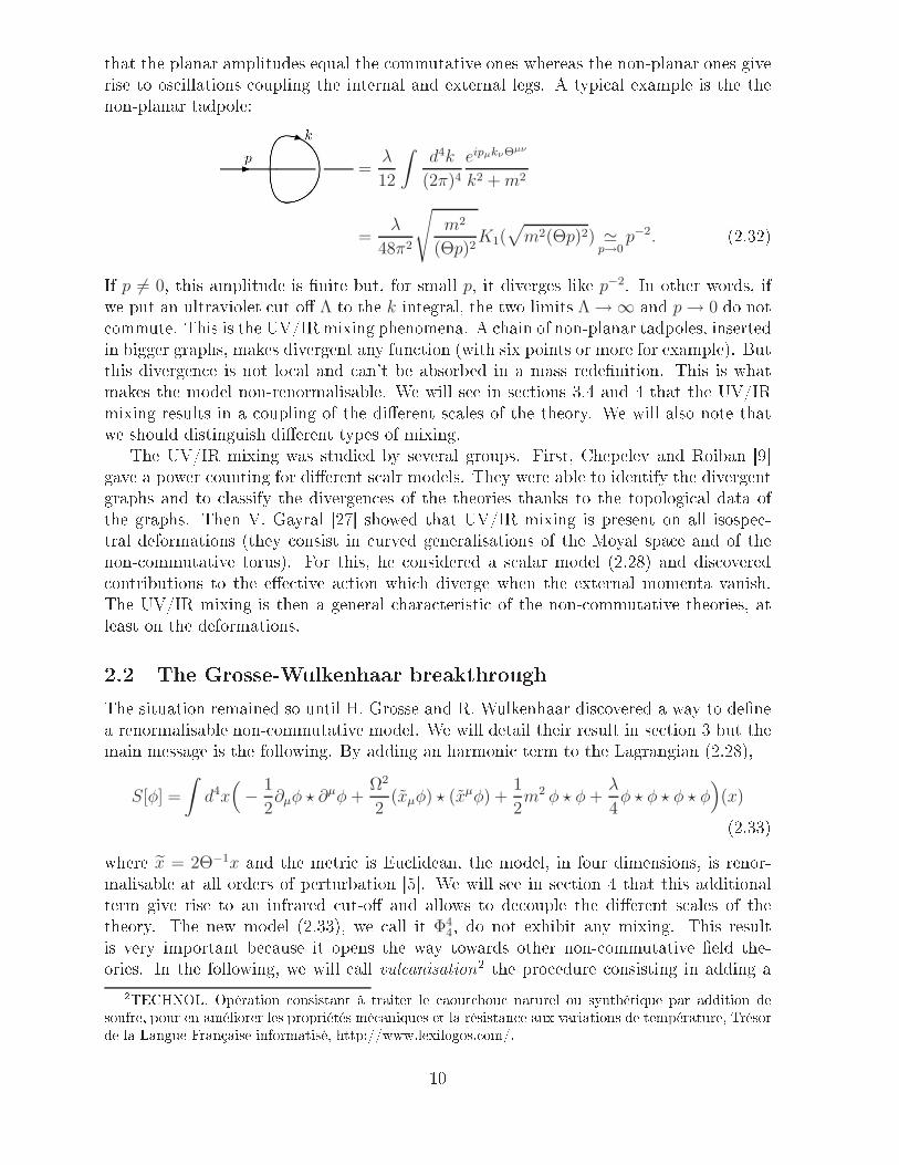
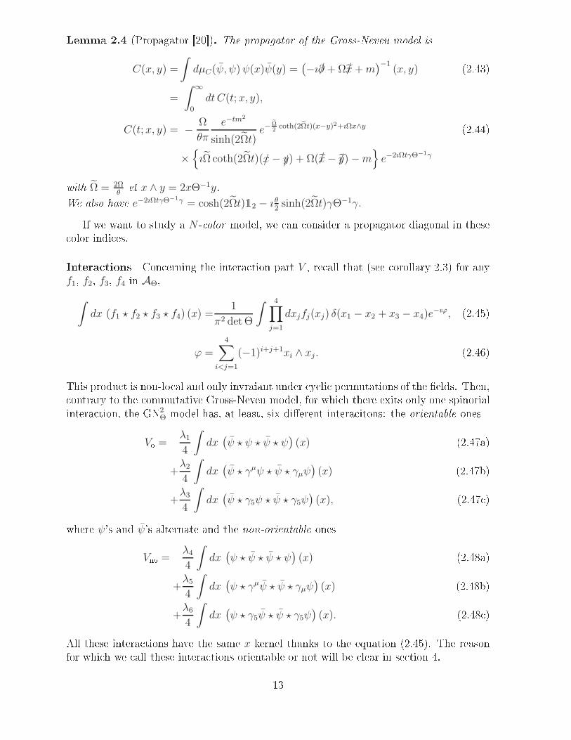
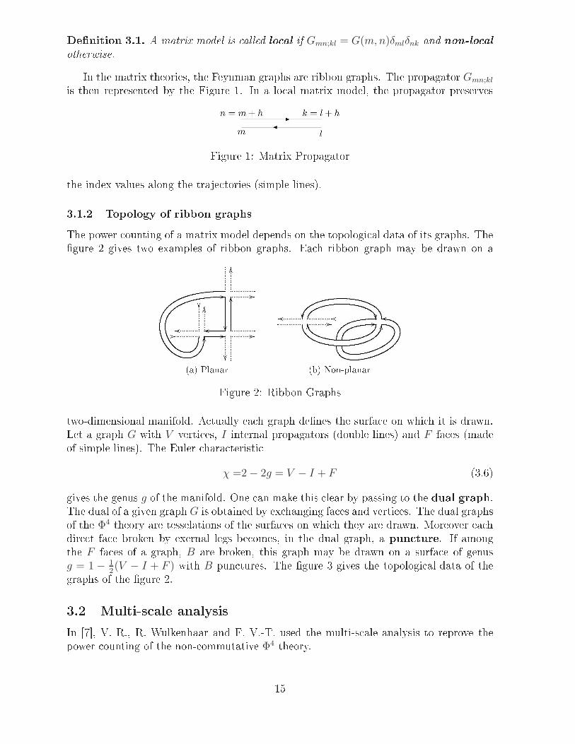
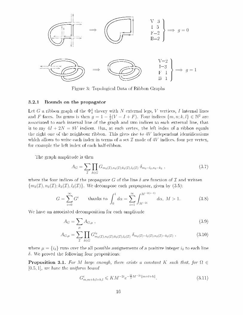
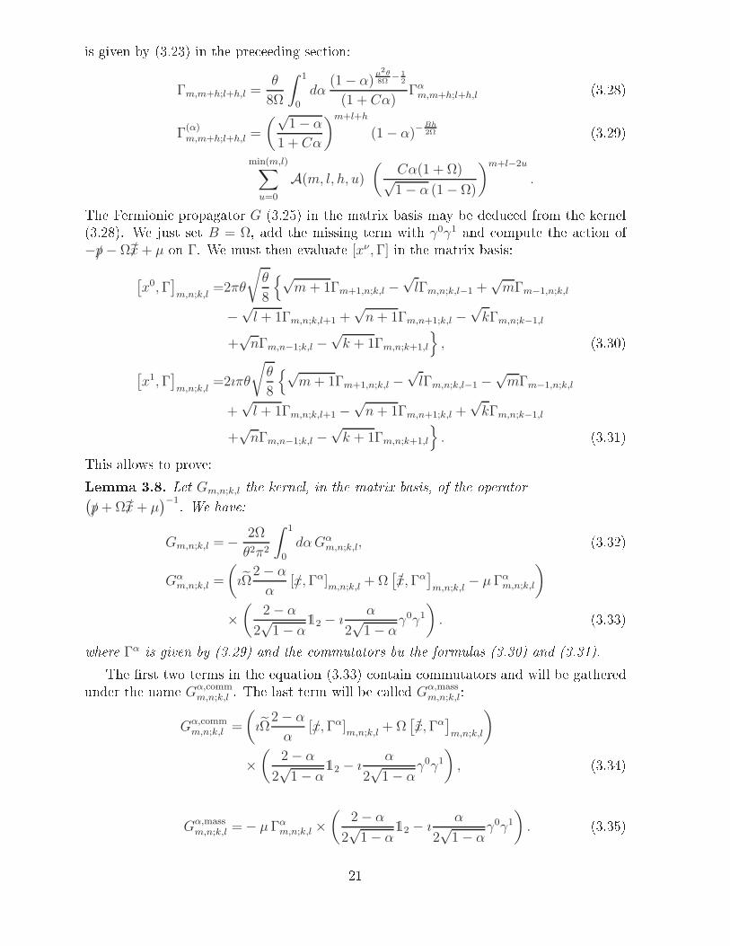
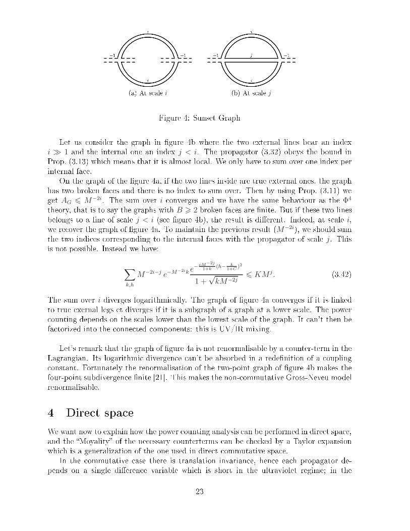
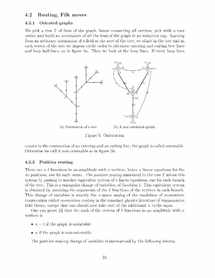
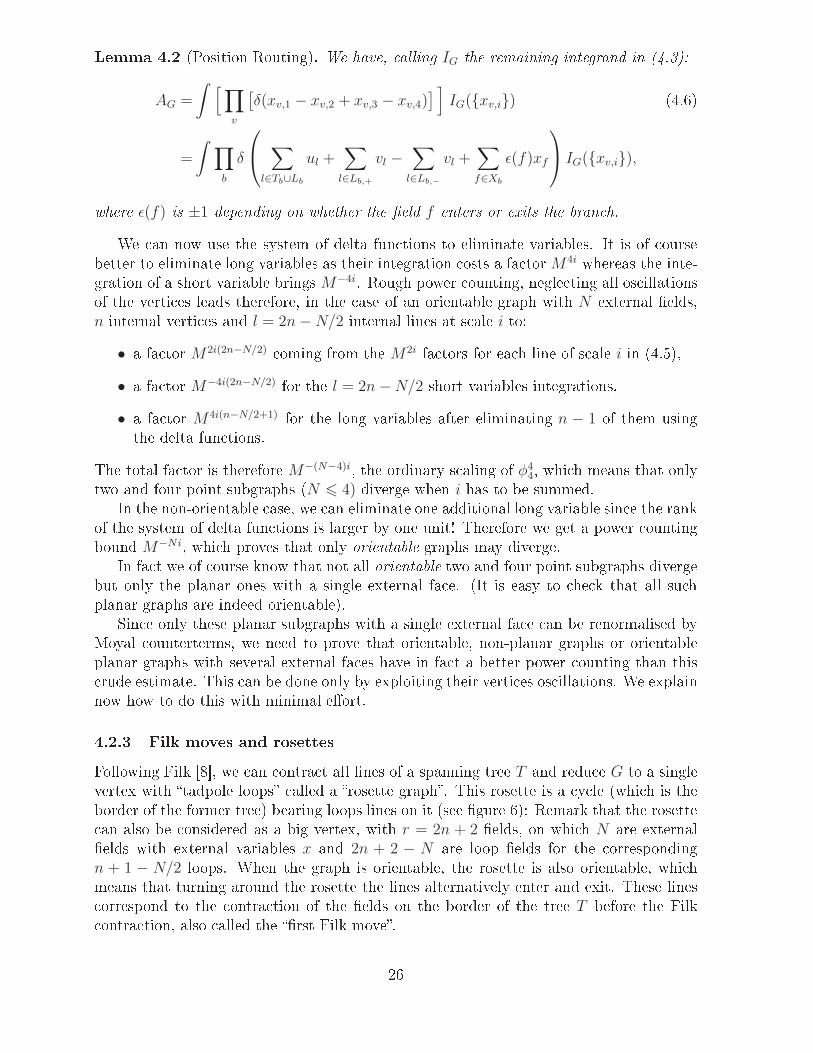
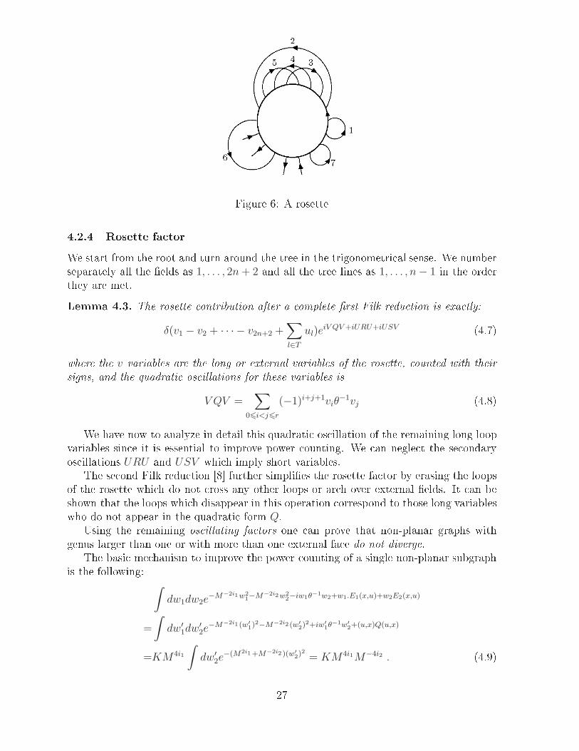
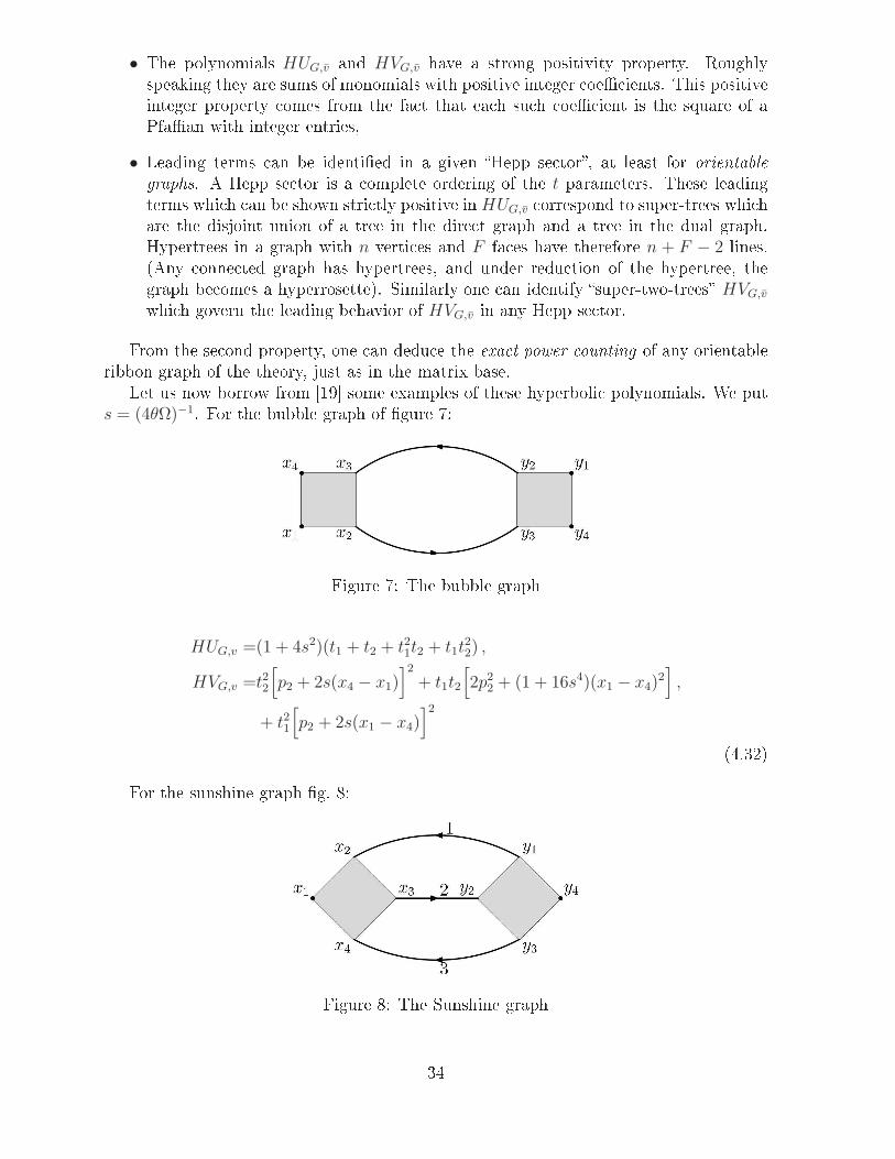
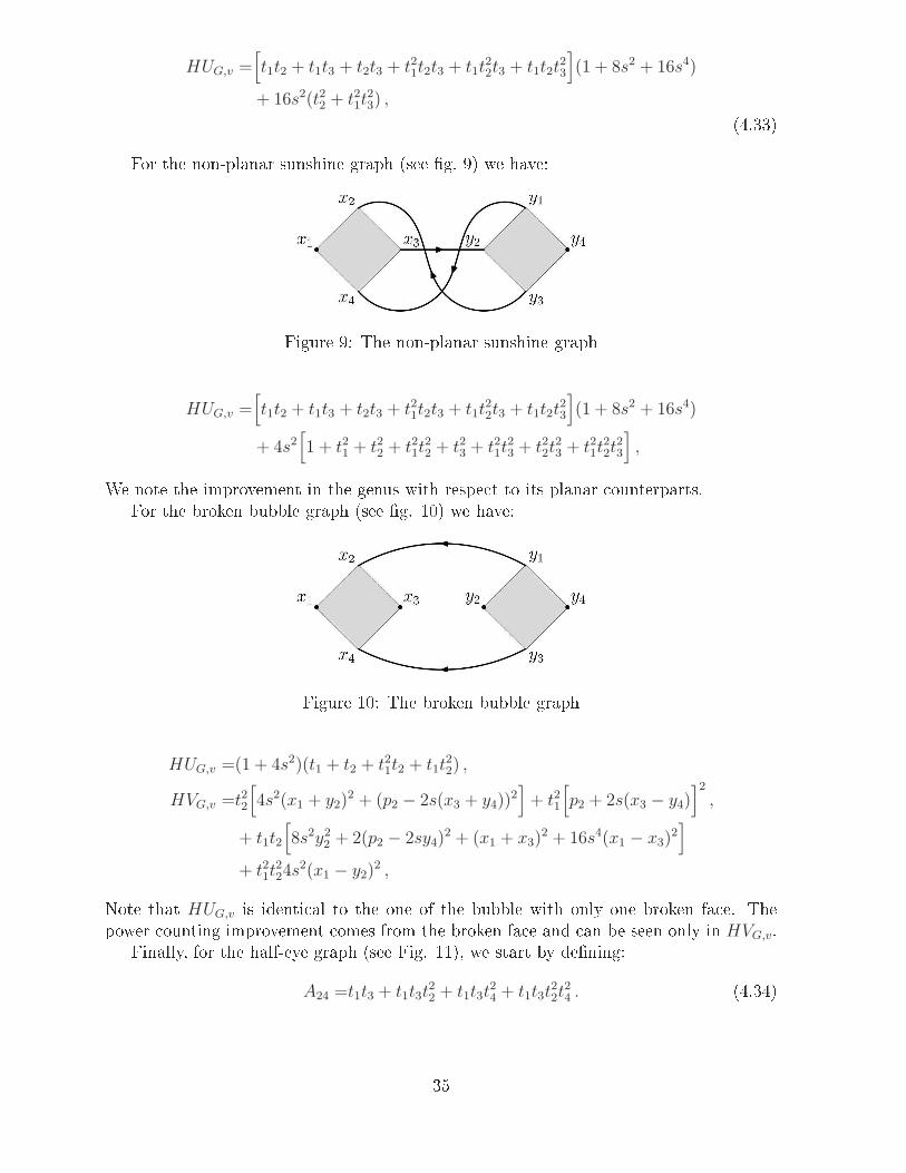
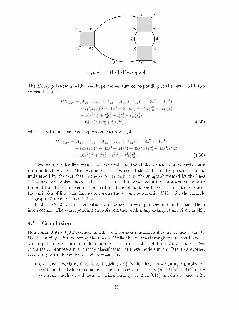
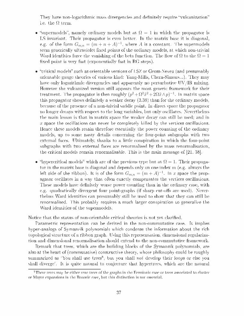
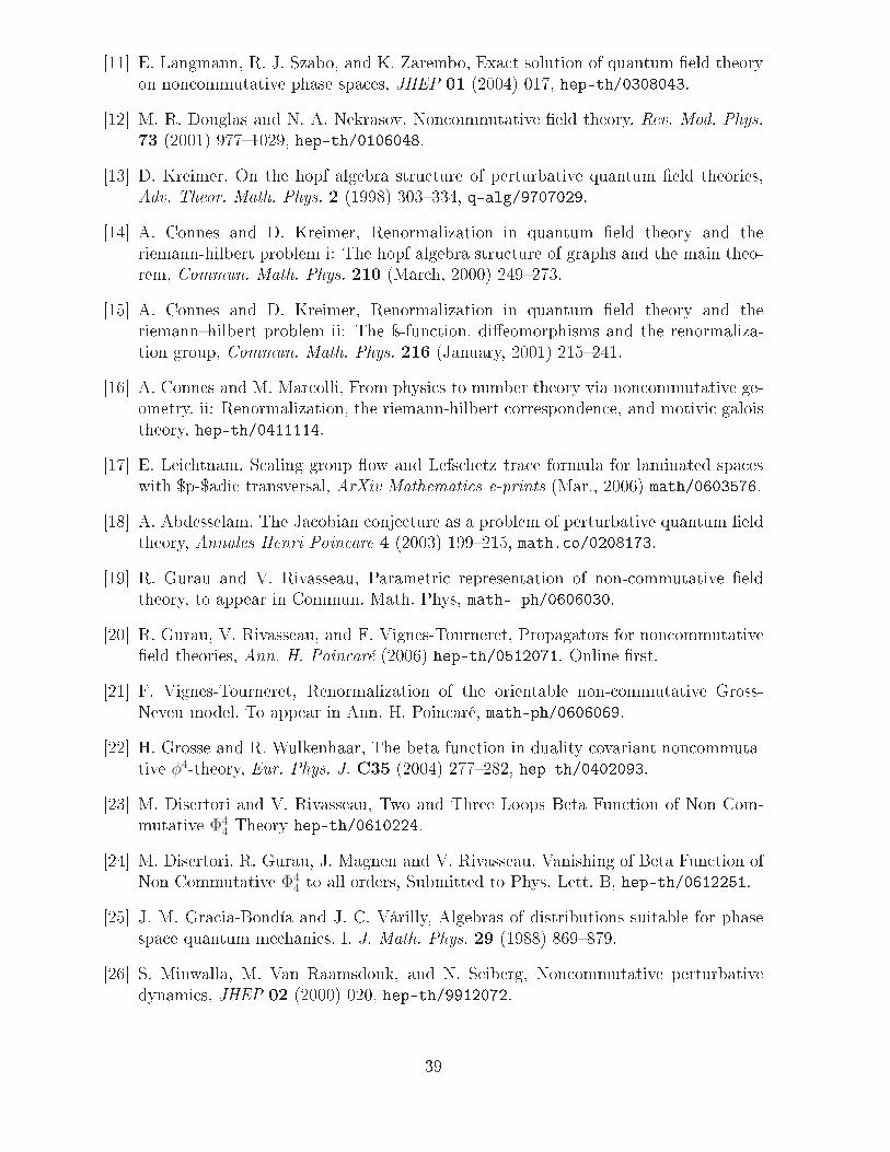
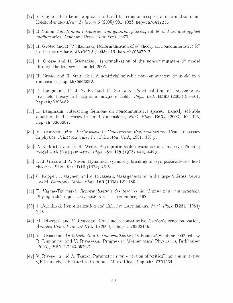

[43 A Lakhoua F Vignes-Tourneret and JC Wallet One-loop Beta Fun13tionsfor the Orientable Non- 13ommutative Gross-Neveu Model submitted to JHEPhep-th0701170
41


