Returns to American Agricultural Research

Returns to American Agricultural Research:Results from a Cointegration Model

Shiva S. Makki, Cameron S. Thraen, and Luther G. Tweeten,Department of Agricultural Economics, Ohio StateUniversity, Columbus, Ohio

This study examines the returns to U.S. agricultural research investments for the years1930 through 1990 using a cointegration model. Time series data on agricultural productiv-ity, public and private research investments, farmers’ education, terms of trade, and com-modity programs were found to be nonstationary and cointegrated. The estimated internalrates of return are 27 percent for public research and 6 percent for private research. Theseestimates from the most comprehensive and timely data assembled to date indicate thatreturns to public agricultural research compare favorably to real returns on alternativelong-run investments, but do not call for large increases in investments suggested byprevious studies or for the drop in public research expenditures appropriated by the U.S.Congress in recent years. 1999 Society for Policy Modeling. Published by ElsevierScience Inc.

1. INTRODUCTION

Much of the technological success of American agriculture isattributable to a well-developed and highly effective system ofpublic and private research and education. This system includesbasic and applied research along with extension education. Invest-ments in research and extension have been a primary source ofU.S. agricultural multifactor productivity growth that averaged 2percent per annum from 1930 to 1990. During this same period,public and private investment in agricultural research grew at anannual rate of 3 and 4 percent, respectively. In 1990, the nationspent about $8 billion on agriculture research and extension, 45

Address correspondence to Dr. Shiva S. Makki, 1800 M Street NW, Washington, DC20036-5831.

The authors thank Keijiro Otsuka and Scott Irwin for their valuable suggestions. Theauthors also appreciate the excellent research assistance provided by Renee Drury.

Received March 1996; final draft accepted November 1996.

Journal of Policy Modeling 21(2):185–211 (1999) 1999 Society for Policy Modeling 0161-8938/99/$–see front matterPublished by Elsevier Science Inc. PII S0161-8938(97)00059-8

186 S. S. Makki, C. S. Thraen, and L. G. Tweeten

percent of which was financed by the public and the rest (55percent) by the private sector.

Numerous studies have reported favorable payoffs from re-search and extension investments made to increase agriculturalproductivity. Huffman and Evenson (1993), for example, reportan internal rate of return (IRR) of 41 percent for public researchand 46 percent for private research and development (R&D).Makki and Tweeten (1993), on the other hand, report a higherIRR to public research and extension (93 percent) compared toprivate R&D (45 percent).1 Chavas and Cox (1992), using a non-parametric approach, report an IRR of 28 percent and 17 percent,respectively for public and private research investments using datafor 1950 to 1982.2 Other studies also report IRRs with estimatesranging from zero to 300 percent (Huffman and Evenson, 1989;Braha and Tweeten, 1986; Davis, 1981; Knutson and Tweeten,1979; Cline, 1975; Griliches, 1964).

There are two notable points about these reported rates ofreturn. First, most are quite high and exceed observed marketrates of return on alternative investments. Malkeil (1990), afteran extensive review of the financial literature, concluded that therate of return on long-term assets in the United States is about10 percent. Second, the wide disparity among IRR estimates raisesquestions as to the sensitivity of these estimates to the use ofdifferent time periods and methodologies. Time series regressionanalyses have been widely used to measure impacts of R&D onagricultural productivity (Griliches, 1964; Cline, 1975; Huffmanand Evenson 1992 and 1993; Makki and Tweeten, 1993). Thesestudies have helped to identify the dynamics of payoffs from in-vestments in developing technology and infrastructure. Inferentialdangers arise, however, in directly applying time series regressionanalysis to estimate economic benefits when variables have strongtrends and are nonstationary. Regression models estimated fromnonstationary series frequently have high R2 statistics, highly sig-nificant coefficient estimates, and very low Durbin–Watson (DW)statistics (Granger and Newbold 1974; Makki and Tweeten, 1993).

1 The two studies, however, differ in their methods of estimation and the chosen timeperiod: the former uses Zellner’s Seemingly Unrelated Regression (SUR) method foryears 1950 to 1982, while the later adopts the polynomial distributed lag (PDL) techniquefor the period 1930–90.

2 Although the nonparametric approach has some advantages over a parametric ap-proach, the major limitation is that statistical testing of the reliability of parameter estimatesis not possible (see Chavas and Cos for details).

RETURNS TO AMERICAN AGRICULTURAL RESEARCH 187

In such situations, the usual statistical tests of regression coeffi-cients can be seriously biased toward accepting a spurious rela-tionship.

As an alternative, cointegration analysis offers an improvedmethod to estimate the long-run dynamic relationship among timeseries economic variables. It deals with multicollinearity and thespurious correlations frequent among time series variables. Thismethod beings together short-run and long-run information inmodeling time series data via an error correction model ECM(Perman, 1991; Ericsson, 1992).

This paper reports the methods and conclusions of an analysisimplementing the cointegration technique to measure the influ-ence of public research and extension and of private research anddevelopment on U.S. agricultural productivity. In our analysis, wecontrol for farmers’ education, government commodity programs,and domestic terms of trade. The analysis is designed to improveestimates of the IRR for public and private research investmentsin U.S. agriculture. Results provide information on the role ofgovernment commodity programs and terms of trade in sustainingU.S. agricultural productivity in the long-run.

The paper proceeds as follows. The first section provides abrief overview of the cointegration method. The second sectionprovides a discussion of the conceptual model. Third, the estima-tion procedure for a cointegration model is presented. The fourthsection contains the empirical results. The final section providesthe summary and policy implications.

2. COINTEGRATION ANALYSIS

Cointegration analysis, introduced by Engle and Granger(1987), provides a structural framework for quantifying and statis-tically testing long-run relationships among economic variables.Cointegration essentially links the long-run (steady-state) behav-ior of economic time series to a statistical modeling of thosevariables. The concepts of cointegration and error correction mod-eling are closely related. As defined by Engle and Granger, twovariables are cointegrated if each variable individually is stationaryin differences (integrated of order d),3 and some linear combina-tion of them is stationary in levels.4 Cointegration implies that

3 A series Pt is said to be integrated of order d if the series becomes stationary afterdifferencing d times.

4 A series Pt is stationary if its mean, variance and autocovariances are invariant withrespect to time.


deviations from equilibrium are stationary, with finite variance,even though the series themselves are nonstationary and haveinfinite variance. Engle and Granger establish that two cointe-grated variables have an ECM representation, and two variablesin an ECM representation must be cointegrated (this is called theGranger Representation theorem).

We illustrate the principle with an example. An equilibriumrelationship between agricultural productivity (Pt) and invest-ments in R&D (Rt) is expressed as

Pt 5 aRt. (1)

Assume that each series by itself is nonstationary, and can bemade stationary by differencing. If agricultural productivitygrowth follows an equilibrium path, then by definition from Equa-tion 1 we have

Pt 2 aRt 5 0 (2)

In most time periods, Equation 2 is not zero, and the system isout of equilibrium. Thus, Equation 2 will not hold in all instanceseven if Equation 1 is the correct specification. However, the systemtends to return to equilibrium in the long run. Therefore, thelinear combination of levels in Equation 2 is more appropriatelyexpressed as

Pt 2 aRt 5 et, (3)

where equilibrium error et measures the extent to which the system(Pt, Rt) is out of equilibrium. If Pt and Rt are both integrated oforder one I(1), then the equilibrium error et will be stationary orI(0), and it will rarely drift far from its mean. The implication ofthis statistical property is that, while the individual series suchas productivity or research expenditures are nonstationary whentaken by themselves, a linear combination of such variables isstationary and thus not expected to diverge from one another inthe long run.

Assuming that agricultural productivity and R&D investmentsare cointegrated, the relationship between them may be expressedby an ECM of the following type:

DPt 5 b * DRt 1 l * (P 2 aR)t21 1 mt, (4)

where DPt and DRt are first difference terms for Pt and Rt, respec-tively. The expression l * (P 2 aR)t21 in Equation 4 contains allthe long-run information on the time series Pt and Rt, and it


measures the extent to which actual data deviate from the long-run relationship among economic variables. This mechanism givesECM an edge over ARIMA models where all variables are differ-enced, resulting in the loss of long-run information provided bythe levels data.

Many economic time series appear to be nonstationary andintegrated (Nelson and Plosser, 1982), which affects the statisticaldistributions of estimators. The notion of cointegration can inprinciple be extended to series with trends and/or explosive auto-regressive roots (Engle and Granger, 1987). The presence of atime variable or lagged explanatory variables does not affect thenull hypothesis of nonstationarity (Dickey and Fuller, 1981). Clas-sical testing procedures, which are invalid under nonstationarity,are often directly applicable to an ECM of cointegrated series.

3. CONCEPTUAL MODEL AND VARIABLES

Table 1 presents a description of each time series variable andits source. All variables are annual data for the United States from1930 through 1990. The conceptual model explaining multifactorproductivity P is

P 5 f(RE,RT,SC,FT,EC,WI) (5)

where variables are defined in Table 1. Public research and exten-sion (RE), private research and development (RT), farm operatorschooling attainment (SC), and weather (WI) variables frequentlyhave been used to account for multifactor productivity and needlittle elaboration (Griliches 1964; Cline 1975; Knutson and Tweeten1979; Braha and Tweeten 1986; Chavas and Cox, 1992; Huffmanand Evenson, 1992, 1993; Makki and Tweeten, 1993; Schimmel-pfennig and Thirtle, 1994). We combine research and extensionbecause they are strong complements whose separate contribu-tions are not easily sorted out.

The variables factor terms of trade FT and government com-modity programs EC ordinarily are not used to explain agriculturalproductivity and hence require some elaboration. Factor terms oftrade may influence productivity if an improved overall economicclimate encourages substitution of improved capital inputs forless productive conventional inputs such as labor. A favorableeconomic climate also can generate cash flow and loosen capitalbudget constraints.


Table 1: Data Source and Variables: 1930–90

VariableName Variable Definition

Multifactor productivity index of the ratio of aggregate crop and livestockproduction to aggregate production inputs, 1990 5 100 (U.S. Department

P of Agriculture, May 1992 and earlier issues).Research and extension real outlays by land-grant universities, the U.S.

Department of Agriculture, state agricultural experiment stations, andCooperative Extension Service, in million 1990 (constant) dollars (Huffman

RE and Evenson, 1993).Private investment in research and development by private industries,

foundations, etc., in millions of 1990 (constant) dollars (Huffman and Evenson,RT 1993).

Schooling attainment of farm operators in years. Data to 1972 from Cline(p. 141) and for later years from Bellamy (1992). Because data from Bellamywere compiled from the Census of Agriculture and Current PopulationReports of the U.S. Census and were not available for every year, we

SC interpolated between years.Factor terms of trade, defined as real prices received by farmers for commodities

per unit of production inputs (Council of Economic Advisors, 1992 and variousFT issues).

Excess production capacity defined as output diverted from the market byacreage diversion, stock accumulation, and subsidized exports, expressed asa percent of farm output (Dvoskin, 1988; updated to 1990 using Dvoskin’s

EC procedure).Weather Index, measuring the impact of nature on farming, and calculated by

Stallings (1960) from annual yield changes on experimental yield plots acrossthe nation treated similarly except the weather, extended by Cline to 1972.Data were extended to 1990 by the authors using deviations of U.S. crop

WI yields from a 7-year centered moving average yield trend.

Heady and Tweeten (1963) (p. 447) found no statistically sig-nificant association between multifactor productivity and com-modity terms of trade, CT, defined as the ratio of the index ofprices received for all crops and livestock, Pq, to the index of pricespaid for all production inputs, Px. It is surprising that a negativeassociation was not found. Because productivity is aggregate out-put Q divided by aggregate input X, in economic equilibriumPqQ 5 PxX so that Q/X 5 Px/Pq. Thus commodity terms of tradedefined as Pq/Px will fall proportional to productivity gains Q/X.Using the wrong price variable in statistical analysis over timewill give the incorrect impression that lower terms of trade raiseproductivity.


We use factor terms of trade, defined as real prices receivedfor commodities per unit of aggregate input, rather than commod-ity terms of trade to measure aggregate economic climate. Becausecommodity terms of trade is FT/P, inclusion of CT as an explana-tory variable introduces specification error because P appears onboth sides of the equation. Thus FT is commodity terms of tradecorrected for productivity. FT has increased over time while CThas substantially declined. Higher levels of FT indicate greaterincentives to add farming resources, some of which may be highlyproductive. Thus, FT is intuitively and conceptually more appeal-ing than CT as a measure of incentives for induced technologicalinnovations (Hayami and Ruttan, 1985). The maintained hypothe-sis is that favorable factor terms of trade raise farm productivity.

Government commodity programs potentially can have variousimpacts on productivity. First, government programs can distortallocation of resources and products, reducing productivity. Sec-ond, programs provide payments that, if decoupled, might loosenbudget constraints and provide funds allowing producers to substi-tute technologically improved inputs for conventional inputs, rai-sing productivity. Third, in constructing P, analysts include di-verted acres in production inputs. However, neither displacedoutput nor government payments are included in output, henceacreage diversion programs can be expected to reduce productiv-ity. Slippage is great, however, as poor land is diverted and com-mercial fertilizers and other improved inputs are substituted forland. Given this conflicting conceptual foundation, the issue ofwhether commodity programs enhance or diminish productivitymust be resolved empirically. Each of the above three potentialimpacts cannot be clearly isolated, but we considered three vari-ables measuring the influence of commodity programs: excesscapacity, payments to farmers, and diverted acres. Excess capacity,EC, was deemed to be the most comprehensive measure of govern-ment distortion, and we included it is our model.5 Our null hypoth-esis is that government commodity programs as measured by EChave no net impact on multifactor productivity.

5 Preliminary analysis indicated that government payments and diverted acres contrib-uted even less than EC to the variation in P. Of course, government programs may alsoinfluence productivity by influencing prices, an influence that would be apparent in thecoefficient of FT discussed above.


4. ESTIMATION PROCEDURE

In practice, the cointegration approach involved three steps.The first step establishes that the series is nonstationary, or morespecifically must be difference stationary.6 The second step estab-lishes whether the multivariate time series are cointegrated. Thefinal step estimates the parameters of the ECM.

4A. Testing for Stationarity

Stationarity is investigated for each variable by testing for unitroots using Augmented Dickey–Fuller (ADF) statistics and Z-sta-tistics, Za and Zt (Said and Dickey, 1984; Phillips and Perron,1988). These residual-based tests are most often used by research-ers due to their simplicity, intuitive clarity, and more importantly,they are more powerful than the non–residual-based tests (J testby Park and Choi, 1988; trace test; eigenvalue test), especiallywhen the number of variables involved increases (Phillips andOuliaris, 1990; Haug, 1993). The autocorrelation function (ACF)and partial autocorrelation function (PACF) also are used to sub-stantiate the two tests, and to choose the order of differencing.

Consider, for example, the time series productivity index Pt. Totest whether this series is nonstationary, we specify the followingfirst order autoregressive model:

Pt 5 a 1 b * Pt21 1 lt, t 5 1,2, . . . , T. (6)

The series is stationary only if |b| , 1. If |b| 5 1, the series hasa unit root implying nonstationarity. We test the null hypothesisof nonstationarity by reparameterizing Equation 6 into a firstdifference equation:

DPt 5 r * Pt21 1 lt, (7)

which is nonstationary under the null r 5 0 (equivalent to b 5 1in Equation 6).

In practice, a time trend (T) can be included in the estimatedmodels to discriminate between unit root nonstationarity (Differ-ence Stationary), and stationarity about a deterministic trend(Trend Stationary). For example, Said and Dickey recommendthe use of the Augmented Dickey–Fuller (ADF) regression ofthe following form:

6 If a nonstationary time series can be made stationary by differencing, then such aseries is referred to as difference stationary data series.


DPt 5 a 1 g * T 1 r * Pt21 1 om

i51

biDPt2i 1 vt. (8)

Lagged first difference terms are included in the model to ensurewhite-noise residuals in the regression of Equation 8. The nullhypothesis r 5 0 implies that Pt is nonstationary. The coefficientr is tested for statistical significance by comparing computed ADFt statistics with critical values. The null hypothesis of nonstationar-ity is rejected if the computed statistic is less than the appropriatecritical value.

Dickey and Fuller (1981) note that the usual t and F tests areinappropriate for testing the null hypothesis of nonstationaritybecause the least squares estimate of b is not distributed aroundunity. They suggest ADF-t and ADF-F statistics as alternativesto the usual t and F tests. Phillips and Perron show that asymptoti-cally the test statistics ADF and Z have similar limit distributions.However, the Z test is preferred over the ADF test for smallsamples, because the former involves nonparametric adjustmentsto the time series structure to ensure that the random componentis white noise. They also demonstrate that whenever uncertaintyexists regarding the dynamic structure of the time series, the Ztest performs more consistently.

4B. Testing for Cointegration

After verifying that the random variables are nonstationary asmeasured in levels, cointegration is investigated using four differentstatistics: ADF, Z, p (Phillips and Ouliaris, 1990), and SW (Stockand Watson, 1988). The existence of cointegration is tested in twostages. First, a cointegrating regression is estimated of the type

Pt 5 a 1 b * Rt 1 et (9)

where Rt is a vector of explanatory variables: REt, RTt, SCt, FTt,ECt. For variables to be cointegrated all the series should beintegrated of the same order and a linear combination of the seriesshould be stationary. Let et be the residuals from Equation 9.These residuals are used to test the null hypothesis of no cointegra-tion, that is, u 5 0, in either of the following specifications: ADFt in the regression:

Det 5 2 u*et21 1 om

i51

di*Det2i, (10)

or Z-test in the regression:


et 5 u * et21 1 ut. (11)

The null hypothesis of no cointegration is rejected if the appro-priate test statistic is less than the critical value.7 Rejection of H0

provides evidence of the existence of an ECM for the time seriesvariables.

4C. Estimating the ECM

Conditional upon finding evidence for cointegration, an ECMof the type in Equation 4 is specified in a more general form:

DPt 5 A 1 let21 1 om

j50

aj DREt2j 1 om

j50

bj DRTt2j

1 g1 DSCt 1 g2 DFTt 1 g3 DECt 1 ut (12)

where all variables are in first differences (indicated by D), et21 isthe equilibrium error obtained from the cointegrating regression(Equation 9), A is the intercept, and ut is the error term. Thecoefficient l indicates the speed with which the relationship movesback to the equilibrium following a shock (l needs to be negativefor dynamic stability). All terms in Equation 12 are I(0), so thatno inferential difficulties arise. The model allows for lagged valuesof public and private research investments. Choosing a lag lengththat is too large or too small will reduce the predictive power ofthe model (Said and Dickey, 1984). An appropriate lag length mis chosen based on the most commonly used model selectioncriteria such as Schwartz Criterion and Akaike Information Crite-rion (Judge, Hill, Griffiths, Lutkepohl, and Lee, 1988; Mills, 1990).

A consistent estimation of Equation 12 is possible if we ruleout simultaneity of the relationship. It is sometimes argued that,in the above model, research could be driving productivity orproductivity driving research, causing a fundamental identificationproblem. The Hausman specification test and Granger causalitytests are performed to check the presence of simultaneity problems,if any (Granger, 1969; Pardey and Craig, 1989; Pindyck and Rubin-feld, 1991). The computation procedure is shown in Appendix A.

5. EMPIRICAL RESULTS

5A. Testing for NonStationarity

Each variable in Table 1 was checked for nonstationarity byvisual inspection of the estimated correlogram, a graph that plots

7 See Phillips and Ouliaris for the construction and comparison of ADF, Z, and pstatistics. SW statistics are illustrated in Stock and Watson.


Figure 1A. U.S. Agricultural productivity (1930–90).

the estimated kth order autocorrelation coefficient as a functionof k, where k is the number of lags. For a stationary variablethe correlogram should show autocorrelations that dampen fairlyquickly as k becomes large. A smooth falling ACF suggests thatthe time series variable may be homogenous nonstationary, whilea PACF with a cut off after the first lag suggests that the variablecan be made stationary by differencing once (Mills, 1990; Kennedy,1992). Based on these correlograms (Figures 1 through 5) we cansay that all variables are first difference stationary.

The data nonstationarity is investigated also using the ADF testand the Z test. First, the variables are tested for the null hypothesisof I(1) or nonstationary against the alternative hypothesis of I(0)or stationary. The decision rule is that, if the computed test statisticis more negative than the respective critical value, we reject thenull hypothesis in favor of the alternative hypothesis. If the hypoth-esis of I(1) is not rejected we need to test whether the series isI(2). This is accomplished using the same tests as before, butreplacing the variable in levels by the variable in differences. Theprocedure is repeated until the order of integration of the seriesis established. The results reported in Table 2 support the hypothe-sis of data nonstationarity in almost every case. The hypothesesof I(0) or I(2) are rejected for all variables except weather in favorof I(1). The weather variable, therefore, is eliminated from the


Figure 1B. Autocorrelation function and partial autocorrelation function forproductivity index.

Figure 2A. Public and private investments on agricultural research and extensionin the United States (1930–90).


Figure 2B. Autocorrelation function and partial autocorrelation function forpublic research and extension.

Figure 2C. Autocorrelation function and partial autocorrelation function forprivate research.


Figure 3A. Farmer’s schooling index in the United States (1930–90).

Figure 3B. Autocorrelation function and partial autocorrelation function forfarmer’s schooling index.


Figure 4A. Agricultural sector factor terms of trade in the United States (1930–90).

Figure 4B. Autocorrelation function and partial autocorrelation function forfactor terms of trade.


Figure 5A. U.S. Agricultural excess capacity (1930–90).

Figure 5B. Autocorrelation function and partial autocorrelation function forexcess capacity.


Table 2: Testing for Nonstationaritya

Variable Rhob ADF Test CV Z Testc CV

LevelsPd 1.00 22.8856 23.89 1.3733 213.87RE 0.59 23.0281 23.89 224.5969 226.01PT 0.80 22.3379 23.89 211.6771 226.01SC 0.86 22.0919 23.89 28.7266 226.01FT 0.63 22.9595 23.89 221.9930 226.01EC 0.93 21.8726 23.89 24.9976 226.01WIe 20.001 24.2286 23.89 260.3735 226.01

First DifferencesD P 20.39 28.7131 23.89 279.7004 226.01D RE 20.17 24.2070 23.89 269.2269 226.01D PT 20.07 25.8586 23.89 263.6373 226.01D SC 0.11 24.0233 23.89 252.1667 226.01D FT 20.19 25.2837 23.89 270.0514 226.01D EC 0.36 25.2186 23.89 238.3232 226.01

a The algorithms given in Gauss Procedures for Cointegrated Regression Models areused for this purpose. Reject the null hypothesis of nonstationarity if the computed statisticis less than the critical value (CV).

b Rho is the autoregresive parameter.c Two statistics, Za and Zt, are associated with Phillips’ and Perron’s Z test. Both tests

are performed for this study, but only Za is reported.d The ADF test for P rejects the null of nonstationarity at lower lags (, 2).e Both tests for WI reject the null of nonstationarity at 5%.

analysis, because it cannot be cointegrated with agricultural pro-ductivity. It can be concluded that the data used in the study werenonstationary in levels, and were stationary in first differences.

5B. Testing for Cointegration

With evidence that each of our data series are nonstationaryand integrated of the same order, we now proceed to test forcointegration. The cointegrating regression (Equation 9) is esti-mated with P as the dependent variable and RE, RT, SC, FT, andEC as explanatory variables. The residuals from the regressionare used to test for cointegration. Table 3 reports the results ofcointegration tests, together with the associated critical values.

The test statistics uniformly indicate that the null hypothesis ofno cointegration can be rejected. We conclude that the time seriesvariables P, RE, RT, SC, FT, and EC move in tandem. All tests


Table 3: Testing for Cointegrationa

Test Test Statistic Critical Valuec

ADF Testb ADF-t 25.12 24.91Z Test Za 256.17 237.98p Test pz 209.60 176.31SW Test SW 229.92 221.21

a In the case of ADF, Z, and SW tests we reject the null of no cointegration if theestimated statistic is less than the critical value. In case of the p test, where the pz statisticpossesses a nonstandard distribution, we reject the null hypothesis if the pz statistic isgreater than the critical values.

b All tests provide consistent estimates of test statistics except the ADF test. The ADFtest is biased toward accepting the null of no cointegration at higher lags (greater than 3).

c Critical values at 5% are taken from Phillips and Ouliaris.

computed with 2-year lags and a trend variable confirm the pres-ence of cointegration at the 5 percent level of significance. Thecointegration suggests that there exist long-run relationshipsamong these variables.8

5C. Cointegration Model

Table 4 reports the results of estimating the error correctionmodel (Equation 12). Both the Hausman specification test andGranger causality test suggest that the causality is unidirectionalfrom R&D to productivity and not vice versa (Appendix A).

A statistically significant negative error correction coefficientimplies that the equilibrium relationship will hold in the long run,even if there were shocks to the relationship. The error correctionterm measures the extent to which actual data deviate from thelong-run relationships among the variables. In essence, it containsall the long-run information provided by levels data.

Choosing appropriate lag lengths is no easy task. Preliminarysensitivity analysis indicate that coefficients are quite stable for awide range of lags. For example, the coefficients for educationdecreased from 0.35 to 0.28 when lags for private research wereincreased from 16 to 28, holding lags for public research at 20. In asimilar experiment in which lags for public research were increasedfrom 16 to 28, the coefficient for education increased from 0.33to 0.38. Due to data limitations, we could not carry out sensitivity

8 It is reasonable to assume that weather is a random phenomenon, and not to haveany long-run relationship with agriculture productivity.


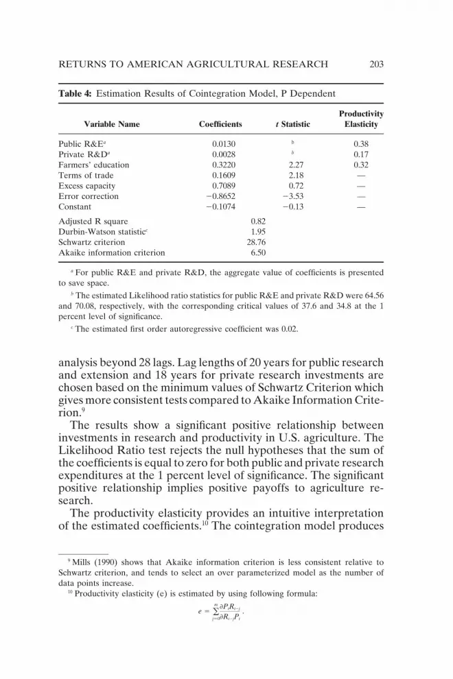
Table 4: Estimation Results of Cointegration Model, P Dependent

ProductivityVariable Name Coefficients t Statistic Elasticity

Public R&Ea 0.0130 b 0.38Private R&Da 0.0028 b 0.17Farmers’ education 0.3220 2.27 0.32Terms of trade 0.1609 2.18 —Excess capacity 0.7089 0.72 —Error correction 20.8652 23.53 —Constant 20.1074 20.13 —

Adjusted R square 0.82Durbin-Watson statisticc 1.95Schwartz criterion 28.76Akaike information criterion 6.50

a For public R&E and private R&D, the aggregate value of coefficients is presentedto save space.

b The estimated Likelihood ratio statistics for public R&E and private R&D were 64.56and 70.08, respectively, with the corresponding critical values of 37.6 and 34.8 at the 1percent level of significance.

c The estimated first order autoregressive coefficient was 0.02.

analysis beyond 28 lags. Lag lengths of 20 years for public researchand extension and 18 years for private research investments arechosen based on the minimum values of Schwartz Criterion whichgives more consistent tests compared to Akaike Information Crite-rion.9

The results show a significant positive relationship betweeninvestments in research and productivity in U.S. agriculture. TheLikelihood Ratio test rejects the null hypotheses that the sum ofthe coefficients is equal to zero for both public and private researchexpenditures at the 1 percent level of significance. The significantpositive relationship implies positive payoffs to agriculture re-search.

The productivity elasticity provides an intuitive interpretationof the estimated coefficients.10 The cointegration model produces

9 Mills (1990) shows that Akaike information criterion is less consistent relative toSchwartz criterion, and tends to select an over parameterized model as the number ofdata points increase.

10 Productivity elasticity (e) is estimated by using following formula:

e 5 om

j50

]PtRt2j

]Rt2jPt

.


a positive long-run elasticity for agriculture research: 0.38 forpublic and 0.17 for private research (Table 4). The results indicatethat a 1 percent increase in public research expenditure raisesproductivity by 0.38 percent, while a 1 percent increase by privateresearch raises farm productivity by only 0.17 percent. The gapbetween public and private response may be due to the differencesin the type of research being conducted by each sector. Publicagricultural research emphasizes investments in basic research,especially including biological and agronomical technologies andhuman resource developments. Private agricultural research em-phasizes investments on applied research and development includ-ing chemical and mechanical technologies and, more recently,biotechnology.11

Results show that education level of farm operators has a sig-nificant positive impact on farm productivity. Skills acquired fromschooling improve farmers’ ability to process information andselect, manage, and operate new technologies. The cointegrationmodel estimates that 1 additional year of education for farm opera-tors raises farm productivity by about 0.32 percent in the longrun. Huffman and Evenson (1993, p. 755) report an even higherproductivity elasticity (0.837) for farmers’ schooling.

Factor terms of trade, defined as real prices received by farmersfor crops and livestock per unit of production input, also plays asignificant role in enhancing farm productivity. If terms of trade arefavorable, farmers have an incentive to purchase technologicallyimproved inputs that raise productivity of agriculture. Each 1percent increase in factor terms of trade raise farm productivityby 0.16 percent in the long run.

Although favorable economic conditions foster productivitygains, government programs intended to improve agriculturalterms of trade are not necessarily the most efficient way to raiseproductivity. The cointegration model indicates that governmentcommodity programs represented by excess capacity are not a

11 The Consultative Group of International Agricultural Research (CGIAR) makes thefollowing distinctions between basic and applied research. Basic research is experimentalor theoretical work undertaken primarily to acquire new knowledge of the underlyingfoundations of phenomena and observable facts without any particular commercial applica-tion or use; applied research, on the other hand, involves investigations directed to thediscovery of new knowledge that has specific commercial objectives with respect to eitherproducts or process, and research designed to adjust technology to specific geo-climaticor socio-economic conditions.


significant factor in improving farm productivity. This result iscontrary to the findings of Makki and Tweeten (1993) and Huff-man and Evenson (1993, p. 208) that indicate a significant positiverelationship between government programs and agricultural pro-ductivity. Those studies, however, did not account for the datanonstationarity and cointegration between the two variables.

5D. Internal Rate of Return

The internal rate of return IRR, defined as the interest ratethat makes the net present value of research investments equalto zero, was calculated using the stream of marginal productsobtained from the cointegration model (Davis, 1981). The proce-dure is implemented by solving the following equation for theinternal rate of returns that makes the net present value of adollar investment equal to zero:

IRR 5 r : o VMPj (11r)2j 2 1.0 5 0.0, (13)

where the value marginal product VMPj is the marginal physicalproduct of agriculture research Rt after j periods times the output

price Pq or 1]Pt1j

]Rt* Pq2, and r is the interest rate.

After appropriately accounting for the nonstationarity in theoriginal variables and specifying the equilibrium condition as acointegrated ECM, we estimate the IRR at 27 percent for publicR&E and as 6 percent for private R&D (Table 5). The estimatefor public R&E is consistent with the IRR estimate reported byChavas and Cox (1992) using a nonparametric approach. However,an advantage of the cointegration approach over the nonparametricapproach is that the former facilitates statistical tests of parameters.

Our calculated rates of return are lower for private researchthan for public research, but still favorable relative to currentmarket rates of return on treasury bills (7 percent) and corporatebonds (8 percent). Chavas and Cox (1992) report a much higherrate of return of 17 percent to private research (Table 5). Theirestimate may have been inflated by not controlling for education.Private research and farmers’ schooling are highly correlated inlevels. With schooling omitted, our estimated internal rate of re-turn for private research was 11 percent. However, analysts usingother methods but controlling for education found even higherrates of return on private R&D (Makki and Tweeten, 1993; Huff-man and Evenson, 1993).


Table 5: Internal Rates of Return to Public and Private Investments to RaiseProductivity of American Agriculture (in percent)

Time Public PrivatePeriod R&E R&D Estimation Procedure

Present Study (1994) 1930–90 27 6 Cointegration/ECMMakki and Tweeten (1993) 1930–90 93 45 Polynomial distributed LagHuffman and Evenson (1993) 1950–82 41 46 Zellner’s SURChavas and Cox (1992) 1950–82 28 17 Non parametricHuffman and Evenson (1989) 1949–74 62 0a Zellner’s SURBraha and Tweeten (1986) 1939–82 50 b Polynomial distributed LagDavis (1981) 1964–74 28–52 b Polynomial distributed LagKnutson and Tweeten (1979) 1969–72 28–35 b Polynomial distributed LagCline (1975) 1939–72 41–50 b Polynomial distributed LagGriliches (1964) 1949–59 300 b Production Function

a Estimates were slightly negative or near zero.b No estimates available.

The results suggest that earlier studies ignoring data nonsta-tionarity and cointegration relationships may have overestimatedthe actual payoffs to research investments. Also, past studies didnot take into consideration explicitly the role of commodity pro-grams and terms of trade that might have resulted in misleadinglyhigh payoffs to research investments.

6. CONCLUSIONS

Most previous analysts used time series regression analysis toevaluate the returns to research investments without correctingfor data nonstationarity. Granger and Newbold (1974) have estab-lished that regressions estimated from nonstationary series fre-quently are biased and represent spurious relationships. Timeseries data on agricultural productivity, public and private researchinvestments, farmers’ education, terms of trade, and commodityprograms were found to be nonstationary and cointegrated inour study. By correcting for nonstationarity, the cointegrationprocedure attempts to improve estimates of the long-run dynamicrelationship among the time series variables. It brings togethershort- and long-run information via error correction modeling.

The empirical findings of this study illustrate the usefulness ofthe cointegration approach in explaining the relationship betweenagricultural productivity and research investments in agriculture,


and in measuring economic returns to agriculture research. Thisstudy finds a significant positive relationship between agriculturalproductivity and public and private investments in research, exten-sion, and development. The estimated internal rates of return are27 percent for public research and 6 percent for private research.Thus earlier studies ignoring data nonstationarity and cointegra-tion relationships may have given misleadingly high estimates ofpayoffs to research investments.

Although rates of return to public research and extension arelower than found in previous studies not employing an error cor-rection model, the estimated long-term rate of returns are highenough to justify continued public investments to raise agriculturalproductivity. The results indicate that economic returns to agricul-ture research in the United States have been favorable relativeto alternative capital investments in the long-run. Public research,especially basic research, can improve conditions for private re-search, and help to fill the gap between the private sector researchinvestments and the socially optimal level of research.

High productivity has given the United States the competitiveadvantage in selling agriculture products in the world markets.Results suggest that commodity programs have no effect on in-creasing farm productivity, while a favorable terms of trade im-proves farm productivity. Given these findings, it appears that theinterest of United States agriculture would be better served byfocusing on R&D and education, which have greater potential topositively impact upon U.S. agriculture performance.

1. APPENDIX A

A Note on Causality

Cointegration says nothing about the direction of the causalrelationship among the variables. A common problem in econom-ics is determining whether changes in one variable are a cause ofchanges in another. For example, changes in R&D cause changesin productivity as assumed in this study, or productivity andR&D are both simultaneously determined causing fundamentalidentification problem in Equation 12. A consistent estimation ofEquation 12 is possible if we can rule out simultaneity of therelationship. To test causality, if any, we applied Hausman specifi-cation test and Granger causality test (Pindyck and Rubinfeld, 1991).


1. Hausman Specification Test

The test in the context of productivity and R&D relationshipin the ECM model Equation 12 is formulated in two steps. Firststep involves specifying a reduced form equation for R&D byregressing R&D on all exogenous variables, which yields

DRt 5 A 1 om

i51

ui DRt2i 1 pDX 1 et, (A.1.)

where Rt is the sum of public and private research investments,and X is a vector of other exogenous variables that affect produc-tivity and research expenditures: schooling, factor terms of trade,commodity programs, and weather factors.

In the second step, we use the residuals from Equation A.1 inestimating the following regression equation:

DPt 5 B 1 om

i50

ji DRt2i 1 let 1 et. (A.2.)

Under the null hypothesis of no simultaneity, Pt and et are uncorre-lated, and thus the coefficient l should equal zero. See Pindyckand Rubinfeld for more details on this test.

2. Granger Causality Test

Granger’s causality test involves two regression functions. First,productivity is regressed on lagged values of itself and researchinvestments, and other relevant exogenous variables. The secondequation involves a similar regression with research investmentsas dependent variable.

DPt 5 A 1 om

i51

aj DPt2j 1 on

i50

bi DRt2i 1 gDX 1 ut (A.3.)

DRt 5 B 1 on

i51

wj DPt2j 1 om

i51

Ci DRt2i 1 GDX 1 vt (A.4.)

For there to be unidirectional causality from Rt to Pt, the estimatedcoefficients of lagged Rt in Equation A.3 should be significantly

different from zero as a group (om

i50

bi ≠ 0) and the sum of the

coefficients on lagged Pt should not be significantly different from

zero (on

j51

aj 5 0). Bilateral causality is suggested when both om

i51

bi ≠

0 in Equation A.3 and on

j50

wj ≠ 0 in Equation A.4, and independence

when they are not significantly different from zero.


Testing Causality: Results from Hausman Specification Test and GrangerCausality Test

1. Hausman Specification Test(A.1) Rt 5 2239.3410.5805 Rt-120.5086 SCt21.2123 FTt235.59 ECt12.9518 WIt

[20.39] [0.64] [20.09] [20.27] [20.73] [0.51]

(A.2) Pt 5 1.055810.0129 Rt-110.0019 et

[0.51] [0.57] [0.05]

2. Granger Causality Test(A.3) Pt 5 219.5321.044 Pt-j10.036 Rt-i11.029 SCt10.076 FTt12.88 ECt10.19 WIt

[21.94][21.18] [2.05] [0.93] [0.99] [3.80] [2.00]

(A.4) Rt 5 265.2416.460 Pt-j20.298 Rt-i280.724 SCt10.08 FTt289.8 ECt21.1219 WIt

[0.31] [0.08] [20.20] [21.03] [0.01] [21.09] [20.13]

Notes: Figures in the parentheses are t values; all variables are in first differences exceptWIt and et; The coefficients for Rt and Pt are sum of 20 and six lagged coefficients, respectively.

Both Hausman specification test and Granger causality test do not reject the null ofno simultaneity in the relationship between productivity and research investments. Weconclude that the causality is unidirectional from research investments to productivity andnot vice versa.

REFERENCESBellamy, D. (1992) Educational Attainment of Farm Operators. Agricultural Income and

Finance. Washington, DC: Economic Research Service, USDA, pp. 37–39.Braha, H., and Tweeten, L.G. (1986) Evaluating Past and Prospective Future Payoffs from

Public Investments to Increase Agricultural Productivity. Technical Bulletin T-163.Stillwater: Agricultural Experiment Station, Oklahoma State University.

Chavas, J.P., and Cox, T.L. (1992) A Non-Parametric Analysis of the Influence of Researchon Agricultural Productivity. American Journal Agricultural Economics 74:583–591.

Cline, P. (1975) Sources of Productivity Change in U.S. Agriculture. Unpublished Ph.D.Thesis. Stillwater: Oklahoma State University.

Council of Economic Advisors. (1992) Economic Report of the President. Washington,DC; U.S. Government Printing Office.

Davis, J. (1981) A Comparison of Procedures for Estimating Returns to Research UsingProduction Functions. Australian Journal of Agricultural Economics 25:60–72.

Dickey, D.A., and Fuller, W.A. (1981) Likelihood Ratio Statistics for Autoregressive TimeSeries with a Unit Root. Econometrica 49:1057–1072.

Dvoskin, D. (1988) Excess Capacity in U.S. Agriculture: An Economic Approach to Mea-surement. Agriculture Economic Report No. 580, Washington, DC: Economic Re-search Service, USDA.

Engle, R.F., and Granger, C.W.J. (1987) Cointegration and Error Correction: Representa-tion, Estimation, and Testing. Econometrica 55:251–276.

Ericsson, N.R. (1992) Cointegration, Exogeneity, and Policy Analysis: An Overview. Jour-nal of Policy Modeling 14:251–280.

Granger, C.W.J. (1969) Investigating Causal Relations By Econometric Models and Cross-Spectral Methods. Econometrica 37:424–438.


Granger, C.W.J., and Newbold, P. (1974) Spurious Regressions in Economics. Journal ofEconometrics 2:111–120.

Griliches, Z. (1964) Research Expenditures, Education, and the Aggregate AgriculturalProduction Function. American Economics Review 54:961–974.

Haug, A.A. (1993) Residual Based Tests for Cointegration: A Monte Carlo Study of SizeDistortions. Economic Letters 41:345–351.

Hayami, Y., and Ruttan, V.W. (1985) Agricultural Development. Baltimore: Johns HopkinsUniversity Press.

Heady, E.O., and Tweeten, L.G. (1963) Resource Demand and Structure of AgriculturalIndustry. Ames: Iowa State University Press.

Huffman, W., and Evenson, R.E. (1989) Supply and Demand Functions for MultiproductU.S. Cash Grain Farms: Biases Caused by Research and Policies. American Journalof Agricultural Economics 71:761–773.

Huffman, W., and Evenson, R.E. (1992) Contributions of Public and Private Science andTechnology to U.S. Agricultural Productivity. American Journal of AgriculturalEconomics 74:751–756.

Huffman, W., and Evenson, R.E. (1993) Science for Agriculture: A Long-Term Perspective.Ames: Iowa State University Press.

Judge, G.G., Hill, R.C., Griffiths, W.E., Lutkepohl H., and Lee, T.C. (1988) Introductionto the Theory and Practice of Econometrics, 2nd edition. New York: John Wiley.

Kennedy, P. (1992) A Guide to Econometrics, 3rd edition. Cambridge, MA: The MITPress.

Knutson, M., and Tweeten, L.G. (1979) Toward an Optimal Rate of Growth in AgriculturalProduction Research and Extension. American Journal of Agricultural Economics61:70–76.

Makki, S.S., and Tweeten, L.G. (1993) Impact of Research, Extension, Commodity Pro-grams, and Prices on Agricultural Productivity. Paper presented at the 1993 Meetingsof the American Agricultural Economic Association, Orlando, Florida.

Malkeil, B.G. (1990) Random Walk Down the Wall Street. 5th edition. New York: NortonPress.

Mills, T.C. (1990) Times Series Techniques for Economists. Cambridge: Cambridge Univer-sity Press.

Nelson, C.R., and Plosser, C.I. (1982) Trends and Random Walks in Macroeconomic TimeSeries. Journal of Monetary Economics 10:139–162.

Pardey, P.G., and Craig, B. (1989) Causal Relationships between Public Sector AgriculturalResearch Expenditures and Output. American Journal of Agricultural Economics71:9–19.

Perman, R. (1991) Cointegration: An Introduction to the Literature. Journal of EconomicStudies 18:3–30.

Phillips, P.C.B., and Ouliaris, S. (1990) Asymptotic Properties of Residual Based Testsfor Cointegration. Econometrica 58:165–193.

Phillips, P.C.B., and Perron, P. (1988) Testing for a Unit Root in Time Series Regression.Biometrica 75:335–346.

Pindyck, R.S., and Rubinfeld, D.L. (1991) Econometric Models and Economic Forecasts,3rd edition. New York: McGraw-Hill.

Said, S.E., and Dickey, D.A. (1984) Testing for Unit Roots in Autoregressive-MovingAverage Models of Unknown Order. Biometrica 71:599–607.

Schimmelpfennig, D., and Thirtle, C. (1994) Cointegration and Causality: Exploring theRelationship Between Agricultural R&D and Productivity. Journal of AgriculturalEconomics 45:220–231.


Stallings, J.L. (1960) Weather Indexes. Journal of Farm Economics 42:180–186.Stock, J.H., and Watson, M.W. (1988) Testing for Common Trends. Journal of American

Statistical Association 83:1097–1107.U.S. Department of Agriculture. (1992) Economic Indicators of the Farm Sector: Production

and Efficiency Statistics, 1990. ECIFS 10-3. Washington, DC: Economic ResearchService, USDA.

Documents

Returns to American Agricultural Research