North American Journal of Economics and Finance Conditional correlations and volatility spillovers between crude oil and stock index returns

North American Journal of Economics and Finance 25 (2013) 116– 138

Contents lists available at SciVerse ScienceDirect

North American Journal ofEconomics and Finance

Conditional correlations and volatility spillovers betweencrude oil and stock index returns�

Chia-Lin Changa,b,∗, Michael McAleerc,d,e, Roengchai Tansuchat f

a Department of Applied Economics, National Chung Hsing University, Taichung, Taiwanb Department of Finance, National Chung Hsing University, Taichung, Taiwanc Econometrics Institute, Erasmus School of Economics, Erasmus University Rotterdam, The Netherlandsd Tinbergen Institute, The Netherlandse Institute of Economic Research, Kyoto University, Japanf Faculty of Economics, Maejo University, Chiang Mai, Thailand

a r t i c l e i n f o

JEL classification:C22C32G17G32

Keywords:Multivariate GARCHVolatility spilloversConditional correlationsCrude oil pricesSpotForward and futures pricesStock indices

a b s t r a c t

This paper investigates the conditional correlations and volatilityspillovers between the crude oil and financial markets, based oncrude oil returns and stock index returns. Daily returns from 2January 1998 to 4 November 2009 of the crude oil spot, forward andfutures prices from the WTI and Brent markets, and the FTSE100,NYSE, Dow Jones and S&P500 stock index returns, are analysedusing the CCC model of Bollerslev (1990), VARMA-GARCH model ofLing and McAleer (2003), VARMA-AGARCH model of McAleer, Hoti,and Chan (2008), and DCC model of Engle (2002). Based on the CCCmodel, the estimates of conditional correlations for returns acrossmarkets are very low, and some are not statistically significant,which means the conditional shocks are correlated only in the samemarket and not across markets. However, the DCC estimates of theconditional correlations are always significant. This result makesit clear that the assumption of constant conditional correlations isnot supported empirically. Surprisingly, the empirical results fromthe VARMA-GARCH and VARMA-AGARCH models provide little evi-dence of volatility spillovers between the crude oil and financialmarkets. The evidence of asymmetric effects of negative and pos-itive shocks of equal magnitude on the conditional variances sug-gests that VARMA-AGARCH is superior to VARMA-GARCH and CCC.

© 2012 Elsevier Inc. All rights reserved.

� For financial support, the first author is most grateful to the National Science Council, Taiwan, the second author thanksthe Australian Research Council, National Science Council, Taiwan, and the Japan Society for the Promotion of Science, and thethird author acknowledges the Faculty of Economics, Maejo University, Thailand.

∗ Corresponding author at: Department of Applied Economics, 250 Kuo Kuang Road, National Chung Hsing University,Taichung 402, Taiwan. Tel.: +886 (04)22840350x309; fax: +886 (04)22860255.

E-mail address: [email protected] (C.-L. Chang).

1062-9408/$ – see front matter © 2012 Elsevier Inc. All rights reserved.http://dx.doi.org/10.1016/j.najef.2012.06.002

dx.doi.org/10.1016/j.najef.2012.06.002

http://www.sciencedirect.com/science/journal/10629408

mailto:[email protected]

dx.doi.org/10.1016/j.najef.2012.06.002

C.-L. Chang et al. / North American Journal of Economics and Finance 25 (2013) 116– 138 117

1. Introduction

Stock market and crude oil markets have developed a mutual relationship over the past few years,with virtually every production sector in the international economy relying heavily on oil as an energysource. Owing to such dependence, fluctuations in crude oil prices are likely to have significant effectson the production sector. The direct effect of an oil price shock may be considered as an input-costeffect, with higher energy costs leading to lower oil usage and decreases in productivity of capi-tal and labour. Further to the direct impacts on productivity, fluctuations in oil prices also causeincome effects in the household sector, with higher costs of imported oil reducing the disposableincome of the household. Hamilton (1983) argues that a sharp rise in oil prices increases uncer-tainly in the operating costs of certain durable goods, thereby reducing demand for durables andinvestment.

The impact of oil prices on macroeconomic variables, such as inflation, real GDP growth rate, unem-ployment rate and exchange rates, is a matter of great concern for all economies. Due to the roleof crude oil on demand and input substitution, more expensive fuel translates into higher costs oftransportation, production and heating, which affect inflation and household discretionary spending.The literature has analysed the effects of major energy prices, economic recession, unemployment,and inflation (see, for example, Cologni & Manera, 2008; Cunado & Perez de Garcia, 2005; Hamilton,1983; Hamilton & Herrera, 2004; Hooker, 2002; Jiménez-Rodríguez & Sánchez, 2005; Kilian, 2008;Lee, Lee, & Ratti, 2001; Lee, Ni, & Ratti, 1995; Mork, 1994; Mork, Olsen, & Mysen, 1994; Park & Ratti,2008; Sadorsky, 1999). Moreover, higher prices may also reflect a stronger business performance andincreased demand for fuel.

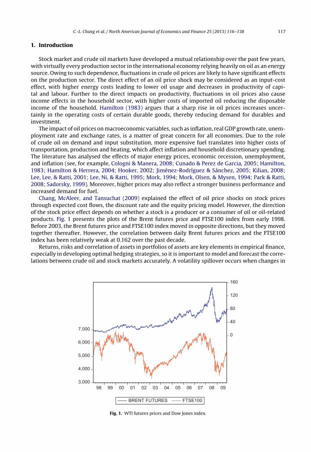
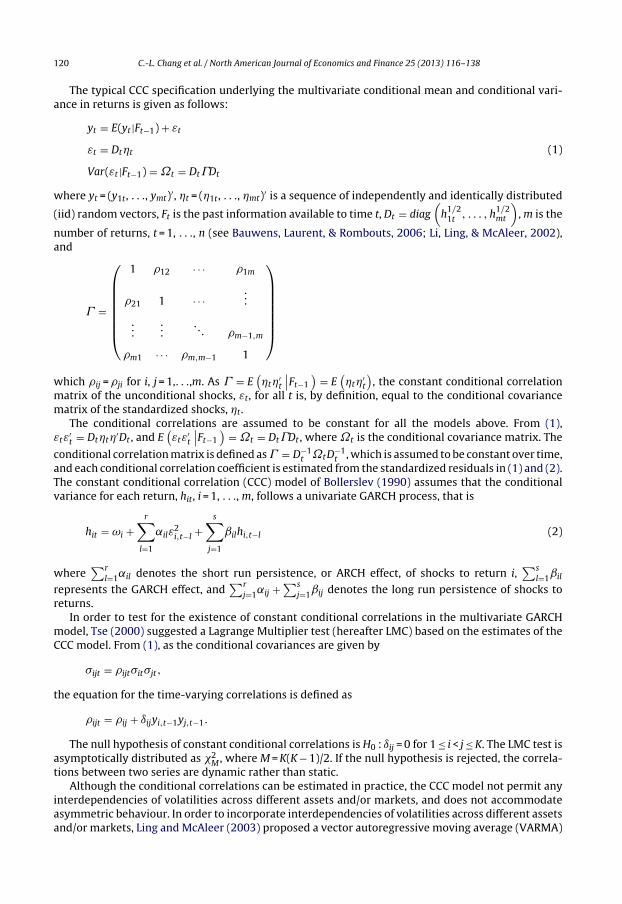
Chang, McAleer, and Tansuchat (2009) explained the effect of oil price shocks on stock pricesthrough expected cost flows, the discount rate and the equity pricing model. However, the directionof the stock price effect depends on whether a stock is a producer or a consumer of oil or oil-relatedproducts. Fig. 1 presents the plots of the Brent futures price and FTSE100 index from early 1998.Before 2003, the Brent futures price and FTSE100 index moved in opposite directions, but they movedtogether thereafter. However, the correlation between daily Brent futures prices and the FTSE100index has been relatively weak at 0.162 over the past decade.

Returns, risks and correlation of assets in portfolios of assets are key elements in empirical finance,especially in developing optimal hedging strategies, so it is important to model and forecast the corre-lations between crude oil and stock markets accurately. A volatility spillover occurs when changes in

3,000

4,000

5,000

6,000

7,000

0

40

80

120

160

98 99 00 01 02 03 04 05 06 07 08 09

BRENT FUTURES FTSE100

Fig. 1. WTI futures prices and Dow Jones index.

118 C.-L. Chang et al. / North American Journal of Economics and Finance 25 (2013) 116– 138

price or returns volatility in one market have a lagged impact on volatility in the financial, energy andstock markets (see, for example, Ågren, 2006; Hammoudeh and Aleisa, 2002; Hammoudeh, Dibooglu,& Aleisa, 2004; Malik and Hammoudeh, 2007; Sadorsky, 2004). Surprisingly, there does not seem tohave been an analysis of the conditional correlations or volatility spillovers between shocks in crude oilreturns and in index returns, despite these issues being very important for practitioners and investorsalike.

The reaction of stock markets to oil price and returns shocks will determine whether stock pricesrationally reflect the impact of news on current and future real cash flows. The paper models theconditional correlations and examines the volatility spillovers between two major crude oil return,namely Brent and WTI (West Texas Intermediate) and four stock index returns, namely FTSE100 (Lon-don Stock Exchange, FTSE), NYSE composite (New York Stock Exchange, NYSE), S&P500 compositeindex, and Dow Jones Industrials (DJ). Some of these issues have been examined empirically using sev-eral recent models of multivariate conditional volatility, namely the CCC model of Bollerslev (1990),VARMA-GARCH model of Ling and McAleer (2003), VARMA-AGARCH model of McAleer, Chan, Hoti,and Lieberman (2008), and DCC model of Engle (2002).

The remainder of the paper is organized as follows. Section 2 reviews the relationship betweenthe crude oil market and stock market. Section 3 discusses various popular multivariate conditionalvolatility models that enable an analysis of volatility spillovers. Section 4 gives details of the data to bein the empirical analysis, descriptive statistics and unit root tests. The empirical results are analysedin Section 5, and some concluding remarks are given in Section 6.

2. Crude oil and stock markets

There is a scant literature on the empirical relationship between the crude oil and stock markets.Jones and Kaul (1996) show the negative reaction of US, Canadian, UK and Japan stock prices to oilprice shocks via the impact of oil price shocks on real cash flows. Ciner (2001) uses linear and non-linear causality tests to examine the dynamic relationship between oil prices and stock markets, andconcludes that a significant relationship between real stock returns and oil futures price is non-linear.Hammoudeh and Aleisa (2002) find spillovers from oil markets to the stock indices of oil-exportingcountries, including Bahrain, Indonesia, Mexico and Venezuela. Kilian and Park (2009) report thatonly oil price increases, driven by precautionary demand for oil over concern about future oil sup-plies, affect stock prices negatively. Driesprong, Jacobsen, and Maat (2008) find a strong relationshipbetween stock market and oil market movements.

Several previous papers have applied vector autoregressive (VAR) models to investigate therelationship between the oil and stock markets. Kaneko and Lee (1995) find that changes in oilprices are significant in explaining Japanese stock market returns. Huang, Masulis, and Stoll (1996)show significant causality from oil futures prices to stock returns of individual firms, but notto aggregate market returns. In addition, they find that oil futures returns lead the petroleumindustry stock index, and three oil company stock returns. Sadorsky (1999) indicates that positiveshocks to oil prices depress real stock returns, using monthly data, and the results from impulseresponse functions suggest that oil price movements are important in explaining movements in stockreturns.

Papapetrou (2001) reveals that the oil price is an important factor in explaining stock price move-ments in Greece, and that a positive oil price shock depresses real stock returns by using impulseresponse functions. Lee and Ni (2002) indicate that, as a large cost share of oil industries, such aspetroleum refinery and industrial chemicals; oil price shocks tend to reduce supply. In contrast, formany other industries, such as the automobile industry, oil price shocks tend to reduce demand. Parkand Ratti (2008) estimate the effects of oil price shocks and oil price volatility on the real stock returnsof the USA and 13 European countries, and find that oil price shocks have a statistically significantimpact on real stock returns in the same month, and real oil price shocks also have an impact on realstock returns across all countries. For emerging stock markets, Maghyereh (2004) finds that oil shockshave no significant impact on stock index returns in 22 emerging economies. However, Basher andSardosky (2006) show strong evidence that oil price risk has a significant impact on stock price returnsin emerging markets.


Regarding the relationship between oil prices and stock markets, Faff and Brailsford (1999) finda positive impact on the oil and gas, and diversified resources, industries, whereas there is a nega-tive impact on the paper and packing, banks and transport industries. Sadorsky (2001) shows thatstock returns of Canadian oil and gas companies are positive and sensitive to oil price increases usinga multifactor market model. In particular, an increase in the oil price factor increases the returnsto Canadian oil and gas stocks. Boyer and Filion (2004) find a positive association between energystock returns and an appreciation in oil and gas prices. Hammoudeh and Li (2005) show that oilprice growth leads the stock returns of oil-exporting countries and oil-sensitive industries in theUSA.

Nandha and Faff (2007) examine the adverse effects of oil price shocks on stock market returnsusing global industry indices. The empirical results indicate that oil price changes have a neg-ative impact on equity returns in all industries, with the exception of mining, and oil and gas.Cong, Wei, Jiao, and Fan (2008) argue that oil price shocks do not have a statistically significantimpact on the real stock returns of most Chinese stock market indices, except for the manufactur-ing index and some oil companies. An increase in oil volatility does not affect most stock returns,but may increase speculation in the mining and petrochemical indexes, thereby increasing the asso-ciated stock returns. Sadorsky (2008) finds that the stock prices of small and large firms respondfairly symmetrically to changes in oil prices, but for medium-sized firms the response is asymmet-ric to changes in oil prices. From simulations using a VAR model, Henriques and Sadorsky (2008)show that shocks to oil prices have little impact on the stock prices of alternative energy compa-nies.

In small emerging markets, especially in the Gulf Cooperating Council (GCC) countries, Hammoudehand Aleisa (2004) show that the Saudi market is the leader among GCC stock markets, and can bepredicted by oil futures prices. Maghyereh and Al-Kandari (2007) apply nonlinear cointegration anal-ysis to examine the linkage between oil prices and stock markets in GCC countries. The empiricalresults indicate that oil prices have a nonlinear impact on stock price indices in GCC countries. Onour(2007) argues that, in the short run, GCC stock market returns are dominated by the influence of non-observable psychological factors. In the long run, the effects of oil price changes are transmitted tofundamental macroeconomic indicators which, in turn, affect the long run equilibrium linkages acrossmarkets.

Recent research has used multivariate GARCH specifications, especially BEKK, to model volatil-ity spillovers between the crude oil and stock markets. Hammoudeh et al. (2004) find that thereare two-way interactions between the S&P Oil Composite index, and oil spot and futures prices.Malik and Hammoudeh (2007) find that Gulf equity markets receive volatility from the oil mar-kets, but only in the case of Saudi Arabia is the volatility spillover from the Saudi market to theoil market significant, underlining the major role that Saudi Arabia plays in the global oil mar-ket. Using a two-regime Markov-switching EGARCH model, Aloui and Jammazi (2009) examine therelationship between crude oil shocks and stock markets from December 1987 to January 2007.The paper focuses on the WTI and Brent crude oil markets and three developed stock markets,namely France, UK and Japan. The results show that the net oil price increase variable play a sig-nificant role in determining both the volatility of real returns and the probability of transition acrossregimes.

3. Econometric models

In order to investigate the conditional correlations and volatility spillovers between crude oilreturns and stock index returns, several multivariate conditional volatility models are used. Thissection presents the CCC model of Bollerslev (1990), VARMA-GARCH model of Ling and McAleer(2003), and VARMA-AGARCH model of McAleer, Hoti, and Chan (2009). These models assume con-stant conditional correlations, and do not suffer from the curse of dimensionality, as compared withthe VECH and BEKK models (see McAleer et al., 2008 and Caporin and McAleer, 2009, 2010 for furtherdetails). In order to make the conditional correlations time dependent, Engle (2002) proposed the DCCmodel.


The typical CCC specification underlying the multivariate conditional mean and conditional vari-ance in returns is given as follows:

yt = E(yt |Ft−1) + εt

εt = Dt�t

Var(εt |Ft−1) = ˝t = Dt�Dt

(1)

where yt = (y1t, . . ., ymt)′, �t = (�1t, . . ., �mt)′ is a sequence of independently and identically distributed

(iid) random vectors, Ft is the past information available to time t, Dt = diag(

h1/21t , . . . , h1/2

mt

), m is the

number of returns, t = 1, . . ., n (see Bauwens, Laurent, & Rombouts, 2006; Li, Ling, & McAleer, 2002),and

� =

⎛⎜⎜⎜⎜⎜⎜⎝

1 �12 · · · �1m

�21 1 · · ·...

......

. . . �m−1,m

�m1 · · · �m,m−1 1

⎞⎟⎟⎟⎟⎟⎟⎠

which �ij = �ji for i, j = 1,. . .,m. As � = E(

�t�′t

∣∣Ft−1)

= E(

�t�′t

), the constant conditional correlation

matrix of the unconditional shocks, εt, for all t is, by definition, equal to the conditional covariancematrix of the standardized shocks, �t.

The conditional correlations are assumed to be constant for all the models above. From (1),εtε′

t = Dt�t�′Dt , and E(

εtε′t

∣∣Ft−1)

= ˝t = Dt�Dt , where ˝t is the conditional covariance matrix. The

conditional correlation matrix is defined as � = D−1t ˝tD

−1t , which is assumed to be constant over time,

and each conditional correlation coefficient is estimated from the standardized residuals in (1) and (2).The constant conditional correlation (CCC) model of Bollerslev (1990) assumes that the conditionalvariance for each return, hit, i = 1, . . ., m, follows a univariate GARCH process, that is

hit = ωi +r∑

l=1

˛ilε2i,t−l +

s∑j=1

ˇilhi,t−l (2)

where∑r

l=1˛il denotes the short run persistence, or ARCH effect, of shocks to return i,∑s

l=1ˇil

represents the GARCH effect, and∑r

j=1˛ij +∑s

j=1ˇij denotes the long run persistence of shocks toreturns.

In order to test for the existence of constant conditional correlations in the multivariate GARCHmodel, Tse (2000) suggested a Lagrange Multiplier test (hereafter LMC) based on the estimates of theCCC model. From (1), as the conditional covariances are given by

�ijt = �ijt�it�jt,

the equation for the time-varying correlations is defined as

�ijt = �ij + ıijyi,t−1yj,t−1.

The null hypothesis of constant conditional correlations is H0 : ıij = 0 for 1 ≤ i < j ≤ K. The LMC test isasymptotically distributed as �2

M , where M = K(K − 1)/2. If the null hypothesis is rejected, the correla-tions between two series are dynamic rather than static.

Although the conditional correlations can be estimated in practice, the CCC model not permit anyinterdependencies of volatilities across different assets and/or markets, and does not accommodateasymmetric behaviour. In order to incorporate interdependencies of volatilities across different assetsand/or markets, Ling and McAleer (2003) proposed a vector autoregressive moving average (VARMA)


specification of the conditional mean in (1), and the following GARCH specification for the conditionalvariances:

˚(L)(Yt − ) = (L)εt (3)

εt = Dt�t

Ht = W +r∑

l=1

Al�εt−l +s∑

l=1

BlHt−l

(4)

where Dt = diag(

h1/2i,t

), Ht = (h1t, . . ., hmt)′, ˚(L) = Im − ˚1L − · · · − ˚pLp and

(L) = Im − 1L − · · · − qLq are polynomials in L, �ε =(

ε21t , . . . ε2

mt

)′, and W, Al for l = 1,. . ., r and

Bl for l = 1, . . ., s are m × m matrices and represent the ARCH and GARCH effects, respectively. Spillovereffects, or the dependence of the conditional variance between crude oil returns and stock indexreturns, are given in the conditional variance for each returns in the portfolio. It is clear that whenAl and Bl are diagonal matrices, (4) reduces to (2), so the VARMA-GARCH model has CCC as a specialcase.

As in the univariate GARCH model, VARMA-GARCH assumes that negative and positive shocks ofequal magnitude have identical impacts on the conditional variance. In order to separate the asym-metric impacts of positive and negative shocks, McAleer et al. (2009) proposed the VARMA-AGARCHspecification for the conditional variance, namely

Ht = W +r∑

l=1

Al�εt−l +r∑

l=1

CiI (�t−l) �εt−l +s∑

l=1

BlHt−l (5)

where Cl are m × m matrices for l = 1, . . ., r, and It = diag(I1t, . . ., Imt) is an indicator function, and is givenas

I(�it) ={

0, εit > 0

1, εit ≤ 0. (6)

If m = 1, (6) collapses to the asymmetric GARCH, or GJR, model of Glosten, Jagannathan, and Runkle(1992). Moreover, VARMA-AGARCH reduces to VARMA-GARCH when Ci = 0 for all i. If Ci = 0 and Ai andBj are diagonal matrices for all i and j, then VARMA-AGARCH reduces to CCC. The parameters of model(1)–(5) are obtained by maximum likelihood estimation (MLE) using a joint normal density. When �t

does not follow a joint multivariate normal distribution, the appropriate estimator is the Quasi-MLE(QMLE).

Unless �t is a sequence of iid random vectors, or alternatively a martingale difference process,the assumption that the conditional correlations are constant may seen unrealistic. In order to makethe conditional correlation matrix time dependent, Engle (2002) proposed a dynamic conditionalcorrelation (DCC) model, which is defined as

yt |It−1∼(0, Qt), t = 1, 2, . . . , n (7)

Qt = Dt�tDt, (8)

where Dt = [diag(ht)]1/2 is a diagonal matrix of conditional variances, and It is the information setavailable to time t. The conditional variance, hit, can be defined as a univariate GARCH model, asfollows:

hit = ωi +p∑

k=1

˛ikεi,t−k +q∑

l=1

ˇilhi,t−l. (9)


Table 1Descriptive statistics.

Returns Mean Max Min SD Skewness Kurtosis Jarque–Bera

FTSE −1.75e−06 0.093 −0.093 0.013 −0.125 8.741 4250.157NYSE 7.58e−05 0.115 −0.102 0.013 −0.299 12.960 12812.11S&P 2.44e−05 0.110 −0.095 0.014 −0.137 10.590 7423.755DJ −0.0001 0.132 −0.121 0.016 −0.244 9.227 5020.704BRSP 0.0005 0.152 −0.170 0.023 −0.047 6.103 1240.415BRFOR 0.0005 0.126 −0.133 0.023 −0.073 5.398 743.048BRFU 0.0005 0.129 −0.144 0.024 −0.145 5.553 849.874WTISP 0.0005 0.213 −0.172 0.027 −0.006 7.877 3062.127WTIFOR 0.0005 0.229 −0.142 0.026 0.099 7.967 3179.933WTIFU 0.0005 0.164 −0.165 0.026 −0.124 7.127 2199.531

If �t is a vector of iid random variables, with zero mean and unit variance, Qt in (8) is the conditionalcovariance matrix (after standardization, �it = yit/

√hit). The �it are used to estimate the dynamic

conditional correlations, as follows:

�t = {(diag(Qt)−1/2}Qt{(diag(Qt)

−1/2} (10)

where the k × k symmetric positive definite matrix Qt is given by

Qt = (1 − �1 − �2)Q̄ + �1�t−1�′t−1 + �2Qt−1 (11)

in which �1 and �2 are non-negative scalar parameters to capture, respectively, the effects of previousshocks and previous dynamic conditional correlations on the current dynamic conditional correlation.As Qt is a conditional on the vector of standardized residuals, (11) is a conditional covariance matrix,and Q̄ is the k × k unconditional variance matrix of �t. For further details, and a critique of DCC andBEKK, see Caporin and McAleer (2009, 2010).

4. Data

For the empirical analysis, daily data are used for the four indexes, namely FTSE100 (LondonStock Exchange: FTSE), NYSE composite (New York Stock Exchange: NYSE), S&P500 composite(Standard and Poor’s: S&P), and Dow Jones Industrials (Dow Jones: DJ), and three crude oil closingprices (spot, forward and futures) of two reference markets, namely Brent and WTI (West TexasIntermediate). Thus, there are six price indexes, namely Brent spot prices FOB (BRSP), Brent one-month forward prices (BRFOR), Brent one-month futures prices (BRFU), WTI spot Cushing prices(WTISP), WTI one-month forward price (WTIFOR), and NYMEX one month futures price (WTIFU).All 3090 prices and price index observations are from 2 January 1998 to 4 November 2009. The

Table 2Unit root tests.

Returns ADF PP

None Constant Constant and trend None Constant Constant and trend

FTSE −27.327 −27.322 −27.318 −57.871 −57.862 −57.853NYSE −42.944 −42.940 −42.939 −59.142 −59.135 −59.134S&P −43.558 −43.552 −43.557 −60.770 −60.760 −60.772DJ −56.785 −56.780 −56.772 −57.002 −57.000 −56.992BRSP −54.904 −54.918 −54.909 −54.909 −54.922 −54.914BRFOR −57.211 −57.230 −57.222 −57.208 −57.229 −57.219BRFU −58.850 −58.869 −58.869 −58.821 −58.847 −58.838WTISP −56.288 −56.299 −56.290 −56.506 −56.539 −56.529WTIFOR −58.000 −58.013 −58.004 −58.181 −58.214 −58.204WTIFU −41.915 −41.934 −41.927 −56.787 −56.804 −56.794

Note: Entries in bold are significant at the 5% level.


data are obtained from DataStream database services, and crude oil prices are expressed in USD perbarrel.

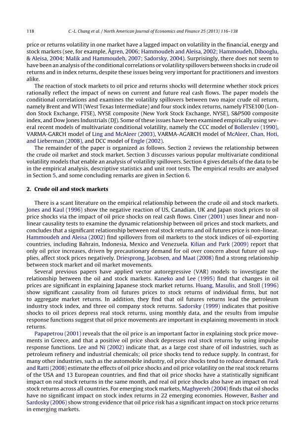
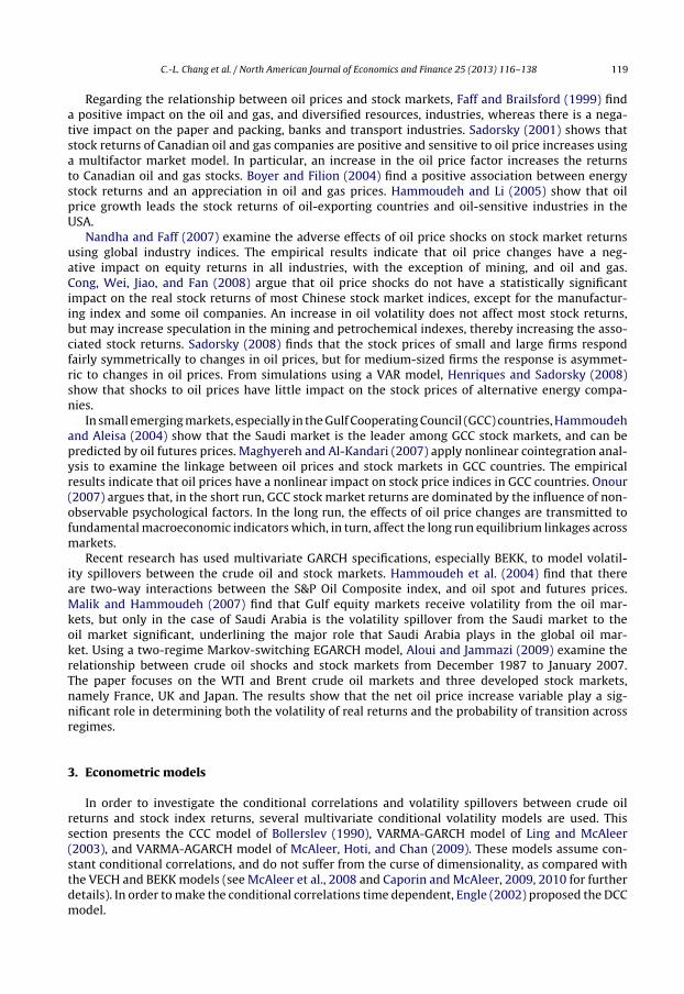
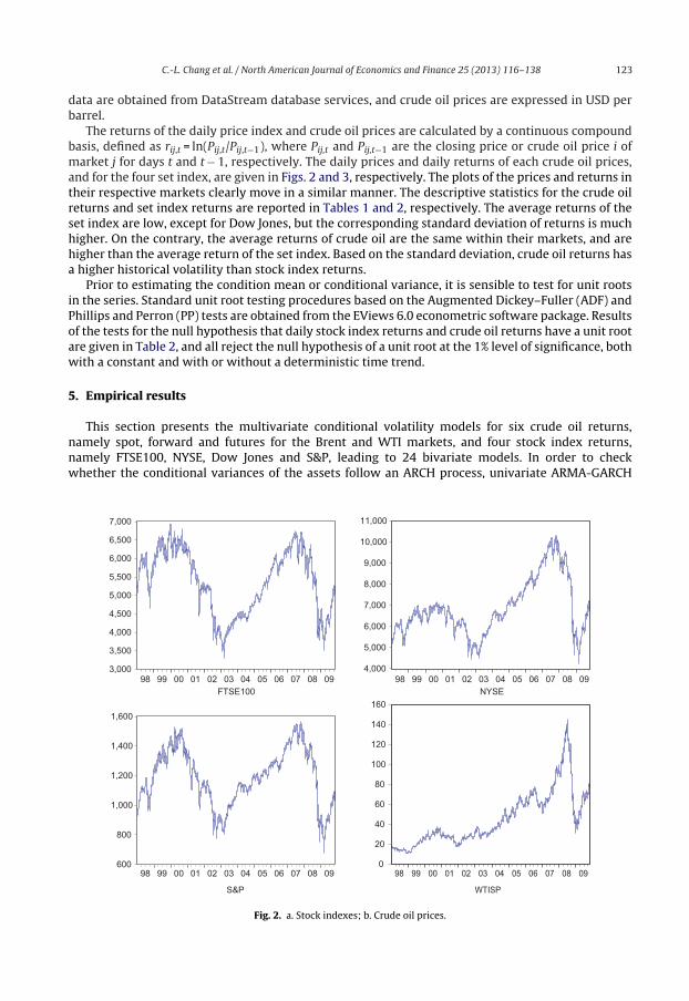
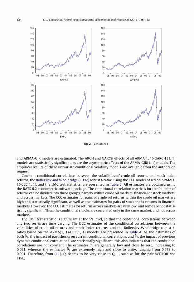
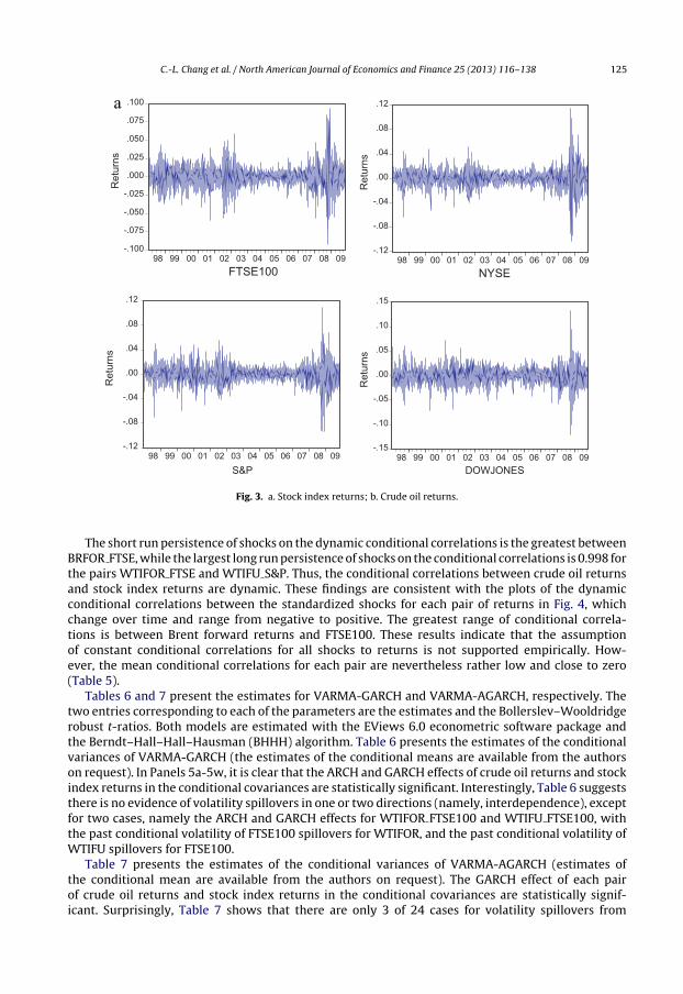
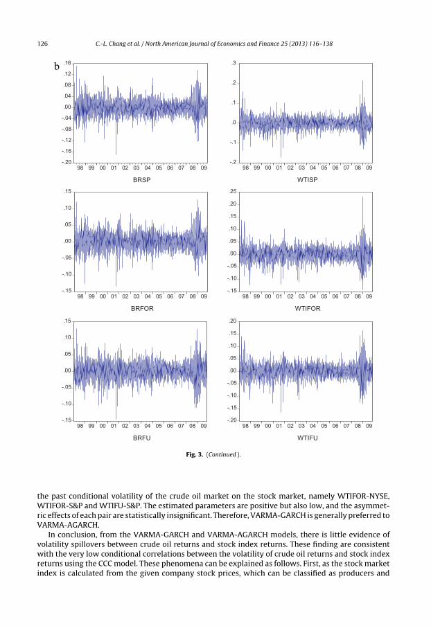
The returns of the daily price index and crude oil prices are calculated by a continuous compoundbasis, defined as rij,t = ln(Pij,t/Pij,t−1), where Pij,t and Pij,t−1 are the closing price or crude oil price i ofmarket j for days t and t − 1, respectively. The daily prices and daily returns of each crude oil prices,and for the four set index, are given in Figs. 2 and 3, respectively. The plots of the prices and returns intheir respective markets clearly move in a similar manner. The descriptive statistics for the crude oilreturns and set index returns are reported in Tables 1 and 2, respectively. The average returns of theset index are low, except for Dow Jones, but the corresponding standard deviation of returns is muchhigher. On the contrary, the average returns of crude oil are the same within their markets, and arehigher than the average return of the set index. Based on the standard deviation, crude oil returns hasa higher historical volatility than stock index returns.

Prior to estimating the condition mean or conditional variance, it is sensible to test for unit rootsin the series. Standard unit root testing procedures based on the Augmented Dickey–Fuller (ADF) andPhillips and Perron (PP) tests are obtained from the EViews 6.0 econometric software package. Resultsof the tests for the null hypothesis that daily stock index returns and crude oil returns have a unit rootare given in Table 2, and all reject the null hypothesis of a unit root at the 1% level of significance, bothwith a constant and with or without a deterministic time trend.

5. Empirical results

This section presents the multivariate conditional volatility models for six crude oil returns,namely spot, forward and futures for the Brent and WTI markets, and four stock index returns,namely FTSE100, NYSE, Dow Jones and S&P, leading to 24 bivariate models. In order to checkwhether the conditional variances of the assets follow an ARCH process, univariate ARMA-GARCH

3,000

3,500

4,000

4,500

5,000

5,500

6,000

6,500

7,000

98 99 00 01 02 03 04 05 06 07 08 09

FTSE100

600

800

1,000

1,200

1,400

1,600

98 99 00 01 02 03 04 05 06 07 08 09

S&P

4,000

5,000

6,000

7,000

8,000

9,000

10,000

11,000

98 99 00 01 02 03 04 05 06 07 08 09

NYSE

0

20

40

60

80

100

120

140

160

98 99 00 01 02 03 04 05 06 07 08 09

WTISP

Fig. 2. a. Stock indexes; b. Crude oil prices.


0

20

40

60

80

100

120

140

160

98 99 00 01 02 03 04 05 06 07 08 09

BRFOR

0

20

40

60

80

100

120

140

160

98 99 00 01 02 03 04 05 06 07 08 09

WTIFOR

0

20

40

60

80

100

120

140

160

98 99 00 01 02 03 04 05 06 07 08 09

BRFU

0

20

40

60

80

100

120

140

160

98 99 00 01 02 03 04 05 06 07 08 09

WTIFU

Fig. 2. (Continued ).

and ARMA-GJR models are estimated. The ARCH and GARCH effects of all ARMA(1, 1)-GARCH (1, 1)models are statistically significant, as are the asymmetric effects of the ARMA-GJR(1, 1) models. Theempirical results of these univariate conditional volatility models are available from the authors onrequest.

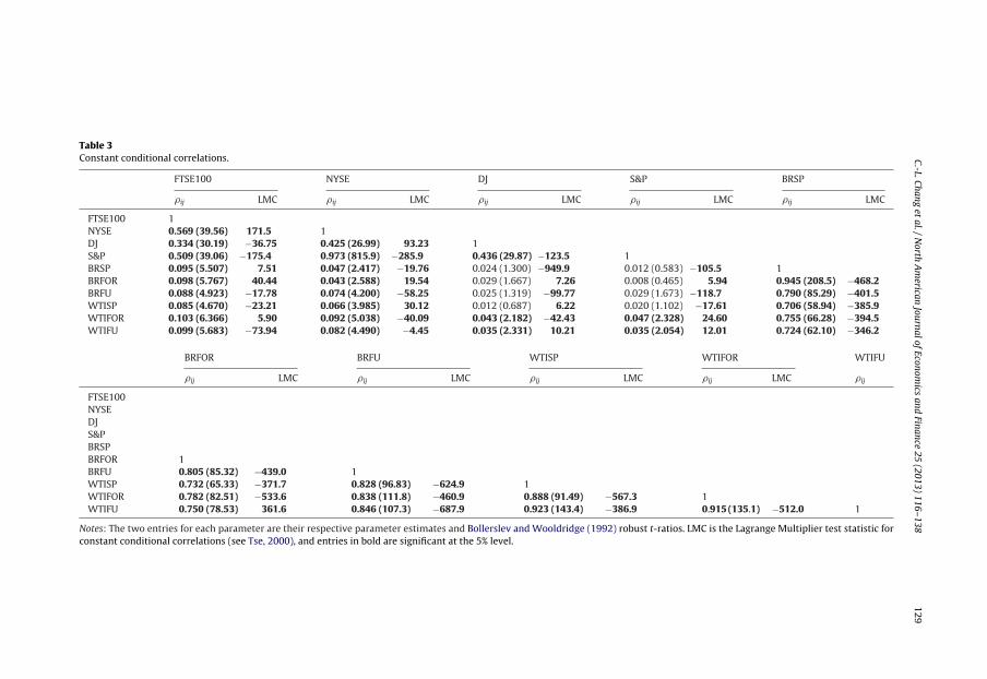
Constant conditional correlations between the volatilities of crude oil returns and stock indexreturns, the Bollerslev and Wooldridge (1992) robust t-ratios using the CCC model based on ARMA(1,1)-CCC(1, 1), and the LMC test statistics, are presented in Table 3. All estimates are obtained usingthe RATS 6.2 econometric software package. The conditional correlation matrices for the 24 pairs ofreturns can be divided into three groups, namely within crude oil markets, financial or stock markets,and across markets. The CCC estimates for pairs of crude oil returns within the crude oil market arehigh and statistically significant, as well as the estimates for pairs of stock index returns in financialmarkets. However, the CCC estimates for returns across markets are very low, and some are not statis-tically significant. Thus, the conditional shocks are correlated only in the same market, and not acrossmarkets.

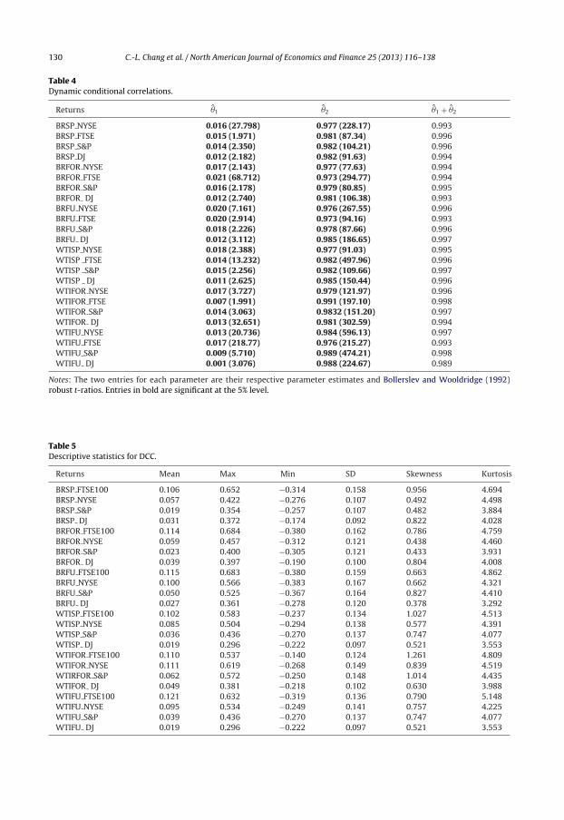
The LMC test statistic is significant at the 5% level, so that the conditional correlations betweenany two series are time varying. The DCC estimates of the conditional correlations between thevolatilities of crude oil returns and stock index returns, and the Bollerslev-Wooldridge robust t-ratios based on the ARMA(1, 1)-DCC(1, 1) models, are presented in Table 4. As the estimates ofboth �̂1, the impact of past shocks on current conditional correlations, and �̂2, the impact of previousdynamic conditional correlations, are statistically significant, this also indicates that the conditionalcorrelations are not constant. The estimates �̂1 are generally low and close to zero, increasing to0.021, whereas the estimates �̂2 are extremely high and close to unity, ranging from 0.973 to0.991. Therefore, from (11), Qt seems to be very close to Qt−1, such as for the pair WTIFOR andFTSE.


-.15

-.10

-.05

.00

.05

.10

.15

98 99 00 01 02 03 04 05 06 07 08 09

DOWJONES

Re

turn

s

-.100

-.075

-.050

-.025

.000

.025

.050

.075

.100

98 99 00 01 02 03 04 05 06 07 08 09

FTSE100

Re

turn

s

-.12

-.08

-.04

.00

.04

.08

.12

98 99 00 01 02 03 04 05 06 07 08 09

NYSE

Re

turn

s

-.12

-.08

-.04

.00

.04

.08

.12

98 99 00 01 02 03 04 05 06 07 08 09

S&P

Re

turn

sa

Fig. 3. a. Stock index returns; b. Crude oil returns.

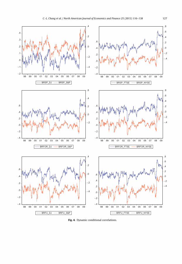
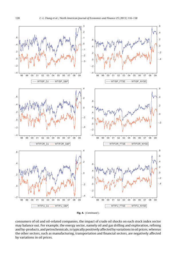
The short run persistence of shocks on the dynamic conditional correlations is the greatest betweenBRFOR FTSE, while the largest long run persistence of shocks on the conditional correlations is 0.998 forthe pairs WTIFOR FTSE and WTIFU S&P. Thus, the conditional correlations between crude oil returnsand stock index returns are dynamic. These findings are consistent with the plots of the dynamicconditional correlations between the standardized shocks for each pair of returns in Fig. 4, whichchange over time and range from negative to positive. The greatest range of conditional correla-tions is between Brent forward returns and FTSE100. These results indicate that the assumptionof constant conditional correlations for all shocks to returns is not supported empirically. How-ever, the mean conditional correlations for each pair are nevertheless rather low and close to zero(Table 5).

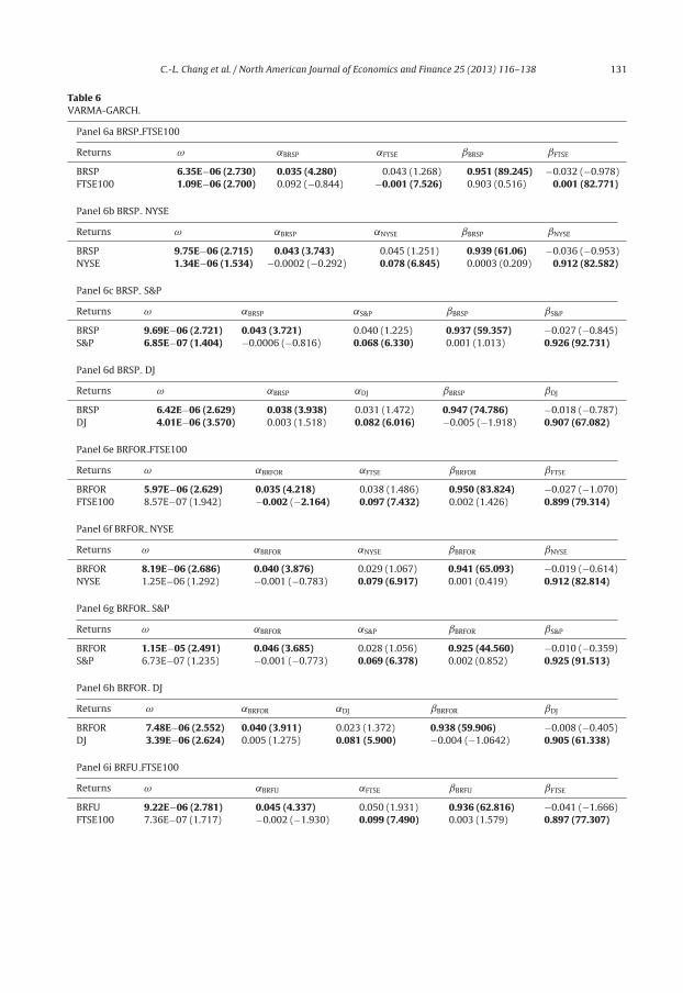
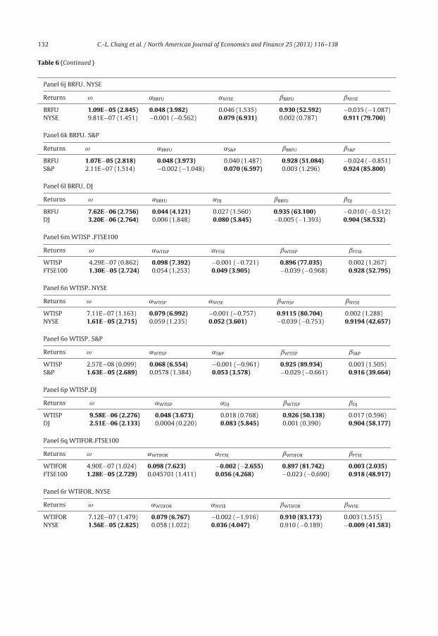
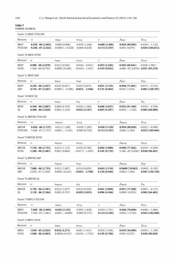
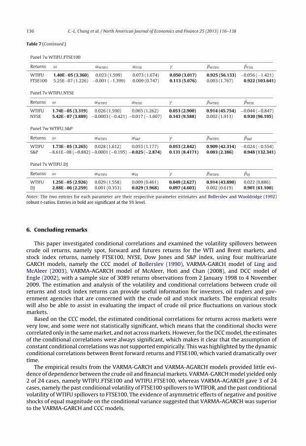
Tables 6 and 7 present the estimates for VARMA-GARCH and VARMA-AGARCH, respectively. Thetwo entries corresponding to each of the parameters are the estimates and the Bollerslev–Wooldridgerobust t-ratios. Both models are estimated with the EViews 6.0 econometric software package andthe Berndt–Hall–Hall–Hausman (BHHH) algorithm. Table 6 presents the estimates of the conditionalvariances of VARMA-GARCH (the estimates of the conditional means are available from the authorson request). In Panels 5a-5w, it is clear that the ARCH and GARCH effects of crude oil returns and stockindex returns in the conditional covariances are statistically significant. Interestingly, Table 6 suggeststhere is no evidence of volatility spillovers in one or two directions (namely, interdependence), exceptfor two cases, namely the ARCH and GARCH effects for WTIFOR FTSE100 and WTIFU FTSE100, withthe past conditional volatility of FTSE100 spillovers for WTIFOR, and the past conditional volatility ofWTIFU spillovers for FTSE100.

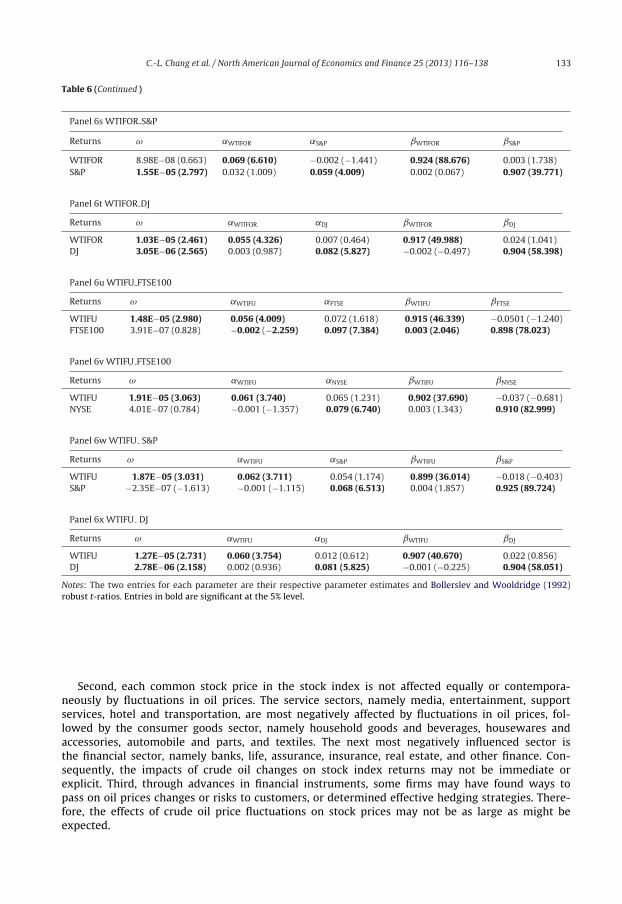
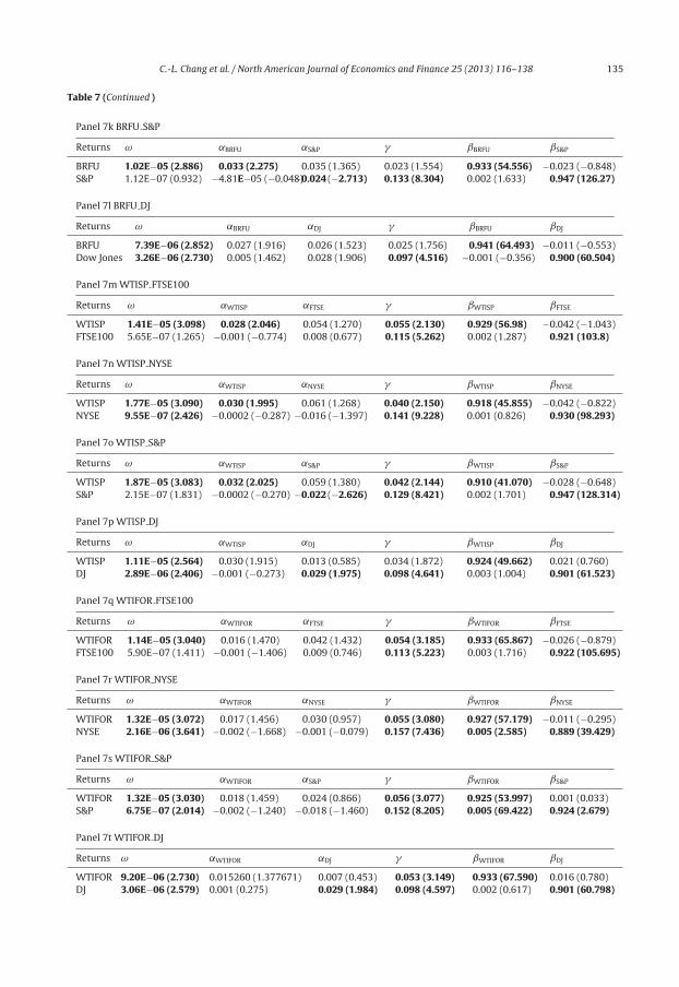
Table 7 presents the estimates of the conditional variances of VARMA-AGARCH (estimates ofthe conditional mean are available from the authors on request). The GARCH effect of each pairof crude oil returns and stock index returns in the conditional covariances are statistically signif-icant. Surprisingly, Table 7 shows that there are only 3 of 24 cases for volatility spillovers from


-.20

-.16

-.12

-.08

-.04

.00

.04

.08

.12

.16

98 99 00 01 02 03 04 05 06 07 08 09

BRSP

-.2

-.1

.0

.1

.2

.3

98 99 00 01 02 03 04 05 06 07 08 09

WTISP

-.15

-.10

-.05

.00

.05

.10

.15

98 99 00 01 02 03 04 05 06 07 08 09

BRFOR

-.15

-.10

-.05

.00

.05

.10

.15

.20

.25

98 99 00 01 02 03 04 05 06 07 08 09

WTIFOR

-.15

-.10

-.05

.00

.05

.10

.15

98 99 00 01 02 03 04 05 06 07 08 09

BRFU

-.20

-.15

-.10

-.05

.00

.05

.10

.15

.20

98 99 00 01 02 03 04 05 06 07 08 09

WTIFU

b


the past conditional volatility of the crude oil market on the stock market, namely WTIFOR-NYSE,WTIFOR-S&P and WTIFU-S&P. The estimated parameters are positive but also low, and the asymmet-ric effects of each pair are statistically insignificant. Therefore, VARMA-GARCH is generally preferred toVARMA-AGARCH.

In conclusion, from the VARMA-GARCH and VARMA-AGARCH models, there is little evidence ofvolatility spillovers between crude oil returns and stock index returns. These finding are consistentwith the very low conditional correlations between the volatility of crude oil returns and stock indexreturns using the CCC model. These phenomena can be explained as follows. First, as the stock marketindex is calculated from the given company stock prices, which can be classified as producers and


-.4

-.2

.0

.2

.4

.6

-.4

-.2

.0

.2

.4

.6

.8

98 99 00 01 02 03 04 05 06 07 08 09

BRSP_FTSE BRSP_NYSE

-.4

-.2

.0

.2

.4

.6

-.4

-.2

.0

.2

.4

.6

.8

98 99 00 01 02 03 04 05 06 07 08 09

BRFOR_FTSE BRFOR_NYSE

-.4

-.2

.0

.2

.4

.6

-.2

.0

.2

.4

.6

98 99 00 01 02 03 04 05 06 07 08 09

BRFOR_DJ BRFOR_S&P

-.4

-.2

.0

.2

.4

.6

-.4

-.2

.0

.2

.4

98 99 00 01 02 03 04 05 06 07 08 09

BRFU_DJ BRFU_S&P

-.4

-.2

.0

.2

.4

.6

-.4

-.2

.0

.2

.4

.6

.8

98 99 00 01 02 03 04 05 06 07 08 09

BRFU_FTSE BRFU_NYSE

-.2

-.1

.0

.1

.2

.3

.4

-.4

-.2

.0

.2

.4

98 99 00 01 02 03 04 05 06 07 08 09

BRSP_DJ BRSP_S&P

Fig. 4. Dynamic conditional correlations.


-.4

-.2

.0

.2

.4

.6

-.3

-.2

-.1

.0

.1

.2

.3

98 99 00 01 02 03 04 05 06 07 08 09

WTISP_DJ WTISP_S&P

-.4

-.2

.0

.2

.4

.6

-.4

-.2

.0

.2

.4

.6

98 99 00 01 02 03 04 05 06 07 08 09

WTISP_FTSE WTISP_NYSE

-.4

-.2

.0

.2

.4

.6

-.4

-.2

.0

.2

.4

98 99 00 01 02 03 04 05 06 07 08 09

WTIFOR_DJ WTIFOR_S&P

-.4

-.2

.0

.2

.4

.6

.8

-.2

.0

.2

.4

.6

98 99 00 01 02 03 04 05 06 07 08 09

WTIFOR_FTSE WTIFOR_NYSE

-.2

.0

.2

.4

.6

-.4

-.2

.0

.2

.4

98 99 00 01 02 03 04 05 06 07 08 09

WTIFU_DJ WTIFU_S&P

-.4

-.2

.0

.2

.4

.6

-.4

-.2

.0

.2

.4

.6

.8

98 99 00 01 02 03 04 05 06 07 08 09

WTIFU_FTSE WTIFU_NYSE


consumers of oil and oil-related companies, the impact of crude oil shocks on each stock index sectormay balance out. For example, the energy sector, namely oil and gas drilling and exploration, refiningand by-products, and petrochemicals, is typically positively affected by variations in oil prices, whereasthe other sectors, such as manufacturing, transportation and financial sectors, are negatively affectedby variations in oil prices.

C.-L. Chang

et al.

/ N

orth A

merican

Journal of

Economics

and Finance

25 (2013) 116– 138129

Table 3Constant conditional correlations.

FTSE100 NYSE DJ S&P BRSP

�ij LMC �ij LMC �ij LMC �ij LMC �ij LMC

FTSE100 1NYSE 0.569 (39.56) 171.5 1DJ 0.334 (30.19) −36.75 0.425 (26.99) 93.23 1S&P 0.509 (39.06) −175.4 0.973 (815.9) −285.9 0.436 (29.87) −123.5 1BRSP 0.095 (5.507) 7.51 0.047 (2.417) −19.76 0.024 (1.300) −949.9 0.012 (0.583) −105.5 1BRFOR 0.098 (5.767) 40.44 0.043 (2.588) 19.54 0.029 (1.667) 7.26 0.008 (0.465) 5.94 0.945 (208.5) −468.2BRFU 0.088 (4.923) −17.78 0.074 (4.200) −58.25 0.025 (1.319) −99.77 0.029 (1.673) −118.7 0.790 (85.29) −401.5WTISP 0.085 (4.670) −23.21 0.066 (3.985) 30.12 0.012 (0.687) 6.22 0.020 (1.102) −17.61 0.706 (58.94) −385.9WTIFOR 0.103 (6.366) 5.90 0.092 (5.038) −40.09 0.043 (2.182) −42.43 0.047 (2.328) 24.60 0.755 (66.28) −394.5WTIFU 0.099 (5.683) −73.94 0.082 (4.490) −4.45 0.035 (2.331) 10.21 0.035 (2.054) 12.01 0.724 (62.10) −346.2

BRFOR BRFU WTISP WTIFOR WTIFU

�ij LMC �ij LMC �ij LMC �ij LMC �ij

FTSE100NYSEDJS&PBRSPBRFOR 1BRFU 0.805 (85.32) −439.0 1WTISP 0.732 (65.33) −371.7 0.828 (96.83) −624.9 1WTIFOR 0.782 (82.51) −533.6 0.838 (111.8) −460.9 0.888 (91.49) −567.3 1WTIFU 0.750 (78.53) 361.6 0.846 (107.3) −687.9 0.923 (143.4) −386.9 0.915 (135.1) −512.0 1

Notes: The two entries for each parameter are their respective parameter estimates and Bollerslev and Wooldridge (1992) robust t-ratios. LMC is the Lagrange Multiplier test statistic forconstant conditional correlations (see Tse, 2000), and entries in bold are significant at the 5% level.


Table 4Dynamic conditional correlations.

Returns �̂1 �̂2 �̂1 + �̂2

BRSP NYSE 0.016 (27.798) 0.977 (228.17) 0.993BRSP FTSE 0.015 (1.971) 0.981 (87.34) 0.996BRSP S&P 0.014 (2.350) 0.982 (104.21) 0.996BRSP DJ 0.012 (2.182) 0.982 (91.63) 0.994BRFOR NYSE 0.017 (2.143) 0.977 (77.63) 0.994BRFOR FTSE 0.021 (68.712) 0.973 (294.77) 0.994BRFOR S&P 0.016 (2.178) 0.979 (80.85) 0.995BRFOR DJ 0.012 (2.740) 0.981 (106.38) 0.993BRFU NYSE 0.020 (7.161) 0.976 (267.55) 0.996BRFU FTSE 0.020 (2.914) 0.973 (94.16) 0.993BRFU S&P 0.018 (2.226) 0.978 (87.66) 0.996BRFU DJ 0.012 (3.112) 0.985 (186.65) 0.997WTISP NYSE 0.018 (2.388) 0.977 (91.03) 0.995WTISP FTSE 0.014 (13.232) 0.982 (497.96) 0.996WTISP S&P 0.015 (2.256) 0.982 (109.66) 0.997WTISP DJ 0.011 (2.625) 0.985 (150.44) 0.996WTIFOR NYSE 0.017 (3.727) 0.979 (121.97) 0.996WTIFOR FTSE 0.007 (1.991) 0.991 (197.10) 0.998WTIFOR S&P 0.014 (3.063) 0.9832 (151.20) 0.997WTIFOR DJ 0.013 (32.651) 0.981 (302.59) 0.994WTIFU NYSE 0.013 (20.736) 0.984 (596.13) 0.997WTIFU FTSE 0.017 (218.77) 0.976 (215.27) 0.993WTIFU S&P 0.009 (5.710) 0.989 (474.21) 0.998WTIFU DJ 0.001 (3.076) 0.988 (224.67) 0.989

Notes: The two entries for each parameter are their respective parameter estimates and Bollerslev and Wooldridge (1992)robust t-ratios. Entries in bold are significant at the 5% level.

Table 5Descriptive statistics for DCC.

Returns Mean Max Min SD Skewness Kurtosis

BRSP FTSE100 0.106 0.652 −0.314 0.158 0.956 4.694BRSP NYSE 0.057 0.422 −0.276 0.107 0.492 4.498BRSP S&P 0.019 0.354 −0.257 0.107 0.482 3.884BRSP DJ 0.031 0.372 −0.174 0.092 0.822 4.028BRFOR FTSE100 0.114 0.684 −0.380 0.162 0.786 4.759BRFOR NYSE 0.059 0.457 −0.312 0.121 0.438 4.460BRFOR S&P 0.023 0.400 −0.305 0.121 0.433 3.931BRFOR DJ 0.039 0.397 −0.190 0.100 0.804 4.008BRFU FTSE100 0.115 0.683 −0.380 0.159 0.663 4.862BRFU NYSE 0.100 0.566 −0.383 0.167 0.662 4.321BRFU S&P 0.050 0.525 −0.367 0.164 0.827 4.410BRFU DJ 0.027 0.361 −0.278 0.120 0.378 3.292WTISP FTSE100 0.102 0.583 −0.237 0.134 1.027 4.513WTISP NYSE 0.085 0.504 −0.294 0.138 0.577 4.391WTISP S&P 0.036 0.436 −0.270 0.137 0.747 4.077WTISP DJ 0.019 0.296 −0.222 0.097 0.521 3.553WTIFOR FTSE100 0.110 0.537 −0.140 0.124 1.261 4.809WTIFOR NYSE 0.111 0.619 −0.268 0.149 0.839 4.519WTIRFOR S&P 0.062 0.572 −0.250 0.148 1.014 4.435WTIFOR DJ 0.049 0.381 −0.218 0.102 0.630 3.988WTIFU FTSE100 0.121 0.632 −0.319 0.136 0.790 5.148WTIFU NYSE 0.095 0.534 −0.249 0.141 0.757 4.225WTIFU S&P 0.039 0.436 −0.270 0.137 0.747 4.077WTIFU DJ 0.019 0.296 −0.222 0.097 0.521 3.553


Table 6VARMA-GARCH.

Panel 6a BRSP FTSE100

Returns ω ˛BRSP ˛FTSE ˇBRSP ˇFTSE

BRSP 6.35E−06 (2.730) 0.035 (4.280) 0.043 (1.268) 0.951 (89.245) −0.032 (−0.978)FTSE100 1.09E−06 (2.700) 0.092 (−0.844) −0.001 (7.526) 0.903 (0.516) 0.001 (82.771)

Panel 6b BRSP NYSE

Returns ω ˛BRSP ˛NYSE ˇBRSP ˇNYSE

BRSP 9.75E−06 (2.715) 0.043 (3.743) 0.045 (1.251) 0.939 (61.06) −0.036 (−0.953)NYSE 1.34E−06 (1.534) −0.0002 (−0.292) 0.078 (6.845) 0.0003 (0.209) 0.912 (82.582)

Panel 6c BRSP S&P

Returns ω ˛BRSP ˛S&P ˇBRSP ˇS&P

BRSP 9.69E−06 (2.721) 0.043 (3.721) 0.040 (1.225) 0.937 (59.357) −0.027 (−0.845)S&P 6.85E−07 (1.404) −0.0006 (−0.816) 0.068 (6.330) 0.001 (1.013) 0.926 (92.731)

Panel 6d BRSP DJ

Returns ω ˛BRSP ˛DJ ˇBRSP ˇDJ

BRSP 6.42E−06 (2.629) 0.038 (3.938) 0.031 (1.472) 0.947 (74.786) −0.018 (−0.787)DJ 4.01E−06 (3.570) 0.003 (1.518) 0.082 (6.016) −0.005 (−1.918) 0.907 (67.082)

Panel 6e BRFOR FTSE100

Returns ω ˛BRFOR ˛FTSE ˇBRFOR ˇFTSE

BRFOR 5.97E−06 (2.629) 0.035 (4.218) 0.038 (1.486) 0.950 (83.824) −0.027 (−1.070)FTSE100 8.57E−07 (1.942) −0.002 (−2.164) 0.097 (7.432) 0.002 (1.426) 0.899 (79.314)

Panel 6f BRFOR NYSE

Returns ω ˛BRFOR ˛NYSE ˇBRFOR ˇNYSE

BRFOR 8.19E−06 (2.686) 0.040 (3.876) 0.029 (1.067) 0.941 (65.093) −0.019 (−0.614)NYSE 1.25E−06 (1.292) −0.001 (−0.783) 0.079 (6.917) 0.001 (0.419) 0.912 (82.814)

Panel 6g BRFOR S&P

Returns ω ˛BRFOR ˛S&P ˇBRFOR ˇS&P

BRFOR 1.15E−05 (2.491) 0.046 (3.685) 0.028 (1.056) 0.925 (44.560) −0.010 (−0.359)S&P 6.73E−07 (1.235) −0.001 (−0.773) 0.069 (6.378) 0.002 (0.852) 0.925 (91.513)

Panel 6h BRFOR DJ

Returns ω ˛BRFOR ˛DJ ˇBRFOR ˇDJ

BRFOR 7.48E−06 (2.552) 0.040 (3.911) 0.023 (1.372) 0.938 (59.906) −0.008 (−0.405)DJ 3.39E−06 (2.624) 0.005 (1.275) 0.081 (5.900) −0.004 (−1.0642) 0.905 (61.338)

Panel 6i BRFU FTSE100

Returns ω ˛BRFU ˛FTSE ˇBRFU ˇFTSE

BRFU 9.22E−06 (2.781) 0.045 (4.337) 0.050 (1.931) 0.936 (62.816) −0.041 (−1.666)FTSE100 7.36E−07 (1.717) −0.002 (−1.930) 0.099 (7.490) 0.003 (1.579) 0.897 (77.307)


Table 6 (Continued )

Panel 6j BRFU NYSE

Returns ω ˛BRFU ˛NYSE ˇBRFU ˇNYSE

BRFU 1.09E−05 (2.845) 0.048 (3.982) 0.046 (1.535) 0.930 (52.592) −0.035 (−1.087)NYSE 9.81E−07 (1.451) −0.001 (−0.562) 0.079 (6.931) 0.002 (0.787) 0.911 (79.700)

Panel 6k BRFU S&P

Returns ω ˛BRFU ˛S&P ˇBRFU ˇS&P

BRFU 1.07E−05 (2.818) 0.048 (3.973) 0.040 (1.487) 0.928 (51.084) −0.024 (−0.851)S&P 2.11E−07 (1.514) −0.002 (−1.048) 0.070 (6.597) 0.003 (1.296) 0.924 (85.800)

Panel 6l BRFU DJ

Returns ω ˛BRFU ˛DJ ˇBRFU ˇDJ

BRFU 7.62E−06 (2.756) 0.044 (4.121) 0.027 (1.560) 0.935 (63.100) −0.010 (−0.512)DJ 3.20E−06 (2.764) 0.006 (1.848) 0.080 (5.845) −0.005 (−1.393) 0.904 (58.532)

Panel 6m WTISP FTSE100

Returns ω ˛WTISP ˛FTSE ˇWTISP ˇFTSE

WTISP 4.29E−07 (0.862) 0.098 (7.392) −0.001 (−0.721) 0.896 (77.035) 0.002 (1.267)FTSE100 1.30E−05 (2.724) 0.054 (1.253) 0.049 (3.905) −0.039 (−0.968) 0.928 (52.795)

Panel 6n WTISP NYSE

Returns ω ˛WTISP ˛NYSE ˇWTISP ˇNYSE

WTISP 7.11E−07 (1.163) 0.079 (6.992) −0.001 (−0.757) 0.9115 (80.704) 0.002 (1.288)NYSE 1.61E−05 (2.715) 0.059 (1.235) 0.052 (3.601) −0.039 (−0.753) 0.9194 (42.657)

Panel 6o WTISP S&P

Returns ω ˛WTISP ˛S&P ˇWTISP ˇS&P

WTISP 2.57E−08 (0.099) 0.068 (6.554) −0.001 (−0.961) 0.925 (89.934) 0.003 (1.505)S&P 1.63E−05 (2.689) 0.0578 (1.384) 0.053 (3.578) −0.029 (−0.661) 0.916 (39.664)

Panel 6p WTISP DJ

Returns ω ˛WTISP ˛DJ ˇWTISP ˇDJ

WTISP 9.58E−06 (2.276) 0.048 (3.673) 0.018 (0.768) 0.926 (50.138) 0.017 (0.596)DJ 2.51E−06 (2.133) 0.0004 (0.220) 0.083 (5.845) 0.001 (0.390) 0.904 (58.177)

Panel 6q WTIFOR FTSE100

Returns ω ˛WTIFOR ˛FTSE ˇWTIFOR ˇFTSE

WTIFOR 4.90E−07 (1.024) 0.098 (7.623) −0.002 (−2.655) 0.897 (81.742) 0.003 (2.035)FTSE100 1.28E−05 (2.729) 0.045701 (1.411) 0.056 (4.268) −0.023 (−0.690) 0.918 (48.917)

Panel 6r WTIFOR NYSE

Returns ω ˛WTIFOR ˛NYSE ˇWTIFOR ˇNYSE

WTIFOR 7.12E−07 (1.479) 0.079 (6.767) −0.002 (−1.916) 0.910 (83.173) 0.003 (1.515)NYSE 1.56E−05 (2.825) 0.058 (1.022) 0.036 (4.047) 0.910 (−0.189) −0.009 (41.583)



Panel 6s WTIFOR S&P

Returns ω ˛WTIFOR ˛S&P ˇWTIFOR ˇS&P

WTIFOR 8.98E−08 (0.663) 0.069 (6.610) −0.002 (−1.441) 0.924 (88.676) 0.003 (1.738)S&P 1.55E−05 (2.797) 0.032 (1.009) 0.059 (4.009) 0.002 (0.067) 0.907 (39.771)

Panel 6t WTIFOR DJ

Returns ω ˛WTIFOR ˛DJ ˇWTIFOR ˇDJ

WTIFOR 1.03E−05 (2.461) 0.055 (4.326) 0.007 (0.464) 0.917 (49.988) 0.024 (1.041)DJ 3.05E−06 (2.565) 0.003 (0.987) 0.082 (5.827) −0.002 (−0.497) 0.904 (58.398)

Panel 6u WTIFU FTSE100

Returns ω ˛WTIFU ˛FTSE ˇWTIFU ˇFTSE

WTIFU 1.48E−05 (2.980) 0.056 (4.009) 0.072 (1.618) 0.915 (46.339) −0.0501 (−1.240)FTSE100 3.91E−07 (0.828) −0.002 (−2.259) 0.097 (7.384) 0.003 (2.046) 0.898 (78.023)

Panel 6v WTIFU FTSE100

Returns ω ˛WTIFU ˛NYSE ˇWTIFU ˇNYSE

WTIFU 1.91E−05 (3.063) 0.061 (3.740) 0.065 (1.231) 0.902 (37.690) −0.037 (−0.681)NYSE 4.01E−07 (0.784) −0.001 (−1.357) 0.079 (6.740) 0.003 (1.343) 0.910 (82.999)

Panel 6w WTIFU S&P

Returns ω ˛WTIFU ˛S&P ˇWTIFU ˇS&P

WTIFU 1.87E−05 (3.031) 0.062 (3.711) 0.054 (1.174) 0.899 (36.014) −0.018 (−0.403)S&P −2.35E−07 (−1.613) −0.001 (−1.115) 0.068 (6.513) 0.004 (1.857) 0.925 (89.724)

Panel 6x WTIFU DJ

Returns ω ˛WTIFU ˛DJ ˇWTIFU ˇDJ

WTIFU 1.27E−05 (2.731) 0.060 (3.754) 0.012 (0.612) 0.907 (40.670) 0.022 (0.856)DJ 2.78E−06 (2.158) 0.002 (0.936) 0.081 (5.825) −0.001 (−0.225) 0.904 (58.051)


Second, each common stock price in the stock index is not affected equally or contempora-neously by fluctuations in oil prices. The service sectors, namely media, entertainment, supportservices, hotel and transportation, are most negatively affected by fluctuations in oil prices, fol-lowed by the consumer goods sector, namely household goods and beverages, housewares andaccessories, automobile and parts, and textiles. The next most negatively influenced sector isthe financial sector, namely banks, life, assurance, insurance, real estate, and other finance. Con-sequently, the impacts of crude oil changes on stock index returns may not be immediate orexplicit. Third, through advances in financial instruments, some firms may have found ways topass on oil prices changes or risks to customers, or determined effective hedging strategies. There-fore, the effects of crude oil price fluctuations on stock prices may not be as large as might beexpected.


Table 7VARMA-AGARCH.

Panel 7a BRSP FTSE100

Returns ω ˛BRSP ˛FTSE � ˇBRSP ˇFTSE

BRSP 6.93E−06 (2.983) 0.009 (0.808) 0.039 (1.264) 0.048 (3.308) 0.954 (90.985) −0.034 (−1.122)FTSE100 9.24E−07 (2.422) −0.0003 (−0.528) 0.008 (0.638) 0.113 (5.107) 0.001 (0.879) 0.924 (104.812)

Panel 7b BRSP NYSE

Returns ω ˛BRSP ˛NYSE � ˇBRSP ˇNYSE

BRSP 8.99E−06 (2.879) 0.012 (0.926) 0.034 (−0.831) 0.053 (3.245) 0.945 (69.641) −0.028 (1.081)NYSE 1.43E−06 (8.792) 0.0002 (0.296) −0.016 (−1.437) 0.143 (9.623) 4.48E−05 (0.054) 0.931 (95.219)

Panel 7c BRSP S&P

Returns ω ˛BRSP ˛S&P � ˇBRSP ˇS&P

BRSP 8.25E−06 (2.827) 0.010 (0.827) 0.024 (0.876) 0.051 (3.155) 0.948 (71.001) −0.015 (−0.533)S&P 4.71E−07 (3.267) −0.0001 (−0.306) −0.023 (−2.544) 0.131 (8.463) 0.947 (1.554) 0.001 (128.707)

Panel 7d BRSP DJ

Returns ω ˛BRSP ˛DJ � ˇBRSP ˇDJ

BRSP 6.54E−06 (2.807) 0.009 (0.745) 0.026 (1.340) 0.048 (3.027) 0.952 (81.340) −0.016 (−0.796)DJ 4.40E−06 (3.820) 0.003 (1.224) 0.032 (2.187) 0.093 (4.397) −0.003 (−1.550) 0.905 (68.889)

Panel 7e BRFOR FTSE100

Returns ω ˛BRFOR ˛FTSE � ˇBRFOR ˇFTSE

BRFOR 5.82E−06 (2.727) 0.012 (1.180) 0.030 (1.283) 0.038 (3.129) 0.954 (90.658) −0.022 (−0.948)FTSE100 7.64E−07 (1.757) −0.001 (−1.163) 0.009 (0.728) 0.113 (5.197) 0.002 (1.294) 0.923 (105.044)

Panel 7f BRFOR NYSE

Returns ω ˛BRFOR ˛NYSE � ˇBRFOR ˇNYSE

BRFOR 7.15E−06 (2.753) 0.012 (1.115) 0.018 (0.740) 0.042 (3.080) 0.949 (77.262) −0.010 (−0.360)NYSE 1.28E−06 (5.481) 0.001 (0.804) −0.017 (−1.653) 0.145 (9.719) 5.54E−05 (0.042) 0.930 (96.441)

Panel 7g BRFOR S&P

Returns ω ˛BRFOR ˛S&P � ˇBRFOR ˇS&P

BRFOR 7.08E−06 (2.733) 0.012 (1.087) 0.014 (0.659) 0.043 (3.116) 0.9489 (74.963) −0.004 (−0.185)S&P 2.63E−07 (1.926) 0.0001 (0.223) −0.025 (−2.790) 0.134 (8.504) 0.002 (1.594) 0.947 (126.729)

Panel 7h BRFOR DJ

Returns ω ˛BRFOR ˛DJ � ˇBRFOR ˇDJ

BRFOR 5.75E−06 (2.581) 0.012 (1.027) 0.014 (0.939) 0.041 (3.009) 0.951 (77.268) −0.002 (−0.131)DJ 3.13E−06 (2.384) 0.003 (0.797) 0.029 (2.053) 0.096 (4.546) 0.0001 (0.035) 0.902 (64.402)

Panel 7i BRFU FTSE100

Returns ω ˛BRFU ˛FTSE � ˇBRFU ˇFTSE

BRFU 7.60E−06 (3.094) 0.026 (2.125) 0.045 (1.828) 0.024 (1.761) 0.946 (79.696) −0.040 (−1.686)FTSE100 7.55E−07 (1.861) −0.001 (−0.889) 0.009 (0.715) 0.114 (5.105) 0.002 (1.2720) 0.922 (102.996)

Panel 7j BRFU NYSE

Returns ω ˛BRFU ˛NYSE � ˇBRFU ˇNYSE

BRFU 1.03E−05 (2.925) 0.032 (2.271) 0.041 (1.431) 0.024 (1.594) 0.935 (56.689) −0.034 (−1.100)NYSE 1.04E−06 (4.003) 0.0004 (0.415) −0.018 (−1.763) 0.145 (9.760) 0.001 (0.555) 0.930 (96.629)



Panel 7k BRFU S&P

Returns ω ˛BRFU ˛S&P � ˇBRFU ˇS&P

BRFU 1.02E−05 (2.886) 0.033 (2.275) 0.035 (1.365) 0.023 (1.554) 0.933 (54.556) −0.023 (−0.848)S&P 1.12E−07 (0.932) −4.81E−05 (−0.048)−0.024 (−2.713) 0.133 (8.304) 0.002 (1.633) 0.947 (126.27)

Panel 7l BRFU DJ

Returns ω ˛BRFU ˛DJ � ˇBRFU ˇDJ

BRFU 7.39E−06 (2.852) 0.027 (1.916) 0.026 (1.523) 0.025 (1.756) 0.941 (64.493) −0.011 (−0.553)Dow Jones 3.26E−06 (2.730) 0.005 (1.462) 0.028 (1.906) 0.097 (4.516) −0.001 (−0.356) 0.900 (60.504)

Panel 7m WTISP FTSE100

Returns ω ˛WTISP ˛FTSE � ˇWTISP ˇFTSE

WTISP 1.41E−05 (3.098) 0.028 (2.046) 0.054 (1.270) 0.055 (2.130) 0.929 (56.98) −0.042 (−1.043)FTSE100 5.65E−07 (1.265) −0.001 (−0.774) 0.008 (0.677) 0.115 (5.262) 0.002 (1.287) 0.921 (103.8)

Panel 7n WTISP NYSE

Returns ω ˛WTISP ˛NYSE � ˇWTISP ˇNYSE

WTISP 1.77E−05 (3.090) 0.030 (1.995) 0.061 (1.268) 0.040 (2.150) 0.918 (45.855) −0.042 (−0.822)NYSE 9.55E−07 (2.426) −0.0002 (−0.287) −0.016 (−1.397) 0.141 (9.228) 0.001 (0.826) 0.930 (98.293)

Panel 7o WTISP S&P

Returns ω ˛WTISP ˛S&P � ˇWTISP ˇS&P

WTISP 1.87E−05 (3.083) 0.032 (2.025) 0.059 (1.380) 0.042 (2.144) 0.910 (41.070) −0.028 (−0.648)S&P 2.15E−07 (1.831) −0.0002 (−0.270) −0.022 (−2.626) 0.129 (8.421) 0.002 (1.701) 0.947 (128.314)

Panel 7p WTISP DJ

Returns ω ˛WTISP ˛DJ � ˇWTISP ˇDJ

WTISP 1.11E−05 (2.564) 0.030 (1.915) 0.013 (0.585) 0.034 (1.872) 0.924 (49.662) 0.021 (0.760)DJ 2.89E−06 (2.406) −0.001 (−0.273) 0.029 (1.975) 0.098 (4.641) 0.003 (1.004) 0.901 (61.523)

Panel 7q WTIFOR FTSE100

Returns ω ˛WTIFOR ˛FTSE � ˇWTIFOR ˇFTSE

WTIFOR 1.14E−05 (3.040) 0.016 (1.470) 0.042 (1.432) 0.054 (3.185) 0.933 (65.867) −0.026 (−0.879)FTSE100 5.90E−07 (1.411) −0.001 (−1.406) 0.009 (0.746) 0.113 (5.223) 0.003 (1.716) 0.922 (105.695)

Panel 7r WTIFOR NYSE

Returns ω ˛WTIFOR ˛NYSE � ˇWTIFOR ˇNYSE

WTIFOR 1.32E−05 (3.072) 0.017 (1.456) 0.030 (0.957) 0.055 (3.080) 0.927 (57.179) −0.011 (−0.295)NYSE 2.16E−06 (3.641) −0.002 (−1.668) −0.001 (−0.079) 0.157 (7.436) 0.005 (2.585) 0.889 (39.429)

Panel 7s WTIFOR S&P

Returns ω ˛WTIFOR ˛S&P � ˇWTIFOR ˇS&P

WTIFOR 1.32E−05 (3.030) 0.018 (1.459) 0.024 (0.866) 0.056 (3.077) 0.925 (53.997) 0.001 (0.033)S&P 6.75E−07 (2.014) −0.002 (−1.240) −0.018 (−1.460) 0.152 (8.205) 0.005 (69.422) 0.924 (2.679)

Panel 7t WTIFOR DJ

Returns ω ˛WTIFOR ˛DJ � ˇWTIFOR ˇDJ

WTIFOR 9.20E−06 (2.730) 0.015260 (1.377671) 0.007 (0.453) 0.053 (3.149) 0.933 (67.590) 0.016 (0.780)DJ 3.06E−06 (2.579) 0.001 (0.275) 0.029 (1.984) 0.098 (4.597) 0.002 (0.617) 0.901 (60.798)



Panel 7u WTIFU FTSE100

Returns ω ˛WTIFU ˛FTSE � ˇWTIFU ˇFTSE

WTIFU 1.40E−05 (3.360) 0.023 (1.599) 0.073 (1.674) 0.050 (3.017) 0.925 (56.133) −0.056 (−1.421)FTSE100 5.25E−07 (1.226) −0.001 (−1.399) 0.009 (0.747) 0.113 (5.076) 0.003 (1.767) 0.922 (103.641)

Panel 7v WTIFU NYSE

Returns ω ˛WTIFU ˛NYSE � ˇWTIFU ˇNYSE

WTIFU 1.74E−05 (3.319) 0.026 (1.590) 0.065 (1.262) 0.053 (2.900) 0.914 (45.754) −0.044 (−0.847)NYSE 5.42E−07 (3.889) −0.0003 (−0.421) −0.017 (−1.607) 0.143 (9.588) 0.002 (1.913) 0.930 (96.195)

Panel 7w WTIFU S&P

Returns ω ˛WTIFU ˛S&P � ˇWTIFU ˇS&P

WTIFU 1.73E−05 (3.265) 0.028 (1.612) 0.053 (1.177) 0.053 (2.842) 0.909 (42.314) −0.024 (−0.554)S&P −8.61E−08 (−0.882) −0.0001 (−0.195) −0.025 (−2.874) 0.131 (8.4171) 0.003 (2.386) 0.948 (132.341)

Panel 7x WTIFU DJ

Returns ω ˛WTIFU ˛DJ � ˇWTIFU ˇDJ

WTIFU 1.25E−05 (2.926) 0.029 (1.558) 0.009 (0.461) 0.049 (2.627) 0.914 (43.890) 0.022 (0.886)DJ 2.88E−06 (2.259) 0.001 (0.353) 0.029 (1.968) 0.097 (4.603) 0.002 (0.619) 0.901 (61.100)


6. Concluding remarks

This paper investigated conditional correlations and examined the volatility spillovers betweencrude oil returns, namely spot, forward and futures returns for the WTI and Brent markets, andstock index returns, namely FTSE100, NYSE, Dow Jones and S&P index, using four multivariateGARCH models, namely the CCC model of Bollerslev (1990), VARMA-GARCH model of Ling andMcAleer (2003), VARMA-AGARCH model of McAleer, Hoti and Chan (2008), and DCC model ofEngle (2002), with a sample size of 3089 returns observations from 2 January 1998 to 4 November2009. The estimation and analysis of the volatility and conditional correlations between crude oilreturns and stock index returns can provide useful information for investors, oil traders and gov-ernment agencies that are concerned with the crude oil and stock markets. The empirical resultswill also be able to assist in evaluating the impact of crude oil price fluctuations on various stockmarkets.

Based on the CCC model, the estimated conditional correlations for returns across markets werevery low, and some were not statistically significant, which means that the conditional shocks werecorrelated only in the same market, and not across markets. However, for the DCC model, the estimatesof the conditional correlations were always significant, which makes it clear that the assumption ofconstant conditional correlations was not supported empirically. This was highlighted by the dynamicconditional correlations between Brent forward returns and FTSE100, which varied dramatically overtime.

The empirical results from the VARMA-GARCH and VARMA-AGARCH models provided little evi-dence of dependence between the crude oil and financial markets. VARMA-GARCH model yielded only2 of 24 cases, namely WTIFU FTSE100 and WTIFU FTSE100, whereas VARMA-AGARCH gave 3 of 24cases, namely the past conditional volatility of FTSE100 spillovers to WTIFOR, and the past conditionalvolatility of WTIFU spillovers to FTSE100. The evidence of asymmetric effects of negative and positiveshocks of equal magnitude on the conditional variance suggested that VARMA-AGARCH was superiorto the VARMA-GARCH and CCC models.


References

Ågren, M. (2006). Does oil price uncertainty transmit to stock markets? Department of Economics, Working Paper, Uppsala Univer-sity, 23.

Aloui, C., & Jammazi, R. (2009). The effects of crude oil shocks on stock market shifts behavior: A regime switching approach.Energy Economics, 31, 789–799.

Basher, S. A., & Sardosky, P. (2006). Oil price risk and emerging stock markets. Global Finance Journal, 17, 224–251.Bauwens, L., Laurent, S., & Rombouts, J. (2006). Multivariate GARCH models: A survey. Journal of Applied Econometrics, 21, 79–109.Bollerslev, T. (1990). Modelling the coherence in short-run nominal exchange rate: A multivariate generalized ARCH approach.

Review of Economics and Statistics, 72, 498–505.Bollerslev, T., & Wooldridge, J. (1992). Quasi-maximum likelihood estimation and inference in dynamic models with time-

varying covariances. Econometric Reviews, 11, 143–172.Boyer, M., & Filion, D. (2004). Common and fundamental factors in stock returns of Canadian oil and gas companies. Energy

Economics, 29, 428–453.Caporin, M., & McAleer, M. (2009). Do we really need both BEKK and DCC? A tale of two covariance models. Available at SSRN:

http://ssrn.com/abstract=1338190Caporin, M., & McAleer, M. (2010). Do we really need both BEKK and DCC? A tale of two multivariate GARCH models. Available

at SSRN: http://ssrn.com/abstract=1549167Chang, C.-L., McAleer, M., & Tansuchat, R. (2009). Volatility spillovers between returns on crude oil futures and oil company

stocks. Available at: http://ssrn.com/abstract=1406983Ciner, C. (2001). Energy shocks and financial markets: nonlinear linkages. Studies in Nonlinear Dynamics & Econometrics, 5(3),

203–212.Cologni, A., & Manera, M. (2008). Oil prices, inflation and interest rates in a structural cointegrated VAR model for the G-7

countries. Energy Economics, 38, 856–888.Cong, R.-G, Wei, Y.-M., Jiao, J.-L., & Fan, Y. (2008). Relationships between oil price shocks and stock market: An empirical analysis

from China. Energy Policy, 36, 3544–3553.Cunado, J., & Perez de Garcia, F. (2005). Oil prices, economic activity and inflation: Evidence for some Asian countries. Quarterly

Review of Economics and Finance, 45(1), 65–83.Driesprong, G., Jacobsen, B., & Maat, B. (2008). Striking oil: Another puzzle? Journal of Financial Economics, 89, 307–327.Engle, R. (2002). Dynamic conditional correlation: A simple class of multivariate generalized autoregressive conditional het-

eroskedasticity models. Journal of Business and Economic Statistics, 20, 339–350.Faff, R. W., & Brailsford, T. (1999). Oil price risk and the Australian stock market. Journal of Energy Finance and Development, 4,

69–87.Glosten, L., Jagannathan, R., & Runkle, D. (1992). On the relation between the expected value and volatility of nominal excess

return on stocks. Journal of Finance, 46, 1779–1801.Hamilton, J. D. (1983). Oil and the macroeconomy since World War II. Journal of Political Economy, 88, 829–853.Hamilton, J. D., & Herrera, A. M. (2004). Oil shocks and aggregate macroeconomic behavior: The role of monetary policy. Journal

of Money, Credit and Banking, 36(2), 265–286.Hammoudeh, S., & Aleisa, E. (2002). Relationship between spot/futures price of crude oil and equity indices for oil-producing

economies and oil-related industries. Arab Economic Journal, 11, 37–62.Hammoudeh, S., & Aleisa, E. (2004). Dynamic relationships among GCC stock markets and NYMEX oil futures. Contemporary

Economics Policy, 22, 250–269.Hammoudeh, S., Dibooglu, S., & Aleisa, E. (2004). Relationships among US oil prices and oil industry equity indices. International

Review of Economics and Finance, 13(3), 427–453.Hammoudeh, S., & Li, H. (2005). Oil sensitivity and systematic risk in oil-sensitive stock indices. Journal of Economics and Business,

57, 1–21.Henriques, I., & Sadorsky, P. (2008). Oil prices and the stock prices of alternative energy companies. Energy Economics, 30,

998–1010.Hooker, M. (2002). Are oil shocks inflationary? Asymmetric and nonlinear specification versus changes in regime. Journal of

Money, Credit and Banking, 34(2), 540–561.Huang, R. D., Masulis, R. W., & Stoll, H. R. (1996). Energy shocks and financial markets. Journal of Futures Markets, 16(1), 1–27.Jiménez-Rodríguez, R., & Sánchez, M. (2005). Oil price shocks and real GDP growth: Empirical evidence for some OECD countries.

Applied Economics, 37(2), 201–228.Jones, C. M., & Kaul, G. (1996). Oil and the stock markets. Journal of Finance, 51(2), 463–491.Kaneko, T., & Lee, B.-S. (1995). Relative importance of economic factors in the U.S. and Japanese stock markets. Journal of the

Japanese and International Economics, 9, 290–307.Kilian, L. (2008). A comparison of the effects of exogenous oil supply shocks on output and inflation in the G7 countries. Journal

of the European Economic Association, 6(1), 78–121.Kilian, L., & Park, C. (2009). The impact of oil price shocks on the U.S. stock market. International Economic Review, 50, 1267–1287.Lee, B. R., Lee, K., & Ratti, R. A. (2001). Monetary policy, oil price shocks, and the Japanese economy. Japan and the World Economy,

13, 321–349.Lee, K., & Ni, S. (2002). On the dynamic effects of oil price shocks: a study using industry level data. Journal of Monetary Economics,

49, 823–852.Lee, K., Ni, S., & Ratti, R. A. (1995). Oil shocks and the macroeconomy: The role of price variability. Energy Journal, 16, 39–56.Li, W.-K., Ling, S., & McAleer, M. (2002). Recent theoretical results for time series models with GARCH errors. Journal of Economic

Surveys, 16, 245–269. Reprinted in M. McAleer and L. Oxley (Eds.). (2002). Contributions to financial econometrics: Theoreticaland practical issues (pp. 9–33). Oxford: Blackwell.

Ling, S., & McAleer, M. (2003). Asymptotic theory for a vector ARMA-GARCH model. Econometric Theory, 19, 278–308.Maghyereh, A. (2004). Oil price shocks and emerging stock markets: A generalized VAR approach. International Journal of Applied

Econometrics and Quantitative Studies, 1(2), 27–40.

http://ssrn.com/abstract=1338190




Maghyereh, A., & Al-Kandari, A. (2007). Oil prices and stock markets in GCC countries: New evidence from nonlinear cointegra-tion analysis. Managerial Finance, 33(7), 449–460.

Malik, F., & Hammoudeh, S. (2007). Shock and volatility transmission in the oil, US and Gulf equity markets. International Reviewof Economics and Finance, 16, 357–368.

McAleer, M., Chan, F., Hoti, S., & Lieberman, O. (2008). Generalized autoregressive conditional correlation. Econometric Theory,24, 1554–1583.

McAleer, M., Hoti, S., & Chan, F. (2009). Structure and asymptotic theory for multivariate asymmetric conditional volatility.Econometric Reviews, 28, 422–440.

Mork, K. (1994). Business cycles and the oil market. Energy Journal, 15, 15–38.Mork, K. A., Olsen, O., & Mysen, H. T. (1994). Macroeconomic responses to oil price increases and decreases in seven OECD

countries. Energy Journal, 15, 19–35.Nandha, M., & Faff, R. (2007). Does oil move equity prices? A global view, Energy Economics, 30, 986–997.Onour, I. (2007). Impact of oil price volatility on Gulf Cooperation Council stock markets’ return. Organization of the Petroleum

Exporting Countries, 31, 171–189.Papapetrou, E. (2001). Oil price shocks, stock markets, economic activity and employment in Greece. Energy Economics, 23,

511–532.Park, J., & Ratti, R. A. (2008). Oil price shocks and stock markets in the U.S. and 13 European countries. Energy Economics, 30,

2587–2608.Sadorsky, P. (1999). Oil price shocks and stock market activity. Energy Economics, 21, 449–469.Sadorsky, P. (2001). Risk factors in stock returns of Canadian oil and gas companies. Energy Economics, 23, 17–28.Sadorsky, P. (2004). Stock markets and energy prices. In Encyclopedia of energy (Vol. 5, pp. 707–717). New York: Elsevier.Sadorsky, P. (2008). Assessing the impact of oil prices on firms of different sizes: Its tough being in the middle. Energy Policy,

36, 3854–3861.Tse, Y. K. (2000). A test for constant correlations in a multivariate GARCH models. Journal of Econometrics, 98, 107–127.

Documents

North American Journal of Economics and Finance Conditional correlations and volatility spillovers between crude oil and stock index returns