Rural-Urban Differences in the Impact of EI

Rural-Urban Differences in the Impact of EI

Martha MacDonald, Saint Mary's University

Shelley Phipps, Dalhousie University

Fiona MacPhail, University of Northern British Columbia

CERF Conference on "Rural/Urban Differences in Economic Development"`

As always, we would like to thank Lynn Lethbridge for her excellent research assistance. We alsogratefully acknowledge the helpful comments of Peter Burton and the financial support of theCanadian Employment Research Forum. Finally, we would like to thank HRDC for granting usaccess to the Canadian Out-of Employment Panel.

2

1. Introduction

During the Social Security Review which preceded the 1996-7 introduction of Employment

Insurance, considerable attention was focused on the uneven distribution of UI benefits across

industries, regions and demographic groups. Primary industries, the Atlantic region and seasonal

workers were all identified as heavy users of the system. Particular attention was paid to the issue

of frequent claimants, for whom UI was argued to constitute a program of income supplementation

rather than insurance (HRDC 1994: 19). While the analysis did not particularly focus on rural

versus urban patterns of UI use, seasonal workers and primary industries are associated with rural

areas. The changes made with EI were designed to discourage frequent use of EI, create

incentives for longer job tenure and increased work time, and more clearly match benefits

received to work effort. The EI reform met with considerable opposition from rural

representatives and groups, who clearly felt they were being unfairly targeted and penalized for

labour market conditions over which they had little control. This paper investigates rural/urban

differences in work patterns and UI/EI use and whether there have been differences in the impact

of the EI reform.

The key program elements which potentially have differential rural-urban impacts include

the hours criteria for eligibility, the way gaps in employment affect the calculation of benefit

levels, the intensity rule and the clawback from high earners. Furthermore, under EI differential

access to income benefits also means differential access to employment and training programs,

which can perpetuate or further widen the rural-urban gap. Some changes were explicitly aimed at

certain categories of workers, known to be more concentrated in rural areas. For example, the

intensity rule was designed to penalize frequent users, and therefore was expected to hurt rural

seasonal workers. The benefits repayment formula was designed to impose mounting penalties on

high earning frequent claimants, who, again, are stereotypically found in certain rural industries.

3

On the other hand, the change to hours-based eligibility was intended to create fairer

access across a variety of work arrangements and may disproportionately benefit rural workers.

For example, the fish plant worker or farm labourer who works sixty hour weeks for ten weeks

may qualify for benefits now that hours, not weeks, are counted. The minimum divisor rule,

however, would penalize these same workers. We are also interested in whether there are gender

differences in how EI impacts rural workers. HRDC evaluations indicated that women were less

likely to be frequent users and less likely to be seasonal workers (HRDC 1994, 1996; Wesa,

1995), so rural women may be less affected by the changes than rural men.

Focus groups conducted on the impact of the Family Income Supplement (Phipps,

MacDonald, MacPhail, 1999) suggested that EI regulations were making it difficult for the many

workers who do not have steady, full-time jobs, or, indeed, regular seasonal jobs (e.g. full-time

for four months), or steady part-time jobs (e.g. twenty hours every week). One can easily picture

how EI rules would play out, and were intended to play out, in these 'regular' work situations.

However, the actual employment patterns of many workers are far more complex, particularly in a

rural context. Atlantic MPs lobbied for changes to the initial EI design, resulting in pilot projects

which mitigated, but did not totally remove, the penalties and work disincentives imposed on those

with fluctuating hours and earnings and gaps in employment. In focus groups held in both rural and

urban locations we heard many examples of how EI was harder to get than UI and provided lower

benefit levels for shorter duration, and it was our impression that the rural groups had been hit the

hardest.

The key difference in rural and urban work is the higher proportion of seasonal jobs in

rural labour markets. Of the four industries characterized by Marshall (1999) as 'highly seasonal',

three are associated with rural areas (agriculture, fishing and trapping, logging and forestry).

While long hours are often worked during the short season, hours can also be irregular and

4

1 A study by Gower (1996) found that CMA’s generally had lower unemployment rates than non-CMA areas,except in the prairies.

fluctuate over the course of the season. The incidence of non-permanent jobs is also higher outside

of CMAs, including temporary and casual jobs as well as seasonal (Perusse 1997). There may be

more or longer gaps in work, either with one employer or between jobs. Rural and urban workers

may also differ in the number of employers they have in a given period of time, either sequentially

or concurrently. While occupational pluralism has been associated with rural areas, this seems to

have decreased in recent years. Rural workers are now more tied to one job, using UI or the work

of other family members to make up an adequate income (MacDonald 1994). The relative lack of

jobs in rural areas may also mitigate against multiple job holding and increase the duration of

unemployment. In terms of demographic differences, we expect the rural labour force to have a

higher proportion of less educated workers and older members (Osberg, Wien and Grude 1995).

All these factors taken together suggest a greater likelihood of unemployment in rural areas, and

therefore a greater reliance on UI/EI.1 We expect a higher claims rate, more frequent claimants,

and longer duration of claims. Men may have proportionately higher claim rates than women in

rural areas, given that women are less likely to be seasonal workers (Marshall 1999).

The EI reform affected eligibility, benefit levels and duration of benefits, each of which

needs to be examined in the rural/urban context. The switch to hours-based eligibility makes it

harder for some and easier for others to qualify. While those who work less than fifteen hours per

week are now potentially eligible, the number of hours required prevents those with very low

hours from qualifying. Those with more than thirty-five hours per week can qualify more easily

under EI, as they might not have enough insured weeks under UI but have enough total hours under

EI. Those with fluctuating hours or hours between fifteen and thirty-five will find it harder to

qualify, as they might have enough insured weeks under UI but not the hours for EI. Overall, we

5

know that EI has reduced eligibility (HRDC 2000). Whether rural workers are harder hit in this

regard depends on the mix of work situations. While rural workers may be more likely to work

more than thirty-five hours per week, they are also more likely have irregular shifts/work, which

work against each other in terms of EI eligibility, so on balance these may cancel each other out.

The attempts to reduce UI dependence of frequent claimants - for example seasonal rural workers -

focused on amount of benefit levels, duration and clawbacks, not eligibility.

In terms of benefit levels, the change in the basic formula for calculating average insured

earnings (using last 26 weeks, with minimum divisor) means that people whose work is not steady

are more likely to have lower average insured earnings than under UI. Those with gaps in

employment, or weeks with small earnings, will be hurt by the new rules. Seasonal workers who

just meet the minimum hours for eligibility will have their average earnings lowered by the

minimum divisor rule. Given the work patterns noted above, we expect rural workers to have

their benefits lowered by the reform more than urban workers. The intensity rule, where benefit

rates are reduced by one percentage point for every twenty weeks of claim in the last five years, is

further expected to affect rural workers more than urban workers, given the greater reliance on

UI/EI.

Overall, the length of benefits was reduced with EI. In addition, the use of hours to

determine weeks of benefit entitlement decreases the duration of entitlement (compared to UI) for

anyone who works less than thirty-five hours a week. To the extent that rural workers tend to work

longer hours, they will be less hurt by this change than their urban counterparts. Each of these

program elements will also affect rural women differently than rural men, given gender differences

in work patterns.

Each of these dimensions is important and we intended to analyse them all in this research,

although it seems likely that rural workers have been most affected in terms of benefit levels.

6

2 We were unable to use cohort 1 as some of the central survey questions were not the same as for latercohorts.

3 The change from weeks-based eligibility to hours-based eligibility was implemented in January 1997,though other aspects of the EI programme came into effect on July 1, 1996.

However, due to the lack of access to HRDC administrative data at this time, we have thus far only

been able to investigate the receipt of UI/EI, not amounts or duration of claims. In this paper we

first we examine rural / urban differences in demographics, job characteristics and work patterns,

noting gender differences. Using a probit analysis, we then analyse whether there are rural/urban

differences in receipt of UI/EI by people who have had a job separation. We examine to what

extent differences in job characteristics, work patterns and labour market conditions account for

the rural/urban differences in UI/EI receipt. Finally, we examine what impact the 1996-7 reform

had on the likelihood of receiving EI and whether the impact differed for workers in rural areas.

In each case, we highlight gender differences. Section 2 outlines the microdata used, Sections 3

and 4 present the quantitative results and Section 5 offers a summary and conclusions.

2. Data and Variable Definitions

This paper uses HRDC’s Canadian Out-of-Employment Panel (COEP) survey data --

cohorts 2 through 10 (October 1995 through December 1997).2 The target population for the COEP

survey is Canadians aged 15 and over, living in the ten provinces or the territories, who had a ‘job

separation’ or ‘a break/change in employment’ between October 1995 and December 1997

inclusive. Survey participants were selected from the HRDC Record of Employment

administrative file. Selected individuals were then contacted by telephone, up to 12 months after

the separation for which they were selected into the sample. We thus have five cohorts of

individuals who had an interruption in their employment or a job loss before January 19973 and

four cohorts who had an interruption in their employment or a job loss after January 1997. Each

7

4 Specifically, we chose individuals whose response to the question “What was the main reason yourRecord of Employment was issued on xx date?” included: 1) end of contract/ end of term; 2) layoff/businessslowdown; 3) quit due to condition of work/dissatisfied with job; 3) dismissal by employer/fired; 4) quit due toother reasons; job ended due to other reasons. We excluded individuals who responded: 1) quit to start anotherjob; 2) injury/illness/disability leave; 3) maternity leave or parental leave; 4) other family responsibilities/personalreasons; 5) return to school; 6) retired; 7) labour dispute. We should note that all of the analyses reported in thepaper was also conducted with the full sample of individuals, regardless of reason for separation and results werequalitatively rather similar.

5 Using the ‘postal code conversion file’ available through the Data Liberation Initiative, we were able toconvert from the Canada Post to the Statistics Canada definition. Statistics Canada indicates urban/rural statususing 5 categories (urban core; urban fringe; rural fringe; urban area outside CMA; rural area outside CMA). Wedefine ‘rural’ observations as those living in ‘rural areas outside CMA’s.’ However, recall that we know only thefirst 3 digits of the postal code. There are often several different final 3 digits associated with any forwardsortation area (i.e., first 3 digits). In most cases, all of these final 3 digits would be located within either ‘rural’ or‘urban’ area. However, in the case where some are urban and some are rural, we use a ‘majority rule’ formula. Thatis, if the majority of the second three digits are in rural areas, then we say that the individual lives in a rural area(which may, of course, be a mis-classification). Although the two methods of classifying ‘urban’ versus ‘rural’resulted in very similar estimates, it seems more reasonable to choose the Canada Post designation, which doesnot involve any guess-work.

cohort is a sample of all individuals with a separation/interruption occurring in a particular

quarter (beginning October - December 1995 and ending October to December 1997). We use

information from the person and employers components of the COEP survey.

Our analysis focuses upon the sample of individuals for whom the ROE job separation

occurred due to ‘unemployment’ (as compared to illness or maternity, for example).4 Observations

were also excluded in the event of non-response to key questions used in our analysis. For

example, we deleted the Northwest Territories and the Yukon due to lack of unemployment rate

data. Our final sample consists of 27, 769 observations (from a possible 39, 306).

Individuals are classified as ‘rural’ as opposed to ‘urban’ on the basis of the first three

digits of their postal codes (i.e., their ‘forward sortation area’). According to Canada Post, a

‘zero’ as the second digit of the postal code indicates rural residence. We should note that the

Canada Post classification of ‘urban’ versus ‘rural’ differs slightly from the Statistics Canada

definition. However, we found relatively little difference in the percentage of observations which

would be classified as ‘rural’ under the two definitions (29.0 percent using Canada Post and 26.6

percent using Statistics Canada).5 We use the Canada Post definition throughout this paper.

8

6 The ‘sample job’ is the one which got the individual into the COEP survey. That is, the individual had ajob, separated from that job, and a ROE that was filed. On the basis of the ROE, the individual was randomlyselected for the COEP survey.

We classify respondents as pre- or post-1997 observations according to the date of the job

separation which led to them being in the COEP survey. That is, the ‘sample job’6 ROE is flagged

in the administrative ROE file. It should be noted that when the change to hours-based eligibility

began in January 1997 weeks worked prior to that date were converted to hours using a conversion

factor of 35. Thus, the switch to a 'real' hours accounting was gradual.

Our analysis focuses upon reported UI/EI benefit receipt. That is, respondents to the

COEP were asked to report whether they received UI/EI benefits at any time between the

separation from the sample job and the date of the interview (a period of about 8 to 12 months,

depending upon exactly when the survey took place for each individual). Of course, we do not

have access to the UI/EI administrative files, so we do not know for certain whether this report is

accurate (UI/EI receipt may be under-reported by the respondents). Note also that benefit receipt

is not the same thing as entitlement. Some individuals may have been entitled and not filed a claim

for reasons of stigma, for example; others may have been entitled but not collected benefits

because they found another job very quickly. Note, finally, that receipt of benefits during this

period of time may or may not connect to the ROE job -- some individuals may have had claims

open; others may have had another job after the ROE job which also terminated within the

appropriate period of time; others may have held the ROE job at the same time as another job.

3. Descriptive Analysis of Urban Versus Rural Unemployed Workers

It is important to keep in mind throughout this paper that we are analysing samples of urban

versus rural unemployed workers, a somewhat unusual procedure. More typically, we might think

9

7 We use the individual file of the 1997 Survey of Consumer Finance. Individuals are classified as‘unemployed’ if they reported any weeks of unemployment during the year. They are classified as ‘in the labourforce’ if they report any weeks of employment or unemployment during the year. The ‘urban/rural’ classificationis the Statistics Canada rather than the Canada Post definition.

of analysing urban versus rural workers or urban versus rural labour markets. To set the rest of our

research in context, we thus feel that it is appropriate to compare the COEP samples of

unemployed workers with Survey of Consumer Finance (SCF) unemployed workers and with SCF

labour-market participants.7 Results from this comparison are reported in Table 1a. A first point

to note is that rural workers constitute a relatively larger share of the sample in the COEP survey

(29.0 percent) than in the SCF survey, even for the SCF sample of unemployed workers (21.9

percent are rural). It is also true that rural workers constitute a larger share of the unemployed

(21.9 percent) than of the labour force (15.7 percent), comparing the two SCF samples.

It is clear, regardless of survey, that rural unemployed workers are more likely than

average to collect UI/EI benefits (72.3 versus 63.2 percent, using COEP; 67.2 versus 58.6 using

SCF). It is also interesting, however, that reported receipt of benefits is somewhat higher using

COEP than using SCF. This makes sense, in that the COEP unemployed have all had recent job

separations, eliminating long term unemployed and new entrants from the sample, who would not

be eligible for UI/EI.

Comparing SCF labour force figures with COEP data for unemployed workers, there are

fewer unemployed workers aged 45+ and more unemployed workers aged 25 to 34 (proportions of

very young workers -- aged 15 to 24 -- are quite similar). There is also a difference between the

COEP and SCF surveys in the estimated age distribution of unemployed workers. In particular,

the SCF indicates significantly more very young unemployed workers (21.5 percent versus 15.4

percent). Finally, compared to the average, both data sets indicate that rural workers are

somewhat older.

10

8 We use the hourly wage from the ROE sample job.

9 An ‘irregular shift’ is one defined by the respondent as other than ‘regular.’ That is, the respondent saidthat he/she worked rotating or split shifts; was on call or casual; or worked an irregular schedule.

Table 1a also suggests that unemployed workers are generally less well educated than the

labour force average (e.g., 25.6 have less than high school using COEP estimates while only 19.6

percent have less than high school using the SCF labour force sample). This is even more

pronounced if we compare all workers with workers reporting unemployment in the SCF (26.8

percent of SCF unemployed workers have less than high school). Regardless of data set

employed, it is also very clear than rural workers have lower levels of education than workers on

average (e.g., 36.9 percent or unemployed rural workers have less than high school education

using the COEP data versus 25.6 percent of all workers).

To summarize, our analysis employs microdata from the COEP, which is a sample of

workers with a recent job separation. We focus, in particular, upon workers whose job separation

could be labeled ‘unemployment.’ Thus, our rural/urban comparisons are of a particular subset of

the labour force -- unemployed workers are more likely than average, for example, to be relatively

young and to have low levels of education. It is also true that rural workers make up a larger share

of the unemployed population than of the labour force over-all.

Table 1b goes on to provide a descriptive analysis of some of the other central explanatory

variables used in our multivariate work. In particular, this table points out some of the important

differences between rural and all unemployed workers in terms of the nature of the work they do

and the nature of the labour market conditions they face. Notice, first, that unemployed rural

workers have lower hourly wages than the average unemployed worker ($13.20 versus $14.05).8

They are more likely to work irregular shifts (59.7 versus 48.6 percent).9 Rural unemployed

11

10 Seasonal workers are those who answered that their ‘usual work schedule’ was ‘on call or casual’ or thatthis layoff was due to ‘the seasonal nature of the work.’

11 The ‘reference period’ consists of the 6 months prior to the job separation leading to the individualbeing in the sample plus the period of time from the ROE job separation until the time of the interview. In total,the reference period usually consists of about 18 months, though this of course varies somewhat depending uponexactly when the interview took place.

12 Note that these are not mutually exclusive categories. An individual who held more than one job at thesame time would also count as an individual with multiple employers in the reference period.

13 We again construct this variable using the first three digits of the respondent’s postal code. Of course,there can be many postal codes beginning with the same first three digits. For 86 percent of our respondents,however, all associated postal codes fell within the same economic region, allowing us to certainly identify theregional unemployment rate. For the remaining observations, we took a weighted average of the unemploymentrates for the relevant economic regions. (For example, if there were 10 full postal codes associated with one setof first 3 digits, and 3 of these were in an economic region with an unemployment rate of 5 percent and 7 were inan economic region with an unemployment rate of 7 percent, we calculated the individual’s regionalunemployment rate as 0.3X5 +0.7X7.) Regional unemployment rates vary with the date of the ROE job separation(i.e., by COEP cohort).

workers are more likely to do seasonal work (43.0 versus 31.2 percent).10 However, rural

unemployed workers are somewhat less likely than all unemployed workers to have had multiple

employers in the reference period;11 they are about equally likely to have held more than one job at

the same time during the reference period.12

Since the switch to an hours criterion for eligibility under EI and the elimination of a

minimum hours condition (previously set at 15 hours per week) was intended to benefit part-time

workers, and those who worked long hours (previously all 'insured weeks' were given equal

weight regardless of hours) we have constructed dummy variables to indicate that the respondent

worked ‘low hours’ (less than 15) or ‘high hours’ (35+) at the ROE job. A somewhat larger

percentage of rural unemployed workers have ‘high hours’ (77.5 versus 74.3 percent). Very few

workers have ‘low hours’ (3.7 percent for all unemployed workers and 2.7 percent for rural

unemployed workers.)

A final potentially important rural/urban difference is the availability of employment in

rural versus urban labour markets. Thus, a very important explanatory variable in our empirical

work is the regional unemployment rate.13 Regional unemployment rates are somewhat higher for

12

rural unemployed workers than for all unemployed workers (11.1 percent versus 10.0 percent).

4. Mutivariate Analysis of Rural/Urban Differences in Receipt of UI/EI

We now analyze how the receipt of UI/EI differs between rural and urban unemployed

workers, and the impact of the EI reform, using a probit model of the probability of receiving UI or

EI benefits. Gender differences in UI/EI receipt are also noted. The results are presented below in

three sections, which discuss the results reported in Tables 2, 3 and 4 respectively.

4.1 Rural/urban Differences in Accessing UI/EI

In the previous section, we noted that rural unemployed workers are more likely, compared

to all unemployed workers, to collect UI/EI benefits and we now consider whether this is still the

case after controlling for differences in the age, education, and gender composition of the rural

population. For example, since rural workers have lower levels of education than workers on

average, this might explain why a higher percentage of rural unemployed workers collect UI/EI.

A probit model of the probability of receiving UI/EI is estimated where the key variable is a

dummy variable indicating that the individual lives in a rural area. The results are presented in

Table 2, where column 1 refers to all unemployed and column 2 refers to only rural unemployed

workers.

The probit results demonstrate that rural workers do have a higher probability of receiving

UI/EI even after controlling for age, education, and gender characteristics. Notice that the 'rural'

coefficient is positive and significant (Table 2, column 1), even after controlling for socio-

demographic variables associated with UI/EI usage such as level of education and age. Thus, this

multivariate result is consistent with the previously noted estimate of a higher percentage of rural

unemployed workers collecting UI/EI compared to the entire sample of unemployed workers.

13

The effects of the socio-demographic variables on UI/EI usage are also as expected. For example,

unemployed workers with less than a high school education are more likely, compared to those

with a high school diploma, to collect UI/EI; and unemployed workers under age 35 are less likely

to collect UI/EI compared to workers aged 35 to 44 years, while older unemployed workers are

more likely.

Analyzing gender differences in receipt of UI/EI, the probit results indicate that for the

entire sample of unemployed workers, men are more likely to receive UI/EI than women, shown by

the negative and significant 'female' variable (Table 2, column 1).This is also the case in rural

areas; notice that in the results for the probit model estimated for only rural unemployed workers,

the female coefficient is larger than for the full sample (Table 2, column 2). The coefficients on

the socio-demographic variables in the rural sample also have the expected signs, as for the entire

sample.

3.2 Labour Market Characteristics and Rural/Urban Differences in UI/EI Receipt

Given that rural unemployed workers are more likely than the average unemployed worker

to collect UI/EI, we now consider whether this is explained by differences in the nature of work

between rural and urban areas. Seasonal jobs and weak labour market conditions are associated

with higher rates of UI/EI usage. Workers who have left full-time jobs are more likely to qualify

for UI/EI than those who had jobs with few hours or irregular work. As noted in Sections 1 and 2

many of these job conditions differ between rural and urban areas and this could be a major

explanation for the difference in UI/EI usage. For example, as noted previously, a higher

percentage of rural unemployed workers are seasonal compared to the percentage of all

unemployed workers and perhaps this helps to explain the higher rates of UI/EI usage among rural

workers. Similarly, is it the case that the higher unemployment rates in rural areas, noted in the

previous section, help to explain the high rate of UI/EI usage?

14

To examine the role played by these factors we estimate a probit model of UI/EI receipt

which controls for a variety of work characteristics and labour market conditions, as well as the

socio-demographics. We include dummy variables for characteristics of the ROE job, including

wage rate, whether the individual works an irregular shift, is seasonal, works 'low' hours, works

'high' hours, and the industry and occupation. We also include two variables reflecting work

patterns, including holding multiple jobs or concurrent jobs over the reference period. Regional

unemployment rates are used to reflect overall labour market conditions.

Although controlling for this set of work characteristics and labour market conditions

reduces the magnitude of the 'rural' effect substantially, rural workers still have a higher

probability of receiving UI/EI. Notice that the RURAL variable is positive and significant in

Table 3 (column 1), although the coefficient is less than half the size of the corresponding

coefficient in Table 2. This finding of a higher rate of UI/EI usage among rural unemployed

workers after controlling for key differences in jobs and labour markets is surprising. Notice that

some of these specific factors affect the probability of receiving UI/EI in the hypothesized manner.

For example, seasonal workers, workers in economic regions with higher unemployment rates, and

those with high hours have higher probabilities of receiving UI/EI. However, while it is perceived

that workers in primary industries and occupations have higher rates of UI/EI usage, this

perception is not supported by the probit for the entire sample. Finally, workers who have more

than one employer, either over the reference period or concurrently are less likely to receive UI/EI

rates of UI/EI receipt, in our results. It may be difficult to accumulate enough insured weeks or

hours to qualify when packaging jobs in these ways (Table 3, column 1).

Most of the factors have a similar impact in rural areas as for the entire sample of

unemployed workers. In particular, for the identically specified model estimated for the rural

sample separately, the coefficients for the key variables of seasonality and unemployment rate are

15

14 Until January 1 1998 at least part of the year had 'automatic conversion' of some weeks into hours. Wetried just comparing the pure UI period to cohort 10, for whom three-quarters of the reference period was in 1997and used actual hours. The results were qualitatively the same.

of similar size (see Table 3, column 2). One notable difference is that the primary industry dummy

variable is positive and significant, as expected, in the rural regression.

In terms of gender differences, once job characteristics and labour market conditions are

taken into account, women have a higher probability of receiving UI/EI compared to men in the

overall sample (Table 3, column 1). In the previous probit results controlling only for socio-

demographic characteristics, the female variable was negative. Statistics Canada data also show

that a lower percentage of unemployed women receive UI than men (CLC 2000). Our results

indicate this gender difference is due to differences in job characteristics. In rural areas, female

unemployed workers have the same probability of receiving UI/EI as men, after controlling for job

characteristics, since the female variable is insignificant (Table 3, column 2).

3.3 Impact of the EI reform on Receipt of Benefits

The switch to an hours-based criterion for determining eligibility could potentially

increase unemployed workers' access to unemployment insurance benefits, if more part-time

workers and seasonal workers who work a relatively high number of hours for a relatively short

period of time become eligible. Despite this possibility, the empirical work so far indicates that

the percentage of workers receiving EI is lower than the percentage receiving UI (HRDC 2000).

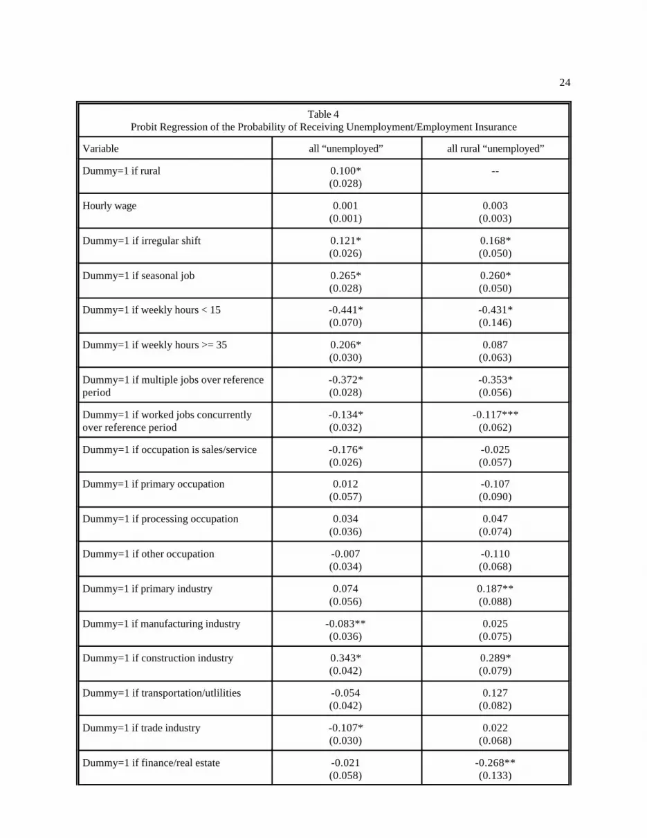
We consider whether this finding is also observed in a multivariate analysis. Therefore, we add to

the probit model of the probability of receiving UI/EI, already discussed, a dummy variable which

indicates whether the individual's job separation occurred after January 1997, in which case the

individual collected EI, rather than UI,14 and we include an interaction of the post 1997 variable

with the rural variable, to see if the impact of the programme changed differed for rural

16

unemployed workers. We also add interactions between the post 1997 variable and key job

characteristics most likely to be associated with a change, given specific EI provisions. The

results are presented in Table 4.

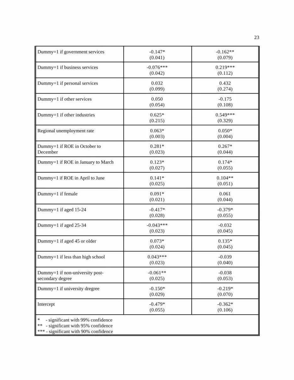
The probit model results indicate that, in general for all unemployed workers, access to

unemployment benefits has declined as a result of the EI reforms. The post January 1997 variable

is negative and significant (Table 4, column 1) indicating that unemployed workers were less

likely to receive EI benefits compared to UI benefits. However, the post97*rural interaction

dummy is not significant (controlling for job characteristics and labour market conditions). Rural

unemployed workers have thus experienced a reduction in likelihood of receiving EI similar to

their urban counterparts with comparable demographic and work characteristics.

While the switch to an hours-based criterion did not increase access overall, were their

particular types of jobs where receipt increased? The short hours and seasonal interaction

variables are insignificant, which indicates that unemployed workers who held seasonal jobs and

jobs with less than 15 hours weekly, have not fared any better than others. However, unemployed

workers who held jobs with a high number of weekly hours, and those with irregular shifts, have

been less hurt in terms of access to benefits. This is as expected given that any extra hours

contribute to eligibility. Notice that these results about seasonality and hours worked, derived

from the probit model estimated for the sample of all unemployed workers, hold for the sample of

all rural unemployed workers (see Table 4, column 2). The variables intending to capture whether

workers have multiple employers had more or less access to unemployment insurance benefits in

the EI period give mixed results (Table 4). For the overall sample and for just rural unemployed

workers, those who had concurrent employers (packaging together jobs) fare worse under EI than

other workers. Those with more than one employer fare better in the overall sample, but not in the

rural regression. Thus, while some workers have been hurt more or less than others, depending on

17

their job characteristics, the likelihood of receiving EI has been lowered for all. Our evidence

suggests that rural unemployed workers have not fared worse as a result of the switch from UI to

EI in terms of receipt of benefits. However, it is worth noting again that this is only one dimension

of the programme, and our previous work (Phipps, MacDonald and MacPhail, 1999) suggests that

there may be more important rural/urban differences in terms of benefit levels and durations. This

remains to be investigated in future research if the appropriate data become available.

5. Summary and Conclusions

This paper has used microdata from the Canadian Out-of Employment Panel (COEP)

survey (October 1995 through December 1997) in a beginning effort to understand urban/rural

differences in the impact of Employment Insurance. Specifically, we have focussed thus far upon

rural/urban differences in receipt of benefits and how this has changed as a result of the move from

UI to EI. The key element of the program change likely to affect benefit receipt is the switch to an

hours criterion as the basis for eligibility. This is likely to help individuals working very few

hours per week (i.e., less than 15) who were previously ineligible or individuals working many

hours per week (i.e., more than 35) who would previously just have received credit for one week,

regardless of the number of hours they worked but who now receive credit for all their hours.

Individuals with fluctuating hours or hours between fifteen and thirty-five will find it harder to

qualify.

Analysis with the COEP data indicates that rural workers are somewhat more likely to

work long hours per week, but are also more likely to work irregular shifts, so it is not a priori

obvious whether we would expect rural workers to gain eligibility or lose eligibility as a result of

the switch to an hours criterion. (Very few workers in either rural or urban areas work fewer than

fifteen hours per week.)

18

Our results further indicate that rural workers have higher receipt of UI/EI, and we are able

to explain about half this difference in terms of differences in demographic characteristics, job

characteristics and labour market conditions which are statistically significant predictors of UI/EI

usage. We are not yet satisfied that we have adequately measured differences in work patterns

between rural and urban workers, especially gaps in employments. It is also true that even

regional unemployment rates do not reflect the specific labour market conditions faced by workers,

and this may be particularly important for rural workers.

Finally, receipt of benefits is lower under EI, compared to UI, for both urban and rural

unemployed workers. However, there does not appear to be a statistically significant difference

between rural and urban workers in the impact of EI on access to EI. Again, however, we make

the qualification that at this stage of our work we have looked at only one aspect of the programme

change and we might expect there to be larger rural/urban differences in, for example, benefit

levels or durations.

19

Table 1aA Comparison of Means COEP versus SCF

All Observations Rural Observations

COEPunempl’d

(ROEjob)

SCFunempl’dpast year

SCFin labourforce inpast year

COEPunempl’d

(ROEjob)

SCFunempl’dpast year

SCFin labourforce inpast year

Rural 29.0% 21.9% 15.7% 100.0% 100.0% 100.0%

Reporting UI/EI 63.2% 58.6% 11.4% 72.3% 67.2% 17.6%

Female 43.9% 41.8% 45.3% 40.8% 38.5% 42.6%

Age 15-24 25-34 35-44 >=45

15.4%28.9%28.0%27.7%

22.7%28.9%26.2%22.3%

16.6%24.8%27.9%30.7%

13.3%26.6%30.4%29.7%

19.3%25.8%29.3%25.5%

16.4%20.3%29.3%33.9%

Education < High school High school Non-university University

25.6%44.8%16.0%13.6%

26.8%31.1%30.3%11.8%

19.6%30.5%32.4%17.5%

36.9%42.9%13.0%7.2%

39.1%26.7%29.6%4.5%

30.3%28.6%32.7%8.4%

Occupation Management/professional/technical Sale/service Primary Processing Other occupations

35.2%20.0%6.6%16.6%21.6%

32.1%25.2%6.9%15.9%19.8%

45.8%24.7%4.5%12.8%12.3%

24.6%16.6%12.9%18.8%27.1%

20.6%21.0%17.0%17.5%23.8%

31.7%20.7%17.6%14.5%15.5%

Industry Primary Manufacturing Construction Transportation/utilities Trade Finance/real estateGoverment services Social services Personal services Business services Other services Other industries

7.0%18.5%12.6%7.1%13.4%2.3%5.5%24.8%0.8%5.0%2.9%0.2%

7.2%16.6%11.5%6.6%14.9%2.9%3.4%14.8%11.0%11.0%

----

5.3%15.8%5.4%7.2%16.8%5.2%6.0%18.2%9.4%10.7%

----

14.1%19.0%14.3%8.8%9.0%1.6%5.4%22.0%0.5%2.5%2.5%0.4%

19.2%17.1%13.1%7.3%10.9%1.4%3.1%11.4%11.0%5.5%

----

20.1%14.7%6.7%7.3%14.3%2.8%4.2%16.3%8.1%5.4%

----

number of observations 27,769 7,720 44,809 10,647 2,721 11,322

note: For the SCF observations, the respondents had to have worked in the past year.

20

Table 1b

All Unemployed Workers Rural Unemployed Workers

Hourly wage rate 14.05 13.2%

Dummy=1 if worker has irregular shift 48.6% 59.7%

Dummy=1 if seasonal worker 31.2% 43.0%

Dummy=1 if weekly hours < 15 3.7% 2.7%

Dummy=1 if weekly hours >=35 74.3% 77.5%

Dummy=1 if worker has multiple jobs inreference period

54.9% 49.1%

Dummy=1 if worker worked jobconcurrently

23.6% 23.3%

Regional unemployment rate 10.0% 11.1%

Dummy=1 if ROE was post January1997

45.2% 45.2%

Number of observations 27,769 10,647

21

Table 2Probit Regression of the Probability of Receiving Unemployment/Employment Insurance

Basic Equation

Variable all “unemployed” all rural “unemployed”

Dummy=1 if rural 0.283*(0.019)

--

Dummy=1 if ROE in October toDecember

0.327*(0.022)

0.330*(0.042)

Dummy=1 if ROE in January to March 0.164*(0.026)

0.212*(0.053)

Dummy=1 if ROE in April to June 0.095*(0.024)

0.007(0.048)

Dummy=1 if female -0.070*(0.017)

-0.110*(0.034)

Dummy=1 if aged 15-24 -0.578*(0.026)

-0.481*(0.051)

Dummy=1 if aged 25-34 -0.077*(0.022)

-0.065(0.043)

Dummy=1 if aged 45 or older 0.086*(0.023)

0.115*(0.043)

Dummy=1 if less than high school 0.160*(0.022)

0.093**(0.038)

Dummy=1 if non-university post-secondary degree

-0.067*(0.024)

-0.037(0.050)

Dummy=1 if university dregree -0.171*(0.026)

-0.277*(0.062)

Intercept 0.212*(0.026)

0.525*(0.048)

* - significant with 99% confidence** - significant with 95% confidence*** - significant with 90% confidence

22


Controlling for Job Characteristics



--

Hourly wage 0.001(0.001)

0.003(0.003)

Dummy=1 if irregular shift 0.149*(0.019)

0.204*(0.038)

Dummy=1 if seasonal job 0.262*(0.021)

0.284*(0.038)

Dummy=1 if weekly hours < 15 -0.462*(0.049)

-0.351*(0.103)

Dummy=1 if weekly hours >= 35 0.247*(0.023)

0.285*(0.047)

Dummy=1 if multiple jobs over referenceperiod

-0.341*(0.021)

-0.305*(0.042)

Dummy=1 if worked jobs concurrentlyover reference period

-0.184*(0.023)

-0.181*(0.046)

Dummy=1 if occupation is sales/service -0.179*(0.026)

-0.031(0.057)

Dummy=1 if primary occupation 0.008(0.057)

-0.119(0.090)

Dummy=1 if processing occupation 0.034(0.035)

0.044(0.074)

Dummy=1 if other occupation -0.011(0.034)

-0.125***(0.068)

Dummy=1 if primary industry 0.076(0.056)

0.193**(0.088)

Dummy=1 if manufacturing industry -0.083**(0.036)

0.031(0.075)

Dummy=1 if construction industry 0.344*(0.042)

0.289*(0.079)

Dummy=1 if transportation/utlilities -0.053(0.042)

0.129(0.081)

Dummy=1 if trade industry -0.104*(0.030)

0.031(0.068)

Dummy=1 if finance/real estate -0.023(0.058)

-0.246***(0.133)

23

Dummy=1 if government services -0.147*(0.041)

-0.162**(0.079)

Dummy=1 if business services -0.076***(0.042)

0.219***(0.112)

Dummy=1 if personal services 0.032(0.099)

0.432(0.274)

Dummy=1 if other services 0.050(0.054)

-0.175(0.108)

Dummy=1 if other industries 0.625*(0.215)

0.549***(0.329)

Regional unemployment rate 0.063*(0.003)

0.050*(0.004)


0.281*(0.023)

0.267*(0.044)


0.174*(0.055)


0.104**(0.051)

Dummy=1 if female 0.091*(0.021)

0.061(0.044)

Dummy=1 if aged 15-24 -0.417*(0.028)

-0.379*(0.055)

Dummy=1 if aged 25-34 -0.043***(0.023)

-0.032(0.045)


0.135*(0.045)

Dummy=1 if less than high school 0.043***(0.023)

-0.039(0.040)


-0.061**(0.025)

-0.038(0.053)


-0.219*(0.070)

Intercept -0.479*(0.055)

-0.362*(0.106)


24




--

Hourly wage 0.001(0.001)

0.003(0.003)

Dummy=1 if irregular shift 0.121*(0.026)

0.168*(0.050)

Dummy=1 if seasonal job 0.265*(0.028)

0.260*(0.050)

Dummy=1 if weekly hours < 15 -0.441*(0.070)

-0.431*(0.146)

Dummy=1 if weekly hours >= 35 0.206*(0.030)

0.087(0.063)

Dummy=1 if multiple jobs over referenceperiod

-0.372*(0.028)

-0.353*(0.056)

Dummy=1 if worked jobs concurrentlyover reference period

-0.134*(0.032)

-0.117***(0.062)

Dummy=1 if occupation is sales/service -0.176*(0.026)

-0.025(0.057)

Dummy=1 if primary occupation 0.012(0.057)

-0.107(0.090)

Dummy=1 if processing occupation 0.034(0.036)

0.047(0.074)

Dummy=1 if other occupation -0.007(0.034)

-0.110(0.068)

Dummy=1 if primary industry 0.074(0.056)

0.187**(0.088)

Dummy=1 if manufacturing industry -0.083**(0.036)

0.025(0.075)

Dummy=1 if construction industry 0.343*(0.042)

0.289*(0.079)

Dummy=1 if transportation/utlilities -0.054(0.042)

0.127(0.082)

Dummy=1 if trade industry -0.107*(0.030)

0.022(0.068)

Dummy=1 if finance/real estate -0.021(0.058)

-0.268**(0.133)

25

Dummy=1 if government services -0.153*(0.041)

-0.163**(0.079)

Dummy=1 if business services -0.073***(0.042)

0.241**(0.113)

Dummy=1 if personal services 0.030(0.099)

0.355(0.273)

Dummy=1 if other services 0.056(0.054)

-0.154(0.109)

Dummy=1 if other industries 0.607*(0.215)

0.545***(0.330)

Regional unemployment rate 0.062*(0.003)

0.051*(0.004)

Dummy=1 if ROE is post January 1997 -0.188*(0.045)

-0.427*(0.087)

Interaction dummy= post97 * rural

0.041(0.040)

--

Interaction dummy = post97 * seasonal job

-0.006(0.041)

0.040(0.074)

Interaction dummy= post97 * hours per week < 15

-0.024(0.097)

0.192(0.205)

Interaction dummy= post97 * hours per week >= 35

0.090**(0.042)

0.405*(0.082)

Interaction dummy= post97 * multiple jobs

0.072***(0.041)

0.100(0.082)

Interaction dummy= post97 * concurrent jobs

-0.110**(0.047)

-0.170***(0.093)

Interaction dummy= post97 * irregular shift

0.062***(0.037)

0.089(0.073)


0.274*(0.023)

0.265*(0.044)


0.174*(0.056)


0.096***(0.051)

Dummy=1 if female 0.092*(0.021)

0.071(0.044)

Dummy=1 if aged 15-24 -0.413*(0.028)

-0.374*(0.055)

Dummy=1 if aged 25-34 -0.043***(0.023)

-0.034(0.045)

26


0.134*(0.045)

Dummy=1 if less than high school 0.044***(0.023)

-0.043(0.041)


-0.061**(0.025)

-0.046(0.053)


-0.222*(0.070)

Intercept -0.387*(0.059)

-0.156(0.114)


27

REFERENCES

Canadian Labour Congress. 2000. "Analysis of UI Coverage for Women". March. www.clc-ctc.ca

Gower, Dave. 1996. "Canada's Unemployment Mosaic in the 1990s", Perspectives on Labour and

Income, Vol. 8, No. 1, Spring: 16-22.

HRDC (Human Resources Development Canada). 1994. "From Employment Insurance to

Unemployment Insurance: A Supplementary Paper". Improving Social Security in Canada.

Ottawa: Minister of Supply and Services.

_________ 1996. Employment Insurance: Gender Impact Analysis". Ottawa.

_________ 2000. "Employment Insurance: 1999 Monitoring and Assessment Report". Ottawa.

MacDonald, Martha. 1994. "Restructuring in the Fishing Industry in Atlantic Canada", in Isabella

Bakker (ed.), The Strategic Silence: Gender and Economic Policy. London: Zed Books

and the North-South Institute.

Marshall, Katherine. 1999. "Seasonality in Employment", Perspectives on Labour and Income,

Vol. 11, No. 1, Spring: 16-22.

Osberg, Lars, Fred Wien and Jan Grude. 1995. Vanishing Jobs: Canada's Changing Workplace.

Toronto: James Lorimer.

Pérusse, Dominique. 1997. "Regional Disparities and Non-permanent Employment", Perspectives

on Labour and Income, Vol. 9, No. 4, Winter: 25-31.

Phipps, Shelley, Martha MacDonald and Fiona MacPhail. 1999. "Impact of the Family Income

Supplement". Final Report. Prepared for Human Resources Development Canada.

Strategic Evaluation and Monitoring Directorate.

Wesa, Lesle. 1995. "Seasonal Employment and the Repeat Use of Unemployment Insurance". UI

Impacts on Worker Behaviour. Ottawa: Human Resources Development Canada

Documents

Rural-Urban Differences in the Impact of EI