Seismic Evaluation Of Clark County Critical Bridges Using

UNLV Theses, Dissertations, Professional Papers, and Capstones

8-2009

Seismic Evaluation Of Clark County Critical Bridges Using Seismic Evaluation Of Clark County Critical Bridges Using

Nonlinear Static Procedures Nonlinear Static Procedures

Ahmad Said Saad University of Nevada, Las Vegas

Follow this and additional works at: https://digitalscholarship.unlv.edu/thesesdissertations

Part of the Civil Engineering Commons, Geotechnical Engineering Commons, and the Structural

Engineering Commons

Repository Citation Repository Citation Saad, Ahmad Said, "Seismic Evaluation Of Clark County Critical Bridges Using Nonlinear Static Procedures" (2009). UNLV Theses, Dissertations, Professional Papers, and Capstones. 1205. https://digitalscholarship.unlv.edu/thesesdissertations/1205

This Thesis is protected by copyright and/or related rights. It has been brought to you by Digital Scholarship@UNLV with permission from the rights-holder(s). You are free to use this Thesis in any way that is permitted by the copyright and related rights legislation that applies to your use. For other uses you need to obtain permission from the rights-holder(s) directly, unless additional rights are indicated by a Creative Commons license in the record and/or on the work itself. This Thesis has been accepted for inclusion in UNLV Theses, Dissertations, Professional Papers, and Capstones by an authorized administrator of Digital Scholarship@UNLV. For more information, please contact [email protected].

http://library.unlv.edu/

http://library.unlv.edu/

https://digitalscholarship.unlv.edu/thesesdissertations

https://digitalscholarship.unlv.edu/thesesdissertations?utm_source=digitalscholarship.unlv.edu%2Fthesesdissertations%2F1205&utm_medium=PDF&utm_campaign=PDFCoverPages

http://network.bepress.com/hgg/discipline/252?utm_source=digitalscholarship.unlv.edu%2Fthesesdissertations%2F1205&utm_medium=PDF&utm_campaign=PDFCoverPages




https://digitalscholarship.unlv.edu/thesesdissertations/1205?utm_source=digitalscholarship.unlv.edu%2Fthesesdissertations%2F1205&utm_medium=PDF&utm_campaign=PDFCoverPages

mailto:[email protected]

SEISMIC EVALUATION OF CLARK COUNTY CRITICAL BRIDGES USING

NONLINEAR STATIC PROCEDURES

by

Ahmad Said Saad

Bachelor of Engineering Ain Shams University, Cairo, Egypt

2004

A thesis submitted in partial fulfillment of the requirements for the

Master of Science in Engineering Department of Civil and Environmental Engineering

Howard R. Hughes College of Engineering

Graduate College University of Nevada, Las Vegas

August 2009

UMI Number: 1469800

INFORMATION TO USERS

The quality of this reproduction is dependent upon the quality of the copy

submitted. Broken or indistinct print, colored or poor quality illustrations and

photographs, print bleed-through, substandard margins, and improper

alignment can adversely affect reproduction.

In the unlikely event that the author did not send a complete manuscript

and there are missing pages, these will be noted. Also, if unauthorized

copyright material had to be removed, a note will indicate the deletion.

______________________________________________________________

UMI Microform 1469800Copyright 2009 by ProQuest LLC

All rights reserved. This microform edition is protected against unauthorized copying under Title 17, United States Code.

_______________________________________________________________

ProQuest LLC 789 East Eisenhower Parkway

P.O. Box 1346 Ann Arbor, MI 48106-1346

THE GRADUATE COLLEGE We recommend that the thesis prepared under our supervision by Ahmad Said Saad entitled Seismic Evaluation of Clark County Critical Bridges Using Nonlinear Static Procedures be accepted in partial fulfillment of the requirements for the degree of Master of Science Civil and Environmental Engineering ALY M. SAID, Committee Chair BARBARA LUKE, Committee Member SAMAAN LADKANY, Committee Member WANDA TAYLOR, Graduate Faculty Representative Ronald Smith, Ph. D., Vice President for Research and Graduate Studies and Dean of the Graduate College August 2009

iii

ABSTRACT

Seismic Evaluation of Clark County Critical Bridges Using Nonlinear Static Procedures

by

Ahmad Said Saad

Dr. Aly M. Said, Examination Committee Chair Assistant Professor of Civil Engineering

University of Nevada, Las Vegas Bridges are vital connective elements in community transportation systems. In the

past, bridges have been severely damaged by earthquakes. However, with proper

mitigation techniques, such as bridge retrofit, severe earthquake damage to bridges can be

avoided. Since the 1970’s, design codes underwent major changes with regard to seismic

analysis and design provisions of structures and bridges. Meanwhile, one third of the

nation’s 600,000 inventoried highway bridges are considered as either structurally

deficient or functionally obsolete.

This study is a part of the “Earthquakes in Southern Nevada” project. Earlier in this

project, buildings and bridges in southern Nevada were studied in order to prioritize their

need for rehabilitation. This prioritization was based on a risk assessment that combines

both vulnerability and importance. In this study, bridges with the highest risk scores were

structurally evaluated against earthquake loads using performance-based approach.

Performance-based approach was chosen for the evaluation process of the bridges as it

iv

had been recognized as an efficient and practical procedure to perform analysis and

evaluation of structures. A nonlinear static procedure, specified by the Federal

Emergency Management Agency, was used in the evaluation process. This procedure

was modified by AlAyed (2002) for the applicability to bridges rather than buildings.

The Maximum Considered Earthquake (MCE) level was used for the evaluation of

five bridges. Seismic loads were applied in two horizontal directions of each bridge:

transverse and longitudinal directions. Nonlinear behavior of the bridge substructure

components (columns) were evaluated and compared to the acceptance criteria. The

acceptance criteria of the bridges set in this study was the Immediate Occupancy

performance level, as these bridges are of high importance and are expected to be fully

operational maintaining the pre-earthquake strength and stiffness of their components.

Most of the evaluated bridges violated the acceptance criteria under the aforementioned

level of earthquake in one or more of the analysis cases. The main two deficiencies

identified in these five bridges were: (1) the insufficient flexural capacity of some

columns at the plastic hinge regions and (2) the inadequate development lengths provided

in the longitudinal reinforcement of the columns, either at the lap splice locations or at

the beam-column joints.

v

TABLE OF CONTENTS

ABSTRACT....................................................................................................................... iii

LIST OF TABLES............................................................................................................. ix

LIST OF FIGURES .......................................................................................................... xii

ACKNOWLEDGEMENTS............................................................................................. xvi

CHAPTER 1 INTRODUCTION ...................................................................................... 1 1.1. Introduction.............................................................................................................. 1 1.2. Project background .................................................................................................. 2 1.3. Objective of this study ............................................................................................. 6 1.4. Organization of this work ........................................................................................ 6

CHAPTER 2 LITERATURE REVIEW ........................................................................... 7 2.1. Introduction.............................................................................................................. 7 2.2. Potential damage to bridge components due to earthquake loads ........................... 7

2.2.1. Factors affecting seismic damage to bridges .................................................... 7 2.2.1.1. Effect of site conditions ....................................................................... 8 2.2.1.2. Bridge construction era ........................................................................ 8 2.2.1.3. Change in bridge condition.................................................................. 8 2.2.1.4. Structural configuration ....................................................................... 9

2.2.2. Damage to bridges observed in recent earthquakes........................................ 10 2.2.2.1. Seismic displacements ....................................................................... 11 2.2.2.2. Abutment slumping............................................................................ 13 2.2.2.3. Column failure ................................................................................... 14

2.2.2.3.1. Flexural strength and ductility failure......................................... 14 2.2.2.3.2. Column shear failure................................................................... 15

2.2.2.4. Cap beam failure ................................................................................ 17 2.2.2.5. Joint failure ........................................................................................ 17 2.2.2.6. Footing failure.................................................................................... 18 2.2.2.7. Failure of steel bridge components .................................................... 19

2.3. Seismic analysis approaches for bridges ............................................................... 19 2.4. Principles of nonlinear analysis ............................................................................. 24

2.4.1. Theoretical background for pushover analysis ............................................... 24 2.5. Previous work on NSP........................................................................................... 31 2.6. Performance-based approach................................................................................. 42

CHAPTER 3 THEORETICAL APPROACH ................................................................ 47 3.1. Introduction............................................................................................................ 47 3.2. Lateral Load Patterns ............................................................................................. 48 3.3. Estimation of Target Displacement ....................................................................... 50

3.3.1. Control node.................................................................................................... 56 3.4. Performance level .................................................................................................. 58

vi

3.5. Seismic loading (Design response spectrum) ........................................................ 60 3.6. Summary of evaluation procedures ....................................................................... 64

CHAPTER 4 BRIDGES ANALYSIS AND EVALUATION........................................ 66 4.1. Introduction............................................................................................................ 66 4.2. Modeling general assumptions .............................................................................. 66

4.2.1. Spectral acceleration (Sa) ................................................................................ 66 4.2.2. Bridge models ................................................................................................. 67 4.2.3. Effective seismic weight ................................................................................. 68 4.2.4. Stiffness reduction .......................................................................................... 68 4.2.5. Acceptance limits............................................................................................ 69

4.2.5.1. Deformation-controlled actions ......................................................... 69 4.2.5.2. Force-controlled actions..................................................................... 72

4.3. Seismic evaluation of the studied bridges.............................................................. 76 4.3.1. Bridge (G-1064).............................................................................................. 76

4.3.1.1. Bridge description.............................................................................. 76 4.3.1.2. Bridge model...................................................................................... 79

4.3.1.2.1. Superstructure ............................................................................. 80 4.3.1.2.2. Substructure ................................................................................ 80 4.3.1.2.3. Effective moment of inertia for bent columns ............................ 82 4.3.1.2.4. Spectral acceleration curve ......................................................... 84

4.3.1.3. Acceptance criteria............................................................................. 84 4.3.1.3.1. Load-deformation curve for plastic hinges ................................. 84 4.3.1.3.2. Force-controlled actions ............................................................. 85

4.3.1.4. Pushover curves and target displacement .......................................... 87 4.3.1.4.1. Transverse direction.................................................................... 87 4.3.1.4.2. Longitudinal direction................................................................. 89

4.3.1.5. Results................................................................................................ 92 4.3.1.5.1. Deformation-controlled actions .................................................. 92 4.3.1.5.2. Force-controlled actions ............................................................. 93

4.3.2. Bridge (G-947)................................................................................................ 99 4.3.2.1. Bridge description.............................................................................. 99 4.3.2.2. Bridge model.................................................................................... 103

4.3.2.2.1. Superstructure ........................................................................... 104 4.3.2.2.2. Substructure .............................................................................. 104 4.3.2.2.3. Effective moment of inertia for bent columns .......................... 104 4.3.2.2.4. Spectral acceleration curve ....................................................... 108

4.3.2.3. Acceptance criteria........................................................................... 108 4.3.2.3.1. Load-deformation curve for plastic hinges ............................... 108 4.3.2.3.2. Force-controlled actions ........................................................... 109

4.3.2.4. Pushover curves and target displacements....................................... 113 4.3.2.5. Results.............................................................................................. 116

4.3.2.5.1. Deformation-controlled actions ................................................ 116 4.3.2.5.2. Force-controlled actions ........................................................... 117

4.3.3. Bridge (H-1211)............................................................................................ 120 4.3.3.1. Bridge description............................................................................ 120 4.3.3.2. Bridge model.................................................................................... 123

vii

4.3.3.2.1. Superstructure ........................................................................... 124 4.3.3.2.2. Substructure .............................................................................. 124 4.3.3.2.3. Effective moment of inertia for pier column ............................ 125 4.3.3.2.4. Spectral acceleration curve ....................................................... 128


4.3.3.4. Pushover curves and target displacement ........................................ 132 4.3.3.5. Results.............................................................................................. 135

4.3.3.5.1. Deformation-controlled actions ................................................ 135 4.3.3.5.2. Force-controlled actions ........................................................... 136

4.3.4. Bridge (G-953).............................................................................................. 138 4.3.4.1. Bridge description............................................................................ 138 4.3.4.2. Bridge model.................................................................................... 140



4.3.4.4. Pushover curves and target displacement ........................................ 151 4.3.4.4.1. Transverse direction.................................................................. 151 4.3.4.4.2. Longitudinal direction............................................................... 154

4.3.4.5. Results.............................................................................................. 157 4.3.4.5.1. Deformation-controlled actions ................................................ 157 4.3.4.5.2. Force-controlled actions ........................................................... 158

4.3.5. Bridge (I-2139) ............................................................................................. 165 4.3.5.1. Bridge description............................................................................ 165 4.3.5.2. Bridge model.................................................................................... 168



4.3.5.4. Pushover curves and target displacement ........................................ 174 4.3.5.4.1. Transverse direction.................................................................. 174 4.3.5.4.2. Longitudinal direction............................................................... 176

4.3.5.5. Results.............................................................................................. 178 4.3.5.5.1. Deformation-controlled actions ................................................ 178 4.3.5.5.2. Force-controlled actions ........................................................... 179

4.4. Discussion of the results ...................................................................................... 180 4.4.1. Flexural deformation..................................................................................... 180 4.4.2. Shear forces................................................................................................... 182

viii

4.4.3. Inadequate reinforcement development........................................................ 183

CHAPTER 5 SUMMARY AND CONCLUSIONS..................................................... 185 5.1. Summary.............................................................................................................. 185 5.2. Conclusions.......................................................................................................... 186 5.3. Recommendations for future research ................................................................. 187

BIBLIOGRAPHY.......................................................................................................... 188

VITA.............................................................................................................................. 195

ix

LIST OF TABLES

Table 1.1 Top 20 high risk bridges ............................................................................. 4 Table 1.2 Exempted bridges from the evaluation process .......................................... 5 Table 3.1 Values for the modification factor 0C (FEMA-356, 2000) ...................... 53 Table 3.2 Values for Effective Mass Factor Cm (FEMA-356, 2000)........................ 54 Table 3.3 Values for modification factor C2 (FEMA-356, 2000)............................. 56 Table 4.1 Site classifications and mapped spectral accelerations for the studied

bridges....................................................................................................... 67 Table 4.2 Modeling parameters and numerical acceptance criteria for nonlinear

procedures for reinforced concrete columns (FEMA-356, 2000)............. 71 Table 4.3 Bridge G-1064 - Modal analysis Output for the 4 units used in the

longitudinal direction................................................................................ 89 Table 4.4 Bridge G-1064 - Target displacements for different units used in the

longitudinal direction................................................................................ 92 Table 4.5 Bridge G-1064 - Plastic hinge rotation values (radians) of bridge columns

at target displacements in the longitudinal direction ................................ 93 Table 4.6 Bridge G-1064 Shear forces (kips) at target displacements in the

transverse direction ................................................................................... 94 Table 4.7 Bridge G-1064 Shear forces (kips) at target displacements in the

longitudinal direction................................................................................ 95 Table 4.8 Bridge G-1064 - Bending moment values (kip-ft) at splice locations of the

columns at target displacement in the longitudinal direction ................... 97 Table 4.9 Bridge G-1064 - Plastic hinge rotation (radians) at splice locations at

target displacement in the longitudinal direction...................................... 98 Table 4.10 Bridge G-947-Calculation of effective moment of inertia for column

sections in bent 1..................................................................................... 105 Table 4.11 Bridge G-947-Calculation of effective moment of inertia for column

sections in bent 2..................................................................................... 105 Table 4.12 Bridge G-947 - Applied loads on bridge columns for load-deformation

calculations ............................................................................................. 109 Table 4.13 Bridge G-947 - Acceptance criteria of the bridge column at each

performance level.................................................................................... 109 Table 4.14 Bridge G-947 - Shear capacity calculations for bridge columns ............ 110 Table 4.15 Bridge G-947 - Calculation of maximum stress that can be developed in

the reinforcement bars at B/C joint......................................................... 111 Table 4.16 Bridge G-947 - Maximum moment that can be developed in column

sections at B/C joints .............................................................................. 113 Table 4.17 Bridge G-947 - Target displacement calculations for the transverse

direction .................................................................................................. 115 Table 4.18 Bridge G-947 - Target displacement calculations for the longitudinal

direction .................................................................................................. 115 Table 4.19 Bridge G-947 - Plastic hinge rotations (radians) at target displacements in

the transverse direction ........................................................................... 116 Table 4.20 Bridge G-947 - Plastic hinge rotations (radians) at target displacements in

the longitudinal direction ........................................................................ 116

x

Table 4.21 Bridge G-947 - Shear forces (kips) at target displacement (transverse direction) ................................................................................................. 117

Table 4.22 Bridge G-947 - Shear forces (kips) at target displacement (longitudinal direction) ................................................................................................. 117

Table 4.23 Bridge G-947 - Bending moment values (kip-ft) at target displacement at the B/C joint locations of the columns.................................................... 118

Table 4.24 Bridge G-947 - Plastic hinge rotations (radians) at target displacements in the transverse direction ........................................................................... 119

Table 4.25 Bridge G-947 - Plastic hinge rotations (radians) at target displacements in the longitudinal direction ........................................................................ 119

Table 4.26 Bridge H-1211- Calculation of effective moment of inertia for column sections in the strong axis ....................................................................... 128

Table 4.27 Bridge H-1211- Calculation of effective moment of inertia for column sections in the weak axis......................................................................... 128

Table 4.28 Bridge H-1211 - Applied loads on bridge column for load-deformation calculations ............................................................................................. 129

Table 4.29 Bridge H-1211 - Acceptance criteria for the lower column section of the bridge ...................................................................................................... 130

Table 4.30 Bridge H-1211 - Shear capacity calculations for bridge columns .......... 131 Table 4.31 Bridge H-1211 - Target displacement calculations for both directions.. 133 Table 4.32 Bridge H-1211 - Plastic hinge rotation values (radians) at target

displacement in both directions .............................................................. 136 Table 4.33 Bridge H-1211 - Shear force values (kips) in the bridge column at target

displacement ........................................................................................... 136 Table 4.34 Bridge G-953 - Sectional properties of the bridge deck ......................... 142 Table 4.35 Bridge G-953 - Column sections definition in the bridge bents ............. 143 Table 4.36 Bridge G-953 - Calculations of the effective moment of inertia for column

sections.................................................................................................... 146 Table 4.37 Bridge G-953 - Applied loads on bridge columns for load-deformation

calculations ............................................................................................. 147 Table 4.38 Bridge G-953 - Shear capacity calculations for bridge columns ............ 148 Table 4.39 Bridge G-953 - Calculation of maximum stresses that can be developed in

the reinforcement bars (B/C joint) .......................................................... 149 Table 4.40 Bridge G-953 - Calculation of maximum stresses that can be developed in

the reinforcement bars at bent 1 (splices location) ................................. 149 Table 4.41 Bridge G-953 - Maximum moment that can be developed in column

sections at B/C joint and splices location without plastic hinge formation................................................................................................................. 151

Table 4.42 Bridge G-953 - Target displacement calculations in the transverse direction .................................................................................................. 153

Table 4.43 Bridge G-953 - Target displacement calculations in the longitudinal direction .................................................................................................. 154

Table 4.44 Bridge G-953 - Plastic hinge rotation values (radians) of bridge bents at target displacement in longitudinal direction.......................................... 157

Table 4.45 Bridge G-953 - Shear forces (kips) in the columns at target displacement in the transverse direction (north) ........................................................... 159

xi

Table 4.46 Bridge G-953 - Shear forces (kips) in the columns at target displacement in the transverse direction (south)........................................................... 160

Table 4.47 Bridge G-953 - Shear forces (kips) in the columns at target displacement in the longitudinal direction .................................................................... 161

Table 4.48 Bridge G-953 - Maximum bending moment values (kip-ft) at target displacement at locations with inadequate reinforcement development lengths ..................................................................................................... 162

Table 4.49 Bridge G-953 – Plastic hinge rotation values (radians) in the longitudinal direction at target displacement at B/C joints for unit 2 ......................... 163

Table 4.50 Bridge G-953 – Plastic hinge rotation values (radians) in the longitudinal direction at target displacement for unit 1 (bent 1)................................. 164

Table 4.51 Bridge I-2139 - Sectional properties of the bridge deck at spans 1 and 3................................................................................................................. 169

Table 4.52 Bridge I-2139 - Applied loads on bridge columns for load-deformation calculations ............................................................................................. 172

Table 4.53 Bridge I-2139 - Acceptance criteria for each column of the bridge ....... 172 Table 4.54 Bridge I-2139 - Shear capacity calculations for bridge columns............ 173 Table 4.55 Bridge I-2139 - Target displacement calculations for the transverse

direction .................................................................................................. 175 Table 4.56 Bridge I-2139 - Target displacement calculations for the longitudinal

direction .................................................................................................. 177 Table 4.57 Bridge I-2139 - Plastic hinge rotation values (radians) at target

displacement in both directions .............................................................. 178 Table 4.58 Bridge I-2139 - Shear force values (kN) in the bridge columns at target

displacement ........................................................................................... 179

xii

LIST OF FIGURES

Figure 1.1 Locations of the 20 ranked bridges on Clark County map, using Google earth............................................................................................................. 5

Figure 2.1 Damage to bridge column caused by post-construction change in boundary condition (Caltrans, 2003) .......................................................................... 9

Figure 2.2 Spans slipped off narrow support seats, 1971 San Fernando earthquake (Caltrans, 2003)......................................................................................... 12

Figure 2.3 Unseating due to bridge skew - plan view of bridge deck (after Priestly et al., 1996) ................................................................................................... 12

Figure 2.4 Abutment slumping and rotation (after Priestly et al., 1996) ................... 13 Figure 2.5 Confinement failure at column top (Caltrans, 2003) ................................ 15 Figure 2.6 Examples of column shear failures (a) within the plastic hinge region and

(b) outside the plastic hinge region (Caltrans, 2003)................................ 16 Figure 2.7 Joint shear failure (a) Cypress Street Viaduct and (b) Southern Freeway

Viaduct, 1989 Loma Prieta earthquake (Caltrans, 2003).......................... 18 Figure 2.8 Pullout failure, 1971 San Fernando earthquake (Caltrans, 2003)............ 19 Figure 2.9 Capacity Spectrum Method (a) development of pushover curve; (b)

conversion of pushover curve to capacity spectrum diagram; (c) conversion of elastic response spectrum to ADRS format; and (d) determination of the displacement demand (Chopra and Goel, 2000) ..... 35

Figure 2.10 Derivation of damping for spectral reduction (ATC, 1996) ..................... 36 Figure 3.1 Idealization of force-displacement curves (FEMA-356, 2000) ................ 51 Figure 3.2 MCE’s Spectral Response Acceleration for 0.2-second period (5% of

critical damping) for Clark County (USGS, 2009)................................... 62 Figure 3.3 MCE’s Spectral Response Acceleration for 1.0-second period (5% of

critical damping) for Clark County (USGS, 2009)................................... 62 Figure 3.4 Construction of horizontal response spectrum (FEMA-356, 2000).......... 63 Figure 4.1 Generalized force-deformation relations for concrete elements (FEMA-

356, 2000) ................................................................................................. 72 Figure 4.2 Bridge G-1064 - Plan and elevation.......................................................... 77 Figure 4.3 Bridge G-1064 - Superstructure................................................................ 78 Figure 4.4 Bridge G-1064 - Elevation of a typical bent............................................. 78 Figure 4.5 Bridge G-1064 - Cross diaphragms at (a) fixed bearing; (b) interior

diaphragm; (c) expansion joint; and (d) abutment expansion joint .......... 79 Figure 4.6 Bridge G-1064 - Structural model for transverse direction analysis ........ 81 Figure 4.7 Bridge G-1064 - Structural models for longitudinal direction (a) unit-1;

(b) unit-2; (c) unit-3; and (d) unit-4 .......................................................... 81 Figure 4.8 Bridge G-1064 - φ−M curves for the bent columns with (a) 16 #8 rebar

and (b) 16 #11 rebar.................................................................................. 83 Figure 4.9 Bridge G-1064 - 5% damped response spectrum for BSE-2 .................... 84 Figure 4.10 Bridge G-1064 - Generalized force-deformation relation for bridge

columns ..................................................................................................... 85 Figure 4.11 Bridge G-1064 - Generalized force-deformation with acceptance criteria

for inadequate splicing in the bridge column reinforcement .................... 87

xiii

Figure 4.12 Bridge G-1064 - Mode-2, The fundamental mode in the transverse direction of the bridge............................................................................... 88

Figure 4.13 Bridge G-1064 - Pushover curves for the transverse direction (a) using the uniform load pattern and (b) using the modal load pattern....................... 88

Figure 4.14 Bridge G-1064 -Fundamental mode shapes in the longitudinal direction of the bridge for (a) unit-1; (b) unit-2; (c) unit-3; and (d) unit-4 .................. 90

Figure 4.15 Bridge G-1064 - Pushover curves for longitudinal direction analysis...... 91 Figure 4.16 Bridge G-1064 - φ−M curve for the bent columns at locations of

reinforcement splice and B/C joints.......................................................... 96 Figure 4.17 Bridge G-947 - Layout and the location of the studied part ................... 100 Figure 4.18 Bridge G-947 - Deck 6W, Plan and elevation ........................................ 101 Figure 4.19 Bridge G-947 - Bent 1 and 2 typical elevation and cap beam plan ........ 102 Figure 4.20 Bridge G-947 - Column section for (a) bent 1 and (b) bent 2................. 103 Figure 4.21 Bridge G-947 - Bridge structural model ................................................. 103 Figure 4.22 Bridge G-947 - φ−M curves for the three column sections along the

columns height of bent-1 ........................................................................ 106 Figure 4.23 Bridge G-947 - φ−M curves for the three column sections along the

columns height of bent-2 ........................................................................ 107 Figure 4.24 Bridge G-947- 5% damped response spectrum for BSE-2 ..................... 108 Figure 4.25 Bridge G-947- Direction used for columns shear capacity calculations. 110 Figure 4.26 Bridge G-947 - φ−M curves for sections with inadequate reinforcement

development at B/C joints (a) at bent 1 columns - strong axis; (b) at bent 1 columns - weak axis; (c) at bents 2 columns - strong axis; and (d) at bent 2 columns - weak axis................................................................................ 112

Figure 4.27 Bridge G-947 - Mode-3, the fundamental mode in the transverse direction................................................................................................................. 113

Figure 4.28 Bridge G-947 - Mode-1, the fundamental mode in the longitudinal direction .................................................................................................. 114

Figure 4.29 Bridge G-947 - Pushover curves in the transverse direction (a)using uniform load pattern (b)using modal pattern .......................................... 114

Figure 4.30 Bridge G-947 - Pushover curves in the longitudinal direction (a)using uniform load pattern (b)using modal pattern .......................................... 115

Figure 4.31 Bridge H-1211 - Plan and elevation........................................................ 120 Figure 4.32 Bridge H-1211 - Bridge section.............................................................. 121 Figure 4.33 Bridge H-1211 - Column sections at (a) top section and (b) bottom

section of the column.............................................................................. 122 Figure 4.34 Bridge H-1211 - (a) End diaphragm section and (b) abutment footing

section ..................................................................................................... 123 Figure 4.35 Bridge H-1211 - Structural model for both transverse and longitudinal

direction .................................................................................................. 123 Figure 4.36 Bridge H-1211 - Column sections as modeled in SAP2000 and their labels

................................................................................................................. 124 Figure 4.37 Bridge H-1211 - φ−M curves in the strong axis for the five column

sections along the pier height.................................................................. 126

xiv

Figure 4.38 Bridge H-1211 - φ−M curves in the weak axis for the five column sections along the pier height.................................................................. 127

Figure 4.39 Bridge H-1211- 5% damped response spectrum for BSE-2 ................... 129 Figure 4.40 Bridge H-1211- φ−M curves at the location of the B/C joint for (a)the

strong axis and (b)the weak axis of the column top section ................... 132 Figure 4.41 Bridge H-1211 - (a) Mode-4, the fundamental mode in the transverse

direction and (b) Mode-1, the fundamental mode in the longitudinal direction .................................................................................................. 134

Figure 4.42 Bridge H-1211 - Pushover curves in (a) the transverse direction and (b) the longitudinal direction.............................................................................. 135

Figure 4.43 Bridge G-953 - Plan and elevation.......................................................... 139 Figure 4.44 Bridge G-953 - Deck section at (a) bent 1; (b) bents 2 and 3; and (c) bents

4 and 5..................................................................................................... 140 Figure 4.45 Bridge G-953 - Structural model for transverse direction analysis ........ 141 Figure 4.46 Bridge G-953 - Structural models for longitudinal direction (a) unit-1; (b)

unit-2; and (c) unit-3. .............................................................................. 141 Figure 4.47 Bridge G-953 - φ−M curves for bent 1 column sections at (a) external

lower column; (b) external upper column; (c) internal lower column; and (d) internal upper column........................................................................ 144

Figure 4.48 Bridge G-953 - φ−M curves for column sections at (a) bents 2 and 3 external column; (b) bents 2 and 3 internal column; (c) bents 4 and 5 external column; and (d) bents 4 and 5 internal column......................... 145

Figure 4.49 Bridge G-953 - 5% damped response spectrum for BSE-2 .................... 146 Figure 4.50 Bridge G-953 - φ−M curves for sections with inadequate reinforcement

development at B/C joints (a) at bent 1-external columns; (b) at bents 2 and 3 - external columns; and (c) at bents 2 and 3 - internal columns ... 150

Figure 4.51 Bridge G-953 - φ−M curves for sections with inadequate reinforcement splices in bent 1 (a) at the external columns and (b) at the internal columns................................................................................................................. 151

Figure 4.52 Bridge G-953 - Mode-2, the fundamental mode in the transverse direction................................................................................................................. 152

Figure 4.53 Bridge G-953 - Pushover curves in the transverse direction using (a) uniform load pattern pushed in the north direction; (b) uniform load pattern pushed in the south direction; (c) modal pattern pushed in the north direction; and (d) modal pattern pushed in the south direction, ............. 153

Figure 4.54 Bridge G-953 -Fundamental mode shapes in the longitudinal direction of the bridge for (a) unit-1; (b) unit-2; and (c) unit-3.................................. 155

Figure 4.55 Bridge G-953 - Pushover curves for longitudinal direction analysis...... 156 Figure 4.56 Bridge I-2139 - Plan and elevation ......................................................... 165 Figure 4.57 Bridge I-2139 - Bridge section ............................................................... 166 Figure 4.58 Bridge I-2139 - Bridge column sections at (a) pier 1 and (b) pier 2....... 167 Figure 4.59 Bridge I-2139 - Bridge cap beam sections at (a) pier 1 and (b) pier 2 ... 168 Figure 4.60 Bridge I-2139 - Structural model for both transverse and longitudinal

direction .................................................................................................. 168 Figure 4.61 Bridge I-2139 - φ−M curve for the pier columns ................................. 170

xv

Figure 4.62 Bridge I-2139 - 5% damped response spectrum for BSE-2.................... 171 Figure 4.63 Bridge I-2139 - Mode-1, the fundamental mode in the transverse direction

................................................................................................................. 174 Figure 4.64 Bridge I-2139 - Pushover curves for the transverse direction using (a)

uniform load pattern and (b) modal pattern ............................................ 175 Figure 4.65 Bridge I-2139 - Mode-7, the fundamental mode in the longitudinal

direction .................................................................................................. 176 Figure 4.66 Bridge I-2139 -Pushover curves for the longitudinal direction using (a)

uniform load pattern and (b) modal pattern ............................................ 177 Figure 4.67 Maximum plastic hinge rotation percentage in the transverse direction of

the studied bridges .................................................................................. 180 Figure 4.68 Maximum plastic hinge rotation percentage in the longitudinal direction of

the studied bridges .................................................................................. 181 Figure 4.69 Maximum shear force in bridge columns as a percentage of the shear

capacity ................................................................................................... 182 Figure 4.70 Maximum plastic hinge rotation percentage (defined by inadequate

development lengths) in the transverse direction of the studied bridges 183 Figure 4.71 Maximum plastic hinge rotation percentage (defined by inadequate

development lengths) in the longitudinal direction of the studied bridges................................................................................................................. 184

xvi

ACKNOWLEDGEMENTS

All praise and thanks to Allah (God) for giving me the strength to complete this work.

I would like to express my gratitude to my advisor, Dr. Aly Said, for the teaching,

support and friendship provided during the study.

As part of the Earthquakes in Southern Nevada project, I would like to thank Dr.

Barbara Luke and Mr. Suchan Lamichhane for providing the seismic site classifications

of the soil underneath the studied bridges.

Thanks to Mr. Mohamed Zeidan for his help in the final stage of this work.

I thank my parents for their continuous support and prayers to me. My mother, you

are the best ever. My father, you are my mentor and everything I know is because of you.

I thank my wife for her support and patience during difficult times of my studies. I thank

my brother and sisters for their continuous support and encouragement.

1

CHAPTER 1

INTRODUCTION

1.1. Introduction

An earthquake is a sudden, rapid shaking of the earth’s crust that can cause severe

damage to structures to the extent of their collapse. Preventing the occurrence of

earthquakes is impossible, whereas it is possible to mitigate their destructive effects.

Seismic design aims at producing structures that can resist certain levels of ground

shaking without excessive damage. Codes and specifications are continuously developing

to improve structures’ performance during seismic events.

In highway systems, bridges are considered the most critical component that may be

affected by earthquakes. In addition to being the most vulnerable and costly component

of the highway, its damage can severely disrupt the traffic. This disruption may have a

great impact on the economy of the region as well as post-earthquake emergency

response, repair, and reconstruction operations. A large number of bridges were designed

and constructed according to codes that had inadequate or no seismic design provisions.

In recent earthquakes (in California, Japan, Central and South America), a number of

bridges did not perform adequately under seismic loads. Despite the fact that they were

designed for earthquake resistance, some of them suffered severe damage or even

collapse due to lack of ductility or poor detailing (Priestly et al., 1996).

The first step in mitigating earthquake losses in transportation systems is identifying

bridges that are likely to fail and cause disruption to these systems. This identification is

2

usually done based on bridges’ vulnerability and importance. Seismic evaluation of these

bridges is the second step and is considered as an essential part of the rehabilitation

process. As defined in FEMA-356 (2000), four different analytical procedures can be

used for the evaluation process of structures in general and can be extended to bridges.

These procedures are: linear static, linear dynamic, nonlinear static (pushover), and

nonlinear dynamic procedures. A brief description of the four analysis methods is

presented in Chapter 2.

Performance-based approach has been recognized among structural engineers as an

efficient approach for evaluation purposes. Since most of the structures are expected to

respond beyond their elastic limits under moderate to high magnitudes of earthquake

ground shaking, it is impractical to implement the performance-based design without a

nonlinear analysis procedure.

1.2. Project background

The Federal Emergency Management Agency (FEMA) lists Clark County, Nevada as

a region of high seismicity. Slemmons et al. (2001) showed that there are eight faults in

Clark County capable of producing earthquakes of magnitude (Mw) between 6.5 and 7.0.

Based on these facts, a proposal was prepared by researchers from UNLV, Department of

Civil and Environmental Engineering and Department of Geoscience in early 2004. Later

that same year the grant was awarded to the UNLV team. Seismic risk assessment for

essential infrastructures located in Clark County was performed. Keller (2006) performed

the seismic risk assessment for buildings of high importance (i.e. hospitals, police

stations, fire stations and schools). Seismic risk assessment of the bridges was performed

3

by Ebrahimpour et al. (2007) and compared to the prioritization of Nevada bridges by

Sanders et al. (1993).

A comprehensive and accurate database for the bridges in Clark County was

established for the classification purpose. The National Bridge Inventory (NBI), a

database maintained by the Federal Highway Administration (FHWA), along with the

Nevada Department of Transportation (NDOT) provided the essential information needed

for bridges’ prioritization. The prioritization process was done based on a risk assessment

that combines (1) the vulnerability assessment and (2) the importance assessment of the

bridges. Table 1.1 lists the top 20 high risk bridges (Ebrahimpour et al., 2007). It also

shows the vulnerability and importance scores in addition to the final combined risk

score.

Some of the ranked bridges were exempted from the seismic evaluation process for

one of the following three reasons:

1- Having a single span. According to the seismic specifications of the AASHTO

(2007), seismic analysis is not required for a single span bridge, regardless of its

seismic zone.

2- The bridge is exactly similar to another bridge which is already evaluated. This is

common in the case of having two typical bridges holding the same route or

highway in the two opposite directions.

3- The bridge is considered in a widening, retrofit or replacement process by the

Nevada Department of Transportation (NDOT) in their present or near future

plans and accordingly there is no need to consider them in the evaluation.

4

Table 1.1 Top 20 high risk bridges

Rank Bridge Latitude Longitude Vulnerability score

Importance score

Risk score

1 H-942S 36.1771694 -115.1509944 0.985 0.964 0.973

2 H-1443 36.1661056 -115.0966611 0.993 0.952 0.968

3 H-948 36.1883556 -115.1432278 1 0.945 0.966

4 G-1064 36.1439861 -115.1659139 0.979 0.958 0.967

5 H-942N 36.1771694 -115.1509944 0.952 0.966 0.961

6 H-1460 36.0584972 -115.0286917 0.943 0.913 0.925

7 G-947 36.1755056 -115.1450361 0.806 1 0.923

8 G-805N 36.1221278 -115.1803806 0.918 0.923 0.921

9 G-805S 36.1216667 -115.1800000 0.918 0.923 0.921

10 B-1448 36.1421056 -115.0912000 0.893 0.912 0.904

11 I-1449 36.1358278 -115.0903194 0.846 0.934 0.899

12 I-956 36.2402194 -115.1017750 0.995 0.812 0.885

13 B-1455 36.0889750 -115.0679083 0.814 0.908 0.87

14 H-946 36.1748222 -115.1491361 0.689 0.99 0.87

15 I-947 36.1755667 -115.1437500 0.667 0.973 0.851

16 I-937 36.1741944 -115.1547889 0.667 0.968 0.848

17 H-1446 36.1462444 -115.0913167 0.685 0.953 0.846

18 H-1211 36.1812139 -115.2442944 0.618 0.995 0.844

19 G-953 36.2034083 -115.1347167 0.797 0.873 0.843

20 I-2139 36.17347222 -115.1576889 0.771 0.89 0.842

Table 1.2 represents the bridges that are exempted from the evaluation process in

addition to the reason of exemption. Out of the 12 remaining bridges, 5 were chosen in

this study for the evaluation. These bridges were chosen to represent diversity in their

number of spans and columns cross sections.

5

Figure 1.1 Locations of the 20 ranked bridges on Clark County map, using

Google earth

Table 1.2 Exempted bridges from the evaluation process

Bridge Rank Reason for Exemption

H-942S 1 Will be replaced

H-942N 5 Will be replaced

G-805N 8 Widening, retrofit (NDOT, 2007)

G-805S 9 Widening, retrofit (NDOT, 2007)

B-1448 10 Single span bridge

B-1455 13 Single span bridge

H-946 14 Widening, retrofit (NDOT, 2007)

I-937 16 Widening, retrofit (NDOT, 2007)

6

1.3. Objective of this study

The main objective of this study is to evaluate the seismic performance of critical

bridges in Clark County using a nonlinear static procedure introduced by the FEMA-356

(2000). This procedure has been developed for the assessment of buildings and was

modified by AlAyed (2002) for applicability to bridges. The assessment of the bridges in

this work is focused only on the behavior of bridge columns under high earthquake

levels.

1.4. Organization of this work

The presented thesis consists of five chapters. The current chapter presents an

overview of the study, the project background along with the objectives of the study. A

literature review is presented in Chapter 2; it includes a presentation of damages that

occurred to bridges in recent earthquakes, a review of the principles of nonlinear analysis,

previous work done in nonlinear static pushover analysis, and an overview of the

performance-based approach. The theoretical approach used in the evaluation process in

this work is described in Chapter 3. The detailed description of the evaluated bridges

along with calculations and evaluation results are presented in Chapter 4. Summary and

conclusions are presented in Chapter 5, in addition to the proposed future research.

7

CHAPTER 2

LITERATURE REVIEW

2.1. Introduction

This chapter presents an extensive survey of previous work done by various

researchers in the field of nonlinear analysis alongside with seismic evaluation of bridges.

It begins with an overview of the potential damage of bridge components by earthquake

loads and the factors affecting them and then discusses different techniques for seismic

analysis of bridges which can also be used for evaluation purposes. Furthermore, a

description of the theoretical background of the nonlinear static analysis procedures and a

review to the performance based approach are presented.

2.2. Potential damage to bridge components due to earthquake loads

In this section two main aspects are briefly discussed to present the possible damage

that can occur to bridges under earthquake ground shaking. These aspects are: (1) factors

affecting seismic damage to bridges and (2) damage observed in bridge components in

recent earthquakes.

2.2.1. Factors affecting seismic damage to bridges

Damage to bridges caused by earthquakes can be categorized into the following two

classes (Chen and Duan, 2003): (1) Primary Damage caused by earthquake ground

shaking or deformation that was the primary cause of damage to the bridge, and that may

have triggered other damage or collapse; and (2) Secondary Damage caused by

redistribution of internal actions for which the structure was not designed. This

8

redistribution is the result of structural failures elsewhere in the bridge. However, the

controlling factors that affect the seismic behavior of the bridge can be classified into the

following categories:

2.2.1.1. Effect of site conditions

Performance of a bridge structure during an earthquake is likely to be influenced by

the bridge proximity to faults and their characteristics. In addition to that, the soil types

underneath bridge substructure components greatly affect the intensity of ground shaking

and ground deformation. Variability of those effects along the length of the bridge may

have higher influences than in the case of buildings because bridges are extended

horizontally.

2.2.1.2. Bridge construction era

Seismic design practices for structures generally and for bridges specifically have

evolved over years, largely reflecting lessons learned from structures’ performance in

past earthquakes (Chen and Duan, 2003). Therefore, the construction era of a bridge is a

good indicator of the likelihood of poor performance with higher damage levels expected

in older construction than in newer construction.

2.2.1.3. Change in bridge condition

Changes in the condition of a bridge can significantly affect its seismic performance.

This factor includes two aspects: (1) deterioration of the bridge components

(superstructure, substructure, bearings, etc.) which reduces the seismic performance of

this component and consequently the overall performance of the bridge; and (2)

construction modifications either during the original construction or during the service

life of the bridge. An example of the latter aspect is illustrated in Figure 2.1, where the

9

bridge columns were restrained with the construction of the wall for the channel, which

shortened the effective length of the columns causing an increase in columns’ shear force

and shifting the nonlinear response from the region of heavy confinement upward to a

zone of light transverse reinforcement where the ductility capacity was inadequate (Chen

and Duan, 2003).

Figure 2.1 Damage to bridge column caused by post-construction change in

boundary condition (Caltrans, 2003)

2.2.1.4. Structural configuration

Generally, structures with regular configurations perform better under earthquake

loads than structures that contain irregularities in their structural systems. This is due to

the fact that regular structures contain even distribution of forces and masses which

10

prevents stress concentrations under abnormal loads, and the inelastic energy dissipation

is promoted in a large number of readily identified yielding components. However, in

practice, bridges with certain configurations are more vulnerable to earthquakes than

others. Experience indicated that a bridge is most likely to be vulnerable if (1) excessive

deformation demands occur in a few brittle elements; (2) the structural configuration is

complex; or (3) the bridge lacks redundancy (Chen and Duan, 2003).

The main points that define the structural configuration are:

a- Structural irregularity such as non-uniform column length or irregular deck

structural system.

b- Long span bridges, where non-uniform soil condition exists along the bridge

length and causes variation in ground excitation at different bridge supports.

c- Bridge layouts (curved, skewed …)

2.2.2. Damage to bridges observed in recent earthquakes

In reviewing bridge damage caused by recent earthquakes, three basic design

deficiencies were identified by Priestly et al. (1996): (1) underestimating seismic

deflections based on the specified lateral load level; (2) incorrect ratio of gravity load to

lateral force, as the design seismic loads were low, and accordingly the envelopes of the

load combinations were different from the actual ones; and (3) not considering the

inelastic structural actions and the associated concepts of ductility and capacity design in

the elastic design process. This last deficiency may lead to inadequate detailing of the

plastic hinge locations preventing it from sustaining large inelastic deformations. These

three deficiencies tend to be consequences of the elastic design philosophy used in the

11

seismic design of bridges prior to 1970 and is still used in some countries (Priestly et al.,

1996).

In this section, most of the bridge damage modes due to seismic loading are

presented, and each of them can be attributed to any of the aforementioned three

deficiencies (Priestly et al., 1996).

2.2.2.1. Seismic displacements

The underestimation of seismic displacement in the design process may be attributed

to any of the following reasons: (1) elastic theory was used in the analysis/design of the

bridge; (2) the gross section stiffnesses were used in the analysis and not the actual

cracked ones; and (3) the lateral force levels used in the analysis were lower than the

actual ones. The following are three failure modes due to underestimating the seismic

displacements in the design process (Priestly et al., 1996).

a- Span failure due to unseating at movement joints: This kind of failure is

mainly caused by the relative movement of bridge spans in the longitudinal

direction exceeding the seating widths, resulting in unseating at unrestrained

movement joints as shown in Figure 2.2. Skew bridges are particularly

vulnerable to such failure due to their tendency to rotate in the direction of

increasing the skew, thus tending to drop off the supports at the acute corners;

see Figure 2.3.

12

Figure 2.2 Spans slipped off narrow support seats, 1971 San Fernando earthquake (Caltrans, 2003)

Inertial Force

Unseating

Longitudinal

Bridge Axis

Unseating

Skew Seat andJoint Movement

Eccentricity

Resistance

Figure 2.3 Unseating due to bridge skew - plan view of bridge deck

(after Priestly et al., 1996)

b- Amplification of displacements due to soil effects: This amplification is mainly

due to constructing the bridge on soft or liquefiable soils. These kinds of soil

generally result in an amplification of structural vibrational response, which

increases the probability of unseating. When bridges are supported on piles

that have either silty sand or sandy silt soil underneath; liquefaction may occur

13

causing a loss of piles support, with excessive vertical and/or lateral

displacements unrelated to vibrational response.

c- Pounding of bridges: This is always caused by insufficient separation between

adjacent structural elements that have the potential to shake freely during

earthquake loading. This mode of damage is common in older construction

where the clearance between adjacent structures was designed to accommodate

only thermal expansion or under-predicted seismic displacements. This may

cause a global failure and jeopardize the safety of the bridge.

2.2.2.2. Abutment slumping

This kind of failure is related to the response of soft (or poorly consolidated) soil

types to the vibration. Due to seismic accelerations, earth pressure on the abutments is

induced because of the longitudinal movement of the deck. When such soil types are

located behind or underneath the abutments, slumping of abutment fill and rotation of

abutments may occur, as shown in Figure 2.4 (Priestly et al., 1996).

(a) Before Failure (b) After Failure Figure 2.4 Abutment slumping and rotation

(after Priestly et al., 1996)

14

2.2.2.3. Column failure

2.2.2.3.1. Flexural strength and ductility failure

The main reason for bridge column failures in recent earthquakes is the unawareness

of the designers, in the past, of the need to build ductility capacity into potential plastic

hinge regions. Four particular deficiencies can be identified in this kind of failure

(Priestly et al., 1996):

a- Inadequate flexural strength: This deficiency is mainly due to the low seismic

force levels that were used to characterize the seismic actions in the design

phase.

b- Undependable column flexural strength: Lap splices for longitudinal bars of

columns were often taken immediately above the foundation, with an

inadequate splice length to develop the strength of the bars. Prior to 1971, lap-

splice as short as 20 bar diameters was commonly provided at the column

bases in bridges of California. Recent earthquakes indicated that this is

insufficient to enable the flexural strength of the column to develop.

Inadequate flexural strength may also result from butt welding of longitudinal

reinforcement close to maximum moment locations.

c- Inadequate flexural ductility: In such a deficiency, the flexural strength of

bridge columns is less than the required strength for elastic response to the

expected seismic intensities. Accordingly, structures must possess ductility to

survive under intense seismic events. The term ductility describes the ability of

the components to deform through several cycles of displacements much larger

than the yield displacements, without significant strength degradation. One

15

important key element that increases ductility of the bridge columns is the

proper confinement using the transverse reinforcement. Figure 2.5 shows a

flexural plastic hinge failure due to the low level of transverse reinforcement at

the plastic hinge region.

Figure 2.5 Confinement failure at column top

(Caltrans, 2003)

d- Premature termination of column reinforcement: Usually the location of bars

termination is based on the design moment envelope. However, due to

diagonal shear cracking, tension shift may occur and the location of maximum

moment will change. As a consequence, failure at the column mid-height may

develop during earthquakes; such failure is considered a flexure-shear failure.

2.2.2.3.2. Column shear failure

Unlike flexural failure, shear failure is a complex failure mechanism. It results from a

combination of mechanisms involving concrete compression shear transfer, aggregate

interlocking, arching action sustained by axial forces and others. If yield is reached in the

transverse reinforcement of a column, flexure-shear crack widths increase rapidly,

16

reducing the shear strength of concrete provided by aggregate interlock. As a

consequence, rapid strength degradation takes place and therefore shear failure is

considered to be brittle. Thus, shear failure is unsuitable for ductile seismic response

(Priestly et al., 1996).

In older column designs, especially if they are designed on the basis of elastic theory,

flexural strength design was conservative. However, shear strength equations for column

design were less conservative than flexural strength design. Accordingly, when high

values of shear/moment ratio develop, generally in short columns, columns will be more

susceptible to shear failure.

Shear failure of bridge columns occurred extensively in recent major earthquakes

(e.g. 1971 San Fernando earthquake, 1994 Northridge earthquake, and 1995 Kobe

earthquake) for various reasons and design deficiencies as mentioned (Priestly et al.,

1996). Figure 2.6 illustrates two of the column failure modes that occurred in the

Northridge earthquake in California, 1994 (Caltrans, 2003).

(a)

(b)

Figure 2.6 Examples of column shear failures (a) within the plastic hinge region and (b) outside the plastic hinge region (Caltrans, 2003)

17

2.2.2.4. Cap beam failure

Three main deficiencies were observed to be the causes of failure in cap beams under

seismic loading: (1) insufficient shear capacity, particularly where seismic and gravity

shears are additive; (2) premature termination of cap beam negative moment

reinforcement; and (3) insufficient anchorage of cap beam reinforcement into joint

regions. The first two deficiencies are encountered in the outrigger cap beams, while the

third prevails in multi-column bents (Priestly et al., 1996).

2.2.2.5. Joint failure

Transfer of shear forces through connections between cap beams and columns may

result in horizontal and vertical joint shear forces far exceeding the shear forces in the

connected members. Joint shear failure is considered to be the major contributor to the

collapse of a 1-mile length of the Cypress Viaduct during the 1989 Loma Prieta

earthquake, with the tragic loss of 43 lives (Priestly et al., 1996). Joint shear forces were

not generally considered part of the bridge design, and accordingly joint shear

reinforcement was inadequate (Priestly et al., 1996). Figure 2.7 illustrates an example of

joint shear failure that occurred in four bent of the Southern Freeway Viaduct in the 1989

Loma Prieta earthquake.

18

(a)

(b)

Figure 2.7 Joint shear failure (a) Cypress Street Viaduct and (b) Southern Freeway Viaduct, 1989 Loma Prieta earthquake (Caltrans, 2003)

2.2.2.6. Footing failure

Footing failure, caused by seismic actions, has comparatively small number of

reported incidences. The following are the deficiencies in footing design that may cause

seismic failure: (1) footing flexural strength; (2) footing shear strength, as shear

reinforcement is rarely provided; (3) joint shear strength in the region immediately below

the column (subjected to high shear stresses); (4) column reinforcement anchorage and

development in the footing (as in Figure 2.8); and (5) inadequate connection between

tension piles and footing.

19

Figure 2.8 Pullout failure, 1971 San Fernando earthquake (Caltrans, 2003)

2.2.2.7. Failure of steel bridge components

There is a general perception that steel bridge components are less susceptible to

bridge damage than concrete components. Although steel bridge components are lighter

than equivalent concrete ones, they may still sustain damage. The main two deficiencies

that occur to steel bridges are (Priestly et al., 1996): (1) buckling of steel I-beam bridge

girders as a result of inadequate bracing and (2) buckling of steel columns, which

significantly reduce ductility capacity.

2.3. Seismic analysis approaches for bridges

Various methods were introduced by different researchers, codes, specifications, and

guidelines to deal with seismic analysis of bridges. To choose the appropriate method,

users need be knowledgeable about these methods and their limitations. This can provide

the required accuracy within reasonable computational efforts. Three levels can be used

to perform seismic evaluation for bridges (Mehta, 1999):

20

• Level 1 is a simple screening using flowcharts based on bridge characteristics

previously known to be vulnerable to seismic activity. It is not necessary to

perform computer modeling or calculations at this level. Buckle et al. (1987)

outlined this procedure, which can be used to quickly screen several “regular”

bridges as defined in the AASHTO Standard Specifications.

• Level 2 evaluation is a schematic assessment. Simple and approximate models

are used to evaluate the applied seismic demand against the capacity of bridge

components. The results are conservative for “regular” structures. However, for

“irregular” structures, this assessment may not be conservative. Irregular

structures may have different forms of irregularity. This includes unusual

geometries, abrupt changes in components stiffnesses, varying soil conditions

and foundations, etc.

• Level 3 evaluation is an in-depth seismic evaluation. This is usually employed

for bridges that cannot be conservatively assessed by a Level 2 evaluation and

for bridges that serve as very critical links in transportation systems. Global and

local 3-D finite element models are developed to compute the seismic demands.

Foundations are modeled considering soil-structure interaction. A site-specific

response spectrum may be developed for seismic input in the case of a very

important bridge.

After determining the appropriate level of evaluation, the seismic analysis is

performed using one of several methods. Four distinct procedures can be used to perform

the analysis for existing structures: linear static, nonlinear static, linear dynamic and

21

nonlinear dynamic procedures (FEMA-273, 1997). Each one of these procedures is

briefly discussed below:

• Linear Static Procedure (LSP): Under this procedure, design seismic forces, their

distribution over the structure, and the resulting internal forces and

displacements are determined using linear (elastic) static analysis. This

procedure may give accurate results when the structure is expected to respond

elastically to the ground shaking, which means the ductility demands are suitably

low. However, this procedure is not recommended for irregular structures. To

determine the applicability of this procedure, FEMA-356 (2000) listed a method

using the demand capacity ratio (DCR). If all the computed DCRs for a

component are less than 1.0, then the evaluated component is expected to

respond elastically to earthquake loads. If all DCRs computed for all critical

actions of all components of the primary elements are less than 2.0, then linear

procedures are still applicable. Various codes and guidelines proposed different

methods and empirical formulas to estimate the lateral forces distribution and the

structure’s natural periods.

• Linear Dynamic Procedure (LDP): Under this procedure, design seismic forces,

their distribution over the structure, and the resulting internal forces and

displacements are determined using linear elastic dynamic analysis. It is similar

to the LSP with the advantage of considering higher modes in the analysis. The

main difference between the two procedures is that, in the LDP, the response

calculations are carried out using either modal spectral or time-history analysis.

Modal spectral analysis is carried out using linear elastic response spectra that

22

are not modified to account for anticipated nonlinear response. This procedure

should be allowed only in case of structures that are expected to respond

elastically under the earthquake loading. This is more applicable in case of high

buildings or when higher modes play a significant role. The number of modes

required to be included in the analysis, as a requirement by FEMA-356 (2000),

is the number that can satisfy at least 90% of the participating mass of the

structure in each of the principal horizontal directions.

• Nonlinear Static Procedure (NSP): This procedure, often called “pushover

analysis”, applies simplified static nonlinear techniques to estimate the seismic

structural deformations. It can be used for the estimation of the dynamic demand

imposed on the structures by earthquake loads. A static lateral load pattern,

equivalent to the seismic load, is applied to the structure in the direction under

consideration. The structure is then displaced (pushed over) incrementally to the

required level of deformation expected by the evaluated earthquake (target

displacement) while the applied load pattern is kept the same. A pushover curve

is then built as the relation between the base shear and the corresponding

displacement. The nonlinear load-deformation relation for each component in

the structure should be defined to account for the possibility of exceeding elastic

limits. NSP can be used for any structure and it is recommended by FEMA-356

(2000) for irregular structures. This procedure should not be used for structures

in which higher modes are significant unless LDP evaluation is also performed

to capture the effect of higher modes. Because the main objective of this study is

to perform seismic evaluation of bridges using this procedure, principles of

23

nonlinear analysis as well as researchers’ previous work in NSP will be

discussed later in this chapter.

• Nonlinear Dynamic Procedure (NDP): This procedure is often called the

nonlinear time-history analysis. It is considered to be the most accurate

procedure, among the four presented procedures, to represent the effect of

earthquake load on structures. It is applicable to any kind of structure except

wood frame structures (FEMA-356, 2000). The main difference between this

procedure and the NSP is in the input, as the NDP uses earthquake records in

form of time vs. acceleration that is applied at the base of the structure. The

structure’s response is incrementally calculated and the stresses and

deformations are considered as an initial condition in the analysis for the next

step. As this procedure is considering the ground motion of the earthquake in the

form of the acceleration vs. time, the target displacement concept is no longer

used. Instead, the design displacements are directly determined from the

analysis. Material inelastic response is considered in the NDP which results in

reasonable calculated internal forces. It is considered as a realistic procedure as

it contains the structure’s full mass participation in the analysis. The main

disadvantage of this method is its high computational efforts, especially with the

uncertainty in the earthquake records, where many time-history records should

be used. Increasing the number of records used in the analysis increases its

computational effort in addition to the increase in the results accuracy. FEMA-

356 (2000) specifies at least 3 time-history records to be used in the analysis to

account for the uncertainty in the time-history records. In this case, the

24

maximum response of the parameter of interest shall be used for design or

evaluation purposes. However, if seven or more records are used for the time-

history, the average response of the parameter of interest may be considered. A

special computer program with nonlinear material and hysteresis model is

required to perform this type of seismic analysis.

2.4. Principles of nonlinear analysis

This section is intended to give a background of the NSP. The NSP described in

FEMA-356 (2000) is based on the capacity spectrum method which was originally

developed by Freeman et al. (1975) and Freeman (1978). Because pushover analysis is

essential for NSP, its theoretical background will be presented next.

2.4.1. Theoretical background for pushover analysis

Static pushover analysis is based on the assumption that the response of the multiple

degrees of freedom (MDF) structure is governed by a single mode that remains constant

through the time-history analysis (Dutta, 1999). The governing equation of motion for

linear MDF system subjected to horizontal earthquake ground motion (single excitation)

is:

)(}{}{}{}{ tqimqkqcqm g&&&&& −=++ Eq. 2.1

where m, c, and k are the mass, classical damping, and lateral stiffness matrices of the

system, respectively, and {i} is the unity vector corresponding to the translational degrees

of freedom (DOF) in the direction under consideration and zeros corresponding to

rotational DOFs. In the modal analysis approach, for linear static systems, the

displacements vector relative to ground q is represented as a truncated series in the form

25

of a coordinate transformation. Specifically, q is written as the product of the mode shape

matrix Φ and a vector of generalized modal coordinates p

)t(p)t(p)t(q r

N

rr Φ== ∑

=1φ Eq. 2.2

where

][ Nm φφφφ KK21=Φ Eq. 2.3

TNm ])t(p)t(p)t(p)t(p[p KK21= Eq. 2.4

where Nm φφφφ KK21 are N mode shape vectors and p1(t) p2(t) …pm(t) …pN(t) are N

modal coordinates . By substituting Eq. 2.2 into Eq. 2.1, it can be rewritten as

)(}{)()()(111

tqimtpktpctpm gr

N

rrr

N

rrr

N

rr &&&&& −=++ ∑∑∑

===

φφφ Eq. 2.5

Pre-multiplying each term in this equation by Tnφ gives

)(}{)()()(111

tqimtpktpctpm gTnr

N

rr

Tnr

N

rr

Tnr

N

rr

Tn &&&&& φφφφφφφ −=++ ∑∑∑

===

Eq. 2.6

Because of the orthogonal relationship between different modes, all terms in each of the

summations vanish, except the r = n term, reducing this equation to

)(}){()()()()()()( tqimtpktpctpm gTnnn

Tnnn

Tnnn

Tn &&&&& φφφφφφφ −=++ Eq. 2.7

The above equation can be rewritten as

)()()()( tqLtpKtpCtpM gnnnn nnn &&&&& −=++ Eq. 2.8

The above equation is similar to the equation of motion for SDF system with the

consideration of the nth mode only and can be rewritten as

)()()(2)( 2 tqtptptp gnnnnnnn &&&&& Γ−=++ ωωζ Eq. 2.9

26

where == nnTn M)m( φφ generalized nth modal mass, nζ = generalized nth modal damping,

nω = generalized nth modal frequency, nL = nth modal excitation factor, and

)/( nnn ML=Γ . Eq. 2.9 is the standard modal equation (Chopra and Goel, 2001). The

right side of Eq. 2.1 can be interpreted as effective inertia forces resulting from

earthquake excitation:

)(}{)( tqimtQ geff &&−= Eq. 2.10

The spatial distribution of these forces over the structure (building or bridge) is defined

by the vector s = m {i} and the time variation )(tqg&& . The contribution of the nth mode to s

and )(tQeff are:

nnn ms φΓ= )()(, tqstQ gnneff &&−= Eq. 2.11

For linear systems, the response of the MDF system to )(, tQ neff is entirely in the nth mode,

with no contribution from other modes.

The solution to Eq. 2.9 can be obtained by comparing this equation to the equation of

motion for an elastic SDF system with natural frequency nω and damping ratio nζ , both

for the nth mode of the MDF system. If a SDF is subjected to )()( tqtu gg &&&& = , the equation

of motion will be

)()()(2)( 2 tutututu gnnnnn &&&&& −=++ ωωζ Eq. 2.12

Comparing Eq. 2.9 and Eq. 2.12 gives

)()( tutp nnn Γ= Eq. 2.13

and substituting Eq. 2.13 in Eq. 2.2 gives the floor displacements due to the nth mode.

27

)()( tutq nnnn φΓ= Eq. 2.14

Any response quantity r(t) such as story drift, internal element forces, etc., can be

represented as (Chopra and Goel, 2001)

)()( tArtr nst

nn = Eq. 2.15

where stnr denotes the modal static response, the static value of r due to external forces

ns , and )/)(()( 2 gtutA nnn ω= is the pseudo-acceleration response of the nth-mode SDF

system (Chopra, 2001).

Eq. 2.14 and Eq. 2.15 represent the response of the MDF system to the total

excitation )(tQeff . Therefore, the response of the system to the total excitation )(tQeff is

∑∑==

Γ==m

nnnn

m

nn tutqtq

11)()()( φ Eq. 2.16

∑∑==

==m

nn

stn

m

nn tArtrtr

11)()()(

Eq. 2.17

The first m modes are considered in the above two equations where m<<N. Equations

2-14 and 2-15 define the contribution of the nth-mode to the response, and equations 2-16

and 2-17 reflect the combination of the response contributions of m modes. The modal

expansion of the spatial distribution of the effective earthquake forces, ns was used in the

derivation of these standard equations, which provides a rational basis for the modal

pushover analysis procedure (Chopra and Goel, 2001).

The peak value 0r of the total response )(tr can be estimated directly from the

response spectrum of the ground motion. In such a response spectrum analysis (RSA), the

peak value 0nr of the nth-mode contribution )(trn to response )(tr is determined from

28

nst

nn Arr =0 Eq. 2.18

where nA is the ordinate ),( nnn TA ζ of the pseudo-acceleration response (or design)

spectrum for the nth-mode single degree of freedom (SDF) system, and nnT ωπ /2= is the

natural vibration period of the nth-mode of the MDF system. The modal peak responses

are combined according to the Square-Root-of-Sum-of-Squares (SRSS) or the Complete

Quadratic Combination (CQC) rules. The SRSS rule provides an estimate of the peak

value of the total response

∑=

=m

nnrr

1

200 Eq. 2.19

It can be noticed that in a static analysis of a structure subjected to lateral forces

nnnn Amf φΓ=0 Eq. 2.20

which will provide the same value of 0nr , the peak nth-mode response as in Eq. 2.18

(Chopra, 2001). Alternatively, this response value can be obtained by static analysis of

the structure subjected to lateral forces distributed over the structure according to

nn ms φ=* Eq. 2.21

and the structure is pushed until the roof displacement reaches 0rnq , the peak value of the

roof displacement (or the control node displacement) due to the nth-mode, which comes

from Eq. 2.14 is

nrnnrn uq φΓ=0 Eq. 2.22

where 2/ nnn gAu ω= . Obviously, nu and nA are available from the response (or design)

spectrum (Chopra and Goel, 2001).

29

The peak modal responses, 0nr , each determined by one pushover analysis, can be

combined according to Eq. 2.19 to obtain an estimate of the peak value 0r of the total

response. This is the basis for the modal pushover analysis (MPA), which was developed

by Chopra and Goel (2001). The MPA for linearly elastic systems is equivalent to the

well-known RSA.

A similar approach, with few differences, was used by Dutta (1999) with the capacity

spectrum method (CSM) to derive the basis for pushover analysis. From Eq. 2.13, the

maximum 0mp , which is the response due to the mth mode, can be rewritten as

),(0 mmdmrn Sq ζωΓ= Eq. 2.23

where ),( mmdS ζω is the spectral displacement corresponding to damping mζ and natural

frequency mω . Multiplying both sides of the above equation by nmφ (the magnitude of the

mth mode at the nth location) yields

),(0 mmdmnmmnmnm Spq ζωφφ Γ== Eq. 2.24

where nmq is the displacement at the nth location due to the mth mode shape. It is clear

that the above equation is similar to Eq. 2.22. Using Eq. 2.24 the spectral displacement

can be solved as

*

1

Δ==Γ

=nm

nm

mnm

nmd PF

qqSφφ

Eq. 2.25

This can also be defined as the effective displacement )( *dS=Δ

∑

∑

=

== N

iimi

N

iimi

w

wPF

1

2

1

)(

)(

φ

φ Eq. 2.26

30

where iw is the tributary weight at location i varying from 1 to N being the total number

of discrete weights for pushover mode-shape locations.

The base shear for the mth mode can be calculated from the force vector

),( mmammm SmF ζωφΓ= Eq. 2.27

where ),( mmaS ζω is the spectral acceleration corresponding to frequency mω and

damping mζ . The base shear capacity can be obtained by adding all the terms of the force

vector. Therefore

WSFV a

N

iim 1

1α==∑

=

Eq. 2.28

where aS in the above equation is the normalized spectral acceleration. This can be used

to define normalized base shear capacity as follows (ATC, 1996 and Dutta, 1999):

1

* /α

WVSC ac == Eq. 2.29

where

∑∑

∑

==

=

⎥⎦

⎤⎢⎣

⎡

⎥⎦

⎤⎢⎣

⎡

=N

iimi

N

ii

N

iimi

gwgw

gw

1

2

1

2

1

/)(/

/)(

φ

φα Eq. 2.30

and ∑=

N

iiw

1= W = total effective weight considered in seismic analysis.

From the above formulation it can be concluded that if the base shear vs.

displacement relation at any location in a MDF system subjected to any arbitrary

distribution of lateral forces is given, it is possible to convert them to *Δ and *cC capacity

31

as a companion to the dS vs. aS demand format by using the transformation mentioned in

Eq. 2.25 and Eq. 2.29, respectively.

Creating a pushover curve includes the application of a force (applied laterally on the

structure) or a lateral displacement incrementally to build the base shear-displacement

curve which can be converted to a *cC vs. *Δ curve. The intersection of this curve with the

aS vs. dS response spectrum is the performance point which gives the demand

displacement. However, the conventional response spectrum ( aS vs. T ) can be converted

to acceleration-displacement response spectrum ( aS vs. dS ).

It also becomes clear that the pushover mode acts like a SDF system if PF and α are

assumed to be equal to unity in Eq. 2.25 and Eq. 2.29. In this case, the shear force vs.

displacement curve can be used synonymously with the spectral acceleration vs.

displacement ( aS vs. dS ). It can be argued that most of the commonly encountered

multi-span standard bridges under large displacement essentially behave like MDF

systems with a single governing mode (Dutta, 1999). This argument is considered to be

the basis of the CSM. Thus, using PF and α , the transformation can be used to convert

the pushover curve to the capacity spectrum curve.

2.5. Previous work on NSP

Most of the research performed within the last 2 decades focused on applying the

NSP for buildings (i.e. COLA (1995); ATC (1996); FEMA-273 (1997); FEMA-356

(2000); Fajfar (2000); and Chopra and Goel (2001)). Only a few studies were published

about using the NSP for seismic analysis of bridges (AlAyed, 2002). NSP is generally

based on pushover analysis, which started in the early 1990s through experimental work

32

(Priestly and Seible, 1991). Priestly and Seible (1994) developed their procedure by

applying it to a number of real assessment and retrofit situations.

In 1995, the City of Los Angeles (COLA) presented a nonlinear static procedure

using what they referred to as the secant method, which uses substitute structure and

secant stiffness. In this method, pushover curves are developed for each element or

component in the structure. The associated element secant stiffness is determined. The

force-displacement behavior of the elements at the assumed displacement level is

represented by that secant stiffness. An elastic model considering the element secant

stiffness is analyzed using the elastic response spectrum. If the analysis predicts a

displacement different than the one used to calculate element stiffness, iteration is

performed using the new displacement to calculate element stiffnesses. Iterations

continue untill the displacement used to calculate the element secant stiffnesses

reasonably matches the displacements predicted by the computer model.

The Applied Technology Council (ATC) (1996) published a report presenting the

Capacity Spectrum Method (CSM). It was presented as nonlinear static procedure to

evaluate performance of reinforced concrete buildings subjected to seismic loadings. This

procedure used the pushover analysis to (1) represent the structure’s lateral force-

resisting capacity; (2) determine the displacement demand produced by the earthquake

intensity on the structure; and (3) verify the acceptable performance level. The structure’s

performance is generally accepted when the structural capacity is larger than the demand

required to satisfy a proper performance level. CSM was adopted by ATC (1996) to

determine the demand displacement, which is defined as the maximum expected response

of the building during the ground motion. In CSM, the demand displacement occurs at a

33

point on the pushover (capacity) curve called the performance point. This performance

point is defined as the point where the seismic capacity of the structure is equal to the

seismic demand imposed on the structure by the specified ground motion. Determination

of the performance point requires a trial and error search. The main steps for applying the

CSM method are briefly described here:

1. Develop the pushover (capacity) curve. Using nonlinear computer analyses, the

structure is pushed and the relation between the base shear V and the roof

displacement Δ (Figure 2.9 (a)) is plotted. This relation is named the pushover

curve and can be built without iterations. However, using linear methods require

iterations and many steps for developing the pushover curve.

2. Convert the pushover curve to the capacity spectrum curve (Figure 2.9 (b)) using

the equation previously mentioned in NSP principles in section 2.4 (Eq. 2.25 and

Eq. 2.29).

3. Convert the elastic response spectrum from its standard format ( aS vs. T ) to

Acceleration Displacement Response Spectrum (ADRS) format ( aS vs. dS )

(Figure 2.9(c)).

4. Determine the displacement demand. This is defined as the intersection of the

capacity spectrum curve and the spectral demand curve, reduced from the elastic

5% damped design spectrum (Figure 2.9 (d)). The point of intersection represents

the nonlinear demand at the same structural displacement. Iterations are needed in

this step, where each iteration includes calculating updated values of the natural

period eqT and the effective damping effβ . Based on the shape of the capacity

34

curve, the estimated displacement demand, and the resulting hysteretic loop, an

approximate effective damping is calculated (Figure 2.10).

5. Convert the displacement demand determined from the previous step back to

global roof displacement.

6. Evaluate the deformations of individual components corresponding to demand

displacement with the capacity of the component. Generally, if the deformation

demand in deformation-controlled components exceeds the permissible values,

then the component is deemed to violate the performance criteria.

35

Figure 2.9 Capacity Spectrum Method (a) development of pushover curve; (b)

conversion of pushover curve to capacity spectrum diagram; (c) conversion of elastic response spectrum to ADRS format; and (d) determination of the displacement demand

(Chopra and Goel, 2000)

36

Figure 2.10 Derivation of damping for spectral reduction (ATC, 1996)

Chopra and Goel (2000) criticized the iterative method in the CSM (introduced in

ATC, 1996) as it requires a sequential analysis of equivalent linear systems. They stated

several deficiencies in the ATC-40 procedure (A) since this iterative procedure did not

converge for some of the systems analyzed in the study. They also stated that Procedure

(A) converged in many cases resulting into deformations much different than dynamic

nonlinear analysis of inelastic system. The CSM procedure (B) gives the same value

determined by Procedure (A) if it converges. It was stated in the study that these

approximate procedures significantly underestimate the deformation for a wide range of

periods and ductility factors with errors up to 50% (the estimated value is about half of

the exact one). It was also mentioned that the elastic design spectrum could be used to

estimate the peak deformation of an inelastic system using the well-known equal

displacement rule without recourse to an iterative procedure.

37

FEMA-273 (1997) introduced the NEHRP Guidelines for Seismic Rehabilitation of

Buildings. In those guidelines, nonlinear static procedure was presented as a simplified

and efficient procedure to evaluate the seismic nonlinear response of buildings. It was

stated in the guidelines that NSP may be used for any structure and any rehabilitation

objective, with few exceptions. The NSP method presented there was named as the

Displacement Coefficient Method (DCM). DCM was intended to be used for the

evaluation of buildings only. It uses the pushover analysis and a modified version of

equal displacement approximation to estimate maximum displacement demand. DCM is

presented in more detail in the next chapter as it is the basis for the theoretical approach

used in this study for the evaluation of the bridges.

Chopra and Goel (2001) developed a procedure based on the structural dynamics

theory; they referred to this procedure as Modal Pushover Analysis (MPA) procedure.

The lateral force-distribution over the building height used in the MPA is proportional to

the modal shape of the elastic system as

nn ms φ=* Eq. 2.31

where *ns is the modal inertia force distribution, m is the mass matrix of the system, and

nφ is the modal shape vector for the nth mode shape. To estimate the peak response 0nr

due to the individual modal terms )()(, tqstQ gnneff &&−= , pushover analysis was used,

where nnn ms φΓ= and nΓ is defined in Eq. 2.9. Considering the nonlinear analysis of the

structure subjected to lateral forces distributed over the building height in accordance

with *ns ; then the structure is pushed to a roof displacement of 0rnu . The value of the roof

displacement can be calculated as:

38

nrnnrn uq φΓ=0 Eq. 2.32

where nu is the peak value of )(tun that can be determined by solving the equation of

motion for the inelastic system or from the inelastic response (design) spectrum (Chopra,

2001). At this roof displacement, the pushover analysis provides an estimate of the peak

value 0nr of any response )(trn . The response value 0nr is an estimate of the response peak

value of the inelastic system to neffQ , governed by the equation of motion or response

spectrum for inelastic system. The total demand 0r is obtained by the combination of the

,....)3,2,1(0 =nrn according to an appropriate modal combination rule.

Whittaker et al. (1998) performed a study, after the development of the DCM by

FEMA-273 (1997), for the purpose of evaluating the validity of this method to predict the

demand (target) displacement. The authors studied the effect of different modification

factors implemented in the DCM to modify the target displacement as shown in Eq. 3.4.

They concluded that the assumption of having the mean inelastic displacement of the

bilinear system equal to the mean elastic displacement is reasonable when the period eT

is greater than ST (where eT and ST are defined in Eq. 3.3 and Eq. 3.7, respectively).

When eT > 0T , the factor 1C (Eq. 3.7 & Eq. 3.8) is used by FEMA-273 (1997) to account

for the possibility that the mean inelastic displacement exceeds mean elastic

displacement.

Chopra et al. (2001) performed an important study in which they investigated the

basic premise of determining the roof displacement of a multistory building from the

deformation of a SDF system. This assumption was used with some modifications by the

FEMA-273 (1997) for the estimation of the target displacement (as will be thoroughly

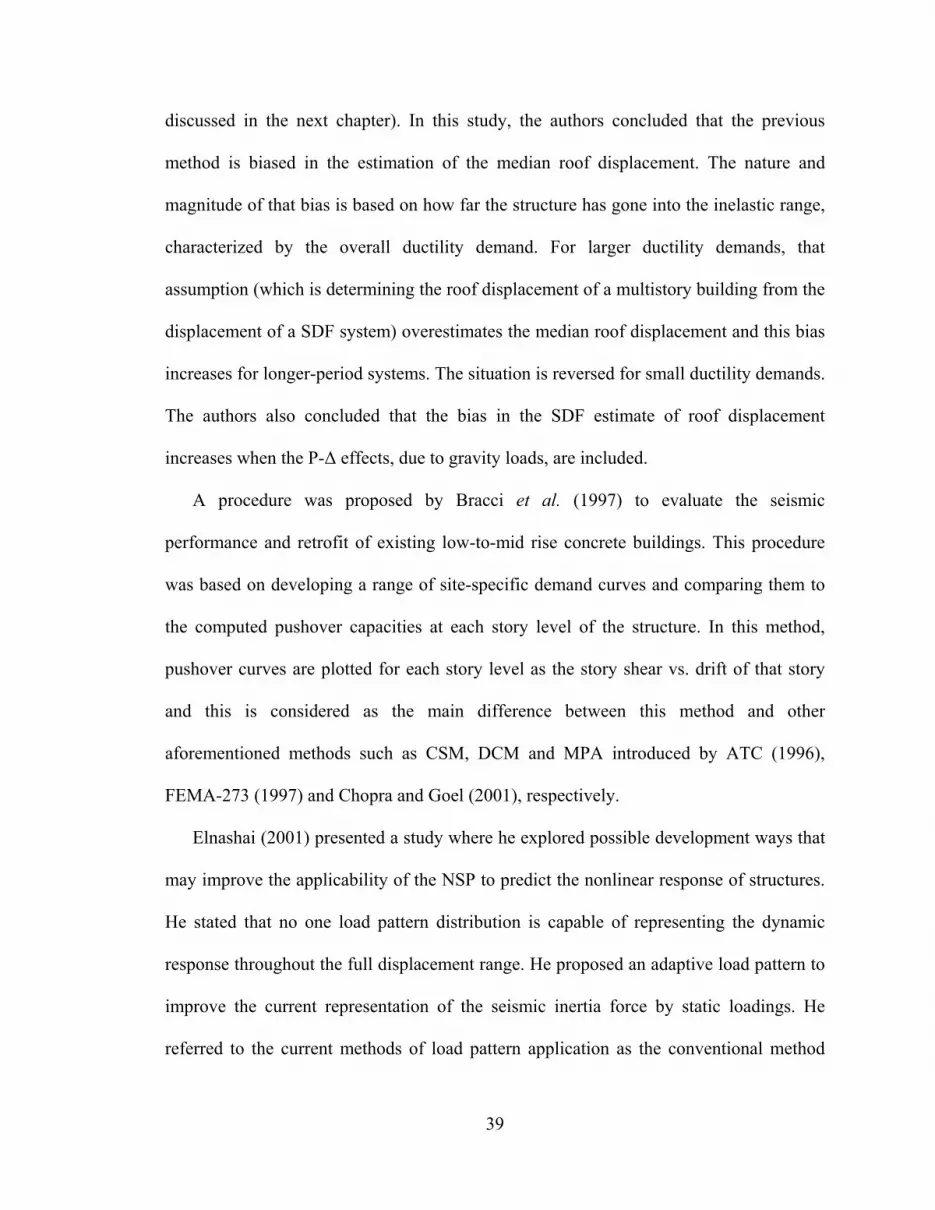
39

discussed in the next chapter). In this study, the authors concluded that the previous

method is biased in the estimation of the median roof displacement. The nature and

magnitude of that bias is based on how far the structure has gone into the inelastic range,

characterized by the overall ductility demand. For larger ductility demands, that

assumption (which is determining the roof displacement of a multistory building from the

displacement of a SDF system) overestimates the median roof displacement and this bias

increases for longer-period systems. The situation is reversed for small ductility demands.

The authors also concluded that the bias in the SDF estimate of roof displacement

increases when the P-Δ effects, due to gravity loads, are included.

A procedure was proposed by Bracci et al. (1997) to evaluate the seismic

performance and retrofit of existing low-to-mid rise concrete buildings. This procedure

was based on developing a range of site-specific demand curves and comparing them to

the computed pushover capacities at each story level of the structure. In this method,

pushover curves are plotted for each story level as the story shear vs. drift of that story

and this is considered as the main difference between this method and other

aforementioned methods such as CSM, DCM and MPA introduced by ATC (1996),

FEMA-273 (1997) and Chopra and Goel (2001), respectively.

Elnashai (2001) presented a study where he explored possible development ways that

may improve the applicability of the NSP to predict the nonlinear response of structures.

He stated that no one load pattern distribution is capable of representing the dynamic

response throughout the full displacement range. He proposed an adaptive load pattern to

improve the current representation of the seismic inertia force by static loadings. He

referred to the current methods of load pattern application as the conventional method

40

and the adaptive method as the advanced method. The results of his adaptive method,

which implemented an incremental updating for the force vector, were closer to the NDP

than the constant force vector. However, the constant force vector is easier and directly

applicable.

CSM was implemented by Shinozuka et al. (2000) in the analysis of girder bridges to

develop fragility curves. Their study is considered as one of the first that applied the

nonlinear static procedure to bridges instead of buildings. They applied lateral forces in

proportion to the fundamental mode shape as

Vw

wF N

iii

iii

⎟⎟⎟⎟

⎠

⎞

⎜⎜⎜⎜

⎝

⎛

=

∑=1

φ

φ Eq. 2.33

Where iF is the lateral force of node ),....,2,1( Nii = ; iw is the dead weight assigned to

node i ; iφ is the amplitude of the fundamental mode at node i ; V is the base shear ; and

N is the number of nodes. The results of this method were compared to the nonlinear

time-history analysis method in the form of fragility curves. The comparison of fragility

curves developed using both methods shows an excellent agreement at least for minor

damage states. For major damage states, because the nonlinearity plays a main role in this

stage, the agreement between the two methods was low. Considering the number of

assumptions in the fragility curves development, they considered that the agreement is

adequate even for the major damage state. Despite the importance of this study in the

contribution for the NSP application on bridges, it does not show any comparison

between different key points such as base shear, plastic hinge rotations, or displacements.

41

Nonlinear static procedures were also implemented in a study by Fenves and Ellery

(1998). In this study, pushover analysis was used to estimate the capacity of the piers.

They were able to define the performance level for each component and accordingly

determined the most likely cause of failure. They found that before reaching the target

displacement produced by the earthquake, the shear capacity curve intersects with the

capacity (pushover) curve. This, in turn, causes the failure of that pier. Their pushover

curves were plotted for each pier individually rather than plotting one pushover curve for

the entire bridge.

A methodology to perform seismic fragility analysis of structures and produce

fragility curves was proposed by Hwang and Huo (1998). They used the displacement-

based approach, which can be considered as an equivalent approach to pushover analysis.

In this approach, displacement demand is compared to the displacement capacity, which

can be represented by the pushover curve.

Dutta (1999) adopted the nonlinear static analysis using the CSM. Given the complete

capacity curve obtained from the pushover analysis, he applied the capacity demand

spectral approach to evaluate the magnitude of the ground acceleration. He also applied

uncertainty to this approach to develop fragility curves.

Pushover analysis was also used for the development of fragility curves for buildings

and bridges by Barron (2000). He estimated the capacity of the structures using static

pushover analysis and compared that with the dynamic pushover analysis. In dynamic

pushover analysis, capacity is estimated for increasing inertia forces. The dynamic

pushover analysis can approximately be obtained from the dynamic analysis using

increasing amplitudes of time-history accelerations. In his study, to account for inelastic

42

response of the structure, Barron implemented updating stiffness of the structure after

each yield point and modal distribution of forces based on the updated mode shape.

Fu and AlAyed (2003) implemented the nonlinear static analysis on a bridge using

the Displacement Coefficient Method (DCM) and compared its results to the nonlinear

dynamic analysis. They applied three different load patterns in the NSP to represent the

inertia forces resulting from earthquakes, and used nine different time-histories to

perform the NDP. They also used two levels of earthquakes in the analyses, the Design

Earthquake Level and the Maximum Considered Earthquake (MCE) level. Their

comparison showed that the nonlinear static analysis gives conservative results compared

to the nonlinear dynamic analysis in the Design Earthquake level and even more

conservative results in the MCE level.

2.6. Performance-based approach

There is a strong relationship between performance-based design and pushover

analysis. Pushover analysis is an important tool to perform performance-based design

(AlAyed, 2002). Accordingly, this section is intended to discuss the performance-based

approach.

Performance-based approach is a general design philosophy in which the design

criteria are expressed in terms of achieving stated performance objectives when the

structure is subjected to stated levels of seismic hazard. The performance targets may be

a level of stress not to exceed, a load, a displacement, a limit state or a target damage

state (Ghobarah, 2001).

The current requirements are based on the importance of the structure, the level of

deformation imposed on the structure, soil conditions, and the ductility of its structural

43

members, especially piers and supports. Performance-based design is focused on meeting

a performance objective, which corresponds to the desired level of service. A

performance level can be defined as the expected behavior of the structure under the

application of the design earthquake; it consists of a combination of damage states to

structural and non-structural components (FEMA-356, 2000). Unlike buildings, bridges

contain fewer nonstructural elements, thus the nonstructural damage may not be included

in choosing the performance level. The performance-based approach has been recently

implemented widely across the United States. Different levels of performance, ranging

from “fully operational” to “near collapse” can be used to meet post-earthquake

conditions.

The Structural Engineering Association of California (SEAOC) (1995), Vision 2000

committee, defined the performance-based engineering as “consisting of the selected

design criteria appropriate structural systems, layout, proportioning and detailing for a

structure and its nonstructural components and contents, and the assurance and control

of construction quality and long term maintenance, such that at specified levels of ground

motions and with defined levels of reliability, the structure will not be damaged beyond

certain limiting states or other usefulness limits”. Four performance levels for buildings

subjected to earthquake design levels were introduced by the SEAOC (1995).

Performance levels can be described as fully operational, operational, life safety, and near

collapse. These performance levels correspond to earthquake design levels that can be

expressed as frequent, occasional, rare, and very rare, respectively. Each of these design

levels is based on a specific recurrence period of 43, 72, 475, and 970 years, respectively.

Performance-based seismic design criteria were proposed by different researchers.

44

Saiidi (1997) proposed three performance levels for bridge seismic design. These

levels are: (1) operational without interruption to traffic flow; (2) operational with minor

damage; and (3) near collapse.

AASHTO (2007) specifications categorized bridges into three categories according to

the bridge importance, these categories are: (1) critical bridges, which must remain open

to all traffic after the design earthquake (which is defined as a 475-year return-period

event) and be usable by emergency vehicles and for security/defense purposes after a

large earthquake (which is defined as a 2500-year return-period event); (2) essential

bridges, which should, as minimum, be open to emergency vehicles and for security

defense purposes immediately after the design earthquake; and (3) other bridges, which

have lower importance than critical and the essential ones, and accordingly lower

performance standards.

ATC-18 (1997) presented two levels of design earthquakes and ground motions,

based on them, two levels of service were recommended. The two levels of earthquakes

are: (1) functional-evaluation ground motion, which is defined as an event having a

probability of occurrence of 30-50% during the design life of the structure; (2) safety-

evaluation ground motion, which is defined as an event having the probability of

occurrence of 10% during the design life of the structure. The first recommended level of

service is the immediate service level, which corresponds to the first ground motion level.

It requires full access of normal traffic almost immediately after the earthquake. The

second is the limited service level, which corresponds to the second ground motion level.

It permits reducing access due to lane closures or restriction of emergency traffic only,

while full service is restorable within months.

45

The California Department of Transportation (Caltrans) (1999) categorized bridges

according to their desired level of performance into ordinary and important bridges. Two

levels of earthquake loading were introduced:

1- Functional-evaluation ground motion, which may be assessed either

deterministically or probabilistically, where the determination of this event is to

be reviewed by a Caltrans consensus group.

2- Safety-evaluation ground motion, which may be assessed either deterministically

or probabilistically. The deterministic assessment corresponds to the Maximum

Credible Earthquake. The probabilistic ground motion for the safety evaluation

typically has a long return period (approximately 1000-2000 years).

Two service levels were defined as Immediate and Limited. Immediate service level

requires full access to normal traffic almost immediately following the earthquake. The

Limited service level permits lane closure and access reduction or restrictions to

emergency traffic only and full service is restorable after months. Three damage levels

were also defined as minimal, repairable and significant.

Floren and Mohammadi (2001) proposed three levels of performance in seismic

design of bridges. They can be described as (1) immediate service (operational without

interruption to traffic flow), where minimal damage has occurred, minor inelastic

response may occur, damage is restricted to narrow flexural cracking in concrete and

permanent deformations are not apparent; (2) limited service (operational with minor

damage), where some structural damage has occurred, concrete cracking, reinforcement

yield, and minor spalling of concrete cover is evident due to inelastic response; (3)

collapse prevention, where significant damage has occurred, concrete cracking,

46

reinforcement yield, and major spalling may require closure for repair. They categorized

the bridges as critical, important, and ordinary. They also used the same earthquake

design levels presented by the SEAOC Vision 2000 committee.

Hwang and Hou (1998) used previous work done by other researchers to define limit

states. They proposed four damage states for buildings. Their damage states are defined

by implementing the displacement-based approach using the inter-story drift ratio (δ) as:

1- No damage state, when δ is less than 0.2%.

2- Insignificant damage state, for δ ranging between 0.2 and 0.5%.

3- Moderate damage state, for δ ranging between 0.5 and 1%.

4- Heavy damage state, when δ is more than 1%.

FEMA-356 (2000) presented many performance levels for buildings, including

structural and nonstructural components. Four levels were presented for damage control

and performance as: (1) operational; (2) immediate occupancy; (3) life safety; and (4)

collapse prevention. Only three levels were concerned with structural elements

performance. These levels are (1) immediate occupancy; (2) life safety; and (3) collapse

prevention. A damage state description for each structural element is presented,

depending on the element (being primary or secondary element in the structural system),

in addition to the plastic hinge rotation, the percentage of the drift, or the strain reached

by the element deformation. Other tables are presented for the non-structural elements. A

more detailed description for the FEMA-356 (2000) performance levels and evaluation

procedures is presented in the next chapter as the NSP of this document is used for the

evaluation of the bridges in this work.

47

CHAPTER 3

THEORETICAL APPROACH

3.1. Introduction

FEMA-356 (2000) presented the “Prestand and Commentary for the Seismic

Rehabilitation of Buildings”, which included a nonlinear static procedure and presented it

as a simplified and efficient procedure to evaluate seismic nonlinear response of

buildings. The DCM was first introduced in the FEMA-273 (1997) then was developed

and applied for bridges by AlAyed (2002). In this bridge evaluation process, the DCM

presented in FEMA-356 (2000) will be used with the same modification used by AlAyed

(2002). DCM uses pushover analysis and a modified version of the equal displacement

demand; it needs no iterations to determine the displacement demand as it implements

coefficients to modify the elastic displacement.

In the pushover analysis concept, a model incorporating the inelastic response of the

structural elements is developed. The load-deformation characteristics of individual

components and elements are directly defined in the model. The structure is then

displaced under monotonically increasing load or displacement, through a specific load

pattern, until either the target displacement is exceeded or the structure becomes unstable.

The resulting internal deformations and forces are determined and compared to the

acceptance criteria for the nonlinear procedures presented in the FEMA-356 (2000). The

target displacement is intended to represent the maximum displacement likely to be

experienced by the structure under the considered earthquake intensity. Because the

48

mathematical model accounts directly for effects of material inelastic response, the

calculated internal forces are assumed to be a reasonable approximation of those expected

during the earthquake. The target displacement may be calculated by any procedure that

accounts for the effects of nonlinear response on displacement amplitude. FEMA-356

(2000) presented a procedure that can be used to calculate the target displacement for

buildings.

3.2. Lateral Load Patterns

FEMA-356 (2000) specified the applied lateral load to the building model in profiles

that approximately simulate the likely distribution of the inertia forces in an earthquake.

For all analyses, at least two vertical distributions of lateral load shall be applied. One

pattern shall be selected from the following two groups (FEMA-356, 2000):

1. A model pattern selected from the following:

a. Equivalent lateral force (ELF) pattern: Using the vertical distribution

factor (defined in equation (3-12) in FEMA-356 (2000)) then distributing

the force on the different floors. This pattern may be used if more than

75% of the total mass participates in the fundamental mode of the

direction under consideration.

b. A distribution proportional to the shape of the fundamental mode in the

direction under consideration. Use of this distribution shall be permitted

only when more than 75% of the total mass participates in this mode.

c. A distribution proportional to the story shear distribution calculated by

combining modal responses from a response spectrum analysis of the

49

building, including sufficient modes to capture at least 90% of the total

building mass, and using the appropriate ground motion spectrum.

2. A second pattern selected from the following (FEMA-356, 2000):

a. A uniform distribution of lateral forces at each level proportional to the

total mass at each level.

b. An adaptive load distribution that changes as the structure is displaced.

The adaptive load distribution shall be modified from the original load

distribution using a procedure that considers the properties of the yielded

structure.

For each evaluated bridge, two load patterns were selected from the aforementioned

ones. The first pattern is (a) in the second group. It is based on lateral forces that are

proportional to the total mass assigned to each node with accordance to the deck mass

distribution. The equation used in the force distribution on the nodes is:

gmF ii ×= Eq. 3.1

where iF is the lateral force at node NNii ),,...,2,1( = is the number of nodes, im is the

mass assigned to node i , and g is the ground acceleration. It is considered as the primary

load pattern and is intended to emphasize the base shear rather than giving high moments

or deformations (AlAyed, 2002). This pattern will be referred to as the “Uniform Load

Pattern”.

The second pattern is (b) in the first group. It represents the deformation of the

structure (or the bridge) in its fundamental mode. The equation on which the distribution

is based is given as:

50

Vm

mF N

iii

iii

⎟⎟⎟⎟

⎠

⎞

⎜⎜⎜⎜

⎝

⎛

=

∑=1

δ

δ Eq. 3.2

where iF , im and N are the same as defined in the first load pattern, Eq. 3.1, and V can be

taken as an optional value since the distribution of the forces is the important part, while

the value is increased incrementally until it reaches the prescribed target displacement or

collapse occurs. This process should be done using the fundamental mode shape, which

has 75% or more of the total mass participating in it. The fundamental mode is

considered to have the highest contribution of all modes to the final deformation of the

structure (or the bridge) under the earthquake load. In the analyses of this work, this

pattern will be referred to as the “Modal Pattern”.

3.3. Estimation of Target Displacement

The effective fundamental period in the direction under consideration is based on the

idealized force-displacement curve described in Figure 3.1. The nonlinear force-

displacement relationship between the base shear and displacement of the control node is

replaced with an idealized relationship to calculate the effective stiffness, eK , and

effective yield strength, yV , of the structure. This relationship is bilinear, with initial

slope eK and post yield slope α . The effective lateral stiffness, eK , is taken as the

secant stiffness calculated at a base at a base shear force equal to 60% of the effective

yield strength of the structure. The post yield slope, α , shall be determined by a line

segment that passes through the actual curve at the calculated target displacement and the

effective yield strength shall not be taken the maximum base shear force at any point

along the actual curve. The effective fundamental period, eT , will be calculated as:

51

eie K

KTT i= Eq. 3.3

where iT is the elastic fundamental period (in seconds) in the direction under

consideration calculated by elastic dynamic analysis, iK is the initial slope of the original

pushover curve, eK is as defined before. eK and iK are shown in Figure 3.1.

Figure 3.1 Idealization of force-displacement curves (FEMA-356, 2000)

The relation between the base shear and the displacement of the control node shall be

established for the displacement of control node ranging between zero to 150% of the

52

target displacement, tδ . The target displacement formula used in the FEMA-356 (2000)

procedures is as follows:

gT

SCCCC eat 2

2

3210 4πδ = Eq. 3.4

where:

eT = effective fundamental period of the structure for the direction under

consideration as defined in Eq. 3.3

0C = modification factor to relate spectral displacement of an equivalent SDOF

system to the roof displacement of the building MDOF system. It is calculated using one

of the following procedures:

a. The first modal participation factor at the level of control node

1,

1,

1,

1,10

1/)(

1/)(

2

CN

ii

ii

CN N

igw

N

igw

PFC φ

φ

φ

φ ×

⎟⎟⎟⎟⎟⎟

⎠

⎞

⎜⎜⎜⎜⎜⎜

⎝

⎛

=

==×=

∑

∑ Eq. 3.5

where iw is the tributary weight at the location i varying from the 1 to N being

the total number of discrete weights for the pushover mode shape locations, 1,iφ is

the amplitude of node i for mode 1, and 1,CNφ is the amplitude of mode 1 at the

control node.

b. The modal participation factor at the level of control node calculated using a

shape vector corresponding to the deflected shape of the building at the target

displacement.

53

1,

1,

1,

0

1/)(

1/)(

2

CN

ii

ii

N

igw

N

igw

C δ

δ

δ

×

⎟⎟⎟⎟⎟⎟

⎠

⎞

⎜⎜⎜⎜⎜⎜

⎝

⎛

=

==

∑

∑ Eq. 3.6

where iw is the same as the previous step, 1,iδ is the amplitude of the shape vector

at joint i , and 1,CNδ is the amplitude of the shape vector at the control node.

c. The appropriate value from Table 3.1.

Table 3.1 Values for the modification factor 0C (FEMA-356, 2000)

Number of stories 1 2 3 5 10

Modification factor C0 1.0 1.2 1.3 1.4 1.5

1C = modification factor to relate expected maximum inelastic displacements to

displacements calculated for linear elastic response

= 1.0 for Te ≥ Ts Eq. 3.7

= [1.0 + (R − 1) Ts / Te] / R for Te < Ts Eq. 3.8

sT = characteristic period of the response spectrum, defined as the period associated

with the transition from the constant acceleration segment of the spectrum to the constant

velocity segment of the spectrum (Figure 3.4).

The factor 1C is intended to account for the difference in peak displacement response

amplitude for nonlinear response as compared to linear response, as observed for

54

buildings with relatively short initial vibration periods. The short initial vibration period

is defined as the time periods that are less than sT as shown in Eq. 3.8.

R = ratio of elastic strength demand to calculated yield strength coefficient, it is

calculated as

my

a CWV

SR

/= Eq. 3.9

where mC is the effective mass factor to account for the higher mode mass participation

effects obtained from Table 3.2 and shall be taken as 1 if the fundamental period, eT , is

greater than 1.0 second.

Table 3.2 Values for Effective Mass Factor Cm (FEMA-356, 2000)

No. of stories

Concrete Moment Frame

Concrete Shear Wall

Concrete Pier-

Spandrel

Steel Moment Frame

Steel Concentric

Braced Frame

Steel Eccentric Braced Frame

Other

1-2 1.0 1.0 1.0 1.0 1.0 1.0 1.0

3 or more 0.9 0.8 0.8 0.9 0.9 0.9 1.0

Eq. 3.9 was changed in the FEMA-356 (2000) from the equation used in the older

version (FEMA-273, 1997) as it used to have the factor ( 0/1 C ) instead of the factor mC .

AlAyed (2002) proposed a modification to this equation (the older version of the

equation) to be:

WVS

CWVS

Ry

a

y

a

/1

/ 0

≤= Eq. 3.10

The reason for such modification is that 0C is the only factor that is affected by the

location of the control node. When the control node is far from the maximum

55

displacement point and has a smaller displacement value, the value of 0C will be small,

which may amplify the value of R many times. A higher value of R may amplify the

values of 1C and 3C . As a preliminary estimation, values of 0C range from 1.0 to 1.5

(Table 3.1). Based on this fact, AlAyed (2002) added the condition in Eq. 3.10 to prevent

the unnecessary amplification of the R factor. Unlike buildings, bridges don’t have a

defined control node (which is defined in buildings as the center of mass of the roof

level), and accordingly, this modification is very important in case of bridges. In the

current bridge evaluation process the modified equation of AlAyed (2002) (Eq. 3.10) will

be used because he included a numerical example that illustrated the estimation of target

displacement when the control node is different from the point of maximum

displacement.

Sa = response spectrum acceleration, g, at the effective fundamental period and

damping ratio of the structure in the direction under consideration. The value of Sa will be

discussed later as well as the earthquake level used in the evaluation process.

Vy = yield strength calculated using results of the NSP for the idealized nonlinear

force-displacement curve developed for the structure (Figure 3.1).

W = effective seismic weight of the structure (discussed in section 4.2.3).

C2 = modification factor to represent the effect of pinched hysteretic shape, stiffness

degradation and strength deterioration on maximum displacement response. Values of C2

for different framing systems are presented in the FEMA-356 (2000) as shown in Table

3.3.

56

Table 3.3 Values for modification factor C2 (FEMA-356, 2000)

T = 0.1 second * T ≥ T0 second * Performance Level Framing Type

11 Framing Type

22 Framing Type

11 Framing Type

22 Immediate Occupancy 1.0 1.0 1.0 1.0

Life Safety 1.3 1.0 1.1 1.0 Collapse

Prevention 1.5 1.0 1.2 1.0 1 Structures in which more than 30 % of the story shear at each level is resisted by components or elements whose strength and stiffness may deteriorate during the design earthquake. 2 All frames not assigned to framing type1. * Linear interpolation may be used for periods between 0.1 and T0.

C3 = modification factor to represent increased displacements due to dynamic P-Δ

effects, for buildings with positive post-yield stiffness, C3 shall be taken as 1.0. For

buildings with negative post-yield stiffness, C3 shall be calculated using Eq. 3.11. Values

for C3 have an upper limit set in section 3.3.1.3 of FEMA-356 (2000)

eTR

C2/3

3

)1(0.1

−+=α

Eq. 3.11

where R and eT as defined above and α is the ratio of post-yield stiffness to effective

elastic stiffness, where the nonlinear force-displacement relationship shall be

characterized by a bilinear relation as shown in Figure 3.1.

g = gravitational acceleration.

3.3.1. Control node

Control node for buildings is defined as the center of mass of the roof level (FEMA-

356, 2000). There is no precise definition for the control node in the ATC (1996) as it

considered the roof floor to be moving as a rigid body. In general, the roof displacement

for the building is known to be the maximum displacement. This is not applicable for

bridges as bridges extend horizontally while buildings extend vertically. This means that

57

the important dimension for buildings is the vertical dimension; as its main restraint is at

the base. However, for bridges, the important dimension is the horizontal one as its main

restraints are at the abutments (AlAyed, 2002).

Control node is defined as the node used to monitor the displacement of the structure.

Its displacement versus the base shear forms the capacity (pushover) curve of the

structure. Two conditions shall be satisfied in the selection of the control node: (1) its

location is expected to have the maximum displacement; (2) its displacement is reflecting

the behavior of the structure (AlAyed, 2002). These two conditions mean that the control

node displacement is affected by the inelastic behavior of any member that contributes to

the stiffness of the structure in the direction under consideration. The second condition is

an essential one and it may cause significant error if it is not satisfied. However, the first

condition seems to be more flexible.

In bridge analysis, two horizontal directions should be considered in the earthquake

load application, longitudinal and transverse directions. In the longitudinal direction, the

bridge usually moves as a rigid body, which gives the same displacement value for all

bridge nodes, if neglecting axial deformations. Accordingly, the selection of the control

node is straightforward.

In the transverse direction, the boundary conditions of the bridge at the abutments are

the main factors that affect its final deformed shape. When the bridge is restrained at both

ends, it will deform in the shape of a simply supported beam. In this case the control node

will be the center of mass of the bridge. However, if the bridge is non-symmetric, the

point of maximum displacement will be shifted. Accordingly, it is necessary to use the

58

modification of the equation of the R ratio that was previously explained in the estimation

of the target displacement.

3.4. Performance level

The main objective of performance-based design is the performance evaluation. A

component or an action is considered satisfied if it meets a prescribed performance level.

The deformation demands are compared to the maximum permissible values for the

components for the deformation-controlled actions. For the force-controlled actions, the

force demand is compared to the strength capacity. If either the deformation demand in a

deformation-controlled element, or force demand in a force-controlled element, exceeds

the permissible values, then the element is deemed to violate the performance criteria.

As mentioned in the previous chapter, FEMA-356 (2000) introduced three structural

performance levels of evaluation to the structural components. These levels are: (1)

Immediate Occupancy (IO), which is defined as the post-earthquake damage state that

remains safe to occupy, essentially retains the pre-earthquake design strength and

stiffness of the structure. In this level of performance, only limited structural damage

occurs. (2) Life Safety, which is defined as the post-earthquake damage state that

includes damage to structural components but retains a margin against onset of partial or

total collapse. In this level of performance, significant damage to structural components

may occur, injuries may take place during the earthquake. However, the overall risk of

life threatening injury is expected to be low. Reoccupying the structure is not guaranteed

immediately after the earthquake. Some structural repairs may need to be implemented or

some bracing members may need to be installed. (3) Collapse Prevention, which is

defined as the post-earthquake state that includes damage to structural components such

59

that the structure continues to support gravity loads but retains no margin against the

collapse. In this level of performance, substantial damage to structure occurs, including

significant degradation in the stiffness and strength of the lateral resisting system.

Nonetheless, all significant components of the gravity-load-resisting system must

continue to support their gravity load demands. Significant risk of injury due to falling

structural debris may exist. The structure may not be safe to reoccupy and technically

impractical to be repaired.

The choice of the required level of performance is based on the choice of the

rehabilitation objective. FEMA-356 (2000) presented three rehabilitation objectives

defined as the Basic, Enhanced and Limited objectives. The Basic Safety Objective

(BSO) is a rehabilitation objective that achieves the dual rehabilitation goals of life safety

level performance for the Basic Safety Earthquake-1 (BSE-1) hazard level and the

collapse prevention level performance for the Basic Safety Earthquake-2 (BSE-2) hazard

level. These two levels of earthquake will be defined in the next section of this chapter.

The Enhanced Rehabilitation Objective is the term that is used for rehabilitation objective

exceeding the BSO. It shall be achieved using one or a combination of the following two

methods (FEMA-356, 2000):

1- Designing for target building performance levels that exceed those of the BSO at

either the BSE-1 or BSE-2 hazard levels, or both.

2- Designing for the target building performance levels of the BSO using an

earthquake hazard level that exceeds either the BSE-1 or BSE-2 hazard levels, or

both.

60

The Limited Rehabilitation Objective is the term used for rehabilitation that provides

building performance less than that of the BSO. Limited rehabilitation objective shall be

achieved using either reduced rehabilitation or partial rehabilitation. Reduced

rehabilitation addresses the entire building structural and nonstructural elements, but with

lower seismic hazard. However, partial rehabilitation objective addresses a portion of the

building without considering the complete lateral-force-resisting system (FEMA-356,

2000).

FEMA-356 (2000) also introduced different performance levels for non-structural

components of the buildings. Bridges, unlike buildings, contain fewer nonstructural

elements. Accordingly, the performance levels for nonstructural damage may be

neglected (AlAyed, 2002). In the bridges evaluation process of this study, due to the high

importance of the bridges, the Enhanced Rehabilitation Objective was chosen. A target

performance level of immediate occupancy at BSE-2 was selected. These bridges, in

accordance with its high importance, should be fully operational without interruption to

traffic flow and without lane closure. The performance level will be applied only to the

bridge substructures (piers or columns), where the plastic hinges are defined. However,

the bridge superstructure (bridge deck) is assumed to behave elastically under earthquake

loads (AlAyed, 2002).

3.5. Seismic loading (Design response spectrum)

To perform the NSP analysis of structures using the DCM, design response spectra

should be available to estimate the factor Sa (spectral acceleration). This factor is an

essential step in the calculation of the target displacement as it represents the level of

earthquake used in the evaluation in addition to the structure location effect and site

61

condition (soil effects). FEMA-356 (2000) implements hazard maps to estimate

parameters used to develop design response spectrum. Two earthquake levels are defined

in FEMA-356 (2000); the first one is the Basic Safety Earthquake-1 (BSE-1) which has a

10% probability of exceedance in 50 years. The second level of earthquake is the Basic

Safety Earthquake-2 (BSE-2) which has a 2% probability of exceedance in 50 years (It

can also be expressed as 10% probability of exceedance in 250 years). This level is also

referred to as the Maximum Considered Earthquake (MCE). The two levels of earthquake

correspond to motions that are expected to occur, on average, about once every 500 and

2500 years respectively (FEMA-356, 2000).

In the bridge evaluation process of this investigation, only the BSE-2 level is used as

mentioned, for the implementation of the Enhanced Rehabilitation Objective. Approved

seismic hazard maps for the conterminous United States, provided by the United States

Geological Survey (USGS), were used in this work in obtaining the short (0.2 second)

and long (1.0 second) period mapped spectral acceleration for each level of earthquake.

Parts of the two maps (contains only Clark County area) are presented in Figure 3.2 and

Figure 3.3.

62

Figure 3.2 MCE’s Spectral Response Acceleration for 0.2-second period

(5% of critical damping) for Clark County (USGS, 2009)

Figure 3.3 MCE’s Spectral Response Acceleration for 1.0-second period

(5% of critical damping) for Clark County (USGS, 2009)

The mapped spectral acceleration is then adjusted according to the bridge site classes

through the following two equations:

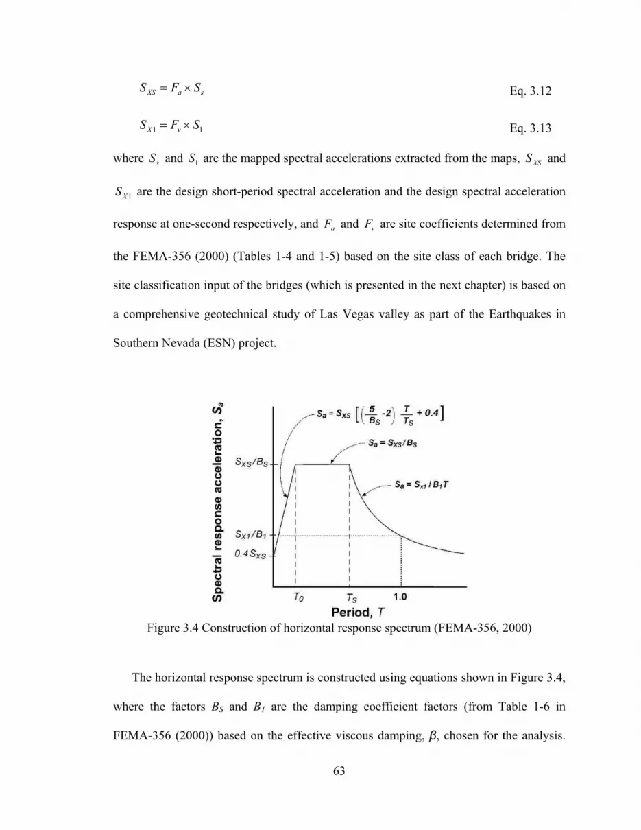
63

saXS SFS ×= Eq. 3.12

11 SFS vX ×= Eq. 3.13

where sS and 1S are the mapped spectral accelerations extracted from the maps, XSS and

1XS are the design short-period spectral acceleration and the design spectral acceleration

response at one-second respectively, and aF and vF are site coefficients determined from

the FEMA-356 (2000) (Tables 1-4 and 1-5) based on the site class of each bridge. The

site classification input of the bridges (which is presented in the next chapter) is based on

a comprehensive geotechnical study of Las Vegas valley as part of the Earthquakes in

Southern Nevada (ESN) project.

Figure 3.4 Construction of horizontal response spectrum (FEMA-356, 2000)

The horizontal response spectrum is constructed using equations shown in Figure 3.4,

where the factors BS and B1 are the damping coefficient factors (from Table 1-6 in

FEMA-356 (2000)) based on the effective viscous damping, β, chosen for the analysis.

64

The effective viscous damping in this work was taken as 5% as the bridges are all of

concrete substructure, while 5% is a good estimation for concrete structures.

3.6. Summary of evaluation procedures

To perform the pushover analysis using the DCM method, the following step-by-step

procedures are used (FEMA-356, 2000):

1. Compute the natural period of the structure for the direction under consideration

using elastic dynamic analysis.

2. Define lateral load pattern from the specified load patterns mentioned before; two

of them should be used in the analysis and the following steps should be repeated

for each pattern.

3. The intensity of the lateral load is increased incrementally in the nonlinear

analysis model and the control node displacement corresponding to each load

increment is determined to plot the pushover curve (control node displacement vs.

base shear force). According to the FEMA-356 (2000) specifications, the

pushover curve should be established for control node displacement ranging

between zero and 150% of the target displacement, δt.

4. The pushover curve is then idealized as a bilinear curve as shown in Figure 3.1.

5. Effective period (Te) is calculated using Eq. 3.3.

6. Pushover curve is used to estimate the target displacement by means of Eq. 3.4.

This step may require iteration if the yield strength and stiffness of the simplified

bilinear relation are sensitive to the target displacement.

65

7. Once the target displacement is estimated, the accumulated forces and

deformations at this displacement of the control node should be used to evaluate

the performance of the structure components as follows:

a. For deformation-controlled actions (e.g. flexure in beams and columns),

the deformation demands are compared to the maximum permissible

values for the component.

b. For force controlled actions (e.g. shear stress and splices of reinforcement

in beams and columns), the strength capacity is compared with the force

demand.

8. For each action, element or component, it is considered to violate the performance

criteria if either (a) the deformation demand in deformation-controlled actions,

component, or elements, or (b) the force demand in the force-controlled actions,

components, or elements, exceeds the permissible values.

66

CHAPTER 4

BRIDGES ANALYSIS AND EVALUATION

4.1. Introduction

In this chapter, a full description of the evaluation process of each bridge is presented,

starting from the description of the bridge, followed by the necessary calculations for the

NSP, and finally the results. Bridges are presented in the order of their importance. In

section 4.2, procedures of bridges analysis and evaluation are described along with the

adopted assumptions.

4.2. Modeling general assumptions

4.2.1. Spectral acceleration (Sa)

Equations for the calculations of the spectral acceleration using the FEMA-356

(2000) were discussed in the previous chapter. The inputs for the Sa calculations for the

studied bridges are: (1) site classifications for the soil underneath the bridges and (2) the

mapped spectral accelerations for long and short time periods for each bridge. As

mentioned in the previous chapter, the mapped spectral accelerations are for the BSE-2

earthquake, with 2% probability of exceedance in 50 years. These two inputs are

presented in Table 4.1.

67

Table 4.1 Site classifications and mapped spectral accelerations for the studied bridges

Mapped Spectral Acceleration (%g) Bridge Site

Classification Ss S1

G-1064 C 55.0 17.5

G-947 D 57.0 17.5

H-1211 C 55.0 17.0

G-953 D 56.5 17.5

I-2139 D 56.5 17.5

4.2.2. Bridge models

Wire frame elements (spine) were used to model the studied bridges using the

SAP2000 program with the bridge module. In the transverse direction, bridges were

modeled as one unit, even in the presence of expansion joints. However, in the

longitudinal direction, bridges were divided into units at expansion joints (when present),

and each unit is evaluated independently. In bridge engineering design, it is a common

practice to divide long bridges into smaller units to alleviate the effect of thermal

expansion. These units are designed to move independently in the longitudinal direction

and work together in the transverse direction (AlAyed, 2002). In the analysis, each unit

has its own control node and its applied inertial forces so that the pushover curve

represents the base shear vs. displacement of the control node of this unit without any

contribution from other units except applied loads as it may affect the columns evaluation

by increasing the P-Δ effect.

In some cases of the longitudinal direction analyses of the bridge units, target

displacements exceeded the values of the expansions provided between the units. In these

68

cases, the bridge units were still pushed to the target displacement values, because the

actual behavior of the bridge deck in the vertical direction is not considered and this may

increase the displaced values of the bents in the longitudinal direction.

4.2.3. Effective seismic weight

The effective seismic weight of the bridges in this work consists of the dead load and

a portion of the live load. Dead load in the analyses represents the structural components

with their full weights in addition to the weights of concrete barriers, pedestrian rails,

wearing surfaces, etc. For the live load portion, FEMA-356 (2000) specifies a portion of

the live load to be considered in the case of building evaluations, but not for bridges. For

buildings, a minimum of 25% of floor live load in case of storage areas, the actual

partitions load if applicable and the total operating weight of permanent equipment are

required in the specifications. Live load in the current study was chosen to be 25% of the

design lane load per AASHTO (2007) specifications. The design lane load is 0.64 kip/ft

/10 ft wide lane. Lumped masses at the nodes of the superstructures included the

additional part from the live load along with the dead load part.

4.2.4. Stiffness reduction

The stiffnesses of all elements were reduced as per the FEMA-356 (2000)

specifications. Shear rigidity was reduced to 40% of its gross value for all elements.

Flexural rigidity for all non-prestressed beams was reduced to 50% of its gross value.

Gross flexural rigidity, with no reduction, was used for prestressed beams. For the bent

columns, the effective flexural rigidity was calculated using the moment-curvature

( φ−M ) relationship to obtain the cracked section characteristics. The proposed effective

moment of inertia ( eI ) by the FEMA-356 (2000) document is 0.5 to 0.7 of the gross

69

section moment of inertia ( gI ), depending on the axial force applied on the column. The

use of the φ−M relationship to evaluate the flexural rigidity of the columns is a more

accurate and realistic approach compared to FEMA’s approach (AlAyed, 2002).

After constructing the φ−M curve and idealizing it, the following formula for the

calculation of the effective moment of inertia is used:

yc

ne E

MI

φ= Eq. 4.1

where eI is the effective moment of inertia for the cracked section, yφ is the curvature at

yield estimated using a bilinear curve to represent φ−M relationship, nM is the nominal

moment corresponding to yφ and cE is the concrete modulus of elasticity. This equation

will be used for each column section to estimate its eI .

4.2.5. Acceptance limits

4.2.5.1. Deformation-controlled actions

For deformation controlled actions, FEMA-356 (2000) expressed the acceptance

criteria as deformation values for each level of performance. A generalized force-

deformation relation for concrete elements and components is represented in the FEMA-

356 (2000) based on the applied loads and the section properties. Table 4.2 (Table 6-8 in

FEMA-356 (2000)) represents the modeling parameters and numerical acceptance criteria

for columns in the nonlinear procedures. This table is used in this study to calculate the

plastic hinge rotations acceptance criteria (in radians) for each of the performance levels.

The generalized load-deformation relation shown in Figure 4.1 describes the general

sequence of stiffness loss of an element. A linear response from A to an effective yield at

B is followed by a linear response at reduced stiffness from B to C, then a sudden

70

reduction in the lateral load resistance to point D, then response at reduced resistance to

E, and final loss of resistance thereafter (FEMA-356, 2000). In the case of the horizontal

axis of this graph taken as the plastic hinge rotation, point B should be on the vertical

axis, which means that the plastic hinge rotation values of all points between A and B are

equal to zero.

71

Table 4.2 Modeling parameters and numerical acceptance criteria for nonlinear procedures for reinforced concrete columns (FEMA-356, 2000)

Modeling Parameters 4 Acceptance Criteria 4

Plastic Rotation Angle, radians Performance Level

Component Type Plastic Rotation Angle, radians

Residual Strength

Ratio Primary Secondary

Conditions

A b C IO

LS CP LS CP i. Columns controlled by flexure 1

'cg fA

P

Trans. Reinf.2 '

cw fdb

V

≤ 0.1 C ≤ 3 0.02 0.03 0.2 0.005 0.015 0.02 0.02 0.03

≤ 0.1 C ≥ 6 0.016 0.024 0.2 0.005 0.012 0.016 0.016 0.024

≥ 0.4 C ≤ 3 0.015 0.025 0.2 0.003 0.012 0.015 0.018 0.0025

≥ 0.4 C ≥ 6 0.012 0.02 0.2 0.003 0.01 0.012 0.013 0.02

≤ 0.1 NC ≤ 3 0.006 0.015 0.2 0.005 0.005 0.006 0.01 0.015

≤ 0.1 NC ≥ 6 0.005 0.012 0.2 0.005 0.004 0.005 0.008 0.012

≥ 0.4 NC ≤ 3 0.003 0.01 0.2 0.002 0.002 0.003 0.006 0.01

≥ 0.4 NC ≥ 6 0.002 0.008 0.2 0.002 0.002 0.002 0.005 0.008

ii. Columns controlled by shear 1, 3

All cases5 − − − − − − .0030 .0040

iii. Columns controlled by inadequate development or splicing along the clear height 1, 3

Hoop spacing ≤ d⁄2 0.01 0.02 0.4 0.005 0.005 0.01 0.01 0.02

Hoop spacing > d⁄2 0.0 0.01 0.2 0.0 0.0 0.0 0.005 0.01

iv. Columns with axial load exceeding 0.70Po 1, 3

Conforming hoops over the entire length 0.015 0.025 0.02 0.0 0.005 0.01 0.01 0.02

All other cases 0.0 0.0 0.0 0.0 0.0 0.0 0.0 0.0 1. When more than one of the conditions i, ii, iii, and iv occurs for a given component, use the minimum appropriate numerical value from the table.

2. “C” and “NC” are abbreviations for conforming and nonconforming transverse reinforcement. A component is conforming if, within the flexural

plastic hinge region, hoops are spaced at ≤ d/3, and if, for components of moderate and high ductility demand, the strength provided by the hoops

(VS) is at least three-fourths of the design shear. Otherwise, the component is considered nonconforming. 3. To qualify, columns must have transverse reinforcement consisting of hoops. Otherwise, actions shall be treated as force-controlled. 4. Linear interpolation between values listed in the table shall be permitted. 5. For column controlled shear, see section 6.5.2.4.2 for acceptance criteria.

72

Figure 4.1 Generalized force-deformation relations for concrete

elements (FEMA-356, 2000)

4.2.5.2. Force-controlled actions

Two main force controlled actions are evaluated in this study: (1) shear capacity of

the columns; (2) development and splice lengths of the reinforcement. For the shear

capacity calculations, FEMA-356 (2000) introduced an equation for the concrete shear

strength calculation, and permitted the use of the ACI 318-08 (2008) equation. The

AASHTO (2007) simplified method of calculating the shear capacity gives quite similar

values to the equation used by ACI 318-08 (2008). In this study, the ACI equation for

sections subjected to axial load will be used for simplicity. Shear capacity equations are

as follows:

scn VVV += Eq. 4.2

where nV is the shear strength of the section, cV and sV are the the concrete contribution

and the transverse reinforcement contribution to the shear strength, respectively. They are

calculated using the formulas in Eq. 4.3 and Eq. 4.4.

73

dbfA

NV wcg

uc

'

200012 ⎟

⎟⎠

⎞⎜⎜⎝

⎛+= Eq. 4.3

where uN is the axial load on the column (lbs), gA is the gross area of the column

section (in2), 'cf is the concrete compressive strength (psi), wb is the width of the

concrete section (in), and d is the depth of the concrete section (in). In case of circular

sections the depth of the concrete section is taken as 80% of the total depth (ACI 318-08,

2008).

sdfA

V ytvs

..= Eq. 4.4

where s is the spacing of the transverse reinforcement (in), vA is the area of the shear

reinforcement within s (in2), and ytf is the yield strength of the transverse reinforcement

(psi). FEMA-356 (2000) specifies that the value of sV shall be reduced to 50% in

resisting shear or torsion in case of having transverse reinforcement spacing ( s )

exceeding half of the member’s effective depth. For the case of spacing exceeding the

effective depth of the member, transverse reinforcement shall be assumed ineffective in

resisting shear or torsion.

Shear force values at the target displacement for all columns are compared to the

calculated values of the shear strength by Eq. 4.2. If the shear force exceeded the strength

of the column, brittle failure is expected and the bent is violating the performance criteria.

Concurrent multidirectional seismic effects are also considered by associating 100% of

design forces and deformations of the transverse direction analysis results plus 30% of

forces (not deformations) of the longitudinal direction analysis results and vice versa.

74

The second force controlled action evaluated in this study is the development and

splice lengths of reinforcement. Two main locations within the bent are critical and

subject to bond slippage under seismic loads; (1) the splice between the dowels from the

foundation to the column reinforcement (if any); and (2) the beam-column (B/C) joint

where the reinforcement of the column terminates. FEMA-356 (2000) refers to the ACI-

318-08 (2008) development and splice length equations, which again gives quite similar

values to the equations of development and splice lengths in the AASHTO (2007). The

equation used in this study for the development length calculation is as follows:

b

c

etyd d

f

fl ⎟

⎟

⎠

⎞

⎜⎜

⎝

⎛=

'20λ

ψψ Eq. 4.5

where dl is the development length (in), yf is the specified yield strength of

reinforcement (psi), 'cf is the specified compressive strength of concrete (psi), tψ and eψ

are factors used to modify development length based on the reinforcement location and

reinforcement coating respectively, λ is a modification factor if light weight concrete is

used, and bd is the reinforcing bar diameter. The splice length in tension is taken as dl0.1

for class A splice and dl3.1 for class B splice, where all splice lengths are considered

tension splices (FEMA-356, 2000).

For development, hook and splice lengths that do not meet the requirements of the

code, FEMA-356 (2000) specifies Eq. 4.6 to calculate the capacity of the existing

reinforcement at the development or splice location.

yd

bs f

ll

f ⎟⎟⎠

⎞⎜⎜⎝

⎛= Eq. 4.6

75

where sf is the maximum stress that can be developed in the bar for the straight

development, hook, or lap splice length bl provided, yf and dl are as defined before.

This equation should be used for the calculations of the plastic hinge properties of the

new section in case of having columns controlled by inadequate development, hook or

splice lengths, and the acceptance criteria for each performance level is provided in Table

4.2.

Each of the three aspects of evaluation (which are (1) the flexural deformation; (2) the

shear forces; and (3) the reinforcement development in the columns), is evaluated

independently at the calculated target displacement.

76

4.3. Seismic evaluation of the studied bridges

4.3.1. Bridge (G-1064)

4.3.1.1. Bridge description

G-1064 is a 12-spans/11-piers bridge, located at the intersection of Sahara Avenue

(overpass) and both of Industrial Road and Western Avenue (underpass). The total length

of the bridge is 900.58 ft, each of the internal spans is 75.25 ft and the two external spans

are 74.04 ft long. The substructure elements are skewed at an angle of 25.19 degrees from

the line perpendicular to the bridge centerline. Figure 4.2 shows the plan and elevation of

the bridge.

As shown in Figure 4.3, the superstructure of this bridge is a girder-type deck

consisting of 12 prestressed girder members of 3.75 ft depth, spaced at 8 ft transversally,

and connected by a 7 inches thick cast-in-place slab. The concrete compressive strength

for this bridge is 4 ksi, and the reinforcement yield strength is 60 ksi.

77

Figure 4.2 Bridge G-1064 - Plan and elevation

78

Figure 4.3 Bridge G-1064 - Superstructure

The substructure of the bridge is a five column frame bent, as shown in Figure 4.4,

with a 3 ft column diameter and a cap beam dimensions of 3.5 ft depth by 4 ft width. The

column length varies with the location of the bent. Figure 4.2 shows the bridge profile

with the deck elevation that increases in the middle spans and decreases close to the

abutments. The concrete columns are fixed to the rectangular footings, and the dowels

from the footing are lap spliced with column reinforcement 8 ft away from the footing

top level.

Figure 4.4 Bridge G-1064 - Elevation of a typical bent

79

Cross diaphragms are provided at every bent location, at the abutments and at the

mid-spans between every two bents. Each three spans are separated by an expansion joint

that discontinues the rotational relation between spans. At the expansion joint location,

two diaphragms are provided, separated by the expansion joint filler, as shown in Figure

4.5.

(a)

(b)

(c)

(d)

Figure 4.5 Bridge G-1064 - Cross diaphragms at (a) fixed bearing; (b) interior diaphragm; (c) expansion joint; and (d) abutment expansion joint

4.3.1.2. Bridge model

Figure 4.6 shows the structural model for the bridge used for the analysis and

evaluation in the transverse direction, while Figure 4.7 (a) to (d) shows the structural

80

models used for the analyses and evaluation of the longitudinal direction. The units are

separated at the locations of the expansion joints.

4.3.1.2.1. Superstructure

The superstructure was modeled with four elements per span; the frame elements are

automatically located in the centroid of the superstructure. The mass of each part of the

bridge deck is lumped to the nodes of the superstructure elements. The cross sectional

area of the bridge deck is 106.67 ft2 and its moment of inertia about the Y and Z axes are

234 and 84978 ft4 respectively (the X-axis is in the longitudinal direction and the Z-axis

is the vertical axis). An additional load of 4.726 kip/ft was added to represent the dead

load from the concrete barriers, the pedestrian rails and the wearing surface overlay. An

additional load of 3.84 kip/ft was added to account for the live load over the six lanes of

the bridge.

4.3.1.2.2. Substructure

The substructure components are skewed bents at 25.19 degrees, the masses of the

cap beams and half of the columns were lumped to the top node of each column. The

abutments were modeled only with their stiffness (no elements), with a release in the

translation in the longitudinal direction (X-axis) and the rotation about the transverse

direction (Y-direction). Link elements were added to relate the superstructure to the cap

beam as the centroid of the deck is higher than the level of the cap beam. These link

elements translate loads but not rotations, as the deck girders are rested on bearings that

isolate the rotation of the deck from the cap beam. Foundations were modeled as fixed

supports.

81

Figure 4.6 Bridge G-1064 - Structural model for transverse direction analysis

(a)

(b)

(c)

(d)

Figure 4.7 Bridge G-1064 - Structural models for longitudinal direction (a) unit-1; (b) unit-2; (c) unit-3; and (d) unit-4

82

4.3.1.2.3. Effective moment of inertia for bent columns

All bent columns for this bridge are similar except for their height which varies from

one bent to another and within each bent. The diameter of all columns is 3 ft with 16 #8

rebars attached in splice (of 2.5 ft length) to 16 #11 dowels extended from the

foundations. The dowels are 8 ft long above the footings top level. Figure 4.8 shows the

φ−M curves for the two sections used in the estimation of the effective moment of

inertia for the bent columns. The average axial load on the columns from the preliminary

analysis, which was used in constructing the φ−M curve, is 425 kips.

For a circular column with 3 ft diameter:

9761.3=gI ft4

From the φ−M idealized curve in Figure 4.8 (a):

1150=nM kip-ft, 00125.0=yφ rad/ft

using the ACI 318-08 (2008) equation “ '000,57 cc fE = ”

5.519119=cE ksf

since yc

ne E

MIφ

= 7722.1=eI ft4

and 4457.09761.37722.1

==g

e

II

Therefore, gross flexural rigidity for columns with #8 rebars will be reduced to 45%

of its value in the analysis.

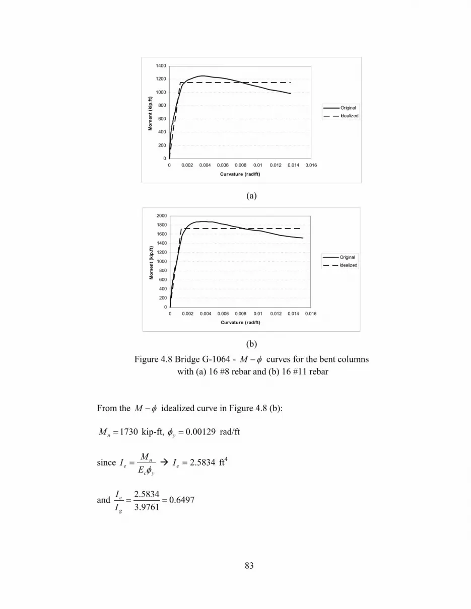
83

0

200

400

600

800

1000

1200

1400

0 0.002 0.004 0.006 0.008 0.01 0.012 0.014 0.016

Curvature (rad/ft)

Mom

ent (

kip.

ft)

Original

Idealized

(a)

0

200

400

600

800

1000

1200

1400

1600

1800

2000

0 0.002 0.004 0.006 0.008 0.01 0.012 0.014 0.016

Curvature (rad/ft)

Mom

ent (

kip.

ft)

Original

Idealized

(b)

Figure 4.8 Bridge G-1064 - φ−M curves for the bent columns with (a) 16 #8 rebar and (b) 16 #11 rebar

From the φ−M idealized curve in Figure 4.8 (b):

1730=nM kip-ft, 00129.0=yφ rad/ft

since yc

ne E

MIφ

= 5834.2=eI ft4

and 6497.09761.35834.2

==g

e

II

84

Therefore, gross flexural rigidity for columns with #11 rebars will be reduced to 65%

of its value in the analysis.

4.3.1.2.4. Spectral acceleration curve

Figure 4.9 shows the response spectrum used for the estimation of ( aS ) values in the

target displacement calculations. From the curve sec088.00 =T and sec438.0=ST .

0.000

0.100

0.200

0.300

0.400

0.500

0.600

0.700

0.000 0.500 1.000 1.500 2.000 2.500 3.000 3.500 4.000

T (sec)

Sa (g

)

Figure 4.9 Bridge G-1064 - 5% damped response spectrum for BSE-2

4.3.1.3. Acceptance criteria

4.3.1.3.1. Load-deformation curve for plastic hinges

From the analysis, the average axial load on the columns for this bridge was 425 kips,

and the maximum shear force on columns was 0.269 kips.

Therefore, 1044.0' =cg fA

P (which is very close to 0.1 (no need for interpolation))

and 0041.0'=

cw fdbV < 3

85

The transverse reinforcement of the column is classified as conforming. Accordingly,

plastic hinge rotation values used for the acceptance criteria (from Table 4.2) will be

0.005 for the Immediate Occupancy (IO), 0.015 for the Life Safety (LS) and 0.02 for the

Collapse Prevention (CP) levels (Figure 4.10).

00.20.4

0.60.8

11.2

1.41.6

0 0.01 0.02 0.03

θp

Q/Q

y

IO

LS

CP

Figure 4.10 Bridge G-1064 - Generalized force-deformation relation

for bridge columns

4.3.1.3.2. Force-controlled actions

a- Shear capacity:

Based on Eq. 4.2, Eq. 4.3, and Eq. 4.4;

425=uN kips, 88.1017=gA in2 (for 36 inches column diameter),

625.3=s in, 62.0=vA in2 for two bars with #5 size, 36=wb in

Therefore, 525.158=cV kips and 547.295=sV kips

Shear capacity of the section is 072.454=+= scn VVV kips

b- Reinforcement development:

Based on Eq. 4.5 and Eq. 4.6;

86

60000=yf psi, 4000' =cf psi

As per ACI 318-08 equations, for #8 reinforcement bar;

Development length 4.47=dl in 95.3= ft and the splice length is 14.53.1 =× dl ft.

The splice length provided at the splice location between the #11 dowels and the #8 bar

of the column reinforcement is 2.5 ft and the development length provided at the beam-

column (B/C) joint is 2 ft.

Therefore, maximum stress that can be developed in the rebars at the splice location is:

18.296014.55.2

=⎟⎠⎞

⎜⎝⎛=sf ksi

and the maximum stress that can be developed in the rebars at the B/C joint location is:

38.306095.30.2

=⎟⎠⎞

⎜⎝⎛=sf ksi

The load-deformation relation at these locations is shown in Figure 4.11, where the yield

stress used for this curve is the new calculated stress ( sf ) from the above calculations.

Figure 4.11 shows the acceptance criteria for the IO and the LS performance levels

coincide at 0.005 radians.

87

00.2

0.40.6

0.81

1.21.4

1.6

0 0.005 0.01 0.015 0.02

θp

Q/Q

y

IO

LS

CP

Figure 4.11 Bridge G-1064 - Generalized force-deformation with acceptance

criteria for inadequate splicing in the bridge column reinforcement

4.3.1.4. Pushover curves and target displacement

4.3.1.4.1. Transverse direction

From the results of the modal analysis of the bridge, the fundamental mode in the

transverse direction was mode 2, with a deformed mode shape shown in Figure 4.12. The

time period for this mode was 1.213 seconds ( sec213.1=iT ). The nonlinear pushover

analysis was performed using both patterns, uniform and modal, and the resulting base

shear-displacement curves are displayed in Figure 4.13.

The control node in this direction was chosen to be the node of the superstructure at

the location of pier number 6 (the middle pier). This node is considered the mid-point of

the bridge and has the highest value of deflection using both uniform and modal patterns.

The displacement of this node vs. the base shear of all columns represents the shown

pushover curves.

88

Figure 4.12 Bridge G-1064 - Mode-2, The fundamental mode in the transverse

direction of the bridge

0

150

300

450

600

750

900

1050

1200

1350

1500

0 0.1 0.2 0.3 0.4 0.5 0.6 0.7 0.8 0.9 1

Displacement (ft)

Bas

e sh

ear (

Kip

s)

(a)

0

150

300

450

600

750

900

1050

1200

1350

1500

0 0.1 0.2 0.3 0.4 0.5 0.6 0.7 0.8 0.9 1

Displacement (ft)

Bas

e sh

ear (

Kip

s)

(b)

Figure 4.13 Bridge G-1064 - Pushover curves for the transverse direction (a) using the uniform load pattern (b) using the modal load pattern

From the pushover curves (Figure 4.13 (a) & (b));

ei KK = 213.1== ie TT sec

Using the effective time period in the response spectrum curve gSa 235.0=

Control node

89

Using the first approach in 0C calculations gives;

309.10161.033.811,10 =×=×= CNPFC φ

Since se TT > 0.11 =C

and 0.132 == CC

Therefore, the target displacement can be calculated as

ftt 368.04213.12.32235.00.10.10.1309.1 2

2

=×××××=π

δ (for both the uniform and

modal patterns)

4.3.1.4.2. Longitudinal direction

Modal analyses results for the four units of the bridge in the longitudinal direction are

shown in Table 4.3. The control node in the longitudinal direction, for each unit, was

chosen to be the furthest on the superstructure to the east at the end pier. Pushover curves

are presented in Figure 4.15 (a) to (h), and then the target displacements for all units are


Table 4.3 Bridge G-1064 - Modal analysis Output for the 4 units used in the longitudinal direction

Unit Fundamental Mode Time

period (Ti, sec)

Modal Participation Factor (PF)

Displacement of Control node

(φ CN, ft)

1 2.52 47.929 0.0209

2 5.33 56.695 0.0176

3 5.55 56.440 0.0177

4 2.57 47.996 0.0208

90

(a)

(b)

(c)

(d)

Figure 4.14 Bridge G-1064 -Fundamental mode shapes in the longitudinal direction of the bridge for (a) unit-1; (b) unit-2; (c) unit-3; and (d) unit-4

91

0

100200

300400

500

600700

800900

1000

0 0.1 0.2 0.3 0.4 0.5 0.6 0.7 0.8 0.9 1

Displacement (ft)

Bas

e sh

ear (

Kip

s)

(a) Unit-1-Uniform load pattern

0

100

200

300

400

500

600

700

800

900

1000

0 0.1 0.2 0.3 0.4 0.5 0.6 0.7 0.8 0.9 1

Displacement (ft)

Bas

e sh

ear (

Kip

s)

(b) Unit-1-Modal pattern

050

100150200250300350400450500550600650700

0 0.25 0.5 0.75 1 1.25 1.5 1.75 2 2.25 2.5

Displacement (ft)

Bas

e sh

ear (

Kip

s)

(c) Unit-2-Uniform load pattern

050

100150200250300350400450500550600650700

0 0.25 0.5 0.75 1 1.25 1.5 1.75 2 2.25 2.5

Displacement (ft)

Bas

e sh

ear (

Kip

s)

(d) Unit-2-Modal pattern

050

100150200250300350400450500550600650700

0 0.25 0.5 0.75 1 1.25 1.5 1.75 2 2.25 2.5

Displacement (ft)

Bas

e sh

ear (

Kip

s)

(e) Unit-3-Uniform load pattern

050

100150200250300350400450500550600650700

0 0.25 0.5 0.75 1 1.25 1.5 1.75 2 2.25 2.5

Displacement (ft)

Bas

e sh

ear (

Kip

s)

(f) Unit-3-Modal Patters

0

100200

300400

500

600700

800900

1000

0 0.1 0.2 0.3 0.4 0.5 0.6 0.7 0.8 0.9 1

Displacement (ft)

Bas

e sh

ear (

Kip

s)

(g) Unit-4-Uniform load pattern

0

100200

300400

500

600700

800900

1000

0 0.1 0.2 0.3 0.4 0.5 0.6 0.7 0.8 0.9 1

Displacement (ft)

Bas

e sh

ear (

Kip

s)

(h) Unit-4-Modal pattern

Figure 4.15 Bridge G-1064 - Pushover curves for longitudinal direction analysis

92

Table 4.4 Bridge G-1064 - Target displacements for different units used in the longitudinal direction

Unit Ti (sec) Te (sec) Sa (g) C0 C1,C2

and C3 tδ (ft)*

1 2.52 2.52 0.113 1.002 1.0 0.586

2 5.33 5.33 0.053 0.998 1.0 1.230

3 5.55 5.55 0.051 0.999 1.0 1.283

4 2.57 2.57 0.111 0.998 1.0 0.598 * Target displacement has an identical value for both uniform and modal pattern for each unit.

4.3.1.5. Results

4.3.1.5.1. Deformation-controlled actions

In the transverse direction, none of the columns experienced plastic hinge formation at

the target displacement. However, in the longitudinal direction, some of the columns

encountered plastic hinge formation with different rotation values depending on the

location of the column. Table 4.5 presents the plastic hinge rotation values at target

displacements in the longitudinal direction. All plastic hinges formed in this direction

were at the bottom part of the columns. This is due to the fact that earthquake loads are

applied in the out-of-plane direction of the bent frame, and the bent columns resist the

lateral load as cantilevers with zero moment at the top. The bents in the bridge are labeled

in a numerical sequence from east to west direction of the bridge as shown in Figure 4.2

and the column labels within the bent (from 1 to 5) is from north to south direction.

From the results presented in Table 4.5, three columns had plastic hinge rotations

violated the acceptance criteria of the IO performance level in each of the two applied

patterns (uniform and modal)

93

Table 4.5 Bridge G-1064 - Plastic hinge rotation values (radians) of bridge columns at target displacements in the longitudinal direction

Bent no. 1 Column 1 2 3 4 5 Uniform 0.001633 0.001661 0.002430 0.003312 0.005046 Modal 0.001632 0.001660 0.002432 0.003317 0.005057

Bent no. 2 Uniform

Uni

t 1

Modal No Plastic Hinge Rotation Observed

Bent no. 3 Column 1 2 3 4 5 Uniform 0.000000 0.000000 0.000000 0.000000 0.000000 Modal 0.000000 0.000000 0.000000 0.000000 0.000813

Bent no. 4 to 6 Uniform

Uni

t 2


Bent no. 6 to 9 Uniform

Uni

t 3


Bent no. 9 and 10 Uniform Modal

No Plastic Hinge Rotation Observed

Bent no. 11 Column 1 2 3 4 5 Uniform 0.006938 0.005386 0.004283 0.003579 0.003496

Uni

t-4

Modal 0.006586 0.005009 0.003937 0.003221 0.003139


a- Shear forces:

None of the columns at the target displacement, in both transverse and longitudinal

directions, encountered a shear force exceeding the shear capacity calculated in the

previous section. Shear forces at target displacements in the transverse and longitudinal

directions are presented in Table 4.6 and Table 4.7, respectively.

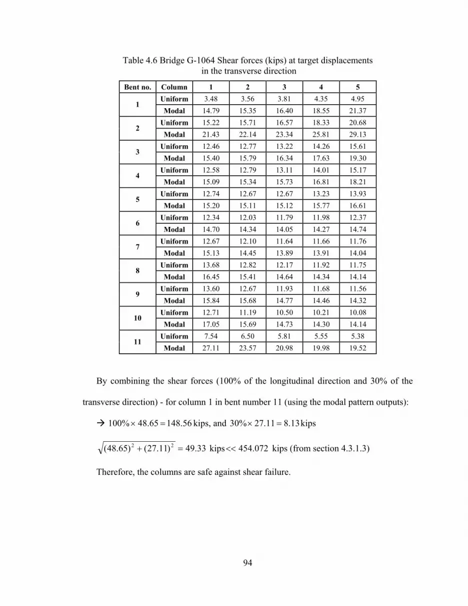
94

Table 4.6 Bridge G-1064 Shear forces (kips) at target displacements in the transverse direction

Bent no. Column 1 2 3 4 5 Uniform 3.48 3.56 3.81 4.35 4.95

1 Modal 14.79 15.35 16.40 18.55 21.37

Uniform 15.22 15.71 16.57 18.33 20.68 2

Modal 21.43 22.14 23.34 25.81 29.13 Uniform 12.46 12.77 13.22 14.26 15.61

3 Modal 15.40 15.79 16.34 17.63 19.30

Uniform 12.58 12.79 13.11 14.01 15.17 4

Modal 15.09 15.34 15.73 16.81 18.21 Uniform 12.74 12.67 12.67 13.23 13.93

5 Modal 15.20 15.11 15.12 15.77 16.61

Uniform 12.34 12.03 11.79 11.98 12.37 6

Modal 14.70 14.34 14.05 14.27 14.74 Uniform 12.67 12.10 11.64 11.66 11.76

7 Modal 15.13 14.45 13.89 13.91 14.04

Uniform 13.68 12.82 12.17 11.92 11.75 8

Modal 16.45 15.41 14.64 14.34 14.14 Uniform 13.60 12.67 11.93 11.68 11.56

9 Modal 15.84 15.68 14.77 14.46 14.32

Uniform 12.71 11.19 10.50 10.21 10.08 10

Modal 17.05 15.69 14.73 14.30 14.14 Uniform 7.54 6.50 5.81 5.55 5.38

11 Modal 27.11 23.57 20.98 19.98 19.52

By combining the shear forces (100% of the longitudinal direction and 30% of the

transverse direction) - for column 1 in bent number 11 (using the modal pattern outputs):

56.14865.48%100 =× kips, and 13.811.27%30 =× kips

33.49)11.27()65.48( 22 =+ kips 072.454<< kips (from section 4.3.1.3)

Therefore, the columns are safe against shear failure.

95

Table 4.7 Bridge G-1064 Shear forces (kips) at target displacements in the longitudinal direction


1 Modal 34.02 37.46 36.29 41.68 43.22

Uniform 23.06 24.80 26.03 30.90 37.35 2

Modal 23.07 24.83 26.08 30.97 37.46 Uniform 24.52 25.61 26.15 29.64 33.89

3 Modal 24.39 26.28 27.63 32.21 35.78

Uniform 17.85 18.45 18.71 21.01 23.78 4

Modal 17.89 19.08 19.91 22.97 26.66 Uniform 15.66 15.57 15.25 16.56 17.92

5 Modal 15.88 16.29 16.44 18.37 20.41

Uniform 14.97 14.56 13.97 14.69 15.58 6

Modal 16.49 15.75 14.92 15.48 16.12 Uniform 16.74 15.72 14.61 14.99 15.27

7 Modal 18.26 16.84 15.44 15.63 15.60

Uniform 21.84 19.87 18.07 17.84 17.41 8

Modal 23.58 21.06 18.89 18.38 17.55 Uniform 30.29 27.25 24.33 23.87 23.51

9 Modal 32.38 28.61 25.18 24.43 23.45

Uniform 21.07 18.48 16.18 15.56 15.01 10

Modal 22.07 19.34 16.94 16.27 15.69 Uniform 48.08 43.96 39.12 39.25 37.36

11 Modal 48.65 44.50 39.58 39.16 37.64


For the reinforcement development and splice lengths: new sectional analyses were

performed to estimate the capacity of the sections at (1) the splice locations and (2) the

B/C joints. These two locations had inadequate development and splice lengths. The

φ−M curves resulting from the sectional analysis at these two locations are presented in

Figure 4.16. The sectional analyses of the sections at the two locations give the same

results as the maximum stress in the reinforcement at the two locations is almost of the

96

same value ( 30=sf ksi). From Figure 4.16, the yielding moment value for the sections

is 820 kip-ft.

0

100

200

300

400

500

600

700

800

900

1000

0 0.005 0.01 0.015

Curvature (rad/ft)

Mom

ent (

Kip

.ft)

Original

Idealized

Figure 4.16 Bridge G-1064 - φ−M curve for the bent columns at

locations of reinforcement splice and B/C joints

In the transverse direction (at the target displacement), all bending moment values for

columns at the two locations were less than 820 kip-ft. This means that the inadequate

development and splice lengths did not govern the design in this direction. Accordingly,

the bridge is not at risk of reinforcement bond slippage at under the MCE, when applied

in the transverse direction.

In the longitudinal direction (at the target displacement), a number of columns had

moment values exceeding the capacity (820 kip-ft) at the location of the splice (not the

B/C joints). The columns bending moment values at target displacements at the splice

locations are presented in Table 4.8. From the values presented in the tables, a number of

columns in this direction had a bending moment value exceeding the capacity (820 kip-

97

ft). Accordingly, new models were analyzed with the nonlinear definitions of the new

plastic hinges that represent the inadequate splice lengths.

Table 4.8 Bridge G-1064 - Bending moment values (kip-ft) at splice locations of the columns at target displacement in the longitudinal direction

Bent no. Column 1 2 3 4 5 Uniform 975 1016 991 1029 994

1 Modal 976 1017 992 1031 996

Uniform 818 847 874 950 1035 2

Modal 819 849 876 952 1037 Uniform 1168 1193 1211 1287 1371

3 Modal 1198 1241 1276 1373 1428

Uniform 957 974 985 1042 1105 4

Modal 993 1024 1049 1124 1207 Uniform 869 868 863 899 933

5 Modal 913 924 930 981 1032

Uniform 851 841 827 849 873 6

Modal 928 908 884 897 914 Uniform 908 882 854 865 873

7 Modal 979 942 903 906 904

Uniform 1063 1017 975 969 958 8

Modal 1136 1075 1020 1003 981 Uniform 1306 1244 1182 1173 1162

9 Modal 1379 1300 1223 1202 1178

Uniform 739 696 656 644 634 10

Modal 773 728 687 674 663 Uniform 982 1005 990 1015 994

11 Modal 990 1015 999 1021 1003

Rotations of the plastic hinges at the target displacements in the modified models are

presented in Table 4.9. Figure 4.11 shows that the acceptance criteria for the IO and the

CP levels are 0.005 and 0.01 radians, respectively. The underlined values displayed in

Table 4.9 represent the plastic hinges that violated the acceptance criteria.

98

Table 4.9 Bridge G-1064 - Plastic hinge rotation (radians) at splice locations at target displacement in the longitudinal direction


1 Modal 0.00969 0.00819 0.01011 0.00981 0.01288

Uniform 0.00380 0.00251 0.00429 0.00355 0.00617 2

Modal 0.00445 0.00316 0.00497 0.00426 0.00693 Uniform 0.00927 0.00811 0.00980 0.00951 0.01247

3 Modal 0.00933 0.00854 0.01090 0.01084 0.01421

Uniform 0.00301 0.00182 0.00354 0.00318 0.00564 4

Modal 0.00304 0.00214 0.00395 0.00413 0.00700 Uniform 0.00096 0.00000 0.00056 0.00000 0.00197

5 Modal 0.00134 0.00000 0.00137 0.00107 0.00342

Uniform 0.00275 0.00116 0.00217 0.00116 0.00279 6

Modal 0.00374 0.00168 0.00258 0.00166 0.00343 Uniform 0.00215 0.00000 0.00054 0.00000 0.00109

7 Modal 0.00257 0.00061 0.00115 0.00000 0.00114

Uniform 0.00549 0.00311 0.00344 0.00187 0.00299 8

Modal 0.00612 0.00340 0.00364 0.00212 0.00320 Uniform 0.01210 0.00957 0.00965 0.00790 0.00922

9 Modal 0.01268 0.00976 0.00985 0.00803 0.00922

Uniform 0.00173 0.00000 0.00000 0.00000 0.00000 10

Modal 0.00095 0.00000 0.00000 0.00000 0.00000 Uniform 0.01383 0.01051 0.01057 0.00829 0.00966

11 Modal 0.01255 0.00932 0.00942 0.00712 0.00838

99

4.3.2. Bridge (G-947)


G-947 is a 23-piers bridge located at the intersection of the U.S. 95-highway

(overpass) and North Casino Boulevard (underpass). In this study, a part of this bridge is

evaluated. Figure 4.17 shows the layout of the whole bridge in addition to the part that

was chosen to be studied. This part of the bridge was chosen for three reasons: (1) it has

an underpass street (North Casino Boulevard) which increases its importance than other

parts of the bridge; (2) it is a straightforward part of the bridge that contains no curvatures

in its horizontal or vertical profile; and (3) its location is far from the abutments’

locations and their stiffnesses would not affect the analysis.

The studied part, which is named as “Deck 6W” by the NDOT, consists of 3-spans

with 2-bents. It is separated from the previous and the next bridge decks with expansion

joints. The total length of this part of the bridge is 255.906 ft, divided into three spans of

79.953 ft, 95.953 ft, and 80 ft long. The concrete compressive strength for this bridge is 3

ksi, and the reinforcement yield strength is 60 ksi.

100

Figure 4.17 Bridge G-947 - Layout and the location of the studied part

The studied part

101

Figure 4.18 Bridge G-947 - Deck 6W, Plan and elevation

Ben

t1B

ent2C

olum

n2

Col

umn

1

102

Figure 4.19 Bridge G-947 - Bent 1 and 2 typical elevation and cap beam plan

The superstructure of the bridge is a cast-in-place box girder concrete deck, with five

intermediate webs. The total width of the bridge deck is 44.67 ft and its depth is 5 ft.

Figure 4.19 illustrates the typical elevation of the two bents in the studied part. It shows

that each of the columns consists of three sections. Sections A, B, and C (as named in

Figure 4.19) have the same dimensions. The only difference between the three sections is

in the longitudinal reinforcement values that curtails from each section to the next one.

Section A

Section B

Section C

Column 2 Column 1

103

Figure 4.20 shows the column sections for the two bents, where the only difference

between the two bent columns is the reinforcement bars used. In the two columns of bent

1, #11 rebars are used, while in the two columns of bent 2, #14 rebars are used.

(a) (b) Figure 4.20 Bridge G-947 - Column section for (a) bent 1 and (b) bent 2


Figure 4.21 shows the structural model used in the bridge analysis for both transverse

and longitudinal directions

Figure 4.21 Bridge G-947 - Bridge structural model

104


The superstructure was modeled with four elements in each of the first and the third

spans, and five elements in the second span. The masses of the superstructure elements

are lumped to the nodes. The cross sectional area of the superstructure is 66.73 ft2, and

the moment of inertia about the Y and Z axes are 259.77 and 11489.19 ft4, respectively.

An additional load of 2.067 kip/ft was added to represent the dead load from the concrete

barrier, the pedestrian rails and the wearing surface overlay. An additional load of 2.56

kip/ft was added to represent the live load over the four lanes of the bridge.


The masses of the cap beams and half of the column masses were lumped to the top

nodes of each column. The abutments were modeled only with their stiffnesses (no

elements), with a release in the longitudinal direction (X-axis) translation and the rotation

about the transverse direction (Y-axis). Link elements were added to relate the

superstructure to the cap beam as the centroid of the deck is higher than the level of the

cap beam. These link elements translate loads and rotations, as the cap beams of the

bridge bents are integrated in the deck box girder. Foundations were modeled as hinged

supports.


Each of the bent columns was modeled with three column sections (A, B, and C as in

Figure 4.19).Sectional analyses were performed to the six sections in both directions to

estimate the effective moment of inertia to be used in the model. φ−M curves for the

six sections in their strong and week axes for bent 1 and 2 are presented in Figure 4.22

105

and Figure 4.23, respectively. Parameters obtained from these figures are used in the

calculations of eI for each column section.

Table 4.26 and Table 4.27 present these parameters in addition to the final percentage

used in the analysis for the strong and weak axes of column sections for bent 1 and 2,

respectively. Calculations in the two tables are following Eq. 4.1, and the concrete

modulus of elasticity used for this bridge ( cE ) is 449570 ksf.

Table 4.10 Bridge G-947-Calculation of effective moment of inertia for column sections in bent 1

Axis Column section Ig (ft4) Mn (kip-ft) Φy (rad/ft) Ie (ft4) Ie/ Ig

A 24.13 4000 0.00060 14.83 0.60

B 24.13 5100 0.00067 16.93 0.70

Stro

ng a

xis

C 24.13 6100 0.00070 19.38 0.80

A 8.82 2500 0.00105 5.30 0.60

B 8.82 3200 0.00115 6.19 0.70

Wea

k ax

is

C 8.82 3880 0.00123 7.02 0.80

Table 4.11 Bridge G-947-Calculation of effective moment of inertia for column sections in bent 2

Axis Column section Ig (ft4) Mn (kip-ft) Φy (rad/ft) Ie (ft4) Ie/ Ig

A 24.13 5100 0.00072 15.76 0.65

B 24.13 6500 0.00080 18.07 0.75

Stro

ng a

xis

C 24.13 7850 0.00085 20.54 0.85

A 8.82 3100 0.00120 5.75 0.65

B 8.82 4100 0.00138 6.61 0.75

Wea

k ax

is

C 8.82 5050 0.00150 7.49 0.85

106

0

1000

2000

3000

4000

5000

0 0.002 0.004 0.006 0.008

Curvature (rad/ft)

Mom

ent (

Kip

.ft)

Original

Idealized

Section-A (Strong axis)

0

500

1000

1500

2000

2500

3000

0 0.005 0.01Curvature (rad/ft)

Mom

ent (

Kip

.ft)

Original

Idealized

Section-A (Weak axis)

0

1000

2000

3000

4000

5000

6000

0 0.002 0.004 0.006 0.008

Curvature (rad/ft)

Mom

ent (

Kip

.ft)

Original

Idealized

Section-B (Strong axis)

0

1000

2000

3000

4000


Mom

ent (

Kip

.ft)

Original

Idealized

Section-B (Weak axis)

0

1000

2000

3000

4000

5000

6000

7000

0 0.002 0.004 0.006 0.008Curvature (rad/ft)

Mom

ent (

Kip

.ft)

Original

Idealized

Section-C (Strong axis)

0

1000

2000

3000

4000

5000

0 0.002 0.004 0.006 0.008 0.01 0.012

Curvature (rad/ft)

Mom

ent (

Kip

.ft)

Original

Idealized

Section-C (Weak axis)

Figure 4.22 Bridge G-947 - φ−M curves for the three column sections along the columns height of bent-1

107

0

1000

2000

3000

4000

5000

6000

0 0.002 0.004 0.006 0.008Curvature (rad/ft)

Mom

ent (

Kip

.ft)

Original

Idealized

Section-A (Strong axis)

0

500

1000

1500

2000

2500

3000

3500

0 0.002 0.004 0.006 0.008 0.01 0.012

Curvature (rad/ft)

Mom

ent (

Kip

.ft)

Original

Idealized

Section-A (Weak axis)

0

1000

2000

3000

4000

5000

6000

7000

8000

0 0.002 0.004 0.006 0.008Curvature (rad/ft)

Mom

ent (

Kip

.ft)

Original

Idealized

Section-B (Strong axis)

0

500

1000

1500

2000

2500

3000

3500

4000

4500


Mom

ent (

Kip

.ft)Original

Idealized

Section-B (Weak axis)

0

1000

2000

3000

4000

5000

6000

7000

8000

9000

0 0.002 0.004 0.006 0.008

Curvature (rad/ft)

Mom

ent (

Kip

.ft)

OriginalIdealized

Section-C (Strong axis)

0

1000

2000

3000

4000

5000

6000


Mom

ent (

Kip

.ft)

Original

Idealized

Section-C (Weak axis) Figure 4.23 Bridge G-947 - φ−M curves for the three column sections

along the columns height of bent-2

108




0.000

0.100

0.200

0.300

0.400

0.500

0.600

0.700

0.800

0.900

0.000 0.500 1.000 1.500 2.000 2.500 3.000 3.500 4.000

T (sec)

Sa (g

)

Figure 4.24 Bridge G-947- 5% damped response spectrum for BSE-2



Table 4.12 presents the applied loads on the bridge columns, from which the

acceptance criteria are calculated. The shear force values are negligible, which makes the

values of ( )'/ cw fdbV for all columns less than 3. From the results of Table 4.12, the

acceptance criteria are presented in Table 4.13.

109

Table 4.12 Bridge G-947 - Applied loads on bridge columns for load-deformation calculations

Bent 1 Bent 2

Column 1 Column 2 Column 1 Column 2

P (lbs) 695720 801750 693010 799360

'cg fA 6030000 6030000 6030000 6030000

'cg fA

P 0.1154 0.1330 0.1149 0.1326

Table 4.13 Bridge G-947 - Acceptance criteria of the bridge column at each performance level

Bent 1 Bent 2


IO 0.0049 0.0048 0.0049 0.0048

LS 0.0148 0.0147 0.0149 0.0147

CP 0.0197 0.0195 0.0198 0.0195


a- Shear capacity:

Based on Eq. 4.2, Eq. 4.3, and Eq. 4.4, shear capacities for each of the bridge

columns were calculated. Table 4.14 presents the shear capacity calculations for each

column section. Shear capacity calculations for the bridge columns were done in the

direction illustrated in Figure 4.25. The indicated direction was chosen to have more

defined column dimensions, which is not easy in the principle axes of the bridge.

110

30°

X

Y

Shear capacitydirection

Figure 4.25 Bridge G-947- Direction used for columns shear capacity calculations

Table 4.14 Bridge G-947 - Shear capacity calculations for bridge columns

Bent 1 Bent 2


Applied axial load - Nu (kips) 695.720 801.750 693.010 799.360

Column width - b (in) 42 42 42 42

Column depth - d (in) 46 46 46 46

Gross sectional area - Ag (in2) 2010.00 2010.00 2010.00 2010.00

Vc (kips) 248.267 253.850 248.125 253.724

Area of trans. reinf. - Av (in2)

0.31x2.5 = 0.775

0.31x2.5 = 0.775

0.31x2.5 = 0.775

0.31x2.5 = 0.775

Spacing of trans. reinf. - s (in) 12 12 12 12

Vs (kips) 178.250 178.250 178.250 178.250

Total shear capacity - Vn (kips) 426.517 432.100 426.375 431.974

111


As the columns in this part of the bridge contained hinged bases, there were no

splices within the column heights. Reinforcement development was only identified at B/C

joint locations. The development length of the reinforcement had a typical value of 3.5 ft.

Based on Eq. 4.6, Table 4.15 presents the maximum stresses that can be developed in the

reinforcement bars at the B/C joints of the bent columns. Accordingly, the sectional

analyses for these sections were performed using the new values of the maximum

stresses. The resulting φ−M curves from the sectional analyses are presented in Figure

4.26.

Table 4.15 Bridge G-947 - Calculation of maximum stress that can be developed in the reinforcement bars at B/C joint

Bent 1 Bent 2


Actual length - lb (ft)

3.5 3.5 3.5 3.5

Required length - ld (ft)

6.44 6.44 7.71 7.71

fs (ksi) 32.609 32.609 27.237 27.237

112

0

1000

2000

3000

4000

5000

0 0.002 0.004 0.006 0.008Curvature (rad/ft)

Mom

ent (

Kip

.ft)

Original

Idealized

(a)

0

500

1000

1500

2000

2500

3000

0 0.002 0.004 0.006 0.008 0.01 0.012 0.014Curvature (rad/ft)

Mom

ent (

Kip

.ft)

Original

Idealized

(b)

0

1000

2000

3000

4000

5000

6000

0 0.002 0.004 0.006 0.008

Curvature (rad/ft)

Mom

ent (

Kip

.ft)

Original

Idealized

(c)

0

500

1000

1500

2000

2500

3000

3500

0 0.002 0.004 0.006 0.008 0.01 0.012 0.014Curvature (rad/ft)

Mom

ent (

Kip

.ft)

Original

Idealized

(d)

Figure 4.26 Bridge G-947 - φ−M curves for sections with inadequate reinforcement development at B/C joints (a) at bent 1 columns - strong axis; (b) at bent 1 columns - weak axis; (c) at bents 2 columns - strong axis; and (d) at bent 2 columns - weak axis

The maximum bending moment values that can be developed corresponding to the

maximum stresses calculated for each section are presented in Table 4.16.

113

Table 4.16 Bridge G-947 - Maximum moment that can be developed in column sections at B/C joints

Column Bent 1 - Column 1 and 2 Bent 2 - Column 1 and 2

Axis Strong Weak Strong Weak

Mn (kip-ft) 4210 2600 4700 2900

4.3.2.4. Pushover curves and target displacements

The fundamental modes in the transverse and longitudinal directions were mode-3

and mode-1, respectively. Figure 4.27 and Figure 4.28 illustrate the fundamental modes

in the two directions. The time period for mode-3 was 0.831 sec, and that for mode-1 was

1.319 sec. Pushover curves for the transverse and longitudinal directions using both load

patterns are shown in Figure 4.29 and Figure 4.30, respectively.

Figure 4.27 Bridge G-947 - Mode-3, the fundamental mode

in the transverse direction

114


in the longitudinal direction

0

250

500

750

1000

1250

1500

0 0.1 0.2 0.3 0.4 0.5

Displacement (ft)

Bas

e sh

ear

(Kip

s)

IdealizedOriginal

(a)

0

250

500

750

1000

1250

1500

0 0.1 0.2 0.3 0.4 0.5

Displacement (ft)

Base

she

ar (K

ips)

Idealized

Original

(b) Figure 4.29 Bridge G-947 - Pushover curves in the transverse direction

(a)using uniform load pattern (b)using modal pattern

115

0

250

500

750

1000

0 0.1 0.2 0.3 0.4 0.5 0.6

Displacement (ft)

Base

she

ar (K

ips)

Idealized

Original

(a)

0

250

500

750

1000

0 0.1 0.2 0.3 0.4 0.5 0.6Displacement (ft)

Bas

e sh

ear (

Kip

s)

Idealized

Original

(b) Figure 4.30 Bridge G-947 - Pushover curves in the longitudinal direction

(a)using uniform load pattern (b)using modal pattern

Using the modal analysis outputs and the parameters obtained from the pushover

curves, the target displacements are calculated in Table 4.17 and Table 4.18 for the

transverse and the longitudinal directions, respectively.

Table 4.17 Bridge G-947 - Target displacement calculations for the transverse direction

Load Pattern Ti (sec) Ki Ke Te (sec) Sa (g) PF φ CN

(ft) C0* tδ (ft)

Uniform 0.831 6550 6550 0.831 0.442 10.586 0.0903 0.955 0.238

Modal 0.831 6700 6700 0.831 0.442 10.586 0.0903 0.955 0.238

*Values of C1, C2 and C3 are equal to 1.0

Table 4.18 Bridge G-947 - Target displacement calculations for the longitudinal direction

Load Pattern Ti (sec) Ki Ke Te (sec) Sa (g) PF φ CN

(ft) C0* tδ (ft)

Uniform 1.319 2600 2600 1.319 0.279 10.665 0.0934 0.996 0.394

Modal 1.319 2580 2580 1.319 0.279 10.665 0.0934 0.996 0.394


116

4.3.2.5. Results


At target displacement, plastic hinges at the top of the columns occurred in the two

directions. Plastic hinge rotation values are presented in Table 4.19 and Table 4.20 for the

transverse and longitudinal directions, respectively. In the two directions, a number of

plastic hinge rotation values violated the acceptance criteria of the IO performance level.

The underlined values in the tables represent the violating plastic hinges.

Table 4.19 Bridge G-947 - Plastic hinge rotations (radians) at target displacements in the transverse direction

Bent 1 Bent 2


Uniform 0.00668 0.00696 0.00000 0.00000

Modal 0.00553 0.00097 0.00533 0.00566

Table 4.20 Bridge G-947 - Plastic hinge rotations (radians) at target displacements in the longitudinal direction

Bent 1 Bent 2


Uniform 0.00595 0.00591 0.00490 0.00496

Modal 0.00578 0.00576 0.00473 0.00470

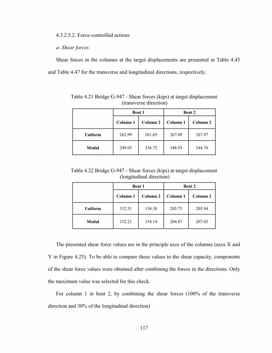
117


a- Shear forces:

Shear forces in the columns at the target displacements are presented in Table 4.45

and Table 4.47 for the transverse and longitudinal directions, respectively.

Table 4.21 Bridge G-947 - Shear forces (kips) at target displacement (transverse direction)

Bent 1 Bent 2


Uniform 262.99 261.65 267.09 267.97

Modal 249.05 236.75 348.93 344.76

Table 4.22 Bridge G-947 - Shear forces (kips) at target displacement (longitudinal direction)

Bent 1 Bent 2


Uniform 152.51 154.38 205.73 205.94

Modal 152.21 154.14 204.87 207.63

The presented shear force values are in the principle axes of the columns (axes X and

Y in Figure 4.25). To be able to compare these values to the shear capacity, components

of the shear force values were obtained after combining the forces in the directions. Only

the maximum value was selected for this check.

For column 1 in bent 2, by combining the shear forces (100% of the transverse

direction and 30% of the longitudinal direction)

118

9334893348100 .).(% =× kips in the Y-axis direction

and 46618720430 ..% =× kips in the X-axis direction

923323046613093348 .)(Sin.)(Cos. =×+× oo kips 37426.< kips (from Table 4.14)

Therefore, all bridge columns are safe against brittle shear failure at the MCE level.


The bending moment values at the column sections that had inadequate reinforcement

development or splice lengths were observed at the target displacement. These values are


Table 4.23 Bridge G-947 - Bending moment values (kip-ft) at target displacement at the B/C joint locations of the columns

Bent 1 Bent 2


Transverse - (Uniform) 6088.53 5823.72 5766.30 5713.67

Transverse - (Modal) 5687.23 5314.21 7599.87 7247.68

Longitudinal - (Uniform) 3451.71 3496.43 4423.77 4425.77

Longitudinal - (Modal) 3443.49 3491.73 4406.13 4461.61

From the results presented in Table 4.23, the bending moment values at the B/C joint

locations in all columns at the target displacement exceeded the values obtained from the

sectional analysis (in Table 4.16). Accordingly, new models were developed with the

nonlinear definitions of the new plastic hinges that represent the inadequate development

lengths. These hinges replaced the other hinges as they are in the same location. The

119

bridge was pushed to the same values of the target displacement in both directions and

the resulting plastic hinge rotation values are presented in Table 4.24 and Table 4.25.

Table 4.24 Bridge G-947 - Plastic hinge rotations (radians) at target displacements in the transverse direction

Bent 1 Bent 2


Uniform 0.00773 0.00832 0.00125 0.00164

Modal 0.00175 0.00233 0.00752 0.00772

Table 4.25 Bridge G-947 - Plastic hinge rotations (radians) at target displacements in the longitudinal direction

Bent 1 Bent 2


Uniform 0.00848 0.00865 0.00908 0.00932

Modal 0.00847 0.00865 0.00905 0.00932

The underlined values of the plastic hinge rotations violated the acceptance criteria of

the IO level. Some of the values are very near to the CP level. Accordingly, the design of

this bridge is governed by the inadequate development lengths of columns longitudinal

reinforcement into the cap beams, and the bridge is at risk of bond slippage at this

location under the MCE level.

120

4.3.3. Bridge (H-1211)


H-1211 is a 2-spans/1-pier bridge located at the intersection of Washington Avenue

(overpass) and the U.S. 95-highway (underpass). The total length of the bridge is 250 ft,

divided into two unequal spans of 130 ft and 120 ft as a west side span and an east side

span, respectively. The plan and elevation of the bridge are shown in Figure 4.31.

Figure 4.31 Bridge H-1211 - Plan and elevation

121

The superstructure of the bridge is a cast-in-place box girder concrete deck, with three

intermediate webs. Figure 4.32 shows the bridge deck section along with the pier column.

The total width of the deck is 40 ft and its total depth is 5 ft. These dimensions are

constant over the bridge length.

Figure 4.32 Bridge H-1211 - Bridge section

The substructure of the bridge consists of a single column pier. The column section is

variable along its height from 12 ft width at the foundation level to 20 ft at the deck

soffit. The two sections of the column (the upper and the lower parts of the column) are

shown in Figure 4.33 (a) and (b). All the longitudinal reinforcement bars in the column

are #11, and all the transverse reinforcement bars are #4. At the end spans (at both

abutments), the bridge deck ends with an end diaphragm. Each of the two diaphragms

rests on a foundation along its length, with a neoprene pad in between to allow for the

expansion of the bridge deck in the longitudinal direction. Figure 4.34 (a) and (b) shows

122

the details of the end diaphragm and its footing. The concrete compressive strength for

this bridge is 3.5 ksi and the reinforcement yield strength is 60 ksi.

(a)

(b)

Figure 4.33 Bridge H-1211 - Column sections at (a) top section and (b) bottom section of the column

123

(a)

(b)

Figure 4.34 Bridge H-1211 - (a) End diaphragm section and (b) abutment footing section


Figure 4.35 shows the structural model used for the evaluation of the bridge in both

transverse and longitudinal directions. The control node in the analysis was chosen to be

the deck node at the location of the pier.

Figure 4.35 Bridge H-1211 - Structural model for both transverse and longitudinal

direction

Control node

124


The superstructure of the bridge was modeled with five (equal in length) elements in

the west span (the longer span) and four elements in the east span of the bridge. The cross

sectional area of the bridge deck is 61.13 ft2, the moment of inertia about the Y-axis is

217.13 ft4 and about the Z-axis is 7192.73 ft4. An additional dead load with a value of

2.864 kip/ft was added to account for the wearing surfaces, the concrete barriers, and the

pedestrian rails. An additional load of 1.25 kip/ft was added to account for the live load

from two traffic lanes.


The variable pier column was modeled as five different sections gradually varying

with its length from 12 ft at the bottom section to 20 ft at the top one. Figure 4.36 shows

the variable sections used in the model.

Figure 4.36 Bridge H-1211 - Column sections as modeled in SAP2000 and their labels

1

2

3

4

5

125

4.3.3.2.3. Effective moment of inertia for pier column

In order to estimate the stiffness reduction in the column, each section (out of the five

sections used in the model) was analyzed to calculate its effective moment of inertia in

both directions. φ−M curves for the five sections in their strong and week axes are

presented in Figure 4.37 and Figure 4.38, respectively. Parameters obtained from these

figures are used in the calculations of eI for each column section.

Table 4.26 and Table 4.27 present these parameters in addition to the final percentage

used in the analysis for the strong and weak axis of the column sections, respectively.

Calculations in the two tables are following Eq. 4.1, and the concrete modulus of

elasticity used for this bridge ( cE ) is 485592 ksf.

126

0

5000

10000

15000

20000

25000

30000

0 0.0005 0.001 0.0015 0.002 0.0025 0.003 0.0035 0.004

Curvature (rad/ft)

Mom

ent (

Kip

.ft)

Original

Idealized

column section-1

0

5000

10000

15000

20000

25000

30000

35000

40000

0 0.001 0.002 0.003 0.004

Curvature (rad/ft)

Mom

ent (

Kip

.ft)

Original

Idealized

column section-2

0

5000

10000

15000

20000

25000

30000

35000

40000

45000

50000

0 0.0005 0.001 0.0015 0.002 0.0025 0.003 0.0035

Curvature (rad/ft)

Mom

ent (

Kip

.ft)

Original

Idealized

column section-3

0

10000

20000

30000

40000

50000

60000

0 0.0005 0.001 0.0015 0.002 0.0025 0.003 0.0035

Curvature (rad/ft)

Mom

ent (

Kip

.ft)

Original

Idealized

column section-4

0

10000

20000

30000

40000

50000

60000

70000

0 0.0005 0.001 0.0015 0.002 0.0025 0.003 0.0035

Curvature (rad/ft)

Mom

ent (

Kip

.ft)

Original

Idealized

column section-5

Figure 4.37 Bridge H-1211 - φ−M curves in the strong axis for the five column sections along the pier height

127

0

2000

4000

6000

8000

10000

12000

0 0.002 0.004 0.006 0.008 0.01 0.012 0.014

Curvature (rad/ft)

Mom

ent (

Kip

.ft)

Original

Idealized

column section-1

0

2000

4000

6000

8000

10000

12000

0 0.002 0.004 0.006 0.008 0.01 0.012 0.014Curvature (rad/ft)

Mom

ent (

Kip

.ft)

Original

Idealized

column section-2

0

2000

4000

6000

8000

10000

12000

14000

0 0.002 0.004 0.006 0.008 0.01 0.012 0.014 0.016

Curvature (rad/ft)

Mom

ent (

Kip

.ft)

Original

Idealized

column section-3

0

2000

4000

6000

8000

10000

12000

14000

16000

0 0.002 0.004 0.006 0.008 0.01 0.012 0.014 0.016Curvature (rad/ft)

Mom

ent (

Kip

.ft)

Original

Idealized

column section-4

0

2000

4000

6000

8000

10000

12000

14000

16000

0 0.002 0.004 0.006 0.008 0.01 0.012 0.014 0.016Curvature (rad/ft)

Mom

ent (

Kip

.ft)

Original

Idealized

column section-5

Figure 4.38 Bridge H-1211 - φ−M curves in the weak axis for the five column sections along the pier height

128

Table 4.26 Bridge H-1211- Calculation of effective moment of inertia for column sections in the strong axis

Column section Ig (ft4) Mn (kip-ft) Φy (rad/ft) Ie (ft4) Ie/ Ig

1 365.64 26000 0.000325 164.75 0.45

2 623.14 34000 0.000325 215.43 0.35

3 967.26 41500 0.000250 341.85 0.35

4 1422.55 54000 0.000227 489.89 0.35

5 2004.99 63000 0.000185 701.29 0.35

Table 4.27 Bridge H-1211- Calculation of effective moment of inertia for column sections in the weak axis

Column section Ig (ft4) Mn (kip-ft) Φy (rad/ft) Ie (ft4) Ie/ Ig

1 41.30 10100 0.00110 18.91 0.45

2 52.42 10500 0.00092 23.63 0.45

3 63.08 11000 0.00102 22.20 0.35

4 73.75 13450 0.00108 25.65 0.35

5 84.42 13800 0.00109 26.07 0.30




129

0.000

0.100

0.200

0.300

0.400

0.500

0.600

0.700

0.000 0.500 1.000 1.500 2.000 2.500 3.000 3.500 4.000

T (sec)

Sa (g

)

Figure 4.39 Bridge H-1211- 5% damped response spectrum for BSE-2



The applied loads on the column, from which the acceptance criteria are calculated,

are presented in Table 4.28. Calculations in this table are done for the lower section

(section 1) as the potential plastic hinge location is at the lower part of the column.

Table 4.28 Bridge H-1211 - Applied loads on bridge column for load-deformation calculations

Axial Load (P) 2235 kips

Shear Force (V) 0.00 kips

'cg fA

P 0.113

'cw fdb

V 0.00

130

The generalized load-deformation relation for each bridge is estimated based on the

values calculated in Table 4.28, and the acceptance criteria are presented in Table 4.29.

Table 4.29 Bridge H-1211 - Acceptance criteria for the lower column section of the bridge

Performance level Column section 1

IO 0.00491

LS 0.01487

CP 0.01978


a- Shear capacity:

Shear capacity of the column was calculated at its lower section. This section is the

smallest section in its dimensions, which makes it the most critical along the column’s

height. Based on Eq. 4.2, Eq. 4.3, and Eq. 4.4, calculations of the column’s shear capacity

in the two directions are presented in Table 4.30.

131

Table 4.30 Bridge H-1211 - Shear capacity calculations for bridge columns

Transverse direction Longitudinal direction

Applied axial load - Nu (kips) 2235 2235

Column depth - d (in) 141 36.25

Column width - b (in) 39.25 144

Gross sectional area - Ag (in2) 5652 5652

Vc (kips) 784.291 739.756

Area of trans. reinf. - Av (in2) 0.2 x 2 = 0.4 0.2 x 7 = 1.4

Spacing of trans. reinf. - s (in) 4 4

Vs (kips) 846.000 761.250

Total shear capacity - Vn (kips) 1630.291 1501.006


The bridge column has no splices along its height, and is properly hooked to the

foundation. However, at the location of the beam-column joint, the development length

provided for the longitudinal reinforcement bars is 5 ft.

Based on Eq. 4.5 and Eq. 4.6;

For #11 rebars,

Development length 96.5=dl ft, which means that the provided development length is

insufficient and Eq. 4.6 should be used to estimate the maximum stress that can be

developed in the rebar as follows:

336.506096.50.5

=⎟⎠⎞

⎜⎝⎛=⎟⎟

⎠

⎞⎜⎜⎝

⎛= y

d

bs f

ll

f ksi

Sectional analysis for the top section of the column was performed using the new

value ( sf ) instead of yf for the reinforcement and the resulting φ−M relationships are

presented in Figure 4.40 for both the strong and the weak axes of the column. The strong

132

axis is used for the transverse direction and the weak axis is used for the longitudinal

direction.

0

10000

20000

30000

40000

50000

60000

70000

0 0.0005 0.001 0.0015 0.002 0.0025 0.003 0.0035

Curvature (rad/ft)

Mom

ent (

Kip

.ft)

Original

Idealized

(a)

0

2000

4000

6000

8000

10000

12000

14000

0 0.004 0.008 0.012 0.016 0.02

Curvature (rad/ft)

Mom

ent (

Kip

.ft)

Original

Idealized

(b)

Figure 4.40 Bridge H-1211- φ−M curves at the location of the B/C joint for (a)the strong axis and (b)the weak axis of the column top section

Figure 4.40 shows that the maximum moment that can be reached at the top column

section is 57,000 kip-ft in the transverse direction and 12,300 kip-ft in the longitudinal

direction.


Evaluation of this bridge was performed using only the uniform load pattern. The

reason for choosing only one pattern is having only one column is the bridge, and the

control node is above this column. In this case using different patterns will be of

insignificant value.

The fundamental modes in the transverse and longitudinal directions were mode-4

and mode-1, respectively. The two modes are illustrated in Figure 4.41 (a) and (b). The

time period for mode-4 was 0.276 sec, while the time period for mode-1 was 0.692 sec.

Figure 4.42 shows the pushover curves for both the transverse and the longitudinal

133

directions. From the pushover curves, parameters used in calculating the target

displacement are presented in Table 4.31 along with its final values.

Table 4.31 Bridge H-1211 - Target displacement calculations for both directions

Direction Te (sec) Sa (g) PF φ CN (ft) C0 C1*

tδ (ft)

Transverse 0.276 0.649 9.723 0.120 1.165 0.901 0.0423

Longitudinal 0.692 0.409 12.821 0.084 1.076 1.0 0.1718

*Values of C2 and C3 are equal to 1.0

The pushover curves in the two directions show that ie KK = . Accordingly, the

effective time period equals the fundamental time period for the analysis in both

directions ( ie TT = ). In addition to that, the value of 1C in the transverse direction is

calculated based on Eq. 3.8 as se TT < . However, in the longitudinal direction, 0.11 =C

as se TT > .

From the pushover curves, in the transverse direction:

1470=yV kips and the effective weight of the bridge 2235=W kips

847.0165.11

2235/1470649.0

=×=R

[ ] [ ] 901.0847.0/276.0/427.0)1847.0(0.1//)1(0.11 =−+=−+= RTTRC es

134

(a)

(b)

Figure 4.41 Bridge H-1211 - (a) Mode-4, the fundamental mode in the transverse direction and (b) Mode-1, the fundamental mode in the

longitudinal direction

135

0

400

800

1200

1600

2000

0 0.02 0.04 0.06 0.08 0.1 0.12

Displacement (ft)

Bas

e sh

ear (

Kip

s)IdealizedOriginal

(a)

0

400

800

1200

1600

2000

0 0.04 0.08 0.12 0.16 0.2 0.24 0.28

Displacement (ft)

Bas

e sh

ear (

Kip

s)

Idealized

Original

(b)

Figure 4.42 Bridge H-1211 - Pushover curves in (a) the transverse direction and (b) the longitudinal direction

4.3.3.5. Results


Plastic hinge rotations formed at the target displacements in both directions are

presented in Table 4.32. It shows that the column did not encounter any plastic hinge

136

rotation in the transverse direction. However, in the longitudinal direction, a plastic hinge

was formed with rotation value 0.00417 radians. When compared to the value presented

in Table 4.29, the plastic hinge rotation did not violate the acceptance criteria of the IO

performance level.

Table 4.32 Bridge H-1211 - Plastic hinge rotation values (radians) at target displacement in both directions

Transverse Longitudinal

Plastic hinge rotation 0.00000 0.00417


a- Shear forces:

Shear forces in the bridge column at the target displacement for both transverse and

longitudinal directions are presented in Table 4.33.

Table 4.33 Bridge H-1211 - Shear force values (kips) in the bridge column at target displacement

Direction Transverse Longitudinal

Shear Force (kips) 1146.23 1280.83

The two values of the shear forces are lower than the shear capacity of the column

section presented in Table 4.30. Thus, the bridge column is safe against shear failure

under the MCE level.

137


At the target displacement in the transverse direction the bending moment value at the

column’s top section is near zero (i.e. did not reach 57,000 kip-ft). However, in the

longitudinal direction, the moment at the column’s top section was 14,872.89 kip-ft

(which exceeded 12,300 kip-ft). Accordingly, another model was analyzed; including the

definition of the plastic hinge at the column’s top section with its reinforcement

maximum stress equals 336.50=sf ksi. The bridge was pushed to the same target

displacement and the top hinge rotation value was 0.00229 radians. From Table 4.2, the

acceptance value is 0.005 radians. Accordingly, the plastic hinge rotation in this direction

did not violate the acceptance criteria and the bridge is not at risk of reinforcement bond

slippage under the MCE level.

138

4.3.4. Bridge (G-953)


G-953 is a 6-spans/5-bents bridge located at the intersection of Carey Avenue

(overpass) and I-15 highway (underpass). The total length of the bridge is 492.1 ft,

measured along the centerline of Carey Avenue. The profile of this bridge is curved in the

horizontal and the vertical directions. This profile makes the evaluation of the bridge in

the transverse direction different than the other bridges in this study as it should be

pushed in the two opposite directions transversely. As shown in the Figure 4.43, the

bridge includes 4 expansion joints. The substructure elements of the bridge are skewed

bents at angles ranging from 38.47 degrees with the line perpendicular to Carey Avenue’s

centerline at the west side to 30.73 degrees at the east side of the bridge. The

superstructure of the bridge is a cast-in-place box girder concrete deck, with 8

intermediate webs. Figure 4.44 (a) to (c) shows the bridge deck sections along with the

different bents of the bridge. The total width of the bridge deck is 75.17 ft. The total

depth of the bridge deck is 4 ft in the first three spans, 5 ft in the last two spans and varies

linearly from 4 ft to 5 ft in span 4. The substructure of the bridge consists of five bents

with variations in their structural systems. Bent 1 contains fixed base columns to the

foundations and fixed to the cap beam. Bents 2 to 5 are frames with hinged base columns

to the foundations and fixed to the cap beams. Each of the bridge bents is symmetric

around its vertical centerline. Accordingly, all bents have two typical external columns

and two typical internal columns. The concrete compressive strength for this bridge is 5

ksi and 3 ksi for the substructure and the superstructure components, respectively. And

the reinforcement yield strength is 60 ksi.

139

Figure 4.43 Bridge G-953 - Plan and elevation

Bent

1

Bent

2

Bent

3

Bent

4

Bent

5

140

(a)

(b)

(c)

Figure 4.44 Bridge G-953 - Deck section at (a) bent 1; (b) bents 2 and 3; and (c) bents 4 and 5


Figure 4.45 shows the structural model used for the analysis of the bridge in the

transverse direction, and Figure 4.46 (a) to (c) shows the structural models used for the

141

analyses of the bridge in the longitudinal direction. The units are separated at the

locations of the expansion joints.

Figure 4.45 Bridge G-953 - Structural model for transverse direction analysis

(a)

(b)

(c)

Figure 4.46 Bridge G-953 - Structural models for longitudinal direction

(a) unit-1; (b) unit-2; and (c) unit-3.

Control node

Fixed base

Hinged bases

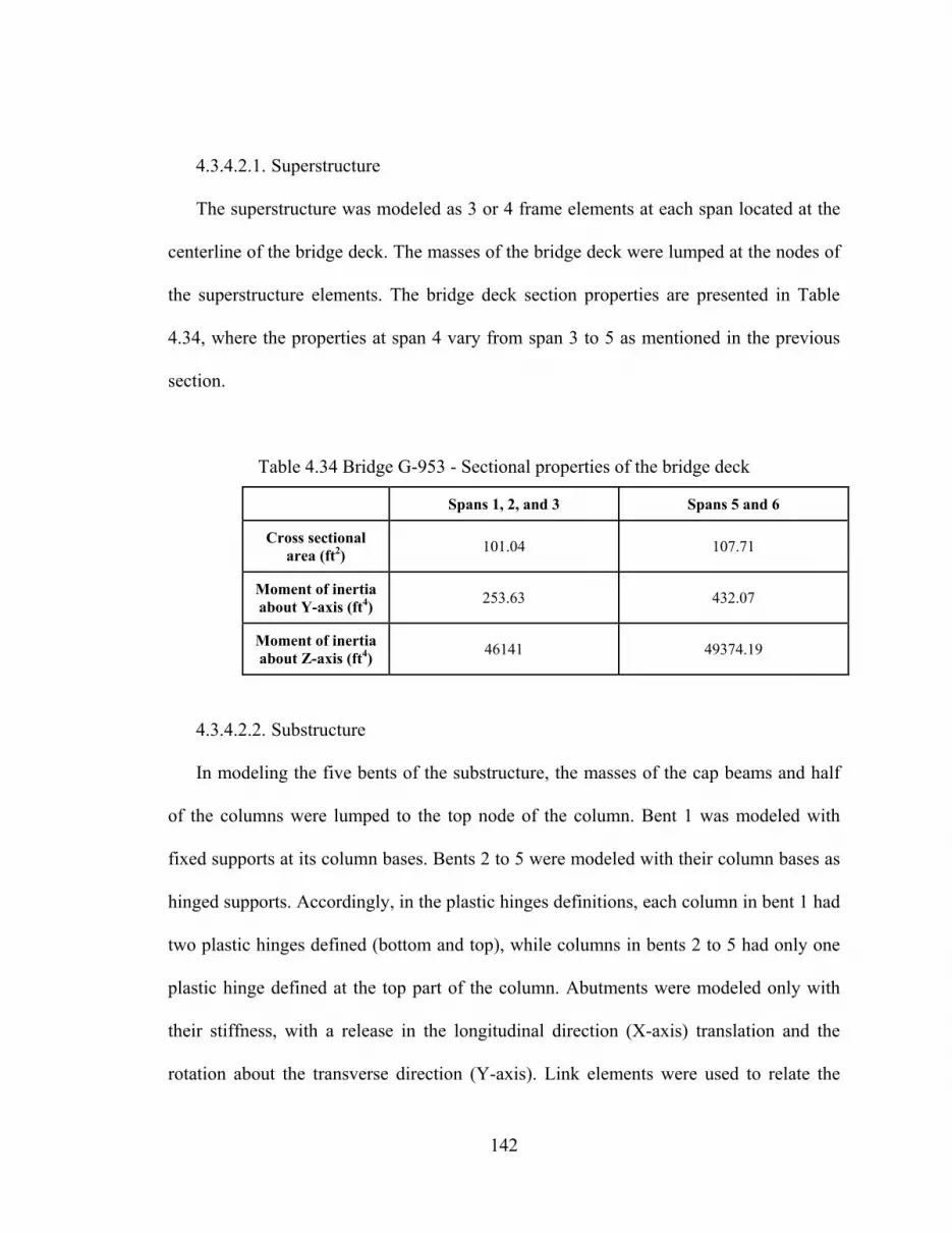
142


The superstructure was modeled as 3 or 4 frame elements at each span located at the

centerline of the bridge deck. The masses of the bridge deck were lumped at the nodes of

the superstructure elements. The bridge deck section properties are presented in Table

4.34, where the properties at span 4 vary from span 3 to 5 as mentioned in the previous

section.

Table 4.34 Bridge G-953 - Sectional properties of the bridge deck

Spans 1, 2, and 3 Spans 5 and 6

Cross sectional area (ft2) 101.04 107.71

Moment of inertia about Y-axis (ft4) 253.63 432.07

Moment of inertia about Z-axis (ft4) 46141 49374.19


In modeling the five bents of the substructure, the masses of the cap beams and half

of the columns were lumped to the top node of the column. Bent 1 was modeled with

fixed supports at its column bases. Bents 2 to 5 were modeled with their column bases as

hinged supports. Accordingly, in the plastic hinges definitions, each column in bent 1 had

two plastic hinges defined (bottom and top), while columns in bents 2 to 5 had only one

plastic hinge defined at the top part of the column. Abutments were modeled only with

their stiffness, with a release in the longitudinal direction (X-axis) translation and the

rotation about the transverse direction (Y-axis). Link elements were used to relate the

143

superstructure to the cap beams. These link elements translate all degrees of freedom as

the cap beam is integrated in the deck at all bents.


Each of the bridge bents had different column sections defined. Bent 1 had four

column sections, two for the external columns and two for the internal columns. Bents 2

and 3 had the same column section definitions (one for the external and one for the

internal column of the bent), and bents 4 and 5 had the same column section definitions

(also one for the external and one for the internal column of the bent). All columns in the

bridge are circular columns with equally distributed reinforcement within the sections.

Table 4.35 presents the columns diameter and reinforcement (longitudinal and transverse)

for each bent.

Table 4.35 Bridge G-953 - Column sections definition in the bridge bents

Bent 1 Bent 2 and 3 Bent 4 and 5

External column Internal column

Lower Upper Lower Upper

External column

Internal column

External column

Internal column

Column diameter (ft) 3.67 3.67 3.67 3.67 3.50 3.50 3.50 3.50

Longitudinal Reinforcement*

24 x 2 #11 12 #11 21 x

2 #11 21 #8 11 #10 12 #11 18 #11 20 #11

Transverse Reinforcement #5 @12 inches

* The 2 #11 are bundled bars, used in the lower part of the external and internal column of bent 1.

φ−M curves for the column sections are presented in Figure 4.47 and Figure 4.48.

And the parameters used in the calculations of the effective moment of inertia of the

columns with its final values are presented in Table 4.36.

144

0

1000

2000

3000

4000

5000

6000

7000

0 0.002 0.004 0.006 0.008 0.01 0.012 0.014

Curvature (rad/ft)

Mom

ent (

Kip

.ft)

Original

Idealized

(a)

0

500

1000

1500

2000

2500

0 0.002 0.004 0.006 0.008 0.01 0.012 0.014

Curvature (rad/m)

Mom

ent (

KN

.m)

Original

Idealized

(b)

0

1000

2000

3000

4000

5000

6000

0 0.002 0.004 0.006 0.008 0.01 0.012 0.014

Curvature (rad/ft)

Mom

ent (

Kip

.ft)

Original

Idealized

(c)

0

500

1000

1500

2000

2500

0 0.002 0.004 0.006 0.008 0.01 0.012

Curvature (rad/ft)

Mom

ent (

Kip

.ft)

Original

Idealized

(d)

Figure 4.47 Bridge G-953 - φ−M curves for bent 1 column sections at (a) external lower column; (b) external upper column; (c) internal lower column; and (d) internal

upper column

145

0

400

800

1200

1600

2000

0 0.002 0.004 0.006 0.008 0.01 0.012

Curvature (rad/ft)

Mom

ent (

Kip

.ft)

Original

Idealized

(a)

0

500

1000

1500

2000

2500

0 0.002 0.004 0.006 0.008 0.01 0.012

Curvature (rad/ft)

Mom

ent (

Kip

.ft)

Original

Idealized

(b)

0

500

1000

1500

2000

2500

3000

0 0.002 0.004 0.006 0.008 0.01

Curvature (rad/ft)

Mom

ent (

Kip

.ft)

Original

Idealized

(c)

0

500

1000

1500

2000

2500

3000

3500

0 0.002 0.004 0.006 0.008 0.01 0.012

Curvature (rad/ft)

Mom

ent (

Kip

.ft)

Original

Idealized

(d)

Figure 4.48 Bridge G-953 - φ−M curves for column sections at (a) bents 2 and 3 external column; (b) bents 2 and 3 internal column; (c) bents 4 and 5 external column;

and (d) bents 4 and 5 internal column

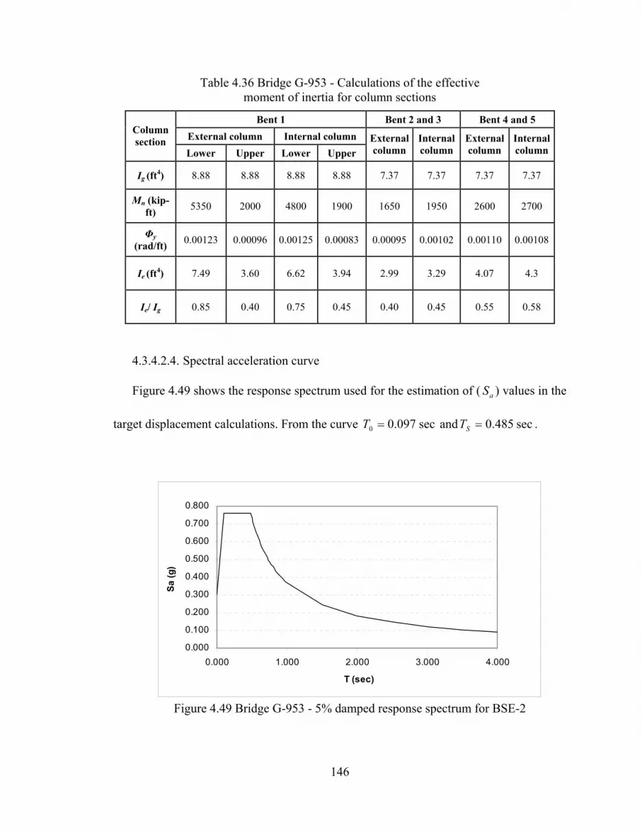
146

Table 4.36 Bridge G-953 - Calculations of the effective moment of inertia for column sections

Bent 1 Bent 2 and 3 Bent 4 and 5 External column Internal column Column

section Lower Upper Lower Upper

External column

Internal column

External column

Internal column

Ig (ft4) 8.88 8.88 8.88 8.88 7.37 7.37 7.37 7.37

Mn (kip-ft) 5350 2000 4800 1900 1650 1950 2600 2700

Φy (rad/ft) 0.00123 0.00096 0.00125 0.00083 0.00095 0.00102 0.00110 0.00108

Ie (ft4) 7.49 3.60 6.62 3.94 2.99 3.29 4.07 4.3

Ie/ Ig 0.85 0.40 0.75 0.45 0.40 0.45 0.55 0.58




0.000

0.100

0.200

0.300

0.400

0.500

0.600

0.700

0.800

0.000 1.000 2.000 3.000 4.000

T (sec)

Sa (g

)

Figure 4.49 Bridge G-953 - 5% damped response spectrum for BSE-2

147



The axial loads applied on each of the bridge columns are presented in Table 4.37.

The shear forces values are negligible, which makes the values of ( )'/ cw fdbV for all

columns less than 3. From the results in Table 4.37, all values of ( )'/ cg fAP for different

column sections are less than 0.1. Accordingly, plastic hinge rotation values used for the

acceptance criteria will be 0.005 radians for the IO, 0.015 radians for the LS, and 0.02

radians for the CP level (same as the values in Figure 4.10).

Table 4.37 Bridge G-953 - Applied loads on bridge columns for load-deformation calculations

Bent 1 Bent 2 and 3 Bent 4 and 5

External column

Internal column

External column

Internal column

External column

Internal column

P (lbs) 400000 480000 485410 566883 637026 595451

'cg fA 7602654 7602654 6927212 6927212 6927212 6927212

'cg fA

P 0.0526 0.0631 0.0701 0.0818 0.0920 0.0860


a- Shear capacity:

Based on Eq. 4.2, Eq. 4.3, and Eq. 4.4, shear capacities for each of the bridge

columns were calculated. Table 4.38 presents the shear capacity calculations for each

column section.

148

Table 4.38 Bridge G-953 - Shear capacity calculations for bridge columns

Bent 1 Bent 2 and 3 Bent 4 and 5 External

column Internal column

External column

Internal column

External column

Internal column

Applied axial load - Nu (kips) 400000 480000 485410 566883 637026 595451

Column diameter - d (in) 44 44 42 42 42 42

Gross sectional area - Ag (in2) 1520.53 1520.53 1385.44 1385.44 1385.44 1385.44

Vc (kips) 247.844 253.606 234.536 240.404 245.456 242.461

Area of trans. reinf. - Av (in2)

0.31x2 =0.62

0.62 0.62 0.62 0.62 0.62

Spacing of trans. reinf. - s (in) 12 12 12 12 12 12

Vs (kips) 109.120 109.120 104.160 104.160 104.160 104.160

Total shear capacity - Vn

(kips) 356.964 362.726 338.696 344.564 349.616 346.621


Two locations of reinforcement development were identified in the bridge. The first

location is at the B/C joints of all bridge columns, and the second location is at the splices

in bent 1 columns. These splices connect the dowels from the foundations to the upper

column longitudinal reinforcement.

149

Table 4.39 Bridge G-953 - Calculation of maximum stresses that can be developed in the reinforcement bars (B/C joint)

Bent 1 Bent 2 and 3 Bent 4 and 5 Column External


External column

Internal column

External column

Internal column


4.0 4.0 4.0 4.0 5.0 5.0


4.98 3.53 4.49 4.98 4.98 4.98

fs (ksi) 48.198 60.00 53.452 48.193 60.00 60.00

Table 4.40 Bridge G-953 - Calculation of maximum stresses that can be developed in the reinforcement bars at bent 1 (splices location)

Bent 1 Column External



3.58 2.5


4.98 3.53

fs (ksi) 43.169 42.493

From Table 4.39, three columns had inadequate development lengths of longitudinal

reinforcement at the B/C joint location. On the other hand, from Table 4.40, two locations

(in bent 1 columns) had inadequate splice length. Accordingly, the maximum stresses that

can be developed in the rebars for the two cases were calculated (in the same tables) and

sectional analyses were performed using the new values of fs. The φ−M curves

resulting from the sectional analyses are presented in Figure 4.50 and Figure 4.51.

150

0

300

600

900

1200

1500

1800

2100

0 0.002 0.004 0.006 0.008 0.01 0.012 0.014

Curvature (rad/m)

Mom

ent (

KN

.m)

Original

Idealized

(a)

0

200

400

600

800

1000

1200

1400

1600

1800

0 0.002 0.004 0.006 0.008 0.01 0.012

Curvature (rad/ft)

Mom

ent (

Kip

.ft)

Original

Idealized

(b)

0

300

600

900

1200

1500

1800

2100

0 0.002 0.004 0.006 0.008 0.01 0.012

Curvature (rad/ft)

Mom

ent (

Kip

.ft)

Original

Idealized

(c)

Figure 4.50 Bridge G-953 - φ−M curves for sections with inadequate reinforcement development at B/C joints (a) at bent 1-external columns; (b) at bents 2 and 3 -

external columns; and (c) at bents 2 and 3 - internal columns

151

0

300

600

900

1200

1500

1800

2100

0 0.002 0.004 0.006 0.008 0.01 0.012 0.014 0.016

Curvature (rad/m)

Mom

ent (

KN

.m)

Original

Idealized

(a)

0

300

600

900

1200

1500

1800

2100

0 0.002 0.004 0.006 0.008 0.01 0.012Curvature (rad/ft)

Mom

ent (

Kip

.ft)

Original

Idealized

(b)

Figure 4.51 Bridge G-953 - φ−M curves for sections with inadequate reinforcement splices in bent 1 (a) at the external columns and (b) at the internal columns

The maximum bending moment values that can be developed corresponding to the

maximum stresses calculated for each section are presented in Table 4.41.

Table 4.41 Bridge G-953 - Maximum moment that can be developed in column sections at B/C joint and splices location without plastic hinge formation

Section location B/C joint Splices

Bent 1 Bent 2 and 3 Bent 1 Column External

column External column

Internal column

External column

Internal column

Mn (kip-ft) 1750 1550 1750 1600 1620



Due to the asymmetry profile of the bridge (being curved in the horizontal direction),

the evaluation of the bridge transversely was done in the two directions, the north and the

south direction of the bridge. The fundamental mode in the transverse direction is shown

152

in Figure 4.52. Its fundamental time period was 0.630 sec. The pushover curves for the

transverse direction in the north and south directions are shown in Figure 4.53 (a) to (d).


in the transverse direction

Based on the values obtained from the modal analysis and the pushover curves, the

target displacement was calculated, and is presented in Table 4.42 along with the

parameters used in its calculations. The values of all parameters obtained from the north

and south direction analyses are quite similar. This is due to the fact that the curvature of

the bridge in the horizontal direction is not of a significant value. Accordingly, the values

of the target displacements in both directions are exactly the same.

153

0

500

1000

1500

2000

0 0.1 0.2 0.3 0.4 0.5

Displacement (ft)

Bas

e sh

ear (

Kip

s)

Idealized

Original

(a)

0

500

1000

1500

2000

0 0.1 0.2 0.3 0.4 0.5

Displacement (ft)

Bas

e sh

ear (

Kip

s)

Idealized

Original

(b)

0

500

1000

1500

2000

0 0.1 0.2 0.3 0.4 0.5

Displacement (ft)

Bas

e sh

ear (

Kip

s)

Idealized

Original

(c)

0

500

1000

1500

2000

0 0.1 0.2 0.3 0.4 0.5

Displacement (ft)

Bas

e sh

ear (

Kip

s)

Idealized

Original

(d) Figure 4.53 Bridge G-953 - Pushover curves in the transverse direction using

(a) uniform load pattern pushed in the north direction; (b) uniform load pattern pushed in the south direction; (c) modal pattern pushed in the north direction; and (d) modal

pattern pushed in the south direction,

Table 4.42 Bridge G-953 - Target displacement calculations in the transverse direction

Load Pattern Ti (sec) Ki Ke Te (sec) Sa (g) PF φ CN (ft) C0* tδ (ft)

Uniform (North) 0.630 4790 4790 0.630 0.583 16.88 0.0768 1.295 0.244

Uniform (South) 0.630 4700 4700 0.630 0.583 16.88 0.0768 1.295 0.244

Modal (North) 0.630 4380 4380 0.630 0.583 16.88 0.0768 1.295 0.244

Modal (South) 0.630 4300 4300 0.630 0.583 16.88 0.0768 1.295 0.244


154


Figure 4.54 (a) to (c) illustrate the fundamental mode shapes of the three units in the

longitudinal direction. The fundamental time periods for unit 1, unit 2 and unit3 are

0.775, 2.094, and 1.262 sec, respectively. The pushover curves for this direction using the

two patterns are illustrated in Figure 4.55 (a) to (f). Parameters used in calculating the

target displacement for each of the three units along with its final values, for both

patterns, are presented in Table 4.43.

Table 4.43 Bridge G-953 - Target displacement calculations in the longitudinal direction

Unit # - Load Pattern Ti (sec) Ki Ke Te (sec) Sa (g) PF φ CN

(ft) C0* tδ (ft)

Unit 1 - Uniform 0.775 3866 3866 0.775 0.474 7.695 0.132 1.019 0.237

Unit 1 - Modal 0.775 3753 3753 0.775 0.474 7.695 0.132 1.019 0.237

Unit 2 - Uniform 2.094 1520 1520 2.094 0.176 12.96 0.0774 1.003 0.631

Unit 2 - Modal 2.094 1520 1520 2.094 0.176 12.96 0.0774 1.003 0.631

Unit 3 - Uniform 1.262 3288 2889 1.346 0.273 11.12 0.0903 1.004 0.405

Unit 3 - Modal 1.262 3322 2978 1.333 0.276 11.12 0.0903 1.004 0.402

*Values of C1, C2 and C3 are equal to 1.0 for all cases

155

(a)

(b)

(c)

Figure 4.54 Bridge G-953 -Fundamental mode shapes in the longitudinal direction of the bridge for (a) unit-1; (b) unit-2; and (c) unit-3

156

0

200

400

600

800

1000

1200

0 0.1 0.2 0.3 0.4Displacement (ft)

Base

she

ar (K

ips)

Idealized

Original

(a) Unit-1-Uniform load pattern

0

200

400

600

800

1000

1200


Bas

e sh

ear (

Kips

)

Idealized

Original

(b) Unit-1-Modal pattern

0

200

400

600

800

1000

0 0.2 0.4 0.6 0.8 1

Displacement (ft)

Base

she

ar (K

ips)

Idealized

Original

(c) Unit-2-Uniform load pattern

0

200

400

600

800

1000

0 0.2 0.4 0.6 0.8 1

Displacement (ft)

Base

she

ar (K

ips)

Idealized

Original

(d) Unit-2-Modal pattern

0

200

400

600

800

1000


Base

she

ar (K

ips)

Idealized

Original

(e) Unit-3-Uniform load pattern

0

200

400

600

800

1000

0 0.2 0.4 0.6 0.8

Displacement (ft)

Bas

e sh

ear (

Kip

s)

Idealized

Original

(f) Unit-3-Modal Patters

Figure 4.55 Bridge G-953 - Pushover curves for longitudinal direction analysis

157

4.3.4.5. Results


In the transverse direction, none of the plastic hinges were formed at the target

displacement in any of the considered directions (north and south) under any of the load

patterns. However, in the longitudinal direction some plastic hinges were formed at the

target displacement. The plastic hinge rotation values of the columns for the three units at

the target displacement are presented in Table 4.44.

Table 4.44 Bridge G-953 - Plastic hinge rotation values (radians) of bridge bents at target displacement in longitudinal direction

Bent no. 1 (Column top hinges) Column* 1 2 3 4 Uniform 0.00063 0.00080 0.00061 0.00000 Modal 0.00070 0.00084 0.00059 0.00000

Bent no. 1 (Column bottom hinges) Column* 1 2 3 4 Uniform

Uni

t 1


Bent no. 2 Column* 1 2 3 4 Uniform 0.00875 0.00817 0.00817 0.00878 Modal 0.00875 0.00817 0.00817 0.00878

Bent no. 3 Column* 1 2 3 4 Uniform 0.00819 0.00768 0.00770 0.00819

Uni

t 2

Modal 0.00819 0.00768 0.00770 0.00819 Bent no. 4 Column* 1 2 3 4 Uniform 0.00169 0.00101 0.00054 0.00000 Modal 0.00257 0.00209 0.00178 0.00139

Bent no. 5 Column* 1 2 3 4 Uniform 0.00668 0.00643 0.00614 0.00577

Uni

t 3

Modal 0.00527 0.00626 0.00719 0.00805 *Columns are named sequentially from south to north direction

158

Some of the plastic hinges, formed in the bent columns, violated the acceptance

criteria for the IO level. These plastic hinges are in bents 2, 3 and 5 and their values are

underlined in Table 4.44.


a- Shear forces:

Shear forces in the columns at the target displacements are presented in Table 4.45,

Table 4.46, and Table 4.47 for the transverse (north), the transverse (south), and the

longitudinal directions, respectively.

159

Table 4.45 Bridge G-953 - Shear forces (kips) in the columns at target displacement in the transverse direction (north)

Bent no. 1

Column* 1 2 3 4

Uniform 81.00 80.67 80.00 80.06

Modal 83.94 83.59 82.89 82.94

Bent no. 2

Column* 1 2 3 4

Uniform 31.58 35.62 35.08 30.88

Modal 33.07 37.24 36.61 32.17

Bent no. 3

Column* 1 2 3 4

Uniform 39.12 43.85 43.09 38.16

Modal 40.94 45.71 44.80 39.55

Bent no. 4

Column* 1 2 3 4

Uniform 56.56 61.32 60.86 56.02

Modal 56.04 60.62 60.08 55.23

Bent no. 5

Column* 1 2 3 4

Uniform 47.91 51.31 50.80 47.54

Modal 41.44 44.41 43.90 41.11

*Columns are named sequentially from south to north direction

160

Table 4.46 Bridge G-953 - Shear forces (kips) in the columns at target displacement in the transverse direction (south)

Bent no. 1

Column* 1 2 3 4

Uniform 79.02 79.14 79.40 79.87

Modal 81.93 82.07 82.32 82.81

Bent no. 2

Column* 1 2 3 4

Uniform 30.71 34.86 35.46 31.41

Modal 32.04 36.45 37.12 32.94

Bent no. 3

Column* 1 2 3 4

Uniform 37.79 42.68 43.40 38.74

Modal 39.14 44.35 45.22 40.53

Bent no. 4

Column* 1 2 3 4

Uniform 55.14 59.93 60.47 55.60

Modal 54.26 59.05 59.68 54.97

Bent no. 5

Column* 1 2 3 4

Uniform 46.52 49.66 50.18 46.83

Modal 40.10 42.78 43.29 40.38


161

Table 4.47 Bridge G-953 - Shear forces (kips) in the columns at target displacement in the longitudinal direction

Bent no. 1

Column* 1 2 3 4

Uniform 149.67 141.99 144.08 156.48 Uni

t 1

Modal 149.66 141.63 144.53 157.42

Bent no. 2

Column* 1 2 3 4

Uniform 48.25 58.84 59.11 48.04

Modal 48.26 58.84 59.11 48.06

Bent no. 3

Column* 1 2 3 4

Uniform 48.12 57.33 57.59 47.82

Uni

t 2

Modal 48.14 57.35 57.61 47.85

Bent no. 4

Column* 1 2 3 4

Uniform 59.62 67.92 69.76 66.32

Modal 39.26 44.25 44.83 42.23

Bent no. 5

Column* 1 2 3 4

Uniform 98.86 99.73 95.27 85.91

Uni

t 3

Modal 95.68 103.11 105.56 101.85


For column 4 in bent 1, by combining the shear forces (100% of the longitudinal

direction and 30% of the transverse direction)

48.15648.156%100 =× kips, and 02.2406.80%30 =× kips

31.158)02.24()48.156( 22 =+ kips 616.349<< kips (from Table 4.38)

Therefore, the bridge columns are safe against shear failure under the MCE level.

162


In the transverse direction, bending moment values at the column sections that had

inadequate reinforcement development or splice lengths were observed at the target

displacement. These values are presented in Table 4.48.

Table 4.48 Bridge G-953 - Maximum bending moment values (kip-ft) at target displacement at locations with inadequate

reinforcement development lengths

Section location B/C joint Splices

Bent 1 Bent 2 and 3 Bent 1 Column External

column External column

External column

External column

Internal column

Transverse - (Uniform-north) 895.90 1121.89 1121.89 432.01 187.31

Transverse - (Uniform-south) 884.13 1112.33 1112.33 425.21 183.12

Transverse - (Modal-north) 927.83 1167.34 1167.34 447.90 194.28

Transverse - (Modal-south) 916.03 1157.78 1157.78 441.15 190.07

By comparing the bending moment values in Table 4.48 to the bending moment

values presented in Table 4.41, none of the sections have exceeded the maximum value.

Accordingly, the design of the columns in this bridge, in the transverse direction is not

governed by the inadequate development lengths of the longitudinal reinforcement.

In the longitudinal direction, plastic hinge rotations were formed in unit 2 (bents 2

and 3) in the top part of the column. This indicates that the reduction in the maximum

stress, which will reduce the capacity of the plastic, will give higher values of plastic

hinge rotations. Accordingly, new models for unit 2 were developed with the values of fs

163

as presented in Table 4.39 for the bents’ external and internal columns. The new models

were pushed to the same target displacements using the uniform load and the modal

patterns. The resultant plastic hinge rotations are presented in Table 4.49.

Table 4.49 Bridge G-953 – Plastic hinge rotation values (radians) in the longitudinal direction at target displacement at B/C joints for unit 2

Bent no. 2 Column 1 2 3 4 Uniform 0.00930 0.00919 0.00928 0.00928 Modal 0.00930 0.00919 0.00913 0.00913

Bent no. 3 Column 1 2 3 4 Uniform 0.00871 0.00877 0.00879 0.00871 Modal 0.00871 0.00877 0.00879 0.00871

All plastic hinge rotation values presented in In the longitudinal direction, plastic

hinge rotations were formed in unit 2 (bents 2 and 3) in the top part of the column. This

indicates that the reduction in the maximum stress, which will reduce the capacity of the

plastic, will give higher values of plastic hinge rotations. Accordingly, new models for

unit 2 were developed with the values of fs as presented in Table 4.39 for the bents’

external and internal columns. The new models were pushed to the same target

displacements using the uniform load and the modal patterns. The resultant plastic hinge

rotations are presented in Table 4.49.

Table 4.49 for the columns of bents 2 and 3 violated the acceptance criteria of IO

(which is 0.005 radians). Following the same steps, a new model for unit 1 was

developed with (1) an additional definition of plastic hinges at the reinforcement splice

locations and (2) a change in the plastic hinge definition of the external column at the

B/C joints. These plastic hinges are defined based on the fs values presented in Table 4.40

164

for the splice locations and Table 4.39 for B/C joints locations. Unit 1 was pushed in the

new model to the target displacement and the resultant plastic rotations at different

locations are presented in Table 4.50.

Table 4.50 Bridge G-953 – Plastic hinge rotation values (radians) in the longitudinal direction at target displacement for unit 1 (bent 1)

Splice locations Column 1 2 3 4 Uniform Modal

No Plastic hinge rotation formed

B/C joint locations Column 1 2 3 4 Uniform 0.00146 0.00111 0.00089 0.00083 Modal 0.00220 0.00172 0.00234 0.00271

From the results presented in Table 4.50, at the target displacement, none of the

columns in bent 1 experienced any plastic hinges rotations at their splice locations.

However, at the B/C joint locations, which had new plastic hinges defined (columns 1

and 4), plastic hinges were formed. As shown in the table, plastic hinge rotation values at

the target displacement did not violate the acceptance criteria, which is 0.005 radians.

165

4.3.5. Bridge (I-2139)


I-2139 is a 3-spans bridge (or part of a bridge) that connects two highways (95 to I-

15) at the “Spaghetti Bowl”. The total length of this part of the bridge is 101.75 meters

(m), divided into three spans of 32, 34.75, and 35 m from east to west direction

respectively. Figure 4.56 shows the plan and elevation of the bridge.

Figure 4.56 Bridge I-2139 - Plan and elevation

166

The abutment on the west side of the bridge is skewed at 10.93 degrees. On the other

side, this bridge ends with an expansion joint to another part of the bridge (not an

abutment) that merges to the I-15 interstate highway. The expansion joint on this side

(the east side) is not skewed.

Figure 4.57 Bridge I-2139 - Bridge section

The superstructure of the bridge (shown in Figure 4.57) is a cast-in-place prestressed

box girder concrete deck, with two intermediate webs. The total width of the deck is a

constant 11.8m width through the entire length of the bridge. The total thickness of the

box girder is 1.3 m within the first span on the west side (span 1), 2 m within the span on

the east side (span 3), and varies from 1.3 m to 2.0 m in the middle span of the bridge.

The substructure of the bridge is a single column for each pier. The columns have an

octagonal shape (shown in Figure 4.58 (a) and (b)), with its longitudinal reinforcement

167

distributed in a circular configuration. The longitudinal column reinforcement for both

piers is 46-D36 (D36 is equivalent to #11 rebars), while the transverse reinforcement

value is different in the two piers. Pier 1 has a spiral transverse reinforcement of D19 at

90 mm pitch while pier 2 has a spiral transverse reinforcement of D22 at 75 mm pitch

(D19 and D22 are equivalent to #6 and #7 rebars, respectively). The columns in the

analysis are considered as circular columns with 1.72 m diameter for simplicity.

(a)

(b)

Figure 4.58 Bridge I-2139 - Bridge column sections at (a) pier 1 and (b) pier 2

The cap beam of the bent has dimensions of 1.3 m depth by 2.1 m width for pier 1

and 2.0 m depth by 2.1 m width as shown in Figure 4.59. Cross diaphragms of 0.2 m

thickness are provided at the mid spans, 1 m thickness at the abutment on the west side of

the bridge. The concrete compressive strength for this bridge is 28 MPa and the

reinforcement yield strength in 414 MPa.

168

(a)

(b)

Figure 4.59 Bridge I-2139 - Bridge cap beam sections at (a) pier 1 and (b) pier 2


The structural model for the bridge used for the analysis in both transverse and

longitudinal directions in shown in Figure 4.60

Figure 4.60 Bridge I-2139 - Structural model for both transverse and longitudinal direction

Pier 1 Column 1

Pier 2 Column 2

Control node

169


The superstructure was modeled with four equal elements in each span with a

distributed mass along the frame elements. The sectional properties of the bridge decks at

the first and the last spans are presented in Table 4.51, the mid span has a variable depth

and its properties vary linearly from pier1 to pier 2. An additional load of 39.24 kN/m

was added allover the deck to represent the dead load from the concrete barriers, and the

wearing surface overlay. An additional load of 18.64 kN/m was added to account for the

live load of two lanes.

Table 4.51 Bridge I-2139 - Sectional properties of the bridge deck at spans 1 and 3

Properties Span 1 (west span) Span 3 (east span)

Cross sectional area (m2) 5.399 6.300

Moment of inertia about X-axis (m4) 1.277 3.662

Moment of inertia about Z-axis (m4) 54.653 64.257


The columns of the two piers were modeled with their heights starting from the

drilled shaft top level (Figure 4.57) to the mid height of the cap beam. Column heights for

pier 1 and 2 are 6.58 m and 5.22 m respectively. Plastic hinges were defined at the top

and bottom parts of the columns. The columns were modeled with fixed end condition at

their lower part. The abutment at the west side of the bridge was modeled as four springs,

representing the four seat-type bearings underneath the four girder webs. On the other

170

side of the bridge (east side), springs with stiffness values representing the existing

column were used in all directions.


The φ−M relationship for the pier columns of the bridge are presented in Figure

4.61. The axial load used in the sectional analysis is 8212 kN, which is the axial load on

the column of pier 2.

For the circular column with 1.72 m diameter

4296.0=gI m4

From the φ−M idealized curve in Figure 4.61:

14500=nM kN.m, 00225.0=yφ rad/m

and 24870062=cE kN/m2

0

2000

4000

6000

8000

10000

12000

14000

16000

18000

0 0.005 0.01 0.015 0.02 0.025 0.03

Curvature (rad/m)

Mom

ent (

KN

.m)

OriginalIdealized

Figure 4.61 Bridge I-2139 - φ−M curve for the pier columns

since yc

ne E

MIφ

= 25912.0=eI m4

171

and 60318.04296.025912.0

==g

e

II

Therefore, Gross flexural rigidity for column sections will be reduced to 60% of its

value in the analysis.




0.000

0.100

0.200

0.300

0.400

0.500

0.600

0.700

0.800

0.000 0.500 1.000 1.500 2.000 2.500 3.000 3.500 4.000

T (sec)

Sa

(g)

Figure 4.62 Bridge I-2139 - 5% damped response spectrum for BSE-2



Table 4.52shows the axial loads on the two columns of the bridge in addition to the

shear forces used in estimating the load-deformation curves.

172

Table 4.52 Bridge I-2139 - Applied loads on bridge columns for load-deformation calculations

Column 1 (pier 1) Column 2 (pier 2)

Axial Load (P) 7497 kN 8212 kN

Shear Force (V) 795 kN 752 kN

'cg fA

P 0.115

(very close to 0.1) 0.126

(interpolation is requireed)

'cw fdb

V 0.063 0.060

The generalized load-deformation relation for each bridge is estimated based on the

values calculated in Table 4.52 by using Table 4.2, and the acceptance criteria are

presented in Table 4.53. The values of the acceptance criteria are slightly different for the

two columns as the axial loads applied on each column is different as shown in Table

4.52.

Table 4.53 Bridge I-2139 - Acceptance criteria for each column of the bridge

Performance level Column 1 (pier 1) Column 2 (pier 2)

IO 0.005 0.00486

LS 0.015 0.0148

CP 0.02 0.0197


a- Shear capacity:

Shear capacity of the columns are presented in Table 4.54 for the two columns of the

bridge. As the columns are circular, the capacities are applicable for the two directions of

loading.

173

Based on Eq. 4.2, Eq. 4.3, and Eq. 4.4 (metric version),

Table 4.54 Bridge I-2139 - Shear capacity calculations for bridge columns

Column 1 (pier 1) Column 2 (pier 2)

Applied axial load - Nu (kN) 7497 8213

Column diameter - d (mm) 1720 1720

Gross sectional area - Ag (mm2) 2323521.9 2323521.9

Vc (kN) 2619.66 2666.52

Area of trans. reinf. - Av (mm2) 284 x 2 = 568 387 x 2 = 774

Spacing of trans. reinf. - s (mm) 90 75

Vs (kN) 3595.21 5878.93

Total shear capacity - Vn (kN) 6214.88 8545.46


Based on Eq. 4.5 and Eq. 4.6 (metric version);

For D36 (#11) rebar,

Development length 65.1=dl m and the splice length is 14.23.1 =× dl m.

All development, splice, and hook lengths provided in the bridge columns at the two

locations are satisfying the codes requirements. These two locations are the splice at the

drilled shaft (pile) underneath the column and the B/C joints. At the first location (splice

with the drilled shaft), a development length of 3.175 m for both columns is provided. At

the second location (the B/C joint), column 1 rebars are hooked in the cap beam as shown

in Figure 4.58 as the beam depth is only 1.3 m. while column 2 rebars are extended

(straight) inside the cap beam as its depth is 2 m, which is sufficient when compared to

the value of dl .

174



The fundamental mode in this direction from the modal analysis was mode-1, which

is illustrated in Figure 4.63. The time period for this mode was 0.6325 seconds. The

pushover curves for both the uniform and the modal patterns are shown in Figure 4.64 (a)

and (b).

Figure 4.63 Bridge I-2139 - Mode-1, the fundamental mode in the

transverse direction

All the parameters used in the target displacement calculation are presented in Table

4.55. The values of Ki and Ke are equal in each case. However, the final target

displacement values are identical in both patterns.

175

Table 4.55 Bridge I-2139 - Target displacement calculations for the transverse direction

Load Pattern

Ti (sec) Ki Ke

Te (sec) Sa (g) PF φ CN (m) C0

* tδ (m)

Uniform 0.633 207212 207212 0.633 0.596 53.56 0.193 1.03 0.059

Modal 0.633 168717 168717 0.633 0.596 53.56 0.193 1.03 0.059 *Values of C1, C2 and C3 are equal to 1.0

0

1000

2000

3000

4000

5000

6000

7000

8000

9000

10000

0 0.02 0.04 0.06 0.08 0.1

Displacement (m)

Bas

e sh

ear (

KN

)

Idealized

Original

(a)

0

1000

2000

3000

4000

5000

6000

7000

8000

9000

0 0.02 0.04 0.06 0.08 0.1

Displacement (m)

Bas

e sh

ear (

KN

)

Idealized

Original

(b)

Figure 4.64 Bridge I-2139 - Pushover curves for the transverse direction using (a) uniform load pattern and (b) modal pattern

176


The fundamental mode shape in this direction was mode-7 (shown in Figure 4.65).

The time period for this mode was 0.1956 sec. The pushover curves for this direction

using the two patterns are illustrated in Figure 4.66 (a) and (b). Parameters used in

calculating the target displacement for both patterns are presented in Table 4.56.

Figure 4.65 Bridge I-2139 - Mode-7, the fundamental mode in the longitudinal direction

In this direction the effective fundamental time period eT was less that sT (from the

spectrum curve), accordingly the value of 1C had to be calculated using Eq. 3.8.

177

0

2000

4000

6000

8000

10000

12000

0 0.004 0.008 0.012 0.016 0.02 0.024

Displacement (m)

Bas

e sh

ear (

KN

)

Idealized

Original

(a)

0

1000

2000

3000

4000

5000

6000

7000

8000

9000

0 0.004 0.008 0.012 0.016 0.02 0.024

Displacement (m)

Bas

e sh

ear (

KN

)

Idealized

Original

(b)

Figure 4.66 Bridge I-2139 -Pushover curves for the longitudinal direction using (a) uniform load pattern and (b) modal pattern

Table 4.56 Bridge I-2139 - Target displacement calculations for the longitudinal direction

Load Pattern Ti (sec) Ki Ke Te (sec) Sa (g) PF φ CN,

(m) C0 C1

* tδ (m)

Uniform 0.196 690431 633803 0.205 0.766 55.38 0.018 0.997 1.85 0.0147

Modal 0.196 661813 562500 0.213 0.766 55.38 0.018 0.997 1.79 0.0153

*Values of C2 and C3 are equal to 1.0

178

From the pushover curves:

1- Uniform load pattern

4500=yV kN and the effective weight of the bridge 15710=W kN

Based on Eq. 3.8 and Eq. 3.10:

6742.215710/4500

766.0==R

[ ] [ ] 85.16742.2/205.0/483.0)16742.2(0.1//)1(0.11 =−+=−+= RTTRC es

2- Modal Pattern

4600=yV kN with the same effective weight,

6161.215710/4600

766.0==R

[ ] [ ] 79.16161.2/213.0/483.0)16161.2(0.1//)1(0.11 =−+=−+= RTTRC es

4.3.5.5. Results


In both directions, none of the columns encountered plastic hinge formation at their

top part. However, plastic hinge rotation values at the columns bottom parts in the two

directions are presented in Table 4.57, where the underlined values are the values that

violated the acceptance criteria for the IO performance level.

Table 4.57 Bridge I-2139 - Plastic hinge rotation values (radians) at target displacement in both directions


Column 1 2 1 2

Uniform 0.00045 0.00595 0.00000 0.00000

Modal 0.00000 0.00559 0.00000 0.00029

179


The only force-controlled action to be checked in this bridge is the shear force values

in the columns at target displacements, as the development, splice and hook lengths are

satisfying the code requirement. Table 4.58 presents the shear force values in the columns

at the target displacements in both directions.

Table 4.58 Bridge I-2139 - Shear force values (kN) in the bridge columns at target displacement


Column 1 2 1 2

Uniform 2676.3 5105.1 2988.1 5224.9

Modal 2104.2 4378.9 1756.0 5556.7

For column 2, combining the shear forces (100% of the longitudinal direction and

30% of the transverse direction)

7.55567.5556%100 =× kN and 7.13139.4378%30 =× kN

9.5709)7.1313()7.5556( 22 =+ kN 56.8545< kN (from Table 4.54)

Therefore, the columns are safe against shear failure under the MCE level.

180

4.4. Discussion of the results

4.4.1. Flexural deformation

Figure 4.67 and Figure 4.68 shows the maximum plastic hinge rotation in bridge

columns in the transverse and longitudinal directions as a percentage of its acceptance

criteria for IO.

0%

20%

40%

60%

80%

100%

120%

140%

160%

180%

G-1064 G-947 H-1211 G-953 I-2139

Figure 4.67 Maximum plastic hinge rotation percentage in the transverse direction of the studied bridges

181

0%

20%

40%

60%

80%

100%

120%

140%

160%

180%

G-1064 G-947 H-1211 G-953 I-2139

Figure 4.68 Maximum plastic hinge rotation percentage in the longitudinal direction of the studied bridges

The results presented in Figure 4.67 shows that bridges which are restrained by

abutments in the two sides (G-1064, H-1211 and G953) did not encounter any plastic

deformation in any of their columns in the transverse direction. However, bridges which

are considered parts of longer bridges (G-947 and I-2139) encountered extensive plastic

hinge rotations that violated the acceptance criteria. These parts of the bridges are not

attached to abutments in the two sides, which greatly affected the results compared to

other bridges. On the other hand, Figure 4.68 shows that in the longitudinal direction,

bridges that were divided into units (to alleviate the thermal expansion overstresses)

encountered the highest values of plastic hinge rotations in their columns (Bridges G-

1064, G-947 and G-953). Nonetheless, bridges that are not divided into units had better

structural integrity and accordingly better performance in the longitudinal direction (e.g.

H-1211).

182

4.4.2. Shear forces

Figure 4.69 shows the percentage of the maximum shear forces in the columns at the

target displacements to their shear capacities. The maximum shear force indicated

represents the direction with the most critical case (transverse or longitudinal) or by

combining the two directions as prescribed in the FEMA-356 (2000) in case of circular

columns.

0%10%20%30%40%50%60%70%80%90%

100%

G-1064 G-947 H-1211 G-953 I-2139

Figure 4.69 Maximum shear force in bridge columns as a percentage of the shear capacity

For the bridges evaluated in this study, shear results in Figure 4.69 demonstrate that the

risk of shear failure in the columns due to earthquake loads is low compared to other

aspects. And for these bridges, older codes provisions for column shear capacity were

sufficient to prevent a shear brittle failure under the MCE level.

183

4.4.3. Inadequate reinforcement development

Figure 4.70 and Figure 4.71 shows the percentage of the maximum plastic hinge

rotation (defined by the inadequate development length of columns longitudinal

reinforcement) formed in columns of each bridge in the transverse and longitudinal

directions, respectively. Each of the percentages in the tables is related to its acceptance

criteria of the IO performance level, which has a value of 0.005 radians for all bridge

columns in this study.

0%

20%

40%

60%

80%

100%

120%

140%

160%

180%

G-1064 G-947 H-1211 G-953 I-2139

Figure 4.70 Maximum plastic hinge rotation percentage (defined by inadequate development lengths) in the transverse direction of the studied bridges

184

0%

50%

100%

150%

200%

250%

300%

G-1064 G-947 H-1211 G-953 I-2139

Figure 4.71 Maximum plastic hinge rotation percentage (defined by inadequate development lengths) in the longitudinal direction of the studied bridges

Only bridge I-2139 had its columns reinforcement development in all locations

conforming to the current codes provisions. Bridges H-1211 had inadequate development

lengths. Despite this fact, at the target displacement, none of the plastic hinge rotations

violated the acceptance criteria of the IO performance level. However, Bridges G-1064,

G-947 and G-953 had inadequate longitudinal reinforcement development lengths with

their plastic hinge rotations violating the acceptance criteria. This violation may put the

bridge columns reinforcement at the risk of bond slippage under earthquake loads.

185

CHAPTER 5

SUMMARY AND CONCLUSIONS

5.1. Summary

A nonlinear static procedure (NSP) was implemented in this study to evaluate five of

the most critical bridges in Clark County. These five bridges were chosen out of the 20

bridges that had the highest risk scores which combine both importance and vulnerability

scores. The evaluation focused on the performance of the bridge columns in three

aspects: (1) flexural deformation; (2) shear forces; and (3) development lengths of the

columns’ longitudinal reinforcement.

The approach used in this study was introduced by FEMA-356 (2000) for the seismic

evaluation of buildings and was evaluated by AlAyed (2002) to be applicable for bridges.

It is recognized as the Displacement Coefficient Method (DCM). This approach uses the

pushover analysis and a modified version of the equal displacement approximation to

estimate the target displacement, which represent the maximum displacement expected

by the structure under the given level of earthquake. The three aforementioned aspects

were evaluated for all bridge columns at their target displacement.

The earthquake level used for the evaluation is the Maximum Considered Earthquake

(MCE). Two different load patterns were used in the analysis in the two horizontal

directions of the bridges. The acceptance criteria in this study were set to be the

immediate occupancy (IO) performance level. This is because of the high importance of

these bridges; this performance level requires full access to normal traffic immediately

186

following earthquakes events. The computer program SAP2000 nonlinear with bridge

module was used in the evaluation of the bridges.

5.2. Conclusions

The following conclusions were made as a result of the work that was completed in

this study:

1- The Displacement Coefficient Method (DCM) is a logical method used for

evaluation of bridges. It requires reasonable computational efforts compared to

other NSP’s that involve iterations in their steps.

2- Using different load patterns in bridge seismic analysis, as prescribed by

FEMA-356 (2000) for buildings, is an important tool that gives, in certain

cases (as in bridge G-947 in this study), different results for different

parameters (plastic hinge rotations, shear forces, etc.). Accordingly, it

increases the confidence of the results.

3- For flexural deformation and inadequate development length of the columns’

longitudinal reinforcement, most of the bridges violated the acceptance criteria

in one or more of the analysis cases. This implies that these bridges would not

be fully operational after major earthquake events. Thus, they should be

considered in rehabilitation plans that include and address deficiencies in the

plastic hinge regions in addition to the locations of the reinforcement

development and splices.

4- Columns’ shear capacities of the five evaluated bridges in this study were

sufficient to prevent brittle shear failure of columns under the considered level

187

of earthquake, even though they were designed and constructed according to

older codes.

5- In the transverse direction, short bridges (with abutments considered in the

analysis) performed considerably better than long bridges (divided into units)

where the abutments had no contribution to the transverse stiffness of the

analyzed unit. Thus, it is recommended that special precautions should be

taken in the design phase of bents and piers away from the abutments in long

bridges.

5.3. Recommendations for future research

The following areas are recommended for future study or additional research:

1- This study was based on the “As Built” structural drawings (blue-prints) for

bridges designed and constructed decades ago. An on-site assessment for the

bridge different components may increase the confidence in the parameters

used in the analysis. This may include non-destructive tests for the concrete

elements to obtain the actual compressive strength, evaluation of the

longitudinal and transverse reinforcement bars, evaluation of the structural fills

used at the abutments to be included in the models in more detail, taking soil-

structure interaction into account in modeling the column bases and evaluation

of the elastomeric bearings to consider their stiffnesses in the bridge models.

2- Experimental verification of the performance levels and the acceptance criteria

given by FEMA-356 (2000) should be done to increase the confidence level in

implementing them on bridges.

188

BIBLIOGRAPHY

AASHTO (2007). “LRDF Bridge design specifications” American Association of State

Highway and Transportation Officials Inc., Washington, DC.

ACI committee 318, (2008). “Building code requirement for structural concrete and

commentary (ACI 318-08).” American Concrete Institute, Farmington Hills, MI.

AlAyed, H., (2002). “Seismic analysis of bridges using nonlinear static procedure”. PhD

dissertation, Department of Civil and Environmental Engineering, University of

Maryland, College Park, Maryland.

Applied Technology Council (ATC), (1996). “Seismic evaluation and retrofit of concrete

buildings”. Rep. No. SSC 96-01: ATC-40, Redwood City, CA.

Barron, R., (2000). “Spectral evaluation of seismic fragility of structures”, PhD

dissertation, Department of Civil, Structural and Environmental Engineering, State

University of New York at Buffalo, Buffalo.

Bentz, E. C., (2000). “Sectional analysis of reinforced concrete members”. PhD

dissertation, Department of Civil Engineering, University of Toronto, Toronto.

Bentz, E. C., Collins, M. P., (2000). “Response-2000”. Software program for load-

deformation response of reinforced concrete sections, http://www.ecf.

utoronto.ca/~bentz/inter4/ inter4.shtml

Bracci, J.M., Kunnath, S.K., and Reinhorn, A.M., (1997). “Seismic performance and

retrofit evaluation of RC structures”, ASCE Journal of Structural Engineering, Vol.

123, No. 1, pp. 3-10.

189

Buckle, I. G., and Friedland, I, M., (1995). “Seismic retrofitting manual for highway

bridges”, (Rep. No. FHWA-RD-94-052), Federal Highway Administration.

McLean, Virginia.

Buckle, I. G., Mayes, R. L., and Button, M. R., (1987). “Seismic design and retrofit

manual for highway bridges”, (Rep. No. FHWA-IP-87-6), Federal Highway

Administration, McLean, Virginia.

California Department of Transportation (Caltrans), (1999). “Seismic design

methodology”, Memo to designers 20-1, CA.

California Department of Transportation’s (Caltrans) Seismic Advisory Board, (2003).

“The Race to Seismic Safety: Protecting California’s Transportation System”, CA.

http://i80.dot.ca.gov/RaceToSeismicSafetyfinal.pdf.

Chen, W-F., and Duan, L., (2003). “Bridge engineering seismic design”, CRC Press,

Florida.

Chopra, A. K. and Goel, R. K., (2000). “Evaluation of NSP to estimate seismic

deformation: SDF systems”, Journal of Structural Engineering, ASCE 126(4), 482-

490.

Chopra, A. K. and Goel, R. K., (2001). “A Modal Pushover Analysis Procedure to

Estimate Seismic Demands for Building: Theory and Preliminary Evaluation”.

Tech. Rep. 2001/3, Pacific Earthquake Engineering Research Center, of University

of California, Berkeley, CA.

Chopra, A.K., (2007). “Dynamics of structures: Theory and applications to earthquake

engineering”, Third Edition, New Jersey: Prentice Hall.

190

Chopra, A.K. and Goel, R.K. and Chintanapakdee, C., (2001). “Statistics of SDF-system

estimate of roof displacement for pushover analysis of buildings”. Tech. Rep.

2001/16, Pacific Earthquake Engineering Research Center, of University of

California, Berkeley, CA.

City of Los Angeles (COLA), (1995). “Earthquake hazard reduction in existing

reinforced concrete frame buildings with masonry infills”, Tech. Report, Los

Angeles.

CSI (2000). SAP2000 Nonlinear Version 11.0.2 with bridge module, Computers and

Structures, Inc., Berkelely, CA.

Dutta, A., (1999). “On energy based seismic analysis and design of highway bridges”.

PhD dissertation, Department of Civil, Structural and Environmental Engineering,

State University of New York at Buffalo, Buffalo.

Ebrahimpour, A., Porter, D.B., Sack, R.L., and Luke, B., (2007). “Seismic Risk

Assessment of Highway Bridges in Clark County, Nevada”. Proc., Symposium on

the Application of Geophysics to Engineering and Environmental Problems, April

1-5, 2007, Denver, CO.

Elnashai, A.S., (2001). “Advanced inelastic (pushover) analysis for Earthquake

applications”. Journal of Structural Engineering and Mechanics in Korea 12(1), 51-

69

Fajfar, P., (2000). “A Nonlinear Analysis Method for Performance-Based Seismic

Design”. Earthquake spectra, 16, 573-592.

191

Federal Emergency Management Agency (FEMA) (1997). “NEHRP Commentary on the

Guidelines for the Seismic Rehabilitation of Buildings”. FEMA-274, Washington,

D.C.

Federal Emergency Management Agency (FEMA) (1997). “NEHRP Guidelines for the

Seismic Rehabilitation of Buildings”. FEMA-273, Washington, D.C.

Federal Emergency Management Agency (FEMA) (2000). “Prestandard and

Commentary for the Seismic Rehabilitation of Buildings”. FEMA-356,

Washington, D.C.

Federal Highway Administration (FHWA) (1996). “Seismic Design of Bridges: Design

Example No. 4- three-Span Continuous CIP Concrete Bridge”. Publ. No. FHWA-

SA-97-009, Springfield, VA.

Fenves, G. L., and Ellery, M., (1998). “Behavior and failure analysis of a multiple-frame

highway bridge in the 1994 Northridge earthquake”. Tech. Report, Pacific

Earthquake Engineering Research center, University of California, Berkeley, CA.

Floren, A. and Mohammadi, J., (2001). “Performance-based design approach in seismic

analysis of bridges”. Journal of Bridge Engineering, ASCE 6(1).37-45.

Freeman, S. A., (1978). "Prediction of response of concrete buildings to severe

earthquake motion". Publ. SP-55, American Concrete Institute. Detroit, 589-605.

Freeman, S. A., Nicoletti, J. P., and Tyrell, J. V., (1975). "Evaluations of existing

buildings for seismic risk - A case study of Puget Sound Naval Shipyard,

Bremerton, Washington”. Proceedings of the U.S. National. Conference on

earthquake engineering, Berkeley, CA.

192

Fu, C. and AlAyed, H., (2003). “Seismic analysis of bridges using Displacement-based

Approach”. (03-3175) Transportation Research Board Annual Meeting, January

12-16, Washington, D.C.

Ghobarah, A., (2001), “Performance based design in earthquake engineering: State of

development”. Engineering Structures, Vol. 23, No. 8, pp. 878-884.

Ghobarah, A., Abou-Elfath, H., and Biddah, A., (1999), “Response-based damage

assessment of structures”, Earthquake Engineering & Structural Dynamics, Vol.

28, No. 1, pp. 79-104.

Hwang, H. H. M. and Huo, J., (1998). “Modeling uncertainty on seismic fragility of

structures”. Structural safety and reliability, pp.1721-1724.

Keller, J. R., (2005). “Seismic vulnerability assessment of essential structures in Clark

County, Nevada”. Msc Thesis, Department of Civil Engineering, Idaho State

University, Idaho.

Keller, J.R., Ebrahimpour, A., Sack, R.L., and Luke, B.A., (2006) “The Seismic

Vulnerability of Critical Public Buildings in Clark County, Nevada”. Proc.,

Symposium on the Application of Geophysics to Engineering and Environmental

Problems, April 2-6, 2006, Seattle, WA.

Mehta, S., (1999). “Seismic analysis options for steel truss bridges”. Modern Steel

Construction, March 1999.

Nevada Department of Transportation (NDOT) (2007), Personal communications with

NDOT.

Porter, D. B., (2006). “Seismic risk assessment of bridges in Clark County, Nevada”. Msc

Thesis, Department of Civil Engineering, Idaho State University, Idaho.

193

Priestly, M. J. N. and Seible, F., (1991). “Retrofitting. G. M. Calvi and M. J. N. Preistly”.

Proceedings, International Workshop on Seismic Design and Retrofitting of

Reinfoced Concrete Bridges, (pp. 529-568). Bormio.

Priestly, M. J. N. and Seible, F., (1994). “Seismic Assessment of Existing bridges”.

Proceedings. 2nd International Workshop on the Seismic Design and Retrofitting of

R.C. Bridges, (pp. 46-70). Queenstown, New Zealand.

Priestly, M. J. N., Seible, F., and Calvi, G. M., (1996). Seismic design and retrofit of

bridges. New York: John Wiley & Sons.

Sack, R.L., Luke, B.A., Ebrahimpour, A., and Keller, J.R., (2006) “Seismic Risk

Assessment of Essential Buildings in Clark County, Nevada.” Proc., 8th U.S.

National Conference on Earthquake Engineering, April 18-22, 2006, San

Francisco, CA.

Saiidi, M.S., (1997) “Working group on bridge design issues”. Conclusions and

Recommendations of the Workshop on Seismic Design Methodologies for the Next

Generation of codes, Bled, Slovenia.

Sanders, D.H., Douglas, B.M., Martin, T.L., (1993). “Seismic Retrofit Prioritization of

Nevada Bridges” (Report # CCEER-93-3). Nevada Department of Transportation,

Carson City, Nevada.

Shinozuka, M., Feng, M.Q., Kim, H., and Kim, S., (2000) “Nonlinear static procedure

for fragility curve development” Journal of Structural Engineering, ASCE 126(12),

1287-1295.

194

Slemmons, D. B.; Bell, J. W., Depolo, C. M.; Ramelli, A. R.; Rasmussen, G. S.;

Langenheim, V. E.; Jachens, R. C.; Smith, K.; and O’donnell, J., (2001).

“Earthquake hazard in Las Vegas, Nevada”. Luke, B.; Jacobson, E.; and Werle, J.

(Editors), Proceedings of the 36th Engineering Geology and Geotechnical

Engineering Symposium, pp. 447–457.

Structural Engineers Association of California (SEAOC), (1995). “Performance based

seismic engineering of buildings – volume I”. Sacramento, CA.

United States Geological Survey (USGS) (2009), USGS National seismic hazard

mapping project, http://earthquake.usgs.gov/research/hazmaps/pdfs/.

Whittaker, A., Constantinou, M., Tsopelas, P., (1998). “Displacement estimates for

performance-based seismic design”, Journal of Structural Engineering, ASCE

124(8), 905-912.

195

VITA

Graduate College University of Nevada, Las Vegas

Ahmad Said Saad

Address: 5400 S. Maryland pkwy, Apt. 110 Las Vegas, Nevada 89119

Degrees:

Bachelor of Civil Engineering, Structural Department, 2004 Ain Shams University, Cairo, Egypt Master of Science in Engineering, Department of Civil and Environmental Engineering, 2009 University of Nevada, Las Vegas

Publications:

Overview of Progressive Collapse Analysis and Retrofit Techniques. Comparison of Different Standards for Progressive Collapse Evaluation Procedures at Various Seismic Conditions.

Thesis Title: Seismic Evaluation of Clark County Critical Bridges Using Nonlinear Static Procedures

Thesis Examination Committee:

Chairperson, Aly Said, Ph.D. Committee Member, Barbara Luke, Ph.D. P.E. Committee Member, Samaan Ladkany, Ph.D. Committee Member, Ying Tian, Ph.D. Graduate Faculty Representative, Wanda Taylor, Ph.D.

Documents

Seismic Evaluation Of Clark County Critical Bridges Using