Semantics of Plan Revision in IntelligentAgents

M. Birna van Riemsdijk

John-Jules Ch. Meyer

Frank S. de Boer

institute of information and computing sciences, utrecht university

technical report UU-CS-2004-002

www.cs.uu.nl

Semantics of Plan Revision in Intelligent Agents

M. Birna van Riemsdijk1 John-Jules Ch. Meyer1 Frank S. de Boer1,2,3

1 ICS, Utrecht University, The Netherlands2 CWI, Amsterdam, The Netherlands

3 LIACS, Leiden University, The Netherlands

Abstract. In this paper, we give an operational and denotational semantics for a 3APLmeta-language, with which various 3APL interpreters can be programmed. We moreoverprove equivalence of these two semantics. Furthermore, we relate this 3APL meta-languageto object-level 3APL by providing a specific interpreter, the semantics of which will proveto be equivalent to object-level 3APL.

1 Introduction

An agent is commonly seen as an encapsulated computer system that is situated in some envi-ronment and that is capable of flexible, autonomous action in that environment in order to meetits design objectives ([19]). Autonomy means that an agent encapsulates its state and makes de-cisions about what to do based on this state, without the direct intervention of humans or others.Agents are situated in some environment which can change during the execution of the agent. Thisrequires flexible problem solving behaviour, i.e. the agent should be able to respond adequatelyto changes in its environment. Programming flexible computing entities is not a trivial task. Con-sider for example a standard procedural language. The assumption in these languages is, that theenvironment does not change while some procedure is executing. If problems do occur during theexecution of a procedure, the program might throw an exception and terminate (see also [20]).This works well for many applications, but we need something more if change is the norm and notthe exception.

A philosophical view that is well recognized in the AI literature is, that rational behaviourcan be explained in terms of the concepts of beliefs, goals and plans4 ([1, 13, 2]). This view hasbeen taken up within the AI community in the sense that it might be possible to program flexible,autonomous agents using these concepts. The idea is, that an agent tries to fulfill its goals byselecting appropriate plans, depending on its beliefs about the world. Beliefs should thus representthe world or environment of the agent; the goals represent the state of the world the agent wantsto realize and plans are the means to achieve these goals. When programming in terms of theseconcepts, beliefs can be compared to the program state, plans can be compared to statements,i.e. plans constitute the procedural part of the agent, and goals can be viewed as the (desired)postconditions of executing the statement or plan. Through executing a plan, the world andtherefore the beliefs reflecting the world will change and this execution should have the desiredresult, i.e. achievement of goals.

This view has been adopted by the designers of the agent programming language 3APL5 ([8]).The dynamic parts of a 3APL agent thus consist of a set of beliefs, a plan6 and a set of goals7. Aplan can consist of sequences of so-called basic actions and abstract plans. Basic actions changethe beliefs8 if executed and abstract plans can be compared to procedure names. To provide forthe possibility of programming flexible behaviour, so-called plan revision rules were added to the

4 In the literature, also the concepts of desires and intentions are often used, besides or instead of goalsand plans, respectively. This is however not important for the current discussion.

5 3APL is to be pronounced as “triple-a-p-l”.6 In the original version this was a set of plans.7 The addition of goals was a recent extension ([18]).8 A change in the environment is a possible “side effect” of the execution of a basic action.

language. These rules can be compared to procedures in the sense that they have a head (theprocedure name) and a body (a plan or statement). The operational meaning of plan revisionrules is similar to that of procedures: if the procedure name or head is encountered in a statementor plan, this name or head is replaced by the body of the procedure or rule, respectively (see [4]for the operational semantics of procedure calls). The difference however is, that the head in aplan revision rule can be any plan (or statement) and not just a procedure name. In procedurallanguages it is furthermore usually assumed that procedure names are distinct. In 3APL however,it is possible that multiple rules are applicable at the same time. This provides for very generaland flexible plan revision capabilities, which is a distinguishing feature of 3APL compared to otheragent programming languages ([12, 15, 6]).

As argued, we consider these general plan revision capabilities to be an essential part of agent-hood. The introduction of these capabilities now gives rise to interesting issues concerning thesemantics of plan execution, the exploration of which is the topic of this paper.

Semantics of plan execution can be considered on two levels. On the one hand, the semantics ofobject-level 3APL can be studied as a function yielding the result of executing a plan on an initialbelief base, where the plan can be revised through plan revision rules during execution. An inter-esting question is, whether a denotational semantic function can be defined that is compositionalin its plan argument.

On the other hand, the semantics of a 3APL interpreter language or meta-language can bestudied, where a plan and a belief base are considered the data on which the interpreter or meta-program operates. This meta-language is the main focus of this paper. To be more specific, wedefine a meta-language and provide an operational and denotational semantics for it. These will beproven equivalent. We furthermore define a very general interpreter in this language, the semanticsof which will prove to be equivalent to the semantics of object-level 3APL.

For regular procedural programming languages, studying a specific interpreter language isin general not very interesting. In the context of agent programming languages it however is,for several reasons. First of all, 3APL and agent-oriented programming languages in general arenon-deterministic by nature. In the case of 3APL for example, it will often occur that severalplan revision rules are applicable at the same time. Choosing a rule for application (or choosingwhether to execute an action from the plan or to apply a rule if both are possible), is the task ofa 3APL interpreter. The choices made, affect the outcome of the execution of the agent. In thecontext of agents, it is interesting to study various interpreters, as different interpreters will giverise to different agent types. An interpreter that for example always executes a rule if possible,thereby deferring action execution, will yield a thoughtful and passive agent. In a similar way, verybold agents can be constructed or agents with characteristics anywhere on this spectrum. Theseconceptual ideas about various agent types fit well within the agent metaphor and therefore it isworthwhile to study an interpreter language and the interpreters that can be programmed in it(see also [3]).

Secondly, as pointed out by Hindriks ([7]), differences between various agent languages oftenmainly come down to differences in their meta-level reasoning cycle or interpreter. To provide fora comparison between languages, it is thus important to separate the semantic specification ofobject-level and meta-level execution.

Finally, and this was the original motivation for this work, we hope that the specification of adenotational semantics for the meta-language might shed some light onto the issue of specifying adenotational semantics for object-level 3APL. It however seems, contrary to what one might think,that the denotational semantics of the meta-language cannot be used to define a denotationalsemantics for object-level 3APL. We will elaborate on this issue in section 6.2. In this paper, wegive an operational and denotational semantics for a 3APL meta-language, with which various3APL interpreters can be programmed. We moreover prove equivalence of these two semantics.Furthermore, we relate this 3APL meta-language to object-level 3APL by providing a specificinterpreter, the semantics of which will prove to be equivalent to object-level 3APL.

3APL interpreter language, what’s the role of the interpreter (scheduling rule application andaction execution)), operational vs denotational semantics, plan revision, reflection, introspection

3

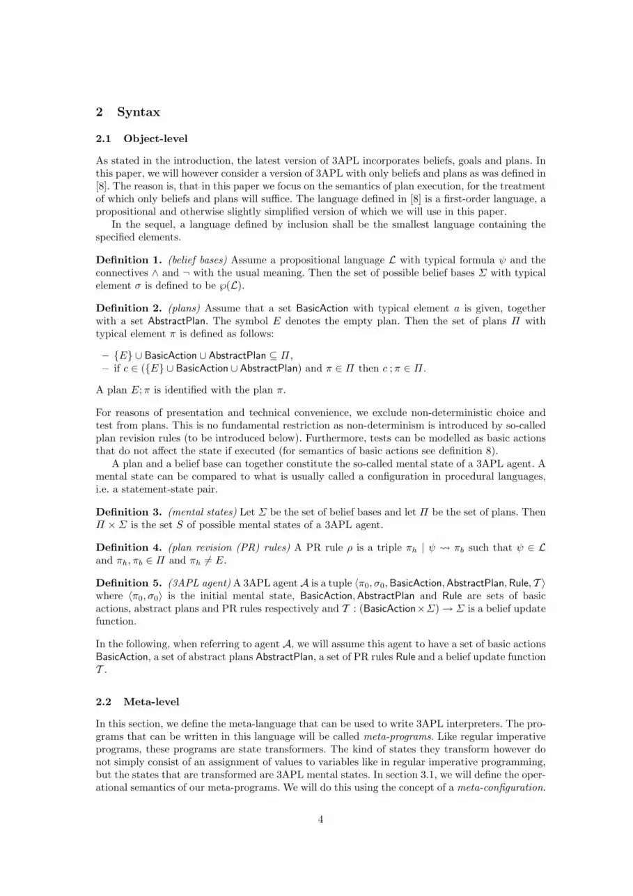
2 Syntax

2.1 Object-level

As stated in the introduction, the latest version of 3APL incorporates beliefs, goals and plans. Inthis paper, we will however consider a version of 3APL with only beliefs and plans as was defined in[8]. The reason is, that in this paper we focus on the semantics of plan execution, for the treatmentof which only beliefs and plans will suffice. The language defined in [8] is a first-order language, apropositional and otherwise slightly simplified version of which we will use in this paper.

In the sequel, a language defined by inclusion shall be the smallest language containing thespecified elements.

Definition 1. (belief bases) Assume a propositional language L with typical formula ψ and theconnectives ∧ and ¬ with the usual meaning. Then the set of possible belief bases Σ with typicalelement σ is defined to be ℘(L).

Definition 2. (plans) Assume that a set BasicAction with typical element a is given, togetherwith a set AbstractPlan. The symbol E denotes the empty plan. Then the set of plans Π withtypical element π is defined as follows:

– {E} ∪ BasicAction ∪ AbstractPlan ⊆ Π,– if c ∈ ({E} ∪ BasicAction ∪ AbstractPlan) and π ∈ Π then c ;π ∈ Π.

A plan E;π is identified with the plan π.

For reasons of presentation and technical convenience, we exclude non-deterministic choice andtest from plans. This is no fundamental restriction as non-determinism is introduced by so-calledplan revision rules (to be introduced below). Furthermore, tests can be modelled as basic actionsthat do not affect the state if executed (for semantics of basic actions see definition 8).

A plan and a belief base can together constitute the so-called mental state of a 3APL agent. Amental state can be compared to what is usually called a configuration in procedural languages,i.e. a statement-state pair.

Definition 3. (mental states) Let Σ be the set of belief bases and let Π be the set of plans. ThenΠ ×Σ is the set S of possible mental states of a 3APL agent.

Definition 4. (plan revision (PR) rules) A PR rule ρ is a triple πh | ψ πb such that ψ ∈ Land πh, πb ∈ Π and πh 6= E.

Definition 5. (3APL agent) A 3APL agentA is a tuple 〈π0, σ0,BasicAction,AbstractPlan,Rule, T 〉where 〈π0, σ0〉 is the initial mental state, BasicAction,AbstractPlan and Rule are sets of basicactions, abstract plans and PR rules respectively and T : (BasicAction×Σ) → Σ is a belief updatefunction.

In the following, when referring to agent A, we will assume this agent to have a set of basic actionsBasicAction, a set of abstract plans AbstractPlan, a set of PR rules Rule and a belief update functionT .

2.2 Meta-level

In this section, we define the meta-language that can be used to write 3APL interpreters. The pro-grams that can be written in this language will be called meta-programs. Like regular imperativeprograms, these programs are state transformers. The kind of states they transform however donot simply consist of an assignment of values to variables like in regular imperative programming,but the states that are transformed are 3APL mental states. In section 3.1, we will define the oper-ational semantics of our meta-programs. We will do this using the concept of a meta-configuration.

4

A meta-configuration consists of a meta-program and a mental state, i.e. the meta-program is theprocedural part and the mental state is the “data” on which the meta-program operates.

The basic elements of meta-programs are the execute action and the apply(ρ) action (calledmeta-actions). The execute action is used to specify that a basic action from the plan of an agentshould be executed. The apply(ρ) action is used to specify that a PR rule ρ should be applied to theplan. Through the execution of meta-actions, a mental state can thus be transformed. To iterateexecution of meta-actions, meta-programs can also contain a while construct. Composite meta-programs can be constructed using a sequential composition operator and a non-deterministicchoice operator.

Below, the meta-programs and meta-configurations for agent A are defined.

Definition 6. (meta-programs) We assume a set Bexp of boolean expressions with typical elementb. Let b ∈ Bexp and ρ ∈ Rule, then the set Prog of meta-programs with typical element P is definedas follows:

P ::= execute | apply(ρ) | while b do P od | P1;P2 | P1 + P2.

Definition 7. (meta-configurations) Let Prog be the set of meta-programs and let S be the setof mental states. Then Prog × S is the set of possible meta-configurations.

3 Operational Semantics

In [8], the operational semantics of 3APL is defined using transition systems ([11]). A transitionsystem for a programming language consists of a set of derivation rules for deriving transitions forthis language. A transition is a transformation of one configuration into another and it correspondsto a single computation step. In the following section, we will repeat the transition system for 3APLgiven in [8] (adapted to fit our simplified language) and we will call it the object-level transitionsystem. We will furthermore give a transition system for the meta-programs defined in section2.2 (the meta-level transition system). Then in the last section, we will define the operationalsemantics of the object- and meta-programs using the defined transition systems.

3.1 Transition Systems

The transition systems defined in the following sections assume 3APL agent A.

Object-level The object-level transition system (Transo) is defined by the rules given below. Thetransitions are labeled to denote the kind of transition. This is needed in the proofs of section 4.1.

Definition 8. (action execution) Let a ∈ BasicAction.

T (a, σ) = σ′

〈a;π, σ〉 →execute 〈π, σ′〉

In the transition rule for rule application, we use the operator •. π1 •π2 denotes a plan of which π1

is the first part and π2 is the second: π1 is the prefix of this plan. The operator is needed, becauseplans have a list structure (see definition 2). The plan π1;π2 is thus not syntactically correct.Plans have a list structure, because we do not want to semantically distinguish two plans withequal leaves, but a differing tree structure. There should for example be no semantic differencebetween the plans a; (b; c) and (a; b); c. A list structure therefore suffices, but the trade-off is thatwe cannot use the sequential composition operator to denote prefixing of more than one element.

Definition 9. (rule application) Let ρ : πh | ψ πb ∈ Rule.

σ |= ψ

〈πh • π, σ〉 →apply(ρ) 〈πb • π, σ〉

5

Meta-level The meta-level transition system (Transm) is defined by the rules below, specifyingwhich transitions from one meta-configuration to another are possible. As for the object-leveltransition system, the transitions are labeled to denote the kind of transition.

An execute meta-action is used to execute a basic action. It can thus only be executed ina mental state, if the first element of the plan in that mental state is a basic action. As in theobject-level transition system, the basic action a must be executable and the result of executinga on belief base σ is defined using the function T . After executing the meta-action execute, themeta-program is empty and the basic action is gone from the plan. Furthermore, the belief baseis changed as defined through T .

Definition 10. (action execution) Let a ∈ BasicAction.

T (a, σ) = σ′

〈execute, (a;π, σ)〉 →execute 〈E, (π, σ′)〉

A meta-action apply(ρ) is used to specify that PR rule ρ should be applied. It can be executed ina mental state if ρ is applicable in that mental state. The execution of the meta-action in a mentalstate results in the plan of that mental state being changed as specified by the rule.

Definition 11. (rule application) Let ρ : πh | ψ πb ∈ Rule.

σ |= ψ

〈apply(ρ), (πh • π, σ)〉 →apply(ρ) 〈E, (πb • π, σ)〉

In order to define the transition rule for the while construct, we first need to specify the semanticsof boolean expressions Bexp.

Definition 12. (semantics of boolean expressions) We assume a function W of type Bexp →(S →W ) yielding the semantics of boolean expressions, where W is the set of truth values {tt, ff}with typical formula β.

The transition for the while construct is then defined in a standard way below. The transitionis labeled with idle, to denote that this is a transition that does not have a counterpart in theobject-level transition system.

Definition 13. (while)

W(b)(s)〈while b do P od, s〉 →idle 〈P ; while b do P od, s〉

¬W(b)(s)〈while b do P od, s〉 →idle 〈E, s〉

The transitions for sequential composition and non-deterministic choice are defined as follows ina standard way. The variable x is used to pass on the type of transition through the derivation.

Definition 14. (sequential composition) Let x ∈ {execute, apply(ρ), idle | ρ ∈ Rule}.

〈P1, s〉 →x 〈P ′1, s′〉〈P1;P2, s〉 →x 〈P ′1;P2, s′〉

Definition 15. (non-deterministic choice) Let x ∈ {execute, apply(ρ), idle | ρ ∈ Rule}.

〈P1, s〉 →x 〈P ′1, s′〉〈P1 + P2, s〉 →x 〈P ′1, s′〉

〈P2, s〉 →x 〈P ′2, s′〉〈P1 + P2, s〉 →x 〈P ′2, s′〉

6

3.2 Operational Semantics

Using the transition systems defined in the previous section, transitions can be derived for 3APLand for the meta-programs. Individual transitions can be put in sequel, yielding so called com-putation sequences. In the following definitions, we define computation sequences and we specifythe functions yielding these sequences, for the object- and meta-level transition systems. We alsodefine the function κ, yielding the last element of a computation sequence if this sequence is finiteand the special state ⊥ otherwise. These functions will be used to define the operational semantics.

Definition 16. (computation sequences) The sets S+ and S∞ of respectively finite and infinitecomputation sequences are defined as follows:

S+ = {s1, . . . , si, . . . , sn | si ∈ S, 1 ≤ i ≤ n, n ∈ N},S∞ = {s1, . . . , si, . . . | si ∈ S, i ∈ N}.

Let S⊥ = S ∪ {⊥} and δ ∈ S+ ∪ S∞. The function κ : (S+ ∪ S∞) → S⊥ is defined by:

κ(δ) ={

last element of δ if δ ∈ S+,⊥ otherwise.

The function κ is extended to handle sets of computation sequences as follows:

κ({δi | i ∈ I}) = {κ(δi) | i ∈ I}.

Definition 17. (functions for calculating computation sequences) The functions Co and Cm arerespectively of type S → ℘(S+ ∪ S∞) and Prog → (S → ℘(S+ ∪ S∞)).

Co(s) = {s1, . . . , sn ∈ ℘(S+) | s→t1 s1 →t2 . . .→tn〈E, σn〉

is a finite sequence of transitions in Transo} ∪{s1, . . . , si, . . . ∈ ℘(S∞) | s→t1 s1 →t2 . . .→ti si →ti+1 . . .

is an infinite sequence of transitions in Transo}Cm(P )(s) = {s1, . . . , sn ∈ ℘(S+) | 〈P, s〉 →x1 〈P1, s1〉 →x2 . . .→xn

〈E, sn〉is a finite sequence of transitions in Transm} ∪

{s1, . . . , si, . . . ∈ ℘(S∞) | 〈P, s〉 →x1 〈P1, s1〉 →x2 . . .→xi 〈Pi, si〉 →xi+1 . . .is an infinite sequence of transitions in Transm}

Note that both Co and Cm return sequences of mental states. Co just returns the mental statescomprising the sequences of transitions derived in Transo, whereas Cm removes the meta-programcomponent of the meta-configurations of the transition sequences derived in Transm. The reasonfor defining these functions in this way is, that we want to prove equivalence of the object- andmeta-level transition systems: both yield the same transition sequences with respect to the mentalstates (or that is for a certain meta-program, see section 4). Also note that for Co as well as forCm, we only take into account infinite sequences and successfully terminating sequences, i.e. thosesequences ending in a mental state or meta-configuration with an empty plan or meta-programrespectively.

The operational semantics of object- and meta-level programs are functions Oo and Om, yield-ing, for each mental state s and possibly meta-program P , a set of mental states correspondingto the final states reachable through executing the plan of s or executing the meta-program Prespectively. If there is an infinite execution path, the set of mental states will contain the element⊥.

Definition 18. (operational semantics) Let s ∈ S. The functions Oo and Om are respectively oftype S⊥ → ℘(S⊥) and Prog → (S⊥ → ℘(S⊥)).

Oo(s) = κ(Co(s))Om(P )(s) = κ(Cm(P )(s))Oo(⊥) = Om(P )(⊥) = {⊥}

Note that the operational semantic functions can take any state s ∈ S⊥, including ⊥, as input.This will turn out to be necessary for giving the equivalence result of section 6.

7

4 Equivalence of Oo and Om

In the previous section, we have defined the operational semantics for 3APL and for meta-programs. Using the meta-language, one can write various 3APL interpreters. Here we will consideran interpreter of which the operational semantics will prove to be equivalent to the object-leveloperational semantics of 3APL. This interpreter for agent A is defined by the following meta-program.

Definition 19. (interpreter) Let⋃n

i=1 ρi = Rule, s ∈ S and let notEmptyP lan ∈ Bexp be aboolean expression such that W(notEmptyP lan)(s) = tt if the plan component of s is not equalto E and W(notEmptyP lan)(s) = ff otherwise. Then the interpreter can be defined as follows.

while notEmptyP lan do (execute + apply(ρ1) + . . . + apply(ρn)) od

In the sequel, we will use the keyword interpreter to abbreviate this meta-program.

This interpreter thus iterates the execution of a non-deterministic choice between all basic meta-actions, until the plan component of the mental state is empty. Intuitively, if there is a possibilityfor the interpreter to execute some meta-action in mental state s, resulting in a changed states′, it is also possible to go from s to s′ in an object-level execution through a correspondingobject-level transition. At each iteration, an executable meta-action is non-deterministically chosenfor execution. The interpreter thus as it were, non-deterministically chooses a path through theobject-level transition tree. The possible transitions defined by this interpreter correspond to thepossible transitions in the object-level transition system and therefore the object-level operationalsemantics is equivalent to the meta-level operational semantics of this meta-program. In the sequelwe will provide some lemma’s and a corollary from which this equivalence result will prove to followimmediately. As equivalence of object-level and meta-level operational semantics holds for inputstate ⊥ by definition 18, we will only need to prove equivalence for input states s ∈ S.

Before moving on to proving the equivalence theorem, we have to make the following remark.The equivalence between object-level 3APL and the interpreter defined above only holds if Ruledoes not contain reactive rules of the form E | ψ πb. The reason is, that we chose the emptyplan as a termination condition for the interpreter and the interpreter will thus stop applying rulesin a mental state once the plan in this state is empty. Rule application is however still a possibletransition in the object-level transition system in case of the presence of reactive rules, as theseare applicable to empty plans. We thus exclude reactive rules from the set Rule. This restrictioncould be relaxed, but the interpreter would have to be adapted to yield the equivalence result (thecondition of the while would have to be true). For reasons of space and clarity, we will not discussthis possibility here. Furthermore, having an empty plan or program as a termination conditionis in line with the notion of successful termination in procedural programming languages.

4.1 Equivalence Theorem

We prove a weak bisimulation between Transo and Transm(interpreter). From this, we can thenprove that Oo and Om(interpreter) are equivalent. In order to do this, we first state the followingproposition. It follows immediately from the transition systems.

Proposition 1. (object-level versus meta-level transitions)

s→execute s′ is a transition in Transo ⇔〈execute, s〉 →execute 〈E, s′〉 is a transition in Transm

s→apply(ρ) s′ is a transition in Transo ⇔

〈apply(ρ), s〉 →apply(ρ) 〈E, s′〉 is a transition in Transm

A weak bisimulation between two transition systems in general, is a relation between the systemssuch that the following holds: if a transition step can be derived in system one, it should be

8

possible to derive a “similar” (sequence of) transition(s) in system two and if a transition step canbe derived in system two, it should be possible to derive a “similar” (sequence of) transition(s)in system one. To explain what we mean by “similar” transitions, we need the notion of an idletransition. In a transition system, certain kinds of transitions can be labelled as an idle transition,for example transitions derived using the while rule (definition 13). These transitions can beconsidered “implementation details” of a certain transition system and we do not want to takethese into account when studying the relation between this and another transition system. Anon-idle transition in system one now is similar to a sequence of transitions in system two if thefollowing holds: this sequence of transitions in system two should consist of one non-idle transitionand otherwise idle transitions, and the non-idle transition in this sequence should be similar to thetransition in system one, i.e. the relevant elements of the configurations involved, should match.

In the context of our transition systems Transo and Transm, we can now phrase the followingbisimulation lemma.

Lemma 1. (weak bisimulation) Let +∗ abbreviate (execute + apply(ρ1) + . . . + apply(ρn)). LetTransm(P ) be the restriction of Transm to those transitions that are part of some sequence of tran-sitions starting in initial meta-configuration 〈P, s0〉, with s0 ∈ S an arbitrary mental state. Thena weak bisimulation exists between Transo and Transm(interpreter), i.e. the following propertieshold.

s→x s′ is a transition in Transo ⇒1 〈interpreter, s〉 →idle 〈+∗; interpreter, s〉 →t 〈interpreter, s′〉

is a transition in Transm(interpreter)

〈+∗; interpreter, s〉 →t 〈interpreter, s′〉is a transition in Transm(interpreter) ⇒2 s→x s

′ is a transition in Transo

Proof. (⇒1) Assume s→t s′ is a transition in Transo for t ∈ {execute, apply(ρ) | ρ ∈ Rule}. Using

proposition 1, the following then is a transition in Transm.

〈(execute + apply(ρ1) + . . . + apply(ρn)); interpreter, s〉 →t 〈interpreter, s′〉 (1)

Furthermore, by the assumption that s →t s′ is a transition in Transo and by the assumption

that no reactive rules are contained in Rule (see introduction of section 4), we know that the planof s is not empty as both rule application and basic action execution require a non-empty plan.Now, using the fact that the plan of s is not empty, the following transition can be derived inTransm(interpreter).

〈interpreter, s〉 →idle 〈(execute + apply(ρ1) + . . . + apply(ρn)); interpreter, s〉 (2)

The transitions (2) and (1) can be concatenated, yielding the desired result.

(⇒2) Assume 〈+∗; interpreter, s〉 →t 〈interpreter, s′〉 is a transition in Transm(interpreter). Then,〈+∗, s〉 →t 〈E, s′〉 must be a transition in Transm (definition 14). Therefore, by proposition 1, wecan conclude that s→x s

′ is a transition in Transo.

We are now in a position to give the equivalence theorem of this section.

Theorem 1. (Oo = Om(interpreter))

∀s ∈ S : Oo(s) = Om(interpreter)(s)

Proof. Proving this theorem amounts to showing the following: s ∈ Oo ⇔ s ∈ Om(interpreter).(⇒) Assume s ∈ Oo. This means that a sequence of transitions s0 →t1 . . .→tn

s must be derivablein Transo. By repeated application of lemma 1, we know that then there must also be a sequenceof transitions in Transm(interpreter) of the following form:

〈interpreter, s0〉 →idle . . .→tn−1 〈interpreter, s′〉 →idle 〈+∗; interpreter, s′〉 →tn〈interpreter, s〉. (3)

9

As s ∈ Oo, we know that there cannot be a transition s→tn+1 s′′ for some mental state s′′, i.e. it

is not possible to execute an execute or apply meta-action in s. Therefore, we know that the onlypossible transition from 〈interpreter, s〉 in (3) above, is . . . →idle 〈E, s〉. From this, we have thats ∈ Om(interpreter).

(⇐) Assume that s ∈ Om(interpreter). Then there must be a sequence of transitions inTransm(interpreter) of the form:

〈interpreter, s0〉 →idle 〈+∗; interpreter, s0〉 →t1 . . .→tn−1

〈interpreter, s′〉 →idle 〈+∗; interpreter, s′〉 →tn〈interpreter, s〉 →idle 〈E, s〉.

From this, we can conclude by lemma 1 that s0 →t1 . . .→tn−1 s′ →tn s 6→ must be a sequence of

transitions in Transo. Therefore, it must be the case that s ∈ Oo.

Note that it is easy to show that Oo = Om(P ) does not hold for all meta-programs P .

5 Denotational Semantics

In this section, we will define the denotational semantics of meta-programs. The method used isthe fixed point approach as can be found in Stoy ([16]). The semantics greatly resembles the onein De Bakker ([4], Chapter 7) to which we refer for a detailed explanation of the subject.

A denotational semantics for a programming language in general, is, like an operational seman-tics, a function taking a statement P and a state s and yielding a state (or set of states in case of anon-deterministic language) resulting from executing P in s. The denotational semantics for meta-programs is thus, like the operational semantics of definition 18, a function taking a meta-programP and mental state s and yielding the set of mental states resulting from executing P in s, i.e. afunction of type Prog → (S⊥ → ℘(S⊥))9. Contrary however to an operational semantic function,a denotational semantic function is not defined using the concept of computation sequences and,in contrast with most operational semantics, it is defined compositionally ([17], [10], [4]).

5.1 Preliminaries

In order to define the denotational semantics of meta-programs, we need some mathematicalmachinery. Most importantly, the domains used in defining the semantics of meta-programs aredesigned as so-called complete partial orders (CPO’s). A CPO is a set with an ordering on itselements with certain characteristics (see definition 25). This concept is defined in terms of thenotions of partially ordered sets, least upper bounds and chains.

Definition 20. (partially ordered set) Let C be an arbitrary set. A partial order v on C is asubset of C × C which satisfies:

1. c v c (reflexivity),2. if c1 v c2 and c2 v c1 then c1 = c2 (antisymmetry),3. if c1 v c2 and c2 v c3 then c1 v c3 (transitivity).

In the sequel, we will be concerned not only with arbitrary sets with partial orderings, but alsowith sets of functions with an ordering. A partial ordering on a set of functions of type C1 → C2

can be derived from the orderings on C1 and C2 as defined below.

Definition 21. (partial ordering on functions) Let (C1,v1) and (C2,v2) be two partially orderedsets. An ordering v on C1 → C2 is defined as follows, where f, g ∈ C1 → C2:

f v g ⇔ ∀c ∈ C1 : f(c) v2 g(c).

9 The type of the denotational semantic function is actually slightly different as will become clear in thesequel, but that is not important for the current discussion.

10

Definition 22. (least upper bound) Let C ′ ⊆ C. z ∈ C is called the least upper bound of C ′ if:

1. z is an upper bound: ∀x ∈ C ′ : x v z,2. z is the least upper bound: ∀y ∈ C : ((∀x ∈ C ′ : x v y) ⇒ z v y).

The least upper bound of a set C ′ will be denoted by⊔C ′.

Definition 23. (least upper bound of a sequence) The least upper bound of a sequence 〈c0, c1, . . .〉is denoted by

⊔∞i=0 ci or by

⊔〈ci〉∞i=0 and is defined as follows, where “c in 〈ci〉∞i=0” means that c

is an element of the sequence 〈ci〉∞i=0:⊔〈ci〉∞i=0 =

⊔{c | c in 〈ci〉∞i=0}.

We will now define the notion of a chain. A chain on a set C with some order v can be defined intwo ways. It can first of all be defined as a subset X ⊆ C with a total ordering, i.e. for all x, y ∈ X,either x v y or y v x. Secondly, it can be defined as a finite or infinite sequence, the elements ofwhich have to be ordered in a certain way. This is specified for infinite sequences in the definitionbelow.

Definition 24. (chains) A chain on (C,v) is an infinite sequence 〈ci〉∞i=0 such that for i ∈ N :ci v ci+1.

The two definitions of chains are related as follows. If (C,v) is a partial order, the following holds:if 〈ci〉∞i=0 is a chain in C, the set {c | c in 〈ci〉∞i=0} is also a chain in C. For an ordering that is notpartial, this does not have to hold (take for example as C the set of natural numbers with thenon-reflexive and non-transitive ordering x v y ⇔ y = x+ 1 and take as a sequence 〈0, 1, 2, . . .〉).Note that the number of distinct elements of an infinite sequence can be finite or infinite. In linewith other literature on semantics of programming languages ([4], [9], [14], [17]), we will use thedefinition of chains as sequences. As we only use it in the context of partial orders, these chainsare related to chains defined as sets as explained.

Having defined partially ordered sets, least upper bounds and chains, we are now in a positionto define complete partially ordered sets.

Definition 25. (CPO) A complete partially ordered set is a set C with a partial order v whichsatisfies the following requirements:

1. there is a least element with respect to v, i.e. an element ⊥ ∈ C such that ∀c ∈ C : ⊥ v c,2. each chain 〈ci〉∞i=0 in C has a least upper bound (

⊔∞i=0 ci) ∈ C.

The following facts about CPO’s of functions will turn out to be useful. For proofs, see for exampleDe Bakker ([4]).

Fact 1. (CPO of functions) Let (C1,v1) and (C2,v2) be CPO’s. Then (C1 → C2,v) with v asin definition 21 is a CPO.

Fact 2. (least upper bound of a chain of functions) Let (C1,v1) and (C2,v2) be CPO’s and let〈fi〉∞i=0 be a chain of functions in C1 → C2. Then the function λc1 ·

⊔∞i=0 fi(c1) is the least upper

bound of this chain and therefore (⊔∞

i=0 fi)(c1) =⊔∞

i=0 fi(c1) for all c1 ∈ C1.

The semantics of meta-programs will be defined using the notion of the least fixed point of afunction on a CPO.

Definition 26. (least fixed point) Let (C,v) a CPO, f : C → C and let x ∈ C.

– x is a fixed point of f iff f(x) = x– x is a least fixed point of f iff x is a fixed point of f and for each fixed point y of f : x v y

The least fixed point of a function f is denoted by µf .

11

If a function f on a CPO is continuous, the fixed point theorem as specified below in fact 3 tellsus that the least fixed point of f exists and that it is equal to the least upper bound of the chain〈f i(⊥)〉∞i=0. This will turn out to be a useful fact in proving that the denotational semantic functionis well-defined and in addition, it will prove to be more intuitive to explain the semantics in termsof chains of functions, rather than in terms of least fixed points of functions.

Definition 27. (continuity) Let (C1,v1), (C2,v2) be CPO’s. Then a function f : C1 → C2 iscontinuous iff for each chain 〈ci〉∞i=0 in C1, the following holds:

f(⊔∞

i=0 ci) =⊔∞

i=0 f(ci).

Fact 3. (fixed point theorem) Let C be a CPO and let f : C → C. If f is continuous, then theleast fixed point µf exists and equals

⊔∞i=0 f

i(⊥), where f0(⊥) = ⊥ and f i+1(⊥) = f(f i(⊥)).

For a proof, see for example De Bakker ([4]).

5.2 Definition

Having explained some basics about CPO’s in general, we will now show how the domains used indefining the semantics of meta-programs are designed as CPO’s. The reason for designing theseas CPO’s will become clear in the sequel.

Definition 28. (domains of interpretation) Let W be the set of truth values of definition 12 andlet S be the set of possible mental states of definition 3. Then the sets W⊥ and S⊥ are defined asCPO’s as follows:

W⊥ = W ∪ {⊥W⊥} CPO by β1 v β2 iff β1 = ⊥W⊥ or β1 = β2,S⊥ = S ∪ {⊥} CPO analogously.

Note that we use ⊥ to denote the bottom element of S⊥ and that we use ⊥C for the bottomelement of any other set C. As the set of mental states is extended with a bottom element, wenow augment the specification of the semantics of boolean expressions to include a clause for thiselement.

Definition 29. (semantics of boolean expressions) The semantics of boolean expressions is asassumed in definition 12 for s ∈ S and is augmented with the following clause for the mental state⊥ ∈ S⊥, yielding a function of type Bexp→ (S⊥ →W⊥).

W(b)(⊥) = ⊥W⊥

In the sequel, it will be useful to have an if-then-else function as defined below.

Definition 30. (if-then-else) Let C be a CPO, c1, c2,⊥C ∈ C and β ∈W⊥. Then the if-then-elsefunction of type W⊥ → C is defined as follows.

if β then c1 else c2 fi =

c1 if β = ttc2 if β = ff⊥C if β = ⊥W⊥

Because our meta-language is non-deterministic, the denotational semantics is not a function fromstates to states, but a function from states to sets of states. These resulting sets of states can befinite or infinite. An example of a meta-program yielding an infinite set of states is the following:TODO good example. In case of bounded non-determinism10, these infinite sets of states have ⊥as one of their members. This property may be explained by viewing the execution of a programas a tree of computations and then using Konig’s lemma which tells us that a finitely-branching10 Bounded non-determinism means that at any state during computation, the number of possible next

states is finite.

12

tree with infinitely many nodes has at least one infinite path (see [4]). The meta-language is indeedbounded non-deterministic11 and the result of executing a meta-program P in some state, is thuseither a finite set of states or an infinite set of states containing ⊥. We therefore specify thefollowing domain as the result domain of the denotational semantic function instead of ℘(S⊥).

Definition 31. (T ) The set T with typical element τ is defined as follows: T = {τ ∈ ℘(S⊥) |τ finite or ⊥ ∈ τ}.

The advantage of using T instead of ℘(S⊥) as the result domain, is that T can nicely be designedas a CPO with the following ordering ([5]).

Definition 32. (Egli-Milner ordering) Let τ1, τ2 ∈ T . τ1 v τ2 holds iff either⊥ ∈ τ1 and τ1\{⊥} ⊆τ2, or ⊥ 6∈ τ1 and τ1 = τ2. Under this ordering, the set {⊥} is ⊥T .

We are now ready to give the denotational semantics of meta-programs. We will first give thedefinition and then justify and explain it.

Definition 33. (denotational semantics of meta-programs) Let φ1, φ2 : S⊥ → T . Then we definethe following functions.

φ : T → T = λτ ·⋃

s∈τ φ(s)φ1 ◦ φ2 : S⊥ → T = λs · φ1(φ2(s))

Let (π, σ) ∈ S. The denotational semantics of meta-programs M : Prog → (S⊥ → T ) is thendefined as follows.

MJexecuteK(π, σ) =

{(π′, σ′)} if π = a;π′

with a ∈ BasicAction and T (a, σ) = σ′

∅ otherwiseMJexecuteK ⊥ = ⊥T

MJapply(ρ)K(π, σ) =

{(πb ◦ π′, σ)} if σ |= ψ and π = πh ◦ π′with ρ : πh | ψ πb ∈ Rule

∅ otherwiseMJapply(ρ)K ⊥ = ⊥T

MJwhile b do P odK = µΦMJP1;P2K = MJP2K ◦MJP1KMJP1 + P2K = MJP1K ∪MJP2K

The function Φ : (S⊥ → T ) → (S⊥ → T ) used above is defined asλφ · λs · if W(b)(s) then φ(MJP K(s)) else {s} fi, using definition 30.

Meta-actions The semantics of meta-actions is straight forward. The result of executing anexecute meta-action in some mental state s, is a set containing the mental state resulting fromexecuting the basic action of the plan of s. The result is empty if there is no basic action on theplan to execute. The result of executing an apply(ρ) meta-action in state s, is a set containing themental state resulting from applying ρ in s. If ρ is not applicable, the result is the empty set.

While The semantics of the while construct is more involved. We will try to explain it by firstdefining a set of requirements on the semantics and then giving an intuitive understanding of thegeneral ideas behind the semantics. Next, we will go into more detail on the semantics of a whileconstruct in deterministic languages, followed by details on the semantics as defined above for ournon-deterministic language.

Now, what we want to do, is define a function specifying the semantics of the while constructMJwhile b do P odK, the type of which should be S⊥ → T , in accordance with the type of M.The function can moreover not be defined circularly, but it should be defined compositionally, i.e.11 Only a finite number of rule applications and action executions are possible in any state.

13

it can only use the semantics of the guard and of the body of the while. This ensures that Mis well-defined. The semantics of the while can thus not be defined as MJwhile b do P odK =MJif b then P ; while b do P od else skip fiK where skip is a statement doing nothing, becausethis would violate the requirement of compositionality.

Intuitively, the semantics of while b do P od should correspond to repeatedly executing P ,until b is false. The semantics could thus be something like:

MJif b then P ; if b then P ; . . . else skip fi else skip fiK.

The number of nestings of if-then-else constructs should however be infinite, as we cannot deter-mine in advance how many times the body of the while loop will be executed, worse still, it couldbe the case that it will be executed an infinite number of times in case of non-termination. Asprograms are however by definition finite syntactic objects (see definition 6), the semantics of thewhile cannot be defined in this way. The idea of the solution now is, not to try to specify thesemantics at once using infinitely many nestings of if-then-else constructs, but instead to specifythe semantics using approximating functions, where some approximation is at least as good asanother if it contains more nestings of if-then-else constructs. So to be a little more specific, whatwe do is specify a sequence of approximating functions 〈φi〉∞i=0, where φi roughly speaking corre-sponds to executing the body of the while construct less than i times and the idea now is thatthe limit of this sequence of approximations is the semantics of the while we are looking for.

Deterministic languages Having provided some vague intuitive ideas about the semantics, we willnow go into more detail and use the theory on CPO’s of section 5.1. To simplify matters, we willfirst consider a deterministic language. The function defining the semantics of the while shouldthen be of type S⊥ → S⊥. The domain S⊥ is designed as a CPO and therefore the domain offunctions S⊥ → S⊥ is also a CPO (see fact 1). What we are looking for, is a chain of approximatingfunctions 〈φi〉∞i=0 in this CPO S⊥ → S⊥, the least upper bound of which should yield the desiredsemantics for the while. As we are looking for a chain (see definition 24) of functions 〈φi〉∞i=0, itshould be the case that for all s ∈ S⊥ : φi(s) v φj(s) for i ≤ j. Intuitively, a function φj is “asleast as good” an approximation as φi.

Approximating functions with the following behaviour will do the trick. A function φi shouldbe defined such, that the result of φi applied to an initial state s0, is the state in which the whileloop terminates if less than i runs through the loop are needed for termination. If i or more runsare needed, i.e. if the execution of the while has not terminated after i− 1 runs, the result shouldbe ⊥. To illustrate how these approximating functions can be defined to yield this behaviour, wewill give the first few approximations φ0, φ1 and φ2. In order to do this, we need to introduce aspecial statement diverge, which yields the state ⊥ if executed. It can be shown that with thefunctions φi as defined below, 〈φi〉∞i=0 is indeed a chain. Therefore it has a least upper bound bydefinition, which ensures that the semantics is well-defined.

φ0 = MJdivergeKφ1 = MJif b then P ; diverge else skip fiKφ2 = MJif b then

P ; if b then P ; diverge else skip fielse skip fiK

...

These definitions can be generalized, yielding the following definition of the functions φi in whichwe use the if-then-else function of definition 30.

φ0 = ⊥S⊥→S⊥

= λs · ⊥φi+1 = λs · if W(b)(s) then φi(MJP K(s)) else s fi

Now, as 〈φi〉∞i=0 is a chain, so is 〈φi(s0)〉∞i=0. Using fact 2, we know that⊔∞

i=0 φi = λs0 ·⊔∞

i=0 φi(s0)or (

⊔∞i=0 φi)(s0) =

⊔∞i=0 φi(s0), i.e. the semantics of the execution of the while construct in an

initial state s0, is the least upper bound of the chain 〈φi(s0)〉∞i=0.

14

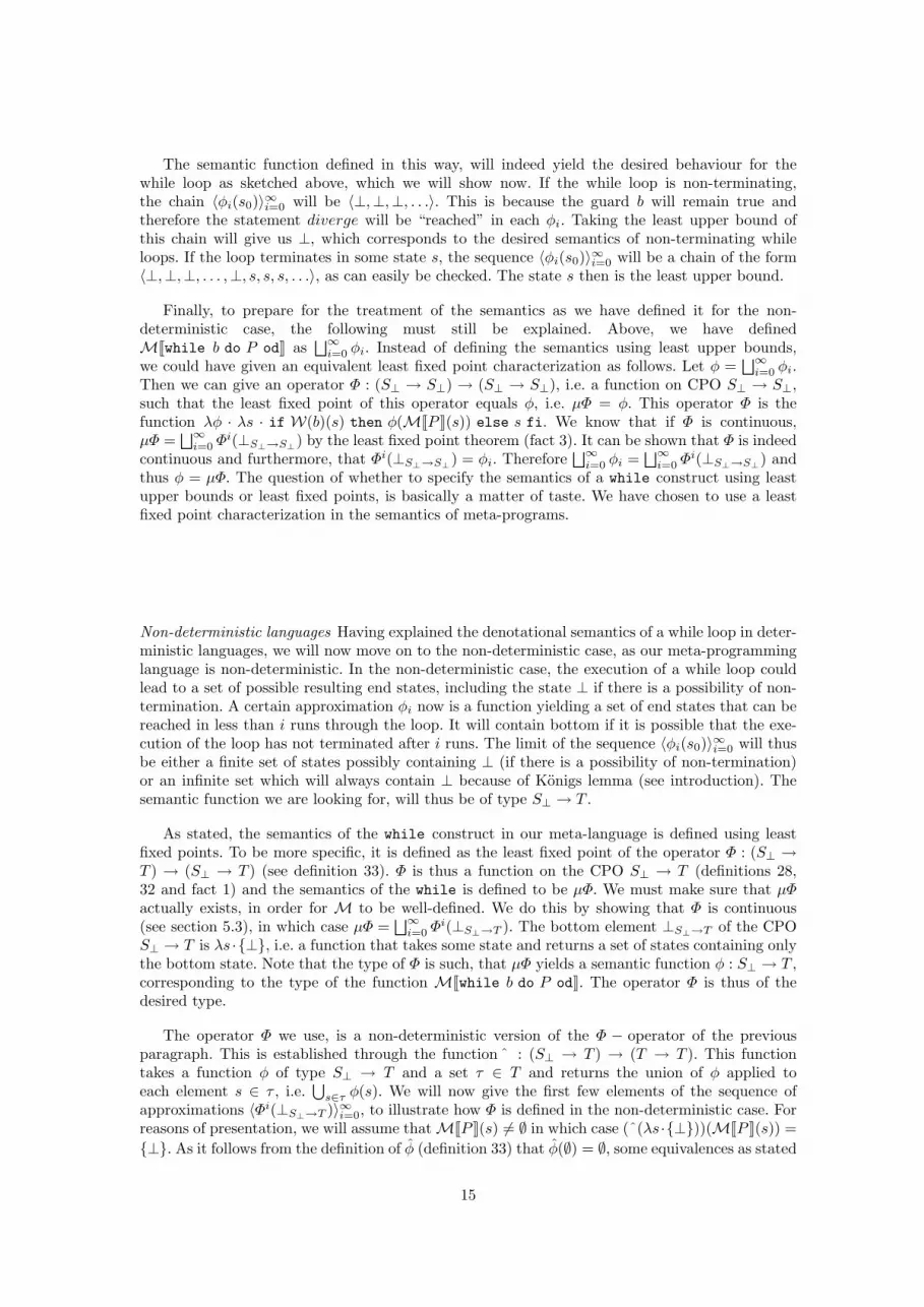
The semantic function defined in this way, will indeed yield the desired behaviour for thewhile loop as sketched above, which we will show now. If the while loop is non-terminating,the chain 〈φi(s0)〉∞i=0 will be 〈⊥,⊥,⊥, . . .〉. This is because the guard b will remain true andtherefore the statement diverge will be “reached” in each φi. Taking the least upper bound ofthis chain will give us ⊥, which corresponds to the desired semantics of non-terminating whileloops. If the loop terminates in some state s, the sequence 〈φi(s0)〉∞i=0 will be a chain of the form〈⊥,⊥,⊥, . . . ,⊥, s, s, s, . . .〉, as can easily be checked. The state s then is the least upper bound.

Finally, to prepare for the treatment of the semantics as we have defined it for the non-deterministic case, the following must still be explained. Above, we have definedMJwhile b do P odK as

⊔∞i=0 φi. Instead of defining the semantics using least upper bounds,

we could have given an equivalent least fixed point characterization as follows. Let φ =⊔∞

i=0 φi.Then we can give an operator Φ : (S⊥ → S⊥) → (S⊥ → S⊥), i.e. a function on CPO S⊥ → S⊥,such that the least fixed point of this operator equals φ, i.e. µΦ = φ. This operator Φ is thefunction λφ · λs · if W(b)(s) then φ(MJP K(s)) else s fi. We know that if Φ is continuous,µΦ =

⊔∞i=0 Φ

i(⊥S⊥→S⊥) by the least fixed point theorem (fact 3). It can be shown that Φ is indeedcontinuous and furthermore, that Φi(⊥S⊥→S⊥) = φi. Therefore

⊔∞i=0 φi =

⊔∞i=0 Φ

i(⊥S⊥→S⊥) andthus φ = µΦ. The question of whether to specify the semantics of a while construct using leastupper bounds or least fixed points, is basically a matter of taste. We have chosen to use a leastfixed point characterization in the semantics of meta-programs.

Non-deterministic languages Having explained the denotational semantics of a while loop in deter-ministic languages, we will now move on to the non-deterministic case, as our meta-programminglanguage is non-deterministic. In the non-deterministic case, the execution of a while loop couldlead to a set of possible resulting end states, including the state ⊥ if there is a possibility of non-termination. A certain approximation φi now is a function yielding a set of end states that can bereached in less than i runs through the loop. It will contain bottom if it is possible that the exe-cution of the loop has not terminated after i runs. The limit of the sequence 〈φi(s0)〉∞i=0 will thusbe either a finite set of states possibly containing ⊥ (if there is a possibility of non-termination)or an infinite set which will always contain ⊥ because of Konigs lemma (see introduction). Thesemantic function we are looking for, will thus be of type S⊥ → T .

As stated, the semantics of the while construct in our meta-language is defined using leastfixed points. To be more specific, it is defined as the least fixed point of the operator Φ : (S⊥ →T ) → (S⊥ → T ) (see definition 33). Φ is thus a function on the CPO S⊥ → T (definitions 28,32 and fact 1) and the semantics of the while is defined to be µΦ. We must make sure that µΦactually exists, in order for M to be well-defined. We do this by showing that Φ is continuous(see section 5.3), in which case µΦ =

⊔∞i=0 Φ

i(⊥S⊥→T ). The bottom element ⊥S⊥→T of the CPOS⊥ → T is λs ·{⊥}, i.e. a function that takes some state and returns a set of states containing onlythe bottom state. Note that the type of Φ is such, that µΦ yields a semantic function φ : S⊥ → T ,corresponding to the type of the function MJwhile b do P odK. The operator Φ is thus of thedesired type.

The operator Φ we use, is a non-deterministic version of the Φ − operator of the previousparagraph. This is established through the function ˆ : (S⊥ → T ) → (T → T ). This functiontakes a function φ of type S⊥ → T and a set τ ∈ T and returns the union of φ applied toeach element s ∈ τ , i.e.

⋃s∈τ φ(s). We will now give the first few elements of the sequence of

approximations 〈Φi(⊥S⊥→T )〉∞i=0, to illustrate how Φ is defined in the non-deterministic case. Forreasons of presentation, we will assume that MJP K(s) 6= ∅ in which case (ˆ(λs ·{⊥}))(MJP K(s)) ={⊥}. As it follows from the definition of φ (definition 33) that φ(∅) = ∅, some equivalences as stated

15

below would not hold in this case.

Φ0(⊥S⊥→T ) = λs · {⊥}Φ1(⊥S⊥→T ) = Φ(Φ0(⊥S⊥→T ))

= Φ(λs · {⊥})= λs · if W(b)(s) then (ˆ(λs · {⊥}))(MJP K(s)) else {s} fi= λs · if W(b)(s) then {⊥} else {s} fi

Φ2(⊥S⊥→T ) = Φ(Φ1(⊥S⊥→T ))= Φ(λs · if W(b)(s) then {⊥} else {s} fi)= λs · if W(b)(s)

then(ˆ(λs′ · if W(b)(s′)

then{⊥}

else{s′} fi))(MJP K(s))

else {s} fiΦ3(⊥S⊥→T ) = Φ(Φ2(⊥S⊥→T ))

= . . .

The zeroth approximation by definition (see fact 3) always yields the bottom element of theCPO S⊥ → T . The first approximation is a function that takes an initial state s and yields eitherthe set {⊥} if the guard is true in s, i.e. if there will be one or more runs through the loop, or theset {s} if the guard is false in s, i.e. if the while loop is such that it terminates in s without goingthrough the loop. The second approximation is a function that takes an initial state s and yields,like the first approximation, the set {s} if the guard is false in s. It thus returns the same result asthe first approximation if it takes less than one runs through the loop to terminate. This is exactlywhat we want, as the first approximation will be as good as it gets in this case. If the guard istrue in s, the function λs′ · if W(b)(s′) then {⊥} else {s′} fi is applied to each state in the setof states resulting from executing the body of the while in s, i.e. the set MJP K(s) which we willrefer to by τ ′. The function thus takes some state s′ from τ ′ and either yields {s′} if the guard istrue in s′, i.e. if the while can terminate in s′ after one run through the loop, or yields {⊥} if theguard is false in s′, i.e. if the execution path going through s′ has not ended. The functionˆnowtakes the union of the results for each s′, yielding a set of states containing the states in whichthe while loop can end after one run through the loop, and containing ⊥ if it is possible that thewhile loop has not terminated after one run. The function Φ is thus defined such that a certainapproximation Φi(⊥S⊥→T ) is a function yielding a set of end states that can be reached in lessthan i runs through the loop. It will contain ⊥ if it is possible that the execution of the loop hasnot terminated after i runs.

Sequential Composition and Non-deterministic Choice The semantics of the sequentialcomposition and non-deterministic choice operator is as one would expect.

5.3 Continuity of Φ

In the previous section, we have given the denotational semantics of meta-programs. In this defi-nition, the semantics of the while construct was defined to be the least fixed point of the operatorΦ on the CPO S⊥ → T . As stated, we must make sure that this least fixed point µΦ actuallyexists, in order for M to be well-defined. This can be done by showing that Φ is continuous (seefact 3), which is what we will do in this section. We will repeat the definition of Φ here.

Definition 34. (the operator Φ) The operator Φ : (S⊥ → T ) → (S⊥ → T ) is defined for somemeta-program P ∈ Prog as follows, with W as in definition 29, the if-then-else function as in

16

definition 30 and M and φ as in definition 33.

Φ = λφ · λs · if W(b)(s) then φ(MJP K(s)) else {s} fi

In definition 27, the concept of continuity was defined. As we will state below in fact 4, an equivalentdefinition can be given using the concept of monotonicity of a function.

Definition 35. (monotonicity) Let (C,v), (C ′,v) be CPO’s and c1, c2 ∈ C. Then a functionf : C → C ′ is monotone iff the following holds:

c1 v c2 ⇔ f(c1) v f(c2).

Fact 4. (continuity) Let (C,v), (C ′,v) be CPO’s and let f : C → C ′ be a function. Then:

for all chains 〈ci〉∞i=0 in C : f(⊔∞

i=0 ci) =⊔∞

i=0 f(ci)⇔

f is monotone and for all chains 〈ci〉∞i=0 in C : f(⊔∞

i=0 ci) v⊔∞

i=0 f(ci)

Proof. (⇒): Assume for all chains 〈ci〉∞i=0 in C : f(⊔〈ci〉∞i=0) =

⊔〈f(ci)〉∞i=0. Then f(

⊔〈ci〉∞i=0) v⊔

〈f(ci)〉∞i=0 trivially holds for all chains 〈ci〉∞i=0 in C. To prove: monotonicity of f .Let c, c′ ∈ C and assume c v c′. The following holds: f(c) v

⊔{f(c), f(c′)}. As

⊔{f(c), f(c′)} =⊔

〈f(ci)〉∞i=0 with 〈f(ci)〉∞i=0 ∈ Chain({f(c), f(c′)}), we can conclude that f(c) v f(⊔〈ci〉∞i=0) with

〈ci〉∞i=0 ∈ Chain({c, c′}) by assumption. As⊔〈ci〉∞i=0 =

⊔{c, c′}, we can conclude that f(c) v f(c′),

using that c′ =⊔{c, c′}.

(⇐): Assume that f is monotone and that f(⊔〈ci〉∞i=0) v

⊔〈f(ci)〉∞i=0 holds for all chains 〈ci〉∞i=0 in C.

Then we need to prove that for all chains 〈ci〉∞i=0 in C :⊔〈f(ci)〉∞i=0 v f(

⊔〈ci〉∞i=0). Take an ar-

bitrary chain 〈ci〉∞i=0 in C. Let X = {c | c in 〈ci〉∞i=0} and let X ′ = {f(c) | c in 〈ci〉∞i=0} = {f(x) |x ∈ X}. To prove:

⊔X ′ v f(

⊔X).

Take some x ∈ X. Then x v⊔X and thus by monotonicity of f : f(x) v f(

⊔X). With x

having been chosen arbitrarily, we may conclude that f(⊔X) is an upper bound of X ′. Hence,⊔

X ′ v f(⊔X).

Below, we will prove continuity of Φ by proving that Φ is monotone and that for all chains〈φi〉∞i=0 in S⊥ → T , the following holds: Φ(

⊔∞i=0 φi) v

⊔∞i=0 Φ(φi).

Monotonicity of Φ

Lemma 2. (monotonicity of Φ)

The function Φ as given in definition 34 is monotone, i.e. the following holds for all φi, φj ∈ S⊥ → T :

φi v φj ⇒ Φ(φi) v Φ(φj).

Proof. Take arbitrary φi, φj ∈ S⊥ → T . Suppose that φi v φj . Then we need to prove that ∀s ∈S⊥ : Φ(φi)(s) v Φ(φj)(s). Take an arbitrary s ∈ S⊥. We need to prove that Φ(φi)(s) v Φ(φj)(s),i.e. that

if W(b)(s) then φi(MJP K(s)) else {s} fi v if W(b)(s) then φj(MJP K(s)) else {s} fi.

We distinguish three cases.

1. Suppose W(b)(s) = ⊥W⊥ , then to prove: {⊥} v {⊥}. This is true by definition 32.2. Suppose W(b)(s) = ff , then to prove: {s} v {s}. This is true by definition 32.3. Suppose W(b)(s) = tt, then to prove: φi(MJP K(s)) v φj(MJP K(s)). Let τ ′ = MJP K(s). Using

the definition of φ, we rewrite what needs to be proven into⋃s′∈τ ′ φi(s′) v

⋃s′∈τ ′ φj(s′). Now we can distinguish two cases.

17

(a) Suppose ⊥ 6∈⋃

s′∈τ ′ φi(s′). Then to prove:⋃

s′∈τ ′ φi(s′) =⋃

s′∈τ ′ φj(s′). From the as-sumption that ⊥ 6∈

⋃s′∈τ ′ φi(s′), we can conclude that ⊥ 6∈ φi(s′) for all s′ ∈ τ ′. Using the

assumption that φi(s) v φj(s) for all s ∈ S⊥, we have that φi(s′) = φj(s′) for all s′ ∈ τ ′

and therefore⋃

s′∈τ ′ φi(s′) =⋃

s′∈τ ′ φj(s′).(b) Suppose ⊥ ∈

⋃s′∈τ ′ φi(s′). Then to prove: (

⋃s′∈τ ′ φi(s′)) \ {⊥} ⊆

⋃s′∈τ ′ φj(s′), i.e.⋃

s′∈τ ′(φi(s′) \ {⊥}) ⊆⋃

s′∈τ ′ φj(s′). Using the assumption that φi(s) v φj(s) for alls ∈ S⊥, we have that for all s′ ∈ τ ′, either φi(s′) \ {⊥} ⊆ φj(s′) or φi(s′) = φj(s′),depending on whether ⊥ ∈ φi(s). From this we can conclude that

⋃s′∈τ ′(φi(s′) \ {⊥}) ⊆⋃

s′∈τ ′ φj(s′).

Theorem 2. (continuity of Φ) The function Φ as given in definition 34 is continuous, i.e. Φ ismonotone and for all chains 〈φi〉∞i=0 in S⊥ → T , the following holds:

Φ(∞⊔

i=0

φi) v∞⊔

i=0

Φ(φi).

Proof. Monotonicity of Φ was proven in lemma 2. We therefore only need to prove that for all chains〈φi〉∞i=0 in S⊥ → T and for all s ∈ S⊥, the following holds:(Φ(

⊔∞i=0 φi))(s) v (

⊔∞i=0 Φ(φi))(s). Take an arbitrary chain 〈φi〉∞i=0 in S⊥ → T and an arbitrary

state s ∈ S⊥. Then to prove:

if W(b)(s) thenˆ(∞⊔

i=0

φi)(τ) else {s} fi v∞⊔

i=0

if W(b)(s) then φi(τ) else {s} fi,

where τ = M[P ](s). We distinguish three cases.

1. Suppose W(b)(s) = ⊥W⊥ , then to prove: {⊥} v⊔∞

i=0{⊥}, i.e. {⊥} v {⊥}. This is true bydefinition 32.

2. Suppose W(b)(s) = ff , then to prove: {s} v⊔∞

i=0{s}, i.e. {s} v {s}. This is true by definition32.

3. Suppose W(b)(s) = tt, then to prove:ˆ(⊔∞

i=0 φi)(τ) v⊔∞

i=0 φi(τ). If we can prove that ∀τ ∈ T :ˆ(

⊔∞i=0 φi)(τ) v

⊔∞i=0 φi(τ), i.e.ˆ(

⊔∞i=0 φi) v

⊔∞i=0 φi, we are finished. A proof of the continuity

of ˆ is given in De Bakker [4], from which we can conclude what needs to be proven.

6 Equivalence of Meta-level Operational and Denotational Semantics

In the previous section, we have given a denotational semantic function for meta-programs and wehave proven that this function is well-defined. In section 6.1, we will prove that the denotationalsemantics for meta-programs is equal to the operational semantics for meta-programs. From thiswe can conclude that the denotational semantics of the interpreter of section 4 is equal to theoperational semantics of this interpreter. As the operational semantics of this interpreter is equalto the operational semantics of object-level 3APL (as proven in section 4.1), the denotationalsemantics of the interpreter is equal to the operational semantics of 3APL. One could thus arguethat we give a denotational semantics for 3APL. This will be discussed in section 6.2.

6.1 Equivalence Theorem

Theorem 3. (Om = M) Let Om : Prog → (S⊥ → ℘(S⊥)) be the operational semantics ofmeta-programs (definition 18) and let M : Prog → (S⊥ → T ) be the denotational semanticsof meta-programs (definition 33). Then, the following equivalence holds for all meta-programsP ∈ Prog and all mental states s ∈ S⊥.

Om(P )(s) = M(P )(s)

18

In this section, we will use O to denote Om and C to denote Cm.

Proof. Kuiper [9] proves equivalence of the operational and denotational semantics of a non-deterministic language with procedures but without a while construct. The proof involves struc-tural induction on programs. As the cases of sequential composition and non-deterministic choicehave been proven by Kuiper (and as they can easily be adapted to fit our language of meta-programs), we will only provide a proof for the atomic meta-actions and for the while construct.

We will now explain how the equivalence will be proven. The way to prove the equivalenceresult as was done by Kuiper, is the following. In case C(P )(s) ∈ ℘(S+), induction on the sum ofthe length of the computation sequences in C(P )(s) is applied, thus proving Om(P )(s) = M(P )(s)in this case. In case there is an infinite computation sequence in C(P )(s) and so ⊥ ∈ O(P )(s), weprove O(P )(s) \ {⊥} ⊆M(P )(s) by induction on the length of individual computation sequences.This yields O(P ) v M(P ). For the reasons behind this way of proving the result, we refer toKuiper [9]. Proving M(P ) v O(P ) by standard techniques then completes the proof.

O(P )(s) = M(P )(s) holds trivially for s = ⊥, so in the sequel we will assume s ∈ S.

(1) O(P )(s) vM(P )(s)

Case A: ⊥ 6∈ O(P )(s) i.e. C(P )(s) ∈ ℘(S+)If C(P )(s) ∈ ℘(S+), then we prove O(P )(s) = M(P )(s) by cases, applying induction on the

sum of the lengths of the computation sequences.

1. P ≡ executeLet (π, σ) ∈ S. If π = a;π′ with a ∈ BasicAction, π′ ∈ Π and T (a, σ) = σ′, then the followingcan be derived directly from definitions 18, 16 and 33.

O(execute)(π, σ) = κ(C(execute)(π, σ))= {(π′, σ′)}= M(execute)(π, σ)

Otherwise O(execute)(π, σ) = ∅ = M(execute)(π, σ).2. P ≡ apply(ρ)

Let (π, σ) ∈ S. If σ |= ψ and π = πh ◦ π′ and if ρ : πh | ψ πb ∈ Rule then the following canbe derived directly from definitions 18, 16 and 33.

O(apply(ρ))(π, σ) = κ(C(apply(ρ))(π, σ))= {(πb ◦ π′, σ)}= M(apply(ρ))(π, σ)

Otherwise O(apply(ρ))(π, σ) = ∅ = M(apply(ρ))(π, σ).3. P ≡ while b do P ′ od

In case W(b)(s) = ff , we have that O(while b do P ′ od)(s) = {s} = M(while b do P ′ od)(s)by definition. In the sequel, we will show that the equivalence also holds in case W(b)(s) = tt.For this, we will need the following addition and variation to lemma’s given by Kuiper, whichonly hold in case W(b)(s) = tt.

O(while b do P ′ od)(s) = O(P ′; while b do P ′ od)(s) (lemma 7, Kuiper)M(while b do P ′ od)(s) = M(P ′; while b do P ′ od)(s) (lemma 13, Kuiper)

The function “length” yields the sum of the lengths of the computation sequences in a set.From the assumption that C(P )(s) ∈ ℘(S+), we can conclude that C(P )(s) is a finite set

19

(lemma 16, Kuiper). From definition 17, we can then conclude the following.

length(C(P ′)(s)) < length(C(P ′; while b do P ′ od)(s)) <∞length(C(while b do P ′ od)(κ(C(P ′)(s))) < length(C(P ′; while b do P ′ od)(s)) <∞

So, by induction we have:O(P ′)(s) = M(P ′)(s)O(while b do P ′ od)(κ(C(P ′)(s))) = M(while b do P ′ od)(κ(C(P ′)(s)))

The proof is then as follows:O(while b do P ′ od)(s)= O(P ′; while b do P ′ od)(s) (lemma 7, above)= O(while b do P ′ od) ◦ O(P ′)(s) (lemma 7, Kuiper)= O(while b do P ′ od)(κ(C(P ′)(s))) (definition 18)= M(while b do P ′ od)(κ(C(P ′)(s))) (induction hypothesis)= M(while b do P ′ od)(O(P ′)(s)) (definition 18)= M(while b do P ′ od) ◦M(P ′)(s) (induction hypothesis)= M(P ′; while b do P ′ od)(s) (definition 33)= M(while b do P ′ od)(s) (lemma 13, above)

Case B: ⊥ ∈ O(P )(s)If P and s are such that ⊥ ∈ O(P )(s) then we prove by cases that

O(P )(s)\{⊥} ⊆ M(P )(s), applying induction on the length of the computation sequence cor-responding to that outcome, i.e. we prove that for s′ 6= ⊥: s′ ∈ O(P )(s) ⇒ s′ ∈M(P )(s)).

1. P ≡ executeEquivalence was proven in case A.

2. P ≡ apply(ρ)Equivalence was proven in case A.

3. P ≡ while b do P ′ odConsider a computation sequence

δ = 〈s1, . . . , sn(= s′)〉 ∈ C(while b do P ′ od)(s).

From definition 17 of the function C, we can conclude that there are intermediate statessj , sj+1 6= ⊥ in this sequence δ, i.e. δ = 〈s1, . . . , sj , sj+1, . . . , sn(= s′)〉 (where s1 can coincidewith sj), with sj = sj+1 and moreover:

〈s1, . . . , sj〉 ∈ C(P ′)(s) and〈sj+1, . . . , sn〉 ∈ C(while b do P ′ od)(sj).

The following can be derived immediately from the above.

length(〈s1, . . . , sj〉) < length(〈s1, . . . , sn〉)length(〈sj+1, . . . , sn〉) < length(〈s1, . . . , sn〉)

We thus have the following induction hypothesis.

sj ∈ O(P ′)(s) ⇒ sj ∈M(P ′)(s)s′ ∈ O(while b do P ′ od)(sj) ⇒ s′ ∈M(while b do P ′ od)(sj)

As 〈s1, . . . , sj〉 ∈ C(P ′)(s), we know that sj ∈ O(P ′)(s) (definition 18) and similarly we canconclude that s′ ∈ O(while b do P ′ od)(sj). We thus have, using the induction hypothesis,that:

sj ∈M(P ′)(s) ands′ ∈M(while b do P ′ od)(sj).

From this we can conclude the following, deriving what was to be proven.

s′ ∈M(P ′; while b do P ′ od)(s) (definition 33)s′ ∈M(while b do P ′ od)(s) (lemma 13, above)

20

(2) M(P )(s) v O(P )(s)

1. P ≡ executeEquivalence was proven in case (1).

2. P ≡ apply(ρ)Equivalence was proven in case (1).

3. P ≡ while b do P ′ odWe will use induction on the entity (i, length(P )) where length(P ) denotes the length ofthe statement P and we use ordering (i1, l1) < (i2, l2) iff either i1 < i2 or i1 = i2 andl1 < l2. Clearly, length(P ′) < length(while b do P ′ od) holds. Therefore (i, length(P ′)) <(i, length(while b do P ′ od)) holds.We know that M(while b do P ′ od) = µΦ =

⊔∞i=0 Φ

i(⊥S⊥→T ) by continuity of Φ (theo-rem 2). Let φi = Φi(⊥S⊥→T ). We thus need to prove that

⊔∞i=0 φi v O(while b do P ′ od).

So, if we can prove that φi v O(while b do P ′ od) holds for all i, we will have the de-sired result. We will prove this by induction on the entity (i, length(P )). As (i, length(P ′)) <(i, length(while b do P ′ od)) and (i, l) < (i+ 1, l), our induction hypothesis will be:

M(P ′) v O(P ′) andφi v O(while b do P ′ od).

The induction basis is provided as φ0 = ⊥S⊥→T v O(while b do P ′ od) holds. From this wehave to prove that for all s ∈ S : φi+1(s) v O(while b do P ′ od)(s). Take an arbitrary s ∈ S.We have to prove that:

Φ(φi)(s) v O(while b do P ′ od)(s) i.e. by definition 33φi(M(P ′)(s)) v O(while b do P ′ od)(s) i.e. by lemma 7 above and Kuiperφi(M(P ′)(s)) v O(while b do P ′ od)(O(P ′)(s)) (∗).

We know that M(P ′)(s) = O(P ′)(s) by the induction hypothesis and the fact that we havealready proven M(P ′)(s) w O(P ′)(s). Let τ ′ = M(P ′)(s) = O(P ′)(s) and let s′ ∈ τ ′. By theinduction hypothesis, we have that φi(s′) v O(while b do P ′ od)(s′) for all s′ ∈ S⊥. Fromthis, we can conclude that

⋃s′∈τ φi(s′) v

⋃s′∈τ O(while b do P ′ od)(s′) (see the proof of

monotonicity of Φ, lemma 2), which can be rewritten into what was to be proven (∗) usingthe definitions of φi and function composition.

In section 4, we showed that the object-level operational semantics of 3APL is equal to the meta-level operational semantics of the interpreter we specified in definition 19. In section 6.1 we thenshowed that it holds for any meta-program that its operational semantics is equal to its deno-tational semantics. This holds in particular for the interpreter of definition 19, i.e. we have thefollowing corollary.

Corollary 1. (Oo = M(interpreter)) From theorems 1 and 3 we can conclude that the followingholds.

Oo = M(interpreter)

6.2 Denotational Semantics of Object-level 3APL

Corollary 1 states an equivalence between a denotational semantics and the object-level opera-tional semantics for 3APL. The question is, whether this denotational semantics can be called adenotational semantics for object-level 3APL.

A denotational (or operational) semantic function in general takes a statement and an initialstate and yields the state (or set of states in case of a non-deterministic language) resulting fromexecuting this statement in the initial state. When viewing 3APL on the object-level, plans are thestatements which can be executed, resulting in a change to a belief base. Now let Σ⊥ = Σ∪{⊥Σ⊥}.

21

A denotational (or operational) semantics for 3APL then, should be a function taking a plan π ∈ Πand a belief base σ ∈ Σ⊥ and yielding a set of belief bases in ℘(Σ⊥), i.e. a function of type:

Π → (Σ⊥ → ℘(Σ⊥)). (4)

This type can be rewritten into the following equivalent type12.

(Π × (Σ ∪ {⊥Σ⊥})) → ℘(Σ⊥) (5)

The functions Oo and M(interpreter) however, are of type S⊥ → ℘(S⊥)13. These functions thusyield a set of mental states as opposed to yielding a set of belief bases. This can be remedied for Oo

in a natural way by adapting the definition of the computation sequence generating function Co.In case of the denotational semantics, a function of the desired type could for example be definedas follows.

Definition 36. (N ) Let snd be a function yielding the second element, i.e. the belief base, of amental state in S and yielding ⊥Σ⊥ for input ⊥. This function is extended to handle sets of mentalstates through the functionˆ, as was done in definition 33. Then N : S⊥ → ℘(Σ⊥) is defined asfollows.

N = λs · snd(MJinterpreterK(s))

As S⊥ = (Π ×Σ) ∪ {⊥} (see definitions 3 and 16), the function N is of type:

((Π ×Σ) ∪ {⊥}) → ℘(Σ⊥). (6)

If we for the moment disregard the possibility of a ⊥ input, we get the type:

(Π ×Σ) → ℘(Σ⊥). (7)

Disregarding a ⊥Σ⊥ input, this type is equivalent to the desired type 5. So, if we assume an inputmental state s ∈ S, the function N is of the type we were looking for and it is defined using thedenotational semantic function M. The question now is, whether it is legitimate to characterizethe function N as being a denotational semantics for 3APL. The answer is no, for the followingreason. As stated in the introduction of section 5, a denotational semantic function in general isa function of type Prog → (S⊥ → ℘(S⊥)), i.e. taking a statement in Prog and a state in S⊥and yielding a set of states in ℘(S⊥) and, most importantly, it should be defined compositionallyin Prog. A denotational semantic function for 3APL should thus be defined compositionally inΠ, i.e. the semantics of for example a;π should be defined in terms of the semantics of a and π.This is obviously not the case for the function N and therefore this function is not a denotationalsemantics for 3APL.

So, it seems that the specification of the denotational semantics for meta-programs cannotbe used to define a denotational semantics for object-level 3APL. The difficulty of specifying acompositional semantic function is due to the nature of the PR rules: these rules can transformnot just atomic statements, but any sequence of statements. The semantics of an atomic statementcan thus depend on the statements around it. We will illustrate the problem using an example.

a bb; c dc e

Now the question is, how we can define the semantics of a; c? Can it be defined in terms of thesemantics of a and c? The semantics of a would have to be something involving the semantics of band the semantics of c something with the semantics of e, taking into account the PR rules given12 Let f be a function of type 4 and define f∗ as f∗(π, σ) = (f(π))(σ). The function f∗ is of type 5 and

has the same behaviour as f by definition.13 M(interpreter) is actually defined to be of type S⊥ → T , but T ⊂ ℘(S⊥), so we may extend the result

type to ℘(S⊥).

22

above. The semantics of a; c should however also be defined in terms of the semantics of d, becauseof the second PR rule: a; c can be rewritten to b; c, which can be rewritten to d. Moreover, if b isnot a basic action, the third rule cannot be applied and the semantics of e would be irrelevant. So,although we do not have a formal proof, it seems that the semantics of the sequential compositionoperator14 of a 3APL plan or program cannot be defined using only the semantics of the parts ofwhich the program is composed.

Another way to look at this issue is the following. In a regular procedural program, computationcan be defined using the concept of a program counter. This counter indicates the location in thecode, of the statement that is to be executed next or the procedure that is to be called next. If aprocedure is called, the program counter jumps to the body of this procedure. Computation of a3APL program cannot be defined using such a counter. Consider for example the PR rules definedabove and assume an initial plan a; c. Initially, the program counter would have to be at the startof this initial plan. Then, the first PR rule is “called” and the counter jumps to b, i.e. the bodyof the first rule. According to the semantics of 3APL, it should be possible to get to the body ofthe second PR rule, as the statement being executed is b; c. There is however no reason for theprogram counter to jump from the body of the first rule to the body of the second rule.

7 Related Work and Conclusion

The concept of a meta-language for programming 3APL interpreters was first considered by Hin-driks ([7]). Our meta-language is similar to, but simpler than Hindriks’ language. The main differ-ence is that Hindriks includes constructs for explicit selection of a PR rule from a set of applicableones. These constructs were not needed in this paper. Dastani defines a meta-language for 3APLin [3]. This language is similar to, but more extensive than Hindriks’ language. Dastani’s maincontribution is the definition of constructs for explicit planning. Using these constructs, the pos-sible outcomes of a certain sequence of rule applications and action executions can be calculatedin advance, thereby providing the possibility to choose the most beneficial sequence. Contrary toour paper, these papers do not discuss the relation between object-level and meta-level semantics,nor do they give a denotational semantics for the meta-language.

Concluding, we have proven equivalence of an operational and denotational semantics for a3APL meta-language. We furthermore related this 3APL meta-language to object-level 3APLby proving equivalence between the semantics of a specific interpreter and object-level 3APL.Although these results were obtained for a simplified 3APL language, we conjecture that it willnot be fundamentally more difficult to obtain similar results for full first order 3APL15.

As argued in the introduction, studying interpreter languages of agent programming languagesis important. In the context of 3APL and PR rules, it is especially interesting to investigatethe possibility of defining a denotational or compositional semantics, for such a compositionalsemantics could serve as the basis for a (compositional) proof system. It seems, considering theinvestigations as described in this paper, that it will however be very difficult if not impossible todefine a denotational semantics for object-level 3APL. As it is possible to define a denotationalsemantics for the meta-language, an important issue for future research will be to investigate thepossibility and usefulness of defining a proof system for the meta-language, using this to proveproperties of 3APL agents.

References

1. M. E. Bratman. Intention, plans and practical reason. Harvard University Press, Massachusetts, 1987.

2. P. R. Cohen and H. J. Levesque. Intention is choice with commitment. Artificial Intelligence, 42:213–261, 1990.

14 or actually of the plan concatenation operator •15 The requirement of bounded non-determinism will in particular not be violated.

23

3. M. Dastani, F. S. de Boer, F. Dignum, and J.-J. Ch. Meyer. Programming agent deliberation –an approach illustrated using the 3apl language. In Proceedings of the second international jointconference on autonomous agents and multiagent systems (AAMAS’03), pages 97–104, Melbourne,2003.

4. J. de Bakker. Mathematical Theory of Program Correctness. Series in Computer Science. Prentice-HallInternational, London, 1980.

5. H. Egli. A mathematical model for nondeterministic computations. Technical report, ETH, Zurich,1975.

6. G. d. Giacomo, Y. Lesperance, and H. Levesque. ConGolog, a Concurrent Programming LanguageBased on the Situation Calculus. Artificial Intelligence, 121(1-2):109–169, 2000.

7. K. Hindriks, F. S. de Boer, W. van der Hoek, and J.-J. C. Meyer. Control structures of rule-basedagent languages. In J. Muller, M. P. Singh, and A. S. Rao, editors, Proceedings of the 5th InternationalWorkshop on Intelligent Agents V : Agent Theories, Architectures, and Languages (ATAL-98), volume1555, pages 381–396. Springer-Verlag: Heidelberg, Germany, 1999.

8. K. V. Hindriks, F. S. de Boer, W. van der Hoek, and J.-J. Ch. Meyer. Agent programming in 3APL.Int. J. of Autonomous Agents and Multi-Agent Systems, 2(4):357–401, 1999.

9. R. Kuiper. An operational semantics for bounded nondeterminism equivalent to a denotational one.In J. W. de Bakker and J. C. van Vliet, editors, Proceedings of the International Symposium onAlgorithmic Languages, pages 373–398. North-Holland, 1981.

10. P. D. Mosses. Denotational semantics. In J. van Leeuwen, editor, Handbook of Theoretical ComputerScience, volume B: Formal Models and Semantics, pages 575–631. Elsevier, Amsterdam, 1990.

11. G. Plotkin. A structural approach to operational semantics. Technical report, Aarhus University,Computer Science Department, 1981.

12. A. S. Rao. AgentSpeak(L): BDI agents speak out in a logical computable language. In W. van derVelde and J. Perram, editors, Agents Breaking Away (LNAI 1038), pages 42–55. Springer-Verlag, 1996.

13. A. S. Rao and M. P. Georgeff. Modeling rational agents within a BDI-architecture. In J. Allen,R. Fikes, and E. Sandewall, editors, Proceedings of the Second International Conference on Principlesof Knowledge Representation and Reasoning (KR’91), pages 473–484. Morgan Kaufmann, 1991.

14. J. C. Reynolds. Theories of Programming Languages. Cambridge University Press, Cambridge, 1998.15. Y. Shoham. Agent-oriented programming. Artificial Intelligence, 60:51–92, 1993.16. J. E. Stoy. Denotational Semantics: The Scott-Strachey Approach to Programming Language Theory.

MIT Press, Cambridge, MA, 1977.17. R. Tennent. Semantics of Programming Languages. Series in Computer Science. Prentice-Hall Inter-

national, London, 1991.18. M. B. van Riemsdijk, W. van der Hoek, and J.-J. Ch. Meyer. Agent programming in Dribble: from

beliefs to goals with plans. In Proceedings of the second international joint conference on autonomousagents and multiagent systems (AAMAS’03), pages 393–400, Melbourne, 2003.

19. M. Wooldridge. Agent-based software engineering. IEE Proceedings Software Engineering, 144(1):26–37, 1997.

20. M. Wooldridge and P. Ciancarini. Agent-Oriented Software Engineering: The State of the Art. InP. Ciancarini and M. Wooldridge, editors, First Int. Workshop on Agent-Oriented Software Engineer-ing, volume 1957, pages 1–28. Springer-Verlag, Berlin, 2000.

24