Semantics, Representations and Grammars for Deep Learning

Semantics, Representations and Grammars for Deep Learning

David Balduzzi

Deep learning is currently the subject of intensive study. However, fundamental concepts such as representations are notformally defined – researchers “know them when they see them” – and there is no common language for describing and

analyzing algorithms. This essay proposes an abstract framework that identifies the essential features of current practice

and may provide a foundation for future developments.The backbone of almost all deep learning algorithms is backpropagation, which is simply a gradient computation dis-

tributed over a neural network. The main ingredients of the framework are thus, unsurprisingly: (i) game theory, to for-malize distributed optimization; and (ii) communication protocols, to track the flow of zeroth and first-order information.

The framework allows natural definitions of semantics (as the meaning encoded in functions), representations (as functions

whose semantics is chosen to optimized a criterion) and grammars (as communication protocols equipped with first-orderconvergence guarantees).

Much of the essay is spent discussing examples taken from the literature. The ultimate aim is to develop a graphical

language for describing the structure of deep learning algorithms that backgrounds the details of the optimization procedureand foregrounds how the components interact. Inspiration is taken from probabilistic graphical models and factor graphs,

which capture the essential structural features of multivariate distributions.

Contents

0 Introduction 10.1 What is a representation? . . . . . . . . . . . . . . . . . . . . . . . . . . . . . . . . . . . . . 20.2 Distributed representations . . . . . . . . . . . . . . . . . . . . . . . . . . . . . . . . . . . . 20.3 Related work . . . . . . . . . . . . . . . . . . . . . . . . . . . . . . . . . . . . . . . . . . . . 4

1 Semantics and Representations 41.1 Supervised learning . . . . . . . . . . . . . . . . . . . . . . . . . . . . . . . . . . . . . . . . 61.2 Unsupervised learning . . . . . . . . . . . . . . . . . . . . . . . . . . . . . . . . . . . . . . . 71.3 Reinforcement learning . . . . . . . . . . . . . . . . . . . . . . . . . . . . . . . . . . . . . . 7

2 Protocols and Grammars 82.1 Error backpropagation . . . . . . . . . . . . . . . . . . . . . . . . . . . . . . . . . . . . . . . 102.2 Variational autoencoders . . . . . . . . . . . . . . . . . . . . . . . . . . . . . . . . . . . . . 122.3 Generative-Adversarial networks . . . . . . . . . . . . . . . . . . . . . . . . . . . . . . . . . . 132.4 Deviator-Actor-Critic (DAC) model . . . . . . . . . . . . . . . . . . . . . . . . . . . . . . . . 142.5 Kickback (truncated backpropagation) . . . . . . . . . . . . . . . . . . . . . . . . . . . . . . 16

0. INTRODUCTION

Deep learning has achieved remarkable successes in object and voice recognition, machine translation,reinforcement learning and other tasks [1–5]. From a practical standpoint the problem of supervisedlearning is well-understood and has largely been solved – at least in the regime where both labeled dataand computational power are abundant. The workhorse underlying most deep learning algorithms is errorbackpropagation [6–9], which is simply gradient descent distributed across a neural network via the chainrule.

Gradient descent and its variants are well-understood when applied to convex or nearly convex objec-tives [10–13]. In particular, they have strong performance guarantees in the stochastic and adversarialsettings [14–17]. The reasons for the success of gradient descent in non-convex settings are less clear, al-though recent work has provided evidence that most local minima are good enough [18,19]; that modernconvolutional networks are close enough to convex for many results on rates of convergence apply [20];and that the rate of convergence of gradient-descent can control generalization performance, even innonconvex settings [21].

Taking a step back, gradient-based optimization provides a well-established set of computational prim-itives [22], with theoretical backing in simple cases and empirical backing in others. First-order optimiza-tion thus falls in broadly the same category as computing an eigenvector or inverting a matrix: given

2 Balduzzi

sufficient data and computational resources, we have algorithms that reliably find good enough solutionsfor a wide range of problems.

This essay proposes to abstract out the optimization algorithms used for weight updates and focuson how the components of deep learning algorithms interact. Treating optimization as a computationalprimitive encourages a shift from low-level algorithm design to higher-level mechanism design: we canshift attention to designing architectures that are guaranteed to learn distributed representations suitedto specific objectives. The goal is to introduce a language at a level of abstraction where designers canfocus on formal specifications (grammars) that specify how plug-and-play optimization modules combineinto larger learning systems.

0.1. What is a representation?

Let us recall how representation learning is commonly understood. Bengio et al describe representationlearning as “learning transformations of the data that make it easier to extract useful information whenbuilding classifiers or other predictors” [23]. More specifically, “a deep learning algorithm is a particularkind of representation learning procedure that discovers multiple levels of representation, with higher-levelfeatures representing more abstract aspects of the data” [24]. Finally, LeCun et al state that multiplelevels of representations are obtained “by composing simple but non-linear modules that each transformthe representation at one level (starting with the raw input) into a representation at a higher, slightlymore abstract level. With the composition of enough such transformations, very complex functions canbe learned. For classification tasks, higher layers of representation amplify aspects of the input that areimportant for discrimination and suppress irrelevant variations” [5].

The quotes describe the operation of a successful deep learning algorithm. What is lacking is a char-acterization of what makes a deep learning algorithm work in the first place. What properties must analgorithm have to learn layered representations? What does it mean for the representation learned byone layer to be useful to another? What, exactly, is a representation?

In practice, almost all deep learning algorithms rely on error backpropagation to “align” the represen-tations learned by different layers of a network. This suggests that the answers to the above questionsare tightly bound up in first-order (that is, gradient-based) optimization methods. It is therefore unsur-prisingly that the bulk of the paper is concerned with tracking the flow of first-order information. Theframework is intended to facilitate the design of more general first-order algorithms than backpropagation.

Semantics. To get started, we need a theory of the meaning or semantics encoded in neural networks.Since there is nothing special about neural networks, the approach taken is inclusive and minimalistic.Definition 1 states that the meaning of any function is how it implicitly categorizes inputs by assigningthem to outputs. The next step is to characterize those functions whose semantics encode knowledge,and for this we turn to optimization [25].

Representations from optimizations. Nemirovski and Yudin developed the black-box computationalmodel to analyze the computational complexity of first-order optimization methods [26–29]. The black-box model is a more abstract view on optimization than the Turing machine model: it specifies a com-munication protocol that tracks how often an algorithm makes queries about the objective. It is useful torefine Nemirovski and Yudin’s terminology by distinguishing between black-boxes, which respond withzeroth-order information (the value of a function at the query-point), and gray-boxes1, which respondwith zeroth- and first-order information (the gradient or subgradient).

With these preliminaries in hand, Definition 4 proposes that a representation is a function that is alocal solution to an optimization problem. Since we do not restrict to convex problems, finding globalsolutions is not feasible. Indeed, recent experience shows that global solutions are often not necessarypractice [1–5]. The local solution has similar semantics to – that is, it represents – the ideal solution. Theideal solution usually cannot be found: due to computational limitations, since the problem is nonconvex,because we only have access to a finite sample from an unknown distribution, etc.

To see how Definition 4 connects with representation learning as commonly understood, it is necessaryto take a detour through distributed optimization and game theory.

0.2. Distributed representations

Game theory provides tools for analyzing distributed optimization problems where a set of players aimto minimizes losses that depend not only on their actions, but also the actions of all other players in the

1Gray for gradient.

Semantics, Representations and Grammars for Deep Learning 3

game [30, 31]. Game theory has traditionally focused on convex losses since they are more theoreticallyamenable. Here, the only restriction imposed on losses is that they are differentiable almost everywhere.

Allowing nonconvex losses means that error-backpropagation can be reformulated as a game. Interest-ingly, there is enormous freedom in choosing the players. They can correspond to individual units, layers,entire neural networks, and a variety of other, intermediate choices. An advantage of the game-theoreticformulation is thus that it applies at many different scales.

Nonconvex losses and local optima are essential to developing a scale-free formalism. Even when itturns out that particular units or a particular layer of a neural network are solving a convex problem,convexity is destroyed as soon as those units or layers are combined to form larger learning systems.Convexity is not a property that is preserved in general when units are combined into layers or layersinto networks. It is therefore convenient to introduce the computational primitive arglocopt to denotethe output of a first-order optimization procedure, see Definition 4.

A concern about excessive generality. A potential criticism is that the formulation is too broad. Verylittle can be said about nonconvex optimization in general; introducing games where many players jointlyoptimize a set of arbitary nonconvex functions only compounds the problem.

Additional structure is required. A successful case study can be found in [20], which presents a detailedgame-theoretic analysis of rectifier neural networks. The key to the analysis is that rectifier units arealmost convex. The main result is that the rate of convergence of a neural network to a local optimum iscontrolled by the (waking-)regret of the algorithms applied to compute weight updates in the network.

Whereas [20] relied heavily on specific properties of rectifer nonlinearities, this paper considers a wide-range of deep learning architectures. Nevertheless, it is possible to carve out an interesting subclass ofnonconvex games by identifying the composition of simple functions as an essential feature common todeep learning architectures. Compositionality is formalized via distributed communication protocols andgrammars.

Grammars for games. Neural networks are constructed by composing a series of elementary operations.The resulting feedforward computation is captured via as a computation graph [32–37]. Backpropagationtraverses the graph in reverse and recursively computes the gradient with respect to the parameters ateach node.

Section 2 maps the feedforward and feedback computations onto the queries and responses that arise inNemirovski and Yudin’s model of optimization. However, queries and responses are now highly structured.In the query phase, players feed parameters into a computation graph (the Query graph Q) that performsthe feedforward sweep. In the response phase, oracles reveal first-order information that is fed into a secondcomputation graph (the Response graph R).

In most cases the Response graph simply implements backpropagation. However, there are exam-ples where it does not. Three are highlighted here, see section 2.3, and especially sections 2.4 and 2.5.Other algorithms where the Response graphs do not simply implement backprop include difference targetpropagation [38] and feedback alignment [39] (both discussed briefly in section 2.5) and truncated back-propagation through time [40–42], where a choice is made about where to cut backprop short. Exampleswhere the query and response graph differ are of particular interest, since they point towards more generalclasses of deep learning algorithms.

A distributed communication protocol is a game with additional structure: the Query and Responsegraphs, see Definition 7. The graphs capture the compositional structure of the functions learned by aneural network and the compositional structure of the learning procedure respectively. It is important forour purposes that (i) the feedforward and feedback sweeps correspond to two distinct graphs and (ii) thecommunication protocol is kept distinct from the optimization procedure. That is, the communicationprotocol specifies how information flows through the networks without specifying how players make useof it. Players can be treated as plug-and-play rational agents that are provided with carefully constructedand coordinated first-order information to optimize as they see fit [43,44].

Finally, a grammar is a distributed communication protocol equipped with a guarantee that the re-sponse graph encodes sufficient information for the players to jointly find a local optimum of an objectivefunction. The paradigmatic example of a grammar is backpropagation. A grammar is a thus a gamedesigned to perform a task. A representation learned by one (p)layer is useful to another if the gameis guaranteed to converge on a local solution to an objective – that is, if the players interact though agrammar. It follows that the players build representations that jointly encode knowledge about the task.

4 Balduzzi

Caveats. What follows is provisional. The definitions are a first attempt to capture an interesting, andperhaps useful, perspective on deep learning. The essay contains no new theorems, algorithms or exper-iments, see [20, 45, 46] for “real work” based on the ideas presented here. The essay is not intended tobe comprehensive. Many details are left out and many important aspects are not covered: most notably,probabilistic and Bayesian formulations, and various methods for unsupervised pre-training.

A series of worked examples. In line with its provisional nature, much of the essay is spent apply-ing the framework to worked examples: error backpropagation as a supervised model [8]; variationalautoencoders [47] and generative adversarial networks [48] for unsupervised learning; the deviator-actor-critic (DAC) model for deep reinforcement learning [46]; and kickback, a biologically plausible variantof backpropagation [45]. The examples were chosen, in part, to maximize variety and, in part, based onfamiliarity. The discussions are short; the interested reader is encouraged to consult the original papersto fill in the gaps.

The last two examples are particularly interesting since their Response graphs differ substantially frombackpropagation. The DAC model constructs a zeroth-order black-box to estimate gradients rather thanquerying a first-order gray-box. Kickback prunes backprop’s Response graph by replacing most of itsgray-boxes with black-boxes and approximating the chain rule with (primarily) local computations.

0.3. Related work

Bottou and Gallinari proposed to decompose neural networks into cooperating modules [49,50]. Decom-posing more general algorithms or models into collections of interacting agents dates back to the shriekingdemons that comprised Selfridge’s Pandemonium [51] and a long line of related work [52–59]. The focuson components of neural networks as players, or rational agents, in their own right developed here derivesfrom work aimed at modeling biological neurons game-theoretically, see [60–64].

A related approach to semantics based on general value functions can be found in Sutton et al [65], seeremark 1. Computation graphs as applied to backprop are the basis of the Python library Theano [34–36]and provide the backbone for automatic/algorithmic differentiation [32,33].

Grammars are a technical term in the theory of formal languages relating to the Chomsky hierarchy [66].There is no apparent relation between that notion of grammar and the one presented here, aside from bothrelating to structural rules governing composition. Formal languages and deep learning are sufficientlydisparate fields that there is little risk of terminological confusion. Similarly, the notion of semanticsintroduced here is distinct from semantics in the theory of programming languages.

Although game theory was originally developed to model human interactions [30], it has been pointedout that it may be more directly applicable to interacting populations of algorithms, so-called machinaeconomicus [67–72]. This paper goes one step further to propose that games played over first-ordercommunication protocols are a key component of the foundations of deep learning.

A source of inspiration for the essay is Bayesian networks and Markov random fields. Probabilisticgraphical models and factor graphs provide simple, powerful ways to encode a multivariate distribution’sindependencies into a diagram [73–75]. They have greatly facilitated the design and analysis of proba-bilistic algorithms. However, there is no comparable framework for distributed optimization and deeplearning. The essay is intended as a first step in this direction.

1. SEMANTICS AND REPRESENTATIONS

This section defines semantics and representations. In short, the semantics of a function is how it cate-gorizes its inputs; a function is a representation if it is selected to optimize an objective. The connectionbetween the definition of representation below and “representation learning” is clarified in section 2.1.

Possible world semantics was introduced by Lewis to formalize the meaning of sentences in terms ofcounterfactuals [76]. Let P be a proposition about the world. Its truth depends on its content and thestate of the world. Rather than allowing the state of the world to vary, it is convenient to introduce theset W of all possible worlds.

Let us denote proposition P applied in world w ∈W by P(w). The meaning of P is then the mappingvP : W → 0, 1 which assigns 1 or 0 to each w ∈ W according to whether or not proposition P(w) istrue. Equivalently, the meaning of the proposition is the ordered pair consisting of: all worlds, and thesubset of worlds where it is true:

W︸︷︷︸set of possible worlds

⊃ v−1P (1)︸︷︷︸

subset of worlds where P is true


For example, the meaning of Pblue(that) =“that is blue” is the subset v−1Pblue

(1) of possible worlds whereI am pointing at a blue object. The concept of blue is rendered explicit in an exhaustive list of possibleexamples.

A simple extension of possible world semantics from propositions to arbitrary functions is as follows [77]:

Definition 1 (semantics).Given function f : X → Y , the semantics or meaning of output y ∈ Y is the ordered pair of sets

X︸︷︷︸set of possible inputs

⊃ f−1(y)︸︷︷︸subset causing f to output y

Functions implicitly categorize inputs by assigning outputs to them; the meaning of an output is thecategory.

Whereas propositions are true or false, the output of a function is neither. However, if two functionsboth optimize a criterion, then one can refer to how accurately one function represents the other. Beforewe can define representations we therefore need to take a quick detour through optimization:

Definition 2 (optimization problem).An optimization problem is a pair (Θ,R) consisting in parameter-space Θ ⊂ Rd and objective R :Θ→ R that is differentiable almost everywhere.

The solution to the global optimization problem is

θ∗ = argoptθ∈Θ

R(θ),

which is either a maximum or minimum according to the nature of the objective.

The solution may not be unique; it also may not exist unless further restrictions are imposed. Suchdetails are ignored here.

Next recall the black-box optimization framework introduced by Nemirovski and Yudin [26–29].

Definition 3 (communication protocol).A communication protocol for optimizing an unknown objective R : Θ → R consists in a User (orPlayer) and an Oracle. On each round, User presents a query θ ∈ Θ. Oracle can respond in one of twoways, depending on the nature of the protocol:

• Black-box (zeroth-order) protocol.Oracle responds with the value R(θ).

Player Rθ

Player RR(θ)

• Gray-box (first-order) protocol.Oracle responds with either the gradient ∇R(θ) or with the gradient together with the value.

Player Rθ

Player OracleR∇θR

The protocol specifies how Player and Oracle interact without specifying the algorithm used by Playerto decide which points to query. The next section introduces distributed communication protocols as ageneral framework that includes a variety of deep learning architectures as special cases – again withoutspecifying the precise algorithms used to perform weight updates.

Unlike [26,28] we do not restrict to convex problems. Finding a global optimum is not always feasible,and in practice often unnecessary.

Definition 4 (representation).Let F ⊂ f : X → Y be a function space and

f : Θ→ F : θ 7→ fθ(•)

be a map from parameter-space to functions. Further suppose that objective function R : F → R is given.

6 Balduzzi

A representation is a local solution to the optimization problem

fθ where θ ∈ arglocoptθ∈Θ

R(fθ),

corresponding to a local maximum or minimum according to whether the objective is minimized or max-imized.

Intuitively, the objective quantifies the extent to which functions in F categorize their inputs similarly.The operation arglocopt applies a first-order method to find a function whose semantics resembles theoptimal solution fθ∗ where θ∗ = argoptθ∈ΘR(fθ).

In short, representations are functions with useful semantics, where usefulness is quantifed using aspecific objective: the lower the loss or higher the reward associated with a function, the more useful itis. The relation between Definition 4 and representations as commonly understood in the deep learningliterature is discussed in section 2.1 below.

Remark 1 (value function semantics).In related work, Sutton et al [65] proposed that semantics – i.e. knowledge about the world – can be encodedin general value functions that provide answers to specific questions about expected rewards. Definition 1is more general than their approach since it associates a semantics to any function. However, the functionmust arise from optimizing an objective for its semantics to accurately represent a phenomenon of interest.

1.1. Supervised learning

The main example of a representation arises under supervised learning.

Representation 1 (supervised learning).Let X and Y be an input space and a set of labels and ` : Y × Y → R be a loss function. Suppose thatfθ : X → Y | θ ∈ Θ is a parametrized family of functions.

• Nature which samples labeled pairs (x, y) i.i.d. from distribution PXY , singly or in batches.• Predictor chooses parameters θ ∈ Θ.• Objective is

R(θ) = E(x,y)∼PXY

[`(fθ(x), y)].

The query and responses phases can be depicted graphically as

Predictor R = Ex,y[` fθ]θ

Predictor OracleR∇θR

The predictor fθ = arglocminθ∈ΘR(θ) is then a representation of the optimal predictor fθ∗ =argminθ∈ΘR(θ).

A commonly used mapping from parameters to functions is

f : Θ→ F : θ 7→ fθ(•) := 〈φ(•),θ〉where a feature map φ : X → Rd is fixed.

The setup admits a variety of complications in practice. Firstly, it is typically infeasible even to find alocal optimum. Instead, a solution that is within some small ε > 0 of the local optimum suffices. Secondly,the distribution PXY is unknown, so the expectation is replaced by a sum over a finite sample. The qualityof the resulting representation has been extensively studied in statistical learning theory [78]. Finally, itis often convenient to modify the objective, for example by incorporating a regularizer. Thus, a moredetailed presentation would conclude that

θ ≈ arglocminθ∈Θ

n∑i=1

`(fθ(xi), yi) + Ω(θ)

yields a representation fθ of the solution to argminθ EPXY[`(fθ(x), y)]. To keep the discussion and notation

simple, we do not consider any of these important details.It is instructive to unpack the protocol, by observing that the objective R is a composite function

involving f(θ, x), `(f, y) and E[•]:


Query Nature

Predictor f `

x

θ

y

Response

Predictor Oracle`

Oraclef

∗∇f `

∇θ f

∇θ(` f)δθ

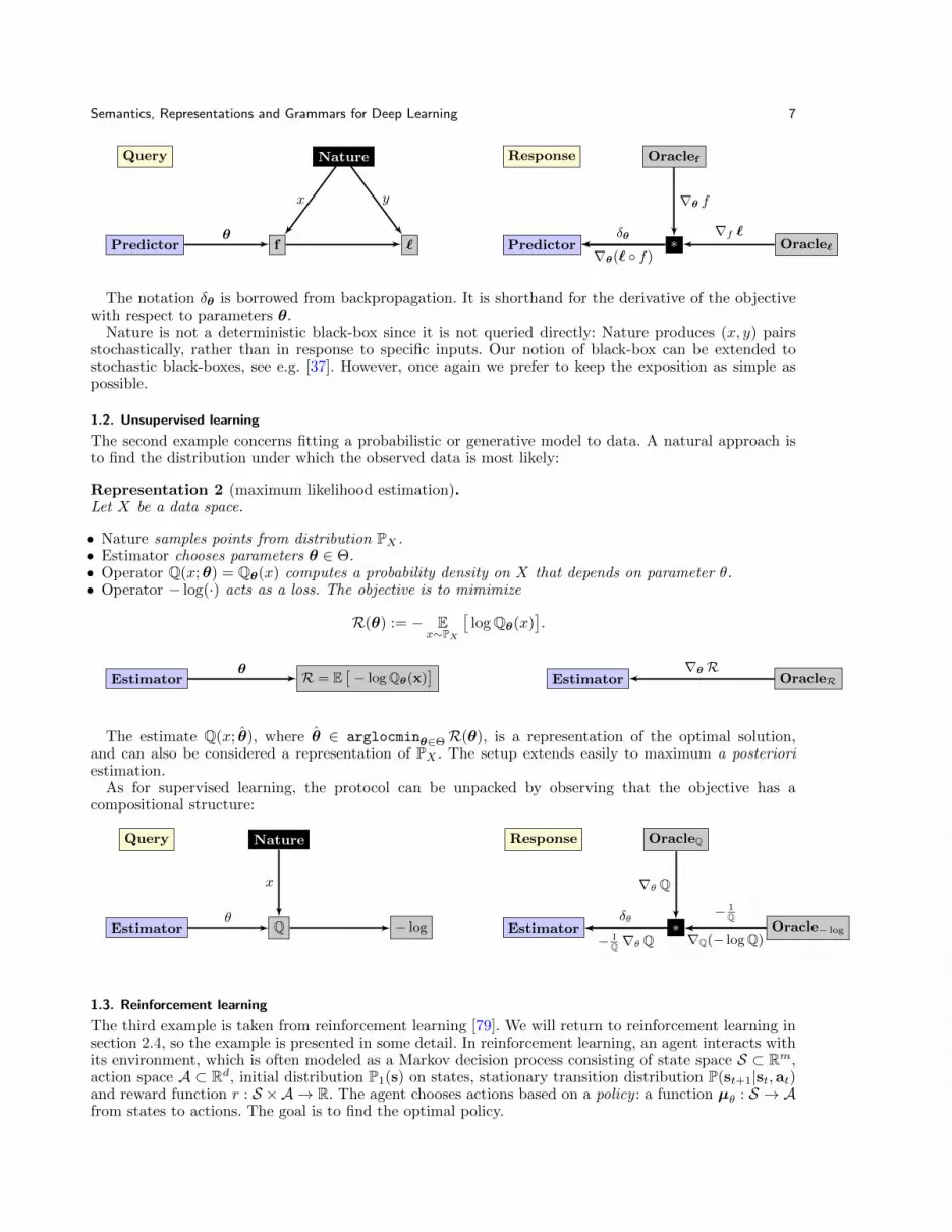
The notation δθ is borrowed from backpropagation. It is shorthand for the derivative of the objectivewith respect to parameters θ.

Nature is not a deterministic black-box since it is not queried directly: Nature produces (x, y) pairsstochastically, rather than in response to specific inputs. Our notion of black-box can be extended tostochastic black-boxes, see e.g. [37]. However, once again we prefer to keep the exposition as simple aspossible.

1.2. Unsupervised learning

The second example concerns fitting a probabilistic or generative model to data. A natural approach isto find the distribution under which the observed data is most likely:

Representation 2 (maximum likelihood estimation).Let X be a data space.

• Nature samples points from distribution PX .• Estimator chooses parameters θ ∈ Θ.• Operator Q(x;θ) = Qθ(x) computes a probability density on X that depends on parameter θ.• Operator − log(·) acts as a loss. The objective is to mimimize

R(θ) := − Ex∼PX

[logQθ(x)

].

Estimator R = E[− logQθ(x)

]θEstimator OracleR

∇θR

The estimate Q(x; θ), where θ ∈ arglocminθ∈ΘR(θ), is a representation of the optimal solution,and can also be considered a representation of PX . The setup extends easily to maximum a posterioriestimation.

As for supervised learning, the protocol can be unpacked by observing that the objective has acompositional structure:

Query Nature

Estimator Q − log

x

θ

Response

Estimator Oracle− log

OracleQ

∗− 1

Q

∇Q(− logQ)

∇θ Q

− 1Q ∇θ Q

δθ

1.3. Reinforcement learning

The third example is taken from reinforcement learning [79]. We will return to reinforcement learning insection 2.4, so the example is presented in some detail. In reinforcement learning, an agent interacts withits environment, which is often modeled as a Markov decision process consisting of state space S ⊂ Rm,action space A ⊂ Rd, initial distribution P1(s) on states, stationary transition distribution P(st+1|st,at)and reward function r : S ×A → R. The agent chooses actions based on a policy : a function µθ : S → Afrom states to actions. The goal is to find the optimal policy.

8 Balduzzi

Actor-critic methods break up the problem into two pieces [80]. The critic estimates the expected valueof state-action pairs given the current policy, and the actor attempts to find the optimal policy using theestimates provided by the critic. The critic is typically trained via temporal difference methods [81,82].

Let Pt(s → s′,µ) denote the distribution on states s′ at time t given policy µ and initial state s att = 0 and let ρµ(s′) =

∫S∑∞t=0 γ

tP1(s)Pt(s → s′,µ)ds. Let rγt =∑∞τ=t γ

τ−tr(sτ ,aτ ) be the discountedfuture reward. Define the value of a state-action pair as

Qµ(s,a) = E[rγ1 |S1 = s,A1 = a;µ].

Unfortunately, the value-function Qµ(s,a) cannot be queried. Instead, temporal difference methods takea bootstrapped approach by minimizing the Bellman error:

`BE(v) = E(s,a)∼(ρµ,µ)

[(r(s,a) + γQv(s′,µ(s′))−Qv(s,a)

)2]where s′ is the state subsequent to s.

Representation 3 (temporal difference learning).Critic interacts with black-boxes Actor and Nature.2

• Critic plays parameters v.• Operator Q and `BE estimates the value function and compute the Bellman error. In practice, it turns

out to clone the value-estimate periodically and compute a slightly modified Bellman error:

`BE(v) = E(s,a)∼(ρµ,µ)

[(r(s,a) + γQv(s′,µ(s′))−Qv(s,a)

)2]where Qv is the cloned estimate. Cloning improves the stability of TD-learning [4]. A nice conceptualside-effect of cloning is that TD-learning reduces to gradient descent.

Query NatureActor

Critic Q `BE

s

W

ra

Response

Critic Oracle`BE

OracleQ

∗∇Q `BE

∇WQ

δW

The estimate is a representation of the true value function.

Remark 2 (on temporal difference learning as first-order method).Temporal difference learning is not strictly speaking a gradient-based method [82]. The residual gradientmethod performs gradient descent on the Bellman error, but suffers from double sampling [83]. Projectedfixpoint methods minimize the projected Bellman error via gradient descent and have nice convergenceproperties [84–86]. An interesting recent proposal is implicit TD learning [87], which is based on implicitgradient descent [88].

Section 2.4 presents the Deviator-Actor-Critic model which simultaneously learns a value-functionestimate and a locally optimal policy.

2. PROTOCOLS AND GRAMMARS

It is often useful to decompose complex problems into simpler subtasks that can handled by specializedmodules. Examples include variational autoencoders, generative adversarial networks and actor-criticmodels. Neural networks are particularly well-adapted to modular designs, since units, layers and evenentire networks can easily be combined analogously to bricks of lego [49].

However, not all configurations are viable models. A methodology is required to distinguish gooddesigns from bad. This section provides a basic language to describe how bricks are glued together thatmay be a useful design tool. The idea is to extend the definitions of optimization problems, protocols andrepresentations from section 1 from single to multi-player optimization problems.

2Nature’s outputs depend on Actor’s actions, so the Query graph should technically have an additional arrow from Actorto Nature.


Definition 5 (game).A distributed optimization problem or game

([N ],Θ, `) is a set [N ] = 1, . . . N of players, a

parameter space Θ =∏Ni=1 Θi, and loss vector ` = (`1, . . . , `N ) : Θ → RN . Player i picks moves from

Θi ⊂ Rdi and incurs loss determined by `i : Θ→ R. The goal of each player is to minimize its loss, whichdepends on the moves of the other players.

The classic example is a finite game [30], where player i has a menu of di-actions and chooses a

distribution over actions, θi ∈ Θi = 4di = (θ1, . . . , θdi) :∑dij=1 θj = 1 and θj ≥ 0 on each round.

Losses are specified for individual actions, and extended linearly to distributions over actions. A naturalgeneralization of finite games is convex games where the parameter spaces are compact convex sets andeach loss `i is a convex function in its ith-argument [89]. It has been shown that players implementingno-regret algorithms are guaranteed to converge to a correlated equilibrium in convex games [89–91].

The notion of game in Definition 5 is too general for our purposes. Additional structure is required.

Definition 6 (computation graph).A computation graph is a directed acyclic graph with two kinds of nodes:

• Inputs are set externally (in practice by Players or Oracles).• Operators produce outputs that are a fixed function of their parents’ outputs.

Computation graphs are a useful tool for calculating derivatives [32–36]. For simplicity, we restrict todeterministic computation graphs. More general stochastic computation graphs are studied in [37].

A distributed communication protocol extends the communication protocol in Definition 3 to multi-player games using two computation graphs.

Definition 7 (distributed communication protocol).A distributed communication protocol is a game where each round has two phases, determined bytwo computation graphs:

• Query phase. Players provide inputs to the Query graph (Q) that Operators transform into outputs.• Response phase. Operators in Q act as Oracles in the Response graph (R): they input subgradients that

are transformed and communicated to the Players.

The moves chosen by Players depend only on their prior moves and the information communicated tothem by the Response graph.

The protocol specifies how Players and Oracles communicate without specifying the optimization al-gorithms used by the Players. The addition of a Response graph allows more general computations thansimply backpropagating the gradients of the Query phase. The additional flexibility allows the designof new algorithms, see sections 2.4 and 2.5 below. It is also sometimes necessary for computational rea-sons. For example, backpropagation through time on recurrent networks typically runs over a truncatedResponse graph [40–42].

Suppose that we wish to optimize an objective function R : Θ → R that depends on all the moves ofall the players. Finding a global optimum is clearly not feasible. However, we may be able to constructa protocol such that the players are jointly able to find local optima of the objective. In such cases, werefer to the protocol as a grammar:

Definition 8 (grammar).A grammar for objective R : Θ→ R is a distributed communication protocol where the Response graphprovides sufficient first-order information to find a local optimum of (R,Θ).

The guarantee ensures that the representations constructed by Players in a grammar can be combinedinto a coherent distributed representation. That is, it ensures that the representations constructed by thePlayers transform data in a way that is useful for optimizing the shared objective R.

The Players’ losses need not be explicitly computed. All that is necessary is that the Response phasecommunicate the gradient information needed for Players to locally minimize their losses – and that doingso yields a local optimum of the objective.

Basic building blocks: function composition (Q) and the chain rule (R). Functions can be insertedinto grammars as lego-like building blocks via function composition during queries and the chain ruleduring responses. Let G(θ, F ) be a function that takes inputs θ and F , provided by a Player and by

10 Balduzzi

upstream computations respectively. The output of G is communicated downstream in the Query phase:

Query Player

GF

θ

G

Response Player

∗

OracleG

(∇θ G) · δG δθ

δF

(∇F G) · δG

δG

∇θ,F G

The chain rule is implemented in the Response phase as follows. OracleG reports the gradient∇θ,F G :=(∇θ G,∇F G) in the Response phase. Operator “∗” computes the products (∇θ G · δG,∇F G · δG) viamatrix multiplication. The projection of the product onto the first and second components3 are reportedto Player and upstream respectively.

Summary of guarantees. A selection of examples are presented below. Guarantees fall under the followingbroad categories:

1. Exact gradients.Under error backpropagation the Response graph implements the chain rule, which guarantees thatPlayers receive the gradients of their loss functions; see section 2.1.

2. Surrogate objectives.The variational autoencoder uses a surrogate objective: the variational lower bound. Maximizing thesurrogate is guaranteed to also maximize the true objective, which is computational intractable; seesection 2.2.

3. Learned objectives.In the case of generative adversarial network and the DAC-model, some of the players learn a loss thatis guaranteed to align with the true objective, which is unknown; see sections 2.3 and 2.4.

4. Estimated gradient.In the DAC-model and kickback, gradient estimates are substituted for the true gradient; see sec-tions 2.4 and 2.5. Guarantees are provided on the estimates.

Remark 3 (fine- and coarse-graining).There is considerable freedom regarding the choice of players. In the examples below, players are typicallychosen to be layers or entire neural networks to keep the diagrams simple. It is worth noting that zoomingin, such that players correspond to individual units, has proven to be a useful tool when analyzing neuralnetworks [20, 45, 46].

The game-theoretic formulation is thus scale-free and can be coarse- or fine-grained as required. Amathematical language for tracking the structure of hierarchical systems at different scales is providedby operads, see [92] and the references therein, which are the natural setting to study the composition ofoperators that receive multiple inputs.

2.1. Error backpropagation

The main example of a grammar is a neural network using error backpropagation to perform supervisedlearning. Layers in the network can be modeled as players in a game. Setting each (p)layer’s objective asthe network’s loss, which it minimizes using gradient ascent, yields backpropagation.

Grammar 1 (backpropagation).An L-layer neural network can be reformulated as a game played between L + 1 players, correspondingto Nature and the Layers of the network. The query graph for a 3-layer network is:

3Alternatively, to avoid having “∗” produce two outputs, the entire vector can be reported in both direction with theirrelevant components ignored.


Query

Nature

Layer1 Layer2 Layer3 Nature

S1 S2 S3 `

θ1 θ2 θ3 y

x S1 S2 S3

• Nature plays samples datapoints (x, y) i.i.d. from PX×Y and acts as the zeroth player.• Layeri plays weight matrices θi.• Operators compute Si(θi, Si−1) := Si(θi · Si−1) for each layer, along with loss `(SL, y).

The response graph performs error backpropagation:

Response

Oracle1 Oracle2 Oracle3

Oracle`∗ ∗ ∗

Layer1 Layer2 Layer3

∇θ1 S1 ∇θ2,S1 S2 ∇θ3,S2 S3

∇S3 `

δS3δS1

(∇S1 S2) · δ2

δS2

(∇S2 S3) · δ3

(∇θ1 S1) · δS1 δθ1 (∇θ2 S2) · δS2 δθ2 (∇θ3 S3) · δS3 δθ3

The protocol can be extended to convolutional networks by replacing the matrix multiplications performedby each operator, Si(θi · Si−1), with convolutions and adding parameterless max-pooling operators [93].

Guarantee. The loss of every (p)layer is

`(θ, x, y) = `y SθL · · · Sθ1(x) where `y(•) := `(•, y) where Sθi(•) := Si(θi · •).

It follows by the chain rule that R communicates ∇θi ` to player i. 2

Representation learning. We are now in a position to relate the notion of representation in definition 4with the standard notion of representation learning in neural networks. In the terminology of section 1,each player learns a representation. The representations learned by the different players form a coherentdistributed representation because they jointly optimize a single objective function.

Abstractly, the objective can be written as

R(θ1, . . . ,θL) = E(x,y)∼PXY

[`(S(θ1, . . . ,θL, x), y

)],

where S(θ1, . . . ,θL, x) = SθL · · · Sθ1

(x). The goal is to minimize the composite objective.

If we set θ1:L ∈ arglocmin(θ1,...,θL)∈ΘR(θ1, . . . ,θL) then the function Sθ1:L: X → Y fits the definition

of representation above. Moreover, the compositional structure of the network implies that Sθ1:Lis com-

posed of subrepresentations corresponding to the optimizations performed by the different players in the

grammar: each function Sθj(•) is a local optimum – where θj ∈ arglocminθj∈Θj

R(θ1, . . . ,θj , . . . , θL)

is optimized to transform its inputs into a form that is useful to network as a whole.

Detailed analysis of convergence rates. Little can be said in general about the rate of converge of thelayers in a neural network since the loss is not convex. However, neural networks can be decomposedfurther by treating the individual units as players. When the units are linear or rectilinear, it turns outthat the network is a circadian game. The circadian structure provides a way to convert results about theconvergence of convex optimization methods into results about the global convergence a rectifier networkto a local optimum, see [20].

12 Balduzzi

2.2. Variational autoencoders

The next example extends the unsupervised setting described in section 1.2. Suppose that observationsx(i)Ni=1 are sampled i.i.d. from a two-step stochastic process: a latent value z(i) is sampled from P(z),after which x(i) is sampled from P(x|z(i)).

The goal is to (i) find the maximum likelihood estimator for the observed data and (ii) estimate theposterior distribution on z conditioned on an observation x. A straightforward approach is to maximizethe marginal likelihood

θ∗ := argmaxθ

N∏i=1

Qθ(x(i)), where Qθ(x) =

∫Qθ(x|z)Qθ(z)dz, (1)

and then compute the posterior

Qθ∗(z|x) =Qθ∗(x|z)Qθ∗(z)

Qθ∗(x).

However, the integral in Eq. (1) is typically untractable, so a more roundabout tactic is required. Theapproach proposed in [47] is to construct two neural networks, a decoder Dθ(x|z) that learns a genera-tive model approximating P(x|z), and an encoder Eφ(z|x) that learns a recognition model or posteriorapproximating P(z|x).

It turns out to be useful to replace the encoder with a deterministic function, Gφ(ε,x), and a noisesource, Pnoise(ε) that are compatible. Here, compatible means that sampling z ∼ Eφ(z|x) is equivalentto sampling ε ∼ Pnoise(ε) and computing z := Gφ(ε,x).

Grammar 2 (variational autoencoder).A variational autoencoder is a game played between Encoder, Decoder, Noise and Environment. Thequery graph is

Query Nature

Noise

Encoder Decoder

G D

L2L1 +

φ θx x

ε

Pnoise

• Environment plays i.i.d. samples from P(x)• Noise plays i.i.d. samples from Pnoise(ε). It also communicates its density function Pnoise(ε), which is

analogous to a gradient – and the reason that Noise is gray rather than black-box.• Encoder and Decoder play parameters φ and θ respectively.• Operator z = Gφ(ε,x) is a neural network that encodes samples into latent variables.• Operator Dθ(z,x) is a neural network that estimates the probability of x conditioned on z.• The remaining operators compute the (negative) variational lower bound

L(θ,φ; x) =

∫Pnoise(ε) log

Pnoise(ε)Pprior(Gφ(ε,x))︸︷︷︸L1

+ Eε∼Pnoise(ε)

[− logDθ

(Gφ(ε,x),x

)]︸︷︷︸

L2

.

The response graph implements backpropagation:


Response

OracleG OracleD

OracleL1 OracleL2Oracle+

+ ∗

∗ ∗

∗ Encoder Decoder

∇φG

∇G,θ D

δD

∇D L2∇G L1 1 1

δG

(∇G D) · δD

∇G L1

δφ

(∇θ D) · δD δθ

Guarantee. The guarantee has two components:

1. Maximizing the variational lower bound yields (i) a maximum likelihood estimator and (ii) an estimateof the posterior on the latent variable [47].

2. The chain rule ensures that the correct gradients are communicated to Encoder and Decoder.

The first guarantee is that the surrogate objective computed by the query graph yields good solutions.The second guarantee is that the response graph communicates the correct gradients. 2

2.3. Generative-Adversarial networks

A recent approach to designing generative models is to construct an adversarial game between Forger andCurator [48]. Forger generates samples; Curator aims to discriminate the samples produced by Forgerfrom those produced by Nature. Forger aims to create samples realistic enough to fool Curator.

If Forger plays parameters θ and Curator plays φ then the game is described succinctly via

arglocminθ

arglocmaxφ

[E

x∼P(x)

[logDφ(x)

]+ Eε∼Pnoise(ε)

[log(1−Dφ(Gθ(ε)))

]],

where Gθ(ε) is a neural network that converts noise in samples and Dφ(x) classifies samples as fake ornot.

Grammar 3 (generative adversarial networks).Construct a game played between Forger and Curator, with ancillary players Noise and Environment:

• Environment samples images i.i.d. from P(x).• Noise samples i.i.d. from P(ε).• Forger and Curator play parameters θ and φ respectively.• Operator Gθ(ε) is a neural network that produces fake image x = Gθ(ε).• Operator Dφ(x) is a neural network that estimates the probability that an image is fake.• The remaining operators compute a loss that Curator minimizes and Forger maximizes

L(θ,φ) = Ex∼P(x)

[logDφ(x)

]︸︷︷︸

`disc

+ Eε∼P(ε)

[log(1−Dφ(Gθ(ε))

)]︸︷︷︸

`gen

14 Balduzzi

Query

Noise

NatureForger Curator

G D

D

`disc

`gen +

x

θ φ

φ

ε

Note there are two copies of Operator D in the Query graph. The response graph implements the chainrule, with a tweak that multiplies the gradient communicated to Forger by (−1) to ensure that Forgermaximizes the loss that Curator is minimizing.

Response

Forger

Curator

∗ ∗ ∗

∗∗+

Oracle`gen

Oracle`disc

Oracle+

OracleG OracleD

OracleD

(∇θ G) · δG

δθ

(∇φD) · δgenD

∇φ `disc

δG

−(∇GD) · δgenD ∇G,φD

∇φD

∇θ G ∇D `gen

1

1

δdiscD(∇φD) · δdiscD

∇φ `disc

δgenD

∇D `gen

δφ

Guarantee. For a fixed Forger that produces images with probability PForger(x), the optimal Curatorwould assign

D∗PForger,PNature(x) =

PNature(x)

PNature(x) + PForger(x)(2)

The guarantee has two components:

1. For fixed Forger, the Curator in (2) is the global optimum for L.2. The chain rule ensures the correct gradients are communicated to Curator and Forger.

It follows that the network converges to a local optimum where Curator represents (2) and Forger repre-sents the “ideal Forger” that would best fool Curator. 2

The generative-adversarial network is the first example where the Response graph does not simplybackpropagate gradients: the arrow labeled δG is computed as −(∇GD) · δD, whereas backpropagationwould use (∇GD) · δD. The minus sign arises due to the adversarial relationship between Forger andCurator – they do not optimize the same objective.

2.4. Deviator-Actor-Critic (DAC) model

As discussed in section 1.3, actor-critic algorithms decompose the reinforcement learning problem intotwo components: the critic, which learns an approximate value function that predicts the total discountedfuture reward associated with state-action pairs, and the actor, which searches for a policy that maximizesthe value appoximation provided by the critic. When the action-space is continuous, a natural approachis to follow the gradient [94–96]. In [94], it was shown how to compute the policy gradient given thetrue value function. Furthermore, sufficient conditions were provided for an approximate value functionlearned by the critic to yield an unbiased estimator of the policy gradient. More recently [96] providedanalogous results for deterministic policies.


The next example of a grammar is taken from [46], which builds on the above work by introducing athird algorithm, Deviator, that directly estimates the gradient of the value function estimated by Critic.

Grammar 4 (DAC model).Construct a game played by Actor, Critic, Deviator, Noise and Environment:

Query

Actor

Deviator

Critic

Noise

Nature

µ

G

Q

`

θ

W

V

ε

s

s

s

r

• Nature samples states from P(st+1|st,at) and announces rewards r(st,at) that are a function of theprior state and action; Noise samples ε ∼ N(0, σ2 · Id).• Actor, Critic and Deviator play parameters θ, V and W respectively.• Operator µ is a neural network that computes actions a = µθ(s).• Operator QV(s,µθ(s)) is a neural network that estimates the value of state-action pairs.• Operator GW(s,µθ(s)) is a neural network that estimates the gradient of the value function.• The remaining Operator computes the Bellman gradient error (BGE) which Critic and Deviator min-

imize

`BGE(rt, Q, Q,G, ε) =(rt + γQ−Q−

⟨G, ε

⟩)2

.

The response graph backpropagates the gradient of `BGE to Critic and Deviator, and communicates theoutput of Operator G, which is a gradient estimate, to Actor:

Response

Actor

Deviator

CriticOracleµ

OracleGG

OracleQ

Oracle`

∗

∗

∗(∇θ µ) · δµ

δθ

(∇W G) · δG

δW

(∇VQ) · δQ

δV

∇θ µ

∇G `

δG

∇Q `δQ

∇W G

Gδµ

∇VQ

Note that instead of backpropagating first-order information in the form of gradient∇µG, the Responsegraph instead backpropagates zeroth-order information in the form of gradient-estimate G, which is

computed by the Query graph during the feedforward sweep. We therefore write δµ and δθ (instead ofδµ and δθ) to emphasize that the gradients communicated to Actor are estimates.

As in section 1.3, an arrow from Actor to Nature is omitted from the Query graph for simplicity.

Guarantee. The guarantee has the following components:

1. Critic estimates the value function via TD-learning [79] with cloning for improved stability [4].2. Deviator estimates the value gradient via TD-learning and the gradient perturbation trick [46].3. Actor follows the correct gradient by the policy gradient theorem [94,96].4. The internal workings of each neural network are guaranteed correct by the chain rule.

It follows that Critic and Deviator represent the value function and its gradient; and that Actor representsthe optimal policy. 2

16 Balduzzi

Two appealing features of the algorithm are that (i) Actor is insulated from Critic, and only interactswith Deviator and (ii) Critic and Deviator learn different features adapted to representing the valuefunction and its gradient respectively. Previous work used the derivative of the value-function estimate,which is not guaranteed to have compatible function approximation, and can lead to problems when thevalue-function is estimated using functions such as rectifiers that are not smooth [97–99].

2.5. Kickback (truncated backpropagation)

Finally we consider Kickback, a biologically-motivated variant of Backprop with reduced communicationrequirements [45]. The problem that kickback solves is that backprop requires two distinct kinds of signalsto be communicated between units – feedforward and feedback – whereas only one signal type – spikes –are produced by cortical neurons. Kickback computes an estimate of the backpropagated gradient usingthe signals generated during the feedforward sweep. Kickback also requires the gradient of the loss withrespect to the (one-dimensional) output to be broadcast to all units, which is analogous to the role playedby diffuse chemical neuromodulators [100–102].

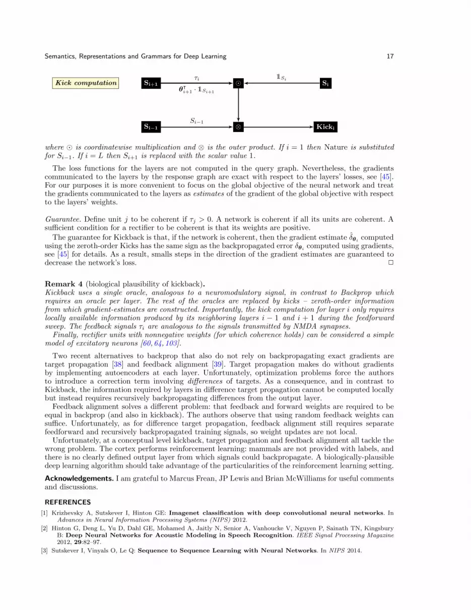
Grammar 5 (kickback).The query graph is the same as for backpropagation, except that the Operator for each layer produces theadditional output τi−1 := θᵀi+1 · 1Si+1 :

Query

Nature

Layer1 Layer2 Layer3 Nature

S1 S2 S3 `

θ1 θ2 θ3 y

S1x S2 S3

θᵀ1 · 1S1 θᵀ2 · 1S2 θᵀ3 · 1S3τ0 τ1 τ2

• Nature samples labeled data (x, y) from PX×Y .• Layers by weight matrices θi. The output of the neural network is required to be one-dimensional• Operators for each layer compute two outputs: Si = max(0,θi · Si−1) and τi−1 = θᵀi · 1Si

where1a = 1 if a ≥ 0 and 0 otherwise.• The task is regression or binary classification with loss given by the mean-squared or logistic error. It

follows that the derivative of the loss with respect to the network’s output β = ∇S3 ` is a scalar.

The response graph contains a single Oracle that broadcasts the gradient of the loss with respect to thenetwork’s output (which is a scalar). Gradient estimates for each Layer are computed using a mixtureof Oracle and local zeroth-order information referred to as Kicks:

Response

Kick1 Kick2 Kick3

Oracle`

∗ ∗ ∗

Layer1 Layer2 Layer3

β = ∇S3 `ββ

δθ1 δθ2 δθ3

Kicki is computed using locally available zeroth-order information as follows


Kick computation

Si−1

SiSi+1

Kicki⊗

Si−1

1Siτi

θᵀi+1 · 1Si+1

where is coordinatewise multiplication and ⊗ is the outer product. If i = 1 then Nature is substitutedfor Si−1. If i = L then Si+1 is replaced with the scalar value 1.

The loss functions for the layers are not computed in the query graph. Nevertheless, the gradientscommunicated to the layers by the response graph are exact with respect to the layers’ losses, see [45].For our purposes it is more convenient to focus on the global objective of the neural network and treatthe gradients communicated to the layers as estimates of the gradient of the global objective with respectto the layers’ weights.

Guarantee. Define unit j to be coherent if τj > 0. A network is coherent if all its units are coherent. Asufficient condition for a rectifier to be coherent is that its weights are positive.

The guarantee for Kickback is that, if the network is coherent, then the gradient estimate δθicomputed

using the zeroth-order Kicks has the same sign as the backpropagated error δθicomputed using gradients,

see [45] for details. As a result, smalls steps in the direction of the gradient estimates are guaranteed todecrease the network’s loss. 2

Remark 4 (biological plausibility of kickback).Kickback uses a single oracle, analogous to a neuromodulatory signal, in contrast to Backprop whichrequires an oracle per layer. The rest of the oracles are replaced by kicks – zeroth-order informationfrom which gradient-estimates are constructed. Importantly, the kick computation for layer i only requireslocally available information produced by its neighboring layers i − 1 and i + 1 during the feedforwardsweep. The feedback signals τi are analogous to the signals transmitted by NMDA synapses.

Finally, rectifier units with nonnegative weights (for which coherence holds) can be considered a simplemodel of excitatory neurons [60, 64, 103].

Two recent alternatives to backprop that also do not rely on backpropagating exact gradients aretarget propagation [38] and feedback alignment [39]. Target propagation makes do without gradientsby implementing autoencoders at each layer. Unfortunately, optimization problems force the authorsto introduce a correction term involving differences of targets. As a consequence, and in contrast toKickback, the information required by layers in difference target propagation cannot be computed locallybut instead requires recursively backpropagating differences from the output layer.

Feedback alignment solves a different problem: that feedback and forward weights are required to beequal in backprop (and also in kickback). The authors observe that using random feedback weights cansuffice. Unfortunately, as for difference target propagation, feedback alignment still requires separatefeedforward and recursively backpropagated training signals, so weight updates are not local.

Unfortunately, at a conceptual level kickback, target propagation and feedback alignment all tackle thewrong problem. The cortex performs reinforcement learning: mammals are not provided with labels, andthere is no clearly defined output layer from which signals could backpropagate. A biologically-plausibledeep learning algorithm should take advantage of the particularities of the reinforcement learning setting.

Acknowledgements. I am grateful to Marcus Frean, JP Lewis and Brian McWilliams for useful commentsand discussions.

REFERENCES

[1] Krizhevsky A, Sutskever I, Hinton GE: Imagenet classification with deep convolutional neural networks. InAdvances in Neural Information Processing Systems (NIPS) 2012.

[2] Hinton G, Deng L, Yu D, Dahl GE, Mohamed A, Jaitly N, Senior A, Vanhoucke V, Nguyen P, Sainath TN, KingsburyB: Deep Neural Networks for Acoustic Modeling in Speech Recognition. IEEE Signal Processing Magazine2012, 29:82–97.

[3] Sutskever I, Vinyals O, Le Q: Sequence to Sequence Learning with Neural Networks. In NIPS 2014.

18 Balduzzi

[4] Mnih V, Kavukcuoglu K, Silver D, Rusu AA, Veness J, Bellemare MG, Graves A, Riedmiller M, Fidjeland AK, OstrovskiG, Petersen S, Beattie C, Sadik A, Antonoglou I, King H, Kumaran D, Wierstra D, Legg S, Hassabis D: Human-levelcontrol through deep reinforcement learning. Nature 2015, 518(7540):529–533.

[5] LeCun Y, Bengio Y, Hinton G: Deep learning. Nature 2015, 521:436–444.

[6] Werbos PJ: Beyond Regression: New Tools for Prediction and Analysis in the Behavioral Sciences. PhDthesis, Harvard 1974.

[7] Rumelhart DE, Hinton GE, Williams RJ: Learning representations by back-propagating errors. Nature 1986,323:533–536.

[8] Rumelhart D, Hinton G, Williams R: Parallel Distributed Processing. Vol I: Foundations. MIT Press 1986.

[9] Schmidhuber J: Deep Learning in Neural Networks: An Overview. Neural Networks 2015, 61:85–117.

[10] Robbins H, Monro S: A stochastic approximation method. Annals of Math Stat 1951, 22(3):400–407.

[11] Nemirovski A, Yudin DB: On Cezari’s convergence of the steepest descent method for approximating saddlepoint of convex-concave functions. Sov. Math. Dokl. 1978, 19.

[12] Nemirovski A: Efficient methods for large-scale convex optimization problems. Ekonomika i MatematicheskieMetody 1979, 15.

[13] Nemirovski A, Juditsky A, Lan G, Shapiro A: Robust stochastic approximation approach to stochastic pro-gramming. SIAM J. Optim. 2009, 19(4):1574–1609.

[14] Zinkevich M: Online Convex Programming and Generalized Infinitesimal Gradient Ascent. In ICML 2003.

[15] Cesa-Bianchi N, Lugosi G: Prediction, Learning and Games. Cambridge University Press 2006.

[16] Bottou L, Bousquet O: The Tradeoffs of Large Scale Learning. In NIPS 2010.

[17] Shalev-Shwartz S: Online Learning and Online Convex Optimization. Foundations and Trends in MachineLearning 2011, 4(2):107–194.

[18] Choromanska A, Henaff M, Mathieu M, Arous GB, LeCun Y: The loss surface of multilayer networks. In AISTATS2014.

[19] Choromanska A, LeCun Y, Arous GB: Open Problem: The landscape of the loss surfaces of multilayer net-works. In COLT 2015.

[20] Balduzzi D: Deep Online Convex Optimization by Putting Forecaster to Sleep. In arXiv:1509.01851 2015.

[21] Hardt M, Recht B, Singer Y: Train faster, generalize better: Stability of stochastic gradient descent. InarXiv:1509.01240 2015.

[22] Gordon GJ: No-regret algorithms in online convex programs. In NIPS 2006.

[23] Bengio Y, Courville A, Vincent P: Representation Learning: A Review and New Perspectives. IEEE Trans.Pattern Analysis and Mach. Intell. 2013, 35(8):1798–1828.

[24] Bengio Y: Deep Learning of Representations: Looking Forward. In Statistical Language and Speech Processing.Edited by Dediu AH, Martın-Vide C, Mitkov R, Truthe B, Springer 2013.

[25] Sra S, Nowozin S, Wright SJ: Optimization for Machine Learning. MIT Press 2012.

[26] Nemirovski AS, Yudin DB: Problem complexity and method efficiency in optimization. Wiley-Interscience 1983.

[27] Agarwal A, Bartlett P, Ravikumar P, Wainwright MJ: Information-theoretic lower bounds on the oracle com-plexity of convex optimization. In NIPS 2009.

[28] Raginsky M, Rakhlin A: Information-Based Complexity, Feedback and Dynamics in Convex Programming.IEEE Trans. Inf. Theory 2011, 57(10):7036–7056.

[29] Arjevani Y, Shalev-Shwartz S, Shamir O: On Lower and Upper Bounds for Smooth and Strongly ConvexOptimization Problems. In arXiv:1503.06833 2015.

[30] von Neumann J, Morgenstern O: Theory of Games and Economic Behavior. Princeton University Press 1944.

[31] Nisan N, Roughgarden T, Tardos E, Vazirani V (Eds): Algorithmic Game Theory, Cambridge University Press 2007.

[32] Griewank A, Walther A: Evaluating derivatives: principles and techniques of algorithmic differentiation. SIAM 2008.

[33] Baydin AG, Pearlmutter BA: Automatic Differentiation of Algorithms for Machine Learning. JMLR: Workshopand Conference Proceedings 2014, ICML 2014 AutoML Workshop:1–7.

[34] Bergstra J, Breuleux O, Bastien F, Lamblin P, Pascanu R, Desjardins G, Turian J, Warde-Farley D, Bengio Y: Theano:A CPU and GPU Math Expression Compiler. In Proc. Python for Scientific Comp. Conf. (SciPy) 2010.

[35] Bastien F, Lamblin P, Pascanu R, Bergstra J, Goodfellow I, Bergeron A, Bouchard N, Bengio Y: Theano: new featuresand speed improvements. In NIPS Workshop: Deep Learning and Unsupervised Feature Learning 2012.

[36] van Merrienboer B, Bahdanau D, Dumoulin V, Serdyuk D, Warde-Farley D, Chorowski J, Bengio Y: Blocks and Fuel:Frameworks for deep learning. In arXiv:1506.00619 2015.

[37] Schulman J, Heess N, Weber T, Abbeel P: Gradient Estimation Using Stochastic Computation Graphs. InNIPS 2015.

[38] Lee DH, Zhang S, Fischer A, Bengio Y: Difference Target Propagation. In ECML PKDD 2015.

[39] Lillicrap TP, Cownden D, Tweed DB, Ackerman CJ: Random feedback weights support learning in deep neuralnetworks. In arXiv:1411.0247 2014.

[40] Elman J: Finding structure in time. Cognitive Science 1990, 14(2):179–211.

[41] Williams RJ, Peng J: An efficient gradient-based algorithm for on-line training of recurrent network tra-jectories. Neural Comp 1990, 2(4):490–501.


[42] Williams RJ, Zipser D: Gradient-Based Learning Algorithms for Recurrent Networks and Their Computa-tional Complexity. In Backpropagation: Theory, Architectures, and Applications. Edited by Chauvin Y, RumelhartD, Lawrence Erlbaum Associates 1995.

[43] Russell S, Norvig P: Artificial Intelligence: A Modern Approach. Prentice Hall, 3rd edition 2009.

[44] Gershman SJ, Horvitz EJ, Tenenbaum J: Computational rationality: A converging paradigm for intelligencein brains, minds, and machines. Science 2015, 349(6245):273–278.

[45] Balduzzi D, Vanchinathan H, Buhmann J: Kickback cuts Backprop’s red-tape: Biologically plausible creditassignment in neural networks. In AAAI 2015.

[46] Balduzzi D, Ghifary M: Compatible Value Gradients for Reinforcement Learning of Continuous Deep Poli-cies. In arXiv:1509.03005 2015.

[47] Kingma DP, Welling M: Auto-Encoding Variational Bayes. In ICLR 2014.

[48] Goodfellow IJ, Pouget-Abadie J, Mirza M, Xu B, Warde-Farley D, Ozair S, Courville A, Bengio Y: Generative Ad-versarial Nets. In NIPS 2014.

[49] Bottou L, Gallinari P: A framework for the cooperation of learning algorithms. In NIPS 1991.

[50] Bottou L: From machine learning to machine reasoning: An essay. Machine Learning 2014, 94:133–149.

[51] Selfridge OG: Pandemonium: a paradigm for learning. In Mechanisation of Thought Processes: Proc SymposiumHeld at the National Physics Laboratory 1958.

[52] Klopf AH: The hedonistic neuron: A theory of memory, learning and intelligence. Washington: Hemi-sphere 1982.

[53] Barto AG: Learning by statistical cooperation of self-interested neuron-like computing elements. HumanNeurobiol 1985, 4:229–256.

[54] Minsky M: The society of mind. Simon and Schuster 1986.

[55] Baum EB: Toward a Model of Intelligence as an Economy of Agents. Machine Learning 1999, 35(155-185).

[56] Kwee I, Hutter M, Schmidhuber J: Market-based reinforcement learning in partially observable worlds. InICANN 2001.

[57] von Bartheld CS, Wang X, Butowt R: Anterograde Axonal Transport, Transcytosis, and Recycling of Neu-rotrophic Factors: The Concept of Trophic Currencies in Neural Networks. Molecular Neurobiology 2001,24.

[58] Seung HS: Learning in Spiking Neural Networks by Reinforcement of Stochastic Synaptic Transmission.Neuron 2003, 40(1063-1073).

[59] Lewis SN, Harris KD: The Neural Market Place: I. General Formalism and Linear Theory. In bioRxiv 2014.

[60] Balduzzi D, Besserve M: Towards a learning-theoretic analysis of spike-timing dependent plasticity. In Ad-vances in Neural Information Processing Systems (NIPS) 2012.

[61] Balduzzi D, Ortega PA, Besserve M: Metabolic cost as an organizing principle for cooperative learning.Advances in Complex Systems 2013, 16(2/3).

[62] Balduzzi D, Tononi G: What can neurons do for their brain? Communicate selectivity with spikes. Theoryin Biosciences 2013, 132:27–39.

[63] Balduzzi D: Randomized co-training: from cortical neurons to machine learning and back again. RandomizedMethods for Machine Learning Workshop, Neural Inf Proc Systems (NIPS) 2013.

[64] Balduzzi D: Cortical prediction markets. In Proc. 13th Int Conf on Autonomous Agents and Multiagent Systems(AAMAS) 2014.

[65] Sutton R, Modayil J, Delp M, Degris T, Pilarski PM, White A, Precup D: Horde: A Scalable Real-time Architec-ture for Learning Knowledge from Unsupervised Motor Interaction. In Proc. 10th Int. Conf. on Aut Agentsand Multiagent Systems (AAMAS) 2011.

[66] Hopcroft JE, Ullman JD: Introduction to automata theory, languages, and computation. Addison-Wesley 1979.

[67] Lay N, Barbu A: Supervised aggregation of classifiers using artificial prediction markets. In 27th InternationalConference on Machine Learning (ICML) 2010.

[68] Abernethy J, Frongillo R: A Collaborative Mechanism for Crowdsourcing Prediction Problems. In Adv inNeural Information Processing Systems (NIPS) 2011.

[69] Storkey A: Machine Learning Markets. In 14th International Conference on Artificial Intelligence & Statistics(AISTATS) 2011.

[70] Parkes DC, Wellman MP: Economic reasoning and artificial intelligence. Science 2015, 349(6245):267–272.

[71] Frongillo R, Reid M: Convergence Analysis of Prediction Markets via Randomized Subspace Descent. InNIPS 2015.

[72] Syrgkanis V, Agarwal A, Luo H, Schapire R: Fast Convergence of Regularized Learning in Games. In NIPS2015.

[73] Pearl J: Probabilistic Reasoning in Intelligent Systems: Networks of Plausible Inference. Morgan Kaufmann 1988.

[74] Kschischang F, Frey BJ, Loeliger HA: Factor graphs and the sum-product algorithm. IEEE Trans. Inf. Theory2001, 47(2):498–519.

[75] Wainwright MJ, Jordan MI: Graphical Models, Exponential Families, and Variational Inference. Foundationsand Trends in Machine Learning 2008, 1(1-2):1–305.

[76] Lewis D: On the Plurality of Worlds. Oxford & New York: Basil Blackwell 1986.

20 Balduzzi

[77] Balduzzi D: Falsification and Future Performance. In Algorithmic Probability and Friends: Bayesian Predictionand Artificial Intelligence, Volume 7070 of LNAI. Edited by Dowe D, Springer 2013:65–78.

[78] Vapnik V: The Nature of Statistical Learning Theory. Springer 1995.

[79] Sutton RS, Barto AG: Reinforcement Learning: An Introduction. MIT Press 1998.

[80] Barto AG, Sutton RS, Anderson CW: Neuronlike Adapative Elements That Can Solve Difficult LearningControl Problems. IEEE Trans. Systems, Man, Cyb 1983, 13(5):834–846.

[81] Sutton R: Learning to predict by the method of temporal differences. Machine Learning 1988, 3:9–44.

[82] Dann C, Neumann G, Peters J: Policy Evaluation with Temporal Differences: A Survey and Comparison.JMLR 2014, 15:809–883.

[83] Baird LC: Residual algorithms: Reinforcement learning with function approximation. In ICML 1995.

[84] Sutton R, Maei HR, Precup D, Bhatnagar S, Silver D, Szepesvari C, Wiewiora E: Fast Gradient-Descent Methodsfor Temporal-Difference Learning with Linear Function Approximation. In ICML 2009.

[85] Sutton R, Szepesvari C, Maei HR: A convergent O(n) algorithm for off-policy temporal-difference learningwith linear function approximation. In Adv in Neural Information Processing Systems (NIPS) 2009.

[86] Maei HR, Szepesvari C, Bhatnagar S, Sutton R: Toward Off-Policy Learning Control with Function Approxi-mation. In ICML 2010.

[87] Tamar A, Toulis P, Mannor S, Airoldi EM: Implicit Temporal Differences. In NIPS workshop on large-scale rein-forcement learning and Markov decision problems 2014.

[88] Toulis P, Rennie J, Airoldi EM: Statistical analysis of stochastic gradient methods for generalized linearmodels. In ICML 2014.

[89] Stoltz G, Lugosi G: Learning correlated equilibria in games with compact sets of strategies. Games andEconomic Behavior 2007, 59:187–208.

[90] Foster DP, Vohra RV: Calibrated Learning and Correlated Equilibrium. Games and Economic Behavior 1997,21:40–55.

[91] Blum A, Mansour Y: From External to Internal Regret. JMLR 2007, 8:1307–1324.

[92] Spivak DI: The operad of wiring diagrams: Formalizing a graphical language for databases, recursion, andplug-and-play circuits. In arXiv:1305.0297 2013.

[93] LeCun Y, Bottou L, Bengio Y, Haffner P: Gradient-based Learning Applied to Document Recognition. Proc.of the IEEE 1998, 86:2278–2324.

[94] Sutton R, McAllester D, Singh S, Mansour Y: Policy gradient methods for reinforcement learning with functionapproximation. In NIPS 1999.

[95] Deisenroth MP, Neumann G, Peters J: A Survey on Policy Search for Robotics. Foundations and Trends inMachine Learning 2011, 2(1-2):1–142.

[96] Silver D, Lever G, Heess N, Degris T, Wierstra D, Riedmiller M: Deterministic Policy Gradient Algorithms. InICML 2014.

[97] Prokhorov DV, Wunsch DC: Adaptive Critic Designs. IEEE Trans. Neur. Net. 1997, 8(5):997–1007.

[98] Hafner R, Riedmiller M: Reinforcement learning in feedback control: Challenges and benchmarks fromtechnical process control. Machine Learning 2011, 84:137–169.

[99] Lillicrap TP, Hunt JJ, Pritzel A, Heess N, Erez T, Tassa Y, Silver D, Wierstra D: Continuous control with deepreinforcement learning. In NIPS 2015.

[100] Schultz W, Dayan P, Montague P: A neural substrate of prediction and reward. Science 1997, 275(1593-1599).

[101] Pawlak V, Wickens JR, Kirkwood A, Kerr JND: Timing is not everything: neuromodulation opens the STDPgate. Front. Syn. Neurosci 2010, 2(146).

[102] Dayan P: Twenty-Five Lessons from Computational Neuromodulation. Neuron 2012, 76:240–256.

[103] Glorot X, Bordes A, Bengio Y: Deep Sparse Rectifier Neural Networks. In Proc. 14th Int Conference on ArtificialIntelligence and Statistics (AISTATS) 2011.

Documents

Semantics, Representations and Grammars for Deep Learning