Embed Size (px)
Citation preview

Discussion Papers in Economics
Department of Economics and Related Studies
University of York
Heslington
York, YO10 5DD
No. 14/26
Semiparametric GEE Analysis in Partially Linear
Single-Index Models for Longitudinal Data
Jia Chen, Degui Li, Hua Liang and Suojin Wang


Semiparametric GEE Analysis in Partially Linear
Single-Index Models for Longitudinal Data
Jia Chen∗ Degui Li† Hua Liang‡ Suojin Wang§
December 1, 2014
Abstract
In this article, we study a partially linear single-index model for longitudinal data under
a general framework which includes both the sparse and dense longitudinal data cases. A
semiparametric estimation method based on the combination of the local linear smoothing
and generalized estimation equations (GEE) is introduced to estimate the two parameter
vectors as well as the unknown link function. Under some mild conditions, we derive the
asymptotic properties of the proposed parametric and nonparametric estimators in different
scenarios, from which we find that the convergence rates and asymptotic variances of the
proposed estimators for sparse longitudinal data would be substantially different from those
for dense longitudinal data. We also discuss the estimation of the covariance (or weight) ma-
trices involved in the semiparametric GEE method. Furthermore, we provide some numerical
studies to illustrate our methodology and theory.
Keywords: GEE, local linear smoothing, longitudinal data, semiparametric estimation,
single-index models.
JEL Classifications: C14, C13, C33
∗Department of Economics and Related Studies, University of York, Heslington, York, YO10 5DD, UK.
Email address: [email protected]†Department of Mathematics, University of York, Heslington, York, YO10 5DD, UK. Email address:
[email protected]‡Department of Statistics, George Washington University, Washington, D.C., 20052, US. Email address:
[email protected]§Department of Statistics, Texas A&M University, College Station, TX, 77843, US. Email address:
1

1. Introduction
Consider a semiparametric partially linear single-index model defined by
Y (t) = Z>(t)β + η(X>(t)θ
)+ e(t), t ∈ T , (1.1)
where T is a bounded time interval, β and θ are two unknown vectors of parameters with
dimensions d and p, respectively, η(·) is an unknown link function, Y (t) is a scalar stochastic
process, Z(t) and X(t) are covariates with dimensions d and p, respectively, and e(t) is
the random error process. For the case of independent and identically distributed (i.i.d.) or
weakly dependent time series data, there has been extensive literature on statistical inference
of model (1.1) since its introduction by Carroll et al. (1997). Several different approaches
have been proposed to estimate the unknown parameters and link function involved, see,
for example, Xia et al. (1999), Yu and Ruppert (2002), Xia and Hardle (2006), Wang et
al. (2010) and Ma and Zhu (2013). The recent paper by Liang et al. (2010) further developed
semiparametric techniques for the variable selection and model specification testing issues
in the context of model (1.1).
In this paper, we are interested in studying the above partially linear single-index model
in the context of longitudinal data which arise frequently in many fields of research, such
as biology, climatology, economics and epidemiology, and thus has attracted considerable
attention in the literature in recent years. Various parametric models and methods have
been studied in depth for longitudinal data; see Diggle et al. (2002) and the references
therein. However, the parametric models may be misspecified in practice, which may lead
to inconsistent estimates and incorrect conclusions being drawn from the longitudinal data.
Hence, to address this issue, in recent years, there has been a large literature on how to relax
the parametric assumptions on the longitudinal data models and many nonparametric and
semiparametric models have thus been investigated; see, for example, Lin and Ying (2001),
Lin and Carroll (2001, 2006), He et al. (2002), Fan and Li (2004), Wang et al. (2005), Wu
and Zhang (2006), Zhang et al. (2009), Li and Hsing (2010), and Jiang and Wang (2011).
Suppose that we have a random sample with n subjects from model (1.1). For the
ith subject, i = 1, . . . , n, the response variable Yi(t) and the covariatesZi(t), Xi(t)
are
collected at random time points tij, j = 1, . . . ,mi, which are distributed in a bounded time
interval T according to the probability density function fT (t). Here mi is the total number
of observations for the ith subject. To accommodate such longitudinal data, model (1.1) is
2

written in the following framework:
Yi(tij) = Z>i (tij)β + η(X>i (tij)θ
)+ ei(tij) (1.2)
for i = 1, . . . , n and j = 1, . . . ,mi. When mi varies across the subjects, the longitudinal data
set under investigation is unbalanced. Several nonparametric and semiparametric models can
be viewed as special cases of model (1.2). For instance, when β = 0, model (1.2) reduces to
the single-index longitudinal data model (Jiang and Wang, 2011; Chen et al., 2013a); when
p = 1 and θ = 1, model (1.2) reduces to the partially linear longitudinal data model (Fan
and Li, 2004). To avoid confusion, we let β0 and θ0 be the true values of the two parameter
vectors. For identifiability reasons, θ0 is assumed to be a unit vector with the first non-
zero element being positive. Furthermore, we allow that there exists certain within-subject
correlation structure for ei(tij), which makes the model assumption more realistic but the
development of estimation methodology more challenging.
To estimate the parameters β0, θ0 as well as the link function η(·) in model (1.2), we
first apply the local linear approximation to the unknown link function, and then introduce
a profile weighted least squares approach to estimate the two parameter vectors based on
the technique of generalized estimation equations (GEE). Under some mild conditions, we
derive the asymptotic properties of the developed parametric and nonparametric estimators
in different scenarios. Our framework is flexible in that mi can either be bounded or tend
to infinity. Thus, both the dense and sparse longitudinal data cases can be included. Dense
longitudinal data means that there exists a sequence of positive numbers Mn such that
minimi ≥Mn, and Mn →∞ as n→∞ (see, for example, Hall et al., 2006; and Zhang and
Chen, 2007), whereas sparse longitudinal data means that there exists a positive constant
M∗ such that maximi ≤ M∗ (see, for example, Yao et al., 2005; Wang et al., 2010). We
show that the convergence rates and asymptotic variances of our semiparametric estimators
in the sparse case are substantially different from those in the dense case. Furthermore,
we show that the proposed semiparametric GEE (SGEE)-based estimators are generally
asymptotically more efficient than the profile unweighted least squares (PULS) estimators,
when the weights in the SGEE method are chosen as the conditional covariance matrix of
the errors given the covariates. We also introduce a semiparametric approach to estimate
the covariance matrices (or weights) involved in the SGEE method, which is based on a
variance-correlation decomposition and consists of two steps: first estimate the conditional
variance function using a robust nonparametric method that accommodates heavy-tailed
3

errors; and second estimate the parameters in the correlation matrix. A simulation study
and a real data analysis are provided to illustrate our methodology and theory.
The rest of the paper is organized as follows. In Section 2, we introduce the SGEE
methodology to estimate β0, θ0 and η(·). Section 3 establishes the large sample theory for
the proposed parametric and nonparametric estimators and gives some related discussions.
Section 4 discusses how to determine the weight matrices in the estimation equations. Section
5 gives some numerical examples to investigate the finite sample performance of the proposed
approach. Section 6 concludes the paper. Technical assumptions are given in Appendix A.
The proofs of the main results are given in Appendix B. Some auxiliary lemmas as well as
their proofs are provided in Appendix C.
2. Estimation methodology
Various semiparametric estimation approaches have been proposed to estimate model
(1.1) in the case of i.i.d. observations (or weakly dependent time series data). See, for ex-
ample, Carroll et al. (1997) and Liang et al. (2010) for the profile likelihood method; Yu
and Ruppert (2002) and Wang et al. (2010) for “remove-one-component” technique using
penalized spline and local linear smoothing, respectively; Xia and Hardle (2006) for the min-
imum average variance estimation approach. However, there is limited literature on partially
linear single-index models for longitudinal data because of the more complicated structures
involved. Recently, Chen et al. (2013b) studied a partially linear single-index longitudinal
data model with individual effects. To remove the individual effects and derive consistent
semiparametric estimators, they had to limit their discussions to the dense and balanced
longitudinal data case. Ma et al. (2013) considered a partially linear single-index longitudi-
nal data model by using polynomial splines to approximate the unknown link function, but
their discussion was limited to the sparse and balanced longitudinal data case. In contrast,
as mentioned in the Introduction, our framework includes both the sparse and dense lon-
gitudinal data cases. Meanwhile, observations are allowed to be collected at irregular and
subject specific time points. All this provides much wider applicability in our framework.
Furthermore, to improve the efficiency of the semiparametric estimation, we develop a new
profile weighted least squares approach to estimate the parameters β0, θ0 as well as the link
function η0(·).
To simplify the presentation, let Yi =(Yi(ti1), . . . , Yi(timi)
)>,Xi =
(Xi(ti1), . . . ,Xi(timi)
)>,
Zi =(Zi(ti1), . . . ,Zi(timi)
)>, ei =
(ei(ti1), . . . , ei(timi)
)>, and η(Xi,θ) =
(η(X>i (ti1)θ
), . . . ,
4

η(X>i (timi)θ
))>. With the above notation, model (1.2) can then be re-written as
Yi = Ziβ0 + η(Xi,θ0) + ei. (2.1)
We further let Y = (Y>1 , . . . ,Y>n )>, Z =
(Z>1 , . . . ,Z
>n
)>, E = (e>1 , . . . , e
>n )>, η(X,θ) =(
η>(X1,θ), . . . ,η>(Xn,θ)
)>. Then, model (2.1) is equivalent to
Y = Zβ0 + η(X,θ0) + E. (2.2)
Our estimation procedure is based on the profile likelihood method, which is commonly
used in semiparametric estimation; see, for example, Fan and Huang (2005) and Fan et
al. (2007). Let Yij = Yi(tij), Zij = Zi(tij), and Xij = Xi(tij). For given β and θ, we can
estimate η(·) and its derivative η′(·) at point u by minimizing the following loss function
Ln(a, b∣∣β,θ) =
n∑i=1
wi
mi∑j=1
[yij − Z>ijβ − a− b(X>ijθ − u)
]2K(X>ijθ − u
h
), (2.3)
where K(·) is a kernel function, h is a bandwidth and wi, i = 1, . . . , n, are some weights.
It is well-known that the local linear smoothing has advantages over the Nadaraya-Watson
kernel method, such as higher asymptotic efficiency, design adaption and automatic boundary
correction (Fan and Gijbels, 1996). As in the existing literature such as Wu and Zhang
(2006), the weights wi can be specified by two schemes: wi = 1/Tn (type 1) and wi = 1/(nmi)
(type 2), where Tn =∑n
i=1 mi. The type 1 weight scheme corresponds to an equal weight
for each observation, while the type 2 scheme corresponds to an equal weight within each
subject. As discussed in Huang et al. (2002) and Wu and Zhang (2006), the type 1 scheme
might be a practical choice if the number of observations is relatively similar across the
subjects, while the type 2 scheme may be appropriate otherwise. As the longitudinal data
under investigation are allowed to be unbalanced, in this paper, we use wi = 1/(nmi), which
was also used by Li and Hsing (2010), and Kim and Zhao (2012). We denote
(η(u∣∣β,θ), η′(u
∣∣β,θ))>
= arg mina,b
Ln(a, b∣∣β,θ). (2.4)
By some elementary calculations (see, for example, Fan and Gijbels, 1996), we have
η(u∣∣β,θ) =
n∑i=1
si(u∣∣θ)(Yi − Ziβ
)(2.5)
5

for given β and θ, where
si(u∣∣θ) = (1, 0)
[ n∑i=1
X>i (u∣∣θ)Ki(u
∣∣θ)Xi(u∣∣θ)]−1
X>i (u∣∣θ)Ki(u
∣∣θ),
Xi(u∣∣θ) =
(Xi1(u
∣∣θ), . . . ,Ximi(u∣∣θ))>, Xij(u
∣∣θ) =(1,X>ijθ − u
)>,
Ki(u∣∣θ) = diag
(wiK
(X>i1θ − uh
), . . . , wiK
(X>imiθ − uh
)).
Based on the profile least squares approach with the first-stage local linear smoothing,
we can construct estimators of the parameters β0 and θ0. We start with the PLUS (pro-
file unweighted least squares) method which ignores the possible within-subject correlation
structure. Define the loss function by
Qn0(β,θ) =n∑i=1
[Yi − Ziβ − η(Xi|β,θ)
]>[Yi − Ziβ − η(Xi|β,θ)
]=
[Y− Zβ − η(X|β,θ)
]>[Y− Zβ − η(X|β,θ)
], (2.6)
where, for given β and θ, η(Xi|β,θ) and η(X|β,θ) are the local linear estimators of the
vectors η(Xi,θ) and η(X,θ), respectively. The PULS estimators of β0 and θ0 are obtained
by minimizing Qn0(β,θ), and we denote them by β and θ, respectively.
Although it is easy to verify that both β and θ are consistent, they are not efficient as
the within-subject correlation structure is not taken into account. Hence, to improve the
efficiency of the parametric estimators, we next introduce a GEE-based method to estimate
the parameters β0 and θ0. Existing literature on GEE-based method in longitudinal data
analysis includes Liang and Zeger (1986), Xie and Yang (2003) and Wang (2011). Let
W = diagW1, . . . ,Wn, where Wi = R−1i and Ri is an mi×mi working covariance matrix
whose estimation will be discussed in Section 4. Define
ρZ(Xi,θ) =(ρZ(X>i1θ|θ), . . . , ρZ(X>imiθ|θ)
)>, ρZ(u|θ) = E
[Zij|X>ijθ = u
],
ρX(Xi,θ) =(ρX(X>i1θ|θ), . . . , ρX(X>imiθ|θ)
)>, ρX(u|θ) = E
[Xij|X>ijθ = u
],
Λi(θ) =(Zi − ρZ(Xi,θ),
[η′(Xi,θ)⊗ 1>p
][Xi − ρX(Xi,θ)
]),
where η′(Xi,θ) is a column vector with its elements being the derivatives of η(·) at points
X>ijθ, j = 1, . . . , mi, 1p is a p-dimensional vector of ones, ⊗ is the Kronecker product, and
denotes the componentwise product. The construction of the parametric estimators is
based on the following equation:
n∑i=1
Λ>i (θ)Wi
[Yi − Ziβ − η(Xi|β,θ)
]= 0, (2.7)
6

where Λi(θ) is an estimator of Λi(θ) with ρZ(Xi,θ), ρX(Xi,θ), and η′(Xi,θ) replaced
by their corresponding local linear estimated values. Let β and θ be the solutions to the
weighted estimation equations defined in (2.7). Corollary 3.1 below shows that the SGEE-
based estimators β and θ are generally asymptotically more efficient than the PULS esti-
mators β and θ, when the weights are chosen appropriately.
Replacing β and θ in η(·) by β and θ, respectively, we obtain the local linear estimator
of the link function η(·) at u by
η(u) = η(u|β, θ) =n∑i=1
si(u∣∣θ)(Yi − Ziβ
). (2.8)
In Section 3 below, we will give the large sample properties of the estimators proposed
above, and in Section 4, we will discuss how to choose the working covariance matrix Ri.
3. Theoretical properties
Before establishing the large sample theory for the proposed parametric and nonpara-
metric estimators, we introduce some notations. Let Λi = Λi(θ0), and assume that there
exist two positive definite matrices Ω0 and Ω1 as well as a sequence ωn such that ωn →∞,
1
ωn
n∑i=1
Λ>i WiΛiP→ Ω0, (3.1)
1
ωn
n∑i=1
E[Λ>i Wieie
>i WiΛi
]→ Ω1, (3.2)
max1≤i≤n
E[Λ>i Wieie
>i WiΛi
]= o(ωn), (3.3)
as n→∞. The conditions (3.2) and (3.3) ensure that the Lindeberg-Feller condition can be
satisfied and thus the classical central limit theorem for independent sequence (Petrov, 1995)
would be applicable. Throughout the paper, we assume that the choice of Wi would not
affect the form of ωn. We first give the asymptotic distribution theory for the SGEE-based
estimators β and θ.
Theorem 3.1. Suppose that Assumptions 1–5 in Appendix A, and (3.1)–(3.3) are satisfied.
Then, we have
ω1/2n
β − β0
θ − θ0
d−→ N(0,Ω+
0 Ω1Ω+0
)(3.4)
as n→∞, where A+ is the Moore-Penrose inverse matrix of A.
7

Remark 3.1. Theorem 3.1 establishes the asymptotically normal distribution theory for β
and θ with convergence rate ω1/2n , which is usually with the same asymptotic order as T
1/2n
(Tn is the total number of observations). The specific forms of ωn, Ω0 and Ω1 can be derived
for some particular cases. For instance, when longitudinal data is balanced, i.e., mi ≡ m,
ωn = nm. Furthermore, if E[e2ij] ≡ σ2
e , and Wi, i = 1, . . . , n, are m ×m identity matrices
(i.e., eij are i.i.d.), where eij = ei(tij) is independent of the covariates, then we can show
that
Ω0 =
Ω0(1) Ω0(2)
Ω>0 (2) Ω0(3)
and Ω1 = σ2e
Ω0(1) Ω0(2)
Ω>0 (2) Ω0(3)
,
where
Ω0(1) = E[
Z(t)− ρZ(X(t)>θ0|θ0)][
Z(t)− ρZ(X(t)>θ0|θ0)]>
,
Ω0(2) = Eη′(X(t)>θ0)
[Z(t)− ρZ(X(t)>θ0|θ0)
][X(t)− ρX(X(t)>θ0|θ0)
]>,
Ω0(3) = E[η′(X(t)>θ0)
]2[X(t)− ρX(X(t)>θ0|θ0)
][X(t)− ρX(X(t)>θ0|θ0)
]>.
Hence, Ω+0 Ω1Ω
+0 reduces to σ2
eΩ+0 .
In Theorem 3.1 above, we only require n → ∞. Thus, both the sparse and dense
longitudinal data cases can be included in a unified framework. For the sparse longitudinal
data case whenmi is bounded by certain positive constant, we can take ωn = n and prove that
(3.4) still holds. For the dense longitudinal data case where minimi ≥ Mn with Mn → ∞,
we assume that there exists v(·) such that
v(mi)→∞,Λ>i WiΛi
v(mi)
P→ Ω0 andE[Λ>i Wieie
>i WiΛi
]v(mi)
→ Ω1, as mi →∞.
Letting ωn =∑n
i=1 v(mi), we can prove (3.4). As more observations are available in the
dense longitudinal data case, the convergence rate for the parametric estimators is faster
than OP (√n) in the sparse longitudinal data case.
The following corollary shows that the SGEE-based estimators β and θ are generally
asymptotically more efficient than the PULS estimators β and θ when the weights Wi in
(2.7) are chosen as the inverse of the conditional covariance matrix of ei given Xi and Zi.
Corollary 3.1. Suppose that the weights Wi in (2.7) are chosen as the inverse of the
conditional covariance matrix of ei given Xi and Zi, and the conditions of Theorem 3.1
are satisfied. Then, the SGEE-based estimators β and θ are generally asymptotically more
8

efficient than the PULS estimators β and θ which minimize Qn0(β,θ) in (2.6) with respect
to β and θ.
To establish the asymptotic distribution theory for the nonparametric estimator η(u)
under a unified framework, we assume that there exist a sequence ϕn(h) and a constant
0 < σ2∗ <∞ such that
ϕn(h) = o(ωn), ϕn(h) max1≤i≤n
E[si(u|θ0)eie
>i s>i (u|θ0)
]= o(1), (3.5)
and
ϕn(h)n∑i=1
E[si(u|θ0)eie
>i s>i (u|θ0)
]→ σ2
∗ . (3.6)
The first restriction in (3.5) is imposed to ensure that the parametric convergence rates are
faster than the nonparametric convergence rates, and the second restriction in (3.5) and the
condition in (3.6) are imposed for the derivation of the asymptotic variance of the local linear
estimator η(u) and the satisfaction of the Lindeberg-Feller condition. The specific forms of
ϕn(h) and σ2∗ will be discussed in Remark 3.2 below. Let µj =
∫vjK(v)dv for j = 0, 1, 2, · · · ,
and η′′0(·) be the second-order derivative of η0(·).
Theorem 3.2. Suppose that the conditions of Theorem 3.1, (3.5) and (3.6) are satisfied.
Then, we have
ϕ1/2n (h)
[η(u)− η0(u)− bη(u)h2
] d−→ N(0, σ2∗), (3.7)
where bη(u) = η′′0(u)µ2/2.
Remark 3.2. Theorem 3.2 provides the asymptotically normal distribution theory for the
nonparametric estimator η(u) with convergence rate ϕ1/2n (h). The forms of ϕn(h) and σ2
∗ can
be specified for some particular cases. As an example, consider the case where eij = vi + εij,
in which εij are i.i.d. across both i and j with E[εij] = 0 and E[ε2ij] = σ2
ε , and vi is an i.i.d.
sequence of random variables with E[vi] = 0 and E[v2i ] = σ2
v and is independent of εij. In
this case, we note that
E[ mi∑
j=1
K(X>ijθ0 − u
h
)eij]2
= E[ mi∑
j=1
K(X>ijθ0 − u
h
)(vi + εij)
]2=
mi∑j=1
E[K2(X>ijθ0 − u
h
)(vi + εij)
2]
+∑j1 6=j2
E[K(X>ij1θ0 − u
h
)×K
(X>ij2θ0 − uh
)(vi + εij1)(vi + εij2)
]= mihν0fθ0(u)(σ2
v + σ2ε) +mi(mi − 1)h2µ2
0f2θ0
(u)σ2v ,
9

where νj =∫vjK2(v)dv, j = 0, 1, 2, and fθ0(·) is the probability density function of X>ijθ0.
For the sparse longitudinal data case, mi(mi−1)h2µ20f
2θ0
(u)σ2v is dominated bymihν0fθ0(u)
(σ2v + σ2
ε) as mi is bounded and h→ 0. Then, by Lemma C.1 in Appendix C and some ele-
mentary calculations, we can prove that
n∑i=1
E[si(u|θ0)eie
>i s>i (u|θ0)
]=
1
(nh)2
n∑i=1
mihν0fθ0(u)(σ2v + σ2
ε)
m2i
=ν0fθ0(u)(σ2
v + σ2ε)
n2h
n∑i=1
1
mi
. (3.8)
Hence, in this case, we can take ϕn(h) = (n2h)(∑n
i=11mi
)−1
which has the same order as
nh, and σ2∗ = ν0fθ0(u)(σ2
v + σ2ε). Such result is similar to Theorem 1 (i) in Kim and Zhao
(2012).
For the dense longitudinal data case, mihν0fθ0(u)(σ2v + σ2
ε) is dominated by mi(mi −1)h2µ2
0f2θ0
(u)σ2v if we assume that mih→∞. Then, by Lemma C.1 again, we can prove that
n∑i=1
E[si(u|θ0)eie
>i s>i (u|θ0)
]=
1
(nh)2
n∑i=1
mi(mi − 1)h2µ20f
2θ0
(u)σ2v
m2i
=µ2
0f2θ0
(u)σ2v
n.
Hence, in this case, we can take ϕn(h) = n and σ2∗ = µ2
0f2θ0
(u)σ2v , which are analogous
to Theorem 1 (ii) in Kim and Zhao (2012) and quite different from those in the sparse
longitudinal data case.
4. Estimation of covariance matrices
Estimation of the weight or working covariance matrices which are involved in the SGEE
(2.7) is critical to improving the efficiency of the proposed semiparametric estimators. How-
ever, the unbalanced longitudinal data structure, which can be either sparse or dense, makes
such covariance matrix estimation very challenging, and some existing estimation methods
based on balanced data (such as Wang, 2011) cannot be directly used here. In this sec-
tion, we introduce a semiparametric estimation approach that is applicable to unbalanced
longitudinal data. This approach is based on a variance-correlation decomposition, and
the estimation of the working covariance matrices then consists of two steps: first estimate
the conditional variance function using a robust nonparametric method that accommodates
heavy-tailed errors; and second estimate the parameters in the correlation matrix.
For each 1 ≤ i ≤ n, let Ri be the covariance matrix of ei, Σi = diagσ2(ti1), . . . , σ2(timi)
with σ2(tij) = E
[e2i (tij)
∣∣tij] = E[e2i (tij)
∣∣tij,Xi(tij),Zi(tij)]
for j = 1, . . . ,mi, and Ci be the
10

correlation matrix of ei. Assume that there exists a q-dimensional parameter vector φ such
that Ci = Ci(φ) where Ci(·), 1 ≤ i ≤ n, are pre-specified. By the variance-correlation
decomposition, we have
Ri = Σ1/2i Ci(φ)Σ
1/2i . (4.1)
We first estimate the conditional variance function σ2(·) in the diagonal matrix Σi by
using a nonparametric method. In recent years, there has been a rich literature on the study
of nonparametric conditional variance estimation; see, for example, Ruppert et al. (1997),
Fan and Yao (1998), Yu and Jones (2004) and Fan et al. (2007). However, when the errors
are heavy-tailed, which is not uncommon is economic and financial data analysis, most of
these existing methods may not perform well. This motivates us to devise an estimation
method that is robust to heavy-tailed errors. Let r(tij) =[Yij − Z>ijβ0 − η(X>ijθ0)
]2, where
Yij = Yi(tij), Zij = Zi(tij), and Xij = Xi(tij). We can then find random variable ξ(tij) so
that r(tij) = σ2(tij)ξ2(tij) and E
[ξ2(tij)|tij
]= 1 with probability 1. By applying the log-
transformation (see Peng and Yao, 2003; Gao, 2007; and Chen et al., 2009 for the application
of this transformation in time series analysis) to r(tij), we have
log r(tij) = log[τσ2(tij)
]+ log
[τ−1ξ2(tij)
]≡ σ2
(tij) + ξ(tij), (4.2)
where τ is a positive constant such that E[ξ(tij)] = E
log[τ−1ξ2(tij)
]= 0. Here, ξ(tij)
could be viewed as an error term in the model (4.2). As rij = r(tij) are unobservable, we
replace them with rij =[Yij − Z>ijβ − η(X>ijθ)
]2. To estimate σ2
(t), we define
Ln(a, b)
=n∑i=1
wi
mi∑j=1
[log(rij + ζn)− a− b(tij − t)
]2K1
(tij − th1
), (4.3)
where K1(·) is a kernel function, h1 is a bandwidth satisfying Assumption 9 in Appendix
A, wi = 1/(nmi) as in Section 2, and ζn → 0 as n → ∞. Throughout this paper, we set
ζn = 1/Tn, where Tn =∑n
i=1mi. The ζn is added in log(rij + ζn) to avoid the occurrence
of invalid log 0 as ζn > 0 for any n. Such a modification would not affect the asymptotic
distribution of the conditional variance estimation under certain mild restrictions. Then
σ2(t) can be estimated by
σ2(t) = a, where (a, b)> = arg min
a,bLn(a, b). (4.4)
On the other hand, noting that
expσ2(tij)
τ
ξ2(tij) = rij and E[ξ2(tij)] = 1,
11

the constant τ can be estimated by
τ =[ 1
Tn
n∑i=1
mi∑j=1
rij exp−σ2(tij)
]−1
. (4.5)
We then estimate σ2(t) by
σ2(t) =expσ2
(t)τ
. (4.6)
It is easy to see that thus defined estimator σ2(t) is always positive.
Suppose that there exist a sequence ϕn(h1) which depends on h1, and a constant 0 <
σ2 <∞ such that
ϕn(h1) = o(ωn),ϕn(h1)
h21
max1≤i≤n
w2iE[ mi∑j=1
ξ(tij)K1
(tij − th1
)]2= o(1) (4.7)
andϕn(h1)
h21
E[ n∑i=1
wi
mi∑j=1
ξ(tij)K1
(tij − th1
)]2 → σ2, (4.8)
which are similar to those in (3.5) and (3.6). Define
bσ1(t) =expσ2
(t)2τ
σ2(t)
∫v2K1(v)dv,
bσ2(t) =expσ2
(t)2τ
E[σ2(tij)]
∫v2K1(v)dv,
where σ2(·) is the second-order derivative of σ2
(·). We then establish the asymptotic distri-
bution of σ2(t) in the following theorem, whose proof is given in Appendix C.
Theorem 4.1. Suppose the conditions in Theorems 3.1 and 3.2, Assumptions 6–9 in Ap-
pendix A, (4.7) and (4.8) are satisfied. Then, we have
ϕ1/2n (h1)
σ2(t)− σ2(t)− [bσ1(t)− bσ2(t)]h2
1
d−→ N
(0,σ4(t)
fT (t)σ2), (4.9)
where fT (·) is the density function of the observation times tij.
Remark 4.1. Theorem 4.1 can be seen as an extension of Theorem 1 in Chen et al. (2009)
from the time series case to the longitudinal data case. The longitudinal data framework
in this paper is quite flexible and includes both sparse and dense data types. Following the
discussion in Remark 3.2, we can also show that under some mild conditions, the nonpara-
metric conditional variance estimation would have different convergence rates for the two
data types.
12

We next discuss how to obtain the optimal value of the parameter vector φ. Let Σi be
the estimator of Σi with σ2(tij) being replaced by σ2(tij) which was defined in (4.6) and
R∗i (φ) = Σ1/2
i Ci(φ)Σ1/2
i . Recall that β and θ are the estimated values of the parameters
β0 and θ0, respectively, by taking Wi as the identity matrix in the estimation equations,
and that they are consistent. With β and θ, we then construct the local linear estimator of
the link function η(u) = η(u|β, θ), the residuals ei ≡ Yi −Ziβ− η(Xi, θ), and Λi ≡ Λi(θ),
where η(Xi, θ) is defined in the same way as η(Xi,θ) but with η(·) and θ replaced by η(·)and θ, respectively. Motivated by equations (3.1) and (3.2), we construct
Ω∗0(φ) =n∑i=1
Λ>i
[R∗i (φ)
]−1Λi and Ω∗1(φ) =
n∑i=1
Λ>i
[R∗i (φ)
]−1eie>i
[R∗i (φ)
]−1Λi. (4.10)
By Theorem 3.1, the sandwich formula estimate[Ω∗0(φ)
]+Ω∗1(φ)
[Ω∗0(φ)
]+is asymptotically
proportional to the asymptotic covariance of(β>, θ>)>
. The optimal value of φ, denoted by
φ, can be chosen to minimize the determinant∣∣[Ω∗0(φ)
]+Ω∗1(φ)
[Ω∗0(φ)
]+∣∣. Such a method
is called the minimum generalized variance method (Fan et al., 2007). Then, we can choose
the covariance matrices as Ri(φ) = Σ1/2
i Ci(φ)Σ1/2
i .
5. Numerical studies
In this section, we first study the finite sample performance of the proposed SGEE
estimator through Monte Carlo simulation, and then give an empirical application of the
proposed model and methodology. In the simulation study, for comparison, we also report
the performance of the PULS estimators which minimizes the loss function defined in (2.6).
5.1. Simulation study
We investigate both sparse and dense longitudinal data cases with an average time di-
mension m of 10 for the sparse data and 30 for the dense data. The data are generated with
one of the two types of within-subject correlation structure: AR(1) and ARMA(1,1), and
with each type we investigate the robustness of the proposed estimator to misspecification
of the correlation structure.
Simulated data are generated from model (1.2) with two-dimensional Zi(tij) and three-
dimensional Xi(tij),
β0 = (2, 1)>, θ0 = (2, 1, 2)>/3 and η(u) = 0.5 exp(u).
The covariates (Z>i (tij),X>i (tij))
> are generated independently from a five-dimensional nor-
mal distribution with mean 0, variance 1 and correlation 0.1. The observation times tij are
13
generated in the same way as in Fan et al. (2007). For each subject, 0, 1, 2, . . . , T is a
set of scheduled times, and each scheduled time from 1 to T has a 0.2 probability of being
skipped; each actual observation time is a perturbation of a non-skipped scheduled time,
i.e., a uniform [0, 1] random number is added to the non-skipped scheduled time. Here T
is set to be 12 or 36, which corresponds to an average time dimension of m = 10 or m = 30,
respectively. For each i, the error terms ei(tij) are generated from a Gaussian process with
mean 0, variance function
var[e(t)] = σ2(t) = 0.25 exp(t/12), (5.1)
and an ARMA(1,1) correlation structure
cor(e(t), e(s)) =
1 t = s
γρ|t−s| t 6= s(5.2)
or an AR(1) correlation structure with γ = 1 in (5.2). The number of subjects, n, is taken
to be 30 or 50. The values for γ and ρ are (γ, ρ) = (0.85, 0.9) in the ARMA(1,1) correlation
structure and (γ, ρ) = (1, 0.9) in the AR(1) structure.
For each combination of m, n, and the correlation structure, the number of simulation
replications is 200. For the selection of the bandwidth, however, due to the running time
limitation we first run a leave-one-unit-out (i.e., leave out observations on one subject at a
time) cross-validation (CV) to choose the optimal bandwidth in 20 replications. We then use
the average of the optimal bandwidths from these 20 replications as the bandwidth for the
following 200 replications. The bias – calculated as the average of the estimates from the 200
replications minus the true parameter values, the standard deviation (SD) – calculated as the
sample standard deviation of the 200 estimates, and the median absolute deviation (MAD)
– calculated as the median absolute deviation of the 200 estimates are reported in Tables 5.1
and 5.2. Table 5.1 gives the results obtained under the correct specification of an underlying
AR(1) correlation structure, and Table 5.2 gives those obtained under correct specification
of an underlying ARMA(1,1) structure. The results show that the SGEE estimates are
comparable with the corresponding PULS estimates in terms of bias and are more efficient
than the PULS estimates, which supports the asymptotic theory developed in Section 3.
The performance of both estimators improves as either time dimension or the number of the
subjects increases.
Insert Table 5.1 here
14

Insert Table 5.2 here
In Figures 5.1 and 5.2, we also plot the local linear estimated link function from a typical
realization together with the real curve for each combination of n and m.
Insert Figure 5.1 here
Insert Figure 5.2 here
To study the robustness of the SGEE and PULS estimators to correlation structure mis-
specification, we fit an AR(1) working correlation structure in (2.7) when the true correlation
structure is ARMA(1,1). Table 5.3 reports the results under this misspecification. The table
shows that in the presence of correlation structure misspecification, the SGEE still produces
more efficient estimates of the parameters than the PULS method.
Insert Table 5.3 here
5.2. Real data analysis
We next illustrate the partially linear single-index model and the proposed SGEE esti-
mation method through an empirical example for exploring the relationship between lung
function and air pollution. There is voluminous literature studying the effects of air pollution
on people’s health. For a review of the literature, the reader is referred to Arden Pope III et
al. (1995). Many studies have found association between air pollution and health problems
such as increased respiratory symptoms, decreased lung function, increased hospitalizations
or hospital visits for respiratory and cardiovascular diseases, and increased respiratory mor-
bidity (Dockery et al., 1989, Kinney et al., 1989, Pope, 1991, Braun-Fahrlander et al., 1992,
Lipfert and Hammerstrom, 1992). While earlier research often used time series or cross-
sectional data to evaluate the health effects of air pollution, recent advances in longitudinal
data analysis techniques offer greater opportunities for studying this problem. In this paper,
we will examine whether air pollution has a significant adverse effect on lung function, and, if
so, by what extent. The use of the partially linear single-index model and the SGEE method
would provide greater modelling flexibility than linear models and allow the within-subject
correlation to be adequately taken into account. We will use a longitudinal data set obtained
from a study where a total of 971 4th-grade children aged between 8 years and 14 years old
15

(at their first visit to the hospital/clinic) were followed over 10 years. During each yearly
visit of the children to the hospital/clinic, records on their forced expiratory volume (FEV),
asthma symptom at visit (ASSPM, 1 for those with symptoms and 0 for those without),
asthmatic status (ASS, 1 for asthma patient and 0 for non-asthma patient), gender (G, 1
for males and 0 for females), race (R, 1 for non-whites and 0 for whites), age (A), height
(H), BMI, and respiratory infection at visit (RINF, 1 for those with infection and 0 for those
without) were taken. Together with the measurements from the children, the mean levels
of ozone and NO2 in the month prior to the visit were also recorded. Due to dropout or
other reasons, the majority of children had 4 or 5 years of records, and the total number of
observations in the data set is 3809.
As in many other studies, the FEV will be used as a measure of lung function, and its log-
transformed values, log(FEV), will be used as the response values in our model. The main
interest is to determine whether higher levels of ozone and NO2 would lead to decrements in
lung function. To account for the effects of other confounding factors, we include all other
recorded variables. As age and height exhibit strong co-linearity (with a correlation of 0.78),
we will only use height in the study. In fitting the partially linear single-index model to the
data, all the continuous variables (i.e., FEV, H, BMI, OZONE and NO2) are log-transformed,
and the log(BMI), log(OZONE) and log(NO2) are included in the single-index part. The
log(H) and all the binary variables are included in the linear part of the model.
The scatter plots of the response variable against the continuous regressors are shown
in Figure 5.3, and the box plots of the response against the binary regressors are given in
Figure 5.4. The estimated model is as follows
log(FEV) = 0.0325 ∗G− 0.0111 ∗ASS− 0.0671 ∗ R− 0.0047 ∗ASSPM− 0.0068 ∗ RINF
(0.0041) (0.0080) (0.0059) (0.0085) (0.0043)
+ 2.3206 ∗ log(H) + η[0.9929 ∗ log(BMI)− 0.0924 ∗ log(OZONE)− 0.0753 ∗ log(NO2)
],
(0.0307) (0.0560) (0.0127) (0.0125)
where the numbers in the parentheses under the estimated coefficients are their respective
standard errors. The estimated link function and its 95% confidence band are plotted in
Figure 5.5.
From Figure 5.5, it can be seen that the estimated link function is overall increasing. The
95% confidence bands show that the linear approximation for the unspecified link function
would be rejected, and thus the partially liner single-index model might be more appropri-
16

ate than the traditional linear regression model. Meanwhile, it can be seen from the above
estimated model that height and BMI are significant positive factors in accounting for lung
function. Taller children and children with larger BMI tend to have higher FEV. Further-
more, male and white children (R = 0 for whites and 1 for non-white) have, on average,
higher lung function than female or non-white children. Furthermore, both OZONE and
NO2 in the single-index component have negative effects on children’s lung function, as the
estimated coefficients for OZONE and NO2 are negative and the estimated link function is
increasing. And although these negative effects are relatively small in magnitude compared
to the effect of BMI, they are statistically significant. This means that higher levels of ozone
and NO2 tend to lead to reduced lung function as represented by lower values of FEV.
Insert Figure 5.3 here
Insert Figure 5.4 here
Insert Figure 5.5 here
6. Conclusions
In this paper, we study a partially linear single-index modelling structure for possible
unbalanced longitudinal data under a general framework which includes both the sparse and
dense longitudinal data cases. An SGEE method with the first-stage local linear smoothing
is introduced to estimate the two parameter vectors as well as the unspecified link function.
In Theorems 3.1 and 3.2, we derive the asymptotic properties of the proposed parametric
and nonparametric estimators in different scenarios, from which we find that the convergence
rates and asymptotic variances of the resulting estimators in the sparse longitudinal data
case could be substantially different from those in the dense longitudinal data. In Section
4, we also propose a semiparametric method to estimate the covariance matrices which are
involved in the estimation equations. The conditional variance function is estimated by using
the log-transformed local linear method, and the parameters in the correlation matrices are
estimated by the minimum generalized variance method. In particular, if the correlation
matrices are correctly specified, as is stated in Corollary 3.1, the SGEE-based estimators β
and θ are generally asymptotically more efficient than the corresponding PULS estimators
β and θ in the sense that the SGEE estimators have equal or smaller asymptotic variances.
17

Both the simulation study and empirical data analysis in Section 5 show that the proposed
approaches work well in the finite sample case.
7. Acknowledgements
Liang’s research was partially supported by NSF grants DMS-1007167 and DMS-1207444
and by Award Number 11228103, made by National Natural Science Foundation of China.
Wang’s research was partially supported by Award Number KUS-CI-016-04 made by King
Abdullagh University of Science and Technology (KAUST).
Appendix A: Regularity conditions
To establish the asymptotic properties of the SGEE estimators proposed in Section 2,
we introduce the following regularity conditions, although some of them might not be the
weakest possible.
Assumption 1. The kernel function K(·) is a bounded and symmetric probability density
function with compact support. Furthermore, the kernel function has the continuous
first-order derivative function denoted by K ′(·).
Assumption 2 (i). The errors eij ≡ ei(tij), 1 ≤ i ≤ n, 1 ≤ j ≤ mi, are independent across
i (i.e., ei, 1 ≤ i ≤ n, are mutually independent, where ei were defined in Section 2).
(ii). The covariates Xij and Zij, 1 ≤ i ≤ n, 1 ≤ j ≤ mi, are i.i.d. random vectors.
(iii). The errors eij are uncorrelated with the covariates Zij and Xij, and for each
i, eij, 1 ≤ j ≤ mi, may be correlated with each other. Furthermore, E[eij] = 0,
0 < E[e2ij] <∞ and E[|eij|2+δ] <∞ for some δ > 0.
Assumption 3 (i). The density function fθ(·) of X>ijθ is positive and has a continuous
second-order derivative in U = x>θ : x ∈ X , θ ∈ Θ, where Θ is the parameter space
for θ and X is a compact support of Xij.
(ii). The function ρZ(u|θ) = E[Zij|X>ijθ = u] has a bounded and continuous second-
order derivative (with respect to u) for any θ ∈ Θ, and E[‖Zij‖2+δ
]<∞, where δ was
defined in Assumption 2 (iii) and ‖ · ‖ is the Euclidean norm.
Assumption 4. The link function η(·) has continuous derivatives up to the second order.
18

Assumption 5. Let the bandwidth h satisfy
ωnh6 → 0,
n2h2
Nn(h) log n→∞, T
22+δn log n
h2Nn(h)= o(1), (A.1)
where Nn(h) =∑n
i=1 1/(mih), Tn =∑n
i=1mi and δ was defined in Assumption 2(iii).
We next give some regularity conditions, which are needed to derive the asymptotic
property of the nonparametric conditional variance estimators in Section 4.
Assumption 6. The kernel function K1(·) is a continuous and symmetric probability density
function with compact support.
Assumption 7. The observation times, tij, are i.i.d. and have a continuous probability
density function fT (t) which has a compact support T . The density function of ξ2(tij)
is continuous and bounded. Let δ > 2, which strengthens the moment conditions in
Assumptions 2 and 3.
Assumption 8. The conditional variance function σ2(·) has a continuous second-order
derivative and satisfies inft∈T σ2(t) > 0. Let σ2(·) and σ2(·) be its first-order and
second-order derivative functions, respectively.
Assumption 9. Let the bandwidth h1 satisfy
h1 → 0,T
22+δ/2n log n
h21Nn(h1)
= o(1), (A.2)
where Nn(h1) =∑n
i=1 1/(mih1).
Remark A.1. Assumptions 1 and 6 impose some mild restrictions on the kernel functions.
These conditions have been used by existing literature in i.i.d. and weakly dependent time
series cases (see, for example, Fan and Gijbels, 1996; Gao, 2007). The compact support
restriction on the kernel functions can be removed if we impose certain restriction on the
tail of the kernel function. In Assumption 2(i), the longitudinal data under investigation is
assumed to be independent across subjects i, which is not uncommon in longitudinal data
analysis (see, for example, Wu and Zhang, 2006; Zhang et al., 2009). Assumption 2(ii) is
imposed to simplify the presentation of the asymptotic results, and it can be relaxed at
the cost of more complicated forms for asymptotic variances of the proposed estimators.
19

In Assumption 2(iii), we allow the error terms to have certain within-subject correlation,
which makes the model assumptions more realistic. Assumption 3 gives some commonly-
used conditions in partially linear single-index models; see Xia and Hardle (2006) and Chen
et al. (2013b) for example. Assumption 4 is a mild smoothness condition on the link function
imposed for the application of the local linear fitting. Assumptions 5 and 9 give a set of
restrictions on the two bandwidths h and h1, which are involved in the estimation of the link
function and the conditional variance function, respectively. Assumption 7 imposes a mild
condition on the observation times (see, for example, Jiang and Wang, 2011) and strengthens
the moment conditions on eij and Zij. However, such moment conditions are not uncommon
in the asymptotic theory for nonparametric conditional variance estimation (Chen et al.,
2009). Since the local linear smoothing technique is applied, certain smoothness condition
has to be assumed on σ2(·), as is done in Assumption 8.
Appendix B: Proofs of the main results
In this appendix, we provide the detailed proofs of the main results given in Section 3.
Proof of Theorem 3.1. By the definition of the weighted local linear estimators in (2.4)
and (2.5), we have
η(u∣∣β,θ)− η(u) =
n∑i=1
si(u∣∣θ)(Yi − Ziβ
)− η(u)
=n∑i=1
si(u∣∣θ)ei +
n∑i=1
si(u∣∣θ)Zi
(β0 − β
)+
n∑i=1
si(u∣∣θ)[η(Xi,θ0)− η(Xi,θ)
]+
n∑i=1
si(u∣∣θ)η(Xi,θ)− η(u)
≡ In1 + In2 + In3 + In4. (B.1)
For In1, note that by a first-order Taylor expansion of K(·), we have, for i = 1, . . . , n and
j = 1, . . . ,mi,
K(X>ijθ − u
h
)= K
(X>ijθ0 − uh
)+K ′
(X>ijθ∗ − uh
)X>ij(θ − θ0)
h,
where K ′(·) is the first-order derivative of K(·) and θ∗ = θ0 +λ∗(θ−θ0), 0 < λ∗ < 1. Hence,
20

by some standard calculations and the assumption that n2h2/Nn(h) log n → ∞, we have
In1 =n∑i=1
si(u∣∣θ0)ei +
n∑i=1
[si(u
∣∣θ)− si(u∣∣θ0)
]ei
=n∑i=1
si(u∣∣θ0)ei +OP
(‖θ − θ0‖ ·
√Nn(h) log n
nh
)=
n∑i=1
si(u∣∣θ0)ei + oP
(‖θ − θ0‖
)(B.2)
for any u ∈ U and θ ∈ Θ.
By Lemma C.2 in Appendix C, we can prove that
In2 = −ρ>Z(u)(β − β0) +OP
(‖β − β0‖2 + ‖θ − θ0‖2
)(B.3)
for any u ∈ U , where ρZ(u) ≡ ρZ(u|θ0) = E[Zij|X>ijθ0 = u].
Note that
η(X>ijθ)− η(X>ijθ0) = η′(X>ijθ0)X>ij(θ − θ0) +OP (‖θ − θ0‖2),
which, together with Lemma C.3 in Appendix C, leads to
In3 = −η′(u)ρ>X(u)(θ − θ0) +OP
(‖θ − θ0‖2
)(B.4)
for any u ∈ U , where ρX(u) ≡ ρX(u|θ0) = E[Xij|X>ijθ0 = u
].
By a second-order Taylor expansion of η(·) and the first-order Taylor expansion of K(·)used to handle In1, we can prove that, for any u ∈ U , we have
In4 =1
2µ2η
′′(u)h2[1 +OP (h)] + oP (‖θ − θ0‖). (B.5)
By (B.1)–(B.5), we can prove that, uniformly for i = 1, . . . , n and j = 1, . . . ,mi,
η(X>ijθ
∣∣β, θ)− η(X>ijθ0)
= η(X>ijθ
∣∣β, θ)− η(X>ijθ0
∣∣β, θ)+ η(X>ijθ0
∣∣β, θ)− η(X>ijθ0)
= η′(X>ijθ0
∣∣β, θ)X>ij(θ − θ0
)+ η(X>ijθ0
∣∣β, θ)− η(X>ijθ0) +OP
(‖θ − θ0‖2
)= η′(X>ijθ0)X>ij
(θ − θ0
)+
n∑k=1
sk(X>ijθ0)ek − ρ>Z(X>ijθ0)(β − β0)(1 + oP (1))
−η′(X>ijθ0)ρ>X(X>ijθ0)(θ − θ0)(1 + oP (1)) +1
2µ2η
′′(X>ijθ0)h2
+OP (h3) +OP
(‖θ − θ0‖2 + ‖β − β0‖2
), (B.6)
21

where sk(X>ijθ0) ≡ sk(X
>ijθ0
∣∣θ0).
By the definitions of β and θ (see (2.7) in Section 2), we have
n∑i=1
Λ>i (θ)Wi
[Yi − Ziβ − η(Xi|β, θ)
]= 0. (B.7)
By the uniform consistency results for the local linear estimators (such as Lemmas C.2 and
C.3 in Appendix C), we can approximate Λi(θ) in (B.7) by Λi = Λi(θ0) when deriving the
asymptotic distribution theory. Then, we have
0 =n∑i=1
Λ>i (θ)Wi
[Yi − Ziβ − η(Xi|β, θ)
]=
n∑i=1
Λ>i Wi
[Yi − Ziβ − η(Xi|β, θ)
]+
n∑i=1
(Λi(θ)−Λi)>Wi
[Yi − Ziβ − η(Xi|β, θ)
]P∼
n∑i=1
Λ>i Wi
[Yi − Ziβ − η(Xi|β, θ)
][1 +OP (‖θ − θ0‖)
], (B.8)
where anP∼ bn denotes an = bn(1 + oP (1)). Furthermore, note that
Yi − Ziβ − η(Xi|β, θ) = ei − Zi
(β − β0
)−[η(Xi|β, θ)− η(Xi,θ0)
],
which together with (B.6), (B.8) and the bandwidth condition ωnh6 = o(1), we can show
thatn∑i=1
Λ>i Wiei −n∑i=1
Λ>i WiZi
(β − β0
)−
n∑i=1
Λ>i Wi
[η(Xi|β, θ)− η(Xi,θ0)
]=
n∑i=1
Λ>i Wi
[ei −
n∑k=1
sk(Xi,θ0)ek
]−
n∑i=1
Λ>i Wi
[Zi − ρZ(Xi,θ0)
](β − β0
)(1 + oP (1))
−n∑i=1
Λ>i Wi
[η′(Xi,θ0)⊗ 1>p
][Xi − ρX(Xi,θ0)
](θ − θ0
)(1 + oP (1))
+OP
(‖β − β0‖2 + ‖θ − θ0‖2
), (B.9)
where sk(Xi,θ) =(s>k (X>i1θ|θ), . . . , s>k (X>imiθ|θ)
)>, ρZ(Xi,θ0) and ρX(Xi,θ0) were defined
in Section 2.
Following the standard proof in the existing literature (see, for example, Ichimura, 1993;
Chen et al., 2013b), we can show the weak consistency of β and θ. Also note that
n∑i=1
Λ>i WiΛi
β − β0
θ − θ0
=n∑i=1
Λ>i Wi
[η′(Xi,θ0)⊗ 1>p
][Xi − ρX(Xi,θ0)
](θ − θ0
),
+n∑i=1
Λ>i Wi
[Zi − ρZ(Xi,θ0)
](β − β0
)(B.10)
22

andn∑i=1
Λ>i Wi
[ n∑k=1
sk(Xi,θ0)ek
]= oP (ω1/2
n ). (B.11)
By (B.8)–(B.11) and the fact that∑n
i=1 Λ>i WiΛi = OP (ωn), we have β − β0
θ − θ0
P∼[ n∑i=1
Λ>i WiΛi
]+[ n∑i=1
Λ>i Wiei
]. (B.12)
By (3.1)–(3.3), (B.12) and the classical central limit theorem for independent sequence, we
can show that (3.4) in Theorem 3.1 holds.
Proof of Corollary 3.1. By Theorem 3.1, the PULS estimators β and θ have the following
asymptotic normal distribution:
ω1/2n
β − β0
θ − θ0
d−→ N(0,Ω+
0∗Ω1∗Ω+0∗
)(B.13)
where Ω0∗ and Ω1∗ are two matrices such that
1
ωn
n∑i=1
Λ>i ΛiP→ Ω0∗,
1
ωn
n∑i=1
E[Λ>i ViΛi
]→ Ω1∗,
and Vi is the conditional covariance matrix of ei given Xi and Zi.
On the other hand, when the weights Wi, i = 1, . . . , n, are chosen as the inverse of Vi,
by Theorem 3.1, we have
ω1/2n
β − β0
θ − θ0
d−→ N(0,Ω+
∗
), (B.14)
where Ω∗ is a positive definite matrix such that
1
ωn
n∑i=1
E[Λ>i V+
i Λi
]→ Ω∗.
By (B.13) and (B.14), to prove Corollary 3.1, we only need to show Ω+0∗Ω1∗Ω
+0∗ −Ω+
∗ is
nonnegative definite. Letting Θi = Ω+0∗ΛiV
1/2i −Ω+
∗ ΛiV−1/2i , we have
ΘiΘ>i =
(Ω+
0∗ΛiV1/2i −Ω+
∗ ΛiV−1/2i
)(Ω+
0∗ΛiV1/2i −Ω+
∗ ΛiV−1/2i
)>= Ω+
0∗ΛiViΛiΩ+0∗ −Ω+
0∗ΛiΛiΩ+∗ −Ω+
∗ ΛiΛiΩ+0∗ + Ω+
∗ ΛiV+i ΛiΩ
+∗ ,
23

which indicates that1
ωn
n∑i=1
E[ΘiΘ
>i
]→ Ω+
0∗Ω1∗Ω+0∗ −Ω+
∗ . (B.15)
As E[ΘiΘ
>i
]is nonnegative definite, by (B.15), we can prove that Ω+
0∗Ω1∗Ω+0∗ −Ω+
∗ is also
nonnegative definite. Hence, the proof of Corollary 3.1 is completed.
Proof of Theorem 3.2. Note that
η(u)− η(u) =n∑i=1
si(u∣∣θ)(Yi − Z>i β
)− η(u)
=n∑i=1
si(u∣∣θ)ei −
[ n∑i=1
si(u∣∣θ)η(Xi,θ0)− η(u)
]+
n∑i=1
si(u∣∣θ)Z>i
(β0 − β
)≡ In1,∗ + In2,∗ + In3,∗. (B.16)
By Assumption 1, we have
K(X>ijθ − u
h
)= K
(X>ijθ0 − uh
)+K ′
(X>ijθ♦ − uh
)X>ij(θ − θ0)
h, (B.17)
where θ♦ = θ0 + λ♦(θ − θ0) for some 0 < λ♦ < 1. By Theorem 3.1, we have
‖θ − θ0‖+ ‖β − β0‖ = OP (ω−1/2n ). (B.18)
From (B.17), (B.18) and (3.6), it follows that
In3,∗ =n∑i=1
si(u∣∣θ0)Z>i
(β0 − β
)+
n∑i=1
[si(u
∣∣θ)− si(u∣∣θ0)
]Z>i(β0 − β
)= OP (ω−1/2
n ) +OP (ω−1n ) = oP (ϕ−1/2
n (h)). (B.19)
Similarly to the proof of (B.5), we can show that
In2,∗ =1
2η′′(u)µ2h
2(1 + oP (1)). (B.20)
We finally consider In1,∗. By (B.17) and (B.18), we can show that∑n
i=1 si(u∣∣θ0)ei is the
leading term of In1,∗. Letting zi(θ0) = si(u∣∣θ0)ei and by Assumption 2, it is easy to check
that zi(θ0) : i ≥ 1 is a sequence of independent random variables. By Assumption 2(iii),
we have E[zi(θ0)] = 0. By (3.5), (3.6) and the central limit theorem, it can be readily seen
that
ϕ1/2n (h)In1,∗
d→ N(0, σ2∗). (B.21)
In view of (B.16), (B.19)–(B.21), the proof of Theorem 3.2 is completed.
24

Appendix C: Some auxiliary lemmas and proof of Theorem 4.1
In this appendix, we give some technical lemmas which have been used to prove the main
results in Appendix B, and the proof of Theorem 4.1 in Section 4. As in Appendix B, let C
denote a generic positive constant whose value may change from line to line. Define
Vij(u,θ, κ) =1
h
(X>ijθ − uh
)κK(X>ijθ − u
h
), κ = 0, 1, 2, . . . ,
for i = 1, . . . , n and j = 1, . . . ,mi. We next give the uniform consistency results of the
weighted nonparametric kernel-based estimators for the longitudinal data, which are of in-
dependent interest.
Lemma C.1. Suppose that Assumptions 1, 2(ii) and 3(i) in Appendix A are satisfied and
h→ 0,n2
Nn(h) log n→∞, log n
h2Nn(h)= O(1), (C.1)
where Nn(h) =∑n
i=1 1/mih. Then, we have, for any integer κ ≥ 0 and as n→∞,
sup(u,θ>)>∈U(Θ)
∣∣∣ 1n
n∑i=1
1
mi
mi∑j=1
Vij(u,θ, κ)− fθ(u)µκ
∣∣∣ = OP
(hτκ +
√Nn(h) log n
n
), (C.2)
where U(Θ) =
(u,θ>)> : u ∈ U , θ ∈ Θ
, U is defined in Assumption 3(i), Θ is a parameter
space, µκ =∫vκK(v)dv, τκ = 1 if κ is odd, and τκ = 2 if κ is even.
Proof. For simplicity, let εn =
√Nn(h) logn
n. To prove (C.2), it suffices to show that
sup(u,θ>)>∈U(Θ)
∣∣∣ 1n
n∑i=1
1
mi
mi∑j=1
Vij(u,θ, κ)− E[Vij(u,θ, κ)]
∣∣∣ = OP (εn), (C.3)
and
sup(u,θ>)>∈U(Θ)
∣∣∣E[Vij(u,θ, κ)]− fθ(u)µκ
∣∣∣ = O(hτκ). (C.4)
By Assumptions 1, 2(ii) and 3(i) in Appendix A, we have
E[Vij(u,θ, κ)] =1
h
∫ (u1 − uh
)κK(u1 − u
h
)fθ(u1)du1
=
∫vκK(v)fθ(u+ hv)dv
= fθ(u)µκ + f ′θ(u)µκ+1h+O(h2)
uniformly for (u,θ>)> ∈ U(Θ), which implies that (C.4) holds.
Let us now turn to the proof of (C.3). The main idea is to consider covering of the set
U(Θ) by a finite number of subsets S(k), which are centered at s>k ≡(uk,θ
>k
)with radius
25

r = o(h2). Letting Nn be the total number of such subsets, S(k), k = 1, 2, . . . , Nn, then
Nn = O(r−(p+1)). It is easy to show that
sup(u,θ>)>∈U(Θ)
∣∣∣ 1n
n∑i=1
1
mi
mi∑j=1
Vij(u,θ, κ)− E[Vij(u,θ, κ)]
∣∣∣= max
1≤k≤Nn
∣∣∣ 1n
n∑i=1
1
mi
mi∑j=1
Vij(sk, κ)− E[Vij(sk, κ)]
∣∣∣+ max
1≤k≤Nnsup
(u,θ>)>∈S(k)
∣∣∣ 1n
n∑i=1
1
mi
mi∑j=1
[Vij(u,θ, κ)− Vij(sk, κ)
]∣∣∣+ max
1≤k≤Nnsup
(u,θ>)>∈S(k)
∣∣∣ 1n
n∑i=1
1
mi
mi∑j=1
E[Vij(u,θ, κ)]− E[Vij(sk, κ)]
∣∣∣≡ Πn1 + Πn2 + Πn3, (C.5)
where Vij(sk, κ) = Vij(uk,θk, κ).
Noting that K(·) is Lipschitz continuous by Assumption 1 and taking r = Cεnh2 for
some positive constant C, we have
Πn2 = OP
( rh2
)= OP (εn), Πn3 = O(εn). (C.6)
For Πn1, we apply the Bernstein inequality for i.i.d. random variables (see, for example,
van der Vaart and Wellner, 1996) to obtain the convergence rate. Note that by Assumptions
1, 2(ii) and 3(i),
1
mi
mi∑j=1
∣∣∣Vij(sk, κ)− E[Vij(sk, κ)]∣∣∣ ≤ C
hfor some C > 0, (C.7)
and
Var[ 1
mi
mi∑i=1
Vij(sk, κ)]
=1
m2i
· Var[ mi∑i=1
Vij(sk, κ)]≤ C
mih, (C.8)
By (C.7), (C.8), Assumption 2(ii) and the Bernstein inequality, we have, for some sufficiently
large positive constant Cε,
P(Πn1 > Cεεn) ≤ Nn exp −n2C2
ε ε2n(
2CNn(h) + 2nCεn3h
)≤ Nn exp
−n2C2ε ε
2n
CεNn(h)
≤ Nn exp−Cε log n = o(1), (C.9)
which implies that
Πn1 = OP (εn). (C.10)
26

In view of (C.5), (C.6) and (C.10), we have shown (C.3), completing the proof of Lemma
C.1.
Lemma C.2. Suppose that Assumptions 3(ii) and 5, and the conditions in Lemma C.1 are
satisfied. Then, we have
sup(u,θ>)>∈U(Θ)
∣∣∣ n∑i=1
si(u|θ)Zi − ρZ(u|θ)∣∣∣ = OP
(h2 + εn
), (C.11)
where si(u|θ) was defined in Section 2, ρZ(u|θ) = E[Zij|X>ijθ = u
], εn =
√Nn(h) logn
nand
Nn(h) was defined in Lemma C.1.
Proof. Letting H = diag(1, h), then by Lemma C.1 we have
H−1[ 1
n
n∑i=1
X>i (u|θ)Ki(u|θ)Xi(u|θ)
]H−1 = fθ(u) diag(1, µ2) + oP (1). (C.12)
uniformly for (u,θ>)> ∈ U(Θ), where Xi(u|θ) and Ki(u|θ) were defined in Section 2.
We then use arguments similar to those in the proof of Lemma C.1 to show that
sup(u,θ>)>∈U(Θ)
∣∣∣ 1n
n∑i=1
1
mi
mi∑j=1
Vij,Z(u,θ, κ)− fθ(u)µκρZ(u|θ)∣∣∣ = OP (hτκ + εn), (C.13)
where
Vij,Z(u,θ, κ) =Zij
h
(X>ijθ − uh
)κK(X>ijθ − u
h
), κ = 0, 1, . . . .
By the bandwidth condition in Assumption 5, we can choose a positive and slowly varying
function L(·) such that as n→∞
L(n)→∞ andL(n)T
22+δn log n
h2Nn(h)= o(1).
Furthermore, let l(·) be any positive function such that
l(n)→∞, l(n) L(n), as n→∞,
where an bn means an = o(bn). To prove (C.13), we need only to show that
sup(u,θ>)>∈U(Θ)
1
n
n∑i=1
1
mi
mi∑j=1
Vij,Z(u,θ, κ)− E[Vij,Z(u,θ, κ)]
= oP (l(n)εn) (C.14)
and
sup(u,θ>)>∈U(Θ)
∣∣∣E[Vij,Z(u,θ, κ)]− fθ(u)µκρZ(u|θ)∣∣∣ = OP
(hτκ). (C.15)
27
By Assumptions 1, 2(ii) and 3(ii), we have
E[Vij,Z(u,θ, κ)] =1
h
∫ (u1 − uh
)κK(u1 − u
h
)fθ(u1)ρZ(u1|θ)du1
=
∫vκK(v)fθ(u+ hv)ρZ(u+ hv|θ)dv
= fθ(u)ρZ(u|θ)µκ + f ′θ(u|θ)ρZ(u|θ)µκ+1h
+fθ(u)ρ′Z(u|θ)µκ+1h+O(h2)
uniformly in (u,θ>)> ∈ U(Θ), which implies (C.15).
As in the proof of Lemma C.1, the main idea in proving (C.14) is to consider covering
of the set U(Θ) by a finite number of subsets S(k) centered at sk with radius r = o(h2).
Letting sk and Nn be defined as in the proof of Lemma C.1, it is easy to show that
sup(u,θ>)>∈U(Θ)
∣∣∣ 1n
n∑i=1
1
mi
mi∑j=1
Vij,Z(u,θ, κ)− E[Vij,Z(u,θ, κ)]
∣∣∣= max
1≤k≤Nn
∣∣∣ 1n
n∑i=1
1
mi
mi∑j=1
Vij,Z(sk, κ)− E[Vij,Z(sk, κ)]
∣∣∣+ max
1≤k≤Nnsup
(u,θ>)>∈S(k)
∣∣∣ 1n
n∑i=1
1
mi
mi∑j=1
[Vij,Z(u,θ, κ)− Vij,Z(sk, κ)
]∣∣∣+ max
1≤k≤Nnsup
(u,θ>)>∈S(k)
∣∣∣ 1n
n∑i=1
1
mi
mi∑j=1
E[Vij,Z(u,θ, κ)]− E[Vij,Z(sk, κ)]
∣∣∣≡ Πn4 + Πn5 + Πn6, (C.16)
where Vij,Z(sk, κ) = Vij,Z(uk,θk, κ).
Similar to the proof of (C.6) as above, taking r = O (εnh2), we have
Πn5 + Πn6 = OP
( rh2
)= OP (εn) = oP (εnl(n)). (C.17)
We next obtain the convergence rate for Πn4, which is slightly more complicated than its
counterpart in the proof of Lemma C.1. As Zij may be unbounded, we apply a truncation
method. For this purpose, we define
V ij,Z(k) = Vij,Z(sk, κ)I‖Zij‖ ≤ T
12+δn l(n)
and
Vij,Z(k) = Vij,Z(sk, κ)− V ij,Z(k),
28

where I· is an indicator function. It is easy to show that
Πn4 ≤ max1≤k≤Nn
∣∣∣ 1n
n∑i=1
1
mi
mi∑j=1
(V ij,Z(k)− E[V ij,Z(k)])∣∣∣
+ max1≤k≤Nn
∣∣∣ 1n
n∑i=1
1
mi
mi∑j=1
(Vij,Z(k)− E[Vij,Z(k)])∣∣∣
≡ Πn4,1 + Πn4,2. (C.18)
Note that for any η > 0,
P(
Πn4,2 > ηεnl(n))≤ P
(max
1≤k≤Nnmax
1≤i≤n,1≤j≤mi|Vij,Z(k)| > 0
)≤
n∑i=1
mi∑j=1
P(‖Zij‖ > T
12+δn l(n)
)= O
(l−(2+δ)(n)
)= o(1),
which leads to
Πn4,2 = oP (εnl(n)). (C.19)
We then use the Bernstein inequality to deal with the convergence of Πn4,1. Note that
for any k, we have
1
mi
mi∑j=1
∣∣∣V ij,Z(k)− E[V ij,Z(k)]∣∣∣ ≤ CT
12+δn l(n)
h(C.20)
and
Var[ 1
mi
mi∑j=1
V ij,Z(k)]≤ C
mih, (C.21)
where C is a positive constant which is independent of k.
By (C.20), (C.21), Assumptions 2(ii), 5 and the Bernstein inequality for i.i.d. random
variables, we have, for any η > 0,
P(
Πn4,1 > ηεnl(n))≤ Nn exp
−η2n2ε2nl2(n)
2C[Nn(h) + nT
12+δn l(n)h−1ηεn
]≤ Nn exp −Cl(n) log(n)
= O(Nnn−Cl(n)) = o(1). (C.22)
Hence, we have
Πn4,1 = oP (εnl(n)). (C.23)
By (C.16)–(C.19) and (C.23), we know that (C.14) holds, which, together with (C.15),
implies that (C.13) holds. In view of (C.12) and (C.13) as well as the definition of si(u|θ),
(C.11) is readily seen.
29

Lemma C.3. Let
η(Xi,θ) =(η′(X>i1θ)Xi1, . . . , η
′(X>imiθ)Ximi
)>,
and suppose that the conditions in Lemma C.2 are satisfied. Then we have
sup(u,θ>)>∈U(Θ)
∣∣∣ n∑i=1
si(u|θ)η(Xi,θ)− η′(u)ρX(u|θ)∣∣∣ = OP
(h2 + εn
), (C.24)
where ρX(u|θ) = E[Xij|X>ijθ = u
].
Proof. The proof is similar to the proofs of Lemmas C.1 and C.2 given above. We thus
omit the details.
We next give the proof of Theorem 4.1, whose main idea is analogous to the proof of
Theorem 1 in Chen et al. (2009) in the time series context.
Proof of Theorem 4.1. Note that
σ2(t)− σ2(t) =expσ2
(t)τ
− expσ2(t)τ
=[expσ2
(t)τ
− expσ2(t)τ
]+[expσ2
(t)τ
− expσ2(t)τ
]≡ Ξn1 + Ξn2. (C.25)
We first consider Ξn2. By a first-order Taylor expansion and some standard techniques
in local linear estimation, we can show that
Ξn2P∼ expσ2
(t)τ
[σ2(t)− σ2
(t)]
P∼ expσ2(t)
τfT (t)h1
n∑i=1
wi
mi∑j=1
[log(rij + ζn)− σ2
(t)− σ2(t)(tij − t)
]K1
(tij − th1
)=
expσ2(t)
τfT (t)h1
n∑i=1
wi
mi∑j=1
[σ2(tij)− σ2
(t)− σ2(t)(tij − t)
]K1
(tij − th1
)+
expσ2(t)
τfT (t)h1
n∑i=1
wi
mi∑j=1
[log(rij + ζn)− log(rij)
]K1
(tij − th1
)+
expσ2(t)
τfT (t)h1
n∑i=1
wi
mi∑j=1
ξ(tij)K1
(tij − th1
)≡ Ξn2,1 + Ξn2,2 + Ξn2,3, (C.26)
where anP∼ bn denotes an = bn(1 + oP (1)).
30

Noting that E[ξ(tij)] = 0, by (4.7) and the central limit theorem, it is readily proven
that
ϕ1/2n (h1) · Ξn2,3
d−→ N(0,
exp2σ2(t)
τ 2fT (t)σ2), (C.27)
where exp2σ2(t)
τ2= σ4(t) by relevant definition in (4.2).
By Assumption 8 and a second-order Taylor expansion of σ2(·), we can show that
Ξn2,1 =expσ2
(t)2τ
σ2(t)h
21
∫v2K1(v)dv + oP (h2
1) = h21bσ1(t) + oP (h2
1). (C.28)
We next prove that Ξn2,2 is asymptotically negligible (compared with Ξn2,3). Let χn =
log−2(Tn)ϕ−1/2n (h1) and ξ(tij) be defined as in Section 4 such that r(tij) = σ2(tij)ξ
2(tij) and
E[ξ2(tij)|tij] = 1 with probability 1. Note that
Ξn2,2 =expσ2
(t)τfT (t)h1
n∑i=1
wi
mi∑j=1
[log(rij + ζn)− log(rij)
]K1
(tij − th1
)Iξ2(tij) ≤ χn
+
expσ2(t)
τfT (t)h1
n∑i=1
wi
mi∑j=1
[log(rij + ζn)− log(rij)
]K1
(tij − th1
)Iξ2(tij) > χn
≡ Ξn2,21 + Ξn2,22. (C.29)
Recalling that ζn = 1/Tn, by Assumption 7 and the definitions of rij and rij, we have
|Ξn2,21| ≤expσ2
(t)τfT (t)h1
log(Tn)
n∑i=1
wi
mi∑j=1
K1
(tij − th1
)I(ξ2(tij) ≤ χn)
+
expσ2(t)
τfT (t)h1
n∑i=1
wi
mi∑j=1
∣∣ log(σ2(tij)ξ2(tij))
∣∣K1
(tij − th1
)I(ξ2(tij) ≤ χn)
≤ OP (χn log Tn) +
expσ2(t)
τfT (t)h1
∣∣ logχn∣∣ n∑i=1
wi
mi∑j=1
K1
(tij − th1
)I(ξ2(tij) ≤ χn)
= OP (χn log Tn + χn| logχn|)
= oP (ϕ−1/2n (h1)). (C.30)
In a way similar to Fan and Yao (1998) and Chen et al. (2009), we can show that Ξn2,22 =
oP (ϕ−1/2n (h1)), which, in combination with (C.30), implies
Ξn2,2 = oP (ϕ−1/2n (h1)). (C.31)
We next consider Ξn1. Following the proofs of Lemmas C.2 and C.3 above, we can simi-
larly prove the uniform convergence rates for the local linear estimator of the link function.
31

Then, by Theorem 3.1 and (4.5), we can show that
1
τ− 1
τ
P∼[ 1
Tn
n∑i=1
mi∑j=1
rij(
exp−σ2(tij) − exp−σ2
(tij))]
+[ 1
Tn
n∑i=1
mi∑j=1
(rij − rij) exp−σ2(tij)
]=
1
Tn
n∑i=1
mi∑j=1
rij exp−σ2(tij)
(exp−σ2
(tij) + σ2(tij) − 1
)+ oP (ϕ−1/2(h1) + h2
1)
= − 1
Tn
n∑i=1
mi∑j=1
ξ2(tij)
2τσ2(tij)h
21
∫v2K1(v)dv + oP (ϕ−1/2(h1) + h2
1)
= −h21
2τE[σ2(tij)
]µ2 + oP (ϕ−1/2(h1) + h2
1),
which implies that
Ξn1 = −expσ2(t)h2
1
2τE[σ2(tij)
]µ2 + oP (ϕ−1/2(h1) + h2
1) = −h21bσ2(t) + oP (ϕ−1/2(h1) + h2
1).
(C.32)
In view of (C.25)–(C.32), we have completed the proof of Theorem 4.1.
References
[1] Braun-Fahrlander, C., Ackermann-Liebrich, U., Schwartz, J., Gnehm, H. P., Rutishauser,
M. and Wanner H. U. (1992). Air pollution and respiratory symptoms in preschool children. American
Review of Respiratory Disease 145, 42–47.
[2] Carroll, R. J., Fan, J., Gijbels, I. and Wand, M. (1997). Generalized partially linear single-index
models. Journal of American Statistical Association 92, 477–489.
[3] Chen, J., Gao, J. and Li, D. (2013a). Estimation in single-index panel data models with heterogeneous
link function. Econometric Reviews 32, 928–955.
[4] Chen, J., Gao, J. and Li, D. (2013b). Estimation in partially linear single-index panel data models
with fixed effects. Journal of Business and Economic Statistics 31, 315–330.
[5] Chen, L. H., Cheng, M. Y. and Peng, L. (2009). Conditional variance estimation in heteroscedastic
regression models. Journal of Statistical Planning and Inference 139, 236–245.
[6] Diggle, P. J., Heagerty, P., Liang, K. Y. and Zeger, S. L. (2002). Analysis of Longitudinal
Data. Oxford University Press: London.
32

[7] Dockery, D. W., Speizer, F. E., Stram, D. O., Ware, J. H., Spengler, J. D. and Ferris,
B. G. Jr. (1989). Effects of inhalable particles on respiratory health of children. American Review of
Respiratory Disease 139, 587–594.
[8] Fan, J. and Gijbels, I. (1996). Local Polynomial Modeling and Its Applications. Chapman and Hall:
London.
[9] Fan, J. and Huang, T. (2005). Profile likelihood inferences on semiparametric varying coefficient
partially linear models. Bernoulli 11, 1031–1059.
[10] Fan, J., Huang, T. and Li, R. (2007). Analysis of longitudinal data with semiparametric estimation
of covariance function. Journal of the American Statistical Association 102, 632–641.
[11] Fan, J. and Li, R. (2004). New estimation and model selection procedures for semiparametric modeling
in longitudinal data analysis. Journal of the American Statistical Association 99, 710–723.
[12] Fan, J. and Yao, Q. (1998). Efficient estimation of conditional variance function in stochastic regres-
sion. Biometrika 85, 645–660.
[13] Gao, J. (2007). Nonlinear Time Series: Semiparametric and Nonparametric Methods. Chapman and
Hall/CRC: London.
[14] Hall, P., Muller, H. G. and Wang, J. (2006). Properties of principal component methods for
functional and longitudinal data analysis. Annals of Statistics 34, 1493–1517.
[15] Huang, J., Wu, C. O. and Zhou, L. (2002). Varying-coefficient models and basis function approxi-
mations for the analysis of repeated measurements. Biometrika 89, 111–128.
[16] Ichimura, H. (1993). Semiparametric least squares (SLS) and weighted SLS estimation of single-index
models. Journal of Econometrics 58, 71–120.
[17] Jiang, C. and Wang, J. (2011). Functional single-index models for longitudinal data. Annals of
Statistics 39, 362–388.
[18] Kim, S. and Zhao, Z. (2013). Unified inference for sparse and dense longitudinal models. Biometrika
100, 203–212.
[19] Kinney, P. L., Ware, J. H., Spengler, J. D., Dockery, D. W., Speizer, F. E. and Ferris,
B. G. Jr. (1989). Short-term pulmonary function change in association with ozone levels. American
Review of Respiratory Disease 139, 56–61.
[20] Li, Y. and Hsing, T. (2010). Uniform convergence rate for nonparametric regression and principle
component analysis in functional/longitudinal data. Annals of Statistics 38, 3321–3351.
[21] Liang, H., Liu, X., Li, R. and Tsai, C. (2010). Estimation and testing for partially linear single-
index models. Annals of Statistics 38, 3811–3836.
33

[22] Liang, K. Y. and Zeger, S. L. (1986). Longitudinal data analysis using generalised linear models.
Biometrika 73, 12–22.
[23] Lin, D. and Ying, Z. (2001). Semiparametric and nonparametric regression analysis of longitudinal
data (with discussion). Journal of the American Statistical Association 96, 103–126.
[24] Lipfert, F. W. and Hammerstrom, T. (1992). Temporal patterns in air pollution and hospital
admissions. Environmental Research 59, 374–399.
[25] Lin, X. and Carroll, R. J. (2001). Semiparametric regression for clustered data using generalised
estimation equations. Journal of the American Statistical Association 96, 1045–1056.
[26] Lin, X. and Carroll, R. J. (2006). Semiparametric estimation in general repeated measures prob-
lems. Journal of the Royal Statistical Society, Series B 68, 68–88.
[27] Ma, S., Liang, H. and Tsai, C. L. (2013). Partially linear single-index models for repeated mea-
surements. Working paper.
[28] Ma, Y. and Zhu, L. (2013). Doubly robust and efficient estimators for heteroscedastic partially linear
single-index models allowing high dimensional covariates. Journal of the Royal Statistical Society, Series
B 75, 305–322.
[29] Peng, L. and Yao, Q. (2003). Least absolute deviations estimation for ARCH and GARCH models.
Biometrika 90, 967–975.
[30] Petrov, V. V. (1995). Limit Theorems of Probability Theory-Sequence of Independent Random Vari-
ables. Oxford Science Publications: Oxford.
[31] Pope, C. A. III. (1991). Respiratory hospital admissions associated with PM10 pollution in Utah, Salt
Lake, and Cache Valleys. Archives of Environmental Health: An International Journal 46, 90–97.
[32] Pope, C. A. III., Bates, D. V. and Raizenne, M. E. (1995). Health effects of particulate air
pollution: time for reassessment? Environmental Health Perspectives 103, 472–480.
[33] Ruppert, D., Wand, M. P., Holst, U. and Hossjer, O. (1997). Local polynomial variance function
estimation. Technometrics 39, 262–273.
[34] van der Vaart, A. W. and Wellner, J. (1996). Weak Convergence and Empirical Processes with
Applications to Statistics. Springer.
[35] Wang, L. (2011). GEE analysis of clustered binary data with diverging number of covariates. Annals
of Statistics 39, 389–417.
[36] Wang, J., Xue, L., Zhu, L. and Chong, Y. (2010). Estimation for a partially-linear single-index
model. Annals of Statistics 38, 246–274.
34

[37] Wang, N., Carroll, R. J. and Lin, X. (2005). Efficient semiparametric marginal estimation for
longitudinal/cluster data. Journal of the American Statistical Association 100, 147–157.
[38] Wang, S., Qian, L. and Carroll, R. J. (2010). Generalized empirical likelihood methods for
analyzing longitudinal data. Biometrika 97, 79–93.
[39] Wu, H. and Zhang, J. (2006) Nonparametric Regression Methods for Longitudinal Data Analysis:
Mixed-Effects Modeling Approaches. Wiley Series in Probability and Statistics.
[40] Xia, Y. and Hardle, W. (2006). Semi-parametric estimation of partially linear single-index models.
Journal of Multivariate Analysis 97, 1162–1184.
[41] Xia, Y., Tong, H. and Li, W. K. (1999). On extended partially linear single-index models.
Biometrika, 86, 831–842.
[42] Xie, M. and Yang, Y. (2003). Asymptotics for generalized estimating equations with large cluster
sizes. Annals of Statistics 31, 310–347.
[43] Yao, F., Muller, H. G. and Wang, J. (2005). Functional data analysis for sparse longitudinal data.
Journal of the American Statistical Association 100, 577–590.
[44] Yu, K. and Jones, M. C. (2004). Likelihood-based local linear estimation of the conditional variance
function. Journal of the American Statistical Association 99, 139–144.
[45] Yu, Y. and Ruppert, D. (2002). Penalized spline estimation for partially linear single-index models.
Journal of the American Statistical Association 97, 1042–1054.
[46] Zhang, J. and Chen, J. (2007). Statistical inferences for functional data. Annals of Statistics 35,
1052–1079.
[47] Zhang, W., Fan, J. and Sun, Y. (2009). A semiparametric model for cluster data. Annals of Statistics
37, 2377–2408.
35

Table 5.1. Performance of SGEE and PULS estimation methods under correct
specification of an underlying AR(1) correlation structure
n 30 50
m Parameters Methods Bias SD MAD Bias SD MAD
10
β1
PULS 0.0048 0.0402 0.0288 -0.0030 0.0308 0.0195
SGEE -0.0026 0.0508 0.0081 -0.0016 0.0259 0.0074
β2
PULS -0.0024 0.0409 0.0243 0.0049 0.0267 0.0180
SGEE -0.0018 0.0298 0.0110 0.0033 0.0310 0.0077
θ1
PULS -0.0049 0.0299 0.0180 -0.0009 0.0197 0.0134
SGEE -0.0013 0.0164 0.0083 -0.0002 0.0118 0.0046
θ2
PULS 0.0011 0.0380 0.0229 -0.0016 0.0237 0.0161
SGEE 0.0026 0.0188 0.0100 0.0006 0.0108 0.0067
θ3
PULS 0.0018 0.0314 0.0188 0.0006 0.0203 0.0147
SGEE -0.0007 0.0182 0.0090 -0.0004 0.0088 0.0052
30
β1
PULS 0.0003 0.0408 0.0277 0.0016 0.0328 0.0222
SGEE -0.0081 0.1134 0.0106 0.0007 0.0108 0.0083
β2
PULS -0.0020 0.0425 0.0317 0.0005 0.0351 0.0202
SGEE -0.0017 0.0420 0.0096 -0.0064 0.0152 0.0079
θ1
PULS 0.0020 0.0315 0.0213 -0.0020 0.0244 0.0182
SGEE -0.0008 0.0247 0.0075 0.0001 0.0148 0.0064
θ2
PULS -0.0035 0.0340 0.0240 -0.0083 0.0278 0.0163
SGEE -0.0027 0.0242 0.0090 -0.0013 0.0104 0.0066
θ3
PULS -0.0027 0.0321 0.0185 0.0045 0.0267 0.0169
SGEE 0.0009 0.0230 0.0074 0.0001 0.0162 0.0068
36

Table 5.2. Performance of SGEE and PULS estimation methods under correct
specification of an underlying ARMA(1,1) correlation structure
n 30 50
m Parameters Methods Bias SD MAD Bias SD MAD
10
β1
PULS -0.0029 0.0400 0.0280 0.0006 0.0322 0.0221
SGEE -0.0025 0.0244 0.0155 0.0418×10⁻³ 0.0193 0.0124
β2
PULS 0.0032 0.0386 0.0282 -0.0045 0.0299 0.0205
SGEE 0.0009 0.0249 0.0171 0.1378×10⁻³ 0.0212 0.0126
θ1
PULS -0.0004 0.0267 0.0181 -0.2799×10⁻³ 0.0188 0.0126
SGEE -0.0002 0.0161 0.0104 0.5767×10⁻³ 0.0146 0.0073
θ2
PULS -0.0047 0.0343 0.0209 0.5278×10⁻³ 0.0223 0.0156
SGEE -0.0031 0.0192 0.0113 -0.2302×10⁻³ 0.0145 0.0087
θ3
PULS 0.0008 0.0253 0.0158 -0.9189×10⁻³ 0.0201 0.0121
SGEE 0.0011 0.0148 0.0102 -0.9375×10⁻³ 0.0146 0.0074
30
β1
PULS -0.0026 0.0450 0.0296 -0.0016 0.0374 0.0273
SGEE 0.0005 0.0214 0.0138 0.0015 0.0288 0.0105
β2
PULS -0.0013 0.0461 0.0291 0.0035 0.0361 0.0252
SGEE 0.0040 0.0335 0.0147 0.0014 0.0152 0.0104
θ1
PULS -0.0014 0.0296 0.0192 -0.0010 0.0207 0.0159
SGEE -0.0005 0.0166 0.0095 0.0006 0.0092 0.0063
θ2
PULS -0.0050 0.0355 0.0231 0.0011 0.0229 0.0173
SGEE -0.0037 0.0371 0.0120 -0.0003 0.0116 0.0072
θ3
PULS 0.0017 0.0279 0.0186 -0.0006 0.0215 0.0154
SGEE 0.0009 0.0181 0.0095 -0.0007 0.0100 0.0070
37

Table 5.3. Performance of parameter estimation methods under misspecification of an
underlying ARMA(1,1) correlation structure
n 30 50
m Parameters Methods Bias SD MAD Bias SD MAD
10
β1
PULS 0.0072 0.0410 0.0357 -0.0038 0.0299 0.0201
SGEE -0.0054 0.0261 0.0210 -0.0055 0.0211 0.0147
β2
PULS 0.0068 0.0336 0.0256 0.0037 0.0290 0.0163
SGEE 0.0025 0.0267 0.0157 0.0023 0.0190 0.0136
θ1
PULS 0.0037 0.0166 0.0114 0.0061 0.0157 0.0096
SGEE 0.0033 0.0144 0.0122 0.0016 0.0163 0.0081
θ2
PULS -0.0092 0.0303 0.0184 -0.0084 0.0224 0.0174
SGEE -0.0007 0.0198 0.0144 -0.0045 0.0203 0.0130
θ3
PULS -0.0005 0.0229 0.0158 -0.0028 0.0160 0.0111
SGEE -0.0035 0.0141 0.0094 0.0000 0.0134 0.0092
30
β1
PULS 0.0066 0.0403 0.0259 -0.0221 0.0502 0.0252
SGEE 0.0093 0.0144 0.0087 0.0001 0.0165 0.0118
β2
PULS -0.0138 0.0435 0.0353 0.0107 0.0312 0.0233
SGEE -0.0017 0.0268 0.0096 0.0035 0.0170 0.0096
θ1
PULS 0.0027 0.0252 0.0165 0.0020 0.0181 0.0067
SGEE 0.0054 0.0136 0.0078 0.0019 0.0096 0.0098
θ2
PULS -0.0063 0.0265 0.0245 0.0021 0.0315 0.0273
SGEE 0.0009 0.0198 0.0118 0.0046 0.0136 0.0094
θ3
PULS -0.0011 0.0285 0.0258 -0.0042 0.0217 0.0136
SGEE -0.0065 0.0178 0.0137 -0.0046 0.0120 0.0084
38
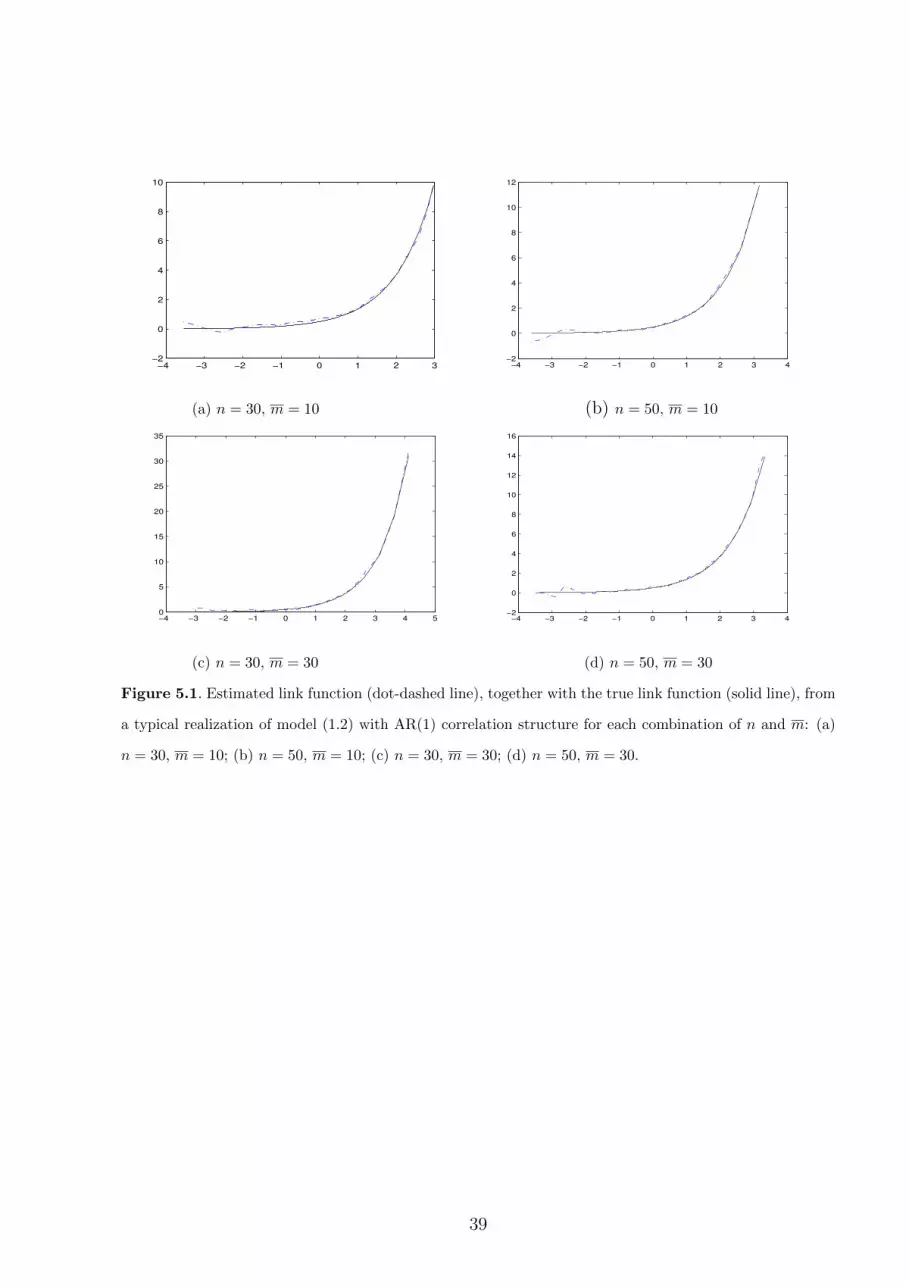
−4 −3 −2 −1 0 1 2 3−2
0
2
4
6
8
10
−4 −3 −2 −1 0 1 2 3 4−2
0
2
4
6
8
10
12
(a) n = 30, m = 10 (b) n = 50, m = 10
−4 −3 −2 −1 0 1 2 3 4 50
5
10
15
20
25
30
35
−4 −3 −2 −1 0 1 2 3 4−2
0
2
4
6
8
10
12
14
16
(c) n = 30, m = 30 (d) n = 50, m = 30
Figure 5.1. Estimated link function (dot-dashed line), together with the true link function (solid line), from
a typical realization of model (1.2) with AR(1) correlation structure for each combination of n and m: (a)
n = 30, m = 10; (b) n = 50, m = 10; (c) n = 30, m = 30; (d) n = 50, m = 30.
39
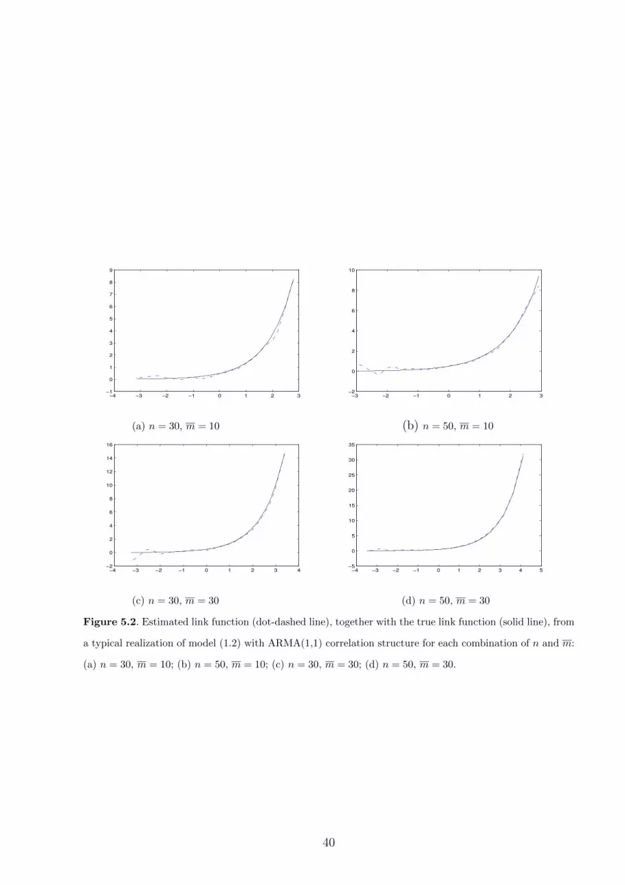
−4 −3 −2 −1 0 1 2 3−1
0
1
2
3
4
5
6
7
8
9
−3 −2 −1 0 1 2 3−2
0
2
4
6
8
10
(a) n = 30, m = 10 (b) n = 50, m = 10
−4 −3 −2 −1 0 1 2 3 4−2
0
2
4
6
8
10
12
14
16
−4 −3 −2 −1 0 1 2 3 4 5−5
0
5
10
15
20
25
30
35
(c) n = 30, m = 30 (d) n = 50, m = 30
Figure 5.2. Estimated link function (dot-dashed line), together with the true link function (solid line), from
a typical realization of model (1.2) with ARMA(1,1) correlation structure for each combination of n and m:
(a) n = 30, m = 10; (b) n = 50, m = 10; (c) n = 30, m = 30; (d) n = 50, m = 30.
40

4.7 4.9 5.1
7.0
8.0
log(H)
log
(FE
V)
0.4 0.8 1.2 1.6
7.0
8.0
log(BMI)
log
(FE
V)
2.5 3.0 3.5 4.0 4.5
7.0
8.0
log(OZONE)
log
(FE
V)
1.0 2.0 3.0
7.0
8.0
log(NO2)
log
(FE
V)
Figure 5.3. The scatter plots of the response variable log(FEV) against the continuous regressors, i.e.,
(clockwise from top left) log(H), log(BMI), log(NO2), log(OZONE).
41
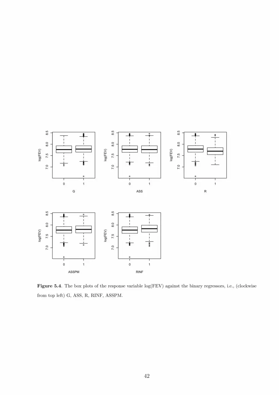
0 1
7.0
7.5
8.0
8.5
G
log(FEV)
0 1
7.0
7.5
8.0
8.5
ASS
log(FEV)
0 1
7.0
7.5
8.0
8.5
R
log(FEV)
0 1
7.0
7.5
8.0
8.5
ASSPM
log(FEV)
0 1
7.0
7.5
8.0
8.5
RINF
log(FEV)
Figure 5.4. The box plots of the response variable log(FEV) against the binary regressors, i.e., (clockwise
from top left) G, ASS, R, RINF, ASSPM.
42

0.0 0.2 0.4 0.6 0.8 1.0 1.2
-4.2
-4.0
-3.8
-3.6
-3.4
lx
ly
Figure 5.5. The estimated link function and its 95% confidence band.
43


