Shape Reconstruction Incorporating Multiple Nonlinear Geometric Constraints

TH

E

U N I V E RS

IT

Y

OF

ED I N B U

RG

H

School of Informatics, University of Edinburgh

Shape Reconstruction Incorporating Multiple Non-linear GeometricConstraints

by

Naoufel Werghi, Robert Fisher, Anthony Ashbrook, Craig Robertson

Informatics Research Report EDI-INF-RR-0211

School of Informatics June 2004http://www.informatics.ed.ac.uk/

Shape Reconstruction Incorporating Multiple Non-linearGeometric Constraints

Naoufel Werghi, Robert Fisher, Anthony Ashbrook, Craig Robertson

Informatics Research Report EDI-INF-RR-0211

SCHOOL of INFORMATICS

June 2004

Final version appears in Constraints, Vol.7, Issue 2, pp.117-149, 2002

Abstract :This paper deals with the reconstruction of 3D geometric shapes based on observed noisy 3D measurements and

multiple coupled non-linear shape constraints. Here a shape could be a complete object, a portion of an object, a part ofa building, etc. The paper suggests a general incremental framework whereby constraints can be added and integrated inthe model reconstruction process, resulting in an optimal trade-off between minimization of the shape fitting error andthe constraint tolerances. After defining sets of main constraints for objects containing planar and quadratic surfaces,the paper shows that our scheme is well behaved and the approach is valid through application on different real parts.This work is the first to give such a large framework for the integration of numerical geometric relationships in objectmodelling from range data. The technique is expected to have great impact in reverse engineering applications andmanufactured object modelling where the majority of parts are designed with intended feature relationships.

Keywords : Reverse engineering, geometric constraints, constrained shape reconstruction, shape optimization

Copyright c�

2004 by The University of Edinburgh. All Rights Reserved

The authors and the University of Edinburgh retain the right to reproduce and publish this paper for non-commercialpurposes.

Permission is granted for this report to be reproduced by others for non-commercial purposes as long as this copy-right notice is reprinted in full in any reproduction. Applications to make other use of the material should be addressedin the first instance to Copyright Permissions, School of Informatics, The University of Edinburgh, 2 Buccleuch Place,Edinburgh EH8 9LW, Scotland.

Shape Reconstruction Incorporating Multiple Non-linearGeometric Constraints

Naoufel Werghi, Robert Fisher, Anthony Ashbrook and Craig RobertsonDivision of Informatics, University of Edinburgh5 Forrest Hill, Edinburgh EH1 2QL, UKEmail: {naoufelw, rbf, anthonya, craigr}@dai.ed.ac.uk

Abstract. This paper deals with the reconstruction of 3D geometric shapes based on observednoisy 3D measurements and multiple coupled non-linear shape constraints. Here a shape couldbe a complete object, a portion of an object, a part of a building etc. The paper suggests ageneral incremental framework whereby constraints can be added and integrated in the modelreconstruction process, resulting in an optimal trade-off between minimization of the shapefitting error and the constraint tolerances. After defining sets of main constraints for objectscontaining planar and quadric surfaces, the paper shows that our scheme is well behavedand the approach is valid through application on different real parts. This work is the firstto give such a large framework for the integration of numerical geometric relationships inobject modelling from range data. The technique is expected to have a great impact in reverseengineering applications and manufactured object modelling where the majority of parts aredesigned with intended feature relationships.

Keywords: Reverse engineering, geometric constraints, constrained shape reconstruction,shape optimization

Abbreviations: CAD – Computer Aided-design; 3D – Three-Dimensional; LS – Least squares

Table of Contents

1 Introduction 22 Related work 43 The geometric constraints 64 Optimization of shape satisfying the constraints 85 Implementation 146 A simple example 147 Experiments 178 Conclusion 31

c�

2000 Kluwer Academic Publishers. Printed in the Netherlands.

revisedpaper.tex; 6/04/2000; 15:35; p.1

2

3D scanning

CAD model

Design with CAD

Optical measurement

Optimization

Rapid prototyping

12

3

4

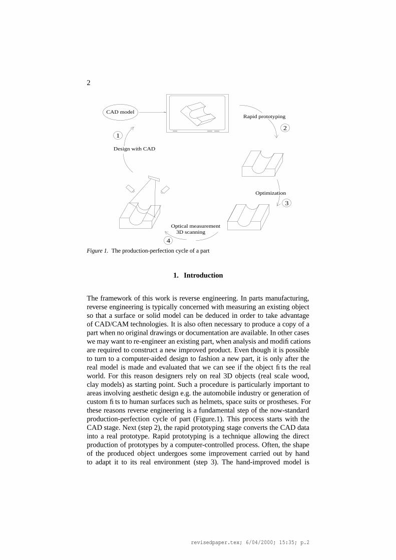
Figure 1. The production-perfection cycle of a part

1. Introduction

The framework of this work is reverse engineering. In parts manufacturing,reverse engineering is typically concerned with measuring an existing objectso that a surface or solid model can be deduced in order to take advantageof CAD/CAM technologies. It is also often necessary to produce a copy of apart when no original drawings or documentation are available. In other caseswe may want to re-engineer an existing part, when analysis and modificationsare required to construct a new improved product. Even though it is possibleto turn to a computer-aided design to fashion a new part, it is only after thereal model is made and evaluated that we can see if the object fits the realworld. For this reason designers rely on real 3D objects (real scale wood,clay models) as starting point. Such a procedure is particularly important toareas involving aesthetic design e.g. the automobile industry or generation ofcustom fits to human surfaces such as helmets, space suits or prostheses. Forthese reasons reverse engineering is a fundamental step of the now-standardproduction-perfection cycle of part (Figure.1). This process starts with theCAD stage. Next (step 2), the rapid prototyping stage converts the CAD datainto a real prototype. Rapid prototyping is a technique allowing the directproduction of prototypes by a computer-controlled process. Often, the shapeof the produced object undergoes some improvement carried out by handto adapt it to its real environment (step 3). The hand-improved model is


3

3D scanning

CAD model

Design with CAD

Optical measurement

Optimization

Rapid prototyping

New constraints

12

3

4

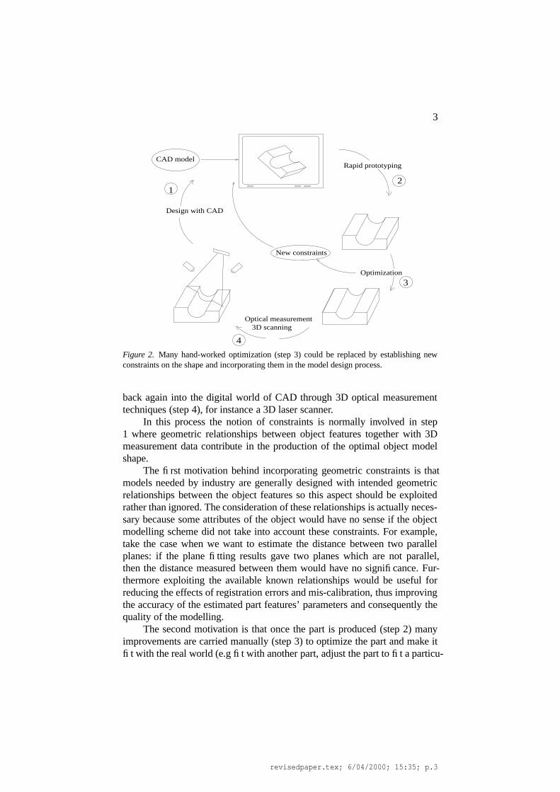
Figure 2. Many hand-worked optimization (step 3) could be replaced by establishing newconstraints on the shape and incorporating them in the model design process.

back again into the digital world of CAD through 3D optical measurementtechniques (step 4), for instance a 3D laser scanner.

In this process the notion of constraints is normally involved in step1 where geometric relationships between object features together with 3Dmeasurement data contribute in the production of the optimal object modelshape.

The first motivation behind incorporating geometric constraints is thatmodels needed by industry are generally designed with intended geometricrelationships between the object features so this aspect should be exploitedrather than ignored. The consideration of these relationships is actually neces-sary because some attributes of the object would have no sense if the objectmodelling scheme did not take into account these constraints. For example,take the case when we want to estimate the distance between two parallelplanes: if the plane fitting results gave two planes which are not parallel,then the distance measured between them would have no significance. Fur-thermore exploiting the available known relationships would be useful forreducing the effects of registration errors and mis-calibration, thus improvingthe accuracy of the estimated part features’ parameters and consequently thequality of the modelling.

The second motivation is that once the part is produced (step 2) manyimprovements are carried manually (step 3) to optimize the part and make itfit with the real world (e.g fit with another part, adjust the part to fit a particu-


4

lar customer). These improvements could be represented by new constraintson the part’s shape. By integrating these constraints into the CAD designprocess step (Figure.2) the work piece optimization would be reduced to theminimum tasks and hence many cycles in the part production process wouldbe saved. In other cases, such improvements could not be achieved by handdue to the complexity of the object or when we want to extend the applicationof the process to complex environments such as buildings or industrial plants.

Our problem is presented as follows: Given sets of 3D measurementpoints representing surfaces belonging to a certain object, we want to estimatethe different parameters of the surfaces, taking into account the geometricrelationships between these surfaces and the specific shapes of surfaces aswell.

A state vector �p is associated to the object, which includes all paramet-ers related to the patches. The shape defined by the parameter vector �p hasto best fit the data while satisfying the constraints. Consider F

� �p � to be anobjective function defining the relationship between the set of data and theparameters and Ck

� �p � , k � 1 �� M the set of constraint functions defining thegeometric constraints. Ck

� �p � is a vector function associated with constraintk. The problem can be then stated as follows: Find the parameter vector �pminimizing the function F

� �p � subject to the constraints

Ck� �p �� τk � k � 1 �� M (1)

Here τk represents the tolerance related to the constraint Ck. Ideally the tol-erances have zero values, but practically, for geometric constraints they areassigned certain values which reflect the allowed geometric inaccuracies inthe relative locations and shapes of features. It is up to the designer to setthe tolerances, however an appropriate definition of the tolerances for a givenobject can be set up by using the scheme developed by Requicha [16].

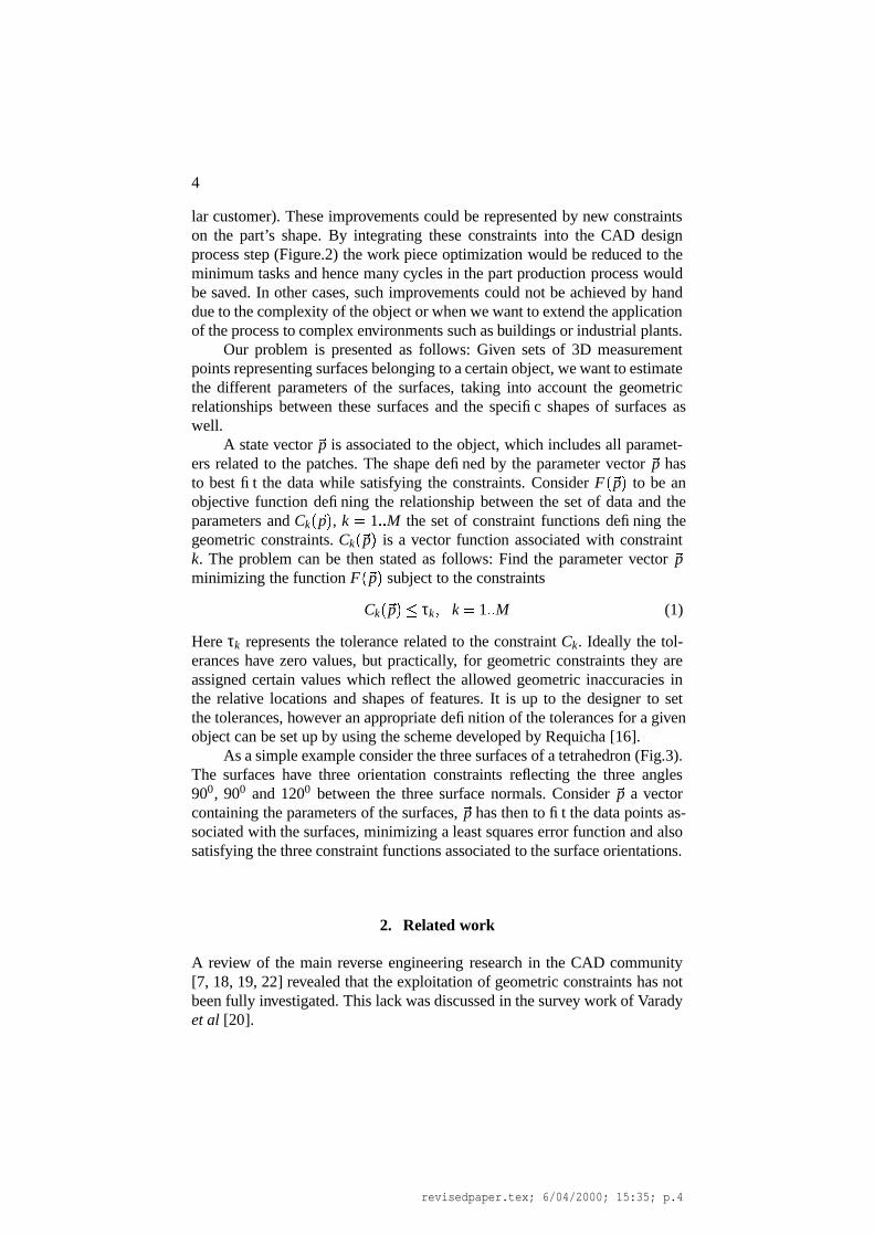
As a simple example consider the three surfaces of a tetrahedron (Fig.3).The surfaces have three orientation constraints reflecting the three angles900, 900 and 1200 between the three surface normals. Consider �p a vectorcontaining the parameters of the surfaces, �p has then to fit the data points as-sociated with the surfaces, minimizing a least squares error function and alsosatisfying the three constraint functions associated to the surface orientations.

2. Related work

A review of the main reverse engineering research in the CAD community[7, 18, 19, 22] revealed that the exploitation of geometric constraints has notbeen fully investigated. This lack was discussed in the survey work of Varadyet al [20].


5

S1

S2

S3

Tetrahedron

Figure 3. The tetrahedron object with the extracted surfaces

Incorporating geometric relationships in object modelling has to tackletwo problems. The first is how to represent the constraints. The second is howto integrate these constraints into the shape fitting process. These two aspectsare not entirely independent, the shape fitting technique imposes restrictionson the constraint representation and vice versa.

A first step in the direction of incorporating constraints for ensuring theconsistency of the reconstruction was done by Porrill [15]. He linearized aset of nonlinear constraints and combined them with a Kalman filter appliedto wire frame model construction. Porrill’s method takes advantage of therecursive linear estimation of the Kalman filter, but guarantees satisfaction ofthe constraints only to linearized first order. Additional iterations are neededat each step if more accuracy is required. This last condition has been takeninto account in the work of De Geeter et al [4] by defining a “SmoothlyConstrained Kalman Filter”. The key idea of their approach is to replace non-linear constraints by a set of linear constraints applied iteratively and updatedby new measurements in order to reduce the linearization error. However, thecharacteristics of Kalman filtering makes these methods essentially adaptedfor iteratively acquired data and many data samples. Moreover, there was nomechanism for determining how successfully the constraints were satisfiedand only lines and planes were considered in both of the above works.

The constraints considered by Bolle et al [2] in their approach to 3Dobject position covered only the shape of the surfaces. They chose a specificrepresentation for the treated features: plane, cylinder and sphere.

Compared to Porrill’s and De Geeter’s work, our approach avoids thedrawbacks of linearization, since the constraints are completely implemented.Moreover, our approach covers a larger category of feature shapes. Regard-ing the work of Bolle [2], the type of constraints which can be held by ourapproach go beyond the restricted set of surface shapes and cover also thegeometric relationships between object features. To our knowledge the workappears to be the first to give such a large framework for the integration ofgeometric relationships for object reconstruction.


6

3. The geometric constraints

The set of constraints associated with a given object can be divided mainlyinto two categories. The first one is the surface intrinsic constraints coveringthe geometric properties which arise from the specific shapes of the surfaces.This category includes particular properties of the surface such as symmetrywith respect to a point or a line. For quadric surfaces such as cones or cross-section cylinders this property is the circular shape of the surface.

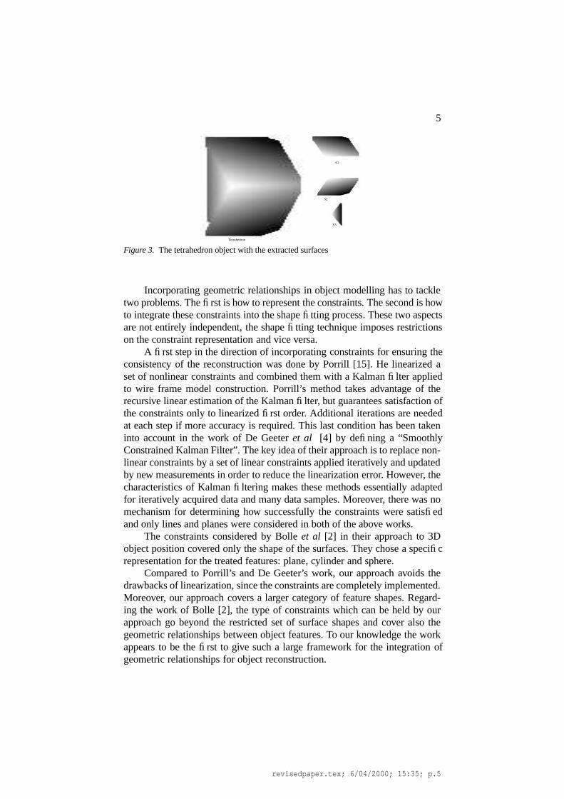
The second category named, the feature extrinsic constraints, defines thegeometric and topological relationships between the different object features.Table I summarizes these relationships. We notice here that points and linesin this table may be either physical features of the object like summits orvertices and edges or implicit features like centres, axes of symmetry. Thislist is not exhaustive and this classification may not be unique. Neverthelessit covers a large number of constraints in manufactured objects.

Table I. Relationships between features.

point line plane quadric surface

point coincident inclusion inclusion inclusion

separation separation separation separation

line - coincident inclusion inclusion

relative orientation relative orientation relative orientation

separation separation separation

plane - - coincident relative orientation

relative orientation separation

separation

quadric surface - - - coincident

relative orientation

separation

3.1. COINCIDENCE CONSTRAINTS

Shapes commonly contain features which are associated to the same geomet-ric entity (Figure.4.a) or which coincide at the same position (Figure.4.b). Inthe first case these constraints are implicitly imposed by considering the sameparameters for each feature. In the second case the parameters associated toeach feature are equated and the resulting equations have then to be satisfied.


7

E E

P

1

1

2

2P+

Cyl

Cyl

CirCir

C

D

2

1

12

(a)

(b)

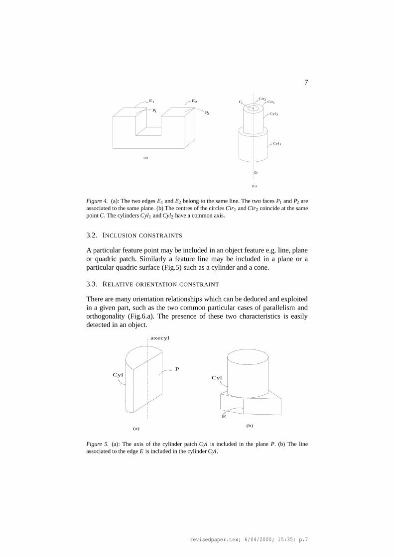
Figure 4. (a): The two edges E1 and E2 belong to the same line. The two faces P1 and P2 areassociated to the same plane. (b) The centres of the circles Cir1 and Cir2 coincide at the samepoint C. The cylinders Cyl1 and Cyl2 have a common axis.

3.2. INCLUSION CONSTRAINTS

A particular feature point may be included in an object feature e.g. line, planeor quadric patch. Similarly a feature line may be included in a plane or aparticular quadric surface (Fig.5) such as a cylinder and a cone.

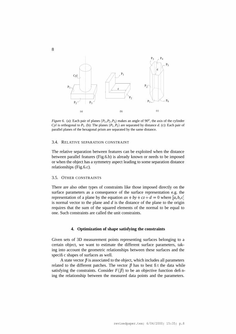
3.3. RELATIVE ORIENTATION CONSTRAINT

There are many orientation relationships which can be deduced and exploitedin a given part, such as the two common particular cases of parallelism andorthogonality (Fig.6.a). The presence of these two characteristics is easilydetected in an object.

P

axecyl

CylCyl

E

(a)(b)

Figure 5. (a): The axis of the cylinder patch Cyl is included in the plane P. (b) The lineassociated to the edge E is included in the cylinder Cyl.


8

PP

P

Cyl

1

2 3

P

P

1

d

2

P

P P

P

PP1

2

3 4

5

6

(a) (b) (c)

d

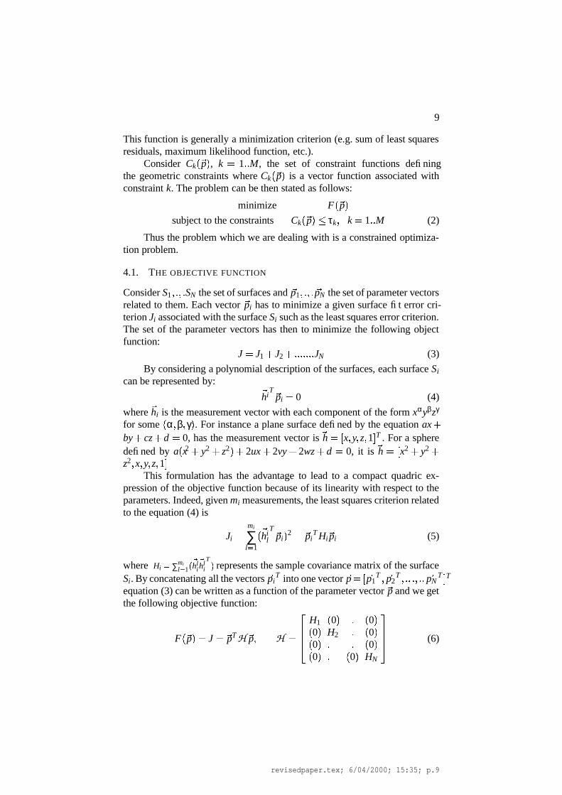
Figure 6. (a): Each pair of planes � P1 � P2 � P3 � makes an angle of 90o, the axis of the cylinderCyl is orthogonal to P1. (b): The planes � P1 � P2 � are separated by distance d. (c): Each pair ofparallel planes of the hexagonal prism are separated by the same distance.

3.4. RELATIVE SEPARATION CONSTRAINT

The relative separation between features can be exploited when the distancebetween parallel features (Fig.6.b) is already known or needs to be imposedor when the object has a symmetry aspect leading to some separation distancerelationships (Fig.6.c).

3.5. OTHER CONSTRAINTS

There are also other types of constraints like those imposed directly on thesurface parameters as a consequence of the surface representation e.g. therepresentation of a plane by the equation ax � by � cz � d � 0 where � a � b � c �is normal vector to the plane and d is the distance of the plane to the originrequires that the sum of the squared elements of the normal to be equal toone. Such constraints are called the unit constraints.

4. Optimization of shape satisfying the constraints

Given sets of 3D measurement points representing surfaces belonging to acertain object, we want to estimate the different surface parameters, tak-ing into account the geometric relationships between these surfaces and thespecific shapes of surfaces as well.

A state vector �p is associated to the object, which includes all parametersrelated to the different patches. The vector �p has to best fit the data whilesatisfying the constraints. Consider F

� �p � to be an objective function defin-ing the relationship between the measured data points and the parameters.


9

This function is generally a minimization criterion (e.g. sum of least squaresresiduals, maximum likelihood function, etc.).

Consider Ck� �p � , k � 1 �� M, the set of constraint functions defining

the geometric constraints where Ck� �p � is a vector function associated with

constraint k. The problem can be then stated as follows:

minimize F� �p �

subject to the constraints Ck� �p � � τk � k � 1 �� M (2)

Thus the problem which we are dealing with is a constrained optimiza-tion problem.

4.1. THE OBJECTIVE FUNCTION

Consider S1 � � � � SN the set of surfaces and �p1 � � � � �pN the set of parameter vectorsrelated to them. Each vector �pi has to minimize a given surface fit error cri-terion Ji associated with the surface Si such as the least squares error criterion.The set of the parameter vectors has then to minimize the following objectfunction:

J � J1 � J2 � �� JN (3)

By considering a polynomial description of the surfaces, each surface Si

can be represented by:�hi

T �pi � 0 (4)

where �hi is the measurement vector with each component of the form xαyβzγ

for some�α � β � γ � . For instance a plane surface defined by the equation ax �

by � cz � d � 0, has the measurement vector is �h � � x � y � z � 1 � T . For a spheredefined by a

�x2 � y2 � z2 � � 2ux � 2vy � 2wz � d � 0, it is �h � � x2 � y2 �

z2 � x � y � z � 1 �This formulation has the advantage to lead to a compact quadric ex-

pression of the objective function because of its linearity with respect to theparameters. Indeed, given mi measurements, the least squares criterion relatedto the equation (4) is

Ji �mi

∑l � 1

� �hil

T �pi � 2 � �piT Hi �pi (5)

where Hi� ∑mi

l � 1 ��hl

i

�hl

i

T � represents the sample covariance matrix of the surfaceSi. By concatenating all the vectors �pi

T into one vector �p � � �p1T � �p2

T � � � � � � � �pNT � T

equation (3) can be written as a function of the parameter vector �p and we getthe following objective function:

F� �p � � J � �pT H �p � H �

��

H1�0 � � �

0 ��0 � H2 � �

0 ��0 � � � �

0 ��0 � � �

0 � HN

�� (6)


10

Such a function is convex if and only if the matrix H is positive, whichis the case. Besides, under the above form, the objective equation containsseparate terms for the data and the parameters. The data matrix H can bethus computed off-line before the optimization.

The objective function could be taken as the likelihood of the range datagiven the parameters (with a negative sign since we want to minimize). Thelikelihood function has the advantage of accounting for the statistical aspectof the measurements. As a first step, we have chosen the least squares func-tion. The integration of the data noise characteristics in the LS function can bedone afterwards with no particular difficulty, leading to the same estimationof the likelihood function in the case of the Gaussian distribution.

4.2. CONSTRAINT FORMULATION

The different constraints are implemented under a matrix formulation. Thematrix notation leads to a compact form and avoids expressions with manyvariables in particular for the second order derivatives that may be eventuallyneeded in the optmization algorithm. This allows a fast, automatic and easyimplementation of the constraints.

Some intrinsic constraints, for instance circularity of quadric surfacescould be imposed implicitly by choosing a suitable form of the surface equa-tion. However, the implementation of the reduced form in the optimizationalgorithm may cause some complexity. Indeed, because of the nonlinearityof these forms, it has not been possible to get an objective function withseparated terms for the data and the parameters. Thus, the data terms could notbe computed off-line. This may increase the computational cost dramatically.Examples of how constraints can be implemented are found in section 6.

4.3. THE OPTIMIZATION ALGORITHM

Optimization techniques fall into two broad branches namely OperationResearch techniques and the recent evolutionary techniques.

Evolutionary computation techniques [10, 11] have been having increas-ing attraction for their potential to solve complex problems. In short they arestochastic optimization methods. They are conveniently presented using themetaphor of natural evolution: they start from a randomly generated set ofpoints or solutions of the search space (population of individuals). Then thisset evolves following a process close the natural selection principle. At eachstage a new population is generated using simulated genetic operations suchas mutation or crossover. The probability of survival of the new solutions de-pends on how well they fit a given evaluation function. The best are kept withhigh probability and the worst are discarded. This process is repeated untilthe set of solutions converges to the one best fitting the evaluation function.


11

The main advantages of the evolutionary techniques is that they do nothave many mathematical requirements about the optimization problem. Theyare 0-order methods, in the sense that they operate only on the objectivefunction and they can handle linear or nonlinear problems, constrained orunconstrained.

The main drawback of these techniques is that they are highly timeconsuming. This is due to the fact that to ensure convergence, the numberof generated solutions has to be high, and at each iteration all the solutionshave to be evaluated. This increases the computation time dramatically.

The second branch of the optimization techniques are the classical op-eration research techniques. They are more mature than the evolutionarytechniques. They involve search techniques, numerical analysis and differ-ential tools. Most of these techniques use an iterative scheme. A reasonableinitialisation causes significant speedup in convergence. A detailed reviewand analysis of these optimization techniques could be found in [8, 9].

We believe that the evolutionary techniques are suitable mainly to theoptimization cases where objective functions and constraints are very com-plex, presenting hard-handled aspects such nonlinearity, non-differentiability,or do have not explicit forms. Indeed the earlier mentioned characteristics ofthe evolutionary techniques allow them to by-pass these problems.

As our optimization problem does not have these problems, the opera-tional research techniques are more appropriate. This argument is supportedby the time-consuming characteristic of the evolutionary techniques, wherethe average scale of the processing time is on the order of hours. This charac-teristic makes these methods not appropriate for interactive user environmentsand impractical for a static verification and checking of the results whenexperiments have to be repeated many times. The other important reasonfor opting for search techniques is that we can obtain a reasonable initialestimate of the model parameters. This initial solution is the estimation ofthe model parameters without considering the constraints. This estimation isnot far away from the optimal one since it is obtained from the real objectprototype.

Theoretically a solution of the problem stated in (2) is given by findingthe set

� �p � λ1 � λ2 � � � � � λk � minimizing the following equation:

E� �p � � F

� �p � �M

∑k � 1

λkCk� �p �

F� �p � � �pT H �p (7)

Ck� �p � � �pT Ak �p � BT

k �p � Ck

Under the Khun-Tucker conditions [8](Chapter 9), namely that the ob-jective function and the constraint functions are continuously differentiableand the gradients of the constraint functions are linearly independent, the


12

optimal set� �p � λ1 � λ2 � � � � � λk � minimizing (7) is the solution of the system:

∂F∂ �p �

M

∑k � 1

λk∂Ck

∂ �p � 0 (8)

In some particular cases it is possible to get a closed form solution for(8) such as the generalized eigenvalues methods. This depends on the char-acteristics of the constraint functions and whether it is possible to combinethem efficiently with the objective function. When the constraints are linear(having the form A �p � B � 0) the standard quadratic programming methodscould be applied to solve this system.

However the geometric constraints are mainly non-linear. Generally itis not trivial to develop an analytical solution for such problem. In this casean algorithmic numerical approach could be of great help taking into accountthe increasing capabilities of computing.

Now if we look to the objective function and the constraint functionsin (7) we see that they are explicitly defined as a function of the paramet-ers, they are smooth, differentiable and they both have a quadratic structure.From (5) we can notice that each submatrix Hi of H in (6) is the sum of

cross-product terms �hli�hli

T. Thus Hi as well as H are positive definite. Con-

sequently the objective function is convex. Such functions could be efficientlyminimized. Besides it has the important property that its minimum is global.If the constraint functions are squared, thus enforced to be also convex, theoptimization problem (7) would be a convex optimization problem for λk � 0.For such problem an optimal solution exists, moreover this solution corres-ponds to the solution of the system (8) defined by the Khun-Tucker conditions[17](section 27,28).

The problem would be to determine the set� �p � λ1 � λ2 � � � � � λk � minimiz-

ing:

E� �p � � F

� �p � �M

∑k � 1

λk�Ck

� �p � 2 � � λk � 0 (9)

To provide a numerical solution of this problem we have been investigat-ing an approach in the framework of sequential unconstrained minimization.The basic idea is to attach different penalty functions to the objective functionF� �p � in such a way that the optimal solutions of successive unconstrained

problems approach the optimal solution of the problem (9). Indeed the term∑M

k � 1 λk�Ck

� �p � 2 � could be seen as a penalty function controlling the con-straints satisfaction. The scheme then increments the set of λk iteratively, ateach step minimize (9) by a standard non-constrained technique, update thesolution �p, and repeat the process until the constraints are satisfied. For equalvalues of λk, Fiacco and McCormick [6] have shown that the solutions of(9) converge towards the same solution of the problem (2) when λk tends toinfinity.


13

In more detail the proposed algorithm is: We start with a parameter vec-tor �p

�0 � that minimizes the least squares objective function and attempt to find

a nearby vector �p�1 � that minimizes (9) for small values λk. Then we iterat-

ively increase the set of λk slightly and solve for a new optimal parameter�p

�n � 1 � using the previous �p

�n � . At each iteration n, the algorithm increases

each λk by a certain amount and a new �p�n � is found such that the optimiz-

ation function is minimized by means of the standard Levenberg-Marquardtalgorithm (see Appendix). The parameter vector �p

�n � is then updated to the

new estimate �p�n � 1 � which becomes the initial estimate at the next values

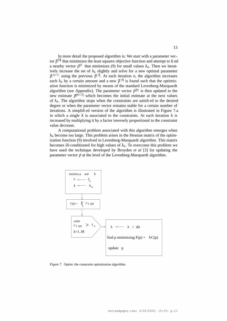
of λk. The algorithm stops when the constraints are satisfied to the desireddegree or when the parameter vector remains stable for a certain number ofiterations. A simplified version of the algorithm is illustrated in Figure 7.ain which a single λ is associated to the constraints. At each iteration λ isincreased by multiplying it by a factor inversely proportional to the constraintvalue decrease.

A computational problem associated with this algorithm emerges whenλk become too large. This problem arises in the Hessian matrix of the optim-ization function (9) involved in Levenberg-Marquardt algorithm. This matrixbecomes ill-conditioned for high values of λk. To overcome this problem wehave used the technique developed by Broyden et al [3] for updating theparameter vector �p at the level of the Levenberg-Marquardt algorithm.

k (p)C

λ initialise p and

p0

p

λ λ 0

k (p)CΣk

C(p) =

find p minimizing F(p) + C(p) λ

kτ> λ λ + ∆λ

while

k=1..M

update p

Figure 7. Optim: the constraint optimization algorithm.


14

The initialization of the parameter vector is crucial to guarantee the con-vergence of the algorithm to the desired solution. For this reason the initialvector was the one which best fitted the set of data in the absence of con-straints. This vector can be obtained by estimating each surface’s parametervector separately and then concatenating the vectors into a single one. Nat-urally, the option of minimizing the objective function F

� �p � alone has to beavoided since it leads to the trivial null vector solution. On the other hand, theinitial values λk have to be large enough to avoid the above trivial solutionand to give the constraints a certain weight. A convenient value for the initialλk is :

λ�0 �

k � F� �p

�0 � �

Ck� �p �

0 � � (10)

where �p�0 � is the initial parameter estimation obtained by concatenating the

unconstrained estimates.

5. Implementation

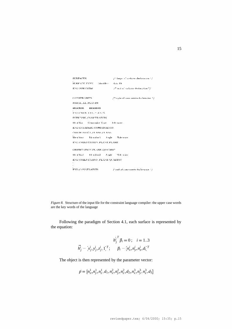
First, the algorithm was developed and implemented under MATLAB, mainlyto check the behaviour and the convergence of the algorithm as well as thevalidity of the results. This version rapidly turned out to be inconvenient sincea new implementation is needed to be done for each part. The next step wasthen to develop a program which can hold any part and automatically convertthe information given by the user about the object (surfaces and constraints)into a structure (set of objective function and constraint functions) ready tobe integrated into the optimization algorithm. A simple constraint languagecompiler was developed under C++ for this purpose. The input file is a listof statements in which the user declares the surfaces, their identifications andthe files where the associated 3D measurement points are stored. Then theconstraints are declared with their associated values and tolerances. Figure 8shows the structure of the input file and the language statements.

The whole package (the compiler and the optimization algorithm) hasbeen implemented on a 200Mhz SUN Ultrasparc workstation. The computa-tion time is in the range of 3-10 minutes for the different test objects. Thisrange is suitable for CAD work.

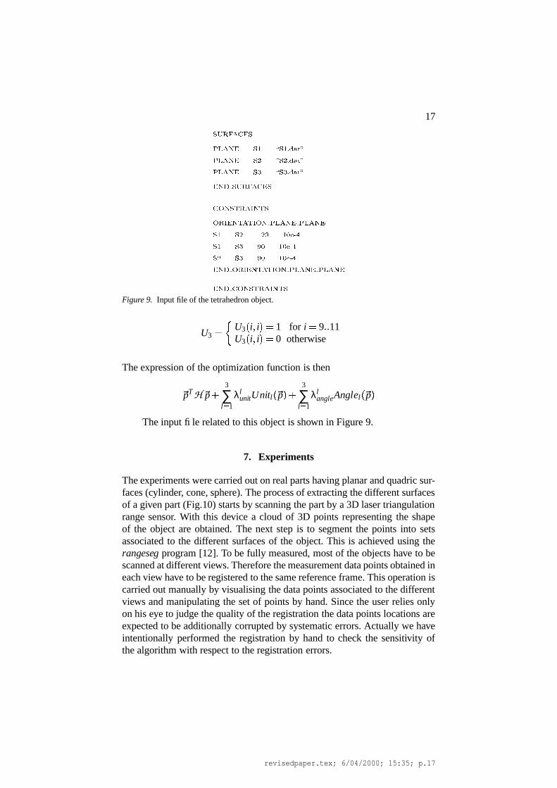
6. A simple example

Consider a simple polyhedral object, for instance a partial tetrahedron. Sup-pose that the tetrahedron is composed from three surfaces, S1 � S2 and S3

(Fig.3).


15

�� !� "�#��$��%��#$& "� �"�'(� ��)�*

+��-,/.102� 34%��'(� 56�$ %�"*'("756& �

+�28�9 ��/� :�;�$��%��*�<�(�� "�#��%��#$& "* �"*'(� ��)��

=>8>��,��348�,�� :�?�@�� A��2#��!'( �"*� ��'(��%��#$& "� �"�'(� ��)�*

0@��BCBC�2B 02BC��8��/�

+34%��'(� 56�$ �D 34%��$��'(� 56�� (E

+�28�9 0@��BCBC�2B 02BC��8��/�

348�,��348>��3! =>8>��,��3 8�,��

+34%��'(� 56�$ ��*��!'( �"�� '�,2F�G�� ,C��& �$ �"*��#$�

+�28�9 348�,��348>��3! =>8>��,��348�,��

=>��34�28�,<��,3!=>8 02BC��8�� 0/BH��8��

+34%��'(� 56�$ �D 34%��$��'(� 56�� (E ��& � ,C��& �� "��#��

+�28�9 =1��34�28�,C�2,3!=>8 02BC��8�� 02BC��8��

=>��34�28�,<��,3!=>8 02BC��8�� I1��9>��3!

+34%��'(� 56�$ �D 34%��$��'(� 56�� (E ��& � ,C��& �� "��#��

+�28�9 =1��34�28�,C�2,3!=>8 02BC��8�� I>��9>��3!

+++�28�9 =>8>��,��348�,�� :�?�$��%��*�<#$�*��!'( �"�� '(��%��#$& "* �"*'(� ��)��

Figure 8. Structure of the input file for the constraint language compiler: the upper case wordsare the key words of the language

Following the paradigm of Section 4.1, each surface is represented bythe equation:

�hij

T �pi � 0 ; i � 1 �� 3�hi

j � � xij � yi

j � zij � 1 � T ; �pi � � ni

x � niy � ni

z � di � T

The object is then represented by the parameter vector:

�p � � n1x � n1

y � n1z � d1 � n2

x � n2y � n2

z � d2 � n3x � n3

y � n3z � d3 �


16

The objective function is expressed by:

F� �p � � J � �pT H �p �

�� H1

�0 � 4

�0 � 4�

0 � 4 H2�0 � 4�

0 � 4�0 � 4 H3

��

whereHi � ∑

j

� �hij �� hi

j � T

The surfaces have three orientation constraints reflecting the three angles900, 900 and 1200 between the three surface normals �n1, �n2 and �n3. Theseconstraints are represented by the following equations

�n1T �n2 �� 0 � 5

�n1T �n3 � 0

�n2T �n3 � 0

from which the constraint functions are deduced:

Angle1� �p � � � �pT A1 �p � 0 � 5 � 2 � 0

Angle2� �p � � � �pT A2 �p � 2 � 0

Angle3� �p � � � �pT A3 �p � 2 � 0

where

A1 ��

A1�i � j � � A1

�j � i � � 1 � 2 if i � 1 � t � j � 5 � t � 0 � t � 2

A1�i � j � � A1

�j � i � � 0 otherwise

A2 ��

A2�i � j � � A2

�j � i � � 1 � 2 if i � 1 � t � j � 9 � t � 0 � t � 2

A2�i � j � � A2


A3 ��

A3�i � j � � A3

�j � i � � 1 � 2 if i � 5 � t � j � 9 � t � 0 � t � 2

A3�i � j � � A3


The surfaces normals are also constrained to be unit. This leads to thefollowing unit constraints:

Unit1� �p � � � �pTU1 �p � 1 � 2 � 0

Unit2� �p � � � �pTU2 �p � 1 � 2 � 0

Unit3� �p � � � �pTU3 �p � 1 � 2 � 0

where U1, U2 and U3 are diagonal matrices defined by

U1 ��

U1�i � i �� 1 for i � 1 �� 3

U1�i � i �� 0 otherwise

U2 ��

U2�i � i �� 1 for i � 5 �� 7

U2�i � i �� 0 otherwise


17��

��

��

��

��! ��"�

$#%��&��'(��&��

#%�$'(��&)�*&$'(#%� *� �� %��

�� + �,+�-/.10

�� 23+ �4+�-5.10

�� 23+ �4+�-5.10

��! #��'(*��&6�7&$'8#%� �� %��

��! �#%��&��$��'(��&��

Figure 9. Input file of the tetrahedron object.

U3 ��

U3�i � i � � 1 for i � 9 �� 11

U3�i � i � � 0 otherwise

The expression of the optimization function is then

�pT H �p �3

∑l � 1

λlunitUnitl

� �p � �3

∑l � 1

λlangleAnglel

� �p �

The input file related to this object is shown in Figure 9.

7. Experiments

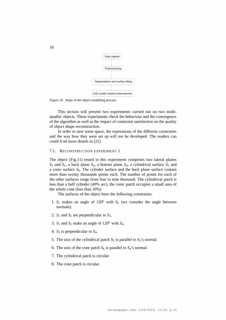
The experiments were carried out on real parts having planar and quadric sur-faces (cylinder, cone, sphere). The process of extracting the different surfacesof a given part (Fig.10) starts by scanning the part by a 3D laser triangulationrange sensor. With this device a cloud of 3D points representing the shapeof the object are obtained. The next step is to segment the points into setsassociated to the different surfaces of the object. This is achieved using therangeseg program [12]. To be fully measured, most of the objects have to bescanned at different views. Therefore the measurement data points obtained ineach view have to be registered to the same reference frame. This operation iscarried out manually by visualising the data points associated to the differentviews and manipulating the set of points by hand. Since the user relies onlyon his eye to judge the quality of the registration the data points locations areexpected to be additionally corrupted by systematic errors. Actually we haveintentionally performed the registration by hand to check the sensitivity ofthe algorithm with respect to the registration errors.


18

Data capture

Preprocessing

Segmentation and surface fitting

CAD model creation-improvement

Figure 10. Steps of the object modelling process

This section will present two experiments carried out on two multi-quadric objects. These experiments check the behaviour and the convergenceof the algorithm as well as the impact of constraint satisfaction on the qualityof object shape reconstruction.

In order to save some space, the expressions of the different constraintsand the way how they were set up will not be developed. The readers cancould find more details in [21].

7.1. RECONSTRUCTION EXPERIMENT 1

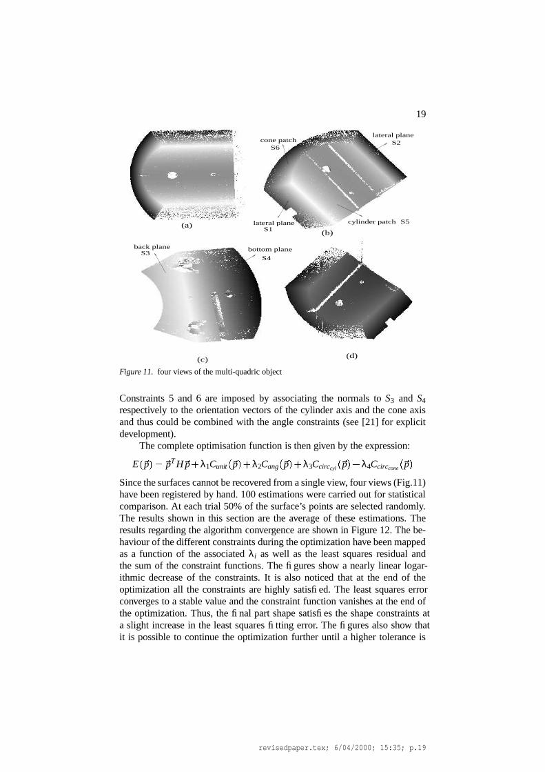
The object (Fig.11) tested in this experiment comprises two lateral planesS1 and S2, a back plane S3, a bottom plane S4, a cylindrical surface S5 anda conic surface S6. The cylinder surface and the back plane surface containmore than twenty thousands points each. The number of points for each ofthe other surfaces range from four to nine thousand. The cylindrical patch isless than a half cylinder (40% arc), the conic patch occupies a small area ofthe whole cone (less than 30%)

The surfaces of the object have the following constraints:

1. S1 makes an angle of 120o with S2 (we consider the angle betweennormals).

2. S1 and S2 are perpendicular to S3.

3. S1 and S2 make an angle of 120o with S4.

4. S3 is perpendicular to S4.

5. The axis of the cylindrical patch S5 is parallel to S3’s normal.

6. The axis of the cone patch S6 is parallel to S4’s normal.

7. The cylindrical patch is circular.

8. The cone patch is circular.


19

(a)(b)

(c) (d)

lateral plane

S1cylinder patch

S2cone patch

S5

S6

back planeS3

bottom plane

S4

lateral plane

Figure 11. four views of the multi-quadric object

Constraints 5 and 6 are imposed by associating the normals to S3 and S4

respectively to the orientation vectors of the cylinder axis and the cone axisand thus could be combined with the angle constraints (see [21] for explicitdevelopment).

The complete optimisation function is then given by the expression:

E� �p � � �pT H �p � λ1Cunit

� �p � � λ2Cang� �p � � λ3Ccirccyl

� �p � � λ4Ccirccone

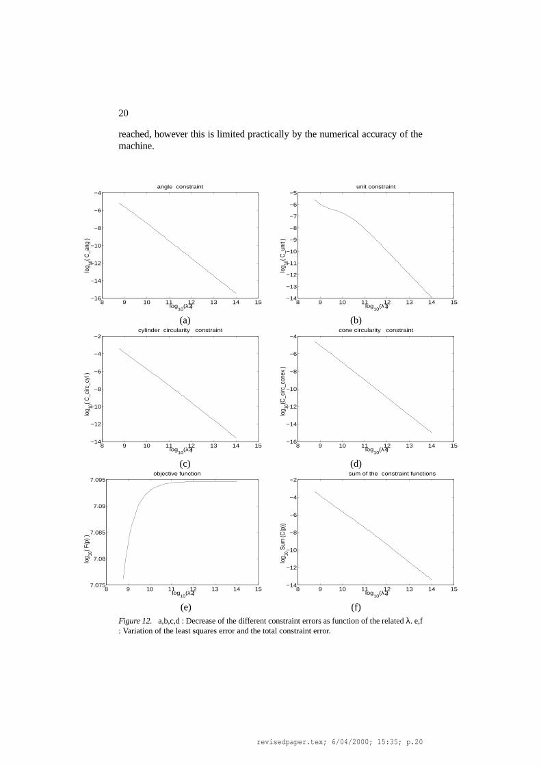
� �p �Since the surfaces cannot be recovered from a single view, four views (Fig.11)have been registered by hand. 100 estimations were carried out for statisticalcomparison. At each trial 50% of the surface’s points are selected randomly.The results shown in this section are the average of these estimations. Theresults regarding the algorithm convergence are shown in Figure 12. The be-haviour of the different constraints during the optimization have been mappedas a function of the associated λi as well as the least squares residual andthe sum of the constraint functions. The figures show a nearly linear logar-ithmic decrease of the constraints. It is also noticed that at the end of theoptimization all the constraints are highly satisfied. The least squares errorconverges to a stable value and the constraint function vanishes at the end ofthe optimization. Thus, the final part shape satisfies the shape constraints ata slight increase in the least squares fitting error. The figures also show thatit is possible to continue the optimization further until a higher tolerance is


20

reached, however this is limited practically by the numerical accuracy of themachine.

8 9 10 11 12 13 14 15−16

−14

−12

−10

−8

−6

−4

log10

(λ2 )

log 10

( C_a

ng )

angle constraint

8 9 10 11 12 13 14 15−14

−13

−12

−11

−10

−9

−8

−7

−6

−5

log10

(λ1 )

log 10

( C_u

nit )

unit constraint

(a) (b)

8 9 10 11 12 13 14 15−14

−12

−10

−8

−6

−4

−2

log10

(λ3 )

log 10

( C_c

irc_c

yl )

cylinder circularity constraint

8 9 10 11 12 13 14 15−16

−14

−12

−10

−8

−6

−4

log10

(λ4 )

log 10

(C_c

irc_c

onex

)

cone circularity constraint

(c) (d)

8 9 10 11 12 13 14 157.075

7.08

7.085

7.09

7.095

log10

(λ2 )

log 10

( F(p

) )

objective function

8 9 10 11 12 13 14 15−14

−12

−10

−8

−6

−4

−2

log10

(λ2 )

log 10

Sum

(C(p

))

sum of the constraint functions

(e) (f)Figure 12. a,b,c,d : Decrease of the different constraint errors as function of the related λ. e,f: Variation of the least squares error and the total constraint error.


21

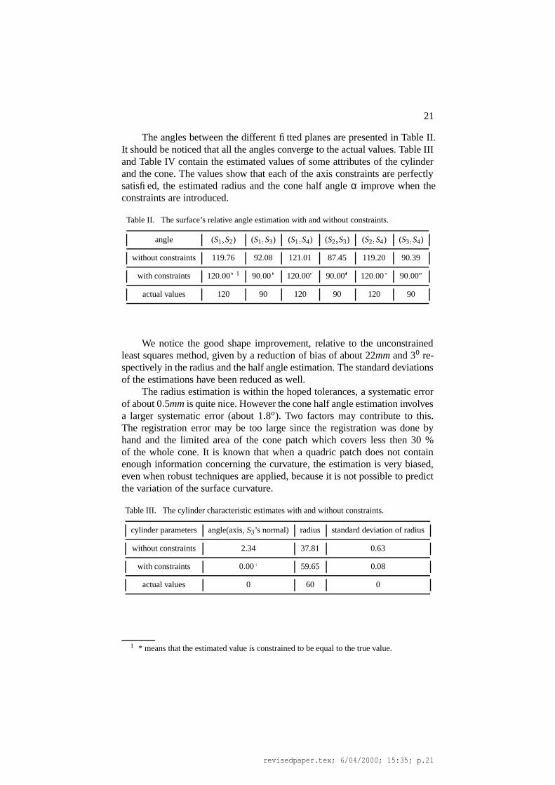
The angles between the different fitted planes are presented in Table II.It should be noticed that all the angles converge to the actual values. Table IIIand Table IV contain the estimated values of some attributes of the cylinderand the cone. The values show that each of the axis constraints are perfectlysatisfied, the estimated radius and the cone half angle α improve when theconstraints are introduced.

Table II. The surface’s relative angle estimation with and without constraints.

angle (S1 � S2) (S1 � S3) (S1 � S4) (S2 � S3) (S2 � S4) (S3 � S4)

without constraints 119.76 92.08 121.01 87.45 119.20 90.39

with constraints 120 � 00� 1 90 � 00

�

120 � 00�

90 � 00�

120 � 00�

90 � 00�

actual values 120 90 120 90 120 90

We notice the good shape improvement, relative to the unconstrainedleast squares method, given by a reduction of bias of about 22mm and 30 re-spectively in the radius and the half angle estimation. The standard deviationsof the estimations have been reduced as well.

The radius estimation is within the hoped tolerances, a systematic errorof about 0 � 5mm is quite nice. However the cone half angle estimation involvesa larger systematic error (about 1 � 8o). Two factors may contribute to this.The registration error may be too large since the registration was done byhand and the limited area of the cone patch which covers less then 30 %of the whole cone. It is known that when a quadric patch does not containenough information concerning the curvature, the estimation is very biased,even when robust techniques are applied, because it is not possible to predictthe variation of the surface curvature.

Table III. The cylinder characteristic estimates with and without constraints.

cylinder parameters angle(axis, S3’s normal) radius standard deviation of radius

without constraints 2.34 37.81 0.63

with constraints 0 � 00�

59.65 0.08

actual values 0 60 0

1 * means that the estimated value is constrained to be equal to the true value.


22

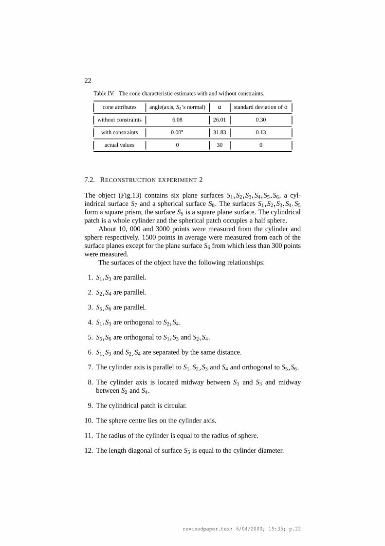
Table IV. The cone characteristic estimates with and without constraints.

cone attributes angle(axis, S4’s normal) α standard deviation of α

without constraints 6.08 26.01 0.30


31.83 0.13

actual values 0 30 0

7.2. RECONSTRUCTION EXPERIMENT 2

The object (Fig.13) contains six plane surfaces S1 � S2 � S3 � S4 � S5 � S6, a cyl-indrical surface S7 and a spherical surface S8. The surfaces S1 � S2 � S3 � S4 � S5

form a square prism, the surface S5 is a square plane surface. The cylindricalpatch is a whole cylinder and the spherical patch occupies a half sphere.

About 10, 000 and 3000 points were measured from the cylinder andsphere respectively. 1500 points in average were measured from each of thesurface planes except for the plane surface S6 from which less than 300 pointswere measured.

The surfaces of the object have the following relationships:

1. S1 � S3 are parallel.



4. S1 � S3 are orthogonal to S2 � S4.

5. S5 � S6 are orthogonal to S1 � S3 and S2 � S4.

6. S1 � S3 and S2 � S4 are separated by the same distance.

7. The cylinder axis is parallel to S1 � S2 � S3 and S4 and orthogonal to S5 � S6.

8. The cylinder axis is located midway between S1 and S3 and midwaybetween S2 and S4.

9. The cylindrical patch is circular.

10. The sphere centre lies on the cylinder axis.

11. The radius of the cylinder is equal to the radius of sphere.

12. The length diagonal of surface S5 is equal to the cylinder diameter.


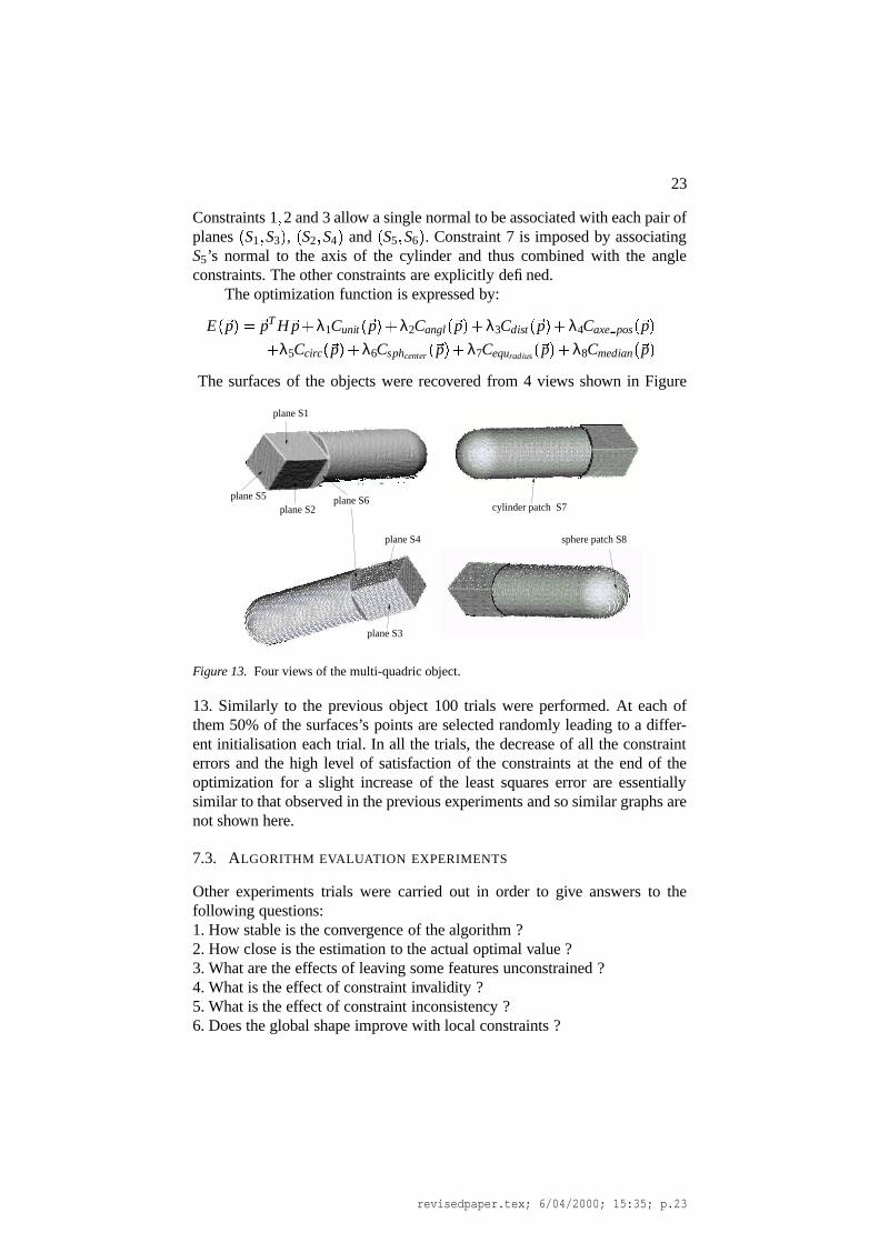
23

Constraints 1 � 2 and 3 allow a single normal to be associated with each pair ofplanes

�S1 � S3 � ,

�S2 � S4 � and

�S5 � S6 � . Constraint 7 is imposed by associating

S5’s normal to the axis of the cylinder and thus combined with the angleconstraints. The other constraints are explicitly defined.

The optimization function is expressed by:

E� �p � � �pT H �p � λ1Cunit

� �p � � λ2Cangl� �p � � λ3Cdist

� �p � � λ4Caxe pos� �p �

� λ5Ccirc� �p � � λ6Csphcenter

� �p � � λ7Cequradius

� �p � � λ8Cmedian� �p �

The surfaces of the objects were recovered from 4 views shown in Figure

plane S1

plane S2plane S5 plane S6

plane S3

plane S4 sphere patch S8

cylinder patch S7

Figure 13. Four views of the multi-quadric object.

13. Similarly to the previous object 100 trials were performed. At each ofthem 50% of the surfaces’s points are selected randomly leading to a differ-ent initialisation each trial. In all the trials, the decrease of all the constrainterrors and the high level of satisfaction of the constraints at the end of theoptimization for a slight increase of the least squares error are essentiallysimilar to that observed in the previous experiments and so similar graphs arenot shown here.

7.3. ALGORITHM EVALUATION EXPERIMENTS

Other experiments trials were carried out in order to give answers to thefollowing questions:1. How stable is the convergence of the algorithm ?2. How close is the estimation to the actual optimal value ?3. What are the effects of leaving some features unconstrained ?4. What is the effect of constraint invalidity ?5. What is the effect of constraint inconsistency ?6. Does the global shape improve with local constraints ?


24

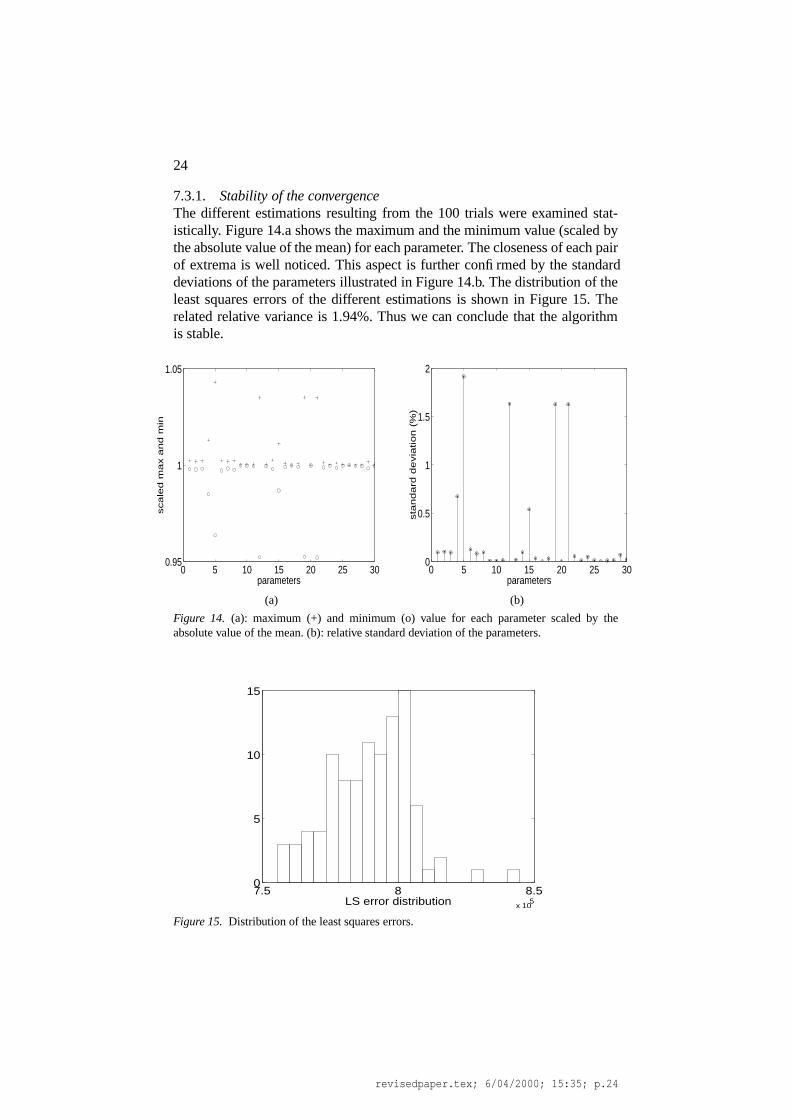
7.3.1. Stability of the convergenceThe different estimations resulting from the 100 trials were examined stat-istically. Figure 14.a shows the maximum and the minimum value (scaled bythe absolute value of the mean) for each parameter. The closeness of each pairof extrema is well noticed. This aspect is further confirmed by the standarddeviations of the parameters illustrated in Figure 14.b. The distribution of theleast squares errors of the different estimations is shown in Figure 15. Therelated relative variance is 1.94%. Thus we can conclude that the algorithmis stable.

0 5 10 15 20 25 300.95

1

1.05

parameters

sca

led

ma

x a

nd

min

0 5 10 15 20 25 300

0.5

1

1.5

2

parameters

sta

nd

ard

de

via

tio

n (

%)

(a) (b)

Figure 14. (a): maximum (+) and minimum (o) value for each parameter scaled by theabsolute value of the mean. (b): relative standard deviation of the parameters.

7.5 8 8.5x 10

5

0

5

10

15

LS error distribution

Figure 15. Distribution of the least squares errors.


25

7.3.2. Closeness to the actual optimal solutionBy “actual optimal solution” we mean the estimation obtained from a processwhere the constraints are defined, incorporated and satisfied within the leastsquares error formulation. The solution provided in this case completely sat-isfies the constraints. So one may ask how close is the estimate obtained byour approach to this optimal solution. As we have mentioned previously, suchan ideal and elegant formulation is difficult or impossible to achieve for manyobjects due to the complexity and to the non-linearity of the geometric con-straints. In fact one purpose and motivation of our approach is to overcomethis problem. Nevertheless it is possible for some simple particular cases tocombine the constraints with the least squares error.

So, in order to make a comparison with the optimal solution a sub-part ofthe multi-quadric object shown in Figure 13 was considered. It is composedof the two parallel planes S1 and S3. The objective is to estimate the planes’orientation taking into account the parallel constraint. For the first case, theparallel constraint is implicitly considered by associating one normal to bothplanes. The optimization function is then:

�nT H �n � λ�1 � �nT �n �

where H is the appropriate data matrix. The second term of the function is theunit constraint. A closed form solution is provided by the eigenvalue method.

In the second case each plane was assigned a different normal vector.The equality of the two normals has to be satisfied through the optimizationprocess. According to our approach the objective function is:

�n1T H1 �n1 � �n3

T H3 �n3 � λ1�1 � �n1

T �n1 � 2 � λ2�1 � �n3

T �n3 � 2 � λ3�1 � �n1

T �n3 � 2

100 tests were applied for each of the two cases. The average of theresults are summarized in Table V. The estimations are similar in the two

Table V. Mean estimates of S1 and S3 normal and LS error in the two types of solutions.�n

�n1

�n3 angle(

�n1 � �

n3) (degree) LS error

Closed form

0 � 5316

0 � 6733

0 � 5139

- - - 9.07

Optimization -

0 � 5316

0 � 6733

0 � 5139

0 � 5316

0 � 6733

0 � 5139

0.00 9.06

cases. This shows that both solutions converge to the same value and almost


26

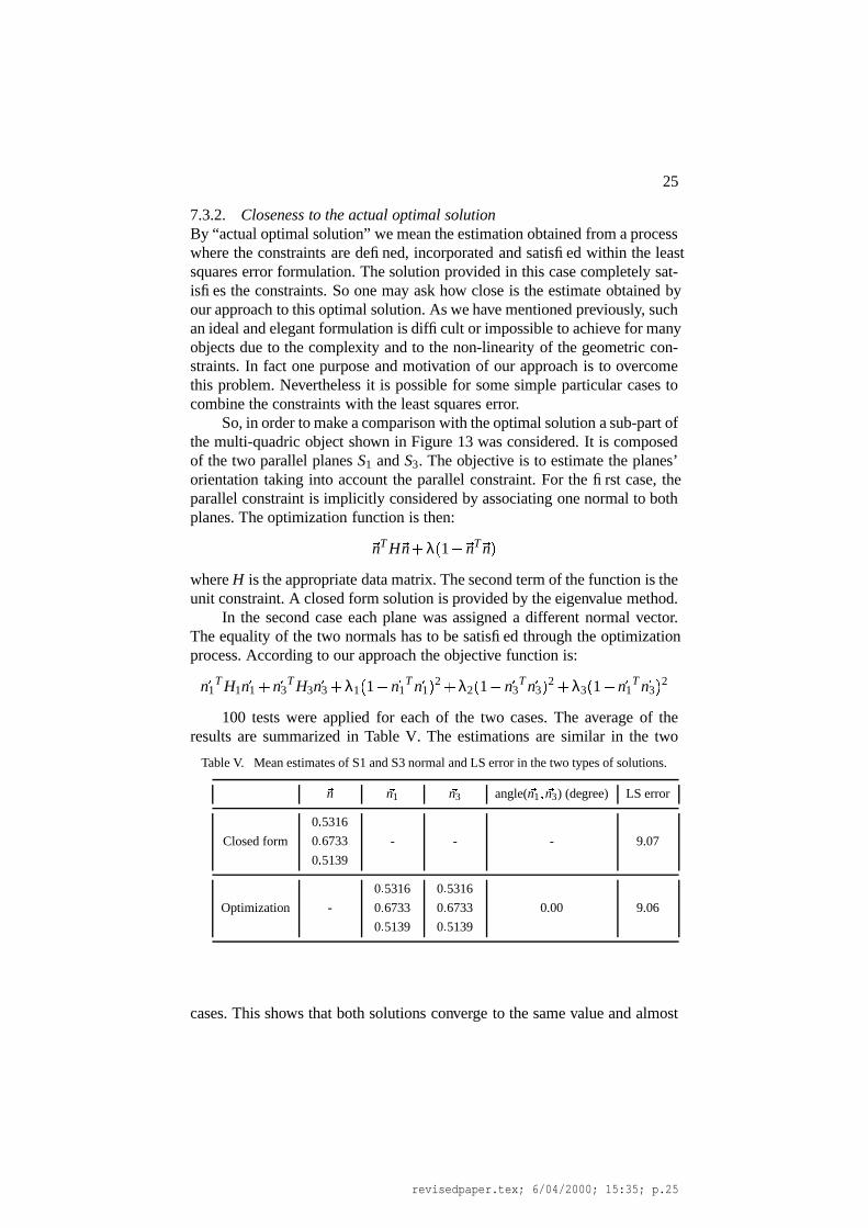
equally minimize the least squares error. The LS of the second solution isslightly lower than the optimal solution one. This is because in the optimalcase the constraint is perfectly satisfied so the least squares error has to absorball the error. The same convergence of the two solutions is further confirmedfrom the distribution of the difference between the two approaches (angle� �n � �nc � where �nc is the mean of �n1 and �n3) and the difference between therelated LS residuals from the 100 trials (Fig.16). Thus we conclude that ouroptimization process leads us to solutions that are very close to the optimal.

−5 −4.8 −4.6 −4.4 −4.2 −4 −3.80

2

4

6

8

10

12

14

16

log10

(angle(nc,n ))

−5 −4.5 −4 −3.5 −30

2

4

6

8

10

12

14

log10

(|LSc − LS

i|/mean(LS

i))

(a) (b)

Figure 16. (a): Distribution of the estimation difference. (b): Distribution of the LS residualsdifference.

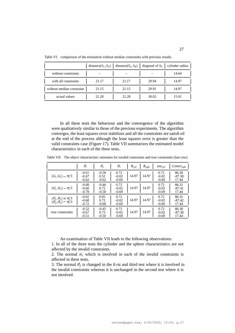
7.3.3. Leaving some features unconstrainedAnother series of tests has been performed without considering the diagonalconstraint (constraint 12). This is in order to check if this will affect the pos-ition of the four plane surfaces with respect to the cylinder axis and thereforethe estimation of the edge of the square surface S5. Results are shown inTable VI with the previous results for comparison. It is noticed that the radiusestimation is not affected but the incorporation of the additional constraintsslightly reduces the diagonal length error.

7.3.4. Invalidity of the constraintsSuppose that one or more constraints do not reflect the actual relationshipsbetween features and therefore are invalid. What would be the behaviour ofthe algorithm? Will these “false constraints” be satisfied? What could be theresulting estimated model ?

To answer these questions, some angle constraints were set to an incor-rect values. Three tests were carried out, in the first the angle

� �n1 � �n2 � was setto π � 3, in the second the angle

� �n1 � �n5 � was set to π � 3 and in the third testboth angles

� �n1 � �n5 � and� �n2 � �n5 � were set to π � 3 (note that the correct angles

are π � 2 for both angles).


27

Table VI. comparison of the estimation without median constraints with previous results.

distance(S1 � S3) distance(S2 � S4) diagonal of S5 cylinder radius

without constraints – – – 14.64

with all constraints 21.17 21.17 29.94 14.97

without median constraint 21.15 21.15 29.91 14.97

actual values 21.28 21.28 30.02 15.01

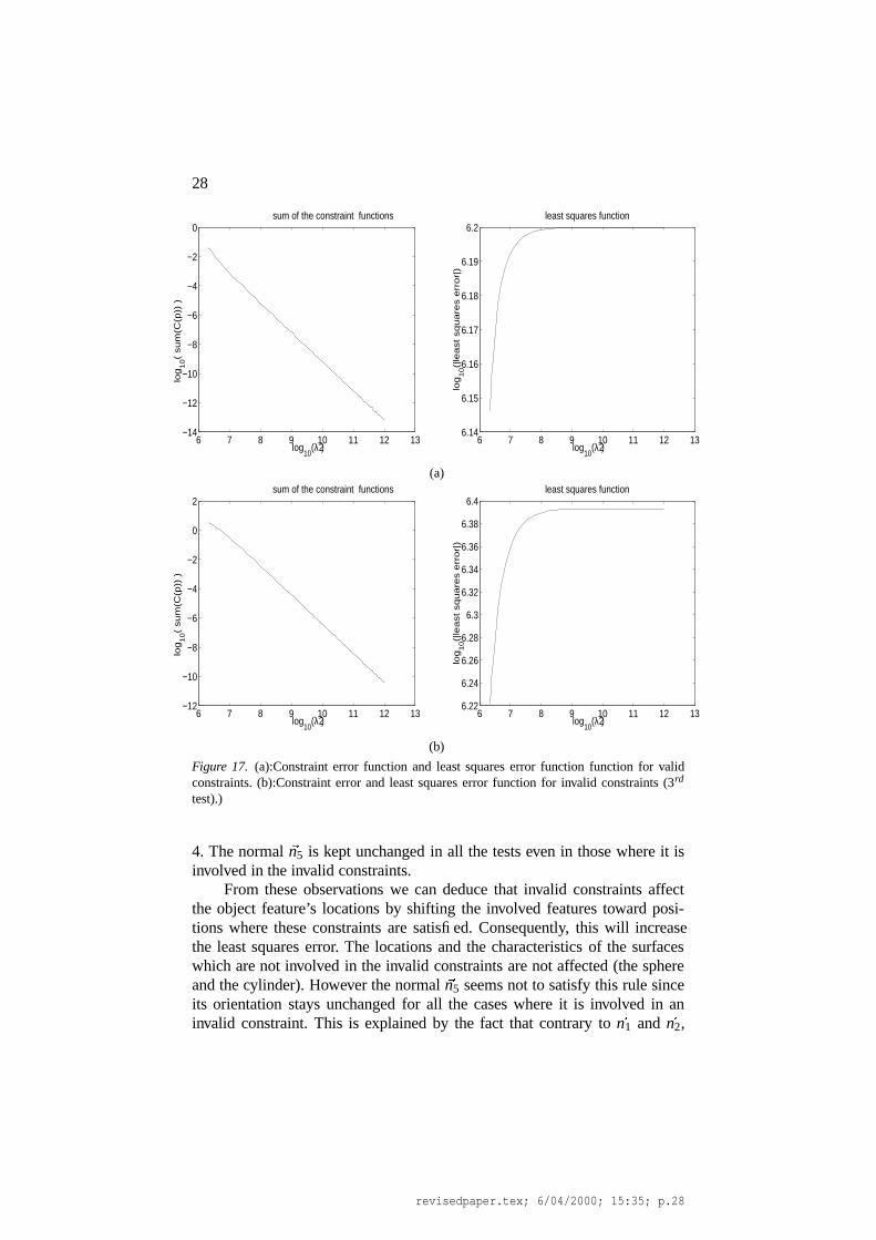
In all these tests the behaviour and the convergence of the algorithmwere qualitatively similar to those of the previous experiments. The algorithmconverges, the least squares error stabilizes and all the constraints are satisfiedat the end of the process although the least squares error is greater than thevalid constraints case (Figure 17). Table VII summarizes the estimated modelcharacteristics in each of the three tests.

Table VII. The object characteristic estimates for invalid constraints and true constraints (last row).�n1

�n2

�n5 Rcyl Rsph axecyl Centersph

� �n1 � �

n2 � � π�3

-0.61-0.47-0.62

-0.580.52-0.62

0.72-0.02-0.69

14.97 14.970.72-0.02-0.69

86.30-87.3817.44

� �n1 � �

n5 � � π�3

-0.08-0.60-0.78

-0.460.72-0.50

0.72-0.02-0.69

14.97 14.970.72-0.02-0.69

86.31-87.4117.44

� �n1 � �

n5 � � π�3� �

n2 � �n5 � � π

�3

-0.02-0.68-0.72

0.050.72-0.68

0.72-0.02-0.69

14.97 14.970.72-0.02-0.69

86.31-87.4217.44

true constraints-0.52-0.67-0.51

-0.450.73-0.50

0.72-0.02-0.69

14.97 14.970.72-0.02-0.69

86.30-87.3817.44

An examination of Table VII leads to the following observations:1. In all of the three tests the cylinder and the sphere characteristics are notaffected by the invalid constraints.2. The normal �n1 which is involved in each of the invalid constraints isaffected in three tests.3. The normal �n2 is changed in the first and third test where it is involved inthe invalid constraints whereas it is unchanged in the second test where it isnot involved.


28

6 7 8 9 10 11 12 13−14

−12

−10

−8

−6

−4

−2

0

log10

(λ2 )

log

10(

su

m(C

(p))

)


6 7 8 9 10 11 12 136.14

6.15

6.16

6.17

6.18

6.19

6.2

log10

(λ2 )lo

g1

0(|

lea

st

sq

ua

res e

rro

r|)

least squares function

(a)

6 7 8 9 10 11 12 13−12

−10

−8

−6

−4

−2

0

2

log10

(λ2 )

log

10(

su

m(C

(p))

)


6 7 8 9 10 11 12 136.22

6.24

6.26

6.28

6.3

6.32

6.34

6.36

6.38

6.4

log10

(λ2 )

log

10(|

lea

st

sq

ua

res e

rro

r|)


(b)

Figure 17. (a):Constraint error function and least squares error function function for validconstraints. (b):Constraint error and least squares error function for invalid constraints (3rd

test).)

4. The normal �n5 is kept unchanged in all the tests even in those where it isinvolved in the invalid constraints.

From these observations we can deduce that invalid constraints affectthe object feature’s locations by shifting the involved features toward posi-tions where these constraints are satisfied. Consequently, this will increasethe least squares error. The locations and the characteristics of the surfaceswhich are not involved in the invalid constraints are not affected (the sphereand the cylinder). However the normal �n5 seems not to satisfy this rule sinceits orientation stays unchanged for all the cases where it is involved in aninvalid constraint. This is explained by the fact that contrary to �n1 and �n2,


29

�n5 is also involved in other constraints, in particular it is constrained to havethe same orientation as the cylinder axis. The satisfaction of this constraintkeeps it collinear to the cylinder axis and prevents its orientation from beingaffected. Thus the algorithm satisfies the invalid constraints in which �n5 isinvolved by acting on the other normals involved in these constraints.

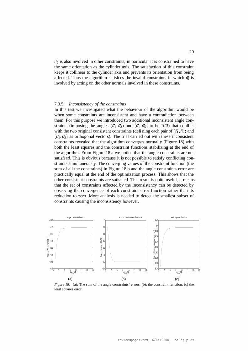
7.3.5. Inconsistency of the constraintsIn this test we investigated what the behaviour of the algorithm would bewhen some constraints are inconsistent and have a contradiction betweenthem. For this purpose we introduced two additional inconsistent angle con-straints (imposing the angles

� �n1 � �n2 � and� �n1 � �n5 � to be π � 3) that conflict

with the two original consistent constraints (defining each pair of� �n1 � �n2 � and� �n1 � �n5 � as orthogonal vectors). The trial carried out with these inconsistent

constraints revealed that the algorithm converges normally (Figure 18) withboth the least squares and the constraint functions stabilizing at the end ofthe algorithm. From Figure 18.a we notice that the angle constraints are notsatisfied. This is obvious because it is not possible to satisfy conflicting con-straints simultaneously. The converging values of the constraint function (thesum of all the constraints) in Figure 18.b and the angle constraints error arepractically equal at the end of the optimization process. This shows that theother consistent constraints are satisfied. This result is quite useful, it meansthat the set of constraints affected by the inconsistency can be detected byobserving the convergence of each constraint error function rather than itsreduction to zero. More analysis is needed to detect the smallest subset ofconstraints causing the inconsistency however.

6 7 8 9 10 11 12 13−0.5

−0.45

−0.4

−0.35

−0.3

−0.25

−0.2

−0.15

log10

(λ2 )

log

10(

C_

an

gl(p

) )

angle constraint function

6 7 8 9 10 11 12 13−0.4

−0.2

0

0.2

0.4

0.6

0.8

1

log10

(λ2 )

log

10(

su

m (

C(p

)) )


6 7 8 9 10 11 12 136.24

6.26

6.28

6.3

6.32

6.34

6.36

6.38

6.4

6.42

log10

(λ2 )

log

10(|

lea

st

sq

ua

res e

rro

r|)


(a) (b) (c)

Figure 18. (a): The sum of the angle constraints’ errors. (b): the constraint function. (c) theleast squares error


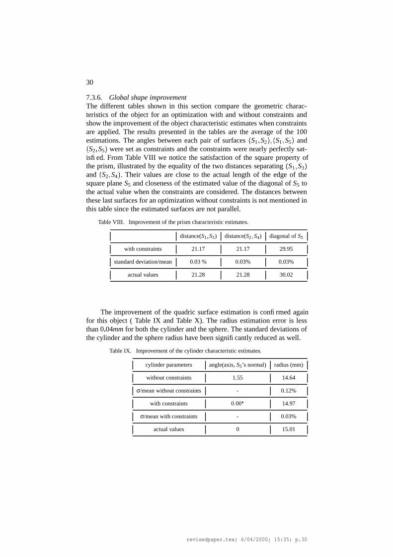
30

7.3.6. Global shape improvementThe different tables shown in this section compare the geometric charac-teristics of the object for an optimization with and without constraints andshow the improvement of the object characteristic estimates when constraintsare applied. The results presented in the tables are the average of the 100estimations. The angles between each pair of surfaces

�S1 � S2 � �

�S1 � S5 � and�

S2 � S5 � were set as constraints and the constraints were nearly perfectly sat-isfied. From Table VIII we notice the satisfaction of the square property ofthe prism, illustrated by the equality of the two distances separating

�S1 � S3 �

and�S2 � S4 � . Their values are close to the actual length of the edge of the

square plane S5 and closeness of the estimated value of the diagonal of S5 tothe actual value when the constraints are considered. The distances betweenthese last surfaces for an optimization without constraints is not mentioned inthis table since the estimated surfaces are not parallel.

Table VIII. Improvement of the prism characteristic estimates.

distance(S1 � S3) distance(S2 � S4) diagonal of S5

with constraints 21.17 21.17 29.95

standard deviation/mean 0.03 % 0.03% 0.03%

actual values 21.28 21.28 30.02

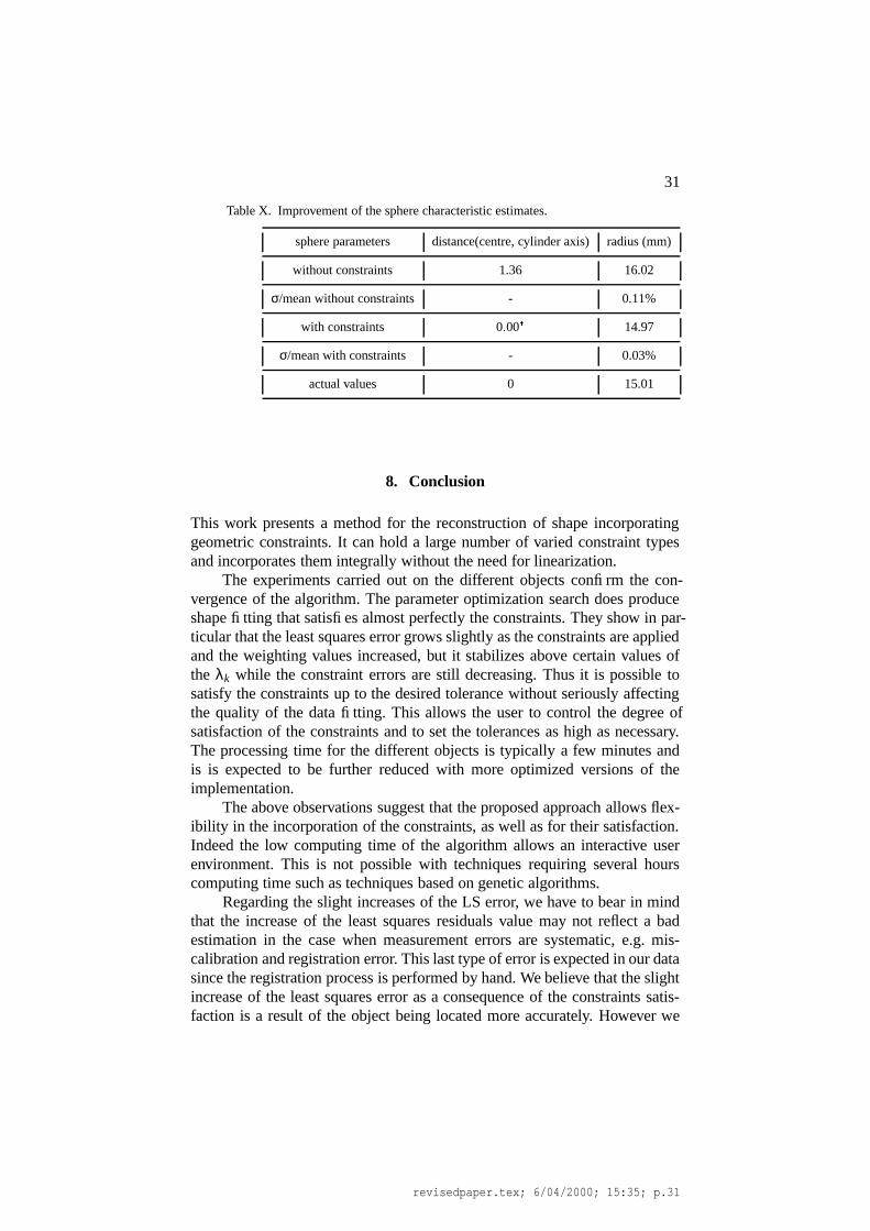
The improvement of the quadric surface estimation is confirmed againfor this object ( Table IX and Table X). The radius estimation error is lessthan 0 � 04mm for both the cylinder and the sphere. The standard deviations ofthe cylinder and the sphere radius have been significantly reduced as well.

Table IX. Improvement of the cylinder characteristic estimates.

cylinder parameters angle(axis, S5’s normal) radius (mm)

without constraints 1.55 14.64

σ/mean without constraints - 0.12%


14.97

σ/mean with constraints - 0.03%

actual values 0 15.01


31

Table X. Improvement of the sphere characteristic estimates.

sphere parameters distance(centre, cylinder axis) radius (mm)

without constraints 1.36 16.02

σ/mean without constraints - 0.11%


14.97

σ/mean with constraints - 0.03%

actual values 0 15.01

8. Conclusion

This work presents a method for the reconstruction of shape incorporatinggeometric constraints. It can hold a large number of varied constraint typesand incorporates them integrally without the need for linearization.

The experiments carried out on the different objects confirm the con-vergence of the algorithm. The parameter optimization search does produceshape fitting that satisfies almost perfectly the constraints. They show in par-ticular that the least squares error grows slightly as the constraints are appliedand the weighting values increased, but it stabilizes above certain values ofthe λk while the constraint errors are still decreasing. Thus it is possible tosatisfy the constraints up to the desired tolerance without seriously affectingthe quality of the data fitting. This allows the user to control the degree ofsatisfaction of the constraints and to set the tolerances as high as necessary.The processing time for the different objects is typically a few minutes andis is expected to be further reduced with more optimized versions of theimplementation.

The above observations suggest that the proposed approach allows flex-ibility in the incorporation of the constraints, as well as for their satisfaction.Indeed the low computing time of the algorithm allows an interactive userenvironment. This is not possible with techniques requiring several hourscomputing time such as techniques based on genetic algorithms.

Regarding the slight increases of the LS error, we have to bear in mindthat the increase of the least squares residuals value may not reflect a badestimation in the case when measurement errors are systematic, e.g. mis-calibration and registration error. This last type of error is expected in our datasince the registration process is performed by hand. We believe that the slightincrease of the least squares error as a consequence of the constraints satis-faction is a result of the object being located more accurately. However we


32

intend to investigate a more robust form for the objective function involvingthe data noise statistics.

The different trials applied on the multi-quadric objects confirm the sta-bility of the convergence of the algorithm. The low values of the parameters’variances illustrates the stability of the solution provided by the optimizationsearch process. The tests have shown as well that the proposed approach leadsto an estimate which is close to the optimal solution in the case where theconstraints could be combined with the least squares error. The experimentsalso show that applying the constraints to only some features does not ser-iously affect the estimation of the unconstrained surfaces. The estimation isstill improved compared to the case of unconstrained optimization.

The examination of some constraint invalidity cases has shown the con-straints are always satisfied whether they are valid or not and the behaviour ofthe algorithm is typically the same. The satisfaction of an invalid constraintleads to the relocation of the involved and less constrained features (havingmore degrees of freedom) toward positions where the inconsistency is re-moved. However, this will result in a false object model. The trial performedwith constraint inconsistency revealed the same behaviour regarding the con-vergence of the algorithm but the inconsistent constraints are not satisfied atthe end of the optimization. This suggests that constraint validity and con-sistency checking have to be done before starting the optimization process,or at least examination of the constraint error results to determine if a set ofinconsistent constraints have been supplied.

Regarding the shape estimation accuracy, the comparison of the objectdimension estimates with those from unconstrained fitting confirms that theproposed approach improves the quality of the shape reconstruction to a highdegree. For the second quadric object the radius of the cylinder and the spherehave an estimation error in the range of 0 � 04mm, the edge of the square prismhas an estimation error around 0 � 1mm. The radius of the cylinder patch estim-ated from the registered half cylinder has an estimation error around 0 � 01mm.For a single view it is less than 0 � 5mm. The same range of error is obtainedfor the radius of the cylinder patch of the first multi-quadric object.

Results for the cone patch are less satisfactory for the first multi-quadricobject. This is mainly due to the relatively small area of the conic patch.Actually, we intentionally chose to work with small patches because uncon-strained fitting surface techniques fail to give reasonable estimates in this case(see the radius estimation in Table III) even with robust algorithms due to the“poorness” of the information embodied in the patch.

Although the experiments presented in this work were performed onsingle objects, the proposed approach can hold for multiple objects. Indeed,generally industrial parts are designed to fit to each other, so geometric rela-tionships between the parts may be considered and the resulting constraintscan be incorporated as well in the optimization process.


33

Another area we are starting to investigate is how one might automatic-ally identify inter-surface relationships that can have a constraint applied. Inmanufacturing objects, simple angular and spatial relationships are given bydesign. So, it should be straightforward to define simple statistical tests thathypothesize standard feature relationships, subject to the feature’s statisticalposition distribution. With this analysis, a computer program could propose avariety of constraints that a human could either accept or reject, after whichshape reconstruction could occur.

The proposed technique restricts its scope to applications where a reas-onable initial solution is available. Also the approach can hold only geometricconstraints that can be represented by continuous and differentiable functions.More complex objects with higher order surfaces can use by the approach asfar as this condition is fulfilled.

Finally, although this work is mainly intended for object modelling itmay be extended to any constrained built environment application, for ex-ample modelling of different parts of an industrial plant (pipes, reservoirs,etc) needs the consideration of the geometric relationships between thesedifferent parts in order that the whole model will be consistent. The sameis true as well for modelling different compartments of buildings. Cities areprobably too under-constrained.

ACKNOWLEDGEMENT

The work presented in this paper was funded by UK EPSRC grant GR/L25110.


34

References

1. R. Anderl, R Mendegen. Modelling with constraints: Theoretical foundation andapplication. CAD, Vol. 28, No 3, pp 155-168 1996.

2. R.M.Bolle, D.B.Cooper. On Optimally Combining Pieces of Information, with Applica-tion to Estimating 3-D Complex-Object Position from Range Data. IEEE Trans. PAMI,Vol.8, No.5, pp.619-638, September 1986.

3. C.G. Broyden, N.F. Attia. Penalty Functions, Newton’s Method and Quadratic Pro-gramming. Journal of optimization theory and applications, Vol.58, No.3, pp.377-385.,1988.

4. J.De Geeter, H.V.Brussel, J.De Schutter, M. Decreton. A Smoothly Constrained KalmanFilter. IEEE Trans. PAMI pp.1171-1177, No.10, Vol.19, October 1997.

5. Chang-Xue Feng, A. Kusiak. Constraints-based design of parts. CAD, Vol.27, No.5,1995 pp 343-352.

6. A.V. Fiacco, G.P. McCormick. Nonlinear Programming: Sequential UnconstrainedMinimization Techniques. John Wiley and Sons, New York 1968.

7. A.F. Fitzgibbon, D.W. Eggert, R.B. Fisher. High-level CAD model acquisition fromrange images. CAD, Vol.29, No.4, pp.321-330, 1997.

8. R.Fletcher. Practical Methods of Optimization. John Wiley & Sons, 1987.

9. P.E.Gill, W.Murray, M.H.Wright. Practical Optimization. Academic Press, 1981.

10. D.E. Goldberg. Genetic Algorithms in Search, Optimization and Machine Learning.Addison-Wesley, Reading, MA, 1989.

11. Z. Michalewicz. Genetic Algorithms + Data Structures = Evolution Programs. Springer-Verlag, 1996.

12. A. Hoover, G. Jean-Baptiste, X. Jiang, P. J. Flynn, H. Bunke, D. Goldgof, K. Bowyer, D.Eggert, A. Fitzgibbon, R. Fisher. An Experimental Comparison of Range SegmentationAlgorithms. IEEE Trans. PAMI, Vol.18, No.7, pp.673-689, July 1996.

13. S.L.S. Jacoby, J.S. Kowalik, J.T.Pizzo. Iterative Methods for Nonlinear OptimizationProblems. Prentice-Hall, Inc. Englewood Cliffs, New Jersey, 1972.

14. W. Murray. An Algorithm for Constrained Minimization. Optimization, Ed. R.Fletcher,pp.247-258, Academic Press, London, 1969.

15. J.Porrill. Optimal Combination and Constraints for Geometrical Sensor Data. Interna-tional Journal of Robotics Research, Vol.7, No.6, pp.66-78, 1988.

16. A.A.G. Requicha. Representation of Tolerances in Solid Modelling: Issues and Al-ternative Approaches. Solid Modelling by Computers: from Theory to Applications,J.W.Boyse amd M.S.Pickett, Eds. New York: Plenum, 1984, pp.3-22.

17. R.T. Rockafellar. Convex Analysis. Princeton University Press, 1970.

18. A.P. Rockwood, J. Winget. Three-dimensional object reconstruction from two-dimensional images. CAD, Vol.29, No.4, pp.279-286, 1997.

19. B.S. Shin, Y.G. Shin. Fast 3D solid model reconstruction from orthographic views.CAD, Vol.30, No.1, pp.63-76.

20. T. Varady, R. R. Martin, J. Cox. Reverse engineering of geometric models, anintroduction. CAD, Vol.29, No.4, pp. 255-268, 1997.


35

21. N.Werghi, R.B.Fisher, A.Ashbrook, C.Robertson. Modelling Objects Having QuadricSurfaces Incorporating Geometric Constraint. Proc. ECCV’98, pp.185-201, Freiburg,Germany, June 1998.

22. Q.W. Yan, C.L.P. Chen, Z. Tang. Reconstruction of 3D objects from orthographicprojections. CAD, Vol.26, No.9, 1994.

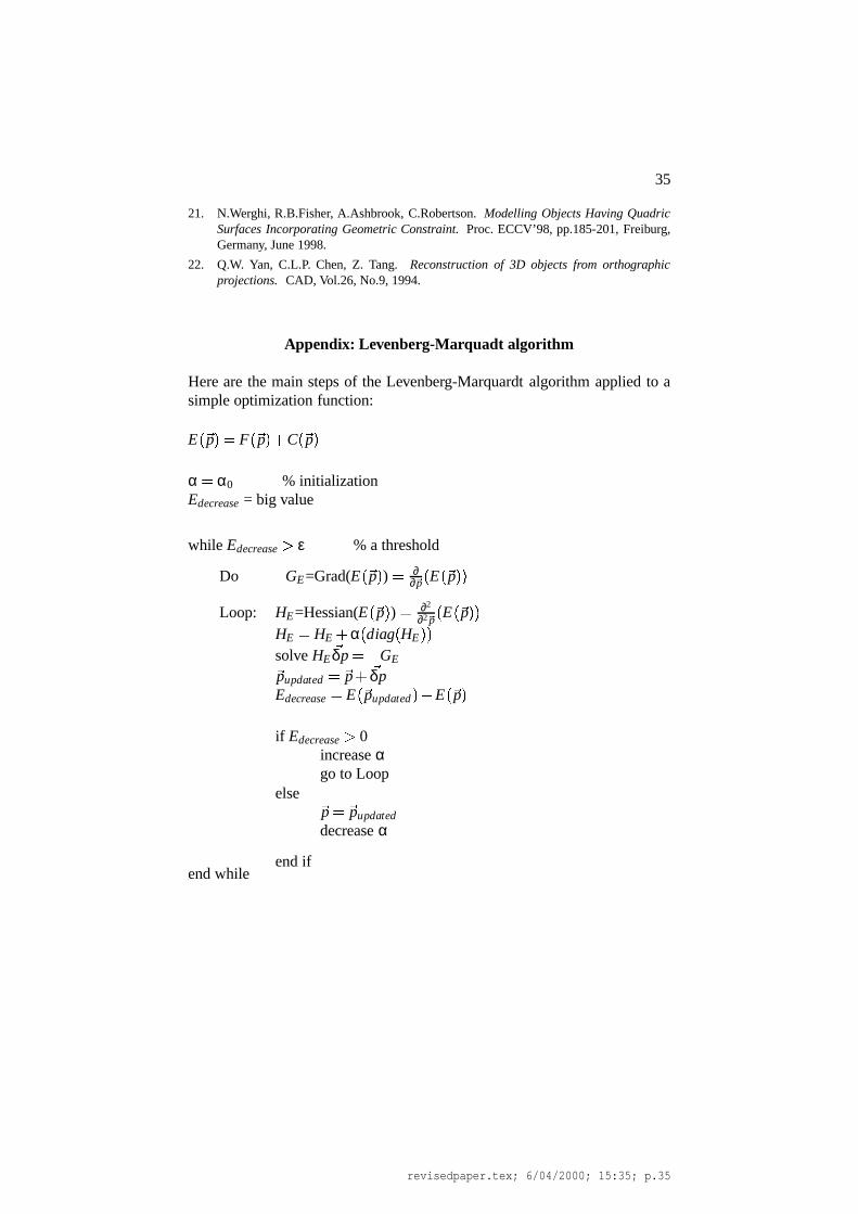
Appendix: Levenberg-Marquadt algorithm

Here are the main steps of the Levenberg-Marquardt algorithm applied to asimple optimization function:

E� �p � � F

� �p � � C� �p �

α � α0 % initializationEdecrease = big value

while Edecrease � ε % a threshold

Do GE=Grad(E� �p � ) � ∂

∂ �p

�E� �p � �

Loop: HE=Hessian(E� �p � ) � ∂2

∂2 �p

�E� �p � �

HE � HE � α�diag

�HE � �

solve HE�δp � � GE

�pupdated � �p � �δpEdecrease � E

� �pupdated � � E� �p �

if Edecrease � 0increase αgo to Loop

else�p � �pupdated

decrease α

end ifend while



Documents

Shape Reconstruction Incorporating Multiple Nonlinear Geometric Constraints