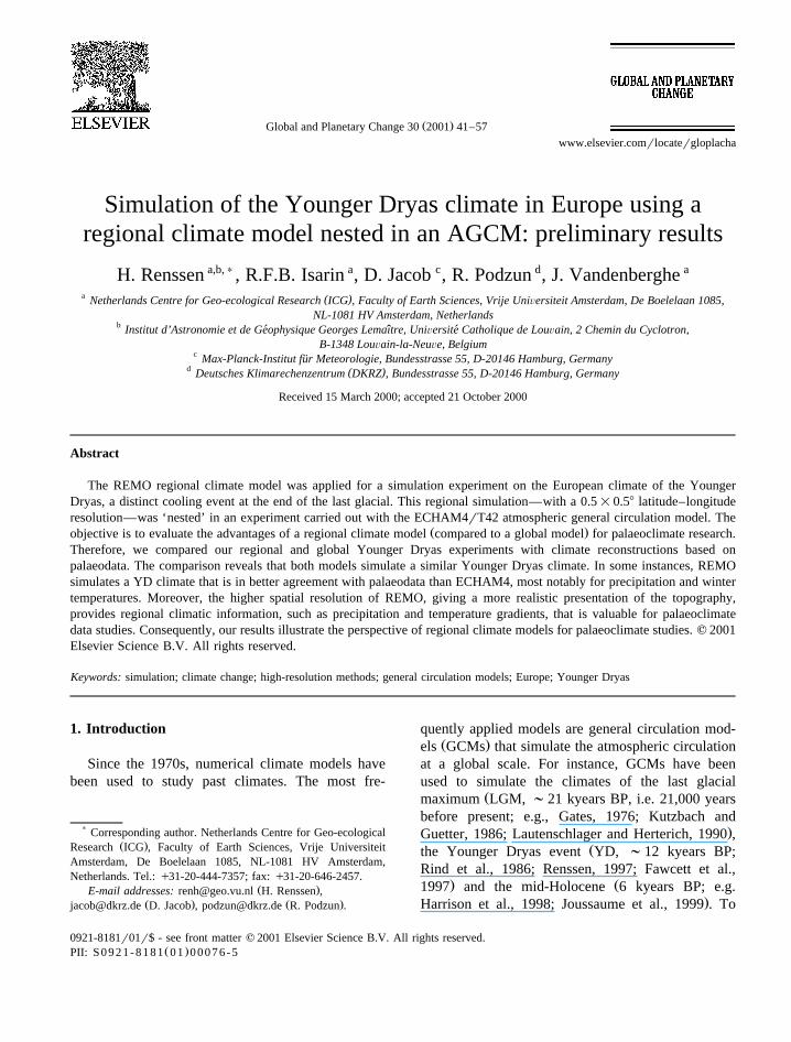
Ž .Global and Planetary Change 30 2001 41–57www.elsevier.comrlocatergloplacha

Simulation of the Younger Dryas climate in Europe using aregional climate model nested in an AGCM: preliminary results

H. Renssen a,b,), R.F.B. Isarin a, D. Jacob c, R. Podzun d, J. Vandenberghe a

a ( )Netherlands Centre for Geo-ecological Research ICG , Faculty of Earth Sciences, Vrije UniÕersiteit Amsterdam, De Boelelaan 1085,NL-1081 HV Amsterdam, Netherlands

b Institut d’Astronomie et de Geophysique Georges Lemaıtre, UniÕersite Catholique de LouÕain, 2 Chemin du Cyclotron,´ ˆ ´B-1348 LouÕain-la-NeuÕe, Belgium

c Max-Planck-Institut fur Meteorologie, Bundesstrasse 55, D-20146 Hamburg, Germany¨d ( )Deutsches Klimarechenzentrum DKRZ , Bundesstrasse 55, D-20146 Hamburg, Germany

Received 15 March 2000; accepted 21 October 2000

Abstract

The REMO regional climate model was applied for a simulation experiment on the European climate of the YoungerDryas, a distinct cooling event at the end of the last glacial. This regional simulation—with a 0.5=0.58 latitude–longituderesolution—was ‘nested’ in an experiment carried out with the ECHAM4rT42 atmospheric general circulation model. The

Ž .objective is to evaluate the advantages of a regional climate model compared to a global model for palaeoclimate research.Therefore, we compared our regional and global Younger Dryas experiments with climate reconstructions based onpalaeodata. The comparison reveals that both models simulate a similar Younger Dryas climate. In some instances, REMOsimulates a YD climate that is in better agreement with palaeodata than ECHAM4, most notably for precipitation and wintertemperatures. Moreover, the higher spatial resolution of REMO, giving a more realistic presentation of the topography,provides regional climatic information, such as precipitation and temperature gradients, that is valuable for palaeoclimatedata studies. Consequently, our results illustrate the perspective of regional climate models for palaeoclimate studies. q 2001Elsevier Science B.V. All rights reserved.

Keywords:simulation; climate change; high-resolution methods; general circulation models; Europe; Younger Dryas

1. Introduction

Since the 1970s, numerical climate models havebeen used to study past climates. The most fre-

) Corresponding author. Netherlands Centre for Geo-ecologicalŽ .Research ICG , Faculty of Earth Sciences, Vrije Universiteit

Amsterdam, De Boelelaan 1085, NL-1081 HV Amsterdam,Netherlands. Tel.: q31-20-444-7357; fax: q31-20-646-2457.

Ž .E-mail addresses:renh@geo.vu.nl H. Renssen ,Ž . Ž .jacob@dkrz.de D. Jacob , podzun@dkrz.de R. Podzun .

quently applied models are general circulation mod-Ž .els GCMs that simulate the atmospheric circulation

at a global scale. For instance, GCMs have beenused to simulate the climates of the last glacial

Žmaximum LGM, ;21 kyears BP, i.e. 21,000 yearsbefore present; e.g., Gates, 1976; Kutzbach and

.Guetter, 1986; Lautenschlager and Herterich, 1990 ,Žthe Younger Dryas event YD, ;12 kyears BP;

Rind et al., 1986; Renssen, 1997; Fawcett et al.,. Ž1997 and the mid-Holocene 6 kyears BP; e.g.

.Harrison et al., 1998; Joussaume et al., 1999 . To

0921-8181r01r$ - see front matter q 2001 Elsevier Science B.V. All rights reserved.Ž .PII: S0921-8181 01 00076-5

( )H. Renssen et al.rGlobal and Planetary Change 30 2001 41–5742

analyse model performance, the results of these stud-ies have been compared with climate reconstructions

Žbased on palaeodata e.g. Kutzbach and Wright,1985; Texier et al., 1997; Renssen and Isarin, 1998;

.Kohfeld and Harrison, 2000 . However, the differ-ences in spatial scale between model results andreconstructions often pose a problem. GCMs coverthe entire globe and have coarse resolutions with atypical distance between grid points of 200–500 km.In contrast, palaeoclimate reconstructions are usuallycreated for specific regions and are therefore more

Ž .detailed Crowley and North, 1991 . Consequently,to make GCM-data comparisons meaningful, largeand spatially extensive proxy datasets are required tomake reconstructions that cover at least a continentŽ .Isarin and Renssen, 1999 . However, such datasetsare only available for ideal time-periods. Usingdownscaling techniques may solve this spatial-scaleproblem. It should be noted that downscaling doesnot resolve the differences in temporal scale between

Ž .climate simulations mean for ;500–1000 yearsŽ .and proxy data representing shorter time-periods .

This follows from the boundary conditions used todrive palaeoclimate experiments, which often repre-

Žsent average conditions for at least 500 years forexample, ice sheet extent and sea surface tempera-

.tures , implying that the simulated climate is to beconsidered as a 500-year mean.

Downscaling methods may be divided into statis-tical and dynamical techniques. Statistical techniquesare based on relationships between measurements oflocal modern climate and the climate simulated inlarger-scale models. These relationships may bebased on regression, circulation patterns or stochasticweather generators. In studies of climate change,typically, GCMs are applied to simulate the global-scale climate following a certain scenario and, subse-quently, the statistical relations are used to infer the

Ž .local climate Mitchell and Hulme, 1999 . In con-trast, dynamical techniques make use of physicallybased climate models with a higher spatial resolu-tion. These models may be GCMs with a grid that isvariable, so that the resolution can be optimised for

Žthe region of interest e.g. Deque and Piedelievre,.1995 . Alternatively, regional climate models

Ž .RCMs can be ‘nested’ in a GCM. This procedureinvolves the definition of a certain regional domain,for which the RCM simulates the climate at a rela-

Ž .tively high resolution i.e. 50–70 km , while thelateral boundary conditions are produced by a GCMŽe.g. Giorgi, 1990; Giorgi et al., 1990; Giorgi and

.Mearns, 1991; Jones et al., 1995 . It should berealised that in the latter procedure, potential system-atic errors in the GCM are transferred to the RCM.Despite its potential, the ‘nested’ approach has onlybeen applied in a few palaeoclimate studies. For

Ž .instance, Hostetler et al. 1994 simulated the LGMclimate of the western USA with a nested RCM.However, to our knowledge, no studies using thisnested technique have been published for simulationsof the palaeoclimate in Europe.

We applied this ‘nested’ method to perform aŽsimulation of the Younger Dryas YD, or Greenland

.Stadial 1; Bjorck et al., 1998 climate in Europe. YD¨is a distinct cold period at the end of the last glacialŽ .around 12 kyears BP that is clearly registered ingeological records surrounding the Atlantic OceanŽ .see, e.g. Lowe et al., 1995; Walker, 1995 . In thispaper, we present the results of an integration withYD surface boundary conditions that was performedwith the REMO-RCM developed at the Max-

ŽPlanck-Institute for Meteorology Jacob and Podzun,.1997, 2000 . This integration was nested in a YD

simulation carried out with the ECHAM4 AGCMŽ .see Renssen et al., 2000 . Our aim is to evaluate theadvantages of the use of an RCM for palaeoclimateresearch, by comparing the regional and global simu-lation results with palaeodata, giving information on

Žthe YD climate in Europe e.g. Isarin, 1997; Renssen.and Isarin, 1998; Isarin and Bohncke, 1999 . As

computing costs for nested experiments are relativelyhigh, we restricted the duration of the nested integra-tion to 3 years. We realise that an experiment with a3-year duration is too short to make decisive conclu-sions and, therefore, we consider our results as pre-liminary.

2. Methods

2.1. AGCM

Global-scale experiments were performed withŽ .the ECHAM4 European Centre HAMburg AGCM

Ž .of the Max-Planck-Institute MPI for Meteorology,Hamburg. This spectral AGCM, with 19 atmospheric

( )H. Renssen et al.rGlobal and Planetary Change 30 2001 41–57 43

layers, is capable of simulating satisfactorily themain features of the modern global circulationŽ .Roeckner et al., 1996 . We applied the T42-version,which translates to horizontal resolution of ;2.88latitude–longitude. A detailed description of theECHAM4 model can be found in Roeckner et al.Ž .1992, 1996 and Deutsches KlimarechenzentrumŽ .1994 .

2.2. RCM

The regional model used in this study is theŽ .REMO REgional MOdel RCM that was developed

by the MPI for Meteorology, together with DeutschesŽ .Klimarechenzentrum DKRZ , Forschungszentrum

Ž .Geesthacht GKSS and Deutscher WetterdienstŽ .DWD . REMO is based on the Europa-Model de-veloped at DWD. In addition to the physical pa-rameterisation packages of the Europa-model, thephysical parameterisation schemes used in the globalclimate model ECHAM4 were implemented. Weapplied the version of REMO with physics equiva-lent to those in the ECHAM4 model. The spatialresolution of the REMO-version used in this studyconsists of a surface grid of 0.58 longitude by 0.58

Žlatitude and 20 layers in the vertical direction Jacob.and Podzun, 1997 . We used the standard domain for

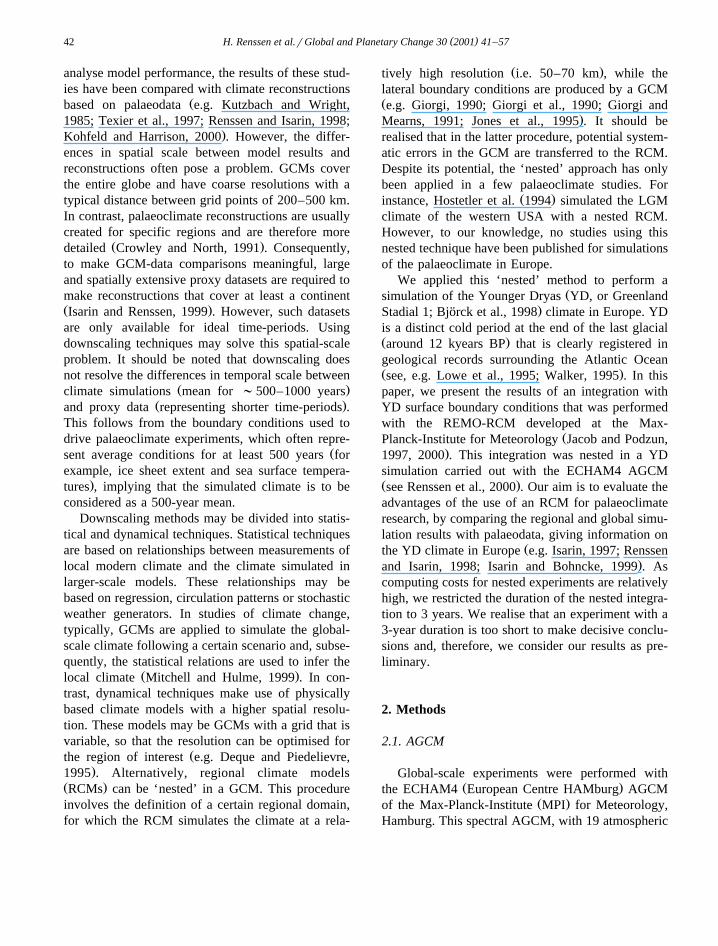
Europe, with 81=91 grid points and rotated spheri-cal coordinates with the North Pole at 1708W, 32.58NŽ .see Fig. 1a . In our experiments, REMO uses 6-hourupdates of the following ECHAM time-varying fieldsas lateral boundary conditions: surface pressure, hor-izontal velocities, temperature and moisture. Theprognostic variables in REMO are relaxed towardsthese lateral boundary conditions in a zone of eightgrid rows towards margins of the domain, following

Ž .a scheme of Davies 1976 . The REMO results nearthese margins may be unrealistic due to the nestingprocedure and are not considered in the analysis.

2.3. Experimental design

The results of two ECHAM4-T42 experiments areŽ .discussed in this paper see Table 1 . The first

Ž .experiment T42-CTL is a simulation of the modernclimate, in which present-day boundary conditionswere prescribed. The used sea surface temperaturesŽ . ŽSSTs were based on the 1979–1988 mean i.e.

ŽFig. 1. Land–ice–sea mask for YD conditions dark greys land. Ž . Žice, greys land, whitessea . a REMO model 0.5=0.58 lati-

. Ž .tude–longitude , shown area is ‘nested’ domain, b ECHAM4-Ž .T42 ;2.8=;2.88 latitude–longitude .

.so-called climatological SSTs that was compiledŽ .from various sources by Reynolds 1988 . The dura-

tion of T42-CTL was 16 model years, of which thefirst 2 years are discarded to account for modelspin-up.

ŽIn the second ECHAM4-T42 experiment T42-.YD, 12-year duration , we prescribed the following

boundary conditions according to the YD situation:Ž .ocean surface conditions SSTs and sea ice , ice

sheets, land–sea distribution, vegetation parameters,Žconcentration of greenhouse gasses i.e. CO , CH ,2 4

.N O , insolation and permafrost. The prescribed2Ž .SSTs were lowered compared to T42-CTL in the

Atlantic and Pacific Oceans in agreement with oceanŽ .model experiments Schiller et al., 1997 and geolog-

( )H. Renssen et al.rGlobal and Planetary Change 30 2001 41–5744

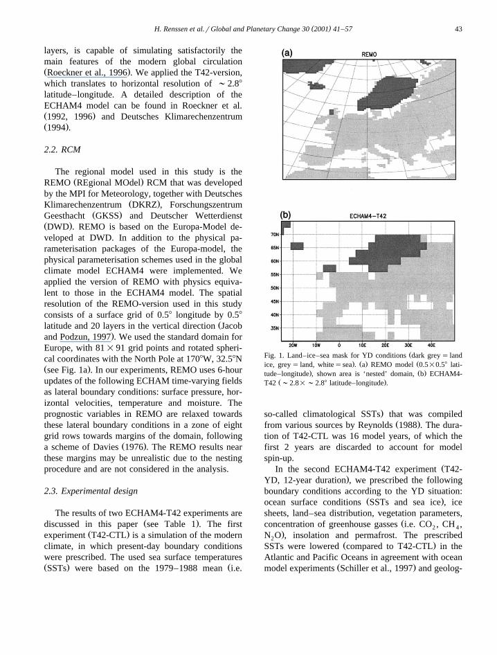
Table 1Ž .Design of the experiments, results of which are shown in this paper ‘k’ denotes kyears BP

Ž . Ž . Ž . Ž .T42-CTL 14 years T42-YD 10 years REMO-CTL 10 years REMO-YD 3 years

SSTsqsea ice 0 k YD in N Atlantic; 0 k YD in N Atlanticy28C in N Pacific

Ice sheets 0 k 12 k 0 k 12 kInsolation 0 k 12 k 0 k 12 kCO rCH rN O 353r1720r310 246r500r265 353r1720r310 246r500r2652 4 2

Vegetation parameters 0 k YD 0 k YD

Ž . Ž . Ž . Ž .The atmospheric concentration of CO ppm , CH ppb and N O ppb is based on Antarctic ice core analyses by Raynaud et al. 1993 .2 4 2

Experiment REMO-CTL was nested in T42-CTL and REMO-YD was nested in T42-YD.

Ž .ical data Sarnthein et al., 1995 . A cooling of up to108C was prescribed in the Atlantic Ocean north of308N, resulting in a southward expansion of sea iceŽ .Sarnthein et al., 1995 . The sea ice margin wassituated at 708N in summer and at 558N in winterŽ .see Renssen, 1997 for details . In the N Pacific, acooling of 28C was defined north of 408N, in accor-

Ždance with ocean core analysis e.g. Kallel et al.,.1988 and coupled atmosphere–ocean model experi-Ž .ments Mikolajewicz et al., 1997 . As suggested by

Ž .marine data Schulz, 1995; Thunell and Miao, 1996 ,we assumed that no ocean cooling occurred in thetropics during the YD. Ice sheet topography was

Ž .defined according to Peltier 1994 , and insolationŽ .was prescribed following Berger 1978 . The follow-

ing parameters were changed to give a representationŽ .of the YD vegetation reconstruction of Adams 1997 :

surface background albedo, leaf area index, vegeta-Žtion ratio, forest ration and roughness length see

.Renssen and Lautenschlager, 2000 . A simple per-mafrost parameterisation was applied by taking thefollowing two measures for grid cells where per-

Ž .mafrost was present during YD: 1 fixed sub-zeroŽ .temperatures in the lowest two soil layers, 2 soil

Žhumidity fixed at field capacity see Renssen et al.,.2000 . Note that experiment T42-YD is discussed in

Ždetail elsewhere Renssen et al., 2000; Renssen and.Isarin, 2001 .

Analogous to the ECHAM4 simulations, we car-ried out two experiments with REMO to simulate the

Žmodern and YD climates viz. REMO-CTL and.REMO-YD, see Table 1 . These REMO experiments

were nested in the ECHAM4 experiments describedabove, i.e. REMO-CTL in T42-CTL and REMO-YDin T42-YD. In the domain shown in Fig. 1a, weprescribed YD surface parameters that were based on

the same sources as in the ECHAM4 simulation.ŽMaps of these boundary conditions i.e. vegetation.parameters and ice sheet orography were digitised

onto the 0.58 grid to obtain input files for REMO. Inaddition, we altered the land–sea mask to take the

Ž;60 m lower sea level into account Fairbanks,.1989 . It should be noted that no additional details

have been added to the fields of vegetation parame-Ž .ters e.g. due to regional vegetation differences , so

that the spatial resolution of these parameters iscomparable in REMO-YD and T42-YD. Fig. 1a,bshows the land–ice–sea masks for the YD experi-ments, for both ECHAM and REMO, for a directcomparison. Obviously, the land–ice–sea mask usedin REMO provides much more detail than that ofECHAM. This is also true for the surface elevationprescribed in both models. It is expected that thesedifferences will produce corresponding spatial detailsin the simulation results, most notably in surfacetemperature and precipitation.

3. Results

3.1. Introduction to the results presented

We focus our analysis on surface variables, asreconstructions based on palaeodata are available forthe surface climate. Recently, reconstructions of theYD surface temperatures in Europe—based onpalaeobotanical and periglacial data—became avail-

Ž .able Isarin, 1997; Isarin and Bohncke, 1999 . More-over, fossil aeolian features provide information onthe high-intensity winds and on the atmospheric

Ž .circulation during YD time Isarin et al., 1997 .Furthermore, studies on former lake levels and riverregimes give qualitative information on past varia-

( )H. Renssen et al.rGlobal and Planetary Change 30 2001 41–57 45

Žtions in precipitation Bohncke et al., 1988; Bohncke,.1993; Magny and Ruffaldi, 1995; Huisink, 1997 .

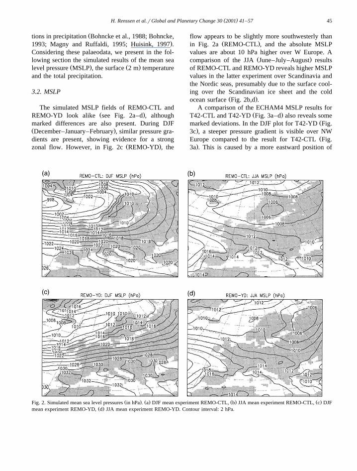
Considering these palaeodata, we present in the fol-lowing section the simulated results of the mean sea

Ž . Ž .level pressure MSLP , the surface 2 m temperatureand the total precipitation.

3.2. MSLP

The simulated MSLP fields of REMO-CTL andŽ .REMO-YD look alike see Fig. 2a–d , although

marked differences are also present. During DJFŽ .December–January–February , similar pressure gra-dients are present, showing evidence for a strong

Ž .zonal flow. However, in Fig. 2c REMO-YD , the

flow appears to be slightly more southwesterly thanŽ .in Fig. 2a REMO-CTL , and the absolute MSLP

values are about 10 hPa higher over W Europe. AŽ .comparison of the JJA June–July–August results

of REMO-CTL and REMO-YD reveals higher MSLPvalues in the latter experiment over Scandinavia andthe Nordic seas, presumably due to the surface cool-ing over the Scandinavian ice sheet and the cold

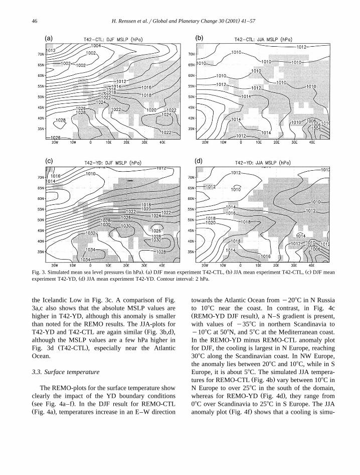
Ž .ocean surface Fig. 2b,d .A comparison of the ECHAM4 MSLP results for

Ž .T42-CTL and T42-YD Fig. 3a–d also reveals someŽmarked deviations. In the DJF plot for T42-YD Fig.

.3c , a steeper pressure gradient is visible over NWŽEurope compared to the result for T42-CTL Fig.

.3a . This is caused by a more eastward position of

Ž . Ž . Ž . Ž .Fig. 2. Simulated mean sea level pressures in hPa . a DJF mean experiment REMO-CTL, b JJA mean experiment REMO-CTL, c DJFŽ .mean experiment REMO-YD, d JJA mean experiment REMO-YD. Contour interval: 2 hPa.

( )H. Renssen et al.rGlobal and Planetary Change 30 2001 41–5746

Ž . Ž . Ž . Ž .Fig. 3. Simulated mean sea level pressures in hPa . a DJF mean experiment T42-CTL, b JJA mean experiment T42-CTL, c DJF meanŽ .experiment T42-YD, d JJA mean experiment T42-YD. Contour interval: 2 hPa.

the Icelandic Low in Fig. 3c. A comparison of Fig.3a,c also shows that the absolute MSLP values arehigher in T42-YD, although this anomaly is smallerthan noted for the REMO results. The JJA-plots for

Ž .T42-YD and T42-CTL are again similar Fig. 3b,d ,although the MSLP values are a few hPa higher in

Ž .Fig. 3d T42-CTL , especially near the AtlanticOcean.

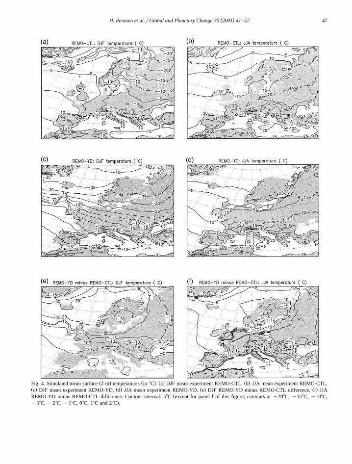
3.3. Surface temperature

The REMO-plots for the surface temperature showclearly the impact of the YD boundary conditionsŽ .see Fig. 4a–f . In the DJF result for REMO-CTLŽ .Fig. 4a , temperatures increase in an E–W direction

towards the Atlantic Ocean from y208C in N Russiato 108C near the coast. In contrast, in Fig. 4cŽ .REMO-YD DJF result , a N–S gradient is present,with values of y358C in northern Scandinavia toy108C at 508N, and 58C at the Mediterranean coast.In the REMO-YD minus REMO-CTL anomaly plotfor DJF, the cooling is largest in N Europe, reaching308C along the Scandinavian coast. In NW Europe,the anomaly lies between 208C and 108C, while in SEurope, it is about 58C. The simulated JJA tempera-

Ž .tures for REMO-CTL Fig. 4b vary between 108C inN Europe to over 258C in the south of the domain,

Ž .whereas for REMO-YD Fig. 4d , they range from08C over Scandinavia to 258C in S Europe. The JJA

Ž .anomaly plot Fig. 4f shows that a cooling is simu-

( )H. Renssen et al.rGlobal and Planetary Change 30 2001 41–57 47

Ž . Ž . Ž . Ž .Fig. 4. Simulated mean surface 2 m temperatures in 8C . a DJF mean experiment REMO-CTL, b JJA mean experiment REMO-CTL,Ž . Ž . Ž . Ž .c DJF mean experiment REMO-YD, d JJA mean experiment REMO-YD, e DJF REMO-YD minus REMO-CTL difference, f JJA

ŽREMO-YD minus REMO-CTL difference. Contour interval: 58C except for panel f of this figure; contours at y208C, y158C, y108C,.y58C, y28C, y18C, 08C, 18C and 28C .

( )H. Renssen et al.rGlobal and Planetary Change 30 2001 41–5748

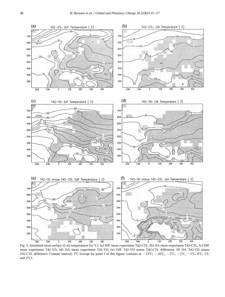
Ž . Ž . Ž . Ž . Ž .Fig. 5. Simulated mean surface 2 m temperatures in 8C . a DJF mean experiment T42-CTL, b JJA mean experiment T42-CTL, c DJFŽ . Ž . Ž .mean experiment T42-YD, d JJA mean experiment T42-YD, e DJF T42-YD minus T42-CTL difference, f JJA T42-YD minus

ŽT42-CTL difference. Contour interval: 58C except for panel f of this figure; contours at y158C, y108C, y58C, y28C, y18C, 08C, 18C.and 28C .

( )H. Renssen et al.rGlobal and Planetary Change 30 2001 41–57 49

Ž .lated in N–NE Europe more than 108C and alongŽ .the coast few degrees , whereas over most of the

interior of the continent, the values are similar inREMO-CTL and REMO-YD. An exception to thispattern is visible over the S North Sea region, wherea positive JJA temperature anomaly of 28C is appar-ent in Fig. 4f. The latter can be supposedly explainedas an effect of the different land–sea masks used inboth experiments, causing the S North Sea region tobe defined as land in REMO-YD and as sea inREMO-CTL. Consequently, in REMO-YD, the re-gion is heated in summer more easily than inREMO-CTL, in which the temperature is determinedby the prescribed SSTs.

As expected, the REMO temperature results areŽ .consistent with the ECHAM4 results Fig. 5a–f .

Ž .The T42-CTL plots Fig. 5a,b are very similar toŽ .their REMO counterparts Fig. 4a,b , although less

Ž .details are present. Also, in Fig. 5b JJA T42-CTL ,the temperatures are somewhat lower than in Fig. 4bŽ .JJA REMO-CTL , in SE Europe and in SW France.Compared to the REMO results, the YD results

Ž .produced by ECHAM4 Fig. 5c–d give slightlyhigher temperatures for DJF and generally lowervalues for JJA. The most striking difference between

Žthe DJF anomaly plot Fig. 5e, T42-YD minus T42-. Ž .CTL and its REMO counterpart Fig. 4e is the less

intense cooling between 508N and 608N in theECHAM result. In general, the simulated JJA

Ž .anomalies of ECHAM4-T42 Fig. 5f and REMOŽ .Fig. 4f are comparable. An exception forms NWEurope, where ECHAM4 produced a cooling ofaround 5–108C, whereas in the REMO-result, the

Ž .JJA-anomalies are slightly negative y18C to y58CŽ .along the coastal region and slightly positive 0–18C

in the interior of France and the Low Countries. TheJJA temperatures in the S North Sea region arerelatively high, as can be seen by northward excur-sions of the 108C and y58C isotherms in the T42-YD

Ž .and YD-CTL anomaly plots, respectively Fig. 5d,f .A similar effect was seen in the REMO results, andwas explained by the differences in land–sea masks.However, the T42-YD temperatures do not exceedthe T42-CTL values, as is the case with REMO.

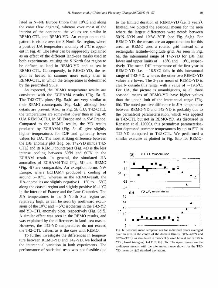
To further investigate the differences in tempera-ture between REMO-YD and T42-YD, we looked atthe interannual variation in both experiments. Theperformance of statistical tests was not feasible due

Ž .to the limited duration of REMO-YD i.e. 3 years .Instead, we plotted the seasonal means for the areawhere the largest differences were noted: between

Ž .508N–608N and 108W–308E see Fig. 6a,b . ForREMO-YD, the means are an approximation for thisarea, as REMO uses a rotated grid instead of arectangular latitude–longitude grid. As seen in Fig.6a, the interannual range of T42-YD for DJF haslower and upper limits of y188C and y98C, respec-tively. The mean DJF temperature of the first year in

Ž .REMO-YD i.e. y16.58C falls in this interannualrange of T42-YD, whereas the other two REMO-YDvalues are lower. The 3-year mean of REMO-YD isclearly outside this range, with a value of y19.68C.For JJA, the picture is unambiguous, as all threeseasonal means of REMO-YD have higher values

Žthan the upper limit of the interannual range Fig..6b . The noted positive difference in JJA temperature

between REMO-YD and T42-YD is probably due tothe permafrost parameterisation, which was appliedin T42-CTL but not in REMO-YD. As discussed in

Ž .Renssen et al. 2000 , this permafrost parameterisa-tion depressed summer temperatures by up to 58C inT42-YD compared to T42-CTL. We performed asimilar exercise as plotted in Fig. 6a,b for REMO-

Fig. 6. Seasonal mean temperatures for individual years averagedŽover an area in the centre of the domain limits: 508N–608N and

. Ž .108W–308E , as simulated in T42-YD closed boxes and REMO-Ž . Ž . Ž .YD closed triangles . a DJF, b JJA. The open figures are the

multi-year means, with the interannual range shown for the T42-YD mean by "2 standard deviations.

( )H. Renssen et al.rGlobal and Planetary Change 30 2001 41–5750

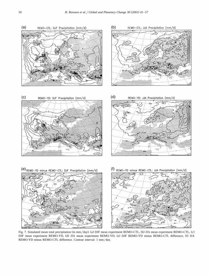
Ž . Ž . Ž . Ž .Fig. 7. Simulated mean total precipitation in mmrday . a DJF mean experiment REMO-CTL, b JJA mean experiment REMO-CTL, cŽ . Ž . Ž .DJF mean experiment REMO-YD, d JJA mean experiment REMO-YD, e DJF REMO-YD minus REMO-CTL difference, f JJA

REMO-YD minus REMO-CTL difference. Contour interval: 1 mmrday.

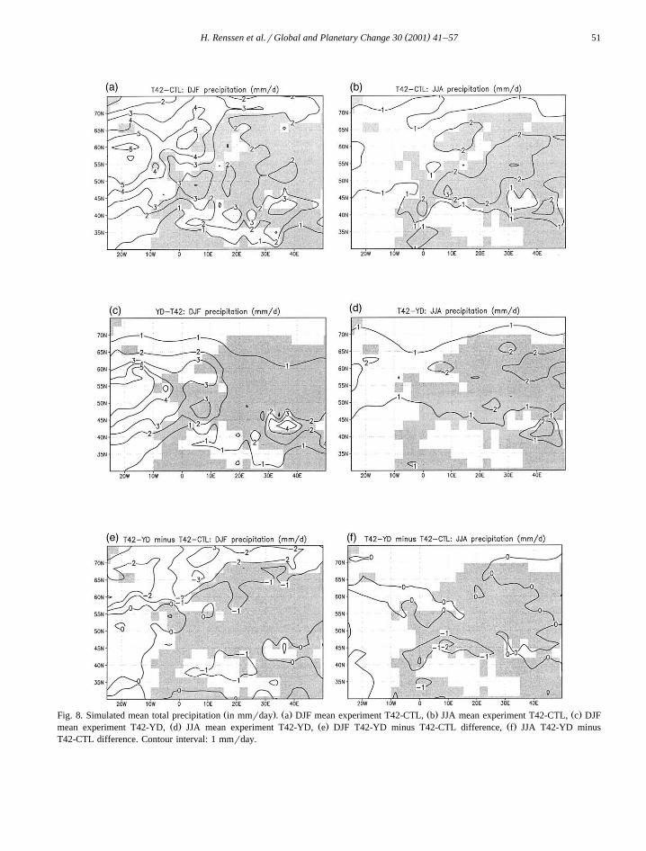
( )H. Renssen et al.rGlobal and Planetary Change 30 2001 41–57 51

Ž . Ž . Ž . Ž .Fig. 8. Simulated mean total precipitation in mmrday . a DJF mean experiment T42-CTL, b JJA mean experiment T42-CTL, c DJFŽ . Ž . Ž .mean experiment T42-YD, d JJA mean experiment T42-YD, e DJF T42-YD minus T42-CTL difference, f JJA T42-YD minus

T42-CTL difference. Contour interval: 1 mmrday.

( )H. Renssen et al.rGlobal and Planetary Change 30 2001 41–5752

CTL and T42-CTL. This indicated that the interan-nual ranges of the two experiments overlap to a large

Ž .degree not shown . To conclude, the differencesbetween REMO-YD and T42-YD appear to bemeaningful, but the limited duration of REMO-YDmakes it impossible to reach a decisive conclusionon this matter.

3.4. Total precipitation

ŽThe precipitation values simulated by REMO Fig..7a–f clearly show the influence of topography, since

Ž .the highest values up to 6–7 mmrday are producedin mountainous regions such as Scandinavia, Scot-land and the Alps. In the DJF-season, there is moreprecipitation than in summer. In the DJF result for

Ž .REMO-YD Fig. 7c , the zone with precipitation ismore latitudinally restricted, as opposed to the result

Ž .of REMO-CTL Fig. 7a —the values are very lowŽ .less than 1 mmrday in the N Scandinavia and overthe Mediterranean. However, the core of the DJFstorm track is more intensive in REMO-YD than inREMO-CTL, as is seen by the positive anomaly over

ŽW Europe see Fig. 7e; )1 mmrday over the Irish.Sea . In the JJA season, the REMO-YD minus

REMO-CTL anomaly is negative over the entirecontinent. The magnitude of this negative anomaly

Žincreases from west to east i.e. going inland, see.Fig. 7f .

Again, the REMO results are consistent with theECHAM4 results, although the topographic effect is

Ž .barely present Fig. 8a–f . The DJF storm track isŽ .also narrower in the YD-result Fig. 8c compared to

Ž .the control experiment Fig. 8a . Moreover, the coreof the main precipitation belt has shifted southward

Ž . Ž .from 608N Fig. 8a to about 528N Fig. 8c . As aresult, a small positive anomaly is visible over Britain

Ž .in Fig. 8e compare with REMO result in Fig. 7e . Inthe JJA anomaly plot, the deviation is generally

Ž .negative over the continent see Fig. 8f .

4. Discussion

4.1. What was the YD climate in Europe like accord-ing to palaeodata?

A compilation of aeolian data from NW Europerevealed that prevalent dune-forming winds during

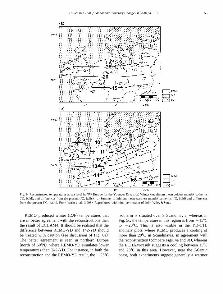
Ž .the YD were all westerly Isarin et al., 1997 . Pre-sumably, these winds represent the average wintercirculation regime. Moreover, temperature recon-structions for the European YD climate suggest aN–S thermal gradient and very low winter tempera-tures, ranging from y258C at 558N to y158C at

Ž .508N see Fig. 9a; Isarin et al., 1998 . These valuestranslate to a cooling, compared to today, rangingfrom 308C in Ireland and Britain to 158C in Russia.The summer conditions were less dramatic, withtemperatures varying from 108C in Scotland and S

ŽSweden, to 158C in central France Fig. 9b; Isarin et.al., 1998 . These temperatures imply a cooling of

3–68C compared to today. It should be realised thatthe uncertainty of these reconstructions is estimated

Ž .at "28C Isarin and Bohncke, 1999 . Furthermore,several studies suggest that the early part of the YDwas a relatively wet phase in W Europe, as indicatedby high lake levels and by increased river activityŽe.g. Vandenberghe and Bohncke, 1985; Bohncke,

.1993; Magny and Ruffaldi, 1995; Huisink, 1997 .According to these same studies, the later part of YDseems to have been drier. It should be noted that thisview is not coherent throughout Europe, as in NNorway and in Poland, the early YD was drier than

Žthe later part e.g. Goslar et al., 1993; Birks et al.,.1994; Walker, 1995 . Assuming that these discussed

palaeodata are reliable, we can evaluate our YDsimulations by comparing the results with these data.

4.2. Is REMO producing a more realistic YD climatethan ECHAM4?

The MSLP plots for REMO and ECHAM bothŽshow a strong westerly flow over W Europe see

.Figs. 2c and 3c during winter. This is in agreementwith westerly dune-forming winds as reconstructed

Ž .with the aid of aeolian features Isarin et al., 1997 .We see no evidence for a glacial anticyclone over

Ž .the Scandinavian ice sheet Figs. 2c–d and 3c–d , aswas simulated in several GCM simulation studies on

Žthe LGM climate e.g. Kutzbach and Wright, 1985;.Rind, 1987 . Consequently, the REMO results con-

firm our conclusions from earlier studies that west-erly flow was dominant in Europe during the YDŽ .Renssen et al., 1996; Isarin et al., 1997, 1998 . This

Žwesterly flow transported cold air cooled over the.extended N Atlantic sea ice to NW Europe.

( )H. Renssen et al.rGlobal and Planetary Change 30 2001 41–57 53

Ž . Ž .Fig. 9. Reconstructed temperatures at sea level in NW Europe for the Younger Dryas. a Winter maximum mean coldest month isothermsŽ . Ž . Ž . Ž . Ž .8C, bold , and differences from the present 8C, italic . b Summer minimum mean warmest month isotherms 8C, bold and differences

Ž . Ž .from the present 8C, italic . From Isarin et al. 1998 . Reproduced with kind permission of John Wiley&Sons.

Ž .REMO produced winter DJF temperatures thatare in better agreement with the reconstructions thanthe result of ECHAM4. It should be realised that thedifference between REMO-YD and T42-YD should

Ž .be treated with caution see discussion of Fig. 6a .The better agreement is seen in northern EuropeŽ .north of 508N , where REMO-YD simulates lowertemperatures than T42-YD. For instance, in both thereconstruction and the REMO-YD result, the y258C

isotherm is situated over S Scandinavia, whereas inFig. 5c, the temperature in this region is from y158Cto y208C. This is also visible in the YD-CTLanomaly plots, where REMO produces a cooling ofmore than 208C in Scandinavia, in agreement with

Ž .the reconstruction compare Figs. 4e and 9a , whereasthe ECHAM-result suggests a cooling between 158Cand 208C in this area. However, near the Atlanticcoast, both experiments suggest generally a warmer

( )H. Renssen et al.rGlobal and Planetary Change 30 2001 41–5754

winter climate in Europe than the reconstructions.For example, in Ireland, a winter temperature ofy208C to y258C is reconstructed using geological

Ž .data Fig. 9a , while a value from 08C to y158C isŽ .simulated Figs. 4c and 5c . The latter model–data

mismatch is probably caused by the prescribed win-ter sea ice margin, which is located at 608N near theW European coast in REMO-YD and T42-YD.

Ž .Renssen and Isarin 1998 argued that during YD,this sea ice margin was probably situated at 528N,thus explaining the reconstructed temperature ofy258C in Ireland. Hence, the extended N Atlanticsea ice cover played a key role in forcing the YD

Žwinter temperatures in Europe Isarin et al., 1998;.Renssen and Isarin, 1998 .

Ž .The model–data comparison for the summer JJAtemperatures gives an ambiguous picture. In NWEurope, the summer temperatures in the REMO-YDresult are higher than those generated by T42-YD.For instance, the temperature between 508N and

Ž .558N is over 158C in the REMO-YD result Fig. 4d ,whereas this value in T42-YD ranges from 108C to

Ž .158C Fig. 5d . The latter model result correspondsŽ .better with the reconstruction Fig. 9b . As noted

before, the difference in JJA temperatures betweenREMO-YD and T42-YD can be attributed to the useof a permafrost parameterisation in T42-YD, whichproduces an additional depression of the surface

Ž .temperatures Renssen et al., 2000 . In addition, it isnoted that the reconstructed temperatures are mini-mum values, meaning that they could have been

Ž .higher in reality see Isarin and Bohncke, 1999 .The precipitation fields simulated by REMO are

in general agreement with the discussed palaeodata.For winter, there is a tendency of precipitation in-

Ž .crease in W Europe see Fig. 7e; YD-CTL anomaly ,whereas there is a negative anomaly visible over therest of Europe. In summer, the YD-CTL anomaly is

Ž .negative everywhere on the continent Fig. 7f . Inthe T42-YD result, the same trend is visible, with aslight precipitation increase near the Atlantic coastcompared to T42-CTL. It should be realised, how-ever, that ECHAM4 has a highly smoothed topogra-phy, making the simulation of orography-inducedprecipitation a weak point in this model. In earlierstudies, we explained the relatively high precipitationvalues during the YD by a positioning of the main

Žstorm track over NW Europe Renssen et al., 1996;

.Isarin et al., 1998 . Today, this main storm track isŽlocated more to the North i.e. between Scotland and

.Iceland . Thus, whereas in most places, precipitationŽwas reduced during the YD due to the lower water

.content of cold air; c.f. Rind, 1987 , precipitationincreased over NW Europe as a result of the positionof the main storm track. During winter, this positionof the storm track was directly related to the location

Žof the Atlantic sea ice margin see Renssen et al.,.1996 .

In summary, the YD climates simulated by REMOand ECHAM4 are very similar on a continentalscale, although some differences are noted. Themodel–data comparison shows that REMO generateswinter temperatures that are in better agreement withproxy data. The opposite is true for JJA tempera-tures, which are better reproduced by ECHAM4 dueto the application of a permafrost parameterisation.We may conclude that, considering palaeoclimateresearch, the biggest advantage of the use of anRCM instead of an AGCM, lies in the more detailedinformation that is provided. For instance, someonestudying palaeoclimate records, obtained from thecoastal region of Scandinavia, would be very inter-ested to receive information on the gradients intemperature and precipitation provided by the RCM.It is very likely that these regional records have beeninfluenced by these gradients, so that the spatialscale of the RCM is here in better agreement withthe data than an AGCM would be. Once again, itshould be noted that our REMO-YD experiment hasa duration of only 3 years, which is generally consid-ered too short for climate studies. Therefore, ourresults should be regarded as preliminary. We think,however, that our results provide a good startingpoint for future palaeoclimate studies using nestedRCMs.

5. Conclusions

We simulated the Younger Dryas climate in Eu-rope with the REMO regional climate model nestedin an AGCM simulation, performed with the EC-HAM-T42 model. Such a regional simulation of apalaeoclimate in Europe has not been performedbefore. Note that our REMO simulation on theYounger Dryas has a duration of only 3 years, and

( )H. Renssen et al.rGlobal and Planetary Change 30 2001 41–57 55

that we consider our conclusions as preliminary. Acomparison of these REMO and ECHAM4 simula-tion results on the one hand, with climate reconstruc-tions based on palaeodata on the other hand, suggeststhe following:

Ž .1 The Younger Dryas climates produced by theREMO and ECHAM4 models are similar on a conti-nental scale. Both REMO and ECHAM4 produced

Ž .higher winter temperatures 0–108C in W EuropeŽthan indicated by palaeodata from y158C to

.y258C . We suggest that this model–data mismatchis caused by the winter sea ice margin, which proba-

Ž .bly was located further south at 528N during theYounger Dryas, than prescribed in the simulationexperiments. Some differences between the twomodels have also been found. REMO simulated YD

Ž .winter temperatures from y208C to y358C inScandinavia that correspond well with reconstruc-tions. ECHAM4 gives a too warm climate for thisarea. On the other hand, compared to the ECHAM4-result, REMO generated higher YD summer temper-atures in continental Europe. It appears that theECHAM4-result is in better agreement with recon-structed summer temperatures, although it must berealised that the latter estimates are minimal values.The difference in summer temperatures is attributedto a permafrost parameterisation that is applied inECHAM4, but not in REMO. Compared to a modernclimate experiment, REMO simulated a precipitationincrease over W Europe during winter, whereas anegative anomaly was calculated in the rest of Eu-rope.

Ž .2 In palaeoclimate research, the application of aregional climate model has advantages over the useof a global model, since the higher resolution pro-vides a spatial scale that corresponds to palaeocli-mate reconstructions. The detailed precipitation dis-tribution and temperature gradients produced byREMO for the Younger Dryas are more suitable forcomparison with regional palaeoclimate studies thanthe results generated by ECHAM4, in which thetopography is highly smoothed.

Acknowledgements

The constructive comments of P. Valdes, F. Giorgiand S.L. Weber are gratefully acknowledged. We are

Žindebted to L. Bengtsson Max-Planck-Institut fur¨

.Meteorologie, Hamburg for providing excellentcomputing facilities and to M. LautenschlagerŽ .Deutsches Klimarechenzentrum, Hamburg for theadvise. HR and RFBI are supported by the DutchNational Research Programme on Global Air Pollu-tion and Climate Change.

References

Adams, J.M., 1997. Global Land Environments Since the LastInterglacial. Oak Ridge National Laboratory, TN, USA,www.esd.ornl.govrernrqenrnerc.html.

Berger, A.L., 1978. Long-term variations of daily insolation andQuaternary climatic changes. Journal of the Atmospheric Sci-ences 35, 2363–2367.

Birks, H.H., Paus, A., Svendsen, J.L., Alm, T., Mangerud, J.,Landvik, J.Y., 1994. Late Weichselian environmental changein Norway, including Svalbard. Journal of Quaternary Science9, 133–145.

INTIMATE members, Bjorck, S., Walker, M.J.C., Cwynar, L.C.,¨Johnsen, S., Knudsen, K.-L., Lowe, J.J., Wohlfarth, B., 1998.An event stratigraphy for the Last Termination in the NorthAtlantic region based on the Greenland ice-core record: aproposal by the INTIMATE group. Journal of QuaternaryScience 13, 283–292.

Bohncke, S.J.P., 1993. Lateglacial environmental changes in TheNetherlands: spatial and temporal patterns. Quaternary ScienceReviews 12, 707–717.

Bohncke, S., Vandenberghe, J., Wijmstra, T.A., 1988. Lake levelchanges and fluvial activity in the Late Glacial lowland val-

Ž .leys. In: Lang, G., Schluchter, C. Eds. , Lake, Mire and River¨Environments. Balkema, Rotterdam, pp. 115–121.

Crowley, T.J., North, G.R., 1991. Paleoclimatology. Oxford Univ.Press, Oxford.

Davies, H.C., 1976. A lateral boundary formulation for multi-levelprediction models. Quarterly Journal of the Royal Meteorolog-ical Society 102, 405–418.

Deque, M., Piedelievre, J.Ph., 1995. High resolution climatesimulation over Europe. Climate Dynamics 11, 321–329.

Deutsches Klimarechenzentrum, 1994. The ECHAM 3 atmo-spheric general circulation model. Deutsches Klimarechenzen-trum, Technical Report No. 6, Hamburg.

Fairbanks, R.G., 1989. A 17,000-year glacio-eustatic sea levelrecord: influence of glacial melting rates on the YoungerDryas event and deep-ocean circulation. Nature 342, 637–642.

´Fawcett, P.J., Agustsdottir, A.M., Alley, R.B., Shuman, C.A.,´ ´1997. The Younger Dryas termination and North Atlantic deepwater formation: insight from climate model simulations andGreenland ice cores. Paleoceanography 12, 23–38.

Gates, W.L., 1976. Modeling the ice-age climate. Science 191,1138–1144.

Giorgi, F., 1990. Simulation of regional climate using a limitedarea model nested in a general circulation model. Journal ofClimate 3, 941–963.

Giorgi, F., Mearns, L.O., 1991. Approaches to the simulation of

( )H. Renssen et al.rGlobal and Planetary Change 30 2001 41–5756

regional climate change: a review. Reviews of Geophysics 29,191–216.

Giorgi, F., Marinucci, M.R., Visconti, G., 1990. Use of a limited-area model nested in a general circulation model for regionalclimatic simulation over Europe. Journal of Geophysical Re-search 95, 18413–18431.

Goslar, T., Kuc, T., Ralska-Jasiewiczowa, M., Rozanski, K.,Arnold, M., Bard, E., van Geel, B., Pazdur, M.F., Szeroczyn-ska, K., Wicik, B., Wieckowski, K., Walanus, A., 1993.High-resolution lacustrine record of the late glacialrholocenetransition in Europe. Quaternary Science Reviews 12, 287–294.

Harrison, S.P., Jolly, D., Laarif, F., Abe-Ouchi, A., Dong, B.,Herterich, K., Hewitt, C., Joussaume, S., Kutzbach, J.E.,Mitchell, J., De Noblet, N., Valdes, P., 1998. Intercomparisonof simulated global vegetation distributions in response to 6kyr BP orbital forcing. Journal of Climate 11, 2721–2742.

Hostetler, S.W., Giorgi, F., Bates, G.T., Bartlein, P.J., 1994.Lake-atmosphere feedbacks associated with Paleolakes Bon-neville and Lahontan. Science 263, 665–668.

Huisink, M., 1997. Late-glacial sedimentological and morphologi-cal changes in a lowland river in response to climatic change:the Maas, southern Netherlands. Journal of Quaternary Sci-ence 12, 209–223.

Isarin, R.F.B., 1997. Permafrost distribution and temperatures inEurope during the Younger Dryas. Permafrost and PeriglacialProcesses 8, 313–333.

Isarin, R.F.B., Bohncke, S.J.P., 1999. Mean July temperaturesduring the Younger Dryas in northwestern and central Europeas inferred from climate indicator plant species. QuaternaryResearch 51, 158–173.

Isarin, R.F.B., Renssen, H., 1999. Reconstructing and modellinglate Weichselian climates: the Younger Dryas in Europe as acase study. Earth-Science Reviews 48, 1–38.

Isarin, R.F.B., Renssen, H., Koster, E.A., 1997. Surface windclimate during the Younger Dryas in Europe as inferred fromaeolian records and model simulations. Palaeogeography,Palaeoclimatology, Palaeoecology 134, 127–148.

Isarin, R.F.B., Renssen, H., Vandenberghe, J., 1998. The impactof the North Atlantic ocean on the Younger Dryas climate innorth-western and central Europe. Journal of Quaternary Sci-ence 13, 447–453.

Jacob, D., Podzun, R., 1997. Sensitivity studies with the regionalclimate model REMO. Meteorology and Atmospheric Physics63, 119–129.

Jacob, D., Podzun, R., 2000. Investigation of the annual andinterannual variability of the water budget over the Baltic Seadrainage basin using the regional climate model REMO.WMOrTD-No. 987, Rep. 30. WMO, Geneva, pp. 7.10–7.11.

Jones, R.G., Murphy, J.M., Noguer, M., 1995. Simulation ofclimate change over Europe using a nested regional-climatemodel: I. Assessment of control climate, including sensitivityto location of lateral boundaries. Quarterly Journal of theRoyal Meteorological Society 121, 1413–1449.

Joussaume, S., Taylor, K.E., Braconnot, P., Mitchell, J.F.B.,Kutzbach, J.E., Harrison, S.P., Prentice, I.C., Broccoli, A.J.,Abe-Ouchi, A., Bartlein, P.J., Bonfils, C., Dong, B., Guiot, J.,Herterich, K., Hewitt, C.D., Jolly, D., Kim, J.W., Kislov, A.,Kitoh, A., Loutre, M.F., Masson, V., McAvaney, B., McFar-

lane, N., de Noblet, N., Peltier, W.R., Peterschmitt, J.Y.,Pollard, D., Rind, D., Royer, J.F., Schlesinger, M.E., Syktus,J., Thompson, S., Valdes, P., Vettoretti, G., Webb, R.S.,Wyputta, U., 1999. Monsoon changes for 6000 years ago:results of 18 simulations from the Paleoclimate Modeling

Ž .Intercomparision Project PMIP . Geophysical Research Let-ters 26, 859–862.

Kallel, N., Labeyrie, L.D., Arnold, M., Okada, H., Dudleyn,W.C., Duplessy, J.C., 1988. Evidence of cooling during theYounger Dryas in the western North Pacific. OceanologicaActa 11, 369–375.

Kohfeld, K., Harrison, S., 2000. How well can we simulate pastclimates? Evaluating the models using global palaeoenviron-mental datasets. Quaternary Science Reviews 19, 321–346.

Kutzbach, J.E., Guetter, P.J., 1986. The influence of changingorbital parameters and surface boundary conditions on climatesimulations for the past 18,000 years. Journal of the Atmo-spheric Sciences 43, 1726–1759.

Kutzbach, J.E., Wright Jr., H.E., 1985. Simulation of the climateof 18,000 years BP: results for North AmericanrNorth At-lanticrEuropean sector and comparison with the geologicrecord of North America. Quaternary Science Reviews 4,147–187.

Lautenschlager, M., Herterich, K., 1990. Atmospheric response toice age conditions: climatology near earth’s surface. Journal ofGeophysical Research 95, 22547–22557.

NASP members, Lowe, J.J., 1995. Palaeoclimate of the NorthAtlantic seaboards during the last glacialrinterglacial transi-tion. Quaternary International 28, 51–61.

Magny, M., Ruffaldi, P., 1995. Younger Dryas and early holocenelake-level fluctuations in the Jura mountains, France. Boreas24, 155–172.

Mikolajewicz, U., Crowley, T.J., Schiller, A., Voss, R., 1997.Modelling teleconnections between the North Atlantic andNorth Pacific during the Younger Dryas. Nature 387, 384–387.

Mitchell, T.D., Hulme, M., 1999. Predicting regional climatechange: living with uncertainty. Progress in Physical Geogra-phy 23, 57–78.

Peltier, W.R., 1994. Ice age paleotopography. Science 265, 195–201.

Raynaud, D., Jouzel, J., Barnola, J., Chappellaz, J., Delmas, R.J.,Lorius, C., 1993. The ice record of greenhouse gases. Science259, 926–933.

Renssen, H., 1997. The global response to Younger Dryas bound-ary conditions in an AGCM simulation. Climate Dynamics 13,587–599.

Renssen, H., Isarin, R.F.B., 1998. Surface temperature in NWEurope during the Younger Dryas: AGCM simulation com-pared with temperature reconstructions. Climate Dynamics 14,33–44.

Renssen, H., Isarin, R.F.B., 2001. The two major warming phasesof the last deglaciation at ;14.7 and ;11.5 kyr cal BP inEurope: climate reconstructions and AGCM experiments.Global and Planetary Change 30, 117–154.

Renssen, H., Lautenschlager, M., 2000. Effect of vegetation in aclimate model simulation on the Younger Dryas. Global andPlanetary Change 26, 423–433.

Renssen, H., Lautenschlager, M., Schuurmans, C.J.E., 1996. The

( )H. Renssen et al.rGlobal and Planetary Change 30 2001 41–57 57

atmospheric winter circulation during the Younger Dryas sta-dial in the AtlanticrEuropean sector. Climate Dynamics 12,813–824.

Renssen, H., Isarin, R.F.B., Vandenberghe, J., Lautenschlager,M., Schlese, U., 2000. Permafrost as a critical factor inpalaeoclimate modelling: the Younger Dryas case in Europe.Earth and Planetary Science Letters 176, 1–5.

Reynolds, R.W., 1988. A real-time global sea surface temperatureanalysis. Journal of Climate 1, 75–86.

Rind, D., 1987. Components of the ice age circulation. Journal ofGeophysical Research 92, 4241–4281.

Rind, D., Peteet, D., Broecker, W., McIntyre, A., Ruddiman, W.,1986. The impact of cold North Atlantic sea surface tempera-tures on climate: implications for the Younger Dryas coolingŽ .11–10 k . Climate Dynamics 1, 3–33.

Roeckner, E., Arpe, K., Bengtsson, L., Brinkop, S., Dumenil, L.,¨Esch, M., Kirk, E., Lunkeit, F., Ponater, M., Rockel, B.,Sausen, R., Schlese, U., Schubert, S., Windelband, M., 1992.Simulation of the present-day climate with the ECHAM model:impact of model physics and resolution. Max-Planck-Institutfur Meteorologie Report No. 93, Hamburg.¨

Roeckner, E., Arpe, K., Bengtsson, L., Christoph, M., Claussen,M., Dumenil, L., Esch, M., Giorgetta, M., Schlese, U.,¨Schulzweida, U., 1996. The atmospheric general circulationmodel ECHAM-4: model description and simulation of pre-sent-day climate. Max-Planck-Institute fur Meteorologie Re-¨port No. 218, Hamburg.

Sarnthein, M., Jansen, E., Weinelt, M., Arnold, M., Duplessy,J.C., Erlenkeuser, H., Flatøy, A., Johannessen, G., Johan-

nessen, T., Jung, S., Koc, N., Labeyrie, L., Maslin, M.,Pflaumann, U., Schulz, H., 1995. Variations in Atlantic sur-face ocean paleoceanography, 508–808N: a time-slice recordof the last 30,000 years. Paleoceanography 10, 1063–1094.

Schiller, A., Mikolajewicz, U., Voss, R., 1997. The stability of theNorth Atlantic thermohaline circulation in a coupled ocean–atmosphere general circulation model. Climate Dynamics 13,325–347.

Schulz, H., 1995. Meeresoberflachentemperaturen vor 10,000¨Jahren-Auswirkungen des fruhholozanen Insolationsmaximum.¨ ¨Berichte-Reports, Geologisches-Palaontologische Institut Uni-¨versitat Kiel 73.¨

Texier, D., de Noblet, N., Harrison, S.P., Haxeltine, A., Jolly, D.,Joussaume, S., Laarif, F., Prentice, I.C., Tarasov, P., 1997.Quantifying the role of biosphere–atmosphere feedbacks inclimate change: coupled model simulations for 6000 years BPand comparison with palaeodata for northern Eurasia andnorthern Africa. Climate Dynamics 13, 865–882.

Thunell, R.C., Miao, Q.M., 1996. Sea surface temperatures of theWestern Equatorial Pacific Ocean during the Younger Dryas.Quaternary Research 46, 72–77.

Vandenberghe, J., 1985. The Weichselian late glacial in a smallŽ .lowland valley Mark river, Belgium and the Netherlands .

Bulletin de l’Association Francaise pour l’etude du Quater-´naire 2, 167–175.

Walker, M.J.C., 1995. Climatic change in Europe during the lastglacial interglacial transition. Quaternary International 28, 63–76.