Solution of Integral Equations by a Chebyshev Expansion Method

Many applications of physical quan-tum phenomena require the solu-tion of the Schrödinger equation,which is usually performed nu-

merically with a finite difference algorithm suchas Numerov or Runge-Kutta. But some applica-tions, including resonances, barrier penetrations,and other situations that call for a solution out tolarge distances, require high accuracy.

An example of such a situation is the collisionbetween atoms at extremely low temperatures.Understanding such collisions is important forstudying astrophysical applications,1 describingthe state of atoms or molecules called Bose-Einstein condensates, and understanding super-fluidity in liquids formed from weakly interactingatoms, such as Helium. The quantum mechani-cal wave function for the He – He molecule, inview of the weak binding energy of 4.1 10–9

atomic units of energy,2 extends to such large dis-tances that it requires accurate numerical valuesout to 3,000 atomic units. Another example thatrequires knowledge of the wave function out to

large distances is the solution of the quantum-mechanical three-body system in configurationspace. Attempts to extend the spectral method forthe solution of the two-body Schrödinger equa-tion to the three-body Faddeev equation are alsoin progress.3

For these cases, we’ve developed a method thatfirst transforms the differential equation into acorresponding Lippman-Schwinger (L-S) inte-gral equation and then solves the latter by a spec-tral-expansion method that uses Green’sfunctions. This method is accurate and econom-ical. With this article, we present a pedagogicalexplanation of the spectral-expansion techniqueand the related solution method of the integralequation (the spectral integral equation method[S-IEM]) that we developed. Four online appen-dices at http://csdl.computer.org/comp//mags/cs/2005/06/c6toc.htm further amplify the materialwe present in this article.

Spectral ExpansionWe demonstrate a spectral expansion’s main fea-ture—namely, its rapid convergence—with a simpleexample; more extensive discussions are availablein related literature.4 For the spectral-expansionfunctions, we use Chebyshev polynomials, al-though other orthogonal polynomials such as Le-gendre are also often used. We use Chebyshevpolynomials because they’re particularly well suited

58 COMPUTING IN SCIENCE & ENGINEERING

AN EFFICIENT NUMERICALSPECTRAL METHOD FOR SOLVINGTHE SCHRÖDINGER EQUATION

FEATURES P E C T R A LM E T H O D S

Spectral expansions of a smooth function converge rapidly and are suited for accuratesolutions of differential or integral equations. Based on such expansions, the authors havedeveloped a numerical algorithm for solving the Schrödinger equation.

GEORGE H. RAWITSCHER AND ISRAEL KOLTRACHT

University of Connecticut

1521-9615/05/$20.00 © 2005 IEEE

Copublished by the IEEE CS and the AIP

NOVEMBER/DECEMBER 2005 59

for obtaining the antiderivatives that appear in in-tegral equation solutions.

We can describe spectral accuracy as follows: Ifa function f(x), –1 x 1 is expanded in terms ofChebyshev polynomials Tj(x),

(1)

then the error in truncating the expansion after nterms is proportional to (n + 1)–p, where p is thenumber of continuous derivatives that the functionf has in the interval –1 < x < 1. Furthermore, thistruncation error is also proportional to the expan-sion’s (n + 1)th coefficient, which means that aftera certain number of terms, the coefficients aj de-crease rapidly with j according to the same law j–p.In particular, if f (x) is infinitely differentiable, thenthe coefficients ai converge to zero asymptoticallyfaster than any fixed power of (1/j). Hence, we canalso refer to the phrase spectral convergence as super-algebraic convergence.

We can now illustrate these properties by ex-panding the function f(x) = exp(x) in the interval –1< x < 1 into Chebyshev polynomials. The coeffi-cients aj in Equation 1 are given by

(2)

which follows from the orthogonality relation

dx = 0 if j k= /2 if j = k 0= if j = k = 0.

(3)

We can calculate the integral in Equation 2 ana-lytically. In view of Equation 6.9.19 from MiltonAbramowitz and Irene Stegun’s book,5 the result isaj = 2Ij(1), where Ij(z) is a modified Bessel functionof order j. Using the asymptotic expansion for largeorders of a Bessel function (Equation 9.3.1 fromthe Abramowitz and Stegun book),5 an approxi-mation to aj for large values of the index j is

; j . (4)

Equation 4 shows that the value of aj decreases with

aj

ejj

j

2

2 2π

T x T x xk j( ) ( )( ) /1 2 1 21

1− −

−∫

ae T x x dx

e j

j

xj=

−

=

−

−∫2 1

2

2 1 2

1

1

π

πθθ

( )( )

cos( )

/

cos ddθπ0∫ ,

f xa

a T xj jj

( ) ( )= +=

∞

∑0

12

Expanded Online Material

The CiSE Web site (http://csdl.computer.org/comp//mags/cs/2005/06/c6toc.htm) includes four appendices

that expand on the method we present in this article. Theycover the following topics:

Appendix 1: Matlab Program for Scattering in a Morse Po-tential. This appendix lists the main program and the variousfunctions it calls. The program is set up to calculate the phaseshifts for the radial L = 0 wave function for the Morse potential,which we describe in the main text, for a particular range ofwave-numbers k. It can be easily modified to use different po-tentials (morse.m is called by the function vfg.m) or work fordifferent values of the incident energy.

Appendix 2: Accuracy of Spectral Expansions. We use theexpansion of the function exp(x) in terms of Chebyshev poly-

nomials to illustrate in more detail the accuracy considera-tions we describe in the ”Spectral Expansion” section. Thisappendix shows that accuracy is lost by taking derivatives butnot lost by doing integrals.

Appendix 3: Calculation of the Coefficients A and B in theSpectral Integration Equation Method. The matrices in-volved in the numerical solution of the integral equation bythe spectral method (S-IEM) that we describe in the “IntegralEquation Method” section are developed in detail in this ap-pendix. A numerical implementation of Method B by meansof a Matlab program is in Appendix 1.

Appendix 4: Comparison with Other Methods. The litera-ture contains many methods to solve the Schrödinger equa-tion. This appendix describes some of the methods related tothe S-IEM.

a2 a4 a6 a8

Equation 2 2.715 E – 1 5.474 E – 3 4.450 E – 5 1.992 E – 7Equation 4 2.60 E – 1 5.32 E – 3 4.40 E – 5 1.958 E – 7

Table 1. Chebyshev expansion coefficients a(k) of f(x) = exp(x).


j faster than any fixed power of j, as Table 1 alsodemonstrates. The first row of the table lists thevalues of aj for j = 2, 4, 6, and 8 as calculated fromEquation 2—the results for the odd values of jaren’t shown—and the second row gives the valuesobtained from the asymptotic approximation(Equation 4). The table shows that the coefficientsdecrease rapidly with the order j.

The truncation error in the expansion is definedas n(x) = f(x) – fn(x), where fn(x) denotes the sum inEquation 1 that’s taken from j = 1 to jmax = n – 1. Auseful property of spectral expansions is that thiserror decreases with n proportionally to an, whichis the first expansion coefficient not included in thesum. Figure 1 demonstrates this, showing the ration(x)/an for n = 2, 4, 6, and 8 for the case that f(x) =exp(x). The figure shows that the curves are ap-proximately contained between ±1—that is, thetruncation error is of the same magnitude as an in-dependently of the value of x. Hence, the trunca-tion error doesn’t show a Gibbs phenomenon at theendpoints, as it would for an expansion into aFourier series.

The relation we just mentioned between thetruncation error and the Chebyshev coefficients’magnitude provides a convenient method for im-posing an accuracy tolerance in the integral equa-tion’s S-IEM solution in configuration space. Theoverall radial range 0 r T is subdivided intopartitions of variable size (we describe this inmore detail in the next section). If the last fewChebyshev expansion coefficients in a particularpartition aren’t smaller than the imposed toler-ance, then the partition’s size is reduced until it

meets the tolerance criterion. Clenshaw and Cur-tis,6 who originated this spectral integrationtechnique, recommend using the average size ofthe three last consecutive coefficients as an accu-racy criterion.

Once the expansion’s coefficients ai (see Equa-tion 1) are known for j = 0, 1, … N, then we have asemianalytical approximation to the function f(x),given by the truncated form of Equation 1:

, (5)

which lets us evaluate fN at any point x in the in-terval [–1, +1] without the need to carry outinterpolations.

A method for obtaining the coefficients aj thatdoesn’t require us to evaluate the integrals in Equa-tion 2 is available elsewhere.6 It consists of consid-ering the N + 1 zeros a of TN+1 for = 0, 1, ..., N;evaluating the expansion (Equation 5) at x = a for = 0, 1, ..., N; and thus obtaining a set of N + 1 lin-ear equations for the coefficients aj. The matrix thatrelates the column vector of the f (a) to the aj vec-tor has elements formed from the values Tj(a),with j, = 0, 1, ..., N. This matrix is calculated inthe Matlab function-subroutine C_CM1 includedin Appendix 1 online.

The Chebyshev expansion is particularly wellsuited for obtaining the integral x–1 fN(x´)dx´ of thefunction fN with minimal loss of accuracy. The ex-pansion of this antiderivative function in terms ofChebyshev polynomials

(6)

has the property that we can easily obtain the co-efficients bj in terms of the coefficients aj, via a ma-trix usually denoted as SL (see Appendix 1 online),because the integral from –1 to x of a particular Tjis given by a linear combination of Ti(x) with i j+ 1. For example, x–1T2(x´)dx´ = [T3(x) – 3T1(x) –2T0(x)]/6, and x–1T3(x´)dx´ = [T4(x) – 2T2(x) +T0(x)]/8. The sum in Equation 6 should rigorouslygo to the upper limit N + 1, but in numerical cal-culations, the (N + 1)th term is generally ignored.A similar matrix, called SR, exists in order to obtaina Chebyshev expansion of

∫1x fN(x´)dx´. Both matri-

ces SL and SR are given by the subroutine SL_SR,contained in the online Appendix 1. Appendix 2online provides a numerical verification that theexpansions of the function fN and of its antideriv-ative FN have the same accuracy, for example f (x)= exp(x).

F x f x dx b T xN N j jj

Nx( ) ( ) ( )= =

=

+

− ∑∫ ′ ′0

1

1

f xa

a T xN j jj

N( ) ( )= +

=∑0

12

1.5

1.0

0.5

0.0

–0.5

–1.0

n/a

n

x

n = 2n = 4n = 6n = 8

–1.0 –0.5 0.0 0.5 1.0

Figure 1. Truncation errors in the expansion of f(x) = exp(x) intoChebyshev polynomials, divided by the first expansion coefficient notincluded in the sum.


The derivatives with respect to x of fN can alsobe obtained via Chebyshev expansions, but tomaintain a prescribed accuracy, the truncationvalue N must be increased accordingly. This is be-cause the derivative of the truncation error N(x)is larger than the magnitude of N(x), due to thehigh-order Chebyshev polynomials’ oscillatorynature. (We discuss this point further in Appen-dix 2 online.)

It’s usually difficult to obtain a function’s accu-rate Fourier components because of the oscillatorynature of the integrands involved. However, oncethe coefficients of a Chebyshev expansion (Equa-tion 5) of a function fN(x) are obtained, the Fouriercomponents –1

+1 f (x)sin(ax)dx and –1+1 f(x)cos(ax)dx of

that function can also be obtained with small addi-tional errors, as follows. If we know the coefficientsdk of the function’s expansion

(7)

then we can easily obtain the integrals –1+1 f(x)sin(ax)dx by applying the matrix SL, which

we described earlier, on the row vector of the coef-ficients dk, remembering that Tk(1) = 1.

To obtain the coefficients dk, we require theintegral

(8)

in view of Equations 1 and 3. By using the relation

2Tk(x)Tj(x) = Tk+j(x) + T|k–j|(x), (9)

we can perform the integrals on the right-hand sideof Equation 8 analytically in terms of Bessel J func-tions by using the expression7

. (10)

For Chebyshev polynomials of an even order, theseintegrals vanish. Similarly, we can obtain the coef-ficients of the Chebyshev expansion of fN(x)cos(ax)by using7

. (11)

In this manner, we avoid the loss of accuracy in the

integrals that occurs for large values of a.Finally, we can use the Chebyshev expansions

on any interval [a, b] by means of the linear trans-formation

(12)

that maps r [a, b] into x [–1, 1].

Integral Equation MethodFor the case of the radial one-dimensionalSchrödinger equation,

(d2/dr2 + k2) = V, (13)

where k is the wave number in units of inverselength, and V(r) is the potential in units of inverselength squared that contains the L(L + 1)/r2 singu-larity, the most suitable equivalent integral equa-tion for the S-IEM is the L-S equation

(r) = sin(kr) + 0T G0(r, r´)V(r´)(r´)dr´, (14)

where G0 is the undistorted Green’s function. Inconfiguration space, G0 has the well-knownsemiseparable form G0 = –(1/k)sin(kr<)cos(kr>).(For negative energies, we would have–(1/K)sinh(Kr<)exp(–Kr>).)

Even though we know that the errors in an in-tegral equation’s numerical solution (such as Equa-tion 14) are smaller than the errors in anequivalent differential equation’s solution, it’s cus-tomary to solve the latter. The reason is that thealgorithms for solving a differential equation bymeans of finite difference methods are simple anddon’t require extensive storage space. By contrast,an integral equation’s discretization usually leadsto large nonsparse matrices and, hence, requiresmore computer time and storage space. Therefore,the gain in accuracy of the integral equation for-mulation is normally offset by a manifold increasein computational time. Our method circumventsthis problem.

Our S-IEM8,9 for solving Equation 14 is an ex-tension of Greengard and Rokhlin’s method.10

Our method has excellent accuracy and stability,as Figure 2 demonstrates. The S-IEM’s basic ideais to divide the radial interval 0 r T into parti-tions and obtain two special solutions of the re-stricted L-S equation in each partition, called Y(r)and Z(r). These functions in one partition are in-dependent of the corresponding functions inother partitions. We obtain these functions by ex-panding them into a set of Chebyshev polynomi-als and calculating the expansion’s coefficients in

xb a

rb ab a

=−

− +−

2

T xax

xdx an

nn2 2 21

1

11( )

cos( )( ) ( )

−= −

−∫ π J

T xax

xdx an

nn2 1 2 2 11

1

11+ +− −

= −∫ ( )sin( )

( ) ( )π J

T x f xax

xdx

a T xa

k

j k

( ) ( )sin( )

( )sin(

1 21

1

−

=

−

+∫

xx

xT x dxj

j

)( )

1 21

1

−−

+∫∑

f x ax d T xk kk

M( ) sin( ) ( ),=

=∑

0


each partition by solving the corresponding inte-gral equation restricted to that partition. This ex-pansion is spectral—that is, it converges rapidlyonce the number of terms exceeds a certainvalue—and the error of truncating the expansionbeyond that value is known, as the “Spectral Ex-pansion” section explained. Each partition’s sizeis determined automatically in terms of a pre-scribed accuracy parameter tol by an adaptive pro-cedure that’s related to the size of the expansioncoefficients of Y(r) and Z(r). Once we obtain thefunctions Y and Z in each partition, the globalfunction in that partition is expressed as a lin-ear combination of the Y and Z. We subsequentlycalculate the coefficients A and B of that combi-nation by solving a sparse matrix equation (we ex-plain this in more detail later). (Bogdan Mihailahas also recently developed spectral expansions tosolve integral equations, albeit not using Green’sfunctions or partitions.11,12)

We provide a more detailed explanation of theS-IEM here. The boundary conditions, and henceour choice of the Green’s function (see Equation14), is appropriate for a scattering situation. Be-yond a large radial distance called T, we set thepotential other than the centripetal or Coulomb

potentials to zero. We then partition the radial in-terval [0, T] into M subintervals i, with i = 1, 2, ...,M; the lower and upper boundaries of interval iare denoted as bi–1 and bi, respectively, with bM =T. In each partition, we define the integral oper-ator Ki as

(15)

When Ki is applied on a function (r), the result is,by definition,

(16)

In partition i, researchers can obtain the two func-tions Yi(r) and Zi(r) by solving the integral equations

Yi(r) = sin(kr) + Ki, Yi(r), bi–1 r bi (17)

Zi(r) = cos(kr) + Ki, Zi(r), bi–1 r bi, (18)

which we can also write as

(1 – Ki)Yi = sin(kr); bi–1 r bi(1 – Ki)Zi = cos(kr); bi–1 r bi. (19)

We don’t need additional boundary conditionsto make the solutions of Equation 19 unique un-less the operator (1 – Ki) has zero eigenvalues. Thissituation differs, of course, from the solutions ofthe differential Equation 13 because the functionssin(kr) and cos(kr) are eigenvectors of the opera-tor (d2/dr2 + k2) corresponding to a zero eigen-value. If the operator (1 – Ki) accidentally has azero eigenvalue in a particular partition, then bydecreasing the partition’s size, the zero eigenvalueshould disappear because the “size” of Ki decreasescorrespondingly. Another advantage of the inte-gral equation method over the differential equa-tion method is that the operator Ki is compact,whereas the operator (d2/dr2 + k2) is not. We canapproximate a compact operator to ever-increas-ing accuracy by using a separable expansion into aset of basis vectors, and hence the operator’s nu-merical representation (or discretization) is nu-merically stable.

Once the Chebyshev expansion coefficients of

Ki

b

r

r

kkr dr kr V r r

i

ψ

ψ

( )

cos( ) sin( ) ( ) ( )

≡

−−

11

′ ′ ′ ′∫∫

∫− 1k

kr dr kr V r rr

bisin( ) cos( ) ( ) ( ).′ ′ ′ ′ψ

Ki b

r

kkr dr kr V r

i

= −

−

−∫

11

cos( ) sin( ) ( )′ ′ ′

11

1

kkr dr kr V r

br

b

i

isin( ) cos( ) ( ),′ ′ ′∫− ≤≤ ≤r bi .

Log

(err

or)

–2

–4

–6

–8

–10

–12

–140 2 4 6 8 10

(k – 1.50710) × 105

LD (LogarithmicDerivative method)

NUM (sixth-orderNumerov method)

S-IEM(Spectral integrationequation method)

A

B

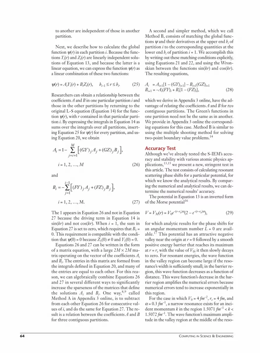
Figure 2. Comparison of the accuracies of three computationalmethods. The numerical error in the scattering phase shift (in units of) for scattering from a Morse potential in a narrow resonance region isshown as a function of the incident momentum k. The error is obtainedby comparing the numerical phase shift with the correspondinganalytical value.17 The momentum closest to the resonance occurs for k= 1.5076 fm. The Morse potential parameters, defined in Equation 29,are A0 = 4 fm–2, re = 4 fm, and = 0.3 fm–1. The accuracy parameter forcase B is tol = 1.e – 12.


the solutions of Equation 19 are obtained, we canobtain the values of the functions Y and Z and theirderivatives at the boundary points of the partitioni from Equation 17 by inserting for r the value bi–1or bi, respectively. The derivatives are expressed interms of the integrals we define next, hence there’sno loss of accuracy (contrary to the case in whichwe calculate the derivatives explicitly, as explainedin the “Spectral Expansion” section). In the presentcase, the derivatives’ accuracy is the same as that ofthe integrals, which, in turn, is equal to the accu-racy of the integrands’ expansion coefficients interms of Chebyshev polynomials. These integralsare the dimensionless quantities

(20)

In terms of these, we obtain

Yi(bi–1) = sin(kbi–1)[1 – (GY)i]Yi´(bi–1) = k cos(kbi–1)[1 – (GY)i]Zi (bi–1) = cos(kbi–1) – sin(kbi–1)(GZ)i]Zi´(bi–1) = –k[sin(kbi–1) + cos(kbi–1)(GZ)i] (21)

and

Yi(bi) = sin(kbi) – cos(kbi)(FY)iYi´(bi) = k[cos(kbi) + sin(kbi)(FY)i]Zi (bi) = cos(kbi)[1 – (FZ)i]Zi´(bi–1) = –k sin(kbi–1)[1 – (FZ)i], (22)

where a prime indicates a derivative with respect tor. Because the functions Y and Z obey the sameSchrödinger equation, the Wronskian of thesefunctions, W(Y, Z) = Y´Z – YZ´, is independent ofthe point r within the interval i if V is a local po-tential. Using Equations 21 and 22, we can expressthe Wronskian at r = bi–1 and r = bi, respectively, interms of the overlap integrals defined in Equation20. We obtain

W(Y, Z)bi–1 = k[1 – (GY)i]W(Y, Z)bi = k[1 – (FZ)i], (23)

which implies that

(GY)i = (FZ)i, (24)

a result that’s borne out in the numerical calcula-tions. This result also shows that if (GY) becomesclose to unity in a particular partition, the functionsY and Z will no longer be significantly linearly in-dependent of each other, which means the S-IEMbecomes unreliable in this partition. The remedyis to decrease the partition’s length because thevalue of (GY) will then also decrease. Equation 22is important for matching the global solution inone partition to that in the next one, as Appendix 3online shows.

Equation 19’s solution in each interval i is ac-complished by expanding these functions in termsof Chebyshev polynomials and solving the matrixequations for the corresponding coefficients. (Theprocedure is well described elsewhere,8 so wewon’t repeat it here.) However, a few remarks arein order:

• The solutions of Equations 19 yield the expan-sion of the functions Yi(r) and Zi(r) in terms ofChebyshev polynomials with high spectral accu-racy by using Chebyshev collocation points ineach partition, together with the Curtis-Clen-shaw quadrature,6 as described in the “SpectralExpansion” section.

• Equation 19 is not the Schrödinger equation’s in-verse, otherwise there would be no gain in accu-racy by using the integral equation.

• The inverse of the operator (1 – Ki) always existsif the partition i is made small enough becausethen the operator Ki becomes small in compari-son to the unit operator 1.

• Calculating the functions Yi(r) and Zi(r) isn’tcomputationally expensive because the numberof collocation points in each partition is small (16,usually), hence the matrices involved, althoughnot sparse, are small (for example, 16 16).

• As we mentioned in the “Spectral Expansion”section, we can prescribe the calculation accuracyof the functions Yi(r) and Zi(r) ahead of time byexamining the magnitude of the expansions’ lastthree coefficients. If they aren’t smaller than theprescribed tolerance parameter, the partition’ssize is reduced by a factor of two, and the accu-racy will increase correspondingly. This adjust-ment of partition sizes can be done automatically(as other work13 demonstrates in detail and wediscuss later).

• The method is suitable for parallel computingbecause the functions Yi(r) and Zi(r) and the re-spective overlap integrals required for propagat-ing the global wave function from one partition

( ) sin( ) ( ) ( ) .FZk

kr V r Z r dri ib

b

i

i=−

∫1

1

( ) cos( ) ( ) ( ) ;GZk

kr V r Z r dri ib

b

i

i=−

∫1

1

( ) sin( ) ( ) ( ) ;FYk

kr V r Y r dri ib

b

i

i=−

∫1

1

( ) cos( ) ( ) ( ) ;GYk

kr V r Y r dri ib

b

i

i=−

∫1

1


to another are independent of those in anotherpartition.

Next, we describe how to calculate the globalfunction (r) in each partition i. Because the func-tions Yi(r) and Zi(r) are linearly independent solu-tions of Equation 13, and because the latter is alinear equation, we can express the function (r) asa linear combination of these two functions:

(r) = AiYi(r) + BiZi(r), bi–1 r bi. (25)

Researchers can obtain a relationship between thecoefficients A and B in one particular partition i andthose in the other partitions by returning to theoriginal L-S equation (Equation 14) for the func-tion (r), with r contained in that particular parti-tion i. By expressing the integrals in Equation 14 assums over the integrals over all partitions, insert-ing Equation 25 for (r) for every partition, and us-ing Equation 20, we obtain

i = 1, 2, …, M (26)

and

i = 1, 2, …, M. (27)

The 1 appears in Equation 26 and not in Equation27 because the driving term in Equation 14 issin(kr) and not cos(kr). When i = 1, the sum inEquation 27 is set to zero, which requires that B1 =0. This requirement is compatible with the condi-tion that (0) = 0 because Z1(0) 0 and Y1(0) = 0.

Equations 26 and 27 can be written in the formof a matrix equation, with a large 2M 2M ma-trix operating on the vector of the coefficients Aiand Bi. The entries in this matrix are formed fromthe integrals defined in Equation 20, and many ofthe entries are equal to each other. For this rea-son, we can algebraically combine Equations 26and 27 in several different ways to significantlyincrease the sparseness of the matrices that definethe solutions Ai and Bi. One way,8,9 calledMethod A in Appendix 3 online, is to subtractfrom each other Equation 26 for consecutive val-ues of i, and do the same for Equation 27. The re-sult is a relation between the coefficients A and Bfor three contiguous partitions.

A second and simpler method, which we callMethod B, consists of matching the global func-tions and their derivatives at the upper end bi ofpartition i to the corresponding quantities at thelower end bi of partition i + 1. We accomplish thisby writing out these matching conditions explicitly,using Equations 21 and 22, and using the Wron-skian between the functions sin(kr) and cos(kr).The resulting equations,

Ai = Ai+1[1 – (GY)i+1] – Bi+1(GZ)i+1Bi+1 = –Ai(FY)i + Bi[1 – (FZ)i], (28)

which we derive in Appendix 3 online, have the ad-vantage of relating the coefficients A and B for twocontiguous partitions. The Green’s functions inone partition need not be the same as in another.We provide in Appendix 3 online the correspond-ing equations for this case. Method B is similar tousing the multiple shooting method for solvingtwo-point boundary value problems.14

Accuracy TestAlthough we’ve already tested the S-IEM’s accu-racy and stability with various atomic physics ap-plications,13,15 we present a new, stringent test inthis article. The test consists of calculating resonantscattering phase shifts for a particular potential, forwhich we know the analytical results. By compar-ing the numerical and analytical results, we can de-termine the numerical results’ accuracy.

The potential in Equation 13 is an inverted formof the Morse potential16

V = VM(r) = V0e–(r–re)(2 – e–(r–re)), (29)

for which analytic results for the phase shifts foran angular momentum number L = 0 are avail-able.17 This potential has an attractive negativevalley near the origin at r = 0 followed by a smoothpositive energy barrier that reaches its maximumat r = re with the value of V0; it then slowly decaysto zero. For resonant energies, the wave functionin the valley region can become large if the reso-nance’s width is sufficiently small; in the barrier re-gion, this wave function decreases as a function ofdistance. This wave function’s decrease in the bar-rier region amplifies the numerical errors becausenumerical errors tend to increase exponentially inthis region.

For the case in which V0 = 4 fm–2, re = 4 fm, and = 0.3 fm–1, a narrow resonance exists for an inci-dent momentum k in the region 1.5071 fm–1 < k <1.5072 fm–1. The wave function’s maximum ampli-tude in the valley region at the middle of the reso-

B FY A FZ Bi j j j jj

i= − +

=

−

∑ ( ) ( ) ,1

1

A GY A GZ Bi j j j jj i

M= − +

= +∑1

1( ) ( ) ,


nance, near k = 1.50716 fm, is close to 300 (asymp-totically, it’s equal to 1). Table I in George Raw-itscher and his colleagues’ article17 gives the phaseshifts’ analytic values in this resonance region; Fig-ure 2 illustrates the corresponding numerical er-rors for various methods of calculation. Themomenta k on the x-axis are the excess over themomentum at the resonance’s left side, k = 1.50710fm–1. We obtained the IEM curves A and B withthe two versions of the S-IEM method that we de-scribe in this article:

• NUM is a sixth-order Numerov method, whichwe also denote as Milne’s method (Essaid Zerradat Delaware State University performed thesecalculations), and

• the LD curve is obtained with the LogarithmicDerivative method (which Naduvalath Balakr-ishnan at the Institute for Theoretical and Mol-ecular Physics, Harvard-Smithsonian Center forAstrophysics, and Ionel Simbotin at the Univer-sity of Connecticut implemented with theMolscat code).

We set the matching radius for the two finite dif-ference methods, LD and NUM, at T = 50 fm, butfor the more precise S-IEM results, we had to usethe larger value T = 100 fm. Rawitscher and his col-leagues’ article17 extrapolates the correspondinganalytical comparison values from the exact ana-lytical result for T = to the distances of T = 50and T = 100 fm by a Green’s function iteration pro-cedure.13 Figure 2 shows that S-IEM’s accuracy issix orders of magnitudes higher than that of theNumerov method.

We obtained Method B’s results with a Matlabprogram, which we transcribe in Appendix 1 on-line, and took the tolerance parameter as tol =10–12, which resulted in 68 partitions. The errorfor the functions Y and Z in each partition were oforder 10–14 or smaller, and the computing time re-quired to obtain the results for the 11 different kvalues was 10 seconds on a Windows 98 Dell Op-tiplex computer with a speed of 500 MHz and 128Mbytes of RAM. It’s likely that Method B isslightly more accurate than Method A becauseMatlab has 16 figures of accuracy, whereas double-precision Fortran, which we used to obtainMethod A’s results, only has between 14 and 15 fig-ures of accuracy.

Figure 3 illustrates the S-IEM’s ability to auto-matically determine the partitions’ size for thesame case as Figure 2. The maximum radial posi-tion is T = 100 fm, not shown here. For tol =10–12, there are nine bins from r = 0 to r = 10 fm,

whereas for tol = 10–6, there are only four. Thecorresponding largest error in the phase shift (inunits of ) is approximately 3 10–11 and 3 10–5,respectively.

Because the S-IEM is considerably morestable than finite difference methods, itmight become the method of choice forparticular applications, such as atomic

physics calculations that involve large distancesor require high accuracy and must be performedin configuration space. Using the S-IEM, re-searchers can naturally implement the asymptoticboundary conditions of the wave function, be-cause it’s a solution of an integral equation usingGreen’s functions. A simple way to distinguish aspectral method from a finite difference method,be it for the solution of a differential or an inte-gral equation, is that in a particular partition, themesh points in the former aren’t equispaced,whereas in the latter they are. Even though wecan substantially increase finite difference meth-ods’ accuracy by extrapolating the algorithms toequivalent zero-sized distance between meshpoints,18 such extrapolation methods might be-come cumbersome. Spectral methods for im-proving the accuracy of the derivatives in

Bin

num

ber

10

8

6

4

2

0 2 4 6 8 10

tol = 1.e(–12)tol = 1.e(–6)

Bin position (fm)

Figure 3. Bin size determined by S-IEM for a prescribed tolerance. Thecalculation is for the case of a resonance in a Morse potential (seeFigure 2). The horizontal axis shows the right-hand coordinates of binsi, and the vertical axis shows the corresponding bin number i, with i = 1,2, ... . The total number of partitions is larger than the figure showsbecause the maximum radial distance (100 fm) is larger than the radialdistance shown.


differential equation solutions also exist.19 TheS-IEM is a type of Spectral Domain Decomposi-tion Method (per the terminology from JohnPhilip Boyd’s book20)—that is, in each partition(or domain) the solution is spectrally expandedand the coefficients of the expansion in one par-tition are related to those in another by matchingthe functions with the first-order derivatives atthe boundary. The S-IEM is one of a class of sim-ilar methods, which we describe in more detail inAppendix 4 online.

In each partition, only two independent basisfunctions Y(r) and Z(r) are required to expressthe global solution. When there’s more than onechannel coupled to other channels, that numberincreases proportionally to the number of chan-nels present.9 The functions Y(r) and Z(r) are so-lutions of both the Schrödinger and L-Sequations for that partition, and we can precal-culate them independently of the functions inother partitions by using our spectral expansionmethod. Matching the global solution from onepartition to the next for Method B proceeds sim-ilarly to that of many other methods, but it hasthe advantage that we can calculate the solution’sderivatives at the matching points by means ofintegrals. Hence, we can avoid the loss ofaccuracy that is usually involved when takingderivatives.

If NC coupled channels exist in the Schrödingerequation, the computational complexity of the S-IEM scales is NC

3. This is similar to how finite dif-ference methods scale, and it becomes computerintensive if NC becomes large. In this case, iterativemethods become desirable because they scale as NC

2

times the number of iterations. We’re currently in-vestigating such methods.

AcknowledgmentsWe are grateful to Ionel Simbotin for stimulatingconversations regarding Method B.

References1. E. Bodo, F.A. Gianturco, and A. Dalgarno, “F+D2 Reaction at Ul-

tracold Temperatures,” J. Chemical Physics, vol. 116, no. 21,2002, pp. 9222–9227.

2. K.T. Tang, J.P. Toennies, and C.L. Yiu, “Accurate Analytical He-He van der Waals Potential Based on Perturbation Theory,”Physics Rev. Letters, vol. 74, 1995, pp. 1546–1549.

3. G. Rawitscher and I. Koltracht, “A Spectral Integral Method forthe Solution of the Faddeev Equations in Configuration Space,”Nuclear Physics, vol. A 737CF, 2004, pp. S314–S316.

4. D. Gottlieb and S.A. Orzsag, “Numerical Analysis of SpectralMethods: Theory and Applications,” Proc. CBMS-NSF RegionalConf. Series in Applied Mathematics #26, SIAM Press, 1977.

5. M. Abramowitz and I. Stegun, eds., Handbook of MathematicalFunctions, Dover, 1972.

6. C.W. Clenshaw and A.R. Curtis, “A Method for Numerical Inte-gration on an Automatic Computer,” Numerical Mathematics,vol. 2, 1960, p. 197.

7. I.S. Gradshteyn and I.M. Ryzhik, Tables of Integrals, Series, andProducts, Academic Press, 1980, p. 836.

8. R.A. Gonzales et al., “Integral Equation Method for the Contin-uous Spectrum Radial Schrodinger Equation,” J. ComputationalPhysics, vol. 134, 1997, pp. 134–149.

9. R.A. Gonzales et al., “Integral Equation Method for CoupledSchrödinger Equations,” J. Computational Physics, vol. 153, 1999,pp. 160–202.

10. L. Greengard and V. Rokhlin, “On the Numerical Solution ofTwo-Point Boundary Value Problems,” Communications in Pureand Applied Mathematics, vol. 44, 1991.

11. B. Mihaila and I. Mihaila, “Numerical Approximations usingChebyshev Polynomial Expansions: El-Gendi’s Method Revis-ited,” J. Physics A: Mathematical and General, vol. 35, 2002, pp.731–746.

12. B. Mihaila and R.E. Shaw, “Parallel Algorithm with Spectral Con-vergence for Nonlinear Integro-Differential Equations,” J. PhysicsA: Mathematical and General, vol. 35, 2002, p. 5315.

13. G.H. Rawitscher et al., “Comparison of Numerical Methods forthe Calculation of Cold Atom Collisions,” J. Chemical Physics, vol.111, 1999, pp. 10418–10426.

14. J. Stoer and R. Bulirsch, Introduction to Numerical Analysis, 2nded., Springer Verlag, 1992, section 7.3.5.5.

15. G.H. Rawitscher, S.-Y. Kang, and I. Koltracht, “A Novel Methodfor the Solution of the Schrodinger Equation in the Presence ofExchange Terms,” J. Chemical Physics, vol. 118, no. 23, 2003, pp.9149–9156.

16. A.P.M. Morse, “Diatomic Molecules According to Wave Mechan-ics. II Vibrational Levels,” Physics Rev., vol. 34, July 1929, p. 57.

17. G. Rawitscher et al., “Resonances and Quantum Scattering forthe Morse Potential as a Barrier,” Am. J. Physics, vol. 70, no. 9,2002, p. 935.

18. W.B. Gragg, “On Extrapolation Algorithms for Ordinary InitialValue Problems,” SIAM J., series B, Numerical Analysis, vol. 2, no.3, 1965, pp. 384–403.

19. D.A. Mazzotti, “Spectral Difference Methods for Solving the Dif-ferential Equations of Chemical Physics,” J. Chemical Physics, vol.117, no. 6, 2002, p. 2455.

20. J.P. Boyd, Chebyshev and Fourier Spectral Methods, Springer Ver-lag, 1989, chapter 19.

George H. Rawitscher is a professor at the Universityof Connecticut. His research interests include theoret-ical and computational analysis of nuclear and atomicscattering. Rawitscher has a PhD in physics from Stan-ford University. He is a member of the American Phys-ical Society and Sigma Pi Sigma. Contact him [email protected].

Israel Koltracht is a professor at the University ofConnecticut. His research interests include computa-tional mathematics with applications to physics.Koltracht has a PhD in mathematics from the Weiz-mann Institute, Israel. He is a member of the Interna-tional Linear Algebra Society. Contact him [email protected].

An Efficient Numerical Spectral Method for Solving the Schrödinger Equation

George H. Rawitscher and Israel Koltracht


Appendix 4: Comparison with Other Methods

Our spectral integral equation method (S-IEM) is one of a class of well-known methods that divide the spatial domain into partitions (also called sectors or domains)1 and expand the solution on a suitable set of basis functions in each partition. One example is Roy Gordon’s method,2–4 which uses Airy basis functions. The potential in each partition is approximated by a linear function, and the Airy functions are the differential equation’s corresponding exact solutions. This method was included among the comparisons performed for the atom-atom scattering case.5 Gordon’s method is widely used for atomic physics calculations; one implementation is available elsewhere.6,7 This “potential following method” is particularly efficient when the potential varies slowly with distance. Another example is Light and Walker’s method,8 in which the potential in each partition is approximated by a constant. In this case, we simply write the Green’s function that propagates the solution from one end of the partition to the other in terms of sine and cosine functions. This method lends itself well to propagating the inverse of the solution’s logarithmic derivative from one end of a partition to the other, without calculating the solution itself. This is called the R-matrix propagation method, which Burke and Noble implemented.9 In the main article text,10 we include this method, implemented with the code Molscat,11 among the comparisons carried out for the barrier penetration calculation (see Figure 1 in the main article).

Baluja and colleagues12 give a “function following” method that expands the Green’s function in a given partition in terms of Legendre polynomials, without making approximations on the potentials. This method is implemented in the computer code FARM.9 The resulting expansion of the distorted Green’s function G(r, r′) is separable—that is, it is given as a sum over products of functions u(r) × v(r′). We can obtain a similar form by using Sturmian basis functions,13–15 but such expansions don’t converge to high accuracy because the derivative of a Green’s function has a discontinuity at the points r = r′. Our S-IEM doesn’t suffer from this difficulty because we obtain the distorted Green’s function G(r, r′) in terms of the exact undistorted Green’s function G0(r, r′), and G0 is given exactly in terms of its semiseparable form given in the main text.10 Formally, the relation between G and G0 is expressed through the relation

G = (1 – G0V)–1G0;

numerically, the solution of the equations for the functions Y and Z (Equation 19 in the main article text10) is equivalent to expressing the distorted Green’s function in terms of the undistorted one. (We’re indebted to Ian Thompson for the helpful comments on which we based this paragraph.)

Several general comments regarding the numerical advantages of the S-IEM are as follows

• The “big” matrices involved in calculating the coefficients A and B are sparse and can be solved by Gaussian elimination. Because the number of floating-point operations (flops) is proportional to the number of partitions M, the S-IEM’s computational complexity is comparable to the computational complexity of the solution of differential equations. This sparseness property results from the semiseparable nature of the integration kernel K we define in the main article text10 (also shown in related literature16,17), but applies only in the configuration representation of the Green’s function. This part of our procedure differs substantially from related work.18

• We can reliably implement the scattering boundary conditions because the Green’s function

incorporates the asymptotic boundary conditions automatically. However, in the coupled channel case for angular momentum numbers L > 0, the coupled equations must be solved as many times as there are open channels because our Green’s functions consist of sin(kr) and cos(kr), rather than of Riccati-Bessel functions. We have shown17 that researchers can obtain the desired linear combination of the solutions without appreciable loss of accuracy because the matrix required in the solution for the coefficients has a condition number not much larger than unity. This means that our various solutions are linearly independent to a high degree, contrary to what can be the case with the solution of differential equations..

• The S-IEM is economical in the total number of mesh points required in the interval [0, T] because in each partition the spectral collocation method requires few mesh points (like in the case of Gauss-Legendre integration as compared to Simpson’ integration), and the code automatically adjusts the length of each partition to satisfy the required accuracy tolerance criterion. This means that only in the regions where many meshpoints are required will there be many partitions.

• We can distribute the calculation onto parallel processors because the functions Y and Z, as well as the overlap integrals required for calculating the matrices that determine the coefficients A and B, can be calculated separately for each partition independently of the other ones. This is an important point because if the number of channels increases from 1 to NC, the overlap integrals (GY)i, (GZ)i, (FY)i, and (FZ)i become matrices of dimension NC × NC, hence the total number of overlap integrals increases accordingly.

• Method B has the advantage that the Green’s functions in one partition need not be the same as those in another partition. This is the case, for instance, if the momentum k in a given partition

is chosen to be the local momentum ki = 21( )ik V b −− . In this case, the equations that

connect the α from one partition to that of a contiguous partition are of the type given by Equation M in Appendix 3

The third point is important because, due to the small number of total mesh points, the accumulation of machine round-off errors is correspondingly small. In addition, as is well known, integration is numerically more stable than differentiation (see Appendix 2 related work19 ). Hence, the accumulation of the inherent round-off error is smaller for an integral equation’s numerical solution than for the numerical solution of differential equations. Figure 1 in the article by Reo.A. Gonzales and his colleagues 16 clearly illustrates this feature for the case of the calculation of Bessel functions.

Related research20 also demonstrates the spectral integral method’s efficiency compared to a finite difference method. This work20 calculates the phase shift of an incident electron scattering from the ground state of the Hydrogen atom, with inclusion of the Fock exchange terms. Figure 2 of this article20 shows that as the number M of partitions increases, the number of stable significant figures in the phase shift increases very rapidly for the S-IEM, illustrating the method’s spectral nature. By comparison, for a method employing finite difference techniques based on an equispaced set of mesh points,21–23 the number of stable significant figures increases much more slowly with the number of mesh points. With 4,000 mesh points, the finite difference method21 reaches six significant figures of stability, whereas the S-IEM reaches 11 significant figures with 100 mesh points in the same radial interval. Nevertheless, this example isn’t very realistic physically because neither calculation includes the virtual excitations of the bound electron to the myriad possible states, both bound and in the continuum.

Researchers (including George Rawitscher) have also preformed a benchmark calculation using the S-IEM involving two coupled channels, one closed and one open.5 They investigated the numerical stability of the L = 0 scattering phase shift as a function of the number of mesh points used and compared it with various other methods of calculation (see the results in Figure 5 of Rawitscher and colleagues’ article).5 In this case, the stability of a finite-element method was comparable to that of the S-IEM Method A. This benchmark calculation was recently used7 for comparison with results obtained with a finite difference method in which the potential in each partition is assumed to be constant (similar to the case with one form

of the Gordon method), and the corrections are taken into account iteratively.

References 1. J.P. Boyd, Chebyshev and Fourier Spectral Methods, Springer Verlag, 1989.

2. R.G. Gordon, “Constructing Wave Functions for Bound States and Scattering,” J. Chemical Physics, vol.

51(1), 1969, p. 14-25.

3. B. J. Alder, S. Fernbach, and M. Rotenberg, eds., Methods in Computational Physics, Academic, vol. 10,

1971, pp. 81–110

4. F.H. Mies, “Molecular Theory of Atomic Collisions: Calculated Cross Sections for H++F(2P),”, Physics

Review, vol. A7, no. 3, 1973, p. 957.

5. G.H. Rawitscher et al., “Comparison of Numerical Methods for the Calculation of Cold Atom Collisions,” J.

Chemical Physics, vol. 111, 1999, pp. 10418–10426.

6. J.A. Christley and I.J. Thompson, “CRCWFN: Coupled Real Coulomb Wavefunctions,” Computer. Physics

Communications, vol. 79, 1994, pp. 143–155.

7. L.Gr. Ixaru, “LILIX-A Package for the Solution of the Coupled Channel Schrodinger Equation,” Computer

Physics Communications, vol. 147, 2002, pp. 834–852.

8. J.C. Light and R.B. Walker, “An R Matrix Approach to the Solution of Coupled Equations for Atom-

Molecule Reactive Scattering,” J. Chemical Physics, vol. 65, 1976, pp. 4272–4282.

9. V.M. Burke and C.J. Noble, “Farm — A Flexible Asymptotic R-Matrix Package,” Computer Physics

Communications, vol. 85, 1995, pp. 471–500.

10. G.H. Rawitscher and I. Koltracht, “An Efficient Numerical Spectral Method for Solving the Schrödinger

Equation,” Computing in Science & Eng., vol. 7, no. 6, 2005, pp. xx–xx.

11. J.M. Hutson and S. Green, Molscat computer code, version 14, Collaborative Computational Project No 6,

Engineering and Physical Sciences Research Council, 1994.

12. K.L. Baluja, P.J. Burke, and L.A. Morgan, “R-Matrix Propagation Program for Solving Coupled Second-

Order Differential Equations,” Computer Physics Communications,, vol. 27, 1982, pp. 299–307.

13. G. Rawitscher, “Positive Energy Weinberg States for the Solution of Scattering Problems,” Physics Review,

vol. C 25, 1982, pp. 2196–2213.

14. G. H. Rawitscher and G. Delic, “Sturmian Representation of the Optical Model Potential due to Coupling to

Inelastic Channels,” Physics Review, vol. C 29, 1984, pp. 1153–1162.

15. K. Amos et al., “An Algebraic Solution of the Multichannel Problem Applied to Low Energy Nucleon–

Nucleus Scattering,” Nuclear Physics,, vol. A728, 2003, pp. 65–69.

16. R.A. Gonzales et al., “Integral Equation Method for the Continuous Spectrum Radial Schrodinger Equation,”

J. Computational Physics, vol. 134, 1997, pp. 134–149.

17. R.A. Gonzales et al., “Integral Equation Method for Coupled Schrodinger Equations,” J. Computational

Physics, vol. 153, 1999, pp. 160–202.

18. L. Greengard and V. Rokhlin, <<article title will be provided soon>>, Commun. Pure Appl. Math., vol. 2,

1960, p. 197.

19. R.L. Burden and J. Douglas Faires, Numerical Analysis, 7th ed., Brooks/Cole, 2001, sections 4.4 & 5.2 pp.

203, 263

20. G.H. Rawitscher, S.-Y. Kang, I. Koltracht, “A Novel Method for the Solution of the Schrodinger Equation in

the Presence of Exchange Terms,” J. Chemical Physics, vol. 118, 2003, pp. 9149-9156.

21. W.N. Sams and D.J. Kouri, “Noniterative Solutions of Integral Equations for Scattering. I. Single Channels,”

J. Chemical Physics, vol. 51, 1969, pp. 4809–4814.

22. R. Smith and R. J. Henry, eds., “Noniterative Integral-Equation Approach to Scattering Problems,” Physics

Review, vol. A7, 1973, pp. 1585–1590.

23. R.J.W. Henry, S.P. Rountree and E.R. Smith, “A General Program to Calculate Atomic Continuum Processes

using the NIEM Method,” Computer Physics Communications, vol. 23, 1981, pp. 233–273.




Appendix 3: Calculating the Coefficients A and B in the Spectral Integration Equation Method

As we explained in the main article,1 we can obtain a relationship between the coefficients A and B in one particular partition i and those in the other partitions by returning to the original Lippman-Schwinger equations.

ψ(r) = sin(kr) + ∫0T G0(r, r′)V(r′)ψ(r′)dr′, (A)

for the function ψ(r), with r contained in that particular partition i. The result is

1

1 ( ) ( )M

i j j j jj i

A GY A GZ B= +

= − + ∑ , i = 1, 2, ..., M (B)

and

1

1

( ) ( )i

i j j j jj

B FY A FZ B−

= = − + ∑ , i = 1, 2, ..., M, (C)

where the quantities (GY)i, (GZ)i, (FY)i, and (FZ)i are overlap integrals, defined in main article.1 We can describe two methods for solving for the coefficients Ai and Bi, i = 1, 2, ..., M.

Method A This method2,3 consists of writing Equation B for a particular value of i, and subtracting from it the Equation B written for the previous value of —that is, i – 1, , and similarly for Equation C. By defining the column vectors

1 0; ;

0 0i

ii

A

Bα ω ς

= = =

, (D)

we obtain

12 1

21 23 2

32 34 3

1, 2 1, 1

, 1

..

.. ..

M M M M M

M M M

α ςα ςα ς

α ςα ω

− − − −

−

=

I M 0

M I M

M I M

M I M

0 M I

, (E)

where I and 0 are two-by-two unit and zero matrices, respectively, and where

1,( ) 1 ( )

0 0i i

i iGY GZ

−−

=

M , i = 2, 3, …, M (F)

and

, 11 1

0 0

( ) ( ) 1i ii iFY GZ−− −

= −

M , i = 2, 3, …, M. (G)

Equation E generally connects the A and B’s of three contiguous partitions—for example, M21α1 + α2 + M23α3 = ζ. The solution of the matrix Equation E for the quantities αi , i = 1, 2, …M, leads to the results we labeled A in Figure 2 in the main article text.1

Method B A second and simpler method, B, consists of matching the global functions ψ and their derivatives at the upper end bi of partition i to the corresponding quantities at the lower end bi of partition i + 1. We accomplish this by writing out these matching conditions explicitly, using the relations between the overlapping integrals (GY)i, (GZ)i, (FY)i, and (FZ)i and the functions Yi and Zi and their derivatives at the boundaries of the partition i, given by Equations 20 through 23 in the main article,1 and by using the Wronskian between the functions sin(kr) and cos(kr). We can write the resulting equations

Ai = Ai+1[1 – (GY)i+1] – Bi+1(GZ)i+1

Bi+1 = –Ai(FY)i + Bi[1 – (FZ)i] (H)

in matrix form

Γiαi = Ωi+1αi+1, i = 1, 2, …, M – 1 (I)

with

1 0

( ) 1 ( )ii iFY FZ

= − −

Γ (J)

1 ( ) ( )

0 1i i

iGY GZ− −

=

Ω . (K)

By successive applications of Equation I

αi+1 = (Ωi+1)–1 ΓiαI, (L)

we can relate the coefficients Ai and Bi in all partitions i = 2, 3, ..., M to A1 and B1. By setting the latter to 1 and 0, respectively, we ensure that ψ(0) = 0. By matching ψ(bM) to the scattering solution AF + BG, where F and G are Ricati-Bessel and Ricati-Neumann functions, or regular and irregular Coulomb functions if a Coulomb potential is present, we obtain the scattering phase shift δ = arc tan (B/A) and an overall normalization factor A for the global wave function ψ. This matching equation is

1( , ) ( , )1

( , ) ( , )M

MM

AW g W g

BW f W fk

−− − =

Γ

A F G

B F G, (M)

where W represents the Wronskian, and f and g stand for sin(kr) and cos(kr), respectively. We can obtain the same result by combining Equations B and C in a different way than in Method A.

The latter procedure consists of first writing Equation B into a (2 × 1) column form involving the vectors αi, and subsequently subtracting equations with contiguous i-values from each other but leaving the last equation in its original form. The result is

1 2 1

2 3 2

3 4 3

1 1

1 2 3 1

..

.. ..

..M M M

M M

α ςα ςα ς

α ςγ γ γ γ α ω

− −

−

− − −

= −

Γ ΩΓ Ω

Γ Ω

Γ ΩI

, (N)

where

0 0

( ) ( )ii iFY FZ

γ =

. (O)

The first M – 1 rows in Equation E are equivalent to Equation I, and the last row

1

1

1

0

M

i i Mi

γ α α−

=

+ =

∑ (P)

represents a normalization condition for finding the value of A1. We can show that Equation P is compatible with the requirement that B1 = 0. Using Method B with two adjoining partitions can be similar to using the multiple shooting method for solving two-point boundary value problems.4 We obtained the result B in Figure 2 of the main article text with the Method B we describe here.

Acknowledgment We are grateful to Ionel Simbotin for stimulating conversations that led to the development of Method B.

References 1. G.H. Rawitscher and I. Koltracht, “An Efficient Numerical Spectral Method for Solving the Schrödinger


2. R.A. Gonzales et al., “Integral Equation Method for the Continuous Spectrum Radial Schrodinger Equation,”

J. Computational Physics, vol. 134, <<issue number or month?>>, 1997, pp. 134–149.

3. R.A. Gonzales et al., “Integral Equation Method for Coupled Schrodinger Equations,” J. Computational

Physics, vol. 153, <<issue number or month?>>, 1999, pp. 160–202.

4. J. Stoer and R. Bulirsch, Introduction to Numerical Analysis, 2nd ed., Springer Verlag, 1992, section 7.3.5.5.




Appendix 2: Accuracy of Spectral Expansions

The accuracy considerations for the spectral expansion of a function into Chebyshev polynomials, which we describe in

the “Spectral Expansion” section of the main article, is further developed in this appendix, still by means of the

example f = exp(x).

The expansion of the function, truncated at the upper limit N, is given by

0

1

( ) ( )2

N

N j jj

af x a T x

== +∑ . (A)

We obtained the coefficients aj with the collocation method described in C.W. Clenshaw and A.R. Curtis’ article.1 It consists of considering the N + 1 zeros ξa of TN+1 for α = 0, 1, …, N; evaluating the expansion (Equation A) at x = ξa for α = 0, 1, …, N; and thus obtaining a set of N + 1 linear equations for the coefficients aj. The corresponding matrix that relates the column vector of the f(ξa) to the vector of the aj has elements formed from the values Tj(ξa), with j, α = 0, 1, ..., N, and is obtained from the subroutine C_CM1 in Appendix 1 For N = 9 and 13, the result for the errors are given in Tables A and C, respectively.

Table A. Errors of the Chebyshev expansion of various functions associated with f(x) = exp(x). They are the indefinite integral F (Equation B), the function f Equation A), and the first and second derivatives (Equation C). The number of terms in each of the expansions

is 10 (N = 9). The quantities without a subscript represent the exact values of these functions.

x FN – F fN – f fN(1) – f(1) fN

(2) – f(2

–0.8 .25(–11) –.51(–9) .12(–8) .14(–6)

–0.6 .11(–8) .51(–9) .10(–8) –.81(–7)

–0.4 .29(–9) –.30(–9) –.48(–8) .37(–7)

–0.2 .27(–9) –.23(–9) .49(–8) .24(–7)

0.0 .11(–8) –.55(–9) .50(–10) –.55(–7)

0.2 .37(–9) –.24(–9) –.52(–8) .23(–7)

0.4 .20(–9) –.32(–9) .51(–8) .41(–7)

0.6 .11(–8) .57(–9) –.10(–8) –.91(–7)

0.8 .21(–10) –.58(–9) –.15(–8) .16(–6)

The Chebyshev expansion is particularly suited to obtain the integral ∫–1

xfN(x′)dx′ of the function fN without a significant loss of accuracy. An expansion of this antiderivative function in terms of Chebyshev polynomials

1

10

( ) ( ') ' ( )Nx

N N j jj

F x f x dx b T x+

−=

= = ∑∫ (B)

has the property that we can easily obtain the coefficients bj in terms of the coefficients aj via a matrix usually denoted as SL. The reason is that the integral from –1 to x of a particular Tj is given by a linear combination of Ti(x) with i ≤ j + 1. For example, ∫–1

x T2(x′)dx′ = [T3(x) – 3T1(x) – 2T0(x)]/6, and ∫–1x

T3(x′)dx′ = [T4(x) – 2T2(x) + T0(x)]/8. The sum in Equation 2 should rigorously go to the upper limit N + 1, but the (N + 1)th term is generally ignored in numerical calculations. A similar matrix, SR, exists in order to obtain a Chebyshev expansion of ∫x

1fN(x′)dx′. Column 2 in Table A demonstrates that the accuracy of the expansions of the functions f = exp(x) and of its antiderivative F is nearly the same, for the same number of terms.

We can also obtain the derivatives fN(1) = dfN/dx, fN

(2) = d2fN/dx2, and so on of fN via Chebyshev expansions, but with a loss of accuracy unless the truncation limit N’s value increases. Columns 4 and 5 in Table A illustrate this. We can understand this loss of accuracy as follows: To obtain dfN/dx, we can take the derivatives of the Chebyshev polynomials term by term in Equation A:

( ) ( )

1

( ) ( )N

n nj jN

j

f x a T x=

= ∑ , n = 1, 2, …, (C)

So that the error εN(n)(x) = f(n)(x) – fN

(n)(x) equals the derivative of the remainder dnεN/dxn and the latter can be approximated by aN+1TN+1

(n)(x). However, the larger the value of N, the more oscillatory the function TN+1(x), and hence the n – th derivative is correspondingly larger than the function itself by approximately the factor (N + 1)n,. The derivative of a polynomial of order j is a polynomial of order j – 1, whose magnitude is of order j times the original polynomial—for example, d2Tj(x)/dx2 = [xdTj/dx – j2Tj]/(1 – x2). This leads us to expect that the errors for a derivative of order n are related to the coefficient of the next to last Chebyshev polynomial, (TN+1) times (N + 1)n. Table B lists coefficients ai and aj × j2. By comparing Tables A and B, and also Tables A and C, we see how this expectation is borne out. We can also consider the function c(x) = cos(Nπx/2). For n = 10, this function has 10 zeros in the interval –1 ≤ x ≤ 1, and its second derivative with respect to x is (Nπ/2)2 × c(x). This again suggests that dnεN/dxn ≅ (N + 1)n × εN.

Table B. Coefficients aj and aj × j2 for the expansion of exp(x).

j 7 8 9 10 11

aj .32(–5) .20(–6) .11(–7) .55(–9) .25(–10)

aj × j2 .16(–3) .13(–4) .88(–6) .55(–7) .30(–8)

Table C. Same as Table A, for N = 13.

x FN –F fN – f fN(1) – f(1) fN

(2) – f(2)

–0.8 .29(–14) .72(–15) .24(–14) –.44(–12)

–0.6 .36(–15) .33(–15) .21(–13) .12(–12)

–0.4 .31(–14) .44(–15) –.32(–13) –.15(–12)

–0.2 –.56(–16) –.22(–14) .29(–13) .37(–12)

0.0 .33(–14) .48(–14) –.11(–13) –.57(–12)

0.2 .11(–15) –.40(–14) –.21(–13) .57(–12)

0.4 .24(–14) .20(–14) .44(–13) –.37(–12)

0.6 .67(–15) 0 –.42(–13) .25(–12)

0.8 .29(–14) .88(–15) .19(–13) –.69(–12)

A second method consists of writing a Chebyshev expansion for df/dx

10

1

/ ( )2

N

N j jj

cdf dx c T x

−

== + ∑ (D)

and noting that the expansion coefficients cj are related to the coefficients aj in Equation A as follows: cN–1 = 2NaN, cN–2 = 2(N – 1)an–1, and for j ≤ N – 2, cj–1 = cj+1 + 2jaj. The error in dfN/dx is approximately equal to the magnitude of cN, which in turn lets us determine the value of N from the relation cN = 2(N + 1)aN+1. This shows that the truncation errors in a differential equation’s solution tend to be larger than the truncation errors in an integral equation’s solution.

In the numerical example we provide here, the upper value N of the sums in the Chebyshev expansions is N = 9, but in the integral equation’s numerical solution, as described in the “Accuracy test” section of the main article, N = 15, which. leads to accuracies of the order of 10–14,. Table C demonstrates the rapid gain in accuracy for a small increase in the value of N... The accuracy increases approximately by four or five orders of magnitude as N increases from 9 to 13.

Reference 1. C.W. Clenshaw and A.R. Curtis, “A Method for Numerical Integration on an Automatic Computer,”

Numerical Mathematics, vol. 2, <<issue number or month?>>, 1991, p. 197.




Appendix 1: Matlab Program for Scattering in a Morse Potential

This appendix contains all the Matlab m-files needed to calculate the scattering of a particle in a 1D potential for a partial wave with L = 0, using the numerical spectral integral equation (S-IEM) method we describe in the main article text.1 The potential included is an inverted Morse potential that has a negative (attractive) valley at small distances and a repulsive barrier at intermediate distances, and that decays exponentially to zero for large distances. This potential supports various resonances for different incident energies. We calculate the phase shifts for various energies contained within one such resonance and compare them with the analytic results, as we describe in the main text,1 to measure our method’s accuracy.

We list here the main program, IEM_Morse_res.m, and the various function-subroutines that it calls. The function-subroutine meshiem calculates a partition’s size for a given input tolerance parameter; this subroutine calls mapxtor and vfg. The potential and the Green’s functions (sin(kr) and cos(kr)) are calculated by function-subroutine vfg. The potential is calculated by calling an appropriate subroutine (morse in the present case) that different potential subroutines can replace. The function-subroutine YZ calculates the local functions Y and Z; it calls mdiag and vfg.

Reference 1. G.H. Rawitscher and I. Koltracht, “An Efficient Numerical Spectral Method for Solving the Schrödinger


Main program IEM_Morse_res.m

% IEM_Morse_res.m is a MATLAB program that

% solves a one dimensional, one channel, positive energy (scattering)

% Lippmann-Schwinger eq. using The Chebyshev spectral expansion method,

% for a resonance scattering in a inverted Morse potential with a

% barrier

% Subroutines needed are C_CM1, SL_SR, meshiem, YZ, vfg, morse,

% mapxtor, and mdiag.

% meshiem calls vfg and mapxtor

% vfg calls a potential subroutine, that in this case is: morse

% YZ calls vfg and mdiag

%

clear all

tic % starts here to count the elapsed time

N=16 %number of Chebyshev mesh points in each partition, as described

% more precisely in the subroutine C_CM1 below

T=100 % maximum radial distance

%T=100

nloop=10

bstart= 0.2

bstart= 0 % leftmost radial distance of the first partition

Amorse=4; REmorse=4;amorse=1/0.33; % parameters for the Morse potential

tol=1.e-12

rcut=bstart % the potential is replaced by a constant for r<rcut

%k=0.10

%K = 41.47 % K=(hbar)^2/(reduced mass of nucleon)

K=1

%if K=1, this means that the potentials and energies have

% already been divided by K.

% The resulting dimensions of the energy and potential is inverse

% lenght squared, and the wave number k is one over a length. For

% this morse pot'l case, the unit of length is femto-meter

% anal50 is the set of L=0 phase shifts obtained analytically at a a

%distance of 50 fm. See Am. J. of Phys. vol 70, p. 935 (02).

% The first column is the value of k, the second is the phase shift

% in units of pi.

% anal100 is the same as anal50 for a matching radius of 100 fm

anal50=[

1.507100000000000e+000 -4.568483126920000e-001

1.507110000000000e+000 -4.533212648736000e-001

1.507120000000000e+000 -4.480714272385000e-001

1.507130000000000e+000 -4.394398160329000e-001

1.507140000000000e+000 -4.226587240332000e-001

1.507150000000000e+000 -3.765904018859000e-001

1.507160000000000e+000 -4.635282299884000e-002

1.507170000000000e+000 4.113560735221000e-001

1.507180000000000e+000 4.687007391308000e-001

1.507190000000000e+000 4.877779485905000e-001

1.507200000000000e+000 4.972300508370000e-001

1.507210000000000e+000 -4.971373180371000e-001

1.507220000000000e+000 -4.934015231054000e-001];

anal100=[

1.507100000000000e+000 -4.56851148617700e-001

1.507110000000000e+000 -4.53324094250100e-001

1.507120000000000e+000 -4.48074247045200e-001

1.507130000000000e+000 -4.39442620401400e-001

1.507140000000000e+000 -4.22661499186800e-001

1.507150000000000e+000 -3.76593103155600e-001

1.507160000000000e+000 -4.63555541276000e-002

1.507170000000000e+000 4.11353023527700e-001

1.507180000000000e+000 4.68697775626900e-001

1.507190000000000e+000 4.87775017641500e-001

1.507200000000000e+000 4.97227136582100e-001];

%[a,b] = size(anal100);

[a,b] = size(anal100); %this determines the number of k-values to be

% used in various do-loops later on

for n=1:a;

tandl(n)=1;

kk(n)=0;

end

[C,CM1,xz]=C_CM1(N); % these matrices map the vector of the function into

% the vector of the expansion coefficients (all column vectors)

[SL,SR]=SL_SR(N); % these are the right and left indefinite quadrature

% matrices in the Chebyshev space, described below

% b = SL(a).

% b is the column vector of the Ch. coeffs

% of the integral from -1 to x of f(x)dx,

% a is the column vector of the Ch. coeffs of the expansion of f.

% ditto for SR, for the integr from x to +1 SRCM1=SR*CM1;

%these are matrices that occur again and again in the calcu-

%lation of the local functions Y and Z in each partition.

SLCM1=SL*CM1;

nkmax=8;

nkmin=5

%for nk=1:13;

%for nk=nkmin:nkmax;

for nk=1:a

b1=bstart;

k=1.5071+(nk-1)*0.00001;

%determines the k-values for this particular resonance calculation

kk(nk)=k;

%K=1/0.04783258

% np = 1, 2, ...npm is the index thatlabels the partitions.

% Partition np starts with bp(np-1) and goes to bp(np),

% also called b1 and b2.

% partition 1 starts with b1 prescribed above.

% These partition numbers are stored in the array mp,

% the expansion coeffs aY for Y(x) in partition np for n= 0, 1, ..N are %

contained in the matrix aYp, (NP1 by npm) with column

% np containing aY for partition np;

% ditto for Z, aZp; ditto for the overlap integrals, in matrix overlp.

% the method to establish the length of each partition is as follows.

% Starting from the left end b1, the length of the partition is first

% estimated from the local wave number kbar as 3.2*pi/kbar,

% i.e., about 10 Cheb. points per local wave length. For this

% particular estimate of the size of the partition

% the Cheb. Expansion coeffs. of the potential times the F-

% component of the greens function (sin(kr)) is calculated with Cheb

% indices 0, 1, ...N. If the sum of the abs. values

% of the last three coeffs is larger than the

% prescribed tolerance, the size of the partition is divided by two.

% The process is repeated until the accuracy criterion is satisfied,

% with a maximum of nloop repetions, and a first approximation to

% b2 is found.

% This approximate value is then further refined by doing the full

% calculation of the functions Y and Z in this particular partition,

% and if the tolerance criterion, based on the square root of the

% sum of the squares of the three last Cheb. coefficients

% for both Y and Z, is met, the do-loop is exited.

% The results for the CH. Coeffs of Y and Z are stored in the matrices

% aYp and aZp, and the overlap integrals are stored in the matrix

% overlp. Each column corresponds to a particular value of np.

%

% The last partition ends at bp(npm) = T, and usually is of a

% smaller length than what the tolerance parameter requires.

b2p=b1;

np=1;

mp(1)=1; errp(1)=0; bp(1)=0;

% j is the partition number

%display(' here it calls mesh')

format short e

while b2p < T;

% subroutine meshiem finds the first approximation b2 to the end of

% the partition.

[b2,err]=meshiem(N,nloop,b1,tol,rcut,k,K,xz,C,CM1);

delta = b2-b1;

%b2;

%display('now enter YZ loop')

% subroutine YZ calculates the functions Y and Z in the partition for

% which it is called. This routine calls the subroutine vfg, that in turn

% calls the potential sub-routine.

% In order to change the potential, it has to be done by changing the

% potential subroutine called by vfg.

for i=1:nloop;

[aY,aZ,afv,overlaps,errYZ]=YZ(N,b1,b2,rcut,k,K,xz,SLCM1,SRCM1,C,CM1);

erYZ(i)=errYZ;

%display(' YZ loop errYZ')

%errYZ,delta

delt(i)=delta;

if errYZ > tol

delta=delta/2;

b2=b1+delta;

else break

end

end

% the final value of b2 is now found so that both Y and Z satisfy the

% tolerance criterion.

bp(np)= b2;

[v,f,g]=vfg(b2,rcut,k);

% This gives the value of the potential at b2, needed later plotting

vp(np)=v;

b2p=b2;

b1=b2;

mp(np)=np;

% The values of err, aY, aZ, overlaps are now stored in the respective

% matrices.

errp(np)=errYZ;

aYp(:,np)=aY;

aZp(:,np)=aZ;

overlp(:,np)= overlaps;

np=np+1;

%display(' YZ end loop delta YZerr ')

%[delt',erYZ']

%display(' overlap integrals fvy gvy, fvz, gvz')

%overlaps'

%display(' converged Cheb exp coeffs for fv Y and Z')

%[afv,aY, aZ]

end

% now the last partition going to b2=T will be constructed, and the

% results of the last partition (end of the "while" loop) will be

% overridden by the calculation for the last partition with b2=T.

% This is needed since the right hand radial value of the last

% partition may not coincide with the pre-assigned value T.

b1=bp(np-2);

b2=T;

bp(np-1)=T;

[v,f,g]=vfg(T,rcut,k);

vp(np-1)=v;

mp(np-1)=np-1;

[aY,aZ,afv,overlaps,errYZ]=YZ(N,b1,b2,rcut,k,K,xz,SLCM1,SRCM1,C,CM1);

npm=np-1;

%display(' overlap integrals for final partitn: fvy gvy, fvz, gvz')

%overlaps'

%display(' converged Cheb exp coeffs for fv Y and Z')

%[afv,aY, aZ]

errp(np-1)=errYZ;

aYp(:,np-1)=aY;

aZp(:,np-1)=aZ;

overlp(:,np-1)= overlaps;

%format short g

[v,f,g]=vfg(rcut,rcut,k);

%display('v at b0')

% v;,rcut;

%display (' np b2(np) v(b2) error(np) after convergence')

%[mp',bp',vp',errp']

format short e

%display(' converged Cheb exp coeffs for Y in all partitions')

%aYp

%display(' converged Cheb exp coeffs for Z in all partitions')

%aZp

%display(' converged overlaps in all partitions')

%overlp

% *******

% now the values of the overlaps and the aY, and the aZ are stored from

% np= 1 to np = npm,

% The values of the coeffs A, B for each partition are obtained in

% terms of the previous partition. The row [A,B]' is called alpha

% Omega(np+1)*alpha(np+1) = gamma(np)* alpha(np)= beta(np)

% alpha(np+1)=omega(np+1)\beta(np)

% beta (np+1)= gamma(np+1)*alpha(np+1), etc

% start a do-loop from np=2 to np=npm, to carry out the above,

% and first

% obtain beta(1) by assuming A(1)=1, B(1)=0, and beta(1)= [1,-FVY]

np=1;

%below some of the overlap integrals are stored

FVY=overlp(1,np); GVY= overlp(2,np); FVZ=overlp(3,np); GVZ=overlp(4,np);

%beta=[1;-FVY]; A(1) = 1; B(1)=0;

beta=[-FVY;1]; A(1) = 1; B(1)=0;

for np=2:npm;

FVY=overlp(1,np); GVY= overlp(2,np); FVZ=overlp(3,np); GVZ=overlp(4,np);

%omega =[1-GVY,-GVZ;0,1];

omega =[0,1;1-GVY,-GVZ];

alpha =omega\beta;

% this value of beta is carried over from the previous cycle

A(np)=alpha(1); B(np)=alpha(2);

%BoA(np)=B(np)/A(np);

%gamma = [1,0;-FVY,1-FVZ];

gamma = [-FVY,1-FVZ;1,0];

beta = gamma*alpha;

tand(np)=beta(1)/beta(2);

%ctand(nk)=beta(2)/beta(1);

%delta(nk)=(atan2(beta(1),beta(2)))/pi;

%delta(nk)=(atan(tand(nk)))/pi;

end

%this is the end of the partition loop

tandl(nk)=tand(npm);

end %This is the end of the k-loop

display (' np b2(np) v(b2) error(np) after convergence')

[mp',bp',vp',errp']

% Delta is the phase shift

delta=(atan(tandl))/pi;

format long e

% now

% print out the errors, compared to the values stored in the analytic

% values stored in anal50 or anal100 The corresponding matching point

% T was inserted manually at the start of the program , line 13. Also

% the value of the tolerance that determines the size of a partition

% so as to achieve a desired accuracy for the local functions Y and Z

% is read in at the start of the program

diff=abs(delta'-anal100(:,2));

%diff=abs(delta'-anal100(:,2));

logdiff=log10(diff);

%display('coeffs A and B for each partition, and tan(delta)')

display(' k, delta/pi')

format short e

%[tol,N,T,bstart]

[Amorse,REmorse, amorse]

%format long e

kk=(kk-1.5071)*1.e5;

[kk',diff,logdiff]

% tic and toc determine the time elapsed in between

toc

% This is the end of main program, IEM_Morse_res.m,

file C_CM1.m

function [C,CM1,xz]=C_CM1(N)

%f(x)=sum(1:NP1)a(n) T(j=N-1,x), j is the max power of x in T(j,x)

% here there is no a_0, but a(1)= a_0/2

%calculate the coefficients a(j);

% j=0 to N from the Clenshaw Curtis alg.

% column vector a = CM1 * (column vector of the f's)

% column vector f at Ch. zeros of T(j=N+1) = C * (column vector a)

% xz is the column vector of the zeros of T(j=N+1)

% format short g

% format short e

% N is the highest order Chebyshev included in the expansion of f(x)

NP1=N+1;

format long e

%calc the zeros of Chebyshev of order NP1. Here m=j+1

for m=1:NP1

theta(m)=(-1+2*m)*pi/(2*NP1);

y(m)=cos(theta(m));

%f(m)=exp(y(m));

end

xz=y'

%disp( 'the values of x and f(x)')

%[y',f'];

%Now calculate the matrix CM1(NP1,NP1) (i.e, the inverse of C)

% this requires the matrix

% T(i,j)=T(0, x0,x1,..xN);T(1,x0,x1,..xN);

for i=1:NP1

for j=1:NP1

T(i,j)=(cos((i-1)*theta(j)));

if i==1

A(i,j)=1/2;

else A(i,j)=T(i,j);

end

end

end

C=T';

CM1=A*(2/NP1);

%O=CM1*C;

%O;

%test if CM1 is the inverse of C.

% yes, O= unity matrix

return

file SL_SR.m

function [SL,SR]=SL_SR(N)

% N is the highest order Chebyshev included in the expansion of f(x)

%b=SL*a, b is the column vector of the coefficients of the expansion

%into Chb's of integral from -1 to x of f(x) dx

%c=SR*a, c is the column vector of the coefficients of the expansion

%into Chb's of integral from x to 1 of f(x) dx

%first construct the integr routines SL=M11*U11

NP1=N+1

for i=1:NP1

for j=1:NP1

M11(i,j)=0;

U11(i,j)=0;

B(i,j)=0;

if i==j

M11(i,j)=1;

M22(i,j)=-1;

end

end

end

% now fill the top row

i=1; M11(i,2)=1; M22(1,1)=1; M22(1,2)=1;

for j= 3:NP1

M11(i,j)= M11(i,j-1)*(-1);

M22(i,j)= 1;

end

%disp (' M')

%M11;

%M22;

%now construct U11

aux=0;

for i=2:NP1-1

aux=aux+2;

U11(i,i+1)=-1/aux;

U11(i,i-1)=1/aux;

end

U11(2,1)=1;

U11(NP1,NP1-1)=1/(aux+2);

%disp('U; SL=M*U ')

%U11;

SL=M11*U11;

SR=M22*U11;

% These are the NP1*NP1 integration matrices

return

% file C_CM1.m ends here

file maprtox.m

function x=maprtox(b1,b2,r)

% x is the column vector of NP1 numbers in (-1,+1)

% r is the corresponding column vector stretching from (b1, b2)

auxm = (b2-b1)/2;

auxp = (b2+b1)/2;

auxr = auxp/auxm;

x = (1/auxm)*r-auxr;

return

file mapxtor.m

function r=mapxtor(b1,b2,x)

% x is the column vector of NP1 numbers in (-1,+1)

% r is the corresponding column vector stretching from (b1, b2)

auxm = (b2-b1)/2;

auxp = (b2+b1)/2;

auxr = auxp/auxm;

r = auxm*(x+auxr);

return

file mdiag.m

function D=mdiag(x)

% x is a column vector of MP1 elements to be placed on the diagonal of

% matrix D

[NP1,p] = size(x);

A = zeros(NP1,NP1);

for i= 1:NP1

A(i,i)=x(i);

end

D=A;

return

file meshiem.m

function [b2,err]=meshiem(N,nloop,b1,tol,rcut,k,K,xz,C,CM1)

% calculates the value of the b2, the right limit of the partition that

% starts at the left with b1,

% based on the magnitudes of the last few coeffs of the Chebyshev

% expansion of v.*f. If they are larger than tol then the

% partition is cut in half

[v,f,g] =vfg(b1,rcut,k);

%display('v(b1)')

%v

v=v/K;

kloc=sqrt(abs(k*k-v));

if kloc < k

kloc=k;

end

delta=10/kloc;

for i=1:nloop

del(i)=delta;

b2t = b1+delta;

%b2t is the trial partition right hand limit

r = mapxtor(b1,b2t,xz);

% maps the vector xz into the radial distance vector r

[v,f,g]=vfg(r,rcut,k);

v=v/K; %now v stands for VBAR

av=CM1*(v);

af=CM1*(f);

afv=CM1*(f.*v);

[afv];

aux=afv(N+1)^2 + afv(N)^2 + afv(N-1)^2;

err(i)=sqrt(aux);

b2=b2t;

if err(i) > tol

delta=delta/2;

else

break

end

end

[del',err'];

return

% end of meshiem

file morse.m

function v=morse(rr);

VBAR = 4;

alpha = 1/0.3 ;

x = (rr-4)/alpha;

y=exp(-x);

z= (y-2);

v=-VBAR*(y.*z);

return;

file vfg.m

function [v,f,g]=vfg(r,RCUT,k)

% given the range of points in r from b1 to b2,

% then calculate the corresponding potential values

[NP1,p]=size(r);

for i=1:NP1

if(r(i)<=RCUT)

rr(i)=RCUT;

else

rr(i)=r(i);

end

end

vv=morse(rr);

% For other potentials replace the above subroutine

% by one that corresponds to a different potential

% for example vv=MalfTj(rr);

v=vv';

%Dv=mdiag(v) this diag matrix is not needed here;

f=sin(k*r);%Df=mdiag(f);

g=cos(k*r);%Dg=mdiag(g);

return

% end of file vfg.m

file YZ.m

function [aY,aZ,afv,OVERLAPS,errYZ]=YZ(N,b1,b2,rcut,k,K,xz,SLCM1,SRCM1,C,CM1)

% solves the integral eq. for the Chebyshev expansion coefficients of

% the local functions Y and Z in the interval b1 <r < b2,

% N is the order of the last Chebyshev used in the expansion of Y and Z

% k = the wave number for the Greens functions

% K = h^2/(2M) in MeV fm^2.

% The potentials called by the subroutines are in MeV,

% hence VBAR=V/K and EBAR = k^2 = E/K are in fm^(-2)

%

NP1=N+1;

FACTOR=(b2-b1)/(2*k);

% (b2-b1)/2 converts the integration over dr into integr over dx

% dividing by K converts the potential calculated in MeV to the

% units of fm^(-2) and k is the wave number in fm^(-1). Hence, after

% the multiplication by the FACTOR, the integrals over products of

% functions (f, g, or X, or Y) times potential times dx

% have no dimension.

I=eye(NP1);

% I is the unit matrix NP1xNP1

% xz is the column vector of the zeros of the Ch pol of order NP1=N+1

% af = CM1(f(xz)) is the column vector of the Ch. Coeffs of the

% expansion of f.

% Here af(1) is the coeff of T(0,x) , i.e., =af0/2; f(xz)=C(af)

% is the column vector of the values of f(x) at the zeros xz

format short e

%[SL,SR]=SL_SR(N);

% b = SL(a).

% b is the column vector of the Ch. coeffs

% of the integral from -1 to x of f(x) dx,

% and a b is the column vector of the Ch. coeffs of the expansion of f.

% ditto for SR, for the integr from x to +1

r = mapxtor(b1,b2,xz);

% maps the vector xz into the radial distance vector r

[v,f,g]=vfg(r,rcut,k);

v=v/K; %now v stands for VBAR

Dv=mdiag(v); %Dv is the diagonal matrix that has the vector v at its diagonal

Df=mdiag(f);

Dg=mdiag(g);

%display(' x r v f g');

[xz,r,v,f,g];

av=CM1*(v);

af=CM1*(f);

afv=CM1*(f.*v);

ag=CM1*(g);

%SLCM1=SL*CM1;

%SRCM1=SR*CM1;

MG = CM1*(Df*C*SRCM1*Dg + Dg*C*SLCM1*Df)*Dv*C;

M=(I+FACTOR*MG);

aY = M\af;

aZ = M\ag;

aux=aY(N+1)^2 + aY(N)^2 + aY(N-1)^2;

aux=aux + aZ(N+1)^2 + aZ(N)^2 + aZ(N-1)^2;

errYZ=sqrt(aux);

%display(' Cheb exp coeffs for v v*f Y Z f g');

[av, afv,aY,aZ,af, ag];

Y=C*aY;

Z=C*aZ;

%Now calculate the overlap integrals

% first calculate the integrals from -1 to x of g*v*z

bgvz=SLCM1*(g.*v.*Z);

bfvz=SLCM1*(f.*v.*Z);

bgvy=SLCM1*(g.*v.*Y);

bfvy=SLCM1*(f.*v.*Y);

% next sum the coefficients of the Cheb expansion of the integral,

% in order to get the integral from -1 to +1 or from b1 to b2.

% This is so because when x = 1, all chebyshevs are equal to 1.

GVZ=FACTOR*sum(bgvz);

FVZ=FACTOR*sum(bfvz);

GVY=FACTOR*sum(bgvy);

FVY=FACTOR*sum(bfvy);

OVERLAPS=[FVY;GVY;FVZ;GVZ];

Return

% this is the end of subroutine YZ,

% All programs are now listed above

Documents

Solution of Integral Equations by a Chebyshev Expansion Method