arX

iv:1

110.

4399

v1 [

mat

h.A

P] 1

9 O

ct 2

011

Some properties of layer potentials and boundary

integral operators for the wave equation

Vıctor Domınguez∗& Francisco–Javier Sayas†

October 21, 2011

Abstract

In this work we establish some new estimates for layer potentials of the acoustic

wave equation in the time domain, and for their associated retarded integral op-

erators. These estimates are proven using time-domain estimates based on theory

of evolution equations and improve known estimates that use the Laplace transform.

AMS Subject Classification. 35L05, 31B10, 31B35, 34K08

1 Introduction

In this paper we prove some new bounds for the (two and three dimensional) time domainacoustic wave equation layer potentials and their related boundary integral operators.

In 1986, Alain Bamberger and Tuong Ha–Duong published two articles (references [2]and [3]) on retarded integral equations for wave propagation. These seminal papers estab-lished much of what is known today about retarded layer potentials, proving continuity oflayer potentials and their associated integral operators as well as invertibility properties ofsome relevant integral operators. The analysis of both papers has two key ingredients: (a)the time variable is dealt with by using a Laplace transform; (b) estimates in the Laplacedomain are proved using variational techniques in free space, very much in the spirit of[15] (see also [14]). Even if the results in [2] and [3] are given only for the three dimen-sional case (retarded operators with no memory), because of the way the analysis is given,all results can be easily generalized to any space dimension. An additional aspect that isrelevant in [2] and [3] is the justification of time-and-space Galerkin discretization of someassociated retarded boundary integral equations, a result that sparked intense activity inthe French numerical analysis community on integral methods for acoustic, electromag-netic and elastic waves in the time domain. Not surprisingly, when Lubich’s convolution

∗Dep. Ingenierıa Matematica e Informatica, E.T.S.I.I.T., Universidad Publica de Navarra. 31500 -

Tudela, Spain. victor.dominguez@unavarra.es. Research partially supported by Project MTM2010-

21037†Department of Mathematical Sciences, University of Delaware, Newark, DE 19716, USA

fjsayas@math.udel.edu

1

quadrature techniques started to be applied to retarded boundary integral equations (thishappened in [13]), the key results of Bamberger and Ha-Duong were instrumental in prov-ing convergence estimates for a method that relies heavily on the Laplace transform ofthe symbol of the operator, even though it is a marching-on-in-time scheme. The rele-vance of having precise bounds in the Laplace domain for numerical analysis purposes hasalso been expanded in more recent work at the abstract level (with the recent analysis ofRK–CQ schemes in [5] and [6]) and with applications to the wave equation at differentstages of discretization ([12], [4], [8])

In this paper we advance in the project of developing the theory of retarded layerpotentials with a view on creating a systematic approach to the analysis of CQ-BEM(Convolution Quadrature in time and Boundary Element Methods in space) for scatteringproblems. As opposed to most existing analytical approaches –while partially followingthe approach of [17]–, we will use purely time-domain techniques, inherently based ongroups of isometries associated to unbounded operators and on how they can be usedto treat initial value problems for differential equations of the second order in Hilbertspaces. We will show how to identify both surface layer potentials with solutions of waveequations with homogeneous initial conditions, homogeneous Dirichlet conditions on adistant boundary and non-homogeneous transmission conditions on the surface where thepotentials are defined. This identification will hold true for a limited time-interval, anda different dynamic equation (with a new cut-off boundary placed farther away from theoriginal surface) has to be dealt with for larger time intervals. In its turn, this will makeus be very careful with dependence of constants in all bounds with respect to the (size ofthe) domain. Bounds for the solution of the associated evolution equations will dependon quite general results for non-homogeneous initial value problems. A delicate pointwill be proving that the strong solutions of these truncated (in time and space) problemscoincides with the weak distributional definitions of the layer potentials. Since the type ofresults we will be using are not common knowledge for persons who might be interestedin this work, and due to the fact that the kind of bounds we need are not standard in thetheory of C0-semigroups (and, as such, cannot be located in the best known references onthe subject), we will give a self-contained exposition of the theory as we need it, basedon the simple idea of separation of variables, the Duhamel principle, and very carefulhandling of orthogonal-series-valued functions.

From the point of view of what we obtain, let us emphasize that all bounds improveresults that can be proved by estimates that use the Laplace transform. Improvementhappens in reduced regularity requirements and in slower growth of constants as a functionof time. This goes in addition to our overall aim of widening the toolbox for analysis oftime-domain boundary integral equations, which we hope will be highly beneficial foranalysis of novel discretization techniques for them.

Although results will be stated and proved for the acoustic wave equation (in anydimension larger than one), all results hold verbatim for linear elastic waves, as can beeasily seen from how the analysis uses a very limited set of tools that are valid for bothfamilies of wave propagation problems. Extension to Maxwell equations is likely to be,however, more involved.

The paper is structured as follows. Retarded layer potentials and their associatedintegral operators are introduced in Section 2, first formally in their strong integral forms

2

and as solutions of transmission problems, and then rigorously through their Laplacetransforms. Section 3 contains the statements of the two mains results of this paper, oneconcerning the single layer potential and the other concerning the double layer potential.Sections 4 and 5 contain the proofs of Theorems 3.1 and 3.2 respectively. In Section6 we use the same kind of techniques to produce two more results, much in the samespirit, concerning the exterior Steklov-Poincare (Dirichlet-to-Neumann and Neumann-to-Dirichlet) operators. In Section 7 we compare the kind of results that can be obtainedwith bounds in the Laplace domain with the results of Sections 3 and 6. In Section 8 westate some basic results including bounds on non-homogeneous problems associated to thewave equation with different kinds of boundary conditions; these results have been used inthe previous sections. Finally, Appendix A includes the already mentioned treatment ofsome problems related to the wave equation by means of rigorous separation of variables.

Notation, terminology and background. Given a function of a real variable withvalues in a Banach space X , ϕ : R → X , we will say that it is causal when ϕ(t) = 0 for allt < 0. If ϕ is a distribution with values in X , we will say that it is causal when the supportof ϕ is contained in [0,∞). The space of k-times continuously differentiable functionsI → X (where I is an interval) will be denoted Ck(I;X). The space of bounded linearoperators between two Hilbert spaces X and Y is denoted L(X, Y ) and endowed with thenatural operator norm. Standard results on Sobolev spaces will be used thorough. Foreasy reference, see [1] or [14]. Some very basic knowledge on vector-valued distributions onthe real line will be used: it is essentially limited to concepts like differentiation, support,Laplace transform, identification of functions with distributions, etc. All of this can beconsulted in [10].

On time differentiation. There will be two kinds of time derivatives involved in thiswork: for classical strong derivatives with respect to time of functions defined in [0,∞)with values on a Banach space X(understanding the derivative as the right derivative att = 0), we will use the notation u; for derivatives of distributions on the real line withvalues in a Banach space X , we will use the notation u′. Partial derivatives with respectto t will only make a brief appearance in a formal argument.

Remark 1.1. If u : [0,∞) → X is a continuous function and we define

(Eu)(t) :=

u(t), t ≥ 0,0, t < 0,

(1)

then Eu defines a causal X-valued distribution. If u ∈ C1([0,∞);X) and u(0) = 0, then(Eu)′ = Eu. Also, if u is an X-valued distribution and X ⊂ Y with continuous injection,then u is a Y -valued distribution and their distributional derivatives are the same, that is,when we consider the X-valued distribution u′ as a Y -valued distribution, we obtain thedistributional derivative of the Y -valued distribution u. This fact is actually a particularcase of the following fact: if u is an X-valued distribution and A ∈ L(X, Y ), then Au isa Y -valued distribution and (Au)′ = Au′.

3

2 Retarded layer potentials

Let Ω− be a bounded open set in Rd with Lipschitz boundary Γ and let Ω+ := R

d \ Ω−.We assume that the set Ω+ is connected. No further hypothesis concerning the geometricsetup will be made in this article. The normal vector field on Γ, point from Ω− to Ω+ willbe denoted ν.

Classical integral form of the layer potentials. For densities λ, ϕ : Γ × R → R

that are causal as functions of their real variable (time), we can define the retarded singlelayer potential by

(S ∗ λ)(x, t) :=∫

Γ

λ(y, t− |x− y|)4π|x− y| dΓ(y),

and the retarded double layer potential by

(D ∗ ϕ)(x, t) :=

∫

Γ

∇y

(ϕ(z, t− |x− y|)

4π|x− y|

)∣∣∣z=y

· ν(y)dΓ(y)

=

∫

Γ

(x− y) · ν(y)4π|x− y|3

(ϕ(y, t− |x− y|) + |x− y|ϕ(y, t− |x− y|)

)dΓ(y).

These are valid formulas for x ∈ R3 \ Γ as long as the densities are smooth enough. The

two dimensional layer potentials are defined by

(S ∗ λ)(x, t) :=1

2π

∫

Γ

∫ t−|x−y|

0

λ(y, τ)√(t− τ)2 − |x− y|2

dΓ(y) dτ

and

(D ∗ ϕ)(x, t) :=1

2π

∫

Γ

ϕ(u, t− |x− y|)|x− y|

(x− y) · ν(y)√(t− τ)2 − |x− y|2

dΓ(y)

− 1

2π

∫

Γ

∫ t−|x−y|

0

ϕ(y, τ)

(t− τ)2 − |x− y|2(x− y) · ν(y)√(t− τ)2 − |x− y|2

dΓ(y)dτ.

Convolutional notation for potentials and operators will be used throughout. As we willshortly see, the convolution symbol makes reference to the time-convolution.

Layer potentials via transmission problems. In a first step, layer potentials can beunderstood as solutions of transmission problems. Let γ− (resp. γ+) denote the operatorthat restricts functions on Ω− (resp. Ω+) to Γ, i.e., the interior (resp. exterior) traceoperator. Let similarly ∂±ν denote the interior and exterior normal derivative operators.Jumps across Γ will be denoted

[[γu]] := γ−u− γ+u, [[∂νu]] := ∂−ν u− ∂+ν u,

while averages will be denoted

γu := 12(γ−u+ γ+u), ∂νu := 1

2(∂−ν u+ ∂+ν u).

4

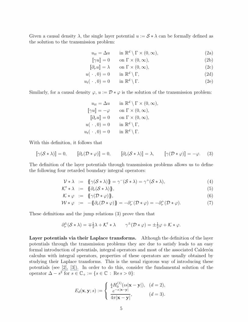
Given a causal density λ, the single layer potential u := S ∗ λ can be formally defined asthe solution to the transmission problem:

utt = ∆u in Rd \ Γ× (0,∞), (2a)

[[γu]] = 0 on Γ× (0,∞), (2b)

[[∂νu]] = λ on Γ× (0,∞), (2c)

u( · , 0) = 0 in Rd \ Γ, (2d)

ut( · , 0) = 0 in Rd \ Γ. (2e)

Similarly, for a causal density ϕ, u := D ∗ ϕ is the solution of the transmission problem:

utt = ∆u in Rd \ Γ× (0,∞),

[[γu]] = −ϕ on Γ× (0,∞),

[[∂νu]] = 0 on Γ× (0,∞),

u( · , 0) = 0 in Rd \ Γ,ut( · , 0) = 0 in Rd \ Γ.

With this definition, it follows that

[[γ(S ∗ λ)]] = 0, [[∂ν(D ∗ ϕ)]] = 0, [[∂ν(S ∗ λ)]] = λ, [[γ(D ∗ ϕ)]] = −ϕ. (3)

The definition of the layer potentials through transmission problems allows us to definethe following four retarded boundary integral operators:

V ∗ λ := γ(S ∗ λ) = γ−(S ∗ λ) = γ+(S ∗ λ), (4)

Kt ∗ λ := ∂ν(S ∗ λ), (5)

K ∗ ϕ := γ(D ∗ ϕ), (6)

W ∗ ϕ := −∂ν(D ∗ ϕ) = −∂−ν (D ∗ ϕ) = −∂+ν (D ∗ ϕ). (7)

These definitions and the jump relations (3) prove then that

∂±ν (S ∗ λ) = ∓12λ +Kt ∗ λ γ±(D ∗ ϕ) = ±1

2ϕ+K ∗ ϕ.

Layer potentials via their Laplace transforms. Although the definition of the layerpotentials through the transmission problems they are due to satisfy leads to an easyformal introduction of potentials, integral operators and most of the associated Calderoncalculus with integral operators, properties of these operators are usually obtained bystudying their Laplace transforms. This is the usual rigorous way of introducing thesepotentials (see [2], [3]). In order to do this, consider the fundamental solution of theoperator ∆− s2 for s ∈ C+ := s ∈ C : Re s > 0:

Ed(x,y; s) :=

ı4H

(1)0 (ıs|x− y|), (d = 2),

e−s |x−y|

4π|x− y| , (d = 3).

5

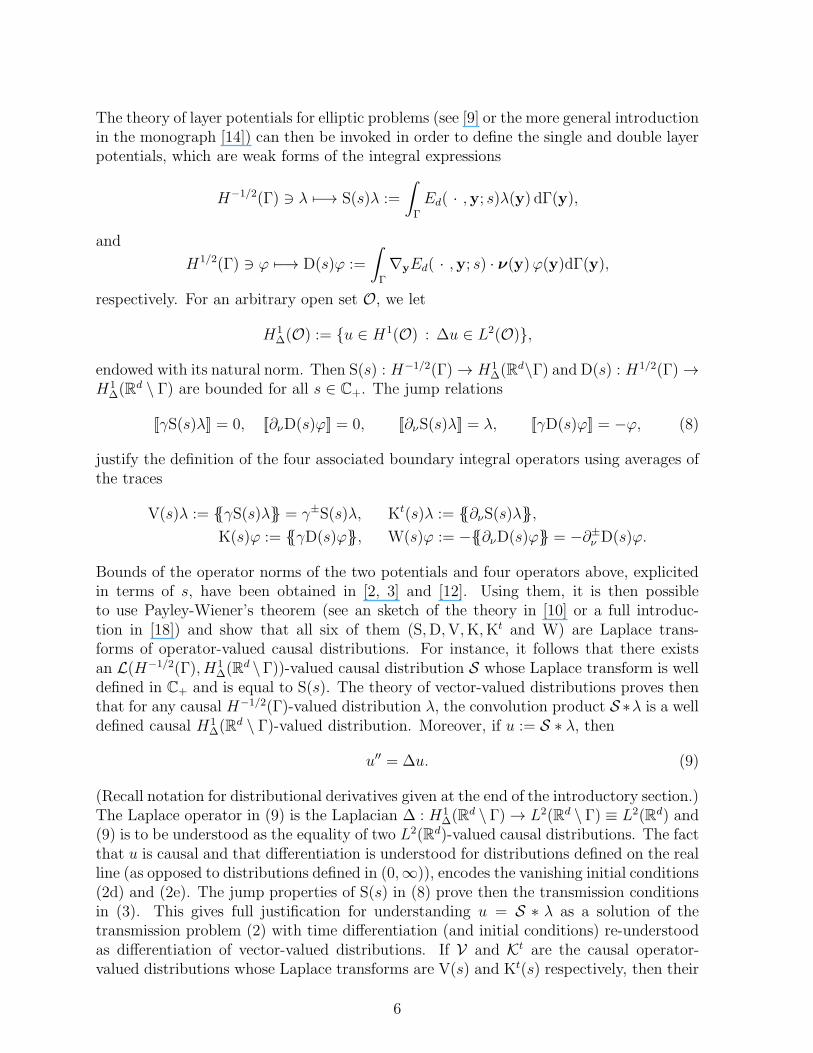
The theory of layer potentials for elliptic problems (see [9] or the more general introductionin the monograph [14]) can then be invoked in order to define the single and double layerpotentials, which are weak forms of the integral expressions

H−1/2(Γ) ∋ λ 7−→ S(s)λ :=

∫

Γ

Ed( · ,y; s)λ(y) dΓ(y),

and

H1/2(Γ) ∋ ϕ 7−→ D(s)ϕ :=

∫

Γ

∇yEd( · ,y; s) · ν(y)ϕ(y)dΓ(y),

respectively. For an arbitrary open set O, we let

H1∆(O) := u ∈ H1(O) : ∆u ∈ L2(O),

endowed with its natural norm. Then S(s) : H−1/2(Γ) → H1∆(R

d\Γ) and D(s) : H1/2(Γ) →H1

∆(Rd \ Γ) are bounded for all s ∈ C+. The jump relations

[[γS(s)λ]] = 0, [[∂νD(s)ϕ]] = 0, [[∂νS(s)λ]] = λ, [[γD(s)ϕ]] = −ϕ, (8)

justify the definition of the four associated boundary integral operators using averages ofthe traces

V(s)λ := γS(s)λ = γ±S(s)λ, Kt(s)λ := ∂νS(s)λ,K(s)ϕ := γD(s)ϕ, W(s)ϕ := −∂νD(s)ϕ = −∂±ν D(s)ϕ.

Bounds of the operator norms of the two potentials and four operators above, explicitedin terms of s, have been obtained in [2, 3] and [12]. Using them, it is then possibleto use Payley-Wiener’s theorem (see an sketch of the theory in [10] or a full introduc-tion in [18]) and show that all six of them (S,D,V,K,Kt and W) are Laplace trans-forms of operator-valued causal distributions. For instance, it follows that there existsan L(H−1/2(Γ), H1

∆(Rd \Γ))-valued causal distribution S whose Laplace transform is well

defined in C+ and is equal to S(s). The theory of vector-valued distributions proves thenthat for any causal H−1/2(Γ)-valued distribution λ, the convolution product S ∗λ is a welldefined causal H1

∆(Rd \ Γ)-valued distribution. Moreover, if u := S ∗ λ, then

u′′ = ∆u. (9)

(Recall notation for distributional derivatives given at the end of the introductory section.)The Laplace operator in (9) is the Laplacian ∆ : H1

∆(Rd \ Γ) → L2(Rd \ Γ) ≡ L2(Rd) and

(9) is to be understood as the equality of two L2(Rd)-valued causal distributions. The factthat u is causal and that differentiation is understood for distributions defined on the realline (as opposed to distributions defined in (0,∞)), encodes the vanishing initial conditions(2d) and (2e). The jump properties of S(s) in (8) prove then the transmission conditionsin (3). This gives full justification for understanding u = S ∗ λ as a solution of thetransmission problem (2) with time differentiation (and initial conditions) re-understoodas differentiation of vector-valued distributions. If V and Kt are the causal operator-valued distributions whose Laplace transforms are V(s) and Kt(s) respectively, then their

6

time convolutions with a given causal density λ satisfy the identities (4) and (5) thusidentifying the two possible definitions of the time domain integral operators associatedto the single layer potential.

The same considerations can be applied for a rigorous definition of the double layerpotential in the sense of convolutions of vector-valued distributions. Note that bothlayer potentials had been introduced directly (without using the Laplace transform) inthe three dimensional case in [11], with a theory that cannot be easily extended to thetwo-dimensional case.

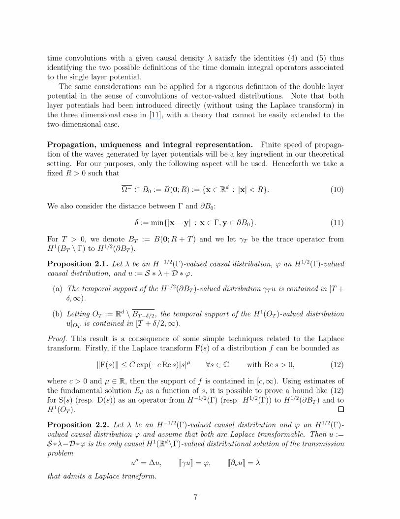
Propagation, uniqueness and integral representation. Finite speed of propaga-tion of the waves generated by layer potentials will be a key ingredient in our theoreticalsetting. For our purposes, only the following aspect will be used. Henceforth we take afixed R > 0 such that

Ω− ⊂ B0 := B(0;R) := x ∈ Rd : |x| < R. (10)

We also consider the distance between Γ and ∂B0:

δ := min|x− y| : x ∈ Γ,y ∈ ∂B0. (11)

For T > 0, we denote BT := B(0;R + T ) and we let γT be the trace operator fromH1(BT \ Γ) to H1/2(∂BT ).

Proposition 2.1. Let λ be an H−1/2(Γ)-valued causal distribution, ϕ an H1/2(Γ)-valuedcausal distribution, and u := S ∗ λ+D ∗ ϕ.

(a) The temporal support of the H1/2(∂BT )-valued distribution γTu is contained in [T +δ,∞).

(b) Letting OT := Rd \ BT−δ/2, the temporal support of the H1(OT )-valued distribution

u|OTis contained in [T + δ/2,∞).

Proof. This result is a consequence of some simple techniques related to the Laplacetransform. Firstly, if the Laplace transform F(s) of a distribution f can be bounded as

‖F(s)‖ ≤ C exp(−cRe s)|s|µ ∀s ∈ C with Re s > 0, (12)

where c > 0 and µ ∈ R, then the support of f is contained in [c,∞). Using estimates ofthe fundamental solution Ed as a function of s, it is possible to prove a bound like (12)for S(s) (resp. D(s)) as an operator from H−1/2(Γ) (resp. H1/2(Γ)) to H1/2(∂BT ) and toH1(OT ).

Proposition 2.2. Let λ be an H−1/2(Γ)-valued causal distribution and ϕ an H1/2(Γ)-valued causal distribution ϕ and assume that both are Laplace transformable. Then u :=S∗λ−D∗ϕ is the only causal H1(Rd\Γ)-valued distributional solution of the transmissionproblem

u′′ = ∆u, [[γu]] = ϕ, [[∂νu]] = λ

that admits a Laplace transform.

7

3 Main results

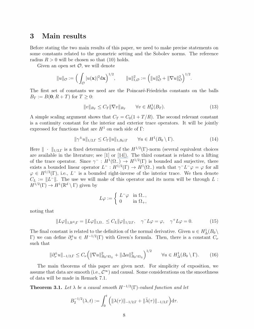
Before stating the two main results of this paper, we need to make precise statements onsome constants related to the geometric setting and the Sobolev norms. The referenceradius R > 0 will be chosen so that (10) holds.

Given an open set O, we will denote

‖u‖O :=(∫

O

|u(x)|2dx)1/2

, ‖u‖21,O :=(‖u‖2O + ‖∇u‖2O

)1/2

.

The first set of constants we need are the Poincare-Friedrichs constants on the ballsBT := B(0;R + T ) for T ≥ 0:

‖v‖BT≤ CT‖∇v‖BT

∀v ∈ H10 (BT ). (13)

A simple scaling argument shows that CT = C0(1 + T/R). The second relevant constantis a continuity constant for the interior and exterior trace operators. It will be jointlyexpressed for functions that are H1 on each side of Γ:

‖γ±u‖1/2,Γ ≤ CΓ‖u‖1,B0\Γ ∀u ∈ H1(B0 \ Γ). (14)

Here ‖ · ‖1/2,Γ is a fixed determination of the H1/2(Γ)-norm (several equivalent choicesare available in the literature; see [1] or [14]). The third constant is related to a liftingof the trace operator. Since γ− : H1(Ω−) → H1/2(Γ) is bounded and surjective, thereexists a bounded linear operator L− : H1/2(Γ) → H1(Ω−) such that γ−L−ϕ = ϕ for allϕ ∈ H1/2(Γ), i.e., L− is a bounded right-inverse of the interior trace. We then denoteCL := ‖L−‖. The use we will make of this operator and its norm will be through L :H1/2(Γ) → H1(Rd \ Γ) given by

Lϕ :=

L−ϕ in Ω−,0 in Ω+,

noting that

‖Lϕ‖1,Rd\Γ = ‖Lϕ‖1,Ω−≤ CL‖ϕ‖1/2,Γ, γ−Lϕ = ϕ, γ+Lϕ = 0. (15)

The final constant is related to the definition of the normal derivative. Given u ∈ H1∆(B0\

Γ) we can define ∂±ν u ∈ H−1/2(Γ) with Green’s formula. Then, there is a constant Cν

such that

‖∂±ν u‖−1/2,Γ ≤ Cν

(‖∇u‖2B0∩Ω±

+ ‖∆u‖2B0∩Ω±

)1/2

∀u ∈ H1∆(B0 \ Γ). (16)

The main theorems of this paper are given next. For simplicity of exposition, weassume that data are smooth (i.e., C∞) and causal. Some considerations on the smoothnessof data will be made in Remark 7.1.

Theorem 3.1. Let λ be a causal smooth H−1/2(Γ)-valued function and let

B−1/22 (λ, t) :=

∫ t

0

(‖λ(τ)‖−1/2,Γ + ‖λ(τ)‖−1/2,Γ

)dτ.

8

Then for all t ≥ 0

‖(S ∗ λ)(t)‖1,Rd ≤ CΓ

(‖λ(t)‖−1/2,Γ +

√1 + C2

t B−1/22 (λ, t)

), (17)

‖(V ∗ λ)(t)‖1/2,Γ ≤ C2Γ

(‖λ(t)‖−1/2,Γ +

√1 + C2

t B−1/22 (λ, t)

), (18)

‖(Kt ∗ λ)(t)‖−1/2,Γ ≤√2CνCΓ

(‖λ(t)‖−1/2,Γ +B

−1/22 (λ, t)

). (19)

Theorem 3.2. Let ϕ be a causal smooth H1/2(Γ)-valued function and let

B1/22 (ϕ, t) :=

∫ t

0

(‖ϕ(τ)‖1/2,Γ + ‖ϕ(τ)‖1/2,Γ

)dτ,

B1/24 (ϕ, t) :=

∫ t

0

(4‖ϕ(τ)‖1/2,Γ + 5‖ϕ(τ)‖1/2,Γ + ‖ϕ(4)(τ)‖1/2,Γ

)dτ.

Then for all t ≥ 0

‖(D ∗ ϕ)(t)‖1,Rd\Γ ≤ CL

(‖ϕ(t)‖1/2,Γ +

√1 + C2

t B1/22 (ϕ, t)

), (20)

‖(K ∗ ϕ)(t)‖1/2,Γ ≤ CΓCL

(‖ϕ(t)‖1/2,Γ +

√1 + C2

t B1/22 (ϕ, t)

), (21)

‖(W ∗ ϕ)(t)‖−1/2,Γ ≤√2CνCL

(4‖ϕ(t)‖1/2,Γ + 2‖ϕ(t)‖1/2,Γ +B

1/24 (ϕ, t)

). (22)

4 The single layer potential

Since the convolution operator λ 7→ S ∗ λ preserves causality, in order to obtain boundsat a given value of the time variable t = T , only the value of λ in (T,∞) is not relevant.Therefore, we can assume without loss of generality that the growth of λ allows it to havea Laplace transform. We can actually assume that λ is compactly supported for the sakeof the arguments that follow.

Introduction of a cut-off boundary. Let u := S ∗λ. By Proposition 2.2, u is a causaldistribution with values in X := H1(Rd)∩H1

∆(Rd \Γ). Moreover, it is the only (X-valued

causal distributional Laplace transformable) solution of

u′′ = ∆u and [[∂νu]] = λ, (23)

with the differential equation taking place in the sense of distributions with values inL2(Rd \Γ) ≡ L2(Rd), while the transmission condition is to be understood in the sense ofH−1/2(Γ)-valued distributions. Let now T > 0 be fixed and let BT and δ be as in Section2. We look for a causal distribution with values in

XT := H10 (BT ) ∩H1

∆(BT \ Γ)such that

u′′T = ∆uT and [[∂νuT ]] = λ. (24)

This differential equation is understandable in the sense of L2(BT )-valued distributions.We will show that for smooth data λ, this problem has strong solutions, with the timederivatives understood in the classical sense.

9

Proposition 4.1. As H1∆(BT \ Γ)-valued distributions, u = uT in (−∞, T + δ).

Proof. Consider the H1∆(BT \ Γ)-valued distribution w := u− uT = u|BT

− uT . Then

w′′ = ∆w, [[∂νw]] = 0, and γTw = γTu.

Since the support of γTu is contained in [T + δ,∞) (by Proposition 2.1), so is the supportof w, which proves the result.

Proposition 4.2. For causal λ ∈ C2(R;H−1/2(Γ)), the unique solution of (24) satisfies

uT ∈ C2([0,∞);L2(BT )) ∩ C1([0,∞);H10(BT )) ∩ C([0,∞);XT ), (25)

the strong initial conditions uT (0) = uT (0) = 0 and the bounds for all t ≥ 0

‖uT (t)‖1,BT≤ CΓ

(‖λ(t)‖−1/2,Γ +

√1 + C2

T B−1/22 (λ, t)

), (26)

‖∇uT (t)‖BT≤ CΓ

(‖λ(t)‖−1/2,Γ +B

−1/22 (λ, t)

), (27)

‖∆uT (t)‖BT \Γ ≤ CΓ

(‖λ(t)‖−1/2,Γ +B

−1/22 (λ, t)

). (28)

Proof. Consider first the function u0 : [0,∞) → H10 (BT ) defined by solving the steady-

state problems

−∆u0(t) + u0(t) = 0 in BT \ Γ, [[∂νu0(t)]] = λ(t), γTu0(t) = 0,

for t ≥ 0. The variational formulation of this family of boundary value problems is

[u0(t) ∈ H1

0 (BT ),

(∇u0(t),∇v)BT+ (u0(t), v)BT

= 〈λ(t), γv〉Γ ∀v ∈ H10 (BT ),

where 〈·, ·〉Γ is the H−1/2(Γ) × H1/2(Γ) duality product. Therefore, a simple argumentyields

‖u0(t)‖1,BT≤ CΓ‖λ(t)‖−1/2,Γ, ‖∆u0(t)‖BT \Γ ≤ CΓ‖λ(t)‖−1/2,Γ. (29)

Note that u0(t) is the result of applying a bounded linear (time-independent) mapH−1/2(Γ) →XT to λ(t). Therefore, since λ is twice continuously differentiable in [0,∞), it follows that

‖u0(t)‖1,BT≤ CΓ‖λ(t)‖−1/2,Γ, ‖∆u0(t)‖BT \Γ ≤ CΓ‖λ(t)‖−1/2,Γ. (30)

We next consider the function v0 : [0,∞) → H2(BT ) ∩H10 (BT ) that solves the evolution

problemv0(t) = ∆v0(t) + u0(t)− u0(t) t ≥ 0, v0(0) = v0(0) = 0, (31)

i.e., the hypotheses of Proposition 8.1 hold with f = u0 − u0. Therefore, using (29)-(30),it follows that

‖∆v0(t)‖BT≤

∫ t

0

‖∇u0(τ)−∇u0(τ)‖BTdτ ≤ CΓB

−1/22 (λ, t), (32)

10

as well as

‖v0(t)‖BT≤ CTCΓB

−1/22 (λ, t), ‖∇v0(t)‖BT

≤ CΓB−1/22 (λ, t). (33)

If we now define uT := u0 + v0, then the regularity requirement (25) is satisfied and thethree bounds in the statement of the proposition are direct consequences of (29), (32) and(33). Moreover,

uT (t) = ∆uT (t), [[∂νuT (t)]] = λ(t), γTuT (t) = 0 ∀t ≥ 0.

Note also that uT (0) = u0(0) = 0 and uT (0) = u0(0) = 0, since λ(0) = 0 and λ(0) = 0(λ : R → H−1/2(Γ) is assumed to be C2 and causal). Therefore, considering the extensionoperator (1) it follows that EuT is an XT -valued causal distribution, (EuT )

′′ = EuT =E∆uT = ∆EuT and [[∂νEuT ]] = E[[∂νuT ]] = Eλ|(0,∞) = λ. Therefore, EuT satisfies (24)and the proof is finished.

Proof of Theorem 3.1 By Proposition 2.1, the distribution u|Rd\BT−δ/2

vanishes in the

time interval (−∞, T + δ/2). Therefore, by Proposition 4.1, uT (t) = 0 in the annulardomain BT \ BT−δ/2 for all t ≤ T + δ/2. This makes the extension by zero of uT (t)to Rd \ BT an element of H1

∆(Rd \ Γ) for all t ≤ T + δ/2. (Note that the overlapping

annular region is needed to ensure that the Laplace operator does not generate a singulardistribution on ∂BT .) Then, the argument of Proposition 4.1 can be used to show thatthe distribution u can be identified with this extension in the time interval (−∞, T +δ/2).Therefore, identifying u(T ) = uT (T ), the inequalities of Proposition 4.2 yield

‖(S ∗ λ)(T )‖1,Rd ≤ CΓ

(‖λ(T )‖−1/2,Γ +

√1 + C2

T B−1/22 (λ, T )

), (34)

‖∇(S ∗ λ)(T )‖Rd ≤ CΓ

(‖λ(T )‖−1/2,Γ +B

−1/22 (λ, T )

), (35)

‖∆(S ∗ λ)(T )‖Rd\Γ ≤ CΓ

(‖λ(T )‖−1/2,Γ +B

−1/22 (λ, T )

). (36)

We can now substitute all occurrences of T by t, since T was arbitrary. The result is nowalmost straightforward. First of all, (34) is just (17). Also, by the trace inequality (14)and the fact that V ∗ λ = γ±(S ∗ λ), (18) is a direct consequence of (17). Finally, thebound for the normal derivative (16), the fact that Kt ∗λ = ∂ν(S ∗λ), and inequalities(35)-(36) prove (19).

5 The double layer potential

We start by introducing a cut-off boundary ∂BT as in Section 4 (for arbitrary T > 0).We are going to compare u := D ∗ ϕ with the causal distribution uT with values in

YT := v ∈ H1∆(BT \ Γ) : γTu = 0,

such thatu′′T = ∆uT , [[γuT ]] = −ϕ and [[∂νuT ]] = 0. (37)

11

The same argument as the one of Proposition 4.1 shows that, as H1∆(BT \ Γ)-valued

distributions u = uT in (−∞, T + δ), where δ is defined in (11). Smoothness of thesolution of (37) and bounds for it in different norms will be proved in two steps. Notethat, from the point of view of regularity Proposition 5.2 improves the initial estimate ofProposition 5.1, but that more regularity of ϕ is used in the process.

Proposition 5.1. For causal ϕ ∈ C2(R;H1/2(Γ)), the unique solution of (37) satisfies

uT ∈ C1([0,∞);L2(BT )) ∩ C([0,∞);H1(BT \ Γ)), (38)

the strong initial conditions uT (0) = uT (0) = 0 and the bounds for all t ≥ 0

‖uT (t)‖1,BT \Γ ≤ CL

(‖ϕ(t)‖1/2,Γ +

√1 + C2

T B1/22 (ϕ, t)

), (39)

‖∇uT (t)‖BT \Γ ≤ CL

(‖ϕ(t)‖1/2,Γ +B

1/22 (ϕ, t)

). (40)

Proof. Let first u0 : [0,∞) → H1(BT \ Γ) be given by solving the steady-state problems

−∆u0(t) + u0(t) = 0 in BT \ Γ, [[γu0(t)]] = −ϕ(t), (41a)

γTu0(t) = 0, [[∂νu0(t)]] = 0, (41b)

for each t ≥ 0. The variational formulation of (41) is

u0(t) ∈ H1(BT \ Γ),[[γu0(t)]] = −ϕ(t), γTu0(t) = 0,

(∇u0(t),∇v)BT \Γ + (u0(t), v)BT= 0 ∀v ∈ H1

0 (BT ).

(42)

Using the lifting operator (15), we can choose the test v = u0(t) + Lϕ(t) ∈ H10 (BT ) in

(42), and prove the estimate

‖u0(t)‖1,BT \Γ ≤ ‖Lϕ(t)‖1,BT \Γ ≤ CL‖ϕ(t)‖1/2,Γ. (43)

Since u0(t) is the result of applying a linear bounded (time-independent) map H1/2(Γ) →YT to ϕ(t), it follows that

‖u0(t)‖1,BT \Γ ≤ CL‖ϕ(t)‖1/2,Γ. (44)

We then consider v0 : [0,∞) → H10 (BT ) to be a solution of

v0(t) = ∆v0(t) + u0(t)− u0(t) t ≥ 0, v0(0) = v0(0) = 0, (45)

with the equation taking place inH−1(BT ) (that is, v0 is a weak solution in the terminologyof Section 8). By Proposition 8.2 (the right-hand side f := u0 − u0 : [0,∞) → L2(BT ) iscontinuous) we can bound

‖∇v0(t)‖BT≤

∫ t

0

‖u0(τ)− u0(τ)‖BTdτ ≤ CLB

1/22 (ϕ, t), (46)

12

where we have applied (43)-(44).Let us then define uT := u0 + v0. Since ϕ ∈ C2([0,∞);H1/2(Γ)), it follows that u0 ∈

C2([0,∞);H1(BT \ Γ)) and v0 ∈ C1([0,∞);L2(BT )) ∩ C([0,∞);H10(BT )) by Proposition

8.2. Therefore, uT satisfies (38). Since ϕ(0) = ϕ(0) = 0, it follows that uT (0) = uT (0) = 0.Considering (41) and (45) (recall that v0 takes values in H1

0 (BT )), it follows that

uT (t) = ∆uT (t), [[γuT (t)]] = −ϕ(t), [[∂νuT (t)]] = 0, γTuT = 0, ∀t ≥ 0.

Noting that ‖v0(t)‖BT≤ CT‖∇v0(t)‖BT

, and using (43), (44), and (46), it follows that uTsatisfies the bounds (39) and (40).

The delicate point of this proof lies in showing that uT can be identified with theYT -valued distributional solution of (37), since v0 is not a continuous YT -valued function.However, w0(t) :=

∫ t

0v0(τ)dτ is a continuous function with values in H2(BT ) ∩ H1

0 (BT )(see Proposition 8.2) and therefore in YT . We can then define uT := Eu0 + (Ew0)

′, whichis a causal YT -valued distribution for which we can easily prove that

[[γuT ]] = E[[γu0]] + (E[[γw0]])′ = −Eϕ|(0,∞) = −ϕ

and similarly [[∂ν uT ]] = 0. Since w0 ∈ C2([0,∞);L2(BT )) ∩ C([0,∞); YT ), and w0(0) =w0(0) = 0, it follows that (Ew0)

′′ = Ew0 = E∆w0 = ∆Ew0 and therefore u′′T = (Eu0)′′ +

(E∆w0)′ = ∆Eu0 + ∆(Ew0)

′ = ∆uT . Thus, uT satisfies (37). Finally, since w0 ∈C1([0,∞);H1

0(BT )) and w0(0) = 0, it is clear that, as an H10(BT )-valued distribution

(Ew0)′ = Ew0 = Ev0 and thus, as an H1(BT \ Γ)-valued distribution uT = EuT , and the

bounds (39) and (40) are satisfied by the solution of (37).

Proposition 5.2. For causal ϕ ∈ C4(R;H1/2(Γ)), the unique solution of (37) satisfies

uT ∈ C2([0,∞);L2(BT )) ∩ C1([0,∞);H1(BT \ Γ)) ∩ C([0,∞); YT )) (47)

and the bounds for all t ≥ 0

‖∆uT (t)‖BT \Γ ≤ CL

(4‖ϕ(t)‖1/2,Γ + 2‖ϕ(t)‖1/2,Γ +B

1/24 (ϕ, t)

). (48)

Proof. Consider now the solution of the problems

−∆u1(t) + u1(t) = L(ϕ(t)− ϕ(t)) in BT \ Γ, [[γu1(t)]] = −ϕ(t), (49a)

γTu1(t) = 0, [[∂νu1(t)]] = 0, (49b)

for each t ≥ 0, where L is the lifting operator of (15). Using the variational formulationof (49) and the fact that u1(t) + Lϕ(t) ∈ H1

0 (BT ), it follows that

‖u1(t)+Lϕ(t)‖1,BT \Γ ≤ ‖Lϕ(t)‖1,BT \Γ+‖L(ϕ(t)−ϕ(t))‖BT≤ CL(2‖ϕ(t)‖1/2,Γ+‖ϕ(t)‖1/2,Γ)

and therefore‖u1(t)‖1,BT \Γ ≤ CL(3‖ϕ(t)‖1/2,Γ + ‖ϕ(t)‖1/2,Γ). (50)

Using (49) and (50) it also follows that

‖∆u1(t)‖BT≤ ‖u1(t)‖BT

+ ‖L(ϕ(t)− ϕ(t))‖BT≤ CL(4‖ϕ(t)‖1/2,Γ + 2‖ϕ(t)‖1/2,Γ). (51)

13

Differentiating (50) twice with respect to t, it follows that

‖u1(t)‖1,BT \Γ ≤ CL(3‖ϕ(t)‖1/2,Γ + ‖ϕ(4)(t)‖1/2,Γ). (52)

Consider next the evolution equation that looks for v1 : [0,∞) → YT such that

v1 = ∆v1(t) + f(t) ∀t ≥ 0, v1(0) = v1(0) = 0, (53)

wheref(t) := u1(t)− u1(t) + L(ϕ(t)− ϕ(t)) = ∆u1(t)− u1(t).

Note that [[γf(t)]] = 0 for all t, and that f : [0,∞) → H10(BT ) is continuous. Moreover,

by (50) and (52), we can bound

‖∇f(t)‖BT≤ ‖f(t)‖1,BT

≤ CL

(4‖ϕ(t)‖1/2,Γ + 5‖ϕ(t)‖1/2,Γ + ‖ϕ(4)(t)‖1/2,Γ

). (54)

By Proposition 8.1, problem (53) has a unique (strong) solution and we can bound

‖∆v1(t)‖BT≤

∫ t

0

‖∇f(τ)‖BTdτ ≤ CLB4(ϕ, t). (55)

If we finally define uT := u1+v1, the smoothness of u1 : [0,∞) → YT (directly inheritedfrom that of ϕ) and the regularity of v1 that is derived from Proposition 8.1 prove that(47) holds. The bound (48) is a direct consequence of (51) and (53). The fact that theextension EuT is the YT -valued causal distributional solution of (37) can be proved withthe same kind of arguments that were used at the end of the proof of Propositions 4.2.

Proof of Theorem 3.2. With exactly the same arguments that allowed to prove (34),(35) and (36) as a consequence of Proposition 4.2, we can prove that for all t ≥ 0

‖(D ∗ ϕ)(t)‖1,Rd\Γ ≤ CL

(‖ϕ(t)‖1/2,Γ +

√1 + C2

t B1/22 (ϕ, t)

), (56)

‖∇(D ∗ ϕ)(t)‖Rd\Γ ≤ CL

(‖ϕ(t)‖1/2,Γ +B

1/22 (ϕ, t)

), (57)

‖∆(D ∗ ϕ)(t)‖Rd\Γ ≤ CL

(4‖ϕ(t)‖1/2,Γ + 2‖ϕ(t)‖1/2,Γ +B

1/24 (ϕ, t)

), (58)

as a consequence of Propositions 5.1 and 5.2. The bounds of Theorem 3.2 are nowstraightforward. Inequality (20) is just (56), while the fact that K ∗ ϕ = γ(D ∗ ϕ) andthe trace inequality (14) prove (20). Finally the bound for the normal derivative (16),the definition of W ∗ ϕ = −∂±ν (D ∗ ϕ) and inequalities (57)-(58) prove (22).

6 Exterior Steklov-Poincare operators

In this section we include bounds on the exterior Dirichlet-to-Neumann and Neumann-to-Dirichlet operators that can be obtained with the same techniques than in the previous sec-tions. We give some details for the easier case (the Neumann-to-Dirichlet operator,whose

14

treatment runs in parallel to that of the single layer retarded potential) in order to em-phasize the need of dealing with some slightly different evolution problems as part of theanalysis process.

Let us consider the bounded open set B+T := BT ∩ Ω+ and the space

VT := u ∈ H1(B+T ) : γTu = 0. (59)

We can then consider the associated Poincare-Friedrichs inequality

‖u‖B+

T≤ ET‖∇u‖B+

T∀u ∈ VT . (60)

Recalling that BT is a ball with radius R+T , it is possible to take ET ≤ 2(R+T ) (see [7,Chapter II, Section 1]). Since the exterior trace operator γ+ : V0 → H1/2(Γ) is surjective,

it has a bounded right-inverse. By extending this right-inverse by zero to Ω+ \B+0 we can

construct L+ : H1/2(Γ) → H1(Ω+) satisfying

‖L+ϕ‖1,Ω+= ‖L+ϕ‖1,B+

T≤ C+

L ‖ϕ‖1/2,Γ, γ+L+ϕ = ϕ ∀ϕ ∈ H1/2(Γ). (61)

Note that, in particular, γTL+ϕ = 0 for all T ≥ 0 and all ϕ.

Theorem 6.1. For causal λ ∈ C2(R;H−1/2(Γ)), the unique causal H1∆(Ω+)-valued Laplace

transformable distribution such that

u′′ = ∆u, ∂+ν u = λ, (62)

satisfies the bounds

‖u(t)‖1,Ω+≤ CΓ

(‖λ(t)‖−1/2,Γ +

√1 + E2

T B−1/22 (λ, t)

)∀t ≥ 0. (63)

Finally the associated Neumann-to-Dirichlet operator NtD(λ) := γ+u (where u is thesolution of (62)) satisfies the bounds

‖NtD(λ)(t)‖1/2,Γ ≤ C2Γ

(‖λ(t)‖−1/2,Γ +

√1 + E2

T B−1/22 (λ, t)

)∀t ≥ 0. (64)

Proof. The proof is very similar to the one of Theorem 3.1. By solving steady stateproblems, we first construct u0 : [0,∞) → H1(B+

T ) satisfying

−∆u0(t) + u0(t) = 0 in B+T , ∂+ν u0(t) = λ(t), γTu0(t) = 0. (65)

A simple argument allows us to bound

‖u0(t)‖1,B+

T≤ CΓ‖λ(t)‖−1/2,Γ and ‖u0(t)‖1,B+

T≤ CΓ‖λ(t)‖−1/2,Γ. (66)

This function feeds the evolution equation looking for v0 : [0,∞) → DT (the set DT isdefined in (79)) that satisfies

v0(t) = ∆v0(t) + u0(t)− u0(t) t ≥ 0, v0(t) = v0(t) = 0. (67)

15

We now apply the general result on the wave equation with mixed boundary conditions(Proposition 8.3) that guarantees the existence of a strong solution of (67) satisfying thebounds

‖v0(t)‖B+

T≤ ETCΓB

−1/22 (λ, t), ‖∇v0(t)‖B+

T≤ CΓB

−1/22 (λ, t). (68)

Adding the solutions of (65) and (67) we obtain a function uT := u0 + v0 : [0,∞) →H1

∆(B+T ) ∩ VT satisfying u(t) = ∆u(t), ∂νuT (t) = λ(t) and vanishing initial conditions

at t = 0. The extension EuT is then an (H1∆(B

+T ) ∩ VT )-valued causal distributional

solution of (62) (with the Laplace operator acting only in the bounded domain B+T ).

The arguments of Proposition 4.1 and at the beginning of the proof of Theorem 3.1 canbe applied verbatim in order to identify the function that extends uT (t) by zero to theexterior of BT with the H1

∆(Ω+)-valued distributional solution of (62) for t ≤ T + δ/2.Finally, the bound (63) for t = T is a straightforward consequence of (66), (68), andthe identification of u(T ) = uT (T ), while (64) follows from (63) and the trace inequality(14).

Theorem 6.2. For causal ϕ ∈ C4(R;H1/2(Γ)), the unique causal H1∆(Ω+)-valued Laplace

transformable distribution such that

u′′ = ∆u, γ+u = ϕ, (69)

satisfies the bounds

‖u(t)‖1,Ω+≤ C+

L

(‖ϕ(t)‖1/2,Γ +

√1 + E2

T B1/22 (ϕ, t)

)∀t ≥ 0. (70)

Finally the associated Dirichlet-to-Neumann operator DtN(ϕ) := ∂+ν u (where u is thesolution of (69)) satisfies the bounds

‖DtN(ϕ)(t)‖−1/2,Γ ≤√2CνC

+L

(4‖ϕ(t)‖1/2,Γ + 2‖ϕ(t)‖1/2,Γ +B

1/24 (ϕ, t)

). (71)

Proof. This result can be proved like Theorem 3.2 by resorting to a double decompositionof a localized version of problem (69) (obtained by adding a boundary condition γTu = 0)as a sum of an adequate steady-state lifting of the Dirichlet data plus the solution ofan evolution problem. The proof is almost identical to that of Theorem 3.2: the maindifference is in the evolution problem, that now contains Dirichlet boundary conditionson Γ as well as on ∂BT (see Remark 8.1).

7 Comparison with Laplace domain bounds

The original analysis for the layer operators and associated integral equations, given in[2] and [3], was entirely developed in the resolvent set (that is, by taking the Laplacetransform). Those results can be used to derive uniform bounds similar to those ofTheorems 3.1 and 3.2. We next show how to obtain these estimates and show that ourtechnique produces stronger estimates, in terms of requiring less regularity of the densitiesand having constants that increase less fast with respect to t.

16

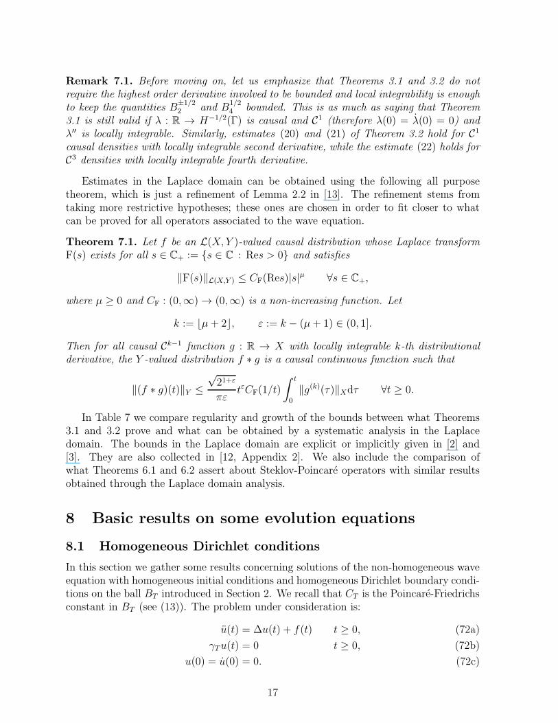
Remark 7.1. Before moving on, let us emphasize that Theorems 3.1 and 3.2 do notrequire the highest order derivative involved to be bounded and local integrability is enoughto keep the quantities B

±1/22 and B

1/24 bounded. This is as much as saying that Theorem

3.1 is still valid if λ : R → H−1/2(Γ) is causal and C1 (therefore λ(0) = λ(0) = 0) andλ′′ is locally integrable. Similarly, estimates (20) and (21) of Theorem 3.2 hold for C1

causal densities with locally integrable second derivative, while the estimate (22) holds forC3 densities with locally integrable fourth derivative.

Estimates in the Laplace domain can be obtained using the following all purposetheorem, which is just a refinement of Lemma 2.2 in [13]. The refinement stems fromtaking more restrictive hypotheses; these ones are chosen in order to fit closer to whatcan be proved for all operators associated to the wave equation.

Theorem 7.1. Let f be an L(X, Y )-valued causal distribution whose Laplace transformF(s) exists for all s ∈ C+ := s ∈ C : Res > 0 and satisfies

‖F(s)‖L(X,Y ) ≤ CF(Res)|s|µ ∀s ∈ C+,

where µ ≥ 0 and CF : (0,∞) → (0,∞) is a non-increasing function. Let

k := ⌊µ+ 2⌋, ε := k − (µ+ 1) ∈ (0, 1].

Then for all causal Ck−1 function g : R → X with locally integrable k-th distributionalderivative, the Y -valued distribution f ∗ g is a causal continuous function such that

‖(f ∗ g)(t)‖Y ≤√21+ε

πεtεCF(1/t)

∫ t

0

‖g(k)(τ)‖Xdτ ∀t ≥ 0.

In Table 7 we compare regularity and growth of the bounds between what Theorems3.1 and 3.2 prove and what can be obtained by a systematic analysis in the Laplacedomain. The bounds in the Laplace domain are explicit or implicitly given in [2] and[3]. They are also collected in [12, Appendix 2]. We also include the comparison ofwhat Theorems 6.1 and 6.2 assert about Steklov-Poincare operators with similar resultsobtained through the Laplace domain analysis.

8 Basic results on some evolution equations

8.1 Homogeneous Dirichlet conditions

In this section we gather some results concerning solutions of the non-homogeneous waveequation with homogeneous initial conditions and homogeneous Dirichlet boundary condi-tions on the ball BT introduced in Section 2. We recall that CT is the Poincare-Friedrichsconstant in BT (see (13)). The problem under consideration is:

u(t) = ∆u(t) + f(t) t ≥ 0, (72a)

γTu(t) = 0 t ≥ 0, (72b)

u(0) = u(0) = 0. (72c)

17

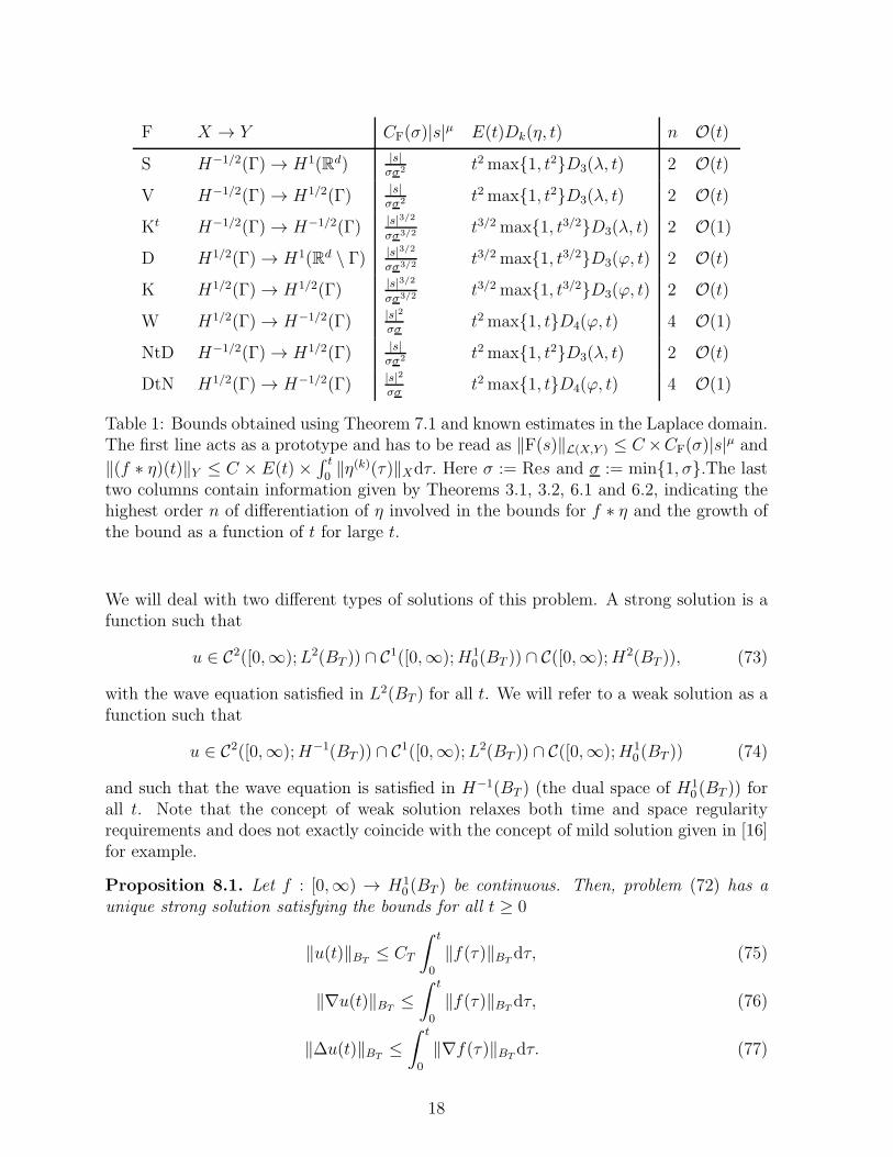
F X → Y CF(σ)|s|µ E(t)Dk(η, t) n O(t)

S H−1/2(Γ) → H1(Rd) |s|σσ2 t2max1, t2D3(λ, t) 2 O(t)

V H−1/2(Γ) → H1/2(Γ) |s|σσ2 t2max1, t2D3(λ, t) 2 O(t)

Kt H−1/2(Γ) → H−1/2(Γ) |s|3/2

σσ3/2 t3/2 max1, t3/2D3(λ, t) 2 O(1)

D H1/2(Γ) → H1(Rd \ Γ) |s|3/2

σσ3/2 t3/2 max1, t3/2D3(ϕ, t) 2 O(t)

K H1/2(Γ) → H1/2(Γ) |s|3/2

σσ3/2 t3/2 max1, t3/2D3(ϕ, t) 2 O(t)

W H1/2(Γ) → H−1/2(Γ) |s|2

σσt2max1, tD4(ϕ, t) 4 O(1)

NtD H−1/2(Γ) → H1/2(Γ) |s|σσ2 t2max1, t2D3(λ, t) 2 O(t)

DtN H1/2(Γ) → H−1/2(Γ) |s|2

σσt2max1, tD4(ϕ, t) 4 O(1)

Table 1: Bounds obtained using Theorem 7.1 and known estimates in the Laplace domain.The first line acts as a prototype and has to be read as ‖F(s)‖L(X,Y ) ≤ C ×CF(σ)|s|µ and

‖(f ∗ η)(t)‖Y ≤ C × E(t)×∫ t

0‖η(k)(τ)‖Xdτ. Here σ := Res and σ := min1, σ.The last

two columns contain information given by Theorems 3.1, 3.2, 6.1 and 6.2, indicating thehighest order n of differentiation of η involved in the bounds for f ∗ η and the growth ofthe bound as a function of t for large t.

We will deal with two different types of solutions of this problem. A strong solution is afunction such that

u ∈ C2([0,∞);L2(BT )) ∩ C1([0,∞);H10(BT )) ∩ C([0,∞);H2(BT )), (73)

with the wave equation satisfied in L2(BT ) for all t. We will refer to a weak solution as afunction such that

u ∈ C2([0,∞);H−1(BT )) ∩ C1([0,∞);L2(BT )) ∩ C([0,∞);H10(BT )) (74)

and such that the wave equation is satisfied in H−1(BT ) (the dual space of H10 (BT )) for

all t. Note that the concept of weak solution relaxes both time and space regularityrequirements and does not exactly coincide with the concept of mild solution given in [16]for example.

Proposition 8.1. Let f : [0,∞) → H10 (BT ) be continuous. Then, problem (72) has a

unique strong solution satisfying the bounds for all t ≥ 0

‖u(t)‖BT≤ CT

∫ t

0

‖f(τ)‖BTdτ, (75)

‖∇u(t)‖BT≤

∫ t

0

‖f(τ)‖BTdτ, (76)

‖∆u(t)‖BT≤

∫ t

0

‖∇f(τ)‖BTdτ. (77)

18

Proposition 8.2. Let f : [0,∞) → L2(BT ) be continuous. Then problem (72) has aunique weak solution, and the bound (76) is still valid. Finally, the function w(t) :=∫ t

0u(τ)dτ is continuous from [0,∞) to H2(BT ).

Remark 8.1. Propositions 8.1 and 8.2 still hold for the Dirichlet problem in the domainB+

T := BT ∩ Ω+ with the following modifications: the space H2(BT ) has to be substitutedby H1

∆(B+T ), and the constant CT in (75) has to be substituted by the constant ET of the

Poincare-Friedrichs inequality (60).

8.2 Mixed conditions

Let us now consider the set B+T := BT ∩ Ω+ and the evolution problem

u(t) = ∆u(t) + f(t) t ≥ 0, (78a)

γTu(t) = 0 t ≥ 0, (78b)

∂+ν u(t) = 0 t ≥ 0, (78c)

u(0) = u(0) = 0. (78d)

We thus consider the spaces VT given in (59) and

DT := u ∈ VT : ∆u ∈ L2(B+T ), ∂+ν u = 0 (79)

= u ∈ VT ∩H1∆(B

+T ) : (∇u,∇v)Ω+

+ (u, v)Ω+= 0 ∀v ∈ VT.

Proposition 8.3. For f ∈ C([0,∞);VT ), the initial value problem (78) has a uniquesolution

u ∈ C2([0,∞);L2(Ω)) ∩ C1([0,∞);VT ) ∩ C([0,∞);DT ),

satisfying

‖u(t)‖B+

T≤ CT

∫ t

0

‖f(τ)‖B+

Tdτ, (80)

‖∇u(t)‖B+

T≤

∫ t

0

‖f(τ)‖B+

Tdτ, (81)

‖∆u(t)‖B+

T≤

∫ t

0

‖∇f(τ)‖B+

Tdτ. (82)

If f ∈ C([0,∞);L2(Ω)) there exists a unique weak solution of (78) (that is, with theequation satisfied in V ′

T )

u ∈ C2([0,∞);V ′T ) ∩ C1([0,∞);L2(Ω)) ∩ C([0,∞);VT ),

satisfying (81) and such that w(t) :=∫ t

0u(τ)dτ is in C([0,∞);DT ).

19

A Wave equations by separation of variables

In this section we are going to give a direct proof of a generalization Propositions 8.1and 8.2. This proof will be based on direct arguments with generalized Fourier seriesand will allows us to obtain the needed uniform estimates of non-homogeneous evolutionequation of the second order in terms of L1 norms of the data. The Hilbert structure ofthe functional spaces is going to be used in depth, allowing us to obtain strong resultsthat cannot be easily derived with a direct application of the best known results on thetheory of semigroups of operators. This is not to say that these results do no exist, butwe think it can be of interest (especially within the boundary integral community) to seea direct proof of these theorems based on functional analysis tools that are common forresearchers integral equations.

A.1 Three lemmas about series

In all the following results X is a separable Hilbert space and I := [a, b] is a compactinterval.

Lemma A.1. Assume that cn : I → X are continuous,

(cn(t), cm(t))X = 0 ∀n 6= m, ∀t ∈ I, (83)

and

‖cn(t)‖2X ≤Mn ∀t ∈ I, ∀n with∞∑

n=1

Mn <∞.

Then the series

c(t) :=

∞∑

n=1

cn(t) (84)

converges uniformly in t to a continuous function.

Proof. Let sN :=∑N

n=1 cn ∈ C(I;X). For all M > N ,

‖sM(t)− sN (t)‖2X =M∑

n=N+1

‖cn(t)‖2X ≤M∑

n=N+1

Mn,

which proves that sN(t) converges uniformly. Continuity of the limit is a direct conse-quence of the uniform convergence of the series.

Lemma A.2. Assume that cn : I → X are continuously differentiable,

(cn(t), cm(τ))X = 0 ∀n 6= m, ∀t, τ ∈ I, (85)

and

‖cn(t)‖2X + ‖cn(t)‖2X ≤Mn ∀t ∈ I, ∀n with∞∑

n=1

Mn <∞.

Then the uniformly convergent series (84) defines a C1(I;X) function and it can be dif-ferentiated term by term.

20

Proof. The hypothesis (85) implies (83) as well as

(cn(t), cm(t))X = 0 ∀n 6= m, ∀t ∈ I.

If sN :=∑N

n=1 cn ∈ C1(I;X), then

‖sM(t)− sN(t)‖2X + ‖sM(t)− sN(t)‖2X =

M∑

n=N+1

‖cn(t)‖2X ≤M∑

n=N+1

Mn,

and therefore sN is Cauchy in C1(I;X) and thus convergent. The fact that the derivativesof the series converges to the series of the derivatives is part of what convergence inC1(I;X) means.

Lemma A.3. Let f : I → X be a continuous function and let φn be a Hilbert basis ofX. Then

f(t) =∞∑

n=1

(f(t), φn)Xφn

uniformly in t ∈ I.

Proof. Note first that for fixed t, f(t) ∈ X can be expanded in the Hilbert basis, soconvergence of the series is easy to prove. Next, consider the square of the norms of theN -th partial sums

aN(t) :=∥∥∥

N∑

n=1

(f(t), φn)Xφn

∥∥∥2

X=

N∑

n=1

|(f(t), φn)X |2,

which are continuous functions of t. The pointwise limit is ‖f(t)‖2X , which is also a contin-uous function of t. Since the sequence aN is increasing, by Dini’s Theorem, convergenceaN → ‖f( · )‖2X is uniform. Finally

∥∥∥f(t)−N∑

n=1

(f(t), φn)Xφn

∥∥∥2

X=

∞∑

n=N+1

|(f(t), φn)X |2 = ‖f(t)‖2X − aN(t),

which proves the uniform convergence of the series.

A.2 The Dirichlet spectral series of the Laplace operator

Let Ω be a Lipschitz domain and consider the sequence of Dirichlet eigenvalues andeigenfunctions of the Laplace operator:

φn ∈ H10 (Ω) −∆φn = λnφn.

The sequence is taken with non-decreasing values of λn and assuming (φn, φm)Ω = δnm,for all m,n, i.e., L2(Ω)-orthonormality of eigenfunctions. Thus, φn is a Hilbert basis ofL2(Ω) and consequently, for all u ∈ L2(Ω)

‖u‖2Ω =∞∑

n=1

|(u, φn)Ω|2 (86)

21

and

u =∞∑

n=1

(u, φn)Ωφn, (87)

with convergence in L2(Ω). Using the orthogonality (∇φn,∇φm)Ω = δnmλn, we can provethat

H10 (Ω) =

u ∈ L2(Ω) :

∞∑

n=1

λn|(u, φn)Ω|2 <∞

and

‖∇u‖2Ω =

∞∑

n=1

λn|(u, φn)Ω|2 ∀u ∈ H10 (Ω). (88)

This expression gives a direct estimate of the corresponding Poincare-Friedrichs inequalityas

‖u‖Ω ≤ 1√minλn

‖∇u‖Ω =: C‖∇u‖Ω ∀u ∈ H10 (Ω).

Moreover, if u ∈ H10 (Ω), the series representation (86) converges in H1

0 (Ω).

The associated Green operator is the operator G : L2(Ω) → D(∆) given by

u := Gf solution of u ∈ H10 (Ω), −∆u = f in Ω.

Here D(∆) := u ∈ H10 (Ω) : ∆u ∈ L2(Ω). Note that for the case of a smooth domain

D(∆) = H10 (Ω) ∩ H2(Ω), although this fact will not be used in the sequel. The space

D(∆) is endowed with the norm ‖∆ · ‖Ω. The series representation of G is given by theexpression

Gf =∞∑

n=1

λ−1n (f, φn)Ωφn

(with convergence in L2(Ω)). Picard’s Criterion can then be used to show that G issurjective and

D(∆) =u ∈ L2(Ω) :

∞∑

n=1

λ2n|(u, φn)Ω|2.

Two more series representations are then directly available, one for the Laplacian

−∆u =

∞∑

n=1

λn(u, φn)Ωφn ∀u ∈ D(∆),

(with convergence in L2(Ω)) and another one for its norm

‖∆u‖2Ω =∞∑

n=1

λ2n|(u, φn)Ω|2 ∀u ∈ D(∆). (89)

22

A.3 Strong solutions of the wave equation

We start the section with a reminder of one of the possible versions of Duhamel’s principlethat will be useful in the sequel. Its proof is straightforward.

Lemma A.4. Let g : [0,∞) → R be a continuous function, ω > 0 and define

α(t) :=

∫ t

0

ω−1 sin(ω(t− τ))g(τ)dτ.

Then α ∈ C2([0,∞), α(0) = α(0) = 0,

α(t) =

∫ t

0

cos(ω(t− τ))g(τ)dτ

and α(t) + ω2α(t) = g(t) for all t ≥ 0.

For notational convenience, we will write ξn :=√λn.

Proposition A.5. Let f : [0,∞) → H10 (Ω) be a continuous function and consider the

sequence

un(t) :=

(∫ t

0

ξ−1n sin

(ξn(t− τ)

)(f(τ), φn)Ωdτ

)φn, n ≥ 1.

Then, the function

u(t) :=∞∑

n=1

un(t) (90)

satisfiesu ∈ C2([0,∞);L2(Ω)) ∩ C1([0,∞);H1

0(Ω)) ∩ C([0,∞);D(∆)). (91)

Moreover, u is the unique strong solution of the following evolution equation:

u(t) = ∆u(t) + f(t) ∀t ≥ 0, u(0) = u(0) = 0. (92)

Proof. As a direct consequence of Lemma A.4, it follows that un ∈ C2([0,∞);X), whereX is any of L2(Ω), H1

0 (Ω) or D(∆). Also, for all t ≥ 0

un(t) =

(∫ t

0

cos(ξn(t− τ)

)(f(τ), φn)Ωdτ

)φn,

un(t) = (f(t), φn)Ωφn − λnun(t) = (f(t), φn)Ωφn +∆un(t),

and(un(t), um(τ))Ω = (∇un(t),∇um(τ))Ω = 0 ∀n 6= m, ∀t, τ ≥ 0. (93)

By (89), it follows that for t ∈ [0, T ],

‖∆un(t)‖2Ω = λ2n

∣∣∣∣∫ t

0

ξ−1n sin

(ξn(t− τ)

)(f(τ), φn)Ωdτ

∣∣∣∣2

≤ λnt

∫ t

0

|(f(τ), φn)Ω|2dτ ≤ T

∫ T

0

λn|(f(τ), φn)Ω|2dτ =:M (1)n .

23

By the Monotone Convergence Theorem and (88), we easily show that

∞∑

n=1

M (1)n = T

∫ T

0

( ∞∑

n=1

λn|(f(τ), φn)Ω|2)dτ = T

∫ T

0

‖∇f(τ)‖2Ωdτ.

Thanks to these bounds and (93) (recall that ∆un(t) = −λnun(t)), Lemma A.1 can benow applied in the space X = D(∆) and interval I = [0, T ] for arbitrary T > 0 and wethus prove that u ∈ C([0,∞);D(∆)) ⊂ C([0,∞);H1

0(Ω)) ⊂ C([0,∞);L2(Ω)). Note thatthe series (90) converges for all t and therefore, using the fact that un(0) = 0, it followsthat u(0) = 0. Note also that in particular

∆u(t) =

∞∑

n=1

∆un(t) (94)

uniformly in t ∈ [0, T ] for arbitrary T .In a second step, we use (88) to bound

‖∇un(t)‖2Ω + ‖∇un(t)‖2Ω = λn

∣∣∣∣∫ t

0

ξ−1n sin

(ξn(t− τ)

)(f(τ), φn)Ωdτ

∣∣∣∣2

+λn

∣∣∣∣∫ t

0

cos(ξn(t− τ)

)(f(τ), φn)Ωdτ

∣∣∣∣2

≤ T

∫ T

0

(1 + λn)|(f(τ), φn)Ω|2dτ =:M (2)n .

By the Monotone Convergence Theorem and the series representations of the norms (86)and (88), we obtain

∞∑

n=1

M (2)n = T

∫ T

0

(‖∇f(τ)‖2Ω + ‖f(τ)‖2Ω

)dτ.

Using (93), we can apply Lemma A.2 in the space X = H10 (Ω) and the intervals I = [0, T ]

to prove that u ∈ C1([0,∞);H10(Ω)) ⊂ C1([0,∞);L2(Ω)). From this, it follows that u(0) =

0.In a third step, we notice that by (94) and Lemma A.3

∞∑

n=1

(∆un(t) + (f(t), φn)Ωφn

)= ∆u(t) + f(t),

with convergence in L2(Ω) uniformly in t ∈ [0, T ] for any T . Since un(t) = ∆un(t) +(f(t), φn)Ωφn, it follows that the series of the second derivatives L2(Ω)-converges, uni-formly in t, to a continuous function. Since the series of the first derivatives is t-uniformlyL2(Ω)-convergent (it is actually H1

0 (Ω)-convergent, as we have seen before), it follows thatu(t) = ∆u(t) + f(t) for all t ≥ 0, and that u ∈ C([0,∞);L2(Ω)).

Finally, if u satisfies (91) and the homogeneous wave equation

u(t) = ∆u(t) ∀t ≥ 0, u(0) = u(0) = 0, (95)

then, a simple well-known energy argument shows that u ≡ 0, which proves uniquenessof strong solution to (92).

24

Proposition A.6. Let u be the function of Proposition A.5. Then, for all t ≥ 0,

‖∆u(t)‖Ω ≤∫ t

0

‖∇f(τ)‖Ωdτ and ‖∇u(t)‖Ω ≤∫ t

0

‖f(τ)‖Ωdτ. (96)

Proof. For arbitrary t > 0 consider the functions gn( · ; t) : [0, t] → D(∆) given by

gn(τ ; t) := ξ−1n sin(ξn(t− τ))(f(τ), φn)Ωφn.

These functions are mutually orthogonal in D(∆) and H10 (Ω). Note that ψn := λ

−1/2n φn

is a complete orthonormal set in H10 (Ω) and that

(∇v,∇ψn)Ω = λn(v, ψn)Ω ∀n, ∀v ∈ H10 (Ω).

It is then easy to prove the bounds

‖∆gn(τ ; t)‖2Ω ≤ |(∇f(τ),∇ψn)Ω|2 ∀τ ∈ [0, t], ∀n, (97)

‖∇gn(τ ; t)‖2Ω ≤ |(f(τ), φn)Ω|2 ∀τ ∈ [0, t], ∀n. (98)

Note that by Lemma A.3, the series

∞∑

n=1

|(∇f(τ),∇ψn)Ω|2 = ‖∇f(τ)‖2Ω, and∞∑

n=1

|(f(τ), φn)Ω|2 = ‖f(τ)‖2Ω (99)

converge uniformly in τ ∈ [0, t]. Using (97) and (99), it is clear that

[0, t] ∋ τ 7−→ g(τ ; t) :=

∞∑

n=1

gn(τ ; t) (100)

is well defined as a D(∆)-convergent series. Since convergence of the series (99) it alsofollows that the series (100) is τ -uniformly convergent in D(∆) and therefore in H1

0 (Ω)as well. Uniform convergence then allows to interchange summation and integral signs inthe following equalities

u(t) =

∞∑

n=1

un(t) =

∞∑

n=1

∫ t

0

gn(τ ; t)dτ =

∫ t

0

∞∑

n=1

gn(τ ; t)dτ =

∫ t

0

g(τ ; t)dτ.

Applying now (97), (99), and Bochner’s Theorem in the space D(∆), it follows that

‖∆u(t)‖Ω ≤∫ t

0

‖∆g(τ ; t)‖Ωdτ ≤∫ t

0

‖∇f(τ)‖Ωdτ.

Similarly, (98), (99), and Bochner’s Theorem in H10 (Ω), prove that

‖∇u(t)‖Ω ≤∫ t

0

‖∇g(τ ; t)‖Ωdτ ≤∫ t

0

‖f(τ)‖Ωdτ,

which finishes the proof.

25

A.4 Weak solutions of the wave equation

In this section we deal with solutions of the evolution problem (92) when f : [0,∞) →L2(Ω) is continuous. In this case, we will understand the wave equation as taking placein H−1(Ω) for all t ≥ 0. We first make some precisions about dual spaces and operators.

As customary in the literature, we let H−1(Ω) be the representation of the dual spaceof H1

0 (Ω) that is obtained when L2(Ω) is identified with its own dual space. If we denoteby ( · , · )Ω the corresponding representation of the H−1(Ω)×H1

0 (Ω) duality product asan extension of the L2(Ω) inner product, then

‖v‖−1 := sup06=u∈H1

0(Ω)

(v, u)Ω‖∇u‖Ω

=( ∞∑

n=1

λ−1n |(v, φn)Ω|2

)1/2

. (101)

The Laplace operator admits a unique extension ∆ : H10 (Ω) → H−1(Ω) given by the

duality product−(∆u, v)Ω = (∇u,∇v)Ω ∀u, v ∈ H1

0 (Ω)

and admitting the series representation

−∆u =

∞∑

n=1

λn(u, φn)Ωφn ∀u ∈ H10 (Ω),

with convergence in H−1(Ω). Here ∆ is just the distributional Laplace operator.

Proposition A.7. Let f : [0,∞) → L2(Ω) be continuous. Then the initial value problem(92) has a unique solution with regularity

u ∈ C2([0,∞);H−1(Ω)) ∩ C1([0,∞);L2(Ω)) ∩ C([0,∞);H10(Ω)). (102)

This solution satisfies the bound

‖∇u(t)‖Ω ≤∫ t

0

‖f(τ)‖Ωdτ ∀t ≥ 0.

Finally the function w(t) :=∫ t

0u(τ)dτ is continuous from [0,∞) to D(∆).

Proof. Consider first the operator

G1/2f :=

∞∑

n=1

λ−1/2n (f, φn)Ωφn.

Because of the series representation of the norms (see (86), (88), (89) and (101)) it issimple to see that G1/2 defines an isometric isomorphism from H−1(Ω) to L2(Ω), fromL2(Ω) to H1

0 (Ω) and from H10(Ω) to D(∆). It is also clear that ∆G−1/2 = G−1/2∆ as a

bounded operator from D(∆) to H−1(Ω).As a simple consequence of the above, G1/2f ∈ C([0,∞);H1

0(Ω)) and the problem

v(t) = ∆v(t) +G1/2f(t) ∀t ≥ 0, v(0) = v(0) = 0

26

has a unique strong solution by Proposition A.5. We next define u := G−1/2v. By therelations between the norms given by G±1/2 and by the regularity of v given by PropositionA.5, it follows that u satisfies (102). It is also clear that u(0) = u(0) = 0. Additionally,

u(t) = G−1/2v(t) = G−1/2(∆v(t)+G1/2f(t)) = ∆G−1/2v(t)+f(t) = ∆u(t)+f(t) ∀t ≥ 0,

which makes u a weak solution of (92). Also, by Proposition A.6,

‖∇u(t)‖Ω = ‖∆v(t)‖Ω ≤∫ t

0

‖∇G1/2f(τ)‖Ωdτ =

∫ t

0

‖f(τ)‖Ωdτ.

To prove uniqueness of weak solution, we note that if u satisfies (102) and the initialvalue problem (95) (with the equation satisfies in H−1(Ω)), then G1/2u is a strong solutionof (95) and it is therefore identically zero.

Finally, it u is the weak solution of (92) and w =∫ t

0u, then w ∈ C2([0,∞);L2(Ω))

and it satisfies

∆w(t) = w(t)−∫ t

0

f(τ)dτ ∀t.

(This is an equality as elements of H−1(Ω) for all t.) However, the right hand side ofthe latter expression is a continuous function with values in L2(Ω) and therefore w ∈C([0,∞);D(∆)).

A.5 A simple generalization

Consider now a closed subspace V such that H10 (Ω) ⊂ V ⊂ H1(Ω) and that V does not

contain non-zero constant functions, so that there exists C such that ‖u‖Ω ≤ C‖∇u‖for all u ∈ V. We then consider the set

D := u ∈ V : ∆u ∈ L2(Ω), (∇u,∇v)Ω + (∆u, v)Ω = 0 ∀v ∈ H1(Ω),

endowed with the norm ‖∆ · ‖Ω. We can thus obtain a complete orthonormal set ofeigenfunctions

φn ∈ D, −∆φn = λnφn.

The entire theory can be repeated for these more general boundary conditions, substitut-ing H1

0 (Ω) by V , D(∆) by D and H−1(Ω) by the representation of V ′ that arises fromidentifying L2(Ω) with its dual. In this case ∆ : V → V ′ is not the distributional Lapla-cian since elements of V ′ cannot be understood as distributions unless V = H1

0 (Ω). Inany case, the results of Propositions A.5, A.6 and A.7 can be easily adapted to this newsituation, namely. Proposition 8.3 is just a particular case.

References

[1] R. A. Adams and J. J. F. Fournier. Sobolev spaces, volume 140 of Pure and AppliedMathematics (Amsterdam). Elsevier/Academic Press, Amsterdam, second edition,2003.

27

[2] A. Bamberger and T. H. Duong. Formulation variationnelle espace-temps pour lecalcul par potentiel retarde de la diffraction d’une onde acoustique. I. Math. MethodsAppl. Sci., 8(3):405–435, 1986.

[3] A. Bamberger and T. H. Duong. Formulation variationnelle pour le calcul de ladiffraction d’une onde acoustique par une surface rigide. Math. Methods Appl. Sci.,8(4):598–608, 1986.

[4] L. Banjai and V. Gruhne. Efficient long-time computations of time-domain bound-ary integrals for 2D and dissipative wave equation. J. Comput. Appl. Math.,235(14):4207–4220, 2011.

[5] L. Banjai and C. Lubich. An error analysis of Runge-Kutta convolution quadrature.BIT, 51(3):83–496, 2011.

[6] L. Banjai, C. Lubich, and J. M. Melenk. Runge-Kutta convolution quadrature foroperators arising in wave propagation. Numer. Math., 119(1):1–20, 2011.

[7] D. Braess. Finite elements. Cambridge University Press, Cambridge, third edition,2007. Theory, fast solvers, and applications in elasticity theory, Translated from theGerman by Larry L. Schumaker.

[8] Q. Chen and P. Monk. Discretization of the time domain cfie for acoustic scatteringproblems using convolution quadrature. Submitted.

[9] M. Costabel. Boundary integral operators on Lipschitz domains: elementary results.SIAM J. Math. Anal., 19(3):613–626, 1988.

[10] R. Dautray and J.-L. Lions. Mathematical analysis and numerical methods for scienceand technology. Vol. 5. Springer-Verlag, Berlin, 1992. Evolution problems. I, Withthe collaboration of Michel Artola, Michel Cessenat and Helene Lanchon.

[11] A. R. Laliena and F.-J. Sayas. A distributional version of Kirchhoff’s formula. J.Math. Anal. Appl., 359(1):197–208, 2009.

[12] A. R. Laliena and F.-J. Sayas. Theoretical aspects of the application of convolutionquadrature to scattering of acoustic waves. Numer. Math., 112(4):637–678, 2009.

[13] C. Lubich. On the multistep time discretization of linear initial-boundary valueproblems and their boundary integral equations. Numer. Math., 67(3):365–389, 1994.

[14] W. McLean. Strongly elliptic systems and boundary integral equations. CambridgeUniversity Press, Cambridge, 2000.

[15] J.-C. Nedelec and J. Planchard. Une methode variationnelle d’elements finis pourla resolution numerique d’un probleme exterieur dans R3. Rev. Francaise Automat.Informat. Recherche Operationnelle Ser. Rouge, 7(R-3):105–129, 1973.

[16] A. Pazy. Semigroups of linear operators and applications to partial differential equa-tions, volume 44 of Applied Mathematical Sciences. Springer-Verlag, New York, 1983.

28

[17] F.-J. Sayas. Energy estimates for Galerkin semidiscretizations of time domain bound-ary integral equations. Submitted.

[18] F. Treves. Topological vector spaces, distributions and kernels. Academic Press, NewYork, 1967.

29