Sparse approximations for high fidelity compression of network traffic data

Sparse Approximations for High FidelityCompression of Network Traffic Data

William Aiello †

University of British [email protected]

Anna Gilbert§

University of [email protected]

Brian RexroadAT & T Labs

[email protected]

Vyas Sekar ‡

Carnegie Mellon [email protected]

AbstractAn important component of traffic analysis and networkmonitoring is the ability to correlate events across multi-ple data streams, from different sources and from differenttime periods. Storing such a large amount of data for vi-sualizing traffic trends and for building prediction modelsof “normal” network traffic represents a great challenge be-cause the data sets are enormous. In this paper we presentthe application and analysis of signal processing techniquesfor effective practical compression of network traffic data.We propose to use a sparse approximation of the networktraffic data over a rich collection of natural building blocks,with several natural dictionaries drawn from the network-ing community’s experience with traffic data. We observethat with such natural dictionaries, high fidelity compres-sion of the original traffic data can be achieved such thateven with a compression ratio of around 1:6, the compres-sion error, in terms of the energy of the original signal lost,is less than 1%. We also observe that the sparse represen-tations are stable over time, and that the stable componentscorrespond to well-defined periodicities in network traffic.

1 Introduction

Traffic monitoring is not a simple task. Network opera-tors have to deal with large volumes of data, and need toidentify and respond to network incidents in real-time. Thetask is complicated even further by the fact that monitoringneeds to be done on multiple dimensions and timescales.It is evident that network operators wish to observe trafficat finer granularities across different dimensions for a mul-titude of reasons that include: 1. real-time detection and

†Majority of this work was done when the author was a member ofAT & T Labs-Research

‡Majority of this work was done when the author was a research internat AT & T Labs-Research

§Majority of this work was done when the author was a member ofAT & T Labs-Research. The author is supported by an Elizabeth CrosbyFaculty Fellowship.

response to network failures and isolating errant networksegments, 2. real-time detection of network attacks such asDDoS and worms, and installation of filters to protect net-work entities, and 3. finer resolution root-cause analysis ofthe incidents and automated/semi-automated drill down ofthe incident.To meet these requirements, we must be able to gen-erate and store traffic data on multiple resolution scalesin space (network prefixes and physical network entitiessuch as links, routers), and in time (storing the traffic ag-gregates at multiple time resolutions). Such requirementsnaturally translate into increased operational costs due tothe increased storage requirement. We often transport largeportions of the historical data across a network to individ-ual operators, import pieces of data into statistical analy-sis and visualization software for modeling purposes, andindex and run queries against various historical databasesfor data drill down. Thus the management overhead in-volved in handling such large data sets, and the computa-tional overhead in accessing and processing the large vol-umes of historical data also increases. We must reduce thestorage size of the data, not only for efficient managementof historical traffic data, but also to accommodate fine dataresolution across space and time.The compression techniques we investigate are “lossy”compression methods. For most network monitoring appli-cations that utilize historical traffic data, it often suffices tocapture salient features of the underlying traffic. We canthus afford some error by ignoring the low-energy stochas-tic components of the signal, and gain better compressionusing lossy compression techniques (as opposed to losslesscompression methods such as gzip [11] which reduce thestorage size of the data only and do not reduce the size ofthe input to monitoring applications). The overall goal ofsuch compression techniques is to obtain high fidelity (i.e.low error) representations with as little storage as possible.In particular, we use a compression method called sparserepresentation over redundant dictionaries. A visual in-spection of aggregated network traffic for many high vol-

Internet Measurement Conference 2005 USENIX Association 253

ume ports reveals three components. First, there is a naturaldiurnal variation for many ports and/or other periodic vari-ations as well. Second, there are spikes, dips, and othercomponents of the traffic that appear to be the result ofnon-periodic events or processes. Finally, the traffic ap-pears to be stochastic over small time scales with variancemuch smaller than the periodic variations for high volumeports. Representing a signal with all three components us-ing a single orthonormal basis, such as a Fourier basis or awavelet representation is not likely to yield good compres-sion: a basis that represents periodic signals well will notrepresent non-periodic signals efficiently and vice versa.The methods presented in this paper allow us to use twoor more orthonormal bases simultaneously. A set of two ormore orthonormal bases is called a redundant dictionary.Hence, with an appropriate set of orthonormal bases as theredundant dictionary, the periodic and the significant non-periodic portions of the traffic time series can both be rep-resented efficiently within the same framework.Sparse representation or approximation over redundantdictionaries does not make assumptions about the under-lying distributions in the traffic time series. As a result,sparse approximation can guarantee high fidelity regard-less of changes in the underlying distributions. In addition,there are highly efficient, provably correct algorithms forsolving sparse approximation problems. These algorithmsscale with the data and can be easily adapted to multiplesources of data. They are greedy algorithms, known asmatching or orthogonal matching pursuit.The primary contribution of this paper is a rigorous in-vestigation of the method of sparse representation over re-dundant dictionaries for the compression of network timeseries data. We propose and evaluate several redundant dic-tionaries that are naturally suited for traffic time series data.We conclude that these methods achieve significant com-pression with very high fidelity across a wide spectrum oftraffic data. In addition, we also observe that the sparserepresentations are stable, not only in terms of their selec-tion in the sparse representation over time but also in termsof the individual amplitudes in the representation. Thesestable components correspond to well-defined periodicitiesin network traffic, and capture the natural structure of traf-fic time series data. To the best of our knowledge, this isthe first thorough application of sparse representations forcompressing network traffic data.We discuss related work in Section 2, and present aoverall motivation for compression in Section 3. In Sec-tion 4 we describe in more detail the framework of match-ing (greedy) pursuit over redundant dictionaries. Section 5describes our traffic data set, derived from a large Internetprovider. We evaluate the efficacy of our compression tech-niques in Section 6. Section 7 presents some network traf-fic monitoring applications that demonstrate the utility ofthe compression methods we used. Section 8 discusses the

scope for improving the compression, before we concludein Section 9.

2 Related Work

Statisticians concern themselveswith subset selection in re-gression [13] and electrical engineers use sparse represen-tations for the compression and analysis of audio, image,and video signals (see [4, 6, 12] for several example refer-ences).Lakhina, et al. [9, 10] examine the structure of networktraffic using Principal Component Analysis (PCA). Theobservations in our work provide similar insight into thestructure of network traffic. There are two compelling rea-sons for using sparse approximations over redundant dic-tionaries, as opposed to PCA alone, for obtaining similarfidelity-compression tradeoffs. First, the description lengthfor sparse approximation is much shorter than for PCA,since the principal vectors require substantially more spaceto represent than simple indices into a dictionary. Second,PCA like techniques may capture and identify the (predom-inant) structure across all measurements, but may not beadequate for representing subtle characteristics on individ-ual traffic aggregates.Barford, et al. [1] use pseudo-spline wavelets as the ba-sis wavelet to analyze the time localized normalized vari-ance of the high frequency component to identify signalanomalies. The primary difference is our application of sig-nal processing techniques for compressing network trafficdata, as opposed to using signal decomposition techniquesfor isolating anomalies in time series data.There are several methods for data reduction for gener-ating compact traffic summaries for specific real-time ap-plications. Sketch based methods [8] have been used foranomaly detection on traffic data, while Estan et al. [3] dis-cuss methods for performing multi-dimensional analysis ofnetwork traffic data. While such approaches are appealingfor real-time traffic analysis with low CPU and memory re-quirements, they do not address the problems of dealingwith large volumes of historical data that arise in networkoperations. A third, important method of reducing data issampling [2] the raw data before storing historical infor-mation. However, in order for the sampled data to be anaccurate reflection of the raw data, one must make assump-tions regarding the underlying traffic distributions.

3 Compression

It is easy to (falsely) argue that compression techniqueshave considerably less relevance when the current cost of(secondary) storage is less than $1 per GB. Large opera-tional networks indeed have the unenviable task of man-aging many terabytes of measurement data on an ongoing

Internet Measurement Conference 2005 USENIX Association254

basis, with multiple data streams coming from differentrouters, customer links, and measurement probes. Whileit may indeed be feasible to collect, store, and manage sucha large volume of data for small periods of time (e.g. forthe last few days), the real problem is in managing largevolumes of historical data. Having access to historical datais a crucial part of a network operator’s diagnostic toolkit.The historical datasets are typically used for building pre-diction models for anomaly detection, and also for buildingvisual diagnostic aids for network operators. The storagerequirement increases not only because of the need for ac-cess to large volumes of historical traffic data, but also thepressing need for storing such historical data across differ-ent spatial and temporal resolutions, as reference modelsfor fine-grained online analysis.It may be possible to specify compression and summa-rization methods for reducing the storage requirement forspecific traffic monitoring applications that use historicaldata. However, there is a definite need for historical ref-erence data to be stored at fine spatial and temporal res-olutions for a wide variety of applications, and it is oftendifficult to ascertain the set of applications and diagnostictechniques that would use these datasets ahead of time. Thecompression techniques discussed in this paper have the de-sirable property that they operate in an application-agnosticsetting, without making significant assumptions regardingthe underlying traffic distributions. Since many trafficmon-itoring applications can tolerate a small amount of error inthe stored values, lossy compression techniques that canguarantee a high fidelity representation with small storageoverhead are ideally suited for our requirements. We findthat our techniques provide very accurate compressed rep-resentations so that there is only a negligible loss of accu-racy across a wide spectrum of traffic monitoring applica-tions.The basic idea behind the compression techniques usedin this paper is to obtain a sparse representation of the giventime series signal using different orthonormal and redun-dant bases. While a perfect lossless representation can beobtained by keeping all the coefficients of the representa-tion (e.g. using all Fourier or wavelet coefficients), we canobtain a compressed (albeit lossy) representation by onlystoring the high energy coefficients, that capture a substan-tial part of the original time series signal.Suppose we have a given time series signal of length N .For example, in our data set consisting of hourly aggregatesof traffic volumes, N=168 over a week, for a single trafficmetric of interest. We can obtain a lossless representationby using up a total storage ofN×k bits, where k representsthe cost of storing each data point. Alternatively, we canobtain a sparse representation usingm coefficients using atotal storage space ofm×k′+ |D| bits, where the term |D|represents the length of the dictionary used for compres-sion, and k′ represents the cost of storing the amplitude

associated with each coefficient. The |D| term representsthe cost of storing the list of selected indices as a bit-vectorof length equal to the size of the dictionary. The lengthof the dictionary |D| is equal to αN , with the value α be-ing one for an orthonormal basis (e.g., Fourier, Wavelet,Spike) or equal to two in the case of a redundant dictionaryconsisting of Fourier and Spike waveforms. The effectivecompression ratio is thus (mk′ + αN)/(Nk). Assumingk ≈ k′ (the cost of storing the raw and compressed coeffi-cients are similar) and α � k (the values in considerationare large integers or floats), the effective compression (evenwith this naive encoding) is approximately equal to m/N1. The primary focus of this paper is not to come up with anoptimal encoding scheme for storing the m coefficients toextract the greatest per-bit compression. Rather we wish toexplore the spectrum of signal compression techniques, us-ing different natural waveforms as dictionaries for achiev-ing a reasonable error-compression tradeoff.A natural error metric for lossy compression techniquesin signal processing is the energy of the residual, whichis the vector difference between the original signal and thecompressed representation. Let S be the original signal andCs represent the compressed representation of S. The sig-nal R = S − Cs represents the residual signal. We use thefollowing relative error metric ‖R‖2

‖S‖2 where ‖ · ‖ representsthe L2 (Euclidean) norm of a vector. The error metric rep-resents the fraction of the energy in the original signal thatis not captured in the compressed model. For example, arelative error of 0.01 implies that the energy of the residualsignal (not captured by the compressed representation) isonly 1% of the energy of the original signal. Our resultsindicate that we can achieve high fidelity compression formore than 90% of all traffic aggregates, with a relative er-ror of less than 0.01 using only m = 30 coefficients, forthe hourly aggregates withN = 168. Since a m-coefficientrepresentation of the signal implies a compression ratio ofroughly m/N , with N = 168, a 30-coefficient representa-tion corresponds to a compression ratio of roughly 1:6.Consider the following scenario. An operator wishes tohave access to finer resolution historical reference data col-lected on a per application port basis (refer Section 5 fora detailed description of the datasets used in this paper).Suppose the operator wants to improve the temporal gran-ularity by going from hourly aggregates to 10 minute ag-gregates. The new storage requirement is a non-negligible60/10 × X = 6X , where X represents the current stor-age requirement (roughly 1GB of raw data per router perweek). Using the compression techniques presented in thispaper, by finding small number of dictionary componentsto represent the time series data, the operator can easily off-set this increased storage cost.Further, we observe (refer Section 8.2) that moving tofiner temporal granularities does not actually incur substan-tially higher storage cost. For example we find that the


same fidelity of compression (at most 1% error) can be ob-tained for time-series data at fine time granularity (aggre-gated over five minute intervals) by using a similar numberof coefficients as those used for data at coarser time gran-ularities (hourly aggregates). Thus by using our compres-sion techniques operators may in fact be able to substan-tially cut down storage costs, or alternatively use the stor-age “gained” for improving spatial granularities (collectingdata from more routers, customers, prefixes, etc).In the next section, we present a brief overview on theuse of redundant dictionaries for compression, and presenta greedy algorithm for finding a sparse representation overa redundant dictionary.

4 Sparse Representations over RedundantDictionaries

One mathematically rigorous method of compression isthat of sparse approximation. Sparse approximation prob-lems arise in a host of scientific, mathematical, and engi-neering settings and find greatest practical application inimage, audio, and video compression [4, 6, 12], to namea few. While each application calls for a slightly differ-ent problem formulation, the overall goal is to identify agood approximation involving a few elementary signals—a sparse approximation. Sparse approximation problemshave two characteristics. First, the signal vector is approx-imated with a linear model of elementary signals (drawnfrom a fixed collection of several orthonormal bases). Sec-ond, there is a compromise between approximation error(usually measured with Euclidean norm) and the numberof elementary signals in the linear combination.One example of a redundant dictionary for signals oflength N is the union

D =

{cos

(πk(t + 12 )

N

)}⋃{δk(t)

},

where k = 0, . . . , N − 1, of the cosines and the spikes onN points. The “spike” function δk(t) is zero if t 6= k and isone if t = k. Either basis of vectors is complete enough torepresent a time series of length N but it might take morevectors in one basis than the other to represent the signal.To be concrete, let us take the signal

X(t) = 3 cos(π8(t + 1

2 )100

)− 5δ10(t) + 15δ20(t)

plotted in Figure 1(a). The spectrum of the discrete cosinetransform (DCT) of X is plotted in Figure 1(b). For thisexample, all the coefficients are nonzero. That is, if wewrite

X(t) =1

100

99∑

k=0

X̂(k) cos(πk(t + 1

2 )100

)

0 10 20 30 40 50 60 70 80 90 100−10

−5

0

5

10

15

20

Time (hour of week)

Tra

ffic

volu

me

(a) An example signal Xwhich has a short repre-sentation over the redun-dant dictionaryD.

0 10 20 30 40 50 60 70 80 90 100−5

0

5

10

15

20

25

Frequency

(b) The discrete cosinetransform (DCT) of theexample signalX.

Figure 1: The example signal X and its discrete cosinetransform (DCT).

as a linear combination of vectors from the cosine basis,then all 100 of the coefficients X̂(k) are nonzero. Also, ifwe write X(t) as a linear combination of spikes, then wemust use almost all 100 coefficients as the signal X(t) isnonzero in almost all 100 places. Contrast these two ex-pansions for X(t) with the expansion over the redundantdictionary D

X(t) = 3 cos(π8(t + 1

2 )100

)− 5δ10(t) + 15δ20(t).

In this expansion there are only three nonzero coefficients,the coefficient 3 attached to the cosine term and the two co-efficients associated with the two spikes present in the sig-nal. Clearly, it is more efficient to store three coefficientsthan all 100. With three coefficients, we can reconstruct ordecompress the signal exactly. For more complicated sig-nals, we can keep a few coefficients only and obtain a goodapproximation to the signal with little storage. We obtain ahigh fidelity (albeit lossy) compressed version of the signal.Observe that because we used a dictionary which consistsof simple, natural building blocks (cosines and spikes), weneed not store 100 values to represent each vector in thedictionary. We do not have to write out each cosine or spikewaveform explicitly.Finding the optimal dictionary for a given application isa difficult problem and good approximations require do-main specific heuristics. Our contribution is the identifica-tion of a set of dictionaries that are well-suited for com-pressing traffic time-series data, and in empirically justi-fying the choice of such dictionaries. Prior work on un-derstanding the dimensionality of network traffic data us-ing principal component analysis [10] identifies three typesof eigenflows: periodic, spikes, and noise. With this intu-ition, we try different dictionaries drawn from three basicwaveforms: periodic functions (or complex exponentials),


spikes, and wavelets. Dictionaries that are comprised ofthese constituent signals are descriptive enough to capturethe main types of behavior but not so large that the algo-rithms are unwieldy.

4.1 Greedy Pursuit AlgorithmsA greedy pursuit algorithm at each iteration makes the bestlocal improvement to the current approximation in hope ofobtaining a good overall solution. The primary algorithmis referred to as Orthogonal Matching Pursuit (OMP), de-scribed in Algorithm 4.1. In each step of the algorithm,the current best waveform is chosen from the dictionaryto approximate the residual signal. That waveform is thensubtracted from the residual and added to the approxima-tion. The algorithm then iterates on the residual. At theend of the pursuit stage, the approximation consists of alinear combination of a small number of basic waveforms.We fix some notation before describing the algorithm. Thedictionary D consists of d vectors ϕj of length N each.We write these vectors ϕj as the rows in a matrix Φ andrefer to this matrix as the dictionary matrix. OMP is one ofthe fastest2 provably correct algorithm for sparse represen-tation over redundant dictionaries, assuming that the dic-tionary satisfies certain geometric constraints [5] (roughly,the vectors in the dictionary must be almost orthogonal toone another). The algorithm is provably correct in that ifthe input signal consists of a linear combination of exactlym vectors from the dictionary, the algorithm finds thosemvectors exactly. In addition, if the signal is not an exactcombination of m vectors but it does have an optimal ap-proximation usingm vectors, then the algorithm returns anm-term linear combination whose approximation error tothe input signal is within a constant factor of the optimalapproximation error. If we seekm vectors in our represen-tation, the running time of OMP is O(mdN). Dictionarieswhich are unions of orthonormal bases (which meet the ge-ometric condition for the correctness of OMP), are of sized = kN , so the running time for OMP with such dictionar-ies is O(mkN2).

Algorithm 4.1 (OMP)INPUT:• A d × N matrixΦ• A vector v of measurements of length N• The desired number of termsm in the compressed sig-nal

OUTPUT:• A set ofm indices λ1, . . . , λm

• An N -dimensional residual rm

PROCEDURE:1. Initialize the residual r0 = v and the iteration counter

t = 1.

2. Find the index λt of the vector with the largest dotproduct with the current residual

λt = argmaxj |〈rt−1, ϕj〉| .

3. Let Pt be the orthogonal projection onto the span ofthe current vectors span {ϕλ : λ1, . . . , λt}. Calculatethe new residual:

rt = v − Pt v.

4. Increment t, and return to Step 2 if t < m.

Note that if we had a single orthonormal basis as the dic-tionary D, the representation obtained using Algorithm 4.1is exactly the same as the projection onto the orthonormalbasis. For example, if we just had a Fourier basis, the co-efficients obtained from a regular Fourier transform wouldexactly match the coefficients obtained from the matchingpursuit procedure.

5 Data Description

The primary data set we have used for evaluating our meth-ods consists of traffic aggregates collected over a 20 weekperiod (between January and June 2004) at a large Tier-1Internet provider’s IP backbone network. The dataset con-sists of traffic aggregates in terms of flow, packet, and bytecounts. The dimensions of interest over which the aggre-gates are collected are:

• TCP Ports: Traffic to and from each of the 65535 TCPports.

• UDP Ports: Traffic to and from each of the 65535UDP ports.

• AggregatedNetwork Prefixes: Traffic to and from net-work prefixes aggregated at a set of predefined net-work prefixes.

The traffic aggregates were generated from flow recordsusing traffic collection tools similar to Netflow [14], aggre-gated over multiple links in the provider’s Internet back-bone. In this particular data set, the traffic volume countsare reported on an hourly basis. For example, for each TCPport the data set contains the total number of flows, packets,and bytes on that port. The data set aggregates each met-ric (i.e., flows, packets, and bytes) for both incoming (i.e.,traffic with this port was the destination port) and outgoingtraffic (i.e., traffic with this port as the source port). Suchper-port and per-prefix aggregates are routinely collectedat many large ISPs and large enterprises for various trafficengineering and traffic analysis applications.It is useful to note that such data sets permit interest-ing traffic analysis including observing trends in the traffic


data, and detecting and diagnosing anomalies in the net-work data. For many types of network incidents of interest(outages, DoS and DDoS attacks, worms, viruses, etc.) thedataset has sufficient spatial granularity to diagnose anoma-lies. For example, the number of incoming flows into spe-cific ports can be an indication of malicious scanning activ-ity or worm activity, while the number of incoming flowsinto specific prefixes may be indicative of flash-crowds orDoS attacks targeted at that prefix.For the following discussions, we consider the data inweek long chunks, partly because a week appears to be thesmallest unit within which constituent components of thesignal manifest themselves, and also because a week is aconvenient time unit from an operational viewpoint.

6 Results

In this section, we demonstrate how we can use sparse ap-proximations to compress traffic time series data. We lookat the unidimensional aggregates along each port/protocolpair and prefix as an independent univariate signal. Inthe following sections, unless otherwise stated, we workwith the total number of incoming flows into a particularport. We observe similar results with other traffic aggre-gates such as the number of packets and the number of in-coming bytes incoming on each port, and for aggregatedcounts for the number of outgoing flows, packets, bytes oneach port—we do not present these results for brevity. Wepresent the results only for the TCP and UDP ports and notethat the compression results for aggregated address prefixeswere similar.Since an exhaustive discussion of each individual portwould be tedious, we identify 4 categories of ports, pre-dominantly characterized based on the applications that usethese ports. For each of the categories the following discus-sion presents results for a few canonical examples.

1. High volume, popular application ports (e.g., HTTP,SMTP, DNS).

2. P2P ports (e.g., Kazaa, Gnutella, E-Donkey).

3. Scan target ports (e.g., Port 135, Port 139) .

4. Random low volume ports.

6.1 Fourier DictionaryOur first attempt at selecting a suitable dictionary for com-pression was to exploit the periodic structure of traffic timeseries data. A well known fact, confirmed by several mea-surements [9, 10, 15], is the fact that network traffic whenviewed at sufficient levels of aggregation exhibits remark-ably periodic properties, the strongest among them beingthe distinct diurnal component. It is of interest to identify

these using frequency spectrum decomposition techniques(Fourier analysis). It is conceivable that the data can becompressed using a few fundamental frequencies, and thetraffic is essentially a linear combination of these harmon-ics with some noisy stochastic component.To understand the intuition behind using the frequencyspectrum as a source of compression we show in Figure 2the power spectrum of two specific ports for a single week.In each case the power spectrum amplitudes are normal-ized with respect to the maximum amplitude frequency forthat signal (usually the mean or 0th frequency component),and the y-axis is shown on a log-scale after normalization.We observe that the power spectrum exhibits only a fewvery high energy components. For example the centralpeak and the high energy band around it corresponds to themean (0th) frequency in the Fourier decomposition, whilethe slightly lesser peaks symmetric around zero, and closeto it correspond to the high energy frequencies that have awavelength corresponding to the duration of a day.

−100 −80 −60 −40 −20 0 20 40 60 80 10010−8

10−7

10−6

10−5

10−4

10−3

10−2

10−1

100

Frequency Index

Norm

aliz

ed P

ow

er

(a) Port 25/TCP

−100 −80 −60 −40 −20 0 20 40 60 80 10010−8

10−7

10−6

10−5

10−4

10−3

10−2

10−1

100

Frequency Index

Norm

aliz

ed P

ow

er

(b) Port 4662/TCP

Figure 2: Frequency power spectrum of time-series of in-coming flows on specific ports over a single week

We also show the how the normalized amplitude de-creases when we sort the frequency components in de-scending order of their amplitudes in Figure 3. We observethat there is indeed a sharp drop (the figures are in log-scaleon y-axis) in the energy of the frequency components after20-30 components for the different signals considered.We observe that a small number of components do cap-ture a significant portion of the energy, which suggests arather obvious compression scheme. For each week-longtime series, pick the k frequencies that have the highestenergies in the power spectrum. Figure 4 indicates that us-ing 40 coefficients per week (around 40/168 = 25% of theoriginal signal size) coefficients yields a relative error ofless than 0.05 for more than 90% of all ports3. A relativeerror of 0.05 using our relative error metric indicates thataround 95% of the original signal energy was captured inthe compressed form. We observe in Figure 5 that the cor-responding compressibility of UDP ports is slightly worse.


0 20 40 60 80 100 120 140 160 18010−8

10−7

10−6

10−5

10−4

10−3

10−2

10−1

100

Frequency Index Sorted by Energy

Nor

mal

ized

ene

rgy

in fr

eque

ncy

spec

trum

(a) Port 25/TCP

0 20 40 60 80 100 120 140 160 18010−8

10−7

10−6

10−5

10−4

10−3

10−2

10−1

100

Frequency Index Sorted by Energy

Nor

mal

ized

ene

rgy

in fr

eque

ncy

spec

trum

(b) Port 4662/TCP

Figure 3: Energy of the frequencies sorted in descendingorder for specific ports

The reason is that the traffic volumes on UDP ports tend toexhibit far lesser aggregation, in terms of absolute volumesand popularity of usage of particular ports. Intuitively oneexpects that with higher volumes and aggregation levels,the traffic would exhibit more periodic structure, which ex-plains the better compression for TCP ports as opposed toUDP ports.

0 0.05 0.1 0.15 0.20

0.1

0.2

0.3

0.4

0.5

0.6

0.7

0.8

0.9

1

Relative error in terms of residual energy

Fra

ctio

n of

por

ts

20 coeffts40 coeffts60 coeffts80 coeffts

Figure 4: CDFs of relative error for TCP ports (incomingflows) with Fourier dictionary

The Fourier basis is one simple orthonormal basis. Thereare a host of other orthonormal bases which have beenemployed for compressing different datasets. Waveletshave traditionally been used for de-noising and compres-sion in image and audio applications. The effectivenessof a wavelet basis depends on the choice of the “motherwavelet” function. However, identifying the best basis forrepresenting either a given signal or a class of signals isa hard problem, for which only approximate answers ex-ist using information-theoretic measures [17]. For our ex-periments we tried a variety of wavelet families includingthe well studied Daubechies family of wavelets, and otherderivatives such as Symlets and Coiflets. Our observationis that the families of wavelets we tested had poorer perfor-

0 0.05 0.1 0.15 0.20

0.1

0.2

0.3

0.4

0.5

0.6

0.7

0.8

0.9

1

Relative error in terms of residual energy

Fra

ctio

n of

por

ts

20 coeffts40 coeffts60 coeffts80 coeffts

Figure 5: CDFs of relative error for UDP ports (incomingflows) with Fourier dictionary

mance when compared with the Fourier basis. Although anexhaustive discussion of choosing the ideal wavelet familyis beyond the scope of this paper, our experiments with ahost of wavelet families indicate that the traffic time-seriescannot be efficiently compressed using wavelets (as an or-thonormal basis) alone.

6.2 Using Redundant DictionariesOur choice of the Fourier dictionary was motivated by theobservation that the traffic time-series when viewed at areasonable level of aggregation possesses a significant pe-riodic component. Therefore, using Fourier basis functionsas part of the redundant dictionary seems a reasonable start-ing point. There are however, other interesting incidents wewish to capture in the compressed representation. Experi-ence with traffic data indicates that interesting events withhigh volume (and hence high signal energy) include possi-bly anomalous spikes, traffic dips, and slightly prolongedhigh traffic incidents. Such isolated incidents, localized intime, cannot be succinctly captured using only a Fourierbasis. Fortunately, these events can be modeled either us-ing spike functions appropriately placed at different timeindices, or using Haar wavelets (square waveforms) of dif-ferent scales and all translations. The fully-translationalHaar wavelets at all scales and all translations form a richredundant dictionary of size N log N . By contrast, the or-thonormal basis of Haar wavelets is of size N and consistsof the Haar wavelets at all scales and only those translationswhich match the scale of the wavelet.Table 1 compares a host of possible dictionaries on se-lected ports. Over the entire spectrum of port types, we ob-serve that specific bases are indeed better suited than oth-ers for specific ports. For example, we observe that forsome high volume and P2P ports using a Fourier dictio-nary gives better compression than using a wavelet or full-translation Haar dictionary, while for some of the random


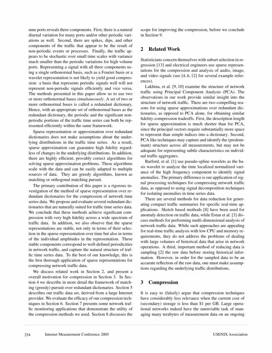
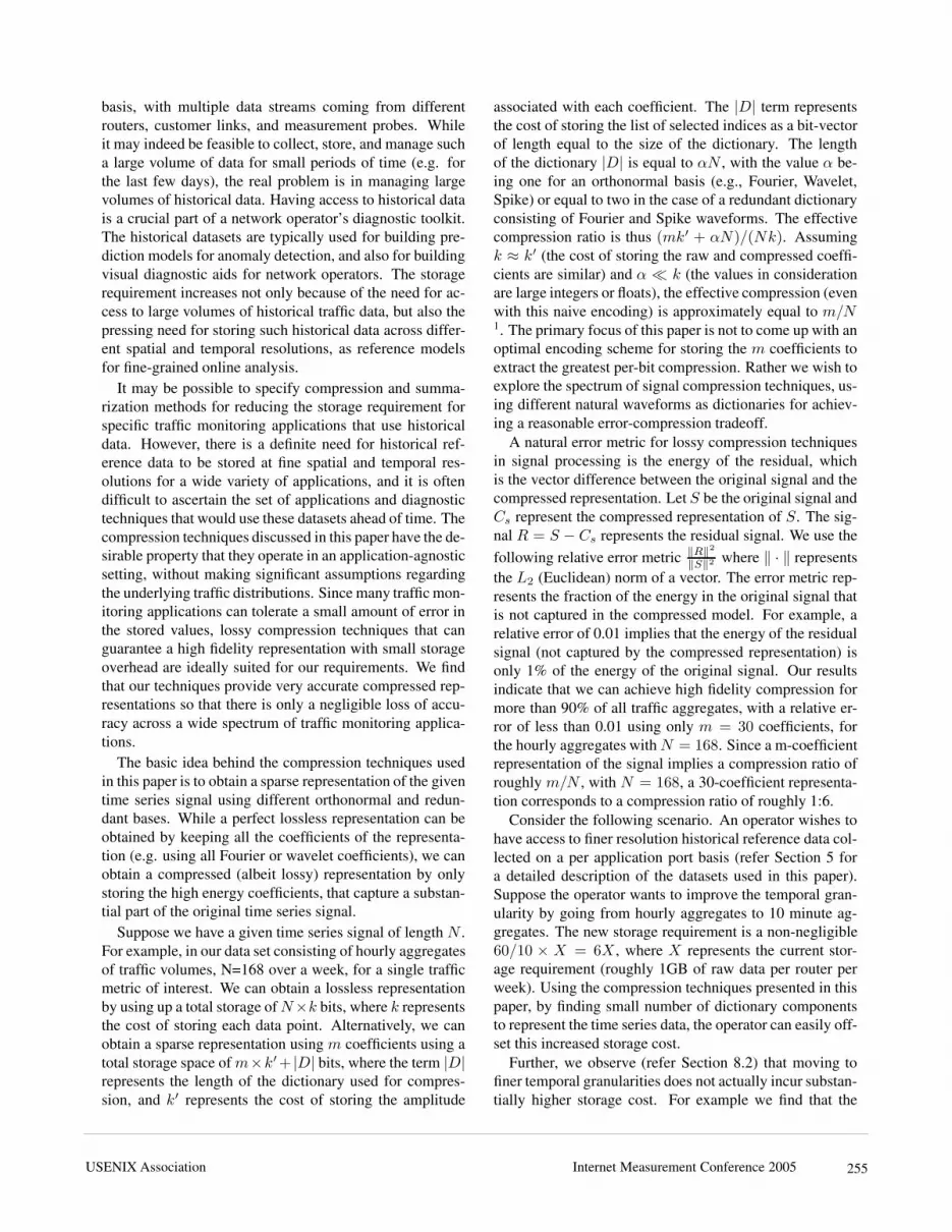
and scan ports, the wavelet or full-translation Haar dictio-nary give better compression. In some cases (e.g. port 114)we also find that using spikes in the dictionary gives thelowest compression error.Rather than try to optimize the basis selection for eachspecific port, we wish to use redundant dictionaries that canbest capture the different components that can be observedacross the entire spectrum of ports. Hence we use redun-dant dictionaries composed of Fourier, fully-translationalHaar, and Spike waveforms and observe that we can ex-tract the best compression (in terms of number of coeffi-cients selected), across an entire family of traffic time se-ries data. We compare three possible redundant dictionar-ies: Fourier+ Haar wavelets (referred to asDF+H), Fourier+ Spikes (referred to as DF+S), and Fourier + Spikes +Haar wavelets (referred to as DF+H+S). Within each dic-tionary the error-compression tradeoff is determined by thenumber of coefficients chosen (Recall that a m-coefficientrepresentation roughly corresponds to a compression ratioof m/N ). A fundamental property of the greedy pursuitapproach is that with every iteration the residual energy de-creases, and hence the error is a monotonically decreas-ing function of the number of modes chosen. We evaluatethe error-compression tradeoffs for these different dictio-naries in Figures 6 and 7, where we assume that we areconstrained to use 30 coefficients (roughly correspondingto using only one-sixth of the data points for each week).We observe two main properties of using the redundant dic-tionary approach. First, the compressibility is substantiallyenhanced by expanding the dictionary to include eitherspikes or Haar wavelets, in addition to the periodic Fouriercomponents, i.e., using redundant dictionaries yields bet-ter fidelity for the same storage cost as compared to a sin-gle orthonormal basis. The second property we observewith the particular choice of basis functions on the trafficdata is a monotonicity property – adding a richer basis setto the dictionary helps the compressibility. For examplethe error-compression tradeoff that results with DF+H+S

is never worse than either DF+H or DF+S . The compres-sion does come at a slightly higher computation cost, sincethe time to compress the time series depends on the sizeof the dictionary used, as the compression time scales inlinearly with the number of vectors in the dictionary (referSection 4).In Figures 8 and 9 we show how the 95th percentile ofthe relative error across all the ports decreases as a functionof the number of coefficients used for representing the traf-fic data for each port for TCP and UDP ports respectively.We find that after 30-35 coefficients we gain little by addingadditional coefficients, i.e., the marginal improvement inthe fidelity of the representation becomes less significant.We will address this issue again in Section 8, by consid-ering the rate of decrease of the residual as a function ofthe number of modes selected for specific ports, to derive

0 0.02 0.04 0.06 0.08 0.10

0.1

0.2

0.3

0.4

0.5

0.6

0.7

0.8

0.9

1

Relative Error

Fra

ctio

n of

por

ts

F+HF+SF+H+S

Figure 6: CDFs of relative error for TCP ports (incomingflows) with 30 coefficients for different dictionaries

0 0.02 0.04 0.06 0.08 0.10

0.1

0.2

0.3

0.4

0.5

0.6

0.7

0.8

0.9

1

Relative Error

Fra

ctio

n of

por

ts

F+HF+SF+H+S

Figure 7: CDFs of relative error for UDP ports (incomingflows) with 30 coefficients for different dictionaries

stopping criteria for obtaining compressed representations.

6.3 Analysis of Selected Modes

We proceed to analyze the set of dictionary componentsthat are chosen in the compressed representation using theredundant dictionaries for different ports, along differentspatial and temporal dimensions. First, we are interestedto see if there is substantial similarity in the set of dictio-nary components selected in the compressed representationacross different ports. Second, we want to observe the tem-poral properties of compression; i.e., for a fixed traffic di-mension, how does one week differ from another in termsof the components selected from the redundant dictionary?Third, we want to identify possible sources of correlationacross the different traffic aggregates (flows, packets, bytes,both to and from) on a particular port of interest. Such anal-ysis not only helps us to understand the nature of the un-derlying constituent components that make up each traffic


Table 1: Compression error with 30 coefficient representation for selected TCP ports (Legend: F = Fourier, W = Ortho-normal db4 wavelets, H = Fully-translational Haar wavelets, S = Spikes)

Port Type Port Number Relative error with different dictionariesDF DW DS DH DF+S DF+H DF+H+S DH+S

High Volume 25 0.0005 0.0026 0.8446 0.0007 0.0004 0.0004 0.0004 0.000780 0.0052 0.0256 0.7704 0.0074 0.0052 0.0018 0.0018 0.0073

P2P 1214 0.0003 0.0036 0.0007 0.8410 0.0003 0.0001 0.0001 0.00076346 0.0009 0.0056 0.8193 0.0013 0.0009 0.0005 0.0005 0.0013

Scan 135 0.0016 0.0216 0.7746 0.0049 0.0015 0.0008 0.0008 0.00499898 0.0066 0.0143 0.7800 0.0036 0.0063 0.0032 0.0032 0.0036

Random 5190 0.0023 0.0280 0.7916 0.0040 0.0023 0.0010 0.0010 0.0039114 0.5517 0.1704 0.0428 0.0218 0.0097 0.0218 0.0068 0.0068

5 10 15 20 25 30 35 40 45 500

0.02

0.04

0.06

0.08

0.1

0.12

0.14

0.16

0.18

Number of coefficients

Rel

ativ

e E

rror

F+HF+SF+H+S

Figure 8: 95th percentile of relative error vs. number ofcoefficients selected for TCP ports (incoming flows)

time series but also enables us to identify possible sourcesof joint compression, to further reduce the storage require-ments. For the discussion presented in this section, we usethe dictionary DF+S (Fourier + Spike) as the redundantdictionary for our analysis.

6.3.1 Spatial Analysis Across Ports

We observe that the majority of selected dictionary com-ponents are restricted to a small number of ports—thisis expected as these modes capture the minor variationsacross different ports, and also represent traffic spikes thatmay be isolated incidents specific to each port. We alsoobserve that there are a few components that are consis-tently selected across almost all the ports. These compo-nents that are present across all the ports under consider-ation include the mean (zero-th Fourier component), thediurnal/off-diurnal periodic components, and a few otherperiodic components which were found to be the high-est energy components in the Fourier analysis presented inSection 6.1.

5 10 15 20 25 30 35 40 45 500

0.05

0.1

0.15

0.2

0.25

0.3

0.35

0.4

0.45

0.5


Rel

ativ

e E

rror

F+HF+SF+H+S

Figure 9: 95th percentile of relative error vs. number ofcoefficients selected for UDP ports (incoming flows)

6.3.2 Temporal Analysis Across Multiple Weeks

We also analyze, for specific instances of ports as definedby our four categories, the temporal stability of the set ofcomponents that are selected across different weeks overthe 20 week data set, using 30 modes per week. As before,we use DF+S as the redundant dictionary for compres-sion. For each dictionary component (periodic componentor spike) that is selected in the compressed representationover the 20 week period, we count the number of weeks inwhich it is selected. We show in Figure 10 the number ofcomponents that have an occurrence count more than x, asa function of x. We observe that the majority of the compo-nents are selected only for 1-2 weeks, which indicates thatthese captured subtle traffic variations from week to week.To further understand the stability of the components, wedivide them into 3 categories: components that occur everyweek, components that occurred greater than 50% of thetime (i.e, were selected 10-20 times over the 20 week pe-riod), and components that occurred fewer than 50% of thetime (i.e., fewer than 10 times). Table 2 presents the break-


0 2 4 6 8 10 12 14 16 18 200

50

100

150

Occurence count over 20 weeks

Num

ber o

f mod

es w

ith o

ccur

ence

cou

nt >

x

Port 25: SMTPPort 80: HTTPPort 110: POP3

(a) High Volume Ports

0 2 4 6 8 10 12 14 16 18 200

20

40

60

80

100

120

140

160

180

200


Num

ber o

f mod

es w

ith o

ccur

ence

cou

nt >

x

Port 135: Blaster?Port 9898: Dabber?Port 139: NetBIOS

(b) Scan Target Ports

0 2 4 6 8 10 12 14 16 18 200

20

40

60

80

100

120

140

160


Num

ber o

f mod

es w

ith o

ccur

ence

cou

nt >

x

Port 1214: KazaaPort 4662: EdonkeyPort 6346: Gnutella

(c) P2P Ports

0 2 4 6 8 10 12 14 16 18 200

20

40

60

80

100

120

140

160

180

200


Num

ber o

f mod

es w

ith o

ccur

ence

cou

nt >

x

Port 1162Port 43276Port 65506

(d) Random Ports

Figure 10: Occurrence counts using a 30 coefficient representation withDF+S :Fourier+Spike over a 20 week period

down for the above classification for different ports in eachcategory, and also shows the type of components that occurwithin each count-class. We find that across all the ports,the dictionary components that are always selected in thecompressed representation correspond to periodic compo-nents such as the diurnal and off-diurnal frequencies.The stability of a component depends not only on thefact that it was selected in the compressed representation,but also on the amplitude of the component in the com-pressed representation. Hence, we also analyze the ampli-tudes of the frequently occurring components (that occurgreater than 50% of the time) across the 20 week dataset.Figures 11 and 12 show the mean and deviation of the am-plitudes returned by the greedy pursuit procedure for thesefrequently occurring components. For clarity, we show theamplitudes of the real and imaginary part of the Fourier(periodic) components separately. For each port, we firstsort the components according to the average magnitude(i.e, the energy represented by both the real and imaginaryparts put together) over the 20 week period. We normal-ize the values of the average amplitude in both real andimaginary parts, and the deviations by the magnitude of themean (or zero-th Fourier) component. We observe that theamplitudes are fairly stable for many Fourier componentsacross the different port types. These results suggest thatthese stable (Fourier) frequencies may indeed form funda-mental components of the particular traffic time series. Therelative stability of amplitudes in the compressed represen-tation also indicates that it may be feasible to build trafficmodels, that capture the fundamental variations in traffic,using the compressed representations.

6.3.3 Spatial Analysis Across Traffic Metrics

The last component of our analysis explores the similar-ity in the traffic data across different aggregates for a givenport, within each week. One naturally expects a strong cor-relation between the number of flows, the number of pack-ets, and the number of bytes for the same port, and alsoreasonable correlation between the total incoming volume

2 4 6 8 10 12 14 16 18 20

−0.1

−0.05

0

0.05

0.1

0.15

Nor

mal

ized

am

plitu

de

Dictionary components sorted by average magnitude

(a) Real part

2 4 6 8 10 12 14 16 18 20

−0.1

−0.05

0

0.05

0.1

0.15

Nor

mal

ized

am

plitu

de


(b) Imaginary part

Figure 11: Stability of amplitudes of dictionary compo-nents selected – High volume: Port 80

and the total outgoing volume of traffic on the same port 4.Figure 13 confirms this natural intuition about the nature ofthe traffic aggregates. We observe that for the high volumeand P2P application ports, more than two-thirds of the dic-tionary components are commonly selected across all thedifferent traffic aggregates and we also find that more than30 components are selected across at least 4 of the traf-fic aggregates (bytes, packets, flows both to and from theport). We found that such similarity in the selected compo-nents across the different aggregates is less pronounced forthe scan target ports and the random ports under consider-ation. Our hypothesis is that the distribution of packets perflow and bytes per packet are far more regular for the highvolume applications (for example most HTTP, P2P packetsuse the maximum packet size to get maximum throughput)than on the lesser known ports (which may be primarilyused as source ports in small sized requests).

7 Applications

7.1 Visualization

One of the primary objectives of compression is to presentto the network operator a high fidelity approximation that


Table 2: Analyzing stable dictionary components for different classes of ports

Port Type Port Number All 20 weeks 10-20 weeks 0-10 weeksPeriodic Spike Periodic Spike Periodic Spike

High Volume 25 5 0 18 0 23 10280 11 0 19 0 15 33

P2P 1214 5 0 21 0 20 1046346 7 0 17 0 23 94

Scan 135 5 0 24 0 15 639898 3 0 20 0 35 67

Random 5190 11 0 10 0 27 7365506 1 0 15 0 31 147

2 4 6 8 10 12 14 16 18 20

−0.1

−0.05

0

0.05

0.1

0.15

Nor

mal

ized

am

plitu

de


(a) Real part

2 4 6 8 10 12 14 16 18 20

−0.1

−0.05

0

0.05

0.1

0.15

Nor

mal

ized

am

plitu

de


(b) Imaginary part

Figure 12: Stability of amplitudes of dictionary compo-nents selected – P2P Port: 1214

captures salient features of the original traffic metric of in-terest. Visualizing historical traffic patterns is a crucial as-pect of traffic monitoring that expedites anomaly detectionand anomaly diagnosis involving a network operator, whocan use historical data as visual aids. It is therefore impera-tive to capture not only the periodic trends in the traffic, butalso the isolated incidents of interest (for example, a post-lunch peak in Port 80 traffic, the odd spike in file sharingapplications, etc).Figure 14 shows some canonical examples from each ofthe four categories of ports we described earlier. In eachcase we show the original traffic time series over a weekand the time series reconstructed from the compressed rep-resentation using 1:6 compression with DF+H+S(Fourier+ Haar + Spike). We also show the residual signal, whichis the point-wise difference between the original signal andthe compressed reconstruction. The traffic values are nor-malized with respect to the maximum traffic on that portobserved for the week. We find that the compressed repre-sentations provide a high fidelity visualization of the orig-inal traffic data. Not surprisingly, the ports which exhibitthe greatest amount of regularity in the traffic appear to bemost easily compressible and the difference between theactual and compressed representation is almost negligible

1 1.5 2 2.5 3 3.5 4 4.5 5 5.5 615

20

25

30

35

40

45

Occurence count over six traffic aggregatesN

umbe

r of m

odes

with

occ

uren

ce c

ount

> x

Port 25: SMTPPort 80: HTTPPort 110: POP3

(a) High Volume Ports

1 1.5 2 2.5 3 3.5 4 4.5 5 5.5 615

20

25

30

35

40

45

50

55

60

Occurence count over six traffic aggregates

Num

ber o

f mod

es w

ith o

ccur

ence

cou

nt >

x

Port 1214: KazaaPort 4662: EdonkeyPort 6346: Gnutella

(b) P2P Ports

Figure 13: Occurrence counts using 30 coefficient repre-sentation with DF+S :Fourier+Spike over different trafficaggregates for a single week

for these cases. It is also interesting to observe in eachcase that the compressed representation captures not onlythe periodic component of the signal, but also traffic spikesand other traffic variations.

7.2 Traffic Trend Analysis

Analyzing trends in traffic is a routine aspect in network op-erations. Operators would like to understand changes andtrends in the application mix that is flowing through thenetwork (e.g. detecting a a new popular file sharing proto-col). Understanding traffic trends is also crucial for trafficengineering, provisioning, and accounting applications. Itis therefore desirable that such trend analysis performed onthe compressed data yields accurate results when comparedto similar trend analysis on the raw (uncompressed) data. Asimple method to extract trends over long timescales is totake the weekly average, and find a linear fit (using simplelinear regression to find the slope of the line of best fit) tothe weekly averages over multiple weeks of data. In Fig-ure 15, we plot the relative error in estimating such a lineartrend. We estimate the trend using 20 weeks of data for dif-


0 20 40 60 80 100 120 140 160 180−0.2

0

0.2

0.4

0.6

0.8

1

1.2

Time (hour of week)

Nor

mal

ized

Tra

ffic

Vol

ume

Original TrafficCompressed RepresentationResidual

(a) Port 80

0 20 40 60 80 100 120 140 160 180−0.2

0

0.2

0.4

0.6

0.8

1

1.2

Time (hour of week)

Nor

mal

ized

Tra

ffic

Vol

ume


(b) Port 6346

0 20 40 60 80 100 120 140 160 180−0.2

0

0.2

0.4

0.6

0.8

1

1.2

Time (hour of week)

Nor

mal

ized

Tra

ffic

Vol

ume


(c) Port 9898

0 20 40 60 80 100 120 140 160 180−0.2

0

0.2

0.4

0.6

0.8

1

1.2

Time (hour of week)

Nor

mal

ized

Tra

ffic

Vol

ume


(d) Port 43726

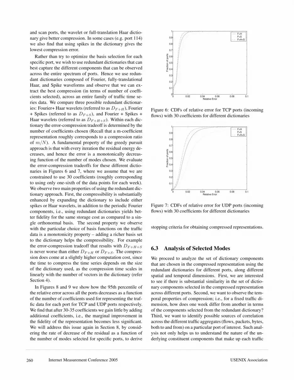
Figure 14: Miscellaneous Ports usingDF+H+S : Fourier + Haar Wavelets + Spikes

25 135 139 1214 4662 6346 98980

0.5

1

1.5

2

2.5

3

3.5

4

4.5x 10−3

TCP Port

Rel

ativ

e er

ror i

n es

timat

ing

trend

Figure 15: Relative error in estimating traffic trends

ferent ports, and in each case we estimate the slope of thebest linear fit on the raw data and on the compressed data(using a 30 coefficient representation usingDF+H+S ). Weobserve that across the different ports, the relative error inestimating the trend is less than 0.5%, which reaffirms thehigh fidelity of the compression techniques.

7.3 Modeling and Anomaly Detection

We observed in Section 6.3 that the underlying fundamen-tal components are stable (both in terms of occurrence andtheir amplitudes) over time. It is conceivable that trafficmodels for anomaly detection can be learned on the com-pressed data alone. Our initial results suggest that traf-fic models [15] learned from compressed data have al-most identical performance to models learned from un-compressed data, and hence compression does not affectthe fidelity of traffic modeling techniques. Ongoing workincludes evaluating different models for building predic-tion models for real-time anomaly detection using accurateyet parsimonious prediction models generated from the in-sights gained from the compression procedures.

8 Discussion

8.1 Stopping Criteria

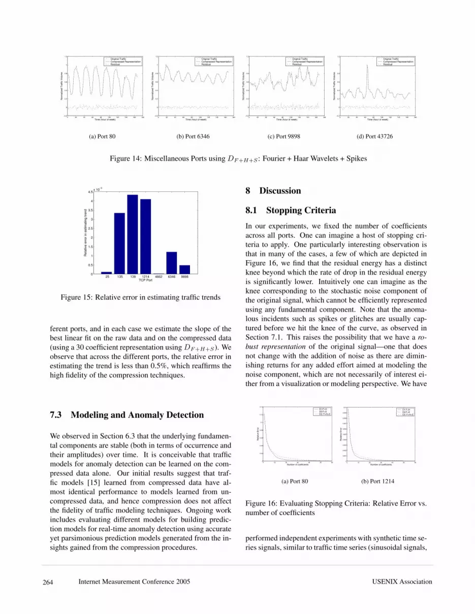
In our experiments, we fixed the number of coefficientsacross all ports. One can imagine a host of stopping cri-teria to apply. One particularly interesting observation isthat in many of the cases, a few of which are depicted inFigure 16, we find that the residual energy has a distinctknee beyond which the rate of drop in the residual energyis significantly lower. Intuitively one can imagine as theknee corresponding to the stochastic noise component ofthe original signal, which cannot be efficiently representedusing any fundamental component. Note that the anoma-lous incidents such as spikes or glitches are usually cap-tured before we hit the knee of the curve, as observed inSection 7.1. This raises the possibility that we have a ro-bust representation of the original signal—one that doesnot change with the addition of noise as there are dimin-ishing returns for any added effort aimed at modeling thenoise component, which are not necessarily of interest ei-ther from a visualization or modeling perspective. We have

0 10 20 30 40 50 600

0.02

0.04

0.06

0.08

0.1

0.12

0.14


Rel

ativ

e E

rror

D1:F+HD2:F+SD3: F+H+S

(a) Port 80

0 10 20 30 40 50 600

0.001

0.002

0.003

0.004

0.005

0.006

0.007

0.008

0.009

0.01


Rel

ativ

e E

rror

D1:F+HD2:F+SD3: F+H+S

(b) Port 1214

Figure 16: Evaluating Stopping Criteria: Relative Error vs.number of coefficients

performed independent experiments with synthetic time se-ries signals, similar to traffic time series (sinusoidal signals,


with spikes and different noise patterns thrown in). We ob-serve that in almost all the cases we observe a distinct kneein the redundant dictionary decomposition, once the fun-damental high energy components get picked. We also findthat the asymptotic slope of the curve of the residual energybeyond the knee has a unique signature that is characterizedby the nature of the noise component (Gaussian or “White”vs. Power-law or “Colored”), and the redundant dictionaryused.

8.2 Smaller ScalesAt an appropriate aggregation level, network traffic will ex-hibit some periodicities. Traffic time series data from avariety of settings (enterprise and university) also confirmthis hypothesis. These data typically represent the aggre-gate traffic at the border of a reasonably large network withfairly high aggregation levels. We believe that the methodsfor time-series compression using matching pursuit withredundant dictionaries are still applicable to data even atslightly lower scales of aggregation.One of the objectives of compressing the time series isto enable different scales of time resolution for anomalydetection. It is imperative that the time scale for detectingtraffic anomalies be less than the minimum time requiredfor a large network attack to saturate. When the compres-sion is applied to traffic aggregates at finer time granulari-ties (e.g. for each week if we had volume counts for eachfive minute bin instead of hourly time bins), one expectsthat the effective compression would be better. The ratio-nale behind the intuition arises from the fact that the highenergy fundamental components correspond to relativelylow frequency components, and such pronounced period-icities are unlikely to occur at finer time-scales. As a pre-liminary confirmation of this intuition, we performed thesame compression procedures on a different data set, con-sisting of 5 minute traffic rates collected from SNMP datafrom a single link. Note that with 5-minute time intervals,we have 168 × 12 = 2016 data points per week. Figure 17the relative error as a function of the number of coefficientsused in the compressed representation (using DF+S). Weobserve that with less than 40 ( = 2% of the original spacerequirement) coefficients we are able to adequately com-press the original time-series (with a relative error of lessthan 0.005), which represents significantly greater possi-ble compression than those observed with the hourly ag-gregates.

8.3 Encoding TechniquesWe observed that with larger dictionaries that include full-translation wavelets, we can achieve better compression.There is, however, a hidden cost in the effective compres-sion with larger dictionaries as the indices of a larger dic-

0 10 20 30 40 50 60 70 80 90 1000

0.01

0.02

0.03

0.04

0.05

0.06


Rel

ativ

e E

rror

FF+S

Figure 17: Compressing SNMP data collected at fiveminute intervals from a single link

tionary potentially require more bits to represent than theindices of a smaller dictionary. One can imagine betterways of encoding the dictionary indices (e.g., using Huff-man coding) to reduce the amount of space used up forstoring the dictionary indices in addition to the componentamplitudes. Our work explored the potential benefit of us-ing signal processing methods for lossy compression andwe observed that there is a substantial reduction in the stor-age requirement using just the methods presented in this pa-per. Many compression algorithms use lossy compressiontechniques along with efficient encoding techniques (loss-less compression) to get the maximum compression gain,and such combinations of lossy and lossless compressionmethods can be explored further.

8.4 Joint CompressionWe observe that there are multiple sources of correlationacross the different traffic dimensions that may be addition-ally utilized to achieve better compression. The temporalstability of the compressed representations (Section 6.3.2)suggests there is scope for exploiting the similarity acrossdifferent weeks for the same traffic aggregate. For exam-ple, we could build a stable model over k weeks of data foreach port/prefix and only apply the sparse approximationto the difference of each particular week from the model.Alternately one could imagine applying the simultaneouscompression algorithms [16] across the different weeks forthe same port. The simultaneous compression algorithmsapproximate all these signals at once using different linearcombinations of the same elementary signals, while bal-ancing the error in approximating the data against the to-tal number of elementary signals that are used. We alsoobserved that there is reasonable correlation in spatial di-mensions, since the compressed representation of differenttraffic aggregates such as flows, packets, and bytes showsignificant similarity (Section 6.3.3).The observations of the low dimensionality of networktraffic data across different links also raises the possibil-ity of using Principal Component Analysis (PCA) [10] for


extracting better spatial compression, both across differenttraffic aggregates (e.g. different ports, across time) andacross different measurements (e.g. across per-link, per-router counts). PCA like methods can be used to extract thesources of correlation before one applies redundant dictio-nary approaches to compress the traffic data. For examplewe can collapse the 20 week data set for a single port into asingle matrix of traffic data, on which PCA like techniquescan be applied to extract the first few common components,and the redundant dictionary can be applied on the residual(the projection on the non-principal subspace) to obtain ahigher fidelity representation.

9 Conclusions

There is a pressing need for fine-grained traffic analysis atdifferent scales and resolutions across space and time fornetwork monitoring applications. Enabling such analysisrequires the ability to store large volumes of historical dataacross different links, routers, and customers, for generat-ing visual and diagnostic aids for network operators. Inthis paper, we presented a greedy pursuit approach overredundant dictionaries for compressing traffic time seriesdata, and evaluated them using measurements from a largeISP. Our observations indicate that the compression modelspresent a high fidelity representation for a wide variety oftraffic monitoring applications, using less than 20% of theoriginal space requirement. We also observe that most traf-fic signals can be compressed and characterized in terms ofa few stable frequency components. Our results augur wellfor the visualization and modeling requirements for largescale traffic monitoring. Ongoing work includes evaluatingand extracting sources of compression across other spatialand temporal dimensions, and evaluating the goodness oftraffic models generated from compressed representations.

References[1] BARFORD, P., KLINE, J., PLONKA, D., AND RON, A. A SignalAnalysis of Network Traffic Anomalies. In Proc. of ACM/USENIXInternet Measurement Workshop (2002).

[2] DUFFIELD, N. G., LUND, C., AND THORUP, M. Charging FromSampled Network Usage. In Proc. of ACM SIGCOMM InternetMeasurement Workshop (2001).

[3] ESTAN, C., SAVAGE, S., AND VARGHESE, G. Automatically In-ferring Patterns of Resource Consumption in Network Traffic. InProc. of ACM SIGCOMM (2003).

[4] FROSSARD, P., VANDERGHEYNST, P., I VENTURA, R. M. F., ANDKUNT, M. A posteriori quantization of progressive matching pursuitstreams. IEEE Trans. Signal Processing (2004), 525–535.

[5] GILBERT, A. C., MUTHUKRISHNAN, S., AND STRAUSS, M. J.Approximation of functions over redundant dictionaries using co-herence. In Proc. of 14th Annual ACM-SIAM Symposium on Dis-crete Algorithms (2003).

[6] GRIBONVAL, R., AND BACRY, E. Harmonic decomposition of au-dio signals with matching pursuit. IEEE Trans. Signal Processing(2003), 101–111.

[7] INDYK, P. High-dimensional computational geometry. PhD thesis,Stanford University, 2000.

[8] KRISHNAMURTHY, B., SEN, S., ZHANG, Y., AND CHEN, Y.Sketch-based ChangeDetection: Methods, Evaluation, and Applica-tions. In Proc. of ACM/USEINX Internet Measurement Conference(2003).

[9] LAKHINA, A., CROVELLA, M., AND DIOT, C. Diagnosingnetwork-wide traffic anomalies. In Proc. of ACM SIGCOMM(2004).

[10] LAKHINA, A., PAPAGIANNAKI, K., CROVELLA, M., DIOT, C.,KOLACZYK, E., AND TAFT, N. Structural analysis of network traf-fic flows. In Proc. of ACM SIGMETRICS (2004).

[11] LEMPEL, A., AND ZIV, J. Compression of individual sequences viavariable-rate coding. IEEE Transactions on Information Theory 24,5 (1978), 530–536.

[12] MALLAT, S., AND ZHANG, Z. Matching pursuits with time fre-quency dictionaries. IEEE Trans. Signal Processing 41, 12 (1993),3397–3415.

[13] MILLER, A. J. Subset selection in regression, 2nd ed. Chapmanand Hall, London, 2002.

[14] Cisco Netflow. http://www.cisco.com/warp/public/732/Tech/nmp/netflow/index.shtml.

[15] ROUGHAN, M., GREENBERG, A., KALMANEK, C., RUMSEWICZ,M., YATES, J., AND ZHANG, Y. Experience in measuring in-ternet backbone traffic variability: Models, metrics, measurementsand meaning. In Proc. of International Teletraffic Congress (ITC)(2003).

[16] TROPP, J. A., GILBERT, A. C., AND STRAUSS, M. J. Algorithmsfor simultaneous sparse approximation part i: Greedy pursuit. sub-mitted (2004).

[17] ZHUANG, Y., AND BARAS, J. S. Optimal wavelet basis selectionfor signal representation. Tech. Rep. CSHCN TR 1994-7, Institutefor Systems Research, Univ. of Maryland, 1994.

Notes1Typically, k′ is less than k, i.e. the magnitudes of the amplitudes of

the dictionary components are less than the original time series.2The slowest step in OMP is choosing the waveform which maximizes

the dot product with the residual at each step. We can speed up this stepwith a Nearest Neighbors data structure [7] and reduce the time complex-ity for each iteration toN + polylog(d).3Note that for each Fourier coefficient, we need to store both the real

part and the imaginary part. It appears that we may actually need twicethe space. However, the amplitudes for frequency f and frequency −fare the same (except that they are complex conjugates of one another),we can treat them as contributing only two coefficients to the compressedrepresentation together in total as opposed to four coefficients.4We however note that there may be certain exceptional situations

(e.g., worm or DDoS attacks that use substantially different packet andbyte types) where such stable correlations between the flow, packet, andbyte counts may not always hold.


Documents

Sparse approximations for high fidelity compression of network traffic data