arX

iv:m

ath/

0008

011v

2 [

mat

h.A

G]

3 J

ul 2

002

CERN-TH/2000-203, UPR-894T, RU-00-5B

Spectral involutions on rational elliptic surfaces

Ron Donagi1, Burt A. Ovrut2, Tony Pantev1 and Daniel Waldram3

1Department of Mathematics, University of Pennsylvania

Philadelphia, PA 19104–6395, USA2Department of Physics, University of Pennsylvania

Philadelphia, PA 19104–6396, USA3Theory Division, CERN CH-1211, Geneva 23, Switzerland, and

Department of Physics, The Rockfeller University

New York, NY 10021

Abstract

In this paper we describe a four dimensional family of special rational elliptic sur-faces admitting an involution with isolated fixed points. For each surface in this familywe calculate explicitly the action of a spectral version of the involution (namely of itsFourier-Mukai conjugate) on global line bundles and on spectral data. The calculationis carried out both on the level of cohomology and in the derived category. We find thatthe spectral involution behaves like a fairly simple affine transformation away from theunion of those fiber components which do not intersect the zero section. These resultsare the key ingredient in the construction of Standard-Model bundles in [DOPWa].

MSC 2000: 14D20, 14D21, 14J60

1 Introduction

Let Z → S be an elliptic fibration on a smooth variety Z, i.e. a flat morphism whosegeneric fiber is a curve of genus one, and which has a section S → Z. The choice ofsuch a section defines a Poincare sheaf P on Z ×S Z. The corresponding Fourier-Mukaitransform FM : Db(Z) → Db(Z) is then an autoequivalence of the derived category Db(Z)of complexes of coherent sheaves on Z. It sets up an equivalence between SL(r,C)-bundleson Z and spectral data consisting of line bundles (and their degenerations) on spectral coversC ⊂ Z which are of degree r over S. This equivalence has been used extensively to constructvector bundles on elliptic fibrations and to study their moduli [FMW97, Don97, BJPS97].

For many applications it is important to remove the requirement of the existence of asection, i.e. to allow genus one fibrations. This could be done in two ways.

The ‘spectrum’ of a degree zero semistable rank r bundle on a genus one curve E consistsof r points in the Jacobian Pic0(E), rather than in E = Pic1(E) itself. So one approach isto consider spectral covers C contained in the relative Jacobian Pic0(Z/S). But the spectral

1

data in this case no longer involves a line bundle on C; instead, it lives in a certain non-trivial gerbe, or twisted form of Pic(C). So the essential problem becomes the analysis ofthis gerbe.

The second approach is to find an elliptic fibration π : X → B together with a group Gacting compatibly on X and B (but not preserving the section of π) such that the action onX is fixed point free and the quotient is the original Z → S. One can then use the Fourier-Mukai transform to construct vector bundles on X. The problem becomes the determinationof conditions for such a bundle onX to beG-equivariant, hence to descend to Z. Equivalentlywe need to know the action of each g ∈ G on spectral data. This is the restriction of theaction onDb(X) of the Fourier-Mukai conjugate FM−1g∗FM of g∗. This will be referredto as the spectral action of g. Unfortunately, the spectral action can be quite complicated:both global vector bundles on X and sheaves supported on C can go to complexes on X ofamplitude greater than one.

In this paper, we work out such a spectral action in one class of examples consistingof special rational elliptic surfaces. In the second part [DOPWa] of this paper we use thisanalysis to construct special bundles on certain non-simply connected smooth Calabi-Yauthreefolds. These special bundles in turn are the main ingredient for the construction ofHeterotic M-theory vacua having the Standard Model symmetry group SU(3)×SU(2)×U(1)and three generations of quarks and leptons. The physical significance of such vacua isexplained in [DOPWb] and was the original motivation of this work.

Here is an outline of the paper. We begin in section 2 with a review of the basic propertiesof rational elliptic surfaces. Within the eight dimensional moduli space of all rational ellipticsurfaces we focus attention on a five dimensional family of rational elliptic surfaces admittinga particular involution τ , and then we restrict further to a four dimensional family of surfaceswith reducible fibers. This seems to be the simplest family of surfaces for which one needsthe full force of Theorem 7.1: for general surfaces in the five dimensional family, the spectralinvolution T := FM−1 τ ∗ FM of τ takes line bundles to line bundles, while in the fourdimensional subfamily it is possible for T to take a line bundle to a complex which can notbe represented by any single sheaf. We study the five dimensional family in section 3 andthe four dimensional subfamily in section 4. This section concludes, in subsection 4.3, witha synthetic construction of the surfaces in the four dimensional subfamily. This constructionmaybe less motivated than the original a priori analysis we use, but it is more concise andwe hope it will make the exposition more accessible.

In the remainder of the paper we work out the actions of τ , FM , T , first at the levelof cohomology in sections 5 and 6, and then on the derived category in section 7. The mainresult is Theorem 7.1, which says that T behaves like a fairly simple affine transformationaway from the union of those fiber components which do not intersect the zero section. Acorollary is that for spectral curves which do not intersect the extra vertical components,all the complications disappear. This fact together with the cohomological formulas fromsections 5 and 6 will be used in [DOPWa] to build invariant vector bundles on a family ofCalabi-Yau threefolds constructed from the rational elliptic surfaces in our four dimensionalsubfamily.

2

Acknowledgements: We would like to thank Ed Witten, Dima Orlov, and RichardThomas for valuable conversations on the subject of this work.

R. Donagi is supported in part by an NSF grant DMS-9802456 as well as a UPenn Re-search Foundation Grant. B. A. Ovrut is supported in part by a Senior Alexander vonHumboldt Award, by the DOE under contract No. DE-AC02-76-ER-03071 and by a Univer-sity of Pennsylvania Research Foundation Grant. T. Pantev is supported in part by an NSFgrant DMS-9800790 and by an Alfred P. Sloan Research Fellowship. D. Waldram would liketo thank Enrico Fermi Institute at The University of Chicago and the Physics Departmentof The Rockefeller University for hospitality during the completion of this work.

Contents

1 Introduction 1

2 Rational elliptic surfaces 3

3 Special rational elliptic surfaces 53.1 Types of involutions on a rational elliptic surfaces . . . . . . . . . . . . . . . 63.2 The Weierstrass model of B . . . . . . . . . . . . . . . . . . . . . . . . . . . 83.3 The quotient B/αB. . . . . . . . . . . . . . . . . . . . . . . . . . . . . . . . 10

4 The four dimensional subfamily of special rational elliptic surfaces 144.1 The quotient B/τB . . . . . . . . . . . . . . . . . . . . . . . . . . . . . . . . 144.2 The basis in H2(B,Z) . . . . . . . . . . . . . . . . . . . . . . . . . . . . . . 174.3 A synthetic construction . . . . . . . . . . . . . . . . . . . . . . . . . . . . . 23

5 Action on cohomology 265.1 Action of (−1)B . . . . . . . . . . . . . . . . . . . . . . . . . . . . . . . . . . 265.2 Action of αB . . . . . . . . . . . . . . . . . . . . . . . . . . . . . . . . . . . . 265.3 Action of t∗ζ . . . . . . . . . . . . . . . . . . . . . . . . . . . . . . . . . . . . 27

6 The cohomological Fourier-Mukai transform 28

7 Action on bundles 33

2 Rational elliptic surfaces

A rational elliptic surface is a rational surface B which admits an elliptic fibration β : B →P1. It can be described as the blow-up of the plane P2 at nine points A1, . . . , A9 which are

3

the base points of a pencil ftt∈P1 of cubics. The map β is recovered as the anticanonicalmap of B and the proper transform of ft is β−1(t).

In particular the topological Euler characteristic of B is χ(B) = χ(P2) + 9 = 12. For ageneric B the map β has twelve distinct singular fibers each of which has a single node. Forfuture use we denote by B# ⊂ B the open set of regular points of β and we set β# := β|B# .

Under mild general position requirements [DPT80] each subset of eight of these pointsdetermines the pencil of cubics and hence the ninth point. In particular we see that therational elliptic surfaces depend on 2 · 8 − dim PGL(3,C) = 8 parameters.

Let e1, . . . , e9 be the exceptional divisors in B corresponding to the Ai’s. Let ℓ be thepreimage of the class of a line in P2 and let f := β∗OP1(1). Note that

f = −KB = 3ℓ−9∑

i=1

ei

and that ℓ, e1, . . . , e9 form a basis of H2(B,Z).The curves e1, e2, . . . , e9 are sections of the map β : B → P1. Choosing a section

e : P1 → B determines a group law on the fibers of β#. The inversion for this group law is aninvolution on B# which for a general B extends to a well defined involution (−1)B,e : B → B.When B or e are understood from the context we will just write (−1)B or (−1). Theinvolution (−1)B,e fixes the section e as well as a tri-section of β which parameterizes thenon-trivial points of order two. The quotient Wβ/(−1)B,e is a smooth rational surface whichis ruled over the base P1. For a general B this quotient is the Hirzebruch surface F2 andthe image of e is the exceptional section of F2. This gives yet another realization of B as abranched double cover of F2.

A convenient way to describe the involution (−1)B,e is through the Weierstrass model

w : Wβ → P1 of Bβ

//P1

ehh .

The model Wβ is described explicitly as follows. By relative duality R1β∗OB∼= OP1(−1).

This implies that β∗OB(3e) = (OP1 ⊕OP1(2) ⊕OP1(3))∨. Let

p : P := P(OP1 ⊕OP1(2) ⊕OP1(3)) → P1.

be the natural projection. The linear system OB(3e) defines a map ν : B → P compatiblewith the projections. The Weierstrass model Wβ is defined to be the image of this map. Itis given explicitly by an equation

y2z = x3 + (p∗g2)xz2 + (p∗g3)z

3

where g2 ∈ H0(OP1(4)) and g3 ∈ H0(OP1(6)) and x, y and z are the natural sections ofOP (1) ⊗ p∗OP1(2), OP (1) ⊗ p∗OP1(3) and OP (1) respectively.

In terms of Wβ the section e is given by x = z = 0 and the involution (−1)B,e sends y to−y. The tri-section of fixed points of (−1)B,e is given by y = 0.

4

The Mordell-Weil group MW = MW(B, e) is the group of sections of β. As a set MW

is the collection of all sections of β : B → P1 or equivalently all sections of β# : B# → P1.The group law on MW is induced from the addition law on the group scheme β# : B# → P1

and so e corresponds to the neutral element in MW(B, e). For a section ξ ⊂ B we will put[ξ] for the corresponding element of MW. Note that the natural map

c1 : MW(B, e) → Pic(B), [ξ] 7→ OB(ξ).

is not a group homomorphism. When written out in coordinates, it involves both a linearpart and a quadratic term (see e.g. [Man64]). However, when B is smooth the map c1induces a linear map to a quotient of Pic(B) which describes MW(B, e) completely. Indeed,let B be smooth and let T ⊂ Pic(B) be the sublattice generated by e and all the componentsof the fibers of β. Then c1 induces a map

c1 : MW(B, e) → Pic(B)/T , [ξ] 7→ (OB(ξ) mod T )

which is a linear isomorphism [Shi90, Theorem 1.3]

There is a natural group homomorphism t : MW → BirAut(B) assigning to each sectionξ ∈ MW the birational automorphism tξ : B 99K B, which on the open set B# is justtranslation by ξ with respect to the group law determined by e. When β : B → P1 isrelatively minimal the map tξ extends canonically to a biregular automorphism of B [Kod63,Theorem 2.9].

3 Special rational elliptic surfaces

In the second part of this paper [DOPWa] we will work with Calabi-Yau threefolds X whichare elliptically fibered over a rational elliptic surface B. Any involution τX on an elliptic CYπ : X → B commuting with π induces (either the identity or) an involution τB on the baseB. In order for τX to act freely on X we need the fixed points of τB to be disjoint from thediscriminant of π. If B is a rational elliptic surface, then the discriminant of π is a sectionin K−12

B = OB(12f) and so (−1)B will not do. We want to describe some special rationalelliptic surfaces which admit additional involutions. Within the 8 dimensional family ofrational elliptic surfaces we describe first a 5 dimensional family of surfaces which admitan involution αB. The fixed locus of αB has the right properties but it turns out that αBdoes not lift to a free involution on X. However, one can easily show that each αB canbe corrected by a translation tζ (for a special type of section ζ) to obtain an additionalinvolution τB which does the job. Unfortunately the general member of the 5 dimensionalfamily leads to a Calabi-Yau manifold which does not admit any bundles satisfying all theconstraints required by the Standard Model of particle physics (see [DOPWa]). We thereforespecialize further to a 4 dimensional family of surfaces for which the extra involution τB canbe constructed in an explicit geometric way. This provides some extra freedom which enablesus to carry out the construction. The involution αB fixes one fiber of β and four points in

5

another fiber. The involution τB fixes only four points in one fiber. A special feature ofthe 4 dimensional family is that it consists of B’s for which β has at least two I2 fibers.This translates into a special position requirement on the nine points in P2. Another specialfeature of the 4 dimensional family is seen in the double cover realization of B where thequotient B/(−1) becomes F0 = P1 × P1 instead of F2.

We thank Chad Schoen for pointing out that essentially the same surfaces and threefoldswere constructed in section 9 of [Sch88]. The explicit example he gives there for what he callsthe “m = 2 case” happens to exactly coincide with our four-dimensional family of rationalelliptic surfaces. With small modifications, his construction could have given our full five-dimensional family as well. Schoen’s construction technique is rather different than ours. Heconstructs the equivalent of our rational elliptic surface B and involution αB directly (thesurfaces we call B,B/αB are called Y0, T0 in [Sch88]); then he invokes a general result of Oggand Shafarevich for the existence of a logarithmic transform Y with quotient T ; and finally,results from classification theory are used to deduce existence of an abstract isomorphism ofY with Y0 such that his T becomes our B/τB.

In the next several sections we will describe the structure of the rational elliptic surfacesthat admit additional involutions. This rather extensive geometric analysis is ultimatelydistilled into a fairly simple synthetic construction of our surfaces which is explained insection 4.3. The impatient reader who is interested only in the end result of the constructionand wants to avoid the tedious geometric details is advised to skip directly to section 4.3.

3.1 Types of involutions on a rational elliptic surfaces

Consider a smooth rational elliptic surface Bβ

//P1

ehh with a fixed section. For any auto-

morphism τB of B we have τ ∗BKB∼= KB. Since K−1

B = β∗OP1(1) this implies that τB inducesan automorphism τP1 : P1 → P1. If τB is an involution we have two possibilities: eitherτP1 = idP1 or τP1 is an involution of P1.

Both of these cases occur and lead to Calabi-Yau manifolds with freely acting involutions.For concreteness here we only treat the case when τP1 is an involution. The case τP1 = idP1

can be analyzed easily in a similar fashion.If τP1 is an involution, then τP1 will have two fixed points on P1 which we will denote by

0,∞ ∈ P1. Note that every involution on P1 is uniquely determined by its fixed points andso specifying τP1 is equivalent to specifying the points 0,∞ ∈ P1. Next we classify the typesof involutions on B that lift a given involution τP1 .

Lemma 3.1 Let β : B → P1 be a rational elliptic surface and let τP1 : P1 → P1 be a fixed

6

involution. There is a canonical bijection

Involutions τB : B → B, satisfyingτP1 β = β τB.

↔

Pairs (αB, ζ) consisting of:

• An involution αB : B → B,satisfying τP1 β = β αBwhich leaves the zero sectioninvariant, i.e. αB(e) = e.

• A section ζ of β satisfyingαB(ζ) = (−1)B(ζ).

Proof. Let τB : B → B be such that τP1 β = β τB. Put ζ = τB(e) for the image of thezero section under τB and let αB = t−ζ τB.

Then αB is an automorphism of B which induces τP1 on P1 and preserves the zero sectione ⊂ B. So α2

B : B → B will be an automorphism of B which acts trivially on P1. But

t−ζ τB = τB t−τ∗−1

B/P1 (ζ)

where τ ∗B/P1 : Pic0(B/P1) → Pic0(B/P1) is the involution on the relative Picard scheme

induced from τB. In particular we have that α2B must be a translation by a section. Indeed

we have

α2B = t−ζ τB τB t−τ∗−1

B/P1 (ζ) = t−ζ−τ∗−1

B/P1 (ζ).(3.1)

Combined with the fact that α2B preserves e (3.1) implies that α2

B = idB. On the otherhand, if we use the zero section e to identify Pic0(B/P1) → P1 with β# : B# → P1, thenτ ∗B/P1 = αB. Indeed, let ξ ∈ Pic0(B/P1) and let x ∈ P1 be the projection of the point ξ. Letfx ⊂ B be the fiber of β over x. Denote by mξ ∈ fx the unique smooth point in fx for whichOfx(mξ) = ξ⊗Ofx(e(x)). Then by definition τ ∗B(ξ) is a line bundle of degree zero on fx suchthat

Ofx(τB(mξ)) = τBξ ⊗Ofx(τB(e(x))) = τBξ ⊗Ofx(ζ(x)).

In other words under the identification of Pic0(fx) with the smooth locus of fx via e(x) theline bundle τ ∗Bξ → fx corresponds to the unique point pξ of fx such that

Ofx(pξ) = Ofx(τB(mξ)) ⊗Ofx(e(x) − ζ(x)).

But the right hand side of this identity equals Ofx(αB(mξ)) by definition and so pξ = αB(mξ).Combined with the identity (3.1) and the fact that t : MW(B) → Aut(B) is injective

this yields

αB(ζ) = (−1)B(ζ).

7

Conversely, given a pair (αB, ζ) we set τB = tζαB. Clearly τB is an automorphism ofB whichinduces τP1 on P1. Furthermore we calculate τ 2

B = tζ αB tζ αB = tζ αB αB t−ζ = idB.The lemma is proven. 2

The above lemma implies that in order to understand all involutions τB it suffices to under-stand all pairs (αB, ζ). Since the involutions αB stabilize e it follows that αB will have tonecessarily act on the Weierstrass model of B. In the next section we analyze this action inmore detail.

3.2 The Weierstrass model of B

Let as before τP1 : P1 → P1 be an involution and let (t0 : t1) be homogeneous coordinateson P1 such that τP1((t0 : t1)) = (t0 : −t1) and 0 = (1 : 0) and ∞ = (0 : 1). Since t0and t1 are a basis of H0(P1,OP1(1)) and since OP1(1) is generated by global sections we canlift the action of τP1 to OP1(1). For concreteness choose the lift t0 7→ t0, t1 7→ −t1. SinceH0(P1,OP1(k)) = SkH0(P1,OP1(1)) we get a lift of the action of τP1 to the line bundlesOP1(k) for all k. We will call this action the standard action of τP1 on OP1(k). Via thestandard action the involution τP1 acts also on the vector bundle OP1 ⊕OP1(2)⊕OP1(3) andhence we get a standard lift τP : P → P of τP1 satisfying τ ∗POP (1) ∼= OP (1).

Assume that we are given an involution αB : B → B which induces τP1 on P1 andpreserves the section e. We have the following

Lemma 3.2 (i) There exists a unique involution αWβ: Wβ → Wβ such that the natural

map ν : B →Wβ satisfies αWβ ν = ν αB.

(ii) Let W ⊂ P be a Weierstrass rational elliptic surface. Then the involution τP1 lifts toan involution on W which preserves the zero section if and only if τP (W ) = W .

(iii) If w : Wβ → P1 is not isotrivial, then αWβis either τP |Wβ

or τP |Wβ (−1)Wβ

.

Proof. Since α∗B(OB(e)) ∼= OB(e), there exists an involution on the total space of the

bundle OB(e) which acts linearly on the fibers and induces the involution αB on B. Indeed- the square γ α∗

Bγ of the isomorphism γ : α∗B(OB(e))→OB(e) is a bundle automorphism

of OB(e) (acting trivially on the base) and so is given by multiplication by some non-zerocomplex number λ ∈ C. Rescaling the isomorphism γ by

√λ−1 then gives the desired lift.

In this way the involution αB induces an involution on Oe(−e) = OP1(1) which liftsthe action of τP1. Let us normalize the lift of αB to OB(e) so that the induced action onOe(−e) = OP1(1) coincides with the standard action of τP1 . Thus the Weierstrass modelWβ ⊂ P must be stable under the corresponding τP and the restriction of τP to Wβ is aninvolution that preserves the zero section of w and induces τP1 on the base. By constructionτP |Wβ

coincides with the involution induced from αB up to a composition with (−1)Wβ. This

finishes the proof of the lemma. 2

We are now ready to construct the Weierstrass models of all surfaces B that admit aninvolution αB. Similarly to the proof of Lemma 3.2, the fact that τ ∗POP (1) ∼= OP (1) implies

8

that the action of τP can be lifted to an action on OP (1). Since there are two possible such liftsand they differ by multiplication by ±1 ∈ C× we can use the identification OP (1)|B = OB(3e)to choose the unique lift that will induce the standard action of τP1 on OP1(3) = Oe(−3e).With these choices we define an action

τ ∗P : H0(P,OP (r) ⊗ p∗OP (s)) → H0(P,OP (r) ⊗ p∗OP (s))

of τP on the global sections of any line bundle on P . Note that by construction we haveτ ∗Px = x, τ ∗Py = y and τ ∗P z = z.

Consider the general equation of the Weierstrass model Wβ of B:

y2z = x3 + (p∗g2)xz2 + (p∗g3)z

3.(3.2)

Here g2 ∈ H0(OP1(4)) and g3 ∈ H0(OP1(6)). The fact Wβ ⊂ P is stable under τP impliesthat the image of the Weierstrass equation (3.2) under τ ∗P must be a proportional Weierstrassequation. In particular we ought to have τ ∗

P1g2 = g2 and τ ∗P1g3 = g3.

Conversely, for any g2 ∈ H0(OP1(4)) and g3 ∈ H0(OP1(6)) which are invariant for thestandard action of τP1 it follows that τP will preserve the Weierstrass surface W given bythe equation (3.2). Note that for a generic choice of g2 and g3 the surface W will be smoothand so B = W , αB = τP |W . When W is singular, the surface B is the minimal resolution ofsingularities of W and hence αW = τP |W determines uniquely αB by the universal propertyof the minimal resolution.

Next we describe the fixed locus of αB. Note that since αB induces τP1 on P1 the fixedpoints of αB will necessarily sit over the two fixed points of τP1 . So in order to understandthe fixed locus of αB it suffices to understand the action of αB on the two αB-stable fibersof β - namely f0 = β−1(0) and f∞ = β−1(∞).

Lemma 3.3 Let αB be the involution on B induced from τP |Wβ(with the above normaliza-

tions). Then αB fixes f0 pointwise and has four isolated fixed points on f∞, namely thepoints of order two.

Proof. The curve f0 is a smooth cubic in the projective plane

P0 = P(O0 ⊕O(2)0 ⊕O(3)0),

Where O(k)0 denotes the fiber of the line bundle OP1(k) at the point 0 ∈ P1. Note that 1,t0(0)2 and t0(0)3 span the lines O0, O(2)0 and O(3)0 respectively and so τP1 acts triviallyon those lines via its standard action. So if we identify those lines with C via the basis1, t0(0)2 and t0(0)3, then X0 := x|P0 , Y0 := y|P0 and Z0 := z|P0 become identified withsections of the line bundle OP0(1) and can be used as homogeneous coordinates on P0 inwhich τP |P0 : P0 → P0 is given by (X0 : Y0 : Z0) 7→ (X0 : Y0 : Z0). In other words τP |P0 actsas the identity on P0 and hence αB preserves pointwise the cubic

f0 : Y 20 Z0 = X3

0 + g2(1 : 0)X0Z20 + g3(1 : 0)Z3

0 ⊂ B.

9

In a similar fashion f∞ is a cubic in the projective plane

P∞ = P(O∞ ⊕O(2)∞ ⊕O(3)∞).

In this case the lines O∞, O(2)∞ and O(3)∞ have frames 1, t21 and t31 respectively and so τP1

acts trivially on O∞ and O(2)∞ and by multiplication by −1 on O(3)∞. This means that ifwe use these frames to identify O∞, O(2)∞ and O(3)∞ with C we get projective coordinatesX∞ := x|P∞

, Y∞ := y|P∞and Z∞ := z|P∞

in which τP |P∞acts as (X∞ : Y∞ : Z∞) 7→ (X∞ :

−Y∞ : Z∞) and f∞ has equation

Y 2∞Z∞ = X3

∞ + g2(0 : 1)X∞Z2∞ + g3(0 : 1)Z3

∞.

In other words αB|f∞ = (−1)B|f∞ and so αB has four isolated fixed points on f∞ coincidingwith the points of order two on f∞. 2

Note that if we consider the involution αB (−1)B instead of αB we will get the samedistribution of fixed points with f0 and f∞ switched, i.e. we will get four isolated fixedpoints on f0 and a trivial action on f∞.

3.3 The quotient B/αB.

Let β : B → P1 be a rational elliptic surface whose Weierstrass model is given by (3.2), withg2 ∈ H0(OP1(4)) and g3 ∈ H0(OP1(6)) being invariant for the standard action of τP1 . For thetime being we will assume that g2 and g3 are chosen generically so that B = W is smoothand β has twelve I1 fibers necessarily permuted by τP1.

We have a commutative diagram

B //

β

B/αB

P1sq

// P1

where sq : P1 → P1 is the squaring map (t0 : t1) 7→ (t20 : t21).Now by the analysis of the fixed points of αB above we have that B/αB → P1 is a genus

one fibration which has six I1 fibers. Furthermore we saw that the only singularities of B/αBare four singular points of type A1 sitting on the fiber over ∞ = (0 : 1) ∈ P1.

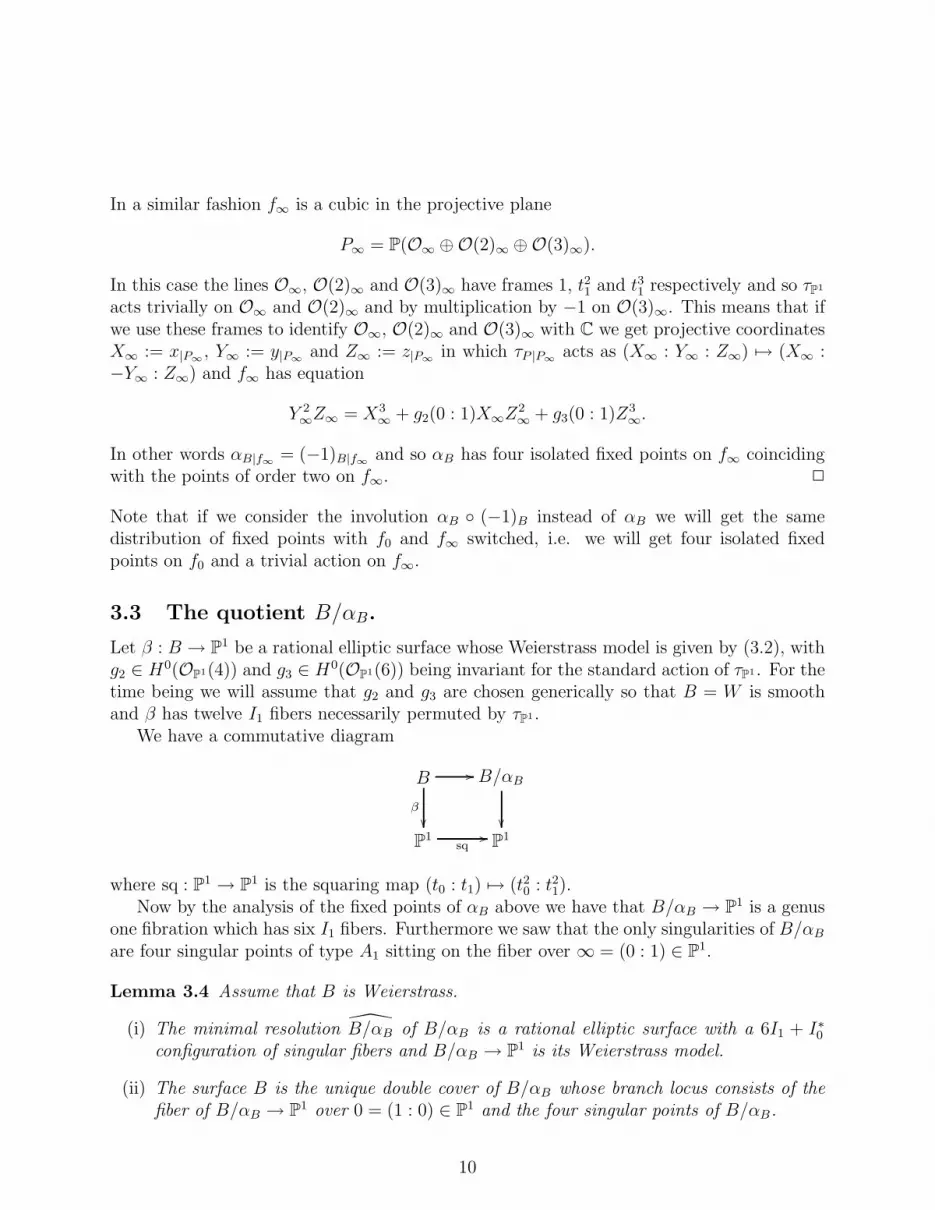
Lemma 3.4 Assume that B is Weierstrass.

(i) The minimal resolution B/αB of B/αB is a rational elliptic surface with a 6I1 + I∗0configuration of singular fibers and B/αB → P1 is its Weierstrass model.

(ii) The surface B is the unique double cover of B/αB whose branch locus consists of thefiber of B/αB → P1 over 0 = (1 : 0) ∈ P1 and the four singular points of B/αB.

10

Proof. By construction B/αB → P1 is a genus one fibered surface with seven singular fibers- six fibers of type I1 (i.e. the images of the twelve I1 fibers of β under the quotient map

B → B/αB) and one I∗0 fiber (i.e. the fiber of B/αB → P1 over ∞ ∈ P1). Moreover sincethe section e : P1 → B is stable under αB we see that e(P1)/αB ⊂ B/αB will again be asection of the genus one fibration that passes through one of the singular points. So the

proper transform of e(P1)/αB in B/αB will be a section of B/αB → P1 which intersects theI∗0 fiber at a point on one of the four non-multiple components. 2

In fact the quotient B → B/αB can be constructed directly as a double cover of the quadricQ ∼= F0 = P1 × P1. In particular this gives a geometric construction of B as an iterateddouble cover of Q.

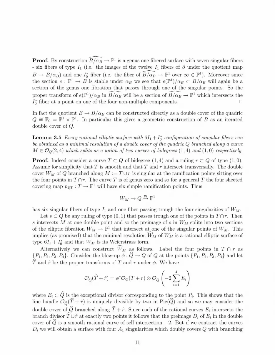
Lemma 3.5 Every rational elliptic surface with 6I1 + I∗0 configuration of singular fibers canbe obtained as a minimal resolution of a double cover of the quadric Q branched along a curveM ∈ OQ(2, 4) which splits as a union of two curves of bidegrees (1, 4) and (1, 0) respectively.

Proof. Indeed consider a curve T ⊂ Q of bidegree (1, 4) and a ruling r ⊂ Q of type (1, 0).Assume for simplicity that T is smooth and that T and r intersect transversally. The doublecover WM of Q branched along M := T ∪ r is singular at the ramification points sitting overthe four points in T ∩ r. The curve T is of genus zero and so for a general T the four sheetedcovering map p1|T : T → P1 will have six simple ramification points. Thus

WM → Qp1→ P1

has six singular fibers of type I1 and one fiber passing trough the four singularities of WM .Let s ⊂ Q be any ruling of type (0, 1) that passes trough one of the points in T ∩r. Then

s intersects M at one double point and so the preimage of s in WM splits into two sectionsof the elliptic fibration WM → P1 that intersect at one of the singular points of WM . Thisimplies (as promised) that the minimal resolution WM of WM is a rational elliptic surface oftype 6I1 + I∗0 and that WM is its Weierstrass form.

Alternatively we can construct WM as follows. Label the four points in T ∩ r asP1, P2, P3, P4. Consider the blow-up φ : Q→ Q of Q at the points P1, P2, P3, P4 and let

T and r be the proper transforms of T and r under φ. We have

OQ(T + r) = φ∗OQ(T + r) ⊗OQ

(−2

4∑

i=1

Ei

)

where Ei ⊂ Q is the exceptional divisor corresponding to the point Pi. This shows that theline bundle OQ(T + r) is uniquely divisible by two in Pic(Q) and so we may consider the

double cover of Q branched along T + r. Since each of the rational curves Ei intersects thebranch divisor T ∪ r at exactly two points it follows that the preimage Di of Ei in the doublecover of Q is a smooth rational curve of self-intersection −2. But if we contract the curvesDi we will obtain a surface with four A1 singularities which doubly covers Q with branching

11

along M = T ∪ r, i.e. we will get the surface WM . In other words the double cover of Qbranched along T + r must be the surface WM . Let ψ : WM → Q and ψ : WM → Q denotethe covering maps and let φ : WM → WM be the blow-up that resolves the singularitiesof WM . Hence the elliptic fibrations on WM and WM are given by the composition mapsω := p1 ψ : WM → P1 and ω := p1 ψ φ : WM → P1 respectively.

Finally to write WM as a quotient WM = B/αB (respectively WM as a quotient WM =

B/αB we proceed as follows. If there exists a Weierstrass rational elliptic surface β : B → P1

so that WM = B/αB, then κ : B → WM will be the unique double cover of WM branchedalong the fiber (WM)0 := ω−1(0) and at the four singular points of WM . In view of the

universal property of the blow-up we may instead consider the unique double cover κ : B →WM which is branched along the divisor (WM)0 +

∑4i=1Di. To see that such a cover exists

observe that ω−1(∞) is a Kodaira fiber of type I∗0 and we have ω−1(∞) = 2V +∑4

i=1Di,

where 2V = ψ∗(r) is the double component of ω−1(∞). This yields

OWM

((WM)0 +

4∑

i=1

Di

)= ω∗OP1(2) ⊗OWM

(−2V )

and so OWM((WM)0 +

∑4i=1Di) is divisible by two in Pic(WM). But from the construction

of WM it follows immediately that π1(WM) = 0 and so Pic(WM) is torsion-free. Due to this

there is a unique square root of the line bundle OWM((WM)0 +

∑4i=1Di) and we get a unique

root cover κ : B → Q as desired.Let Di ⊂ B denote the component of the ramification divisor of κ which maps to Di.

Note that each Di is a smooth rational curve and that since κ∗Di = 2Di we have

Di · Di =1

4κ∗(D2

i ) =1

4· 2 ·D2

i =1

4· 2 · (−2) = −1.

Therefore we can contract the disjoint (−1) curves Di4i=1 to obtain a smooth surface B

which covers WM two to one with branching exactly along (WM)0 and the the four singularpoints of WM . If we now denote the covering involution of κ : B → WM by αB we have

WM = B/αB and WM = B/αB. This construction is clearly invertible, so the lemma a isproven. 2

Corollary 3.6 All rational elliptic surfaces β : B → P1 which admit an involution αB, whichpreserves the zero section e of β and induces an involution on P1, form a five dimensionalirreducible family.

Proof. According to lemma 3.5 every such surface B determines and is determined by thecurve M = T ∪ r ⊂ Q and by the choice of a smooth fiber (WM)0 of WM . The curve Mdepends on dim |OQ(1, 4)|+dim |OQ(1, 0)|−dimAut(Q) = 9+1−6 = 4 parameters. Addingone more parameter for the choice of (WM)0 we obtain the statement of the corollary. 2

12

It is convenient to assemble all the surfaces and maps described above in the followingcommutative diagram:

B

ε

β

κ // WM

φ

ω

ψ// Q

φ

p1

B

β

κ //WM

ω

ψ// Q

p1

P1sq

// P1id

// P1

where the maps φ, φ and ε are blow-ups. The maps ψ, ψ, κ and κ are double covers and ω,ω, β and β are elliptic fibrations.

Now we are ready to look for the involutions τB.Let B and αB be as in the previous section. As explained in Section 3.1, in order to

describe all possible involutions τB we need to describe all sections ζ : P1 → B such thatα∗Bζ = (−1)∗Bζ .

Remark 3.7 The existence of such a section ζ can be shown by solving an equation in thegroup MW. For this, observe that since αB preserves the fibers of β it must send a section toa section. Thus αB induces a bijection αMW : MW → MW, which is uniquely characterizedby the property

c1(αMW([ξ])) = OB(αB(ξ)).

Also, by the definition of (−1)B we know that c1(−[ξ]) = (−1)B(ξ) and hence we need toshow the existence of a section ζ , such that αMW([ζ ]) = −[ζ ].

The first step is to observe that since the isomorphism τ ∗P1B→B preserves the group

structure on the fibers, the induced bijection αMW on sections is actually a group automor-phism.

Next note that for the general B in the five dimensional family from Corollary 3.6, thelattice T has rank two since the general such B has only singular fibers of type I1 and soT = Ze ⊕ Zf . Moreover αB|T = idT , and so the space of anti-invariants of α∗

B acting onPic(B) ⊗ Q injects into the space of anti-invariants of αMW. But in Section 3.3 we showedthat B/αB is again a rational elliptic surface which has four A1 singularities. In particularrk(Pic(B/αB)) = 6 and so there is a 4-dimensional space of anti-invariants for the α∗

B actionon Pic(B) ⊗ Q.

This implies that αMW has a 4 dimensional space of anti-invariants on MW ⊗ Q andhence we can find a section ζ 6= e with αMW([ζ ]) = −[ζ ]. The involution τB correspondingto (αB, ζ) will have only four isolated fixed points.

13

4 The four dimensional subfamily of special rational

elliptic surfaces

From now on we will restrict our attention to a 4-dimensional subfamily of the 5-dimensionalfamily of surfaces of Corollary 3.6. We do this for two reasons:

• Mathematically, this seems to be the simplest family where the full range of possiblebehavior of the spectral involution T = FM−1τ ∗BFM is present, see Proposition 7.1.Indeed, for a generic surface in the five dimensional family, T takes line bundles to linebundles, so everything can be rephrased without the use of the derived category.

• In terms of our motivation from the physics, this specialization is needed for the con-struction of the Standard Model bundles. By taking fiber products of surfaces fromthe five dimensional family one indeed gets a smooth Calabi-Yau with a freely actinginvolution. However, it turns out that for a generic such B, the cohomology of theresulting Calabi-Yau is not rich enough to lead to invariant vector bundles satisfyingthe Chern class constraints from [DOPWa].

4.1 The quotient B/τB

The starting point of the construction of the four dimensional family is the following simpleobservation: since ζ must satisfy α∗

B(ζ) = (−1)∗B(ζ) it will help to work with rational ellipticsurfaces B for which we know the geometric relationship between the two involutions αB and(−1)B. In the previous section we interpreted the involution αB as the covering involutionof the map κ. On the other hand the involution (−1)B was the group inversion along thefibers of β corresponding to a zero section e : P1 → B which was chosen to be one of the twocomponents of the preimage in B of a ruling of type (0, 1) in Q which passes trough one ofthe four points in T ∩ r. Since in this setup the involutions αB and (−1)B are genericallyunrelated it is natural to look for a special configuration of the curves T and r for which(−1)B can be related to the maps κ and ψ.

Lemma 4.1 Consider the family of rational elliptic surfaces B obtained as an iterated doublecover B →WM → Q for which the component T of the branch curve M is split further intoa union T = s∪T where s is a ruling of Q of type (0, 1) and T is a curve of type (1, 3). Letas before e be the section of B mapping to s ⊂ Q. Then we have:

(i) The involution (−1)B,e is a lift of the covering involution of the double cover ψ : WM →P1.

(ii) For a general pair (B, αB) corresponding to a branch curve M = s ∪ T ∪ r there existthree pairs of sections of β labeled by the non-trivial points of order two on f0 and suchthat the two members of each pair are interchanged both by αB and (−1)B.

14

Proof. If the curve T is chosen to be general and smooth, then the branch curve M hasfive nodes P, P1, P2, P3, P4. Here as before P1, P2, P3, P4 = T ∩ r and the extra point Pis the intersection point of the curves T and s.

Let p, p1, p2, p3, p4 ⊂ WM denote the corresponding singularities of WM . Observe thatfor a general choice of the curve T and the point 0 ∈ P1 the singularity p ∈ WM is notcontained in the branch locus (WM)0 ∪p1, p2, p3, p4 of the map κ. In particular the doublecover of WM branched along (WM)0 ∪ p1, p2, p3, p4 will have two A1 singularities at thetwo preimages p1 and p2 of the point p. In order to get a smooth rational elliptic surfacewe have to to blow up this two points. Abusing slightly the notation we will denote by Bthe resulting smooth surface and by κ : B →WM the composition of the blow-up map withthe double cover of WM branched along (WM)0 ∪ p1, p2, p3, p4. Let n1, n2 ⊂ B denote theexceptional curves corresponding to p1 and p2 and let o1, o2 denote proper transforms inB of the two preimages of the fiber ω−1(ω(p)) in the double cover of WM branched along(WM)0 ∪ p1, p2, p3, p4. Here we have labeled o1 and o2 so that p1 ∈ o1 and p2 ∈ o2.From this picture it is clear that β : B → P1 is a smooth rational elliptic surface with a8I1 + 2I2 configuration of singular fibers which is symmetric with respect to the involutionτP1 . Furthermore the two I2 fibers of β are just the curves o1 ∪ n1 and o2 ∪ n2 and the twofixed points 0,∞ of τP1 correspond to two smooth fibers f0 and f∞ of β. Note also thatthe proper transform of the section s ⊂ Q via the generically finite map ψ κ : B → Qis an irreducible rational curve e ⊂ B which is a section of β : B → P1. Moreover theinversion (−1)B with respect to e commutes with the covering involution αB for the map κand descends to an inversion (−1)WM

along the fibers of the elliptic fibration ω : WM → P1

which fixes the image of e pointwise. But by construction the image of e in WM is just thecomponent of the ramification divisor of the cover ψ : WM → Q sitting over s ⊂ Q. Inparticular (−1)WM

is just the covering involution for the map ψ.We are now ready to construct a section ζ : P1 → B of β satisfying α∗

B(ζ) = (−1)B(ζ).Indeed, assume that such a section exists.

Due to the fact that αB|f0 = idf0 we have ζ(0) = −ζ(0) i.e. ζ(0) is a point of order two onf0. Now from the Weierstrass equation (3.2) of B it is clear that the general B cannot havemonodromy Γ0(2) and so without a loss of generality we may assume that ζ 6= −ζ = α∗

Bζ .Consider now the image κ(ζ) ⊂ WM = B/αB of ζ in WM . We have κ−1(κ(ζ)) = ζ ∪ α∗

Bζ .On the other hand the preimage of the general elliptic fiber of ω : WM → P1 via κ splits asa disjoint union of two fibers of β and so αB|f0 = idf0 we have ζ(0) = −ζ(0) i.e. ζ(0) is apoint of order two on f0. Consider now the image κ(ζ) ⊂ WM = B/αB of ζ in WM . Wehave κ−1(κ(ζ)) = ζ ∪ α∗

Bζ . On the other hand the preimage of the general elliptic fiber ofω : WM → P1 via κ splits as a disjoint union of two fibers of β and so

κ(ζ) · ω−1(pt) =1

2κ∗(κ(ζ) · ω−1(pt)) =

1

2(ζ + α∗ζ) · (2β−1(pt)) = 2

i.e. the smooth rational curve κ(ζ) is a double section of ω. Moreover the condition α∗Bζ = −ζ

combined with the property αB|B∞= (−1)B∞

implies that (α∗B)ζ(∞) = ζ(∞) and so the

double cover ω|κ(ζ) : κ(ζ) → P1 is branched exactly over the points 0,∞. Furthermore since

15

ζ(0) is a point of order two on f0 it must lie on the preimage of T in B and so the tworamification points of the cover ω|κ(ζ) : κ(ζ) → P1 must both lie on the ramification divisorof the double cover ψ : WM → Q as depicted on Figure 1.

....

.

.

.

.

..

.

.

.

.

B WM Q

QWMB

0 0 08 8 8

PI 1 IP1 IP1

ψ

ψ

φ φ

p1

κ

κ

ε

β ω

T

r

r

E2

E3E4

D3D4

D1D2

D3D4

κ(ζ)

q

s

E1

Tq

s

.p

2D

D1

ζ−

ζ

en n21

Figure 1: The section ζ

Also note that if we pullback to B the involution of WM acting along the fibers of ψ wewill get precisely (−1)B. Combined with the fact that α∗

Bζ = (−1)∗Bζ this shows that κ(ζ) isstable under the involution of WM acting along the fibers of ψ and so ψ−1(ψ(κ(ζ))) = κ(ζ).Put q := ψ(κ(ζ)). Then q is a smooth rational curve which intersects each of the curvesT and r at a single point so that the double cover ψ|κ(ζ) : κ(ζ) → q is branched exactly atq ∩ (T ∪ r). So q is the unique ruling of type (0, 1) on Q which passes trough the pointψ(κ(ζ(0))) ∈ T ∩Q0.

Conversely if we start with any ruling q of type (0, 1) that passes trough one of the fourpoints in T ∩ f0 we see that ψ−1(q) is a smooth rational curve which is a double cover of qwith branch divisor q ∩ (T ∪ r). Since the rulings of type (1, 0) pull back to a single fiber of

16

ω via ψ we see that

ψ−1(q) · ω−1(pt) = ψ∗(q · p−11 (pt)) = 2q · p−1

1 (pt) = 2,

and so q is a double section of the elliptic fibration ω : WM → P1 which is tangent to thefibers (WM)0 and (WM)∞. Also it is clear that for T and r in general position the point q∩ris not one of the four points in T ∩ r and so the point of contact of ψ−1(q) and (WM)∞ isnot one of the four isolated branch points of the covering κ : B →WM . So ψ−1(q) intersectsthe branch locus of κ at a single point with multiplicity two - namely the point of contact of(WM)0 and ψ−1(q). This implies that the preimage of ψ−1(q) in B splits into two sectionsof β that intersect at a point on the fiber f0 and are exchanged both by αB and (−1)B. Thelemma is proven. 2

Finally, let τB be the involution of B corresponding to the pair (αB, ζ) constructed in theprevious lemma. Then the quotient B/τB is again a genus one fibered rational surface whichsimilarly to B/αB has four A1 singularities all sitting on fiber over ∞ ∈ P1. However B/τBhas also a smooth double fiber and so is only genus one fibered. The minimal resolution ofB/τB in this case has a 4I1 + I2 + I∗0 +2I0 configuration of singular fibers.

4.2 The basis in H2(B,Z)

In order to describe an integral basis of the cohomology of B we need to find a descriptionof our B as a blow-up of P2 in the base points of a pencil of cubics.

To achieve this we will use a different fibration on B, namely the fibration

Bψκ

//

δ

77Qp2 //P1.

induced from the projection of the quadric Q onto its second factor. The fibers of δ canbe studied directly in terms of the degree four map ψ κ : B → Q but it is much moreinstructive to use instead an alternative description of B as a double cover of a quadric.

In section 4.1 we saw that the description of B as an iterated double cover

Bκ→WM

ψ→ Q

of the quadric Q yields two commuting involutions αB and (−1)B on B. By construction thequotient B/αB can be identified with the blow-up of the rational elliptic surface WM at theA1 singularity p ∈WM sitting over the unique intersection point P = s∩T. In particularif we consider the Stein factorization of the generically finite map κ : B →WM we get

B →Wβ →WM .

Here Wβ is the Weierstrass model of β : B → P1 and B → Wβ is the blow-up the twoA1 singularities of Wβ and the map Wβ → WM is the double cover branched at (WM)0 ∪p1, p2, p3, p4.

17

Similarly we can describe the quotients B/(−1)B and B/((−1)B αB) as blow-ups ofappropriate double covers of Q. Indeed the curves on Q that play a special role in thedescription of B as an iterated double cover are: the (1, 3) curve T, the (0, 1) ruling s andthe (1, 0) rulings r = r∞ = p−1

1 (∞) and r0 = p−11 (0).

Consider the double cover ω′ : WM ′ → Q branched along the curve M ′ = T∪r0 = s∪T∪r0and the double cover Sq : Q → Q branched along the union of rulings r0 ∪ r∞. Clearly Qis again a quadric which is just a the fiber product of p1 : Q → P1 with the squaring mapsq : P1 → P1, i.e. we have a fiber-square

QSq

//

p1

Q

p1

P1sq

// P1

The preimage T := Sq−1(T) ⊂ Q of T in Q is a genus two curve doubly covering T withbranching at the six points T∩ (r0 ∪ r∞). Also, the preimage s = Sq−1(s) is a rational curvedoubly covering the ruling s branched at the two points s ∩ (r0 ∪ r∞). In particular, s is a

ruling of type (0, 1) on Q. Similarly, if we denote by r0 and r∞ the two components of the

ramification divisor of Sq : Q→ Q, then r0 and r∞ are rulings of type (1, 0) on Q.Now it is clear that the Weierstrass model Wβ of B can be described as either of the

following

• Wβ → WM is the double cover branched at the fiber (WM)0 and the four pointsp1, p2, p3, p4 of order two of the fiber (WM)∞.

• Wβ → WM ′ is the double cover branched at the fiber (WM)∞ and the four points oforder two of the fiber (WM)0.

• Wβ → Q is the double cover branched at the curve s ∪ T.

Furthermore

• The quotient B/αB → WM is the blow-up of WM at the A1 singularity p sitting overthe point P ∈ Q of intersection of s and T. The map B → B/αB is the double coverof B/αB branched at the fiber (B/αB)0 and the four points of order two of (B/αB)∞.

• The quotient B/(αB (−1)B) → WM ′ is the blow-up of WM ′ at the A1 singularitysitting over the point of intersection of s and T. The map B → B/(αB (−1)B) is thedouble cover of B/(αB (−1)B) branched at the fiber (B/αB)∞ and the four points oforder two of (B/αB)0.

• The quotient B/(−1)B is the blow-up of Q at the two intersection points of s and T.

The map B → B/(−1)B is the double cover branched at the strict transform of s∪ T.

18

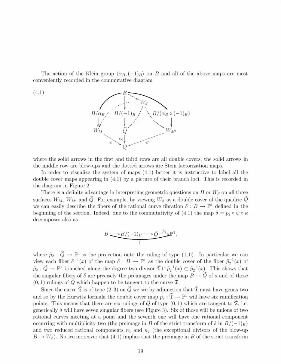
The action of the Klein group 〈αB, (−1)B〉 on B and all of the above maps are mostconveniently recorded in the commutative diagram

B

''Wβ

((

B/αB

B/(−1)B

B/(αB (−1)B)

WM

ψ %%KKKKKKKKKQ

Sq

WM ′

ψ′

uujjjjjjjjjjjjjjjjj

Q

(4.1)

where the solid arrows in the first and third rows are all double covers, the solid arrows inthe middle row are blow-ups and the dotted arrows are Stein factorization maps.

In order to visualize the system of maps (4.1) better it is instructive to label all thedouble cover maps appearing in (4.1) by a picture of their branch loci. This is recorded inthe diagram in Figure 2.

There is a definite advantage in interpreting geometric questions on B or Wβ on all three

surfaces WM , WM ′ and Q. For example, by viewing Wβ as a double cover of the quadric Qwe can easily describe the fibers of the rational curve fibration δ : B → P1 defined in thebeginning of the section. Indeed, due to the commutativity of (4.1) the map δ = p2 ψ κdecomposes also as

B //

δ

44B/(−1)B //Qp2 //P1,

where p2 : Q → P1 is the projection onto the ruling of type (1, 0). In particular we canview each fiber δ−1(x) of the map δ : B → P1 as the double cover of the fiber p−1

2 (x) of

p2 : Q → P1 branched along the degree two divisor T ∩ p−12 (x) ⊂ p−1

2 (x). This shows that

the singular fibers of δ are precisely the preimages under the map B → Q of s and of those(0, 1) rulings of Q which happen to be tangent to the curve T.

Since the curve T is of type (2, 3) on Q we see by adjunction that T must have genus two

and so by the Hurwitz formula the double cover map p2 : T → P1 will have six ramificationpoints. This means that there are six rulings of Q of type (0, 1) which are tangent to T, i.e.generically δ will have seven singular fibers (see Figure 3). Six of those will be unions of tworational curves meeting at a point and the seventh one will have one rational componentoccurring with multiplicity two (the preimage in B of the strict transform of s in B/(−1)B)and two reduced rational components n1 and n2 (the exceptional divisors of the blow-upB →Wβ). Notice moreover that (4.1) implies that the preimage in B of the strict transform

19

Wβ

(1,0)

....sssssssssssssssss

yysssssssssssssssss

(0,1)

(2,3)

....(1,0)

KKKKKKKKKKKKKKKKK

%%KKKKKKKKKKKKKKKKK

WM

(1,3)

(0,1)

(1,0)

KKKKKKKKKKKKKK

%%KKKKKKKKKKKKKK

Q

(1,0)(1,0)

WM ′

(1,3)

(0,1)

(1,0)

ssssssssssssss

yyssssssssssssss

Q

Figure 2: Wβ as a double cover of a quadric

2e

δ

n

6

4

eB

5ee

1 n2

3

e1e2e

...

.

.

P

.I

.

1

Figure 3: The singular fibers of δ

of s in B/(−1)B is precisely the zero section e of the elliptic fibration β : B → P1 and sothe non-reduced fiber of δ is just the divisor 2e + n1 + n2 on B. In fact, one can describeexplicitly the (0, 1) rulings of Q that are tangent to the curve T. Indeed let pt ∈ r0 ∩ T be

20

one of the three intersection points of r0 and T. Choose (analytic) local coordinates (x, y)on a neighborhood pt ∈ U ⊂ Q so that pt = (0, 0), r0 has equation x = 0 in U and the (0, 1)

ruling through pt ∈ Q has equation y = 0 in U . Let U ⊂ Q be the preimage of U in Q.Then there are unique coordinates (u, v) on U such that the double cover U → U is givenby (u, v) 7→ (u2, v) = (x, y). Due to our genericity assumption1 the local equation of T in

U will be x = ay + (higher order terms) for some number a. Thus the pullback of r0 to U

will be given by u = 0 and T will have equation u2 = av + (higher order terms). Since by

construction v = 0 is the local equation of a (0, 1) ruling of Q it follows that T is tangent to

the three (0, 1) rulings of Q passing through the three intersection points in T ∩ r0. In the

same way one sees that T is tangent to the three (0, 1) rulings of Q passing through the three

intersection points in T ∩ r∞. This accounts for all six (0, 1) rulings of Q that are tangent

to T.We are now ready to describe B as the blow-up of P2 at the base locus of a pencil of

cubics. Each component of a reduced singular fiber of δ is a curve of self-intersection (−1)on B. For every such fiber choose one of the components and label it by ei, i = 1, 2, . . . , 6(see Figure 3). Now e, e1, e2, . . . , e6 is a collection of seven disjoint (−1) curves on therational elliptic surface B. The curves n1 and n2 are rational (−2) curves on B and so ifwe contract e each of them will become a (−1) curve. So if we contract e, e1, e2, . . . , e6 andafter that we contract n1 we will end up with a Hirzebruch surface. Moreover numericallye, e + n1, e1, e2, . . . , e6 behave like eight disjoint (−1) curves on B and so the result of thecontraction of e, n1, e1, e2, . . . , e6 should be F1. Contracting the infinity section of F1 we willfinally obtain P2 as the blow down of nine (−1) divisors on B. Let e7 denote the infinity

section of F1. To make things explicit let us identify e7 as a curve coming from Q. Denote bye ⊂ Q the image of e7 in Q. Then e is an irreducible curve which intersects the generic (0, 1)

ruling at one point. This implies that e is of type (1, k) on Q and so e must be a rationalcurve. In particular the map e7 → e ought to be an isomorphism and e7 ∪ (−1)∗B(e7) is thepreimage in B of the strict transform of e in B/(−1)B. Equivalently e7 ∪ (−1)∗B(e7) is thestrict transform in B of the preimage of e in Wβ. This implies that the preimage of e in Wβ

is reducible and so e must have order of contact two with the branch divisor s ∪ T of thecovering Wβ → Q at each point where e and s ∪ T meet. Since e · s = (1, k) · (0, 1) = 1 this

implies that e must pass through one of the two intersection points of s ∩ T and be tangentto T at (e · T − 1)/2 points. But

e · T − 1

2=

(1, k) · (2, 3) − 1

2= k + 1

and so e7 · (−1)∗Be7 = k + 1. From here we can calculate k. Indeed, on one hand we knowthat e27 = −1 and so

(e7 + (−1)∗Be7)2 = −2 + 2 + 2k = 2k.

1We are assuming that T meets r0 and r∞ transversally.

21

On the other hand e7 +(−1)∗Be7 is the preimage in B of the strict transform of e in B/(−1)B.

But B/(−1)B is simply the blow-up of Q at the two intersection points of s and T and e

passes trough only one of those points and so the strict transform of e in B/(−1)B hasself-intersection e2 − 1. In other words

(e7 + (−1)∗Be7)2 = 2(e2 − 1) = 2(2k − 1) = 4k − 2,

and so k = 1.Therefore, in order to reconstruct e7 starting from Q we need to find a (1, 1) curve e on

Q which passes through one of the two points in s∩ T and tangent to T at two extra points.But curves like that always exist. Indeed, the linear system |OQ(1, 1)| embeds Q in P3. Pick

a point J ∈ s ∩ T and let j : Q 99K P2 be the linear projection of Q from that point. Nowthe (1, 1)-curves passing through J are precisely the preimages via j of all lines in P2 and

so the curve e will be just the preimage under j of a line in P2 which is bitangent to j(T).

To understand better the curve j(T) ⊂ P2 note that it has degree (1, 1) · (2, 3) − 1 = 4 and

that the map j : T → j(T) is a birational morphism. Furthermore any (1, 1)-curve passingtrough J and another point on the (1, 0) ruling through J will have to contain the whole

(1, 0) ruling. Since the (1, 0) ruling trough J intersects T at J and two extra pointsJ ′ and

J ′′, it follows that j(J ′) = j(J ′′). Therefore j(T) is a nodal quartic in P2 and the curve

e ⊂ Q corresponds to a bitangent line of this nodal quartic. The normalization of this nodalquartic is just the genus two curve T and the lines in P2 correspond just to sections in thecanonical class ω

Tthat have poles at the two preimages of the node. But a linear system

of degree 4 on a genus two curve is always two dimensional and so the space of lines in P2

is canonically isomorphic with |ωT(J ′ + J ′′)|. In other words, finding the bitangent lines to

j(T) in P2 is equivalent to finding all divisors in |ωT(J ′ + J ′′)| of the form 2D where D is

an effective divisor of degree two on T. Since every degree two line bundle on a genus twocurve is effective we see that finding e just amounts to choosing a non-trivial square root ofthe degree four line bundle ω

T(J ′ + J ′′).

Going back to the description of B as the blow-up of P2 at the base points of a pencil ofcubics assume for concreteness that J is the point in s∩ T corresponding to the exceptionalcurve n1 ⊂ B. Let e ⊂ Q be a (1, 1) curve which passes trough J and is bitangent to T attwo extra points. Let e7 ⊂ B be one of the components of the preimage in B of the stricttransform of e7 in B/(−1)B. Label by e1, . . . , e6 the components of the reduced singularfibers of δ : B → P1 which do not intersect e7. Then e1, . . . , e6 and e and e7 are disjoint(−1) curves on B. After contracting these eight curves and the image of the curve n1 wewill get a P2.

Let c : B → P2 denote this contraction map and let ℓ = c∗OP2(1) be the pullback ofthe class of a line via c. Thus Pic(B) is generated over Z by the classes of the curves ℓ,e1, . . . , e6, e, e7 and n1. In particular, if we put

e9 := ee8 := e+ n1

22

we see that

H2(B,Z) = Zℓ⊕ (⊕9i=1Zei),

with ℓ2 = 1, ℓ · ei = 0 and ei · ej = −δij .

Note that in this basis we have

n1 = e8 − e9

o1 = f − e8 + e9

n2 = ℓ− e7 − e8 − e9

o2 = 2ℓ− e1 − e2 − e3 − e4 − e5 − e6.

(4.2)

4.3 A synthetic construction

Before we proceed with the calculation of the action of τB on H2(B,Z) it will be helpful toanalyze how the surface B and the map c : B → P2 can be reconstructed synthetically fromgeometric data on P2.

First we will need a general lemma describing a birational involution of P2 fixing somesmooth cubic pointwise.

Lemma 4.2 Let Γ ⊂ P2 be a smooth cubic and let b ∈ Γ. There exists a unique birationalinvolution α : P2

99K P2 which preserves the general line through b and fixes the general pointof Γ. Let b1, b2, b3, b4 ∈ Γ be the four ramification points for the linear projection of Γ fromb. Then

(i) α sends a general line to a cubic which is nodal at b and passes through the bi’s.

(ii) α sends the net of conics through b1, b2, b3 to the net of cubics that are nodal at b4 andpass through b, b1, b2, b3.

Proof. Let α : P299K P2 be a birational involution which fixes the general point of the

cubic Γ and preserves the general line through b ∈ Γ. If b ∈ L ⊂ P2 is a general line, thenL ∩ Γ consists of three distinct points b, 0L,∞L. Since α preserves L it follows that α|L isa birational involution of L which fixes the points 0L and ∞L. But any birational involutionof P1 is biregular, has exactly two fixed points and is uniquely determined by its fixed points.Thus the restriction of α on the generic line through b is uniquely determined and so therecan be at most one such α. Conversely we can use this uniqueness to show the existenceof α. Indeed, choose coordinates (x : y : z) in P2 so that b = (0 : 0 : 1) and Γ is given bythe equation F (x, y, z) = 0 with F a homogeneous cubic polynomial. Since b ∈ Γ we canwrite F = F1z

2 + F2z + F3 with Fd a homogeneous polynomial in (x, y) of degree d. Let(x : y : z) be a point in P2 and let L = (x : y : z + t)t∈P1 be the line through b and

23

(x : y : z). The involution α|L will have to fix the two additional (besides b) intersectionpoints of L and Γ. The values of t corresponding to these points are just the roots of theequation F (x, y, z + t) = 0, that is the solutions to

F1(x, y)t2 + Fz(x, y, z)t+ F (x, y, z) = 0.(4.3)

On the other hand since t is the affine coordinate on L the involution α|L : P1 → P1 will begiven by a fractional linear transformation

t 7→ at+ b

ct+ d

for some complex numbers a, b, c and d. The condition that α|L 6= idL but α2|L = idL is

equivalent to d = −a.In these terms the fixed points of α|L correspond to the values of t for which

ct2 − 2at− b = 0.(4.4)

Comparing (4.3) with (4.4) we conclude that a = −(1/2)Fz(x, y, z), b = −F (x, y, z) andc = F1(x, y) and so

α|L((x : y : z + t)) =

(x : y : z − Fz(x, y, z)t+ 2F (x, y, z)

2F1(x, y)t+ Fz(x, y, z)

).

In particular for t = 0 we must have

α((x : y : z)) = α|L((x : y : z)) =

(x : y : z − 2

F (x, y, z)

Fz(x, y, z)

).(4.5)

Now the formula (4.5) clearly defines a birational automorphism α of P2 and it is straight-forward to check that α2 = idP2. This shows the existence and uniqueness of α.

To prove the remaining statements note that the α that we have just defined lifts to a

biregular involution α on the blow-up g : P2 → P2 of P2 at the points b, b1, b2, b3, b4. Let

Σ,Σ1,Σ2,Σ3,Σ4 ⊂ P2 denote the corresponding exceptional divisors and let ℓ = g∗OP2(1)be the class of a line. By definition α preserves the general line through b and the cubic Γ.Hence α will preserve the proper transforms of Γ and the general line through b, i.e.

α(ℓ− Σ) = ℓ− Σ

α

(3ℓ− Σ −

4∑

i=1

Σi

)= 3ℓ− Σ −

4∑

i=1

Σi.

Also it is clear (e.g. from (4.5)) that α identifies the proper transform of the line through band bi with Σi and so

α(Σi) = ℓ− Σ − Σi

24

for i = 1, 2, 3, 4. Therefore we get two equations for α(ℓ) and α(Σ):

α(ℓ) − α(Σ) = ℓ− Σ

3α(ℓ) − α(Σ) = 7ℓ− 5Σ − 2

4∑

i=1

Σi,

which yield α(ℓ) = 3ℓ− 2Σ −∑4

i=1 Σi and α(Σ) = 2ℓ− Σ −∑4

i=1 Σi.If now L is a line not passing through any of the points b, b1, b2, b3, b4 we see that the

proper transform L of L in P2 is an irreducible curve such that α(L) is in the linear system

|3ℓ− 2Σ−∑4

i=1 Σi|. In particular α(L) intersects Σ at two points and intersects each Σi at

a point. So α(L) = g(α(L)) is a cubic which is nodal at b and passes through each of thebi’s. This proves part (i) of the lemma.

Similarly if C is a conic through b1, b2 and b3, then C is an irreducible curve in the linear

system |2ℓ− Σ1 − Σ2 − Σ3| on P2. Hence α(C) is an irreducible curve in the linear system

|3ℓ−Σ−Σ1 −Σ2 −Σ3 − 2Σ4| and so α(C) = g(α(C)) is a cubic passing through b, b1, b2, b3which is nodal at b4. The lemma is proven. 2

For our synthetic construction of B we will start with a nodal cubic Γ1 ⊂ P2 and willdenote its node by A8 ∈ Γ1. Pick four other points on Γ1 and label them A1, A2, A3, A7.For generic such choices there is a unique smooth cubic Γ which passes through the pointsA1, A2, A3, A7, A8 and is tangent to the line 〈A7Ai〉 at the point Ai for i = 1, 2, 3 and 8.Consider the pencil of cubics spanned by Γ and Γ1. All cubics in this pencil pass throughA1, A2, A3, A7, A8 and are tangent to Γ at A8. Let A4, A5, A6 be the remaining three basepoints. Each cubic in the pencil intersects the line N2 := 〈A7A8〉 in the same divisorA7 + 2A8 ∈ Div(N2). Therefore there is a reducible cubic Γ2 = N2 ∪ O2 in the pencil.Generically O2 will be a smooth conic as depicted on Figure 4. By Lemma 4.2 there is a

.

...

. ...

Γ1

A7

A1A2

A3

A4 A5

A6

A8

N2

O2

9A

Figure 4: The pencil of cubics determining B

birational involution α of P2 corresponding to Γ with b = A7. Note that by construction

25

bi = Ai for i = 1, 2, 3 and b4 = A8. By Lemma 4.2(ii) we know that α(O2) is a nodalcubic with a node at A8 which passes through A1, A2, A3 and A7. Since the involution αfixes A4, A5, A6 ∈ Γ it also follows that α(O2) contains A4, A5, A6. The intersection numberα(O2) with Γ1 is therefore at least 6 + 2 · 2 = 10 and so α(O2) = Γ1. Moreover α collapsesN2 to A8. This shows that α preserves the pencil.

We define B to be the blow-up of P2 at the points Ai, i = 1, . . . , 8 and the point A9

which is infinitesimally near to A8 and corresponds to the tangent direction N2. The pencilof cubics becomes the anticanonical map β : B → P1. The reducible fibers are fi = ni ∪ oi,i = 1, 2 where n2, o2 are the proper transforms of N2, O2, o1 is the proper transform of Γ1

and n1 is the proper transform of the exceptional divisor corresponding to A8. In order toconform with the notation in Section 2 we denote by ei for i = 1, . . . , 7 and 9 the exceptionaldivisors corresponding to Ai, i = 1, . . . , 7 and 9 and by e8 the reducible divisor e9 + n1.

The involution α : P299K P2 lifts to a biregular involution αB : B → B. The induced

involution τP1 of P1 has two fixed points 0,∞ ∈ P1. One of them, say 0, will be the imageβ(Γ). We will use e9 as the zero section e : P1 → B. Note that (−1)∗Bei = α∗

Bei for i = 1, 2, 3and so we can take ζ = e1.

5 Action on cohomology

First we describe the action of the automorphisms (−1)B, αB, tζ and τB on H•(B,Z).

5.1 Action of (−1)B

From the discussion in section 4.2 it is clear that (−1)B preserves the fibers of δ : B → P1

and exchanges the two components of the six singular fibers of δ which are unions of tworational curves meeting at a point. Furthermore from the description of B as a blow-up ofP2 at nine points (see section 4.2) it follows that the class of the fiber of δ is ℓ− e7. Hence(−1)B(ℓ − e7) = ℓ − e7 and (−1)B(ei) + ei = ℓ − e7 for i = 1, . . . , 6. Also, by the sameanalysis we see that (−1)B preserves n1 and n2 and since (−1)B preserves f by definition,it follows that (−1)B preserves o1 and o2 as well. Similarly (−1)B preserves e9 by definitionand so (−1)∗B(e8) = (−1)∗B(e9 + n1) = e9 + n1 = e8. Finally we can solve the equations(−1)∗B(ℓ − e7) = ℓ − e7 and (−1)∗B(o2) = o2 to get (−1)B(ℓ) = f + ℓ − 2e7 + e8 + e9 and(−1)∗B(e7) = f − e7 + e8 + e9.

5.2 Action of αB

Again from the analysis in section 4.2 and the geometric description of B/αB and its Weier-strass model WM we see that αB preserves the classes of the fibers of the two fibrationsβ : B → P1 and δ : B → P1. In particular we have α∗

B(f) = f , α∗B(ℓ − e7) = ℓ − e7

and α∗B(e9) = e9. Also αB interchanges o1 and o2 and hence interchanges n1 and n2. From

the relationship between the ramification divisors defining WM and Q we see that αB willexchange the two components of the three singular fibers of δ corresponding to the three

26

intersection points in T ∩ r0, i.e. α∗B(ej) + ej = ℓ − e7 for j = 1, 2, 3. Similarly αB will

preserve the two components of the singular fibers of δ corresponding to the three inter-section points in T ∩ r∞, that is α∗

B(ei) = ei for i = 4, 5, 6. Finally, solving the equationsα∗B(ℓ − e7) = ℓ − e7 and α∗

B(o1) = o2 we get α∗B(ℓ) = 3ℓ − e1 − e2 − e3 − 2e7 − e8 and

α∗B(e7) = 2ℓ− e1 − e2 − e3 − e7 − e8.

5.3 Action of t∗ζ

By definition we have t∗ζ(f) = f . In order to find the action of tζ on the classes ei we will

use the fact that tζ is defined in terms of the addition law on β# : B# → P1.Since tζ preserves each fiber of β : B → P1, the curve t∗ζ(n1) will have to be either n1 or

o1. But ζ = e1 and so ζ · n1 = 0 and ζ · o1 = 1, so since n#1 is the identity component of the

disconnected group n#1 ∪ o#

1 = (n1 ∪ o1) − (n1 ∩ o1), we must have t∗ζ(n1) = o1. In the sameway one can argue that t∗ζ(n2) = o2 and t∗ζ(oi) = ni for i = 1, 2.

Next note that since tζ is compatible with the group scheme structure of B# we musthave t∗ζ(ξ) = c1([ξ] − [ζ ]) for any section ξ of β. Using this relation we calculate:

t∗ζ(e1) = c1([e1] − [e1]) = e9,

t∗ζ(e9) = c1([e9] − [e1]) = (−1)B([e1]) = ℓ− e1 − e7,

which in turn implies t∗ζ(e8) = t∗ζ(e9 + n1) = ℓ− e1 − e7 + o1 = f + ℓ− e1 − e7 − e8 + e9.The previous formulas identify cohomology classes in H2(B,Z) or equivalently line bun-

dles on B. However observe that the above formulas can also be viewed as equality ofdivisors, due to the fact that the line bundles in question correspond to sections of β, andso each of these is represented by a unique (rigid) effective divisor.

Also since the addition law on an elliptic curve is defined in terms of the Abel-Jacobimap we see that for a section ξ of β, the restriction of the line bundle c1([ξ]− [e1])⊗OB(−e9)to the generic fiber of β will be the same as the restriction of OB(ξ − e1). By the see-sawprinciple the difference of these two line bundles will have to be a combination of componentsof fibers of β, i.e.

t∗ζ(ξ) = c1([ξ] − [e1]) = ξ − e1 + e9 + aξ1n1 + aξ2n2 + aξf.

Intersecting both sides with n1 and taking into account that (t−1ζ )∗(n1) = o1 we get o1 · ξ =

ξ · n1 + 1 − 2aξ1. Similarly when we intersect with n2 we get o2 · ξ = ξ · n2 + 1 − 2aξ2. Inparticular since for i = 2, . . . , 6 we have ei · n1 = ei · n2 = 0 and ei · o1 = ei · o2 = 1 we getaei

1 = aei2 = 0 and so t∗ζ(ei) = ei − e1 + e9 + aeif . Using the fact that (t∗ζ(ei))

2 = −1 we findthat aei = 1 and thus

t∗ζ(ei) = ei − e1 + e9 + f

for i = 2, . . . , 6.

27

Finally, for e7 we have e7 ·n1 = e7 ·o2 = 0 and e7 ·n2 = e7 ·o1 = 1 and so t∗ζ(e7) = e7−e1 +e9 + n2 + ae7f . From (t∗ζ(e7))

2 = −1 we find ae7 = 0 and therefore t∗ζ(e7) = e7 − e1 + e9 + n2.This completes the calculation of the action of t∗ζ on H2(B,Z). The action of τ ∗B is easily

obtained since by definition we have τ ∗B = α∗B t∗ζ .

All these actions are summarized in Table 1 below.

(−1)∗B t∗ζ α∗B τ ∗B

f f f f fe1 ℓ− e1 − e7 e9 ℓ− e1 − e7 e9ej , ℓ− ej − e7 f + ej − e1 + e9 ℓ− ej − e7 f − ej + e1 + e9j = 2, 3ei, ℓ− ei − e7 f + ei − e1 + e9 ei f − ℓ+ ei+i = 4, 5, 6 +e1 + e7 + e9e7 f − e7 + e8 + e9 ℓ− e1 − e8 2ℓ− (e1 + e2+ ℓ− e2 − e3

+e3 + e7 + e8)e8 e8 f + ℓ+ e9− ℓ− e7 − e8 f − ℓ+ e1+

−e1 − e7 − e8 +e7 + e8 + e9e9 e9 ℓ− e1 − e7 e9 e1

ℓ ℓ+ f− 2f + 2ℓ− 3e1− 3ℓ− (e1 + e2+ 2f + 2(e1 + e9)−−2e7 + e8 + e9 −e7 − e8 + 2e9 +e3 + 2e7 + e8) −(e2 + e3) + e7

Table 1: Action of (−1)B, αB, tζ and τB on H•(B,Z)

6 The cohomological Fourier-Mukai transform

For the purposes of the spectral construction we will need also the action of the relativeFourier-Mukai transform for β : B → P1 on the cohomology of B. By definition the Fourier-Mukai transform is the exact functor on the bounded derived category Db(B) of B given bythe formula

FMB : Db(B) // Db(B)

F //R•p1∗(p

∗2F

L⊗ PB).

Here p1, p2 are the projections of B ×P1 B to its two factors, and PB is the Poincare sheaf:

PB := OB(∆ − e×P1 B −B ×P1 e− q∗OP1(1)),

with q = β p1 = β p2. Using the zero section e : P1 → B we can identify B with therelative moduli space M(B/P1) of semistable (w.r.t. to a suitable polarization), rank one,

28

degree zero torsion free sheaves along the fibers of β : B → P1. Under this identification,the sheaf PB → B ×P1 B = B ×P1 M(B/P1) becomes the universal sheaf. This puts us inthe setting of [BM, Theorem 1.2] and implies that FMB is an autoequivalence of Db(B). Inparticular we can view any vector bundle V → B in two different ways - as V and as theobject FMB(V ) ∈ Db(B).

The cohomological Fourier-Mukai transform is defined as the unique linear map

fmB : H•(B,Q) → H•(B,Q)

satisfying:

fmB ch = ch FMB.(6.1)

Explicitly,

fmB(x) = pr2∗(pr∗1(x) · ch(j∗P) · td(B × B)) · td(B)−1,

where pri are the projections of B×B to its factors and j : B×P1 B → B×B is the naturalinclusion.

We will need an explicit description of the cohomological spectral involution

tB := fm−1B τ ∗B fmB.

For this we proceed to calculate the action of fmB and fm−1B in the obvious basis in

cohomology.Let pt ∈ H4(B,Z) denote the class Poincare dual to the homology class of a point in B

and let 1 ∈ H0(B,Z) be the class which is Poincare dual to the fundamental class of B. Theclasses 1, f , e1, . . . , e9, pt constitute a basis of H•(B,Q).

To calculate fmB we will use the identity (6.1) together with a calculation of the actionof FMB on certain basic sheaves, which is carried out in Lemma 6.1 below.

The first observation is that there are two ways to lift a sheaf G on P1 to a sheaf on B.First we may consider the pullback β∗(G). Second, for any section ξ : P1 → B of β we mayform the push-forward ξ∗G. These two lifts behave quite differently. For example, if G is aline bundle, then β∗G is a line bundle on B, whereas ξ∗G is a torsion sheaf on B supportedon ξ. The action of FMB interchanges these two types of sheaves (up to a shift):

Lemma 6.1 For any sheaf G on P1 and any section ξ of β we have:

FMB(β∗G) = e∗(G⊗OP1(−1))[−1]FMB(ξ∗G) = β∗G⊗OB(ξ − e) ⊗ β∗OP1(−e · ξ − 1),

where as usual for a complex K• = (Ki, diK) and an integer n ∈ Z we put K•[n] for thecomplex having (K[n])i = Kn+i and dK[n] = (−1)ndK.

29

Proof. By definition we have FMB(β∗G) = Rp2∗(p∗1β

∗G ⊗ PB). But β p1 = β p2 andso by the projection formula we get FMB(β∗G) = Rp2∗(p

∗2β

∗G⊗ PB) = β∗G⊗Rp2∗PB. Inorder to calculate Rp2∗PB, note first that Rp2∗PB is a complex concentrated in degrees zeroand one since p2 is a morphism of relative dimension one. Next observe that R0p2∗PB = 0.Indeed, by definition PB is a rank one torsion free sheaf on B ×P1 B, and so R0p2∗PB mustbe a torsion free sheaf on B. On the other hand, from the definition of PB we see that bothR0p2∗PB and R1p2∗PB are torsion sheaves on B whose reduced support is precisely e ⊂ B.Therefore R0p2∗PB is torsion and torsion free at the same time and so R0p2∗PB = 0 . Thisimplies that Rp2∗PB = R1p2∗PB[−1]. Now, since R2p2∗PB = 0 we can apply the cohomologyand base change theorem [Har77, Theorem 12.11] to conclude that R1p2∗PB has the basechange property for arbitrary (i.e. not necessarily flat) morphisms. In particular consideringthe base change diagram

B = B ×P1 e

//

β

B ×P1 B

p2

P1

e// B

we have that

e∗R1p2∗PB = R1β∗(PB|B×P1e) = R1β∗OB = (β∗ωB/P1)∨

= (β∗(OB(−f) ⊗ β∗O(2)))∨ = OP1(−1).

Since e ⊂ B is the reduced support of R1p2∗PB and (R1p2∗PB)|e is a line bundle, it fol-lows that e ⊂ B is actually the scheme theoretic support of R1p2∗PB and so R1p2∗PB =e∗OP1(−1), which finishes the proof of the first part of the lemma.

Let now ξ : P1 → B be a section of β. Then FMB(ξ∗G) = Rp2∗(p∗1ξ∗G⊗PB). But p∗1ξ∗G

is a sheaf onB×P1B supported on ξ×P1B ⊂ B×P1B and is in fact the extension by zero of thesheaf β∗G on B = ξ×P1B. Moreover by definition we have PB|ξ×

P1B = OB(ξ−e−(e·ξ+1)f).Taking into account that p2 : ξ ×P1 B → B is an isomorphism, we get the second statementof the lemma. 2

With all of this said we are now ready to derive the explicit formulas for fmB. First,observe that ch(OB) = 1 and so by (6.1) and Lemma 6.1 we have

fmB(1) = ch(FMB(OB)) = ch(FMB(β∗OP1))= ch(e∗(OP1(−1))[−1]) = −ch(e∗(OP1(−1)).

But from the short exact sequence of sheaves on B

0 → OB(−e− f) → OB(−f) → e∗OP1(−1) → 0

we calculate

ch(e∗(OP1(−1)) = ch(OB(−f)) − ch(OB(−e− f))

= (1 − f + 0 · pt) ·(

1 + (e− f) +1

2pt

)

= e− 1

2pt .

30

In other words fmB(1) = −e+ (1/2) pt = −e9 + (1/2) pt.Next we calculate fmB(pt). Let t ∈ P1 be a fixed point. Then pt = ch(Oe(t)) = ch(e∗Ot)

and so

fmB(pt) = ch(FMB(e∗Ot))= ch(Of ) = ch(OB) − ch(OB(−f))= 1 − (1 − f + 0 · pt) = f.

To calculate fmB(f) note that ch(OB(f)) = 1 + f and so

fmB(f) = ch(FMB(OB(f))) − fmB(1)= ch(FMB(β∗OP1(1))) − fmB(1)

= ch(e∗OP1[−1]) −(−e+

1

2pt

)

= −[ch(OB) − ch(OB(−e))] + e− 1

2pt

= −[1 −

(1 − e− 1

2pt

)]+ e− 1

2pt

= − pt .

Finally we calculate fmB(ei). If i = 1, . . . , 7, the class ei is a class of a section ei : P1 → Bof β and so we can apply Lemma 6.1 to Oei

. We have ch(Oei) = ei + (1/2) pt and hence

fmB(ei) = ch(FMB(Oei)) − 1

2fmB(pt)

= ch(FMB(ei∗OP1)) − 1

2fmB(pt)

= ch(OB(ei − e9 − f)) − 1

2f

= 1 + (ei − e9 − f) − pt−1

2f

= 1 + (ei − e9 −3

2f) − pt .

For e9 we get in the same way

fmB(e9) = ch(OB) − 1

2f = 1 − 1

2f,

and so it only remains to calculate fmB(e8).Unfortunately we can not use the same method for calculating fmB(e8) since e8 is only a

numerical section of β and splits as a union of two irreducible curves e8 = e9 +n1. However,recall that the automorphism αB : B → B moves a section to a section. Consequently αB(e7)will be another section of β. Let a : P1 → B denote the map corresponding to αB(e7). Then

ch(OαB(e7)) = ch(OB) − ch(OB(−αB(e7)) = αB(e7) +1

2pt .

31

Thus

fmB(αB(e7)) = ch(FMB(a∗OP1)) − 1

2f = ch(OB(αB(e7) − e9 − (e9 · αB(e7) + 1)f) − 1

2f.

But according to Table 1 we have e9 · αB(e7) = e9 · (2ℓ− e1 − e2 − e3 − e7 − e8) = 0 and so

fmB(αB(e7)) = 1 + αB(e7) − e9 −3

2f − pt .

In terms of e8 this reads

2fmB(ℓ) − fmB(e8) = 1 + 2ℓ−3∑

i=1

ei − e7 − e8 − e9 −3

2f − pt+fmB(

3∑

i=1

ei + e7)

= 1 + 2ℓ−3∑

i=1

ei − e7 − e8 − e9 −3

2f − pt+

+

(4 +

3∑

i=1

ei + e7 − 4e9 − 6f − 4 pt

)

= 5 + (2ℓ− 15

2f − e8 − 5e9) − 5 pt .

Also from fmB(f) = − pt we get

3fmB(ℓ) − fmB(e8) = 8 + (3ℓ− 12f − e8 − 8e9) − 8 pt .

Solving these two equations for fmB(e8) results in

fmB(e8) = 1 + (e8 − e9 −3

2f) − pt,

which completes the calculation of fmB.In summary, the action of t and the auxiliary actions of fmB and fm−1

B are recordedin tables 3 and 2 respectively.

fmB fm−1B

1 −e9 + 12pt e9 + 1

2pt

pt f −ff − pt ptei, 1 + ei − e9 − 3

2f − pt −1 + ei − e9 − 3

2f + pt

i 6= 9e9 1 − 1

2f −1 − 1

2f

Table 2: Action of the cohomological Fourier-Mukai transform

32

tB

1 1pt ptf fej 2f + 2e9 − ej − 2 ptj = 1, 2, 3ei, 2f − ℓ+ 2e9 + e7 + ei − pti = 4, 5, 6e7 f + ℓ− e1 − e2 − e3 + e9 − pte8 2f − ℓ+ 2e9 + e7 + e8 − pte9 e9

ℓ 5f − e1 − e2 − e3 + e7 + 5e9 − 3 pt

Table 3: Action of fm−1B τ ∗B fmB on cohomology

7 Action on bundles

In this section we show how the cohomological computations in the previous section lift toactions of the Fourier-Mukai transform FMB and the spectral involution T B := FM−1

B τ ∗BFMB on (complexes of) sheaves on B. Recall that the Chern character intertwines FMB

and fmB: fmB ch = ch FMB. Similarly, it intertwines TB and tB: tB ch = ch TB.Note that the Fourier-Mukai transform of a general sheaf F on B is a complex of sheaves,

not a single sheaf. Nevertheless, all the sheaves we are interested in are taken by TB again tosheaves. To explain what is going on exactly we will need to introduce some notation first.Put c1 : Db(B) → Pic(B) for the first Chern class map in Chow cohomology. In combinationwith T B, the map c1 induces a well defined map

Pic(B) → Coh(B) ⊂ Db(B)TB→ Db(B)

c1→ Pic(B),(7.1)

where Pic(B) denotes the Picard category whose objects are all line bundles on B and whosemorphisms are the isomorphisms of line bundles. Since TB is an autoequivalence, the map(7.1) descends to a well defined map of sets

TB : Pic(B) = π0(Pic(B)) → Pic(B).

If we identify Pic(B) and H2(B,Z) via the first Chern class map, we can describe TB

alternatively as TB(−) = [tB(exp(c1(−)))]2 ∈ H2(B,Z).Denote by PicW (B) ⊂ Pic(B) the subgroup generated by f and the classes of all sections

of β that meet the neutral component of each fiber. A straightforward calculation showsthat PicW (B) = Span(f, e9, f + ei− e1 + e96

i=2, 2e7 − e8 + 2f) (note that f + ei− e1 + e9 isthe class of the section [ei]− [e1] and 2e7 − e8 + 2f is the class of the section 2[e7]) and thatSpan(o1, o2)

⊥ = Span(e9, ei− e16i=2, ℓ− e7 − 2e1, 2ℓ− e8 − 4e1). In particular PicW (B) is a

sublattice of index 3 in Span(o1, o2)⊥. With this notation we have:

33

Theorem 7.1 Let L be a line bundle on B. Then

(i) The complex TB(L) ∈ D[0,1](B) becomes a line bundle when restricted on the open setB− (o1 ∪ o2). More precisely, the zeroth cohomology sheaf H0(T B(L)) is a line bundleon B and the first cohomology sheaf H1(TB(L)) is supported on the divisor o1 + o2.

(ii) The map T B satisfies

TB(L) = τ ∗B(L) ⊗OB((c1(L) · (e− ζ))f + (c1(L) · f + 1)(e− ζ + f)).

(iii) For every L ∈ PicW (B) the image TB(L) is a line bundle on B and so

TB(L) = τ ∗B(L) ⊗OB((c1(L) · (e− ζ))f + (c1(L) · f + 1)(e− ζ + f)).

In particular T B : PicW (B) → (PicW (B) + (e− ζ + f)) ⊂ Pic(B) is an affine isomor-phism.

Proof. The proof of this proposition is rather technical and involves some elementary butlong calculations in the derived category Db(B).

Since TB = FM−1B τ ∗B FMB we need to understand FM−1

B . The following lemma isstandard.

Lemma 7.2 The inverse FM−1B of the Fourier-Mukai functor FMB is isomorphic to the

functor

DB FMB DB : Db(B) → Db(B),

where DB is the (naive) Serre duality functor DB(F ) := R•Hom(F, ωB) with ωB being thecanonical line bundle on B.

Proof. It is well known (see e.g. [Orl97, Section 2]) that FMB has left and right adjointfunctors FM ∗

B and FM !B which are both isomorphic to FM−1

B . Furthermore, these adjointfunctors can be defined by explicit formulas, see [Orl97, Section 2], e.g. the right adjoint isgiven by:

FM !B(F ) = R pr1∗(pr∗2 F

L⊗ P∨))⊗ωB[2].

Here pri : B×B → B are the projections onto the two factors, P → B×B is the extensionby zero of PB and K∨ := R•Hom(K,OB×B). Using e.g. the formula for the right adjointfunctor, the relative duality formula [Har66] and the fact that ωB is a line bundle, onecalculates

FM !B(F ) = R pr1∗(pr∗2 F

L⊗ P∨)⊗ωB[2]

= R pr1∗((pr∗2 FL⊗ P∨) ⊗ pr∗2 ωB[2] ⊗ pr∗2 ω

−1B ) ⊗ ωB

= R pr1∗(pr∗2(F ⊗ ω−1B )

L⊗ P∨ ⊗ pr∗2 ωB[2]) ⊗ ωB

= (R pr1∗(pr∗2(F∨ ⊗ ωB)

L⊗ P)∨ ⊗ ωB

= (FMB(DB(F )))∨ ⊗ ωB= DB FMB DB(F ).

34

which proves the lemma. 2

Next observe that Pic(B) is generated by all sections of β. Indeed Pic(B) is generatedby ℓ and e1, e2, . . . , e9. The divisor classes e1, . . . , e7 and e9 are already sections of β. AlsoαB(e1) = ℓ− e1 − e9 is a section and so ℓ is contained in the group generated by all sections.Furthermore, αB(e7) = 2ℓ− e1 − e2 − e3 − e7 − e8 is a section and so e8 is contained in thegroup generated by all sections.

In view of this it suffices to prove parts (i) and (ii) of the theorem for line bundles of theform L = OB(

∑aiξi) where ai ∈ Z and ξi are sections of β.

Put V0 := e∗OP1(−1). Consider the group Ext1(V0,OB) of extensions of V0 by OB.Since e2 = −1 we have V0 = e∗e

∗OB(e) and so V0 fits in a short exact sequence

0 → OB → OB(e) → V0 → 0.(7.2)

In particular we have a quasi-isomorphism [OB → OB(e)]→V0 where in the complex

[OB → OB(e)],

the sheaf OB is placed in degree −1 and OB(e) is placed in degree 0. Thus we have

Ext1(V0,OB) = HomDb(B)(V0,OB[1]) = HomDb(B)([OB → OB(e)],OB[1])= H0(B, [OB → OB(e)]∨[1]) = H0(B, [OB(−e) → OB]),

where in the complex [OB(−e) → OB] the sheaf OB is placed in degree zero. In par-ticular we have a quasi-isomorphism [OB(−e) → OB]→e∗OP1 and hence Ext1(V0,OB) =H0(B, e∗OP1) = C. This shows that there is a unique (up to isomorphism) sheaf V1 which isa non-split extension of V0 by OB. But from (7.2) we see that the line bundle OB(e) is onesuch extension, i.e. we must have V1

∼= OB(e).Next consider the group of extensions Ext1(V1,OB(f)) = H1(B,V∨

1 ⊗ O(f)). By theLeray spectral sequence we have a short exact sequence

0 → H1(P1, (β∗V∨1 ) ⊗O(1)) → H1(B,V∨

1 ⊗O(f)) → H0(P1, (R1β∗V∨1 ) ⊗O(1)) → 0.

But β∗(V∨1 ) = β∗O(−e) = 0 andR1β∗(V∨

1 ) = R1β∗O(−e) = O(−1). Thus Ext1(V1,OB(f)) =H0(P1,O) = C and so there is a unique (up to isomorphism) non-split extension

0 → OB(f) → V2 → V1 → 0.

Arguing by induction we see that for every a ≥ 1 there is a unique up to isomorphismvector bundle Va → B of rank a on B satisfying β∗(V∨

a ) = 0, R1β∗(V∨a ) = O(−a) and

Ext1(Va,OB(af)) = C is generated by the non-split short exact sequence

0 → OB(af) → Va+1 → Va → 0.

Alternatively, for each positive integer we can consider the vector bundle Ψa of rank a whichis defined recursively as follows:

35

• Ψ1 := OB, and

• Ψa+1 is the unique non-split extension

0 → OB(af) → Ψa+1 → Ψa → 0.

The fact that the Ψa’s are correctly defined can be checked exactly as above. Moreoverfor each a ≥ 1 Va can be identified with the unique non-split extension

0 → Ψa → Va → e∗OP1(−1) → 0.

Let now ξ : P1 → B be a section of β. The first step in calculating TB is given in thefollowing lemma.

Lemma 7.3 For any integer a we have

FM(OB(aξ)) =

V−a ⊗OB(ξ − e− (ξ · e+ 1)f)[−1], for a ≤ 0

V∨a ⊗OB(−f) ⊗OB(ξ − e− (ξ · e+ 1)f), for a > 0

Proof. By Lemma 6.1 we know that FMB(OB) = e∗O(−1)[−1] which gives the statementof the lemma for a = 0. To prove the statement for a = −1 consider the short exact sequence

0 → OB(−ξ) → OB → ξ∗OP1 → 0(7.3)

of sheaves on B. For an object K ∈ Db(B) let FM iB(K) denote the i-th cohomology sheaf

of the complex FMB(K). Since FMB is an exact functor on Db(B) it sends any shortexact sequence to a long exact sequence of cohomology sheaves. Applying FMB to (7.3)and using Lemma 6.1 we get

0 // FM 0B(OB(−ξ)) // 0 // OB(ξ − e− (1 + ξ · e)f) "%#$

'&--[[[

FM 1B(OB(−ξ)) // e∗O(−1) // 0.

Thus FM 0B(OB(−ξ)) = 0 and FM 1

B(OB(−ξ)) fits in a short exact sequence

0 → OB(−e) → FM 1B(OB(−ξ)) ⊗O(−ξ + (1 + ξ · e)f) → e∗OP1 → 0.(7.4)

Since (7.3) is non-split and FMB is an additive functor, it follows that (7.4) will not split.But Ext1(e∗OP1 ,OB(−e)) = Ext1(e∗OP1(e),OB) = C as we saw above and therefore we musthave

FMB(OB(−ξ)) ∼= OB(ξ − (1 + ξ · e)f)[−1] = V1 ⊗OB(ξ − e− (1 + ξ · e)f)[−1].

36

Assume that the Lemma is proven for OB(−aξ) for some positive a. Then we have a shortexact sequence of sheaves on B

0 → OB(−(a + 1)ξ) → OB(−aξ) → ξ∗OP1(a) → 0.(7.5)

Applying FMB to (7.5) and using Lemma 6.1 we get

0 // FM 0B(O(−(a + 1)ξ)) // 0 // O(ξ − e+ (a− 1 − ξ · e)f) "%#$

'&--\\\

FM 1B(O(−(a + 1)ξ)) // FM 1

B(O(−aξ)) // 0.

and so again FM 0B(OB(−(a+1)ξ)) = 0. Furthermore, by the inductive hypothesis we have

FM 1B(O(−aξ)) = Va ⊗OB(ξ − e− (1 + ξ · e)f) and so by the same reasoning as above the

short exact sequence

0 → OB(af) → FM 1B(OB(−(a + 1)ξ)) ⊗O(e− ξ + (1 + ξ · e)f) → Va → 0

must be non-split. Since Va+1 is the only such non-split extension, we must have

FMB(OB(−(a + 1)ξ)) = Va+1 ⊗OB(ξ − e− (1 + ξ · e)f)[−1].

This completes the proof of the lemma for all a ≤ 0. The argument for a > 0 is exactly thesame and is left as an exercise. 2

The next step is to calculate the action of T B on line bundles of the form OB(aξ).Due to Lemma 7.2 we have TB = DB FMB DB τ ∗B FMB. Since τB is an

automorphism of B we have DB τ ∗B = τ ∗B DB and so

TB = (DB FMB) τ ∗B (DB FMB).(7.6)

To calculate DB(FMB(OB(aξ)) we need to distinguish two cases: a = 0 and a 6= 0. Whena = 0, we have DB((FMB(OB)) = DB(e∗O(−1)[−1]). But as we saw above the short exactsequence (7.2) induces a quasi-isomorphism

OB

↓OB(e)

0

1

q.i.−→ e∗O(−1)[−1].

Applying duality one gets

DB(e∗O(−1)[−1]) =

OB(−e)↓OB

−1

0⊗OB(−f) =

OB(−e− f)↓

OB(−f)

−1

0= e∗OP1(−1).

But for a 6= 0 the sheaves FMB(OB(aξ)) are locally free and so we get

DB FMB(OB(aξ)) =

V∨−a ⊗OB(e− ξ + (ξ · e)f)[1], for a < 0

V0, for a = 0

Va ⊗OB(e− ξ + (1 + ξ · e)f), for a > 0.

37

To apply τ ∗B next we need to calculate τ ∗BVa. For this recall that Va is isomorphic to theunique non-split extension

0 → Ψa → Va → e∗OP1(−1) → 0.

Since τB(f) = f and Ψa is built by successive extensions of multiples of f , it follows thatτ ∗BΨa

∼= Ψa for every a. So Wa := τ ∗BVa is the unique non-split extension

0 → Ψa → Wa → ζ∗OP1(−1) → 0,

where as before ζ = τ ∗B(e). With this notation we have

τ ∗B DB FMB(OB(aξ)) =

W∨−a ⊗OB(ζ − τ ∗B(ξ) + (ξ · e)f)[1], for a < 0

ζ∗OP1(−1), for a = 0

Wa ⊗OB(ζ − τ ∗B(ξ) + (1 + ξ · e)f), for a > 0.

Now to finish the calculation of T B(OB(aξ)) we have to work out FMB(Wa ⊗OB(ζ − φ))and FMB(W∨

a ⊗ OB(ζ − φ)) for all a > 0 and all sections φ : P1 → B of β. Again weproceed by induction in a.

Let a = 1. By definition W1 is the unique non-split extension

0 → OB → W1 → ζ∗O(−1) → 0,

and hence W1 = OB(ζ) and W∨1 = OB(−ζ). In particular W∨

1 ⊗ OB(ζ − φ) = OB(−φ).Consequently by Lemma 7.3 we get

FMB(W∨1 ⊗OB(ζ − φ)) = V1 ⊗OB(φ− e− (1 + φ · e)f)[−1] = OB(φ− (1 + φ · e)f)[−1].

Substituting φ = τ ∗B(ξ) we get

FM τ ∗B DB FMB(OB(−ξ)) = OB(τ ∗B(ξ) − (1 + τ ∗B(ξ) · e− ξ · e)f)= OB(τ ∗B(ξ) − (1 + ξ · ζ − ξ · e)f).

Let now a = 2. We have a short exact sequence

0 → OB(f) → W2 → OB(ζ) → 0

and so

0 → OB(−φ) → W∨2 ⊗OB(ζ − φ) → OB(ζ − φ− f) → 0.(7.7)

In particular we need to calculate FMB(OB(ζ − φ)). For this note that since OB(ζ − φ)is a line bundle which has degree zero on the fibers of β, the sheaf FM 0

B(OB(ζ − φ)) willhave to be torsion free and torsion at the same time and so FM 0

B(OB(ζ − φ)) = 0 (see theargument on p. 30). Consequently if we apply FMB to the exact sequence

0 → OB(ζ − φ) → OB(ζ) → φ∗OP1(ζ · φ) → 0,

38

we will get a short exact sequence of sheaves

0 → OB(ζ − 2e− 2f) → OB(φ− e− (1 + φ · e− φ · ζ)f) → FM 1B(OB(ζ − φ)) → 0.

In other words FM 1B(OB(ζ − φ)) ⊗ OB(e − φ + (1 + φ · e − φ · ζ)f) = OD, where D is an

effective divisor in the linear system |OB(φ− ζ + e+ (1 − φ · e+ φ · ζ)f)|.To understand this linear system better consider the section µ : P1 → B for which

[µ] = [φ] − [ζ ] in MW(B, e). Then as in section 5 we can write

OB(φ− ζ) = OB(µ− e+ af + bn1 + cn2).

Taking into account that µ · ni = 1 − φ · ni and that µ2 = −1 we can solve for a, b and c toget

a = −1 + φ · e− φ · ζ + φ · n1 + φ · n2, b = −φ · n1, c = −φ · n2,

which yields

OB(φ− ζ + e+ (1 − φ · e+ φ · ζ)f) = OB(µ+ (φ · n1)o1 + (φ · n2)o2)= OB(µ+ (µ · o1)o1 + (µ · o2)o2).

Therefore, the numerical section µ+ (φ · n1)o1 + (φ · n2)o2 is the only effective divisor in thelinear system |OB(φ− ζ + e+ (1 − φ · e+ φ · ζ)f)| and so D = µ+ (φ · n1)o1 + (φ · n2)o2 asdivisors. Note that the fact that φ is a section implies that φ · ni is either zero or one, andso D is always reduced.

This implies FMB(OB(ζ − φ)) = iD∗OD ⊗ OB(φ− e − (1 + φ · e − φ · ζ)f)[−1], whereiD : D → B is the natural inclusion. Next note that by definition of FMB we haveFMB(K ⊗ β∗M) = FMB(K) ⊗ β∗M for any locally free sheaf M → P1. Thus

FMB(OB(ζ − φ− f)) = iD∗OD ⊗OB(φ− e− (2 + φ · e− φ · ζ)f)[−1].

We are now ready to apply FMB to (7.7). The result is

0 // 0 // S0 // 0 "%#$

'& ..]]] OB(φ− (1 + φ · e)f) // S1 // iD∗i∗DOB(φ− e− (2 + φ · e− φ · ζ)f) // 0,

where Si := FM iB(W∨

2 ⊗OB(ζ − φ)).Writing L := OB(−e − (1 − φ · ζ)f) and F := S1 ⊗ OB(−φ + (1 + φ · e)f), we find a

non-split short exact sequence

0 → OB → F → iD∗i∗DL → 0.(7.8)

Next we analyze the space of such extensions. We want to calculate

Ext1(iD∗i∗DL,OB) = HomDb(B)(iD∗i

∗DL,OB[1]) = H0(B, (iD∗i

∗DL)∨[1]).

39

As before, after tensoring the short exact sequence

0 → OB(−D) → OB → iD∗OD → 0

of the effective divisor D by L we get a quasi-isomorphism

L(−D)↓L

−1

0

q.i.−→ iD∗i∗DL,

and so

(iD∗i∗DL)∨[1] =

L∨

↓L∨(D)

−1

0= iD∗i

∗D(L∨(D)).

In particular Ext1(iD∗i∗DL,OB) = H0(B, iD∗i

∗D(L∨(D))) = H0(D, i∗D(L∨(D))). Since D is

a tree of smooth rational curves, the dimension of the space of global sections of the linebundle i∗D(L∨(D)) will depend only on the degree of L∨(D) on each component of D. ButD = µ + (φ · n1)o1 + (φ · n2)o2 = µ + (µ · o1)o1 + (µ · o2)o2 and since µ is a section of β weknow that µ · oi is either 0 or 1. We can distinguish three cases:

(a) µ · o1 = µ · o2 = 0, i.e. µ ∈ PicW (B) and D = µ;

(b) µ intersects only one of the oi’s, i.e. D is the union of µ and that oi;

(c) µ · o1 = µ · o2 = 1 and so D = µ+ o1 + o2.

Also since D is linearly equivalent to φ− ζ + e+ (1 − φ · e+ φ · ζ)f we find

L · µ = −1, L · o1 = L · o2 = 0.

This gives the following answers for Ext1(iD∗i∗DL,OB):

in case (a): Since D = µ we have (L∨(D))|D = (L∨(µ))|µ = Oµ(1) ⊗ Oµ(−1) = Oµ and so

Ext1(iD∗i∗DL,OB) = H0(µ,Oµ) = C.

in case (b): Say for concreteness µ·o1 = 1 and µ·o2 = 0. ThenD = µ+o1 is a normal crossingdivisor with a single singular point x = µ∩o1. Then (L∨(D))|µ = Oµ(1)⊗Oµ = Oµ(1) and(L∨(D))|o1 = Oo1 ⊗Oo1(−1) = Oo1(−1). Hence (L∨(D))|D is the line bundle on D obtainedby identifying the fiber (Oµ(1))x with the fiber (Oo1(−1))x. Since H0(Oo1(−1)) = 0 it followsthat Ext1(iD∗i

∗DL,OB) = H0(D, (L∨(D))|D) can be identified with the space of all sections

of Oµ(1) that vanish at x ∈ µ, i.e. we again have Ext1(iD∗i∗DL,OB) = C.

in case (c): The divisor D = µ + o1 + o2 is again a normal crossings divisor but has nowtwo singular points x1 and x2, where xi = µ ∩ oi for i = 1, 2. In this case we have(L∨(D))|µ = Oµ(2) and (L∨(D))|oi

= Ooi(−1). Hence Ext1(iD∗i

∗DL,OB) gets identified with

40

the space of all sections in Oµ(2) vanishing at the points x1 and x2 and is therefore onedimensional.

In other words we always have a unique (up to isomorphism) choice for the sheaf F . Infact, it is not hard to identify the middle term of the non-split extension (7.8). Indeed, leto := D − µ be the union of the vertical components of D. We have a short exact sequence:

0 → Oo(−µ) → H0(o,Oo(µ)) ⊗Oo → Oo(µ) → 0.

When we pull it back via

OB(µ) → Oo(µ)

we get a non-split sequence

0 → Oo(−µ) → F ′ → OB(µ) → 0.

Since we have already seen that such an extension is unique, we conclude that F ′ = F .We have shown that FMB(W∨

2 ⊗OB(ζ − φ))[1] is a rank one sheaf on B such that:

• The torsion in FMB(W∨2 ⊗OB(ζ − φ))[1] is Oo(−µ).

• FMB(W∨2 ⊗OB(ζ − φ))/(torsion) = OB(2φ− ζ + e+ (φ · ζ − 2φ · e)f − o).

• The sheaf FMB(W∨2 ⊗ OB(ζ − φ))[1] is the unique non-split extension of the line

bundle OB(2φ− ζ + e+ (φ · ζ − 2φ · e)f − o) by the torsion sheaf Oo(−µ).

Let a = 3. Then the short exact sequence

0 → OB(2f) → W3 → W2 → 0

induces a short exact sequence

0 → W∨2 ⊗OB(ζ − φ) → W∨

3 ⊗OB(ζ − φ) → OB(ζ − φ− 2f) → 0.

Applying FMB one gets again that FM 0B(W∨

3 ⊗OB(ζ−φ)) = 0 and FM 1B(W∨

3 ⊗OB(ζ−φ))fits in the non-split short exact sequence

0 → FM 1B(W∨

2 (ζ − φ)) → FM 1B(W∨

3 (ζ − φ)) → FM 1B(O(ζ − φ)) ⊗O(−2f) → 0.(7.9)

Now recall that

FMB(OB(ζ − φ)) = iD∗i∗DOB(φ− e− (1 + φ · e− φ · ζ)f),

41

where D = µ + (µ · o1)o1 + (µ · o2)o2 is the unique effective divisor in the linear system|OB(φ− ζ + e+ (1 − φ · e+ φ · ζ)f)|.

In particular we have

µ · e = φ · e− 1 + 1 − φ · e+ φ · ζ = φ · ζµ · ζ = φ · ζ + 1 + 1 − φ · e+ φ · ζ − µ · o1 − µ · o2 = 2 − φ · e+ 2φ · ζ − µ · o1 − µ · o2

µ · φ = −1 − φ · ζ + φ · e+ 1 − φ · e+ φ · ζ − (µ · o1)(φ · o1) − (µ · o2)(φ · o2) = 0,

and hence

i∗µOB(φ− e− (1 + φ · e− φ · ζ)f) = Oµ(−1 − φ · e).

We are now ready to calculate FMB(OB(ζ − φ))⊗O(−2f) for the three possible shapes ofthe divisor D.

Case (a) D = µ and so FMB(OB(ζ − φ)) ⊗O(−2f) = Oµ(−3 − φ · e). Furthermore we

showed that in this case we have FM 1B(W∨

2 (ζ −φ)) = OB(2φ− ζ + e+ (φ · ζ − 2φ · e)f) andso after twisting (7.9) by OB(2φ− ζ + e+ (φ · ζ − 2φ · e)f)−1 we get a non-split short exactsequence

0 → OB →? → Oµ(a) → 0,

where

? = FM 1B(W∨

3 (ζ − φ)) ⊗OB(2φ− ζ + e+ (φ · ζ − 2φ · e)f)−1,

and

a = −3 − φ · e+ µ · (−2φ+ ζ − e− (φ · ζ − 2φ · e)f) = −1.

Therefore we must have ? = OB(µ) = OB(φ− ζ + e+ (1 − φ · e+ φ · ζ)f) and so

FM 1B(W∨

3 (ζ − φ)) = OB(3φ− 2ζ + 2e+ (1 − 3φ · e+ 2φ · ζ)f).

Case (b) In this case µ intersects exactly one of the oi, say o1. Then D = µ + o1 and so

FM 1B(OB(ζ−φ))⊗OB(−2f) = Oµ(−3−φ·e)∪xOo1 Moreover the torsion in FM 1

B(W∨2 (ζ−

φ)) is Oo1(−1) and FM 1B(W∨

2 (ζ − φ))/(torsion) = OB(2φ− ζ + e+ (φ · ζ − 2φ · e)f − o1).Tensoring (7.9) with Oo1 and taking into account the fact that FM 1

B(W∨2 (ζ − φ))|o1 =

C2 ⊗Oo1 we get a long exact sequence of Tor sheaves

. . . // TorOB1 (Oµ(−3 − φ · e) ∪x Oo1 ,Oo1) "%#$

'&++WW

C2 ⊗Oo1// FM 1

B(W∨3 (ζ − φ))|o1

// Oo1// 0.

Next we calculate TorOB1 (Oµ(−3 − φ · e) ∪x Oo1 ,Oo1).

42

Lemma 7.4 TorOB1 (Oµ(−3 − φ · e) ∪x Oo1 ,Oo1) = 0

Proof. Recall that for any integer a we have the following short exact sequence of sheaveson B:

0 → Oo1(−1) → Oµ(a) ∪x Oo1 → Oµ(a) → 0.

Tensoring this sequence with Oo1 we obtain a long exact sequence of Tor sheaves:

TorOB1 (Oo1(−1),Oo1)

// TorOB1 (Oµ(a) ∪x Oo1 ,Oo1)

// TorOB1 (Oµ(a),Oo1) "%#$

'&

--ZZZZZZ

Oo1(−1) // Oo1// Ox

// 0.

In order to calculate the sheaves TorOB1 (Oo1(−1),Oo1) and TorOB

1 (Oµ(a),Oo1) recall that we

have TorOBi (K,M) = H−i(K

L⊗OB

M) for any two objects K,M ∈ Db(B). Now note thatOo1(−1) = Oo1 ⊗OB(−µ) and that

Oo1

q.i.=

OB(−o1)↓OB

−1

0, Oµ(a)

q.i.=

OB(af − µ)↓

OB(af)

−1

0,

and so

Oµ(a)L⊗ Oo1

q.i.=

OB(−µ− o1)↓

OB(−µ) ⊕OB(−o1)↓OB

−2

−1

0

⊗OB(af).

Similarly

Oo1(−1)L⊗ Oo1

q.i.=

OB(−2o1)↓

OB(−o1) ⊕OB(−o1)↓OB

−2

−1

0

⊗OB(−µ).

Consequently TorOBi (Oo1(−1),Oo1) = TorOB

i (Oµ(a),Oo1) = 0 for all i 6= 0. This proves thelemma. 2

The previous lemma implies that FM 1B(W∨

3 (ζ−φ))|o1 = C3⊗Oo1 and that FM 1B(W∨

3 (ζ−φ))

43

fits in the commutative diagram

0

0

0

0 // OB(2φ− ζ + e+ (φζ − 2φe)f − 2o1) //

? //

Oµ(−4 − φe) //

0

0 // FM 1B(W∨

2 (ζ − φ)) //

FM 1B(W∨

3 (ζ − φ)) //

Oµ(−3 − φe) ∪x Oo1//

0

0 // C2 ⊗Oo1//

C3 ⊗Oo1//

Oo1//

0

0 0 0

where ? is a non-split extension of Oµ(−4 − φe) by OB(2φ − ζ + e + (φζ − 2φe)f − 2o1).This implies that ? = OB(2φ− ζ + e+ (φζ − 2φe)f − 3o1) and that FM 1

B(W∨3 (ζ − φ)) fits

in a short exact sequence

0 → OB(3φ− 2ζ + 2e+ (1 + 2φζ − 3φe)f − 3o1) → FM 1B(W∨

3 (ζ − φ)) → C3 ⊗Oo1 → 0.

In particular we see that the torsion in FM 1B(W∨

3 (ζ − φ)) is supported on o1.The same reasoning applied to the restriction of (7.9) to µ instead of o1 implies that

FM 1B(W∨

3 (ζ − φ))/(torsion) is isomorphic to the line bundle OB(3φ− 2ζ + 2e+ (1 + 2φζ −3φe)f − 2o1). Since OB(3φ − 2ζ + 2e + (1 + 2φζ − 3φe)f − 2o1)|o1 = Oo1(2) we concludethat the torsion in FM 1

B(W∨3 (ζ − φ)) is isomorphic to the kernel of the natural map C3 ⊗

Oo1∼= H0(o1,Oo1(2x)) ⊗ Oo1 → Oo1(2x)

∼= Oo1(2). In particular we see that the torsion inFM 1

B(W∨3 (ζ − φ)) is a rank two vector bundle on o1, which has no sections and is of degree

−2, i.e. is isomorphic to Oo1(−1) ⊕Oo1(−1).

Case (c) In this case D = µ+ o1 + o2. An analysis, analogous to the one used in case (b),

now shows that the torsion in FM 1B(W∨

3 (ζ − φ)) is isomorphic to Oo1(−1)⊕2 ⊕Oo2(−1)⊕2

and that FM 1B(W∨

3 (ζ − φ))/(torsion) is isomorphic to the line bundle OB(3φ − 2ζ + 2e +(1 + 2φζ − 3φe)f − 2o1 − 2o2).

Continuing inductively we get that for every a ≥ 1 the object FMB(W∨a ⊗OB(ζ−φ))[1]

is a rank one sheaf on B such that

• The torsion in FMB(W∨a ⊗OB(ζ − φ))[1] is isomorphic to

O⊕(a−1)(φ·n1)o1

(−1) ⊕O⊕(a−1)(φ·n2)o2

(−1).

(In this formula it is tacitly understood that the direct sum of zero copies of a sheaf isthe zero sheaf.)

• The sheaf FMB(W∨a ⊗OB(ζ − φ))[1]/(torsion) is isomorphic to the line bundle

OB(aφ− (a− 1)ζ + (a− 1)e+ ((a− 2) + (a− 1)φ · ζ − aφ · e)f− (a− 1)(φ · n1)o1 − (a− 1)(φ · n2)o2).

44

Now by substituting φ = τ ∗B(ξ) in the above formula and by noticing that D(Ooi(−1)) =

Ooi(−1)[−1] we obtain

H0TB(OB(−aξ)) == OB(τ ∗B(−aξ) + ((−aξ) · (e− ζ))f + (1 − a)(e− ζ + f)

+ (a− 1)(ξ · o1)o1 + (a− 1)(ξ · o2)o2),

H1TB(OB(−aξ)) = O⊕(a−1)(ξ·o1)o1

(−1) ⊕O⊕(a−1)(ξ·o2)o2

(−1),

for all a ≥ 1. We have already analyzed the case a = 0 above and so this proves the theoremfor L = OB(−aξ) and a ≥ 0. The cases L = OB(aξ) with a > 0 or L = OB(

∑aiξi) with

different ξi’s are analyzed in exactly the same way. 2

Remark 7.5 (i) The calculation of TB(L) in the proof of Theorem 7.1 works equally wellon a rational elliptic surface in the five dimensional family from Corollary 3.6 (with thechoice of ζ as in Remark 3.7). Since in this case PicW (B) = Pic(B), we see that for a general

B in the five dimensional family we have TB|Pic(B) = TB. In particular TB sends all linebundles to line bundles and induces an affine automorphism on Pic(B).

(ii) In the proof of Theorem 7.1 we also showed that the statement of Theorem 7.1(iii)admits a partial inverse. Namely, we showed that if L is a multiple of a section, then TB(L)is a line bundle if and only if L ∈ PicW (B).

The previous theorem shows that the TB action on Pic(B) is somewhat complicated. Ifwe work modulo the exceptional curves o1, o2, the formulas simplify considerably. (Workingmodulo o1, o2 amounts to contracting these two curves.)

Corollary 7.6 The action of TB induces an affine automorphism of Pic(B)/(Zo1 ⊕ Zo2),namely:

TB(L) = α∗B(L) ⊗OB(e− ζ + f) mod (o1, o2).

Proof. Apply Theorem 7.1 together with (4.2). 2

Using these two results we can now describe the action of TB on sheaves supported oncurves in B. Let C ⊂ B be a curve which is finite over P1. Denote by iC : C → B theinclusion map. For the purposes of the spectral construction we will need to calculate theaction of the spectral involution TB on sheaves of the form iC∗i

∗CL for some L ∈ Pic(B):

Proposition 7.7 Let C ⊂ B be a curve which is finite over P1 and such that OB(C) ∈PicW (B) (for example we may take C in the linear system |re+ kf | for some integers r, k).Let L ∈ Pic(B). Put D := αB(C). Then

45

(a) TB(iC∗i∗CL) = iD∗i

∗D(T B(L)).

(b) TB(iC∗i∗CL) = iD∗i

∗D(α∗

B(L) ⊗OB(e− ζ + f)).

Proof. Since C is assumed to be finite over P1 it follows that i∗CL will be flat over P1 andso V = FMB(L) will be a vector bundle on B of rank r = C · f , which is semistable andof degree zero on every fiber of β. But then τ ∗BV will be again a vector bundle of this type.Moreover if ft is a general fiber of β then we can write V|ft

∼= a1 ⊕ . . .⊕ ar, where ai are linebundles of degree zero on ft. In fact if we put p1, . . . , pr = C∩ft for the intersection pointsof C and ft we have ai = Oft(pi − e(t)). Now τB induces an isomorphism τB : fτ

P1 (t) → ftand

(τ ∗BV )|fτP1(t)

= τ ∗Ba1 ⊕ . . .⊕ τ ∗Bar.

By definition τB = tζ αB. Since every translation on an elliptic curve induces the identity onPic0 it follows that τ ∗Bai = α∗

Bai = OfτP1 (t)

(αB(pi)−e(fτP1 (t))). This shows that FM−1

B (τ ∗BV )

will be a line bundle supported on D = αB(C) and so to prove (a) we only need to identifythis line bundle explicitly.

Consider the short exact sequence

0 → L(−C) → L→ iC∗i∗CL→ 0.

Applying the exact functor TB we get a long exact sequence of sheaves

0 // H0TB(L(−C)) // H0TB(L) // T B(iC∗i∗CL) "%#$

'&--[[[ H1TB(L(−C)) // H1TB(L) // 0.

However, by parts (i) and (iii) of Theorem 7.1 we have

H1TB(L(−C)) = H1T B(L)

and so T B(iC∗i∗CL) fits in a short exact sequence

0 → H0TB(L(−C)) → H0TB(L) → T B(iC∗i∗CL) → 0.

But in the proof of Theorem 7.1 we showed that for any line bundle K ∈ Pic(B) one has

H0T B(K) = TB(K) ⊗OB((c1(K) · o1)o1 + (c1(K) · o2)o2).

Taking into account that O(oi)|C = OC we can twist the above exact sequence by

OB(−(c1(K) · o1)o1 − (c1(K) · o2)o2)

to obtain

0 → TB(L(−C)) → T B(L) → TB(iC∗i∗CL) → 0.

46

To calculate T B(L(−C)) let Ω : Pic(B) → Pic(B) denote the linear part of the affine

map TB. In other words Ω(L) = τ ∗B(L) + (c1(L) · (e − ζ))f + (c1(L) · f)(e − ζ + f) and

TB(L) = ω(L) + (e− ζ + f). Then T B(L(−C)) = TB(L) ⊗OB(−Ω(C)).Using the formula describing Ω one checks immediately that Ω is a linear involution of

Pic(B) which preserves the intersection pairing. Also we have Ω(o1) = −o2 and Ω(o2) = −o2

and so Ω preserves Span(o1, o2)⊥. But according to Corollary 7.6 the restriction of Ω to

Span(o1, o2)⊥ ⊃ PicW (B) coincides with the restriction of α∗

B, which yields

TB(L(−C)) = TB(L) ⊗OB(−Ω(C)) = TB(L) ⊗OB(−α∗B(C)) = TB(L) ⊗OB(−D).

Consequently TB(iC∗i∗CL) fits in the exact sequence

0 → TB(L) ⊗OB(−D) → TB(L) → TB(iC∗i∗CL) → 0.

But as we saw above T B(iC∗i∗CL) is the extension by zero of some line bundle on D and

so we must have TB(iC∗i∗CL) = iD∗i

∗DT B(L). Finally note that α∗

B preserves PicW (B) since

α∗B(o1) = o2. Therefore D is disjoint from o1 and o2 and so the restriction of TB(L) to D

will be the same as the restriction of the projection of TB(L) onto Span(o1, o2)⊥. Applying

again Corollary 7.6 we get that iD∗i∗DT B(L) = iD∗i

∗DOB(α∗

BL+(e−ζ+f)). The Propositionis proven. 2

References

[BJPS97] M. Bershadsky, A. Johansen, T. Pantev, and V. Sadov. On four-dimensionalcompactifications of F -theory. Nuclear Phys. B, 505(1-2):165–201, 1997, hep-th/9701165.

[BM] T. Bridgeland and A. Maciocia. Fourier-Mukai transforms for K3 and ellipticfibrations, arXiv:math.AG/9908022.

[Don97] R. Donagi. Principal bundles on elliptic fibrations. Asian J. Math., 1(2):214–223,1997, alg-geom/9702002.

[DOPWa] R. Donagi, B. Ovrut, T. Pantev, and D. Waldram. Standard-Model bundles,math.AG/0008010.

[DOPWb] R. Donagi, B. Ovrut, T. Pantev, and D. Waldram. Standard-Model bundles onnon-simply connected Calabi-Yau threefolds, hep-th/0008008.

[DPT80] M. Demazure, H.C. Pinkham, and B. Teissier, editors. Seminaire sur les Sin-gularites des Surfaces, number 777 in Lecture Notes in Mathematics. Springer,1980. Held at the Centre de Mathematiques de l’Ecole Polytechnique, Palaiseau,1976–1977.

47

[FMW97] R. Friedman, J. Morgan, and E. Witten. Vector bundles and F theory. Comm.Math. Phys., 187(3):679–743, 1997, hep-th/9701162.

[Har66] R. Hartshorne. Residues and duality. Springer-Verlag, Berlin, 1966. Lecture notesof a seminar on the work of A. Grothendieck, given at Harvard 1963/64. With anappendix by P. Deligne. Lecture Notes in Mathematics, No. 20.

[Har77] R. Hartshorne. Algebraic geometry, volume 52 of Grad. Texts Math. Springer-Verlag, 1977.

[Kod63] K. Kodaira. On compact analytic surfaces. III. Ann. of Math., 78:1–40, 1963.

[Man64] Yu. Manin. The Tate height of points on an Abelian variety, its variants andapplications. Izv. Akad. Nauk SSSR Ser. Mat., 28:1363–1390, 1964.

[Orl97] D. Orlov. Equivalences of derived categories and K3 surfaces. J. Math. Sci. (NewYork), 84(5):1361–1381, 1997, alg-geom/9606006. Algebraic geometry, 7.

[Sch88] C. Schoen. On fiber products of rational elliptic surfaces with section. Math. Z.,197(2):177–199, 1988.

[Shi90] T. Shioda. On the Mordell-Weil lattices. Comment. Math. Univ. St. Paul.,39(2):211–240, 1990.

48