arX

iv:0

712.

3276

v1 [

hep-

th]

19

Dec

200

7

UAB-FT–636

Stable skyrmions from extra dimensions

Alex Pomarola and Andrea Wulzerb

aIFAE, Universitat Autonoma de Barcelona, 08193 Bellaterra, BarcelonabInstitut de Theorie des Phenomenes Physiques, EPFL, CH–1015 Lausanne, Switzerland

Abstract

We show that skyrmions arising from compact five dimensional models have stable sizes. We

numerically obtain the skyrmion configurations and calculate their size and energy. Although

their size strongly depends on the magnitude of localized kinetic-terms, their energy is quite

model-independent ranging between 50− 65 times F 2π/mρ, where Fπ is the Goldstone decay

constant and mρ the lowest Kaluza-Klein mass. These skyrmion configurations interpolate

between small 4D YM instantons and 4D skyrmions made of Goldstones and a massive

vector boson. Contrary to the original 4D skyrmion and previous 5D extensions, these

configurations have sizes larger than the inverse of the cut-off scale and therefore they are

trustable within our effective 5D approach. Such solitonic particles can have interesting

phenomenological consequences as they carry a conserved topological charge analogous to

baryon number.

1 Introduction

Non-linear σ-models can have topological stable configurations known as skyrmions [1]. For

Goldstone fields parametrizing the coset G/H , skyrmions can exist always that π3(G/H) 6= 0.

Nevertheless, the existence of non-singular configurations cannot be determined within the

non-linear σ-model, since their size strongly depends on the UV-completion of the model at

scales around 4πFπ, where Fπ is the Goldstone decay constant.

Five dimensional gauge theories provide UV-completions of the non-linear σ-models. 1

Any compact 5D gauge theory, in which the bulk gauge symmetry G is broken down to H

at one boundary and to nothing at the other, is described at low-energies by a 4D non-

linear G/H σ-model with Fπ ∼√

M5/L, where M5 is the inverse squared of the 5D gauge

coupling and L is the compactification scale in conformal coordinates. The cut-off scale of

the 5D gauge theories is estimated to be Λ5 ∼ 24π3M5. Therefore, provided that M5 & 1/L,

these theories are valid up to energies much larger than the scale 4πFπ. Being this the case,

compact five dimensional gauge theories allows us to address the question of the stability of

the skyrmion configurations and calculate their properties. This is the subject of this paper.

We will calculate numerically the skyrmion configuration arising from compact extra

dimensional models, concentrating in flat and AdS spaces. We will show that these configu-

rations have stable sizes, calculable within the regime of validity of our effective 5D theory.

The size, however, depends not only on M5 and L, but also on the coefficient of the low-

est higher-dimensional operator of the 5D theory. The energy of the skyrmion will also be

calculated and shown to be predicted in a narrow range.

Attemps to address the stability of the skyrmion in extra dimensional models can be

found recently in the literature [2–6]. Nevertheless, we consider that none of them address

fully consistently the stability of the skyrmion configuration (to determine the size within

the higher-dimensional effective theory approach). Our analysis is also the first to exactly

calculate the skyrmion configuration in 5D models that requires the use of numerical meth-

ods.

The interest in the existence of these topological objects is not only theoretical but

also phenomenological. In the recent years there has been a lot of activity in using extra

dimensions in order to break the electroweak symmetry. In these examples the existence

of topologically stable particles can lead to important cosmological implications. Another

1Strictly speaking, 5D theories provide only UV-extensions of the non-linear σ-models since they are notwell-defined theories at arbitrarily high energies.

1

interest in skyrmion configuration arises in the context of warped 5D spaces. The AdS/CFT

correspondence tells us that skyrmions in 5D are the dual of the ”baryons” of 4D strongly

coupled theories. Therefore studying these 5D solitons can be useful to learn about the

properties of the baryons.

2 Skyrmions in compact and warped 5D spaces

We will be looking for skyrmion configurations arising from the global symmetry breaking

pattern SU(2)L×SU(2)R → SU(2)V . These configurations will still be valid for any breaking

G → H always that G and H contains respectively SU(2)L × SU(2)R and SU(2)V as a

subgroup. This includes, for example, the case SU(N)L × SU(N)R → SU(N)V .

The class of 5D theories that we will be considering corresponds to the following one.

They are SU(2)L×SU(2)R gauge theories with metric ds2 = a(z)2 (dxµdxµ − dz2), where xµ

represent the usual 4 coordinates (4D indeces are raised and lowered with the flat Minkowski

metric) and z, which runs in the interval [zuv, zir], denotes the extra dimension. We will take

a(z) ≥ a(zir) = 1. We will denote respectively LM and RM , where M = (µ, 5), the SU(2)L

and SU(2)R gauge connections parametrized by LM = LaMσa/2 and RM = Ra

Mσa/2 where

σa are the Pauli matrices. The chiral symmetry breaking is imposed on the boundary at

z = zir (IR-boundary) by requiring the following boundary conditions:

(Lµ − Rµ) |z=zir= 0 , (Lµ5 + Rµ5) |z=zir

= 0 , (1)

where the 5D field strenght is defined as LMN = ∂MLN −∂NLM −i[LM , LN ] and analogously

for R. At the other boundary, the UV-boundary, we impose Dirichlet conditions to all the

fields:

Lµ |z=zuv= Rµ |z=zuv

= 0 . (2)

The Kaluza–Klein (KK) and holographic description of the 5D theory described above has

been extensively studied in the literature [7,8]. From a 4D point of view, the theory resembles

to large-Nc QCD where the Goldstone bosons or pions are associated to the fifth gauge field

component, and the ρ and a1 resonances correspond to the gauge KK-states. At low-energies

all these 5D theories are described by an (SU(2)L × SU(2)R)/SU(2)V non-linear σ-model.

We are looking for static finite energy solutions of the classical equations of motion (EOM)

of the above 5D theory. 4D Lorentz invariance allows us to take the anstatz L0 = R0 = 0,

Lµ = Lµ(x, z) and Rµ = Rµ(x, z), where 0 and µ label, respectively, the temporal and spacial

coordinates while x denotes ordinary 3-space. Starting from the usual 5D YM action the

2

energy of this field configuration reads

E =

∫d3x

∫ zir

zuv

dz a(z)M5

2Tr[LµνL

µν + RµνRµν]

, (3)

where the indeces are now raised and lowered by the Euclidean 4D metric. Finding solutions

to the EOM is the same as minimizing the energy functional Eq. (3), which closely resembles

the Euclidean YM action in 4D. Our problem is therefore very similar to the one of finding

SU(2) instantons, even though, as we will see later, there are some important differences

which will not allow us to find an analitic solution.

The topological charge of the soliton will be defined by

Q =1

32π2

∫d3x

∫ zir

zuv

dz ǫµνρσ Tr[LµνLρσ − RµνRρσ

], (4)

which is the difference between the L and R instanton charges. In order to show that Q is

a topological integer number, and with the aim of making the relation with the skyrmion

more precise, it is convenient to go to the axial gauge L5 = R5 = 0. The latter can be

easily reached, starting from a generic gauge field configuration, by means of a Wilson-line

transformation. In the axial gauge both boundary conditions Eqs. (1) and (2) cannot be

simultaneously satisfied. Let us then keep Eq. (1) but modify the UV-boundary condition

to

Li |z=zuv= i U(x)∂iU(x)† , Ri |z=zuv

= 0 , (5)

where Li and Ri are the gauge fields in the axial gauge and i runs over the 3 ordinary space

coordinates. The field U(x) in the equation above precisely corresponds to the Goldstone

field in the 4D interpretation [9] once a static Ansatz is taken. By using a form notation [10]

A = −i Aµdxµ and remembering that F ∧ F = dω3(A), the 4D integral in Eq. (4) can be

rewritten as an integral of the third Chern–Simons form ω3(A) on the 3D boundary of the

space:

Q =1

8π2

∫

3D

[ω3(L) − ω3(R)

]. (6)

The contribution to Q coming from the IR-boundary vanishes as the L and R terms in

Eq. (6) cancel each other due to Eq. (1). This is crucial for Q to be quantized and it is the

reason why we have to choose the relative minus sign among the L and R instanton charges

in the definition of Q. At the x2 → ∞ boundary, the contribution to Q also vanishes since in

the axial gauge ∂5Ai = 0 (in order to have F5i = 0). We are then left with the UV-boundary

which we can topologically regard as the 3-sphere S3. Therefore, we find

Q = − 1

8π2

∫

uv

ω3

[Li

(= i U∂iU

†)]

=1

24π2

∫d3x ǫijkTr

[U∂iU

† U∂jU† U∂kU

†]

∈ Z . (7)

3

The charge Q is equal to the Cartan–Maurer integral invariant for SU(2) which is an integer.

Then solutions with nonzero Q, if they exist, cannot trivially correspond to a pure gauge

configuration and they must have positive energy. Moreover, the particles associated to

solitons with Q = ±1 will be stable given that they have minimal charge. Eq. (7) also tells

us that the non-trivial configuration U(x) corresponds to a 4D skyrmion with B being the

baryon number. In a general gauge, the value of U(x) will be given by

U(x) = P

{exp

[−i

∫ zir

zuv

dz′ R5(x, z′)

]}· P{

exp

[i

∫ zir

zuv

dz′ L5(x, z′)

]}, (8)

where P indicates path ordering. From a KK perspective, the 5D soliton that we are looking

for can be considered to be a 4D skyrmion made of Goldstone bosons and the massive tower

of KK gauge bosons.

We want to find a numerical solution to the 4D EOM arising from the energy functional

of Eq.(3) with suitable boundary conditions enforcing Q = 1. To do that, as we will now

discuss, the axial gauge is not an appropriate choice. We will then restart with in a gauge-

independent way and specify later on the new gauge-fixing condition. It is expected on

general grounds that the solution will be maximally symmetric, i.e. invariant under all

symmetry transformations which are compatible with the boundary conditions. We impose,

first of all, invariance under ”cylindrical” transformations, i.e. combined SU(2) gauge and

3D spacial rotations. This corresponds to the following Ansatz [11]:

Laj = −1 + φL

2 (r, z)

r2ǫjakxk +

φL1 (r, z)

r3

(r2δja − xjxa

)+

AL1 (r, z)

r2xjxa ,

La5 =

AL2 (r, z)

rxa , (9)

and similarly for Rµ. We have reduced our original 4D problem to a much simpler 2 di-

mensional one, being xµ = {r, z} (where r =√

x2) the 2D coordinates. The Ansatz has

partially fixed the gauge leaving only a U(1)L × U(1)R subgroup. The allowed trans-

formations are those which preserve the cylindrical symmetry and have the form gL,R =

exp[i αL,R(r, z)xaσa/(2r)]. Under this symmetry AL,Rµ transform as gauge fields (AL,R

µ →AL,R

µ + ∂µαL,R) and φL,R = φL,R1 + iφ2

L,R are complex scalars of charge +1.

In addition to the global symmetries, our problem has also discrete ones. Those are the

L ↔ R interchange and ordinary parity x → −x. The charge Q is odd under each of these

transformations, so we cannot impose our solution to be separately invariant under both,

but only under their combined action. We can then further reduce our Ansatz by imposing

4

Lµ(x, z) = Rµ(−x, z):

A1 ≡ AR1 = −AL

1 , A2 ≡ AR2 = −AL

2 ,

φ1 ≡ φR1 = −φL

1 , φ2 ≡ φR2 = φL

2 . (10)

Our solution is now fully specified by 4 real 2D functions Aµ and φ. We have a residual U(1)

invariance corresponding to g†L = gR = exp[i α(r, z)xaσa/(2r)] under which Aµ is the gauge

field and φ has charge +1.

By substituting the Ansatz Eqs. (9) and (10) into the energy Eq. (3), one finds

E = 16π

∫ ∞

0

dr

∫ zir

zuv

dz M5 a(z)

[1

2|Dµφ|2 +

1

8r2F 2

µν +1

4r2

(1 − |φ|2

)2]

. (11)

In flat space, a(z) = 1, this corresponds to a 2D Abelian Higgs model (with metric gµν =

r2δµν). For a general warp factor we have, however, a non-metrical theory. Substituting the

Ansatz in the topological charge Eq. (4) we find

Q =1

2π

∫ ∞

0

dr

∫ zir

zuv

dz ǫµν

[∂µ(−iφ∗Dνφ + h.c.) + Fµν

]. (12)

The charge can be written, as it should, as an integral over the 1D boundary of the 2D

space. We will choose the boundary conditions in such a way that the first term of Eq. (12)

vanishes, and therefore Q will coincide with the magnetic flux, i.e. the topological charge of

the Abelian Higgs model.

In order to solve numerically the EOM associated with Eq. (11), they must be recast

in the form of a 2D system of non-linear Elliptic Partial Differential Equations (EPDE).

The numerical resolution of the 2D EPDE boundary value problem has indeed been widely

studied and very simple and powerful packages exist. This is the reason why we cannot work

in the axial gauge, since the EOM for A1 is not elliptic in this gauge. We will impose the

2D Lorentz gauge condition ∂µAµ = 0. The equations for Aν become J ν = ∂µ(r2a F µν) =

r2a �Aν + ∂µ(r2a)F µν , where � is the 2D Laplacian and J is the current of the field φ. In

this way we have a system of 4 EPDE and 4 real unknown functions which we can determine

numerically. Since we are counting the two gauge field components as independent functions,

one can wonder whether the gauge-fixing condition is satisfied. Notice however that by

taking the ∂ν derivative of the EOM for Aν and observing that the current is conserved,

∂νJν = 0, on the solutions of the EOM for φ, we find an EPDE for ∂νA

ν which reads

[(r2a)� + ∂µ(r2a)∂µ](∂νAν) = 0. This equation has a unique solution once the boundary

conditions are given. If we impose ∂νAν = 0 at the boundaries, the gauge will then be

automatically mantained everywhere in the bulk.

5

We will solve the EOM in the rectangle (z ∈ [zuv, zir] , r ∈ [0, R]) and we will numerically

take the limit R → ∞. At the three sides z = zir, z = zuv and r = R we impose the following

boundary conditions

z = zir :

φ1 = 0∂2φ2 = 0A1 = 0∂2A2 = 0

, z = zuv :

φ1 = 0φ2 = −1A1 = 0∂2A2 = 0

, r = R :

φ = −i eiπz/L

∂1A1 = 0A2 = π

L

, (13)

where L is the conformal length of the extra dimension:

L =

∫ zir

zuv

dz = zir − zuv . (14)

Few comments are in order. The conditions on the IR and UV boundary for φ1,2 and A1

come respectively from Eqs. (1) and (2), while the condition for A2 arises from the gauge

fixing. On the boundary at r = R we have chosen the fields φ and A2 with a nontrivial

profile consistent, however, with E → 0 at R → ∞; the condition for A1 comes again from

the gauge fixing. Our choice of boundary conditions is such that the charge Eq. (12) receives

contributions only from the boundary at r = R. The r = 0 boundary of our rectangular

domain is special, given that the EOM become singular there. The software which we will

employ (FEMLAB 3.1) permits us to extend the domain up to r = 0 because it never uses

the EOM on the boundary lines; the equations on that points are provided by the boundary

conditions. Some special care is required, however, to enforce the program to converge to a

regular solution. We find that to impose regularity the following conditions are needed:

r = 0 :

φ1/r → A1

(1 + φ2)/r → 0A2 → 0∂1A1 = 0

. (15)

The conditions for φ1,2 and A2 are extracted from Eq. (9) by requiring the gauge fields to

be well defined 5D vectors, while the condition for A1 is the gauge fixing. To impose these

conditions and obtain regular solutions we define the rescaled fields χ1,2: φ1 = rχ1 and

φ2 = −1 + rχ2. The boundary condition Eq. (15) reads now χ1 = A1, χ2 = 0 and A2 = 0,

plus the gauge-fixing condition ∂1A1 = 0. The rescaled fields χ1,2, together with A1,2, are

actually the ones used in our numerical computations.

Any gauge-invariant information about the 5D soliton such as the energy and charge

densities Eqs. (11) and (12) respectively can be directly extracted with our procedure. It

would be also interesting, however, to know also what the profile of the skyrmion is. To this

end we have to go to the axial gauge, as we discussed above. From Eq. (8) we have

U(x) = exp

[−i σix

i/r

∫ zir

zuv

dz′A2(r, z′)

]≡ exp

[i f(r)σix

i/r]

. (16)

6

We immediatly see that our boundary conditions imply f(0) = 0 and f(∞) = −π, as it

should be for a skyrmion in which f(r) undergoes a −π variation when r goes from 0 to ∞.

When applying the above described numerical method, however, we do not find any

solution for either a flat or warped extra dimension. The 5D theory which we are considering

does not possess any non-singular soliton and the reason is the following [3, 4]. The energy

Eq. (3) of a 5D soliton configuration is bounded from below:

E ≥∫

d3x

∫ zir

zuv

dz a(z)M5

4Tr∣∣ǫµνρσF

µνF ρσ∣∣ ≥ 8π2M5 |Q| , (17)

where we take taken, for simplicity, the Ansatz Lµν(x, z) = Rµν(−x, z) ≡ Fµν(x, z) and in

the last inequality we have used a(z) ≥ a(zir) = 1. The first inequality can be saturated

if Fµν is self-dual or antiself-dual, while the the lower bound 8π2M5|Q| is approached (in

warped spaces) when these (anti)self-dual configurations are centered at z = zir and tend to

zero size (since a(z) has its minimum at z = zir). This is the case of a 4D YM instanton

configuration of infinitesimal size, ρ → 0, with the identification of the Euclidean time tE

with z, and centered at z = zIR. This is clear since the limit ρ → 0 is equivalent to keeping

the instanton size fixed and taking to zero all other dimensional parameters, the curvature

and the extra dimensional size , a(z) → 1 and zuv → −∞ respectively. In this limit the

energy Eq. (3) corresponds to the 4D Euclidian action that is minimized by an instanton of

arbitrary size. This means that the 5D soliton that we are looking for is a singular instanton

configuration.

An alternative way to see this is by explicitly calculating the energy of the instanton

configuration in the limit of small size. This is done in the Appendix. For a flat space we

obtain

E(ρ) ≃ 8π2M5

[1 +

1

4

( ρ

L

)4]

, (18)

while for the AdS space we have

E(ρ) ≃ 8π2M5

[1 +

ρ

2L

]. (19)

In both cases we see that the minimum of the energy is achieved for ρ → 0.

2.1 IR-boundary terms

The problem of stabilizing the radius of the soliton configuration can be overcome if there is

a repulsive force on the IR-boundary that pushes the instanton to large sizes. The simplest

possibility is to introduce an IR-boundary kinetic term for the gauge fields:

SIR = −∫

d4xα

2Tr [LµνL

µν + RµνRµν ]∣∣∣z=zir

. (20)

7

Figure 1: We plot the bulk energy density Eq. (11) of our numerical solution for flat (leftpanel) and AdS (right panel) space. Both plots are obtained for α/(LM5) = 0.1.

The presence of this term is expected in these theories since it is unavoidably induced at

the loop level. An NDA estimate gives α ∼ 1/(16π2). Furthermore, as we will show in

section 2.3, Eq. (20) is the lowest higher-dimensional operator of our effective 5D theory and

therefore the most important one beyond Eq. (3).

Using Eqs. (9) and (10) and the fact that φ1 = A1 = 0 at z = zir, we can write the

boundary energy Eq. (20) as

EIR = 8πα

∫ ∞

0

dr

[(∂1φ2)

2 +1

2r2(1 − φ2

2)2

] ∣∣∣∣∣z=zir

. (21)

We can see that this term favors large instanton configurations by substituting the instanton

Eq. (36) in Eq. (21). We obtain

EIR(ρ) = 6π2α

ρ, (22)

that grows for small ρ. Therefore we expect that the presence of Eq. (21) will guarantee the

existence of non-singular 5D solitons. These configurations cannot be found analytically and

for this reason we have to rely on numerical analysis. The effect of Eq. (21) corresponds to

a change of the IR-boundary condition for φ2. Instead of that in Eq. (13), we have now

∂2φ2

∣∣∣z=zir

=α

M5

[∂2

1φ2 +1

r2φ2(1 − φ2

2)

]∣∣∣∣z=zir

. (23)

8

Figure 2: Left panel: the thick line represents the soliton energy which we obtained numer-ically in the case of flat space. This is well approximated by Eq. (30) (dashed line) andEq. (33) (dotted line) for, respectively, small and large values of α/(LM5). Right panel:the same plot for AdS; the approximated curves are provided by Eq. (31) (dashed line) andEq. (33) (dotted line).

2.2 Numerical results

To find numerically the 5D soliton configuration we use the software package FEMLAB

3.1 [12]. This is a numerical package for solving EPDE based on the finite element method.

We have concentrated on two different spaces:

Flat: a(z) = 1 , (24)

AdS: a(z) =zir

zwith zuv → 0 . (25)

Fig. 1 shows an example of the numerical results that we get; for α/(LM5) = 0.1 we plot

the bulk energy density of the soliton in flat and AdS space. Notice that the size of the AdS

soliton is sensibly smaller than the flat one and that the energy density vanishes at z = zuv

in the case of AdS while it does not in flat space. This is consistent with the holographic

CFT interpretation of the AdS soliton. Being localized at the IR-boundary, the soliton is a

composite state of the CFT.

In Fig. 2 we present the total energy of the soliton configuration Etotal = E + EIR for

different values of α/(M5L). This approximately corresponds to the mass of the soliton 2

MN ≃ Etotal. Although the energy of the soliton is quite sensitive to α/(M5L) for large

values of this quantity, this is not the case when Etotal is expressed as a function of the PGB

2Here we work at the semi-classical level neglecting corrections due to the quantization of the soliton.

9

decay constant Fπ and the mass of the lowest KK-state mρ that are calculated to be

F 2π =

2M5

L, mρ ≃ π

2L

(1 +

π2α

4M5L

)−1/2

for flat space , (26)

F 2π =

4M5

L, mρ ≃ 3π

4L

(1 +

9π2α

32M5L

)−1/2

for AdS space , (27)

where Fπ is normalized such that the coefficient in front of the kinetic term of the Goldstone

is F 2π/4. In Fig. 3 we show the ratio MNmρ/F

2π for different values of α. We see that this ratio

only varies a 20% and stays in the range 50−65, resulting in a relatively model-independent

prediction of the soliton mass. We define the radius ρ0 of the configuration as the mean

radius of the topological charge density, i.e.

ρ20 =

1

2π

∫ ∞

0

dr

∫ zir

zuv

dzr2 + (z − zir)

2

2ǫµν

[∂µ(−iφ∗Dνφ + h.c.) + Fµν

]. (28)

For the instanton configuration in a flat uncompactified space ρ0 coincides with ρ. The radius

ρ0 will go to zero as α → 0 and will diverge for α → ∞. In order to show the behaviour of

ρ0 in these two limits, we plot in Fig. 4 the following combinations: ρ0[M5/(αL)]1/2 for both

flat and AdS space and ρ0[M5/(αL4)]1/5 for flat space only. We will show below how these

behaviours can be analytically deduced.

The numerical results presented above have a simple interpretation in the limit in which

the boundary term Eq. (20) dominates or not over the bulk Eq. (3). This corresponds to

the limits α ≫ M5L and α ≪ M5L respectively. We will discuss each in turn.

α ≪ M5L: In this limit the energy of the soliton is dominated by the bulk contribution,

and therefore we expect that the instanton configuration is a good approximation of the true

solution. In this case we can find the size of the configuration by minimizing the instanton

energy with respect to ρ. For flat space, the minimum of Eqs. (18) and (22) corresponds to

ρ0 ≃(

3α

4M5L

)1/5

L , (29)

that leads to the total energy

Etotal ≃ 8π2M5

(1 +

5

4

(3α

4M5L

)4/5)

. (30)

For AdS space, the minimization of Eqs. (19) and (22) gives

ρ0 ≃√

3α

2M5LL , Etotal ≃ 8π2M5

(1 +

√3α

2M5L

). (31)

10

Figure 3: The ratio MNmρ/F2π is plotted as a function of α/(LM5) for a flat(dashed line)

and AdS space. The behaviour for large α/(LM5) is consistent with Eq. (33) while at smallα/(LM5) we obtain Eq. (32).

These analytical results agree in the small α limit with the numerical ones. From Fig. 4 we see

in fact that ρ0 scales as (α/(M5L))1/5 and (α/(M5L))1/2 for flat and AdS space respectively

in the limit of small α. The energy in this limit is approximately given by the instanton

energy 8π2M5 independently of the metric or the compactification of the extra dimension as

can be seen from Fig. 2. Finally, the energy can be rewritten as

MN ≃ 2π3 F 2π

mρ

(flat space), MN ≃ 3π3

2

F 2π

mρ

(AdS space) , (32)

in accordance with Fig. 3.

α ≫ M5L: In this limit the boundary term Eq. (20) is dominat, and one finds that the

effective low-energy theory below 1/L corresponds to the following one. It is a 4D theory

with a non-linearly realized SU(2)L×SU(2)R global symmetry in which the SU(2)V subgroup

is weakly gauged. The gauge coupling is given by g = 1/√

α and the mass of the gauge boson

is then mρ = gFπ where Fπ is the Goldstone decay constant defined above. This is valid

independently of the geometry of the extra dimension. One can find this result by ordinary

KK reduction that below 1/L leads to massless scalars (L5−R5), the Goldstones, plus a KK-

state of (Lµ +Rµ) with mass ∼√

M5/(Lα) –see Eqs. (26) and (27). A better understanding

of the large α limit, however, can be obtained by following a ”holographic” prescription and

treating the bulk gauge fields and its value at the IR-boundary as distinct variables. The

bulk plus the UV-boundary sector has a global SU(2)L ×SU(2)R symmetry broken down to

nothing due to the boundary condition Eq. (2). Its 4D spectrum contains the heavy states

of mass of order 1/L and the Goldstone bosons. On the other hand, the IR-boundary (see

Eq. (1) and Eq. (20)) corresponds to a gauging of only the SU(2)V subgroup of the global

11

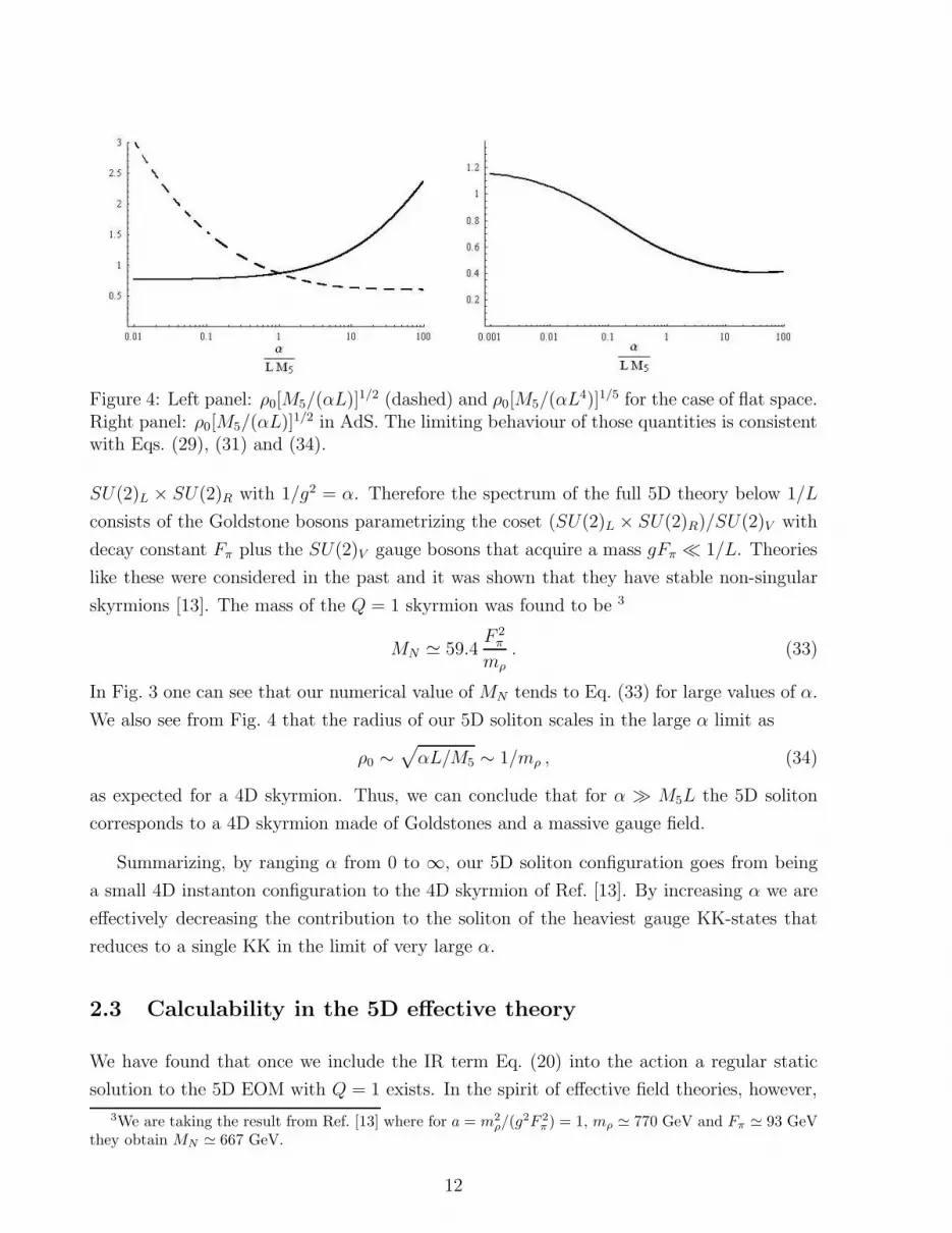
Figure 4: Left panel: ρ0[M5/(αL)]1/2 (dashed) and ρ0[M5/(αL4)]1/5 for the case of flat space.Right panel: ρ0[M5/(αL)]1/2 in AdS. The limiting behaviour of those quantities is consistentwith Eqs. (29), (31) and (34).

SU(2)L × SU(2)R with 1/g2 = α. Therefore the spectrum of the full 5D theory below 1/L

consists of the Goldstone bosons parametrizing the coset (SU(2)L × SU(2)R)/SU(2)V with

decay constant Fπ plus the SU(2)V gauge bosons that acquire a mass gFπ ≪ 1/L. Theories

like these were considered in the past and it was shown that they have stable non-singular

skyrmions [13]. The mass of the Q = 1 skyrmion was found to be 3

MN ≃ 59.4F 2

π

mρ. (33)

In Fig. 3 one can see that our numerical value of MN tends to Eq. (33) for large values of α.

We also see from Fig. 4 that the radius of our 5D soliton scales in the large α limit as

ρ0 ∼√

αL/M5 ∼ 1/mρ , (34)

as expected for a 4D skyrmion. Thus, we can conclude that for α ≫ M5L the 5D soliton

corresponds to a 4D skyrmion made of Goldstones and a massive gauge field.

Summarizing, by ranging α from 0 to ∞, our 5D soliton configuration goes from being

a small 4D instanton configuration to the 4D skyrmion of Ref. [13]. By increasing α we are

effectively decreasing the contribution to the soliton of the heaviest gauge KK-states that

reduces to a single KK in the limit of very large α.

2.3 Calculability in the 5D effective theory

We have found that once we include the IR term Eq. (20) into the action a regular static

solution to the 5D EOM with Q = 1 exists. In the spirit of effective field theories, however,

3We are taking the result from Ref. [13] where for a = m2

ρ/(g2F 2

π ) = 1, mρ ≃ 770 GeV and Fπ ≃ 93 GeVthey obtain MN ≃ 667 GeV.

12

the action also contains an infinite number of 5D higher-dimensional operators which are

suppressed by inverse powers of the cut-off scale Λ5, and it is of crucial importance to

establish how much our results are sensitive to such operators.

The contribution to the soliton energy of the higher-dimensional operators is easily es-

timated by substituting the soliton configuration into the operators. Since these operators

have at least one more dimension of energy, their coefficients are suppressed by one more

power of Λ−15 . On dimensional grounds, therefore, the contribution to the energy of the

new operators carries on more powers of 1/(Λ5ρ0) where the radius ρ0 is the typical size of

the soliton. We must check that 1/(Λ5ρ0) ≪ 1 in such a way that a sensible perturbative

expansion, analogous to the E/Λ5 expantion for a scattering amplitude at energies E < Λ5,

can be performed. If this is the case the 5D soliton can be studied with our 5D effective

theory in the sense that we can compute its properties, to a certain degree of accuracy, by

only including a finite number of operators into the action.

By looking at Eqs. (29) and (31) , we find that ρ0Λ5 ∼ (Λ5L)4/5 and ρ0Λ5 ∼ (Λ5L)1/2

respectively for a flat and AdS space. Therefore, as long as Λ5L ≪ 1 (as it should for our

extra-dimensional theory to make sense), we have 1/(Λ5ρ0) ≪ 1 as needed in order to trust

our soliton within the 5D effective approach. We can see this in more detail by considering

a specific 6-dimensional bulk operator such as FMNDRDRF MN that, by the NDA counting,

is suppressed by M5/Λ25 where Λ5 ∼ 24π3M5. The contribution of this operator to the

soliton energy is of order δE ∼ 8π2M5/(Λ5ρ0)2 that should be compared with the boundary

energy Eq. (22). The relative correction δE/Eir(ρ0) ∼ (24π3αΛ5ρ0)−1 plays the role of the

expansion parameter. Using Eqs. (29) and (31) we get, respectively

(24π3α

)−6/5(Λ5L)−4/5 and

(24π3α

)−3/2(Λ5L)−1/2 . (35)

If α, whose NDA value is 1/(16π2), is not unnaturaly small and Λ5L > 1, the contribution to

the energy of the new operator is safely small. Notice that, contrary to the naive expectation,

we did not loose too much in our perturbation parameter because of the fact that we needed

to include the operator Eq. (20) to stabilize the soliton. If we would have found a solution

for α = 0, its size would have been given by ρ0 ∼ L and we wolud have obtained, instead of

Eq. (35), a perturbative expansion parameter of order 1/(Λ5L).

We can safely neglect any d-dimensional bulk and brane-localized operators with, respec-

tively, d > 6 and d > 5. The only operator that could be important in our analysis is the

five-dimensional Chern-Simons (CS) term which, by NDA, is suppressed by M5/Λ5 ∼ α, and

therefore it can be as significant as Eq. (22). This term is however absent in our case due to

its relation with the anomalies of the theory; it vanishes because SU(2) is an anomaly-free

13

group. Even in models where the CS term can be present, like for example in U(2) gauge

theories, its effect could be as small as that of dimension 6-operators [4], even though the

situation is not completely clear. We leave the analysis of the CS effects for the future.

The issue of calculability is particularly compelling in our case, and it is different from

what happens in the 4D Skyrme model in which all operators give comparable contribu-

tions. 4 The problem, in the case of the 4D skyrmions, comes from the fact that a higher-

dimensional operator of the form α (∂U)4 must be added to the Goldstone kinetic term

F 2π (∂U)2 in order to obtain a regular solution of the EOM [1,14]. The value of α estimated

by NDA is F 2π/Λ2, where Λ ∼ 4πFπ is the cut-off of the chiral lagrangian. We then see that

F 2π factorizes in front of the action and the cut-off Λ is the only dimensionful quantity which

enters into the EOM, setting the radius of the skyrmion to ρ0 ∼ 1/Λ. In our 5D case also

a higher-dimensional operator is needed to stabilize the soliton. Its coefficient is given by

α ∼ M5/Λ5 and then also the 5D coupling M5 factorizes in front of the action. Nevertheless,

our soliton configuration not only depends on the 5D cut-off Λ5, but also on the conformal

lenght L. This is the crucial difference from the 4D Skyrme model; a combination of L and

Λ5 sets the size of the 5D soliton fixing it to a scale larger than 1/Λ5.

3 Conclusions

We have studied skyrmion configurations arising from compact five dimensional models. We

have shown that the size of these skyrmions is stabilized by the presence of IR-boundary

kinetic terms. This size is always larger than the inverse of the 5D cut-off scale 1/Λ5,

and therefore consistent within our 5D effective theory. This is different from previous 5D

models [3,4] in which the skyrmion size was found to be of order 1/Λ5. We have numerically

obtained the skyrmion configurations for different values of α (the coefficient of the IR-

boundary kinetic term), and calculated their size and energy. Although the size of the

skyrmions depends strongly on α, their energy is quite model-independent. By varying α

these skyrmion configurations smoothly interpolates between small 4D instantons and 4D

skyrmions made of Goldstones and a massive gauge boson.

The existence of stable skyrmion configurations in extra dimensional models rises different

phenonemological issues. For example, theories of electroweak symmetry breaking arising

from extra dimensions will have this type of stable configurations, and therefore the analysis

of their cosmological consequences are of great importance. For 5D Higgsless [7] or composite

4When this is the case, not only the effective theory does not give us any quantitative information on thesoliton, but also its very existence is doubtful.

14

Higgs models [15] in which Fπ = 246/ǫ GeV (where ǫ ≤ 1) and mρ ≃ 1.2/ǫ TeV, we find a

soliton energy MN ∼ (2.5 − 3)/ǫ TeV. These TeV stable particles are possible dark matter

candidates, therefore the precise determination of their relic abundances is of important

phenomenological interest. These configurations can also be useful in holographic models

of 4D strong interactions. The AdS/CFT correspondence tells us that these 5D solitons

correspond to the ”baryons” of the dual theory. The 5D AdS model studied here has already

been proposed as a holographic model of QCD, giving predictions for the meson spectrum

and couplings in good agreement with the experimental data [8]. The skyrmion found here

gives an approximate value for the mass of the proton. We find MN ≃ 500 − 650 GeV, too

low compared with the experimental value ∼ 1 GeV. We must notice, however, that in our

analysis we have not included the 5D CS term, responsible in holographic QCD models of

the Wess-Zumino-Witten (WZW) term. It is known that the presence of the WZW term has

important impact on the skyrmion mass [16], so we can expect that including the CS in our

analysis can enhance our prediction of the proton mass. These and other phenomenological

questions deserve a further analysis that we leave for a future work.

Acknowledgments

We would like to thank Gia Dvali and Jose Antonio Carrillo for valuable conversations.

We also thank Josep Maria Mondelo for helping us with FEMLAB. This work has been

partly supported by the FEDER Research Project FPA2005-02211, the DURSI Research

Project SGR2005-00916 and the European Union under contract MRTN-CT-2004-503369

and MRTN-CT-2006-035863.

Appendix: The instanton energy in compact and warped

spaces

In the 2D notation used in this paper the BPST instanton with center at (x = 0, z = zir)

and size ρ corresponds to [17]

φ1 = r∂zΦ

Φ≡ φ1(ρ) , φ2 = −1 − r

∂rΦ

Φ≡ φ2(ρ) ,

A1 =∂zΦ

Φ≡ A1(ρ) , A2 = − ∂rΦ

Φ≡ A2(ρ) ,

(36)

where

Φ =1

ρ2 + r2 + (z − zir)2. (37)

The singular instanton of size ρ → 0 solves, up to a gauge transformation, the variational

problem defined by the energy Eq. (11) and the boundary conditions Eqs. (13) and (15).

15

Indeed, it has the same topological charge (Q = 1) of the solution we were looking for and,

since its 2D energy density is a δ-function at r = 0, z = zir, it has the minimal energy

E = 8π2M5 which saturates the lower bound of Eq. (17).

We can explicitly check that the instanton Eq. (36) fullfills, for any ρ, the boundary

conditions at r = 0 and z = zir given in Eqs. (13) and (15). At the other two boundaries

the instanton of size ρ → 0 has different boundary conditions:

z = zuv :

φ = φ(0) = −iei β

A1 = A1(0) = ∂1β∂µAµ = 0

, r → ∞ :

φ = φ(0) = −iei β

A2 = A2(0) = ∂2β∂µA

µ = 0, (38)

where β = 2 arctan [r/(zir − z)]. These boundary conditions are, as anticipated, topologi-

cally equivalent to those in Eq. (13) and then one can convert one into the other by a gauge

transformation. Instead of gauge rotating the instanton of ρ = 0 to make it fulfill Eq. (13), it

is more convenient to rephrase our original problem in the new gauge and the new boundary

conditions Eq. (38).

Let us consider instantons of small but non-vanishing size. We would like to compute

the energy E(ρ) of such configurations. We already know that E(ρ) will have an absolute

minimum at ρ = 0; this means that a small instanton is subject to an ”attractive force”

which tends to shrink its size to zero. By computing ∂ρE(ρ) one can measure the strength

of this force. It is important to remark that there are two different effects which make the

force arise. The first one, which is essentially local, is due to the curvature of the space and

therefore it is only present in warped spaces. It pushes the instanton to be localized as much

as possible at zir where the warp factor has its minimal value and then it is energetically

favorable. The second effect is non-local and is due to the presence of the boundary at zuv

which confines the solution into a finite volume. At the more technical level the two effects

come, respectively, from the fact that the instanton fails to fulfill the bulk EOM when the

space is warped and the boundary condition Eq. (38) at zuv. It cannot then be a stable

configuration.

To compute E(ρ) let us first try to substitute the instanton configuration in the energy

functional Eq. (11). We call EB the ”bulk” contribution to the energy which we obtain in

this way. We will see later that this is not the only contribution to E(ρ). For a generic warp

16

factor we have 5

EB(ρ) = 12 π2M5

∫ 0

−L/ρ

dya(zir + ρy)

(1 + y2)5/2= 12 π2M5

∑

n

ρncn(ρ/L)a(n)(zir)

n!, (39)

where we have expanded a(z) in Taylor series around z = zir and

cn(ρ/L) =

∫ 0

−L/ρ

dyyn

(1 + y2)5/2. (40)

The leading term of EB in the small ρ expantion comes from the n = 0 term which reads

12 π2M5c0(ρ/L) ≃ 8 π2M5

(1 − 3

8

ρ4

L4+ O(ρ6/L6)

), (41)

where we have also expanded c0(ρ/L) around ρ = 0 and have kept, for future convenience,

the first correction of order ρ4. A linear contribution to the energy can only come from the

n = 1 term and is given by

− 4 π2M5ρ a(1)(zir)(1 + O(ρ3/L3)

). (42)

If a(1) is non zero, this term must be negative since the warp factor is a decreasing function

of z. Therefore the above term gives, as expected, an attractive force which makes the

instanton shrink. In the case of AdS, Eq. (25), we have a(1) = −1/L and we obtain the

result of Eq. (19). For a space with a(1) = 0 the linear contribution vanishes and the leading

correction to the energy, which comes from the n = 2 term, is of O(ρ2/L2). Making the space

less and less warped near zir we are increasing the power of ρ/L of the instanton energy, and

therefore making the attractive force weaker and weaker at small ρ. This process however

stops at order ρ4/L4. The n = 4 term is proportional to c4 ∼ ln ρ, and for n > 4 we have

cn ∼ 1/ρn−4, so all terms n ≥ 4 contribute at the order ρ4/L4 to the energy. Therefore we

expect that the weakest possible force will be obtained from a energy of O(ρ4/L4) that is,

as we will now show, what actually happens in the case of flat space.

For flat space only the n = 0 term appears in Eq. (39) and EB is given by Eq. (41). We

then immediatly see that EB cannot be the total instanton energy. If so, the point ρ = 0

would not be a minimum but a maximum, and we would not find an attractive but a repulsive

force. The reason why there is an extra contribution to the energy is that the instanton of

finite size does not respect the boundary condition at zuv. Therefore, it does not belong to

5We are considering, everywhere in this Appendix, zuv 6= 0 because for zuv = 0 the energy of theinstanton in the AdS slice diverges. Our numerical computations show however that the true solution iswidely insensitive to the position of the UV-boundary and the results we derive here can be applyied forzuv = 0 as well.

17

the set of allowed field configurations on which our variational problem is defined. In order

to find the instanton energy we need a different formulation of the variational problem in

which the allowed field configurations do not necessarily respect the boundary condition.

The latter will arise, like the EOM, from the minimization of a new energy functional which

is now defined to act on a more general set of configurations, to which the instanton belongs.

This new functional is given by Eq. (11) and the UV-boundary term 6

Euv = 8πM5a(zuv)

∫ ∞

0

dr

[(φ − φ(0)

)∗Dzφ +

(φ − φ(0)

)Dzφ

∗ − r2

2

(A1 − A1(0)

)F12

]

zuv

.

(43)

It is easily understood why the addition of Euv makes the UV boundary conditions arise as

EOM. The variation of Eq. (11) and (43) gives, in addition to the usual bulk terms whose

cancellation will give rise to the EOM, localized UV-terms of the form(φ − φ

)∗δ(Dzφ)

and(A1 − A1

)δ(F12). Requiring those terms to vanish enforces the boundary conditions in

Eq. (38).

We can finally compute the energy E(ρ) of the finite size instanton. It is given by the

sum of EB in Eq. (39) and Euv in Eq. (43), in which of course we have to substitute the

instanton configuration. The latter term reads

Euv(ρ) = 5π2M5a(zuv)ρ4

L4, (44)

and gives, for a generic warped metric, a ρ4 contribution to the energy. This contribution

does not affect the result in the case of the AdS slice, since it is subleading, but it is crucial

in flat space as it corrects the negative sign which we found in Eq. (41). Adding EB and Euv

we obtain Eq. (18).

References

[1] T. H. R. Skyrme, Proc. Roy. Soc. Lond. A 260 (1961) 127.

[2] D. T. Son and M. A. Stephanov, Phys. Rev. D 69 (2004) 065020.

[3] D. K. Hong, M. Rho, H. U. Yee and P. Yi, Phys. Rev. D 76 (2007) 061901.

[4] H. Hata, T. Sakai, S. Sugimoto and S. Yamato, arXiv:hep-th/0701280.

6We can obtain this result by using Lagrange Multipliers that allows to include boundary constraints inthe functional to minimize.

18

[5] D. K. Hong, T. Inami and H. U. Yee, Phys. Lett. B 646 (2007) 165; K. Nawa, H. Sug-

anuma and T. Kojo, Phys. Rev. D 75 (2007) 086003.

[6] C. T. Hill, Phys. Rev. Lett. 88 (2002) 04160.

[7] C. Csaki, C. Grojean, L. Pilo and J. Terning, Phys. Rev. Lett. 92, 101802 (2004);

Y. Nomura, JHEP 0311 (2003) 050; R. Barbieri, A. Pomarol and R. Rattazzi, Phys.

Lett. B 591, 141 (2004).

[8] J. Erlich, E. Katz, D. T. Son and M. A. Stephanov, Phys. Rev. Lett. 95 (2005) 261602;

L. Da Rold and A. Pomarol, Nucl. Phys. B 721 (2005) 79.

[9] G. Panico and A. Wulzer, JHEP 0705 (2007) 060.

[10] We are following the notations of C. S. Chu, P. M. Ho and B. Zumino, Nucl. Phys. B

475, 484 (1996) [arXiv:hep-th/9602093].

[11] E. Witten, Phys. Rev. Lett. 38 (1977) 121.

[12] See http://www.comsol.com.

[13] Y. Igarashi, M. Johmura, A. Kobayashi, H. Otsu, T. Sato and S. Sawada, Nucl. Phys.

B 259 (1985) 721.

[14] G. S. Adkins, C. R. Nappi and E. Witten, Nucl. Phys. B 228 (1983) 552.

[15] R. Contino, L. Da Rold and A. Pomarol, Phys. Rev. D 75 (2007) 055014.

[16] G. S. Adkins and C. R. Nappi, Phys. Lett. B 137 (1984) 251.

[17] N. S. Manton, Phys. Lett. B 76 (1978) 111.

19