Star formation efficiency in galaxy clusters

arX

iv:0

804.

1102

v2 [

astr

o-ph

] 2

6 Ju

n 20

08

Astronomy & Astrophysics manuscript no. 9168 c© ESO 2013February 19, 2013

Star formation efficiency in galaxy clusters

T. F. Lagana1, G. B. Lima Neto1, F. Andrade-Santos1, and E. S. Cypriano2

1 Universidade de Sao Paulo, Instituto de Astronomia, Geofısica e Ciencias Atmosfericas, Departamento de Astronomia, Ruado Matao 1226, Cidade Universitaria, 05508-090, Sao Paulo, SP, Brazil.

2 Department of Physics & Astronomy, University College London, London, WC1E 6BT, England.

Received 29 November 2007 / Accepted 5 April 2008

ABSTRACT

Context. The luminous material in clusters of galaxies exists in two forms: the visible galaxies and the X-ray emittingintra-cluster medium. The hot intra-cluster gas is the major observed baryonic component of clusters, about six times moremassive than the stellar component. The mass contained within visible galaxies is approximately 3% of the dynamical mass.Aims. Our aim was to analyze both baryonic components, combining X-ray and optical data of a sample of five galaxy clusters(Abell 496, 1689, 2050, 2631 and 2667), within the redshift range 0.03 < z < 0.3. We determined the contribution of stars ingalaxies and the intracluster medium to the total baryon budget.Methods. We used public XMM-Newton data to determine the gas mass and to obtain the X-ray substructures. Using theoptical counterparts from SDSS or CFHT we determined the stellar contribution.Results. We examine the relative contribution of galaxies, intra-cluster light and intra-cluster medium to baryon budget inclusters through the stellar-to-gas mass ratio, estimated with recent data. We find that the stellar-to-gas mass ratio withinr500 (the radius within which the mean cluster density exceeds the critical density by a factor of 500), is anti-correlated withthe ICM temperature, which range from 24% to 6% while the temperature ranges from 4.0 to 8.3 keV. This indicates that lessmassive cold clusters are more prolific star forming environments than massive hot clusters.

Key words. galaxies: clusters: general-X-ray: galaxies: cluster-galaxies: luminosity function, mass function

1. Introduction

Galaxy clusters occupy an unique position in the hierarchi-cal scenario of structure formation as they are the largestbound and relaxed structures to form in the Universe (e.g.,Tozzi 2007). An important step in understanding galaxyclusters is to take into account all of their components.Fukugita et al. (1998) presented an estimate of the totalbudget of baryons in all states: most of the baryons arestill in the form of ionized gas and the stars and rem-nants represent only 17% of the baryons. In a similar workEttori (2003) presented the cluster “baryonic pie” of whichapproximately 70% is composed of the hot intra-clustermedium and almost 13% composed of stars.

The ratio of gas to stellar mass is particularly interest-ing because it is related to the star formation efficiency ofclusters. Studying the Hydra cluster, David et al. (1990)computed the ratio of gas to stellar mass and it was foundthat the gas mass is almost 4 times that of stars. UsingEinstein results from the literature, they extended thisanalysis to systems ranging from poor groups to rich clus-ters and a correlation between Mgas/Mstars and the gastemperature was suggested.

Lin et al. (2003) analyzed a sample of 13 clusters, find-ing that the gas-to-stellar mass ratio increases from 5.9to 10.4 from low- to high-mass clusters and their best-fitcorrelation for M500 − L500 differs from L500 ∝ M500 by3σ, indicating a mass-to-light ratio increasing with mass.These two results strongly suggest a decrease of star for-mation efficiency in more massive environments. Recently,Gonzalez et al. (2007), who also used gas masses from theliterature, estimated the contribution of stars in galaxies,intracluster stars and gas to the baryon budget. These au-thors, who took into account the intracluster light (ICL)to the baryon budget, confirming the previous trend of in-creasing Mstar/Mgas with decreasing temperature foundby David et al. (1990); Lin et al. (2003). Roussel et al.(2000), found that a typical stellar contribution to thebaryonic mass is between 5% and 20%, inside the virial ra-dius, even though they claim that the stellar-to-gas massratio is roughly independent of temperature.

Although the baryon budget has been addressed inmany studies (David et al. 1990; Fukugita et al. 1998;Ettori 2003; Gonzalez et al. 2007) there are good reasonsto revisit it. The most important reason is the stellar con-

http://arxiv.org/abs/0804.1102v2

2 T. F. Lagana et al.: Star formation efficiency in galaxy clusters

tent contribution to the baryon fraction. Second, cosmo-logical simulations can precisely predict the baryon frac-tion within r500 (see Sect. 7), which is approximately theradius in which the X-ray observations are reliable deter-mined.

To readdress this question, we choose five XMM-Newton public data clusters with SDSS or CFHT(Canada-France-Hawaii Telescope) counterparts to studythe gaseous and the stellar baryon budgets.

X-ray studies of galaxy clusters are particularly rele-vant to this issue as they provide the determination of thegas mass. An important task is to describe well the surfacebrightness profile, since the gas mass determination relieson it.

The baryonic stellar component can be estimated byintegrating the luminosity function to obtain the total lu-minosity and then adding the intra-cluster light (ICL) con-tribution. Using an appropriate stellar mass-to-light ratiowe have converted the total luminosity into stellar masses.

The paper is organized as follows: Observations anddata treatment are described in Sect. 2; we present thegas density distribution in Sect. 3; the temperature spec-tral analysis appears in Sect. 4; the dynamical analysisbased on temperature and substructure maps is presentedin Sect. 5; the stellar baryonic determination is presentedin Sect. 6; the mass determination is described in Sect. 7.Finally we present our discussion in Sect. 8 and we con-clude in Sect. 9.

All distance-dependent quantities are derived assum-ing the Hubble constant H0 = 70 km s−1 Mpc−1, ΩM =0.3 and, ΩΛ= 0.7. Magnitudes are given in the AB systemunless otherwise stated. All errors are relative to a 68%confidence level.

2. Observations and data treatment

2.1. Sample

The objects in our sample were drawn from a set of Abellclusters with both XMM-Newton public archive and SDSSoptical counterparts. We have also chosen only clusterswith redshifts in the range 0.03 < z < 0.3 so that thecluster image could be well resolved and were smaller thanthe detector field of view. We thus had 6 clusters in thisselection. Then we imposed that clusters have exposuretimes of at least 10 ks after data reduction and filtering(pipeline), and flare cleaning (see Sect. 2.2). We endedup with 3 clusters: 1689, A2050 and A2631. We have notused either the temperature or the object morphology asa criterion for cluster selection.

To enlarge this sample, we added the cluster A496 thatwas observed with the Canada-France-Hawaii Telescope

(CFHT) and for A2667 we used total luminosity from theliterature (Covone et al. 2006b). Properties of the wholesample are presented in Table 1.

2.2. X-rays

We used data from all EPIC cameras (MOS1, MOS2and PN). For data reduction we used the XMM-NewtonScience Analysis System (SAS) v6.0.4 and calibrationdatabase with all updates available prior to February,2006. The initial data screening was applied using recom-mended sets of event patterns, 0-12 and 0-4 for the MOSand PN cameras, respectively.

The light curves are not constant and large variationsin intensity are visible. These variations, which we callflares, are caused by soft energy protons produced by solaractivity. It is better to discard flare periods and reducethe effective exposure time to improve the signal-to-noiseratio. The light curves in the energy range of [1-10] keVwere filtered to reject periods of high background. Thecleaned light curves exhibited stable mean count rates andexposure times are given in Table 2. We considered eventsinside the field-of-view (FOV) and we excluded all badpixels.

In periods free of background flaring, the backgroundis dominated by X-rays at low energies and particles athigh energies. The X-ray component includes a signif-icant contribution from Galactic emission which varieswith position on the sky. Since cluster emission decreaseswith distance from the center, the background compo-nent becomes more important towards the outskirts. Thebackground was taken into account by extracting MOS1,MOS2 and PN spectra from the publicly available EPICblank sky templates described by Lumb et al. (2002).

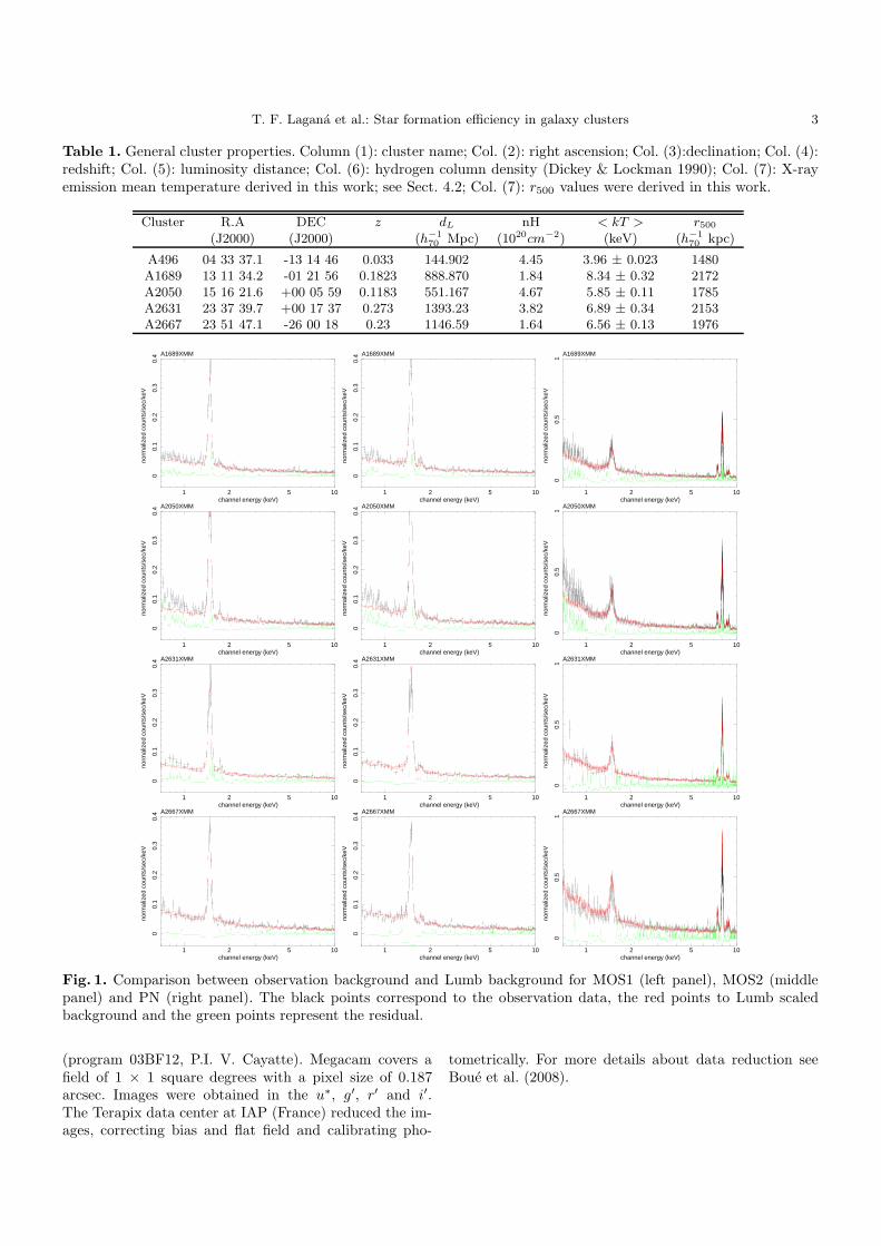
The background was normalized using a spectrum ob-tained in an annulus (between 9-11 arcmin) where thecluster emission is no longer detected. A normalized spec-trum was then subtracted, yielding a residual spectrum asshown in Fig. 1.

As A496 is a nearby cluster its emissivity extends up tothe outskirts of the image and for this reason we could notapply this technique of background normalization. For thiscluster, we subtracted the background without normaliz-ing it. If the background had not been well subtracted wewould have had an emission excess at the outskirts. Dueto this excess, we would have obtained from the fit of thetemperature profile higher temperatures toward the out-skirts. Even so, our temperature profile is in agreementwith the results obtained by Tamura et al. (2001).

2.3. Optical: SDSS and CFHT

In order to investigate the optical component of A1689,A2050 and A2631, we downloaded from the Sloan DigitalSky Survey Data release 5 (Adelman-McCarthy et al.2007) the model magnitudes dereddened for all galaxiesinside r500 (derived in this work from an X-ray analysis,see Sect. 7). Since extinction is less in the i′ band we usedthis band to construct luminosity functions. The galaxycatalog is essentially complete down to 23.5 i′ magnitude.

A496 was observed with the Canada-France-HawaiiTelescope (CFHT) with the Megacam camera in 2003

T. F. Lagana et al.: Star formation efficiency in galaxy clusters 3

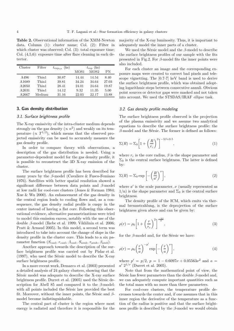
Table 1. General cluster properties. Column (1): cluster name; Col. (2): right ascension; Col. (3):declination; Col. (4):redshift; Col. (5): luminosity distance; Col. (6): hydrogen column density (Dickey & Lockman 1990); Col. (7): X-rayemission mean temperature derived in this work; see Sect. 4.2; Col. (7): r500 values were derived in this work.

Cluster R.A DEC z dL nH < kT > r500

(J2000) (J2000) (h−170 Mpc) (1020cm−2) (keV) (h−1

70 kpc)

A496 04 33 37.1 -13 14 46 0.033 144.902 4.45 3.96 ± 0.023 1480A1689 13 11 34.2 -01 21 56 0.1823 888.870 1.84 8.34 ± 0.32 2172A2050 15 16 21.6 +00 05 59 0.1183 551.167 4.67 5.85 ± 0.11 1785A2631 23 37 39.7 +00 17 37 0.273 1393.23 3.82 6.89 ± 0.34 2153A2667 23 51 47.1 -26 00 18 0.23 1146.59 1.64 6.56 ± 0.13 1976

1 102 5

00.

10.

20.

30.

4

norm

aliz

ed c

ount

s/se

c/ke

V

channel energy (keV)

A1689XMM

1 102 5

00.

10.

20.

30.

4

norm

aliz

ed c

ount

s/se

c/ke

V


A1689XMM

1 102 5

00.

51

norm

aliz

ed c

ount

s/se

c/ke

V


A1689XMM

1 102 5

00.

10.

20.

30.

4

norm

aliz

ed c

ount

s/se

c/ke

V


A2050XMM

1 102 5

00.

10.

20.

30.

4

norm

aliz

ed c

ount

s/se

c/ke

V


A2050XMM

1 102 5

00.

51

norm

aliz

ed c

ount

s/se

c/ke

V


A2050XMM

1 102 5

00.

10.

20.

30.

4

norm

aliz

ed c

ount

s/se

c/ke

V


A2631XMM

1 102 5

00.

10.

20.

30.

4

norm

aliz

ed c

ount

s/se

c/ke

V


A2631XMM

1 102 5

00.

51

norm

aliz

ed c

ount

s/se

c/ke

V


A2631XMM

1 102 5

00.

10.

20.

30.

4

norm

aliz

ed c

ount

s/se

c/ke

V


A2667XMM

1 102 5

00.

10.

20.

30.

4

norm

aliz

ed c

ount

s/se

c/ke

V


A2667XMM

1 102 5

00.

51

norm

aliz

ed c

ount

s/se

c/ke

V


A2667XMM

Fig. 1. Comparison between observation background and Lumb background for MOS1 (left panel), MOS2 (middlepanel) and PN (right panel). The black points correspond to the observation data, the red points to Lumb scaledbackground and the green points represent the residual.

(program 03BF12, P.I. V. Cayatte). Megacam covers afield of 1 × 1 square degrees with a pixel size of 0.187arcsec. Images were obtained in the u∗, g′, r′ and i′.The Terapix data center at IAP (France) reduced the im-ages, correcting bias and flat field and calibrating pho-

tometrically. For more details about data reduction seeBoue et al. (2008).


Table 2. Observational information of the XMM-Newtondata. Column (1): cluster name; Col. (2): Filter inwhich cluster was observed; Col. (3): total exposure time;Col. (4,5,6): exposure time after flare cleaning in each de-tector.

Cluster Filter texptot(ks) texp (ks)

MOS1 MOS2 PN

A496 Thin1 30.87 14.44 14.54 8.40A1689 Thin1 39.81 34.24 34.64 27.03A2050 Thin1 28.41 24.01 24.64 19.87A2631 Thin1 14.12 9.32 11.35 5.00A2667 Medium 31.16 22.03 22.17 13.88

3. Gas density distribution

3.1. Surface brightness profile

The X-ray emissivity of the intra-cluster medium dependsstrongly on the gas density (∝ n2) and weakly on its tem-perature (∝ T 1/2), which means that the observed pro-jected emissivity can be used to accurately measure thegas density profile.

In order to compare theory with observations, adescription of the gas distribution is needed. Using aparameter-dependent model for the gas density profile, itis possible to reconstruct the 3D X-ray emission of thecluster.

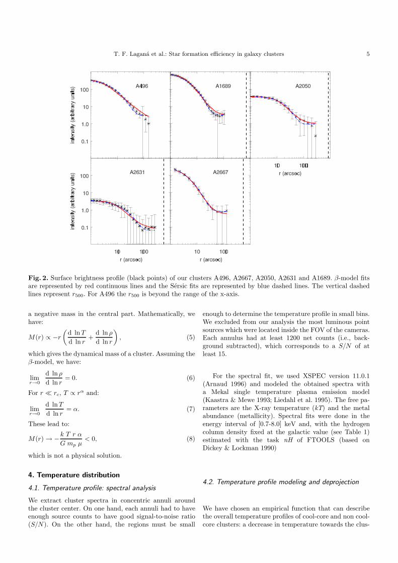
The surface brightness profile has been described formany years by the β-model (Cavaliere & Fusco-Femiano1976). Satellites with better spatial resolution showed asignificant difference between data points and β-modelat low radii for cool-core clusters (Jones & Forman 1984;Xue & Wu 2000). An enhancement of the gas density inthe central region leads to cooling flows and, as a con-sequence, the gas density radial profile is cuspy in thecenter instead of having a flat core. Following this obser-vational evidence, alternative parametrizations were triedto model this emission excess, notably with the use of thedouble β-model (Ikebe et al. 1999; Vikhlinin et al. 2006;Pratt & Arnaud 2005). In this model, a second term wasintroduced to take into account the change of slope in thedensity profile in the cluster core. This leads to a six pa-rameter function (Scool, rcool, βcool, Samb, ramb, βamb).

Another approach towards the description of the sur-face brightness profile was carried out by Pislar et al.(1997), who used the Sersic model to describe the X-raysurface brightness profile.

In a more recent work, Demarco et al. (2003) presenteda detailed analysis of 24 galaxy clusters, showing that theSersic model was adequate to describe the X-ray surfacebrightness profile. Durret et al. (2005) used the Sersic de-scription for Abell 85 and compared it to the β-model:with all points included the Sersic law provided the bestfit. Moreover, without the inner points, the Sersic and β-model become indistinguishable.

The central part of cluster is the region where mostenergy is radiated and therefore it is responsible for the

majority of the X-ray luminosity. Thus, it is important toadequately model the inner parts of a cluster.

We used the Sersic model and the β-model to describethe surface brightness profiles of our sample with the fitspresented in Fig.2. For β-model fits the inner points werealso included.

For each cluster an image and the corresponding ex-posure maps were created to correct bad pixels and tele-scope vignetting. The [0.7-7] keV band is used to derivethe surface brightness profile, which was obtained adopt-ing logarithmic steps between consecutive annuli. Obviouspoint sources or detector gaps were masked and not takeninto account. We used the STSDAS/IRAF ellipse task.

3.2. Gas density profile modeling

The surface brightness profile observed is the projectionof the plasma emissivity and we assume two analyticalequations to describe the surface brightness profile: theβ-model and the Sersic. The former is defined as follows:

Σ(R) = Σ0

[

1 +

(

R

rc

)2]−3β+0.5

, (1)

where rc is the core radius, β is the shape parameter andΣ0 is the central surface brightness. The latter is definedby:

Σ(R) = Σ0 exp

[

−(

R

a′

)ν]

, (2)

where a′ is the scale parameter, ν (usually represented as1/n) is the shape parameter and Σ0 is the central surfacebrightness.

The density profile of the ICM, which emits via ther-mal bremsstrahlung, is the deprojection of the surfacebrightness given above and can be given by:

ρ(r) = ρ0

[

1 +

(

r

rc

)2]−3β

2

, (3)

for the β-model and, for the Sersic we have:

ρ(r) = ρ0

(

r

a

)−p′

exp

[

−(

r

a

)ν]

, (4)

where p′ = p/2, p = 1 − 0.6097ν + 0.05563ν2 and a =a′ 21/ν (Durret et al. 2005).

Note that from the mathematical point of view, theSersic has fewer parameters than the double β-model and,we can adequately compute important quantities such asthe total mass with no more than three parameters.

For cool-core clusters, the temperature profile de-creases towards the center and, if one assumes that in thisinner region the derivative of the temperature as a func-tion of the radius is positive and that the surface bright-ness profile is described by the β-model we would obtain


Fig. 2. Surface brightness profile (black points) of our clusters A496, A2667, A2050, A2631 and A1689. β-model fitsare represented by red continuous lines and the Sersic fits are represented by blue dashed lines. The vertical dashedlines represent r500. For A496 the r500 is beyond the range of the x-axis.

a negative mass in the central part. Mathematically, wehave:

M(r) ∝ −r

(

d lnT

d ln r+

d ln ρ

d ln r

)

, (5)

which gives the dynamical mass of a cluster. Assuming theβ-model, we have:

limr→0

d ln ρ

d ln r= 0. (6)

For r ≪ rc, T ∝ rα and:

limr→0

d lnT

d ln r= α. (7)

These lead to:

M(r) → −k T r α

G mp µ< 0, (8)

which is not a physical solution.

4. Temperature distribution

4.1. Temperature profile: spectral analysis

We extract cluster spectra in concentric annuli aroundthe cluster center. On one hand, each annuli had to haveenough source counts to have good signal-to-noise ratio(S/N). On the other hand, the regions must be small

enough to determine the temperature profile in small bins.We excluded from our analysis the most luminous pointsources which were located inside the FOV of the cameras.Each annulus had at least 1200 net counts (i.e., back-ground subtracted), which corresponds to a S/N of atleast 15.

For the spectral fit, we used XSPEC version 11.0.1(Arnaud 1996) and modeled the obtained spectra witha Mekal single temperature plasma emission model(Kaastra & Mewe 1993; Liedahl et al. 1995). The free pa-rameters are the X-ray temperature (kT) and the metalabundance (metallicity). Spectral fits were done in theenergy interval of [0.7-8.0] keV and, with the hydrogencolumn density fixed at the galactic value (see Table 1)estimated with the task nH of FTOOLS (based onDickey & Lockman 1990)

4.2. Temperature profile modeling and deprojection

We have chosen an empirical function that can describethe overall temperature profiles of cool-core and non cool-core clusters: a decrease in temperature towards the clus-


Table 3. Fits results. Column (1): cluster name; Col. (2): slope parameter of the β-model; Col. (3,4): scale radius inarcsec and in h−1

70 kpc of the β-model; Col. (5): electron number density of the central region calculated by means ofthe β-model; Col. (6): slope parameter of the Sersic fit; Col. (7,8) scale radius in arcsec and in h−1

70 kpc of the Sersicmodel; Col. 9 electron number density of the central region calculated by means of the Sersic model.

β-model SersicCluster β rc rc n0 ν a′ a′ n0

(arcsec) (h−170 kpc) cm−3 (arcsec) (h−1

70 kpc) cm−3

A496 0.410 ± 0.015 23.48 ± 0.28 15.48 ± 0.18 0.084 0.390 ± 0.046 3.6 ± 0.23 2.37 ± 0.15 0.036A1689 0.550 ± 0.025 25.72 ± 0.23 79.16 ± 0.71 0.065 0.650 ± 0.030 12.78 ± 0.16 39.32 ± 0.48 0.012A2050 0.43 ± 0.028 10.22 ± 0.73 22.0 ± 1.5 0.026 1.285 ± 0.047 15.33 ± 0.32 56.4 ± 1.2 0.010A2631 0.732 ± 0.073 21.2 ± 2.5± 82.6 ± 9.6 0.051 1.001 ± 0.066 14.9 ± 1.2 58.0 ± 4.7 0.013A2667 0.660 ± 0.017 30.8 ± 1.9 113.25 ± 6.99 0.039 0.570 ± 0.034 6.3 ± 1.5 23.1 ± 5.4 0.022

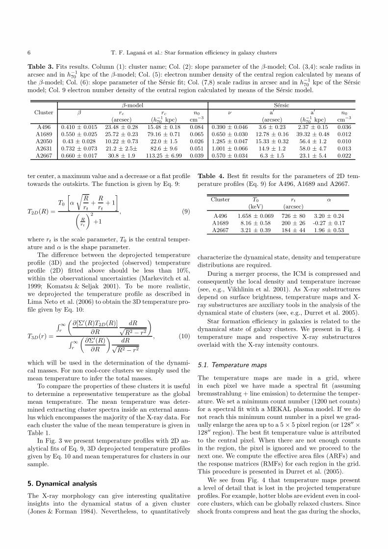
ter center, a maximum value and a decrease or a flat profiletowards the outskirts. The function is given by Eq. 9:

T2D(R) =

T0

[

α

√

R

rt+

R

rt+ 1

]

(

Rrt

)2

+1

, (9)

where rt is the scale parameter, T0 is the central temper-ature and α is the shape parameter.

The difference between the deprojected temperatureprofile (3D) and the projected (observed) temperatureprofile (2D) fitted above should be less than 10%,within the observational uncertainties (Markevitch et al.1999; Komatsu & Seljak 2001). To be more realistic,we deprojected the temperature profile as described inLima Neto et al. (2006) to obtain the 3D temperature pro-file given by Eq. 10:

T3D(r) =

∫ ∞

r

(

∂[Σ′(R)T2D(R)]

∂R

dR√R2 − r2

)

∫ ∞

r

(

∂Σ′(R)

∂R

)

dR√R2 − r2

, (10)

which will be used in the determination of the dynami-cal masses. For non cool-core clusters we simply used themean temperature to infer the total masses.

To compare the properties of these clusters it is usefulto determine a representative temperature as the globalmean temperature. The mean temperature was deter-mined extracting cluster spectra inside an external annu-lus which encompasses the majority of the X-ray data. Foreach cluster the value of the mean temperature is given inTable 1.

In Fig. 3 we present temperature profiles with 2D an-alytical fits of Eq. 9, 3D deprojected temperature profilesgiven by Eq. 10 and mean temperatures for clusters in oursample.

5. Dynamical analysis

The X-ray morphology can give interesting qualitativeinsights into the dynamical status of a given cluster(Jones & Forman 1984). Nevertheless, to quantitatively

Table 4. Best fit results for the parameters of 2D tem-perature profiles (Eq. 9) for A496, A1689 and A2667.

Cluster T0 rt α(keV) (arcsec)

A496 1.658 ± 0.069 726 ± 80 3.20 ± 0.24A1689 8.16 ± 0.58 200 ± 26 -0.27 ± 0.17A2667 3.21 ± 0.39 184 ± 44 1.96 ± 0.53

characterize the dynamical state, density and temperaturedistributions are required.

During a merger process, the ICM is compressed andconsequently the local density and temperature increase(see, e.g., Vikhlinin et al. 2001). As X-ray substructuresdepend on surface brightness, temperature maps and X-ray substructures are auxiliary tools in the analysis of thedynamical state of clusters (see, e.g., Durret et al. 2005).

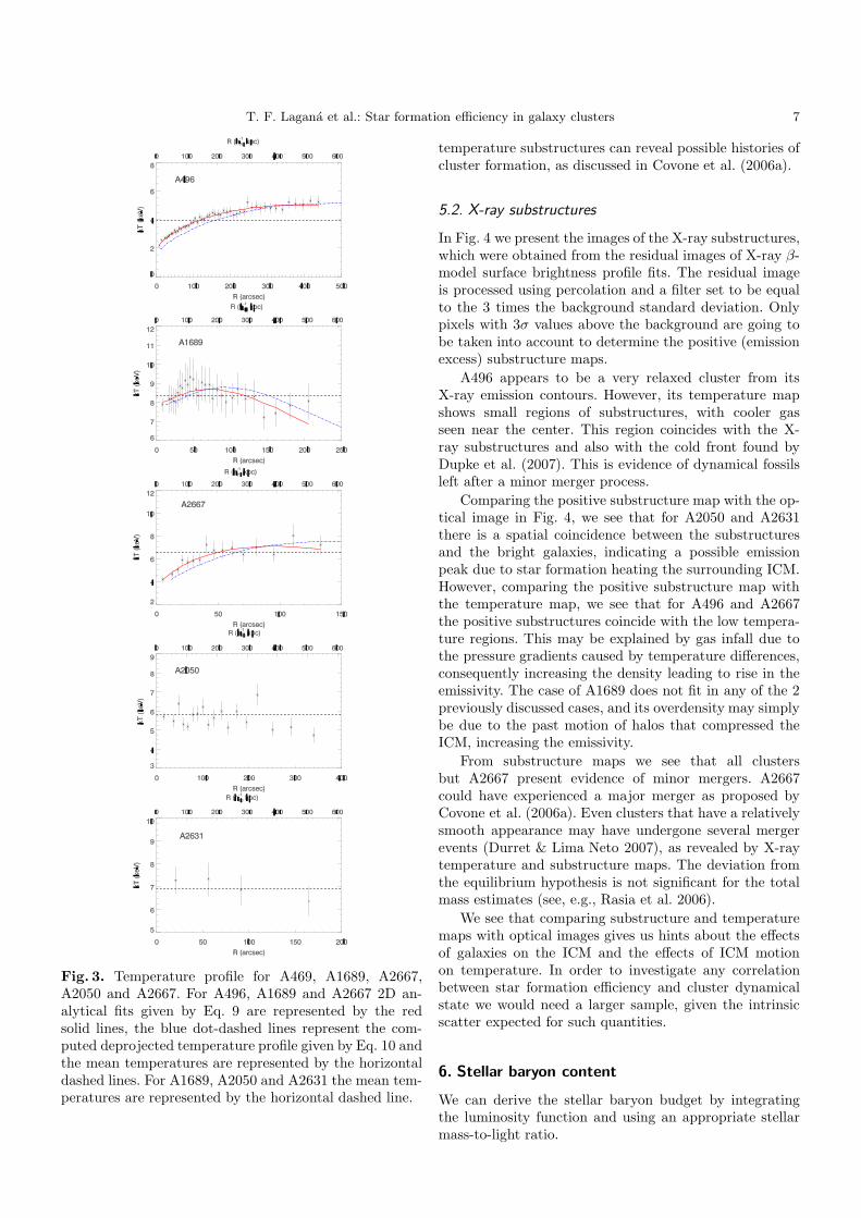
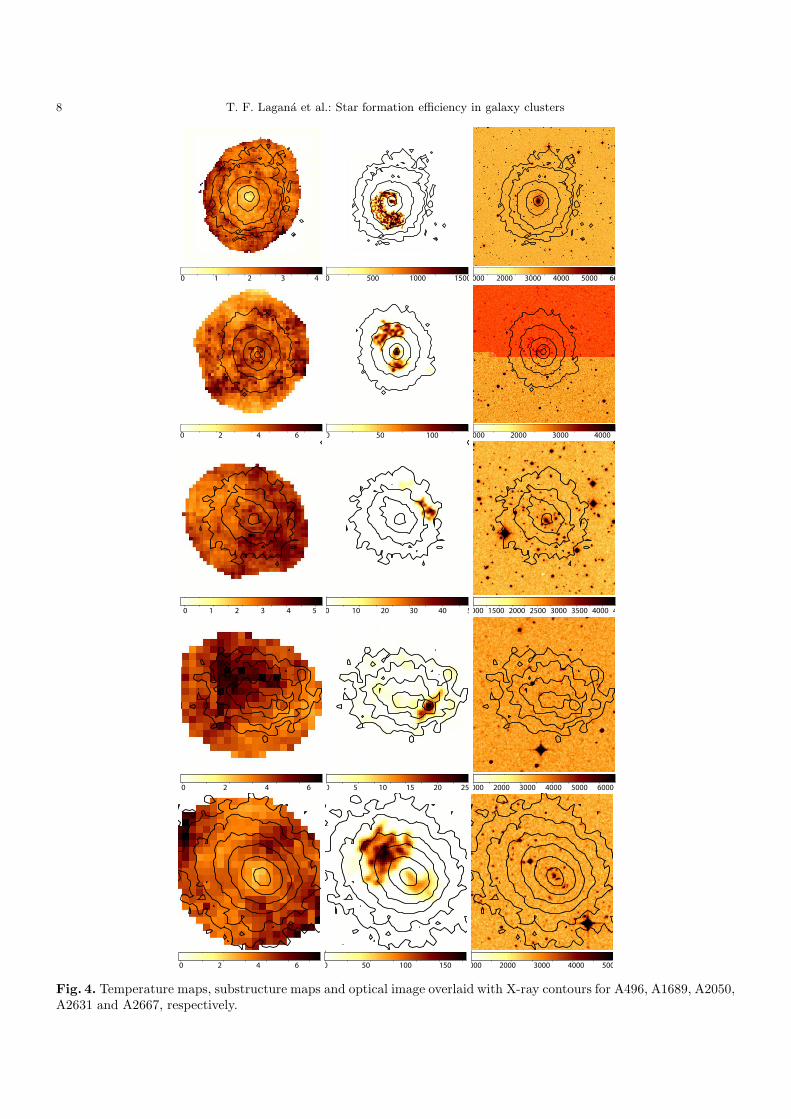
Star formation efficiency in galaxies is related to thedynamical state of galaxy clusters. We present in Fig. 4temperature maps and respective X-ray substructuresoverlaid with the X-ray intensity contours.

5.1. Temperature maps

The temperature maps are made in a grid, wherein each pixel we have made a spectral fit (assumingbremsstrahlung + line emission) to determine the temper-ature. We set a minimum count number (1200 net counts)for a spectral fit with a MEKAL plasma model. If we donot reach this minimum count number in a pixel we grad-ually enlarge the area up to a 5 × 5 pixel region (or 128′′ ×128′′ region). The best fit temperature value is attributedto the central pixel. When there are not enough countsin the region, the pixel is ignored and we proceed to thenext one. We compute the effective area files (ARFs) andthe response matrices (RMFs) for each region in the grid.This procedure is presented in Durret et al. (2005).

We see from Fig. 4 that temperature maps presenta level of detail that is lost in the projected temperatureprofiles. For example, hotter blobs are evident even in cool-core clusters, which can be globally relaxed clusters. Sinceshock fronts compress and heat the gas during the shocks,


Fig. 3. Temperature profile for A469, A1689, A2667,A2050 and A2667. For A496, A1689 and A2667 2D an-alytical fits given by Eq. 9 are represented by the redsolid lines, the blue dot-dashed lines represent the com-puted deprojected temperature profile given by Eq. 10 andthe mean temperatures are represented by the horizontaldashed lines. For A1689, A2050 and A2631 the mean tem-peratures are represented by the horizontal dashed line.

temperature substructures can reveal possible histories ofcluster formation, as discussed in Covone et al. (2006a).

5.2. X-ray substructures

In Fig. 4 we present the images of the X-ray substructures,which were obtained from the residual images of X-ray β-model surface brightness profile fits. The residual imageis processed using percolation and a filter set to be equalto the 3 times the background standard deviation. Onlypixels with 3σ values above the background are going tobe taken into account to determine the positive (emissionexcess) substructure maps.

A496 appears to be a very relaxed cluster from itsX-ray emission contours. However, its temperature mapshows small regions of substructures, with cooler gasseen near the center. This region coincides with the X-ray substructures and also with the cold front found byDupke et al. (2007). This is evidence of dynamical fossilsleft after a minor merger process.

Comparing the positive substructure map with the op-tical image in Fig. 4, we see that for A2050 and A2631there is a spatial coincidence between the substructuresand the bright galaxies, indicating a possible emissionpeak due to star formation heating the surrounding ICM.However, comparing the positive substructure map withthe temperature map, we see that for A496 and A2667the positive substructures coincide with the low tempera-ture regions. This may be explained by gas infall due tothe pressure gradients caused by temperature differences,consequently increasing the density leading to rise in theemissivity. The case of A1689 does not fit in any of the 2previously discussed cases, and its overdensity may simplybe due to the past motion of halos that compressed theICM, increasing the emissivity.

From substructure maps we see that all clustersbut A2667 present evidence of minor mergers. A2667could have experienced a major merger as proposed byCovone et al. (2006a). Even clusters that have a relativelysmooth appearance may have undergone several mergerevents (Durret & Lima Neto 2007), as revealed by X-raytemperature and substructure maps. The deviation fromthe equilibrium hypothesis is not significant for the totalmass estimates (see, e.g., Rasia et al. 2006).

We see that comparing substructure and temperaturemaps with optical images gives us hints about the effectsof galaxies on the ICM and the effects of ICM motionon temperature. In order to investigate any correlationbetween star formation efficiency and cluster dynamicalstate we would need a larger sample, given the intrinsicscatter expected for such quantities.

6. Stellar baryon content

We can derive the stellar baryon budget by integratingthe luminosity function and using an appropriate stellarmass-to-light ratio.


0 1 2 3 4 5 6 70 500 1000 15001000 2000 3000 4000 5000 600

0 2 4 6 0 50 100 1000 2000 3000 4000

0 1 2 3 4 5 6 7 80 10 20 30 40 51000 1500 2000 2500 3000 3500 4000 450

0 2 4 6 0 5 10 15 20 251000 2000 3000 4000 5000 6000

0 2 4 6 0 50 100 150 1000 2000 3000 4000 5000

Fig. 4. Temperature maps, substructure maps and optical image overlaid with X-ray contours for A496, A1689, A2050,A2631 and A2667, respectively.


The galaxy luminosity function (GLF) is one of the ba-sic statistical properties of galaxies in clusters. The GLFgives the number of galaxies per bin of magnitude and inmost cases, the bright galaxies can be fit by a Schechterfunction (Schechter & Press 1976). In the case of deepobservations there appear to be two components in theGLF: the bright and faint galaxies. This faint end can beseen for magnitudes greater than Mi′ = 18 and for thesecases it is impossible to well describe the GLF with a sin-gle Schechter function (Biviano et al. 1995; Durret et al.2002).

We have performed analytical fits to the GLF forfour (A496, A1689, A2050 and A2631) of our five clus-ters in order to estimate the total luminosity and thenthe stellar baryon content. For A2667 we used LK =(1.2 ± 0.1) × 1012h−2

70 L⊙ given by Covone et al. (2006b),based on ISAAC data (Wolfram et al. 1999). As this lu-minosity was computed within R = 110h−1

70 kpc in the Kband, a filter transformation to the Sloan i′ band was done(as described in Sec. 6.3) and the total luminosity functionwas extrapolated to r500 as described in Sect. 6.3.

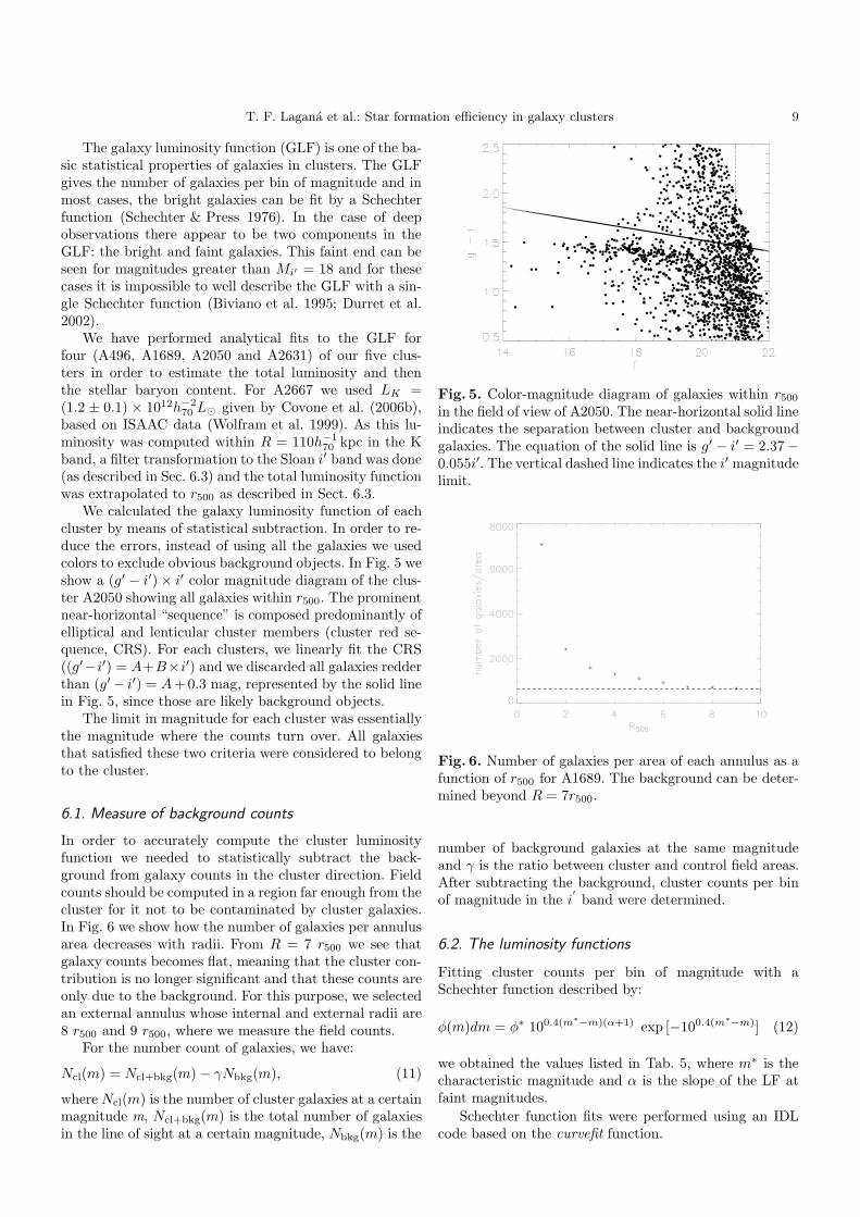
We calculated the galaxy luminosity function of eachcluster by means of statistical subtraction. In order to re-duce the errors, instead of using all the galaxies we usedcolors to exclude obvious background objects. In Fig. 5 weshow a (g′ − i′) × i′ color magnitude diagram of the clus-ter A2050 showing all galaxies within r500. The prominentnear-horizontal “sequence” is composed predominantly ofelliptical and lenticular cluster members (cluster red se-quence, CRS). For each clusters, we linearly fit the CRS((g′−i′) = A+B×i′) and we discarded all galaxies redderthan (g′ − i′) = A+0.3 mag, represented by the solid linein Fig. 5, since those are likely background objects.

The limit in magnitude for each cluster was essentiallythe magnitude where the counts turn over. All galaxiesthat satisfied these two criteria were considered to belongto the cluster.

6.1. Measure of background counts

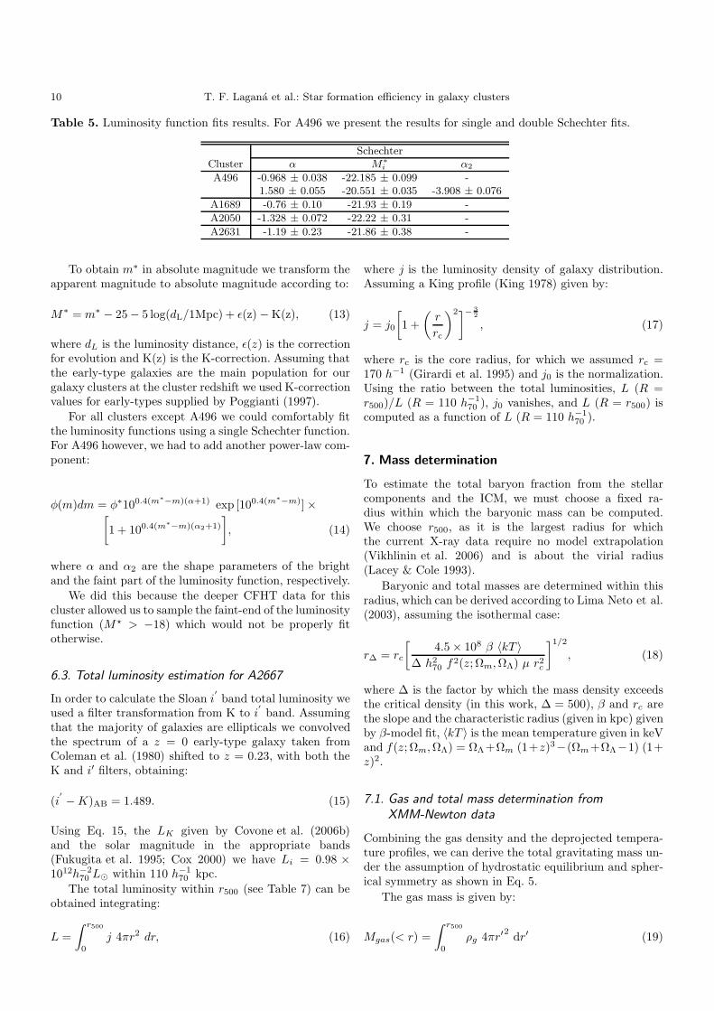
In order to accurately compute the cluster luminosityfunction we needed to statistically subtract the back-ground from galaxy counts in the cluster direction. Fieldcounts should be computed in a region far enough from thecluster for it not to be contaminated by cluster galaxies.In Fig. 6 we show how the number of galaxies per annulusarea decreases with radii. From R = 7 r500 we see thatgalaxy counts becomes flat, meaning that the cluster con-tribution is no longer significant and that these counts areonly due to the background. For this purpose, we selectedan external annulus whose internal and external radii are8 r500 and 9 r500, where we measure the field counts.

For the number count of galaxies, we have:

Ncl(m) = Ncl+bkg(m) − γNbkg(m), (11)

where Ncl(m) is the number of cluster galaxies at a certainmagnitude m, Ncl+bkg(m) is the total number of galaxiesin the line of sight at a certain magnitude, Nbkg(m) is the

Fig. 5. Color-magnitude diagram of galaxies within r500

in the field of view of A2050. The near-horizontal solid lineindicates the separation between cluster and backgroundgalaxies. The equation of the solid line is g′ − i′ = 2.37 −0.055i′. The vertical dashed line indicates the i′ magnitudelimit.

Fig. 6. Number of galaxies per area of each annulus as afunction of r500 for A1689. The background can be deter-mined beyond R = 7r500.

number of background galaxies at the same magnitudeand γ is the ratio between cluster and control field areas.After subtracting the background, cluster counts per binof magnitude in the i

′

band were determined.

6.2. The luminosity functions

Fitting cluster counts per bin of magnitude with aSchechter function described by:

φ(m)dm = φ∗ 100.4(m∗−m)(α+1) exp [−100.4(m∗

−m)] (12)

we obtained the values listed in Tab. 5, where m∗ is thecharacteristic magnitude and α is the slope of the LF atfaint magnitudes.

Schechter function fits were performed using an IDLcode based on the curvefit function.


Table 5. Luminosity function fits results. For A496 we present the results for single and double Schechter fits.

SchechterCluster α M∗

i α2

A496 -0.968 ± 0.038 -22.185 ± 0.099 -1.580 ± 0.055 -20.551 ± 0.035 -3.908 ± 0.076

A1689 -0.76 ± 0.10 -21.93 ± 0.19 -

A2050 -1.328 ± 0.072 -22.22 ± 0.31 -

A2631 -1.19 ± 0.23 -21.86 ± 0.38 -

To obtain m∗ in absolute magnitude we transform theapparent magnitude to absolute magnitude according to:

M∗ = m∗ − 25 − 5 log(dL/1Mpc) + ǫ(z) − K(z), (13)

where dL is the luminosity distance, ǫ(z) is the correctionfor evolution and K(z) is the K-correction. Assuming thatthe early-type galaxies are the main population for ourgalaxy clusters at the cluster redshift we used K-correctionvalues for early-types supplied by Poggianti (1997).

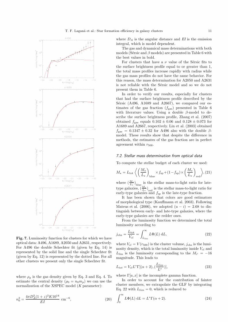
For all clusters except A496 we could comfortably fitthe luminosity functions using a single Schechter function.For A496 however, we had to add another power-law com-ponent:

φ(m)dm = φ∗100.4(m∗−m)(α+1) exp [100.4(m∗

−m)] ×[

1 + 100.4(m∗−m)(α2+1)

]

, (14)

where α and α2 are the shape parameters of the brightand the faint part of the luminosity function, respectively.

We did this because the deeper CFHT data for thiscluster allowed us to sample the faint-end of the luminosityfunction (M⋆ > −18) which would not be properly fitotherwise.

6.3. Total luminosity estimation for A2667

In order to calculate the Sloan i′

band total luminosity weused a filter transformation from K to i

′

band. Assumingthat the majority of galaxies are ellipticals we convolvedthe spectrum of a z = 0 early-type galaxy taken fromColeman et al. (1980) shifted to z = 0.23, with both theK and i′ filters, obtaining:

(i′ − K)AB = 1.489. (15)

Using Eq. 15, the LK given by Covone et al. (2006b)and the solar magnitude in the appropriate bands(Fukugita et al. 1995; Cox 2000) we have Li = 0.98 ×1012h−2

70 L⊙ within 110 h−170 kpc.

The total luminosity within r500 (see Table 7) can beobtained integrating:

L =

∫ r500

0

j 4πr2 dr, (16)

where j is the luminosity density of galaxy distribution.Assuming a King profile (King 1978) given by:

j = j0

[

1 +

(

r

rc

)2]− 3

2

, (17)

where rc is the core radius, for which we assumed rc =170 h−1 (Girardi et al. 1995) and j0 is the normalization.Using the ratio between the total luminosities, L (R =r500)/L (R = 110 h−1

70 ), j0 vanishes, and L (R = r500) iscomputed as a function of L (R = 110 h−1

70 ).

7. Mass determination

To estimate the total baryon fraction from the stellarcomponents and the ICM, we must choose a fixed ra-dius within which the baryonic mass can be computed.We choose r500, as it is the largest radius for whichthe current X-ray data require no model extrapolation(Vikhlinin et al. 2006) and is about the virial radius(Lacey & Cole 1993).

Baryonic and total masses are determined within thisradius, which can be derived according to Lima Neto et al.(2003), assuming the isothermal case:

r∆ = rc

[

4.5 × 108 β 〈kT 〉∆ h2

70 f2(z; Ωm, ΩΛ) µ r2c

]1/2

, (18)

where ∆ is the factor by which the mass density exceedsthe critical density (in this work, ∆ = 500), β and rc arethe slope and the characteristic radius (given in kpc) givenby β-model fit, 〈kT 〉 is the mean temperature given in keVand f(z; Ωm, ΩΛ) = ΩΛ+Ωm (1+z)3−(Ωm+ΩΛ−1) (1+z)2.

7.1. Gas and total mass determination from

XMM-Newton data

Combining the gas density and the deprojected tempera-ture profiles, we can derive the total gravitating mass un-der the assumption of hydrostatic equilibrium and spher-ical symmetry as shown in Eq. 5.

The gas mass is given by:

Mgas(< r) =

∫ r500

0

ρg 4πr′2

dr′ (19)


Fig. 7. Luminosity function for clusters for which we haveoptical data: A496, A1689, A2050 and A2631, respectively.For A496 the double Schechter fit (given by Eq. 14) isrepresented by the solid line and the single Schechter fit(given by Eq. 12) is represented by the dotted line. For allother clusters we present only the single Schechter fit.

where ρg is the gas density given by Eq. 3 and Eq. 4. Toestimate the central density (ρ0 = n0mp) we can use thenormalization of the XSPEC model (K parameter):

n20 =

4πD2A(1 + z)2K1014

EIcm−6, (20)

where DA is the angular distance and EI is the emissionintegral, which is model dependent.

The gas and dynamical mass determinations with bothmodels (Sersic and β models) are presented in Table 6 withthe best values in bold.

For clusters that have a ν value of the Sersic fits tothe surface brightness profile equal to or greater than 1,the total mass profiles increase rapidly with radius whilethe gas mass profiles do not have the same behavior. Forthis reason, the mass determination for A2050 and A2631is not reliable with the Sersic model and so we do notpresent them in Table 6.

In order to verify our results, especially for clustersthat had the surface brightness profile described by theSersic (A496, A1689 and A2667), we compared our es-timates of the gas fraction (fgas) presented in Table 6with literature values. Using a double β-model to de-scribe the surface brightness profile, Zhang et al. (2007)obtained fgas equals 0.102 ± 0.06 and 0.128 ± 0.073 forA1689 and A2667, respectively. Lin et al. (2003) obtainedfgas = 0.1347 ± 0.32 for A496 also with the double β-model. These results show that despite the difference inmethods, the estimates of the gas fraction are in perfectagreement within r500.

7.2. Stellar mass determination from optical data

To compute the stellar budget of each cluster we used:

M⋆ = Ltot

⟨(

M⋆

L⋆

)

blue

×fsp+(1−fsp)×(

M⋆

L⋆

)

red

⟩

, (21)

where (M⋆

L⋆)blue

is the stellar mass-to-light ratio for late-

type galaxies, (M⋆

L⋆)red

is the stellar mass-to-light ratio forearly-type galaxies and fsp is the late-type fraction.

It has been shown that colors are good estimatorsof morphological type (Kauffmann et al. 2003). FollowingMateus et al. (2006), we adopted (u − i) = 2.68 to dis-tinguish between early- and late-type galaxies, where theearly-type galaxies are the redder ones.

From the luminosity function we determined the totalluminosity according to

jobs =Ltot

Vcl=

∫ ∞

Llim

LΦ(L) dL, (22)

where Vcl = V (r500) is the cluster volume, jobs is the lumi-nosity density, which is the total luminosity inside Vcl andLlim is the luminosity corresponding to the Mi′ = −16magnitude. This leads to

Ltot = VclL∗Γ[(α + 2), (

Llim

L∗)], (23)

where Γ[a, x] is the incomplete gamma function.In order to account for the contribution of fainter

cluster members, we extrapolate the GLF by integratingEq. 22 with Llim = 0, which is reduced to∫ ∞

0

LΦ(L) dL = L∗Γ(α + 2). (24)


Using this extrapolation, the total luminosity values wouldbe on average 5% greater. Since this extrapolation doesnot greatly change our prior results, we do not use it.

The late-type and early-type stellar mass-to-light ra-tios were estimated from Kauffmann et al. (2003) and con-verted to the i′-band:

(M/Li)⋆ = 0.74 M⊙/L⊙, (25)

for late-types and

(M/Li)⋆ = 1.70 M⊙/L⊙, (26)

for early-types.For A2667 and A496 we do not have enough color in-

formation to derive the late-type fraction. In these caseswe assumed that 80% are early-types and 20% are late-types to derive a stellar mass-to-light ratio, as these valuesare the average fraction found for the other three clusters.

Fitting just a Schechter expression for the A496 lu-minosity function gives a stellar mass of 1.56 × 1012M⊙

instead of 3.51× 1012M⊙ obtained from the fit of Eq. 14.For this cluster the faint-end contributes 33% of the stellarmass. This gives us a clue about the error we are introduc-ing in not considering the faint-end for the other clusters.Our stellar baryon content is underestimated and thesefaint galaxies can contribute differently from cluster tocluster.

7.3. Intracluster light contribution

Many authors have detected a diffuse stellar com-ponent (Zibetti et al. 2005; Covone et al. 2006a;Krick & Bernstein 2007; Gonzalez et al. 2000, 2007)that has possibly been stripped out from galaxies thateventually merged to form the brightest cluster galaxy(BCG) (Murante et al. 2007) or from the tidal strippingof cluster members (Cypriano et al. 2006). The generalconsensus is that every cluster has an intracluster light(ICL) component (Gonzalez et al. 2007).

The ICL represents the minor component of thebaryonic budget, and its contribution to the total lu-minosity has been estimated to account for (6 − 22)%(Krick & Bernstein 2007), (10−15)% (Rudick et al. 2006)and 10% (Zibetti 2007). Another approach was used byGonzalez et al. (2007) who considered in their analysis thecontribution of the giant BCG and the ICL as a singleentity (ICL+BCG) that contributes on average 40% and30% of the total stellar light, within r500 and r200, respec-tively.

Covone et al. (2006a) studied the diffuse light ofA2667, but because of the much smaller field-of-view ofthe WFPC2 data they measured only the cD contributionto the total light.

In order to consider the ICL contribution to the baryonbudget we assumed, for the five clusters in our sample, acontribution of ∼ 10% to the total luminosity and we usedthe early-type galaxy mass-to-light ratio to obtain the ICLmass contribution.

8. Discussion

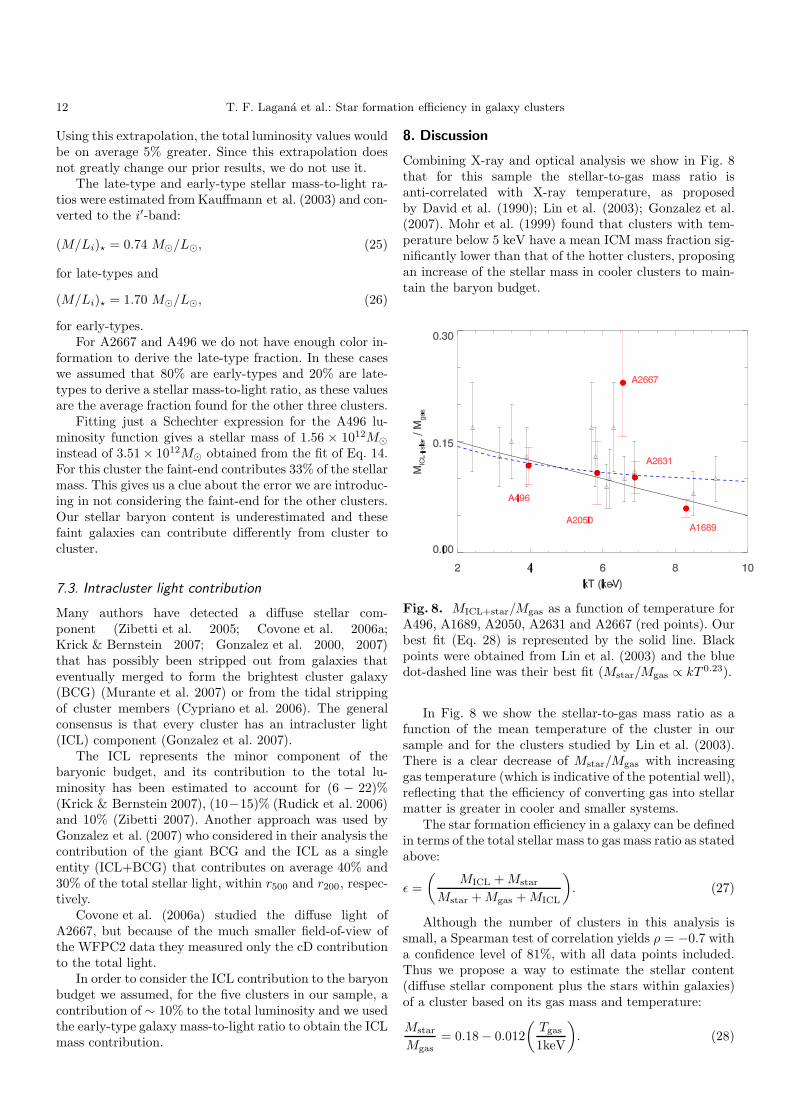
Combining X-ray and optical analysis we show in Fig. 8that for this sample the stellar-to-gas mass ratio isanti-correlated with X-ray temperature, as proposedby David et al. (1990); Lin et al. (2003); Gonzalez et al.(2007). Mohr et al. (1999) found that clusters with tem-perature below 5 keV have a mean ICM mass fraction sig-nificantly lower than that of the hotter clusters, proposingan increase of the stellar mass in cooler clusters to main-tain the baryon budget.

Fig. 8. MICL+star/Mgas as a function of temperature forA496, A1689, A2050, A2631 and A2667 (red points). Ourbest fit (Eq. 28) is represented by the solid line. Blackpoints were obtained from Lin et al. (2003) and the bluedot-dashed line was their best fit (Mstar/Mgas ∝ kT 0.23).

In Fig. 8 we show the stellar-to-gas mass ratio as afunction of the mean temperature of the cluster in oursample and for the clusters studied by Lin et al. (2003).There is a clear decrease of Mstar/Mgas with increasinggas temperature (which is indicative of the potential well),reflecting that the efficiency of converting gas into stellarmatter is greater in cooler and smaller systems.

The star formation efficiency in a galaxy can be definedin terms of the total stellar mass to gas mass ratio as statedabove:

ǫ =

(

MICL + Mstar

Mstar + Mgas + MICL

)

. (27)

Although the number of clusters in this analysis issmall, a Spearman test of correlation yields ρ = −0.7 witha confidence level of 81%, with all data points included.Thus we propose a way to estimate the stellar content(diffuse stellar component plus the stars within galaxies)of a cluster based on its gas mass and temperature:

Mstar

Mgas= 0.18 − 0.012

(

Tgas

1keV

)

. (28)


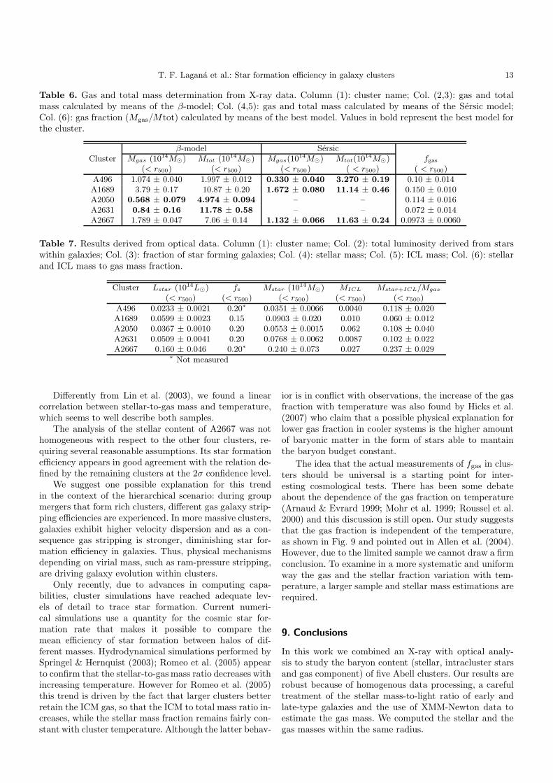
Table 6. Gas and total mass determination from X-ray data. Column (1): cluster name; Col. (2,3): gas and totalmass calculated by means of the β-model; Col. (4,5): gas and total mass calculated by means of the Sersic model;Col. (6): gas fraction (Mgas/Mtot) calculated by means of the best model. Values in bold represent the best model forthe cluster.

β-model SersicCluster Mgas (1014M⊙) Mtot (1014M⊙) Mgas(10

14M⊙) Mtot(1014M⊙) fgas

(< r500) (< r500) (< r500) ( < r500) ( < r500)

A496 1.074 ± 0.040 1.997 ± 0.012 0.330 ± 0.040 3.270 ± 0.19 0.10 ± 0.014A1689 3.79 ± 0.17 10.87 ± 0.20 1.672 ± 0.080 11.14 ± 0.46 0.150 ± 0.010A2050 0.568 ± 0.079 4.974 ± 0.094 – – 0.114 ± 0.016A2631 0.84 ± 0.16 11.78 ± 0.58 – – 0.072 ± 0.014A2667 1.789 ± 0.047 7.06 ± 0.14 1.132 ± 0.066 11.63 ± 0.24 0.0973 ± 0.0060

Table 7. Results derived from optical data. Column (1): cluster name; Col. (2): total luminosity derived from starswithin galaxies; Col. (3): fraction of star forming galaxies; Col. (4): stellar mass; Col. (5): ICL mass; Col. (6): stellarand ICL mass to gas mass fraction.

Cluster Lstar (1014L⊙) fs Mstar (1014M⊙) MICL Mstar+ICL/Mgas

(< r500) (< r500) (< r500) (< r500) (< r500)

A496 0.0233 ± 0.0021 0.20∗ 0.0351 ± 0.0066 0.0040 0.118 ± 0.020A1689 0.0599 ± 0.0023 0.15 0.0903 ± 0.020 0.010 0.060 ± 0.012A2050 0.0367 ± 0.0010 0.20 0.0553 ± 0.0015 0.062 0.108 ± 0.040A2631 0.0509 ± 0.0041 0.20 0.0768 ± 0.0062 0.0087 0.102 ± 0.022A2667 0.160 ± 0.046 0.20∗ 0.240 ± 0.073 0.027 0.237 ± 0.029

∗ Not measured

Differently from Lin et al. (2003), we found a linearcorrelation between stellar-to-gas mass and temperature,which seems to well describe both samples.

The analysis of the stellar content of A2667 was nothomogeneous with respect to the other four clusters, re-quiring several reasonable assumptions. Its star formationefficiency appears in good agreement with the relation de-fined by the remaining clusters at the 2σ confidence level.

We suggest one possible explanation for this trendin the context of the hierarchical scenario: during groupmergers that form rich clusters, different gas galaxy strip-ping efficiencies are experienced. In more massive clusters,galaxies exhibit higher velocity dispersion and as a con-sequence gas stripping is stronger, diminishing star for-mation efficiency in galaxies. Thus, physical mechanismsdepending on virial mass, such as ram-pressure stripping,are driving galaxy evolution within clusters.

Only recently, due to advances in computing capa-bilities, cluster simulations have reached adequate lev-els of detail to trace star formation. Current numeri-cal simulations use a quantity for the cosmic star for-mation rate that makes it possible to compare themean efficiency of star formation between halos of dif-ferent masses. Hydrodynamical simulations performed bySpringel & Hernquist (2003); Romeo et al. (2005) appearto confirm that the stellar-to-gas mass ratio decreases withincreasing temperature. However for Romeo et al. (2005)this trend is driven by the fact that larger clusters betterretain the ICM gas, so that the ICM to total mass ratio in-creases, while the stellar mass fraction remains fairly con-stant with cluster temperature. Although the latter behav-

ior is in conflict with observations, the increase of the gasfraction with temperature was also found by Hicks et al.(2007) who claim that a possible physical explanation forlower gas fraction in cooler systems is the higher amountof baryonic matter in the form of stars able to mantainthe baryon budget constant.

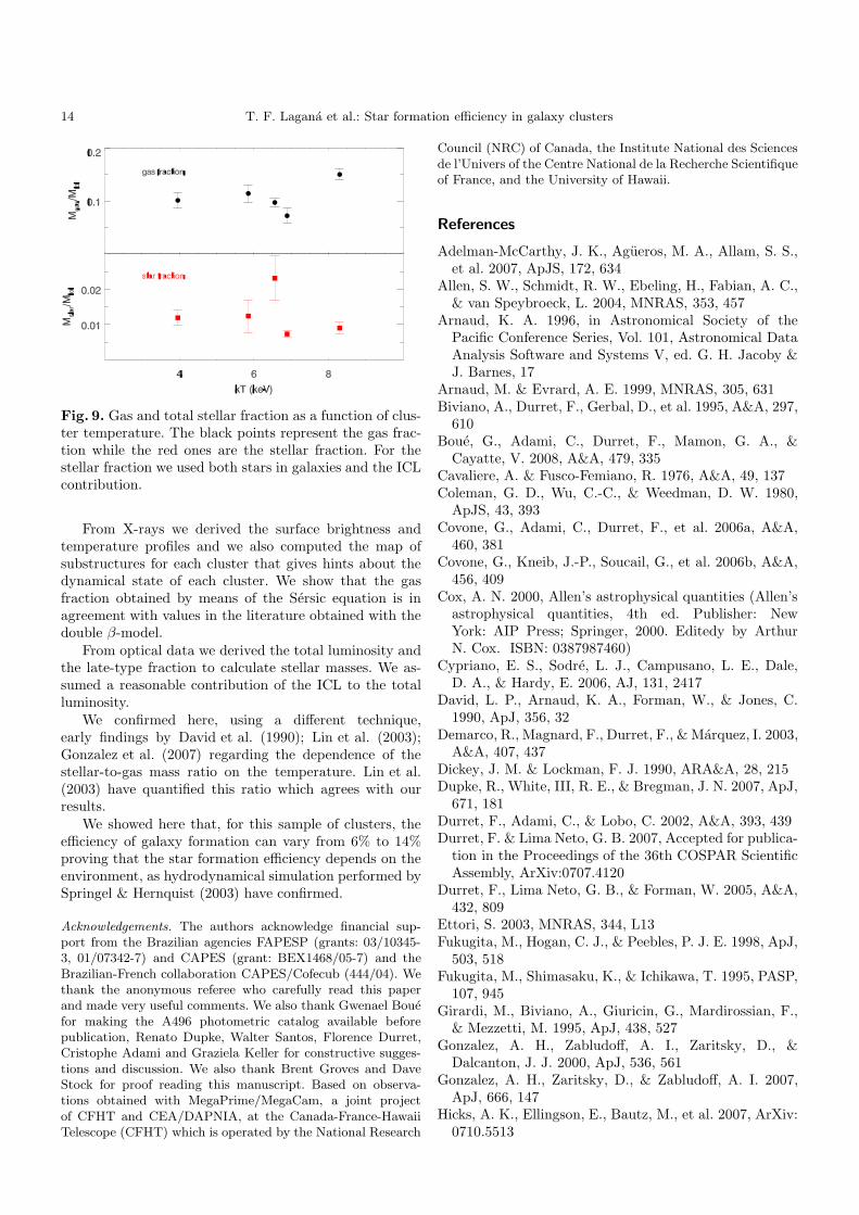
The idea that the actual measurements of fgas in clus-ters should be universal is a starting point for inter-esting cosmological tests. There has been some debateabout the dependence of the gas fraction on temperature(Arnaud & Evrard 1999; Mohr et al. 1999; Roussel et al.2000) and this discussion is still open. Our study suggeststhat the gas fraction is independent of the temperature,as shown in Fig. 9 and pointed out in Allen et al. (2004).However, due to the limited sample we cannot draw a firmconclusion. To examine in a more systematic and uniformway the gas and the stellar fraction variation with tem-perature, a larger sample and stellar mass estimations arerequired.

9. Conclusions

In this work we combined an X-ray with optical analy-sis to study the baryon content (stellar, intracluster starsand gas component) of five Abell clusters. Our results arerobust because of homogenous data processing, a carefultreatment of the stellar mass-to-light ratio of early andlate-type galaxies and the use of XMM-Newton data toestimate the gas mass. We computed the stellar and thegas masses within the same radius.


Fig. 9. Gas and total stellar fraction as a function of clus-ter temperature. The black points represent the gas frac-tion while the red ones are the stellar fraction. For thestellar fraction we used both stars in galaxies and the ICLcontribution.

From X-rays we derived the surface brightness andtemperature profiles and we also computed the map ofsubstructures for each cluster that gives hints about thedynamical state of each cluster. We show that the gasfraction obtained by means of the Sersic equation is inagreement with values in the literature obtained with thedouble β-model.

From optical data we derived the total luminosity andthe late-type fraction to calculate stellar masses. We as-sumed a reasonable contribution of the ICL to the totalluminosity.

We confirmed here, using a different technique,early findings by David et al. (1990); Lin et al. (2003);Gonzalez et al. (2007) regarding the dependence of thestellar-to-gas mass ratio on the temperature. Lin et al.(2003) have quantified this ratio which agrees with ourresults.

We showed here that, for this sample of clusters, theefficiency of galaxy formation can vary from 6% to 14%proving that the star formation efficiency depends on theenvironment, as hydrodynamical simulation performed bySpringel & Hernquist (2003) have confirmed.

Acknowledgements. The authors acknowledge financial sup-port from the Brazilian agencies FAPESP (grants: 03/10345-3, 01/07342-7) and CAPES (grant: BEX1468/05-7) and theBrazilian-French collaboration CAPES/Cofecub (444/04). Wethank the anonymous referee who carefully read this paperand made very useful comments. We also thank Gwenael Bouefor making the A496 photometric catalog available beforepublication, Renato Dupke, Walter Santos, Florence Durret,Cristophe Adami and Graziela Keller for constructive sugges-tions and discussion. We also thank Brent Groves and DaveStock for proof reading this manuscript. Based on observa-tions obtained with MegaPrime/MegaCam, a joint projectof CFHT and CEA/DAPNIA, at the Canada-France-HawaiiTelescope (CFHT) which is operated by the National Research

Council (NRC) of Canada, the Institute National des Sciencesde l’Univers of the Centre National de la Recherche Scientifiqueof France, and the University of Hawaii.

References

Adelman-McCarthy, J. K., Agueros, M. A., Allam, S. S.,et al. 2007, ApJS, 172, 634

Allen, S. W., Schmidt, R. W., Ebeling, H., Fabian, A. C.,& van Speybroeck, L. 2004, MNRAS, 353, 457

Arnaud, K. A. 1996, in Astronomical Society of thePacific Conference Series, Vol. 101, Astronomical DataAnalysis Software and Systems V, ed. G. H. Jacoby &J. Barnes, 17

Arnaud, M. & Evrard, A. E. 1999, MNRAS, 305, 631Biviano, A., Durret, F., Gerbal, D., et al. 1995, A&A, 297,

610Boue, G., Adami, C., Durret, F., Mamon, G. A., &

Cayatte, V. 2008, A&A, 479, 335Cavaliere, A. & Fusco-Femiano, R. 1976, A&A, 49, 137Coleman, G. D., Wu, C.-C., & Weedman, D. W. 1980,

ApJS, 43, 393Covone, G., Adami, C., Durret, F., et al. 2006a, A&A,

460, 381Covone, G., Kneib, J.-P., Soucail, G., et al. 2006b, A&A,

456, 409Cox, A. N. 2000, Allen’s astrophysical quantities (Allen’s

astrophysical quantities, 4th ed. Publisher: NewYork: AIP Press; Springer, 2000. Editedy by ArthurN. Cox. ISBN: 0387987460)

Cypriano, E. S., Sodre, L. J., Campusano, L. E., Dale,D. A., & Hardy, E. 2006, AJ, 131, 2417

David, L. P., Arnaud, K. A., Forman, W., & Jones, C.1990, ApJ, 356, 32

Demarco, R., Magnard, F., Durret, F., & Marquez, I. 2003,A&A, 407, 437

Dickey, J. M. & Lockman, F. J. 1990, ARA&A, 28, 215Dupke, R., White, III, R. E., & Bregman, J. N. 2007, ApJ,

671, 181Durret, F., Adami, C., & Lobo, C. 2002, A&A, 393, 439Durret, F. & Lima Neto, G. B. 2007, Accepted for publica-

tion in the Proceedings of the 36th COSPAR ScientificAssembly, ArXiv:0707.4120

Durret, F., Lima Neto, G. B., & Forman, W. 2005, A&A,432, 809

Ettori, S. 2003, MNRAS, 344, L13Fukugita, M., Hogan, C. J., & Peebles, P. J. E. 1998, ApJ,

503, 518Fukugita, M., Shimasaku, K., & Ichikawa, T. 1995, PASP,

107, 945Girardi, M., Biviano, A., Giuricin, G., Mardirossian, F.,

& Mezzetti, M. 1995, ApJ, 438, 527Gonzalez, A. H., Zabludoff, A. I., Zaritsky, D., &

Dalcanton, J. J. 2000, ApJ, 536, 561Gonzalez, A. H., Zaritsky, D., & Zabludoff, A. I. 2007,

ApJ, 666, 147Hicks, A. K., Ellingson, E., Bautz, M., et al. 2007, ArXiv:

0710.5513


Ikebe, Y., Makishima, K., Fukazawa, Y., et al. 1999, ApJ,525, 58

Jones, C. & Forman, W. 1984, ApJ, 276, 38Kaastra, J. S. & Mewe, R. 1993, A&AS, 97, 443Kauffmann, G., Heckman, T. M., White, S. D. M., et al.

2003, MNRAS, 341, 33King, I. R. 1978, ApJ, 222, 1Komatsu, E. & Seljak, U. 2001, MNRAS, 327, 1353Krick, J. E. & Bernstein, R. A. 2007, AJ, 134, 466Lacey, C. & Cole, S. 1993, MNRAS, 262, 627Liedahl, D. A., Osterheld, A. L., & Goldstein, W. H. 1995,

ApJ, 438, L115Lima Neto, G. B., Capelato, H. V., Sodre, Jr., L., &

Proust, D. 2003, A&A, 398, 31Lima Neto, G. B., Lagana, T. F., & Durret, F. 2006, in

ESA Special Publication, Vol. 604, The X-ray Universe2005, ed. A. Wilson, 747

Lin, Y.-T., Mohr, J. J., & Stanford, S. A. 2003, ApJ, 591,749

Lumb, D. H., Warwick, R. S., Page, M., & De Luca, A.2002, A&A, 389, 93

Markevitch, M., Vikhlinin, A., Forman, W. R., & Sarazin,C. L. 1999, ApJ, 527, 545

Mateus, A., Sodre, L., Cid Fernandes, R., et al. 2006,MNRAS, 370, 721

Mohr, J. J., Mathiesen, B., & Evrard, A. E. 1999, ApJ,517, 627

Murante, G., Giovalli, M., Gerhard, O., et al. 2007,MNRAS, 377, 2

Pislar, V., Durret, F., Gerbal, D., Lima Neto, G. B., &Slezak, E. 1997, A&A, 322, 53

Poggianti, B. M. 1997, A&AS, 122, 399Pratt, G. W. & Arnaud, M. 2005, A&A, 429, 791Rasia, E., Ettori, S., Moscardini, L., et al. 2006, MNRAS,

369, 2013Romeo, A. D., Portinari, L., & Sommer-Larsen, J. 2005,

MNRAS, 361, 983Roussel, H., Sadat, R., & Blanchard, A. 2000, A&A, 361,

429Rudick, C. S., Mihos, J. C., & McBride, C. 2006, ApJ,

648, 936Schechter, P. & Press, W. H. 1976, ApJ, 203, 557Springel, V. & Hernquist, L. 2003, MNRAS, 339, 312Tamura, T., Bleeker, J. A. M., Kaastra, J. S., Ferrigno,

C., & Molendi, S. 2001, A&A, 379, 107Tozzi, P. 2007, X-ray emission from Clusters of GalaxiesVikhlinin, A., Kravtsov, A., Forman, W., et al. 2006, ApJ,

640, 691Vikhlinin, A., Markevitch, M., & Murray, S. S. 2001, ApJ,

551, 160Wolfram, K. D., Dymond, K. F., Budzien, S. A., et al.

1999, in Proc. SPIE 3818, 149, G. R. Carruthers, K. F.Dymond Eds., ed. G. R. Carruthers & K. F. Dymond,Vol. 3818, 149

Xue, Y.-J. & Wu, X.-P. 2000, MNRAS, 318, 715Zhang, Y.-Y., Finoguenov, A., Bohringer, H., et al. 2007,

A&A, 467, 437Zibetti, S. 2007, ArXiv:0709.0659, 709

Zibetti, S., White, S. D. M., Schneider, D. P., &Brinkmann, J. 2005, MNRAS, 358, 949

Documents

Star formation efficiency in galaxy clusters