The observed concentration-mass relation for galaxy clusters

arX

iv:a

stro

-ph/

0703

126v

1 7

Mar

200

7Mon. Not. R. Astron. Soc.000, 000–000 (0000) Printed 5 February 2008 (MN LATEX style file v2.2)

The Observed Concentration-Mass Relation for Galaxy Clusters

Julia M. Comerford1 and Priyamvada Natarajan2,3

1Astronomy Department, 601 Campbell Hall, University of California, Berkeley, CA 94720-34112Department of Astronomy, Yale University, P.O. Box 208101, New Haven, CT 06520-81013Department of Physics, Yale University, P.O. Box 208120, New Haven, CT 06520-8120

5 February 2008

ABSTRACTThe properties of clusters of galaxies offer key insights into the assembly process of structurein the universe. Numerical simulations of cosmic structureformation in a hierarchical, darkmatter dominated universe suggest that galaxy cluster concentrations, which are a measure ofa halo’s central density, decrease gradually with virial mass. However, cluster observationshave yet to confirm this correlation. The slopes of the run of measured concentrations withvirial mass are often either steeper or flatter than predicted by simulations. In this work, wepresent the most complete sample of observed cluster concentrations and masses yet assem-bled, including new measurements for 10 strong lensing clusters, thereby more than doublingthe existing number of strong lensing concentration estimates. We fit a power law to the ob-served concentrations as a function of virial mass, and find that the slope is consistent with theslopes found in simulations, though our normalization factor is higher. Observed lensing con-centrations appear to be systematically larger than X-ray concentrations, a more pronouncedeffect than found in simulations. We also find that at fixed mass, the bulk of observed clusterconcentrations are distributed log-normally, with the exception of a few anomalously highconcentration clusters. We examine the physical processeslikely responsible for the discrep-ancy between lensing and X-ray concentrations, and for the anomalously high concentrationsin particular. The forthcoming Millennium simulation results will offer the most comprehen-sive comparison set to our findings of an observed concentration-mass power law relation.

Key words: cosmology: observations – dark matter – gravitational lensing – galaxies: clus-ters: general

1 INTRODUCTION

Galaxy clusters are the most recent structures to assemble in a hier-archicalΛCDM universe and therefore offer important clues to thedetailed understanding of the growth of structure in the universe.TheΛCDM paradigm is well studied and observationally supportedon the largest scales by the cosmic microwave background data,high-z supernovae, and galaxy surveys. Clusters of galaxies area useful laboratory to further test this paradigm, as their masses,abundances, and other properties such as baryon fraction providekey cosmological constraints.

Clusters also provide overwhelming evidence for the existenceof copious amounts of dark matter in the universe. The bulk ofthemass of a cluster is dark matter (∼ 85%), with hot baryonic gascontributing about10% and the rest provided by the stellar contentof the constituent galaxies.

One of the key predictions of CDM is the excellent fit to den-sity profiles on a wide range of scales provided by the Navarro-Frenk-White (NFW) form (Navarro et al. 1996, 1997), or withmodifications to the inner slope (Moore et al. 1999; Navarro et al.2004). In numerical simulations of structure formation, itis foundthat this profile fits dwarf galaxy scale dark matter halos as well

as massive, cluster scale dark matter halos. For a typical clusterdark matter halo in these simulations, the density profile steepensfor radii larger than the halo’s typical scale radius (defined moreprecisely in§ 2 below).

A useful diagnostic, the halo concentration, can be defined asthe ratio of the halo’s virial radius to its scale radius. This con-centration parameter reflects the central density of the halo, whichdepends on the halo’s assembly history and thereby on its time offormation. Since in the hierarchical structure formation scenariomassive galaxy clusters are the most recent bound objects toform,their concentrations are a crucial probe of the mean densityof theuniverse at relatively late epochs.

As originally suggested by Navarro et al. (1996) and sup-ported by later numerical simulations of cosmological structure for-mation (Bullock et al. 2001; Hennawi et al. 2007), a halo’s concen-tration parameter is related to its virial mass, with the concentrationdecreasing gradually with mass. Given this prediction it isimpor-tant to test this trend with observational data, as this offers an in-direct check on the veracity of the paradigm itself. The situationat present with observed clusters with measured concentrations isunclear due to the plurality of methods employed to derive these

c© 0000 RAS

http://arXiv.org/abs/astro-ph/0703126v1

2 Comerford & Natarajan

concentrations as well as systematics arising from the complex dy-namics and its effect on mass distributions.

In this paper, we present new concentration measurements for10 strong lensing clusters and combine our results with other mea-surements in the literature to construct an observed concentration-mass relation for galaxy clusters. In§ 2, we present the basic defi-nitions and equations relevant to computing concentrations. In thefollowing section,§ 3, we define the observational sample and thevarious methods used to select these clusters. We present the con-structed observed concentration-mass relation in§ 4, and exam-ine the distribution of concentrations at fixed mass in§ 5. In § 6,we explore the physical effects that might cause anomalously highmeasurements of concentration for some clusters, and present ourconclusions in§ 7.

One of the key points we emphasize is that the clusters in thiscompiled sample have their masses and concentrations measuredusing a variety of different methods: strong lensing, weak lens-ing, X-ray temperatures, line of sight velocity distributions, and thecaustic method. In several cases, a cluster’s mass and concentrationare measured using multiple methods that yield different results,and it is these discrepancies that are of interest. Throughout this pa-per, we adopt a spatially flat cosmological model dominated by colddark matter and a cosmological constant (Ωm0 = 0.3, ΩΛ0 = 0.7,h = 0.7).

2 DEFINITION OF THE CONCENTRATIONPARAMETER

Cosmological simulations of structure formation suggest that darkmatter halos, independent of mass or cosmology, follow the den-sity profile given by Navarro et al. (1996, 1997). The sphericallyaveraged NFW profile is given by

ρ(r) =ρs

(r/rs)(1 + r/rs)2, (1)

whereρs is a characteristic density andrs is the scale radius, whichdescribes the transition point where the density profile turns overfrom ρ ∝ r−1 to ρ ∝ r−3. The mass contained within radiusr ofan NFW halo that produces gravitational lensing of the backgroundsources is

M(6 r) = 4πΣcritκsr2s

»

ln(1 + x) − x

1 + x

–

, (2)

wherex ≡ r/rs andΣcrit is the critical surface mass density, de-fined as

Σcrit ≡c2

4πG

Ds

DlDls

, (3)

which depends on the angular diameter distancesDl,s,ls fromthe observer to the lens, to the source, and from the lens to thesource, respectively. The scale convergence isκs = ρsrs/Σcrit

(Bartelmann 1996).The concentration parameter of a halo is the ratio of its virial

radius to its scale radius, and is representative of the halo’s cen-tral density. In much of the literature discussing cluster concen-trations, two distinct definitions of the virial radius are commonlyused. First, the virial radius may be defined as the radiusr200 atwhich the average halo density is 200 times the critical densityat the halo redshift. In this case, the concentration is denoted asc200 ≡ r200/rs. In an alternative convention, the virial radius is de-fined as the radiusrvir at which the average halo density is∆vir(z)times the mean density at the halo redshiftz, where∆vir(z) =

(18π2+82x−39x2)/(1+x) andx ≡ Ωm(z)−1 (Hu & Kravtsov2003). The resultant halo concentration iscvir ≡ rvir/rs.

For ease of comparison with other work, we will henceforthreport all measurements in terms of both definitions of virial radius:c200 and the corresponding halo massM200 ≡ M(6 r200), andcvir and the correspondingMvir ≡ M(6 rvir).

3 OBSERVATIONAL SAMPLE

To determine the observed relation between concentration andvirial mass for galaxy clusters, we compile a sample of all knownobservationally-determined concentrations and the correspondingvirial masses. The bulk of our sample is drawn from pre-existingdata in the literature, but we also incorporate new concentration andmass determinations for 10 strong lensing clusters. This compila-tion presents the most complete sample of observed cluster con-centrations and virial masses yet assembled; in total, our sampleconsists of 182 unique measurements for 100 galaxy clusters.

3.1 New Concentrations for 10 Strong Lensing Clusters

Comerford et al. (2006) used the strong lensing arcs observed in10 galaxy clusters to fit elliptical NFW dark matter density pro-files to each cluster. Using their best-fit scale radius and scale con-vergence parameters, as well as the observed cluster and arcred-shifts, we determine a concentration and mass for each lens,shownin Table 1. We compute errors in concentration and mass basedon the errors derived for the best-fit NFW parameters. As detailedin Comerford et al. (2006) these errors are quite small (and likelyunderestimate the true error) because they apply to one particularmodel and do not reflect degeneracies between models.

In particular, for several lensing clusters, the best-fit massdistribution is bi-modal and due to the difficulty of convertingthese mass models accurately to a single NFW parameterizationto derive the concentration, we retain in our sample only clustersthat are well defined by a primary single dark matter halo. Ourfits to the clusters ClG 2244−02, 3C 220.1, MS 2137.3−2353,MS 0451.6−0305, and MS 1137.5+6625 fulfill this criterion, morethan doubling the number of existing cluster concentrationandmass measurements, with errorbars, from strong lensing.

Two of the clusters from Comerford et al. (2006),ClG 0054−27 and Cl 0016+1609, do not have published arcredshifts, preventing us from determining the cluster’s criticalsurface mass density (Equation 3) and therefore the virial mass orthe concentration parameter. Instead, we assume a ratio of angulardiameter distancesDs/Dls = 1 to calculate the concentrationsand masses for these two clusters, reported in Table 1. We excludethese two clusters, however, from the analysis that follows.

3.2 Compiling Published Observations

We combine our concentration and mass measurements with thosein the literature to create a complete sample of observed galaxycluster concentrations and virial masses. The mass distributions ofthese clusters are fit using a variety of observational methods, andin many cases a cluster is independently fit by different authorsusing different methods. The assumption of spherical or axial sym-metry of the halo often figures prominently in mass calculations.We briefly outline below each of the methods employed in the de-termination of a dark matter halo’s mass distribution.

c© 0000 RAS, MNRAS000, 000–000

Observed Cluster Concentration-Mass Relation 3

Table 1. New cluster concentrations and masses determined via strong lensing.

Cluster Lensa c200 M200 cvir Mvir

(1014 M⊙) (1014 M⊙)

ClG 2244−02 4.3 ± 0.4 4.5 ± 0.9 5.2 ± 0.5 5.2 ± 1.1Abell 370 G1 4.8 ± 0.2 9.0 ± 1.0 5.8 ± 0.3 10. ± 1

G2 5.2 ± 0.3 6.7 ± 0.7 6.3 ± 0.3 7.7 ± 0.83C 220.1 4.3 ± 0.2 3.1 ± 0.3 5.0 ± 0.2 3.5 ± 0.3

MS 2137.3−2353 13 ± 1 2.9 ± 0.4 16 ± 1 3.2 ± 0.4MS 0451.6−0305 5.5 ± 0.3 18 ± 2 6.4 ± 0.3 20. ± 2MS 1137.5+6625 3.3 ± 0.2 6.5 ± 0.7 3.8 ± 0.2 7.2 ± 0.8ClG 0054−27b G1 1.2 ± 0.1 0.42 ± 0.07 1.5 ± 0.1 0.52 ± 0.09

G2 2.1 ± 0.1 0.95 ± 0.12 2.5 ± 0.1 1.1 ± 0.1Cl 0016+1609b DG 256 2.1 ± 0.1 1.1 ± 0.2 2.5 ± 0.1 1.3 ± 0.2

DG 251 2.3 ± 0.1 0.51 ± 0.06 2.7 ± 0.1 0.59 ± 0.07DG 224 3.1 ± 0.2 3.1 ± 0.4 3.6 ± 0.2 3.6 ± 0.4

Cl 0939+4713 G1 4.5 ± 0.3 0.71 ± 0.11 5.4 ± 0.4 0.81 ± 0.12G2 3.7 ± 0.3 1.1 ± 0.2 4.5 ± 0.3 1.2 ± 0.2G3 4.5 ± 0.2 1.4 ± 0.1 5.4 ± 0.3 1.6 ± 0.2

ZwCl 0024+1652 #362 4.6 ± 0.2 3.1 ± 0.1 5.5 ± 0.3 2.6 ± 0.3#374 4.3 ± 0.2 3.7 ± 0.5 5.1 ± 0.3 4.2 ± 0.5#380 3.4 ± 0.2 2.7 ± 0.3 4.1 ± 0.2 3.2 ± 0.3

aSee Comerford et al. (2006) for lens identification.bBecause these cluster arcs have no published redshifts, we calculate the concentration and mass assumingDs/Dls = 1. Note that we do not use theseconcentration and mass determinations in our observed concentration-mass fit.

Strong lensing (SL) — Strong lensing typically occurs whenthe projected surface mass density in the inner regions of a cluster issufficiently high to produce one or more distorted images of asin-gle background galaxy. The observed positions, orientations, andmagnifications of the lensed images are used to constrain themassdistribution of the cluster lens. The integrated mass determined inthe inner regions of a cluster from strong lensing effects isoftensystematically higher than that determined using X-ray data, lead-ing to higher values of the estimated concentration parameter com-pared to the average galaxy cluster that is not a lens. This effectis due to the fact that lensing clusters and in particular those thatexhibit strong lensing tend to preferentially sample the high massend of the cluster mass function.

Weak lensing (WL) — The gravitational tidal field caused bya mass distribution produces elongated, tangential distortions ofbackground objects. These weak distortions are observed atlargeradii from the center of lensing clusters and their statistical anal-yses provide a direct measure of the density profile of the clusterlens at intermediate to large radii.

Combined weak lensing and strong lensing (WL+SL) — Ifboth weak and strong lensing measurements of a cluster are used incombination, they can be used to effectively break the mass-sheetdegeneracy (Schneider & Seitz 1995) that often plagues solitarystrong or weak lensing mass measurements. Therefore, the com-bination of strong and weak lensing can provide a more accurateand calibrated mass distribution for a cluster.

X-ray temperature — The hot gas in galaxy clusters emits X-rays via bremsstrahlung radiation and atomic line emission. Thesurface brightness distribution and the measured cluster tempera-ture can be used to determine the density profile. Combining thetemperature and density information yields the cluster mass. How-ever, the X-ray technique for mass determination assumes that theintra-cluster gas is distributed in a spherically symmetric fashionand is in hydrostatic equilibrium (Evrard et al. 1996). These as-sumptions may be untenable; for example, observed buoyant bub-

bles near the cores of galaxy clusters suggest the hot gas maynotbe strictly in hydrostatic equilibrium (e.g., Churazov et al. 2001).

Line of sight velocity distribution (LOSVD) — The LOSVDfor a cluster is a function relating the number of cluster galaxieswith their line of sight velocities. This function is parameterizedby velocity moments, which can be measured observationally(forexample, the second moment of the LOSVD is the square of theline of sight velocity dispersion). Combining these results with theJeans equation, assuming spherical symmetry, determines the po-tential and therefore the density profile of the cluster itself.

Caustic method (CM) — When the line of sight velocity isplotted against the projected clustercentric radius, member galax-ies in a cluster align in a distinctively flaring pattern. Theedges ofthese flares are called caustics and demarcate the cluster infall re-gion (Kaiser 1987). Based on the location and amplitude of thesecaustics, we can infer the cluster potential and therefore the massof a cluster. However, this technique relies upon the assumptions ofspherical symmetry and does not adequately take into account thenon-linearities in structure formation.

A variety of definitions are used in the literature for the virialradius, and for consistency we employ the Hu & Kravtsov (2003)formula to convert all concentrations and masses to our preferredconvention of (c200, M200) and (cvir, Mvir). We also convert all thedata to a flatΛCDM cosmological model (Ωm0 = 0.3, ΩΛ0 = 0.7,h = 0.7). The entire sample is presented in Table A-1, which weuse to define an observed cluster concentration-mass relation.

4 THE OBSERVED CONCENTRATION-MASSRELATION

To discern the trend between concentration and mass, we firstcullour sample down to only those concentrations that have corre-sponding virial mass estimates and that have published errors inboth quantities. This narrows our sample down to 62 clusters.

c© 0000 RAS, MNRAS000, 000–000


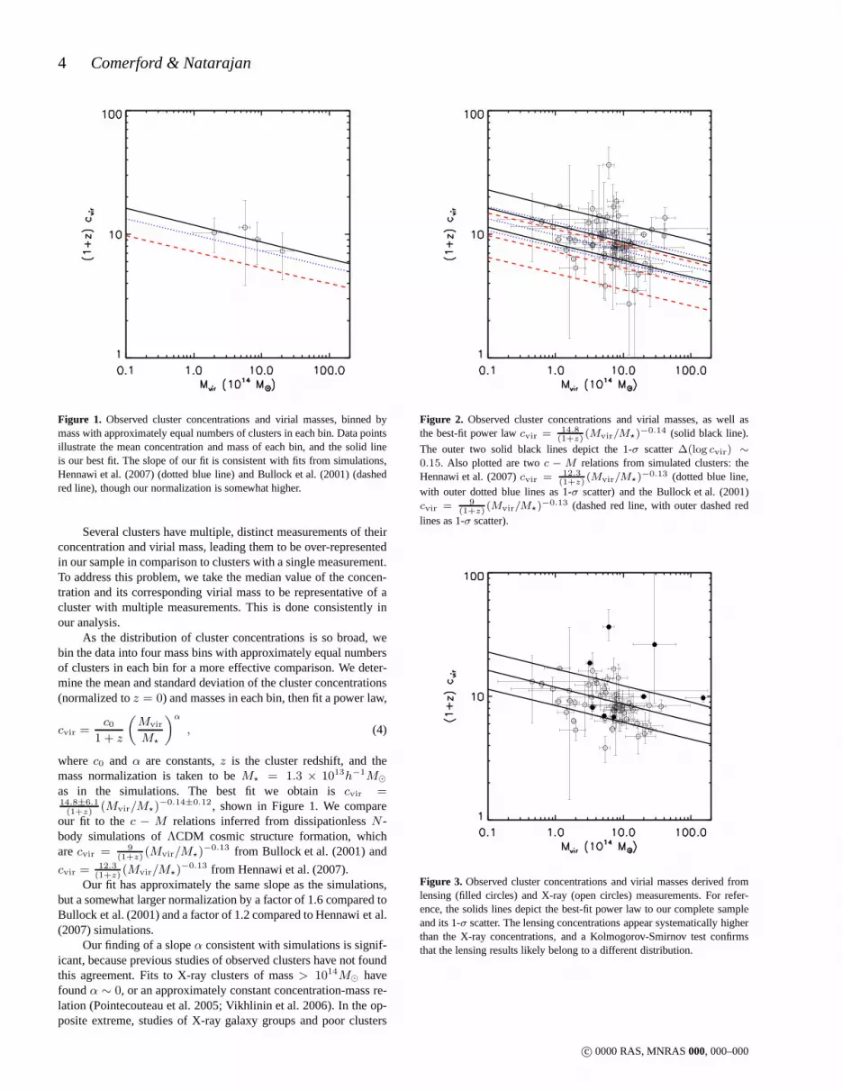
Figure 1. Observed cluster concentrations and virial masses, binnedbymass with approximately equal numbers of clusters in each bin. Data pointsillustrate the mean concentration and mass of each bin, and the solid lineis our best fit. The slope of our fit is consistent with fits from simulations,Hennawi et al. (2007) (dotted blue line) and Bullock et al. (2001) (dashedred line), though our normalization is somewhat higher.

Several clusters have multiple, distinct measurements of theirconcentration and virial mass, leading them to be over-representedin our sample in comparison to clusters with a single measurement.To address this problem, we take the median value of the concen-tration and its corresponding virial mass to be representative of acluster with multiple measurements. This is done consistently inour analysis.

As the distribution of cluster concentrations is so broad, webin the data into four mass bins with approximately equal numbersof clusters in each bin for a more effective comparison. We deter-mine the mean and standard deviation of the cluster concentrations(normalized toz = 0) and masses in each bin, then fit a power law,

cvir =c0

1 + z

„

Mvir

M⋆

«α

, (4)

wherec0 and α are constants,z is the cluster redshift, and themass normalization is taken to beM⋆ = 1.3 × 1013h−1M⊙

as in the simulations. The best fit we obtain iscvir =14.8±6.1(1+z)

(Mvir/M⋆)−0.14±0.12, shown in Figure 1. We compare

our fit to the c − M relations inferred from dissipationlessN -body simulations ofΛCDM cosmic structure formation, whicharecvir = 9

(1+z)(Mvir/M⋆)

−0.13 from Bullock et al. (2001) and

cvir = 12.3(1+z)

(Mvir/M⋆)−0.13 from Hennawi et al. (2007).

Our fit has approximately the same slope as the simulations,but a somewhat larger normalization by a factor of 1.6 compared toBullock et al. (2001) and a factor of 1.2 compared to Hennawi et al.(2007) simulations.

Our finding of a slopeα consistent with simulations is signif-icant, because previous studies of observed clusters have not foundthis agreement. Fits to X-ray clusters of mass> 1014M⊙ havefoundα ∼ 0, or an approximately constant concentration-mass re-lation (Pointecouteau et al. 2005; Vikhlinin et al. 2006). In the op-posite extreme, studies of X-ray galaxy groups and poor clusters

Figure 2. Observed cluster concentrations and virial masses, as wellasthe best-fit power lawcvir = 14.8

(1+z)(Mvir/M⋆)−0.14 (solid black line).

The outer two solid black lines depict the 1-σ scatter∆(log cvir) ∼

0.15. Also plotted are twoc − M relations from simulated clusters: theHennawi et al. (2007)cvir = 12.3

(1+z)(Mvir/M⋆)−0.13 (dotted blue line,

with outer dotted blue lines as 1-σ scatter) and the Bullock et al. (2001)cvir = 9

(1+z)(Mvir/M⋆)−0.13 (dashed red line, with outer dashed red

lines as 1-σ scatter).

Figure 3. Observed cluster concentrations and virial masses derivedfromlensing (filled circles) and X-ray (open circles) measurements. For refer-ence, the solids lines depict the best-fit power law to our complete sampleand its 1-σ scatter. The lensing concentrations appear systematically higherthan the X-ray concentrations, and a Kolmogorov-Smirnov test confirmsthat the lensing results likely belong to a different distribution.

c© 0000 RAS, MNRAS000, 000–000


0.0

0.1

0.2

0.3

0.4

0.5

PD

F

0 10 20 30(1+z) cvir

0.0

0.1

0.2

0.3

0.4

PD

F

0 10 20 30 40(1+z) cvir

Figure 4. Log-normal fits to normalized histograms of observed clus-ter concentrations, binned by mass. The mass ranges areMvir < 4 ×

1014M⊙, 4 × 1014M⊙ < Mvir < 7.3 × 1014M⊙, 7.3 × 1014M⊙ <Mvir < 12 × 1014M⊙, andMvir > 12 × 1014M⊙ for bin 1 to bin 4,respectively. For each mass bin the expectation valueµ, standard deviationσ, andχ2 of the best-fit log-normal function are also given.

with lower virial masses in the range of∼ 1013 M⊙ find steepslopes ofα = −0.226 (Gastaldello et al. 2006) andα = −0.44(Sato et al. 2000). Finally, the Buote et al. (2006) sample ofX-raygalaxy systems ranging in mass from1013M⊙ to 1015M⊙ has aslope ofα = −0.172.

Both observations and simulations find a large scatter in con-centration for a given virial mass, which is likely due to thevari-ation in halo collapse epochs and histories (Bullock et al. 2001).Comparing our best fit to the unbinned clusters, shown in Figure 2,we find a 1-σ scatter of∆(log cvir) ∼ 0.15 in our relation. Thesimulations have scatters of∼ 0.18 in Bullock et al. (2001) and∼ 0.098 in Hennawi et al. (2007) (calculated from data courtesyof J. Hennawi). However, we cannot directly compare these totheobservationally derived scatters due to the differing systematics.

We note that the concentrations of clusters determined fromlensing methods (weak, strong, and a combination of the two)aresystematically higher than the concentrations determinedby othermethods. Figure 3 shows the distribution of lensing concentrationsrelative to X-ray concentrations; a Kolmogorov-Smirnov test findsonly a 28% probability that the two are in fact derived from thesame parent distribution.

A similar, though less pronounced, effect has been found innumerical simulations of clusters. Hennawi et al. (2007) identifiedlensing clusters from their simulated sample by using ray tracing tocompute strong lensing cross sections for each cluster, andfoundthat the simulated strong lensing clusters have on average 34%higher concentrations than the total simulated cluster population.In our observed sample, we find a larger fraction: about 55% higherconcentrations on average for observed strong lensing clusters.

Why are lensing concentrations systematically higher thanX-ray concentrations? Several known physical effects are implicatedin explaining this discrepancy. The X-ray method of determining amass distribution depends on the assumption of hydrostaticequilib-

0.0

0.1

0.2

0.3

0.4

0.5

PD

F

0 10 20 30(1+z) cvir

0.0

0.1

0.2

0.3

0.4

PD

F

0 10 20 30 40(1+z) cvir

Figure 5. As Fig. 4, but with concentrations greater than 2-σ from the ex-pectation value omitted. This excluded the highest concentration cluster inbin 2 and in bin 3. The resultant fits improved by up to a factor of 6 in χ2.

rium, which breaks down for unrelaxed clusters. As a result,X-raymeasurements may underpredict concentrations for unrelaxed sys-tems such as clusters undergoing mergers.

In particular, if non-thermal sources of pressure support arepresent and significant, for example due to the presence of a mag-netic field on small scales in the inner regions of a cluster, theassumption of hydrostatic equilibrium will tend to underestimatethe total mass and hence yield a systematically lower value forthe concentration. Loeb & Mao (1994) argue that for the clusterAbell 2218, a factor of about2 − 3 discrepancy in the strong lens-ing determined mass and the X-ray determined mass (under theas-sumption of hydrostatic equilibrium) enclosed within 200 kpc canbe explained with the existence of an equi-partition magnetic field.This effect alone could likely close the gap between X-ray and lens-ing concentrations.

In addition to underpredicted X-ray concentrations, overpre-dicted lensing concentrations could also contribute to thediscrep-ancy in concentration estimates. In particular, lensing concentra-tions can be inflated due to the effects of halo triaxiality, substruc-ture along the line of sight, and adiabatic contraction in the darkmatter due to the collapse of baryons in the inner regions of halos.

It is impossible to observationally determine a distant halo’sthree-dimensional shape, and most mass-finding techniquesassumea spherical halo. However, a spherical halo model fit to a triax-ial cluster, if projected along the major axis, would overestimateboth the cluster’s concentration and its virial mass (Gavazzi 2005;Oguri et al. 2005). If a halo were significantly elongated along theline of sight, its concentration could be overestimated up to 50%and its virial mass estimation could double (Corless & King 2006).Methods now exist to estimate the shape of a dark matter halo fromthe observed intracluster gas (Lee & Suto 2003).

Structure along the line of sight to the cluster can alsocontribute to a higher estimated concentration. Simulations ofKing & Corless (2007) determined that multiple subhalos close tothe line of sight are most effective at increasing the concentrationestimate of the main halo. Neglecting large-scale structure, as most

c© 0000 RAS, MNRAS000, 000–000


0

10

20

30

40

c vir

Figure 6. Observed concentrations for the cluster Abell 1689, ordered fromlowest to highest. Only weak lensing measurements produce the anoma-lously highcvir > 10 concentrations (dashed line).

halo mass models do, can artificially and substantially inflate con-centration estimates.

Finally, adiabatic contraction in the halo core could substan-tially increase a cluster’s concentration, as argued by Gnedin et al.(2004). The dissipative collapse of baryons in the centers of darkmatter halos induces a steepening of the dark matter densitypro-file in these regions. This steepening will systematically increasethe concentrations. Adiabatic contraction could explain why ourobserved lensing concentrations are yet higher than the simulatedcluster lens concentrations in our comparison. The Hennawiet al.(2007) simulated lensing clusters are products of dissipationlesssimulations, whereas observed clusters have presumably undergoneadiabatic contraction and a corresponding steepening in the densityprofile, yielding a higher value for the concentration.

5 CONCENTRATIONS FOR FIXED HALO MASS

Numerical simulations further indicate that concentrations for fixedhalo mass are log-normally distributed. To test this hypothesis forobserved clusters, we examine the clusters grouped into four massbins, as detailed in§ 4. We then fit a log-normal function to thedistribution of concentrations in each bin. For ourx = (1+ z)cvir,the log-normal probability density function (PDF) is

f(x; µ, σ) =1√

2πσxexp

„

−(lnx − µ)2

2σ2

«

, (5)

whereµ andσ are the expectation value and standard deviation.The panels in Figure 4 show the best-fit log-normal functions

to each mass bin, as well as the expectation value, standard devia-tion, andχ2 for each fit. The concentrations appear to be consistentwith a log-normal distribution, with the exception of a couple ofhigh concentration clusters that lie beyond the tail of the distribu-tion. To determine how well the bulk of concentrations, without theoutliers, is fit by a log-normal distribution, we omit all concentra-tions greater than 2-σ from the expectation value. This cut elimi-

0

10

20

30

40

c vir

Figure 7. Observed concentrations for the cluster MS 2137.3−2353, or-dered from lowest to highest. Note that all of the smaller values of concen-trationcvir < 12 (dashed line), which are more consistent with predictionsfrom observed and simulatedc − M relations, are from X-ray measure-ments.

nates one cluster from bin 2 (top row, right in Fig. 4) and one frombin 3 (bottom row, left in Fig. 4).

The resultant fits, shown in Figure 5, have improved in good-ness of fit to the data by a factors of 6 and 2 inχ2 for bin 2 and bin3, respectively. All four bins are now well-fit by a log-normal func-tion, suggesting that the vast majority of observed clusters followa log-normal distribution, but with a few outliers with substantiallyhigher concentrations.

These outliers are ZwCl 0024+1652 (in bin 2) andMS 2137.3−2353 (in bin 3), and their anomalously high concen-trations are well documented in the literature. Possible explanationsfor these high concentrations are presented in the next section.

6 ANOMALOUSLY HIGH CONCENTRATIONCLUSTERS

Three clusters stand out for their anomalously high concentrations,which are several sigma higher than the predicted concentration-mass relations. They are the lensing clusters ZwCl 0024+1652(cvir = 26; Kneib et al. 2003), Abell 1689, and MS 2137.3−2353.

Although there are only lensing measurements of theZwCl 0024+1652 concentration, multiple strong lensing, weaklensing, combined strong and weak lensing, and X-ray measure-ments have been made of the concentrations and virial massesofboth Abell 1689 and MS 2137.3−2353. Many of these individualmeasurements are even consistent with concentration-massrela-tions, leading us to ask whether the anomalously high concentra-tions are indeed real, and what the physical explanation forthesehigh concentrations might be.

Figure 6 illustrates the range of concentrations measured forthe cluster Abell 1689. Strikingly, if not for the weak lensing mea-surements, this cluster would have a rather typical range ofconcen-trations. Apparently some systematic effect causes the weak lens-ing concentrations to be inflated relative to concentrations inferred

c© 0000 RAS, MNRAS000, 000–000


via other methods. For instance, the weak lensing signal could bemore sensitive to substructure close to the line of sight, causingconcentration overestimates, as discussed in§ 4.

We see an analogous effect in MS 2137.3−2353, shown inFigure 7. Here, all of the smaller, unsurprising concentration val-ues are the result of X-ray measurements. Lensing measurementsproduce most of the anomalously high concentrations.

As discussed in§ 4, X-ray concentrations can be systemati-cally low for clusters that do not conform to the assumption of hy-drostatic equilibrium. And, lensing concentrations can beelevateddue to projection effects, substructure, or adiabatic contraction. Weexpect lensing concentrations to be greater than X-ray concentra-tions, but it is yet unclear whether the anomalously high lensingconcentrations of these three clusters are real.

This concern has been addressed for each of the three anoma-lously high concentration clusters. The high lensing concentra-tion of MS 2137.3−2353 may be explained by an elongatedhalo with its major axis close to the line of sight (Gavazzi2005). Also, ZwCl 0024+1652 exhibits prominent substructurethat may account for its high concentration estimates. For example,Kneib et al. (2003) identify a main clump with high concentrationas well as a secondary, low concentration clump, while this paper(Table 1) fits threecvir ∼ 5 clumps to ZwCl 0024+1652.

Perhaps the most progress has been made in explainingAbell 1689’s concentration, which has been measured to be ashighascvir = 37.4 (Halkola et al. 2006) but has come down to a con-sensus ofcvir ∼ 6 − 8 (Limousin et al. 2006) due to careful, de-tailed modeling including an unprecedented large number ofstronglensing constraints.

7 SUMMARY AND CONCLUSIONS

We have presented a comprehensive set of observed galaxy clus-ter concentrations and virial masses, including new concentrationestimates for 10 strong lensing clusters. With this data, wefit thedependence of the concentration parameter with virial massto apower law to compare with the relation obtained in simulations.The main results of this analysis are:

1. The observed cluster concentrations and virial masses arebest fit by the power lawcvir = 14.8±6.1

(1+z)(Mvir/M⋆)

−0.14±0.12

with M⋆ = 1.3 × 1013 h−1 M⊙. The slope is consistent with thevalue of−0.13 found by simulations, in contrast to previous obser-vational studies which found a steeper slope or no slope at all. Thenormalization of our best fit is at least 20% higher than the normal-izations found by simulations. We suspect that adiabatic contrac-tion and a steepening of the dark matter density profile in responseto the collapse of baryons in real clusters offers a likely explanationfor this systematic offset.

2. Cluster concentrations derived from lensing analyses aresystematically higher than concentrations derived via X-ray tem-peratures. We find that observed strong lensing clusters have con-centrations 55% higher, on average, than the rest of the cluster pop-ulation, a larger factor than found in simulations. The discrepancybetween lensing and X-ray concentrations is likely due to somecombination of X-ray concentrations underpredicted for unrelaxedclusters and lensing concentrations overpredicted due to halo triax-iality, structure along the line of sight, and adiabatic contraction.

3. For fixed mass, the majority of observed clusters are dis-tributed log-normally in concentration, with a few exceptions. Thelog-normal distribution is predicted by simulations, but has notbeen measured observationally prior to this work. The exceptions

to this log-normal distribution are two clusters well-known for theiranomalously high concentration measurements.

4. The three clusters with the highest concentration measure-ments have been well studied, and the physical effects (suchas haloelongation, substructure, and adiabatic contraction) behind theselarge concentrations are better understood. These effectsneed to beaccounted for with careful modeling.

Although our observed concentration-mass relation for galaxyclusters is reasonably consistent (albeit with a higher normaliza-tion) with present simulations, the Millennium simulationwill of-fer the best comparison set to the observed relation reported here.This simulation will offer ample statistics spanning all four massbins for a direct comparison with our data.

ACKNOWLEDGMENTS

J.M.C. and P.N. acknowledge insightful and useful discussions withMatthias Bartelmann. We also benefited from exchanges at thecon-centration discussion group at the KITP workshop on applicationsof gravitational lensing. J.M.C. acknowledges support by aNa-tional Science Foundation Graduate Research Fellowship.

REFERENCES

Allen S. W., Schmidt R. W., Fabian A. C., Ebeling H., 2003, MN-RAS, 342, 287

Andersson K. E., Madejski G. M., 2004, ApJ, 607, 190Bardeau S., Kneib J.-P., Czoske O., Soucail G., Smail I., EbelingH., Smith G. P., 2005, A&A, 434, 433

Bartelmann M., 1996, A&A, 313, 697Broadhurst T., et al., 2005, ApJ, 621, 53Broadhurst T., Takada M., Umetsu K., Kong X., Arimoto N.,Chiba M., Futamase T., 2005, ApJ, 619, L143

Bullock J., Kolatt T., Sigad Y., Somerville R., Kravtsov A.,KlypinA., Primack J., Dekel A., 2001, MNRAS, 321, 559

Buote D. A., Gastaldello F., Humphrey P. J., Zappacosta L., Bul-lock J. S., Brighenti F., Mathews W. G., 2006, ArXiv Astro-physics e-prints

Buote D. A., Humphrey P. J., Stocke J. T., 2005, ApJ, 630, 750Buote D. A., Lewis A. D., 2004, ApJ, 604, 116Churazov E., Bruggen M., Kaiser C. R., Bohringer H., FormanW., 2001, ApJ, 554, 261

Clowe D., 2003, in Bowyer S., Hwang C.-Y., eds, AstronomicalSociety of the Pacific Conference Series Wide-Field Weak Lens-ing Cluster Mass Reconstructions. pp 271–+

Clowe D., Schneider P., 2001a, ArXiv Astrophysics e-printsClowe D., Schneider P., 2001b, A&A, 379, 384Clowe D., Schneider P., 2002, A&A, 395, 385Comerford J. M., Meneghetti M., Bartelmann M., Schirmer M.,2006, ApJ, 642, 39

Corless V., King L., 2006, ArXiv Astrophysics e-printsDavid L. P., Nulsen P. E. J., McNamara B. R., Forman W., JonesC., Ponman T., Robertson B., Wise M., 2001, ApJ, 557, 546

Evrard A. E., Metzler C. A., Navarro J. F., 1996, ApJ, 469, 494Gastaldello F., Buote D. A., Humphrey P. J., Zappacosta L., Bul-lock J. S., Brighenti F., Mathews W. G., 2006, ArXiv Astro-physics e-prints

Gavazzi R., 2002, New Astronomy Review, 46, 783Gavazzi R., 2005, A&A, 443, 793

c© 0000 RAS, MNRAS000, 000–000


Gavazzi R., Fort B., Mellier Y., Pello R., Dantel-Fort M., 2003,A&A, 403, 11

Gnedin O. Y., Kravtsov A. V., Klypin A. A., Nagai D., 2004, ApJ,616, 16

Halkola A., Seitz S., Pannella M., 2006, MNRAS, 372, 1425Hennawi J. F., Dalal N., Bode P., Ostriker J. P., 2007, ApJ, 654,714

Hu W., Kravtsov A. V., 2003, ApJ, 584, 702Kaiser N., 1987, MNRAS, 227, 1Kelson D. D., Zabludoff A. I., Williams K. A., Trager S. C.,Mulchaey J. S., Bolte M., 2002, ApJ, 576, 720

Khosroshahi H. G., Maughan B. J., Ponman T. J., Jones L. R.,2006, MNRAS, 369, 1211

King L., Corless V., 2007, MNRAS, 374, L37King L. J., Clowe D. I., Schneider P., 2002, A&A, 383, 118Kling T. P., Dell’Antonio I., Wittman D., Tyson J. A., 2005, ApJ,625, 643

Kneib J., Hudelot P., Ellis R. S., Treu T., Smith G. P., Marshall P.,Czoske O., Smail I., Natarajan P., 2003, ApJ, 598, 804

Lee J., Suto Y., 2003, ApJ, 585, 151Lewis A. D., Buote D. A., Stocke J. T., 2003, ApJ, 586, 135Limousin M., Richard J., Kneib J. ., Jullo E., Fort B., SoucailG., Elıasdottir A., Natarajan P., Smail I., Ellis R. S., Czoske O.,Hudelot P., Bardeau S., Ebeling H., Smith G. P., 2006, ArXivAstrophysics e-prints

Loeb A., Mao S., 1994, ApJ, 435, L109Łokas E. L., Mamon G. A., 2003, MNRAS, 343, 401Łokas E. L., Wojtak R., Gottlober S., Mamon G. A., Prada F.,2006, MNRAS, 367, 1463

Markevitch M., Vikhlinin A., Forman W. R., Sarazin C. L., 1999,ApJ, 527, 545

Maughan B. J., Jones C., Jones L. R., Van Speybroeck L., 2006,ArXiv Astrophysics e-prints

McLaughlin D. E., 1999, ApJ, 512, L9Medezinski E., Broadhurst T., Umetsu K., Coe D., Benitez N.,Ford H., Rephaeli Y., Arimoto N., Kong X., 2006, ArXiv Astro-physics e-prints

Molikawa K., Hattori M., Kneib J.-P., Yamashita K., 1999, A&A,351, 413

Moore B., Quinn T., Governato F., Stadel J., Lake G., 1999, MN-RAS, 310, 1147

Navarro J., Frenk C., White S., 1996, ApJ, 462, 563Navarro J., Frenk C., White S., 1997, ApJ, 490, 493Navarro J. F., Hayashi E., Power C., Jenkins A. R., Frenk C. S.,White S. D. M., Springel V., Stadel J., Quinn T. R., 2004, MN-RAS, 349, 1039

Oguri M., Takada M., Umetsu K., Broadhurst T., 2005, ApJ, 632,841

Pointecouteau E., Arnaud M., Kaastra J., de Plaa J., 2004, A&A,423, 33

Pointecouteau E., Arnaud M., Pratt G. W., 2005, A&A, 435, 1Pratt G. W., Arnaud M., 2005, A&A, 429, 791Rines K., Diaferio A., 2006, AJ, 132, 1275Rines K., Geller M. J., Kurtz M. J., Diaferio A., 2003, AJ, 126,2152

Sato S., Akimoto F., Furuzawa A., Tawara Y., Watanabe M., Ku-mai Y., 2000, ApJ, 537, L73

Schmidt R. W., Allen S. W., 2006, ArXiv Astrophysics e-printsSchneider P., Seitz C., 1995, A&A, 294, 411Vikhlinin A., Kravtsov A., Forman W., Jones C., Markevitch M.,Murray S. S., Van Speybroeck L., 2006, ApJ, 640, 691

Vikhlinin A., Markevitch M., Murray S. S., Jones C., Forman W.,

Van Speybroeck L., 2005, ApJ, 628, 655Voigt L. M., Fabian A. C., 2006, MNRAS, 368, 518Wang Y., Xu H., Zhang Z., Xu Y., Wu X.-P., Xue S.-J., Li Z.,2005, ApJ, 631, 197

Williams L. L. R., Saha P., 2004, AJ, 128, 2631Xu H., Jin G., Wu X.-P., 2001, ApJ, 553, 78Zekser K. C., White R. L., Broadhurst T. J., Benıtez N., FordH. C., Illingworth G. D., Blakeslee J. P., Postman M., Jee M. J.,Coe D. A., 2006, ApJ, 640, 639

APPENDIX A: COMPLETE COMPILATION OFOBSERVED CLUSTER CONCENTRATIONS AND VIRIALMASSES

Table A-1 contains the full data set of observed cluster concentra-tions and virial masses used in this paper. We convert all concentra-tions and masses to our definitions of virial radius (given in§ 2) anduseh = 0.7 throughout. In all, there are 182 unique measurementsof 100 clusters.

c© 0000 RAS, MNRAS000, 000–000


Table A-1: Cluster concentrations and masses

Cluster z Method c200 M200 cvir Mvir Reference(1014 M⊙) (1014 M⊙)

Virgo 0.003 X-ray 2.8 ± 0.7 4.2 ± 0.5 3.8 ± 0.9 5.4 ± 0.9 McLaughlin (1999)Abell 1060 0.01 LOSVD 10.6+17.1

−7.7 3.8+0.4−0.7 13.9+21.9

−10.0 4.4+1.1−1.0 Łokas et al. (2006)

X-ray 8.4 ± 0.6 11.1 ± 0.8 Xu et al. (2001)Abell 262 0.0163 LOSVD 3.1+8.7

−2.4 2.1+0.2−0.6 4.2+11.2

−3.2 2.7+1.2−1.0 Łokas et al. (2006)

X-ray 6.7 ± 0.5 0.929 ± 0.082 8.9 ± 0.7 1.100 ± 0.106 Gastaldello et al. (2006)X-ray 5.29 ± 0.43 7.03 ± 0.55 Vikhlinin et al. (2005)X-ray 12.9 ± 1.1 16.8 ± 1.4 Xu et al. (2001)

Abell 194 0.018 CM 6.27 1.09 8.30 1.30 Rines et al. (2003)MKW 4 0.0200 X-ray 9.4 ± 0.7 0.54 ± 0.027 12.3 ± 0.8 0.624 ± 0.034 Gastaldello et al. (2006)

X-ray 3.85 ± 0.22 1.11 ± 0.15 5.17 ± 0.28 1.37 ± 0.20 Vikhlinin et al. (2005)Abell 3581 0.0218 X-ray 9.81+6.30

−5.40 0.39+2.23−0.27 12.8+8.1

−6.9 0.45+2.76−0.31 Voigt & Fabian (2006)

Abell 1367 0.022 CM 16.9 5.46 21.9 6.11 Rines et al. (2003)Abell 1656 0.023 CM 10.0 11.2 13.1 12.9 Rines et al. (2003)

LOSVD 7.0 11.8 ± 0.3 9.3 13.9 ± 4 Łokas & Mamon (2003)Abell 539 0.029 CM 14.7 3.63 19.0 4.09 Rines et al. (2003)Abell 2199 0.030 CM 7.47 4.67 9.80 5.47 Rines et al. (2003)

LOSVD 7.79+11.26−6.02 6.0+1.5

−1.8 10.2+14.4−7.8 7.0+3.3

−2.4 Łokas et al. (2006)LOSVD 4 5 5 6 Kelson et al. (2002)X-ray 8.2 ± 0.4 10.7 ± 0.5 Xu et al. (2001)X-ray 10 13 Markevitch et al. (1999)

AWM 4 0.0317 X-ray 6.8 ± 0.6 1.375 ± 0.146 8.9 ± 0.8 1.619 ± 0.182 Gastaldello et al. (2006)Abell 496 0.0329 CM 14.0 3.13 18.1 3.53 Rines et al. (2003)

LOSVD 6.9+12.9−4.8 4.5+0.3

−0.7 9.1+16.4−6.2 5.2+1.0

−1.1 Łokas et al. (2006)X-ray 10.4 ± 0.6 13.5 ± 0.8 Xu et al. (2001)X-ray 6 8 Markevitch et al. (1999)

Abell 2063 0.0337 X-ray 5.1 ± 0.3 6.8 ± 0.4 Xu et al. (2001)2A 0335+096 0.0347 X-ray 8.18+18.83

−7.20 1.4+115.5−1.0 10.7+23.9

−9.3 1.6+175.4−1.2 Voigt & Fabian (2006)

Abell 2052 0.0348 X-ray 9.7 ± 0.7 12.6 ± 0.9 Xu et al. (2001)MKW 9 0.0382 X-ray 5.41 ± 0.67 1.20 ± 0.30 7.14 ± 0.86 1.44 ± 0.38 Pointecouteau et al. (2005)

X-ray 5.4 ± 0.7 1.20 7.1 ± 0.9 1.44 Pratt & Arnaud (2005)Abell 3571 0.039 X-ray 4.9 ± 0.2 6.5 ± 0.3 Xu et al. (2001)Abell 576 0.04 CM 10.9 9.51 14.1 10.85 Rines et al. (2003)RXJ0137 0.0409 X-ray 6.34 0.99 8.32 1.17 Rines & Diaferio (2006)

X-ray 4.9 ± 2.4 6.5 ± 3.1 Buote & Lewis (2004)Abell 160 0.0432 X-ray 10.14 0.91 13.16 1.04 Rines & Diaferio (2006)Abell 1983 0.0442 X-ray 3.83 ± 0.71 1.59 ± 0.61 5.10 ± 0.91 1.97 ± 0.82 Pointecouteau et al. (2005)Abell 119 0.0446 CM 6.29 4.07 8.25 4.81 Rines et al. (2003)

X-ray 2.55 2.36 3.45 3.06 Rines & Diaferio (2006)X-ray 3.3 ± 0.2 4.4 ± 0.3 Xu et al. (2001)

MKW 3S 0.045 X-ray 6.4 ± 0.7 8.4 ± 0.9 Xu et al. (2001)Abell 168 0.0451 CM 5.19 4.30 6.84 5.17 Rines et al. (2003)

X-ray 7.69 2.24 10.03 2.61 Rines & Diaferio (2006)Abell 4059 0.0478 X-ray 4.8 ± 0.2 6.3 ± 0.3 Xu et al. (2001)Abell 3558 0.048 LOSVD 1.9+4.0

−1.2 9.0+0.3−2.3 2.6+5.1

−1.6 12.1+3.0−4.2 Łokas et al. (2006)

X-ray 4.0 ± 0.2 5.3 ± 0.3 Xu et al. (2001)Abell 2717 0.049 X-ray 4.6 ± 0.3 1.510 ± 0.089 6.0 ± 0.3 1.839 ± 0.122 Gastaldello et al. (2006)

X-ray 4.21 ± 0.25 1.57 ± 0.19 5.58 ± 0.32 1.92 ± 0.25 Pointecouteau et al. (2005)X-ray 4.2 ± 0.3 1.57 5.6 ± 0.4 1.92 Pratt & Arnaud (2005)

Abell 3562 0.0499 X-ray 5.4 ± 0.8 7.1 ± 1.0 Xu et al. (2001)Hydra A 0.0538 X-ray 12.3 ± 0.18 1.02 ± 0.41 15.9 ± 0.23 1.15 ± 0.47 David et al. (2001)Abell 85 0.0557 X-ray 4.50 3.36 5.93 4.08 Rines & Diaferio (2006)

X-ray 7.5 ± 0.6 9.8 ± 0.8 Xu et al. (2001)Sersic 159 03 0.0564 X-ray 6.16+3.42

−2.79 2.3+7.9−1.4 8.05+4.34

−3.56 2.7+10.0−1.7 Voigt & Fabian (2006)

Abell 2319 0.0564 X-ray 5.8 ± 0.2 7.6 ± 0.3 Xu et al. (2001)Abell 133 0.0569 X-ray 4.77 ± 0.42 4.41 ± 0.59 6.28 ± 0.53 5.33 ± 0.77 Vikhlinin et al. (2005)Abell 1991 0.0586 X-ray 5.78 ± 0.35 1.63 ± 0.18 7.56 ± 0.45 1.94 ± 0.22 Pointecouteau et al. (2005)

X-ray 5.7+0.4−0.3 1.63 7.5+0.5

−0.4 1.94 Pratt & Arnaud (2005)

c© 0000 RAS, MNRAS000, 000–000


Table A-1 –Continued


X-ray 6.40 ± 0.46 1.65 ± 0.24 8.35 ± 0.58 1.94 ± 0.30 Vikhlinin et al. (2005)Abell 3266 0.0594 X-ray 3.9 ± 0.2 5.2 ± 0.3 Xu et al. (2001)Abell 3158 0.0597 LOSVD 2.5+0.57

−1.8 11.4+1.7−3.0 3.3+7.2

−2.4 14.8+6.5−5.0 Łokas et al. (2006)

Abell 1795 0.063 X-ray 4.45+0.86−0.77 7.48+2.32

−1.58 5.86+1.09−0.98 9.07+3.03

−2.03 Schmidt & Allen (2006)X-ray 4.28+2.23

−2.41 8.9+54.5−5.6 5.64+2.84

−3.09 10.8+74.4−7.0 Voigt & Fabian (2006)

X-ray 4.82 ± 0.26 8.38 ± 0.79 6.32 ± 0.33 10.10 ± 1.01 Vikhlinin et al. (2005)X-ray 7.6 ± 0.3 9.9 ± 0.4 Xu et al. (2001)

Abell 644 0.0704 X-ray 4.6 ± 0.9 7 6.0 ± 1.2 8 Buote et al. (2005)X-ray 4.6 ± 0.2 6.0 ± 0.3 Xu et al. (2001)

Abell 401 0.0748 X-ray 4.2 ± 0.3 5.5 ± 0.4 Xu et al. (2001)Abell 3112 0.0750 X-ray 7.06+3.62

3.23 2.9+13.5−1.9 9.14+2.82

−3.05 3.4+16.4−2.2 Voigt & Fabian (2006)

Abell 2029 0.0767 X-ray 6.64+0.34−0.38 7.66+0.77

−0.58 8.60+0.42−0.48 8.97+0.94

−0.71 Schmidt & Allen (2006)X-ray 4.38+1.64

−1.76 20.+57−16 5.74+2.08

−2.24 24+74−20. Voigt & Fabian (2006)

X-ray 6.00 ± 0.30 10.81 ± 1.08 7.80 ± 0.38 12.76 ± 1.33 Vikhlinin et al. (2005)X-ray 4.4 ± 0.9 12 ± 2 5.8 ± 1.1 15 ± 3 Lewis et al. (2003)X-ray 8.4 ± 0.6 10.8 ± 0.8 Xu et al. (2001)

RXJ1159.8+5531 0.081 X-ray 8.3 ± 2.1 0.787 ± 0.533 10.6 ± 2.6 0.908 ± 0.686 Gastaldello et al. (2006)X-ray 2.63 ± 0.43 3.51 ± 0.55 Vikhlinin et al. (2005)

Abell 1651 0.0825 X-ray 4.9 ± 0.2 6.4 ± 0.3 Xu et al. (2001)Abell 2597 0.0852 X-ray 5.86 ± 0.50 3.00 ± 0.33 7.59 ± 0.63 3.54 ± 0.42 Pointecouteau et al. (2005)

X-ray 6.7 ± 0.6 8.7 ± 0.8 Xu et al. (2001)Abell 478 0.088 X-ray 3.92+0.36

−0.33 13.1+2.3−2.1 5.13+0.45

−0.41 16.0+3.0−2.6 Schmidt & Allen (2006)

X-ray 2.88+2.02−→2.88 34+→∞,a

−26 3.81+2.56−→3.81 43+→∞,a

−33 Voigt & Fabian (2006)X-ray 4.22 ± 0.39 10.8 ± 1.8 5.52 ± 0.49 13.1 ± 2.3 Pointecouteau et al. (2005)X-ray 5.33 ± 0.39 10.53 ± 1.51 6.92 ± 0.49 12.51 ± 1.88 Vikhlinin et al. (2005)X-ray 4.2 ± 0.4 11 5.5 ± 0.5 13 Pointecouteau et al. (2004)X-ray 3.67+0.31

−0.35 18.4+4.8−2.4 4.82+0.39

−0.44 22.6+6.2−3.1 Allen et al. (2003)

X-ray 6.7 ± 0.4 8.6 ± 0.5 Xu et al. (2001)PKS0745−191 0.103 X-ray 5.86+1.56

−1.07 11.82+4.70−3.55 7.55+1.95

−1.34 13.89+5.85−1.07 Schmidt & Allen (2006)

X-ray 5.46+3.22−2.88 9.7+52.2

−8.5 7.05+4.04−3.63 11+67

−10. Voigt & Fabian (2006)X-ray 5.12 ± 0.40 10.0 ± 1.2 6.62 ± 0.50 11.9 ± 1.5 Pointecouteau et al. (2005)X-ray 3.83+0.52

−0.27 18.6+3.5−4.0 5.00+0.66

−0.34 22.7+4.5−5.1 Allen et al. (2003)

RXJ1416.4+2315 0.137 X-ray 11.2 ± 4.5 3.1 ± 1.0 14.1 ± 5.6 3.5 ± 1.3 Khosroshahi et al. (2006)Abell 1068 0.1375 X-ray 3.69 ± 0.26 5.68 ± 0.49 4.77 ± 0.33 6.90 ± 0.65 Pointecouteau et al. (2005)Abell 1413 0.143 X-ray 4.44+0.78

−0.75 9.31+2.69−1.77 5.69+0.97

−0.94 11.11+3.45−2.23 Schmidt & Allen (2006)

X-ray 5.82 ± 0.50 6.50 ± 0.65 7.41 ± 0.62 7.59 ± 0.82 Pointecouteau et al. (2005)X-ray 4.42 ± 0.24 10.67 ± 1.17 5.66 ± 0.30 12.73 ± 1.47 Vikhlinin et al. (2005)

Abell 2204 0.152 WL 6.3 12+3−2 8.0 14+3

−2 Clowe & Schneider (2002)WL 4.3 5.5 Clowe & Schneider (2001a)X-ray 9.75+2.92

−2.16 7.48+2.63−1.80 12.2+3.60

−2.67 8.44+3.14−2.12 Schmidt & Allen (2006)

X-ray 4.59 ± 0.37 11.8 ± 1.3 5.86 ± 0.46 14.0 ± 1.7 Pointecouteau et al. (2005)Abell 907 0.1603 X-ray 5.21 ± 0.60 6.28 ± 0.63 6.61 ± 0.75 7.37 ± 0.82 Vikhlinin et al. (2005)Abell 1689 0.18 SL 6.0 ± 0.5 30. 7.6 ± 0.6 35 Halkola et al. (2006)

SL 5.70+0.34−0.50 130.+88

−57 7.18+0.42−0.62 151+104

−67 Zekser et al. (2006)SL 6.5+1.9

−1.6 34+1−2 8.2+2.1

−1.8 40.+1−1 Broadhurst et al. (2005)

WL 30.4 37.4 Halkola et al. (2006)WL 22.1+2.9

−4.7 27.2+3.5−5.7 Medezinski et al. (2006)

WL 3.5+0.5−0.3 14.1+6.3

−4.7 4.5+0.6−0.4 17.1+7.8

−5.8 Bardeau et al. (2005)WL 11.0+1.14

−0.90 17.3 ± 1.7 13.7+1.4−1.1 19.3 ± 2.0 Broadhurst et al. (2005)

WL 7.9 9.9 Clowe (2003)WL 4.8 8.50 6.1 10.0 King et al. (2002)WL 6 8 Clowe & Schneider (2001b)WL 6.0 7.6 Clowe & Schneider (2001a)WL+SL 7.6+0.3

−0.5 23 9.5+0.4−0.6 26 Halkola et al. (2006)

WL+SL 7.6 ± 1.6 13.2 ± 2 9.5 ± 2.0 15.1 ± 2 Limousin et al. (2006)X-ray 7.7+1.7

−2.6 9.6+2.1−3.2 Andersson & Madejski (2004)

Abell 383 0.188 X-ray 3.76+0.53−0.68 6.62+2.56

−1.34 4.78+0.65−0.84 7.95+3.28

−1.68 Schmidt & Allen (2006)

c© 0000 RAS, MNRAS000, 000–000




X-ray 6.41 ± 0.57 4.10 ± 0.47 8.03 ± 0.70 4.72 ± 0.57 Vikhlinin et al. (2005)MS 0839.9+2938 0.194 X-ray 6.5 ± 0.1 6.1 8.1 ± 0.1 7.0 Wang et al. (2005)MS 0451.5+0250 0.202 X-ray 3.79 129 4.80 154 Molikawa et al. (1999)Abell 963 0.206 X-ray 4.39+0.88

−0.88 7.47+3.05−1.80 5.53+1.07

−1.08 8.81+3.84−2.21 Schmidt & Allen (2006)

X-ray 5.72+0.78−1.07 7.04+1.96

−1.26 7.16+0.95−1.31 8.14+2.43

−1.51 Allen et al. (2003)RXJ0439.0+0520 0.208 X-ray 6.66+1.53

−1.21 3.97+1.78−1.19 8.30+1.87

−1.48 4.54+2.13−1.40 Schmidt & Allen (2006)

RXJ1504.1−0248 0.215 X-ray 3.77+1.05−1.09 17.5+13.5

−5.6 4.75+1.28−1.34 20.9+17.3

−6.97 Schmidt & Allen (2006)MS 0735.6+7421 0.216 X-ray 6.85 22 8.51 25 Molikawa et al. (1999)MS 1006.0+1202 0.221 X-ray 4.19 31 5.26 36 Molikawa et al. (1999)Abell 2390 0.230 X-ray 2.58 ± 0.19 16.58 ± 1.93 3.28 ± 0.23 20.45 ± 2.57 Vikhlinin et al. (2005)

X-ray 3.20+1.79−1.57 20.6+59.7

−11.6 4.04+2.18−1.93 24.9+79.7

−14.4 Allen et al. (2003)Abell 2667 0.233 X-ray 3.02+0.74

−0.85 13.6+10.6−4.6 3.82+0.90

−1.04 16.5+13.9−5.8 Allen et al. (2003)

RXJ2129.6+0005 0.235 X-ray 4.07+2.31−1.97 6.46+12.6

−3.14 5.09+2.80−2.41 7.63+16.3

−3.83 Schmidt & Allen (2006)MS 1910.5+6736 0.246 X-ray 4.65 8.7 5.78 10. Molikawa et al. (1999)Abell 1835 0.252 WL 2.96 23.8+3.5

−3.2 3.72 28.8+4.2−3.9 Clowe & Schneider (2002)

WL 4.8 5.96 Clowe & Schneider (2001a)X-ray 3.42+0.45

−0.31 21.2+4.62−5.03 4.28+0.55

−0.37 25.3+5.78−6.21 Schmidt & Allen (2006)

X-ray 3.13+1.37−1.44 24+104

−16 3.93+1.66−1.76 29+136

−20. Voigt & Fabian (2006)X-ray 4.21+0.53

−0.61 18.2+8.4−3.0 5.24+0.64

−0.74 21.4+10.3−3.7 Allen et al. (2003)

MS 1455.0+2232 0.259 X-ray 10.9 14 13.2 15 Molikawa et al. (1999)Abell 611 0.288 X-ray 5.08+1.72

−1.61 6.81+4.68−2.11 6.24+2.06

−1.94 7.83+5.78−2.53 Schmidt & Allen (2006)

X-ray 4.58+2.36−2.22 9.4+16.6

−3.9 5.64+2.83−2.68 11+21

−5 Allen et al. (2003)Zwicky 3146 0.291 X-ray 2.32+2.31

−→2.32 28.1+→∞−16.3 2.91+2.78

−→2.91 34.5+→∞−20.9 Schmidt & Allen (2006)

Abell 2537 0.295 X-ray 4.83+2.32−1.59 7.58+5.88

−3.04 5.93+2.78−1.91 8.74+7.28

−3.64 Schmidt & Allen (2006)MS 1008.1−1224 0.301 X-ray 4.40 34 5.40 39 Molikawa et al. (1999)MS 2137.3−2353 0.313 SL 13 ± 1 2.9 ± 0.4 16 ± 1 3.2 ± 0.4 This paper

SL 11.92+0.77−0.74 7.56+0.63

−0.54 14.34+0.91−0.88 8.29+0.71

−0.61 Gavazzi (2005)SL 12.5+5

−6 7.9 15.0+6−7 8.6 Gavazzi et al. (2003)

SL 11.7 ± 2.1 7.23 ± 1.90 14.1 ± 2.5 7.93 ± 2.17 Gavazzi (2002)WL 12+12

−8 9.3+85.4−7.8 14+14

−10. 10.+100.−9 Gavazzi et al. (2003)

WL+SL 11.73 ± 0.55 7.72+0.47−0.42 14.11 ± 0.65 8.47+0.53

−0.48 Gavazzi (2005)X-ray 7.21+0.58

−0.59 4.70+0.81−0.56 8.75+0.69

−0.71 5.27+0.94−0.65 Schmidt & Allen (2006)

X-ray 5.28+2.41−2.52 8.0+32.0

−4.8 6.44+2.87−3.02 9.1+39.0

−5.6 Voigt & Fabian (2006)X-ray 8.71+1.22

−0.92 4.25+0.84−0.88 10.5+1.5

−1.1 4.72+0.96−1.00 Allen et al. (2003)

X-ray 12.4 11 14.9 12 Molikawa et al. (1999)MACSJ0242.6-2132 0.314 X-ray 6.69+1.23

−0.92 4.85+1.64−1.31 8.12+1.46

−1.09 5.47+1.92−1.51 Schmidt & Allen (2006)

MS 0353.6−3642 0.320 X-ray 4.84 32 5.91 36 Molikawa et al. (1999)MACSJ2229.8-2756 0.324 X-ray 7.70+3.66

−2.62 2.74+2.02−1.00 9.30+4.34

−3.11 3.06+2.38−1.15 Schmidt & Allen (2006)

MS 1224.7+2007 0.327 X-ray 11.3 9.2 13.5 10. Molikawa et al. (1999)MS 1358.4+6245 0.328 X-ray 5.84 26 7.09 29 Molikawa et al. (1999)ClG 2244−02 0.33 SL 4.3 ± 0.4 4.5 ± 0.9 5.2 ± 0.5 5.2 ± 1.1 This paperMACSJ0947.2+7623 0.345 X-ray 5.41+1.86

−1.51 10.69+8.41−4.04 6.54+2.20

−1.79 12.15+10.04−4.71 Schmidt & Allen (2006)

MACSJ1931.8-2635 0.352 X-ray 3.11+1.87−1.88 16.2+→∞,a

−8.6 3.81+2.22−2.25 19.2+→∞,a

−10.5 Schmidt & Allen (2006)RXJ1532.9+3021 0.3615 X-ray 2.77+2.28

−2.28 19+675−16 3.40+2.70

−2.75 23+1006−19 Voigt & Fabian (2006)

MACSJ1532.9+3021 0.363 X-ray 4.71+1.32−1.25 8.46+5.96

−2.73 5.69+1.56−1.47 9.67+7.19

−3.22 Schmidt & Allen (2006)MS 1512.4+3647 0.372 X-ray 7.82 7.2 9.35 7.9 Molikawa et al. (1999)MACSJ1720.3+3536 0.391 X-ray 4.37+1.21

−0.88 9.01+4.63−3.30 5.26+1.42

−1.04 10.31+5.55−3.87 Schmidt & Allen (2006)

ZwCl 0024+1652 0.395 WL+SL 22+9−5 5.7+1.1

−1.0 26+10.−6 6.1+1.2

−1.1 Kneib et al. (2003)MACSJ0429.6-0253 0.399 X-ray 7.64+1.57

−1.10 3.66+1.11−0.97 9.09+1.84

−1.29 4.05+1.27−1.10 Schmidt & Allen (2006)

MACSJ0159.8-0849 0.405 X-ray 4.93+1.01−1.07 11.59+6.29

−3.30 5.90+1.18−1.25 13.13+7.46

−3.84 Schmidt & Allen (2006)MS 0302.7+1658 0.426 X-ray 7.39 8.5 8.75 9.4 Molikawa et al. (1999)MACSJ0329.7-0212 0.450 X-ray 4.74+0.75

−0.78 6.62+2.57−1.56 5.62+0.88

−0.91 7.48+3.03−1.81 Schmidt & Allen (2006)

RXJ1347.5−1145 0.451 WL 15+64−10 27+26

−14 18+74−12 29+31

−15 Kling et al. (2005)X-ray 4.79+0.68

−0.37 32.0+6.1−8.2 5.68+0.79

−0.43 36.1+7.1−9.5 Schmidt & Allen (2006)

X-ray 4.37+1.39−1.24 33+48

−18 5.20+1.62−1.45 37+57

−21 Voigt & Fabian (2006)X-ray 6.34+1.61

−1.35 23.7+14.2−9.3 7.49+1.87

−1.57 26.3+16.3−10.5 Allen et al. (2003)

3C 295 0.461 X-ray 7.79+1.04−0.90 3.57+0.81

−0.65 9.15+1.20−0.90 3.93+0.92

−0.73 Schmidt & Allen (2006)

c© 0000 RAS, MNRAS000, 000–000




X-ray 7.90+1.71−1.72 37.6+15.9

−10.2 9.28+1.98−1.99 41.3+18.1

−11.4 Allen et al. (2003)MACSJ1621.6+3810 0.461 X-ray 5.97+2.95

−1.94 7.10+5.33−2.90 7.05+3.42

−2.26 7.91+6.25−3.31 Schmidt & Allen (2006)

MACSJ1311.0-0311 0.494 X-ray 4.42+1.39−1.05 6.22+3.71

−2.15 5.22+1.60−1.22 7.02+4.38

−2.49 Schmidt & Allen (2006)MACSJ1423.8+2404 0.539 X-ray 7.69+0.70

−0.79 5.28+1.13−0.76 8.92+0.81

−0.91 5.77+1.27−0.84 Schmidt & Allen (2006)

MS 0015.9+1609 0.546 X-ray 4.37 93.3 5.11 105 Molikawa et al. (1999)MS 0451.6−0305 0.55 SL 5.5 ± 0.3 18 ± 2 6.4 ± 0.3 20. ± 2 This paper3C 220.1 0.62 SL 4.3 ± 0.2 3.1 ± 0.3 5.0 ± 0.2 3.5 ± 0.3 This paperSDSS J1004+4112 0.68 SL 5 3.87 6 4.25 Williams & Saha (2004)MACSJ0744.9+3927 0.686 X-ray 4.32+1.43

−1.06 8.83+4.84−3.16 4.95+1.61

−1.20 9.78+5.60−3.58 Schmidt & Allen (2006)

MS 1137.5+6625 0.783 SL 3.3 ± 0.2 6.5 ± 0.7 3.8 ± 0.2 7.2 ± 0.8 This paperClJ 1226.9+3332 0.89 X-ray 7.9+1.7

−1.4 6.8+1.6−1.2 8.8+1.9

−1.5 7.2+1.7−1.3 Maughan et al. (2006)

c© 0000 RAS, MNRAS000, 000–000

Documents

The observed concentration-mass relation for galaxy clusters