STAT 408: ANALYSIS OF EXPERIMENTAL DESIGN LECTURE NOTES: ONE-WAY CLASSIFICATION The One way Classification One-Way Analysis of Variance

STAT 408: ANALYSIS OF EXPERIMENTAL DESIGN LECTURE NOTES: ONE-WAY CLASSIFICATION

S.A. YEBOAH FSS, FASG, MSc, BSc (Hons) Page 1

The One way Classification One-Way Analysis of Variance

1.1 Observational and Experimental Studies

Research studies may often be classified as either observational or experimental, although some are a mixture of the two.

1.1.1 Observational Studies

In an observational study, data are collected without any attempt to manipulate or influence the outcome.

For example: Fish may be collected from three different regions of a lake, in order to compare

their weights over the three locations. Children from three different schools may be compared for their performance on

an achievement test. Households from three suburbs are surveyed to compare their incomes and

political opinions. 1.1.2 Experimental Studies

In experiments usually some manipulation is attempted, in order to see if the outcome is related to the factor being controlled. For example:

Twenty plots of carrots are grown in a field. Each plot is randomly allocated to one of five fertilizers, with four plots for each fertilizer. At the end of the experiment, the carrots from each plot are weighed. The yield of carrots with different fertilizers is being studied.

Twenty children from a class are each randomly assigned to one of five different

teaching methods, four children to each method. After three weeks of teaching, each child is tested for understanding of the material taught. The different teaching methods are being compared.

People with a certain disease are randomly allocated to three different drugs. The

drugs are being compared for their influence on the progress of the disease. The goal of a study is to find out the relationships between certain explanatory factors

and response variables.

The nature of the study matters when it comes to interpretation of results.



An experimental study aims to answer the question: whether there is a cause-and-effect relationship between the explanatory factor and the response variable.

An observational study usually can only answer whether there is an association between the explanatory factor and the response variable. In general, external evidence is required to rule out possible alternative explanations for a cause-and-effect relationship.

Regression and ANOVA Models

Regression models and ANOVA models can be used for both observational and

experimental data.

– It is much easier to use regression methods for observational data, in particular when

variable selection is an issue.

– In many ways an ANOVA framework is easier to utilize for experiments.

Regression models can include both qualitative and quantitative explanatory variables.

– Regression models assume that there is some sort of linear relationship between quantitative

explanatory variables (or transformations) and the response.

Analysis of variance (ANOVA) models assume all explanatory variables (quantitative and

qualitative) enter the model as qualitative variables.

– Quantitative explanatory variables are normally converted to qualitative explanatory

variables.

– There are no assumptions about the nature of the statistical relation between the

explanatory variables and the response.

Effectively no difference between ANOVA models and regression models with qualitative

explanatory variables.



Analysis of Variance

We must consider the method of analysis when designing a study. The method of analysis

depends on the nature of the data and the purpose of the study.

Analysis of variance, ANOVA, is a statistical procedure for analyzing continuous data,

sampled from two or more populations, or from experiments in which two or more

treatments are used. It extends the two-sample t -test to compare the means from more than

two groups.

ANOVA is typically used when the effects of one or more explanatory variables are of

interest.

The goal of ANOVA is to determine if there is a difference between the mean response

associated with each factor level or treatment. If there is a difference, determine the nature of

the difference.

Basic Concepts

We shall start with a simple real life problem that many of us face.

Nowadays most of us use gas for cooking purposes. Most of the gas users are customers of gas companies.

The customers get their refills (filled gas cylinders) through the agents of these companies.

One of the customers, Mrs. Mensah, who buys her gas from ABC gas agent, has faced a problem in the recent past.

She observed that her cylinders were not lasting as long as they used to be in the past. So she suspected that the amount of gas in the refills was less compared to what she

used to get in the past. She knew that she is supposed to get 14.2 kgs of gas in every refill.

She explained her problem to the customers’ complaints section of the ABC gas company.

Subsequently, the company made a surprise check on an ABC agent.

They took 25 cylinders that were being supplied to customers from this agency and

measured the amount of gas in each of these cylinders.

The 25 observations were statistically analyzed and through a simple test of hypothesis

it was inferred that the mean amount of gas in the cylinders supplied by the ABC agent

was significantly lower than 14.2 kgs.



On investigation, it was revealed that the agent was tapping gas from cylinders before

they are being supplied to the customers.

There were five agents of the company in the town where Mrs. Mensah was living.

To protect customers’ interests, the company decided to carry out surprise checks on all

the agents from time to time.

During each check, they picked up 7 cylinders at random from each of the five agents

resulting in the data given in the table below. Is it possible to test from this data whether

the mean amount of gas per cylinder differs from agent to agent?

It is possible to carry out a simple test of hypothesis for each of the agents separately.

But there is a better statistical procedure to do this simultaneously. We shall see how

this can be done.

Source of Variation You know that variation is inevitable in almost all the variables (measurable

characteristics) that we come across in practice.

For example, the amount of gas in two refills is not the same irrespective of whether the

gas is tapped or not.

Consider the data in the table below.

We have the weights of gas in 35 cylinders taken at random, seven from each of the five

agents.

These 35 weights exhibit variation. You will agree that some of the possible reasons for

this variation are one or more of the following:-

The gas refilling machine at the company does not fill every cylinder with exactly

same amount of gas.

There may be some leakage problem in some of the cylinders.

The agency/agents might have tapped gas from some of these cylinders.

All the 35 cylinders are not filled by the same filling machine.

Thus, the variation in the 35 weights might have come from different sources.

Though the variation is attributable to several sources, depending upon the situation,

we will be interested in analyzing whether most of this variation can be due to

differences in one (or more) of the sources.



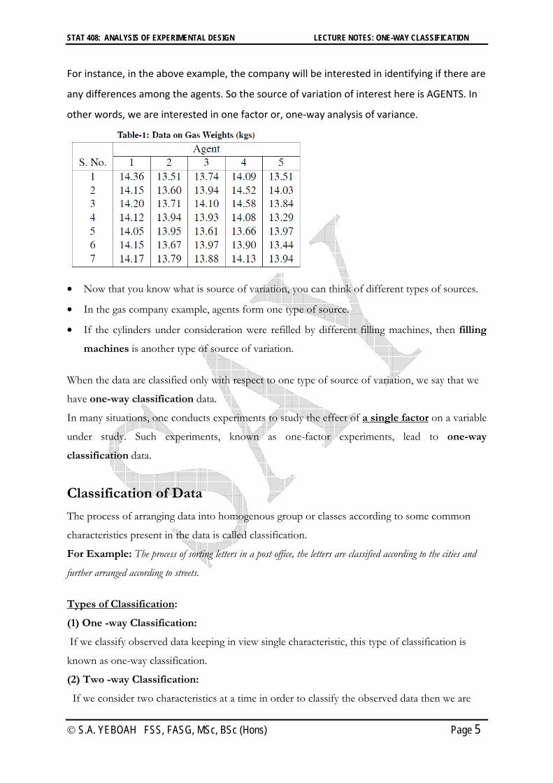
For instance, in the above example, the company will be interested in identifying if there are

any differences among the agents. So the source of variation of interest here is AGENTS. In

other words, we are interested in one factor or, one-way analysis of variance.

Now that you know what is source of variation, you can think of different types of sources.

In the gas company example, agents form one type of source.

If the cylinders under consideration were refilled by different filling machines, then filling

machines is another type of source of variation.

When the data are classified only with respect to one type of source of variation, we say that we

have one-way classification data.

In many situations, one conducts experiments to study the effect of a single factor on a variable

under study. Such experiments, known as one-factor experiments, lead to one-way

classification data.

Classification of Data The process of arranging data into homogenous group or classes according to some common

characteristics present in the data is called classification.

For Example: The process of sorting letters in a post office, the letters are classified according to the cities and

further arranged according to streets.

Types of Classification:

(1) One -way Classification:

If we classify observed data keeping in view single characteristic, this type of classification is

known as one-way classification.

(2) Two -way Classification:

If we consider two characteristics at a time in order to classify the observed data then we are



doing two way classifications.

(3) Multi -way Classification:

We may consider more than two characteristics at a time to classify given data or observed data.

In this way we deal in multi-way classification.

For Example: The population of world may be classified by Religion, Sex and Literacy.

Single-Factor Experiments

We generally classify scientific experiments into two broad categories, namely, single-factor

experiments and multifactor experiment.

Definition: Whenever an experimenter is concerned with comparing the means/effects of a

single factor having at least 3 levels whether the levels are (i) quantitative or qualitative or (ii)

fixed or random, the experiment is referred to as a single factor experiment.

In a single-factor experiment, only one factor varies while others are kept constant. In these experiments, the treatments consist solely of different levels of the single variable

factor.

If there is only one factor, and if the response variable is continuous and satisfies a few other

conditions to be discussed later, then the statistical analysis of the experimental data is done

by one-way analysis of variance.

In multi-factor experiments (also referred to its factorial experiments), two or more factors

vary simultaneously.

In single factor experiments the response variable Y is continuous There are two key differences regarding the explanatory variable X. 1. It is a qualitative variable (e.g. gender, location, etc). Instead of calling it an explanatory

variable, we now refer to it as a factor.

2. No assumption (i.e. linear relationship) is made about the nature of the relationship

between X and Y. Rather we attempt to determine whether the response differ

significantly at different levels of X.

We will consider two single-factor ANOVA models: Model I: This is a model where the factor levels are fixed by the researcher. Conclusions will

pertain only to the means associated with each of the fixed factor levels.



Model II: This is a model where the factor levels are random, that is, the levels are randomly

selected by the researcher from a population of factor levels. Conclusions will extend to the

population of factor levels.

Fixed Factors Model (Model I) There are two ways of parameterizing the model:

1. Cell means model

2. Factor effects model

Notation X (or A) is the qualitative factor

r (or a or k) is the number of levels

we often refer to these as groups or treatments

Y is the continuous response variable

ijy is the jth observation in the ith group.

ki ,,2,1 L levels of the factor X.

inj ,,2,1 L observations at factor level i.

The total number of observations is ∑k

iinN

1

In general, we have a single factor with 2k levels (treatments) and ni replicates for each

treatment.

Cell Means Model

ijiijy Where

ijy is the jth observation on treatment i,

i is the theoretical mean of all observations at level i.

ij is a random deviation of ijy about the ith mean i . ij is called the random error. Model Assumptions

),0(~ 2Niid

ij

),(~ 2i

iid

ij Ny



Parameters The parameters of the model are: ),,,( 2

21 kL

Estimates

For each level i, get an estimate of the variance,1

)(1

2

2∑

n

yys

in

jiij

i

Estimate i by the mean of the observations at level i. That is, i

n

jij

ii n

yy

i

∑1ˆ

We combine these 2is to get an estimate of 2 in the following way.

Pooled Estimate of 2

The pooled estimate is

MSEkN

yy

kN

sn

n

sns

k

i

n

jiij

k

iii

k

ii

k

iii

i

∑∑∑

∑

∑1 1

2

1

2

1

1

22

2

)()1(

)1(

)1(

In the special case that there are an equal number of observations per group ( nni ) then

nkN and this becomes

∑∑ k

ii

k

ii

skknk

sns

1

21

2

2 1)1(

a simple average of 2is

Hypothesis Tests The hypothesis that all treatments are equally effective becomes:

kH ...: 210 all means are equal vrs

jiH :1 for at least one i, j not all the means are equal

Factor Effects Model

An equivalent from of the model:

Effects Model: ijiijy ⎩⎨⎧

injki

,...2,1,...2,1

Where 01∑

k

ii (balanced design) 0

1∑

k

iiin (unbalanced design)



is the “weighted" or overall mean of the treatment means

i The treatment effect (deviation up or down from the grand mean) of the ith treatment and

is defined to be ii

i can be thought of as the average effect that factor level i has on the overall mean.

Another interpretation is to think of i as an adjustment that needs to be made to the overall

mean given that you know data comes from factor level i.

Parameters

The parameters of the factor effects model are: ),,,,( 221 kL There are k+2 of these.

Estimation of Model Parameters

We now wish to estimate the model parameters, based on the effects model ( , i , 2 ). The most popular method of estimation is the method of least squares (LS) which determines the

estimators of and i by minimizing the sum of squares of the errors.

∑∑∑∑k

i

n

jiij

k

i

n

jij

ii

yL1 1

2

1 1

2 )(

We use the “^” (hat) notation to represent least squares estimators, as well as, predicted (or

fitted) values.

Minimization of L via partial differentiation (with the zero-sum constraint 01∑

k

ii ) provides

the estimates:

∑∑y

Ny

N

yk

i

n

jij

i

1 1ˆ

yyii for i=1,…,k,

iijijij yyeˆ

iijy ˆˆˆ = iij yy

iijijijijij yyyye ˆˆ

iiii yyyyˆˆˆ



Proof

Consider the fixed effect one-way ANOVA model

ijiijy ( ki ,,1L inj ,,1L ) where and i are fixed, but unknown, parameters and the sij ' are independent random

variables with E( ij ) = 0 and Var( ij ) = 2 .

The least squares estimators, ˆ and i , of the parameters and i are obtained by

minimizing the sum of squares of the errors ( sij ' ).

We have iijij y

Let the sum of squared errors be

∑∑∑∑k

i

n

jiij

k

i

n

jij

ii

yL1 1

2

1 1

2 )(

Mathematically, we want to find kˆ,ˆ,ˆ 1 L that minimize

∑∑∑∑k

i

n

jiij

k

i

n

jij

ii

yL1 1

2

1 1

2 )ˆˆ(ˆ

A solution can be found by using the Normal equations which are found equating the partial

derivatives to 0 and then solving:

∑∑k

i

n

jiij

i

yL1 1

)ˆˆ(2ˆ (1)

∑in

jiij

i

yL1

)ˆˆ(2ˆ ki ,,1L (2)

Setting (1) equal to zero gives

∑∑k

i

n

jiij

i

yL1 1

0)ˆˆ(2ˆ



∑∑ ∑∑∑∑⇒k

i

n

j

k

i

n

ji

k

i

n

jij

i ii

y1 1 1 11 1

ˆˆ

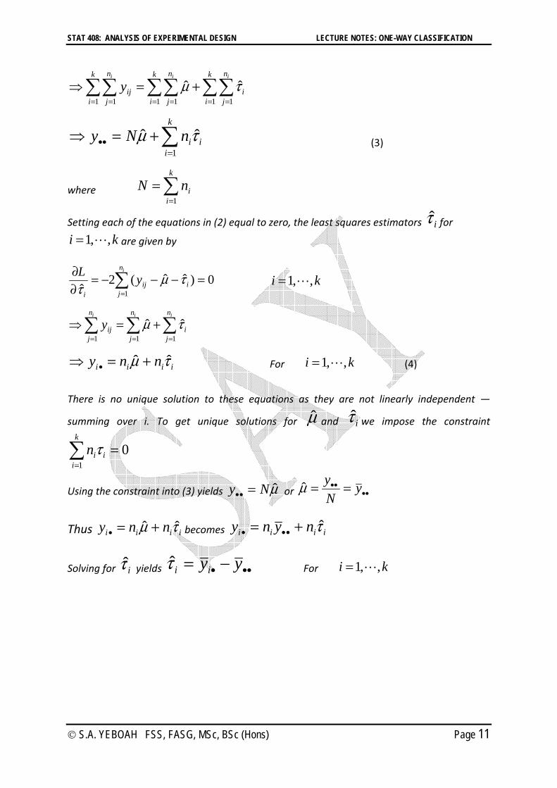
∑⇒k

iiinNy

1

ˆˆ (3)

where ∑k

iinN

1

Setting each of the equations in (2) equal to zero, the least squares estimators i for ki ,,1L are given by

0)ˆˆ(2ˆ 1

∑in

jiij

i

yL ki ,,1L

∑∑∑⇒iii n

ji

n

j

n

jijy

111

ˆˆ

iiii nny ˆˆ⇒ For ki ,,1L (4) There is no unique solution to these equations as they are not linearly independent —

summing over i. To get unique solutions for ˆ and i we impose the constraint

01∑

k

iiin

Using the constraint into (3) yields ˆNy or yNyˆ

Thus iiii nny ˆˆ becomes iiii nyny ˆ

Solving for i yields yyii For ki ,,1L



Hypothesis Tests

The cell means model hypotheses were

kH ...: 210

jiH :1 for at least one i, j (not all the i are equal)

For the factor effects model these translate to

0...: 210 kH

0:1 iH for at least one i Thus, the one way ANOVA for testing the equality of treatment effects is identical to the

ANOVA for testing the equality of treatment means.

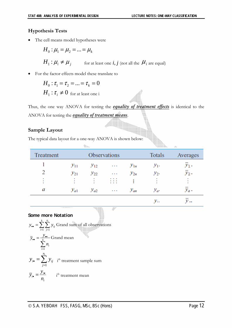
Sample Layout The typical data layout for a one-way ANOVA is shown below:

Some more Notation

∑∑k

i

n

jij

i

yy1 1

Grand sum of all observations

∑

k

iin

yy

1

Grand mean

∑in

jiji yy

1 ith treatment sample sum

i

ii n

yy ith treatment mean



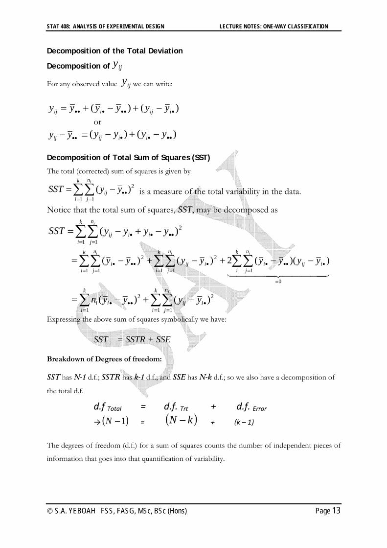
Decomposition of the Total Deviation

Decomposition of ijy

For any observed value ijy we can write:

)()( iijiij yyyyyy or

yyij = )()( yyyy iiij Decomposition of Total Sum of Squares (SST)

The total (corrected) sum of squares is given by

∑∑k

i

n

jij

i

yySST1 1

2)( is a measure of the total variability in the data.

Notice that the total sum of squares, SST, may be decomposed as

∑∑k

i

n

jiiij

i

yyyySST1 1

2)(

∑∑ ∑∑∑∑k

i

n

j

k

i

n

jiijiiij

k

i

n

ji

i ii

yyyyyyyy1 1

0

1

2

1 1

2 ))((2)()(44444 344444 21

∑∑∑k

i

n

jiij

k

iii

i

yyyyn1 1

2

1

2 )()(

Expressing the above sum of squares symbolically we have:

SST = SSTR + SSE Breakdown of Degrees of freedom: SST has N-1 d.f.; SSTR has k-1 d.f.; and SSE has N-k d.f.; so we also have a decomposition of

the total d.f.

d.f Total = d.f. Trt + d.f. Error → 1N = kN + (k – 1)

The degrees of freedom (d.f.) for a sum of squares counts the number of independent pieces of

information that goes into that quantification of variability.



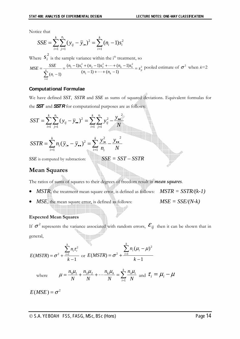
Notice that

∑∑∑k

iii

k

i

n

jiij snyySSE

i

1

2

1 1

2 )1()(

Where 2is is the sample variance within the ith treatment, so

2

1

2222

211

1

)1()1()1()1()1(

)1(p

k

kkk

ii

snn

snsnsn

n

SSEMSE∑ L

L pooled estimate of 2 when k=2

Computational Formulae

We have defined SST, SSTR and SSE as sums of squared deviations. Equivalent formulas for

the SST and SSTR for computational purposes are as follows:

NyyyySST

k

i

n

jij

k

i

n

jij

ii 2

1 1

2

1 1

2)( ∑∑∑∑

Ny

nyyynSSTR

k

i i

ik

iii

2

1

2

1

2)( ∑∑

SSE is computed by subtraction: SSE = SST – SSTR

Mean Squares

The ratios of sums of squares to their degrees of freedom result in mean squares.

MSTR, the treatment mean square error, is defined as follows: MSTR = SSTR/(k-1)

MSE, the mean square error, is defined as follows: MSE = SSE/(N-k)

Expected Mean Squares

If 2 represents the variance associated with random errors, ij then it can be shown that in

general,

1)( 1

2

2∑

k

nMSTRE

k

iii

or 1

)()( 1

2

2∑

k

nMSTRE

k

iii

where ∑k

i

iikk

Nn

Nn

Nn

Nn

1

2211 L and ii

2)(MSEE



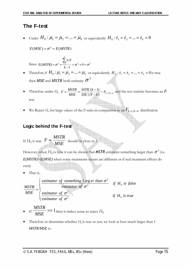
The F-test Under kH ...: 210 or equivalently 0...: 210 kH

)()( 2 MSTREMSEE

Since 2212 01

0)(

∑k

nMSTRE

k

ii

Therefore if kH ...: 210 or equivalently 0...: 210 kH is true

then MSE and MSTR both estimate 2

Therefore under H0 kNkFkNSSE

kSSTRMSE

MSTRF ,1~)()1( and the test statistic becomes an F-

test.

We Reject H0 for large values of the F-ratio in comparison to an kNkF ,1 distribution Logic behind the F-test

If H0 is true MSEMSTRF should be close to 1.

However, when H0 is false it can be shown that MSTR estimates something larger than 2 (i.e.

E(MSTR)>E(MSE) when some treatments means are different or if real treatment effects do

exist)

That is,

⎪⎪⎩

⎪⎪⎨

⎧

trueisHifofestimatorofestimator

falseisHifofestimator

thanerlsomethingofestimator

MSEMSTR

02

2

02

2arg

If 1MSE

MSTRthen it makes sense to reject H0

Therefore to determine whether H0 is true or not, we look at how much larger than 1

MSTR/MSE is.



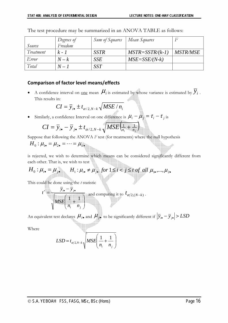
The test procedure may be summarized in an ANOVA TABLE as follows:

Source

Degrees of Freedom

Sum of Squares Mean Squares F

Treatment k - 1 SSTR MSTR=SSTR/(k-1) MSTR/MSE Error N – k SSE MSE=SSE/(N-k) Total N – 1 SST

Comparison of factor level means/effects

A confidence interval on one mean i is estimated by whose variance is estimated by iy . This results in:

ikNi nMSEtyCI /,2/

Similarly, a confidence Interval on one difference is jiji is

ji nnkNji MSEtyyCI 11,2/

Suppose that following the ANOVA F test (for treatments) where the null hypothesis

kH L210 : is rejected, we wish to determine which means can be considered significantly different from each other. That is, we wish to test

jiH :0 jiH :1 21 ,...,1 alloftjifor This could be done using the t statistic

⎟⎟⎠

⎞⎜⎜⎝

⎛

ji

ji

nnMSE

yyt

11 and comparing it to )(,2 kNt .

An equivalent test declares i and j to be significantly different if LSDyy ji Where

⎟⎟⎠

⎞⎜⎜⎝

⎛

jikN nn

MSEtLSD 11,2



Random Effects Model for One-way ANOVA (ANOVA Model II) So far we have studied experiments and models with only fixed effect factors: factors whose

levels have been specifically fixed (in advance) by the experimenter, and where the interest is

in comparing the response for just these fixed levels.

A random effect factor is one that has many possible levels, and where the interest is in the

variability of the response over the entire population of levels, but we only include a random

sample of levels in the experiment. The factor levels are meant to be representative of a general population of possible levels. We are interested in whether that factor has a significant effect in explaining the response,

but only in a general way. For example, we're not interested in a detailed comparison of level

2 vs. level 3, say. Examples: Classify as fixed or random effect.

1. The purpose of the experiment is to compare the effects of three specific dosages of a

drug on response.

2. A textile mill has a large number of looms. Each loom is supposed to provide the

same output of cloth per minute. To check whether this is the case, five looms are

chosen at random and their output is noted at different times.

3. A manufacturer suspects that the batches of raw material furnished by his supplier

differ significantly in zinc content. Five batches are randomly selected from the

warehouse and the zinc content of each is measured.

4. Four different methods for mixing Portland cement are economical for a company to

use. The company wishes to determine if there are any differences in tensile strength

of the cement produced by the different mixing methods. 5. A drug company has its products manufactured in a large number of locations, and

suspects that the purity of the product might vary from one location to another.

Three locations are randomly chosen, and several samples of product from each are

selected and tested for purity.



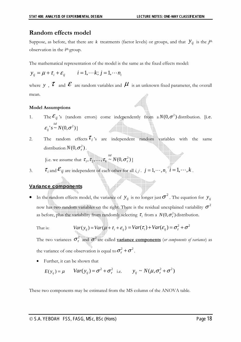
Random effects model Suppose, as before, that there are k treatments (factor levels) or groups, and that ijy is the jth

observation in the ith group. The mathematical representation of the model is the same as the fixed effects model:

iijiij njkiy LL ,1;,1

where y , and are random variables and is an unknown fixed parameter, the overall

mean. Model Assumptions

1. The ij ’s (random errors) come independently from a ),0( 2N distribution. [i.e.

),0(~' 2Nsiid

ij ]

2. The random effects i ’s are independent random variables with the same

distribution ),0( 2N .

[i.e. we assume that ),0(~,,, 221 N

iid

kK ]

3. i and ij are independent of each other for all i, j . inj ,,1L ki ,,1L .

Variance components

In the random effects model, the variance of ijy is no longer just 2 . The equation for ijy

now has two random variables on the right. There is the residual unexplained variability 2

as before, plus the variability from randomly selecting i from a ),0( 2N distribution.

That is: )()( ijiij VaryVar 22)()( iji VarVar

The two variances 2 and 2 are called variance components (or components of variance) as

the variance of one observation is equal to 22 .

Further, it can be shown that

)( ijyE 22)( ijyVar i.e. ),(~ 22Nyij

These two components may be estimated from the MS column of the ANOVA table.



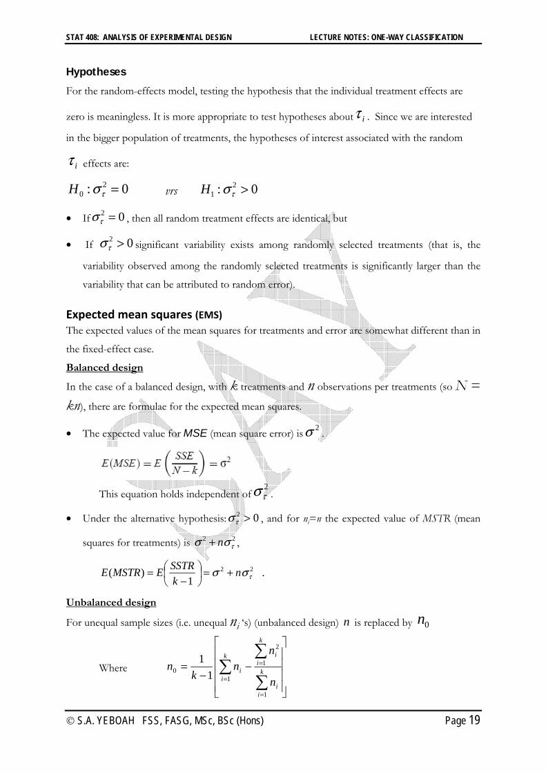
Hypotheses

For the random-effects model, testing the hypothesis that the individual treatment effects are

zero is meaningless. It is more appropriate to test hypotheses about i . Since we are interested

in the bigger population of treatments, the hypotheses of interest associated with the random

i effects are:

0: 20H vrs 0: 2

1H

If 02 , then all random treatment effects are identical, but

If 02 significant variability exists among randomly selected treatments (that is, the

variability observed among the randomly selected treatments is significantly larger than the

variability that can be attributed to random error).

Expected mean squares (EMS) The expected values of the mean squares for treatments and error are somewhat different than in

the fixed-effect case.

Balanced design

In the case of a balanced design, with k treatments and n observations per treatments (so N = kn), there are formulae for the expected mean squares.

The expected value for MSE (mean square error) is 2 .

This equation holds independent of2

.

Under the alternative hypothesis: 02 , and for ni=n the expected value of MSTR (mean

squares for treatments) is 22 n ,

22

1)( n

kSSTREMSTRE ⎟

⎠⎞

⎜⎝⎛ .

Unbalanced design

For unequal sample sizes (i.e. unequal ni ‘s) (unbalanced design) n is replaced by 0n

Where

⎥⎥⎥⎥

⎦

⎤

⎢⎢⎢⎢

⎣

⎡

∑

∑∑ k

ii

k

iik

ii

n

nn

kn

1

1

2

10 1

1



ANOVA of variance

The ANOVA decomposition of total variability is still valid; That is, the ANOVA identity is still SST = SSTR + SSE as for the fixed effects model and

the formulae for computing the sums of squares remain unchanged The computational procedure and construction of the ANOVA table for the random effects

model are identical to the fixed-effects case. The conclusions, however, are quite different because they apply to the entire population of

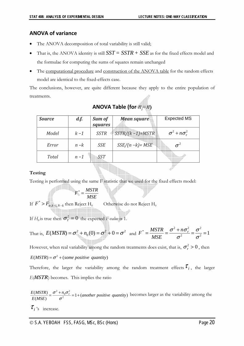
treatments. ANOVA Table (for ni=n)

Source d.f. Sum of squares

Mean square Expected MS

Model k −1 SSTR SSTR/(k −1)=MSTR 22 n

Error n –k SSE SSE/(n −k)= MSE 2

Total n −1 SST

Testing

Testing is performed using the same F statistic that we used for the fixed effects model:

MSEMSTRF *

If kNkFF ,1,* then Reject H0 Otherwise do not Reject H0

If H0 is true then 02 the expected F-value is 1.

That is, 220

2 0)0()( nMSTRE and 12

2

2

22* n

MSEMSTRF

However, when real variability among the random treatments does exist, that is, 02 , then

)()( 2 quantitypositivesomeMSTRE

Therefore, the larger the variability among the random treatment effects i , the larger

E(MSTR) becomes. This implies the ratio

)(1)()(

2

20

2

quantitypositiveanothernMSEE

MSTRE becomes larger as the variability among the

i ’s increase.



Unbiased Estimators

The parameters of the one-way random effects model are , 2 and 2

. Mean As in the fixed effects case, we estimate by

∑∑y

Ny

N

yk

i

n

jij

i

1 1ˆ

Estimation of 2 and 2

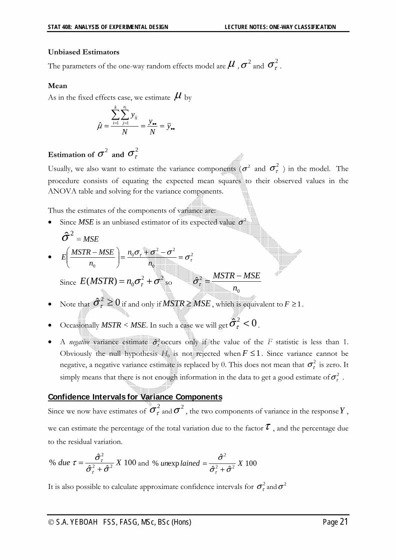
Usually, we also want to estimate the variance components ( 2 and 2 ) in the model. The procedure consists of equating the expected mean squares to their observed values in the ANOVA table and solving for the variance components. Thus the estimates of the components of variance are: Since MSE is an unbiased estimator of its expected value 2

2ˆ = MSE

2

0

220

0⎟⎟⎠

⎞⎜⎜⎝

⎛n

nn

MSEMSTRE

Since 220)( nMSTRE so

0

2ˆn

MSEMSTR

Note that 0ˆ 2if and only if MSEMSTR , which is equivalent to 1F .

Occasionally MSTR < MSE. In such a case we will get 0ˆ 2.

A negative variance estimate 2ˆ occurs only if the value of the F statistic is less than 1. Obviously the null hypothesis H0 is not rejected when 1F . Since variance cannot be negative, a negative variance estimate is replaced by 0. This does not mean that 2 is zero. It simply means that there is not enough information in the data to get a good estimate of 2 .

Confidence Intervals for Variance Components

Since we now have estimates of 2

and2 , the two components of variance in the responseY ,

we can estimate the percentage of the total variation due to the factor , and the percentage due

to the residual variation.

100ˆˆ

ˆ% 22

2

Xdue and 100ˆˆ

ˆexp% 22

2

Xlainedun

It is also possible to calculate approximate confidence intervals for 2 and 2



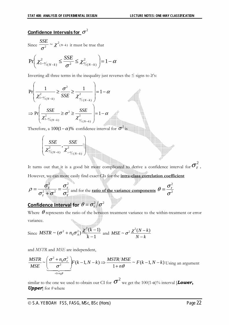
Confidence Intervals for 2

Since )(2

2 ~ kNSSE

it must be true that

⎟⎠⎞

⎜⎝⎛ 1Pr

)(2

2)(21 22 kNkN

SSE

Inverting all three terms in the inequality just reverses the ≤ signs to ’s:

⎟⎟⎟

⎠

⎞

⎜⎜⎜

⎝

⎛111Pr

)(

2

2

)(21

22 kNkN

SSE

⎟⎟⎟

⎠

⎞

⎜⎜⎜

⎝

⎛⇒ 1Pr

)(

22

)(21

22 kNkN

SSESSE

Therefore, a )%1(100 confidence interval for 2 is

⎟⎟⎟

⎠

⎞

⎜⎜⎜

⎝

⎛

)(

2)(

2

212

,kNkN

SSESSE

It turns out that it is a good bit more complicated to derive a confidence interval for2

.

However, we can more easily find exact CIs for the intra-class correlation coefficient

2

2

22

2

Yand for the ratio of the variance components 2

2

Confidence Interval for 22 Where represents the ratio of the between treatment variance to the within-treatment or error

variance.

Since 1

)1()(~2

20

2

kknMSTR A and

kNkNMSE )(~

22

and MSTR and MSE are independent,

),1(~1

),1(~

01

2

20

2

kNkFnMSEMSTRkNkFn

MSEMSTR

n

⇒⎟⎟⎠

⎞⎜⎜⎝

⎛

4434421

Using an argument

similar to the one we used to obtain our CI for 2

we get the 100(1-)% interval [Lower, Upper] for θ where



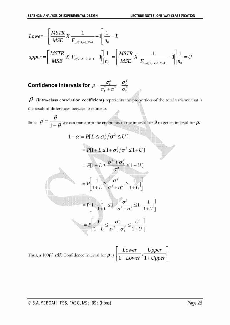
LnF

XMSE

MSTRLowerkNk ⎥

⎥⎦

⎤

⎢⎢⎣

⎡

0,1,2

111

01,,2

11n

FXMSE

MSTRupper kkN ⎥⎦⎤

⎢⎣⎡ U

nFX

MSEMSTR

kNk ⎥⎥⎦

⎤

⎢⎢⎣

⎡

0,,1,21

111

Confidence Intervals for 2

2

22

2

Y

(intra-class correlation coefficient) represents the proportion of the total variance that is

the result of differences between treatments

Since 1 we can transform the endpoints of the interval for θ to get an interval for ρ:

Thus, a 100(1- )% Confidence Interval for ρ is ⎥⎦

⎤⎢⎣

⎡Upper

UpperLower

Lower1

,1

][1 22 ULP

]111[ 22 ULP

]11[ 2

22

ULP

⎥⎦

⎤⎢⎣

⎡UL

P1

11

122

2

⎥⎦

⎤⎢⎣

⎡UL

P1

1111

11 22

2

⎥⎦

⎤⎢⎣

⎡U

UL

LP11 22

2



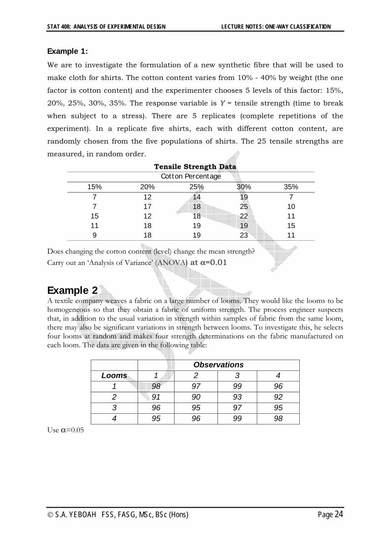
Example 1:

We are to investigate the formulation of a new synthetic fibre that will be used to

make cloth for shirts. The cotton content varies from 10% - 40% by weight (the one

factor is cotton content) and the experimenter chooses 5 levels of this factor: 15%,

20%, 25%, 30%, 35%. The response variable is Y = tensile strength (time to break

when subject to a stress). There are 5 replicates (complete repetitions of the

experiment). In a replicate five shirts, each with different cotton content, are

randomly chosen from the five populations of shirts. The 25 tensile strengths are

measured, in random order.

Tensile Strength Data Cotton Percentage

15% 20% 25% 30% 35% 7 12 14 19 7 7 17 18 25 10

15 12 18 22 11 11 18 19 19 15 9 18 19 23 11

Does changing the cotton content (level) change the mean strength?

Carry out an ‘Analysis of Variance’ (ANOVA) at =0.01

Example 2 A textile company weaves a fabric on a large number of looms. They would like the looms to be homogeneous so that they obtain a fabric of uniform strength. The process engineer suspects that, in addition to the usual variation in strength within samples of fabric from the same loom, there may also be significant variations in strength between looms. To investigate this, he selects four looms at random and makes four strength determinations on the fabric manufactured on each loom. The data are given in the following table:

Observations Looms 1 2 3 4

1 98 97 99 96 2 91 90 93 92 3 96 95 97 95 4 95 96 99 98

Use =0.05

Documents

STAT 408: ANALYSIS OF EXPERIMENTAL DESIGN LECTURE NOTES: ONE-WAY CLASSIFICATION The One way Classification One-Way Analysis of Variance