Embed Size (px)
Citation preview
Eur. Phys. J. B 5, 859–867 (1998) THE EUROPEANPHYSICAL JOURNAL Bc©
EDP SciencesSpringer-Verlag 1998
Static magneto-optical birefringenceof size-sorted γ−Fe2O3 nanoparticles
E. Hasmonay1, E. Dubois2, J.-C. Bacri1,a, R. Perzynski1,b, Yu.L. Raikher3, and V.I. Stepanov3
1 Laboratoire des Milieux Desordonnes et Heterogenes, Universite Pierre et Marie Curie, Tour 13, Case 78,4 place Jussieu, 75252 Paris Cedex 05, France
2 Laboratoire des Liquides Ioniques et Interfaces Chargees, Universite Pierre et Marie Curie, Batiment F,Case 63, 4 place Jussieu, 75252 Paris Cedex 05, France
3 Laboratory of Kinetics of Anisotropic Fluids, Institute of Continuous Media Mechanics,Urals Branch of the Russian Academy of Sciences, 1 Korolyov St., Perm 614013, Russia
Received: 9 January 1998 / Received in final form and Accepted: 5 May 1998
Abstract. Magnetic birefringence experiments under static field are performed on ionic ferrofluid samplesbased on γ−Fe2O3. A colloidal size-sorting of the particles allows to obtain narrow size distributions. Theoptical birefringence of the solutions is found positive and can be described by a Langevin formalism. Itscales as H2 in the low field limit. In the high field limit the particles size dependence of the saturationbirefringence is compatible with a surface anisotropy constant KS = 2.8× 10⁻² erg cm−2 associated witha particle elongation of 1.25 both coherent with Neel predictions of surface anisotropy in small grains.
PACS. 75.50.Mm Magnetic liquids – 78.20.Ls Magnetooptical effects – 78.66.J Nanocrystallinematerials, optical properties
1 Introduction
Chemically synthesized [1] ionic ferrofluids based onmaghemite (γ−Fe2O3) nanoparticles exhibit strong opti-cal birefringence under magnetic fields [2]. Isotropic in zerofield, the solutions in which the particles are dispersedbecome optically uniaxial under field. This macroscopiceffect, which saturates in high fields, is related to the mi-croscopic optical anisotropy of the particles and to theirorientation with respect to the field direction. If they areproperly dispersed in their carrier, it is an intrinsic prop-erty of the particles: at low volume fraction Φ, the birefrin-gence is then proportional to Φ. Such optical experiments[3] are useful tools to probe the dynamics of the particlescarrier, for example their viscoelastic properties [4].
However the sign and the physical origin of this particleoptical anisotropy is still under discussions. The birefrin-gence may have several origins:
- a field-induced effect in the particle material [5], however,within the accuracy and in the field range of standardmeasurements, no optical anisotropy of the solutions isobserved if the particles are dispersed in a zero magneticfield in a carrier subsequently frozen (for example, a tightpolymeric matrix [2] or a silica aero-gel [6]);
a Also at: Universite Denis Diderot (Paris VII), UFR dePhysique, 2 place Jussieu, 75251 Paris Cedex 05.
b e-mail: [email protected]
- the internal optical anisotropy of the magnetic particles,but as tested by X-rays and neutron scattering the ferritecore of the particles has a cubic crystalline structure un-able to induce birefringence; a tetragonal order of vacan-cies exists in bulk γ−Fe2O3, but it disappears in nanosizedparticles smaller than 200 nm [7];
- a shape anisotropy of the particles, electron microscopy[8] evidences more rock-like particles than elongated ellip-soids.
Recently a size sorting of the ferrofluid particles bya colloidal method [9] has allowed a definite progress inthe knowledge of the magnetic anisotropy of those smallγ−Fe2O3 nanograins. A FerroMagnetic Resonance experi-ment (FMR) [10] has demonstrated that this anisotropy ispositive and uniaxial, coming from surface magnetic de-fects. It is presumably related to the magnetically dis-ordered surface and to a small shape eccentricity. Thesepoints are compatible with a quasielastic neutron scatter-ing experiment [11]. Several other works [12–15] report onthe importance of surface effects in the fine grain mag-netism at the scale of 2 to 10 nm, in particular for ironoxide materials. We shall investigate here, using a mag-netic birefringence experiment, the optical anisotropy ofour γ−Fe2O3 nanograins.
In this paper after a short theoretical recall on themagnetic birefringence of a monodisperse ferrofluid solu-tion of monodomain particles, we present our size-sortedsamples and the birefringence experiments. The results are
860 The European Physical Journal B
then compared to different models and discussed in termsof polydispersity and surface anisotropy of the particles.
2 Theoretical background
We assume that all the particles in the suspension areidentical with a volume V . From the magnetic viewpoint,each particle is considered in the model as a single-domainwith a uniform magnetizationmS and a uniaxial magneticanisotropy. For the latter, its magnitude is characterizedby the energy Ea and its direction by the unit vector νalong the easy axis of the particle. Given that, the particlemagnetic moment may be written as µ = µe where µ =mSV and ||e|| = 1. The orientation-dependent part ofthe magnetic energy of the particle in the external fieldH = Hh (where ||h|| = 1) then writes
U = −µH(e · h)−Ea(e · ν)2. (1)
As is shown in references [16–18], the birefringence of adilute suspension of anisotropic particles is determined bythe orientational order tensor
αik =3
2
(〈νiνk〉 −
1
3δik
)(2)
where in the static case the statistical average must betaken over the equilibrium distribution
W0 = Z−10 exp(−U/kBT )
Z0 =
∫exp(−U/kBT )dedν (3)
with U from equation (1).This averaging may be carried out rigorously and
yields
αik =3
2
[1−
3L(ξ)
ξ
][d
dσlnR(σ)−
1
3
]×
(3
2hihk −
1
2δik
), (4)
where the dimensionless parameters
ξ = mSV H/kBT, σ = Ea/kBT (5)
are introduced, ξ (the Langevin parameter) and σ beingrespectively the magnetic energy and the anisotropy en-ergy of one grain normalized to the thermal energy kBT .
The functions constituting expression (4) are well-known: L(ξ) is the first Langevin function, L2(ξ) =1−3L(ξ)/ξ is the second Langevin function and the prop-erties of the integral
R(σ) =
∫ 1
0
exp(σx2)dx
were studied, for example, in reference [19]. The asymp-totic forms for the particle-size dependent factors entering
expression (4) are:
1−3L(ξ)
ξ=
{ξ2/15 if ξ � 1,
1− 3/ξ if ξ � 1,
3
2
[d
dσlnR(σ)−
1
3
]=
{2σ/15 if σ � 1,
1− 3/2σ if σ � 1.(6)
Both functions grow monotonously with their respectivearguments, and both of them eventually tend to the unitysaturation levels.
An important conclusion following from equations(4–6) is that to achieve a high degree of orientation notjust a high magnetic field (i.e., ξ � 1) is necessary. Tothe same extent a high magnetic anisotropy (i.e., σ � 1)is essential. In other words, providing the particles aremagnetically soft (σ � 1), the suspension would dwell inan orientationally disordered state whatever high is theapplied field.
Writing the pertinent expressions of references [16–18]in the framework of an effective medium theory for thebirefringence ∆n, one arrives at a simple formula
∆n = BαΦ (7)
where α is the component of tensor (4) along the directionof the applied field. In our notations it reads
α =
[1−
3L(ξ)
ξ
] [d
dσlnR(σ)−
1
3
]. (8)
The coefficient B may be written as
B =1
2nsolv(χel‖ − χ
el⊥) (9)
nsolv being the optical index of the low absorbing carrierand χel|| (respectively χel⊥) being the effective electric sus-
ceptibility of the particle along (respectively perpendicu-lar) its anisotropy axis. The explicit form of (χel|| − χ
el⊥)
depends on the physical origin of the optical anisotropy[16–18].
Thus, for a given value of σ, ∆n tends toward a max-imum ∆nS in high field which is proportional to the par-ticle volume fraction Φ:
∆nS = δn0Φ with δn0 = B
[d
dσlnR(σ)−
1
3
](10)
and we may write:
for ξ � 1 ∆n = ∆nSξ2
15∝ H2 (11)
for ξ � 1 ∆n = ∆nS
(1−
3
ξ
)· (12)
3 Ferrofluid samples
Our magnetic liquid samples are ionic ferrofluids, basedon nanoparticles made of an iron oxide: maghemite,

E. Hasmonay et al.: Magneto-optical birefringence of γ−Fe2O3 particles 861
γ−Fe2O3. They are chemically synthesized after the Mas-sart’s method [1]: a coprecipitation in an alkaline mediumof an aqueous mixture of Fe2+ and Fe3+ salts. Bulkmaghemite has an inverse spinel structure with Fe3+ ionsvacancies in the octahedral metal sublattice. At room tem-perature, bulk magnetization of γ−Fe2O3 is mS = 400 G,with a Curie temperature extrapolated to 590 ◦C, wellabove room temperature. The magnetocrystalline volumicanisotropy of bulk maghemite is cubic [20] with KV =4.7× 10+4 erg cm−3. Our γ−Fe2O3 nanoparticles of typ-ical size 10 nm have:
- a monodomain magnetic core of maghemite, as testedby X-rays and neutron diffraction;
- surrounded by a more disordered spin layer, giving anamorphous foot to the X-rays diffraction pattern andleading to a slight size dependence of mS (this depen-dence is here always less than 20% and will be ne-glected in the present work).
FMR experiments have evidenced [10] the uniaxialmagnetic anisotropy of those particles, with an anisotropyconstant equal to Ks = 2.8×10⁻² erg cm−2. This positiveanisotropy finds its origin in the poorly crystallized spinslayer which is localized at the particle surface and has athickness of the order of an elementary crystalline cell.
Those chemically synthesized particles are alsomacroions: they bear surface ligands (here either hydrox-oligands (-OH) or citrate ligands (-LH)) leading to a su-perficial density of charges |Σ| ≈ 20 µCcm−2 [8,21] in theappropriate range of pH (in water: pH < 6 or pH > 9 forligands -OH and 5 < pH < 9 for the ligands -LH). If noextra electrolyte is added, the strong electrostatic inter-particle repulsions allow the ferrofluid solutions to be col-loidally stable even under magnetic fields [22]. The volumefraction Φ of magnetic particles is determined by chemicaltitration of ions.
The ferrofluid samples present a size distribution ofmagnetic particles which is, in a first approximation, welldescribed by a log-normal distribution of particles diame-ters [23]:
f(d) =1
√2πsd
exp
[−
ln2(d/d0)
2s2
](13)
where ln d0 corresponds to the mean value of ln d and sis the standard deviation. This size distribution may beprobed by various techniques [8,23–25]:
- the geometric size by electron microscopy or (non po-larized) Small Angle Neutron Scattering (SANS);
- the crystalline size by Debye-Scherrer X-rays determi-nation;
- the magnetic size by magnetization measurements orpolarized SANS.
All these determinations are found close to each otherwith our γ−Fe2O3 samples [8,25]. After the chemical syn-thesis, the ferrofluid samples are rather polydisperse witha value ranging from 0.3 to 0.5. The addition of an elec-trolyte to the ferrofluid solution may destabilize the col-loid. It leads to a phase separation in two liquid phases
Table 1. This table presents for each sample, its ligand andits liquid carrier, the diameter dmagn0 and standard deviationsmagn, obtained by the magnetization characterization (fit ofthe experimental magnetization curve by the first Langevinfunction associated to the log-normal distribution function). Italso gives the diameter dRX from X-rays measurements whenavailable and the parameter σmagn calculated for each sample(see text for its expression).
Sample Surface Carrier dmagn0 smagn dRX σmagn
ligands liquid (nm) (nm)
A -OH water 13 0.4 - 3.6
B -OH water 11 0.4 - 2.6
C -LH glycerine 6.6 0.4 - 0.9
D -OH water 8.5 0.3 10 1.5
E -OH water 9 0.3 - 1.4
F -OH water 7 0.3 10.4 0.9
G -OH water - - 10.4 -
H -LH glycerine 6.8 0.2 - 0.9
I -LH glycerine 8.2 0.15 - 1.4
J -LH glycerine 6.9 0.15 - 1
of different concentrations [26], the biggest particles go-ing preferably to the dense phase. As the phase diagramof the colloidal demixion is size dependent, it is possi-ble by a fractionated precipitation to separate the ini-tial sample in several ones of different mean sizes [9,26].These new samples are stable colloids without added salts[8,21,27] and have a standard deviation s lowered downto 0.15–0.25.
In this work, we compare samples of various d0 withstandard deviation s ranging from 0.15 to 0.4. In order toavoid interparticle interactions the volume fraction Φ ofparticles is always less than 1.5% and the ionic strengthas low as possible. The liquid carrier is either water orglycerine, at room temperature. The colloidal stability ofthe samples is checked by an optical diffraction methodup to a magnetic field of 1 T. Magnetic size characteristicsof the samples are presented in Table 1, they are deducedfrom magnetization measurements (and for some few sam-ples from Debye-Scherrer X-rays determination). Becauseof the rotational degree of freedom of the particles, liquidferrofluid solutions are superparamagnetic materials. Inthe dilute limit (Φ � 1), the magnetization curve M(H)is ruled by the Langevin formalism and is a superpositionof single-grains contributions [2]. Neglecting the small sizedependence of mS , the magnetic size distribution is thendeduced from a best fit of the reduced magnetization curveto M/Msat =
∫d3L(ξ)f(d)dd/
∫d3f(d)dd, the saturation
value Msat of M being approximated by the maximumvalue of M at 1 T. The Debye-Scherrer measured diame-ter averages the size distribution as dRX = d0 exp(2.5s2)[28].

862 The European Physical Journal B
P
1
2
P
L
G
PCS
λ/4 AP
P
Y
XÊ
θ
AÊf ÊÊÊÊAi
O
45°
P
y
xh
45°
z
λ/4 : fast axis
λ/4 : slow axis
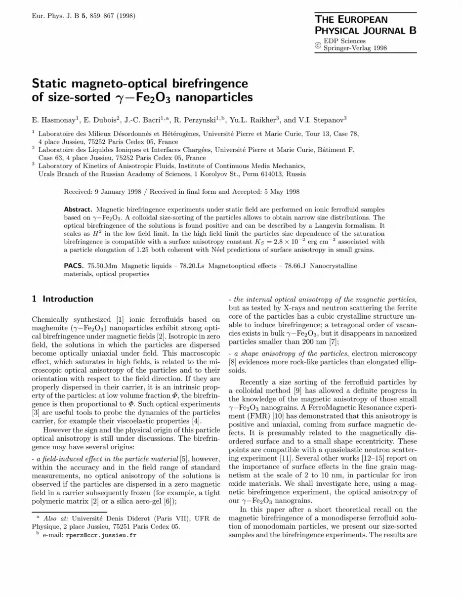
Fig. 1. First experimental optical device. Laser (L) beam goesthrough polarizer (P), sample (S) submitted to a constant mag-netic field (created by polar pieces (P1, P2) measured by theHall effect probe linked to a gaussmeter (G)), a quarter waveplate (λ/4), an analyzer (A). Transmitted light intensity isdetected by a photocell (PC). The inset presents respective di-rections of polarizer (P) parallel to slow axis of quarter waveplate (X), constant magnetic field (H), initial direction of an-alyzer (Ai) perpendicular to (P) and parallel to the fast axisof quarter wave plate (Y) and final direction of analyzer (Af)which makes an angle θ with (Ai).
Table 1 presents the samples characteristics, theirsurface ligands, liquid carrier and size distribution. Anevaluation of the parameter σmagn = Ea/kBT =KSπ(dmagn0 )2/kBT is given for each sample. We performexperiments in the range σmagn ≥ 1.
4 Optical experiments
4.1 Determination of the birefringence signwith a simple optical device
The sign of the magnetic birefringence of a ferrofluid ishere determined with the optical device of Figure 1: weanalyze the polarization of the light transmitted by theferrofluid sample under field. The He-Ne laser light (L)of wavelength λ0 = 632.8 nm propagates along (Oz),goes through a polarizer (P), the ferrofluid sample (S)submitted to an horizontal magnetic field produced bythe polar pieces (P1, P2) of an electromagnet, a quar-terwave plate (λ/4) (for the wavelength of the laser) andan optical detector (PC). The angle of the optical rotat-ing elements are recorded with a precision of 0.5 degree.Crossed polarizer (P) and analyzer (Ai) are first put at45◦ of the horizontal magnetic field H = Hh (see insetof Fig. 1). The λ/4 plate is then introduced with its slow
optical axis parallel to the polarizer (P) (its fast axis isthus parallel to (Ai)).
The ferrofluid sample is set in a non-birefringent glasscell of thickness e and the magnetic field H is switched on.H varies from 0 to 4000 Oe by 500 Oe steps. The glass cellis thermally connected to a Peltier device to control thesample temperature. As magnetic field is switched on, theparticles align along the field, and the solution becomesoptically birefringent with an optical axis collinear to theapplied magnetic field. The medium then behaves as abirefringent plate characterized by a phase-lag ϕ relatedto the birefringence ∆n of the sample of thickness e byϕ = 2πe∆n/λ0 (∆n is defined by ∆n = n|| − n⊥, n|| be-ing the optical index in the direction of the magnetic fieldand n⊥ the optical index in the perpendicular direction).Our ferrofluid solutions are also dichroic. In a first approx-imation we neglect this effect which is small. We shall goback to this point with the second optical measurement.
At the output of (P) the wave is linearly polarized andthe electric field writes in the referential (O, x, y) (seeinset of Fig. 1) :
EP
(Elaser√
2cosωt,−
Elaser√2
cosωt
). (14)
After crossing the ferrofluid cell of transmission coefficientt it gets an elliptic polarization. In a first approximation tis taken isotropic and independent of the direction of theapplied magnetic field H. Under H the components of theelectric field become:
EFF
(Elaser√
2t cos(ωt− ϕ),−
Elaser√2t cosωt
). (15)
and projected along (O, X, Y) at 45◦ of the magnetic fielddirection:
EFF
(Elasert cos
ϕ
2cos(ωt−
ϕ
2
),
Elasert sinϕ
2sin(ωt−
ϕ
2
)). (16)
Going through the λ/4 plate, the component EX gets aπ/2 delay and the wave is again linearly polarized.
The components EX and EY have then the same phase
Eλ/4
∣∣∣∣∣∣∣∣∣∣EX = Elasert cos ϕ2 cos
(ωt− ϕ
2 −π2
)= Elasert cos ϕ2 sin
(ωt− ϕ
2
)EY = Elasert sin ϕ
2 sin(ωt− ϕ
2
) . (17)
The direction of the linear polarization forms an angle ϕ/2with Y, tan(ϕ/2) = EY /EX ; there is some light transmit-ted by the device. Turning the analyzer from its first po-sition Ai (perpendicular to the polarizer), to the positionAf , by extinguishing the transmitted light gives both thesign of ϕ and its value ϕ = 2θ. The sign of ϕ is given bythe sign of θ in the plane (O, x, y).

E. Hasmonay et al.: Magneto-optical birefringence of γ−Fe2O3 particles 863
0
2 0
4 0
6 0
8 0
100
120
140
0 1 2 3 4
Sample ISample J
H (Oe)
θ (degrees)
Fig. 2. Measured angle θ as a function of applied magneticfield H as determined with the optical device of Figure 1. (◦)sample I; Φ = 1.5%; e = 700 µm, (♦) sample J; Φ = 1.5%;e = 500 µm. The full lines are guides for the eyes.
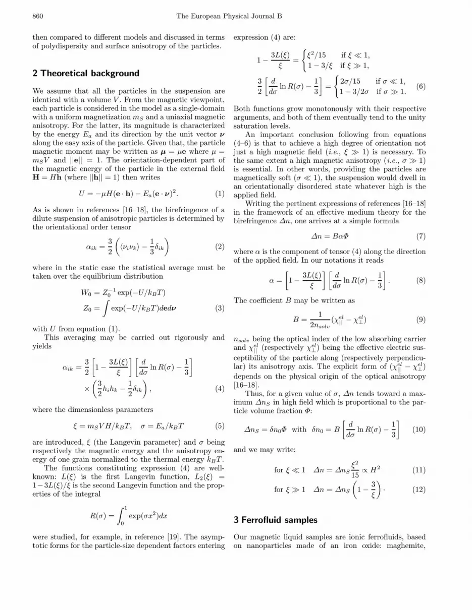
P
PEMP A
1
2
P
C
L
G
PC
LIA
S
45°
P
u//
AY X
Fig. 3. Second optical device. Laser (L) beam goes through po-larizer (P), PhotoElastic Modulator (PEM), sample (S) put be-tween polar pieces (P1, P2), analyzer (A) and photocell (PC).The field is measured with a Hall effect probe connected to agaussmeter (G). The PhotoElastic Modulator oscillation fre-quency is used as a reference by the Lock-In Amplifier (LIA)to detect the ω component of the light intensity transmitted bythe setup. Gaussmeter and lock-in amplifier are connected toa computer (C) which stores the experimental data. The insetdisplays relative orientations of optical elements: analyzer (A),polarizer (P), constant magnetic field (H = u‖) and photoe-lastic modulator (X and Y).
Figure 2 presents the results ∆n = θλ0/πe as a func-tion of the applied field H obtained with sample I (cellthickness e = 700 µm) and sample J (e = 500 µm). Thebirefringence is found positive and is an increasing func-tion of the magnetic field H.
4.2 Optical device with an optical modulator:experimental determination of ∆n(H)
The optical device used here is shown in Figure 3. Thesample (S) of thickness e is put between the pole pieces(P1, P2) of an electromagnet (Hmax ≈ 1.1 × 10⁴ Oe),
in the beam of a He-Ne laser (L) of low power (1 mW)between a polarizer (P) and an analyzer (A). The pho-tocell (PC) detects the transmitted light. A PhotoElas-tic Modulator (PEM) is interposed between the polar-izer and the ferrofluid sample. The PEM modulates at50 kHz the phase of the signal between two perpendiculardirections. A Lock-In amplifier (LIA) compares the elec-tric signal from the photocell (PC) to the reference signalfrom the modulator, and give the component at the samefrequency.
The optical set-up with axes of magnetic field H(h = u||), polarizer P (= u⊥), analyzer A and photoelas-tic modulator (X,Y) is sketched in the inset of Figure 3.The electric field E at the output of the modulator is:
E = (E0/√
2)(X + Yeiδ) (18)
with δ = a sin(ωt) and ω/2π = 50 kHz. After crossing thesample, the electric field is then:
E = (E0/√
2)(√
t‖(eiδ − 1)u‖ +
√t⊥(eiδ + 1)eiϕu⊥
)(19)
with ϕ = 2π∆ne/λ and t|| and t⊥ transmission coefficients(now taken respectively parallel to field and perpendicu-lar) defined in intensity.
At the analyzer output the electric field becomes:
E2 =(E0/2
√2) (√
t||(1− eiδ
)+√t⊥(eiδ + 1
)eiϕ)X.
(20)
The light intensity I collected by the photocell is:
I =(E2
0/4) [t|| (1− cos δ) + t⊥ (1 + cos δ)
−2√t||t⊥ sinϕ sin δ
]. (21)
Expanding and in terms of Bessel functions:
I =(E2
0/4)
×
[(t|| + t⊥
)+(t⊥ − t||
)J0(a)
]−4√t||t⊥J1(a) sinϕ sinωt
+2(t⊥ − t||
)J2(a) cos 2ωt
. (22)
Thus intensity component I2 at pulsation 2ω is propor-tional to the sample dichroism whereas the intensity com-ponent I1 at pulsation ω is related to the sample bire-fringence. For a modulation a = π/2, J1(a) = 0.56 isclose to its maximum and the I1 component is optimized.For our ferrofluids I1 is proportional to sinϕ. If e is wellchosen several oscillations occur in our range of field (seeFig. 4). The variations of ∆n as a function of the magneticfield may be deduced from these measurements. Figure 5presents the results for sample I when increasing the mag-netic field in a log-log plot representation (∆n values arefound identical for increasing or decreasing the magneticfield). In the Φ range of the experiment and within its5% accuracy, ∆n is proportional to the volume fraction Φ

864 The European Physical Journal B
1 01 1 02 1 03 1 04
Sample I
0
0.2
0.4
0.6
0.8
1
1.2|Sin(ϕ)|
H (Oe)
Fig. 4. Intensity component I1 as a function of applied mag-netic field H as determined with the device of Figure 3. Forsample I; Φ = 1.5%; e = 700 µm. I1 is proportional to | sinϕ|.
1 0- 6
1 0- 5
1 0- 4
1 0- 3
1 01 1 02 1 03 1 04
∆n
H (Oe)
< dLF
>=10.1 nm
H2∆ n∝
0
1 0
2 0
3 0
4 0
5 0
0 4 0 0 0 8 0 0 0
H (Oe)
3∆nS/(∆n
S-∆n)
< dHF
>=9.5 nm
Fig. 5. Birefringence ∆n of sample I (Φ = 1.5%) as a functionof applied magnetic field H in a log-log representation. Open(respectively gray) symbols: ∆n determined with the opticaldevice of Figure 3 (resp. Fig. 1). The dotted horizontal linemarks the maximum ∆nS = 8.8 × 10⁻⁴ of ∆n. The full lineis a best fit of the low field behavior: ∆n ∝ H2. The insetillustrates the high field behavior of ∆n. For dLF and dHFdefinitions, see the text.
of particles. These both facts strongly indicate that in suchsolutions magnetic birefringence is not due to a coopera-tive process of particle agglomeration in the field but toa single particle effect. No influence of the liquid carrier,water or glycerine is detected in our experiment. For acomparison, the ∆n variations of sample I obtained bythe first experimental technique (see Sect. 4.1) are alsoplotted in Figure 5.
1 0- 3
1 0- 2
1 0- 1
1
1 01 1 02 1 03
Sample CSample ISample J
H (Oe)
∆n/∆nS
Fig. 6. Reduced birefringence ∆n/∆nS as a function of ap-plied magnetic field H in a log-log representation for threedifferent samples – full lines are best fits of the low field be-havior ∆n ∝ H2. They respectively correspond to dLF = 13.4nm, dLF = 10.1 nm and dLF = 7.6 nm for samples C, I and J.
Table 2. This table presents the results of the birefringenceexperiments dbir0 , sbir, δn0 and σbir obtained for by a fit of theexperimental curve by the second Langevin function associatedto the log-normal distribution function.
Sample Surface Carrier dbir0 sbir δn0 σbir
ligands liquid (nm)
A -OH water 19.9 0.4 0.2 8.4
B -OH water 14.7 0.4 0.15 4.6
C -LH glycerine 7.5 0.4 0.076 1.2
D -OH water 10.5 0.3 0.115 2.3
E -OH water 9.5 0.3 0.093 1.9
F -OH water 8.4 0.3 0.08 1.5
G -OH water 12.8 0.2 0.13 3.5
H -LH glycerine 6.6 0.2 0.044 0.9
I -LH glycerine 9.2 0.15 0.058 1.8
J -LH glycerine 6.1 0.2 0.037 0.8
5 Discussion
5.1 Comparison to the monodisperse model
5.1.1 Low field behavior
Our samples exhibit in low magnetic fields a behaviorcompatible with the expression (10) of the monodispersemodel of Section 2. In low fields ∆n is found to be pro-portional to H2 (see Figs. 5 and 6). This H2 behavioris a second point demonstrating that the birefringence ofthe samples is coming from individual particles at leastin low fields. From expression (11), a magnetic size ofthe particles may be deduced. For example for sample Iof Figure 5 we find a low-field-averaged particle diame-ter dLF of 10.1 nm close to the magnetic characteristicsof the particles.

E. Hasmonay et al.: Magneto-optical birefringence of γ−Fe2O3 particles 865
5.1.2 High field behavior
The birefringence∆n(H) always saturates in high fields toa value ∆nS proportional to Φ. The ratio δn0 = ∆nS/Φ isindependent of Φ but depends on the sample (see Tab. 2).For example for sample I: δn0 = 5.8×10⁻²; in Table 2 δn0
ranges from 0.04 to 0.2. Such a particle size dependenceis compatible with expression (10).
The experimental evolution of ∆n(H) toward satura-tion ∆nS is compared, for sample I, in the inset of Fig-ure 5, to expression (12): the high field prediction of themonodisperse model. This plot allows another particle sizedetermination. We find for sample I a high-field-averagedparticle diameter dHF of 9.5 nm close to the low field one.This is compatible with the small width of the magneticdistribution of this sample.
5.1.3 Polydispersity of the system
Whatever close are dLF and dHF , they are however dif-ferent. To go on with a comparison to theories, it is nownecessary to introduce in the model the polydispersity.However the problem in its full generality is difficult tohandle and we have chosen to analyze two extreme situa-tions.
(i) δn0 is a function of the particle diameter (seeEq. (10) and Tab. 2). In a first analysis we neglect theδn0 variations for the particles of a given sample alongthe width of its distribution: we approximate the particlesby spheres with a log-normal distribution of diameter andanalyze the field variations of ∆n to deduce a diameterdistribution.
(ii) In a second analysis, we consider only the highfield results for which ∆n is assimilated to ∆nS . We thenapproximate the particles by ellipsoids of free eccentric-ity in order to check the dependencies of δn0. It opens adiscussion on the origin of the optical anisotropy of ourferrofluid solutions and on the possibility of chaining ofthe particles in very high fields.
5.2 Log-normal distribution of spherical particles
In this first (and standard) approximation, δn0 is sup-posed to be weakly dependent on the particle size. Wethus neglect its variation among the size distribution ofeach sample and assimilate here δn0 = ∆nS/Φ to a con-stant for each sample. We approximate the particles tospheres with a log-normal distribution of diameters (seeEq. (13)) characterized by dbir0 and sbir.
We may then compute:
∆nLN(H)
∆nS=∫ +∞
0
d3
(1−
3L(ξ(d,H))
ξ(d,H)
)f(d, dbir0 , sbir)dd∫ +∞
0
d3f(d, dbir0 , sbir)dd
· (23)
1 0- 3
1 0- 2
1 0- 1
1
1 01 1 02 1 03 1 04
∆n/∆nS
Log-Normal fit
∆n/∆nS
H (Oe)
Fig. 7. Reduced birefringence ∆n/∆nS as a function of ap-plied magnetic field H in a log-log representation for sample I.The full line is the best fit of expression (23) with a log-normaldistribution of diameters with dbir0 = 9.2 nm and sbir = 0.15.
The curve ∆n(H)/∆nS reduces to a function of two pa-rameters dbir0 and sbir (if mS is known). Taking dbir0 andsbir as free parameters, a best fit [29] of the experimen-tal measurements ∆n(H)/∆nS to the expression (23) isplotted for sample I in Figure 7. It leads to dbir0 = 9.2nm and sbir = 0.15 compatible with the previous low-fieldand high-field-averaged diameters namely:
dLF = 6√〈d9〉�〈d3〉 = dbir0 exp(6sbir
2
) = 10.5 nm,
dHF = 3√〈d3〉 = dbir0 exp(1.5sbir
2
) = 9.5 nm,
Table 2 collects dbir0 and sbir for all our samples. The stan-dard deviation sbir and dbir0 are always close to those foundfrom magnetization measurements. However dbir0 is mostlyslightly larger than dmagn0 .
5.3 Analysis of the high-field results in the hypothesisof elongated ellipsoids
In order to check the limits of the previous description, wenow approximate in high fields the solution by an assemblyof ellipsoids of eccentricity ε =
√1− (b/a)2 where a/b
is the aspect ratio of the ellipsoid. We suppose here theoptical anisotropy as coming from the elongated shape ofthe spheroids, the birefringence being positive.
Then equation (9) reads:
B =1
2nsolv(N⊥ −N‖)Re
[Q2
(1 +QN⊥)(1 +QN‖)
]. (24)
The coefficients N‖ and N⊥ in equation (24) are the com-ponents (at the frequency of the light) of the depolariza-tion tensor along and perpendicular to the major particleaxis, respectively. Note that here the depolarization ten-sor is normalized as to have a unit trace: 2N⊥ +N‖ = 1.The factor Q in formula (24) is
Q = n2part/n
2solv − 1 (25)

866 The European Physical Journal B
where npart is the refraction index of the particle sub-stance. In this simple model we assume that npart is scalar,although this quantity is complex. The particle materialis absorbing as well as refractive, here we have after refer-ence [30], npart = 3.2− 0.15i.
To relate the coefficient B to the particle aspect ratio,we note that for an ellipsoid of revolution:
N⊥ = (1−N‖)/2, N⊥ −N‖ = (1− 3N‖)/2. (26)
The analytical expression for N‖ in the case of an elon-gated spheroid reads [31]:
N‖ =1− ε2
ε2
(1
2ln
1 + ε
1− ε− ε
). (27)
To simplify the description we make the approximation ofa given polydispersity in size for the spheroids but not inaspect ratio letting thus the B parameter to be particlesize independent. Assuming that the aspect ratio is nottoo large, we are allowed to keep the previous sphericalapproximation for the particle size distribution using thelog-normal distribution function of expression (13). Wethen obtain for the reduced birefringence in high fields:
δn0 =∆nS
Φ=
B∫d3
[1−
3L(ξM)
ξM
] [d
dσlnσ −
1
3
]f(d, dbir0 , sbir)dd∫
d3f(d, dbir0 , sbir)dd(28)
with ξM = (d/dM )3, dM = 2.7 nm being a “magnetic
effective length” at 1 T (dM = 3√
6kBT/πmSH). The ex-pression (28) depends on the coefficient B, on the sizedistribution characterized by dbir0 and sbir and on the sizedependence of the magnetic anisotropy σ. In our ionicmaghemite, σmagn is known [10] to scale as d2, being dom-inated by surface contributions. We thus write the currentdimensionless value σ as:
σ = KSS/kBT = πKSd2/kBT = d2/d2
a, (29)
where the auxiliary parameter da =√kBT/πKS is an
anisotropy effective length. We perform the fitting usingthe Levenberg-Marquardt method [29]. For the criterion ofthe quality of the fit we take the specific residual χ2, thatis the total residual divided by the number of experimentalpoints involved in the particular calculation. We performthe attempt of fitting with two “degrees of freedom” viz.the anisotropy diameter da and the amplitude B, usingd0 and s values from Table 2. The calculation yields thefollowing results:
da = 6.78 nm; B = 0.207; χ2 = 8.70× 10⁻⁵. (30)
An adequate graphic representation of the undertaken fit-ting should be expressed as a 3D diagram of δn0 versus d0
and s. Figure 8 shows four cross-sections of this 3D plot for
0
0.05
0.1
0.15
0.2
0.25
0 5 1 0 1 5 2 0 2 5
δn0 (a) sbir = 0.15
d0bir
0
0.05
0.1
0.15
0.2
0.25
0 5 1 0 1 5 2 0 2 5
δn0 (b) sbir = 0. 2
d0bir
0
0.05
0.1
0.15
0.2
0.25
0 5 1 0 1 5 2 0 2 5
δn0 (c)
d0bir
sbir = 0. 3
0
0.05
0.1
0.15
0.2
0.25
0 5 1 0 1 5 2 0 2 5
δn0 (d)
d0bir
sbir = 0. 4
Fig. 8. Results of fitting using the polydisperse model. Eachcurve corresponds to a particular value of the distributionwidth sbir. The black dots represent the experimental valuesof δn0.
different values of the distribution width sbir. The theo-retical curves are calculated with the aid of equations (29,30).
Using relation (29), one gets a determination of theanisotropy constant KS = kBT/πd
2a = 2.8 × 10⁻² erg
cm−2 agreeing rather well with the independent estima-tion obtained in reference [10] from the high-frequencymagnetic measurements (FMR), i.e., by a completely dif-ferent way of estimation. We have given in Table 2, thedimensionless parameter σbir = πKS(dbir0 )2/kBT deducedfor each sample from these birefringence measurements.For the less polydisperse samples, they are rather close tothe magnetic parameter σmagn of Table 1 indicating thatthe optical anisotropy can be correlated to the magneticone.
Neel [32] has proposed for magnetic particles with typ-ical size lower than 10 nm, the existence of a structuralanisotropy coming from the discontinuity of magnetic in-teractions between individual spins which reside at theparticle surface. This layer is characterized by a surfaceanisotropy constant KSR and an axis locally perpendic-ular to the surface. In the case of spherical particles thetotal contribution of this surface effect is equal to zero butfor non-spherical particles (ellipsoids) there is a non-zerocontribution. Neel has calculated that the surface layermay be described by the KS parameter, effective surfaceanisotropy constant linked to KSR through:
KS =4
15ε2KSR, (31)
where ε is the eccentricity of the ellipsoid of revolution andwhere the value of KSR ranges from 0.1 to 1 erg cm−2.

E. Hasmonay et al.: Magneto-optical birefringence of γ−Fe2O3 particles 867
The effective value of the aspect ratio (a/b) of the par-ticles is a sensitive point. It may be deduced from our fit,through coefficient B and a graphic resolution of equa-tions (24, 25) using the experimental optical index npart.We obtain with our model a/b = 1.25 meaning ε = 0.6.It demonstrates the very low degree of aggregation of theparticles even under a 1 T magnetic field. Rather in favorof a single particle regime than a developed aggregation,this value is also low enough to justify the use of a spher-ical approximation in our model for the particle size dis-tribution. Our experimental value of ε put in the formula(31) leads to an evaluation of KSR = 0.29 erg cm−2 ingood agreement with the Neels predictions given above.
6 Conclusion
This work is an experimental investigation of magneto-optical birefringence of ionic ferrofluids based on chemi-cally synthesized γ−Fe2O3 nanoparticles. From this staticstudy on a large number of samples with various particlesize distributions, we find that:
- The birefringence ∆n of the solution is for our sam-ples and in the low concentration range investigated here,related to a single grain behavior.
- The birefringence of the solution and that of the in-dividual particles are positive. This is compatible withthe positive magnetic anisotropy found by FMR measure-ments on the same samples.
- The magnetic field dependence of ∆n can be scaledwith a Langevin formalism from the very low field regime(where ∆n ∝ H2) to the very high field regime (where∆n/Φ is a constant dependent on the particle size distri-bution).
- The origin of the particles optical anisotropy can becorrelated to a surface magnetic anisotropy of effectiveconstant KS = 2.8 × 10⁻² erg cm−2 and a slight ellip-ticity of the particles of the order of 1.25 (that could berelated to the rock-like shape of the particles). This is anew optical evidence of the importance of the surface mag-netism in iron oxide nanodispersions supported by severalrecent magnetic measurements [10–15].
We thank J. Servais and P. Lepert for their technical assistance.This work was supported by “Le Reseau Formation-Recherche”n◦ 96P0079 of MENESRIP and from the Russian side by thegrant n◦ 98-02-16453 of Russian Foundation of Basic Research.
References
1. R. Massart, IEEE Trans. Magn. 17, 1247 (1981).2. Magnetic Fluids and Applications Handbook, edited by B.
Berkovski (Begell House Inc. Publ., New-York, 1996).3. H.W. Davies, J.P. Llewellyn, J. Phys. D 12, 311 (1979).4. J.-C. Bacri, D. Gorse, J. Phys. France 44, 985 (1983);
J.-C. Bacri, R. Perzynski, Complex Fluids, edited by L.Garrido (Springer-Verlag, Berlin, 1993), p. 85.
5. J. Ferre, G.A. Gehring, Rep. Prog. Phys. 47, 513 (1984).6. F. Chaput, J.-P. Boilot, M. Canva, A. Brun, R. Perzynski,
D. Zins, J. Non-Cryst. Solids 160, 177 (1993).7. K. Haneda, A.H. Morish, Solid State Commun. 22, 779
(1977); B. Gillot, F. Bouton, J. Solid State Chem. 32, 303(1980); L.Q. Amaral, F.A. Tourinho, Braz. J. Phys. 25,142 (1995).
8. E. Dubois, Ph.D. thesis, Universite Pierre et Marie Curie,Paris (1997).
9. R. Massart, E. Dubois, V. Cabuil, E. Hasmonay, J. Magn.Magn. Mater. 149, 1 (1995).
10. F. Gazeau, E. Dubois, J.-C. Bacri, F. Gendron,R. Perzynski, Yu.L. Raikher, V.I. Stepanov, Proceed-ings of the Second International Workshop on FineParticle Magnetism (Bangor, UK, 1996), p. 66; F.Gazeau, J.-C. Bacri, F. Gendron, R. Perzynski, Yu.L.Raikher, V.I. Stepanov, E. Dubois, J. Magn. Magn.Mater. 186, 175 (1998).
11. F. Gazeau, E. Dubois, M. Hennion, R. Perzynski, Yu.L.Raikher, Europhys. Lett. 40, 575 (1997).
12. R.H. Kodama, A.E. Berkowitz, E.J. McNiff Jr., S. Foner,Phys. Rev. Lett. 77, 394 (1996).
13. R.H. Kodama, A.E. Berkowitz, E.J. McNiff Jr., S. Foner,J. Appl. Phys. 81, 5552 (1997).
14. J.L. Dormann, F. D’Orazio, E. Tronc, P. Prene, J.-P.Jolivet, D. Fiorani, R. Cherkaoui, M. Nogues, Phys. Rev.B 53, 14291 (1996).
15. C. Bellouard, M. Hennion, I. Mirebeau, J. Magn. Magn.Mater. 140, 357 (1995).
16. A. Peterlin, H.A. Stuart, Z. Phys. 112, 129 (1939).17. Yu.N. Skibin, V.V. Chekanov, Yu.L. Raikher, Sov. Phys.
JETP 45, 496 (1977).18. P.C. Scholten, IEEE Trans. Magn. 16, 221 (1980).19. Yu.L. Raikher, M.I. Shliomis, Adv. Chem. Phys. 87, 595
(1994).20. J.B. Birks, Proc. Phys. Soc. B 63, 65 (1950).21. E. Dubois, V. Cabuil, J.-C. Bacri, R. Perzynski (to be
published).22. J.-C. Bacri, R. Perzynski, D. Salin, V. Cabuil, R. Massart,
J. Magn. Magn. Mater. 85, 27 (1990).23. J.-C. Bacri, R. Perzynski, D. Salin, V. Cabuil, R. Massart,
J. Magn. Magn. Mater. 62, 36 (1986).24. J.-C. Bacri, F. Boue, V. Cabuil, R. Perzynski, Coll. Surf.
A 80, 11 (1993).25. F. Gazeau, Ph.D. thesis, Universite Denis Diderot, Paris,
1997.26. J.-C. Bacri, R. Perzynski, D. Salin, V. Cabuil, R. Massart,
J. Coll. Interf. Sci. 132, 43 (1989).27. E. Dubois, V. Cabuil, F. Boue, J.-C. Bacri, R. Perzynski,
Progr. Coll. Polym. Sci. 104, 173 (1997).28. E. Tronc, D. Bonnin, J. Phys. Lett. 46, L437 (1985).29. W.H. Press, B.P. Flannery, S.A. Teukolsky, W.T.
Vetterling, Numerical Recipes, The Art of Scientific Com-puting (Cambridge University Press, Cambridge, 1989).
30. J. Lenglet, Ph.D. thesis, Universite Denis Diderot, Paris,1996.
31. L.D. Landau, E.M. Lifshitz, Electrodynamics of Continu-ous Media (Pergamon Press, Oxford, 1960), p. 42.
32. L. Neel, J. Phys. Radium 15, 225 (1954).


