RESEARCH ARTICLE

Synchronization of chaotic nonlinear continuous neural networkswith time-varying delay

P. Balasubramaniam • R. Chandran •

S. Jeeva Sathya Theesar

Received: 9 November 2010 / Revised: 10 May 2011 / Accepted: 17 June 2011 / Published online: 6 July 2011

� Springer Science+Business Media B.V. 2011

Abstract In this paper, the synchronization problem for

delayed continuous time nonlinear complex neural net-

works is considered. The delay dependent state feed back

synchronization gain matrix is obtained by considering

more general case of time-varying delay. Using Lyapunov

stability theory, the sufficient synchronization criteria are

derived in terms of Linear Matrix Inequalities (LMIs). By

decomposing the delay interval into multiple equidistant

subintervals, Lyapunov-Krasovskii functionals (LKFs) are

constructed on these intervals. Employing these LKFs,

new delay dependent synchronization criteria are pro-

posed in terms of LMIs for two cases with and without

derivative of time-varying delay. Numerical examples are

illustrated to show the effectiveness of the proposed

method.

Keywords Synchronization � Neural networks �Time-varying delay � Delay decomposition �Maximum admissible upper bound (MAUB)

Introduction

During the past decade, control and synchronization of

chaotic systems have become an important topic, since the

pioneering work of Pecora and Carroll in 1990 (Carroll and

Pecora 1990, 1991). Chaos synchronization has been

widely investigated due to its applications in creating

secure communication systems (Yu and Liu 2003; Feki

2003). Both Hopfield Neural Networks (HNNs) and Cel-

lular Neural Networks (CNNs) have attracted considerable

attention in recent decades and have been widely applied in

number of engineering and scientific fields including image

processing, computing technology, solving linear and

nonlinear algebraic equations and so on (Lou and Cui

2006; Arik 2003).

Moreover, Haken (2007) has presented a neural net

model describing biological activity in visual cortex and

coined a problem that synchronization between groups of

neurons may be the key to solution of ‘‘binding problem’’.

In addition to that noise-induced complete synchroniza-

tion and frequency synchronization in coupled spiking

and bursting neurons studied in Shi et al. (2008). Also in

Jirsa (2008) it has been proved that time delay plays a

vital role in synchronized states of spiking-burst neuronal

networks.

On the other hand, artificial neural networks models

can also exhibit chaotic behavior (Lou and Cui 2007;

Gilli 1993; Lu 2002) due to the fact that small pertur-

bation in initial conditions may lead to large deviation in

system dynamics and so synchronization of chaotic

neural networks has also become an important area of

study. Some authors have paid attention to the synchro-

nization of neural networks (Chen et al. 2004; Chao Jung

et al. 2006; Cui and Lou 2009; Gao et al. 2009; Wang

et al. 2010). In Cui and Lou (2009), some sufficient

P. Balasubramaniam (&) � S. Jeeva Sathya Theesar

Department of Mathematics, Gandhigram Rural Institute,

Deemed University, Gandhigram, Tamilnadu 624 302, India

e-mail: balugru@gmail.com

S. Jeeva Sathya Theesar

e-mail: sjstheesar@gmail.com

R. Chandran

Department of Computer Science, Government Arts College,

Melur, Madurai, Tamilnadu 625 106, India

e-mail: rchandran62@gmail.com

123

Cogn Neurodyn (2011) 5:361–371

DOI 10.1007/s11571-011-9162-0

conditions for exponential synchronization of neural

networks with time-varying delays have been given in

terms of feasible solution in the form of Linear Matrix

Inequalities (LMIs). In Gao et al. (2009), based on the

Lyapunov method a delay independent sufficient syn-

chronization conditions in term of LMIs for chaotic

recurrent neural networks with time-varying delays using

nonlinear feedback control have been obtained. Delay-

dependent conditions, which contains information con-

cerning time delay, are usually less conservative than

delay-independent ones. In addition, synchronization

between neurons both in biological neuronal network and

artificial neural network is essential for information

processing. The study of synchronization problem of

delayed neural networks may proceed to study complex

synchronization between spike-burst neurons. In this

paper, we propose a novel synchronization criterion

based on delay decomposition approach to derive a

maximum admissible upper bound (MAUB) of the time

delay such that two identical chaotic nonlinear continu-

ous neural networks with time-varying delay is syn-

chronized asymptotically. The larger MAUB of time

delay implies less conservatism of delay-dependent syn-

chronization criterion. Moreover the gain matrix of the

controller for slave system can be determined based on

LMIs, which can be easily solved by various convex

optimization algorithms (Boyd et al. 1994). In this paper,

in order to obtain some less conservative sufficient

conditions, we adapted the method proposed by Zhang

and Han (2009). Interior point algorithm implemented in

MATLAB LMI toolbox is employed to solve the derived

LMIs.

To the best of authors knowledge, the delay decompo-

sition approach to delay-dependent synchronization anal-

ysis for continuous time nonlinear complex neural

networks with time-varying delay has never been tackled in

any of the previous literature. Based on LKF approach,

some new synchronization criteria are proposed in the form

of LMIs, which are dependent on the size of the time delay.

Numerical examples are given to illustrate the feasibility

and effectiveness of proposed method.

Notations Throughout this paper, Rn and R

n�n denote

n-dimensional Euclidean space and the set of all

n 9 n real matrices respectively. I denotes the identity

matrix and P-1 denotes the inverse matrix of P. The

notation � always denotes the symmetric block in one

symmetric matrix. The superscript T denotes the trans-

position and the notation X C Y (respectively, X [ Y),

where X and Y are symmetric matrices, means that X -

Y is positive semi-definite (respectively, positive definite).

Matrices, if not explicitly stated, are assumed to have

compatible dimensions.

Synchronization problem and preliminaries

Based on the master-slave concept, the unidirectional

coupled nonlinear neural networks are described by the

following delay differential equation. The master system

is

_xiðtÞ ¼ �ciðxiðtÞÞ þXn

j¼1

aijfjðxjðtÞÞ

þXn

j¼1

bijfjðxjðt � sðtÞÞÞ þ Ii:

ð1Þ

and the slave system is

_yiðtÞ ¼ �ciðyiðtÞÞ þXn

j¼1

aijfjðyjðtÞÞ

þXn

j¼1

bijfjðyjðt � sðtÞÞÞ þ Ii þ uiðtÞ:

i ¼ 1; 2; . . .; n:

ð2Þ

where n C 2 denotes the number of neurons in the

networks, xi(t) and yi(t) are the state variables associ-

ated with ith neuron of master and slave systems

respectively at time t. aij and bij indicate the intercon-

nection strength among the neurons without and with

time-varying delay respectively. The neuron activation

function fi describes the manner in which the neurons

respond to each other. Ii denotes the constant external

input and ui(t) be an unidirectional-coupled term, which

is considered as control input and will be appropri-

ately designed to obtain certain control objective. Fur-

thermore, s(t) is the time-varying delay such that

0� sðtÞ��s: System (1) and (2) possess initial condi-

tions xiðtÞ ¼ /iðtÞ 2 Cð½�s; 0�;RÞ and yiðtÞ ¼ uiðtÞ 2Cð½�s; 0�;RÞ known as delay history functions for

master (1) and slave (2) systems respectively, where

Cð½�s; 0�;RÞ denotes the set of all continuous functions

from ½�s; 0� to R.

We further assume that cið�Þ and fjð�Þ satisfy the fol-

lowing conditions:

(A1): Each function ci : R! R is locally Lipschitz and

nondecreasing function, that is, there exists a positive

real di such that c0iðxÞ ¼ di for any x 2 R at which ci is

differentiable function.

362 Cogn Neurodyn (2011) 5:361–371

123

(A2): Each function fj : R! R is monotonic nonde-

creasing and globally Lipschitz, that is, there exists a

positive real lj such that

0� ðfjðxÞ � fjðyÞÞðx� yÞ � lj for any x; y 2 R;with x 6¼ y

and j ¼ 1; 2; . . .; n:

Define the synchronization error ei(t) = xi(t) - yi(t). Thus

the error dynamic system can be represented as

_eiðtÞ ¼ �biðeiðtÞÞ þXn

j¼1

aijgjðejðtÞ; yjðtÞÞ

þXn

j¼1

bijgjðejðt � sðtÞ; yjðt � sðtÞÞÞ � uiðtÞ:ð3Þ

where bi(ei(t)) = ci(xi(t)) - ci(yi(t)) and gjðejð�Þ; yjð�ÞÞ ¼fjðejð�Þ þ yjð�ÞÞ � fjðyjð�ÞÞ.

For notational purpose, we denote gjðejð�Þ; yjð�ÞÞ as

gjðejð�ÞÞ: From (A2), one can obtain that gjðejð�ÞÞ satisfying

0� ejð�Þgjðejð�ÞÞ� lje2j ð�Þ ð4Þ

and from (A1) and according to Lebourg theorem (see

Theorem 2.3.7 in Clarke 1983), there exists ci C di such

that bi(ei(t)) = ciei(t).

In order to ensure synchronization of coupled neural

networks, the control input ui(t) is designed as follows

uiðtÞ ¼Xn

j¼1

wijðxjðtÞ � yjðtÞÞ:

uðtÞ ¼

u1ðtÞu2ðtÞ

..

.

unðtÞ

266664

377775¼

w11 w12 . . . w1n

w21 w22 . . . w2n

..

. ... . .

. ...

wn1 wn2 . . . wnn

266664

377775

x1ðtÞ � y1ðtÞx2ðtÞ � y2ðtÞ

..

.

xnðtÞ � ynðtÞ

266664

377775

¼ KeðtÞ:ð5Þ

where eðtÞ ¼ ½e1ðtÞ;e2ðtÞ; . . .;enðtÞ�T ; K¼ ðwijÞn�n 2 Rn�n

is the state feedback control gain matrix to be determined

for synchronizing both master and slave systems. Thus

from Eqs. 3 and 5, we rewrite the error dynamic system as

_eiðtÞ ¼ �cieiðtÞ þXn

j¼1

aijgjðejðtÞÞ

þXn

j¼1

bijgjðejðt � sðtÞÞÞ �Xn

j¼1

wijejðtÞ:ð6Þ

Transforming Eq. 6 into compact form as

_eðtÞ ¼ �DeðtÞ þ AgðeðtÞÞ þ Bgðeðt � sðtÞÞÞ � KeðtÞ:¼ �CeðtÞ þ AgðeðtÞÞ þ Bgðeðt � sðtÞÞÞ ð7Þ

where C = D ? K, D = diag{ci}, A = (aij)n9n, B =

(bij)n9n, and gðeð�ÞÞ ¼ ½g1ðe1ð�ÞÞ; g2ðe2ð�ÞÞ; . . .; gnðenð�ÞÞ�T .

Now we are stating the following Lemmas, which will

be more useful in the sequel.

Lemma 2.1 [Han (Zhang and Han 2009)] For any

constant matrix R 2 Rn�n;R ¼ RT [ 0; scalar h with

0� sðtÞ � h\1 and a vector-valued function

_x : ½t � h; t� ! Rn; the following integration is well

defined, then

�sðtÞZ t

t�sðtÞ

_xTðsÞR _xðsÞds�xðtÞ

xðt � sðtÞÞ

� �T �R R

�R

� �

xðtÞxðt � sðtÞÞ

� �:

Lemma 2.2 (Schur complement) Let P, Q, R be given

matrices of appropriate dimensions such that R [ 0.

Then

P QQT �R

� �\0, Pþ QT R�1Q\0

Based on the available information on the time-

varying delay, we will consider the following two

cases.

Case I s (t) is a continuous function satisfying

0� sðtÞ��s\1; 8 t� 0; ð8Þ

Case II s (t) is a differentiable function satisfying

0� sðtÞ� s\1; _sðtÞ� l\1; 8 t� 0; ð9Þ

where s and l are scalars.

Synchronization criteria

In this section we introduce LKFs to derive some new

delay-dependent synchronization criterion for nonlinear

continuous neural networks with time-varying delay sys-

tem described by Eqs. 1 and 2.

Theorem 3.1 Under case I and hypotheses (A1)–(A2),

for a given scalar �s[ 0; the master-slave neural networks

(1) and (2) are completely synchronized with control

gain K ¼ ~Y ~P�1 if there exist positive definite symmet-

ric matrices ~P ¼ ~PT [ 0; ~Qi ¼ ~QTi [ 0; ~Ri ¼ ~RT

i [ 0; ði ¼1; 2; . . .;NÞ; any matrix ~Y and diagonal matrices ~S1 [ 0;~S2 [ 0 such that the LMI (10) holds for all

k 2 f1; 2; . . .;Ng,

Cogn Neurodyn (2011) 5:361–371 363

123

where

~ai ¼�2D ~P� 2 ~Y þ ~Q1 � ~R1 i ¼ 1;~Qi � ~Qi�1 � ~Ri � ~Ri�1; i ¼ 2. . .N;� ~QN � ~RN ; i ¼ N þ 1:

8<

: ð11Þ

~bi ¼~Q1 � 2~S1 i ¼ 1;

~Qi � ~Qi�1; i ¼ 2. . .N;� ~QN ; i ¼ N þ 1:

8<

: ð12Þ

~R ¼ ~R1 þ ~R2 þ � � � þ ~RN ; ð13ÞL ¼ diagðl1; l2; . . .; lnÞ: ð14Þ

Proof Let N [ 0 be an integer. We decompose the delay

interval ½��s; 0� into N equidistant subintervals, that is,

½��s; 0� ¼[N

j¼1

½�jd;�ðj� 1Þd�;

where d ¼ �s=N. Then choosing different matrix pairs

(Qj, Rj) on ½�jd;�ðj� 1Þd�; ðj ¼ 1; 2; . . .;NÞ, we construct

the following new LKF:

VðeðtÞÞ ¼ V1ðeðtÞÞ þ V2ðeðtÞ þ V3ðeðtÞÞ ð15Þ

where

V1ðeðtÞÞ ¼ eTðtÞPeðtÞ;

V2ðeðtÞÞ ¼XN

j¼1

Z�ðj�1Þd

�jd

eðt þ sÞgðeðt þ sÞÞ

� �T

Qj

eðt þ sÞgðeðt þ sÞÞ

� �ds;

V3ðeðtÞÞ ¼XN

j¼1

dZ�ðj�1Þd

�jd

Z t

tþh

_eTðsÞRj _eðsÞdsdh

with P ¼ PT [ 0;Qj ¼ QTj [ 0 and Rj ¼ RT

j [ 0;

ðj ¼ 1; 2; . . .;NÞ.Taking the derivative of V(e(t)) in Eq. 15 with respect to

t along the trajectory of Eq. 7 yields

_VðeðtÞÞ ¼ _V1ðeðtÞÞ þ _V2ðeðtÞÞ þ _V3ðeðtÞÞ: ð16Þ

where

_V1ðeðtÞÞ ¼ 2eTðtÞP _eðtÞ¼ 2eTP½�CeðtÞ þ AgðeðtÞÞ þ Bgðeðt � sðtÞÞÞ�

ð17Þ

N¼

~a1~R1 0 . . . 0 0 . . . 0 0 0 A ~Pþ ~ST

1 L 0 0 . . . 0 0 B ~P � ~PDTd� ~YTd

~a2~R2 . . . 0 0 . . . 0 0 0 0 0 0 . . . 0 0 0 0

� ~a3 . . . 0 0 . . . 0 0 0 0 0 0 . . . 0 0 0 0

..

. ... ..

. . .. ..

. ... . .

. ... ..

. ... ..

. ... ..

. . .. ..

. ... ..

. ...

� � . . . ~ak 0 . . . 0 0 ~Rk 0 0 0 . . . 0 0 0 0

� � . . . � ~akþ1 . . . 0 0 ~Rk 0 0 0 . . . 0 0 0 0

..

. ... ..

. . .. ..

. ... . .

. ... ..

. ... ..

. ... ..

. . .. ..

. ... ..

. ...

� � . . . � � . . . ~aN~RN 0 0 0 0 . . . 0 0 0 0

� � . . . � � . . . � ~aNþ1 0 0 0 0 . . . 0 0 0 0

� � . . . � � . . . � � �2 ~Rk 0 0 0 . . . 0 0 ~ST2 L 0

� � . . . � � . . . � � � ~b1 0 0 . . . 0 0 0 ~PATd

� � . . . � � . . . � � � � ~b2 0 . . . 0 0 0 0

� � . . . � � . . . � � � � � ~b3 . . . 0 0 0 0

..

. ... ..

. . .. ..

. ... . .

. ... ..

. ... ..

. ... ..

. . .. ..

. ... ..

. ...

� � . . . � � . . . � � � � � � . . . ~bN 0 0 0

� � . . . � � . . . � � � � � � . . . � ~bNþ1 0 0

� � . . . � � . . . � � � � � � . . . � � �2~S2~PBTd

� � . . . � � . . . � � � � � � . . . � � � ~R� 2 ~P

26666666666666666666666666666666666666666664

37777777777777777777777777777777777777777775

\0

ð10Þ

364 Cogn Neurodyn (2011) 5:361–371

123

_V2ðeðtÞÞ ¼XN

j¼1

½eTðt � ðj� 1ÞdÞQjeðt � ðj� 1ÞdÞ

� eTðt � jdÞQjeðt � jdÞþ gTðeðt � ðj� 1ÞdÞÞQjgðeðt � ðj� 1ÞdÞÞ� gTðeðt � jdÞÞQjgðeðt � jdÞÞ�

ð18Þ

_V3ðeðtÞÞ ¼XN

j¼1

d2 _eTðtÞRj _eðtÞ

�XN

j¼1

dZt�ðj�1Þd

t�jd

_eTðsÞRj _eðsÞds:

ð19Þ

XN

j¼1

d2 _eTðtÞRj _eðtÞ ¼ nTðtÞ½d2CTRC�nðtÞ: ð20Þ

where R ¼PN

j¼1 Rj,

nðtÞ ¼ ½eTðtÞ eTðt � dÞ. . .eTðt � NdÞ eTðt � sðtÞÞgTðeðtÞÞ gTðeðt � dÞÞ gTðeðt � 2dÞÞ. . .gTðeðt � NdÞÞ gTðeððt � sðtÞÞÞÞ�T ð21Þ

and C ¼ ½�C 0 . . . 0 A 0 . . . 0 B� ð22Þ

We now disclose the interrelationship between e(t -

s(t)) and eðtÞ; eðt � dÞ; . . .; eðt � NdÞ by utilizing the

integral terms in Eq. 19. Since s(t) is a continuous function

satisfying Eq. 8 V t C 0, there should exist a positive

integer k 2 f1; 2; . . .;Ng such that sðtÞ 2 ½ðk � 1Þd; kd�: In

this situation,

� dZt�ðk�1Þd

t�kd

_eTðsÞRk _eðsÞds

¼ �dZt�sðtÞ

t�kd

_eTðsÞRk _eðsÞds� dZt�ðk�1Þd

t�sðtÞ

_eTðsÞRk _eðsÞds

� � ½kd� sðtÞ�Zt�sðtÞ

t�kd

_eTðsÞRk _eðsÞds

� ½sðtÞ � ðk � 1Þd�Zt�ðk�1Þd

t�sðtÞ

_eTðsÞRk _eðsÞds: ð23Þ

Applying Lemma 2.1 to the last two integral terms in

Eq. 23 and after simple manipulations, we have

�dZt�ðk�1Þd

t�kd

_eTðsÞRk _eðsÞds�gTðtÞ�2Rk Rk Rk

�Rk 0

� �Rk

24

35gðtÞ;

ð24Þwhere

gðtÞ ¼ ½eTðt � sðtÞÞ eTðt � ðk � 1ÞdÞ eTðt � kdÞ�T :

For j = k, we also have the following inequality by Lemma 2.1:

�dZt�ðj�1Þd

t�jd

_eTðsÞRj _eðsÞds

� eðt�ðj�1ÞdÞeðt� jdÞ

� �T �Rj Rj

�Rj

� �eðt�ðj�1ÞdÞ

eðt� jdÞ

� �:

ð25Þ

Combining Eqs. 24 and 25, we have

�XN

j¼1

dZt�ðj�1Þd

t�jd

_eTðsÞRj _eðsÞds� nTðtÞðWÞnðtÞ: ð26Þ

�R1 R1 0 . . . 0 0 . . . 0 0 0 0 . . . 0

�R2�R1 R2 . . . 0 0 . . . 0 0 0 0 . . . 0

� �R3�R2 . . . 0 0 . . . 0 0 0 0 . . . 0

..

. ... ..

. . .. ..

. ... . .

. ... ..

. ... ..

. . .. ..

.

� � . . . �Rk�Rk�1 0 . . . 0 0 Rk 0 . . . 0

� � . . . � �Rkþ1�Rk . . . 0 0 Rk 0 . . . 0

..

. ... ..

. . .. ..

. ... . .

. ... ..

. ... ..

. . .. ..

.

� � . . . � � . . . �RN �RN�1 RN 0 0 . . . 0

� � . . . � � . . . � �RN 0 0 . . . 0

� � . . . � � . . . � � �2Rk 0 . . . 0

� � . . . � � . . . � � � 0 . . . 0

..

. ... ..

. . .. ..

. ... . .

. ... ..

. ... ..

. . .. ..

.

� � . . . � � . . . � � � � . . . 0

2

6666666666666666666666666664

3

7777777777777777777777777775

ð2Nþ4Þ�ð2Nþ4Þ

ð27Þ

Cogn Neurodyn (2011) 5:361–371 365

123

where W is given in Eq. 27 (see previous page). From the

sector condition, the following inequalities hold

�2gTðeðtÞÞS1gðeðtÞÞ þ 2eTðtÞLS1gðeðtÞÞ� 0: ð28Þ

� 2gTðeðt � sðtÞÞÞS2gðeðt � sðtÞÞÞþ 2eTðt � sðtÞÞLS2gðeðt � sðtÞÞÞ� 0:

ð29Þ

Therefore, using Eqs. 17–26 in Eq. 16 and adding Eqs. 28,

29 to Eq. 16 we have

_VðeðtÞÞ� nTðtÞ½Uþ d2CTRC�nðtÞ: ð30Þ

where U is given in Eq. 31, and

ai ¼�2PC þ Q1 � R1 i ¼ 1

Qi � Qi�1 � Ri � Ri�1; i ¼ 2. . .N�QN � RN ; i ¼ N þ 1

8<

: ð32Þ

bi ¼Q1 � 2S1 i ¼ 1

Qi � Qi�1; i ¼ 2. . .N�QN ; i ¼ N þ 1

8<

: ð33Þ

A sufficient condition for synchronization of the master-

slave systems described by Eqs. 1 and 2 is that there exist

real diagonal matrices S1, S2 and positive semi definite

matrices P ¼ PT [ 0;Qi ¼ QTi [ 0;Ri ¼ RT

i [ 0 ði ¼1; 2. . .;NÞ of appropriate dimensions, such that

_VðeðtÞÞ� nTðtÞ½Uþ d2CTRC�nðtÞ ð34Þ

� � ðkÞeTðtÞeðtÞ\0 8 t 6¼ 0 with k[ 0: ð35Þ

In order to guarantee Eq. 34, we require the following

condition

½Uþ d2CTRC�\0; ð36Þ

which can be written by Lemma 2.2 as

UdCT R�R

� �\0; ð37Þ

where U is defined in Eq. 31.

Equation 37 contains bilinear matrix inequalities, which

may not be solved efficiently if used directly. Thus the

novel matrix transformation for LMIs is used. Pre and post

multiply Eq. 37 with diagfP�1;P�1;P�1; . . .;P�1;P�1;

P�1;P�1;P�1;P�1; . . .;P�1;P�1;P�1; R�1g and apply-

ing change of variables P�1QiP�1 ¼ ~Qi;P

�1RiP�1 ¼

~Ri;P�1S1 P�1 ¼ ~S1;P

�1S2P�1 ¼ ~S2;KP�1 ¼ ~Y ;P�1 ¼ ~P

and C = (D ? K), we get U1 which has represented as

an Eq. 38.

a1 R1 0 � � � 0 0 � � � 0 0 0 PAþ ST1 L 0 . . . 0 0 PB

a2 R2 � � � 0 0 � � � 0 0 0 0 0 . . . 0 0 0

� a3 � � � 0 0 � � � 0 0 0 0 0 . . . 0 0 0

..

. ... ..

. . .. ..

. ... . .

. ... ..

. ... ..

. ... . .

. ... ..

. ...

� � � � � ak 0 � � � 0 0 Rk 0 0 . . . 0 0 0

� � � � � � akþ1 � � � 0 0 Rk 0 0 . . . 0 0 0

..

. ... ..

. . .. ..

. ... . .

. ... ..

. ... ..

. ... . .

. ... ..

. ...

� � � � � � � � � � aN RN 0 0 0 . . . 0 0 0

� � � � � � � � � � � aNþ1 0 0 0 . . . 0 0 0

� � � � � � � � � � � � �2Rk 0 0 . . . 0 0 ST2 L

� � � � � � � � � � � � � b1 0 � � � 0 0 0

� � � � � � � � � � � � � � b2 � � � 0 0 0

..

. ... ..

. . .. ..

. ... . .

. ... ..

. ... ..

. ... . .

. ... ..

. ...

� � � � � � � � � � � � � � � � � � bN 0 0

� � � � � � � � � � � � � � � � � � � �bNþ1 0

� � � � � � � � � � � � � � � � � � � � �2S2

2666666666666666666666666666664

3777777777777777777777777777775

ð31Þ

366 Cogn Neurodyn (2011) 5:361–371

123

It is noted that Eq. 38 is not to be an LMI condition

because of the term R�1; which is equal to ~P ~R�1 ~P: It can

be written as � ~P ~R�1 ~P� ~R� 2 ~P resulting from

ð ~P� ~RÞT ~R�1ð ~P� ~RÞ ¼ ~P ~R�1 ~P� 2 ~Pþ ~R� 0.

This leads to LMI (10). Considering all possibilities of

k in the set f1; 2; . . .;Ng; we arrive at the conclusion that

Eq. 10 holds for all k 2 f1; 2; . . .;Ng. This completes the

proof. h

Remark 3.2 Since fjðxð�ÞÞ describe the neuron behavior,

the results proposed in this paper can be easily applied to

Hopefield neural networks ðfjðxð�ÞÞ ¼ tanhðxð�ÞÞÞ and to

Cellular neural networks ðfjðxð�ÞÞ ¼ 0:5ðjxð�Þ þ 1j �jxð�Þ � 1jÞÞ etc., Moreover unlike in Gao et al. (2009) and

Hu (2009), we have presented less conservative relaxed

sufficient synchronization criterions by removing the con-

straints l ¼ _sðtÞ\1.

Case II s(t) is a differentiable function satisfying Eq. 9.

In this case, the derivative of the time-varying delay is

available. We will use this additional information to pro-

vide a less conservative result. For this goal, we will

modify V(e(t)) as

V̂ðeðtÞÞ ¼ VðeðtÞÞ þZ t

t�sðtÞ

eðsÞgðeðsÞÞ

� �T

SeðsÞ

gðeðsÞÞ

� �ds;

ð39Þ

where S = ST [ 0 and ~S ¼ P�1SP�1.

Remark 3.3 Notice that for constant time delay case,

Theorem 1, can be utilized without using the Eq. 23

(without time-varying delay interrelationship). On the other

hand using the information on derivative of delay _sðtÞ ¼l ¼ 0 which is based on case II, synchronization criteria

for constant time delay neural networks can be obtained

from the following theorem.

Theorem 3.4 Under case II and hypotheses (A1)–(A2),

for given scalars s[ 0 and l[ 0, the master-slave

neural networks (1) and (2) are completely synchronized

with control gain K ¼ ~Y ~P�1 if there exist positive definite

symmetric matrices ~P ¼ ~PT ¼ P�1 [ 0; ~S ¼ ~ST [ 0; ~Qi ¼~QT

i [ 0; ~Ri ¼ ~RTi [ 0; ði ¼ 1; 2; ; . . .;NÞ and diagonal

matrices ~S1 [ 0; ~S2 [ 0 such that the following LMI holds

for all k 2 f1; 2; . . .;Ng,

N̂\0: ð40Þ

where N̂ ¼ Nþ diagf~S; 0; . . .; 0;�ð1� lÞ~S; ~S; 0; . . .; 0;�ð1� lÞ~S; g with N is defined in Eq. 10.

Synchronization algorithm

The main aim of the present study is to design a linear error

state feedback controller of the form (5) such that the master

~a1~R1 0 . . . 0 0 . . . 0 0 0 A ~Pþ ~ST

1 L 0 0 . . . 0 0 B ~P � ~PDTd� ~YTd~a2

~R2 . . . 0 0 . . . 0 0 0 0 0 0 . . . 0 0 0 0

� ~a3 . . . 0 0 . . . 0 0 0 0 0 . . . 0 0 0 0

..

. ... ..

. . .. ..

. ... . .

. ... ..

. ... ..

. ... ..

. . .. ..

. ... ..

. ...

� � . . . ~ak 0 . . . 0 0 ~Rk 0 0 . . . 0 0 0 0

� � . . . � ~akþ1 . . . 0 0 ~Rk 0 0 . . . 0 0 0 0

..

. ... ..

. . .. ..

. ... . .

. ... ..

. ... ..

. ... ..

. . .. ..

. ... ..

. ...

� � . . . � � . . . ~aN~RN 0 0 0 0 . . . 0 0 0 0

� � . . . � � . . . � ~aNþ1 0 0 0 0 . . . 0 0 0 0

� � . . . � � . . . � � �2 ~Rk 0 0 0 . . . 0 0 � ~S2T L 0

� � . . . � � . . . � � � ~b1 0 0 . . . 0 0 0 ~PATd� � . . . � � . . . � � � � ~b2 0 . . . 0 0 0 0

� � . . . � � . . . � � � � � ~b3 . . . 0 0 0 0

..

. ... ..

. . .. ..

. ... . .

. ... ..

. ... ..

. ... ..

. . .. ..

. ... ..

. ...

� � . . . � � . . . � � � � � � . . . ~bN 0 0 0

� � . . . � � . . . � � � � � � . . . � ~bNþ1 0 0

� � . . . � � . . . � � � � � � . . . � � �2~S2~PBTd

� � . . . � � . . . � � � � � � . . . � � � R�1

26666666666666666666666666666666664

37777777777777777777777777777777775

ð2Nþ5Þ�ð2Nþ5Þ

\0

ð38Þ

Cogn Neurodyn (2011) 5:361–371 367

123

(1) and the slave (2) systems synchronized asymptotically.

Theorem 3.1 and 3.4 provide new criteria for synchroni-

zation which are dependent on the delay. In adequate to the

above results, finding the MAUB of �s can be formulated as a

optimization problem for the symmetric, positive definite

decision variables ~P; ~Qi; ~Ri; ~S1; and ~S2 for i ¼ 1; 2; . . .;N;

and for all k 2 f1; 2; . . .;Ng: For example, consider the

problem of finding MAUB for case I from Theorem 3.1 as

max �s

s:t: LMI ð10Þ:ð41Þ

If the problem described in Eq. 41 has a feasible solution

set for all i, and k, then there is a delay limit �s and the

corresponding control gain K exists such that the master (1)

and the slave (2) systems synchronized asymptotically.

The suboptimal problem can be easily solved by interior

point algorithm given in Matlab LMI toolbox or cone-

complementary algorithm implemented in YALMIP using

SeDuMi solver or any other LMI solvers. In order to obtain

the control gain K while maximizing the delay �s; an iter-

ative algorithm is presented as follows.

Step 1: Fix the number of decomposition N0. Set

j = 0, N = N0, and d = 0.

Step 2: Solve the LMI feasibility problem given in Eq. 41

for the positive definite matrices ~P; ~Qi; ~Ri; ~S1; ~S2;

and any matrix ~Y for i ¼ 1; 2; . . .;N; and for all

k 2 f1; 2; . . .;NgStep 3: If a feasible solution exists and positive value for

d exists, then �s ¼ N�d and the control gain is

K ¼ ~Y ~P�1:

Step 4: Set j = j ? 1. If K and �s are desirable end the

process. Else Go to Step 2 by taking N = N0 ? 1.

Numerical examples

In this section, two examples are provided to show the

effectiveness of the proposed methods.

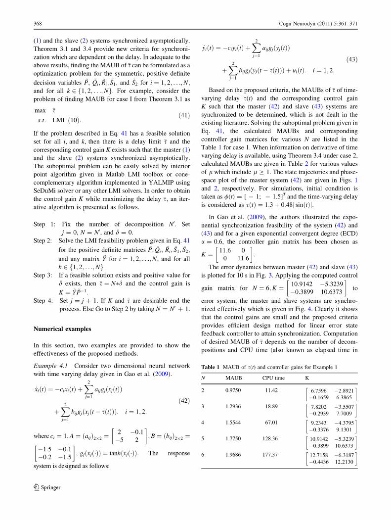
Example 4.1 Consider two dimensional neural network

with time varying delay given in Gao et al. (2009).

_xiðtÞ ¼ �cixiðtÞ þX2

j¼1

aijgjðxjðtÞÞ

þX2

j¼1

bijgjðxjðt � sðtÞÞÞ: i ¼ 1; 2:

ð42Þ

where ci ¼ 1;A ¼ ðaijÞ2�2 ¼2 �0:1�5 2

� �;B ¼ ðbijÞ2�2 ¼

�1:5 �0:1�0:2 �1:5

� �; gjðxjð�ÞÞ ¼ tanhðxjð�ÞÞ: The response

system is designed as follows:

_yiðtÞ ¼ �ciyiðtÞ þX2

j¼1

aijgjðyjðtÞÞ

þX2

j¼1

bijgjðyjðt � sðtÞÞÞ þ uiðtÞ: i ¼ 1; 2:

ð43Þ

Based on the proposed criteria, the MAUBs of �s of time-

varying delay s(t) and the corresponding control gain

K such that the master (42) and slave (43) systems are

synchronized to be determined, which is not dealt in the

existing literature. Solving the suboptimal problem given in

Eq. 41, the calculated MAUBs and corresponding

controller gain matrices for various N are listed in the

Table 1 for case 1. When information on derivative of time

varying delay is available, using Theorem 3.4 under case 2,

calculated MAUBs are given in Table 2 for various values

of l which include l C 1. The state trajectories and phase-

space plot of the master system (42) are given in Figs. 1

and 2, respectively. For simulations, initial condition is

taken as /(t) = [ - 1; - 1.5]T and the time-varying delay

is considered as sðtÞ ¼ 1:3þ 0:48j sinðtÞj:

In Gao et al. (2009), the authors illustrated the expo-

nential synchronization feasibility of the system (42) and

(43) and for a given exponential convergent degree (ECD)

a = 0.6, the controller gain matrix has been chosen as

K ¼ 11:6 0

0 11:6

� �:

The error dynamics between master (42) and slave (43)

is plotted for 10 s in Fig. 3. Applying the computed control

gain matrix for N ¼ 6;K ¼ 10:9142 �5:3239

�0:3899 10:6373

� �to

error system, the master and slave systems are synchro-

nized effectively which is given in Fig. 4. Clearly it shows

that the control gains are small and the proposed criteria

provides efficient design method for linear error state

feedback controller to attain synchronization. Computation

of desired MAUB of �s depends on the number of decom-

positions and CPU time (also known as elapsed time in

Table 1 MAUB of s(t) and controller gains for Example 1

N MAUB CPU time K

2 0.9750 11.42 6:7596 �2:8921

�0:1659 6:3865

� �

3 1.2936 18.89 7:8202 �3:5507

�0:2939 7:7009

� �

4 1.5544 67.01 9:2343 �4:3795

�0:3376 9:1301

� �

5 1.7750 128.36 10:9142 �5:3239

�0:3899 10:6373

� �

6 1.9686 177.37 12:7158 �6:3187

�0:4436 12:2130

� �

368 Cogn Neurodyn (2011) 5:361–371

123

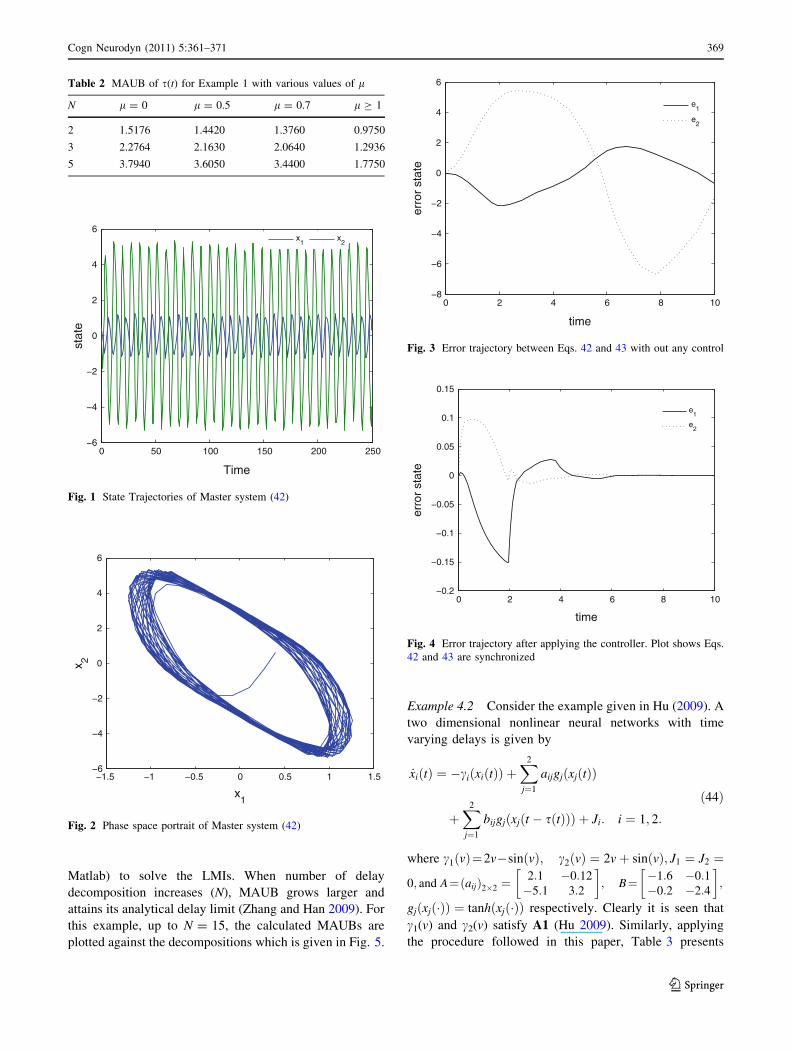
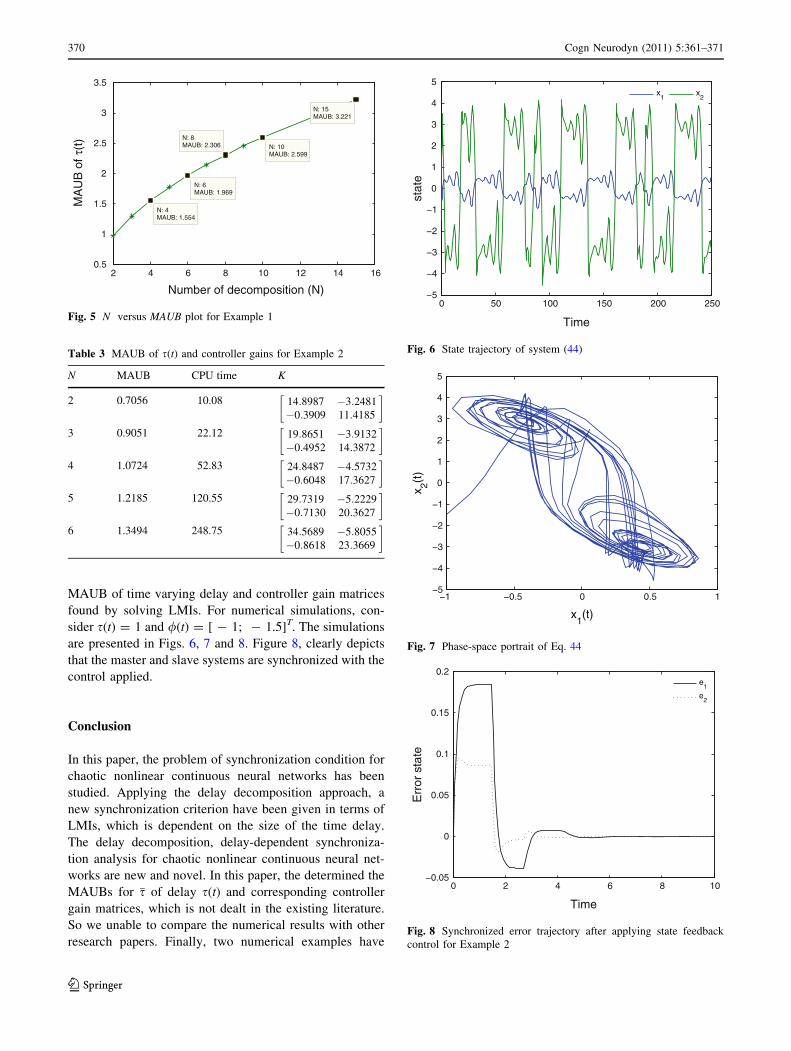
Matlab) to solve the LMIs. When number of delay

decomposition increases (N), MAUB grows larger and

attains its analytical delay limit (Zhang and Han 2009). For

this example, up to N = 15, the calculated MAUBs are

plotted against the decompositions which is given in Fig. 5.

Example 4.2 Consider the example given in Hu (2009). A

two dimensional nonlinear neural networks with time

varying delays is given by

_xiðtÞ ¼ �ciðxiðtÞÞ þX2

j¼1

aijgjðxjðtÞÞ

þX2

j¼1

bijgjðxjðt � sðtÞÞÞ þ Ji: i ¼ 1; 2:

ð44Þ

where c1ðvÞ¼2v�sinðvÞ; c2ðvÞ ¼ 2vþ sinðvÞ; J1 ¼ J2 ¼

0; and A¼ðaijÞ2�2 ¼2:1 �0:12

�5:1 3:2

� �; B¼ �1:6 �0:1

�0:2 �2:4

� �;

gjðxjð�ÞÞ ¼ tanhðxjð�ÞÞ respectively. Clearly it is seen that

c1(v) and c2(v) satisfy A1 (Hu 2009). Similarly, applying

the procedure followed in this paper, Table 3 presents

0 50 100 150 200 250−6

−4

−2

0

2

4

6

Time

stat

e

x

1x

2

Fig. 1 State Trajectories of Master system (42)

0 2 4 6 8 10−0.2

−0.15

−0.1

−0.05

0

0.05

0.1

0.15

time

erro

r st

ate

e1

e2

Fig. 4 Error trajectory after applying the controller. Plot shows Eqs.

42 and 43 are synchronized

−1.5 −1 −0.5 0 0.5 1 1.5−6

−4

−2

0

2

4

6

x1

x 2

Fig. 2 Phase space portrait of Master system (42)

0 2 4 6 8 10−8

−6

−4

−2

0

2

4

6

time

erro

r st

ate

e1

e2

Fig. 3 Error trajectory between Eqs. 42 and 43 with out any control

Table 2 MAUB of s(t) for Example 1 with various values of l

N l = 0 l = 0.5 l = 0.7 l C 1

2 1.5176 1.4420 1.3760 0.9750

3 2.2764 2.1630 2.0640 1.2936

5 3.7940 3.6050 3.4400 1.7750

Cogn Neurodyn (2011) 5:361–371 369

123

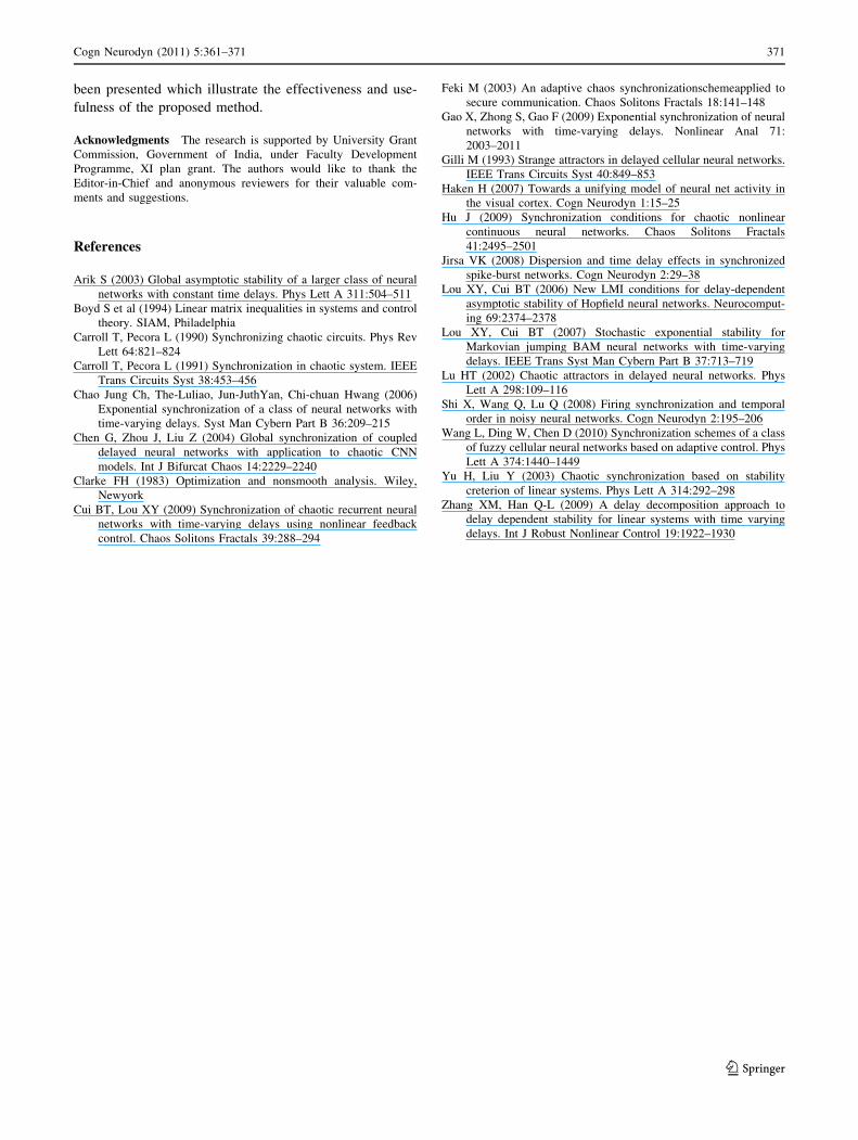
MAUB of time varying delay and controller gain matrices

found by solving LMIs. For numerical simulations, con-

sider s(t) = 1 and /(t) = [ - 1; - 1.5]T. The simulations

are presented in Figs. 6, 7 and 8. Figure 8, clearly depicts

that the master and slave systems are synchronized with the

control applied.

Conclusion

In this paper, the problem of synchronization condition for

chaotic nonlinear continuous neural networks has been

studied. Applying the delay decomposition approach, a

new synchronization criterion have been given in terms of

LMIs, which is dependent on the size of the time delay.

The delay decomposition, delay-dependent synchroniza-

tion analysis for chaotic nonlinear continuous neural net-

works are new and novel. In this paper, the determined the

MAUBs for �s of delay s(t) and corresponding controller

gain matrices, which is not dealt in the existing literature.

So we unable to compare the numerical results with other

research papers. Finally, two numerical examples have

Table 3 MAUB of s(t) and controller gains for Example 2

N MAUB CPU time K

2 0.7056 10.08 14:8987 �3:2481

�0:3909 11:4185

� �

3 0.9051 22.12 19:8651 �3:9132

�0:4952 14:3872

� �

4 1.0724 52.83 24:8487 �4:5732

�0:6048 17:3627

� �

5 1.2185 120.55 29:7319 �5:2229

�0:7130 20:3627

� �

6 1.3494 248.75 34:5689 �5:8055

�0:8618 23:3669

� �

0 2 4 6 8 10−0.05

0

0.05

0.1

0.15

0.2

Time

Err

or s

tate

e

1

e2

Fig. 8 Synchronized error trajectory after applying state feedback

control for Example 2

−1 −0.5 0 0.5 1−5

−4

−3

−2

−1

0

1

2

3

4

5

x1(t)

x 2(t)

Fig. 7 Phase-space portrait of Eq. 44

0 50 100 150 200 250−5

−4

−3

−2

−1

0

1

2

3

4

5

Time

stat

e

x1

x2

Fig. 6 State trajectory of system (44)

2 4 6 8 10 12 14 160.5

1

1.5

2

2.5

3

3.5

N: 15MAUB: 3.221

Number of decomposition (N)

MA

UB

of τ

(t)

N: 10MAUB: 2.599

N: 8MAUB: 2.306

N: 6MAUB: 1.969

N: 4MAUB: 1.554

Fig. 5 N versus MAUB plot for Example 1

370 Cogn Neurodyn (2011) 5:361–371

123

been presented which illustrate the effectiveness and use-

fulness of the proposed method.

Acknowledgments The research is supported by University Grant

Commission, Government of India, under Faculty Development

Programme, XI plan grant. The authors would like to thank the

Editor-in-Chief and anonymous reviewers for their valuable com-

ments and suggestions.

References

Arik S (2003) Global asymptotic stability of a larger class of neural

networks with constant time delays. Phys Lett A 311:504–511

Boyd S et al (1994) Linear matrix inequalities in systems and control

theory. SIAM, Philadelphia

Carroll T, Pecora L (1990) Synchronizing chaotic circuits. Phys Rev

Lett 64:821–824

Carroll T, Pecora L (1991) Synchronization in chaotic system. IEEE

Trans Circuits Syst 38:453–456

Chao Jung Ch, The-Luliao, Jun-JuthYan, Chi-chuan Hwang (2006)

Exponential synchronization of a class of neural networks with

time-varying delays. Syst Man Cybern Part B 36:209–215

Chen G, Zhou J, Liu Z (2004) Global synchronization of coupled

delayed neural networks with application to chaotic CNN

models. Int J Bifurcat Chaos 14:2229–2240

Clarke FH (1983) Optimization and nonsmooth analysis. Wiley,

Newyork

Cui BT, Lou XY (2009) Synchronization of chaotic recurrent neural

networks with time-varying delays using nonlinear feedback

control. Chaos Solitons Fractals 39:288–294

Feki M (2003) An adaptive chaos synchronizationschemeapplied to

secure communication. Chaos Solitons Fractals 18:141–148

Gao X, Zhong S, Gao F (2009) Exponential synchronization of neural

networks with time-varying delays. Nonlinear Anal 71:

2003–2011

Gilli M (1993) Strange attractors in delayed cellular neural networks.

IEEE Trans Circuits Syst 40:849–853

Haken H (2007) Towards a unifying model of neural net activity in

the visual cortex. Cogn Neurodyn 1:15–25

Hu J (2009) Synchronization conditions for chaotic nonlinear

continuous neural networks. Chaos Solitons Fractals

41:2495–2501

Jirsa VK (2008) Dispersion and time delay effects in synchronized

spike-burst networks. Cogn Neurodyn 2:29–38

Lou XY, Cui BT (2006) New LMI conditions for delay-dependent

asymptotic stability of Hopfield neural networks. Neurocomput-

ing 69:2374–2378

Lou XY, Cui BT (2007) Stochastic exponential stability for

Markovian jumping BAM neural networks with time-varying

delays. IEEE Trans Syst Man Cybern Part B 37:713–719

Lu HT (2002) Chaotic attractors in delayed neural networks. Phys

Lett A 298:109–116

Shi X, Wang Q, Lu Q (2008) Firing synchronization and temporal

order in noisy neural networks. Cogn Neurodyn 2:195–206

Wang L, Ding W, Chen D (2010) Synchronization schemes of a class

of fuzzy cellular neural networks based on adaptive control. Phys

Lett A 374:1440–1449

Yu H, Liu Y (2003) Chaotic synchronization based on stability

creterion of linear systems. Phys Lett A 314:292–298

Zhang XM, Han Q-L (2009) A delay decomposition approach to

delay dependent stability for linear systems with time varying

delays. Int J Robust Nonlinear Control 19:1922–1930

Cogn Neurodyn (2011) 5:361–371 371

123