Embed Size (px)
Citation preview

Systematic Derivation of the Weakly Non-Linear Theory ofThermoacoustic Devices
Version II
P.H.M.W. in ’t panhuis, S.W. Rienstra, J. Molenaar
Dep. of Mathematics and Computer ScienceTechnische Universiteit Eindhoven
P.O. Box 513, 5600 MB Eindhoven, The Netherlands
Abstract
Thermoacoustics is the field concerned with transformations between thermal and acousticenergy. This paper teaches the fundamentals of two kinds of thermoacoustic devices: the ther-moacoustic prime mover and the thermoacoustic heat pump or refrigerator.
Two technologies, involving standing wave and traveling wave modes, are considered. We willinvestigate the case of a porous medium and two heat exchangers placed in a gas-filled resonator,in which either a standing or traveling wave is maintained. The central problem is the interactionbetween the porous medium and the sound field in the tube. The conventional thermoacoustictheory is reexamined and a systematic and consistent weaklynon-linear theory is constructedbased on dimensional analysis and small parameter asymptotics.
The difference with conventional thermoacoustic theory lies in the dimensional analysis. Thisis a powerful tool in understanding physical effects which are coupled to several dimensionlessparameters that appear in the equations, such as the Mach number, the Prandtl number, the Lautrecnumber and several geometrical quantities. By carefully analyzing limiting situations in whichthese parameters differ in orders of magnitude, we can studythe behavior of the system as afunction of parameters connected to geometry, heat transport and viscous effects.
1. Introduction
The most general interpretation of thermoacoustics, as described by Rott[21], includes all effects inacoustics in which heat conduction and entropy variations of the (gaseous) medium play a role. Inthis paper, however, we will focus specifically on thermoacoustic devicesexploiting thermoacousticconcepts to produce useful refrigeration, heating, or work.
1.1 A brief history
Thermoacoustics has a long history that dates back more than two centuries.For the most part heat-driven oscillations were subject of these investigations. The reverse process, generating temperaturedifferences using acoustic oscillations, is a relatively new phenomenon. The first qualitative expla-nation was given in 1887 by Lord Rayleigh in his classical work ”The Theory of Sound” [15]. Heexplains the production of thermoacoustic oscillations as follows:
1
”If heat be given to the air at the moment of greatest condensation (compression) or takenfrom it at the moment of greatest rarefaction (expansion), the vibration isencouraged”.
Rayleigh’s qualitative understanding turned out to be correct, but a quantitatively accurate theoret-ical description of those phenomena was not achieved until much later. Thebreakthrough came in1969, when Rott and coworkers started a series of papers [17], [18], [20], [22] in which a successfullinear theory of thermoacoustics was given. The first to give a comprehensive picture, was Swift [23]in 1988. He implemented Rott’s theory of thermoacoustic phenomena into creatingpractical thermoa-coustic devices. His work included a short history, experimental results,discussions on how to buildthese devices, and a coherent development of the theory based on Rott’s work. Since then Swift andothers have contributed a lot to the development of thermoacoustic devices.In 2002 Swift [25] alsowrote a textbook, providing a complete introduction into thermoacoustics and treating several kindsof thermoacoustic devices. Recently Tijani [26] wrote a Ph.D thesis based on Swift’s work in whichhe also discusses the linear theory of thermoacoustics. Most of the work on thermoacoustic deviceshas been been reviewed by Garrett [4] in 2003.
1.2 Classification
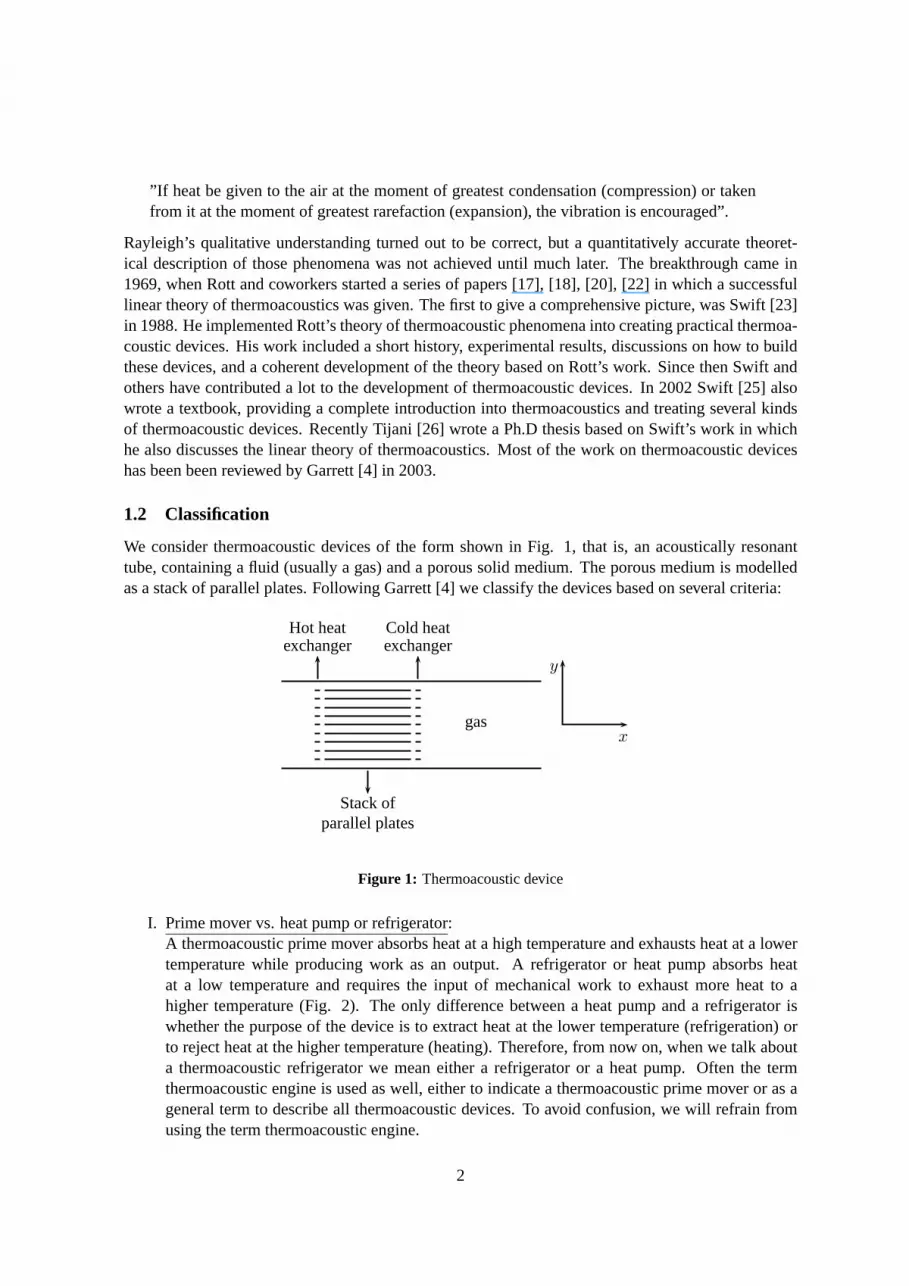
We consider thermoacoustic devices of the form shown in Fig. 1, that is, anacoustically resonanttube, containing a fluid (usually a gas) and a porous solid medium. The porous medium is modelledas a stack of parallel plates. Following Garrett [4] we classify the devicesbased on several criteria:
gasx
y
Stack ofparallel plates
Hot heatexchanger
Cold heatexchanger
Figure 1: Thermoacoustic device
I. Prime mover vs. heat pump or refrigerator:A thermoacoustic prime mover absorbs heat at a high temperature and exhausts heat at a lowertemperature while producing work as an output. A refrigerator or heat pump absorbs heatat a low temperature and requires the input of mechanical work to exhaustmore heat to ahigher temperature (Fig. 2). The only difference between a heat pump and a refrigerator iswhether the purpose of the device is to extract heat at the lower temperature(refrigeration) orto reject heat at the higher temperature (heating). Therefore, from now on, when we talk abouta thermoacoustic refrigerator we mean either a refrigerator or a heat pump. Often the termthermoacoustic engine is used as well, either to indicate a thermoacoustic prime mover or as ageneral term to describe all thermoacoustic devices. To avoid confusion, we will refrain fromusing the term thermoacoustic engine.
2

TH
QH
DeviceW
QC
TC
(a) Prime mover
TH
QH
DeviceW
QC
TC
(b) Refrigerator or heat pump
Figure 2: The flows of work and heat inside (a) a thermoacoustic prime mover and (b) a thermoacoustic refrig-erator or heat pump
II. Stack-based devices vs. regenerator-based devices:A second classification depends on whether the porous medium used to exchange heat with theworking fluid is a ”stack” or a ” regenerator”. Inside a regenerator thepore size is much smallerthan inside a stack. Garrett [4] uses the so-called Lautrec numberNL to indicate the differencebetween a stack and regenerator. The Lautrec number is defined as the ratio between the halfpore size and the thermal penetration depth1. If NL & 1 the porous medium is called a stackand if NL ≪ 1 it is called a regenerator. This definition of stacks and regenerators is slightlydifferent from Garret’s2, but is chosen to stress that the pore size inside a regenerator is verysmall.
III. Standing-wave devices vs. traveling-wave devices:Finally thermoacoustic devices can also be categorized depending on whether there is a travel-ing or a standing sound wave inside the thermoacoustic device. In section 3.1.7 we show that itis beneficiary to use a stack inside a standing-wave device and a regenerator inside a traveling-wave device. Therefore one could also classify thermoacoustic devicesas either standing-wavestack-based devices or traveling-wave regenerator-based devices.
1.3 Basic principle of the thermoacoustic effect
The thermoacoustic effect can be understood by following a given parcel of fluid as it moves throughthe stack or regenerator. Fig. 3 displays the (idealized) cycles a typical fluid parcel goes through as itoscillates alongside the plate. The fluid parcel follows a four-step cycle which depends on the kind ofdevice.
• Stack-based devices:The basic thermodynamic cycle in a stack-based acoustic refrigerator or prime mover consists oftwo reversible adiabatic steps (step 1,3 in Fig. 3(a,b)) and two irreversible isobaric heat-transfersteps (step 2,4 in Fig. 3(a,b)).
As NL & 1, there will be an imperfect thermal contact between the fluid and the solid. Asa result a phase shift, or time delay, arises between the pressure and the temperature of thegas parcels that are at a distance of a few thermal penetration depths from the stack plate.
1The thermal penetration depth is the distance heat can diffuse through within a characteristic time2Garrett defines the porous medium to be a stack ifNL ≥ 1, and a regenerator ifNL < 1
3

1 - Compression
−→
2 - Cooling
δQ1
δW1
3 - Expansion
←−
4 - Heating
δQ2
δW2
(a) Stack-based refrigerator(small∇T )
1 - Compression
−→
2 - Heating
δQ1
δW1
3 - Expansion
←
4 - Cooling
δQ2
δW2
(b) Stack-based prime mover(large∇T )
1 - Heating
δQ1
δW1
−→
2 - Compression
3 - Cooling
δQ2
δW2
←−
4 - Expansion
(c) Regenerator-based refrig-erator (small∇T )
1 - Heating
δQ1
δW1
−→
2 - Expansion
3 - Cooling
δQ2
δW2
←
4 - Compression
(d) Regenerator-based primemover (large∇T )
Figure 3: Typical fluid parcels executing the four steps (1-4) of the thermodynamic cycle in (a) a stack-basedstanding-wave refrigerator, (b) a stack-based standing wave prime mover, (c) a regenerator-basedtraveling wave refrigerator and (d) a regenerator-based traveling wave prime mover.
4

Parcels that are farther away have no thermal contact and are simply compressed and expandedadiabatically and reversibly by the sound wave. Therefore parcels thatare about a thermalpenetration depth away from the plate have good enough thermal contact toexchange someheat with the plate, but at the same time are in poor enough contact to producea time delaybetween motion and heat transfer.
The fact that the operation of stack-based thermoacoustic devices requires pressure and dis-placement to be primarily in phase, explains why stack-based devices are also called standing-wave devices.
The difference between the prime-mover and the refrigerator depends on the magnitude of thetemperature gradient along the stack plates. During compression (step 1) the fluid parcel is bothwarmed (adiabatically) and displaced along the plate. Next, if the temperature gradient alongthe stack is large enough, the plate temperature will be larger than the fluid parcel temperature.Hence heat will flow from the plate to the fluid (step 2). This is the case in Fig. 3(b). Thenthe parcel expands and moves back to the original position (step 3). There the temperature ofthe parcel will still be higher than the plate temperature and heat will flow fromthe fluid to theplate (step 4). As a result heat is transported from a high to a low temperature, thus producinga certain amount of work. In other words the device acts as a prime mover. Similarly if thetemperature gradient along the plate is small enough, we find that heat is transported from a lowto a high temperature, thus requiring a certain amount of work. Thereforethe cycle shown inFig. 3(a) corresponds to a refrigerator.
Thus we find that a low temperature gradient along the plate is the condition fora refrigeratorand a high temperature gradient is the condition for a prime mover. The criticaltemperaturegradient is where the temperature change along the plate just matches the adiabatic temperaturechange of the fluid parcel.
• Regenerator-based devices:The basic thermodynamic cycle in a regenerator-based acoustic refrigerator or prime moverconsists of two isochoric displacement steps during which heat is exchanged (step 1,3 in Fig.3(c,d)) and two isothermal compression and expansion steps (step 2,4 in Fig. 3(c,d)).
Because the pores in a regenerator are so small compared tot the thermal penetration depth,there will be an almost perfect thermal contact between the fluid and the solid. Therefore duringthe motion (step 2, 4) the temperature of the wall and the fluid parcel will be the same. As aresult there will be a continuous exchange of heat between the gas and the solid, which takesplace over a vanishingly small temperature difference and therefore onlya negligibly amount ofentropy is created. During the compression and expansion (step 1,3), thetemperature remainsconstant.
The gas oscillating inside a regenerator requires the same phasing betweenpressure and velocityas a traveling acoustic wave. Therefore regenerator-based devicesare also called traveling-wavedevices.
The main advantage of regenerator-based devices with respect to stack-based devices is thatthere are no irreversible processes, so that the ideal efficiency is equal to the Carnot efficiency.On the other hand, because the pores are so narrow, there may be significant viscous dissipationwhich could lower the efficiency dramatically.
Usually the displacement of one fluid parcel is small with respect to the length of the plate. Thusthere will be an entire train of adjacent fluid parcels, each confined to a short region of length2x1 and
5

passing on heat as in a bucket brigade (Fig. 4). Although a single parcel transports heatδQ over avery small interval,δQ is shuttled along the entire plate because there are many parcels in series.
QC
TC L TH
QH
2x1 2x1 2x1
δQ
︸ ︷︷ ︸
W
Figure 4: Work and heat flow inside a thermoacoustic refrigerator. Theoscillating fluid parcels work as abucket brigade, shuttling heat along the stack plate from one parcel of gas to the next. As a resultheatQ is transported from the left to the right, using workW . Inside a prime mover the arrows willbe reversed, i.e. heatQ is transported from the right to the left and workW is produced.
1.4 Scope
Motivated by the work of Swift [23], [25] and Tijani [26], this paper tries to reconstruct the lineartheory of thermoacoustics in a systematic and consistent manner using dimensional analysis and smallparameter asymptotics.
We will start in section 2 with a detailed description of the model and an overviewof the governingequations and boundary conditions. Then in section 3 we try to solve the equations assuming there isno mean steady flow. This is done both for stack- and regenerator-based devices. This is repeated insection 4, but now with a mean steady flow. Finally section 5 shows the different energy flows andtheir interaction in thermoacoustic devices.
2. General thermoacoustic theory
We will model the thermoacoustic devices as depicted in Fig. 5 (see also [23] and [26]), where thedevice is modeled as an acoustically resonant tube, containing a gas and a porous solid medium. Fornow we will not make any assumptions on whether the tube is open or closed. The porous medium ismodeled as a stack of parallel plates, each of thickness2l and lengthL. The space between the platesis equal to2R.
2.1 Governing equations
We will focus on what happens inside the stack. The general equations describing the thermodynamicbehavior are [6]
ρ
[∂v
∂t+ (v · ∇)v
]
= −∇p + µ∇2v + ρb +(
ξ +µ
3
)
∇(∇ · v), (2.1.1)
∂ρ
∂t+ ∇ · (ρv) = 0, (2.1.2)
6

gas
Stack ofparallel plates
Hot heatexchanger
Cold heatexchanger
(a) Overall view
etc.
Plate
Gas
Plate2lxy′
Gas2Rxy
Plate
L
(b) Expanded view of stack
Figure 5: A thermoacoustic device modelled as an acoustically resonant tube, containing a gas, a stack ofparallel plates and heat exchangers at both sides of the stack.
ρcp
(
∂T
∂t+ v · ∇T
)
− βT
(∂p
∂t+ v · ∇p
)
= K∇ · (∇T ) + Σ:∇v. (2.1.3)
Hereρ is the density,v is the velocity,p is the pressure,T is the temperature,s is the entropy perunit mass,b is the total body force,µ and ξ are the dynamic (shear) and second (bulk) viscosity,respectively;K is the gas thermal conductivity,cp is the specific heat per unit mass,β is the thermalexpansion coefficient andΣ is the viscous stress tensor, with components
Σij = µ
(∂vi
∂xj+
∂vj
∂xi− 2
3δij
∂vk
∂xk
)
+ ξδij∂vk
∂xk
. (2.1.4)
Furthermoreρ is related top andT according to (A.4.9)
dρ =γ
c2dp − ρβ dT . (2.1.5)
Finally, the temperatureTs in the plates satisfies the diffusion equation
ρscs∂Ts
∂t= Ks∇
2Ts, (2.1.6)
whereKs, cs andρs are the thermal conductivity, the specific heat per unit mass and the densityofthe stack’s material, respectively.
These equations will be linearized and simplified using the following assumptions
• The theory is linear; second-order effects, such as acoustic streamingand turbulence, are ne-glected.
• The plates are fixed and rigid.
• The temperature variations along the stack are much smaller than the absolute temperature.
7

• The temperature dependence of viscosity is neglected.
• Oscillating variables have harmonic time dependence at a single angular frequencyω.
At the boundaries we impose the no-slip condition
v = 0, y = ±R. (2.1.7)
The temperatures in the plates and in the gas are coupled at the solid-gas interface where continuityof temperature and heat fluxes is imposed.
T∣∣∣y=±R
= Ts
∣∣∣y′=∓l
=: Tb(x), (2.1.8a)
K
(
∂T
∂y
)
y=±R
= Ks
(
∂Ts
∂y′
)
y′=∓l
, (2.1.8b)
We do not impose any conditions at the stack ends, as we are mainly interestedabout what happensinside the stack, ignoring any entrance effects.
The next step is the rescaling of the variables in (2.1.1), (2.1.2) and (2.1.3)such that the equationsare dimensionless. We assume a 2D-model where gravity is the only body force and rescale as follows
x = Lx, y = Ry, y′ = ly′, t =1
ωt, (2.1.9a)
u = Cu, v = εCv, p = DC2p, ρ = Dρ, T =C2
cpT, b = gb, (2.1.9b)
ρs = Dsρs, Ts =C2
cpTs, (2.1.9c)
c = Cc, β =cp
C2β, (2.1.9d)
whereC is a typical speed of sound,g is the gravitational acceleration,D andDs are typical densitiesfor the fluid and solid, respectively, andε is the aspect ratio of a stack pore defined as
ε = R/L ≪ 1. (2.1.10)
Clearly, ε is a dimensionless parameter. In total there are 15 physical parameters in thisproblemexpressible in 5 independent fundamental physical quantities. Therefore, using the Buckinghamπtheorem [1], we know that 10 independent dimensionless parameters canbe constructed from theoriginal 14 parameters. In addition toε, we will use the following dimensionless parameters:
εp = l/L, ϑ =RKs
lK, κ =
ωL
C, γ =
cp
cv, A =
U
C, (2.1.11a)
Fr =U2
gL, Wo =
√2
R
δν, NL =
R
δk
, Np =l
δs, Pr =
2N2L
Wo2. (2.1.11b)
wherecv is the isochoric specific heat,λ = 2πc/ω is the wavelength,ω is the frequency,U is a typicalfluid speed,εp is the aspect ratio of the stack plates,κ is a dimensionless wave number (Helmholtz
8

number),A is a Mach number,Fr is the Froude number,Pr is the Prandtl number,Wo is the Wom-ersley number andNL andNp are the Lautrec numbers (as defined by Garrett [4]) related to the fluidand plate, respectively. Here the parametersδν , δk andδs are the viscous penetration depth, and thethermal penetration depths for the fluid and solid, respectively.
δν =
√
2ν
ω, δk =
√
2χ
ω, δs =
√
2χs
ω. (2.1.12)
Hereν = µ/D is the kinematic viscosity andχ = K/(Dcp) is the thermal diffusivity of the fluid.It can be shown that the first 9 of the dimensionless parameters in (2.1.11) together withε form 10independent dimensionless parameters. Obviously the Prandtl number is determined completely bythe Womersley and Lautrec numbers.
We assume that the velocity is small compared to the speed of sound, i.e. the Mach numberA issmall. This can be used to linearize the equations mentioned afore. Letq be any of the fluid variables(p, v, T , etc..), then expandingq in powers ofA with an equilibrium stateq0 we find
q(x, y, t) = q0(x, y) +∞∑
k=1
Akq′k(x, y, t), A ≪ 1. (2.1.13a)
where we assume harmonic time-dependence forq1 with dimensionless frequency 1, so that we canwrite
q′1(x, y, t) = Re[q1(x, y)eit
]. (2.1.13b)
Sinceu = O(A), we find thatv0 = (u0, v0) ≡ 0. Moreover we demand
u1 6= 0, (2.1.14)
We call (2.1.13) a weakly non-linear expansion to indicate that, although we assume small amplitudes,we still include terms of higher order inA.
In dimensionless form we obtain the following system of equations
∂ρ
∂t+
∂(ρu)
∂x+
∂(ρv)
∂y= 0, (2.1.15)
ρ
(∂u
∂t+ u
∂u
∂x+ v
∂u
∂y
)
= −∂p
∂x+
κ
Wo2
(
ε2 ∂2u
∂x2+
∂2u
∂y2
)
+A2
Frρbx
+εκ
Wo2
(ξ
µ+
1
3
)(∂2u
∂x2+
∂2v
∂x∂y
)
, (2.1.16)
ε2ρ
(∂v
∂t+ u
∂v
∂x+ v
∂v
∂y
)
= −∂p
∂y+
ε2κ
Wo2
(
ε2 ∂2v
∂x2+
∂2v
∂y2
)
+A2ε
Frρby
+ε2κ
Wo2
(ξ
µ+
1
3
)(∂2u
∂x∂y+
∂2v
∂y2
)
, (2.1.17)
ρ
(∂T
∂t+ u
∂T
∂x+ v
∂T
∂y
)
− βT
(∂p
∂t+ u
∂p
∂x+ v
∂p
∂y
)
=κ
2N2L
(
ε2 ∂2T
∂x2+
∂2T
∂y2
)
+κ
Wo2
[(∂u
∂y
)2
+ O(ε)
]
. (2.1.18)
9

ρs∂Ts
∂t=
κ
2N2p
(
ε2p
∂2Ts
∂x2+
∂2Ts
∂y′2
)
, (2.1.19)
ρ1 = −ρ0βT1 +γ
c2p1. (2.1.20)
subject to
v|y=±1= 0, (2.1.21a)
T |y=±1= Ts|y′=∓1
=: Tb(x), (2.1.21b)
∂T
∂y
∣∣∣∣y=±1
= ϑ∂Ts
∂y′
∣∣∣∣y′=∓1
. (2.1.21c)
3. Thermoacoustic devices without streaming
This chapter discusses both stack-based and regenerator-based thermoacoustic devices in the absenceof streaming. With streaming there exists a steady mean velocity, that is superimposed on the largerfirst-order oscillations. This will be discussed further in the next section.
To solve the equations given in the previous section we need to know the magnitude of the dimen-sionless parameters involved. First note that
κ =ωL
C=
cL
Cλ=
cL
λ∼ L
λ. (3.0.22)
Thus the dimensionless wave number is a measure for the relative length of thestack. Here we willmake the ”short-stack” approximationL ≪ λ (κ ≪ 1), where the stack is considered to be shortcompared to the engine with the restriction thatκ is the largest among the small parameters.
The Womersley number and the Lautrec number are related by2N2L = PrWo2. The Prandtl
number only depends on material parameters and is usually close to 1. As a resultNL andWo shouldbe of the same order of magnitude. Normally in standing wave machinesR ∼ δk (stack) and intraveling wave machinesR ≪ δk (regenerator). Also we assume thatNp ∼ NL.
Furthermore we assume that the amplitudes of the acoustic oscillations can be taken arbitrarilysmall, with the restriction thatε2 ≪ A, so that∂2q0/∂x2 can be neglected with respect to∂2q1/∂y2
(O(ε2) versusO(A)). Swift[23] and Tijani [26] also treated this case, although they did not makethese assumptions explicit. Finally, we also assume that
ϑ = O(1), Fr = O(1). (3.0.23)
Summarizing we have
ε2p ≪ ε2 ≪ A ≪ κ2 ≪ 1, ϑ = O(1), Fr = O(1), (3.0.24)
and
Wo ∼ 1, NL ∼ 1, Np ∼ 1, for a stack, (3.0.25)
Wo ≪ 1, NL ≪ 1, Np ≪ 1, for a regenerator. (3.0.26)
10

The presence ofκ as a small parameter suggests the following alternative expansions for the fluidvariablesq
q = q0(x, y) + AκmqRe[(
q10(x, y) + κq11(x, y) + κ2q12(x, y))eiκt]+ · · · . (3.0.27)
The variables here have either one or two indices. The first index always indicates the correspondingpower ofA and the second index shows the corresponding power ofκ. When necessary we will alsouse a third index to indicate the power ofε. If any of these indices are left out, it means that the poweris zero.
As A is a Mach number, we demand thatmv = 0. Anticipating thatu ∼ p− p0 in the sound fieldin the main pipe, we also demandmp = 0. Note that the terms second order inA can be neglectedsinceA ≪ κ2 ≪ 1.
3.1 Short stack
In this section we will restrict ourselves to the case of a stack, i.e.
Wo ∼ 1, NL ∼ 1, Np ∼ 1. (3.1.1)
3.1.1 The horizontal velocityu1
Substitute the expansions given in (3.0.27) in they-component of the momentum equation (2.1.17).Collecting, the zeroth order terms we find∂p0/∂y = 0. Next collecting terms up to orderAκ2 wealso find
A∂p10
∂y+ Aκ
∂p11
∂y+ Aκ2 ∂p12
∂y= 0. (3.1.2)
This equation can only be satisfied if
∂p10
∂y=
∂p11
∂y=
∂p12
∂y= 0. (3.1.3)
We do the same for thex-component (2.1.16). The zeroth order equation yields∂p0/∂x = 0. Keepingterms of order up toAκ we obtain
iAκρ0u10 = −Adp10
dx− Aκ
dp11
dx+
Aκ
Wo2
∂2u10
∂y2, (3.1.4)
Collecting terms of orderA we find that∂p10/∂x = 0. Hence
p = p0 + ARe[(p10 + κp11(x)) eit
]+ · · · . (3.1.5)
Next, collecting the terms of orderAκ, we find thatu10 satisfies
iρ0u10 = −dp11
dx+
1
Wo2
∂2u10
∂y2. (3.1.6)
and applying the boundary conditionsu1(x,±1) = 0, we obtain
u10(x, y) =i
ρ0
dp11
dx
[
1 − cosh(ανy)
cosh(αν)
]
, (3.1.7)
11

where
αν = (1 + i)√
ρ0
R
δν= (1 + i)
√ρ0
2Wo. (3.1.8)
In the same way it can be shown that
u11(x, y) =i
ρ0
dp12
dx
[
1 − cosh(ανy)
cosh(αν)
]
. (3.1.9)
This coincides with the solution found by Swift [23] and Tijani [26] in a dimensional form.
3.1.2 The temperatureTs in the plate
Using the rescaled energy equation (2.1.18) and the diffusion equation (2.1.19) we will try to findT andTs. First we solve (2.1.19) subject to (2.1.21b). Substitute the expansions from (3.0.27) into(2.1.19). To leading order we find that∂2Ts0/∂y′2 = 0. That meansTs0 is at most linear iny′. Inview of symmetry we find thatTs0
is in fact constant iny′, i.e.
Ts(x, y′, t) = Ts0(x) + AκmT Re
[(Ts10
(x, y′) + κTs11(x, y′)
)eiκt]+ · · · , (3.1.10)
Sinceρs0= ρs0
(p0, Ts0), we also assume that
ρs(x, y′, t) = ρs0(x) + AκmρRe
[(ρs10
(x, y′) + κρs11(x, y′)
)eit]+ · · · , (3.1.11)
Collecting terms of orderA we find
2iρs0N2
p Ts10=
∂2Ts10
∂y′2. (3.1.12)
Imposing (2.1.21b)
Ts10(x,±1) = Tb10(x), (3.1.13)
we find that the solution to(3.1.12) is given by
Ts10(x, y′) = Tb10(x)
cosh(αsy′)
cosh(αs), (3.1.14)
where
αs = (1 + i)ρs0
l
δs= (1 + i)ρs0
Np. (3.1.15)
Similarly
Ts11(x, y′) = Tb11(x)
cosh(αsy′)
cosh(αs), (3.1.16)
The exact expression forTb1 should be determined from matchingTs with T .
12

3.1.3 The temperatureT between the plates
We substitute the expansions shown in (2.1.13) into equation (2.1.18). To leading order we find∂2T0/∂y2 = 0. That meansT0 is at most linear iny. In view of symmetry we find thatT0 is in factconstant iny. Therefore we expandT as
T (x, y, t) = T0(x) + AκmT Re[(T10(x, y) + κT11(x, y)) eit
]+ · · · , (3.1.17)
Sinceρ0 = ρ0(p0, T0), we assume that also
ρ(x, y, t) = ρ0(x) + AκmρRe[(ρ10(x, y) + κρ11(x, y)) eit
]+ · · · , (3.1.18)
With these results we find to leading order
iκ1+mT ρ0T10 + ρ0u10
dT0
dx=
κ1+mT
2N2L
∂2T10
∂y2. (3.1.19)
We choosemT = −1 to balance the equation. Then, inserting the expression foru10 given in (3.1.7),we obtain
iρ0T10 + idT0
dx
dp11
dx
[
1 − cosh(ανy)
cosh(αν)
]
=1
2N2L
∂2T10
∂y2. (3.1.20)
Next forT11 we find the following differential equations
iρ0T11 − iβT0p10 + ρ0u11
dT0
dx=
1
2N2L
∂2T11
∂y2. (3.1.21)
Inserting (3.1.9), we obtain
iρ0T11 + idT0
dx
dp12
dx
[
1 − cosh(ανy)
cosh(αν)
]
− iβT0p10 =1
2N2L
∂2T11
∂y2. (3.1.22)
Applying the boundary conditions in (2.1.21), we can solve (3.1.20) and (3.1.22)
T10(x, y) = − 1
ρ0
dT0
dx
dp11
dx
[
1 − Pr
Pr − 1
cosh(ανy)
cosh(αν)
]
− 1
ρ0
1 + εsfν
fk
(Pr − 1)(1 + εs)
dT0
dx
dp11
dx
cosh(αky)
cosh(αk), (3.1.23a)
T11(x, y) =βT0
ρ0
p10 −1
ρ0
dT0
dx
dp12
dx
[
1 − Pr
Pr − 1
cosh(ανy)
cosh(αν)
]
−[
βT0
ρ0
p10 +1
ρ0
1 + εsfν
fk
Pr − 1
dT0
dx
dp12
dx
]
cosh(αky)
(1 + εs) cosh(αk). (3.1.23b)
where
αk = (1 + i)√
ρ0
R
δk
= (1 + i)√
ρ0NL, (3.1.24)
εs =
√Kρ0cp tanh(αk)√
Ksρs0cs tanh(αs), fν =
tanh(αν)
αν, fk =
tanh(αk)
αk
. (3.1.25)
Note that if we had takenA ≪ ε2 (compare with (3.0.24)), i.e. the amplitudes of the oscillationscan be taken arbitrarily small, then the termd2T0/dx2 will appear in the equations. Then, for theequations to be satisfied, we must have thatT0 = Ts0
is linear inx.
13

3.1.4 The pressurep
In order to derive the dimensionless alternative for Rott’s wave equation (cf. [17], [18]), we start withthe continuity equation. From the equation of state (2.1.20) we find thatmρ = mT = −1. Now toleading order, we obtain
iρ10 +∂
∂x(ρ0u10) + ρ0
∂v10
∂y= 0, (3.1.26)
Using thex-derivative of equation (3.1.6), the equation of state (2.1.20), and inserting the expressionfor T10, we ultimately find
− βdT0
dx
dp11
dx
[
1 − Pr
Pr − 1
cosh(ανy)
cosh(αν)
]
− β1 + εs
fν
fk
(Pr − 1)(1 + εs)
dT0
dx
dp11
dx
cosh(αky)
cosh(αk)
− d2p11
dx2+
1
Wo2
∂3u10
∂x∂y2+ iρ0
∂v10
∂y= 0. (3.1.27)
Next we integrate with respect toy from 0 to1. Note thatv(x, 0) = 0 because of symmetry. Finally,inserting (3.1.7), we obtain Rott’s wave equation (dimensionless)
fk − fν
(Pr − 1)(1 + εs)β
dT0
dx
dp11
dx+ ρ0
d
dx
(1 − fν
ρ0
dp11
dx
)
= 0, (3.1.28)
Here we used
ρ0
d
dx
(1
ρ0
)
= − 1
ρ0
dρ0
dx= − 1
ρ0
∂ρ0
∂T0
dT0
dx= β
dT0
dx.
This result was also found by Rott [18], Swift [23] and Tijani [26]. For an ideal gas and ideal stackwith εs = 0 this result was first obtained in [17]. Note that in Rott’s result there is one term more inthe equation (namely(1+ (γ − 1)fk/(1+ εs))p1). The dimensional analysis shows that this term canbe neglected.
Going one order higher we can show, similar to the analysis above, thatp12 satisfies the followingequation.
i
c2
[
1 +γ − 1
1 + εsfk − (c2β2T0 − γ + 1)
(
1 − fk
1 + εs
)]
p10
+fk − fν
(Pr − 1)(1 + εs)β
dT0
dx
dp12
dx+ ρ0
d
dx
(1 − fν
ρ0
dp12
dx
)
= 0. (3.1.29)
Furthermore, if we impose the dimensionless equivalent of relation (A.4.6)
c2β2T0 = γ − 1,
then (3.1.29) transforms into
1
c2
[
1 +γ − 1
1 + εsfk
]
p10 +fk − fν
(Pr − 1)(1 + εs)β
dT0
dx
dp12
dx+ ρ0
d
dx
(1 − fν
ρ0
dp12
dx
)
= 0. (3.1.30)
14

3.1.5 Acoustic power
The time-averaged acoustic powerd ˙W used (or produced in the case of a prime mover) in a segmentof lengthdx can be found from
d ˙W
dx= Ag
d
dx
[
〈p1′u1
′〉]
, (3.1.31)
where the overbar indicates time average (over one period), brackets〈 〉 indicate averaging in they-
direction andAg is the cross-sectional area of the gas within the stack. Next˙W andAg are rescaledas
˙W = R2DC3W , Ag = R2Ag. (3.1.32)
As p is independent ofy, we find
dW
dx= A2Ag
d
dx
[
p′1〈u1
′〉]
(3.1.33)
It can be shown that the productp′1〈u1
′〉 satisfies
p′1〈u1
′〉 =1
2Re [p1〈u1
∗〉] , (3.1.34)
where the star denotes complex conjugation. Inserting (3.1.34) into (3.1.33)yields
dW
dx=
1
2A2AgRe
[
p1
d〈u1∗〉
dx+ 〈u1
∗〉dp1
dx
]
. (3.1.35)
Next, inserting (3.0.27), we find
dW
dx=
1
2A2Ag
{
Re
[
p10
d〈u10∗〉
dx
]
+ κRe
[
p10
d〈u11∗〉
dx+ p11
d〈u10∗〉
dx+ 〈u10
∗〉dp11
dx
]}
+ · · · .
(3.1.36)
Combining equations (3.1.9) and (3.1.28), we find
dp11
dx= − iρ0〈u10〉
1 − fν, (3.1.37)
and
d〈u10〉dx
= id
dx
(1 − fν
ρ0
dp11
dx
)
= − fk − fν
(Pr − 1)(1 + εs)(1 − fν)β
dT0
dx〈u10〉. (3.1.38)
Similarly we obtain
d〈u11〉dx
= id
dx
(1 − fν
ρ0
dp12
dx
)
=fk − fν
(1 − Pr)(1 + εs)(1 − fν)β
dT0
dx〈u11〉 −
i
ρ0c2
[
1 +γ − 1
1 + εsfk
]
p10. (3.1.39)
15

As a result we find
dW
dx= A2 dW20
dx+ A2κ
dW21
dx+ · · · , (3.1.40)
where
dW20
dx=
1
2
Agβ
1 − Pr
dT0
dxRe
[f∗
k − f∗ν
(1 + ε∗s)(1 − f∗ν )
p10〈u10∗〉]
+ · · · , (3.1.41a)
dW21
dx=
1
2
Agβ
1 − Pr
dT0
dxRe
[f∗
k − f∗ν
(1 + ε∗s)(1 − f∗ν )
(
p10〈u11∗〉 + p11〈u10
∗〉)]
− 1
2Agρ0
Im(fν)
|1 − fν |2|〈u10〉|2 −
Ag
2ρ0c2
γ − 1
1 + εsIm (−fk) |p10|2. (3.1.41b)
Three different effects can be observed in (3.1.41). The first term in(3.1.41a), (3.1.41b) is calledthe source or sink term because it either absorbs (refrigerator, heatpump) or produces acoustic power(prime mover). This term is the unique contribution to thermoacoustics. The second term in (3.1.41b)is the thermal relaxation dissipation term and the third term in (3.1.41b) is the viscous dissipationterm. These two terms are always present whenever a wave interacts with asolid surface, and have adissipative effect in thermoacoustics.
One could repeat the previous analysis for a long stack (κ = O(1)) as well, in which case we get
dW2
dx=
1
2Ag
{κρ0Im(fν)
|1 − fν |2|〈u1〉|2 + κ
γ − 1
ρ0c2Im
[f∗
k
1 + ε∗s
]
|p1|2
− β
Pr − 1
dT0
dxRe
[f∗
k − f∗ν
(1 − f∗ν )(1 + ε∗s)
p1〈u1∗〉]}
. (3.1.42)
3.1.6 The dissipation in acoustic power
To see the effect of changing the stack length and reducing the pore size, we test how (3.1.41) behavesfor smallNL or Wo and smallκ. It can be shown that (3.1.41) behaves as
dW2
dx= sink term − thermal dissipation relaxation− viscous dissipation
= O(1) − O(κN2
L
)− O
( κ
Wo2
)
.
(3.1.43)
Dissipation is usually undesirable, so the dissipation terms should be smaller thanthe sink term. Forthe thermal relaxation dissipation this is already the case, provided the stack isshort enough (κ ≪ 1).Furthermore reducing the pore size will reduce thermal relaxation dissipation even more. For theviscous dissipation the situation is different. If the pore size becomes too small(NL, Wo → 0),viscous dissipation will play an increasingly important role. Therefore, from (3.1.43), we find thefollowing inequalities
κ ≪ Wo2 ≪ 1. (3.1.44)
If κ andWo satisfy these inequalities, then viscous and thermal relaxation dissipation canboth beneglected with respect to the sink/source term.
16

Summarizing, reducing the pore size decreases thermal relaxation dissipation and increases theviscous dissipation. The latter can be compensated by taking the stack shortenough, as indicatedin (3.1.44). Note that in the case of small pores viscous dissipation is alwaysmore important thanthermal relaxation dissipation.
3.1.7 The sink/source term in acoustic power
We saw in (3.1.41) that the sink/source term, which we will define asW s2 , was of greatest interest
in thermoacoustic engines and refrigerators. To interpretW s20 we will assumeεs = 0 and neglect
viscosity, so thatfν = 0 andPr = 0,
dW s20
dx=
Agβ
2
dT0
dx[Re (fk) Re (p10〈u10
∗〉) + Im (−fk) Im (p10〈u10∗〉)] . (3.1.45)
In a standing wave systemIm (p10〈u10∗〉) is large and thereforeIm (−fk) is important. Fig. 6
shows that the maximal value is attained forNL ∼ 1, which is exactly the condition assumed for astack in a standing wave system. In the case of a traveling wave systemRe (p10〈u10
∗〉) is large andRe (fk) is important. Fig. 6 shows thatRe (fk) reaches its maximal value forNL ≪ 1, which wasthe condition for a regenerator.
0 1 2 3 4 5 6−0.5
0
0.5
1
NL
fk
real partimaginary part
Figure 6: Real and imaginary part offk, plotted as a function of the Lautrec numberNL.
3.1.8 Time-averaged total powerH
Finally we will derive an expression for the time-averaged total power˜H in the stack, correct tosecond order inA. We consider the thermoacoustic refrigerator as shown in Fig. 5(a), driven by aloudspeaker. We assume that the refrigerator is thermally insulated from thesurroundings, except atthe two heat exchangers, so that heat can be exchanged with the outsideworld only via the two heatexchangers. Work can only be exchanged at the loudspeaker piston.
By conservation of energy we have (A.5.6)
∂
∂t
(1
2ρv2 + ρǫ
)
= −∇ ·[
v
(1
2ρv2 + ρh
)
− K∇T − v · Σ
]
, (3.1.46)
17

whereǫ andh are the internal energy and enthalpy per unit mass, respectively andΣ is the viscousstress tensor as defined in (2.1.4). The expression on the left represents the rate-of-change of theenergy in a unit volume of the fluid, while that on the right is the divergence of the total power densitywhich consists of transfer of mass by the motion of the fluid, transfer of heat and total power due tointernal friction, respectively. Integrating (3.1.46) with respect toy (andy′) from y = 0 to y′ = 0 andtime-averaging (up to second order inA) yields
d
dx
[∫ R
0
ρuv2 dy +
∫ R
0
ρuh dy −∫ R
0
K∂T
∂xdy −
∫ l
0
Ks∂Ts
∂xdy′
−∫ R
0
uΣ11 + vΣ21 dy
]
= 0. (3.1.47)
The quantity within the square brackets isH/Π, the time-averaged total power per unit perimeteralongx. Thus for a cyclic refrigerator (prime mover) without heat flows to the surroundings, the time-
averaged total powerH2 (correct up to second order) alongx must be independent ofx. Rescalingyields
H
Π= ε2
∫1
0
ρuv2 dy +
∫1
0
ρuh dy − ε2κ
2N2L
∫1
0
∂T
∂xdy −
ϑε2pκ
2N2L
∫ l
0
∂T s
∂xdy′
− εκ
Wo2
∫1
0
u∂u
∂y
[1 + O(ε2)
]dy, (3.1.48)
where ˜H, h andΠ were rescaled as
˜H = R2DC3H, h = C2h, s = cps, Π = RΠ. (3.1.49)
The second integral on the right hand side, can be written up to second order as follows.
ρuh = Aρ0h0u′1+ A2ρ0h0u′
2+ A2h0ρ′1u
′1+ A2ρ0h′
1u′
1+ · · · . (3.1.50)
The first term disappears becauseu′1
= Re [u1eit] = 0. The second and third term cancel because thesecond order time-averaged mass flux is assumed zero
∫1
0
(
ρ0u′2+ ρ′
1u′
1
)
dy = 0. (3.1.51)
Therefore, inserting the relation
dh = dT +1
ρ(1 − βT )dp, (3.1.52)
we obtain
H
Π= A3ε2
∫1
0
ρ0u1v21
dy + A2
∫1
0
(ρ0T0u1T1 + (1 − βT0)p1u1
)dy
−(ε2 + ϑε2
p
) κ
2N2L
dT0
dx− A2ε
κ
Wo2
∫1
0
u1
∂u1
∂ydy + · · · , (3.1.53)
18

Clearly the first and last term on the right hand side can be neglected with respect to the second term.As a result we are left with
H
Π= A2
∫1
0
ρ0u′1T ′
1dy + A2
∫1
0
(1 − βT0)p′1u′1
dy −(ε2 + ϑε2
p
) κ
2N2L
dT0
dx. (3.1.54)
Substituting the expansions given in (3.0.27) we find
H =A2Ag
2κ
∫1
0
ρ0Re [u∗10T10] dy +
1
2A2Ag
∫1
0
ρ0Re [u∗10T11 + u∗
11T10] dy
+1
2A2Ag
∫1
0
(1 − βT0)Re [p10u∗10] dy − (ε2 + ϑε2
p)κAg
2N2L
dT0
dx+ · · ·
=: A2H2-10 + A2H200 +(ε2 + ϑε2
p
)κH012 + · · · . (3.1.55)
with H2-10, H200 andH012 defined as
H2-10 =Ag
2
∫1
0
ρ0Re [u∗10T10] dy, (3.1.56a)
H200 =Ag
2
∫1
0
ρ0Re [u∗10T11 + u∗
11T10] dy +Ag
2
∫1
0
(1 − βT0)Re [p10u∗10] dy, (3.1.56b)
H012 = − Ag
2N2L
dT0
dx, (3.1.56c)
where the first index indicates the order ofA, the second ofκ and the third ofε. Inserting theexpressions obtained forT1 andu1 into (3.1.56), we find
H2-10 =Agρ0|〈u10〉|2
2(1 − Pr)|1 − fν |2dT0
dxIm
[
f∗ν +
(1 + εsfν
fk)(fk − f∗
ν )
(1 + εs)(Pr + 1)
]
, (3.1.57a)
H200 =Ag
2Re
[
p10〈u10∗〉(
1 − βT0(fk − f∗ν )
(1 + εs)(1 − f∗ν )(1 + Pr)
)]
+Agρ0Re [〈u10〉〈u11
∗〉]2(1 − Pr)|1 − fν |2
dT0
dxIm
[
f∗ν +
(1 + εsfν
fk)(fk − f∗
ν )
(1 + εs)(Pr + 1)
]
. (3.1.57b)
H012 = − Ag
2N2L
dT0
dx, (3.1.57c)
H210 represents the contribution of the conduction of heat through gas and stack material to the totaltotal power andH2-10 andH200 represent the contribution of the thermoacoustic heat flow. Thereforewe find in the case of a short stack with the assumptions given in (3.0.24), that the total power is notso much affected by conduction of heat through gas and stack material.
3.2 Short regenerator
In the previous section we considered the case of a stack, where the Lautrec and Womersley numberwere of order 1. Here we will discuss the regenerator, for whichWo andNL are very small. Therefore
19

we have to relateWo andNL to the other small parameters in (3.0.24). In section 3.1.6 we saw thatto reduce viscous dissipationWo should satisfyκ ≪ Wo2 ≪ 1. Therefore we will examine whathappens whenWo approaches its lower bound
√κ, i.e. we chooseWo =
√κ. To simplify the
equations even further, we also assumeNL = Np. The remaining assumptions remain the same, sothat
ε2p
κ≪ ε2
κ≪ A ≪ κ2 ≪ Wo2 = 2PrN2
L ≪ 1, ϑ, Pr, Fr = O(1), (3.2.1)
We expand the fluid variables in the same way as we did in (3.0.27) for the short stack
q = q0(x, y) + κmqRe[(q10(x, y) + κq11(x, y)) eit
]+ · · · . (3.2.2)
3.2.1 The horizontal velocityu1
Substitute the expansions given in (3.0.27) in they-component of the momentum equation (2.1.17).To leading order we find∂p0/∂y = 0. Hence
p = p0 + ARe[(p10(x) + κp11(x)) eit
]+ · · · . (3.2.3)
Next, neglecting terms with order higher thanAκ, we obtain
A∂p10
∂y+ Aκ
∂p11
∂y= 0. (3.2.4)
This equation can only be satisfied if∂p10/∂y = ∂p11/∂y = 0. We do the same for thex-component(2.1.16). To leading order we find∂p0/∂x = 0. Next, we only keep terms of order up toAκ andAκ2/Wo2 and neglect higher order terms. This leads to
iAκρ0u10 = −Adp10
dx− Aκ
dp11
dx+
Aκ
Wo2
(∂2u10
∂y2+ κ
∂2u11
∂y2
)
, (3.2.5)
Now we insert
Wo =√
κ ≪ 1. (3.2.6)
Collecting the terms of orderA, we find thatu10 satisfies
∂2u10
∂y2=
dp10
dx, (3.2.7)
and applying the boundary conditionsu10(x,±1) = 0, we obtain
u10(x, y) = −1
2
dp10
dx(1 − y2). (3.2.8)
Finally, collecting the terms of orderAκ, we find
− i
2
dp10
dxρ0(1 − y2) = −dp11
dx+
∂2u11
∂y2, (3.2.9)
where we substituted (3.2.8) foru10. Applying the boundary conditionsu11(x,±1) = 0, we obtain
u11(x, y) =i
24
dp10
dxρ0(1 − y2)(5 − y2) − 1
2
dp11
dx(1 − y2). (3.2.10)
20

3.2.2 The temperatureTs in the plate
Using the rescaled energy equation (2.1.18) and the diffusion equation (2.1.19) we will try to findT andTs. First we solve (2.1.19) subject to (2.1.21b). Substitute the expansions from (3.0.27) into(2.1.19). To leading order we obtain∂2Ts0/∂y′2 = 0. That meansTs0 is at most linear iny′. In viewof symmetry we find thatTs0
is in fact constant iny′, i.e.
Ts(x, y′, t) = Ts0(x)+AκmT Re
[(Ts10
(x, y′) + κTs11(x, y′) + κ2Ts12
(x, y′))eiκt]+· · · , (3.2.11)
Collecting terms up to orderAκmT +2 we find
iκPrρs0(Ts10
+ κTs11) =
∂2Ts10
∂y′2+ κ
∂2Ts11
∂y′2+ κ2 ∂2Ts12
∂y′2= 0.
Then to leading order we find
∂2Ts10
∂y′2= 0.
Imposing (2.1.21b) we find
Ts10(x, y′) = Tb10(x), (3.2.12)
Next we find forTs11
∂2Ts11
∂y′2= iPrρs0
Tb10 .
Applying the boundary conditions in (2.1.21b) we find
Ts11(x, y′) = − i
2Prρs0
Tb10(x)(1 − y′2
)+ Tb11(x). (3.2.13)
Finally Ts12satisfies
∂2Ts12
∂y′2= iPrρs0
Ts11= iPrρs0
Tb11 +1
2Pr2ρ2
s0Tb10
(1 − y′2
).
Applying the boundary conditions in (2.1.21b) we find
Ts12(x, y′) = − 1
24Pr2ρ2
s0Tb10
(y′4 − 6y′2 + 5
)− i
2Prρs0
Tb11
(1 − y′2
)+ Tb12(x). (3.2.14)
The exact expression forTb1 should be determined from matchingTs with T .
3.2.3 The temperatureT between the plates
We substitute the expansions shown in (2.1.13) into equation (2.1.18). To leading order we find∂2T0/∂y2 = 0. That meansT0 is at most linear iny. In view of symmetry we find thatT0 is in factconstant iny. Therefore we expandT as
T (x, y, t) = T0(x) + AκmT Re[(
T10(x, y) + κT11(x, y) + κ2T12(x, y))eit]+ · · · , (3.2.15)
21

Sinceρ0 = ρ0(p0, T0), we assume that also
ρ(x, y, t) = ρ0(x) + AκmT Re[(
ρ10(x, y) + κρ11(x, y) + κ2ρ12(x, y))eit]+ · · · , (3.2.16)
Collecting terms up to orderAκ we find
Aρ0u10
dT0
dx+ iAκ1+mT ρ0T10 − iAκβT0p10 =
κmT
Pr
(
A∂2T10
∂y2+ Aκ
∂2T11
∂y2
)
. (3.2.17)
Obviously mT cannot be positive, otherwiseu10 ≡ 0. Two possible choices remain:mT = 0,mT = −1. With mT = 0 the first and last term in (3.2.17) are balanced, whereas withmT = −1 thefirst two terms are balanced.
Let’s first examine the casemT = 0. To leading order we find
ρ0
Pr
2
dp10
dx
dT0
dx(y2 − 1) =
∂2T10
∂y2.
where we substituted the expression foru10 given in (3.1.7). Applying the boundary conditions in(2.1.21b), we find
T10(x, y) = ρ0
Pr
24
dp10
dx
dT0
dx
(y4 − 6y2 + 5
)+ Tb10 .
Now Tb10 still needs to be determined. The remaining boundary conditions in (2.1.21c),however,cannot be satisfied, unless
dp10
dx= 0 ⇒ u10(x, y) = 0,
Again we findu10 ≡ 0, contradicting (2.1.14) and thusmT 6= 0.Next consider the casemT = −1. To leading order we find∂2T10/∂y2 = 0, hence
T10(x) = Ts10(x) = Tb10(x), (3.2.18)
whereTb10 is yet to be determined.Tb10 will be fixed by solving the equation forT11. Note how thisagrees with our intuition that for very small pores the temperature of the plate and gas parcels will bepractically the same. Collecting the terms of orderA, we find
−ρ0
2
dT0
dx
dp10
dx(1 − y2) + iρ0Tb10 =
1
Pr
∂2T11
∂y2.
Applying the boundary conditions in (2.1.21b), we find
T11(x, y) =Prρ0
24
dT0
dx
dp10
dx(y4 − 6y2 + 5) − i
2Prρ0Tb10
(1 − y2
)+ Tb11 .
The boundary conditions in (2.1.21c) lead to
Tb10 = T10 = Ts10= − i
3
ρ0
ρ0 + ϑρs0
dT0
dx
dp10
dx,
=iρ0
ρ0 + ϑρs0
dT0
dx〈u10〉. (3.2.19)
22
As a result we find
T11(x, y) =Prρ0
24
dT0
dx
dp10
dx(y4 − 6y2 + 5) − Pr
6
ρ20
ρ0 + ϑρs0
dT0
dx
dp10
dx
(1 − y2
)+ Tb11 ,
(3.2.20)
Ts11(x, y′) = −Pr
6
ρ0ρs0
ρ0 + ϑρs0
dT0
dx
dp10
dx
(1 − y′2
)+ Tb11 , (3.2.21)
whereTb11 is yet to be determined. To findTb11 we have to go one order higher. Collecting terms oforderAκ, we find
ρ0u11
dT0
dx+ iρ0T11 − iβT0p10 =
1
Pr
∂2T12
∂y2.
Applying the boundary conditions in (2.1.21b), we find
T12(x, y) =iPr(1 + Pr)
720
dT0
dx
dp10
dxρ20(y
6 − 15y4 + 75y2 − 61)
+ρ0Pr
24
dT0
dx
dp11
dx
(y4 − 6y2 + 5
)+
i
2PrβT0p10
(1 − y2
)
− Pr2
24ρ20Tb10
(y4 − 6y2 + 5
)− iPrρ0
2Tb11
(1 − y2
)+ Tb12 ,
with Tb12 still unknown. The boundary conditions in (2.1.21c) lead to
Tb11 =
{
−1
3Pr
ρ20 + ϑρ2
s0
ρ0 + ϑρs0
+
(2
5Pr +
27
40
)
ρ0
}ρ0
ρ0 + ϑρs0
dT0
dx〈u10〉
+iρ0
ρ0 + ϑρs0
dT0
dx〈u11〉 +
βT0p10
ρ0 + ϑρs0
. (3.2.22)
3.2.4 The pressurep
In order to derive Rott’s wave equation, we start with the continuity equation. From the equation ofstate (2.1.20) we find thatmρ = mT = −1. Thus up to terms of orderAκ we find
− iAρ0βT10 − iAκρ0βT11 + iAκγ
c2p10 + A
∂
∂x(ρ0u10) + Aκ
∂
∂x(ρ0u11)
+ ρ0
∂v10
∂y+ Aκρ0
∂v11
∂y= 0, (3.2.23)
where we inserted the equation of state (2.1.20). Collecting terms of orderA andAκ, we obtain
−iρ0βT10 +∂
∂x(ρ0u10) + ρ0
∂v10
∂y= 0, (3.2.24)
−iρ0βT11 + iγ
c2p10 +
∂
∂x(ρ0u11) + ρ0
∂v11
∂y= 0. (3.2.25)
23
Inserting the expressions forT1 andu1, we ultimately find
−iρ0βTb10 −1
2
d
dx
(
ρ0
dp10
dx
)(1 − y2
)+ ρ0
∂v10
∂y= 0,
and
− iρ0βTb11 −1
2
d
dx
(
ρ0
dp11
dx
)(1 − y2
)+ ρ0
∂v11
∂y+ i
γ
c2p10
− iPrρ20β
dT0
dx
dp10
dx
{1
24(y4 − 6y2 + 5) − 1
6
ρ0
ρ0 + ϑρs0
(1 − y2
)}
+i
24
d
dx
(
ρ20
dp10
dx
)
(y4 − 6y2 + 5) = 0.
Next we integrate with respect toy from 0 to 1. Note thatv(x, 0) = 0 because of symmetry andv(x, 1) = 0 because of the boundary conditions. We obtain
d
dx
(
ρ0
dp10
dx
)
= −3iρ0βTb10 = − ρ20β
ρ0 + ϑρs0
dT0
dx
dp10
dx, (3.2.26a)
=3ρ2
0β
ρ0 + ϑρs0
dT0
dx〈u10〉, (3.2.26b)
d
dx
(
ρ0
dp11
dx
)
= −3iρ0βTb11 + 3iγ
c2p10 − iPrρ2
0βdT0
dx
dp10
dx
{11
40− 1
3
ρ0
ρ0 + ϑρs0
}
+ i11
40
d
dx
(
ρ20
dp10
dx
)
= −3iρ0βTb11 + 3iγ
c2p10 +
(33
40− Pr
)
ρ20βTb10
+ i33
40(1 + Pr)ρ2
0βdT0
dx〈u10〉. (3.2.26c)
Imposing two boundary conditions for bothp10 andp11 will give a complete boundary value problemfor p10 andp11.
During the derivation leading to this result, the following assumptions were used
ε2p
κ≪ ε2
κ≪ A ≪ κ2 ≪ 1, ϑ = O(1), κ = Wo2 =
2N2L
Pr=
2N2p
Pr, (3.2.27)
3.2.5 Acoustic power
Remember from the previous section that the time-averaged acoustic powerd ˙W is given by
dW
dx=
1
2A2Ag
d
dx(Re [p1〈u1
∗〉]) (3.2.28)
24

Inserting (3.2.2) into (3.2.28) yields
dW
dx=
1
2A2Ag
{
Re
[
p10
d〈u10∗〉
dx+ 〈u10
∗〉dp10
dx
]
+κRe
[
p10
d〈u11∗〉
dx+ p11
d〈u10∗〉
dx+ 〈u10
∗〉dp11
dx+ 〈u11
∗〉dp10
dx
]}
+ · · ·
=: A2 dW20
dx+ A2κ
dW21
dx+ · · · . (3.2.29)
Combining equations (3.2.8), (3.2.10) and (3.2.26), we find after a lengthy calculation
d〈u10〉dx
= −1
3
d2p10
dx2= − 1
3ρ0
d
dx
(
ρ0
dp10
dx
)
+1
3ρ0
dρ0
dx
dp10
dx
=ϑρs0
ρ0 + ϑρs0
βdT0
dx〈u10〉. (3.2.30)
d〈u11〉dx
=11i
40ρ0β
dT0
dx〈u10〉 −
11i
40ρ0
d〈u10〉dx
− 1
3
d2p11
dx2
=11i
40
ρ20β
ρ0 + ϑρs0
dT0
dx〈u10〉 −
1
3ρ0
d
dx
(
ρ0
dp11
dx
)
− 1
3β
dT0
dx
dp11
dx
= − i
3Prρ0β
ρ20 + ϑρ2
s0
(ρ0 + ϑρs0)2
dT0
dx〈u10〉 + i
(27
40− 11Pr
15
)ρ20β
ρ0 + ϑρs0
dT0
dx〈u10〉
− 11i
40Prρ0β
dT0
dx〈u10〉 + i
β2T0p10
ρ0 + ϑρs0
− iγ
ρ0c2p10 +
ϑρs0β
ρ0 + ϑρs0
dT0
dx〈u11〉. (3.2.31)
Inserting this result into (3.2.29), we find
dW20
dx=
1
2AgRe
[
p10
d〈u10∗〉
dx+ 〈u10
∗〉dp10
dx
]
=1
2Ag
ϑρs0
ρ0 + ϑρs0
βdT0
dxRe [p10〈u10
∗〉] − 3
2Ag|〈u10〉|2, (3.2.32a)
dW21
dx=
1
2AgRe
[
p10
d〈u11∗〉
dx+ p11
d〈u10∗〉
dx+ 〈u10
∗〉dp11
dx+ 〈u11
∗〉dp10
dx
]
=1
2Ag
{(27
40− 11Pr
15
)ρ0
ρ0 + ϑρs0
− 1
3Pr
ρ20 + ϑρ2
s0
(ρ0 + ϑρs0)2
− 11
40Pr
}
ρ0βdT0
dxIm [p10〈u10
∗〉]
+1
2Ag
ϑρs0β
ρ0 + ϑρs0
dT0
dxRe [p10〈u11
∗〉 + p11〈u10∗〉] − 3AgRe [〈u10〉〈u11
∗〉] (3.2.32b)
The first term inW20 and the first two terms inW21 are the sink/source terms. They either absorb (re-frigerator) or produce acoustic power (prime mover) depending on the magnitude of the temperaturegradient along the stack. The last term in bothW20 andW21 is the viscous dissipation. To find thethermal relaxation dissipation we would have to go one order higher inκ. Thus, as expected, viscousdissipation plays a key role in regenerators and thermal relaxation dissipation only a minor role. This
25

is to be expected because if the pores become smaller then viscous dissipation will increase. Fur-thermore due to the perfect thermal contact between the gas parcels and the plate, thermal relaxationdissipation will decrease.
Finally, if we look at (3.2.32a), then we can see that this almost exactly coincides with the sinkterm in (3.1.45), forNL ≪ 1 (Im(−fk) → 0 andRe(fk) → 1).
3.2.6 Time-averaged total powerH
In section 3.1.8 we saw that the time-averaged total powerH in the stack is given by
H = A2Ag
∫1
0
ρ0u′1T ′
1dy + A2
∫1
0
(1 − βT0)p′1u′1
dy −ε2 + ϑε2
p
Pr
dT0
dx. (3.2.33)
Substituting the expansions given in (3.2.2) we find
H =1
2A2κ−1Ag
∫1
0
ρ0Re [u∗10T10] dy +
1
2A2Ag
∫1
0
ρ0Re [u∗10T11 + u∗
11T10] dy
+1
2A2Ag
∫1
0
(1 − βT0)Re [p10u∗10] dy −
ε2 + ϑε2p
PrAg
dT0
dx+ · · ·
=: A2κ−1H2-10 + A2H200 +(ε2 + ϑε2
p
)H002 + · · · . (3.2.34)
InsertingT1 andu1 into (3.2.34), we find
H2-10 =Ag
2Re
[iρ2
0
ρ0 + ϑρs0
dT0
dx|〈u10〉|2
]
= 0, (3.2.35)
H200 =Ag
2
ρ0 + (1 − βT0)ϑρs0
ρ0 + ϑρs0
Re [p10〈u10∗〉] − Ag
2
ρ20
ρ0 + ϑρs0
dT0
dxIm [〈u10〉〈u11
∗〉]
(3.2.36)
− Ag
2
{1
3Pr
ρ20 + ϑρ2
s0
(ρ0 + ϑρs0)2
−(
4
15Pr +
27
40
)ρ0
ρ0 + ϑρs0
− 17
105Pr
}
ρ20
dT0
dx|〈u10〉|2,
H002 = −Ag
Pr
dT0
dx. (3.2.37)
H002 represents the contribution of the conduction of heat through gas and stack material to the totaltotal power andH2-10 andH200 represent the contribution of the thermoacoustic heat flow. The termH002 is an undesirable nuisance, but can normally be neglected providedε andεp are small enough.
4. Thermoacoustic devices with streaming
This chapter discusses thermoacoustic devices with streaming. Streaming refers to a steady mass-fluxdensity or velocity, usually of second order, that is superimposed on the larger first-order oscillations.With the addition of a steady non-zero mean velocity alongx, the gas moves through the tube ina repetitive ”102 steps forward, 98 steps backward” manner. As a result we will have to adapt ourexpansions in (2.1.13) to include a steady mean flowum. However, we will still assume thatum =um/C ≪ 1. We include this in our expansion by demanding
um = Aαum,α + o (Aα) , (4.0.38)
26

for some constantα > 0 and withum,α 6= 0. This suggests the following alternative expansion forv
and the remaining fluid variablesq
v(x, y, t) =∞∑
j=1
Aαjvm,αj(x, y) +
∞∑
k=1
Akv′k(x, y, t), (4.0.39a)
q(x, y, t) = q0(x, y) +∞∑
j=1
Aαjqm,αj(x, y) +
∞∑
k=1
Akq′k(x, y, t), (4.0.39b)
whereαj = jα andq′1 is assumed to be of the form
q′1(x, y, t) = Re[q1(x, y)eiκt
]. (4.0.40)
We will insert these expansions in the equations and boundary conditions given in (2.1.15)-(2.1.21).
4.1 Estimatingα
So far we have not made any comments on the exact value ofα other than that it should be positive.It turns out that with the choice of dimensionless parameters made thusfar,α has to be equal to 2.We will show this here only for the case of a ”long” stack (κ = O(1), NL, = O(1)) to simplify thecalculations. A similar analysis can be performed for the short stack or regenerator.
We start with the same ordering for the dimensionless parameters as in (3.0.24)for the case with-out a mean flow except that nowκ = O(1).
κ = O(1), Wo = O(1), NL = O(1), Np = O(1), ϑ = O(1), Fr = O(1), (4.1.1a)
ε2p ≪ ε2 ≪ A ≪ 1, (4.1.1b)
We can distinguish three cases:0 < α < 2, α = 2 andα > 2.
0 < α < 2:Let us first assume0 < α < 2 and insert the expansions (4.0.39) into thex-component of the time-averaged momentum equation. Taking terms up to orderAα and usingp0 is constant, we find
Aα κ
Wo2
∂2um,α
∂y2= Aα dpm,α
dx. (4.1.2)
This leads to
um,α = −Wo2
2κ
dpm,α
dx(1 − y2). (4.1.3)
Next we insert the expansions into the time-averaged heat equation for theplate temperature.Collecting terms of orderAα we find
d2Tsm,α
dy′2= 0, ⇒ Tsm,α = Tsm,α(x).
Furthermore collecting theAα-terms in the time-averaged temperature equations we also find
κ
2N2L
∂2Tm,α
∂y2= ρ0um,α
dT0
dx= −Wo2ρ0
2κ
dT0
dx
dpm,α
dx(1 − y2).
27

Integrating twice with respect toy and applying the boundary conditions given in (2.1.21b), we obtain
Tm,α =Wo2N2
Lρ0
12κ2
dT0
dx
dpm,α
dx(y4 − 6y2 + 5) + Tsm,α(x).
The remaining boundary conditions given in (2.1.21c) say
∂Tm,α
∂y(x,±1) = ϑ
dTsm,α
dy′(x,∓1),
The right hand side of this condition is zero, so we find
Wo2N2Lρ0
3κ2
dT0
dx
dpm,α
dx(y3 − 3y)
∣∣∣∣y=±1
= ±2Wo2N2Lρ0
3κ2
dT0
dx
dpm,α
dx= 0.
This equation can only be satisfied ifdpm,α/dx = 0 and thus alsoum,α = 0. This contradicts ourinitial assumption given in (4.0.38), thatum,α 6= 0. We conclude thatα ≥ 2.
α > 2:Suppose now thatα > 2, then to leading order the time-averaged momentum equation becomes
A2κRe [iρ1u∗1] + A2ρ0Re
[
u∗1
∂u1
∂x+ v∗1
∂u1
∂y
]
=A2
Frρ0bx. (4.1.4)
However, the first-order variables occurring in this equation have already been determined and there-fore this equation will not be satisfied in general. The same can be said about the heat equation andthe energy equation. We concludeα cannot be larger than two.
Summarizing, it is clear thatα = 2. That means if there is a mean velocity then it is essentiallysecond order in the amplitudeA. This was also suggested by Swift [25]. The reason that the analysisdoes not go wrong forα = 2 is that then products of first order terms balance the second order time-independent terms (e.g. the terms in equation (4.1.2) and (4.1.4)). The nexttwo sections will showhow this can be done for the short stack and regenerator.
4.2 Short stack
We will assume the same ordering for the dimensionless parameters as in (3.0.24) for the case withouta mean flow
Wo = O(1), NL = O(1), Np = O(1), ϑ = O(1), Fr = O(1), (4.2.1a)
ε2p ≪ ε2 ≪ A ≪ κ2 ≪ 1, (4.2.1b)
and expand the fluid perturbation variablesq1 andqm,α as
q1(x, y) = κmq{q10(x, y) + κq11(x, y) + κ2q12(x, y) + · · ·
}, (4.2.2a)
qm,α(x, y) = κmqm{qm,α0(x, y) + κqm,α1(x, y) + κ2qm,α2(x, y) + · · ·
}. (4.2.2b)
28

4.2.1 The steady horizontal velocity componentum,α
Takeα = 2 as shown in the previous section. Asα > 1 the calculation of the first order perturbationvariablesT1, Ts1
, u1 andp1 in the previous chapter remains unaffected. Substituting the expansions(4.0.39) into the time-averaged momentum equation, collecting theA2 terms and expanding inκ, wefind
A2Re
[
−iρ0βT10u∗10 + ρ0u
∗10
∂u10
∂x+ ρ0v
∗10
∂u10
∂y
]
= −A2κmpmdpm,20
dx
+A2
Frρ0bx + A2κ1+mum
1
Wo2
∂2um,20
∂y2.
Takingmum = −1 andmpm = 0 balances the equation. As a result we find thatum,20 andpm,20
satisfy
1
Wo2
∂2um,20
∂y2− dpm,20
dx= Re
[
−iρ0βT10u∗10 + ρ0u
∗10
∂u10
∂x+ ρ0v
∗10
∂u10
∂y
]
− 1
Frρ0bx. (4.2.3)
Thus the mean velocity and pressure are driven by first order oscillations and body forces (gravity).
4.2.2 The steady temperatureTsm,α in the plate
The time-averaged part of the diffusion equation forTs reads
1
2A2κRe
[iρs1
T ∗s1
]+
A2κ
2N2p
∂2Tsm,α
∂y′2= 0. (4.2.4)
Here we only included terms up to orderA2. Expanding inκ, we find
1
2κ−1Re
[iρs10
T ∗s10
]= κ1+mTm
1
2N2p
∂2Tsm,20
∂y′2= 0. (4.2.5)
The choicemTm = −2 balances the equation and thusTsm,20satisfies
Re[iρs10
T ∗s10
]=
1
N2p
∂2Tsm,20
∂y′2= 0. (4.2.6)
4.2.3 The steady temperatureTm,α
Substituting the expansions (4.0.39) in the time-averaged temperature equation, we obtain
1
2A2κRe [iρ1T
∗1 − iβp1T
∗1 ] +
1
2A2Re
[
ρ0u∗1
∂T1
∂x+ ρ0v
∗1
∂T1
∂y− βT0u
∗1
dp1
dx
]
+
A2ρ0um,2dT0
dx=
A2κ
2N2L
∂2Tm,2
∂y2+
1
2
A2κ
Wo2
∣∣∣∣
∂u1
∂y
∣∣∣∣
2
. (4.2.7)
Again we only included terms up to orderA2. Expanding inκ, we find to leading order
1
2N2L
∂2Tm,20
∂y2− ρ0
dT0
dxum,20 =
1
2ρ0Re
[
u∗10
∂T10
∂x+ v∗10
∂T10
∂y
]
. (4.2.8)
29

Remember that the variablesp1, T1, Ts1 andu1 are given by the expressions in the previous chapter,asα > 1. Solving (4.2.6) and (4.2.8) subject to the boundary conditions
Tm,20(x,±1) = Tsm,20(x,±1), (4.2.9a)
∂Tm,20
∂y(x,±1) = ϑ
∂Tsm,20
∂y(x,∓1). (4.2.9b)
we will find Tm,20 andTsm,20.
4.2.4 The continuity equation
Substituting the expansions (4.0.39) in the time-averaged continuity equation, we obtain
∂(ρ0um,2)
∂x+ ρ0
∂vm,2
∂y+
1
2Re
[∂(ρ1u
∗1)
∂x+
∂(ρ1v∗1)
∂y
]
= 0.
Integrating with respect toy from 0 to 1 and expanding inκ, we find to leading order
d
dx
∫1
0
ρ0um,20 dy − 1
2
d
dxRe
[∫1
0
(ρ0βT10u∗10) dy
]
= 0.
Hence
dM2-1
dx= 0, (4.2.10)
where
M2-1 = ρ0
∫1
0
um,20 dy − 1
2ρ0βRe
[∫1
0
T10u∗10 dy
]
. (4.2.11)
4.2.5 The unsteady termsp1, u1 and T1
As α > 1 the calculation of the perturbation variablesT1, u1, p1 in the previous chapter remainsunaffected. Thus forp1 we have
p10 = constant,
fk − fν
(Pr − 1)(1 + εs)β
dT0
dx
dp11
dx+ ρ0
d
dx
(1 − fν
ρ0
dp11
dx
)
= 0,
1
c2
[
1 +γ − 1
1 + εsfk
]
p10 +fk − fν
(Pr − 1)(1 + εs)β
dT0
dx
dp12
dx+ ρ0
d
dx
(1 − fν
ρ0
dp12
dx
)
= 0.
Foru1 we have
u10(x, y) =i
ρ0
dp11
dx
[
1 − cosh(ανy)
cosh(αν)
]
,
u11(x, y) =i
ρ0
dp12
dx
[
1 − cosh(ανy)
cosh(αν)
]
.
30

Finally, for T1 we have
T10(x, y) = − 1
ρ0
dT0
dx
dp11
dx
[
1 − Pr
Pr − 1
cosh(ανy)
cosh(αν)
]
− 1
ρ0
1 + εsfν
fk
(Pr − 1)(1 + εs)
dT0
dx
dp11
dx
cosh(αky)
cosh(αk),
T11(x, y) =βT0
ρ0
p10 −1
ρ0
dT0
dx
dp12
dx
[
1 − Pr
Pr − 1
cosh(ανy)
cosh(αν)
]
−[
βT0
ρ0
p10 +1
ρ0
1 + εsfν
fk
Pr − 1
dT0
dx
dp12
dx
]
cosh(αky)
(1 + εs) cosh(αk), .
4.2.6 Time-averaged total powerH
In the same way as we did in equation (3.1.55) in the absence of a mean flow, wecan derive anequation for the time-averaged total powerH. In the case of a mean flow, we get an additional termin equation (3.1.50) involvingum,2, that is
ρuh = Aρ0h0u′1+ A2ρ0h0u′
2+ A2h0ρ′1u
′1+ A2ρ0h′
1u′
1+ A2ρ0h0um,2 + · · ·
= A2h0ρ′1u′1+ A2ρ0h′
1u′
1+ A2ρ0h0um,2 + · · · .
With this change, we also get an additional steady flow termHm,2-10 in equation (3.1.55)
H = A2κ−1Hm,2-10+A2κ−1H2-10+A2H200+A2Hm,200 +(ε2 + ϑε2
p
)κH012 + · · · , (4.2.12)
where
Hm,2-10 = ρ0h0
∫1
0
um,20 dy +h0
2Re
[∫1
0
ρ10u∗10 dy
]
= ρ0h0
∫1
0
um,20 dy − 1
2ρ0h0βRe
[∫1
0
T10u∗10 dy
]
= h0M2-1, (4.2.13)
and similarly
Hm,200 = h0M20.
4.3 Short regenerator
We will assume the same ordering for the dimensionless parameters as in (3.2.27) for the case withouta mean flow
ε2p
κ≪ ε2
κ≪ A ≪ κ2 ≪ 1, ϑ = O(1), κ = Wo2 =
2N2L
Pr=
2N2p
Pr. (4.3.1)
and again expand the fluid perturbation variablesq1 andqm,α as
q1(x, y) = κmq{q10(x, y) + κq11(x, y) + κ2q12(x, y) + · · ·
}, (4.3.2a)
31
qm,2(x, y) = κmqm{qm,20(x, y) + κqm,21(x, y) + κ2qm,22(x, y) + · · ·
}. (4.3.2b)
In the same way as we did for the stack, the mean time-independent terms can beobtained. We willnot repeat this analysis and only mention the final outcome.
4.3.1 The steady flow terms
Forum,2 andpm,2 we findmum = mpm = 0, hence
um,2 = um,20 + · · · , pm,2 = pm,20 + · · · ,
with um,20 andpm,20 satisfying
∂2um,20
∂y2− dpm,20
dx= Re
[
−iρ0βT10u∗10 + ρ0u
∗10
∂u10
∂x+ ρ0v
∗10
∂u10
∂y
]
− 1
Frρ0bx, (4.3.3)
dM20
dx= 0, (4.3.4)
subject toum,20(x,±1) = um,21(x,±1) = 0 with
M20 = ρ0〈um,20〉 −1
2ρ0βRe
[∫1
0
(T10u∗11 + T11u
∗10) dy
]
+1
2Re[ γ
c2p10〈u10
∗〉]
. (4.3.5)
For the steady temperature terms we findmTm = −1 and thus
Tm,2 = κ−1Tm,20 + · · · , Tsm,2= κ−1Tsm,20
+ · · · ,
with Tm,20 andTsm,20satisfying
1
Pr
∂2Tm,20
∂y2=
1
2ρ0Re
[
u∗10
∂T10
∂x+ v∗10
∂T10
∂y
]
, (4.3.6)
1
Pr
∂2Tsm,20
∂y′2= Re
[iρs10
T ∗s10
], (4.3.7)
subject to
Tm,20(x,±1) = Tsm,20(x,±1), (4.3.8a)
∂Tm,20
∂y(x,±1) = ϑ
∂Tsm,20
∂y(x,∓1). (4.3.8b)
4.3.2 The unsteady flow terms
As α > 1 the calculation of the perturbation variablesT1, u1, p1 in the previous chapter remainsunaffected. Thus forp1 we have
d
dx
(
ρ0
dp10
dx
)
− ρ20β
ρ0 + ϑρs0
dT0
dx
dp10
dx,
d
dx
(
ρ0
dp11
dx
)
= −3iρ0βTb11 + 3iγ
c2p10 +
(33
40− Pr
)
ρ20βTb10
+ i33
40(1 + Pr)ρ2
0βdT0
dx〈u10〉.
32

Foru1 we have
u10(x, y) = −1
2
dp10
dx(1 − y2),
u11(x, y) =i
24
dp10
dxρ0(1 − y2)(5 − y2) − 1
2
dp11
dx(1 − y2).
Finally, for T1 we have
T10(x) =iρ0
ρ0 + ϑρs0
dT0
dx〈u10〉,
T11(x, y) =Prρ0
24
dT0
dx
dp10
dx(y4 − 6y2 + 5) − Pr
6
ρ20
ρ0 + ϑρs0
dT0
dx
dp10
dx
(1 − y2
)+ Tb11 ,
4.3.3 Time-averaged total powerH
In the same way as we did for the stack we find an additional steady flow termHm,210, so that
H = A2Hm,200 + A2H200 +(ε2 + ϑε2
p
)H002 + · · · , (4.3.9)
where
Hm,200 = h0M20. (4.3.10)
5. Energy fluxes in thermoacoustic devices
The preceding sections show the derivation of expressions for the totalpower flowH2 and the acousticpowerW2 absorbed in a thermoacoustic refrigerator or heat pump or produced in aprime mover. Asnoted earlier in equation (3.1.55), the total power is the sum of the acoustic power, the hydrodynamicheat flux and the conduction heat flux. This section will give an idealized illustration of the differentflows and their interaction in a thermoacoustic refrigerator.
Fig. 7(a) shows a standing wave refrigerator thermally insulated from the surroundings except atthe heat exchangers left and right of the stack, where heat can be exchanged with the surroundings.The arrows show the different energy flows into or out of the system except for the conductive heatflow which is neglected for ease of discussion. A loudspeaker (driver) sustains a standing acousticwave in the resonator by supplying acoustic powerW2 in the form of a traveling acoustic wave.Equation (3.1.40) shows that part of this wave will be used to sustain the standing wave against thethermal and viscous dissipations, and the rest of the power will be used bythe thermoacoustic effectto transport heat from the cold heat exchanger to the hot heat exchanger.
Fig. 7(b) illustrates the behavior of the different energy flows as a function of the position in thetube. A part of the acoustic power delivered by the speaker is dissipatedat the resonator wall (first andsecond term in (3.1.40), to the left and right of the stack. The part dissipated at the right of the stackshows up as heat at the cold heat exchanger, decreasing the effective cooling power of the refrigerator.The acoustic power in the stack decreases monotonously, as it is used to transport heat from the coldheat exchanger to the hot heat exchanger, and to overcome viscous forces inside the stack. This powerused shows up as heat at the hot heat exchanger. The power dissipated at the tube wall to the left ofthe stack also shows up as heat at the hot heat exchanger.
33

Driver Thermallyinsulated tube
W2 H2
Control volume
TH
QH
TC
QC
(a)
Acoustic powerW2
Heat powerQ2
Total powerH2
QH
QC
(b)
Figure 7: (a) A standing wave refrigerator, insulated everywhere except at the heat exchangers. (b) Illustrationof W2, Q2 andH2 in the refrigerator. The discontinuities inH2 are due to heat transfers at the heatexchangers.
Inside the stack, the heat flux grows fromQC at the right end of the stack toQH at the left endof the stack. The two discontinuities in the heat flux arise as a result of the heat exchangers atTC
andTH , supplying heatQC and removing heatQH . The total power flow is everywhere the sum ofacoustic work and heat fluxes. Within the stack the total power remains constant.
Conservation of energy holds everywhere. Applying the principle of energy conservation to thecontrol volume shown in Fig. 7(a), in steady state over a cycle, the energyinside the control volumecannot change. Hence the rateH2 at which energy flows out is equal to the rateQC at which energyflows in. Similarly we also find thatW2 is equal toQH − QC .
6. Numerical integration of Rott’s acoustic approximation
The previous sections have shown how the acoustic pressurep1, velocityu1, densityρ1 and tempera-tureT1 can be calculated based on a given mean temperatureT0. Furthermore the total powerH canbe calculated givenp1, 〈u1〉, M2, T0 anddT0/dx. Thus the question still remains how to determinethe mean temperatureT0.
In section 3.1.8 we have shown that for a cyclic refrigerator (prime mover)without heat flows to
34

the surroundings, the time-averaged total powerE2 alongx must be independent ofx, i.e. E2 shouldsatisfy,
H2
(
T0,dT0
dx, 〈u1〉, p1; M2
)
= constant. (6.0.11)
where we assumeM2 is a given constant. If a constant total power is imposed, then (6.0.12) yields afirst order differential equation forT0 of the following kind:
dT0
dx= F
(
T0, 〈u1〉, p1; M2, H2
)
, (6.0.12)
whereF : R×C2×R
2 → R is a known function. Additionally, e.g. for a stack, the equations derivedfor u1 andp1 can be rewritten into the following equations for〈u1〉 andp1,
d〈u10〉dx
= G3
(
T0,dT0
dx
)
〈u10〉, (6.0.13a)
d〈u11〉dx
= G3
(
T0,dT0
dx
)
〈u11〉 − G1(T0)p10, (6.0.13b)
dp10
dx= 0, (6.0.13c)
dp11
dx= G2(T0)〈u10〉, (6.0.13d)
whereG1, G2 andG3 are given by
G1(T0) =i
ρ0c2
(
1 +γ − 1
1 + εsfk
)
,
G2(T0) = − iρ0
1 − fν,
G3
(
T0,dT0
dx
)
=β(fk − fν)
(1 − Pr)(1 + εs)(1 − fν)
dT0
dx.
Note thatρ0, fν andfk can all be expressed inT0 only.Summarizing, it is clear thatT0, p1 and〈u1〉 have to be solved simultaneously from a coupled
system of three ordinary differential equation with suitable boundary conditions, given the constanttime-averaged mass-fluxM2 and total powerH2. SinceT0 is real-valued andp1 and〈u1〉 are complex-valued, there are in fact 5 ordinary differential equations for the five real quantitiesT0, Re(p1), Im(p1),Re(〈u1〉) andIm(〈u1〉). Hence 5 real conditions are necessary to fixT0, p1 and〈u1〉.
7. Conclusions
A linear theory of thermoacoustics has been developed based on a dimensional analysis and usingsmall parameter asymptotics. The validity domain of this linear theory can be expressed in the dimen-sionless parameters. For the stack this is
ε2p ≪ ε2 ≪ A ≪ κ2 ≪ 1, (7.0.14a)
35

Wo = O(1), NL = O(1), Np = O(1), ϑ = O(1), Fr = O(1), (7.0.14b)
and for the regenerator we have
ε2p
κ≪ ε2
κ≪ A ≪ κ2 = Wo4 ≪ 1, (7.0.15a)
Wo ∼ NL, Np ∼ NL, ϑ = O(1) Fr = O(1). (7.0.15b)
Using this linear theory all the relevant variables could be determined. Similar results to those of Swift[23], [25] were obtained. The effect of the dimensionless parameters ismost clear in the acousticpower. Viscous and thermal relaxation dissipation is reduced by taking the stack short (κ ≪ 1).On the other hand, reducing the pore size (NL ≪ 1) increases the viscous dissipation and reducesthe thermal relaxation dissipation. However, the former can be prevented by taking the stack shortenough, such thatκ ≪ Wo2 ≪ 1.
The linearization was first performed assuming no streaming. Repeating the analysis with stream-ing by adding a (small) steady mean velocity showed that the mean velocity had to be second orderin the (dimensionless) amplitudeA. In fact streaming is always present and arises due to body forcesand first-order oscillations.
Acknowledgements
This project3 is part of a twin PhD program with the Physics Low Temperature Group. Theau-thors would like to thank the Technology Foundation (STW), Shell, the Netherlands Energy ResearchFoundation (ECN) and Aster Thermoacoustics for funding this project.
3Project number: 10002154
36

A Nomenclature
Note that the tildes are used to indicate dimensional variables
A.1 General constants and variablesC typical speed of sound
c speed of sound
cp isobaric specific heat
cv isochoric specific heat
D typical density
˜H total power
h specific enthalpy
K thermal conductivity
l plate half-thickness
L length of the stack plates
p pressure
˜Q heat flux
s specific entropy
t time
T temperature
U typical fluid speed
u velocity component in direction of sound propagation
v velocity component perpendicular to the direction of sound propagation
˜W acoustic power
x space coordinate along sound propagation
y space coordinate perpendicular to sound propagation
R plate half-separation
β isobaric volumetric expansion coefficient
δ penetration depth
ǫ specific internal energy
χ thermal diffusivity
λ wave length
µ dynamic (shear) viscosity
ν kinematic viscosity
ξ second (bulk) viscosity
ρ density
Σ viscous stress tensor
37

ω angular frequency of the acoustic oscillations
A.2 Dimensionless Numbers
A =U
Camplitude of the acoustic oscillations (Mach number) (A.2.1)
NL =R
δk
Lautrec number for the fluid (A.2.2)
Np =l
δsLautrec number for the solid (A.2.3)
Pr =2N2
L
Wo2Prandtl number (A.2.4)
Wo =√
2R
δνWomersley Number (A.2.5)
ε =R
Laspect ratio of the space between two stack plates (A.2.6)
εp =l
Laspect ratio of the stack plate (A.2.7)
γ =cp
cvratio isobaric and isochoric specific heat (A.2.8)
ϑ =RKs
lKratio of the heat fluxes leaving the gas and the plate (A.2.9)
κ =ωL
Cdimensionless wavenumber (Helmholtz number) (A.2.10)
A.3 Thermoacoustic auxiliary functions and variables
fk =tanh(αk)
αk
(A.3.1)
fν =tanh(αν)
αν, Rott’s function (A.3.2)
αν = (1 + i)R
δν(A.3.3)
αk = (1 + i)R
δk
(A.3.4)
αs = (1 + i)l
δs(A.3.5)
38

εs =
√Kρ0cp tanh(αk)√
Ksρs0cs tanh(αs)stack heat capacity ratio (A.3.6)
A.4 Thermodynamic constants and relations
These relations were taken from [3].
c2 =
(∂p
∂ρ
)
s
, (A.4.1)
cp = T
(∂s
∂T
)
p
=
(
∂h
∂T
)
p
, (A.4.2)
cv = T
(∂s
∂T
)
ρ
=
(∂ǫ
∂T
)
ρ
, (A.4.3)
β = −1
ρ
(∂ρ
∂T
)
p
, (A.4.4)
γ =cp
cv, (A.4.5)
c2β2T = cp(γ − 1), (A.4.6)
p = ρh − ρǫ, (A.4.7)
ds =cp
TdT − β
ρdp, ⇒ s1 =
cp
T0
T1 −β
ρ0
p1, (A.4.8)
dρ =γ
c2dp − ρβ dT , ⇒ ρ1 =
γ
c2p1 − ρ0βT1, (A.4.9)
dh = Tds +1
ρdp, ⇒ h1 = T0s1 +
p1
ρ0
, (A.4.10)
dǫ = Tds +p
ρ2dρ, ⇒ ǫ1 = T0s1 −
p0
ρ20
ρ1, (A.4.11)
For an ideal gas some of these equations simplify. An ideal gas is a gas for which p/(ρT ) = constant.The value of this constant is denoted byR.
p = ρRT , (A.4.12)
R = cp − cv, (A.4.13)
βT = 1, (A.4.14)
39

c2 = γRT , (A.4.15)
Some ideal gases have the special property that their specific heatscp andcv are constant. These gasesare called perfect gases4
A.5 Fundamental equations
These equations were taken from [6].
∂ρ
∂t+ ∇ · (ρv) = 0, (A.5.1)
ρ
[∂v
∂t+ (v · ∇)v
]
= −∇p + µ∇2v +(
ξ +µ
3
)
∇(∇ · v), (A.5.2)
ρT
(∂s
∂t+ v · ∇s
)
= ∇ · (K∇T ) + Σ:∇v, (A.5.3)
ρs∂Ts
∂t= χs∇
2Ts, (A.5.4)
Using the thermodynamic relations in (A.4.8) - (A.4.11) we can also add the following equations
ρcp
(
∂T
∂t+ v · ∇T
)
− βT
(∂p
∂t+ v · ∇p
)
= K∇ · (∇T ) + Σ:∇v, (A.5.5)
∂
∂t
(1
2ρv2 + ρǫ
)
= −∇ ·[
v
(1
2ρv2 + ρh
)
− K∇T − v · Σ
]
, (A.5.6)
A.6 Sub- and superscripts and special symbols
∼ dimensional
− time-averaging
〈 〉 y-averaging
∗ complex conjugate
· time-differentiation
C cold
H hot
k thermalm mean
p isobaric, plate
r real-valued
4Sometimes in literature different definitions are used for ideal and perfect gases. Chapman [3] for example makes nodistinction between ideal and perfect gases.
40

s stack, sink, source
v isochoric
δ boundary layer
ν viscous
41

References
[1] E. Buckingham,On physically similar systems: Illustrations of the use of dimensional equations,Physical Review (1914), 345–376.
[2] P.H. Ceperley,A pistonless stirling engine - the traveling wave heat engine, Journal of AcousticalSociety of America66 (1979), 1508.
[3] C.J. Chapman,High speed flow, University Press, Cambridge, 2000.
[4] S.L. Garrett,Thermoacoustic engines and refrigerators, American Journal of Physics72 (2004),11–17.
[5] S.L. Garrett and S. Backhauss,The power of sound, American Scientist88 (2000), 516–525.
[6] L.D. Landau and E. M. Lifshitz,Fluid mechanics, Pergamon Press, Oxford, 1959.
[7] J. Liang,Thermodynamic cycles in oscillating flow regenerators, Journal of Applied Physics82(1997), 4159–4165.
[8] J.A. Lycklamaa Nijeholt, M.E.H. Tijani, and S. Spoelstra,Simulation of a traveling-wave ther-moacoustic engine using computational fluid dynamics, Journal of Acoustical Society of Amer-ica118(2005), 2265–2270.
[9] P. Merkli and H. Thomann,Thermoacoustic effects in a resonant tube, Journal of Fluid Mechan-ics 70 (1975), 161.
[10] J.L. Neuringer and G.E. Hudson,An investigation of sound vibrations in a tube containing aheat source, Journal of Acoustical Society of America24 (1952), 667–674.
[11] W. Pat Arnott, H.E. Bass, and R. Raspet,General formulation of thermoacoustics for stackshaving arbitrarily shaped pore cross sections, Journal of Acoustical Society of America90(1991), 3228–3237.
[12] G. Petculescu,Fundamental measurements in standing-wave and traveling-wave thermoacous-tics, Ph.D. Thesis, Ohio University, 2002.
[13] R. Raspet, H.E. Bass, and J. Kordomenos,Thermoacoustics of traveling waves: Theoreticalanalysis for an inviscid ideal gas, Journal of Acoustical Society of America94 (1993), 2232–2239.
[14] R. Raspet, J. Brewster, and H.E. Bass,A new approximation method for thermoacoustic calcu-lations, Journal of Acoustical Society of America103(1998), 2395–2400.
[15] Lord Rayleigh,Theory of sound, vol. II, Dover, New York, 1945.
[16] P.L. Rijke,Notizuber eine neue Art, die in einer an beiden Enden offenen Rohre enthalteneLiftin Schwingungen zu verstezen, Annalen Physik107(1859), 339.
[17] N. Rott,Damped and thermally driven acoustic oscillations in wide and narrow tubes, Journalof Applied Mathematics and Physics20 (1969), 230–243.
42

[18] , Thermally driven acoustic oscillations. part II: Stability limit for helium, Journal ofApplied Mathematics and Physics24 (1973), 54–72.
[19] , The influence of heat conduction on acoustic streaming, Journal of Applied Mathemat-ics and Physics25 (1974), 417–421.
[20] , Thermally driven acoustic oscillations. part III: Second-order heat flux, Journal ofApplied Mathematics and Physics26 (1975), 43–49.
[21] , Thermoacoustics, Advances in Applied Mechanics20 (1980), 135–175.
[22] N. Rott and G. Zouzoulas,Thermally driven acoustic oscillations. part IV: Tubes with variablecross-section, Journal of Applied Mathematics and Physics27 (1976), 197–224.
[23] G.W. Swift, Thermoacoustic engines, Journal of Acoustical Society of America84 (1988),1146–1180.
[24] , Thermoacoustic engines and refrigerators, Physics Today (1995), 22–28.
[25] , A unifying perspective for some engines and refrigerators, Acoustical Society of Amer-ica, Melville, 2002.
[26] M.E.H. Tijani, Loudspeaker-driven thermoacoustic refrigeration, Universiteitsdrukkerij Eind-hoven, Eindhoven, 2001.
[27] J.C. Wheatley, G.W. Swift, and A. Migliori,The natural heat engine, Los Alamos Science(1986), 2–33.
43


