Systematization, Implementation and Analysis of the Overall

TEKSTİL ve KONFEKSİYON 29(2), 2019 121

TEKSTİL VE KONFEKSİYON

Vol: 29, No.: 2 DOI: 10.32710/tekstilvekonfeksiyon.457170

Systematization, Implementation and Analysis of the Overall Throughput Effectiveness Calculation for the Finishing Processes after WeavingDuygu Yılmaz Eroğlu *

Department of Industrial Engineering, Bursa Uludağ University,

Görükle Campus, Bursa 16059, Turkey

Corresponding Author: Duygu Yılmaz Eroğlu, [email protected]

ABSTRACT

For the sustainability of continuous improvement, the importance of acquiring as much data as possible from the production field is indisputable. However, converting these data into key performance indicators in a lean production system is much more important. This paper focuses on the finishing processes of the weaving industry in a real production plant. In the study, roll of fabric based traceability is first provided by a radio frequency identification (RFID) and programmable logic controller (PLC) automation structure. In the next step, the calculation of the overall equipment effectiveness (OEE) for each process is provided, and a method of converting these OEE values to the unique indicator as the overall throughput effectiveness (OTE) is proposed. In the last phase of the paper, after getting OTE value automatically, it was aimed to reveal the relationship between the production environment parameters and the OTE indicator. A revised hybrid genetic algorithm was proposed to determine the most important production environment parameters that affect OTE results. Multiple linear regression was utilized to verify the result of the developed algorithm.

ARTICLE HISTORY

Received: 04.09.2018

Accepted: 02.04.2019

KEYWORDS

Overall throughput effectiveness, overall equipment effectiveness, finishing processes, weaving

1. INTRODUCTION

Lean production management, and thinking have existing for more than 50 years. To eliminate wastes, observing, measuring and taking precautions are the main steps. The OEE indicator, which is an effective metric for lean manufacturing, is known as a standard to measure manufacturing productivity that takes into account all losses. To reach high OEE metrics, high quality parts must be produced as fast as possible with zero downtimes. While defining the methodology of total productive maintenance, Nakajima, established the concept of overall equipment effectiveness (OEE) by measuring the efficiency of equipment in the plant [1]. Jeong and Phillips, reported OEE as the most effective method of the total productive maintenance application program [2]. In the study of Huang et al., they presented that the overall objective of total productive maintenance is to increase OEE values [3]. Nahar et al. focused on reducing unplanned downtime, breakdowns and accidents in their paper [4]. In their study, the aim was to implement the total productive maintenance logic in a knitting factory by observing OEE values of sewing

machines. Williamson [5] defined the OEE metric as the total equipment performance measure that indicates the degree to which the equipment is doing what it is supposed to do.

Nakajima [1], detected the relationship between availability, performance, and quality factors with six losses that affected the OEE value negatively. OEE is obtained by multiplying these three factors. Availability aims to measure the effect of planned and unplanned downtime on the system. Performance, on the other hand, is intended to measure the effect of deviations of the actual operating time over the theoretical cycle time. Finally, the quality factor indicates the effect of the non-good quantity on the total productivity.

A review of the existing literature about the considered problem can be summarized as following part of this section. After referring to some of the studies on OEE and extensions of OEE, the papers that focused on feature subset selection methods and metaheuristic (e.g.: genetic algorithms) are investigated. The main contributions of this study are emphasized in the last paragraph of this section

To cite this article: Eroğlu, D.Y. 2019. Systematization, implementation and analysis of the overall throughput effectiveness calculation for the finishing processes after weaving. Tekstil ve Konfeksiyon, 29(2), 121-132.

122 TEKSTİL ve KONFEKSİYON 29(2), 2019

There are two important components of an OEE implementation for manufacturing companies. The first one is the top management’s trust into the study, and the second one is the automation contribution on the data collection process. Binti Aminuddin et al. [6] studied this topic, and top management’s effect on OEE studies in the production industry was presented. The questionnaire survey was collected from 139 companies that produced worldwide. An important point in the study was the relationship between OEE and automation. It was determined that 54% of 105 companies that implement OEE, used both automation and manual data collection together, 42% of them used only automation and 9% of these companies collected the data only manually.

OEE is an efficiency measurement method used by companies that manufacture in different industries. For example, in the study that was conducted by Ahmed and Ahmad [7], they focused on the six largest downtime losses that were used to calculate the OEE of the ring frame section in the yarn production process. Green and Taylor focused on the use of OEE in the pharmaceutical manufacturing sector [8]. The continuous flow structure in the mentioned industry required the calculation of OEE in each production step. It was shown that the capacity utilization had increased in the study. In another study that was conducted by Tsarouhas [9], OEE analysis was conducted in a cheese production plant, and the results showed that, two main obstacles to achieve the OEE target were speed and breakdown losses. The objectives, such as strengthening the maintenance strategy of the machines, were taken into account, and the result of the analyses was evaluated in detail. In the work performed by Vijayakumar and Gajendran [10], the OEE values of the machines in the plastic injection process in the automotive industry were increased by better resource utilization rates.

The diversity of order production types, order quantities, and the technology levels of the production industry have compelled factories to generate different efficiency concepts that fit their needs. Overall line effectiveness, overall factory effectiveness, and overall throughput effectiveness (OTE) are some of the mentioned concepts that are shaped by the needs of companies. Nachiappan and Anantharaman presented an approach that would measure overall line effectiveness on continuous production lines, with world class manufacturing focuses [11]. A computer simulation was performed to observe overall line effectiveness in a production system with N machines. Simultaneously, bottleneck operations could also be observed in the mentioned study. A metric such as overall line effectiveness = line availability * line performance * line quality was defined in a factory in which a serial production system existed in the study. According to Braglia et al. [12], the overall line effectiveness calculation methodology that was proposed by Nachiappan and Anantharaman [11] was not suitable for systems that include work-in-process inventory. Therefore, they developed a new methodology for overall line effectiveness. The developed algorithm was tested by considering the technological production line with the data of CNC machines.

In the study of Oechsner et al. [13], it was emphasized that machine-based OEE measurement was only useful for measuring machine-related productivity, but a new method

for overall factory effectiveness should be developed. While factory integration was provided by materials and energy efficiency, cost of ownership, OEE and information technology solutions, it was stated that overall factory effectiveness could be considered as a common output of all of them. Therefore, they developed a method to calculate overall factory effectiveness. In a study by Muthiah and Huang, a methodology for overall throughput effectiveness (OTE) was developed for systems with serial sub-systems that had multiple processes (parallel subsystems) [14]. In the proposed methodology, both OTE calculations and bottleneck detections were made.

In another study that was conducted by Muchiri and Pintelon [15], different terminologies and formulations used in the literature to measure productivity at the level of equipment and factory were examined. They also analyzed two industry samples related to OEE. There are also studies in the literature that show OEE is also related to other performance measures. For example, the study by Ahire and Relkar presented the relationship between OEE and failure mode and effects analysis [16]. Gibbons and Burgess examined the relationships between six sigma and OEE [17].

There are usually large numbers of features in datasets of production processes, and it might be required to determine the most relevant ones. In this study, after the OTE calculation process, the feature selection process will be implemented to reveal the most important subset of features. Filters, wrappers and embedded methods can be considered three main categories for feature selection [18]. Saeys et al. presented a study that includes advantages and disadvantages of different filters, wrappers, and embedded methods [19]. Metaheuristics are used as a wrapper or embedded methods for feature subset selection in the literature. Marinakis & Marinaki [20] proposed a hybrid particle swarm optimization heuristic for feature selection. Maldonado et al. [21] used kernel K-means as a clustering technique in the suggested unsupervised method for embedded feature selection. The genetic algorithm is a well-known metaheuristic based on the principles of genetics and natural selection that was developed by Holland [22] in the early 1970s. In the literature, hybrid genetic algorithms are used in different forms. For example, Zhao et al. [23] suggested a genetic algorithm that uses a support vector machine as a classifier in their study. For a hyperspectral image classification task, Li et al. [24] developed a methodology that used a genetic algorithm. Yilmaz Eroglu & Kilic [25] presented a hybrid genetic algorithm that uses a k-nearest neighbor classifier. The special structure of the chromosomes not only eliminates infeasible solutions but also provides the weights of the features. In the study, the algorithm was evaluated with datasets in the literature. Then, the method was used to determine the most important innovation determinants.

This study used the data of a real production plant in Kayseri, Turkey that produces mattress ticking fabric. Güncel Yazilim R&D Center, the firm that is cooperating in the project, supports the realization of OEE integration with enterprise resource planning system. Some features of the examined problem in this article are listed as follows;


RFID technology is used to obtain the planned and unplanned down-time on a “roll of fabric” basis.

Production environment parameters (e.g., humidity, temperature, pressure) of each machine are obtained from a PLC system.

There are serial processes machines that process the roll of fabric continuously.

The processing rates of each machine are different from each other.

Quality levels of orders are evaluated after the last process.

The main contributions of this study are evaluated in terms of the adopted methodology and the field of application. The first contribution is that the applied methodology is particularly tailored to the finishing process after weaving. In the OTE calculation technique that inspired [14] this study, the minimum theoretical processing rate is considered a second time in the last stage. However, the great differences between processes in the theoretical processing rate for this implementation, revealed the need for a new methodology for the OTE calculation. Therefore, a process importance coefficient is added into the formulation. Another decision consideration was whether OTE should be calculated on a lot basis or on a roll of fabric basis. After the roll of fabric basis was chosen as the OTE calculation decision, a transformation is applied to the collected data via RFID and PLC to achieve the desired data (e.g., theoretical processing duration, unplanned downtime). The second contribution is defining the most important production environment features that affect the OTE indicator. To prescribe important factors that the senior decision makers should focus on to improve the OTE values, a hybrid genetic algorithm and multiple linear regression methods are applied to the collected data.

2. PROPOSED METHODOLOGY

In this real application, the textile firm in the weaving industry aims to implement an OTE procedure in the finishing processes and determine the most important process parameters that impact the OTE indicator.

To reach these objectives, the production environment will be analyzed first, then the OTE calculation procedure will be explained, and the relationship between the process parameters and OTE values will be introduced by utilizing a hybrid genetic algorithm and multiple linear regression methods.

2.1 Production Environment and Automation Requirements

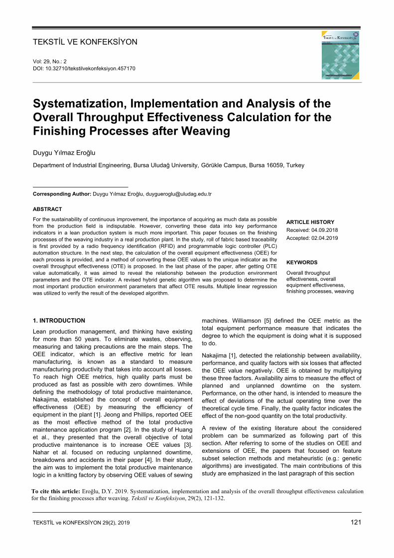
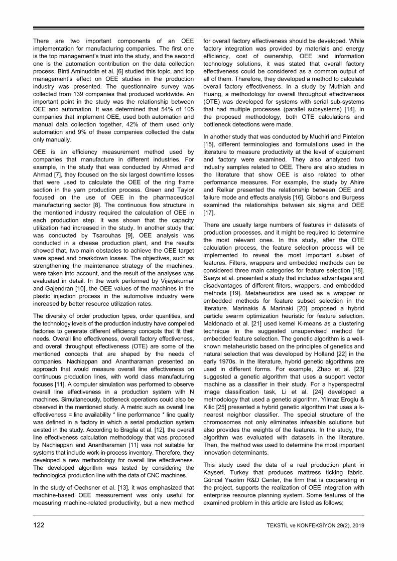
To implement the OTE procedure, data collection via RFID and PLC infrastructures are required to be completed by the firm. Fig. 1 shows an example of serial processing of the finishing operations after the weaving process. In that system, a calendering machine presses the weaved fabric roll, to obtain the required finish. Fig. 2 shows an example of a calendering machine and roll of fabric in the real production plant. The tumbler operation is a specialized tumbler dryer system and the finishing machine operation helps the fabric to dry and complete the finishing operations. Note that the finishing process operation requirements change from one order to another. For example, an order may need lamination; therefore, the required material is laminated to the fabric before the finishing machine operation, which may increase the number of operations to five.

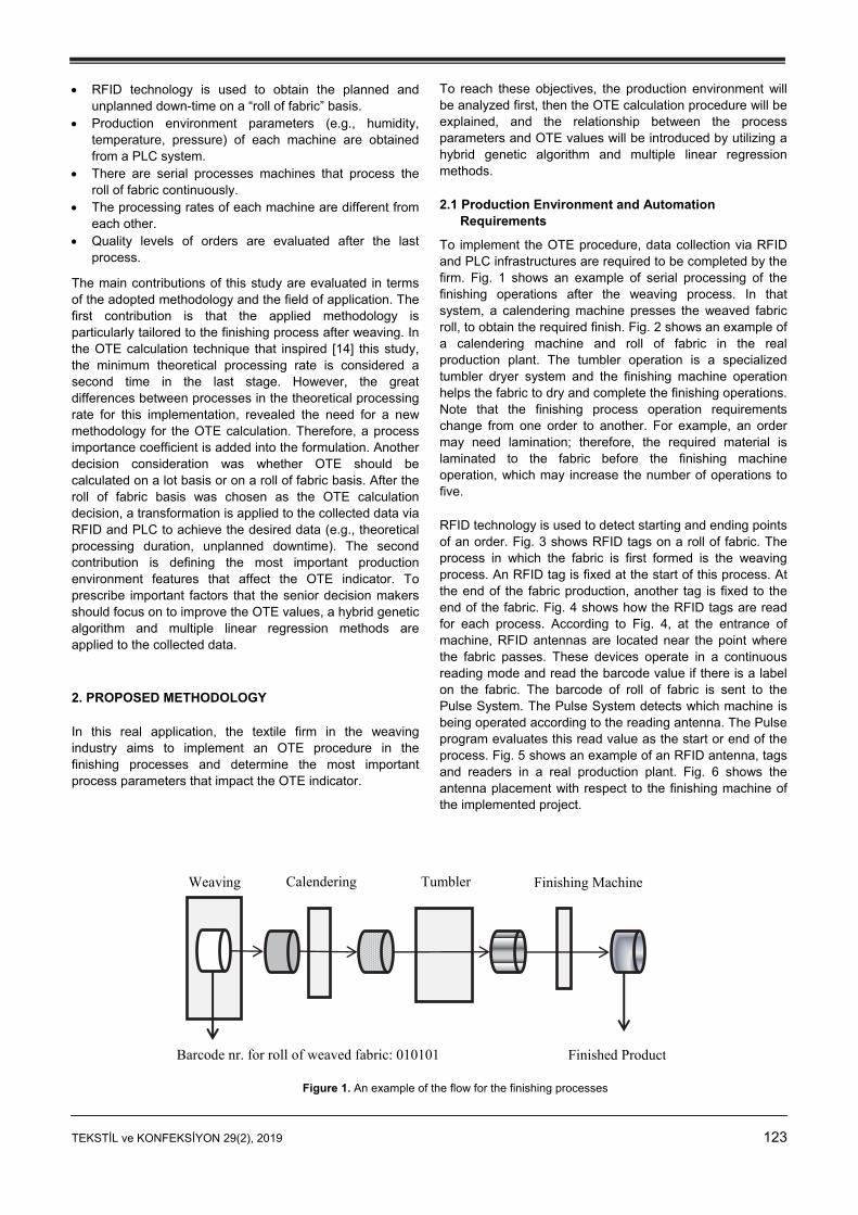
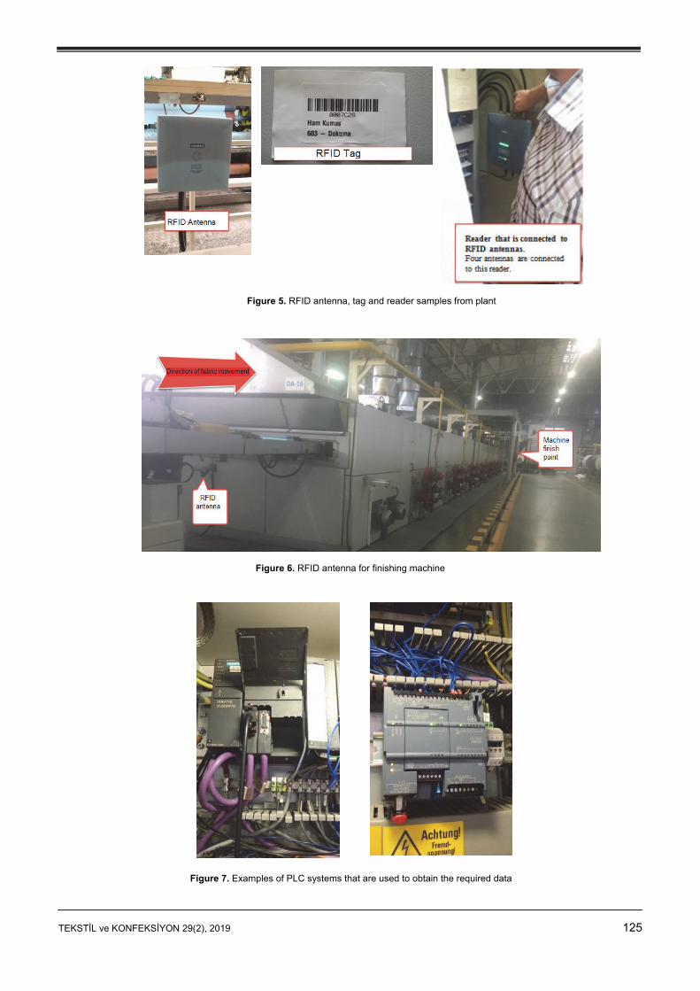
RFID technology is used to detect starting and ending points of an order. Fig. 3 shows RFID tags on a roll of fabric. The process in which the fabric is first formed is the weaving process. An RFID tag is fixed at the start of this process. At the end of the fabric production, another tag is fixed to the end of the fabric. Fig. 4 shows how the RFID tags are read for each process. According to Fig. 4, at the entrance of machine, RFID antennas are located near the point where the fabric passes. These devices operate in a continuous reading mode and read the barcode value if there is a label on the fabric. The barcode of roll of fabric is sent to the Pulse System. The Pulse System detects which machine is being operated according to the reading antenna. The Pulse program evaluates this read value as the start or end of the process. Fig. 5 shows an example of an RFID antenna, tags and readers in a real production plant. Fig. 6 shows the antenna placement with respect to the finishing machine of the implemented project.

Figure 1. An example of the flow for the finishing processes

Weaving Calendering Tumbler Finishing Machine

Finished Product Barcode nr. for roll of weaved fabric: 010101


Figure 2. Roll of fabric in a calendaring machine

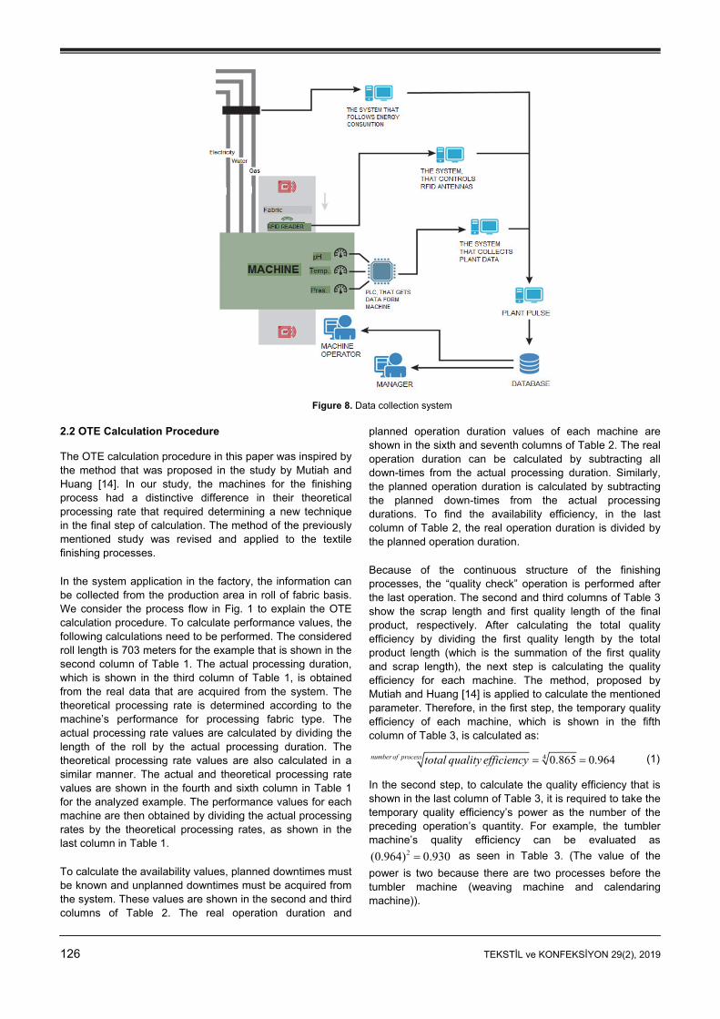
Another important consideration is obtaining the machine environment parameters (e.g., pH, pressure, temperature) for each finishing process. Fig. 7 shows some examples of the PLC system that obtains data from the system. PLC is used not only to obtain these data, but also to obtain the weaving speed data from the looms. Fig. 8 demonstrates the data flow in the system. The collected data are sent to Pulse System that is coded by Güncel Yazilim R&D Center. The system then makes the data meaningful.

Figure 3. RFID tags fixed on roll of fabric in the weaving process

Figure 4. RFID tags’ reading procedure for a machine


Figure 5. RFID antenna, tag and reader samples from plant

Figure 6. RFID antenna for finishing machine

Figure 7. Examples of PLC systems that are used to obtain the required data


Figure 8. Data collection system

2.2 OTE Calculation Procedure The OTE calculation procedure in this paper was inspired by the method that was proposed in the study by Mutiah and Huang [14]. In our study, the machines for the finishing process had a distinctive difference in their theoretical processing rate that required determining a new technique in the final step of calculation. The method of the previously mentioned study was revised and applied to the textile finishing processes.

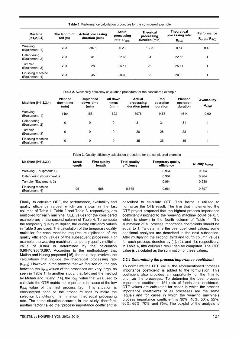
In the system application in the factory, the information can be collected from the production area in roll of fabric basis. We consider the process flow in Fig. 1 to explain the OTE calculation procedure. To calculate performance values, the following calculations need to be performed. The considered roll length is 703 meters for the example that is shown in the second column of Table 1. The actual processing duration, which is shown in the third column of Table 1, is obtained from the real data that are acquired from the system. The theoretical processing rate is determined according to the machine’s performance for processing fabric type. The actual processing rate values are calculated by dividing the length of the roll by the actual processing duration. The theoretical processing rate values are also calculated in a similar manner. The actual and theoretical processing rate values are shown in the fourth and sixth column in Table 1 for the analyzed example. The performance values for each machine are then obtained by dividing the actual processing rates by the theoretical processing rates, as shown in the last column in Table 1.

To calculate the availability values, planned downtimes must be known and unplanned downtimes must be acquired from the system. These values are shown in the second and third columns of Table 2. The real operation duration and

planned operation duration values of each machine are shown in the sixth and seventh columns of Table 2. The real operation duration can be calculated by subtracting all down-times from the actual processing duration. Similarly, the planned operation duration is calculated by subtracting the planned down-times from the actual processing durations. To find the availability efficiency, in the last column of Table 2, the real operation duration is divided by the planned operation duration.

Because of the continuous structure of the finishing processes, the “quality check” operation is performed after the last operation. The second and third columns of Table 3 show the scrap length and first quality length of the final product, respectively. After calculating the total quality efficiency by dividing the first quality length by the total product length (which is the summation of the first quality and scrap length), the next step is calculating the quality efficiency for each machine. The method, proposed by Mutiah and Huang [14] is applied to calculate the mentioned parameter. Therefore, in the first step, the temporary quality efficiency of each machine, which is shown in the fifth column of Table 3, is calculated as:

4 0.865 0.964number of process total quality efficiency (1)

In the second step, to calculate the quality efficiency that is shown in the last column of Table 3, it is required to take the temporary quality efficiency’s power as the number of the preceding operation’s quantity. For example, the tumbler machine’s quality efficiency can be evaluated as

2(0.964) 0.930 as seen in Table 3. (The value of the

power is two because there are two processes before the tumbler machine (weaving machine and calendaring machine)).


Table 1. Performance calculation procedure for the considered example

Machine (i=1,2,3,4)

The length of roll (m)

Actual processing duration (min)

Actual processing rate: Ract(i)

Theorical processing

duration (min)

Theoretical processing rate:

Rth(i)

Performance

Ract(i) / Rth(i)

Weaving (Equipment: 1)

703 3078 0.23 1305 0.54 0.43

Calendering (Equipment: 2)

703 31 22.68 31 22.68 1

Tumbler (Equipment: 3)

703 28 25.11 28 25.11 1

Finishing machine (Equipment: 4)

703 35 20.09 35 20.09 1

Table 2. Availability efficiency calculation procedure for the considered example

Machine (i=1,2,3,4) Planned

down time (min)

Unplanned down time

(min)

All down times (min)

Actual processing

duration (min)

Real operation duration

Planned operation duration

Availability

Aeff(i)


1464 158 1622 3078 1456 1614 0.90


0 0 0 31 31 31 1


0 0 0 28 28 28 1


0 0 0 35 35 35 1

Table 3. Quality efficiency calculation procedure for the considered example

Machine (i=1,2,3,4) Scrap length

First quality length

Total quality efficiency

Temporary quality efficiency Quality Qeff(i)

Weaving (Equipment: 1) 0.964 0.964

Calendering (Equipment: 2) 0.964 0.964

Tumbler (Equipment: 3) 0.964 0.930


95 608 0.865 0.964 0.897

Finally, to calculate OEE, the performance, availability and quality efficiency values, which are shown in the last columns of Table 1, Table 2 and Table 3, respectively, are multiplied for each machine. OEE values for the considered example are in the second column of Table 4. To compute the temporary quality multiplier, the quality efficiency values in Table 3 are used. The calculation of the temporary quality multiplier for each machine requires multiplication of the quality efficiency values of the subsequent processes. For example, the weaving machine’s temporary quality multiplier value of 0.804 is determined by the calculation 0.964*0.930*0.897. According to the methodology that Mutiah and Huang proposed [15], the next step involves the calculations that include the theoretical processing rate (Rth(i)). However, in the process that we focused on, the gap between the Rth(i) values of the processes are very large, as seen in Table 1. In another study, that followed the method by Mutiah and Huang [14], the Rth(i) value that was used to calculate the OTE metric lost importance because of the low Rth(i) value of the first process [26]. This situation is encountered because the procedure tries to make the selection by utilizing the minimum theoretical processing rate. The same situation occurred in this study; therefore, another factor called the “process importance coefficient” is

described to calculate OTE. This factor is utilized to normalize the OTE result. The firm that implemented the OTE project proposed that the highest process importance coefficient assigned to the weaving machine could be 0.7, which is shown in the fourth column of Table 4. The summation of all process importance coefficients should be equal to 1. To determine the best coefficient values, some additional analyses are described in the next subsection. After multiplying the second, third and fourth column values for each process, denoted by (1), (2), and (3), respectively, in Table 4, fifth column’s result can be computed. The OTE value is calculated as the summation of these values.

2.2.1 Determining the process importance coefficient

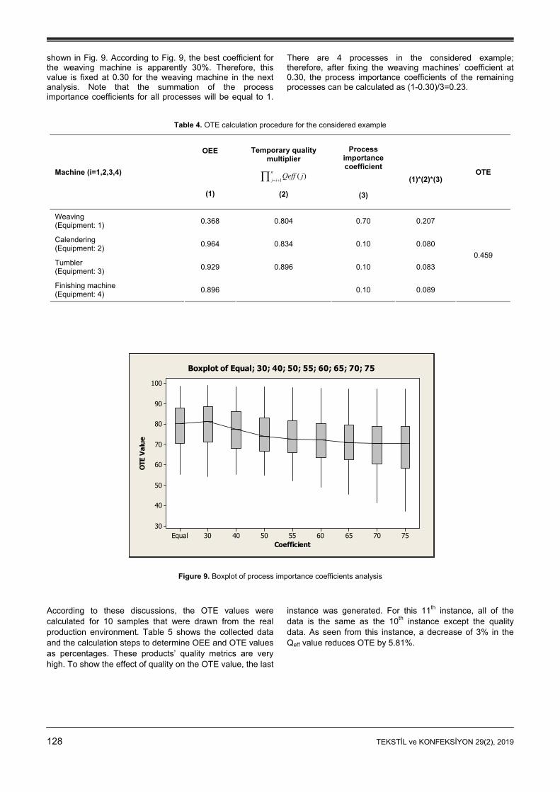
To normalize the OTE value, the aforementioned “process importance coefficient” is added to the formulation. This coefficient also provides an opportunity for the firm to prioritize the processes. To determine the best process importance coefficient, 154 rolls of fabric are considered. OTE values are calculated for cases in which the process importance coefficients of all processes are the same (equal) and for cases in which the weaving machine’s process importance coefficient is 30%, 40%, 50%, 55%, 60%, 65%, 70%, and 75%. The boxplot of the analysis is


shown in Fig. 9. According to Fig. 9, the best coefficient for the weaving machine is apparently 30%. Therefore, this value is fixed at 0.30 for the weaving machine in the next analysis. Note that the summation of the process importance coefficients for all processes will be equal to 1.

There are 4 processes in the considered example; therefore, after fixing the weaving machines’ coefficient at 0.30, the process importance coefficients of the remaining processes can be calculated as (1-0.30)/3=0.23.

Table 4. OTE calculation procedure for the considered example

Machine (i=1,2,3,4)

OEE

(1)

Temporary quality multiplier

1( )

n

j iQeff j

(2)

Process importance coefficient

(3)

(1)*(2)*(3)

OTE


0.368 0.804 0.70 0.207


0.964 0.834 0.10 0.080


0.929 0.896 0.10 0.083


0.896 0.10 0.089

0.459

Figure 9. Boxplot of process importance coefficients analysis

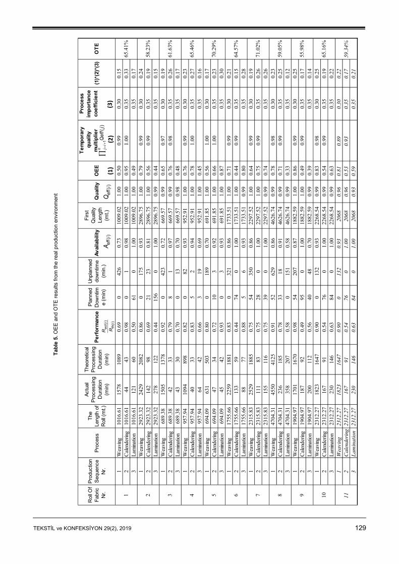
According to these discussions, the OTE values were calculated for 10 samples that were drawn from the real production environment. Table 5 shows the collected data and the calculation steps to determine OEE and OTE values as percentages. These products’ quality metrics are very high. To show the effect of quality on the OTE value, the last

instance was generated. For this 11th instance, all of the data is the same as the 10th instance except the quality data. As seen from this instance, a decrease of 3% in the Qeff value reduces OTE by 5.81%.

7570656055504030Equal

100

90

80

70

60

50

40

30

Coefficient

OTE

Val

ue

Boxplot of Equal; 30; 40; 50; 55; 60; 65; 70; 75


Rol

l Of

Fab

ric

Nr.

Pro

duct

ion

Seq

uenc

e N

r.P

roce

ssT

he

Leng

th o

f R

oll (

mt.)

Act

ual

Pro

cess

ing

Dur

atio

n (m

in)

The

oret

ical

P

roce

ssin

g D

urat

ion

(min

)

Pe

rfo

rman

ceP

lann

ed

Dow

ntim

e (m

in)

Unp

lann

ed

dow

ntim

e (m

in.)

Av

aila

bili

ty

Firs

t Q

ualit

y Le

ngth

(m

t.)

Qu

alit

y O

EE

Te

mp

ora

ry q

ual

ity

mu

ltip

lier

Pro

cess

im

po

rtan

ce

coe

ffic

ien

t(1

)*(2

)*(3

)O

TE

1W

eavi

ng10

16.6

115

7810

890.

690

426

0.73

1009

.02

1.00

0.50

0.99

0.30

0.15

2C

alen

derin

g10

16.6

144

430.

980

10.

9810

09.0

21.

000.

951.

000.

350.

333

Lam

inat

ion

1016

.61

121

600.

5061

01.

0010

09.0

21.

000.

490.

350.

171

Wea

ving

2923

.32

2429

2082

0.86

017

50.

9328

96.7

51.

000.

790.

990.

300.

242

Cal

ende

ring

2923

.32

142

980.

6921

230.

8128

96.7

51.

000.

560.

990.

350.

193

Lam

inat

ion

2923

.32

278

122

0.44

156

01.

0028

96.7

50.

990.

440.

350.

151

Wea

ving

689.

3815

0513

780.

920

423

0.72

669.

570.

990.

650.

970.

300.

192

Cal

ende

ring

689.

3842

330.

798

10.

9766

9.57

0.99

0.76

0.98

0.35

0.26

3L

amin

atio

n68

9.38

4330

0.70

013

0.70

669.

570.

980.

480.

350.

171

Wea

ving

957.

9410

9489

80.

820

820.

9395

2.91

1.00

0.76

0.99

0.30

0.23

2C

alen

derin

g95

7.94

4033

0.83

52

0.94

952.

911.

000.

781.

000.

350.

273

Lam

inat

ion

957.

9464

420.

663

190.

6995

2.91

1.00

0.45

0.35

0.16

1W

eavi

ng69

4.09

631

503

0.80

018

90.

7069

1.85

1.00

0.56

1.00

0.30

0.17

2C

alen

derin

g69

4.09

4734

0.72

103

0.92

691.

851.

000.

661.

000.

350.

233

Lam

inat

ion

694.

0945

420.

930

30.

9369

1.85

1.00

0.87

0.35

0.30

1W

eavi

ng17

55.6

622

5918

810.

830

321

0.86

1733

.51

1.00

0.71

0.99

0.30

0.21

2C

alen

derin

g17

55.6

613

359

0.44

740

1.00

1733

.51

1.00

0.44

0.99

0.35

0.15

3L

amin

atio

n17

55.6

688

770.

885

60.

9317

33.5

10.

990.

800.

350.

281

Wea

ving

2315

.83

2529

1885

0.75

5435

00.

8622

97.5

21.

000.

640.

990.

300.

192

Cal

ende

ring

2315

.83

111

830.

7528

01.

0022

97.5

21.

000.

750.

990.

350.

263

Lam

inat

ion

2315

.83

155

116

0.75

390

1.00

2297

.52

0.99

0.74

0.35

0.26

1W

eavi

ng47

04.3

145

5041

250.

9152

629

0.86

4626

.74

0.99

0.78

0.98

0.30

0.23

2C

alen

derin

g47

04.3

123

618

50.

7833

180.

9146

26.7

40.

990.

710.

990.

350.

253

Lam

inat

ion

4704

.31

358

207

0.58

015

10.

5846

26.7

40.

990.

330.

350.

121

Wea

ving

1904

.97

1701

1670

0.98

5420

70.

8718

82.5

91.

000.

860.

990.

300.

252

Cal

ende

ring

1904

.97

187

920.

4995

01.

0018

82.5

91.

000.

490.

990.

350.

173

Lam

inat

ion

1904

.97

200

112

0.56

4048

0.70

1882

.59

0.99

0.39

0.35

0.14

1W

eavi

ng23

12.2

718

2316

470.

900

132

0.93

2268

.54

0.99

0.83

0.98

0.30

0.25

2C

alen

derin

g23

12.2

716

791

0.54

760

1.00

2268

.54

0.99

0.54

0.99

0.35

0.19

3L

amin

atio

n23

12.2

723

014

60.

6384

01.

0022

68.5

40.

990.

630.

350.

221

Wea

ving

2312

.27

1823

1647

0.90

013

20.

9320

680.

960.

810.

890.

300.

222

Cal

ende

ring

2312

.27

167

910.

5476

01.

0020

680.

960.

530.

930.

350.

173

Lam

inat

ion

2312

.27

230

146

0.63

840

1.00

2068

0.93

0.59

0.35

0.21

65.4

1%

58.2

3%

61.6

3%

65.4

6%

70.2

9%

1 2 3 4 5 106 1159

.34%

65.1

6%

64.5

7%

71.0

2%

59.0

5%

55.9

8%

7 8 9

()

()

act

i

thi

R R(

)ef

fi

A(

)ef

fi

Q1

()

n ji

Qef

fj

(1)

(2)

(3)

Tab

le 5

. O

EE

an

d O

TE

res

ults

fro

m th

e re

al p

rodu

ctio

n en

viro

nmen

t


3. DETECTING THE MOST IMPORTANT ENVIRONMENTAL PARAMETERS FOR MACHINES

One of the aims of the study was to identify the most important machine environment parameters (e.g. pH, temperature, speed) that affect the OTE value. To that end, the hybrid genetic algorithm, which was proposed by Yilmaz Eroglu and Kilic [25] to understand the most important innovation parameters, was adapted to the current problem. The algorithm was coded in C# programming language and implemented on a computer with an Intel Core i7-3612QM processor running at 2.10 GHz. The outputs are OTE values in this problem that are represented by real numbers. After running the algorithm, the most important environmental parameters for the machines were detected. Then, the firm was provided a short list of these parameters to focus on and to improve the productivity.

Some important points for the algorithm are as follows.

Random numbers constitute the chromosomes in the genetic algorithm. This structure not only ensures the feasibility of the chromosome but also provides simultaneous feature selection and weighting.

The fitness function of the algorithm considers both classification accuracy and the number of features.

The random selection method and elitism are used in the selection phase, and crossover and mutation operations are also applied as genetic operations.

A local search algorithm is integrated into the algorithm for all chromosomes to improve the algorithm.

A k-NN (k-nearest neighbor) classifier is adopted to obtain the classification accuracy as the fitness function.

A 10-fold cross validation approach is used in the hybrid genetic algorithm. Note that, 10 runs are executed in each fold with different random seeds each time.

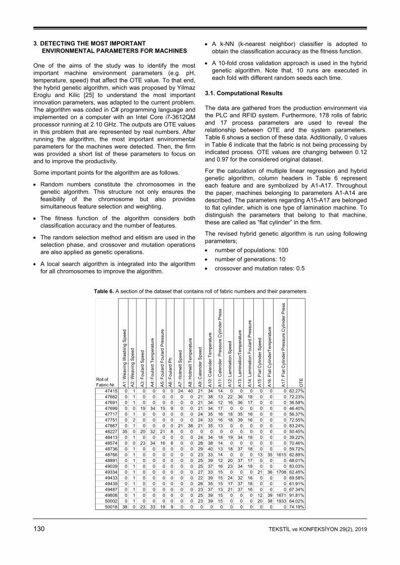
3.1. Computational Results The data are gathered from the production environment via the PLC and RFID system. Furthermore, 178 rolls of fabric and 17 process parameters are used to reveal the relationship between OTE and the system parameters. Table 6 shows a section of these data. Additionally, 0 values in Table 6 indicate that the fabric is not being processing by indicated process. OTE values are changing between 0.12 and 0.97 for the considered original dataset.

For the calculation of multiple linear regression and hybrid genetic algorithm, column headers in Table 6 represent each feature and are symbolized by A1-A17. Throughout the paper, machines belonging to parameters A1-A14 are described. The parameters regarding A15-A17 are belonged to flat cylinder, which is one type of lamination machine. To distinguish the parameters that belong to that machine, these are called as “flat cylinder” in the firm.

The revised hybrid genetic algorithm is run using following parameters;

number of populations: 100

number of generations: 10

crossover and mutation rates: 0.5

Table 6. A section of the dataset that contains roll of fabric numbers and their parameters

Roll of Fabric Nr. A

1: W

eav

ing

Wa

shin

g S

pe

ed

A2

: We

avin

g S

pee

d

A3

: Fo

ular

d S

pee

d

A4

: Fo

ular

d T

em

pera

ture

A5

: Fo

ular

d F

oul

ard

Pre

ssu

re

A6

: Fo

ular

d P

h

A7

: Hot

mel

t Spe

ed

A8

: Hot

mel

t Te

mpe

ratu

re

A9

: Cal

end

er S

pee

d

A1

0: C

ale

nde

r Te

mpe

ratu

re

A1

1: C

ale

nde

r P

ress

ure

Cyl

ind

er P

ress

A1

2: L

amin

atio

n S

pee

d

A1

3: L

amin

atio

nT

emp

era

ture

A1

4: L

amin

atio

n F

oul

ard

Pre

ssu

re

A1

5: F

lat C

ylin

der

Sp

eed

A1

6: F

lat C

ylin

derT

emp

era

ture

A1

7: F

lat C

ylin

der

Pre

ssu

re C

ylin

der

Pre

ss

OT

E

47415 0 1 0 0 0 0 24 40 21 34 14 0 0 0 0 0 0 82.27%47662 0 1 0 0 0 0 0 0 21 38 13 22 36 18 0 0 0 72.23%47691 0 1 0 0 0 0 0 0 21 34 12 16 36 17 0 0 0 36.58%47699 0 0 19 34 15 9 0 0 21 34 17 0 0 0 0 0 0 46.40%47717 0 1 0 0 0 0 0 0 24 35 16 18 35 16 0 0 0 56.37%47751 0 2 0 0 0 0 0 0 24 33 16 18 39 16 0 0 0 72.55%47867 0 1 0 0 0 0 21 38 21 35 13 0 0 0 0 0 0 83.24%48227 35 0 20 32 21 8 0 0 0 0 0 0 0 0 0 0 0 50.45%48413 0 1 0 0 0 0 0 0 24 34 18 19 34 18 0 0 0 39.22%48574 0 0 23 34 16 8 0 0 28 38 14 0 0 0 0 0 0 70.46%48736 0 1 0 0 0 0 0 0 29 40 13 18 37 18 0 0 0 59.72%48766 0 1 0 0 0 0 0 0 23 33 14 0 0 0 13 35 1615 62.88%48891 0 1 0 0 0 0 0 0 25 39 12 20 37 17 0 0 0 68.01%49039 0 1 0 0 0 0 0 0 25 37 16 23 34 18 0 0 0 83.03%49334 0 1 0 0 0 0 0 0 27 33 15 0 0 0 21 36 1708 62.45%49433 0 1 0 0 0 0 0 0 22 39 15 24 32 16 0 0 0 69.58%49439 0 1 0 0 0 0 0 0 26 35 15 17 37 18 0 0 0 61.91%49487 0 1 0 0 0 0 0 0 23 37 13 21 37 16 0 0 0 67.34%49808 0 1 0 0 0 0 0 0 25 39 15 0 0 0 12 39 1671 91.81%50002 0 1 0 0 0 0 0 0 23 39 15 0 0 0 20 38 1933 64.02%50018 38 0 23 33 19 9 0 0 0 0 0 0 0 0 0 0 0 74.19%


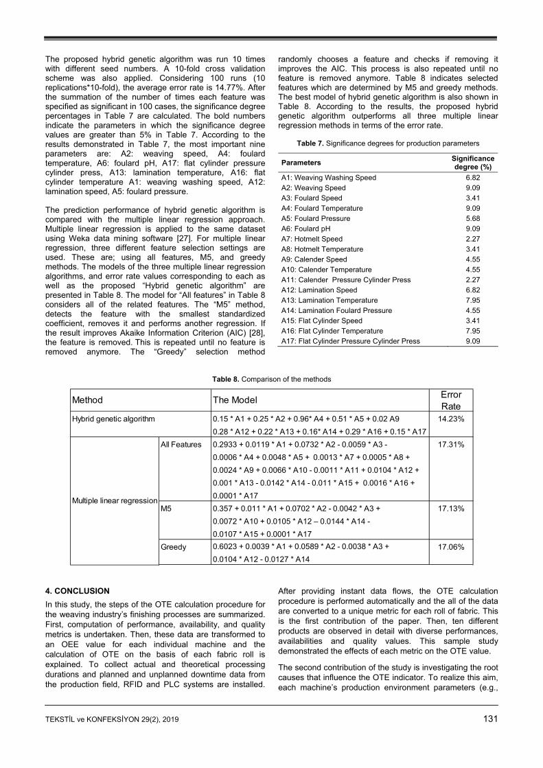
The proposed hybrid genetic algorithm was run 10 times with different seed numbers. A 10-fold cross validation scheme was also applied. Considering 100 runs (10 replications*10-fold), the average error rate is 14.77%. After the summation of the number of times each feature was specified as significant in 100 cases, the significance degree percentages in Table 7 are calculated. The bold numbers indicate the parameters in which the significance degree values are greater than 5% in Table 7. According to the results demonstrated in Table 7, the most important nine parameters are: A2: weaving speed, A4: foulard temperature, A6: foulard pH, A17: flat cylinder pressure cylinder press, A13: lamination temperature, A16: flat cylinder temperature A1: weaving washing speed, A12: lamination speed, A5: foulard pressure.

The prediction performance of hybrid genetic algorithm is compared with the multiple linear regression approach. Multiple linear regression is applied to the same dataset using Weka data mining software [27]. For multiple linear regression, three different feature selection settings are used. These are; using all features, M5, and greedy methods. The models of the three multiple linear regression algorithms, and error rate values corresponding to each as well as the proposed “Hybrid genetic algorithm” are presented in Table 8. The model for “All features” in Table 8 considers all of the related features. The “M5” method, detects the feature with the smallest standardized coefficient, removes it and performs another regression. If the result improves Akaike Information Criterion (AIC) [28], the feature is removed. This is repeated until no feature is removed anymore. The “Greedy” selection method

randomly chooses a feature and checks if removing it improves the AIC. This process is also repeated until no feature is removed anymore. Table 8 indicates selected features which are determined by M5 and greedy methods. The best model of hybrid genetic algorithm is also shown in Table 8. According to the results, the proposed hybrid genetic algorithm outperforms all three multiple linear regression methods in terms of the error rate.

Table 7. Significance degrees for production parameters

Parameters Significance degree (%)

A1: Weaving Washing Speed 6.82

A2: Weaving Speed 9.09

A3: Foulard Speed 3.41

A4: Foulard Temperature 9.09

A5: Foulard Pressure 5.68

A6: Foulard pH 9.09

A7: Hotmelt Speed 2.27

A8: Hotmelt Temperature 3.41

A9: Calender Speed 4.55

A10: Calender Temperature 4.55

A11: Calender Pressure Cylinder Press 2.27

A12: Lamination Speed 6.82

A13: Lamination Temperature 7.95

A14: Lamination Foulard Pressure 4.55

A15: Flat Cylinder Speed 3.41

A16: Flat Cylinder Temperature 7.95

A17: Flat Cylinder Pressure Cylinder Press 9.09

Table 8. Comparison of the methods

Method The ModelError Rate

Hybrid genetic algorithm 0.15 * A1 + 0.25 * A2 + 0.96* A4 + 0.51 * A5 + 0.02 A9 14.23%

0.28 * A12 + 0.22 * A13 + 0.16* A14 + 0.29 * A16 + 0.15 * A17

All Features 0.2933 + 0.0119 * A1 + 0.0732 * A2 - 0.0059 * A3 - 17.31%

0.0006 * A4 + 0.0048 * A5 + 0.0013 * A7 + 0.0005 * A8 +

0.0024 * A9 + 0.0066 * A10 - 0.0011 * A11 + 0.0104 * A12 +

0.001 * A13 - 0.0142 * A14 - 0.011 * A15 + 0.0016 * A16 +

0.0001 * A17

M5 0.357 + 0.011 * A1 + 0.0702 * A2 - 0.0042 * A3 + 17.13%

0.0072 * A10 + 0.0105 * A12 – 0.0144 * A14 -

0.0107 * A15 + 0.0001 * A17

Greedy 0.6023 + 0.0039 * A1 + 0.0589 * A2 - 0.0038 * A3 + 17.06%

0.0104 * A12 - 0.0127 * A14

Multiple linear regression

4. CONCLUSION

In this study, the steps of the OTE calculation procedure for the weaving industry’s finishing processes are summarized. First, computation of performance, availability, and quality metrics is undertaken. Then, these data are transformed to an OEE value for each individual machine and the calculation of OTE on the basis of each fabric roll is explained. To collect actual and theoretical processing durations and planned and unplanned downtime data from the production field, RFID and PLC systems are installed.

After providing instant data flows, the OTE calculation procedure is performed automatically and the all of the data are converted to a unique metric for each roll of fabric. This is the first contribution of the paper. Then, ten different products are observed in detail with diverse performances, availabilities and quality values. This sample study demonstrated the effects of each metric on the OTE value.

The second contribution of the study is investigating the root causes that influence the OTE indicator. To realize this aim, each machine’s production environment parameters (e.g.,


pH, temperature, speed) were collected automatically. The RFID and PLC system ensured the parameter and OTE value coupling for each roll of fabric order. To obtain a sustainable improvement, the relationship between OTE and basic production parameters was examined with a hybrid genetic algorithm and multiple linear regression. According to results, the most important factors that affect the OTE value could be detected.

Acknowledgement

This work was supported by Güncel Yazılım R&D Center and The Scientific and Technical Research Council of Turkey (TUBİTAK-TEYDEB- 7151608).

REFERENCES

1. Nakajima, S. (1988). Introduction to TPM: Total Productive Maintenance.(Translation). Productivity Press, Inc., ISBN 0-91529-923-2.

2. Jeong, K. Y., & Phillips, D. T. (2001). Operational efficiency and effectiveness measurement. International Journal of Operations and Production Management, 21(11),1404-1416.

3. Huang, S. H., Dismukes, J. P., Shi, J., Su, Q., Wang, G., Razzak, M. A., & Robinson, D. E. (2002). Manufacturing system modeling for productivity improvement. Journal of Manufacturing Systems, 21(4), 249-259.

4. Nahar, K., Islam, M. M., Rahman, M. M., & Hossain, M. M. (2012, December). Evaluation of OEE for implementing Total Productive Maintenance (TPM) in sewing machine of a knit factory. In Proc. the Global Engineering, Science and Technology Conference, 28-29.

5. Williamson, R. M. (2006). Using Overall Equipment Effectiveness: the Metric and the Measures. Strategic Work Systems. Inc., Columbus NC, 28722, 1-6.

6. Binti Aminuddin, N. A., Garza-Reyes, J. A., Kumar, V., Antony, J., & Rocha-Lona, L. (2016). An analysis of managerial factors affecting the implementation and use of overall equipment effectiveness. International Journal of Production Research, 54(15), 4430-4447.

7. Ahmed, M., & Ahmad, N. (2011). An application of Pareto analysis and cause-and-effect diagram (CED) for minimizing rejection of raw materials in lamp production process. Management Science and Engineering, 5(3), 87-95.

8. Green, C., & Taylor, D. (2016). Consolidating a Distributed Compound Management Capability into a Single Installation: The Application of Overall Equipment Effectiveness to Determine Capacity Utilization. Journal of laboratory automation, 21(6), 811-816.

9. Tsarouhas, P. H. (2013). Equipment performance evaluation in a production plant of traditional Italian cheese. International Journal of Production Research, 51(19), 5897-5907.

10. Vijayakumar, S. R., & Gajendran, S. (2014). Improvement of overall equipment effectiveness (OEE) in injection moulding process industry. IOSR J Mech Civil Eng, 2(10), 47-60.

11. Nachiappan, R. M., & Anantharaman, N. (2006). Evaluation of overall line effectiveness (OLE) in a continuous product line manufacturing system. Journal of Manufacturing Technology Management, 17(7), 987-1008.

12. Braglia, M., Frosolini, M., and Zammori, F. (2008). Overall equipment effectiveness of a manufacturing line (OEEML) An integrated approach to assess systems performance. Journal of Manufacturing Technology Management, 20(1), 8-29.

13. Oechsner, R., Pfeffer, M., Pfitzner, L., Binder, H., Müller, E., & Vonderstrass, T. (2002). From overall equipment efficiency (OEE) to overall Fab effectiveness (OFE). Materials Science in Semiconductor Processing, 5(4), 333-339.

14. Muthiah, K. M. N., & Huang, S. H. (2007). Overall throughput effectiveness (OTE) metric for factory-level performance monitoring and

bottleneck detection. International Journal of Production Research, 45(20), 4753-4769.

15. Muchiri, P., & Pintelon, L. (2008). Performance measurement using overall equipment effectiveness (OEE): literature review and practical application discussion. International Journal of Production Research, Vol: 46(13), pp: 3517-3535.

16. Ahire, C. P., & Relkar, A. S. (2012). Correlating failure mode effect analysis (FMEA) and overall equipment effectiveness (OEE). Procedia Engineering, 38, 3482-3486.

17. Gibbons, P. M., & Burgess, S. C. (2010). Introducing OEE as a measure of lean Six Sigma capability. International Journal of Lean Six Sigma, 1(2), 134-156.

18. Guyon, I., & Elisseeff, A. (2003). An introduction to variable and feature selection. Journal of machine learning research, 3(Mar), 1157-1182.

19. Saeys, Y., Inza, I., & Larrañaga, P. (2007). A review of feature selection techniques in bioinformatics. Bioinformatics, Vol: 23(19), 2507-2517.

20. Marinakis, Y., & Marinaki, M. (2013, May). A hybridized particle swarm optimization with expanding neighborhood topology for the feature selection problem. In International Workshop on Hybrid Metaheuristics (37-51). Springer, Berlin, Heidelberg.

21. Maldonado, S., Carrizosa, E., & Weber, R. (2015). Kernel Penalized K-means: A feature selection method based on Kernel K-means. Information sciences, 322, 150-160.

22. Holland, J. H. (1992). Adaptation in natural and artificial systems: an introductory analysis with applications to biology, control, and artificial intelligence, MIT press.

23. Zhao, M., Fu, C., Ji, L., Tang, K., & Zhou, M. (2011). Feature selection and parameter optimization for support vector machines: A new approach based on genetic algorithm with feature chromosomes, Expert Systems with Applications, 38(5), 5197-5204.

24. Li, S., Wu, H., Wan, D., & Zhu, J. (2011). An effective feature selection method for hyperspectral image classification based on genetic algorithm and support vector machine. Knowledge-Based Systems, 24(1), 40-48.

25. Eroglu, D. Y., & Kilic, K. (2017). A novel Hybrid Genetic Local Search Algorithm for feature selection and weighting with an application in strategic decision making in innovation management. Information Sciences, 405, 18-32.

26. Yılmaz Eroglu, D. (2017). Calculating Overall Effectiveness in Serial Subsystem with Multiple Product. Journal of Current Researches on Engineering, Science and Technology (JoCREST), 3(2).

27. Hall, M., Frank, E., Holmes, G., Pfahringer, B., Reutemann, P., & Witten, I. H. (2009). The WEKA data mining software: an update. ACM SIGKDD explorations newsletter, 11(1),10-18.

28. Akaike, H. (1974). A new look at the statistical model identification. In Selected Papers of Hirotugu Akaike, Springer, New York, NY, 215-222.

Documents

Systematization, Implementation and Analysis of the Overall