Embed Size (px)
Citation preview
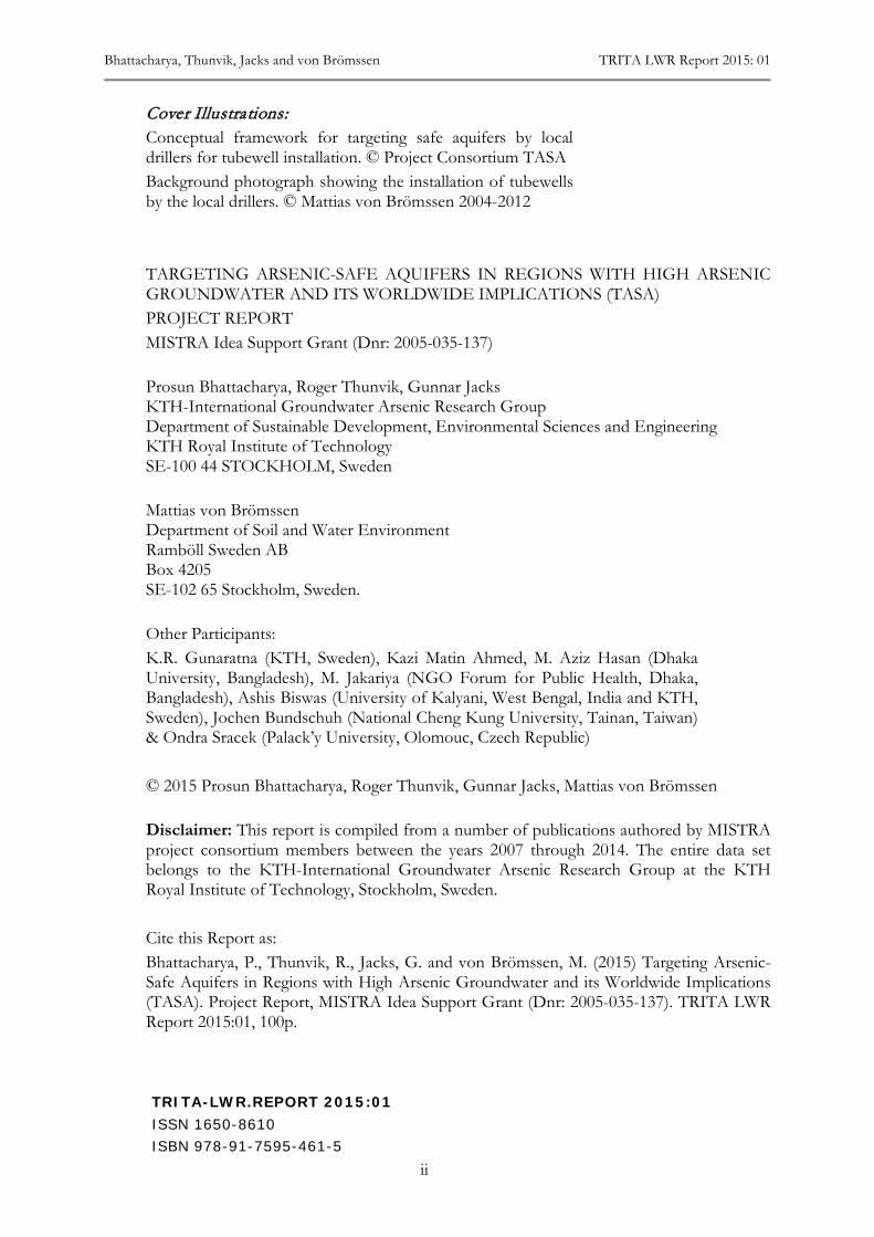
Redox classification
Black White Off-White Red
Sediment colour
0.0
4.0
8.0
12.0
16.0
20.0
Fe
mg
/l
Black White Off-White Red
Sediment colour
0.0
0.8
1.6
2.4
3.2
4.0
Mn
mg
/l
Black White Off-White Red
Sediment colour
0.0
1.0
2.0
3.0
4.0
5.0
SO
4 m
g/l
red
off-white
white
black
MnMntottot
FeFetottot
SOSO4422--
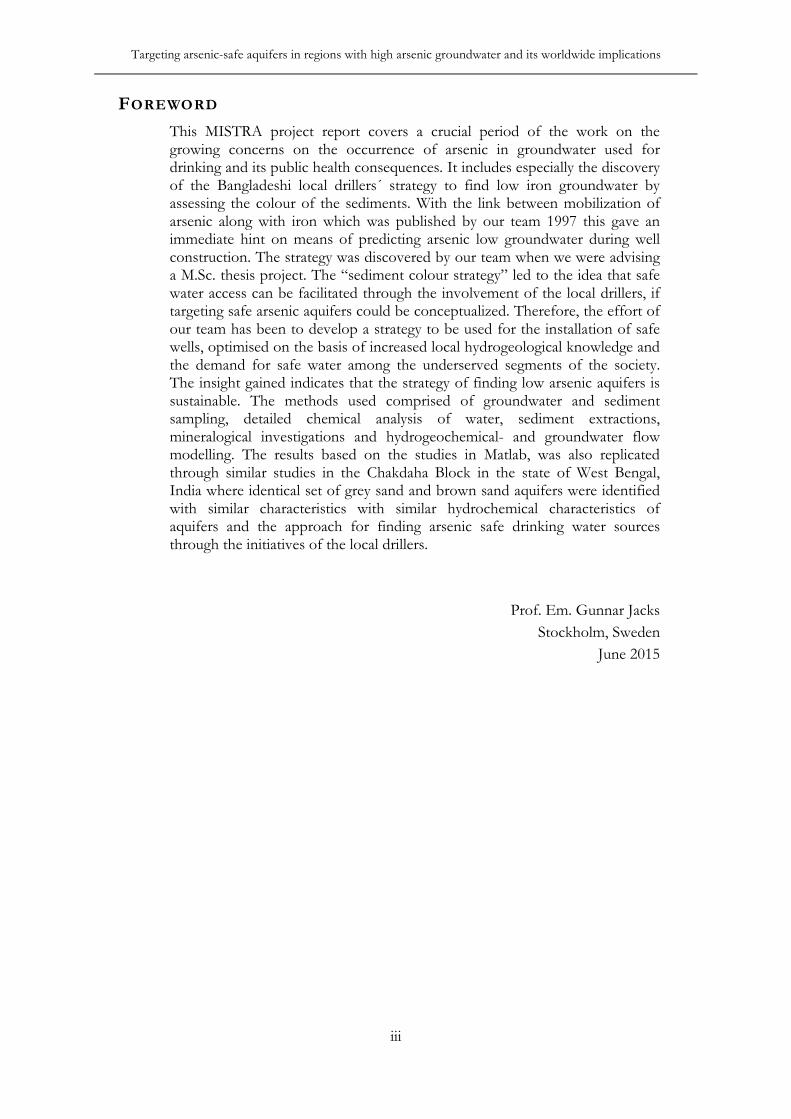
8th International Conference on the Biogeochemistry of Trace Elements (ICOBTE), Adelaide, Australia
Prediction of risk for high arsenicgroundwater
REDOFF-WHITE
WHITEBLACK
RISK
High Neglible?
REDOX
Very reduced Less reduced
2.4
3.2
4.0
redMnMnMnMnMnMnMnMnMnMnMnMnMnMnMntottottottottottottottottottottottottottottottottottottottottottottottottottottottottottot
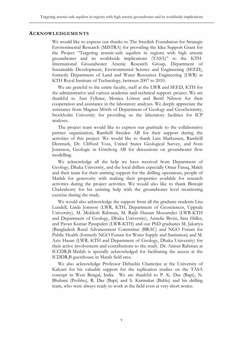
Correlating sediment- and groundwater chemistry
Easily recognisable geological features (sediment colors)
Low-As groundwater
Local technique: Economically & socially
sustainable
Scientific validation of sustainability
Arsenic
TRITA-LWR.REPORT 2015:01ISSN 1650-8610ISBN 978-91-7595-461-5
Naturally occurring arsenic (As) in groundwater has undermined the success of supplying safe drinking water in Bangladesh. Arsenic is mobilized in groundwater through reductive dissolution of Fe(III)-oxyhydroxide especially in the younger (Holocene) sediments leading to severe public health consequences. Many of the mitigation options provided during the last two decades have not been well accepted by the people and instead, local well drillers target aquifers for abstrac-tion of arsenic-safe groundwater on the basis of the colour of the sediments. This MISTRA Idea Support Grant project report incorporates the results of the studies carried out to validate the local drillers´ strategy in Bangladesh to low arsenic groundwater by assessing the colour of the sediments through system-atic groundwater and sediment sampling, detailed chemical analysis of water, sediment extractions, mineralogical investigations and hydrogeochemical- and groundwater � ow modelling.
The studies carried out in Matlab in Chandpur District of Bangladesh indicate that the idea on targeting low-arsenic groundwater is facilitated through identi� -cation of the colour of the sediments with decreasing levels of As concentrations in black, o� -white, white and red as perceived by the local drillers. Each of the sediment colour category is characterized by a set of unique hydrochemical char-acteristics that can be used to conceptualize a “sediment colour strategy” that would enable the local drillers to identify arsenic-safe aquifers. Thus, linking the colour of the sediments with groundwater chemistry would be useful to develop a simple sediment colour-based tool for targeting shallow aquifers for the instal-lation of As safe community tubewells for the local drillers through more careful evaluation of the sensitivity of the hydrogeochemical results with respect to the colour of the sediments. The results based on the studies in Matlab, was also rep-licated in Chakdaha Block in West Bengal, India, where identical set of grey sand and brown sand aquifers were identi� ed with similar sediment and hydrochem-ical characteristics of aquifers and the approach for � nding arsenic-safe drinking water sources through the initiatives of the local drillers in a sustainable manner.
Targeting Arsenic-Safe Aquifers in Regions with High Arsenic Groundwater and its Worldwide Implications (TASA)PROSUN BHATTACHARYA, ROGER THUNVIK,GUNNAR JACKS, MATTIAS VON BRÖMSSEN
KTH ROYAL INSTITUTE OF TECHNOLOGY
IN COOPERATION WITH:
REPORT, MISTRA IDEA SUPPORT GRANTSTOCKHOLM, SWEDEN 2015
KTH ROYAL INSTITUTE OF TECHNOLOGY DEPARTMENT OF SUSTAINABLE DEVELOPMENT, ENVIRONMENTAL SCIENCE AND ENGINEERING
www.kth.se
P. BHATTACHARYA, R. THUNVIK, G. JACKS & M. VON BRÖM
SSEN Targeting Arsenic-Safe Aquifers in Regions w
ith High Arsenic G
roundwater and its W
orldwide Im
plications (TASA)K
TH 2015
Targe&ng Arsenic-‐Safe Aquifers in Regions with High Arsenic Groundwater and its Worldwide Implica&ons (TASA)
Project Report
MISTRA Idea Support Grant (Dnr: 2005-035-137)
PROSUN BHATTACHARYA, ROGER THUNVIK, GUNNAR JACKS, MATTIAS VON BRÖMSSEN
TRITA-LWR.REPORT 2015:01
ISSN 1650-8610
ISBN 978-91-7595-461-5
KTH ROYAL INSTITUTE OF TECHNOLOGY
DEPARTMENT OF SUSTAINABLE DEVELOPMENT, ENVIRONMENTAL SCIENCE AND ENGINEERING
OMSLAG FRAMSIDA:
Vänster justerat logotyper enligt
h#ps://intra.kth.se/administra2on/kommunika2on/grafiskprofil/samprofilering-‐hur-‐kth-‐syns-‐2llsammans-‐med-‐andra-‐parter-‐1.450081
(Första bilden)
Bilden Nederst ska det vara blåa randen ovan på bilden
TARGETING ARSENIC-SAFE AQUIFERS IN REGIONS WITH HIGH ARSENIC
GROUNDWATER AND ITS WORLDWIDE IMPLICATIONS (TASA)
Project Report
MISTRA Idea Support Grant Dnr: 2005-035-137
Prosun Bhattacharya, Roger Thunvik, Gunnar Jacks, Mattias von Brömssen
Stockholm, Sweden June 2015
Bhattacharya, Thunvik, Jacks and von Brömssen TRITA LWR Report 2015: 01
ii
Cover Illustrations: Conceptual framework for targeting safe aquifers by local drillers for tubewell installation. © Project Consortium TASA Background photograph showing the installation of tubewells by the local drillers. © Mattias von Brömssen 2004-2012 TARGETING ARSENIC-SAFE AQUIFERS IN REGIONS WITH HIGH ARSENIC GROUNDWATER AND ITS WORLDWIDE IMPLICATIONS (TASA) PROJECT REPORT MISTRA Idea Support Grant (Dnr: 2005-035-137) Prosun Bhattacharya, Roger Thunvik, Gunnar Jacks KTH-International Groundwater Arsenic Research Group Department of Sustainable Development, Environmental Sciences and Engineering KTH Royal Institute of Technology SE-100 44 STOCKHOLM, Sweden Mattias von Brömssen Department of Soil and Water Environment Ramböll Sweden AB Box 4205 SE-102 65 Stockholm, Sweden. Other Participants: K.R. Gunaratna (KTH, Sweden), Kazi Matin Ahmed, M. Aziz Hasan (Dhaka University, Bangladesh), M. Jakariya (NGO Forum for Public Health, Dhaka, Bangladesh), Ashis Biswas (University of Kalyani, West Bengal, India and KTH, Sweden), Jochen Bundschuh (National Cheng Kung University, Tainan, Taiwan) & Ondra Sracek (Palack’y University, Olomouc, Czech Republic) © 2015 Prosun Bhattacharya, Roger Thunvik, Gunnar Jacks, Mattias von Brömssen Disclaimer: This report is compiled from a number of publications authored by MISTRA project consortium members between the years 2007 through 2014. The entire data set belongs to the KTH-International Groundwater Arsenic Research Group at the KTH Royal Institute of Technology, Stockholm, Sweden. Cite this Report as: Bhattacharya, P., Thunvik, R., Jacks, G. and von Brömssen, M. (2015) Targeting Arsenic-Safe Aquifers in Regions with High Arsenic Groundwater and its Worldwide Implications (TASA). Project Report, MISTRA Idea Support Grant (Dnr: 2005-035-137). TRITA LWR Report 2015:01, 100p.
TRITA-LWR.REPORT 2015:01 ISSN 1650-8610 ISBN 978-91-7595-461-5
Targeting arsenic-safe aquifers in regions with high arsenic groundwater and its worldwide implications
iii
FOREWORD This MISTRA project report covers a crucial period of the work on the growing concerns on the occurrence of arsenic in groundwater used for drinking and its public health consequences. It includes especially the discovery of the Bangladeshi local drillers´ strategy to find low iron groundwater by assessing the colour of the sediments. With the link between mobilization of arsenic along with iron which was published by our team 1997 this gave an immediate hint on means of predicting arsenic low groundwater during well construction. The strategy was discovered by our team when we were advising a M.Sc. thesis project. The “sediment colour strategy” led to the idea that safe water access can be facilitated through the involvement of the local drillers, if targeting safe arsenic aquifers could be conceptualized. Therefore, the effort of our team has been to develop a strategy to be used for the installation of safe wells, optimised on the basis of increased local hydrogeological knowledge and the demand for safe water among the underserved segments of the society. The insight gained indicates that the strategy of finding low arsenic aquifers is sustainable. The methods used comprised of groundwater and sediment sampling, detailed chemical analysis of water, sediment extractions, mineralogical investigations and hydrogeochemical- and groundwater flow modelling. The results based on the studies in Matlab, was also replicated through similar studies in the Chakdaha Block in the state of West Bengal, India where identical set of grey sand and brown sand aquifers were identified with similar characteristics with similar hydrochemical characteristics of aquifers and the approach for finding arsenic safe drinking water sources through the initiatives of the local drillers.
Prof. Em. Gunnar Jacks Stockholm, Sweden
June 2015

Bhattacharya, Thunvik, Jacks and von Brömssen TRITA LWR Report 2015: 01
iv
Targeting arsenic-safe aquifers in regions with high arsenic groundwater and its worldwide implications
v
ACKNOWLEDGEMENTS We would like to express our thanks to The Swedish Foundation for Strategic Environmental Research (MISTRA) for providing the Idea Support Grant for the Project “Targeting arsenic-safe aquifers in regions with high arsenic groundwater and its worldwide implications (TASA)” to the KTH-International Groundwater Arsenic Research Group, Department of Sustainable Development, Environmental Science and Engineering (SEED), formerly Department of Land and Water Resources Engineering (LWR) at KTH Royal Institute of Technology, between 2007 to 2010.
We are grateful to the entire faculty, staff at the LWR and SEED, KTH for the administrative and various academic and technical support. project. We are thankful to Ann Fylkner, Monica Löwen and Bertil Nilsson for their cooperation and assistance in the laboratory analyses. We deeply appreciate the assistance from Magnus Mörth of Department of Geology and Geochemistry, Stockholm University for providing us the laboratory facilities for ICP analyses.
The project team would like to express our gratitude to the collaborative partner organization, Ramböll Sweden AB for their support during the activities of this project. We would like to thank Lars Markussen, Ramböll Denmark, Dr. Clifford Voss, United States Geological Survey, and Sven Jonasson, Geologic in Göteborg AB for discussions on groundwater flow modelling.
We acknowledge all the help we have received from Department of Geology, Dhaka University, and the local drillers especially Omar Faruq, Malek and their team for their untiring support for the drilling operations, people of Matlab for generosity with making their properties available for research activities during the project activities. We would also like to thank Biswajit Chakraborty for his untiring help with the groundwater level monitoring exercise during the study.
We would also acknowledge the support from all the graduate students Lisa Lundell, Linda Jonsson (LWR, KTH, Department of Geosciences, Uppsala University), M. Moklesh Rahman, M. Rajib Hassan Mozumder (LWR-KTH and Department of Geology, Dhaka University), Annelie Bivén, Sara Häller, and Pavan Kumar Pasupuleti (LWR-KTH) and our PhD graduates M. Jakariya (Bangladesh Rural Advancement Committee (BRAC) and NGO Forum for Public Health (formerly NGO Forum for Water Supply and Sanitation) and M. Aziz Hasan (LWR, KTH and Department of Geology, Dhaka University) for their active involvement and contributions to the study. Dr. Anisur Rahman at ICCDR,B-Matlab is specially acknowledged for facilitating the access at the ICDDR,B guesthouse in Matab field area.
We also acknowledge Professor Debashis Chatterjee at the University of Kalyani for his valuable support for the replication studies on the TASA concept in West Bengal, India. We are thankful to P. K. Das (Bapi), N. Bhabani (Probhu), R. Das (Bapi) and S. Karmakar (Bablu) and his drilling team, who were always ready to work at the field even at very short notice.

Bhattacharya, Thunvik, Jacks and von Brömssen TRITA LWR Report 2015: 01
vi
We are grateful to all our international colleagues working in cooperation with the KTH-International Groundwater Research Group for all fruitful discussions on our research outcomes and common research issues related to arsenic contamination in groundwater sources.
Prosun Bhattacharya, Roger Thunvik, Gunnar Jacks, Mattias von Brömssen
Stockholm, Sweden June 2015
Targeting arsenic-safe aquifers in regions with high arsenic groundwater and its worldwide implications
vii
TABLE OF CONTENT Foreword iii Acknowledgements v Table of Content vii Executive Summary ix 1. Introduction 1
1.1. Chronic arsenic exposure 2 1.2. Societal needs and cross-cutting issues 2 1.3. Lessons learnt from previous mitigation activities 3
2. Rationale 3 3. Research Objectives 4 4. Project area and Hydrogeological Setting 5
4.1. The Project Area 5 4.2. Geological Setting 5 4.3. Precipitation and Climate 6 4.4. Hydrogeological Setting 6
5. Work Components 7 5.1. Hydrogeological investigations 7
5.1.1. Groundwater flow and hydraulics 8 5.1.2. Groundwater sampling and analyses 8 5.1.3. Sediment sampling and characterization 9
5.2. Adsorption studies 11 5.2.1. Selective extractions 11 5.2.2. Batch adsorption experiments 12 5.2.3. Column experiments 12
5.3. Geochemical modelling 12 5.3.1. Aqueous speciation modelling 12 5.3.2. Simulation of As adsorption characteristics of aquifer sediments 15
5.4. Geomicrobiology 16 5.4.1. Sediment sampling 16 5.4.2. Isolation and characterization of microbiota 16
5.5. Conceptualisation 17 6. Results and Discussion 17
6.1. Hydrogeological field investigations 17 6.1.1. Aquifer delineation based on borelogs 17 6.1.2. Estimation of groundwater abstraction in Matlab 17 6.1.3. Hyraullic head monitoring results 19 6.1.4. Hydraulic testing 21 6.1.5. Groundwater flow modelling 24 6.1.6. Groundwater flow models 28 6.1.7. Suggested model and aquifer characteristics. 34 6.1.8. Linking the modelling results with groundwater age 37
6.2. Hydrogeochemical characteristics 37 6.2.1. On-site field parameters 37 6.2.2. Major ion characteristics 37 6.2.3. Hydrochemical facies 42
Bhattacharya, Thunvik, Jacks and von Brömssen TRITA LWR Report 2015: 01
viii
6.2.4. Redox sensitive elements 42 6.2.5. Relationships between hydrochemical parameters 47 6.2.6. Speciation modeling 49
6.3. Sediment characteristics 52 6.3.1. Sequence of aquifer sediments 52 6.3.2. Mineralogical characteristics 52 6.3.3. Sediment geochemistry 54
6.4. Arsenic adsorption dynamics 58 6.4.1. Extraction data 58 6.4.2. Adsorption isotherms 59 6.4.3. Column breakthrough study 61 6.4.4. Linking adsorption dynamics of arsenic with aquifer environments 64
6.5. Microbial characterization 65 6.5.1. Characterization of microorganisms 65 6.5.2. Potential relevance 65
7. Concept for targeting safe aquifer in high arsenic regions 65 7.1. Perception of sediment color by local drillers 66 7.2. Relation between sediment colours and groundwater chemistry 66 7.3. Adsorption dynamics of arsenic in oxidized sediments 68 7.4. Risks for cross-contamination between aquifers 68
7.4.1. Risks from hydrological perspectives and groundwater flow modelling 68 7.4.2. Risks of cross-contamination of the oxidized aquifers based on adsorption modelling 70
8. Testing the Idea for Worldwide Implication 70 8.1. Replication study in West Bengal 70 8.2. Location of the study area 71 8.3. Groundwater sampling and analysis 71 8.4. Sediment sampling and characterization 72 8.5. Hydrochemical characteristics 72
8.5.1. Physicochemical characteristics 72 8.5.2. Major ion chemistry and hydrochemical facies 74 8.5.3. Distribution of redox sensitive species 74
8.6. Speciation modelling 76 8.7. Aquifer characterization 77 8.8. Consequences of safe drinking water supply from BSA 81
9. Concluding Remarks 82 10. References 84 Appendix I. Mistra Project Outcomes 94
A1 PhD Theses 94 A2 Selected Publications 94
Journal articles 94 Edited books 96 Special Issues of Peer-reviewed journals 97
A3 MISTRA POPULAR SCIENTIFIC DISSEMINATIONS 97
Targeting arsenic-safe aquifers in regions with high arsenic groundwater and its worldwide implications
ix
EXECUTIVE SUMMARY Naturally occurring arsenic (As) in Holocene aquifers in Bangladesh have undermined a long success of supplying the population with safe drinking water. Arsenic is mobilized in reducing environments through reductive dissolution of Fe(III)-oxyhydroxides. Several studies have shown that many of the tested mitigation options have not been well accepted by the people. Instead, local drillers target presumed safe groundwater on the basis of the colour of the sediments. The overall objective of the study has thus been focussed on assessing the potential for local drillers to target As safe groundwater. The specific objectives have been to validate the correlation between aquifer sediment colours and groundwater chemical composition, characterize aqueous and solid phase geochemistry and dynamics of As mobility and to assess the risk for cross-contamination of As between aquifers in Matlab Upazila in southeastern Bangladesh. In Matlab, drillings to a depth of 60 m revealed two distinct hydrostratigraphic units, a strongly reducing aquifer unit with black to grey sediments overlying a patchy sequence of weathered and oxidised white, yellowish-grey to reddish-brown sediment. The aquifers are separated by an impervious clay unit. The reducing aquifer is characterized by high concentrations of dissolved As, DOC, Fe and PO4
3- tot. On the other hand, the off-white and red sediments contain relatively higher concentrations of Mn and SO4
2- and low As. Groundwater chemistry correlates well with the colours of the aquifer sediments. Geochemical investigations indicate that secondary mineral phases control dissolved concentrations of Mn, Fe and PO4
3- tot. Dissolved As is influenced by the amount of Hfo, pH and PO43- tot
as a competing ion. Laboratory studies suggest that oxidised sediments have a higher capacity to absorb As. Monitoring of hydraulic heads and groundwater modelling illustrate a complex aquifer system with three aquifers to a depth of 250 m. Groundwater modelling studies illustrate two groundwater flow-systems: i) a deeper regional predominantly horizontal flow system, and ii) a number of shallow local flow systems. It was confirmed that groundwater irrigation, locally, affects the hydraulic heads at deeper depths. The aquifer system is however fully recharged during the monsoon. Groundwater abstraction for drinking water purposes in rural areas poses little threat for cross-contamination. Installing irrigation- or high capacity drinking water supply wells at deeper depths is however strongly discouraged and assessing sustainability of targeted low-As aquifers remain a main concern.
Delineation of safe aquifer(s) that can be targeted by cheap drilling technology for tubewell (TW) installation becomes highly imperative to ensure access to safe and sustainable drinking water sources for the As-affected population in Bengal Basin. In order to replicate the salient outcomes of the Matlab study results, an investigation was carried out in Chakdaha Block of Nadia district, West Bengal, India covering an area of ~100 km2 to investigate the potentiality of brown sand aquifers (BSA) as a safe drinking water source which is currently being practiced in the area for safe tubewell installation. The results revealed salient hydrogeochemical contrasts within the sedimentary sequence designated as shallow grey sand aquifers (GSA) and the brown sand aquifers (BSA) within shallow depth (< 70 m). These two sand groups with all possible variability in the colour shades were analogous to the reducing and the
Bhattacharya, Thunvik, Jacks and von Brömssen TRITA LWR Report 2015: 01
x
oxidized sequences as delineated aquifers based on the sediment color as perceived by the local driller in Matlab. Although the major ion compositions indicated close similarity, the redox conditions were markedly different in groundwater abstracted from the two group of aquifers. The redox condition in the BSA is delineated to be Mn oxy-hydroxide reducing, not sufficiently lowered for As mobilization into groundwater. In contrast, lower Eh in groundwater of GSA, along with the enrichments of NH4
+, PO43-, Fe and As
reflect reductive dissolution of Fe-oxyhydroxide coupled to microbially mediated oxidation of organic matter as the prevailing redox process causing As mobilization into groundwater of this aquifer type. In some segments of GSA in the Chakadaha region, there were indications of very low redox status, reached to the stage of SO4
2- reduction, which might sequester dissolved As from groundwater by co-precipitation with authigenic pyrite. The groundwater of the BSA had consistently low concentration of As with concomitant elevated concentration of Mn.
The outcomes of the TASA project has thus established a scientific knowledge linking relationship between the colour of aquifer sediments, redox-conditions and hydrogeochemical parameters that provides unique opportunity for the local drillers in rural communities to target As-safe aquifers for well installations in Bangladesh. The red/brown sand aquifers are the prime targets for As-safe drinking water well installations and the concept could be used to target aquifers in similar environments in other areas with similar hydrogeological setting. However, the results also reveal that groundwater abstracted from most low As red/brown sand aquifers are often characterized by elevated concentration of Mn which warrants rigorous assessment of attendant health risk for Mn prior to considering mass scale exploitation of these aquifers from the perspectives of the drinking water safety plan and ensuring sustainability in drinking water supply especially in rural areas. Key words: Arsenic, drinking water supply, geochemistry, hydrogeology, modelling, groundwater, sediment color, safe aquifers, sustainability.
Targeting arsenic-safe aquifers in regions with high arsenic groundwater and its worldwide implications
1
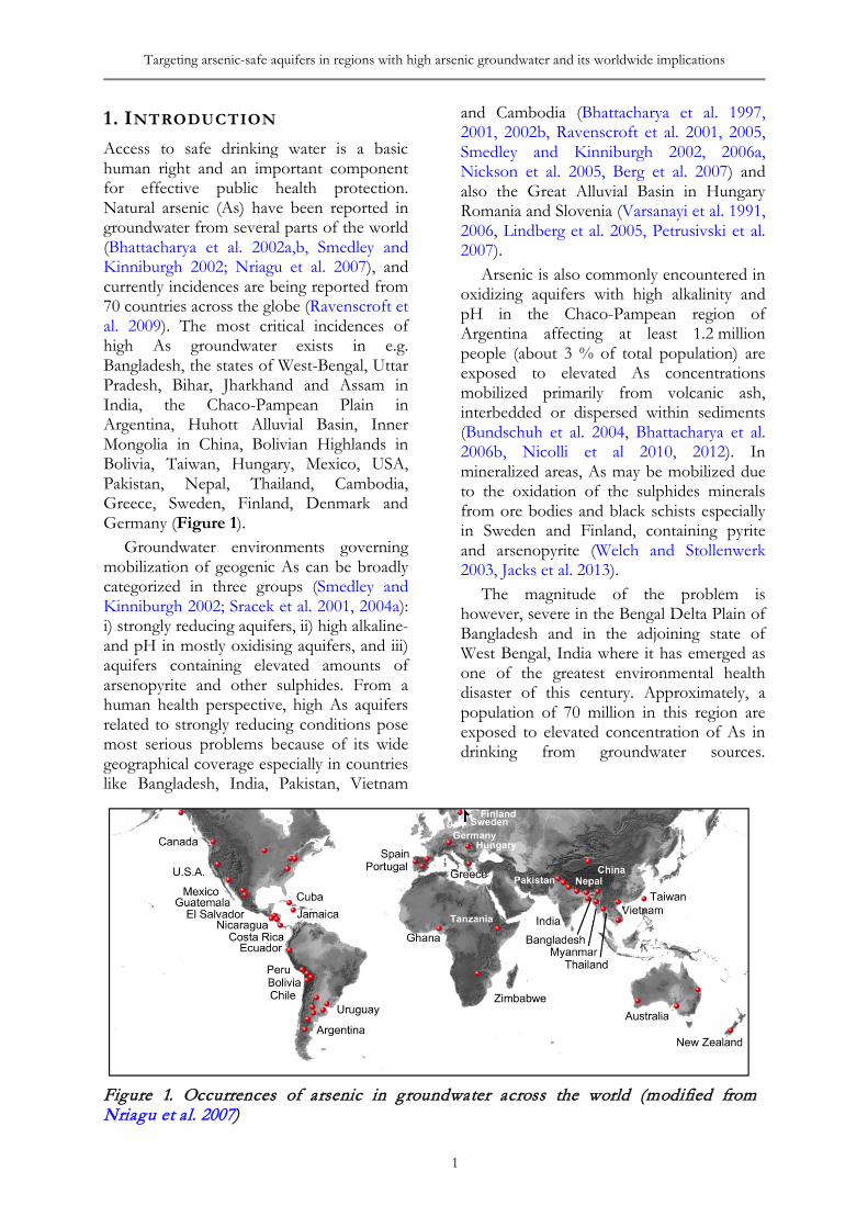
1. INTRODUCTION Access to safe drinking water is a basic human right and an important component for effective public health protection. Natural arsenic (As) have been reported in groundwater from several parts of the world (Bhattacharya et al. 2002a,b, Smedley and Kinniburgh 2002; Nriagu et al. 2007), and currently incidences are being reported from 70 countries across the globe (Ravenscroft et al. 2009). The most critical incidences of high As groundwater exists in e.g. Bangladesh, the states of West-Bengal, Uttar Pradesh, Bihar, Jharkhand and Assam in India, the Chaco-Pampean Plain in Argentina, Huhott Alluvial Basin, Inner Mongolia in China, Bolivian Highlands in Bolivia, Taiwan, Hungary, Mexico, USA, Pakistan, Nepal, Thailand, Cambodia, Greece, Sweden, Finland, Denmark and Germany (Figure 1).
Groundwater environments governing mobilization of geogenic As can be broadly categorized in three groups (Smedley and Kinniburgh 2002; Sracek et al. 2001, 2004a): i) strongly reducing aquifers, ii) high alkaline- and pH in mostly oxidising aquifers, and iii) aquifers containing elevated amounts of arsenopyrite and other sulphides. From a human health perspective, high As aquifers related to strongly reducing conditions pose most serious problems because of its wide geographical coverage especially in countries like Bangladesh, India, Pakistan, Vietnam
and Cambodia (Bhattacharya et al. 1997, 2001, 2002b, Ravenscroft et al. 2001, 2005, Smedley and Kinniburgh 2002, 2006a, Nickson et al. 2005, Berg et al. 2007) and also the Great Alluvial Basin in Hungary Romania and Slovenia (Varsanayi et al. 1991, 2006, Lindberg et al. 2005, Petrusivski et al. 2007).
Arsenic is also commonly encountered in oxidizing aquifers with high alkalinity and pH in the Chaco-Pampean region of Argentina affecting at least 1.2 million people (about 3 % of total population) are exposed to elevated As concentrations mobilized primarily from volcanic ash, interbedded or dispersed within sediments (Bundschuh et al. 2004, Bhattacharya et al. 2006b, Nicolli et al 2010, 2012). In mineralized areas, As may be mobilized due to the oxidation of the sulphides minerals from ore bodies and black schists especially in Sweden and Finland, containing pyrite and arsenopyrite (Welch and Stollenwerk 2003, Jacks et al. 2013).
The magnitude of the problem is however, severe in the Bengal Delta Plain of Bangladesh and in the adjoining state of West Bengal, India where it has emerged as one of the greatest environmental health disaster of this century. Approximately, a population of 70 million in this region are exposed to elevated concentration of As in drinking from groundwater sources.
Figure 1. Occurrences of arsenic in groundwater across the world (modified from Nriagu et al. 2007)
Bhattacharya, Thunvik, Jacks and von Brömssen TRITA LWR Report 2015: 01
2
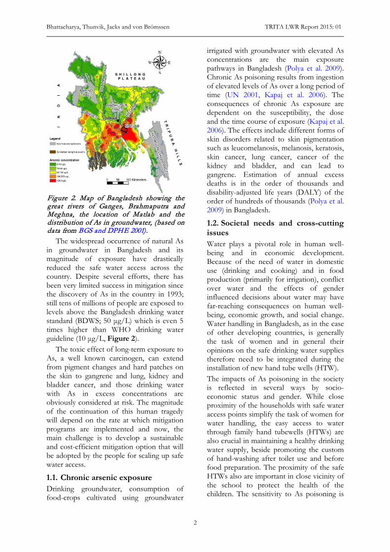
The widespread occurrence of natural As in groundwater in Bangladesh and its magnitude of exposure have drastically reduced the safe water access across the country. Despite several efforts, there has been very limited success in mitigation since the discovery of As in the country in 1993; still tens of millions of people are exposed to levels above the Bangladesh drinking water standard (BDWS; 50 μg/L) which is even 5 times higher than WHO drinking water guideline (10 μg/L, Figure 2).
The toxic effect of long-term exposure to As, a well known carcinogen, can extend from pigment changes and hard patches on the skin to gangrene and lung, kidney and bladder cancer, and those drinking water with As in excess concentrations are obviously considered at risk. The magnitude of the continuation of this human tragedy will depend on the rate at which mitigation programs are implemented and now, the main challenge is to develop a sustainable and cost-efficient mitigation option that will be adopted by the people for scaling up safe water access.
1.1. Chronic arsenic exposure Drinking groundwater, consumption of food-crops cultivated using groundwater
irrigated with groundwater with elevated As concentrations are the main exposure pathways in Bangladesh (Polya et al. 2009). Chronic As poisoning results from ingestion of elevated levels of As over a long period of time (UN 2001, Kapaj et al. 2006). The consequences of chronic As exposure are dependent on the susceptibility, the dose and the time course of exposure (Kapaj et al. 2006). The effects include different forms of skin disorders related to skin pigmentation such as leucomelanosis, melanosis, keratosis, skin cancer, lung cancer, cancer of the kidney and bladder, and can lead to gangrene. Estimation of annual excess deaths is in the order of thousands and disability-adjusted life years (DALY) of the order of hundreds of thousands (Polya et al. 2009) in Bangladesh.
1.2. Societal needs and cross-cutting issues Water plays a pivotal role in human well-being and in economic development. Because of the need of water in domestic use (drinking and cooking) and in food production (primarily for irrigation), conflict over water and the effects of gender influenced decisions about water may have far-reaching consequences on human well-being, economic growth, and social change. Water handling in Bangladesh, as in the case of other developing countries, is generally the task of women and in general their opinions on the safe drinking water supplies therefore need to be integrated during the installation of new hand tube wells (HTW). The impacts of As poisoning in the society is reflected in several ways by socio-economic status and gender. While close proximity of the households with safe water access points simplify the task of women for water handling, the easy access to water through family hand tubewells (HTWs) are also crucial in maintaining a healthy drinking water supply, beside promoting the custom of hand-washing after toilet use and before food preparation. The proximity of the safe HTWs also are important in close vicinity of the school to protect the health of the children. The sensitivity to As poisoning is
Figure 2. Map of Bangladesh showing the great rivers of Ganges, Brahmaputra and Meghna, the location of Matlab and the distribution of As in groundwater, (based on data from BGS and DPHE 2001).
Targeting arsenic-safe aquifers in regions with high arsenic groundwater and its worldwide implications
3
also related to economic status of the individuals which in turn affect the nutritional status as well as affordability to secure access to safe water. Higher cost involvement in installing As-safe deep wells causes the poor communities vulnerable to As poisoning. The poorer sections of the society consume more water (hence exposed to more As) as they work harder. The worse nutritional status of poor households, and particularly the women of those households, may mean that As contamination has more severe physiological consequences for them.
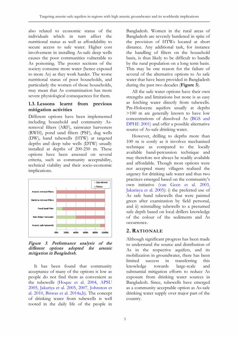
1.3. Lessons learnt from previous mitigation activities Different options have been implemented including household and community As-removal filters (ARF), rainwater harvesters (RWH), pond sand filters (PSF), dug wells (DW), hand tubewells (HTW) at targeted depths and deep tube wells (DTW) usually installed at depths of 200-250 m. These options have been assessed on several criteria, such as community acceptability, technical viability and their socio-economic implications.
Figure 3. Performance analysis of the different options adopted for arsenic mitigation in Bangladesh.
It has been found that community acceptance of many of the options is low as people do not find them as convenient as the tubewells (Hoque et al. 2004, APSU 2005, Jakariya et al. 2005, 2007, Johnston et al. 2010, Biswas et al. 2014a,b). The concept of drinking water from tubewells is well rooted in the daily life of the people in
Bangladesh. Women in the rural areas of Bangladesh are severely burdened in spite of the provision of HTWs located at short distance. Any additional task, for instance the handling of filters on the household basis, is thus likely to be difficult to handle by the rural population on a long term basis. This may be one reason for the failure of several of the alternative options to As safe water that have been provided in Bangladesh during the past two decades (Figure 3).
All the safe water options have their own strengths and limitations but none is as easy as fetching water directly from tubewells. Pre-Holocene aquifers usually at depths >100 m are generally known to have low concentrations of dissolved As (BGS and DPHE 2001) and offer a possible alternative source of As-safe drinking water.
However, drilling to depths more than 100 m is costly as it involves mechanised technique as compared to the locally available hand-percussion technique and may therefore not always be readily available and affordable. Though most options were not accepted many villagers realized the urgency for drinking safe water and thus two practices emerged based on the community’s own initiative (van Geen et al. 2003, Jakariaya et al. 2005): i) the preferred use of As safe hand tubewells that were painted green after examination by field personal, and ii) reinstalling tubewells to a presumed safe depth based on local drillers knowledge of the colour of the sediments and As occurrence.
2. RATIONALE Although significant progress has been made to understand the source and distribution of As in the respective aquifers, and its mobilization in groundwater, there has been limited success in transferring this knowledge towards large-scale and substantial mitigation efforts to reduce As exposure from drinking water sources in Bangladesh. Since, tubewells have emerged as a community acceptable option as As-safe drinking water supply over major part of the country.
Bhattacharya, Thunvik, Jacks and von Brömssen TRITA LWR Report 2015: 01
4
Based on the long term research mostly carried out between 1998-2005 on prevailing aquifer conditions, at country- wide as well as local scales, the scientific community has been able to delineate the principle mechanisms of genesis and mobilization of As in groundwater (Mukherjee and Bhattacharya 2001, Ahmed et al. 2004, Akai et al. 2004, BGS 2001, Bhattacharya et al. 1997, 2001, 2002a,b, Bundschuh et al. 2004, Harvey et al. 2002, McArthur et al. 2004, Nickson et al. 1998, Smedley and Kinniburgh 2002, van Geen et al. 2003, Zheng et al. 2005). However, in many of these regions the distribution of As is extremely heterogeneous, both laterally as well as vertically and As-safe and unsafe tubewells have been encountered in close vicinity at places located <25 m from each other.
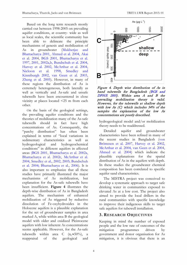
On the basis of the geological settings, the prevailing aquifer conditions and the theories of mobilization many of the As-safe tubewells should in fact have high concentrations of As. Consequently, the “patchy distribution” has often been explained in terms of “local variations in sedimentary characteristics as well as hydrogeological and hydrogeochemical conditions” in different aquifers in affected areas (BGS 2001, Bhattacharya et al. 2002a, Bhattacharya et al. 2002c, McArthur et al. 2004, Smedley et al., 2002, 2005; Bundschuh et al. 2004; Bhattacharya et al., 2006). It is also important to emphasize that all these studies have primarily illustrated the major mechanisms of As mobilization, but explanation for the As-safe tubewells have been insufficient. Figure 4 illustrates the depth-wise distribution of As in Bangladesh aquifers. The mechanism of enhanced mobilization of As triggered by reductive dissolution of Fe-oxyhydroxides in the Holocene aquifers is a plausible explanation for the set of groundwater samples in area marked A, while within area B the geological model with older and oxidized Pleistocene aquifers with low inherent As concentrations seems applicable. However, for the As-safe tubewells within area C (nC≈50%), a reappraisal of the geological and
hydrogeological model and/or mobilization theory needs to be readdressed.
Detailed aquifer and groundwater characteristics have been refined in many of the recent studies in Bangladesh (von Brömssen et al. 2007, Harvey et al. 2002, McArthur et al. 2004, van Geen et al. 2004, Ahmed et al. 2004) which indicate the plausible explanations for the spatial distribution of As in the aquifers with depth. In these studies the groundwater chemical composition has been correlated to specific aquifer sand characteristics.
The MISTRA project was conceived to develop a systematic approach to target safe drinking water in communities exposed to elevated As at a low cost. The project also aimed to provide the local drillers in the rural communities with specific knowledge to improve their indigenous skills to target safe aquifers for tubewell installation.
3. RESEARCH OBJECTIVES Keeping in mind the number of exposed people and the low rate of outcomes of the mitigation programmes driven by government and donor organisation for As mitigation, it is obvious that there is an
Figure 4. Depth wise distribution of As in hand tubewells for Bangladesh (BGS and DPHE 2001). Within area A and B the prevailing mobilization theory is valid. However, for the tubewells at shallow depth with low As (C) which includes 54% of the samples the explanation of the low As concentrations are poorly described.
Targeting arsenic-safe aquifers in regions with high arsenic groundwater and its worldwide implications
5
urgent need for the people themselves to find practical mitigation options. Thus the overall objective of the present research has been to develop a concept for local drillers to target As-safe aquifers in regions with high As groundwater of geogenic origin. This could be a sustainable option for safe drinking water in many regions in the world with groundwater containing geogenic As exceeding the WHO permissible drinking water limit.
4. PROJECT AREA AND HYDROGEOLOGICAL SETTING
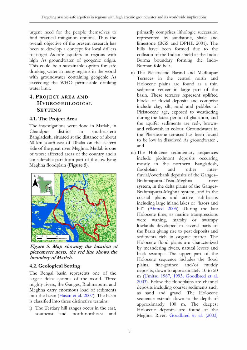
4.1. The Project Area The investigations were done in Matlab, in Chandpur district in southeastern Bangladesh, situated at the distance of about 60 km south-east of Dhaka on the eastern side of the great river Meghna. Matlab is one of worst affected areas of the country and a considerable part form part of the low-lying Meghna floodplain (Figure 5).
4.2. Geological Setting The Bengal basin represents one of the largest delta systems of the world. Three mighty rivers, the Ganges, Brahmaputra and Meghna carry enormous load of sediments into the basin (Hasan et al. 2007). The basin is classified into three distinctive terrains: i) The Tertiary hill ranges occur in the east,
southeast and north-northeast and
primarily comprises lithologic succession represented by sandstone, shale and limestone (BGS and DPHE 2001). The hills have been formed due to the collision of the Indian shield at the Indo-Burma boundary forming the Indo-Burman fold belt.
ii) The Pleistocene Barind and Madhupur Terraces in the central north and Holocene plains are found as a thin sediment veneer in large part of the basin. These terraces represent uplifted blocks of fluvial deposits and comprise include clay, silt, sand and pebbles of Pleistocene age, exposed to weathering during the latest period of glaciation, and the aquifer sediments are red-, brown- and yellowish in colour. Groundwater in the Pliestocene terraces has been found to be low in dissolved As groundwater , and
iii) The Holocene sedimentary sequences include piedmont deposits occurring mostly in the northern Bangladesh, floodplain and other inter-fluvial/overbank deposits of the Ganges–Brahmaputra–Tista–Meghna river system, in the delta plains of the Ganges-Brahmaputra-Meghna system, and in the coastal plains and active sub-basins including large inland lakes or “haors and bil” (Ahmed 2005). During the late Holocene time, as marine transgressions were waning, marshy or swampy lowlands developed in several parts of the Basin giving rise to peat deposits and sediments rich in organic matter. The Holocene flood plains are characterized by meandering rivers, natural levees and back swamps. The upper part of the Holocene sequence includes the flood plains, fine-grained and/or muddy deposits, down to approximately 10 to 20 m (Umitsu 1987, 1993, Goodbred et al. 2003). Below the floodplains are channel deposits including coarser sediments such as sand and gravel. The Holocene sequence extends down to the depth of approximately 100 m. The deepest Holocene deposits are found at the Meghna River. Goodbred et al. (2003)
Figure 5. Map showing the location of piezometer nests, the red line shows the boundary of Matlab.
Bhattacharya, Thunvik, Jacks and von Brömssen TRITA LWR Report 2015: 01
6
identified oxidized surfaces that may coincide with oxidized low-As aquifers (von Brömssen et al. 2007) at a depth of 80 m between Comilla and Meghna and at shallow depths (<20 m) between Comilla and Dhaka. The floodplain is covered by non-calcareous grey to dark grey flood plain soil (Brammer 1996). A thick sequence of the Quaternary sediment constitutes the substratum of the study area. The topmost Holocene sequence is composed of alluvial sand, silt and clay with marsh clay. The location of the Meghna river channel has been relatively constant over the last 18 ka (Umitsu 1993). It can be assumed that the present location of the Meghna coincide with the location of Palaeo-Meghna river channel dating back to 120 ka BP (BGS and DPHE 2001). Thus it can be assumed that the sedim ents near and below the present river channel are relatively coarse with high permeability. This has also been observed in borelogs collected by DPHE/DFID/JICA (2006).
4.3. Precipitation and Climate Bangladesh has a typical South-Asian tropical monsoon climate with considerable variation in rainfall over the year. Most parts of Bangladesh, including Matlab, receive precipitation more than 1 500 mm annually, however, in the hilly areas of north eastern
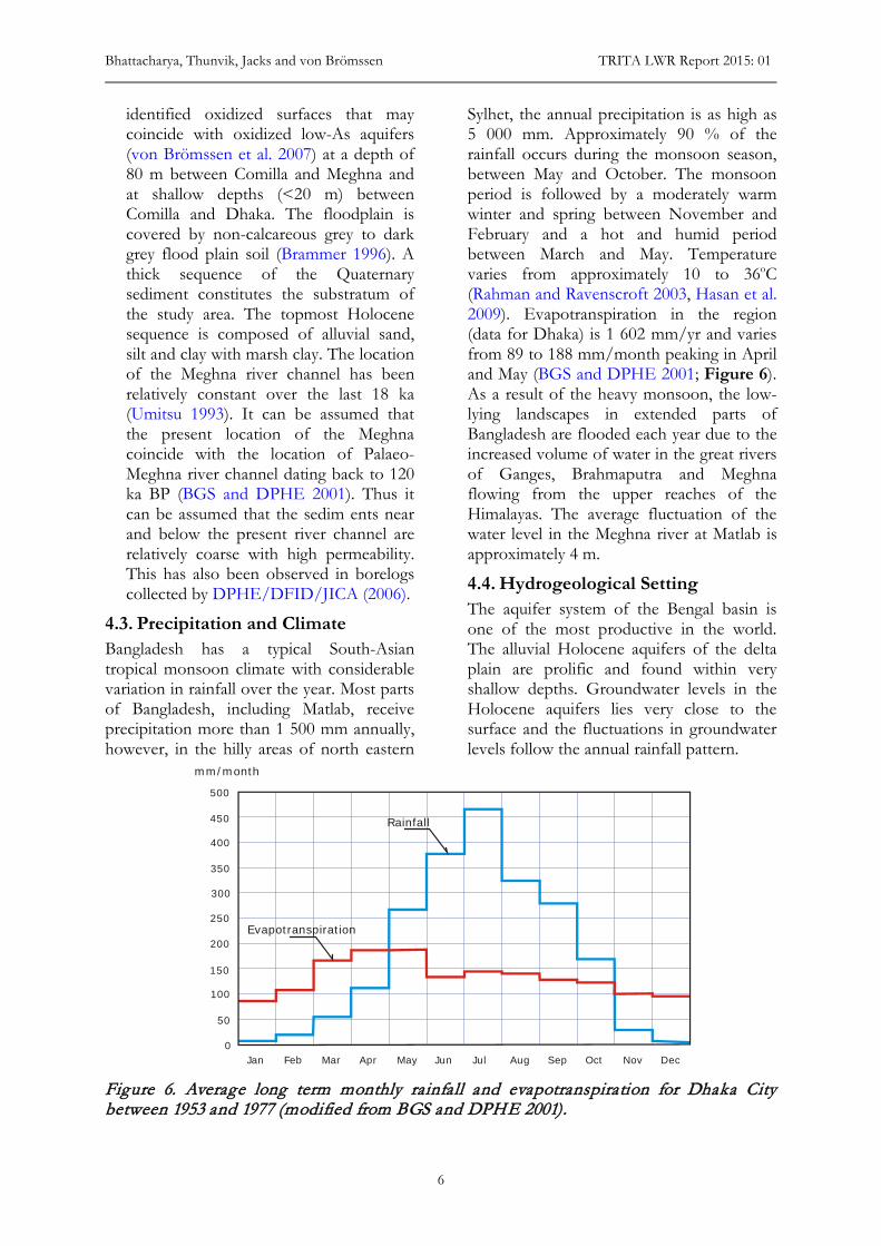
Sylhet, the annual precipitation is as high as 5 000 mm. Approximately 90 % of the rainfall occurs during the monsoon season, between May and October. The monsoon period is followed by a moderately warm winter and spring between November and February and a hot and humid period between March and May. Temperature varies from approximately 10 to 36oC (Rahman and Ravenscroft 2003, Hasan et al. 2009). Evapotranspiration in the region (data for Dhaka) is 1 602 mm/yr and varies from 89 to 188 mm/month peaking in April and May (BGS and DPHE 2001; Figure 6). As a result of the heavy monsoon, the low-lying landscapes in extended parts of Bangladesh are flooded each year due to the increased volume of water in the great rivers of Ganges, Brahmaputra and Meghna flowing from the upper reaches of the Himalayas. The average fluctuation of the water level in the Meghna river at Matlab is approximately 4 m.
4.4. Hydrogeological Setting The aquifer system of the Bengal basin is one of the most productive in the world. The alluvial Holocene aquifers of the delta plain are prolific and found within very shallow depths. Groundwater levels in the Holocene aquifers lies very close to the surface and the fluctuations in groundwater levels follow the annual rainfall pattern.
Figure 6. Average long term monthly rainfall and evapotranspiration for Dhaka City between 1953 and 1977 (modified from BGS and DPHE 2001).
Jan
500
mm/month
Rainfall
Evapotranspiration
450
400
350
300
250
200
150
100
50
0Feb Mar Apr May Jun Jul Aug Sep Oct Nov Dec
Targeting arsenic-safe aquifers in regions with high arsenic groundwater and its worldwide implications
7
Locally, groundwater level fluctuations are affected by groundwater abstraction although in most places the system is fully recharged after monsoonal precipitation. Amplitudes of natural groundwater level fluctuations are in the order of 2-5 m over the year. As Bangladesh experiences a tropical monsoon climate with heavy rainfall during June to October, the groundwater levels start to increase during May/June and decreases in September/October. The groundwater levels are lowest during the end of April to early May (BGS and DPHE 2000, Hasan et al. 2007).
A number of attempts have been made to describe the aquifer distribution (UNDP 1982, EPC/MMP 1991, BGS and DPHE 2001, DPHE/DFID/JICA 2006, Mukherjee et al. 2007, 2008) and most of the aquifer models were established on the basis of the lithological units. For instance, EPC/MMP (1991) had developed a four-layer model taking into account the vertical head differences for the assessment of water balance. The alluvial aquifers of Bangladesh are mostly semi-confined to confined in nature. Most aquifer tests have been analysed by classical methods based on tests with partial penetration of the aquifers and transmissivity, hydraulic conductivity and storage coefficients have been determined from a large number of pumping tests (BGS and DPHE 2000).
Three groundwater flow systems have been identified in Bangladesh (Ravenscroft 2001): i) a local system, down to 10 m, this system is
a product of local topography such as levees, local hills, terraces, haors and bils and rivers,
ii) an intermediate flow system with flow path down to a couple of 100 m driven by the larger terraces, major rivers etc. and
iii) a basin-scale flow system, down to a depth of several 1,000 m. This system would include the entire Bengal basin with its borders in the Tertiary Hills towards east, the Indian shield towards west, the Shillong plateau to the north and the Bay of Bengal in the south.
Groundwater flow patterns have been affected because of heavy abstraction of groundwater for irrigation and drinking water purposes (Michael and Voss 2009a, b). Domestic drinking water wells in rural areas of Bangladesh are generally small diameter hand-pump wells. These hand-pump wells can easily be installed to a depth up to 100 m depending on local geological conditions. Based on population and per capita use, groundwater abstraction for domestic usage can be calculated. Approximately 50 l/day/person is used for domestic purposes in Bangladesh, in some areas of rural Bangladesh as much as 30 mm/yr can be abstracted for domestic purposes (Michael and Voss 2008). However groundwater abstraction for irrigation purposes is about an order of magnitude more in rural areas and in some areas more than 600 mm/yr is used. Today, the abstraction of groundwater for irrigation and drinking purposes, construction of water channels and embankments and road construction etc. have substantially changed the natural surface water and groundwater flow pattern.
5. WORK COMPONENTS Combinations of different approaches were followed to assess the hydrogeological criteria for delineation of low As groundwater in the aquifer system for further development by local and rural people in southeastern-Bangladesh. Focus was laid on delineation of As safe aquifers by linking recognizable geological features to typical groundwater compositions through field-work in close collaboration with the local drillers. The methods used comprised of groundwater and sediment sampling, detailed chemical analysis of water, sediment extractions, mineralogical investigations and hydrogeochemical- and groundwater modelling (von Brömssen et al. 2008, Hasan et al. 2009, Robinson et al. 2011, Jakariya 2007, von Brömssen et al. 2012, von Brömssen et al. 2014, Mukherjee et al. 2008).
5.1. Hydrogeological investigations A comprehensive hydrogeological investigation was carried out to understand the prevailing hydrological and biogeo-
Bhattacharya, Thunvik, Jacks and von Brömssen TRITA LWR Report 2015: 01
8
chemical processes responsible for mobilization and immobilization of As for identifying the safe aquifers, their sustainability and the risk for cross-contamination.
5.1.1. Groundwater flow and hydraulics Multilevel piezometer nests (n=10) and pumping wells (n=5) were installed for determination of the groundwater level fluctuation, monitoring and sampling for groundwater chemistry and performing pumping tests. Hydraulic heads were monitored on weekly basis between May 2009 and October 2010 from ten piezometer nests and the data were used. to prepare hydrographs at varying depth of the aquifer system and to investigate the vertical gradients within the aquifer system. The information is important for investigating the hydraulic properties of the aquifers in order to assess the risk for cross-contamination induced from e.g. irrigation-wells that have much higher flow than drinking water tubewells. A conventional hydraulic test was done in January 2008 in order to determine hydraulic properties of the shallow aquifers including the vertical and horizontal hydraulic conductivity.
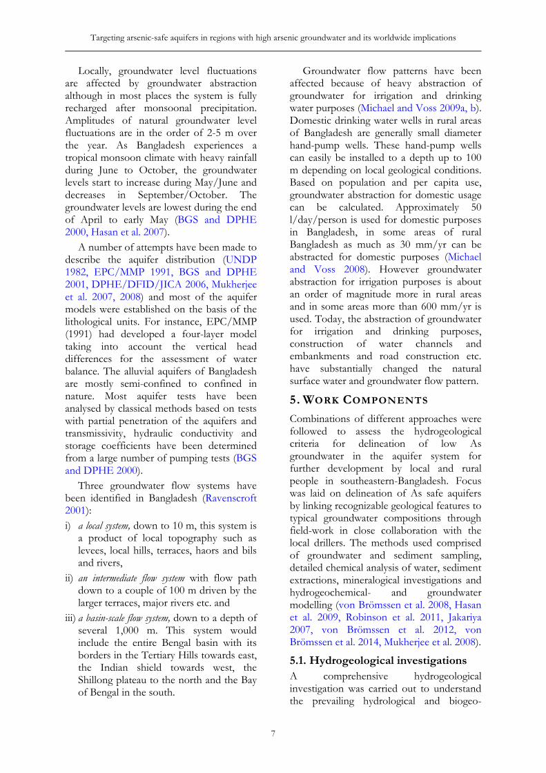
The computer code MODFLOW was used to generate a three-dimensional finite difference groundwater model to study the groundwater flow of the aquifer system. The flow chart followed for the groundwater modelling exercise is presented in Figure 7. A regional steady state- and transient flow model was constructed. The models were run for both undisturbed and disturbed conditions including abstraction of groundwater for irrigation purposes. The steady state model was calibrated to match 14C dating while the transient models were calibrated to match measured hydraulic heads in the piezometer nests. Abstraction from irrigation wells were introduced into the model, based on an existing survey in the area.
The hydrostratigraphy was delineated through analysis of the drilling logs from the piezometer installations and 14C analysis
(incl. 13C) was used for estimation of groundwater age in the study area.
Figure 7. The flow chart followed for groundwater modelling. 5.1.2. Groundwater sampling and analyses Groundwater sampling were carried out from the existing wells and the piezometer nests installed in Matlab following the procedure described by Bhattacharya et al. (2002b). Field parameters such as pH, redox potential (Eh), temperature, and electrical conductivity (EC) were measured in the field in a flow-through cell. The pH and Eh were measured using an EcoScan pH 6 meter. Samples collected for analyses included: a) filtered aliquot (using Sartorius 0.20 μm online filters) for major anion determination; b) aliquot filtered and acidified with suprapure HNO3 (14 M) for the cations and other trace element determination including As (Bhattacharya et al. 2002b). Arsenic speciation was performed with Disposable Cartridges® (MetalSoft Center, PA) in the field (Meng et al. 2001) which adsorb As(V), but allows As(III) to pass through.
Targeting arsenic-safe aquifers in regions with high arsenic groundwater and its worldwide implications
9
Major anions, F−, Cl−, and SO42− were
analyzed in filtered unacidified water samples, with a DionexDX-120 ion chromatograph with an IonPac As14 column. NO3-N, PO4-P and NH4-N were analyzed with a Tecator Aquatec 5400 spectrophotometer. The major cations (Ca, Mg, Na and K) and minor and trace elements (Fe, Mn, As) were analyzed by inductively coupled plasma (ICP) emission spectrometry (Varian Vista-PRO Simultaneous ICP-OES) at Stockholm University. Dissolved organic carbon (DOC) in the water samples was determined on a Shimadzu 5000 TOC analyser with a detection limit of 0.5 mg/L and precision of ±10% at the detection limit.
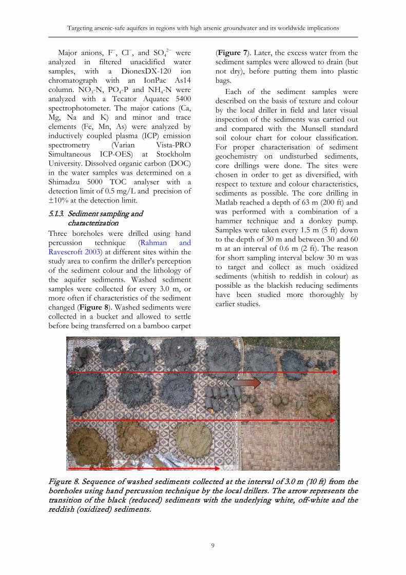
5.1.3. Sediment sampling and characterization
Three boreholes were drilled using hand percussion technique (Rahman and Ravescroft 2003) at different sites within the study area to confirm the driller's perception of the sediment colour and the lithology of the aquifer sediments. Washed sediment samples were collected for every 3.0 m, or more often if characteristics of the sediment changed (Figure 8). Washed sediments were collected in a bucket and allowed to settle before being transferred on a bamboo carpet
(Figure 7). Later, the excess water from the sediment samples were allowed to drain (but not dry), before putting them into plastic bags.
Each of the sediment samples were described on the basis of texture and colour by the local driller in field and later visual inspection of the sediments was carried out and compared with the Munsell standard soil colour chart for colour classification. For proper characterisation of sediment geochemistry on undisturbed sediments, core drillings were done. The sites were chosen in order to get as diversified, with respect to texture and colour characteristics, sediments as possible. The core drilling in Matlab reached a depth of 63 m (200 ft) and was performed with a combination of a hammer technique and a donkey pump. Samples were taken every 1.5 m (5 ft) down to the depth of 30 m and between 30 and 60 m at an interval of 0.6 m (2 ft). The reason for short sampling interval below 30 m was to target and collect as much oxidized sediments (whitish to reddish in colour) as possible as the blackish reducing sediments have been studied more thoroughly by earlier studies.
Figure 8. Sequence of washed sediments collected at the interval of 3.0 m (10 ft) from the boreholes using hand percussion technique by the local drillers. The arrow represents the transition of the black (reduced) sediments with the underlying white, off-white and the reddish (oxidized) sediments.
Bhattacharya, Thunvik, Jacks and von Brömssen TRITA LWR Report 2015: 01
10
The core-samples were splited vertically for lithological and mineralogical studies as well as sequential extraction. At that time, a coal-like vegetation remains were collected and sent for dating through 14C analysis. The 14C analysis was performed at the Radiocarbon Dating Laboratory in Lund using Single Stage Accelerator Mass Spectrometry (SSAMS).
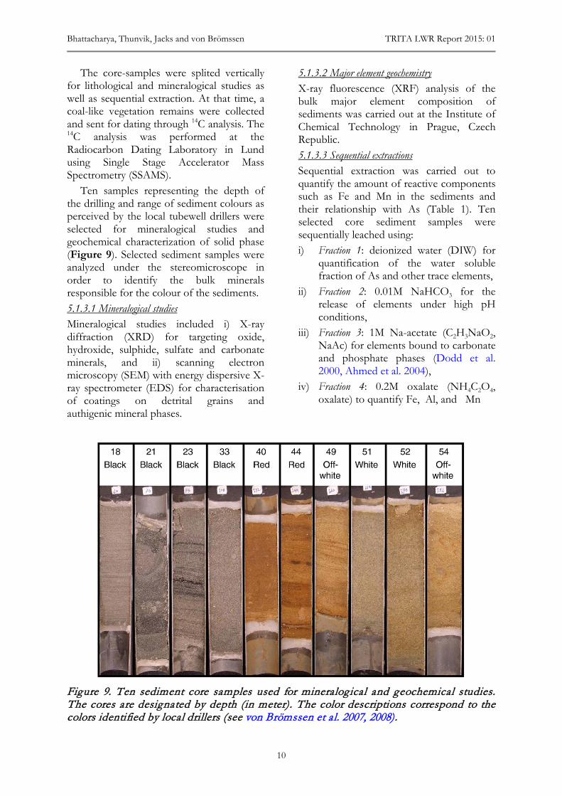
Ten samples representing the depth of the drilling and range of sediment colours as perceived by the local tubewell drillers were selected for mineralogical studies and geochemical characterization of solid phase (Figure 9). Selected sediment samples were analyzed under the stereomicroscope in order to identify the bulk minerals responsible for the colour of the sediments. 5.1.3.1 Mineralogical studies Mineralogical studies included i) X-ray diffraction (XRD) for targeting oxide, hydroxide, sulphide, sulfate and carbonate minerals, and ii) scanning electron microscopy (SEM) with energy dispersive X-ray spectrometer (EDS) for characterisation of coatings on detrital grains and authigenic mineral phases.
5.1.3.2 Major element geochemistry X-ray fluorescence (XRF) analysis of the bulk major element composition of sediments was carried out at the Institute of Chemical Technology in Prague, Czech Republic. 5.1.3.3 Sequential extractions Sequential extraction was carried out to quantify the amount of reactive components such as Fe and Mn in the sediments and their relationship with As (Table 1). Ten selected core sediment samples were sequentially leached using: i) Fraction 1: deionized water (DIW) for
quantification of the water soluble fraction of As and other trace elements,
ii) Fraction 2: 0.01M NaHCO3 for the release of elements under high pH conditions,
iii) Fraction 3: 1M Na-acetate (C2H3NaO2, NaAc) for elements bound to carbonate and phosphate phases (Dodd et al. 2000, Ahmed et al. 2004),
iv) Fraction 4: 0.2M oxalate (NH4C2O4, oxalate) to quantify Fe, Al, and Mn
Figure 9. Ten sediment core samples used for mineralogical and geochemical studies. The cores are designated by depth (in meter). The color descriptions correspond to the colors identified by local drillers (see von Brömssen et al. 2007, 2008).
Targeting arsenic-safe aquifers in regions with high arsenic groundwater and its worldwide implications
11
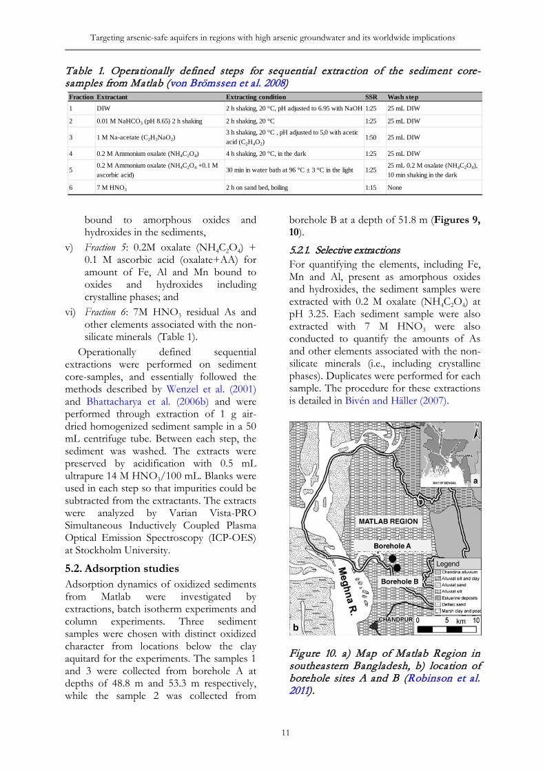
Table 1. Operationally defined steps for sequential extraction of the sediment core-samples from Matlab (von Brömssen et al. 2008)
bound to amorphous oxides and hydroxides in the sediments,
v) Fraction 5: 0.2M oxalate (NH4C2O4) + 0.1 M ascorbic acid (oxalate+AA) for amount of Fe, Al and Mn bound to oxides and hydroxides including crystalline phases; and
vi) Fraction 6: 7M HNO3 residual As and other elements associated with the non-silicate minerals (Table 1).
Operationally defined sequential extractions were performed on sediment core-samples, and essentially followed the methods described by Wenzel et al. (2001) and Bhattacharya et al. (2006b) and were performed through extraction of 1 g air-dried homogenized sediment sample in a 50 mL centrifuge tube. Between each step, the sediment was washed. The extracts were preserved by acidification with 0.5 mL ultrapure 14 M HNO3/100 mL. Blanks were used in each step so that impurities could be subtracted from the extractants. The extracts were analyzed by Varian Vista-PRO Simultaneous Inductively Coupled Plasma Optical Emission Spectroscopy (ICP-OES) at Stockholm University.
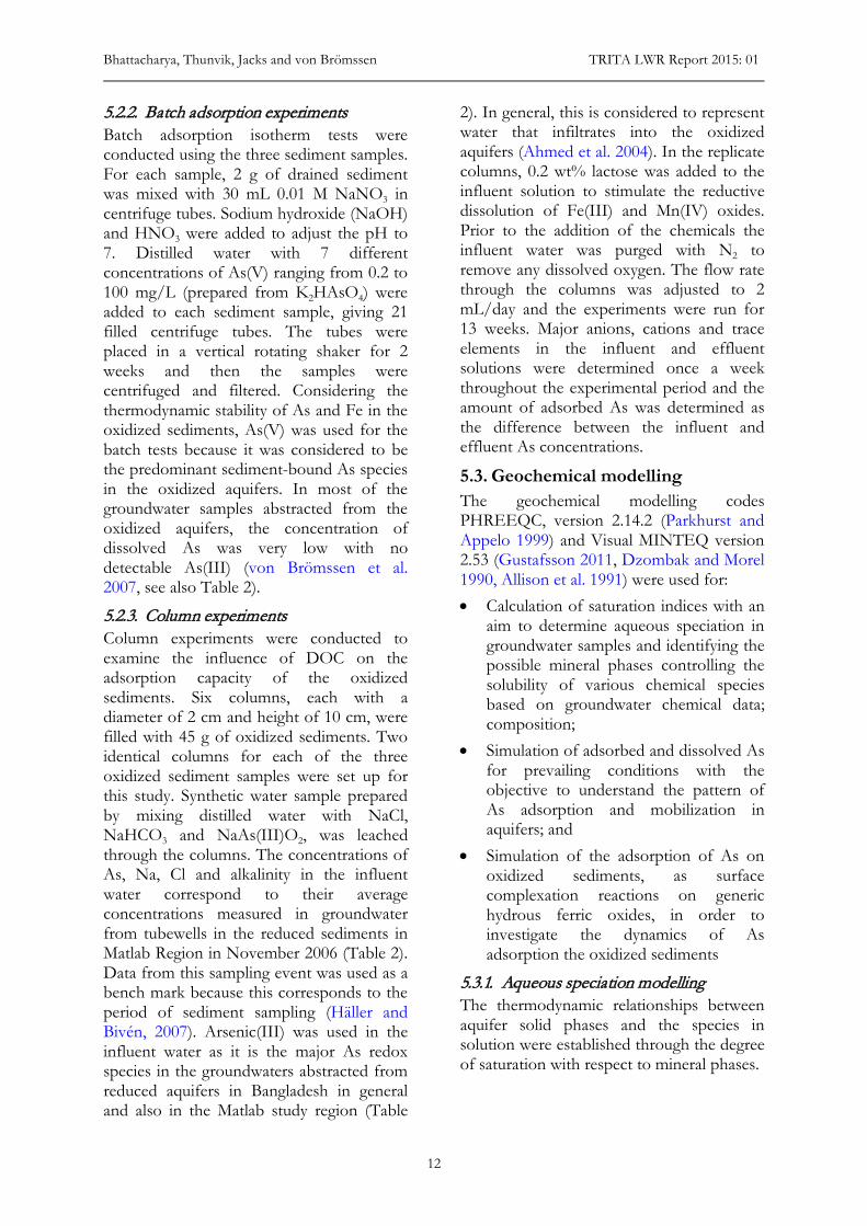
5.2. Adsorption studies Adsorption dynamics of oxidized sediments from Matlab were investigated by extractions, batch isotherm experiments and column experiments. Three sediment samples were chosen with distinct oxidized character from locations below the clay aquitard for the experiments. The samples 1 and 3 were collected from borehole A at depths of 48.8 m and 53.3 m respectively, while the sample 2 was collected from
borehole B at a depth of 51.8 m (Figures 9, 10).
5.2.1. Selective extractions For quantifying the elements, including Fe, Mn and Al, present as amorphous oxides and hydroxides, the sediment samples were extracted with 0.2 M oxalate (NH4C2O4) at pH 3.25. Each sediment sample were also extracted with 7 M HNO3 were also conducted to quantify the amounts of As and other elements associated with the non-silicate minerals (i.e., including crystalline phases). Duplicates were performed for each sample. The procedure for these extractions is detailed in Bivén and Häller (2007).
Figure 10. a) Map of Matlab Region in southeastern Bangladesh, b) location of borehole sites A and B (Robinson et al. 2011).
Fraction Extractant Extracting condition SSR Wash step
1 DIW 2 h shaking, 20 °C, pH adjusted to 6.95 with NaOH 1:25 25 mL DIW
2 0.01 M NaHCO3 (pH 8.65) 2 h shaking 2 h shaking, 20 °C 1:25 25 mL DIW
3 1 M Na-acetate (C2H3NaO2) 3 h shaking, 20 °C , pH adjusted to 5,0 with acetic acid (C2H4O2)
1:50 25 mL DIW
4 0.2 M Ammonium oxalate (NH4C2O4) 4 h shaking, 20 °C, in the dark 1:25 25 mL DIW
50.2 M Ammonium oxalate (NH4C2O4 +0.1 M ascorbic acid)
30 min in water bath at 96 °C ± 3 °C in the light 1:2525 mL 0.2 M oxalate (NH4C2O4), 10 min shaking in the dark
6 7 M HNO3 2 h on sand bed, boiling 1:15 None
Bhattacharya, Thunvik, Jacks and von Brömssen TRITA LWR Report 2015: 01
12
5.2.2. Batch adsorption experiments Batch adsorption isotherm tests were conducted using the three sediment samples. For each sample, 2 g of drained sediment was mixed with 30 mL 0.01 M NaNO3 in centrifuge tubes. Sodium hydroxide (NaOH) and HNO3 were added to adjust the pH to 7. Distilled water with 7 different concentrations of As(V) ranging from 0.2 to 100 mg/L (prepared from K2HAsO4) were added to each sediment sample, giving 21 filled centrifuge tubes. The tubes were placed in a vertical rotating shaker for 2 weeks and then the samples were centrifuged and filtered. Considering the thermodynamic stability of As and Fe in the oxidized sediments, As(V) was used for the batch tests because it was considered to be the predominant sediment-bound As species in the oxidized aquifers. In most of the groundwater samples abstracted from the oxidized aquifers, the concentration of dissolved As was very low with no detectable As(III) (von Brömssen et al. 2007, see also Table 2).
5.2.3. Column experiments Column experiments were conducted to examine the influence of DOC on the adsorption capacity of the oxidized sediments. Six columns, each with a diameter of 2 cm and height of 10 cm, were filled with 45 g of oxidized sediments. Two identical columns for each of the three oxidized sediment samples were set up for this study. Synthetic water sample prepared by mixing distilled water with NaCl, NaHCO3 and NaAs(III)O2, was leached through the columns. The concentrations of As, Na, Cl and alkalinity in the influent water correspond to their average concentrations measured in groundwater from tubewells in the reduced sediments in Matlab Region in November 2006 (Table 2). Data from this sampling event was used as a bench mark because this corresponds to the period of sediment sampling (Häller and Bivén, 2007). Arsenic(III) was used in the influent water as it is the major As redox species in the groundwaters abstracted from reduced aquifers in Bangladesh in general and also in the Matlab study region (Table
2). In general, this is considered to represent water that infiltrates into the oxidized aquifers (Ahmed et al. 2004). In the replicate columns, 0.2 wt% lactose was added to the influent solution to stimulate the reductive dissolution of Fe(III) and Mn(IV) oxides. Prior to the addition of the chemicals the influent water was purged with N2 to remove any dissolved oxygen. The flow rate through the columns was adjusted to 2 mL/day and the experiments were run for 13 weeks. Major anions, cations and trace elements in the influent and effluent solutions were determined once a week throughout the experimental period and the amount of adsorbed As was determined as the difference between the influent and effluent As concentrations.
5.3. Geochemical modelling The geochemical modelling codes PHREEQC, version 2.14.2 (Parkhurst and Appelo 1999) and Visual MINTEQ version 2.53 (Gustafsson 2011, Dzombak and Morel 1990, Allison et al. 1991) were used for: • Calculation of saturation indices with an
aim to determine aqueous speciation in groundwater samples and identifying the possible mineral phases controlling the solubility of various chemical species based on groundwater chemical data; composition;
• Simulation of adsorbed and dissolved As for prevailing conditions with the objective to understand the pattern of As adsorption and mobilization in aquifers; and
• Simulation of the adsorption of As on oxidized sediments, as surface complexation reactions on generic hydrous ferric oxides, in order to investigate the dynamics of As adsorption the oxidized sediments
5.3.1. Aqueous speciation modelling The thermodynamic relationships between aquifer solid phases and the species in solution were established through the degree of saturation with respect to mineral phases.
Targeting arsenic-safe aquifers in regions with high arsenic groundwater and its worldwide implications
13
Table 2. Typical water quality parameters measured in groundwater from the oxidized and the reduced aquifers in the Matlab study area (KTH-International Groundwater Arsenic Research Group groundwater monitoring data between 2004-2008)
Depth pH Temp HCO3 Cl NO3-N PO4-P Na K Mg Ca Total As As(III) Total Fe Total Mn DOC Sim °C mg/L mg/L mg/L mg/L mg/L mg/L mg/L mg/L μg/L μg/L mg/L mg/L mg/L mg/L
A Off-white 11-May-04 57.9 6.12 26.8 107 255 0.20 210 75.9 4.2 25.8 53.8 <DL <DL 0.13 2.53 0.53 53.030-jan-05 6.27 26.2 106 233 0.85 169 88.1 3.8 23.9 57.1 <DL <DL 0.28 2.59 0.91 48.829-nov-06 6.40 25.8 234 234 0.43 156 82.3 3.4 24.9 58.8 16 nd 0.32 2.62 0.80 34.818-jan-08 6.34 25.6 233 245 <DL 87 91.1 3.9 33.2 57.0 <DL <DL 0.26 2.54 4.92 43.217-mar-09 6.50 26.1 125 267 1.23 57 77.0 2.0 24.4 62.2 <DL 9 0.40 1.51 1.29 18.9
B Yellow 11-May-04 57.9 6.39 26.6 136 149 0.23 349 54.3 3.4 20.8 43.1 <DL <DL 0.32 1.99 1.01 43.730-jan-05 6.59 25.6 154 179 0.20 71 59.9 2.4 20.2 53.9 <DL <DL 0.79 2.04 0.36 39.928-nov-06 6.60 25.0 147 147 0.23 61 54.7 2.3 21.4 56.7 13 nd 0.81 2.04 1.35 29.818-jan-08 6.76 24.8 320 152 0.01 102 53.7 2.5 26.3 50.8 <DL <DL 0.72 2.12 1.82 37.7
16 Red 27-May-04 61.0 6.17 26.7 96 206 0.49 293 62.4 3.6 24.4 53.0 <DL <DL 0.46 3.19 1.41 49.130-jan-05 6.14 26.1 117 232 0.30 166 67.2 3.2 22.3 62.5 <DL <DL 0.37 3.16 0.56 44.529-nov-06 6.40 25.8 187 187 0.65 123 60.7 2.9 22.6 57.5 11 nd 0.70 3.14 0.78 32.318-jan-08 6.47 23.5 256 189 <DL 150 59.6 3.3 28.1 60.4 6 <DL 1.00 3.27 1.68 43.802-apr-09 7.10 27.0 116 185 0.39 54 68.3 2.7 25.4 65.6 <DL 8 0.71 4.30 2.19 26.415-mar-09 6.40 26.3 163 246 1.05 64 79.1 3.3 25.7 55.6 <DL 7 0.51 2.78 1.42 22.9
19 Off-white 29-apr-04 59.4 6.20 26.5 112 234 1.00 135 78.8 3.6 26.5 53.2 <DL <DL 0.20 3.58 0.54 50.230-jan-05 6.29 26.2 116 285 0.39 101 80.8 3.1 23.0 57.9 <DL <DL 0.21 3.53 0.65 43.229-nov-06 6.50 26.2 216 216 1.12 77 76.2 2.9 25.1 60.6 8.20 0.17 3.61 0.67 32.1
20 Off-white 29-apr-04 59.4 6.19 26.7 107 186 0.54 334 58.4 3.7 22.4 49.7 <DL <DL 0.41 2.90 0.47 54.730-jan-05 6.32 26.3 87 283 0.27 199 78.6 3.3 21.6 56.8 <DL <DL 0.27 3.01 0.53 43.729-nov-06 6.30 25.0 216 216 0.82 199 75.2 3.0 24.1 60.0 7 nd 0.43 3.21 0.86 32.718-jan-08 6.45 25.3 224 230 <DL 177 81.8 3.5 31.9 60.5 6 <DL 0.25 3.15 2.73 41.116-mar-09 6.50 26.2 139 232 0.95 79 81.8 2.9 26.0 68.5 <DL 8 0.23 4.31 1.74 26.606-apr-09 7.00 26.7 105 214 0.74 35 70.3 2.7 24.8 57.0 11 7 0.25 3.78 1.20 21.2
22 Off-white 29-apr-04 59.4 6.55 26.9 164 138 5.01 526 67.1 3.0 19.4 37.8 <DL 9.63 3.81 1.74 1.18 39.830-jan-05 6.68 26.5 164 170 0.18 509 72.2 2.9 19.1 40.7 <DL <DL 4.85 1.60 0.40 35.928-nov-06 6.40 24.9 201 201 1.14 67 80.1 2.6 25.2 50.7 <DL nd 0.28 2.50 1.39 29.218-jan-08 6.66 25.3 263 197 <DL 75 87.1 2.8 32.5 42.5 <DL <DL 0.35 2.33 1.56 33.611-mar-09 6.60 27.0 136 129 0.60 17 49.4 2.1 20.0 41.7 <DL 6.63 3.95 2.24 1.43 19.7
26 Red 29-apr-04 53.3 6.19 26.5 113 169 0.51 392 55.2 3.3 21.1 45.5 <DL <DL 0.24 2.34 1.00 53.630-jan-05 6.30 26.1 112 210 0.20 234 58.6 3.1 19.6 48.8 <DL <DL 0.27 2.35 0.60 48.928-nov-06 6.40 22.6 167 167 0.94 242 54.7 3.0 21.5 55.0 6 nd 0.42 2.40 0.97 35.018-jan-08 6.59 26.2 265 170 <DL 209 60.0 3.1 27.9 51.1 <DL <DL 0.42 2.32 2.11 41.9
32 Red 30-apr-04 64.0 6.38 26.8 140 150 1.01 212 59.5 3.4 19.0 39.6 <DL <DL 0.37 3.96 1.18 46.330-jan-05 6.40 26.3 174 196 0.22 88 63.4 3.1 19.1 49.6 <DL <DL 0.37 3.68 0.73 41.028-nov-06 6.50 25.1 156 156 0.52 80 60.5 2.8 20.2 50.4 10 nd 0.47 3.81 0.79 31.518-jan-08 6.72 25.9 299 154 <DL 82 66.7 3.1 26.0 48.7 <DL <DL 0.36 3.50 2.72 37.912-mar-09 6.5 27.0 125 104 0.42 82 52.9 2.6 22.0 47.3 <DL 12.35 0.56 2.61 1.14 23.2
35 Off-white 30-apr-04 79.3 6.33 26.8 118 199 0.39 199 68.6 3.9 24.1 47.7 <DL <DL 0.33 2.57 0.93 55.830-jan-05 6.31 26.2 128 268 0.30 115 74.4 3.6 22.7 54.9 <DL <DL 0.29 2.67 0.32 50.028-nov-06 6.60 29.1 196 196 0.60 113 67.4 3.2 23.4 58.7 <DL nd 0.45 2.69 0.80 36.018-jan-08 6.68 25.8 364 204 <DL 96 75.6 3.7 32.9 72.6 <DL <DL 0.40 2.72 0.85 46.614-mar-09 7.00 26.8 455 309 1.23 46 75.5 3.0 26.6 64.2 <DL <DL 0.31 3.71 1.25 30.7
43 White 3-May-04 59.4 6.55 26.8 206 292 0.89 1583 137.4 3.7 33.7 62.1 12 12 8.90 0.25 0.87 42.030-jan-05 6.51 26.6 174 397 0.40 1508 144.4 3.4 28.5 69.6 17 14 8.61 0.26 0.99 37.719-jan-08 6.79 25.1 288 288 0.00 1223 130.3 3.6 37.7 69.2 21 <DL 9.83 0.25 0.99 35.6
44 White 3-May-04 57.9 6.77 26.8 415 272 1.22 3933 202.1 4.7 34.0 62.8 37 35.78 7.06 0.22 1.95 39.030-jan-05 6.73 26.5 402 368 1.15 3941 223.8 4.4 29.4 72.0 43 44.72 7.06 0.24 2.66 36.429-nov-06 6.70 27.1 264 264 0.54 3671 205.1 3.8 29.2 68.3 64 nd 6.97 0.25 2.09 26.719-jan-08 6.84 24.8 501 276 0.24 3163 192.4 4.5 36.3 67.5 52 10 6.92 0.27 3.20 33.805-apr-09 7.50 26.6 410 277 <DL 3803 210.1 3.5 32.2 80.2 42 36 8.23 0.28 3.02 21.3
51 Off-white 30-apr-04 57.9 6.66 26.7 355 530 0.98 555 374.7 4.1 28.7 57.1 <DL <DL 0.14 1.93 0.65 32.230-jan-05 6.62 26.5 350 720 2.51 370 385.7 3.6 25.3 62.0 <DL <DL 0.13 1.91 0.81 28.830-nov-06 6.70 25.2 518 518 1.65 405 357.3 3.3 25.8 62.7 <DL <DL 0.29 1.93 0.89 23.019-jan-08 6.71 22.9 840 424 <DL 310 382.5 3.6 33.4 60.3 <DL 25 0.16 1.76 2.35 26.605-apr-09 6 26.3 306 601 2.79 1026 263.8 3.1 30.8 72.2 44 43 0.13 1.94 2.03 16.6
58 Off-white 1-May-04 57.9 6.66 26.8 319 648 1.51 1583 406.4 4.9 40.4 77.7 22 19 2.06 1.76 0.68 30.930-jan-05 6.69 26.3 292 893 0.47 1305 432.6 4.3 32.2 89.9 27 25 2.05 1.78 1.27 27.629-nov-06 6.70 24.4 603 603 0.00 1417 388.0 3.7 33.6 79.7 35 nd 2.47 1.741 0.83 22.319-jan-08 6.87 24.3 760 638 0.00 1299 362.0 4.5 41.3 79.8 34 9 2.74 1.76 3.42 27.004-apr-09 7.40 27.0 353 256 0.94 1440 344.0 3.3 36.9 90.9 44 34 2.62 2.18 1.62 16.8
63 Red 1-May-04 68.6 6.51 26.6 166 433 1.23 222 208.5 6.1 42.2 79.0 <DL <DL 0.34 2.16 1.00 35.630-jan-05 6.50 26.1 166 674 0.66 156 221.7 5.4 34.7 93.4 <DL <DL 0.43 2.21 0.68 32.128-nov-06 6.60 24.9 493 493 <DL 147 209.4 4.8 37.2 92.0 7 <DL 0.81 2.36 1.94 24.719-jan-08 6.62 24.9 407 521 0.54 128 237.7 6.0 52.7 93.8 <DL <DL 0.81 2.37 2.98 31.006-apr-09 6.6 26.7 187 47 1.75 96 232.9 4.9 46.6 119.4 10 10 0.81 3.32 1.65 20.8
25 Black 30-apr-04 24.4 6.81 26.1 307 83 0.62 7282 102.3 6.2 17.0 36.1 241 241 6.77 0.14 3.79 43.130-jan-05 7.00 25.8 305 110 0.46 7552 104.9 5.7 17.1 40.6 260 nd 6.92 0.14 4.67 39.828-nov-06 7.00 25.5 294 94 0.58 6789 95.0 5.0 19.1 50.9 383 380 7.54 0.16 5.37 29.818-jan-08 6.85 23.0 663 86 0.12 6960 89.4 5.8 22.3 42.8 323 109 7.04 0.18 4.01 37.4
37 Black 1-May-04 39.6 6.58 26.8 189 356 1.00 3642 189.0 5.3 25.3 51.4 23 19 9.18 0.28 1.05 52.330-jan-05 6.62 26.3 193 433 0.54 3442 195.6 4.8 23.6 58.4 25 23 9.09 0.29 1.24 46.128-nov-06 6.70 25.3 297 297 0.77 3465 170.7 4.4 25.9 67.7 39 39 9.61 0.31 1.57 33.818-jan-08 6.58 25.9 261 158 <DL 3137 155.0 3.2 25.4 49.2 <DL <DL 9.00 0.25 2.30 41.9
53 Black 1-May-04 16.8 6.65 26.7 202 13 0.17 5657 8.2 3.6 11.5 45.1 148 144 11.5 0.63 3.29 55.230-jan-05 6.72 26.4 185 15 0.10 5867 8.0 3.2 11.0 45.5 163 160 11.9 0.60 3.17 47.9
54 Black 1-May-04 25.9 6.62 26.6 409 16 0.24 7297 35.4 6.4 36.4 91.9 274 259 6.98 0.10 4.11 48.430-jan-05 6.73 26.3 441 10 0.10 6841 25.1 5.7 30.9 145.6 312 306 8.76 0.29 4.39 40.430-nov-06 6.80 24.0 430 20 <DL 6078 32.3 5.0 31.9 90.4 408 nd 6.79 0.10 3.99 31.719-jan-08 6.85 24.8 487 151 0.10 5097 28.8 4.4 41.8 89.8 349 326 7.51 0.08 4.78 21.0
57 Black 1-May-04 25.9 6.67 26.5 499 12 0.20 7610 22.3 6.3 36.1 119.6 245 239 7.84 304 5.02 44.630-jan-05 6.75 26.2 405 10 0.10 6895 22.4 5.4 28.7 137.4 259 235 7.47 300 4.59 39.130-nov-06 6.80 25.4 445 8 <DL 6253 19.2 4.8 30.2 110.6 339 nd 7.42 319 4.09 29.719-jan-08 6.88 23.9 450 8 0.60 6341 22.8 5.2 39.6 109.7 252 90 6.58 305 5.63 35.5
Sample ID
Sediment colour
Sampling Date
OXIDIZED SEDIMENT
REDUCED SEDIMENT
Bhattacharya, Thunvik, Jacks and von Brömssen TRITA LWR Report 2015: 01
14
Saturation index (SI) is defined as:
=
spKIAPSI log …………….. (eqn. 1)
where IAP is the ion activity product and
Ksp is the solubility product for a mineral at a given temperature. When SI=0 (IAP=Ksp) the solution is at thermodynamic equilibrium with respect to a specific mineral and when SI>0 the water is supersaturated with respect to a mineral and vice versa. Calculation of SI was done to identify possible sinks and sources of dissolved elements and for further interpretation of
possible reactions controlling the aqueous chemistry (Sracek et al. 2004a,b).
Saturation indices were calculated using PHREEQC version 2.14.2 (Parkhurst and Appelo, 1999) with the WATEQ4F thermodynamic database. Eh values measured in field and corrected with respect to standard hydrogen electrode (SHE) were used for speciation of redox couples. The model calculated the activities of different species of each element and then using these activities saturation indices were calculated. Since the measured redox potential (Eh) is a
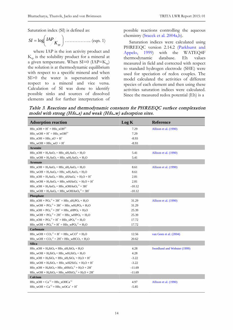
Table 3. Reactions and thermodynamic constants for PHREEQC surface complexation model with strong (Hfo_s) and weak (Hfo_w) adsorption sites.
Adsorption reaction Log K Reference Hfo_sOH + H+ = Hfo_sOH2+ 7.29 Allison et al. (1990) Hfo_wOH + H+ = Hfo_wOH2+ 7.29 Hfo_sOH = Hfo_sO- + H+ -8.93 Hfo_wOH = Hfo_wO- + H+ -8.93 Arsenite Hfo_sOH + H3AsO3 = Hfo_sH2AsO3 + H2O 5.41 Allison et al. (1990) Hfo_wOH + H3AsO3 = Hfo_wH2AsO3 + H2O 5.41 Arsenate Hfo_sOH + H3AsO4 = Hfo_sH2AsO4 + H2O 8.61 Allison et al. (1990) Hfo_wOH + H3AsO4 = Hfo_wH2AsO4 + H2O 8.61 Hfo_sOH + H3AsO4 = Hfo_sHAsO4
- + H2O + H+ 2.81 Hfo_wOH + H3AsO4 = Hfo_wHAsO4
- + H2O + H+ 2.81 Hfo_sOH + H3AsO4 = Hfo_sOHAsO4
-3 + 3H+ -10.12 Hfo_wOH + H3AsO4 = Hfo_wOHAsO4
-3 + 3H+ -10.12 Phosphate Hfo_sOH + PO4
-3 + 3H+ = Hfo_sH2PO4 + H2O 31.29 Allison et al. (1990) Hfo_wOH + PO4
-3 + 3H+ = Hfo_wH2PO4 + H2O 31.29 Hfo_sOH + PO4
-3 + 2H+ = Hfo_sHPO4- + H2O 25.39
Hfo_wOH + PO4-3 + 2H+ = Hfo_wHPO4
- + H2O 25.39 Hfo_sOH + PO4
-3 + H+ = Hfo_sPO4-2 + H2O 17.72
Hfo_wOH + PO4-3 + H+ = Hfo_wPO4
-2 + H2O 17.72 Carbonate Hfo_wOH + CO3
-2 + H+ = Hfo_wCO3- + H2O 12.56 van Geen et al. (2004) Hfo_wOH + CO3
-2 + 2H+= Hfo_wHCO3 + H2O 20.62 Silica Hfo_sOH + H4SiO4 = Hfo_sH3SiO4 + H2O 4.28 Swedlund and Webster (1999) Hfo_wOH + H4SiO4 = Hfo_wH3SiO4 + H2O 4.28 Hfo_sOH + H4SiO4 = Hfo_sH2SiO4
- + H2O + H+ -3.22 Hfo_wOH + H4SiO4 = Hfo_wH2SiO4
- + H2O + H+ -3.22 Hfo_sOH + H4SiO4 = Hfo_sHSiO4
-2 + H2O + 2H+ -11.69 Hfo_wOH + H4SiO4 = Hfo_wHSiO4
-2 + H2O + 2H+ -11.69 Calcium Hfo_sOH + Ca+2 = Hfo_sOHCa+2 4.97 Allison et al. (1990) Hfo_wOH + Ca+2 = Hfo_wOCa+ + H+ -5.85
Targeting arsenic-safe aquifers in regions with high arsenic groundwater and its worldwide implications
15
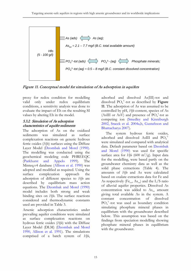
Figure 11. Conceptual model for simulation of As adsorption in aquifers proxy for redox condition for modelling valid only under redox equilibrium conditions, a sensitivity analysis was done to evaluate the impact of Eh on the resulting SI values by altering Eh in the model.
5.3.2. Simulation of As adsorption characteristics of aquifer sediments The adsorption of As on the oxidized sediments was simulated as surface complexation reactions on generic hydrous ferric oxides (Hfo) surfaces using the Diffuse Layer Model (Dzombak and Morel (1990). The modelling was conducted using the geochemical modeling code PHREEQC (Parkhurst and Appelo 1999). The Minteq.v4 database (Allison et al. 1990) was adopted and modified as required. Using the surface complexation approach the adsorption of different species to Hfo are described by equilibrium mass action equations. The Dzombak and Morel (1990) model includes both strong and weak binding sites on Hfo. The surface reactions considered and thermodynamic constants used are provided in Table 3. Arsenic adsorption chatacteristics under prevailing aquifer conditions were simulated as surface complexation reactions on hydrous ferric oxides (Hfo) with the Diffuse Layer Model (DLM) (Dzombak and Morel 1990, Allison et al. 1991). The simulations comprised of a batch system of Hfo,
adsorbed and dissolved As(III)-tot and dissolved PO4
3--tot as described by Figure 11. The adsorption of As was assumed to be controlled by pH, Hfo content, species of As (AsIII or AsV) and presence of PO4
3-tot as competing ion (Smedley and Kinniburgh 2002, Sracek et al. 2004a,b, Gustafsson and Bhattacharya 2007).
The system hydrous ferric oxides, adsorbed and dissolved AsIII and PO4
3- were simulated and compared with analytical data. Default parameter based on Dzombak and Morel (1990) was used for specific surface area for Hfo (600 m2/g). Input data for the modelling, were based partly on the groundwater chemistry data as well as the solid phase extractions (Table 4). The amounts of Hfo and As were calculated based on oxalate extractions data for Fe and As respectively (Feox, Asox) and the L/S ratio of alluvial aquifer properties. Dissolved As concentration was added to Asox amount giving total available As in the system. A constant concentration of dissolved PO4
3--tot was used as boundary condition simulating phosphate mineral phases in equilibrium with the groundwater described below. This assumption was based on the findings from speciation modelling showing phosphate mineral phases in equilibrium with the groundwater.
Hfo(5 - 100 g/l)
As (ads) As (aq);
Astot = 2.1 – 7.7 mg/l (B.C. total available amount)
PO43--tot (ads) PO4
3-- (aq) Phosphate minerals;
PO43--tot (aq) = 0.5 – 8 mg/l (B.C. constant dissolved concentration)
Bhattacharya, Thunvik, Jacks and von Brömssen TRITA LWR Report 2015: 01
16
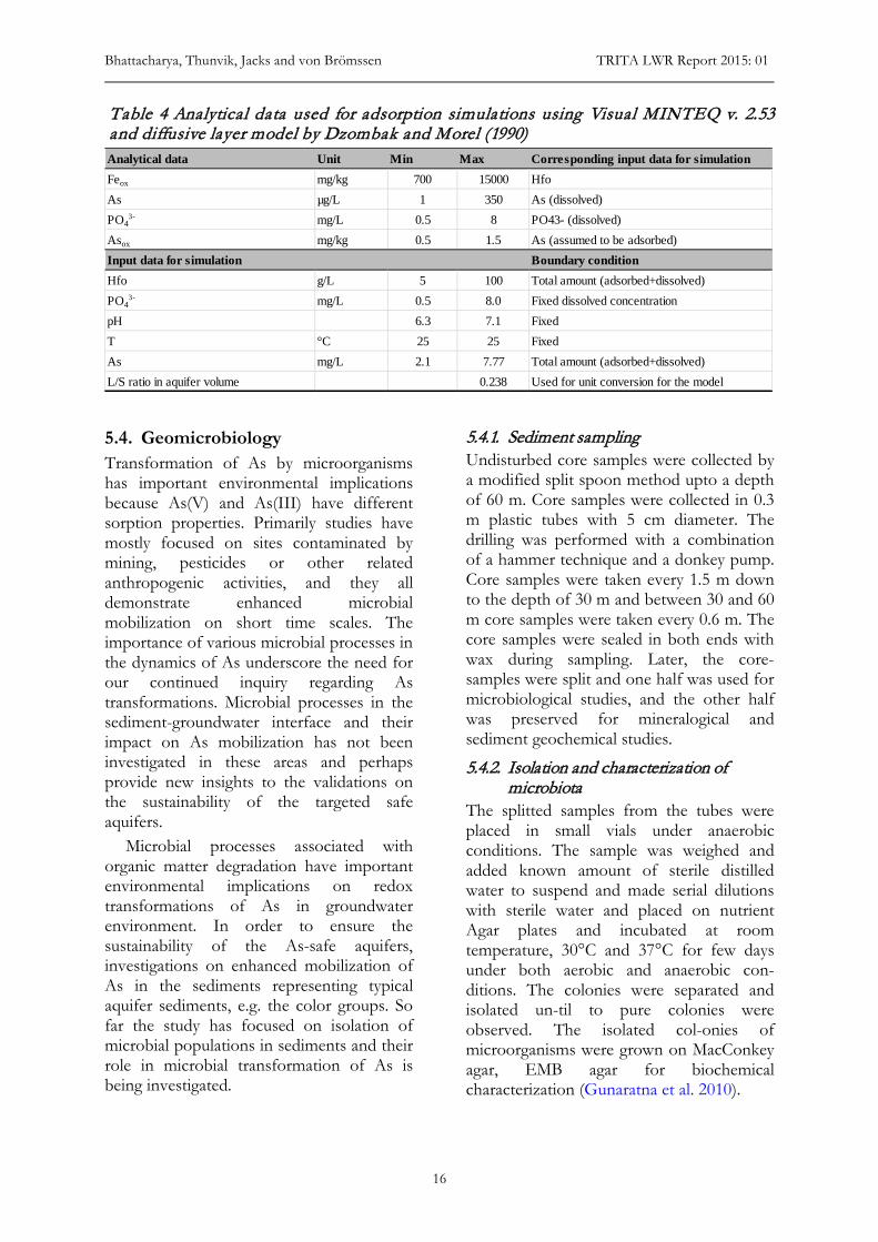
Table 4 Analytical data used for adsorption simulations using Visual MINTEQ v. 2.53 and diffusive layer model by Dzombak and Morel (1990)
5.4. Geomicrobiology Transformation of As by microorganisms has important environmental implications because As(V) and As(III) have different sorption properties. Primarily studies have mostly focused on sites contaminated by mining, pesticides or other related anthropogenic activities, and they all demonstrate enhanced microbial mobilization on short time scales. The importance of various microbial processes in the dynamics of As underscore the need for our continued inquiry regarding As transformations. Microbial processes in the sediment-groundwater interface and their impact on As mobilization has not been investigated in these areas and perhaps provide new insights to the validations on the sustainability of the targeted safe aquifers.
Microbial processes associated with organic matter degradation have important environmental implications on redox transformations of As in groundwater environment. In order to ensure the sustainability of the As-safe aquifers, investigations on enhanced mobilization of As in the sediments representing typical aquifer sediments, e.g. the color groups. So far the study has focused on isolation of microbial populations in sediments and their role in microbial transformation of As is being investigated.
5.4.1. Sediment sampling Undisturbed core samples were collected by a modified split spoon method upto a depth of 60 m. Core samples were collected in 0.3 m plastic tubes with 5 cm diameter. The drilling was performed with a combination of a hammer technique and a donkey pump. Core samples were taken every 1.5 m down to the depth of 30 m and between 30 and 60 m core samples were taken every 0.6 m. The core samples were sealed in both ends with wax during sampling. Later, the core-samples were split and one half was used for microbiological studies, and the other half was preserved for mineralogical and sediment geochemical studies.
5.4.2. Isolation and characterization of microbiota
The splitted samples from the tubes were placed in small vials under anaerobic conditions. The sample was weighed and added known amount of sterile distilled water to suspend and made serial dilutions with sterile water and placed on nutrient Agar plates and incubated at room temperature, 30°C and 37°C for few days under both aerobic and anaerobic con-ditions. The colonies were separated and isolated un-til to pure colonies were observed. The isolated col-onies of microorganisms were grown on MacConkey agar, EMB agar for biochemical characterization (Gunaratna et al. 2010).
Analytical data Unit Min Max Corresponding input data for simulationFeox mg/kg 700 15000 HfoAs µg/L 1 350 As (dissolved)PO4
3- mg/L 0.5 8 PO43- (dissolved)Asox mg/kg 0.5 1.5 As (assumed to be adsorbed)Input data for simulation Boundary condition Hfo g/L 5 100 Total amount (adsorbed+dissolved)PO4
3- mg/L 0.5 8.0 Fixed dissolved concentrationpH 6.3 7.1 FixedT °C 25 25 FixedAs mg/L 2.1 7.77 Total amount (adsorbed+dissolved)L/S ratio in aquifer volume 0.238 Used for unit conversion for the model
Targeting arsenic-safe aquifers in regions with high arsenic groundwater and its worldwide implications
17
The isolated colonies were grown overnight in Nutrient Broth at respective temperatures. The DNA was extracted using Qiagen DNA isolation kit. The DNA template was used to amplify the 16SrRNA gene using PCR method. The universal forward and reverse primers were used in the PCR reaction. The reaction conditions were 98°C for 30 sec; 98°C for 10 sec, 55°C for 30 sec, 72°C for 30 sec under 30 cycles and final extension at 72°C for 10 min. The reaction product was analyzed by running electrophoresis on 1% agarose gel. The product was then analyzed for sequencing and the sequence was later compared in NCBI data base using Blast search.
5.5. Conceptualisation The practice of installation of safe tubewells with local technique has already reached the affluent class of rural population. In order to develop and intensify this practice we are proposing a strategy for the local drillers to target safe aquifers in regions with high As groundwater.
In order to identify safe aquifers, their sustainability and the risk for cross-contamination etc., a hydrogeological investigation including prevailing biogeochemical processes responsible for mobilization and immobilization of As has been discussed in the light of the various outcomes and results of this research project.
6. RESULTS AND DISCUSSION 6.1. Hydrogeological field investigations 6.1.1. Aquifer delineation based on borelogs A 3-D subsurface aquifer model was developed using the program Rockworks (v. 2004). Based on the generalized description of the sediments, three aquifers denoted as Aquifer 1, Aquifer 2 and Aquifer 3 were delineated (Figure 12). The three aquifers are separated by two dominantly silty clay aquitards (Aquitard 1 and Aquitard 2), identified and described by Mozumder (2011) and Mozumder et al. (2011). The
subsurface sequence of the study area has been divided into six hydrostratigraphic units. In most cases, the lower two units are missing within the explored depth. The so-called ‘‘oxidized aquifer’’ (von Brömssen et al. 2007) occurs as Aquifer 1 and/or in the upper reaches of Aquifer 2. Aquifer 1 composed predominately of fine sand and ranges with thickness between 25 and 60 m. The aquitard delineating the two Aquifers 1 and 2 is significant from a hydraulic point of view and dominated by silty clay and sandy clay units with thickness varying between between 3 and 59 m. This. The aquitard has been encountered at depths varying between 39 and 70 m as revealed by the drilling logs prepared during piezometer installation at different sites (Figure 13).
6.1.2. Estimation of groundwater abstraction in Matlab
The total groundwater abstraction rate for Matlab (both North and South) was estimated to 176 mm/yr. The survey of irrigation wells revealed that the maximum abstraction amounts to 143 mm/yr (81%) from shallow depths (<50 m), 25 mm/yr (14%) from depths between 50–75 m and only 8 mm/yr (5%) from depths below 75 m. The entire irrigation season is between November to June with the maximum abstraction for irrigation from January to April. In Matlab the present groundwater abstraction is slightly less than in other parts of the country, 200 mm/yr has been assumed for Bangladesh on average (Michael and Voss, 2008). If all irrigation water were to be tapped from the deep low-As aquifers, the risk of cross contamination from shallow high-As aquifers would increase significantly. However, the adsorption of As must be considered as well because this process would slow the transport of As significantly (Stollenwerk et al. 2007, von Brömssen et al. 2008, Robinson et al. 2011). Irrigation wells are not evenly distributed in the area, they are rather installed in clusters. Thus, the effect from pumping will differ locally within Matlab Upazila.
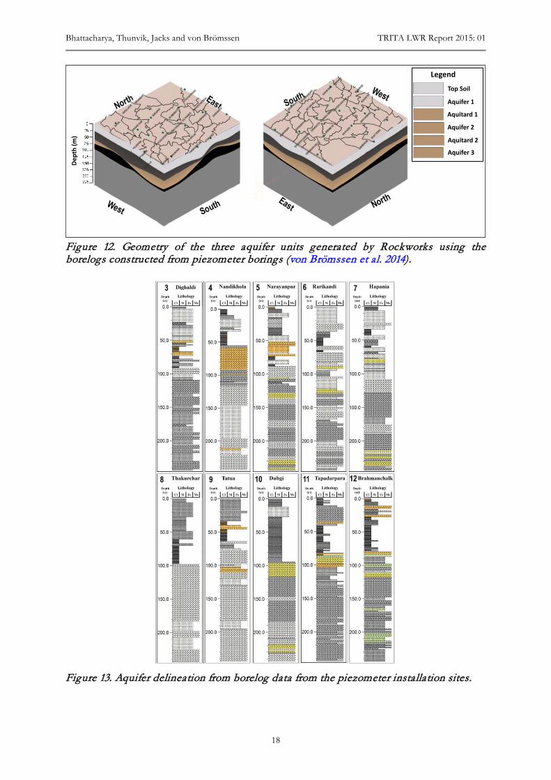
Bhattacharya, Thunvik, Jacks and von Brömssen TRITA LWR Report 2015: 01
18
Figure 12. Geometry of the three aquifer units generated by Rockworks using the borelogs constructed from piezometer borings (von Brömssen et al. 2014).
Figure 13. Aquifer delineation from borelog data from the piezometer installation sites.
0
00
Dept
h(m
)
Aquifer 1
Aquitard 1
Aquifer 2
Aquitard 2
Aquifer 3
Top Soil
Legend
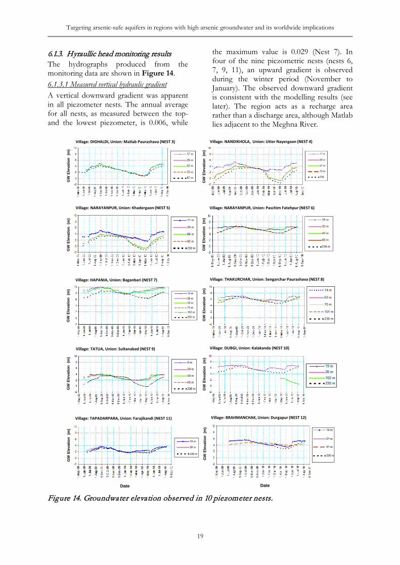
Targeting arsenic-safe aquifers in regions with high arsenic groundwater and its worldwide implications
19
6.1.3. Hyraullic head monitoring results The hydrographs produced from the monitoring data are shown in Figure 14. 6.1.3.1 Measured vertical hydraulic gradient A vertical downward gradient was apparent in all piezometer nests. The annual average for all nests, as measured between the top- and the lowest piezometer, is 0.006, while
the maximum value is 0.029 (Nest 7). In four of the nine piezometric nests (nests 6, 7, 9, 11), an upward gradient is observed during the winter period (November to January). The observed downward gradient is consistent with the modelling results (see later). The region acts as a recharge area rather than a discharge area, although Matlab lies adjacent to the Meghna River.
Figure 14. Groundwater elevation observed in 10 piezometer nests.
GW
Ele
vatio
n (m
)G
W E
leva
tion
(m)
GW
Ele
vatio
n (m
)
GW
Ele
vatio
n (m
)G
W E
leva
tion
(m)
GW
Ele
vatio
n (m
)
GW
Ele
vatio
n (m
)G
W E
leva
tion
(m)
GW
Ele
vatio
n (m
)G
W E
leva
tion
(m)
DateDate
Village: DIGHALDI, Union: Matlab Paurashava (NEST 3) Village: NANDIKHOLA, Union: Utter Nayergaon (NEST 4)
Village: THAKURCHAR, Union: Sengarchar Paurashava (NEST 8)Village: HAPANIA, Union: Baganbari (NEST 7)
Village: NARAYANPUR, Union: Khadergaon (NEST 5) Village: NARAYANPUR, Union: Paschim Fatehpur (NEST 6)
Village: TATUA, Union: Sultanabad (NEST 9) Village: DUBGI, Union: Kalakanda (NEST 10)
Village: TAPADARPARA, Union: Farajikandi (NEST 11) Village: BRAHMANCHAK, Union: Durgapur (NEST 12)
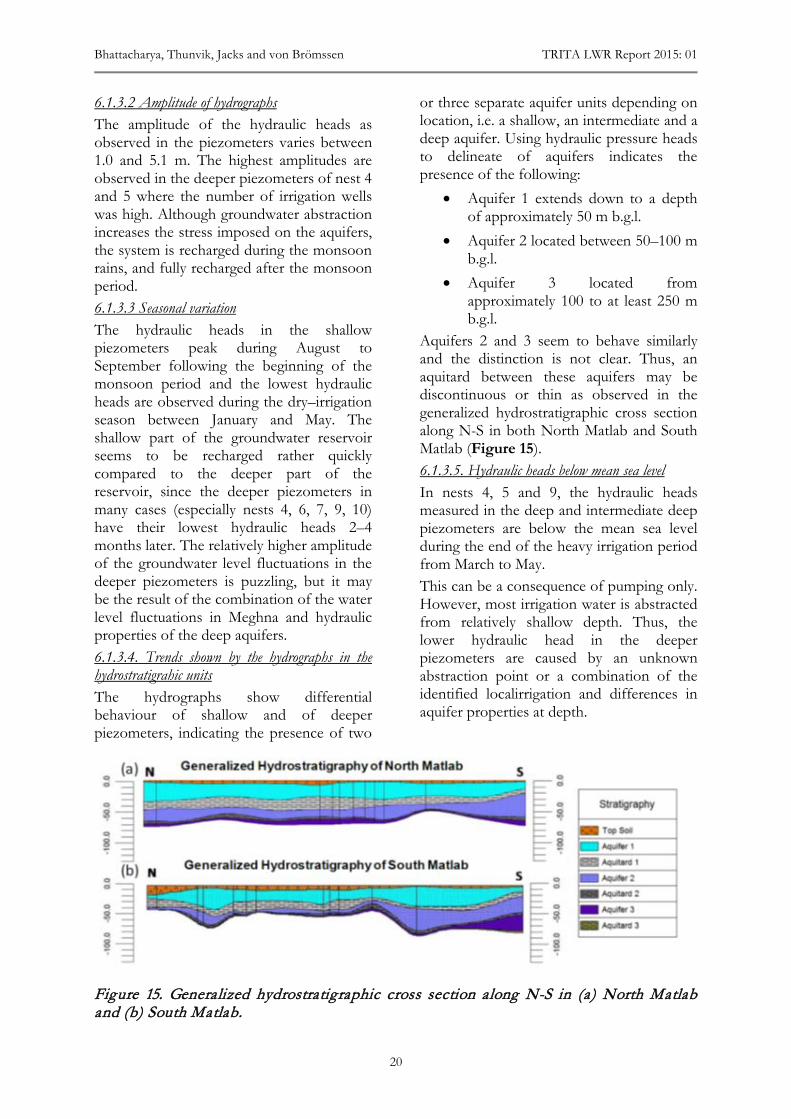
Bhattacharya, Thunvik, Jacks and von Brömssen TRITA LWR Report 2015: 01
20
6.1.3.2 Amplitude of hydrographs The amplitude of the hydraulic heads as observed in the piezometers varies between 1.0 and 5.1 m. The highest amplitudes are observed in the deeper piezometers of nest 4 and 5 where the number of irrigation wells was high. Although groundwater abstraction increases the stress imposed on the aquifers, the system is recharged during the monsoon rains, and fully recharged after the monsoon period. 6.1.3.3 Seasonal variation The hydraulic heads in the shallow piezometers peak during August to September following the beginning of the monsoon period and the lowest hydraulic heads are observed during the dry–irrigation season between January and May. The shallow part of the groundwater reservoir seems to be recharged rather quickly compared to the deeper part of the reservoir, since the deeper piezometers in many cases (especially nests 4, 6, 7, 9, 10) have their lowest hydraulic heads 2–4 months later. The relatively higher amplitude of the groundwater level fluctuations in the deeper piezometers is puzzling, but it may be the result of the combination of the water level fluctuations in Meghna and hydraulic properties of the deep aquifers. 6.1.3.4. Trends shown by the hydrographs in the hydrostratigrahic units The hydrographs show differential behaviour of shallow and of deeper piezometers, indicating the presence of two
or three separate aquifer units depending on location, i.e. a shallow, an intermediate and a deep aquifer. Using hydraulic pressure heads to delineate of aquifers indicates the presence of the following:
• Aquifer 1 extends down to a depth of approximately 50 m b.g.l.
• Aquifer 2 located between 50–100 m b.g.l.
• Aquifer 3 located from approximately 100 to at least 250 m b.g.l.
Aquifers 2 and 3 seem to behave similarly and the distinction is not clear. Thus, an aquitard between these aquifers may be discontinuous or thin as observed in the generalized hydrostratigraphic cross section along N-S in both North Matlab and South Matlab (Figure 15). 6.1.3.5. Hydraulic heads below mean sea level In nests 4, 5 and 9, the hydraulic heads measured in the deep and intermediate deep piezometers are below the mean sea level during the end of the heavy irrigation period from March to May. This can be a consequence of pumping only. However, most irrigation water is abstracted from relatively shallow depth. Thus, the lower hydraulic head in the deeper piezometers are caused by an unknown abstraction point or a combination of the identified localirrigation and differences in aquifer properties at depth.
Figure 15. Generalized hydrostratigraphic cross section along N-S in (a) North Matlab and (b) South Matlab.
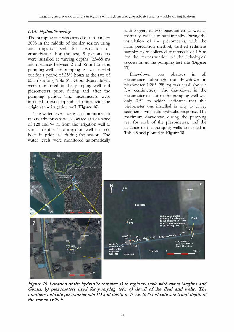
Targeting arsenic-safe aquifers in regions with high arsenic groundwater and its worldwide implications
21
6.1.4. Hydraulic testing The pumping test was carried out in January 2008 in the middle of the dry season using and irrigation well for abstraction of groundwater. For the test, 9 piezometers were installed at varying depths (23–88 m) and distances between 2 and 36 m from the pumping well, and pumping test was carried out for a period of 23½ hours at the rate of 65 m3/hour (Table 5),. Groundwater levels were monitored in the pumping well and piezometers prior, during and after the pumping period. The piezometers were installed in two perpendicular lines with the origin at the irrigation well (Figure 16).
The water levels were also monitored in two nearby private wells located at a distance of 128 and 94 m from the irrigation well at similar depths. The irrigation well had not been in prior use during the season. The water levels were monitored automatically
with loggers in two piezometers as well as manually, twice a minute initially. During the installation of the piezometers, with the hand percussion method, washed sediment samples were collected at intervals of 1.5 m for the reconstruction of the lithological succession at the pumping test site (Figure 17).
Drawdown was obvious in all piezometers although the drawdown in piezometer 1:285 (88 m) was small (only a few centimetres). The drawdown in the piezometer closest to the pumping well was only 0.52 m which indicates that this piezometer was installed in silty to clayey sediments with little hydraulic response. The maximum drawdown during the pumping test for each of the piezometers, and the distance to the pumping wells are listed in Table 5 and plotted in Figure 18.
Figure 16. Location of the hydraulic test site: a) in regional scale with rivers Meghna and Gumti, b) piezometers used for pumping test, c) detail of the field and wells. The numbers indicate piezometer site ID and depth in ft, i.e. 2:70 indicate site 2 and depth of the screen at 70 ft.
a
b
c
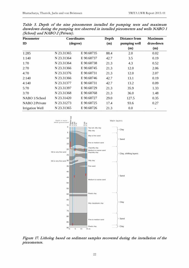
Bhattacharya, Thunvik, Jacks and von Brömssen TRITA LWR Report 2015: 01
22
Table 5. Depth of the nine piezometers installed for pumping tests and maximum drawdown during the pumping test observed in installed piezometers and wells NABO 1 (School) and NABO 2 (Private). Piezometer ID
Coordinates (degree)
Depth (m)
Distance from pumping well
(m)
Maximum drawdown
(m) 1:285 N 23.31365 E 90.68735 88.4 2.0 0.02 1:140 N 23.31364 E 90.68737 42.7 3.5 0.19 1:70 N 23.31364 E 90.68738 21.3 4.3 0.52 2:70 N 23.31366 E 90.68745 21.3 12.0 2.06 4:70 N 23.31376 E 90.68731 21.3 12.0 2.07 2:140 N 23.31366 E 90.68746 42.7 13.1 0.19 4:140 N 23.31377 E 90.68731 42.7 13.2 0.09 5:70 N 23.31397 E 90.68729 21.3 35.9 1.33 3:70 N 23.31368 E 90.68768 21.3 36.0 1.48 NABO 1/School N 23.31420 E 90.68727 29.0 127.5 0.35 NABO 2/Private N 23.31273 E 90.68725 17.4 93.6 0.27 Irrigation Well N 23.31365 E 90.68726 21.3 0.0 -
Figure 17. Litholog based on sediment samples recovered during the installation of the piezometers.
0 Top soil, silty clay
Silty clay Clay
Clay, shifting layers
Clay
Clay
Sand
Sand
Sand
Silty clay
Silty clay/plastic clay
Plastic clay
Plastic clay
Clay/silty clay
Clay/silty claySilt to very fine sand
Silt to very fine sand
Fine sand
Silty to fine sand
Fine to medium sand
Fine to medium sand
Medium to coarse sand
Medium to coarse sand
Irrig
atio
n w
ell
1:28
5
1:70
2:70
2:14
0
1:14
0
5
10
15
20
25
30
35
40
45
50
55
60
65
70
75
80
85
0 5 10 15 m90
Depth in meter below ground level
Main layers
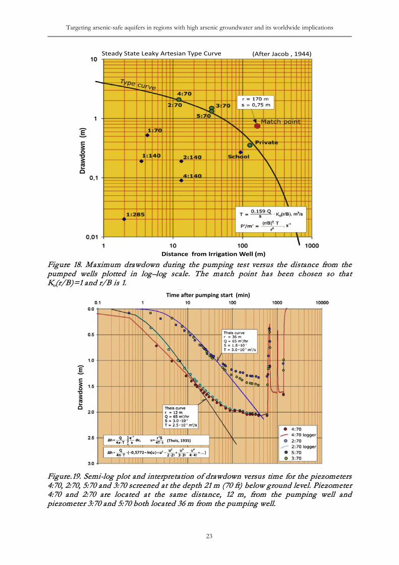
Targeting arsenic-safe aquifers in regions with high arsenic groundwater and its worldwide implications
23
Figure 18. Maximum drawdown during the pumping test versus the distance from the pumped wells plotted in log–log scale. The match point has been chosen so that Ko(r/B)=1 and r/B is 1.
Figure.19. Semi-log plot and interpretation of drawdown versus time for the piezometers 4:70, 2:70, 5:70 and 3:70 screened at the depth 21 m (70 ft) below ground level. Piezometer 4:70 and 2:70 are located at the same distance, 12 m, from the pumping well and piezometer 3:70 and 5:70 both located 36 m from the pumping well.
Draw
down
(m)
Steady State Leaky Artesian Type Curve (After Jacob , 1944)
Distance from Irrigation Well (m)
Time after pumping start (min)
Dra
wdo
wn
(m)
(Theis, 1935)
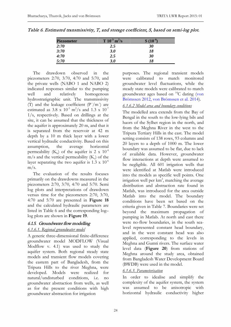
Bhattacharya, Thunvik, Jacks and von Brömssen TRITA LWR Report 2015: 01
24
Table 6. Estimated transmissivity, T, and storage coefficient, S, based on semi-log plot.
Piezometer T 10-3 m2/s S (10-4) 2:70 2.5 30 3:70 3.0 18 4:70 2.5 30 5:70 3.0 18
The drawdown observed in the
piezometers 2:70, 3:70, 4:70 and 5:70, and the private wells (NABO 1 and NABO 2) indicated responses similar to the pumping well and relatively homogenous hydrostratigraphic unit. The transmissivity (T) and the leakage coefficient (P´/m´) are estimated as 3.8 x 10⁻³ m2/s and 1.3 x 10⁻⁷ 1/s, respectively. Based on drillings at the site, it can be assumed that the thickness of the aquifer is approximately 20 m, and that it is separated from the reservoir at 42 m depth by a 10 m thick layer with a lower vertical hydraulic conductivity. Based on this assumption, the average horizontal permeability (Kh) of the aquifer is 2 x 10⁻⁴ m/s and the vertical permeability (Kv) of the layer separating the two aquifer is 1.3 x 10⁻⁶ m/s.
The evaluation of the results focuses primarily on the drawdowns measured in the piezometers 2:70, 3:70, 4:70 and 5:70. Semi log plots and interpretations of drawdown versus time for the piezometers 2:70, 3:70, 4:70 and 5:70 are presented in Figure 18 and the calculated hydraulic parameters are listed in Table 6 and the corresponding log–log plots are shown in Figure 19.
6.1.5. Groundwater flow modelling 6.1.6.1. Regional groundwater model A generic three-dimensional finite-difference groundwater model MODFLOW (Visual Modflow v. 4.1) was used to study the aquifer system. Both regional steady state models and transient flow models covering the eastern part of Bangladesh, from the Tripura Hills to the river Meghna, were developed. Models were realized for natural/undisturbed conditions, i.e. no groundwater abstraction from wells, as well as for the present conditions with high groundwater abstraction for irrigation
purposes. The regional transient models were calibrated to match monitored groundwater level fluctuations, while the steady state models were calibrated to match groundwater ages based on 14C dating (von Brömssen 2012, von Brömssen et al. 2014). 6.1.6.2 Model area and boundary conditions The modelled area extends from the Bay of Bengal in the south to the low-lying bils and haors of the Sylhet region in the north, and from the Meghna River in the west to the Tripura Tertiary Hills in the east. The model setting consists of 138 rows, 93 columns and 20 layers to a depth of 1000 m. The lower boundary was assumed to be flat, due to lack of available data. However, groundwater flow interactions at depth were assumed to be negligible. All 601 irrigation wells that were identified at Matlab were introduced into the models as specific well points. One irrigation well per km2, matching the average distribution and abstraction rate found in Matlab, was introduced for the area outside Matlab into the model. The boundary conditions have been set based on the criteria given in Table 7. Boundaries were set beyond the maximum propagation of pumping in Matlab. At north and east there were no-flow boundaries, in the south sea-level represented constant head boundary, and in the west constant head was also applied, corresponding to the levels in Meghna and Gumti rivers. The surface water level data (Figure 20) from stations of Meghna around the study area, obtained from Bangladesh Water Development Board (BWDB) were used in the model. 6.1.6.3. Parameterisation In order to idealise and simplify the complexity of the aquifer system, the system was assumed to be anisotropic with horizontal hydraulic conductivity higher
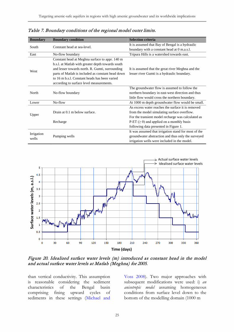
Targeting arsenic-safe aquifers in regions with high arsenic groundwater and its worldwide implications
25
Table 7. Boundary conditions of the regional model outer limits.
Figure 20. Idealized surface water levels (m) introduced as constant head in the model and actual surface water levels at Matlab (Meghna) for 2005. than vertical conductivity. This assumption is reasonable considering the sediment characteristics of the Bengal basin comprising fining upward cycles of sediments in these settings (Michael and
Voss 2008). Two major approaches with subsequent modifications were used: i) an anisotropic model assuming homogeneous conditions from surface level down to the bottom of the modelling domain (1000 m
Boundary Boundary condition Selection criteria
South Constant head at sea-level. It is assumed that Bay of Bengal is a hydraulic boundary with a constant head at 0 m.a.s.l.
East No-flow boundary Tripura Hills is a watershed towards east.
West
Constant head at Meghna surface to appr. 140 m b.s.l. at Matlab with greater depth towards south and lesser towards north. R. Gumti, surrounding parts of Matlab is included as constant head down to 16 m b.s.l. Constant heads has been varied according to surface level measurements.
It is assumed that the great river Meghna and the lesser river Gumti is a hydraulic boundary.
North No-flow boundary The groundwater flow is assumed to follow the northern boundary in east-west direction and thus little flow would cross the northern boundary.
Lower No-flow At 1000 m depth groundwater flow would be small.
Upper
Drain at 0.1 m below surface. Recharge
As excess water reaches the surface it is removed from the model simulating surface overflow. For the transient model recharge was calculated as P-ET (≥ 0) and applied on a monthly basis following data presented in Figure 1.
Irrigation wells Pumping wells
It was assumed that irrigation stand for most of the groundwater abstraction and thus only the surveyed irrigation wells were included in the model.
Time (days)
Surf
ace
wat
erle
vels
(m, a
.s.l.
)
Actual surface water levels Idealised surface water levels
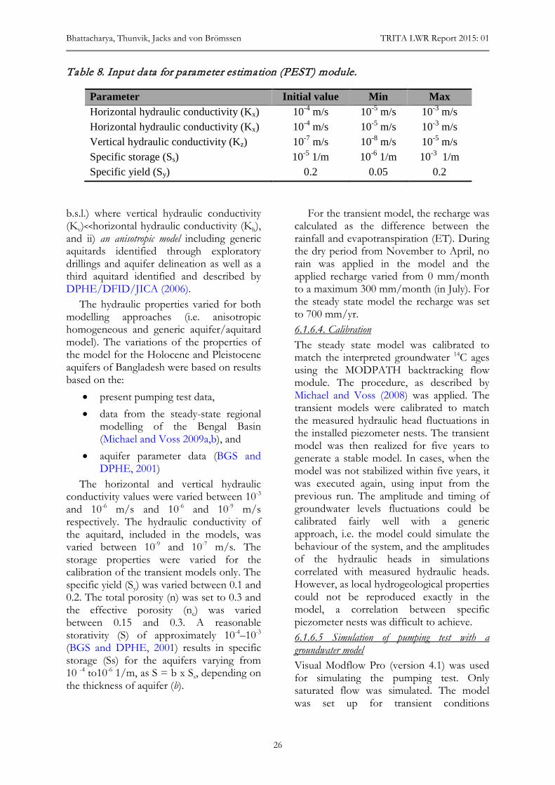
Bhattacharya, Thunvik, Jacks and von Brömssen TRITA LWR Report 2015: 01
26
Table 8. Input data for parameter estimation (PEST) module.
b.s.l.) where vertical hydraulic conductivity (Kv)<<horizontal hydraulic conductivity (Kh), and ii) an anisotropic model including generic aquitards identified through exploratory drillings and aquifer delineation as well as a third aquitard identified and described by DPHE/DFID/JICA (2006).
The hydraulic properties varied for both modelling approaches (i.e. anisotropic homogeneous and generic aquifer/aquitard model). The variations of the properties of the model for the Holocene and Pleistocene aquifers of Bangladesh were based on results based on the:
• present pumping test data, • data from the steady-state regional
modelling of the Bengal Basin (Michael and Voss 2009a,b), and
• aquifer parameter data (BGS and DPHE, 2001)
The horizontal and vertical hydraulic conductivity values were varied between 10-3 and 10-6 m/s and 10-6 and 10-9 m/s respectively. The hydraulic conductivity of the aquitard, included in the models, was varied between 10-9 and 10-7 m/s. The storage properties were varied for the calibration of the transient models only. The specific yield (Sy) was varied between 0.1 and 0.2. The total porosity (n) was set to 0.3 and the effective porosity (ne) was varied between 0.15 and 0.3. A reasonable storativity (S) of approximately 10-4–10-3 (BGS and DPHE, 2001) results in specific storage (Ss) for the aquifers varying from 10 -4 to10-6 1/m, as S = b x Ss, depending on the thickness of aquifer (b).
For the transient model, the recharge was calculated as the difference between the rainfall and evapotranspiration (ET). During the dry period from November to April, no rain was applied in the model and the applied recharge varied from 0 mm/month to a maximum 300 mm/month (in July). For the steady state model the recharge was set to 700 mm/yr. 6.1.6.4. Calibration The steady state model was calibrated to match the interpreted groundwater 14C ages using the MODPATH backtracking flow module. The procedure, as described by Michael and Voss (2008) was applied. The transient models were calibrated to match the measured hydraulic head fluctuations in the installed piezometer nests. The transient model was then realized for five years to generate a stable model. In cases, when the model was not stabilized within five years, it was executed again, using input from the previous run. The amplitude and timing of groundwater levels fluctuations could be calibrated fairly well with a generic approach, i.e. the model could simulate the behaviour of the system, and the amplitudes of the hydraulic heads in simulations correlated with measured hydraulic heads. However, as local hydrogeological properties could not be reproduced exactly in the model, a correlation between specific piezometer nests was difficult to achieve. 6.1.6.5 Simulation of pumping test with a groundwater model Visual Modflow Pro (version 4.1) was used for simulating the pumping test. Only saturated flow was simulated. The model was set up for transient conditions
Parameter Initial value Min Max Horizontal hydraulic conductivity (Kx) 10-4 m/s 10-5 m/s 10-3 m/s Horizontal hydraulic conductivity (Kx) 10-4 m/s 10-5 m/s 10-3 m/s Vertical hydraulic conductivity (Kz) 10-7 m/s 10-8 m/s 10-5 m/s Specific storage (Ss) 10-5 1/m 10-6 1/m 10-3 1/m Specific yield (Sy) 0.2 0.05 0.2
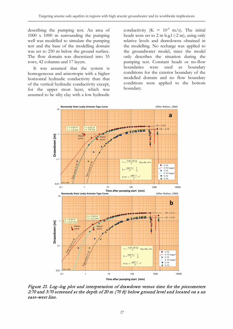
Targeting arsenic-safe aquifers in regions with high arsenic groundwater and its worldwide implications
27
describing the pumping test. An area of 1000 x 1000 m surrounding the pumping well was modelled to simulate the pumping test and the base of the modelling domain was set to 250 m below the ground surface. The flow domain was discretized into 35 rows, 42 columns and 17 layers.
It was assumed that the system is homogeneous and anisotropic with a higher horizontal hydraulic conductivity than that of the vertical hydraulic conductivity except, for the upper most layer, which was assumed to be silty clay with a low hydraulic
conductivity (K = 10-8 m/s). The initial heads were set to 2 m b.g.l (-2 m), using only relative levels and drawdowns obtained in the modelling. No recharge was applied to the groundwater model, since the model only describes the situation during the pumping test. Constant heads or no-flow boundaries were used as boundary conditions for the exterior boundary of the modelled domain and no flow boundary conditions were applied to the bottom boundary.
Figure 21. Log–log plot and interpretation of drawdown versus time for the piezometers 2:70 and 3:70 screened at the depth of 20 m (70 ft) below ground level and located on a an east–west line.
a
b
Dra
wdo
wn
(m)
Dra
wdo
wn
(m)
Time after pumping start (min)
Time after pumping start (min)
Nonsteady State Leaky Artesian Type Curve (After Walton, 1960)
Nonsteady State Leaky Artesian Type Curve (After Walton, 1960)
Bhattacharya, Thunvik, Jacks and von Brömssen TRITA LWR Report 2015: 01
28
General aquifer properties for the shallow aquifers in the flood plains of the Bengal Basin given by BGS and DPHE (2001) were used as initial values for the calibration. The model was calibrated to match the measured drawdown in the piezometers during the pumping test. The parameter estimation module (PEST) was used to calibrate the model (von Brömssen et al. 2014).
The data used for the optimisation and the calibrated values of hydraulic conductivities of the aquifer match the previous studies results, i.e. the hydraulic conductivities are within the same order of magnitude (Table 8). The PEST module used to calibrate the model also revealed acceptable results (Table 6), except for piezometer 1:70 that appears to be installed in silty and clayey sediments and/or was not working properly as it does not response accordingly. Measured and simulated drawdowns for selected piezometers are shown in Figure 21.
A number of pumping tests would have been ideally performed to ascertain the representativity of the pumping test for Matlab, however the results correlates with literature findings (BGS and DPHE 2001) The test however amply demonstrates the distinct hydraulic properties in terms of horizontal and vertical conductivity for the aquifer system (see Table 6).
6.1.6. Groundwater flow models 6.1.7.1. Steady state flow model In order to reproduce regional groundwater flow pattern, hydraulic conductivity (Kh and Kv) were varied during modelling. Backward particle tracking was used for the calibration of the groundwater travel times versus estimated groundwater ages (Table 9). Particles were released from the study area at depth corresponding to the corrected 14C groundwater dating, representing the boundary between different flow systems (Michael and Voss 2008).
Groundwater age estimates through anisotropic homogeneous modelling approach were younger than the 14C dating, of groundwater in the aquifer depths up to
75 m for all models. Using a ratio Kh/Kv > 1000 in the model, for depths of 200 m and beyond, the simulated groundwater ages were found to be unreasonably old (>50 k yr) and thus did not comply with the ages estimated by Aggarwal et al. (2000) and Hoque (2010). This also assumes that the groundwater travelling distances needs to be considerably long, all the way to the eastern boundary of the model as well as the prevalence of a long regional flow system at very shallow depth, i.e. 30 m and below.
Based on the aquifer delineation, a four layer model was also developed. This modelling approach improved the calibration of estimated groundwater ages. The accuracy of the model improved, when aquitards with hydraulic conductivity ranges 10-8 – 10-9 m/s were considered. Figure 22 illustrates the differences in regional groundwater flow patterns between the homogeneous anisotropic model and the four layer aquifer/aquitard model.
The sensitivity of the model to hydraulic properties of shallower domain as well as low hydraulic conductivity of the Tertiary Hill terrain was tested and evaluated. Simulated groundwater ages at Matlab were not sensitive to these changes and the calibration did not change. The groundwater simulations clearly identified two flow-systems, a regional horizontal flow system with recharge areas at the Tripura Hills and local flow systems driven by local topography. The local flow systems reach a depth of approximately 30 m b.g.l. in Matlab, based on the calibrated steady state modelling results.
In Matlab, very few deep (>100m) irrigation- and production wells are installed and the vertical gradient observed in most piezometer nests out of the irrigation period is likely to reflect natural groundwater flow conditions. The vertical hydraulic gradient of 0.01 based on the observed field measurements is also consistent with the models developed for the study area.
The local recharge zones result in elevated hydraulic heads compared to the heads of the regional flow. Even though
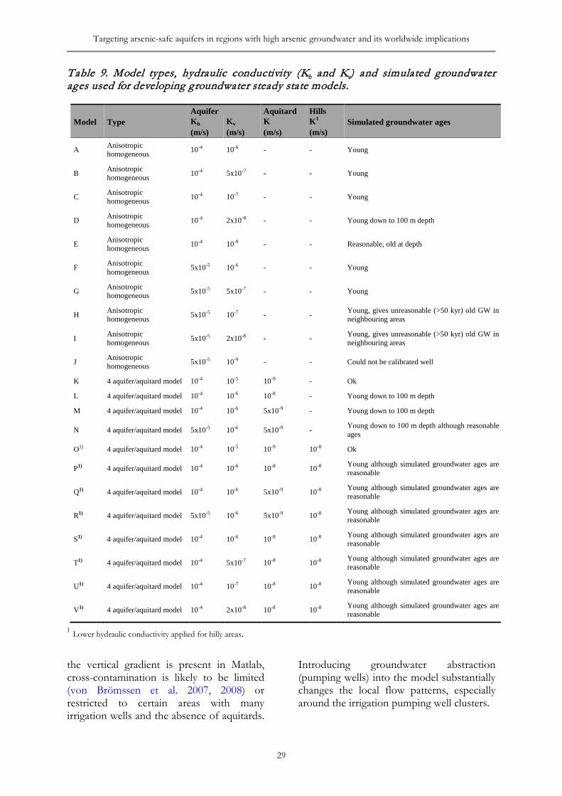
Targeting arsenic-safe aquifers in regions with high arsenic groundwater and its worldwide implications
29
Table 9. Model types, hydraulic conductivity (Kh and Kv) and simulated groundwater ages used for developing groundwater steady state models.
1 Lower hydraulic conductivity applied for hilly areas. the vertical gradient is present in Matlab, cross-contamination is likely to be limited (von Brömssen et al. 2007, 2008) or restricted to certain areas with many irrigation wells and the absence of aquitards.
Introducing groundwater abstraction (pumping wells) into the model substantially changes the local flow patterns, especially around the irrigation pumping well clusters.
Aquifer Aquitard Hills Model Type Kh Kv K K1 Simulated groundwater ages (m/s) (m/s) (m/s) (m/s)
A Anisotropic homogeneous 10-4 10-6 - - Young
B Anisotropic homogeneous 10-4 5x10⁻⁷ - - Young
C Anisotropic homogeneous 10-4 10-7 - - Young
D Anisotropic homogeneous 10-4 2x10⁻⁸ - - Young down to 100 m depth
E Anisotropic homogeneous 10-4 10-9 - - Reasonable, old at depth
F Anisotropic homogeneous 5x10⁻⁵ 10-6 - - Young
G Anisotropic homogeneous 5x10⁻⁵ 5x10⁻⁷ - - Young
H Anisotropic homogeneous 5x10⁻⁵ 10-7 - - Young, gives unreasonable (>50 kyr) old GW in
neighbouring areas
I Anisotropic homogeneous 5x10⁻⁵ 2x10⁻⁸ - - Young, gives unreasonable (>50 kyr) old GW in
neighbouring areas
J Anisotropic homogeneous 5x10⁻⁵ 10-9 - - Could not be calibrated well
K 4 aquifer/aquitard model 10-4 10-5 10-9 - Ok
L 4 aquifer/aquitard model 10-4 10-6 10-8 - Young down to 100 m depth
M 4 aquifer/aquitard model 10-4 10-6 5x10⁻⁹ - Young down to 100 m depth
N 4 aquifer/aquitard model 5x10⁻⁵ 10-6 5x10⁻⁹ - Young down to 100 m depth although reasonable ages
O1) 4 aquifer/aquitard model 10-4 10-5 10-9 10-8 Ok
P1) 4 aquifer/aquitard model 10-4 10-6 10-8 10-8 Young although simulated groundwater ages are reasonable
Q1) 4 aquifer/aquitard model 10-4 10-6 5x10⁻⁹ 10-8 Young although simulated groundwater ages are reasonable
R1) 4 aquifer/aquitard model 5x10⁻⁵ 10-6 5x10⁻⁹ 10-8 Young although simulated groundwater ages are reasonable
S1) 4 aquifer/aquitard model 10-4 10-6 10-8 10-8 Young although simulated groundwater ages are reasonable
T1) 4 aquifer/aquitard model 10-4 5x10⁻⁷ 10-8 10-8 Young although simulated groundwater ages are reasonable
U1) 4 aquifer/aquitard model 10-4 10-7 10-8 10-8 Young although simulated groundwater ages are reasonable
V1) 4 aquifer/aquitard model 10-4 2x10⁻⁸ 10-8 10-8 Young although simulated groundwater ages are reasonable
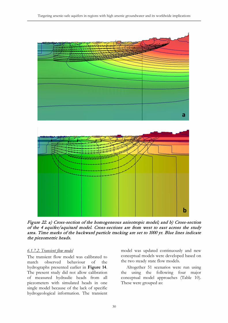
Targeting arsenic-safe aquifers in regions with high arsenic groundwater and its worldwide implications
30
Figure 22. a) Cross-section of the homogeneous anisotropic model; and b) Cross-section of the 4 aquifer/aquitard model. Cross-sections are from west to east across the study area. Time marks of the backward particle tracking are set to 1000 yr. Blue lines indicate the piezometric heads. 6.1.7.2. Transient flow model The transient flow model was calibrated to match observed behaviour of the hydrographs presented earlier in Figure 14. The present study did not allow calibration of measured hydraulic heads from all piezometers with simulated heads in one single model because of the lack of specific hydrogeological information. The transient
model was updated continuously and new conceptual models were developed based on the two steady state flow models.
Altogether 51 scenarios were run using the using the following four major conceptual model approaches (Table 10). These were grouped as:
a
b
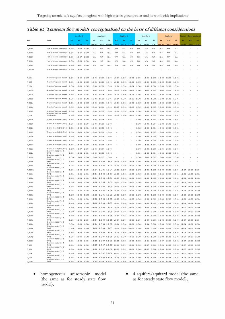
Targeting arsenic-safe aquifers in regions with high arsenic groundwater and its worldwide implications
31
Table 10. Transient flow models conceptualized on the basis of different considerations
• homogeneous anisotropic model (the same as for steady state flow model),
• 4 aquifers/aquitard model (the same as for steady state flow model),
File Type Kh Kv Ss Kh Kv Ss Kh Kv Ss Kh Kv Ss Kh Kv Ss Kh Kv Ss
(m/s) (m/s) (1/m) (m/s) (m/s) (1/m) (m/s) (m/s) (1/m) (m/s) (m/s) (1/m) (m/s) (m/s) (1/m) (m/s) (m/s) (1/m)
T_009b Homogeneous anisotropic 1.E-04 1.E-08 1.E-05 N/A N/A N/A N/A N/A N/A N/A N/A N/A N/A N/A N/A - - -
T_009c Homogeneous anisotropic 1.E-04 1.E-06 1.E-05 N/A N/A N/A N/A N/A N/A N/A N/A N/A N/A N/A N/A - - -
T_009h Homogeneous anisotropic 1.E-04 1.E-07 1.E-05 N/A N/A N/A N/A N/A N/A N/A N/A N/A N/A N/A N/A - - -
T_010c Homogeneous anisotropic 1.E-04 1.E-08 1.E-04 N/A N/A N/A N/A N/A N/A N/A N/A N/A N/A N/A N/A - - -
T_010d Homogeneous anisotropic 1.E-04 1.E-07 1.E-04 N/A N/A N/A N/A N/A N/A N/A N/A N/A N/A N/A N/A - - -
T_012m Homogeneous anisotropic 1.E-05 1.E-08 1.E-04 - - - - - - - - - - - - - - -
T_10e 4 aquifer/aquitard model 1.E-04 1.E-06 1.E-05 1.E-04 1.E-06 1.E-05 1.E-04 1.E-06 1.E-05 1.E-04 1.E-06 1.E-05 2.E-08 2.E-08 1.E-05 - - -
T_10f 4 aquifer/aquitard model 1.E-04 1.E-06 1.E-05 1.E-05 1.E-06 1.E-05 1.E-05 1.E-06 1.E-05 1.E-05 1.E-06 1.E-05 2.E-08 2.E-08 1.E-05 - - -
T_10g 4 aquifer/aquitard model 1.E-04 1.E-06 1.E-03 1.E-04 1.E-06 1.E-04 1.E-04 1.E-06 1.E-04 1.E-04 1.E-06 1.E-04 2.E-08 2.E-08 1.E-04 - - -
T_012b 4 aquifer/aquitard model 1.E-04 1.E-06 1.E-03 1.E-04 1.E-06 1.E-03 1.E-04 1.E-06 1.E-03 1.E-04 1.E-06 1.E-05 1.E-08 1.E-08 1.E-03 - - -
T_012c 4 aquifer/aquitard model 1.E-04 1.E-06 1.E-03 1.E-04 1.E-06 1.E-03 1.E-04 1.E-06 1.E-03 1.E-04 1.E-06 1.E-03 1.E-08 1.E-08 1.E-03 - - -
T_012d 4 aquifer/aquitard model 1.E-04 1.E-06 1.E-05 1.E-04 1.E-06 1.E-05 1.E-04 1.E-06 1.E-05 1.E-05 1.E-08 1.E-05 1.E-08 1.E-08 1.E-05 - - -
T_012e 4 aquifer/aquitard model 1.E-04 1.E-06 1.E-05 1.E-04 1.E-06 1.E-05 1.E-04 1.E-06 1.E-05 1.E-05 1.E-06 1.E-05 1.E-08 1.E-08 1.E-05 - - -
T_012q 4 aquifer/aquitard model 5.E-05 1.E-06 1.E-05 5.E-05 1.E-06 1.E-05 5.E-05 1.E-06 1.E-05 1.E-05 1.E-08 1.E-05 5.E-08 5.E-08 1.E-05 - - -
T_010i 4 aquifer/aquitard model 1.E-04 1.E-05 1.E-04 1.E-04 1.E-05 1.E-04 1.E-04 1.E-05 1.E-04 1.E-04 1.E-05 1.E-05 1.E-09 1.E-09 1.E-05 - - -
T_10h4 aquifer/aquitard model no Meghna 1.E-04 1.E-06 1.E-04 1.E-04 1.E-06 1.E-04 1.E-04 1.E-06 1.E-05 1.E-04 1.E-06 1.E-05 2.E-08 2.E-08 1.E-04 - - -
T_012f 2 layer model (1+2;3+4) 1.E-04 1.E-06 1.E-04 1.E-04 1.E-06 1.E-04 - - - 1.E-05 1.E-08 1.E-04 1.E-04 1.E-06 1.E-04 - - -
T_012h 2 layer model (1+2;3+4) 1.E-04 1.E-06 1.E-04 1.E-04 1.E-06 1.E-04 - - - 1.E-05 1.E-08 1.E-04 1.E-04 1.E-06 1.E-04 - - -
T_012i 2 layer model (1+2;3+4) 1.E-04 1.E-08 1.E-04 1.E-04 1.E-08 1.E-04 - - - 1.E-06 1.E-08 1.E-04 1.E-04 1.E-08 1.E-04 - - -
T_012j 2 layer model (1+2;3+4) 1.E-04 1.E-08 1.E-04 1.E-04 1.E-08 1.E-04 - - - 1.E-06 1.E-08 1.E-05 1.E-04 1.E-08 1.E-04 - - -
T_012k 2 layer model (1+2;3+4) 1.E-05 1.E-08 1.E-04 1.E-05 1.E-08 1.E-04 - - - 1.E-06 1.E-08 1.E-05 1.E-05 1.E-08 1.E-04 - - -
T_012l 2 layer model (1+2;3+4) 1.E-04 1.E-08 1.E-04 1.E-04 1.E-08 1.E-04 - - - 1.E-06 1.E-09 1.E-05 1.E-05 1.E-08 1.E-04 - - -
T_012n 2 layer model (1+2;3+4) 1.E-04 1.E-06 1.E-04 1.E-04 1.E-06 1.E-04 - - - 1.E-06 1.E-08 1.E-04 1.E-04 1.E-06 1.E-04 - - -
T_012o 2 layer model (1+2;3+4) 1.E-05 1.E-07 1.E-04 1.E-05 1.E-07 1.E-04 - - - 1.E-06 1.E-08 1.E-05 1.E-05 1.E-07 1.E-04 - - -
T_012g3 aquifer model (1; 2; 3+4) 1.E-04 1.E-08 1.E-04 1.E-04 1.E-08 1.E-04 - - - 1.E-04 1.E-06 1.E-04 1.E-04 1.E-08 1.E-04 - - -
T_012p3 aquifer model (1; 2; 3+4) 1.E-04 1.E-05 1.E-04 1.E-04 1.E-05 1.E-04 - - - 1.E-04 1.E-05 1.E-05 1.E-09 1.E-09 1.E-04 - - -
T_010k3 aquifer model (1; 2; 3+4) 1.E-04 1.E-06 1.E-04 1.E-04 1.E-06 1.E-04 1.E-05 1.E-05 1.E-05 1.E-05 1.E-05 1.E-05 5.E-09 5.E-09 1.E-04 - - -
T_010l3 aquifer model (1; 2; 3+4) 1.E-04 1.E-06 1.E-04 1.E-04 1.E-06 1.E-04 1.E-05 1.E-05 1.E-05 1.E-05 1.E-05 1.E-05 5.E-09 5.E-09 1.E-04 - - -
T_010m3 aquifer model (1; 2; 3+4) 1.E-04 1.E-06 1.E-04 1.E-04 1.E-06 1.E-04 1.E-05 1.E-05 1.E-05 1.E-05 1.E-05 1.E-05 5.E-09 5.E-09 1.E-04 1.E-07 1.E-07 1.E-04
T_010n3 aquifer model (1; 2; 3+4) 1.E-04 1.E-06 1.E-04 1.E-04 1.E-06 1.E-04 1.E-05 1.E-05 1.E-05 1.E-05 1.E-05 1.E-05 5.E-09 5.E-09 1.E-04 1.E-08 1.E-08 1.E-04
T_010o3 aquifer model (1; 2; 3+4) 1.E-04 1.E-06 1.E-04 1.E-04 1.E-06 1.E-04 1.E-05 1.E-06 1.E-05 1.E-05 1.E-06 1.E-05 5.E-09 5.E-09 1.E-04 1.E-08 1.E-08 1.E-04
T_010p3 aquifer model (1; 2; 3+4) 1.E-04 1.E-06 1.E-04 1.E-06 1.E-06 1.E-05 1.E-06 1.E-06 1.E-05 1.E-06 1.E-06 1.E-05 5.E-09 5.E-09 1.E-04 1.E-08 1.E-08 1.E-04
T_010q3 aquifer model (1; 2; 3+4) 1.E-04 1.E-06 1.E-04 1.E-06 1.E-06 1.E-05 1.E-06 1.E-06 1.E-05 1.E-06 1.E-06 1.E-05 5.E-09 5.E-09 1.E-04 1.E-08 1.E-08 1.E-04
T_010r3 aquifer model (1; 2; 3+4) 1.E-04 1.E-06 1.E-04 1.E-06 1.E-06 1.E-06 1.E-06 1.E-06 1.E-06 1.E-06 1.E-06 1.E-06 5.E-09 5.E-09 1.E-04 1.E-08 1.E-08 1.E-06
T_010s3 aquifer model (1; 2; 3+4) 1.E-05 1.E-05 5.E-05 1.E-05 1.E-05 1.E-05 1.E-05 1.E-05 1.E-05 1.E-05 1.E-05 1.E-05 5.E-09 5.E-09 1.E-04 1.E-08 1.E-08 1.E-05
T_010t3 aquifer model (1; 2; 3+4) 1.E-04 1.E-06 1.E-04 1.E-06 1.E-06 1.E-05 1.E-06 1.E-06 1.E-05 1.E-06 1.E-06 1.E-05 5.E-09 5.E-09 1.E-04 1.E-08 1.E-08 1.E-04
T_010u3 aquifer model (1; 2; 3+4) 1.E-04 1.E-06 1.E-04 1.E-06 1.E-06 1.E-05 1.E-06 1.E-06 1.E-05 1.E-06 1.E-06 1.E-05 5.E-09 5.E-09 1.E-04 1.E-08 1.E-08 1.E-04
T_010v3 aquifer model (1; 2; 3+4) 1.E-05 1.E-05 1.E-04 5.E-04 5.E-04 1.E-05 1.E-04 1.E-04 5.E-06 1.E-04 1.E-04 5.E-06 2.E-08 2.E-08 5.E-06 1.E-07 1.E-07 5.E-06
T_020a3 aquifer model (1; 2; 3+4) 1.E-05 1.E-05 1.E-04 5.E-04 5.E-04 1.E-05 1.E-04 1.E-04 5.E-06 1.E-04 1.E-04 5.E-06 2.E-08 2.E-08 5.E-06 1.E-07 1.E-07 5.E-06
T_020b3 aquifer model (1; 2; 3+4) 1.E-05 1.E-05 1.E-04 1.E-04 1.E-04 1.E-05 1.E-04 1.E-04 5.E-06 1.E-04 1.E-04 5.E-06 2.E-08 2.E-08 5.E-06 1.E-05 1.E-05 5.E-06
T_020c3 aquifer model (1; 2; 3+4) 1.E-04 1.E-06 1.E-04 1.E-04 1.E-04 1.E-05 1.E-04 1.E-04 5.E-06 1.E-04 1.E-04 5.E-06 2.E-08 2.E-08 5.E-06 1.E-07 1.E-07 1.E-04
T_020d3 aquifer model (1; 2; 3+4) 5.E-04 1.E-06 1.E-04 1.E-04 1.E-04 1.E-05 1.E-04 1.E-04 5.E-06 1.E-04 1.E-04 5.E-06 2.E-08 2.E-08 5.E-06 5.E-04 1.E-06 1.E-04
T_020e3 aquifer model (1; 2; 3+4) 5.E-04 1.E-06 1.E-04 1.E-06 1.E-06 1.E-05 1.E-04 1.E-04 5.E-06 1.E-04 1.E-04 5.E-06 2.E-08 2.E-08 5.E-06 5.E-04 1.E-06 1.E-04
T_020f3 aquifer model (1; 2; 3+4) 1.E-04 1.E-06 1.E-04 1.E-05 1.E-05 1.E-05 1.E-05 1.E-05 5.E-06 1.E-05 1.E-05 5.E-06 2.E-08 2.E-08 5.E-06 1.E-04 1.E-06 1.E-04
T_020g3 aquifer model (1; 2; 3+4) 1.E-04 1.E-06 5.E-05 1.E-05 1.E-07 8.E-06 1.E-05 1.E-05 5.E-06 1.E-05 1.E-05 1.E-06 2.E-08 2.E-08 5.E-06 1.E-07 1.E-07 5.E-05
T_020h3 aquifer model (1; 2; 3+4) 1.E-04 1.E-06 1.E-04 1.E-05 1.E-07 8.E-06 8.E-06 1.E-05 5.E-06 5.E-06 1.E-05 1.E-06 1.E-07 1.E-07 5.E-06 1.E-07 1.E-07 5.E-05
T_20i3 aquifer model (1; 2; 3+4) 1.E-04 1.E-06 1.E-04 1.E-05 1.E-07 8.E-06 5.E-06 5.E-07 5.E-06 5.E-06 5.E-07 5.E-06 5.E-08 5.E-08 5.E-06 1.E-07 1.E-07 5.E-05
T_20j3 aquifer model (1; 2; 3+4) 1.E-04 1.E-06 1.E-04 1.E-06 1.E-07 8.E-06 5.E-06 5.E-07 5.E-06 5.E-06 5.E-07 5.E-06 5.E-08 5.E-08 5.E-06 1.E-07 1.E-07 5.E-05
T_20k3 aquifer model (1; 2; 3+4) 1.E-04 1.E-06 1.E-04 1.E-06 1.E-07 5.E-06 5.E-06 5.E-07 1.E-06 5.E-06 5.E-07 1.E-06 5.E-08 5.E-08 5.E-06 1.E-07 1.E-07 5.E-05
T_20l3 aquifer model (1; 2; 3+4) 1.E-04 1.E-06 1.E-04 1.E-06 1.E-08 5.E-05 1.E-05 1.E-06 1.E-05 1.E-05 1.E-06 1.E-05 2.E-08 2.E-08 1.E-05 1.E-06 1.E-06 1.E-04
T_20m3 aquifer model (1; 2; 3+4) 1.E-04 1.E-06 1.E-04 1.E-06 1.E-08 5.E-05 1.E-05 1.E-06 1.E-06 1.E-05 1.E-06 1.E-06 2.E-08 2.E-08 1.E-05 1.E-06 1.E-06 1.E-04
Aquitard Topsoil (if not aquitard)Aquifer 1 Aquifer 2 Aquifer 3 Aquifer 4
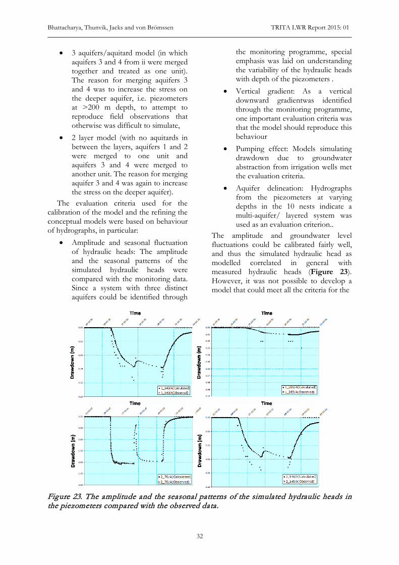
Bhattacharya, Thunvik, Jacks and von Brömssen TRITA LWR Report 2015: 01
32
• 3 aquifers/aquitard model (in which aquifers 3 and 4 from ii were merged together and treated as one unit). The reason for merging aquifers 3 and 4 was to increase the stress on the deeper aquifer, i.e. piezometers at >200 m depth, to attempt to reproduce field observations that otherwise was difficult to simulate,
• 2 layer model (with no aquitards in between the layers, aquifers 1 and 2 were merged to one unit and aquifers 3 and 4 were merged to another unit. The reason for merging aquifer 3 and 4 was again to increase the stress on the deeper aquifer).
The evaluation criteria used for the calibration of the model and the refining the conceptual models were based on behaviour of hydrographs, in particular:
• Amplitude and seasonal fluctuation of hydraulic heads: The amplitude and the seasonal patterns of the simulated hydraulic heads were compared with the monitoring data. Since a system with three distinct aquifers could be identified through
the monitoring programme, special emphasis was laid on understanding the variability of the hydraulic heads with depth of the piezometers .
• Vertical gradient: As a vertical downward gradientwas identified through the monitoring programme, one important evaluation criteria was that the model should reproduce this behaviour
• Pumping effect: Models simulating drawdown due to groundwater abstraction from irrigation wells met the evaluation criteria.
• Aquifer delineation: Hydrographs from the piezometers at varying depths in the 10 nests indicate a multi-aquifer/ layered system was used as an evaluation criterion..
The amplitude and groundwater level fluctuations could be calibrated fairly well, and thus the simulated hydraulic head as modelled correlated in general with measured hydraulic heads (Figure 23). However, it was not possible to develop a model that could meet all the criteria for the
Figure 23. The amplitude and the seasonal patterns of the simulated hydraulic heads in the piezometers compared with the observed data.
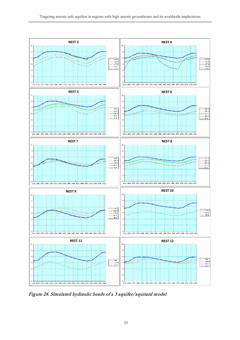
Targeting arsenic-safe aquifers in regions with high arsenic groundwater and its worldwide implications
33
Figure 24. Simulated hydraulic heads of a 3 aquifer/aquitard model
NEST 9
NEST 7 NEST 8
NEST 5 NEST 6
NEST 3 NEST 4
NEST 10
NEST 11 NEST 12
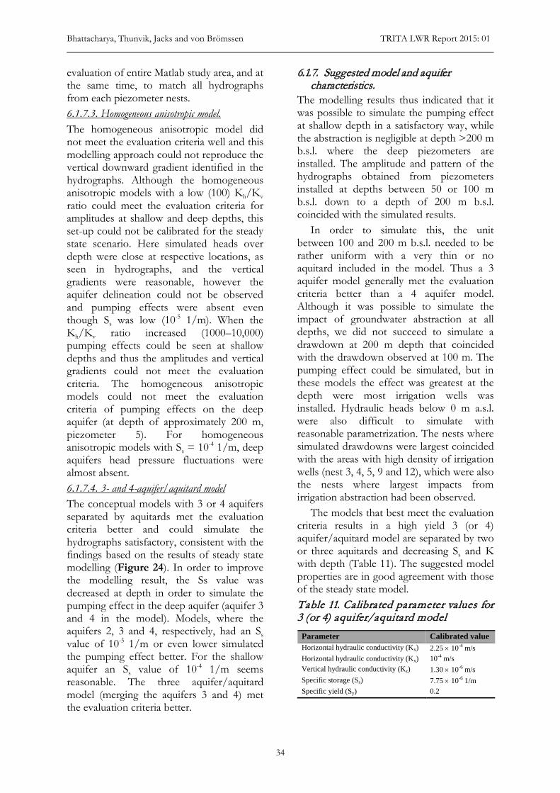
Bhattacharya, Thunvik, Jacks and von Brömssen TRITA LWR Report 2015: 01
34
evaluation of entire Matlab study area, and at the same time, to match all hydrographs from each piezometer nests. 6.1.7.3. Homogeneous anisotropic model. The homogeneous anisotropic model did not meet the evaluation criteria well and this modelling approach could not reproduce the vertical downward gradient identified in the hydrographs. Although the homogeneous anisotropic models with a low (100) Kh/Kv ratio could meet the evaluation criteria for amplitudes at shallow and deep depths, this set-up could not be calibrated for the steady state scenario. Here simulated heads over depth were close at respective locations, as seen in hydrographs, and the vertical gradients were reasonable, however the aquifer delineation could not be observed and pumping effects were absent even though Ss was low (10-5 1/m). When the Kh/Kv ratio increased (1000–10,000) pumping effects could be seen at shallow depths and thus the amplitudes and vertical gradients could not meet the evaluation criteria. The homogeneous anisotropic models could not meet the evaluation criteria of pumping effects on the deep aquifer (at depth of approximately 200 m, piezometer 5). For homogeneous anisotropic models with Ss = 10-4 1/m, deep aquifers head pressure fluctuations were almost absent. 6.1.7.4. 3- and 4-aquifer/aquitard model The conceptual models with 3 or 4 aquifers separated by aquitards met the evaluation criteria better and could simulate the hydrographs satisfactory, consistent with the findings based on the results of steady state modelling (Figure 24). In order to improve the modelling result, the Ss value was decreased at depth in order to simulate the pumping effect in the deep aquifer (aquifer 3 and 4 in the model). Models, where the aquifers 2, 3 and 4, respectively, had an Ss value of 10-5 1/m or even lower simulated the pumping effect better. For the shallow aquifer an Ss value of 10-4 1/m seems reasonable. The three aquifer/aquitard model (merging the aquifers 3 and 4) met the evaluation criteria better.
6.1.7. Suggested model and aquifer characteristics.
The modelling results thus indicated that it was possible to simulate the pumping effect at shallow depth in a satisfactory way, while the abstraction is negligible at depth >200 m b.s.l. where the deep piezometers are installed. The amplitude and pattern of the hydrographs obtained from piezometers installed at depths between 50 or 100 m b.s.l. down to a depth of 200 m b.s.l. coincided with the simulated results.
In order to simulate this, the unit between 100 and 200 m b.s.l. needed to be rather uniform with a very thin or no aquitard included in the model. Thus a 3 aquifer model generally met the evaluation criteria better than a 4 aquifer model. Although it was possible to simulate the impact of groundwater abstraction at all depths, we did not succeed to simulate a drawdown at 200 m depth that coincided with the drawdown observed at 100 m. The pumping effect could be simulated, but in these models the effect was greatest at the depth were most irrigation wells was installed. Hydraulic heads below 0 m a.s.l. were also difficult to simulate with reasonable parametrization. The nests where simulated drawdowns were largest coincided with the areas with high density of irrigation wells (nest 3, 4, 5, 9 and 12), which were also the nests where largest impacts from irrigation abstraction had been observed.
The models that best meet the evaluation criteria results in a high yield 3 (or 4) aquifer/aquitard model are separated by two or three aquitards and decreasing Ss and K with depth (Table 11). The suggested model properties are in good agreement with those of the steady state model. Table 11. Calibrated parameter values for 3 (or 4) aquifer/aquitard model
Parameter Calibrated value Horizontal hydraulic conductivity (Kx) 2.25 × 10⁻⁴ m/s Horizontal hydraulic conductivity (Kx) 10-4 m/s Vertical hydraulic conductivity (Kz) 1.30 × 10⁻⁶ m/s Specific storage (Ss) 7.75 × 10⁻⁶ 1/m Specific yield (Sy) 0.2
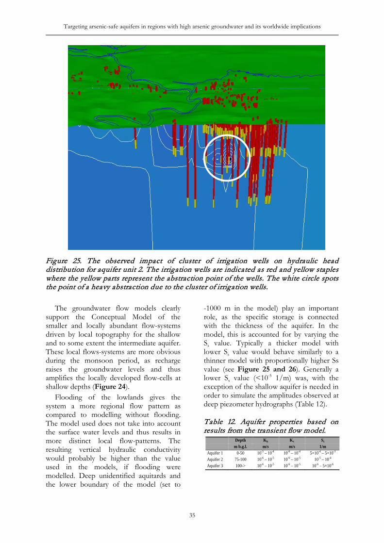
Targeting arsenic-safe aquifers in regions with high arsenic groundwater and its worldwide implications
35
Figure 25. The observed impact of cluster of irrigation wells on hydraulic head distribution for aquifer unit 2. The irrigation wells are indicated as red and yellow staples where the yellow parts represent the abstraction point of the wells. The white circle spots the point of a heavy abstraction due to the cluster of irrigation wells.
The groundwater flow models clearly support the Conceptual Model of the smaller and locally abundant flow-systems driven by local topography for the shallow and to some extent the intermediate aquifer. These local flows-systems are more obvious during the monsoon period, as recharge raises the groundwater levels and thus amplifies the locally developed flow-cells at shallow depths (Figure 24).
Flooding of the lowlands gives the system a more regional flow pattern as compared to modelling without flooding. The model used does not take into account the surface water levels and thus results in more distinct local flow-patterns. The resulting vertical hydraulic conductivity would probably be higher than the value used in the models, if flooding were modelled. Deep unidentified aquitards and the lower boundary of the model (set to
-1000 m in the model) play an important role, as the specific storage is connected with the thickness of the aquifer. In the model, this is accounted for by varying the Ss value. Typically a thicker model with lower Ss value would behave similarly to a thinner model with proportionally higher Ss value (see Figure 25 and 26). Generally a lower Ss value (<10-5 1/m) was, with the exception of the shallow aquifer is needed in order to simulate the amplitudes observed at deep piezometer hydrographs (Table 12).
Table 12. Aquifer properties based on results from the transient flow model.
Depth Kh Kv Ss m b.g.l. m/s m/s 1/m Aquifer 1 0-50 10-5 – 10-4 10-6 – 10-4 5×10⁻⁴ – 5×10⁻³
Aquifer 2 75-100 10-6 – 10-5 10-6 – 10-5 10-5 – 10-4 Aquifer 3 100-> 10-6 – 10-5 10-6 – 10-5 10-6 – 5×10⁻⁶
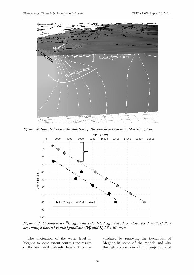
Bhattacharya, Thunvik, Jacks and von Brömssen TRITA LWR Report 2015: 01
36
Figure 26. Simulation results illustrating the two flow system in Matlab region.
Figure 27. Groundwater 14C age and calculated age based on downward vertical flow assuming a natural vertical gradient (1%) and Kv 1.5 x 10⁻⁸ m/s.
The fluctuation of the water level in Meghna to some extent controls the results of the simulated hydraulic heads. This was
validated by removing the fluctuation of Meghna in some of the models and also through comparison of the amplitudes of
MatlabR. Meghna Local flow zone
Regional flow
0
10
20
30
40
50
60
70
80
90
100
0 2000 4000 6000 8000 10000 12000 14000 16000 18000
Age (yr BP)
Dep
th (
m.b
.g.l
)
14C age Calculated
Targeting arsenic-safe aquifers in regions with high arsenic groundwater and its worldwide implications
37
hydraulic heads at depth. In models where the hydrographs at depth were flat, the corresponding field data from deep piezometer in nest 11 showed fluctuating water levels due to its close proximity to Meghna.
6.1.8. Linking the modelling results with groundwater age
The 14C-activity in the groundwater samples varied from 23 to 86 pMC (percent modern carbon), d13C values ranged between -19.6‰ and -13.1‰. The corrected groundwater age is linearly correlated with the depth of tube wells and the groundwater samples were old; ages 1250–11 960 yr indicate restricted groundwater flow at depth below 30 m. The estimated groundwater ages at the depth of 40 m (6100 yr) coincided with the estimated age of sediments at the depth of 36 m in the area (8000 yr; von Brömssen et al. 2008). The groundwater ages also coincide with the findings of Aggarwal et al. (2000) and Hoque (2010) (Figure 27 and Table 12).
Table 13. 14C-activity and δ13C values for tubewells samples
When measured and calculated ages are
compared, the measured vertical gradient of 0.01 and the vertical hydraulic conductivity (Kv) of 1.5 x 10⁻⁸ m/s fit the slope of the 14C-age of groundwater with depth (Figure 27). If 14C ages are extrapolated young groundwater would be expected at a depth of approximately 25 m b.g.l., which coincides with the depth of the previously described local flow-systems (Table 13).
6.2. Hydrogeochemical characteristics 6.2.1. On-site field parameters The physico-chemical parameters of the groundwater samples collected from black, white, off-white, and white group of
sediments are presented in Table 14. In general, groundwater temperatures are typically within the range of 25.7 to 29.6°C.
Groundwater pH was essentially circum-neutral ranging from 6.32 to 7.84 (Figure 28a). Higher pH values are found in samples derived from black sediments containing higher levels of As. This is because the black sediments representing the most reducing environment where H+ has consumed through the reduction of iron, manganese, and ammonium. The median values of redox potential (Eh) in groundwater derived from black, white, off-white, and red sediments were 211.5, 227, 268, and 274 mV respectively which indicate that the black group of sediments are most reduced, followed by white, off-white, and red sediments (Figure 28b). The electrical conductivity (EC) of all water samples reveals high values regardless of corresponding sediment colors. This is may be due to the presence of high Na+ and Cl– in groundwater samples. However, the highest median value of 1630 μS/cm observed in samples screened from red sediments (Table 14, Figure 28c).
6.2.2. Major ion characteristics Salient chemical composition of the groundwater screened at four different color groups of the aquifer sediments is summarized in Table 15.
Sodium (Na+) and Chloride (Cl–) ion concentrations of the groundwater samples surpassed all major ion concentrations regardless of the depth of sampling (Table 15). Water samples collected from the red (R) sediments show the highest Na+ (median: ≈355 mg/L) and Cl– (median: ≈463 mg/L) concentrations, followed by Na+ and Cl– concentrations observed in water samples screened from off-white (OW), white (W), and Black (B) sediments (Figure 29a-b). Because the red and off-white sediments are mostly targeted for groundwater withdrawal from these sediments along with water level decline might result in changed water circulation pattern and induce saline water to move from the surrounding clay/shale layers to
Tubewell Depth 14C-activity δ13C Estimated age No m pMC ‰ yr 54 26 85.89 ± 0.45 -17.6 1 250 ± 65 37 40 47.23 ± 0.30 -17.3 6 100± 65 32 49 53.26 ± 0.34 -13.1 5 095 ± 65 58 58 36.80 ± 0.28 -17.6 8 065 ± 65 63 69 28.98 ± 0.25 -19.6 10 865 ± 80 35 80 22.67 ± 0.23 -12.9 11 960 ± 80
Bhattacharya, Thunvik, Jacks and von Brömssen TRITA LWR Report 2015: 01
38
Table 14. Physico-chemical parameters of the groundwater samples collected from black, white, off-white, and red group of sediments
Figure 28. Box and Whiskers plot showing the variability of pH, Eh and SEC in groundwater samples from the fore sediment groups, black (B), white(W), off-white (OW) and red (R).
Physico-chemical parameter
sediment colors Minm Maxm Average Q25 Q50 Q75
Temperature Black 25.7 29.5 26.95 26.6 26.8 27.275
(°C) White 26.2 29.1 27.39 26.85 27.2 27.95
Off-white 26.2 29.4 27.43 26.925 27.25 27.775
Red 26.2 29.6 27.30 26.6 27.2 27.7
pH Black 6.32 7.3 6.91 – – –
White 6.34 7.84 6.77 – – –
Off-white 6.35 7.03 6.61 – – –
Red 6.34 7.35 6.69 – – –
Eh Black 147 339 226.67 196.75 211.5 268.25
(mV) White 168 280 229.11 199 227 267.5
Off-white 167 342 255.43 228 268 279.75
Red 191 322 280.32 259 274 311
Electrical Conductivity Black 300 5330 1201.73 610 960 1400
(μS/cm) White 260 4170 1423.33 770 1245 1717.5
Off-white 460 6190 1374.82 805 1025 1705
Red 500 3810 1667.06 870 1630 2050
a b
c
Sediment Color Sediment Color
Sediment Color
pH
Eh(m
V)
EC (µ
S/cm
)
Targeting arsenic-safe aquifers in regions with high arsenic groundwater and its worldwide implications
39
Table 15 Summary of the major ion composition of groundwater samples with corresponding sediment colors encountered at screen depths
the sandy sequences resulting an additional increase in salinity.
Water samples collected from the black sediments contain very high bicarbonate (HCO3
-) concentrations (median: 424 mg/L) (Figure 29c) due to the presence of high organic content in the black sediments (eqn. 2). Water samples screened from white, off-white, and red sediments contain significantly low (almost half of that of black) HCO3
- concentrations (Table 15). High HCO3
- concentrations in water samples derived from black sediments can
also be attributed to carbonate dissolution. Carbonate (CO3
2-) ions produced from calcite/dolomite dissolution associate with available hydrogen ions (H+) of the anoxic groundwater system to form HCO3
¯ (eqn. 3). High HCO3
- concentrations in the black sediments can also be attributed to sulfate (SO4
2-) reduction (eqn. 4). 8FeOOH + CH3COOH + 14H2CO3 8Fe2+ + 16HCO3
¯ + 12H2O ……… (eqn. 2) CaCO3 Ca2+ + CO3
2- …………....(eqn. 3)
Parameter Color Min Max Average Q25 Q50 Q75 As (total) Black 2.8 968 273 83 252.5 397 (μg/L) White 8.8 359 68.6 15.2 20.3 51.8
Off-white 5.0 94 27.2 11.8 17.4 37.9
Red 2.8 35.5 16.6 12.9 15.1 18.9 Fe (total) Black 0.22 13.3 5.8 2.86 4.87 8.21 (mg/L) White 0.11 12.9 3.9 1.86 2.94 5.00
Off-white 0.07 11.0 3.1 0.21 2.25 3.68
Red 0.12 14.3 2.1 0.41 0.63 1.79 NH4
+ Black 0 42.7 5.69 1.55 3.47 6.14 (mg/L) White 0 8.6 1.86 0.06 0.37 1.94
Off-white 0 52.3 2.89 0 0 0.43
Red 0 2.75 0.45 0 0 0.36 PO4
3- Black 0.05 4.52 1.54 0.65 1.36 1.99 (mg/L) White 0.04 2.75 0.65 0.14 0.29 0.68
Off-white 0.03 6.29 0.60 0.04 0.14 0.46
Red 0.01 1.20 0.18 0.03 0.04 0.11 Mn2+ Black 0.05 2.92 0.73 0.19 0.54 1.04 (mg/L) White 0.02 1.30 0.29 0.09 0.19 0.28
Off-white 0.04 3.16 1.32 0.20 1.12 1.88
Red 0.04 4.82 1.71 0.74 1.54 2.47 NO3
– Black 0.05 2.00 0.23 0.05 0.05 0.28 mg/L White 0.05 0.52 0.072 0.05 0.05 0.03
Off-white 0.05 0.41 0.032 0.05 0.05 0.05
Red 0.05 2.083 0.22 0.05 0.05 0.05 DOC Black 1.42 23.23 7 4.16 5.81 8.04 mg/L White 1.28 18.78 4.14 2 2.96 3.68
Off-white 1.20 25.41 3.82 1.33 1.95 4.32
Red 1.14 39.11 4.04 1.35 1.71 1.92
Bhattacharya, Thunvik, Jacks and von Brömssen TRITA LWR Report 2015: 01
40
Figure 29. Box and Whiskers plot showing the variability of a) Na+, b) Cl-, c) HCO3
-, d) SO4
2-, e) K+, and f) Ca2+ in groundwater samples from the four sediment groups, black (B), white(W), off-white (OW) and red (R). CH2O+½ SO4
2- ½H2S + HCO3-...(eqn. 4)
In compliance with eqn. 3, comparatively lower levels of SO4
2- can be observed in
groundwater samples derived from black and white sediments (median: ≈0.5 mg/L) than that derived from red and off-white sediments with a median value of ≈0.8 mg/L
(Figure 29d) which validate the existence of a more reducing environment in the black/white sediments than in red/off-white sediments. However, high molar ratio of Cl–/SO4
2- due to elevated Cl– concentrations in groundwater also indicates sulfate reduction.
High concentrations (median: 5.26 mg/L; (Figure 29e) of potassium (K+) in the groundwater samples screened from black sediments may be due to the predominance
Targeting arsenic-safe aquifers in regions with high arsenic groundwater and its worldwide implications
41
of clay layers (K-feldspars alters to silica, clay, and K+ as it interacts with groundwater) within the top 40 to 50 meter of the aquifer sequence. Weathering of biotite can be one of the major sources of not only Fe-oxyhydroxides which play a significant role in the process of As mobilization (Hasan et al. 2009) in the black sediments, but also a source of high K+ (eqn. 5).
2KFe3AlSi3O10(OH)2 (biotite)+14H+ +H2O 2K+ + 6Fe2+ + 4H4SiO4
0 + Al2Si2O5(OH)4 (kaolinite)………..…(eqn. 5)
Another source of high K+ in black sediments could be the K+ assimilated by plants becoming available following the decomposition of plant remains at the end of the growing season (Hem 1985). In the natural recycling that occurs in the croplands at Matlab, this potassium might be leached
into the soil by rains during the dormant season or made available by the gradual decay of the organic material. Some leakage of potassium to the shallow ground water could be possible in this way. Though no significant trend can be observed in Mg2+ concentrations (median: ≈25 mg/L) within the groundwater samples collected from the four color-classified sediment groups, Ca2+ concentrations in water samples derived from black sediments is significantly higher (median: 87 mg/L) than that in water samples collected from white (median: 49 mg/L), off-white (median: 64 mg/L), or red (median: 66.4 mg/L) sediments (Figure 29f). This can be attributed to dissolution of calcite or other carbonate minerals (eqn. 2); which has been identified as one of the sources of high HCO3
- concentrations in groundwaters abstracted from the black sediments.
Figure 30. Spatial distribution of major ions in individual groundwater samples collected from the study area represented by circular diagrams. Sampling depth is mentioned at the center of each pie diagram).
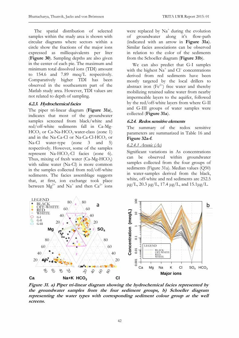
Bhattacharya, Thunvik, Jacks and von Brömssen TRITA LWR Report 2015: 01
42
The spatial distribution of selected samples within the study area is shown with circular diagrams where sectors within a circle show the fractions of the major ions expressed as milliequivalents per liter (Figure 30). Sampling depths are also given in the center of each pie. The maximum and minimum total dissolved ions (TDI) amount to 154.6 and 7.89 meq/L respectively. Comparatively higher TDI has been observed in the southeastern part of the Matlab study area. However, TDI values are not related to depth of sampling.
6.2.3. Hydrochemical facies The piper tri-linear diagram (Figure 31a), indicates that most of the groundwater samples screened from black/white and red/off-white sediments fall in Ca-Mg-HCO3 or Ca-Na-HCO3 water-class (zone 1) and in the Na-Ca-Cl or Na-Ca-Cl-HCO3 or Na-Cl water-type (zone 3 and 5) respectively. However, some of the samples represent Na-HCO3-Cl facies (zone 6). Thus, mixing of fresh water (Ca-Mg-HCO3) with saline water (Na-Cl) is more common in the samples collected from red/off-white sediments. The facies assemblage suggests that, at first, ion exchange took place between Mg2+ and Na+ and then Ca2+ ions
were replaced by Na+ during the evolution of groundwater along it’s flow-path (indicated with an arrow in Figure 31a). Similar facies associations can be observed in relation to the color of the sediments from the Schoeller diagram (Figure 31b).
We can also predict that G-I samples with the highest Na+ and Cl– concentrations derived from red sediments have been mostly targeted by the local drillers to abstract iron (Fe2+) free water and thereby mobilizing retained saline water from nearby impermeable layers to the aquifer, followed by the red/off-white layers from where G-II and G-III groups of water samples were collected (Figure 31a).
6.2.4. Redox sensitive elements The summary of the redox sensitive parameters are summarized in Table 16 and Figure 32a-f. 6.2.4.1 Arsenic (As) Significant variations in As concentrations can be observed within groundwater samples collected from the four groups of sediments (Figure 31a). Median values (Q50) in water-samples derived from the black, white, off-white and red sediments are 252.5 μg/L, 20.3 μg/L, 17.4 μg/L, and 15.1μg/L.
Figure 31. a) Piper tri-linear diagram showing the hydrochemical facies represented by the groundwater samples from the four sediment groups, b) Schoeller diagram representing the water types with corresponding sediment colour group at the well screens.
LEGEND80 60 40 20 20 40 60 80
20
40
60
80 80
60
40
20
20
40
60
80
20
40
60
80
Ca Na+K HCO3 Cl
Mg SO4
N
N
N
N
N
N
N
N
N
NN
N
NN
N
N
N
N
N
N
N
NN
N
NN
N
N
N
N
N
N
N
N
N
N
NN
N
N
N
N
N
N
N
N
N
N
NN
N
NN
N
N
N
N
N
N
N
N
N
N
N
N
N
N
N
N
N
N
N
NN
N
N
N
N
N
N
N
N
N
N
N
N
N
N
N
N
N
N
N
N
N
N
N
N
N
N
N
N
N
N
N
N
N
N
N
N
N
N
N
N
N
N
N
N
N
N
N
N
N
N
N
N
N
N
N
N
N
N
N
N
N
DD
D
D
D
D
D
D
D
D
D
D
D
D
D
D
D
D
D
D
D
D
D
D
D
D
D
D
D
D
DD
D
DD
D
D
D
D
DD
D
D
D
D
D
D
D
D
D
D
D
D
D
D
D
D
DD
D
D
D
D
J
J
J
J
J
J
J
J
J
JJ
J
J
J
J
JJ
J
JJ
J
JJ
J
JJ
J
JJ
J
JJ
J
J
J
J
J
J
J
J
J
J
JJ
J
JJ
J
JJ
J
J
J
J
J
J
J
J
J
J
J
J
J
JJ
J
J
J
J
JJ
J
JJ
J
J
J
J
JJ
J
J
J
J
A
A
A
A
A
A
AA
A
A
A
A
A
A
A
A
A
A
AA
A
A
A
A
A A
A
A
A
A
AA
A
A
A
A
A
A
A
A
A
A
A A
A
A
A
A
A
A
A
A
A
A
N BLACKD OFF-WHITEJ REDA WHITE
1
2
3
4
5
6
G-I
G-IIIG-II
(a)
Ca Mg Na K Cl SO4 HCO3
Major ions
0
0
0
1
10
100
Con
cent
rati o
n (m
eq/l
)100
10
10.1
0.01
0.001
LE
WHITE
Major ions
BLACKOFF-WHITEREDWHITE
LEGEND
Na+K
Mg
Ca Na+K HCO3 Cl
a b
Con
cent
ratio
n(m
eq/L
)
SO4
Ca Mg Na K Cl SO4 HCO3
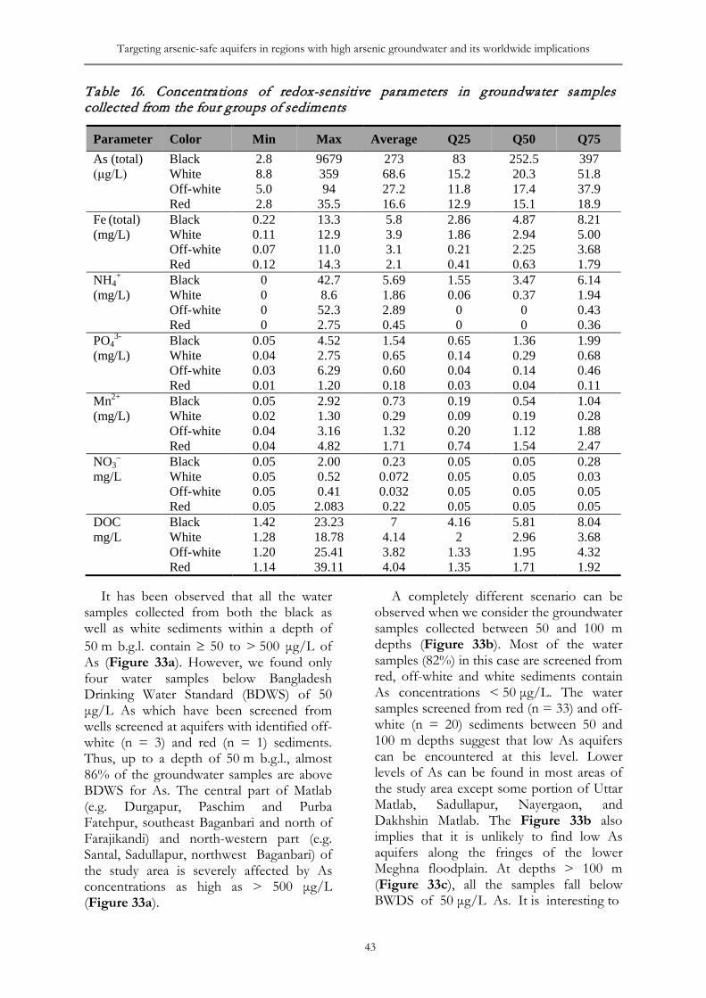
Targeting arsenic-safe aquifers in regions with high arsenic groundwater and its worldwide implications
43
Table 16. Concentrations of redox-sensitive parameters in groundwater samples collected from the four groups of sediments
It has been observed that all the water
samples collected from both the black as well as white sediments within a depth of 50 m b.g.l. contain ≥ 50 to > 500 μg/L of As (Figure 33a). However, we found only four water samples below Bangladesh Drinking Water Standard (BDWS) of 50 μg/L As which have been screened from wells screened at aquifers with identified off-white (n = 3) and red (n = 1) sediments. Thus, up to a depth of 50 m b.g.l., almost 86% of the groundwater samples are above BDWS for As. The central part of Matlab (e.g. Durgapur, Paschim and Purba Fatehpur, southeast Baganbari and north of Farajikandi) and north-western part (e.g. Santal, Sadullapur, northwest Baganbari) of the study area is severely affected by As concentrations as high as > 500 μg/L (Figure 33a).
A completely different scenario can be observed when we consider the groundwater samples collected between 50 and 100 m depths (Figure 33b). Most of the water samples (82%) in this case are screened from red, off-white and white sediments contain As concentrations < 50 μg/L. The water samples screened from red (n = 33) and off-white (n = 20) sediments between 50 and 100 m depths suggest that low As aquifers can be encountered at this level. Lower levels of As can be found in most areas of the study area except some portion of Uttar Matlab, Sadullapur, Nayergaon, and Dakhshin Matlab. The Figure 33b also implies that it is unlikely to find low As aquifers along the fringes of the lower Meghna floodplain. At depths > 100 m (Figure 33c), all the samples fall below BWDS of 50 μg/L As. It is interesting to
Parameter Color Min Max Average Q25 Q50 Q75 As (total) Black 2.8 9679 273 83 252.5 397 (μg/L) White 8.8 359 68.6 15.2 20.3 51.8
Off-white 5.0 94 27.2 11.8 17.4 37.9
Red 2.8 35.5 16.6 12.9 15.1 18.9 Fe (total) Black 0.22 13.3 5.8 2.86 4.87 8.21 (mg/L) White 0.11 12.9 3.9 1.86 2.94 5.00
Off-white 0.07 11.0 3.1 0.21 2.25 3.68
Red 0.12 14.3 2.1 0.41 0.63 1.79 NH4
+ Black 0 42.7 5.69 1.55 3.47 6.14 (mg/L) White 0 8.6 1.86 0.06 0.37 1.94
Off-white 0 52.3 2.89 0 0 0.43
Red 0 2.75 0.45 0 0 0.36 PO4
3- Black 0.05 4.52 1.54 0.65 1.36 1.99 (mg/L) White 0.04 2.75 0.65 0.14 0.29 0.68
Off-white 0.03 6.29 0.60 0.04 0.14 0.46
Red 0.01 1.20 0.18 0.03 0.04 0.11 Mn2+ Black 0.05 2.92 0.73 0.19 0.54 1.04 (mg/L) White 0.02 1.30 0.29 0.09 0.19 0.28
Off-white 0.04 3.16 1.32 0.20 1.12 1.88
Red 0.04 4.82 1.71 0.74 1.54 2.47 NO3
– Black 0.05 2.00 0.23 0.05 0.05 0.28 mg/L White 0.05 0.52 0.072 0.05 0.05 0.03
Off-white 0.05 0.41 0.032 0.05 0.05 0.05
Red 0.05 2.083 0.22 0.05 0.05 0.05 DOC Black 1.42 23.23 7 4.16 5.81 8.04 mg/L White 1.28 18.78 4.14 2 2.96 3.68
Off-white 1.20 25.41 3.82 1.33 1.95 4.32
Red 1.14 39.11 4.04 1.35 1.71 1.92
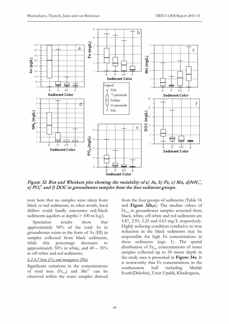
Bhattacharya, Thunvik, Jacks and von Brömssen TRITA LWR Report 2015: 01
44
Figure 32. Box and Whiskers plot showing the variability of a) As, b) Fe, c) Mn, d)NH 4
+, e) PO4
3- and f) DOC in groundwater samples from the four sediment groups. note here that no samples were taken from black or red sediments; in other words, local drillers could hardly encounter red/black sediments aquifers at depths > 100 m b.g.l.
Speciation results show that approximately 90% of the total As in groundwater exists in the form of As (III) in samples collected from black sediments, while this percentage decreases to approximately 50% in white, and 40 – 35% in off-white and red sediments. 6.2.4.2 Iron (Fe) and manganese (Mn) Significant variations in the concentrations of total iron (Fetot) and Mn2+ can be observed within the water samples derived
from the four groups of sediments (Table 16 and Figure 32b,c). The median values of Fetot in groundwater samples screened from black, white, off-white and red sediments are 4.87, 2.93, 2.25 and 0.63 mg/L respectively. Highly reducing condition conducive to iron reduction in the black sediments may be responsible for high Fe concentrations in these sediments (eqn. 1). The spatial distribution of Fetot concentrations of water samples collected up to 50 meter depth in the study area is presented in Figure 34a. It is noteworthy that Fe concentrations in the southeastern half including Matlab South(Dakshin), Uttar Upaldi, Khadergaon,
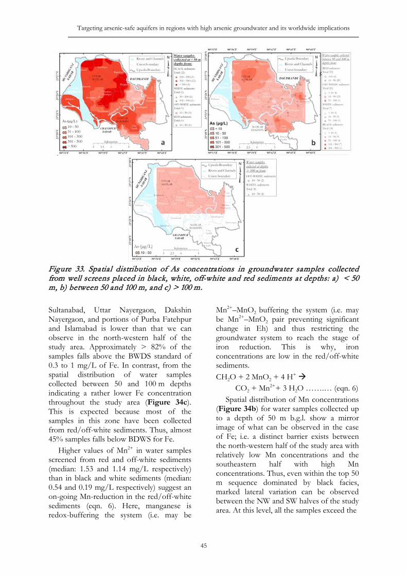
Targeting arsenic-safe aquifers in regions with high arsenic groundwater and its worldwide implications
45
Figure 33. Spatial distribution of As concentrations in groundwater samples collected from well screens placed in black, white, off-white and red sediments at depths: a) < 50 m, b) between 50 and 100 m, and c) > 100 m. Sultanabad, Uttar Nayergaon, Dakshin Nayergaon, and portions of Purba Fatehpur and Islamabad is lower than that we can observe in the north-western half of the study area. Approximately > 82% of the samples falls above the BWDS standard of 0.3 to 1 mg/L of Fe. In contrast, from the spatial distribution of water samples collected between 50 and 100 m depths indicating a rather lower Fe concentration throughout the study area (Figure 34c). This is expected because most of the samples in this zone have been collected from red/off-white sediments. Thus, almost 45% samples falls below BDWS for Fe.
Higher values of Mn2+ in water samples screened from red and off-white sediments (median: 1.53 and 1.14 mg/L respectively) than in black and white sediments (median: 0.54 and 0.19 mg/L respectively) suggest an on-going Mn-reduction in the red/off-white sediments (eqn. 6). Here, manganese is redox-buffering the system (i.e. may be
Mn2+–MnO2 buffering the system (i.e. may be Mn2+–MnO2 pair preventing significant change in Eh) and thus restricting the groundwater system to reach the stage of iron reduction. This is why, iron concentrations are low in the red/off-white sediments. CH2O + 2 MnO2 + 4 H+
CO2 + Mn2++ 3 H2O …….… (eqn. 6) Spatial distribution of Mn concentrations
(Figure 34b) for water samples collected up to a depth of 50 m b.g.l. show a mirror image of what can be observed in the case of Fe; i.e. a distinct barrier exists between the north-western half of the study area with relatively low Mn concentrations and the southeastern half with high Mn concentrations. Thus, even within the top 50 m sequence dominated by black facies, marked lateral variation can be observed between the NW and SW halves of the study area. At this level, all the samples exceed the
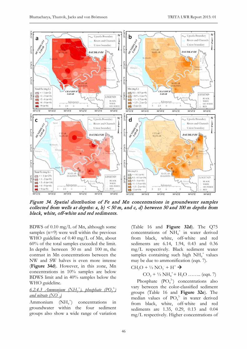
Bhattacharya, Thunvik, Jacks and von Brömssen TRITA LWR Report 2015: 01
46
Figure 34. Spatial distribution of Fe and Mn concentrations in groundwater samples collected from wells at depths: a, b) < 50 m, and c, d) between 50 and 100 m depths from black, white, off-white and red sediments.
BDWS of 0.10 mg/L of Mn, although some samples (n=9) were well within the previous WHO guideline of 0.40 mg/L of Mn, about 60% of the total samples exceeded the limit. In depths between 50 m and 100 m, the contrast in Mn concentrations between the NW and SW halves is even more intense (Figure 34d). However, in this zone, Mn concentrations in 10% samples are below BDWS limit and in 40% samples below the WHO guideline. 6.2.4.3 Ammonium (NH4
+), phosphate (PO43-)
and nitrate (NO¯3)
Ammonium (NH4+) concentrations in
groundwater within the four sediment groups also show a wide range of variation
(Table 16 and Figure 32d). The Q75 concentrations of NH4
+ in water derived from black, white, off-white and red sediments are 6.14, 1.94, 0.43 and 0.36 mg/L respectively. Black sediment water samples containing such high NH4
+ values may be due to ammonification (eqn. 7). CH2O + ½ NO3
- + H+ CO2 + ½ NH4
++ H2O …….. (eqn. 7) Phosphate (PO4
3-) concentrations also vary between the color-classified sediment groups (Table 16 and Figure 32e). The median values of PO4
3- in water derived from black, white, off-white and red sediments are 1.35, 0.29, 0.13 and 0.04 mg/L respectively. Higher concentrations of
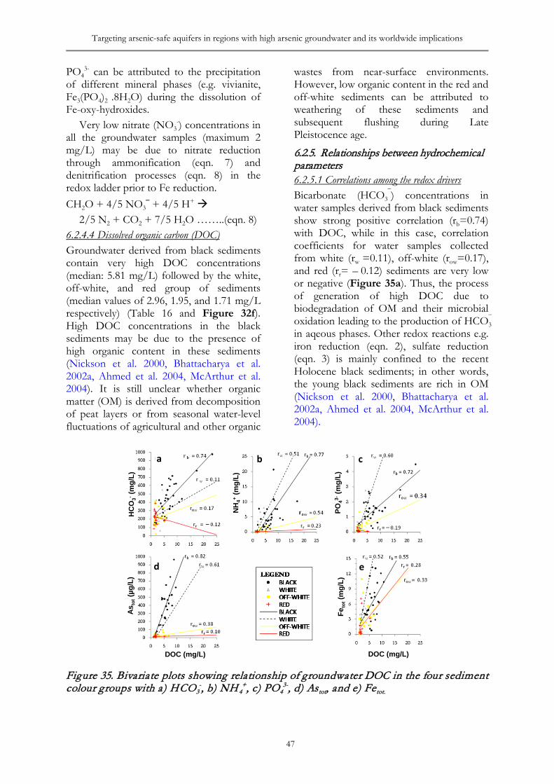
Targeting arsenic-safe aquifers in regions with high arsenic groundwater and its worldwide implications
47
PO43- can be attributed to the precipitation
of different mineral phases (e.g. vivianite, Fe3(PO4)2 .8H2O) during the dissolution of Fe-oxy-hydroxides.
Very low nitrate (NO3-) concentrations in
all the groundwater samples (maximum 2 mg/L) may be due to nitrate reduction through ammonification (eqn. 7) and denitrification processes (eqn. 8) in the redox ladder prior to Fe reduction. CH2O + 4/5 NO3
– + 4/5 H+ 2/5 N2 + CO2 + 7/5 H2O ……..(eqn. 8)
6.2.4.4 Dissolved organic carbon (DOC) Groundwater derived from black sediments contain very high DOC concentrations (median: 5.81 mg/L) followed by the white, off-white, and red group of sediments (median values of 2.96, 1.95, and 1.71 mg/L respectively) (Table 16 and Figure 32f). High DOC concentrations in the black sediments may be due to the presence of high organic content in these sediments (Nickson et al. 2000, Bhattacharya et al. 2002a, Ahmed et al. 2004, McArthur et al. 2004). It is still unclear whether organic matter (OM) is derived from decomposition of peat layers or from seasonal water-level fluctuations of agricultural and other organic
wastes from near-surface environments. However, low organic content in the red and off-white sediments can be attributed to weathering of these sediments and subsequent flushing during Late Pleistocence age.
6.2.5. Relationships between hydrochemical parameters 6.2.5.1 Correlations among the redox drivers Bicarbonate (HCO3
¯) concentrations in water samples derived from black sediments show strong positive correlation (rb=0.74) with DOC, while in this case, correlation coefficients for water samples collected from white (rw =0.11), off-white (row=0.17), and red (rr= – 0.12) sediments are very low or negative (Figure 35a). Thus, the process of generation of high DOC due to biodegradation of OM and their microbial oxidation leading to the production of HCO3
¯ in aqeous phases. Other redox reactions e.g. iron reduction (eqn. 2), sulfate reduction (eqn. 3) is mainly confined to the recent Holocene black sediments; in other words, the young black sediments are rich in OM (Nickson et al. 2000, Bhattacharya et al. 2002a, Ahmed et al. 2004, McArthur et al. 2004).
Figure 35. Bivariate plots showing relationship of groundwater DOC in the four sediment colour groups with a) HCO3
-, b) NH 4+, c) PO4
3-, d) Astot, and e) Fetot.
a b c
e
DOC (mg/L)DOC (mg/L)
PO43-
(mg/
L)
HC
O3-
(mg/
L)
NH
4+(m
g/L)
Asto
t(µ
g/L)
Feto
t(m
g/L)
d
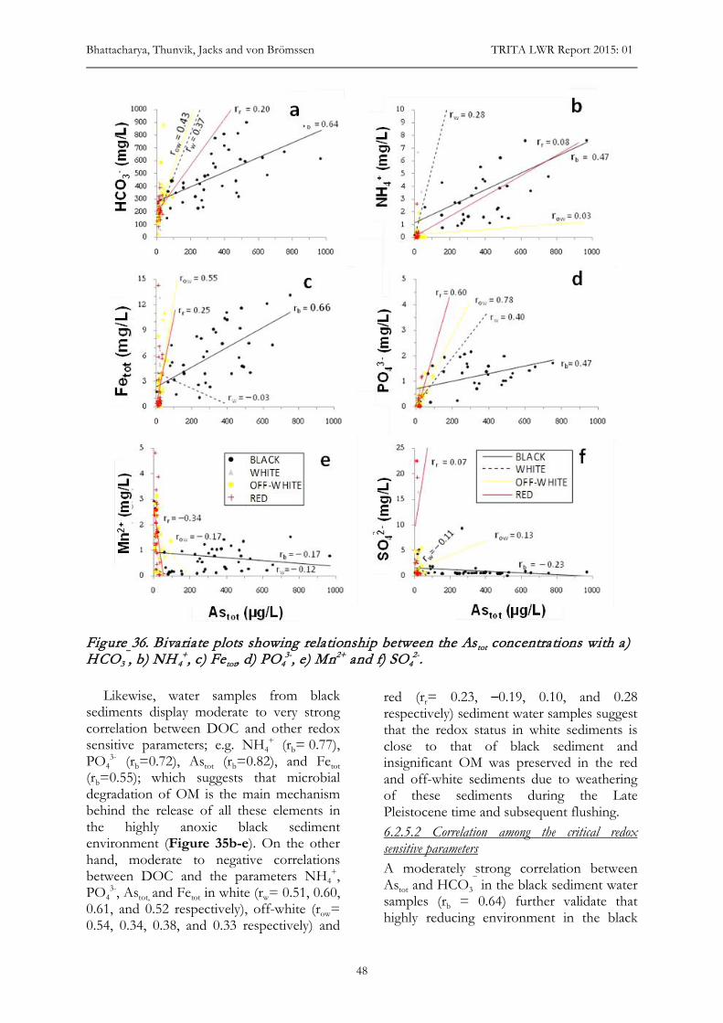
Bhattacharya, Thunvik, Jacks and von Brömssen TRITA LWR Report 2015: 01
48
Figure 36. Bivariate plots showing relationship between the Astot concentrations with a) HCO3
¯, b) NH 4+, c) Fetot, d) PO4
3-, e) Mn2+ and f) SO42-.
Likewise, water samples from black
sediments display moderate to very strong correlation between DOC and other redox sensitive parameters; e.g. NH4
+ (rb= 0.77), PO4
3- (rb=0.72), Astot (rb=0.82), and Fetot (rb=0.55); which suggests that microbial degradation of OM is the main mechanism behind the release of all these elements in the highly anoxic black sediment environment (Figure 35b-e). On the other hand, moderate to negative correlations between DOC and the parameters NH4
+, PO4
3-, Astot, and Fetot in white (rw= 0.51, 0.60, 0.61, and 0.52 respectively), off-white (row= 0.54, 0.34, 0.38, and 0.33 respectively) and
red (rr= 0.23, –0.19, 0.10, and 0.28 respectively) sediment water samples suggest that the redox status in white sediments is close to that of black sediment and insignificant OM was preserved in the red and off-white sediments due to weathering of these sediments during the Late Pleistocene time and subsequent flushing. 6.2.5.2 Correlation among the critical redox sensitive parameters A moderately strong correlation between Astot and HCO3
¯ in the black sediment water samples (rb = 0.64) further validate that highly reducing environment in the black
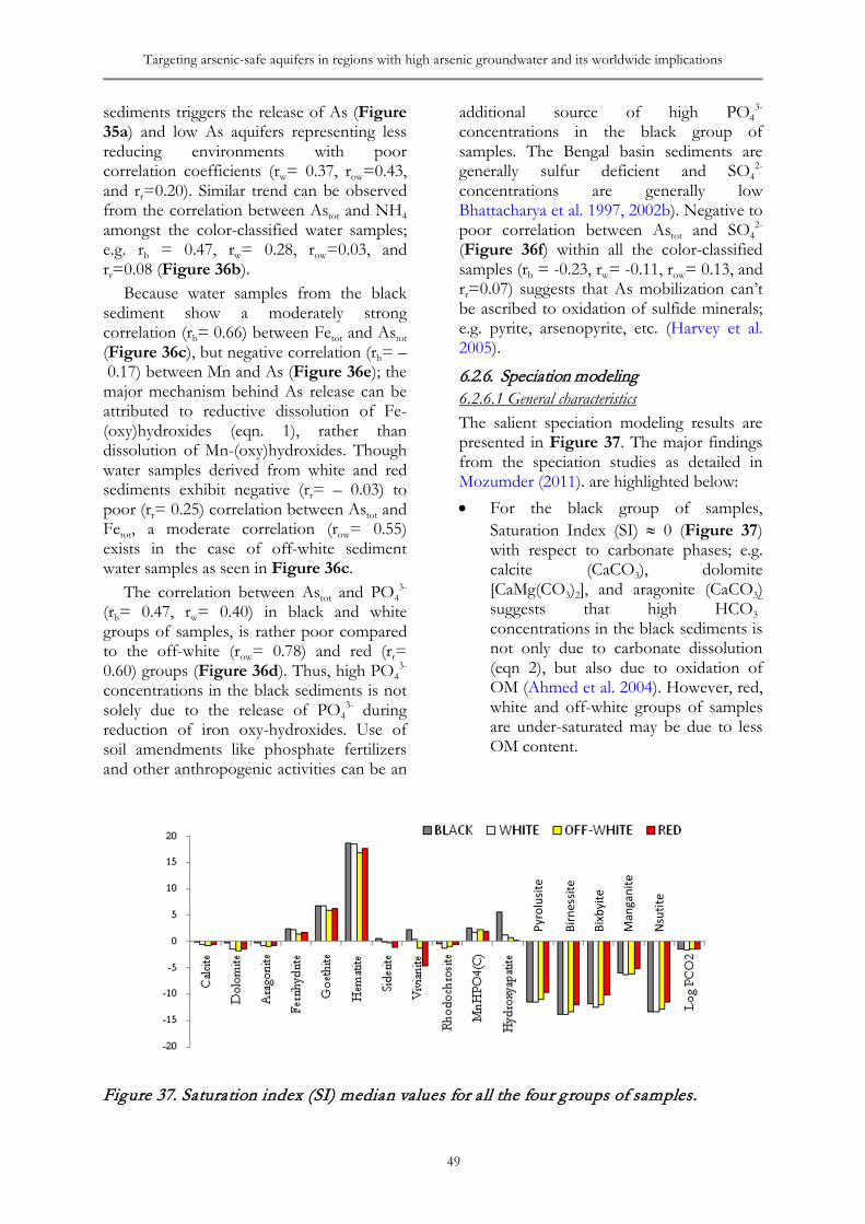
Targeting arsenic-safe aquifers in regions with high arsenic groundwater and its worldwide implications
49
sediments triggers the release of As (Figure 35a) and low As aquifers representing less reducing environments with poor correlation coefficients (rw= 0.37, row=0.43, and rr=0.20). Similar trend can be observed from the correlation between Astot and NH4 amongst the color-classified water samples; e.g. rb = 0.47, rw= 0.28, row=0.03, and rr=0.08 (Figure 36b).
Because water samples from the black sediment show a moderately strong correlation (rb= 0.66) between Fetot and Astot (Figure 36c), but negative correlation (rb= – 0.17) between Mn and As (Figure 36e); the major mechanism behind As release can be attributed to reductive dissolution of Fe-(oxy)hydroxides (eqn. 1), rather than dissolution of Mn-(oxy)hydroxides. Though water samples derived from white and red sediments exhibit negative (rr= – 0.03) to poor (rr= 0.25) correlation between Astot and Fetot, a moderate correlation (row= 0.55) exists in the case of off-white sediment water samples as seen in Figure 36c.
The correlation between Astot and PO43-
(rb= 0.47, rw= 0.40) in black and white groups of samples, is rather poor compared to the off-white (row= 0.78) and red (rr= 0.60) groups (Figure 36d). Thus, high PO4
3- concentrations in the black sediments is not solely due to the release of PO4
3- during reduction of iron oxy-hydroxides. Use of soil amendments like phosphate fertilizers and other anthropogenic activities can be an
additional source of high PO43-
concentrations in the black group of samples. The Bengal basin sediments are generally sulfur deficient and SO4
2- concentrations are generally low Bhattacharya et al. 1997, 2002b). Negative to poor correlation between Astot and SO4
2- (Figure 36f) within all the color-classified samples (rb = -0.23, rw= -0.11, row= 0.13, and rr=0.07) suggests that As mobilization can’t be ascribed to oxidation of sulfide minerals; e.g. pyrite, arsenopyrite, etc. (Harvey et al. 2005).
6.2.6. Speciation modeling 6.2.6.1 General characteristics The salient speciation modeling results are presented in Figure 37. The major findings from the speciation studies as detailed in Mozumder (2011). are highlighted below: • For the black group of samples,
Saturation Index (SI) ≈ 0 (Figure 37) with respect to carbonate phases; e.g. calcite (CaCO3), dolomite [CaMg(CO3)2], and aragonite (CaCO3) suggests that high HCO3
¯ concentrations in the black sediments is not only due to carbonate dissolution (eqn 2), but also due to oxidation of OM (Ahmed et al. 2004). However, red, white and off-white groups of samples are under-saturated may be due to less OM content.
Figure 37. Saturation index (SI) median values for all the four groups of samples.
Nsu
tite
Man
gani
te
Bixb
yite
Bi
rnes
site
Pyro
lusit
e
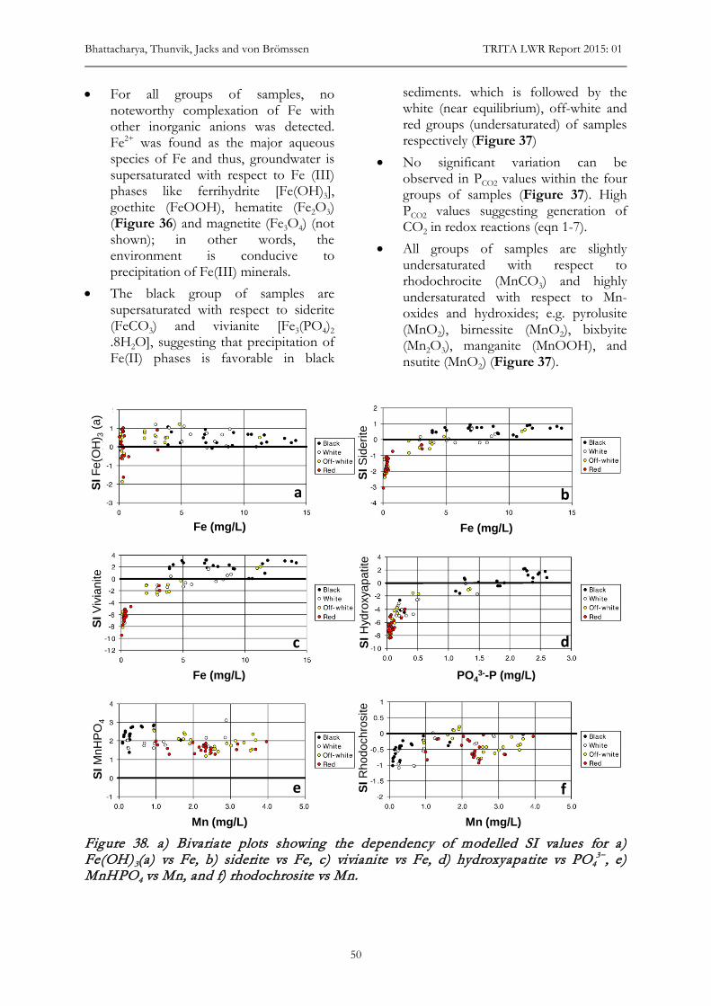
Bhattacharya, Thunvik, Jacks and von Brömssen TRITA LWR Report 2015: 01
50
• For all groups of samples, no noteworthy complexation of Fe with other inorganic anions was detected. Fe2+ was found as the major aqueous species of Fe and thus, groundwater is supersaturated with respect to Fe (III) phases like ferrihydrite [Fe(OH)3], goethite (FeOOH), hematite (Fe2O3) (Figure 36) and magnetite (Fe3O4) (not shown); in other words, the environment is conducive to precipitation of Fe(III) minerals.
• The black group of samples are supersaturated with respect to siderite (FeCO3) and vivianite [Fe3(PO4)2 .8H2O], suggesting that precipitation of Fe(II) phases is favorable in black
sediments. which is followed by the white (near equilibrium), off-white and red groups (undersaturated) of samples respectively (Figure 37)
• No significant variation can be observed in PCO2 values within the four groups of samples (Figure 37). High PCO2 values suggesting generation of CO2 in redox reactions (eqn 1-7).
• All groups of samples are slightly undersaturated with respect to rhodochrocite (MnCO3) and highly undersaturated with respect to Mn-oxides and hydroxides; e.g. pyrolusite (MnO2), birnessite (MnO2), bixbyite (Mn2O3), manganite (MnOOH), and nsutite (MnO2) (Figure 37).
Figure 38. a) Bivariate plots showing the dependency of modelled SI values for a) Fe(OH)3(a) vs Fe, b) siderite vs Fe, c) vivianite vs Fe, d) hydroxyapatite vs PO4
3−, e) MnHPO4 vs Mn, and f) rhodochrosite vs Mn.
aSIFe
(OH
) 3(a
)
b
c d
e f
SIS
ider
iteSI
Rho
doch
rosi
teSI
Hyd
roxy
apat
ite
SIM
nHP
O4
SIVi
vian
ite
Fe (mg/L) Fe (mg/L)
Fe (mg/L)
Mn (mg/L) Mn (mg/L)
PO43--P (mg/L)
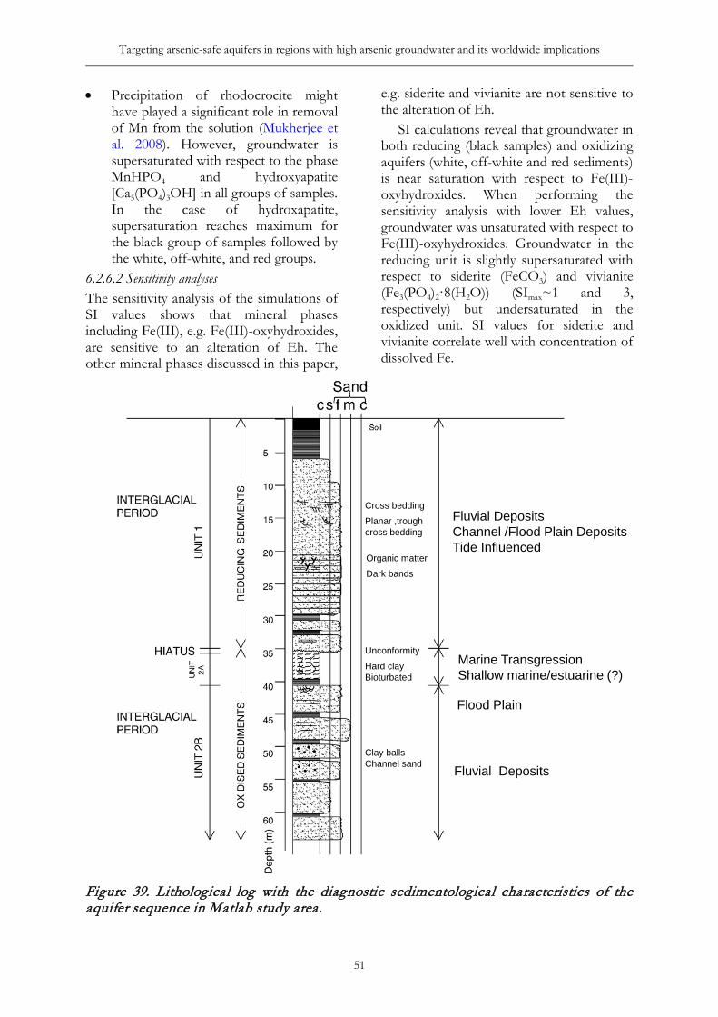
Targeting arsenic-safe aquifers in regions with high arsenic groundwater and its worldwide implications
51
• Precipitation of rhodocrocite might have played a significant role in removal of Mn from the solution (Mukherjee et al. 2008). However, groundwater is supersaturated with respect to the phase MnHPO4 and hydroxyapatite [Ca5(PO4)3OH] in all groups of samples. In the case of hydroxapatite, supersaturation reaches maximum for the black group of samples followed by the white, off-white, and red groups.
6.2.6.2 Sensitivity analyses The sensitivity analysis of the simulations of SI values shows that mineral phases including Fe(III), e.g. Fe(III)-oxyhydroxides, are sensitive to an alteration of Eh. The other mineral phases discussed in this paper,
e.g. siderite and vivianite are not sensitive to the alteration of Eh.
SI calculations reveal that groundwater in both reducing (black samples) and oxidizing aquifers (white, off-white and red sediments) is near saturation with respect to Fe(III)-oxyhydroxides. When performing the sensitivity analysis with lower Eh values, groundwater was unsaturated with respect to Fe(III)-oxyhydroxides. Groundwater in the reducing unit is slightly supersaturated with respect to siderite (FeCO3) and vivianite (Fe3(PO4)2·8(H2O)) (SImax~1 and 3, respectively) but undersaturated in the oxidized unit. SI values for siderite and vivianite correlate well with concentration of dissolved Fe.
Figure 39. Lithological log with the diagnostic sedimentological characteristics of the aquifer sequence in Matlab study area.
Fluvial Deposits
Marine TransgressionShallow marine/estuarine (?)
Flood Plain
Fluvial DepositsChannel /Flood Plain DepositsTide Influenced
Clay ballsChannel sand
Cross bedding
Planar ,troughcross bedding
Organic matter
Dark bands
Unconformity
Hard clayBioturbated
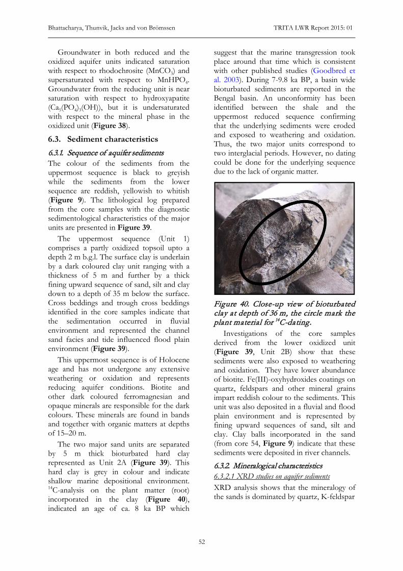
Bhattacharya, Thunvik, Jacks and von Brömssen TRITA LWR Report 2015: 01
52
Groundwater in both reduced and the oxidized aquifer units indicated saturation with respect to rhodochrosite (MnCO3) and supersaturated with respect to MnHPO4. Groundwater from the reducing unit is near saturation with respect to hydroxyapatite (Ca5(PO4)3(OH)), but it is undersaturated with respect to the mineral phase in the oxidized unit (Figure 38).
6.3. Sediment characteristics 6.3.1. Sequence of aquifer sediments The colour of the sediments from the uppermost sequence is black to greyish while the sediments from the lower sequence are reddish, yellowish to whitish (Figure 9). The lithological log prepared from the core samples with the diagnostic sedimentological characteristics of the major units are presented in Figure 39.
The uppermost sequence (Unit 1) comprises a partly oxidized topsoil upto a depth 2 m b.g.l. The surface clay is underlain by a dark coloured clay unit ranging with a thickness of 5 m and further by a thick fining upward sequence of sand, silt and clay down to a depth of 35 m below the surface. Cross beddings and trough cross beddings identified in the core samples indicate that the sedimentation occurred in fluvial environment and represented the channel sand facies and tide influenced flood plain environment (Figure 39).
This uppermost sequence is of Holocene age and has not undergone any extensive weathering or oxidation and represents reducing aquifer conditions. Biotite and other dark coloured ferromagnesian and opaque minerals are responsible for the dark colours. These minerals are found in bands and together with organic matters at depths of 15–20 m.
The two major sand units are separated by 5 m thick bioturbated hard clay represented as Unit 2A (Figure 39). This hard clay is grey in colour and indicate shallow marine depositional environment. 14C-analysis on the plant matter (root) incorporated in the clay (Figure 40), indicated an age of ca. 8 ka BP which
suggest that the marine transgression took place around that time which is consistent with other published studies (Goodbred et al. 2003). During 7-9.8 ka BP, a basin wide bioturbated sediments are reported in the Bengal basin. An unconformity has been identified between the shale and the uppermost reduced sequence confirming that the underlying sediments were eroded and exposed to weathering and oxidation. Thus, the two major units correspond to two interglacial periods. However, no dating could be done for the underlying sequence due to the lack of organic matter.
Figure 40. Close-up view of bioturbated clay at depth of 36 m, the circle mark the plant material for 14C-dating.
Investigations of the core samples derived from the lower oxidized unit (Figure 39, Unit 2B) show that these sediments were also exposed to weathering and oxidation. They have lower abundance of biotite. Fe(III)-oxyhydroxides coatings on quartz, feldspars and other mineral grains impart reddish colour to the sediments. This unit was also deposited in a fluvial and flood plain environment and is represented by fining upward sequences of sand, silt and clay. Clay balls incorporated in the sand (from core 54, Figure 9) indicate that these sediments were deposited in river channels.
6.3.2. Mineralogical characteristics 6.3.2.1 XRD studies on aquifer sediments XRD analysis shows that the mineralogy of the sands is dominated by quartz, K-feldspar
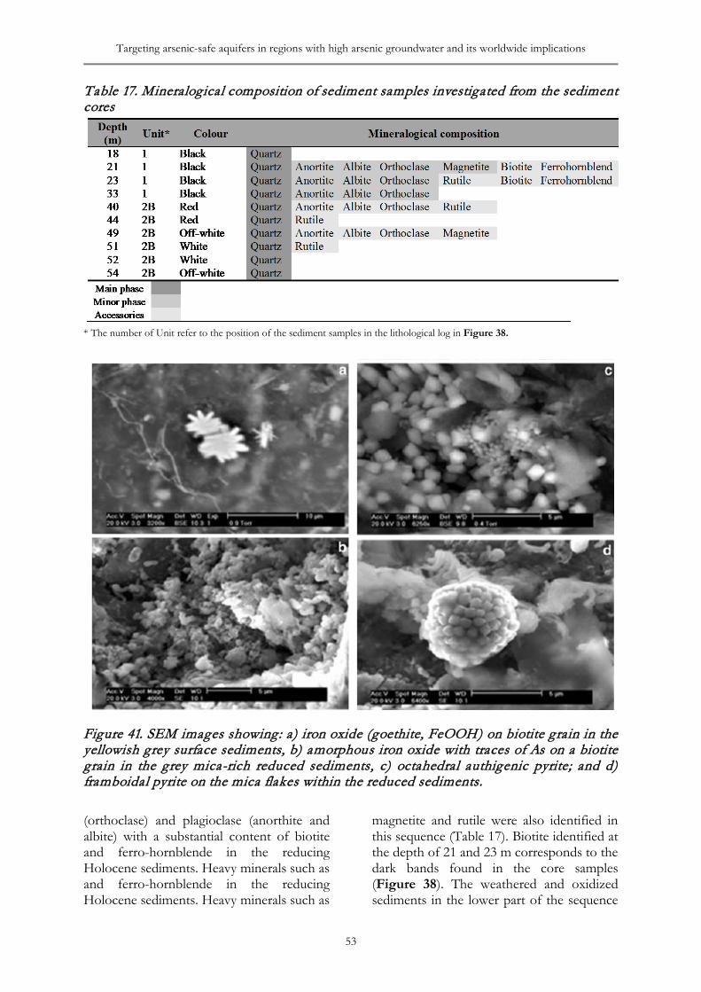
Targeting arsenic-safe aquifers in regions with high arsenic groundwater and its worldwide implications
53
Table 17. Mineralogical composition of sediment samples investigated from the sediment cores
* The number of Unit refer to the position of the sediment samples in the lithological log in Figure 38.
Figure 41. SEM images showing: a) iron oxide (goethite, FeOOH) on biotite grain in the yellowish grey surface sediments, b) amorphous iron oxide with traces of As on a biotite grain in the grey mica-rich reduced sediments, c) octahedral authigenic pyrite; and d) framboidal pyrite on the mica flakes within the reduced sediments. (orthoclase) and plagioclase (anorthite and albite) with a substantial content of biotite and ferro-hornblende in the reducing Holocene sediments. Heavy minerals such as and ferro-hornblende in the reducing Holocene sediments. Heavy minerals such as
magnetite and rutile were also identified in this sequence (Table 17). Biotite identified at the depth of 21 and 23 m corresponds to the dark bands found in the core samples (Figure 38). The weathered and oxidized sediments in the lower part of the sequence
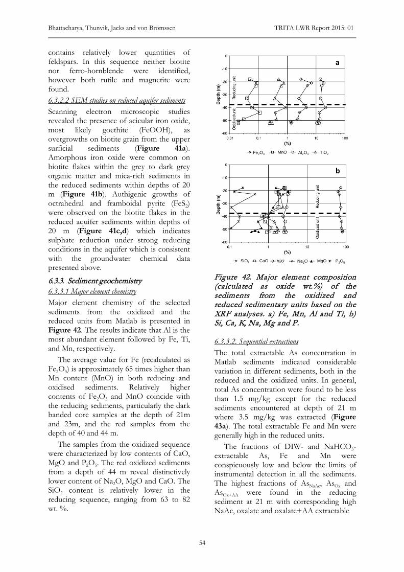
Bhattacharya, Thunvik, Jacks and von Brömssen TRITA LWR Report 2015: 01
54
contains relatively lower quantities of feldspars. In this sequence neither biotite nor ferro-hornblende were identified, however both rutile and magnetite were found. 6.3.2.2 SEM studies on reduced aquifer sediments Scanning electron microscopic studies revealed the presence of acicular iron oxide, most likely goethite (FeOOH), as overgrowths on biotite grain from the upper surficial sediments (Figure 41a). Amorphous iron oxide were common on biotite flakes within the grey to dark grey organic matter and mica-rich sediments in the reduced sediments within depths of 20 m (Figure 41b). Authigenic growths of octrahedral and framboidal pyrite (FeS2) were observed on the biotite flakes in the reduced aquifer sediments within depths of 20 m (Figure 41c,d) which indicates sulphate reduction under strong reducing conditions in the aquifer which is consistent with the groundwater chemical data presented above.
6.3.3. Sediment geochemistry 6.3.3.1 Major element chemistry Major element chemistry of the selected sediments from the oxidized and the reduced units from Matlab is presented in Figure 42. The results indicate that Al is the most abundant element followed by Fe, Ti, and Mn, respectively.
The average value for Fe (recalculated as Fe2O3) is approximately 65 times higher than Mn content (MnO) in both reducing and oxidised sediments. Relatively higher contents of Fe2O3 and MnO coincide with the reducing sediments, particularly the dark banded core samples at the depth of 21m and 23m, and the red samples from the depth of 40 and 44 m.
The samples from the oxidized sequence were characterized by low contents of CaO, MgO and P2O5. The red oxidized sediments from a depth of 44 m reveal distinctively lower content of Na2O, MgO and CaO. The SiO2 content is relatively lower in the reducing sequence, ranging from 63 to 82 wt. %.
Figure 42. Major element composition (calculated as oxide wt.%) of the sediments from the oxidized and reduced sedimentary units based on the XRF analyses. a) Fe, Mn, Al and Ti, b) Si, Ca, K, Na, Mg and P.
6.3.3.2. Sequential extractions The total extractable As concentration in Matlab sediments indicated considerable variation in different sediments, both in the reduced and the oxidized units. In general, total As concentration were found to be less than 1.5 mg/kg except for the reduced sediments encountered at depth of 21 m where 3.5 mg/kg was extracted (Figure 43a). The total extractable Fe and Mn were generally high in the reduced units.
The fractions of DIW- and NaHCO3-extractable As, Fe and Mn were conspicuously low and below the limits of instrumental detection in all the sediments. The highest fractions of AsNaAc, AsOx and AsOx+AA were found in the reducing sediment at 21 m with corresponding high NaAc, oxalate and oxalate+AA extractable
Fe2O3 MnO Al2O3 TiO2
CaO Na2OSiO2 MgO P2O5
a
b
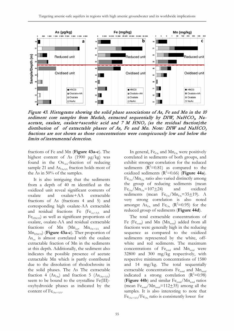
Targeting arsenic-safe aquifers in regions with high arsenic groundwater and its worldwide implications
55
Figure 43. Histograms showing the solid phase associations of As, Fe and Mn in the 10 sediment core samples from Matlab, extracted sequentially by DIW, NaHCO3, Na-acetate, oxalate, oxalate+ascorbic acid and 7 M HNO3 (as the residual fraction)the distribution of of extractable phases of As, Fe and Mn. Note: DIW and NaHCO3 fractions are not shown as those concentrations were conspicuously low and below the limits of instrumental detection. fractions of Fe and Mn (Figure 43a-c). The highest content of As (1900 μg/kg) was found in the OxAA-fraction of reducing sample 21 and AsOxAA fraction holds most of the As in 50% of the samples.
It is also intriguing that the sediments from a depth of 40 m identified as the oxidized unit reveal significant contents of oxalate and oxalate+AA extractable fractions of As (fractions 4 and 5) and corresponding high oxalate-AA extractable and residual fractions Fe (Feox+AA and FeHNO3) as well as significant proportions of oxalate, oxalate-AA and residual extractable fractions of Mn (Mnox, MnOx+AA and MnHNO3) (Figure 43a-c). Ther proportion of Asox is almost correlated with the oxalate extractable fraction of Mn in the sediments at this depth. Additionally, the sediment also indicates the possible presence of acetate extractable Mn which is partly contributed due to the dissolution of rhodochrosite in the solid phases. The As The extractable fraction 4 (AsOx) and fraction 5 (AsOx+AA) seem to be bound to the crystalline Fe(III)-oxyhydroxide phases as indicated by the content of FeOx+AA.
In general, FeOx and MnOx were positively correlated in sediments of both groups, and exhibit stronger correlation for the reduced sediments (R2=0.81) as compared to the oxidized sediments (R2=0.66) (Figure 44a). FeOx/MnOx ratio also varied distinctly among the group of reducing sediments (mean FeOx/MnOx=107+24) and oxidized sediments (mean FeOx/MnOx=35+19). A very strong correlation is also noted amongst AsOx and FeOx (R2=0.95) for the reduced group of sediments (Figure 44d).
The total extractable concentrations of Fe (Fetotal) and Mn (Mntotal) added from all fractions were generally high in the reducing sequence as compared to the oxidized sediments represented by the white, off-white and red sediments. The maximum concentrations of Fetotal and Mntotal were 32800 and 300 mg/kg respectively, with respective minimum concentrations of 1580 and 14 mg/kg. The total sequentially extractable concentrations Fetotal and Mntotal indicated a strong correlation (R2=0.98) (Figure 44b) and similar Fetotal/Mntotal ratios (mean Fetotal/Mntotal=112+35) among all the samples. It is also interesting to note that FeOx+AA/FeOx ratio is consistently lower for
a b c
As (µg/kg) Fe (mg/kg) Mn (mg/kg)Sa
mpl
e/D
epth
(m)
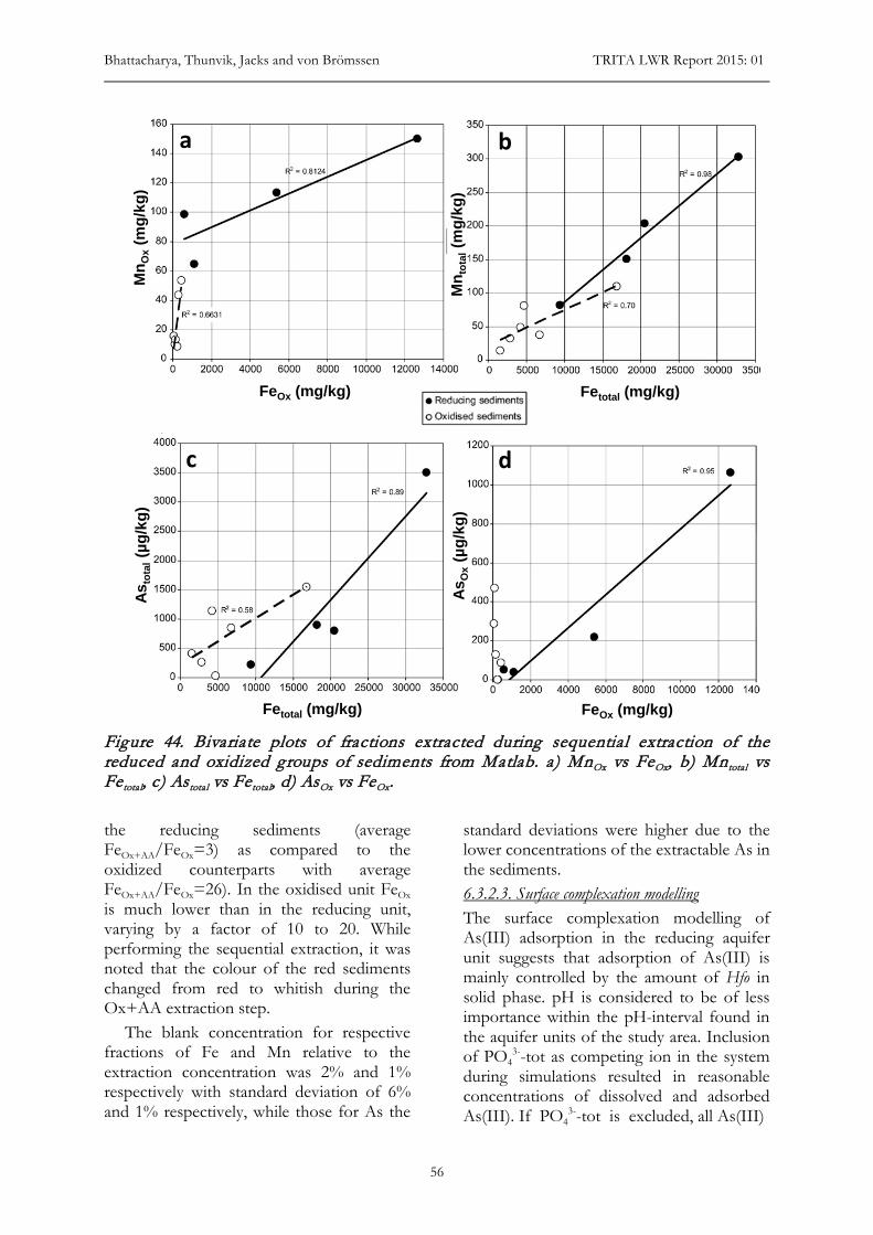
Bhattacharya, Thunvik, Jacks and von Brömssen TRITA LWR Report 2015: 01
56
Figure 44. Bivariate plots of fractions extracted during sequential extraction of the reduced and oxidized groups of sediments from Matlab. a) MnOx vs FeOx, b) Mntotal vs Fetotal, c) Astotal vs Fetotal, d) AsOx vs FeOx. the reducing sediments (average FeOx+AA/FeOx=3) as compared to the oxidized counterparts with average FeOx+AA/FeOx=26). In the oxidised unit FeOx is much lower than in the reducing unit, varying by a factor of 10 to 20. While performing the sequential extraction, it was noted that the colour of the red sediments changed from red to whitish during the Ox+AA extraction step.
The blank concentration for respective fractions of Fe and Mn relative to the extraction concentration was 2% and 1% respectively with standard deviation of 6% and 1% respectively, while those for As the
standard deviations were higher due to the lower concentrations of the extractable As in the sediments. 6.3.2.3. Surface complexation modelling The surface complexation modelling of As(III) adsorption in the reducing aquifer unit suggests that adsorption of As(III) is mainly controlled by the amount of Hfo in solid phase. pH is considered to be of less importance within the pH-interval found in the aquifer units of the study area. Inclusion of PO4
3--tot as competing ion in the system during simulations resulted in reasonable concentrations of dissolved and adsorbed As(III). If PO4
3--tot is excluded, all As(III)
Fetotal (mg/kg)
FeOx (mg/kg)
Mn O
x(m
g/kg
)
FeOx (mg/kg)
Fetotal (mg/kg)
Mn t
otal
(mg/
kg)
a b
c d
Asto
tal(µ
g/kg
)
AsO
x(µ
g/kg
)
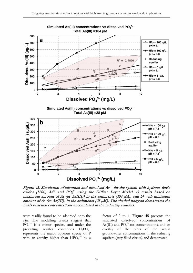
Targeting arsenic-safe aquifers in regions with high arsenic groundwater and its worldwide implications
57
Figure 45. Simulation of adsorbed and dissolved AsIII for the system with hydrous ferric oxides (Hfo), AsIII and PO4
3− using the Diffuse Layer Model. a) results based on maximum amount of As (as As(III)) in the sediments (104 µM), and b) with minimum amount of As (as As(III)) in the sediments (28 µM). The shaded polygon demarcates the fields of actual concentrations encountered in the reducing aquifers. were readily found to be adsorbed onto the Hfo. The modelling results suggest that PO4
3− is a minor species, and under the prevailing aquifer conditions H2PO4
− represents the major aqueous specie of P with an activity higher than HPO4
2− by a
factor of 2 to 4. Figure 45 presents the simulated dissolved concentrations of As(III) and PO4
3--tot concentrations, and an overlay of the plots of the actual groundwater concentrations in the reducing aquifers (grey filled circles) and demarcated
Dissolved PO43- (mg/L)
g/L
g/L
g/L
g/L
g/L
g/L
g/L
g/L
Dissolved PO43- (mg/L)
Dis
solv
ed A
s(III
) (µg
/L)
Dis
solv
ed A
s(III
) (µg
/L)
a
Simulated As(III) concentrations vs dissolved PO43-
Total As(III) =28 µM
Simulated As(III) concentrations vs dissolved PO43-
Total As(III) =104 µM
b
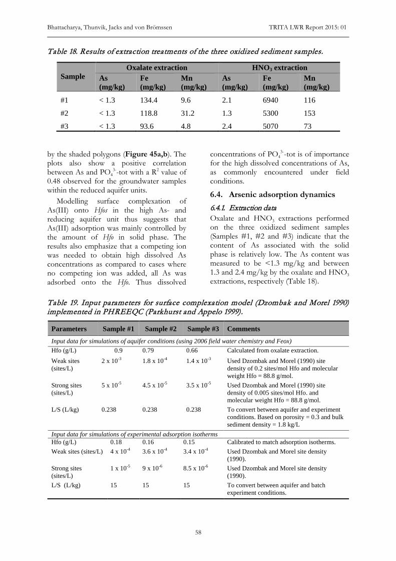
Bhattacharya, Thunvik, Jacks and von Brömssen TRITA LWR Report 2015: 01
58
Table 18. Results of extraction treatments of the three oxidized sediment samples.
by the shaded polygons (Figure 45a,b). The plots also show a positive correlation between As and PO4
3--tot with a R2 value of 0.48 observed for the groundwater samples within the reduced aquifer units.
Modelling surface complexation of As(III) onto Hfos in the high As- and reducing aquifer unit thus suggests that As(III) adsorption was mainly controlled by the amount of Hfo in solid phase. The results also emphasize that a competing ion was needed to obtain high dissolved As concentrations as compared to cases where no competing ion was added, all As was adsorbed onto the Hfo. Thus dissolved
concentrations of PO43--tot is of importance
for the high dissolved concentrations of As, as commonly encountered under field conditions.
6.4. Arsenic adsorption dynamics 6.4.1. Extraction data Oxalate and HNO3 extractions performed on the three oxidized sediment samples (Samples #1, #2 and #3) indicate that the content of As associated with the solid phase is relatively low. The As content was measured to be <1.3 mg/kg and between 1.3 and 2.4 mg/kg by the oxalate and HNO3 extractions, respectively (Table 18).
Table 19. Input parameters for surface complexation model (Dzombak and Morel 1990) implemented in PHREEQC (Parkhurst and Appelo 1999).
Sample
Oxalate extraction HNO3 extraction As (mg/kg)
Fe (mg/kg)
Mn (mg/kg)
As (mg/kg)
Fe (mg/kg)
Mn (mg/kg)
#1 < 1.3 134.4 9.6 2.1 6940 116
#2 < 1.3 118.8 31.2 1.3 5300 153
#3 < 1.3 93.6 4.8 2.4 5070 73
Parameters Sample #1 Sample #2 Sample #3 Comments
Input data for simulations of aquifer conditions (using 2006 field water chemistry and Feox) Hfo (g/L) 0.9 0.79 0.66 Calculated from oxalate extraction. Weak sites (sites/L)
2 x 10⁻³ 1.8 x 10⁻⁴ 1.4 x 10⁻³ Used Dzombak and Morel (1990) site density of 0.2 sites/mol Hfo and molecular weight Hfo = 88.8 g/mol.
Strong sites (sites/L)
5 x 10⁻⁵ 4.5 x 10⁻⁵ 3.5 x 10⁻⁵ Used Dzombak and Morel (1990) site density of 0.005 sites/mol Hfo. and molecular weight Hfo = 88.8 g/mol.
L/S (L/kg) 0.238 0.238 0.238 To convert between aquifer and experiment conditions. Based on porosity = 0.3 and bulk sediment density = 1.8 kg/L
Input data for simulations of experimental adsorption isotherms Hfo (g/L) 0.18 0.16 0.15 Calibrated to match adsorption isotherms. Weak sites (sites/L) 4 x 10⁻⁴ 3.6 x 10⁻⁴ 3.4 x 10⁻⁴ Used Dzombak and Morel site density
(1990). Strong sites (sites/L)
1 x 10⁻⁵ 9 x 10⁻⁶ 8.5 x 10⁻⁶ Used Dzombak and Morel site density (1990).
L/S (L/kg) 15 15 15 To convert between aquifer and batch experiment conditions.
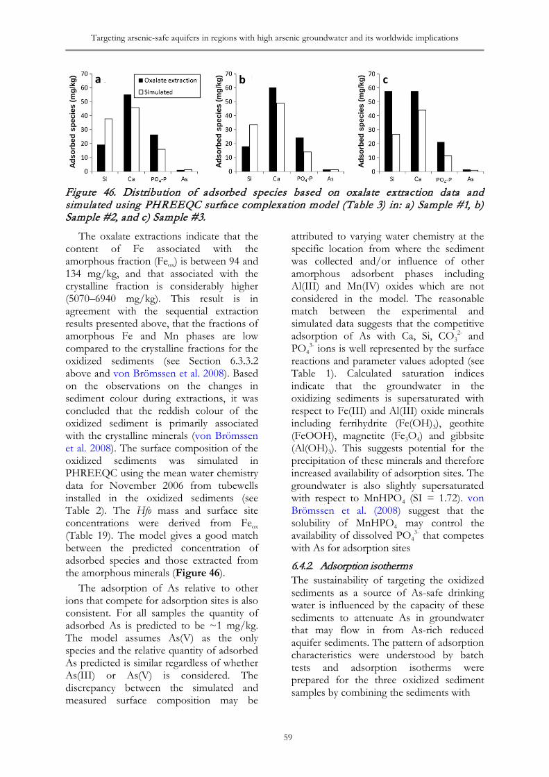
Targeting arsenic-safe aquifers in regions with high arsenic groundwater and its worldwide implications
59
Figure 46. Distribution of adsorbed species based on oxalate extraction data and simulated using PHREEQC surface complexation model (Table 3) in: a) Sample #1, b) Sample #2, and c) Sample #3.
The oxalate extractions indicate that the content of Fe associated with the amorphous fraction (Feox) is between 94 and 134 mg/kg, and that associated with the crystalline fraction is considerably higher (5070–6940 mg/kg). This result is in agreement with the sequential extraction results presented above, that the fractions of amorphous Fe and Mn phases are low compared to the crystalline fractions for the oxidized sediments (see Section 6.3.3.2 above and von Brömssen et al. 2008). Based on the observations on the changes in sediment colour during extractions, it was concluded that the reddish colour of the oxidized sediment is primarily associated with the crystalline minerals (von Brömssen et al. 2008). The surface composition of the oxidized sediments was simulated in PHREEQC using the mean water chemistry data for November 2006 from tubewells installed in the oxidized sediments (see Table 2). The Hfo mass and surface site concentrations were derived from Feox (Table 19). The model gives a good match between the predicted concentration of adsorbed species and those extracted from the amorphous minerals (Figure 46).
The adsorption of As relative to other ions that compete for adsorption sites is also consistent. For all samples the quantity of adsorbed As is predicted to be ~1 mg/kg. The model assumes As(V) as the only species and the relative quantity of adsorbed As predicted is similar regardless of whether As(III) or As(V) is considered. The discrepancy between the simulated and measured surface composition may be
attributed to varying water chemistry at the specific location from where the sediment was collected and/or influence of other amorphous adsorbent phases including Al(III) and Mn(IV) oxides which are not considered in the model. The reasonable match between the experimental and simulated data suggests that the competitive adsorption of As with Ca, Si, CO3
2- and PO4
3- ions is well represented by the surface reactions and parameter values adopted (see Table 1). Calculated saturation indices indicate that the groundwater in the oxidizing sediments is supersaturated with respect to Fe(III) and Al(III) oxide minerals including ferrihydrite (Fe(OH)3), geothite (FeOOH), magnetite (Fe3O4) and gibbsite (Al(OH)3). This suggests potential for the precipitation of these minerals and therefore increased availability of adsorption sites. The groundwater is also slightly supersaturated with respect to MnHPO4 (SI = 1.72). von Brömssen et al. (2008) suggest that the solubility of MnHPO4 may control the availability of dissolved PO4
3- that competes with As for adsorption sites
6.4.2. Adsorption isotherms The sustainability of targeting the oxidized sediments as a source of As-safe drinking water is influenced by the capacity of these sediments to attenuate As in groundwater that may flow in from As-rich reduced aquifer sediments. The pattern of adsorption characteristics were understood by batch tests and adsorption isotherms were prepared for the three oxidized sediment samples by combining the sediments with
Adso
rbed
spec
ies
(mg/
kg)
Adso
rbed
spec
ies
(mg/
kg)
Adso
rbed
spec
ies
(mg/
kg)a b c
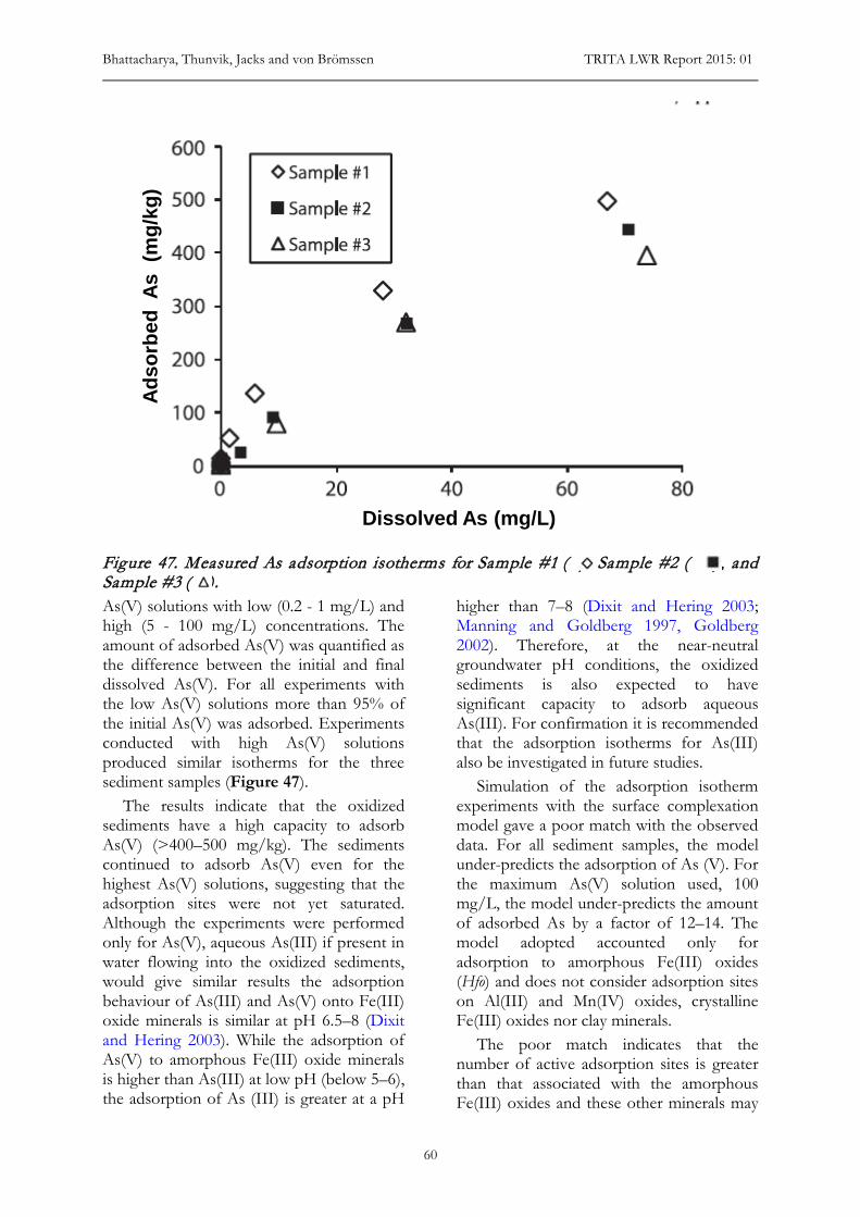
Bhattacharya, Thunvik, Jacks and von Brömssen TRITA LWR Report 2015: 01
60
Figure 47. Measured As adsorption isotherms for Sample #1 ( ), Sample #2 ( ), and Sample #3 ( ). As(V) solutions with low (0.2 - 1 mg/L) and high (5 - 100 mg/L) concentrations. The amount of adsorbed As(V) was quantified as the difference between the initial and final dissolved As(V). For all experiments with the low As(V) solutions more than 95% of the initial As(V) was adsorbed. Experiments conducted with high As(V) solutions produced similar isotherms for the three sediment samples (Figure 47).
The results indicate that the oxidized sediments have a high capacity to adsorb As(V) (>400–500 mg/kg). The sediments continued to adsorb As(V) even for the highest As(V) solutions, suggesting that the adsorption sites were not yet saturated. Although the experiments were performed only for As(V), aqueous As(III) if present in water flowing into the oxidized sediments, would give similar results the adsorption behaviour of As(III) and As(V) onto Fe(III) oxide minerals is similar at pH 6.5–8 (Dixit and Hering 2003). While the adsorption of As(V) to amorphous Fe(III) oxide minerals is higher than As(III) at low pH (below 5–6), the adsorption of As (III) is greater at a pH
higher than 7–8 (Dixit and Hering 2003; Manning and Goldberg 1997, Goldberg 2002). Therefore, at the near-neutral groundwater pH conditions, the oxidized sediments is also expected to have significant capacity to adsorb aqueous As(III). For confirmation it is recommended that the adsorption isotherms for As(III) also be investigated in future studies.
Simulation of the adsorption isotherm experiments with the surface complexation model gave a poor match with the observed data. For all sediment samples, the model under-predicts the adsorption of As (V). For the maximum As(V) solution used, 100 mg/L, the model under-predicts the amount of adsorbed As by a factor of 12–14. The model adopted accounted only for adsorption to amorphous Fe(III) oxides (Hfo) and does not consider adsorption sites on Al(III) and Mn(IV) oxides, crystalline Fe(III) oxides nor clay minerals.
The poor match indicates that the number of active adsorption sites is greater than that associated with the amorphous Fe(III) oxides and these other minerals may
Dissolved As (mg/L)
Adso
rbed
As (
mg/
kg)
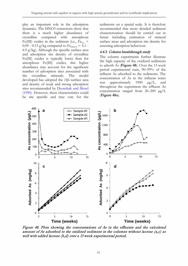
Targeting arsenic-safe aquifers in regions with high arsenic groundwater and its worldwide implications
61
play an important role in the adsorption dynamics. The HNO3 extractions show that there is a much higher abundance of crystalline compared with amorphous Fe(III) oxides in the sediment (i.e., FeOx = 0.09 - 0.13 g/kg compared to FeHNO3 = 5.1 - 6.9 g/kg). Although the specific surface area and adsorption site density of crystalline Fe(III) oxides is typically lower than for amorphous Fe(III) oxides, this higher abundance may account for the significant number of adsorption sites associated with the crystalline minerals. The model developed has adopted the Hfo surface area and density of weak and strong adsorption sites recommended by Dzombak and Morel (1990). However, these characteristics could be site specific and may vary for the
sediments on a spatial scale. It is therefore recommended that more detailed sediment characterization should be carried out in future including estimation of mineral surface areas and adsorption site density for assessing adsorption behaviour.
6.4.3. Column breakthrough study The column experiments further illustrate the high capacity of the oxidized sediments to adsorb As (Figure 48). Over the 13 week period experimental runs, 90–99% of the influent As adsorbed to the sediments. The concentration of As in the influent water was approximately 1900 µg/L, and throughout the experiment the effluent As concentration ranged from 20–200 µg/L (Figure 48a).
Figure 48. Plots showing the concentrations of As in the effluents and the calculated amount of As adsorbed to the oxidized sediment in the columns without lactose (a,c) as well with added lactose (b,d) over a 13 week experimental period.
a
Adso
rbed
As (
mg/
kg)
As c
once
ntra
tion
(µg/
L)
Time (weeks) Time (weeks)
Adso
rbed
As (
mg/
kg)
As c
once
ntra
tion
(µg/
L) b
c d
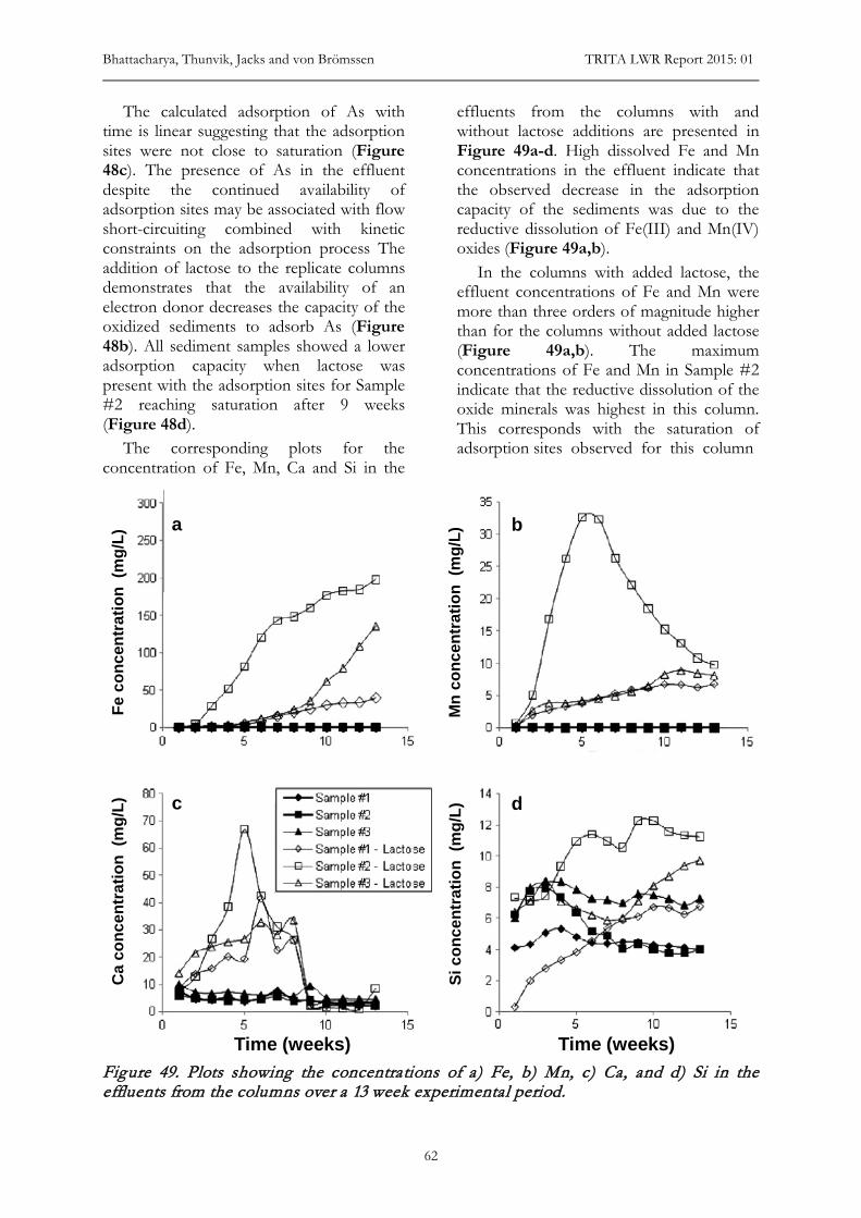
Bhattacharya, Thunvik, Jacks and von Brömssen TRITA LWR Report 2015: 01
62
The calculated adsorption of As with time is linear suggesting that the adsorption sites were not close to saturation (Figure 48c). The presence of As in the effluent despite the continued availability of adsorption sites may be associated with flow short-circuiting combined with kinetic constraints on the adsorption process The addition of lactose to the replicate columns demonstrates that the availability of an electron donor decreases the capacity of the oxidized sediments to adsorb As (Figure 48b). All sediment samples showed a lower adsorption capacity when lactose was present with the adsorption sites for Sample #2 reaching saturation after 9 weeks (Figure 48d).
The corresponding plots for the concentration of Fe, Mn, Ca and Si in the
effluents from the columns with and without lactose additions are presented in Figure 49a-d. High dissolved Fe and Mn concentrations in the effluent indicate that the observed decrease in the adsorption capacity of the sediments was due to the reductive dissolution of Fe(III) and Mn(IV) oxides (Figure 49a,b).
In the columns with added lactose, the effluent concentrations of Fe and Mn were more than three orders of magnitude higher than for the columns without added lactose (Figure 49a,b). The maximum concentrations of Fe and Mn in Sample #2 indicate that the reductive dissolution of the oxide minerals was highest in this column. This corresponds with the saturation of adsorption sites observed for this column
Figure 49. Plots showing the concentrations of a) Fe, b) Mn, c) Ca, and d) Si in the effluents from the columns over a 13 week experimental period.
Time (weeks) Time (weeks)
Fe c
once
ntra
tion
(mg/
L)C
a co
ncen
trat
ion
(mg/
L)
Mn
conc
entr
atio
n(m
g/L)
Si c
once
ntra
tion
(mg/
L)
a b
c d
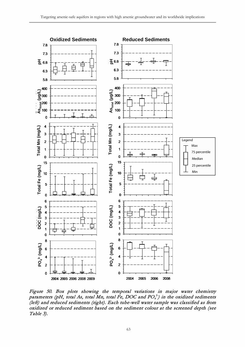
Targeting arsenic-safe aquifers in regions with high arsenic groundwater and its worldwide implications
63
Figure 50. Box plots showing the temporal variations in major water chemistry parameters (pH, total As, total Mn, total Fe, DOC and PO4
3-) in the oxidized sediments (left) and reduced sediments (right). Each tube-well water sample was classified as from oxidized or reduced sediment based on the sediment colour at the screened depth (see Table 3).
Tota
l Mn
(mg/
L)
Tota
l Mn
(mg/
L)
DO
C (m
g/L)
DO
C (m
g/L)
Tota
l Fe
(mg/
L)
Tota
l Fe
(mg/
L)
PO43
-(m
g/L)
PO43-
(mg/
L)
PO43-
(mg/
L)
Asto
tal(µ
g/L)
Astto
tal(µ
g/L)
pHpHOxidized Sediments Reduced Sediments
Bhattacharya, Thunvik, Jacks and von Brömssen TRITA LWR Report 2015: 01
64
(see Figure 49b). The effluent concentrations of Ca and Si were also greater for the columns with lactose added, particularly for Sample #2. This suggests that these ions were released as Mn(IV) and Fe(III) oxides were reduced (Figure 49c,d). Reductive dissolution of Mn(IV) oxides should occur in preference to Fe(III) oxides in the sequence of redox reactions (Bhattacharya et al. 2002a, Appelo and Postma, 2005).
While the effluent concentrations indicate that this did occur for Sample #2, these reactions and the microbially mediated biogeochemical processes were perhaps common for all columns. The rates of reaction are however affected by the complex consortia of reducing microbes in the sediment as well as the relative stability of the specific Fe(III) and Mn(IV) oxide specie present. Although the reduction of Fe(III) and Mn(IV) oxides adds alkalinity (HCO3
-) to the solution, the oxidation of lactose adds acidity (H+). This leads to the effluent pH dropping to around 5 as compared to near-neutral for columns without lactose addition. While decreasing pH has been shown to reduce the adsorption of As(III) to Fe(III) oxides (Dixit and Hering, 2003, 2006), the effluent pH decrease does not account for the significant reduction in the observed adsorption capacity of the sediments.
6.4.4. Linking adsorption dynamics of arsenic with aquifer environments
Analysis of the tube-well water demonstrated that DOC concentrations are higher in the reduced sediments compared to the oxidized sediments (Figure 50, see also Figure 32). Infiltrating surface waters would also typically also have a much higher organic content (Harvey et al. 2006). As a result, these experiments show that if groundwater from reduced sediments, or alternatively surface waters, flows into the oxidized sediments, increased DOC availability will enhance the reductive dissolution of oxide minerals triggering the mobilization of As (Bhattacharya et al. 2002b, 2006a). The type and reactivity of C used in this column study is different to the complex organic matter that exists in natural aquifer systems. In natural aquifers the reductive dissolution of Fe(III) and Mn(IV) oxides by DOC will be strongly controlled by kinetics of the microbial processes. These kinetics and the type and reactivity of the organic matter available in the sediments needs to be further investigated to more accurately predict: i) the capacity of the oxidized sediments to attenuate dissolved As in the infiltrating water and, ii) the potential for the dissolution of Fe(III) and Mn(IV) oxides and subsequent release of sediment-bound As, in cases of cross-contamination.
Table 20. Distribution of microbial population in the sediments
Depth (m) Sediment Color Gram stain Growth in As-media Microbial species
12.7 Black -ve +ve Acinetobacter spp.
25.4 Black -ve +ve Rhodococcus spp.
25.4 Black -ve -ve Pseudomonas spp.
25.4 Black -ve +ve Acinetobacter spp.
25.4 Black +ve -ve Bacillus spp.
42.4 Off-white/red +ve +ve Arthrobacter spp.
45.9 Off-white/red -ve +ve Burkholderia spp.
51.0 Off-white/red +ve +ve Exiguobacterium spp.
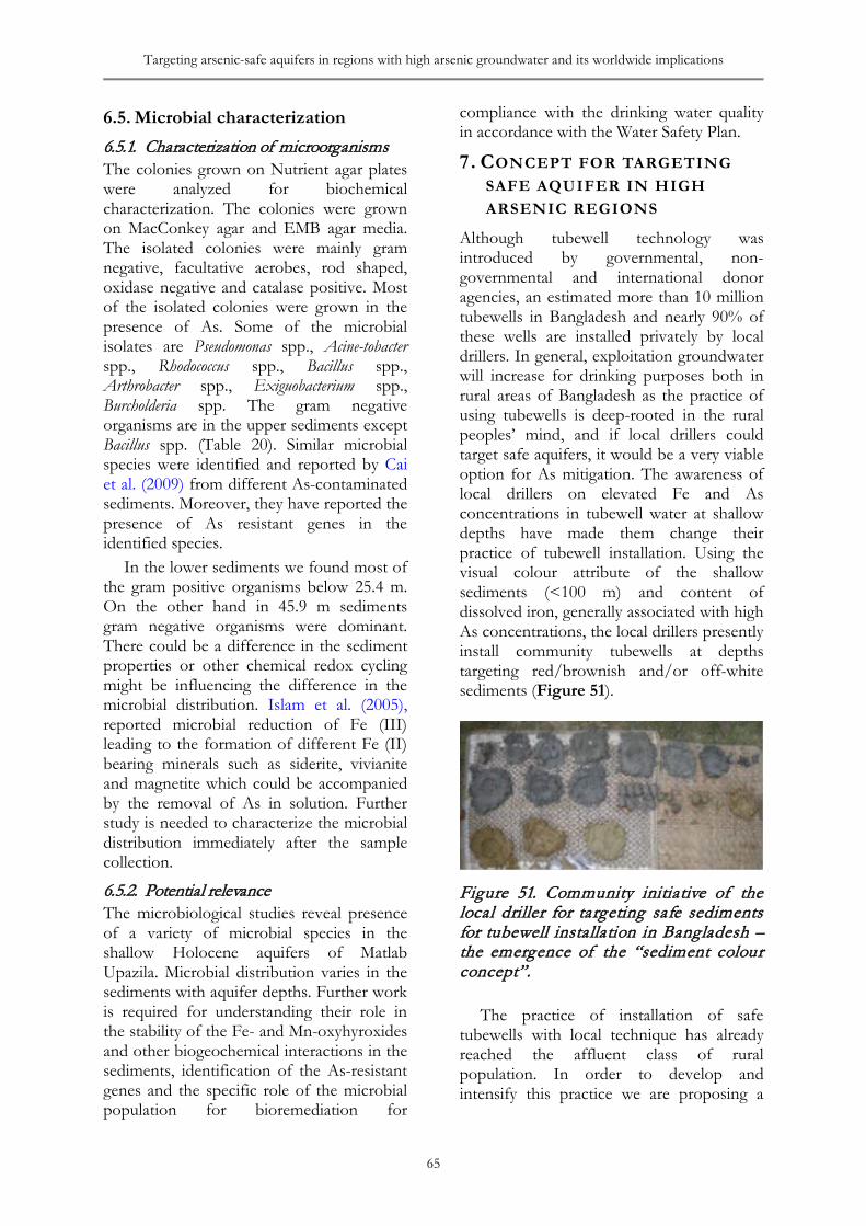
Targeting arsenic-safe aquifers in regions with high arsenic groundwater and its worldwide implications
65
6.5. Microbial characterization 6.5.1. Characterization of microorganisms The colonies grown on Nutrient agar plates were analyzed for biochemical characterization. The colonies were grown on MacConkey agar and EMB agar media. The isolated colonies were mainly gram negative, facultative aerobes, rod shaped, oxidase negative and catalase positive. Most of the isolated colonies were grown in the presence of As. Some of the microbial isolates are Pseudomonas spp., Acine-tobacter spp., Rhodococcus spp., Bacillus spp., Arthrobacter spp., Exiguobacterium spp., Burcholderia spp. The gram negative organisms are in the upper sediments except Bacillus spp. (Table 20). Similar microbial species were identified and reported by Cai et al. (2009) from different As-contaminated sediments. Moreover, they have reported the presence of As resistant genes in the identified species.
In the lower sediments we found most of the gram positive organisms below 25.4 m. On the other hand in 45.9 m sediments gram negative organisms were dominant. There could be a difference in the sediment properties or other chemical redox cycling might be influencing the difference in the microbial distribution. Islam et al. (2005), reported microbial reduction of Fe (III) leading to the formation of different Fe (II) bearing minerals such as siderite, vivianite and magnetite which could be accompanied by the removal of As in solution. Further study is needed to characterize the microbial distribution immediately after the sample collection.
6.5.2. Potential relevance The microbiological studies reveal presence of a variety of microbial species in the shallow Holocene aquifers of Matlab Upazila. Microbial distribution varies in the sediments with aquifer depths. Further work is required for understanding their role in the stability of the Fe- and Mn-oxyhyroxides and other biogeochemical interactions in the sediments, identification of the As-resistant genes and the specific role of the microbial population for bioremediation for
compliance with the drinking water quality in accordance with the Water Safety Plan.
7. CONCEPT FOR TARGETING SAFE AQUIFER IN HIGH ARSENIC REGIONS
Although tubewell technology was introduced by governmental, non-governmental and international donor agencies, an estimated more than 10 million tubewells in Bangladesh and nearly 90% of these wells are installed privately by local drillers. In general, exploitation groundwater will increase for drinking purposes both in rural areas of Bangladesh as the practice of using tubewells is deep-rooted in the rural peoples’ mind, and if local drillers could target safe aquifers, it would be a very viable option for As mitigation. The awareness of local drillers on elevated Fe and As concentrations in tubewell water at shallow depths have made them change their practice of tubewell installation. Using the visual colour attribute of the shallow sediments (<100 m) and content of dissolved iron, generally associated with high As concentrations, the local drillers presently install community tubewells at depths targeting red/brownish and/or off-white sediments (Figure 51).
Figure 51. Community initiative of the local driller for targeting safe sediments for tubewell installation in Bangladesh – the emergence of the “sediment colour concept”.
The practice of installation of safe tubewells with local technique has already reached the affluent class of rural population. In order to develop and intensify this practice we are proposing a
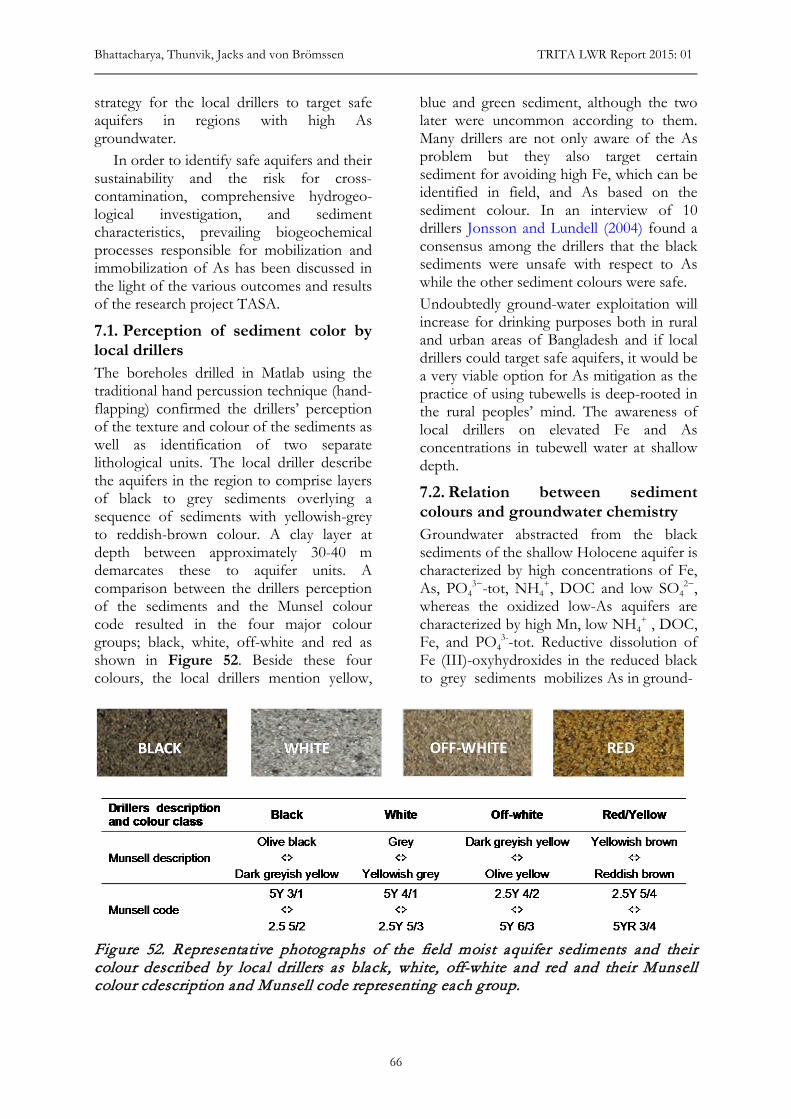
Bhattacharya, Thunvik, Jacks and von Brömssen TRITA LWR Report 2015: 01
66
strategy for the local drillers to target safe aquifers in regions with high As groundwater.
In order to identify safe aquifers and their sustainability and the risk for cross-contamination, comprehensive hydrogeo-logical investigation, and sediment characteristics, prevailing biogeochemical processes responsible for mobilization and immobilization of As has been discussed in the light of the various outcomes and results of the research project TASA.
7.1. Perception of sediment color by local drillers The boreholes drilled in Matlab using the traditional hand percussion technique (hand-flapping) confirmed the drillers’ perception of the texture and colour of the sediments as well as identification of two separate lithological units. The local driller describe the aquifers in the region to comprise layers of black to grey sediments overlying a sequence of sediments with yellowish-grey to reddish-brown colour. A clay layer at depth between approximately 30-40 m demarcates these to aquifer units. A comparison between the drillers perception of the sediments and the Munsel colour code resulted in the four major colour groups; black, white, off-white and red as shown in Figure 52. Beside these four colours, the local drillers mention yellow,
blue and green sediment, although the two later were uncommon according to them. Many drillers are not only aware of the As problem but they also target certain sediment for avoiding high Fe, which can be identified in field, and As based on the sediment colour. In an interview of 10 drillers Jonsson and Lundell (2004) found a consensus among the drillers that the black sediments were unsafe with respect to As while the other sediment colours were safe. Undoubtedly ground-water exploitation will increase for drinking purposes both in rural and urban areas of Bangladesh and if local drillers could target safe aquifers, it would be a very viable option for As mitigation as the practice of using tubewells is deep-rooted in the rural peoples’ mind. The awareness of local drillers on elevated Fe and As concentrations in tubewell water at shallow depth.
7.2. Relation between sediment colours and groundwater chemistry Groundwater abstracted from the black sediments of the shallow Holocene aquifer is characterized by high concentrations of Fe, As, PO4
3−-tot, NH4+, DOC and low SO4
2−, whereas the oxidized low-As aquifers are characterized by high Mn, low NH4
+ , DOC, Fe, and PO4
3--tot. Reductive dissolution of Fe (III)-oxyhydroxides in the reduced black to grey sediments mobilizes As in ground-
Figure 52. Representative photographs of the field moist aquifer sediments and their colour described by local drillers as black, white, off-white and red and their Munsell colour cdescription and Munsell code representing each group.
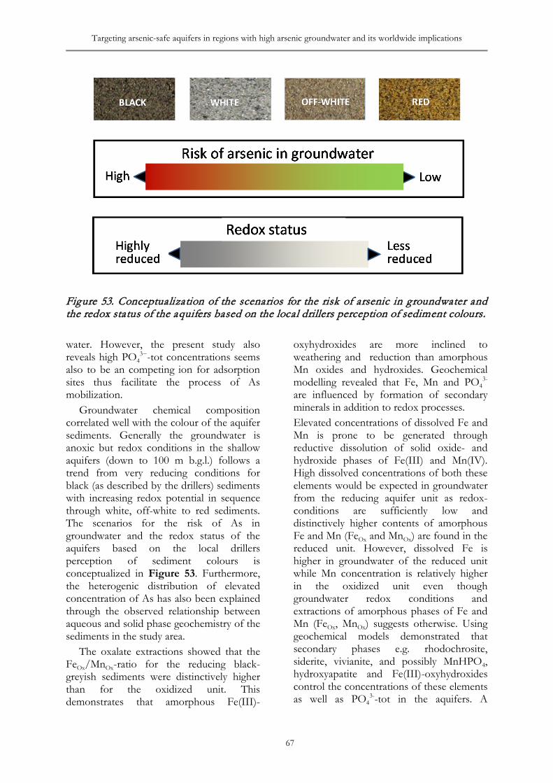
Targeting arsenic-safe aquifers in regions with high arsenic groundwater and its worldwide implications
67
Figure 53. Conceptualization of the scenarios for the risk of arsenic in groundwater and the redox status of the aquifers based on the local drillers perception of sediment colours. water. However, the present study also reveals high PO4
3−-tot concentrations seems also to be an competing ion for adsorption sites thus facilitate the process of As mobilization.
Groundwater chemical composition correlated well with the colour of the aquifer sediments. Generally the groundwater is anoxic but redox conditions in the shallow aquifers (down to 100 m b.g.l.) follows a trend from very reducing conditions for black (as described by the drillers) sediments with increasing redox potential in sequence through white, off-white to red sediments. The scenarios for the risk of As in groundwater and the redox status of the aquifers based on the local drillers perception of sediment colours is conceptualized in Figure 53. Furthermore, the heterogenic distribution of elevated concentration of As has also been explained through the observed relationship between aqueous and solid phase geochemistry of the sediments in the study area.
The oxalate extractions showed that the FeOx/MnOx-ratio for the reducing black-greyish sediments were distinctively higher than for the oxidized unit. This demonstrates that amorphous Fe(III)-
oxyhydroxides are more inclined to weathering and reduction than amorphous Mn oxides and hydroxides. Geochemical modelling revealed that Fe, Mn and PO4
3- are influenced by formation of secondary minerals in addition to redox processes. Elevated concentrations of dissolved Fe and Mn is prone to be generated through reductive dissolution of solid oxide- and hydroxide phases of Fe(III) and Mn(IV). High dissolved concentrations of both these elements would be expected in groundwater from the reducing aquifer unit as redox-conditions are sufficiently low and distinctively higher contents of amorphous Fe and Mn (FeOx and MnOx) are found in the reduced unit. However, dissolved Fe is higher in groundwater of the reduced unit while Mn concentration is relatively higher in the oxidized unit even though groundwater redox conditions and extractions of amorphous phases of Fe and Mn (FeOx, MnOx) suggests otherwise. Using geochemical models demonstrated that secondary phases e.g. rhodochrosite, siderite, vivianite, and possibly MnHPO4, hydroxyapatite and Fe(III)-oxyhydroxides control the concentrations of these elements as well as PO4
3--tot in the aquifers. A
Bhattacharya, Thunvik, Jacks and von Brömssen TRITA LWR Report 2015: 01
68
plausible behavior of Fe, Mn, As, PO43--tot,
pH and HCO3- and their interactions at the
solid-aqueous phase interface within the sediments could be explained through the results of geochemical modelling. Geochemical modelling based on experimental data demonstrated that the mobility of As is largely influenced by Hfo, pH and competing ions. In addition to reductive dissolution of Fe(III)-oxyhydroxides it is expected that relatively high PO4
3−-tot concentrations compete for adsorption sites is stimulating As mobilization.
Decomposition of organic matter induce reductive dissolution of Fe(III)-oxyhydroxides and mobilization of As into the groundwater. Active reduction in the grey to dark grey aquifer is also indicated by the depletion of dissolved SO4
2- and formation of authigenic pyrite. In the yellowish grey oxidized topsoil dominance of crystalline iron oxides and hydroxides like magnetite, hematite and goethite. Weathering of biotite seems to plays a crucial role for generation of Fe(III)-oxyhydroxide. The presence of amorphous Fe(III)-oxyhydroxides in the mica rich dark grey reduced sediment, mostly as grain coatings were revealed by SEM and XRD studies.
7.3. Adsorption dynamics of arsenic in oxidized sediments Laboratory investigations on As adsorption dynamics demonstrates that the oxidized sediments have a high capacity to absorb As. For batch isotherm experiments As(V) was used because sampling of tube-wells indicate this is the dominant aqueous redox species in the oxidized sediments. It is suggested that the adsorption of As(III) is examined as well. Simulations of the experimental isotherms underpredict the adsorption capacity. This may indicate that that crystalline Fe(III) oxides, Mn(IV) oxides, Al(III) oxides and clay minerals may also contribute to the adsorption capacity of the sediment.
Column experiments on oxidized sediments with As(III) and lactose added to
the influent water showed that the adsorption capacity may be reduced by high levels of DOC or other electron donors. The column experiments demonstrated that the decreased adsorption capacity was due to the reductive dissolution of Fe(III)-oxyhydroxides and Mn(IV)-oxides due to the microbial interactions induced by the addition of lactose. However, in natural aquifers with present DOC the reactions are expected to be much slower as DOC is a much more complex and may be refractive in character. The complex processes of adsorption however need further investigations on mineralogy, laboratory experiments together with geochemical modelling for accurate site specific prediction of the fate and dynamics of As in aquifers with high influx of DOC in groundwater.
7.4. Risks for cross-contamination between aquifers 7.4.1. Risks from hydrological perspectives
and groundwater flow modelling The groundwater models developed proved to be useful as a tool for enhancing the understating of the groundwater flow system when combined with field observations of seasonal hydraulic head monitoring in piezometer nests and 14C analysis with subsequent dating of groundwater.
Hydrogeological field investigations and groundwater flow modelling demonstrated that Matlab acts essentially as a recharge area even though the area is adjacent to river Meghna. The groundwater simulations could identify at least two flow-systems; i) a deeper regional horizontal flow system with recharge areas at the Tripura Hills in the east and ii) small local flow systems driven by local topography and with local groundwater recharge. The local flow systems reach a depth of approximately 30 m b.g.l. in Matlab for calibrated groundwater models and is consistent with analyzed 14C ages that indicate that young groundwater should be expected down to a depth of approximately 25 m b.g.l. while being older below (>1,000 yr). This demonstrates that the groundwater flow at depth (below local flow
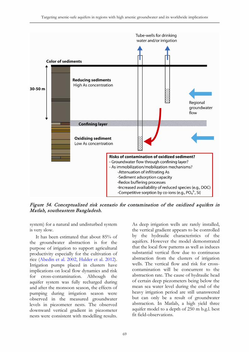
Targeting arsenic-safe aquifers in regions with high arsenic groundwater and its worldwide implications
69
Figure 54. Conceptualized risk scenario for contamination of the oxidized aquifers in Matlab, southeastern Bangladesh. system) for a natural and undisturbed system is very slow.
It has been estimated that about 85% of the groundwater abstraction is for the purpose of irrigation to support agricultural productivity especially for the cultivation of rice (Abedin et al. 2002, Halder et al. 2012). Irrigation pumps placed in clusters have implications on local flow dynamics and risk for cross-contamination. Although the aquifer system was fully recharged during and after the monsoon season, the effects of pumping during irrigation season were observed in the measured groundwater levels in piezometer nests. The observed downward vertical gradient in piezometer nests were consistent with modelling results.
As deep irrigation wells are rarely installed, the vertical gradient appears to be controlled by the hydraulic characteristics of the aquifers. However the model demonstrated that the local flow patterns as well as induces substantial vertical flow due to continuous abstraction from the clusters of irrigation wells. The vertical flow and risk for cross-contamination will be concurrent to the abstraction rate. The cause of hydraulic head of certain deep piezometers being below the mean sea water level during the end of the heavy irrigation period are still unanswered but can only be a result of groundwater abstraction. In Matlab, a high yield three aquifer model to a depth of 250 m b.g.l. best fit field-observations.
Bhattacharya, Thunvik, Jacks and von Brömssen TRITA LWR Report 2015: 01
70
7.4.2. Risks of cross-contamination of the oxidized aquifers based on adsorption modelling
The results through our studies as well as a series of other studies have shown that redox conditions and dissolved As concentration are related to the colour of the aquifer sediments (Bhattacharya et al. 2010, Bundschuh et al. 2010, Jonsson and Lundell 2004, von Brömssen et al. 2007, 2008). Overlying black–gray aquifer sediments tend to be reducing with high dissolved As levels. Off-white, yellowish and reddish sediments are oxidized at shallow depths (<100 m) with low risk of elevated As concentrations. However, there is concern that tube-wells installed in As-safe sediments may become enriched in As over time. Water abstraction from the As-safe sediments may induce flow of reduced groundwater from surrounding sediments with high As concentration or surface water that is rich in electron donors such as DOC to the As-safe aquifer zones (Polya and Charlet 2009) to the safe aquifer zones as conceptualized in Figure 54).
While the oxidized sediments may initially have a high capacity to adsorb As, this capacity may be reduced by the increased availability of electron donors that stimulate the reduction of Fe(III) and Mn(IV) oxides (Bhattacharya et al. 2009, Sharif et al. 2008, Stollenwerk et al. 2007). The reduction of these minerals may lead to the transfer of sediment-bound As to the groundwater. An increased availability of ions that compete with As for adsorption sites (e.g., PO4
3-, Si, Ca, HCO3-) may also
stimulate the release of sediment-bound As (Nath et al. 2009, Polya and Charlet, 2009). Understanding of the adsorption behaviour of the oxidized sediments and their ability to attenuate As if cross contamination occurs is, therefore, needed to evaluate the sustainability of targeting the shallow As-safe sediments. Although prior studies have examined the processes leading to As mobilization in the reduced sediments, there is limited understanding of the adsorption processes in the oxidized sediments.
This study has shown that the oxidized sediments in Matlab Region, have a high capacity to absorb As, although they currently have a relatively low sediment-bound As content (below 2.5 mg/kg). This suggests targeting these sediments for installation of tube-wells may be a simple sustainable solution for delivering safe drinking water to the rural communities in areas where these oxidized sediments exist at shallow depth. The As adsorption processes however are complex and require further investigation to more accurately assess the risks of cross-contamination. This assessment needs to be coupled with rigorous long-term monitoring of the water chemistry in tube-wells installed in the oxidized sediments. Discrepancy in the amount of solid phase Fe estimated from oxalate extractions and calibrated based on measured As(V) adsorption isotherms indicate that a significant portion of the adsorption sites in the oxidized sediments are associated with solid phase crystalline, rather than amorphous, Fe. The good match between the shape of the simulated and experimental adsorption isotherms, and the ability of the model to predict the amounts of As and other adsorbing species bound to the amorphous Fe minerals, indicate that the model and parameter values adopted was able to adequately represent the adsorption behaviour in the oxidized sediments. The capacity of the oxidized sediments to attenuate As may be decreased by high levels of DOC (or other electron donors) in water infiltrating the safe aquifer layers and this may lead to the reductive dissolution of Fe(III) and Mn(IV) oxides and the subsequent release of As. The reactivity and rate of degradation of the DOC present in the aquifer layers at Matlab requires further investigation.
8. TESTING THE IDEA FOR WORLDWIDE IMPLICATION
8.1. Replication study in West Bengal For the validation of the ongoing indigenous drilling practice by local drillers in other parts of the Bengal Basin, this replication study was carried out in Chakdaha Block of
Targeting arsenic-safe aquifers in regions with high arsenic groundwater and its worldwide implications
71
the Nadia district in West Bengal, India. A number of studies in West Bengal, India (McArthur et al. 2004, 2011, Pal and Mukherjee, 2008, 2009, Biswas et al. 2014a) have attempted to link the color of aquifer sediments with the occurrence of As in groundwater. It has been reported that grey sand aquifers (GSA) are mostly contaminated with dissolved As (>10 μg/L), whereas brown sand aquifers (BSA) may be safe (<10 μg/L). The classification of the aquifers as shallow grey sand aquifers (GSA) and the brown sand aquifers (BSA) within shallow depth (< 70 m) have shown all possible variability in the colour shades and analogous to the reducing and the oxidized sequences as delineated aquifers based on the sediment color as perceived by the local driller in Matlab. (von Brömssen et al. 2007). The BSA sediments analogous to the sequence of oxidized unit with red sand colours within shallow depth in Matlab study area has been suggested to be targeted for safe drinking water supply in Bangladesh (von Brömssen et al. 2007, Bundschuh et al. 2010). However, so far no attempt has been made to validate the redox status of these two aquifers, which could be extremely important for assessing the long term sustainability of BSA for safe drinking water supply.
8.2. Location of the study area In order to validate the local drillers approach to target safe aquifers based on sediment colour, a detailed hydro-geochemical investigation was carried out to assess the redox status of groundwater abstracted from BSA and GSA aquifers within shallow depth (~70 m) within an area (100 km2; 23.02–23.14°N, 88.49–88.62°E) is located approximately60 km north of Kolkata city, in the Chakdaha Block of Nadia district, West Bengal. The area is. bounded on the west by river Hooghly (distributaries of river Ganges) and by the river Ichamati to the east (Figure 55).
8.3. Groundwater sampling and analysis Samples of groundwater were collected from 57 wells (35 from GSA and 22 from BSA)
from the existing TWs at shallow depth (~70 m, except for 3 wells installed in BSA) close to 29 drilled borehole locations (Figure 55). Prior to groundwater sampling the TWs were purged continuously until pH, electrical conductivity (EC) temperature (T) and oxidation reduction potential (ORP, latter corrected with respect to standard hydrogen electrode for Eh) were stabilized. The pH, EC, T, ORP and dissolved oxygen (DO) were measured in a flow cell fitted with electrodes for ORP and DO (Biswas et al. 2012, 2014b) and the alkalinity (HCO3
-) was measured by titrating with 0.02 N H2SO4 on site prior to groundwater sampling. From each TW four sets of groundwater samples were preserved after filtering through 0.45 μm Axiva® membrane filters for Fe(II), DOC, anion, major cation, trace elements and As(III) analyses. As(III) and (V) were separated in the field through a Disposable Cartridge® packed with an ion exchanger, at a flow rate of 5 mL/min (Metal Soft Centre, Highland Park, USA, Meng et al. (2001). The samples for quantification of As(III), major cations and trace elements were acidified with 14N, Suprapur HNO3 (Merck). In the field all samples were stored in ice box and finally after return to the laboratory, samples were stored in refrigerator at 4°C prior to analyses.
To minimize redox alteration, Fe(II), NH4
+ and anions were analyzed overnight after sampling following the procedure outlined APHA, 1998 and detailed in Biswas et al. (2012). The analysis of DOC was carried out on a Shimadzu 5000 TOC analyser at the KTH Royal Institute of Technology. Anions and NH4
+ were analyzed in the same sample by Metrohm Ion Chromatography (model 761 Compact IC) at the University of Kalyani, West Bengal. Major cations and trace elements were analyzed by inductively coupled plasma optical emission spectrometer (ICP-OES, Varian Vista-PRO) at the Stockholm University. Ten percent of the samples (n=6) were randomly analyzed to test the precision of analysis by ICP-OES. For all the elements the precision of the analysis
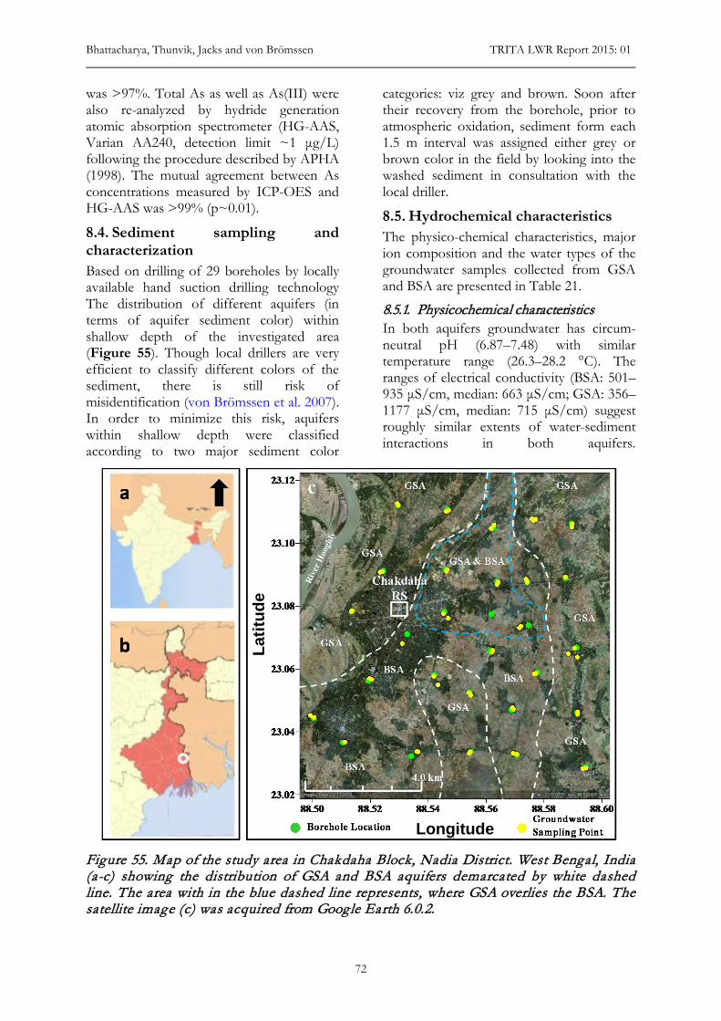
Bhattacharya, Thunvik, Jacks and von Brömssen TRITA LWR Report 2015: 01
72
was >97%. Total As as well as As(III) were also re-analyzed by hydride generation atomic absorption spectrometer (HG-AAS, Varian AA240, detection limit ~1 μg/L) following the procedure described by APHA (1998). The mutual agreement between As concentrations measured by ICP-OES and HG-AAS was >99% (p~0.01).
8.4. Sediment sampling and characterization Based on drilling of 29 boreholes by locally available hand suction drilling technology The distribution of different aquifers (in terms of aquifer sediment color) within shallow depth of the investigated area (Figure 55). Though local drillers are very efficient to classify different colors of the sediment, there is still risk of misidentification (von Brömssen et al. 2007). In order to minimize this risk, aquifers within shallow depth were classified according to two major sediment color
categories: viz grey and brown. Soon after their recovery from the borehole, prior to atmospheric oxidation, sediment form each 1.5 m interval was assigned either grey or brown color in the field by looking into the washed sediment in consultation with the local driller.
8.5. Hydrochemical characteristics The physico-chemical characteristics, major ion composition and the water types of the groundwater samples collected from GSA and BSA are presented in Table 21.
8.5.1. Physicochemical characteristics In both aquifers groundwater has circum-neutral pH (6.87–7.48) with similar temperature range (26.3–28.2 °C). The ranges of electrical conductivity (BSA: 501–935 μS/cm, median: 663 μS/cm; GSA: 356–1177 μS/cm, median: 715 μS/cm) suggest roughly similar extents of water-sediment interactions in both aquifers.
Figure 55. Map of the study area in Chakdaha Block, Nadia District. West Bengal, India (a-c) showing the distribution of GSA and BSA aquifers demarcated by white dashed line. The area with in the blue dashed line represents, where GSA overlies the BSA. The satellite image (c) was acquired from Google Earth 6.0.2.
Latit
ude
Longitude
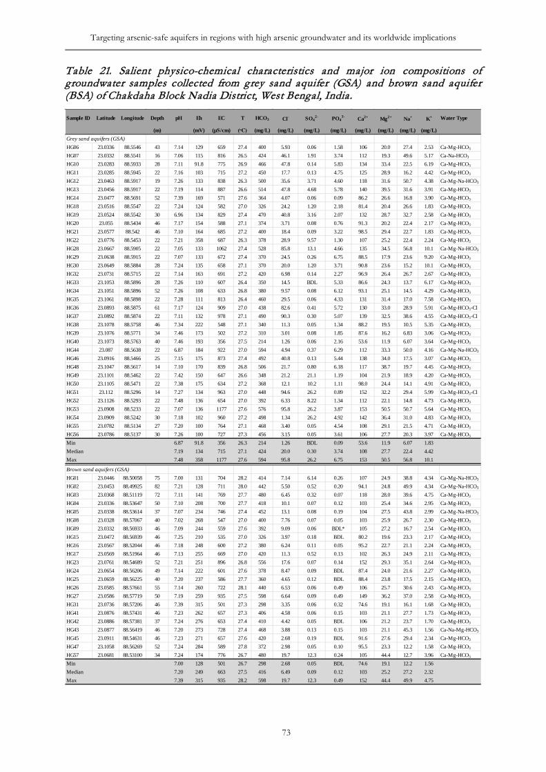
Targeting arsenic-safe aquifers in regions with high arsenic groundwater and its worldwide implications
73
Table 21. Salient physico-chemical characteristics and major ion compositions of groundwater samples collected from grey sand aquifer (GSA) and brown sand aquifer (BSA) of Chakdaha Block Nadia District, West Bengal, India.
Sample ID Latitude Longitude Depth pH Eh EC T HCO3 Cl- SO42- PO4
3- Ca2+ Mg2+ Na+ K+ Water Type
(m) (mV) (µS/cm) (ᵒC) (mg/L) (mg/L) (mg/L) (mg/L) (mg/L) (mg/L) (mg/L) (mg/L)Grey sand aquifers (GSA)HG06 23.0336 88.5546 43 7.14 129 659 27.4 400 5.93 0.06 1.58 106 20.0 27.4 2.53 Ca-Mg-HCO3
HG07 23.0332 88.5541 16 7.06 115 816 26.5 424 46.1 1.91 3.74 112 19.3 49.6 5.17 Ca-Na-HCO3
HG10 23.0283 88.5933 28 7.11 91.8 775 26.9 466 47.8 0.14 5.83 134 33.4 22.5 6.19 Ca-Mg-HCO3
HG11 23.0285 88.5945 22 7.16 103 715 27.2 450 17.7 0.13 4.75 125 28.9 16.2 4.42 Ca-Mg-HCO3
HG12 23.0463 88.5917 19 7.26 133 838 26.3 500 35.6 3.71 4.60 118 31.6 50.7 4.38 Ca-Mg-Na-HCO3
HG13 23.0456 88.5917 22 7.19 114 887 26.6 514 47.8 4.68 5.78 140 39.5 31.6 3.91 Ca-Mg-HCO3
HG14 23.0477 88.5691 52 7.39 169 571 27.6 364 4.07 0.06 0.09 86.2 26.6 16.8 3.90 Ca-Mg-HCO3
HG18 23.0516 88.5547 22 7.24 124 582 27.0 326 24.2 1.20 2.18 81.4 20.4 26.6 1.83 Ca-Mg-HCO3
HG19 23.0524 88.5542 30 6.96 134 829 27.4 470 40.8 3.16 2.07 132 28.7 32.7 2.58 Ca-Mg-HCO3
HG20 23.055 88.5434 46 7.17 154 588 27.1 374 3.71 0.08 0.76 91.3 20.2 22.4 2.17 Ca-Mg-HCO3
HG21 23.0577 88.542 46 7.10 164 685 27.2 400 18.4 0.09 3.22 98.5 29.4 22.7 1.83 Ca-Mg-HCO3
HG22 23.0776 88.5453 22 7.21 358 687 26.3 378 28.9 9.57 1.30 107 25.2 22.4 2.24 Ca-Mg-HCO3
HG28 23.0667 88.5905 22 7.05 133 1062 27.4 528 85.8 13.1 4.66 135 34.5 56.8 10.1 Ca-Mg-Na-HCO3
HG29 23.0638 88.5915 22 7.07 133 672 27.4 370 24.5 0.26 6.75 88.5 17.9 23.6 9.20 Ca-Mg-HCO3
HG30 23.0649 88.5884 28 7.24 135 658 27.1 370 20.0 1.20 3.71 90.8 23.6 15.2 10.1 Ca-Mg-HCO3
HG32 23.0731 88.5715 22 7.14 163 691 27.2 420 6.98 0.14 2.27 96.9 26.4 26.7 2.67 Ca-Mg-HCO3
HG33 23.1053 88.5896 28 7.26 110 607 26.4 350 14.5 BDL 5.33 86.6 24.3 13.7 6.17 Ca-Mg-HCO3
HG34 23.1051 88.5896 52 7.26 108 633 26.8 380 9.57 0.08 6.12 93.1 25.1 14.5 4.29 Ca-Mg-HCO3
HG35 23.1061 88.5898 22 7.28 111 813 26.4 460 29.5 0.06 4.33 131 31.4 17.0 7.58 Ca-Mg-HCO3
HG36 23.0893 88.5875 61 7.17 124 909 27.0 438 82.6 0.41 5.72 130 33.0 28.9 5.91 Ca-Mg-HCO3-ClHG37 23.0892 88.5874 22 7.11 132 978 27.1 490 90.3 0.30 5.07 139 32.5 38.6 4.55 Ca-Mg-HCO3-ClHG38 23.1078 88.5758 46 7.34 222 548 27.1 340 11.3 0.05 1.34 88.2 19.5 10.5 5.35 Ca-Mg-HCO3
HG39 23.1076 88.5771 34 7.46 173 502 27.2 310 3.01 0.08 1.85 87.6 16.2 6.83 3.06 Ca-Mg-HCO3
HG40 23.1073 88.5763 40 7.46 193 356 27.5 214 1.26 0.06 2.16 53.6 11.9 6.07 3.64 Ca-Mg-HCO3
HG44 23.087 88.5638 22 6.87 184 922 27.0 594 4.94 0.37 6.29 112 33.3 50.0 4.16 Ca-Mg-Na-HCO3
HG46 23.0916 88.5466 25 7.15 175 873 27.4 492 40.8 0.13 5.44 138 34.0 17.5 3.07 Ca-Mg-HCO3
HG48 23.1047 88.5617 14 7.10 170 839 26.8 506 21.7 0.80 6.18 117 38.7 19.7 4.45 Ca-Mg-HCO3
HG49 23.1101 88.5462 22 7.42 150 647 26.6 348 21.2 21.1 1.19 104 21.9 18.9 4.20 Ca-Mg-HCO3
HG50 23.1105 88.5471 22 7.38 175 634 27.2 368 12.1 10.2 1.11 98.0 24.4 14.1 4.91 Ca-Mg-HCO3
HG51 23.112 88.5296 14 7.27 134 963 27.0 448 94.6 26.2 0.89 152 32.2 29.4 5.99 Ca-Mg-HCO3-ClHG52 23.1126 88.5293 22 7.48 136 654 27.0 392 6.33 8.22 1.34 112 22.1 14.8 4.73 Ca-Mg-HCO3
HG53 23.0908 88.5233 22 7.07 136 1177 27.6 576 95.8 26.2 3.87 153 50.5 50.7 5.64 Ca-Mg-HCO3
HG54 23.0909 88.5242 30 7.18 102 960 27.2 498 1.34 26.2 4.92 142 36.4 31.0 4.83 Ca-Mg-HCO3
HG55 23.0782 88.5134 27 7.20 100 764 27.1 468 3.40 0.05 4.54 108 29.1 21.5 4.71 Ca-Mg-HCO3
HG56 23.0786 88.5137 30 7.26 100 727 27.3 456 3.15 0.05 3.61 106 27.7 20.3 3.97 Ca-Mg-HCO3
Min 6.87 91.8 356 26.3 214 1.26 BDL 0.09 53.6 11.9 6.07 1.83Median 7.19 134 715 27.1 424 20.0 0.30 3.74 108 27.7 22.4 4.42Max 7.48 358 1177 27.6 594 95.8 26.2 6.75 153 50.5 56.8 10.1
Brown sand aquifers (GSA)HG01 23.0446 88.50058 75 7.00 131 704 28.2 414 7.14 6.14 0.26 107 24.9 38.8 4.34 Ca-Mg-Na-HCO3
HG02 23.0453 88.49925 82 7.21 128 711 28.0 442 5.50 0.52 0.20 94.1 24.8 49.9 4.34 Ca-Mg-Na-HCO3
HG03 23.0368 88.51119 72 7.11 141 769 27.7 480 6.45 0.32 0.07 118 28.0 39.6 4.75 Ca-Mg-HCO3
HG04 23.0336 88.53647 50 7.10 208 700 27.7 418 10.1 0.07 0.12 103 25.4 34.6 2.95 Ca-Mg-HCO3
HG05 23.0338 88.53614 37 7.07 234 746 27.4 452 13.1 0.08 0.19 104 27.5 43.8 2.99 Ca-Mg-Na-HCO3
HG08 23.0328 88.57067 40 7.02 268 547 27.0 400 7.76 0.07 0.05 103 25.9 26.7 2.30 Ca-Mg-HCO3
HG09 23.0332 88.56933 46 7.09 244 559 27.6 392 9.09 0.06 BDL* 105 27.2 16.7 2.54 Ca-Mg-HCO3
HG15 23.0472 88.56939 46 7.25 210 535 27.0 326 3.97 0.18 BDL 80.2 19.6 23.3 2.17 Ca-Mg-HCO3
HG16 23.0567 88.52044 46 7.18 248 600 27.2 380 6.24 0.11 0.05 95.2 22.7 21.1 2.24 Ca-Mg-HCO3
HG17 23.0569 88.51964 46 7.13 255 669 27.0 420 11.3 0.52 0.13 102 26.3 24.9 2.11 Ca-Mg-HCO3
HG23 23.0761 88.54689 52 7.21 251 896 26.8 556 17.6 0.07 0.14 152 29.3 35.1 2.64 Ca-Mg-HCO3
HG24 23.0654 88.56206 49 7.14 222 601 27.6 378 8.47 0.09 BDL 87.4 24.0 21.6 2.27 Ca-Mg-HCO3
HG25 23.0659 88.56225 40 7.20 237 586 27.7 360 4.65 0.12 BDL 88.4 23.8 17.5 2.15 Ca-Mg-HCO3
HG26 23.0585 88.57661 55 7.14 260 722 28.1 440 6.53 0.06 0.49 106 25.7 30.6 2.43 Ca-Mg-HCO3
HG27 23.0586 88.57719 50 7.19 259 935 27.5 598 6.64 0.09 0.49 149 36.2 37.0 2.58 Ca-Mg-HCO3
HG31 23.0736 88.57206 46 7.39 315 501 27.3 298 3.35 0.06 0.32 74.6 19.1 16.1 1.68 Ca-Mg-HCO3
HG41 23.0876 88.57431 46 7.23 262 657 27.3 406 4.58 0.06 0.15 103 21.1 27.7 1.73 Ca-Mg-HCO3
HG42 23.0886 88.57381 37 7.24 276 653 27.4 410 4.42 0.05 BDL 106 21.2 23.7 1.70 Ca-Mg-HCO3
HG43 23.0877 88.56419 46 7.20 273 728 27.4 468 3.88 0.13 0.15 103 21.1 45.3 1.56 Ca-Na-Mg-HCO3
HG45 23.0911 88.54631 46 7.23 271 657 27.6 420 2.68 0.19 BDL 91.6 27.6 29.4 2.34 Ca-Mg-HCO3
HG47 23.1058 88.56269 52 7.24 284 589 27.8 372 2.98 0.05 0.10 95.5 23.3 12.2 1.58 Ca-Mg-HCO3
HG57 23.0681 88.53100 34 7.24 174 776 26.7 480 19.7 12.3 0.24 105 44.4 12.7 3.96 Ca-Mg-HCO3
Min 7.00 128 501 26.7 298 2.68 0.05 BDL 74.6 19.1 12.2 1.56Median 7.20 249 663 27.5 416 6.49 0.09 0.12 103 25.2 27.2 2.32Max 7.39 315 935 28.2 598 19.7 12.3 0.49 152 44.4 49.9 4.75
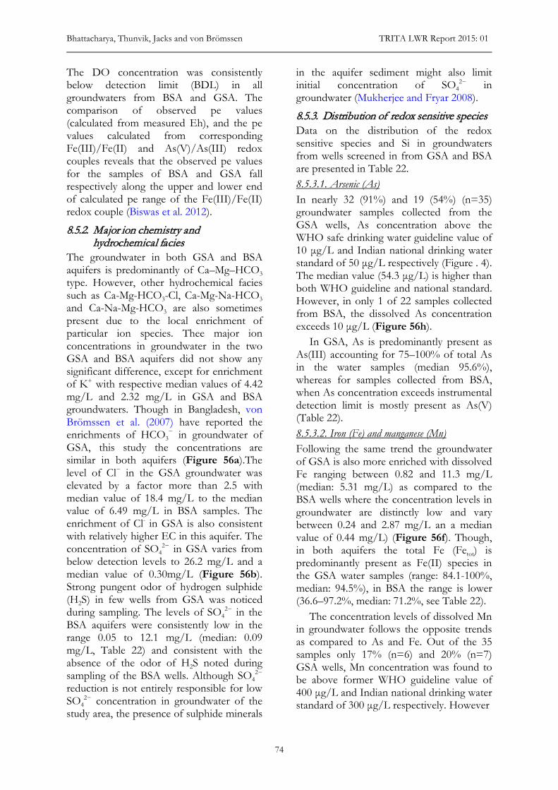
Bhattacharya, Thunvik, Jacks and von Brömssen TRITA LWR Report 2015: 01
74
The DO concentration was consistently below detection limit (BDL) in all groundwaters from BSA and GSA. The comparison of observed pe values (calculated from measured Eh), and the pe values calculated from corresponding Fe(III)/Fe(II) and As(V)/As(III) redox couples reveals that the observed pe values for the samples of BSA and GSA fall respectively along the upper and lower end of calculated pe range of the Fe(III)/Fe(II) redox couple (Biswas et al. 2012).
8.5.2. Major ion chemistry and hydrochemical facies
The groundwater in both GSA and BSA aquifers is predominantly of Ca–Mg–HCO3 type. However, other hydrochemical facies such as Ca-Mg-HCO3-Cl, Ca-Mg-Na-HCO3 and Ca-Na-Mg-HCO3 are also sometimes present due to the local enrichment of particular ion species. Thee major ion concentrations in groundwater in the two GSA and BSA aquifers did not show any significant difference, except for enrichment of K+ with respective median values of 4.42 mg/L and 2.32 mg/L in GSA and BSA groundwaters. Though in Bangladesh, von Brömssen et al. (2007) have reported the enrichments of HCO3
− in groundwater of GSA, this study the concentrations are similar in both aquifers (Figure 56a).The level of Cl− in the GSA groundwater was elevated by a factor more than 2.5 with median value of 18.4 mg/L to the median value of 6.49 mg/L in BSA samples. The enrichment of Cl- in GSA is also consistent with relatively higher EC in this aquifer. The concentration of SO4
2− in GSA varies from below detection levels to 26.2 mg/L and a median value of 0.30mg/L (Figure 56b). Strong pungent odor of hydrogen sulphide (H2S) in few wells from GSA was noticed during sampling. The levels of SO4
2− in the BSA aquifers were consistently low in the range 0.05 to 12.1 mg/L (median: 0.09 mg/L, Table 22) and consistent with the absence of the odor of H2S noted during sampling of the BSA wells. Although SO4
2− reduction is not entirely responsible for low SO4
2− concentration in groundwater of the study area, the presence of sulphide minerals
in the aquifer sediment might also limit initial concentration of SO4
2− in groundwater (Mukherjee and Fryar 2008).
8.5.3. Distribution of redox sensitive species Data on the distribution of the redox sensitive species and Si in groundwaters from wells screened in from GSA and BSA are presented in Table 22. 8.5.3.1. Arsenic (As) In nearly 32 (91%) and 19 (54%) (n=35) groundwater samples collected from the GSA wells, As concentration above the WHO safe drinking water guideline value of 10 μg/L and Indian national drinking water standard of 50 μg/L respectively (Figure . 4). The median value (54.3 μg/L) is higher than both WHO guideline and national standard. However, in only 1 of 22 samples collected from BSA, the dissolved As concentration exceeds 10 μg/L (Figure 56h).
In GSA, As is predominantly present as As(III) accounting for 75–100% of total As in the water samples (median 95.6%), whereas for samples collected from BSA, when As concentration exceeds instrumental detection limit is mostly present as As(V) (Table 22). 8.5.3.2. Iron (Fe) and manganese (Mn) Following the same trend the groundwater of GSA is also more enriched with dissolved Fe ranging between 0.82 and 11.3 mg/L (median: 5.31 mg/L) as compared to the BSA wells where the concentration levels in groundwater are distinctly low and vary between 0.24 and 2.87 mg/L an a median value of 0.44 mg/L) (Figure 56f). Though, in both aquifers the total Fe (Fetot) is predominantly present as Fe(II) species in the GSA water samples (range: 84.1-100%, median: 94.5%), in BSA the range is lower (36.6–97.2%, median: 71.2%, see Table 22).
The concentration levels of dissolved Mn in groundwater follows the opposite trends as compared to As and Fe. Out of the 35 samples only 17% (n=6) and 20% (n=7) GSA wells, Mn concentration was found to be above former WHO guideline value of 400 μg/L and Indian national drinking water standard of 300 μg/L respectively. However
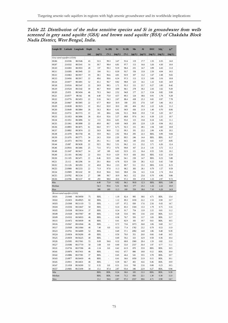
Targeting arsenic-safe aquifers in regions with high arsenic groundwater and its worldwide implications
75
Table 22. Distribution of the redox sensitive species and Si in groundwater from wells screened in grey sand aquifer (GSA) and brown sand aquifer (BSA) of Chakdaha Block Nadia District, West Bengal, India.
Sample ID Latitude Longitude Depth As As (III) Fe Fe (II) Mn Al DOC NH4+ Si4+
(m) (µg/L) (% ) (mg/L) (% ) (µg/L) (µg/L) (mg/L) (mg/L) (mg/L)Grey sand aquifers (GSA)HG06 23.0336 88.5546 43 53.5 99.3 3.47 91.6 119 17.7 1.55 0.35 14.0HG07 23.0332 88.5541 16 30.7 98.4 6.81 97.7 113 16.6 3.26 4.30 10.0HG10 23.0283 88.5933 28 137 99.3 9.19 98.4 231 14.7 3.99 4.43 11.0HG11 23.0285 88.5945 22 104 91.1 8.30 93.7 156 13.9 2.59 4.04 10.5HG12 23.0463 88.5917 19 38.1 96.6 4.81 92.9 107 13.2 1.67 2.48 9.65HG13 23.0456 88.5917 22 49.6 99.6 6.24 97.3 113 12.3 3.00 3.16 10.8HG14 23.0477 88.5691 52 45.1 96.7 0.82 98.8 123 14.1 1.32 0.43 14.9HG18 23.0516 88.5547 22 26.9 98.5 1.71 95.3 115 25.7 0.27 1.83 8.42HG19 23.0524 88.5542 30 46.7 90.8 4.09 84.1 278 30.2 2.43 1.62 9.20HG20 23.055 88.5434 46 70.3 94.0 2.52 94.8 177 21.7 0.54 0.82 9.90HG21 23.0577 88.542 46 4.40 75.0 4.57 89.3 124 38.6 0.91 1.78 9.28HG22 23.0776 88.5453 22 9.16 94.3 2.67 88.4 438 25.3 0.81 0.97 7.78HG28 23.0667 88.5905 22 67.7 86.0 10.9 100 255 27.6 5.87 3.46 10.3HG29 23.0638 88.5915 22 83.2 82.0 10.0 100 404 29.2 2.22 6.26 11.2HG30 23.0649 88.5884 28 54.3 86.4 6.41 94.9 436 21.9 1.40 0.70 8.06HG32 23.0731 88.5715 22 101 88.6 3.06 91.5 90.8 25.9 7.10 3.20 10.7HG33 23.1053 88.5896 28 83.4 95.6 5.27 88.8 97.6 24.1 0.39 2.22 10.7HG34 23.1051 88.5896 52 113 83.6 6.01 95.0 123 23.8 0.34 3.45 11.1HG35 23.1061 88.5898 22 49.0 86.7 6.00 94.8 203 22.8 1.29 0.94 10.2HG36 23.0893 88.5875 61 66.0 97.7 6.75 92.3 155 28.5 1.94 3.60 10.8HG37 23.0892 88.5874 22 56.9 96.8 7.22 99.3 191 22.2 2.06 4.36 10.5HG38 23.1078 88.5758 46 19.9 96.5 2.92 90.4 295 22.3 BDL 0.99 9.04HG39 23.1076 88.5771 34 24.3 93.8 2.20 89.5 246 14.4 BDL BDL 8.17HG40 23.1073 88.5763 40 29.1 91.1 1.68 84.5 149 23.6 4.61 0.57 8.85HG44 23.087 88.5638 22 92.5 99.2 5.31 96.2 111 23.2 3.71 6.26 12.4HG46 23.0916 88.5466 25 71.6 97.3 9.76 99.8 167 21.4 1.91 3.72 11.3HG48 23.1047 88.5617 14 147 100 6.02 92.9 121 16.4 0.55 5.93 10.2HG49 23.1101 88.5462 22 16.6 91.0 4.20 91.9 426 26.6 BDL 0.32 6.54HG50 23.1105 88.5471 22 8.46 92.9 3.06 94.1 239 14.7 BDL 0.23 5.88HG51 23.112 88.5296 14 20.1 86.6 4.78 92.9 550 28.5 0.22 0.42 7.60HG52 23.1126 88.5293 22 40.8 90.4 2.23 89.7 511 23.1 BDL 0.33 8.23HG53 23.0908 88.5233 22 71.9 97.8 11.3 98.2 383 28.1 0.79 1.57 9.59HG54 23.0909 88.5242 30 85.8 96.6 9.63 98.8 256 14.5 0.34 2.74 10.4HG55 23.0782 88.5134 27 308 99.7 10.9 94.5 152 25.6 0.70 4.96 9.86HG56 23.0786 88.5137 30 293 98.0 10.6 97.2 193 27.8 1.33 2.97 9.72Min 4.40 75.0 0.82 84.1 90.8 12.3 BDL BDL 5.88Median 54.3 95.6 5.31 94.5 177 23.1 1.32 2.22 10.0Max 308 100 11.3 100 550 38.6 7.10 6.26 14.9
Brown sand aquifers (GSA)HG01 23.0446 88.50058 75 BDL - 1.19 82.4 985 38.6 4.71 BDL 13.4HG02 23.0453 88.49925 82 BDL - 1.12 89.3 1030 22.2 1.53 0.90 13.7HG03 23.0368 88.51119 72 BDL - 1.07 97.2 830 17.6 2.56 0.43 14.7HG04 23.0336 88.53647 50 BDL - 0.24 83.3 1504 13.3 1.79 0.75 11.6HG05 23.0338 88.53614 37 BDL - 0.24 91.7 754 13.9 2.22 0.81 11.2HG08 23.0328 88.57067 40 BDL - 0.28 53.6 691 13.6 2.02 BDL 11.5HG09 23.0332 88.56933 46 BDL - 0.30 76.7 593 13.7 1.83 BDL 11.7HG15 23.0472 88.56939 46 BDL - 0.41 82.9 183 19.7 0.61 BDL 10.5HG16 23.0567 88.52044 46 BDL - 0.72 73.6 1073 26.8 1.06 0.60 11.7HG17 23.0569 88.51964 46 7.40 0.0 0.53 77.4 1782 23.2 0.79 0.53 11.9HG23 23.0761 88.54689 52 BDL - 0.49 57.1 2082 14.8 1.86 0.48 9.39HG24 23.0654 88.56206 49 BDL - 0.50 76.0 351 26.0 0.66 0.40 10.5HG25 23.0659 88.56225 40 BDL - 0.49 59.2 323 32.9 0.58 0.36 10.4HG26 23.0585 88.57661 55 8.69 94.6 0.32 68.8 1960 28.4 1.59 0.82 11.9HG27 23.0586 88.57719 50 3.68 0.0 0.40 55.0 2337 26.4 1.97 0.77 11.1HG31 23.0736 88.57206 46 2.24 0.0 0.42 61.9 870 25.9 BDL BDL 10.5HG41 23.0876 88.57431 46 BDL - 0.62 67.7 886 18.8 0.12 BDL 10.4HG42 23.0886 88.57381 37 BDL - 0.45 44.4 541 19.5 3.78 BDL 10.7HG43 23.0877 88.56419 46 BDL - 0.41 36.6 1050 21.9 0.15 BDL 10.1HG45 23.0911 88.54631 46 BDL - 0.39 66.7 402 16.6 0.46 BDL 10.9HG47 23.1058 88.56269 52 0.35 0.0 0.31 51.6 769 22.6 0.08 0.23 10.5HG57 23.0681 88.53100 34 15.1 87.4 2.87 93.4 346 22.9 0.27 BDL 9.94Min BDL BDL 0.24 36.6 183 13.3 BDL BDL 9.39Median BDL BDL 0.44 71.2 850 22.1 1.30 0.30 11.0Max 15.1 94.6 2.87 97.2 2337 38.6 4.71 0.90 14.7
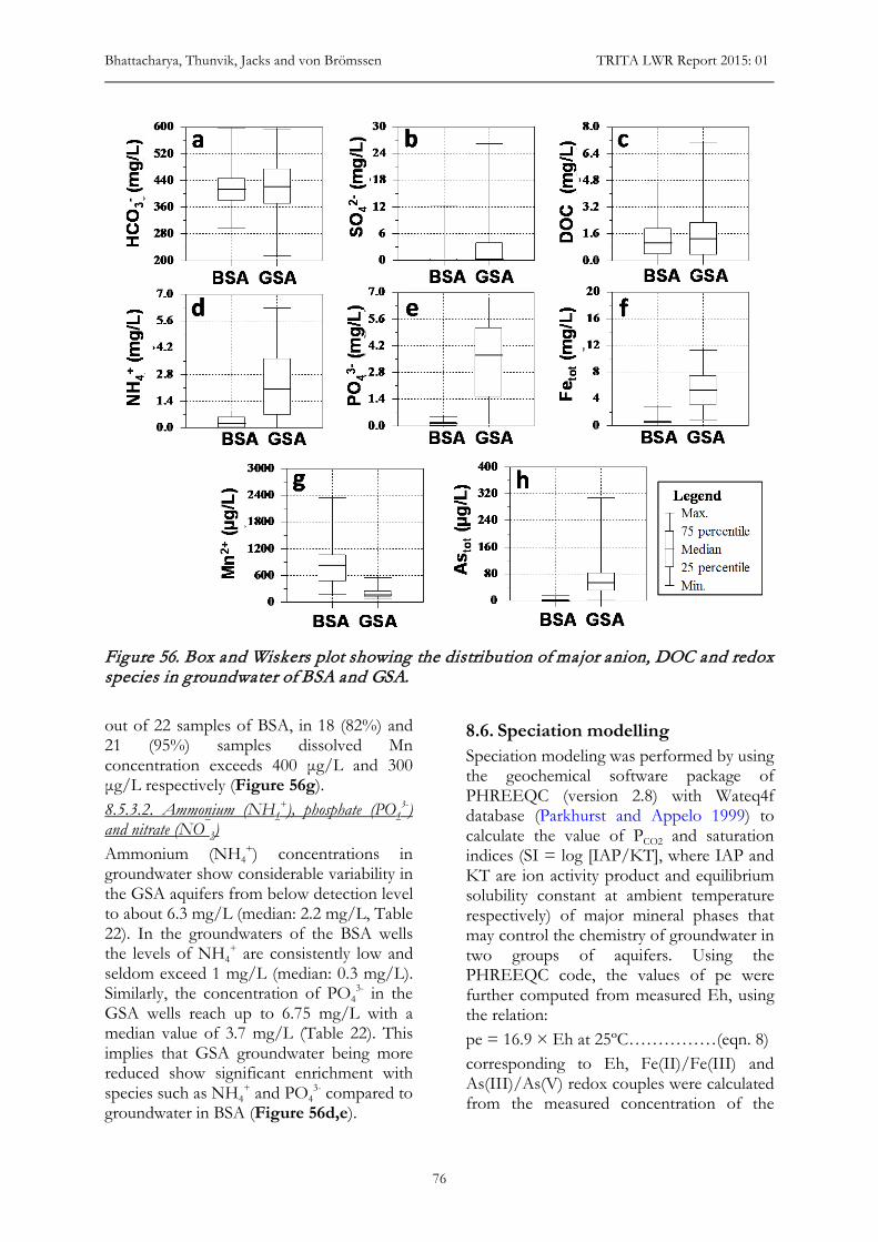
Bhattacharya, Thunvik, Jacks and von Brömssen TRITA LWR Report 2015: 01
76
Figure 56. Box and Wiskers plot showing the distribution of major anion, DOC and redox species in groundwater of BSA and GSA. out of 22 samples of BSA, in 18 (82%) and 21 (95%) samples dissolved Mn concentration exceeds 400 μg/L and 300 μg/L respectively (Figure 56g). 8.5.3.2. Ammonium (NH4
+), phosphate (PO43-)
and nitrate (NO¯3)
Ammonium (NH4+) concentrations in
groundwater show considerable variability in the GSA aquifers from below detection level to about 6.3 mg/L (median: 2.2 mg/L, Table 22). In the groundwaters of the BSA wells the levels of NH4
+ are consistently low and seldom exceed 1 mg/L (median: 0.3 mg/L). Similarly, the concentration of PO4
3- in the GSA wells reach up to 6.75 mg/L with a median value of 3.7 mg/L (Table 22). This implies that GSA groundwater being more reduced show significant enrichment with species such as NH4
+ and PO43- compared to
groundwater in BSA (Figure 56d,e).
8.6. Speciation modelling Speciation modeling was performed by using the geochemical software package of PHREEQC (version 2.8) with Wateq4f database (Parkhurst and Appelo 1999) to calculate the value of PCO2 and saturation indices (SI = log [IAP/KT], where IAP and KT are ion activity product and equilibrium solubility constant at ambient temperature respectively) of major mineral phases that may control the chemistry of groundwater in two groups of aquifers. Using the PHREEQC code, the values of pe were further computed from measured Eh, using the relation: pe = 16.9 × Eh at 25ºC……………(eqn. 8) corresponding to Eh, Fe(II)/Fe(III) and As(III)/As(V) redox couples were calculated from the measured concentration of the
Targeting arsenic-safe aquifers in regions with high arsenic groundwater and its worldwide implications
77
Figure 57. Box and Wiskers plot showing the calculated mineral saturation indices (SI) for groundwater samples from BSA and GSA in the Chakdaha study area in West Bengal, India The highlighted differences in the median SI values indicate that the solubility of Fe is the principal indicator of the redox status and strongly controlled by siderite and vivianite in the GSA groundwater.
Fe(II)/Fe(III) and As(III)/As(V) redox pairs respectively to assess the key redox processes regulating the prevailing redox potential in the aquifers.
The calculated PCO2 ranged between 10−3.42 to 10−2.9 atm, (median: 10−3.01 atm) and 10−3.63 to 10−2.61 atm (median: 10−3.05 atm) in the groundwater samples from BSA and GSA respectively. The SI calculation indicated that mosts groundwaters were nearly at equilibrium with calcite and dolomite (Figure 57a,b).
The distribution of SI for the major mineral phases, which may regulate the concentration of Fe(II) and Mn(II) in groundwater reveals that groundwater in BSA are mostly at equilibrium with respect to rhodochrosite (MnCO3), whereas equilibriums with respect to siderite (FeCO3) and vivianite [Fe3(PO4)2:8H2O] are prevailing in groundwater of GSA (Figure 57c,e,f). Saturation Indices values further indicate that MnHPO4 and Fe(III) mineral phases such as ferric hydroxide [Fe(OH)3], goethite (FeOOH), hematite (Fe2O3) and magnetite (Fe3O4) are stable in both aquifers of the study area.
The differences in the median SI values between the BSA and GSA highlighted in Figure 56a-f, demonstrates that among the redox sensitive species, Mn and Fe, there is a wide difference in the SI values of Fe minerals, siderite and vivianite in the BSA and GSA and the solubility of Fe is strongly controlled by siderite and vivianite in the GSA groundwater (Figure 57e,f). On the other hand, although rhodochrosite exerts control on the solubility of Mn both in the BSA and GSA, the bandwidth is a narrow which perhaps could be explained through a narrow range of variability in the SI values of MnHPO4 and exerts a greater control on the solubility of Mn in the GSA as compared to the BSA. (Figure 57 c,d).
8.7. Aquifer characterization The BSA was distributed along central (north–south transect) and southwestern region, whereas the distribution of GSA was limited to northwest (beside Hooghly river) and eastern region (parallel to north–south transact of BSA) of the investigated area (Figure 56). In most of the boreholes, drilling revealed recovery of sand with a diverse range of sediment color and texture
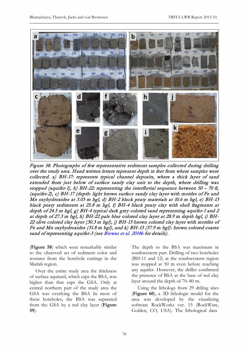
Bhattacharya, Thunvik, Jacks and von Brömssen TRITA LWR Report 2015: 01
78
Figure 58. Photographs of few representative sediment samples collected during drilling over the study area. Hand written letters represent depth in feet from where samples were collected. a) BH-17: represents typical channel deposits, where a thick layer of sand extended from just below of surface sandy clay unit to the depth, where drilling was stopped (aquifer-1), b) BH-22: representing the interfluvial sequence between 50 – 70 ft, (aquifer-2), c) BH-17 (depth: light brown surface sandy clay layer with mottles of Fe and Mn oxyhydroxides at 3.03 m bgl, d) BH-2 black peaty materials at 10.6 m bgl, e) BH-13 black peaty sediments at 25.8 m bgl, f) BH-4 black peaty clay with shell fragments at depth of 24.5 m bgl, g ) BH-4 typical dark grey colored sand representing aquifer-1 and 2 at depth of 27.3 m bgl, h) BH-22 pale blue colored clay layer at 28.9 m depth bgl, i) BH-22 olive colored clay layer (30.3 m bgl), j) BH-13 brown colored clay layer with mottles of Fe and Mn oxyhydroxides (31.8 m bgl), and k) BH-13 (37.9 m bgl): brown colored coarse sand of representing aquifer-3 (see Biswas et al. 2014b for details). (Figure 58) which were remarkably similar to the observed set of sediment color and textures from the borehole cuttings in the Matlab region.
Over the entire study area the thickness of surface aquitard, which caps the BSA, was higher than that caps the GSA. Only at central northern part of the study area the GSA was overlying the BSA In most of these boreholes, the BSA was separated from the GSA by a red clay layer (Figure 59).
The depth to the BSA was maximum in southwestern part. Drilling of two boreholes (BH-11 and 12) at the southwestern region was stopped at 50 m even before reaching any aquifer. However, the driller confirmed the presence of BSA at the base of red clay layer around the depth of 70–80 m.
Using the lithologs from 29 driling sites (Figure 60), a 3D lithologic model for the area was developed by the visualizing software RockWorks ver. 15 (RockWare, Golden, CO, USA). The lithological data
a b
c d
k
j
i
h
g
f
e
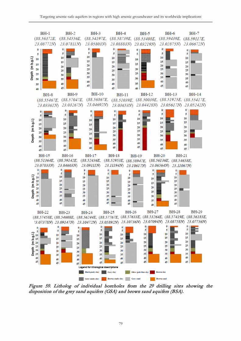
Targeting arsenic-safe aquifers in regions with high arsenic groundwater and its worldwide implications
79
Figure 59. Litholog of individual boreholes from the 29 drilling sites showing the disposition of the grey sand aquifers (GSA) and brown sand aquifers (BSA).
Dep
th(m
b.g
.l.)
Dep
th(m
b.g
.l.)
Dep
th(m
b.g
.l.)
Dep
th(m
b.g
.l.)
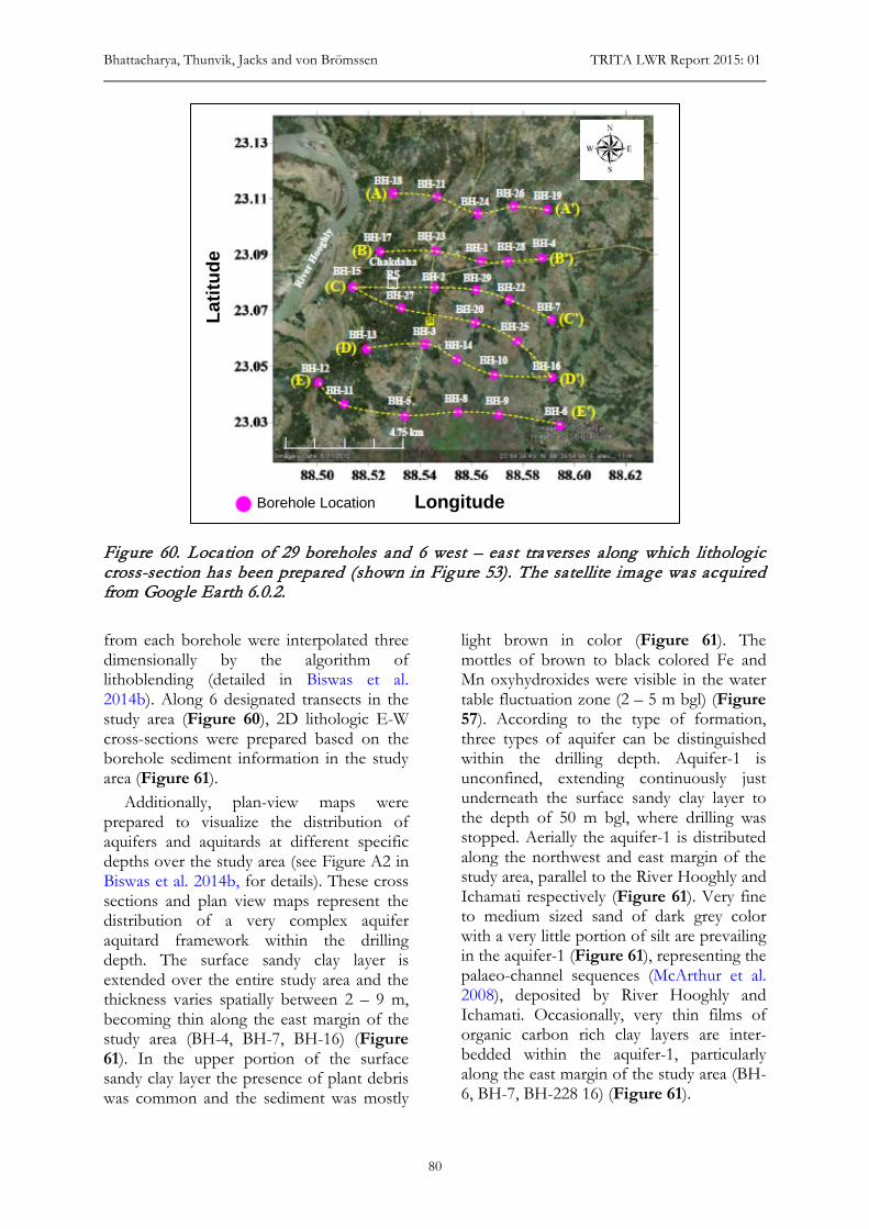
Bhattacharya, Thunvik, Jacks and von Brömssen TRITA LWR Report 2015: 01
80
Figure 60. Location of 29 boreholes and 6 west – east traverses along which lithologic cross-section has been prepared (shown in Figure 53). The satellite image was acquired from Google Earth 6.0.2. from each borehole were interpolated three dimensionally by the algorithm of lithoblending (detailed in Biswas et al. 2014b). Along 6 designated transects in the study area (Figure 60), 2D lithologic E-W cross-sections were prepared based on the borehole sediment information in the study area (Figure 61).
Additionally, plan-view maps were prepared to visualize the distribution of aquifers and aquitards at different specific depths over the study area (see Figure A2 in Biswas et al. 2014b, for details). These cross sections and plan view maps represent the distribution of a very complex aquifer aquitard framework within the drilling depth. The surface sandy clay layer is extended over the entire study area and the thickness varies spatially between 2 – 9 m, becoming thin along the east margin of the study area (BH-4, BH-7, BH-16) (Figure 61). In the upper portion of the surface sandy clay layer the presence of plant debris was common and the sediment was mostly
light brown in color (Figure 61). The mottles of brown to black colored Fe and Mn oxyhydroxides were visible in the water table fluctuation zone (2 – 5 m bgl) (Figure 57). According to the type of formation, three types of aquifer can be distinguished within the drilling depth. Aquifer-1 is unconfined, extending continuously just underneath the surface sandy clay layer to the depth of 50 m bgl, where drilling was stopped. Aerially the aquifer-1 is distributed along the northwest and east margin of the study area, parallel to the River Hooghly and Ichamati respectively (Figure 61). Very fine to medium sized sand of dark grey color with a very little portion of silt are prevailing in the aquifer-1 (Figure 61), representing the palaeo-channel sequences (McArthur et al. 2008), deposited by River Hooghly and Ichamati. Occasionally, very thin films of organic carbon rich clay layers are inter-bedded within the aquifer-1, particularly along the east margin of the study area (BH-6, BH-7, BH-228 16) (Figure 61).
Latit
ude
Borehole Location Longitude
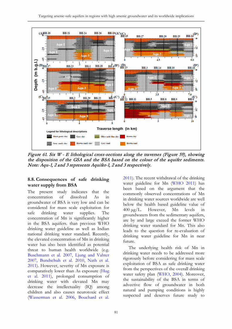
Targeting arsenic-safe aquifers in regions with high arsenic groundwater and its worldwide implications
81
Figure 61. Six W - E lithological cross-sections along the traverses (Figure 59), showing the disposition of the GSA and the BSA based on the colour of the aquifer sediments. Note: Aqu-1, 2 and 3 represents Aquifer-1, 2 and 3 respectively.
8.8. Consequences of safe drinking water supply from BSA The present study indicates that the concentration of dissolved As in groundwater of BSA is very low and can be considered for mass scale exploitation for safe drinking water supplies. The concentration of Mn is significantly higher in the BSA aquifers. than previous WHO drinking water guideline as well as Indian national drinking water standard. Recently, the elevated concentration of Mn in drinking water has also been identified as potential threat to human health worldwide (e.g. Buschmann et al. 2007, Ljung and Vahter 2007, Bundschuh et al. 2010, Nath et al. 2011). However, severity of Mn exposure is comparatively lower than As exposure (Hug et al. 2011), prolonged consumption of drinking water with elevated Mn may decrease the intellectuality (IQ) among children and also causes neurotoxic effect (Wasserman et al. 2006, Bouchard et al.
2011). The recent withdrawal of the drinking water guideline for Mn (WHO 2011) has been based on the argument that the commonly observed concentrations of Mn in drinking water sources worldwide are well below the health based guideline value of 400 μg/L. However, Mn levels in groundwaters from the sedimentary aquifers, are by and large exceed the former WHO drinking water standard for Mn. This also leads to the question for re-evaluation of drinking water guideline for Mn in near future.
The underlying health risk of Mn in drinking water needs to be addressed more rigorously before considering for mass scale exploitation of BSA as safe drinking water from the perspectives of the overall drinking water safety plan (WHO, 2004). Moreover, the sustainability of the BSA in terms of advective flow of groundwater in both natural and pumping conditions is highly suspected and deserves future study to
Dep
th(m
b.g
.l.)
Traverse length (in km)Legend for lithological descriptions
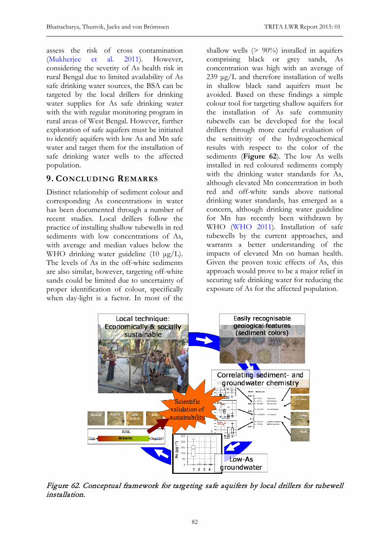
Bhattacharya, Thunvik, Jacks and von Brömssen TRITA LWR Report 2015: 01
82
assess the risk of cross contamination (Mukherjee et al. 2011). However, considering the severity of As health risk in rural Bengal due to limited availability of As safe drinking water sources, the BSA can be targeted by the local drillers for drinking water supplies for As safe drinking water with the with regular monitoring program in rural areas of West Bengal. However, further exploration of safe aquifers must be initiated to identify aquifers with low As and Mn safe water and target them for the installation of safe drinking water wells to the affected population.
9. CONCLUDING REMARKS Distinct relationship of sediment colour and corresponding As concentrations in water has been documented through a number of recent studies. Local drillers follow the practice of installing shallow tubewells in red sediments with low concentrations of As, with average and median values below the WHO drinking water guideline (10 μg/L). The levels of As in the off-white sediments are also similar, however, targeting off-white sands could be limited due to uncertainty of proper identification of colour, specifically when day-light is a factor. In most of the
shallow wells (> 90%) installed in aquifers comprising black or grey sands, As concentration was high with an average of 239 μg/L and therefore installation of wells in shallow black sand aquifers must be avoided. Based on these findings a simple colour tool for targeting shallow aquifers for the installation of As safe community tubewells can be developed for the local drillers through more careful evaluation of the sensitivity of the hydrogeochemical results with respect to the color of the sediments (Figure 62). The low As wells installed in red coloured sediments comply with the drinking water standards for As, although elevated Mn concentration in both red and off-white sands above national drinking water standards, has emerged as a concern, although drinking water guideline for Mn has recently been withdrawn by WHO (WHO 2011). Installation of safe tubewells by the current approaches, and warrants a better understanding of the impacts of elevated Mn on human health. Given the proven toxic effects of As, this approach would prove to be a major relief in securing safe drinking water for reducing the exposure of As for the affected population.
Figure 62. Conceptual framework for targeting safe aquifers by local drillers for tubewell installation.
Targeting arsenic-safe aquifers in regions with high arsenic groundwater and its worldwide implications
83
Local driller target low-As aquifers as a viable option for providing people water for safe drinking. If low As aquifers can be delineated by features local drillers can use for installation of safe drinking water tubewells, this option should be promoted on national as well as local scale. Even so, this study has highlighted that risk for cross-contamination may occur locally. Installing irrigation or production wells for heavy abstraction at depth without proper management on the aquifers sustainability is strongly discouraged (Michael and Voss 2008, Burgess et al. 2010). Improved monitoring of tube wells is strongly encouraged (van Geen et al. 2007, Polya and Charlet 2009, Bhattacharya et al. 2011).
Targeting safe aquifers can thus be based on sediment colour and may prove to be a simple solution for delivering safe drinking water not only this region and but also in other regions with similar geological conditions. Understanding hydrogeological suitability of an area is of prime importance
for tubewell installation. The assessment of targeting the safe aquifers may vary from a detailed investigation of subsurface hydrogeological system to a more simple installation of multi-level piezometer nests for monitoring of groundwater quality. For selecting the sites for monitoring wells it would be recommended to discuss with the local drillers to incorporate their knowledge about the local distribution of the target aquifers. In addition, mapping of large capacity water supply wells and clusters of irrigation wells is preferred to be done in order to identify the risks for cross contamination which could be induced due to multiple abstractions.
The results from this and similar studies can further contribute to develop a pragmatic management and mitigation policy with a holistic approach for the future use of the groundwater resources for drinking water supplies where sustainability of low As aquifers in regions with elevated concentrations remain a main concern.
Bhattacharya, Thunvik, Jacks and von Brömssen TRITA LWR Report 2015: 01
84
10. REFERENCES Abedin, M. J., Cresser, M. S., Meharg, A. A., Feldmann, J., Cotter-Howells, J., 2002. Arsenic
accumulation and metabolism in rice (Oryza Sativa L.). Environmental Science and Technology 36: 962-968.
Aggarwal, P.K., Basu A.R., Poreda R.J., Kulkarni K.M., Froehlich K., Tarafdar S.A., Ali M., Ahmed N., Hussain A., Rahman M., Ahmed S.R., 2000. Isotope hydrology of groundwater in Bangladesh: implications for characterization and mitigation of arsenic in groundwater. IAEA-TC Project: BGD/8/016, IAEA, Vienna.
Ahmed, K.M., 2005. Management of the groundwater arsenic disaster in Bangladesh. In: Bundschuh, J., Bhattacharya, P. and Chandrashekharam, D. (Eds.) Natural Arsenic in Groundwater: Occurrence, Remediation and Management. Taylor and Francis Group, London, UK, pp. 283-296.
Ahmed, K.M., Bhattacharya, P., Hasan, M.A., Akhter, S.H., Alam, S.M.M., Bhuyian, M.A.H., Imam, M.B., Khan, A.A., Sracek, O., 2004. Arsenic contamination in groundwater of alluvial aquifers in Bangladesh: An overview. Applied Geochemistry 19(2): 181-200.
Akai, J., Izumi, K., Fukuhara, H., Masuda, H., Nakano, S., Yoshimura, T., Ohfuji, H., Anwar, H.M., Akai, K., 2004. Mineralogical and geomicrobiological investigations on groundwater arsenic enrichment in Bangladesh. Applied Geochemistry 19:215-230.
Allison, J.D.D., Brown, S., Novo-Gradac, K.J., 1991. MINTEQA2, a Geochemical Assessment Data Base and Test Cases for Environmental Systems. EPA, Athens, GA, U.S.
Anawar, H.M., Akai, J., Komaki, K., Terao, H., Yoshioka, T., Ishizuka, T., Safiullah, S., Kato, K., 2003. Geochemical occurrence of arsenic in groundwater of Bangladesh: sources and mobilization processes. Journal of Geochemical Exploration 77:109-131.
Appelo, C.A.J., Postma, D., 1999. Geochemistry, groundwater and pollution. AA Balkema Publishers, 536 p.
APSU, 2005. Arsenic Policy Support Unit, Interim report. Risk Assessment of Arsenic Mitigation Options, RAAMO II, Phase II Report, May 2005. International Training Network Centre, ITN, Bangladesh.
BGS and DPHE, 2001. Arsenic contamination of groundwater, vol 2, Final Report, BGS Tech. Rep. WC/00/19, British Geological Survey, Keyworth.
Bhattacharya, P., Chatterjee, D., Jacks, G., 1997. Occurrence of Arsenic-contaminated Groundwater in Alluvial Aquifers from Delta Plains, Eastern India: Options for Safe Drinking Water Supply. International Journal of Water Resources Development 13(1): 79-92.
Bhattacharya, P., Jacks G., Jana J., Sracek A., Gustafsson J.P., Chatterjee D., 2001. Geochemistry of the Holocene Alluvial sediments of Bengal Delta Plain from West Bengal, India: Implications on arsenic contamination in groundwater. In: Jacks G., Bhattacharya P. and Khan A.A. (Eds.) Groundwater Arsenic Contamination in the Bengal Delta Plain of Bangladesh, KTH Special Publication, TRITA-AMI Report 3084: 21-40.
Bhattacharya, P., Frisbie, S.H., Smith, E., Naidu, R., Jacks, G., Sarkar B., 2002a. Arsenic in the Environment: A Global Perspective. In: Sarkar, B. (Ed.) Handbook of Heavy Metals in the Environment,. Marcell Dekker Inc., New York, USA, pp. 147-215.
Bhattacharya, P., Jacks, G., Ahmed, K.M., Routh, J., Khan, A.A., 2002b. Arsenic in Groundwater of the Bengal Delta Plain Aquifers in Bangladesh. Bulletin of Environmental Contamination and Toxicology 69: 538-545.
Bhattacharya, P., Mukherjee, A.B., Jacks, G. and Nordqvist, S., 2002c. Metal contamination at a wood preservation site: characterisation and experimental studies on remediation. Science of the Total Environment 290(1-3): 165-180.
Bhattacharya, P., Ahmed, K.M., Hasan, M.A., Broms, S., Fogelström, J., Jacks, G., Sracek, O., von Brömssen, M., Routh, J., 2006a. Mobility of arsenic in groundwater in a part of Brahmanbaria district, NE Bangladesh. In: Naidu, R., Smith, E., Owens, G., Bhattacharya, P., Nadebaum, P. (Eds.), Managing Arsenic in the Environment: From Soil to Human Health. CSIRO Publishing, Melbourne, Australia, pp. 95-115.
Targeting arsenic-safe aquifers in regions with high arsenic groundwater and its worldwide implications
85
Bhattacharya, P., Claesson, M., Bundschuh, J., Sracek, O., Fagerberg, J., Jacks, G., Martin, R.A., Storniolo, A.R., Thir, J.M., 2006b. Distribution and mobility of arsenic in the Río Dulce Alluvial aquifers in Santiago del Estero Province, Argentina. Science of the Total Environment 358: 97-120.
Bhattacharya, P., von Brömssen, M., Hasan, M.A., Ahmed, K M., Jacks, G., Sracek, O., Huq, S.M.I., Naidu, R., Smith, E., Owens, G., 2008. Arsenic mobilisation in the Holocene flood plains in Southcentral Bangladesh: Evidences from the hydrogeochemical trends and modeling results. In: Bhattacharya, P., Ramanathan, AL., Mukherjee A.B., Bundschuh, J., Chandrasekharam, D., Keshari, A.K. (Eds.) Groundwater for Sustainable Development: Problems, Perspectives and Challenges. Taylor and Francis/A. A. Balkema, The Netherlands, pp. 283-299.
Bhattacharya, P., Hossain, M., Rahman, S.N., Robinson, C., Nath, B., Rahman, M., Islam, M., von Brömssen, M., Ahmed, K.M., Jacks, G., Chowdhury, D., Rahman, M., Jakariya, M., Persson, L-Å., Vahter, M., 2011. Temporal and seasonal variability of arsenic in drinking water wells in Matlab, southeastern Bangladesh: A preliminary evaluation on the basis of a 4 year study. Journal of Environmental Science and Health, Part A 46: 1177-1184.
Berg, M., Stengel, C., Trang, P.T.K., Viet, P.H. Sampson, M.L., Leng, M., Samreth, S., Fredericks, D., 2007. Magnitude of arsenic pollution in the Mekong and Red River Deltas — Cambodia and Vietnam. Science of the Total Environment 372: 413-425.
Biswas, A., Nath, B., Bhattacharya, P., Halder, D., Kundu, A.K., Mandal, U., Mukherjee, A., Chatterjee, D., Mörth, C.-M., Jacks, G. 2012. Hydrogeochemical contrast between brown and grey sand aquifers in shallow depth of Bengal Basin: Consequences for sustainable drinking water supply. Science of the Total Environment 431: 402-412.
Biswas, A., Gustafsson, J.P., Neidhardt, H., Halder, D., Kundu, A.K., Chatterjee, D., Berner, Z., Bhattacharya, P., 2014a. Role of competing ions in the mobilization of arsenic in groundwater of Bengal Basin: Insight from surface complexation modelling. Water Research 55: 30-39.
Biswas, A., Bhattacharya, P., Mukherjee, A., Nath, B., Alexanderson, H., Kundu, A.K., Chatterjee, D., Jacks, G., 2014b. Shallow hydrostratigraphy in an arsenic affected region of Bengal Basin: Implication for targeting safe aquifers for drinking water supply. Science of the Total Environment 485-486: 12-22.
Bivén, A., Häller, S., 2007. Arsenic adsorption behaviour of oxidised aquifers in Matlab Upazila, Bangladesh. Master Thesis, Royal Institute of Technology, Stockholm, Sweden.
Bouchard, M.F., Sauvé, S., Barbeau, B., Legrand, M., Brodeur, M.E., Bouffard, T., Limoges, E., Bellinger, D.C., Mergler, D., 2011. Intellectual impairment in school-age children exposed to manganese from drinking water. Environmental Health Perspectives 119: 138-143
Brammer, H., 1996. The Geography of the Soils of Bangladesh. University Press Ltd. Breit, G.N., Yount, J.C., Uddin, M.N., Muneem, A.A., Lowers, H.A., Driscoll, R.L., Whitney, J.W., 2006.
Compositional data for Bengal delta sediment collected from boreholes at Srirampur, Kachua. Bangladesh. US Geological Survey Open-File Report 1222, 58 p.
Breit, G.N., Yount, J.C., Uddin, M.N., Muneem, A.A., Lowers, H.A., Berry, C.J., Whitney, J.W., 2007. Compositional data for Bengal delta sediment collected from a borehole at Rajoir, Bangladesh. US Geological Survey Open-File Report 1022, 46 p.
Bundschuh, J., Farias, B., Martin, R., Storniolo, A., Bhattacharya, P., Cortes, J., Bonorino, G., Alboury, R., 2004. Grounwater arsenic in the Chaco-Pampean Plain, Argentina: Case study from Robles County, Santiago del Estero Province. Applied Geochemistry 19(2): 231-243.
Bundschuh, J., Litter, M.I., Ciminelli, V.S.T., Margada, M.E., Cornejo, L., Hayas, S.F., Hoinkis, J., Alarcón-Herrera, M.T., Armienta, M.A., Bhattacharya, P., 2010. Emerging mitigation needs and sustainable options for solving the arsenic problems of rural and isolated urban areas in Latin America. Water Research 44: 5828-5845.
Burgess, W.G., Hoque, M.A., Michael, H.A., Voss, C.I., Breit, G.N., Ahmed, K.M., 2010. Vulnerability of deep groundwater in the Bengal Aquifer System to contamination by arsenic. Nature Geoscience 3: 83–87.
Buschmann, J., Berg, M., Stengel, C., Sampson, M.L., 2007. Arsenic and manganese contamination of drinking water resources in Cambodia: Coincidence of risk areas with low relief topography. Environmental Science and Technology41, 2146–2152.
Bhattacharya, Thunvik, Jacks and von Brömssen TRITA LWR Report 2015: 01
86
Cai, L., Liu, G., Rensing, C., Wang, G., 2009. Genes involved in arsenic transformation and resistance associated with different levels of arsenic-contaminated soils BMC Microbiology 9:4.
Caldwell, B.K., Smith, W.T., Caldwell, J.C., Mitra, S.N., 2005. Trends in water usage and knowledge of arsenicosis in Bangladesh. Population, Space and Place 11(4): 211-223.
Chakraborti, D., Rahman, M.M., Paul, K., Chowdhury, U.K., Sengupta, M.K., Lodh, D., Chanda, C.R., Saha, K.C., Mukherjee, S.C., 2002. Arsenic calamity in the Indian Subcontinent: What lessons have been learned? Talanta 58: 3-22.
Chatterjee, D., Roy, R.K., Basu, B.B., 2005. Riddle of arsenic in groundwater of Bengal Delta Plain-role of non-inland source and redox traps. Environmental Geology 49: 188-206.
Claesson, M., Fagerberg, J., 2003. Arsenic in ground water of Santiago del Estero – Sources, mobility patterns and remediation with natural materials. Master Thesis, Dept. of Land and Water Resources Engineering, KTH, Stockholm, Sweden, TRITA-LWR-EX-03-05, 59 p.
Cohen, D., Ward, C.R., 1991. Sednorm-a program to calculate a normative mineralogy for sedimentary rocks based on chemical analyses. Computers and Geosciences 17(9):1235-1253.
Correll, R., Huq, S.M.I., Smith, E., Owens, G., Naidu, R., 2006. Dietary intake of arsenic from crops. In: Naidu, R., Smith, E., Owens, G., Bhattacharya, P., Nadebaum, P. (Eds.) Managing arsenic in the environment: from soil to human health. CSIRO Publishing; Melbourne, Australia, pp. 251-268.
Datta, S., Neal, A.W., Mohajerin, T.J., Ocheltree, T., Rosenheim, B.E., White, C.D., Johannesson, K.H., 2011. Perennial ponds are not an important source of water or dissolved organic matter to groundwaters with high arsenic concentrations in West Bengal, India. Geophysical Research Letters 38, L20404.
Dixit, S., Hering, J.G., 2003. Comparison of arsenic(V) and arsenic(III) sorption onto iron oxide minerals: Implications for arsenic mobility. Environmental Science and Technology 37: 4182-4189.
Dixit, S., Hering, J.G., 2006. Sorption of Fe(II) and As(III) on goethite in single- and dual-sorbate system. Chemical Geology 228: 6-15.
Dodd, J., Large, D.J., Fortey, N.J., Milodowski, A.E., Kemi, S., 2000. A petrographic investigation of two sequential extraction techniques applied to anaerobic canal bed mud. Environmental Geochemistry and Health 22: 281–296.
DPHE/DFID/JICA, 2006. Development of Deep Aquifer Database and Preliminary Deep Aquifer Map. Department of Public Health Engineering (DPHE), Government of Bangladesh, and Arsenic Policy Support Unit (APSU), Japan International Cooperation Agency (JICA), Bangladesh, Dhaka.
Dzombak, D.A., Morel, F.M.M., 1990. Surface Complexation Modelling-Hydrous Ferric Oxide. John Wiley, New York, USA, 393 p.
EPC/MMP, 1991. Dhaka Region Groundwater and Subsidence Study, Final Report. Engineering and Planning Consultants, Dhaka and Sir M. Macdonalds and Partners, UL. Report for Dhaka Water Supply and Sewerage. Authority under assignment to the World Bank.
Filgueiras, A.V., Lavilla, I., Bendicho, C., 2002. Chemical sequential extraction for metal partioning in environmental solid samples. Journal of Environmental Monitoring 4: 823-857.
Goldberg, S., 2002. Competitive adsorption of arsenate and arsenite on oxides and clay minerals. Soil Sci. Soc. Am. J. 66:413–421.
Goldberg, S., Johnston C.T., 2001. Mechanisms of arsenic adsorption on amorphous oxides evaluated using macroscopic measurements, vibrational spectroscopy and surface complexation modeling. Journal of Colloid and Interface Science 234: 204-216.
Goodbred S.L., Kuehl S.A., Steckler M.S., Sarker M.H., 2003. Controls on facies distribution and stratigraphic preservation in the Ganges–Brahmaputra delta sequence. Sedimentary Geology 155: 301–16.
Gunaratna, K.R., Shokri, A., Bhattacharya, P., Jacks, G., Bundschuh, J., von Brömssen, M., 2010. Microbial characterization of Holocene alluvial sediments in the Meghna Flood Plain of Matlab Upazila, Bangladesh In: J.-S. Jean, J. Bundschuh & P. Bhattacharya (Eds.) “Arsenic in Geosphere and Human Diseases, As 2010”. Interdisciplinary Book Series: “Arsenic in the Environment—Proceedings”. Series Editors: Jochen Bundschuh and Prosun Bhattacharya, CRC Press/Taylor and Francis, UK, pp. 140-142.
Targeting arsenic-safe aquifers in regions with high arsenic groundwater and its worldwide implications
87
Gustafsson, J.P., 2011. Visual MINTEQ 3.0 Program, Website http://www.lwr.kth.se/english/OurSoftWare/Vminteq/index.html.
Gustafsson, J.P., Bhattacharya, P., 2007. Geochemical modelling of arsenic adsorption to oxide surfaces. In: Bhattacharya, P., Mukherjee, A.B., Bundschuh, J., Zevenhoven, R., Loeppert, R.H. (Eds.), Arsenic in Soil and Groundwater Environment: Biogeochemical Interactions, Health Effects and Remediation, Trace Metals and other Contaminants in the Environment, vol. 9. Elsevier B.V., Amsterdam, The Netherlands, pp. 153-200.
Halder, D., Bhowmick, S., Biswas, A., Mandal, U., Nriagu, J., Guha Mazumdar, D.N., Chatterjee, D., Bhattacharya, P., 2012. Consumption of Brown Rice: a potential pathway for arsenic exposure in rural Bengal. Environmental Science and Technology 46: 4142-4148.
Harvey, C.F., Swartz, C.H., Badruzzaman, A.B.M., Keon-Blute, N., Yu, W., Ali, M.A., Jay, J., Beckie, R., Niedan, V., Brabander, D., Oates, P.M., Ashaque, K.N., Islam, S., Hemond, H.F., Ahmed, M.F., 2002. Arsenic mobility and groundwater extraction in Bangladesh. Science 298: 1602-1606.
Harvey, C. F., Keon, N., W., Y., Ali, A., Jay, J., Beckie, R., Niedan, V., Brabander, D, Oates, P., Ahsfaque, K., Islam, S., Hemond, H.F., Ahmed, F., 2005. Groundwater arsenic contamination on the Ganges Delta: Biogeochemistry, hydrology, human perturbations, and human suffering on a large scale. Comptes-Rendus: Geoscience 337(1-2): 285-296.
Hasan, M.A., Ahmed, K.M., Sracek, O., Bhattacharya, P., von Brömssen, M., Broms, S., Fogelström, J., Mazumder, M. L., Jacks, G., 2007. Arsenic in shallow groundwater of Bangladesh: investigations from three different physiographic settings. Hydrogeology Journal 15: 1507-1522
Hasan, M.A., von Brömssen, M., Bhattacharya, P., Ahmed, K.M., Sikder, A.M., Jacks, G., Sracek, O., 2009. Geochemistry and mineralogy of shallow alluvial aquifers in Daudkandi upazila in the Meghna flood plain, Bangladesh. Environmental Geology 57: 499–511.
Hem, J.D., 1985. Study and Interpretation of the Chemical Characteristics of Natural Water. US Geological Survey Water Supply Paper 2254.
Hoque, B.A., Hoque, M.M., Ahmed, T., Islam, S., Azad, A.K., Ali, N., Hossaina, M., Hossain, M.S., 2004. Demand-based water options for arsenic mitigation: an experience from rural Bangladesh. Public Health 118(1):70-77.
Hoque, M.A., 2010. Models for Managing Deep Aquifer in Bangladesh, Ph.D. Thesis. Univ. College London, UK.
Hoque, M.A., Burgess, W.G., Shamsudduha, M., Ahmed, K.M., 2011. Delineating low-arsenic groundwater environments in the Bengal Aquifer. Applied Geochemistry 26: 614-623.
Horneman, A., van Geen, A., Kent, D. V., Mathe, P. E., Zheng, Y., Dhar, R. K., O’Connel, S. O., Hoque, M. A., Aziz, Z., Shamsudduha, M., Seddique, A A., Ahmed, K. M., 2004. Decoupling of As and Fe release to Bangladesh groundwater under reducing conditions. Part I: Evidence from sediment profiles. Geochimica et Cosmochimica Acta 68(17): 3459-3473.
Hug, S.J., Gaertner, D., Roberts, L.C., Schrimmer, M., Ruettimann, T., Rosenberg, T.M., Badruzzaman, A.B.M., Ali, M.A., 2011. Avoiding high concentrations of arsenic, manganese and salinity in deep tubewells in Munshiganj District, Bangladesh. Applied Geochemistry 26: 1077-1085.
Huq, S.M.I., Correll, R., Naidu, R., 2006. Arsenic accumulation in food sources in Bangladesh. In: Naidu, R., Smith, E., Owens, G., Bhattacharya, P. & Nadebaum, P. (Eds.) Managing Arsenic in the Environment: from soil to human health. CSIRO Publishing, Melbourne, pp. 279-290.
Jacks, G., Slejkovec, Z., Mörth, M., Bhattacharya, P., 2013. Redox-cycling of arsenic along the water pathways in sulfidic metasediment areas in northern Sweden. Applied Geochemistry 35: 35-43 (DOI:10.1016/j.apgeochem.2013.05.002).
Jakariya, M., 2007. Arsenic in Tubewell Water: of Bangladesh. and Approaches for Sustainable Mitigation. TRITA-LWR PhD Thesis 1033, 28p.
Jakariya, M., Rahman, M., Chowdhury, A.M.R., Rahman, M., Yunus, M., Bhiuya, A., Wahed, M.A., Bhattacharya, P., Jacks, G., Vahter M., Persson, L.-Å., 2005. Sustainable safe water options in Bangladesh: experiences from the Arsenic Project at Matlab (AsMat). In: Bundschuh, J., Bhattacharya, P., Chandrashekharam, D. (Eds.) Natural Arsenic in Groundwater: Occurrence, Remediation and Management. A.A. Balkema, Taylor and Francis Group, London, pp. 319-330.
Bhattacharya, Thunvik, Jacks and von Brömssen TRITA LWR Report 2015: 01
88
Jakariya, M., von Brömssen, M., Jacks, G., Chowdhury, A.M.R., Ahmed, K.M., Bhattacharya, P., 2007. Searching for sustainable arsenic mitigation strategy in Bangladesh: experience from two upazilas. International Journal of Environment and Pollution 31(3/4): 415-430.
JICA-Japanese International Development Agency, 2002. The study on the groundwater development of deep aquifers for safe drinking water supply to arsenic affected areqs in western Bangladesh. Kokusai Kogyo Co. Ltd., and Mitsui Mineral Development Engineering Co. Ltd.
Johnston, R.B., Hanchett, S., Khan, M.H., 2010. The socio-economics of arsenic removal. Nature Geoscience 3: 2-3.
Jonsson, L., Lundell, L. 2004. Targeting safe aquifers in regions with arsenic-rich groundwater in Bangladesh. Case study in Matlab Upazila. Minor Field Studies No 277. Swedish University of Agricultural Sciences, SLU External Relations, Uppsala. ISSN 1402-3237.
Kapaj, S., Peterson, H., Liber, K., Bhattacharya, P., 2006. Human health effects from chronic arsenic poisoning - A Review. Journal of Environmental Science and Health Part A 41: 2399-2428.
Kar, S., Maity, J.P., Jean, J-S., Liu, C-C., Nath, B., Yang, H-J., Bundschuh, J., 2010. Arsenic-enriched aqufers: Occurences and mobilization of arsenic in groundwater of Ganges Delta Plain, Barasat, West-Bengal, India. Applied Geochemistry 25: 1805-1814.
Kendie, S.B., 1996. Some factors influencing effective utilisation of drinking water facilities: women, income and health in north Ghana. Environmental Management 20(1): 1-10.
Lindberg, A.-L., Goessler, W., Gurzau, E., Koppova, K., Rudnai, P., Kumar, R., Fletcher, T., Leonardi, G., Slotova, K., Gheorghiu, E., Vahter, M., 2006. Arsenic exposure in Hungary, Romania and Slovakia. Journal of Environmental Monitoring. 8: 203–208.
Ljung, K., Vahter, M., 2007. Time to re-evaluate the guideline value for manganese in drinking water? Environmental Health Perspectives 115: 1533-1538.
Lowers, H.A., Breit, G.N., Foster, A.L., Whitney, J., Yount, J., Uddin, M.N., Muneem, A.A., 2007. Arsenic incorporation into authigenic pyrite, Bengal Basin sediment, Bangladesh. Geochimica et Cosmochimica Acta 71: 2699-2717.
Mandal, B.K., Suzuki, K.T., 2002. Arsenic round the world: a review. Talanta 58: 201-235. Manning, B.A., Goldberg, S., 1997. Adsorption and stability of arsenic(III) at the clay mineral–water
interface. Environmental Science Technology 31: 2005-2011. McArthur, J.M., Ravencroft, P., Safiullah, S., Thirlwall, M.F., 2001. Arsenic in groundwater: testing
pollution mechanism for sedimentary aquifers in Bangladesh. Water Resources Research 37: 109-117. McArthur, J., Banerjee, D., Hudson-Edwards, K., Mishrab, R., Purohit, R., Ravenscroft, P., P., Cronin,
A., Howarth, R.J., Chatterjee, A., Talukder, T., Lowry, D., Houghton, S., Chadha, D.K., 2004. Natural organic matter in sedimentary basins and its relation to arsenic in anoxic ground water: the example of West Bengal and its worldwide implications. Applied Geochemistry 19: 1255-1293.
McArthur, J.M., Ravenscroft, P., Banerjee, D.M., Milsom, J., Hudson-Edwards, K.A., Sengupta, S., Bristow, C., Sarkar, A., Tonkin, S., Purohit, R., 2008. How paleosols influence groundwater flow and arsenic pollution: A model from the Bengal Basin and its worldwide implication. Water Resources Research 44: W11411.
McArthur, J.M., Nath, B., Banerjee, D.M., Purohit, R., Grassineau, N., 2011. Palaeosol control on groundwater flow and pollutant distribution: The example of arsenic. Environmental Science Technology 45: 1376-1383.
Meharg, A.A., Scrimgeour, C., Hossain, S.A., Fuller, K., Cruickshank, K., Williams, P.N., Kinniburgh, D.G., 2006. Codeposition of organic carbon and arsenic in Bengal Delta Aquifers. Environmental Science Technology 40: 4928-4935.
Meng, X., Korfiatis, G.P., Christodoulatos, C., Bang S., 2001. Treatment of arsenic in Bangladesh well water using a household co-precipitation and filtration system. Water Research 35(12): 2805-2810.
Michael, H.A., Voss, C.I., 2008. Evaluation of the sustainability of deep groundwater as an arsenic-safe resource in the Bengal Basin. Proceedings of the National Academy of Sciences of the United States of America 105: 8531–8536.
Targeting arsenic-safe aquifers in regions with high arsenic groundwater and its worldwide implications
89
Michael, H., Voss, C., 2009a. Controls on groundwater flow in the Bengal Basin of India and Bangladesh: regional modeling analysis. Hydrogeology Journal 17: 1561–1577.
Michael, H., Voss, C., 2009b. Estimation of regional-scale groundwater flow properties in the Bengal Basin of India and Bangladesh. Hydrogeology Journal 17: 1329–1346.
Milton, A.H., Hasan, Z., Shahidullah, S.M., Sharmin, S., Jakariya, M.D., Rahman, M., Dear, K., Smith, W., 2004. Association between nutritional status and arsenicosis due to chronic arsenic exposure in Bangladesh. International Journal of Environmental Health Research 14(2): 99-108.
Mozumder, M.R.H., 2011. Aqueous Phase Geochemical Characterisation and Delineation of Low Arsenic Aquifers in Matlab Upazila, SE Bangladesh. M.Sc. Thesis, Royal Institute of Technology, LWR-EX-11:08, 38p.
Mozumder, M.R.H., Bhattacharya, P., Ahmed, K.M., Hossain, M., Hasan, M.A., Islam, M.M., Jacks, G., von Brömssen, M., 2011. Groundwater redox-facies and aquifer sediment color characteristics in Matlab Upazila, SE Bangladesh. Geological Soceity of America, Abstracts with Programs 43(5): 222.
Mukherjee, A., Fryar, A.E., 2008. Deeper groundwater chemistry and geochemical modelling of the arsenic affected western Bengal basin, West Bengal, India. Applied Geochemistry 23: 863-892.
Mukherjee, A., Fryar, A.E., Howell, P., 2007. Regional hydrostratigraphy and groundwater flow modeling of the arsenic affected western Bengal basin, West Bengal, India. Hydrogeology Journal 15: 1397–1418.
Mukherjee, A., von Brömssen, M., Scanlon, B.R., Bhattacharya, P., Fryar, A.E., Hasan, M.A., Ahmed, K.M., Chatterjee, D., Jacks, G., Sracek, O., 2008. Hydrogeochemical comparison between the Bhagirathi and Meghna sub-basins, Bengal basin, India and Bangladesh: effects of overlapped redox zones on dissolved arsenic. Journal of Contaminant Hydrology 99: 31-48.
Mukherjee, A., Fryar, A.E., Scanlon, B.R., Bhattacharya, P., Bhattacharya, A., 2011. Elevated arsenic in deeper groundwater of the western Bengal basin, India: extent and controls from regional to local scale. Applied Geochemistry 26(4): 600-613.
Mukherjee, A.B., Bhattacharya, P., 2001. Arsenic in groundwater in the Bengal Delta Plain: Slow Poisoning in Bangladesh. Environmental Reviews 9:189-220.
Naidu, R., Smith, E., Owens, G., Bhattacharya, P., Nadebaum, P., 2006. Managing Arsenic in the Environment: From Soil to Human Health. CSIRO Publishing, Melbourne, Australia, 656 p.
Nath, B., Chakraborty, S., Burnol, A., Stüben, D., Chatterjee, D., Charlet, L. 2009. Mobility of arsenic in the sub-surface environment: An integrated hydrogeochemical study and sorption model of the sandy aquifer materials. Journal of Hydrology 364: 236-248.
Nath, B., Maity, J.P., Jean, J.S., Birch, G., Kar, S., Yang, H.J., Lee, M.K., Hazra, R., Chatterjee, D., 2011. Geochemical characterization of arsenic-affected alluvial aquifers of the Bengal Delta (West Bengal and Bangladesh) and Chianan Plains (SW Taiwan): Implications for human health. Applied Geochemistry 26: 705–711.
Nickson, R, McArthur, J., Burgess, W.G., Ahmed, K.M., Ravencroft, P., Rahman, M., 1998. Arsenic poisoning of Bangladesh groundwater. Nature 1998: 395-338.
Nickson, R, McArthur, J., Ravenscroft, P., Burgess, W.G., Ahmed, K.M., 2000. Mechanism of arsenic release to groundwater, Bangladesh and West Bengal. Applied Geochemistry 15: 403-413
Nickson, R.T., McArthur, J.M., Shrestha, B., Kyaw-Myint, T.O., Lowry, D., 2005. Arsenic and other drinking water quality issues, Muzaffargarh District, Pakistan. Applied Geochemistry 20(1):55-68.
Nicolli, H.B., Bundschuh, J., García, J.W., Falcón, C.M., Jean, J.-S. 2010. Sources and controls for the mobility of arsenic in oxidizing groundwaters from loess-type sediments in arid/semi-arid dry climates — evidence from the Chaco–Pampean plain (Argentina). Water Research 44: 5589–604.
Nicolli, H.B., Bundschuh, J., Blanco, M. del C., Panarello, H.O., Dapeña. C., Jean, J.-S. 2012. Arsenic and associated trace elements in groundwater from the Chaco–Pampean plain: results from 100 years of research. Science of the Total Environment 429: 36-56.
Nriagu, J.O., Bhattacharya, P., Mukherjee, A.B., Bundschuh, J., Zevenhoven, R., Loeppert, R.H., 2007. Arsenic in soil and groundwater: an overview. In: Bhattacharya, P., Mukherjee, A.B., Bundschuh, J., Zevenhoven, R. & Loeppert, R.H. (Eds.) Arsenic in Soil and Groundwater Environment:
Bhattacharya, Thunvik, Jacks and von Brömssen TRITA LWR Report 2015: 01
90
Biogeochemical Interactions, Health Effects and Remediation, Trace Metals and other Contaminants in the Environment, Volume 9, Elsevier B.V. Amsterdam, The Netherlands, pp. 3–60.
Pal, T., Mukherjee, P.K., 2008. ‘Orange sand’ – a geological solution for arsenic pollution in Bengal Delta. Current Science 94: 31-33.
Pal, T., Mukherjee, P.K., 2009. Study of subsurface geology in locating arsenic-free groundwater in Bengal Delta, West Bengal, India. Environmental Geology 56: 1211-1125.
Parkhurst, D.L., Appelo, C.A.J., 1999. Users's Guide to PHREEQC (Version 2)-A Computer Program for Speciation, Batch-reaction, One-dimensional Transport and Inverse Geochemical Calculations. U.S. GEOLOGICAL SURVEY, Denver, Colorado, USA. 99-4259.
Petrusivski, B., Sharma, S., Schippers, J.C., Shordt, K., 2007. Arsenic in drinking water. Thematic Overview Paper 17. IRC International Water and Sanitation Centre. 57p.
Polya, D., Charlet, L., 2009. Rising arsenic risk? Nature Geoscience 2: 383-384. Polya, D.A., Mondal, D., Giri, A.K., 2009. Quantification of deaths and DALYs arising from chronic
exposure to arsenic in groundwaters utilized for drinking, cooking and irrigation of food crops in Preedy, V.R. & Watson, R. (Eds.) Handbook of Disease Burdens and Quality of Life Measures, Springer Science+Business Media LLC, USA, pp. 701-728.
Postma, D., Jakobsen, R., 1996. Redox zonation: equilibrium constraints on the Fe(III)/SO4-reduction interface. Geochimica et Cosmochimca Acta 60(17): 3169-3175.
Quevauviller, P., Rauret, G., Griepink, B., 1993. Single and sequential extraction in sediment and soils. International Journal of Environmental Analytical Chemistry 51:231-235.
Radloff, K.A., Zheng, Y., Michael, H.M., Stute, M., Bostick, B.C., Milhajlov, I., Bounds, M., Huq, M.R.,m Chowdhury, I., Rahman, M.W., Schlosser, P., Ahmed, K.M., van Geen, A. 2011. Arsenic migration to deep groundwater in Bangladesh influenced by adsorption and water demand. Nature Geoscience, NGEO 12833.
Rahman, A.A., Ravenscroft, P., 2003. Groundwater Resources and Development in Bangladesh – Background to the Arsenic Crisis, Agricultural Potential and the Environment. Bangladesh Centre for Advanced Studies. Dhaka:University Press Ltd.
Ravenscroft, P., 2001. Distribution of groundwater arsenic in Bangladesh related to geology. In: Bhattacharya, P., Jacks, G. & Khan, A.A. (Eds.) Groundwater Arsenic Contamination in the Bengal Delta Plain of Bangladesh. Proceedings of the KTH-Dhaka University Seminar, KTH Special Publication, TRITA-AMI Report 3084, pp. 41–56.
Ravenscroft, P., McArthur, J.M., Hoque, B.A., 2001. Geochemical and palaeohydrological controls on pollution of groundwater by arsenic. In: Chappell, W.R., Abernathy, C.O. & Calderon, R.L. (Eds.) Arsenic Exposure and Health Effects IV. Elsevier, Oxford, pp. 53-57.
Ravenscroft, P., Burgess, W., Ahmed, K., Burren, M., Perrin, J., 2005. Arsenic in groundwater of the Bengal Basin, Bangladesh: Distribution, field relations, and hydrogeological setting. Hydrogeology Journal 13(5-6): 727-751.
Ravenscroft, P., Brammer, H., Richards, K.S., 2009. Arsenic Pollution: A Global Synthesis. Wiley-Blackwell, U.K., 588p.
Reza, S.A.H.M., Jean, J-S., Lee, M-K., Yang, H-J., Liu, C-C., 2010. Arsenic enrichment and mobilization in the Holocene alluvial aquifers of the Chapai-Nawabganj district, Bangladesh: A geochemical and statistical study. Applied Geochemistry 25: 1280-1289.
Reza, S.A.H.M., Jean, J-S., Lee, M-K., Luo, S-D., Bundschuh, J., Li, H-C-., Yang, H-J., Liu, C-C., 2011. Interrelationship of TOC, As, Fe, Mn, Al and Si in shallow alluvial aquifers in Chapai-Nawabganj district, Bangladesh: implication for potential source of organic carbon. Environmental Earth Science 63: 955-967.
Robinson, C., Hossain, M., von Brömssen, M., Bhattacharya, P., Häller, S., Bivén, A., Jacks, G., Ahmed, K.M., Hasan, M.A., Thunvik, R., 2011. Dynamics of arsenic adsorption in the targeted arsenic-safe aquifers in Matlab, South-eastern Bangladesh: insight from experimental studies. Applied Geochemistry 26: 624–635.
Roychowdhury, T., Uchino, T., Tokunaga, H., Ando, M., 2002. Survey of arsenic in food composites from an arsenic-affected area of West Bengal, India. Food and Chemical Toxicology 40(11): 1611-21.
Targeting arsenic-safe aquifers in regions with high arsenic groundwater and its worldwide implications
91
Saha, D., Sinha, U.K., Dwivedi, S.N., 2011. Characterization of recharge processes in shallow nd deeper aquifers using isotopic signatures and geochemical behaviour of groundwater in an arsenic-enriched part of the Ganga Plain. Applied Geochemistry 26: 432-443.
Sarkar, B., 2002. Heavy Metals in the Environment. Marcel Dekker, Inc., New York, 725 p. Sharif, M.U., Davis, R.K., Steele, K.F., Kim, B., Hays, P.D., Kresse, T.M., Fazio, J.A., 2008. Distribution
and variability of redox zones controlling spatial variability of arsenic in the Mississippi River Valley alluvial aquifer, southeastern Arkansas. Journal of Contaminant Hydrology 99: 49-67.
Sikder, M.S., Maidul, Z.M., Ali, M., Rahman, M.H., 2005. Socio-economic status of chronic arsenicosis patients in Bangladesh. Mymensingh Medical Journal 14(1): 50-53.
Singh, N., Jacks, G., Bhattacharya, P., 2005. Women and community water supply programmes: An analysis from a socio-cultural perspective. Natural Resources Forum 29(3): 213-223.
Smedley, P.L., Kinniburgh, D.G., 2002. A review of the source, behaviour and distribution of arsenic in natural waters. Applied Geochemistry 17: 517-568.
Smedley, P., Kinniburgh, D.G., Macdonald D.M.J., Nicolli, H.B., Barros, A.J., Tullio, J.O., Pearce, J.M., Alonso, M.S., 2005. Arsenic associations in sediments from loess aquifer of La Pampa, Argentina. Applied Geochemistry 20: 989-1016.
Smith, A.H., Lingas, E.O., Rahman, M. 2000. Contamination of drinking-water by arsenic in Bangladesh: a public health emergency. Bulletin of the World Health Organization 78(9): 1093-1103.
Sracek, A., Bhattacharya, P., Jacks, G., Gustafsson, J.P., 2001. Mobility of arsenic and geochemical modeling in groundwater environment. In: G. Jacks, P. Bhattacharya and A.A. Khan (Editors), Groundwater Arsenic Contamination in the Bengal Delta Plains of Bangladesh: Proceedings of the KTH-Dhaka UniversitySeminar, University of Dhaka, Bangladesh. KTH Special Publication, TRITA-AMI REPORT 3084: 9-20.
Sracek, O., Bhattacharya, P., Jacks, G., Gustafsson, J.-P., von Brömssen, M., 2004a. Behavior of arsenic and geochemical modeling of arsenic enrichment in aqueous environments. Applied Geochemistry 19(2): 169-180.
Sracek, O., Bhattacharya, P., von Brömssen, M., Jacks, G., Ahmed, K. M., 2004b. Natural enrichment of arsenic in groundwaters of Brahmanbaria district, Bangladesh: geochemistry, speciation modelling and multivariate statistics. In: J. Bundschuh, P. Bhattacharya and D. Chandrasekharam (Eds.)Natural Arsenic in Groundwater: Occurrence, Remediation and Management. Balkema, London, pp. 133-144.
Stollenwerk, K.G., 2005. Arsenic Attenuation by Oxidized Aquifer Sediments, Bangladesh, Behavior of Arsenic in Aquifers, Soils and Plants: Implications for Management. International Maize and Wheat Improvement Centre (CYMMYT), Cornell University, Texas A&M University, United States Geological Survey, Geological Survey of Bangladesh, Dhaka, Bangladesh.
Stollenwerk, K.G., Breit, G.N., Welch, A.H., Yount, J.C., Whitney, J.W., Forster, A.L., Uddin, M.N., Majumder, R.K., Ahmed, N., 2007. Arsenic attenuation by oxidised sediments in Bangladesh. Science of the Total Environment 379: 133-150.
Stüben, D., Berner, Z., Chandrasekharam, D., Karmakar, J., 2003. Arsenic enrichment in groundwater of West Bengal, India: geochemical evidence for mobilization of As under reducing conditions. Applied Geochemistry 18(9): 1417-1434.
Stute, M., Zheng, Y., Schlosser, P., Horneman, A., Dhar, R.K., Hoque, M.A., Seddique, A.A., Shamsudduha, M., Ahmed, K.M., van Geen, A., 2007. Hydrological control of As concentrations in Bangladesh groundwater. Water Resources Research 43: W09417.
Swartz, C.H., Blute, N.K., Bodruzzaman, B., Ali, M.A., Brabander, D., Jay, J., Besabcon, J., Islam, S., Hemond, H.F., Harvey, C., 2004. Mobility of arsenic in a Bangladesh aquifer: inferences from geochemical profiles, leaching data, and mineralogical characterization. Geochimica et Cosmochimica Acta 68 (22): 4539-4557.
Swedlund, P.J., Webster, J.G., 1999. Adsorption and polymerisation of silicic acid on ferrihydrite, and its effect on arsenic adsorption. Water Research 33(16): 3413-3422.
Tessier, A., Campbell, P.G.C., Bisson, M., 1979. Sequential extraction procedure for the speciation of particulate trace metals. Analytical Chemistry 51: 844-851.
Bhattacharya, Thunvik, Jacks and von Brömssen TRITA LWR Report 2015: 01
92
Tuccillo, M.E., Cozzarelli, I.M., Herman, J.S., 1999. Iron reduction in the sediments of a hydrocarbon-contaminated aquifer. Applied Geochemistry 14: 655-667.
Uddin, A., Shamsudduha, M., Saunders, J.A., Lee, M-K., Ahmed, K.M., Chowdhury, M.T., 2011. Mineralogical profiling of alluvial sediments from arsenic-affected Ganges-Brahmaputra floodplain in central Bangladesh. Applied Geochemistry 26: 470-483.
Umitsu M., 1987. Late Quaternary sedimentary environment and landform evolution in the Bengal lowland. Geographical Review of Japan 60: 164-78.
Umitsu M., 1993. Late Quaternary sedimentary environments and landforms in the Ganges Delta. Sedimentary Geology 83: 177–86.
UN, 2001. United Nations Synthesis Report on Arsenic in Drinking Water. Draft Report. UNDP, 1982. Groundwater Survey: The Hydrogeological Conditions of Bangladesh. UNDP Technical
Report DP/UN/BGD-74-009/1, 113 p. Vahter, M.E., Li, L., Nermell, B., Rahman, A., Arifeen, A.E., Rahman, M., Persson, L-Å., Ekström, E-C.,
2006. Arsenic Exposure in Pregnancy: A Population-based Study in Matlab, Bangladesh. Journal of Health, Population and Nutrition 24(2): 236-245.
van Geen, A., Zheng, Y., Versteeg, R., Stute, M., Horneman, A., Dhar, R., Steckler, M., Gelman, A., Small, C., Ahsan, H., Graziano, J.H., Hussain, I., Ahmed, K.M., 2003. Spatial variability of arsenic in 6000 tube wells in a 25 km2 area of Bangladesh. Water Resources Research 39: 1140-1155.
van Geen, A., Rose, J., Thoral, S., Garnier, J.M., Zheng, Y., Bottero, J.Y., 2004. Decoupling of As and Fe release to Bangladesh groundwater under reducing conditions. Part II: evidence from sediment incubations. Geochimica et Cosmochimica Acta 68(17): 3475-86.
van Geen, A., Cheng, Z., Jia, Q., Seddique, A.A., Rahman, M.W., Rahman, M.M., Ahmed, K.M., 2007. Monitoring 51 community wells in Araihazar, Bangladesh, for up to 5 years: Implications for arsenic mitigation. Journal of Environmental Science and Health Part A 42: 1729-1740.
Varsányi, I., Fodré, Z.s., Bartha, A., 1991. Arsenic in drinking water and mortality in the Southern Great Plain, Hungary. Environmental Geochemistry and Health 13: 14–23.
Varsányi, I., Kovács, L.Ó., 2006. Arsenic, iron and organic matter in sediments and groundwater in the Pannonian Basin, Hungary. Applied Geochemistry 21: 949–963.
Vencelides, Z., Sracek, O., Prommer, H., 2007. Modelling of iron cycling and its impact on the electron balance at a petroleum hydrocarbon contaminated site in Hnevice, Czech Republic. Journal of Contaminant Hydrology 89: 270-294.
von Brömssen, M., 1999. Genesis of high arsenic groundwater in the Bengal delta plains, West-Bengal and Bangladesh, Stockholm. M.Sc. thesis, LWR, KTH.
von Brömssen, M., 2012. Hydrogeological and geochemical assessment of aquifer systems with geogenic arsenic in southeastern Bangladesh – Targeting low arsenic aquifers for safe drinking water supplies in Matlab. PhD Thesis, TRITA LWR PhD 1063, 46 p.
von Brömssen, M., Bhattacharya, P., Ahmed, K.M., Jakariya, M., Jonsson, L., Lundell, L., Jacks, G., 2005. Targeting safe aquifers in regions with elevated arsenic in groundwater of Matlab Upazila, Bangladesh. In: Lombi, E., Tyrell, S., Nolan, A., McLaughlin, M., Pierzynski, G., Gerzabek, M., Lepp, N., Leyval, C., Selim, M., Zhao, F., Grant, C., Parker, D. (eds.) ICOBTE 8-2005, Symposium 4, 8th International Conference on the Biogeochemistry of Trace Elements (April 3-7, 2005), Book of Abstracts, Adelaide, Australia: 190-191.
von Brömssen, M., Jakariya, M., Bhattacharya, P., Ahmed, K.M., Hasan, M.A., Sracek, O., Jonsson, L., Lundell, L., Jacks, G., 2007. Targeting low-arsenic in Matlab Upazila, Southeastern Bangladesh. Science of the Total Environment 379(2–3): 121-132.
von Brömssen, M., Larsson, S.H., Bhattacharya, P., Hasan, M.A., Ahmed, K.M., Jakariya, M., Sikder, A.M., Sracek, O., Bivén, A., Doušová, B., Patriarca, C., Thunvik, R., Jacks, G., 2008. Geochemical characterisation of shallow aquifer sediments of Matlab Upazila, Southeastern Bangladesh – implications for targeting low-As aquifers. Journal of Contaminant Hydrology 99(1-4): 137-149.
von Brömssen, M., Markussen, L., Bhattacharya, P., Ahmed, K.M., Hossain, M., Jacks, G., Sracek, O., Thunvik, R., Hasan, M.A., Islam, M.M., Rahman, M.M., 2014. Hydrogeological investigation for
Targeting arsenic-safe aquifers in regions with high arsenic groundwater and its worldwide implications
93
assessment of the sustainability of low-arsenic aquifers as a safe drinking water source in regions with high-arsenic groundwater in Matlab, southeastern Bangladesh. Journal of Hydrology 518: 373-392.
Wasserman, G.A., Liu, X., Parvez, F., Factor-Litvak, P., Ahsan, H., Levy, D., Kline, J., van Geen, A., Mey, J., Slavkovich, V., Siddique, A.B., Islam, T., Graziano, J.H., 2011. Asenic and manganese exposure and children’s intellectual function. NeuroToxicology 32: 450-457.
Welch, A.L., Stollenwerk, K.G., 2003. Arsenic in Ground Water, Geochemistry and Occurrence. Kluwer Academic Publishers, Boston, 475 p.
Wenzel, W.W., Kirchbaumer, N., Prohaska, T., Stingeder, G., Lombi, E., Adriano, D.C., 2001 Arsenic fractionation in soils using an improve sequential extraction procedure. Analytica Chimica Acta 436: 309-323.
WHO, 2004. Guidelines Drinking Water Quality, Third edition, Volume 1, Recommendations. Geneva 2004 515 p.
WHO, 2011. Guideline for Drinking Water Quality. Fourth edition. Geneva: World Health Organization: Singapore; 2011.
Williams, P. N., Price, A. H., Raab, A., Hossain, S. A., Feldmann, J., Meharg, A. A., 2005. Variation in arsenic speciation and concentration in paddy rice related to dietary exposure. Environmental Science and Technology 39: 5531-5540.
Williams, P.N., Islam, M.R., Adomako, E.E., Raab, A., Hossain, S.A., Zhu, Y.G., Felfmann, J., Meharg, A.A., 2006. Increase in rice grain arsenic for regions of Bangladesh irrigating paddies with elevated arsenic in groundwaters. Environmental Science and Technology 40: 4903-4908.
Yan, X-P., Kerrich, R., Hendry, M.J., 2000. Distribution of arsenic (III), arsenic (V) and total inorganic arsenic in porewaters from a thick till and clay rich aquitard sequence, Saskatchewan, Canada. Geochimica et Cosmochimca Acta 62: 2637-2648.
Zheng, Y., van Geen, A., Stute, M., Dhar, R., Mo, Z., Cheng, Z., Horneman, A., Gavrieli, I., Simpson, H.J., Versteeg, R., Steckler, M., Grazioli-Venier, A., Goodbred, S., Shahnewaz, M., Shamsudduha, M., Hoque, M.A., Ahmed, K.M., 2005. Geochemical and hydrogeological contrast between shallow and deeper aquifers in two villages of Araihazar, Bangladesh: implication for deeper aquifers as drinking water sources. Geochimica et Cosmochimica Acta 69(22): 5203-5218.
Bhattacharya, Thunvik, Jacks and von Brömssen TRITA LWR Report 2015: 01
94
APPENDIX I. MISTRA PROJECT OUTCOMES A1 PhD Theses Md. Jakariya (2007) Arsenic in Tubewell Water: of Bangladesh. and Approaches for Sustainable Mitigation. (Awarded 24 May, 2007) M. Aziz Hasan (2008) Arsenic in Alluvial Aquifers in the Meghna Basin, Southeastern Bangladesh: Hydrogeological and Geochemical Characterisation. (Awarded 5 November 2008) Mattias von Brömssen (2012) Hydrogeological and Geochemical Assessment of Aquifer Systems with Geogenic Arsenic in Southeastern Bangladesh: Targeting Low Arsenic Aquifers for Safe Drinking Water Supplies in Matlab. (Awarded 20 January, 2012) Ashis Biswas (2014) Arsenic Geochemistry in the Alluvial Aquifers of West Bengal, India Implications for Targeting Safe Aquifers for Sustainable Drinking Water Supply. (Awarded 23 September 2013)
A2 Selected Publications Journal articles 1. Bhattacharya, P., Ahmed, K.M., Hasan, M.A., Broms, S., Fogelström, J., Jacks, G., Sracek,
O., von Brömssen, M. & Routh, J. (2006) Mobility of arsenic in groundwater in a part of Brahmanbaria district, NE Bangladesh In: Naidu, R., Smith, E., Owens, G., Bhattacharya, P. & Nadebaum. P, (Eds.) Managing Arsenic in the Environment: From soil to human health. CSIRO Publishing, Melbourne, Australia, pp. 95-115. (ISBN: 0643068686)
2. Naidu, R. & Bhattacharya, P. (2006) Management and remediation of arsenic from contaminated water. In: Naidu, R., Smith, E., Owens, G., Bhattacharya, P. & Nadebaum. P, (Eds.) Managing Arsenic in the Environment: From soil to human health. CSIRO Publishing, Melbourne, Australia, pp. 331-354. (ISBN: 0643068686)
3. Mukherjee, A.B., Bhattacharya, P., Jacks, G. Banerjee, D.M., Ramanathan, A.L., Mahanta, C. Chandrashekharam, D., Chatterjee, D. & Naidu, R. (2006) Groundwater Arsenic Contamination in India: Extent and severity. In: Naidu, R., Smith, E., Owens, G., Bhattacharya, P. & Nadebaum. P, (Eds.) Managing Arsenic in the Environment: From soil to human health. CSIRO Publishing, Melbourne, Australia, pp. 533-594. (ISBN: 0643068686)
4. Bhattacharya, P., Welch, A.H., Stollenwerk, K.G., McLaughlin, M.J., Bundschuh, J. & Panaullah, G. (2007) Arsenic in the Environment: Biology and Chemistry. Science of the Total Environment 379: 109-120 (doi:10.1016/j.scitotenv.2007.02.037).
5. von Brömssen, M., Jakariya, Md., Bhattacharya, P., Ahmed, K. M., Hasan, M.A., Sracek, O., Jonsson, L., Lundell, L. & Jacks G. (2007) Targeting low-arsenic aquifers in groundwater of Matlab Upazila, Southeastern Bangladesh. Science of the Total Environment 379: 121-132 (doi:10.1016/j.scitotenv.2006.06.028).
6. Jakariya, M., Vahter, M., Rahman, M., Wahed, M.A., Hore, S.K., Bhattacharya, P., Jacks, G., Persson, L.-Å. (2007) Screening of arsenic in tubewell water with field test kits: evaluation of the method from public health perspective. Science of the Total Environment 379: 167-175 (doi:10.1016/j.scitotenv.2006.11.053).
7. Jakariya, M., von Brömssen, M., Jacks, G., Chowdhury, A.M.R., Ahmed, K.M. & Bhattacharya, P. (2007) Searching for sustainable arsenic mitigation strategy in Bangladesh: experience from two upazilas. Int. J. Environment and Pollution. 31(3/4): 415-430.
8. Jakariya, M., Bhattacharya, P. (2007) Use of GIS in local level participatory planning for arsenic mitigation: A case study from Matlab upazila, Bangladesh. J. Environ. Sci. Health, Part A. 42(12): 1933-1944. (DOI: 10.1080/10934520701567221).
9. Nriagu, J.O., Bhattacharya, P., Mukherjee, A.B., Bundschuh, J., Zevenhoven, R. & Loeppert, R.H. (2007) Arsenic in soil and groundwater: an overview. In: Bhattacharya, P., Mukherjee, A.B., Bundschuh, J., Zevenhoven, R. & Loeppert, R.H. (Eds.) Arsenic in Soil and Groundwater Environment: Biogeochemical Interactions, Health Effects and Remediation, Trace Metals
Targeting arsenic-safe aquifers in regions with high arsenic groundwater and its worldwide implications
95
and other Contaminants in the Environment, Volume 9, Elsevier B.V. Amsterdam, The Netherlands: 3–60 (doi 10.1016/S0927-5215(06)09001-1).
10. Gustafsson, J. P. & Bhattacharya, P. (2007) Geochemical Modelling of Arsenic Adsorption to Oxide Surfaces. In: Bhattacharya, P., Mukherjee, A.B., Bundschuh, J., Zevenhoven, R. & Loeppert, R.H. (Eds.) Arsenic in Soil and Groundwater Environment: Biogeochemical Interactions, Health Effects and Remediation, Trace Metals and other Contaminants in the Environment, Volume 9, Elsevier B.V. Amsterdam, The Netherlands: 153-200 (doi 10.1016/S0927-5215(06)09006-1).
11. Hasan, M. A., Ahmed, K. M., Sracek, O., Bhattacharya, P., von Brömssen, M., Broms, S., Fogelström, J., Mazumder, M. L., Jacks, G. (2007) Arsenic in shallow groundwater of Bangladesh: investigations from three different physiographic settings. Hydrogeol. Jour. 15: 1507-1522 (DOI 10.1007/s10040-007-0203-z)
12. Bhattacharya, P., von Brömssen, M., Hasan, M.A., Jacks, G., Ahmed, K.M., Sracek, O., Jakariya, M., Huq, S.M.I. Naidu, R., Smith, E. & Owens, G. (2008) Arsenic mobilisation in the Holocene flood plains in South-central Bangladesh: Evidences from the hydrogeochemical trends and modeling results. In: Bhattacharya, P., Ramanathan, AL., Mukherjee A.B., Bundschuh, J., Chandrasekharam, D. & Keshari, A.K. (eds.) Groundwater for Sustainable Development: Problems, Perspectives and Challenges. Taylor and Francis/A. A. Balkema, The Netherlands: 283-299.
13. Mukherjee, A., Bhattacharya, P., Savage, K., Foster, A. & Bunschuh, J. (2008) Distribution of geogenic arsenic in hydrologic systems: controls and challenges. J. Cont. Hydrol. 99(1-4): 1-7 (doi: 10.1016/j.jconhyd.2008.04.002).
14. Mukherjee-Goswami, A., Nath, B., Jana, J., Sahu, S.J., Sarkar, M.J., Jacks, G., Bhattacharya, P., Mukherjee, A., Polya, D.A., Jean, J.-S., Chatterjee, D. (2008) Hydrogeochemical behavior of arsenic-enriched groundwater in the deltaic environment: Comparison between two study sites in West Bengal, India. J. Cont. Hydrol.. 99(1-4): 22-30 (doi: 10.1016/j.jconhyd.2008.04.004).
15. Mukherjee, A., von Brömssen, M., Scanlon, B.R., Bhattacharya, P., Fryar, A.E., Hasan, M.A., Ahmed, K.M., Chatterjee, D., Jacks, G. & Sracek, O. (2008) Hydrogeochemical comparison between the Bhagirathi and Meghna sub-basins, Bengal basin, India and Bangladesh: effects of overlapped redox zones on dissolved arsenic. J. Cont. Hydrol. 99(1-4): 31-48 (doi:10.1016/j.jconhyd.2007.10.005).
16. von Brömssen, M., Larsson, S.H., Bhattacharya, P., Hasan, M.A., Ahmed, K.M., Jakariya, M., Sikder, A.M., Sracek, O., Bivén, A., Doušová, B., Patriarca, C., Thunvik, R. & Jacks, G. (2008) Geochemical characterisation of shallow aquifer sediments of Matlab Upazila, Southeastern Bangladesh – implications for targeting low-As aquifers. J. Cont. Hydrol.. 99(1-4): 137-149 (doi:10.1016/j.jconhyd.2008.05.005).
17. Bundschuh, J., García, M.E., Birkle, P., Cumbal, L.H. & Bhattacharya, P. (2009) Occurrence, health effects and remediation of arsenic in groundwaters of Latin America. In: J. Bundschuh, M.A. Armienta, P. Birkle, P. Bhattacharya, J. Matschullat & A.B. Mukherjee (eds.): Natural Arsenic in Groundwater of Latin America -― Occurrence, health impact and remediation. Interdisciplinary Book Series: “Arsenic in the Environment” Volume 1, J. Bundschuh & P. Bhattacharya (Series Editors), CRC Press/Balkema, Leiden, The Netherlands, pp. 3-16. ISBN: 978-0-415-40771-7.
18. Sracek, O., Novák, M., Sulovský, P., Martin, R., Bundschuh J.& Bhattacharya, P. (2009) Mineralogical study of arsenic-enriched aquifer sediments at Santiago del Estero, Northwest Argentina. In: J. Bundschuh, M.A. Armienta, P. Birkle, P. Bhattacharya, J. Matschullat & A.B. Mukherjee (eds.): Natural Arsenic in Groundwater of Latin America -― Occurrence, health impact and remediation Interdisciplinary Book Series: “Arsenic in the Environment” Volume 1, J. Bundschuh & P. Bhattacharya (Series Editors), CRC Press/Balkema, Leiden, The Netherlands, pp. 61-68. ISBN: 978-0-415-40771-7.
Bhattacharya, Thunvik, Jacks and von Brömssen TRITA LWR Report 2015: 01
96
19. Jakariya, M., Bhattacharya, P., Hassan, M.M., Ahmed, K.M., Hasan, M.A. & Nahar, S. (2009) Temporal variations of groundwater arsenic contrations in Southwest Bangladesh. In: J. Bundschuh, M.A. Armienta, P. Birkle, P. Bhattacharya, J. Matschullat & A.B. Mukherjee (eds.): Natural Arsenic in Groundwater of Latin America -― Occurrence, health impact and remediation. Interdisciplinary Book Series: Arsenic in the Environment Volume 1, J. Bundschuh & P. Bhattacharya (Series Editors), CRC Press/Balkema, Leiden, The Netherlands, pp. 225-233. ISBN: 978-0-415-40771-7.
20. Bundschuh, J., Bhattacharya, P., von Brömssen, M., Jakariya, M., Jacks, G., Thunvik, R., Litter, M.I. & García, M.E. (2009) Arsenic-safe aquifers as a socially acceptable source of safe drinking water —What can rural Latin America learn from Bangladesh experiences? In: J. Bundschuh, M.A. Armienta, P. Birkle, P. Bhattacharya, J. Matschullat & A.B. Mukherjee (eds.): Natural Arsenic in Groundwater of Latin America -― Occurrence, health impact and remediation. Interdisciplinary Book Series: Arsenic in the Environment Volume 1, J. Bundschuh & P. Bhattacharya (Series Editors), CRC Press/Balkema, Leiden, The Netherlands, pp. 677-685. ISBN: 978-0-415-40771-7.
21. Kim, K.-W., Bang, S., Zhu, Y-G., Meharg, A.A. & Bhattacharya, P. (2009) Arsenic geochemistry, transport mechanism in the soil–plant system, human and animal health issues. Envion. International 31(3): 453-454. (doi 10.1016/j.envint.2009.01.001
22. Hasan, M.A., von Brömssen, M., Bhattacharya, P., Ahmed, K. M., Sikder, A.M., Jacks, G. & Sracek, O. (2009) Geochemistry and mineralogy of shallow alluvial aquifers in Daudkandi upazila in the Meghna flood plain, Bangladesh. Env. Geol. 57: 499-511. (DOI 10.1007/s00254-008-1319-8).
23. Rahman, M.M., Naidu, R., Bhattacharya, P. (2009) Arsenic contamination in groundwater in the Southeast Asia region. Environ. Geochem. & Health 31: 9–21 (DOI 10.1007/s10653-008-9233-2)
24. Bhattacharya, P., Hasan, M.A., Sracek, O., Smith, E., Ahmed, K.M., von Brömssen, M., Huq S.M.I, Naidu, R. (2009) Groundwater chemistry and arsenic mobilizationin the Holocene flood plains in south-central Bangladesh. Environ. Geochem. & Health 31: 23-44 (DOI 10.1007/s10653-008-9230-5)
25. Mukherjee, A., Bhattacharya, P., Shi, F., Fryar, A.E., Mukherjee, A.B., Xie, Z.M., Sracek, O., Jacks, G. & Bundschuh, J. (2009) Trends of solute chemistry evolution in the groundwater of arsenic-affected Huhhot basin, Inner Mongolia, P.R. China: its similarity and dissimilarity with the western Bengal basin, India. Applied Geochemistry 24(12): 1835-1851 (doi.10.1016/j.apgeochem.2009.06.005)
26. Hasan, M.A., Bhattacharya, P.,. Sracek, O., Ahmed, K.M., von Brömssen, M. & Jacks, G. (2009) Geological controls on groundwater chemistry and arsenic mobilization: Hydrogeochemical study along an E-W transect in the Meghna basin, Bangladesh. Jour. Hydrology 378: 105-118. (DOI: 10.1016/j.jhydrol.2009.09.016)
27. Biswas, A., Nath, B., Bhattacharya, P., Halder, D., Kundu, A.K., Mandal, U., Mukherjee, A., Chatterjee, D., Mörth, C.-M. & Jacks, G. (2012) Hydrogeochemical contrast between brown and grey sand aquifers in shallow depth of Bengal Basin: Consequences for sustainable drinking water supply. Science of the Total Environment 431: 402-412 (doi:10.1016/j.scitotenv.2012.05.031).
28. Biswas, A., Bhattacharya, P., Mukherjee, A., Nath, B., Alexanderson, H., Kundu, A.K., Chatterjee, D. & Jacks, G. (2014) Shallow hydrostratigraphy in an arsenic affected region of Bengal Basin: Implication for targeting safe aquifers for drinking water supply. Science of the Total Environment 485-486: 12-22 (doi: 10.1016/j.scitotenv.2014.03.045).
Edited books 1. “Managing Arsenic in the Environment: From soil to human health”, Editors: R Naidu (University of
South Australia, Adelaide, SA, Australia), E Smith, G. Owens (University of South Australia,
Targeting arsenic-safe aquifers in regions with high arsenic groundwater and its worldwide implications
97
Adelaide, SA, Australia), P Bhattacharya (Sweden) & P. Nadebaum (Australia) (eds.), © 2006, CSIRO Publishing, Australia ISBN: 0643068686, 664p.
2. “Arsenic in Soil and Groundwater Environment: Biogeochemical Interactions, Health Impacts and Remediation”. Elsevier Science, BV, Netherlands (P Bhattacharya (Sweden), A.B. Mukherjee (Finland), J. Bundschuh (Costa Rica), R. Zevenhoven (Finland) & R. Loeppert (USA) (eds.) In the Elsevier Series “Trace Elemnts in the Environment” Series, Volume 9 Series Editor: Jerome Nriagu May, 2007, © 2007 ElsevierBV, Amsterdam, The Netherlands, ISBN-13: 978-0-444-51820-0, 653p.
3. “Groundwater and Sustainable Development: Problems, Perspectives and Challenges” P. Bhattacharya, AL Ramanathan, A.B. Mukherjee, J. Bundschuh D. Chandrashekharam & AK Keshari (eds) © 2008, Taylor & Francis Group, London, ISBN 978-0-415-40776-2, 460p.
4. “Natural arsenic in groundwaters of Latin America ― Occurrence, health impact and remediation”. Bundschuh, J. Armienta, M.A., P. Birkle, Bhattacharya, P., Matschullat, J..& Mukherjee, A.B. (eds.) Interdisciplinary Book Series: “Arsenic in the Environment” Volume 1, Series Editors: Jochen Bundschuh and Prosun Bhattacharya, © 2009 CRC Press/Taylor and Francis ( ISBN: 978-0-415-40771-7).
5. “Assessment of Groundwater Resources and Management”. AL Ramanathan, P. Bhattacharya, AK Keshari, J. Bundschuh, D. Chandrashekharam & SK Singh (eds) © 2009, I.K. International Publishing House Pvt. Ltd., New Delhi, Bangalore India, ISBN 978-81-906757-2-7, 486p.
6. “The Global Arsenic Problem: Challenges for Safe Water Production”. N. Kabay, J. Bundschuh, B. Hendry, M. Bryjak, K. Yoshizuka, P. Bhattacharya & S. Anac (eds.) Interdisciplinary Book Series: “Arsenic in the Environment” Volume 1, Series Editors: Jochen Bundschuh and Prosun Bhattacharya © 2010 CRC Press/Taylor and Francis (ISBN-13: 978-0-415-57521-8)
7. “Arsenic in Geosphere and Human Diseases”. J.-S. Jean, J. Bundschuh & P. Bhattacharya Interdisciplinary Book Series: “Arsenic in the Environment—Proceedings As 2010” Series Editors: Jochen Bundschuh and Prosun Bhattacharya © 2010 CRC Press/Taylor and Francis (ISBN-13: 978-0-415-57898-1)
Special Issues of Peer-reviewed journals 1. Guest Editor (The Science of the Total Environment) “Arsenic in the Environment: Biology and
Chemistry” Editors: Bhattacharya, P., Welch, A.H., Stollenwerk, K.G. McLaughlin, M., Bundschuh, J. & Panaullah., G, July 2007, Sci. Tot. Environ. v. 379 (2-3): 106-266.
2. Guest Editor (Journal of Contaminant Hydrology) “Distribution of Geogenic Arsenic in Hydrologic Systems: Controls and Challenges” Editors: Mukherjee, A., Bhattacharya, P., Savage, K., Foster, A. & Bunschuh, J. July, 2008, J. Cont. Hydrol. v. 99 (1-4): 1-150.
3. Guest Editor (Environment International) “Arsenic Geochemistry, Transport Mechanism in the Soil-Plant System, Human and Animal Health Issues” Editors: Kim, K.-W., Bang, S., Zhu, Y. G., Meharg, A. A. & Bhattacharya, P., April, 2009. Environmental International. v. 35(3): 453-515.
4. Guest Editor (Environmental Geochemistry and Health) “Arsenic in the Environment—Risks and Management Strategies” Editors: Naidu, R. & Bhattacharya, P., April, 2009 Environmental Geochemistry and Health v. 31 (Supplement 1): 1-113.
5. Guest Editor (Applied Geochemistry) “Arsenic and Other Toxic Elements in Global Groundwater Systems” Eds. Mukherjee, A., Bhattacharya, P., Fryar, A.E., April, 2011 Applied Geochemistry v. 26(4): 415-654.
6. Guest Editor (The Science of the Total Environment) “Arsenic in Latin America, an unrevealed continent: Occurrence, health effects and mitigation” Eds. Bundschuh, J., Litter, M. & Bhattacharya, P., July 2012 v. 429 (Special Section): 1-122.
A3 MISTRA POPULAR SCIENTIFIC DISSEMINATIONS 1. Mistra (2011) “Han letar efter arsenikfritt grundvatten”. Mistra Nyhetsbrev 9: 10-11. 2. Mistra (2013) “Röd sand har blivit symbol för säkert dricksvatten”. In: Henrik Lundström
(Ed.) Djärva Projekt med Stor Potential, Mistras Idéstöd 2001–2011:33.
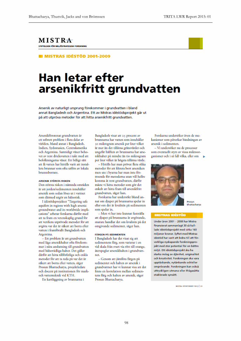
Bhattacharya, Thunvik, Jacks and von Brömssen TRITA LWR Report 2015: 01
98
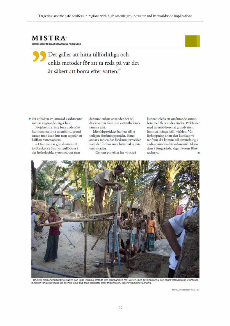
Targeting arsenic-safe aquifers in regions with high arsenic groundwater and its worldwide implications
99
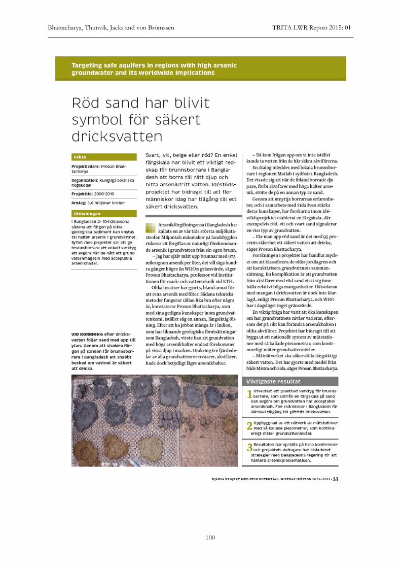
Bhattacharya, Thunvik, Jacks and von Brömssen TRITA LWR Report 2015: 01
100
Redox classification
Black White Off-White Red
Sediment colour
0.0
4.0
8.0
12.0
16.0
20.0
Fe
mg
/l
Black White Off-White Red
Sediment colour
0.0
0.8
1.6
2.4
3.2
4.0
Mn
mg
/l
Black White Off-White Red
Sediment colour
0.0
1.0
2.0
3.0
4.0
5.0
SO
4 m
g/l
red
off-white
white
black
MnMntottot
FeFetottot
SOSO4422--
8th International Conference on the Biogeochemistry of Trace Elements (ICOBTE), Adelaide, Australia
Prediction of risk for high arsenicgroundwater
REDOFF-WHITE
WHITEBLACK
RISK
High Neglible?
REDOX
Very reduced Less reduced
2.4
3.2
4.0
redMnMnMnMnMnMnMnMnMnMnMnMnMnMnMntottottottottottottottottottottottottottottottottottottottottottottottottottottottottottot
Correlating sediment- and groundwater chemistry
Easily recognisable geological features (sediment colors)
Low-As groundwater
Local technique: Economically & socially
sustainable
Scientific validation of sustainability
Arsenic
TRITA-LWR.REPORT 2015:01ISSN 1650-8610ISBN 978-91-7595-461-5
Naturally occurring arsenic (As) in groundwater has undermined the success of supplying safe drinking water in Bangladesh. Arsenic is mobilized in groundwater through reductive dissolution of Fe(III)-oxyhydroxide especially in the younger (Holocene) sediments leading to severe public health consequences. Many of the mitigation options provided during the last two decades have not been well accepted by the people and instead, local well drillers target aquifers for abstrac-tion of arsenic-safe groundwater on the basis of the colour of the sediments. This MISTRA Idea Support Grant project report incorporates the results of the studies carried out to validate the local drillers´ strategy in Bangladesh to low arsenic groundwater by assessing the colour of the sediments through system-atic groundwater and sediment sampling, detailed chemical analysis of water, sediment extractions, mineralogical investigations and hydrogeochemical- and groundwater � ow modelling.
The studies carried out in Matlab in Chandpur District of Bangladesh indicate that the idea on targeting low-arsenic groundwater is facilitated through identi� -cation of the colour of the sediments with decreasing levels of As concentrations in black, o� -white, white and red as perceived by the local drillers. Each of the sediment colour category is characterized by a set of unique hydrochemical char-acteristics that can be used to conceptualize a “sediment colour strategy” that would enable the local drillers to identify arsenic-safe aquifers. Thus, linking the colour of the sediments with groundwater chemistry would be useful to develop a simple sediment colour-based tool for targeting shallow aquifers for the instal-lation of As safe community tubewells for the local drillers through more careful evaluation of the sensitivity of the hydrogeochemical results with respect to the colour of the sediments. The results based on the studies in Matlab, was also rep-licated in Chakdaha Block in West Bengal, India, where identical set of grey sand and brown sand aquifers were identi� ed with similar sediment and hydrochem-ical characteristics of aquifers and the approach for � nding arsenic-safe drinking water sources through the initiatives of the local drillers in a sustainable manner.
Targeting Arsenic-Safe Aquifers in Regions with High Arsenic Groundwater and its Worldwide Implications (TASA)PROSUN BHATTACHARYA, ROGER THUNVIK,GUNNAR JACKS, MATTIAS VON BRÖMSSEN
KTH ROYAL INSTITUTE OF TECHNOLOGY
IN COOPERATION WITH:
REPORT, MISTRA IDEA SUPPORT GRANTSTOCKHOLM, SWEDEN 2015
KTH ROYAL INSTITUTE OF TECHNOLOGY DEPARTMENT OF SUSTAINABLE DEVELOPMENT, ENVIRONMENTAL SCIENCE AND ENGINEERING
www.kth.se
P. BHATTACHARYA, R. THUNVIK, G. JACKS & M. VON BRÖM
SSEN Targeting Arsenic-Safe Aquifers in Regions w
ith High Arsenic G
roundwater and its W
orldwide Im
plications (TASA)K
TH 2015
Targe&ng Arsenic-‐Safe Aquifers in Regions with High Arsenic Groundwater and its Worldwide Implica&ons (TASA)
Project Report
MISTRA Idea Support Grant (Dnr: 2005-035-137)
PROSUN BHATTACHARYA, ROGER THUNVIK, GUNNAR JACKS, MATTIAS VON BRÖMSSEN
TRITA-LWR.REPORT 2015:01
ISSN 1650-8610
ISBN 978-91-7595-461-5
KTH ROYAL INSTITUTE OF TECHNOLOGY
DEPARTMENT OF SUSTAINABLE DEVELOPMENT, ENVIRONMENTAL SCIENCE AND ENGINEERING
OMSLAG FRAMSIDA:
Vänster justerat logotyper enligt
h#ps://intra.kth.se/administra2on/kommunika2on/grafiskprofil/samprofilering-‐hur-‐kth-‐syns-‐2llsammans-‐med-‐andra-‐parter-‐1.450081
(Första bilden)
Bilden Nederst ska det vara blåa randen ovan på bilden
Targe&ng Arsenic-‐Safe Aquifers in Regions with High Arsenic Groundwater and its Worldwide Implica&ons (TASA)
Project Report
MISTRA Idea Support Grant (Dnr: 2005-035-137)
PROSUN BHATTACHARYA, ROGER THUNVIK, GUNNAR JACKS, MATTIAS VON BRÖMSSEN
TRITA-LWR.REPORT 2015:01
ISSN 1650-8610
ISBN 978-91-7595-461-5
KTH ROYAL INSTITUTE OF TECHNOLOGY
DEPARTMENT OF SUSTAINABLE DEVELOPMENT, ENVIRONMENTAL SCIENCE AND ENGINEERING
OMSLAG FRAMSIDA:
Vänster justerat logotyper enligt
h#ps://intra.kth.se/administra2on/kommunika2on/grafiskprofil/samprofilering-‐hur-‐kth-‐syns-‐2llsammans-‐med-‐andra-‐parter-‐1.450081
(Första bilden)
Bilden Nederst ska det vara blåa randen ovan på bilden