Embed Size (px)
Citation preview
DI
SC
US
SI
ON
P
AP
ER
S
ER
IE
S
Forschungsinstitut zur Zukunft der ArbeitInstitute for the Study of Labor
Taxing Women: A Macroeconomic Analysis
IZA DP No. 5962
September 2011
Nezih GunerRemzi KaygusuzGustavo Ventura
Taxing Women:
A Macroeconomic Analysis
Nezih Guner ICREA-MOVE, Universitat Autonoma de Barcelona,
Barcelona GSE, CEPR and IZA
Remzi Kaygusuz Sabanci University
Gustavo Ventura Arizona State University
Discussion Paper No. 5962 September 2011
IZA
P.O. Box 7240 53072 Bonn
Germany
Phone: +49-228-3894-0 Fax: +49-228-3894-180
E-mail: [email protected]
Any opinions expressed here are those of the author(s) and not those of IZA. Research published in this series may include views on policy, but the institute itself takes no institutional policy positions. The Institute for the Study of Labor (IZA) in Bonn is a local and virtual international research center and a place of communication between science, politics and business. IZA is an independent nonprofit organization supported by Deutsche Post Foundation. The center is associated with the University of Bonn and offers a stimulating research environment through its international network, workshops and conferences, data service, project support, research visits and doctoral program. IZA engages in (i) original and internationally competitive research in all fields of labor economics, (ii) development of policy concepts, and (iii) dissemination of research results and concepts to the interested public. IZA Discussion Papers often represent preliminary work and are circulated to encourage discussion. Citation of such a paper should account for its provisional character. A revised version may be available directly from the author.

IZA Discussion Paper No. 5962 September 2011
ABSTRACT
Taxing Women: A Macroeconomic Analysis* Based on well-known evidence on labor supply elasticities, several authors have concluded that women should be taxed at lower rates than men. We evaluate the quantitative implications of taxing women at a lower rate than men. Relative to the current system of taxation, setting a proportional tax rate on married females equal to 4% (8%) increases output and married female labor force participation by about 3.9% (3.4%) and 6.9% (4.0%), respectively. Gender-based taxes improve welfare and are preferred by a majority of households. Nevertheless, welfare gains are higher when the U.S. tax system is replaced by a proportional, gender-neutral income tax. JEL Classification: E62, H31, J12, J22 Keywords: taxation, two-earner households, labor force participation Corresponding author: Nezih Guner MOVE Campus de Belleterra-UAB Edifici B (s/n) 08193 Cedanyola del Valles Barcelona Spain E-mail: [email protected]
* We thank editors Thomas Cooley and Yongsung Chang, our discussant Richard Rogerson, and participants at the 77th Meeting of the Carnegie-Rochester Conference on Public Policy at New York University for their detailed comments and suggestions. We also thank Virginia Sanchez-Marcos, Tim Kehoe and seminar and conference participants at State University Higher School of Economics (Moscow) and the 2011 Society for Economic Dynamics Annual Meetings in Gent. Guner acknowledges support from European Research Council (ERC) Grant 263600. The usual disclaimer applies.
1 Introduction
Two observations are central to this paper. First, it is well known that the labor supply
elasticities of women are larger than those of men, especially when the extensive margin is
considered.1 Second, the current U.S. tax system is biased against women�s work in the
marketplace. Since the U.S. system taxes the income of households and not the income of
individuals, for a married woman who considers entering the labor force, her marginal tax
rate depends on her husband�s income. Given the current levels of marginal tax rates, this
is arguably a substantial impediment to labor force participation.
These observations have motivated work in the theory of optimal taxation. From standard
public-�nance principles, the higher labor supply elasticities of women suggest that they
should be taxed at lower rates than men. Boskin and Sheshinski (1983) were possibly the
�rst to establish this insight. They focused on the optimal linear-income taxation of two-
earner households with exogenously given di¤erences in labor supply elasticities between men
and women.2 More recently, Alesina, Ichino, and Karabarbounis (2011) put forward more
forcefully the idea of di¤erential taxation of men and women within a model in which gender
di¤erences in labor supply elasticities emerge endogenously. Under parametric restrictions,
they conclude that married women should be taxed at lower rates than married men.3
Although the above results are attractive for their policy implications, work in this area
has been almost exclusively theoretical, and a quantitative evaluation of the relative merits of
di¤erential taxation by gender is still missing. It is an open question what are the expected,
quantitative e¤ects associated to changing the current structure of taxation in this direction.
In this paper, we �ll this void. We ask: what are the aggregate e¤ects of taxing married
females at lower rates? What are the welfare implications of these lower tax rates? To answer
these questions, we use a model able to capture a number of key cross-sectional observations
for the problems at hand. We build a life-cycle model populated by heterogeneous single
and married agents. Individuals di¤er in terms of their labor endowments, which di¤er both
1See Blundell and McCurdy (1999) and Keane (2010) for surveys of estimates. With growing labor forceparticipation of females, the labor supply elasticity of men and women recently became more similar (seeBlau and Kahn, 2007; Heim, 2007). There still exist, however, substantial di¤erences.
2In an earlier paper, Rosen (1975) hints at the same issue. Apps and Rees (1988) reach a similar conclusionwithin a model with home production. See Apps and Rees (2010) for an excellent summary and discussionof these results.
3Kleven, Kreiner, and Saez (2009), following Mirelees (1971), study the optimal taxation of couples in amodel economy where the planner does not observe the ability of primary earner or the cost of participationfor the secondary earner. As a result, the government faces a multidimensional screening problem. Theyshow that if the participation of the secondary earner is a signal of the couple being better o¤, the secondaryearner faces a tax and this tax is declining in the primary earner�s earnings.
2
initially and how they evolve over the life cycle. In particular, the labor market productivities
of females are endogenous and depend on their labor market histories: not working is costly
for females since if they do not work their human capital depreciates. Married households
decide if both or only one members should work, in the presence or absence of (costly)
children and the structure of the tax system. In this context, changes in the structure of
taxation lead to changes in participation rates and aggregate labor supply, and can have
large welfare consequences.
We calibrate our model to the U.S. economy under the current tax system, taking into
account observed heterogeneity in skill endowments, marital segregation by skill, labor-force
participation rates as well as the presence of children and their cost. As we explain in
detail in Guner, Kaygusuz and Ventura (2010), the parameterized environment is capable
of jointly reproducing a host of labor supply observations. The model is consistent with the
wage-gender gap and its evolution over the life cycle, female labor force participation by
educational attainment, and the pattern of participation rates by women with and without
children as they age. This makes the model environment an ideal vehicle to evaluate the
consequences of di¤erential taxation by gender.
Within the model disciplined by data, we then proceed to study the e¤ects of a tax
system that imposes di¤erent proportional taxes on the labor earnings of married females.
Following Alesina et al (2011), we will refer to these as gender-based taxes, albeit their
particular implementation will be connected to marital status as we explain below. The
gender-based taxes that we consider nest as special cases the equal tax rates on men and
women. Hence, a virtue of our analysis is that it allows us to separate the e¤ects of di¤erential
taxation of married females, from the e¤ects associated to the elimination or reduction of
tax progressivity.
We consider two implementations of gender-based taxes. First, we consider replacing
the U.S. tax system by proportional tax rates on labor earnings of married females that
are lower than for the rest (married males, singles). We refer to this case as the broad-base
case, as the reduction in tax rates on married females is �nanced by all other agents. In our
second scenario, we �rst calculate a revenue-neutral proportional tax applied to all agents
independent of their gender. We then assign this tax rate to singles, and reduce the tax rates
on the labor earnings of married females increasing only the tax rates on married males. We
refer to this case as the narrow-base case, as only tax rates on married males are used to
achieve revenue neutrality.
We �nd that a shift to proportional tax rates has substantial e¤ects. Replacing the
current tax structure by a proportional income tax at a 10.2% rate increases aggregate
3
hours worked by 3.2% and aggregate output by 3.2% across steady states. As marginal tax
rates are reduced for majority of households, married females increase their labor market
participation by 2.8%. Taking into account changes in labor supply along the extensive as
well as the intensive margin, the overall contribution of married females to changes in hours
is substantial and amounts to 48.9%.
The e¤ects of proportional taxes outlined above are ampli�ed when married females are
taxed at lower rates. If taxes on married females are lowered to 4% (8%) in our narrow-base
case, output increases by 4.0% (3.5%) and aggregate hours increase by 4.2% (3.6%) across
steady states. These �ndings are driven by the much stronger responses of married females;
they increase their participation by 6.9% (4.2%), and contribute 65.8% (56.1%) to the overall
changes in hours. This is all not surprising, as tax rates are reduced on the group that reacts
the most to tax changes. Similar results hold under our broad-base case.
To assess welfare e¤ects from our experiments, we compute transitions between steady
states under the assumption of a small-open economy. We �nd that gender-based taxes lead
to a welfare improvement to a majority of households alive at the date when the structure of
taxes change. Nevertheless, we �nd that proportional income tax at a uniform rate dominates
gender-based taxes in terms of aggregate welfare gains. While a proportional income tax on
all delivers aggregate welfare gains of about 1.1% in consumption terms, a di¤erential tax
rate of 4% (8%) on married females implies gains of about 0.4% (0.7%). As we explain in
section 7.1, this result is driven by the e¤ects associated to taxing married men at higher
rates as in revenue-neutral tax reforms lower taxes on married females have to be �nanced
by higher taxes on married males. While households where married women have a higher
initial labor endowment tend to gain from the shift to gender-based taxes, most married
households in our model are those where males have higher labor productivity. This is due
to the observed marital sorting by skill, and initial wage gaps. Hence, the higher tax rates
on males that accompany the lower rates on females have a net detrimental consequence on
the welfare of most married households, and thus on aggregate welfare. These conclusions
hold in a variety of robustness checks.
Our paper is organized as follows. Section 2 presents a simple example that highlights
the e¤ects of di¤erential tax rates on females on labor supply and participation decisions.
Sections 3 and 4 present the model economy. Sections 3 discusses calibration. In section 6
we explain in detail the nature of the quantitative experiments that we conduct. Section 7
contains the main �ndings of the paper. Section 8 analyzes the sensitivity of our results via
a number of robustness checks. Finally, section 9 concludes.
4
1.1 Current U.S. Taxes
It is well known that the current U.S. tax system is biased against women�s work.4 As we
mentioned earlier, this bias originates from the fact that the U.S. tax system taxes the income
of households, not the income of individuals. As a result, for a woman who considers entering
the labor force, her marginal tax rate depends on her husbands�income. In addition, given
the progressivity built in the system, the tax rate on her �rst dollar of income increases with
the household�s income (inframarginal income).
In related work (Guner, Kaygusuz and Ventura, 2011), we examine in detail the relation-
ship between taxes e¤ectively paid by households and their income in a large cross-sectional
data from the U.S. Internal Revenue Service for the year 2000. Using this data, we estimate
e¤ective average tax rates. In Figure 1, we present the average tax rates and corresponding
marginal rates, for a married couple with 2 children in the year 2000.5 To illustrate the bias
against women�s work, imagine a married couple in which only the husband works and earns
about the mean household income in the U.S. (about $ 58,375 in the 2000 IRS data). The
average and marginal tax rates of this household are about 7.9% and 15.5%, respectively.
Hence, the marginal tax rate that the household faces is 15.5% for woman�s �rst hour of
work. Together with payroll taxes and the additional child care expenses that the family
might face, the combined reduction on the additional income that the female generates can
be substantial, leading to disincentives for labor market participation. For higher income
households, as Figure 1 indicates, the disincentives can be much stronger. For a household
at twice the level of mean income, the marginal tax rate is about 20.8%, whereas for a house-
hold at �ve times mean income, the marginal tax rate amounts to about 27.8%. Figure 1
also shows average and marginal tax rates for a single household (�head of household�) with
two children. These households face higher taxes than married ones. Still a married female
would be less distorted in terms of her labor supply decisions if she was taxed as an indi-
vidual at the singles�rates. Consider again a female whose husband earns about the mean
household income. Suppose her earnings are about 0.6 times her husband�s earnings. If she
was taxed as an individual facing the tax schedule of singles, her marginal tax rate would
be 13%, whereas if she �les jointly with her husband her marginal rate would be 19.2%.
Table 1 presents more detailed information about marginal tax rates faced by married
households. The table shows marginal tax rates at di¤erent levels of household�s income, that
changes according to di¤erent hypothetical earnings for married female (secondary earner).
Using our estimates, this is done for when she is about to enter the labor force, at low
4See McCa¤ery (1999) for a comprehensive description.5See section 5 for details.
5
earnings (one- half mean income), or at higher earnings (mean income).
As we note in Guner et al (2011), the aforementioned marginal tax rates are lower bounds
on the marginal rates faced by married households. This follows from the fact that the
marginal tax rates reported are calculated from average tax rates, and take into account all
the inframarginal deductions that households have access to. E¤ective marginal tax rates
are good approximations at low levels of income. At high levels of income, reported marginal
tax rates are non-trivially higher than e¤ective marginal rates.6
More broadly, international evidence suggests that di¤erences in taxation might indeed
matter for cross-country di¤erences in female labor force participation. Bick and Fuchs-
Schuendeln (2011) provide a detailed account of how household incomes are taxed in di¤erent
OECD countries (both in terms of the unit of taxation and the tax burden on the secondary
earners). They study a model of household labor supply and show that di¤erences in taxes
can account for a large part of cross-country di¤erences in married female labor supply. Fig-
ure 2, which is based on their analysis, shows the relation between tax burden on secondary
earner and married female labor supply, where the tax burden is measured as the ratio of
the tax liabilities of a two-earner household to a one-earner one. It is clear that higher taxes
on secondary earners are associated with lower female labor force participation. It is also
worth noting that low labor force participation of countries like the U.S., Germany, France
and Portugal are countries that tax jointly household income.7
2 Taxing Married Women Di¤erently
In this section, we present a simple static, decision-problem example that illustrates how dif-
ferential taxation of married females a¤ects labor supply decisions in two earner households,
at the intensive and extensive margins.
A one-earner household Consider a married couple. The household decides whether
only one or both members should work and if so, how much. Let x and z denote the
labor market productivities (wage rates) of males and females, respectively. Let �H be a
proportional tax on the labor income of the male, and let �L be a proportional tax on the
6For instance, the average recorded marginal rate at �ve times mean income is about 34.0%, more thansix percentage points above the marginal rate computed from our e¤ective tax function.
7The U.S. and Germany are joint taxation countries where the unit of taxation is household and taxliabilities are calculated based on total household income. France and Portugal are family taxation countries,where tax liabilities are calculated roughly by dividing total household income by the number of familymembers. See Kesselman (2008) for a classi�cation of di¤erent countries according to how they tax householdincome.
6
labor income of the female.
Consider �rst the problem if only one member (husband) works. The household problem
is given by
maxlm;1
f2[log((1� �H)zlm;1)| {z }=log(c)
]�W (lm;1)g;
where lm;1 is the labor choice of the primary earner (husband). The subscript 1 represents the
choice of a one-earner household. The function W (:) stands for the instantaneous disutility
associated to work time. The function W (:) is di¤erentiable and strictly convex.
Household utility when only one member works is given by
V1(�H) = 2[log((1� �H)zl�m;1)]�W (l�m;1);
where a 0�0 denotes an optimal choice.
A two-earner household When both members work, the household incurs a utility
cost q, drawn from a distribution with cumulative distribution function �(q). Then the
problem is given by
maxlm;2;lf;2
f2[log((1� �H)zlm;2 + (1� �L)xlf;2)| {z }=log(c)
]
�W (lm;2)�W (lf;2)� qg;
where the subscript 2 represents the choices of a two-earner household. Let the solutions to
this problem be denoted by l�m;2 and l�f;2. Household utility in this case equals
V2(�H ; �L)� q = 2[log((1� �H)zl�m;2 + (1� �L)xl
�f;2)]
�W (l�m;2)�W (l�f;2)� q:
Letting the function W (:) adopt the functional form that we will use later, 'l1+1 , it is
easy to �nd that relative labor supplies depend on relative productivities, the relative tax
wedge and the Frisch elasticity , and is given by
l�f;2l�m;2
=�xz
� � 1� �L1� �H
� It follows that a higher relative productivity of the female, or a lower relative tax distortion
on her, increases her labor supply relative to her partner.
7
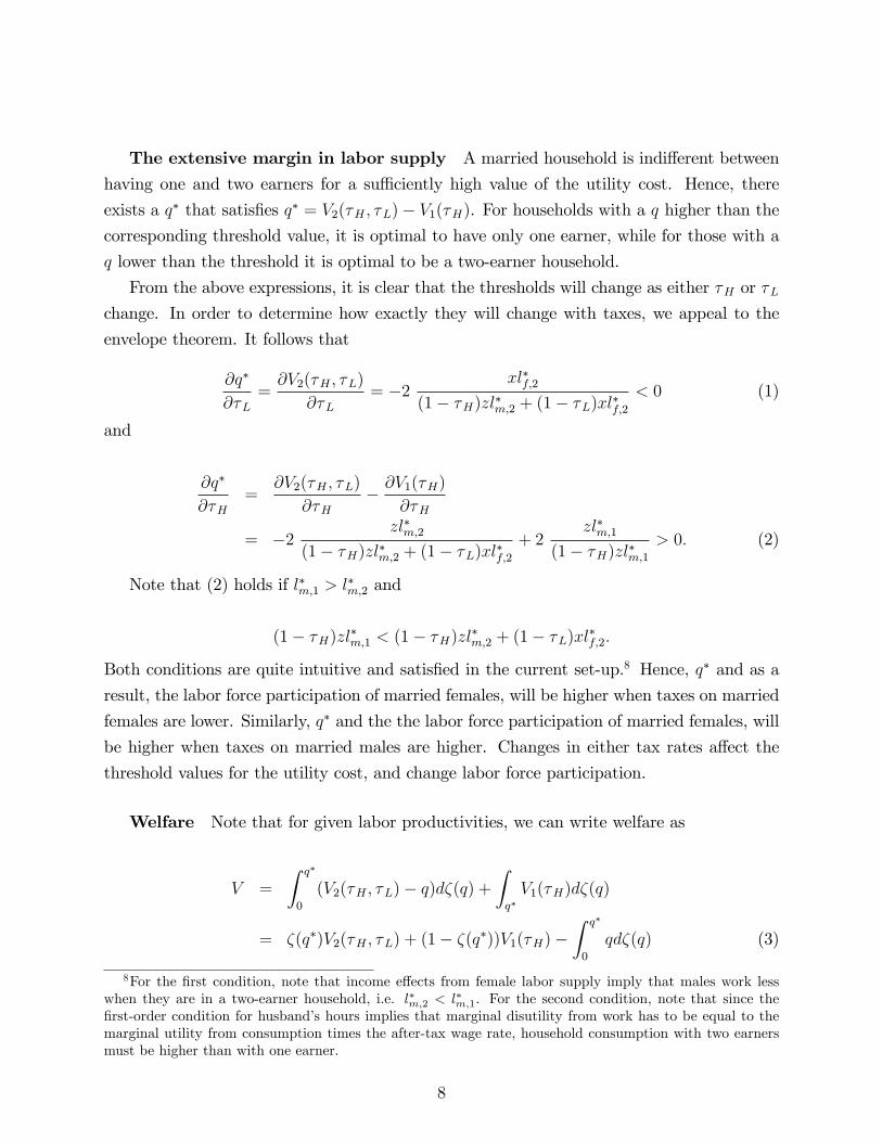
The extensive margin in labor supply A married household is indi¤erent between
having one and two earners for a su¢ ciently high value of the utility cost. Hence, there
exists a q� that satis�es q� = V2(�H ; �L)� V1(�H). For households with a q higher than the
corresponding threshold value, it is optimal to have only one earner, while for those with a
q lower than the threshold it is optimal to be a two-earner household.
From the above expressions, it is clear that the thresholds will change as either �H or �Lchange. In order to determine how exactly they will change with taxes, we appeal to the
envelope theorem. It follows that
@q�
@�L=@V2(�H ; �L)
@�L= �2
xl�f;2(1� �H)zl�m;2 + (1� �L)xl�f;2
< 0 (1)
and
@q�
@�H=
@V2(�H ; �L)
@�H� @V1(�H)
@�H
= �2zl�m;2
(1� �H)zl�m;2 + (1� �L)xl�f;2+ 2
zl�m;1(1� �H)zl�m;1
> 0: (2)
Note that (2) holds if l�m;1 > l�m;2 and
(1� �H)zl�m;1 < (1� �H)zl
�m;2 + (1� �L)xl
�f;2:
Both conditions are quite intuitive and satis�ed in the current set-up.8 Hence, q� and as a
result, the labor force participation of married females, will be higher when taxes on married
females are lower. Similarly, q� and the the labor force participation of married females, will
be higher when taxes on married males are higher. Changes in either tax rates a¤ect the
threshold values for the utility cost, and change labor force participation.
Welfare Note that for given labor productivities, we can write welfare as
V =
Z q�
0
(V2(�H ; �L)� q)d�(q) +
Zq�V1(�H)d�(q)
= �(q�)V2(�H ; �L) + (1� �(q�))V1(�H)�Z q�
0
qd�(q) (3)
8For the �rst condition, note that income e¤ects from female labor supply imply that males work lesswhen they are in a two-earner household, i.e. l�m;2 < l�m;1. For the second condition, note that since the�rst-order condition for husband�s hours implies that marginal disutility from work has to be equal to themarginal utility from consumption times the after-tax wage rate, household consumption with two earnersmust be higher than with one earner.
8
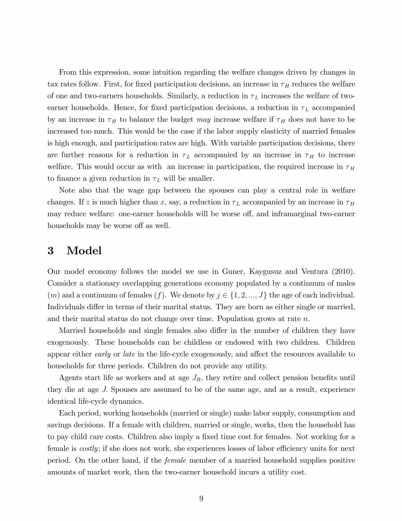
From this expression, some intuition regarding the welfare changes driven by changes in
tax rates follow. First, for �xed participation decisions, an increase in �H reduces the welfare
of one and two-earners households. Similarly, a reduction in �L increases the welfare of two-
earner households. Hence, for �xed participation decisions, a reduction in �L accompanied
by an increase in �H to balance the budget may increase welfare if �H does not have to be
increased too much. This would be the case if the labor supply elasticity of married females
is high enough, and participation rates are high. With variable participation decisions, there
are further reasons for a reduction in �L accompanied by an increase in �H to increase
welfare. This would occur as with an increase in participation, the required increase in �Hto �nance a given reduction in �L will be smaller.
Note also that the wage gap between the spouses can play a central role in welfare
changes. If z is much higher than x, say, a reduction in �L accompanied by an increase in �Hmay reduce welfare: one-earner households will be worse o¤, and inframarginal two-earner
households may be worse o¤ as well.
3 Model
Our model economy follows the model we use in Guner, Kaygusuz and Ventura (2010).
Consider a stationary overlapping generations economy populated by a continuum of males
(m) and a continuum of females (f). We denote by j 2 f1; 2; :::; Jg the age of each individual.Individuals di¤er in terms of their marital status. They are born as either single or married,
and their marital status do not change over time. Population grows at rate n:
Married households and single females also di¤er in the number of children they have
exogenously. These households can be childless or endowed with two children. Children
appear either early or late in the life-cycle exogenously, and a¤ect the resources available to
households for three periods. Children do not provide any utility.
Agents start life as workers and at age JR; they retire and collect pension bene�ts until
they die at age J: Spouses are assumed to be of the same age, and as a result, experience
identical life-cycle dynamics.
Each period, working households (married or single) make labor supply, consumption and
savings decisions. If a female with children, married or single, works, then the household has
to pay child care costs. Children also imply a �xed time cost for females. Not working for a
female is costly; if she does not work, she experiences losses of labor e¢ ciency units for next
period. On the other hand, if the female member of a married household supplies positive
amounts of market work, then the two-earner household incurs a utility cost.
9
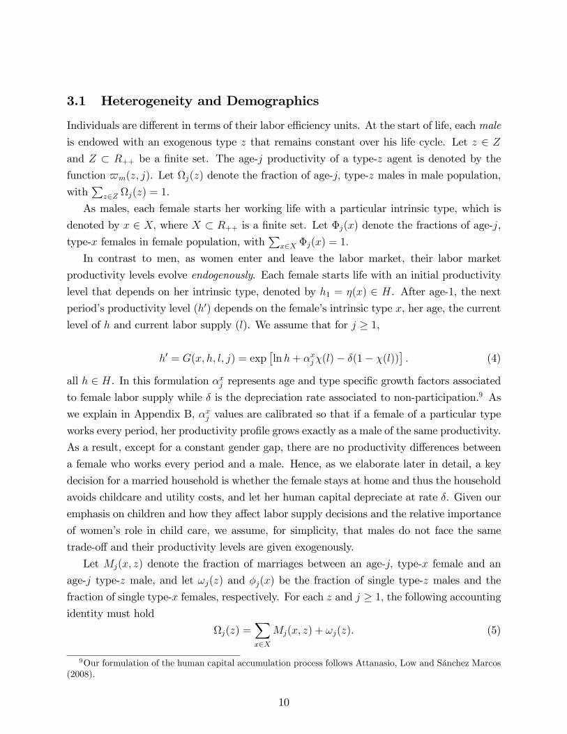
3.1 Heterogeneity and Demographics
Individuals are di¤erent in terms of their labor e¢ ciency units. At the start of life, each male
is endowed with an exogenous type z that remains constant over his life cycle. Let z 2 Z
and Z � R++ be a �nite set. The age-j productivity of a type-z agent is denoted by the
function $m(z; j). Let j(z) denote the fraction of age-j; type-z males in male population,
withP
z2Z j(z) = 1.
As males, each female starts her working life with a particular intrinsic type, which is
denoted by x 2 X; where X � R++ is a �nite set. Let �j(x) denote the fractions of age-j,
type-x females in female population, withP
x2X �j(x) = 1:
In contrast to men, as women enter and leave the labor market, their labor market
productivity levels evolve endogenously. Each female starts life with an initial productivity
level that depends on her intrinsic type, denoted by h1 = �(x) 2 H. After age-1, the next
period�s productivity level (h0) depends on the female�s intrinsic type x, her age, the current
level of h and current labor supply (l). We assume that for j � 1,
h0 = G(x; h; l; j) = exp�lnh+ �xj�(l)� �(1� �(l))
�: (4)
all h 2 H. In this formulation �xj represents age and type speci�c growth factors associatedto female labor supply while � is the depreciation rate associated to non-participation.9 As
we explain in Appendix B, �xj values are calibrated so that if a female of a particular type
works every period, her productivity pro�le grows exactly as a male of the same productivity.
As a result, except for a constant gender gap, there are no productivity di¤erences between
a female who works every period and a male. Hence, as we elaborate later in detail, a key
decision for a married household is whether the female stays at home and thus the household
avoids childcare and utility costs, and let her human capital depreciate at rate �. Given our
emphasis on children and how they a¤ect labor supply decisions and the relative importance
of women�s role in child care, we assume, for simplicity, that males do not face the same
trade-o¤ and their productivity levels are given exogenously.
Let Mj(x; z) denote the fraction of marriages between an age-j; type-x female and an
age-j type-z male, and let !j(z) and �j(x) be the fraction of single type-z males and the
fraction of single type-x females, respectively. For each z and j � 1; the following accountingidentity must hold
j(z) =Xx2X
Mj(x; z) + !j(z): (5)
9Our formulation of the human capital accumulation process follows Attanasio, Low and Sánchez Marcos(2008).
10

Since the marital status does not change, Mj(x; z) = M(x; z) and !j(z) = !(z) for all j;
which implies j(z) = (z): Similarly, for age-j; type-x females, we have
�j(x) =Xz2Z
Mj(x; z) + �j(x): (6)
Since marital status does not change �j(x) = �(x) and �j(x) = �(x) for all j
We assume that each cohort is 1 + n bigger than the previous one. The demographic
structure is stationary so that age j agents are a fraction �j of the population at any point
in time. The weights are normalized to add up to one, and satis�es �j+1 = �j=(1 + n):
3.2 Children
Children are assigned exogenously to married couples and single females at the start of life,
depending on the intrinsic type of parents. Each married couple and single female can be
of three types: early child bearers, late child bearers, and those without any children. Early
and late child bearers have two children for three periods. Early child bearers have these
children in ages j = 1; 2; 3 while late child bearers have children attached to them in ages
j = 2; 3; 4:
We assume that if a female with children (married or single) works, then the household
has to pay for child care costs. Child care costs depend on the age of the child (s). For a
household with children of age s 2 f1; 2; 3g, the household needs to purchase d(s) units of(child care) labor services for their two children. Since the competitive price of child care
services is the wage rate w, the total cost of child care services for two children equals wd(s).
Each young, s = 1; child also implies a time cost for the mother, whether she is working or
not.
3.3 Preferences and Technology
The momentary utility function for a single female is given by
USf (c; l; ky) = log(c)� '(l + ky{)1+1 ;
where c is consumption, l is time devoted to market work, ' is a parameter controlling the
disutility of work, { is �xed time cost having two age-1 (young) children for a female, and is the intertemporal elasticity of labor supply. Here ky 2 f0; 1g stands for the absence orpresence of of age-1 (young) children in the household. Since a single male does not have
any children, his utility function is simply given by
USm (c; l) = log(c)� '(l)1+1 :
11
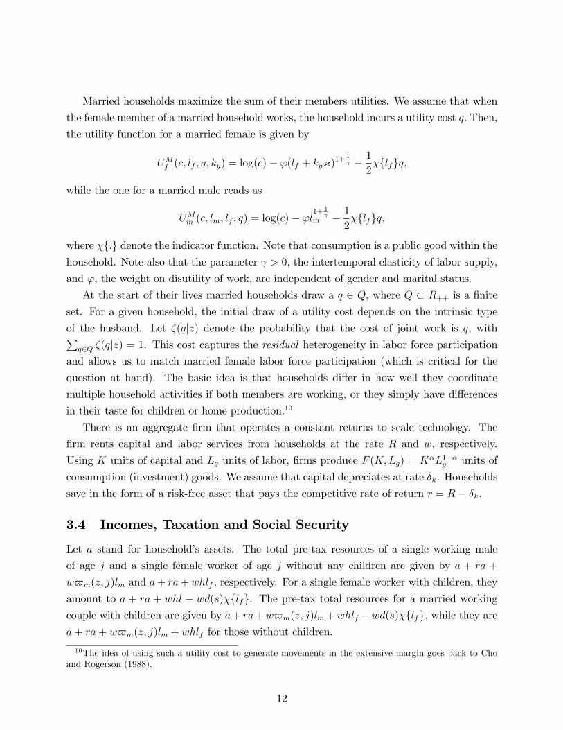
Married households maximize the sum of their members utilities. We assume that when
the female member of a married household works, the household incurs a utility cost q: Then,
the utility function for a married female is given by
UMf (c; lf ; q; ky) = log(c)� '(lf + ky{)1+1 � 1
2�flfgq;
while the one for a married male reads as
UMm (c; lm; lf ; q) = log(c)� 'l1+ 1
m � 1
2�flfgq;
where �f:g denote the indicator function. Note that consumption is a public good within thehousehold. Note also that the parameter > 0, the intertemporal elasticity of labor supply,
and ', the weight on disutility of work, are independent of gender and marital status.
At the start of their lives married households draw a q 2 Q; where Q � R++ is a �nite
set. For a given household, the initial draw of a utility cost depends on the intrinsic type
of the husband. Let �(qjz) denote the probability that the cost of joint work is q, withPq2Q �(qjz) = 1. This cost captures the residual heterogeneity in labor force participation
and allows us to match married female labor force participation (which is critical for the
question at hand). The basic idea is that households di¤er in how well they coordinate
multiple household activities if both members are working, or they simply have di¤erences
in their taste for children or home production.10
There is an aggregate �rm that operates a constant returns to scale technology. The
�rm rents capital and labor services from households at the rate R and w, respectively.
Using K units of capital and Lg units of labor, �rms produce F (K;Lg) = K�L1��g units of
consumption (investment) goods. We assume that capital depreciates at rate �k. Households
save in the form of a risk-free asset that pays the competitive rate of return r = R� �k.
3.4 Incomes, Taxation and Social Security
Let a stand for household�s assets. The total pre-tax resources of a single working male
of age j and a single female worker of age j without any children are given by a + ra +
w$m(z; j)lm and a+ ra+whlf , respectively. For a single female worker with children, they
amount to a + ra + whl � wd(s)�flfg. The pre-tax total resources for a married workingcouple with children are given by a+ ra+w$m(z; j)lm+whlf �wd(s)�flfg; while they area+ ra+ w$m(z; j)lm + whlf for those without children.
10The idea of using such a utility cost to generate movements in the extensive margin goes back to Choand Rogerson (1988).
12
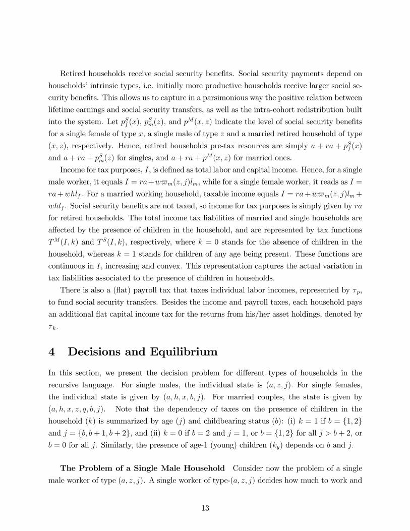
Retired households receive social security bene�ts. Social security payments depend on
households�intrinsic types, i.e. initially more productive households receive larger social se-
curity bene�ts. This allows us to capture in a parsimonious way the positive relation between
lifetime earnings and social security transfers, as well as the intra-cohort redistribution built
into the system. Let pSf (x); pSm(z); and p
M(x; z) indicate the level of social security bene�ts
for a single female of type x, a single male of type z and a married retired household of type
(x; z), respectively. Hence, retired households pre-tax resources are simply a + ra + pSf (x)
and a+ ra+ pSm(z) for singles, and a+ ra+ pM(x; z) for married ones.
Income for tax purposes, I, is de�ned as total labor and capital income. Hence, for a single
male worker, it equals I = ra+w$m(z; j)lm, while for a single female worker, it reads as I =
ra+whlf . For a married working household, taxable income equals I = ra+w$m(z; j)lm+
whlf . Social security bene�ts are not taxed, so income for tax purposes is simply given by ra
for retired households. The total income tax liabilities of married and single households are
a¤ected by the presence of children in the household, and are represented by tax functions
TM(I; k) and T S(I; k), respectively, where k = 0 stands for the absence of children in the
household, whereas k = 1 stands for children of any age being present. These functions are
continuous in I, increasing and convex. This representation captures the actual variation in
tax liabilities associated to the presence of children in households.
There is also a (�at) payroll tax that taxes individual labor incomes, represented by � p,
to fund social security transfers. Besides the income and payroll taxes, each household pays
an additional �at capital income tax for the returns from his/her asset holdings, denoted by
� k.
4 Decisions and Equilibrium
In this section, we present the decision problem for di¤erent types of households in the
recursive language. For single males, the individual state is (a; z; j): For single females,
the individual state is given by (a; h; x; b; j). For married couples, the state is given by
(a; h; x; z; q; b; j). Note that the dependency of taxes on the presence of children in the
household (k) is summarized by age (j) and childbearing status (b): (i) k = 1 if b = f1; 2gand j = fb; b+ 1; b+ 2g, and (ii) k = 0 if b = 2 and j = 1, or b = f1; 2g for all j > b+ 2, or
b = 0 for all j. Similarly, the presence of age-1 (young) children (ky) depends on b and j:
The Problem of a Single Male Household Consider now the problem of a single
male worker of type (a; z; j). A single worker of type-(a; z; j) decides how much to work and
13
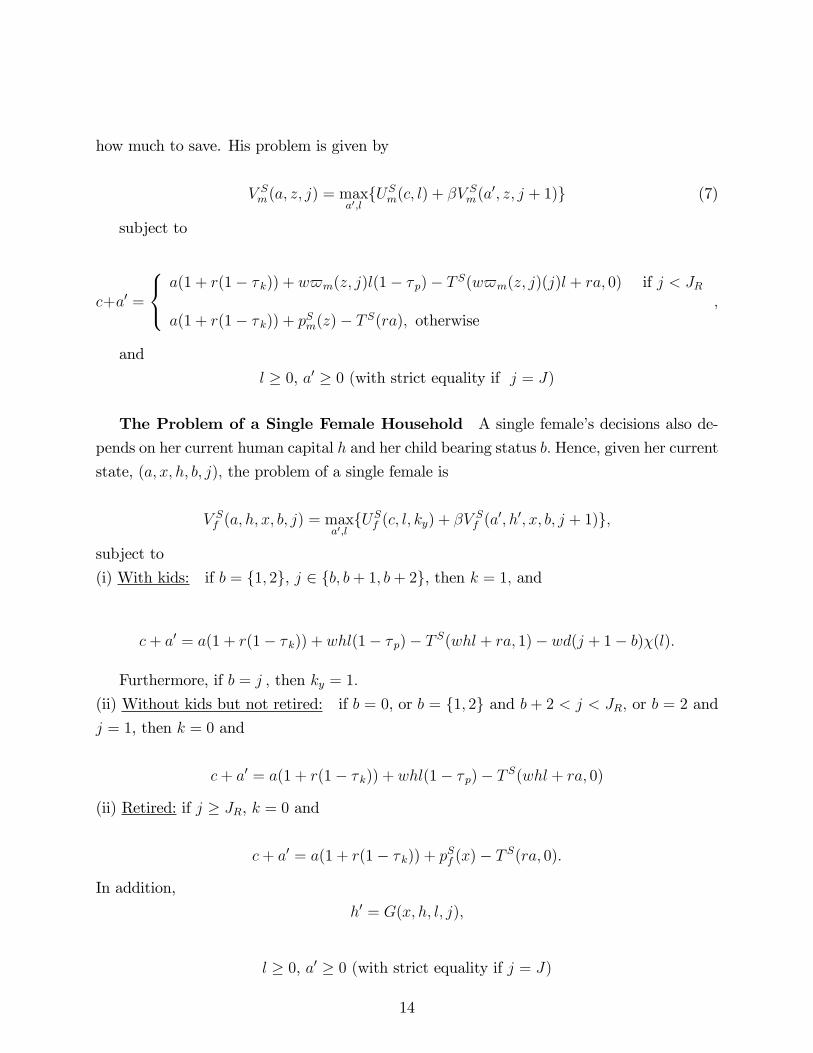
how much to save. His problem is given by
V Sm(a; z; j) = max
a0;lfUSm(c; l) + �V S
m(a0; z; j + 1)g (7)
subject to
c+a0 =
8<:a(1 + r(1� � k)) + w$m(z; j)l(1� � p)� T S(w$m(z; j)(j)l + ra; 0) if j < JR
a(1 + r(1� � k)) + pSm(z)� T S(ra); otherwise
;
and
l � 0, a0 � 0 (with strict equality if j = J)
The Problem of a Single Female Household A single female�s decisions also de-
pends on her current human capital h and her child bearing status b: Hence, given her current
state, (a; x; h; b; j); the problem of a single female is
V Sf (a; h; x; b; j) = max
a0;lfUSf (c; l; ky) + �V S
f (a0; h0; x; b; j + 1)g;
subject to
(i) With kids: if b = f1; 2g, j 2 fb; b+ 1; b+ 2g, then k = 1; and
c+ a0 = a(1 + r(1� � k)) + whl(1� � p)� T S(whl + ra; 1)� wd(j + 1� b)�(l):
Furthermore, if b = j ; then ky = 1:
(ii) Without kids but not retired: if b = 0, or b = f1; 2g and b + 2 < j < JR; or b = 2 and
j = 1, then k = 0 and
c+ a0 = a(1 + r(1� � k)) + whl(1� � p)� T S(whl + ra; 0)
(ii) Retired: if j � JR, k = 0 and
c+ a0 = a(1 + r(1� � k)) + pSf (x)� T S(ra; 0):
In addition,
h0 = G(x; h; l; j);
l � 0, a0 � 0 (with strict equality if j = J)
14
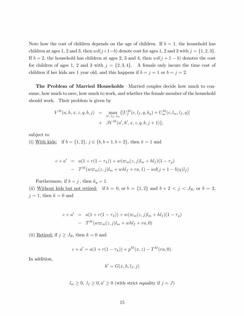
Note how the cost of children depends on the age of children. If b = 1; the household has
children at ages 1, 2 and 3, then wd(j+1�b) denote cost for ages 1, 2 and 3 with j = f1; 2; 3g.If b = 2; the household has children at ages 2, 3 and 4, then wd(j + 1� b) denotes the cost
for children of ages 1, 2 and 3 with j = f2; 3; 4g. A female only incurs the time cost of
children if her kids are 1 year old, and this happens if b = j = 1 or b = j = 2:
The Problem of Married Households Married couples decide how much to con-
sume, howmuch to save, howmuch to work, and whether the female member of the household
should work. Their problem is given by
V M(a; h; x; z; q; b; j) = maxa0; lf ; lm
f[UMf (c; lf ; q; ky) + UMm (c; lm; lf ; q)]
+ �V M(a0; h0; x; z; q; b; j + 1)g;
subject to
(i) With kids: if b = f1; 2g, j 2 fb; b+ 1; b+ 2g, then k = 1 and
c+ a0 = a(1 + r(1� � k)) + w($m(z; j)lm + hlf )(1� � p)
� TM(w$m(z; j)lm + whlf + ra; 1)� wd(j + 1� b)�(lf )
Furthermore, if b = j ; then ky = 1:
(ii) Without kids but not retired: if b = 0, or b = f1; 2g and b + 2 < j < JR; or b = 2,
j = 1, then k = 0 and
c+ a0 = a(1 + r(1� � k)) + w($m(z; j)lm + hlf )(1� � p)
� TM(w$m(z; j)lm + whlf + ra; 0)
(ii) Retired: if j � JR, then k = 0 and
c+ a0 = a(1 + r(1� � k)) + pM(x; z)� TM(ra; 0):
In addition,
h0 = G(x; h; lf ; j)
lm � 0; lf � 0; a0 � 0 (with strict equality if j = J)
15
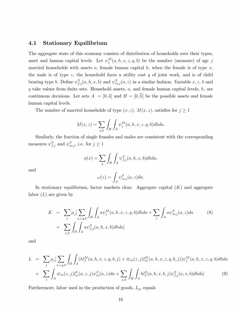
4.1 Stationary Equilibrium
The aggregate state of this economy consists of distribution of households over their types,
asset and human capital levels. Let Mj (a; h; x; z; q; b) be the number (measure) of age j
married households with assets a, female human capital h, when the female is of type x,
the male is of type z, the household faces a utility cost q of joint work, and is of child
bearing type b. De�ne Sf;j(a; h; x; b) and Sm;j(a; z) in a similar fashion. Variable x; z; b and
q take values from �nite sets. Household assets, a; and female human capital levels, h; are
continuous decisions. Let sets A = [0; a] and H = [0; h] be the possible assets and female
human capital levels.
The number of married households of type (x; z); M(x; z); satis�es for j � 1
M(x; z) =Xq;b
ZH
ZA
Mj (a; h; x; z; q; b)dhda:
Similarly, the fraction of single females and males are consistent with the corresponding
measures Sf;j and Sm;j, i.e. for j � 1
�(x) =Xb
ZH
ZA
Sf;j(a; h; x; b)dhda;
and
!(z) =
ZA
Sm;j(a; z)da:
In stationary equilibrium, factor markets clear. Aggregate capital (K) and aggregate
labor (L) are given by
K =Xj
�j[Xx;z;q;b
ZH
ZA
a Mj (a; h; x; z; q; b)dhda+Xz
ZA
a Sm;j(a; z)da (8)
+Xx;b
ZH
ZA
a Sf;j(a; h; x; b)dhda]
and
L =Xj
�j[Xx;z;q;b
ZH
ZA
(hlMf (a; h; x; z; q; b; j) +$m(z; j)lMm (a; h; x; z; q; b; j))
Mj (a; h; x; z; q; b)dhda
+Xz
ZA
$m(z; j)lSm(a; z; j)
Sm(a; z)da+
Xx;b
ZH
ZA
hlSf (a; h; x; b; j) Sf;j(a; x; b)dhda] (9)
Furthermore, labor used in the production of goods, Lg, equals
16
Lg = L� [Xx;z;q
Xb=1;2
Xj=b;b+2
�j
ZH
ZA
�flMf gd(j + 1� b) Mj (a; h; x; z; q; b)dhda
+Xx
Xb=1;2
Xj=b;b+2
�j
ZH
ZA
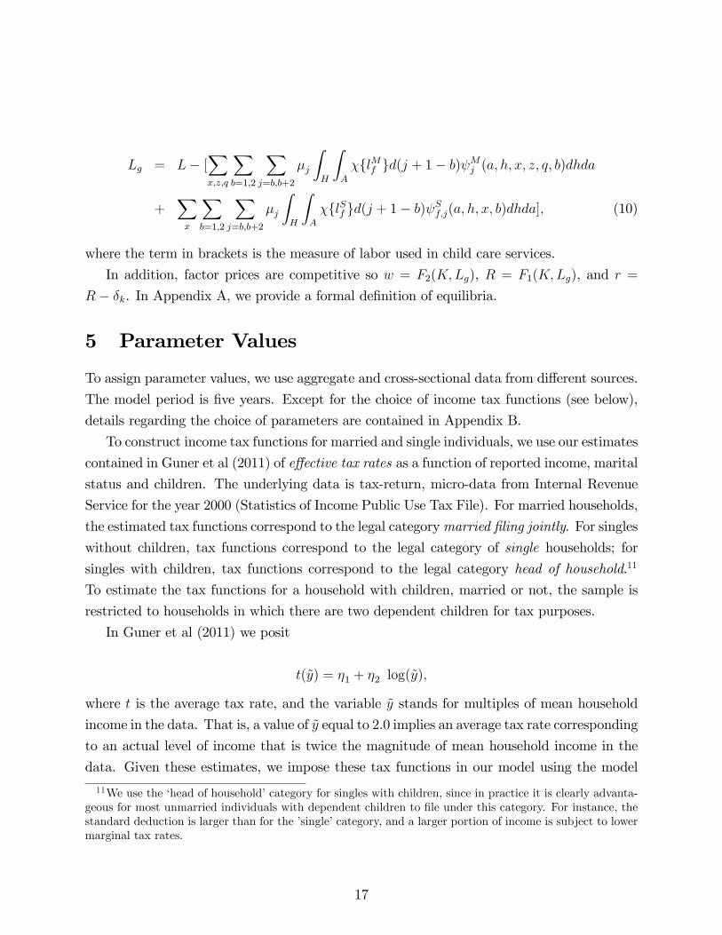
�flSf gd(j + 1� b) Sf;j(a; h; x; b)dhda]; (10)
where the term in brackets is the measure of labor used in child care services.
In addition, factor prices are competitive so w = F2(K;Lg), R = F1(K;Lg), and r =
R� �k. In Appendix A, we provide a formal de�nition of equilibria.
5 Parameter Values
To assign parameter values, we use aggregate and cross-sectional data from di¤erent sources.
The model period is �ve years. Except for the choice of income tax functions (see below),
details regarding the choice of parameters are contained in Appendix B.
To construct income tax functions for married and single individuals, we use our estimates
contained in Guner et al (2011) of e¤ective tax rates as a function of reported income, marital
status and children. The underlying data is tax-return, micro-data from Internal Revenue
Service for the year 2000 (Statistics of Income Public Use Tax File). For married households,
the estimated tax functions correspond to the legal categorymarried �ling jointly. For singles
without children, tax functions correspond to the legal category of single households; for
singles with children, tax functions correspond to the legal category head of household.11
To estimate the tax functions for a household with children, married or not, the sample is
restricted to households in which there are two dependent children for tax purposes.
In Guner et al (2011) we posit
t(~y) = �1 + �2 log(~y);
where t is the average tax rate, and the variable ~y stands for multiples of mean household
income in the data. That is, a value of ~y equal to 2.0 implies an average tax rate corresponding
to an actual level of income that is twice the magnitude of mean household income in the
data. Given these estimates, we impose these tax functions in our model using the model
11We use the �head of household�category for singles with children, since in practice it is clearly advanta-geous for most unmarried individuals with dependent children to �le under this category. For instance, thestandard deduction is larger than for the �single�category, and a larger portion of income is subject to lowermarginal tax rates.
17
counterpart of ~y and mean income. That is, total tax liabilities amount to t(~y)� ~y �mean
household income.
Estimates for �1 and �2 are contained in Table 2 for di¤erent tax functions we use in
our quantitative analysis. Figure 1 displays estimated average and marginal tax rates for
di¤erent multiples of household income for married and single households with two children.
Our estimates imply that a married household at around mean income faces an average tax
rate of about 7.9% and marginal tax rate of 15.5%. As a comparison, a single household
at the half of mean income faces average and marginal tax rates that are 3.3% and 11.5%,
respectively. At twice the mean income level, the average and marginal rates for a married
household amount to 13.2% and 20.8%, respectively, while a single household at the mean
income level has an average tax rate of 9% and a marginal tax rate of 17.2%.
Table 3 summarizes our parameter choices. Table 4 shows the performance of the bench-
mark model in terms of the targets we impose. The table also shows how well the benchmark
calibration reproduces the labor force participation of married females. The model has no
problem in reproducing jointly these observations as the table demonstrates.
6 The Quantitative Experiments
We study the e¤ects of moving from the current U.S. tax system to a tax system where
di¤erent proportional tax rates on labor earnings coexist, �L an �H . All households pay a
common additional proportional tax rate on capital income, � �k. In all cases considered, the
experiments are revenue neutral. The social security system remains intact so each worker
still pay the same proportional payroll tax � p as in the benchmark economy:
We �rst implement a revenue-neutral proportional income tax reform and compute the
common proportional income tax � such that �L = �H = � . Once the common proportional
income tax rate � is calculated, we set �L < � and �nd �H > � that achieves revenue
neutrality. Naturally, our formulation incorporates a trade o¤: if lower tax rates �L are
chosen, a higher tax rate �H becomes necessary to achieve budget balance. We consider two
cases of di¤erential taxation of married females, depending on the tax base used to balance
the budget. Let Em and Ef be the labor income of males and females, respectively. In
our narrow-base case, under di¤erential tax rates for married females, we assume that the
after-tax labor income of a single male is simply Em(1 � �); while for single females it is
given by Ef (1� �): For married males and females, respectively, the after-tax labor income
is given by Em(1� �H) and Ef (1� �L): Hence, the narrow case taxes married females at a
lower rate and achieves revenue-neutrality by applying higher taxes only on married males.
18
The narrow-base case follows the proposal of Alesina et al (2011) and highlights the basic
trade-o¤ associated to lowering taxing on married women and increasing taxes on married
men.
In our broad-base case, married females face �L and everyone else (married or single) face
�H . Hence, the after-tax labor income of a single male is simply Em(1� �H); while for singlefemales it is given by Ef (1� �H): For married males and females, respectively, the after-taxlabor income is given by Em(1� �H) and Ef (1� �L): Since lower taxes on married females
are �nanced by a larger tax base, �H that achieved revenue neutrality will be lower in the
broad-base case, and this might matter for the aggregate e¤ects of gender based taxes.
In both cases, the capital income tax rate equals � �k = � k + � . That is, capital income of
all households is taxed at the rate original rate � k plus the marginal rate � from proportional
taxation. It follows that when we make �L and �H di¤erent from each other, the tax rates
on capital are unchanged. Therefore, our results capture the consequences of taxing di¤erent
people di¤erently in terms of their labor earnings, without changes in the tax rate on capital
income.
All our experiments are conducted under the assumption of a small-open economy: the
rate of return to capital and the wage rate are unchanged across steady states. To achieve
revenue neutrality, we balance the budget period by period via adjusting � for the propor-
tional income tax experiment, or �H for gender-based taxation experiments.
7 Findings
We report �rst in this section steady-state comparisons of economies in relation to the
benchmark. As the e¤ects on aggregate outcomes (such as female labor force participation,
aggregate hours and output) change monotonically with lower taxes on females, we only
report results for two values of �L: Table 5 shows key aggregate �ndings for the case of a
proportional income tax (� = �H = �L), and for two levels of tax rates for females, (�L = 8%)
and (�L = 4%), under broad and narrow tax-base cases.
We start by discussing the results from a shift to a proportional income tax. In this
case, by construction, marginal and average tax rates on capital and labor income become
equal for all households, eliminating in this way the non-linearities of the current system
discussed earlier. In the new steady state, the uniform tax rate that balances the budget
equals 10.2%. As Table 5 demonstrates, the introduction of a proportional income tax leads
to substantial e¤ects on output and factor inputs. Total labor supply (hours adjusted by
e¢ ciency units) increases by 3.0%. Aggregate capital increases by 3.6%. As a result of these
19
changes, aggregate output increases substantially by about 3.2% across steady states.
Table 5 also shows more disaggregated responses in labor supply to a proportional tax,
that take place at the intensive margin for both males and females, as well as at the exten-
sive margin for married females. Recall that in the benchmark economy, the tax structure
generates non-trivial disincentives to savings and work since average and marginal tax rates
increase with incomes. In addition, married females who decide to enter the labor force are
taxed at their partner�s current marginal tax rate. With the elimination of these disincen-
tives, the changes in hours worked by married females are much larger than the aggregate
change in hours. The introduction of a �at-rate income tax implies that the labor force par-
ticipation of married females increases by about 2.8%, while hours per worker rise by about
2.9% for females, and about 2.6% for males. Taking stock of intensive and the extensive
margins, total hours for married females increases by about 5.8%.
Di¤erential taxation of married females ampli�es the e¤ects discussed above. As �Lbecomes lower than �H , married households �nd optimal to shift hours worked from males
to females and thus, participation rates increase. The level of �H that achieves revenue
neutrality ranges from 10.95% (for �L = 8% with broad tax base) to 13.45% (for �L = 4%
with narrow tax base). The change in labor force participation sharply increases as �L is
reduced: this change goes from 2.8% under a proportional tax to about 6.5% and 6.9% under
a tax rate on married females of 4%. These e¤ects are re�ected in the resulting increases in
output; while output increases by about 3.2% under a proportional income tax, the increases
are larger as the tax rate on married females is reduced.
Two aspects of the �ndings so far are worth mentioning here. First, as Table 5 shows,
the aggregate e¤ects of gender-based taxes are largely independent of the tax base under
consideration. The e¤ects on participation rates and labor supply are slightly higher under
the narrow-tax base, as the gap between tax rates on married females and married males is
larger there, but the di¤erences between the cases are rather small. Hence, for the e¤ects
on aggregates, whether taxes to balance the budget are raised on married males or everyone
else is of second-order importance. Second, the bulk of aggregate gains in output and labor
supply emerge under a proportional tax. Gender-based taxes add relatively little to output
and aggregate labor supply: a simple proportional tax accounts for about 80% (77%) of the
output (labor) gains under �L = 4% (with the narrow tax base).
The Importance of Married Females How large is the contribution of married
females to changes in hours and labor supply? The bottom panel of Table 5 sheds light
on this question. We calculate the fraction of total hours and labor changes, accounted for
20

by the responses of married females. About 48.9% (48.2%) of the total changes in hours
(labor) are accounted for the responses of married females under a simple proportional tax.
With �L = 8%, this fraction raises to 56.1% (55.8%), whereas for �L = 4% it becomes
65.8% (65.5%). These results are striking, and lead to the conclusion that the majority of
gains in hours worked upon tax changes are connected to the behavior of married females.
Furthermore, as tax rates on married females are reduced, they account for a larger share of
the changes associated to tax changes.
Who changes participation? We concentrate now on the identity of married females
who change their behavior along the extensive margin, and the consequent e¤ects on their
human capital. Table 6 shows the participation changes for di¤erent skill levels and child-
bearing status, for the case of the proportional tax and narrow-tax base under �L = 8% and
�L = 4%.
The results clearly indicate that less-skilled married females and those with children
respond more to the tax changes. Note, for instance, that at the lowest value for the tax
rate on married females, 4%, married females with a high school degree or less increase their
participation by about 11%. Meanwhile, married females with a college degree or more,
increase participation by much less, 4.2%. Given this behavior, it should be expected that
females with children would react more than those without children to tax changes: lower
types are more likely to have children as well as to have them early. In addition, as we
elaborated in Guner et al (2010), income e¤ects lead females with children to react more
strongly to tax changes.
Multiple factors account for the asymmetry in participation responses by skill. First,
notice that the labor force participation of high-type married females is quite large in the
benchmark economy to begin with, leaving relatively little room to react to tax changes.
Second, marginal tax rates on women drop even for low types, and drop drastically with
the lower values of �L. Recall that in the benchmark economy, the marginal tax rate on
a household with an income equal to one-half average income is about 10.2% while the
marginal rate amounts to about 15.5% for those with a mean income level. The corresponding
marginal rates are now 10.2%, 8% and 4%, and in the case of gender-based taxes, their e¤ect
is compounded by the correspondingly higher marginal rates on married males. Finally, since
our benchmark is forced to account for the participation patterns in our parameterization, the
shape of the distributions (cdf) of utility costs di¤er non-trivially according to the husband�s
type. This leads to a typically larger slope in the cdf for married households with less-skilled
females. It follows that changes in participation decisions rules result in larger e¤ects for the
21
group of less-skilled females than for high-skilled ones.
7.1 Welfare Analysis
We now discuss the welfare implications of the tax changes discussed so far. Given our
�ndings on the similarities between the broad-base scenario and the narrow-base one, we
focus our attention on the latter in conjunction with the case of a proportional income
tax. We compute transitions between steady states and report multiple welfare �ndings for
individuals alive at the date when the tax system is changed. To achieve budget neutrality,
we �nd in each period either the proportional tax rate � or the tax rate �H , that generate
the same amount of tax collections as in the benchmark economy.
In order to quantify gains/losses relative to the benchmark economy, we compute the
common, percentage change in consumption in the benchmark economy, that keeps house-
holds indi¤erent between the benchmark steady state and transition path driven by the
alternative regime. We do this for all households, as well as for di¤erent groups of them, and
discuss how their welfare is impacted upon tax changes.
Table 7 reports the consumption compensation for di¤erent age groups, the common
compensation for all households alive at the start of the change in the tax regime, and the
fraction of households who experience a welfare gain. Table 7 shows that about 57% of
households bene�t from the shift to proportional income taxation. The table also reveals
that the aggregate welfare gain is substantial, which amounts to about 1.1% increase in
consumption. It is important to note here that welfare gains display an inverted U-shape
as a function of age; younger households lose from the shift to a proportional income tax
whereas middle-age households gain, and gain substantially. The old households also gain
but their gains are lower than those of middle-aged households. This re�ects the fact that
young and old households, who have lower incomes than middle-aged ones, pay relatively
lower taxes under the current (progressive) U.S. tax system than under a proportional income
tax.
As the tax rate on married females is reduced from the proportional tax level, the ag-
gregate fraction of winners remains relatively constant. Moving from the current U.S. tax
system to gender-based taxes generate aggregate welfare gains; they amount to 0.7% under
a tax rate on married females of 8%, and about 0.4% under a tax rate of 4%.12 As it was
the case with proportional taxes, welfare gains display an inverted U-shape since younger
12Under �L = 8%, the tax rate on married males amounts to 13.8% in the �rst period of the transition,declining monotonically to about 11.6% after ten model periods. Under �L = 4%, the tax rate on marriedmales is about 15.9% in the �rst period, declining to about 13.5% after ten model periods.
22
households are negatively a¤ected as a group whereas middle-age ones gain.
A central implication from these �ndings is that, even when there are non-trivial gains in
taxing married women at proportionally lower rates than married males, the gains associated
to moving to a simple proportional income tax are larger. This also holds in experiments
(not reported) for the broad-base case. Since in the narrow-base case, tax rates on singles
are not a¤ected by the comparison (recall that by design these tax rates are �xed at the
proportional tax levels), the �ndings suggest that there are e¤ects on married households
that operate di¤erently as we move in the direction of gender-based taxes. We focus on these
e¤ects below.
Married Households Gender-based taxes, with a narrow tax base, e¤ectively reduce
taxes on married females and increase taxes on married males. As a result, the aggregate
welfare gains and losses that we report in Table 7 mainly re�ect gains and losses for married
households. In order to highlight the welfare e¤ects on them, we present results in Table 8 for
di¤erent types of married households born at the date when the tax changes are implemented,
organized by the skills of each of the spouses and their childbearing status. In each cell the
�rst entry show the results for the case of a proportional income tax, while the numbers in
parenthesis are for �L = 4%:
For the proportional income tax case, the results reveal large di¤erences in welfare gains
and losses. Households with spouses with high labor productivity gain, whereas those with
relatively low initial productivity lose. The di¤erences in welfare changes between types can
be substantial; whereas childless couples in which both members have post-college education
gain about 5.4%, their counterparts with high school education or less lose by about 1.7%.
The presence of children does not a¤ect this conclusion at the qualitative level, but clearly
a¤ects the magnitude of resulting welfare gains/losses. As households with children are less
likely to be two-earner households, they are less likely to bene�t from lower taxes on females
and more likely to su¤er from the higher taxes on males. As a result, the presence of children
mitigate welfare gains and enhance welfare losses. Not surprisingly, households with children
early in their life cycle tend to have lower gains and larger losses relative to households where
children appear late.
How will di¤erent types of married households be a¤ected by a shift from a gender-neutral
proportional tax to gender-based taxes? Intuitively, there are three di¤erent types of married
households to consider. First, there are households where even at lower rates, wives do not
participate in the labor market. Second, there are households where both members work
before and after a move to gender-based taxes. In these households, whether they gain or
23
not relative to a gender-neutral proportional tax depends mainly on the wage-gender gap
between the spouses. If the husband is earning substantially more than the wife, they stand
to lose from a move to di¤erential taxation, as the household has to pay higher taxes in
exchange. On the other hand, if the wife has higher wages than the husband, the household
will gain. Finally, there is the third group where female will enter the labor force after a move
to gender-based taxes. How would these three groups fare under a such a policy shift? The
�rst group (non-working wives) will be better o¤ with gender-neutral proportional income
taxes as this will imply lower taxes on husbands. The second (working wives) group is also
likely to prefer gender-neutral taxes as formost of these households, females face lower wages
than males. Finally, it is an open question if the third group (wives who start working), will
prefer gender-neutral or gender-based taxes. This will depend on changes in the tax liability
of females versus males associated with the shift to gender-based taxes.
Consider now the results for gender-based taxes. To �x ideas, consider �rst those house-
holds in which both spouses have the same types (along the diagonal). For these cases,
welfare gains (losses) are uniformly lower (higher) under �L = 4% relative to the case of
the proportional income tax.13 In particular, among households with low-type husbands
and wives, gender-based taxation generates large welfare losses as these households consist
mainly of working husband and non-working wives and they are clearly hurt by higher taxes
on husbands. As we start moving in the direction of higher labor endowments for females or
lower labor endowments for males, welfare losses are reduced and welfare gains start emerg-
ing or increase relative to the proportional income tax case. Indeed, independent of their
child bearing status, only for households in which the wife has more than college education
and the husband has some college education or less, the welfare numbers are better under
�L = 4% than under proportional taxes. As we argued above, these households gain more
in relation to a uniform proportional tax as taxes on the relatively more productive spouse
are reduced, while in all other cases the opposite is true. Altogether, it follows that a crucial
reason for the lower welfare gains under gender-based taxes is the wage di¤erences between
spouses. For households in which spouses have the same type (about half of married house-
holds in our economy), there is an initial wage-gender gap that continues over the life cycle.
For households in which females are lower types than males, wage di¤erences are further
ampli�ed by di¤erences in skills. As a result, for majority of households in our economy,
husbands have higher wages than their wives. Therefore, the higher tax rates on males have a
large impact on welfare that dominates the e¤ects resulting from lower tax rates on females.
Summing up, the message of our results is clear. Di¤erential taxation of married males
13We obtain similar results with �L = 8%:
24
and females at proportional rates improves welfare in aggregate terms relative to the bench-
mark economy, and a majority of households are better o¤. Nevertheless, due to sorting and
the presence of wage-gender gaps, the resulting gains are smaller than those emerging under
a proportional income tax.
8 Robustness
We now investigate the extent to which our �ndings regarding gender-based taxes are sen-
sitive to particular features of the environment. We consider three experiments, under a
narrow tax base, with a summary of quantitative �ndings in Table 9. In the �rst case,
we consider the e¤ects of a transfer system where the government fully subsidizes childcare
costs. In the second case, we conduct the benchmark experiments under a higher intertem-
poral elasticity ( = 1). In the third set of experiments, we change the nature of the reform
experiments: we evaluate the introduction of gender-based taxes departing from a steady
state with proportional, gender-neutral tax rates.
Child Care Transfers Given the progressive nature of taxes in the benchmark econ-
omy, their replacement by proportional taxes leads to welfare losses for poorer households.
These losses are magni�ed for poorer households with children, as Table 8 demonstrates. To
assess whether these distributional e¤ects matter for the evaluation of gender-based taxes,
we introduce a transfer system along with the tax reforms, where the government fully cov-
ers pecuniary child care costs whenever present. We do this under a proportional tax and a
gender-based tax.
The following features of the results are worth noting. First, the child care transfer in-
creases the importance of the extensive margin, and leads to larger responses in participation
rates. Table 9 indicates that under proportional taxes and child care transfers, female labor
force participation increases by 9.3% across steady states, which is more than three times the
corresponding increase in the previous experiments. These e¤ects are naturally magni�ed
under gender-based taxes, with an increase of about 12.4%. Hence, child care subsidies as a
form of implicit subsidies to work by married women can have substantial consequences.
Second, in terms of welfare, the results still indicate that gender-based taxes are dom-
inated by a proportional tax. At the onset of transition, the magnitude of welfare gains
under child care transfers is substantially lower than in the original set of experiments. This
re�ects the fact that taxes at t = t0 are higher for childless, middle age and older house-
holds who receive no bene�ts from the transfer policy. In contrast, newborn households are
25
much better o¤ in the new steady states with a proportional or gender-bases taxes when the
transfer is present than in the new steady states without transfers.
Higher Intertemporal Elasticity To what extent our �ndings depend on the assump-
tion of a relatively low value for the intertemporal elasticity of labor supply? To answer this
question, we calibrate our economy again under the higher value of = 1, and report results
for the set of experiments conducted earlier.
As Table 9 shows, there are much larger e¤ects on labor supply across steady states
under = 1 than in the benchmark value of this parameter. These e¤ects, however, mostly
emerge from the responses along the intensive margin. This is expected, as a large elasticity
naturally leads to larger changes in hours worked among those who work. And since both
men and women respond strongly, the consequences of replacing progressive taxes on output
are much larger than under the benchmark elasticity value.
In terms of welfare gains, welfare gains measured at the start of the transition are, not
surprisingly, larger than with the lower elasticity value. Nevertheless, the qualitative nature
of our earlier results remain: albeit gender-based taxes can lead to large welfare gains, they
deliver lower welfare gains than a simple proportional tax.14
Alternative Initial Conditions Do our �ndings depend on the distribution of agents
in the initial steady state? Since this distribution depends on the tax system in place when
gender-based taxes are introduced, we investigate the consequences of introducing these in
a steady state with a proportional income tax rather instead of progressive taxes.15
The last column of Table 9 shows the consequences of introducing gender-based taxes with
�L = 4%. Note that by construction, the values in the upper panel coincide with those for
the narrow case for �L = 4%. Welfare gains measured as of t = t0 are negative, and amount
to about -0.5%. Similar results hold for other tax rates; that is, a uniform proportional tax
dominates gender-based tax rates in welfare terms. Thus, the nature of our initial welfare
results hold, regardless of whether we start from a steady state with progressive taxes or one
with proportional tax rates.
14It is important to note, however, that the welfare e¤ects of a proportional tax and gender-based taxeslook more similar with a higher value of : A higher reduces the asymmetries between men and women, byincreasing the importance of intensive margin and by reducing the e¤ect of �xed-time cost of young childrenon female labor supply decision.15We thank Richard Rogerson for suggesting this robustness experiment.
26
9 Concluding Remarks
A central result from this paper is that, on a measure of aggregate welfare, a shift to gender-
based taxes delivers welfare gains, and that a majority of households would support such
a change. Nevertheless, these gender-based taxes are dominated by the replacement of
the current structure of taxes by a uniform, proportional tax system on all households.
Put di¤erently, we found mixed support for gender-based proportional taxes in our model
economy.
It is worth emphasizing at this point that a central concern in the current paper is the
detailed consideration of the female labor supply decision, in order to capture the hetero-
geneity observed in the data. In doing so, we admittedly have abstracted from some factors
that may lead to the optimality of di¤erential taxation by gender, as considered by Alesina
et al (2011). Our results highlight one reason why lower taxes on married females might
not improve welfare relative to a simple proportional tax: lower taxes on females have to
be �nanced by higher taxes on married males and taxing high earners in married couples at
higher rates can be costly.
Since our welfare results stand in contrast with results on the optimality of gender-based
taxes, we conclude by relating our model with the model in the aforementioned paper. In
both papers, the elasticity of female labor supply is endogenous; in Alesina et al (2010) it
is driven by comparative advantage in home production and career investments, whereas in
our model is a¤ected by the participation decision of married females. There are income
e¤ects in labor supply in our model, while in their paper, home and market consumption
goods enter linearly in preferences. Their model is e¤ectively a static setup, amenable for
theoretical analysis, while ours incorporates life-cycle behavior and capital accumulation.
A central di¤erence between Alesina et al (2011) and our paper relates to marriage and
the modeling of household decisions. All individuals are married in equilibrium in Alesina et
al (2011), while we explicitly consider married and single people. In particular, we assume
that (i) marital status and marital sorting is exogenous to the model, and unlike Alesina
et al (2011), (ii) there is no bargaining a¤ecting household decisions as there is nothing to
disagree on. Endogenous marriage coupled with bargaining over the gains from marriage
would clearly a¤ect the identity of winners and losers from the shift to gender-based taxes
and therefore, the scope and magnitude of welfare gains. Gender-based taxes can also a¤ect
incentives to acquire education, which in our model is exogenously given to individuals at the
start of the life cycle. Future research should determine whether these features are important
enough to overcome our welfare �ndings.
27
References
[1] Alesina, A., Ichino, A., Karabarbounis, L., 2011. Gender Based Taxation and the Divi-
sion of Family Chores. American Economic Journal: Economic Policy 3, 1�40.
[2] Apps, P., Rees, R., 1988. Taxation and the Household. Journal of Public Economics
35(3), 355�369.
[3] Apps, P., Rees, R., 2010. Taxation of Couples. In: Cigno, A., Pestieau, P., Rees, R.
(Eds), Taxation and the Family. MIT Press (forthcoming).
[4] Attanasio, O., Low, H., Marcos, V. S., 2008. Explaining Changes in Female Labor
Supply in a Life-Cycle Model. American Economic Review 98(4), 1517-42.
[5] Bick, A., Fuchs-Schuendeln, N. 2011. Taxation and Labor Supply of Married Females:
A Cross-Country Analysis. Working Paper.
[6] Blau, F., Kahn, L., 2007. Changes in the Labor Supply Behavior of Married Women:
1980-2000. Journal of Labor Economics 25, 393-438.
[7] Blundell, R., MaCurdy, T., 1999. Labor Supply: a Review of Alternative Approaches.
In: Ashenfelter, O.A., Card, D. (Eds.), Handbook of Labor Economics. North Holland,
Amsterdam, pp. 1599-1695.
[8] Boskin, M., Sheshinski, E., 1983. Optimal Tax Treatment of the Family: Married Cou-
ples. Journal of Public Economics 20(3), 281�297.
[9] Cho, J., Rogerson, R. 1988. Family Labor Supply and Aggregate Fluctuations. Journal
of Monetary Economics, 21(2), 233-245.
[10] Cooley, T. F., Prescott, E., 1995. Economic Growth and Business Cycles. In: Cooley, T.
F. (Eds.), Frontiers of Business Cycle Research. Princeton University Press, Princeton,
pp. 1-38.
[11] Domeij, D., Floden, M., 2006. The Labor-Supply Elasticity and Borrowing Constraints:
Why Estimates are Biased. Review of Economic Dynamics 9(2), 242-262.
[12] Guner, N., Kaygusuz, R., Ventura, G., 2010. Taxation and Household Labor Supply.
Working paper.
28
[13] Guner, N., Kaygusuz, R., Ventura, G., 2011. Income Taxation of U.S. Households: Basic
Facts. IZA Discussion Paper No: 5549.
[14] Heathcote, J., Storesletten, K., Violante, G., 2009. Consumption and Labor Supply
with Partial Insurance: An Analytical Framework. Mimeo.
[15] Heim, B. T., 2007. The Incredible Shrinking Elasticities: Married Female Labor Supply,
1978�2002. Journal of Human Resources 42, 881�91.
[16] Katz, L. F., Murphy, K. M., 1992. Changes in Relative Wages, 1963-1987: Supply and
Demand Factors. The Quarterly Journal of Economics 107(1), 35-78.
[17] Keane, M. P., 2010. Taxes and Female Labor Supply: A Survey. University of Technol-
ogy Sydney Working Paper no.160.
[18] Kesselman, J. R. 2008. Income Splitting and Joint Taxation of Couples What�s Fair?
The Institute for Research on Public Policy, Choices 14, no.1.
[19] Kleven, H., Kreiner, C.T., Saez, E., 2009. The Optimal Taxation of Couples. Econo-
metrica 77, 537-560.
[20] McCa¤ery, E. J., 1999. Taxing Women. The University of Chicago Press, Chicago.
[21] Mincer, J., Ofek, H., 1982. Interrupted Work Careers: Depreciation and Restoration of
Human Capital. Journal of Human Resources 17, 3-14
[22] Mirlees, J. A., 1971. An Exploration in the Theory of Optimal Income Taxation. The
Review of Economic Studies 38, 175�208.
[23] Rosen, H. S., 1977. Is It Time to Abandon Joint Filing? National Tax Journal 30(4),
423�428.
[24] Rupert, P., Rogerson, R., Wright, R., 2000. Homework in Labor Economics: Household
Production and Intertemporal Substitution. Journal of Monetary Economics 46(3), 557-
579.
29
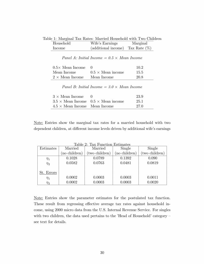
Table 1: Marginal Tax Rates: Married Household with Two ChildrenHousehold Wife�s Earnings MarginalIncome (additional income) Tax Rate (%)
Panel A: Initial Income = 0.5 � Mean Income
0.5� Mean Income 0 10.2Mean Income 0.5 � Mean income 15.52 � Mean Income Mean Income 20.8
Panel B: Initial Income = 3.0 � Mean Income
3 � Mean Income 0 23.93.5 � Mean Income 0.5 � Mean income 25.14.5 � Mean Income Mean Income 27.0
Note: Entries show the marginal tax rates for a married household with two
dependent children, at di¤erent income levels driven by additional wife�s earnings
Table 2: Tax Function EstimatesEstimates Married Married Single Single
(no children) (two children) (no children) (two children)�1 0.1028 0.0789 0.1392 0.090�2 0.0582 0.0763 0.0481 0.0819
St. Errors�1 0.0002 0.0003 0.0003 0.0011�2 0.0002 0.0003 0.0003 0.0020
Note: Entries show the parameter estimates for the postulated tax function.
These result from regressing e¤ective average tax rates against household in-
come, using 2000 micro data from the U.S. Internal Revenue Service. For singles
with two children, the data used pertains to the �Head of Household�category �
see text for details.
30
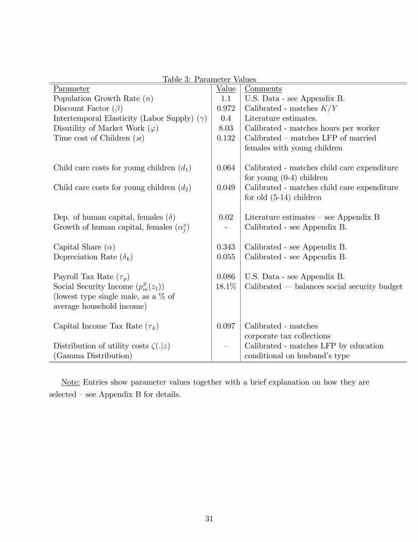
Table 3: Parameter ValuesParameter Value CommentsPopulation Growth Rate (n) 1.1 U.S. Data - see Appendix B.Discount Factor (�) 0.972 Calibrated - matches K=YIntertemporal Elasticity (Labor Supply) ( ) 0.4 Literature estimates.Disutility of Market Work (') 8.03 Calibrated - matches hours per workerTime cost of Children ({) 0.132 Calibrated �matches LFP of married
females with young children
Child care costs for young children (d1) 0.064 Calibrated - matches child care expenditurefor young (0-4) children
Child care costs for young children (d2) 0.049 Calibrated - matches child care expenditurefor old (5-14) children
Dep. of human capital, females (�) 0.02 Literature estimates �see Appendix BGrowth of human capital, females (�xj ) - Calibrated - see Appendix B.
Capital Share (�) 0.343 Calibrated - see Appendix B.Depreciation Rate (�k) 0.055 Calibrated - see Appendix B.
Payroll Tax Rate (� p) 0.086 U.S. Data - see Appendix B.Social Security Income (pSm(z1)) 18.1% Calibrated � balances social security budget(lowest type single male, as a % ofaverage household income)
Capital Income Tax Rate (� k) 0.097 Calibrated - matchescorporate tax collections
Distribution of utility costs �(:jz) � Calibrated - matches LFP by education(Gamma Distribution) conditional on husband�s type
Note: Entries show parameter values together with a brief explanation on how they are
selected �see Appendix B for details.
31
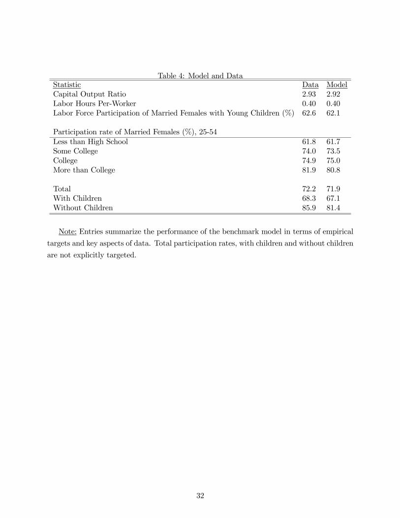
Table 4: Model and DataStatistic Data ModelCapital Output Ratio 2.93 2.92Labor Hours Per-Worker 0.40 0.40Labor Force Participation of Married Females with Young Children (%) 62.6 62.1
Participation rate of Married Females (%), 25-54Less than High School 61.8 61.7Some College 74.0 73.5College 74.9 75.0More than College 81.9 80.8
Total 72.2 71.9With Children 68.3 67.1Without Children 85.9 81.4
Note: Entries summarize the performance of the benchmark model in terms of empirical
targets and key aspects of data. Total participation rates, with children and without children
are not explicitly targeted.
32
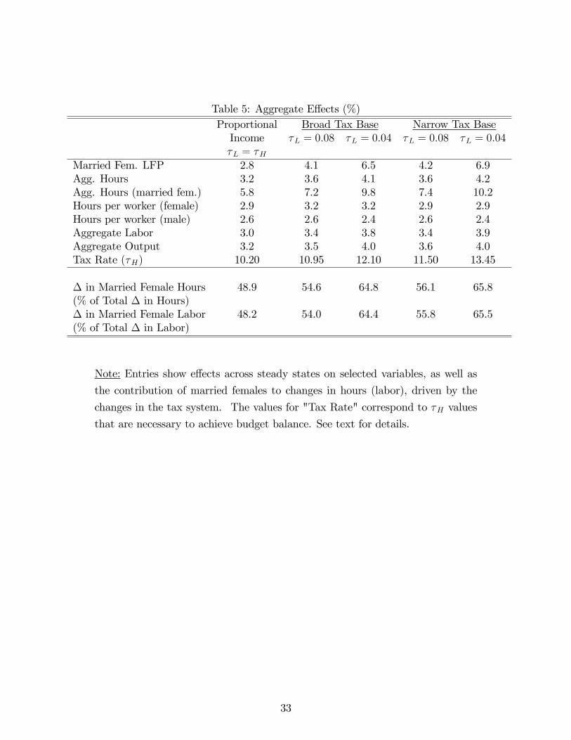
Table 5: Aggregate E¤ects (%)Proportional Broad Tax Base Narrow Tax BaseIncome �L = 0:08 �L = 0:04 �L = 0:08 �L = 0:04�L = �H
Married Fem. LFP 2.8 4.1 6.5 4.2 6.9Agg. Hours 3.2 3.6 4.1 3.6 4.2Agg. Hours (married fem.) 5.8 7.2 9.8 7.4 10.2Hours per worker (female) 2.9 3.2 3.2 2.9 2.9Hours per worker (male) 2.6 2.6 2.4 2.6 2.4Aggregate Labor 3.0 3.4 3.8 3.4 3.9Aggregate Output 3.2 3.5 4.0 3.6 4.0Tax Rate (�H) 10.20 10.95 12.10 11.50 13.45
� in Married Female Hours 48.9 54.6 64.8 56.1 65.8(% of Total � in Hours)� in Married Female Labor 48.2 54.0 64.4 55.8 65.5(% of Total � in Labor)
Note: Entries show e¤ects across steady states on selected variables, as well as
the contribution of married females to changes in hours (labor), driven by the
changes in the tax system. The values for "Tax Rate" correspond to �H values
that are necessary to achieve budget balance. See text for details.
33
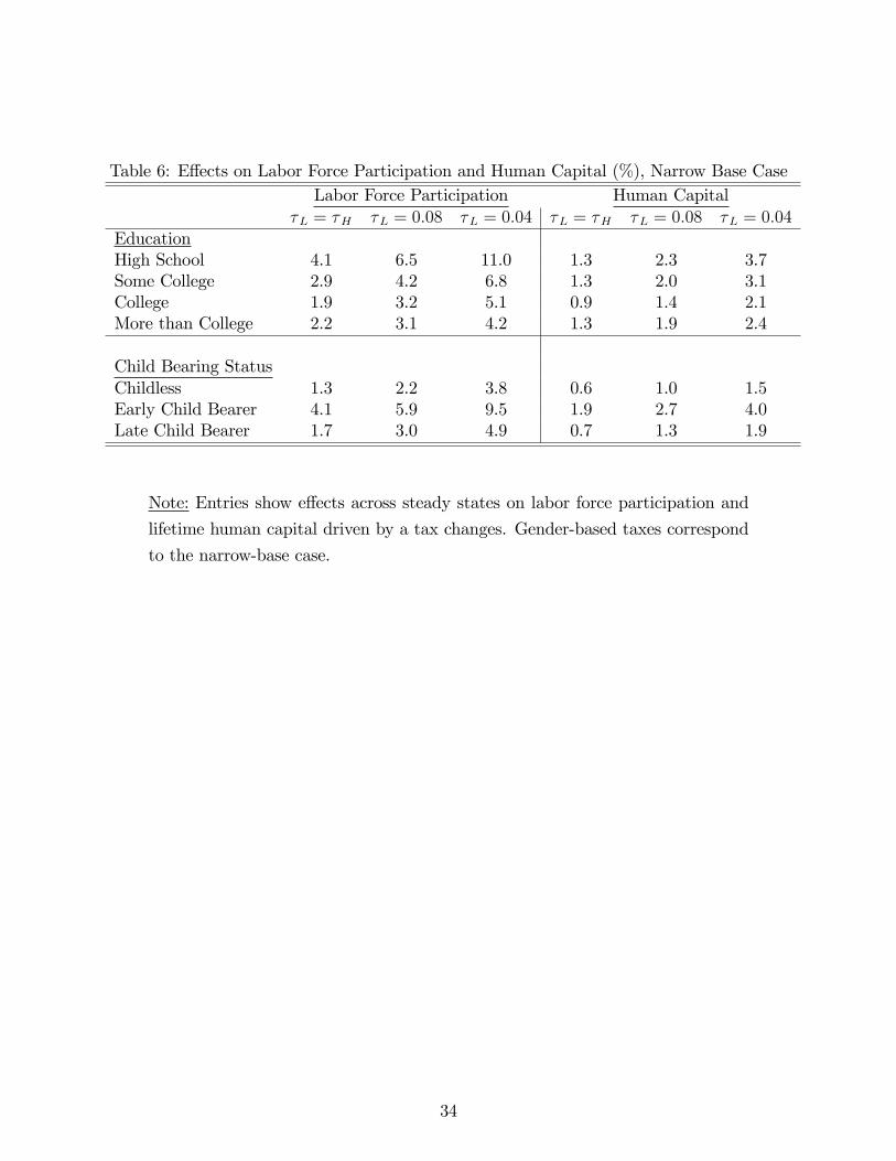
Table 6: E¤ects on Labor Force Participation and Human Capital (%), Narrow Base CaseLabor Force Participation Human Capital
�L = �H �L = 0:08 �L = 0:04 �L = �H �L = 0:08 �L = 0:04EducationHigh School 4.1 6.5 11.0 1.3 2.3 3.7Some College 2.9 4.2 6.8 1.3 2.0 3.1College 1.9 3.2 5.1 0.9 1.4 2.1More than College 2.2 3.1 4.2 1.3 1.9 2.4
Child Bearing StatusChildless 1.3 2.2 3.8 0.6 1.0 1.5Early Child Bearer 4.1 5.9 9.5 1.9 2.7 4.0Late Child Bearer 1.7 3.0 4.9 0.7 1.3 1.9
Note: Entries show e¤ects across steady states on labor force participation and
lifetime human capital driven by a tax changes. Gender-based taxes correspond
to the narrow-base case.
34
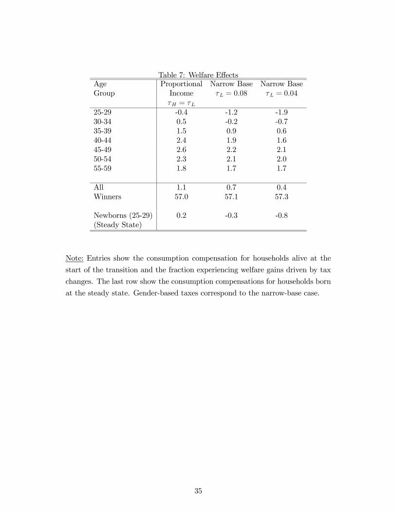
Table 7: Welfare E¤ectsAge Proportional Narrow Base Narrow BaseGroup Income �L = 0:08 �L = 0:04
�H = �L25-29 -0.4 -1.2 -1.930-34 0.5 -0.2 -0.735-39 1.5 0.9 0.640-44 2.4 1.9 1.645-49 2.6 2.2 2.150-54 2.3 2.1 2.055-59 1.8 1.7 1.7
All 1.1 0.7 0.4Winners 57.0 57.1 57.3
Newborns (25-29) 0.2 -0.3 -0.8(Steady State)
Note: Entries show the consumption compensation for households alive at the
start of the transition and the fraction experiencing welfare gains driven by tax
changes. The last row show the consumption compensations for households born
at the steady state. Gender-based taxes correspond to the narrow-base case.
35
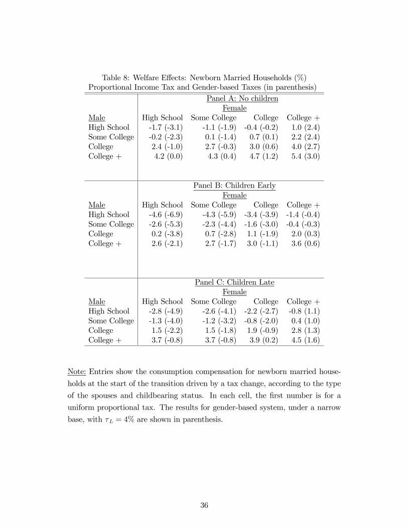
Table 8: Welfare E¤ects: Newborn Married Households (%)Proportional Income Tax and Gender-based Taxes (in parenthesis)
Panel A: No childrenFemale
Male High School Some College College College +High School -1.7 (-3.1) -1.1 (-1.9) -0.4 (-0.2) 1.0 (2.4)Some College -0.2 (-2.3) 0.1 (-1.4) 0.7 (0.1) 2.2 (2.4)College 2.4 (-1.0) 2.7 (-0.3) 3.0 (0.6) 4.0 (2.7)College + 4.2 (0.0) 4.3 (0.4) 4.7 (1.2) 5.4 (3.0)
Panel B: Children EarlyFemale
Male High School Some College College College +High School -4.6 (-6.9) -4.3 (-5.9) -3.4 (-3.9) -1.4 (-0.4)Some College -2.6 (-5.3) -2.3 (-4.4) -1.6 (-3.0) -0.4 (-0.3)College 0.2 (-3.8) 0.7 (-2.8) 1.1 (-1.9) 2.0 (0.3)College + 2.6 (-2.1) 2.7 (-1.7) 3.0 (-1.1) 3.6 (0.6)
Panel C: Children LateFemale
Male High School Some College College College +High School -2.8 (-4.9) -2.6 (-4.1) -2.2 (-2.7) -0.8 (1.1)Some College -1.3 (-4.0) -1.2 (-3.2) -0.8 (-2.0) 0.4 (1.0)College 1.5 (-2.2) 1.5 (-1.8) 1.9 (-0.9) 2.8 (1.3)College + 3.7 (-0.8) 3.7 (-0.8) 3.9 (0.2) 4.5 (1.6)
Note: Entries show the consumption compensation for newborn married house-
holds at the start of the transition driven by a tax change, according to the type
of the spouses and childbearing status. In each cell, the �rst number is for a
uniform proportional tax. The results for gender-based system, under a narrow
base, with �L = 4% are shown in parenthesis.
36
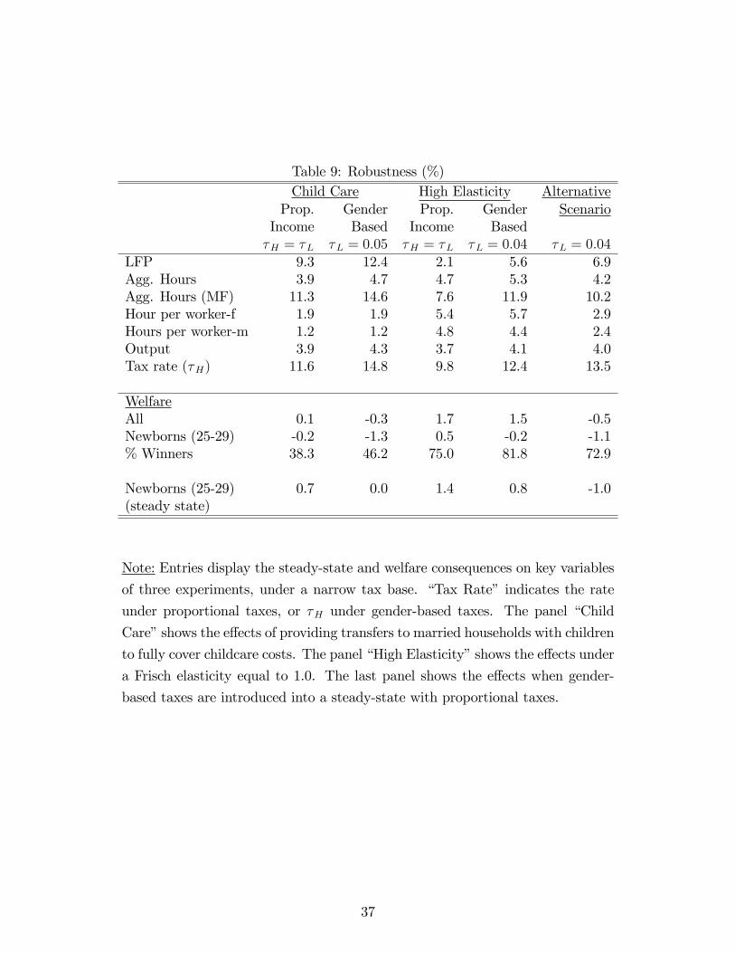
Table 9: Robustness (%)Child Care High Elasticity Alternative
Prop. Gender Prop. Gender ScenarioIncome Based Income Based�H = �L �L = 0:05 �H = �L �L = 0:04 �L = 0:04
LFP 9.3 12.4 2.1 5.6 6.9Agg. Hours 3.9 4.7 4.7 5.3 4.2Agg. Hours (MF) 11.3 14.6 7.6 11.9 10.2Hour per worker-f 1.9 1.9 5.4 5.7 2.9Hours per worker-m 1.2 1.2 4.8 4.4 2.4Output 3.9 4.3 3.7 4.1 4.0Tax rate (�H) 11.6 14.8 9.8 12.4 13.5
WelfareAll 0.1 -0.3 1.7 1.5 -0.5Newborns (25-29) -0.2 -1.3 0.5 -0.2 -1.1% Winners 38.3 46.2 75.0 81.8 72.9
Newborns (25-29) 0.7 0.0 1.4 0.8 -1.0(steady state)
Note: Entries display the steady-state and welfare consequences on key variables
of three experiments, under a narrow tax base. �Tax Rate� indicates the rate
under proportional taxes, or �H under gender-based taxes. The panel �Child
Care�shows the e¤ects of providing transfers to married households with children
to fully cover childcare costs. The panel �High Elasticity�shows the e¤ects under
a Frisch elasticity equal to 1.0. The last panel shows the e¤ects when gender-
based taxes are introduced into a steady-state with proportional taxes.
37
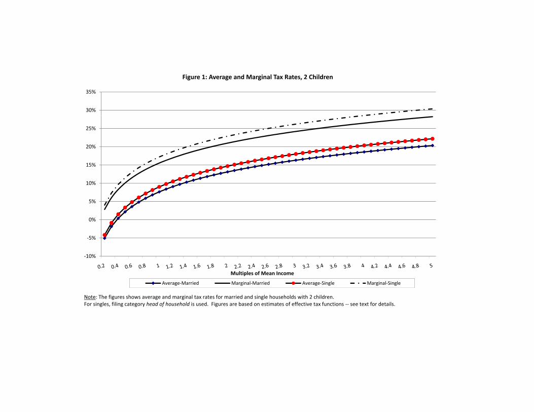
30%
35%
Figure 1: Average and Marginal Tax Rates, 2 Children
15%
20%
25%
5%
10%
15%
‐10%
‐5%
0%
Multiples of Mean Income
Average‐Married Marginal‐Married Average‐Single Marginal‐Single
Note: The figures shows average and marginal tax rates for married and single households with 2 children. For singles, filing category head of household is used. Figures are based on estimates of effective tax functions ‐‐ see text for details.
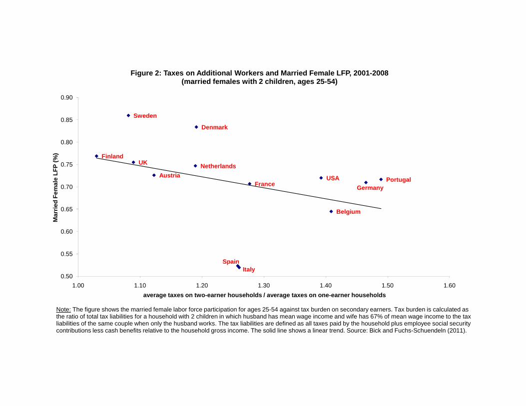
Austria
Belgium
Denmark
Finland
France Germany
Netherlands
Portugal
Sweden
UK
USA
0 55
0.60
0.65
0.70
0.75
0.80
0.85
0.90
Mar
ried
Fem
ale
LFP
(%)
Figure 2: Taxes on Additional Workers and Married Female LFP, 2001-2008(married females with 2 children, ages 25-54)
SpainItaly
0.50
0.55
1.00 1.10 1.20 1.30 1.40 1.50 1.60average taxes on two-earner households / average taxes on one-earner households
Note: The figure shows the married female labor force participation for ages 25-54 against tax burden on secondary earners. Tax burden is calculated as the ratio of total tax liabilities for a household with 2 children in which husband has mean wage income and wife has 67% of mean wage income to the tax liabilities of the same couple when only the husband works. The tax liabilities are defined as all taxes paid by the household plus employee social security contributions less cash benefits relative to the household gross income. The solid line shows a linear trend. Source: Bick and Fuchs-Schuendeln (2011).
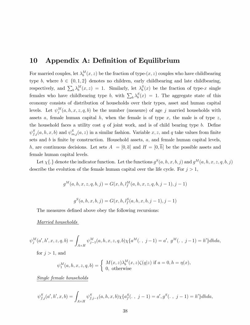
10 Appendix A: De�nition of Equilibrium
For married couples, let �Mb (x; z) be the fraction of type-(x; z) couples who have childbearing
type b; where b 2 f0; 1; 2g denotes no children, early childbearing and late childbearing,respectively, and
Pb �
Mb (x; z) = 1. Similarly, let �Sb (x) be the fraction of type-x single
females who have childbearing type b; withP
b �Sb (x) = 1: The aggregate state of this
economy consists of distribution of households over their types, asset and human capital
levels. Let Mj (a; h; x; z; q; b) be the number (measure) of age j married households with
assets a, female human capital h, when the female is of type x, the male is of type z,
the household faces a utility cost q of joint work, and is of child bearing type b. De�ne
Sf;j(a; h; x; b) and Sm;j(a; z) in a similar fashion. Variable x; z; and q take values from �nite
sets and b is �nite by construction. Household assets, a; and female human capital levels,
h; are continuous decisions. Let sets A = [0; a] and H = [0; h] be the possible assets and
female human capital levels.
Let �f:g denote the indicator function. Let the functions gS(a; h; x; b; j) and gM(a; h; x; z; q; b; j)describe the evolution of the female human capital over the life cycle. For j > 1,
gM(a; h; x; z; q; b; j) = G(x; h; lMf (a; h; x; z; q; b; j � 1); j � 1)
gS(a; h; x; b; j) = G(x; h; lSf (a; h; x; b; j � 1); j � 1)
The measures de�ned above obey the following recursions:
Married households
Mj (a0; h0; x; z; q; b) =
ZA�H
Mj�1(a; h; x; z; q; b)�faM(: ; j�1) = a0; gM(: ; j�1) = h0gdhda;
for j > 1; and
M1 (a; h; x; z; q; b) =
�M(x; z)�Mb (x; z)�(qjz) if a = 0; h = �(x),0; otherwise
Single female households
Sf;j(a0; h0; x; b) =
ZA�H
Sf;j�1(a; h; x; b)�faSf (: ; j � 1) = a0; gS(: ; j � 1) = h0gdhda;
38
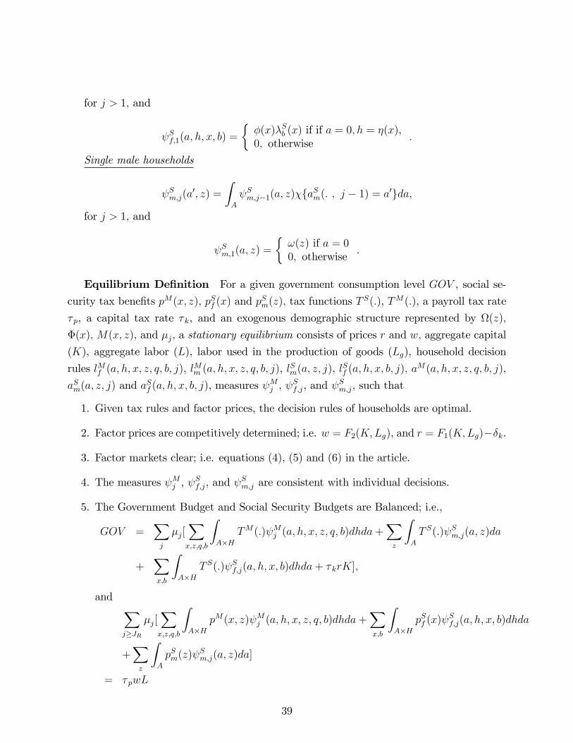
for j > 1; and
Sf;1(a; h; x; b) =
��(x)�Sb (x) if if a = 0; h = �(x),0; otherwise
:
Single male households
Sm;j(a0; z) =
ZA
Sm;j�1(a; z)�faSm(: ; j � 1) = a0gda;
for j > 1; and
Sm;1(a; z) =
�!(z) if a = 00; otherwise
:
Equilibrium De�nition For a given government consumption level GOV , social se-
curity tax bene�ts pM(x; z), pSf (x) and pSm(z); tax functions T
S(:), TM(:), a payroll tax rate
� p, a capital tax rate � k, and an exogenous demographic structure represented by (z);
�(x); M(x; z), and �j; a stationary equilibrium consists of prices r and w; aggregate capital
(K), aggregate labor (L), labor used in the production of goods (Lg), household decision
rules lMf (a; h; x; z; q; b; j), lMm (a; h; x; z; q; b; j), l
Sm(a; z; j), l
Sf (a; h; x; b; j); a
M(a; h; x; z; q; b; j),
aSm(a; z; j) and aSf (a; h; x; b; j), measures
Mj ,
Sf;j, and
Sm;j; such that
1. Given tax rules and factor prices, the decision rules of households are optimal.
2. Factor prices are competitively determined; i.e. w = F2(K;Lg), and r = F1(K;Lg)��k.
3. Factor markets clear; i.e. equations (4), (5) and (6) in the article.
4. The measures Mj , Sf;j, and
Sm;j are consistent with individual decisions.
5. The Government Budget and Social Security Budgets are Balanced; i.e.,
GOV =Xj
�j[Xx;z;q;b
ZA�H
TM(:) Mj (a; h; x; z; q; b)dhda+Xz
ZA
T S(:) Sm;j(a; z)da
+Xx;b
ZA�H
T S(:) Sf;j(a; h; x; b)dhda+ � krK];
and Xj�JR
�j[Xx;z;q;b
ZA�H
pM(x; z) Mj (a; h; x; z; q; b)dhda+Xx;b
ZA�H
pSf (x) Sf;j(a; h; x; b)dhda
+Xz
ZA
pSm(z) Sm;j(a; z)da]
= � pwL
39
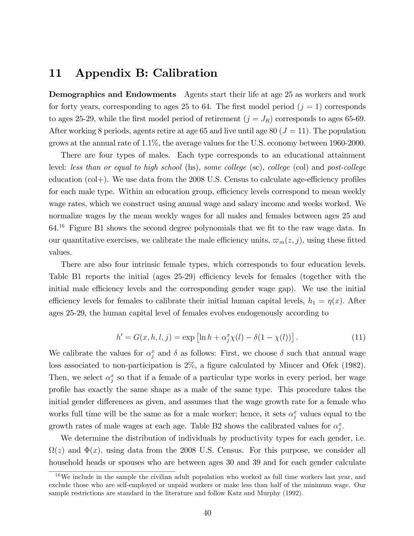
11 Appendix B: Calibration
Demographics and Endowments Agents start their life at age 25 as workers and work
for forty years, corresponding to ages 25 to 64. The �rst model period (j = 1) corresponds
to ages 25-29, while the �rst model period of retirement (j = JR) corresponds to ages 65-69.
After working 8 periods, agents retire at age 65 and live until age 80 (J = 11): The population
grows at the annual rate of 1.1%, the average values for the U.S. economy between 1960-2000.
There are four types of males. Each type corresponds to an educational attainment
level: less than or equal to high school (hs), some college (sc), college (col) and post-college
education (col+). We use data from the 2008 U.S. Census to calculate age-e¢ ciency pro�les
for each male type. Within an education group, e¢ ciency levels correspond to mean weekly
wage rates, which we construct using annual wage and salary income and weeks worked. We
normalize wages by the mean weekly wages for all males and females between ages 25 and
64.16 Figure B1 shows the second degree polynomials that we �t to the raw wage data. In
our quantitative exercises, we calibrate the male e¢ ciency units, $m(z; j); using these �tted
values.
There are also four intrinsic female types, which corresponds to four education levels.
Table B1 reports the initial (ages 25-29) e¢ ciency levels for females (together with the
initial male e¢ ciency levels and the corresponding gender wage gap). We use the initial
e¢ ciency levels for females to calibrate their initial human capital levels, h1 = �(x): After
ages 25-29, the human capital level of females evolves endogenously according to
h0 = G(x; h; l; j) = exp�lnh+ �xj�(l)� �(1� �(l))
�: (11)
We calibrate the values for �xj and � as follows: First, we choose � such that annual wage
loss associated to non-participation is 2%, a �gure calculated by Mincer and Ofek (1982).
Then, we select �xj so that if a female of a particular type works in every period, her wage
pro�le has exactly the same shape as a male of the same type. This procedure takes the
initial gender di¤erences as given, and assumes that the wage growth rate for a female who
works full time will be the same as for a male worker; hence, it sets �xj values equal to the
growth rates of male wages at each age. Table B2 shows the calibrated values for �xj :
We determine the distribution of individuals by productivity types for each gender, i.e.
(z) and �(x); using data from the 2008 U.S. Census. For this purpose, we consider all
household heads or spouses who are between ages 30 and 39 and for each gender calculate
16We include in the sample the civilian adult population who worked as full time workers last year, andexclude those who are self-employed or unpaid workers or make less than half of the minimum wage. Oursample restrictions are standard in the literature and follow Katz and Murphy (1992).
40
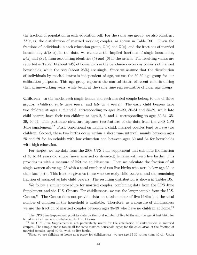
the fraction of population in each education cell. For the same age group, we also construct
M(x; z); the distribution of married working couples, as shown in Table B3. Given the
fractions of individuals in each education group, �(x) and (z), and the fractions of married
households, M(x; z); in the data, we calculate the implied fractions of single households,
!(z) and �(x), from accounting identities (5) and (6) in the article. The resulting values are
reported in Table B4 about 74% of households in the benchmark economy consists of married
households, while the rest (about 26%) are single. Since we assume that the distribution
of individuals by marital status is independent of age, we use the 30-39 age group for our
calibration purposes. This age group captures the marital status of recent cohorts during
their prime-working years, while being at the same time representative of older age groups.
Children In the model each single female and each married couple belong to one of three
groups: childless, early child bearer and late child bearer. The early child bearers have
two children at ages 1, 2 and 3, corresponding to ages 25-29, 30-34 and 35-39, while late
child bearers have their two children at ages 2, 3, and 4, corresponding to ages 30-34, 35-
39, 40-44. This particular structure captures two features of the data from the 2008 CPS
June supplement.17 First, conditional on having a child, married couples tend to have two
children. Second, these two births occur within a short time interval, mainly between ages
25 and 29 for households with low education and between ages 30 and 34 for households
with high education.
For singles, we use data from the 2008 CPS June supplement and calculate the fraction
of 40 to 44 years old single (never married or divorced) females with zero live births. This
provides us with a measure of lifetime childlessness. Then we calculate the fraction of all
single women above age 25 with a total number of two live births who were below age 30 at
their last birth. This fraction gives us those who are early child bearers, and the remaining
fraction of assigned as late child bearers. The resulting distribution is shown in Tables B5.
We follow a similar procedure for married couples, combining data from the CPS June
Supplement and the U.S. Census. For childlessness, we use the larger sample from the U.S.
Census.18 The Census does not provide data on total number of live births but the total
number of children in the household is available. Therefore, as a measure of childlessness
we use the fraction of married couples between ages 35-39 who have no children at home.19
17The CPS June Supplement provides data on the total number of live births and the age at last birth forfemales, which are not available in the U.S. Census.18The CPS June Supplement is not particularly useful for the calculation of childlessness in married
couples. The sample size is too small for some married household types for the calculation of the fraction ofmarried females, aged 40-44, with no live births.19Since we use children at home as a proxy for childlessness, we use age 35-39 rather than 40-44. Using
41
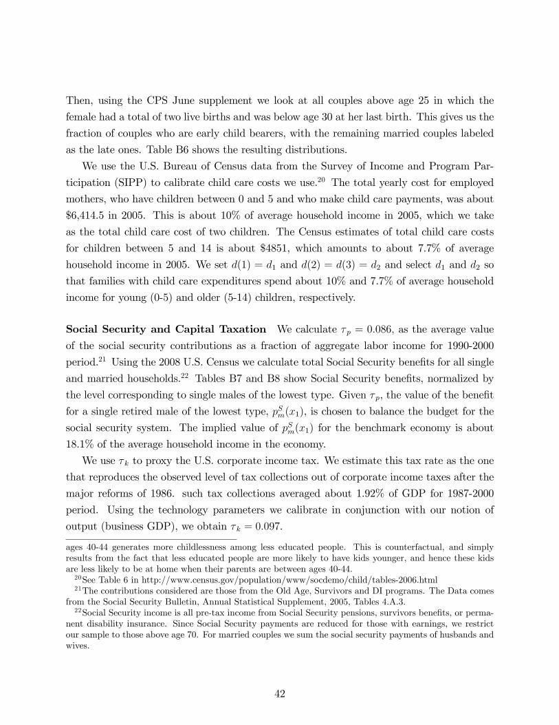
Then, using the CPS June supplement we look at all couples above age 25 in which the
female had a total of two live births and was below age 30 at her last birth. This gives us the
fraction of couples who are early child bearers, with the remaining married couples labeled
as the late ones. Table B6 shows the resulting distributions.
We use the U.S. Bureau of Census data from the Survey of Income and Program Par-
ticipation (SIPP) to calibrate child care costs we use.20 The total yearly cost for employed
mothers, who have children between 0 and 5 and who make child care payments, was about
$6,414.5 in 2005. This is about 10% of average household income in 2005, which we take
as the total child care cost of two children. The Census estimates of total child care costs
for children between 5 and 14 is about $4851, which amounts to about 7.7% of average
household income in 2005. We set d(1) = d1 and d(2) = d(3) = d2 and select d1 and d2 so
that families with child care expenditures spend about 10% and 7.7% of average household
income for young (0-5) and older (5-14) children, respectively.
Social Security and Capital Taxation We calculate � p = 0:086; as the average value
of the social security contributions as a fraction of aggregate labor income for 1990-2000
period.21 Using the 2008 U.S. Census we calculate total Social Security bene�ts for all single
and married households.22 Tables B7 and B8 show Social Security bene�ts, normalized by
the level corresponding to single males of the lowest type. Given � p, the value of the bene�t
for a single retired male of the lowest type, pSm(x1), is chosen to balance the budget for the
social security system. The implied value of pSm(x1) for the benchmark economy is about
18.1% of the average household income in the economy.
We use � k to proxy the U.S. corporate income tax. We estimate this tax rate as the one
that reproduces the observed level of tax collections out of corporate income taxes after the
major reforms of 1986. such tax collections averaged about 1.92% of GDP for 1987-2000
period. Using the technology parameters we calibrate in conjunction with our notion of
output (business GDP), we obtain � k = 0:097.
ages 40-44 generates more childlessness among less educated people. This is counterfactual, and simplyresults from the fact that less educated people are more likely to have kids younger, and hence these kidsare less likely to be at home when their parents are between ages 40-44.20See Table 6 in http://www.census.gov/population/www/socdemo/child/tables-2006.html21The contributions considered are those from the Old Age, Survivors and DI programs. The Data comes
from the Social Security Bulletin, Annual Statistical Supplement, 2005, Tables 4.A.3.22Social Security income is all pre-tax income from Social Security pensions, survivors bene�ts, or perma-
nent disability insurance. Since Social Security payments are reduced for those with earnings, we restrictour sample to those above age 70. For married couples we sum the social security payments of husbands andwives.
42
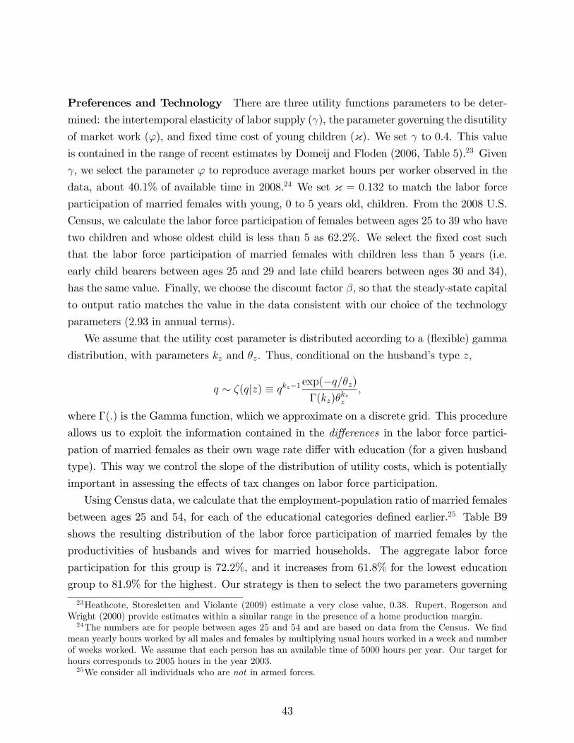
Preferences and Technology There are three utility functions parameters to be deter-
mined: the intertemporal elasticity of labor supply ( ), the parameter governing the disutility
of market work ('), and �xed time cost of young children ({). We set to 0.4. This valueis contained in the range of recent estimates by Domeij and Floden (2006, Table 5).23 Given
, we select the parameter ' to reproduce average market hours per worker observed in the
data, about 40.1% of available time in 2008.24 We set { = 0:132 to match the labor forceparticipation of married females with young, 0 to 5 years old, children. From the 2008 U.S.
Census, we calculate the labor force participation of females between ages 25 to 39 who have
two children and whose oldest child is less than 5 as 62.2%. We select the �xed cost such
that the labor force participation of married females with children less than 5 years (i.e.
early child bearers between ages 25 and 29 and late child bearers between ages 30 and 34),
has the same value. Finally, we choose the discount factor �, so that the steady-state capital
to output ratio matches the value in the data consistent with our choice of the technology
parameters (2.93 in annual terms).
We assume that the utility cost parameter is distributed according to a (�exible) gamma
distribution, with parameters kz and �z. Thus, conditional on the husband�s type z,
q � �(qjz) � qkz�1exp(�q=�z)�(kz)�
kzz
;
where �(:) is the Gamma function, which we approximate on a discrete grid. This procedure
allows us to exploit the information contained in the di¤erences in the labor force partici-
pation of married females as their own wage rate di¤er with education (for a given husband
type). This way we control the slope of the distribution of utility costs, which is potentially
important in assessing the e¤ects of tax changes on labor force participation.
Using Census data, we calculate that the employment-population ratio of married females
between ages 25 and 54, for each of the educational categories de�ned earlier.25 Table B9
shows the resulting distribution of the labor force participation of married females by the
productivities of husbands and wives for married households. The aggregate labor force
participation for this group is 72.2%, and it increases from 61.8% for the lowest education
group to 81.9% for the highest. Our strategy is then to select the two parameters governing
23Heathcote, Storesletten and Violante (2009) estimate a very close value, 0.38. Rupert, Rogerson andWright (2000) provide estimates within a similar range in the presence of a home production margin.24The numbers are for people between ages 25 and 54 and are based on data from the Census. We �nd
mean yearly hours worked by all males and females by multiplying usual hours worked in a week and numberof weeks worked. We assume that each person has an available time of 5000 hours per year. Our target forhours corresponds to 2005 hours in the year 2003.25We consider all individuals who are not in armed forces.
43
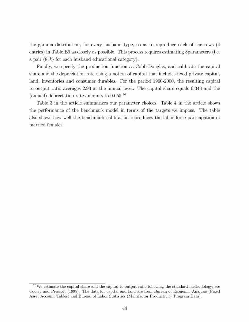
the gamma distribution, for every husband type, so as to reproduce each of the rows (4
entries) in Table B9 as closely as possible. This process requires estimating 8parameters (i.e.
a pair (�; k) for each husband educational category).
Finally, we specify the production function as Cobb-Douglas, and calibrate the capital
share and the depreciation rate using a notion of capital that includes �xed private capital,
land, inventories and consumer durables. For the period 1960-2000, the resulting capital
to output ratio averages 2.93 at the annual level. The capital share equals 0.343 and the
(annual) depreciation rate amounts to 0.055.26
Table 3 in the article summarizes our parameter choices. Table 4 in the article shows
the performance of the benchmark model in terms of the targets we impose. The table
also shows how well the benchmark calibration reproduces the labor force participation of
married females.
26We estimate the capital share and the capital to output ratio following the standard methodology; seeCooley and Prescott (1995). The data for capital and land are from Bureau of Economic Analysis (FixedAsset Account Tables) and Bureau of Labor Statistics (Multifactor Productivity Program Data).
44
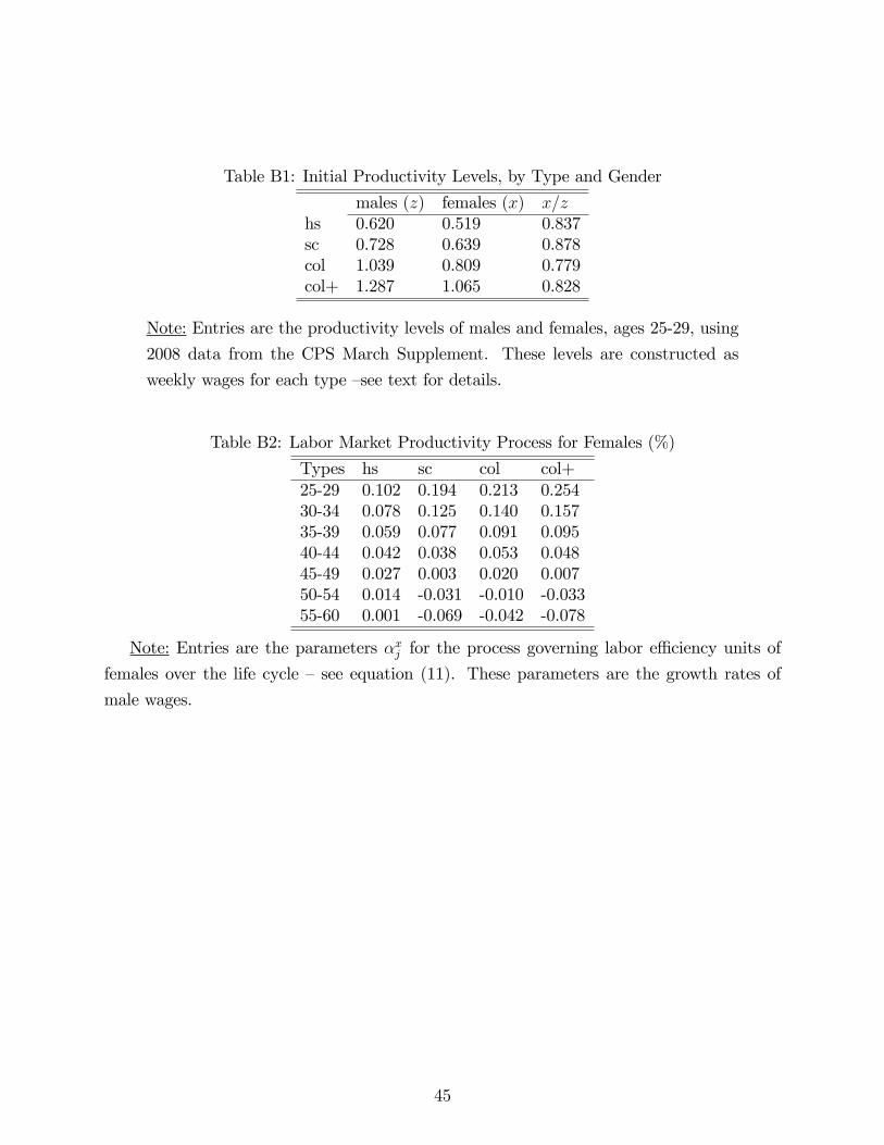
Table B1: Initial Productivity Levels, by Type and Gender
males (z) females (x) x=zhs 0.620 0.519 0.837sc 0.728 0.639 0.878col 1.039 0.809 0.779col+ 1.287 1.065 0.828
Note: Entries are the productivity levels of males and females, ages 25-29, using
2008 data from the CPS March Supplement. These levels are constructed as
weekly wages for each type �see text for details.
Table B2: Labor Market Productivity Process for Females (%)
Types hs sc col col+25-29 0.102 0.194 0.213 0.25430-34 0.078 0.125 0.140 0.15735-39 0.059 0.077 0.091 0.09540-44 0.042 0.038 0.053 0.04845-49 0.027 0.003 0.020 0.00750-54 0.014 -0.031 -0.010 -0.03355-60 0.001 -0.069 -0.042 -0.078
Note: Entries are the parameters �xj for the process governing labor e¢ ciency units of
females over the life cycle �see equation (11). These parameters are the growth rates of
male wages.
45
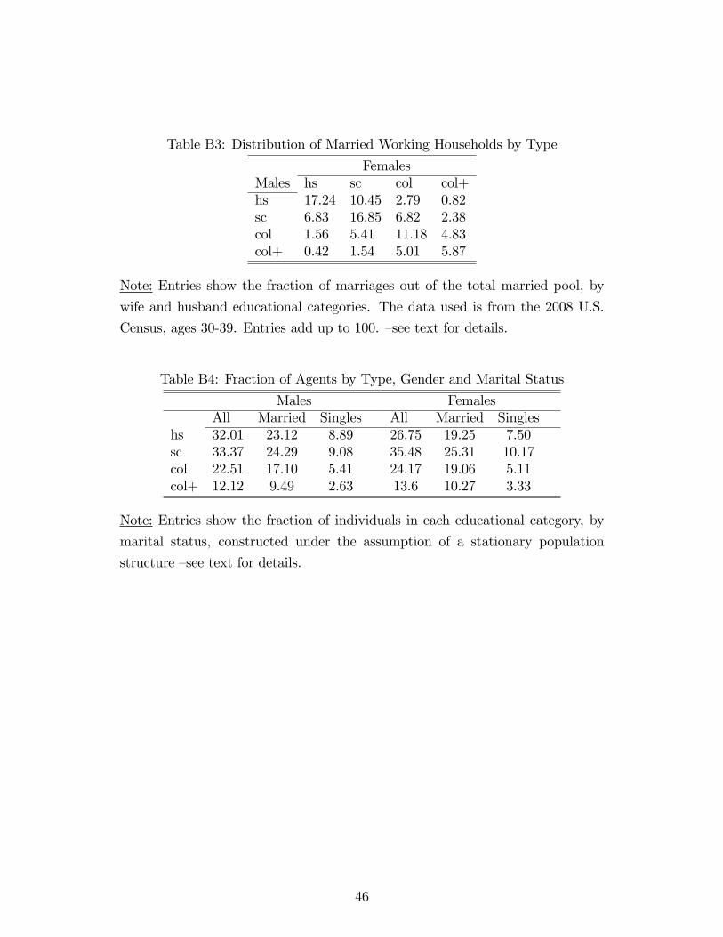
Table B3: Distribution of Married Working Households by Type
FemalesMales hs sc col col+hs 17.24 10.45 2.79 0.82sc 6.83 16.85 6.82 2.38col 1.56 5.41 11.18 4.83col+ 0.42 1.54 5.01 5.87
Note: Entries show the fraction of marriages out of the total married pool, by
wife and husband educational categories. The data used is from the 2008 U.S.
Census, ages 30-39. Entries add up to 100. �see text for details.
Table B4: Fraction of Agents by Type, Gender and Marital Status
Males FemalesAll Married Singles All Married Singles
hs 32.01 23.12 8.89 26.75 19.25 7.50sc 33.37 24.29 9.08 35.48 25.31 10.17col 22.51 17.10 5.41 24.17 19.06 5.11col+ 12.12 9.49 2.63 13.6 10.27 3.33
Note: Entries show the fraction of individuals in each educational category, by
marital status, constructed under the assumption of a stationary population
structure �see text for details.
46
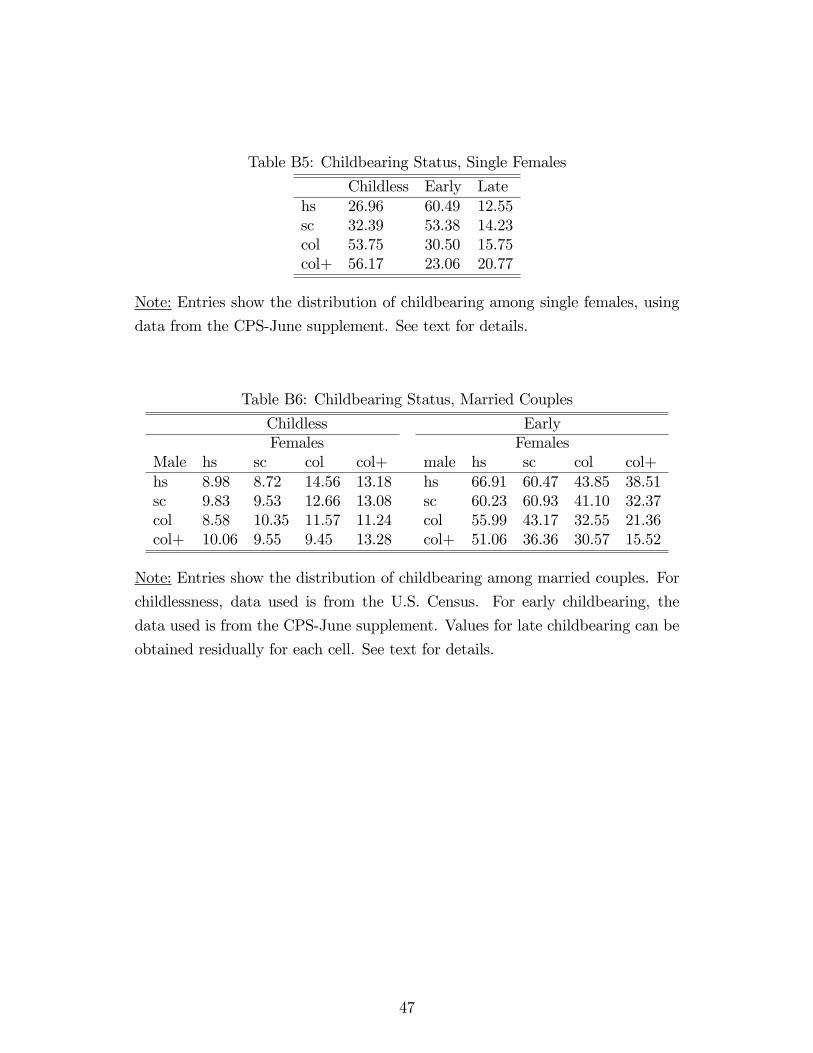
Table B5: Childbearing Status, Single Females
Childless Early Latehs 26.96 60.49 12.55sc 32.39 53.38 14.23col 53.75 30.50 15.75col+ 56.17 23.06 20.77
Note: Entries show the distribution of childbearing among single females, using
data from the CPS-June supplement. See text for details.
Table B6: Childbearing Status, Married Couples
Childless EarlyFemales Females
Male hs sc col col+ male hs sc col col+hs 8.98 8.72 14.56 13.18 hs 66.91 60.47 43.85 38.51sc 9.83 9.53 12.66 13.08 sc 60.23 60.93 41.10 32.37col 8.58 10.35 11.57 11.24 col 55.99 43.17 32.55 21.36col+ 10.06 9.55 9.45 13.28 col+ 51.06 36.36 30.57 15.52
Note: Entries show the distribution of childbearing among married couples. For
childlessness, data used is from the U.S. Census. For early childbearing, the
data used is from the CPS-June supplement. Values for late childbearing can be
obtained residually for each cell. See text for details.
47
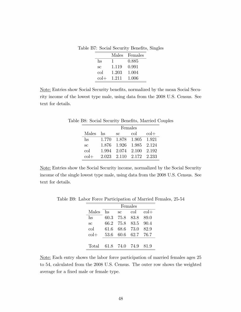
Table B7: Social Security Bene�ts, Singles
Males Femaleshs 1 0.885sc 1.119 0.991col 1.203 1.004col+ 1.211 1.006
Note: Entries show Social Security bene�ts, normalized by the mean Social Secu-
rity income of the lowest type male, using data from the 2008 U.S. Census. See
text for details.
Table B8: Social Security Bene�ts, Married Couples
FemalesMales hs sc col col+hs 1.770 1.878 1.905 1.921sc 1.876 1.926 1.985 2.124col 1.994 2.074 2.100 2.192col+ 2.023 2.110 2.172 2.233
Note: Entries show the Social Security income, normalized by the Social Security
income of the single lowest type male, using data from the 2008 U.S. Census. See
text for details.
Table B9: Labor Force Participation of Married Females, 25-54
FemalesMales hs sc col col+hs 60.3 75.8 83.8 89.0sc 66.2 75.8 83.5 90.4col 61.6 68.6 73.0 82.9col+ 53.6 60.6 62.7 76.7
Total 61.8 74.0 74.9 81.9
Note: Each entry shows the labor force participation of married females ages 25
to 54, calculated from the 2008 U.S. Census. The outer row shows the weighted
average for a �xed male or female type.
48
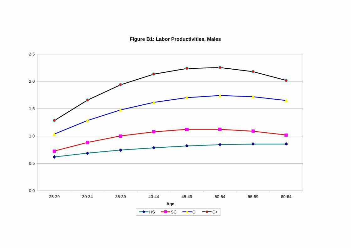
Figure B1: Labor Productivities, Males
0,0
0,5
1,0
1,5
2,0
2,5
25-29 30-34 35-39 40-44 45-49 50-54 55-59 60-64
Age
HS SC C C+


