iii

Acknowledgement

Acknowledgements are due to King Fahd University of Petroleum and Minerals for

support of this research.

I would like to express my profound gratitude and appreciation to my thesis chairman, Dr.

Khaled Al-Ramadan for his guidance and for his critical review of the manuscript. Sincere thanks

are also due to my thesis committee members, Dr. Ahmad Yasin and Dr. Gabor Korvin, for their

excellent advice and comments during this time and for their contribution to this work.

Appreciation and thanks are due to Chairman Dr. Abdulaziz Al-Shaibani and other faculty

and colleagues of Earth Sciences Department for their support during my study.

I would like to thank the management of Saudi Aramco for providing the facilities used in

this study. Of these I‟m grateful to Mr. Abdulaziz Al-Gaoud, Berri, AFK, and Shaybah Team

Leader for his support throughout the duration of the study. My thanks principally go to my

mentor Dr. Ahmad Yasin for providing the template for the work conducted and guidance through

the theory and extensive literature reviews. A special thank-you goes to Dr. Aus Al-Tawil-

Reservoir Characterization Manager- for his constant support and understanding of part-time

graduate students.

Finally, my sincere thanks are extended to my family and friends for their support and

encouragement during the period of this study.

iv

Table of Contents

Approval Page ................................................................................................................................... ii

Acknowledgement ........................................................................................................................... iii

Table of Contents ..............................................................................................................................iv

List Of Figures ................................................................................................................................... x

List Of Tables ..............................................................................................................................xxxiv

Thesis Abstract ............................................................................................................................xxxvi

الرسالة ملخص ................................................................................................................................. xxxviii

Chapter 1 ............................................................................................................................................ 1

Introduction ........................................................................................................................................ 1

Saturation Height Modeling ........................................................................................................ 6

Establish Geological Framework ......................................................................................... 6

Determine Reservoir-Wide Fluid Interfaces ........................................................................ 7

Model Permeability in Non-Cored Wells ............................................................................ 8

Determine Rock-Fluid Properties ........................................................................................ 9

Determine Fluid Properties .................................................................................................. 9

Define Reservoir Quality Groups ...................................................................................... 10

Correct and Convert Capillary Pressure Data to Reservoir Conditions ............................. 10

Normalize Capillary Pressure Curves using J-Function Approach .......................................... 11

v

Calculate J-Function from Log Porosity, Permeability and Capillary Pressure ....................... 11

Fit J Curves to Rock Quality Groups ........................................................................................ 12

Calculate Water Saturation Profiles from J Curves .................................................................. 12

Chapter 2 .......................................................................................................................................... 13

Theory of Saturation Height Modelling ........................................................................................... 13

Introduction ............................................................................................................................... 13

Capillary Pressure ..................................................................................................................... 14

Surface Tension (ST) and Interfacial Tension (IFT) ................................................................ 17

Wettability ................................................................................................................................. 17

Capillary Pressure Expression .................................................................................................. 19

Capillary Pressure in Reservoir Rocks ..................................................................................... 22

Saturation History and Capillary Pressure ................................................................................ 25

Definition of Fluid Contacts ..................................................................................................... 31

Free Water Level (FWL) ................................................................................................... 33

Initial Oil Water Contact (IOWC) ..................................................................................... 33

Producing Oil Water Contact (POWC) ............................................................................. 34

Economic Oil Water Contact (EOWC).............................................................................. 34

Completion or Dry Oil Water Contact (COWC) ............................................................... 34

Initial Oil Water Transition Zone ...................................................................................... 34

Producing Oil Water Transition Zone ............................................................................... 34

Connate Water Saturation (Swc) ......................................................................................... 35

vi

Irreducible Water Saturation (Swirr) ................................................................................... 35

Free Oil Level (FOL) ......................................................................................................... 35

Gas Oil Contact (GOC) ...................................................................................................... 35

Gas Oil Transition Zone .................................................................................................... 35

Fluid Contacts in Water- and Oil-Wet Reservoirs .................................................................... 36

Capillary Pressure Conversion to Reservoir Conditions .......................................................... 38

Conversion of Reservoir Capillary Pressure to Height above Free Water Level ..................... 40

Pore Radius Computation from Capillary Pressure .................................................................. 41

Curve Fitting Functions of Capillary Pressure Data ................................................................. 42

Simple Non-Linear Function ............................................................................................. 43

Logarithmic Function ........................................................................................................ 43

Simple Exponential Function ............................................................................................. 44

Advanced Exponential Function ........................................................................................ 45

Hyperbolic Function .......................................................................................................... 46

Lambda Function ............................................................................................................... 47

Thomeer Function .............................................................................................................. 48

Averaging and Normalising Capillary Pressure Data ............................................................... 49

Averaging by Thomeer Method ......................................................................................... 50

Averaging by Heseldin Method ......................................................................................... 52

Data Interpolation Method ................................................................................................. 54

Leverett‟s J Function Method ............................................................................................ 55

vii

Skelt-Harrison Method ...................................................................................................... 60

Equivalent Radius Function Normalising Method ............................................................ 61

Well Log Derived Capillary Pressure Curves ........................................................................... 62

Cuddy Method of Saturation Height Modeling based on Log Saturations ........................ 63

Saturation Height Function and Model ..................................................................................... 64

Saturation Height Model Classifications ........................................................................... 66

Saturation Height Modeling Process ................................................................................. 69

Estimation of Down-Dip Free Water Level from Capillary Pressure Curves .......................... 72

Saturation Height Modeling Advantages .................................................................................. 74

Chapter 3 .......................................................................................................................................... 76

Petrophysics of Carbonate Reservoirs ............................................................................................. 76

Petrophysical Model of Rocks .................................................................................................. 76

Matrix and Fabric of Carbonate Rocks ..................................................................................... 81

Volume of Shale ....................................................................................................................... 92

Porosity ..................................................................................................................................... 95

Porosity Measued on Core ................................................................................................. 96

Porosity Assessed from Single Logs ................................................................................. 97

Porosity Assessed from Density and Neutron Cross-Plot ............................................... 101

Porosity Assessed from Three or More Logs .................................................................. 103

Secondary and Vug Porosity in Carbonates .................................................................... 105

Water Saturation ..................................................................................................................... 108

viii

Determination of Formation Water Resistivity (RW) ....................................................... 112

Picking Hydrocarbon Water Interfaces ............................................................................ 114

Chapter 4 ........................................................................................................................................ 115

Permeability and Petrophysical Rock Types ................................................................................. 115

Darcy‟s Law and Permeability ................................................................................................ 115

Linear Form of Darcy‟s Law ........................................................................................... 118

Radial Form of Darcy‟s Law ........................................................................................... 119

Permeability Equations ........................................................................................................... 120

Petrophysical Rock Types ....................................................................................................... 125

Hydraulic Flow Unit Rock Types ........................................................................................... 127

Winland (and Pittman) Rock Types ........................................................................................ 131

Lucia Rock Types ................................................................................................................... 134

Thomeer Rock Types .............................................................................................................. 135

Prediction of Hydraulic Flow Unit Rock Types in Uncored Wells ........................................ 139

Chapter 5 ........................................................................................................................................ 141

Application of Hydraulic Flow Unit Rock Typing and Saturation-Height Modelling ................. 141

Reservoir Description ............................................................................................................. 141

Hydraulic Flow Unit Identification ......................................................................................... 158

Hydraulic Flow Unit and Permeability Prediction in Un-Cored Wells or Intervals ............... 161

Capillary Pressure Datums of Free Water and Oil Levels ...................................................... 168

Gas, Oil and Water Properties ................................................................................................ 169

ix

Normalizing Capillary Pressure Curves by the J-Function Method ....................................... 169

Computation of Water Saturation ........................................................................................... 173

Conclusion .............................................................................................................................. 178

Appendix A .................................................................................................................................... 181

Measurement and Processing of Capillary Pressure Data ............................................................. 181

Sample Selection and Testing Conditions .............................................................................. 182

Pressure Equilibrium Method ................................................................................................. 183

Mercury Injection Method ...................................................................................................... 184

Mercury Injection Capillary Pressure Basic Data ............................................................ 185

Mercury Injection Data Plots ........................................................................................... 191

Capillary Pressure (CP) Data Corrections ....................................................................... 193

Centrifuge Method .................................................................................................................. 206

Porous Plate Method ............................................................................................................... 208

Stress Correction of Capillary Pressure Data .......................................................................... 212

Clay-Bound Water Correction of Capillary Pressure Data ..................................................... 213

Wettability and Interfacial Tension Effects on Capillary Pressure Data ................................ 214

Appendix B .................................................................................................................................... 215

SI and Oilfield Units ...................................................................................................................... 215

SI and Oilfield Units ............................................................................................................... 216

References ...................................................................................................................................... 222

Vita ................................................................................................................................................. 229

x

List Of Figures

Figure 2.1. An inflated balloon has higher pressure on its concave side (inside) and lower pressure

on its convex side (outside). Its surface is stretched due to tension. ........................................ 15

Figure 2.2. A bubble of oil within water has higher pressure on its concave side and its interface

with water is stretched due to tension. ..................................................................................... 16

Figure 2.3. A tube with water below and oil above also has a curved interface, which makes an

angle (theta) with the wall of the tube. The concave side of the interface should have higher

pressure as explained in Figure 2.1 and 2.2. The oil and water interface is again stretched and

is in tension. ............................................................................................................................. 16

Figure 2.4. The equilibrium of forces at a water-oil-rock interface. The interfacial tension between

water and oil is σwo, oil and rock is σso, water and rock is σsw. After Amyx et al. (1960) ....... 18

Figure 2.5. Schematic diagram showing four matrix grains in a rock with an inter-granular pore

that is filled by water and oil. The water phase touches the matrix grains all along hence the

rock is wetted by water and water is the wetting phase. Oil does not touch the matrix grain

hence it is non-wetting, therefore, oil is non-wetting phase. ................................................... 19

Figure 2.6. An open capillary tube placed vertically in a container that is open to air. The water

and air pressure profile is depicted to the right, which points to the ΔP or differential pressure

at the air-water interface. Surface pressure of the water in the open container is equal to

atmospheric pressure. Pressure above the water meniscus in capillary tube is also equal to

atmospheric pressure. The pressure variation along the height of water in the capillary tube

results in a sharp pressure discontinuity at the meniscus interface. ......................................... 20

xi

Figure 2.7. Interconnected pores in the reservoir rock behave like a bundle of capillary tubes of

different diameters. The entry of hydrocarbon in a rock is dependent on the pores of largest

radii (minimum entry pressure). The pore entry pressure is dependent on the height (h) above

the Free Water Level. In this diagram T is the interfacial tension and θ is contact angle of the

interface with the capillary tube wall. ...................................................................................... 22

Figure 2.8. A porous reservoir rock, represented as a bundle of capillaries of different diameter,

would have a transition zone in which water saturation is gradually reduced to connate water

saturation at its top. The left-part of the diagram shows a schematic bundle of capillary tubes

standing vertically in an open water container, which defines Free Water Level at its top. A

minimum capillary displacement pressure (Pcd) is needed to force entry of oil into the largest

capillary, therefore, for a certain height above Free Water Level, water saturation would be

100%. The capillary entry pressure increases as the radius of capillary decreases. The vertical

dimension in this diagram could be considered as representing capillary pressure (right-part)

or height above Free Water Level. ........................................................................................... 23

Figure 2.9. Left; a typical capillary pressure curve showing entry pressure, plateau and transition

zone and irreducible wetting phase saturation. Right; the capillary entry pressure increases as

interfacial tension increases but the irreducible wetting phase saturation remains almost

unmoved. Modified after Dandekar (2006). ............................................................................ 24

Figure 2.10. A schematic plot showing a capillary pressure curve for primary drainage in which

wetting phase (water) is expelled as hydrocarbons are injected into the rock until water can

not be displaced any more at irreducible water saturation (Swirr). It also shows a capillary

pressure curve for imbibition in which wetting phase is soaking back into rock plug as oil is

xii

expelled. The imbibition curve intersects saturation axis at Sor (residual oil saturation) when

capillary pressure has decreased to zero. After Zinszner and Pellerin (2007). ........................ 26

Figure 2.11. A schematic plot that shows a second drainage imposed on a sample having oil at

residual saturation. The sample had attained irreducible water saturation at the end of first

drainage (oil injection into water saturated sample) then it was allowed to soak water back

into it (oil expelled) during spontaneous imbibition. At the end of spontaneous imbibition

rock sample had oil at irreducible saturation. Then oil is injected again, which leads back to

irreducible water saturation. The difference of saturation history between first and second

drainage is called trap hysteresis. The difference between first imbibition and second drainage

is called drag hysteresis. After Zinszner and Pellerin (2007). ................................................. 27

Figure 2.12. Advancing (θa) and receding (θr) angles of a drop of oil between a stationary top

plate and a displacing bottom plate (Leach et al., 1962; Donaldson & Alam, 2008). This oil

drop is made to move in water by displacing the lower plate very slowly while keeping the

upper plate stationary. It simulates water displacement by oil in a capillary (drainage

process), which has an advancing angle. It also simulates oil displacement by water

(imbibition process), which has oil receding angle. ................................................................. 28

Figure 2.13. The capillary pressure curve for a water-wet rock; (1) oil displacing water from Sw =

1, (2) spontaneous imbibition of water, (3) forced displacement of oil to Swor (residual oil to

water flood), (4) threshold pressure PT(2) must be exceeded before oil can be injected, (5)

forced displacement of water by oil. PT(1) is entry pressure for oil to enter the rock. The

shaded A1 is greater than A2 for the water-wet rock. Swi is connate or irreducible water

xiii

saturation, which is achieved at the end of 1st drainage cycle. After Donaldson and Alam

(2008). ...................................................................................................................................... 29

Figure 2.14. The capillary pressure curve for an oil-wet rock; (1) oil spontaneously imbibes in the

rock, (2) water does not imbibe, (3) a threshold pressure (PT) must be exceeded before water

will displace oil, (4) oil will imbibe, (5) oil displacement of water. Area A2 is greater than A1.

After Donaldson and Alam (2008). .......................................................................................... 30

Figure 2.15. (a) fluid phase distribution in water-wet pore, (b) fluid phase distribution in oil-wet

pore, (c) fluid phase distribution in mixed-wet pore. The blue represents water, green

represents oil and red represents gas phase. After Zhou and Blunt (1998). ............................ 31

Figure 2.16. This diagram represents a water-wet reservoir, which consists of a rock whose pore

geometry is uniform. The reservoir contains cap-gas and oil below which there is water

saturated rock having same pore geometry as the reservoir. A cross-section of this reservoir

on the right shows water leg, water-oil transition zone, oil zone, gas-oil transition zone and

gas cap. On the left capillary and saturation versus height curve is shown. The diagram shows

various fluid interfaces in relation to its position on its capillary pressure or saturation versus

height curve. The fluid interfaces start from Free Water Level, 100 per cent water saturated

zone above Free Water Level, water-oil transition zone, oil-water contact, oil zone, Free Oil

Level, oil-gas transition zone and gas cap. .............................................................................. 32

Figure 2.17. A schematic cross-section of a reservoir in which reservoir quality decreases towards

left (pore throats are getting smaller). It has same Free Water Level but its oil-water contact

(IOWC or Initial Oil Water Contact) is variable and is shallower towards the left. After

Dahlberg (1995). ...................................................................................................................... 33

xiv

Figure 2.18. Schematic capillary pressure profiles and pressure versus elevation trends in oil drive

(water-wet and oil-wet reservoirs). In water-wet reservoir oil pressure trend versus elevation

is defined by point pressures taken away from FWL in both oil and water column. The MHL

stands for Moveable Hydrocarbon Level at which pressure difference between water and oil

phase is Pt. FWL is below MHL or Producing Oil Water Contact. The oil saturation up to the

MHL is residual. The capillary pressure above FWL is positive. In oil-wet reservoir FWL is

above MWL or Moveable Water Level that is the level above which no water is produced. It

is completion or dry oil water contact (COWC). Transition zone lies below MWL to level

where oil saturation is irreducible. The water saturation is residual at FWL in oil-wet

reservoir. The capillary pressure in oil-wet reservoir is negative in oil zone below FWL.

Commonly point pressures taken in reservoir with formation tester tool are either scattered

near FWL. A good pressure trend is only established by points taken away from FWL.

Modified after Desbrandes et al. (1990). ................................................................................. 37

Figure 2.19. Oil water interfacial tension at a given temperature is related to oil gravity in API

(American Petroleum Institute) degrees. For example, a light crude has a lower interfacial

tension than a heavy crude at same temperature. After Core Labs (2004). ............................. 39

Figure 2.20. Pore throat radii size distribution versus incremental pore volume graph that is

computed from a mercury injection capillary pressure curve. This carbonate rock has a set of

larger pores whose equivalent radius is about 300 microns. It also has a large number of much

smaller pores with radius less than 1 microns. ......................................................................... 42

Figure 2.21. The non-linear function used to fit capillary pressure data for three samples. ............ 43

Figure 2.22. The logarithmic function used to fit capillary pressure data for three samples. .......... 44

xv

Figure 2.23. The exponential function used to fit data for three samples. ....................................... 45

Figure 2.24. The advanced exponential function used to fit capillary pressure data for three

samples. .................................................................................................................................... 46

Figure 2.25. The hyperbolic function used to fit capillary pressure data for three samples. ........... 47

Figure 2.26. The lambda function used to fit capillary pressure data for three samples. ................ 48

Figure 2.27. The Thomeer type curves with gradually increasing pore geometric or G-factors from

left to right. ............................................................................................................................... 49

Figure 2.28. Thomeer parameters (BVnw∞ , Pd, G) that are obtained from individual curves are

plotted against porosity. A relationship exists between these three parameters and porosity. 51

Figure 2.29. Thomeer parameters (BVnw∞ , Pd, G) that are obtained from individual curves are

plotted against Flow Zone Indicator {0.0314*SQRT(K/PHIE)}. A better defined relationship

exists between these three parameters and Flow Zone Indicator. ............................................ 52

Figure 2.30. Thomeer parameter (BVnw∞) that is obtained from individual curves at particular

pressures are plotted against porosity and curves for each pressure are fitted. The curve fitting

function is a hyperbolic equation in which there are two fitting parameters A and B. The

parameters A and B are plotted for all curves (constant pressures) against capillary pressure.

Capillary pressure curves can be generated using parameters (A & B) and height above free

water level. ............................................................................................................................... 54

Figure 2.31. JSw versus wetting phase saturation Sw for the example reservoir (see Chapter 5) in

which capillary pressure data are converted into J space and classified into 5 units based on

Rock Quality Index (RQI=0.0314*SQRT(K/PHIE) divided by normalized porosity (PHIZ).

The capillary pressure data (corrected for closure and surface corrections) are plotted (top

xvi

graph). Five JSw relations are defined (shown by coloured lines) and each relation has a low,

medium and high curve (dashed left is low, solid middle in medium, dashed right is high). On

the right, a well plot is shown in which porosity (grey curve), water saturation computed from

resistivity (blue curve) and water saturation computed from middle JSw curves (red curve) are

plotted against true vertical depth subsea in feet. The computed saturation from seven middle

JSw curves (red curve) reasonably match resistivity computed saturation (blue curve). .......... 59

Figure 2.32. Wetting phase saturation Sw for a reservoir (data filtered for HU1, HU2, HU3 only) is

plotted against true vertical depth subsea (TVDSS) in feet. Each colour corresponds to a

different well, which plots according to its structural position. The data at 4830 feet has high

water saturations (in good hydraulic units) beds and marks the oil water contact. An

approximate curve can be defined (red curve) that represents capillary pressure trend in the

reservoir (see Chapter 5). ......................................................................................................... 63

Figure 2.33. A sketch to explain saturation height model concept. Three rocks are considered (unit

1, 2, 3) that consist of bundle of parallel capillary tubes. These rocks are stacked vertically

(left) above Free Water Level (thick blue line). The three rock units have three sets of

saturation height curves (U1, U2 and U3 curves). Each saturation height curve family is

defined by three curves (left or low Sw, middle and right or high Sw). Each rock unit has

porosity and permeability that is normally and log-normally distributed. Because porosity and

permeability varies in each rock unit, therefore, saturation height curves also vary within the

transition zone. Above the transition zone the three curves in each rock unit merge together.

A schematic Sw log is sketched in red which shows variations at two scales or orders. The

first order variation is due to stacking of different rock units. The second order variation is

xvii

due to variation of porosity and permeability in each rock unit. Modified after Cronquist

(2001). ...................................................................................................................................... 66

Figure 2.34. Classification and workflow of saturation height modeling. The term SCAL refers to

Special Core Analysis or capillary pressure tests that are conducted on core plugs. .............. 67

Figure 2.37. A diagram to explain saturation height modeling process and its implementation in

the three-dimensional geological model. Starting from the top-right corner, a three-

dimensional model is constructed based on a top and base structural map and stratigraphic

zonation. The three-dimensional geological model is also populated with geological or

sedimentological facies. The saturation height model work begins at wells where porosity and

permeability data (measured on core plugs) are grouped into petrophysical rocks and

correlated to logs such as gamma ray, density, neutron, resistivity and sonic transit time.

Capillary pressure curves measured on core samples from all petrohysical rocks are corrected

and normalized. The relationship of petrophysical rocks with sedimentological facies is also

explored, which will be used later to distribute petrophysical rocks in three dimensions. The

predictive model established between permeability or petrophysical rocks and logs is used to

identify petrophysical rocks in uncored wells. The predicted permeability or petrophysical

rocks must closely match those measured on core. Pressure elevation analysis and fluids

analyses are used to identify reservoir compartments (if any) and respective Free Water

Levels are established. Using the established normalized saturation height functions for each

petrophysical rock, water saturations are calculated at wells and compared with water

saturations computed from resistivity. If there is good correlation at well between resistivity

and capillary computed water saturations then these functions are used in the three

xviii

dimensional porosity, permeability or petrophysical rock models to compute water saturations

in the geological model. Many of the modeling processes are iterative, which is indicated by

red circular arrows. .................................................................................................................. 70

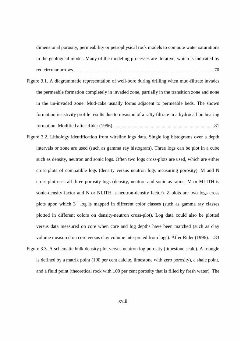
Figure 3.1. A diagrammatic representation of well-bore during drilling when mud-filtrate invades

the permeable formation completely in invaded zone, partially in the transition zone and none

in the un-invaded zone. Mud-cake usually forms adjacent to permeable beds. The shown

formation resistivity profile results due to invasion of a salty filtrate in a hydrocarbon bearing

formation. Modified after Rider (1996). .................................................................................. 81

Figure 3.2. Lithology identification from wireline logs data. Single log histograms over a depth

intervals or zone are used (such as gamma ray histogram). Three logs can be plot in a cube

such as density, neutron and sonic logs. Often two logs cross-plots are used, which are either

cross-plots of compatible logs (density versus neutron logs measuring porosity). M and N

cross-plot uses all three porosity logs (density, neutron and sonic as ratios; M or MLITH is

sonic-density factor and N or NLITH is neutron-density factor). Z plots are two logs cross

plots upon which 3rd

log is mapped in different color classes (such as gamma ray classes

plotted in different colors on density-neutron cross-plot). Log data could also be plotted

versus data measured on core when core and log depths have been matched (such as clay

volume measured on core versus clay volume interpreted from logs). After Rider (1996). ... 83

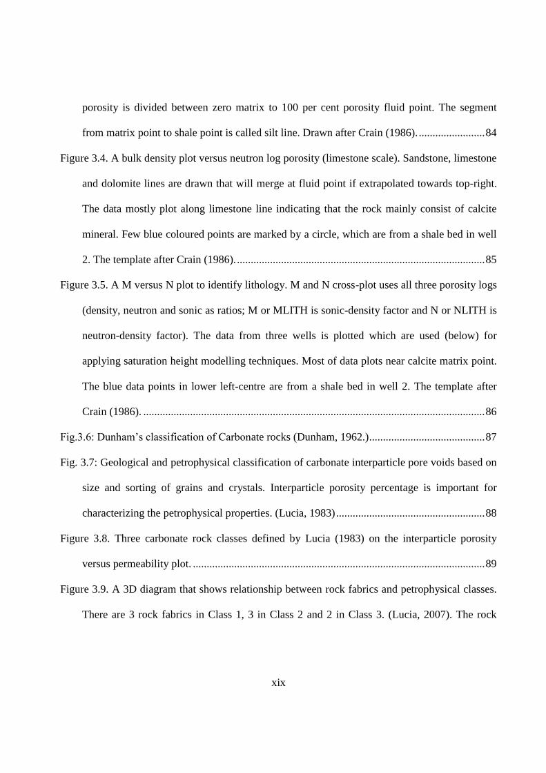
Figure 3.3. A schematic bulk density plot versus neutron log porosity (limestone scale). A triangle

is defined by a matrix point (100 per cent calcite, limestone with zero porosity), a shale point,

and a fluid point (theoretical rock with 100 per cent porosity that is filled by fresh water). The

xix

porosity is divided between zero matrix to 100 per cent porosity fluid point. The segment

from matrix point to shale point is called silt line. Drawn after Crain (1986). ........................ 84

Figure 3.4. A bulk density plot versus neutron log porosity (limestone scale). Sandstone, limestone

and dolomite lines are drawn that will merge at fluid point if extrapolated towards top-right.

The data mostly plot along limestone line indicating that the rock mainly consist of calcite

mineral. Few blue coloured points are marked by a circle, which are from a shale bed in well

2. The template after Crain (1986). .......................................................................................... 85

Figure 3.5. A M versus N plot to identify lithology. M and N cross-plot uses all three porosity logs

(density, neutron and sonic as ratios; M or MLITH is sonic-density factor and N or NLITH is

neutron-density factor). The data from three wells is plotted which are used (below) for

applying saturation height modelling techniques. Most of data plots near calcite matrix point.

The blue data points in lower left-centre are from a shale bed in well 2. The template after

Crain (1986). ............................................................................................................................ 86

Fig.3.6: Dunham‟s classification of Carbonate rocks (Dunham, 1962.) .......................................... 87

Fig. 3.7: Geological and petrophysical classification of carbonate interparticle pore voids based on

size and sorting of grains and crystals. Interparticle porosity percentage is important for

characterizing the petrophysical properties. (Lucia, 1983) ...................................................... 88

Figure 3.8. Three carbonate rock classes defined by Lucia (1983) on the interparticle porosity

versus permeability plot. .......................................................................................................... 89

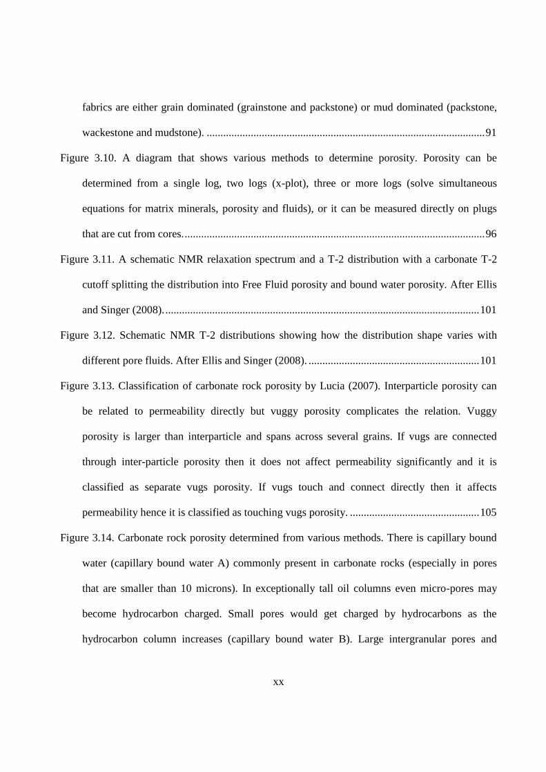
Figure 3.9. A 3D diagram that shows relationship between rock fabrics and petrophysical classes.

There are 3 rock fabrics in Class 1, 3 in Class 2 and 2 in Class 3. (Lucia, 2007). The rock

xx

fabrics are either grain dominated (grainstone and packstone) or mud dominated (packstone,

wackestone and mudstone). ..................................................................................................... 91

Figure 3.10. A diagram that shows various methods to determine porosity. Porosity can be

determined from a single log, two logs (x-plot), three or more logs (solve simultaneous

equations for matrix minerals, porosity and fluids), or it can be measured directly on plugs

that are cut from cores. ............................................................................................................. 96

Figure 3.11. A schematic NMR relaxation spectrum and a T-2 distribution with a carbonate T-2

cutoff splitting the distribution into Free Fluid porosity and bound water porosity. After Ellis

and Singer (2008). .................................................................................................................. 101

Figure 3.12. Schematic NMR T-2 distributions showing how the distribution shape varies with

different pore fluids. After Ellis and Singer (2008). .............................................................. 101

Figure 3.13. Classification of carbonate rock porosity by Lucia (2007). Interparticle porosity can

be related to permeability directly but vuggy porosity complicates the relation. Vuggy

porosity is larger than interparticle and spans across several grains. If vugs are connected

through inter-particle porosity then it does not affect permeability significantly and it is

classified as separate vugs porosity. If vugs touch and connect directly then it affects

permeability hence it is classified as touching vugs porosity. ............................................... 105

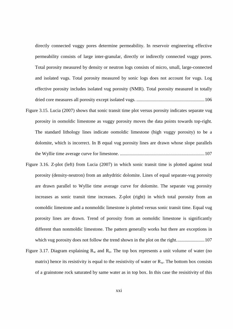
Figure 3.14. Carbonate rock porosity determined from various methods. There is capillary bound

water (capillary bound water A) commonly present in carbonate rocks (especially in pores

that are smaller than 10 microns). In exceptionally tall oil columns even micro-pores may

become hydrocarbon charged. Small pores would get charged by hydrocarbons as the

hydrocarbon column increases (capillary bound water B). Large intergranular pores and

xxi

directly connected vuggy pores determine permeability. In reservoir engineering effective

permeability consists of large inter-granular, directly or indirectly connected vuggy pores.

Total porosity measured by density or neutron logs consists of micro, small, large-connected

and isolated vugs. Total porosity measured by sonic logs does not account for vugs. Log

effective porosity includes isolated vug porosity (NMR). Total porosity measured in totally

dried core measures all porosity except isolated vugs. .......................................................... 106

Figure 3.15. Lucia (2007) shows that sonic transit time plot versus porosity indicates separate vug

porosity in oomoldic limestone as vuggy porosity moves the data points towards top-right.

The standard lithology lines indicate oomoldic limestone (high vuggy porosity) to be a

dolomite, which is incorrect. In B equal vug porosity lines are drawn whose slope parallels

the Wyllie time average curve for limestone. ........................................................................ 107

Figure 3.16. Z-plot (left) from Lucia (2007) in which sonic transit time is plotted against total

porosity (density-neutron) from an anhydritic dolomite. Lines of equal separate-vug porosity

are drawn parallel to Wyllie time average curve for dolomite. The separate vug porosity

increases as sonic transit time increases. Z-plot (right) in which total porosity from an

oomoldic limestone and a nonmoldic limestone is plotted versus sonic transit time. Equal vug

porosity lines are drawn. Trend of porosity from an oomoldic limestone is significantly

different than nonmoldic limestone. The pattern generally works but there are exceptions in

which vug porosity does not follow the trend shown in the plot on the right. ....................... 107

Figure 3.17. Diagram explaining Rw and Ro. The top box represents a unit volume of water (no

matrix) hence its resistivity is equal to the resistivity of water or Rw. The bottom box consists

of a grainstone rock saturated by same water as in top box. In this case the resisitivity of this

xxii

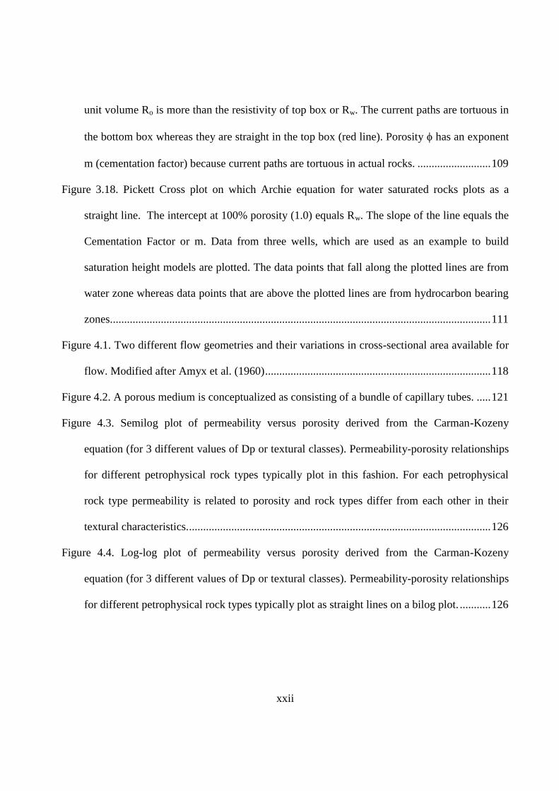
unit volume Ro is more than the resistivity of top box or Rw. The current paths are tortuous in

the bottom box whereas they are straight in the top box (red line). Porosity has an exponent

m (cementation factor) because current paths are tortuous in actual rocks. .......................... 109

Figure 3.18. Pickett Cross plot on which Archie equation for water saturated rocks plots as a

straight line. The intercept at 100% porosity (1.0) equals Rw. The slope of the line equals the

Cementation Factor or m. Data from three wells, which are used as an example to build

saturation height models are plotted. The data points that fall along the plotted lines are from

water zone whereas data points that are above the plotted lines are from hydrocarbon bearing

zones. ...................................................................................................................................... 111

Figure 4.1. Two different flow geometries and their variations in cross-sectional area available for

flow. Modified after Amyx et al. (1960) ................................................................................ 118

Figure 4.2. A porous medium is conceptualized as consisting of a bundle of capillary tubes. ..... 121

Figure 4.3. Semilog plot of permeability versus porosity derived from the Carman-Kozeny

equation (for 3 different values of Dp or textural classes). Permeability-porosity relationships

for different petrophysical rock types typically plot in this fashion. For each petrophysical

rock type permeability is related to porosity and rock types differ from each other in their

textural characteristics. ........................................................................................................... 126

Figure 4.4. Log-log plot of permeability versus porosity derived from the Carman-Kozeny

equation (for 3 different values of Dp or textural classes). Permeability-porosity relationships

for different petrophysical rock types typically plot as straight lines on a bilog plot. ........... 126

xxiii

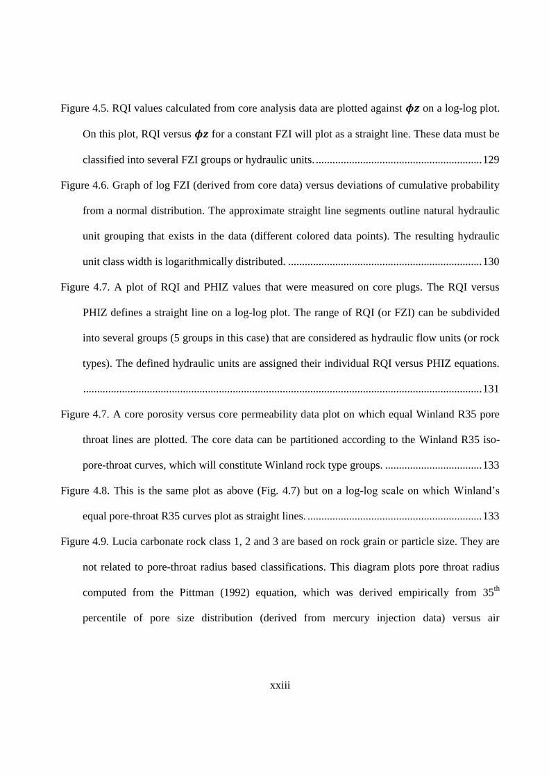
Figure 4.5. RQI values calculated from core analysis data are plotted against on a log-log plot.

On this plot, RQI versus for a constant FZI will plot as a straight line. These data must be

classified into several FZI groups or hydraulic units. ............................................................ 129

Figure 4.6. Graph of log FZI (derived from core data) versus deviations of cumulative probability

from a normal distribution. The approximate straight line segments outline natural hydraulic

unit grouping that exists in the data (different colored data points). The resulting hydraulic

unit class width is logarithmically distributed. ...................................................................... 130

Figure 4.7. A plot of RQI and PHIZ values that were measured on core plugs. The RQI versus

PHIZ defines a straight line on a log-log plot. The range of RQI (or FZI) can be subdivided

into several groups (5 groups in this case) that are considered as hydraulic flow units (or rock

types). The defined hydraulic units are assigned their individual RQI versus PHIZ equations.

................................................................................................................................................ 131

Figure 4.7. A core porosity versus core permeability data plot on which equal Winland R35 pore

throat lines are plotted. The core data can be partitioned according to the Winland R35 iso-

pore-throat curves, which will constitute Winland rock type groups. ................................... 133

Figure 4.8. This is the same plot as above (Fig. 4.7) but on a log-log scale on which Winland‟s

equal pore-throat R35 curves plot as straight lines. ............................................................... 133

Figure 4.9. Lucia carbonate rock class 1, 2 and 3 are based on rock grain or particle size. They are

not related to pore-throat radius based classifications. This diagram plots pore throat radius

computed from the Pittman (1992) equation, which was derived empirically from 35th

percentile of pore size distribution (derived from mercury injection data) versus air

xxiv

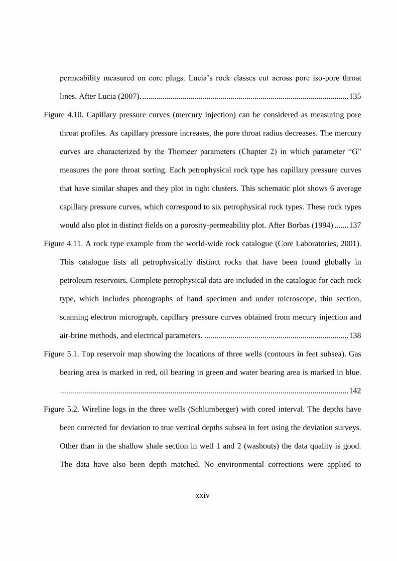
permeability measured on core plugs. Lucia‟s rock classes cut across pore iso-pore throat

lines. After Lucia (2007). ....................................................................................................... 135

Figure 4.10. Capillary pressure curves (mercury injection) can be considered as measuring pore

throat profiles. As capillary pressure increases, the pore throat radius decreases. The mercury

curves are characterized by the Thomeer parameters (Chapter 2) in which parameter “G”

measures the pore throat sorting. Each petrophysical rock type has capillary pressure curves

that have similar shapes and they plot in tight clusters. This schematic plot shows 6 average

capillary pressure curves, which correspond to six petrophysical rock types. These rock types

would also plot in distinct fields on a porosity-permeability plot. After Borbas (1994) ....... 137

Figure 4.11. A rock type example from the world-wide rock catalogue (Core Laboratories, 2001).

This catalogue lists all petrophysically distinct rocks that have been found globally in

petroleum reservoirs. Complete petrophysical data are included in the catalogue for each rock

type, which includes photographs of hand specimen and under microscope, thin section,

scanning electron micrograph, capillary pressure curves obtained from mecury injection and

air-brine methods, and electrical parameters. ........................................................................ 138

Figure 5.1. Top reservoir map showing the locations of three wells (contours in feet subsea). Gas

bearing area is marked in red, oil bearing in green and water bearing area is marked in blue.

................................................................................................................................................ 142

Figure 5.2. Wireline logs in the three wells (Schlumberger) with cored interval. The depths have

been corrected for deviation to true vertical depths subsea in feet using the deviation surveys.

Other than in the shallow shale section in well 1 and 2 (washouts) the data quality is good.

The data have also been depth matched. No environmental corrections were applied to

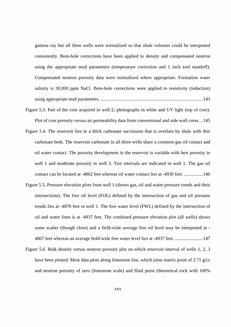
xxv

gamma ray but all three wells were normalized so that shale volumes could be interpreted

consistently. Bore-hole corrections have been applied to density and compensated neutron

using the appropriate mud parameters (temperature correction and 1 inch tool standoff).

Compensated neutron porosity data were normalized where appropriate. Formation water

salinity is 30,000 ppm NaCl. Bore-hole corrections were applied to resistivity (induction)

using appropriate mud parameters. ........................................................................................ 143

Figure 5.3. Part of the core acquired in well 2; photographs in white and UV light (top of core).

Plot of core porosity versus air permeability data from conventional and side-wall cores. .. 145

Figure 5.4. The reservoir lies in a thick carbonate succession that is overlain by shale with thin

carbonate beds. The reservoir carbonate in all three wells share a common gas oil contact and

oil water contact. The porosity development in the reservoir is variable with best porosity in

well 1 and moderate porosity in well 3. Test intervals are indicated in well 1. The gas oil

contact can be located at -4862 feet whereas oil water contact lies at -4930 feet. ................ 146

Figure 5.5. Pressure elevation plots from well 1 (shows gas, oil and water pressure trends and their

intersections). The free oil level (FOL) defined by the intersection of gas and oil pressure

trends lies at -4878 feet in well 1. The free water level (FWL) defined by the intersection of

oil and water lines is at -4937 feet. The combined pressure elevation plot (all wells) shows

some scatter (though close) and a field-wide average free oil level may be interpreted at -

4867 feet whereas an average field-wide free water level lies at -4937 feet. ........................ 147

Figure 5.6. Bulk density versus neutron porosity plot on which reservoir interval of wells 1, 2, 3

have been plotted. Most data plots along limestone line, which joins matrix point of 2.71 g/cc

and neutron porosity of zero (limestone scale) and fluid point (theoretical rock with 100%

xxvi

porosity and bulk density of 1 g/cc). A small set of data points cluster (mostly in well 3) to

the right of the dolomite line indicating shale beds. This shows that the neutron porosity of

shale ranges from 0.35 to 0.40. .............................................................................................. 148

Figure 5.7. M-N lithology plot, which shows most of the data plotting near calcite point whereas a

few data points are at and towards shale point (plot layout is adopted after Crain, 1986). ... 149

Figure 5.8. Plot of effective porosity versus deep resistivity (corrected) for wells 1, 2, 3. A straight

line on this plot has a slope equal to the Archie “m” factor. Three lines are drawn for m

values of 1.8, 1.9 and 2. From special core analysis, the best estimate for the Archie “m”

value is 1.9. The intercept of the lines is at 0.095 (Rw) at the reservoir temperature of 170

degree Fahrenheit. .................................................................................................................. 150

Figure 5.9. Well 1 interpretation: track 1 shows gamma ray, corrected gamma ray, caliper and bit-

size; track 2 and 3 show measured and sub-sea depths; track 4 shows the porosity logs,

photoelectric factor or PEF; track 5 shows corrected shallow, medium, deep resistivity; track

6 shows effective water saturation; track 7 shows interpreted lithology with standard symbols,

porosity and porosity measured on core plugs. ...................................................................... 152

Figure 5.10. Well 2 interpretation: track 1 shows gamma ray, corrected gamma ray, caliper and

bit-size; track 2 and 3 show measured and sub-sea depths; track 4 shows the porosity logs,

photoelectric factor or PEF; track 5 shows corrected shallow, medium, deep resistivity; track

6 shows effective water saturation; track 7 shows interpreted lithology with standard symbols,

porosity and porosity measured on core plugs. ...................................................................... 153

Figure 5.11. Well 3 interpretation: track 1 shows gamma ray, corrected gamma ray, SP, caliper and

bit-size; track 2 and 3 show measured and sub-sea depths; track 4 shows the porosity logs,

xxvii

photoelectric factor or PEF; track 5 shows corrected shallow, medium, deep resistivity; track

6 shows effective water saturation; track 7 shows interpreted lithology with standard symbols

and porosity. ........................................................................................................................... 154

Figure 5.12. Sedimentological core description (well 1, core 1). The facies codes are described in

the text. Dunham‟s Textures: W= wackestone, P= packstone, G= grainstone, and R=

rudstone. Depth is in feet. ...................................................................................................... 156

Figure 5.13. Sedimentological core description (well 2, cores 1 and 2). The facies codes are

described in the text. Dunham‟s Textures: W= wackestone, P= packstone, G= grainstone, and

R= rudstone. Depth is in feet. ................................................................................................ 157

Figure 5.14. Thin-section photographs of various sedimentary facies from well 2 (cores 1 and 2).

The facies codes are written on top left-corner of each photograph. All thin sections were

photographed at (25X) magnification except the middle section of the first row at (100X).

The blue colored areas are blue resin-impregnated macro-pores. The SWPM and PSPG facies

(Skeletal Wackestone with Pelleted Matrix and Peloidal Skeletal Packstone/Grainstone facies

contain most abundant macro-pores). .................................................................................... 158

Figure 5.15. Classification of hydraulic units based on flow zone indicators (FZI), which are

computed from the porosity and air permeability that is measured on core. The FZI are sorted

in a descending order and a cumulative probability is computed, which is converted to

standard normal deviation using the spreadsheet function (NORMSINV). The resulting

values are shifted by 3.5 (arbitrarily) so that negative values are elminated and x-axis scale

can start from zero. Slight differences in slope are noted and marked to define limiting FZI

values of hydraulic units (HU). The HU1 has the best and HU5 has the worst reservoir

xxviii

qualities. The limiting FZI values of HU are shown. Refer to Chapter 4 for details and

references. .............................................................................................................................. 159

Figure 5.16. A plot of core derived reservoir quality index (RQI) versus normalized porosity

(PHIZ) on log-log scale. The hydraulic units identified are distinguished by different colors.

Each HU has a well defined trend. Sedimentary facies are also identified for 11 points.

Packstone-grainstone (PSPG) facies are generally associated with best hydraulic unit rock

type. Skeletal packstones with algal crusts (SPAC) generally belong to low reservoir quality

HU5. Refer to Chapter 4 for details and references. .............................................................. 160

Figure 5.17. Flow zone indicator (FZI) data computed from core measurements are related to log

data (NCGR normalized corrected gamma ray, NNPHIC normalized neutron porosity

corrected, NDT normalized sonic transit time, NRHOBC normalized bulk density corrected)

at equivalent depths and classified by the identified hydraulic unit (HU) groups (color coded).

Generalized trends are defined between FZI and log measurements. These trends of FZI

versus different logs are integrated in a single multiple non-linear equation. ....................... 162

Figure 5.18. Capillary pressure data (mercury injection) obtained on conventional and side-wall

core samples in wells 1, 2, 3. The data on the left graph is uncorrected and on the right graph,

it is corrected for closure and surface vug effects. The data is generally acquired at low

pressure as only mid-plateau and early part of late upper range can be seen. These data were

not used in establishing the FZI prediction model so that it can be used as a control data set.

These capillary pressure curves are later converted to J-space for upscaling or averaging and

then used to build J curves for each hydraulic unit. ............................................................... 164

xxix

Figure 5.19. The hydraulic units (HU) determined from predicted flow zone indicator (FZI) from

logs are shown by red curve in wells 1, 2, 3 (true vertical depth subsea is on the Y-axis) . The

numbers 1 to 5 represent HU1 to HU5 whereas 6 represents shale or non-reservoir quality

rock. The predicted HU curve is overlain by an independent HU data set, which was

determined from routine and side-wall cores (capillary pressure data were acquired on these

core samples using mercury injection method). The predicted HU from logs match closely

with the control data set HU except in few points where HU 1 in core is predicted as HU 2.

................................................................................................................................................ 165

Figure 5.20. Permeability calculated from the predicted flow zone indicator (FZI) curves (red

curve) for the three wells. Red squares are permeability measured on conventional core plugs

and side-wall cores. Black shaded curves on the left represent effective porosity. ............... 166

Figure 5.21. Permeability computed from predicted flow zone indicator (FZI) compared against

core permeability at the corresponding depths. The computed and core permeabilities are

clustered along a 45 degree line without apparent bias. The spread of data points across the 45

degree lines could be due to log problems, core depth matching errors, errors in depthing of

side-wall cores and laboratory measurement errors. .............................................................. 167

Figure 5.22. Permeability computed from predicted flow zone indicator (FZI) compared against

core permeability on a porosity versus permeability plot. The core data points (colored

rectangles) are color coded for their hydraulic unit (legend of diagram). The computed

permeability is shown by green circles. The calculated permeability does not extend beyond

the permeability measured on core. ....................................................................................... 168

xxx

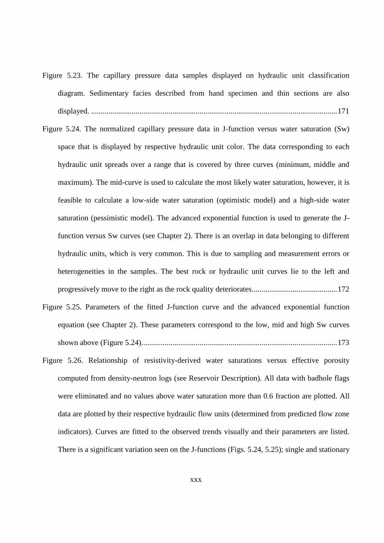
Figure 5.23. The capillary pressure data samples displayed on hydraulic unit classification

diagram. Sedimentary facies described from hand specimen and thin sections are also

displayed. ............................................................................................................................... 171

Figure 5.24. The normalized capillary pressure data in J-function versus water saturation (Sw)

space that is displayed by respective hydraulic unit color. The data corresponding to each

hydraulic unit spreads over a range that is covered by three curves (minimum, middle and

maximum). The mid-curve is used to calculate the most likely water saturation, however, it is

feasible to calculate a low-side water saturation (optimistic model) and a high-side water

saturation (pessimistic model). The advanced exponential function is used to generate the J-

function versus Sw curves (see Chapter 2). There is an overlap in data belonging to different

hydraulic units, which is very common. This is due to sampling and measurement errors or

heterogeneities in the samples. The best rock or hydraulic unit curves lie to the left and

progressively move to the right as the rock quality deteriorates. ........................................... 172

Figure 5.25. Parameters of the fitted J-function curve and the advanced exponential function

equation (see Chapter 2). These parameters correspond to the low, mid and high Sw curves

shown above (Figure 5.24). .................................................................................................... 173

Figure 5.26. Relationship of resistivity-derived water saturations versus effective porosity

computed from density-neutron logs (see Reservoir Description). All data with badhole flags

were eliminated and no values above water saturation more than 0.6 fraction are plotted. All

data are plotted by their respective hydraulic flow units (determined from predicted flow zone

indicators). Curves are fitted to the observed trends visually and their parameters are listed.

There is a significant variation seen on the J-functions (Figs. 5.24, 5.25); single and stationary

xxxi

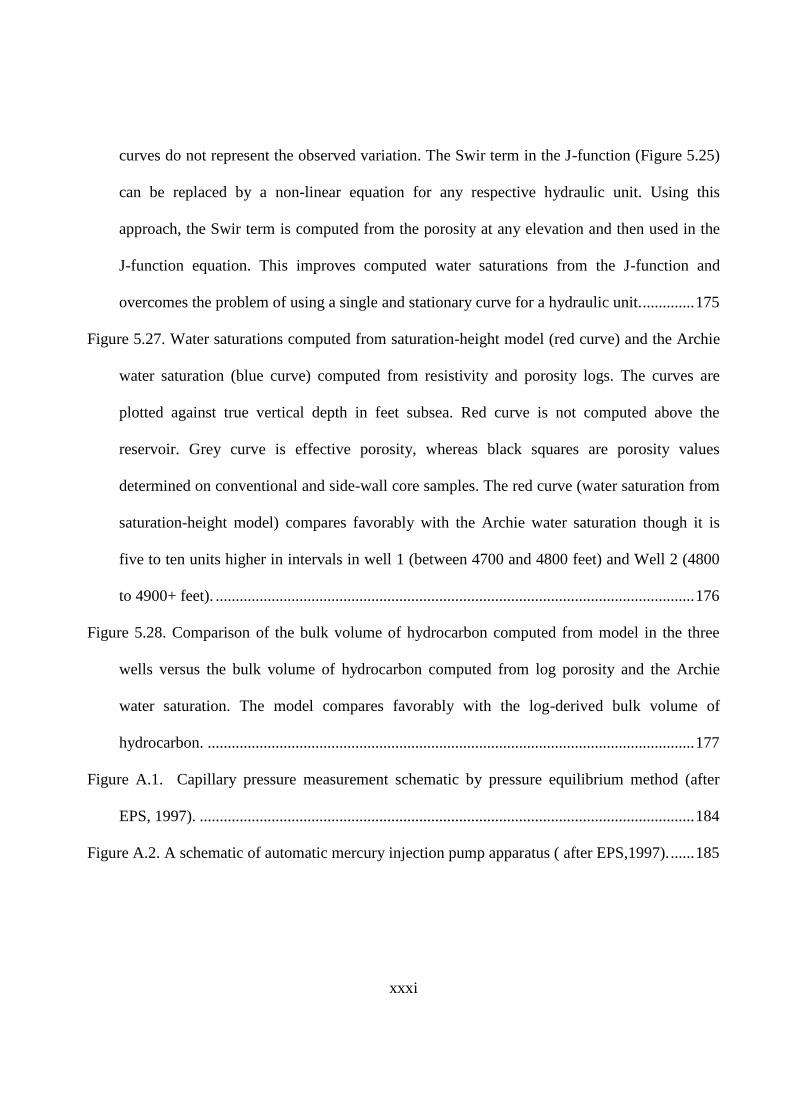
curves do not represent the observed variation. The Swir term in the J-function (Figure 5.25)

can be replaced by a non-linear equation for any respective hydraulic unit. Using this

approach, the Swir term is computed from the porosity at any elevation and then used in the

J-function equation. This improves computed water saturations from the J-function and

overcomes the problem of using a single and stationary curve for a hydraulic unit. ............. 175

Figure 5.27. Water saturations computed from saturation-height model (red curve) and the Archie

water saturation (blue curve) computed from resistivity and porosity logs. The curves are

plotted against true vertical depth in feet subsea. Red curve is not computed above the

reservoir. Grey curve is effective porosity, whereas black squares are porosity values

determined on conventional and side-wall core samples. The red curve (water saturation from

saturation-height model) compares favorably with the Archie water saturation though it is

five to ten units higher in intervals in well 1 (between 4700 and 4800 feet) and Well 2 (4800

to 4900+ feet). ........................................................................................................................ 176

Figure 5.28. Comparison of the bulk volume of hydrocarbon computed from model in the three

wells versus the bulk volume of hydrocarbon computed from log porosity and the Archie

water saturation. The model compares favorably with the log-derived bulk volume of

hydrocarbon. .......................................................................................................................... 177

Figure A.1. Capillary pressure measurement schematic by pressure equilibrium method (after

EPS, 1997). ............................................................................................................................ 184

Figure A.2. A schematic of automatic mercury injection pump apparatus ( after EPS,1997). ...... 185

xxxii

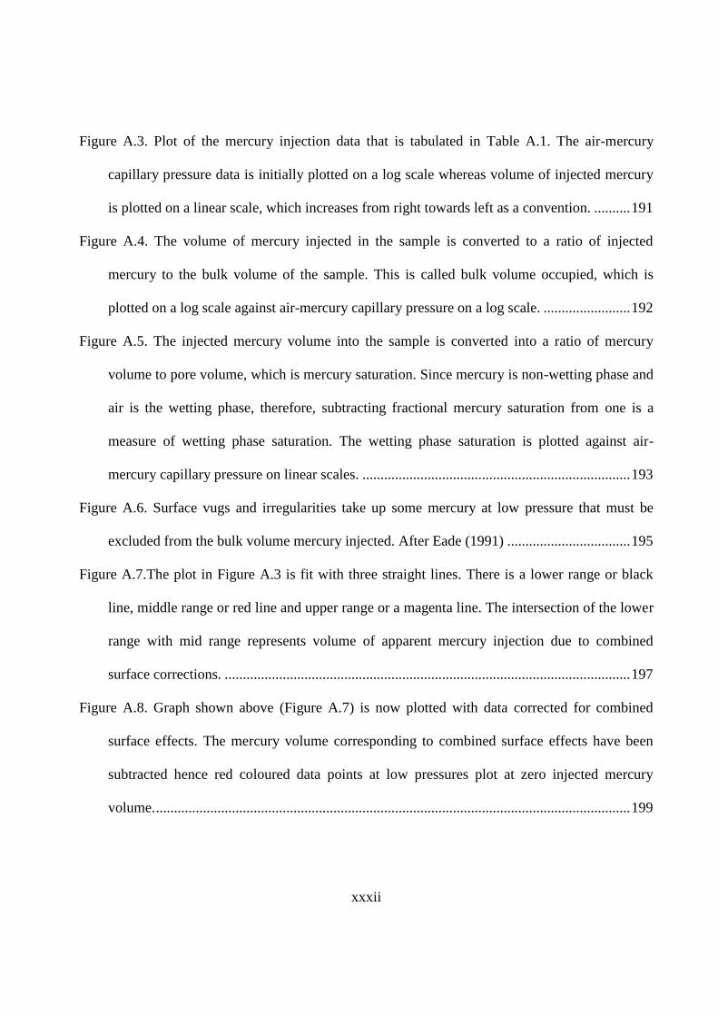
Figure A.3. Plot of the mercury injection data that is tabulated in Table A.1. The air-mercury

capillary pressure data is initially plotted on a log scale whereas volume of injected mercury

is plotted on a linear scale, which increases from right towards left as a convention. .......... 191

Figure A.4. The volume of mercury injected in the sample is converted to a ratio of injected

mercury to the bulk volume of the sample. This is called bulk volume occupied, which is

plotted on a log scale against air-mercury capillary pressure on a log scale. ........................ 192

Figure A.5. The injected mercury volume into the sample is converted into a ratio of mercury

volume to pore volume, which is mercury saturation. Since mercury is non-wetting phase and

air is the wetting phase, therefore, subtracting fractional mercury saturation from one is a

measure of wetting phase saturation. The wetting phase saturation is plotted against air-

mercury capillary pressure on linear scales. .......................................................................... 193

Figure A.6. Surface vugs and irregularities take up some mercury at low pressure that must be

excluded from the bulk volume mercury injected. After Eade (1991) .................................. 195

Figure A.7.The plot in Figure A.3 is fit with three straight lines. There is a lower range or black

line, middle range or red line and upper range or a magenta line. The intersection of the lower

range with mid range represents volume of apparent mercury injection due to combined

surface corrections. ................................................................................................................ 197

Figure A.8. Graph shown above (Figure A.7) is now plotted with data corrected for combined

surface effects. The mercury volume corresponding to combined surface effects have been

subtracted hence red coloured data points at low pressures plot at zero injected mercury

volume. ................................................................................................................................... 199

xxxiii

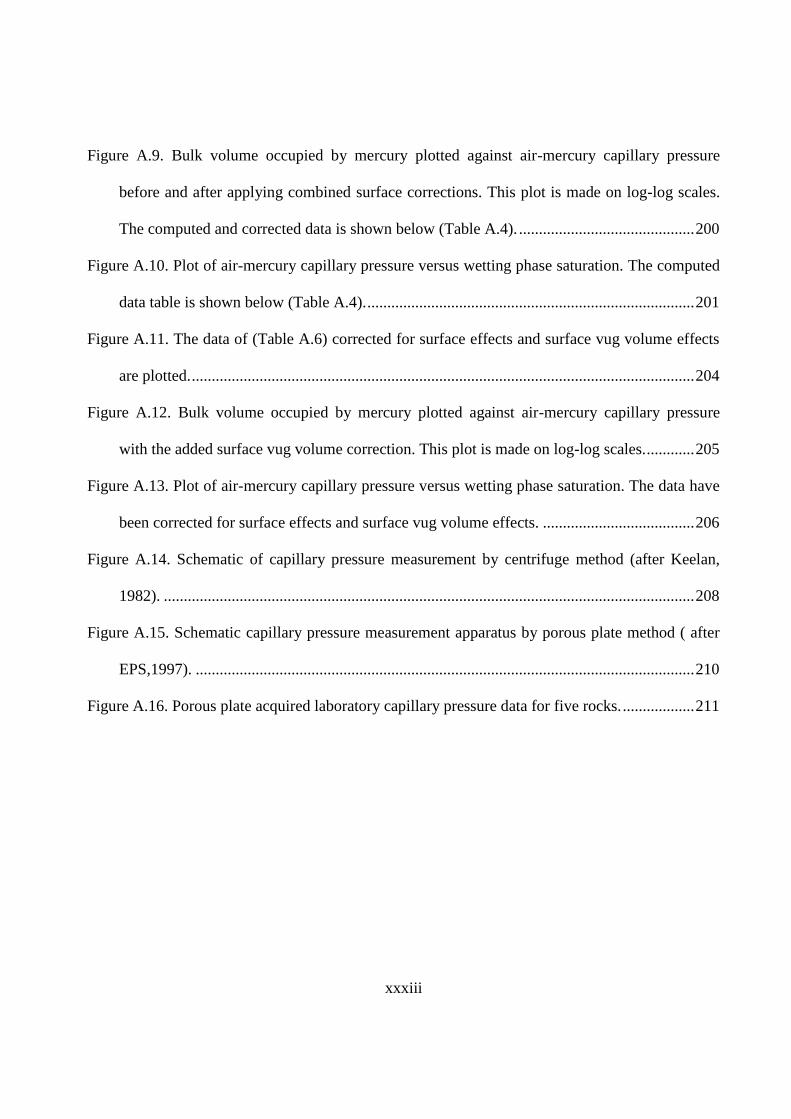
Figure A.9. Bulk volume occupied by mercury plotted against air-mercury capillary pressure

before and after applying combined surface corrections. This plot is made on log-log scales.

The computed and corrected data is shown below (Table A.4). ............................................ 200

Figure A.10. Plot of air-mercury capillary pressure versus wetting phase saturation. The computed

data table is shown below (Table A.4). .................................................................................. 201

Figure A.11. The data of (Table A.6) corrected for surface effects and surface vug volume effects

are plotted. .............................................................................................................................. 204

Figure A.12. Bulk volume occupied by mercury plotted against air-mercury capillary pressure

with the added surface vug volume correction. This plot is made on log-log scales. ............ 205

Figure A.13. Plot of air-mercury capillary pressure versus wetting phase saturation. The data have

been corrected for surface effects and surface vug volume effects. ...................................... 206

Figure A.14. Schematic of capillary pressure measurement by centrifuge method (after Keelan,

1982). ..................................................................................................................................... 208

Figure A.15. Schematic capillary pressure measurement apparatus by porous plate method ( after

EPS,1997). ............................................................................................................................. 210

Figure A.16. Porous plate acquired laboratory capillary pressure data for five rocks. .................. 211

xxxiv

List Of Tables

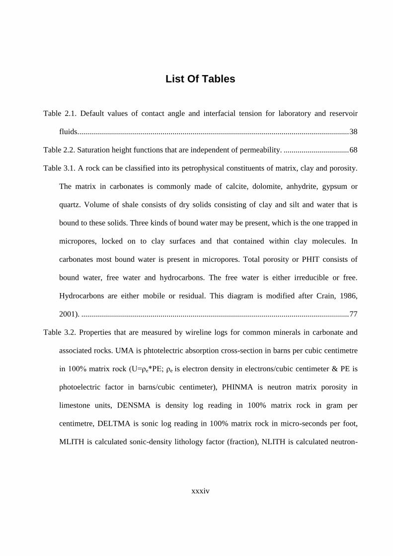
Table 2.1. Default values of contact angle and interfacial tension for laboratory and reservoir

fluids. ........................................................................................................................................ 38

Table 2.2. Saturation height functions that are independent of permeability. ................................. 68

Table 3.1. A rock can be classified into its petrophysical constituents of matrix, clay and porosity.

The matrix in carbonates is commonly made of calcite, dolomite, anhydrite, gypsum or

quartz. Volume of shale consists of dry solids consisting of clay and silt and water that is

bound to these solids. Three kinds of bound water may be present, which is the one trapped in

micropores, locked on to clay surfaces and that contained within clay molecules. In

carbonates most bound water is present in micropores. Total porosity or PHIT consists of

bound water, free water and hydrocarbons. The free water is either irreducible or free.

Hydrocarbons are either mobile or residual. This diagram is modified after Crain, 1986,

2001). ....................................................................................................................................... 77

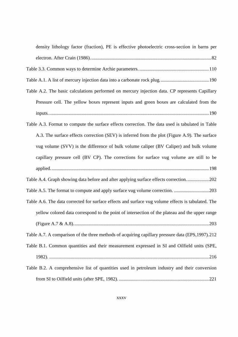
Table 3.2. Properties that are measured by wireline logs for common minerals in carbonate and

associated rocks. UMA is phtotelectric absorption cross-section in barns per cubic centimetre

in 100% matrix rock (U=ρe*PE; ρe is electron density in electrons/cubic centimeter & PE is

photoelectric factor in barns/cubic centimeter), PHINMA is neutron matrix porosity in

limestone units, DENSMA is density log reading in 100% matrix rock in gram per

centimetre, DELTMA is sonic log reading in 100% matrix rock in micro-seconds per foot,

MLITH is calculated sonic-density lithology factor (fraction), NLITH is calculated neutron-

xxxv

density lithology factor (fraction), PE is effective photoelectric cross-section in barns per

electron. After Crain (1986). .................................................................................................... 82

Table 3.3. Common ways to determine Archie parameters. .......................................................... 110

Table A.1. A list of mercury injection data into a carbonate rock plug. ........................................ 190

Table A.2. The basic calculations performed on mercury injection data. CP represents Capillary

Pressure cell. The yellow boxes represent inputs and green boxes are calculated from the

inputs. ..................................................................................................................................... 190

Table A.3. Format to compute the surface effects correction. The data used is tabulated in Table

A.3. The surface effects correction (SEV) is inferred from the plot (Figure A.9). The surface

vug volume (SVV) is the difference of bulk volume caliper (BV Caliper) and bulk volume

capillary pressure cell (BV CP). The corrections for surface vug volume are still to be

applied. ................................................................................................................................... 198

Table A.4. Graph showing data before and after applying surface effects correction. .................. 202

Table A.5. The format to compute and apply surface vug volume correction. ............................. 203

Table A.6. The data corrected for surface effects and surface vug volume effects is tabulated. The

yellow colored data correspond to the point of intersection of the plateau and the upper range

(Figure A.7 & A.8). ................................................................................................................ 203

Table A.7. A comparison of the three methods of acquiring capillary pressure data (EPS,1997). 212

Table B.1. Common quantities and their measurement expressed in SI and Oilfield units (SPE,

1982). ..................................................................................................................................... 216

Table B.2. A comprehensive list of quantities used in petroleum industry and their conversion

from SI to Oilfield units (after SPE, 1982). ........................................................................... 221

xxxvi

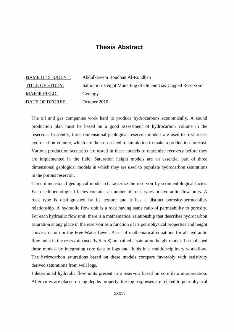
Thesis Abstract

NAME OF STUDENT: Abdulkareem Roudhan Al-Roudhan

TITLE OF STUDY: Saturation-Height Modelling of Oil and Gas-Capped Reservoirs

MAJOR FIELD: Geology

DATE OF DEGREE: October 2010

The oil and gas companies work hard to produce hydrocarbons economically. A sound

production plan must be based on a good assessment of hydrocarbon volume in the

reservoir. Currently, three dimensional geological reservoir models are used to first assess

hydrocarbon volume, which are then up-scaled to simulation to make a production forecast.

Various production scenarios are tested in these models to maximize recovery before they

are implemented in the field. Saturation height models are an essential part of three

dimensional geological models in which they are used to populate hydrocarbon saturations

in the porous reservoir.

Three dimensional geological models characterize the reservoir by sedimentological facies.

Each sedimentological facies contains a number of rock types or hydraulic flow units. A

rock type is distinguished by its texture and it has a distinct porosity-permeability

relationship. A hydraulic flow unit is a rock having same ratio of permeability to porosity.

For each hydraulic flow unit, there is a mathematical relationship that describes hydrocarbon

saturation at any place in the reservoir as a function of its petrophysical properties and height

above a datum or the Free Water Level. A set of mathematical equations for all hydraulic

flow units in the reservoir (usually 5 to 8) are called a saturation height model. I established

these models by integrating core data to logs and fluids in a multidisciplinary work-flow.

The hydrocarbon saturations based on these models compare favorably with resistivity

derived saturations from well logs.

I determined hydraulic flow units present in a reservoir based on core data interpretation.

After cores are placed on log depths properly, the log responses are related to petrophysical

xxxvii

properties measured on core. I established a predictive relationship for hydraulic flow units

using log responses. This relationship is used to predict hydraulic flow units in non-cored

wells. Once that is done, permeability can be calculated in non-cored wells also using the

predicted hydraulic flow units. Each hydraulic flow unit has a saturation versus height

relationship, which is used to calculate hydrocarbon saturations.

A well calibrated saturation height model populates the three dimensional geological model

with hydrocarbon saturations that are related to its sedimentological and petrophysical

properties. The assessments of hydrocarbons in place using such models are more accurate

than traditional mapping methods.

xxxviii

ملخص الرسالة

انشضب عجذانكشى ث سضب :ـــــــــــــــماالس

زخخ انتشجع ثبختالف األستفبع نكبي انجتشل راد انغطبء انغبص :عنوان الرسالة

بنـخاند :ـصـــصـــالتـخ

0202 اكتثش :خ التخرجـاريـت

دت أ تستذ خطظ اإلتبج اندذح عه تقى خذ نحدى . انغبص قظبس خذب نك تتح ثشكم إقتظبدتجزل ششكبد انفظ

حبنب، انبرج اندنخخ انثالثخ األثعبد تستخذو نتقى حدى انفظ انغبص، انت تى إدساخب . انفظ انغبص انخدا ف انك

قجم تفز خطظ اإلتبج، تى إختجبس سبسبد يختهفخ نإلتبج . بد يستقجهخ نإلتبجف ثشبيح يحكبح انك نتقذى تقع

برج . انستقجه ف انبرج اندنخخ انثالثخ األثعبد رنك نتحقق أقظ قذس ي إتبج انحدى انكه نهفظ انغبص ف انك

د قب دققخ نست إشجبع انتشجع ثبختالف اإلستفبع تثم خضء أسبس نز انبرج اندنخخ انثالثخ األثعبد، حث أب تض

.انظخش ثبنفظ انغبص ف انكبي انسبيخ

انبرج اندنخخ انثالثخ األثعبد تظف انك ع طشق انسحبد انشسثخ، انت قذ تحت اناحذح يب عه عذد ي

تحظم . انفبرخ انضح نكم يب-عشف عه ز انحذاد ع طشق عالقخ انسبيختى انت. حذاد انتذفق انذسنك انسجخ ان

( نكم حذح تذفق ذسنك)تخذ عالقخ سبضخ . عهب ي قسخ انفبرخ عه انسبيخ تك فشذح نكم حذح تذفق ذسنك

تعتذ عه انخظبئض انفضبئخ نهظخش يذ اإلستفبع ع يست تظف سجخ انتشجع ثبنفظ ف أ يكب ف انك،

( 8-5عبدح )بنك يدعخ ي انعبدالد انشبضخ نكم حذاد انتذفق انذسنك ف انك . انبء انحش( انعق انشخع)

رج انتشجع ثبختالف اإلستفبع، انت ي أى يضابب أب تكبيم تقبس ث انج بد انظخشخ انسدالد تس ببد ي انع

ظبد يتعذدح قى انتشجع انفط انجخ عه . انجئشخ خظبئض انسائم انخدح ف انك ي خالل خطاد عم راد تخظ

.زا انرج تضب خذا تهك انجخ ي سدم انقبيخ انكشثخ ف انجئش

xxxix

ثعذ تعذم انعق . خدح ف انك تى تحذذب ع طشق تفسش ثببد انعبد انظخشخحذاد انتذفق انذسنك ان

تى إشبء . نهعبد انظخشخ انسدالد انجئشخ ثشكم طحح، تى تأسس عالقخ ثب ثبءا عه انخظبئض انفضبئخ نهظخش

جؤ ثحذاد انتذفق . انسدالد انجئشخعالقخ تجؤخ نكم حذح تذفق ذسنك ثبستخذاو خظبئظب ي ز انعالقخ تستخذو نهت

تجئ طححب، ك . انذسنك ف اثبس انت ال تحت عه عبد طخشخ يستخشخخ عذيب ك زا انرج ان

. نكم حذح تذفق ذسنك( انفبرخانسجخ انفشذح نهسبيخ يع )استخالص قى نهفبرخ انظخشخ ثبءا عه انقى انحظشخ

تستخذو ز انعالقخ . أضب، نكم حذح تذفق ذسنك تخذ عالقخ ث سجخ انتشجع اختالف اإلستفبع انز تخذ ف ز انحذح

.نحسبة سجخ تشجع انفظ ف انرج انتجؤ

شتقخ ي رج تشجع ثبختالف اإلستفبع يعبشثطشقخ ستخذيخ ف رج خنخ ثالث أثعبد ان ست أ قى انتشجع انفط ان

نهفظ انغبص ثبستخذاو ز . خذح، تك يشاعخ نهخظبئض انظخشخ ي بحخ سسثخ ي بحخ فضبئخ تقى انحدى انكه

.ش دقخ ي أسبنت تقى انخشائظ انتقهذخانبرج ك أكث

1

Chapter 1

Introduction

The purpose of a saturation height model is to populate a three-dimensional, geo-cellular,

geological or reservoir simulation model with water saturation values. Fluids always reside in the

pore space of a reservoir. Water is always present in the pore space in the reservoir besides

hydrocarbon. The relative amount of hydrocarbon in a reservoir pore space is always measured in

terms of its water saturation (one minus water saturation equals hydrocarbon saturation). Pore

volume and water saturation in a reservoir are measured by running porosity and resistivity logs in

wells on a wire-line or drill-pipe (Rider, 1996). Pore volume data are modeled away from wells

using geological facies maps and geostatistics, whereas water saturation data are modeled away

from wells using saturation height functions.

In a reservoir rock having same porosity and permeability, water saturation decreases with height

until it assumes a minimum or connate water saturation (Donaldson and Alam, 2008), which can

2

be modeled by means of a mathematical equation. This equation involves porosity, permeability

and height (referenced to a datum) as the principal variables and is called a saturation height

function.

A three-dimensional pore volume model is a precursor of a water saturation model. Pore volume

model is integrated to determine total hydrocarbon pore volume present in a reservoir. The product

of pore volume and water saturation is called bulk volume of water that is present in a reservoir.

One minus bulk volume of water is equal to the bulk volume of hydrocarbons in a reservoir, which

can be integrated to determine the total bulk volume of hydrocarbons present in a reservoir.

Integration of the bulk volume of hydrocarbons in a reservoir before production is called its

original hydrocarbon bulk volume. Usually, oil shrinks and gas expands when they move out from

subsurface reservoir at high pressure and temperature to the surface, which changes the

hydrocarbon volume quantified by a formation volume factor (Ahmed, 2001). The original

hydrocarbon bulk volume when corrected to the surface conditions using formation volume factor

determines original hydrocarbons in place. The hydrocarbon reserves are determined from original

hydrocarbons in place. A representative saturation height model is, therefore, very important

because determination of hydrocarbon reserves depends on it.

Reservoirs can be classified into clastics (sandstone) and carbonates (limestone and dolostone)

depending on their lithology. The methodology of saturation height modelling is similar in clastic

and carbonate reservoirs unless the reservoir has a very large oil column. Carbonate reservoirs

have macro (pore throat sizes 62.5-10 µ) and micro (pore throat smaller than 10 µ) porosities

(Lucia, 1999). A threshold pressure is required for an oil bubble to enter a pore through its throat

(entry or displacement pressure). The entry pressure of a pore is overcome due to buoyancy force

3

that an oil column generates due to the difference of oil and water densities. At great oil column

heights (several hundred psi), there is enough buoyancy force to overcome large pore entry

pressures that are associated with micro-porosity. In carbonate reservoirs where micro-porosity

contain hydrocarbons (due to exceptionally large oil columns), special techniques are required to

model saturation height functions (Tiab and Donaldson, 2004).

Gas is a highly compressible, lighter, and more mobile fluid than oil. There is a much larger

difference in gas and oil densities than oil and water densities, therefore, gas column has much

larger buoyancy force than oil column. For simplicity, saturation height functions of associated gas

columns are often modelled using oil densities. In an oil and associated gas reservoir, the

calculation of buoyancy force must account for gas, oil, and water densities.

In addition to differences in densities, gas-oil and oil-water have very different interfacial tensions

and contact angles that are needed to calculate their capillary pressures. Again, for simplicity, oil-

water interfacial tensions and contact angles are used in associated gas columns. In an oil and

associated gas reservoir, capillary pressure must be calculated using appropriate interfacial

tensions and contact angles.

Complex reservoirs often have layered architecture in which different layers have different

lithologic and fluid characteristics. In simple saturation modelling techniques, often, a reservoir is

classified into layers and each layer is modelled separately. It is better to classify a layered rock

sequence into rock types, each of which have a separate saturation height function. An advanced

modelling layout that can handle rock types and fit multiple saturation height functions

simultaneously should be used.

4

Reservoir rocks penetrated by wells are sub-divided into a layering scheme that is based on

sequence stratigraphic principles. These layers sub-divide reservoir rocks into layers that were

deposited simultaneously and contain a set of genetically related sedimentological facies. The

seismic sections should also be used besides well data to help define a reservoir layering scheme.

Sedimentological facies and diagenesis control reservoir porosity and permeability. Sedimentary

facies are identified by recording sedimentary structures (hydraulic and biogeneic) in cores.

Diagenesis is determined by microscopic study of thin-sections of reservoir rocks. Macro-porosity

is also measured on thin sections under microscope by point-counting technique. Sedimentary

facies are known to have certain geometric characteristics that can be tentatively located in the

sedimentary sequence provided the palaeo-shoreline is known. Sedimentary facies help model the

reservoir away from wells. Petrophysical rock types must be related to sedimentary facies. A range

of petrophysical rock types commonly occur in a sedimentary facies. Different sedimentary facies

have different assemblages of petrophysical rock types (Lucia, 2007). Once sedimentary facies are

modelled away from wells then petrophysical rock types are statistically distributed within them.

Saturation height modelling is a sequential process, which requires many iterations to closely

match with the log water saturation data at well locations (Darling, 2005). It is useful to design a

modelling template in which this sequential process is dynamically linked so that results are

immediately recalculated if model parameters are changed.

In this Thesis, I will review the saturation height modelling methodologies and demonstrate their

application on a carbonate reservoir, which has a small oil column and only contains oil in its

macro-porosity. It will also demonstrate the application of oil-water and gas-oil interfacial tensions

5

and contact angles in the oil column and associated gas column, respectively. I will also formulate

a comprehensive and dynamic modelling layout in a spreadsheet format. This layout is capable of

classifying layered reservoir into seven rock types; apply different capillary pressure datums by

four layers if necessary; fit seven saturation height functions simultaneously; and dynamically

update the model if any parameter is changed. A sequence stratigraphic layering scheme based on

seismic, log, and core data is used in which sedimentary facies are defined. Sedimentary facies are

studied using thin sections, which are used to relate them to petrophysical rock types.

Saturation height modelling is an advanced petrophysical process, which has not been discussed in

detail in the published literature. There is no published book or monograph that describes the

saturation height modelling process in detail. There is a considerable confusion even among

experienced petrophysicists regarding the saturation height modelling. Therefore, an attempt is

made to assemble the theory and process of saturation height modelling in an easy to understand

manner. It is also essential to describe this theory so that the actual modelling process can be

properly explained. For the sake of clarity, the theory and process of saturation height modelling is

described in the earlier chapters. After the theoretical chapters, the actual model will be described

in the latter chapters.

A brief synopsis of saturation height modelling process is given below. Its purpose is to give a

brief overview in the beginning so that the reader can appreciate the organization of the thesis.

Another purpose is to maintain focus while writing later chapters so that only the relevant

information is included. No attempt has been made to add technical references in this introductory

chapter so that it can be made as direct and clear as possible. All relevant technical references will

be listed in the following chapters when the subject matter is discussed in detail.

6

Information that is not directly relevant is not included in the main body of the Thesis. Such

information is presented in the Appendix. The principal subject of the Thesis is first to assemble

the saturation height modelling theory and then to show its application. This process is general and

can be applied on data from any oil and gas reservoir in the world. It is not the purpose of this

Thesis to describe the geology of a reservoir or model saturation versus height for a particular

reservoir. Rather, the purpose is to compile and describe saturation height modelling theory and

demonstrate its application. Therefore, geology of the reservoir is described in brief in the

applications chapter (Chapter#5). The locations and actual names have been omitted.

Saturation Height Modeling

Establish Geological Framework

Define Layering Scheme

Using sequence- and seismic-stratigraphic principles, a layering scheme is to be established, first,

based on well logs, core, and seismic data. It is important to identify reservoir-wide baffles, which

could sub-divide the reservoir into layers with different fluid contacts. These reservoir sub-layers

could be in pressure- and fluid-equilibrium before production starts. After significant production,

these reservoir sub-layers may deplete differently and could develop pressure differentials. It is

important to identify a good layering scheme before or during the saturation height modelling

process. This layering scheme will establish a basic stratigraphic framework for the three

dimensional geological model in which the saturation height model can then be properly applied.

7

Establish Structural Framework

After a layering scheme is established, a structural framework can be defined. Tops are defined in

wells when layers were identified, which were connected using seismic data where feasible.

Faults, folds, and fracture pathways are identified. Top structural maps are prepared using well and

seismic data. Several top maps are prepared often in a reservoir for major layers. Sub-layers are

defined by splitting main layers, often, by making layer isopach maps and adding them to the top

map immediately above.

Identify Geological Facies

After a layering scheme is defined and top maps are prepared, geological facies framework is

defined based on core description, log signatures, and thin-section petrography. Geological facies

are also to be predicted in un-cored wells. Geological facies should lead to the identification of

depositional environments for each layer or sequence. Using present-day analogues, the geological

facies can then be modelled in the three-dimensional geological model. The geological facies will

be related to petrophysical rock property groups. These correlations will then help in distributing

petrophysical properties within the three-dimensional geological facies framework in the

geological model.

Determine Reservoir-Wide Fluid Interfaces

The nature of the various fluid interfaces will be discussed in the following chapters in detail. Here

the purpose is to explain the over-all saturation height modelling process without digressing in

details.

8

Fluid contacts must be determined in wells if they were encountered. There may be significant

differences in fluid interfaces in different wells. In many cases, apparent fluid contacts are present

but they do not represent real fluid interfaces. Real fluid interfaces are easier to interpret when data

from different wells are examined together in their structural context.

Primarily the interface between oil and water is to be determined. In this regard, Free Water Level

(FWL) and Oil Water Contact (OWC) are to be determined. In reservoirs with cap-gas, Free Oil

Level (FOL) and Gas Oil Contact (GOC) are to be determined. The FWL and FOL are always

required in saturation height modelling because buoyancy pressure is calculated using height

above these datums. The OWC and GOC are only required for volumetric computations to

determine original oil and gas in-place.

If FWL and FOL are not known within a narrow range of uncertainty, then, an initial guess is good

enough to start the modelling process. Then, as the complete model is built, the impact of

changing FWL and FOL is seen in terms of computed water saturations, which are compared with

log-derived water saturations. Often, a good guess can be made regarding down-dip FWL or FOL,

if these are not clearly intersected in wells.

Model Permeability in Non-Cored Wells

Saturation height models can be built using equations that do not involve permeability. These

equations and processes will be discussed in the following chapters. This Thesis, however, will use

a method that is dependent on rock permeability.

9

Permeability is measured directly on rock plugs that are cut from cores or measured directly on

cores using permeameter1. Since cores are not cut in all wells, therefore, it is fundamental to model

permeability in non-cored wells and intervals. Wireline logs are run in all wells over cored as well

as uncored sections. Rock properties measured on core are correlated to logs after adjusting core

depths with matching log depths. The correlations established between core permeability and log

properties are then used to predict permeability in uncored wells. This subject will be discussed in

the following chapters in detail.

Determine Rock-Fluid Properties

Capillary pressure involves interfacial tension and contact angles between fluid phases present in

the pore space. Interfacial tension between oil and water and their inter-phase contact angle with

the rock surface is required in order to determine the capillary pressure in the oil column.

Interfacial tension between gas and oil and their interface contact angle with the rock surface is

also required in the gas column.

Determine Fluid Properties

Buoyancy force of oil or gas is zero at FWL or FOL, respectively. Above FWL or FOL, buoyancy

of oil or gas is dependent on the difference of densities of oil and water or gas and oil. Therefore,

densities of water, oil, and gas are needed at reservoir pressure and temperature. Density of water

depends on total dissolved solids, gas in solution, pressure, and temperature. Density of oil

1 Permeameter is an instrument that is used to measure permeability directly on a core without cutting a plug.

10

depends on oil specific gravity, gas in solution, pressure, and temperature. Density of gas depends

on gas gravity or composition, pressure, and temperature. Densities of water, oil, and gas can also

be determined at reservoir conditions from their pressure gradients in the reservoir where they are

in continuous phase. These pressure gradients are determined by joining point pressures that are

measured by formations tester.

Define Reservoir Quality Groups

It is impossible to assign a single average capillary or pseudo-capillary pressure curve to all of the

reservoir rocks. It is generally necessary to subdivide reservoirs into six or at-most seven reservoir

quality classes, and then assign a capillary or pseudo-capillary pressure curve to each class.

Reservoir quality is primarily dependent on porosity (storage capacity) and absolute permeability

(flow capacity). Commonly, reservoir quality groups are defined by subdividing the range of pore

throat radii present in a reservoir into various classes. The „square-root of permeability divided by

porosity‟ is a proxy of reservoir pore throat radius. Therefore, ranges of „square-root of

permeability divided by porosity‟ are defined into various classes (commonly 6 or 7 classes are

sufficient). Using probability plots, reservoir quality classes are defined and distributed normally

in a reservoir.

Correct and Convert Capillary Pressure Data to Reservoir Conditions

Capillary pressure data is measured on rock plugs or chips taken from core. The data is measured

in the laboratory using many fluids that are different from the water, oil, and gas present in the

reservoir. Several corrections must be applied to the laboratory data before it can be used. Some of

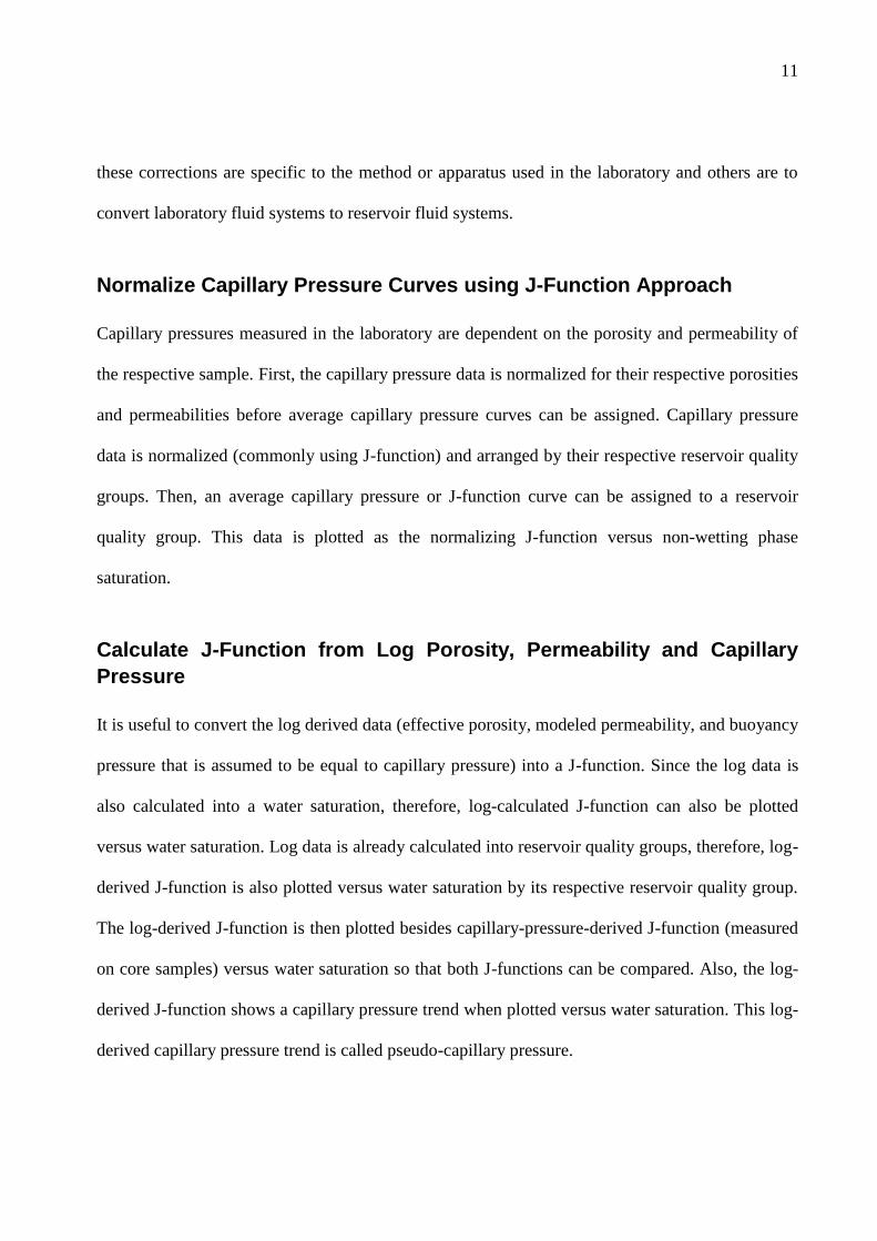
11

these corrections are specific to the method or apparatus used in the laboratory and others are to

convert laboratory fluid systems to reservoir fluid systems.

Normalize Capillary Pressure Curves using J-Function Approach

Capillary pressures measured in the laboratory are dependent on the porosity and permeability of

the respective sample. First, the capillary pressure data is normalized for their respective porosities

and permeabilities before average capillary pressure curves can be assigned. Capillary pressure

data is normalized (commonly using J-function) and arranged by their respective reservoir quality

groups. Then, an average capillary pressure or J-function curve can be assigned to a reservoir

quality group. This data is plotted as the normalizing J-function versus non-wetting phase

saturation.

Calculate J-Function from Log Porosity, Permeability and Capillary

Pressure

It is useful to convert the log derived data (effective porosity, modeled permeability, and buoyancy

pressure that is assumed to be equal to capillary pressure) into a J-function. Since the log data is

also calculated into a water saturation, therefore, log-calculated J-function can also be plotted

versus water saturation. Log data is already calculated into reservoir quality groups, therefore, log-

derived J-function is also plotted versus water saturation by its respective reservoir quality group.

The log-derived J-function is then plotted besides capillary-pressure-derived J-function (measured

on core samples) versus water saturation so that both J-functions can be compared. Also, the log-

derived J-function shows a capillary pressure trend when plotted versus water saturation. This log-

derived capillary pressure trend is called pseudo-capillary pressure.

12

Fit J Curves to Rock Quality Groups

Once capillary-pressure-derived J-functions and log-derived J-functions are plotted versus water

saturation, then, it is feasible to assign an average J-curve to each reservoir quality group.

Calculate Water Saturation Profiles from J Curves

This average J-curve is then used to compute water saturation in the three-dimensional geological

model in any grid block. Water saturations are also calculated from J-functions for each reservoir

quality group and assembled for a well as a log. The J-function water saturations are then

compared with log-derived water saturation for comparison.

13

Chapter 2

Theory of Saturation Height Modelling

Introduction

Modelling of water saturation versus height in an oil or gas reservoir is based on capillary pressure

concept. The understanding of capillary pressure behavior in a porous solid is vital to reservoir

characterization and hydrocarbon production. Capillary behavior is not well understood and often

not applied properly in reservoir characterization. Capillary behavior in a porous solid is the most

important factor that determines the distribution of hydrocarbons in a reservoir.

It is very important to determine a reservoir‟s saturation profile. Saturation interpreted from well

logs does not always give the complete picture. Accuracy of the saturation computed from logs is

influenced by thin-beds, insufficient column penetration, invasion, uncertainty in the Archie and

shaly sand parameters and reservoir heterogeneity (Amabeoku et al., 2006) and (Darling, 2005).

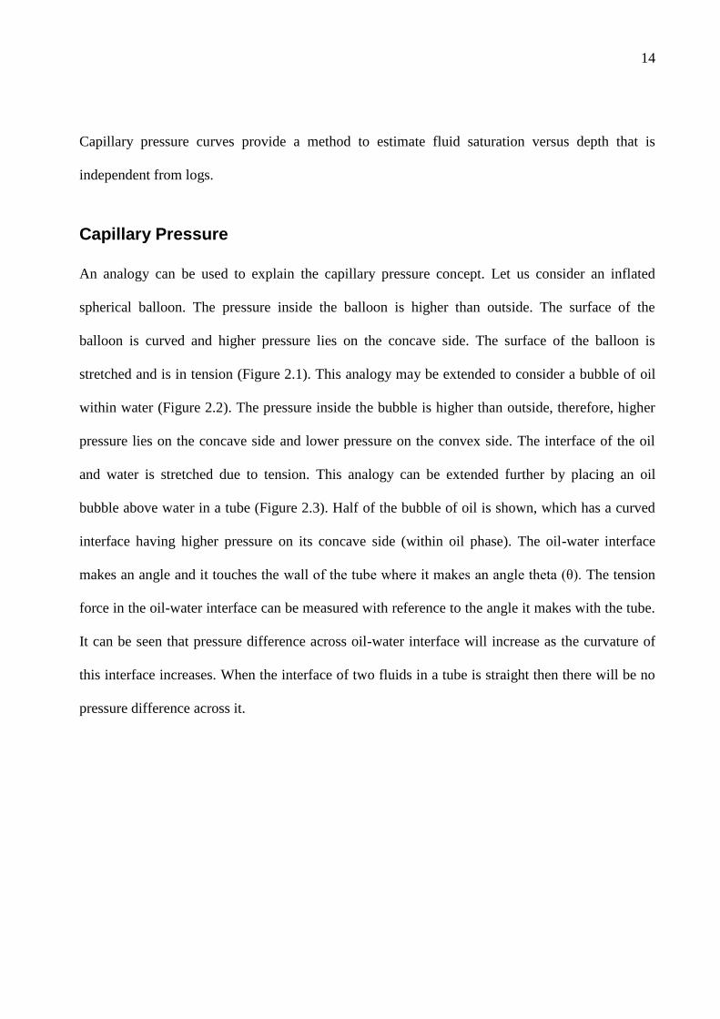
14

Capillary pressure curves provide a method to estimate fluid saturation versus depth that is

independent from logs.

Capillary Pressure

An analogy can be used to explain the capillary pressure concept. Let us consider an inflated

spherical balloon. The pressure inside the balloon is higher than outside. The surface of the

balloon is curved and higher pressure lies on the concave side. The surface of the balloon is

stretched and is in tension (Figure 2.1). This analogy may be extended to consider a bubble of oil

within water (Figure 2.2). The pressure inside the bubble is higher than outside, therefore, higher

pressure lies on the concave side and lower pressure on the convex side. The interface of the oil

and water is stretched due to tension. This analogy can be extended further by placing an oil

bubble above water in a tube (Figure 2.3). Half of the bubble of oil is shown, which has a curved

interface having higher pressure on its concave side (within oil phase). The oil-water interface

makes an angle and it touches the wall of the tube where it makes an angle theta (θ). The tension

force in the oil-water interface can be measured with reference to the angle it makes with the tube.

It can be seen that pressure difference across oil-water interface will increase as the curvature of

this interface increases. When the interface of two fluids in a tube is straight then there will be no

pressure difference across it.

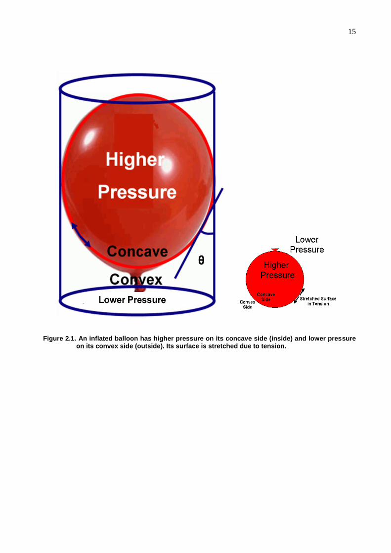
15

Figure 2.1. An inflated balloon has higher pressure on its concave side (inside) and lower pressure on its convex side (outside). Its surface is stretched due to tension.

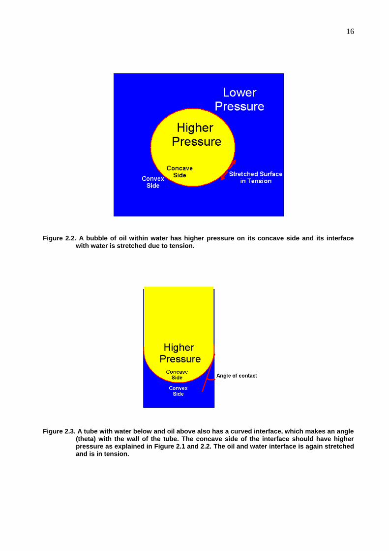
16

Figure 2.2. A bubble of oil within water has higher pressure on its concave side and its interface with water is stretched due to tension.

Figure 2.3. A tube with water below and oil above also has a curved interface, which makes an angle (theta) with the wall of the tube. The concave side of the interface should have higher pressure as explained in Figure 2.1 and 2.2. The oil and water interface is again stretched and is in tension.

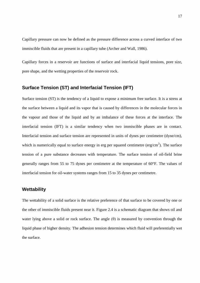
17

Capillary pressure can now be defined as the pressure difference across a curved interface of two

immiscible fluids that are present in a capillary tube (Archer and Wall, 1986).

Capillary forces in a reservoir are functions of surface and interfacial liquid tensions, pore size,

pore shape, and the wetting properties of the reservoir rock.

Surface Tension (ST) and Interfacial Tension (IFT)

Surface tension (ST) is the tendency of a liquid to expose a minimum free surface. It is a stress at

the surface between a liquid and its vapor that is caused by differences in the molecular forces in

the vapour and those of the liquid and by an imbalance of these forces at the interface. The

interfacial tension (IFT) is a similar tendency when two immiscible phases are in contact.

Interfacial tension and surface tension are represented in units of dynes per centimetre (dyne/cm),

which is numerically equal to surface energy in erg per squared centimetre (erg/cm2). The surface

tension of a pure substance decreases with temperature. The surface tension of oil-field brine

generally ranges from 55 to 75 dynes per centimetre at the temperature of 60°F. The values of

interfacial tension for oil-water systems ranges from 15 to 35 dynes per centimetre.

Wettability

The wettability of a solid surface is the relative preference of that surface to be covered by one or

the other of immiscible fluids present near it. Figure 2.4 is a schematic diagram that shows oil and

water lying above a solid or rock surface. The angle (θ) is measured by convention through the

liquid phase of higher density. The adhesion tension determines which fluid will preferentially wet

the surface.

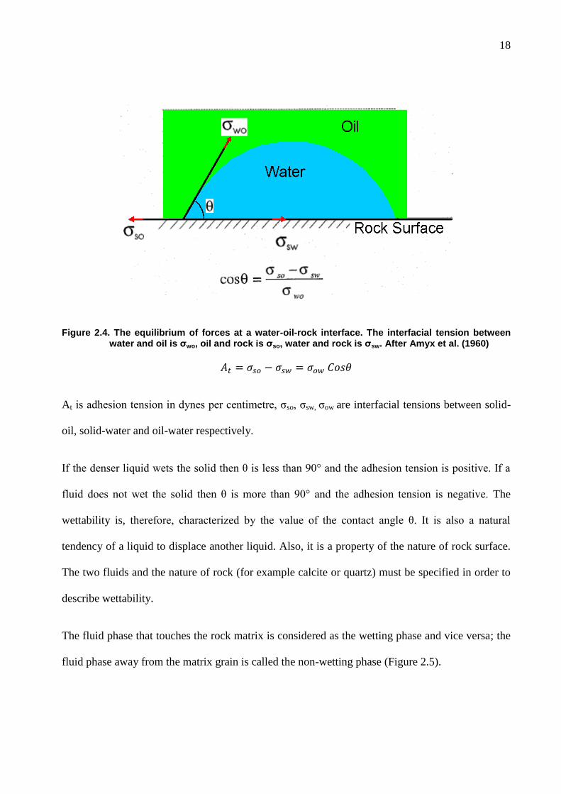
18

Figure 2.4. The equilibrium of forces at a water-oil-rock interface. The interfacial tension between water and oil is σwo, oil and rock is σso, water and rock is σsw. After Amyx et al. (1960)

At is adhesion tension in dynes per centimetre, σso, σsw, σow are interfacial tensions between solid-

oil, solid-water and oil-water respectively.

If the denser liquid wets the solid then θ is less than 90° and the adhesion tension is positive. If a

fluid does not wet the solid then θ is more than 90° and the adhesion tension is negative. The

wettability is, therefore, characterized by the value of the contact angle θ. It is also a natural

tendency of a liquid to displace another liquid. Also, it is a property of the nature of rock surface.

The two fluids and the nature of rock (for example calcite or quartz) must be specified in order to

describe wettability.

The fluid phase that touches the rock matrix is considered as the wetting phase and vice versa; the

fluid phase away from the matrix grain is called the non-wetting phase (Figure 2.5).

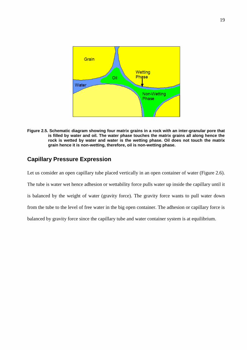
19

Figure 2.5. Schematic diagram showing four matrix grains in a rock with an inter-granular pore that is filled by water and oil. The water phase touches the matrix grains all along hence the rock is wetted by water and water is the wetting phase. Oil does not touch the matrix grain hence it is non-wetting, therefore, oil is non-wetting phase.

Capillary Pressure Expression

Let us consider an open capillary tube placed vertically in an open container of water (Figure 2.6).

The tube is water wet hence adhesion or wettability force pulls water up inside the capillary until it

is balanced by the weight of water (gravity force). The gravity force wants to pull water down

from the tube to the level of free water in the big open container. The adhesion or capillary force is

balanced by gravity force since the capillary tube and water container system is at equilibrium.

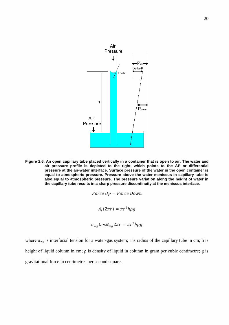
20

Figure 2.6. An open capillary tube placed vertically in a container that is open to air. The water and air pressure profile is depicted to the right, which points to the ΔP or differential pressure at the air-water interface. Surface pressure of the water in the open container is equal to atmospheric pressure. Pressure above the water meniscus in capillary tube is also equal to atmospheric pressure. The pressure variation along the height of water in the capillary tube results in a sharp pressure discontinuity at the meniscus interface.

where σwg is interfacial tension for a water-gas system; r is radius of the capillary tube in cm; h is

height of liquid column in cm; ρ is density of liquid in column in gram per cubic centimetre; g is

gravitational force in centimetres per second square.

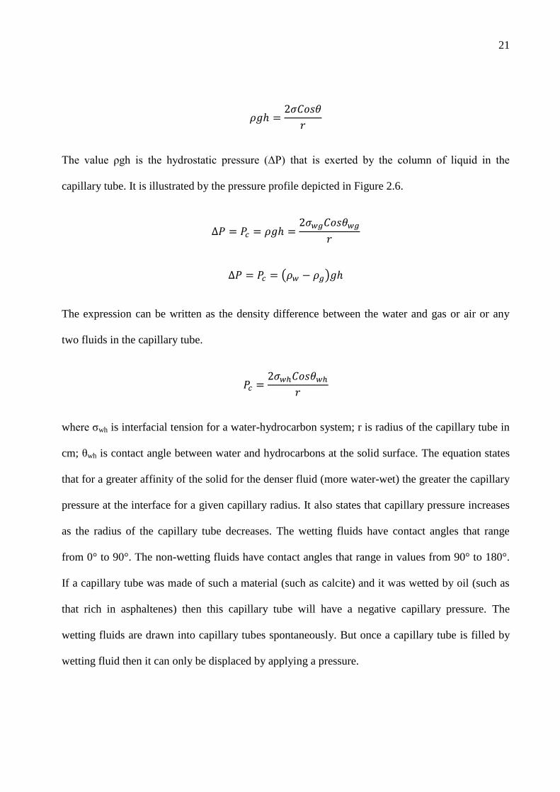
21

The value ρgh is the hydrostatic pressure (ΔP) that is exerted by the column of liquid in the

capillary tube. It is illustrated by the pressure profile depicted in Figure 2.6.

The expression can be written as the density difference between the water and gas or air or any

two fluids in the capillary tube.

where σwh is interfacial tension for a water-hydrocarbon system; r is radius of the capillary tube in

cm; θwh is contact angle between water and hydrocarbons at the solid surface. The equation states

that for a greater affinity of the solid for the denser fluid (more water-wet) the greater the capillary

pressure at the interface for a given capillary radius. It also states that capillary pressure increases

as the radius of the capillary tube decreases. The wetting fluids have contact angles that range

from 0° to 90°. The non-wetting fluids have contact angles that range in values from 90° to 180°.

If a capillary tube was made of such a material (such as calcite) and it was wetted by oil (such as

that rich in asphaltenes) then this capillary tube will have a negative capillary pressure. The

wetting fluids are drawn into capillary tubes spontaneously. But once a capillary tube is filled by

wetting fluid then it can only be displaced by applying a pressure.

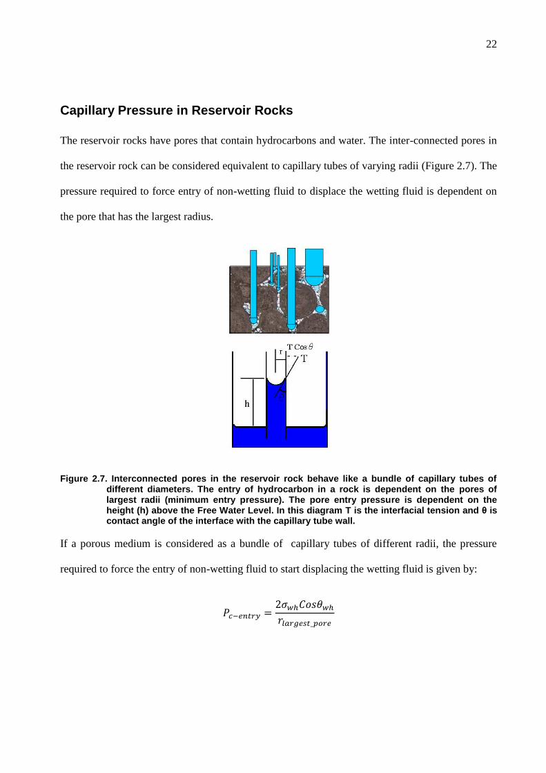
22

Capillary Pressure in Reservoir Rocks

The reservoir rocks have pores that contain hydrocarbons and water. The inter-connected pores in

the reservoir rock can be considered equivalent to capillary tubes of varying radii (Figure 2.7). The

pressure required to force entry of non-wetting fluid to displace the wetting fluid is dependent on

the pore that has the largest radius.

Figure 2.7. Interconnected pores in the reservoir rock behave like a bundle of capillary tubes of different diameters. The entry of hydrocarbon in a rock is dependent on the pores of largest radii (minimum entry pressure). The pore entry pressure is dependent on the height (h) above the Free Water Level. In this diagram T is the interfacial tension and θ is contact angle of the interface with the capillary tube wall.

If a porous medium is considered as a bundle of capillary tubes of different radii, the pressure

required to force the entry of non-wetting fluid to start displacing the wetting fluid is given by:

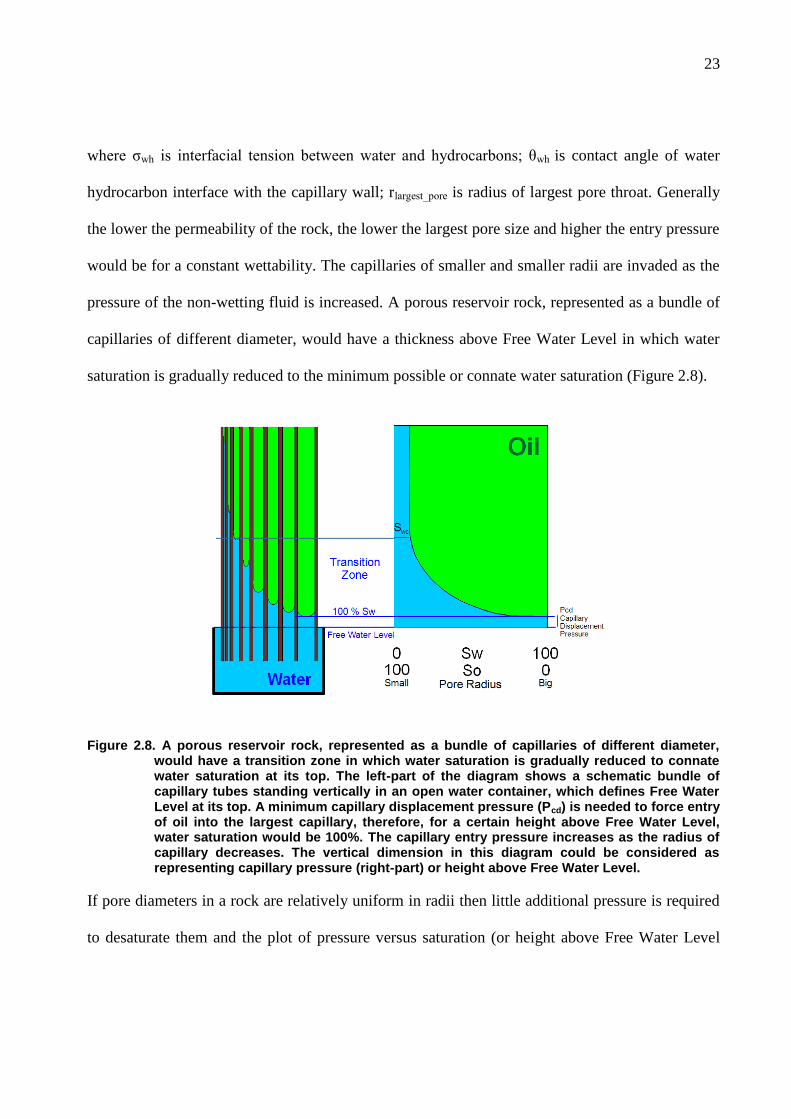
23

where σwh is interfacial tension between water and hydrocarbons; θwh is contact angle of water

hydrocarbon interface with the capillary wall; rlargest_pore is radius of largest pore throat. Generally

the lower the permeability of the rock, the lower the largest pore size and higher the entry pressure

would be for a constant wettability. The capillaries of smaller and smaller radii are invaded as the

pressure of the non-wetting fluid is increased. A porous reservoir rock, represented as a bundle of

capillaries of different diameter, would have a thickness above Free Water Level in which water

saturation is gradually reduced to the minimum possible or connate water saturation (Figure 2.8).

Figure 2.8. A porous reservoir rock, represented as a bundle of capillaries of different diameter, would have a transition zone in which water saturation is gradually reduced to connate water saturation at its top. The left-part of the diagram shows a schematic bundle of capillary tubes standing vertically in an open water container, which defines Free Water Level at its top. A minimum capillary displacement pressure (Pcd) is needed to force entry of oil into the largest capillary, therefore, for a certain height above Free Water Level, water saturation would be 100%. The capillary entry pressure increases as the radius of capillary decreases. The vertical dimension in this diagram could be considered as representing capillary pressure (right-part) or height above Free Water Level.

If pore diameters in a rock are relatively uniform in radii then little additional pressure is required

to desaturate them and the plot of pressure versus saturation (or height above Free Water Level

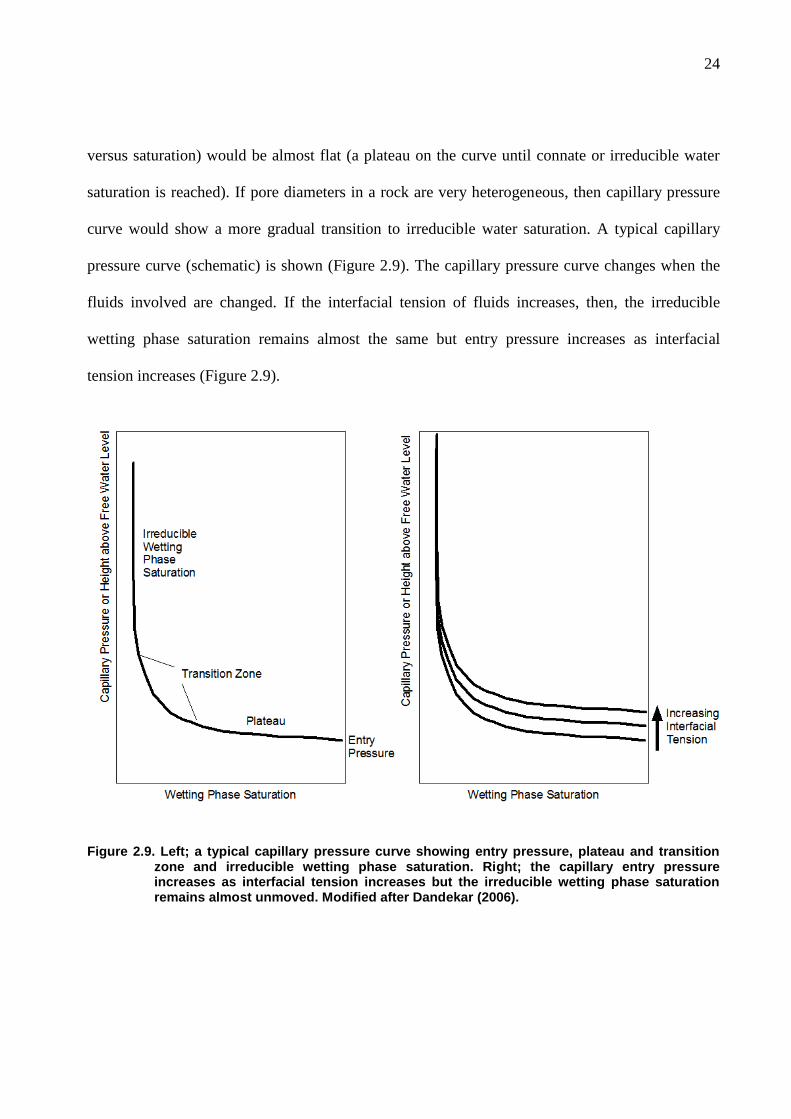
24

versus saturation) would be almost flat (a plateau on the curve until connate or irreducible water

saturation is reached). If pore diameters in a rock are very heterogeneous, then capillary pressure

curve would show a more gradual transition to irreducible water saturation. A typical capillary

pressure curve (schematic) is shown (Figure 2.9). The capillary pressure curve changes when the

fluids involved are changed. If the interfacial tension of fluids increases, then, the irreducible

wetting phase saturation remains almost the same but entry pressure increases as interfacial

tension increases (Figure 2.9).

Figure 2.9. Left; a typical capillary pressure curve showing entry pressure, plateau and transition zone and irreducible wetting phase saturation. Right; the capillary entry pressure increases as interfacial tension increases but the irreducible wetting phase saturation remains almost unmoved. Modified after Dandekar (2006).

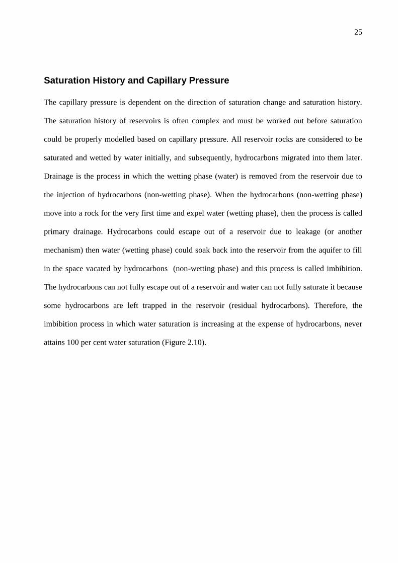
25

Saturation History and Capillary Pressure

The capillary pressure is dependent on the direction of saturation change and saturation history.

The saturation history of reservoirs is often complex and must be worked out before saturation

could be properly modelled based on capillary pressure. All reservoir rocks are considered to be

saturated and wetted by water initially, and subsequently, hydrocarbons migrated into them later.

Drainage is the process in which the wetting phase (water) is removed from the reservoir due to

the injection of hydrocarbons (non-wetting phase). When the hydrocarbons (non-wetting phase)

move into a rock for the very first time and expel water (wetting phase), then the process is called

primary drainage. Hydrocarbons could escape out of a reservoir due to leakage (or another

mechanism) then water (wetting phase) could soak back into the reservoir from the aquifer to fill

in the space vacated by hydrocarbons (non-wetting phase) and this process is called imbibition.

The hydrocarbons can not fully escape out of a reservoir and water can not fully saturate it because

some hydrocarbons are left trapped in the reservoir (residual hydrocarbons). Therefore, the

imbibition process in which water saturation is increasing at the expense of hydrocarbons, never

attains 100 per cent water saturation (Figure 2.10).

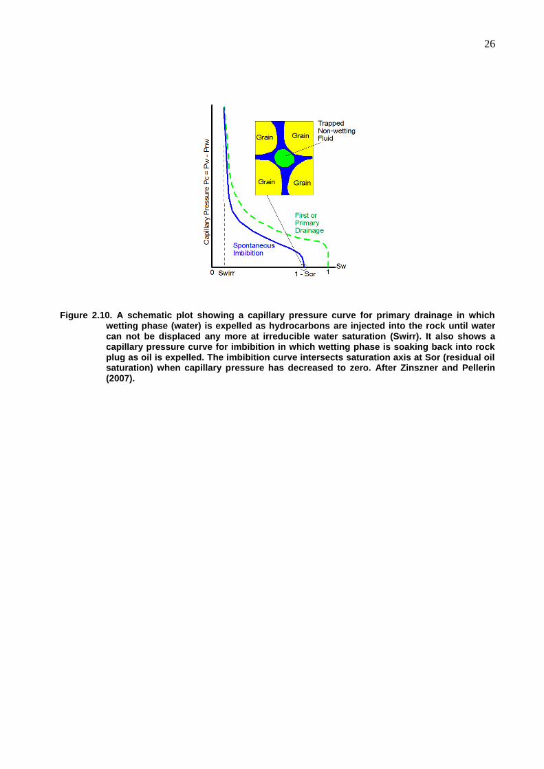
26

Figure 2.10. A schematic plot showing a capillary pressure curve for primary drainage in which wetting phase (water) is expelled as hydrocarbons are injected into the rock until water can not be displaced any more at irreducible water saturation (Swirr). It also shows a capillary pressure curve for imbibition in which wetting phase is soaking back into rock plug as oil is expelled. The imbibition curve intersects saturation axis at Sor (residual oil saturation) when capillary pressure has decreased to zero. After Zinszner and Pellerin (2007).

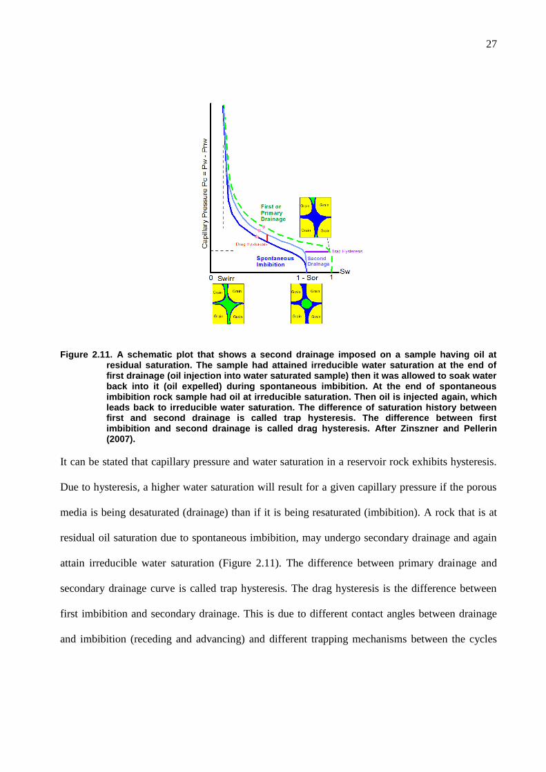
27

Figure 2.11. A schematic plot that shows a second drainage imposed on a sample having oil at residual saturation. The sample had attained irreducible water saturation at the end of first drainage (oil injection into water saturated sample) then it was allowed to soak water back into it (oil expelled) during spontaneous imbibition. At the end of spontaneous imbibition rock sample had oil at irreducible saturation. Then oil is injected again, which leads back to irreducible water saturation. The difference of saturation history between first and second drainage is called trap hysteresis. The difference between first imbibition and second drainage is called drag hysteresis. After Zinszner and Pellerin (2007).

It can be stated that capillary pressure and water saturation in a reservoir rock exhibits hysteresis.

Due to hysteresis, a higher water saturation will result for a given capillary pressure if the porous

media is being desaturated (drainage) than if it is being resaturated (imbibition). A rock that is at

residual oil saturation due to spontaneous imbibition, may undergo secondary drainage and again

attain irreducible water saturation (Figure 2.11). The difference between primary drainage and

secondary drainage curve is called trap hysteresis. The drag hysteresis is the difference between

first imbibition and secondary drainage. This is due to different contact angles between drainage

and imbibition (receding and advancing) and different trapping mechanisms between the cycles

28

(Figure 2.12). The drag hysteresis is the true hysteresis because if the spontaneous imbibition and

secondary drainage cycles are repeated, then the same curves should result (provided that

wettability does not change). There is no hysteresis between primary drainage and spontaneous

imbibition cycles because the difference arises due to permanent trapping of some of the non-

wetting fluid (Zinszner and Pellerin, 2007).

Figure 2.12. Advancing (θa) and receding (θr) angles of a drop of oil between a stationary top plate and a displacing bottom plate (Leach et al., 1962; Donaldson & Alam, 2008). This oil drop is made to move in water by displacing the lower plate very slowly while keeping the upper plate stationary. It simulates water displacement by oil in a capillary (drainage process), which has an advancing angle. It also simulates oil displacement by water (imbibition process), which has oil receding angle.

The differences in capillary pressure between drainage and imbibition cycles are explained by the

different contact angles of the oil-water interface.

Generally, water-phase desaturation is referred to as the drainage cycle and water-phase increasing

is referred to as imbibition (this is true only when water is the wetting phase). In oil-wet porous

medium, this does not apply because the water is the non-wetting phase. The drainage and

imbibition capillary pressure cycles have different patterns for oil-wet and water-wet rock.

The capillary pressure cycle as measured on a water-wet core is shown in Figure 2.13. This cycle

is measured by first injecting oil into a water-saturated core (primary drainage) that is followed by

spontaneous imbibition of water (oil expulsion) until capillary pressure drops to zero (part of

previously injected oil is recovered and oil saturation is reduced to Sor, that is residual oil

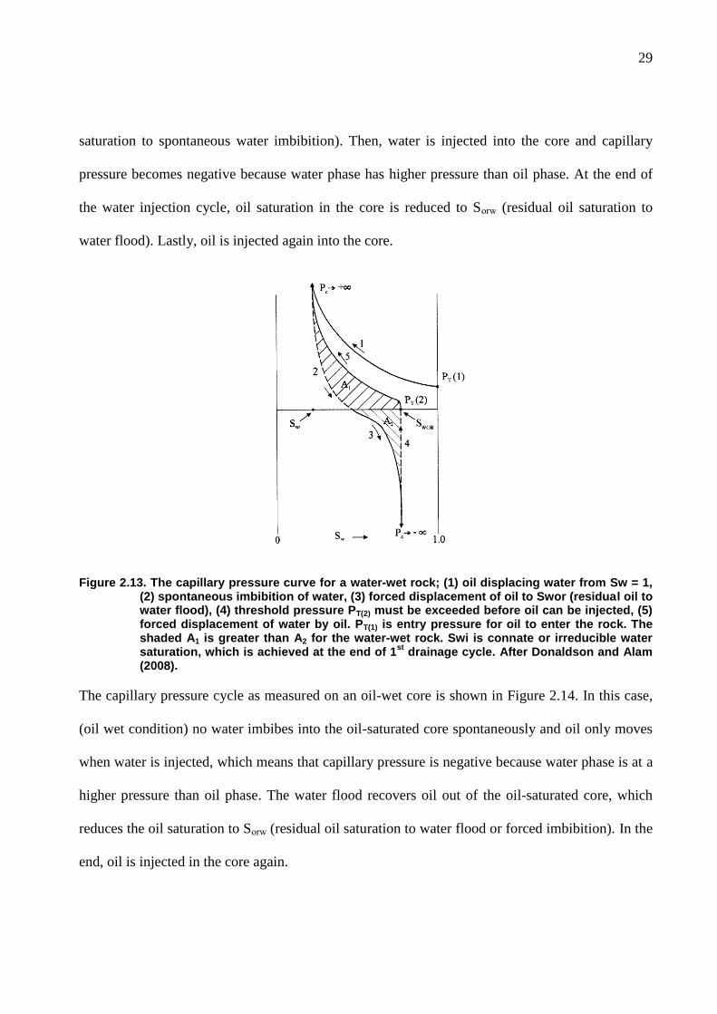
29

saturation to spontaneous water imbibition). Then, water is injected into the core and capillary

pressure becomes negative because water phase has higher pressure than oil phase. At the end of

the water injection cycle, oil saturation in the core is reduced to Sorw (residual oil saturation to

water flood). Lastly, oil is injected again into the core.

Figure 2.13. The capillary pressure curve for a water-wet rock; (1) oil displacing water from Sw = 1, (2) spontaneous imbibition of water, (3) forced displacement of oil to Swor (residual oil to water flood), (4) threshold pressure PT(2) must be exceeded before oil can be injected, (5) forced displacement of water by oil. PT(1) is entry pressure for oil to enter the rock. The shaded A1 is greater than A2 for the water-wet rock. Swi is connate or irreducible water saturation, which is achieved at the end of 1

st drainage cycle. After Donaldson and Alam

(2008).

The capillary pressure cycle as measured on an oil-wet core is shown in Figure 2.14. In this case,

(oil wet condition) no water imbibes into the oil-saturated core spontaneously and oil only moves

when water is injected, which means that capillary pressure is negative because water phase is at a

higher pressure than oil phase. The water flood recovers oil out of the oil-saturated core, which

reduces the oil saturation to Sorw (residual oil saturation to water flood or forced imbibition). In the

end, oil is injected in the core again.

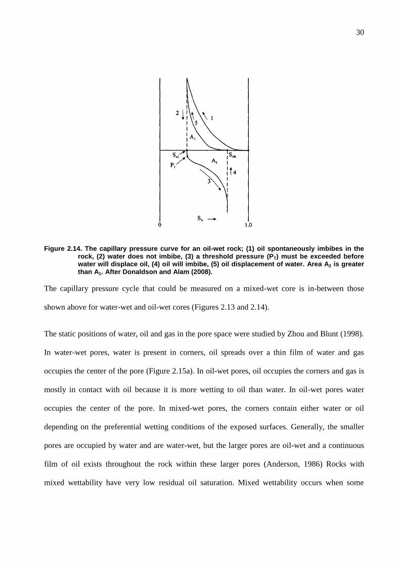
30

Figure 2.14. The capillary pressure curve for an oil-wet rock; (1) oil spontaneously imbibes in the rock, (2) water does not imbibe, (3) a threshold pressure (PT) must be exceeded before water will displace oil, (4) oil will imbibe, (5) oil displacement of water. Area A2 is greater than A1. After Donaldson and Alam (2008).

The capillary pressure cycle that could be measured on a mixed-wet core is in-between those

shown above for water-wet and oil-wet cores (Figures 2.13 and 2.14).

The static positions of water, oil and gas in the pore space were studied by Zhou and Blunt (1998).

In water-wet pores, water is present in corners, oil spreads over a thin film of water and gas

occupies the center of the pore (Figure 2.15a). In oil-wet pores, oil occupies the corners and gas is

mostly in contact with oil because it is more wetting to oil than water. In oil-wet pores water

occupies the center of the pore. In mixed-wet pores, the corners contain either water or oil

depending on the preferential wetting conditions of the exposed surfaces. Generally, the smaller

pores are occupied by water and are water-wet, but the larger pores are oil-wet and a continuous

film of oil exists throughout the rock within these larger pores (Anderson, 1986) Rocks with

mixed wettability have very low residual oil saturation. Mixed wettability occurs when some

31

organic compounds included in the oil react with the water-wet surface of the rock. This reaction

displaces the aqueous film on the rock‟s surface, creating a new oil-wet coating on it (Tiab and

Donaldson, 2004).

Figure 2.15. (a) fluid phase distribution in water-wet pore, (b) fluid phase distribution in oil-wet pore, (c) fluid phase distribution in mixed-wet pore. The blue represents water, green represents oil and red represents gas phase. After Zhou and Blunt (1998).

Definition of Fluid Contacts

It is essential to identify fluid contacts before water saturation can be modelled. It is essential also

to clearly define fluid contacts and distinguish between various kinds of fluid contacts. The subject

of fluid contacts is very complex. So, it useful to describe it first in the most simple situation. It is

assumed that an oil and cap-gas reservoir (water-wet) consists of a rock whose pore geometry is

uniform hence it can be described by a single capillary pressure curve (Figure 2.16).

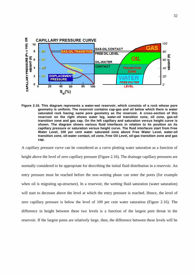
32

Figure 2.16. This diagram represents a water-wet reservoir, which consists of a rock whose pore geometry is uniform. The reservoir contains cap-gas and oil below which there is water saturated rock having same pore geometry as the reservoir. A cross-section of this reservoir on the right shows water leg, water-oil transition zone, oil zone, gas-oil transition zone and gas cap. On the left capillary and saturation versus height curve is shown. The diagram shows various fluid interfaces in relation to its position on its capillary pressure or saturation versus height curve. The fluid interfaces start from Free Water Level, 100 per cent water saturated zone above Free Water Level, water-oil transition zone, oil-water contact, oil zone, Free Oil Level, oil-gas transition zone and gas cap.

A capillary pressure curve can be considered as a curve plotting water saturation as a function of

height above the level of zero capillary pressure (Figure 2.16). The drainage capillary pressures are

normally considered to be appropriate for describing the initial fluid distribution in a reservoir. An

entry pressure must be reached before the non-wetting phase can enter the pores (for example

when oil is migrating up-structure). In a reservoir, the wetting fluid saturation (water saturation)

will start to decrease above the level at which the entry pressure is reached. Hence, the level of

zero capillary pressure is below the level of 100 per cent water saturation (Figure 2.16). The

difference in height between these two levels is a function of the largest pore throat in the

reservoir. If the largest pores are relatively large, then, the difference between these levels will be

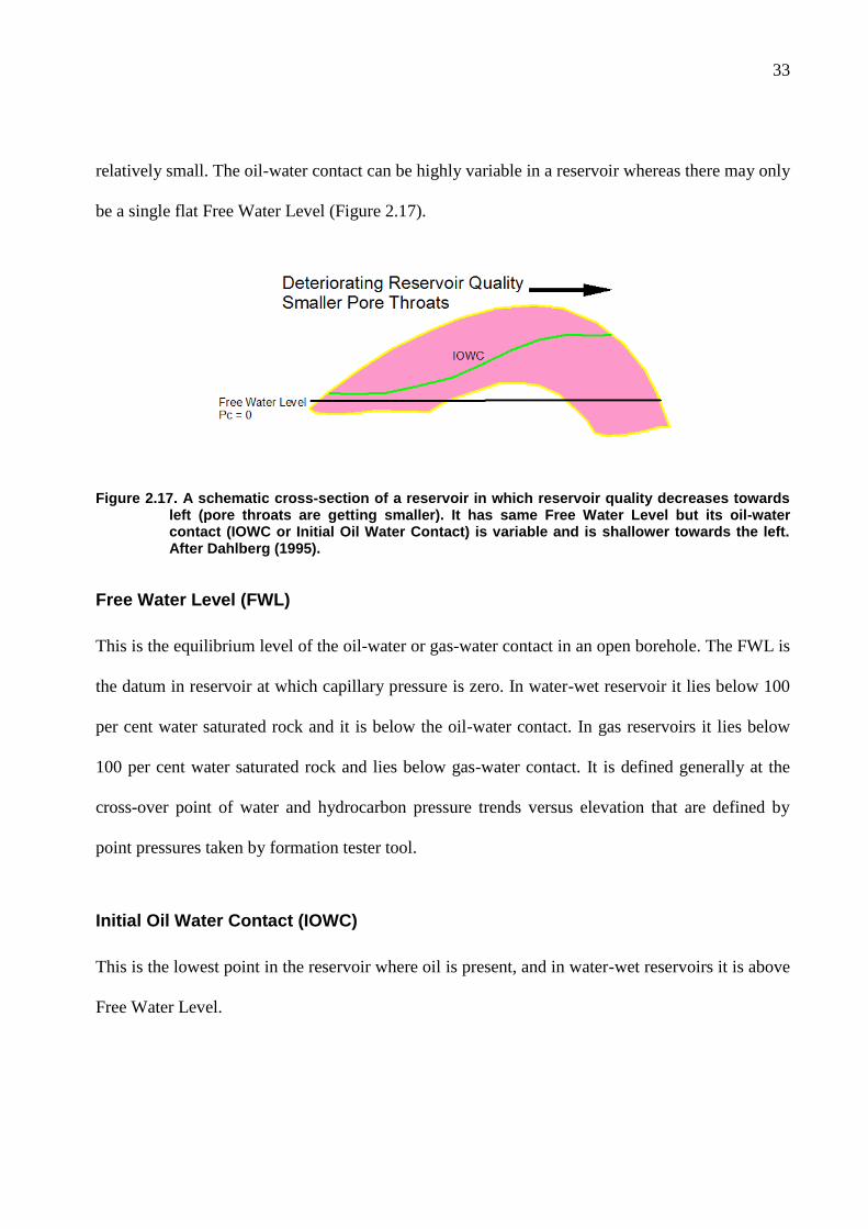
33

relatively small. The oil-water contact can be highly variable in a reservoir whereas there may only

be a single flat Free Water Level (Figure 2.17).

Figure 2.17. A schematic cross-section of a reservoir in which reservoir quality decreases towards left (pore throats are getting smaller). It has same Free Water Level but its oil-water contact (IOWC or Initial Oil Water Contact) is variable and is shallower towards the left. After Dahlberg (1995).

Free Water Level (FWL)

This is the equilibrium level of the oil-water or gas-water contact in an open borehole. The FWL is

the datum in reservoir at which capillary pressure is zero. In water-wet reservoir it lies below 100

per cent water saturated rock and it is below the oil-water contact. In gas reservoirs it lies below

100 per cent water saturated rock and lies below gas-water contact. It is defined generally at the

cross-over point of water and hydrocarbon pressure trends versus elevation that are defined by

point pressures taken by formation tester tool.

Initial Oil Water Contact (IOWC)

This is the lowest point in the reservoir where oil is present, and in water-wet reservoirs it is above

Free Water Level.

34

Producing Oil Water Contact (POWC)

This is the lowest point in the reservoir where oil is produced. It corresponds with the level at

which oil saturation is just above the residual oil saturation.

Economic Oil Water Contact (EOWC)

This is the level in the reservoir where oil production is at or above a minimum required oil rate.

Completion or Dry Oil Water Contact (COWC)

This is the lowest level in the reservoir where no water is produced. It corresponds to the top of

transition zone or the level at which water saturation has decreased to irreducible water saturation.

Initial Oil Water Transition Zone

This is the vertical distance between the Initial Oil Water Contact (IOWC) and Completion Oil

Water Contact (COWC).

Producing Oil Water Transition Zone

This is vertical distance between the Producing Oil Water Contact (POWC) and top of transition

zone where water saturation is at irreducible level. In this interval water and oil are produced

together.

35

Connate Water Saturation (Swc)

This is initial water saturation at any point in the reservoir. It decreases with height above the

IOWC.

Irreducible Water Saturation (Swirr)

This is the minimum water saturation that can be obtained by oil displacing water. The lowest

level of Swirr is at the top of the water-oil transition zone.

Free Oil Level (FOL)

This is the level of gas-oil contact where gas-oil capillary pressure is zero. It lies below the gas-oil

contact. It is generally defined at the cross-over of gas and oil pressures trends versus elevation

that are defined by point pressures taken by formation tester tool.

Gas Oil Contact (GOC)

This is the level in the reservoir where free gas is present in the pore spaces. It is generally defined

by logs (resistivity, density and neutron).

Gas Oil Transition Zone

This is the vertical thickness between Free Oil Level and Gas Oil Contact. This thickness is

generally very small (one or two feet) but it can be thick (several tens to hundreds of feet) in low

permeability (permeability less than 0.1 mD).

36

Fluid Contacts in Water- and Oil-Wet Reservoirs

In an oil-wet reservoir, Free Water Level (as defined by pressure profiles versus elevation) is

above the oil-water contact. The FWL in oil-wet reservoir plots well within the oil column that is

defined from resistivity and porosity logs. The geometry of Free Water Level and oil-water contact

is defined in terms of capillary pressure and pressure-elevation profile (Figure 2.18). The capillary

pressure curve for a water-wet reservoir is apparently inverted in an oil-wet reservoir. The

geometry of pressure-elevation profiles is particularly important in both cases. In an oil-wet

reservoir, water pressure line apparently lies relatively to the right of the oil pressure line and point

pressures taken near Free Water Level are scattered. Another important factor is the difference in

the shapes of the capillary pressure curves. The capillary pressure curves can be taken as a proxy

of water saturation versus height. The capillary pressure or water saturation versus height profile is

very steep in oil-wet reservoirs. Commonly, oil-wet or mixed-wet reservoirs exhibit an atypical

water saturation versus height profile, which have two distinct curvatures. The oil- or mixed-wet

reservoir, if modeled with drainage capillary pressures, falls much short of water saturation that is

interpreted from resistivity and porosity logs. Often, imbibitions type capillary pressure curves

(very steep curves) are necessary to model oil- or mixed-wet reservoir water saturations.

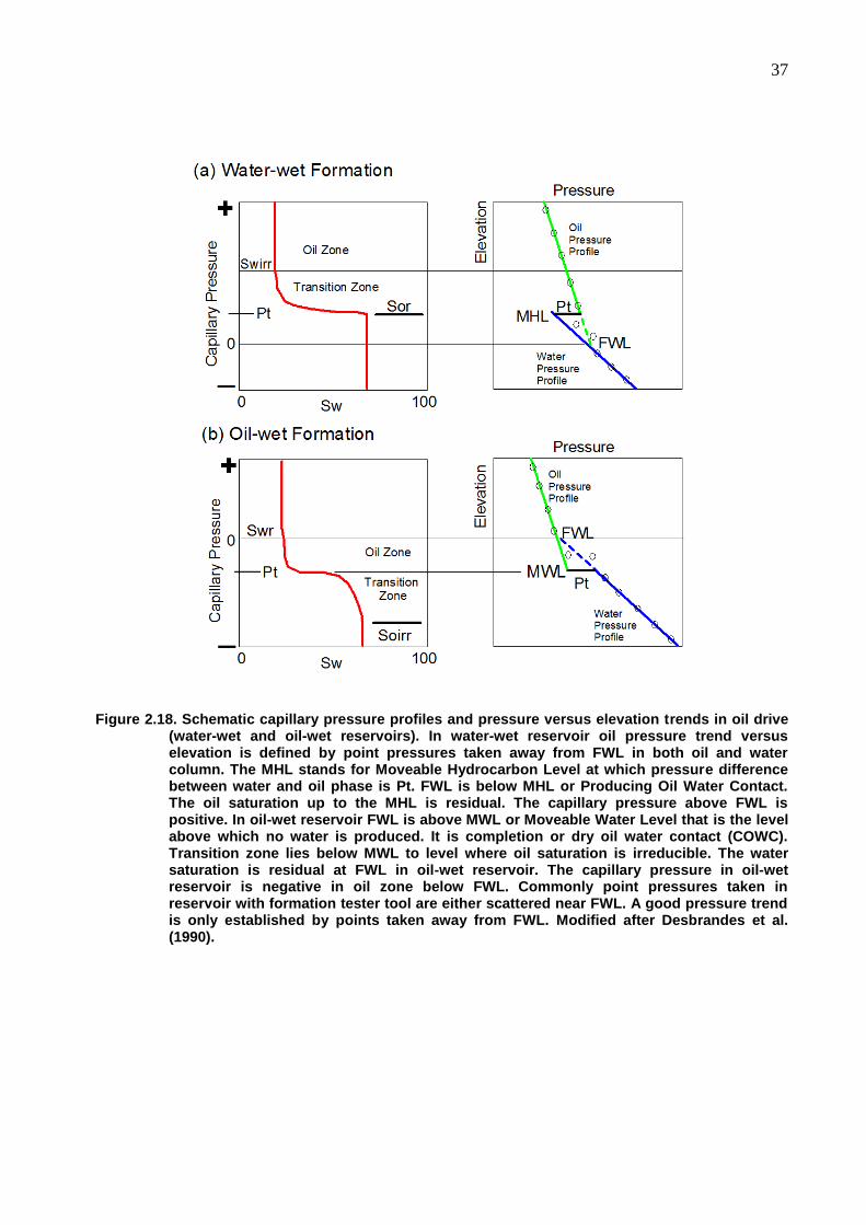
37

Figure 2.18. Schematic capillary pressure profiles and pressure versus elevation trends in oil drive (water-wet and oil-wet reservoirs). In water-wet reservoir oil pressure trend versus elevation is defined by point pressures taken away from FWL in both oil and water column. The MHL stands for Moveable Hydrocarbon Level at which pressure difference between water and oil phase is Pt. FWL is below MHL or Producing Oil Water Contact. The oil saturation up to the MHL is residual. The capillary pressure above FWL is positive. In oil-wet reservoir FWL is above MWL or Moveable Water Level that is the level above which no water is produced. It is completion or dry oil water contact (COWC). Transition zone lies below MWL to level where oil saturation is irreducible. The water saturation is residual at FWL in oil-wet reservoir. The capillary pressure in oil-wet reservoir is negative in oil zone below FWL. Commonly point pressures taken in reservoir with formation tester tool are either scattered near FWL. A good pressure trend is only established by points taken away from FWL. Modified after Desbrandes et al. (1990).

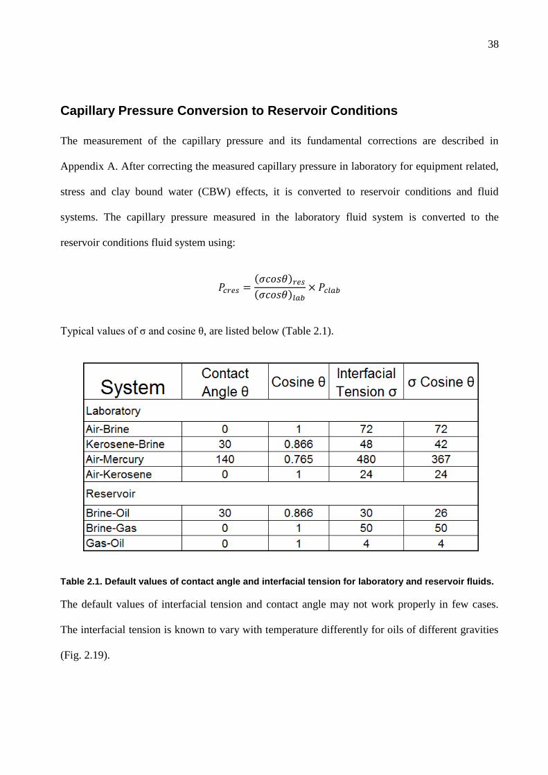
38

Capillary Pressure Conversion to Reservoir Conditions

The measurement of the capillary pressure and its fundamental corrections are described in

Appendix A. After correcting the measured capillary pressure in laboratory for equipment related,

stress and clay bound water (CBW) effects, it is converted to reservoir conditions and fluid

systems. The capillary pressure measured in the laboratory fluid system is converted to the

reservoir conditions fluid system using:

Typical values of σ and cosine θ, are listed below (Table 2.1).

Table 2.1. Default values of contact angle and interfacial tension for laboratory and reservoir fluids.

The default values of interfacial tension and contact angle may not work properly in few cases.

The interfacial tension is known to vary with temperature differently for oils of different gravities

(Fig. 2.19).

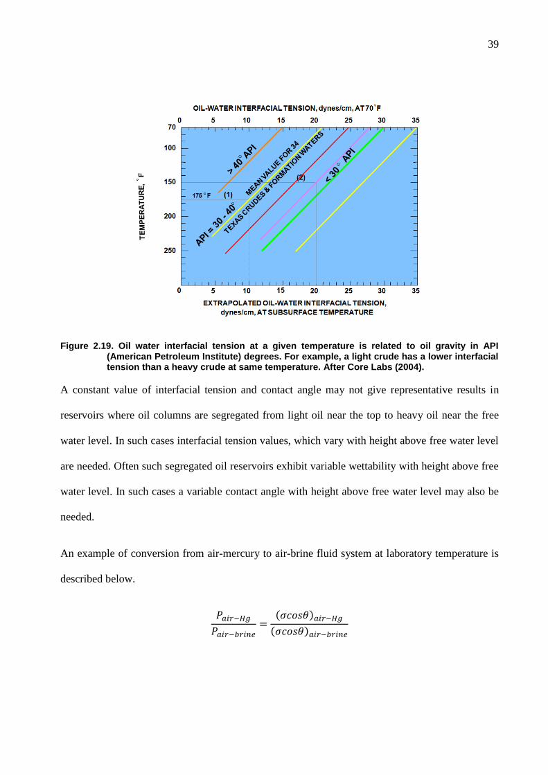
39

Figure 2.19. Oil water interfacial tension at a given temperature is related to oil gravity in API (American Petroleum Institute) degrees. For example, a light crude has a lower interfacial tension than a heavy crude at same temperature. After Core Labs (2004).

A constant value of interfacial tension and contact angle may not give representative results in

reservoirs where oil columns are segregated from light oil near the top to heavy oil near the free

water level. In such cases interfacial tension values, which vary with height above free water level

are needed. Often such segregated oil reservoirs exhibit variable wettability with height above free

water level. In such cases a variable contact angle with height above free water level may also be

needed.

An example of conversion from air-mercury to air-brine fluid system at laboratory temperature is

described below.

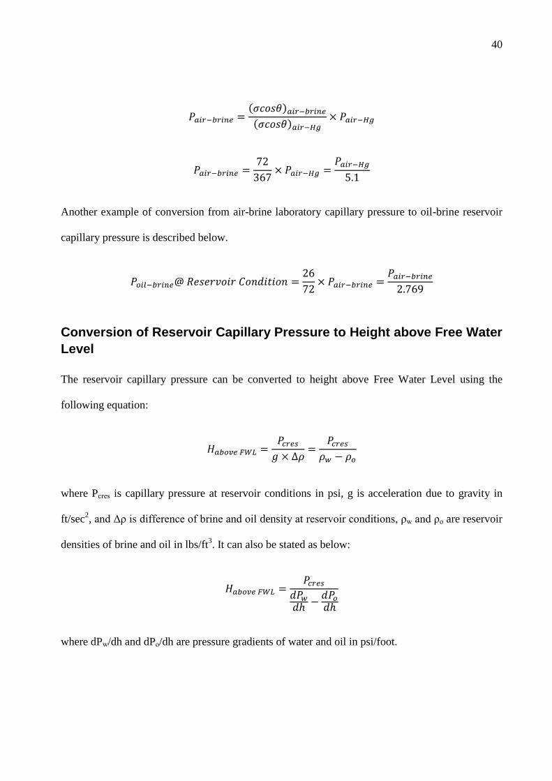
40

Another example of conversion from air-brine laboratory capillary pressure to oil-brine reservoir

capillary pressure is described below.

Conversion of Reservoir Capillary Pressure to Height above Free Water

Level

The reservoir capillary pressure can be converted to height above Free Water Level using the

following equation:

where Pcres is capillary pressure at reservoir conditions in psi, g is acceleration due to gravity in

ft/sec2, and Δρ is difference of brine and oil density at reservoir conditions, ρw and ρo are reservoir

densities of brine and oil in lbs/ft3. It can also be stated as below:

where dPw/dh and dPo/dh are pressure gradients of water and oil in psi/foot.

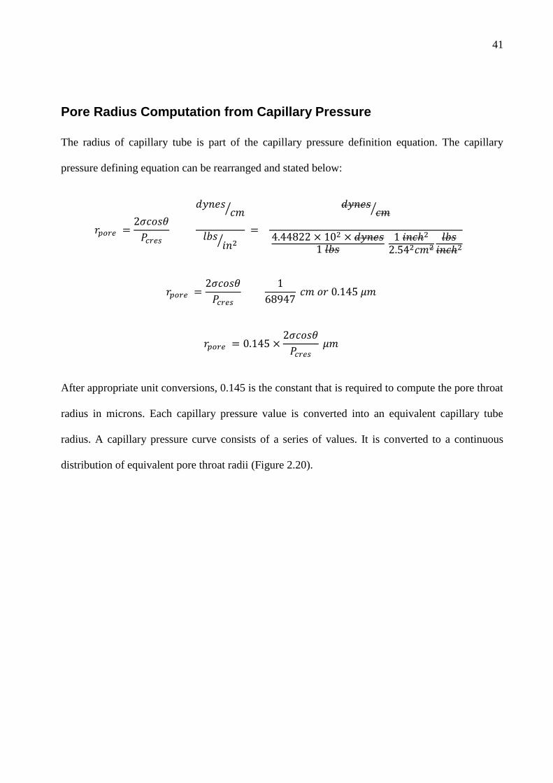
41

Pore Radius Computation from Capillary Pressure

The radius of capillary tube is part of the capillary pressure definition equation. The capillary

pressure defining equation can be rearranged and stated below:

After appropriate unit conversions, 0.145 is the constant that is required to compute the pore throat

radius in microns. Each capillary pressure value is converted into an equivalent capillary tube

radius. A capillary pressure curve consists of a series of values. It is converted to a continuous

distribution of equivalent pore throat radii (Figure 2.20).

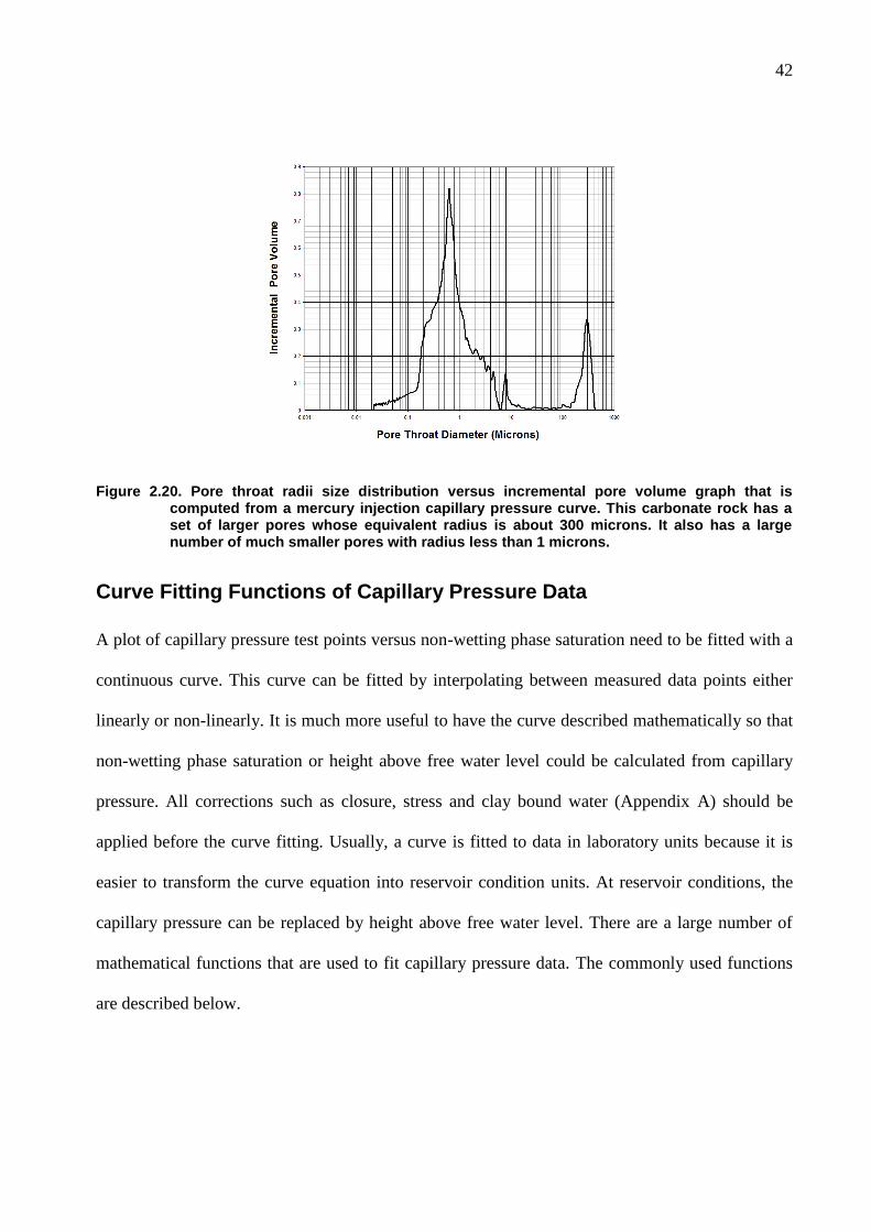
42

Figure 2.20. Pore throat radii size distribution versus incremental pore volume graph that is computed from a mercury injection capillary pressure curve. This carbonate rock has a set of larger pores whose equivalent radius is about 300 microns. It also has a large number of much smaller pores with radius less than 1 microns.

Curve Fitting Functions of Capillary Pressure Data

A plot of capillary pressure test points versus non-wetting phase saturation need to be fitted with a

continuous curve. This curve can be fitted by interpolating between measured data points either

linearly or non-linearly. It is much more useful to have the curve described mathematically so that

non-wetting phase saturation or height above free water level could be calculated from capillary

pressure. All corrections such as closure, stress and clay bound water (Appendix A) should be

applied before the curve fitting. Usually, a curve is fitted to data in laboratory units because it is

easier to transform the curve equation into reservoir condition units. At reservoir conditions, the

capillary pressure can be replaced by height above free water level. There are a large number of

mathematical functions that are used to fit capillary pressure data. The commonly used functions

are described below.

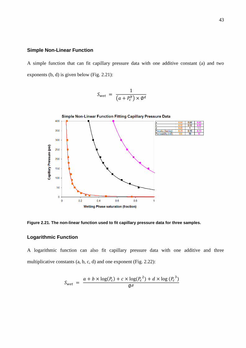
43

Simple Non-Linear Function

A simple function that can fit capillary pressure data with one additive constant (a) and two

exponents (b, d) is given below (Fig. 2.21):

Figure 2.21. The non-linear function used to fit capillary pressure data for three samples.

Logarithmic Function

A logarithmic function can also fit capillary pressure data with one additive and three

multiplicative constants (a, b, c, d) and one exponent (Fig. 2.22):

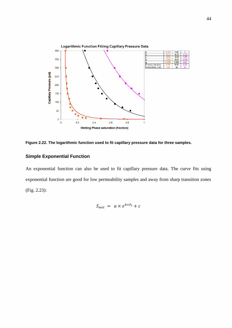
44

Figure 2.22. The logarithmic function used to fit capillary pressure data for three samples.

Simple Exponential Function

An exponential function can also be used to fit capillary pressure data. The curve fits using

exponential function are good for low permeability samples and away from sharp transition zones

(Fig. 2.23):

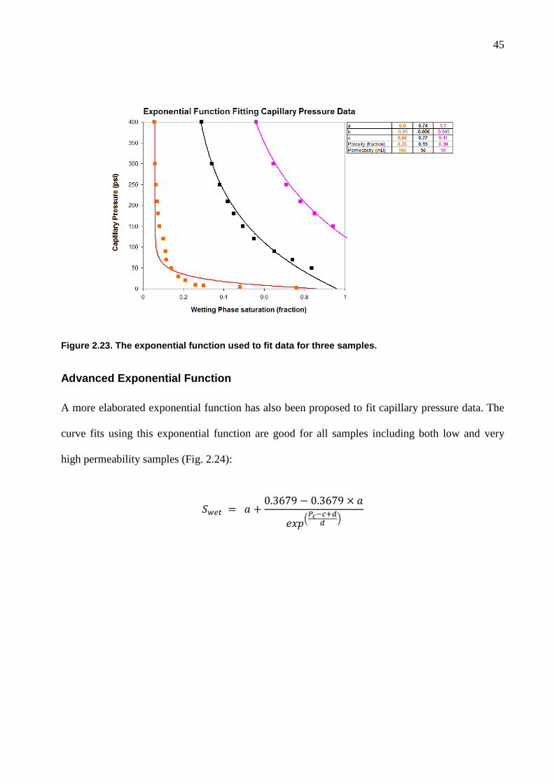
45

Figure 2.23. The exponential function used to fit data for three samples.

Advanced Exponential Function

A more elaborated exponential function has also been proposed to fit capillary pressure data. The

curve fits using this exponential function are good for all samples including both low and very

high permeability samples (Fig. 2.24):

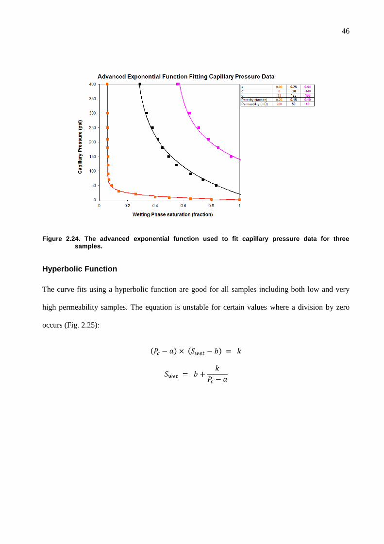
46

Figure 2.24. The advanced exponential function used to fit capillary pressure data for three samples.

Hyperbolic Function

The curve fits using a hyperbolic function are good for all samples including both low and very

high permeability samples. The equation is unstable for certain values where a division by zero

occurs (Fig. 2.25):

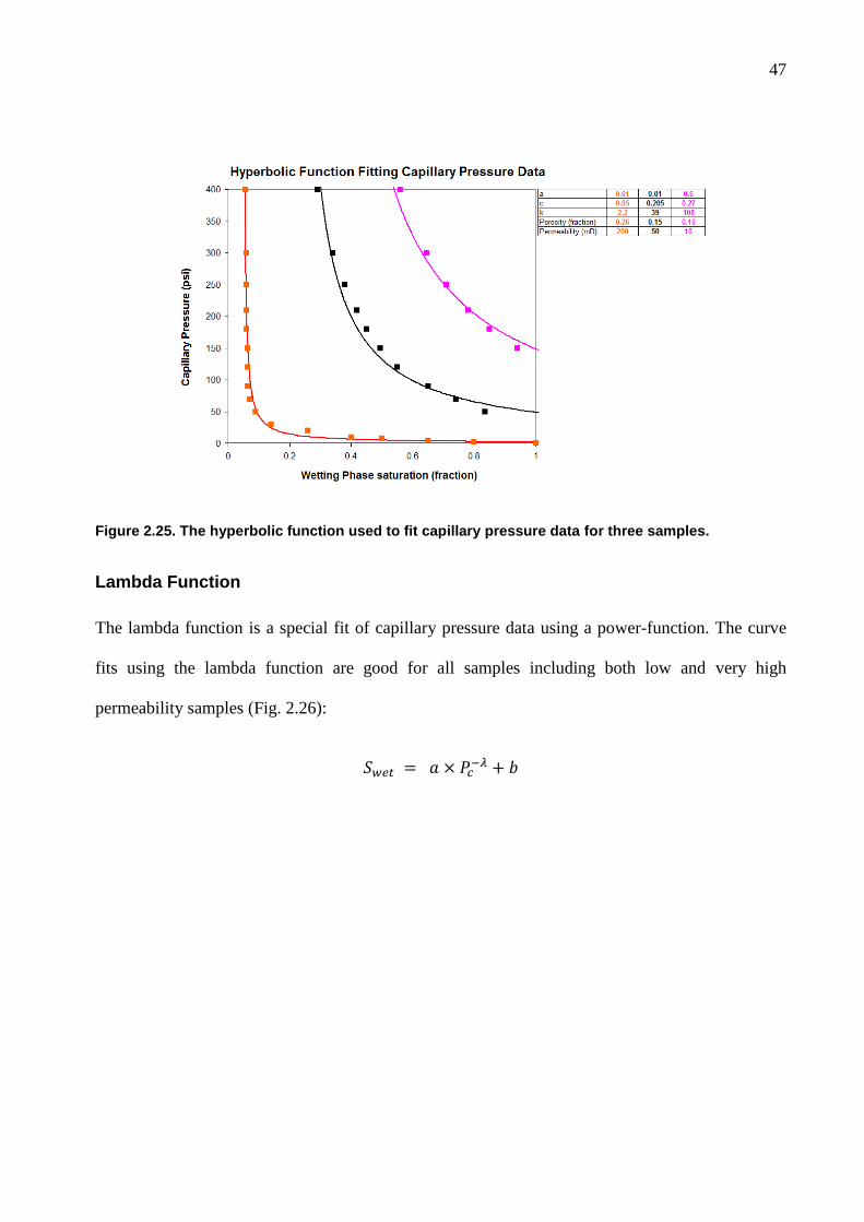
47

Figure 2.25. The hyperbolic function used to fit capillary pressure data for three samples.

Lambda Function

The lambda function is a special fit of capillary pressure data using a power-function. The curve

fits using the lambda function are good for all samples including both low and very high

permeability samples (Fig. 2.26):

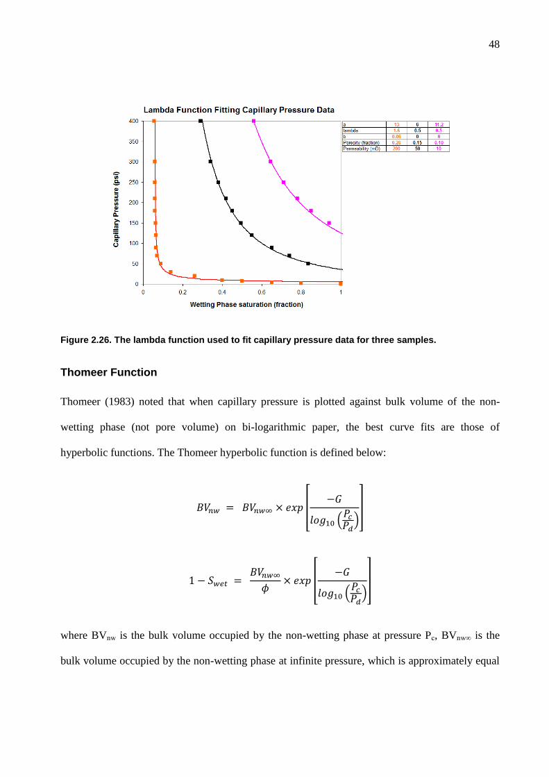
48

Figure 2.26. The lambda function used to fit capillary pressure data for three samples.

Thomeer Function

Thomeer (1983) noted that when capillary pressure is plotted against bulk volume of the non-

wetting phase (not pore volume) on bi-logarithmic paper, the best curve fits are those of

hyperbolic functions. The Thomeer hyperbolic function is defined below:

where BVnw is the bulk volume occupied by the non-wetting phase at pressure Pc, BVnw∞ is the

bulk volume occupied by the non-wetting phase at infinite pressure, which is approximately equal

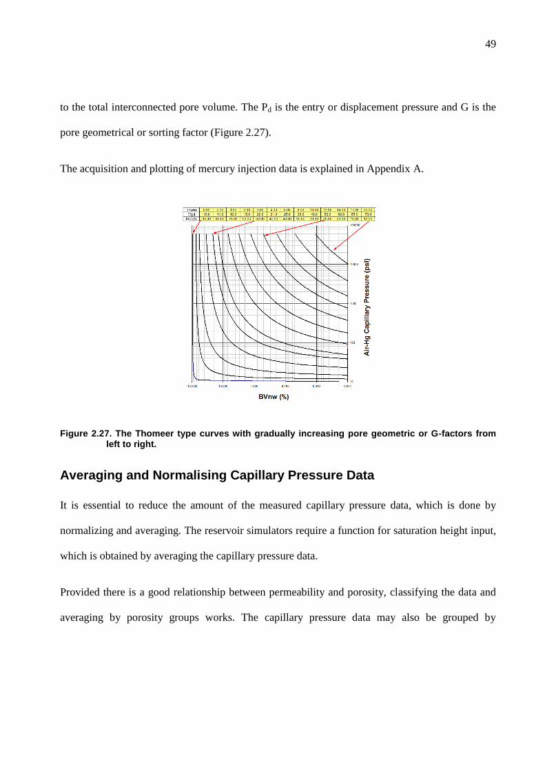
49

to the total interconnected pore volume. The Pd is the entry or displacement pressure and G is the

pore geometrical or sorting factor (Figure 2.27).

The acquisition and plotting of mercury injection data is explained in Appendix A.

Figure 2.27. The Thomeer type curves with gradually increasing pore geometric or G-factors from left to right.

Averaging and Normalising Capillary Pressure Data

It is essential to reduce the amount of the measured capillary pressure data, which is done by

normalizing and averaging. The reservoir simulators require a function for saturation height input,

which is obtained by averaging the capillary pressure data.

Provided there is a good relationship between permeability and porosity, classifying the data and

averaging by porosity groups works. The capillary pressure data may also be grouped by

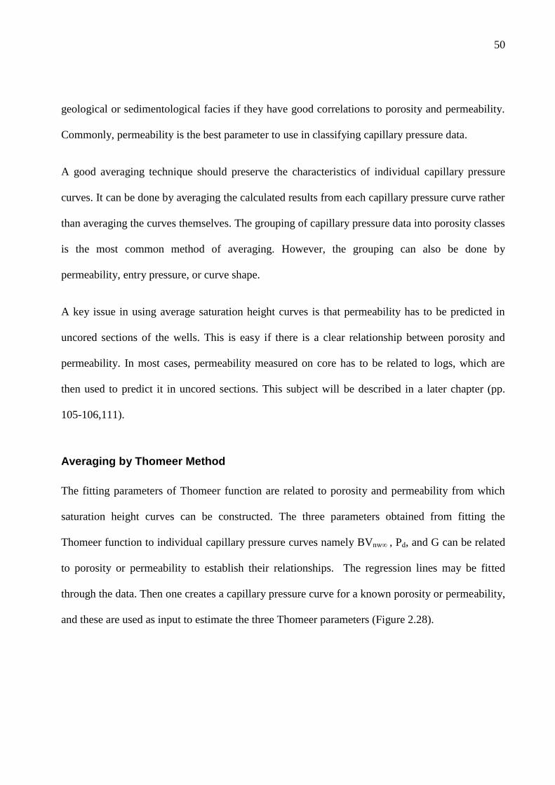
50

geological or sedimentological facies if they have good correlations to porosity and permeability.

Commonly, permeability is the best parameter to use in classifying capillary pressure data.

A good averaging technique should preserve the characteristics of individual capillary pressure

curves. It can be done by averaging the calculated results from each capillary pressure curve rather

than averaging the curves themselves. The grouping of capillary pressure data into porosity classes

is the most common method of averaging. However, the grouping can also be done by

permeability, entry pressure, or curve shape.

A key issue in using average saturation height curves is that permeability has to be predicted in

uncored sections of the wells. This is easy if there is a clear relationship between porosity and

permeability. In most cases, permeability measured on core has to be related to logs, which are

then used to predict it in uncored sections. This subject will be described in a later chapter (pp.

105-106,111).

Averaging by Thomeer Method

The fitting parameters of Thomeer function are related to porosity and permeability from which

saturation height curves can be constructed. The three parameters obtained from fitting the

Thomeer function to individual capillary pressure curves namely BVnw∞ , Pd, and G can be related

to porosity or permeability to establish their relationships. The regression lines may be fitted

through the data. Then one creates a capillary pressure curve for a known porosity or permeability,

and these are used as input to estimate the three Thomeer parameters (Figure 2.28).

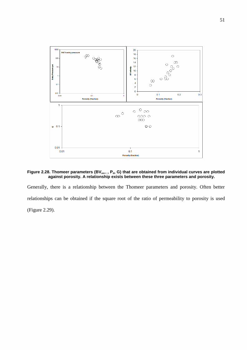
51

Figure 2.28. Thomeer parameters (BVnw∞ , Pd, G) that are obtained from individual curves are plotted against porosity. A relationship exists between these three parameters and porosity.

Generally, there is a relationship between the Thomeer parameters and porosity. Often better

relationships can be obtained if the square root of the ratio of permeability to porosity is used

(Figure 2.29).

52

Figure 2.29. Thomeer parameters (BVnw∞ , Pd, G) that are obtained from individual curves are plotted against Flow Zone Indicator {0.0314*SQRT(K/PHIE)}. A better defined relationship exists between these three parameters and Flow Zone Indicator.

Averaging by Heseldin Method

Heseldin (1974) used porosity to average capillary pressure curves because porosity data is

calculated from wireline logs and directly available across the reservoir. A good relationship

between permeability and porosity often exists causing the method to work reasonably. Firstly, the

capillary pressure data are interpolated to fixed and consistent values of capillary pressure. Then,

porosity is plotted against bulk volume occupied (non-wetting phase) for all samples at the same

53

capillary pressure. The bulk volume occupied (non-wetting phase) is given by PHIE * (1-Swet). A

curve is fitted through the data for the particular pressure. A good fit is usually obtained by a

hyperbolic equation that is given below.

In this equation, A and B are fitting parameters. When BVnw is zero then ϕ axis intercept is

porosity below which hydrocarbons will be unable to enter the rock at the given pressure. A series

of such plots are made for different capillary pressures and the result is a series of curves. Another

plot is made in which capillary pressure is plotted against the parameters A and B and regression

lines are fitted (Figure 2.30). Hence the functions are derived in which parameters A and B are

related to capillary pressure. Using these relations, families of capillary curves can be constructed

from porosity and height above Free Water Level.

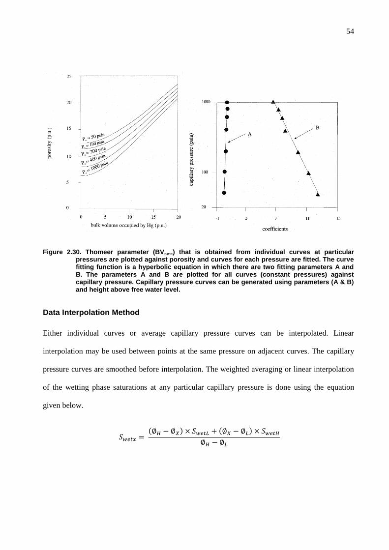
54

Figure 2.30. Thomeer parameter (BVnw∞) that is obtained from individual curves at particular pressures are plotted against porosity and curves for each pressure are fitted. The curve fitting function is a hyperbolic equation in which there are two fitting parameters A and B. The parameters A and B are plotted for all curves (constant pressures) against capillary pressure. Capillary pressure curves can be generated using parameters (A & B) and height above free water level.

Data Interpolation Method

Either individual curves or average capillary pressure curves can be interpolated. Linear

interpolation may be used between points at the same pressure on adjacent curves. The capillary

pressure curves are smoothed before interpolation. The weighted averaging or linear interpolation

of the wetting phase saturations at any particular capillary pressure is done using the equation

given below.

55

where Swetx is the estimated wetting phase saturation of a sample of porosity ϕx at the chosen

capillary pressure. SwetL and ϕL are wetting phase saturation and porosity of the capillary curve

with porosity just lower than the required ϕx. Similarly, SwetH and ϕH are wetting phase saturation

and porosity of the capillary curve with porosity just above the required ϕx.

It is also feasible to interpolate between average capillary pressure curves that are obtained for

various porosity classes.

Leverett’s J Function Method

Leverett (1941) proposed a function to normalise capillary pressure to account for changes in

porosity and permeability. The definition of capillary pressure can be rearranged as follows:

which is equal to a constant and constitutes a dimensionless group, because the numenator and the

denomenator are of the same units (force/area). Leverett (1941) replaced the term “r” (pore throat

radius) with the square root of k (permeability) because both terms have the same dimension

(length). Because porosity (ϕ) is dimensionless, therefore, dividing permeability by porosity does

not change its dimension.

56

where K is permeability to air in milli Darcy and ϕ is effective porosity. Pc is in psi, σ or

interfacial tension is in dynes per centimetre, θ is interface angle in degrees, 0.21645 is a

combined constant for oil field units. This normalisation assumes that porosity and permeability

are closely related. The J function (Jsw) is plotted against wetting phase saturation. If porosity and

permeability are related then, the capillary pressure data would collapse into a narrow band

through which a regression equation can be fitted. Once a relationship between Jsw and Swet is

derived, a capillary pressure curve can be generated from porosity and permeability data. It is

often desireable to group porosity into classes and assign different J functions to them.

The J function assumes a parallel capillary tube model for the rock. This is an oversimplification

in some cases in which the J function fit can be improved by using the formation tortuosity factor

(m) into the J function as below:

In segregared oil columns where oil becomes progressively heavier towards the Free Water Level,

its viscosity may increase from few centi-Poise for good oil to hundreds of centi-Poise for highly

viscous oil. It is found that in such cases it is very useful to include water to oil viscosity ratio with

the square-root of permeability over porosity:

57

where μoil and μwater are viscosities of oil and water at reservoir condition. Since a viscosity ratio is

used the dimensionless nature of the J function is still preserved.

The capillary pressure data is transformed into J-Sw space as individual data points, which are

often grouped by porosity or ratio of permeability to porosity classes. It is then required to fit

suitable curves to these J-Sw data clusters. The functions that are suitable to fit individual capillary

pressure curves (described above) could also be fitted to J-Sw data. An equation similar to Lambda

function (described above) could be fitted as follows.

It is primarily required to compute Sw from given Jsw, therefore, the equation is rearranged and Jsw

is replaced with its constituent variables.

where ρw and ρo are densities and define the pressure gradients of water and oil in psi per foot, H is

height above Free Water Level in feet, σ is in dynes per centimetre, K is permeability in milli

darcy and ϕ is porosity in fractions.

58

As an alternative, a similar equation could be used in which the J parameter is treated as an

independent, and Sw as a dependent variable.

An advanced exponential function (mentioned above) could also be used to fit the J-Sw data:

By substituting the J-function with the equation:

Then, the final equation will be (Fig. 2.31):

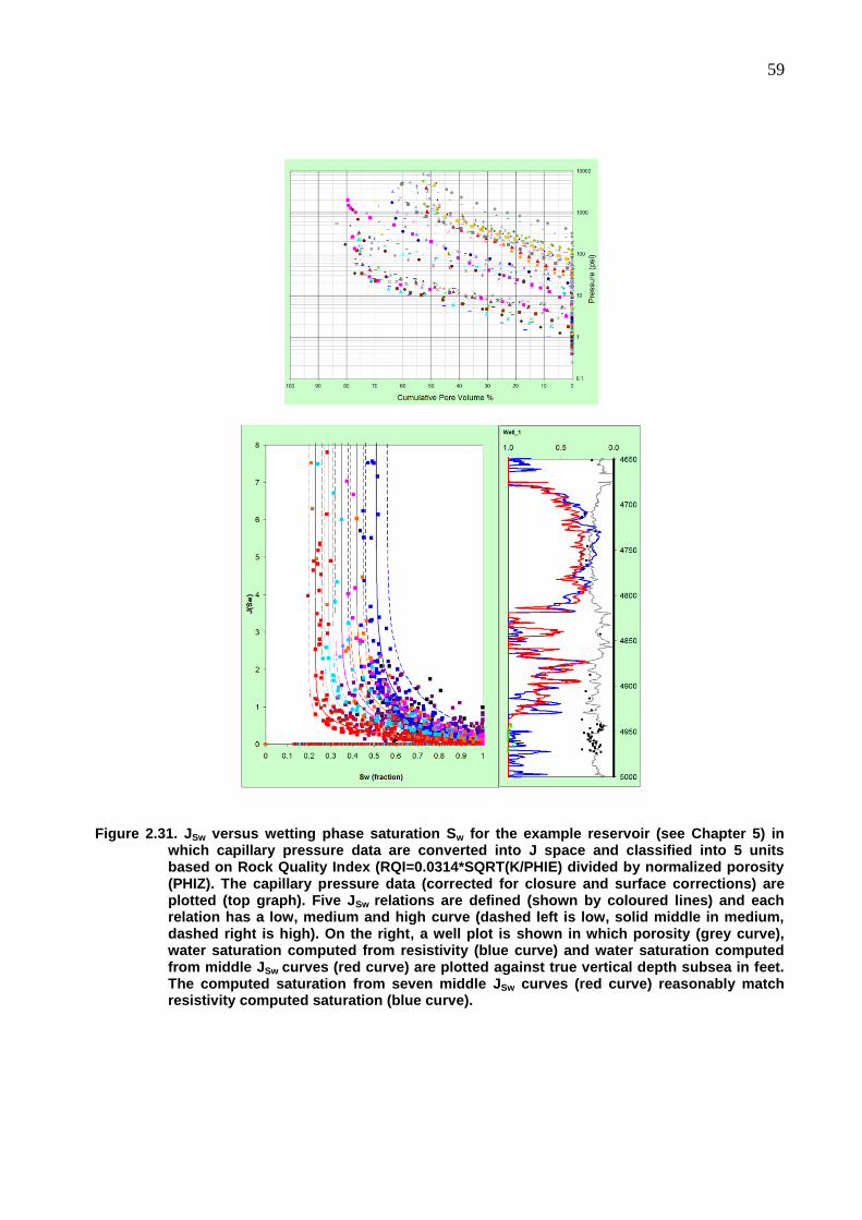
59

Figure 2.31. JSw versus wetting phase saturation Sw for the example reservoir (see Chapter 5) in which capillary pressure data are converted into J space and classified into 5 units based on Rock Quality Index (RQI=0.0314*SQRT(K/PHIE) divided by normalized porosity (PHIZ). The capillary pressure data (corrected for closure and surface corrections) are plotted (top graph). Five JSw relations are defined (shown by coloured lines) and each relation has a low, medium and high curve (dashed left is low, solid middle in medium, dashed right is high). On the right, a well plot is shown in which porosity (grey curve), water saturation computed from resistivity (blue curve) and water saturation computed from middle JSw curves (red curve) are plotted against true vertical depth subsea in feet. The computed saturation from seven middle JSw curves (red curve) reasonably match resistivity computed saturation (blue curve).

60

Skelt-Harrison Method

Skelt and Harrison (1995) proposed a function that can be fitted to either core-derived capillary

pressure or log water saturation versus height data.

where H is height above Free Water Level in feet; a, b, c, d are coefficients; Pc is capillary

pressure in psi. This function makes good use of its non-linearity to provide a fitted curve shape

that actually looks like a capillary pressure curve. The coefficients (a, b, c, d) are dependent on

permeability that are found by curve fitting procedure. Each coefficient allows to shift capillary

pressure curve in different way. Coefficient “a” shifts the curve in x-direction along the water

saturation axis hence it allows a fit to the irreducible water saturation. The coefficient “b” shifts

the curve in the y-direction along the capillary pressure or height axis. The coefficient “c” allows

the inflexion of the capillary pressure curve to be matched. The coefficient “d” allows a block shift

up or down so that an observed Free Water Level could be matched.

Firstly, Skelt-Harrison curve is fitted to the individual capillary pressure curve and its coefficients

a, b, c are used while coefficient d is set to zero. This process leads to a table of parameters a, b, c

for all core plugs with capillary pressure curves. An average coefficient “c” is computed. All

capillary curves are refitted using mean coefficient “c” and new set of coefficient a and b are

derived. Then coefficients a and b are plotted against core plug permeability and a relationship of

61

parameters a and b is obtained versus permeability. By applying a multiplier to the coefficient b in

the Skelt-Harrison equation the domain is switched from capillary pressure to height. Log-derived

water saturation data is also plotted. The coefficient d is now used to move the curve up or down

the log-derived water saturation versus depth until a best fit is obtained, which can be done

visually or by regression.

Equivalent Radius Function Normalising Method

This method was developed for chalk reservoirs in the North Sea that have mostly fine pores

(Engstrom, 1995). A normalising function was formulated for capillary pressure curves from the

chalk reservoir. It involves calculation of an equivalent radius function for each capillary pressure

data point as given below.

where Pce is capillary entry pressure in psi and Pc is the capillary pressure in psi in either

laboratory or equivalent reservoir fluid units. Then EQR is plotted against normalised non-wetting

phase saturation.

where Sw is wetting phase saturation at any capillary pressure and Swir is irreducible wetting phase

saturation. A polynomial function or another function having suitable curve shape is then fitted to

the EQR as a function on Snw*.

62

Well Log Derived Capillary Pressure Curves

It is very useful to plot resistivity-derived water saturations from wells (on different structural

elevations) against true vertical depth (subsea). This plot reveals how water saturations are

decreasing in wells that lie progressively higher on the structure. The plot is often filtered to

emphasize high porosity beds and avoid high water saturations in tight beds in order to see the true

transition zone (Fig. 2.32). This plot reveals a very meaningful trend of water saturation change

versus height above the Free water Level. This plot can also be converted to Jsw versus Sw space to

which various J functions can be fitted directly.

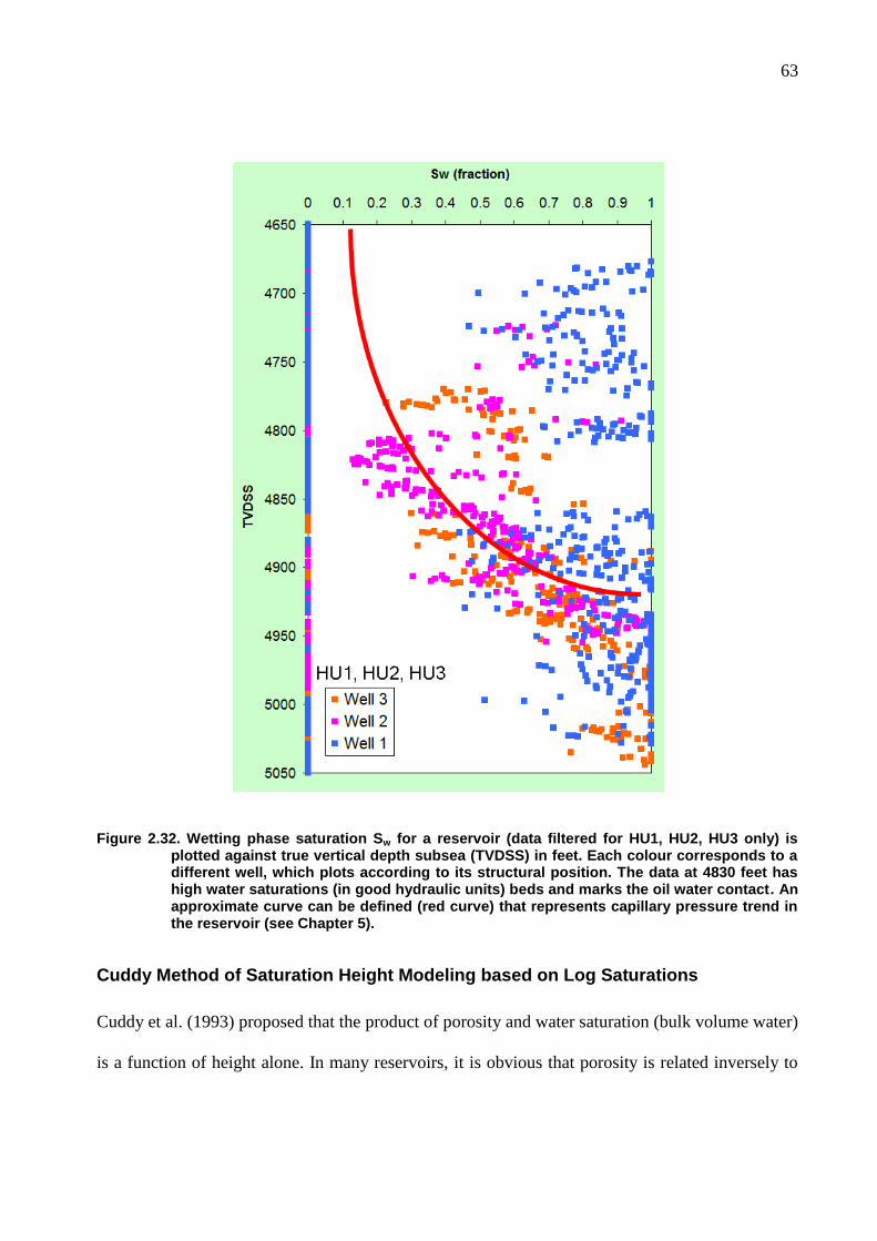
63

Figure 2.32. Wetting phase saturation Sw for a reservoir (data filtered for HU1, HU2, HU3 only) is plotted against true vertical depth subsea (TVDSS) in feet. Each colour corresponds to a different well, which plots according to its structural position. The data at 4830 feet has high water saturations (in good hydraulic units) beds and marks the oil water contact. An approximate curve can be defined (red curve) that represents capillary pressure trend in the reservoir (see Chapter 5).

Cuddy Method of Saturation Height Modeling based on Log Saturations

Cuddy et al. (1993) proposed that the product of porosity and water saturation (bulk volume water)

is a function of height alone. In many reservoirs, it is obvious that porosity is related inversely to

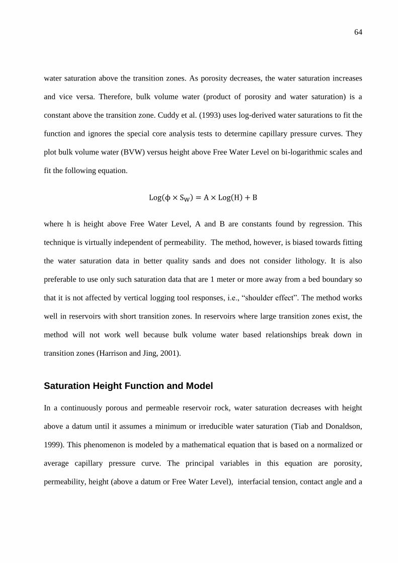
64

water saturation above the transition zones. As porosity decreases, the water saturation increases

and vice versa. Therefore, bulk volume water (product of porosity and water saturation) is a

constant above the transition zone. Cuddy et al. (1993) uses log-derived water saturations to fit the

function and ignores the special core analysis tests to determine capillary pressure curves. They

plot bulk volume water (BVW) versus height above Free Water Level on bi-logarithmic scales and

fit the following equation.

where h is height above Free Water Level, A and B are constants found by regression. This

technique is virtually independent of permeability. The method, however, is biased towards fitting

the water saturation data in better quality sands and does not consider lithology. It is also

preferable to use only such saturation data that are 1 meter or more away from a bed boundary so

that it is not affected by vertical logging tool responses, i.e., “shoulder effect”. The method works

well in reservoirs with short transition zones. In reservoirs where large transition zones exist, the

method will not work well because bulk volume water based relationships break down in

transition zones (Harrison and Jing, 2001).

Saturation Height Function and Model

In a continuously porous and permeable reservoir rock, water saturation decreases with height

above a datum until it assumes a minimum or irreducible water saturation (Tiab and Donaldson,

1999). This phenomenon is modeled by a mathematical equation that is based on a normalized or

average capillary pressure curve. The principal variables in this equation are porosity,

permeability, height (above a datum or Free Water Level), interfacial tension, contact angle and a

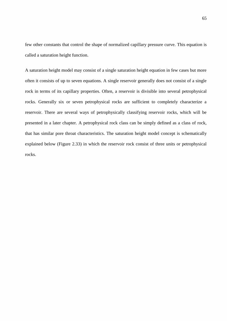
65

few other constants that control the shape of normalized capillary pressure curve. This equation is

called a saturation height function.

A saturation height model may consist of a single saturation height equation in few cases but more

often it consists of up to seven equations. A single reservoir generally does not consist of a single

rock in terms of its capillary properties. Often, a reservoir is divisible into several petrophysical

rocks. Generally six or seven petrophysical rocks are sufficient to completely characterize a

reservoir. There are several ways of petrophysically classifying reservoir rocks, which will be

presented in a later chapter. A petrophysical rock class can be simply defined as a class of rock,

that has similar pore throat characteristics. The saturation height model concept is schematically

explained below (Figure 2.33) in which the reservoir rock consist of three units or petrophysical

rocks.

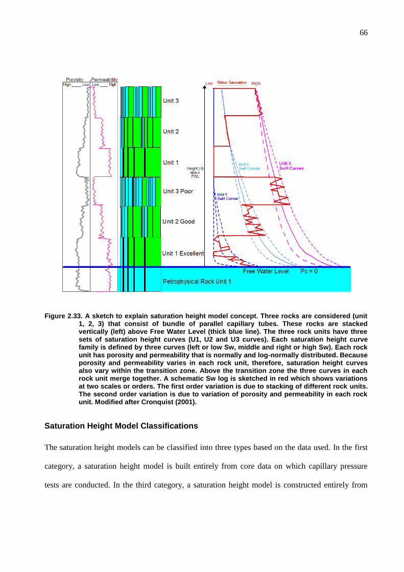
66

Figure 2.33. A sketch to explain saturation height model concept. Three rocks are considered (unit 1, 2, 3) that consist of bundle of parallel capillary tubes. These rocks are stacked vertically (left) above Free Water Level (thick blue line). The three rock units have three sets of saturation height curves (U1, U2 and U3 curves). Each saturation height curve family is defined by three curves (left or low Sw, middle and right or high Sw). Each rock unit has porosity and permeability that is normally and log-normally distributed. Because porosity and permeability varies in each rock unit, therefore, saturation height curves also vary within the transition zone. Above the transition zone the three curves in each rock unit merge together. A schematic Sw log is sketched in red which shows variations at two scales or orders. The first order variation is due to stacking of different rock units. The second order variation is due to variation of porosity and permeability in each rock unit. Modified after Cronquist (2001).

Saturation Height Model Classifications

The saturation height models can be classified into three types based on the data used. In the first

category, a saturation height model is built entirely from core data on which capillary pressure

tests are conducted. In the third category, a saturation height model is constructed entirely from

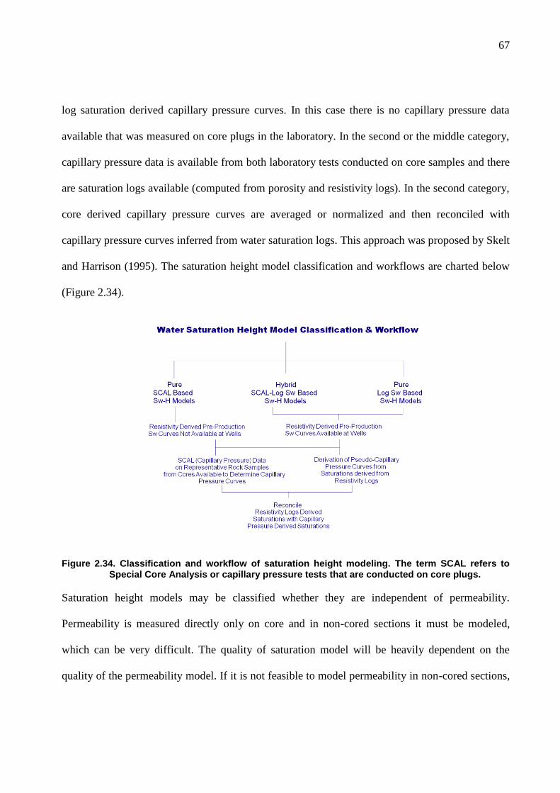
67

log saturation derived capillary pressure curves. In this case there is no capillary pressure data

available that was measured on core plugs in the laboratory. In the second or the middle category,

capillary pressure data is available from both laboratory tests conducted on core samples and there

are saturation logs available (computed from porosity and resistivity logs). In the second category,

core derived capillary pressure curves are averaged or normalized and then reconciled with

capillary pressure curves inferred from water saturation logs. This approach was proposed by Skelt

and Harrison (1995). The saturation height model classification and workflows are charted below

(Figure 2.34).

Figure 2.34. Classification and workflow of saturation height modeling. The term SCAL refers to Special Core Analysis or capillary pressure tests that are conducted on core plugs.

Saturation height models may be classified whether they are independent of permeability.

Permeability is measured directly only on core and in non-cored sections it must be modeled,

which can be very difficult. The quality of saturation model will be heavily dependent on the

quality of the permeability model. If it is not feasible to model permeability in non-cored sections,

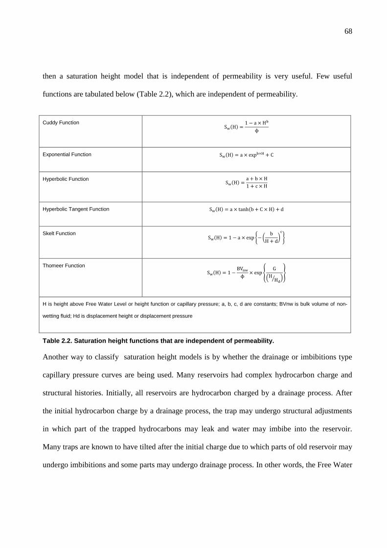
68

then a saturation height model that is independent of permeability is very useful. Few useful

functions are tabulated below (Table 2.2), which are independent of permeability.

Cuddy Function

Exponential Function

Hyperbolic Function

Hyperbolic Tangent Function

Skelt Function

Thomeer Function

H is height above Free Water Level or height function or capillary pressure; a, b, c, d are constants; BVnw is bulk volume of non-

wetting fluid; Hd is displacement height or displacement pressure

Table 2.2. Saturation height functions that are independent of permeability.

Another way to classify saturation height models is by whether the drainage or imbibitions type

capillary pressure curves are being used. Many reservoirs had complex hydrocarbon charge and

structural histories. Initially, all reservoirs are hydrocarbon charged by a drainage process. After

the initial hydrocarbon charge by a drainage process, the trap may undergo structural adjustments

in which part of the trapped hydrocarbons may leak and water may imbibe into the reservoir.

Many traps are known to have tilted after the initial charge due to which parts of old reservoir may

undergo imbibitions and some parts may undergo drainage process. In other words, the Free Water

69

Level has changed in these reservoirs during their history. Commonly, a paleo Free Water Level

can be found, which is often many tens of feet below the current Free Water Level. Between the

two Free Water Levels, hydrocarbons are present and are at or close to residual saturation. Such

reservoirs with complex history can not be modeled by drainage type capillary pressure curves.

Imbibition capillary pressure curves have been presented in the chapter on saturation history above

(pp. 29-31). Such curves are usually steep and they do not start at 100 per cent water saturation.

Saturation Height Modeling Process

The modeling starts with a structural map that is based on seismic and well data. The reservoir is

then zoned using appropriate sequence stratigraphic techniques. Each sequence is based on

advanced studies of core and logs and is distinguished in terms of depositional sedimentary facies

and subsequent diagenetic alterations in its porosity-permeability characteristics.

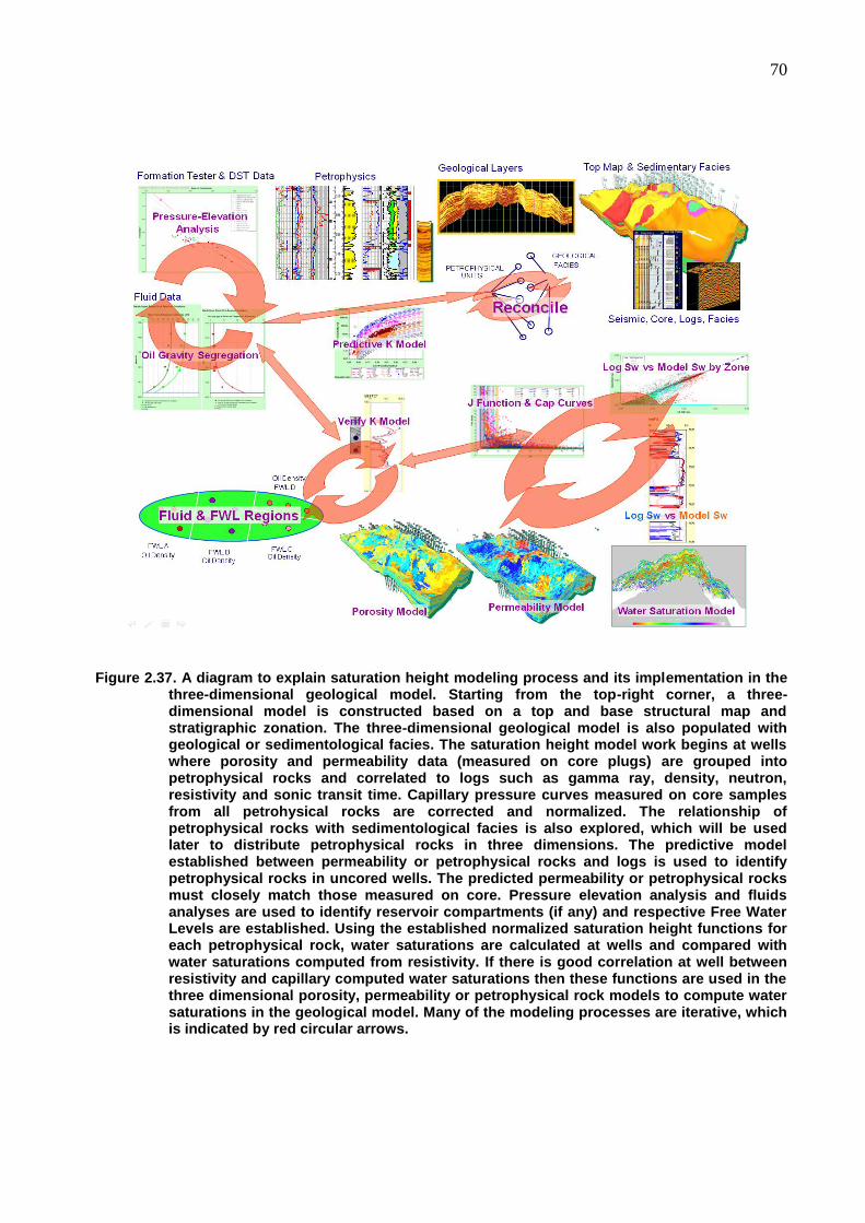
70

Figure 2.37. A diagram to explain saturation height modeling process and its implementation in the three-dimensional geological model. Starting from the top-right corner, a three-dimensional model is constructed based on a top and base structural map and stratigraphic zonation. The three-dimensional geological model is also populated with geological or sedimentological facies. The saturation height model work begins at wells where porosity and permeability data (measured on core plugs) are grouped into petrophysical rocks and correlated to logs such as gamma ray, density, neutron, resistivity and sonic transit time. Capillary pressure curves measured on core samples from all petrohysical rocks are corrected and normalized. The relationship of petrophysical rocks with sedimentological facies is also explored, which will be used later to distribute petrophysical rocks in three dimensions. The predictive model established between permeability or petrophysical rocks and logs is used to identify petrophysical rocks in uncored wells. The predicted permeability or petrophysical rocks must closely match those measured on core. Pressure elevation analysis and fluids analyses are used to identify reservoir compartments (if any) and respective Free Water Levels are established. Using the established normalized saturation height functions for each petrophysical rock, water saturations are calculated at wells and compared with water saturations computed from resistivity. If there is good correlation at well between resistivity and capillary computed water saturations then these functions are used in the three dimensional porosity, permeability or petrophysical rock models to compute water saturations in the geological model. Many of the modeling processes are iterative, which is indicated by red circular arrows.

71

Logs and Core data are matched and modeled so that permeability could be predicted in the

uncored intervals and wells. Petrophysical rock types are now established. Each geological facies

have a group of petrophysical rocks whose relationships are studied and reconciled. Petrophysical

rocks are classified into 5 to 7 discrete groups that are normally distributed.

Formation tester and drill stem tests (DST) pressure data are interpreted besides fluid analysis data

from laboratory such as stock tank oil gravity and oil viscosity. Fluid data at reservoir conditions is

modeled in parallel with pressure profiles. Fluid interfaces determined from pressure profiles are

reconciled with wire-line logs, core and special core analysis data. Significant differences in oil

and water properties are quantified by reservoir blocks if they exist. Seismic data and inversion is

used to define boundaries of such blocks.

Log-computed water saturations are normalized using J function and respective fluid properties by

reservoir zones or blocks. Capillary pressure data from each rock type are superimposed on log

computed saturations.

Porosity and petrophysical rocks at wells are modeled in three dimensions using appropriate

geostatistical techniques. Petrophysical rocks in three dimensions are inverted into permeability.

Water saturations are calculated using capillary curves. Swi relations from special core analysis

need to honor the trends seen from logs. Uncertainty in log-based saturations is explored using a

range of Archie or shaly sand parameters. Matching of computed capillary-based saturations is

examined with log-based saturations by zones or blocks if necessary. Capillary-based saturations

are also examined at well locations with log-based water saturations. Figure 2.35 shows a synopsis

of this process.

72

Estimation of Down-Dip Free Water Level from Capillary Pressure

Curves

In situations where initial oil water contact and Free Water Level has not been established by

logging and formation pressure tester, capillary pressure data may be used to estimate the depth of

Free Water Level. This was suggested by Alger et al. (1989) and Smith et al. (1992). Hawkins et

al. (1993) developed correlations between porosity, water saturation, mercury-air capillary

pressure and air permeability in the form:

where Pc is mercury-air capillary pressure in psi, Pd is mercury air displacement pressure in psi and

G is pore geometrical factor as defined by Thomeer (1960).

Using laboratory capillary pressure data, the coefficients in these equations are modified. In

theory, for a well where water saturations, porosity, and permeability are available the above

equation is solved for G factor, which defines a Thomeer (1960) capillary pressure curve. Then,

the Pd or displacement pressure equation is solved to calculate a Pd log. Then, using the log-

derived water saturation (from resistivity), G factor and Pd, capillary pressure, or Pc are calculated.

The calculated capillary pressure is changed from mercury-air into appropriate reservoir fluid

73

system. The distance to Free Water Level or HFWL is calculated in feet using the equation given

below.

Where Pc is in psi, HFWL is in feet, ρw and ρw are densities in pounds per cubic feet.

This methodology works if the well log interval of interest is in the hydrocarbon/water transition

zone that shows a significant gradient of water saturation versus depth. It should also be

considered whether capillary pressure curves measured at ambient pressures are representative of

the reservoir condition of the rock under stress. A good permeability model is established and can

predict permeability in uncored intervals. In addition, the reservoir fluid densities do not vary with

depth or if they do then they could be modeled. It is also implicit in this method that drainage

capillary pressure curves are valid representations of the profiles of water saturation versus height

above Free Water Level. In some reservoirs, the initial hydrocarbon columns may have shifted due

to tectonic movements or other geological situations. Wettability could have changed, particularly,

if the reservoir is made of carbonates. This causes mixed wettability as some organic compounds

included in the oil react with the water-wet surface of the rock. This reaction displaces the aqueous

film on the rock‟s surface, creating a new oil-wet coating on it (Tiab and Donaldson, 2004).In such

complex situations, water saturation profiles-as logged in a well-would not be represented by the

drainage capillary pressure curves.

74

Saturation Height Modeling Advantages

The primary reason for using saturation height models is to compute the stock tank oil initially in

place (STOIIP) or gas initially in place (GIIP). The saturation height models are considered to give

a better estimation of hydrocarbons in place because they completely supersede the exotic

equations (such as many shaly sand formulas) used by petrophysicist to compute water saturations

(Darling, 2005). Actually, there are significant uncertainties with log-calculated water saturation

(Sw), especially in tight heterogeneous reservoirs (Sheng Ding et al., 2003.) The saturation-height

functions provide accurate water saturation, and they can potentially overcome uncertainties with

log interpretations using Archie equation (Amabeoku et al., 2006.)

The saturation height models are driven by a porosity log that is based on density, neutron, and

sonic logs, which have high bed boundary resolutions. The deep resistivity log is affected

significantly by thin beds and invasion. The water saturations computed from resistivity are also

affected by invasion, thin-bed, and shoulder effects. Water saturations computed from saturation

height model would actually correct for thin bed and invasion effects. It is also important to note

that saturations computed from a height model might be slightly different than those computed

from resistivity.

When reliable core data are available and the elevation of Free water Level is not known or

intersected in a well, then, saturation height functions can be used to predict the down-dip Free

Water Level from log water saturations.

75

A properly calibrated saturation height function reconciles reliable log saturations with core data

and represents the best way to calculate water saturations in a reservoir and implement this

information in static and dynamic models.

76

Chapter 3

Petrophysics of Carbonate Reservoirs

Petrophysical Model of Rocks

The formation rock model is comprised of; (1) matrix rock (Vrock), (2) pore space (or porosity), (3)

within the matrix rock (e), (4) shale content of the matrix rock (Vsh).

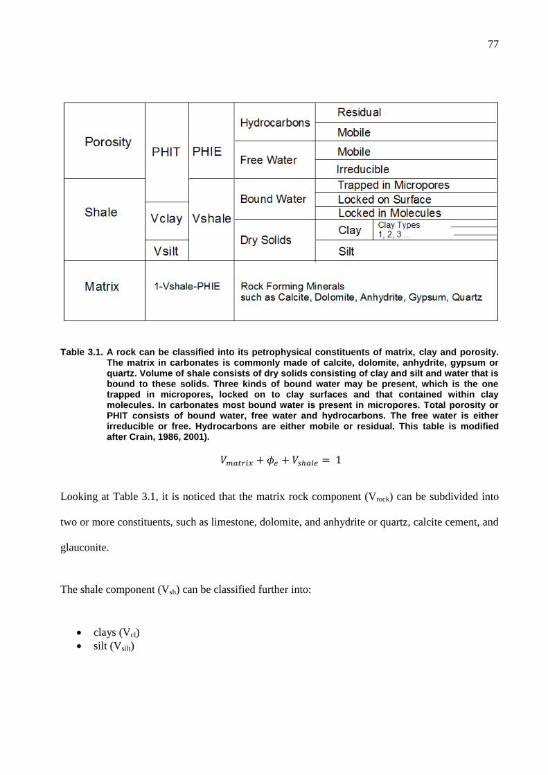
77

Table 3.1. A rock can be classified into its petrophysical constituents of matrix, clay and porosity. The matrix in carbonates is commonly made of calcite, dolomite, anhydrite, gypsum or quartz. Volume of shale consists of dry solids consisting of clay and silt and water that is bound to these solids. Three kinds of bound water may be present, which is the one trapped in micropores, locked on to clay surfaces and that contained within clay molecules. In carbonates most bound water is present in micropores. Total porosity or PHIT consists of bound water, free water and hydrocarbons. The free water is either irreducible or free. Hydrocarbons are either mobile or residual. This table is modified after Crain, 1986, 2001).

Looking at Table 3.1, it is noticed that the matrix rock component (Vrock) can be subdivided into

two or more constituents, such as limestone, dolomite, and anhydrite or quartz, calcite cement, and

glauconite.

The shale component (Vsh) can be classified further into:

clays (Vcl)

silt (Vsilt)

78

water trapped into the shale matrix due to lack of sufficient permeability to allow the water

to escape

water locked onto the surface of the clay minerals

water absorbed chemically into the molecules of the clay minerals

The sum of the volume of these waters is called Clay Bound Water (CBW) or Bulk Volume Water

Shale (BVWSH).

Effective porosity (PHIe) may be subdivided into:

Free or bulk water volume (BVW), as opposed to the bound water in shale

hydrocarbon volume (BVH)

Free water (BVW) is further subdivided into:

a mobile portion free to flow out of the reservoir (BVWm)

an immobile or irreducible water volume bound to the matrix rock by surface tension (BVI

or BVIR)

BVI is sometimes called “bound water.”

Hydrocarbon volume (BVH) can be classified into:

mobile hydrocarbon (BVHm)

residual hydrocarbon (BVHr)

separated into gas and oil volumes in both categories

The sum of BVWm, BVHm, and BVHr is called the free fluid index (FFI) or moveable fluid

(BVM).

79

A new term, called “useful porosity”, has been seen in print recently. It includes only the pore

space filled by moveable water plus all hydrocarbon, excluding irreducible water – this is the same

as BVM.

Total porosity (t) is the sum of:

clay bound water (CBW)

free water, including irreducible water (BVW)

hydrocarbon (BVH)

Effective porosity (e) is the sum of:

free water, including irreducible water (BVW)

hydrocarbon (BVH)

Total water volume (BVWt) is the sum of:

free water, including irreducible water (BVW)

clay bound water (CBW)

Total water saturation (Swt) is the ratio of:

total water volume (BVWt) to

total porosity (PHIt)

Effective water saturation (SW or Swe) is the ratio of:

80

free water volume (BVW) to

effective porosity (PHIe)

Two results of these definitions are obvious:

Free water volume (BVW) is the product of:

water saturation (Swe) and

effective porosity (PHIe)

Hydrocarbon volume (BVH) is the product of:

one minus water saturation (1 – Swe) and

effective porosity.(PHIe)

Irreducible water saturation (Swir) is the ratio of:

immobile or irreducible water volume (BVI) to

effective porosity (PHIe)

The volume of irreducible water (BVI) is thus the product of:

irreducible water saturation (Swir) and

effective porosity. (PHIe)

Due to variations in the amount of flushing with distance from the borehole wall (Figure 3.1), the

water saturation will also vary, if hydrocarbons are present. Similar definitions of water saturation

prevail. The water saturation in the flushed zone is the ratio of the free water in the flushed zone,

to the effective porosity, which is assumed to be the same porosity as in the un-invaded zone.

The amount of free water in the invaded zone is usually higher than in the un-invaded zone, when

oil or gas is present. Hence, water saturation is also higher. This saturation is referred to as Sxo

while the water saturation in the un-invaded zone is referred to as Sw or Swe.

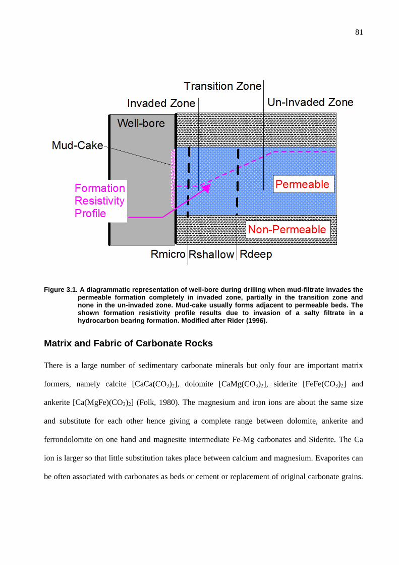
81

Figure 3.1. A diagrammatic representation of well-bore during drilling when mud-filtrate invades the permeable formation completely in invaded zone, partially in the transition zone and none in the un-invaded zone. Mud-cake usually forms adjacent to permeable beds. The shown formation resistivity profile results due to invasion of a salty filtrate in a hydrocarbon bearing formation. Modified after Rider (1996).

Matrix and Fabric of Carbonate Rocks

There is a large number of sedimentary carbonate minerals but only four are important matrix

formers, namely calcite [CaCa(CO3)2], dolomite [CaMg(CO3)2], siderite [FeFe(CO3)2] and

ankerite [Ca(MgFe)(CO3)2] (Folk, 1980). The magnesium and iron ions are about the same size

and substitute for each other hence giving a complete range between dolomite, ankerite and

ferrondolomite on one hand and magnesite intermediate Fe-Mg carbonates and Siderite. The Ca

ion is larger so that little substitution takes place between calcium and magnesium. Evaporites can

be often associated with carbonates as beds or cement or replacement of original carbonate grains.

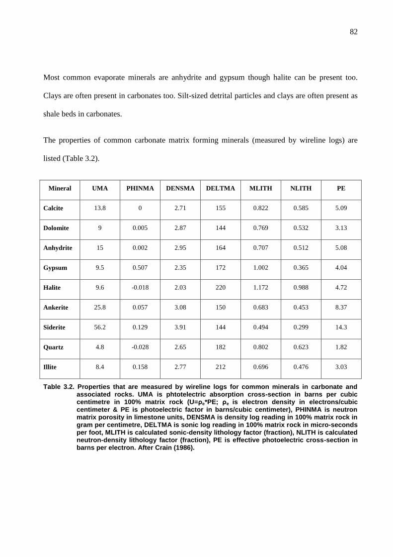
82

Most common evaporate minerals are anhydrite and gypsum though halite can be present too.

Clays are often present in carbonates too. Silt-sized detrital particles and clays are often present as

shale beds in carbonates.

The properties of common carbonate matrix forming minerals (measured by wireline logs) are

listed (Table 3.2).

Mineral UMA PHINMA DENSMA DELTMA MLITH NLITH PE

Calcite 13.8 0 2.71 155 0.822 0.585 5.09

Dolomite 9 0.005 2.87 144 0.769 0.532 3.13

Anhydrite 15 0.002 2.95 164 0.707 0.512 5.08

Gypsum 9.5 0.507 2.35 172 1.002 0.365 4.04

Halite 9.6 -0.018 2.03 220 1.172 0.988 4.72

Ankerite 25.8 0.057 3.08 150 0.683 0.453 8.37

Siderite 56.2 0.129 3.91 144 0.494 0.299 14.3

Quartz 4.8 -0.028 2.65 182 0.802 0.623 1.82

Illite 8.4 0.158 2.77 212 0.696 0.476 3.03

Table 3.2. Properties that are measured by wireline logs for common minerals in carbonate and associated rocks. UMA is phtotelectric absorption cross-section in barns per cubic centimetre in 100% matrix rock (U=ρe*PE; ρe is electron density in electrons/cubic centimeter & PE is photoelectric factor in barns/cubic centimeter), PHINMA is neutron matrix porosity in limestone units, DENSMA is density log reading in 100% matrix rock in gram per centimetre, DELTMA is sonic log reading in 100% matrix rock in micro-seconds per foot, MLITH is calculated sonic-density lithology factor (fraction), NLITH is calculated neutron-density lithology factor (fraction), PE is effective photoelectric cross-section in barns per electron. After Crain (1986).

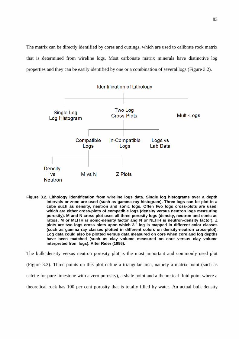
83

The matrix can be directly identified by cores and cuttings, which are used to calibrate rock matrix

that is determined from wireline logs. Most carbonate matrix minerals have distinctive log

properties and they can be easily identified by one or a combination of several logs (Figure 3.2).

Figure 3.2. Lithology identification from wireline logs data. Single log histograms over a depth intervals or zone are used (such as gamma ray histogram). Three logs can be plot in a cube such as density, neutron and sonic logs. Often two logs cross-plots are used, which are either cross-plots of compatible logs (density versus neutron logs measuring porosity). M and N cross-plot uses all three porosity logs (density, neutron and sonic as ratios; M or MLITH is sonic-density factor and N or NLITH is neutron-density factor). Z plots are two logs cross plots upon which 3

rd log is mapped in different color classes

(such as gamma ray classes plotted in different colors on density-neutron cross-plot). Log data could also be plotted versus data measured on core when core and log depths have been matched (such as clay volume measured on core versus clay volume interpreted from logs). After Rider (1996).

The bulk density versus neutron porosity plot is the most important and commonly used plot

(Figure 3.3). Three points on this plot define a triangular area, namely a matrix point (such as

calcite for pure limestone with a zero porosity), a shale point and a theoretical fluid point where a

theoretical rock has 100 per cent porosity that is totally filled by water. An actual bulk density

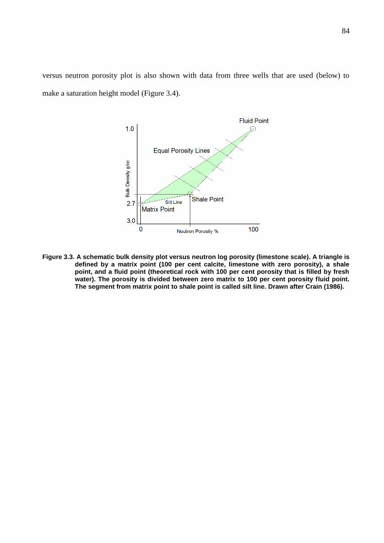
84

versus neutron porosity plot is also shown with data from three wells that are used (below) to

make a saturation height model (Figure 3.4).

Figure 3.3. A schematic bulk density plot versus neutron log porosity (limestone scale). A triangle is defined by a matrix point (100 per cent calcite, limestone with zero porosity), a shale point, and a fluid point (theoretical rock with 100 per cent porosity that is filled by fresh water). The porosity is divided between zero matrix to 100 per cent porosity fluid point. The segment from matrix point to shale point is called silt line. Drawn after Crain (1986).

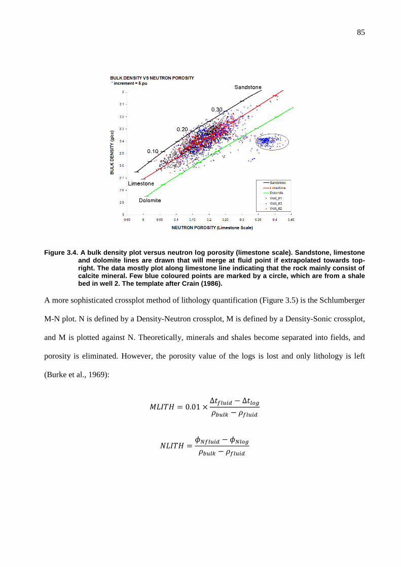
85

Figure 3.4. A bulk density plot versus neutron log porosity (limestone scale). Sandstone, limestone and dolomite lines are drawn that will merge at fluid point if extrapolated towards top-right. The data mostly plot along limestone line indicating that the rock mainly consist of calcite mineral. Few blue coloured points are marked by a circle, which are from a shale bed in well 2. The template after Crain (1986).

A more sophisticated crossplot method of lithology quantification (Figure 3.5) is the Schlumberger

M-N plot. N is defined by a Density-Neutron crossplot, M is defined by a Density-Sonic crossplot,

and M is plotted against N. Theoretically, minerals and shales become separated into fields, and

porosity is eliminated. However, the porosity value of the logs is lost and only lithology is left

(Burke et al., 1969):

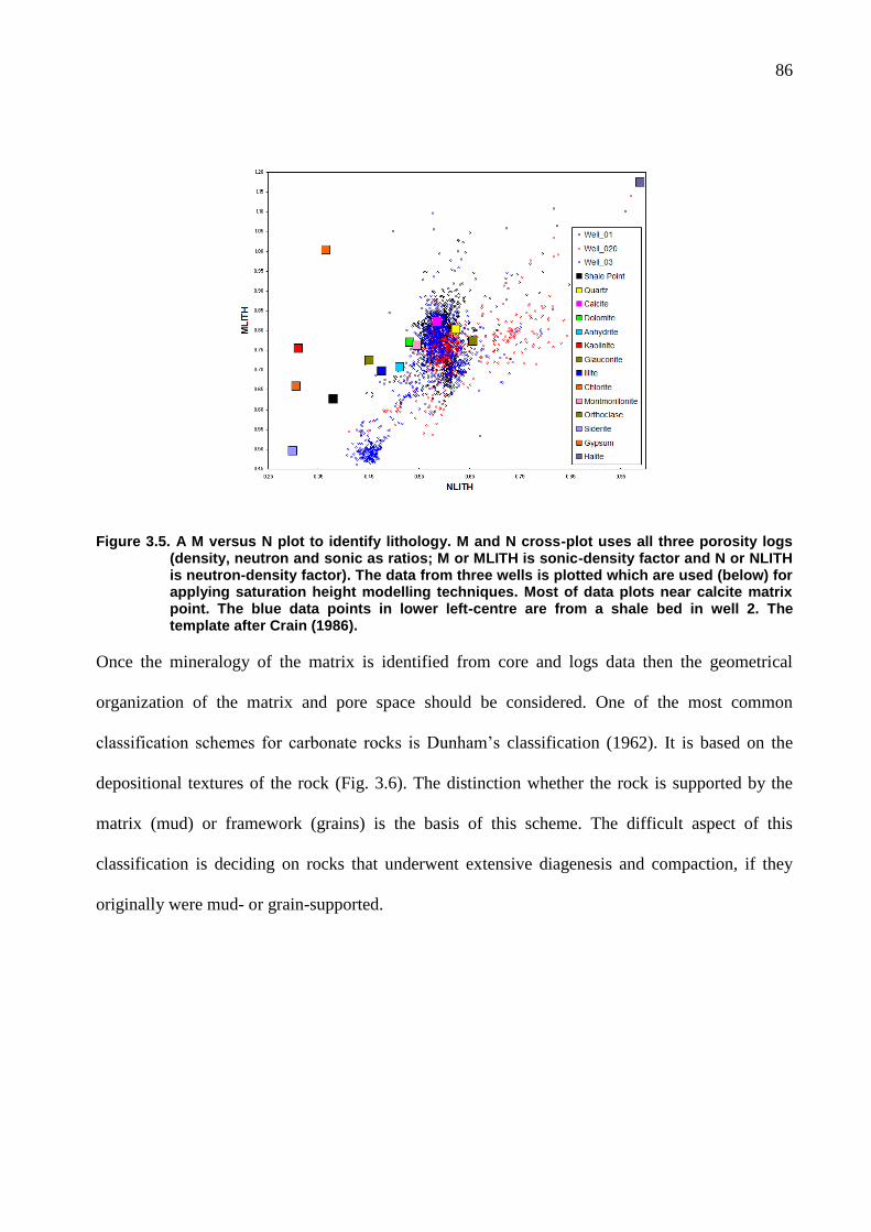
86

Figure 3.5. A M versus N plot to identify lithology. M and N cross-plot uses all three porosity logs (density, neutron and sonic as ratios; M or MLITH is sonic-density factor and N or NLITH is neutron-density factor). The data from three wells is plotted which are used (below) for applying saturation height modelling techniques. Most of data plots near calcite matrix point. The blue data points in lower left-centre are from a shale bed in well 2. The template after Crain (1986).

Once the mineralogy of the matrix is identified from core and logs data then the geometrical

organization of the matrix and pore space should be considered. One of the most common

classification schemes for carbonate rocks is Dunham‟s classification (1962). It is based on the

depositional textures of the rock (Fig. 3.6). The distinction whether the rock is supported by the

matrix (mud) or framework (grains) is the basis of this scheme. The difficult aspect of this

classification is deciding on rocks that underwent extensive diagenesis and compaction, if they

originally were mud- or grain-supported.

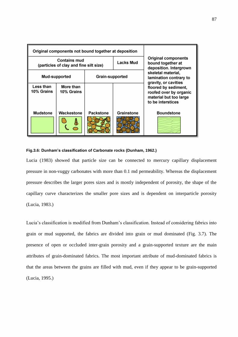
87

Fig.3.6: Dunham’s classification of Carbonate rocks (Dunham, 1962.)

Lucia (1983) showed that particle size can be connected to mercury capillary displacement

pressure in non-vuggy carbonates with more than 0.1 md permeability. Whereas the displacement

pressure describes the larger pores sizes and is mostly independent of porosity, the shape of the

capillary curve characterizes the smaller pore sizes and is dependent on interparticle porosity

(Lucia, 1983.)

Lucia‟s classification is modified from Dunham‟s classification. Instead of considering fabrics into

grain or mud supported, the fabrics are divided into grain or mud dominated (Fig. 3.7). The

presence of open or occluded inter-grain porosity and a grain-supported texture are the main

attributes of grain-dominated fabrics. The most important attribute of mud-dominated fabrics is

that the areas between the grains are filled with mud, even if they appear to be grain-supported

(Lucia, 1995.)

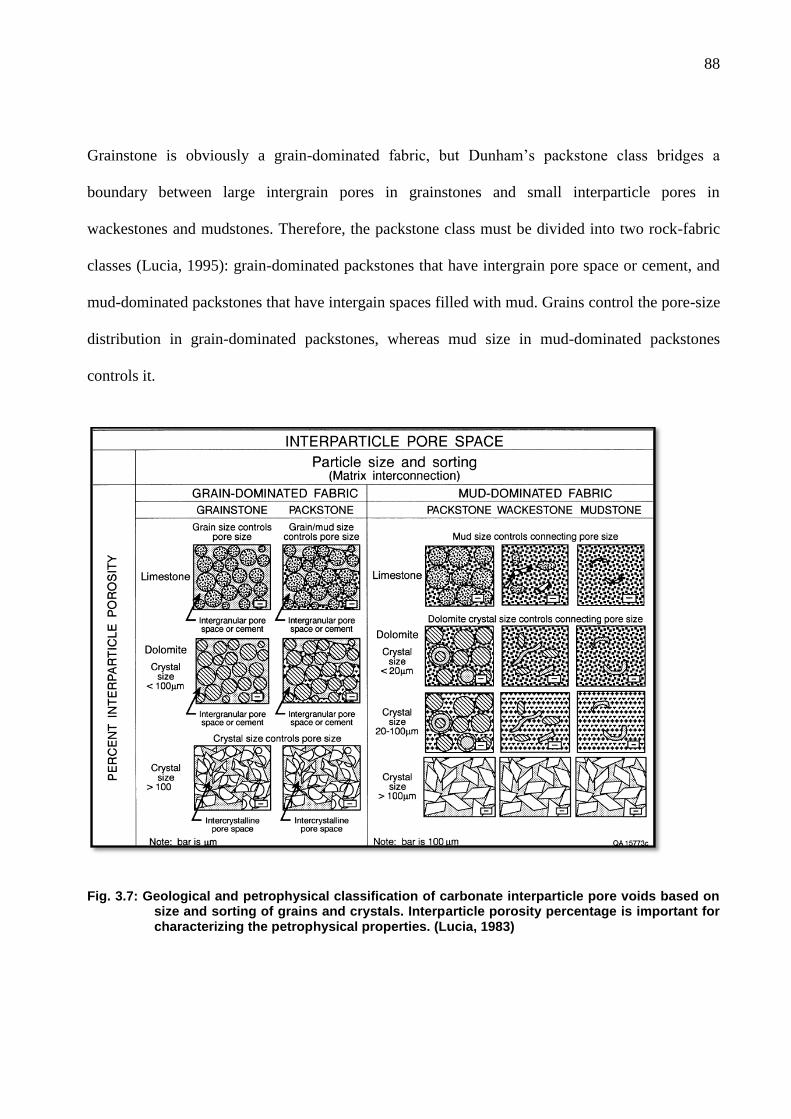
88

Grainstone is obviously a grain-dominated fabric, but Dunham‟s packstone class bridges a

boundary between large intergrain pores in grainstones and small interparticle pores in

wackestones and mudstones. Therefore, the packstone class must be divided into two rock-fabric

classes (Lucia, 1995): grain-dominated packstones that have intergrain pore space or cement, and

mud-dominated packstones that have intergain spaces filled with mud. Grains control the pore-size

distribution in grain-dominated packstones, whereas mud size in mud-dominated packstones

controls it.

Fig. 3.7: Geological and petrophysical classification of carbonate interparticle pore voids based on size and sorting of grains and crystals. Interparticle porosity percentage is important for characterizing the petrophysical properties. (Lucia, 1983)

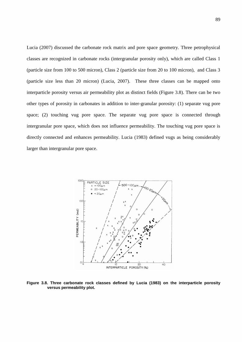
89

Lucia (2007) discussed the carbonate rock matrix and pore space geometry. Three petrophysical

classes are recognized in carbonate rocks (intergranular porosity only), which are called Class 1

(particle size from 100 to 500 micron), Class 2 (particle size from 20 to 100 micron), and Class 3

(particle size less than 20 micron) (Lucia, 2007). These three classes can be mapped onto

interparticle porosity versus air permeability plot as distinct fields (Figure 3.8). There can be two

other types of porosity in carbonates in addition to inter-granular porosity: (1) separate vug pore

space; (2) touching vug pore space. The separate vug pore space is connected through

intergranular pore space, which does not influence permeability. The touching vug pore space is

directly connected and enhances permeability. Lucia (1983) defined vugs as being considerably

larger than intergranular pore space.

Figure 3.8. Three carbonate rock classes defined by Lucia (1983) on the interparticle porosity versus permeability plot.

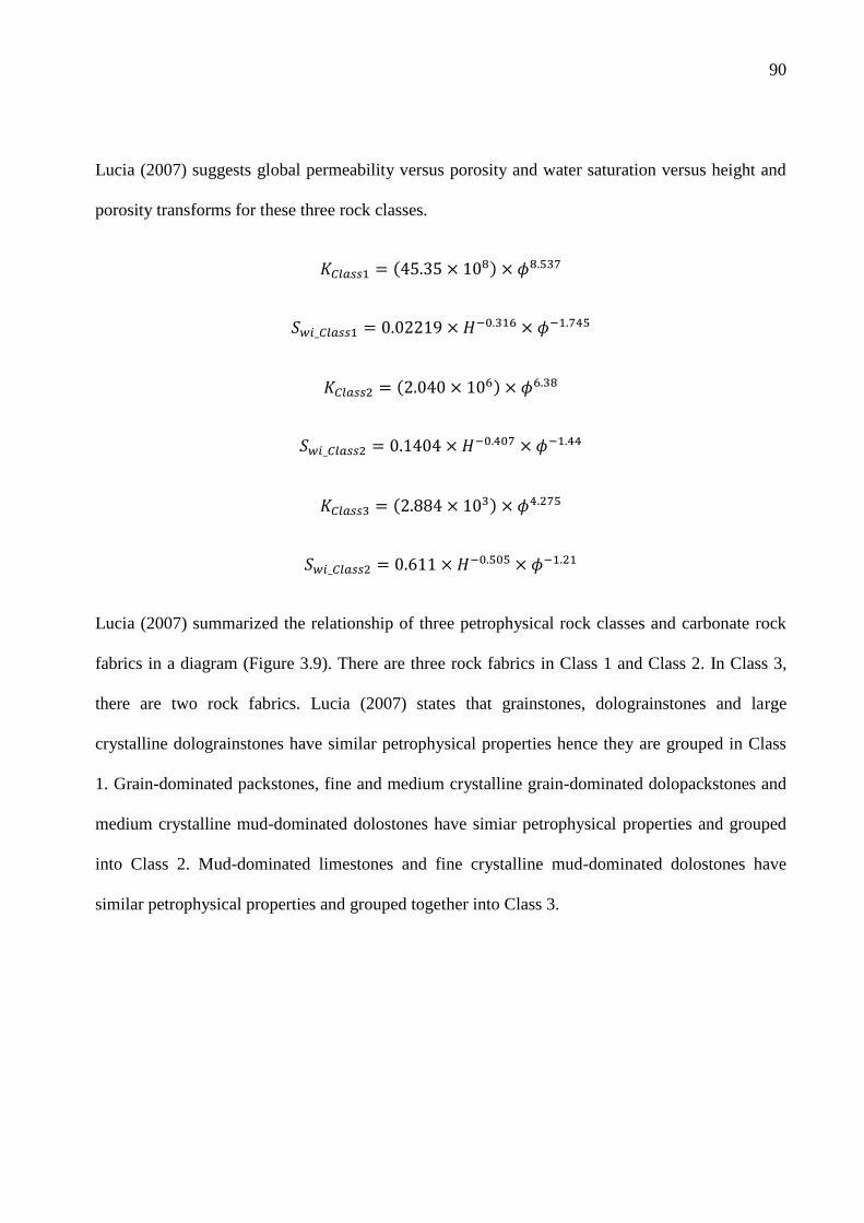
90

Lucia (2007) suggests global permeability versus porosity and water saturation versus height and

porosity transforms for these three rock classes.

Lucia (2007) summarized the relationship of three petrophysical rock classes and carbonate rock

fabrics in a diagram (Figure 3.9). There are three rock fabrics in Class 1 and Class 2. In Class 3,

there are two rock fabrics. Lucia (2007) states that grainstones, dolograinstones and large

crystalline dolograinstones have similar petrophysical properties hence they are grouped in Class

1. Grain-dominated packstones, fine and medium crystalline grain-dominated dolopackstones and

medium crystalline mud-dominated dolostones have simiar petrophysical properties and grouped

into Class 2. Mud-dominated limestones and fine crystalline mud-dominated dolostones have

similar petrophysical properties and grouped together into Class 3.

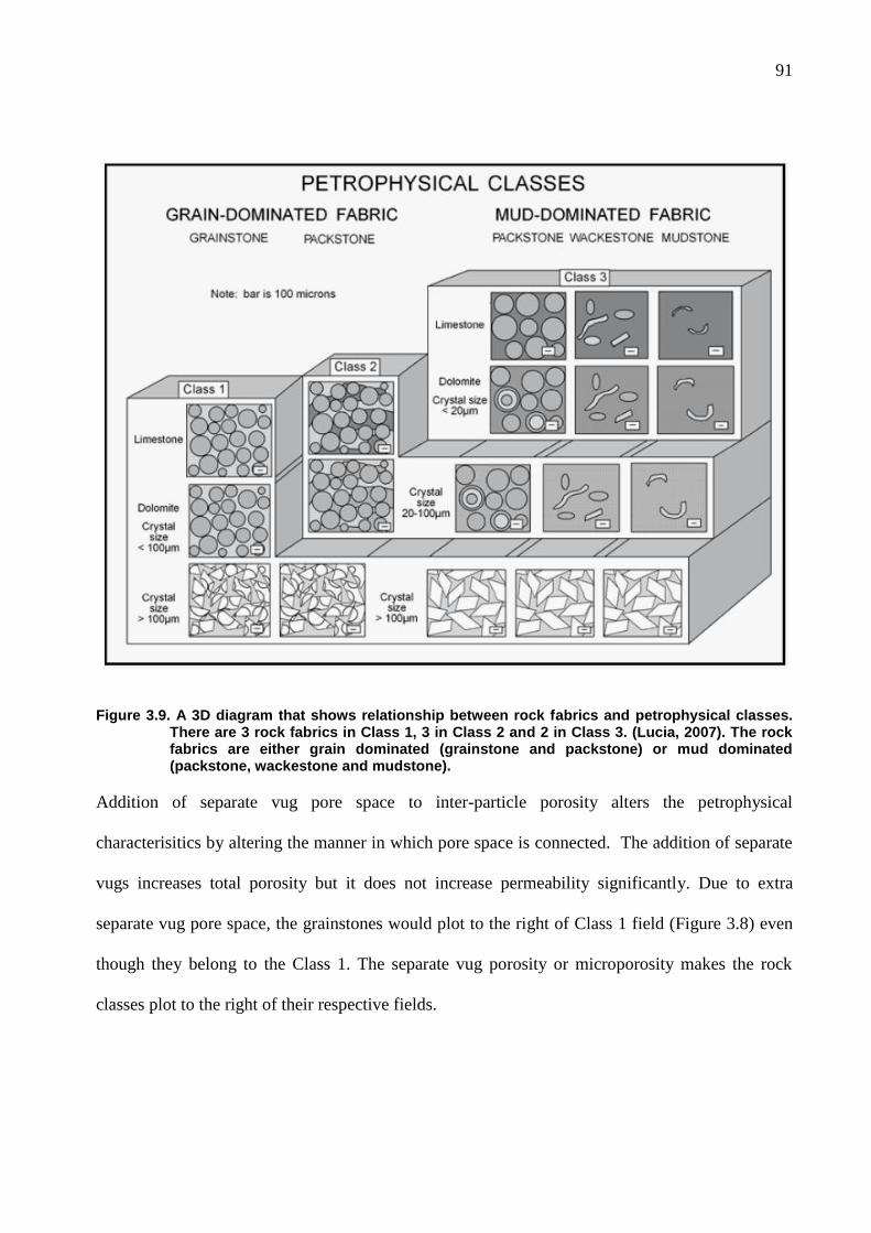
91

Figure 3.9. A 3D diagram that shows relationship between rock fabrics and petrophysical classes. There are 3 rock fabrics in Class 1, 3 in Class 2 and 2 in Class 3. (Lucia, 2007). The rock fabrics are either grain dominated (grainstone and packstone) or mud dominated (packstone, wackestone and mudstone).

Addition of separate vug pore space to inter-particle porosity alters the petrophysical

characterisitics by altering the manner in which pore space is connected. The addition of separate

vugs increases total porosity but it does not increase permeability significantly. Due to extra

separate vug pore space, the grainstones would plot to the right of Class 1 field (Figure 3.8) even

though they belong to the Class 1. The separate vug porosity or microporosity makes the rock

classes plot to the right of their respective fields.

92

Touching vug pores have little relationship to rock fabrics and increase permeability considerably

more than would be expected from the inter-particle pores. Lucia (2007) shows that permeability

in touching vug pore systems can not be characterized by rock fabrics or petrophysical classes.

Often, touching vugs are very large and their permeability can only be characterized through

production tests.

Volume of Shale

Carbonate reservoirs often have little or no clay in their pore space though there are exceptions.

However, shale or marl beds are common in carbonate rock successions. There are shaly and

anhydritic carbonates that were deposited in shallow water or sabkhas. There are mixed

successions of carbonates and siliciclastics in which shale beds and shaly sands may be present.

Clay and shale could infiltrate in carbonate rocks for several tens of feet below sub-aerial exposure

surfaces or disconformities. The shale content of the carbonate reservoirs have to be quantified

when it is present. There are five shale volume indicators: SP, gamma ray, and differences

between neutron and density, sonic and density, and neutron and sonic porosity. Their availability

is controlled by which logging tools were run and their applicability is dictated by the type of rock

and fluid in the formation.

Log interpretation has evolved to recognize that logs sense the petrophysical components of a

rock. Thus, logs respond to clay in shaly carbonates. The general equation for calculation of shale

volume, VSH, using the SP or gamma ray log is written:

93

X is the SP or gamma ray response in the zone of interest. XLS is the log response in clean

limestone. XSH is the response to shale. The selection of these parameters is guided by the

understanding of how much shale is present in the clean and shaly rocks.

When used with the gamma ray log, the equation above may be termed linear gamma ray index,

ISH. For some log analysts, a non-linear relation such as the Steiber relation (given below), is used

to convert this index to shale volume because it is felt that the gamma ray response to clay is non-

linear: (Steiber,1970)

The general equation for calculation of clay volume using the difference between porosity logs is

written:

1 and 2 are porosity values from neutron, density, or sonic logs. They are usually expressed in

limestone units. The porosity values in the denominator are the apparent porosities of shale,

corresponding to those logs used in the numerator.

The different possible shale volume calculations are often combined in a "minimum shale index."

At each depth, the minimum value of each of the indicators is taken as the shale volume. This

reflects the idea that, if in error, the individual methods tend to overestimate shale volume.

94

It is geologically more accurate to refer to clay volume than the volume of shale. Shale is a fine-

grained sedimentary rock that is fissile and usually contains substantial amounts of clay minerals.

Not all clay-rich rocks associated with reservoirs are shales. That is, clay-rich rocks may contain

pores filled with fluid and may not be fissile or laminated.

Results of shale volume computations from logs ought to be consistent with geologic and

petrographic data. Choosing conventional clean limestone and shale parameters may be difficult

and may not be appropriate. With this in mind, the evaluation of the textural occurrence of shale

becomes important as does its effect on the selection of an appropriate saturation equation.

The various shale indicators may provide an insight about sedimentologic or diagenetic processes

that may correspond to features that affect reservoir definition and performance characteristics.

Each indicator may yield somewhat different information. These differences may the suggest that

characteristics of lithology or pore fluid are not as expected.

Shale volume based on the SP log reflects how electrical potential is affected by shale. Other

indicators are not so directly linked to electrical properties. The depth resolution of the SP log is

inferior to other shale indicators and, in the presence of hydrocarbons, XSH from the SP may be too

high.

The gamma ray clay volume may reflect concentrations of uranium. KCl drilling muds produce

large gamma radiation backgrounds that may exacerbate problems of picking the limestone and

shale points.

95

The neutron-density and neutron-sonic apparent shale volume is low or even negative in

formations containing gas. Any calculation using the neutron or density may be invalid where the

contact of the tools with the borehole is poor.

Except for the Steiber relation, all of these shale volume indicators are linear. The assumption of

linearity may be erroneous. The Steiber relation may underestimate shale volume and is very

sensitive to XLS. The results are relatively insensitive to XSH. Comparison with other shale volume

indicators may be inappropriate. Ideally, shale volumes computed by several indicators ought to be

consistent and well-correlated. This view enables the selection of shale values so that the log

analysis is internally consistent.

Porosity

Porosity, one of the most important and fundamental reservoir properties, describes the total

fraction of rock volume available for the storage of liquids or gas. It is the ratio of the pore volume

to the bulk volume of the rock.

where ϕ is porosity, Vmatrix is volume of matrix and Vbulk is bulk volume of the rock. Porosity can

not be directly measured by well log instruments. Logging tools measure physical properties of the

rock, from which porosity is estimated, in conjunction with some assumed or measured

parameters. Porosity can, however, be measured from core plug samples. Porosity is measured or

assessed by several methods (Figure 3.10).

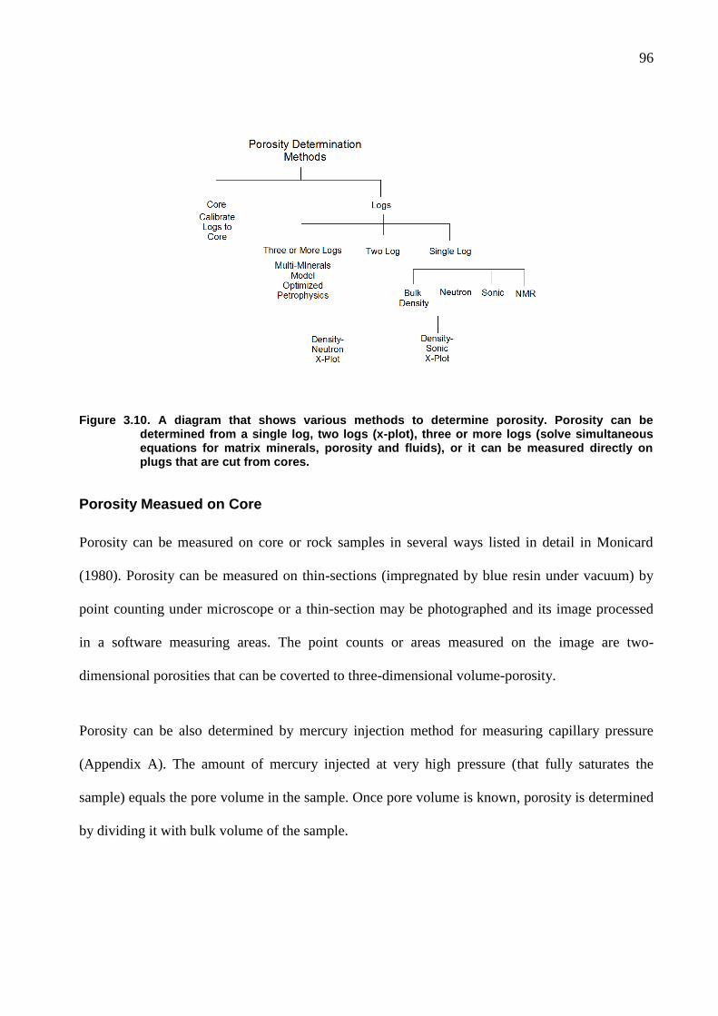
96

Figure 3.10. A diagram that shows various methods to determine porosity. Porosity can be determined from a single log, two logs (x-plot), three or more logs (solve simultaneous equations for matrix minerals, porosity and fluids), or it can be measured directly on plugs that are cut from cores.

Porosity Measued on Core

Porosity can be measured on core or rock samples in several ways listed in detail in Monicard

(1980). Porosity can be measured on thin-sections (impregnated by blue resin under vacuum) by

point counting under microscope or a thin-section may be photographed and its image processed

in a software measuring areas. The point counts or areas measured on the image are two-

dimensional porosities that can be coverted to three-dimensional volume-porosity.

Porosity can be also determined by mercury injection method for measuring capillary pressure

(Appendix A). The amount of mercury injected at very high pressure (that fully saturates the

sample) equals the pore volume in the sample. Once pore volume is known, porosity is determined

by dividing it with bulk volume of the sample.

97

Porosity is also determined by allowing a gas to expand into a dried rock sample placed in a

holder.

In the density method, the weight and volume of a dried sample are determined to obtain the bulk

density. The grain density is determined by a pycnometer. From the grain density and bulk

density, porosity is calculated.

Porosity measured on core samples (often at every foot) is depth-matched to logs, then smoothed

to resolution matching logs. It is then used to calibrate log-calculated porosity.

Porosity Assessed from Single Logs

Porosity can be assessed from single logs, which are sonic, density, neutron, and nuclear magnetic

resonance.

In sonic logs, the Wyllie time-average equation is the conventional means used to convert transit

time, t, to porosity, υ. It is based on a simple linear mixing model for transit time.

where t is transit time, tmatrix and tfluid are transit times for matrix and pore fluid, respectively.

Porosity evaluation in uncompacted sands, using the Wyllie time-average equation, requires a

correction for lack of compaction (Crain, 1986). This factor is s/ and is determined by reference

98

to porosities obtained by other log or core measurements. This method tends to overestimate

porosity in sandstones and hydrocarbon-bearing reservoirs. Empirical corrections to lessen these

errors are implemented using the Compaction Factor (CP) and Hydrocarbon Correction (Hy). The

CP is commonly estimated from the sonic response in the nearby shales. The Hy correction is

approximate and is set equal to 0.9 for oil and 0.7 for gas.

Another empirical equation, by Raymer, Hunt and Gardner, requires no compaction correction

(Raymer et al., 1980).

The constant C ranges from 0.625 to 0.7. A value of 0.6 is recommended for gas reservoirs.

Sonic porosity equations usually work well for rocks that have mainly intergranular porosity.

Porosity that is heterogeneous, due to vugs or fractures, may not be described adequately using

these equations. The sonic transit time corresponds to the fastest path through the rock, so

fractures and vugs may be missed.

Gas in the wellbore or near-wellbore region, improper tool centralization, or formation fracturing

may attenuate the acoustic energy of the transmitted signal. If the detection threshold is set too

99

high, detection of the first P-wave arrival will be missed and a later arrival will be detected. This

is referred to as cycle skipping. It is seen on the logs as erratic response, generally toward higher

transit times. In such cases, the log is not usable.

As with all logs classified as porosity logs, the density log response depends on porosity and

lithology (Gardner and Dumanoir, 1980). Computation of the density porosity, density, is based on

a linear mixing model for density.

The effect of gas in the pore space is to lower the density of the pore fluid and to cause a decrease

in apparent density porosity. This, combined with the lowering of the neutron porosity by gas,

results in the well-known cross-over effect. The combined use of these logs as a qualitative gas

indicator is a big advantage.

The neutron log response also depends on both porosity and lithology. The log is recorded based

on some assumed lithology (usually sandstone or limestone). Because of the significant effects of

lithology, gas, and clay, the neutron porosity is the least reliable of the available logs. Gas may

also have a marked effect on neutron log response due to its relatively low hydrogen density.

Lower count rate ratios for both thermal and epithermal neutrons and substantial decrease in

apparent neutron porosity from its true value will result. Apparent porosity is further reduced by

the excavation effect (Segesman and Liu, 1971).

100

The Nuclear Magnetic Resonance (NMR) log produces a spectrum or a distribution of relaxation

times of protons interacting with the surface of grains in the matrix (Ellis and Singer, 2007). There

are two relaxation times (longitudinal or T1 and transverse or T2). The NMR logging tools

generally do not measure very short relaxation times that are coming from bound water and

microporosity. These logs are mostly measuring relaxation times from larger pores. Therefore,

NMR porosity is often different than that measured by other density or neutron tools. NMR

porosity is usually divided into capillary bound or producible or free fluid. This division is

calibrated by centrifuge capillary pressure measurements that are required to remove capillary

bound fluids. The relaxation signals measured by NMR logs are fitted by curves (exponential

decay functions). The total porosity is the integral (area) under the exponential decay function

fitted to NMR relaxation signal data. The Free Fluid Index (FFI or Free Fluid porosity) is the area

under the NMR exponential decay function to a T-2 value (transverse relaxation signal) that is

chosen based on capillary pressure measurement from centrifuge experiments (Figure 3.11). The

capillary bound water is the sum of all the rest of the spectrum. This T-2 cutoff depends on the

lithology, for example; the T-2 cutoff for carbonate samples is 92 micro-seconds.

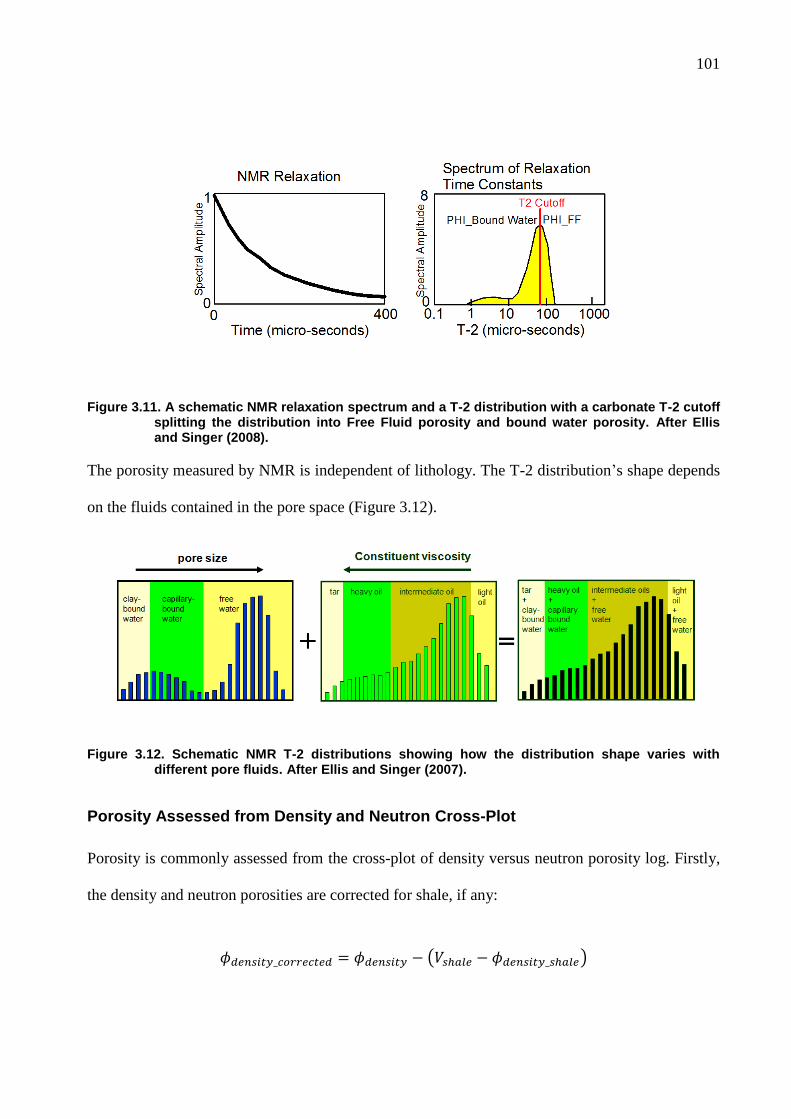
101

Figure 3.11. A schematic NMR relaxation spectrum and a T-2 distribution with a carbonate T-2 cutoff splitting the distribution into Free Fluid porosity and bound water porosity. After Ellis and Singer (2008).

The porosity measured by NMR is independent of lithology. The T-2 distribution‟s shape depends

on the fluids contained in the pore space (Figure 3.12).

Figure 3.12. Schematic NMR T-2 distributions showing how the distribution shape varies with different pore fluids. After Ellis and Singer (2007).

Porosity Assessed from Density and Neutron Cross-Plot

Porosity is commonly assessed from the cross-plot of density versus neutron porosity log. Firstly,

the density and neutron porosities are corrected for shale, if any:

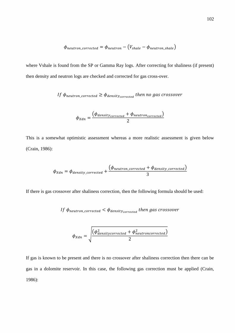
102

where Vshale is found from the SP or Gamma Ray logs. After correcting for shaliness (if present)

then density and neutron logs are checked and corrected for gas cross-over.

This is a somewhat optimistic assessment whereas a more realistic assessment is given below

(Crain, 1986):

If there is gas crossover after shaliness correction, then the following formula should be used:

If gas is known to be present and there is no crossover after shaliness correction then there can be

gas in a dolomite reservoir. In this case, the following gas correction must be applied (Crain,

1986):

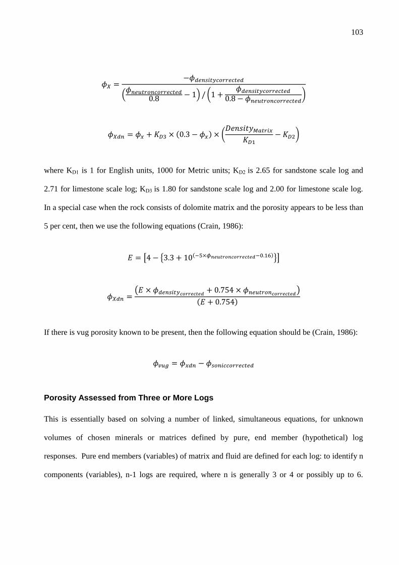
103

where KD1 is 1 for English units, 1000 for Metric units; KD2 is 2.65 for sandstone scale log and

2.71 for limestone scale log; KD3 is 1.80 for sandstone scale log and 2.00 for limestone scale log.

In a special case when the rock consists of dolomite matrix and the porosity appears to be less than

5 per cent, then we use the following equations (Crain, 1986):

If there is vug porosity known to be present, then the following equation should be (Crain, 1986):

Porosity Assessed from Three or More Logs

This is essentially based on solving a number of linked, simultaneous equations, for unknown

volumes of chosen minerals or matrices defined by pure, end member (hypothetical) log

responses. Pure end members (variables) of matrix and fluid are defined for each log: to identify n

components (variables), n-1 logs are required, where n is generally 3 or 4 or possibly up to 6.

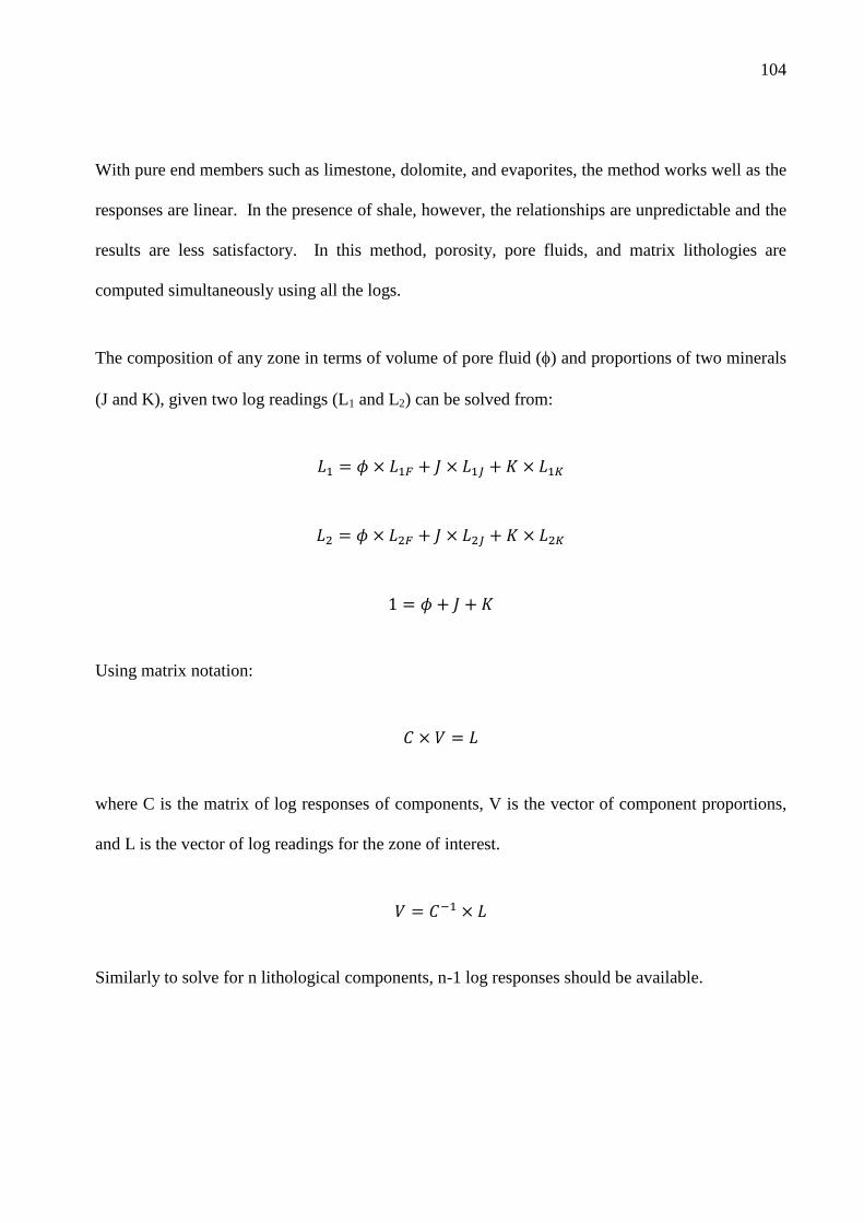
104

With pure end members such as limestone, dolomite, and evaporites, the method works well as the

responses are linear. In the presence of shale, however, the relationships are unpredictable and the

results are less satisfactory. In this method, porosity, pore fluids, and matrix lithologies are

computed simultaneously using all the logs.

The composition of any zone in terms of volume of pore fluid () and proportions of two minerals

(J and K), given two log readings (L1 and L2) can be solved from:

Using matrix notation:

where C is the matrix of log responses of components, V is the vector of component proportions,

and L is the vector of log readings for the zone of interest.

Similarly to solve for n lithological components, n-1 log responses should be available.

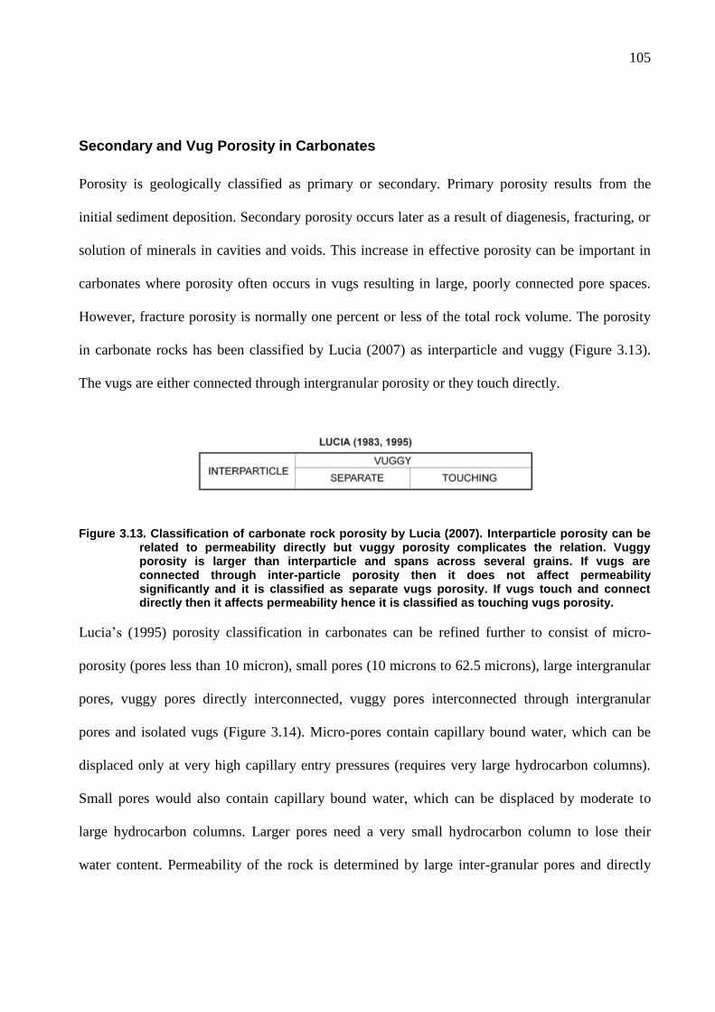
105

Secondary and Vug Porosity in Carbonates

Porosity is geologically classified as primary or secondary. Primary porosity results from the

initial sediment deposition. Secondary porosity occurs later as a result of diagenesis, fracturing, or

solution of minerals in cavities and voids. This increase in effective porosity can be important in

carbonates where porosity often occurs in vugs resulting in large, poorly connected pore spaces.

However, fracture porosity is normally one percent or less of the total rock volume. The porosity

in carbonate rocks has been classified by Lucia (2007) as interparticle and vuggy (Figure 3.13).

The vugs are either connected through intergranular porosity or they touch directly.

Figure 3.13. Classification of carbonate rock porosity by Lucia (2007). Interparticle porosity can be related to permeability directly but vuggy porosity complicates the relation. Vuggy porosity is larger than interparticle and spans across several grains. If vugs are connected through inter-particle porosity then it does not affect permeability significantly and it is classified as separate vugs porosity. If vugs touch and connect directly then it affects permeability hence it is classified as touching vugs porosity.

Lucia‟s (1995) porosity classification in carbonates can be refined further to consist of micro-

porosity (pores less than 10 micron), small pores (10 microns to 62.5 microns), large intergranular

pores, vuggy pores directly interconnected, vuggy pores interconnected through intergranular

pores and isolated vugs (Figure 3.14). Micro-pores contain capillary bound water, which can be

displaced only at very high capillary entry pressures (requires very large hydrocarbon columns).

Small pores would also contain capillary bound water, which can be displaced by moderate to

large hydrocarbon columns. Larger pores need a very small hydrocarbon column to lose their

water content. Permeability of the rock is determined by large inter-granular pores and directly

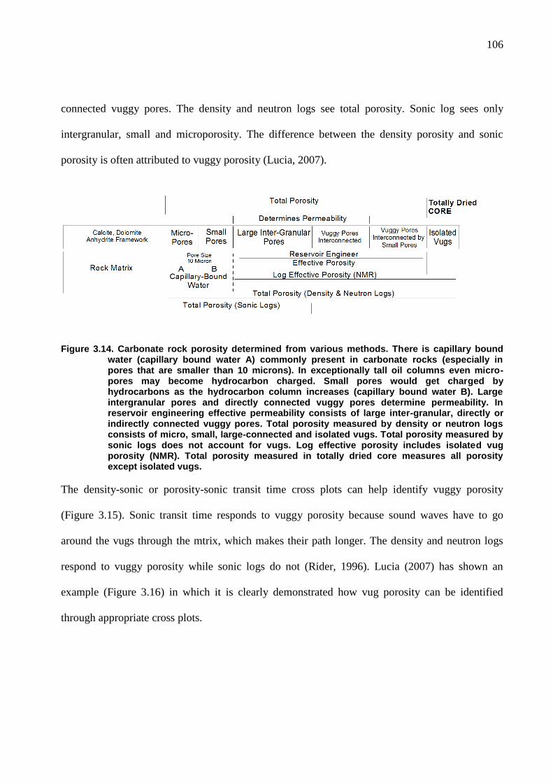
106

connected vuggy pores. The density and neutron logs see total porosity. Sonic log sees only

intergranular, small and microporosity. The difference between the density porosity and sonic

porosity is often attributed to vuggy porosity (Lucia, 2007).

Figure 3.14. Carbonate rock porosity determined from various methods. There is capillary bound water (capillary bound water A) commonly present in carbonate rocks (especially in pores that are smaller than 10 microns). In exceptionally tall oil columns even micro-pores may become hydrocarbon charged. Small pores would get charged by hydrocarbons as the hydrocarbon column increases (capillary bound water B). Large intergranular pores and directly connected vuggy pores determine permeability. In reservoir engineering effective permeability consists of large inter-granular, directly or indirectly connected vuggy pores. Total porosity measured by density or neutron logs consists of micro, small, large-connected and isolated vugs. Total porosity measured by sonic logs does not account for vugs. Log effective porosity includes isolated vug porosity (NMR). Total porosity measured in totally dried core measures all porosity except isolated vugs.

The density-sonic or porosity-sonic transit time cross plots can help identify vuggy porosity

(Figure 3.15). Sonic transit time responds to vuggy porosity because sound waves have to go

around the vugs through the mtrix, which makes their path longer. The density and neutron logs

respond to vuggy porosity while sonic logs do not (Rider, 1996). Lucia (2007) has shown an

example (Figure 3.16) in which it is clearly demonstrated how vug porosity can be identified

through appropriate cross plots.

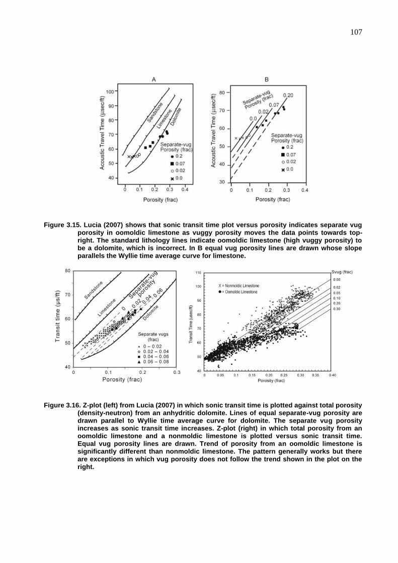
107

Figure 3.15. Lucia (2007) shows that sonic transit time plot versus porosity indicates separate vug porosity in oomoldic limestone as vuggy porosity moves the data points towards top-right. The standard lithology lines indicate oomoldic limestone (high vuggy porosity) to be a dolomite, which is incorrect. In B equal vug porosity lines are drawn whose slope parallels the Wyllie time average curve for limestone.

Figure 3.16. Z-plot (left) from Lucia (2007) in which sonic transit time is plotted against total porosity (density-neutron) from an anhydritic dolomite. Lines of equal separate-vug porosity are drawn parallel to Wyllie time average curve for dolomite. The separate vug porosity increases as sonic transit time increases. Z-plot (right) in which total porosity from an oomoldic limestone and a nonmoldic limestone is plotted versus sonic transit time. Equal vug porosity lines are drawn. Trend of porosity from an oomoldic limestone is significantly different than nonmoldic limestone. The pattern generally works but there are exceptions in which vug porosity does not follow the trend shown in the plot on the right.

108

Water Saturation

Wireline logs are used primarily to determine the quantity of hydrocarbons in place. It is necessary

to determine porosity and the fraction of the pore space filled with hydrocarbons (Etnyre, 1989).

The usual approach is first to determine the water saturation SW, then compute hydrocarbon

saturation as the difference 1-SW.

The calculation of water saturation, SW, for clean (clay-free) rocks is done with the use of Archie's

equation (Archie, 1942).

where Rt is formation resistivity, RW is formation water resistivity, and υ is porosity. The

coefficients a, m, and n depend on lithology, pore structure, and fluid saturation, but are often

assumed to be equal to 1, 2, and 2, respectively.

Resistivity of a rock that is totally saturated with water is called Ro (Figure 3.17). Ratio of

resistivity of water saturated rock (Ro) to that of formation water (Rw) is called Formation

Resistivity Factor or simply Formation Factor (F).

At a constant porosity the Formation Factor is constant. As porosity increases, Ro decreases and F

decreases. The value of F equals 1 when equals 1.0 (all fluid – impossible). The value of F

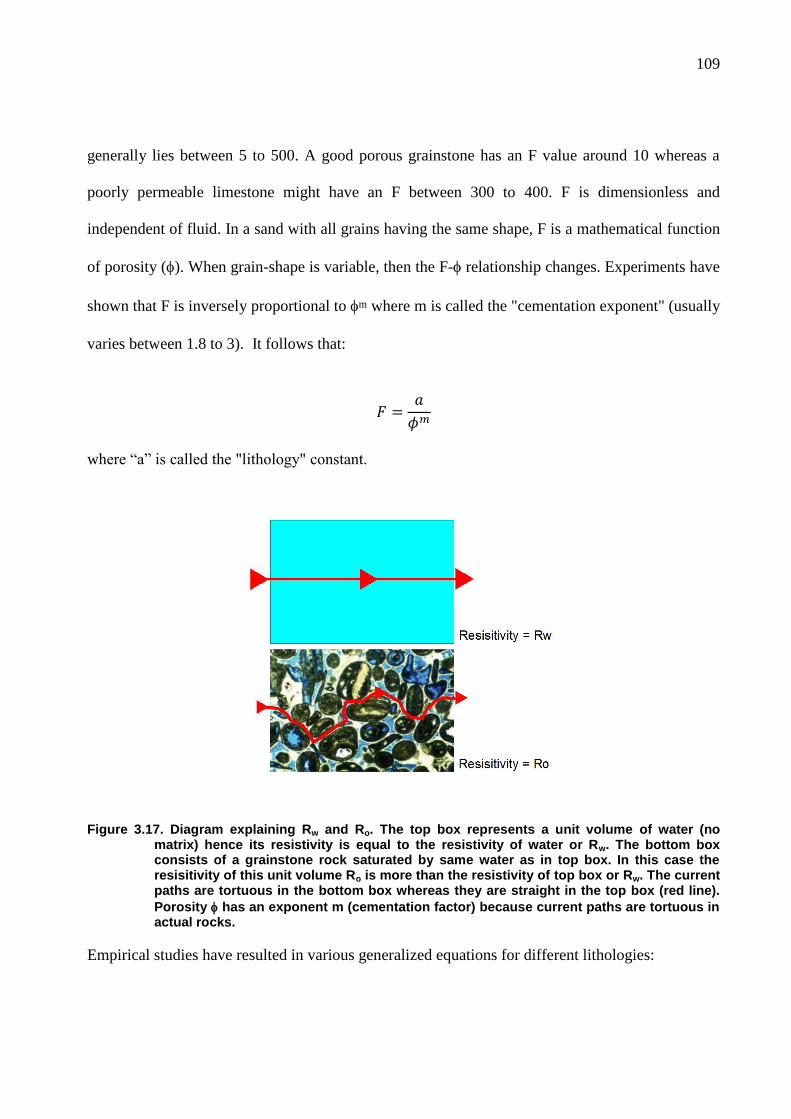
109

generally lies between 5 to 500. A good porous grainstone has an F value around 10 whereas a

poorly permeable limestone might have an F between 300 to 400. F is dimensionless and

independent of fluid. In a sand with all grains having the same shape, F is a mathematical function

of porosity (). When grain-shape is variable, then the F- relationship changes. Experiments have

shown that F is inversely proportional to m where m is called the "cementation exponent" (usually

varies between 1.8 to 3). It follows that:

where “a” is called the "lithology" constant.

Figure 3.17. Diagram explaining Rw and Ro. The top box represents a unit volume of water (no matrix) hence its resistivity is equal to the resistivity of water or Rw. The bottom box consists of a grainstone rock saturated by same water as in top box. In this case the resisitivity of this unit volume Ro is more than the resistivity of top box or Rw. The current paths are tortuous in the bottom box whereas they are straight in the top box (red line).

Porosity has an exponent m (cementation factor) because current paths are tortuous in actual rocks.

Empirical studies have resulted in various generalized equations for different lithologies:

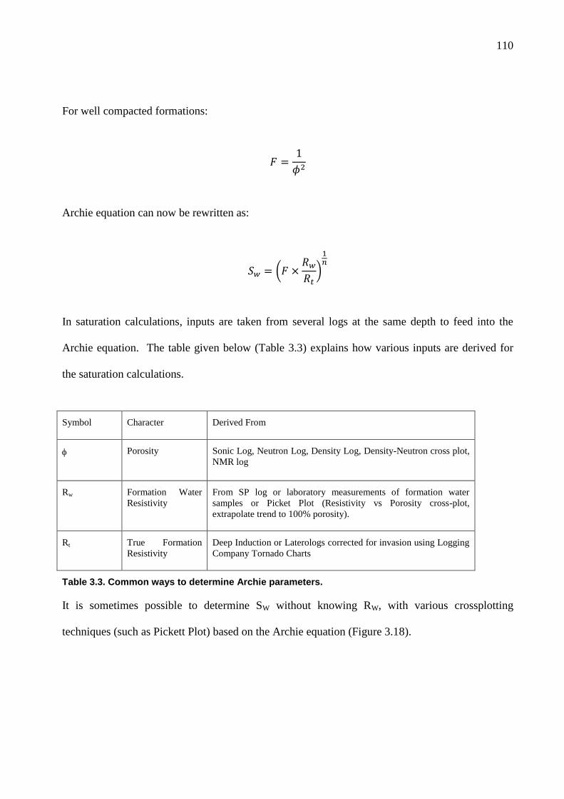
110

For well compacted formations:

Archie equation can now be rewritten as:

In saturation calculations, inputs are taken from several logs at the same depth to feed into the

Archie equation. The table given below (Table 3.3) explains how various inputs are derived for

the saturation calculations.

Symbol Character Derived From

Porosity Sonic Log, Neutron Log, Density Log, Density-Neutron cross plot,

NMR log

Rw Formation Water

Resistivity

From SP log or laboratory measurements of formation water

samples or Picket Plot (Resistivity vs Porosity cross-plot,

extrapolate trend to 100% porosity).

Rt True Formation

Resistivity

Deep Induction or Laterologs corrected for invasion using Logging

Company Tornado Charts

Table 3.3. Common ways to determine Archie parameters.

It is sometimes possible to determine SW without knowing RW, with various crossplotting

techniques (such as Pickett Plot) based on the Archie equation (Figure 3.18).

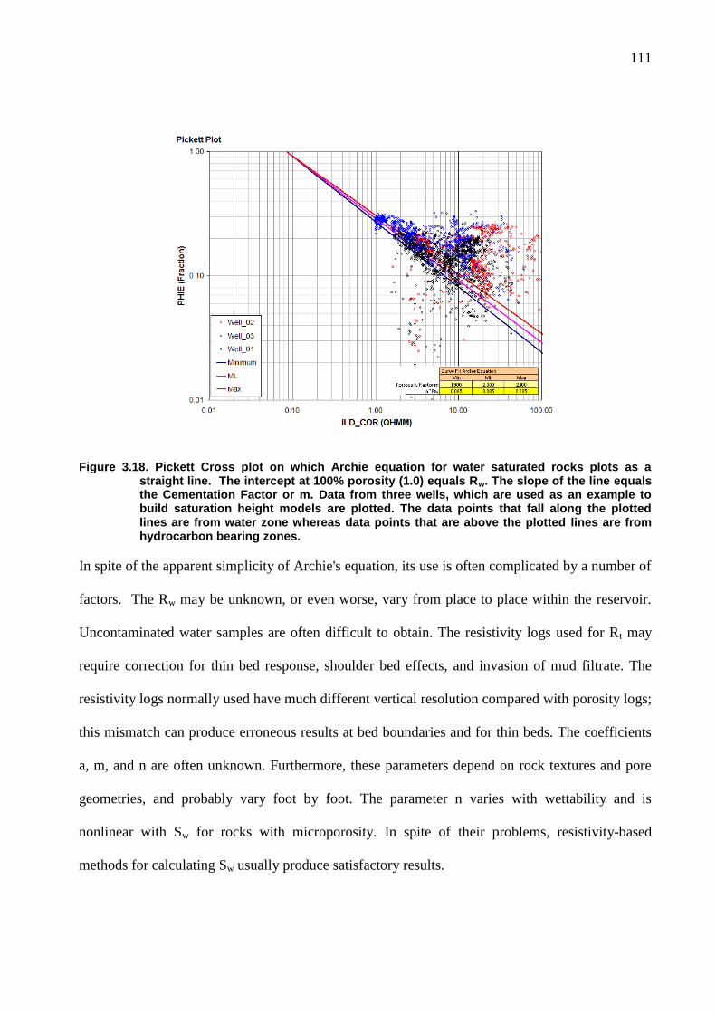
111

Figure 3.18. Pickett Cross plot on which Archie equation for water saturated rocks plots as a straight line. The intercept at 100% porosity (1.0) equals Rw. The slope of the line equals the Cementation Factor or m. Data from three wells, which are used as an example to build saturation height models are plotted. The data points that fall along the plotted lines are from water zone whereas data points that are above the plotted lines are from hydrocarbon bearing zones.

In spite of the apparent simplicity of Archie's equation, its use is often complicated by a number of

factors. The Rw may be unknown, or even worse, vary from place to place within the reservoir.

Uncontaminated water samples are often difficult to obtain. The resistivity logs used for Rt may

require correction for thin bed response, shoulder bed effects, and invasion of mud filtrate. The

resistivity logs normally used have much different vertical resolution compared with porosity logs;

this mismatch can produce erroneous results at bed boundaries and for thin beds. The coefficients

a, m, and n are often unknown. Furthermore, these parameters depend on rock textures and pore

geometries, and probably vary foot by foot. The parameter n varies with wettability and is

nonlinear with Sw for rocks with microporosity. In spite of their problems, resistivity-based

methods for calculating Sw usually produce satisfactory results.

112

Determination of Formation Water Resistivity (RW)

RW can be taken from reference tables in an area (if available), or from the analysis of formation

water recovered in a Drill Stem Test or Repeat Formation Test (care should be taken as it might be

contaminated with drilling mud filtrate). Otherwise, it can be estimated from SP log or from

resistivity log itself in wet zones. It is quite often necessary to correct RW measured at one

temperature to the formation temperature. The equation used to correct RW to another temperature

is:

Where RTformation is resistivity at formation temperature, RTsurface is resistivity at surface

temperature, TSurface and TFormation are temperatures at surface and in the formation (F).

RW can be estimated from Spontenous Potential (SP) log using the following equation:

113

RW is also commonly estimated from resistivity log response in clean and wet zones. Considering

Archie equation when a =1, m=2, n=2:

In a water zone SW = 1

Porosity () can be derived from porosity logs, which are density, neutron, and sonic. Commonly

in computer interpretations, RW (or RWA) curves are calculated and plotted and the appropriate RW

values are chosen graphically.

It is also feasible to estimate RW from the resistivity ratio method:

Similarly;

Where SW = SXO = 1 and a, are same in both the flushed and uninvaded zones:

114

Picking Hydrocarbon Water Interfaces

Using resistivity ratio (Hilchie, 1982):

In a hydrocarbon bearing zone Ri / Rt is less. Water saturation (SW) can be calculated by

comparing Ri / Rt in water zone to that in hydrocarbon zone .

Another method is the Bulk Volume Water method (Asquith and Krygowski, 2004).

WSBVW

BVW is constant in a zone where water is at irreducible saturation (oil or gas leg) for a given

grain-size and pore type. Theoretically BVW equals in the zone of 100% water saturation. In a

computer processed log, BVW will show with depth a zone of irreducible water saturation, the

transition zone, and the hydrocarbon water interface at the top of the 100% water zone.

115

Chapter 4

Permeability and Petrophysical Rock Types

Darcy’s Law and Permeability

The earliest permeability studies date back to the 19th

century when Henry Darcy developed

models to help understand the conductivity of fluids in a porous medium. His experiments were

carried out by flowing water through tubes filled with sorted sand. The Darcy‟s Law was based on

experiments with the potential (similar to pressure) drop p measured over a finite length (L) in a

sand-pack of permeability (K) and cross-sectional area (A). For linear flow of an incompressible

fluid of viscosity ( ) through this sand-pack, the flow rate is related to these variables by

(Ahmed, 2001):

The superficial velocity of the fluid is given by:

116

The derivative of pressure with respect to length is given by:

This leads to differential form of the Darcy‟s Law (Craft and Hawkins, 1959):

The negative sign is due to the direction of flow being the opposite to that of pressure change. In

reservoir rocks, permeability often depends on the direction of measurement. So, vertical

permeability (across beds) is much less than horizontal (along beds). This is due to grain sorting,

thin mud drapes, shale lamina, beddings, or other sedimentary features. The horizontal variation of

permeability is due to fracturing, tectonic stresses, or depositional process-based sedimentary

geometries. In a three dimensional system, the components of velocity are:

117

In anisotropic systems, permeability is a tensor. In anisotropic porous media, flow will occur in the

direction of the highest permeability even when the pressure gradient is not in that direction. A co-

ordinate system can be defined in such a way that off-diagonal terms are zero. In such a principal

co-ordinate space (X, Y, Z):

Six permeability terms are needed to describe flow in three dimensions (kxx, kxy, kxz, kyy, kyz, kzz or

kX, kY, kZ and three angles).

It is important to note that the pressure gradient is proportional to the volume flow rate and not the

mass flow rate. For steady-state flow, the mass flow rate is constant. For incompressible flow, the

volume flow rate is also constant. However, when the fluid is compressible the volume flow rate

varies and the integrated Darcy‟s Law equation is different. The form of the integrated Darcy‟s

Law equation also depends on the geometry of the flow. Two fundamental geometries are often

encountered, namely linear and radial flow.

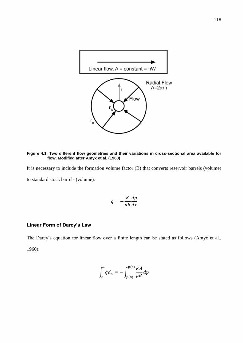
118

Figure 4.1. Two different flow geometries and their variations in cross-sectional area available for flow. Modified after Amyx et al. (1960)

It is necessary to include the formation volume factor (B) that converts reservoir barrels (volume)

to standard stock barrels (volume).

Linear Form of Darcy’s Law

The Darcy‟s equation for linear flow over a finite length can be stated as follows (Amyx et al.,

1960):

119

In oil field units, it can be stated as (Ahmed, 2001):

When pressure is greater at 0 than at L ,then, the flow goes from 0 to L (the difference of pressure

terms in the above equation with bracket is negative). On the contrary, when pressure is greater at

L than at 0, then the flow goes from L to 0.

Radial Form of Darcy’s Law

The area of flow (A) is a function of the radius of the cylinder. Integrating the following equation

(Craft and Hawkins, 1991):

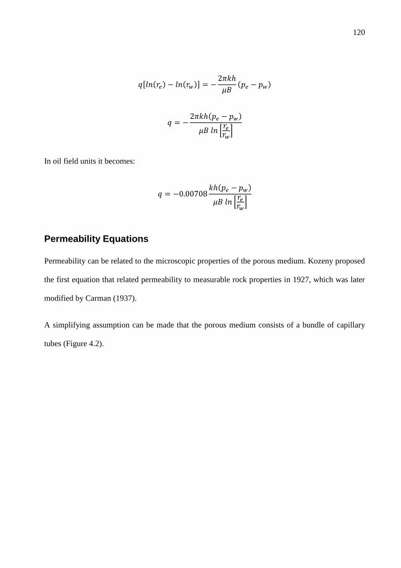
120

In oil field units it becomes:

Permeability Equations

Permeability can be related to the microscopic properties of the porous medium. Kozeny proposed

the first equation that related permeability to measurable rock properties in 1927, which was later

modified by Carman (1937).

A simplifying assumption can be made that the porous medium consists of a bundle of capillary

tubes (Figure 4.2).

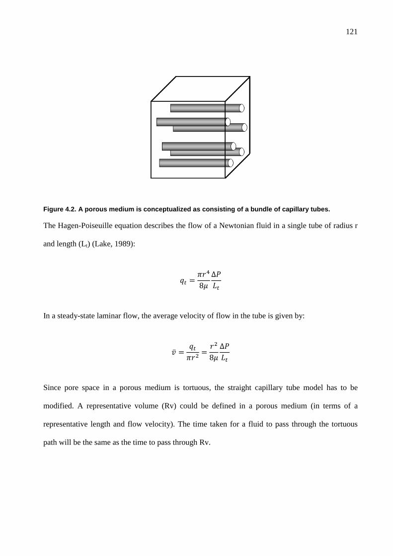
121

Figure 4.2. A porous medium is conceptualized as consisting of a bundle of capillary tubes.

The Hagen-Poiseuille equation describes the flow of a Newtonian fluid in a single tube of radius r

and length (Lt) (Lake, 1989):

In a steady-state laminar flow, the average velocity of flow in the tube is given by:

Since pore space in a porous medium is tortuous, the straight capillary tube model has to be

modified. A representative volume (Rv) could be defined in a porous medium (in terms of a

representative length and flow velocity). The time taken for a fluid to pass through the tortuous

path will be the same as the time to pass through Rv.

122

Combining with the Darcy‟s equation (Lake, 1989):

The tortuousity ( is a variable that defines the straightness of the flow path. A straight tube has a

tortuosity of 1, whereas common porous rocks have tortuousities in the range from 2 to 5. It can be

determined experimentally by resistivity measurements on core samples.

In an actual porous medium the radii of tubes are not uniform, therefore, an equivalent hydraulic

radius has to be defined:

The hydraulic radius for a cylindrical capillary is given by:

123

For a granular or porous medium, it is convenient to use specific surface area, which is defined as:

The specific surface area of a porous medium can be estimated from porosity estimates and grain

size (Amyx et al., 1960). The hydraulic radius can be derived from specific surface area and

porosity.

Substituting the above equation into the permeability equation (above), we get the Carman-

Kozeny equation (Panda & Lake, 1994).

where k is in μm2 and υ is in fractions.

Considering a pack of uniform spheres:

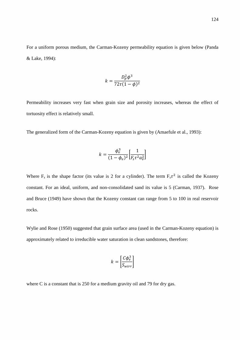
124

For a uniform porous medium, the Carman-Kozeny permeability equation is given below (Panda

& Lake, 1994):

Permeability increases very fast when grain size and porosity increases, whereas the effect of

tortuosity effect is relatively small.

The generalized form of the Carman-Kozeny equation is given by (Amaefule et al., 1993):

Where Fs is the shape factor (its value is 2 for a cylinder). The term Fs is called the Kozeny

constant. For an ideal, uniform, and non-consolidated sand its value is 5 (Carman, 1937). Rose

and Bruce (1949) have shown that the Kozeny constant can range from 5 to 100 in real reservoir

rocks.

Wylie and Rose (1950) suggested that grain surface area (used in the Carman-Kozeny equation) is

approximately related to irreducible water saturation in clean sandstones, therefore:

where C is a constant that is 250 for a medium gravity oil and 79 for dry gas.

125

Timur (1968) extended the Wylie and Rose equation based on laboratory study of sandstone cores.

He proposed:

The difficuly in these equations is to determine the irreducible water saturation (Swirr) from logs.

Petrophysical Rock Types

A rock type refers to both lithological and pore space characteristics of a rock. Archie (1952)

described rock types as being characterized by specific pore geometry (size distribution of pores

and pore throats). This results in specific porosity-permeability relationships, capillary pressure

properties and curves and relationship among permeability, pore size and water saturation.

A petrophysical rock type consists of a group of rocks, which have a similar texture, the same

permeability-porosity relationship, similar capillary pressure curves (Gunter et al., 1997), and a

relationship between permeability, pore-throat size, and water saturation. Hydraulic units are

defined as the representative volumes of the total reservoir rock within which geological properties

that control fluid flow are internally consistent and predictably different from properties of other

rocks (Ebanks et al., 1987).

One of the essential attributes of the rock types is that they have similar particle size (or pore

throat size) distribution. In a rock type, permeability variation is due to porosity changes. Among

different rock types, permeability variation is due to particle size (or pore throat size) changes.

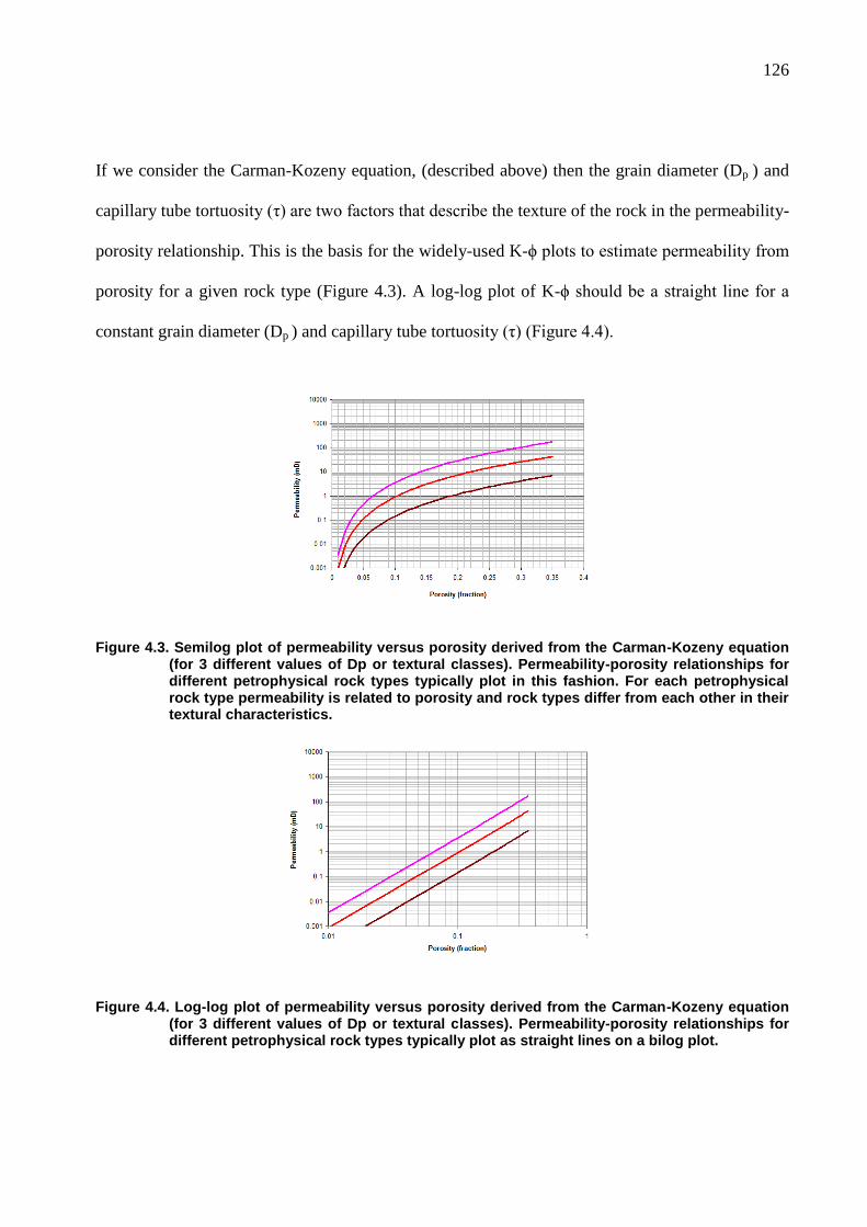
126

If we consider the Carman-Kozeny equation, (described above) then the grain diameter (Dp ) and

capillary tube tortuosity (τ) are two factors that describe the texture of the rock in the permeability-

porosity relationship. This is the basis for the widely-used K-ϕ plots to estimate permeability from

porosity for a given rock type (Figure 4.3). A log-log plot of K-ϕ should be a straight line for a

constant grain diameter (Dp ) and capillary tube tortuosity (τ) (Figure 4.4).

Figure 4.3. Semilog plot of permeability versus porosity derived from the Carman-Kozeny equation (for 3 different values of Dp or textural classes). Permeability-porosity relationships for different petrophysical rock types typically plot in this fashion. For each petrophysical rock type permeability is related to porosity and rock types differ from each other in their textural characteristics.

Figure 4.4. Log-log plot of permeability versus porosity derived from the Carman-Kozeny equation (for 3 different values of Dp or textural classes). Permeability-porosity relationships for different petrophysical rock types typically plot as straight lines on a bilog plot.

127

Since petrophysical rock types have capillary pressure curves that tightly cluster on a Pc-Sw plot

and have similar shapes, therefore, a rock type also has a well-defined saturation versus height

relationship.

Hydraulic Flow Unit Rock Types

Attempts have been made to calculate permeability from porosity by using the Carman-Kozeny

equation (given above). The attempts were unsuccessful because the “Kozeny constant” is actually

a variable and the rocks have to be classified into groups so that each group of rocks have a

consistent Kozeny constant. These groups are called hydraulic flow units. The Kozeny constant

describes the textural aspects of rocks. Different hydraulic units have different porosity-

permeability relationships and capillary pressure curves. Therefore, hydraulic flow units are

petrophysical rock types according to the definition above.

Dividing both sides of the Carman-Kozeny equation (given above) by effective porosity and then

taking a square root leads to:

If permeability is presented in millidarcies then, the following parameter can be defined (Amaefule

et al., 1993).

128

where ϕz is defined as pore volume to grain volume ratio:

Once RQI and FZI have been calculated, the samples should be separated into groups called

hydraulic units (HU). Although there should exist one single FZI value for a hydraulic unit, a

scatter of each FZI around its true mean results due to random measurement errors in core analysis

(Abbaszadeh et al., 1996). When multiple hydraulic units exist, the overall FZI distribution

function is a superposition of the individual distribution functions around their mean FZI.

Identification of each mean FZI or the corresponding hydraulic unit involves decomposition of the

overall FZI distribution into its constituent distributions (Figure 4.5). Such a decomposition can be

done using cluster analysis techniques. A histogram analysis or a probability plot are commonly

used.

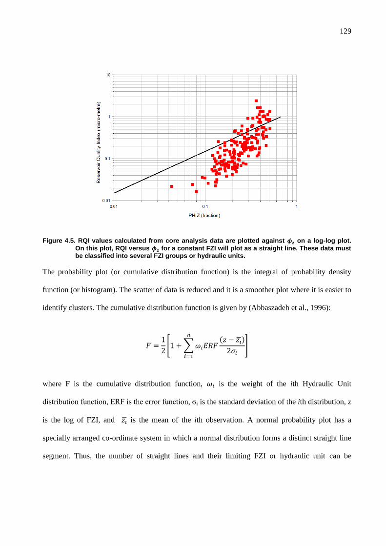
129

Figure 4.5. RQI values calculated from core analysis data are plotted against on a log-log plot.

On this plot, RQI versus for a constant FZI will plot as a straight line. These data must be classified into several FZI groups or hydraulic units.

The probability plot (or cumulative distribution function) is the integral of probability density

function (or histogram). The scatter of data is reduced and it is a smoother plot where it is easier to

identify clusters. The cumulative distribution function is given by (Abbaszadeh et al., 1996):

where F is the cumulative distribution function, is the weight of the ith Hydraulic Unit

distribution function, ERF is the error function, σi is the standard deviation of the ith distribution, z

is the log of FZI, and is the mean of the ith observation. A normal probability plot has a

specially arranged co-ordinate system in which a normal distribution forms a distinct straight line

segment. Thus, the number of straight lines and their limiting FZI or hydraulic unit can be

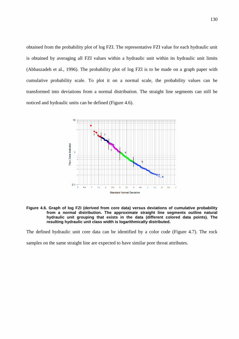
130

obtained from the probability plot of log FZI. The representative FZI value for each hydraulic unit

is obtained by averaging all FZI values within a hydraulic unit within its hydraulic unit limits

(Abbaszadeh et al., 1996). The probability plot of log FZI is to be made on a graph paper with

cumulative probability scale. To plot it on a normal scale, the probability values can be

transformed into deviations from a normal distribution. The straight line segments can still be

noticed and hydraulic units can be defined (Figure 4.6).

Figure 4.6. Graph of log FZI (derived from core data) versus deviations of cumulative probability from a normal distribution. The approximate straight line segments outline natural hydraulic unit grouping that exists in the data (different colored data points). The resulting hydraulic unit class width is logarithmically distributed.

The defined hydraulic unit core data can be identified by a color code (Figure 4.7). The rock

samples on the same straight line are expected to have similar pore throat attributes.

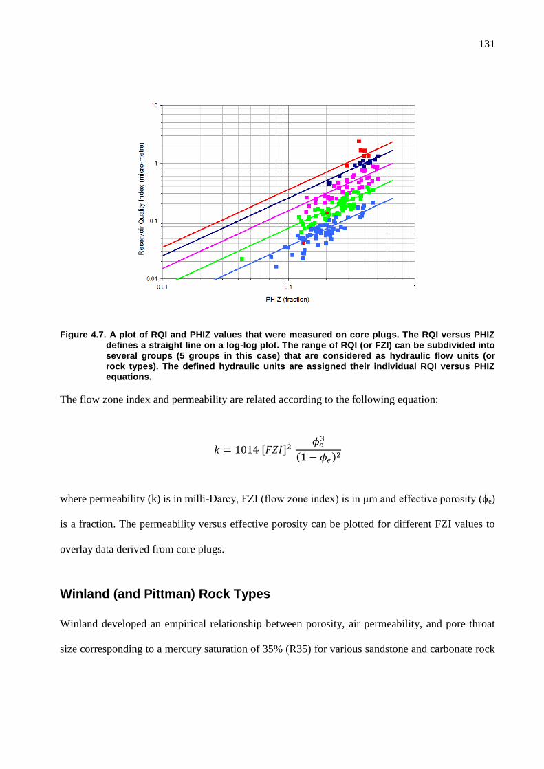
131

Figure 4.7. A plot of RQI and PHIZ values that were measured on core plugs. The RQI versus PHIZ defines a straight line on a log-log plot. The range of RQI (or FZI) can be subdivided into several groups (5 groups in this case) that are considered as hydraulic flow units (or rock types). The defined hydraulic units are assigned their individual RQI versus PHIZ equations.

The flow zone index and permeability are related according to the following equation:

where permeability (k) is in milli-Darcy, FZI (flow zone index) is in μm and effective porosity (ϕe)

is a fraction. The permeability versus effective porosity can be plotted for different FZI values to

overlay data derived from core plugs.

Winland (and Pittman) Rock Types

Winland developed an empirical relationship between porosity, air permeability, and pore throat

size corresponding to a mercury saturation of 35% (R35) for various sandstone and carbonate rock

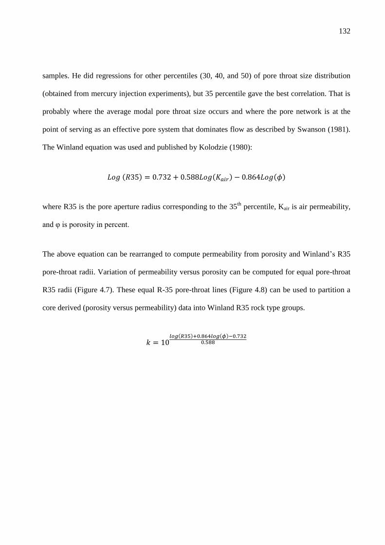
132

samples. He did regressions for other percentiles (30, 40, and 50) of pore throat size distribution

(obtained from mercury injection experiments), but 35 percentile gave the best correlation. That is

probably where the average modal pore throat size occurs and where the pore network is at the

point of serving as an effective pore system that dominates flow as described by Swanson (1981).

The Winland equation was used and published by Kolodzie (1980):

where R35 is the pore aperture radius corresponding to the 35th

percentile, Kair is air permeability,

and υ is porosity in percent.

The above equation can be rearranged to compute permeability from porosity and Winland‟s R35

pore-throat radii. Variation of permeability versus porosity can be computed for equal pore-throat

R35 radii (Figure 4.7). These equal R-35 pore-throat lines (Figure 4.8) can be used to partition a

core derived (porosity versus permeability) data into Winland R35 rock type groups.

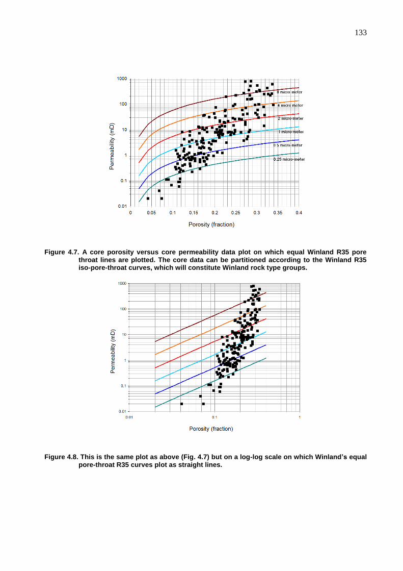
133

Figure 4.7. A core porosity versus core permeability data plot on which equal Winland R35 pore throat lines are plotted. The core data can be partitioned according to the Winland R35 iso-pore-throat curves, which will constitute Winland rock type groups.

Figure 4.8. This is the same plot as above (Fig. 4.7) but on a log-log scale on which Winland’s equal pore-throat R35 curves plot as straight lines.

134

Pittman (1992) carried out mercury injection measurements on 196 sandstone samples from 14

formations. He selected the injection steps 5 percentiles each time going from 10 percentile up to

the 75 percentile. The mean apex of the log-log mercury injection plots was at a mercury

saturation of 36%, which is very close to the 35% that Winland had used. The Pittman equation is

very similar to that of Winland and can be used in a similar fashion to define the Pittman rock

types:

where R35 is the pore aperture radius corresponding to the 35th

percentile, Kair is air permeability,

and υ is porosity in percent.

Lucia Rock Types

Lucia (2007) classified carbonate rocks with interparticle porosity in three classes (namely class 1,

2 and 3). These classes are defined based on particle size. The particle size of class 1 carbonates

ranges from 100 to 500 micro-metre. The class 2 particle size ranges from 20 to 100, whereas class

3 particle size is less than 20 micro-metre. These rock types are identified by macro- and

microscopic description. If vuggy porosity exists then the porosity permeability relations break

down. The Lucia rock types are not related to the pore-throat radius based rock types (Figure 4.9).

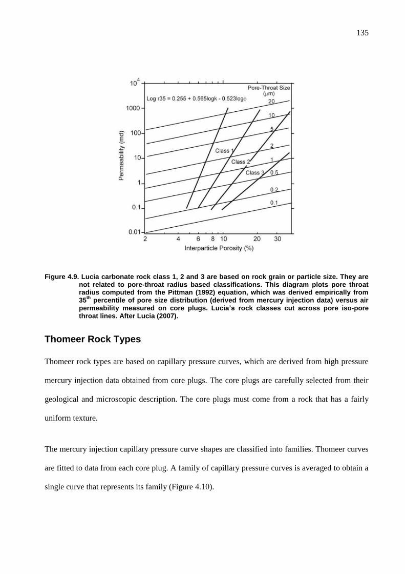
135

Figure 4.9. Lucia carbonate rock class 1, 2 and 3 are based on rock grain or particle size. They are not related to pore-throat radius based classifications. This diagram plots pore throat radius computed from the Pittman (1992) equation, which was derived empirically from 35

th percentile of pore size distribution (derived from mercury injection data) versus air

permeability measured on core plugs. Lucia’s rock classes cut across pore iso-pore throat lines. After Lucia (2007).

Thomeer Rock Types

Thomeer rock types are based on capillary pressure curves, which are derived from high pressure

mercury injection data obtained from core plugs. The core plugs are carefully selected from their

geological and microscopic description. The core plugs must come from a rock that has a fairly

uniform texture.

The mercury injection capillary pressure curve shapes are classified into families. Thomeer curves

are fitted to data from each core plug. A family of capillary pressure curves is averaged to obtain a

single curve that represents its family (Figure 4.10).

136

Mecury injection capillary pressure curves are used to characterize pore systems. The carbonate

rocks contain three types of pore systems in varying proportions (Archie, 1952). The pore type I

(primary intergranular pores) is the most common pore type. The size and sorting of type I pore

type may vary in reservoir rock types. Type I pores reside in a matrix that is made of tightly

interlocking crystals or grains. Type II pores are present in chalky rocks in which crystals or

particles are not effectively interlocked. In type III crystals or particles interlock in different angles

and allow porosity between crystals. The pore type III (intercrystalline pores) are secondary pores

that are commonly present in dolomite.

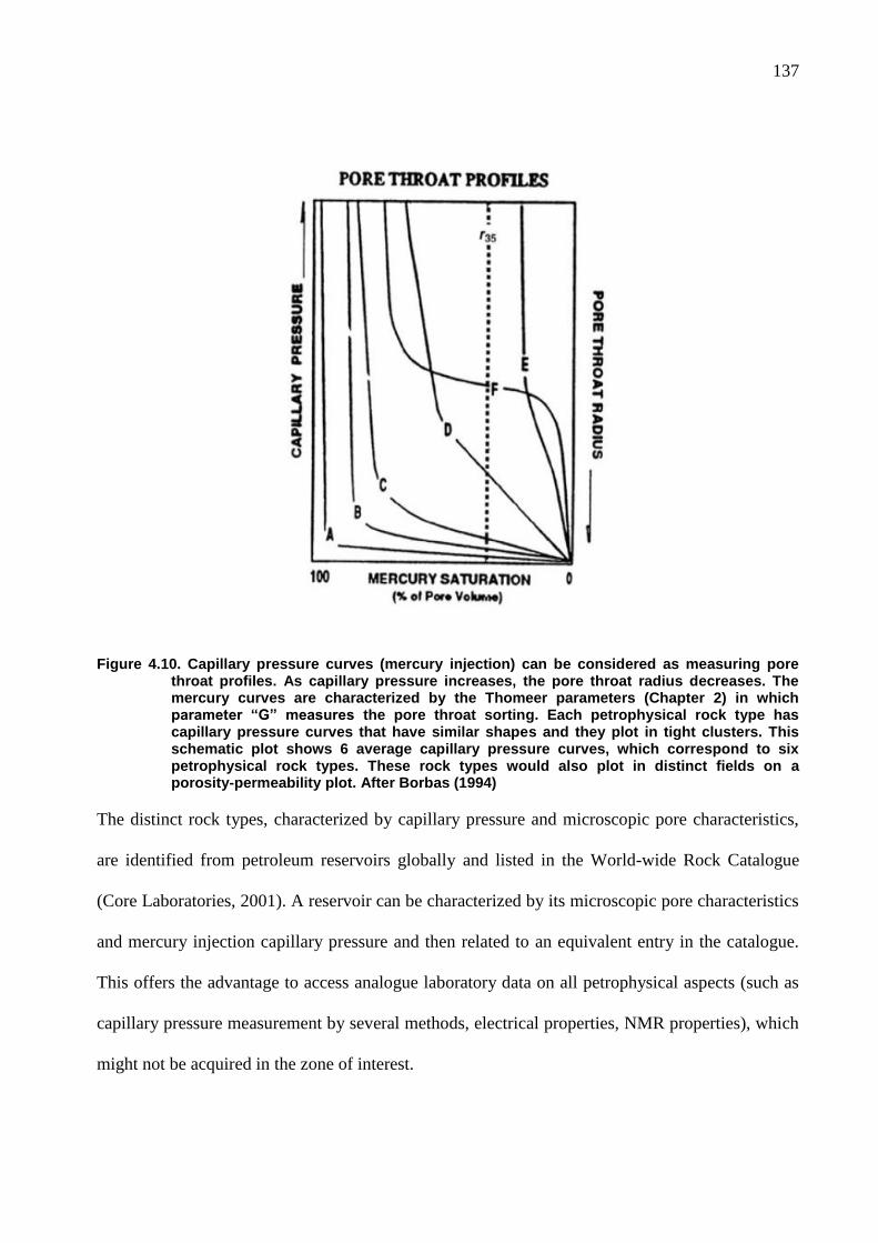
137

Figure 4.10. Capillary pressure curves (mercury injection) can be considered as measuring pore throat profiles. As capillary pressure increases, the pore throat radius decreases. The mercury curves are characterized by the Thomeer parameters (Chapter 2) in which parameter “G” measures the pore throat sorting. Each petrophysical rock type has capillary pressure curves that have similar shapes and they plot in tight clusters. This schematic plot shows 6 average capillary pressure curves, which correspond to six petrophysical rock types. These rock types would also plot in distinct fields on a porosity-permeability plot. After Borbas (1994)

The distinct rock types, characterized by capillary pressure and microscopic pore characteristics,

are identified from petroleum reservoirs globally and listed in the World-wide Rock Catalogue

(Core Laboratories, 2001). A reservoir can be characterized by its microscopic pore characteristics

and mercury injection capillary pressure and then related to an equivalent entry in the catalogue.

This offers the advantage to access analogue laboratory data on all petrophysical aspects (such as

capillary pressure measurement by several methods, electrical properties, NMR properties), which

might not be acquired in the zone of interest.

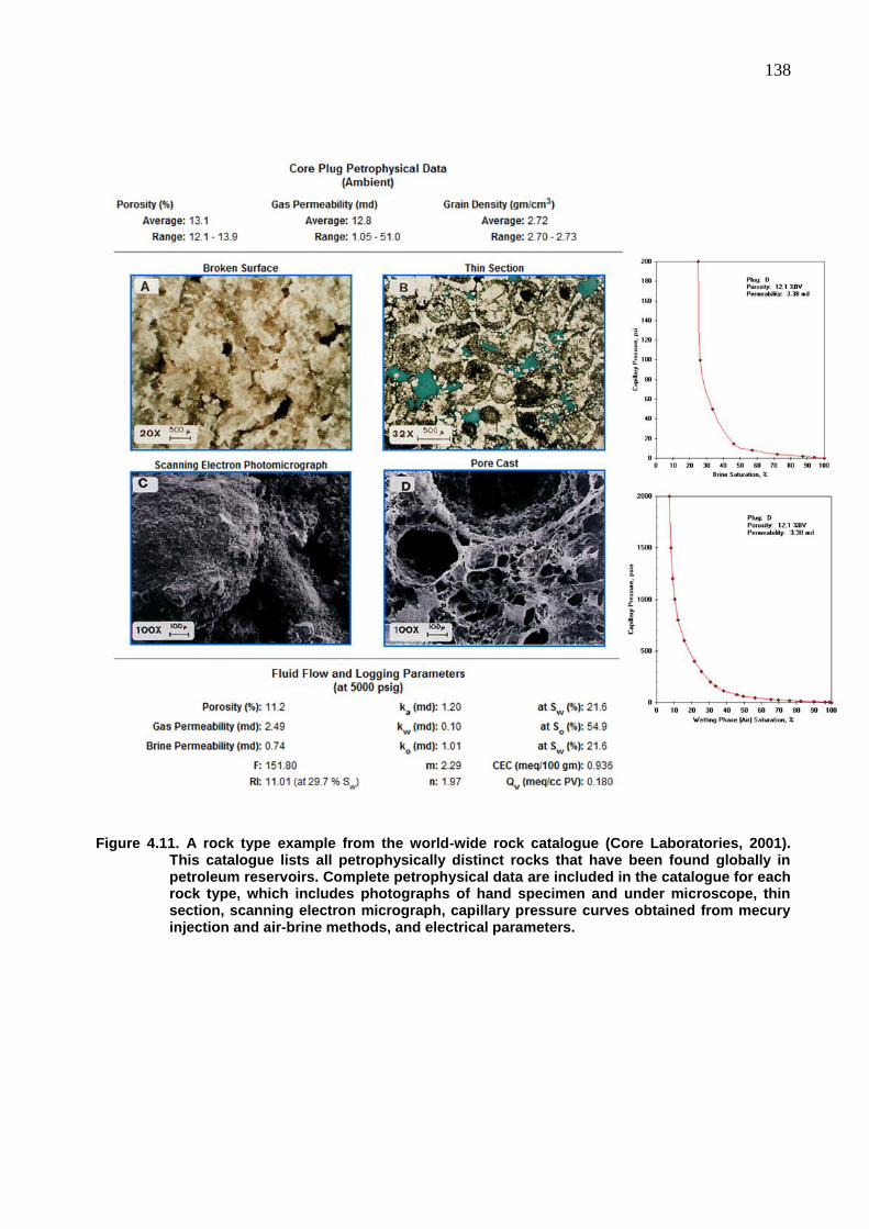
138

Figure 4.11. A rock type example from the world-wide rock catalogue (Core Laboratories, 2001). This catalogue lists all petrophysically distinct rocks that have been found globally in petroleum reservoirs. Complete petrophysical data are included in the catalogue for each rock type, which includes photographs of hand specimen and under microscope, thin section, scanning electron micrograph, capillary pressure curves obtained from mecury injection and air-brine methods, and electrical parameters.

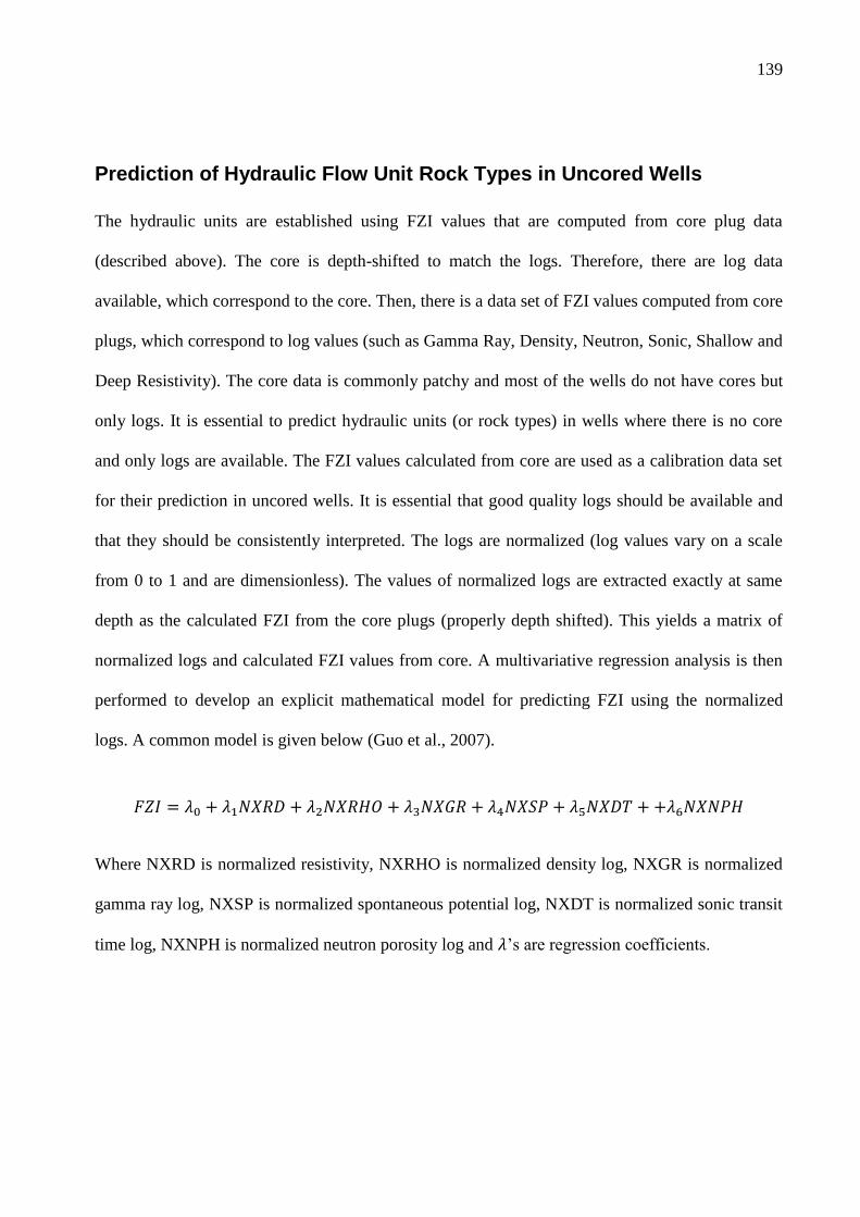
139

Prediction of Hydraulic Flow Unit Rock Types in Uncored Wells

The hydraulic units are established using FZI values that are computed from core plug data

(described above). The core is depth-shifted to match the logs. Therefore, there are log data

available, which correspond to the core. Then, there is a data set of FZI values computed from core

plugs, which correspond to log values (such as Gamma Ray, Density, Neutron, Sonic, Shallow and

Deep Resistivity). The core data is commonly patchy and most of the wells do not have cores but

only logs. It is essential to predict hydraulic units (or rock types) in wells where there is no core

and only logs are available. The FZI values calculated from core are used as a calibration data set

for their prediction in uncored wells. It is essential that good quality logs should be available and

that they should be consistently interpreted. The logs are normalized (log values vary on a scale

from 0 to 1 and are dimensionless). The values of normalized logs are extracted exactly at same

depth as the calculated FZI from the core plugs (properly depth shifted). This yields a matrix of

normalized logs and calculated FZI values from core. A multivariative regression analysis is then

performed to develop an explicit mathematical model for predicting FZI using the normalized

logs. A common model is given below (Guo et al., 2007).

Where NXRD is normalized resistivity, NXRHO is normalized density log, NXGR is normalized

gamma ray log, NXSP is normalized spontaneous potential log, NXDT is normalized sonic transit

time log, NXNPH is normalized neutron porosity log and ‟s are regression coefficients.

140

Once hydraulic units (rock types) are predicted and successfully verified against a control data set,

then, permeability values can be calculated for each hydraulic unit using their respective

permeability-porosity equation.

141

Chapter 5

Application of Hydraulic Flow Unit Rock Typing

and Saturation-Height Modelling

Reservoir Description

There are three wells in the example carbonate reservoir in a narrow anticline (about 9 km long

and up to 3 km wide). All of them are vertical wells.

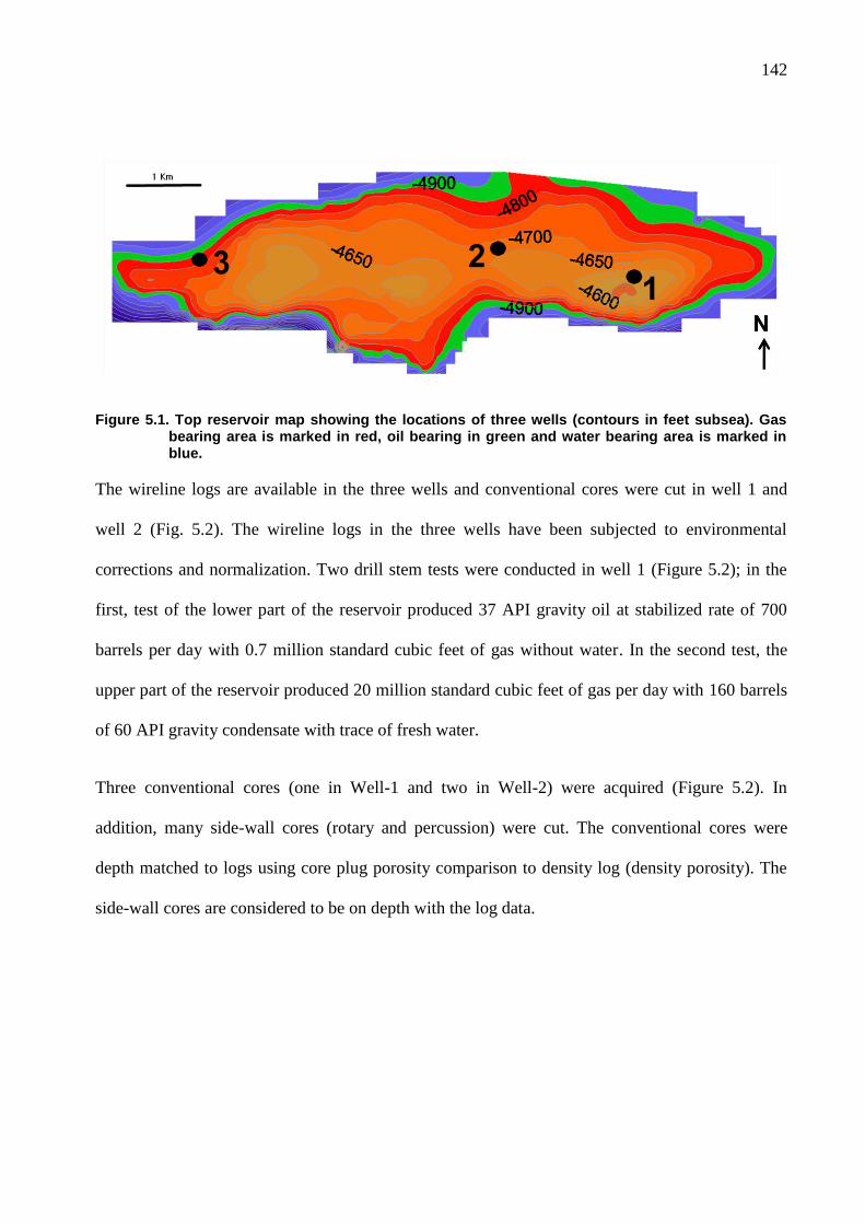
142

Figure 5.1. Top reservoir map showing the locations of three wells (contours in feet subsea). Gas bearing area is marked in red, oil bearing in green and water bearing area is marked in blue.

The wireline logs are available in the three wells and conventional cores were cut in well 1 and

well 2 (Fig. 5.2). The wireline logs in the three wells have been subjected to environmental

corrections and normalization. Two drill stem tests were conducted in well 1 (Figure 5.2); in the

first, test of the lower part of the reservoir produced 37 API gravity oil at stabilized rate of 700

barrels per day with 0.7 million standard cubic feet of gas without water. In the second test, the

upper part of the reservoir produced 20 million standard cubic feet of gas per day with 160 barrels

of 60 API gravity condensate with trace of fresh water.

Three conventional cores (one in Well-1 and two in Well-2) were acquired (Figure 5.2). In

addition, many side-wall cores (rotary and percussion) were cut. The conventional cores were

depth matched to logs using core plug porosity comparison to density log (density porosity). The

side-wall cores are considered to be on depth with the log data.

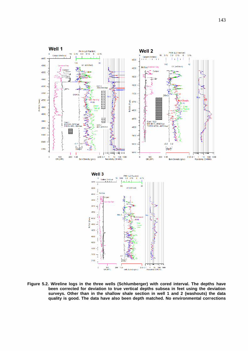
143

Figure 5.2. Wireline logs in the three wells (Schlumberger) with cored interval. The depths have been corrected for deviation to true vertical depths subsea in feet using the deviation surveys. Other than in the shallow shale section in well 1 and 2 (washouts) the data quality is good. The data have also been depth matched. No environmental corrections

144

were applied to gamma ray but all three wells were normalized so that shale volumes could be interpreted consistently. Bore-hole corrections have been applied to density and compensated neutron using the appropriate mud parameters (temperature correction and 1 inch tool standoff). Compensated neutron porosity data were normalized where appropriate. Formation water salinity is 30,000 ppm NaCl. Bore-hole corrections were applied to resistivity (induction) using appropriate mud parameters.

The conventional core was studied in laboratory; besides conventional core analysis (porosity, air

permeability and grain density), special core analysis tests were carried out (mercury injection

capillary pressure, air brine capillary pressure, electrical properties, thin section petrography). The

core recovery and quality was good (Figure 5.3).

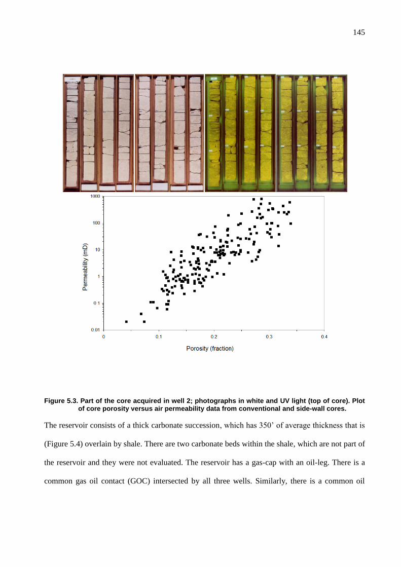
145

Figure 5.3. Part of the core acquired in well 2; photographs in white and UV light (top of core). Plot of core porosity versus air permeability data from conventional and side-wall cores.

The reservoir consists of a thick carbonate succession, which has 350‟ of average thickness that is

(Figure 5.4) overlain by shale. There are two carbonate beds within the shale, which are not part of

the reservoir and they were not evaluated. The reservoir has a gas-cap with an oil-leg. There is a

common gas oil contact (GOC) intersected by all three wells. Similarly, there is a common oil

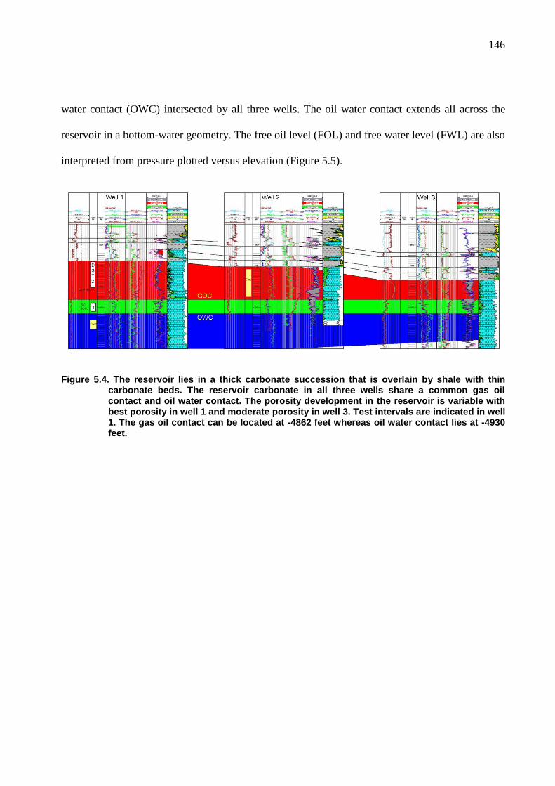
146

water contact (OWC) intersected by all three wells. The oil water contact extends all across the

reservoir in a bottom-water geometry. The free oil level (FOL) and free water level (FWL) are also

interpreted from pressure plotted versus elevation (Figure 5.5).

Figure 5.4. The reservoir lies in a thick carbonate succession that is overlain by shale with thin carbonate beds. The reservoir carbonate in all three wells share a common gas oil contact and oil water contact. The porosity development in the reservoir is variable with best porosity in well 1 and moderate porosity in well 3. Test intervals are indicated in well 1. The gas oil contact can be located at -4862 feet whereas oil water contact lies at -4930 feet.

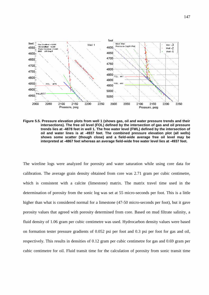
147

Figure 5.5. Pressure elevation plots from well 1 (shows gas, oil and water pressure trends and their intersections). The free oil level (FOL) defined by the intersection of gas and oil pressure trends lies at -4878 feet in well 1. The free water level (FWL) defined by the intersection of oil and water lines is at -4937 feet. The combined pressure elevation plot (all wells) shows some scatter (though close) and a field-wide average free oil level may be interpreted at -4867 feet whereas an average field-wide free water level lies at -4937 feet.

The wireline logs were analyzed for porosity and water saturation while using core data for

calibration. The average grain density obtained from core was 2.71 gram per cubic centimetre,

which is consistent with a calcite (limestone) matrix. The matrix travel time used in the

determination of porosity from the sonic log was set at 55 micro-seconds per foot. This is a little

higher than what is considered normal for a limestone (47-50 micro-seconds per foot), but it gave

porosity values that agreed with porosity determined from core. Based on mud filtrate salinity, a

fluid density of 1.06 gram per cubic centimetre was used. Hydrocarbon density values were based

on formation tester pressure gradients of 0.052 psi per foot and 0.3 psi per foot for gas and oil,

respectively. This results in densities of 0.12 gram per cubic centimetre for gas and 0.69 gram per

cubic centimetre for oil. Fluid transit time for the calculation of porosity from sonic transit time

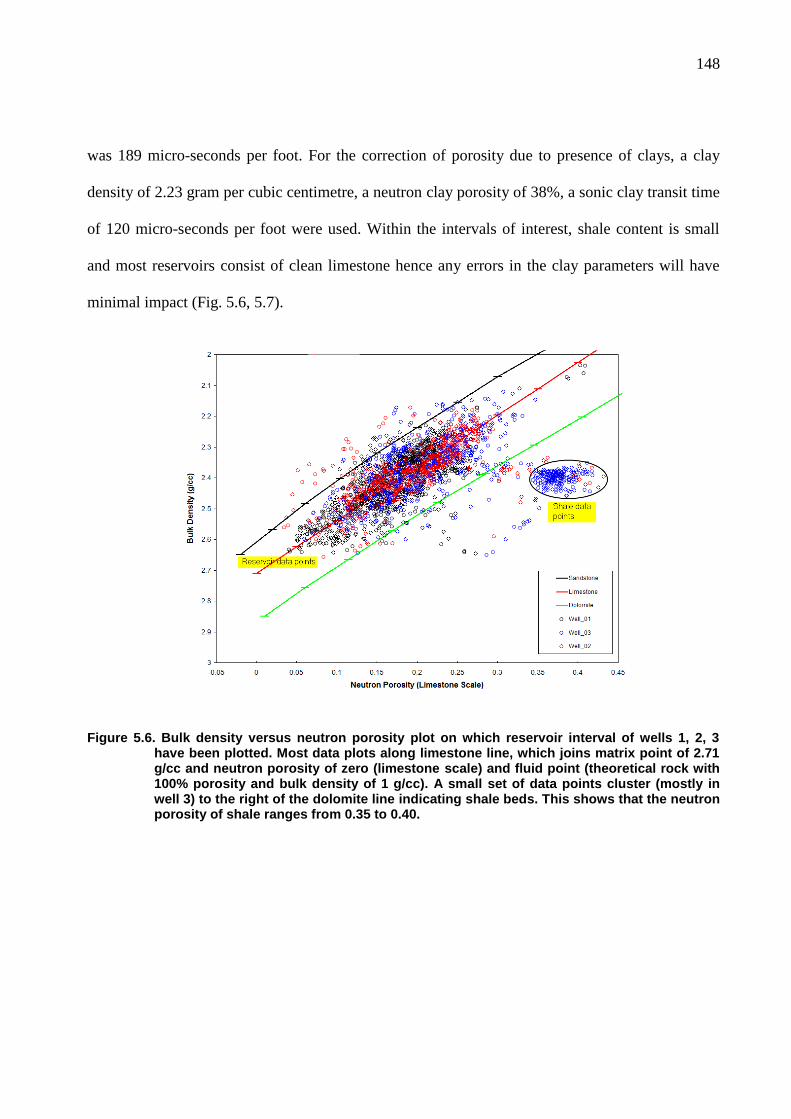
148

was 189 micro-seconds per foot. For the correction of porosity due to presence of clays, a clay

density of 2.23 gram per cubic centimetre, a neutron clay porosity of 38%, a sonic clay transit time

of 120 micro-seconds per foot were used. Within the intervals of interest, shale content is small

and most reservoirs consist of clean limestone hence any errors in the clay parameters will have

minimal impact (Fig. 5.6, 5.7).

Figure 5.6. Bulk density versus neutron porosity plot on which reservoir interval of wells 1, 2, 3 have been plotted. Most data plots along limestone line, which joins matrix point of 2.71 g/cc and neutron porosity of zero (limestone scale) and fluid point (theoretical rock with 100% porosity and bulk density of 1 g/cc). A small set of data points cluster (mostly in well 3) to the right of the dolomite line indicating shale beds. This shows that the neutron porosity of shale ranges from 0.35 to 0.40.

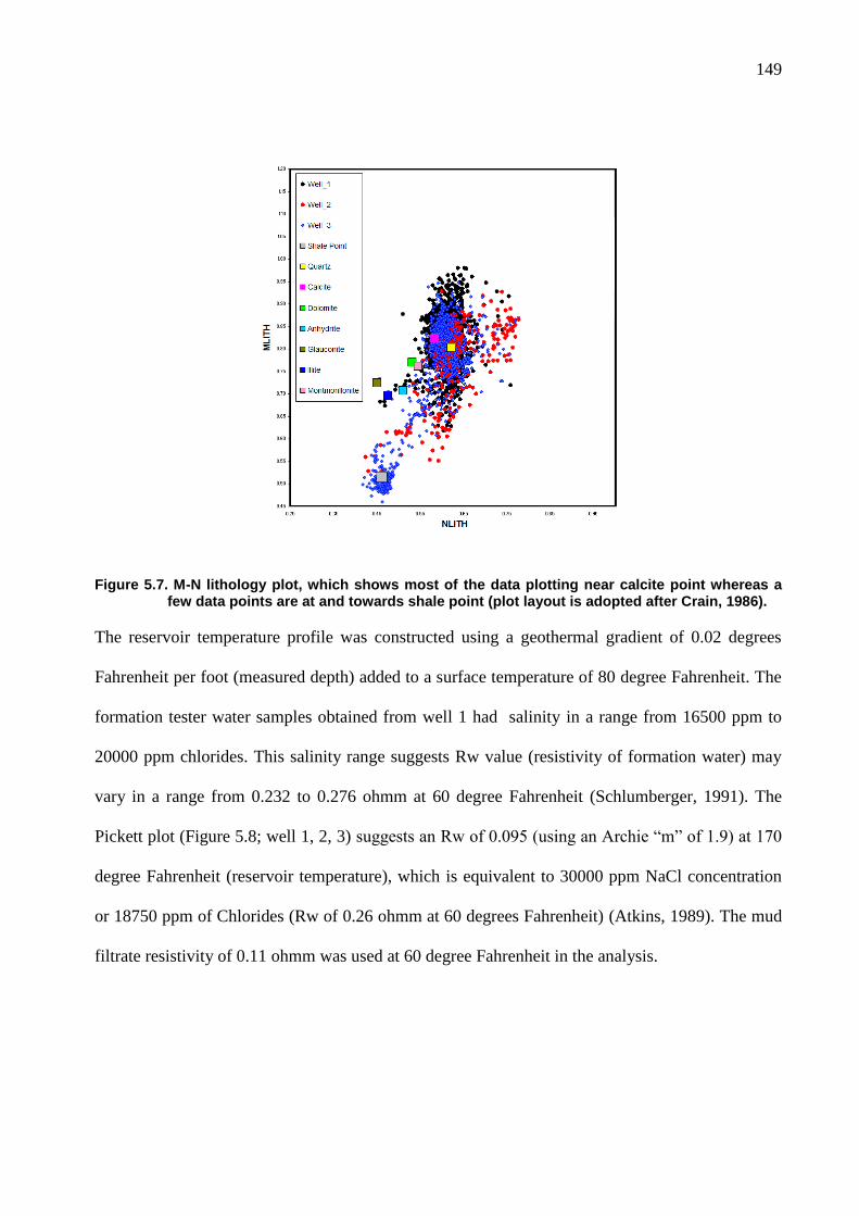
149

Figure 5.7. M-N lithology plot, which shows most of the data plotting near calcite point whereas a few data points are at and towards shale point (plot layout is adopted after Crain, 1986).

The reservoir temperature profile was constructed using a geothermal gradient of 0.02 degrees

Fahrenheit per foot (measured depth) added to a surface temperature of 80 degree Fahrenheit. The

formation tester water samples obtained from well 1 had salinity in a range from 16500 ppm to

20000 ppm chlorides. This salinity range suggests Rw value (resistivity of formation water) may

vary in a range from 0.232 to 0.276 ohmm at 60 degree Fahrenheit (Schlumberger, 1991). The

Pickett plot (Figure 5.8; well 1, 2, 3) suggests an Rw of 0.095 (using an Archie “m” of 1.9) at 170

degree Fahrenheit (reservoir temperature), which is equivalent to 30000 ppm NaCl concentration

or 18750 ppm of Chlorides (Rw of 0.26 ohmm at 60 degrees Fahrenheit) (Atkins, 1989). The mud

filtrate resistivity of 0.11 ohmm was used at 60 degree Fahrenheit in the analysis.

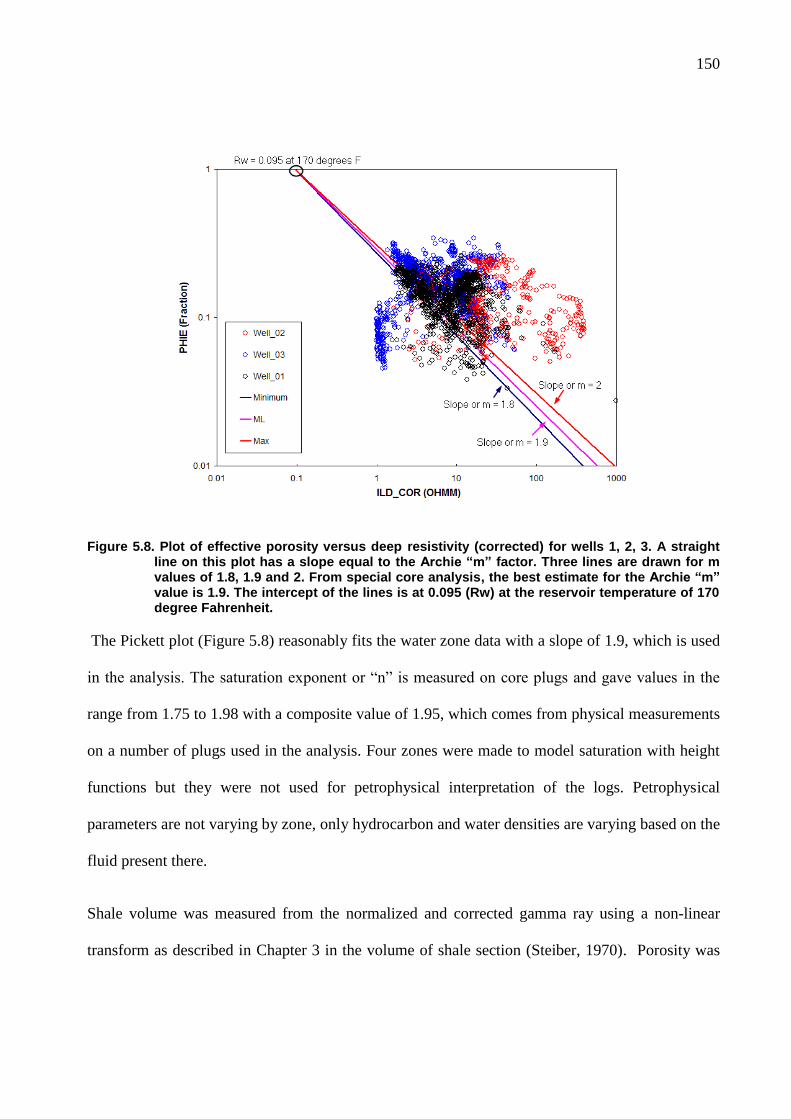
150

Figure 5.8. Plot of effective porosity versus deep resistivity (corrected) for wells 1, 2, 3. A straight line on this plot has a slope equal to the Archie “m” factor. Three lines are drawn for m values of 1.8, 1.9 and 2. From special core analysis, the best estimate for the Archie “m” value is 1.9. The intercept of the lines is at 0.095 (Rw) at the reservoir temperature of 170 degree Fahrenheit.

The Pickett plot (Figure 5.8) reasonably fits the water zone data with a slope of 1.9, which is used

in the analysis. The saturation exponent or “n” is measured on core plugs and gave values in the

range from 1.75 to 1.98 with a composite value of 1.95, which comes from physical measurements

on a number of plugs used in the analysis. Four zones were made to model saturation with height

functions but they were not used for petrophysical interpretation of the logs. Petrophysical

parameters are not varying by zone, only hydrocarbon and water densities are varying based on the

fluid present there.

Shale volume was measured from the normalized and corrected gamma ray using a non-linear

transform as described in Chapter 3 in the volume of shale section (Steiber, 1970). Porosity was

151

determined from the density vs. neutron porosity cross-plot after applying shale and hydrocarbon

corrections. The mineral composition is solved using a set of simultaneous equations according to

the calculated matrix values. The Archie equation is used to determine Sw and because the main

reservoir intervals are almost free of shale, hence a shaly-sand equation was not considered

necessary. The analyzed logs, which are calibrated to core are shown below (Figs. 5.9, 5.10, 5.11).

The density-neutron porosity (calibrated to core) is used in the saturation height model (described

below), which uses capillary pressure curves measured on core to calculate water saturation. The

water saturation derived from resistivity logs is used for a comparison with the values computed

from the saturation height model.

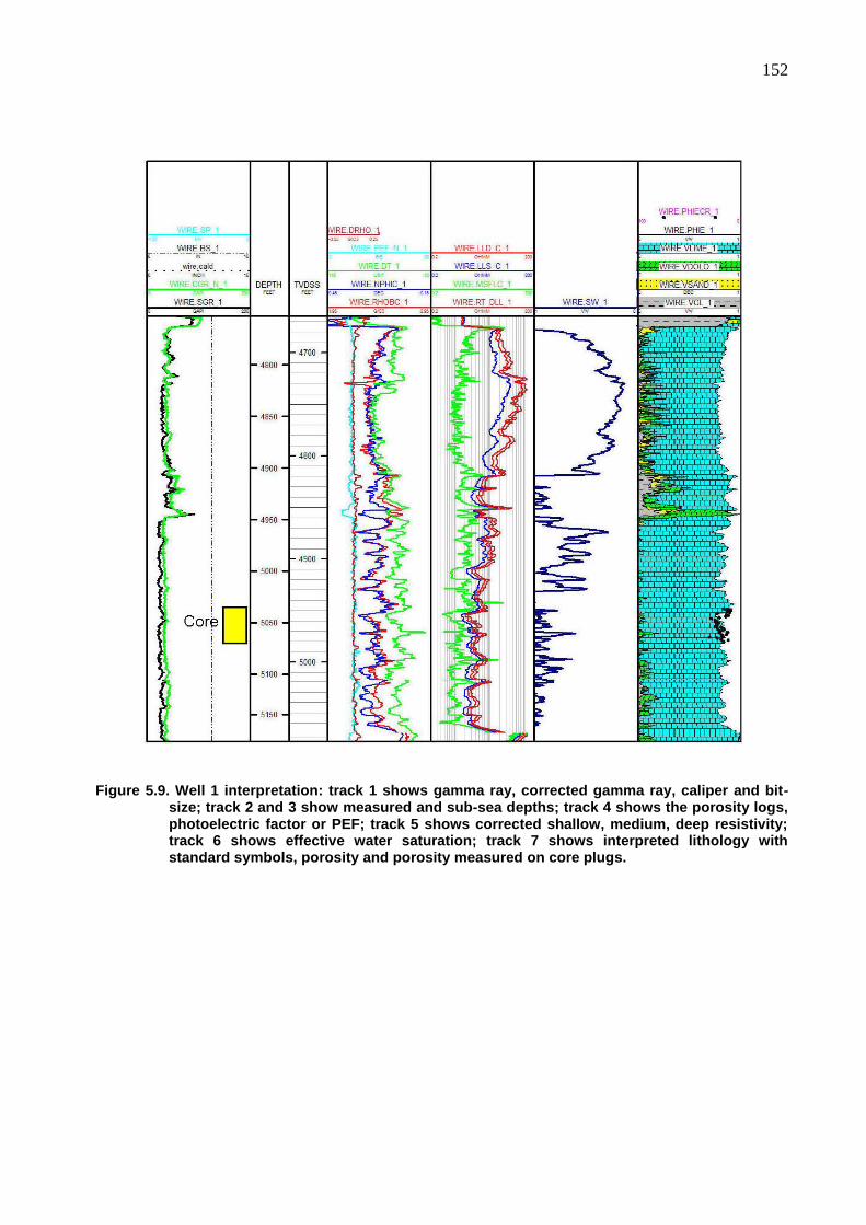
152

Figure 5.9. Well 1 interpretation: track 1 shows gamma ray, corrected gamma ray, caliper and bit-size; track 2 and 3 show measured and sub-sea depths; track 4 shows the porosity logs, photoelectric factor or PEF; track 5 shows corrected shallow, medium, deep resistivity; track 6 shows effective water saturation; track 7 shows interpreted lithology with standard symbols, porosity and porosity measured on core plugs.

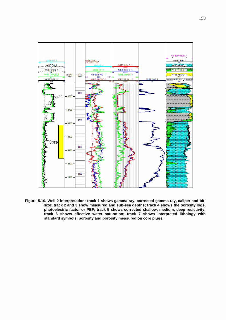
153

Figure 5.10. Well 2 interpretation: track 1 shows gamma ray, corrected gamma ray, caliper and bit-size; track 2 and 3 show measured and sub-sea depths; track 4 shows the porosity logs, photoelectric factor or PEF; track 5 shows corrected shallow, medium, deep resistivity; track 6 shows effective water saturation; track 7 shows interpreted lithology with standard symbols, porosity and porosity measured on core plugs.

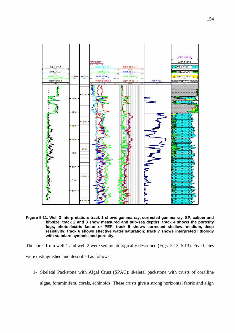
154

Figure 5.11. Well 3 interpretation: track 1 shows gamma ray, corrected gamma ray, SP, caliper and bit-size; track 2 and 3 show measured and sub-sea depths; track 4 shows the porosity logs, photoelectric factor or PEF; track 5 shows corrected shallow, medium, deep resistivity; track 6 shows effective water saturation; track 7 shows interpreted lithology with standard symbols and porosity.

The cores from well 1 and well 2 were sedimentologically described (Figs. 5.12, 5.13). Five facies

were distinguished and described as follows:

1- Skeletal Packstone with Algal Crust (SPAC): skeletal packstone with crusts of coralline

algae, foraminifera, corals, echinoids. These crusts give a strong horizontal fabric and align

155

the skeletal fragments, which are heavily micritized. Foraminifera and other skeletal

fragments are internally cemented with calcite whereas corals are mud filled. (Fig. 5.14).

2- Skeletal Packstone with Pelleted Matrix (SPPM): The grains include coralline algal

fragments, including small rhodoids, larger foraminifera are abundant. Skeletals are

heavily micritized. Matrix locally pelleted and lightly dolomitized. (Fig. 5.14).

3- Rhodoid Rudstone (RHRD): this facies has a fairly strong horizontal fabric. It consists of

algal crusts, rhodoids of several mm diameter, larger foraminifera are abundant. Skeletal

are heavily micritized. The non abundant matrix is pelleted. Calcite cement is intra-

skeletal. Some skeletals are dolomitized. Stylolites are poorly developed with low relief.

(Fig. 5.14).

4- Peloid Skeletal Packstone/Grainstone (PSPG): the grains include larger foraminifera, coral

fragments, miliolids, echinoderms. Skeletals are micritized. Some skeletal fragments and

coral fragments are cement-replaced. (Fig. 5.14).

5- Skeletal Wackestone with Pelleted Matrix (SWPM): the grains include coralline algal

fragments, larger foraminifera, coral fragments. Skeletals are micritized. Minor

intraskeletal calcite cement. Pelleted lime mud matrix. (Fig. 5.14).

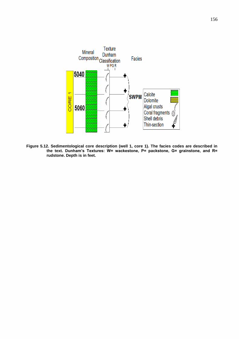
156

Figure 5.12. Sedimentological core description (well 1, core 1). The facies codes are described in the text. Dunham’s Textures: W= wackestone, P= packstone, G= grainstone, and R= rudstone. Depth is in feet.

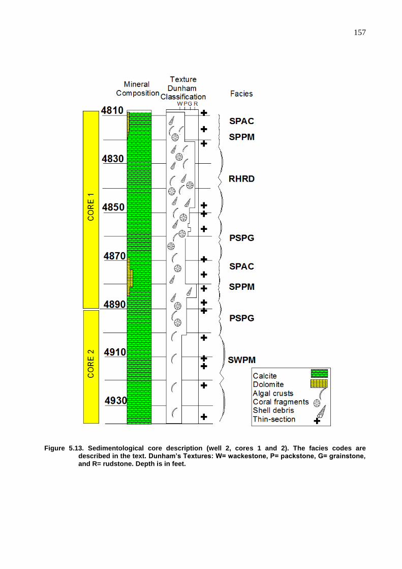
157

Figure 5.13. Sedimentological core description (well 2, cores 1 and 2). The facies codes are described in the text. Dunham’s Textures: W= wackestone, P= packstone, G= grainstone, and R= rudstone. Depth is in feet.

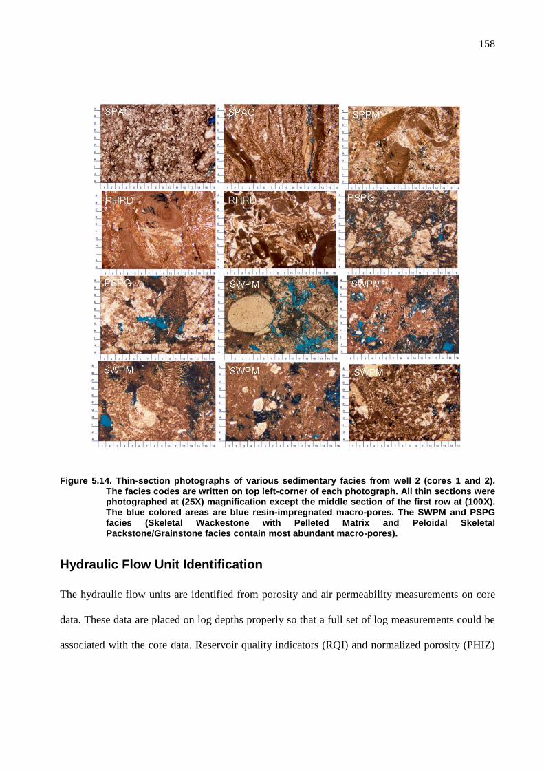
158

Figure 5.14. Thin-section photographs of various sedimentary facies from well 2 (cores 1 and 2). The facies codes are written on top left-corner of each photograph. All thin sections were photographed at (25X) magnification except the middle section of the first row at (100X). The blue colored areas are blue resin-impregnated macro-pores. The SWPM and PSPG facies (Skeletal Wackestone with Pelleted Matrix and Peloidal Skeletal Packstone/Grainstone facies contain most abundant macro-pores).

Hydraulic Flow Unit Identification

The hydraulic flow units are identified from porosity and air permeability measurements on core

data. These data are placed on log depths properly so that a full set of log measurements could be

associated with the core data. Reservoir quality indicators (RQI) and normalized porosity (PHIZ)

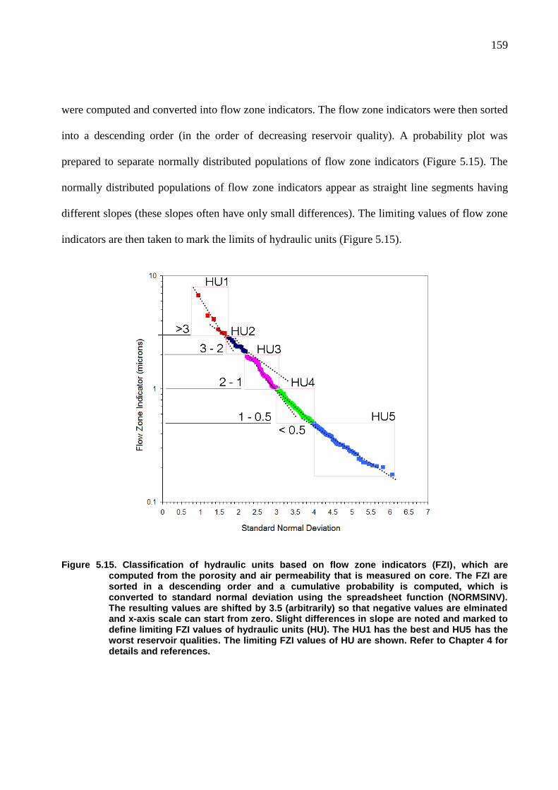
159

were computed and converted into flow zone indicators. The flow zone indicators were then sorted

into a descending order (in the order of decreasing reservoir quality). A probability plot was

prepared to separate normally distributed populations of flow zone indicators (Figure 5.15). The

normally distributed populations of flow zone indicators appear as straight line segments having

different slopes (these slopes often have only small differences). The limiting values of flow zone

indicators are then taken to mark the limits of hydraulic units (Figure 5.15).

Figure 5.15. Classification of hydraulic units based on flow zone indicators (FZI), which are computed from the porosity and air permeability that is measured on core. The FZI are sorted in a descending order and a cumulative probability is computed, which is converted to standard normal deviation using the spreadsheet function (NORMSINV). The resulting values are shifted by 3.5 (arbitrarily) so that negative values are elminated and x-axis scale can start from zero. Slight differences in slope are noted and marked to define limiting FZI values of hydraulic units (HU). The HU1 has the best and HU5 has the worst reservoir qualities. The limiting FZI values of HU are shown. Refer to Chapter 4 for details and references.

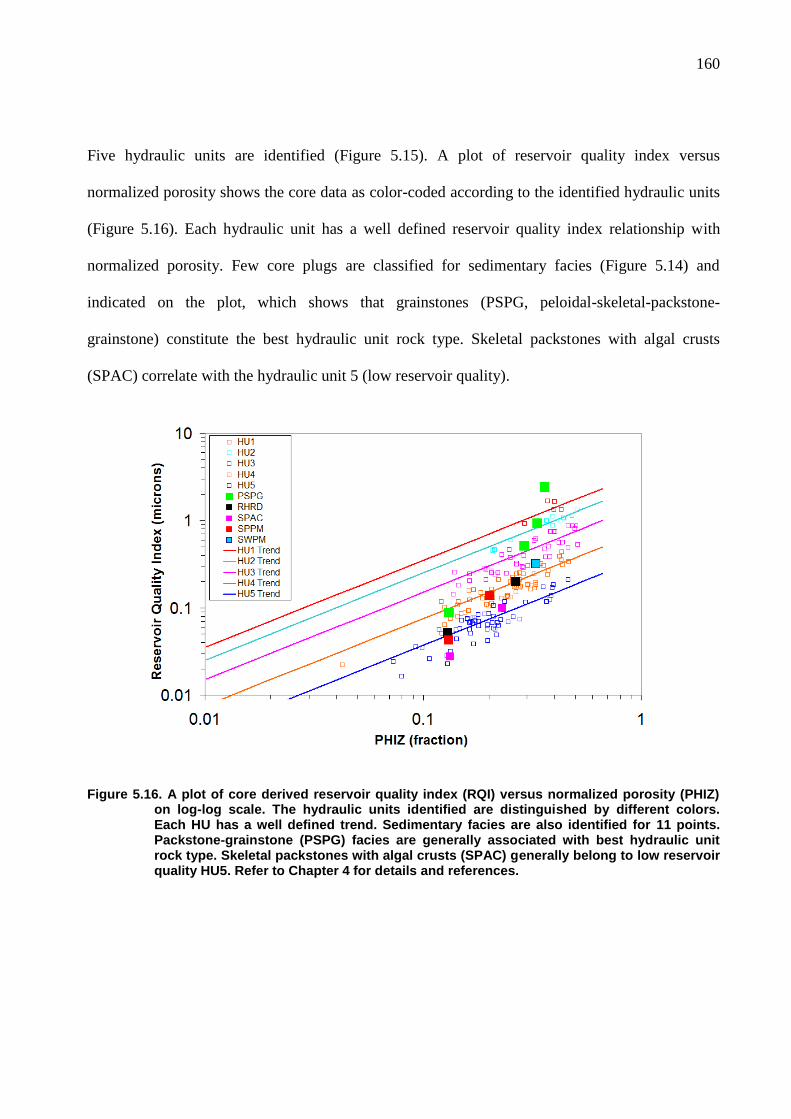
160

Five hydraulic units are identified (Figure 5.15). A plot of reservoir quality index versus

normalized porosity shows the core data as color-coded according to the identified hydraulic units

(Figure 5.16). Each hydraulic unit has a well defined reservoir quality index relationship with

normalized porosity. Few core plugs are classified for sedimentary facies (Figure 5.14) and

indicated on the plot, which shows that grainstones (PSPG, peloidal-skeletal-packstone-

grainstone) constitute the best hydraulic unit rock type. Skeletal packstones with algal crusts

(SPAC) correlate with the hydraulic unit 5 (low reservoir quality).

Figure 5.16. A plot of core derived reservoir quality index (RQI) versus normalized porosity (PHIZ) on log-log scale. The hydraulic units identified are distinguished by different colors. Each HU has a well defined trend. Sedimentary facies are also identified for 11 points. Packstone-grainstone (PSPG) facies are generally associated with best hydraulic unit rock type. Skeletal packstones with algal crusts (SPAC) generally belong to low reservoir quality HU5. Refer to Chapter 4 for details and references.

161

Hydraulic Flow Unit and Permeability Prediction in Un-Cored Wells or

Intervals

The hydraulic flow units are only known where core data exist. The core data does not cover the

whole the reservoir in all wells. The well log data has a resolution of 6 inches (one measurement

every 6 inches). The measurements on core data are performed on plugs taken at 12 inches interval

in conventional cores. The side-wall cores only sparsely sample the reservoir at intervals many

feet apart. Often, measurements on conventional core data (12 inch intervals) are interpolated at 6

inch intervals and smoothed using a moving average filter. These secondary data should not be

used for identifying hydraulic units. The hydraulic units must be identified using primary data that

are obtained from physical measurements on core plugs.

It is essential to make a predictive model to identify hydraulic units at the resolution of well logs

(6 inches). This model can be developed from core data. The core data was placed on proper log

depths so that it is assigned to proper log measurements at the equivalent depths. Trends of various

log measurements are correlated to flow zone indicators (measured on core). Best fit trends are

defined visually (Figure 5.17) because regression analysis is biased towards outliers and extreme

values, due to errors in assigning log depths to core plugs and poor log measurements because of

borehole effects. All logs are normalized, which means they become dimensionless or without

units and their scales are linearized. Log normalization is done before they are correlated to core-

derived flow zone indicators. A multiple non-linear equation is obtained, which computes flow

zone indicators from the normalized log measurements. This equation is used to calculate flow

zone indicators for all wells (in the reservoir section) and compared to core-derived flow zone

indicator values.

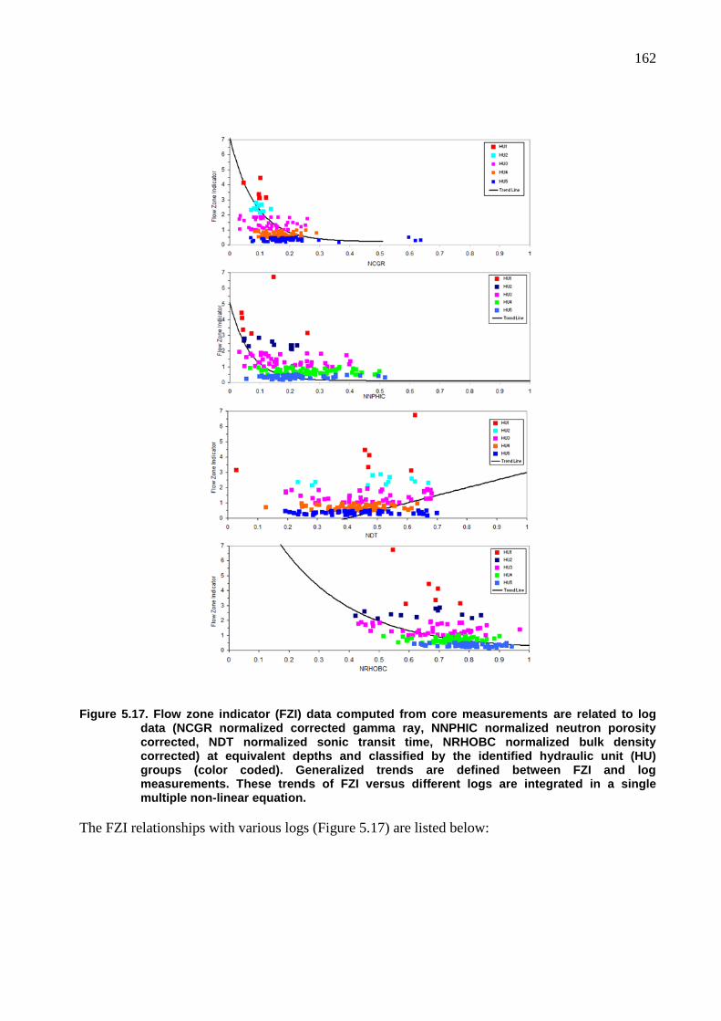
162

Figure 5.17. Flow zone indicator (FZI) data computed from core measurements are related to log data (NCGR normalized corrected gamma ray, NNPHIC normalized neutron porosity corrected, NDT normalized sonic transit time, NRHOBC normalized bulk density corrected) at equivalent depths and classified by the identified hydraulic unit (HU) groups (color coded). Generalized trends are defined between FZI and log measurements. These trends of FZI versus different logs are integrated in a single multiple non-linear equation.

The FZI relationships with various logs (Figure 5.17) are listed below:

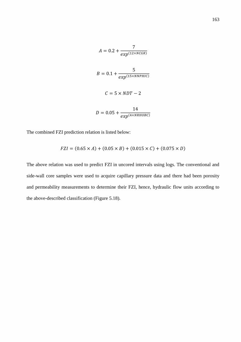
163

The combined FZI prediction relation is listed below:

The above relation was used to predict FZI in uncored intervals using logs. The conventional and

side-wall core samples were used to acquire capillary pressure data and there had been porosity

and permeability measurements to determine their FZI, hence, hydraulic flow units according to

the above-described classification (Figure 5.18).

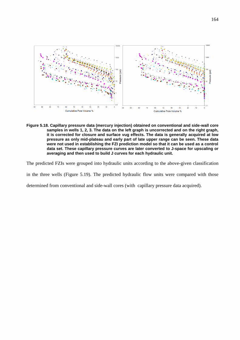
164

Figure 5.18. Capillary pressure data (mercury injection) obtained on conventional and side-wall core samples in wells 1, 2, 3. The data on the left graph is uncorrected and on the right graph, it is corrected for closure and surface vug effects. The data is generally acquired at low pressure as only mid-plateau and early part of late upper range can be seen. These data were not used in establishing the FZI prediction model so that it can be used as a control data set. These capillary pressure curves are later converted to J-space for upscaling or averaging and then used to build J curves for each hydraulic unit.

The predicted FZIs were grouped into hydraulic units according to the above-given classification

in the three wells (Figure 5.19). The predicted hydraulic flow units were compared with those

determined from conventional and side-wall cores (with capillary pressure data acquired).

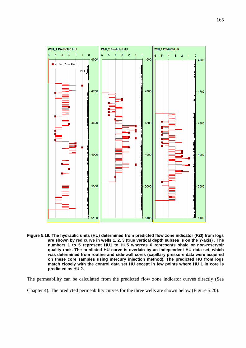
165

Figure 5.19. The hydraulic units (HU) determined from predicted flow zone indicator (FZI) from logs are shown by red curve in wells 1, 2, 3 (true vertical depth subsea is on the Y-axis) . The numbers 1 to 5 represent HU1 to HU5 whereas 6 represents shale or non-reservoir quality rock. The predicted HU curve is overlain by an independent HU data set, which was determined from routine and side-wall cores (capillary pressure data were acquired on these core samples using mercury injection method). The predicted HU from logs match closely with the control data set HU except in few points where HU 1 in core is predicted as HU 2.

The permeability can be calculated from the predicted flow zone indicator curves directly (See

Chapter 4). The predicted permeability curves for the three wells are shown below (Figure 5.20).

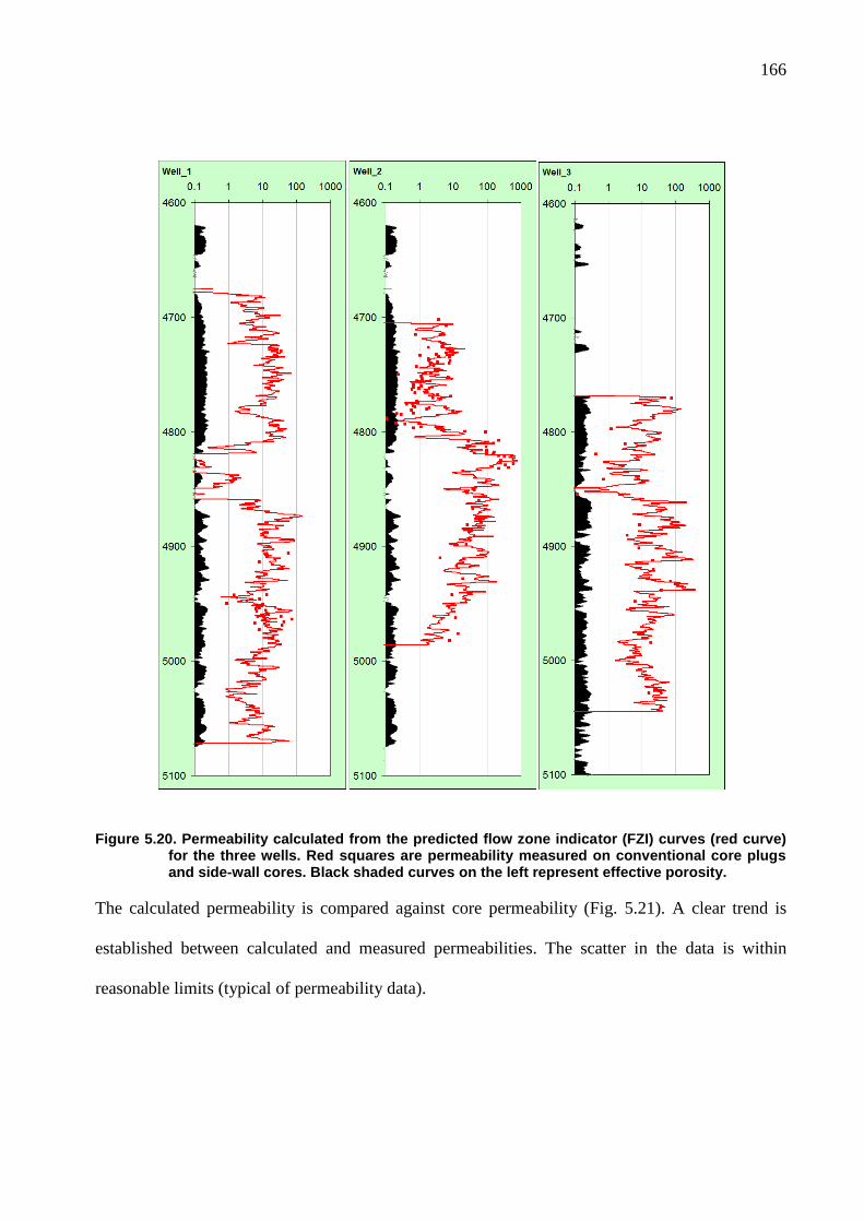
166

Figure 5.20. Permeability calculated from the predicted flow zone indicator (FZI) curves (red curve) for the three wells. Red squares are permeability measured on conventional core plugs and side-wall cores. Black shaded curves on the left represent effective porosity.

The calculated permeability is compared against core permeability (Fig. 5.21). A clear trend is

established between calculated and measured permeabilities. The scatter in the data is within

reasonable limits (typical of permeability data).

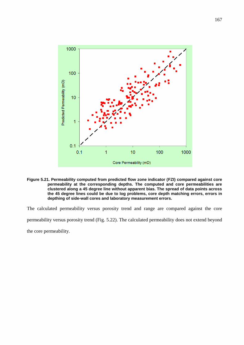
167

Figure 5.21. Permeability computed from predicted flow zone indicator (FZI) compared against core permeability at the corresponding depths. The computed and core permeabilities are clustered along a 45 degree line without apparent bias. The spread of data points across the 45 degree lines could be due to log problems, core depth matching errors, errors in depthing of side-wall cores and laboratory measurement errors.

The calculated permeability versus porosity trend and range are compared against the core

permeability versus porosity trend (Fig. 5.22). The calculated permeability does not extend beyond

the core permeability.

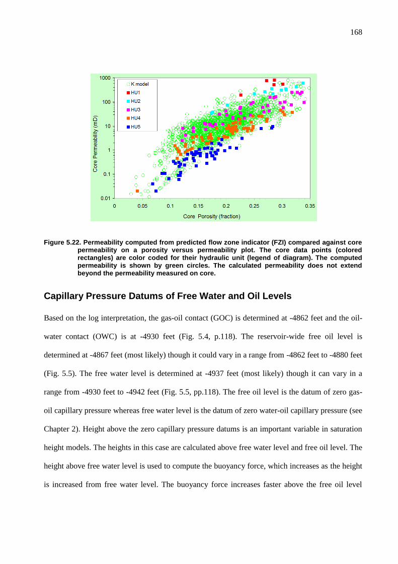
168

Figure 5.22. Permeability computed from predicted flow zone indicator (FZI) compared against core permeability on a porosity versus permeability plot. The core data points (colored rectangles) are color coded for their hydraulic unit (legend of diagram). The computed permeability is shown by green circles. The calculated permeability does not extend beyond the permeability measured on core.

Capillary Pressure Datums of Free Water and Oil Levels

Based on the log interpretation, the gas-oil contact (GOC) is determined at -4862 feet and the oil-

water contact (OWC) is at -4930 feet (Fig. 5.4, p.118). The reservoir-wide free oil level is

determined at -4867 feet (most likely) though it could vary in a range from -4862 feet to -4880 feet

(Fig. 5.5). The free water level is determined at -4937 feet (most likely) though it can vary in a

range from -4930 feet to -4942 feet (Fig. 5.5, pp.118). The free oil level is the datum of zero gas-

oil capillary pressure whereas free water level is the datum of zero water-oil capillary pressure (see

Chapter 2). Height above the zero capillary pressure datums is an important variable in saturation

height models. The heights in this case are calculated above free water level and free oil level. The

height above free water level is used to compute the buoyancy force, which increases as the height

is increased from free water level. The buoyancy force increases faster above the free oil level

169

because gas is a much lighter (low density) fluid than oil. The buoyancy force calculation must use

gas density (reservoir condition) above the free oil level.

Gas, Oil and Water Properties

The densities of water, oil, and gas are needed at the reservoir conditions (reservoir temperature

and pressure) in order to calculate buoyancy forces above the free water level and free oil level.

The interfacial tension and contact angles of water-oil and oil-gas are also needed (see Chapter 2).

The density of water at reservoir condition is determined from the water samples and pressure

gradient of water is established from pressure depth plot (see Reservoir Description). The density

of water is 1.06 gram per cubic centimeter or 66.14 pounds per cubic foot based on a water

pressure gradient of 0.459 psi per foot (0.459 / 0.433 = 1.06; 0.433 is pressure gradient of fresh

water in psi per foot, which corresponds to a density of 1 gram per cubic centimeter). The density

of oil is 0.69 gram per cubic centimeter or 43 pounds per cubic foot that is based on an oil pressure

gradient of 0.3 psi per foot (0.300 / 0.433). The density of gas is 0.12 gram per cubic centimeter or

7.48 pounds per cubic foot that is based on a gas pressure gradient of 0.052 psi per foot (0.052 /

0.433). The sigma cos theta ( ) for water-oil is taken as the standard 26 dynes per centimeter

whereas that of gas-oil ( ) is taken as the standard 4 dynes per centimeter (see Chapter 2; Fig.

2.19).

Normalizing Capillary Pressure Curves by the J-Function Method

The Leverett J-function method is generally applicable in carbonate reservoir with small

hydrocarbon columns in which not enough buoyancy force has been built up for hydrocarbons to

enter the micro-pores. In the carbonate reservoir studied, hydrocarbon columns are relatively small

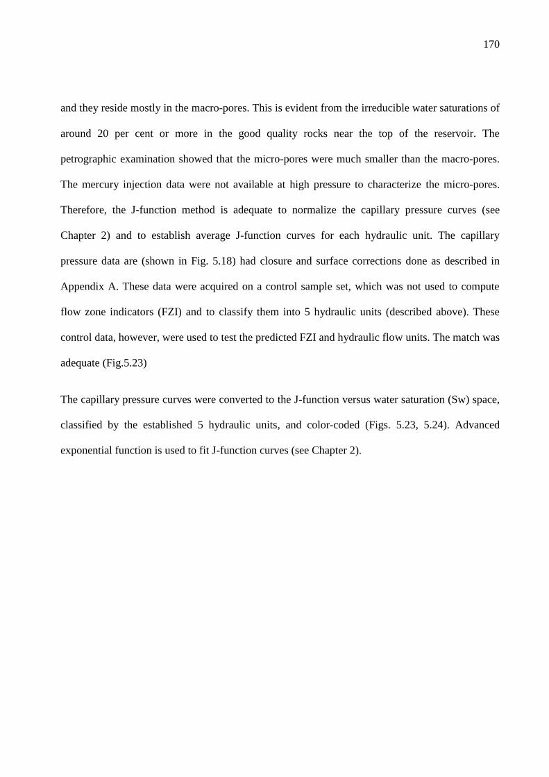
170

and they reside mostly in the macro-pores. This is evident from the irreducible water saturations of

around 20 per cent or more in the good quality rocks near the top of the reservoir. The

petrographic examination showed that the micro-pores were much smaller than the macro-pores.

The mercury injection data were not available at high pressure to characterize the micro-pores.

Therefore, the J-function method is adequate to normalize the capillary pressure curves (see

Chapter 2) and to establish average J-function curves for each hydraulic unit. The capillary

pressure data are (shown in Fig. 5.18) had closure and surface corrections done as described in

Appendix A. These data were acquired on a control sample set, which was not used to compute

flow zone indicators (FZI) and to classify them into 5 hydraulic units (described above). These

control data, however, were used to test the predicted FZI and hydraulic flow units. The match was

adequate (Fig.5.23)

The capillary pressure curves were converted to the J-function versus water saturation (Sw) space,

classified by the established 5 hydraulic units, and color-coded (Figs. 5.23, 5.24). Advanced

exponential function is used to fit J-function curves (see Chapter 2).

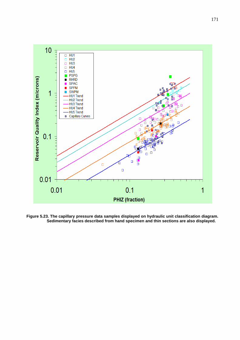
171

Figure 5.23. The capillary pressure data samples displayed on hydraulic unit classification diagram. Sedimentary facies described from hand specimen and thin sections are also displayed.

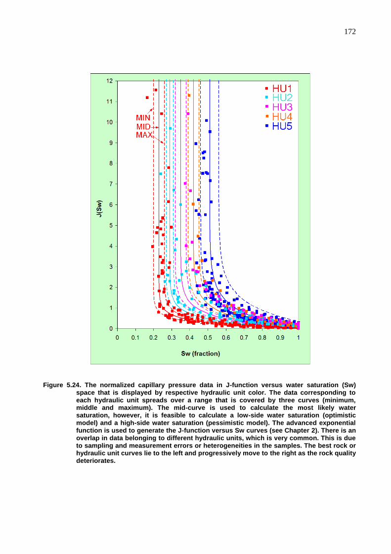
172

Figure 5.24. The normalized capillary pressure data in J-function versus water saturation (Sw) space that is displayed by respective hydraulic unit color. The data corresponding to each hydraulic unit spreads over a range that is covered by three curves (minimum, middle and maximum). The mid-curve is used to calculate the most likely water saturation, however, it is feasible to calculate a low-side water saturation (optimistic model) and a high-side water saturation (pessimistic model). The advanced exponential function is used to generate the J-function versus Sw curves (see Chapter 2). There is an overlap in data belonging to different hydraulic units, which is very common. This is due to sampling and measurement errors or heterogeneities in the samples. The best rock or hydraulic unit curves lie to the left and progressively move to the right as the rock quality deteriorates.

173

The parameters of the J-function curves are given below (Fig. 5.25):

Figure 5.25. Parameters of the fitted J-function curve and the advanced exponential function equation (see Chapter 2). These parameters correspond to the low, mid and high Sw curves shown above (Figure 5.24).

Computation of Water Saturation

The water saturations were computed for the three wells using the hydraulic flow units (computed

from predicted flow zone indicators or FZI), permeability (computed from predicted flow zone

indicators), buoyancy force (computed from height above free water and oil levels and fluid

densities), interfacial tension, and contact angles. Advanced exponential function (see Chapter 2)

is used with parameters given in Fig. 5.25. To overcome the problem of stationary J-function

curve (for each hydraulic unit), relationships of water saturations (derived from resistivity and

porosity; see Reservoir Description) versus porosity were used to determine the Swir term (Fig.

5.26). At each depth, the Swir value is determined from porosity for the respective hydraulic flow

unit. These Swir values are then used in the J-function equation to compute water saturation in the

three wells (Figure 5.27). The water saturation from saturation height model compares favorably

174

to the Archie water saturation. Therefore, a geological model populated with water saturation from

this saturation height model will be representative of the reservoir as recorded in the logs of the

three well.

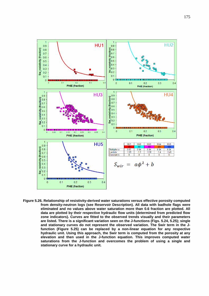
175

Figure 5.26. Relationship of resistivity-derived water saturations versus effective porosity computed from density-neutron logs (see Reservoir Description). All data with badhole flags were eliminated and no values above water saturation more than 0.6 fraction are plotted. All data are plotted by their respective hydraulic flow units (determined from predicted flow zone indicators). Curves are fitted to the observed trends visually and their parameters are listed. There is a significant variation seen on the J-functions (Figs. 5.24, 5.25); single and stationary curves do not represent the observed variation. The Swir term in the J-function (Figure 5.25) can be replaced by a non-linear equation for any respective hydraulic unit. Using this approach, the Swir term is computed from the porosity at any elevation and then used in the J-function equation. This improves computed water saturations from the J-function and overcomes the problem of using a single and stationary curve for a hydraulic unit.

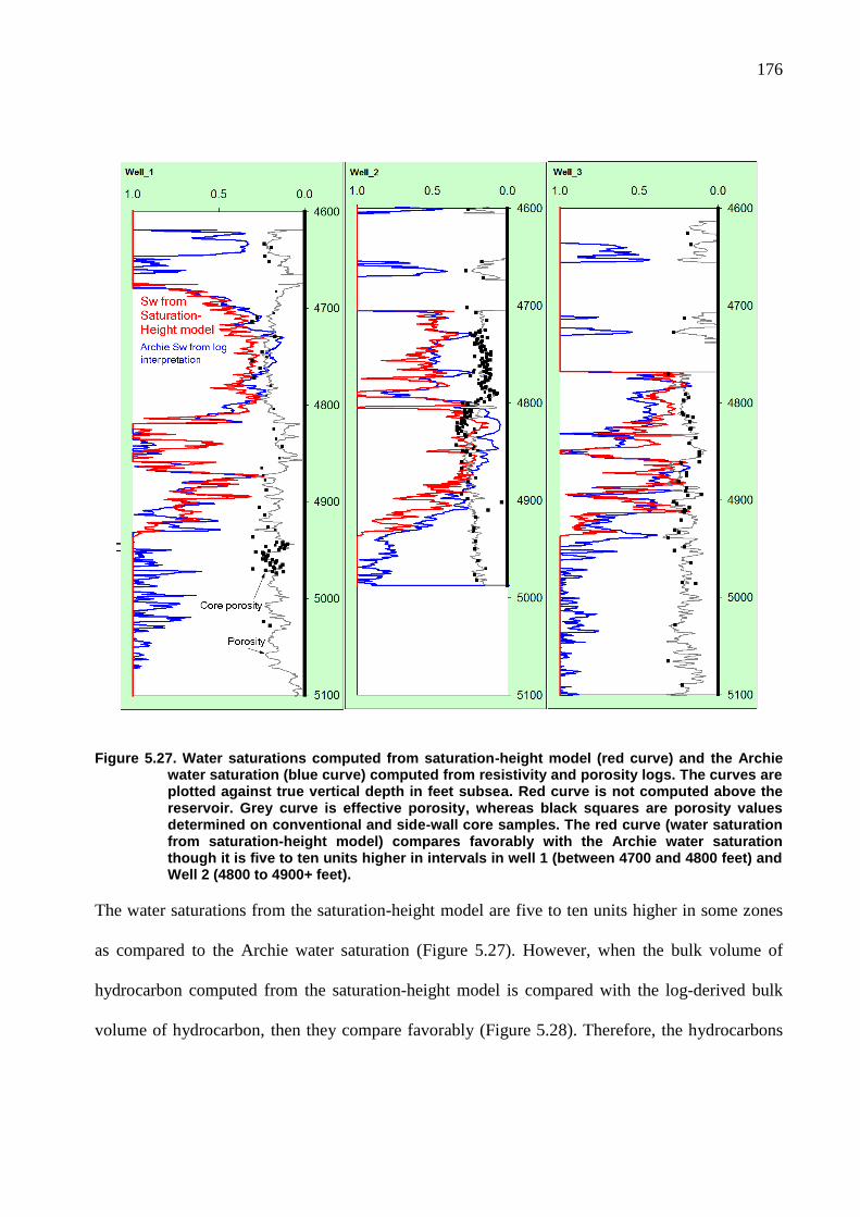
176

Figure 5.27. Water saturations computed from saturation-height model (red curve) and the Archie water saturation (blue curve) computed from resistivity and porosity logs. The curves are plotted against true vertical depth in feet subsea. Red curve is not computed above the reservoir. Grey curve is effective porosity, whereas black squares are porosity values determined on conventional and side-wall core samples. The red curve (water saturation from saturation-height model) compares favorably with the Archie water saturation though it is five to ten units higher in intervals in well 1 (between 4700 and 4800 feet) and Well 2 (4800 to 4900+ feet).

The water saturations from the saturation-height model are five to ten units higher in some zones

as compared to the Archie water saturation (Figure 5.27). However, when the bulk volume of

hydrocarbon computed from the saturation-height model is compared with the log-derived bulk

volume of hydrocarbon, then they compare favorably (Figure 5.28). Therefore, the hydrocarbons

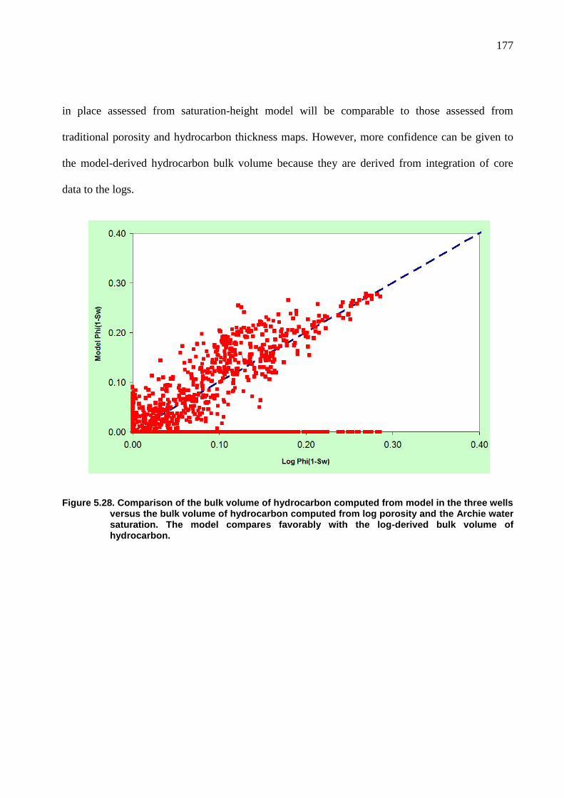
177

in place assessed from saturation-height model will be comparable to those assessed from

traditional porosity and hydrocarbon thickness maps. However, more confidence can be given to

the model-derived hydrocarbon bulk volume because they are derived from integration of core

data to the logs.

Figure 5.28. Comparison of the bulk volume of hydrocarbon computed from model in the three wells versus the bulk volume of hydrocarbon computed from log porosity and the Archie water saturation. The model compares favorably with the log-derived bulk volume of hydrocarbon.

178

Conclusion

A saturation height model is used to populate a three-dimensional geological model with water

saturation values. It requires a three dimensional porosity model, a petrophysical model of rock

types, and a permeability model. It uses free water level as the datum where water-oil capillary

pressure is taken equal to zero and a free oil level at which oil-gas capillary pressure is zero.

Densities of oil, gas and water are needed at reservoir conditions to determine the magnitude of

buoyancy force as the height increases above the free water or oil levels. Interfacial tension and

contact angles between the oil-water and gas-oil are also essential.

Petrophysical rock types or hydraulic flow units are determined based on reservoir rock that is

sampled from core. Capillary pressures are measured on the rock samples using appropriate

techniques. Porosity and air permeability are also measured on core samples besides capillary

pressure data, which are fitted to curves using one of several mathematical equations. A range of

capillary pressure curves within a rock type is averaged to determine its type curve. The Leverett J

function is also an averaging technique, which uses permeability-porosity ratio to normalize

capillary pressure data. Carbonate rocks often have bimodal pore systems in which the larger or

the macro-pores determine permeability. Since J function uses permeability to normalize capillary

pressure data, it may not effectively normalize reservoirs in which the micro-pores are charged

with hydrocarbons because there is enough buoyancy force (due to large height above free water

level) to overcome high capillary entry pressure of micro-pores, which was not the case with the

reservoir of this study.

179

A major step in this process is to develop a model that would correlate petrophysical rock types or

hydraulic flow units (determined on core) to logs and then use logs to predict them in un-cored

intervals or wells. Subsequently, predicted petrophysical rock types or hydraulic flow units are

used to determine permeability from porosity, which should closely match permeability that was

measured on core plugs. In this Thesis, I used these processes and documented them on three wells

of a carbonate reservoir and have drawn specific conclusions and findings from this work:

Saturation height modeling is an essential part of advanced reservoir characterization

process. It integrates core and logs to predict petrophysical rock types in un-cored wells

and results in water saturations that are based on capillary pressure measured on core.

I compiled the theory of saturation height modeling and related petrophysical processes

from a large literature survey and documented them in Chapter 2, 3 and 4. Such a

documentation does not exist in the published literature.

Hydraulic flow units (HU) are adequate to describe petrophysical characteristics of

reservoir rocks. The HU, once determined from core and predicted across wells, are used to

calculate permeability that conforms with the permeability measured on core.

Hydraulic flow units correspond well to textural-based geological classification of

reservoir rocks from core and thin sections. There is a general relationship but not an exact

match. This relationship should be studied so that it helps in assigning hydraulic flow units

to geological facies that are mapped in between wells using the geological model.

180

The plot of water saturations (resistivity derived) versus porosity (bulk volume water or

BVW plot) distinguished the hydraulic flow units that were identified from core. This

further confirmed the petrophysical hydraulic flow unit classification in the example

reservoir.

The J function is an effective method to normalize capillary pressure in such carbonate

reservoirs in which hydrocarbons reside in the macro-pores and hydrocarbon columns are

of moderate size.

The water saturations determined from saturation height model correspond well to water

saturations that were computed using the Archie equation in which porosity and resistivity

inputs were provided by logs.

The water saturations from the saturation-height model are superior than those determined

from resistivity logs. The resistivity logs suffer from shoulder effect and thin bed problems.

The saturation-height model is driven by density-neutron log porosity (high resolution

compared to resistivity logs) and capillary pressure curves, which are free from these

effects.

The hydrocarbon in place determined from a 3D geological model (populated by water

saturations from a saturation-height model) are more accurate than traditional pay

thickness maps that are use resistivity-derived saturations at wells.

The geological model in which saturation-height model has been implemented, can then

be used in a reservoir simulation model.

Appendix A

Measurement and Processing of Capillary Pressure Data

182

Sample Selection and Testing Conditions

It is very important to select proper rock samples from cores to ensure reliable capillary pressure

data acquisition. The samples must represent the range over which porosity and permeability of

the reservoir rock vary. The samples should represent all zones, geological facies, porosity and

permeability classes. Each single sample should be homogeneous and not be a composite of two

different rocks. Usually, saturation measurement error decreases with the increasing size of

sample.

Commonly capillary pressure tests are carried out on cleaned and restored state cores. The

wettability could have been altered to water-wet state whereas reservoir rock could be mixed- or

oil-wet. The shapes of the capillary curves will be much different and not representative of the

reservoir.

The capillary pressure tests are carried out using air-brine, air-mercury or oil-brine fluid systems.

If air-brine and air-mercury fluid systems are used, water-wet reservoir conditions should be

assumed.

Where necessary, capillary pressure tests could be carried out on cleaned-state and restored-state

cores. Few tests should also be done using oil-brine fluid system (for oil reservoir). If the cleaned-

state and restored-state tests generally agree then this gives good indication that the acquired data

is representative.

It is feasible to measure an imbibition curve on a fresh-state or restored-state core because water in

these cores is at or near irreducible saturation. A core sample has to be 100 per cent saturated with

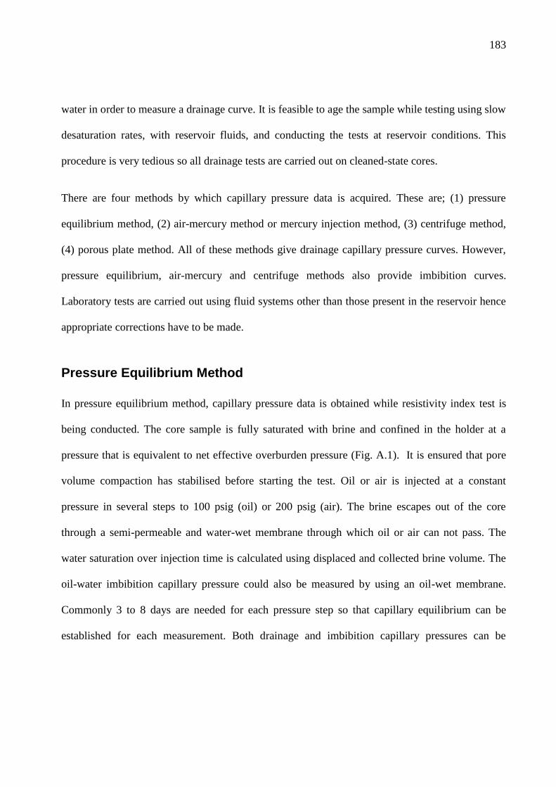
183

water in order to measure a drainage curve. It is feasible to age the sample while testing using slow

desaturation rates, with reservoir fluids, and conducting the tests at reservoir conditions. This

procedure is very tedious so all drainage tests are carried out on cleaned-state cores.

There are four methods by which capillary pressure data is acquired. These are; (1) pressure

equilibrium method, (2) air-mercury method or mercury injection method, (3) centrifuge method,

(4) porous plate method. All of these methods give drainage capillary pressure curves. However,

pressure equilibrium, air-mercury and centrifuge methods also provide imbibition curves.

Laboratory tests are carried out using fluid systems other than those present in the reservoir hence

appropriate corrections have to be made.

Pressure Equilibrium Method

In pressure equilibrium method, capillary pressure data is obtained while resistivity index test is

being conducted. The core sample is fully saturated with brine and confined in the holder at a

pressure that is equivalent to net effective overburden pressure (Fig. A.1). It is ensured that pore

volume compaction has stabilised before starting the test. Oil or air is injected at a constant

pressure in several steps to 100 psig (oil) or 200 psig (air). The brine escapes out of the core

through a semi-permeable and water-wet membrane through which oil or air can not pass. The

water saturation over injection time is calculated using displaced and collected brine volume. The

oil-water imbibition capillary pressure could also be measured by using an oil-wet membrane.

Commonly 3 to 8 days are needed for each pressure step so that capillary equilibrium can be

established for each measurement. Both drainage and imbibition capillary pressures can be

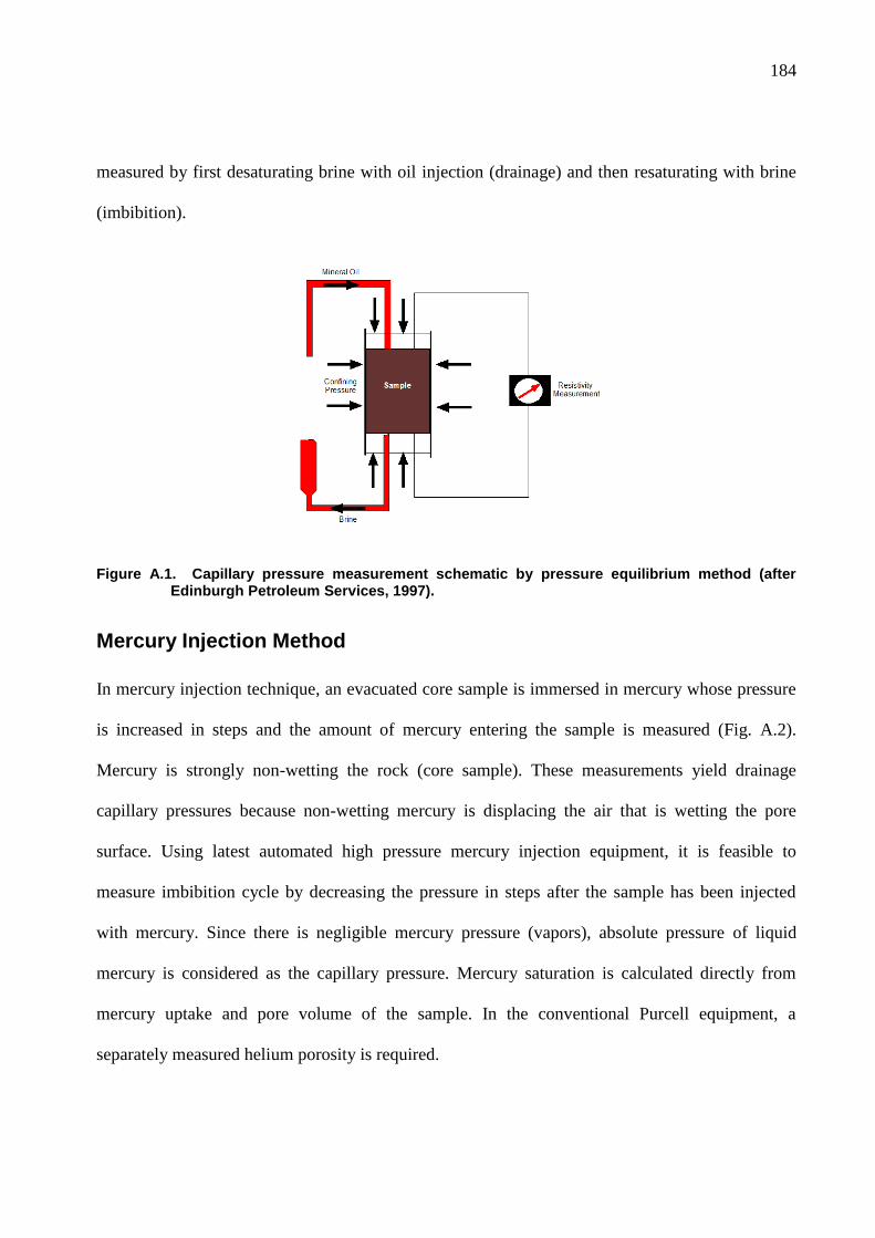
184

measured by first desaturating brine with oil injection (drainage) and then resaturating with brine

(imbibition).

Figure A.1. Capillary pressure measurement schematic by pressure equilibrium method (after Edinburgh Petroleum Services, 1997).

Mercury Injection Method

In mercury injection technique, an evacuated core sample is immersed in mercury whose pressure

is increased in steps and the amount of mercury entering the sample is measured (Fig. A.2).

Mercury is strongly non-wetting the rock (core sample). These measurements yield drainage

capillary pressures because non-wetting mercury is displacing the air that is wetting the pore

surface. Using latest automated high pressure mercury injection equipment, it is feasible to

measure imbibition cycle by decreasing the pressure in steps after the sample has been injected

with mercury. Since there is negligible mercury pressure (vapors), absolute pressure of liquid

mercury is considered as the capillary pressure. Mercury saturation is calculated directly from

mercury uptake and pore volume of the sample. In the conventional Purcell equipment, a

separately measured helium porosity is required.

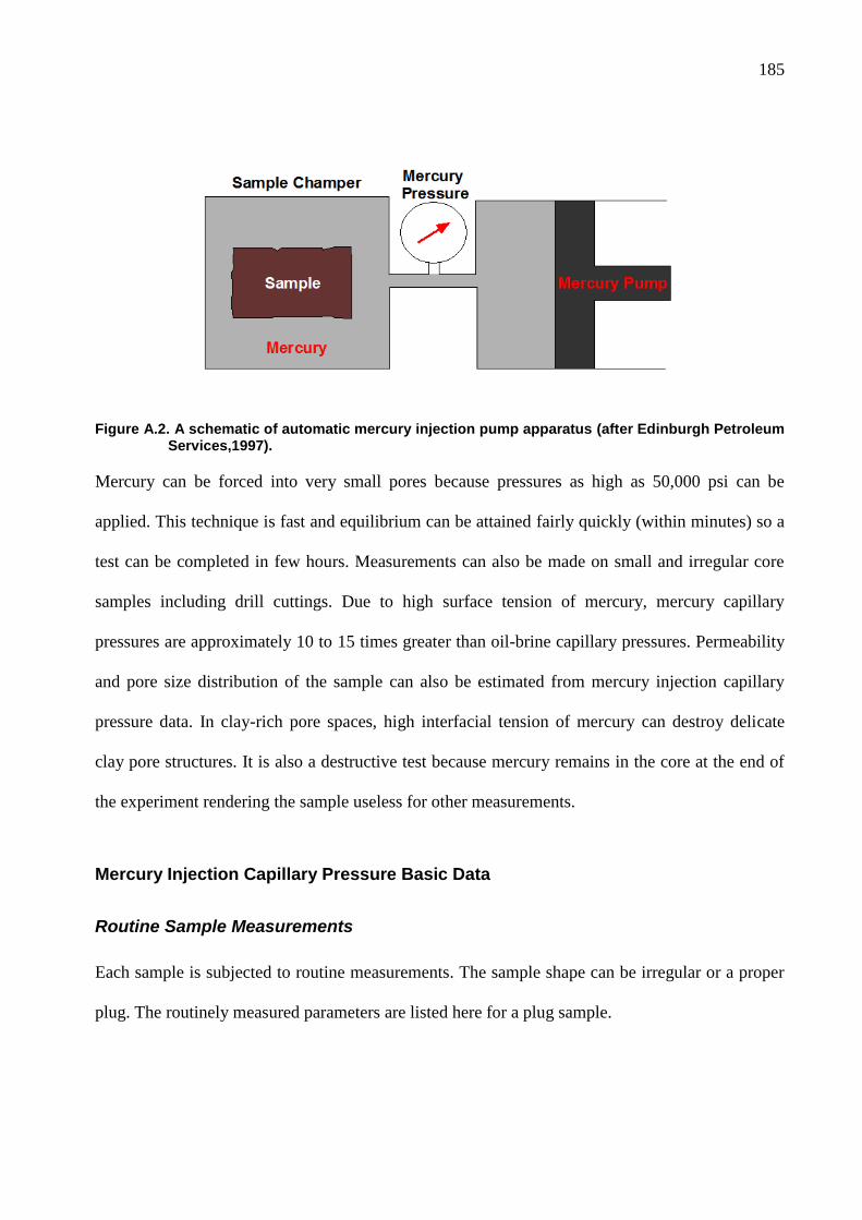
185

Figure A.2. A schematic of automatic mercury injection pump apparatus (after Edinburgh Petroleum Services,1997).

Mercury can be forced into very small pores because pressures as high as 50,000 psi can be

applied. This technique is fast and equilibrium can be attained fairly quickly (within minutes) so a

test can be completed in few hours. Measurements can also be made on small and irregular core

samples including drill cuttings. Due to high surface tension of mercury, mercury capillary

pressures are approximately 10 to 15 times greater than oil-brine capillary pressures. Permeability

and pore size distribution of the sample can also be estimated from mercury injection capillary

pressure data. In clay-rich pore spaces, high interfacial tension of mercury can destroy delicate

clay pore structures. It is also a destructive test because mercury remains in the core at the end of

the experiment rendering the sample useless for other measurements.

Mercury Injection Capillary Pressure Basic Data

Routine Sample Measurements

Each sample is subjected to routine measurements. The sample shape can be irregular or a proper

plug. The routinely measured parameters are listed here for a plug sample.

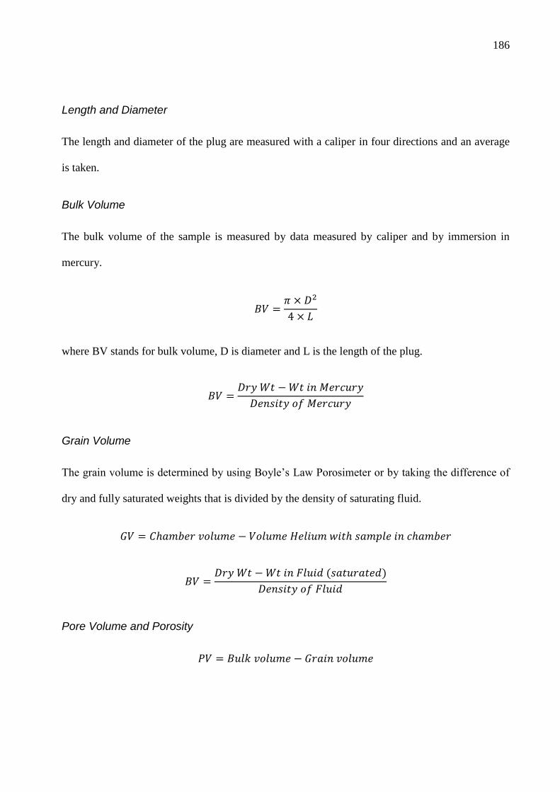
186

Length and Diameter

The length and diameter of the plug are measured with a caliper in four directions and an average

is taken.

Bulk Volume

The bulk volume of the sample is measured by data measured by caliper and by immersion in

mercury.

where BV stands for bulk volume, D is diameter and L is the length of the plug.

Grain Volume

The grain volume is determined by using Boyle‟s Law Porosimeter or by taking the difference of

dry and fully saturated weights that is divided by the density of saturating fluid.

Pore Volume and Porosity

187

Grain Density

The grain density is determined by dividing dry weight by the grain volume.

Air Permeability

Air permeability is measured

Surface Vug Volume (SVV)

It is the difference between bulk volume callipered and bulk volume immersed in mercury, which

indicates the volume of surface vugs or surface irregularities or both. It is also expressed as a

fraction of the pore volume.

Surface Area (SA)

It is determined from the formula for a right cylinder, where SA represents surface area, D is

diameter and L is length of the cylinder. The ratio of surface area to bulk volume is used as a

quality control parameter. The bigger the sample, the smaller the number and the better the data. It

is acceptable if it is about 2.5 or less. If the sample is too small the surface irregulairies will give

large errors in bulk volume and therefore in porosity.

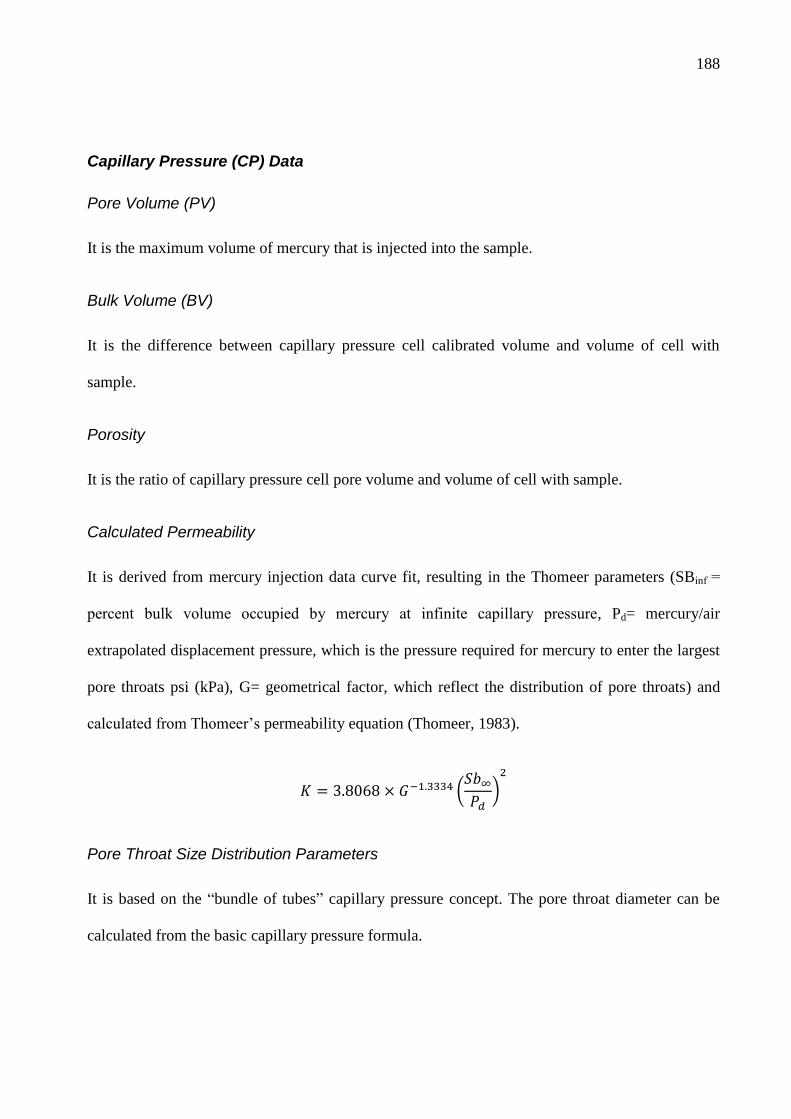
188

Capillary Pressure (CP) Data

Pore Volume (PV)

It is the maximum volume of mercury that is injected into the sample.

Bulk Volume (BV)

It is the difference between capillary pressure cell calibrated volume and volume of cell with

sample.

Porosity

It is the ratio of capillary pressure cell pore volume and volume of cell with sample.

Calculated Permeability

It is derived from mercury injection data curve fit, resulting in the Thomeer parameters (SBinf =

percent bulk volume occupied by mercury at infinite capillary pressure, Pd= mercury/air

extrapolated displacement pressure, which is the pressure required for mercury to enter the largest

pore throats psi (kPa), G= geometrical factor, which reflect the distribution of pore throats) and

calculated from Thomeer‟s permeability equation (Thomeer, 1983).

Pore Throat Size Distribution Parameters

It is based on the “bundle of tubes” capillary pressure concept. The pore throat diameter can be

calculated from the basic capillary pressure formula.

189

Where D is the pore throat diameter.

Contact Angle

The contact angle between air, mercury and solid is 140 degrees.

Interfacial Tension

The interfacial tension between air-mercury is 485 dynes per centimetre.

Sample Description

It is very important to describe grain size and pore types to assess surface effects. A photo with

scale is very useful. The chipped edges and saw marks lead to surface effects.

Mercury Injection Data and Basic Calculation

The mercury injection data and its layout is shown below (Tables A.1 and A.2). Figure A.3 is a

plot of the same data.

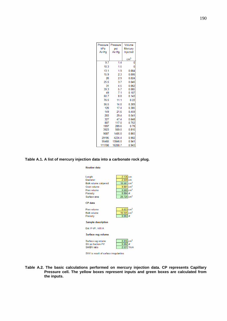
190

Table A.1. A list of mercury injection data into a carbonate rock plug.

Table A.2. The basic calculations performed on mercury injection data. CP represents Capillary Pressure cell. The yellow boxes represent inputs and green boxes are calculated from the inputs.

191

Mercury Injection Data Plots

Bulk Volume Occupied by Mercury

The capillary pressure (Pc) is plotted against ratio of mercury injected to bulk volume of the

sample on a log-log scale (Fig. A.4). It is used to quality control the data and check for surface

effects. The Thomeer parameters are also determined from this plot. The air permeability is also

calculated based on the Thomeer parameters that are determined from the curve fit to the mercury

injection data. The Pc scale can be changed into pore throat diameter scale.

Figure A.3. Plot of the mercury injection data that is tabulated in Table A.1. The air-mercury capillary pressure data is initially plotted on a log scale whereas volume of injected mercury is plotted on a linear scale, which increases from right towards left as a convention.

1

10

100

1000

10000

100000

00.20.40.60.81

Volume Mercury Injected (cubic centimetres)

Air

-Me

rcu

ry C

ap

illa

ry P

res

su

re (

ps

i)

Volume Hg Injected

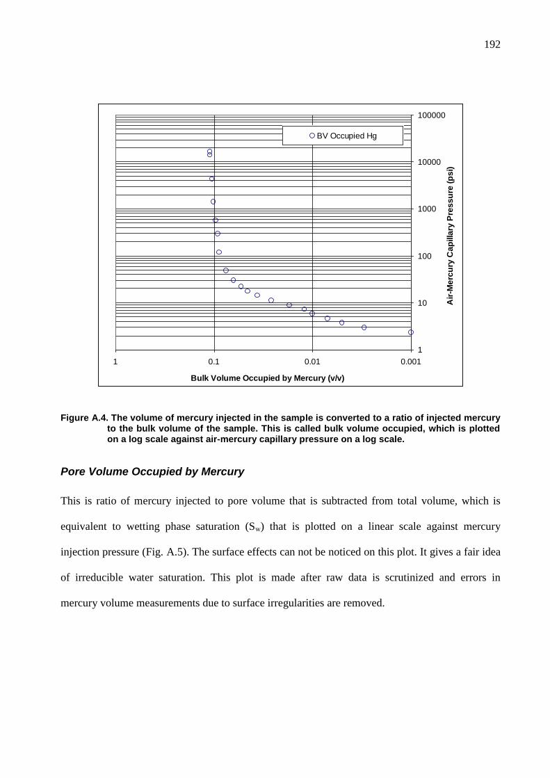
192

Figure A.4. The volume of mercury injected in the sample is converted to a ratio of injected mercury to the bulk volume of the sample. This is called bulk volume occupied, which is plotted on a log scale against air-mercury capillary pressure on a log scale.

Pore Volume Occupied by Mercury

This is ratio of mercury injected to pore volume that is subtracted from total volume, which is

equivalent to wetting phase saturation (Sw) that is plotted on a linear scale against mercury

injection pressure (Fig. A.5). The surface effects can not be noticed on this plot. It gives a fair idea

of irreducible water saturation. This plot is made after raw data is scrutinized and errors in

mercury volume measurements due to surface irregularities are removed.

1

10

100

1000

10000

100000

0.0010.010.11

Bulk Volume Occupied by Mercury (v/v)

Air

-Me

rcu

ry C

ap

illa

ry P

res

su

re (

ps

i)

BV Occupied Hg

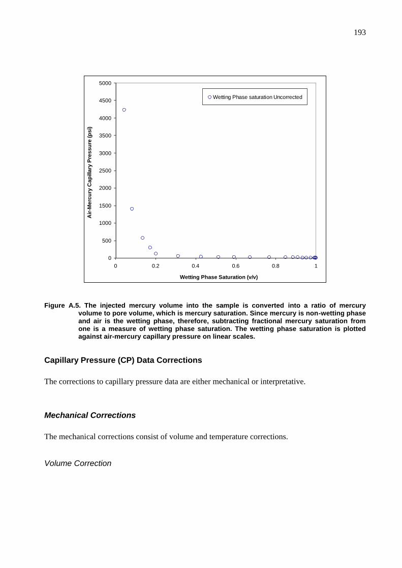
193

Figure A.5. The injected mercury volume into the sample is converted into a ratio of mercury volume to pore volume, which is mercury saturation. Since mercury is non-wetting phase and air is the wetting phase, therefore, subtracting fractional mercury saturation from one is a measure of wetting phase saturation. The wetting phase saturation is plotted against air-mercury capillary pressure on linear scales.

Capillary Pressure (CP) Data Corrections

The corrections to capillary pressure data are either mechanical or interpretative.

Mechanical Corrections

The mechanical corrections consist of volume and temperature corrections.

Volume Correction

0

500

1000

1500

2000

2500

3000

3500

4000

4500

5000

0 0.2 0.4 0.6 0.8 1

Wetting Phase Saturation (v/v)

Air

-Me

rcu

ry C

ap

illa

ry P

res

su

re (

ps

i)

Wetting Phase saturation Uncorrected

194

The volume correction relates to packing of mercury into apparatus irregularities, corners and cell

expansion, which results in false mercury injection readings. These are often calibrated by placing

a zero porosity blank sample into the apparatus, which is pressured up by mercury injection. It is

always a negative correction.

Temperature Correction

Since mercury expands with increase in temperature hence the mercury injection into the sample

must be calibrated for the temperature at the time of the test. This corrections can be positive or

negative. It is approximately 0.003 cm3 for every 5 degrees centigrade change in temperature.

Interpretative Corrections

The sample size, shape, pore geometry and surface irregularities are source of significant errors in

the mercury injection experiment. All these errors occur at low pressure, which is below the

displacement pressure of the sample. These errors are collectively called surface effects.

Surface Vug Factor

It is the volume of mercury that enters the sample at zero pressure in the capillary pressure cell.

The head of mercury above the sample to the upper reference window is sufficient to force

mercury into pores with a diameter greater than 115 micro-meter. It is determined by the

difference between calipered bulk volume and the bulk volume after the sample is immersed in

mercury in the capillary pressure cell. The bulk volume and pore volume ratios must not include

the surface vug factor (Fig. A.6).

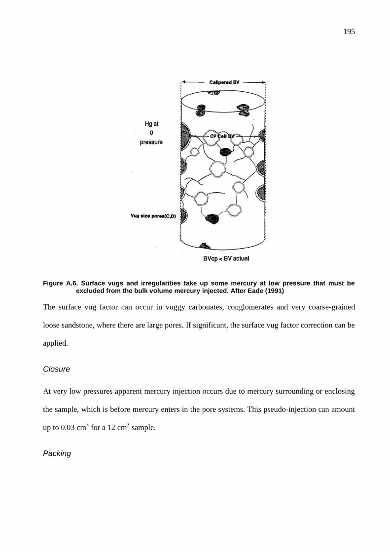
195

Figure A.6. Surface vugs and irregularities take up some mercury at low pressure that must be excluded from the bulk volume mercury injected. After Eade (1991)

The surface vug factor can occur in vuggy carbonates, conglomerates and very coarse-grained

loose sandstone, where there are large pores. If significant, the surface vug factor correction can be

applied.

Closure

At very low pressures apparent mercury injection occurs due to mercury surrounding or enclosing

the sample, which is before mercury enters in the pore systems. This pseudo-injection can amount

up to 0.03 cm3 for a 12 cm

3 sample.

Packing

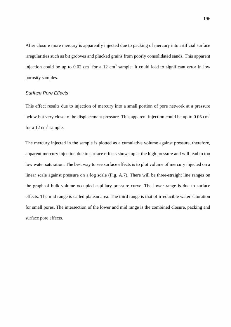
196

After closure more mercury is apparently injected due to packing of mercury into artificial surface

irregularities such as bit grooves and plucked grains from poorly consolidated sands. This apparent

injection could be up to 0.02 cm3 for a 12 cm

3 sample. It could lead to significant error in low

porosity samples.

Surface Pore Effects

This effect results due to injection of mercury into a small portion of pore network at a pressure

below but very close to the displacement pressure. This apparent injection could be up to 0.05 cm3

for a 12 cm3 sample.

The mercury injected in the sample is plotted as a cumulative volume against pressure, therefore,

apparent mercury injection due to surface effects shows up at the high pressure and will lead to too

low water saturation. The best way to see surface effects is to plot volume of mercury injected on a

linear scale against pressure on a log scale (Fig. A.7). There will be three-straight line ranges on

the graph of bulk volume occupied capillary pressure curve. The lower range is due to surface

effects. The mid range is called plateau area. The third range is that of irreducible water saturation

for small pores. The intersection of the lower and mid range is the combined closure, packing and

surface pore effects.

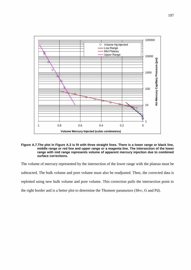
197

Figure A.7.The plot in Figure A.3 is fit with three straight lines. There is a lower range or black line, middle range or red line and upper range or a magenta line. The intersection of the lower range with mid range represents volume of apparent mercury injection due to combined surface corrections.

The volume of mercury represented by the intersection of the lower range with the plateau must be

subtracted. The bulk volume and pore volume must also be readjusted. Then, the corrected data is

replotted using new bulk volume and pore volume. This correction pulls the intersection point to

the right border and is a better plot to determine the Thomeer parameters (Sb∞, G and Pd).

1

10

100

1000

10000

100000

00.20.40.60.81

Volume Mercury Injected (cubic centimetres)

Air

-Me

rcu

ry C

ap

illa

ry P

res

su

re (

ps

i)

Volume Hg Injected

Low RangeMid Plateau

Upper Range

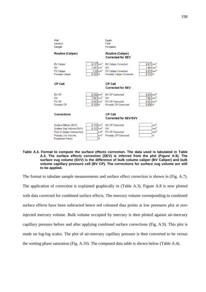
198

Table A.3. Format to compute the surface effects correction. The data used is tabulated in Table A.3. The surface effects correction (SEV) is inferred from the plot (Figure A.9). The surface vug volume (SVV) is the difference of bulk volume caliper (BV Caliper) and bulk volume capillary pressure cell (BV CP). The corrections for surface vug volume are still to be applied.

The format to tabulate sample measurements and surface effect correction is shown in (Fig. A.7).

The application of correction is explained graphically in (Table A.3). Figure A.8 is now plotted

with data corrected for combined surface effects. The mercury volume corresponding to combined

surface effects have been subtracted hence red coloured data points at low pressures plot at zero

injected mercury volume. Bulk volume occupied by mercury is then plotted against air-mercury

capillary pressure before and after applying combined surface corrections (Fig. A.9). This plot is

made on log-log scales. The plot of air-mercury capillary pressure is then converted to be versus

the wetting phase saturation (Fig. A.10). The computed data table is shown below (Table A.4).

199

Figure A.8. Graph shown above (Figure A.7) is now plotted with data corrected for combined surface effects. The mercury volume corresponding to combined surface effects have been subtracted hence red coloured data points at low pressures plot at zero injected mercury volume.

1

10

100

1000

10000

100000

00.20.40.60.81

Volume Mercury Injected (cubic centimetres)

Air

-Merc

ury

Cap

illa

ry P

ressu

re (

psi)

Volume Hg Injected

Low Range

Mid Plateau

Upper Range

Volume Hg Injected Corrected

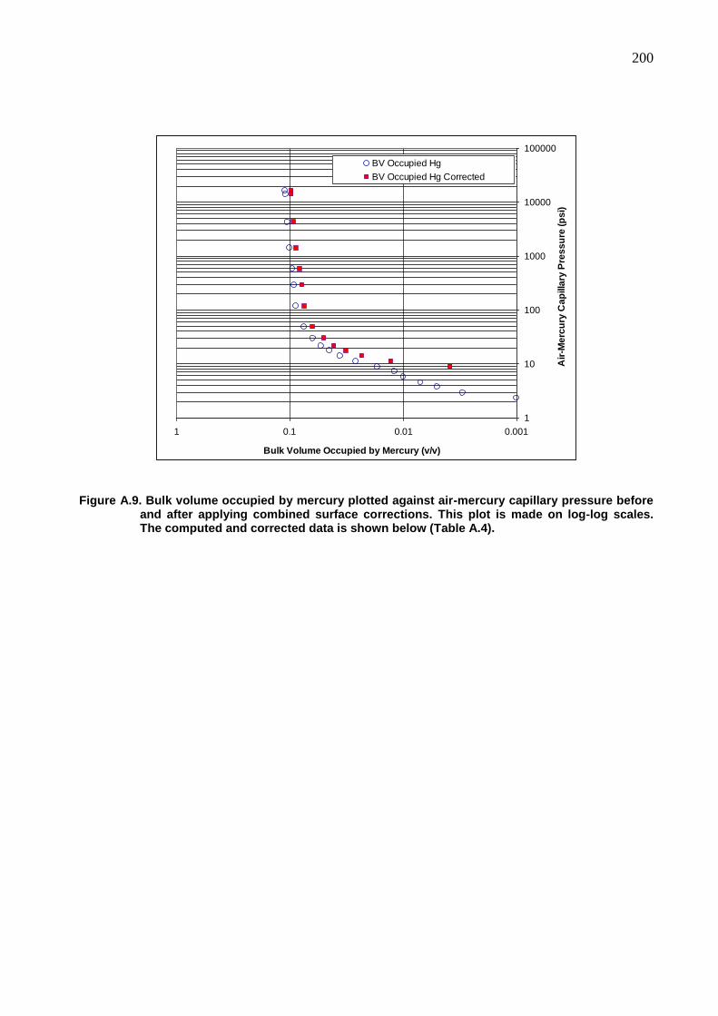
200

Figure A.9. Bulk volume occupied by mercury plotted against air-mercury capillary pressure before and after applying combined surface corrections. This plot is made on log-log scales. The computed and corrected data is shown below (Table A.4).

1

10

100

1000

10000

100000

0.0010.010.11

Bulk Volume Occupied by Mercury (v/v)

Air

-Me

rcu

ry C

ap

illa

ry P

res

su

re (

ps

i)

BV Occupied Hg

BV Occupied Hg Corrected

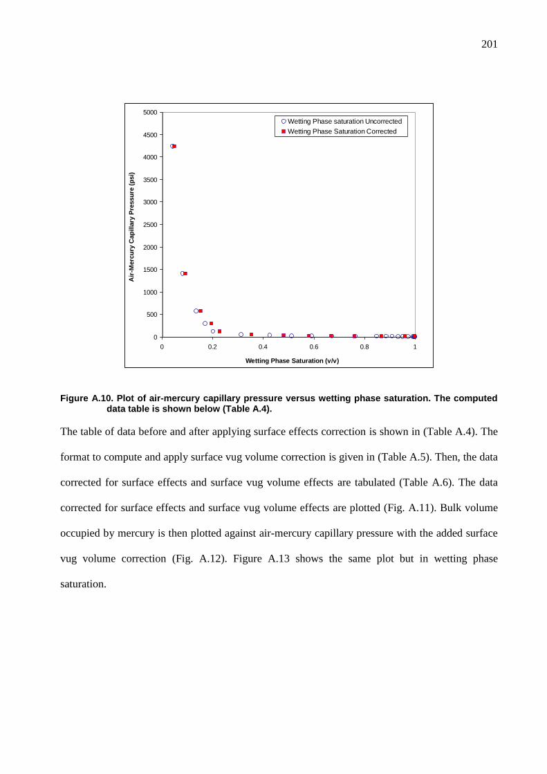
201

Figure A.10. Plot of air-mercury capillary pressure versus wetting phase saturation. The computed data table is shown below (Table A.4).

The table of data before and after applying surface effects correction is shown in (Table A.4). The

format to compute and apply surface vug volume correction is given in (Table A.5). Then, the data

corrected for surface effects and surface vug volume effects are tabulated (Table A.6). The data

corrected for surface effects and surface vug volume effects are plotted (Fig. A.11). Bulk volume

occupied by mercury is then plotted against air-mercury capillary pressure with the added surface

vug volume correction (Fig. A.12). Figure A.13 shows the same plot but in wetting phase

saturation.

0

500

1000

1500

2000

2500

3000

3500

4000

4500

5000

0 0.2 0.4 0.6 0.8 1

Wetting Phase Saturation (v/v)

Air

-Merc

ury

Cap

illa

ry P

ressu

re (

psi)

Wetting Phase saturation Uncorrected

Wetting Phase Saturation Corrected

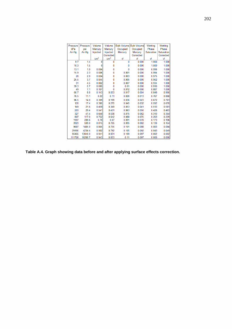
202

Table A.4. Graph showing data before and after applying surface effects correction.

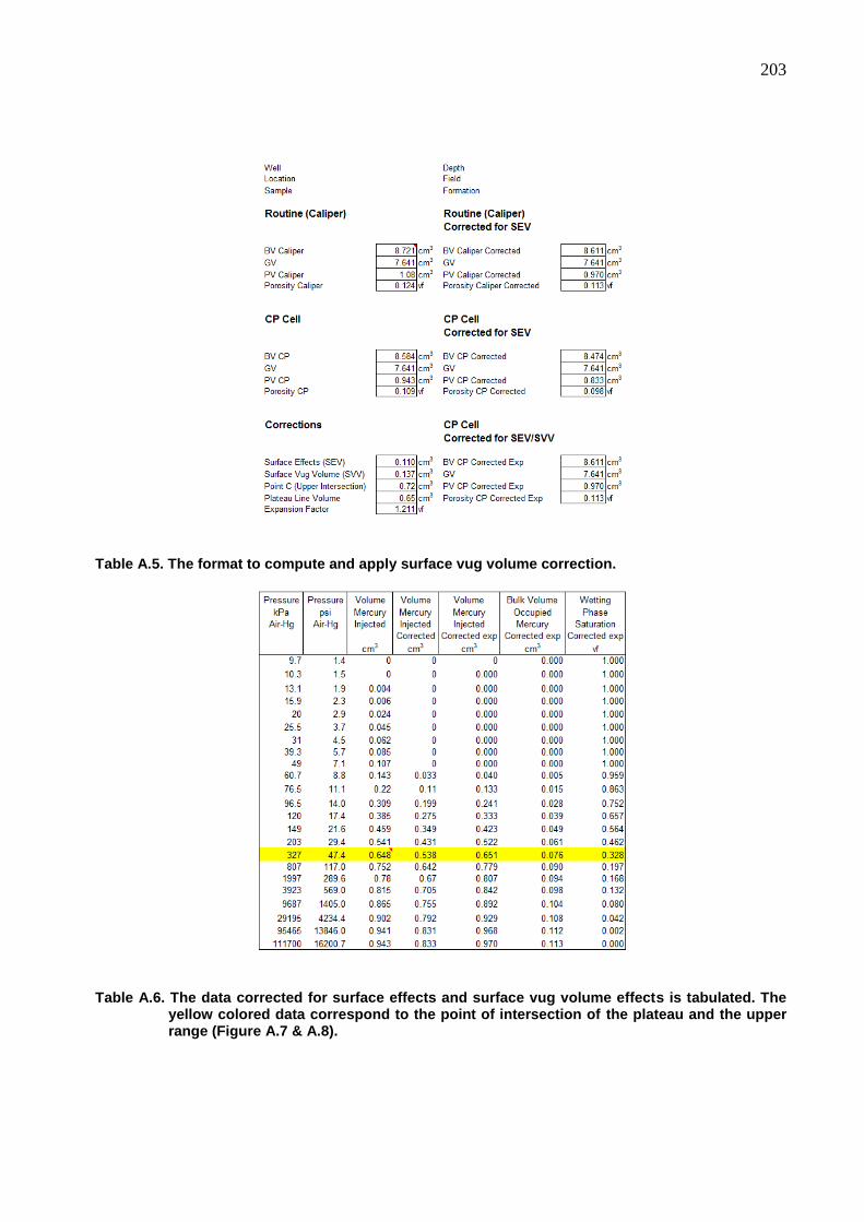
203

Table A.5. The format to compute and apply surface vug volume correction.

Table A.6. The data corrected for surface effects and surface vug volume effects is tabulated. The yellow colored data correspond to the point of intersection of the plateau and the upper range (Figure A.7 & A.8).

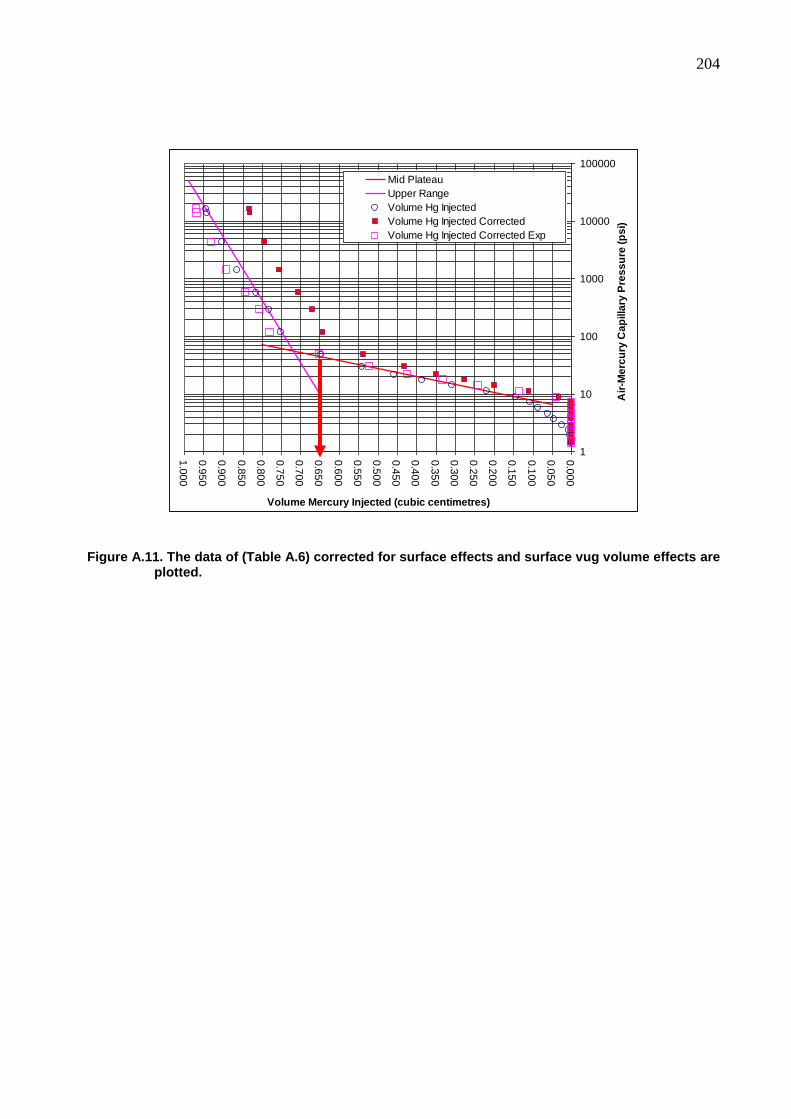
204

Figure A.11. The data of (Table A.6) corrected for surface effects and surface vug volume effects are plotted.

1

10

100

1000

10000

100000

0.0

00

0.0

50

0.1

00

0.1

50

0.2

00

0.2

50

0.3

00

0.3

50

0.4

00

0.4

50

0.5

00

0.5

50

0.6

00

0.6

50

0.7

00

0.7

50

0.8

00

0.8

50

0.9

00

0.9

50

1.0

00

Volume Mercury Injected (cubic centimetres)

Air

-Me

rcu

ry C

ap

illa

ry P

res

su

re (

ps

i)

Mid Plateau

Upper Range

Volume Hg Injected

Volume Hg Injected Corrected

Volume Hg Injected Corrected Exp

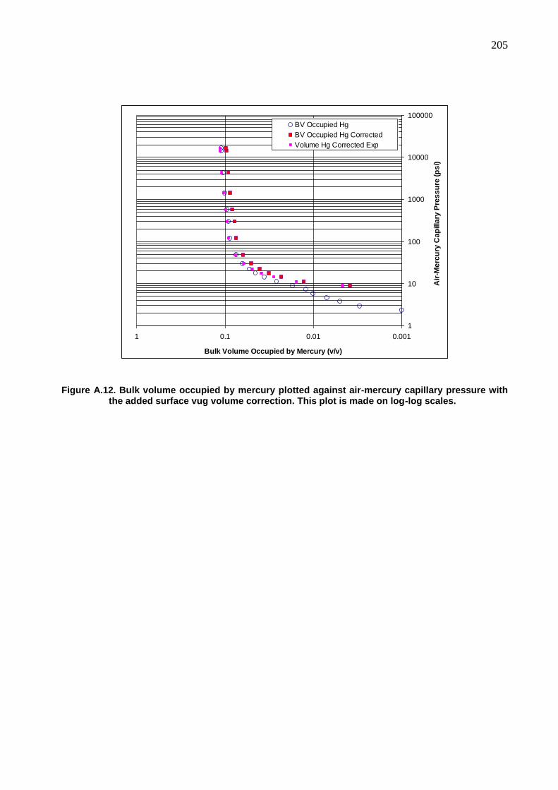
205

Figure A.12. Bulk volume occupied by mercury plotted against air-mercury capillary pressure with the added surface vug volume correction. This plot is made on log-log scales.

1

10

100

1000

10000

100000

0.0010.010.11

Bulk Volume Occupied by Mercury (v/v)

Air

-Me

rcu

ry C

ap

illa

ry P

res

su

re (

ps

i)

BV Occupied Hg

BV Occupied Hg Corrected

Volume Hg Corrected Exp

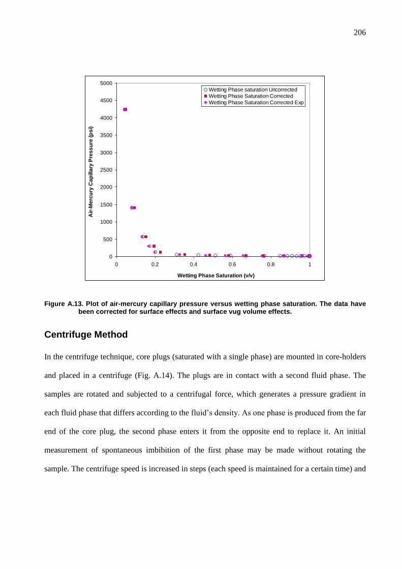
206

Figure A.13. Plot of air-mercury capillary pressure versus wetting phase saturation. The data have been corrected for surface effects and surface vug volume effects.

Centrifuge Method

In the centrifuge technique, core plugs (saturated with a single phase) are mounted in core-holders

and placed in a centrifuge (Fig. A.14). The plugs are in contact with a second fluid phase. The

samples are rotated and subjected to a centrifugal force, which generates a pressure gradient in

each fluid phase that differs according to the fluid‟s density. As one phase is produced from the far

end of the core plug, the second phase enters it from the opposite end to replace it. An initial

measurement of spontaneous imbibition of the first phase may be made without rotating the

sample. The centrifuge speed is increased in steps (each speed is maintained for a certain time) and

0

500

1000

1500

2000

2500

3000

3500

4000

4500

5000

0 0.2 0.4 0.6 0.8 1

Wetting Phase Saturation (v/v)

Air

-Me

rcu

ry C

ap

illa

ry P

res

su

re (

ps

i)Wetting Phase saturation Uncorrected

Wetting Phase Saturation Corrected

Wetting Phase Saturation Corrected Exp

207

cumulative production of the produced phase is measured at each step. Near the end of the test,

measurements are made to determine the pore volume and saturation of the sample.

The data obtained (equilibrium average saturation versus capillary pressure at the inlet face) are

analyzed by the method of Hassler and Brunner (1945). The capillary pressure in this system is

proportional to the square of revolutions per minute (RPM) and six to eight data points are

commonly recorded. The centrifuge remains in motion throughout the test with each selected RPM

held constant until no additional fluid is expelled from the sample. The fluid expelled from the

sample is measured using a stroboscope while the centrifuge is still in motion. The test is not valid

for samples having heterogeneity that is on a smaller scale than the plug (such as vuggy porosity).

The technique is very suitable for weakly cemented sand. The fluids used in a centrifuge

experiment must be degassed. The measurements can be made with preserved, extracted or

restored state core with gas-brine, gas-oil (with or without an irreducible water saturation), or oil-

brine fluids. The centrifuge should never be stopped and restarted or its speed reduced during a

sequence of measurements. The fluids will spontaneously redistribute if the centrifuge slows

down or stops, and hysteresis can cause the subsequent results to differ from those that would have

been obtained otherwise. Few centrifuge core-holders allow imposition of a hydrostatic net

overburden pressure of up to 4000 psi and a temperature up to 160 F. It is generally difficult to

obtain measurements at elevated temperatures or under high overburden pressure.

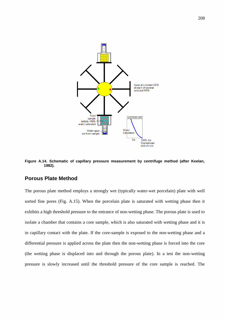
208

Figure A.14. Schematic of capillary pressure measurement by centrifuge method (after Keelan, 1982).

Porous Plate Method

The porous plate method employs a strongly wet (typically water-wet porcelain) plate with well

sorted fine pores (Fig. A.15). When the porcelain plate is saturated with wetting phase then it

exhibits a high threshold pressure to the entrance of non-wetting phase. The porous plate is used to

isolate a chamber that contains a core sample, which is also saturated with wetting phase and it is

in capillary contact with the plate. If the core-sample is exposed to the non-wetting phase and a

differential pressure is applied across the plate then the non-wetting phase is forced into the core

(the wetting phase is displaced into and through the porous plate). In a test the non-wetting

pressure is slowly increased until the threshold pressure of the core sample is reached. The

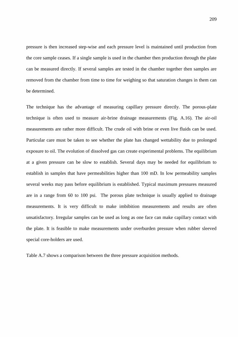
209

pressure is then increased step-wise and each pressure level is maintained until production from

the core sample ceases. If a single sample is used in the chamber then production through the plate

can be measured directly. If several samples are tested in the chamber together then samples are

removed from the chamber from time to time for weighing so that saturation changes in them can

be determined.

The technique has the advantage of measuring capillary pressure directly. The porous-plate

technique is often used to measure air-brine drainage measurements (Fig. A.16). The air-oil

measurements are rather more difficult. The crude oil with brine or even live fluids can be used.

Particular care must be taken to see whether the plate has changed wettability due to prolonged

exposure to oil. The evolution of dissolved gas can create experimental problems. The equilibrium

at a given pressure can be slow to establish. Several days may be needed for equilibrium to

establish in samples that have permeabilities higher than 100 mD. In low permeability samples

several weeks may pass before equilibrium is established. Typical maximum pressures measured

are in a range from 60 to 100 psi. The porous plate technique is usually applied to drainage

measurements. It is very difficult to make imbibition measurements and results are often

unsatisfactory. Irregular samples can be used as long as one face can make capillary contact with

the plate. It is feasible to make measurements under overburden pressure when rubber sleeved

special core-holders are used.

Table A.7 shows a comparison between the three pressure acquisition methods.

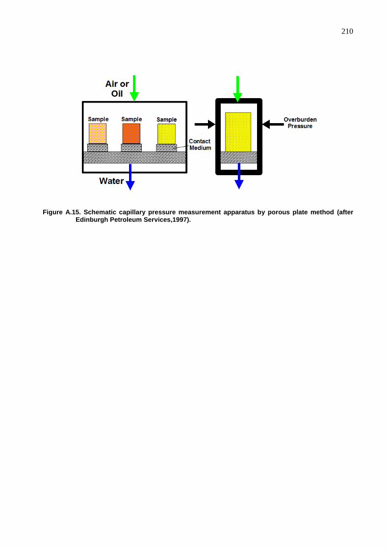
210

Figure A.15. Schematic capillary pressure measurement apparatus by porous plate method (after Edinburgh Petroleum Services,1997).

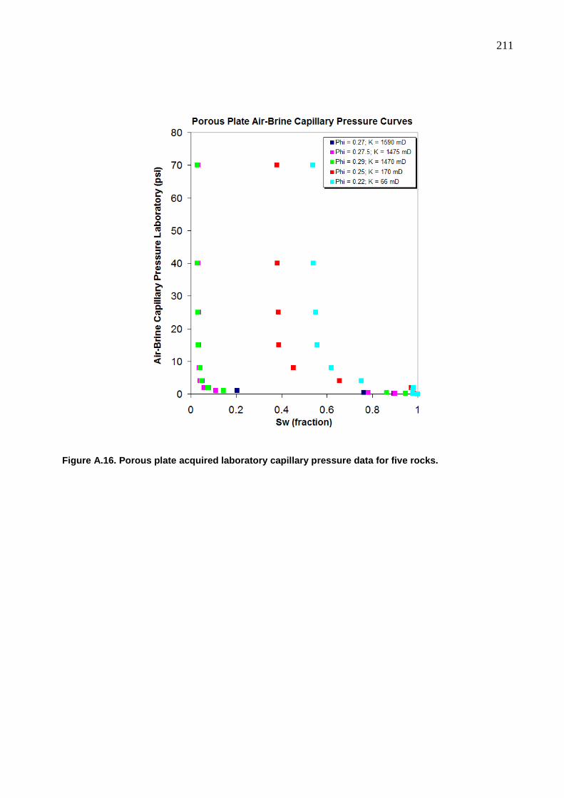
211

Figure A.16. Porous plate acquired laboratory capillary pressure data for five rocks.

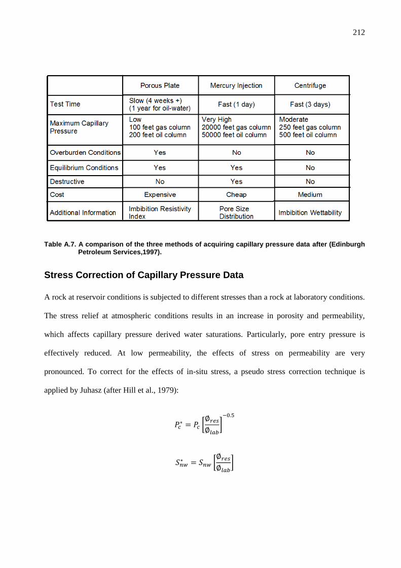
212

Table A.7. A comparison of the three methods of acquiring capillary pressure data after (Edinburgh Petroleum Services,1997).

Stress Correction of Capillary Pressure Data

A rock at reservoir conditions is subjected to different stresses than a rock at laboratory conditions.

The stress relief at atmospheric conditions results in an increase in porosity and permeability,

which affects capillary pressure derived water saturations. Particularly, pore entry pressure is

effectively reduced. At low permeability, the effects of stress on permeability are very

pronounced. To correct for the effects of in-situ stress, a pseudo stress correction technique is

applied by Juhasz (after Hill et al., 1979):

213

where Pc stands for measured capillary pressure, Pc* is stress corrected capillary pressure, Snw is

measured non-wetting phase saturation, Snw* is stress-corrected non-wetting phase saturation.

Total porosity measured in the laboratory is υlab whereas υres is in-situ porosity.

Clay-Bound Water Correction of Capillary Pressure Data

The presence of clays has an effect on the capillary pressure curve. The delicate clays in the pores

are easily damaged by cleaning and drying, which changes microporosity hence the measured

capillary pressure. The clays in the pores also increase pore-entry pressure. The clays can be

preserved by suitable cleaning methods and critical point drying but it does not help as during

capillary pressure experiments clays are destroyed. At reservoir conditions, water associated with

clays as bound water is present in the pore spaces. This clay-bound water is removed during

cleaning and drying of the samples prior to capillary pressure measurements. The air-kerosene

and air-mercury capillary pressure measurements do not account for the effects of clay bound

water. The air-brine capillary pressure measurements using porous plate method include the

effects due to clay bound water when proper salinity brine is used in the measurements. When

capillary pressure curves are corrected for the effect of clay-bound water then each point on the

curve is moved to a higher pressure and a higher wetting phase saturation. The corrections can be

determined by comparison with the same or similar sample whose capillary pressure is measured

by air-mercury and air-brine. Alternatively, a correction suggested by Hill, Shirley and Klein

(1979) can be applied:

214

This method is based on an empirical relationship between the amount of clay-bound water and

Qv, which has been derived from an experimental data set. The cation exchange capacity (CEC)

and formation water salinity are also needed to apply this correction.

where Pc stands for measured capillary pressure, Pc* is CBW corrected capillary pressure, SHg is

measured mercury saturation, SHg* is CBW-corrected mercury saturation. Total porosity measured

in the laboratory is υt whereas υe is effective porosity. The salinity is that of formation water in

grams per litre NaCl equivalent. Qv stands for cation exchange capacity per total pore volume in

milli-equivalent per milli-litre.

Wettability and Interfacial Tension Effects on Capillary Pressure Data

The fluids that are used to measure capillary pressure in the laboratory are different from the

reservoir fluids. The rock wettability in the laboratory may be different from that in the reservoir.

Therefore, when converting measured capillary pressure curves to the reservoir conditions,

differences in rock fluid interaction, interfacial tension and wettability should be considered.

Appendix B

SI and Oilfield Units

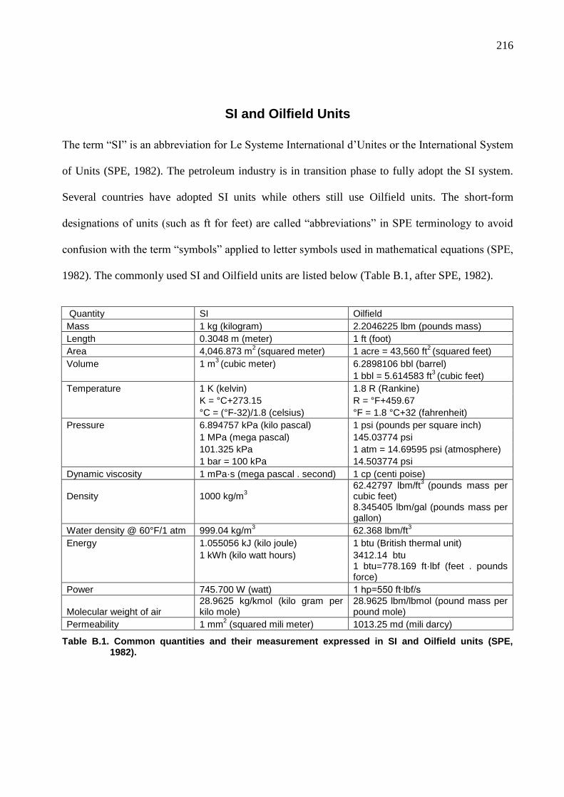
216

SI and Oilfield Units

The term “SI” is an abbreviation for Le Systeme International d‟Unites or the International System

of Units (SPE, 1982). The petroleum industry is in transition phase to fully adopt the SI system.

Several countries have adopted SI units while others still use Oilfield units. The short-form

designations of units (such as ft for feet) are called “abbreviations” in SPE terminology to avoid

confusion with the term “symbols” applied to letter symbols used in mathematical equations (SPE,

1982). The commonly used SI and Oilfield units are listed below (Table B.1, after SPE, 1982).

Quantity SI Oilfield

Mass 1 kg (kilogram) 2.2046225 lbm (pounds mass)

Length 0.3048 m (meter) 1 ft (foot)

Area 4,046.873 m2 (squared meter) 1 acre = 43,560 ft

2 (squared feet)

Volume 1 m3 (cubic meter) 6.2898106 bbl (barrel)

1 bbl = 5.614583 ft3 (cubic feet)

Temperature 1 K (kelvin) 1.8 R (Rankine)

K = °C+273.15 R = °F+459.67

°C = (°F-32)/1.8 (celsius) °F = 1.8 °C+32 (fahrenheit)

Pressure 6.894757 kPa (kilo pascal) 1 psi (pounds per square inch)

1 MPa (mega pascal) 145.03774 psi

101.325 kPa 1 atm = 14.69595 psi (atmosphere)

1 bar = 100 kPa 14.503774 psi

Dynamic viscosity 1 mPa·s (mega pascal . second) 1 cp (centi poise)

Density 1000 kg/m3

62.42797 lbm/ft3

(pounds mass per cubic feet)

8.345405 lbm/gal (pounds mass per gallon)

Water density @ 60°F/1 atm 999.04 kg/m3 62.368 lbm/ft

3

Energy 1.055056 kJ (kilo joule) 1 btu (British thermal unit)

1 kWh (kilo watt hours) 3412.14 btu

1 btu=778.169 ft·lbf (feet . pounds force)

Power 745.700 W (watt) 1 hp=550 ft∙lbf/s

Molecular weight of air 28.9625 kg/kmol (kilo gram per kilo mole)

28.9625 lbm/lbmol (pound mass per pound mole)

Permeability 1 mm2 (squared mili meter) 1013.25 md (mili darcy)

Table B.1. Common quantities and their measurement expressed in SI and Oilfield units (SPE, 1982).

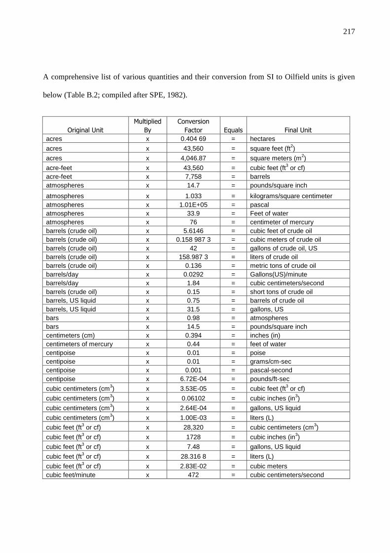
217

A comprehensive list of various quantities and their conversion from SI to Oilfield units is given

below (Table B.2; compiled after SPE, 1982).

Original Unit

Multiplied Conversion

Equals Final Unit By Factor

acres x 0.404 69 = hectares

acres x 43,560 = square feet (ft2)

acres x 4,046.87 = square meters (m2)

acre-feet x 43,560 = cubic feet (ft3 or cf)

acre-feet x 7,758 = barrels

atmospheres x 14.7 = pounds/square inch

atmospheres x 1.033 = kilograms/square centimeter

atmospheres x 1.01E+05 = pascal

atmospheres x 33.9 = Feet of water

atmospheres x 76 = centimeter of mercury

barrels (crude oil) x 5.6146 = cubic feet of crude oil

barrels (crude oil) x 0.158 987 3 = cubic meters of crude oil

barrels (crude oil) x 42 = gallons of crude oil, US

barrels (crude oil) x 158.987 3 = liters of crude oil

barrels (crude oil) x 0.136 = metric tons of crude oil

barrels/day x 0.0292 = Gallons(US)/minute

barrels/day x 1.84 = cubic centimeters/second

barrels (crude oil) x 0.15 = short tons of crude oil

barrels, US liquid x 0.75 = barrels of crude oil

barrels, US liquid x 31.5 = gallons, US

bars x 0.98 = atmospheres

bars x 14.5 = pounds/square inch

centimeters (cm) x 0.394 = inches (in)

centimeters of mercury x 0.44 = feet of water

centipoise x 0.01 = poise

centipoise x 0.01 = grams/cm-sec

centipoise x 0.001 = pascal-second

centipoise x 6.72E-04 = pounds/ft-sec

cubic centimeters (cm3) x 3.53E-05 = cubic feet (ft

3 or cf)

cubic centimeters (cm3) x 0.06102 = cubic inches (in

3)

cubic centimeters (cm3) x 2.64E-04 = gallons, US liquid

cubic centimeters (cm3) x 1.00E-03 = liters (L)

cubic feet (ft3 or cf) x 28,320 = cubic centimeters (cm

3)

cubic feet (ft3 or cf) x 1728 = cubic inches (in

3)

cubic feet (ft3 or cf) x 7.48 = gallons, US liquid

cubic feet (ft3 or cf) x 28.316 8 = liters (L)

cubic feet (ft3 or cf) x 2.83E-02 = cubic meters

cubic feet/minute x 472 = cubic centimeters/second

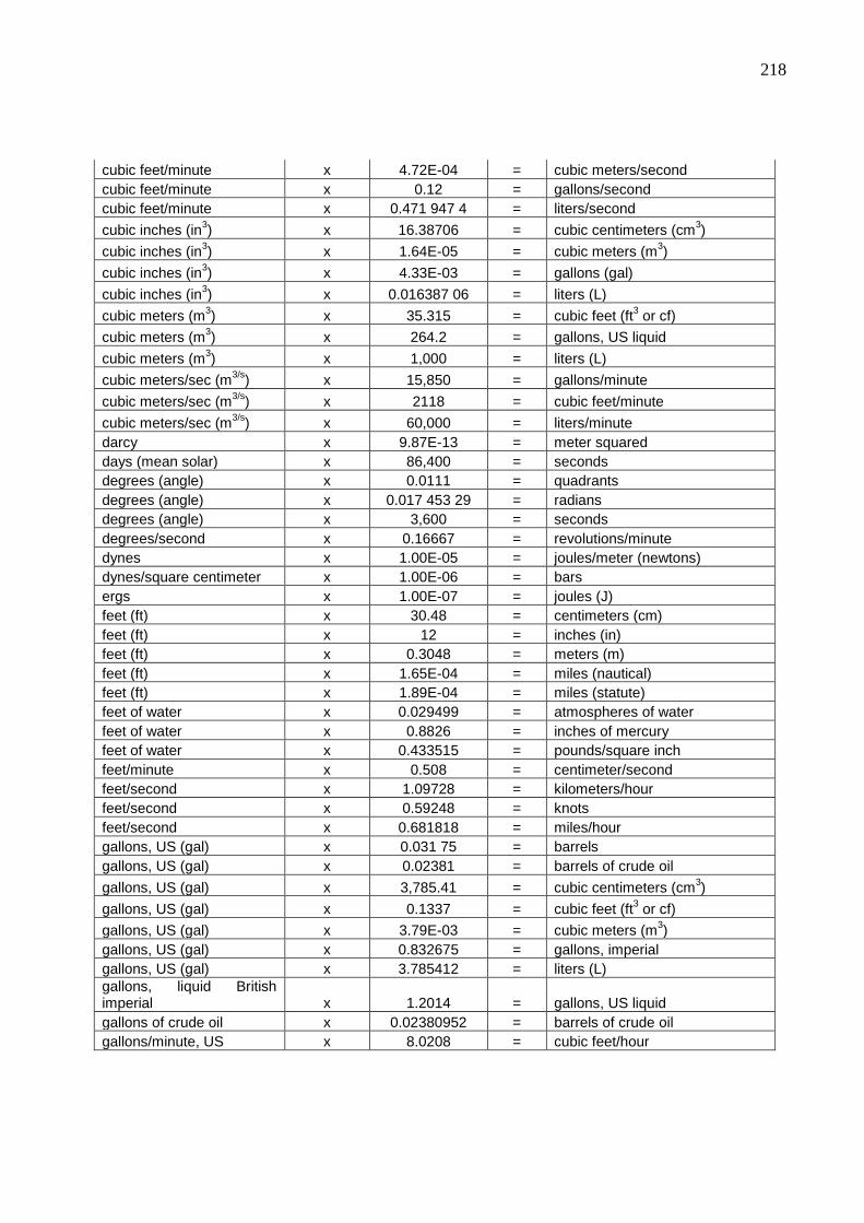
218

cubic feet/minute x 4.72E-04 = cubic meters/second

cubic feet/minute x 0.12 = gallons/second

cubic feet/minute x 0.471 947 4 = liters/second

cubic inches (in3) x 16.38706 = cubic centimeters (cm

3)

cubic inches (in3) x 1.64E-05 = cubic meters (m

3)

cubic inches (in3) x 4.33E-03 = gallons (gal)

cubic inches (in3) x 0.016387 06 = liters (L)

cubic meters (m3) x 35.315 = cubic feet (ft

3 or cf)

cubic meters (m3) x 264.2 = gallons, US liquid

cubic meters (m3) x 1,000 = liters (L)

cubic meters/sec (m3/s

) x 15,850 = gallons/minute

cubic meters/sec (m3/s

) x 2118 = cubic feet/minute

cubic meters/sec (m3/s

) x 60,000 = liters/minute

darcy x 9.87E-13 = meter squared

days (mean solar) x 86,400 = seconds

degrees (angle) x 0.0111 = quadrants

degrees (angle) x 0.017 453 29 = radians

degrees (angle) x 3,600 = seconds

degrees/second x 0.16667 = revolutions/minute

dynes x 1.00E-05 = joules/meter (newtons)

dynes/square centimeter x 1.00E-06 = bars

ergs x 1.00E-07 = joules (J)

feet (ft) x 30.48 = centimeters (cm)

feet (ft) x 12 = inches (in)

feet (ft) x 0.3048 = meters (m)

feet (ft) x 1.65E-04 = miles (nautical)

feet (ft) x 1.89E-04 = miles (statute)

feet of water x 0.029499 = atmospheres of water

feet of water x 0.8826 = inches of mercury

feet of water x 0.433515 = pounds/square inch

feet/minute x 0.508 = centimeter/second

feet/second x 1.09728 = kilometers/hour

feet/second x 0.59248 = knots

feet/second x 0.681818 = miles/hour

gallons, US (gal) x 0.031 75 = barrels

gallons, US (gal) x 0.02381 = barrels of crude oil

gallons, US (gal) x 3,785.41 = cubic centimeters (cm3)

gallons, US (gal) x 0.1337 = cubic feet (ft3 or cf)

gallons, US (gal) x 3.79E-03 = cubic meters (m3)

gallons, US (gal) x 0.832675 = gallons, imperial

gallons, US (gal) x 3.785412 = liters (L)

gallons, liquid British imperial x 1.2014 = gallons, US liquid

gallons of crude oil x 0.02380952 = barrels of crude oil

gallons/minute, US x 8.0208 = cubic feet/hour

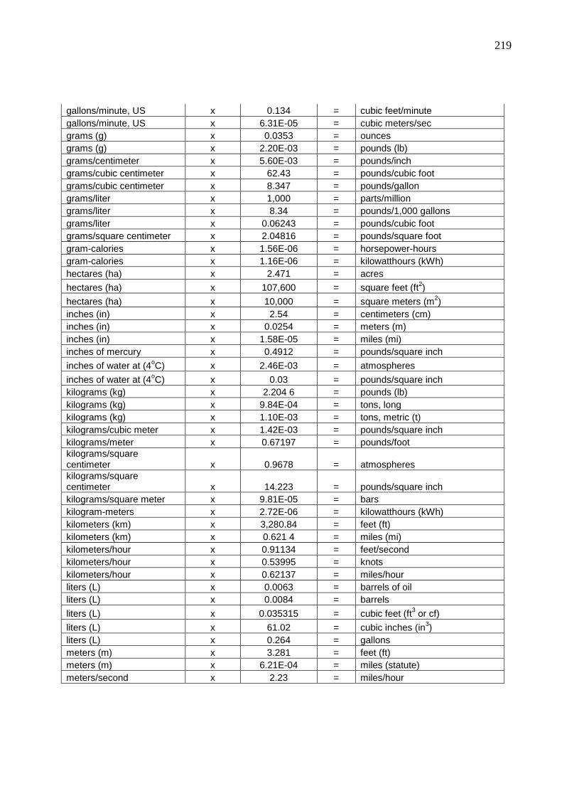
219

gallons/minute, US x 0.134 = cubic feet/minute

gallons/minute, US x 6.31E-05 = cubic meters/sec

grams (g) x 0.0353 = ounces

grams (g) x 2.20E-03 = pounds (lb)

grams/centimeter x 5.60E-03 = pounds/inch

grams/cubic centimeter x 62.43 = pounds/cubic foot

grams/cubic centimeter x 8.347 = pounds/gallon

grams/liter x 1,000 = parts/million

grams/liter x 8.34 = pounds/1,000 gallons

grams/liter x 0.06243 = pounds/cubic foot

grams/square centimeter x 2.04816 = pounds/square foot

gram-calories x 1.56E-06 = horsepower-hours

gram-calories x 1.16E-06 = kilowatthours (kWh)

hectares (ha) x 2.471 = acres

hectares (ha) x 107,600 = square feet (ft2)

hectares (ha) x 10,000 = square meters (m2)

inches (in) x 2.54 = centimeters (cm)

inches (in) x 0.0254 = meters (m)

inches (in) x 1.58E-05 = miles (mi)

inches of mercury x 0.4912 = pounds/square inch

inches of water at (4oC) x 2.46E-03 = atmospheres

inches of water at (4oC) x 0.03 = pounds/square inch

kilograms (kg) x 2.204 6 = pounds (lb)

kilograms (kg) x 9.84E-04 = tons, long

kilograms (kg) x 1.10E-03 = tons, metric (t)

kilograms/cubic meter x 1.42E-03 = pounds/square inch

kilograms/meter x 0.67197 = pounds/foot

kilograms/square centimeter x 0.9678 = atmospheres

kilograms/square centimeter x 14.223 = pounds/square inch

kilograms/square meter x 9.81E-05 = bars

kilogram-meters x 2.72E-06 = kilowatthours (kWh)

kilometers (km) x 3,280.84 = feet (ft)

kilometers (km) x 0.621 4 = miles (mi)

kilometers/hour x 0.91134 = feet/second

kilometers/hour x 0.53995 = knots

kilometers/hour x 0.62137 = miles/hour

liters (L) x 0.0063 = barrels of oil

liters (L) x 0.0084 = barrels

liters (L) x 0.035315 = cubic feet (ft3 or cf)

liters (L) x 61.02 = cubic inches (in3)

liters (L) x 0.264 = gallons

meters (m) x 3.281 = feet (ft)

meters (m) x 6.21E-04 = miles (statute)

meters/second x 2.23 = miles/hour

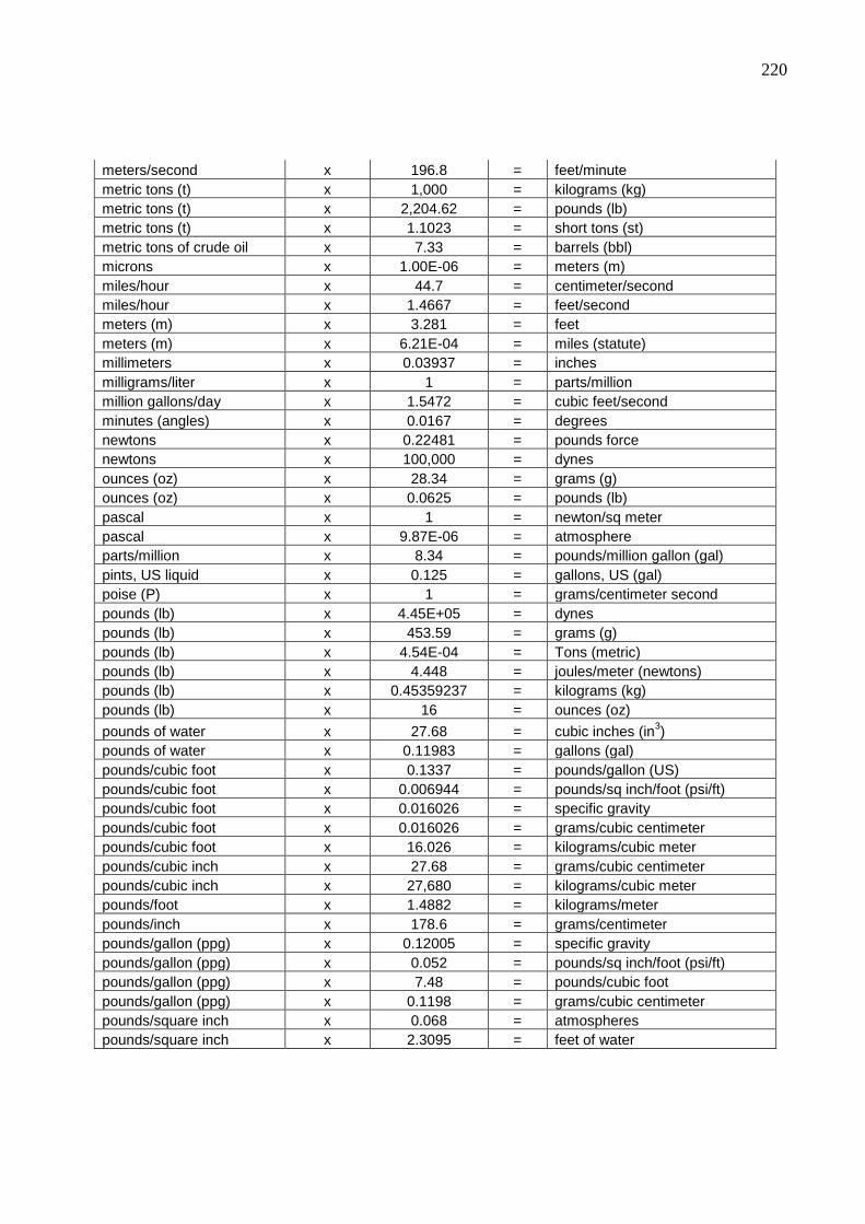
220

meters/second x 196.8 = feet/minute

metric tons (t) x 1,000 = kilograms (kg)

metric tons (t) x 2,204.62 = pounds (lb)

metric tons (t) x 1.1023 = short tons (st)

metric tons of crude oil x 7.33 = barrels (bbl)

microns x 1.00E-06 = meters (m)

miles/hour x 44.7 = centimeter/second

miles/hour x 1.4667 = feet/second

meters (m) x 3.281 = feet

meters (m) x 6.21E-04 = miles (statute)

millimeters x 0.03937 = inches

milligrams/liter x 1 = parts/million

million gallons/day x 1.5472 = cubic feet/second

minutes (angles) x 0.0167 = degrees

newtons x 0.22481 = pounds force

newtons x 100,000 = dynes

ounces (oz) x 28.34 = grams (g)

ounces (oz) x 0.0625 = pounds (lb)

pascal x 1 = newton/sq meter

pascal x 9.87E-06 = atmosphere

parts/million x 8.34 = pounds/million gallon (gal)

pints, US liquid x 0.125 = gallons, US (gal)

poise (P) x 1 = grams/centimeter second

pounds (lb) x 4.45E+05 = dynes

pounds (lb) x 453.59 = grams (g)

pounds (lb) x 4.54E-04 = Tons (metric)

pounds (lb) x 4.448 = joules/meter (newtons)

pounds (lb) x 0.45359237 = kilograms (kg)

pounds (lb) x 16 = ounces (oz)

pounds of water x 27.68 = cubic inches (in3)

pounds of water x 0.11983 = gallons (gal)

pounds/cubic foot x 0.1337 = pounds/gallon (US)

pounds/cubic foot x 0.006944 = pounds/sq inch/foot (psi/ft)

pounds/cubic foot x 0.016026 = specific gravity

pounds/cubic foot x 0.016026 = grams/cubic centimeter

pounds/cubic foot x 16.026 = kilograms/cubic meter

pounds/cubic inch x 27.68 = grams/cubic centimeter

pounds/cubic inch x 27,680 = kilograms/cubic meter

pounds/foot x 1.4882 = kilograms/meter

pounds/inch x 178.6 = grams/centimeter

pounds/gallon (ppg) x 0.12005 = specific gravity

pounds/gallon (ppg) x 0.052 = pounds/sq inch/foot (psi/ft)

pounds/gallon (ppg) x 7.48 = pounds/cubic foot

pounds/gallon (ppg) x 0.1198 = grams/cubic centimeter

pounds/square inch x 0.068 = atmospheres

pounds/square inch x 2.3095 = feet of water

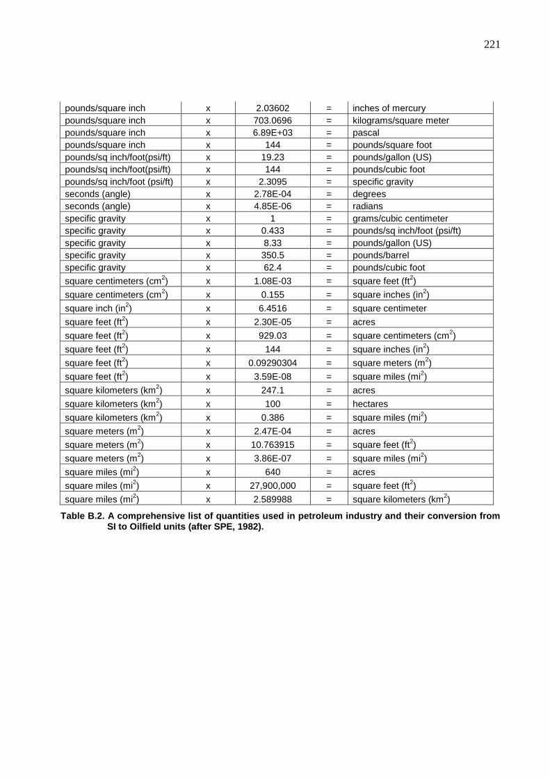
221

pounds/square inch x 2.03602 = inches of mercury

pounds/square inch x 703.0696 = kilograms/square meter

pounds/square inch x 6.89E+03 = pascal

pounds/square inch x 144 = pounds/square foot

pounds/sq inch/foot(psi/ft) x 19.23 = pounds/gallon (US)

pounds/sq inch/foot(psi/ft) x 144 = pounds/cubic foot

pounds/sq inch/foot (psi/ft) x 2.3095 = specific gravity

seconds (angle) x 2.78E-04 = degrees

seconds (angle) x 4.85E-06 = radians

specific gravity x 1 = grams/cubic centimeter

specific gravity x 0.433 = pounds/sq inch/foot (psi/ft)

specific gravity x 8.33 = pounds/gallon (US)

specific gravity x 350.5 = pounds/barrel

specific gravity x 62.4 = pounds/cubic foot

square centimeters (cm2) x 1.08E-03 = square feet (ft

2)

square centimeters (cm2) x 0.155 = square inches (in

2)

square inch (in2) x 6.4516 = square centimeter

square feet (ft2) x 2.30E-05 = acres

square feet (ft2) x 929.03 = square centimeters (cm

2)

square feet (ft2) x 144 = square inches (in

2)

square feet (ft2) x 0.09290304 = square meters (m

2)

square feet (ft2) x 3.59E-08 = square miles (mi

2)

square kilometers (km2) x 247.1 = acres

square kilometers (km2) x 100 = hectares

square kilometers (km2) x 0.386 = square miles (mi

2)

square meters (m2) x 2.47E-04 = acres

square meters (m2) x 10.763915 = square feet (ft

2)

square meters (m2) x 3.86E-07 = square miles (mi

2)

square miles (mi2) x 640 = acres

square miles (mi2) x 27,900,000 = square feet (ft

2)

square miles (mi2) x 2.589988 = square kilometers (km

2)

Table B.2. A comprehensive list of quantities used in petroleum industry and their conversion from SI to Oilfield units (after SPE, 1982).

References

Abbaszadeh, M., Fuji, H., and Fujimoto, F. “Permeability Prediction by Hydraulic Flow Units-

Theory and Applications” SPE 30158. (1996)

Ahmed, Tarek. “Reservoir Engineering Handbook” pp. 189-218. Gulf Professional Publishing,

Houston, TX. (2001)

Alger, R.P., Luffel, D.L., and Truman, R.B. “New unified method of integrating core capillary

pressure data with well logs” SPE Formation Evaluation 16793, p. 145. (1989)

Amabeoku, M. O., Kersey, D, BinNasser, R and Belowi, A. “Relative Permeability Coupled

Saturation-Height Models Based on Hydraulic (Flow) Units in a Gas Field” SPE 102249.

(2006)

Amaefule, J.O., Altunbay, D., Tiab, D., Kersey, D.G., and Keelan, D.K. “Enhanced Reservoir

Description: Using Core and Log Data to Identify Hydraulic (Flow) Units and Predict

Permeability in Uncored Intervals/Wells” SPE 26436. (1993)

Amyx, J.W., Bass Jr., D.M., and Whiting, R.L. “Petroleum Reservoir Engineering - Physical

Properties” McGraw Hill, New York. (1960)

Anderson, W. G. “Wettability Literature Survey- Part 2: Wettability Measurement” SPE Conoco,

Inc. JPT. (November 1986)

Archer J.S. and Wall C. G. “Petroleum Engineering. Principles and Practice” pp. 92-99. Graham &

Trotman, Gaithersburg, MD. (1986)

Archie, G. E. “Electrical Resistivity Log as an Aid in Determining Some Reservoir

Characteristics” AIME, Vol. 146, pp. 54-62. (1942)

Archie, G. E. “Classification of carbonate reservoir and petrophysical considerations” AAPG Bull

36, 2: pp. 278-298 (1952).

223

Asquith, G. and Krygowski, D. “Basic Well Log Analysis” 2nd edition. AAPG Methods in

Exploration Series, 28, Tulsa, OK. 244pp. (2004)

Atkins, P. W. “General Chemistry” Scientific American Books, New York. (1989)

Borbas, Timothy “Predicting Reservoir Performance by Incorporating Pore Geometry” SPWLA

35th

Annual Logging Symposium. (1994)

Burke, J.A. Schmidt, A.W., and Campbell, Jr., R. L. “The Litho-Porosity Cross Plot” SPWLA 10th

Annual Logging Symposium. (1969)

Carman, P.C. “Fluid flow through granular beds” Trans. Inst. Chem. Engr., S32-S48. (1937)

Core Laboratories, World-wide Rock Catalogue, Reservoir Inc, Houston, TX. (2001)

Core Laboratories, Integrated Reservoir Solutions Division, Reservoir Inc, Houston, TX. (2004)

Cosse, R.,. “Basics of Reservoir Engineering”, Editions TECHNIP, Paris. (1993)

Craft, B.C., Hawkins, M.F. “Applied Petroleum Reservoir Engineering” Prentice Hall, NJ. (1959)

Craft, B.C., Hawkins, M.F. “Applied Petroleum Reservoir Engineering” Second Edition. Prentice

Hall, NJ (1991).

Crain, E.R., “The Log Analysis Handbook” Penn Well Books, Tulsa, OK. (1986)

Crain, E.C.” Crain's Petrophysical Pocket Pal” Short Course and Reference Manual,

eText www.sprc2000.net/pocketpal.htm. (2001)

Cronquist, Chapman “Estimation and Classification of Reserves of Crude Oil, Natural Gas, and

Condensate” Society of Petroleum Engineers, TX. (2001)

Cuddy, S., Allinson, G., and Steele, R. “A simple convincing model for calculating water

saturations in southern North Sea gas fields” Paper H, SPWLA 34th

Annual Logging

Symposium. (1993)

224

Dahlberg, E.C. “Applied Hydrodynamics in Petroleum Exploration” 2nd

Edition, Springer-Verlag,

New York. 295pp. (1995)

Dandekar, Abhijit Y. “Petroleum Reservoir Rock and Fluid Properties” Taylor & Francis Group.

(2006)

Darling, T. “Well Logging and Formation Evaluation” Elsevier Publishing Company, Amsterdam.

(2005)

Desbrandes, R., Bassiouni, Z., and Gualdron, R. “In situ wettability determination in depleted

zones” SPE 21182. (1990)

Donaldson, E.C., and Alam, W. “Wettability” Gulf Publishing Company, Houston, TX. (2008)

Donnez, Pierre, “Essentials of Reservoir Engineering” Editions TECHNIP, Paris. (2007)

Dunham, R.J. “Classification of carbonate rocks according to depositional texture” In: Ham, W. E.

(ed.), Classification of carbonate rocks: AAPG Memoir 1: pp. 108-121 (1962).

Eade, J.R. “Practical Capillary Pressure Analysis” Course Notes, Canadian Hunter Exploration

Limited, Calgary. (1991)

Ebanks, W.J., Scheihing, M.H., and Atkinson, C.D. “Flow Units for Reservoir Characterization”

ARCO Oil and Gas Company, pp. 282-285 (1987).

Edinburgh Petroleum Services “Core Analysis: Applications to Petrophysics and Reservoir

Engineering” Course Notes presented at Dhahran (18th

– 26th

November 1997).

Ellis, D.V., and Singer, J.M.”Well Logging for Earth Scientists” Second Edition, Springer-Verlag,

New York. (2007)

Engstrom, F. “A new method to normalize capillary pressure curves” Paper Society of Core

Analysts, 9535, International SCA Symposium. (1995)

225

Etnyre, L.M. “Finding oil and gas from well logs” Van Nostrand Reinhold, New York. (1989)

Folk R.L. “Petrology of Sedimentary Rocks” Hemphill Publication Company, Austin, TX. (1980)

Gardner, J.S., and Dumanoir, J.L. “Litho-Density log interpretation” Trans. SPWLA Annual

Logging Symposium, 21:1-23 (1980)

Gunter, G., Finneran, J., Hartmann, D., and Miller, J. “Early Determination of Reservoir Flow

Units Using an Integrated Petrophysical Method” SPE 38679 (1997).

Guo, G., Diaz, M.A., Paz, F., Smalley, J., and Waninger, E. A. “Rock Typing as an Effective Tool

for Permeability and Water-Saturation Modeling: A Case Study in a Clastic Reservoir in the

Oriente Basin” SPE 97033 (2007).

Harrison, B., and Jing, X.D. “Saturation height methods and their impacts on volumetric

hydrocarbons in place estimates” SPE, 71326. (2001)

Hassler, G.L., and Brunner, E. “Measurement of Capillary Pressure in Small Core Samples”

Transactions AIME, volume 160, 114. (1945)

Hawkins, J.M., Luffel, D.L., and Harris, T.J. “Capillary pressure model predicts distance to

gas/water, oil/water contact” Oil and Gas Journal, 39. (January 1993)

Heseldin, G.M.. “A method of averaging capillary pressure curves” SPWLA, 15th

Annual Logging

Symposium. (1974)

Hilchie, D.W. “Advanced Well Log Interpretation” D.W. Hilchie, Inc., Golden, Colorado (1982)

Hill, H.J., Shirley, O.J. and Klein, G.E. “Bound water in shaly sands – its relation to Qv and other

formation properties” The Log Analyst, May-June, 1979.

Keelan, D. “A Course in Special Core Analysis” Core Laboratories, Houston, TX. (1982)

226

Kolodzie, S., Jr. “Analysis of pore throat size and use of the Waxman-Smits equation to determine

OOIP in Spindle Field, Colorado” SPE 9382. (1980)

Lake, L.W. “Enhanced Oil Recovery” Englewood Cliffs, New Jersey, Prentice Hall, 550p. (1989)

Land, L.S., Prezbindowski D.R. “The origin and evolution of saline formation water, lower

Cretaceous carbonates, South-Central Texas” Journal Hydrology, Vol. 54: pp. 51-74. (1981)

Leach, R.O., Wagner, O.R., Wood, H.W., Harpke, C.F., “A Laboratory and Field Study of

Wettability Adjustment in Water Flooding” SPE 119. (1962)

Leverett, M. C. “Capillary behavior in porous solids.” Trans. AIME, Vol. 142, pp. 152-169.

(1941)

Logan, W. D., Horkowitz, J.P., Laronga, R., Cromwell, D. “Practical application of NMR loggin

in carbonate reservoirs” SPE 38740 (1997)

Lucia, J. F. “Petrophysical parameters estimated from visual description of carbonate rocks: a field

classification of carbonate pore space” JPT, pp. 626-637, March (1983).

Lucia, J. F. “Rock-fabric/ Petrophysical classification of carbonate pore space for reservoir

characterization” AAPG Bull 79, 9: pp. 1275-1300 (1995).

Lucia, J. F. “Carbonate Reservoir Characterization” pp. 1-25. Springer-Verlag Berlin Heidelberg

(1999).

Lucia, J. F. “Carbonate Reservoir Characterization” 2nd

Edition. Springer-Verlag Berlin

Heidelberg (2007).

Monicard, R.P. “Properties of Reservoir Rocks: Core Analyis” Editions TECHNIP, Paris. (1980)

Panda, M.N., Lake, L.W. “Estimation of single-phase of permeability from parameters of particle-

size distribution” AAPG Bull 78, 7: pp. 1028-1039 (1994).

227

Pittman, ED. “Relationship of porosity and permeability to various parameters derived from

mercury injection-capillary pressure curves for sandstone” AAPG Bull 76, 2:191-198. (1992).

Raymer, L. L., Hunt, E. R., and Gardner, J. S. “An improved sonic transit time to porosity

transform” Trans. SPWLA Annual Logging Symposium, 21: Paper P. (1980)

Rider, M.H. “The Geological Interpretation of Well Logs” 2nd

edition. Caithness, Whittle

Publishing. (1996)

Rose,W.D. and Bruce, W.A.” Evaluation of Capillary Character in Petroleum Reservoir Rock”

Transactions AIME, SPE 949127. (1949)

Schlumberger, “Log Interpretation Principles/Applications” 3rd

edition. Schlumberger Educational

Services, Houston,TX. (1991)

Segesman, F.F., and Liu, Olive “The excavation effect” Trans. SPWLA Annual Logging

Symposium, 12: Paper N1-N24. (1971)

Sheng Ding, Tai Pham, and AnPing Yang. “The Use of An Integrated Approach in Estimation of

Water Saturation and Free Water Level in Tight Gas Reservoirs: Case Studies” SPE 84390

(2003).

Skelt, C., and Harrison, R. “An integrated approach to saturation height analysis” SPWLA, 36th

Annual Logging Symposium, Paris. (1995)

Smith, C.R., Tracy, G.W., and Farrar, R.L. “Applied Reservoir Engineering, Volume I” Oil and

Gas Consultants International, Tulsa. (1992)

Society of Petroleum Engineers, “The SI Metric System of Units and SPE Metric Standard”

Society of Petroleum Engineers, Texas. (1982)

Steiber,S. J. Pulsed neutron capture log evaluation in the Louisiana Gulf Coast, SPE 45th

Annual

Meeting, SPE 2961. (1970)

228

Swanson, B.F., 1981. “A simple correlation between permeabilities and mercury capillary

pressure” JPT, 2498. (December, 1981)

Thomeer, J.H.M. “Introduction of a pore geometrical factor defined by the capillary pressure

curve” JPT, 354; Trans AIME, 210. (1960)

Thomeer, J.H.M. ”Capillarity in Rocks” Shell Oil Company, Houston. (1983)

Tiab, D., Donaldson E.C. “Petrophysics: Theory and practice of measuring reservoir rock and

fluid transport properties.” Gulf Publishing Company, Houston, TX. (1999)

Tiab, D., Donaldson E.C. “Petrophysics: Theory and practice of measuring reservoir rock and

fluid transport properties.” 2nd

Edition. Gulf Publishing Company, Houston, TX. (2004)

Timur,A. “An Investigation of permeability, porosity, and residual water saturation relationships”

Trans. SPWLA Annual Logging Symposium, June 23-26. (1968)

Wylie,M.R.J and Rose,W.D.” Some theoretical considerations related to quantitative evaluation of

physical characteristics of reservoir rocks from electric logs data” Transactions AIME, SPE

950105. (1950)

Wyllie and Gregory AR: “Formation Factors of Unconsolidated Porous Media: Influence of

Particle Shape and Effect of Cementation” Petroleum Transactions of the AIME 198: 103-110

(1953)

Zhou, B., and Blunt, M. “Wettability effects in three phase gravity drainage” JPSE, v.20 (June):

203-211. (1998)

Zinszner, B., and Pellerin, F.M.. “A Geoscientist‟s Guide to Petrophysics” Editions TECHNIP,

Paris.(2007)

Vita

Abdulkareem Roudhan graduated from the University of Kansas with a Bachelor of Science

degree in geology in 2003. Right after that, he joined Saudi Aramco and worked for the reservoir

characterization department (RCD) for 2 years as a field geologist. He spent a year with well-site

geology doing casing and coring jobs. In 2006, he went back to RCD to work as a field geologist

concentrating on Arabs, Hanifa, and Hadriya reservoirs. His experience includes carbonate

sedimentology and petrophysics.

Please address correspondence to:

Name: Abdulkareem Roudhan Al-Roudhan

Company: Saudi Aramco Company

Address: P. O. Box 12201, Dhahran 31311, Saudi Arabia

Tel.: +96638739905

Mobile: +966505934067

E-mail: abdulkareem.roudhan@aramco.com

kareeem266045@yahoo.com