Testing the importance of accurate meteorological input fields and parameterizations in atmospheric transport modelling using dream - validation against ETEX-1

tAuthor to whom correspondence should be addressed.Tel.: #45 46301157; fax: #45 46301214; e-mail: [email protected]

Atmospheric Environment Vol. 32, No. 24, pp. 4167—4186, 1998( 1998 Elsevier Science Ltd. All rights reserved

Printed in Great Britain1352—2310/98 $19.00#0.00PII: S1352–2310(98)00170–8

TESTING THE IMPORTANCE OF ACCURATEMETEOROLOGICAL INPUT FIELDS AND

PARAMETERIZATIONS IN ATMOSPHERIC TRANSPORTMODELLING USING DREAM - VALIDATION AGAINST

ETEX-1

J"RGEN BRANDT,*-‡ ANNEMARIE BASTRUP-BIRK,*JESPER H. CHRISTENSEN,* TORBEN MIKKELSEN,-S"REN THYKIER-NIELSEN- and ZAHARI ZLATEV*

*National Environmental Research Institute, Department of Atmospheric Environment, Frederiksborgvej399, P.O. Box 358, DK-4000 Roskilde, Denmark; and -Ris+ National Laboratory, Wind Energy and

Atmospheric Physics Department, Frederiksborgvej 399, P.O. Box 49, DK-4000 Roskilde, Denmark

Abstract—A tracer model, the DREAM, which is based on a combination of a near-range Lagrangianmodel and a long-range Eulerian model, has been developed. The meteorological meso-scale model,MM5V1, is implemented as a meteorological driver for the tracer model. The model system is used forstudying transport and dispersion of air pollutants caused by a single but strong source as, e.g. an accidentalrelease from a nuclear power plant. The model system including the coupling of the Lagrangian model withthe Eulerian model are described. Various simple and comprehensive parameterizations of the mixingheight, the vertical dispersion, and different meterological input data have been implemented in thecombined tracer model, and the model results have been validated against measurements from the ETEX-1release. Several different statistical parameters have been used to estimate the differences between theparameterizations and meterological input data in order to find the best performing solution. ( 1998Elsevier Science Ltd. All rights reserved

Key word index: Accidental release, Eulerian and Lagrangian models, transport modelling, mixing height,vertical dispersion, meteorological data, ETEX-1.

INTRODUCTION

Atmospheric transport of air pollutants is, in prin-ciple, a well-understood process. If information aboutthe state of the atmosphere is given in all details(infinitely accurate information about meteorology as,e.g. wind speed) and infinitely fast computers areavailable, then the advection equation could, in prin-ciple, be solved exactly and the transport could bedescribed in any detail. This is, however, not the case:discretization of the equations and input data areapplied in practice, and this introduces some uncer-tainties and errors in the results. Therefore, manydifferent issues have to be carefully studied in order todiminish these uncertainties and to develop a suffi-ciently accurate transport and dispersion model.Some of these issues are the numerical treatmentof the advection equation, accuracy of the mean

meteorological input fields, and accuracy of para-meterizations of the sub-grid scale phenomena.

Model simulations of the first ETEX release illus-trate the differences caused by using various simpleand comprehensive parameterizations of the mixingheight and of the vertical dispersion. The differentparameterizations have been compared using variousstatistical parameters in order to find the best per-forming solution. Also, different analyzed fields havebeen implemented and compared, either directly inthe tracer model or by using the meso-scale model,MM5V1, as a meteorological driver for the tracermodel.

Numerical treatment of the advection of air pollu-tants from a single source is not a simple problem. Thetraditional Eulerian models have problems with sharpgradients from a single strong source. The sharpgradients cause unwanted oscillations, also known asGibbs phenomena (Brandt et al., 1996c). Several dif-ferent advection algorithms have therefore been testedand compared in order to find the optimal scheme (seee.g. Brandt et al., 1996a, e; Zlatev, 1995). Lagrangian

4167

Fig. 1. Schematic diagram of the model system.

models have, however, problems with uncertainties inthe trajectory calculations on long range, due to expo-nentially increasing errors (see e.g. Jensen, 1994;Baumann and Stohl, 1997). Furthermore, the K-the-ory, which is usually applied for the description ofdispersion in Eulerian models, is unsatisfactory nearto the source. Lagrangian models, on the other hand,are able to describe the dispersion on short scales withgood results. Therefore, a combination of a Lagran-gian model and an Eulerian model has been de-veloped, in order to gain the advantages of both kindsof models.

2. GENERAL CONCEPT OF THE MODEL SYSTEM

The tracer model, which has been developed, isbased on a combination of a Lagrangian meso-scalemodel, the RIs+ Meso-scale PUFF model (RIM-PUFF) (Mikkelsen et al., 1984; Thykier-Nielsen andMikkelsen, 1993), and an Eulerian long-range trans-port model, the Danish Eulerian Model (DEM)(Zlatev et al., 1992; Zlatev, 1995; Bastrup-Birk et al.,1997a, b; Brandt et al., 1996a, e). The Lagrangianmodel is used on the local scale near the source tocalculate the initial transport and dispersion ofthe release, and the Eulerian model is used for long-range transport calculations in the whole model do-main. The combined model is called the DREAM (theDanish Rimpuff and Eulerian Accidental releaseModel) (Brandt et al., 1996b, c, d; Brandt andZlatev, 1997). The meteorological meso-scale modelMM5V1 has been implemented as a meteorologicaldriver for the transport model. This gives a finerspatial and temporal resolution of the meteorologicalinput data used by the tracer model. Especially, themodel’s superior description of the planetary bound-ary layer is essential. MM5V1 was originally de-veloped at Penn State University and NCAR,Boulder, Colorado (Grell et al., 1995). It is used atmany research institutions throughout the world formany different research purposes. The version usedin this model system is the EURAD version ofMM5V1 (EURAD-Project, University of Cologne inGermany).

A schematic diagram of the model system and flowchart are shown in Fig. 1. Meteorological input dataand terrestrial data are given as input to the meteoro-logical driver, MM5V1, or directly to the tracermodel, DREAM. The MM5V1 system consists ofdifferent preprocessors (TERRAIN, DATAGRID andINTERP) which prepare and interpolate input datato the numerical weather prediction model MM5V1.Topography and landuse data with horizontal resolu-tion of 10 min (1

6°) are used. Source data information is

given as input to the Lagrangian model. The meteoro-logical driver and the transport model produce hugeamounts of output data. Therefore, 2D and 3D visual-ization techniques have been developed and imple-mented as important tools for development and

validation of the model and for better understandingof the model results.

2.1. ¹he Eulerian model

Advective transport, dispersion, emission, dry andwet deposition and radioactive decay are described inthe Eulerian modelling framework, by the equation

LC

Lt"! Au

LC

Lx#v

LC

Ly#pR

LC

LpB#K

x

L2C

Lx2#K

y

L2C

Ly2#

LLpAKp

LC

LpB#E(x, y, p, t)

!k$C!"C!k

3C (1)

where C is the tracer concentration, u, v, pR are thewind speed components in the x, y, p directions,respectively, and K

x, K

y, Kp are the dispersion coeffi-

cients. The horizontal dispersion in the Eulerianmodel is set constant (K

x"K

y"10,000 m2 sv1).

k$

represents dry deposition (which, in practice, isapplied as a lower boundary condition in the verticaldispersion term), " is the scavenging coefficient forwet deposition, k

3is representing radioactive decay

and E(x, y, p, t,) is the emission. Deposition and radio-active decay have not been applied in the simulationswith ETEX-1. The vertical discretization in the modelsystem is in p-coordinates and defined by the pressurenormalized by the surface pressure P

4(x, y, t)

p"P!P

5P4!P

5

"

P!P5

P*(2)

4168 J. BRANDT et al.

where P*"P4!P

5. The pressure at the top of the

model domain P5("100 hPa) has been subtracted,

so that p at the top of the model domain is alwayszero.

The model has been split into three submodels(Brandt and Zlatev, 1997) including: (1) three-dimen-sional advection, horizontal dispersion and emission,(2) vertical dispersion and dry deposition, and (3) wetdeposition and radioactive decay. The treatment ofthe advection and dispersion in the Eulerian model isperformed using a finite element algorithm. This algo-rithm has been tested against several other advectionalgorithms using the well-known Molenkamp—Crow-ley rotation test (see, Brandt et al., 1996a, c, e; Zlatev,1995). The finite element scheme is a relative fastscheme. This is important when used operationally.A predictor—corrector algorithm with three correctorshas been used for time integration of the first sub-model (Zlatev, 1995). Time integration in the secondsubmodel is solved using the less expensive and morestable h-method (Christensen, 1995) and the thirdsubmodel is solved directly.

2.2. ¹he ¸agrangian model

The Lagrangian model, which has been imple-mented into the Eulerian model, is a puff model whichsimulates a release changing in time by sequentiallyreleasing a series of Gaussian shaped puffs. In thevertical the Gaussian shape has been transformed intop-coordinates, using the hydrostatic approximationand the ideal gas law. Each puff is advected anddispersed individually along trajectories. The concen-tration at a point (x, y, p), is given by the sum of thecontributions from the total number of puffs, N, as

Cx,y,p"

N+i/1

Mig(p

ci#/)

(2n)3@2pJ 2xyi

pJ piR¹

7

]expA!1

2AAx!x

cipJxyiB

2#A

y!yci

pJxyiB

2

BB]AexpA!

1

2Apci#/

pJ pi

lnAtci

t BB2

B#expA!

1

2A!pci#/

pJ pi

ln(ttci)B

2

B#expA!

1

2Apci#/

pJ pi

lnAtt

ci2t

H.*9BB

2

B (3)

where Miis the mass of the air pollutant in a given

puff and pJxyi

and pJ piare the standard deviations of the

puff i and a measure for the puff size in horizontal andvertical directions, respectively. / is given by/"P

5/P*, (x

ci, y

ci, p

ci) is the coordinate of the puff’s

center of mass, ¹7is the virtual temperature, R is the

gas constant for dry air, and g is the acceleration dueto gravity. The functions t are representing theheight, the puff center, t

ci, and the mixing height,

tH.*x

, and defined by the following:

t"

pP*#P5

P4

tci"

pciP*#P

5P4

(4)

tH.*9

"

pH.*9

P*#P5

P4

where pH.*9

is the mixing height in p-coordinates. Thefirst term on the right-hand side of equation (3) repres-ents the maximum concentration in the center ofa puff. The second and third term represent the hori-zontal and vertical distribution of the concentrations.The last two terms of the vertical distribution are thereflection due to the ground and to the mixing heightH

.*9. The two terms represent two artificial sources:

one below the ground and one above the mixingheight. If the vertical standard deviation pJ pi

is greaterthan twice the mixing height then further artificialsources are needed. In order to avoid a large numberof exponential functions in the expression, total verti-cal mixing is then assumed and equation (3) reduces to

Cx,y,p"

N+i/1

Mig(p

ci#/)

2npJ 2xyi

R¹7

]expA!1

2AAx!x

cipJxyiB

2#A

y!yci

pJxyiB

2

BB]((p

ci#/)(!ln(t

H.*9)))~1. (5)

2.3. Coupling the ¸agrangian model with the Eulerianmodel

Many numerical experiments have been performedin order to find the best-coupling procedure betweenthe Lagrangian model and the Eulerian model. Theaccuracy of the numerical solution as well as thereliability of the coupling between the Eulerian modeland the Lagrangian model have been tested witha modified version of the Molenkampf—Crowley test(Brandt et al., 1996c). The size of the Lagrangian puffsshould be so large when incorporated into the Euler-ian model, that the gradients are relatively smoothand problems with unwanted oscillations are dimin-ished. The size of the subdomain is therefore depen-dent on the size of the individual puffs, which shouldbe larger than the grid resolution in the Eulerianmodel, when the puffs are incorporated into the Euler-ian model. On the other hand, the size of the sub-domain should be minimized in order to minimizecomputing time. The size of the subdomain has beendetermined from numerical experiments with themodified version of the Molenkamp—Crowley rota-tion test.

The puffs are incorporated individually into theEulerian model when the puffs reach the boundary ofthe Lagrangian model area (also referred to as thepuff-coupling in Brandt et al., 1996c). This is illus-trated in Fig. 2 which shows a single puff at the

Testing the meteorological input fields and parameterizations 4169

Fig. 2. Illustration of the coupling between the Lagrangian model and the Eulerian model.

boundary of the Lagrangian domain. When incorpor-ating the puff, the concentrations given by the puff arefirst calculated at the grid cells which are located ina certain area around the puff center. The size of thisarea is determined by a minimum concentration ofinterest. The grid cells, in the area covered by the puff,are then averaged to the grid resolution used in theEulerian model and the puff is removed from the Lag-rangian model. The difference in grid resolution betweenthe Lagrangian model and the Eulerian model is five,which means that 25 grid cells in the Lagrangian modelcorresponds to one grid cell in the Eulerian model.

2.4. Discretizations and overall performanceon a CRA½ C92A

The combined tracer model and MM5V1 are bothdiscretized on the same polar stereographic projection(see e.g. Grell et al., 1995). The optimal horizontal gridresolutions, grid sizes and number of vertical layershave been found from numerical experiments, and are

given in Table 1. It would be preferable to run theMM5V1 with the same horizontal grid resolution asin the tracer model, but the number of grid points inMM5V1 has been limited by computer resources. Themodel system has been optimized and run on a CRAYC92A. The performance of the tracer model on thissuper computer, with the discretizations in Table 1, isdependent on the parameterizations chosen in themodel system. The general performance of the tracermodel is 442 MFLOPS, corresponding to nearly 50%of the peak performance, which is quite good. Theoverall performance of MM5V1 is 220 MFLOPS,corresponding to about 24% of peak performance.

3. PARAMETERIZATION OF THE PLANETARY

BOUNDARY LAYER.

A revised version of the Blackadar’s high-resolutionplanetary boundary-layer (PBL) model is used to


Table 1. Grid resolutions and discretizations used in themodel system

Modell Horizontal gridresolution

Grid size No. of verticallevels

Eulerian 25 km ]25 km 192]192 16Lagrangian 5 km ]5 km 105]105 16MM5V1 50 km ]50 km 96]96 16

calculate the momentum and heat flux profiles whichare used to determine the friction velocity, the sur-face heat flux, and the Monin—Obukhov length(Blackadar, 1979; Arya, 1988; Grell et al., 1995). Thefriction velocity u* is calculated from

u*"MAXAk»

ln (z1/z

0)!t

m

,u*0B (6)

where u*0is a background value (set to 0.1 m s~1 over

land and 0.005 m sv1 over water), k is the von Karmanconstant (k"0.4), z

1is the height of the lowest half

p-level, and z0

is the roughness parameter given asfunction of the different landuse categories (see Fig.11) and of the season. Over water, z

0is calculated as

a function of friction velocity

z0"

0.032u2*g

#z0#

(7)

where z0#

is a background value of 10~4 m. » is givenby

»"J»21#»2

#(8)

»1

is the horizontal wind speed at the lowest modellayer and »

#is a convective velocity, defined by (Grell

et al., 1995)

»#"2JDh

'!h

-D (9)

which is important under conditions of low meanwind speed (non-zero during unstable and neutralconditions and zero under stable conditions). Thefactor of 2 in the expression has the unit (m s~1 K~1).h'

is the potential ground temperature and h1

is thepotential temperature of the lowest model layer. Thesurface heat flux H

4is computed from similarity the-

ory

H4"!c

1o-u*h* (10)

where c1

is the specific heat of dry air at constantpressure (c

1"1004 J K~1 kg~1), o

1is the density of

the air in the lowest model layer and the temperaturescale h* is given by

Ch*"k(h

-!h

')

ln (z1/z

0)!t

)D (11)

t.

and t)

are universal non-dimensional similarityfunctions. Both are functions of the bulk Richardsonnumber Ri

Bwhich characterizes the turbulent state of

the atmosphere due to the relative importance of

thermal instabilities (buoyancy) versus wind shear ef-fects

RiB"

gz-

h7-

(h7-!h

7')

»2(12)

where subscript v represents virtual potential temper-ature. Four cases are possible depending on the valueof the bulk Richardson number and the criticalRichardson number, Ri

C"0.2: stable case, mechan-

ically driven turbulence, unstable with forced convec-tion, and unstable with free convection. For the stablecase, Ri

B'Ri

C, the stability functions are given by

t."t

)"!10 lnA

z-

z0B. (13)

In the case of mechanically driven turbulence we have04Ri

B4Ri

Cand the stability functions are given by

t."t

)"!5A

RiB

1.1!5RiBB lnA

z-

z0B. (14)

Whether the unstable case is in the forced convectionregime or in the free convection regime, depends onthe mixing height H

.*9(see Section 5) and on the

Monin—Obukhov length, ¸, given by (Arya, 1988)

¸"!

c1o1h1u3*

kgH4

. (15)

For the unstable forced convection case RiB(0'

DH.*9

/¸D)1.5, we have

t."t

)"0. (16)

In the unstable free convection case RiB(0 '

DH.*9

/¸D'1.5 and the stability functions are given by

t."!1.86A

z-

¸B!1.07Az-

¸B2!0.249A

z-¸B

3(17)

and

t)"!3.23A

z-

¸B!1.99Az-

¸B2!0.474A

z-¸B

3(18)

the fraction z1/¸ is restricted to be *!2 in these

approximations. In the general case, z1/¸ is a function

of t.

and an iterative solution is required. To savecomputing time t

.can be approximated as an ex-

plicit function of the bulk Richardson number, suchthat

z1¸

"RiB

lnAz-

z0B. (19)

The above scheme ensures continuity of t.

for allvalues of Ri

B(Grell et al., 1995).

4. PARAMETERIZATION OF THE VERTICAL DISPERSION

Two different parameterizations of vertical disper-sion have been implemented in the tracer model for


comparison. These schemes, which are briefly de-scribed in the following, have also been compared tothe very simple assumption of constant vertical dis-persion (100 m2 s~1 below the mixing height and0.1 m2 s~1 above the mixing height, see Section 6).The two schemes are the Louis parameterization andthe parameterization based on Monin—Obukhov sim-ilarity theory. Different parameterizations of disper-sion have also been implemented in the Lagrangianmodel including the Karlsruhe—Julich parameteriz-ation (Thykier-Nielsen and Mikkelsen, 1993), theGifford parameterization (Gifford, 1982), and theparameterization based on Monin—Obukhov sim-ilarity theory (Caughey, 1981; Hanna, 1981). Only theparameterization based on Monin—Obukhov sim-ilarity theory has been used here for simplicity.

4.1. »ertical dispersion based on ¸ouis parameterization

Vertical dispersion can be calculated using theparameterization of Louis (1979), see also Christensen(1995) and Hass (1991). This approach evaluates thevertical dispersion coefficient in z-coordinates, K

z, as

a function of mixing length, wind shear, and the bulkRichardson number, Ri

Bwhich was described in Sec-

tion 3, but is here calculated locally for all layers

RiB"

g*z*h

h*»2(20)

*h is the potential temperature difference across thelayer thickness *z, *» is the horizontal wind speed

difference, and h is the average potential temperatureof a model layer. K

zis calculated from

Kz"maxAA

kz

1#kz/jB2

K*»

*z Kf (RiB),K

z0B (21)

where Kz0

is a background value set to 0.1 m2 s~1,and the asymptotic mixing length j is set to 100 m.The function f can be described in different ways forstable and unstable conditions. The approach usedhere, is derived by Blackadar (1976)

f (RiB)"

0.257*z0.175!RiB

0.257*z0.175. (22)

The dispersion coefficient, K;, in z-coordinates are

transformed into p-coordinates using the hydrostaticapproximation and the ideal gas law. The dispersioncoefficient derived by Louis is used in the whole verti-cal extent of the model. There are, however, questionswhether this parameterization can account for themixing under convective conditions.

4.2. »ertical dispersion based on Monin—Obukhov sim-ilarity theory

In parameterization according to the Monin—Obukhov’s similarity theory, the K

zprofile is based

on the specific turbulent structure in the individualregimes of the atmosphere. The atmosphere is scaledinto different regions depending on the dimensionless

stability H.*9

/¸ (unstable, neutral and stable) and thedimensionless height z/H

.*9(surface layer, boundary

layer and free troposphere) (Hass, 1991). The surfacelayer, where fluxes are nearly constant with height, isdefined as the first 10% of the planetary boundarylayer. Below the height of the planetary boundarylayer H

.*9, K

zis given by

Kz"

ku*z (1!z/H.*9

)2

/ (z/¸). (2)

The quadratic function of z/H.*9

gives a smoothtransition between the surface layer and the atmo-spheric boundary layer. The similarity function/(z/¸), which is used here, was derived by Businger etal. (1971) from experimental data from the KansasField Program in 1968 (Arya, 1988) and given by

/Az

¸B"0.74#4.7Az

¸B , 0(Az

¸B)1 (stable)

/Az

¸B"4.7#0.74Az

¸B , Az

¸B'1 (stable)

/Az

¸B"0.74 , Az

¸B"0 (neutral)

/Az

¸B"0.74A1!9Az

¸BB~1@2

, Az

¸B(0 (unstable)

(24)

Other similarity functions could also be applied. Thecase of the stable condition, where z/¸ '1, preventthe similarity function from becoming too large invery stable conditions. In the convective boundarylayer (H

.*9/¸(!10), the buoyant production of tur-

bulent kinetic energy is the dominant process and thefriction velocity u

*is replaced by the convective velo-

city scale w*. In this regime, K

zis calculated from

(Hass, 1991)

Kz"kw*zA1!

z

H.*9B (25)

where w*

can be expressed as a function of theMonin—Obukhov length

w*"u*AH

.*9kD¸DB

1@3. (26)

Equation (25) does not completely match equation(23) when H

.*9/¸(!10. This does not, however,

gives rise to computational instabilities. Above theplanetary boundary layer, in the free troposphere,K

zis expressed similar to the Louis parameterization

using the Blackadar (1976) expression for the bulkRichardson number dependent function.

5. PARAMETERIZATION OF THE MIXING HEIGHT

The parameterization of vertical dispersion, basedon Monin—Obukhov similarity theory, is very


sensitive to the mixing height H.*9

, and the convectivevelocity scale w

*. Four methods are used here for

comparison. The first method is based on an energybalance equation for the internal boundary layerincluding an equation describing advection and dis-persion of the mixing height. The second scheme esti-mates the mixing height from the potential temp-erature profile (the dry parcel method) combined withsimple formulas for the neutral and stable conditions.This scheme is very simple and computational inex-pensive. It has been included in this study for com-parison with the more comprehensive schemes. In thelast two schemes, the mixing height is calculated fromthe bulk Richardson number approach, during unsta-ble condition and with different parameterizationsduring stable and neutral conditions. The schemeshave also been compared to the simple assumption ofconstant mixing height (Section 6). The convectivevelocity scale is dependent on the mixing height andthese two parameters are therefore calculated iter-atively.

5.1. Parameterization based on the energy balance forthe planetary boundary layer

The height of the mixing layer can be calculatedfrom a simple parameterization based on an energybalance equation for the boundary layer (Berkowiczand Olesen, 1990; Christensen, 1995; 1997)

AN2H.*9

#1.9u2*#w2*

H.*9

BdH

.*9dt

"

w3*#1.25u3*H

.*9

!

u2*#0.5w2*q

(27)

where q is a dissipation time scale ("1100 s). The firstterm on the left-hand side is the increase of the poten-tial energy in the boundary layer and the second termis the increase of the kinetic energy. The first term onthe right-hand side is the growth of the mixing heightdue to buoyancy production (convective energy) andmechanical energy. The second term accounts for thedissipation of the mechanical and convective energy(Christensen, 1995). N is the Brunt—Vaisala frequency,given by

N2"cg¹

(28)

where c is the lapse rate at the mixing height. In areaswith large horizontal differences in surface character-istics, like landuse or topography (as e.g. the transitionfrom sea to land), transport and dispersion of themixing height are required when using the para-meterization by the energy balance for the internalboundary layer. In this parameterization, the internalenergy in the boundary layer is assumed to be a char-acteristic for the air which is following the transport ofthe air masses. The mixing height is transported usingthe two-dimensional advection equation with disper-sion, where the time derivative of the mixing height in

equation (27) is substituted with

dH.*9

dt"

LH.*9

Lt#u

LH.*9

Lx#v

LH.*9

Ly

#w !Kx .*9

L2H.*9

Lx2!K

y .*9

L2H.*9

Ly2(29)

where u,v are vertical mean values of the wind belowthe mixing height and K

x .*9"K

y .*9"104 m2 s~1.

Transport and dispersion of the mixing height aresolved similar to the advection of the tracer usinga finite element algorithm and a predictor—correctormethod for time integration.

5.2. A simple scheme based on the dry parcel method

The dry parcel method for estimating the mixingheight can be used during unstable conditions. Themixing height is defined as the lowest level where thevirtual potential temperature is greater than the vir-tual potential temperature of the first model layer(Hass, 1991). This method therefore requires a highvertical spatial grid resolution in the meteorologicalinput data for the planetary boundary layer. This canbe obtained by using the meteorological driver,MM5V1, as a preprocessor, especially when simula-tion of the radiation balances is calculated usinga multi-level scheme.

For neutral or stable conditions, where the dryparcel method cannot be applied, the mixing heightcan be determined from several different methods.The simple scheme used here accounts for the com-bined effect of rotation, surface boundary flux, andstatic stability in the free flow, where the mixingheight is estimated from (Koracin and Berkowicz,1988)

H.*9

"kSu*¸

f, stable

H.*9

"0.3u*

f, neutral (30)

where f is the Coriolis parameter. This definition as-sumes that the shear induced turbulence in the planet-ary boundary layer causes vertical mixing.

5.3. Estimation from the bulk Richardson number

Estimation of the height of the boundary layer canalso be based on the bulk Richardson number ap-proach (Holtslag et al., 1995; Vogelezang et Holtslag,1996). The boundary-layer height is defined as theheight where the bulk Richardson number reachesa critical value of Ri

C"0.25. For a near neutral or

stable boundary layer, turbulence due to surface fric-tion cannot be ignored. Therefore, a modified bulkRichardson number is used

RiBk"

g(h7k!h@

71)(z

k!z

1)

h@v1

[(uk!u

1)2#(v

k!v

1)2#100u2*]

(31)


where the term 100u2* is accounting for the effect fromfriction (Vogelezang et Holtslag, 1996). z

1and z

kare

the heights of the lowest model level and of the modellevel, k, respectively, h

7kis the virtual potential tem-

perature, and h@7-

is a function of the virtual potentialtemperature of the lowest model layer, defined underunstable conditions

h@7-"h

7-#8.5

H74

w*

(32)

where H74

is the virtual surface heat flux, defined as

H74"(w@h@

7)4. The second term of the right-hand side

of the equation represents a temperature excess, whichis a measure of the strength of convective thermalsin the planetary boundary layer (Vogelezang andHoltslag, 1996).

5.4. Estimation from a combination of the bulkRichardson number and a Zilitinkevich—Mironovscheme.

The implementation of the term, 100u2* , in equation(31) to account for friction is a very simple approach.Therefore, a different approach has been tested herefor comparison. This scheme is based on a combina-tion of the bulk Richardson number algorithm (with-out the term 100u2* ) during unstable conditions anda formulation proposed by Zilitinkevich and Mironov(1996) (see also Robertson et al., 1996) is used forstable and neutral conditions. The mixing height,H

.*9, is calculated by using the recursive formulation

Hn`1.*9

"Hn.*9

!

(a1Hn

.*9)2#a

2Hn

.*9!1

2a21Hn

.*9#a

2

(33)

where the Newton—Raphson algorithm has been ap-plied, and the coefficients a

1and a

2are given by

a1"

f

0.5u*

a2"

1

10¸#

N

20u*

#

JD f D

JDu*¸D#

JDNf D1.7u*

(34)

where N is the Brunt—Vaisala frequency at the mixingheight.

6. MODEL RESULTS AND EXPERIMENTS WITH ETEX-1

The model system has been run with the differentparameterizations (described in the previous sections)and with different meteorological input fields. Themodel results have been validated against ETEX-1.Some examples of model results for ETEX-1 are givenin Section 6.1. Intercomparisons of the different para-meterizations and meteorological input data, usingdifferent statistics, are described in Section 6.2.

6.1. Model results for E¹EX-1

An example of a simulation of ETEX-1 usingDREAM is shown in Fig. 3. The figures show the

surface concentrations 12, 24, 36, 48, 60 and 72 h afterthe start of the release. The square in the figuresaround the source point indicates the area wherethe Lagrangian model is applied. Meteorological in-put data from ECMWF with 0.5° resolution are, inthese calculations, used directly as input to the tracermodel. Parameterization of mixing height isperformed using the bulk Richardson number/Zilitinkevich—Mironov scheme. Vertical dispersionin both the Eulerian and Lagrangian model isparameterized based on Monin—Obukhov similaritytheory.

Figure 4 shows the 0.05 ng m~3 iso-surface of theplume 48 h after start of release in three dimensions(compare with Fig. 3). The surface concentrations areplotted on the iso-surface and are the same as given inFig. 3, 48 h after start of release. The bulk Richardsonnumber is given as vertical slices at the boundaries inFig. 4. The blue color at the boundaries indicates thedomain where the bulk Richardson number exceedsthe critical bulk Richardson number of 0.25 and istherefore an indicator of the height of the planetaryboundary layer. In both Figs 3 and 4, a clear effectfrom the mountains in the southern parts of the plumeis seen. A large vertical distribution of the concentra-tions is also seen in Fig. 4.

Comparisons of some of the model results withmeasurements from ETEX-1, obtained from the Envi-ronment Institute, JRC, Ispra, Italy (Ispra), are shownas scatter plots in Figs 5—9. Not all the measurementstations from Ispra have been included in these com-parisons; at some stations only a few measurementsare available and these stations have been excludedfrom the tests. Measurements were also performed atRis+ National Laboratory, Denmark, during the twoETEX periods (for more information about thismeasurement station, see Brandt et al., 1996b). Thisadditional measurement station (here denoted DK00)has been included in the tests. Figure 5 shows thecalculated and measured total dosages (or integratedconcentrations) at 140 measurement stations. Figure6 shows the measured and calculated maximum con-centrations at the measurement stations. The arrivaltime of the plume and the arrival time of the max-imum concentration to the measurement stations aregiven in Figs 7 and 8. Figure 9 shows the measuredand calculated duration of the plume at the measure-ment stations. For estimation of the arrival times anddurations, it is necessary to choose a threshold valuefor the concentrations in order to be able to determinewhether the plume has arrived to a measurementstation or not. A threshold value of 0.05 ng m~3 waschosen.

The global statistics, where some of them are usedfor the intercomparison of the model results, obtainedby using the different parameterizations and meteoro-logical data (see, Section 6.2), are also given in thefigures. These includes the number of points, the meanvalues, the standard deviations, the correlation coef-ficient with a test statistic, the figure of merit, FM, the


Fig. 3. Model simulation of the development of the plume from ETEX-1, using ECMWF 0.5° meteorologi-cal data. The mixing height is parameterized using the Bulk Richardson number/Zilitinkevich—Mironovscheme and vertical dispersion is based on Monin—Obukhov similarity theory. Upper left figure shows thesituation 12 h after start of release, upper right is 24 h, middle left is 36 h, middle right is 48 h, lower left is60 h and lower right is 72 h after start of release. The square indicates the area where the Lagrangian model

is applied. The Eulerian model is applied in the whole area.


Fig. 4. A three-dimensional illustration of the 0.05 ng m~3 iso-surface from ETEX-1, 48 h after start ofrelease. Meteorological input data and parameterizations are the same as in Fig. 3. The surface concentra-

tion is plotted on the iso-surface (compare with Fig. 3).

bias with the 95% confidence interval, the fractionalbias, FB, the fractional standard deviation, FSD andthe normalized mean square error, NMSE, with the95% confidence interval. A detailed description of thevarious statistical parameters are given in Spiegel(1992) and Mosca et al. (1997). A test for significancehas been performed for the correlation coefficient bythe test parameter t

c"r(N!2)1@2(1!r2)~1@2 where

r is the correlation coefficient and N is the number ofdata (Spiegel, 1992). The test hypothesis is that themodel results and measurements are independentwhich means that the correlation coefficient is zero. Ifthe hypothesis can be rejected at given significancelevel, then the correlation coefficient is assumed to besignificant at that level. Critical values for the testparameter for N"140 are 1.65, 2.61 and 3.34 corre-sponding to significance levels of 0.1 (10%), 0.01 (1%)and 0.001 (0.1%), respectively (Spiegel, 1992).

It is seen in the figures, that the model is able toreproduce the dosages and the maximum concentra-tions within a factor between two and three in the

worst case (see Figs 5 and 6). This is within thecurrently achievable limit of accuracy in long-rangedispersion modelling, according to the conclusionsfrom the ETEX symposium in Vienna, Austria, in1997 (see, Nodop, 1997). The global means and stan-dard deviations are, however, quite similar for themeasured and calculated values. The correlation coef-ficient is strongly significant at a significance levelmuch less than 0.1%. The model gives very goodresults concerning the arrival times and arrival timesof maximum concentration, as seen in Figs 7 and8 with highly significant correlation coefficients closeto one. Also the durations of the plume over themeasurement stations (see Fig. 9) are very well repro-duced (within a factor of two) with a highly significantcorrelation coefficient above 0.8.

Some examples of time series of the measured andcalculated concentrations at eight measurement sta-tions are given in Fig. 10. Measurement stations, bothat short and long range from the location of therelease, are shown. It is seen that the model, in general,


Fig. 5. Measured and calculated dosages (or integrated con-centrations) at the measurement stations.

Fig. 6. Measured and calculated maximum concentrations atthe measurement stations.

Fig. 7. Measured and calculated arrival times at the measure-ment stations.

Fig. 8. Measured and calculated arrival times of maximumconcentrations at the measurement stations.

is able to reproduce the arrival times, the durationsand the shape of the plume at most of the measure-ment stations. It is important to emphasize that eventhough these parameters are very well estimated by

the model, it is very difficult to estimate the dosagesand the maximum concentrations with an uncertaintyless than a factor of two. These two parameters de-pend very strongly on many of the key parameters in


Fig. 9. Measured and calculated durations of the plume atthe measurement stations.

a transport model as, e.g. the mixing height or thedispersion coefficients (especially the vertical disper-sion coefficients). Uncertainties in the estimation ofthese parameters and the choice of parameterizationhave great influence in the calculation of the concen-tration levels. The different parameterizations dependon various key parameters as, e.g. estimation of thefriction velocity or the surface heat flux.

Examples of some of these key parameters, thelanduse categories, the friction velocity, the surfacetemperature, and the surface heat flux, at the time ofrelease of ETEX-1, are given in Fig. 11. The roughnesslength used in the model system is calculated asa function of landuse data and season. The frictionvelocity shown in Fig. 11 is partly a function of theroughness length and wind speed, which is clearlyseen in the figure. The surface heat flux is a function ofthe surface temperature, which is a prognostic vari-able in MM5V1 and calculated by using a multi-levelradiation scheme.

The magnitude of the parameters shown in Fig. 11has a large influence on the calculation of the mixingheight, but the choice of mixing height scheme is alsovery important. This is illustrated in Fig. 12, where themixing height calculated at the time of the release ofETEX-1, by using the four different schemes is shown.The different parameterizations show the same gen-eral patterns, but the magnitude of the mixing heightsvaries within a factor of two and even more in someregions. It is also seen that the general mixing height

patterns are a combined effect of the patterns in thefriction velocity and the surface heat flux, that areshown in Fig. 11.

6.2. Comparison of different parameterizations and me-teorological input data

In Tables 2—4, comparisons of model resultsusing different parameterizations of mixing height inthe model, different parameterizations of vertical dis-persion in the Eulerian model, and different meanmeteorological input data, are shown. The model re-sults have been validated against ETEX-1 measure-ments in these tables using some of the globalstatistics which are calculated in the scatter plots (seeFigs 5—9).

The correlation coefficient with test for significance,the bias with 95% confidence interval (ci(95%)) of themodel results compared to measurements, the nor-malized mean-square error (NMSE) with 95% confi-dence interval (ci(95%)), the fractional bias (FB), thefractional standard deviation (FSD), and the figure ofmerit have been calculated for all the model runs.These parameters together give a good estimate of themodel performance, concerning global concentrationvariability and global concentration levels. For eachmodel run, statistics have been calculated for the totaldosages, the maximum concentration, the arrivaltime, the arrival time of maximum concentration andfor the duration. The results from all different statis-tics have then been ranked (best performance has beengiven the value 1, second best performance has beengiven the value 2, etc.) and the global rank has beencalculated as the sum of the local ranks. The modelresults with the lowest global rank indicate the bestperforming combination of parameterizations andmeteorology. Values in the tables that indicate thebest performing parameterization or meteorology(most significant values) are given in bold. It should beemphasized that all the correlation coefficients in thetables are significant at a significance level of muchless than 0.1%, which is very good.

In Table 2, comparisons of model results usingdifferent parameterizations of mixing height areshown for the same parameterization of vertical dis-persion and same meteorological input data. Theparameterizations have also been compared to thevery simple assumption of constant mixing height of800 m. Some parameterizations are very time con-suming in a transport model. They should therefore asa minimum perform better compared to the use ofconstant values. In general, the bulk Richardson num-ber/Zilitinkevich—Mironov scheme gives the best re-sults with respect to the global rank. The very simpleassumption of constant mixing height gives com-parably good results. It can, however, be assumed thata constant mixing height is too simple in most situ-ations and in longer simulations where the generalweather situation is changing. This is especially true inperiods of strong convection where the mixing heighthas a strong diurnal variation. The energy balance


Fig. 10. Some examples of time series of measured and calculated concentrations at eight measurementstations during ETEX-1 throughout Europe. The time is in hours after start of release. The stations are: B04(Belgium), D13 (Germany), CR03 (Czech Republic), H02 (Hungary), PL03 (Poland), DK00 (Denmark),

SR04 (Slovakia) and N07 (Norway).

method also gives quite good results. The bulkRichardson number scheme show a large bias in dos-ages and maximum concentrations. It seems that thescheme, in general, give a too low mixing height and

therefore much too high concentrations at the surface.The scheme might have problems in estimating themixing height due to the mechanical mixing, which isdescribed very simple in this scheme. The dry parcel


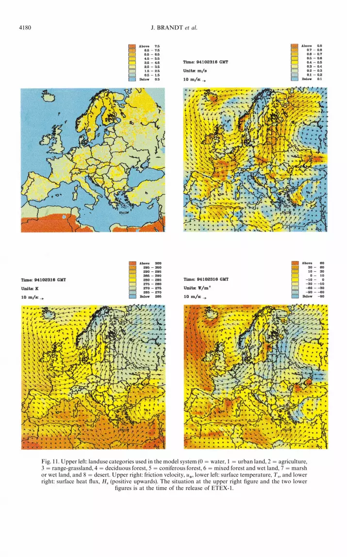
Fig. 11. Upper left: landuse categories used in the model system (0"water, 1"urban land, 2"agriculture,3"range-grassland, 4"deciduous forest, 5"coniferous forest, 6"mixed forest and wet land, 7"marshor wet land, and 8"desert. Upper right: friction velocity, u

*, lower left: surface temperature, ¹

4, and lower

right: surface heat flux, Hs(positive upwards). The situation at the upper right figure and the two lower

figures is at the time of the release of ETEX-1.


Fig. 12. The mixing height calculated by using the four different parameterizations, at the time of release ofETEX-1. Upper left: bulk Richardson number method for unstable conditions and Zilitinkevich-Mironovformula for stable and neutral conditions. Upper right: energy balance method. Lower left: bulk Richardsonnumber method. Lower right: dry parcel method. Please notice that the scale is different for the two upper

and two lower figures.


Tab

le2.

Com

par

ison

sofd

iffer

entpar

amet

eriz

atio

nsofm

ixin

ghei

ghtfo

rETEX

-1,u

sing

EC

MW

F(0

.5°]

0.5°

)met

eoro

logi

cali

npu

tdat

aan

dve

rtic

aldisper

sion

par

amet

eriz

edby

Mon

in-O

bukho

vsim

ilar

ity

theo

ryin

both

the

Eule

rian

and

Lag

rangi

anm

odel

.T

he

stat

istica

lpar

amet

ers

are

the

corr

elat

ion

coeffi

cien

tw

ith

test

stat

istic,

t #(in

bra

cket

s),b

ias

with

the

95%

confi

denc

ein

terv

al,

ci(9

5%)(

inbra

cket

s),n

orm

aliz

edm

ean-s

quar

eer

ror,

NM

SE,w

ith

the

95%

confid

ence

inte

rval

,ci(9

5%)(

inbra

cket

s),f

ract

ional

bia

s,FB,a

ndfrac

tional

stan

dar

ddev

iation

,FSD

(inbra

cket

s),fi

gure

ofm

erit,F

M,a

nd

global

ranks

.Val

ues

inbo

ldar

eth

em

ost

sign

ifica

ntof

the

five

schem

es

Par

amet

erN"

140

Stat

istics

Ene

rgy

bala

nce

met

hod

Bulk

Ric

hard

son

num

ber/

Zili

tink

evic

h—M

irono

v

Bulk

Ric

hard

-so

nnum

ber

Dry

par

cel

met

hod

Con

stan

t(8

00m

)

Dosa

ges

Max

conc.

Arr

.tim

eA

rr.m

axD

ura

tion

Cor

rela

tion

and

(t#)

0.65

(10.

1)0.

66(1

0.4)

0.97

(48.

0)0.

98(6

4.7)

0.81

(16.

3)

0.65

(10.

0)0.

60(8

.76)

0.97

(46.

9)0.

98(6

0.8)

0.82

(17.

0)

0.59

(8.6

1)0.

61(8

.98)

0.98

(63.

3)0.

99(7

8.6)

0.76

(13.

9)

0.61

(9.0

4)0.

52(7

.23)

0.98

(55.

0)0.

98(6

3.3)

0.81

(16.

5)

0.69

(11.

1)0.

66(1

0.3)

0.97

(48.

7)0.

98(6

3.8)

0.86

(19.

7)

Dosa

ges

Max

conc.

Arr

.tim

eA

rr.m

axD

ura

tion

Bia

san

d(c

i(95%

))4.

481

(0.6

12)

0.61

1(0

.202

)2.

475

(3.1

30)

3.65

4(3

.286

)!

0.08

6(1

.188

)

0.22

3(0

.920

)0.

057

(0.1

38)

2.35

7(3

.171

)2.

657

(3.3

27)

!0.

536

(1.1

67)

6.68

6(2

.554

)0.

988

(0.3

61)

0.11

8(3

.166

)0.

032

(3.3

98)

!1.

671

(1.4

17)

1.74

3(1

.420

)0.

265

(0.2

26)

2.59

3(3

.154

)3.

364

(3.3

45)

!0.

621

(1.2

03)

2.34

7(1

.375

)0.

387

(0.1

52)

2.63

6(3

.130

)3.

300

(2.2

82)

!0.

600

(1.0

83)

Dosa

ges

Max

conc.

Arr

.tim

eA

rr.m

axD

ura

tion

NM

SE

and

(ci(9

5%))

2.12

3(0

.491

)2.

678

(0.7

45)

0.03

1(0

.013

)0.

019

(0.0

09)

0.29

8(0

.080

)

1.13

7(0

.249

)1.

803

(0.8

95)

0.03

1(0

.014

)0.

016

(0.0

09)

0.28

6(0

.068

)

4.69

5(1

.277

)6.

271

(1.5

54)

0.02

3(0

.007

)0.

015

(0.0

07)

0.40

3(0

.176

)

2.19

2(0

.751

)3.

919

(1.7

77)

0.02

4(0

.008

)0.

021

(0.0

08)

0.31

5(0

.084

)

1.17

8(0

.284

)1.

738

(0.4

78)

0.02

8(0

.014

)0.

015

(0.0

09)

0.23

6(0

.061

)

Dosa

ges

Max

conc.

Arr

.tim

eA

rr.m

axD

ura

tion

FB

and

(FSD

)0.

612

(1.1

62)

0.69

3(1

.254

)0.

097

(0.0

73)

0.12

1(0

.148

)!

0.00

8(!

0.16

4)

0.04

3(0

.325

)0.

094

(0.5

53)

0.09

3(0

.061

)0.

090

(0.0

93)

!0.

050

(!0.

291)

0.79

4(1

.582

)0.

923

(1.6

74)

0.00

5(0

.127

)0.

001

(0.1

69)

!0.

164

(!0.

267)

0.29

3(1

.023

)0.

374

(1.2

65)

0.10

2(0

.113

)0.

112

(0.1

85)

!0.

058

(!0.

215)

0.37

5(0

.695

)0.

503

(0.8

88)

0.10

3(0

.057

)0.

110

(0.0

91)

!0.

056

(!0.

361)

Dosa

ges

Max

conc.

Arr

.tim

eA

rr.m

axD

ura

tion

FM

42.7

%40

.5%

90.1

%92

.1%

71.5

%

50.9

%49

.3%

90.0

%92

.3%

71.7

%

30.9

%28

.8%

91.2

%92

.9%

69.5

%

44.2

%41

.1%

90.2

%91

.1%

70.8

%

50.8

%46

.4%

90.8

%92

.4%

74.7

%

Glo

bal

rank

(bes

t"40

,w

ors

t"20

0)

117

9114

513

991


Table 3. Comparisons of different parameterizations of vertical dispersion in the Eulerian model for ETEX-1, using ECMWF(0.5° ]0.5°) meteorological input data, mixing height parameterized by the bulk Richardson number/Zilitinkevich—Mironovmethod and vertical dispersion in the Lagrangian model parameterized using Monin—Obukhov similarity theory. The

statistical parameters are the same as in Table 2. Values in bold are the most significant of the three schemes

ParameterN"140

Statistics Louisparameterization

Monin-Obukhovsimilarity

Constant100m2 s~1, 0.1m2 s~1

DosagesMax conc.Arr. timeArr. maxDuration

Correlation and (t#) 0.62 (9.17)

0.55 (7.74)0.98 (56.1)0.98 (63.1)0.79 (15.1)

0.65 (10.0)0.60 (8.76)0.97 (46.9)0.98 (60.8)0.82 (17.0)

0.66 (10.2)0.60 (8.86)0.97 (50.2)0.98 (52.7)0.86 (20.2)


Bias and (ci(95%)) 1.831 (1.205)0.172 (0.167)1.339 (3.210)2.111 (3.461)

!0.279 (1.327)

0.223 (0.920)0.057 (0.138)2.357 (3.171)2.657 (3.327)

!0.536 (1.167)

!0.924 (0.796)!0.014 (0.123)

2.225 (3.041)2.261 (3.247)

!1.929 (1.114)


NMSE and (ci(95%)) 1.591 (0.365)2.382 (0.824)0.026 (0.009)0.021 (0.008)0.333 (0.110)

1.137(0.249)1.803 (0.895)0.031 (0.014)0.016 (0.009)0.286 (0.068)

1.126 (0.309)1.511 (0.624)0.025 (0.014)0.020 (0.009)0.331 (0.113)


FB and FSD 0.305(0.796)0.260 (0.873)0.054 (0.091)0.072 (0.196)

!0.026 (!0.132)

0.043 (0.325)0.094 (0.553)0.093 (0.061)0.090(0.093)

!0.050 (!0.291)

!0.200 (!0.149)!0.024 (0.220)

0.125 (0.095)0.077 (0.049)

!0.191 (!0.615)


FM 45.6%44.5%90.4%91.5%70.5%

50.9%49.3%90.0%92.3%71.7%

52.6%50.2%91.1%91.4%69.2%

Global rank(best"40, worst"120)

91 79 69

method is, in general, performing less well, especiallywith respect to the correlation coefficient of the max-imum concentrations.

In Table 3, comparisons of the different para-meterizations of vertical dispersion in the Eulerianmodel are shown for the same parameterization of themixing height and same meteorological input data.The parameterizations have also been compared tothe very simple parameterization where constant dis-persion coefficients of 100 m2 s~1 below the mixingheight and 0.1 m2 sv1 above the mixing height havebeen assumed. The high dispersion coefficient belowthe mixing height corresponds in practice to full mix-ing of the tracer in the model. It is seen in Table 3, thatthe most simple parameterization (the constant dis-persion coefficients) in general gives the best results,with respect to the global rank, under the meteoro-logical conditions during ETEX-1. The parameteriz-ation based on Monin—Obukhov similarity theory isperforming well compared to the constant dispersion,and gives, in general, better results than the Louisparameterization. The results in Table 3 indicate,however, that full mixing of air pollutants in theplanetary boundary layer is a better approximationthan the local dispersion parameterizations, whensimulating long-range transport phenomena. This

could indicate the importance of using a non-localdispersion scheme which in some conditions givesmore complete mixing of the tracer compared to thetraditional local schemes (see e.g. Petersen et al.,1997).

In Table 4, comparisons of different meteorologicalinput data are shown where the parameterizations areheld the same. The different mean meteorologicalinput data which have been tested are ECMWF datawith 0.5° ]0.5° horizontal resolution, ECMWF datawith 1.5° ]1.5° horizontal resolution, data from theCanadian Meteorological Centre (CMC) with 1.0°]1° horizontal resolution and data obtained by usingMM5V1 with ECMWF (1.5° ]1.5°) meteorlogicaldata as input. Large variations are seen in the differentstatistics indicating that the accuracy of meteorologi-cal data is of vital importance in air pollution trans-port modelling. The meteorological data with thefinest resolution, the ECMWF (0.5° ]0.5°) data, givein general the best results, with respect to the globalrank, compared to measurements. Using the MM5V1model as a meteorological driver for the system im-proves the ECMWF (1.5° ]1.5°) analyzed fieldswhich are used as input to MM5V1, with respect tothe bias, the normalized mean-square error, with 95%confidence intervals, the fractional bias, the fractional


Table 4. Comparisons of the different meteorological input data for ETEX-1, using mixing height parameterized by the bulkRichardson number/Zilitinkevich—Mironov method and vertical dispersion parameterized with Monin—Obukhov similaritytheory in both the Eulerian and Lagrangian model. The statistical parameters are the same as in Table 2. Values in bold are

the most significant of the four meteorological fields

ParameterN"140

Statistics ECMWF(0.5°]0.5°)

ECMWF(1.5°]1.5°)

CMC(1°]1°)

MM5V1(50 km]50 km)


Correlation and (t#) 0.65 (10.0)

0.60 (8.76)0.97 (46.9)0.98 (60.8)0.82 (17.0)

0.51 (6.95)0.60 (8.82)0.89 (22.4)0.89 (23.1)0.76 (13.5)

0.59 (8.68)0.52 (7.14)0.98 (55.7)0.98 (59.0)0.83 (17.2)

0.35 (4.37)0.42 (5.42)0.91 (25.7)0.88 (22.1)0.64 (9.82)


Bias and (ci(95%)) 0.223 (0.920)0.057 (0.138)2.357 (3.171)2.657 (3.327)

!0.536 (1.167)

0.904 (1.711)0.399 (0.275)

!4.586 (3.717)!6.300 (3.969)!5.486 (1.511)

!2.421 (0.814)!0.243 (0.116)

5.025 (3.392)4.082 (3.596)

!3.257 (1.260)

0.464 (1.198)0.181 (0.175)3.739 (3.717)3.718 (4.298)1.179 (1.860)


NMSEand(ci(95%))

1.137 (0.249)1.803 (0.895)0.031 (0.014)0.016 (0.009)0.286 (0.068)

3.511 (0.942)5.371 (1.371)0.114 (0.043)0.071 (0.029)0.601 (0.444)

2.210 (0.671)2.499 (0.720)0.035 (0.012)0.021 (0.009)0.540 (0.149)

1.592 (0.440)1.989 (0.797)0.066 (0.023)0.077 (0.018)0.377 (0.127)


FB and (FSD) 0.043 (0.325)0.094 (0.553)0.093 (0.061)0.090 (0.093)

!0.050 (!0.291)

0.163 (1.156)0.454 (1.497)

!0.209 (0.189)!0.250 (0.139)!0.660 (!0.737)

!0.626 (!0.779)!0.533 (!0.445)

0.188 (0.247)0.134 (0.183)

!0.345 (!0.827)

0.087 (0.026)0.272 (0.580)0.066 (0.023)0.077 (0.018)0.377 (0.127)


FM 50.9%49.3%90.0%92.3%71.7%

32.0%31.2%78.5%83.7%64.6%

44.0%42.7%88.1%90.2%62.1%

39.0%37.7%83.4%80.2%65.2%

Global rank(best"40, worst"160)

55 141 99 102

standard deviation, the figure of merit, and the globalrank. The correlation coefficients are, however, lowercompared to the analyzed fields. Using CMC (1° ]1°)data gives very good results in estimating the arrivaltimes and durations and are in general comparable tothe fine resolution ECMWF data.

7. CONCLUSIONS AND PLANS FOR FUTURE RESEARCH

A tracer model based on a combination of a near-range Lagrangian model and a long-range Eulerianmodel has been developed and validated againstmeasurements from ETEX-1. Different parameteriz-ations of mixing height and vertical dispersion in themodel and different meteorological input data havebeen tested and compared. The model is, in general,able to simulate the arrival times and durations veryaccurately compared to measurements. The calcu-lation of dosages and maximum concentrations areless accurate (within a factor of two to three in theworst case).

The modelled concentration levels are very depen-dent on the parameterization of the vertical dispersionand the height of the planetary boundary layer, whichagain depends on critical parameters as, e.g. the sur-

face heat flux, and the friction velocity. Major differ-ences are also seen in the model results when usingdifferent meteorological input data. The differentparameterizations of the mixing height, which havebeen tested, show the same general patterns, but givelarge differences in the values of the mixing height.Large differences are also seen in the different para-meterizations of vertical dispersion. The very simpleassumption of a high constant vertical dispersion inthe planetary boundary layer seems to give betterresults than the different local dispersion schemes(even the comprehensive scheme based onMonin—Obukhov similarity theory). This could indi-cate that non-local dispersion, which gives morecomplete mixing under convective conditions, has tobe taken into account. Non-local dispersion willtherefore be included in the tracer model in the futureand compared to the schemes based on local K-theory.

The ECMWF (0.5° ]0.5°) meteorological data giveconsiderably better results compared to the meteoro-logical data with lower horizontal resolution, espe-cially the ECMWF (1.5° ]1.5°) data. This emphasizesthe vital importance of accurate meteorological inputdata for long-range transport modelling. Using theMM5V1 as a meteorological driver, compared to the


case where the analyzed fields are used, seems toimprove the results with respect to most of the statis-tics concerning concentration levels, but not with re-spect to the correlation coefficients. Some furtherexperiments have to be done with MM5V1, includinghigher spatial resolution (25 km]25 km horizontalgrid resolution and 30 vertical layers). Also, the use ofthe newer version, MM5V2, which includes morecomprehensive planetary boundary—layer schemes,could improve the results.

Acknowledgements—Meteorological data from the Cana-dian Meteorological Centre have been kindly provided byDr Real D’Amours, Canadian Meteorological Centre, Cana-da. Meteorological data with (1.5° ]1.5°) resolution andlanduse data have been kindly provided by Prof. Dr AdolfEbel, EURAD, University of Cologne, Germany. Measure-ments from ETEX-1 (version etex1.v1.1.960505) have beenkindly provided by the Environment Institute, Joint Re-search Centre, Ispra, Italy. Measurements performed at Ris+National Laboratory during ETEX-1 have been kindly pro-vided by Dr Thomas Ellermann and Dr Erik Lyck, NationalEnvironmental Research Institute, Denmark. This work haspartially been funded by the Danish Research Academy, theDanish Science Research Council and by EU (WEPTEL,EU-ESPRIT project 22727). The authors would like tothank very much for the support. Two unknown refereesmade many helpful remarks, which improved the presenta-tion of the results in this paper. The authors should like tothank them very much.

REFERENCES

Arya, S. P. (1988) Introduction to Micrometeorology, pp. 307.Academic Press, INC, San Diego, CA 92101.

Bastrup-Birk, A., Brandt, J., Uria, I. and Zlatev, Z. (1997a)Studying cumulative ozone exposures in Europe duringa 7-year period. Journal of Geophysical Research 102,(D20), 23,917—23,935.

Bastrup-Birk, A., Brandt, J. and Zlatev, Z. (1997b)Using partitioned ODE solvers in large air pollutionmodels. Systems Analysis Modelling Simulation (inprint).

Baumann, K. and Stohl, A. (1997) Validation of a long-rangetrajectory model using gas balloon tracks from the Gor-don Bennett Cup 95. Journal of Applied Meteorology 36,711-720.

Berkowicz, R. and Olesen, H. R. (1990) Modelling the inter-nal boundary layer at a coastal site. Proceeding from the9th Symposium on ¹urbulence and Diffusion, Roskilde, De-nmark, 30 April—3 May, pp. 311—314.

Blackadar, A. K. (1979) High resolution models of the plan-etary boundary layer. In Advances in EnvironmentalScience and Engineering, eds Pfafflin, J. and E. Ziegler, Vol.1, No. 1, pp. 3-49. Gordon and Breach.

Brandt, J., Dimov, I., Georgiev, K., Wasniewski, J. andZlatev, Z. (1996a) Coupling the Advection and the ChemicalParts of ¸arge Air Pollution Models. Lecture Notes inComputer Science. Applied Parallel Computing, IndustrialComputation and Optimization, Vol. 1184. Proceedings ofthe 3rd International ¼orkshop, PARA’96, UNI-C,Lyngby, Denmark, 18—24 August 1996. pp. 65—76. Spring-er, Berlin, December 1996. eds J. Wasniewski, J. Dongarra,K. Madsen and D. Olesen.

Brandt, J., Ellermann, T., Lyck, E., Mikkelsen, T., Thykier-Nielsen, S. and Zlatev, Z. (1996b) Validation of a combina-tion of two models for long-range tracer simulations. Pro-ceedings of the 21st NA¹O/CCMS International ¹echnical

Meeting on Air Pollution Modelling and its Application,held in Baltimore, Maryland, U.S.A, 6—10 November,1995. S. Gryning and F. A. Schiermeier (eds) Air PollutionModelling and Its Application XI, pp. 461-469. PlenumPress, New York.

Brandt, J., Mikkelsen, T., Thykier-Nielsen, S. and Zlatev, Z.(1996c) Using a combination of two models in tracersimulations. Mathematical and Computer Modelling 23,(10), 99—115.

Brandt, J., Mikkelsen, T., Thykier-Nielsen, S. and Zlatev, Z.(1996d) The Danish Rimpuff and Eulerian accidental re-lease model (The DREAM). Physics and Chemistry of theEarth 21, (5—6), 441—444.

Brandt, J., Wasniewski, J. and Zlatev, Z. (1996e) Handlingthe chemical part in large air pollution models. Journal ofApplied Mathematics and Computer Science 6, (2), 331—351.

Brandt, J. and Zlatev, Z. (1997) Studying long-range trans-port from accidental nuclear releases by mathematicalmodels. Proceedings from the 1st ¼orkshop on ‘‘¸arge-Scale Scientific Computations’’. Varna, Bulgaria, 7—11 June(In print).

Caughey, S. J. (1981) Observed Characteristics of the atmo-spheric boundary layer. Atmospheric ¹urbulence and AirPollution Modelling, eds F.T.M. Nieuwstadt and H. VanDop, pp. 107-158. D. Reidel Publishing Company, Dor-drecht, Holland.

Christensen, J. H. (1995) Transport of air pollution in thetroposphere to the Arctic. Ph.D. thesis, National Environ-mental Research Institute, Roskilde, Denmark, pp. 377.

Christensen, J. H. (1997) The Danish Eulerian HemisphericModel—A three-dimensional air pollution model used forthe arctic. Atmospheric Environment, 31 (24), 4169—4191.

Gifford, F. A. (1982) Horizontal diffusion in the atmosphere:a Lagrangian-dynamical theory. Atmospheric Environment16 (3), 505-512.

Grell, G. A., Dudhia, J. and Stauffer, D. R. (1995) A descrip-tion of the fifth-generation Penn State/NCAR MesoscaleModel (MM5). NCAR/TN-398#STR. NCAR TechnicalNote. June 1995, pp 122. Mesoscale and Microscale Met-eorology Division. National Center for Atmospheric Re-search. Boulder, Colorado.

Hanna, S. R. (1981) Applications in air pollution modelling.In Atmospheric ¹urbulence and Air Pollution Modelling,eds F.T.M. Nieuwstadt and H. Van Dop, pp. 275-310. D.Reidel Publishing Company, Dordrecht, Holland.

Hass, H. (1991) Description of the EURAD Chemistry-Transport-Model Version 2 (CTM2). Mitteilungen ausdem Institut fur Geophysik und Meteorologie der Univer-sitat zu Koln. Herausgeber, A. Ebel, F. M. Neubauer, P.Speth. Heft 83. Koln 1991, pp. 100.

Holtslag, A. A. M., Meijgaard, E. van and De Rooy, W. C.(1995) A comparison of boundary layer diffusion schemesin unstable conditions over land. Boundary ¸ayer Met-eorology 76, 69—95.

Jensen, M. H. (1994) Multifractals and multiscaling. Doctorthesis, Niels Bohr Institute and NORDITA, pp. 179.

Koracin, D. and Berkowicz, R. (1988) Nocturnal boundary-layer height: observations by acoustic sounders and pre-dictions in terms of surface-layer parameters. Boundary¸ayer Meteorology 43, 65—83.

Louis, J. F. (1979) A parametric model of vertical Eddy fluxes inthe atmosphere. Boundary ¸ayer Meteorology 17, 187—202.

Mikkelsen, T., Larsen, S. E. and Thykier-Nielsen, S. (1984)Description of the Ris+ puff diffusion model. Nuclear¹echnology 67, 56—65.

Mosca, S., Graziani, G., Klug, W., Bellasio, R. and Bianconi,R. (1997) ATMES-II—Evaluation of long-range disper-sion models using 1st ETEX release data. Vol. 1, Reportprepared for: ETEX Symposium on Long-range Atmo-spheric Transport, Model Verification and EmergencyResponse, Vienna, May 13—16. Printed by JRC-Environ-ment Institute, TP 321, I-21020 Ispra (VA), Italy 1997, pp.263.


Nodop, K. (ed.). (1997) Proceedings E¹EX symposium onlong-range atmospheric transport, model verification andemergency response, 13—16 May, 1997, Vienna, Austria,Office for Official Publications of the European Commu-nities, Luxembourg, Printed in Italy, pp. 249, 1997.

Petersen, A. C., Beets, C. and Krol, M. C. (1997) Para-meterization of segregation effects due to convectiveboundary-layer mixing in atmospheric chemistry models.In eds G. Geernaert, A. Wall+e Hansen and Z. Zlatev,Regional Modelling of Air Pollution in Europe, Proceedingsof the first REMAPE ¼orkshop, Copenhagen, Denmark,26—27 September, pp. 211—222. Ministry of Environmentand Energy, National Environmental Research Institute,Denmark.

Robertson, L., Langner, J. and Engardt, M. (1996)MATCH—meso-scale atmospheric transport and chem-istry modelling system. Basic transport model descriptionand control experiment with 222Rn. Swedish Meteorologi-cal and Hydrological Institute, S-601 76 Norrkoping,Sweden, RMK No. 70, pp. 37.

Spiegel, M. R. (1992) ¹heory and Problems of Statistics, 2ndedn, Schaum’s Outline Series, pp. 504. McGraw-Hill, NewYork.

Thykier-Nielsen, S. and Mikkelsen, T. (1993) RIMPUFF,Users Guide, Version 33 (PC version). Report, Ris+ Na-tional Laboratory, pp. 60.

Vogelezang, D. H. P. and Holtslag, A. A. M. (1996) Evaluationand model impacts of alternative boundary-layer height for-mulations. Boundary ¸ayer Meteorology 81 (3—4), 245—269.

Zilitinkevich, S. and Mironov, D. V. (1996) A multi-limitformulation for the equilibrium depth of a stably stratifiedboundary layer. Boundary ¸ayer Meteorology 81 (3—4),325—351.

Zlatev, Z. (1995) Computer ¹reatment of ¸arge Air PollutionModels. Environmental Science and ¹echnology ¸ibrary,Vol. 2, pp. 358. Kluwer Academic Publishers, Dordrecht,The Netherlands.

Zlatev, Z., Christensen, J. and Hov, ". (1992) A Eulerian airpollution model for Europe with nonlinear chemistry.Journal of Atmospheric Chemistry 15, 1—37.


Documents

Testing the importance of accurate meteorological input fields and parameterizations in atmospheric transport modelling using dream - validation against ETEX-1