Embed Size (px)
Citation preview
NOTA DILAVORO85.2009
The 2008 WITCH Model: New Model Features and Baseline By Valentina Bosetti and Massimo Tavoni, Fondazione Eni Enrico Mattei, PEI Princeton University and CMCC Enrica De Cian, Fondazione Eni Enrico Mattei and CMCC Alessandra Sgobbi, Fondazione Eni Enrico Mattei and European Commission
The opinions expressed in this paper do not necessarily reflect the position of Fondazione Eni Enrico Mattei
Corso Magenta, 63, 20123 Milano (I), web site: www.feem.it, e-mail: [email protected]
SUSTAINABLE DEVELOPMENT Series Editor: Carlo Carraro The 2008 WITCH Model: New Model Features and Baseline By Valentina Bosetti and Massimo Tavoni, Fondazione Eni Enrico Mattei, PEI Princeton University and CMCC Enrica De Cian, Fondazione Eni Enrico Mattei and CMCC Alessandra Sgobbi, Fondazione Eni Enrico Mattei and European Commission Summary WITCH is an energy-economy-climate model developed by the climate change group at FEEM. The model has been extensively used in the past 3 years for the economic analysis of climate change policies. WITCH is a hybrid top-down economic model with a representation of the energy sector of medium complexity. Two distinguishing features of the WITCH model are the representation of endogenous technological change and the game–theoretic set-up. Technological change is driven by innovation and diffusion processes, both of which feature international spillovers. World countries are grouped in 12 regions which interact with each other in a setting of strategic interdependence. This paper describes the updating of the base year data to 2005 and some new features: the inclusion of non-CO2 greenhouse gases and abatement options, the new specification of low carbon technologies and the inclusion of reducing emissions from deforestation and degradation. Keywords: Climate Policy, Hybrid Modelling, Integrated Assessment, Technological Change JEL Classification: O33, O41, Q43 This paper is part of the research work being carried out by the Sustainable Development Programme of the Fondazione Eni Enrico Mattei and by the Climate Impacts and Policy Division of the EuroMediterranean Center on Climate Change. Financial support from the RECIPE and TOCSIN projects is acknowledged. Address for correspondence: Enrica De Cian Fondazione Eni Enrico Mattei Campo S. Maria Formosa Castello 5252 30123 Venezia Italy Phone: +39 041 2711459 E-mail: [email protected]
1
The 2008 WITCH model: new model features and baseline Valentina Bosetti#, Enrica De Cian**, Alessandra Sgobbi*, Massimo Tavoni#
* Fondazione Eni Enrico Mattei and European Commission
** Fondazione Eni Enrico Mattei and CMCC
# Fondazione Eni Enrico Mattei, PEI Princeton University and CMCC
Abstract
WITCH is an energy-economy-climate model developed by the climate change group at FEEM.
The model has been extensively used in the past 3 years for the economic analysis of climate
change policies. WITCH is a hybrid top-down economic model with a representation of the energy
sector of medium complexity. Two distinguishing features of the WITCH model are the
representation of endogenous technological change and the game–theoretic set-up. Technological
change is driven by innovation and diffusion processes, both of which feature international
spillovers. World countries are grouped in 12 regions which interact with each other in a setting of
strategic interdependence. This paper describes the updating of the base year data to 2005 and some
new features: the inclusion of non-CO2 greenhouse gases and abatement options, the new
specification of low carbon technologies and the inclusion of reducing emissions from deforestation
and degradation.
Keywords: Climate Policy, Hybrid Modelling, Integrated Assessment, Technological Change
JEL Classification: O33, O41, Q43
This paper is part of the research work being carried out by the Sustainable Development Programme of the
Fondazione Eni Enrico Mattei and by the Climate Impacts and Policy Division of the EuroMediterranean
Center on Climate Change. Financial support from the RECIPE and TOCSIN projects is acknowledged.
Corresponding author: Enrica De Cian, Fondazione Eni Enrico Mattei, Campo S. Maria Formosa, Castello
5252, 30123 Venezia, Italy. Tel.: +39 041 2711459. E-mail: [email protected].

2
3
OUTLINE
1. Introduction..................................................................................................................................4 2. Model structure ............................................................................................................................5 2.1. General framework ..................................................................................................................5 2.2. The model ................................................................................................................................6 2.3. The energy sector .....................................................................................................................7 2.4. Endogenous technical change ..................................................................................................9 2.5. Non cooperative solution .........................................................................................................9 3. Database updating: new base year calibration ...........................................................................10 3.1. Population ..............................................................................................................................10 3.2. Economic growth ...................................................................................................................11 3.3. Energy data ............................................................................................................................13 3.3.1. Power generation sector ....................................................................................................14 3.3.2. Non electricity sector .........................................................................................................15 3.3.3. Prices of fossil fuels and exhaustible resources ................................................................15 3.3.4. Carbon emission coefficients of fossil fuels .......................................................................16 3.4. Climate data and feedback .....................................................................................................16 4. Additional sources of GHGs......................................................................................................17 4.1. Non-CO2 GHGs .....................................................................................................................17 4.2. Forestry ..................................................................................................................................18 5. Specific Features in Abatement Technologies...........................................................................19 5.1. Innovative carbon free technologies ......................................................................................19 5.2. International spillovers of knowledge and experience...........................................................22 5.3. Key mitigation options...........................................................................................................23 6. Computational issues .................................................................................................................24 7. Baseline scenario........................................................................................................................25 7.1. Components of emission growth ...........................................................................................25 7.2. Energy supply and prices .......................................................................................................26 7.3. Technological change ............................................................................................................29 7.4. GHG Emissions......................................................................................................................30 7.5. Climate variables....................................................................................................................32 8. Conclusions................................................................................................................................34 9. Bibliography...............................................................................................................................35 10. Appendix: equations and variables ........................................................................................38
4
1. Introduction
The control of climate change is a challenging task, at least for three reasons. Climate change is a
global problem which involves a large number of players, namely all countries in the world.
Climate change is likely to have significant distributional implications, as the expected impacts of
climate change, the costs to mitigate it or adapt to it are not equally distributed.
Secondly, it is a long-term phenomenon. Long-lived Greenhouse Gases (GHG) remain in the
atmosphere from decades to centuries, increasing the concentrations for very long temporal
horizons. As a consequence, mitigation efforts should be undertaken in advance, because today’s
abatement actions will only yield benefits in the distant future.
Thirdly, climate change is characterised by a high degree of uncertainty, both on the environmental
and the economic side. Despite the increasing understanding of the scientific basis behind global
warming, the climate remains a complex system. On the economic side, the future state of
technology and innovation is hard to predict, and therefore the range of mitigation options to cope
with climate change is uncertain. Global warming is an environmental externality and actions that
deal with it respond to strategic incentives.
Sound economic analysis of climate policies should try to encompass the multifaceted dimension of
climate change. The WITCH model, developed by the climate change group at FEEM (Bosetti et
al., 2006; Bosetti et al., 2007), has been designed to explicitly deal with the main features of
climate change. WITCH is a hybrid energy-economy of the world economy, with 12 representative
macro-regions. It is an integrated assessment model (IAM), featuring a reduced form climate
module and region-specific climate change damage functions that provide the climate feedback on
the economic system. It is a forward-looking model, with perfect foresight, that optimises over a
discounted stream of future consumption, over a long-term horizon covering all centuries until
2100. Two distinguishing features of the WITCH model are the representation of endogenous
technological change and the game–theoretic set-up.
The intertemporal structure, the regional dimension and the game theoretical set-up make the
WITCH model suitable for the assessment of long-term, geographic and strategic aspects of climate
change policies.
5
The core structure of the model is described at length in the technical report (Bosetti et al., 2007).
This paper briefly recalls its main characteristics, but the focus is on the new elements of the latest
version, henceforth referred to as WITCH081.
The rest of the paper is structured as follows. Section 2 briefly describes the model structure.
Section 3 reports the updating of the base year data to 2005 and the new dynamic calibration of the
main driving forces behind economic growth. Section 4 describes the introduction of non-CO2
greenhouse gases and of reducing emissions from deforestation and degradation (REDD). Section 5
illustrates the new specification of low carbon technologies and technological progress. Section 6
briefly summarises computational advancements. Section 7 provides an overview of the new
baseline scenario. Finally, Section 8 concludes the paper, summarising the key innovation of the
model.
2. Model structure
2.1. General framework
WITCH – World Induced Technical Change Hybrid – is an optimal growth model of the world
economy that integrates in a unified framework the sources and the consequences of climate
change. A climate module links GHG emissions produced by economic activities to their
accumulation in the atmosphere and the oceans. The effect of these GHG concentrations on the
global mean temperature is derived. A damage function explicitly accounts for the effects of
temperature increases on the economic system. Equations from (A19) to (A33) in the Appendix
describe in detail the climate module.
WITCH08 can feature two different regional aggregations, which have both been calibrated to
reproduce the same observed data.
The first one preserves the same regional grouping as WITCH06. The twelve macro-regions (US,
WESTERN EUROPE, EASTERN EUROPE, KOSAU, CAJANZ, TE, MENA, SSA, SASIA,
CHINA. EASIA, LACA) share similarities in terms of the structure of the economy, energy supply
and demand and resource endowments.
1 We refer to the latest version of the model with WITCH08. The first version instead is referred to as WITCH06.
6
The second regional aggregation is more suitable from the international policy standpoint. The
regions CAJANZ (Canada, Japan, New Zealand), KOSAU (Australia, South Africa, Korea) and
SSA (Sub-Saharan Africa without South Africa) have been changed into AUCANZ (Australia,
Canada, New Zealand), JPNKOR (Korea, Japan) and SSA (Sub‑Saharan Africa, South Africa).
Other regions have remained unchanged.
Regions interact with each other because of the presence of economic (technology, exhaustible
natural resources) and environmental global externalities. For each region a forward-looking agent
maximises its own intertemporal social welfare function, strategically and simultaneously to other
regions. The intertemporal equilibrium is calculated as an open-loop Nash equilibrium, but a
cooperative solution can also be implemented (see section 2.5). More precisely, the Nash
equilibrium is the outcome of a non-cooperative, simultaneous, open membership game with full
information. Through the optimisation process regions choose the optimal dynamic path of a set of
control variables, namely investments in key economic variables.
WITCH is a hard-link hybrid model because the energy sector is fully integrated with the rest of the
economy and therefore investments and the quantity of resources for energy generation are chosen
optimally, together with the other macroeconomic variables. The model can be defined hybrid
because the energy sector features a bottom-up characterisation. A broad range of different fuels
and technologies can be used in the generation of energy. The energy sector endogenously accounts
for technological change, with considerations for the positive externalities stemming from
Learning-By-Doing and Learning-By-Researching. Overall, the economy of each region consists of
eight sectors: one final good, which can be used for consumption or investments, and seven energy
sectors (or technologies): coal, oil, gas, wind & solar, nuclear, electricity, and biofuels.
2.2. The model
The production side of the economy is very aggregated. Each region produces one single
commodity that can be used for consumption or investments. The final good (Y) is produced using
capital ( CK ), labour ( L ) and energy services ( ES ). In the first place capital and labour are
aggregated using a Cobb-Douglas production function. This nest is then aggregated with energy
services with a Constant Elasticity of Substitution production function (CES). Production of net
output is described in equation (A4) in the Appendix. Climate damage (A20), which is a non-linear
function of the gap between current and pre-industrial temperature, drives a wedge between net
output and gross output.
7
The optimal path of consumption is determined by optimising the intertemporal social welfare
function, which is defined as the log utility of per capita consumption, weighted by regional
population, as described in equation (A1). The pure rate of time preference declines from 3% to 2%
at the end of the century, and it has been chosen to reflect historical values of the interest rate.
Energy services, in turn, are given by a combination of the physical energy input and a stock of
energy efficiency knowledge, as illustrated in equation (A6). This way of modelling energy services
allows for endogenous improvements in energy efficiency. Energy efficiency increases with
investments in dedicated energy R&D, which build up the stock of knowledge. The stock of
knowledge can then replace (or substitute) physical energy in the production of energy services.
Energy used in final production is a combination of electric and non electric energy. Electric energy
can be generated using a set of different technology options and non electric energy also entails
different fuels. Each region will choose the optimal intertemporal mix of technologies and R&D
investments in a strategic way.
2.3. The energy sector
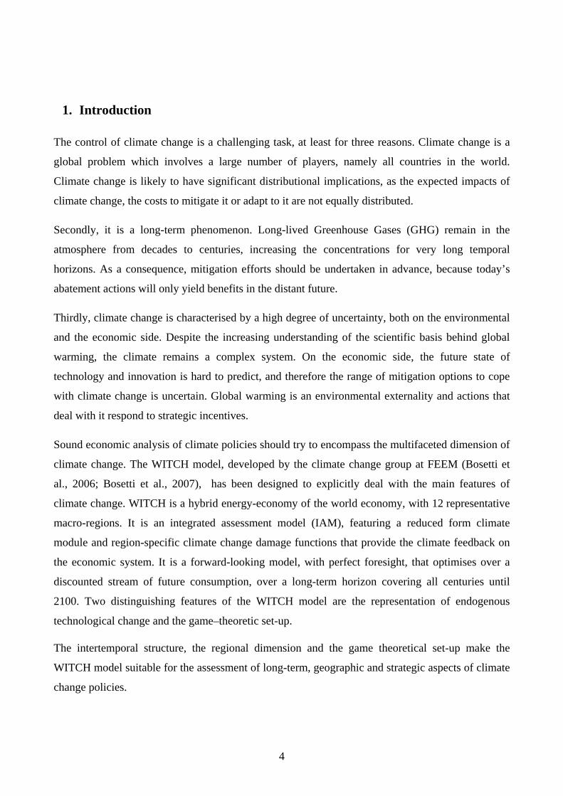
Despite being a top-down model, WITCH includes quite a wide range of technology options to
describe the use of energy and the generation of electricity (see a schematic representation of the
energy sector and its role within the economic module of the model in Figure 1). Energy is
described by a production function that aggregates factors at various levels and with different
elasticities of substitution. The main distinction is among electric generation and non-electric
consumption of energy.
Electricity is generated by a series of traditional fossil fuel-based technologies and carbon-free
options. Fossil fuel-based technologies include natural gas combined cycle (NGCC), fuel oil and
pulverised coal (PC) power plants. Coal-based electricity can also be generated using integrated
gasification combined cycle production with carbon capture and sequestration (CCS). Low carbon
technologies include hydroelectric and nuclear power, renewable sources such as wind turbines and
photovoltaic panels (Wind&Solar) and two breakthrough technologies.
8
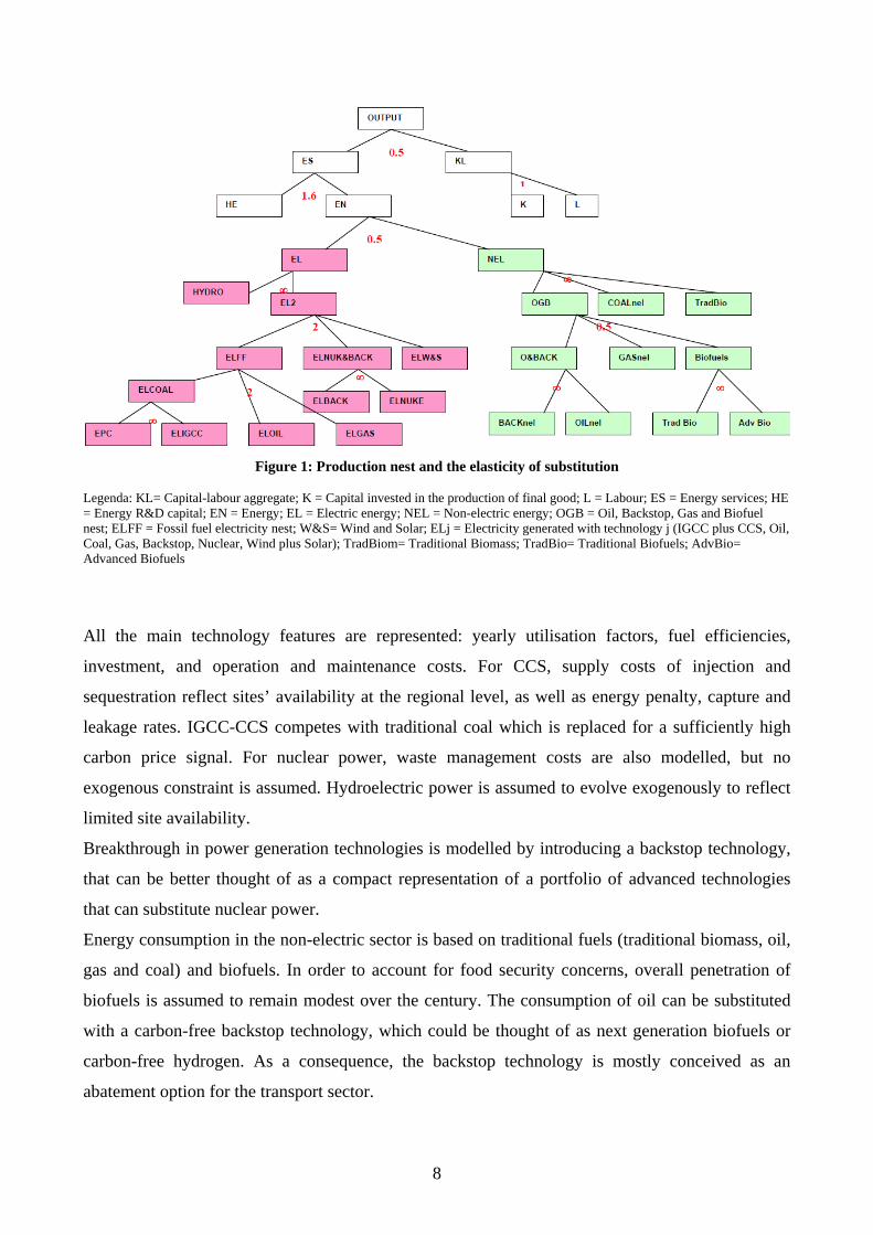
Figure 1: Production nest and the elasticity of substitution
Legenda: KL= Capital-labour aggregate; K = Capital invested in the production of final good; L = Labour; ES = Energy services; HE = Energy R&D capital; EN = Energy; EL = Electric energy; NEL = Non-electric energy; OGB = Oil, Backstop, Gas and Biofuel nest; ELFF = Fossil fuel electricity nest; W&S= Wind and Solar; ELj = Electricity generated with technology j (IGCC plus CCS, Oil, Coal, Gas, Backstop, Nuclear, Wind plus Solar); TradBiom= Traditional Biomass; TradBio= Traditional Biofuels; AdvBio= Advanced Biofuels
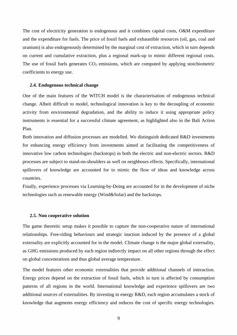
All the main technology features are represented: yearly utilisation factors, fuel efficiencies,
investment, and operation and maintenance costs. For CCS, supply costs of injection and
sequestration reflect sites’ availability at the regional level, as well as energy penalty, capture and
leakage rates. IGCC-CCS competes with traditional coal which is replaced for a sufficiently high
carbon price signal. For nuclear power, waste management costs are also modelled, but no
exogenous constraint is assumed. Hydroelectric power is assumed to evolve exogenously to reflect
limited site availability.
Breakthrough in power generation technologies is modelled by introducing a backstop technology,
that can be better thought of as a compact representation of a portfolio of advanced technologies
that can substitute nuclear power.
Energy consumption in the non-electric sector is based on traditional fuels (traditional biomass, oil,
gas and coal) and biofuels. In order to account for food security concerns, overall penetration of
biofuels is assumed to remain modest over the century. The consumption of oil can be substituted
with a carbon-free backstop technology, which could be thought of as next generation biofuels or
carbon-free hydrogen. As a consequence, the backstop technology is mostly conceived as an
abatement option for the transport sector.
9
The cost of electricity generation is endogenous and it combines capital costs, O&M expenditure
and the expenditure for fuels. The price of fossil fuels and exhaustible resources (oil, gas, coal and
uranium) is also endogenously determined by the marginal cost of extraction, which in turn depends
on current and cumulative extraction, plus a regional mark-up to mimic different regional costs.
The use of fossil fuels generates CO2 emissions, which are computed by applying stoichiometric
coefficients to energy use.
2.4. Endogenous technical change
One of the main features of the WITCH model is the characterisation of endogenous technical
change. Albeit difficult to model, technological innovation is key to the decoupling of economic
activity from environmental degradation, and the ability to induce it using appropriate policy
instruments is essential for a successful climate agreement, as highlighted also in the Bali Action
Plan.
Both innovation and diffusion processes are modelled. We distinguish dedicated R&D investments
for enhancing energy efficiency from investments aimed at facilitating the competitiveness of
innovative low carbon technologies (backstops) in both the electric and non-electric sectors. R&D
processes are subject to stand-on-shoulders as well on neighbours effects. Specifically, international
spillovers of knowledge are accounted for to mimic the flow of ideas and knowledge across
countries.
Finally, experience processes via Learning-by-Doing are accounted for in the development of niche
technologies such as renewable energy (Wind&Solar) and the backstops.
2.5. Non cooperative solution
The game theoretic setup makes it possible to capture the non-cooperative nature of international
relationships. Free-riding behaviours and strategic inaction induced by the presence of a global
externality are explicitly accounted for in the model. Climate change is the major global externality,
as GHG emissions produced by each region indirectly impact on all other regions through the effect
on global concentrations and thus global average temperature.
The model features other economic externalities that provide additional channels of interaction.
Energy prices depend on the extraction of fossil fuels, which in turn is affected by consumption
patterns of all regions in the world. International knowledge and experience spillovers are two
additional sources of externalities. By investing in energy R&D, each region accumulates a stock of
knowledge that augments energy efficiency and reduces the cost of specific energy technologies.
10
The effect of knowledge is not confined to the inventor region but it can spread to other regions.
Finally, the diffusion of knowledge embodied in wind&solar experience is represented by learning
curves linking investment costs with world, and not regional, cumulative capacity. Increasing
capacity thus reduces investment costs for all regions. These externalities provide incentives to
adopt strategic behaviours, both with respect to the environment (e.g. GHG emissions) and with
respect to investments in knowledge and carbon-free but costly technologies.
Two different solutions can be produced: a co-operative one that is globally optimal and a
decentralised, non-cooperative one that is strategically optimal for each given region (Nash
equilibrium). In the cooperative solution all externalities are internalised and therefore it can be
interpreted as a first-best solution. The Nash equilibrium instead can be seen as a second-best
solution. Intermediate degree of cooperation, both in terms of externalities addressed and
participation can also be simulated.
3. Database updating: new base year calibration
WITCH08 has been updated with more recent data and revised estimates for future projection of the
main exogenous drivers. The base calibration year has been set at 2005, for which socio-economic,
energy and environmental variables data are now available. We report on the main hypotheses on
current and future trends on population, economic activity, energy consumption and climate
variables.
3.1. Population
An important driver for the emissions of greenhouse gases is the rate at which population grows. In
the WITCH model, population growth is exogenous. We update the model base year to 2005, and
use the most recent estimates of population growth. The annual estimates and projections produced
by the UN Population Division are used for the first 50 years2. For the period 2050 to 2100, the
updated data are not available, and less recent long-term projections, also produced by the UN
Population Division (UN, 2004) are adopted instead. The differences in the two datasets are
smoothed by extrapolating population levels at 5-year periods for 2050-2100, using average 2050-
2100 growth rates. Similar techniques are used to project population trends beyond 2100.
2 Data are available from http://unstats.un.org/unsd/cdb/cdb_simple_data_extract.asp?strSearch=&srID=13660&from=simple.
11
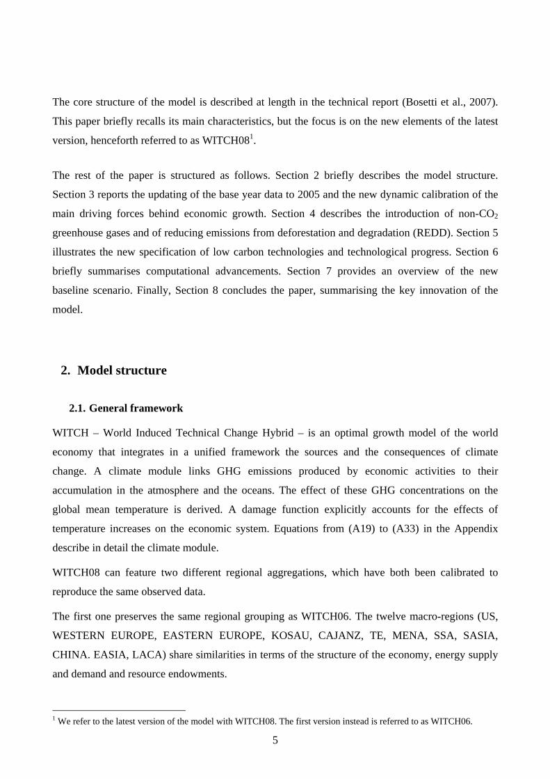
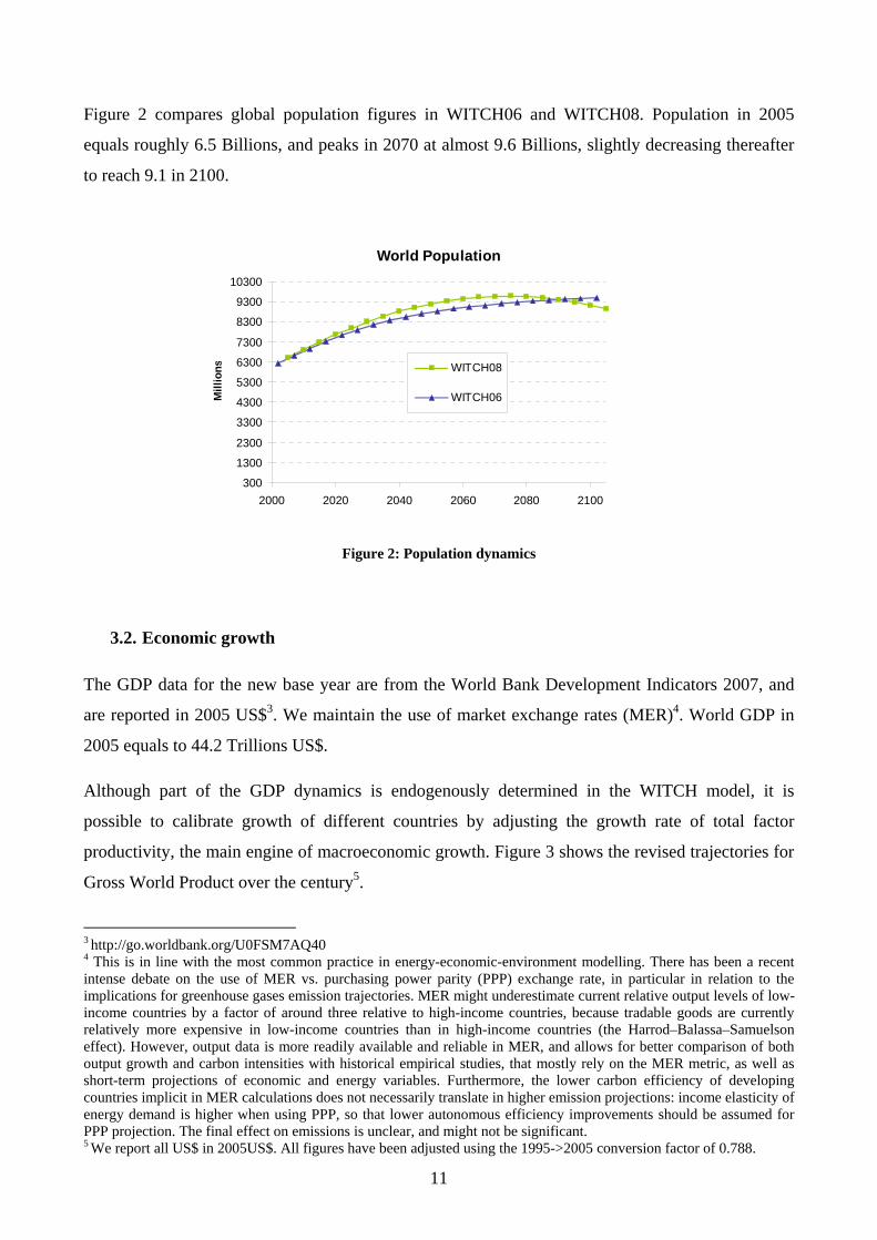
Figure 2 compares global population figures in WITCH06 and WITCH08. Population in 2005
equals roughly 6.5 Billions, and peaks in 2070 at almost 9.6 Billions, slightly decreasing thereafter
to reach 9.1 in 2100.
World Population
300
1300
2300
3300
4300
5300
6300
7300
8300
9300
10300
2000 2020 2040 2060 2080 2100
Mill
ions WITCH08
WITCH06
Figure 2: Population dynamics
3.2. Economic growth
The GDP data for the new base year are from the World Bank Development Indicators 2007, and
are reported in 2005 US$3. We maintain the use of market exchange rates (MER)4. World GDP in
2005 equals to 44.2 Trillions US$.
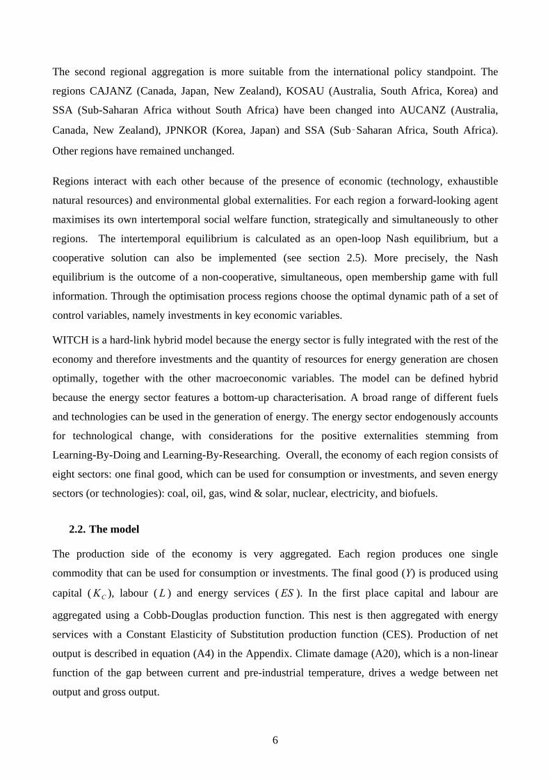
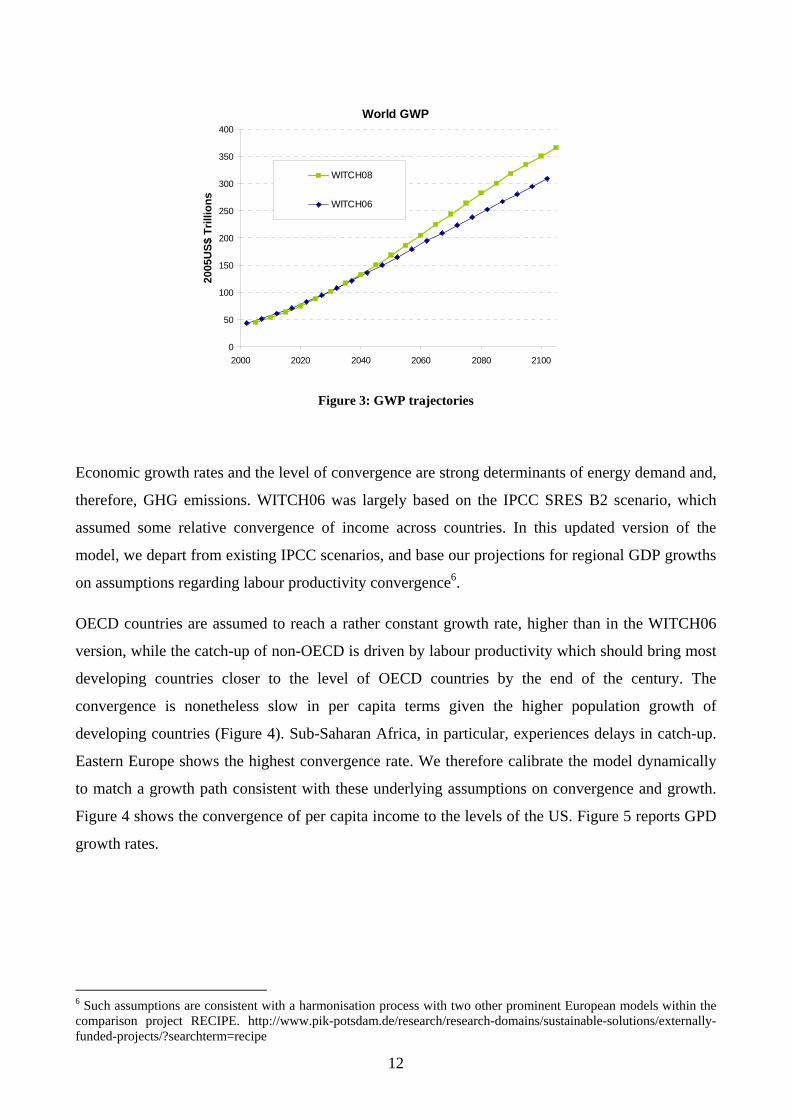
Although part of the GDP dynamics is endogenously determined in the WITCH model, it is
possible to calibrate growth of different countries by adjusting the growth rate of total factor
productivity, the main engine of macroeconomic growth. Figure 3 shows the revised trajectories for
Gross World Product over the century5.
3 http://go.worldbank.org/U0FSM7AQ40 4 This is in line with the most common practice in energy-economic-environment modelling. There has been a recent intense debate on the use of MER vs. purchasing power parity (PPP) exchange rate, in particular in relation to the implications for greenhouse gases emission trajectories. MER might underestimate current relative output levels of low-income countries by a factor of around three relative to high-income countries, because tradable goods are currently relatively more expensive in low-income countries than in high-income countries (the Harrod–Balassa–Samuelson effect). However, output data is more readily available and reliable in MER, and allows for better comparison of both output growth and carbon intensities with historical empirical studies, that mostly rely on the MER metric, as well as short-term projections of economic and energy variables. Furthermore, the lower carbon efficiency of developing countries implicit in MER calculations does not necessarily translate in higher emission projections: income elasticity of energy demand is higher when using PPP, so that lower autonomous efficiency improvements should be assumed for PPP projection. The final effect on emissions is unclear, and might not be significant. 5 We report all US$ in 2005US$. All figures have been adjusted using the 1995->2005 conversion factor of 0.788.
12
World GWP
0
50
100
150
200
250
300
350
400
2000 2020 2040 2060 2080 2100
2005
US$
Tril
lions
WITCH08
WITCH06
Figure 3: GWP trajectories
Economic growth rates and the level of convergence are strong determinants of energy demand and,
therefore, GHG emissions. WITCH06 was largely based on the IPCC SRES B2 scenario, which
assumed some relative convergence of income across countries. In this updated version of the
model, we depart from existing IPCC scenarios, and base our projections for regional GDP growths
on assumptions regarding labour productivity convergence6.
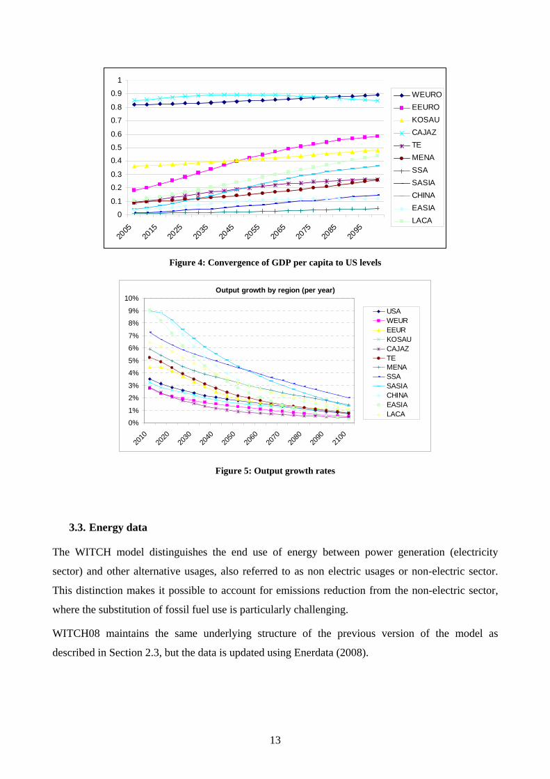
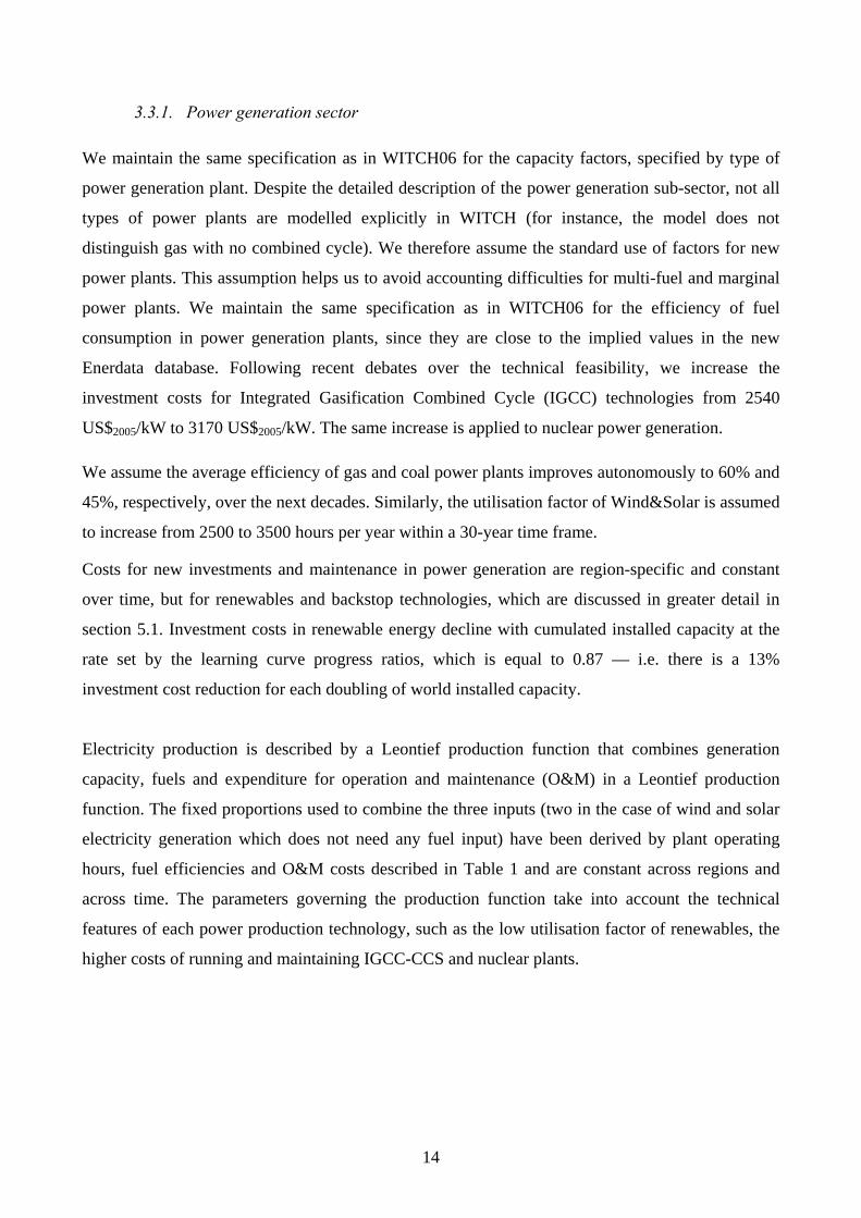
OECD countries are assumed to reach a rather constant growth rate, higher than in the WITCH06
version, while the catch-up of non-OECD is driven by labour productivity which should bring most
developing countries closer to the level of OECD countries by the end of the century. The
convergence is nonetheless slow in per capita terms given the higher population growth of
developing countries (Figure 4). Sub-Saharan Africa, in particular, experiences delays in catch-up.
Eastern Europe shows the highest convergence rate. We therefore calibrate the model dynamically
to match a growth path consistent with these underlying assumptions on convergence and growth.
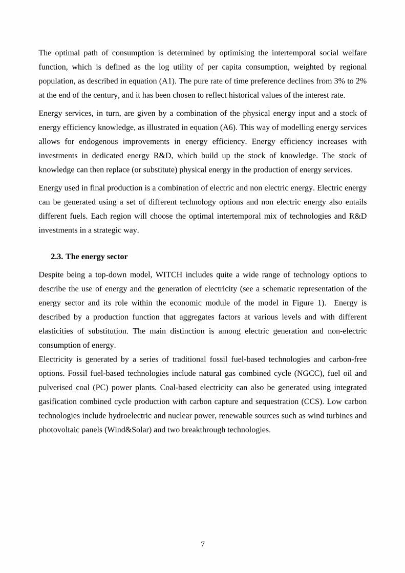
Figure 4 shows the convergence of per capita income to the levels of the US. Figure 5 reports GPD
growth rates.
6 Such assumptions are consistent with a harmonisation process with two other prominent European models within the comparison project RECIPE. http://www.pik-potsdam.de/research/research-domains/sustainable-solutions/externally-funded-projects/?searchterm=recipe
13
0
0.1
0.2
0.3
0.4
0.5
0.6
0.7
0.8
0.9
1
2005
2015
2025
2035
2045
2055
2065
2075
2085
2095
WEUROEEUROKOSAUCAJAZTEMENASSASASIACHINAEASIALACA
Figure 4: Convergence of GDP per capita to US levels
Output growth by region (per year)
0%
1%
2%
3%
4%
5%
6%
7%
8%
9%
10%
2010
2020
2030
2040
2050
2060
2070
2080
2090
2100
USAWEUREEURKOSAUCAJAZTEMENASSASASIACHINAEASIALACA
Figure 5: Output growth rates
3.3. Energy data
The WITCH model distinguishes the end use of energy between power generation (electricity
sector) and other alternative usages, also referred to as non electric usages or non-electric sector.
This distinction makes it possible to account for emissions reduction from the non-electric sector,
where the substitution of fossil fuel use is particularly challenging.
WITCH08 maintains the same underlying structure of the previous version of the model as
described in Section 2.3, but the data is updated using Enerdata (2008).
14
3.3.1. Power generation sector
We maintain the same specification as in WITCH06 for the capacity factors, specified by type of
power generation plant. Despite the detailed description of the power generation sub-sector, not all
types of power plants are modelled explicitly in WITCH (for instance, the model does not
distinguish gas with no combined cycle). We therefore assume the standard use of factors for new
power plants. This assumption helps us to avoid accounting difficulties for multi-fuel and marginal
power plants. We maintain the same specification as in WITCH06 for the efficiency of fuel
consumption in power generation plants, since they are close to the implied values in the new
Enerdata database. Following recent debates over the technical feasibility, we increase the
investment costs for Integrated Gasification Combined Cycle (IGCC) technologies from 2540
US$2005/kW to 3170 US$2005/kW. The same increase is applied to nuclear power generation.
We assume the average efficiency of gas and coal power plants improves autonomously to 60% and
45%, respectively, over the next decades. Similarly, the utilisation factor of Wind&Solar is assumed
to increase from 2500 to 3500 hours per year within a 30-year time frame.
Costs for new investments and maintenance in power generation are region-specific and constant
over time, but for renewables and backstop technologies, which are discussed in greater detail in
section 5.1. Investment costs in renewable energy decline with cumulated installed capacity at the
rate set by the learning curve progress ratios, which is equal to 0.87 — i.e. there is a 13%
investment cost reduction for each doubling of world installed capacity.
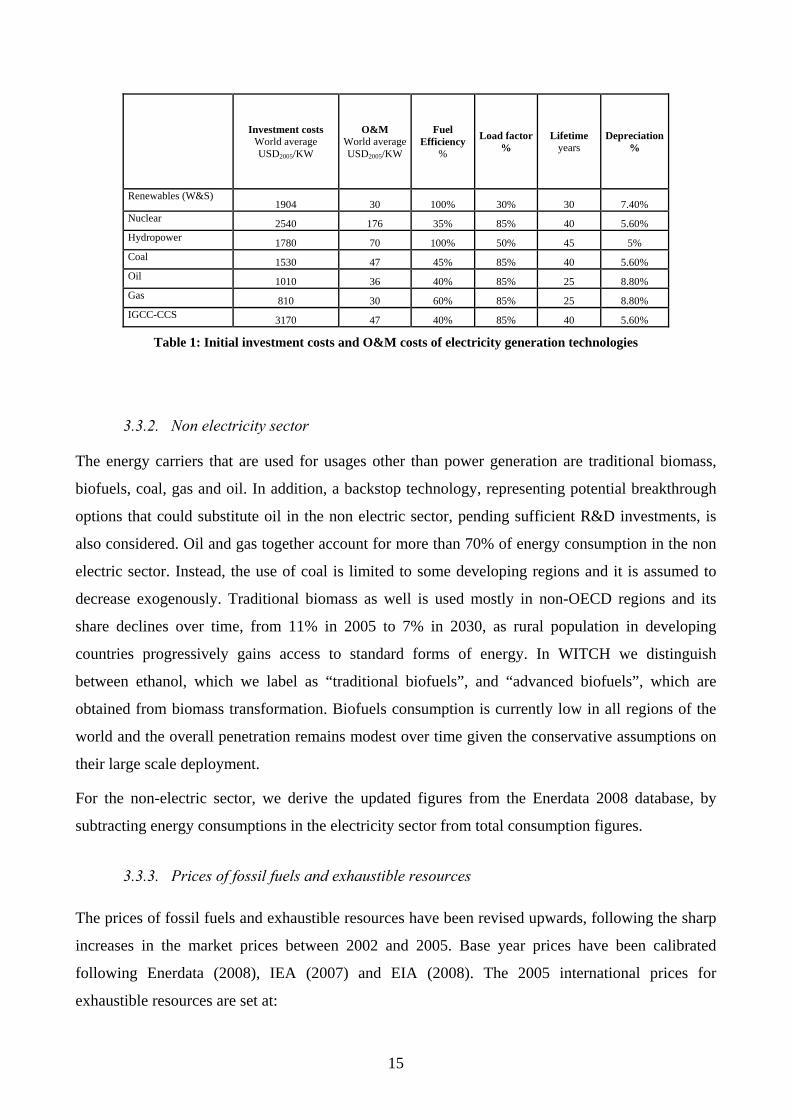
Electricity production is described by a Leontief production function that combines generation
capacity, fuels and expenditure for operation and maintenance (O&M) in a Leontief production
function. The fixed proportions used to combine the three inputs (two in the case of wind and solar
electricity generation which does not need any fuel input) have been derived by plant operating
hours, fuel efficiencies and O&M costs described in Table 1 and are constant across regions and
across time. The parameters governing the production function take into account the technical
features of each power production technology, such as the low utilisation factor of renewables, the
higher costs of running and maintaining IGCC-CCS and nuclear plants.
15
Investment costs World average USD2005/KW
O&M World average USD2005/KW
Fuel Efficiency
%
Load factor%
Lifetime years
Depreciation%
Renewables (W&S) 1904 30 100% 30% 30 7.40%
Nuclear 2540 176 35% 85% 40 5.60% Hydropower 1780 70 100% 50% 45 5% Coal 1530 47 45% 85% 40 5.60% Oil 1010 36 40% 85% 25 8.80% Gas 810 30 60% 85% 25 8.80% IGCC-CCS 3170 47 40% 85% 40 5.60%
Table 1: Initial investment costs and O&M costs of electricity generation technologies
3.3.2. Non electricity sector
The energy carriers that are used for usages other than power generation are traditional biomass,
biofuels, coal, gas and oil. In addition, a backstop technology, representing potential breakthrough
options that could substitute oil in the non electric sector, pending sufficient R&D investments, is
also considered. Oil and gas together account for more than 70% of energy consumption in the non
electric sector. Instead, the use of coal is limited to some developing regions and it is assumed to
decrease exogenously. Traditional biomass as well is used mostly in non-OECD regions and its
share declines over time, from 11% in 2005 to 7% in 2030, as rural population in developing
countries progressively gains access to standard forms of energy. In WITCH we distinguish
between ethanol, which we label as “traditional biofuels”, and “advanced biofuels”, which are
obtained from biomass transformation. Biofuels consumption is currently low in all regions of the
world and the overall penetration remains modest over time given the conservative assumptions on
their large scale deployment.
For the non-electric sector, we derive the updated figures from the Enerdata 2008 database, by
subtracting energy consumptions in the electricity sector from total consumption figures.
3.3.3. Prices of fossil fuels and exhaustible resources
The prices of fossil fuels and exhaustible resources have been revised upwards, following the sharp
increases in the market prices between 2002 and 2005. Base year prices have been calibrated
following Enerdata (2008), IEA (2007) and EIA (2008). The 2005 international prices for
exhaustible resources are set at:
16
- 55 US$/bbl for oil, or roughly 8US$/GJ
- 7.14 US$/GJ for natural gas
- 60 US$/ton for coal, equivalent to 2 US$/GJ. In order to match the large difference in price
increases shown in the Enerdata database, we adjust the mark-up prices
- Uranium ore price tripled from 2002 to 20057, and we thus update to this new level. The cost
of conversion was increased from 5 US$/kg to 11 US$/kg8, while enrichment costs stayed
roughly constant9. We thus slightly increased the cost of conversion and enrichment from
221 to 230 1995 US$/kg.
Country specific mark-ups are set to reproduce regional figures from IEA (2007).
3.3.4. Carbon emission coefficients of fossil fuels
In WITCH08 we maintain the same initial stoichiometric coefficients as in WITCH06. However, in
order to differentiate the higher emission content of non-conventional oil as opposed to
conventional ones, we link the carbon emission coefficient for oil to its availability. Specifically,
the stoichiometric coefficient for oil increases with the cumulative oil consumed so that it increases
by 25% when 2000 Billions Barrels are reached. An upper bound of 50% is assumed. The 2000
figure is calibrated on IEA (2005) estimates on conventional oil resource availability. The 25%
increase is chosen given that estimates range between 14% and 39% (Farrell and Brandt, 2006).
3.4. Climate data and feedback
We continue to use the MAGICC 3-box layer climate model. CO2 concentrations in the atmosphere
have been updated to 2005 at roughly 385ppm and temperature increase above pre-industrial at
0.76°C, in accordance with IPCC 4th Assessment Report (2007). Other parameters governing the
climate equations have been adjusted following Nordhaus (2007)10. We have replaced the
exogenous non-CO2 radiative forcing in equation (A22), O, with specific representation of other
GHGs and sulphates, see Section 4. The damage function of climate change on the economic
activity is left unchanged.
7 http://www.uxc.com/review/uxc_g_price.html 8 http://www.uxc.com/review/uxc_g_ind-c.html 9 http://www.uxc.com/review/uxc_g_ind-s.html 10 http://nordhaus.econ.yale.edu/DICE2007.htm
17
4. Additional sources of GHGs
4.1. Non-CO2 GHGs
Non-CO2 GHGs are important contributors to global warming, and might offer economically
attractive ways of mitigating it11. WITCH06 only considers explicitly industrial CO2 emissions,
while other GHGs, together with aerosols, enter the model in an exogenous and aggregated manner,
as a single radiative forcing component.
In WITCH08, we take a step forward and specify non-CO2 gases, modelling explicitly emissions of
CH4, N2O, SLF (short-lived fluorinated gases, i.e. HFCs with lifetimes under 100 years) and LLF
(long-lived fluorinated, i.e. HFC with long lifetime, PFCs, and SF6). We also distinguish SO2
aerosols, which have a cooling effect on temperature (see equation A21).
Since most of these gases are determined by agricultural practices, we rely on estimates for
reference emissions and a top-down approach for mitigation supply curves. For the baseline
projections of non-CO2 GHGs, we use EPA regional estimates (EPA, 2006). The regional estimates
and projections are available until 2020 only: beyond that date, we use growth rates for each gas as
specified in the IIASA-MESSAGE-B2 scenario12, which has underlying assumptions similar to the
WITCH ones. SO2 emissions are taken from MERGE v.513 and MESSAGE B2: given the very
large uncertainty associated with aerosols, they are translated directly into the temperature effect
(cooling), so that we only report the radiative forcing deriving from GHGs. In any case, sulphates
are expected to be gradually phased out over the next decades, so that eventually the two radiative
forcing measures will converge to similar values.
The equations translating non-CO2 emissions into radiative forcing are taken from MERGE v.5 (see
equations A24 to A27 in the Appendix). The global warming potential (GWP) methodology is
employed, and figures for GWP as well as base year stock of the various GHGs are taken from the
IPCC 4th Assessment Report, Working Group I. The simplified equation translating CO2
concentrations into radiative forcing has been modified from WITCH06 and is now in line with
IPCC14.
11 See the Energy Journal Special Issue (2006) (EMF-21), Multi-Greenhouse Gas Mitigation and Climate Policy - Special Issue n°. 3 and the IPCC 4th AR WG III (IPCC, 2007b) 12 Available at http://www.iiasa.ac.at/web-apps/ggi/GgiDb/dsd?Action=htmlpage&page=regions 13 http://www.stanford.edu/group/MERGE/m5ccsp.html 14 http://www.grida.no/climate/ipcc_tar/wg1/222.htm, Table 6.2, first Row.
18
We introduce end-of-pipe type of abatement possibilities via marginal abatement curves (MAC) for
non-CO2 GHG mitigation. We use MAC provided by EPA for the EMF 21 project15, aggregated for
the WITCH regions. MAC are available for 11 cost categories ranging from 10 to 200 US$/tC. We
have ruled out zero or negative cost abatement options. MAC are static projections for 2010 and
2020, and for many regions they show very low upper values, such that even at maximum
abatement, emissions would keep growing over time. We thus introduce exogenous technological
improvements: for the highest cost category only (the 200 US$/tC) we assume a technical progress
factor that reaches 2 in 2050 and the upper bound of 3 in 2075. We, however, set an upper bound to
the amount of emissions which can be abated, assuming that no more than 90% of each gas
emission can be mitigated. Such a framework enables us to keep non-CO2 GHG emissions
somewhat stable in a stringent mitigation scenario (530e) in the first half of the century, with a
subsequent gradual decline. This path is similar to what is found in the CCSP report16, as well as in
MESSAGE stabilisation scenarios. Nonetheless, the scarce evidence on technology improvements
potential in non-CO2 GHG sectors indicates that a sensitivity analysis should be performed to verify
the impact on policy costs.
4.2. Forestry
Forestry is an important contributor of CO2 emissions and, similarly to non-CO2 gases, it might
provide relatively convenient abatement opportunities. Forestry sector models differ substantially
from energy-economy ones, so that normally the interaction is solved via soft link (e.g. iterative)
coupling. For example, WITCH06 has been coupled with a global timber model to assess the
potential of carbon sinks in a climate stabilisation policy (Tavoni et al. 2007). However, the model
did not include this option in the standard simulation exercises.
WITCH08 is enhanced with baseline emissions and supply mitigation curves for reduced
deforestation. The focus is on REDD17 given its predominant role in CO2 emissions and the policy
importance of this option as stressed in the 2007 Bali Action Plan.
Baseline emissions are provided by the Brent Sohngen GTM model. REDD supply mitigation cost
curves have been built and made suitable to be incorporated in the WITCH model.
Two versions of abatement cost curves have been incorporated in the model representing two
extreme cases. The first version includes abatement curves for the whole century for the Brazilian
tropical forest only and have been developed using Brazil’s data from the Woods Hole Research
15 http://www.stanford.edu/group/EMF/projects/projectemf21.htm 16 http://www.climatescience.gov/Library/sap/sap2-1/finalreport/default.htm 17 Reducing emissions from deforestation and degradation.
19
Center (Nepstad et al. 2008)18. A second version includes abatement curves for all world tropical
forests, based on the Global Timber Model of Brent Sohngen, Ohio State University, used within
the Energy Modeling Forum 21 (2006) and data from the IIASA cluster model (Eliasch 2008).
Bosetti et a. (2009) describes in depth the results from this analysis.
5. Specific Features in Abatement Technologies
5.1. Innovative carbon free technologies
In the short to mid term, energy savings, fuel switching mainly in the power sector, as well as non
fossil fuel mitigation, are believed to be the most convenient mitigation options. In the longer term,
however, one could envisage the possible development of innovative technologies with low or zero
carbon emissions. These technologies, which are currently far from being commercial, are usually
referred to in the literature as backstop technologies, and are characterised as being available in
large supplies. For the purpose of modelling, a backstop technology can be better thought of as a
compact representation of a portfolio of advanced technologies, that would ease the mitigation
burden away from currently commercial options, though it would become available not before a
few decades. This representation has the advantage of maintaining simplicity in the model by
limiting the array of future energy technologies and thus the dimensionality of techno-economic
parameters for which reliable estimates and meaningful modelling characterisation do not exist.
WITCH06 features a series of mitigation options in both the electric and non-electric sectors, such
as nuclear power, CCS, renewables, biofuels etc. However, limited deployment potential of
controversial technologies, such as nuclear, and resource constrained ones such as bioenergy,
suggests that the possibility to invest towards the commercialisation of innovative technologies
should be a desirable feature of models that evaluate long-term policies.
To this extent, WITCH08 is enhanced by the inclusion of two backstop technologies that necessitate
dedicated innovation investments to become economically competitive, even in a scenario with a
climate policy. We follow the most recent characterisation in the technology and climate change
literature, modelling the costs of the backstop technologies with a two-factor learning curve in
which their price declines both with investments in dedicated R&D and with technology diffusion.
This improved formulation is meant to overcome the main criticism of the single factor experience
curves (Nemet, 2006) by providing a more structural -R&D investment-led- approach to the
penetration of new technologies, and thus to ultimately better inform policy makers on the
innovation needs in the energy sector. 18 http://whrc.org/BaliReports/
20
More specifically, we model the investment cost in a backstop technology tec as being influenced
by a Learning-by-Researching process (main driving force before adoption) and by Learning-by-
Doing (main driving force after adoption), the so-called 2-factor learning curve formulation
(Kouvaritakis et al., 2000). ttecP , , the unit cost of technology tec at time t is a function of
deployment, ttecCC , and dedicated R&D stock, ttecDR ,& as described in equation [1]
b
tec
Ttec
c
tec
Ttec
tec
Ttec
CCCC
DRDR
PP
−−
−
⎟⎟⎠
⎞⎜⎜⎝
⎛⎟⎟⎠
⎞⎜⎜⎝
⎛=
0,
,
0,
2,
0,
, *&
& [1]
where the R&D stock (R&D tec) accumulates with the perpetual rule and is also augmented by the
stock of R&D accumulated in other regions through a spillover effect, SPILL
βαδ TtecTtecTtecTtec SPILLDIRDRDR ,,,1, &)1(&& +−⋅=+ [2]
and CC is the cumulative installed capacity (or consumption) of the technology. The specification
of the spillover component, SPILL, is described in equation (A9) in the Appendix. We assume a
two-period time interval (i.e. 10 years) between R&D knowledge and its effect on the price of the
backstop technologies to account for time lags between research and commercialisation.
The two exponents are the Learning-by-Doing index ( b− ) and the Learning-by-Researching index
( c− ). They define the speed of learning and are derived from the learning ratios. The learning ratio
lr is the rate at which the generating cost declines each time the cumulative capacity doubles, while
lrs is the rate at which the cost declines each time the knowledge stock doubles. The relation
between b, c, lr, and lrs can be expressed as in [3]
cb lrslr −− =−=− 21 and 21 [3]
We set the initial prices of the backstop technologies at roughly 10 times the 2005 price of
commercial equivalents (16,000 US$/kW for electric, and 550 US$/bbl for non-electric). The
cumulative deployment of the technology is initiated at 1,000twh and 1,000EJ, respectively, for the
electric and non-electric, an arbitrarily low value (Kypreos, 2007). The backstop technologies are
assumed to be renewable in the sense that the fuel cost component is negligible; for power
21
generation, it is assumed to operate at load factors comparable with those of baseload power
generation.
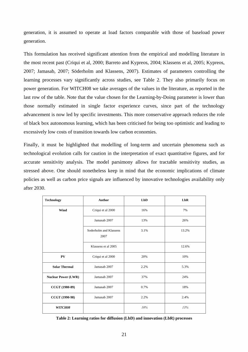
This formulation has received significant attention from the empirical and modelling literature in
the most recent past (Criqui et al, 2000; Barreto and Kypreos, 2004; Klassens et al, 2005; Kypreos,
2007; Jamasab, 2007; Söderholm and Klassens, 2007). Estimates of parameters controlling the
learning processes vary significantly across studies, see Table 2. They also primarily focus on
power generation. For WITCH08 we take averages of the values in the literature, as reported in the
last row of the table. Note that the value chosen for the Learning-by-Doing parameter is lower than
those normally estimated in single factor experience curves, since part of the technology
advancement is now led by specific investments. This more conservative approach reduces the role
of black box autonomous learning, which has been criticised for being too optimistic and leading to
excessively low costs of transition towards low carbon economies.
Finally, it must be highlighted that modelling of long-term and uncertain phenomena such as
technological evolution calls for caution in the interpretation of exact quantitative figures, and for
accurate sensitivity analysis. The model parsimony allows for tractable sensitivity studies, as
stressed above. One should nonetheless keep in mind that the economic implications of climate
policies as well as carbon price signals are influenced by innovative technologies availability only
after 2030.
Technology Author LbD LbR
Criqui et al 2000 16% 7%
Jamasab 2007 13% 26%
Soderholm and Klassens
2007
3.1% 13.2%
Wind
Klassens et al 2005 12.6%
PV Criqui et al 2000 20% 10%
Solar Thermal Jamasab 2007 2.2% 5.3%
Nuclear Power (LWR) Jamasab 2007 37% 24%
CCGT (1980-89) Jamasab 2007 0.7% 18%
CCGT (1990-98) Jamasab 2007 2.2% 2.4%
WITCH08 10% 13%
Table 2: Learning ratios for diffusion (LbD) and innovation (LbR) processes
22
Backstops substitute linearly nuclear power in the electric sector, and oil in the non-electric one. We
assume that once the backstop technologies become competitive thanks to dedicated R&D
investment and pilot deployments, their uptake will not be immediate and complete, but rather there
will be a transition/adjustment period. These penetration limits are a reflection of inertia in the
system, as presumably the large deployment of backstops will require investment in infrastructures
and the re-organisation of the economic system. The upper limit on penetration is set equivalent to
5% of the consumption in the previous period of energy produced by technologies other than the
backstop, plus the energy produced by the backstop itself.
5.2. International spillovers of knowledge and experience
Learning processes via knowledge investments and experience are not likely to remain within the
boundaries of single countries, but to spill to other regions too. The effect of international spillovers
is deemed to be important, and its inclusion in integrated assessment models desirable, since it
allows for a better representation of the innovation market failures and for specific policy exercises.
The WITCH model is particularly suited to perform this type of analysis, since its game theoretic
structure allows distinguishing first- and second-best strategies, and thus to quantify optimal
portfolios of policies to resolve all the externalities arising in global problems such as climate
change.
WITCH06 featured spillovers of experience for Wind&Solar in that the Learning-by-Doing effect
depended on world cumulative installed capacity, so that single regions could benefit from
investments in virtuous countries, thus leading to strategic incentives. An enhanced version was
developed to include spillovers in knowledge for energy efficiency improvements (Bosetti et al.
2008), which are retained also in this WITCH08. As mentioned in section 2.3, energy services are a
CES nest of physical energy and energy knowledge. Energy knowledge depends not only on
regional investments in energy R&D, but also on the knowledge stock that has been accumulated in
other regions. In WITCH08 we continue along this strand of research and model spillovers of both
experience and knowledge in the newly featured backstop technologies. Similarly to the Learning-
By-Doing for Wind&Solar, we assume experience accrues with the diffusion of technologies at the
global level. We also assume knowledge spills internationally. The amount of spillovers entering
each world region depends on a pool of freely available knowledge and on the ability of each
country to benefit from it, i.e. on its absorption capacity. Knowledge acquired from abroad
combines with domestic knowledge stock and investments and thus contributes to the production of
new technologies at home. The parameterisation follows Bosetti et al. (2008) and it is recalled in the
Appendix, equation (A9).
23
5.3. Key mitigation options
The WITCH model features a series of mitigation options in both the power generation sector and
the other usages of energy carriers, e.g. in the non-electric sector.
Mitigation options in the power sector include nuclear, hydroelectric, IGCC-CCS, renewables and a
backstop option that can substitute nuclear.
Nuclear power is an interesting option for decarbonised economies. However, fission still faces
controversial difficulties such as long-term waste disposal and proliferation risks. Light Water
Reactors (LWR) — the most common nuclear technology today — are the most reliable and
relatively least expensive solution. In order to account for the waste management and proliferation
costs, we have included an additional O&M burden in the model. Initially set at 1 mUSD/kWh,
which is the charge currently paid to the US depository at Yucca Mountain, this fee is assumed to
grow linearly with the quantity of nuclear power generated, to reflect the scarcity of repositories and
the proliferation challenge.
Hydorelectric is also a carbon-free option, but it is assumed to evolve exogenously to reflect limited
site availability.
The limited deployment of controversial technologies such as nuclear calls for other alternative
mitigation options. One technology that has received particular attention in the recent past is carbon
capture and sequestration (CCS). In the WITCH model this option can be applied only to integrated
coal gasification combined cycle power plants (IGCC-CCS). In fact, CCS is a promising technology
but still far from large-scale deployment. CCS transport and storage cost functions are region-
specific and they have been calibrated following Hendriks et al. (2004). Costs increase
exponentially with the capacity accumulated by this technology. The CO2 capture rate is set at 90%
and no after-storage leakage is considered. Other technological parameters such as efficiency, load
factor, investment and O&M costs are described in Table 1. In the case of CCS there is no learning
process or research activity that can either reduce investment costs or increase the capture rate.
Electricity from wind and solar is another important carbon-free technology. The rapid development
of wind and solar power technologies in recent years has led to a reduction in investment costs. In
fact, beneficial effects from Learning-By-Doing are expected to decrease investment costs even
further in the next few years. This effect is captured in the WICTH model by letting the investment
cost follow a learning curve. As world-installed capacity in wind and solar doubles, investment cost
diminishes by 13%. International spillovers in Learning-By-Doing are present because we believe it
is realistic to assume that information and best practices quickly circulate in cutting-edge
technological sectors dominated by a few major world investors. This is particularly true if we
consider that the model is constructed on five-year time steps, a time lag that we consider sufficient
24
for a complete flow of technology know-how, human capital and best practices, across firms that
operate in the sector.
Less flexible is the non electric sector. Two are the major mitigation options, the use of biomass and
the deployment of the breakthrough technology. The breakthrough technology can substitute oil and
it can be thought of as next generation biofuels or carbon-free hydrogen to be used in the transport
sector. The overall penetration of traditional (e.g. sugar cane or corn) biofuels remains modest over
time and therefore the mitigation potential coming from this option is quite limited.
Other two important mitigation options are the endogenous improvement of overall energy
efficiency with dedicated energy R&D (section 5.2) and reducing emissions from deforestation and
degradation (section 4.2).
6. Computational issues
The WITCH model is solved numerically using GAMS – General Algebraic Modelling System19.
GAMS is a high-level modelling system for mathematical programming problems, designed to
provide a convenient tool to represent large and complex models in algebraic form, allowing a
simple updating of the model and flexibility in representation, and modular construction.
WITCH features two different solution concepts, a cooperative concept that optimises jointly all
regions, and a non-cooperative decentralised one that is achieved iteratively via an open loop Nash
algorithm in which each region is optimised separately. This second solution was implemented
sequentially in WITCH06.
In WITCH08, the regional maximisation problems for the non-cooperative solution are solved in
parallel, exploiting new computing power afforded by multiple-core hardware, and thus allowing
for a much more rapid solution of the overall optimisation exercise. The solutions of each region’s
maximisation problem are combined in a single step following each iteration – the total number of
parallel solves is therefore equal to the number of regions – twelve in the case of WITCH. The
speed of the solution is thus determined by the slowest region.
The model also runs in batch mode for remote solution, using an SSH interface and a system of
shared files, stored in the remote host computer. The use of Globus Toolkit 4 allows the submission
of the solve jobs to more than one cluster, thus further reducing the execution time needed to find a
solution.
19 http://www.gams.com/
25
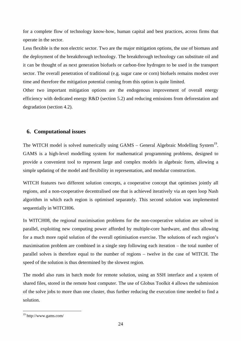
Several tests have been performed for evaluating the scalability and performance of the parallel
algorithm (Figure 6). The execution tests have been made on the SPACI’s HP-XC6000 cluster
ranging from 1 up to 12 CPUs, see Figure 6. Since the GAMS executable is not available for the
considered architecture, an emulator for x86_32 processors has been used. The analytic model of
the parallel execution time highlights how the coarse-grained parallelisation produces a decreasing
efficiency starting from 6 processors. The reason can be found in the imperfect balance of the
workload.20
Figure 6: Execution time
7. Baseline scenario
This section outlines the main output of the WITCH08 baseline scenario which is the non
cooperative, market solution of the model, without stabilisation constraints on GHG concentrations.
The feedback effect of climate change into the economic system is turned off, so that regions’
strategies are not affected by the sensitivity to climate damage.
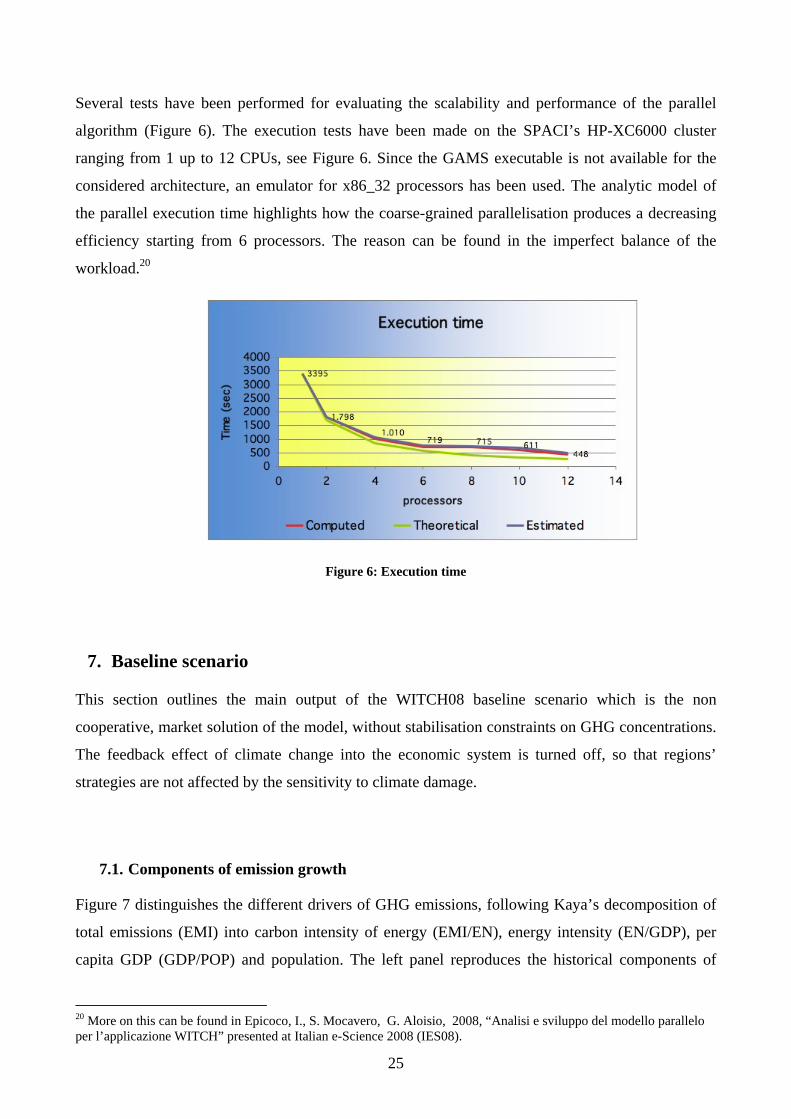
7.1. Components of emission growth
Figure 7 distinguishes the different drivers of GHG emissions, following Kaya’s decomposition of
total emissions (EMI) into carbon intensity of energy (EMI/EN), energy intensity (EN/GDP), per
capita GDP (GDP/POP) and population. The left panel reproduces the historical components of
20 More on this can be found in Epicoco, I., S. Mocavero, G. Aloisio, 2008, “Analisi e sviluppo del modello parallelo per l’applicazione WITCH” presented at Italian e-Science 2008 (IES08).
26
GHG emissions observed over the past thirty years vis-à-vis the short-term WITCH baseline
projections, whereas the right panel depicts the long-term trends produced by the model.
Historically, per capita GDP and population have been the major determinants of emissions growth,
whereas improvements in carbon intensity had the opposing effect of reducing emissions. The long-
term scenario is still characterised by a preponderant role of economic growth, whereas the role of
population fades over time. Economic growth, measured in terms of per capita GDP, is the major
driver of GHG emissions over the whole century whereas population growth contributes to the
increase in GHG emissions up to 2075, when population starts to follow a slightly negative trend. A
decrease in energy intensity has a positive effect on emission reductions, which is however not
sufficiently large to compensate for the pressure of economic and population growth. The carbon
content of energy remains rather constant over time, with a slight carbonisation of energy due to an
increase in coal consumption in fast-growing countries like China and India.
Kaya in the next/past 30 years
0.00
0.50
1.00
1.50
2.00
2.50
EMI GDP/POP EN/GDP EMI/EN POP
WITCH08Historical
Kaya decomposition over the century
-3.00%
-2.00%
-1.00%
0.00%
1.00%
2.00%
3.00%
4.00%
5.00%
2010
2020
2030
2040
2050
2060
2070
2080
2090
2100
EMI/ENEN/GDPpopulationGDP/POP
Figure 7: Components of GHG emissions: historical data and future path
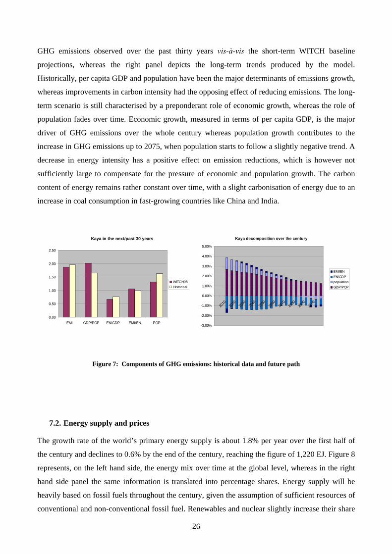
7.2. Energy supply and prices
The growth rate of the world’s primary energy supply is about 1.8% per year over the first half of
the century and declines to 0.6% by the end of the century, reaching the figure of 1,220 EJ. Figure 8
represents, on the left hand side, the energy mix over time at the global level, whereas in the right
hand side panel the same information is translated into percentage shares. Energy supply will be
heavily based on fossil fuels throughout the century, given the assumption of sufficient resources of
conventional and non-conventional fossil fuel. Renewables and nuclear slightly increase their share
27
in total energy supply. Backstop technologies are not deployed in the baseline scenario. Despite the
rising prices of fossil fuels, the incentives are not strong enough to induce the large up-front R&D
investments needed to make these technologies economically competitive.
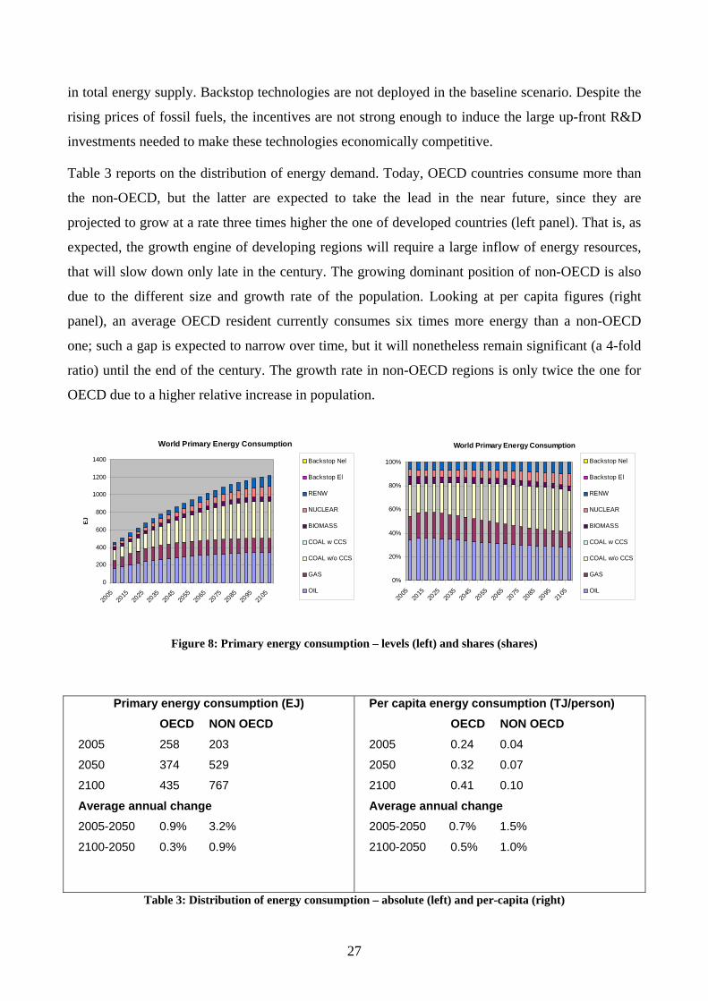
Table 3 reports on the distribution of energy demand. Today, OECD countries consume more than
the non-OECD, but the latter are expected to take the lead in the near future, since they are
projected to grow at a rate three times higher the one of developed countries (left panel). That is, as
expected, the growth engine of developing regions will require a large inflow of energy resources,
that will slow down only late in the century. The growing dominant position of non-OECD is also
due to the different size and growth rate of the population. Looking at per capita figures (right
panel), an average OECD resident currently consumes six times more energy than a non-OECD
one; such a gap is expected to narrow over time, but it will nonetheless remain significant (a 4-fold
ratio) until the end of the century. The growth rate in non-OECD regions is only twice the one for
OECD due to a higher relative increase in population.
Figure 8: Primary energy consumption – levels (left) and shares (shares)
Primary energy consumption (EJ) OECD NON OECD 2005 258 203
2050 374 529
2100 435 767
Average annual change 2005-2050 0.9% 3.2%
2100-2050 0.3% 0.9%
Per capita energy consumption (TJ/person) OECD NON OECD 2005 0.24 0.04
2050 0.32 0.07
2100 0.41 0.10
Average annual change 2005-2050 0.7% 1.5%
2100-2050 0.5% 1.0%
Table 3: Distribution of energy consumption – absolute (left) and per-capita (right)
World Primary Energy Consumption
0
200
400
600
800
1000
1200
1400
2005
2015
2025
2035
2045
2055
2065
2075
2085
2095
2105
EJ
Backstop Nel
Backstop El
RENW
NUCLEAR
BIOMASS
COAL w CCS
COAL w/o CCS
GAS
OIL
World Primary Energy Consumption
0%
20%
40%
60%
80%
100%
2005
2015
2025
2035
2045
2055
2065
2075
2085
2095
2105
Backstop Nel
Backstop El
RENW
NUCLEAR
BIOMASS
COAL w CCS
COAL w/o CCS
GAS
OIL
28
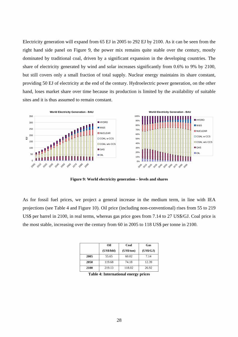
Electricity generation will expand from 65 EJ in 2005 to 292 EJ by 2100. As it can be seen from the
right hand side panel on Figure 9, the power mix remains quite stable over the century, mostly
dominated by traditional coal, driven by a significant expansion in the developing countries. The
share of electricity generated by wind and solar increases significantly from 0.6% to 9% by 2100,
but still covers only a small fraction of total supply. Nuclear energy maintains its share constant,
providing 50 EJ of electricity at the end of the century. Hydroelectric power generation, on the other
hand, loses market share over time because its production is limited by the availability of suitable
sites and it is thus assumed to remain constant.
World Electricity Generation - BAU
0
50
100
150
200
250
300
350
2005
2015
2025
2035
2045
2055
2065
2075
2085
2095
EJ
HYDRO
W&S
NUCLEAR
COAL w CCS
COAL w/o CCS
GAS
OIL
World Electricity Generation - BAU
0%
10%
20%
30%
40%
50%
60%
70%
80%
90%
100%
2005
2015
2025
2035
2045
2055
2065
2075
2085
2095
HYDRO
W&S
NUCLEAR
COAL w CCS
COAL w/o CCS
GAS
OIL
Figure 9: World electricity generation – levels and shares
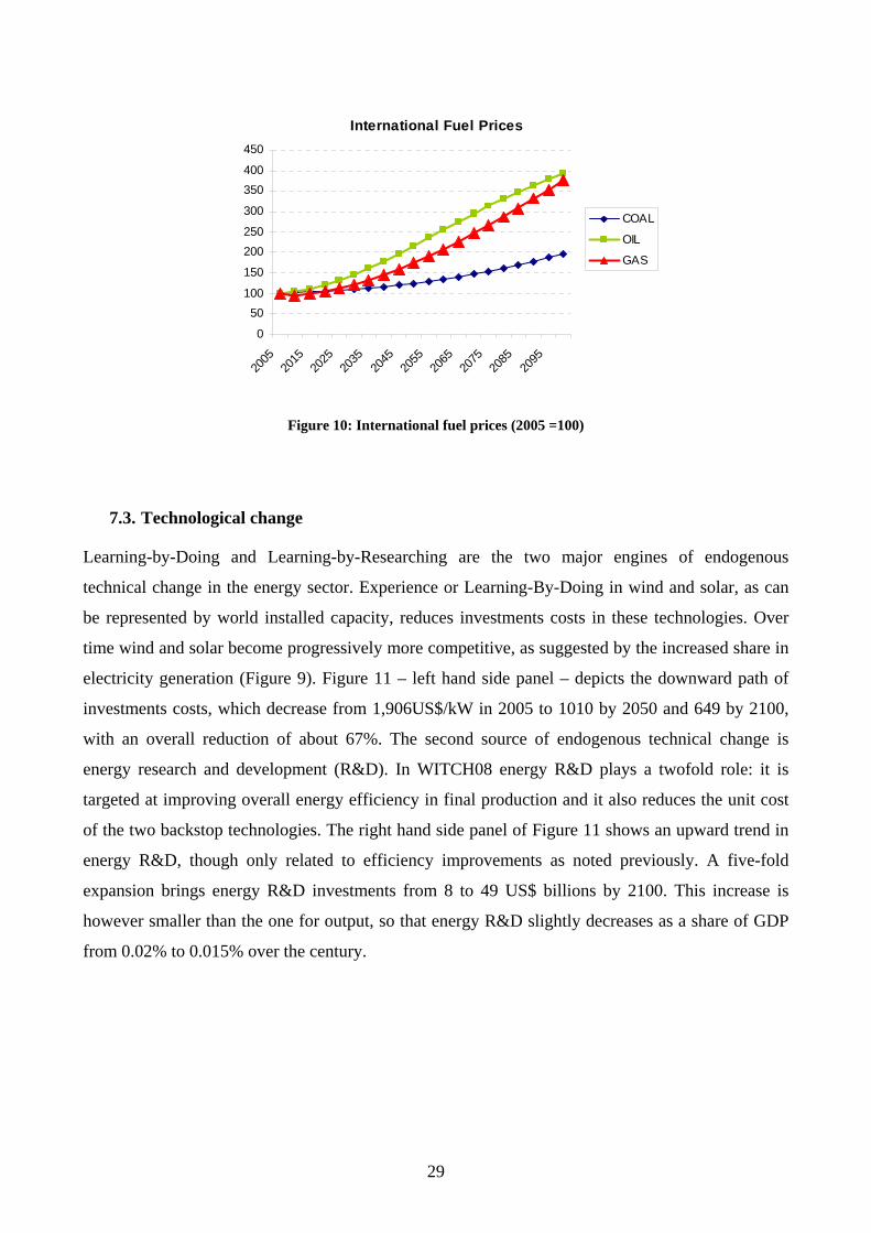
As for fossil fuel prices, we project a general increase in the medium term, in line with IEA
projections (see Table 4 and Figure 10). Oil price (including non-conventional) rises from 55 to 219
US$ per barrel in 2100, in real terms, whereas gas price goes from 7.14 to 27 US$/GJ. Coal price is
the most stable, increasing over the century from 60 in 2005 to 118 US$ per tonne in 2100.
Oil
(US$/bbl)
Coal
(US$/ton)
Gas
(US$/GJ)
2005 55.65 60.02 7.14
2050 119.68 74.18 12.39
2100 219.13 118.02 26.92
Table 4: International energy prices
29
International Fuel Prices
0
50100
150
200250
300
350400
450
2005
2015
2025
2035
2045
2055
2065
2075
2085
2095
COAL
OIL
GAS
Figure 10: International fuel prices (2005 =100)
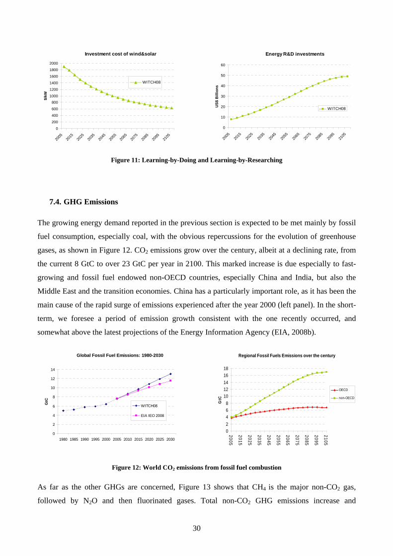
7.3. Technological change
Learning-by-Doing and Learning-by-Researching are the two major engines of endogenous
technical change in the energy sector. Experience or Learning-By-Doing in wind and solar, as can
be represented by world installed capacity, reduces investments costs in these technologies. Over
time wind and solar become progressively more competitive, as suggested by the increased share in
electricity generation (Figure 9). Figure 11 – left hand side panel – depicts the downward path of
investments costs, which decrease from 1,906US$/kW in 2005 to 1010 by 2050 and 649 by 2100,
with an overall reduction of about 67%. The second source of endogenous technical change is
energy research and development (R&D). In WITCH08 energy R&D plays a twofold role: it is
targeted at improving overall energy efficiency in final production and it also reduces the unit cost
of the two backstop technologies. The right hand side panel of Figure 11 shows an upward trend in
energy R&D, though only related to efficiency improvements as noted previously. A five-fold
expansion brings energy R&D investments from 8 to 49 US$ billions by 2100. This increase is
however smaller than the one for output, so that energy R&D slightly decreases as a share of GDP
from 0.02% to 0.015% over the century.
30
Investment cost of wind&solar
0
200
400
600
800
1000
1200
1400
1600
1800
2000
2005
2015
2025
2035
2045
2055
2065
2075
2085
2095
2105
$/kW
WITCH08
Energy R&D investments
0
10
20
30
40
50
60
2005
2015
2025
2035
2045
2055
2065
2075
2085
2095
2105
US$
Bill
ions
WITCH08
Figure 11: Learning-by-Doing and Learning-by-Researching
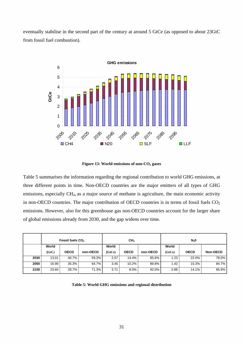
7.4. GHG Emissions
The growing energy demand reported in the previous section is expected to be met mainly by fossil
fuel consumption, especially coal, with the obvious repercussions for the evolution of greenhouse
gases, as shown in Figure 12. CO2 emissions grow over the century, albeit at a declining rate, from
the current 8 GtC to over 23 GtC per year in 2100. This marked increase is due especially to fast-
growing and fossil fuel endowed non-OECD countries, especially China and India, but also the
Middle East and the transition economies. China has a particularly important role, as it has been the
main cause of the rapid surge of emissions experienced after the year 2000 (left panel). In the short-
term, we foresee a period of emission growth consistent with the one recently occurred, and
somewhat above the latest projections of the Energy Information Agency (EIA, 2008b).
Global Fossil Fuel Emissions: 1980-2030
0
2
4
6
8
10
12
14
1980 1985 1990 1995 2000 2005 2010 2015 2020 2025 2030
GtC
WITCH08
EIA IEO 2008
Regional Fossil Fuels Emissions over the century
02468
1012141618
2005
2015
2025
2035
2045
2055
2065
2075
2085
2095
2105
GtC
OECD
non-OECD
Figure 12: World CO2 emissions from fossil fuel combustion
As far as the other GHGs are concerned, Figure 13 shows that CH4 is the major non-CO2 gas,
followed by N2O and then fluorinated gases. Total non-CO2 GHG emissions increase and
31
eventually stabilise in the second part of the century at around 5 GtCe (as opposed to about 23GtC
from fossil fuel combustion).
GHG emissions
0
1
2
3
4
5
6
2005
2015
2025
2035
2045
2055
2065
2075
2085
2095
GtC
e
CH4 N20 SLF LLF
Figure 13: World emissions of non-CO2 gases
Table 5 summarises the information regarding the regional contribution to world GHG emissions, at
three different points in time. Non-OECD countries are the major emitters of all types of GHG
emissions, especially CH4, as a major source of methane is agriculture, the main economic activity
in non-OECD countries. The major contribution of OECD countries is in terms of fossil fuels CO2
emissions. However, also for this greenhouse gas non-OECD countries account for the larger share
of global emissions already from 2030, and the gap widens over time.
Fossil fuels CO2 CH4 N20
World
(GtC) OECD non-OECD World
(GtCe) OECD non-OECD World
(GtCe) OECD Non-OECD
2030 13.01 40.7% 59.3% 2.57 14.4% 85.6% 1.23 22.0% 78.0%
2050 16.99 35.3% 64.7% 3.45 10.2% 89.8% 1.42 15.3% 84.7%
2100 23.60 28.7% 71.3% 3.71 8.0% 92.0% 0.88 14.1% 85.9%
Table 5: World GHG emissions and regional distribution
32
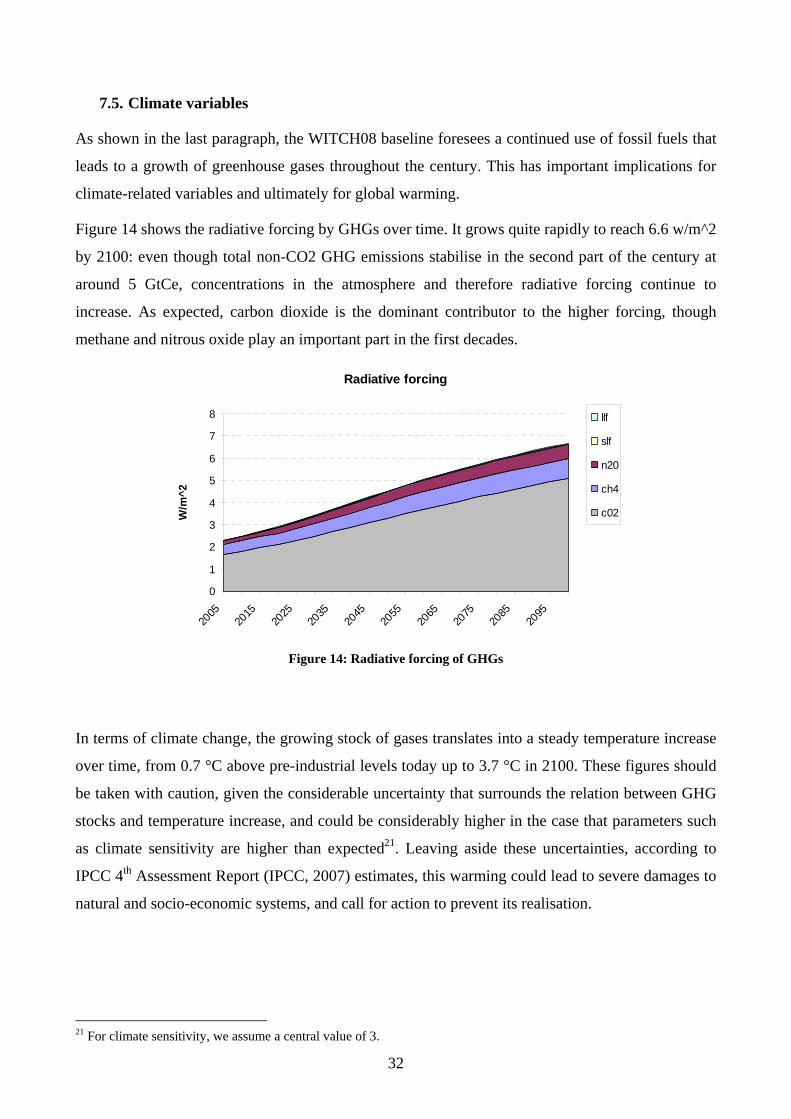
7.5. Climate variables
As shown in the last paragraph, the WITCH08 baseline foresees a continued use of fossil fuels that
leads to a growth of greenhouse gases throughout the century. This has important implications for
climate-related variables and ultimately for global warming.
Figure 14 shows the radiative forcing by GHGs over time. It grows quite rapidly to reach 6.6 w/m^2
by 2100: even though total non-CO2 GHG emissions stabilise in the second part of the century at
around 5 GtCe, concentrations in the atmosphere and therefore radiative forcing continue to
increase. As expected, carbon dioxide is the dominant contributor to the higher forcing, though
methane and nitrous oxide play an important part in the first decades.
Radiative forcing
0
1
2
3
4
5
6
7
8
2005
2015
2025
2035
2045
2055
2065
2075
2085
2095
W/m
^2
llf
slf
n20
ch4
c02
Figure 14: Radiative forcing of GHGs
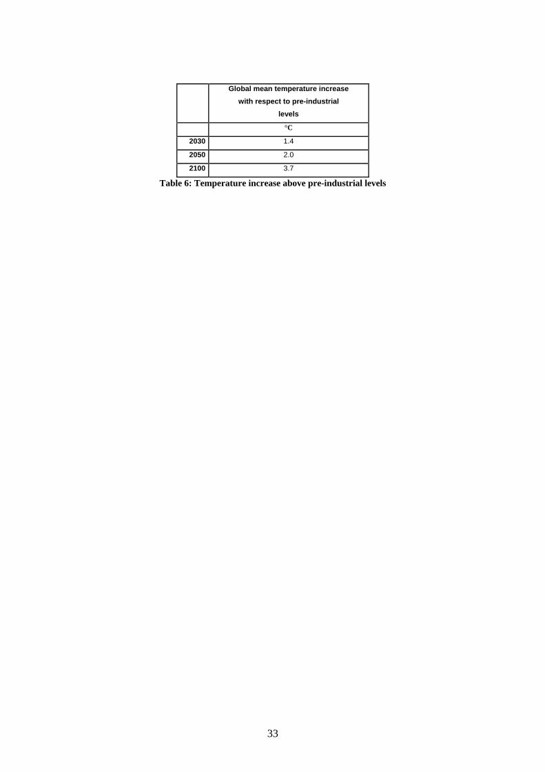
In terms of climate change, the growing stock of gases translates into a steady temperature increase
over time, from 0.7 °C above pre-industrial levels today up to 3.7 °C in 2100. These figures should
be taken with caution, given the considerable uncertainty that surrounds the relation between GHG
stocks and temperature increase, and could be considerably higher in the case that parameters such
as climate sensitivity are higher than expected21. Leaving aside these uncertainties, according to
IPCC 4th Assessment Report (IPCC, 2007) estimates, this warming could lead to severe damages to
natural and socio-economic systems, and call for action to prevent its realisation.
21 For climate sensitivity, we assume a central value of 3.
33
Global mean temperature increase with respect to pre-industrial
levels
°C
2030 1.4
2050 2.0
2100 3.7
Table 6: Temperature increase above pre-industrial levels
34
8. Conclusions
Climate change is a complex issue whose analysis requires models that are able to capture the
international, intertemporal and strategic dimension of climate change. With this regard, the
WITCH model can be considered a successful modelling tool.
WITCH08 improves several aspects of the first version WITCH06. Particular attention has been
paid to improve the evolution of technological change in the energy sector. The possibility of
investing in the commercialisation of innovative technologies is a desirable feature for models
evaluating long-term scenarios. WITCH08 has broadened the set of technology options by
including two backstop technologies, which can be thought of as a compact representation of
technologies that have not yet been commercialised. Special attention is given to the international
dimension of knowledge and experience diffusion.
The second important feature of WITCH08 is the inclusion of non-CO2 greenhouse gases. Other
GHGs are important contributors to global warming and they offer additional mitigation options,
increasing the model flexibility in responding to climate policies.
Reducing emissions from deforestation and degradation (REDD) offers another sizeable, low-cost
abatement option. WITCH08 can include a new baseline projection of land use CO2 emissions and
estimates of the global potential and costs for reducing emissions from deforestation.
The base year data has been updated to 2005 and new data on economic growth, energy prices and
technology costs have been used to re-calibrate the main exogenous drivers of the model, yielding
an updated future socio-economic baseline scenario. The main differences of the new baseline
scenario are driven by the upward revision of long-term world economic growth and mid-term
international energy prices.
35
9. Bibliography
Anderson, D. (2006). Costs and finance of carbon abatement in the energy sector, Paper for the
Stern Review.
Barreto, L. and S. Kypreos (2004). Endogenizing R&D and market experience in the "bottom-up"
energy-systems ERIS model, Technovation 2, 615-629.
Bosetti, V., C. Carraro, M. Galeotti, E. Massetti and M. Tavoni (2006). WITCH: A World Induced
Technical Change Hybrid Model, The Energy Journal. Special Issue on Hybrid Modeling of
Energy-Environment Policies: Reconciling Bottom-up and Top-down: 13-38.
Bosetti, V., C. Carraro, E. Massetti and M. Tavoni (2008). International energy R&D spillovers and
the economics of greenhouse gas atmospheric stabilization, Energy Economics, 30 (6) Pages
2912-2929.
Bosetti, V., R. Lubowski, A. Golub and A. Markandya (2009). Linking Reduced Deforestation and
a Global Carbon Market: Impacts on Costs, Financial Flows, and Technological Innovation,
Fondazione Eni Enrico Mattei Working Paper No 56.09, July 2009.
Criqui, P., G. Klassen and L. Schrattenholzer (2000). The efficiency of energy R&D expenditures.
Economic modeling of environmental policy and endogenous technical change, Amsterdam,
November 16-17, 2000.
Eliasch J. (2008) Climate Change: Financing Global Forests. The Eliasch Review, available at
http://www.occ.gov.uk/activities/eliasch.htm
EIA (2008). Annual Energy Outlook. Energy Information Administration, Washington, DC.
EIA (2008b). International Energy Outlook. Energy Information Administration, Washington, DC.
ENERDATA (2008). Energy Statistics.
EPA Report 430-R-06-003, June 2006. The report is available at
http://www.epa.gov/climatechange/economics/mitigation.html.
Farrell A.E. and Brandt, A.R.(2006). Risks of the oil transition, Environmental Research Letters, 1
(1).
IEA (2007). World Energy Outlook 2007. OECD/IEA, Paris.
IEA (2005). Resources to Reserves – Oil & Gas Technologies for the Energy Markets of the Future.
OECD/IEA, Paris.
IPCC (2007) Climate Change 2007: Synthesis Report. Contribution of Working Groups I, II and III
to the Fourth Assessment.
36
IPCC, (2007b): Climate Change 2007: Mitigation. Contribution of Working Group III to the Fourth
Assessment Report of the Intergovernmental Panel on Climate Change [B. Metz, O.R.
Davidson, P.R. Bosch, R. Dave, L.A. Meyer (eds)], Cambridge University Press,
Cambridge, United Kingdom and New York, NY, USA., XXX pp.
Jamasab, T. (2007). Technical change theory and learning curves: patterns of progress in electric
generation technologies, The Energy Journal 28 (3).
Junginger, M., A. Faaij and W. C. Turkenburg (2005). Global experience curves for wind farms,
Energy Policy 33: 133-150.
Kahouli-Brahmi, S. (2008). Technological learning in energy-environment-economy modelling: a
survey, Energy Policy 36: 138-162.
Klassen, G., A. Miketa, K. Larsen and T. Sundqvist (2005). The impact of R&D on innovation for
wind energy in Denmark, Germany and the United Kingdom, Ecological Economics 54 (2-
3): 227-240.
Kouvaritakis, N., A. Soria and S. Isoard (2000). Endogenous Learning in World Post-Kyoto
Scenarios: Application of the POLES Model under Adaptive Expectations, International
Journal of Global Energy Issues 14 (1-4): 228-248.
Kypreos, S. (2007). A MERGE model with endogenous technical change and the cost of carbon
stabilisation, Energy Policy 35: 5327-5336.
McDonald, A. and L. Schrattenholzer (2001). Learning rates for energy technologies, Energy Policy
29 (4): 255-261.
Nemet, G. F. (2006). Beyond the learning curve: factors influencing cost reductions in
photovoltaics, Energy Policy 34 (17): 3218-3232.
Nemet, G. F. and D. M. Kammen (2007). U.S. energy research and development: declining
investment, increasing need, and the feasibility of expansion, Energy Policy 35 (1): 746-755.
Schock, R. N., W. Fulkerson, M. L. Brown, R. L. San Martin, D. L. Greene and J. Edmonds (1999).
How much is energy research & development worth as insurance? Annual Review of Energy
and the Environment 24: 487-512.
Söderholm, P. and G. Klassen (2007). Wind power in Europe: a simultaneous innovation-diffusion
model, Environmental and Resource Economics 36 (2): 163-190.
Tavoni, M., B. Sohngen and V. Bosetti (2007), Forestry and the carbon market response to stabilise
climate, Energy Policy , 35: 5346–5353.
UN (2004), World Population to 2300, Report No. ST/ESA/SER.A/236, Department of Economic
and Social Affairs, Population Division, New York

37
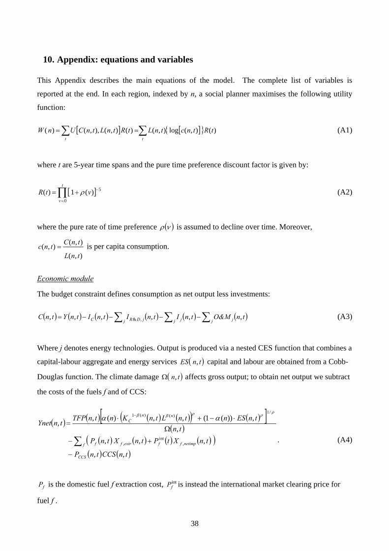
38
10. Appendix: equations and variables
This Appendix describes the main equations of the model. The complete list of variables is
reported at the end. In each region, indexed by n, a social planner maximises the following utility
function:
[ ] [ ]{ }∑∑ ==tt
tRtnctnLtRtnLtnCUnW )(),(log),()(),(),,()( (A1)
where t are 5-year time spans and the pure time preference discount factor is given by:
[ ]∏=
−+=t
v
vtR0
5)(1)( ρ (A2)
where the pure rate of time preference ( )νρ is assumed to decline over time. Moreover,
),(
),(),(tnL
tnCtnc = is per capita consumption.
Economic module
The budget constraint defines consumption as net output less investments:
( ) ( ) ( ) ( ) ( ) ( )∑ ∑∑ −−−−=j j jjj jDRC tnO&MtnItnItnItnYtnC ,,,,,, ,& (A3)
Where j denotes energy technologies. Output is produced via a nested CES function that combines a
capital-labour aggregate and energy services ( )tnES , capital and labour are obtained from a Cobb-
Douglas function. The climate damage ( )tn,Ω affects gross output; to obtain net output we subtract
the costs of the fuels f and of CCS:
( ) ( ) ( ) ( )( ) ( )[ ]( )
( ) ( ) ( ) ( )( )( ) ( )tnCCStnP
tnXtPtnXtnPtn
tnESntnLtnKntnTFPtnYnet
CCS
f netimpffextrff
nnC
,,
,,,,
,))(1(,,)(,,
,int
,
/1)()(1
−
+−
Ω⋅−+⋅
=
∑
−ρ
ρρββ αα
. (A4)
fP is the domestic fuel f extraction cost, intfP is instead the international market clearing price for
fuel f .
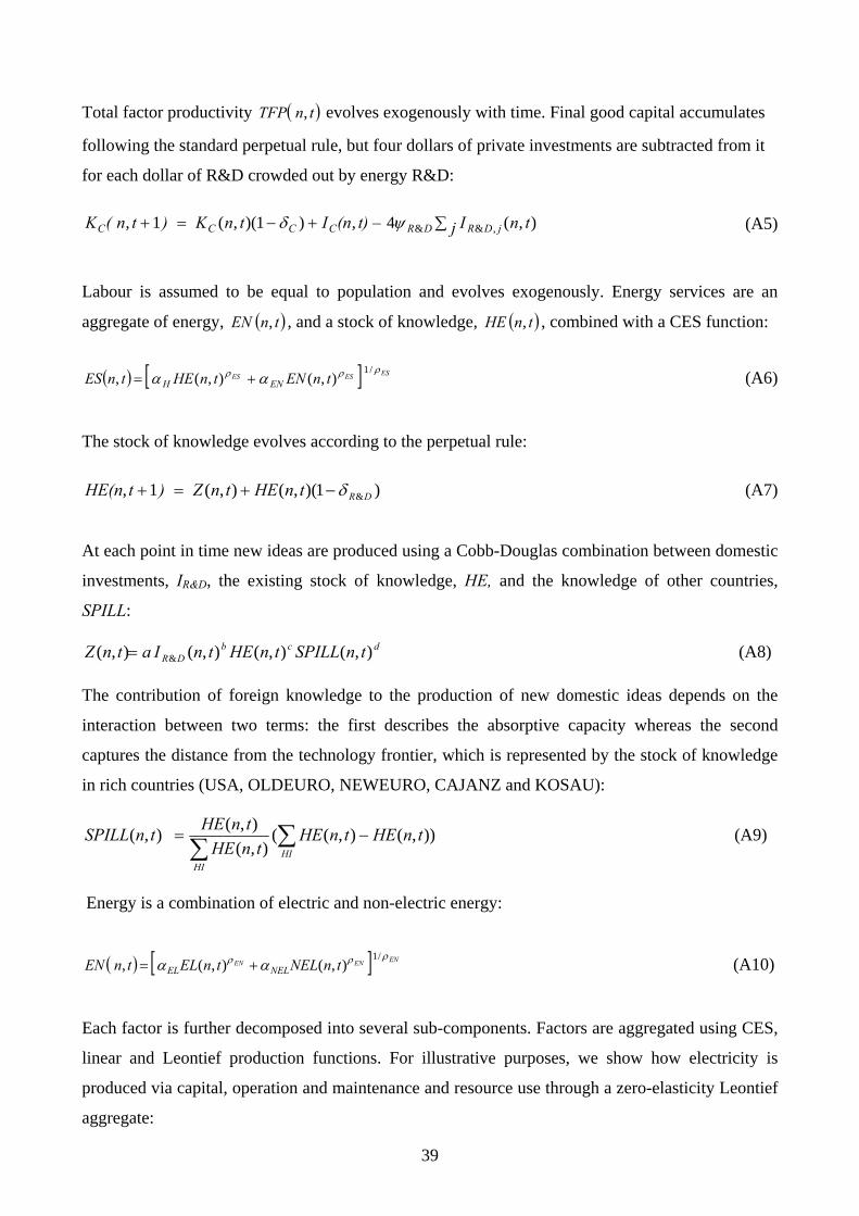
39
Total factor productivity ( )tnTFP , evolves exogenously with time. Final good capital accumulates
following the standard perpetual rule, but four dollars of private investments are subtracted from it
for each dollar of R&D crowded out by energy R&D:
∑+−=+ j tnIt) – (nItn K) tn(K jDRDRCCCC ),(4,)1)(,(1, ,&&ψδ (A5)
Labour is assumed to be equal to population and evolves exogenously. Energy services are an
aggregate of energy, ( )tnEN , , and a stock of knowledge, ( )tnHE , , combined with a CES function:
( ) [ ] ESESES tnENtnHEtnES ENHρρρ αα
/1),(),(, += (A6)
The stock of knowledge evolves according to the perpetual rule:
)1)(,(),(1, &DRtnHEtn Z) tHE(n δ−+=+ (A7)
At each point in time new ideas are produced using a Cobb-Douglas combination between domestic
investments, IR&D, the existing stock of knowledge, HE, and the knowledge of other countries,
SPILL:
dcbDR tnSPILLtnHEtnIatnZ ),(),(),(),( &= (A8)
The contribution of foreign knowledge to the production of new domestic ideas depends on the
interaction between two terms: the first describes the absorptive capacity whereas the second
captures the distance from the technology frontier, which is represented by the stock of knowledge
in rich countries (USA, OLDEURO, NEWEURO, CAJANZ and KOSAU):
)),(),((),(
),(),( tnHEtnHEtnHE
tnHEtnSPILLHI
HI
−= ∑∑ (A9)
Energy is a combination of electric and non-electric energy:
( ) [ ] ENENEN tnNELtnELtnEN NELELρρρ αα
/1),(),(, += (A10)
Each factor is further decomposed into several sub-components. Factors are aggregated using CES,
linear and Leontief production functions. For illustrative purposes, we show how electricity is
produced via capital, operation and maintenance and resource use through a zero-elasticity Leontief
aggregate:
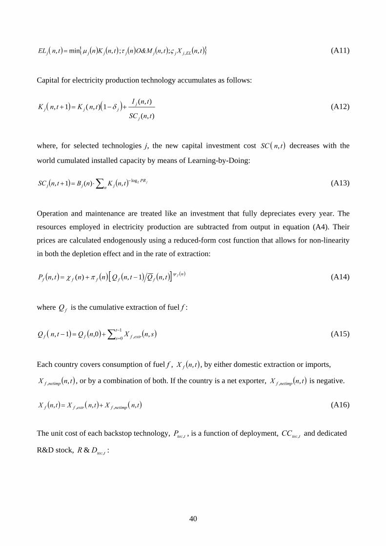
40
( ) ( ) ( ) ( ) ( ) ( ){ }tnXtnO&MntnKntnEL ELjjjjjjj ,;,;,min, ,ςτμ= (A11)
Capital for electricity production technology accumulates as follows:
( ) ( )),(
),(1),(1,
tnSC
tnItnKtnK
j
jjjj +−=+ δ (A12)
where, for selected technologies j, the new capital investment cost ( )tnSC , decreases with the
world cumulated installed capacity by means of Learning-by-Doing:
( ) ( )∑ −⋅=+n
PRjjj
jtnKnBtnSC 2log,)(1, (A13)
Operation and maintenance are treated like an investment that fully depreciates every year. The
resources employed in electricity production are subtracted from output in equation (A4). Their
prices are calculated endogenously using a reduced-form cost function that allows for non-linearity
in both the depletion effect and in the rate of extraction:
( ) ( ) ( ) ( )[ ] ( )nfffff
ftnQtnQnntnP ψπχ ,1,)(, −+= (A14)
where fQ is the cumulative extraction of fuel f :
( ) ( ) ( )∑ −
=+=−
1
0 , ,0,1,t
s extrfff snXnQtnQ (A15)
Each country covers consumption of fuel f , ( )tnX f , , by either domestic extraction or imports,
( )tnX netimpf ,, , or by a combination of both. If the country is a net exporter, ( )tnX netimpf ,, is negative.
( ) ( ) ( )tnXtnXtnX netimpfextrff ,,, ,, += (A16)
The unit cost of each backstop technology, ttecP , , is a function of deployment, ttecCC , and dedicated
R&D stock, ttecDR ,& :
41
b
tec
Ttec
c
tec
Ttec
tec
Ttec
CCCC
DRDR
PP
−−
−
⎟⎟⎠
⎞⎜⎜⎝
⎛⎟⎟⎠
⎞⎜⎜⎝
⎛=
0,
,
0,
2,
0,
, *&
& (A17)
R&D stock accumulates with the perpetual rule and with the contribution of international
knowledge spillovers, SPILL:
βαδ TtecTtecTtecTtec SPILLDIRDRDR ,,,1, &)1(&& +−⋅=+ (A18)
Climate Module
GHGs emissions from the combustion of fossil fuels are derived by applying the CO2
stoichiometric coefficients, 2,COfω to total consumption of fossil fuels, minus the amount of CO2
sequestered:
( ) ( ) ( )tnCCStnXtnCOf fCOf ,,,
2,2 −=∑ ω (A19)
The damage function impacting output varies with global temperature:
( )2,2,1 )()(1),( tTtTtn nn θθ ++=Ω (A20)
Temperature relative to pre-industrial levels increases through augmented radiating forcing F(t),
moderated by the cooling effects of SO2 aerosol, )(tcool :
(A21)
Radiative forcing in turn depends on CO2 atmospheric concentrations ( )tM AT , combined linearly
with the radiative forcing of other GHGs, )(tO :
[ ]{ } )()2log(/)(log)( tOMtMtF PIATAT +−=η (A22)
O(t) = FCH4(t)+FN20(t)+FSLF(t)+FLLF(t) (A23)
FCH4(t) =γ1,CH4 0.036 [γ2,CH4 MATCH4(t)0.5 – γ3,CH4 MPIATCH4(t) 0.5 ] (A24)
[ ]{ } )1()()()()1()()1( 21 +−−−−++=+ tcooltTtTtTtFtTtT LOσλσ
42
FN20(t) =γ1,N20 0.12 [γ2,N20 MATN20(t)0.5 – γ3,N20 MPIATN2O(t) 0.5 ] (A25)
FSLF(t) =2.571 [γ2,SLF MATSLF(t) – γ3,SLF MPIATSLF (t)] (A26)
FLLF(t) =13.026 [γ2,LLF MATLLF(t) – γ3,LLF MPIATLLF (t)] (A27)
CO2 atmospheric concentrations are caused by emissions from fuel combustion and land use
change; a three box-climate module accounts for the interaction between the atmosphere and
oceans:
( )[ ] )()()(,)1( 21112 tMtMtLUtnCOtM UPATn
jAT φφ +++=+ ∑ , (A28)
)()()()1( 321222 tMtMtMtM LOATUPUP φφφ ++=+ , (A29)
)()()1( 2333 tMtMtM UPLOLO φφ +=+ . (A30)
Other GHGs accumulate in the atmosphere according to the following equations:
MATCH4(t+1) – dec2 CH4(t)*0.5*Wo(t+1) = MATCH4(t) dec1CH4nyper(t)+dec2CH4(t)*0.5*Wo(t) (A31)
MATN20(t+1) – dec2 N2O(t)*0.5*Wo(t+1) = MATN2O(t) dec1N2Onyper(t)+dec2N2O(t)*0.5*Wo(t) (A32)
MATSLF(t+1) – dec2 SLF(t)*0.5*Wo(t+1) = MATSLF(t) dec1SLFnyper(t)+dec2SLF(t)*0.5*Wo(t) (A32)
MATLLF(t+1) – dec2 LLF(t)*0.5*Wo(t+1) = MATLLF(t) dec1LLFnyper(t)+dec2LLF(t)*0.5*Wo(t) (A33)
where dec2 and dec1 describes the yearly retention factor and the one period retention factor for
non-CO2 gases, respectively. The time step in WITCH is of 5 years and the parameter nyper(t)
accounts for the number of years in each period. Wo are world emissions of non-CO2 GHGs.
43
W = welfare
U = instantaneous utility C = consumption c = per-capita consumption L = population R = discount factor Y = net output Ιc = investment in final good ΙR&D,EN = investment in energy R&D Ιj = investment in technology j O&M = investment in operation and maintenance ΤFP = total factor productivity Κc = final good stock of capital ES = energy services Ω = climate feedback Pi
int = international fuels’ prices
Pj = fuels’ prices
X,f , extr = extracted fuel resources Xf , netimp fuel resources, net imports PCCS = price of CCS CCS = sequestered CO2 HE = energy knowledge EN = energy EL = electric energy NEL = non-electric energy KC = capital for final good production Κj= capital stock for technology j SCj = investment cost CO2 = emissions from combustion of fossil fuels MAT = atmospheric CO2 concentrations MATCH4 = atmospheric CH4 concentrations MATN20 = atmospheric N20 concentrations MATSLF = atmospheric concentrations of short lived fluorinated gases MATLLF = atmospheric concentrations of long lived fluorinated gases LU = land-use carbon emissions MUP = upper oceans/biosphere CO2 concentrations MLO = lower oceans CO2 concentrations F = radiative forcing FCH4 = radiative forcing of CH4 FN20 = radiative forcing of N20 FSLF = radiative forcing of short lived fluorinated gases

44
FLLF = radiative forcing of long-lived fluorinated gases O = radiative forcing from other gases T = temperature
NOTE DI LAVORO DELLA FONDAZIONE ENI ENRICO MATTEI
Fondazione Eni Enrico Mattei Working Paper Series
Our Note di Lavoro are available on the Internet at the following addresses: http://www.feem.it/Feem/Pub/Publications/WPapers/default.htm
http://www.ssrn.com/link/feem.html http://www.repec.org
http://agecon.lib.umn.edu http://www.bepress.com/feem/
NOTE DI LAVORO PUBLISHED IN 2009 SD 1.2009 Michael Hoel: Bush Meets Hotelling: Effects of Improved Renewable Energy Technology on Greenhouse Gas
Emissions SD 2.2009 Abay Mulatu, Reyer Gerlagh, Dan Rigby and Ada Wossink: Environmental Regulation and Industry LocationSD 3.2009 Anna Alberini, Stefania Tonin and Margherita Turvani: Rates of Time Preferences for Saving Lives in the
Hazardous Waste Site Context SD 4.2009 Elena Ojea, Paulo A.L.D. Nunes and Maria Loureiro: Mapping of Forest Biodiversity Values: A Plural
Perspective SD 5.2009 Xavier Pautrel : Macroeconomic Implications of Demography for the Environment: A Life-Cycle Perspective IM 6.2009 Andrew Ellul, Marco Pagano and Fausto Panunzi: Inheritance Law and Investment in Family Firms IM 7.2009 Luigi Zingales: The Future of Securities Regulation SD 8.2009 Carlo Carraro, Emanuele Massetti and Lea Nicita: How Does Climate Policy Affect Technical Change? An
Analysis of the Direction and Pace of Technical Progress in a Climate-Economy Model SD 9.2009 William K. Jaeger: The Welfare Effects of Environmental Taxation SD 10.2009 Aude Pommeret and Fabien Prieur: Double Irreversibility and Environmental Policy Design SD 11.2009 Massimiliano Mazzanti and Anna Montini: Regional and Sector Environmental Efficiency Empirical Evidence
from Structural Shift-share Analysis of NAMEA data SD 12.2009 A. Chiabai, C. M. Travisi, H. Ding, A. Markandya and P.A.L.D Nunes: Economic Valuation of Forest
Ecosystem Services: Methodology and Monetary Estimates SD 13.2009 Andrea Bigano, Mariaester Cassinelli, Fabio Sferra, Lisa Guarrera, Sohbet Karbuz, Manfred Hafner, Anil
Markandya and Ståle Navrud: The External Cost of European Crude Oil Imports SD 14.2009 Valentina Bosetti, Carlo Carraro, Romain Duval, Alessandra Sgobbi and Massimo Tavoni: The Role of R&D
and Technology Diffusion in Climate Change Mitigation: New Perspectives Using the Witch Model IM 15.2009 Andrea Beltratti, Marianna Caccavaio and Bernardo Bortolotti: Stock Prices in a Speculative Market: The
Chinese Split-Share Reform GC 16.2009 Angelo Antoci, Fabio Sabatini and Mauro Sodini: The Fragility of Social Capital SD 17.2009 Alexander Golub, Sabine Fuss, Jana Szolgayova and Michael Obersteiner: Effects of Low-cost Offsets on
Energy Investment – New Perspectives on REDD – SD 18.2009 Enrica De Cian: Factor-Augmenting Technical Change: An Empirical Assessment SD 19.2009 Irene Valsecchi: Non-Uniqueness of Equilibria in One-Shot Games of Strategic Communication SD 20.2009 Dimitra Vouvaki and Anastasios Xeapapadeas: Total Factor Productivity Growth when Factors of Production
Generate Environmental Externalities SD 21.2009 Giulia Macagno, Maria Loureiro, Paulo A.L.D. Nunes and Richard Tol: Assessing the Impact of Biodiversity
on Tourism Flows: A model for Tourist Behaviour and its Policy Implications IM 22.2009 Bernardo Bortolotti, Veljko Fotak, William Megginson and William Miracky: Sovereign Wealth Fund
Investment Patterns and Performance IM 23.2009 Cesare Dosi and Michele Moretto: Auctioning Monopoly Franchises: Award Criteria and Service Launch
Requirements SD 24.2009 Andrea Bastianin: Modelling Asymmetric Dependence Using Copula Functions: An application to Value-at-
Risk in the Energy Sector IM 25.2009 Shai Bernstein, Josh Lerner and Antoinette Schoar: The Investment Strategies of Sovereign Wealth Funds SD 26.2009 Marc Germain, Henry Tulkens and Alphonse Magnus: Dynamic Core-Theoretic Cooperation in a Two-
Dimensional International Environmental Model IM 27.2009 Frank Partnoy: Overdependence on Credit Ratings Was a Primary Cause of the Crisis SD 28.2009 Frank H. Page Jr and Myrna H. Wooders (lxxxv): Endogenous Network Dynamics SD 29.2009 Caterina Calsamiglia, Guillaume Haeringer and Flip Klijnb (lxxxv): Constrained School Choice: An
Experimental Study SD 30.2009 Gilles Grandjean, Ana Mauleon and Vincent Vannetelbosch (lxxxv): Connections Among Farsighted Agents SD 31.2009 Antonio Nicoló and Carmelo Rodríguez Álvarez (lxxxv): Feasibility Constraints and Protective Behavior in
Efficient Kidney Exchange SD 32.2009 Rahmi İlkiliç (lxxxv): Cournot Competition on a Network of Markets and Firms SD 33.2009 Luca Dall'Asta, Paolo Pin and Abolfazl Ramezanpour (lxxxv): Optimal Equilibria of the Best Shot Game SD 34.2009 Edoardo Gallo (lxxxv): Small World Networks with Segregation Patterns and Brokers SD 35.2009 Benjamin Golub and Matthew O. Jackson (lxxxv): How Homophily Affects Learning and Diffusion in
Networks
SD 36.2009 Markus Kinateder (lxxxv): Team Formation in a Network SD 37.2009 Constanza Fosco and Friederike Mengel (lxxxv): Cooperation through Imitation and Exclusion in Networks SD 38.2009 Berno Buechel and Tim Hellmann (lxxxv): Under-connected and Over-connected Networks SD 39.2009 Alexey Kushnir (lxxxv): Matching Markets with Signals SD 40.2009 Alessandro Tavoni (lxxxv): Incorporating Fairness Motives into the Impulse Balance Equilibrium and Quantal
Response Equilibrium Concepts: An Application to 2x2 Games SD 41.2009 Steven J. Brams and D. Marc Kilgour (lxxxv): Kingmakers and Leaders in Coalition Formation SD 42.2009 Dotan Persitz (lxxxv): Power in the Heterogeneous Connections Model: The Emergence of Core-Periphery
Networks SD 43.2009 Fabio Eboli, Ramiro Parrado, Roberto Roson: Climate Change Feedback on Economic Growth: Explorations
with a Dynamic General Equilibrium Mode GC 44.2009 Fabio Sabatini: Does Social Capital Create Trust? Evidence from a Community of Entrepreneurs SD 45.2009 ZhongXiang Zhang: Is it Fair to Treat China as a Christmas Tree to Hang Everybody’s Complaints? Putting
its Own Energy Saving into Perspective SD 46.2009 Eftichios S. Sartzetakis, Anastasios Xepapadeas and Emmanuel Petrakis: The Role of Information Provision
as a Policy Instrument to Supplement Environmental Taxes: Empowering Consumers to Choose Optimally SD 47.2009 Jean-François Caulier, Ana Mauleon and Vincent Vannetelbosch: Contractually Stable Networks GC 48.2009 Massimiliano Mazzanti, Susanna Mancinelli, Giovanni Ponti and Nora Piva: Education, Reputation or
Network? Evidence from Italy on Migrant Workers Employability SD 49.2009 William Brock and Anastasios Xepapadeas: General Pattern Formation in Recursive Dynamical Systems
Models in Economics SD 50.2009 Giovanni Marin and Massimiliano Mazzanti: Emissions Trends and Labour Productivity Dynamics Sector
Analyses of De-coupling/Recoupling on a 1990-2005 Namea SD 51.2009 Yoshio Kamijo and Ryo Kawasaki (lxxxv): Dynamics, Stability, and Foresight in the Shapley-Scarf Housing
Market IM 52.2009 Laura Poddi and Sergio Vergalli: Does Corporate Social Responsibility Affect the Performance of Firms? SD 53.2009 Valentina Bosetti, Carlo Carraro and Massimo Tavoni: Climate Change Mitigation Strategies in Fast-
Growing Countries: The Benefits of Early Action GC 54.2009 Alireza Naghavi and Gianmarco I.P. Ottaviano: Firm Heterogeneity, Contract Enforcement, and the Industry
Dynamics of Offshoring IM 55.2009 Giacomo Calzolari and Carlo Scarpa: On Regulation and Competition: Pros and Cons of a Diversified
Monopolist SD 56.2009 Valentina Bosetti, Ruben Lubowski and Alexander Golub and Anil Markandya: Linking Reduced
Deforestation and a Global Carbon Market: Impacts on Costs, Financial Flows, and Technological Innovation
IM 57.2009 Emmanuel Farhi and Jean Tirole: Collective Moral Hazard, Maturity Mismatch and Systemic Bailouts SD 58.2009 Kelly C. de Bruin and Rob B. Dellink: How Harmful are Adaptation Restrictions SD 59.2009 Rob Dellink, Michel den Elzen, Harry Aiking, Emmy Bergsma, Frans Berkhout, Thijs Dekker, Joyeeta Gupta:
Sharing the Burden of Adaptation Financing: An Assessment of the Contributions of Countries SD 60.2009 Stefania Tonin, Anna Alberini and Margherita Turvani: The Value of Reducing Cancer Risks at Contaminated
Sites: Are More Heavily Exposed People Willing to Pay More? SD 61.2009 Clara Costa Duarte, Maria A. Cunha-e-Sá and Renato Rosa: The Role of Forests as Carbon Sinks: Land-Use
and Carbon Accounting GC 62.2009 Carlo Altomonte and Gabor Békés: Trade Complexity and Productivity GC 63.2009 Elena Bellini, Gianmarco I.P. Ottaviano, Dino Pinelli and Giovanni Prarolo: Cultural Diversity and Economic
Performance: Evidence from European Regions SD 64.2009 Valentina Bosetti, Carlo Carraro, Enrica De Cian, Romain Duval, Emanuele Massetti and Massimo Tavoni:
The Incentives to Participate in, and the Stability of, International Climate Coalitions: A Game-theoretic Analysis Using the Witch Model
IM 65.2009 John Temple Lang: Article 82 EC – The Problems and The Solution SD 66.2009 P. Dumas and S. Hallegatte: Think Again: Higher Elasticity of Substitution Increases Economic Resilience SD 67.2009 Ruslana Rachel Palatnik and Roberto Roson: Climate Change Assessment and Agriculture in General
Equilibrium Models: Alternative Modeling Strategies SD 68.2009 Paulo A.L.D. Nunes, Helen Ding and Anil Markandya: The Economic Valuation of Marine Ecosystems IM 69.2009 Andreas Madestam: Informal Finance: A Theory of Moneylenders SD 70.2009 Efthymia Kyriakopoulou and Anastasios Xepapadeas: Environmental Policy, Spatial Spillovers and the
Emergence of Economic Agglomerations SD 71.2009 A. Markandya, S. Arnold, M. Cassinelli and T. Taylor: Coastal Zone Management in the Mediterranean:
Legal and Economic Perspectives GC 72.2009 Gianmarco I.P. Ottaviano and Giovanni Prarolo: Cultural Identity and Knowledge Creation in Cosmopolitan
Cities SD 73.2009 Erik Ansink: Self-enforcing Agreements on Water allocation GC 74.2009 Mario A. Maggioni, Francesca Gambarotto and T. Erika Uberti: Mapping the Evolution of "Clusters": A
Meta-analysis SD 75.2009 Nektarios Aslanidis: Environmental Kuznets Curves for Carbon Emissions: A Critical Survey SD 76.2009 Joan Canton: Environmentalists' Behaviour and Environmental Policies SD 77.2009 Christoph M. Rheinberger: Paying for Safety: Preferences for Mortality Risk Reductions on Alpine Roads
IM 78.2009 Chiara D’Alpaos, Michele Moretto, Paola Valbonesi and Sergio Vergalli: "It Is Never too late": Optimal Penalty for Investment Delay in Public Procurement Contracts
SD 79.2009 Henry Tulkens and Vincent van Steenberghe: “Mitigation, Adaptation, Suffering”: In Search of the Right Mix in the Face of Climate Change
SD 80.2009 Giovanni Bella: A Search Model for Joint Implementation SD 81.2009 ZhongXiang Zhang: Multilateral Trade Measures in a Post-2012 Climate Change Regime?: What Can Be
Taken from the Montreal Protocol and the WTO? SD 82.2009 Antoine Dechezleprêtre, Matthieu Glachant, Ivan Hascic, Nick Johnstone and Yann Ménière: Invention and
Transfer of Climate Change Mitigation Technologies on a Global Scale: A Study Drawing on Patent Data SD 83.2009 László Á. Kóczy: Stationary Consistent Equilibrium Coalition Structures Constitute the Recursive Core SD 84.2009 Luca Di Corato and Michele Moretto: Investing in Biogas: Timing, Technological Choice and the Value of
Flexibility from Inputs Mix SD 85.2009 Valentina Bosetti, Enrica De Cian, Alessandra Sgobbi, and Massimo Tavoni: The 2008 WITCH Model: New
Model Features and Baseline
(lxxxv) This paper has been presented at the 14th Coalition Theory Network Workshop held in Maastricht, The Netherlands, on 23-24 January 2009 and organised by the Maastricht University CTN group (Department of Economics, http://www.feem-web.it/ctn/12d_maa.php).


