The constraint based decomposition (CBD) training architecture

Contributed article

The constraint based decomposition (CBD) training architecture

Sorin DraÏghici*

431 State Hall, Department of Computer Science, Wayne State University, Detroit, MI 48202, USA

Received 8 March 1999; revised 18 January 2001; accepted 18 January 2001

Abstract

The Constraint Based Decomposition (CBD) is a constructive neural network technique that builds a three or four layer network, has

guaranteed convergence and can deal with binary, n-ary, class labeled and real-value problems. CBD is shown to be able to solve complicated

problems in a simple, fast and reliable manner. The technique is further enhanced by two modi®cations (locking detection and redundancy

elimination) which address the training speed and the ef®ciency of the internal representation built by the network. The redundancy

elimination aims at building more compact architectures while the locking detection aims at improving the training speed. The computational

cost of the redundancy elimination is negligible and this enhancement can be used for any problem. However, the computational cost of the

locking detection is exponential in the number of dimensions and should only be used in low dimensional spaces. The experimental results

show the performance of the algorithm presented in a series of classical benchmark problems including the 2-spiral problem and the Iris,

Wine, Glass, Lenses, Ionosphere, Lung cancer, Pima Indians, Bupa, TicTacToe, Balance and Zoo data sets from the UCI machine learning

repository. CBD's generalization accuracy is compared with that of C4.5, C4.5 with rules, incremental decision trees, oblique classi®ers,

linear machine decision trees, CN2, learning vector quantization (LVQ), backpropagation, nearest neighbor, Q* and radial basis functions

(RBFs). CBD provides the second best average accuracy on the problems tested as well as the best reliability (the lowest standard deviation).

q 2001 Published by Elsevier Science Ltd.

1. Introduction

Many training algorithms require that the initial architec-

ture of the network be speci®ed as a prerequisite for the

training. If this is the case, one is confronted with the dif®-

cult task of choosing an architecture well suited to the task at

hand. If the chosen architecture is not powerful enough for

the given task (e.g. it does not have enough hidden units or

layers) the training will fail. On the other hand, if the chosen

architecture is too rich, the representation built by the

network will be inappropriate and the network will exhibit

bad generalization properties (e.g. over®tting). There are

two fundamentally different approaches to overcoming

this problem. One of them is to build the network from

scratch adding units as needed. The category of algorithms

following this approach is known as constructive algo-

rithms. The other approach is to start with a very rich initial

architecture and eliminate some of the units either during or

after the training. This category of algorithms is known as

pruning algorithms.

Constructive algorithms share a number of interesting

properties. Most such algorithms are very fast and very

reliable in the sense that they are guaranteed to converge

to a solution for any problem in their scope. However, some

constructive algorithms have a very limited scope and in

general, they are believed to give poor generalization

results. Non-constructive algorithms are much less reliable

than constructive algorithms and can fail to converge even

when a solution exists (Brady, Raghavan & Slawny, 1989).

Some non-constructive algorithms can even converge to

`false' solutions (Brady, Raghavan & Slawny, 1988).

However, some researchers believe that they offer better

generalization results and, therefore, are better suited to

real world problems (SÂmieja, 1993).

More recently, the issue of the `transparency' of a neural

network (or its ability to provide an explanation for its

output) has become very important. Very often, neural

network techniques are used in combination with a separate

rule extraction module in which a different technique is used

to translate the internal architecture of the network into

some human understandable symbolic form. In many appli-

cations, the output of the network inspires little con®dence

without such a symbolic backup which can be analyzed by

human experts.

The technique presented in this paper, the Constraint

Based Decomposition (CBD) is a constructive algorithm

that is guaranteed to ®nd a solution for any classi®cation

Neural Networks 14 (2001) 527±550PERGAMON

Neural

Networks

0893-6080/01/$ - see front matter q 2001 Published by Elsevier Science Ltd.

PII: S0893-6080(01)00040-5

www.elsevier.com/locate/neunet

* Tel.: 11-313-577-5484.

E-mail address: [email protected] (S. DraÏghici).

problem, is fast and builds an architecture as needed. Apart

from these characteristics shared by all algorithms in its

class, CBD has other interesting properties such as: (1) it

is ¯exible and can be used with a variety of weight changing

mechanisms; (2) it is more transparent than other neural

network techniques inasmuch as it can provide a symbolic

description of the internal structure built during the training;

(3) the generalization abilities of the solution are compar-

able with or better than those of other neural and non-neural

machine learning techniques; and (4) it is very stable in the

sense that the generalization accuracy has a very low stan-

dard deviation over many trials.

The paper is organized as follows. First, we present the

basic version of the CBD technique and a proof of its

convergence. Other subsections in this part discuss some

issues related multiclass classi®cation, extending the algo-

rithm to problems with continuous outputs and two other

enhancements of the basic technique. The experimental

section focuses on two aims: (i) assessing the impact of

each individual enhancement upon the performance of the

plain CBD algorithm and (ii) assessing the training and

generalization performances of the CBD algorithm against

other neural and non-neural machine learning techniques.

The training and generalization performances of the CBD

are assessed on two classical benchmarks and 11 problems

from the UCI machine learning repository. The results are

compared with those of 10 other neural and non-neural

machine learning techniques. A discussion section

compares CBD with several related algorithms and techni-

ques. Finally, the last section of the paper presents some

conclusions.

2. The Constraint Based Decomposition (CBD)algorithm

The CBD algorithm consists of (i) a pattern presentation

algorithm, (ii) a construction mechanism for building the net

and (iii) a weight change algorithm for a single layer

network. The pattern presentation algorithm stipulates

how various patterns in the pattern set are presented to the

network. The construction mechanism speci®es how the

units are added to form the ®nal architecture of the trained

network. Both the pattern presentation algorithm and the

construction mechanism are speci®c to the CBD technique.

The weight change algorithm speci®es quantitatively how

the weights are changed from one iteration to another. CBD

can work with any weight change algorithm able to train a

single neuron (gradient descent, conjugate gradient, percep-

tron, etc.) and some of its properties will depend on the

choice of such algorithm.

The technique derived its name from a more general

approach based on the idea of reducing the dimensionality

of the search space through decomposing the problem into

sub-problems using subgoals and constraints de®ned in the

problem space. The description of the general approach is

outside the scope of the present paper, but a formal de®ni-

tion of constraints and a complete description of the more

general approach can be found in Draghici (1994, 1995).

2.1. The ®rst hidden layer

In its simplest form, the CBD is able to solve any classi-

®cation problem involving binary or real valued inputs.

Without loss of generality we shall a classi®cation problem

involving patterns from Rd (d [ N) belonging to two classes

C1 and C2. The goal of our classi®cation problem is to sepa-

rate the patterns in the set S� C1 < C2. For now, we shall

assume that the units used implement a threshold function.

Extensions of the algorithm to other types of units will be

addressed later. We shall also assume that the chosen weight

changing mechanism is able to train reliably a single neuron

(e.g. perceptron for binary values). a reliable weight chan-

ging mechanism is de®ned as an algorithm that will ®nd a

solution in a ®nite time if a solution exists.

The CBD algorithm starts by choosing one random

pattern from each class. Let these patterns be x1 belonging

to C1 and x2 belonging to C2. Let S be the union of C1 and C2

and m1 and m2 be the number of patterns in C1 and C2,

respectively. The two patterns x1 and x2 constitute the

current subgoal Scurrent� {x1, x2} and are removed from

the set S. The training starts with just one hidden unit.

This hidden unit will implement a hyperplane in input

space. The algorithm uses the weight changing mechanism

to move the hyperplane so that it separates the given

patterns x1 and x2. If the pattern set is consistent (i.e. each

pattern belongs to only one class), this problem is linearly

separable.1 Therefore, a solution will always exist and the

weight changing mechanism (assumed to be reliable) will

®nd it. Then, the CBD algorithm will choose another

random pattern from S and add it to the current subgoal

Scurrent. The weight changing mechanism will be invoked

again and will try to adjust the weights so that the current

subgoal (now including three patterns) is separated. This

subgoal training may or may not be successful. If the weight

changing mechanism has been successful in adjusting the

position of the hyperplane so that even the last added pattern

is classi®ed correctly, the algorithm will choose another

random pattern from S, remove it from there, add it to the

current subgoal Scurrent and continue in the same way.

However, unless the classes C1 and C2 are linearly separ-

ableÐwhich would make the problem trivialÐone such

subgoal training will eventually fail. Since all previous

subgoal training was successful, the pattern that caused

the failure was the one that was added last. This pattern

will be removed from the current subgoal. Also recall that

this pattern was removed from S when it was added to

Scurrent. Another pattern will be chosen and removed from

S. DraÏghici / Neural Networks 14 (2001) 527±550528

1 In n-dimensions, one can start with an initial training set that includes n

patterns chosen randomly from the two classes. If these n patterns are in

general positions (i.e. they are not linearly dependent) they are linearly

separable.

S, added to the current subgoal and a new subgoal training

will be attempted. Note that the weight search problem

posed by the CBD algorithm to the weight changing

mechanism is always the simplest possible problem since

it involves just one layer, one unit and a pattern set contain-

ing at most one misclassi®ed pattern. This process will

continue until all patterns in S have been considered. At

this point in time, the algorithm has trained completely

the ®rst hidden unit of the architecture. The position of

the hyperplane implemented by this hidden unit is such

that it correctly classi®es the patterns in the set Scurrent and

it misclassi®es the patterns in the set {C1 < C2} 2 Scurrent. If

the set of misclassi®ed patterns is empty, the algorithm will

stop because the current architecture solves the given

problem. If there are patterns which are misclassi®ed by

the current architecture, the algorithm will analyze the

two half-spaces determined by the hyperplane implemented

by the previous hidden unit. At least one such half-space

will be inconsistent in the sense that it will contain patterns

from both C1 and C2 that are found in this inconsistent half-

space. A new hidden unit will be added and trained in the

same way so that it separates the patterns in the new goal S.

The CBD algorithm is presented in Fig. 1 in a recursive

form which underlines the divide-and-conquer strategy

used. This version of the algorithm also constructs the

symbolic representation of the solution as described

below. The algorithm is presented as a recursive function

which takes as parameters a region of interest in the input

space, one set of patterns from each class and a factor.

Initially, the algorithm will be called with region� Rd, all

patterns in C1 and C2 and a null initial factor.

2.2. Subsequent layers and symbolic representations

Since the patterns are now separated by the hyperplanes

implemented by the hidden units, the outputs can now be

obtained using a variety of methods depending on the parti-

cular needs of the problem. One such method is to synthe-

size the output using a layer of units implementing a logical

AND and another layer implementing a logical OR (see

Fig. 2). This particular method allows the algorithm

shown in Fig. 3 to produce a symbolic description of the

binary function implemented by the network.

Let us assume that the results of the CBD search is a set of

hidden units which implement the hyperplanes h1, h2, ¼, hn.

These hyperplanes will determine a set of regions in the

input space. These regions will be consistent from the

point of view of the given classi®cation problem in

the sense that they will contain only patterns of one class.

Each such region can be expressed as an intersection of

some half-spaces determined by the given hyperplanes. In

the symbolic description provided by the algorithm a consis-

tent region will be described by a term. A term will have the

form Ti� (sign(h1)h1´sign(h2)h2´´ ´ ´´sign(hn)h

n, Cj) where sign(h1) can be 1, 21, or nil and Cj is the class to

which the region belongs. A nil sign means that the corre-

sponding hyperplane does not actually appear in the given

term. A negative sign will be denoted by overlining the

corresponding hyperplane as in �hi. No overline means the

sign is positive.

Each hyperplane will divide the input space into two half-

spaces, one positive and one negative. A hyperplane and its

sign will be represented by a factor. A factor can be used to

represent one of the two half-spaces determined by the

hyperplane. A term is obtained by performing a logical

AND between factors. Not all hyperplanes will contribute

with a factor to all terms. Finally, a logical OR is performed

between terms in order to obtain the expression of the solu-

tion for each class. Fig. 4 presents an example involving two

S. DraÏghici / Neural Networks 14 (2001) 527±550 529

Fig. 1. The CBD algorithm.

Fig. 2. The architecture built by the algorithm.

hyperplanes (lines) in 2D. The ` 1 ' character marks the

positive half-space of each hyperplane. Using the notation

above, the regions in Fig. 4 can be described as follows: A �h1´h2;B � h1´ �h2;C � �h1´ �h2 and D � �h1´h2. If class C1

included the union of regions B and D, we should describe

it as C1 � h1´ �h2 1 �h1´h2.

The ®nal network constructed by CBD will be described

in a symbolic form by a set of expressions as explained

above. Although some interesting conclusions can always

be extracted from such symbolic descriptions (e.g. the

problem is linearly separable or not; some classes are line-

arly separable, etc.), they are not always meaningful to the

end user. Also, these symbolic forms of the solutions might

become complicated for highly non-linear or high dimen-

sional problems. More work needs to be done in order to

explore fully the potential of CBD in this direction but this is

beyond the scope of the present paper.

2.3. Proof of convergence

A simpli®ed version of the algorithm in Fig. 1 will be

used to prove the convergence of the CBD training. This

simpli®ed version presented in Fig. 3 does not store the

solution and it does not look for a good solution. An inef®-

cient solution will suf®ce. In the worst case, the solution

given by this algorithm will construct regions containing

only a single pattern which is very wasteful. Let us assume

there are m (distinct) patterns xi (i � 1;¼;m) of n input

variables. Each pattern xi belongs to one of two classes C1

and C2. It is assumed that m is ®nite.

One can prove that this algorithm converges under the

assumption that, for any two given patterns, a hyperplane

that separates them can be found in a ®nite time. This

assumption is used in step 3. From the termination condition

1 it is clear that if the algorithm terminates, this happens

because the region contains only patterns from the same

class or no patterns at all. Because the two patterns chosen

in step 2 are separated (using the assumption above) in step

3, and because they are removed from the pattern set, both

patternset1 and patternset2 will contain at least one pattern

less than pattern set. This implies that after at most m 2 1

recursive steps the procedure separate will be called with a

region containing just one pattern. Such a region satis®es the

termination condition 1 and the algorithm will terminate.

This worst-case situation happens when the consistent

regions containing only patterns from the same class all

contain just one pattern. In this case, the input space is

shattered into m regions.

Note that the termination condition and the recursive

mechanism are identical for both the simpli®ed algorithm

in Fig. 3 and the CBD algorithm in Fig. 1. The difference

between them is that the CBD algorithm in Fig. 1 tries to

decrease the number of hyperplanes used by trying to opti-

mize their positions with respect to all the patterns in the

current training set (the ®rst for loop in the algorithm in Fig.

1). This means that the CBD algorithm cannot perform

worse than the simpli®ed algorithm, i.e. it is guaranteed to

converge in at most m 2 1 recursive steps for any pattern set

containing m patterns. The number of such steps and

therefore the number of hidden units deployed by the


Fig. 3. A simpli®ed version of the algorithm.

Fig. 4. The formalism used in the symbolic expression of the internal

representation built by the network. The regions can be described as

follows: A� h1´h2, B� h1´ �h2, C � �h1´ �h2 and D � �h1´ �h2.

CBD algorithm in Fig. 1 will be somewhere between

log2{min(m1, m2)} in the best case and max(m1, m2) 2 1

in the worst case. The best case corresponds to a situation in

which the algorithm positions the hyperplanes such that for

each subgoal an equal number of patterns from the least

numerous class is found in each half-space. The worst

case corresponds to a situation in which each hyperplane

only separates one single pattern from the most numerous

class. One should note that the worst-case scenario takes

into consideration only the pattern presentation algorithm

presented above. In practice, d 2 1 patterns in arbitrary

positions in d dimensions will be linearly separable by an

n-dimensional hyperplane so, for a reliable weight changing

mechanism, the worst case will never happen.

3. Enhancements of the constraint based decomposition

3.1. Multiclass classi®cation

The algorithm can be extended to classi®cation problems

involving more than one class in several different ways. Let

us assume the problem involves classes C1, C2, ¼, Ck. The

®rst approach is to choose two arbitrary classes (let us say C1

and C2) and separate them. This will produce a number of

hyperplanes which determine a partition of the input space

into regions R1, R2, ¼, Rp. The ®rst approach is to iterate on

these regions. The algorithm will be called recursively on

each such region until all regions produced contain only

patterns belonging to a single class. Since at every iteration

the number of patterns is reduced by at least one, the algo-

rithm will eventually stop for any ®nite number of patterns.

The second approach iterates on the classes of the

problem. For each remaining class Cj, each pattern will be

taken and fed to the network in order to identify the region

in which this pattern lies. Let this region be Ri and the class

assigned to this region be Cik. The algorithm will be called to

separate Cj from Cik in Ri. In each such subgoal training, the

pattern from classes subsequent to Cj (in the arbitrary order

in which patterns are considered) will be ignored. The algo-

rithm need not worry about the classes precedent to Cj,

because they have already been considered and the current

region is consistent from their point of view. This process

will be repeated until all patterns from all classes have been

considered.

A third approach involves some modi®cations of the

algorithm. The modi®ed algorithm is presented in Fig. 5.

In this case, the algorithm will choose a random pattern xi.

Subsequently, all other patterns considered which do not

belong to the same class Ci will be assigned a new target


Fig. 5. The multiclass CBD algorithm.

value T. Thus, the weight changing mechanism will still be

called on the simplest possible problem: separating just one

misclassi®ed pattern in a two-class problem. Practically, the

hyperplanes will be positioned so that the class of the

pattern chosen ®rst will be separated from all others.

Since the ®rst pattern is chosen at random for each subgoal

pattern (i.e. for each hidden unit), no special preference will

be given to any particular class. This is the approach used to

obtain the results presented below.

If the problem to be solved involves many classes and if a

distributed environment is available, one could consider

another approach to multiclass classi®cation. In this

approach, the algorithm will be executed in parallel on a

number of processors equal to the number of classes in the

problem. Each processor will be assigned a class and will

separate the assigned class from all the others. This can be

achieved through re-labeling the patterns of the n 2 1

classes which are not assigned. The solution provided by

this version of the algorithm will be more wasteful through

the redundancy of the solutions but might still be interesting

due to the parallel features and the availability of `class

experts' i.e. networks specialized in individual classes.

3.2. Continuous outputs

The CBD algorithm was described above in the context of

classi®cation problems. However, this is not an intrinsic

limitation of this algorithm. The algorithm can be extended

to deal with continuous outputs in a very simple manner that

will be described in the following.

A ®rst step is to use only the sign of the patterns in order

to construct the network using the CBD algorithm presented

above. Using only the sign of the patterns transforms the

problem into a classi®cation problem and the algorithm can

be applied directly. The architecture obtained from this step

is already guaranteed to separate the patterns with the hyper-

planes implemented by the ®rst hidden layer. Now, the

threshold activation functions of all neurons will be substi-

tuted by sigmoid activation functions and the training will

proceed with the desired analog values.

Since the hidden layer already separates the patterns, a

low error (correct classi®cation) weight state is guaranteed

to exist for the given problem. The weights of the ®st hidden

layer will be initialized with weight vectors having the same

direction as the weight vectors found in the previous step. A

number of weight changing mechanisms (e.g. backpropaga-

tion, quickprop, conjugate gradient descent, etc.) can now

be used in order to achieve the desired continuous I/O beha-

vior by minimizing the chosen error measure.

3.3. Ef®cient use of the hyperplanes

Due to its divide and conquer approach and the lack of

interaction between solving different problems in different

areas of the input space, the solution built by the CBD

algorithm will not necessarily use the minimum number

of hyperplanes. This is a characteristic common to several

constructive algorithms that was used to argue that such

algorithms exhibit worse generalization in comparison to

other types of algorithms (SÂmieja, 1993). Fig. 6 (left)

presents a non-optimal solution which uses three hyper-

planes in a situation in which two hyperplanes would be

suf®cient. Since the problem is not linearly separable, the

CBD algorithm will start by separating some of the patterns

using a ®rst hidden unit. This ®rst hidden unit will imple-

ment either hyperplane 1 or hyperplane 2. Let us suppose it

implements hyperplane 1. Subsequently, the search will be

performed in each of the half-spaces determined by it. At

least one hyperplane will be required to solve the problem in

each half-space even though one single hyperplane could

separate all patterns.

There are different types of optimizations which can be

performed. In the middle panel of Fig. 6, hyperplanes 4 and

5 are redundant because they classify in the same way (up to

a sign reversal) all patterns in the training set. This type of

redundancy will be called global redundancy because the

hyperplanes perform the same classi®cation at the level of

the entire training set.

This type of redundant units are equivalent to the `non

contributing units' described in Siestma and Dow (1991). In

the cited work, the elimination of this type of redundancy is

done by changing all weights connected to the unit which

will be preserved. A better redundancy elimination method

will be presented shortly.

In the same middle panel of Fig. 6, hyperplanes 2 and 3

are only locally redundant, i.e. they perform the same


Fig. 6. Redundancy issues. Left: a non-optimal solution. Middle: hyperplanes 4 and 5 are globally redundant whereas 2 and 3 are locally redundant. Right:

hyperplanes 2 and 4 separate the patterns in the negative half-space of hyperplane 1. A new hyperplane is needed to separate the patterns in the positive half-

space of 1.

separation in a limited region of the space, in this case, the

positive half-space of hyperplane 1. The hyperplanes are not

globally redundant because they classify patterns (a) and (b)

differently. Consequently, a global search for redundant

units cannot eliminate this type of redundancy.

It is interesting to note that, in the case of the CBD algo-

rithm (and most other constructive techniques), other types

of redundancy, discussed in Siestma and Dow (1991), such

as units which have constant output across the training set or

unnecessary-information units, are avoided by the algorithm

itself.

3.4. Eliminating redundancy

Let us consider the problem presented in the middle panel

of Fig. 6. Let us suppose the ®rst hyperplane introduced

during the training is hyperplane 1. Its negative half-space

is checked for consistency, found to be inconsistent and the

algorithm will try to separate the patterns in this negative

half-space (the others will be ignored for the moment).

Then, let us assume that hyperplane 2 will be placed as

shown (see also the right panel of Fig. 6). Its positive

half-space (intersected with the negative half-space of

hyperplane 1) is consistent and will be labeled as a black

region. The algorithm will now consider the region deter-

mined by the intersection of the negative half-spaces of 1

and 2, which is inconsistent. Hyperplane 4 will be added to

separate the patterns in this region and the global solution

for the negative half-space of 1 will be �h1h2 1 �h1�h2�h4 as a

black region and �h1�h2h4 as a white region.

The situation after adding hyperplanes 1, 2 and 4 is

presented in the right panel of Fig. 6. Then, the algorithm

will consider the positive half-space of hyperplane 1 and will

try to separate the patterns in this region. A new hyperplane

will be introduced to separate the patterns in the positive half-

space of hyperplane 1. Eventually, this hyperplane will end

up between one of the groups of white patterns and the group

of black patterns. Let us suppose it will end up between

groups (a) and (b). This hyperplane will be redundant

because hyperplane 2 could perform exactly the same task.

The redundancy is caused by fact that the algorithm takes

into consideration only local pattern information, i.e. only

the patterns situated in the area currently under considera-

tion, ignoring the others. At the same time, this is one of the

essential features of the algorithm, the feature which ensures

the convergence and yields a high training speed. Consider-

ing all the patterns in the training set is a source of problems

(consider for instance the herd effect, Fahlman & Lebiere,

1990). One seems to face an insoluble question. Can an

algorithm be local so that the training is easy and global

so that too much redundancy is avoided? The answer, at

least for the constructive CBD algorithm, is af®rmative.

The solution is to consider the patterns locally, as in stan-

dard CBD, but to take into consideration previous solutions

as well. Thus, although the patterns are not considered glob-

ally which would make the problem dif®cult, some global

information is used which will eliminate some redundancy

from the ®nal solution.

Let us reconsider separating the patterns in the positive

half-space of hyperplane 1 with a new hyperplane between

groups (a) and (b). Instead of automatically accepting this

position, the algorithm could check whether there are other

hyperplanes that classify the patterns in the positive half-

space of hyperplane 1 in the same way. In this case, hyper-

plane 2 does this and it will be used instead of a new hyper-

plane. Note that this does not affect in any way the previous

partial solutions and, therefore, the convergence of the algo-

rithm is still ensured. At the same time, this modi®cation

ensures the elimination of both global and local redundancy

and is done without taking into consideration all patterns.

Computationally, this check needs only two passes (to

cater for the possibly different signs) through the current

subgoal. In each pass, the output of the candidate hyper-

plane unit is compared with the outputs of the existing

units. If at the end of this, an existing unit is found to behave

like the candidate unit, the existing unit will substitute the

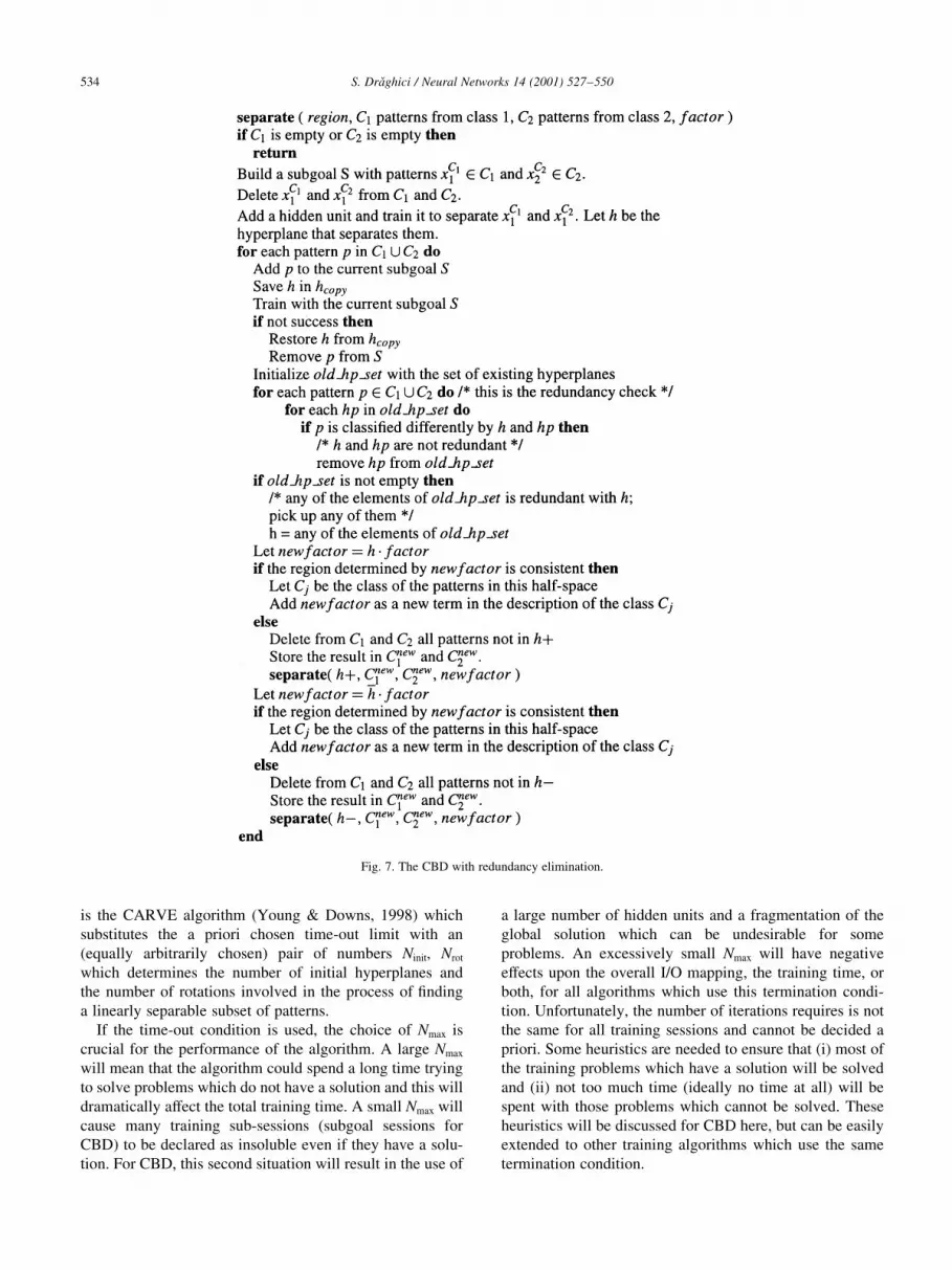
candidate unit which will be discarded. The enhanced algo-

rithm is presented in Fig. 7.

3.5. Locking detection

One of the characteristics of the constraint based decom-

position algorithm is that the actual weight updating is

performed only in very simple networks with just one

non-input neuron. In geometrical terms, only one hyper-

plane is moved at any single time. In the following discus-

sion we shall consider a problem in a d-dimensional space.

There are two qualitatively distinct training situations. The

®rst situation is that of a ®rst training after a new neuron has

been added. In this situation, the pattern set contains

patterns which form a linearly separable problem and the

problem can always be solved. This is because the number

of the patterns is restricted to at most d and the patterns are

assumed to be in general position (i.e. not belonging to a

subspace with fewer dimensions). The second situation is

that of adding a pattern to a training set containing more

than d patterns. In this case, the problem is to move the

existing hyperplane so that even the last added pattern is

correctly classi®ed. There is no guarantee that a solution

exists for this problem because the last pattern could have

made the problem linearly inseparable. This determines a

termination problem. When should the training be stopped if

the error will never go below its limit?

The simplest solution is to use a time-out condition. The

training is halted if no solution has been found in a given

number of iterations Nmax. This condition is used by the

simplest implementation of the CBD algorithm and by the

vast majority of constructive algorithms such as tiling

(Mezard & Nadal, 1989), the upstart (Frean, 1990), exten-

tron (Baffes & Zelle, 1992), the pocket algorithm (Gallant,

1986), divide and conquer networks (Romanuik & Hall,

1993) and so forth. A notable exception to this approach


is the CARVE algorithm (Young & Downs, 1998) which

substitutes the a priori chosen time-out limit with an

(equally arbitrarily chosen) pair of numbers Ninit, Nrot

which determines the number of initial hyperplanes and

the number of rotations involved in the process of ®nding

a linearly separable subset of patterns.

If the time-out condition is used, the choice of Nmax is

crucial for the performance of the algorithm. A large Nmax

will mean that the algorithm could spend a long time trying

to solve problems which do not have a solution and this will

dramatically affect the total training time. A small Nmax will

cause many training sub-sessions (subgoal sessions for

CBD) to be declared as insoluble even if they have a solu-

tion. For CBD, this second situation will result in the use of

a large number of hidden units and a fragmentation of the

global solution which can be undesirable for some

problems. An excessively small Nmax will have negative

effects upon the overall I/O mapping, the training time, or

both, for all algorithms which use this termination condi-

tion. Unfortunately, the number of iterations requires is not

the same for all training sessions and cannot be decided a

priori. Some heuristics are needed to ensure that (i) most of

the training problems which have a solution will be solved

and (ii) not too much time (ideally no time at all) will be

spent with those problems which cannot be solved. These

heuristics will be discussed for CBD here, but can be easily

extended to other training algorithms which use the same

termination condition.


Fig. 7. The CBD with redundancy elimination.

The idea of locking was inspired by a symbolic AI techni-

que (the candidate elimination, Mitchell, 1977, 1978). A lock-

ing situation can be de®ned as a situation in which the

patterns contained in the current training subset determine

the position of the dividing hyperplane up to a suitably chosen

tolerance (see Fig. 8). In this situation, adding new patterns to

the training set and continuing training is useless because the

position of the dividing hyperplane cannot be changed outside

the given tolerance without misclassifying some patterns.

We shall start by considering the following de®nitions:

De®nition. Two sets are said to be linearly separable if

and only if there exists a hyperplane H that separates them.

De®nition. Let C1 and C2 be two linearly separable sets of

patterns from two classes. C1 and C2 determine a locking

situation with tolerance e 0 if and only if for all di, dj,

di�xi;¼; xn� � a1x1 1 ¼ 1 anxn 1 an11

dj�x1;¼; xn� � b1x1 1 ¼ 1 bnxn 1 bn11

such that

1. di(pk) . 0, ;pk [ C1

2. di(pk) , 0, ;pk [ C2

3. dj(pk) . 0, ;pk [ C1

4. dj(pk) , 0, ;pk [ C2

arccos~ni´~nj

u~niuu~nju, e0

where ni � �a1; a2; a3;¼; an� and nj � �b1; b2; b3;¼; bn� are

the gradient vectors of di and dj, respectively.

Conditions 1±4 mean that di and dj are separating hyper-

planes for the classes C1 and C2. The sign of the classi®ca-

tion is not relevant because for any di classifying C1 in its

negative half-space there exist a 2di such that the negative

half-space of di is the positive half-space of 2di. The de®ni-

tion says that the patterns determine a locking situation with

tolerance e 0 if and only if the angle between the normals of

any two separating hyperplanes is less than e 0.

Note that according to this de®nition, any two linearly

separable sets of patterns create a locking situation with

some tolerance. In practice, we are interested in those lock-

ing situations that have a tolerance such that any further

training is likely to be of little use. These instances will

be called tight tolerance locking situations.

A locking detection mechanism by itself would not be

very useful unless one could calculate a meaningful locking

tolerance using some simple statistical properties of the data

set of the given problem. We shall consider a locking situa-

tion as presented in case B in Fig. 8. It is clear that the

patterns impose more restrictions when the pairs of opposite

patterns are further apart (see Fig. 9). For this reason, we

shall consider the furthest two such pairs of patterns for any

given data set.

We can consider the smallest hypersphere S that includes

all patterns. Let the radius of this hypersphere be r. We are

interested in the most restricted situation, so we shall consider

that the two pairs of patterns from Fig. 9 are situated as far

apart as possible, i.e. on the surface of this hypersphere. We


Fig. 8. Two locking situations in two dimensions. The color of the patterns represents their class. The position of the hyperplane cannot be changed without

misclassifying some patterns.

Fig. 9. Two pairs of opposite patterns locking a hyperplane. For the same distance between patterns within a pair, the further away the pairs are, the more

restricted the position of the hyperplane will be.

shall keep the distance between the patterns in pair A ®xed

and we shall study what happens when the distance between

the patterns in pair B increases. Keeping the distance between

the patterns in pair A ®xed and assuming that this distance is

much smaller than the diameter of the hypersphere, means

that we assume the hyperplane can move only by rotation

around the pair A (see Fig. 10).

Furthermore, let us assume that the minimum Euclidean

distance between two patterns from different classes is dmin

and that the two patterns p1 and p2 in pair B are separated by

this distance. If we consider the hyperplane rotating around

the pair A, we obtain an angle b � arcsin�dmin=4r�: This

angle can be taken as a reasonable value for the locking

tolerance since we are interested in movements of the hyper-

plane that will change the classi®cation of at least one point.

Note that considering the case in which the points p1 and p2

are on the hypersphere is a worst-case situation in the sense

that, if another pair of patterns of opposite classes, say p 01 and

p 02, existed closer to the center, the hyperplane would need to

move with an angle more than a in order to change the

classi®cation of any such point. Also note that a tolerance

calculated in this way has only a heuristic value because one

can easily construct arti®cial examples in which changing the

position of the hyperplane by less than a would change the

classi®cation of some patterns. However, the experiments

showed that such a value is useful in practice and determines

an improvement of the training time.

The following criterion will identify some elements

which in¯uence how tight a locking situation is.

3.6. Characterization of a locking situation

Let us consider two sets of patterns from two linearly separ-

able classes Ci and Cj. Let hk be a separating hyperplane, xi be

an arbitrary pattern from Ci and Hkj be the convex hull deter-

mined by the projection on hk of all points in Cj. The following

observations will characterize a locking situation:

1. A necessary condition for a tight tolerance locking situa-

tion determined by xi and Cj is that the projection of xi on

any separating hyperplane hk fall in the convex hull Hkj.

2. A necessary condition for a tight tolerance locking situa-

tion determined by x1;¼; xm1from C1 and y1;¼; ym2

from

C2 is that the intersection of the convex hulls of the projec-

tion of x1;¼; xm1and y1;¼; ym2

on any dividing hyper-

plane be non-degenerate.2

3. The tolerance of the locking situation determined by xi and

Cj is inversely proportional to the maximum distance from

xi to a separating hyperplane hk.

4. The tolerance of the locking situation determined by xi and

Cj is inversely proportional to the maximum distance from

the projection of xi on a dividing hyperplane hk to the

centroid3 of the convex hull Hkj.

A full justi®cation for the criterion above will be omitted for

space reasons. However, the cases 1±4 above are exempli®ed

for the two-dimensional case in Figs. 11 and 12. In these

®gures, the shaded areas represent the set of possible positions

for a dividing hyperplane. The smaller the surface of the

shaded areas, the tighter the locking situation.

3.7. Two locking detection heuristics

We shall present and discuss two heuristics for locking

detection based on the discussion above. Although these

heuristics do not take into consideration all possible types

of locking they have been shown to be able to improve the

training speed. For a more detailed discussion of various

types of locking see Draghici (1995).

Let us suppose there are two classes C1 and C2 in a d-

dimensional space. A possibility for pinpointing the position

of a hyperplane in a d-dimensional space is to have d 1 1

points of which d are on one side of the hyperplane and one

is on the other side of it. This would be the d-dimensional

generalization of the locking situation determined by three

patterns case A in Fig. 8. Although there are other types of

locking situations, the analysis will concentrate on this type

®rst.

For this situation, the extreme positions of the dividing

hyperplane such that all patterns are still correctly classi®ed

are determined by all combinations of d 2 1 patterns from

C1 and a pattern from C2. Each such combination (d points

in a d-dimensional space) determines a hyperplane and all

these hyperplanes determine a simplex4 in the d-dimen-

sional space. If all these hyperplanes are close (the simplex

is squashed towards the dividing hyperplane) then this

hyperplane is pinpointed and the locking has occurred.

The locking test can be a comparison of the gradients of

the hyperplanes determined by combinations of d 2 1 points


Fig. 10. If we rotate a hyperplane around the point A with an angle less than

b , the classi®cation of either p1 or p2 will remain the same.

2 There is no (d 2 1)-dimensional space that includes the intersection.

This also implies that the intersection is not empty.3 The centroid of a set of points p1,¼,pn [ Rd is their arithmetic mean

(p1 1 ´ ´ ´ 1 pn)/d i.e. the point whose coordinates are the arithmetic mean of

the corresponding coordinates of the points p1,¼,pn.4 A simplex is the geometrical ®gure consisting, in d dimensions, of

d 1 1 points (or vertices) and all their interconnecting line segments, poly-

gonal faces, etc. In two dimensions, a simplex is a triangle. In three dimen-

sions it is a tetrahedron, not necessarily the regular tetrahedron.

from one class and one point from the other class. A heur-

istic for locking detection based on the ideas presented

above is given in Fig. 13.

A heuristic able to detect such locking situations will

consider the d points closest to the boundary from each

class. Finding such points requires O(m1 1 m2) computations

where m1 and m2 are the number of patterns in C1 and C2,

respectively. The number of combinations of one pattern from

one class and d patterns from the opposite class as required by

the algorithm given is O(d). In the worst case, d hyperplanes

must be compared for each set of points. Therefore, the heur-

istic needs O(m1 1 m2) 1 O(d2) computations up to this stage.

The number of operations needed to construct the convex hull

of the d patterns closest to the dividing hyperplane is O��d 21��d21�=2�11� in the worst case (Preparata & Shamos, 1985). In

general, the convex hull can be constructed using any classi-

cal computational geometry technique. However, one parti-

cularly interesting technique is the beneath±beyond method

which has the advantage that it is suitable for on-line use (i.e.

it constructs the hull by introducing one point at a time). In

consequence, if the iterative step of the CBD algorithm adds

the new pattern in such a way that the previous d 2 1 patterns

from the hull are still among the closest d patterns, the effort

necessary to construct the convex hull will only be O(fd22)

i.e. linear in the number of (d 2 2)-dimensional facets (note

that we are considering the convex hull of the projections on

the dividing hyperplane which is a (d 2 1)-dimensional

space). The number of operations needed to check whether

the projection of pk is internal to this convex hull is O(d 2 1).

In the best case, the convex hull will not be affected by the

introduction of the new point so the effort will be limited to

checking the distances from the dividing hyperplane which is

O(m). In conclusion, this heuristic will need O(m1 1 m2) in

the best case and O(m1 1 m2) 1 O��d 2 1��d21�=2�11� in the

worst case. Note that d is the number of dimensions of the

input space and, therefore, is always lower than the number of

patterns. If the number of dimensions is larger than the

number of patterns, the patterns (assumed to be in general

position) are linearly independent and the classes are separ-

able, so there is no need to check for locking.

However, there are tight locking situations that are not

detected by the heuristic presented above. An example of

such a locking situation in two dimensions is presented in

case B in Fig. 8. In this particular situation, no subset of two

points from one class and another point from the opposite

class would determine a tight locking situation.

The second locking detection heuristic assumes that the

number of patterns is larger than the dimensionality d (as

justi®ed above) and that the locking is determined by

several patterns from each class.

In these conditions, one could consider the d points

closest to the dividing hyperplane from each class and

calculate the hyperplane determined by them. If the two

hyperplanes are close enough (the angle of their normals

is less than the chosen tolerance e 0) and if the convex

hulls determined by the projections on the dividing hyper-

plane intersect (and the intersection is not degenerate), then

locking is present. The d closest points to the boundary are

found and used to determine a border hyperplane for each

class. The current separating hyperplane is compared with

the two border hyperplanes. If all three are close to each

other, the d closest points from each class are projected on


Fig. 12. A loose locking situation (condition 4). The projection of the white

pattern xi is far from the centroid of the convex hull determined by the

projections of patterns from Cj.

Fig. 11. Left: a loose locking situation (condition 1). The projection of the white pattern does not fall within the convex hull determined by the projections on

the separating hyperplane of the patterns from the opposite class. Middle: a loose locking situation (condition 2). Above, the convex hulls of the projections of

the white and black patterns do not intersect on all dividing hyperplanes. Below, the hulls do intersect and the locking is tight. Right: a loose locking situation

(condition 3). The white pattern is far from the furthest separating hyperplane.

the boundary. If the hulls thus determined intersect in a non-

degenerate way, locking is present. This heuristic is

presented in Fig. 14.

The tolerance of the locking is still inversely proportional

to the distance from the patterns to the dividing hyperplane

as described in the locking characterization above. Thus,

theoretically, there exist situations in which the three hyper-

planes used by the heuristic above are (almost) parallel5

without a tight locking. This can happen if the two `clouds'

of patterns are far from each other but the d closest patterns

from each class happen to determine two parallel hyper-

planes which are also parallel with the current separating

hyperplane. The probability of such a situation is negligible

and the heuristic does not take it into account.

This heuristic needs O(m1 1 m2) operations to ®nd the d

closest patterns and construct the border hyperplanes. In the

best case, nothing more needs to be done. In the worst case,

both convex hulls need to be re-constructed and this will

take O��d 2 1��d21�=2�11� computations. In general, calcu-

lating the intersection of two polyhedrons in a d-dimen-

sional space is computationally intensive. However, the

algorithm does not require the computation of the intersec-

tion, but only the detection of such. A simple (but rather

inef®cient) method for detecting such intersection is to

consider each point in one of the hulls and classify all

vertices of the other hull as either concave, supporting or

re¯ex (as in Section 3.3.6 in Preparata & Shamos, 1985)

which in turn can be done in O��d 2 1��d21�=2�11� in the

worst case.

The characteristics of the heuristics presented above

make them well suited for problems involving a large

number of patterns in a relatively low dimensional space

(less than ®ve variables) due to their worst-case behavior.

In higher dimensional spaces, the savings in training time

provided by detecting locking situations can be offset by the

complexity of the computations necessary by the algorithms

above and the use of the CBD technique without this

enhancement is suggested. However, in low dimensional

spaces, the locking detection can save up to 50% of the

training time as shown by some of the experiments

presented in the next section.

4. Experimental results

4.1. Hypotheses to be veri®ed by the experiments

A ®rst category of experiments was designed to inves-

tigate the effectiveness of the enhancements proposed

above. These experiments compare results obtained with

the plain CBD algorithm to results obtained by activating

one enhancement at a time. Two criteria have been moni-

tored: the size of the network and the duration of the

training. Due to the fact that CBD can be used to generate

either a 3-layer (hidden-AND-OR layers) or a 2-layer

(hidden and output layers) architecture, the total number

of units depends on this choice. Therefore, the size of the

network was characterized only by the number of hyper-

planes used (equal to the number of units on the ®rst

hidden layer) as opposed to the total number of units.

The locking detection is expected to bring an improve-

ment of the training speed without affecting the number of

hyperplanes used in the solution. The redundancy elimi-

nation is expected to reduce the number of hyperplanes

used in the solution without affecting the training speed.


Fig. 14. Heurstic 2 for locking detection in d dimensions.

Fig. 13. Heuristic 1 for locking detection in d dimensions.

5 In d dimensions, the parallelism is not necessarily a symmetric relation.

In this context, parallel is meant as `strictly parallel' (according to the

de®nitions used in Borsuk, 1969) which is a symmetric relation.

These expectations, if con®rmed, would allow the redun-

dancy elimination and the locking detection to be used

simultaneously, summing their positive effects.

All enhancements have been experimented on three

problems: the 2-spiral problem with 194 patterns, the 2-

spiral problem with 770 patterns (for the same total

lengthÐthree times around the origin) and the 2-grid

problem (see Fig. 15). The 2-grid problem can be seen as

a 2D extension of the XOR problem or as a 2D extension of

the parity problem (in the 2-grid problem, the output should

be 1ÐblackÐif the sum of the Cartesian coordinates is

odd). We have chosen this extension to the parity problem

for two reasons. Firstly, we believe it is more dif®cult to

solve such a problem by adding patterns in the same number

of dimensions instead of increasing the number of dimen-

sions and looking merely in the corners of the unit

hypercube. Secondly, we wanted to emphasize the ability

of the technique to cope with real-valued input values, abil-

ity that differentiates CBD from many other constructive

algorithms.

Due to the fact that different algorithms use a different

amount of work per epoch or patterns, a machine indepen-

dent speed comparison of various techniques is not a simple

matter. In order to provide results independent of any parti-

cular machine, operating system or programming language,

the training speed is reported by counting the operations

performed by the algorithm, in a manner similar to that

widely used in the analysis of algorithm complexity

(Knuth, 1976) and to the `connection-crossings' used by

Fahlman (Fahlman & Lebiere, 1990). Due to its constructive

character and its guaranteed convergence properties, CBD

exhibits excellent speed characteristics. A detailed explana-

tion of the methods used to assess the training speed and

speed comparisons with other algorithms are presented in

Draghici (1995). Those experiments showed CBD is a few

orders of magnitude faster than backpropagation in dedi-

cated, custom designed architectures and a few times faster

than other constructive techniques such as divide-and-

conquer networks (Romaniuk & Hall, 1993), on speci®c

problems. The focus of the experiments presented here

was to investigate the generalization properties of CBD

and how they compare with the generalization properties

of other neural and non-neural machine learning techniques.

4.2. Methods used

In order to compare the effects of a particular enhance-

ment, a number of tests were performed using the algorithm

with and without the enhancement. Each individual experi-

ment was run in the same conditions for the two versions:

the same initial weight state, order of the patterns, weight-

changing mechanism, etc. The t-test was used to check

whether the means of the two samples are signi®cantly

different.

A second category of experiments was aimed at compar-

ing the performances of the CBD algorithm with perfor-

mances of other existing machine learning techniques.

Here, the focus of the experiments was the generalization

abilities of the techniques. We used the classical methods of

leave-one-out and n-fold cross-validation as well as separate

training and validation set, as appropriate (Breiman, Fried-

man, Olsen & Stone, 1984).

4.3. Experimental results

The CBD was implements in C11 and Java. The results

presented below were obtained with the Java version imple-

mented by Christopher Gallivan.

4.3.1. Locking detection

The locking detection is expected to be more effective in

some problems and less effective in others. In order to assess

correctly the ef®ciency of this mechanism, a problem of

each category has been chosen. A problem for which the

locking detection mechanism was expected to bring an

important improvement is the 2-spiral problem (proposed

originally by Wieland and cited inLang & Witbrock, 1989).

This is because this problem is characterized by a relatively

large number of patterns in the training set, a high degree of

non-linearity and, therefore, needs a solution with a rela-

tively large number of hyperplanes. Due to the distribution

of the patterns, it was expected that some hyperplanes be

locked into position by some close patterns. The results of

20 trials using 20 different orderings of the patterns in the

training set containing 194 patterns are presented in Fig. 16.

The average number of operations (connection crossings)

used by the variation without locking was 65,340,103.5.


Fig. 15. Two of the benchmarks used: the 2-grid problem with 20 patterns and the 2-spiral problem with 194 patterns.

The locking detection version used only 32,192,110.8

operations which corresponds to an average speed improve-

ment of 50.73%.

The t-test showed that the speed improvement is signi®-

cant for the 5% level of con®dence.6 The same test

performed on data regarding the number of hyperplanes

showed that there is no evidence that the locking affects

the number of hyperplanes.

A problem for which the locking detection mechanism

was not expected to bring such a spectacular improvement is

the 2-grid problem presented in Fig. 15. This problem is

characterized by a relatively small number of patterns in a

training set which is relatively sparsely distributed in the

input space. Thus, it is probable that locking situations

(with the same tolerance) appear less frequently during

the training. Under these conditions, it is normal for the

locking detection to show less improvement over the stan-

dard version of the algorithm. The results of 20 trials using

different orderings of the pattern set are presented in Fig. 17.

The average number of operations without locking was

1,149,094.2 whereas the average number of operations

with locking detection was 1,038,254.1. This corresponds

to an average improvement of 9.65%. The t-test shows that

the improvement is statistically signi®cant for the given

con®dence level even for this problem.

4.3.2. Redundancy elimination

As the constraint based decomposition technique is more

sensitive to the order of the patterns in the training set than

to the initial weight state, 20 trials with different orderings

of the patterns in the pattern set were performed with and

without checking for redundant hyperplanes. The results are

presented in Fig. 18 for the 2-spiral problem. The order of

the patterns in the training set was changed randomly before

each trial. For each trial, the same random permutation of

the patterns in the pattern set was used for both the standard

and the enhanced versions of the algorithm. The standard

version of the algorithm solved the problem with an average

number of 87.65 hyperplanes. The enhanced version of the

algorithm with the redundancy check solved the same

problem with an average of 58.8 hyperplanes which repre-

sents an average improvement of 32.92%.

The t-test shows that the effect of the redundancy elim-

ination upon the number of hyperplanes is signi®cant. The t-

test performed on the number of operations shows that there

is no evidence that the redundancy elimination affects

signi®cantly the training speed.

The algorithm was also tested on a pattern set of the same

2-spiral problem containing 770 patterns. The results are

summarized in Fig. 18. The standard version of the algo-

rithm solved the problem with an average number of 186.50

hyperplanes (over 16 trials). The enhanced version of the

algorithm with the redundancy check solved the same

problem with an average of 99.19 hyperplanes which repre-

sents an improvement of 46.82%. The t-test shows that the

improvement is statistically signi®cant for the 5% con®-

dence level.

The same comparison was performed for the 2-grid

problem (see Fig. 19). The standard version of the algorithm

solved the problem with an average number of 12.45 hyper-

planes (over the 20 trials). The redundancy elimination

reduced the number of hyperplanes to an average of 11.05

which represents an improvement of 11.24%. The t-test

shows that the improvement is statistically signi®cant for

the 5% con®dence level.

The experiments performed above showed that the redun-

dancy elimination is a reliable mechanism that provides


Fig. 17. Comparison between the number of operations (connection cross-

ings) used by the technique with and without the locking detection in

solving the 2-grid problem (20 patterns).

Fig. 16. Comparison between the number of operations (connection crossings) used by the technique with and without the locking detection in solving the 2-

spiral problem with 194 patterns (left) and 770 patterns (right).

6 In fact, the improvement would be signi®cant even for a more stringent

threshold such as 1%.

more compact architectures on a consistent basis with mini-

mal computational effort. However, the locking detection

mechanism proposed is only useful in problems with a

low number of dimensions. This is because the computa-

tional effort necessary to compute the convex hulls and their

intersection depends exponentially on the number of dimen-

sions and becomes quickly more expensive than the compu-

tational effort involved in using a time-out limit. Therefore,

we propose CBD with redundancy elimination as the main

tool for practical use while the locking detection is only an

option useful in low dimensional problems.

4.3.3. Generalization experiments

In order to evaluate the generalization properties of the

algorithm, we have conducted experiments on a number of

classical real-world machine learning data sets. The data

sets used included binary, n-ary, class-labeled and real-

valued problems (Blake, Keogh & Merz, 1998). A summary

of the data sets used is given in Table 1.

The experiments aimed at assessing the generalization

abilities of the networks constructed by the CBD algorithm

were performed with redundancy elimination, but without

locking detection. The current implementation is able to

deal with multiclass problems and does so using the third

approach described in the section dealing with multiclass

classi®cation. This approach chooses randomly one pattern

from any class for every region in which the function is

called. Subsequently, the patterns from the same class as

the pattern chosen will be separated from the other patterns.

We shall refer to the CBD with redundancy elimination,

without locking detection and with the multiclass capabil-

ities as the standard CBD (or simply CBD) for the remainder

of this paper.

We have compared the results provided by CBD with the

results obtained with several machine learning techniques:

CN2 (Clark & Niblett, 1989), C4.5 (Quinlan, 1993), CLEF

(Precup & Utgoff, 1998; Utgoff & Precup, 1997, 1998) and a

symbolic AI system ELEM2 (An & Cercone, 1998). CN2

and C4.5 are well known techniques for constructing clas-

si®ers from examples. CLEF is a variation of a linear

machine combined with a non-linear function approximator

that constructs its own features. ELEM2 is a state-of-the-art

technique able to assess the degree of relevance of various

instances and generate classi®cation rules accordingly.

Also, ELEM2 is able to handle inconsistent data sets and

uses pruning and post-pruning quality measures to improve

the generalization abilities of the model constructed.

A summary of the experimental results comparing CN2,

C4.5, ELEM2, CLEF and CBD is given in Table 2. The

accuracy values reported for the CBD were obtained by

averaging the accuracies obtained on the validation set

over a set of 10 trials for each problem. The weight chan-

ging mechanism was the delta rule with a learning rate of

0.9. The values for CN2, C4.5 and ELEM2 are quoted from

An and Cercone (1998). The accuracy values for CLEF are

those reported in Precup and Utgoff (1998). Of the six real-

world problems studied, CBD yielded the best generaliza-

tion results in three of them and second best on two of the

remaining three. Even on the glass problem on which CBD

performed worst (third best overall), the difference between

CBD's performance and the best performing algorithm in

this group was only 6%.

The results provided by the CBD algorithm do not depend

very much on the initial weight state. Several trials

performed with different initial weight states yielded prac-

tically the same solutions. Also, CBD seems to be rather

insensitive to large variations of the learning rate for many

weight changing mechanisms used. For instance, varying

the learning rate between 0.25 and 0.9 produced differences

of only 2% in the average accuracy. These characteristics of

the CBD algorithm can be seen as advantages and show its


Fig. 19. Comparison between the number of hyperplanes (hidden units on

the ®rst layer) used by the technique with and without the check for redun-

dancy. The training set is that of the 2-grid problem containing 20 patterns.

Fig. 18. Comparison between the number of hyperplanes (hidden units on the ®rst layer) used by the technique with and without the check for redundancy for

the 2-spiral problem containing 194 patterns (left) and 770 patterns (right).

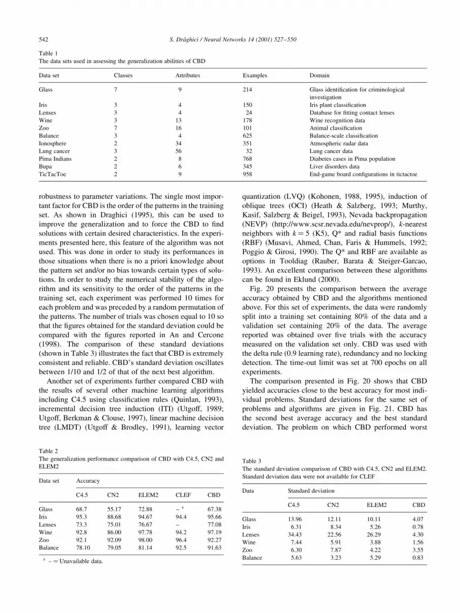
robustness to parameter variations. The single most impor-

tant factor for CBD is the order of the patterns in the training

set. As shown in Draghici (1995), this can be used to

improve the generalization and to force the CBD to ®nd

solutions with certain desired characteristics. In the experi-

ments presented here, this feature of the algorithm was not

used. This was done in order to study its performances in

those situations when there is no a priori knowledge about

the pattern set and/or no bias towards certain types of solu-

tions. In order to study the numerical stability of the algo-

rithm and its sensitivity to the order of the patterns in the

training set, each experiment was performed 10 times for

each problem and was preceded by a random permutation of

the patterns. The number of trials was chosen equal to 10 so

that the ®gures obtained for the standard deviation could be

compared with the ®gures reported in An and Cercone

(1998). The comparison of these standard deviations

(shown in Table 3) illustrates the fact that CBD is extremely

consistent and reliable. CBD's standard deviation oscillates

between 1/10 and 1/2 of that of the next best algorithm.

Another set of experiments further compared CBD with

the results of several other machine learning algorithms

including C4.5 using classi®cation rules (Quinlan, 1993),

incremental decision tree induction (ITI) (Utgoff, 1989;

Utgoff, Berkman & Clouse, 1997), linear machine decision

tree (LMDT) (Utgoff & Brodley, 1991), learning vector

quantization (LVQ) (Kohonen, 1988, 1995), induction of

oblique trees (OCI) (Heath & Salzberg, 1993; Murthy,

Kasif, Salzberg & Beigel, 1993), Nevada backpropagation

(NEVP) (http://www.scsr.nevada.edu/nevprop/), k-nearest

neighbors with k� 5 (K5), Q* and radial basis functions

(RBF) (Musavi, Ahmed, Chan, Faris & Hummels, 1992;

Poggio & Girosi, 1990). The Q* and RBF are available as

options in Tooldiag (Rauber, Barata & Steiger-Garcao,

1993). An excellent comparison between these algorithms

can be found in Eklund (2000).

Fig. 20 presents the comparison between the average

accuracy obtained by CBD and the algorithms mentioned

above. For this set of experiments, the data were randomly

split into a training set containing 80% of the data and a

validation set containing 20% of the data. The average

reported was obtained over ®ve trials with the accuracy

measured on the validation set only. CBD was used with

the delta rule (0.9 learning rate), redundancy and no locking

detection. The time-out limit was set at 700 epochs on all

experiments.

The comparison presented in Fig. 20 shows that CBD

yielded accuracies close to the best accuracy for most indi-

vidual problems. Standard deviations for the same set of

problems and algorithms are given in Fig. 21. CBD has

the second best average accuracy and the best standard

deviation. The problem on which CBD performed worst


Table 2

The generalization performance comparison of CBD with C4.5, CN2 and

ELEM2

Data set Accuracy

C4.5 CN2 ELEM2 CLEF CBD

Glass 68.7 55.17 72.88 ± a 67.38

Iris 95.3 88.68 94.67 94.4 95.66

Lenses 73.3 75.01 76.67 ± 77.08

Wine 92.8 86.00 97.78 94.2 97.19

Zoo 92.1 92.09 98.00 96.4 92.27

Balance 78.10 79.05 81.14 92.5 91.63

a ± �Unavailable data.

Table 3

The standard deviation comparison of CBD with C4.5, CN2 and ELEM2.

Standard deviation data were not available for CLEF

Data Standard deviation

C4.5 CN2 ELEM2 CBD

Glass 13.96 12.11 10.11 4.07

Iris 6.31 8.34 5.26 0.78

Lenses 34.43 22.56 26.29 4.30

Wine 7.44 5.91 3.88 1.56

Zoo 6.30 7.87 4.22 3.55

Balance 5.63 3.23 5.29 0.83

Table 1

The data sets used in assessing the generalization abilities of CBD

Data set Classes Attributes Examples Domain

Glass 7 9 214 Glass identi®cation for criminological

investigation

Iris 3 4 150 Iris plant classi®cation

Lenses 3 4 24 Database for ®tting contact lenses

Wine 3 13 178 Wine recognition data

Zoo 7 16 101 Animal classi®cation

Balance 3 4 625 Balance-scale classi®cation

Ionosphere 2 34 351 Atmospheric radar data

Lung cancer 3 56 32 Lung cancer data

Pima Indians 2 8 768 Diabetes cases in Pima population

Bupa 2 6 345 Liver disorders data

TicTacToe 2 9 958 End-game board con®gurations in tictactoe

in this set of experiments is TicTacToe on which CBD

yielded an accuracy about 24% lower than that of the best

algorithm (C4.5 rules with 99.17%). All results were

obtained using the standard CBD and default values for

all parameters. Better accuracies for this (and any) particular

problem may be obtained by tweaking the various para-

meters that control the training.

If the delta rule is used, the maximum number of epochs

speci®es the amount of effort that the algorithm should

spend in trying to optimize the position of one individual

hyperplane. If this value is low (e.g. 50), CBD will produce

a network with more hyperplanes. If this value is higher

(e.g. 1500), CBD will spend a fair amount of time optimiz-

ing individual hyperplanes and the architecture produced

will be more parsimonious with hyperplanes. Conventional

wisdom based on Occam's razor and the number of free

parameters in the model suggests that a more compact archi-

tecture is likely to provide better generalization perfor-

mance. Such expectations are con®rmed on most

problems. Fig. 22 presents the variations in the number of

hyperplanes and the accuracy as functions of the maximum

number of epochs for the balance and iris data sets. Each

data point on these curves was obtained as an average of ®ve

trials. It is interesting to note that both the accuracy and the

number of hyperplanes remain practically constant for a

very large range of values of the maximum epochs para-

meter showing that CBD is very stable with respect to this

parameter. It is only at the very low end of the range (maxi-

mum number of epochs less than 200) that one can see a

noticeable increase in the number of hyperplanes used and a

corresponding decrease in the accuracy.

4.3.4. Redundancy elimination and generalization

Another question that one may ask regards the effects of

the redundancy elimination upon the generalization perfor-

mance of the algorithms. This question is particularly

important since the redundancy elimination option is on

by default in the standard version of CBD.

If reducing the number of hyperplanes used has the conse-

quence of deteriorating the generalization performance, then

one may not always want the solution with the fewest hyper-

planes. In order to ®nd out the effects of the redundancy

elimination mechanism upon the generalization performance

of the solution network, a number of experiments have been

performed with and without the redundancy elimination. As

an example, Fig. 23 presents some results obtained with and

without redundancy for several problems from the UCI

machine learning repository. No statistically signi®cant


Fig. 20. The generalization performance comparison between CBD and with several existing neural and non-neural machine learning algorithms on various

problems from the UCI machine learning repository. The cross stands for unavailable data. CBD provides the second best average accuracy on the problems

tested.

Fig. 21. The standard deviations of CBD and the other machine learning algorithms on several problems from the UCI machine learning repository. CBD

yielded the lowest standard deviation on the problems tested.

differences were observed between the generalization perfor-

mance obtained with and without redundancy.

4.3.5. Training speed

The training speed is in¯uenced mainly by two factors:

the weight changing mechanism and the locking detection

mechanism. The default weight changing mechanism is the

delta rule. The perceptron rule provides training times

slightly shorter. More complex weight changing mechan-

isms may be expected to yield training times directly

proportional to their complexity.

As discussed, the locking detection mechanism is only

effective in spaces with a low number of dimensions. In

higher dimensional spaces, it is more ef®cient to use a

time-out condition on the number of epochs. In general,

the shorter the time-out value the faster the training.

However, such adjustments need to be made with care

since the time-out value also in¯uences the generalization

performance through the number of hyperplanes used (see

the discussion in the section on generalization). The default

value for the time-out condition is 700 epochs. This value has

been found to provide a good compromise between the train-

ing speed and the generalization results. However, a value as

low as 150 epochs is suf®cient to provide good generaliza-

tion in many cases. Table 4 presents typical training times for

10 problems from the UCI machine learning repository on a

modest laptop with a Pentium III processor running at

500 MHz and 256 M of RAM. The values have been aver-

aged over ®ve trials and rounded to the nearest second. Note

that each trial is a 10-fold cross-validation experiment which

involves training 90% of the patterns 10 times. Such training

speed represents an improvement of several orders of magni-

tude with respect to standard backpropagation and of

approximately 300% with respect to comparable constructive

algorithms such as divide-and-conquer networks (Romaniuk

& Hall, 1993). A more detailed speed comparison can be

found in Draghici (1995). However, such comparisons are

only approximate due to the fact that the speed of most other

algorithms is reported only in CPU time on various

platforms.


Fig. 22. Number of hyperplanes (left axis) and accuracy (right axis) as functions of the maximum number of epochs for the Balance (left) and Iris (right) data

sets. Both curves are very ¯at for a large range of the maximum number of epochs showing that CBD is very stable with respect to this parameter. However, as

the time-out limit becomes very small the algorithm deploys more hyperplanes than necessary and the accuracy starts to degrade.

Fig. 23. The effects of the redundancy elimination mechanism on the generalization capabilities of the solution. `R' denotes experiments performed with the

redundancy elimination mechanism enabled while `NR' denotes experiments performed with the mechanism disabled. No statistically signi®cant differences

were observed.

In order to gain a better understanding of the relationship

between the maximum number of epochs and the results of

the training, we have plotted the number of hyperplanes

used and the training time as functions of the maximum

number of epochs. In order to identify easily the point

where the generalization starts to deteriorate, we have also

plotted the generalization accuracy on the same plot. Fig. 24

presents these dependencies for the balance and iris data

sets. Each data point on these curves was calculated as an

average of ®ve trials. As expected, there is an almost linear

dependency between the maximum epochs parameter and

the total number of epochs performed. Furthermore, the

total number of epochs is directly proportional to the train-

ing time. However, in all cases, the accuracy ¯uctuates very

little for a very large range of the maximum number of

epochs. This shows that CBD is very stable with respect

to the choice of this parameter. However, if the maximum

number of hyperplanes is chosen to be very small, the

performance does deteriorate. This is to be expected, since

for a very small time-out limit the algorithm does not have

the chance to adjust the position of the hyperplane in order

to classify correctly the patterns in the given subgoal. In

consequence, the algorithm will use more hyperplanes

than normally and will over®t the data. This is seen clearly

on the graph for a maximum number of epochs less than 100

when the number of hyperplanes starts to increase and the

accuracy starts to decrease. This is followed by a more

abrupt degradation for values less than 50.

5. Discussion

This section will present some techniques that are related

in various ways with CBD. The main differences and simi-

larities between CBD and each such technique will be

summarized brie¯y. This enumeration of related techniques

is by no means exhaustive. Some reviews of these and other

very good constructive algorithms together with a general

review of various constructive approaches can be found in

Fiesler (1994); Fiesler and Beale (1996); Kwok and Yeung

(1997b); SÂmieja (1993); Thimm and Fiesler (1997).

In its simplest form, the CBD algorithm can be seen as

building a decision tree. For an excellent review of decision

tree techniques see Murthy (1995). In particular, the entropy

nets of Sethi (see Sethi, 1990; Sethi & Otten, 1990) use a

decision tree to classify the regions and two layers of

weights, one for logical AND and one for logical OR.

These layers are similar to those used by CBD. However,

building the decision tree can be a very lengthy process

because it involves testing many candidate questions for


Table 4

The training time of CBD on several problems from the UCI machine learning repository. The values reported are averages over ®ve trials using a time-out

limit of 700 epochs and 10-fold cross-validation. Note that one such trial actually trains 90% of the patterns 10 times. The values have been rounded to the

nearest second. The computer used was a modest Pentium III, 500 MHz laptop with 256 M of RAM

Data set Dimensions Patterns Time (h:min:s) Av. hyperplanes Av. terms

Glass 9 214 1:32 29 35

Ionosphere 34 351 7:25 3 4

Lung cancer 56 32 4 2 3

Wine 13 178 16 2 3

Pima Indians 8 768 1:10:08 68 79

Bupa 6 345 10:05 43 51

TicTacToe 9 958 2:38:07 47 49

Balance 4 625 6:45 22 29

Iris 4 150 10 4 5

Zoo 16 101 5 8 11

Fig. 24. The variation of the number of epochs and training time as a function of the maximum number of epochs for the Balance (left) and Iris (right) data sets.

The accuracy (%) and the training time (s) are measured on the left axis; the total number of epochs is measured on the right axis.

each node in the tree. For instance, CART (Classi®cation

and Regression Trees) uses a standard set of candidate ques-

tions with one candidate test value between each pair of data

points. A candidate question is of the form {Is xm , c}

where xm is a variable and c is the test value for that parti-

cular variable. At each node, CART searches through all the

variables xm, ®nding the best split c for each. Then the best

of the best is found (Breiman et al., 1994). For a problem in

a high dimensionality space and many input patterns, this

can be a very time consuming process. On the other hand,

the techniques which build a network by converting a deci-

sion tree offer some intrinsic optimization. Usually, in the

process of building the tree, some measures are taken to

ensure that the splits optimize some factors such as the

information gain.

CBD builds up the desired I/O surface gradually, one

region after another. The idea of locally constructing the I/

O shape is present in all radial basis funtion (RBF) algorithms

(Broomhead & Lowe, 1988; Moody & Darken, 1989; Musavi

et al., 1992; Poggio & Girosi, 1990). In the RBF case, one

unit with a localized activation function will ensure the

desired response for a small region of the I/O space.

However, there are situations in which a net building piece-

wise linear boundaries is better than an RBF net. Further-

more, for an RBF net to be ef®cient, a pre-processing stage

must be performed and parameters such as radii of the activa-

tion functions, their shape and orientation, the clustering, etc.

must be calculated. By contrast, CBD is relatively simple.

On the other hand, an RBF network will respond only to

inputs which are close to the inputs contained in the training

set. For completely unfamiliar inputs, the RBF network will

remain silent, automatically signaling its incompetence. In

contrast, CBD networks (as any other networks using hyper-

planes) automatically extend their trained behavior to in®-

nity. This means that they produce some response for any

input, no matter how unfamiliar this is. The potential

problems induced by such behavior can be eliminated by

using techniques for validating individual outputs (Bishop,

1994; Courrieu, 1994).

A constructive algorithm related both with CBD and

RBFs is DistAI presented in Yang, Parekh and Honavar

(1998), Yang, Parekh, Honavar and Dobbs (1999). DistAI

constructs a single layer of hyper-spherical threshold

neurons which exclude clusters of training patterns belong-

ing to the same class. However, in DistAI, the weights and

thresholds of the neurons are determined directly by

comparing the distances between various patterns whereas

in CBD the weights are trained in an iterative process.

The ideas of training only one neuron at a time and build-

ing the set gradually are present in most constructive algo-

rithms. The upstart algorithm (Frean, 1990) builds a

hierarchical structure (which can be reduced eventually to

a 2-layer net) by starting with a unit and adding daughter

units which cater for the misclassi®cations of the parents.

Sirat and Nadal (1990) proposed a similar algorithm. Other

interesting constructive techniques are sequential learning

(Marchand, Golea & RuÂjan, 1990), the patch algorithm

(Barmeka, Andree & Taal, 1993), the oil-spot algorithm

(Frattale-Mascioli & Martinelli, 1995)and the techniques

presented in Muselli (1995); RuÂjan and Marchand (1989).

Mezard and Nadal (1989) proposed a tiling algorithm which

starts by training a single unit on the whole training set. The

training is stopped when this unit produces the correct target

on as many patterns as possible. This partial-solution weight

state is given by Gallant's pocket algorithm (Gallant, 1986)

that assumes that if the problem is not linearly separable the

algorithm will spend most of its time in a region of the

weight space providing the fewest errors. However, all

these techniques work for binary units only. Even in its

simplest form, the CBD can deal with both binary and

real-valued inputs. Furthermore, it can be easily extended

in several ways to continuous inputs and outputs.

A recent paper (Parekh, Yang & Honavar, 2000) presents

two constructive algorithms able to cope with multiple

classes. MPyramid-real and MTiling-real are two algo-

rithms that extend the pyramid and tiling algorithms, respec-

tively, and are able to deal with real inputs and multiple

output classes. The problem of how to extend constructive

algorithms from two classes to multiclass classi®cation is

also thoroughly discussed in Draghici (1995) and Parekh,

Yang and Honavar (1995).

Biehl and Opper (1991) present a tiling-like constructive

algorithm for a parity-machine. Buhot and Gordon (2000)

derive upper and lower bounds for the typical storage capa-

city of this constructive algorithm.

The Cascade Correlation (CC) net proposed by Fahl-

man and Labiere (1990)uses the whole pattern set to

construct an architecture of cascading units. In general,

using the whole training set has the advantage that the

solution can be optimized from some point of view. In

CC's case, the weights are chosen so that the correlation

between the output of the last added unit and the output is

maximum. This ensures that the unit is as useful as possi-

ble in the given context. Because of this, in general, CC

will construct networks that use slightly fewer hidden

units than CBD. However, the generalization provided

by CBD is comparable with the generalization offered

by CC. Various extensions and modi®cations of the origi-

nal cascade correlation have been proposed. These

include improvements of the initialization ( Lehtokangas,

1999a; Liang & Dai, 1998), improving generalization

through avoiding over®tting (Tetko & Villa, 1997a,b), a

projection pursuit perspective (Hwang, You, Lay & Jou,

1996) and many others. Cascade correlation has also been

modi®ed for recurrent networks (Fahlman, 1991), parallel

execution (Springer & Gulati, 1995), use with limited

precision weights in hardware implementations (HoÈhfeld

& Fahlman, 1992) and combined with other techniques

such as ARTMAP (Tan, 1997). An empirical evaluation

of six algorithms from the cascade correlation family is

presented in Prechelt (1997).

A technique closely related to cascade correlation is the


Cascade Error Projection (CEP) proposed in Duong and

Daud (1999). The architecture generated by CEP is very

similar to the original CC architecture and is generated in

a similar manner, but using a different criterion. Because of

this, the resulting network has several characteristics that

makes it suitable for hardware implementation in VLSI.

The extentron proposed by Baffes and Zelle (1992) grows

multilayer networks capable of distinguishing non-linearly

separable data using the perceptron rule for linear threshold

units. The extentron looks for the best hyperplane relative to

the examples in the training set. The extentron approaches

the problem of separating non-linearly separable sets by

connecting each hidden unit both to all the inputs and to

all the previous units. Thus, the dimension of the problem's

space is extended and the problem could become linearly

separable. In the worst case, each unit will separate a single

pattern, but experiments showed that this does not happen

unless the problem is `pathologically dif®cult' (the 2-spiral

problem is quoted as such a problem). Experiments showed

that CBD is more ef®cient than this even in solving the 2-

spiral problem. If the extentron is coupled with an output

layer trained by backpropagation (in order to cope with

continuous values), the large number of layers is an impor-

tant disadvantage due to error attenuation across layers. The

architecture generated by CBD always contains the same

number of layers and does not have this problem if the

network is to be subsequently trained with backpropagation.

Furthermore, if the extentron architecture were to be imple-

mented in hardware, synchronization problems might arise

due to the existence of paths with very different lengths

between input and output. This problem is not present in

the case of the solution generated by CBD.

Romaniuk and Hall (1993) proposed a divide-and-

conquer net which builds an architecture similar to that of

a cascade correlation network. Their divide-and-conquer

strategy starts with one neuron and the entire training set.

If the problem is linearly inseparable (which is the usual

situation), the ®rst training is bound to fail and this is

detected by a time-out condition. In comparison, CBD starts

with the minimum problem which is guaranteed to have a

solution. The divide-and-conquer technique has a more

complicated pattern presentation algorithm and requires a

pre-processing stage in which the nearest neighbor is found

for each pattern in the training set.

The CARVE algorithm (Young & Downs, 1998)

constructs the network through adding hidden units

which carve the patterns of one class out of the whole

pattern set. The locking detection mechanism of the CBD

technique and the CARVE algorithm are both inspired by

and make use of classical computational geometry tech-

niques such as the gift wrapping method of constructing

the convex hull. However, the convex hull search is the

centerpiece of the CARVE algorithm (thus making it

computationally expensive), whereas in CBD it is used

only as an optional enhancement (Draghici, 1996). The

connection between linear separability and convex hulls

has also been studied extensively by others (see for

instance Bennett & Bredensteiner, 1998).

The CLEF algorithm proposed in Precup and Utgoff

(1998) combines a version of a linear machine with a non-

linear function approximation that constructs its own

features (Utgoff & Precup, 1997, 1998).

Kwok and Yeung (1997b) study a number of objective

functions for training hidden units in constructive algo-

rithms. Kwok and Yeung (1997a) study the use of construc-

tive algorithms for structure learning in regression

problems. Treadgold and Gedeon (1999a) investigate the

generalization abilities of constructive cascade algorithms.

The Casper algorithm (Treadgold & Gedeon, 1997, 1998,

1999b) addresses the issue of the amount of regularization

necessary in order to obtain good generalization. Hosseini

and Jutten (1999) propose a constructive approach in which

the target network is constructed by adding small, variable-

size accessory networks as opposed to adding simple units.

Campbell and Vicente (1995) present a constructive algo-

rithm that can perform classi®cation of binary or analog

input data using only binary weights. Such weights are parti-

cularly interesting for a hardware implementation. An adap-

tation of CBD for similar purposes is discussed in Draghici

(1998) and Draghici, Beiu & Sethi (1997).

A constructive backpropagation algorithm is presented in

Lehtokangas (1999a). This algorithm combines the classical

idea of backpropagating the error with the constructive

approach of adding units as they are needed. Structure adap-

tation features of constructive backpropagation include the

ability to delete units in order to improve generalization.

The algorithm was tested in modeling problems and

shown to be better than cascade correlation for the problem

studied. A version of this algorithm adapted for recurrent

networks is presented in Lehtokangas (1999a).

Thimm and Fiesler (1997) use a Boolean approximation

of the given problem to construct an initial neural network

topology. Subsequently, this network is trained on the origi-

nal real-valued data. The resulting topology is shown to

exhibit better generalization capabilities than fully

connected high order multilayer perceptrons.

In Hammadi, Ohmameunda, Kaneo & Ito (1998), a

dynamic constructive algorithm is used to construct fault

tolerant feedforward networks. This dynamic constructive

fault tolerant algorithm (DCFTA) estimates a relevance

factor for each weight and uses it to update the weights in a

selective manner.

6. Conclusions

This paper presented the Constraint Based Decomposi-

tion (CBD) as a constructive algorithm with guaranteed

convergence, fast training and good generalization proper-

ties. The CBD training algorithm is composed of any weight

updating algorithm able to train a single neuron (perceptron,

delta rule, etc.), a pattern presentation algorithm and a


network construction method. CBD is able to deal with

binary, n-ary, class-labeled and real-valued problems as

exempli®ed in the experiments presented. Like any

constructive algorithm, CBD does not need an a priori

guess of the necessary network architecture since it

constructs a suf®ciently powerful architecture during the

training. Furthermore, CBD can provide a symbolic descrip-

tion found for any classi®cation problem thus being more

transparent than other neural network algorithms. For real-

valued problems, this symbolic solution is limited to

describing the partitioning of the input space.

The paper also presented two enhancements of the CBD

approach: the locking detection and redundancy elimina-

tion. The locking detection technique uses a computational

geometry approach to detect those situations in which the

current hyperplane is locked into its current position by

some of the patterns in the current subgoal. The elimination

of such problems can increase the speed of the training.

However, in high dimensional spaces the computational

effort required by this detection might offset the speed

gain obtained through the elimination of the linearly inse-

parable problems. Therefore, the use of this enhancement is

only recommended for low dimensional spaces (less than

®ve).

The redundancy elimination technique eliminates locally

and globally redundant hyperplanes. Thus, the algorithm

ensures that the ®nal solution will not contain any useless

hyperplanes (neurons). The technique achieves the goal

normally accomplished by a pruning technique. However,

the redundancy elimination has the added advantages that:

(i) the technique is integrated into the convergence process;

(ii) the units are eliminated on-line, during the training; and,

thus, (iii) no training time is wasted on units that will even-

tually be eliminated.

The experiments presented showed that the technique is

able to cope successfully with a variety of problems ranging

from classical toy-problems like XOR, parity and 2-spirals

up to real-world problems.

CBD was compared with C4.5, C4.5 with rules, incre-

mental decision trees, oblique classi®ers, linear machine

decision trees, CN2, learning vector quantization, backpro-

pagation, nearest neighbor, Q* and radial basis functions on

Glass, Ionosphere, Lung cancer, Wine, Pima Indians, Bupa,

TicTacToe, Balance, Iris, Lenses and Zoo from the UCI

machine learning repository. The cross-validation experi-

ments performed showed that the technique builds fast

and reliable solutions that have generalization performances

that compare favorably with those of several other machine

learning algorithms. The CBD technique may be an argu-

ment against the idea that constructive techniques trade

generalization for training speed. Perhaps one can have

both reliability and good generalization at the same time,

after all. By performing comparisons with non-neural tech-

niques, we think we have also shown that modern neural

network techniques can compete successfully with any

other learning paradigm.

References

An, A., & Cercone, N. (1998). ELEM2: a learning system for more accurate

classi®cations. In R. E. Mercer & E. Neufeld, Lecture notes in arti®cial

intelligence (pp. 426±441). vol. 1418. Berlin: Springer-Verlag.

Baffes, P. T., & Zelle, J. M. (1992). Growing layers of perceptrons; Intro-

ducing the extentron algorithm. In International Joint Conference on

Neural Networks (vol. 2, pp. 392±397). Baltimore.

Barkema, G. T., Andree, H. M. A., & Taal, A. (1993). The patch algorithm:

fast design of binary feedforward neural networks. Network, 5, 393±

407.

Bennett, K. P., & Bredensteiner, E. J. (1998). In C. Gorini, E. Hart, W.

Meyer & T. Phillips, Geometry at work, Washington DC: Mathematical

Association of America.

Biehl, M., & Opper, M. (1991). Tilinglike learning in the parity machine.

Physical Review A, 44 (10), 6888±6894.

Bishop, C. M. (1994). Novelty detection and neural network validation. IEE

Proceedings on Vision, Image and Signal Processing, 141 (4), 217±

222.

Blake, C., Keogh, E., & Merz. C. (1998). UCI repository of machine learn-

ing databases.

Borsuk, K. (1969). Multidimensional analytic geometry, Warsaw: Polish

Scienti®c Publishers.

Brady, M., Raghavan, R., & Slawny, J. (1988). Gradient descent fails to

separate. In Proceedings of the IEEE International Conference on

Neural Networks (vol. 1, pp. 649±656).

Brady, M. L., Raghavan, R., & Slawny, J. (1989). Back propagation fails to

separate where perceptrons succeed. IEEE Transactions on Circuits and

Systems, 36 (5), 665±674.

Breiman, L., Friedman, J. H., Olsen, R. A., & Stone, C. J. (1984). Classi-

®cation and regression trees, Monterey, CA: Wadsworth International.

Broomhead, D. S., & Lowe, D. (1988). Multivariable functional interpola-

tion and adaptive networks. Complex Systems, 2, 321±323.

Buhot, A., & Gordon, M. B. (2000). Storage capacity of a constructive

learning algorithm. Journal of Physics AÐMathematical and General,

33 (9), 1713±1727.

Campbell, C., & Vicente, C. P. (1995). The target switch algorithm: a

constructive learning procedure for feed-forward neural networks

[Letter]. Neural Computation, 7 (6), 1245±1264.

Clark, P., & Niblett, T. (1989). The CN2 induction algorithm. Machine

Learning, 3, 261±283.

Courrieu, P. (1994). Three algorithms for estimating the domain of validity

of feedforward neural networks. Neural Networks, 7 (1), 169±174.

Draghici, S. (1994). The constraint based decomposition training architec-

ture. In Proceedings of World Congress on Neural Networks (vol. 3, pp.

545±555). San Diego, CA.

Draghici, S. (1995). Using constraints to improve generalization and train-

ing of feedforward neural networks: constraint based decomposition

and complex backpropagation. PhD Thesis, University of St. Andrews.

Draghici, S. (1996). Enhancement of the constraint based decomposition

training architecture. In Proceedings of IEEE International Conference

on Neural Networks IJCNN '96 (vol. 1, pp. 317±322). New York: IEEE

Press.

Draghici, S. (1998). On the complexity±capability relationship of adaptive

systems based on VLSI friendly neural networks. In Lecture notes in

arti®cial intelligence, Proceedings of XII Canadian Conference on Arti-

®cial Intelligence AI'98 (vol. 1418, pp. 285±297). Springer-Verlag.

Draghici, S., Beiu, V., & Sethi, I. (1997). A VLSI optimal constructive

algorithm for classi®cation problems. In Smart engineering systems:

neural networks, fuzzy logic, data mining and evolutionary program-

ming (pp. 141±151). New York: ASME Press.

Duong, T. A., & Daud, T. (1999). Cascade error projection: a learning

algorithm for hardware implementation. In J. Mira & J. V. SaÂnchez-

AndreÂes, Foundations and tools for neural modeling, Lecture Notes in

Computer Science (pp. 450±457). Berlin: Springer-Verlag.

Eklund, P. W. (2000). Comparative study of public-domain supervised


machine-learning accuracy on the UCI database. In Proceedings of the

data mining and knowledge discovery: theory, tools and technology

(pp. 39±50). Orlando, FL: SPIE.

Fahlman, S. E. (1991). The recurrent cascade-correlation architecture. In R.

P. Lippmann, J. E. Moody & D. S. Touretzky, Advances in neural

information processing systems 3 (pp. 190±196). Denver, CO: Morgan

Kaufmann.

Fahlman, S. E., & Lebiere, C. (1990). The cascade-correlation learning

architecture (Tech. Rep.). Carnegie Mellon University.

Fiesler, E. (1994). Comparative bibliography of ontogenetic neural

networks. In Proceedings of the International Conference on Neural

Networks (ICANN '94) (pp. 793±796). Sorrento, Italy.

Fiesler, E., & Beale, R. (1996). Handbook of neural computation, New

York: Oxford University Press and The Inst. of Physics. Publ.

Frattale-Mascioli, F. M., & Martinelli, G. (1995). The oil-spot algorithm.

IEEE Transactions on Neural Networks, 6, 794±797.

Frean, M. (1990). The Upstart algorithm: a method for constructing and

training feedforward neural networks. Neural Computation, 2, 198±

209.

Gallant, S. I. (1986). Optimal linear discriminants. In Eighth International

Conference on Pattern Recognition (pp. 849±852). IEEE.

Hammadi, N., Ohmaneunda, T., Kaneo, K., & Ito, H. (1998). Dynamic

constructive fault tolerant algorithm for feedforward neural

networks. IEICE Transactions on Information and Systems, E81D

(1), 115±123.

Heath, S. K. D., & Salzberg, S. (1993). Induction of oblique decision tree.

In IJCAI-93, Washington, DC.

Hosseini, S., & Jutten, C. (1999). Weight freezing in constructive neural

networks: a novel approach. Lecture notes in computer science: engi-

neering applications of bio-inspired arti®cial neural networks (pp.

1607:10±1607:20). Berlin: Springer-Verlag.

Hwang, J. -N., You, S. -S., Lay, S. -R., & Jou, I. -C. (1996). The Cascade-

Correlation learning: a projection pursuit learning perspective. IEEE

Transactions on Neural Networks, 7 (2), 278±289.

HoÈhfeld, M., & Fahlman, S. E. (1992). Learning with limited numerical

precision using the Cascade-Correlation algorithm. IEEE Transactions

on Neural Networks, 3 (4), 602±611.

Knuth, D. E. (1976). Big omicron and big omega and big theta. SIGACT

News, 8 (2), 18±24.

Kohonen, T. (1988). Learning vector quantization. Neural Networks, 1

(Suppl. 1), 303.

Kohonen, T. (1995). Learning vector quantization. The handbook of brain

theory and neural networks (pp. 537±540). Cambridge, MA: MIT

Press.

Kwok, T. -Y., & Yeung, D. -Y. (1997a). Constructive algorithms for struc-

turing learning in feedforward neural networks for regression problems.

IEEE Transactions on Neural Networks, 8 (3), 630±645.

Kwok, T. Y., & Yeung, D. Y. (1997b). Objective functions for training new

hidden units in constructive neural networks. IEEE Transactions on

Neural Networks, 8 (5), 1131±1148.

Lang, K. J., & Witbrock, M. J. (1989). Learninig to tell two spirals apart.

Proceedings of the 1988 Connectionist Models Summer School (pp. 52±

61). San Mateo: Morgan Kaufmann.

Lehtokangas, M. (1999a). Fast initialization for cascade-correlation learn-

ing [Brief paper]. IEEE-NN, 10 (2), 410.

Liang, H., & Dai, G. L. (1998). Improvement of cascade correlation learn-

ing algorithm with an evolutionary initialization. Information Sciences,

112 (1-4), 1±6.

Marchand, M., Golea, M., & RuÂjan, P. (1990). A convergence theorem for

sequential learning in two-layer perceptrons. Europhysics Letters, 11

(6), 487±492.

Mezard, M., & Nadal, J. P. (1989). Learning in feedforward layered

networks: the tiling algorithm. J. Phys. A: Math. Gen., 22, 2191±

2203.

Mitchell, T. M. (1977). Version spaces: a candidate elimination approach to

rule learning. IJCAI, 1, 1139±1151.

Mitchell, T. M. (1978). Version spaces: an approach to concept learning.

Unpublished doctoral dissertation, Stanford University.

Moody, J., & Darken, C. J. (1989). Fast learning in networks of locally-

tuned processing units. Neural Computation, 1, 281±294.

Murthy, K. V. S. (1995). On growing better decision trees from data.

Unpublished doctoral dissertation, Johns Hopkins University.

Murthy, S. K., Kasif, S., Salzberg, S., & Beigel, R. (1993). OCI: rando-

mized induction of oblique decision trees. In Proceedings of the

Eleventh National Conference on Arti®cial Intelligence (pp. 322±

327). Washington, DC.

Musavi, M., Ahmed, W., Chan, K. H., Faris, K., & Hummels, D. (1992). On

the training of radial basis function classi®ers. Neural Networks, 5,

595±603.

Muselli, M. (1995). On sequential construction of binary neural networks.

IEEE Transactions on Neural Networks, 6, 678±690.

Parekh, R. G., Yang, J., & Honavar, V. (1995). Constructive neural network

learning algorithms for multi-category pattern classi®cation (Post-

script). Department of Computer Science, Iowa State University,

Ames, Iowa: Tech. Rep. ISU-CS-TR 95-15.

Parekh, R., Yang, J., & Honavar, V. (2000). Constructive neural-network

learning algorithms for pattern classi®cation. IEEE Transactions on

Neural Networks, 11 (2), 436.

Poggio, T., & Girosi, F. (1990). Networks for approximation and learning.

Proceedings of IEEE, 78 (9), 1481±1497.

Prechelt, L. (1997). Investigation of the cascor family of learning algo-

rithms. Neural Networks, 10 (5), 885±896.

Precup, D., & Utgoff, P. E. (1998). Classi®cation using F-machines and

constructive function approximation. In Proc. 15th International

Conference on Machine Learning (pp. 439±444). San Francisco, CA.

Preparata, F. P., & Shamos, M. I. (1985). Computational geometryÐan

introduction, New York: Springer-Verlag.

Quinlan, J. R. (1993). C4.5: programs for machine learning, San Mateo:

Morgan Kaufmann.

Rauber, T. W., Barata, M. M., & Steiger-Garcao, A. (1993). A tool-box for

analysis and visualization of sensor data in supervision. In Proceedings

of International Conference of Fault Diagnosis, Toulouse, France.

Romaniuk, S. T., & Hall, L. O. (1993). Divide and conquer neural

networks. Neural Networks, 6, 1105±1116.

RuÂjan, P., & Marchand, M. (1989). Learning by minimizing resources in

neural networks. Complex Systems, 3, 229±241.

Sethi, I. K. (1990). Entropy nets: from decision trees to neural networks.

Proceedings of the IEEE, 78, 1605±1613.

Sethi, I., & Otten, M. (1990). Comparison between entropy nets and deci-

sion tree classi®ers. In International Joint Conference on Neural

Networks (vol. 3, pp. 41±46). San Diego, CA.

Siestma, J., & Dow, R. J. F. (1991). Creating arti®cial neural networks that

generalise. Neural Networks, 4, 67±79.

Sirat, J. A., & Nadal, J. P. (1990). The Upstart algorithm: a method for

constructing and training feedforward neural networks. Networks:

Computation in Neural Systems, 1 (4), 423±438.

SÂmieja, F. J. (1993). Neural network constructive algorithms: trading

generalization for learning ef®ciency? Circuits Systems Signal Proces-

sing, 12 (2), 331±374.

Springer, P. L., & Gulati, S. (1995). Parallelizing the cascade-correlation

algorithm using time warp. Neural Networks, 8 (4), 571±577.

Tan, A. -H. (1997). Cascade ARTMAP: integrating neural computation and

symbolic knowledge processing. IEEE Transactions on Neural

Networks, 8 (2), 237±250.

Tetko, I. V., & Villa, A. E. P. (1997a). An ef®cient partition of training data

set improves speed and accuracy of cascade-correlation algorithm.

Neural Processing Letters, 6 (1/2), 51±59.

Tetko, I. V., & Villa, A. E. P. (1997b). An enhancement of general-

ization ability in cascade correlation algorithm by avoidance of over-

®tting/overtraining problem. Neural Processing Letters, 6 (1/2), 43±

50.

Thimm, G., & Fiesler, E. (1997). Two neural network construction meth-

ods. Neural Processing Letters, 6 (1/2), 25±31.


Treadgold, N. K., & Gedeon, T. D. (1997). Extending and bench-marking

the CasPer algorithm. In A. Sattar, Proceedings of the 10th Australian

Joint Conference on Arti®cial Intelligence: Advanced Topics in Arti®-

cial Intelligence (AI-97) (pp. 398±406). vol. 1342. Berlin: Springer.

Treadgold, N. K., & Gedeon, T. D. (1998). Constructing higher order

neurons of increasing complexity in cascade networks. Lecture Notes

in Computer Science, 1416, 557±563.

Treadgold, N. K., & Gedeon, T. D. (1999a). Exploring constructive cascade

networks. IEEE-NN, 10 (6), 1335.

Treadgold, N. K., & Gedeon, T. D. (1999b). A constructive cascade

network with adaptive regularization to appear as Lecture Notes in

Computer Science. In J. Mira & J. Sanchez-Andres, Proceedings of

IWANN'99 (pp. 40±49). Alicante, Spain: Springer-Verlag.

Utgoff, P. E. (1989). Incremental induction of decision trees. Machine

Learning, 4, 161±186.

Utgoff, P. E., & Brodley, C. E. (1991). Linear machine decision trees

(Technical report no. UM-CS-1991-010), University of Massachusetts,

Amherst, Computer Science.

Utgoff, P. E., & Precup, D. (1997). Constructuve function approximation

(Technical report no. 97-04). Amherst, MA: Department of Computer

Science, University of Massachusetts.

Utgoff, P. E., & Precup, D. (1998). Constructive function approximation. In

H. Liu & H. Motoda, Feature extraction, construction and selection: a

data mining perspective, vol. 453. Norwell, MA: Kluwer Academic.

Utgoff, P. E., Berkman, N. C., & Clouse, J. A. (1997). Decision tree

induction based on ef®cient tree restructuring. Machine Learning,

29, 5±44.

Yang, J., Parekh, R., & Honavar, V. (1998). DistAI: an interpattern

distance-based constructive learning algorithm. In World Congress on

Computational Intelligence (pp. 2208±2213). Anchorage, Alaska.

Yang, J., Parekh, R., Honavar, V., & Dobbs, D. (1999). Data-driven theory

re®nement using KBDistAI. Lecture Notes in Computer Science, 1642,

331±342.

Young, S., & Downs, T. (1998). CARVEÐa constructive algorithm for

real-valued examples. IEEE Transactions on Neural Networks, 9 (6),

1180±1190.


Documents

The constraint based decomposition (CBD) training architecture