Policy ReseaRch WoRking PaPeR 4375

The Determinants of Rising Informality in Brazil:

Evidence from Gross Worker Flows

Mariano BoschEdwin Goni

William Maloney

The World BankLatin Ameria and Caribbean RegionChief Economist OfficeOctober 2007

WPS4375

Produced by the Research Support Team

Abstract

The Policy Research Working Paper Series disseminates the findings of work in progress to encourage the exchange of ideas about development issues. An objective of the series is to get the findings out quickly, even if the presentations are less than fully polished. The papers carry the names of the authors and should be cited accordingly. The findings, interpretations, and conclusions expressed in this paper are entirely those of the authors. They do not necessarily represent the views of the International Bank for Reconstruction and Development/World Bank and its affiliated organizations, or those of the Executive Directors of the World Bank or the governments they represent.

Policy ReseaRch WoRking PaPeR 4375

This paper studies gross worker flows to explain the rising informality in Brazilian metropolitan labor markets from 1983 to 2002. This period covers two economic cycles, several stabilization plans, a far-reaching trade liberalization, and changes in labor legislation through the Constitutional reform of 1988. First, focusing on cyclical patterns, the authors confirm that for Brazil, the patterns of worker transitions between formality and informality correspond primarily to the job-to-job dynamics observed in the United States, and not to the traditional idea of the informal queuing for jobs in a

This paper—a product of the Chief Economist Office, Latin America and Caribbean Region—is part of a larger effort in the department to understand labor market dynamics and the nature of informality. Policy Research Working Papers are also posted on the Web at http://econ.worldbank.org. The author may be contacted at wmaloney@worldbank.org.

segmented market. However, the analysis also confirms distinct cyclical patterns of job finding and separation rates that lead to the informal sector absorbing more labor during downturns. Second, focusing on secular movements in gross flows and the volatility of flows, the paper finds the rise in informality to be driven primarily by a reduction in job finding rates in the formal sector. A small fraction of this is driven by trade liberalization, and the remainder seems driven by rising labor costs and reduced flexibility arising from Constitutional reform.

The Determinants of Rising Informality in Brazil: Evidence from Gross Worker Flows*

Mariano Bosch London School of Economics

Edwin Goni World Bank

William Maloney World Bank

First version: October 1997 This version: October 10, 2007

JEL: Gross worker flows, Labor market dynamics, Informality, Developing Countries.

*We are very grateful to Francisco Carneiro, Marcello Estevao, Gustavo Gonzaga Lauro Ramos, Jose Guilherme Reis and Gabriel Ulyssea, to participants in the NBER workshop on informality, October 2006 in Bogota, and to those at the University of Michigan conference on Labor Markets in Developing and Transition Economies, May 2007, in particular Gary Fields, Ann Harrison, Ravi Kanbur, and Jan Svejnar, for helpful advice and reality testing of ideas. All conclusions are, of course, our own. Correspondence: m.bosch@lse.ac.uk, egonipacchioni@worldbank.org, wmaloney@worldbank.org.

I. Introduction

In a single decade, from the mid 1990 to 2000, the share of the Brazilian

metropolitan area work force unprotected by labor legislation and thereby classified as

“informal” rose an astronomical 10 percentage points. This episode is of relevance for

several reasons.

First, such movements have been relatively common over the last decade: Urban

informality increased in Argentina from 1992 to 2003 by 10 percentage points; in

Venezuela from 1995 to 2003 by 8 percentage points.1 To the degree that such increases

represent the progressive exposure of the work force to risk and loss of other benefits,

they are intrinsically worrying.

Second, understanding the causes of these movements can contribute to our

understanding of the drivers of informality more generally. Brazil offers several dramatic

policy changes across the period that theory suggests could affect gross labor flows and

their volatility and hence the steady state size of the formal sector: a far reaching trade

reform, and the establishment of a new Constitution in 1988 that had substantial impacts

on labor costs and flexibility.

Third, unlike Argentina or Venezuela, Brazil offers an excellent panel data set

that, with perhaps the exception of Mexico, is one of the very few in the developing

world to have a sufficient time dimension for us to study the shifts in magnitudes of gross

labor flows associated with two complete business cycles and the secular recomposition

of the labor force.

This paper first applies recent advances in the study of labor market dynamics

over the business cycle, introduced by Shimer (2005b) and Hall (2005) and confirms for

Brazil the patterns identified for the US and for Mexico by Bosch and Maloney (2006): 1 See Gasparini and Tornarolli (2006)

2

the informal sector does not, as a first approximation, correspond to the disadvantaged

sector of a segmented market.2 That said, the relatively higher volatility of job finding

rates in the formal sector leaves the informal sector absorbing more labor during

downturns.

The paper then explores the determinants of the secular changes in gross labor

flows that drove the increase in informality across the 1990s. We find that the driving

dynamic was a reduction in formal sector hiring across the period. In explaining this

reduction, trade liberalization had a statistically significant but relatively minor role while

the changes in labor market legislation associated with the Constitutional reform appear

more important.

Background

As can be inferred from Table 1, in 1980, roughly 35% of the Brazilian labor

force was found either managing small micro firms either as employers or independent

self-employed, or working for firms of various sizes without a signed work card that

would guarantee access to benefits. The implications of such a large uncovered sector

have been the subject of sharp debate for decades. The dominant perspective with

intellectual roots dating at least from Harris and Todaro (1970), equates the sector with

underemployment or disguised unemployment- the disadvantaged sector of a market

segmented by rigidities in the “formal” or covered sector of the economy. However,

another emerging view keys more off the mainstream self-employment literature in the

2 In one of the first works studying gross job flows, Blanchard and Diamond (1991) argued that slowdowns of the economy are characterized by a significant increase in the number of workers transitioning from employment into unemployment. Consistent with this, Davis and Haltiwanger (1990 and 1992) in a series of papers using establishment data showed that job destruction is countercyclical. Both sets of findings constituted empirical support for the predominant search and matching models in the Mortensen and Pissarides tradition. See Mortensen and Pissarides (1994, 1999a and 1999b), Petrongolo and Pissarides (2001) and Pries and Rogerson (2005), Rogerson et al. (2005) for a review of these models and their implications. However, recently Shimer (2005b) and Hall (2005) have argued that, in fact, job separations are largely acyclical, while the finding rate is highly procyclical. That is, contrary to the conventional wisdom, unemployment rises because jobs become hard to find, not because they are destroyed. Further, Shimer (2005b) argues that the response of vacancies and unemployment to productivity shocks predicted by a standard search model explains only around 10% of the observed volatility of the job finding rate. Explaining these stylized facts, Shimer (2005b) and Hall (2005) argue, requires introducing wage rigidities into standard matching models.

3

style of Lucas (1978), Jovanovic (1982) and Evans and Leighton (1989), and argues that,

as a first approximation, the sector should be seen as an unregulated, largely voluntary

self-employed/micro firm sector.3

While the informal sector in all likelihood contains both types of actors, disguised

unemployed and entrepreneurs, its exaggerated size in developing countries raises the

stakes surrounding the relative proportions dramatically: if the roughly 35-60 percent of

the Latin American workers found in the informal sector show dynamics similar to those

of the unemployed, then the labor market distortions in the formal sector are indeed large

and the case for massive reform to eliminate segmentation, compelling. However, should

the dynamics correspond more to a voluntary small firm sector that offers an alternative,

but not obviously inferior income source then aggregate labor force dynamics may differ

from what has been found in the US, but will not necessarily suggest pathology.

In all likelihood, there are elements of both at work. The lower opportunity cost

of being self-employed in poor countries may raise the share of uncovered self-employed

workers in developing countries (See Blau 1987, Maloney 2001). On the other hand,

minimum wages or union wage setting have clearly proved able to generate segmented

markets. In an intermediate position, in theoretical frameworks in the matching tradition

(Mortensen and Pissarides 1994, 1999a, 1999b, Pries and Rogerson 2005), firing costs or

other labor taxes may lead to a reduction in labor demand without inducing segmentation

per se. That is, workers are still indifferent between formal and informal sectors, but the

formal sector demand curve has shifted down. Further, the institutional framework can

also generate incentives for workers to opt out of formality: subsidized social services

delinked from the labor contract, or labor taxes passed on to workers that do not

correspond to an equally valued benefit all shift the labor supply curve to the left. Thus,

it is entirely possible for the formal and informal labor markets to be very integrated in

the sense of offering jobs of similar quality at the margin, while the institutional structure

may be characterized by substantial distortions (see Maloney 2004, Levy 2006). 3 For a review of the literature and early work on transition matrices in developing country see Maloney (1999, 2004)

4

Clearly, this debate over the causes of informality extends to the drivers of

changes in the share of informality as well and this gives the Brazilian case its salience.

Far reaching trade reform began in the mid 1980s but intensified around 1990. As Table

2 shows, import penetration ratios rose and effective rates of protection fell significantly.

In a matching model, the resulting reduction in rents would lead to a reduction in the

value of a vacancy and hence to a reduction in hiring in the formal sector, although not

necessarily segmentation, leaving the residual of the work force to recur to the informal

sector. To date, the most thorough test of the hypothesis of a relationship between trade

liberalization and informality was undertaken by Goldberg and Pavcnik (2003) who,

exploiting sectoral variation in protection across time, found no relationship between the

share of informality and the reduction in trade protection in Brazil, and a modest

relationship in Colombia. However, Gonzaga, Menezes Filho, and Terra (2006) identify

important effects of the Brazilian trade liberalization on the allocation of workers

between skilled and unskilled-intensive sectors as well skill-unskilled earnings

differentials suggesting non-trivial impacts on the labor market that might have an

informal sector counterpart. By extending the series on protection levels and studying the

behavior of job finding and job destruction rates in response to protection variables, we

are able to revisit this question in the context of gross worker flows and find evidence of

a significant, albeit very modest, impact of trade reforms on informality.

The 1988 Constitutional changes had important implications for the labor code in

several areas that theory predicts could lead to increasing informality. First, there was a

generalized increase in labor costs and reduction in formal employer flexibility.

Maximum working hours per week were reduced from 48 to 44, overtime remuneration

was increased from 1.2 to 1.5 times the normal wage rate; vacation pay was raised from

one to 4/3 of the monthly wage, and maternity leave increased from 90 to 120 days.4

Second, some limitations on the power of organized labor were relaxed. Unions were no

longer required to be registered and approved by the Ministry of Labor; decisions to

4 Paes de Barros and Corsueil (2001) among others also note that the maximum continuous work day was reduced from 8 to 6 hours although the exact meaning of this is unclear given that 8 hours remains the standard work day.

5

strike were left entirely to union discretion, the required advance notification to the

employer cut from five to two days, and strikes in certain strategic sectors were no longer

banned. Finally, firing costs were raised. The penalty levied on employers for

unjustified dismissal, a category encompassing most separations considered legitimate for

economic reasons in the US, increased by four times from 10% to 40,% of the

accumulated separation account (FGTS, Fundo de Garantia por Tempo de Serviço).

To date, the most comprehensive work relating these changes to the functioning

of the labor market was undertaken by Paes de Barros and Corseuil (2001) who find that

separation rates decreased after the Constitutional changes for short employment spells

and increased for longer spells, but find inconclusive results on the impacts on flows into

informality from the formal sector. However, again, matching models suggest that

several of these reforms would lead to a reduction in hiring (job finding) rates as opposed

to the separations that Paes de Barros and Corsueil study. By exploiting cross industry

variation in proxies related to these reforms, we find suggestive evidence that the

Constitutional reform had very strong impacts through this second channel.

We begin by exploring the cyclical behavior of gross labor flows to shed light on

the nature of the role of the informal sector in the labor market. We then examine the

determinants of the movements in flows that underlie the secular increase in informality

across the period.

II. Data

We draw on the Monthly Employment Survey (Pesquisa Mensal de Emprego,

hereafter PME5) that conducts extensive monthly household interviews in 6 of the major

metropolitan regions6 and covers roughly 25% of the national labor market. The

questionnaire is extensive in its coverage of participation in the labor market, wages,

hours worked, etc. that are traditionally found in such employment surveys. The PME is

5 For descriptions of the methodology underlying the Pesquisa Mensal de Emprego, see Sedlacek, Barros and Varandas (1990), IBGE (1991) and Oliveira (1999). 6 São Paulo, Rio de Janeiro, Belo Horizonte, Porto Alegre, Recife and Salvador.

6

structured as a rotating panel, tracking each household across four consecutive months

and then dropping it from the sample for 8 months, then reintroducing it again for another

4 months. Each month one fourth of the sample is substituted with a new panel. Thus,

after 4 months the whole initial sample has been rotated, after 8 months a third different

sample is being surveyed, and after 12 months the initial sample is interviewed. Over a

period of two years, three different panels of households are surveyed, and the process

starts again with three new panels. To minimize problems induced by attrition that

increases with the time between interviews, we focus exclusively in the first two

observations. Regrettably, the PME was drastically modified in 2002 and it is not

possible to reconcile the new and old definitions for unemployment and job sectors.7

Hence, our analysis begins in 1983 but stops at 2002.

There is broad consensus in the literature on the definition of informality from a

labor market perspective both in the mainstream and Brazilian literature. A

comprehensive survey of work studying the size and evolution of the Brazilian informal

sector in the labor market can be found in Ulyssea (2005) and a summary of stylized facts

of the eighties and nineties is detailed in Ramos and Reis (1997), Ramos (2002), Ramos

and Brito (2003), Veras (2004), and Ramos and Ferreira (2005a,b). We follow this

literature in definition by dividing employed workers into three sectors: formal salaried

(F)-public employees and workers whose contract is registered in his/her work-card or

carteira de trabalho8 that entitle the worker to labor rights and benefits; informal salaried

(I), salaried workers in private firms without carteira; and informal self employed (S.E.).

Ideally, following the ILO we would distinguish by firm size as well, focusing on

establishments of fewer than 5-10 as informal employees, however the PME does not

tabulate this information and hence, we rely purely on the basis of lack of signed

carteira- as the critical distinguishing characteristic.9

7 We are grateful to Lauro Ramos for providing the old PME dataset for 2002. 8 According to the Brazilian legislation, registered workers are the ones whose labor contract is registered on their work-card. This registration entitles them to several wage and non-wage benefits such as 30 days of paid holiday per year, contribution for social security, right to request unemployment benefit in case of dismissal, monetary compensation if dismissed without a fair cause, maternity and paternity paid leave and so on. 9 The ILO defines informality as consisting of all own-account workers (but excluding administrative workers, professionals and technicians), unpaid family workers, and employers and employees working in

7

The remainder of the sample is divided into two non-employment groups identical

to those in the advanced country literature: those out of the labor force (O.L.F.), and the

unemployed (U). The behavior or these two groups has also received substantial

attention in the US literature and, while not the focus of our analysis, we document how

similarly they behave in Brazil. Tables 1 and 3 retrieve the sector sizes and some worker

characteristics for all five different sectors.

III. Overview: The Brazilian Labor Market, 1983-2002

Movements in employment shares

We first focus at the evolution of each sector’s share of the labor force from 1983-

2002. The period from the late 1980s to the first half of the 1990s was a turbulent one,

comprising a persistent hyperinflation and six major stabilization plans designed to

control it, a Constitutional change, and several other reforms including a dramatic

reduction in barriers to trade. Across the whole period Brazil experienced one major and

two minor recoveries, the 1990 crises, and slow downs in 1999 and 2001 (see Figure 1).

Figure 2 plots the unemployment rate and the share of workers out of the labor force and

Figure 3 the sizes of formal, informal and self employed sectors. Table 1 provides more

detail for 1983, 1989 and 2002, and Table 3 the corresponding worker characteristics.

We divide the period into 4 periods, broadly linking the evolution of the macro

economy and the labor markets.

Period 1: Recovery (1985-1989). The recovery from the recession of the early

1980’s reduced unemployment to levels hovering around 2%. Triple-digit inflation establishments with less than 5. In fact, Bosch and Maloney (2006) find that in Mexico, the ILO’s criteria of small firm size and ours of lack of registration are similar in motivation conceptually and lead to a great deal of overlap. 75% of informal workers are found in firms of 10 or fewer workers. Since owners of firms or self-employed are not obliged to pay social security contributions for themselves, we in fact consider them as informal self-employed with no social security contributions (and hence without the benefits that are perceived by salaried workers holding a carteira).

8

persisted despite the 1986 Cruzado Plan, which created a new currency, eliminated

monetary correction, and froze wages and prices. 1988-89 saw the reforms of the

Constitution and labor legislation.10

Period 2: Plan Collor and structural reforms (1990-1994). The economy entered

a deep recession and record inflation rates in 1990. The Collor Plan undertook sweeping

economic reforms and greater integration into the world economy and in

September/October 1991, the exchange rate was again pegged. Despite the modest

increment in unemployment during this episode (rising from 2% to 3%), it was here that

the secular trends in formal and informal shares became pronounced.

Period 3: Recovery (1995-1998). The Tequila crises led to only a slight slowdown

in mid-1995 after which Brazil experienced a period of recovery with low and stable rates

of unemployment, but continued sustained growth of the informal sector.

Period 4: External shocks (1999-2001). The Asian and Russian crises of 1999

contributed to abandoning the peg of the Real to the US dollar and a modest recession. In

addition, the 2001 slow down of the U.S. economy led to a minor economic slowdown.

Unemployment increased mildly around 1 percentage point across the period and growth

resumed at a steady rate in 2002.

By the end of this period, informality appears to have leveled off at a new plateau

roughly 10 percentage points above its level at the beginning of the 1990s at roughly 50%

of the employed workforce. This trend is now well documented in the literature (see for

example Ramos and Ferreira (2005ab), Ramos and Reis (1997), The World Bank and

IPEA (2002)). Ramos (2002) suggests that the increasing informality was associated with

a structural component rather than with a cyclical one and stresses the increasing share of

services/nontradables (typically an absorber of informal labor) along with the reduction

of manufacturing/tradable sectors (traditional absorber of the formal workforce), but

10 See Paes de Barros and Corseuil (2001) for a summary of the most influential labor related constitutional changes.

9

finds that only 25% of the rise can be explained by such an intersectoral reassignment.

Similarly, Goldberg and Pavcnik (2003) find that when decomposing the change in the

share of informal workers in total employment between 1987 and 1998 into within and

between industry shifts, eighty-eight percent of the increase in the informal employment

in Brazil stems from movement of workers from formal to informal jobs within

industries.11 Hence, the source of the documented trend is largely working through the

composition of subsectors of workers, formal and informal, as opposed to the structure of

the economy.

IV. Gross Flows of Workers

The analysis of gross worker flows in Brazil is rendered complicated by the

substantial macro volatility just documented that accompanied the secular tendencies that

are our primary interest. In particular, it is difficult to know whether we are seeing a

change in how the labor market adjusts to shocks due to micro economic reforms, or the

secular adjustment to a new macro policy regime. In what follows, we will attempt to

tease these apart. Generally speaking, we find patterns of overall gross flows of workers

and their complement, duration within sectors, that are consistent with previous work in

Mexico and, in many cases, the OECD, that suggest that the informal sectors behave

much more like alternative modes of employment than unemployment. However, there is

strong evidence of a sharp change in the early 1990s.

To understand both cyclical and secular movements, we study the transition of

workers among the distinct various sectors of work. The transition probabilities among

sectors are generated, as in Bosch and Maloney (2006) by assuming an underlying

continuous time Markov process can be estimated from the discrete transition data. The

details on the estimation process are in Annex 1.

11 Similar results are reported by Bosch and Maloney (2006) for the Mexican case.

10

Table 4 reports the summary of transition intensities through the workforce

pooling the entire 1983 to 2002 sample. These average results show that duration in

unemployment is very short (a bit more than one month) while inactivity (OLF) is close

to ten months with the probability of acceding to a job correspondingly higher in the

former. Relative durations of employment types are similar to those found elsewhere for

Mexico and Argentina: informal salaried workers show the lowest duration (2 months),

informal self employed the next longest (4 months) and formal salaried the longest at

roughly 10 months.12 Raw durations (Figure 4) show substantial secular decline of

roughly 35% in the formal sector across the period and complementary movements in

Informal Salaried and unemployment from the late 1980s. Both may be consistent with

the shifting of longer tenure workers from the formal to the informal salaried sector and

greater difficulty in leaving unemployment.

To study cyclical movements, we first time-aggregate the underlying monthly

data to quarterly averages. We then follow Shimer (2005a) and remove the trends of the

quarterly averages of each variable using a Hodrick Prescott Filter. Finally, we smooth

the results by computing moving averages of the filtered series with a centered window

of three quarters. The middle periods of these rolling windows are depicted in Figure 4

along with filtered GDP. As is the case in Mexico and the US, countercyclical

movements are observed in the durations of the three employment sectors. However, in

the early 1990s, the pattern becomes muddier. The very high correlations between

detrended durations of formal and informal salaried employment (0.83) suggests that the

factors determining turnover (i.e: macroeconomic conditions dictating quitting or firing)

affect formal and informal jobs in a similar fashion. The non-employment sectors also

reveal the patterns now standard in the mainstream literature and in Mexico: duration of

unemployment moves countercyclically reflecting the ease of finding jobs during

upturns, while duration in OLF is procyclical, likely reflecting voluntary inactivity.13

12 See Bosch and Maloney (2005) 13 Our findings are consistent with those of Flinn and Heckman (1983) for the US that, in Brazil as well, OLF and unemployment are distinct labor market states.

11

These changes in duration correspond, of course, to swings in separation and

transition rates and here again we find great similarities in behavior across the sectors.

The probabilities of transiting between formality and the two sectors of informality

(Figure 5) suggest pro-cyclical patterns of job allocation across all sectors of employment

and the movements are highly correlated within pairs of bilateral flows, especially in the

case of self-employment and formality: the de-trended series of S-F and F-S transition

rates, and I-F and F-I transition rates show correlations of 0.84 and 0.44 respectively.

These patterns correspond closely to the pro-cyclical patterns in job-to-job flows

observed in U.S. literature on job-to-job flows (Shimer 2005c) that are generally

attributed to workers finding better jobs in tighter job markets, or when workers are

involuntarily separated in the normal churning process but find another before entering

the unemployment pool. They are less consistent with the informal sector being the

disadvantaged sector in a segmented labor market which would imply negative

correlation between these flows across the business cycle. That said, again, the raw series

suggest a structural change occurring, in the early 1990s. Flows between SE to F diverge

with F to SE staying high and the reverse falling. The comovements among F and I

broadly reverse sign across the same period.

Figures 6a show the flows from each of the employment sectors into

unemployment and inactivity. For all sectors, as found for the US by Blanchard and

Diamond (1991) and Hall (2005), flows into inactivity are pro-cyclical whereas flows

into unemployment are clearly countercyclical and dramatically so during the 1983 and

1999 crisis. That said, consistent with Mexico, formal separations are relatively invariant

while the informal show the largest volatility in separations, perhaps reflecting the risk

attending informal micro enterprises and the necessary adjustments via quantities to cope

with economic fluctuations. But it is not the case that the informal sectors are playing the

role of disguised unemployment. Table 5 shows that the correlation of the HP de-trended

flows from formality into unemployment, informal salaried and self employed work with

respect to unemployment rate are 0.10 and -0.19 and -0.56 respectively suggesting very

different motivations for entry.

12

Figure 6b suggests a mirroring asymmetry: the job finding rate in the formal

sector is highly pro-cyclical and very volatile (see Table 5). This is also true for the job

finding rate from inactivity. However, the job finding rate in the informal sector although

noisy is reasonably constant, including during the crisis.

To summarize, the broad patterns of duration, transitions among sectors and into

and out of unemployment are all suggestive that the three sectors of work are far more

similar than they are distinct. The flows among them are far closer to the salaried sectors

observed in the US with the informal sector providing competing options rather than a

traditional segmentation view. The different cyclical volatilities of entry and exit with

respect to unemployment, also found in Mexico, do have important resonance with the

debate in the mainstream literature (see Bosch and Maloney 2005) over labor market

functioning and, in addition are critical to how the labor market adjusts to shocks.

V. Accounting for Changes in Unemployment and Sectoral Shares with Gross Flows

Much of the motivation of the analogous US literature has been the desire to

understand how much of changes in unemployment rates are driven by changes in job-

finding, job separation and job reallocation probabilities. We have the same general

interest in developing countries, but in addition, would like to understand the dynamics

underlying the secular movements in sectoral shares discussed above. We follow

Shimer’s (2005a) strategy of isolating the impact of a given type of gross flows on the

aggregate sector sizes by using the generated instantaneous transition probabilities to

construct the predicted steady state values of our five possible states for each period. We

then compute the size of the sector that would result if we allow one particular transition

to vary and leave all the other transitions constant at their average values during the

period (see Annex 2).

13

Unemployment

The upper and lower panels of Figure 7a show the impact of changes of flows into

and out of unemployment and the formal sector on their respective sector sizes. Two

points merit attention. First, Figure 7a suggests that flows from OLF into unemployment

(lower panel) appear to have an inordinate explanatory power until the early 1990s and

maintain a contribution across the entire sample. This is somewhat distinct from the

Mexican case where flows from the informal sectors into unemployment were dominant

drivers of the size of the sector. Second, consistent with the discussion above, reduced

accessions to formality appear to be the most important factor on the outflows side. But

again, there is some difficulty in teasing out cyclical from secular effects. The sharp rise

in unemployment during the 1998 reception seems a combination of a substantial, but not

unprecedented increase in flows into the labor force from inactivity layered on a secular

decrease in the ability to get formal and informal salaried jobs.

Formality

Until the early 1990s, fluctuations in the size of the formal sector were more than

accounted for by procyclical changes in flows into the sector, which were partially offset

by the procyclical movements in separations: That is, in downturns fewer people quit, but

even fewer were able to get jobs. (Figure 7b) This is consistent with the findings for

salaried employment in the US, and with the general story from Mexico about how LDC

labor markets adjust to adverse shocks. During the 1983-85 crisis, flows into formal

employment from all sectors and unemployment (Figure 7b) fell dramatically, leaving the

informal sectors, which show more constant hiring rates during the crisis, to account for a

rising share of workers. In a sense then, as Bosch and Maloney (2006) note for Mexico,

the informal sectors serve the role of a shock absorber of a sort, just not in the traditional

sense of an immediate destination for separated formal workers. But it is important to

highlight that during the recovery, transitions into informality from formal work rise as

do transitions into informal salaried work from unemployment. The upturn provides new

14

opportunities in the small firm sector with the attractions that independence and possibly

better money it offers.

The upper and lower panels of Figure 7b document a break in the determinants in

the size of the formal sector beginning in the early 1990s driven by two important

innovations. First, the flows into formal employment from other sectors during the 1995-

1998 recovery did not increase in anywhere near the same magnitudes that they did in the

1986-1990 recovery. Second, formal separations to all sectors, which previously behaved

in a procyclical fashion that, as mentioned above, offset the forces driving the sector’s

procyclical evolution, now appear to reinforce them. The reduction in flows from All to

F, and in particular from S.E. & I, explains the majority of the decline in the size of the

formal sector from 1990 on, with the remainder explained by the now secularly

increasing separation rate. This finding of the importance of the reduction in formal

hiring may partly explain why Paes de Barros and Corsueil (2001), focusing exclusively

on separations, found no impact of the Constitution on the informal sector. The task in

the next section is to isolate what drove these changes in gross flows, and in particular the

fall in hiring rates.

VI. Constitutional Change or Trade Reforms? Determination of the Dynamics and Size of the Formal Sector

As discussed above, the trade and constitutional reforms have received the most

attention in explaining the observed increase in informality and, to the degree possible we

will attempt to explain the changes in gross labor flows with proxies for these reforms.

Trade Liberalization: We employ two proxies for the liberalization of the trade regime,

Muendler’s (2002) import penetration ratio, and Kume et al.’s (2003) real effective trade

protection rates, both measured by industrial sector for the period 1987-1998. Data is

drawn from Pinheiro and Bacha de Almeida (1994) to complete both series for the period

1983-1986 and from Nassif and Pimentel (2004) to complete the import penetration

series up to 2002. Effective protection is preferred to nominal tariffs as before 1988 non-

15

tariff barriers implied that most tariffs were redundant, that is the tariffs exceeded the

differential between internal and external prices (see Hay 2001 and Kume et. al. 2003).

We assume that individual firms take these changes as exogenous and hence use the

complete series. Since our interest in the end, is to identify the maximum contributions of

trade variables to the evolution of the dependent variables, rather than identify individual

effects, we include both variables simultaneously despite some clear conceptual overlap.

Figure 8 shows the dramatic effects of reforms: a reduction to one-third of the level of

effective protection (from 1988 to 2002) and doubing of import penetration rates (during

the same period). This, along with the fact that higher reductions in the formal hiring

rates observed in diverse industries (see Figure 9) appear accompanied by higher import

penetration ratios14 suggests that trade liberalization may have been important.

We develop three proxies to capture the impact of elements of the Constitutional

reforms discussed in the introduction. Unlike the trade variables, we do not have a

continuous series of arguably exogenous innovations across time, but rather a reform

implemented at one moment.15 Hence, we are especially dependent on the cross

sectional variation in the impact of the reforms for identification. We calculate pre-

reform values for formal workers by sector and then interact them with a dummy for the

Constitution. This effectively exploits the cross sectional impact of the reforms across

several dimensions.

Union density: As discussed above, the reforms generally shifted power toward the

unions and hence we would expect sectors with greater union representation to be more

affected. The National Household Survey (Pesquisa Nacional Por Amostra de

Domicílios16 PNAD), a complementary employment survey with greater coverage but no

14 The relation between changes in hiring rates and effective protection seems to be orthogonal before controlling for any other effect. 15 Impacts of Constitutional changes appear to be of different magnitude for formal and informal workers. For instance, Figure 8 shows a differentiated evolution of the aggregate incidence of overtime and of the tenure of workers before dismissal between both sectors. Nevertheless the time variation of the proxies can certainly be treated as exogenous and attributed to the Constitutional change just for the periods in the neighborhood of 1988. 16 Data to compute the union density by industrial sector and to identify the sources of provision of health services before reforms was drawn from this source.

16

panel dimension, asks workers if they are affiliated with a union and from this we

calculate density by industrial sector over all years where the variable is tabulated (1986,

1988 for the pre constitutional change period and 1992 to 1999, but 1994 for the

remainder). As in Saba (2001), we restrict the sample to individuals of 18 to 65 years of

age, economically active in the formal sector, and earning a positive wage.

Firing Costs: The Constitutional reform raised the penalty on employers upon firing a

worker from 10% to 40% of the mandatory workers separation account, the FGTS, the

accumulation of which, in turn, is a function of tenure. In the spirit of Gonzaga (2003)

and Heckman and Pages (2000), we propose that sectors with longer tenure at firing

would find the Constitutional change more onerous and approximate firing costs by

average tenure (in years). The PME asks fired workers about their tenure in the previous

job and we, again, aggregate to get a measure of tenure by industry.

Overtime: The Constitution reduced the legal limit from 48 to 44 hours per week. We

expect that industries with a larger share of the of the work force working more than the

new legal limit, as reported by the PME, would face the largest adjustments.

In all three cases, we fix the values to the average observed before the

constitutional change in order to be sure that the cross sectional variation is not

endogenously driven after the constitutional change. Figure 9 depicts in scatter plot the

relationship between the changes of formal hiring rates (before and after 1988) and the

level of each of our proxies for the different industrial sectors and shows that,

unconditionally, higher reductions in formal hiring rates are coupled with higher values

of labor costs, of firing costs and of unionization.

We estimate four specifications in which the dependent variable is either the

creation rate of formal jobs (inflows to formal from all other sectors), the destruction rate

of formal jobs (outflows from formal to unemployment sector), the size of the formal

sector, and what Goldberg and Pavcnik (2003) call “industry formality differentials” –

17

differentials conditioned on worker characteristics.17 We confirm Goldberg and

Pavcnik’s (2003) findings that the vast majority (88%) of the change in informality takes

place within sectors and hence seek identification off the variation in the impact of

reforms across sectors.

All the dependent variables are computed yearly for each of the 18 industries18

from 1983-2002, based on the PME and are defined above. The yearly destruction and

creation rates are pooled instantaneous transitions computed using monthly data

following the procedure of Geweke et. al. (1986) outlined in Annex 2. The formal sector

size and the industry differentials corresponds to annual averages computed using the

monthly inputs from the PME . The latter were obtained following Goldberg and

Pavcnik (2003). 19

Our core specification is

jtCCDjTRADEjttjjt uCCDTRADEY ++++= .* ββαα

where represents one of four dependent variables, jtY jα and tα represents the industry

and year fixed effects respectively. jtTRADE is a vector containing both effective tariffs

17Industry differentials come from the following model: where is an indicator for whether a worker i employed in industry j at time t works in the formal sector, is a vector of worker characteristics: gender, age, age

ijtjtijtHtijtijt FINDDIFIHF εβ ++= _ ijtF

ijtH2, education indicators (primary, secondary, superior) with

associated coefficients Htβ and is a set of industry indicators (determining worker i’s industry

affiliation) with associated coefficients (industry formality differentials) ijtI

jtFINDDIF _18 Non Metallic, Metallic, Mechanical, Electrical, Transport, Furniture, Paper, Rubber, Leather, Chemicals, Petroleum, Personal Care, Plastic, Textile, Apparel, Food, Beverage, Tobacco (see Table 2). 19 Following Goldberg and Pavcnik, we first use a linear probability model to regress the informal dummy indicator on a vector of worker characteristics and on a set of industry indicators representing the workers’ industry affiliation. The coefficients on industry indicators can be considered “industry informality differentials” stripped of worker characteristics which are then pooled over time and regressed on trade related industry characteristics using industry fixed effects and in first differences specifications. Their results are based on Brazilian PME and on Colombian National Household Survey. In the first case they suggest that there is no statistical relationship between industry’s exposure to trade and probability of working in the informal sector, in the second, they report that tariffs’ declines are associated with an increase in informal employment prior to labor market reforms and suggest that compared to labor market rigidities, trade policy is of secondary importance in determining the incidence of informality.

18

and imports penetration and jCCD * is a vector of the constitutional variables interacted

with a dummy variable capturing the constitutional change of 1988. Again, though, in

theory, the two trade variables should be capturing similar things, since we are more

interested in “soaking up” as much explanatory power from the trade liberalization that

might be correlated with the constitutional variables than identifying the specific effect of

an individual variable, we include them both.

We begin with five preliminary univariate specifications to explore the

explanatory power of each of the component variables individually and then with the

static specification above. Finally, because we expect that reforms may not work through

the labor market instantaneously, we include two lags of all variables and then proceed to

more parsimonious specifications.

Preliminary analysis of the data reveals substantial trending in the variables

suggesting that the above specifications may yield spurious results. However, Levin Lin

Chu (2002) panel unit roots tests reject non-stationarity in the residuals of the non-

dynamic levels specification suggesting that we can treat it as capturing a cointegrating

relationship. However, as a robustness check, we also estimate a pooled first difference

estimator. All specifications are estimated using Cross Section Weighted Least Squares

and the inference is based on robust (Huber-White) standard errors clustered by industry.

Results

Table 6 reports the estimation of the univariate and static specifications. Although

these are very preliminary models, they generate two suggestive findings. First, the

postulated explanatory variables appear most statistically significant in explaining job

creation, somewhat less sector size and industry differential, and finally very little of job

destruction. Second, both sets of variables appear to have explanatory power for all

dependent variables, albeit to greater or lesser degree.

19

Results of our preferred specification (in levels) are reported in Table 7a.

Introducing dynamics improves the specifications which appear overall well specified,

with most variables entering significantly. Since the trade variables never enter

significantly beyond the contemporaneous, we dropped dynamic terms for them, The

difference specifications in Table 7b are very similar though generally showing lower

levels of significance. The negative autoregressive terms in the latter suggest over-

differentiation lending support to the appropriateness of the levels specification.20

Trade openness, and in particular, import penetration enters significantly and of

predicted sign in all specifications with the exception of job destruction. This is

consistent with Goldberg and Pavcnik’s findings for Colombia, although it conflicts with

those for Brazil where they found no effect of import penetration, albeit with very

different specifications.

The proxies for constitutional change also emerge as significant and generally of

predicted sign with, again, the least satisfactory results appearing in job destruction.

With the exception of a non significant impact on job separations, tenure enters of

predicted overall effect in the industry differentials and creation specifications. The

positive contemporaneous value swamps the expected sign on the first lag in the sector

size specifications to leave an overall unexpected sign. Overtime enters as predicted in

all specifications with the exception of destruction where it enters negatively. Union

power enters strongly significantly as a negative factor in job creation and a positive

factor in destruction, and less significantly, but still of similar effect in industry

differentials. The strongly positive effect on sector size, while perhaps not unintuitive in

itself, nonetheless suggests a different dynamic than the other specifications.

20 It provides useful information besides to help to check consistency of the specifications in levels. For example, although the regression to explain formal job destruction in levels proved to fit the explained variable with a high degree of adjustment, its specification in difference showed to have a poor adjustment and be mainly driven by the AR process of the dependent, reinforcing in some sense the results found by Paes de Barros. This does not occur with the model of job creation that proved also to be consistent and not mainly driven by the AR process in the specification in differences.

20

These results are somewhat at odds with Paes de Barros and Corseuil (2001) who

found no impact of constitutional proxies on labor demand, although since they employ a

manufacturing survey that cannot separate formal and informal workers the way that it is

done here, 21 to the degree that the sampled firms may simply be hiring the same number

of workers, but granting fewer signed work cards, the results could be consistent with our

findings. However, perhaps more consistent with their inability to explain job destruction

rates, these are our least satisfactory specifications. Paes de Barros and Corseuil also use

the PME in a difference in differences analysis of hazard rates of the termination of

formal employment in the next month conditioned on current duration. In this sense, they

are examining a very similar phenomenon to our separation rates.22 They get ambiguous

results in the hazard and transition intensities rates out of employment finding that

separation rates have decreased after the constitutional changes for the short employment

spells and increased for longer spells.23 The finding that resolves both Paes de Barros and

Corseuil and our weak modeling of job destruction, with our reasonably strong modeling

of sector size and industry differentials are the the strong specifications for job creation.

Here, all explanatory variables enter of expected sign and of a high degree of

significance.

The difference specifications are broadly consistent although the negative

autoregressive terms suggest that, in fact, we may be over differencing. Trade protection

has similar signs although here effective rates of protection are the most important (only

21 The sample also differs in not covering firms of under 5 workers and in a different spatial coverage than the PME. They generate their finding by running the coefficients from monthly estimates of the autoregressive term and the short run elasticity with respect to wages on an indicator for the constitutional change and controlling for a set of basic macroeconomic variables. 22 Although they identify two additional possible sources of cross sectional variation (quits versus layoffs and short versus long employment spells), the formal-informal partition of the worker population constitutes the preferred alternative of treatment (formal) and control (informal) groups. 23 When they regress monthly estimates for the aggregated hazard rate on an indicator for the constitutional change, an indicator for the group (treatment and control), a set of macroeconomic indicators and interactions between the group indicator and each of the macroeconomic indicators and also on the constitution indicator, they do not find evidence of any effect of the constitution change on the informal sector. For some cases, they observe that differences between the formal sector’s turnover variation (pre and post the constitutional change) and the informal workers’ turnover variation are positive for some spells and negative for others. For example, for the shortest spell (duration of employment less that 3 months) they found that the turnover variation in the informal workers was greater than in the formal cases, lower for the intermediate spell (duration of employment between 3 and 12 months) and almost equal for the longest spell (duration of employment between one and two years).

21

for industry differentials and creation) and import penetration is not. Both union power

and overtime enter as negative factors in size and creation and a contributor to destruction

in all specifications and significantly. Tenure enters somewhat counter-intuitively in all

differenced specifications.

Figure 10 attempts to quantify the relative contribution of these determinants by

presenting simulations based on the estimated coefficients of the levels specification for

creation, destruction, and formal sector size. Overall, the fitted values capture the

evolution of these series reasonably well. We then examine the impact of trade

liberalization by holding the trade variables at their initial values and using the model to

simulate the evolution of formality. Although the impact on destruction is meager, the

impact on job creation between 1990 and 2002 is important: job creation would have

been higher by 5 percentage points, or about 20% of the total change in job creation.

We repeat this exercise but this time suppressing the effects of our proxies for

constitutional change. We find that with no constitutional changes, the job creation rate

would have maintained a constant average of roughly 70% (i.e. two times its value at the

end of the 1990s) while the destruction rate would have increased only in 0.5 percentage

points. Hence, the impact of the reforms comes virtually entirely through an impact on

hiring rates in the formal sector.

We approach measuring the impact on sector size in two ways. The first is to

repeat the above exercise with the coefficients from the aggregate regression on size. In

fact, the lower panel of Figure 10 suggests that the reform covariates explain little with

most predictive power coming through the time dummies. Formal sector size would have

been 3 percentage points or 4% higher in the absence of trade liberalization with the

constitution contributing modestly.

However, the first two panels of Figure 11 suggest that, in fact the reform

covariates were very important to the trajectories of job creation and destruction leading

to far less creation and, in the case of the Constitution, far less destruction. Hence, our

22

second approach follows Shimer and simulates what the changing creation and

destruction rates imply for the steady state level of formality in the same way as was done

in Figure 7. Figure 11 suggests that the impacts of the reforms were now quite large.24

There is a modest contribution of trade variables (3 percentage points or 21% of the

reduction in formality), but a large impact of the constitutional changes (13 percentage

points or 76% of the reduction in formality). The second panel suggests that the net

effect of the Constitution was so large precisely because reduced creation, which the

Constitutional reforms impacted negatively, had much larger impact on overall size than

destruction which the Constitution generally reduced.

Other possible explanations

In the simulations above, the trade variables explain under 5% of the secular

movements in informality. The remainder is driven largely by discrete indicator variables

interacted with cross sectional variation in constitutional proxies. Ideally, we might have

more time series variation that could concretely rule out other possible phenomena not

related to labor market legislation. We briefly review two possible candidates.

First, along with the Constitutional reforms affecting labor markets were

initiatives changing the nature of health system implemented in the early 1990s that

granted universal access to health services. 25 Carneiro and Henley (2003) suggest that

24 Formula (4) of Annex 2 takes the following form under this assumption: nfffnf

fnf

qqqf = . Notice also

that to perform this simulation, we use as a destruction rate the probability of transiting from the formal to all non formal sectors (not just only employment) 25 See Annex 3 for details. Among the changes contemplated in the Social Security System Reform of 1991 (which comprises pensions, health, and social aid), health related amendments are the only candidates to be considered as possibly determinants. Although pensions reforms loosened the requirements to perceive a pension (age for elegibility and required years of services were lowered) and increased the benefits of recipients (see de Carvalho 2002 for a summary of the characteristics of the Brazilian security system before and after the reform), two reasons reduce its suitability to explain the composition and dynamics of the labor market: first, benefits are computed as a function of documented past earnings over the cumulated time of services except for those perceiving the minimum pensions hence in any of those cases there is no incentive for workers to move between formality or informality because of potential gains in switching due to pensions; second, the reforms should have exerted more effects over the elder population close to retirement which is not the critic mass driving the size and dynamics of the labor sectors.

23

uncovered employment may have risen because employees and employers collude to

avoid costly contributions to a social protection system that is perceived to be

inappropriate, inefficient and poor value for the money.26 In principle, then, a

universalization of health care de-linked from the labor market may have changed the

cost benefit analysis of being enrolled in, and hence contributing to, formal sector

benefits programs. In the end, they conclude that this is unlikely, not only because public

health services continued to be thought of as substantially worse than the formal sector

product, 27 but also because the effective supply of these services was available even for

non contributors several years before the reforms took place (see Table 8), and little

progress had been made on implementing the measures contemplated in the 1991 Social

Security Reform.

Second, there was an increase in the magnitude of flows from the rural to the

urban areas across the 1990s that, in principle, were it all directed toward the informal

sector, might explain part of the rise.28 Two facts lead us to discard this hypothesis. First,

while there was a decrease in the size of the rural sector relative to the urban across the

period, the population growth of the “metropolitan” areas that the PME is representative

of (see Table 9) was roughly equivalent to that observed in non-metropolitan areas.

Hence, there cannot have been substantial net migration into our sample.29 This is

consistent with the fact that the average schooling of informal workers increased

significantly over the nineties and the schooling gap between formal and informal

26 Their estimates suggest that the earnings premium needed in the marketplace to compensate covered workers for having to make social security contributions varies between 7.5% and 12.2% of the mean uncovered hourly wage. 27 The public system acts as a floor, available to all but used primarily by the lower classes (Jack 2000). Although evaluation of standards for minimum quality in infrastructure, human resources, ethical, technical and scientific procedures in hospitals have been implemented, these practices are far from being universal in the services network (PAHO 2005) 28 See Ramos and Ferreira (2005ab) for a comprehensive description of the regional patterns of the Brazilian workforce. 29 Even if all of the rural workforce contraction observed during the nineties would have been a consequence of emigration towards urban zones, it would have only explained 13% of the increase of the urban’s workforce (or 19% of the increase in the urban informal workforce under the assumption that all the rural incoming workers inserted to this sector exclusively). The size of the urban and rural workforce (as well as of the metropolitan and non metropolitan ones) and the size of the formal/informal sectors are computed using the PNAD. This survey covers urban and rural areas of the whole country except for the rural areas of the Northern Region (which comprises the following Unidades da Federação: Rondônia, Acre, Amazonas, Roraima, Pará and Amapá).

24

workers also decreased substantially suggesting that these are not poorer immigrants

from the countryside entering the metropolitan workforce. In fact, Curi and Menezes

Filho (2006) show that formal-informal transitions have been more intensive among more

qualified workers. Second, ceteris paribus, an increase in the supply of unskilled workers

in metropolitan areas should have translated into reducing relative informal/formal wages

and Figure 12 suggests that this was not the case.

In fact, Figure 12 also suggests that for roughly the period 1994-1997, the

expansion of informality was accompanied by a rise in informal earnings relative to the

formal sector30. Fiess, Fugazza and Maloney (2006) find this is correlated with an

appreciation of the exchange rate and consistent with a demand shock to the informal

(nontradable) sector that raised both demand for workers and earnings in the sector. That

is, part of the rise in informality is due to a normal reallocation of workers to a sector that

is intrinsically informal. However, on either side of this interval, the behavior appears to

suggest increasing segmentation accompanying the rise in the sector size which is

consistent with the story we’re discussing here.

VII. Conclusions This paper has sought to explain the evolution of the Brazilian labor market, and

in particular, the expanding informal sector, through the lens of gross labor flows. It

shows that the dynamics of the formal salaried sector in Brazil correspond closely to

those established in Mexico and to those found by Shimer for the United States of

relatively constant job separation rates, but varying job finding rates. As in Mexico, the

informal sector shows more constant hiring rates across the cycle, consistent with a

greater degree of wage flexibility. These findings confirm for Brazil, Bosch and

Maloney’s view of the adjustment of LDC labor markets across the cycle that has

elements of the traditional view of informality across the crisis, but perhaps with an

updated mechanism, and without a connotation of overall inferiority of the sector.

30 Ulyssea (2006) shows that the gap between the gross wage of formal and informal workers has fallen from 1995-2005 nevertheless the opposite can be said about the controlled (by workers characteristics) wage gap.

25

Transitions among all sectors, formal and informal, are broadly pro-cyclical and highly

correlated to each other, providing some of the strongest evidence that most transitions

into informality correspond to job-to-job transitions in the mainstream literature, and less

to disguised unemployment. This is consistent with motivational responses of workers

entering informal self employment in the PNAD that over 62% of the sector stated that

they did not want a formal job. However, during downturns, the formal salaried sector

stops creating new jobs, as is the case in the United States and Mexico, but, net, the

informal sector does not.

However, the secular 10 percentage point contraction of formal employment

across the 1990s suggests other forces at play. We establish that trade liberalization

played a relatively small part in this increase, but find suggestive evidence that several

dimensions of the Constitutional reform, in particular, regulations relating to firing costs,

overtime, and union power, explain much more. Both effects work mostly through the

reduction in hiring rates, rather than separation rates that have been investigated in the

literature to date. Overall, the findings confirm the importance of labor legislation to

firms’ decisions to create new formal sector jobs in Brazil.

26

References Blanchard, O. and P. Diamond (1991);."The Cyclical Behavior of the Gross Flows of U.S. Workers," NBER Reprints 1582 Blau, D. M. (1987); “A time series analysis of self-employment in the United States,” Journal of Political Economy 95:445-67. Bosch, M. and W. Maloney (2005); “Labor Market Dynamics in Developing Countries. Comparative Analysis using Continuous Time Markov Processes,” Policy Research Working Paper 3583. The World Bank. Bosch, M. and W. Maloney (2006); “Gross worker flows in the presence of informal labor markets. The Mexican experience 1987 – 2002,” The World Bank, mimeo. Carneiro, F. and A. Henley (2003); “Social Security Reforms and the Structure of the Labor Market: The case of Brazil,” Report to the Inter-American Conference on Social Security. Chenani, N., V. Mehta and R. Patel (2003); “Review and Evaluation of Health Care Reforms in Brazil,” mimeo. Curi, A. and N. Menezes-Filho (2006); “O mercado de trabalho brasileiro e segmentado? alteracoes no perfil da informalidade e nos diferenciais de salarios nas decadas de 80 e 90.” Estudos Economicos 36(4) São Paulo. Davis, S. and J. Haltiwanger. (1990); "Gross Job Creation and Destruction: Microeconomic Evidence and Macroeconomic Implications," NBER Macroeconomics Annual , 123-168 Davis, S. and J. Haltiwanger (1992); "Gross Job Creation, Gross Job Destruction, and Employment Reallocation," Quarterly Journal of Economics, 107:819-863. De Carvalho, I. (2002); “Old-age benefits and retirement decision of rural elderly in Brazil,” mimeo MIT. De Souza, R. (2002); “O sistema Público de Saúde Brasileiro,” Ministério da Saúde, Brasil. Evans, D. and L. Leighton (1989); “Some empirical aspects of entrepreneurship,” American Economic Review, 79(3). Fiess, N., M. Fugazza and W. Maloney (2006); “Informal Labor Markets and Macroeconomic Fluctuations,” mimeo. The World Bank.

27

Flinn, C. and J. Heckman (1983); “Are Unempoyment and Out of the Labor Force Behaviorally Distinct Labor Force States,” Journal of Labor Economics 1(1):28-42. Gasparini, L. and L. Tornarolli (2006); “Labor Informality in Latin America and the Caribbean: Patterns and Trends from Household Survey Microdata,” mimeo. The World Bank. Geweke, J., R. Marshall and G. Zarkin (1986); “Mobility indices in continuous time Markov chains,” Econometrica 54(6):1407-1423. Goldberg, P. and N. Pavcnik (2003); “The response of the informal sector to trade liberalization,” Journal of Development Economics 72:463– 496. Gonzaga, G. (2003); “Labor Turnover and Labor Legislation in Brazil,” PUC, Rio. Texto para discussão N. 475. Gonzaga, G, N. Menezes Filho and C. Terra (2006) “Trade Liberalization and the evolution of skill earnings differentials in Brazil” Journal of International Economics 68:345-367. Hall, R. (2005); “Employment Efficiency and Sticky Wages: Evidence Flows in the Labor Market,” Review of Economics and Statistics 87(3)397-407. Harmeling, S. (1999); “Health Reform in Brazil, Case Study for Module 3: Reproductive Health and Health Sector Reform,” Core Course on "Population, Reproductive Health and Health Sector Reform" World Bank Institute, Harvard University, Oct. 4-8, 1999. Harris, J. and M. Todaro (1970); "Migration, Unemployment, and Development: A Two-Sector Analysis," American Economic Review, 60(1):126-42.. Hay, D. (2001); “The post 1990 Brazilian trade liberalization and the performance of large manufacturing firms: productivity, market share and profits,” The Economic Journal 111,624:641. Heckman, J., C. Pagés-Serra (2000), “The Cost of Job Security Regulation: Evidence from Latin American Labor Markets”, Economía, 1(1). IBGE. 1991. “Para Compreender a PME.” IBGE, Rio de Janeiro. Jack, W. (2000); “Health Insurance Reform in four Latin American countries. Theory and practice,” The World Bank. Policy Research Working Paper 2492. Jovanovic, B. (1982);.”Selection and The Evolution of Industry,” Econometrica, 50(3): 649-670.

28

Kume, H., G. Piani and C. Bráz de Souza (2003); “A política brasileira de importação no período 1987-98: descrição e avaliação,” in Corseuil, C. and H Kume (eds.) A abertura comercial brasileira nos anos 1990: impactos sobre emprego e salário. Rio de Janeiro: IPEA. Levin, A., C. Lin and C. Chu (2002); “Unit Root Tests in Panel Data: Asymptotic and Finite-. Sample Properties,” Journal of Econometrics, 108, 1-24. Levy, S. (2006); “¿Productividad, Crecimiento y Pobreza en México: Qué sigue después de Progresa-Oportunidades?,” mimeo, The World Bank. Lobato, L. (2000); “Reorganizing the Health Care System in Brazil,” in Reshaping health care in Latin America. A Comparative Analysis of Health Care Reform in Argentina, Brazil, and Mexico, edited by Fleury, S., S. Belmartino and E. Baris, IDRC. Lobato, L. and L. Butlandy (2000); “The Context and Process of Health Care Reform in Brazil,” in Reshaping health care in Latin America. A Comparative Analysis of Health Care Reform in Argentina, Brazil, and Mexico, edited by Fleury, S., S. Belmartino and E. Baris, IDRC. Lucas, R.E. (1978); “On the Size Distribution of Business Firms,” Bell Journal of Economics, 9(2):508-523. Maloney, W. F. (1999); “Does Informality Imply Segmentation in Urban Labor Markets? Evidence from Sectoral Transitions in Mexico,” The World Bank Economic Review, 13(2) 275-302. Maloney, W. F. (2001); ‘‘Self-Employment and Labor Turnover in Developing Countries: Cross-Country Evidence.’’ In S. Devarajan, F. Halsey Rogers, and L. Squire, eds., World Bank Economists Forum. Washington, D.C.: World Bank. Maloney, W. F. (2004); “Informality revisited,” World Development 32(7):1159-1178. Martinez, J. (1999); “Brazil health briefing paper,” IHSD. Mortensen, D. and Ch. Pissarides (1994); "Job Creation and Job Destruction in the Theory of Unemployment," Review of Economic Studies, 61(3):397-415. Mortensen, D. and Ch. Pissarides (1999a); "Job Reallocation, Employment Fluctuations and Unemployment," CEP Discussion Papers 0421, Centre for Economic Performance, LSE. Mortensen, D. and Ch. Pissarides (1999b); "New Developments in Models of Search in the Labour Market," CEPR Discussion Papers 2053.

29

Muendler, M.A., (2002); “Trade, Technology, and Productivity: A Study of Brazilian Manufacturers, 1986– 1998,” University of California, Berkeley, mimeo. Nassif, A. and F. Pimentel (2004); "Estructura e competitividade da Industria Brasileira: o que mudou?, Revista do BNDES, Rio de Janeiro, 2(22):3-19 Oliveira, A. (1999); “Relatório Metodológico: Microdados da Pesquisa Mensal de Emprego,” CEDEPLAR / UFMG, mimeo. Paes de Barros, R. and C. Corseuil (2001); “The Impact of Regulations on Brazilian Labor Market Performance,” IADB, Research Network Working paper #R-427. Pan American Health Organization - PAHO (2005); “Brazil health system profile” Petrongolo, B. and Ch. Pissarides, (2001); "Looking into the Black Box: A Survey of the Matching Function," Journal of Economic Literature, 39(2):390-431. Pinheiro, A. and G. Bacha de Almeida (1994); “Padrões Sectoriais da Proteção na Economia Brasileira,” IPEA. Texto para discussão N. 355. Pries, M. and R. Rogerson (2005); “Hiring Policies, Labor Market Institutions and Labor Market Flows,” Journal of Political Economy 113(4):811-839. Ramos, L. (2002) “A evolução da informalidade no Brasil metropolitano: 1991-2001,” IPEA. Texto para Discussão N. 914. Ramos, L. and M. Brito (2003) “O funcionamento do mercado de trabalho metropolitano brasileiro no período 1991-2002: tendências, fatos estilizados e mudanças estruturais,” IPEA. Nota tecnica. Mercado de trabalho. Ramos, L. and V. Ferreira (2005a); “Padrões espacial e setorial da evolução da informalidade no Brasil 1991-2003,” IPEA. Texto para discussão N. 1099. Ramos, L. and V. Ferreira (2005b); “Padrões Espacial e Setorial da Evolução da Informalidade No Período Pós-Abertura Comercial,” IPEA Ramos, L and J. Reis (1997); “Grau de formalização, nível e qualidade do emprego no mercado de trabalho metropolitano do Brasil,” Mercado de Trabalho - Conjuntura e Análise - nº 5. Reis, C., J. Ribeiro and S. Piola (2001); “Financiamento das Políticas Sociais nos anos 1990: O Caso do Ministério da Saúde,” IPEA. Texto para Discussão 802 Rogerson, R., R. Shimer and R. Wright (2005); “Search-Theoretic Models of the Labor Market: A Survey,” Journal of Economic Literature, 43(4):959-988.

30

Saba, J. (2001); “Unions and the Labor Market in Brazil,” mimeo. University of Brasilia. Sedlacek, G., R. Paes de Barros and S. Varandas (1990); “Segmentação e Mobilidade no Mercado de Trabalho: A Carteira de Trabalho em São Paulo,” Pesquisa e Planejamento Econômico 20 (1):87-103. Shimer, R. (2005a); “Reassessing the Ins and Outs of Unemployment,” University of Chicago. Shimer, R. (2005b); “The Cyclical Behavior of Equilibrium Unemployment and Vacancies,” American Economic Review, 95(1):25-49. Shimer, R. (2005c); “The Cyclicality of Hires, Separations, and Job to Job Transitions”. Federal Reserve of St. Louis review, July/August. 87 (4), pp. 493-507. The World Bank and Instituto de Pesquisa Economica Aplicada (IPEA) (2002); Brazil Jobs Report. Vol I: Policy Briefing. Ulyssea, G. (2005); “Informalidade no mercado de Trabalho brasileiro: uma Resenha da literatura,” IPEA. Texto para discussão N. 1070. Ulyssea, G. (2006); “Regulation of Entry, Labor Market Institutions and the Informal Sector,” IPEA Veras, F. (2004); “Some stylized facts of the informal sector in Brazil in the 1980´s and 1990´s,” IPEA. Texto para Discussão 1020.

31

Annex 1. Estimation of Continuous Time Transition Probabilities

We calculate the transition probabilities across sectors by assuming that the

observed discrete-time mobility process is generated by a continuous-time homogeneous

Markov process Xt defined over a discrete state-space E ={1,….K} where K is the number

of possible states (job sectors) a worker could be found in. The worker if observed at

equally distanced points of time. Starting from the discrete tabulations, one can construct

a discrete time transition matrix P(t,t+n) where

itXjntXnttpij ==+=+ )(|)(Pr(),( for ,...,2,1,0=t and ,...2,1,0=n

being the probability of moving from state i to state j in one step (n). Discrete

time matrices are easily straight forward to compute as the maximum likelihood estimator

for is , being the total number of transitions from state i to state j and

the total number of observations initially in state i. As , this gives rise to a kxk

transition intensity matrix Q where

ijp

ijp iijij nnp /= ijn

in 0→n

)()()( tQP

tdtdP=

(1)

whose solution is given by: tQetP =)( (2)

where Q is a kxk matrix whose entries satisfy

⎪⎭

⎪⎬

⎫

⎪⎩

⎪⎨

⎧

===≤−=

=≠∈= ∑

≠=

+

K

ikkijii

ij

ij Kiijqq

KjiijRqq

,2

,...1,,0

,...,1,,,

(3)

Thus, elements can be interpreted as the instantaneous rates (hazard rates) of

transition from state i to state j. These must be seen as reduced form estimates combining

both the disposition of workers to move to a different state as well as the available

“spaces” in that state: a workers desire to take a certain job and the availability of that

job, quits and fires etc.

ijq

32

In practice, the estimation of the continuous time transition matrix form is subject

to two major difficulties. First of all, solution to equation 2 may not be unique. This is

known as the aliasing problem. That is, it is possible for an observed discrete time matrix

to have been generated by more than one underlying continuous matrix. On the other

hand it is possible that none of the solutions obtained for Q is compatible with the

theoretical model expressed in equation 1 where the elements of Q have to satisfy the set

of restrictions captured in equation 3. This is known as the embeddability problem.

We follow Geweke et al. (1986) approach that proposes a Bayesian procedure for

statistical inference on intensity matrices as well as any function of the estimated

parameters by using a uniform diffuse prior which allows establishing the probability of

embeddability of the discrete-time matrix31. The method consists of drawing a large

number of discrete time matrices from a previously defined “importance function,”

assessing their embeddability and constructing confidence intervals of the parameters or

functions of interests using only the posterior distribution of those matrices that turn out

to be embeddable. This also provides a very natural way of assessing the probability of

embeddability as the proportion of the embeddable draws.32

31 Additional useful inferences can be obtained from estimation of the intensity matrix. For instance,

duration times in state i can be shown to be distributed exponentially , allowing us to retrieve the mean duration time en each sector as 1

)exp(~ iii qd −

)( −−= iii qdE32 The probability of embeddability of all instantaneous transition matrices is in the range between 1 and

0.98

33

Annex 2. Identifying the drivers of the steady state shares

Following Shimer (2005a) we construct the predicted steady state values of our

five possible states for each period using the instantaneous transition probabilities

generated above by solving

sfifufoffsfifufo

fsisusossfsiusos

fisiuioiifisuioi

fusuiuouufusuiuo

ofsoiouoofosoiou

sqiquqoqqqqqffqiquqoqqqqqs

fqsquqoqqqqqifqsqiqoqqqqqufqsqiquqqqqqo

+++=+++

+++=+++

+++=+++

+++=+++

+++=+++

)()(

)()()(

(4)

and adjusting the resulting stocks so the corresponding shares sum to unity. Here,

q is the discrete probability of transition calculated in the immediately previous period

and where o, u, i, s and f are the number of inactive, unemployed self employed, informal

salaried and formal salaried workers. Following Shimer (2005a), we then compute the

size of the sector that would result if we allow one particular transition to vary (i.e.

transitions from formal salaried work into unemployment) and leave all the other

transitions constant at their average values during the period. This allows us to isolate the

impact of a given type of gross flows on the aggregate sector sizes.

34

Annex 3. Brazilian Health Care System There are two main aspects of Brazilian Health System reforms: coverage and financing. Coverage

Extended coverage of health care was not exclusive of the post 1988 Constitution

ages in Brazil. Lobato and Burlandy (2000) points out that from the 1970s on, social

security coverage was extended to workers who previously had none, but benefits

continued to be linked to contributions. In addition, emergency care was expanded to

cover the whole population, independent of an individual’s affiliation with social

security. This provoked an unprecedented increase in the demand for services. The

Instituto Nacional de Assistência Médica da Previdência Social (INAMPS, national

institute of medical care and social security), contracted more and more often with third

parties to care for the increasing clientele. This gave the private sector a progressively

more important role in service provision. As a result, the publicly owned network shrank

and deteriorated. By 1976, for example, only 27% of all hospital beds were public, while

73% belonged to the private sector.

With the intention to decentralize and universalize the provision of health

services, several reforms were introduced. Succinctly, the transformation of the Brazilian

Health system occurred in three phases33

Phase Year Law Actions

1. Integrated Health Actions (Acoes Integradas de Saude – AIS)

1984 Resolução 06/84 Resolução 07/84, MS/MPAS/MEC/ CIPLAN

AIS shifted some supply to under-utilized public hospitals, and coordinated the functions of INAMPS with the Ministry of Health

2. Unified and Decentralised Health Systems (Sistemas Unificados e Descentralizados de Saúde – SUDS)

1987-1988 Decreto no 94657 Ministério da Previdência e Assistência Social, Instituto Nacional de Assistência Médica da Previdência Social.

SUDS led to a transfer of INAMPS staff and facilities to state health secretariats, with the central agency acting solely as a funding conduit (and being renamed the INSS - Instituto Nacional de Segurança Social). Decentralisation became more complete as state and municipal health secretariats assumed control of staff and facilities.

3. Single Health System (Sistema Unico de Saúde –

1988

1990

Constitution Lei Orgânica da

While the SUS in many ways continues the efforts to decentralise the system as provided in the first two phases of health

33 Chenani et. al. (2003), Jack (2000)

35

SUS).

1991

Saúde: Laws 8080 and 8142 Regulation of “Sistema Nacional de Seguridade Social” SNSS: Laws 8212 and 8213

reform, several measures reflect a partial re-centralisation of federal authority34. In 1993 INAMPS was abolished and integrated into the Ministry of Health under the umbrella of the SAS, Secretaria de Açoes de Saúde. The main function of the SAS is to transfer funds to state health secretariats.

Nevertheless, neither decentralization nor universalization were accomplished

after these reforms: by 1997, less than 3% of the municipalities qualified for complete

decentralization and management of health services (Martinez 1999); by 2001, while

89.06% of the municipalities qualified to provide basic attention only 10.14% qualified

for complete decentralization and management (de Souza 2002)

Financing35

Breaking the link between benefits and contributions jeopardized the public health

system. Normatively, 1988 Constitution determined that SUS should be financed from:

- The social security budget which is funded trough salary based compulsory

contributions by employers (incidents sobre folha de salaries –i.e. payroll checks-

, sobre o faturamento – i.e. on gross profit - e sobre o lucro liquido das empresas

– i.e. on net profits) and employees;

- General taxation through federal, state and municipal budgets

- Other sources

Positively however, because neither the Constitution nor the social security

budget specified the amount of resources designated for health, the budget directives law

(Lei de Diretrizes Orçamentárias) fixed a minimum equal to 30% of the social security

budget. This minimum has not been met, however, since 1993, when the Social Security

Institute suspended the transfer of resources to the Ministry of Health. This caused a deep

financial crisis in the sector. In 1992, for instance, resources from compulsory

34 Harmeling (1999) 35 For a comprehensive analysis refer to Reis, Ribeiro and Piola (2001).

36

contributions represented 55% of the public budget for health. From 1993 on, SUS began

to rely upon extraordinary contributions and central government transfers to make up its

budget, which amounted to 60% of its total resources in 1995. A special tax on banking

transactions was imposed in 1996 to solve the problem. On the other hand, states and

municipalities increased the allocation of their own resources to finance the system

(Lobato 2000).

37

Table 1. Shares of the five employment sectors: 1983, 1989 and 2002

Jan-83 Dec-89 Nov-02

Out of the Labor Force 38.74 39.40 43.53

Unemployed 3.86 1.41 4.02

Informal Self Employed 11.62 12.95 13.80

Informal Salaried 9.15 7.69 10.54

Formal Sector 35.74 37.98 27.67

Unassigned 0.89 0.55 0.44

Author’s calculations using the PME.

Table 2. Effective Protection and Import Penetration before and after the Trade Reforms

Industry1983 1990 1998 1983 1990 2002

Nonmetallic Mineral Goods -19.6 38.8 15.4 0.8 1.3 3.8Metallic Mineral Goods 34.2 15.8 14.2 1.5 2.4 4.9Machinery and Equipment 93.3 41.5 18.6 8.8 7.3 20.1Electrical and Electronic Equipment and Components 129.3 62.5 24.5 14.5 13.7 24.5Vehicle and Vehicle Parts -6.5 351.1 129.2 8.2 9.1 13.5Wood Sawing, Wood Products and Furniture 35.2 29.4 15.1 0.5 0.4 2.3Paper Manufacturing, Publishing and Printing 6.7 22.6 14.7 1.7 2.5 4.3Rubber -21.4 70.2 16 2.3 4.9 16.0Non petrochemical Chemicals 86.4 25.2 24.2 8.4 12.8 17.4Petroleum Refining and Petrochemical 62.9 38.5 5.7 3.8 3.8 8.8Pharmaceutical Products, Perfumes and Detergents 103.95 35.8 10 1.9 6.7 12.4Plastics 28.3 50.7 21.9 1.8 2.2 11.5Textiles 36.7 49.2 24.9 1.1 2.8 10.1Apparel and apparel accessories 46.7 67 26.1 0.3 0.5 2.0Footwear and Leather and Hide Products 30.3 28.8 19.4 1.7 4.4 7.0Plant Product Processing (including tobacco) 5.7 30.6 15.4 0.1 3.3 1.6Food 26.1 80.6 20.8 0.9 2.1 2.7Beverages -1.1 94.5 24.1 2.6 2.9 3.1

Import Penetration RatioEffective Protection Rate

Source: Effective Protection rates come from Pinheiro and Bacha de Almeida (1994) for 1983 and from Kume et al. (2003) for 1990 and 1998. Import Penetration Ratios come from Pinheiro and Bacha de Almeida (1994) for 1983, from Muendler (2002) for 1990 and from Nassif and Pimentel (2004) for 2002.

38

Table 3. Characteristics of employed workers: 1983, 1989 and 2002

Age School Hours Wage

Jan-83

Informal Self Employed 40.08 5.34 38.56 0.76

Informal Salaried 29.89 4.89 42.44 0.29

Formal Sector 32.39 7.17 39.59 1.00

Dec-89

Informal Self Employed 40.29 6.17 39.19 1.00

Informal Salaried 30.33 5.54 41.09 0.40

Formal Sector 32.99 7.67 38.69 1.00

Nov-02

Informal Self Employed 42.06 8.18 40.98 1.06

Informal Salaried 33.72 8.09 40.46 0.59

Formal Sector 35.63 9.68 40.87 1.00

Author’s calculations using the PME. The table shows the mean age, years of schooling (school) weekly hours of work (Hours) and the relative average wage with respect to the formal sector.

39

Table 4. Pooled continuous time intensity matrix 1983-2002

O.L.F. U S.E. I FO.L.F. (0.1015) 0.0343 0.0314 0.0244 0.0114

0.00002 0.00001 0.00001 0.00001 0.00001 U 0.4385 (0.8883) 0.1186 0.2360 0.0952

0.00015 0.00021 0.00009 0.00013 0.00008 S.E. 0.0953 0.0220 (0.2434) 0.0956 0.0305

0.00003 0.00002 0.00005 0.00003 0.00002 I 0.1028 0.0598 0.1421 (0.5142) 0.2094

0.00004 0.00004 0.00005 0.00009 0.00006 F 0.0187 0.0139 0.0139 0.0491 (0.0956)

0.00001 0.00001 0.00001 0.00001 0.00002 Duration 9.8532 1.1257 4.1081 1.9450 10.4560

0.00082 0.00013 0.00038 0.00016 0.00099 Note: Pooled instantaneous transition matrix computed using monthly data from the Monthly Labor Survey (PME) from Jan 1983 to Dec 2002 following the procedure by Geweke et al. (1986) outlined in Annex 1. Computations are based on 10.000 Monte Carlo replications. Standard errors are reported in italics. OLF=Out of the Labor Force, U=Unemployment rate, I=Informal Salaried, SE=Informal Self-employed, F=Formal Sector.

40

Table 5. De-Trended Flows: Standard Deviations and Correlations

Standard CorrelationsDeviations U/W.A.P. F/E.A.P. G.D.P.

Shares

O.L.F./W.A.P. 1.61 0.55 -0.83 -0.14U/W.A.P. 0.82 1.00 -0.60 -0.49S.E./E.A.P. 2.86 0.48 -0.96 -0.16I/E.A.P. 2.02 0.68 -0.92 -0.05F/E.A.P. 4.60 -0.60 1.00 0.12

De-trended Flows

O.L.F. to U 0.70 0.77 -0.26 -0.52O.L.F. to S.E. 0.24 -0.18 0.01 -0.07O.L.F. to I 0.21 -0.35 0.05 0.41O.L.F. to F 0.18 -0.61 0.30 0.44

U to O.L.F. 4.38 -0.34 0.00 0.30U to S.E. 1.50 0.03 -0.11 -0.50U to I 2.54 -0.64 0.14 0.58U to F 3.67 -0.64 0.27 0.67

S.E. to O.L.F. 0.77 -0.13 0.04 -0.11S.E. to U 0.56 0.75 -0.25 -0.59S.E. to I 0.79 -0.23 0.10 0.12S.E. to F 0.50 -0.56 0.29 0.31

I to O.L.F. 1.08 -0.37 0.14 0.09I to U 1.07 0.69 -0.23 -0.68I to S.E. 1.27 -0.34 0.17 -0.08I to F 2.22 -0.68 0.28 0.47

F to O.L.F. 0.20 -0.28 0.13 -0.03F to U 0.21 0.10 0.08 -0.19F to S.E. 0.17 -0.56 0.21 0.23F to I 0.37 -0.19 -0.08 0.23

Note: Transition rates among sectors inferred from the continuous time transition matrix for each period using monthly data from the Monthly Labor Survey (PME) from Jan 1983 to Dec 2002 following the procedure by Geweke et al. (1986) outlined in Annex 1. Computations are based on 10.000 Monte Carlo replications. OLF=Out of the Labor Force, U=Unemployed, I=Informal Salaried, SE=Informal Self-employed, F=Formal Sector AP=Active Population, WAP=Working ages population, EAP=Employed in working ages population. The series have been averaged per quarter and de-trended using a HP filter with smoothing parameter 105

41

Table 6. Model in levels (contemporaneous) Dependent: Sector Size 1 2 3 4 5 6

Effective Tariff 0.92 -2.822.98 2.62

Imports Penetration -1.14 -4.454.49 3.76

Tenure 1.66 *** 1.06 ***0.23 0.22

Overtime -11.50 *** 1.091.94 1.56

Union 16.56 *** 12.57 ***2.65 2.78

C 80.40 *** 80.52 *** 77.31 *** 84.84 *** 76.98 *** 75.80 ***0.14 0.31 0.43 0.76 0.53 1.11

R2 (Weighted) 0.995 0.994 0.995 0.994 0.994 0.994R2 (Unweighted) 0.96 0.96 0.96 0.96 0.97 0.97Durbin Watson 0.70 0.69 0.75 0.71 0.75 0.75

Dependent: Industry Differential 1 2 3 4 5 6

Effective Tariff 0.06 0.090.07 0.09

Imports Penetration -0.36 *** -0.42 ***0.14 0.10

Tenure -0.02 * -0.03 *0.01 0.02

Overtime 0.03 0.090.06 0.07

Union 0.03 0.210.10 0.14

C 4.12 *** 4.15 *** 4.17 *** 4.11 *** 4.12 *** 4.13 ***0.00 0.01 0.03 0.02 0.02 0.05

R2 (Weighted) 0.999 0.998 0.998 0.999 0.999 0.998R2 (Unweighted) 0.95 0.95 0.95 0.95 0.95 0.95Durbin Watson 1.15 1.09 1.12 1.15 1.14 1.08

Dependent: Creation 1 2 3 4 5 6

Effective Tariff 0.38 *** 0.46 ***0.13 0.11

Imports Penetration -0.65 *** -0.51 ***0.10 0.09

Tenure -0.05 * -0.06 **0.03 0.03

Overtime -0.16 ** -0.38 ***0.07 0.07

Union -0.16 -0.020.12 0.13

C 0.40 *** 0.46 *** 0.51 *** 0.48 *** 0.45 *** 0.70 ***0.01 0.01 0.06 0.03 0.03 0.04

R2 (Weighted) 0.781 0.770 0.757 0.768 0.761 0.808R2 (Unweighted) 0.60 0.59 0.60 0.60 0.60 0.60Durbin Watson 1.64 1.69 1.68 1.63 1.65 1.74

Dependent: Destruction (U) 1 2 3 4 5 6

Effective Tariff -0.001 -0.0010.003 0.004

Imports Penetration -0.003 -0.0060.005 0.005

Tenure 0.001 0.0010.001 0.001

Overtime -0.004 -0.0030.003 0.003

Union 0.006 ** 0.0030.003 0.003

C 0.012 *** 0.012 *** 0.010 *** 0.013 *** 0.011 *** 0.012 ***0.000 0.000 0.001 0.001 0.001 0.002

R2 (Weighted) 0.807 0.797 0.812 0.806 0.812 0.792R2 (Unweighted) 0.37 0.37 0.38 0.37 0.38 0.39Durbin Watson 1.86 1.87 1.87 1.86 1.87 1.89

Note: For all models, the number of included observations is 20, the number of Cross-section included is 18 and the total pool observations are 360.

42

Legend Coefficients in bold; SD in italics ***, **, * indicate significance at 1%, 5% and 10% level, respectively Creation Proxy of formal job creation (% of people moving from OLF, U, SE, I to F out of total OLF, U, SE and I).

Pooled (by year) instantaneous transition computed using monthly data from the Monthly Labor Survey (PME) from Jan 1983 to Dec 2002 following the procedure by Geweke et al. (1986) outlined in section III. Computations are based on 10.000 Monte Carlo replications.

Destruction Proxy of formal job destruction (% of people moving from F to U out of total F). Pooled (by year) instantaneous transition computed using monthly data from the Monthly Labor Survey (PME) from Jan 1983 to Dec 2002 following the procedure by Geweke et al. (1986) outlined in section III. Computations are based on 10.000 Monte Carlo replications.

Sector size Share of formal (F) on specific sector workforce Industry differentials

Industry informality differentials (betas coming from 1st stage regression in which F is explained with individual characteristics and industry differentials)

Effective Tariff

Effective protection (scaled by 10-3). Sources are: Kume et al. (2003) for 1987-1998; Pinheiro and Bacha de Almeida (1994) for 1983-1986

Imports Penetration

Imports penetration (weighted imports/consumption). Sources are: Muendler (2002) for 1987-1999; Pinheiro and Bacha de Almeida (1994) for 1983-1986; Nassif and Pimentel (2004) for 1999-2002

Tenure Dummy (active since 1989) interacted with tenure (in years) of workers fired in the specific industrial sector (average 1983-1987)

Overtime Dummy (active since 1989) interacted with the proportion of workers working more than 44 hours in the specific industrial sector (average 1983-1987)

Union Dummy (active since 1989) interacted with union enrollment - understood as % of unionized workers in the specific industrial sector - (average 1986 and 1988)

43

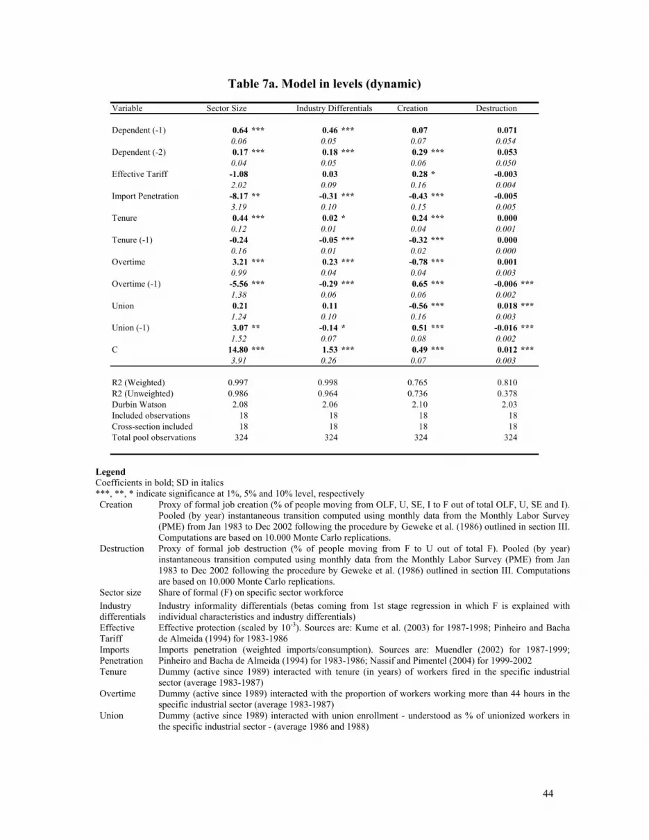
Table 7a. Model in levels (dynamic)

Variable Sector Size Industry Differentials Creation Destruction

Dependent (-1) 0.64 *** 0.46 *** 0.07 0.0710.06 0.05 0.07 0.054

Dependent (-2) 0.17 *** 0.18 *** 0.29 *** 0.0530.04 0.05 0.06 0.050

Effective Tariff -1.08 0.03 0.28 * -0.0032.02 0.09 0.16 0.004

Import Penetration -8.17 ** -0.31 *** -0.43 *** -0.0053.19 0.10 0.15 0.005

Tenure 0.44 *** 0.02 * 0.24 *** 0.0000.12 0.01 0.04 0.001

Tenure (-1) -0.24 -0.05 *** -0.32 *** 0.0000.16 0.01 0.02 0.000

Overtime 3.21 *** 0.23 *** -0.78 *** 0.0010.99 0.04 0.04 0.003

Overtime (-1) -5.56 *** -0.29 *** 0.65 *** -0.006 ***1.38 0.06 0.06 0.002

Union 0.21 0.11 -0.56 *** 0.018 ***1.24 0.10 0.16 0.003

Union (-1) 3.07 ** -0.14 * 0.51 *** -0.016 ***1.52 0.07 0.08 0.002

C 14.80 *** 1.53 *** 0.49 *** 0.012 ***3.91 0.26 0.07 0.003

R2 (Weighted) 0.997 0.998 0.765 0.810R2 (Unweighted) 0.986 0.964 0.736 0.378Durbin Watson 2.08 2.06 2.10 2.03Included observations 18 18 18 18Cross-section included 18 18 18 18Total pool observations 324 324 324 324

Legend Coefficients in bold; SD in italics ***, **, * indicate significance at 1%, 5% and 10% level, respectively Creation Proxy of formal job creation (% of people moving from OLF, U, SE, I to F out of total OLF, U, SE and I).

Pooled (by year) instantaneous transition computed using monthly data from the Monthly Labor Survey (PME) from Jan 1983 to Dec 2002 following the procedure by Geweke et al. (1986) outlined in section III. Computations are based on 10.000 Monte Carlo replications.

Destruction Proxy of formal job destruction (% of people moving from F to U out of total F). Pooled (by year) instantaneous transition computed using monthly data from the Monthly Labor Survey (PME) from Jan 1983 to Dec 2002 following the procedure by Geweke et al. (1986) outlined in section III. Computations are based on 10.000 Monte Carlo replications.

Sector size Share of formal (F) on specific sector workforce Industry differentials

Industry informality differentials (betas coming from 1st stage regression in which F is explained with individual characteristics and industry differentials)

Effective Tariff

Effective protection (scaled by 10-3). Sources are: Kume et al. (2003) for 1987-1998; Pinheiro and Bacha de Almeida (1994) for 1983-1986

Imports Penetration

Imports penetration (weighted imports/consumption). Sources are: Muendler (2002) for 1987-1999; Pinheiro and Bacha de Almeida (1994) for 1983-1986; Nassif and Pimentel (2004) for 1999-2002

Tenure Dummy (active since 1989) interacted with tenure (in years) of workers fired in the specific industrial sector (average 1983-1987)

Overtime Dummy (active since 1989) interacted with the proportion of workers working more than 44 hours in the specific industrial sector (average 1983-1987)

Union Dummy (active since 1989) interacted with union enrollment - understood as % of unionized workers in the specific industrial sector - (average 1986 and 1988)

44

Table 7b. Model in differences

Variable Sector Size Industry Differentials Creation Destruction

Dependent (-1) -0.34 *** -0.45 *** -0.68 *** -0.653 ***0.06 0.05 0.13 0.043

Dependent (-2) -0.30 *** -0.25 *** -0.12 -0.290 ***0.06 0.05 0.13 0.045

Effective Tariff 0.51 0.24 *** 0.52 *** 0.0002.57 0.08 0.17 0.005

Import Penetration 1.88 0.01 -0.28 0.0075.22 0.24 0.25 0.008

Tenure 0.40 *** 0.03 *** 0.26 *** 0.0000.11 0.01 0.02 0.000

Tenure (-1) 0.02 -0.03 *** -0.12 *** -0.0010.11 0.01 0.04 0.001

Overtime 4.46 *** 0.26 *** -0.99 *** 0.004 **1.16 0.06 0.09 0.002

Overtime (-1) -7.71 *** -0.29 *** -0.12 0.014 ***1.36 0.06 0.13 0.002

Union -0.82 0.19 *** -0.58 *** 0.017 ***1.25 0.07 0.08 0.003

Union (-1) -6.86 *** -0.27 *** 0.20 * 0.0021.25 0.07 0.11 0.002

C -1.03 *** -0.03 *** 0.01 -0.001 ***0.12 0.01 0.01 0.000

R2 (Weighted) 0.417 0.672 0.076 0.436R2 (Unweighted) 0.401 0.538 0.673 0.405Durbin Watson 2.08 2.07 2.19 2.17Included observations 17 17 17 17Cross-section included 18 18 18 18Total pool observations 306 306 306 306

Legend Coefficients in bold; SD in italics ***, **, * indicate significance at 1%, 5% and 10% level, respectively x(-1) First lag of x x(-2) Second lag of x Creation Proxy of formal job creation (% of people moving from OLF, U, SE, I to F out of total OLF, U, SE and I).

Pooled (by year) instantaneous transition computed using monthly data from the Monthly Labor Survey (PME) from Jan 1983 to Dec 2002 following the procedure by Geweke et al. (1986) outlined in section III. Computations are based on 10.000 Monte Carlo replications.

Destruction Proxy of formal job destruction (% of people moving from F to U out of total F). Pooled (by year) instantaneous transition computed using monthly data from the Monthly Labor Survey (PME) from Jan 1983 to Dec 2002 following the procedure by Geweke et al. (1986) outlined in section III. Computations are based on 10.000 Monte Carlo replications.

Sector size Share of formal (F) on specific sector workforce Industry differentials

Industry informality differentials (betas coming from 1st stage regression in which F is explained with individual characteristics and industry differentials)

Effective Tariff

Effective protection (scaled by 10-3). Sources are: Kume et al. (2003) for 1987-1998; Pinheiro and Bacha de Almeida (1994) for 1983-1986

Imports Penetration

Imports penetration (weighted imports/consumption). Sources are: Muendler (2002) for 1987-1999; Pinheiro and Bacha de Almeida (1994) for 1983-1986; Nassif and Pimentel (2004) for 1999-2002

Tenure Dummy (active since 1989) interacted with tenure (in years) of workers fired in the specific industrial sector (average 1983-1987)

Overtime Dummy (active since 1989) interacted with the proportion of workers working more than 44 hours in the specific industrial sector (average 1983-1987)

Union Dummy (active since 1989) interacted with union enrollment - understood as % of unionized workers in the specific industrial sector - (average 1986 and 1988)

45

Table 8. Sources of provision of health services before reforms: % structure by labor sector in 1981

Where did the person receive attention S.E. I FPublic network 47.80 58.93 46.65Private network 51.01 40.33 52.26Both 1.19 0.74 1.09

Who paid the attention: S.E. I FParticular 55.93 39.86 30.50Social Security 33.39 46.30 35.37Pre paid 3.83 2.30 6.63Employer 3.16 5.84 24.15Other 3.02 4.88 2More than one 0.67 0.82 0.91

.44

Note: These results are based on the sample of working household heads and the members of their household (the employment category of the household head is assigned to the rest of the members of the household) Source: PNAD 1981, non urban dwellers excluded.

Table 9. Shares of Formal and Informal sectors with respect the Working ages population (in percentages)

Survey Urban Rural Metropolitan Non MetropolitanF PNAD 1981 57.37 18.51 65.57 38.92

PME 1983 63.25I and S.E. PNAD 42.63 81.49 34.43 61.08

PME 36.75Workforce under 15 y.o. (PNAD) in MM 55.12 19.56 24.81 49.87

F PNAD 1990 54.57 26.68 61.04 42.16PME 61.34

I and S.E. PNAD 45.43 73.32 38.96 57.84PME 38.66

Workforce under 15 y.o. (PNAD) 70.20 22.52 30.07 62.66F PNAD 2001 46.78 20.00 51.52 38.95

PME 52.96I and S.E. PNAD 53.22 80.00 48.48 61.05

PME 47.04Workforce under 15 y.o. (PNAD) 102.80 18.21 39.87 81.14

Source: PNAD and PME. PME’s figures correspond to September of the corresponding year.

46

47

Figure 1. GDP cycle*

-15

-10

-5

0

5

10

15

1983

1984

1985

1986

1987

1988

1989

1990

1991

1992

1993

1994

1995

1996

1997

1998

1999

2000

2001

2002

G.D.P. cycle (H&P) G.D.P. (annual growth) * H&P filter applied with smoothing parameter 105

Figure 2. Share of Out of the Labor Force* (O.L.F) and Unemployment* (U)

3637

3839

4041

4243

4445

1983

1984

1985

1986

1987

1988

1989

1990

1991

1992

5

619

9319

9419

9519

9619

9719

9819

9920

0020

0120

02

0

1

2

3

4

O.L.F. U *Out of working ages population.

Figure 3. Share of Formal (F), Informal (I) and Self-employment (S.E.) sectors out

of Employed workforce

0

10

20

30

40

50

60

70

1983

1984

1985

1986

1987

1988

1989

1990

1991

1992

1993

1994

1995

1996

1997

1998

1999

2000

2001

2002

S.E. I F S.E. + I

Figu

re 4

. Mea

n D

urat

ion

Lev

els

024681012141619831984198519861987198819891990199119921993199419951996199719981999200020012002

0.5

0.7

0.9

1.1

1.3

1.5

1.7

1.9

2.1

2.3

2.5

S.E.

FU

(rig

ht)

I (rig

ht)

U

and

O.L

.F.

-1.5

-1.0

-0.50.0

0.5

1.0

1.5

1983

1984

1985

1986

1987

1988

1989

1990

1991

1992

1993

1994

1995

1996

1997

1998

1999

2000

2001

2002-1

0

-50510

O.L

.F. (

H&

P)G

.D.P

. (H

&P)

Rig

ht S

cale

-0.2

0

-0.1

0

0.00

0.10

0.20

1983

1984

1985

1986

1987

1988

1989

1990

1991

1992

1993

1994

1995

1996

1997

1998

1999

2000

2001

2002

-10

-50510

U (H

&P)

G.D

.P. (

H&

P) R

ight

Sca

le

F

-1.5

-1.0

-0.50.0

0.5

1.0

1.5

2.0

19831984198519861987198819891990199119921993199419951996199719981999200020012002

-10

-8-6-4-20246810

F (H

&P)

G.D

.P. (

H&

P) R

ight

Sca

le

I, S.

E.

-0.6

-0.4

-0.20.0

0.2

0.4

0.6

19831984198519861987198819891990199119921993199419951996199719981999200020012002

-10

-8-6-4-20246810

S.E.

(H&

P)I (

H&

P)G

.D.P

. (H

&P)

Rig

ht S

cale

N

ote:

Mea

n du

ratio

n in

ferr

ed fr

om th

e co

ntin

uous

tim

e tra

nsiti

on m

atrix

for

eac

h pe

riod

usin

g m

onth

ly d

ata

from

the

Mon

thly

Lab

or S

urve

y (P

ME)

fro

m J

an

1983

to D

ec 2

002

follo

win

g th

e pr

oced

ure

by G

ewek

e et

al.

(198

6) o

utlin

ed in

Ann

ex 1

. Com

puta

tions

are

bas

ed o

n 10

.000

Mon

te C

arlo

repl

icat

ions

. The

ser

ies

have

bee

n av

erag

ed p

er q

uarte

r, de

-tren

ded

usin

g a

HP

filte

r w

ith s

moo

thin

g pa

ram

eter

105

(exc

ept i

n th

e ca

se o

f th

e pa

nel “

Leve

ls”)

and

sm

ooth

ed u

sing

a 3

qu

arte

r mov

ing

aver

age

smoo

ther

. OLF

=Out

of t

he L

abor

For

ce, U

=Une

mpl

oym

ent r

ate,

I=In

form

al S

alar

ied,

SE=

Info

rmal

Sel

f-em

ploy

ed, F

=For

mal

Sec

tor.

48

Figu

re 5

. Bila

tera

l flo

ws b

etw

een

empl

oym

ent c

ateg

orie

s 5a

. In

Lev

els

0.6

0.8

1.0

1.2

1.4

1.6

1.8

19831984198519861987198819891990199119921993199419951996199719981999200020012002

1.5

2.0

2.5

3.0

3.5

4.0

4.5

F to

S.E

.S.

E. to

F

2.6

3.1

3.6

4.1

4.6

5.1

5.6

6.1

6.6

7.1

19831984198519861987198819891990199119921993199419951996199719981999200020012002

11131517192123252729

F to

II t

o F

5b. D

e-tr

ende

d

-0.4

-0.3

-0.2

-0.10.0

0.1

0.2

0.3

0.4

19831984198519861987198819891990199119921993199419951996199719981999200020012002

-1.0

-0.5

0.0

0.5

1.0

1.5

F to

S.E

.S.

E. to

F

-0.8

-0.6

-0.4

-0.20.0

0.2

0.4

0.6

0.8

19831984198519861987198819891990199119921993199419951996199719981999200020012002

-5-4-3-2-1012345

F to

II t

o F

Not

e: T

rans

ition

s ra

tes

infe

rred

from

the

cont

inuo

us ti

me

trans

ition

mat

rix fo

r eac

h pe

riod

usin

g m

onth

ly d

ata

from

the

Mon

thly

Lab

or S

urve

y (P

ME)

fr

om J

an 1

983

to D

ec 2

002

follo

win

g th

e pr

oced

ure

by G

ewek

e et

al.

(198

6) o

utlin

ed in

Ann

ex 1

. Com

puta

tions

are

bas

ed o

n 10

.000

Mon

te C

arlo

re

plic

atio

ns. T

he se

ries h

ave

been

ave

rage

d pe

r qua

rter,

de-tr

ende

d us

ing

a H

P fil

ter w

ith sm

ooth

ing

para

met

er 1

05 (e

xcep

t in

the

case

of t

he p

anel

s titl

ed

as “

In L

evel

s”) a

nd s

moo

thed

usi

ng a

3 q

uarte

r mov

ing

aver

age

smoo

ther

. OLF

=Out

of t

he L

abor

For

ce, U

=Une

mpl

oym

ent r

ate,

I=In

form

al S

alar

ied,

SE

=Inf

orm

al S

elf-

empl

oyed

, F=F

orm

al S

ecto

r.

49

Figu

re 6

. Job

Cre

atio

n an

d D

estr

uctio

n 6a

. Job

des

truc

tion

Tow

ards

U

-2.5

-2.0

-1.5

-1.0

-0.50.0

0.5

1.0

1.5

2.0

2.5

19831984198519861987198819891990199119921993199419951996199719981999200020012002

-10

-8-6-4-20246810

S.E.

(H&

P)I (

H&

P)F

(H&

P)G

.D.P

. (H

&P)

Righ

t Sca

le

Tow

ards

O.L

.F.

-2.0

-1.5

-1.0

-0.50.0

0.5

1.0

1.5

2.0

19831984198519861987198819891990199119921993199419951996199719981999200020012002

-10

-8-6-4-20246810

S.E.

(H&

P)I (

H&

P)F

(H&

P)G

.D.P

. (H

&P)

Righ

t Sca

le

6b. J

ob c

reat

ion

From

U

-8-6-4-2024681012

19831984198519861987198819891990199119921993199419951996199719981999200020012002

-10

-8-6-4-20246810

S.E.

(H&

P)I (

H&

P)F

(H&

P)G

.D.P

. (H

&P)

Righ

t Sca

le

From

O.L

.F.

-0.6

-0.4

-0.20.0

0.2

0.4

0.6

19831984198519861987198819891990199119921993199419951996199719981999200020012002

-10

-8-6-4-20246810

S.E.

(H&

P)I (

H&

P)F

(H&

P)G

.D.P

. (H

&P)

Righ

t Sca

le

Not

e: C

reat

ion/

Des

truct

ion

rate

s inf

erre

d fr

om th

e co

ntin

uous

tim

e tra

nsiti

on m

atrix

for e

ach

perio

d us

ing

mon

thly

dat

a fr

om th

e M

onth

ly L

abor

Sur

vey

(PM

E) f

rom

Jan

198

3 to

Dec

200

2 fo

llow

ing

the

proc

edur

e by

Gew

eke

et a

l. (1

986)

out

lined

in A

nnex

1. C

ompu

tatio

ns a

re b

ased

on

10.0

00 M

onte

C

arlo

rep

licat

ions

. The

ser

ies

have

bee

n av

erag

ed p

er q

uarte

r, de

-tren

ded

usin

g a

HP

filte

r w

ith s

moo

thin

g pa

ram

eter

105

(exc

ept i

n th

e ca

se o

f th

e pa

nels

titl

ed a

s “I

n Le

vels

”) a

nd s

moo

thed

usi

ng a

3 q

uarte

r m

ovin

g av

erag

e sm

ooth

er.

OLF

=Out

of

the

Labo

r Fo

rce,

U=U

nem

ploy

men

t ra

te,

I=In

form

al S

alar

ied,

SE=

Info

rmal

Sel

f-em

ploy

ed, F

=For

mal

Sec

tor.

50

Figu

re 7

. Act

ual a

nd p

redi

cted

Siz

e of

une

mpl

oym

ent a

nd fo

rmal

sect

or

7a. C

ontr

ollin

g ou

tflo

ws f

rom

Une

mpl

oym

ent

1.0

1.5

2.0

2.5

3.0

3.5

4.0

4.5

5.0

19831984198519861987198819891990199119921993199419951996199719981999200020012002

UU

toF

Uto

IU

toSE

Uto

I&SE

Uto

OU

toA

LL

Con

trol

ling

inflo

ws t

o U

nem

ploy

men

t

1.0

1.5

2.0

2.5

3.0

3.5

4.0

4.5

5.0

19831984198519861987198819891990199119921993199419951996199719981999200020012002

UFt

oUIto

USE

toU

SE&

ItoU

Oto

UA

LLto

U

7b. C

ontr

ollin

g ou

tflo

ws f

rom

For

mal

252729313335373941

19831984198519861987198819891990199119921993199419951996199719981999200020012002

FFt

oIFt

oSE

FtoS

E&I

FtoU

FtoA

LLFt

oO

Con

trol

ling

inflo

ws t

o Fo

rmal

252729313335373941

19831984198519861987198819891990199119921993199419951996199719981999200020012002

FIto

FSE

toF

SE&

ItoF

Uto

FA

LLto

FO

toF

N

ote:

U (A

ctua

l une

mpl

oym

ent r

ate)

and

F (A

ctua

l siz

e of

the

form

al se

ctor

) are

con

stru

cted

usi

ng m

onth

ly d

ata

from

the

Mon

thly

Lab

or S

urve

y (P

ME)

fr

om Ja

n 19

83 to

Dec

200

2. T

hese

serie

s hav

e be

en a

vera

ged

per q

uarte

r. U

(F) t

o i c

orre

spon

ds to

the

stea

dy st

ate

size

of U

(F) d

eriv

ed fr

om e

quat

ion

4 re

sulti

ng o

f app

lyin

g th

e 19

83-2

002

aver

age

trans

ition

rate

of a

ll th

e po

ssib

le fl

ows

exce

pt fo

r the

tran

sitio

n ra

te fr

om U

(F) t

o i;

i to

U (F

) cor

resp

onds

to

the

stea

dy s

tate

siz

e of

U (F

) der

ived

from

equ

atio

n 4

resu

lting

of a

pply

ing

the

1983

-200

2 av

erag

e tra

nsiti

on ra

te o

f all

the

poss

ible

flow

s ex

cept

for

the

trans

ition

rate

from

i to

U (F

). O

=Out

of t

he L

abor

For

ce, I

=Inf

orm

al S

alar

ied,

SE=

Info

rmal

Sel

f-em

ploy

ed, A

LL=

SE, I

and

F (w

hen

pred

ictin

g U

), A

LL=O

, U, I

and

SE

(whe

n pr

edic

ting

F)

51

52

Fi

gure

8. E

volu

tion

of T

rade

Ope

nnes

s and

of t

he v

aria

bles

use

d to

mea

sure

Con

stitu

tiona

l cha

nges

T

rade

Ope

nnes

s

%

of w

orke

rs w

orki

ng o

vert

ime

hour

s

020406080100

120

19831984198519861987198819891990199119921993199419951996199719981999200020012002

024681012

Effe

ctive

Tar

iffs

Impo

rts

Pene

trat

ion

010203040506070

1983

1984

1985

1986

1987

1988

1989

1990

1991

1992

1993

1994

1995

1996

1997

1998

1999

2000

2001

Form

alN

on F

orm

al

Yea

rs o

f ten

ure

of fi

red

wor

kers

U

nion

enr

ollm

ent

1.0

1.5

2.0

2.5

3.0

3.5

4.0

1983

1984

1985

1986

1987

1988

1989

1990

1991

1992

1993

1994

1995

1996

1997

1998

1999

2000

01 20

With

FG

TSW

ithou

t FG

TS

25262728293031323334

1986

1992

1993

1995

1996

1997

1998

1999

Not

es:

Figu

res

corr

espo

nd to

wei

ghte

d av

erag

es o

f all

indu

stria

l sec

tors

(with

wei

ghts

giv

en b

y th

e si

ze o

f eac

h in

dust

rial s

ecto

r). D

efin

ition

s of

plo

tted

varia

bles

cor

resp

ond

to th

ose

desc

ribed

in T

able

7.

FGTS

= F

undo

de

Gar

antia

de

Tem

po d

e Se

rviç

o (L

engt

h of

Ser

vice

Gua

rant

ee F

und)

. Bas

ical

ly, u

nder

the

FGTS

eve

ry f

irm in

Bra

zil h

as to

de

posi

t 8%

of i

ts c

urre

nt fo

rmal

em

ploy

ees w

ages

(8.5

% si

nce

Sept

embe

r 200

1) in

an

acco

unt o

pene

d in

the

wor

ker’

s nam

e in

a st

ate

bank

. Oth

er

than

som

e ex

cept

ions

, wor

kers

can

onl

y w

ithdr

aw m

oney

from

thes

e ac

coun

ts in

cas

e th

ey a

re fi

red

with

out a

“ju

stifi

ed re

ason

”. In

this

cas

e, th

ey

have

acc

ess t

o th

e FG

TS a

ccou

nt b

alan

ce p

lus a

firin

g pe

nalty

pai

d di

rect

ly b

y th

e em

ploy

er.

Figure 9. Trade Openness and Control Variables of Constitutional Changes Vs. Hiring Rates/Size of the Formal Sector

A. Trade Openness

-25

-20

-15

-10

-5

0

5

10

15

20

0 50 100 150

Cha

nge

in th

e H

irin

g R

ates

of t

he F

orm

al S

ecto

r (d

iffer

ence

of a

vera

ge b

efor

e an

d af

ter

1988

)

Effective Tariffs (Average 1983-1987)

-25

-20

-15

-10

-5

0

5

10

15

20

0 5 10 15

Cha

nge

in th

e H

irin

g R

ates

of t

he F

orm

al S

ecto

r (d

iffer

ence

of a

vera

ge b

efor

e an

d af

ter

1988

)

Imports Penetration (Average 1983-1987) B. Control Variables of Constitutional Changes

Overtime by formal workers Tenure of fired formal workers

-16

-14

-12

-10

-8

-6

-4

-2

0

20 40 60 80 100 120% of overtime formal workers (weighted by average excess

hours). Average 1983-1987

Cha

nge

in th

e Si

ze o

f the

For

mal

Sec

tor

(diff

eren

ce o

f ave

rage

bef

ore

and

afte

r 19

88)

-40

-30

-20

-10

0

10

20

1 2 3 4 5 6

Years of Tenure before firing (Average 1983-1987)

Cha

nge

in th

e H

irin

g R

ates

of t

he F

orm

al S

ecto

r (d

iffer

ence

of a

vera

ge b

efor

e an

d af

ter

1988

)

Union enrollment

-25

-20

-15

-10

-5

0

5

10

15

20

10 20 30 40 50 60Cha

nge

in th

e H

irin

g R

ates

of t

he F

orm

al S

ecto

r (d

iffer

ence

of a

vera

ge b

efor

e an

d af

ter

1988

)

% workers enrolled to an Union (1986)

Note: Bubbles’ sizes reflect the relative size of the industrial sector. The regression lines are obtained from WLS univariate regressions where weights are determined by the size of the industrial sector.

53

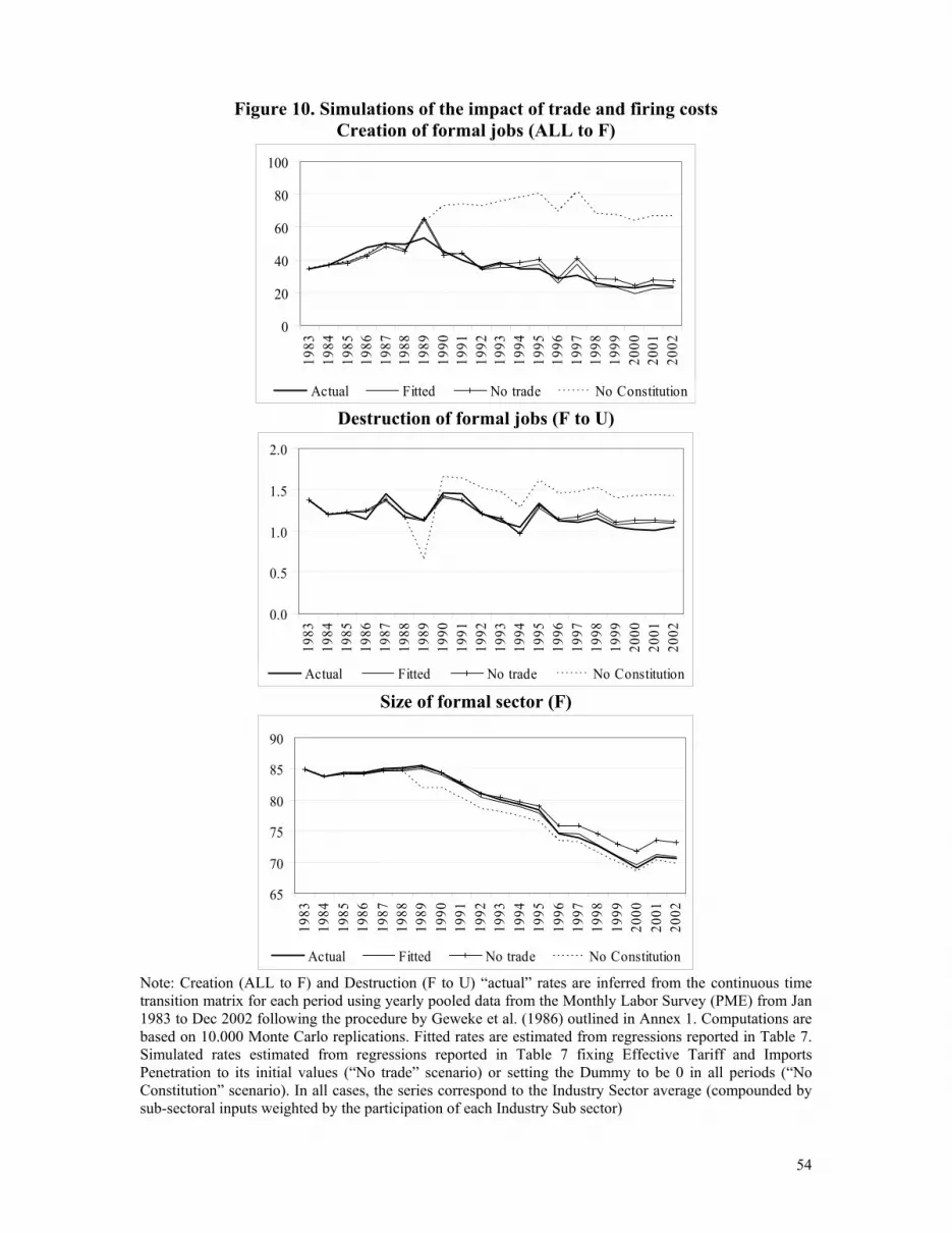
Figure 10. Simulations of the impact of trade and firing costs Creation of formal jobs (ALL to F)

0

20

40

60

80

100

1983

1984

1985

1986

1987

1988

1989

1990

1991

1992

1993

1994

1995

1996

1997

1998

1999

2000

2001

2002

Actual Fitted No trade No Constitution Destruction of formal jobs (F to U)

0.0

0.5

1.0

1.5

2.0

1983

1984

1985

1986

1987

1988

1989

1990

1991

1992

1993

1994

1995

1996

1997

1998

1999

2000

2001

2002

Actual Fitted No trade No Constitution Size of formal sector (F)

65

70

75

80

85

90

1983

1984

1985

1986

1987

1988

1989

1990

1991

1992

1993

1994

1995

1996

1997

1998

1999

2000

2001

2002

Actual Fitted No trade No Constitution

Note: Creation (ALL to F) and Destruction (F to U) “actual” rates are inferred from the continuous time transition matrix for each period using yearly pooled data from the Monthly Labor Survey (PME) from Jan 1983 to Dec 2002 following the procedure by Geweke et al. (1986) outlined in Annex 1. Computations are based on 10.000 Monte Carlo replications. Fitted rates are estimated from regressions reported in Table 7. Simulated rates estimated from regressions reported in Table 7 fixing Effective Tariff and Imports Penetration to its initial values (“No trade” scenario) or setting the Dummy to be 0 in all periods (“No Constitution” scenario). In all cases, the series correspond to the Industry Sector average (compounded by sub-sectoral inputs weighted by the participation of each Industry Sub sector)

54

Figure 11. Actual and predicted size of the industrial formal sector

65

70

75

80

85

90

1983

1984

1985

1986

1987

1988

1989

1990

1991

1992

1993

1994

1995

1996

1997

1998

1999

2000

2001

2002

Actual ShimerShimer no trade Shimer no Constitution

Note: the actual size of the formal sector is constructed using monthly data from the Monthly Labor Survey (PME) from Jan 1983 to Dec 2002. This series has been aggregated per year and corresponds to the Industry sector average (compounded by sub-sectoral inputs weighted by the participation of each Industry Sub sector). The predicted sizes are obtained applying equation in footnote 24 on the fitted values coming from regressions of Table 7 under the neutral and “no trade” and “no Constitution” scenarios.

65

70

75

80

85

90

1983

1984

1985

1986

1987

1988

1989

1990

1991

1992

1993

1994

1995

1996

1997

1998

1999

2000

2001

2002

Actual Shimer fix Destruction Shimer fix Creation

Note: the actual size of the formal sector is constructed using monthly data from the Monthly Labor Survey (PME) from Jan 1983 to Dec 2002. This series has been aggregated per year and corresponds to the Industry sector average (compounded by sub-sectoral inputs weighted by the participation of each Industry Sub sector). The predicted sizes are obtained applying equation in footnote 24 and correspond to the steady state size of F applying the 1983-2002 average transition rate of F to ALL and ALL to F respectively. F = formal, ALL = not formal.

55

Figure 12. Relative wages between sectors

0.3

0.5

0.7

0.9

1.1

1.3

1.5

1983

1984

1985

1986

1987

1988

1989

1990

1991

1992

1993

1994

1995

1996

1997

1998

1999

2000

2001

2002

-10

-8

-6

-4

-2

0

2

4

6

8

10

Wage SE/Wage F Wage I/Wage F G.D.P. (H&P) Right Scale

Note: Monthly Labor Survey (PME) from Jan 1983 to Dec 2002. The series have been averaged per quarter. I=Informal Salaried, SE=Informal Self-employed, F=Formal Sector.

56