Embed Size (px)
Citation preview
THE DETERMINATION OF ACTIVITY COEFFICIENTS ATINFINITE DILUTION
THESIS
Submitted in fulfilment of the requirements for the Degree ofDOCTOR OF PHILOSOPHY
of NATAL UNIVERSITY-DURBAN
by
Warren Charles Moollan
DECLARATION
I hereby certify that the· work presented in this thesis is the result of my owninvestigation under the supervision of-professor T. M. Letcher, and has never been-submitted in candidature for a degree in any other university.
arren Charles Moollan
Professor T. M. Letcher
ACKNOWLEDGEMENTS
The author gratefully makes the following acknowledgements:
To Professor T. M. Letcher, under whose supervision this thesis was conducted, forhis guidance and encouragements during the course of this study.
A special thank to Professor Urszula M. Domariska, for providing me with her moralsupport, her constant guidance, for the interest she has shown in my research, and forinstilling in me the enthusiasm to conduct this work. Also for giving me theopportunity to work with her at the Technical University of ~~saw, where part ofthis research was conducted.
To the Technical staff of the Chemistry Department at the Univer'sity of Natal for theirvaluable assistance especially, Mr. D. Jajevian Mr. K. Singh.
To the staff at the Technical University of Warsaw, especially Dr. A. Goldon, for thehours of stimulating discussion.
To my friends and colleagues in the department, most especially, Mr. H. Mohammed,Mr. Nesan Naidoo, Miss. P. Govender, Mr. A. Nevines and Mr. Paul Whitehead, formaking research such fun.
ABSTRACT
The aim of this work was to extend the theory of Everett and Cruickshank, forthe determination of activity coefficients at infinite dilution, )'73 {where 1 refers to thesolute and 3 to the solvent), to accommodate solvents of moderate volatility, using thegas liquid chromatography (GLC) method. A novel data treatment procedure isintroduced to account for the loss of solvent off the column, during the experiment.The method also allows us to determine the vapour pressure of the solvent. Noauxiliary equipment is required, and the method does not employ the use of apresaturator.
Further, the effect of a polar involatile solute is examined using various typesof solutes. The activity coefficient was found to be independent of column packing andflowrate.
Considering the volatile solvent, the systems investigated by the GLC methodwere straight chain hydrocarbons, (n-pentane, n-hexane and n-heptane), cyclichydrocarbons (cyclopentane, and cyclohexane) and an aromatic compound, benzene.The systems were investigated at 2 temperatures, 280.15 K and 298.15 K. The resultsindicate a clear dependence of the activity coefficient on temperature.
For the polar nonvolatile solvent, sulfolane (tetrahydrothiophene, 1,1 dioxane)was used. The systems studied were sulfolane + n-pentane, n-hexane, n-heptane,cyclopentane, cyclohexane, benzene, tetrahydrofuran, and tetrahydropyran. Thesystems were studied at one temperature, 303.15 K, due to the low melting point ofsulfolane i.e. 301.60 K.
Part of this study into the thermodynamics of solutions'\vas conducted at theTech{lical University of Warsaw, where the equilibria of sulfolane was studied using·two techniques, a dynamic solid-liquid equilibrium method (SLE), and anebulliometriGI vapor-liquid method (VLE) .
The main purpose of this was to apply solution theories to this data in order topredict the.activity coefficient at infinite dilution for the sulfolane mixtures.The systems measured using solid liquid equilibriu-m are sulfolane + tetrahydrofuran,or, 1,4-dioxane, or, I-heptyne, or, 1, 1, l,-trichloroethane, or, benzene, andcyclohexane. The results of these measurements were then described using varioussolution theories, and· new interaction parameters obtained.
The vapour liquid equilibrium systems measured were sulfolane + I-heptyne,or, tetrahyrdofuran, or, 1,1, I-trichloroethane, and tetrachloromethane. Here as in SLEthe results were described using solution theories.
The results of both the VLE and SLE measurements were used in a multipleoptimization procedure to produce new parameters for the interaction of sulfolane withvarious groups, using two group contribution method, DISQUAC and modifiedUNIFAC.The predicted activity coefficients compare well with the measured values using GLC.
CHAPTER 1. INTRODUCTION 1
CHAPTER 2. METHODS OF MEASURING ACTIVITY COEFFICIENTSAT INFINITE DILUTION OTHER THAN G.L.C. 5
2.1. Activity Coefficients at Infinite Dilution from Binary Vapour PressureEquilibrium 6
2.2. The Ebulliometric Method for the Measurements of Activity Coefficientsat Infinite Dilution. 6
2.2.1. Description of Equipment used and Principles of the Method 72.2.2. Procedure 92.2.3. Data Analysis 9
2.3. Measurement of the Activity Coefficients at Infinite dilution by means of theInert Gas Stripping Method. 11
2.3.1. Principles of the Method 122.3.2. Equipment and Procedure 142.3.3. Data Analysis 15
2.4. Modification of the Inert Gas Stripping Method for Measuring ActivityCoefficients at Infinite Dilution 18
2.4.1 Experimental 192.4.1.1. Apparatus 192.4.1.2. Procedure 20
2.5. Infinite Dilution Activity Coefficients using a Differential Static Cell Method212.5.1. Theory 222.5.2. Equipment and Procedure. 232.5.3. Chemicals 252.5.4. Data Analysis 25
2.6. The Dew Point Technique for Determining 1'72.6.1. Theory of the Dew Point Technique2.6.2. Apparatus2.6.3. Materials2.6.4. Procedure2.6.5. Data Reduction
2.7. Other methods
2.8.. Use of Activity Coefficients at Infinite Dilution.
2626272929293031
32
CHAPTER 3: THEORY OF GAS LIQUID ClffiOMATOGRAPHY 36
3.1. Gas Chromatography Principles3.1.1. Assumptions
3.2. Summary of the G.L.C. Theory Involving 1'73
3637
38
3.3. Detailed Theory of G.L.C. 403.3.1. The Theoretical Plate Concept3.3.2. Relation of the Net Retention Volume and the Activity Coefficient
to the Partition Coefficient 433.3.3. The Pressure Dependence of the Partition Coefficient 533.3.4. The Elution Process 583.3.5. The Net Retention Volume of an Ideal Carrier Gas 653.3.6. Treatment of a Volatile Solvent 66
3.3.6.1. Review of Work Using Volatile Stationary Phases 673.3.6.2. A Novel Method for taking Volatile Solvents into
Account 68
CHAPTER 4. APPARATUS AND EXPERIMENTAL PROCEDURE FORTHE DETERMINATION OF 1'73 BY GAS LIQUIDCHROMATOGRAPHY 70
4.1 The Design of the Gas-Liquid Chromatograph4.1.1. Flow Control4.1.2. Pressure Measurement4.1.3. Flow Rate Measurements4.1.4. Column Temperature Control4.1.5 Sample Injection and the Injection System4.1.6. G.L.C. Columns4.1.7. Detectors
7072727276767878
4.2. Experimental Procedure 814.2.1. Preparation of the Stationary Phase 814.2.2. Measurement Procedure 82
4.2.2.1. Treatment of a Volatile Solvent (n-Dodecane) 824.2.2.2. Treatment of a Polar Solvent (n-Sulfolane) 83
4.3.1. Calculation of l'734.3.2. Discussion
4.4. Determination of 1'73 of Solutes in a Polar Solvent (Sulfolane)4.4 .1. Calculation of 1'734.4.2. Discussion
909293
CHAPTER 5 EXCESS MOLAR VOLUMES OF l\!IIXING 105
5.1. Excess Molar Volumes of Mixing
5.1.1. Density Measurements5.1.1.1. Pycnometric Measurements5.1.1.2. The Mechanical Oscillator Densitometer
5.1.2. Direct Dilatometric Measurements5.1.2.1. Batch Dilatometry5.1.2.2. Continuous Dilution Dilatometry
5.2. The Anton Paar DMA 601 Vibrating Tube Densitometer5.2. 1. Design of the System5.2.2. Operation Procedure5.2.3. Preparation of Mixtures
5.3 Results
105106106106106
107108109'
109109112112
113
CHAPTER 6 EXCESS MOLAR ENTHALPIES OF MIXING 12:1
6.1. H: Measurements
6.2. The LKB 2107 Microcalorimeter6.2.1. Principle of Operation
6.3. The 2277 Thermal Activity Monitor (TAM)6.3.1. Principles of Operation
6.4. Operation Procedure and Actual Sample Measurement
6.5. Preparation of Mixtures
6.6. Friction Effects and Flow Rate Determination6.7. Results
122
122122
123:123
125
128
128130
CHAPTER 7 VAPOUR LIQUID EQUILIBRIA 136
7.1. Vapour Pressure Measurements 1377.1.1. The Static Method 1377.1.2. The Dynamic Method 139
7.2. Experimental Procedure 1407.2.1. Apparatus 1407.2.2. Auxillary Equipment 1447.2.3. Methods of Determining Vapour Pressures
and Mole Fraction 1447.2.4. Determination of P, T, x, and y 1457.2.5. Materials 146
7.3. Thermodynamics of Phase Equilibrium 1467.3.1. The Vapor Phase 1467.3.2. The Liquid Phase 1507.3.3. Vapour Liquid Equilibrium Data for a Solute + Sulfolane 150
7.4. Parameter Optimization 1567.4.1. The Least Squares Regression 157
7.4.1.2. Least Squares Objective Functions for the ActivityCoefficient Models 157'
7.4.2. The Maximum Likelihood Regression 160
CHAPTER 8. SOLID LIQUID EQUILIBRruM 1'&7
8.1. Solubility of Solids in Liquids 188
8.3.Eutectic Compositions 192
8.3. Activity Coefficients 196
8.4. Experimental Section 196'8.4.1. Materials 1968.4.2. Procedure 196
8.5.Results and Discussion 197
CHAPTER 9 ACTIVITY COEFFICIENTS AND EXCESSFUNCTIONS 209
236248'25i,25325.6
9.1. The Activity Coefficient 209
9.2 Normalization of Activity Coefficients 211
9.3. The Relationship Between Activity coefficients and Excess Functions in 213Binary 11ixtures
9.3.1. The two suffix 11ARGULES EQUATION 2139.3.2. The Redlich-Kister Expansion 2159.3.3. Wohl's Expression for the Excess Gibbs Energy 2179.3.4. The van Laar Equation 2189.3.5. The WILSON, NRTL, and UNIQUAC Equations 220
9.3.5.1. The WILSON Equation 2209.3.5.2. Renon's NonRandom Two-Liquid
(NRTL) Equation 2239.3.5.3. The Universal Quasi-chemical
(UNIQUAC) Equation 227
9.4. Group Contribution Methods 2319.4.1. Definition of Groups 2329.4.2. UNIFAC (UNIQUAC Functional-Group Activity Coefficient
11odel) 233:9.4.3. The Dispersive Quasichemical (DISQUAC) Theory 236
9.4.3.1. Theory of DISQUAC 2369.4.3.1.1. The Configurational Partition
Function9.4.3.1.2. Excess Free Energy9.4.3.1.3. The Excess Ener.gy9.4.3.1.4. Application to real 11ixtures9.4.3.1.5. The Zeroth Approximation
9.5. 11uliple Optimization Using DISQUAC and 11odified'UNIFAC9.5.1 Results and Discussion9.5.2. Conclusions
APPENDIX IAPPENDIX II
References
2582592'69.
284285
1
CHAPTER 1
INTRODUCTION
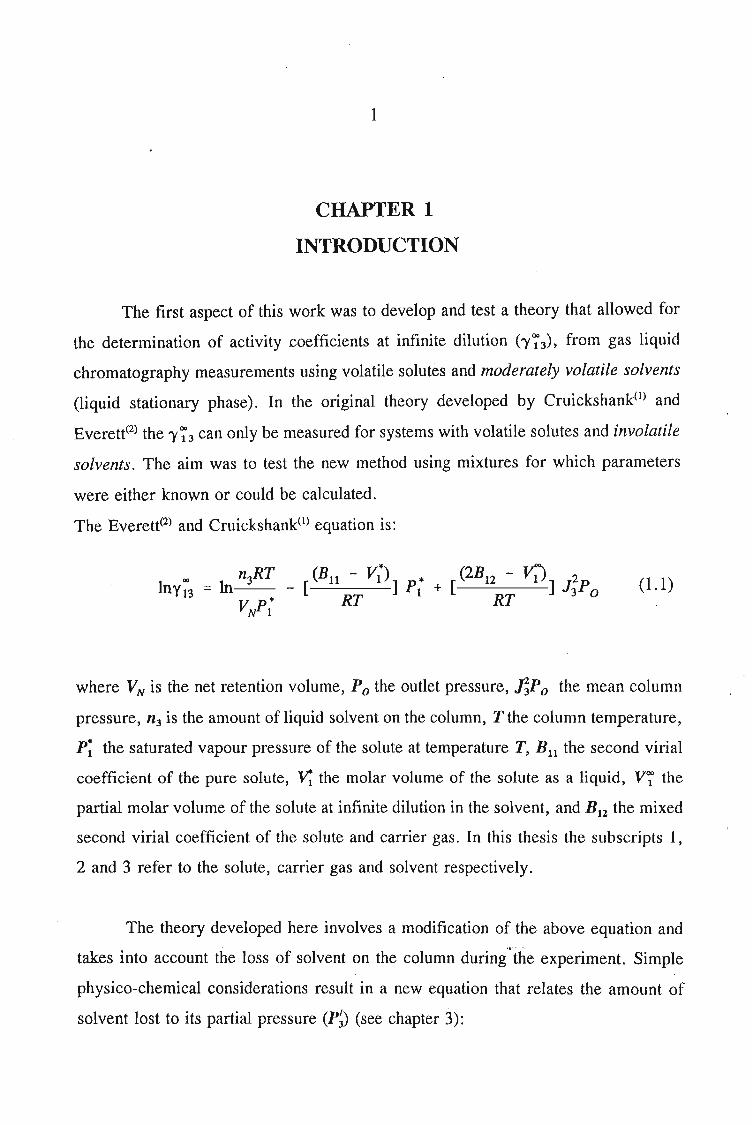
The first aspect of this work was to develop and test a theory that allowed for
the determination of activity coefficients at infinite dilution ('Y~3)' from gas liquid
chromatography measurements using volatile solutes and moderately volatile solvents
(liquid stationary phase). In the original theory developed by Cruickshank(l) and
Everett(2) the 'Y~ 3 can only be measured for systems with volatile solutes and involatile
solvents. The aim was to test the new method using mixtures for which parameters
were either known or could be calculated.
The Everett(2) and Cruickshank(l) equation is:
(1.1)
where VN is the net retention volume, Po the outlet pressure, J;p0 the mean column
pressure, n3 is the amount of liquid solvent on the column, T the column temperature,
P~ the saturated vapour pressure of the solute at temperature T, Bu the second virial
coefficient of the pure solute, ~ the molar volume of the solute as a liquid, V7 the
partial molar volume of the solute at infinite dilution in the solvent, and B12 the mixed
second virial coefficient of the solute and carrier gas. In this thesis the subscripts I,
2 and 3 refer to the solute, carrier gas and solvent respectively.
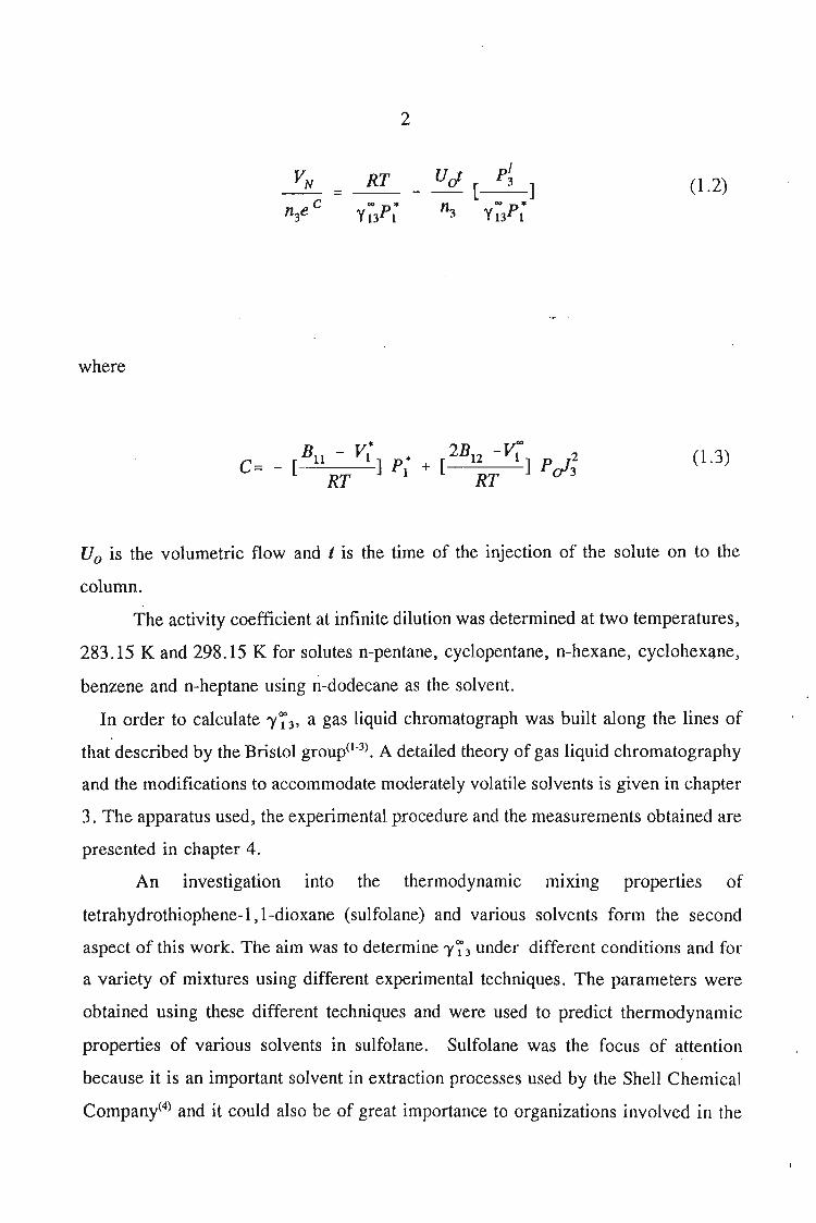
The theory developed here involves a modification of the above equation and
takes into account the loss of solvent on the column during'~the experiment. Simple
physico-chemical considerations result in a new equation that relates the amount of
solvent lost to its partial pressure (P~) (see chapter 3):
where
2
RT=--
Ut pI_0"' [ 3]n cop.
3 y 13 1
(1.2)
B - V· 2B-v:"c= _ [11 1] p. + [ 12 1 ] P 12
RT 1 RT 0'3
(1.3)
u0 is the volumetric flow and t is the time of the injection of the solute on to the
column.
The activity coefficient at infinite dilution was determined at two temperatures,
283.15 K and 298.15 K for solutes n-pentane, cyclopentane, n-hexane, cyclohexane,
benzene and n-heptane using n-dodecane as the solvent.
In order to calculate 1'73' a gas liquid chromatograph was built along the lines of
that described by the Bristol group(I-3). A detailed theory of gas liquid chromatography
and the modifications to accommodate moderately volatile solvents is given in chapter
3. The apparatus used, the experimental procedure and the measurements obtained are
presented in chapter 4.
An investigation into the thermodynamic mIxmg properties of
tetrahydrothiophene-l, I-dioxane (sulfolane) and various solvents form the second
aspect of this work. The aim was to determine 1'73 under different conditions and for
a variety of mixtures using different experimental techniques. The parameters were
obtained using these different techniques and were used to predict thermodynamic
properties of various solvents in sulfolane. Sulfolane was the focus of attention
because it is an important solvent in extraction processes used by the Shell Chemical
Company(4) and it could also be of great importance to organizations involved in the
3
separation of organic compounds, such as SASOL.
The work involved exposure to a large number of experimental techniques viz.
G.L.C., excess molar volume determination, excess molar enthalpy determination,
solid liquid equilibrium, and vapour liquid equilibrium. The work also concentrates
on many of the most important theories relating to liquid mixtures and solution. ego
WILSON(S), NRTV6) , UNIQUAC(7) , UNIFAC(8) and DISQUAC(9).
Chapters 5 and 6 discuss the methods used to measure the excess molar
volumes and enthalpy respectively. The systems studied are: an alkyne + sulfolane
at 303.15 K. The results obtained are discussed in relation to the significant
interactions between sulfolane and the alkynes.
In chapter 7, the vapour liquid equilibria method employed in this work is
discussed. The Rogalski(1O) modified Swktoslawski(1l) dynamic ebulliometer still was
used to obtain binary vapour-liquid equilibria for the following systems at 338.15 K
or 353.15 K: I-heptyne, or tetrahydrofuran, or 1,4-dioxane, or tetrachloromethan~or
1,1,1-trichloroethane + sulfolane, over the whole concentration range. The data is
described using the Margules(12), van Laar(13), WILSON, NRTL and UNIQUAC
equations.
The solid liquid equilibria measurements are discussed in chapter 8. THe
systems studied here are: I-heptyne, or tetrahydrofuran, or l,4-dioxane, or
tetrachloromethane or trichloroethane + sulfolane. The results of the correlation of
solubility for sulfolane in the solvents with respect to the solid-solid phase transition
in sulfolane is given in terms of the WILSON, NRTL and UNIQUAC equations,
utilizing parameters taken from solid-liquid equilibria for the simple eutectic mixtures
only. The correlations have been done using the data reported here as well as data
published earlier. (14-17)
Chapter 9 concentrates on exammmg the well-established theories of
4
correlations and predicting activity coefficients at finite and infinite dilution. A detailed
discussion of two group contribution methods (modified UNIFAC and DISQUAC) is
also given. These two methods are used to predict the activity coefficients of sulfolane
in a variety of mixtures at different temperatures using the excess enthalpy, VLE, and
SLE data presented here, as well as data published earlier. New parameters for the
interactions of various groups (CH), CH2 , Cl, A-CH2 , C6H6 etc.) with sulfolane (as
a single group) are obtained for both modified UNIFAC and DISQUAC.
5
CHAPfER 2.
METHODS OF MEASURING ACTIVITY COEFFICIENTS
AT INFINITE DILUTION OTHER THAN G.L.C.
Activity coefficients permit the specific measurements ofunlike pair interactions
in solution without any dependence on composition functionality or mixing rules. (18)
Activity coefficients at infinite dilution ('Y7.J, where 1 refers to the solute and 3 to the
solvent) are ofgreat interest to the practising chemist and chemical engineerfrom both
a theoretical and a practical point of view. This activity coefficient characterizes the
behaviour ofan ilJfinitely dilute material (the solute) which is completely surrounded
by solvent molecules. A knowledge of activity coefficients at infinite dilution is
important not only for the development ofnew thermodynamic models but they are also
important for the adjustment of reliable model parameters(18) and in the choice of
solvents for processes such as extractive rectification, extraction, or absorption (19).
Infinite dilution activity coefficients havefound numerous applications in characterizing
solution behaviour. They can be used to generate accurate binary parameters for
solution modeli20-21), .to predict the existence ofazeotropes(22) "'a~ to estimate mutual
solubilities. (23) In addition they can be used to calculate kinetic solvent effects with
relationships such as the Bronsted-Bjerrum relationship(24). One can accurately
construct an entire binary vapour liquid equilibrium curve from the two activity
coefficients at infinite dilution (25-27) using liquid mixing models based on two
parameters.
This chapter deals with the determination ofdetermining 'Y73from experimental
methods other than Gas Liquid Chromatography (28). This method is the subject of
Chapters 3-4. The methods discussed are: Differential Ebulliometry(20), the Inert Gas
Stripping Method(29), a modification of the Inert Gas Stripping Method(30) , the
Differential Static Cell Method(3l), and the Dew Point Technique(32). The experimental
methods are discussed in order to give a brief insight into the complexities of each
6
method and the equipment required. These methods are also compared to the method
employed in this work (gas liquid chromatography, Chapter 3 and 4). This chapter
puts into perspective the work carried out and described in Chapters 3 and 4.
2.1. Activity Coefficients at Infmite Dilution from Binary Vapour Liquid
Equilibrium
Activity coefficients at infinite dilution are often determined from the
extrapolation of VLE data(27). If a vapour composition method, (rather than a total
pressure technique) is used, one may calculate activity coefficients from each data
point and extrapolate graphically. Unless the data are particularly accurate and
plentiful in the dilute region, their extrapolation to infinite dilution is very
imprecise(20). Chapter 7 gives a detailed account of the equipment and theory of
binary vapour liquid equilibrium measurements. This method is not discussed in this
chapter, as it is not a method relating to infinite dilution.
2.2. The Ebulliometric Method for the Measurements of Activity Coefficients
at Infinite Dilution.
Eckert et al. (20) proposed the Differential Ebulliometric Technique for the
measurement of 1'73' The differential ebulliometer used is similar in some respects to
that described previously by NuW33). It involves boiling a solution in an ebulliometer
connected, through condensers to a common manifold, with a second ebulliometer
containing pure boiling solvent. In this way the vapour pressure of the two boiling
liquids are maintained at the same pressure. The system used by Eckert et al. (20) is
depicted in figure 2.1. The data is analyzed using equation 2.'1 following the method
developed by Gautreaux and Coates (34) with additional terms (the fugacity coefficients)
included to account for vapour-phase nonideality:
..Yl3 =
7
v p. &1>. dp·,.,,(P;)p.[P._(1_P._3 +_3 (_3) )](_3)(aTf'+'1 3 3 3 RT 4>; ap To dT aX1 P
p; 4>~ exp[(P; - P;)VII RT
(2.1)
where P; and P; are vapour pressures of component 1 (the solute) and 3 (the solvent)
respectively. cjJ~P) is the fugacity coefficient of component 1 at the vapour pressure of
component 3, cjJ; and cjJ; are the fugacity coefficients of components 1 and 3 at their
vapour pressures, respectively. VI and V3 are the molar volumes of components 1 and
3 respectively, and Xl the mole fraction of component I in the liquid phase.
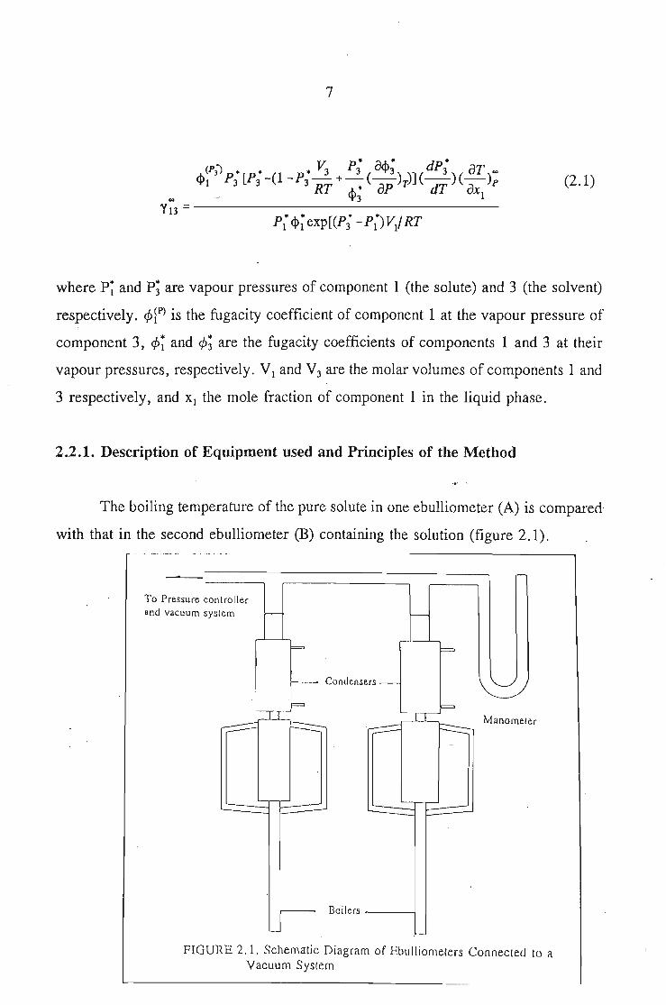
2.2.1. Description of Equipment used and Principles of the Method
The boiling temperature of the pure solute in one ebulliometer (A) is compared
with that in the second ebulliometer (B) containing the solution (figure 2.1).
~ ~
To Pressure controllerand vacuum system - I--
'--
= =
- Condensers-
= =.1 I Manometer
~ f=::::::::-- .--;::::::::::. F====:--
'--r- _'-.----J LI-_-_-
I-
-
-
Boilers -_--j
-
-
FIGURE 2.1. Schematic Diagram of Ebulliometers Connected 10 aVacuum System
8
Small fluctuations in pressure have minimal effect on the 1'73' In addition, the
pressure, and in consequence the temperature, at which 1'73 is determined, can be
readily set and controlled. A vacuum pump is connected through a solenoid valve to
the manifold, which includes a 15-L ballasf tank. (20) The tank is controlled through a
relay, by a differential sulphuric acid manostat, and dry air is,.continuously bled into
the system. Control of better than + 0.2 mmHg is usually achieved and the pressure
was read to better than + 0.1 mm from a mercury manometer using a cathetometer.
The boiling point elevation is often measured with a quartz crystal thermometer with
matching sensing probes capable of resolution to 0.00 I K. (20) The ebulliometer used
by
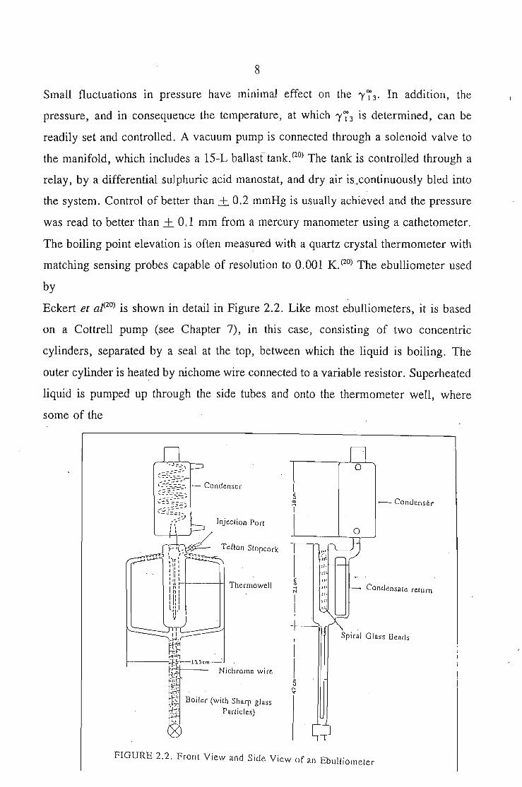
Eckert et al(20) is shown in detail in Figure 2.2. Like most ebulliometers, it is based
on a Cottrell pump (see Chapter 7), in this case, consisting of two concentric
cylinders, separated by a seal at the top, between which the liquid is boiling. The
outer cylinder is heat~d by nichome wire connected to a variable resistor. Superheated
liquid is pumped up through the side tubes and onto the thermometer well, where
some of the
Injection PorI
Tenon Stopcork
r-t----H Thermowell
~---w:ct-l~~cm
Nichrome wire
Boiler (with Sharp glass
Particles)
I5'"T
I .:.: ~.
5 ....., ,,,N
;:;
I :;:
! .,
-~
I
II
I5"...
o
>-- Condenser-
Condensate rerum
Spiral Glass Beads
FIGURE 2.2. Front View and Side View of an Eblllliomeler
9
liquid is taken up by evaporation. The remaining liquid passes down the outsides of
the thermowell, slowed by helical beads, returns via the inner cylinder, and is joined
by the cooled condensate. The whole ebulliometer is thoroughly insulated.
Using too small a volume of solute (1) is impractical, since the original liquid
composition would be drastically affected by the enrichment of vapour with the more
volatile component. It is in fact, this complication that has led to questions about the
applicability of ebulliometry to mixtures(35).
2.2.2. Procedure
Initially, both ebulliometers (A and B) are filled gravimetrically with pure
solvent to a level about 25 mm from the side tube. The pressure control is set, the
liquid heated to boiling, and the system allowed to come to equilibrium (usually about
30 minutes). With both ebulliometers containing pure solvent only, the optim,um
heating rate and any systematic offset in the measured temperature difference is
determined. Either pure solute or a gravimetrically prepared mixture is injected into
the ebulliometer through a septum stopper with a syringe. The syringe is weighed
before and after each injection to obtain an injected mass in the order of 1 g, to a
precision of + 0.1 mg. When equilibrium is again reached, (5 - 15 minutes) the
pressure and the temperature differences are recorded. The procedure can be repeated
a number of times.
2.2.3. Data Analysis
The ebulliometric data are analyzed following the method development by
Gautreaux and Coates (34) with additional fugacity terms included' for the vapour-phase
non-idealities. A rigorous expression for the activity coefficient at infinite dilution can
10
be readily derived in terms of pure component properties and the limiting slope of the
temperature versus composition curve ie. (aT/ax)';:
...Y13 =
• V P • a<l> • dp·",(P3 ) p. [p. _(1_P._3 +_3 (_3) )](_3)( aT)""""1 3 3 3 RT <1>; ap To dT aX1 P
p; <1>; exp[(P; - P;) Vd RT
(2.1)
Equation 2.1, is based on liquid-phase nonideality. The fugacity coefficients
terms, are obtained by Eckert(20) from virial coefficients estimated using the method
of Hayden and O'Connell. (36)
The quantity determined experimentally is (aT/axY; which is the limiting
composition derivative of the temperature. The advantage of using the equation is that
no functional dependence of the activity coefficient on composition is assumed. Instead
of extrapolating finite activity coefficients to the infinite value, an inherently uncertain
process, the limiting slopes of nearly linear x-T curves whose end points are alw~ys
fixed, are measured.
Equation 2.1 can be used to examine the sensitivity of 'Y~3 to errors in the
measured limiting slope and thus provide a criterion for the applicability of the
ebulliometric method to a given binary system. If we disregard the fugacity coefficient
term and the Poynting correction all of which have minor si$I)ificance anyway, the
equation becomes(20)
dp·p. __3 (aT)""
3 dT ax P
p.1
(2.2)
The 'Y~3 is essentially the algebraic sum of the two terms. Since it may become
11
the difference between two much larger numbers, extremely high accuracy is needed
in the data. To measure the sensitivity Eckert(20) considered the fractional change in
1'73 with the equivalent change of the limiting slope;
(2.3)
Since the activity coefficient of the solvent is unity at this limit and the total
pressure is the vapour pressure of the solvent, the second term on the right hand side
is essentially the relative volatility at infinite dilution.
The ebulliometric method is thus best suited to solvents ofsimilar volatility. If
the solute is much less volatile than the solvent, 1'73 determination will be difficult
unless its value is very high. If the solute is more volatile than the solvent, the liquid
composition correction becomes important. While this causes no instability in the data
reduction, heavy reliance must be set on the estimated values of the vapour space and
the liquid holdup. There is also an increased risk of losing some solute through the
condenser during a run.
2.3. Measurement of the Activity Coefficients at Infinite dilution by means of
the Inert Gas Stripping Method.
The inert gas stripping method presented by Leori et al. (29) is a fast and accurate
method for the determination of 'Y73 of a solute dissolved in a liquid mixture. It is
based on the study of the solute elution with time and the solute is stripped from the
solution by a constant flow of gas. The basis of the method of Leori(29) is a
measurement of the desorption of a solute from a solution as .~ function of time. The
solute is present in the solution at a very low concentration and is desorbed by the
12
passage of an inert gas at a constant flow rate. During the desorption, samples of the
vapour phase are withdrawn and their compositions are determined. It is important to
ensure a large gas-liquid interface, a sufficiently long time contact between the two
phases, and good dispersion of bubbles in the liquid. Under such conditions, the gas
leaving the saturation vessel may be expected to be very close to equilibrium with the
liquid mixture. The variation of solute concentration in the gaseous phase is measured
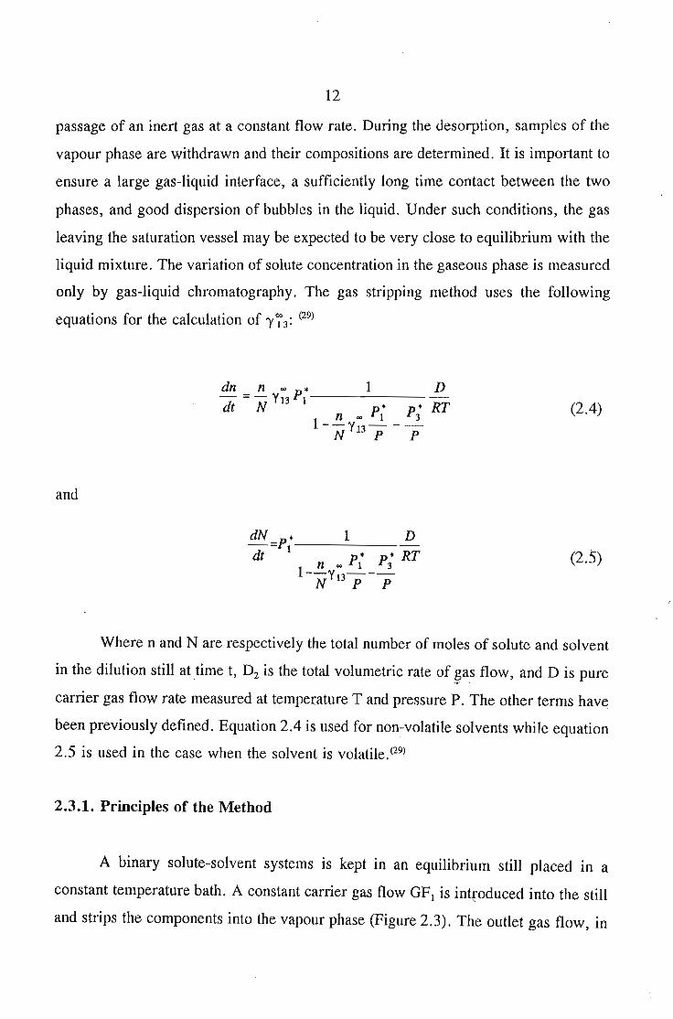
only by gas-liquid chromatography. The gas stripping method uses the following
equations for the calculation of 'Y73: (29)
and
dN =-Pl* 1 Ddt p* p* RTn .. 1 3
l--Y13---N P P
(2.4)
(2.5)
Where nand N are respectively the total number of moles of solute and solvent
in the dilution still at time t, D2 is the total volumetric rate of ¥a_s flow, and D is pure
carrier gas flow rate measured at temperature T and pressure P. The other terms have
been previously defined. Equation 2.4 is used for non-volatile solvents while equation
2.5 is used in the case when the solvent is volatile. (29)
2.3.1. Principles of the Method
A binary solute-solvent systems is kept in an equilibrium still placed in a
constant temperature bath. A constant carrier gas flow GF l is introduced into the still
and strips the components into the vapour phase (Figure 2.3). The outlet gas flow, in
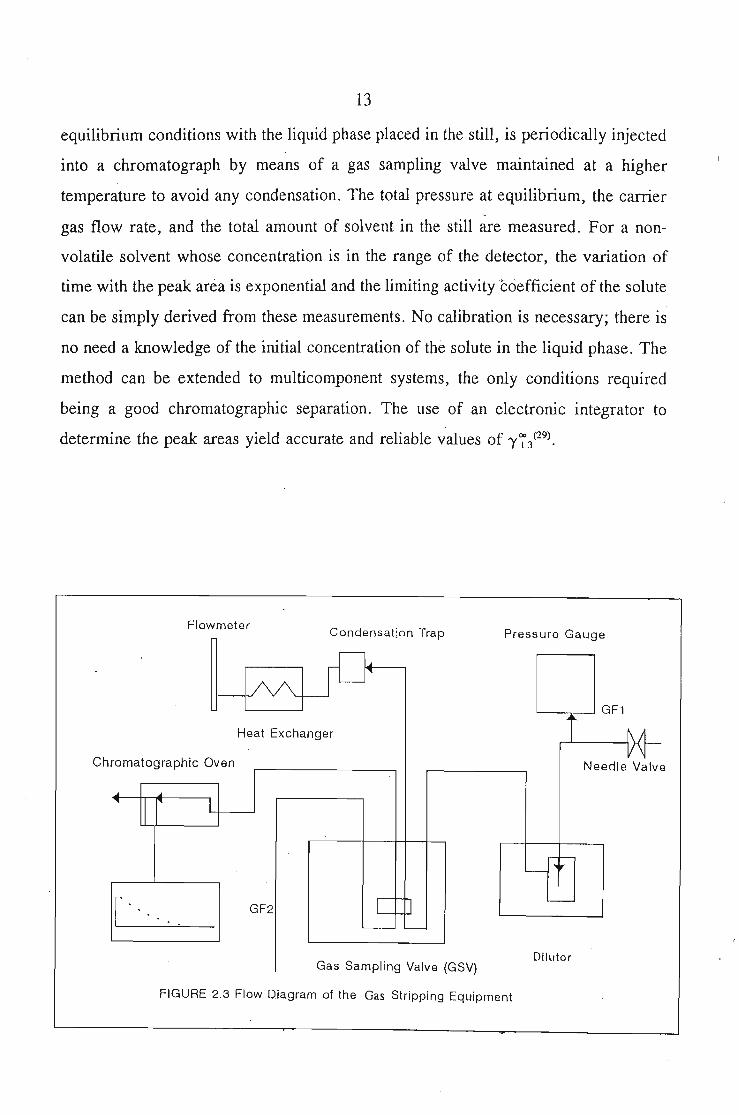
13
equilibrium conditions with the liquid phase placed in the still, is periodically injected
into a chromatograph by means of a gas sampling valve maintained at a higher
temperature to avoid any condensation. The total pressure at equilibrium, the carrier
gas flow rate, and the total amount of solvent in the still are measured. For a non
volatile solvent whose concentration is in the range of the detector, the variation of
time with the peak area is exponential and the limiting activity 'coefficient of the solute
can be simply derived from these measurements. No calibration is necessary; there is
no need a knowledge of the initial concentration of the solute in the liquid phase. The
method can be extended to multicomponent systems, the only conditions required
being a good chromatographic separation. The use of an electronic integrator to
determine the peak areas yield accurate and reliable values of 1'7}29).
Flowmeter
~_~JJn,atjonT,ap
Heat Exchanger
Chromatographic Oven
Pressure Gauge
'---y--' GF1
iNeedle Valve
11 I~ I
GF2 CJ--
-
Gas Sampling Valve GSV
FIGURE 2.3 Flow Oiagram of the Gas Stripping Equipment
Dilutor
14
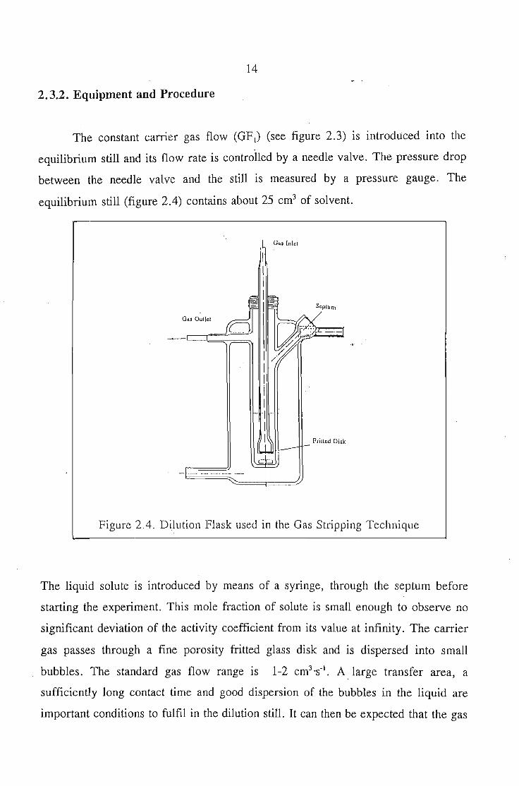
2.3.2. Equipment and Procedure
The constant carrier gas flow (GFI) (see figure 2.3) is introduced into the
equilibrium still and its flow rate is controlled by a needle valve. The pressure drop
between the needle valve and the still is measured by a pressure gauge. The
equilibrium still (figure 2.4) contains about 25 cm3 of solvent.
Gas Dullet
PrilleJ Disk
Figure 2.4. Dilution Flask used in the Gas Stripping Technique
The liquid solute is introduced by means of a syringe, through the septum before
starting the experiment. This mole fraction of solute is small enough to observe no
significant deviation of the activity coefficient from its value at infinity. The carrier
gas passes through a fine porosity fritted glass disk and is dispersed into small
bubbles. The standard gas flow range is 1-2 cm3"$-1. A. large transfer area, a
sufficiently long contact time and good dispersion of the bubbles in the liquid are
important conditions to fulfil in the dilution still. It can then be expected that the gas
15
leaving the device is very nearly in thermodynamic equilibrium with the liquid phase.
Liquid droplet entrainment is limited by keeping the dead space for the gas phase
small enough to obtain steady state conditions in a short time. The gas outlet is
wrapped with a heating tape to avoid any condensation of organic vapours which are
diluted in the carrier gas stream. The outlet is connected to a gas sampling valve
immersed in a thermostatic bath filled with silicon oil and maintained at 323.15 K. All
the metal connections used are swagelock connectors with inox ferrules. The gas flows
through the sampling loop, and is evacuated after passing through the precision soap
film flow meter. A trap condenses the organic vapours before measurements of the
carrier gas flow rate. The heat exchanger is a 40 m copper coil placed in a
thermostatic water bath; its purpose is to keep gas flow rate at ambient temperature
for a precise measurement of the flow rate GFI' The gas sampling valve (GSV) allows
the introduction of a sample of a constant number of moles of GF1 into GF2 • Gas
stream GF2 then enters the chromatographic column placed in the oven. (29)
2.3.3. Data Analysis
If it is assumed that the gas phase is in equilibrium with the liquid phase, it is
possible to write the equilibriu,m equations (neglecting gas phase corrections):
(2.6)
where y1 is the mole fraction of component 1 in the vapour phase.
If nand N are respectively the total number of moles of solute and solvent in
the dilution still at time t, the quantities (-dn) and (-dN) withdrawn from the solution
during a change of time, dt, by the carrier gas flow are given by:
16
D2 dtdn = -y p-
1 RT(2.7)
(2.8)
where D2 is the total volumetric rate of gas flowing out of the still converted to the
pressure P and temperature T.
From the above equations it can be deduced that
and
dN = _p* D2
dt 3 RT
An overall mass balance around the dilution still gives
where D is the pure carrier gas flow rate at the measured T and P.
Combining the equations and replacing Xl by
(2.9)
(2.10)
(2.11)
the results are
· 17
x = _n_ "".!!.. (at infinite dilution conditions)1 n+N N
(2.12)
and
dn n co •
- =-Y13 P tdt N (2.4)
(2.5)
Equations 2.4 and 2.5 are the basic differential equations relating the variations of the
amounts of solute and solvent with time. Integrating equation 2.4 and assuming that
in the case of a non volatile solvent, N is considered constant, the resulting equation
IS, .
n D P; ..In- =-- Yl3t
no RT N(2.13)
where I10 is the initial value of n at t = O.
Since the sampling loop of the gas sampling valve is maintained at a constant
temperature, the amount of solute injected into the column is proportional to the solute
partial pressure over the solution. It can therefore be deduced that,
-,- ~'.
(2.14)
18
where SI is the solute peak area. Therefore
(2.15)
Equation 2.14 indicates an exponential variation of solute peak area with time.
In the case of a volatile solvent integration of the differential system formed by
equations 2.4 and 2.5 yield
(2.16)
2.4. Modification of the Inert Gas Stripping Method for Measuring Activity
Coefficients at Infinite Dilution
Surovy et al(30) proposed a modification to Leori' S (29) gas stripping method
(section 2.3) for the measurement of the limiting activity coefficient. Compared to the
previous method, the modification consists of a change in the apparatus and
measurement of the decrease in solute concentration in the liquid phase only. In the
original apparatus of Leori and co workers(29) the inert strippirig gas is fed to the liquid
phase through a tube terminated with a frit. In order to prevent the vapour or organic
substance from condensing in the gas stream, whilst leaving the saturation vessel, both
the outlet and the sampling valve are heated. The positioning and shape of the outlet
vessel should help ensure gas phase homogeneity, and hence reproducibility of the
results. The gas phase homogeneity and the absence of vapour condensation in the
19
stream of the stripping gas before entry to the chromatographic column are important
features which require special attention.
Modifications by Surovy<30) and co workers, include the measurement of the
decrease in solute concentration in the liquid phase which.
2.4.1 Experimental
2.4.1.1. Apparatus
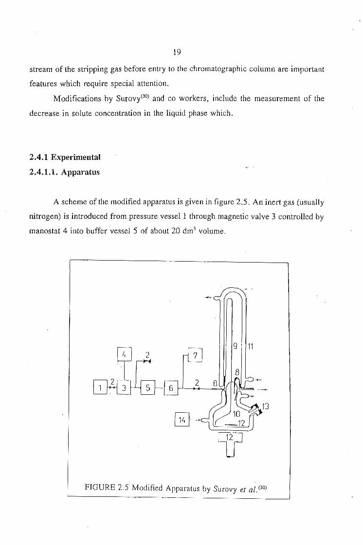
A scheme of the modified apparatus is given in figure 2.5. An inert gas (usually
nitrogen) is introduced from pressure vessel 1 through magnetic valve 3 controlled by
manostat 4 into buffer vessel 5 of about 20 dm3 volume.
9 11
8
FIGURE 2.5 Modified Apparatus by Surovy et a/. (30)
20
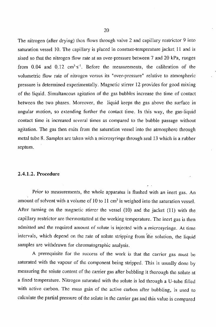
The nitrogen (after drying) then flows through valve 2 and capillary restrictor 9 into
saturation vessel 10. The capillary is placed in constant-temperature jacket 11 and is
sized so that the nitrogen flow rate at an over-pressure between 7 and 20 kPa, ranges
from 0.04 and 0.12 cm3 ·s-1. Before the measurements, the calibration of the
volumetric flow rate of nitrogen versus its 11 over-pressure 11 relative to atmospheric
pressure is determined experimentally. Magnetic stirrer 12 provides for good mixing
of the liquid. Simultaneous agitation of the gas bubbles increase the time of contact
between the two phases. Moreover, the liquid keeps the gas above the surface in
angular motion, so extending further the contact time. In this way, the gas-liquid
contact time is increased several times as compared to the bubble passage without
agitation. The gas then exits from the saturation vessel into the atmosphere through
metal tube 8. Samples are taken with a microsyringe through seal 13 which is a rubber
septum.
2.4.1.2. Procedure
Prior to measurements, the whole apparatus is flushed with an inert gas. An
amount of solvent with a volume of 10 to 11 cm3 is weighed into the saturation vessel.
After turning on the magnetic stirrer the vessel (10) and the jacket (11) with the
capillary restrictor are thermostatted at the working temperature. The inert gas is then
admitted and the required amount of solute is injected with a microsyringe. At time
intervals, which depend on the rate of solute stripping from'th-e solution, the liquid
samples are withdrawn for chromatographic analysis.
A prerequisite for the success of the work is that the earner gas must be
saturated with the vapour of the component being stripped. This is usually done by
measuring the solute content of the carrier gas after bubbling it thorough the solute at
a fixed temperature. Nitrogen saturated with the solute is led through a V-tube filled
with active carbon. The mass gain of the active carbon after bubbling, is used to
calculate the partial pressure of the solute in the carrier gas and this value is compared
21
with the saturated vapour pressure at the temperature of the saturation vessel. All
chemicals used, have to be of a high purity which in most cases means vacuum
fractional distillation on a column.
2.5. Infinite Dilution Activity Coefficients using a Differential Static Cell Method
Sandler et al.(31), have developed a new static cell apparatus (Figure 2.6) to
measure the activity coefficients at infinite dilution for binary systems. Here the direct
measurements of 'Y~3 is determined by measuring the equilibrium total pressure at a
temperature T above a liquid of known composition. (37). The static cell is particularly
suited for the measurements of equilibrium pressures of systems with large relative
volatilities or with partial miscibility. An important aspect of the static cell is that
measurements are made at equilibrium conditions in contrast to a dynamic apparatus,
such as a vapour-liquid still or an ebulliometer, which operate at steady state with
temperature gradients and with liquid and condensed vapour holdups. However the
solvents and the solutes used here, must be totally free of any impurities, especially
dissolved gases or volatile components which, even at low concentrations, would
significantly affect the measured pressure. Therefore all chemicals must be degassed
before operation.
The differential static cell was developed by Sandler et al. (31) to overcome
problems associated with the measurement of 'Y73 with dynamic equipment(38). In
particular, since there is no condensed vapour holdup to alter the composition of
gravimetrically prepared mixtures, static cells can be used to measure 'Y~3 of systems
with a higher solute volatility than is possible with ebulliometers. Static cells can also
be used for solvents with poor boiling properties, such as -water(29) over large
temperature ranges. Data treatment for the calculation of 'Y73 is similar to that of the
ebulliometric method using Equation 2.1.
22
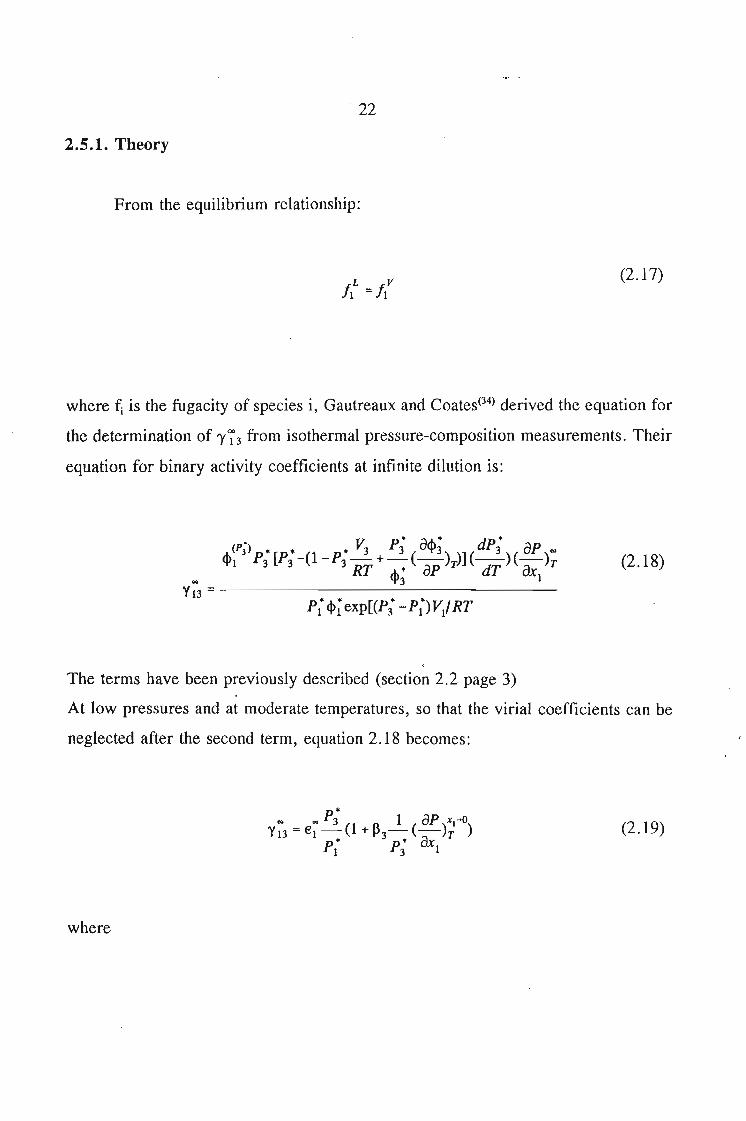
2.5.1. Theory
From the equilibrium relationship:
(2.17)
where fj is the fugacity of species i, Gautreaux and Coates(34) derived the equation for
the determination of 'Y~3 from isothermal pressure-composition measurements. Their
equation for binary activity coefficients at infinite dilution is:
..y 13 ;::
v P * a'" * dP *4>(P;> P * [P *-(1 _P *_3 + _3 (_'t'_3) )] (_3) ( ap)",1 3 3 3 RT 4>; ap To dT aX1 T
P; 4>~ exp[(P; -P;)VdRT
(2.18)
The terms have been previously described (section 2.2 page 3)
At low pressures and at moderate temperatures, so that the virial coefficients can be
neglected after the second term, equation 2.18 becomes:
(2.19)
where
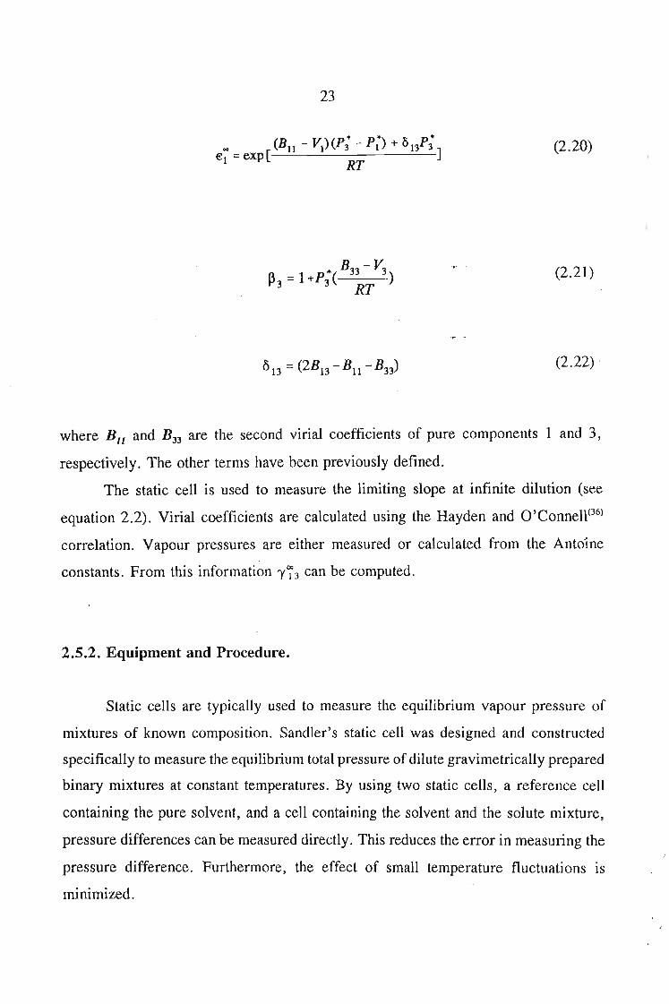
23
B -vA = l+P"( 33 3)tJ3 3 RT
(2.20)
(2.21)
(2.22) .
where Bll
and B33 are the second virial coefficients of pure components 1 and 3,
respectively. The other terms have been previously defined.
The static cell is used to measure the limiting slope at infinite dilution (see
equation 2.2). Virial coefficients are calculated using the Hayden and O'Connell(36)
correlation. Vapour pressures are either measured or calculated from the Antoine
constants. From this information ,73 can be computed.
2.5.2. Equipment and Procedure.
Static cells are typically used to measure the equilibrium vapour pressure of
mixtures of known composition. Sandler's static cell was designed and constructed
specifically to measure the equilibrium total pressure of dilute gravimetrically prepared
binary mixtures at constant temperatures. By using two static cells, a reference cell
containing the pure solvent, and a cell containing the solvent and the solute mixture,
pressure differences can be measured directly. This reduces the error in measuring the
pressure difference. Furthermore, the effect of small temperature fluctuations is
minimized.

24
A schematic diagram of the apparatus is shown in figure 2.6. The static cell
apparatus consists of two glass cells each having an injection port, sealed with double
septum-, for the addition of solvent and solute. Additional equipment used for the static
cell measurements consists of a temperature bath that can be manouvered so that the
static cells can be removed or placed on the static cell manifold.
Before each series of measurements is started, all the septa are replaced, and
the glass wear washed and dried in an oven. The cell to which the solute injections are
made together with the septa and the stirring bar, are weighed before being attached
to the degassing manifold. Once attached, the solvent is added, the cells are capped,
and a vacuum is applied to one cell at a time.
Consiant temprerature I"sulalion Box
Vaccum Olllu.nll.1Pr.uureTra05duC8(
ConslanttemperalurWater Bath
Heating Pad
Mixing Cell Reference Cell
FIGURE 2.6 Schematic Diagram of the DifferentialStatic Cell Equilibrium Apparatus
25
Once the solvents have been boiled, the cells are placed in an ultrasonic bath
for further degassing. A vacuum is again applied to one cell at a time for
approximately 3-5 minutes, and the cycle is repeated 4-6 times. If the solvent is
moderately volatile, the procedure is similar except that degassing cycles are shorter.
Alternatively, freeze-thaw cycles using liquid nitrogen are used for very volatile
solvents.
The cells are then attached to the manifold containing the pressure transducer.
A vacuum is then applied to the transducer, and the zero point of the pressure
transducer is then recorded. By opening and closing certain valves, the transducer is
isolated from the vacuum pump and is exposed to the vapour of the solvent. After the
vapour pressure measurements, the mixing cell is prepared for the solute injection, by
disconnecting the cell, and placing it in a hot water bath for about 10 minutes, so that
the vapour pressure in the cell is slightly greater than I atm. This prevents air from
entering the cell during injection. The degassed solute is then injected in to the cell,
using a syringe of known weight. The cell is cooled to the water bath temperature.
The pressure is then recorded every 5 minutes for 30-45 minutes until a constant value
is obtained. The injection procedure is repeated about five times, doubling the solute
volumes with each injection. Solute quantities are usually 10 J-tl for the first injection.
2.5.3. Chemicals
The purity of the solutes is crucial to the determination of 'Y73 from static cell
measurements. The highest purity solvents available are used in all experiments.
2.5.4. Data Analysis
The measurements made are total pressure and mole fraction. The change in
pressure is expressed as a function of the liquid mole fraction. A second degree
polynomial is fitted to the data:
26
(2.23)
By using this polynomial an accurate value of the limiting slope (ap/aX)T can be
obtained which is equal to the parameter b. The limiting slope is used in equation 2.18
to calculate 'Y73'
2.6. The Dew Point Technique for Determining 'Y73
Trampe and Eckert(32) have developed the a Dew Point Technique for the
determination of 'Y73 of a very dilute vapour phase. This method is especially
applicable to systems of low solute volatility, precisely where other methods such as
ebulliometry and headspace gas chromatography become less precise. The technique
is analogous to the differential ebulliometer and involves the change of temperat\lre
of the dew point of a vapour solvent when a dilute amount of solute is added.
The expression relating 'Y73 of a solute in a solvent to a change in the dew point
temperature (aT/ay\); at constant pressure is derived in a similar fashion to that of the
ebulliometer technique, ie. equation 2.1.
2.6.1. Theory of the Dew Point Technique
Once agam, disregarding the fugacity coefficient terms and the Poynting
correction, all of which are generally of little significance at low pressure, and
expressing the relative volatility of a solute infinitely dilute in a solvent can be
expressed by:
27
(2.24)
By substituting Equation 2.24 into Equation 2.1 an expression relating the measured.
dew point temperature to the relative volatility of the pure solute in the solvent is
obtained,
(2.25)
The quantities have been previously defined.
From equation 2.25 it can be ~oted that the expression depends only on the properties
of the solvent and the temperature.
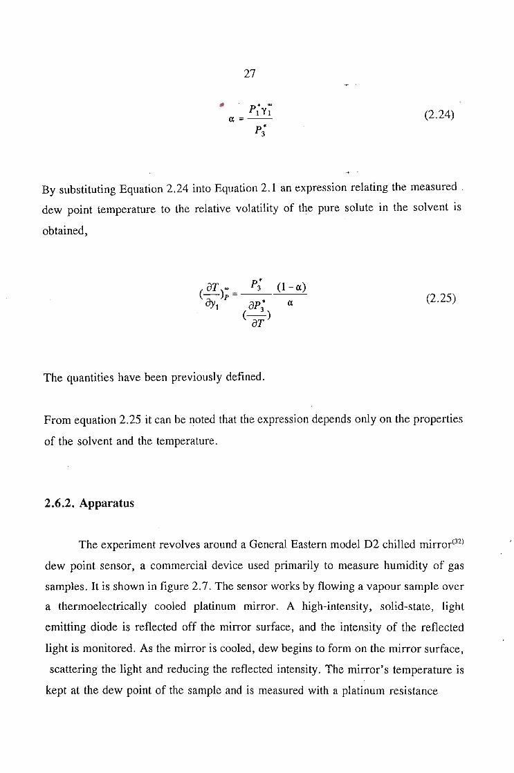
2.6.2. Apparatus
The experiment revolves around a General Eastern model D2 chilled mirror(32)
dew point sensor, a commercial device used primarily to measure humidity of gas
samples. It is shown in figure 2.7. The sensor works by flowing a vapour sample over
a thermoelectrically cooled platinum mirror. A high-intensity, solid-state, light
emitting diode is reflected off the mirror surface, and the intensity of the reflected
light is monitored. As the mirror is cooled, dew begins to form on the mirror surface,
scattering the light and reducing the reflected intensity. The mirror's temperature is
kept at the dew point of the sample and is measured with a platinum resistance
28
OPTICAL BALANCE
LEDREGULATION
-----,"---- SA M PLE
THERMOELECTRIC1----1 HEAT PUMP
289 K DEW POINT'-----' TEMPERATURE
• (32)FIGURE 2.7. Dew POInt Sensor
--------------------------------IIII
PRESSURECONTROLLER
- - - - - - - - - - - - - -I,,I
N 2 ---1-----.--- -,---j p
SOLVENTIMIXTURES
CONSTANTTEMPERATURE
VACUUM AIR BATH .-----, r'\..------I
PUMP
RESTRICTOR
P-ER"'--'I'--STALT(C :I PREHEA
PUMP
DEW POINTSENSOR
TRAP ORCONDENSER
FIGURE 2.8. Overall design of the svstem used to measure the Activity coefficient atinfinite dilution by dew point measurements.(J"1)
29
thermometer embedded just below the mirror surface.
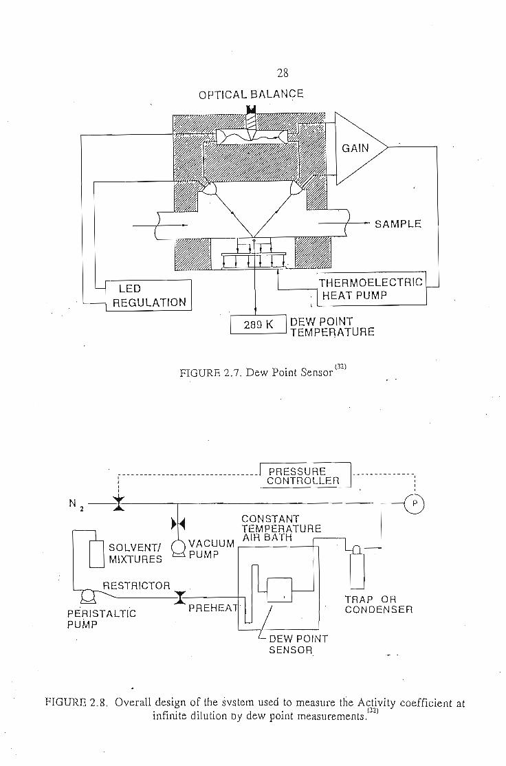
The sensor is used in the experimental setup as shown in figure 2.8. Pure
solvent or a solution of known composition is pumped through silica tubing. The
liquid is "pumped" and not "pulled" into the system as a result of the pressure drop,
thus ensuring a relatively constant flow rate. The vapour then flows through the
sensor exits from the oven and is cooled and collected in a water-cooled condenser,
or an ice trap.
2.6.3. Materials
High purity solvents are required, and the water content in the solvents has to be kept
as low as is possible.
2.6.4. Procedure
The solutions are made up gravimetrically and are stirred for 30 minutes wjth
a magnetic stirrer. The oven temperature is set so that the sensor is maintained at
approximately 5 K above the expected dew point and held fairly constant. The preheat
section is heated to 40 - 60 K higher than the dew point temperature. Although this
is not critical, it must be hot enough to totally vaporise the solution. The mirror
surface is cleaned with acetone before the pressure is set to give the desired
temperature. At each temperature a liquid flow rate must be determined. The vapour
flow rate was found not to affect the dew point measurements.
Pure solvent is pumped through the system for approxiiiuitely 10 minutes. The
cooling current in the sensor mirror is switched on, and the mirror is cooled to the
dew point temperature. When the sensor signals that it has control of the dew layer
on the mirror surface, the temperature of the mirror and the system pressure are
recorded for approximately 10 minutes. The cooling current is then disabled and the
pure solvent is replaced with a solution. The procedure is repeated four or five times
with increasing solute concentrations.
30
2.6.4. Data Reduction
The temperature values are all found by taking the difference between each
corrected solution dew point _temperature and the first pure solvent dew point
measurement. The experimental dT - Ydata are fitted to various empirical equations:
or
or
1 A B-=-+-!1T YI Y1Y3
(quadratic)
(cubic)
(van !Aar)
(2.26)
(2.27)
(2.28)
In the first two expreSSIOns (aT/ay,) '; = A, and in the third expreSSIOn
(aT /ay,) '; is equal to I /B. (32) The fits are generally close to linear. The value for the
limiting slope is taken from the expression that has the smallest standard deviation of
fit given by:
}](!1T -!1T )2-!,a = [ calc exp' ] 2
(n-N)(2.29)
where n is the number of experimental points and N is the n~mber of adjustable
31
parameters in the equation. This value of (aT/ay I); is used in equation 2.1 to obtain
1'73' Since the experiment relies on difference in temperatures there is no need for
temperature calibration. Also, since this is a vapour phase and 'flow experiment, there
is no need to make corrections- in the vapour phase composition.
2.7. Other methods
Other less well-establish methods for the determination of activity coefficients
at infinite dilution have been reported in the literature. (40-41) One such method is a
variation of headspace Gas Liquid Chromatography that minimizes the difficulties of
calibration found in direct headspace chromatography<4O). In this method the liquid
, space consists of two (virtually immiscible) solvents. Small amounts of solute are first
added to one of the solvents, and then increments of the second solute are added,
along with continual sampling and analysis of the equilibrium vapour space. The
changes in solute concentration in the vapour can be rdated to a partition coefficient,
which in turn can be related to an infinite dilution activity coefficient. This indirect
headspace chromatography is especially applicable to systems of higher relative
volatility.
A relatively new method developed by Ray(41) is the determination of Binary
Activity Coefficients from Microdroplet Evaporation. Although this method does not
measure the activity coefficient at infinite dilution it is of some importance as it can
be used to measure both 1'1 and 1'3' The method is based on the evaporation of a
constant-composition droplet containing two components that differ markedly in
volatility. The method accurately estimates activity coefficients of both components.
This new technique was developed to simultaneously determine the evaporation rate
and composition of a droplet from intensity peaks observed in the light scattered by
the droplet. It has no upper or lower limits on the relatively volatility of the system
and is particularly suitable for systems containing one relatively nonvolatile
component.
32
2.8. Use of Activity Coefficients at Infinite Dilution
Thermodynamic models of liquid mixtures for GE are generally constructed is
such a way that a given number of empirical parameters must be determined on the
basis of experimental data. The equations developed thus far generally require two or
three parameters perbinary system. However the activity coefficient at infinite dilution
can be used to predict finite activity coefficients only if a one parameter model is used
ego Margules(l2) or Van Laar(l3). If both ')'~3 and ')';1 were obtainable experimentally
then there are many two parameter models available, ego Wilson(5) and UNIQUAC(7),
that can be used to predict finite concentration activity coefficients. A detailed
discussion of these models, among others, is given in Chapter 9.
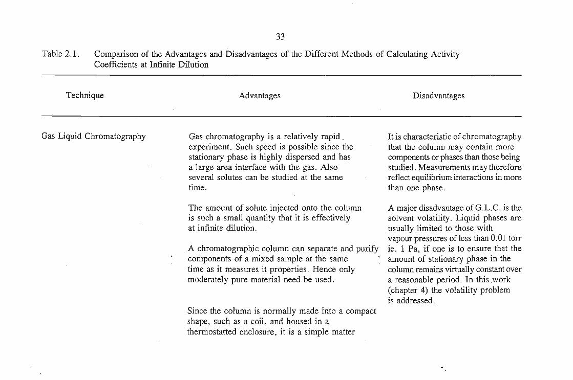
Table 2.1.
33
Comparison of the Advantages and Disadvantages of the Different Methods of Calculating ActivityCoefficients at Infinite Dilution
Technique
Gas Liquid Chromatography
Advantages
Gas chromatography is a relatively rapid _experiment. Such speed is possible since thestationary phase is highly dispersed and hasa large area interface with the gas. Alsoseveral solutes can be studied at the sametime.
The amount of solute injected onto the columnis such a small quantity that it is effectivelyat infinite dilution.
A chromatographic column can separate and purifycomponents of a mixed sample at the same i
time as it measures it properties. Hence onlymoderately pure material need be used.
Since the column is normally made into a compactshape, such as a coil, and housed in athermostatted enclosure, it is a simple matter
Disadvantages
It is characteristic of chromatographythat the column may contain morecomponents or phases than those beingstudied. Measurements may thereforereflect equilibrium interactions in morethan one phase.
A major disadvantage of G.L.C. is thesolvent volatility. Liquid phases areusually limited to those withvapour pressures of less than 0.01 torrie. 1 Pa, if one is to ensure that theamount of stationary phase in thecolumn remains virtually constant overa reasonable period. In this work(chapter 4) the volatility problemis addressed.
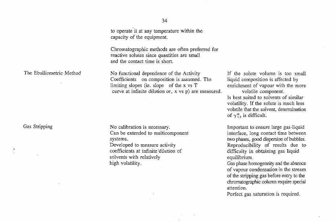
The Ebulliometric Method
Gas Stripping
34
to operate'it at any temperature within thecapacity of the equipment.
Chromatographic methods are often preferred forreactive solutes since quantities are smalland the contact time is short.
No functional dependence of the ActivityCoefficients on composition is assumed. Thelimiting slopes (ie. slope of the x vs Tcurve at infinite dilution or, x vs p) are measured.
No calibration is necessary.Can be extended to multicomponentsystems.Developed to measure activitycoefficients at infinite idilution ofsolvents with relativelyhigh volatility.
If the solute volume is too smallliquid composition is affected byenrichment of vapour with the more
volatile component.Is best suited to solvents of similarvolatility. If the solute is much lessvolatile that the solvent, determinationof 'Y73 is difficult.
Important to ensure large gas-liquidinterface, long contact time betweentwo phases, good dispersion of bubbles.Reproducibility of results due todifficulty in obtaining gas liquidequilibrium. .Gas phase homogeneity and the absenceof vapour condensation in the streamof the stripping gas before entry to thechromatographic column require specialattention.Perfect gas saturation is required.
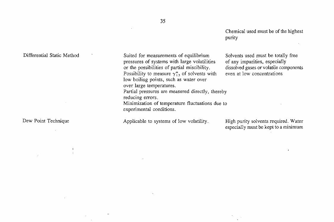
Solvents used must be totally freeof any impurities, especiallydissolved gases or volatile componentseven at low concentrations
Differential Static Method
35
Chemical used must be of the highestpurity
Suited for measurements of equilibriumpressures of systems with large volatilitiesor the possibilities of partial miscibility.Possibility to measure 1'73 of solvents withlow boiling points, such as water overover large temperatures.Partial pressures are measured directly, therebyreducing errors.Minimization of temperature fluctuations due toexperimental conditions.
Dew Point Technique Applicable to systems of low volatility. High purity solvents required. Waterespecially must be kept to a minimum
36
CHAPTER 3
THEORY OF GAS LIQUID CHROMATOGRAPHY
3.1. Gas Chromatography Principles
The chromatographic process involves the distribution of a solute component
(1) between two phases, a mobile phase (2) and a solvent stationary phase (3). The
two phases are mutually well dispersed with a large area of contact. In Gas Liquid
Chromatography (G.L.C.) the liquid stationary phase (eg. dodecane or sulfolane) is
dispersed on an inert solid support, such as celite, which is packed into a column. The
liquid is held on the surface and in the pores of the support, while a stream of inert
gas, the mobile phase, flows continuously through the spaces between the particles. (42)
In the elution process a small quantity of solute is introduced into the column
at the inlet. The solute zone or peak is carried through the column by the mobile phase
and its emergence at the other end is observed by a suitable detector (in this work two
types of thermal conductivity detectors were used). The velocity with which the peak
travels through the column is less than that of the mobile phase and depends on the
distribution coefficient of the solute between the two phases. (43)
When the solute reaches the column, an equilibrium is set up between the liquid
phase and the carrier gas phase so that a proportion of the sample always remains in
the gas phase. This portion moves a little further along the column in the carrier gas
stream, where it again equilibrates with the stationary phase. At the same time,
material already dissolved in the stationary phase re-enters the gas phase so as to
restore equilibrium with the clean carrier gas, which follows the zone of vapour. (24)
This process in which carrier gas containing the vapour is strippyd by the solvent in
front of the zone, while vapour enters carrier gas at the rear of the zone, goes on
37
continuously with the result that the zone of vapour moves along the column more or
less compactly. The speed at which the zone moves depends mainly on two factors,
the rate of flow of the carrier gas and the partition coefficient of the solute between
carrier gas and liquid phase. The faster the flow of carrier gas the faster the zone
moves, and the more strongly the vapour is retained on to the solvent, the more
slowly the zone moves. When two or more components are present in the sample,
each usually behaves independently of the other, so that for a given carrier gas flow
rate, the speed of the zone of each component will depend on the extent to which it
is retained. Since different substances differ in their retention, they may therefore be
separated by making use of their different speeds of progress through the column.
When eluted the solutes will appear one after the other in the gas stream, the fastest
first and the slowest last. The gas liquid chromatographic process is one ofequilibrium
between a vapour and a liquid, and the retention is a function of the solutes vapour
pressure and the interaction between the solute and solvent (this process involves the
dissolution of the vapour in the solvent).
3.1.1. Assumptions
One of the theories related to the determination of activity coefficients at infinite
dilution is the plate theory and rests on the following assumptions. (43)
(i)
(ii)
The column can be divided into a large number of theoretical plates.- ·r -
The partition coefficient is constant throughout the range of concentration
encountered, that is, Henry's Law is obeyed. This is only true for very low
solute concentrations.
(iii) The solute volume upon introduction into the column occupies only a small
portion of the column length.
(iv) There is negligible resistance to mass transfer from gas to solvent i.e. the rate
at which equilibrium is reached is very much greater than the rate of travel of
38
solute down the column. Equilibrium exists at each stage in the process ie.
theoretical plate.
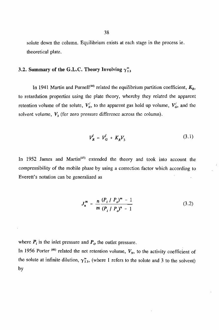
3.2. Summary of the G.L.C.Theory Involving 1'73
In 1941 Martin and Purnen<44) related the equilibrium partition coefficient, KR,
to retardation properties using the plate theory, whereby they related the apparent
retention volume of the solute, V~, to the apparent gas hold up volume, V~, and the
solvent volume, V3 (for zero pressure difference across the column).
(3.1)
In 1952 lames and Martin(45) extended the theory and took into account the
compressibility of the mobile phase by using a correction factor which according to
Everett's notation can be generalized as
(3.2)
where Pi is the inlet pressure and Po the outlet pressure.
In 1956 Porter (46) related the net retention volume, VN , to the activity coefficient of
the solute at infinite dilution, 1'73' (where 1 refers to the solute and 3 to the solvent)
by
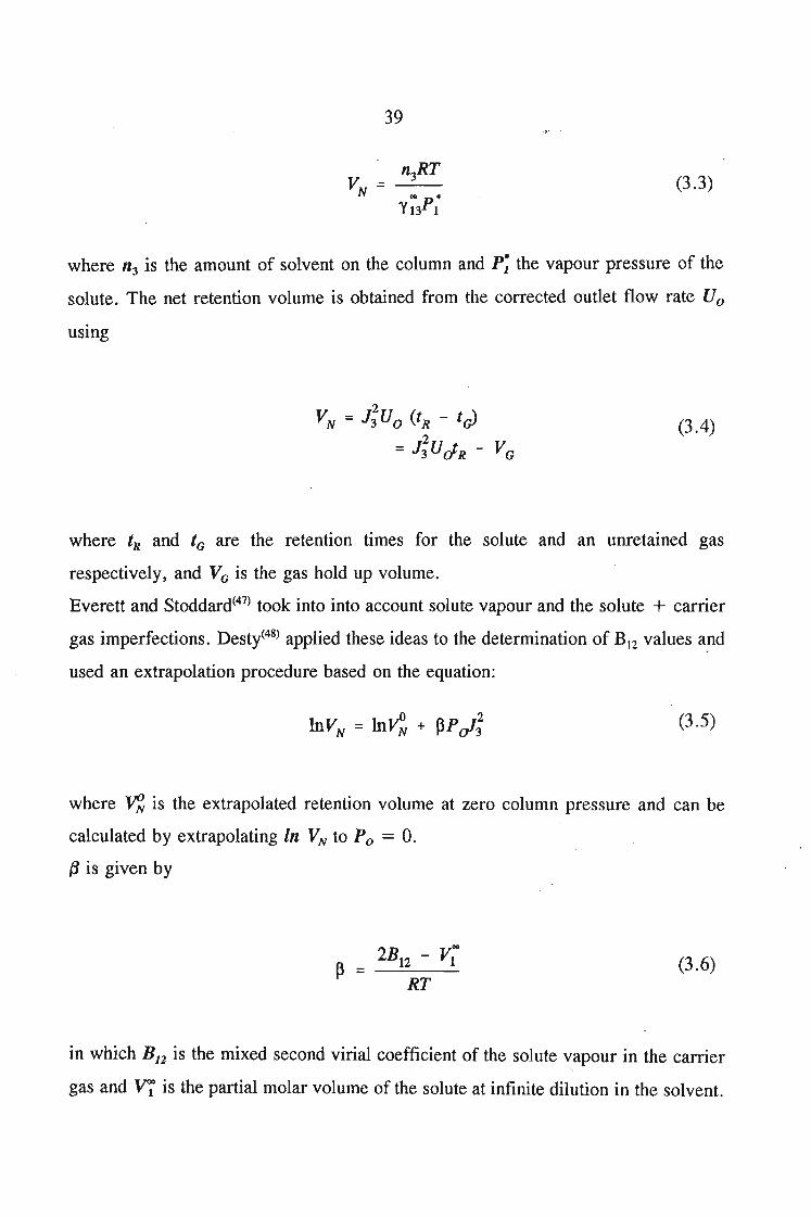
39
(3.3)
where n3 is the amount of solvent on the column and P; the vapour pressure of the
solute. The net retention volume is obtained from the corrected outlet flow rate U0
usmg
(3.4)
where tR and tG are the retention times for the solute and an unretained gas
respectively, and VG is the gas hold up volume.
Everett and Stoddard(47) took into into account solute vapour and the solute + carrier
gas imperfections. Desty(48) applied these ideas to the determination of B12 values and
used an extrapolation procedure based on the equation:
(3.5)
where ~ is the extrapolated retention volume at zero column pressure and can be
calculated by extrapolating In VN to Po = O.
{j is given by
2B12 - V;~=--
RT(3.6)
in which B12 is the mixed second virial coefficient of the solute vapour in the carrier
gas and v: is the partial molar volume of the solute at infinite dilution in the solvent.
40
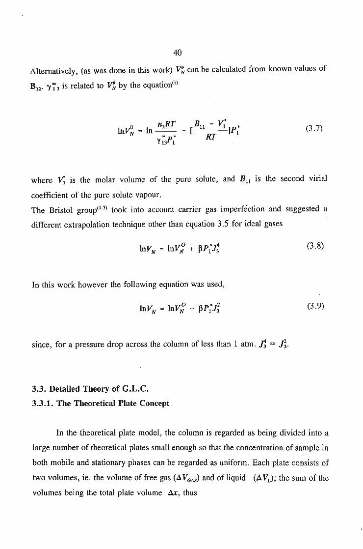
Alternatively, (as was done in this work) V~ can be calculated from known values of
Bu . 1'73 is related to V~ by the equation(l)
(3.7)
where ~ is the molar volume of the pure solute, and Bll is the second virial
coefficient of the pure solute vapour.
The Bristol group(l-3) took into account carrier gas imperfection and suggested a
different extrapolation technique other than equation 3.5 for ideal gases
(3.8)
In this work however the following equation was used,
(3.9)
since, for a pressure drop across the column of less than I atm . .n = .fj.
3.3. Detailed Theory of G.L.C.
3.3.1. The Theoretical Plate Concept
In the theoretical plate model, the column is regarded as being divided into a
large number of theoretical plates small enough so that the concentration of sample in
both mobile and stationary phases can be regarded as uniform. Each plate consists of
two volumes, ie. the volume of free gas (.:1VGAS) and of liquid (.:1VL); the sum of the
volumes being the total plate volume .:ix, thus
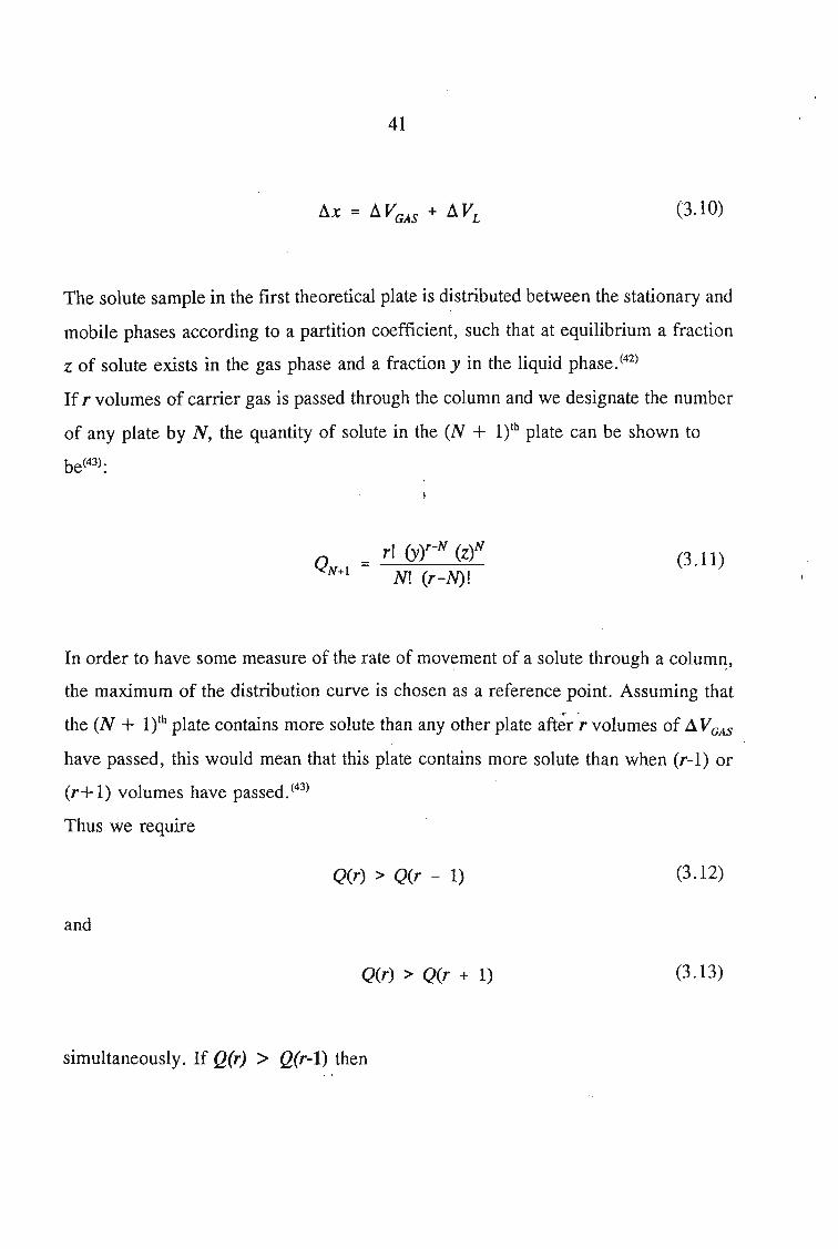
41
(3.10)
The solute sample in the first theoretical plate is distributed between the stationary and
mobile phases according to a partition coefficient, such that at equilibrium a fraction
z of solute exists in the gas phase and a fraction y in the liquid phase. (42)
If r volumes of carrier gas is passed through the column and we designate the number
of any plate by N, the quantity of solute in the (N + lyh plate can be shown to
be(43) :
TI (yy-N (Z)NQN+1 :;: -~-~-
N! (r-N)!(3.11)
In order to have some measure of the rate of movement of a solute through a colum~,
the maximum of the distribution curve is chosen as a reference point. Assuming that
the (N + l)th plate contains more solute than any other plate after -r volumes of AVGAS
have passed, this would mean that this plate contains more solute than when (r-1) or
(r+ 1) volumes have passed. (43)
Thus we require
(l(r) > (l(r - 1)
and
(l(r) > (l(r + 1)
simultaneously. If Q(r) > Q(r-l) then
(3.12)
(3.13)
42
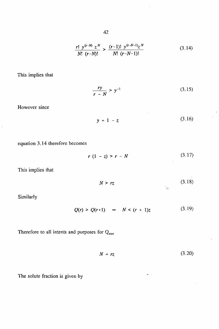
rl y(r-N> z N > (r-l)1 y(r-N-l)Z N
N! (r-N)! N1 (r-N-l)!
This implies that
ry > y-lr - N
However since
y = 1 - z
equation 3.14 therefore becomes
r (1 - z) > r - N
This implies that
N> rz
Similarly
Q(r) > Q(r+1) ~ N < (r + 1)z
Therefore to all intents and purposes for Qmax
N = rz
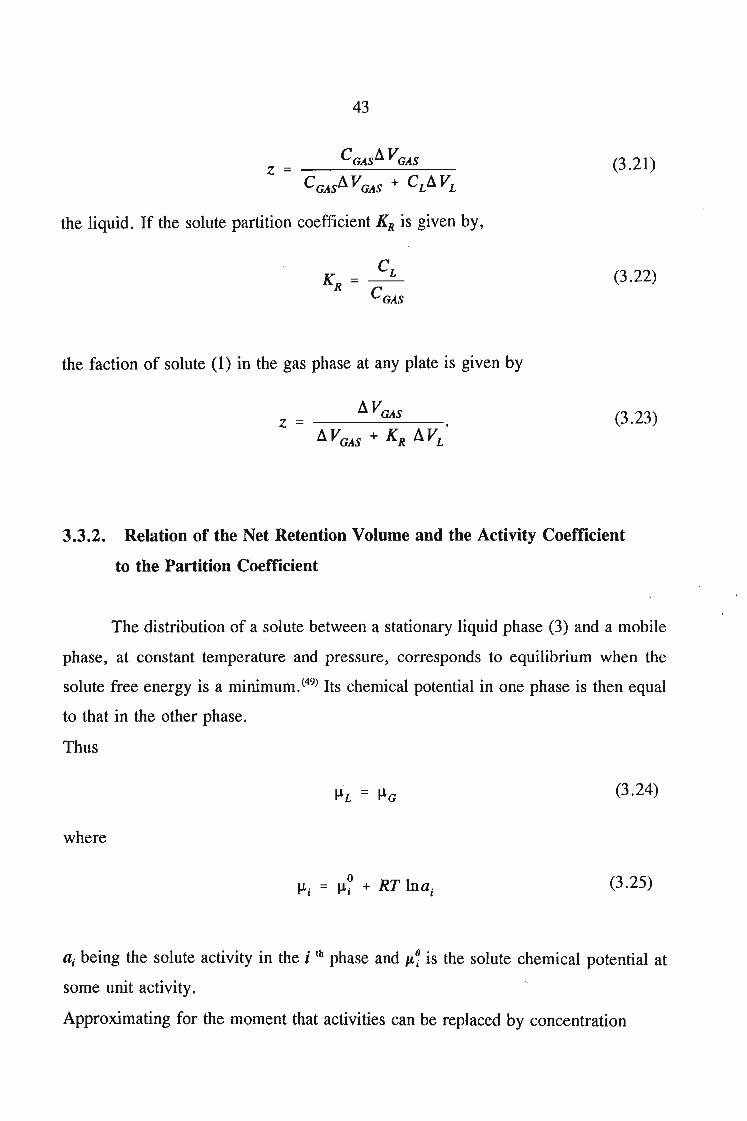
The solute fraction is given by
(3.14)
(3.15)
(3.16)
(3.17)
(3.18)
(3.19)
(3.20)
43
the liquid. If the solute partition coefficient KR is given by,
CLK =--
R CGAS
the faction of solute (1) in the gas phase at any plate is given by
(3.21)
(3.22)
(3.23)
3.3.2. Relation of the Net Retention Volume and the Activity Coefficient
to the Partition Coefficient
The distribution of a solute between a stationary liquid phase (3) and a mobile
phase, at constant temperature and pressure, corresponds to equilibrium when the
solute free energy is a minimum. (49) Its chemical potential in one phase is then equal
to that in the other phase.
Thus
where
j.LL = j.LG (3.24)
(3.25)
a j being the solute activity in the i lh phase and p.~ is the solute chemical potential at
some unit activity.
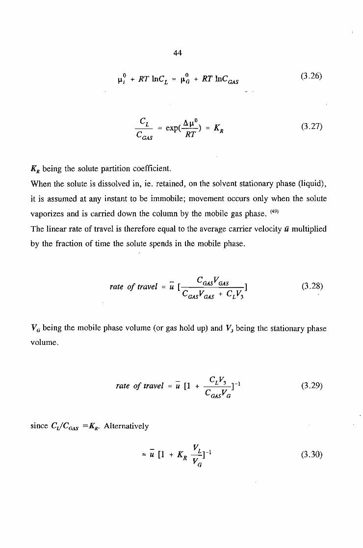
Approximating for the moment that activities can be replaced by concentration
44
o 0J.Li + RT lnCL = J.LG + RT lnCGAS
CL L\J.L0.= exp(-) = K
C RT RGAS
(3.26)
(3.27)
KR being the solute partition coefficient.
When the solute is dissolved in, ie. retained, on the solvent stationary phase (liquid),
it is assumed at any instant to be immobile; movement occurs only when the solute
vaporizes and is carried down the column by the mobile gas phase. (49)
The linear rate of travel is therefore equal to the average carrier velocity ii multiplied
by the fraction of time the solute spends in the mobile phase.
rate of travel = u[ CGASV GAS ]
CGASVGAS + C LV 3
(3.28)
VG being the mobile phase volume (or gas hold up) and V3 being the stationary phase
volume.
- CLV3 ]-1rate of travel = u [1 + ---CGASVG
since CLICG.4S =KR• Alternatively
V= u [1 + K -.£r1
R VG
(3.29)
(3.30)
45
Icolumn length (L)
rate of trave = ----=------'--'-retention time (tR)
Therefore the retention time is given by
(3.31)
(3.32)
The quantity L/u is identical to tG, the time a non-retained solute (KR = 0) requires
to pass through the column.
(3.33)
To convert retention times to gas volumes the flow rate of the mobile phase generally
measured at the column outlet, must be known. The measured flow rate (Uc) must
therefore be corrected to the conditions prevailing in the column; that is
(3.34)
where T is the column temperature, Tfm is the flowmeter temperature, P/tn is the
flowmeter vapour pressure at Tfm , Pw is the water vapour pressure at Tfm. The apparent
gas hold up (VG) and retention (V,) volumes are now given by
(3.35)
46
(3.36)
by substituting equation 3.35 and 3.36 into eq.3.33
(3.37)
From equation 3.1
(3.38)
In order for a mobile phase to flow through a column a pressure gradient must
exist. This necessitates the introduction of a gas compression factor, as first
recognized by James and Martin (45) in 1952.
Consider a carrier gas flowing through a packed column of uniform cross
section A at a pressure P, and velocity u. The volume throughout must be constant
within the column so that by Boyles law, (43)
Pu = Plflo = P u (3.39)
where P is the average pressure, Po the outlet pressure, ii the average velocity and Uo
the outlet velocity. The velocity at any given point is given by
Pouou =--P
(3.40)
47
The velocity can also be related to the pressure gradient dp within a length dx along
the column, the column specific permeability coefficient K, porosity e and gas
viscosity, through Darcy's law(43)
KdPu =
"dx
Substituting for u in equation 3.40
(3.41)
Pd'-oP
Therefore
KdP= ---
e"dx(3.42)
Kdx = [- ] PdPe"uoPo
Multiplying by P we obtain
The average value of a continuous function F(x) is
F(x) = J F(x)dxJdx
(3.43)
(3.44)
(3.45)
48
(3.46)
P being the average pressure over the column. Integrating over the column pressure
gradient, which is bounded by. the inlet (PJ and outlet (Po) pressure
P = ~ [(PIP0>3 - 1]
Po 3 (PIP0)2 - 1
Since P/Po = VIVo, then
- 3 (PIP \2 - 1V=-V [ DJ ]=JV
2 0 (PIP0)3 _ 1 0
where
(3.47)
(3.48)
(3.49)
49
(3.50)
Gas volumes measured at the column outlet can therefore be corrected to the average
column pressure by multiplying by the fraction VIVo which is,given by the symbol J.
Everett (2) suggested that the compressibility correction can be represented as
J; = .!!:- [{p/pc)m - 1]
m (p/pc)n - 1
The fully corrected gas hold up volume is given by VG = .J; V~
Therefore from equation 3.37
(3.2)
(3.51)
The term J;V~ is given the symbol ~ and is referred to as the corrected retention
volume(I).
(3.52)
The product KRV3 = VN , the net retention volume.
Therefore
50
(3.53)
The solute partial pressure over its infinitely dilute solution (Henry law region) in the
liquid phase is
(3.54)
where 1'73 is the activity coefficient at infinite dilution and p~ is the vapour pressure
of the pure solute.
Recognizing that Xl = n~/n/44) where Xl is the solute mole fraction in the liquid
phase, n~ is the solute molar amount in the liquid, and n3 is the liquid phase molar
amount.
Dividing by V3
(3.55)
Therefore
=
.. * LY13 PI ndn3
V3
(3.56)
51
(3.57)
where Pt is the solute partial vapour pressure and P~ is the solute saturation vapour
pressure.
For ideal gases
(3.58)
and
(3.5~)
From equation 3.56
(3.60) .
and from equation 3.57
52
Substituting equation 3.57 and 3.58 into equation 3.59
(3.61)
n3 PIK =[--
R 00 '"
Y13 PI
PVV 11 [~ V]
GJ RT 3(3.62)
RT (3.63)
(3.64)
where VL is the molar volume of the liquid stationary phase
Mass of stationary phase (WL)n3 Molar mass of stationary phase (M3)
The partition coefficient is then given by
(3.65)
53
K =R(3.66)
(3.67)
But
Therefore
n3 RTVN = ---
Y~3 pt
3.3.3. The Pressure Dependence of the Partition Coefficient(42)
(3.68)
(3.3)
The partition coefficient at infinite dilution, KR , in a static system can be
defined as
(3.69)
where n~ is the number of mole of I in volume V3 of liquid and n~ is the number of
54
mole of 1 in volume VG of gas. n~ = Yl nG and ni = x1nL where nG is the total
number of mole of gas (solute + carrier gas) in volume, VG, of carrier gas, nL is the
total number of mole of liquid (solute + solvent) in VL , YI is the mole fraction of
solute 1 in the gas, and Xl is the mole fraction of solute 1 in liquid.
(3.70)
where VG is the molar volume in the gas phase.
In the limit of infinite dilution of the solute (l) in gas phase (2)(42)
2RT (C222 - Bi2>
+ B22 + PP RT
(3.71)
(3.72)
where P is the carrier gas pressure, B22 is the second virial coefficient of carrier gas
and C222 is the third virial coefficient of the carrier gas.
KR
== lim -0 _x_1n_3 _R_T [1 + _B_22_P + _{C_2_22_-_B_i_2p 2 +•..]x V:V'l P RT (R1)2
where n3 = nL
Now since Yl P = PI (partial pressure of solute),
(3.73)
55
(3.74)
2lim Pt::: n3RT [1 + B
22..!- + C222-B22 p 2 +.•.]
x-o V K RT (R1)2Xl 3 R
multiplying by 1/P~
(3.75)
(3.76)
But
(3.77)
It can be shown that 1'73 (T,P) is related to the activity coefficient at zero pressure
and infinite dilution 1'73 (T,O) by
56
Substituting into the equation for 'Y~3 (T,P)
where
(3.79)
(3.80)
m[1
has been approximated by
Solving for KR in equation 3.80
Therefore
n3RTlnK
R= In _--..:.._-
ptV3y~3(T,0)
57
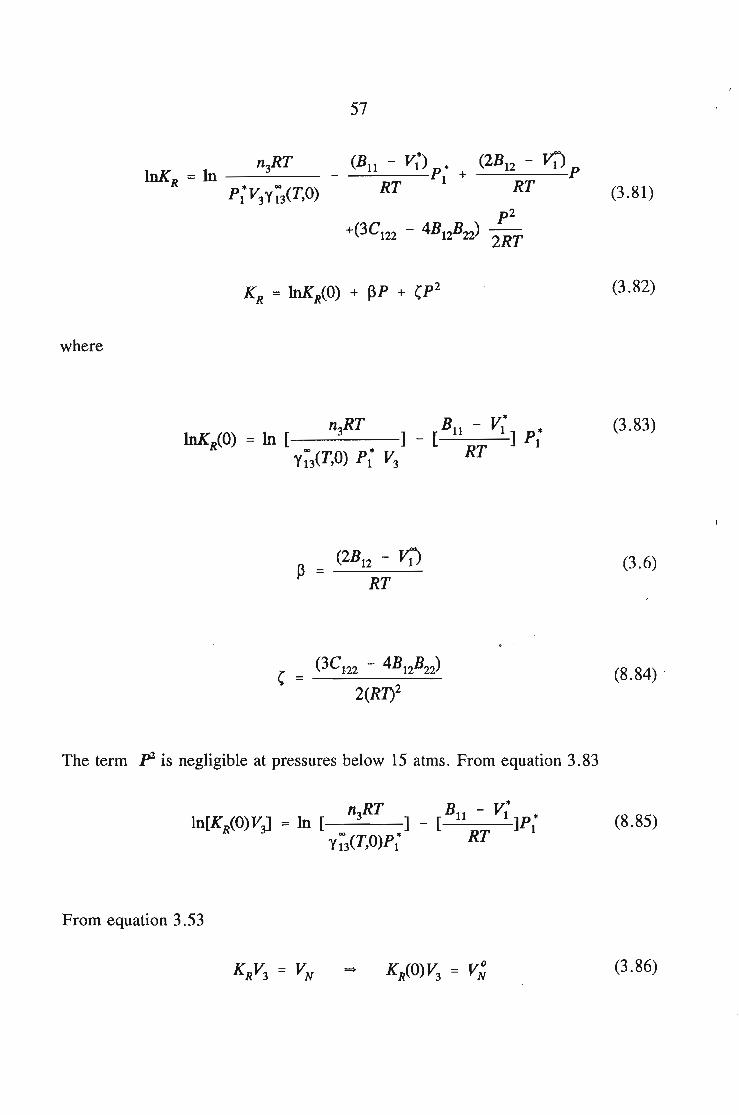
(3.81)
where
(3.82)
n RT B - V* (3 83)InK (0) = In [ 3 ] _ [11 1 ] pt .
R Y~3(T,O) p; V3 RT
p =(2B12 - v;)
RT(3.6)
(8.84) .
The term p2 is negligible at pressures below 15 atms. From equation 3.83
n RT B - V*In[K
R(0)V
3] = In [ 3 ] _ [11 1 ]p* (8.85)
RT 1Y~3(T,O)Pl*
From equation 3.53
(3.86)
58
where ~ is the retention volume at zero mean column pressure
n RT B - y*InY o == In [ 3 ] _ [11 1] p*
N ~ * RT 1Y13(T,O)Pl
(3.7)
Equation 3.85 expresses the pressure dependence of the partition coefficient KR •
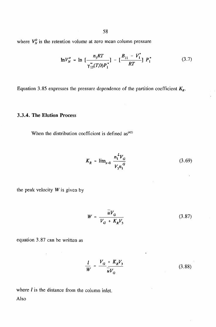
3.3.4. The Elution Process
When the distribution coefficient is defined as (42)
the peak velocity W is given by
equation 3.87 can be written as
(3.69)
(3.87)
IW
(3.88)
where I is the distance from the column inlet.
Also
59
1w
=dt
dl= (3.89)
where t is the retention time ie. the time taken for the peak to travel a distance 1.
Now ii is the volumetric flow rate of the carrier gas therefore iiVG can be replaced by
u
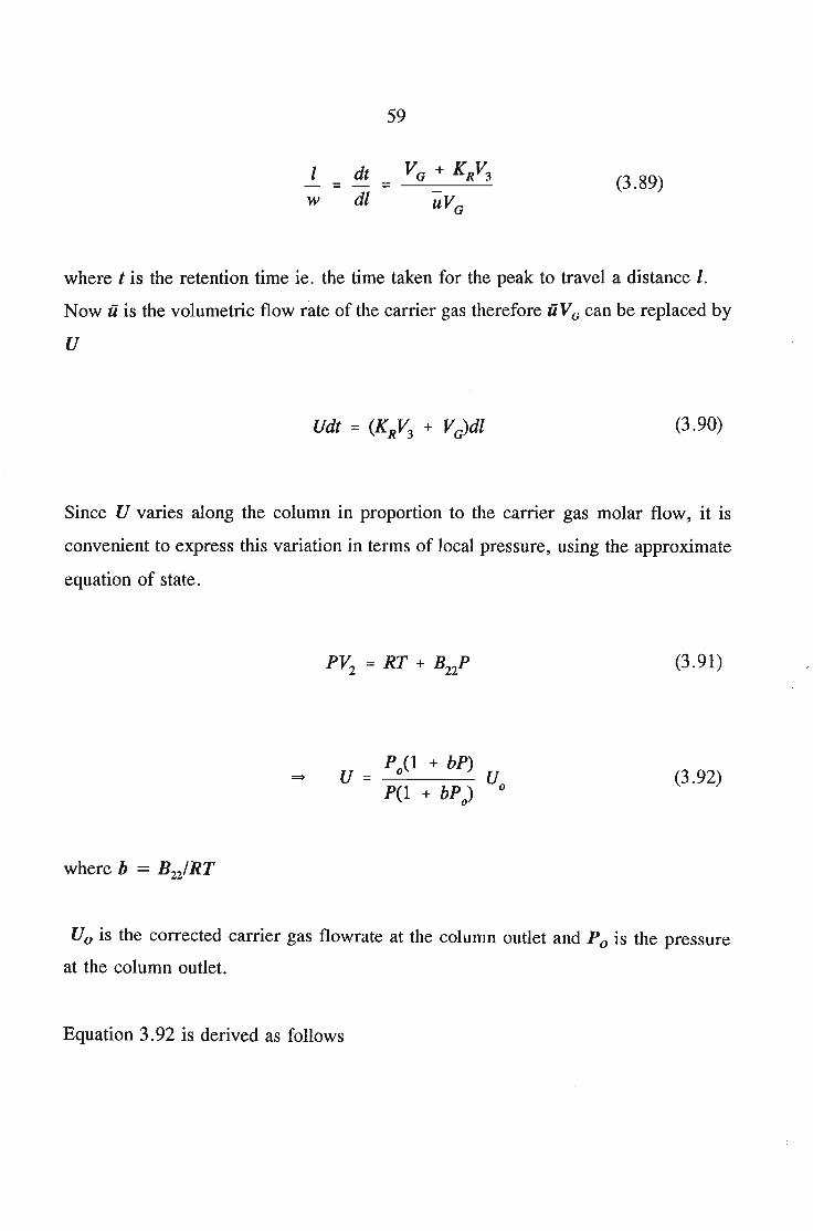
(3.90)
Since U varies along the column in proportion to the carrier gas molar flow, it is
convenient to express this variation in terms of local pressure, using the approximate
equation of state.
(3.91)
(3.92)
Vo is the corrected carrier gas flowrate at the column outlet and Po is the pressure
at the column outlet.
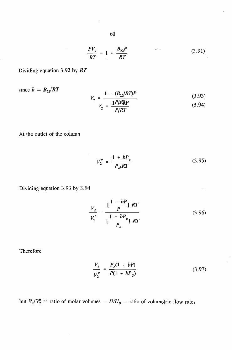
Equation 3.92 is derived as follows
60
PV2 = 1RT
(3.91)
Dividing equation 3.92 by RT
1 + (B2iR1)Pv: = -----2 IPJRrpv: = ---
2 P/RT
(3.93)
(3.94)
=-----
At the outlet of the column
1 + bPV20 = 0
PjRT
Dividing equation 3.93 by 3.94
[1 + bP] RTP
1 + bP[ 0] RT
Po
Therefore
(3.95)
(3.96)
(3.97)
but Vz/l1 = ratio of molar volumes = VIVo = ratio of volumetric flow rates
61
(3.92)
substituting for U in equation 3.90
(3.98)
u0 dt is the volume of gas leaving the column outlet as the elution peak advances a
distance dl. Because of the difficulty of defining VG accurately it is more convenient
to consider instead UcI1(, the volume of carrier gas measured- at the column outlet
which passes the elution peak during its progress from I to I + dl.
This is obtained by allowing V3 = 0 (value corresponding to no liquid phase). This
is simply
(3.99)
The retention volume VR is the same given in equation 3.38 ie. the observed retention
volume minus the gas holdup at the column outlet. Since KR is a function of pressure,
the most direct way to integrate the equation is to change the variable from I to P by
means of Darcy's law.(43)
dP = -ueT]
dl K(3.100)
dl = dx
62
dP
dx=
uA
(1.101)
where A takes into account the column packing permeability. If the pressure < 50
atms the Chapman-Enskog(2) relation in approximation form can be used ie.
where
Bna = 0.175 RT
Combining with Darcy's law
dl=- a dPuo(l + aPO)Tl
But carrier gas pressure varies according to
UP(1 + bP~U0 = -------:-
Po(l + bP)
but
U = dPAo dl 11
also
(3.102)
(3.103)
(3.92)
(3.104)
(3.105)
63
substituting equations 3.92 and 3.106 into equation 3.105
(3.106)
UPC! + bPJ
Po(1 + bP)dP A
=dL 11
0Cl + aP)
C3.107)
dl = __A_P_C_l_+_b_P--:J_d_l'__P0(1 + bP)U11 o(1 + aP)
Integrating
L - A(1 + bP) rPI P dPUC11JP }po (1 + bPJ(1 + aP)
Dividing equation 3.103 by equation 3.109
AP(I+bPJdP
C3.108)
(3.109)
dlL
P0(1 +bP) U11 o(1 +aPJ
A(1 +bP) rPI P
UC11O>P }po Cl +bPo)Cl +aPcflP)
LPdP
(3.110)
dl = (1 + aP)(1 + bP)
i PI PdPPo (1 + aP)(1 + bP)
(3.111)
64
equation 3.108 states that
1 + bPo P dldVR = KRV3------
Po 1 + bP
Substituting equation 3.111 and 3.112 into equation 3.99
LPdP
(3.82)
(3.112)
(3.113)
(3.114)
Also by substituting equations 3.112 and 3.108 into equation 3.99
pp (p2 l+bPo P AP(l+bPJbP (3.11dV = [K (0) + e +e ][V3 • ][ ] 5)
R R Po l+bP Po(l+bP)UTlo(l+aP)
By integration
(3.116)
65
The above equation gives the required relationship between the retention volume VR
and the partition coefficient.
3.3.5. The Net Retention Volume of an Ideal Carrier Gas
In the case of an ideal carrier gas a and b in equation 3.116 and B22 (second
viral coefficient of the carrier gas) are all zero. Therefore
By integration
where
K (O)V (Pi p 2 e PP eCP2 dPR 3 JpV
R= -'-0 _
P (Pip dPo Jp
o
(3.117)
(3.118)
(3.119)
since rep0 ,n)2 is negligible at pressures below 15 atm equation 3.118 approximates
to
(3.8)
66
But
(3.7)
Therefore substituting for In~(T) and {3
n RT B - Y· 2B - v:-In In 3 ] _ [11 1 ]p. + [12 1]p,4 (3 .120)
VN = [ RT 1 RT \ er 3Y~3(T,O)P;
This is identical to equation 1.1 since for pressures a pressure drop across the column
of less than 1 atm ~ ~ J~ and 'Y7J(T,0) = 'Y7J'
The above equation was developed by Everett(2) and Cruickshank(l) for the
determination of activity coefficients at infinite dilution.
In this work the following equation was used,
n RT B - y* 2B - y oo
InV = In[ 3 ] _ [11 1 ]p. + [12 1]p,3N 00 p. RT 1 RT er2
y13 1
where.n ~ J~
3.3.6. Treatment of a Volatile Solvent
(3.121)
The usual method (using equation 3.120) for determining activity coefficients
at infinite dilution developed by Cruickshank(l) and Everett(2) is restricted to volatile
solutes (eg. n-pentane, n-hexane and n-heptane) and involatile solvents (eg.
dotricontane,squalane, and dinonylphthlate).
67
3.3.6.1. Review of Work Using Volatile Stationary Phases
Some workers (employing the G.L.C method) have taken the volatility of the
solvent into account by using a presaturator. (42) Evaporation off the column by the
stationary phase is avoided by pre-saturating the carrier gas with vapour of the volatile
phase before it enters the column. The presaturator involved bubbling the carrier gas
through the liquid or passing the carrier gas through a short precolumn which, like the
main column, contained a stationary phase coated on a solid support. This technique
was introduced by Kwantes and Rijnders.(50) However, even though the carrier gas is
saturated with vapour it still removes the stationary phase as it expands along the
column. Since a smaller pressure drop led to less evaporation of the stationary phase,
a coarse packing was used which reduced the pressure drop considerably. While the
use of a precolumn and coarse packing kept the bleed rate very low, the loss cannot
be eliminated completely.
Another method was introduced by Kurkchi and Iogansen(51). They proposed
weighing the column before and after use, assuming that the solvent loss was constant
with time. This then gave them the amount of solvent lost during the course of the
experiment.
Langer et al(52) monitored the loss of solvent by measuring the retention time
of a solute at intervals, taking the first reading as soon as the column reached its
operating temperature. A graph of retention time against elapsed time of operation was
plotted. The graph was then extrapolated to zero time and the correct retention time
obtained. Letcher(53) successfully used this method for the determination of the activity
of various hydrocarbons with decahydronaphthalene as the volatile stationary phase.
Yet another method employed successfully by Letcher, was the use of an
"internal standard". This method uses a solute of known activity coefficient.
Throughtout the experiment, the solute is injected and its 'Y73 monitored with the loss
68
of solvent of the column. The change of the 'Y~ J value with time, gives an indication
of the rate of solvent loss of the column. An extension of this work is to measure, at
the same flowrate, the retention times of a solute of known 'Y~J (a standard) and a
solute of an unknown 'Y~J' Using equations 3.3 and 3.4 the following ratio can be
established:
(3.122)
y ~3 (standardl;(standard
Therefore 'Y~ J can be simply an quickly calculated from the retention times of the two
solutes only.
3.3.6.2. A Novel Method for taking Volatile Solvents into Account
In the present work, Everett's(2) and Cruickshank'sO) method (for solvents of low
volatility) has been extended to accommodate a solvent of low volatility by assuming
equilibrium along the entire column, and taking into account the vapour pressure of
the solute p~. During its passage through the column the carrier gas becomes charged
with solvent vapour. The total amount of solvent lost from the column, n;, may be
expressed in terms of the total volume of gas which has passed through the column,
the partial pressure, P;, of the solvent in the gas at the column outlet and the time t
elapsed from the start of the carrier gas passing through the column. The corrected gas
flow rate, Vo, measured at the outlet is maintained constant during the whole
experiment. The expression for n; is given by
UdP~
RT(3.123)
69
In this work the partial pressure of the solvent in the carrier gas was very much less
than 1 per cent of the total gas pressure. It is probably further reduced in the
flowmeter. Therefore no correction was applied to the flowrate for the presence of the
solvent. Equation 3.120 becomes
where
Hence
B - V· 2B - v:-C= _ [11 1] p. + [12 1] P ,3
RT 1 RT 0'2
(3.124)
(3.125)
RT=--
U t= a + b [~]
n3
(3.126)
By plotting VNln3ec against Uotln3 a straight line should be obtained, gIvmg an
intercept of RT1"I73 P; (a) and a slope of P~/RT Cb). The values of "173 and P~ are
obtained graphically from this linear relationship.
70
CHAPTER 4
APPARATUS AND EXPERIMENTAL PROCEDURE FOR THE
DETERMINATION OF 1'73 BY GAS LIQUID CHROMATOGRAPHY
The gas-liquid chromatograph used for the determination of the activity
coefficients at i1ifinite dilutions was similar to that used by Cruickshank(l) and also by
Marsicano(54) (where VN was determined as a junction of P; and hence B12 was
obtained together with 1'73 (see equation 3.130). The chromatograph used in this
work, was identical to that used by Letcher53). The mixed virial coefficients, B 12 , were
calculated (using equation 4. 1) from McGlashan and Potter's equation(55) and Hudson
and McCoubrey's combining rulei56,57) following Letcher et al., (58) and 1'73 was
determined from retention times.
4.1 The Design of the Gas-Liquid Chromatograph
The basic plan of the gas chromatograph is shown in figure 4.1. This type of
chromatograph is suitable for physico-chemical measurements. The scheme is similar
to that of a commercial analytical chromatograph except for the addition of a
manometer to register the column inlet pressure, an accurate flowmeter to measure the
flowrate (0.01 s) and an accurate temperature controller to regulate the temperature
of the column (+ 0.01 K). Two types of thermal conductivity detectors (T. C.D) were
used in this work, differing only in the make and design of the detector. The
advantage of using a thermal conductivity detector or a katharometer is that the flow
meter can be placed downstream of the column exit. The flow and pressure control
unit was constructed mainly of 6.35 mm o.d. (1/4 inch) copper tubing and Swagelock
couplings. The flow-meter and manometer were constructed of thick-walled glass
tubing.
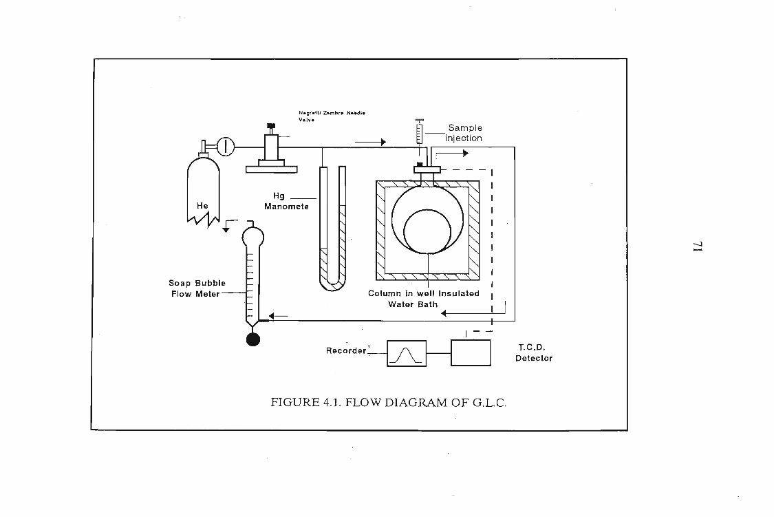
-.:J......
__ Sampleinjection
~
Column in well Insulated
Water Bath ~ I
Negr.ttl Zambr. N••dl.V.lv.
..-
Hg __Manomete
rHe
Soap BubbleFlow Meter~
1--
Rec~rder~--AH I T.C.D.Detector
FIGURE 4.1. FLOW DIAGRAM OF G.L.c.
72
4.1.1. Flow Control
Good flow control was achieved by using a two-stage pressure regulator, attached
to a pressure cylinder, in conjunction with a Negretti and Zambra precision pressure
regulating valve which controlled the pressure to better than 0.1 tOIT. 1 The column
outlet in the experiment was connected to the flow-meter which was open to the
atmosphere. It not was necessary to monitor the outlet pressure since variations in
atmospheric pressure would have small effects on the flow-rate only if the column
impedance was unusually high. (43) A buffer vessel was placed at the column outlet to
minimise the effect of pressure changes due to slight disturbances in the laboratory
atmosphere.
4.1.2. Pressure Measurement
The outlet pressure was considered to be atmospheric and was measured on a
normal Fortin barometer. The column inlet pressure was measured with a mercury
manometer using a kathetometer capable of measuring to within + 0.01 mm Hg.. A
trap was attached to one end of the manometer to retain mercury in case of an
accidental pressure surge.
4.1.3. Flow Rate Measurements
The measurement of the gas flow-rate was carried out with a soap bubble meter
(figure 4.2), constructed from a graduated 100 ml burette, which was situated
downstream of the column. Since helium was used as the carrier gas, it was necessary
to ensure that air did not enter the burette during flow measurements since light gases,
such as helium, diffuse more rapidly through soap films than air which would cause
the actual flow-rate to be different from the rate of film movement. To prevent back
diffusion of air a rubber bung with a tiny hole was placed at the flowmeter outlet. The
hole was large enough not to cause a significant pressure rise in the flow tubes.
1 1 torr = 1 mmHg
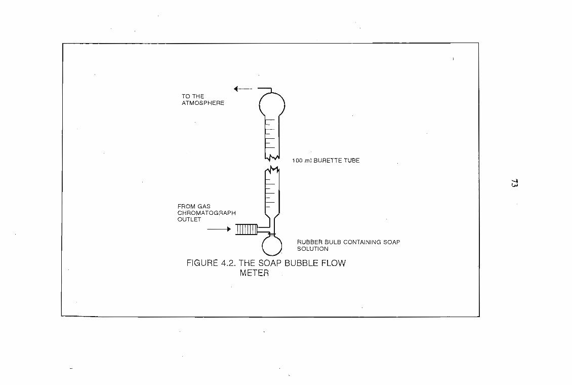
.--TO THEATMOSPHERE
100 ml BURETTE TUBE
........VJ
FROM GASCHROMATOGRAPHOUTLET
...r~
RUBBER BULB CONTAINING SOAPSOLUTION
FIGURE 4.2. THE SOAP BUBBLE FLOWMETER
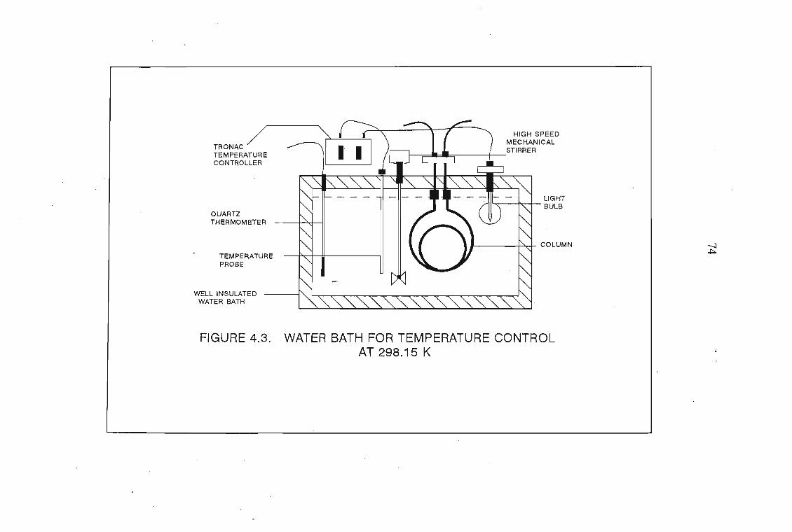
QUARTZTHERMOMETER
TEMPERATUREPROBE
WELL INSULATEDWATER BATH
HIGH SPEEDMECHANICAL
I •• I I STIRRER
LIGHT/11' <: ~<: I BULB
• I '< I COLUMN -..J~
FIGURE 4.3. WATER BATH FOR TEMPERATURE CONTROLAT 298.15 K
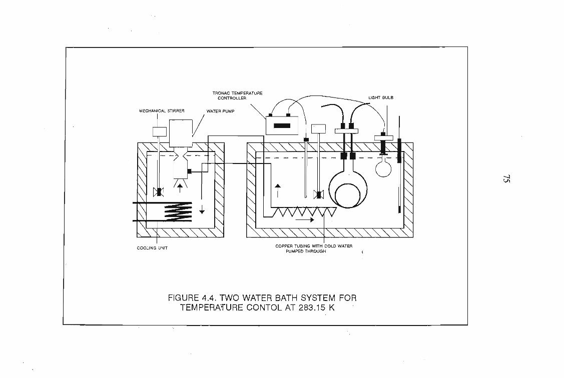
COOLING UNIT
TRONAC TEMPERATURECONTROLLER
COPPER TUBING WITH COLD WATERPUMPED THROUGH
FIGURE 4.4. TWO WATER BATH SYSTEM FORTEMPERAfURE CONTOL AT 283.15 K
-JVI
76
4.1.4. Column Temperature Control
Good temperature control was essential since the vapour pressure (of the solute
and the solvent) is temperature dependent. This was achieved by immersing the
column in a well-stirred water bath. The temperature at 298.15 K (using a single
waterbath) was controlled by a Tronac temperature controller in conjunction with a
light bulb as the low thermal capacity heater (figure 4.3).
The temperature was measured using an accurate quartz thermometer. The bath
temperature was always known to an accuracy of better than 0.01 K. For the control
of the temperature at 283.15 K two water baths were used (figure 4.4). The
temperature of one bath (not used for accurate temperature control) was kept at
approximately 280 K using a large cooling unit and an immersion heater. The bath
was kept well stirred using two high speed mechanical stirrers. The temperature in the
second bath (containing the column) was maintained at 283.15 K by pumping water
from the first bath through a 6 m coil of copper tubing placed on the floor of the
second bath. As with temperature control at 298.15 K the temperature in the second
bath was controlled by a Tronac temperature controller and a light bulb as the heater
element. The temperature was monitored using a quartz thermometer calibrated using
a platinum resistance thermometer (SA Bureau of Standards). (See Appendix 1)
4.1.5 Sample Injection and the Injection System
The solutes used were usually of the purest grade available although this was
not necessary since the nature of the chromatographic column separates impurities
from the solute being studied, thereby not affecting the retention times of the solutes.
Samples were injected using a microsyringe and sample sizes varied from 0.1 JoLl to .
1.0 JoL1. The injection system for both the Gow-Mac and Shandon detectors was the
same and was specially designed to minimise back diffusion, gas hold up, multiple
septum perforation and damage to the syringe. It consisted of an inner tube located
concentrically inside an outer tube (figure 4.5). Carrier gas entering at the one end of
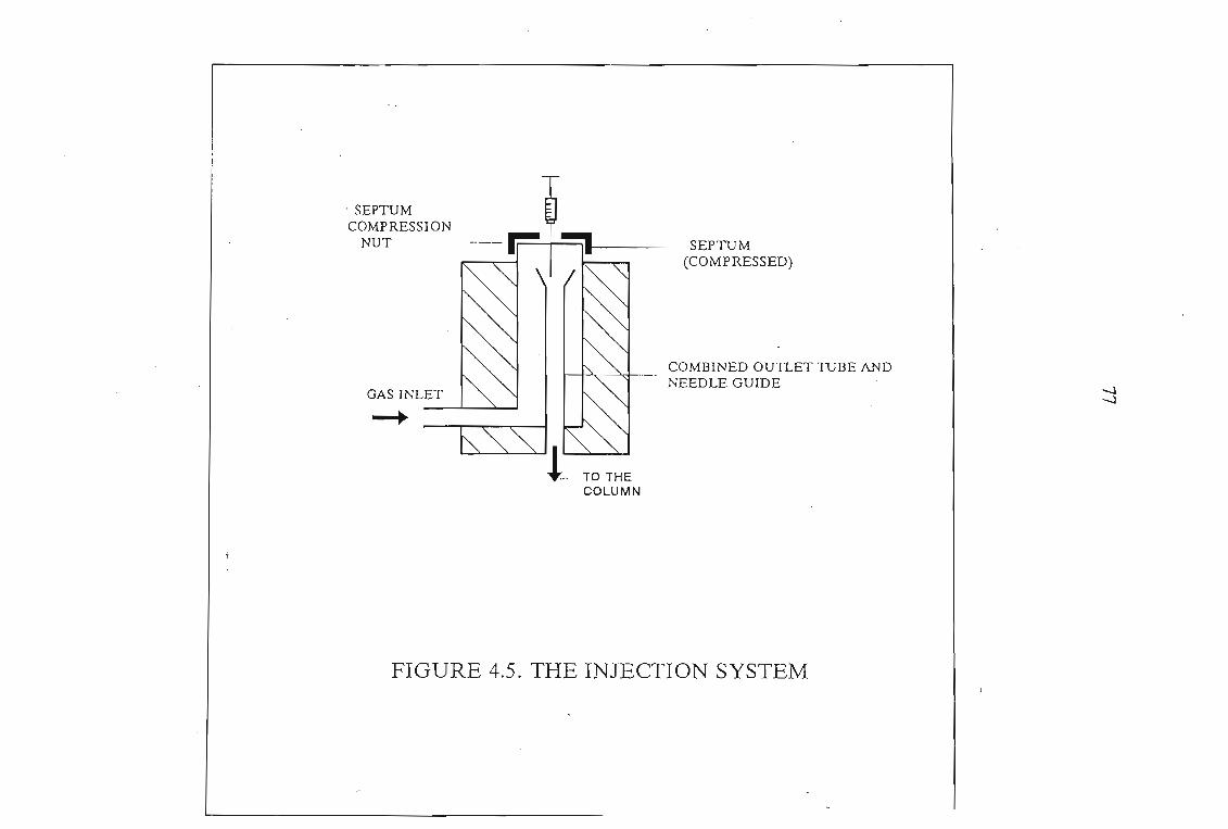
· SEPTUMCOMPRESSION
NUT
GAS INLET__'L.-""':''>--J'
-+
TO THECOLUMN
SEPTUM(COMPRESSED)
COMBINED OUTLET TUBE ANDNEEDLE GUIDE -..:s
-..:s
FIGURE 4.5. THE INJECTION SYSTEM
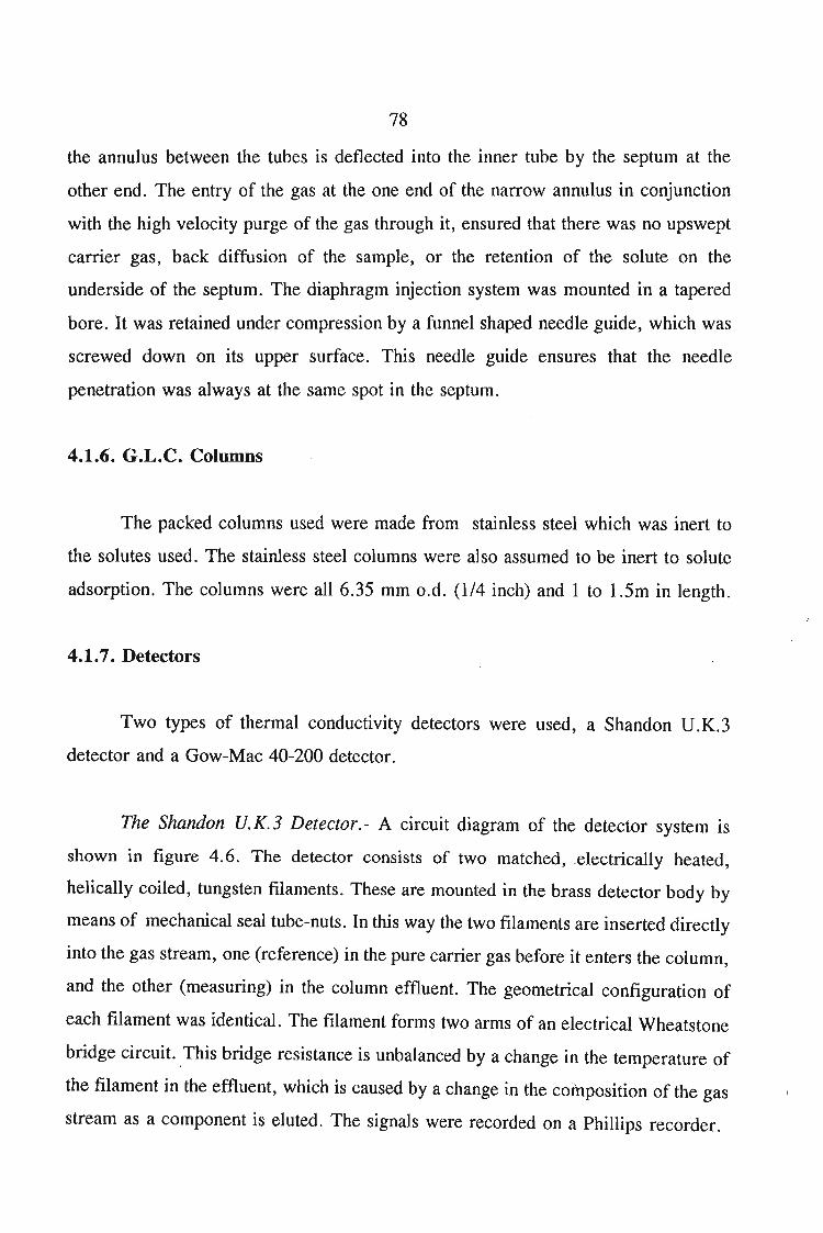
78
the annulus between the tubes is deflected into the inner tube by the septum at the
other end. The entry of the gas at the one end of the narrow annulus in conjunction
with the high velocity purge of the gas through it, ensured that there was no upswept
carrier gas, back diffusion of the sample, or the retention of the solute on the
underside of the septum. The diaphragm injection system was mounted in a tapered
bore. It was retained under compression by a funnel shaped needle guide, which was
screwed down on its upper surface. This needle guide ensures that the needle
penetration was always at the same spot in the septum.
4.1.6. G.L.C. Columns
The packed columns used were made from stainless steel which was inert to
the solutes used. The stainless steel columns were also assumed to be inert to solute
adsorption. The columns were all 6.35 mm o.d. (114 inch) and I to I.5m in length.
4.1.7. Detectors
Two types of thermal conductivity detectors were used, a Shandon U.K.3
detector and a Gow-Mac 40-200 detector.
The Shandon U.K.3 Detector.- A circuit diagram of the detector system is
shown in figure 4.6. The detector consists of two matched,electrically heated,
helically coiled, tungsten filaments. These are mounted in the brass detector body by
means of mechanical seal tube-nuts. In this way the two filaments are inserted directly
into the gas stream, one (reference) in the pure carrier gas before it enters the column,
and the other (measuring) in the column effluent. The geometrical configuration of
each filament was identical. The filament forms two arms of an electrical Wheatstone
bridge circuit. ,This bridge resistance is unbalanced by a change in the temperature of
the filament in the effluent, which is caused by a change in the composition of the gas
stream as a component is eluted. The signals were recorded on a Phillips recorder.
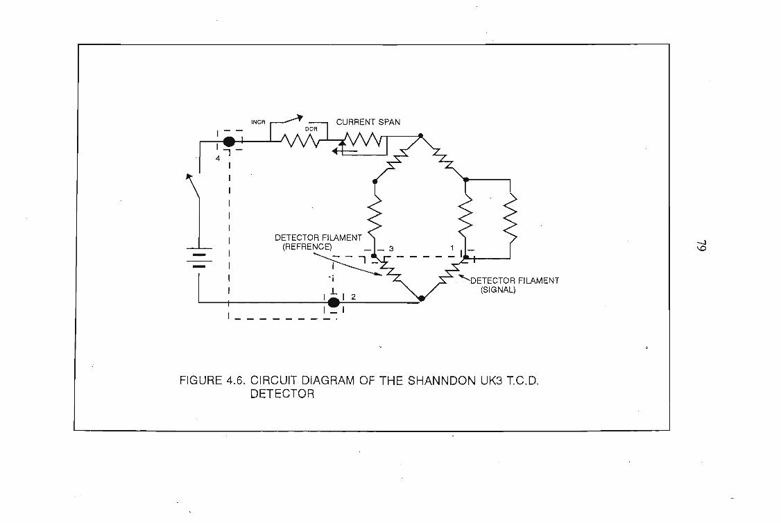
--
CURRENT SPAN
~"""DETECTOR FILAMENT(SIGNAL)
...:...J\0
FIGURE 4.6. CIRCUIT DIAGRAM OF THE SHANNDON UK3 T.C.D.DETECTOR
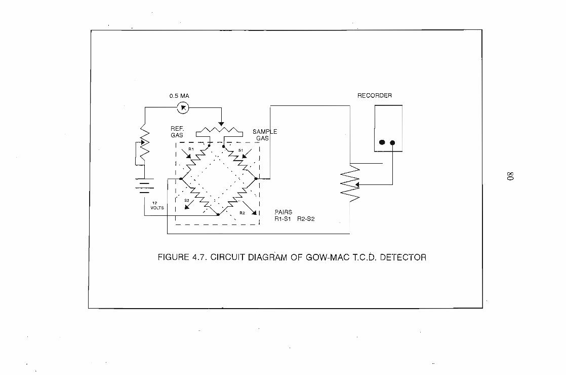
0.5 MA
SAMPLEGAS
PAIRSR1-S1 R2-S2
RECORDER
00o
FIGURE 4.7. CIRCUIT DIAGRAM OF GOW-MAC T.c.b. DETECTOR
81
The Gow-Mac 40-200 Detector.- A circuit diagram of the four filament Gow
Mac detector cell is shown in figure 4.7; In this detector four tungsten filaments lie
in the gas path. It is a semi-diffusion cell of a flow-through design with a response
time less than 1.0 second. The stream of pure gas is split so that half of the pure gas
enters the reference chamber and passes over the two reference filaments and the other
half of the gas enters the column. The gas emerging from the column flows over the
measuring filaments. The filaments used are of the same design as those used in the
Shandon detector.
4.2. Experimental Procedure
4.2.1. Preparation of the Stationary Phase
The stationary phase was prepared following the procedure used by
Marsicano. (54) The columns were cleaned with hot soap solution followed by acetone,
rinsed with distilled water, and dried with nitrogen. Celite was used as the solid
support for the stationary phase. The column loading (mass solute/total mass coated
solid support) ranged between 3 to 15 mass per cent. The packing was prepared by
adding a known mass of solvent to a known mass of celite. The combined mass was
noted. A solvent in which the stationary phase is soluble (diethyl ether) was added
(approx. 50 ml) and the contents were swirled gently in order to dissolve the
stationary phase and distribute it throughout the celite. The ether was slowly removed
by the application of a vacuum using a Buchi rotary evaporator without heating. The
flask was rotated slowly to minimise disintegration of the fragile celite. The last trace
of ether was removed by allowing the flask to stand in a fume hood. The coated celite
was weighed and reweighed on completion to check that all the ether had been
removed and that no stationary phase had been lost. An uncoiled stainless steel column
was packed using a plastic funnel and rubber tubing of known mass. The funnel was
attached to the column by the tubing and the coated celite was poured into the funnel.
The other end of the column was plugged with glass wool. A rubber stopper was
attached to this end which was lightly tapped on the floor during packing. The column
82
was also lightly tapped with a rubber-covered metal rod. On completion the funnel and
tubing were weighed and the amount of stationary phase added was determined by
difference. The column was plugged with glass wool at the open end and coiled. We
believe that the small amount of compression produced on coiling does not
significantly change the properties of the packing, nor its adsorptive properties.
4.2.2. Measurement Procedure
4.2.2.1. Treatment of a Volatile Solvent (n-Dodecane)
Measurements of the flow-rate (which was kept constant), retention times of
solute and unretained gas (nitrogen), and temperature were made for each column.
The flowrate was set, depending on the length of the column and the amount of
solvent on the column, so that the column would have a life of about 3-4 hours. The
system was allowed to equilibrate for about 10-15 min before the first injection was
made. When several solutes are studied on a single column, the solutes are injected
simultaneously as a mixture. Solutes chosen for such measurements must have
significantly different retention times to allow each component to be fully resolved at
the detector. Incorporation of air to determine the gas holdup was accomplished by
first taking up the desired volume of solute into the syringe and withdrawing the
plunger further to admit a suitable volume of air before making an injection.
Retention times were calculated from distance measurements on the chart from
the point of injection to the point at which the tangents to the peak intersect (figure
4.8). These are then converted to retention times using the ·chart speed which was
accurately measured using a stopwatch.
The carrier gas flow-rate was measured regularly throughout each run using an
accurate stopwatch. Prior to measuring the flow-rate a stream of bubbles was sent
through the flowmeter to allow the interior walls of the burette to be thoroughly
wetted by the soap solution to avoid errors arising from uneven movement of the
83
bubble film due to surface tension effects and the possibility that the burette was not
fully saturated with water vapour.
4.2.2.2. Treatment of a Polar Solvent (n-Sulfolane)
In the case of a polar solute (Sulfolane) no modification of the data treatment
procedure is required. Measurements of the flow-rate (which was varied), retention
times of solute and unretained gas (nitrogen), and temperature were made for each
column. The flowrate was changed throughout the experiment. The system was
allowed to equilibrate for about 10-15 min after changing the flowrate to allow
equilibrium to be established. As with n-dodecane, when several solutes are studied
on a single column, the solutes are injected simultaneously as a mixture. Solutes
chosen for such measurements must have significantly different retention times to
allow each component to be fully resolved at the detector. The determination of the
gas hold up, (using nitrogen),was conducted in the same manner as was done in the
case of a volatile solvent. Measurement of retention times was done using the tangent
method as explained earlier.
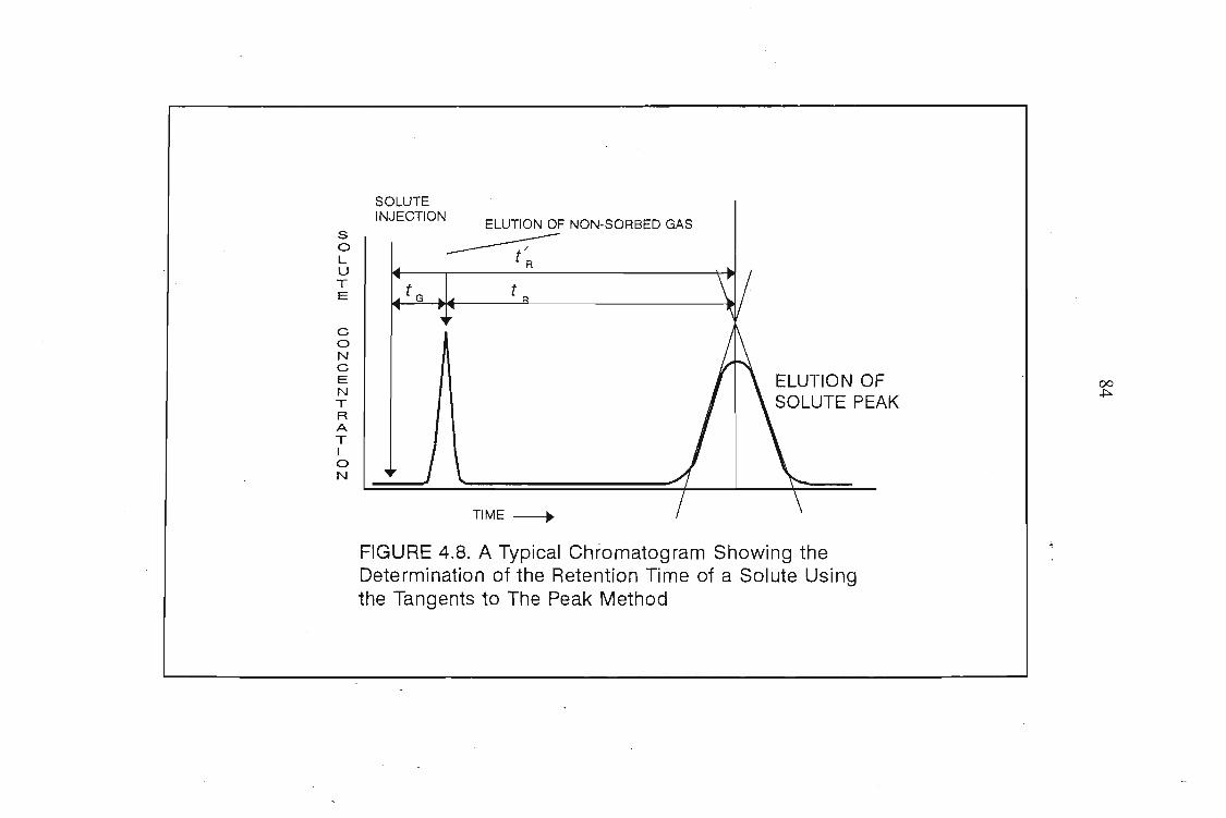
soLUTE
coNCENTRATIoN
SOLUTEINJECTION
ELUTION OF NON-SORBED GAS
TIME~
ELUTION OFSOLUTE PEAK
00~
FIGURE 4.8. A Typical Chromatogram Showing theDetermination of the Retention Time of a Solute Usingthe Tangents to The Peak Method
85
4.3. The Determination of 1'73 of Solutes in a Moderately Volatile
(n-Dodecane)
Solvent
The method used is described in chapter 3, section 3.3.6 5. The systems
involving moderately volatile solvents, is used to determine 1'73 for the investigated
in this work were: n-pentane, n-hexane, n-heptane, cyclopentane, cyclohexane, and
benzene in the solvent n-dodecane, at the temperatures 280.15 K and 298.15 K.
The flow rate of the helium was maintained constant for each set of
measurements on a particular column. Each column was used for a time (t) which
ranged from 3 to 4 hours. The helium flow rate ranged from 1.2xl0-6 m3's-1 to
2.8xl0-6 m3 's-1 and was measured using a calibrated bubble meter and the results were
corrected for water vapour pressure. The injection volume used was about 0.1 mm3.
The column temperature was controlled to within 0.01 K.
The solvent, dodecane, was supplied by BDH. The suppliers quoted a mole
fraction purity of 0.99. The solvent was used without further purification at a column
loading of (3 to 10) mass per cent. The solutes used were n-pentane, n-hexane, n
heptane, cyclopentane, cyclohexane, and benzene, and were supplied by Aldrich. It
was not necessary to purify the solutes further as the chromatographic column
separated impurities from the major solute component.
Results were collected from seven columns loaded with dodecane. The gas holdup
volume was determined by injecting nitrogen into the carrier gas. Table 4.1
summarizes all the operating conditions.
The mixed virial coefficients, B l2 , were calculated (using equation 4.1) from
McGlashan and Potter's equation(55) and Hudson and McCoubrey's combining
rules(56,57) following Letcher et al., (58) using n1 = 5 (pentane and cyclopentane), n1
=6 (hexane, cyclohexane, and benzene), nl = 7 (heptane) and n2 = 1 (helium).
86
B1Z
/VC,IZ = 0.43 - 0.886(Tc,12/T) - 0.694(Tc,lz/T)Z - 0.0375(n12 - 1)(Tc,lz/T )4.5 (4.1)
where
(4.2)
(4.3)
(4.4)
and
(4.5)
The second virial coefficients for the pure compounds were calculated from
Deiters equation of state, following Baonza et al. (59) The vapour pressures for the
solutes were obtained from the literature. (60) The molar volumes were determined from
density values, which were obtained from the literature. (61) The values of the properties
used in the calculation of 1'73 are given in Table 4.2.
4.3.1. Calculation of 'Y73
The calculation 'Y73 for a volatile solvent is explained in Chapter 3 (3.3.6).
From the experimental readings, values of VN were calculated using the programme
GAMMA (see Appendix 2) which uses the following equations,
(3.4)
87
and
VN _= RT
n3e C Y~3P;'
U t pi_O"[ 3]n "p.
3 Y13 1
(3.126)
The linear equation (3.126) is fitted to each set of results (usually involving about 15
injections for each solute, collected from each of the seven columns as done
previously(62,63») using a method of least squares analysis. From the intercept of that
line RT/'Y7JP~ was obtained and the activity coefJ::icient at infinite dilution ("17 J) wast
calculated. From the ratio of the slope to the intercept the quantity (RT/P~) was.
obtained and consequently, P~, the partial pressure of the. solvent at the temperature
of the experiment was calculated. All the plots were linear.
4.3.2. Discussion
Activity coefficients at infinite dilution have been reported for the volatile
hydrocarbon solutes, n-pentane [CHlCH2)3CH3] , n-hexane [CHlCH2)4CH3] , n-heptane
[CH3(CH2}5CH3], cyclopentane [c-CjH IO], cyclohexane [c-C6H12] and benzene [c-C6H6]
in involatile alkane solvents n-pentadecane [CHlCHJ13CH3] to n-hexatricontane
[CHlCHJ34CH3], (64-68) as well as in the volatile alkane solvents n-octane
[CHJ(CH2)6CH3] and n-decane [CH3(CH2)8CH3]. (67) All these values have been
determined using the G.L.C. method. Where 1'73 values at 298.15 K were not
available, the literature data at other temperatures were extrapolated to 298.15 K.
Finite concentration activity coefficients have been determined for many of the above
solutes in volatile alkane solvents n-pentane [CH3(CH2)3CH3] to n-octane
[CH3(CH2)6CH3], (63-68) but very few measurements have been made on mixtures of the
above solutes and the alkanes ranging from n-nonane [CH3(CH2)7CH3] to
CH3(CH~12CH3. Of the systems presented in this work, the only finite concentration
88
activity coefficient results found in the literature was for [x{CH3(CH2)4CH3 or c-C6H 12
or c-C6H6} + (1-x) CH3(CH2) IOCH3]. (79-84) We have used these data to predict activity
coefficients at infinite dilution and have compared the predicted values with the
. experimentally determined values reported here.
In order to put the new experimental results reported here in context with the
results obtained from the literature, all the results have been graphed in figures 4.9
and 4.10.
The results obtained in reference (67) by Kwantes and Rjinders did not take into
account the solute vapour and solute + carrier gas imperfections. Furthermore in
order to prevent loss of the stationary liquid during the experiment Kwantes and
Rjinders presaturated the carrier gas with the solvent before introducing the gas into
the g.l.c. column. To reduce loss of solvent to a minimum a coarse-graded support
was used. Our experience with presaturated columns has not been very successful.
The activity coefficients at infinite diluti?n for the solutes in the solvents
CHlCH~3CH3 to CHlCH2)6CH3 was calculated from finite concentration data, (79-84)
by the use of the Guggenheim-Miller-Flory-Huggins (G-M-F-H) equation, (57,58) ,
In 1'13 = In (I-ct>I)/X3 + (1-I/r)ct>1 + xct>i (4.7)
which becomes at XI = 0,
In 1'73 = In (lIr) + (l - lIr) + X (4.8)
The calculated values are given in Table 4.4. The G-M-F-H equation is also used
to predict the activity coefficient at infinite dilution from finite concentration data
obtained from the literature for the solutes n-hexane [CH3(CHJ4CH3] (85) , cyclohexane
[c-C6Hd(86) and benzene [c-C6H6](87) in the solvent n-dodecane [CHJCCH2) IOCH3]. The
calculated 1'73 are given in Table 4.3. The average standard deviations of 1'73 is +0.005 and an estimate of the accuracy is < 0.01. The quasi-lattice theory(73) has been
used here to predict 1'73 far an alkane (1) + dadecane (3). The-value of Wab used in
this work, wab/kT = 0.1733, was obtained from the literature(S7>, where Cruickshank
et al. used a mean value of Wab for a system of simple hydrocarbons in octadecane.
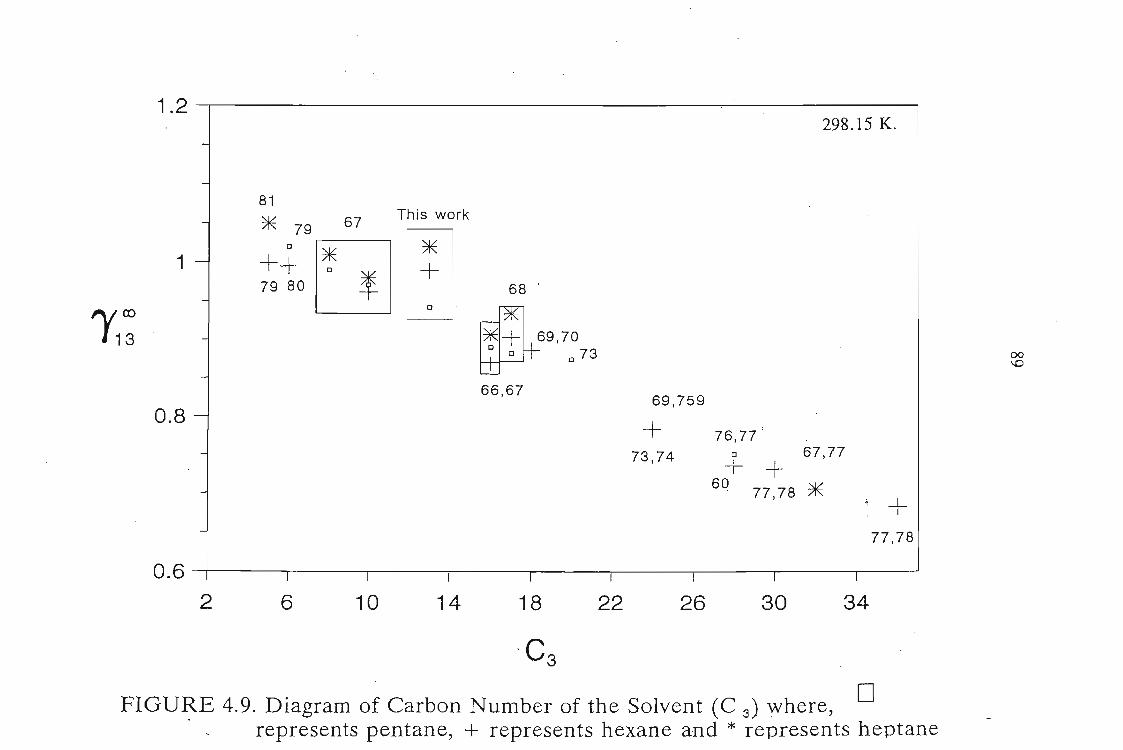
298.15 K.1.2 --rl-----------------:---=~~'
r 1:
1
0.8
81 67
* 079[iJ++ 0
79 80 l
This work
*+o
68 '
~~~69,70o 0 73
c
66,6769,759
+73,74
76,77o+ + 67,77
6077,78 * i+
00\0
77,78
0.6 I I I I I I I I I
2 6 10 14 18 22 26 30 34
'C3
FIGURE 4.9. Diagram of Carbon Number of the Solvent (C 3) where, 0. represents pentane, + represents hexane and * represents heptane
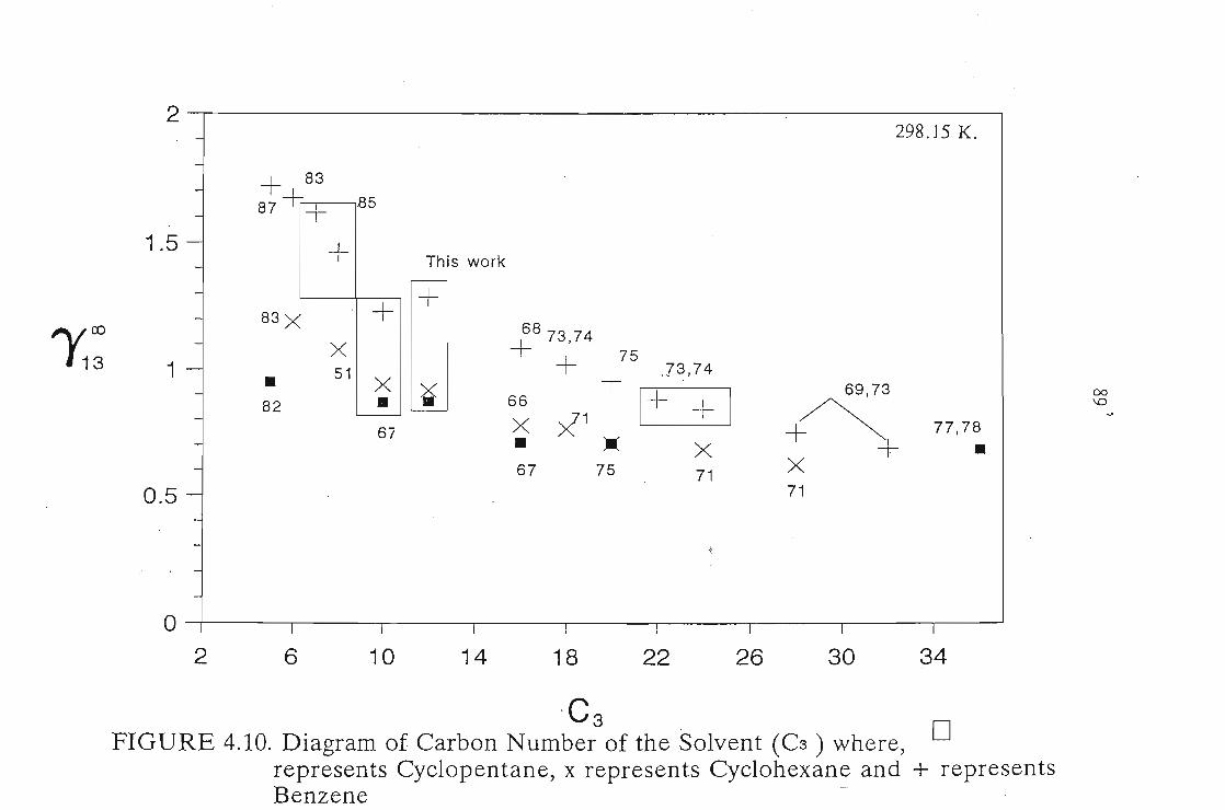
2 ' I
298.]5 K.
+1'+
83
+~Fl8587
+
00\D
77,78
•+~X +71
X7175
><,,1
•67
68 73 ,74
+ + 75 ]3,74
+ 1+ + I66
X•
This work
>.i
X51, X
•67
83X
•82
1
1 .5
0.5
~:
o I I I I I I I '
2 6 10 14 18 22 26 30 34
'C 3FIGURE 4.10. Diagram of Carbon Number of the Solvent (C3 ) where, 0
represents Cyclopentane, x represents Cyclohexane and + representsBenzene -
90
The predictions are compared with our experimental results in Table 4.3.
The 'Y73 values obtained from the literature and from this work can be
summarized using a simple polynomial
'Y73 = k + I'C3 + m'C~ (4.9)
where C3 is the carbon number of the solvent. The coefficients of the polynomial bI,
b2 and b3 are given in Table 4.5.
As discussed previously(62,63) (and In chapter 3, section 3.3.6), this method is
capable of predicting the vapour pressure, p~, of the solvent. Using the results from
the slope of equation 3.125, the vapour pressures obtained here are, 4.2 + 3.0 Pa,
and 21.2 + 4.1 Pa at 280.15 K, and 298.15 K respectively. The standard deviations
are calculated from at least 18 measurements. The vapour pressure of dodecane at
these temperatures have not been reported in the literature. Keistler and Winkel(88)
have however measured the vapour pressure of dodecane in the range 90.1 K to 213.3
K. Extrapolation of their results, fitted to an Antoine equation, gives values for the
saturated vapour pressure of 2.7 Pa and 15.5 Pa at the temperatures 280.15 K, and
298.15 K respectively.
4.4. The Determination of 1'73 of Solutes in a Polar Solvent (Sulfolane)
Sulfolane is a highly polar compound and has found extensive use in petroleum
refining for the recovery by liquid extraction, of aromatic compounds, including
benzene, from catalytic reformats. (14)
The activity coefficient at infinite dilution for a series of n-alkane solutes (Cr
C7), cycloalkanes (C5 and C6), benzene, tetrahydrofuran, and tetrahydropyran have
been measured in a polar solvent, tetrahydrothiophene-l, I-dioxane (sulfolane) at
303.15 K. The effect of the size of the injection volumes of the solute and the solvent
loading on the column was investigated in order to ensure infinite dilution and non-
91
adsorption conditions respectively. The mixed second virial coefficients used in this
work were calculated in the same manner as in section 4.3 The 1'73 results obtained
here highlights the polar nature of sulfolane. Despite the obvious importance of the
activity coefficients at finite concentrations or at infinite dilution for these mixtures,
activity coefficients have been reported for only three of the mixtures reported here
(hexane, cyc10hexane and benzene). The reason for this could lie with the
experimental difficulties in measuring the mixing properties of a volatile component
at low concentrations in a viscous and involatile solvent. Furthermore most of the
solutes discussed here do not dissolve in sulfolane over the whole composition range. I
However some of these properties are particularly well suited for the a.L.C. method
we have chosen. All measurements were carried out at 303.15 K.
The solvent, tetrahydrothiophene-l, I-dioxane, was supplied by Janssen
Chimica. The suppliers quoted a mole-fraction purity of 0.99. The solvent was used
without further purification at a column loading of (4 to 25) mass percent. The solutes
used were pentane, hexane, heptane, cyc1opentane, cyc1ohexane, benzene,
tetrahydrofuran, and tetrahydropyran and were supplied by Aldrich. It was not
necessary to purify the solutes further as the chromatographic column separated
impurities from the major solute component.
The flow rate of the helium was kept constant for each measurement on a
particular column. About 15 to 20 minutes was allowed between each measurements
to ensure equilibrium. The helium flow rate was measured using a calibrated bubble
meter and the results were corrected for water vapour. The injection volume used was
about between 0.1 to 1 mm3• The column temperature was controlled in a well
insulated water bath to within 0.01 K.
Data was collected for three columns loaded with sulfolane with helium used
as the carrier gas. Table 4.6 gives the column preparation conditions. The retention
time to was determined using nitrogen. To check the g.l.c. technique used, a test
92
system of hexane and hexadecane was run. The results compared well with the results
in the literature(l). To ensure that equilibrium conditions prevailed, the effect of
varying flow rate on the calculated activity coefficient was monitored and found to be
independent of flow rate. Also the symmetrical peaks obtained confirmed that
equilibrium had been established. To ensure that infinite dilution conditions were
satisfied, the injection volume was varied and the effect on the calculated 1'73 was
monitored over a range of 0.1 mm3 to 1.0 mm3• The results showed that the injection
volume did not influence the calculated 1'73' No loss of solvent from the column was
experienced, so there was no need to make allowances as was done in previous
studies. (62,63)
Varying the solvent loading on the column from (4 to 25) mass percent, had no
measurable effect on the calculated 1'73 and hence solute-solvent adsorption was
considered to be negligible.
The critical data and ionization energies used in the calculation of B12 are given in
table 2 using n1 = 4 (tetrahydrofuran), n1 = 5 (pentane, cyclopentane and
tetrahydropyran), n1 = 6 (hexane, cyclohexane, and benzene), n1 = 7 (heptane) and
n2 = 1 (helium). The vapour pressures for the solutes were obtained from the
literature. (60,61) These values as well as the calculated virial coefficients are all listed
in table 4.7. Table 4.8 gives the operating conditions as well as the calculated 1'73'
4.4.1. Calculation of 'Y~J
No modification of the theory is required for a polar solvent. The retention time
of both the solute and the unretained gas, along with the flow-rate and the inlet and
outlet pressures is all the experimental data that is required to calculate 'Y~J.
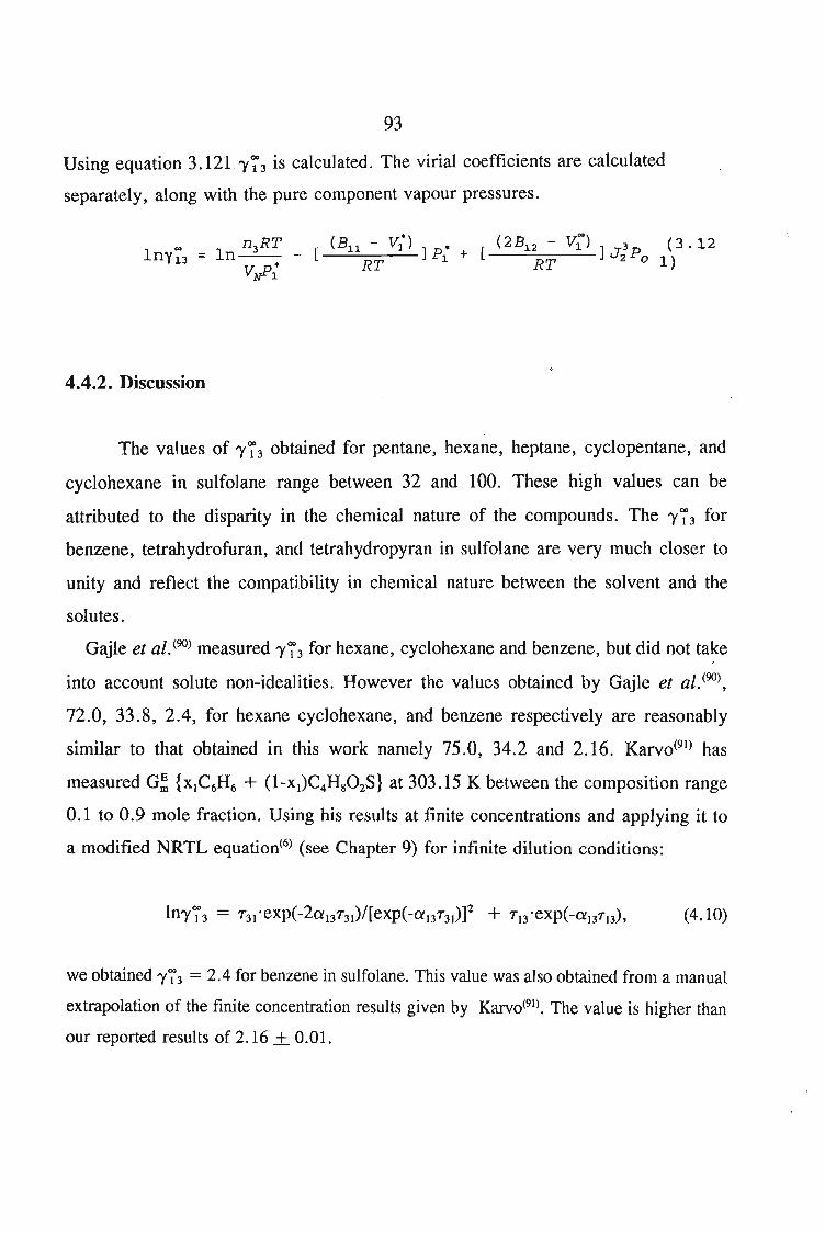
93
Using equation 3.121 l'7J is calculated. The virial coefficients are calculated
separately, along with the pure component vapour pressures.
4.4.2. Discussion
The values of 1'~3 obtained for pentane, hexane, heptane, cyclopentane, and
cyc10hexane in sulfolane range between 32 and 100. These high values can be
attributed to the disparity in the chemical nature of the compounds. The 1'~3 for
benzene, tetrahydrofuran, and tetrahydropyran in sulfolane are very much closer to
unity and reflect the compatibility in chemical nature between the solvent and the
solutes.
Gajle et al. (90) measured 1'~3 for hexane, cyclohexane and benzene, but did not take
into account solute non-idealities. However the values obtained by Gajle et al. (90),
72.0, 33.8, 2.4, for hexane cyclohexane, and benzene respectively are reasonably
similar to that obtained in this work namely 75.0, 34.2 and 2.16. Karvo(91) has
measured G; {x tC6H6 + (l-x t)C4Hg0 2S} at 303.15 K between the composition range
0.1 to 0.9 mole fraction. Using his results at finite concentrations and applying it to
a modified NRTL equation(6) (see Chapter 9) for infinite dilution conditions:
(4.10)
we obtained 'Y~3 = 2.4 for benzene in sulfolane. This value was also obtained from a manual
extrapolation of the finite concentration results given by KarvO(91). The value is higher than
our reported results of 2.16 + 0.01.
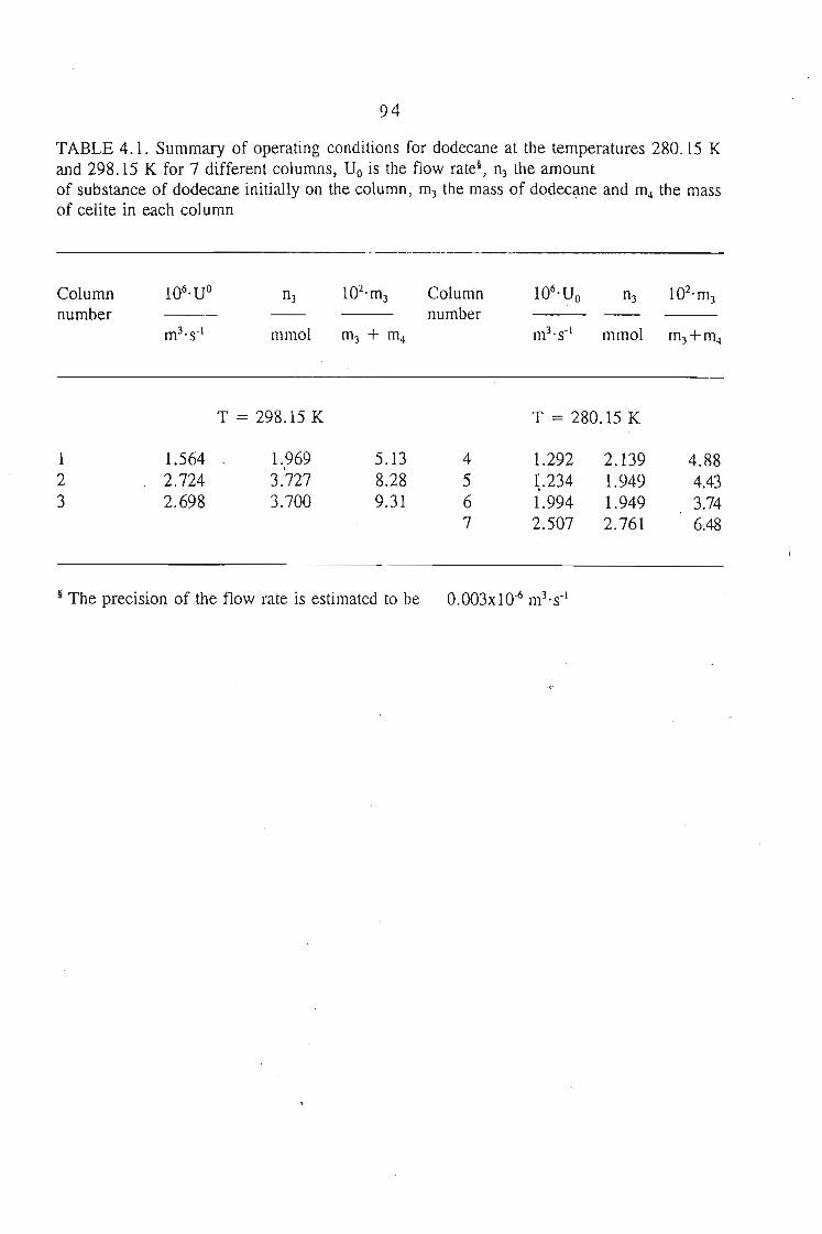
94
TABLE 4.1. Summary of operating conditions for dodecane at the temperatures 280.15 Kand 298.15 K for 7 different columns, Uo is the flow rate§, n3 the amountof substance of dodecane initially on the column, m3 the mass of dodect;lne and m4 the massof celite in each column
Columnnumber
Columnnumber
T = 298.15 K T = 280.15 K
1 1.564 1.969 5.13 4 1.292 2.139 4.882 2.724 3.727 8.28 5 \.234 1.949 4.433 2.698 3.700 9.31 6 1.994 1.949 3.74
7 2.507 2.761 6.48
§ The precision of the flow rate is estimated to be 0.003xlO-6 m3's-1
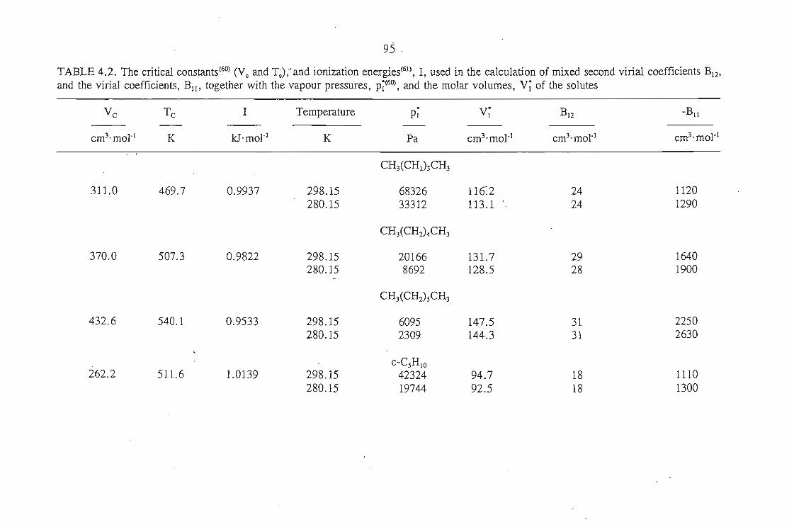
95
TABLE 4.2. The critical constants(60) (Vc and T~),~'and ionization energies(61), I, used in the calculation of mixed second virial coefficients B12,
and the virial coefficients, BII , together with the vapour pressures, p;(60), and the molar volumes, V; of the solutes
Vc Tc I Temperature.
V; B12 -BIIPI
-cm3·mol-1 K kJ·mo1-' K Pa cm3'mo1-1 cm3·mol-1 cm3·mol-'
CH3(CH2)3CH3
311.0 469.7 0.9937 298.15 68326 116:2 24 1120280.15 33312 113.1 24 1290
CH3(CH2)4CH3
370.0 507.3 0.9822 298.15 20166 131.7 29 1640280.15 8692 128.5 28 1900
CH3(CH2) sCH3
432.6 540.1 0.9533 298.15 6095 147.5 31 2250280.15 2309 144.3 31 2630
c-CSH IO
262.2 511.6 1.0139 298.15 42324 94.7 18 1110280.15 19744 92.5 18 1300
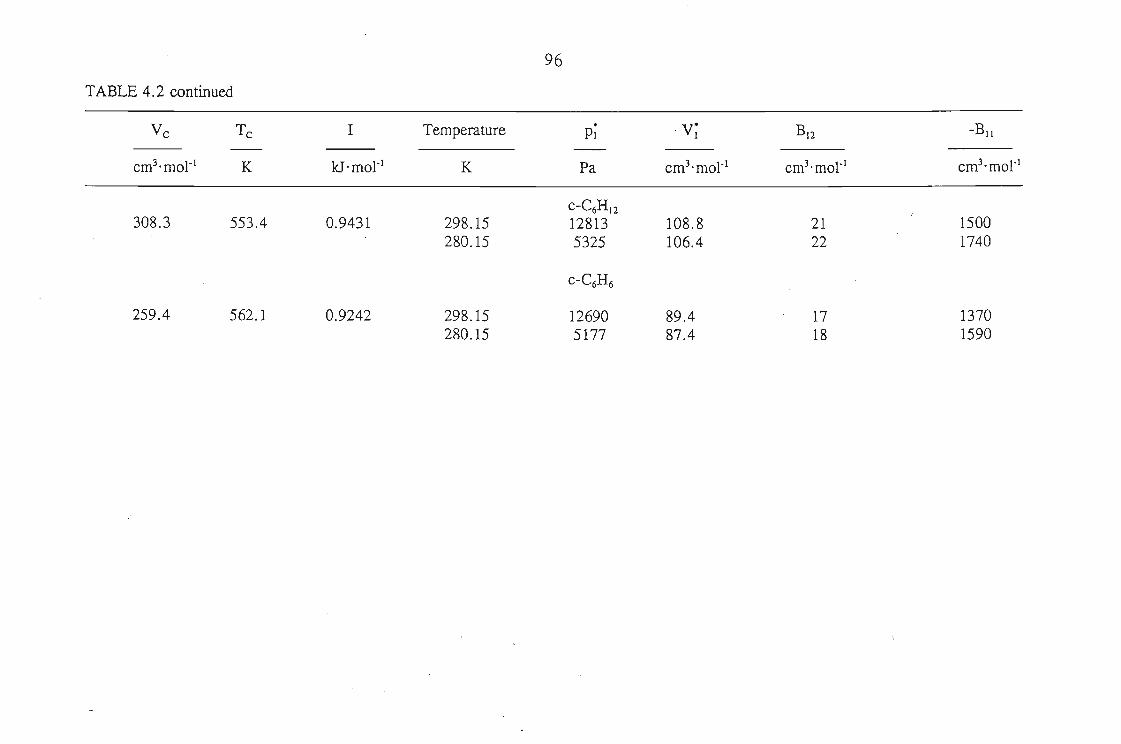
96
TABLE 4.2 continued
Vc Tc I Temperature . . V; B12 -B IlPI-
cm3'mol- l K kJ'mol-l K Pa cm3'mol-l cm3'mol-l cm3'mol-l
c-C6H12308.3 553.4 0.9431 298.15 12813 108.8 21 1500
280.15 5325 106.4 22 1740
c-C6H6
259.4 562.1 0.9242 298.15 12690 89.4 17 1370280.15 5177 87.4 18 1590
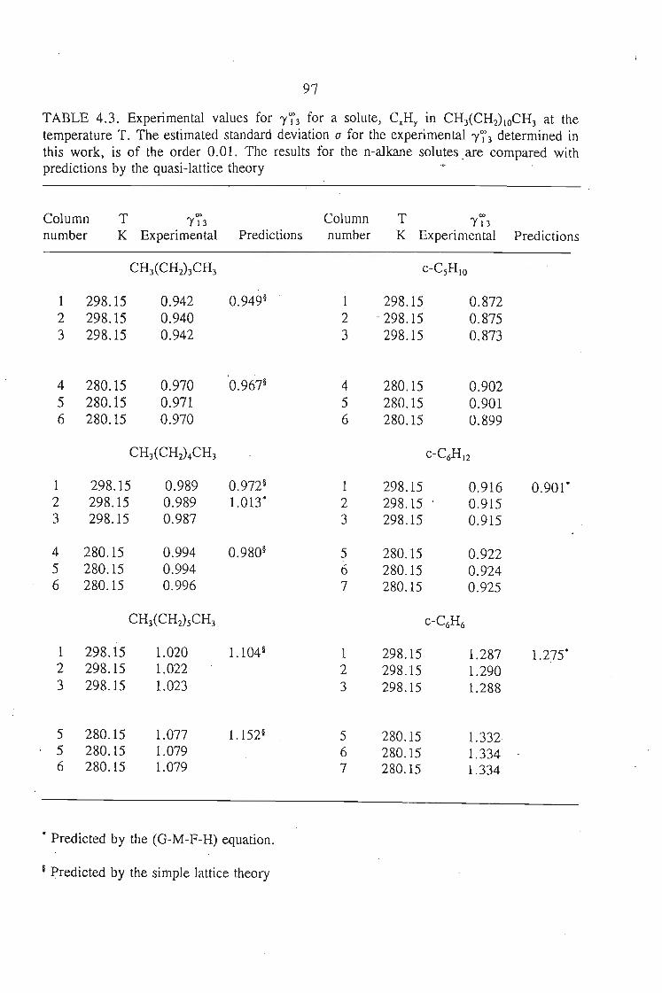
97
TABLE 4.3. Experimental values for 'Yf3 for a solute, CxHy in CH3(CH2) IOCH3 at thetemperature T. The estimated standard deviation a for the experimental 'Yf3 determined inthis work, is of the order 0.01. The results for the n-alkane solutes .are compared withpredictions by the quasi-lattice theory ,v- -
Column T 00 Column ·T 00
'Y 1 3 'Y 1 3
number K Experimental Predictions number K Experimental Predictions
CH3(CH2)3CH3 c-CjH IO
1 298.15 0.942 0.949§ 1 298.15 0.8722 298.15 0.940 2 298.15 0.8753 298.15 0.942 3 298.15 0.873
,4 280.15 0.970 0.967§ 4 280.15 0.9025 280.15 0.971 5 280.15 0.9016 280.15 0.970 6 280.15 0.899
CHJCCH2)4CH3 c-C6H 12
1 298.15 0.989 0.972§ 1 298.15 0.916 0.901"2 298.15 0.989 1.013" 2 298.15 0.9153 298.15 0.987 3 298.15 0.915
4 280.15 0.994 0.980§ 5 280.15 0.9225 280.15 0.994 6 280.15 0.9246 280.15 0.996 7 280.15 0.925
CH3(CH2)jCH3 c-C6H6
1 298.15 1.020 1.104§ 1 298.15 ·1.287 1.275"2 298.15 1.022 2 298.15 1.2903 298.15 1.023 3 298.15 1.288
5 280.155 280.156 280.15
1.0771.0791.079
567
280.15280.15280.15
1.3321.3341.334
• Predicted by the (G-M-F-H) equation.
§ Predicted by the simple lattice theory
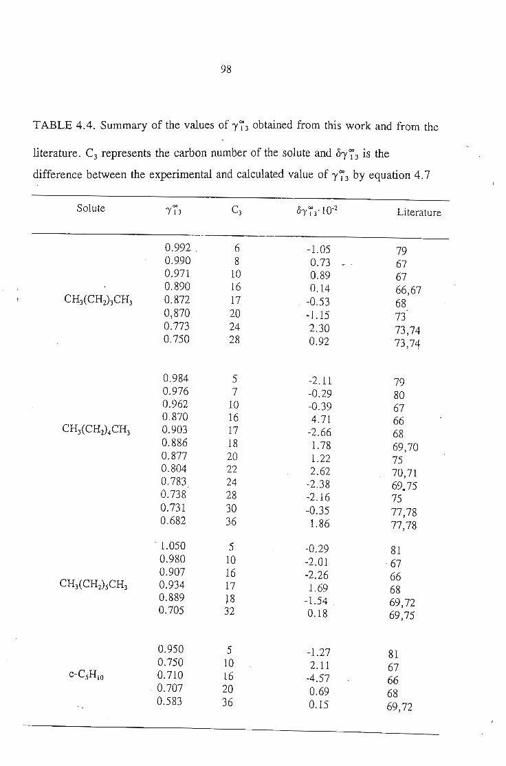
98
TABLE 4.4. Summary of the values of "173 obtained from this work and from the
literature. C3 represents the carbon number of the solute and 01'73 is the
difference between the experimental and calculated value of "173 by equation 4.7
Solute 0> C3 °'Y73' 1O-2 Literature'Y I 3
0.992 , 6 -1.05 790.9.90 8 0.73 670.971 10 0.89 670.890 16 0.14 66,67
CHlCH2)3CH3 0.872 17 -0.53 680,870 20 -1.15 730.773 24 2.30 73,740.750 28 0.92 73,74
0.984 5 -2.11 790.976 7 -0.29 800.962 10 -0.39 670.870 16 4.71 66
CH3(CH2)4CH3 0.903 17 -2.66 680.886 18 1.78 69,700.877 20 1.22 750.804 22 2.62 70,710.783 24 -2.38 694 750.738 28 -2.16 750.731 30 -0.35 77,780.682 36 1.86 77,78
. 1.050 5 -0.29 810.980 10 -2.01 ' 670.907 16 -2.26 66
CH3(CH2)sCH3 0.934 17 1.69 680.889 ~8 -1.54 69,720.705 32 0.18 69,75
0.950 5 -1.27 810.750 10 2.11 67
c-CSHIO 0.710 16 -4.57 66·0.707 20 0.69 68
0.583 36 0.15 69,72
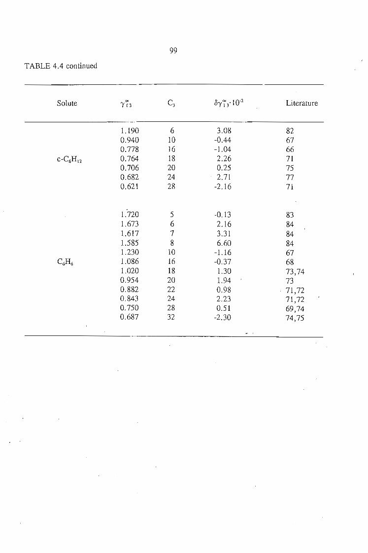
TABLE 4.4 continued
99
Solute 00 C3 Ol'~3.10-2 LiteratureI'D
1.190 6 3.08 820.940 10 -0.44 670.778 16 -1.04 66
c-C6H12 0.764 . 18 2.26 710.706 20 0.25 750.682 24 2.71 770.621 28 -2.16 71
,1.720 5 -0.13 831.673 6 2.16 841.617 7 3.31 841.585 8 6.60 841.230 10 -1.16 67
C6H6 1.086 16 -0.37 681.020 18 1.30 73,740.954 20 1.94 730.882 22 0.98 ' 71,720.843 24 2.23 71,720.750 28 0.51 69,740.687 32 -2.30 74,75
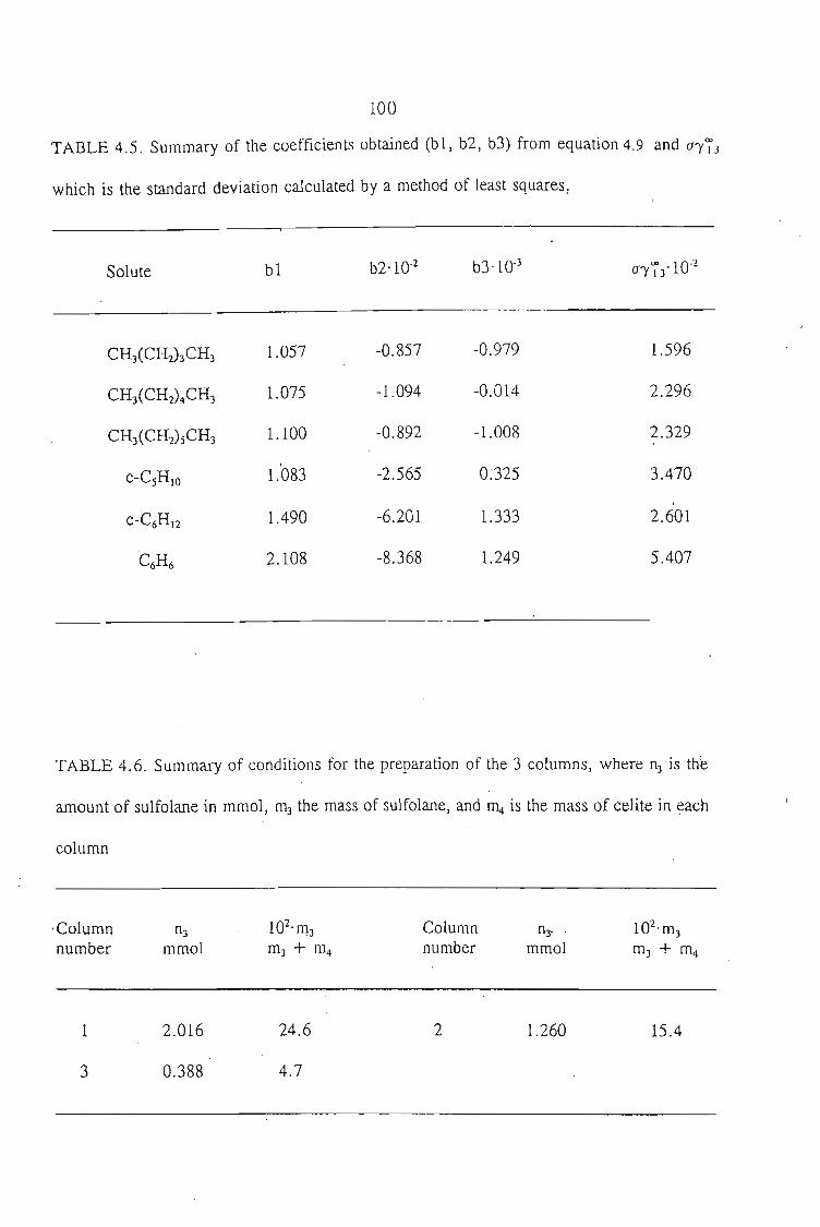
100
TABLE 4.5. Summary of the coefficients obtained (b1, b2, b3) from equation 4.9 and a'Y';'3
which is the standard deviation calculated by a method of least squares;
Solute b1 b2·1O-2 b3·1O-3
CH3(CH2)3CH3 1.057 -0.857 -0.979 1.596
CH3(CH2)4CH3 1.075 -1.094 -0.014 2.296
CH3(CH2)5CH3 1.100 -0.892 -1.008 2.329
,
c-C5HIO 1.083 -2.565 0.325 3.470
c-C6H12 1.490 -6.201 1.333 2.601
C6H6 2.108 -8.368 1.249 5.407
TABLE 4.6. Summary of conditions for the preparation of the 3 columns, where n3 is the
amount of sulfo1ane in mmo1, m3 the mass of sulfolane, and m4 is the mass of celite in ~ach
column
'Columnnumber
1
3
2.016
0.388
24.6
4.7
Columnnumber
2
n:t' mmo1
1.260 15.4
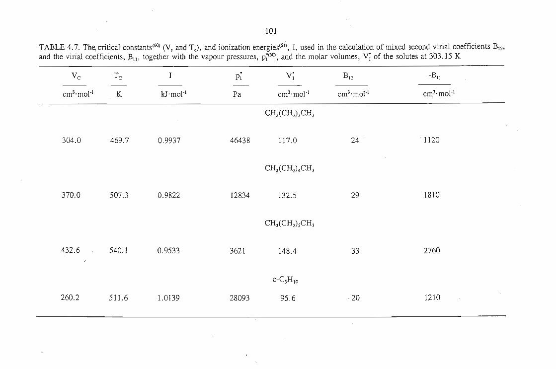
101
TABLE 4.7. Thelcritical constants(60) (Vc and Tc), and ionization energies(61), I, used in the calculation of mixed second virial coefficients B12,
and the virial coefficients, J311 , together with the vapour pressures, p~(60J, and the molar volumes, V~ of the solutes at 303.15 K
Vc
cm3'mol-1
304.0
370.0
432.6
260.2
Tc
K
469.7
507.3
540.1
511.6
I
kJ 'mol-1
0.9937
0.9822
0.9533
1.0139
p~
Pa
46438
12834
3621
28093
V;cm3'mol-1
CH3(CHI )3CH3
117.0
CH3(CHI )4CH3
132.5
CH3(CHI )sCH3
148.4
c-CSH IO
95.6
B12
cm3'mol-1
24
29
33
·20
-BI1
cm3 'mol-1
·1120
1810
2760
1210
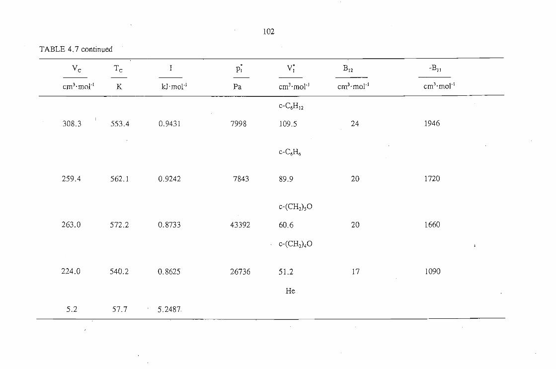
259.4 562.1 0.9242 7843
c-C6H6
89.9 20 1720
c-(CH2)sO
263.0 572.2 0.8733 43392 60.6 20 1660
c-(CH2)40
224.0 540.2 0.8625 26736 51.2 17 1090
He
5.2 57.7 5.2487
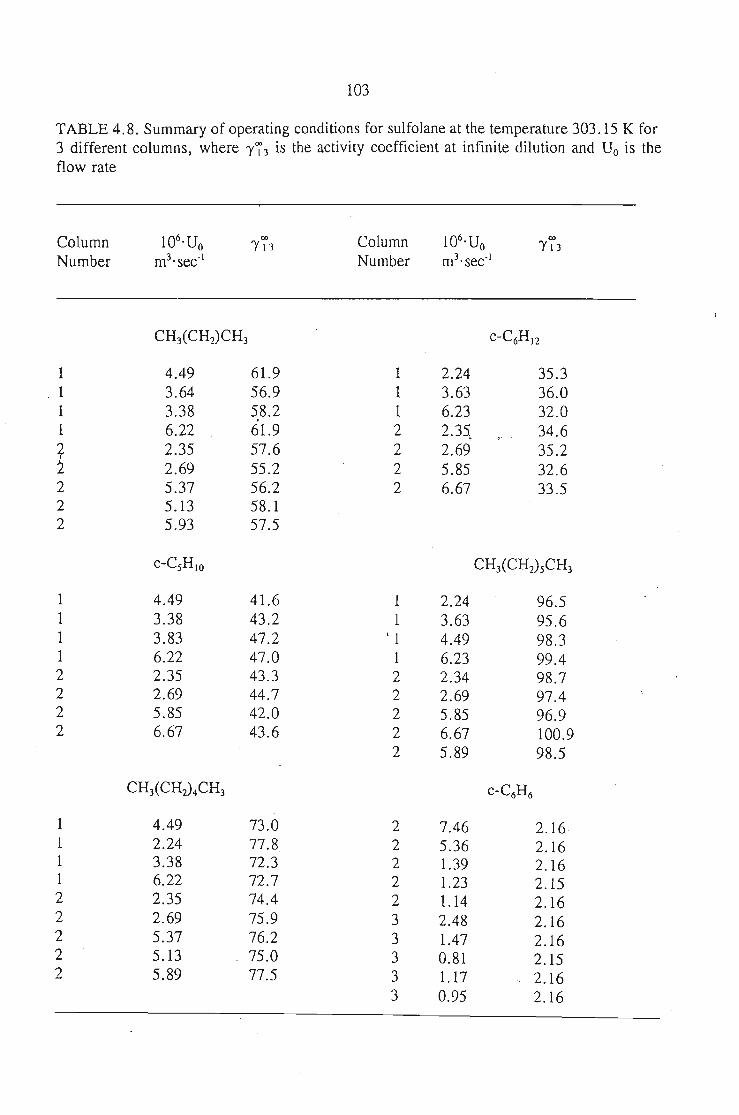
103
TABLE 4.8. Summary of operating conditions for sulfolane at the temperature 303.15 K for3 different columns, where 'Y73 is the activity coefficient at infinite dilution and Do is theflow rate
ColumnNumber
co'Y 13 Column
Number
co'Y 13
CH3(CH2)CH3 c-C6H 12
1 4.49 61.9 1 2.24 35.3. 1 3.64 56.9 1 3.63 36.0
1 3.38 58.2 1 6.23 32.00
1 6.22 61.9 2 2.35, 34.6
f 2.35 57.6 2 2.69 35.22 2.69 55.2 2 5.85 32.62 5.37 56.2 2 6.67 33.52 5.13 58.12 5.93 57.5
c-CSH IO CH3(CH2)sCH3
1 4.49 41.6 1 2.24 96.51 3.38 43.2 1 3.63 95.61 3.83 47.2 ' 1 4.49 98.31 6.22 47.0 1 6.23 99.42 2.35 43.3 2 2.34 98.72 2.69 44.7 2 2.69 97.42 5.85 42.0 2 5.85 96.92 6.67 43.6 2 6.67 100.9
2 5.89 98.5
CHiCH2)4CH3 c-C6H6
1 4.49 73.0 2 7.46 2.161 2.24 77.8 2 5.36 2.161 3.38 72.3 2 1.39 2.161 6.22 72.7 2 1.23 2.152 2.35 74.4 2 1.14 2.162 2.69 75.9 3 2.48 2.162 5.37 76.2 3 1.47 2.162 5.13 75.0 3 0.81 2.152 5.89 77.5 3 1.17 2.16
3 0.95 2.16
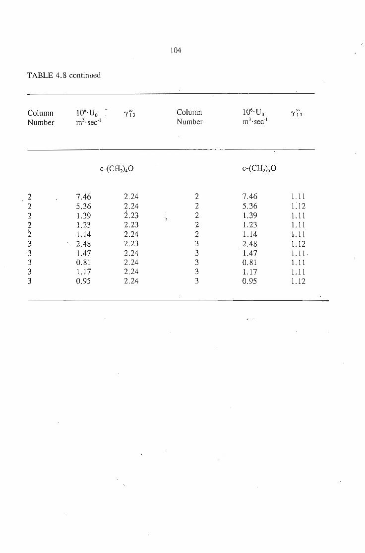
TABLE 4.8 continued
104
ColumnNumber
1Q6·UO
m3·sec·!ColumnNumber
2 7.46 2.24 2 7.46 1.112 5.36 2.24 2 5.36 1:122 1.39 2.23 2 1.39 1.112 1.23 2.23 2 1.23 1.11I
2 1.14 2.24 2 1.14 1.113 2.48 2.23 3 2.48 1.123 1.47 2.24 3 1.47 1.11·3 0.81 2.24 3 0.81 1.113 1.17 2.24 3 1.17 1.113 0.95 2.24 3 0.95 1.12
105
CHAPTER 5
EXCESS MOLAR VOLUMES OF MIXING
Excess functions are thermodynamic properties ofsolution which are in excess
ofan ideal (or ideally dilute) solution at the same conditions oftemperature, pressure
and composition. For an ideal solution all excess functions are zero. For example an
excess molar function of mixing, X;', for a binary mixture is given by(72)
E iXm = X(octua/sohltiOflalT.P,x) - X(ide4lsohltioflalthesameT,P,x)
(5.1)
where X is a thermodynamic property such as enthalpy, volumes or Gibbs energy. In
this work the excess molar volumes, V;; of mixing for the following systems were
measured: sulfolane + an unsaturated hydrocarbon ( 1-hexyne or 1-heptyne or 1
octyne) at 303.15 K.
5.1. Excess Molar Volumes of Mixing
The excess molar volume, V;;, ofcomponent 1, at a concentration x J is defined
(5.2)
where Vi and \.1 are the molar volumes ofpure solute and solvent, respectively, and
XJ + X3 = 1. The last term is the ideal molar volume of the mixture. The volume
changes for the binary mixture can be determined experimentally in one oftwo ways,
namely directly from density measurements (densitometer or pycnometric) or from a
more direct dilatometric method, ie. by measuring the resultant volume change upon·
mixing ofthe two components. Both these methods have been extensively reviewed by
106
Battino(93), Letcher'94), Handa and Benson(95) and by Stokes and Marsh. (96-98)
5.1.1. Density Measurements
5.1.1.1. Pycnometric Measurements
Scatchard, et al. (99) were the first to describe the use of a pycnometer to obtain
the density of binary mixtures. The pycnometer consists of a bulb with a capacity of
about 10 cm3, and arms with an internal diameter of 1 mm. During measurements, the
bulb is filled using a hypodermic syringe. Potentially serious errors could arise due
to inadequate mixing, evaporation and vapour space composition. However careful
measurements with excellent accuracy and reproducibility have been reported using
this method. (lOO)
5.1.1.2. The Mechanical Oscillator Densitometer
Remote or external measunng cells (as used in the densitometer) were
developed to eliminate the inherent sources of error in the pycnometer technique and
to achieve the highest possible accuracy and precision of the density(JoI) . The
introduction of the remote cell offers a method for liquid measurements according to
the oscillating sample tube method(I02). The density determination is based, in
principle, on measuring the period of oscillation of a vibrating U-shaped sample tube
which is either filled with sample or through which the sample is continuously
flowing. The accuracy of the method is limited to some extent by four factors(Jo3): the
calibration procedure, the viscosity of the sample, the pressure of the system and the
temperature control. The density of the sample is related to the resonance frequency
of an electronically excited mechanical oscillator and the period of oscillation of the
sample contained in the oscillator(l04). The effective mass (M) of the oscillator is
composed of its own unknown mass (Mo) as well as the unknown mass of the sample,
and the density p contained in volume V, and is given by
107
The resonance frequency is given by(93) .
1 1
21t V = (clM)1. = [ c ]1.(Mo + Vp)
(5.3)
(5.4)
where the mass M is attached to a spring of constant elasticity c, under the condition
that the oscillator performs an undamped oscillation(95). Rearranging and making p the
subject of the formulae
Mo 2P = - =A +B't
- C 1V+(-)(-)
41t2V y2
(5.5)
where T = l/V, ie. the period of oscillation, and A and B are constants characteristic
of the oscillator.
Densities are measured relative to a reference material:
(5.6)
where Po is the density of the reference material (usually the pure solvent, distilled
water, or air) and To is its corresponding period of oscillation.
5.1.2. Direct· Dilatometric Measurements
Highly accurate measurements are obtainable by direct measurements using
dilatometry. (95) The method eliminates the need for time consuming procedures such
as filling and weighing the pycnometer, and reduces errors arising from weight,
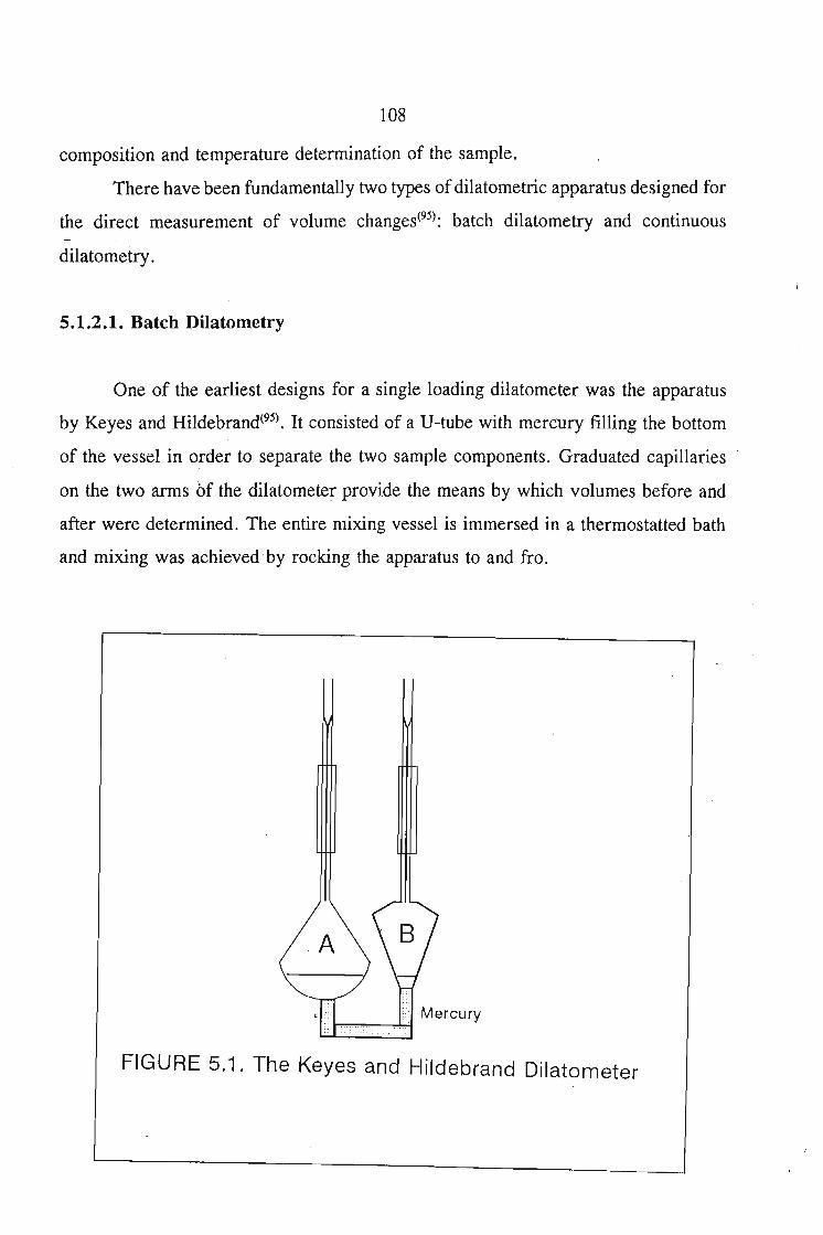
108
composition and temperature determination of the sample.
There have been fundamentally two types ofdilatometric apparatus designed for
the direct measurement of volume changes(95): batch dilatometry and continuous
dilatometry .
5.1.2.1. Batch Dilatometry
One of the earliest designs for a single loading dilatometer was the apparatus
by Keyes and Hildebnlnd(95). It consisted of a U-tube with mercury filling the bottom
of the vessel in o,rder to separate the two sample. components. Graduated capillaries
on the two arms of the dilatometer provide the means by which volumes before and
after were determined. The entire mixing vessel is immersed in a thermostatted bath
and mixing was achieved· by rocking the apparatus to and fro.
Mercury.....,..,.""".",......,..,lH
FIGURE 5.1. The Keyes and Hildebrand Dilatometer
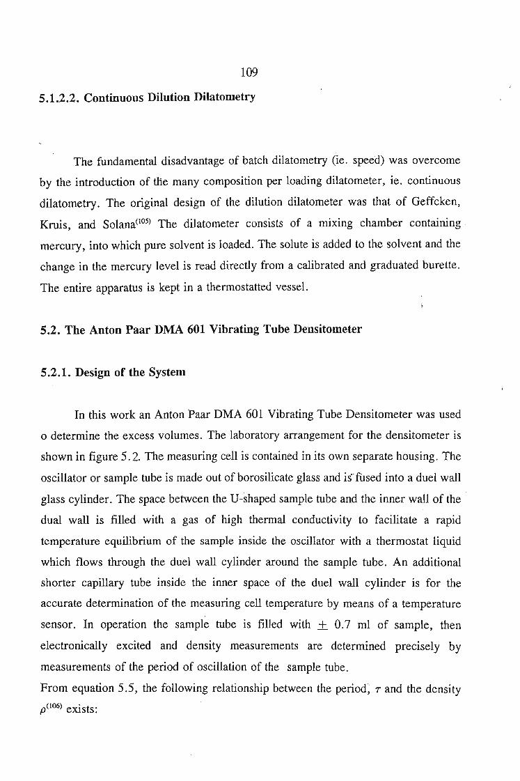
109
5.1.2.2. Continuous Dilution Dilatometry
.-
The fundamental disadvantage of batch dilatometry (ie. speed) was overcome
by the introduction of the many composition per loading dilatometer, ie. continuous
dilatometry. The original design of the dilution dilatometer was that of Geffcken,
Kruis, and Solana(105) The dilatometer consists of a mixing chamber containing.
mercury, into which pure solvent is loaded. The solute is added to the solvent and the
change in the mercury level is read directly from a calibrated and graduated burette.
The entire apparatus is kept in a thermostatted vessel.
5.2. The Anton Paar DMA 601 Vibrating Tube Densitometer
5.2.1. Design of the System
In this work an Anton Paar DMA 601 Vibrating Tube Densitometer was used
o determine the excess volumes. The laboratory arrangement for the densitometer is
shown in figure 5.2. The measuring cell is contained in its own separate housing. The
oscillator or sample tube is made out of borosilicate glass and i~rfused into a duel wall
glass cylinder. The space between the U-shaped sample tube and the inner wall of the'
dual wall is filled with a gas of high thermal conductivity to facilitate a rapid
temperature equilibrium of the sample inside the oscillator with a thermostat liquid
which flows through the duel wall cylinder around the sample tube. An additional
shorter capillary tube inside the inner space of the duel wall cylinder is for the
accurate determination of the measuring cell temperature by means of a temperature
sensor. In operation the sample tube is filled with + 0.7 ml of sample, then
electronically excited and density measurements are determined precisely by
measurements of the period of oscillation of the sample tube.
From equation 5.5, the following relationship between the period, T and the density
p(106) exists:
110
(5.5)
where A and B are instrument constants that are determined through calibration
measurements with substances of known density. The constants A and B contain the
spring constants of the oscillator as well as the empty oscillator's mass and that
volume of the sample involved in the oscillation. An unknown sample density, Px, with
a period value Tx, can thus be calculated from equation 5.6 as,
(5.6)
where water is the calibrating substance.
A prerequisite for the measurement of densities to a high level of accuracy is
good temperature control of the sample tube(106). In the instrument used in this work
the temperature was monitored using a thermistor inserted inside the inner space of
the duel wall cylinder of the sample tube. The achievable accuracy in density depends
on the achievable operating temperature. A good external thermostat with a
temperature stability of +0.01 K can yield an uncertainty in the density measurement
of approximately + 6 x 10⁻⁶ g.cm3• For this reason the stability was controlled to
within 0.002 K in this work.
Errors may occur during the injection of the mixture into the sample cell. If the
mixture is introduced too fast, tiny air bubbles may be generated, which results in an
errorous T value. Precaution was taken during sample introduction to ensure no
trapment of air. In this work the pure solvents were degassed by boiling before the
making up of the mixtures.
Uniform temperature control was achieved through the 'use of two variable
speed mechanical stirrers. An auxiliary cooling system comprising a 50 litre water
bath cooled by a Grants refrigeration coil, was incorporated to assist with the
temperature control of the main water bath. Water from this 'auxiliary bath was
pumped via a Haake immersion thermostat unit at a rate of 2.8 litre/min through a
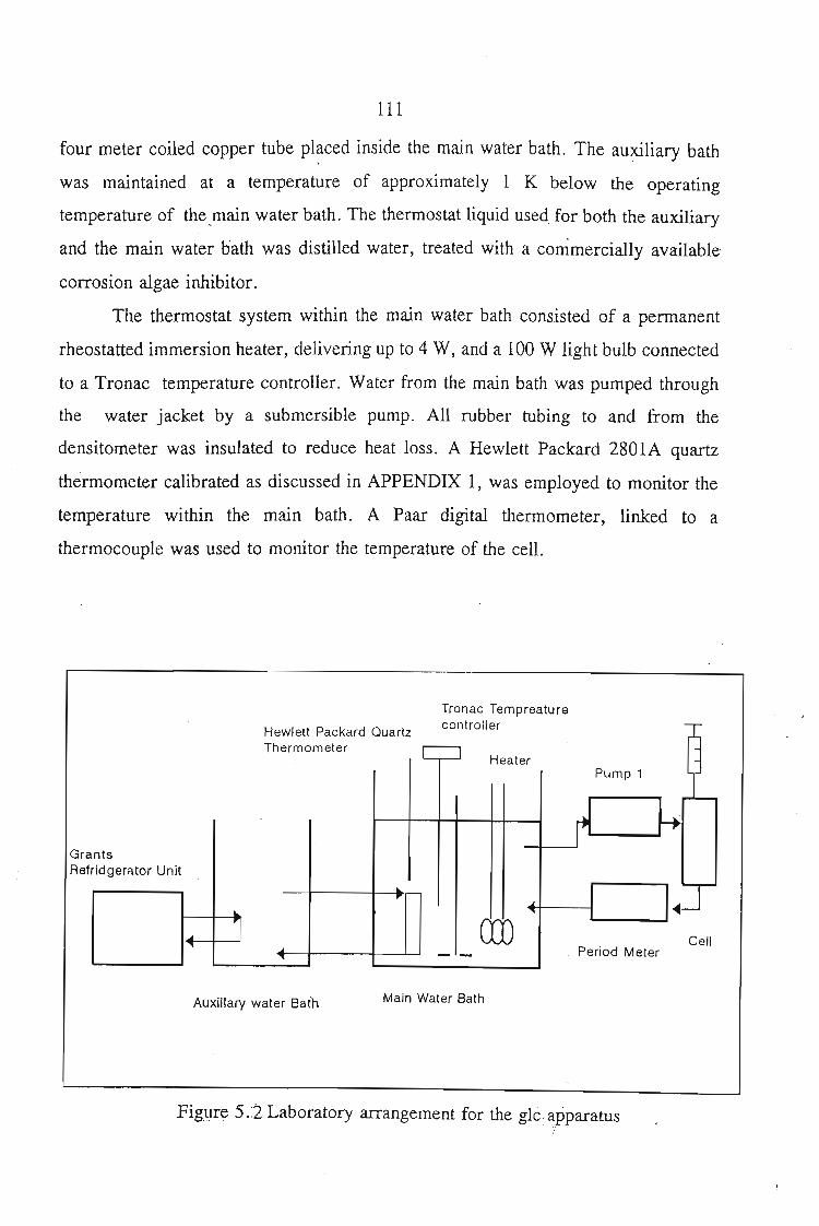
111
four meter coiled copper tube pl~ced inside the main water bath. The auxiliary bath
was maintained at a temperature of approximately 1 K below the operating
temperature of the,main water bath. The thermostat liquid used, for both the auxiliary
and the main water bath was distilled water, treated with a commercially available
corrosion algae inhibitor.
The thermostat system within the main water bath consisted of a permanent
rheostatted immersion heater, delivering up to 4 W, and a 100 W light bulb connected
to a Tronac temperature controller. Water from the main bath was pumped through
the water jacket by a submersible pump. All rubber tubing to and from the
densitometer was insulated to reduce heat loss. A Hewlett Packard 2801A quartz
thermometer calibrated as discussed in APPENDIX 1, was employed to monitor the
temperature within the main bath. A Paar digital thermometer, linked to a
thermocouple was used to monitor the temperature of the cell.
GrantsRefridgerator Unit
Hewlett Packard QuartzThermometer
Tronac Tempreaturecontroller
HeaterPump 1
Period MeterCell
Auxiliary water Bath Main Water Bath
Figure 5.:2 Laboratory arrangement for the glc apparatus
112
5.2.2. Operation Procedure
Prior to each experimental run, the cell was flushed thoroughly with warm
methanol, and then acetone. After flushing, compressed air was blown through the·
cell. A constant period value, T, for the sample tube filled with air was obtained
before the sample is introduced. Double distilled pre-boiled water (used as the
calibrated standard sample) was then introduced into the cell by means of a glass
syringe, equipped with a teflon nozzle, ensuring a leak proof fit at the sample cell
syringe junction. The injection process was carried out slowly and carefully, enabling
the liquid to properly wet the walls of the cell, and thus reducing the risk of trapping
air bubbles in the U-tube. The sample was always filled past its nodal points and the
syringe was left in place at the inlet point during each measurement. The outlet of the
cell was sealed with a teflon plug to reduce evaporation. The solutions were
introduced in to the sample cell in exactly the same manner as the distilled water.
With the cell illumination light off, the photoelectric portion of the excitation
system was automatically activated. Each measuring cycle was allowed to continue
until a constant period value was obtained. Period values for water (reference
substance), pure solvents and air were determined between each solution injection.
These valves were not only required for the density calculations, but also permitted
a continuous check on both the purity of samples and the densitometer operation. The
precision of T, judged by repeated measurements for the same solution at different
times, was estimated to be better than 2 x 10⁻⁶ Hz.
5.2.3. Preparation of Mixtures
The pure solvents were degassed before sample solutions were made up by
immersing the sample into a sonic bath for 30 minutes. The mixtures were then made
up in five cm3 flasks with ground glass stoppers.Care was taken to first add the least
volatile component into the flask, and that the completed mixture left a small vapour-
113
just large enough to aid mixing. The mixtures were made up shortly before injection
into the densitometer, and were shaken vigorously to ensure complete mixing.
5.3. Results
The excess molar volumes of the following systems were measured at
303.15 K: sulfolane + I-hexyne, or I-heptyne or l-octyne., The excess volumes were
measured as part of an investigation into the thermodynamic mixing properties of the
binary mixtures formed with sulfolane. Although the measurements of excess volumes
is not a good indicator of the interactions involved in binary mixtures it can provide
evidence of specific interactions. Various theories of solution, have been proposed to
describe excess volumes of mixing ie., the Flory-Patterson Theory(107), the Extended
Real Associated Solution Theory (ERAS)(108) and the Patterson-Treszczanowicz(109)
theory. Due to the strong dipole-dipole interaction between sulfolane and the alkynes,
the simple Flory Patterson(107) equation fails to describe the mixing curve. In the
absence of any hydrogen bonding (as in the case of sulfolane and the alkynes) the
theories of ERAS(108) and Patterson-Treszczanowicz(109) are also unable to describe the
mixing curve accurately. In this work, all attempts at fitting theses theories to the VE
data have been excluded as the results were very poor.
The Redlich-Kister equation,(lIO) (equation 5.7) has been fitted to the excess
volumes data. The results together with the Redlich-Kister parameters are given in
Table 5.1.
(5.7)
The partial molar excess volumes (Vi and Vi) are calculated using equation 5.8. and
are listed in Table 5.1. The partial molar volumes at infinite dilution for both the
solute (1) and the solvent (3) are calculated using equations 5.9. and 5.10. The
calculated values are listed in Table 5.1.
114
At infinite dilution the equation is simplified and the partial molar excess volume is:
(5.9)
and
(5.10)
The standard deviation of the excess molar volume, a(V;), is obtained using the
following equation,
(V E Vj2 1a(Vj = [:E~_ m(cal) - m ]"2
m 1-1 (n-2)(3.11)
Graphs of excess molar volumes and the partial molar volumes at 303.15 K for all
systems studied are given in figures 5.:3 - 5.8. ,
The very large negative excess volumes quoted in Table 5.1 indicate a strong
interaction between sulfolane + alkynes. This supports the evidence obtained from the
VLE (Chapter 7) and SLE (Chapter 8) results.
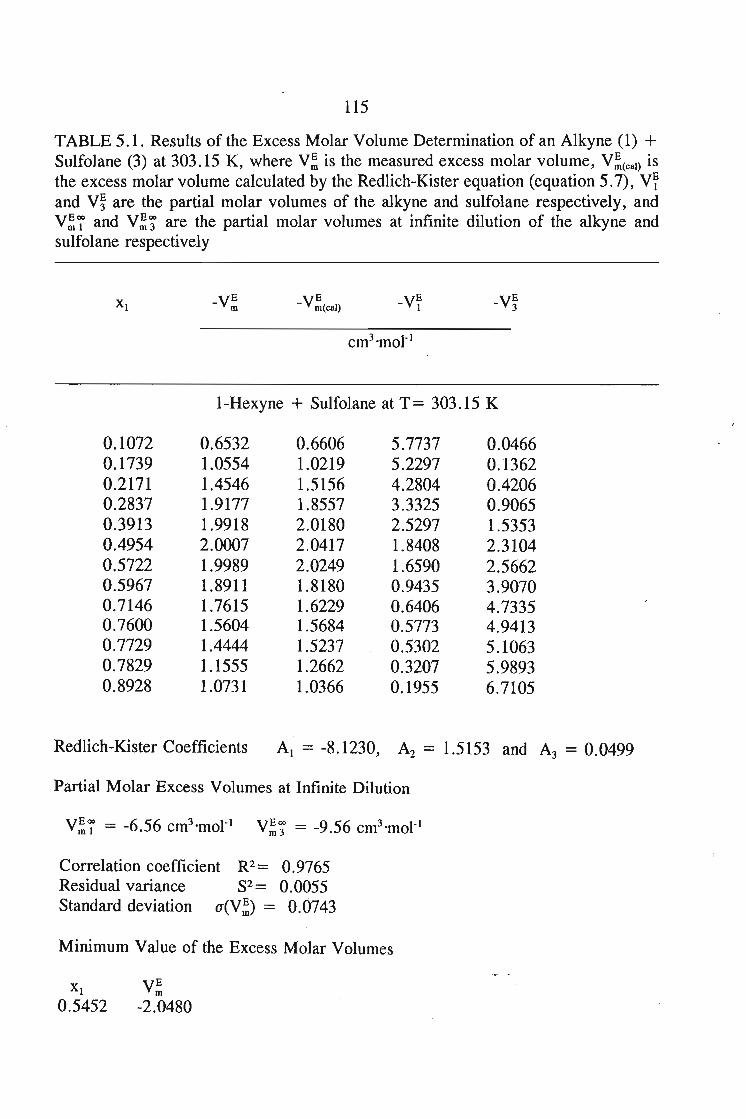
115
TABLE 5.1. Results of the Excess Molar Volume Determination of an Alkyne (1) +Sulfolane (3) at 303.15 K, where V; is the measured excess molar volume, V;(Cal) isthe excess molar volume calculated by the Redlich-Kister equation (equation 5.7), Vrand V~ are the partial molar volumes of the alkyne and sulfolane respectively, andV;';" and V;c; are the partial molar volumes at infinite dilution of the alkyne andsulfolane respectively
-V~
I-Hexyne + Sulfolane at T= 303.15 K
0.1072 0.6532 0.6606 5.7737 0.04660.1739 1.0554 1.0219 5.2297 0.13620.2171 1.4546 1.5156 4.2804 0.42060.2837 1.9177 1.8557 3.3325 0.90650.3913 1.9918 2.0180 2.5297 1.53530.4954 2.0007 2.0417 1.8408 2.31040.5722 1.9989 2.0249 1.6590 2.56620.5967 1.8911 1.8180 0.9435 3.90700.7146 1.7615 1.6229 0.6406 4.73350.7600 1.5604 1.5684 0.5773 4.94130.7729 1.4444 1.5237 0.5302 5.10630.7829 1.1555 1.2662 0.3207 5.98930.8928 1.0731 1.0366 0.1955 6.7105
Redlich-Kister Coefficients At = -8.1230, A2 = 1.5153 and A3 = 0.0499
Partial Molar Excess Volumes at Infinite Dilution
Correlation coefficient R2= 0.9765Residual variance S2= 0.0055Standard deviation (J(V;) = 0.0743
Minimum Value of the Excess Molar Volumes
Xl
0.5452V E
ID
-2.0480
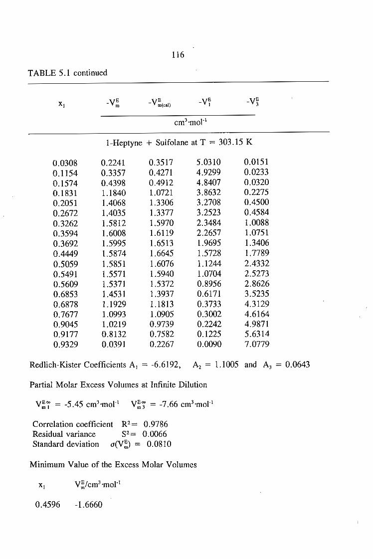
116
TABLE 5.1 continued
_VE -V;(Cal) -VI[ VEXI m - 3
cm3 'mol-1
1-Heptyne + Sulfolane at T = 303.15 K
0.0308 0.2241 0.3517 5.0310 0.01510.1154 0.3357 0.4271 4.9299 0.02330.1574 0.4398 0.4912 4.8407 0.03200.1831 1.1840 1.0721 3.8632 0.22750.2051 1.4068 1.3306 3.2708 0.45000.2672 1.4035 1.3377 3.2523 0.45840.3262 1.5812 1.5970 2.3484 1.00880.3594 1.6008 1.6119 2.2657 1.07510.3692 1.5995 1.6513 1.9695 1.34060.4449 1.5874 1.6645 1.5728 1.77890.5059 1.5851 1.6076 1.1244 2.43320.5491 1.5571 1.5940 1.0704 2.52730.5609 1.5371 1.5372 0.8956 2.86260.6853 1.4531 1.3937 0.6171 3.52350.6878 1.1929 1.1813 0.3733 4.31290.7677 1.0993 1.0905 0.3002 4.61640.9045 1.0219 0.9739 0.2242 4.98710.9177 0.8132 0.7582 0.1225 5.63140.9329 0.0391 0.2267 0.0090 7.0779
Redlich-Kister Coefficients Al = -6.6192, A2 = 1.1005 and A3 = 0.0643
Partial Molar Excess Volumes at Infinite Dilution
Correlation coefficient R2= 0.9786Residual variance S2= 0.0066Standard deviation a(V;) = 0.0810
Minimum Value of the Excess Molar Volumes
0.4596 -1.6660
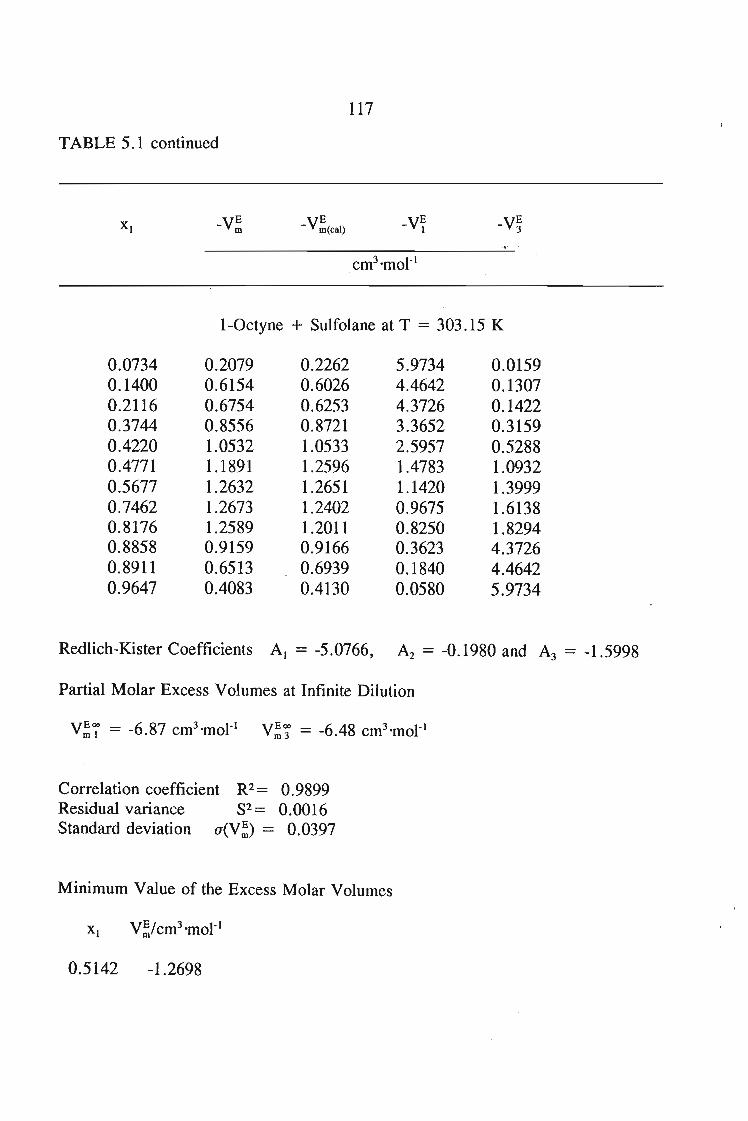
117
TABLE 5.1 continued
YE- I YE
- 3
1-0ctyne + Sulfolane at T = 303.15 K
0.0734 0.2079 0.2262 5.9734 0.01590.1400 0.6154 0.6026 4.4642 0.13070.2116 0.6754 0.6253 4.3726 0.14220.3744 0.8556 0.8721 3.3652 0.31590.4220 1.0532 1.0533 2.5957 0.52880.4771 1.1891 1.2596 1.4783 1.09320.5677 1.2632 1.2651 1.1420 1.39990.7462 1.2673 1.2402 0.9675 1.61380.8176 1.2589 1.2011 0.8250 1.82940.8858 0.9159 0.9166 0.3623 4.37260.8911 0.6513 0.6939 0.1840 4.46420.9647 0.4083 0.4130 0.0580 5.9734
Redlich-Kister Coefficients Al = -5.0766, A2 = -0.1980 and A3 = -1.5998
Partial Molar Excess Volumes at Infinite Dilution
Correlation coefficient R2= 0.9899Residual variance S2= 0.0016Standard deviation o{Y;) = 0.0397
Minimum Yalue of the Excess Molar Volumes
0.5142 -1.2698
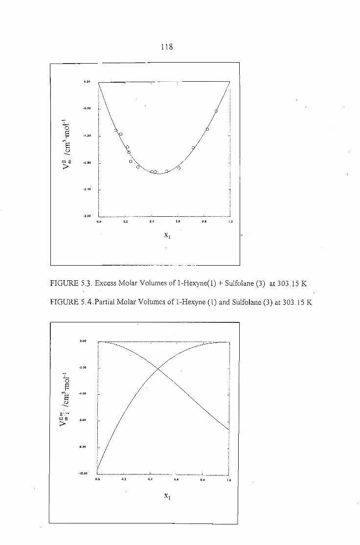
118
0.00
ooo
o
o
.,. I.1.,2Q _
,,. Il::::::: .
,,.·1
-3.00 L ..:... j l L J
Ul8
>
.....:-.o~
"'8u-
0-0 0.1 0.' '-" 0.' 1.0
FIGURE 5.3. Excess Molar Volumes of 1-Hexyne(1) + Sulfolane (3) at 303.15 K
FIGURE 5. 4. Partial Molar Volumes of 1-Hexyne (1) and Sulfolane (3) at 303.15 K
0.00 .---------,-----------------;----------------,------------------;-_.:;:---=--=_._,
_2.00
~8ca .....00
u--8'~
Ul E -4.00
>
.... 00
·10.00
iL ._c..••_.••_._.__••.."._ _ ..•.;_ __._.•.•_ ,••....•._ .....•j
0.0 0.2 0.' 0.' 0.' 1.0
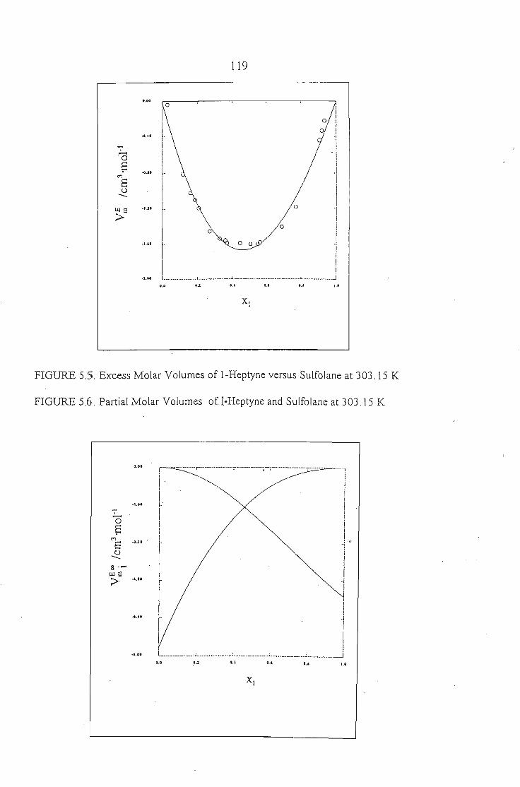
119
11
0
io ,, i
I 0 iL. ·f
t 1,!i . i! .~ .1I iI I
i~. 0 '1I !I 0 0 !r' 0 0 'jI i
I i!
L . J__ •••__••• • ..l. __ • •••••••••••••••••__ • •••••• l. .. __ . .• .j
0.00
~ .•o
.1.JO
-1.&0
-1.00 ... ... ... ... I.'
FIGURE 5.5. Excess Molar Volumes of I-Heptyne versus Sulfolane at 303.15 K
FIGURE 5.6. Partial Molar Volumes ofl·Heptyne and Sulfolane at 303.15 K
0.00
.t.ao
......0
FM
·J..10a(.)-8 .-~e
> ~.1O
,'.00
·-·---------r--------·-:-----·----i-~---------_·_-----."';"-.~...;;;.....~--,
,. ii
I !I i~ ~! ;! ii ir i! !t ~-i iI ii I
! ir. J!i I
I Ir ~I IL _ l. ;_._ , _J... .,J ... ... ... I.'
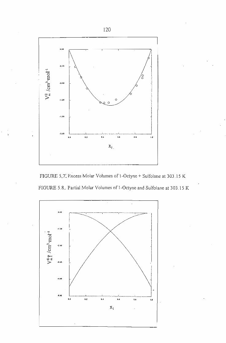
120
0.00
-1.00
.:-.o;:
'"8uUJ2
>
i
I I.•.•• f· '1
I I
I0 I
I 0 .!.:-0.110 ..
". [ ° °°1Irl
iI iI i
I .. .!..1.00 l .._.._~_~ .!__ ._l • ... ._. ~
... •.> ... ... ...
FIGURE 5.7~ExcessMolar Volumes of l-Octyne + Sulfolane at 303.15 K
FIGURE 5.8. Partial Molar Volumes of l-Octyne and Sulfolane at 303.15 K
0.00
·1..20
.:.....0
~<"'l
-2."QEU-8-
I.Il 2·
> -.1.60
-4.00
I I
i iI i~ ~
1
1 I
Iir 1
i ,~ 1
I il i
" '1
l _.._.L.••• ••.••• ; ••••••_ •••••••_.J •••_ ••••••••••_ •••• _ •••••••••J ..'G.G G.' G,' G.' t.'
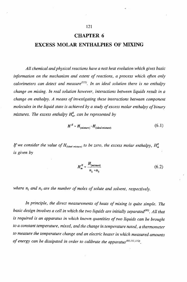
121
CHAPTER 6
EXCESS MOLAR ENTHALPIES OF MIXING
All chemical andphysical reactions have a nett heat evolution which gives basic
information on the mechanism and extent of reactions, a process which often only
calorimeters can detect and measure(111). In an ideal solution there is no enthalpy
change on mixing. In real solution however, interactions between liquids result in a
change on enthalpy. A means of investigating these interactions between component
molecules in the liquid state is achieved by a study ofexcess molar enthalpy ofbinary
mixtures. The excess enthalpy H;, can be represented by
H E = H(mixturt) - H(ideal mmure) (6.1)
Ifwe consider the value of H(ideal mixture) to be zero, the excess molar enthalpy, H;,
is given by
(6.2)
where nJ and n3 are the number ofmoles of solute and solvent, respectively.
In principle, the direct measurements of heats of mixing is quite simple. The
basic design involves a cell in which the two liquids are initially separated(93). All that
is required is an apparatus in which known quantities of two liquids can be brought
to a constant temperature, mixed, and the change in temperature noted, a thermometer
to measure the temperature change and an electric heater in which measured amounts
of energy can be dissipated in order to calibrate the apparatus (93,111 ,112).
122
6.1. ~ Measurements
Two types of calorimeters were used in this work, the commercially available
LKB 2107-101 microcalorimeter, and the Thermometric 2277 Thermal Activity flow-
mix microcalorimeter.
6.2. The LKB 2107 Microcalorimeter
6.2.1. Principle of Operation
The isothermal flow mix measuring cylinder for the LKB calorimeter used in
this work is discussed in great detail in the literature. (1l3) The mixing vessel has a
separate inlet and comprises a spiral-wound 24 carat gold tube of 1 mm i.d. and with
a volume of 0.5 cm3• The design is such that adequate mixing is achieved with no
vapour space. The mixing vessel is in thermal contact with a pair of matched
thermocouples in the thermopiles and an aluminium heat-sink assembly, with the heat
sink compound covering all the surfaces of these items. An exothermic reaction results
in heat flow to the heat sink assembly, while the opposite effect is observed for the
endothermic reactions. In each case the resultant temperature difference is detected by
the thermopiles positioned between the vessel and the heat sink. The output from the
thermopiles is amplified and fed to a digital readout system and a Perkin-Elmer 561
chart recorder.
The aluminium block heat sink assembly is contained within an insulated
housing. A heater and a temperature sensor are mounted within the heat sink. The
entire arrangement is contained within an LKB thermostat which consists of a
thermostatically controlled air bath to maintain the temperature required for this
investigation. Water, cooled to 287 K by a Labcon Thermostat unit is pumped through
at a rate of 8 cm3 ·s-1•
The LKB was used in conjunction with a LKB control unit. This incorporates
a power supply capable of providing an adjustable current to the calibration heaters
123
within the insulated mixing vessel assembly, and a facility for heating and monitoring
the temperature of the calorimeter heat sink assembly. This heating facility helps to
reduce the equilibrium time of the apparatus during 11 startup It or when raising the
operating temperature. It was always switched off when measurements with the
instrument were made.
Since liquids entering the microcalorimeter are required to be within 0.05 K of
the experimental temperature, they were first routed through an external heat exchange
fitted into a recess in the bottom of the air bath of the thermostat unit and then through
the internal heat exchangers, situated inside the housing containing the mixing vessel
assembly. Samples were introduced using two Jubilee peristaltic pumps, capable of
stable flow rates ranging from 0.03 - 0.2 cm3• min- I
• Viton tubing, 1.5 mm i.d., and
teflon tubing, 1.2 mm i.d. were used in the pumps and flows lines respectively. The
temperature inside the microcalorimeter was monitored using a Hewlett Packard 2804·
A quartz thermometer and was found to be constant to better than 0.01 K.
6.3. The 2277 Thermal Activity Monitor (TAM)
6.3.1. Principles of Operation
The 2277 Thermal Activity Monitor circulator equipped with an external
thermostatic water circulator (Thermometric 2219 Multi-temp 11) and a pair of Eldex
variable speed piston pumps capable of stable flow rates from 0.05 to 3 ml'min- I was
also employed in this work. The TAM utilizes the heat flow or'heat leakage principle
where heat produced in a thermally defined vessel flows away in an effort to establish
thermal equilibrium with its surroundings. The calorimetric mixing device used in the
TAM has a 24 carat gold flow-mix cell where two different liquids can be mixed. The
flow mix cell has a small bore T-piece at the base of the measuring cup where the two
incoming flows are mixed. After mixing the reaction takes place as the mixed flow
passes the spiral around the measuring cup and out to waste. The measuring cup is
124
sandwiches between a pair of Peltier thermopile heat sensors. These sensors are in
contact with a heat sink:. The system is designed so that the main path for the flow
of heat to or from the measuring cup is through the Peltier elements. The Peltier
elements act as a thermoelectric generators capable of responding to temperature
gradients of less than one millionth of a degree celsius. These highly sensitive
detectors convert the heat energy into a voltage signal proportional to the heat flow.
Results are presented as a measure of the thermal energy produced by a sample per
unit of time.
Results are quantified where known power values are passed through built in
precision resistors. Precision wire wound resistors are located within each measuring
cup to represent a reaction during electric calibration. The calibration resistors is
integral with the measuring cup, to simulate as near as possible, the position of the
reaction. This ensures that the output from the detector will be, as near as possible,
identical to the output when the power is dissipated from the resistor as from the
sample. During the calibration, a know current is passed through _the appropriate
channel heater resistor, and because the resistors value is know, a specific thermal
power gIves a calibration level that may then be used to determine experimental
results. (114)
The entire assembly is located in a stainless steel cylinder. Each cylinder has
two measuring cup assemblies just described; the Peltier elements in each measuring
cup are connected in series but in opposition so that the resultant signal represents the
difference in the heat flow from the two measuring cups. This design allows one
measurement cup assembly to be used for the sample and the other to be used as the
blank:.
This instrument is suitable for the solvents used in this investigation as outside
the calorimeter unit the liquids are in contact with Teflon and' glass only. Inside
contacts are the gold tube of the heat exchanger and the mixing cell and the teflon
125
tubes. Samples were introduced into the cell using two Eltron piston pumps capable
of producing flow rates from 0.5 to 3.0 cm3min-1•
The sensitivity and high level of precision of the TAM is largely due to the
stability of the infinite heat sink which surrounds the measuring cylinders. This heat
sink is formed by a closed 25 litre thermostatted water bath to + 2 x 10⁻³ K within the
experimental range. Water is continuously circulated by being pumped upwards into
a cylindrical stainless steel tank, where it overflows into a similar but larger outer
tank. The pump then re-circulates the water from the outer tank back into the inner
tank. Several inactive controlling systems work together to maintain the water
temperature whose signals are fed to an electronic temperature regulator unit. The 25
litre thermostat is filled with deionised water and a corrosion inhibitor containing
sodium nitrate, sodium metasilicate and benzotriazole.
6.4. Operation Procedure and Actual Sample Measurement
The solvent used, sulpholane has a melting point of 301.60 K, therefore the
pumps and the tubing that are normally at room temperature had to be insulted above
the sulpholane melting point to allow it to be pumped into the calorimeters. This was
done by designing a housing for the pumps and tubing using a well insulated glove
box with a Goldair heater, which circulated warm air within the housi~g.
For both instruments, an initial equilibrium time of at least three days was
required. Power to the equipment was left on continuously for the duration of the
experimental determination to ensure that thermal equilibrium was maintained in the
temperature control units. The flow lines were filled with water overnight. In the
morning warm methanol was pumped through each flow line at a rate of 0.8 cm3 's-1
for 15 minutes before introduction of the component liquids.
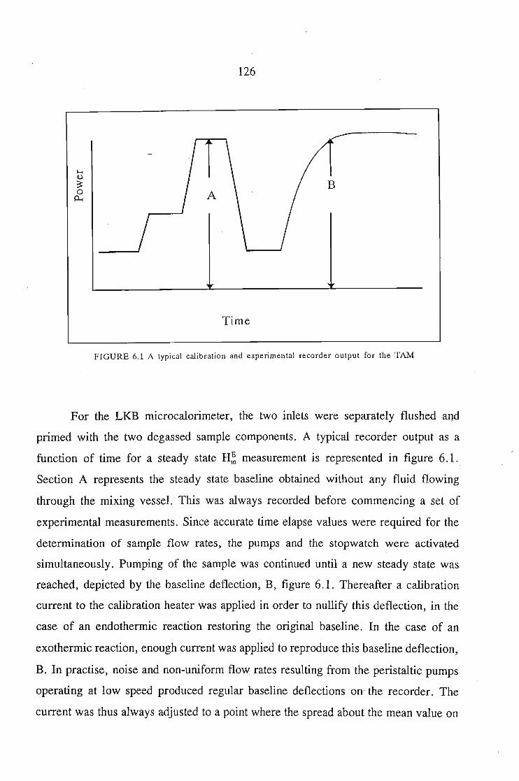
126
B
Time
FIGURE 6.1 A typical calibration and experimen tal recorder output for the TAM
For the LKB microcalorimeter, the two inlets were separately flushed aI}d
primed with the two degassed sample components. A typical recorder output as a
function of time for a steady state H; measurement is represented in figure 6.1.
Section A represents the steady state baseline obtained without any fluid flowing
through the mixing vessel. This was always recorded before commencing a set of
experimental measurements. Since accurate time elapse values were required for the
determination of sample flow rates, the pumps and the stopwatch were activated
simultaneously. Pumping of the sample was continued until a new steady state was
reached, depicted by the baseline deflection, B, figure 6.1. Thereafter a calibration
current to the calibration heater was applied in order to nullify this deflection, in the
case of an endothermic reaction restoring the original baseline. In the case of an
exothermic reaction, enough current was applied to reproduce this baseline deflection,
B. In practise, noise and non-uniform flow rates resulting from the peristaltic pumps
operating at low speed produced regular baseline deflections on the recorder. The
current was thus always adjusted to a point where the spread about the mean value on
127
the deflected baseline was reproduced about the zero flow-baseline.
Once the regular baseline had been regained, both pumps were switched off.
The molar flow rates, f1 and f2 were determined by weighing the two component flasks
before and after each experimental run. From these masses and -the time elapsed for
the experiment, the molar flow rates were determined. A Mettler AE240 electronic·
balance, accurate to 0.0001 g was used for the mass determinations.
For the TAM, due to sensitivity of the instrument and the absence of a control unit
containing an inbuilt current supply, calibration at the individual flow rates was
necessary. This involves flushing one of the component solvents through both the inlet
tubes at a flow rate similar to that for the actual experimental determination. A know
current, I, from an external power source is simultaneously passed through the inbuUt
resistor and since R for the resistor is known, the expected thermal power, P, can be
obtained from the equation,
(6.3)
and the calorimeter power reading is adjusted accordingly. Both the pumps, and the
external power supply were switched off, the baseline was allowed to return to zero
and flow of the second sample component in one of the lines was initiated for
sufficient time to coat the tubing. Experiments were carried out according to a method
similar to that of the LKB microcalorimeter with the flow rates exactly like those used
in the calibration.
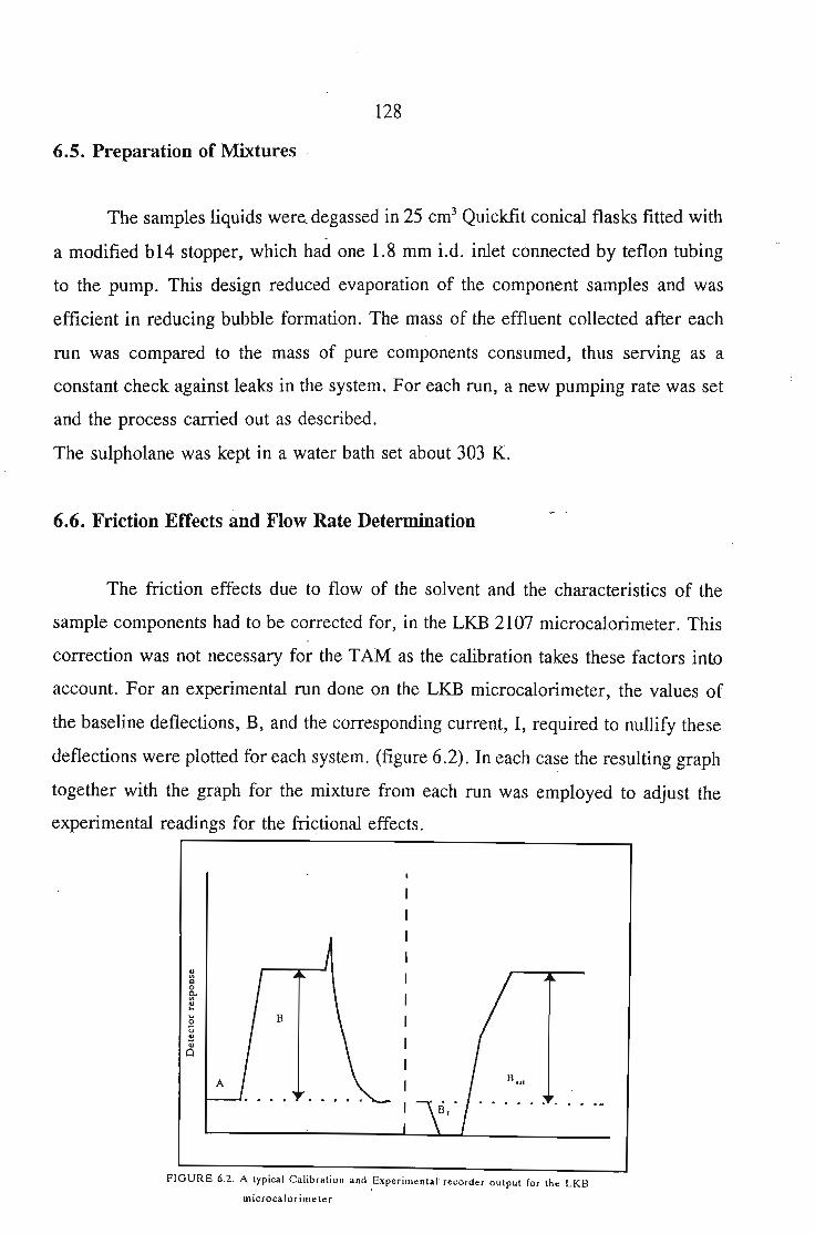
128
·6.5. Preparation of Mixtures
The samples liquids were, degassed in 25 cm3 Quickfit conical flasks fitted with
a modified b14 stopper, which had one 1.8 mm i.d. inlet connected by teflon tubing
to the pump. This design reduced evaporation of the component samples and was
efficient in reducing bubble formation. The mass of the effluent collected after each
run was compared to the mass of pure components consumed, thus serving as a
constant check against leaks in the system. For each run, a new pumping rate was set
and the process carried out as described.
The sulpholane was kept in a water bath set about 303 K.
6.6. Friction Effects and Flow Rate Determination
The friction effects due to flow of the solvent and the characteristics of the
sample components had to be corrected for, in the LKB 2107 microcalorimeter. This
correction was not necessary for the TAM as the calibration takes these factors intD
account. For an experimental run done on the LKB microcalorimeter, the values of
the baseline deflections, B, and the corresponding current, I, required to nullify these
deflections were plotted for each system. (figure 6.2). In each case the resulting graph
together with the graph for the mixture from each run was employed to adjust the
experimental readings for the frictional effects.
FIGURE 6.2. A typical Calibration and ,Experimentar recorder output for the LKB
microcalorimeter
129
These calibrations were carried out collectively at the end of a series of experimental
runs for a system. Each calibration involved purging the mixing vessel with the
effluent from a particular run. With the same pumping parameters as were employed
for that particular run, any heating effect due to friction exhibited a deflection, Br in
figure 6.2. The experimental detector voltage shift was thus corrected to
(6.4)
The indicated calibration current, Icah corresponds to Bo' was then interpolated from
the experimentally determined graph and was passed through the calorimeter heater,
thereby producing a baseline deflection to BCal in figure 6.2. The excess molar enthalpy
was thus calculated from (23)
HE = [(Bo(Ical R/Bcal]
m if1 +h)(6.5)
were R is the resistance heater. It is however, observed that Bo ::::::: BCa1 for flow rates
less than 0.80 cm3 min- l• Since the majority of the experimental runs were carried out
at flows rate less than this, the above calibration procedure became unnecessary in
many cases and H; was then determined by
(6.6)
For exothermic reactions, the steady state deflection, B, was noted and a current, I,
was applied to double this deflection. Heating due to frictional effects would once
again produce a deflection, Br, and hence equation 6.4 becomes
130
(6.7)
The TAM was, however, found to give more precise results for small endothermic
and exothermic reactions. The calorimeters were tested using the data of Stokes and
Marsh(96) to confirm technique and procedure. The test system was (benzene +cyclohexane) and the results obtained were always within 10 J 'mot1 of the smooth
curve obtained by Stokes and Marsh. (96)
6.7. Results
The excess enthalpies for the following systems were measured at 303.15 K:
sulfolane + l-hexyne, l-heptyne and l-octyne. The results are given in Table 6.1.
The Redlich-Kister equation,(97)(equation 6.8) is fitted to the excess enthalpy
data. The results together with the Redlich-Kister parameters are given in Table 6.1.
(6.8)
The partial molar excess enthalpies are calculated using equation 6.9 and are listed in
Table 6.1. The partial molar enthalpies at infinite dilution for both the solute (1) and
the solvent (3) are calculated using equations 6.10. and6.11. The calculated values
are listed in Table 6.1.
(6.9)
At infinite dilution the equation simplifies to
131
and
E.. n AH3 = ~i=1 i
(6.10)
(6.11)
The standard deviation of the excess molar enthalpy, a(H~), is obtained using the
following equation,
- (HE H52 1o(HE... = [~~_ m(cal) - m ]"2
m) 1-1 (n-2)(6.12)
where n is the number of parameters.
Excess molar enthalpies and the partial molar enthalpies at 303.15 K for all systems
studied are given in Table 6.1.
The HE data is positive over the whole range of concentration. This is m,?st
likely a result of the dissociation of the sulfolane and also the alkynes which mask the
any association between sulfolane and the alkynes. The association between sulfolane
and the alkynes appear to be small. The oxygens on the sulfolane molecule appear to
be shielded.
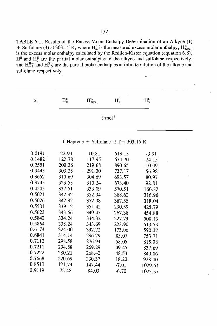
132
TABLE 6.1. Results of the Excess Molar Enthalpy Determination of an Alkyne (1)+ Sulfolane (3) at 303.15 K, where H~ is the measured excess molar enthalpy, H~(Cal)
is the excess molar enthalpy calculated by the Redlich-Kister equation (equation 6.8),H~ and H~ are the partial molar enthalpies of the alkyne and sulfolane respectively,and H~7 and H~~ are the partial molar enthalpies at infinite dilution of the alkyne andsulfolane respectively
J 'mol-!
I-Heptyne + Sulfolane at T= 303.15 K
0.0191 22.94 10.81 613.15 -0.910.1482 122.78 117.95 634.70 -24.150.2551 200.36 219.68 890.65 -10.090.3445 303.25 291.30 737.17 56.980.3652 310.69 304.69 693.57 80.970.3745 323.53 310.24 673.40 92.810.4205 337.51 333.09 570.51 160.820.5021 342.92 352.94 388.62 316.960.5026 342.92 352.98 387.55 318.040.5501 339.12 351.42 290.59 425.790.5623 343.66 349.45 267.38 454.880.5842 334.24 344.32 227.73 508.130.5864 338.24 343.69 223.90 513.530.6174 324.00 332.72 173.06 590.370.6841 314.14 296.29 85.07 753.710.7112 298.58 276.94 58.05 815.980.7211 294.88 269.29 49.45 837.690.7222 280.21 268.42 48.53 840.060.7668 220.69 230.37 18.20 928.000.8510 121.74 147.44 -7.01 1029.610.9119 72.48 84.03 -6.70 1023.37
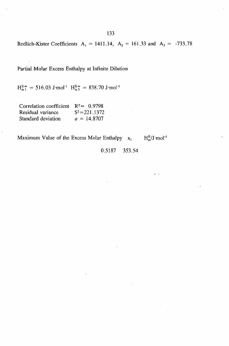
133
Red1ich-Kister Coefficients Al = 1411.14, A2 = 161.33 and A3 = -733.78
Partial Molar Excess Erithalpy at Infinite Dilution
Correlation coefficient R2= 0.9798Residual variance S2=221.1372Standard deviation (J = 14.8707
Maximum Value of the Excess Molar Enthalpy XI
0.5187 353.54
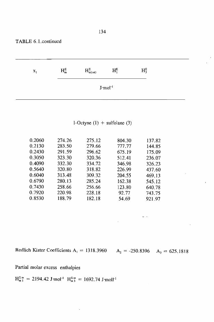
134
TABLE 6.1.continued
1-0ctyne (1) + sulfolane (3)
H~
0.2060 274.26 275.12 804.30 137.820.2130 283.50 279.66 777.77 144.850.2430 291.59 296.62 675.19 175.090.3050 323.30 320.36 512.41 236.070.4090 332.30 334.72 346.98 326.230.5640 320.80 318.82 226.99 437.600.6040 313.48 309.32 204.55 469.130.6790 280.13 285.24 162.38 545.120.7430 258.66 256.66 123.80 640.780.7920 220.98 228.18 92.77 743.750.8530 188.79 182.18 54.69 921.97
Redlich Kister Coefficients At = 1318.3960 A2 = -250.8396 A3 = 625.1818
Partial molar excess enthalpies
H;7 = 2194.42 J'mot l H;~ = 1692.74 J'moll- I
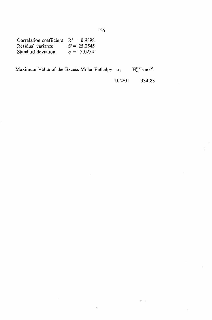
135
Correlation coefficient R2= 0.9898Residual variance S2 = 25.2545Standard deviation (J = 5.0254
Maximum Value of the Excess Molar Enthalpy XI
0.4201 334.83
136
CHAPTER 7
VAPOUR LIQUID EQillLmRIA
Reliable and accurate vapour-liquid equilibrium (VLE) data are always needed
for process engineering design and also provide useful information in the
understanding of the behaviour of liquid mixtures.
Two broad areas ofVLE measurements can be distinguished, viz. low pressure
and high pressure. Most ofthe low pressure VLE measurements are done on two types
ofequipment, dynamic (circulation) stills and static equilibrium cells. It is stated that
the highest accuracy ofmeasurements is obtained by means ofa static cell (]O), i.e. a
method in which the liquid and the vapour phases are in a state of equilibrium and
boiling does not occur. The long time necessary for equilibrium, the need for
degassing of samples, and the expensive axillary equipment required are the most
important drawbacks ofthis method. The dynamic stills, working in the stationary state
ofboiling under the pressure ofan inert gas, are considerably simpler in operation}
but are usually less accurate. (10,11) .
In this work, the Rogalski(]o,115) modified Swietoslawski dynamic ebulliometer
still(ll) is used to produce VLE measurements accurately in the low pressure region.
Modifications to the ebulliometer include (i) stable hydrodynamic and thermal
conditions under pressure from 100 to 300 kPa andfrom room temperature to 500 K,
even in the case when the mixtures investigated consist of substances of widely
differing vapour pressures, (10) and (ii) the composition ofthe liquid and vapour streams
leaving the equilibrium chamber are maintained constant until the streams have passed
through the sample chambers and until they correspond to the thermodynamically
consistent values of pressure and temperature. (10) The ebulliometer produces VLE
measurements rapidly and accurately over a wide temperature range. It is also suited
137
for determinations at very low concentrations.
Binary Vapour-Liquid Equilibria for the following systems at 338.15 K or
353.15 K were measured: I-heptyne I or tetrahydrofuran or 1,4-dioxane I or
tetrachloromethane or trichloroethane + sulfolane,over the whole concentration
range. The data are described using the Margu!es(l2) I van Laar'13) I WILSON5) I NRTL(6)
and UNIQUAcP) equations.
7.1. Vapour Pressure Measurements
7.1.1. The Static Method
When one component is involatile, the vapour phase consists almost entirely of
the volatile component; hence it is unnecessary to analyze this phase. Under these
conditions the circulating still (dynamic) methods are of little use. The most
satisfactory method for these systems is the static method. In the static method, a
mixture of known composition is contained in a vessel attached to a manometer, both
being immersed in a thermostat. The manometer may be a nulling type, a differential
type, or an absolute type. (116) The major difficulty of the static method is the need to
completely remove all traces of air from the system and the liquids.
Following the suggestions of Barker, (27) that the vapour-phase composition of
a mixture of two volatile liquids can be calculated from a knowledge of T, P, and x
over the composition range, the static method has also been used extensively for
measuring vapour pressures above mixtures of volatile liquids.
One of the earliest precision static systems was described by AlIen, Everett, and
PenneyY 17) This apparatus is suitable for measurements at room temperature and
above. The unknown vapour pressure was balanced against a known pressure of air
using a metal-bellows nulling manometer,017) The null position was determined
optically. Baxendale, Enustun, and Stern(l18) have described a similar apparatus, where
138
the bellows were replaced by a mercury "cut-off" nulling manometer. McGlashan and
Williamson(119) built a static apparatus that could measure the pressure to + 3 Pa and
the temperature to + 0.003 K. In this case a known mass of degassed involatile
material is contained in a cell of known volume. The container contains a "break-seal"
which separates the volatile material from the manometer. By suitable manipulation
of vacuum taps and the withdrawal of the mercury below the "cut-off", the solute is
distilled into the container with the involatile material. The vapour pressure above the
mixture is then determined at the required temperature, by making measurements at
known temperatures close to the required temperatures and interpolating the result. (116)
It was found by McGlashan(119) that unless the surface of the liquid is continuously
disturbed by a stirrer, equilibrium can take up to 40 hours. With efficient stirring
equilibrium is normally achieved within 1 hour after a major temperature change. (107)
Gomez-Ibanez and Shieh(86) described a similar apparatus except that five ampoules
containing the volatile material could be loaded simultaneously into the cell containing
the involatile material.
7.1.2. The Dynamic Method
It is sometimes suggested that methods of vapour-pressure measurements which
depend on boiling are less accurate than static methods, presumably because of the
possibility of superheating the liquid. (116) This is the method employed in this work.
The problems with obtaining a sufficiently large sample of the condensate
vapour, along with the difficulty of establishing a steady state which differs
insignificantly from true equilibrium, has led to a large number of designs of
recirculating stills. The stills are based on a common recirculating principle shown in
figure 7.1.
A mixture A is boiled and the vapours pass through B. After complete condensation,
the condensate is collected in C and returns, in a controlled manner, to A for
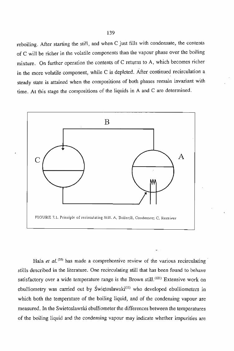
139
reboiling. After starting the still, and when C just fills with condensate, the contents
of C will be richer in the volatile components than the vapour phase over the boiling
mixture. On further operation the contents of C retllrns to A, which becomes richer
in the more volatile component, while C is depleted. After continued recirculation a
steady state is attained when the compositions of both phases remain invariant with
time. At this stage the compositions of the liquids in A and C are determined.
B
c A
FIGURE 7.1. Principle of recirculating Still. A, Boiler;B, Condensor; C, Receiver
Rala et al. (35) has made a comprehensive review of the various recirculating
stills described in the literature. One recirculating still that has been found to behave
satisfactory over a wide temperature range is the Brown still. (121) Extensive work on
ebulliometry was carried out by Swi~toslawski(ll) who developed ebulliometers in
which both the temperature of the boiling liquid, and of the condensing vapour are
measured. In the Swietoslawski ebulliometer the differences between the temperatures
of the boiling liquid and the condensing vapour may indicate whether impurities are
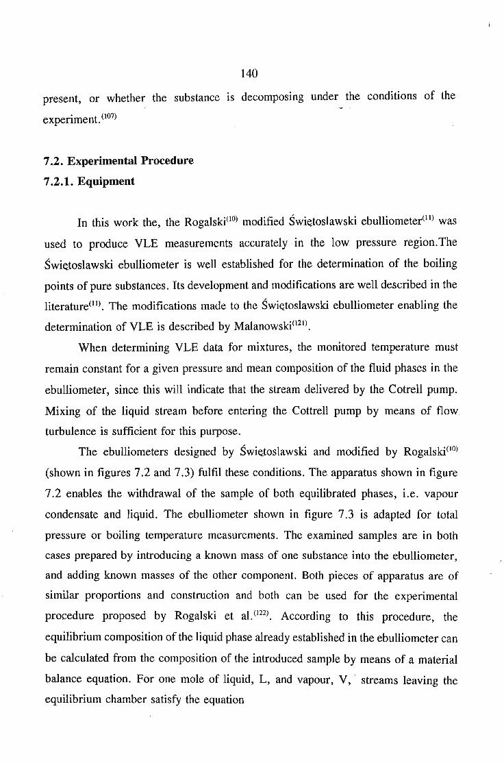
140
present, or whether the substance IS decomposing under the conditions of the
experiment. (l07)
7.2. Experimental Procedure
7.2.1. Equipment
In this work the, the Rogalski(lO) modified Swietoslawski ebulliometer(ll) was
used to produce VLE measurements accurately in the low pressure region.The
Swietoslawski ebulliometer is well established for the determination of the boiling
points of pure substances. Its development and modifications are well described in the
literature(ll). The modifications made to the Swi~toslawski ebulliometer enabling the
determination of VLE is described by Malanowski(l21).
When determining VLE data for mixtures, the monitored temperature must
remain constant for a given pressure and mean composition of the fluid phases in the
ebulliometer, since this will indicate that the stream delivered by the Cotrell pump.
Mixing of the liquid stream before entering the Cottrell pump by means of flow
turbulence is sufficient for this purpose.
The ebulliometers designed by Swktoslawski and modified by Rogalski(lO)
(shown in figures 7.2 and 7.3) fulfil these conditions. The apparatus shown in figure
7.2 enables the withdrawal of the sample of both equilibrated phases, i.e. vapour
condensate and liquid. The ebulliometer shown in figure 7.3 is adapted for total
pressure or boiling temperature measurements. The examined samples are in both
cases prepared by introducing a known mass of one substance into the ebulliometer,
and adding known masses of the other component. Both pieces of apparatus are of
similar proportions and construction and both can be used for the experimental
procedure proposed by Rogalski et al. (122). According to this procedure, the
equilibrium composition of the liquid phase already established in the ebulliometer can
be calculated from the composition of the introduced sample by means of a material
balance equation. For one mole of liquid, L, and vapour, V, . streams leaving the
equilibrium chamber satisfy the equation
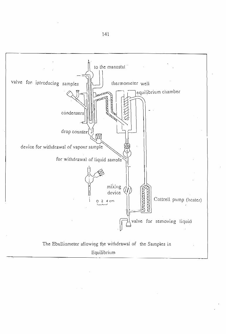
device for withdrawal of vapour samPle"
for withdrawal of liquid sample
valve for introducing
141
to the manostat-
thermometer well
mi:<lngdevice
o 2 4 cm~
ICottrell pump (heater)
valve for removing liquid
The Ebulliometer allowif)g the withdrawal of the Samples in
Equilibrium
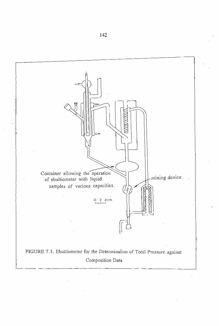
142
Co'ntainer allowing the operation·. of ebulliometer with liquid·
samples of various capacities.
o 2 4cm~
mixing device
FIG·URE 7.3. EbulIiometerfor the Determination of Total Pressure against
Composition Data
143
V +L = 1 (7.1)
The mole fraction of component i in the sample, CL, is related to the mole
fraction of this component in the liquid phase, Xi' and in the vapour phase, Yi by the
equation
Defining the coefficient of evaporation, f, by
v!=L
(7.2)
(7.3)
and comparing equations 7.1 and 7.2, the relation enabling the calculation of liquid
phase composition by an iterative procedure is obtained, viz. (115)
X. = q._1_+-=..!_I I 1+(y/x
j)!
(7.4)
For an ebulliometer correctly designed and properly operated, the coefficient
f depends little on the system investigated and is fairly constant over the range of
temperature and pressure applied in usual ebulliometeric measurements.
The ebulliometers presented earlier offer both the working abilities of an
equilibrium still (determination of full VLE data) and an ebulliometer (determination
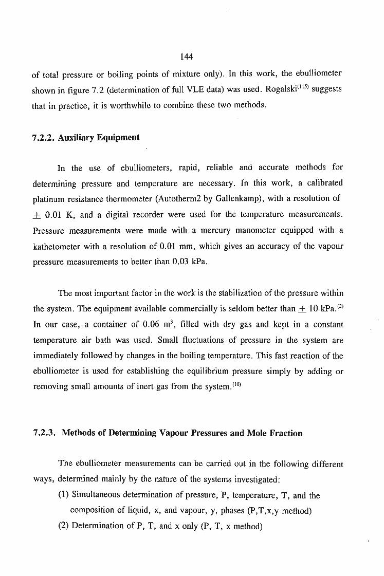
144
of total pressure or boiling points of mixture only). In this work, the ebulliometer
shown in figure 7.2 (determination of full VLE data) was used. Rogalski(115) suggests
that in practice, it is worthwhile to combine these two methods.
7.2.2. Auxiliary Equipment
In the use of ebulliometers, rapid, reliable and accurate methods for
determining pressure and temperature· are necessary. In this work, a calibrat~d
platinum resistance thermometer (Autotherm2 by Gallenkamp), with a resolution of
+ 0.01 K, and a digital recorder were used for the temperature measurements.
Pressure measurements were made with a mercury manometer equipped with a
kathetometer with a resolution of 0.01 mm, which gives an accuracy of the vapour
pressure measurements to better than 0.03 kPa.
The most important factor in the work is the stabilization of the pressure within
the system. The equipment available commercially is seldom better than + 10 kPa. (2)
In our case, a container of 0.06 m3, filled with dry gas and kept in a constant
temperature air bath was used. Small fluctuations of pressure in the system are
immediately followed by changes in the boiling temperature. This fast reaction of the
ebulliometer is used for establishing the equilibrium pressure simply by adding or
removing small amounts of inert gas from the system. (10)
7.2.3. Methods of Determining Vapour Pressures and Mole Fraction
The ebulliometer measurements can be carried out in the following different
ways, determined mainly by the nature of the systems investigated:
(1) Simultaneous determination of pressure, P, temperature, T, and the
composition of liquid, x, and vapour, y, phases (P,T,x,y method)
(2) Determination of P, T, and x only (P, T, x method)
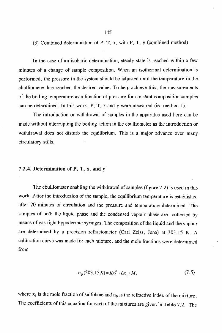
145
(3) Combined determination of P, T, x, with P, T, Y(f;Qmbined method)
In the case of an isobaric determination, steady state is reached within a few
minutes of a change of sample composition. When an isothermal determination is
performed, the pressure in the system should be adjusted until the temperature in the
ebulliometer has reached the desired value. To help achieve this, the measurements
of the boiling temperature as a function of pressure for constant composition samples
can be determined. In this work, P, T, x and y were measured (ie. method 1).
The introduction or withdrawal of samples in the apparatus used here can be
made without interrupting the boiling action in the ebulliometer as the introduction or
withdrawal does not disturb the equilibrium. This is a major advance over many
circulatory stills.
7.2.4. Determination of P, T, x, and y
The ebulliometer enabling the withdrawal of samples (figure 7.2) is used in this
work. After the introduction of the sample, the equilibrium temperature is established
after 20 minutes of circulation and the pressure and temperature determined. The
samples of both the liquid phase and the condensed vapour phase are collected by
means of gas-tight hypodermic syringes. The composition of the liquid and the vapour
are determined by a precision refractometer (Carl Zeiss, Jena) at 303.15 K. A
calibration curve was made for each mixture, and the mole fractions were determined
from
(7.5)
where X3 is the mole fraction of sulfolane and nD is the refractive index of the mixture.
The coefficients of this equation for each of the mixtures are given in Table 7.2. The
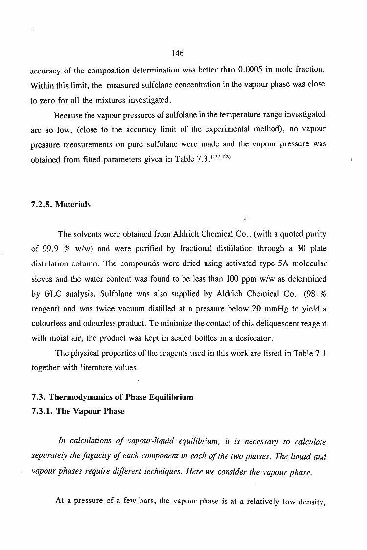
146
accuracy of the composition determination was better than 0.0005 in mole fraction.
Within this limit, the measured sulfolane concentration in the vapour phase was close
to zero for all the mixtures investigated.
Because the vapour pressures of sulfolane in the temperature range investigated
are so low, (close to the accuracy limit of the experimental method), no vapour
pressure measurements on pure sulfolane were made and the vapour pressure was
obtained from fitted parameters given in Table 7.3. (127, 129)
7.2.5. Materials
The solvents were obtained from Aldrich Chemical Co., (with a quoted purity
of 99.9 % w/w) and were purified by fractional distillation through a 30 plate
distillation column. The compounds were dried using activated type 5A molecular
sieves and the water content was found to be less than 100 ppm w/w as determined
by GLC analysis. Sulfolane was also supplied by Aldrich Chemical Co., (98 -%
reagent) and was twice vacuum distilled at a pressure below 20 mmHg to yield a
colourless and odourless product. To minimize the contact of this deliquescent reagent
with moist air, the product was kept in sealed bottles in a desiccator.
The physical properties of the reagents used in this work are listed in Table 7.1
together with literature values.
7.3. Thermodynamics of Phase Equilibrium
7.3.1. The Vapour Phase
In calculations of vapour-liquid equilibrium, it is necessary to calculate
separately the fugacity of each component in each ofthe two phases. The liquid and
vapour phases require different techniques. Here we consider the vapour phase.
At a pressure of a few bars, the vapour phase is at a relatively low density,
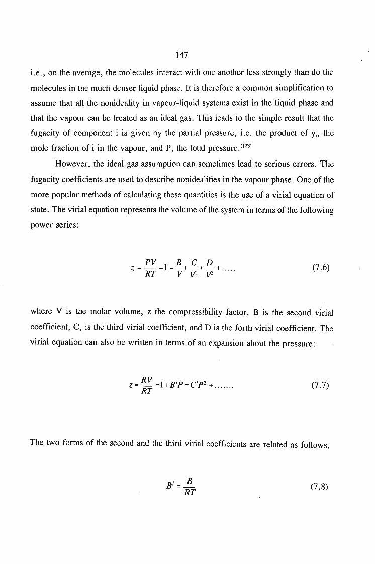
147
i.e., on the average, the molecules interact with one another less strongly than do the
molecules in the much denser liquid phase. It is therefore a common simplification to
assume that all the nonideality in vapour-liquid systems exist in the liquid phase and
that the vapour can be treated as an ideal gas. This leads to the simple result that the
fugacity of component i is given by the partial pressure, i.e. the product of Yi' the
mole fraction of i in the vapour, and P, the total pressure. (123)
However, the ideal gas assumption can sometimes lead to serious errors. The
fugacity coefficients are used to describe nonidealities in the vapour phase. One of the
more popular methods of calculating these quantities is the use of a virial equation of
state. The virial equation represents the volume of the system in terms of the following
power senes:
PV B C Dz = RT =I =V + v2 + yJ + ..... (7.6)
where V is the molar volume, z the compressibility factor, B is the second virial
coefficient, C, is the third virial coefficient, and D is the forth virial coefficient. The
virial equation can also be written in terms of an expansion about the pressure:
RVz=- =1+B'P=C'P2 +RT . (7.7)
The two forms of the second and the third virial coefficients are related as follows ,
B'=~RT
(7.8)
148
et = C-B2
(RIY(7.9)
The virial coefficients are functions only of temperature. In the case of
mixtures, concentration dependant mixing rules are used to calculate the virial
coefficients. For simplicity the equation is truncated after the second virial coefficient.
The equation is then accurate only at low to moderate pressures.
One of the advantages of the virial expansion is the relationship between the
virial coefficients and the intermolecular forces. For an ideal gas, the intermolecular
forces between the molecules are zero, and the virial coefficients are zero. Under such
conditions, the corresponding factor z is equal to unity. At conditions other than ideal,
expressions for the virial coefficients can be related to the intermolecular forces
through the use of statistical mechanics. For mixtures, the second virial coefficient is
given by the following theoretically based mixing rule,
(7.10)
Here m is the number of components and Bjj is the virial coefficients representing the
interaction between the components i and j.
The fugacity coefficient is given by,
where cPi is the fugacity coefficient and fj is the fugacity of component i. Truncating
149
/; JP RTRTIncP.=RTIn- = [v.--]dPI 'Yl 0 I P
(7.11)
the virial expression after the second term, and substituting the pressure explicit
equation into equation 7.11, we arrive at an expression for the fugacity coefficient
after differentiation and integrating
(7.12)
One of the more successful methods used to calculate second virial coefficients
is that of Hayden and O'Connen<36) (used for calculation of GE shown in Table 7.4).
The method is a predictive method, with the virial coefficients being functions of
.dipole moment, temperature, pressure, critical temperature, critical pressure, and the
degree of association between the interacting components. The virial coefficients' is
assumed to be the sum of two types of interactions:
(7.13)
where Bfj is the contribution due to relatively "free" molecules, those in which
physical forces are weak, and B?j is the contribution due to bound or dimerized
molecules. To use equation 7,12, virial coefficients Bij which depend on temperature
are required.
150
7.3.2. The Liquid Phase
In the liquid mixture the activity coefficients are directly related to the molar
excess Gibbs energy GE defined by, (123)
(7.14)
Many functional forms of the excess Gibbs energy have been developed over the
years. These mathematical models, based on molecular considerations, provides a
convenient method fur expressing GE as a function of x. From this function an
individual activity coefficient 'Yi for component i can be calculated from GE using the
relationship
anG E
RTIny=[ t ]I an. T,p,nJ~1
I
(15)
where nj is the number of moles. Some of the more successful GE solution models are
described in chapter 9 in great detail. These include among others, the WILSON, (5)
NRTL,(6) UNIQUAC,(7) and DISQUAC(9) models. Modified UNIFAC(8) model was
tested as well. All these theories have been used to describe the VLE data measured
in this work.
7.3.3: Vapour Liquid Equilibrium Data for a Solute + Sulfolane
Isothermal vapour-liquid equilibria at 338.15 K or 353.15 K for 1-heptyne, or
tetrahydrofuran or l,4-dioxane, or tetrachloromethane Of trichlof()ethane + sulfolane
binary mixtures have been determined using an ebulliometric (P,T,x,y) method. The
151
excess molar Gibbs energies determined from the vapour-liquid equilibrium data
present positive trends for all mixtures, with the maximum varying from 480 J ·mot l
to 1550 J ·mol- I . The data reported have been successfully described using the
Margules, van Laar, Wilson, NRTL and UNIQUAC equations, using the program
VLE given in APPENDIX 1.
Because of the important industrial applications of sulfolane, several
investigators have studied the vapour-liquid phase equilibria (VLE) for binary (124-126)
and ternary mixtures containing sulfolane and aromatic hydrocarbons (benzene,
toluene, ethylbenzene) or dichloromethane or propan-2-ol. VLE data for mixtures
containing sulfolane have not often been the subject of a theoretical interpretation.
For the mixtures studied in this work, no experimental data have been published
in the literature. I-Heptyne was chosen because it contained a triple carbon-carbon
bond, tetrahydrofuran and 1,4-dioxane as cyclic ethers containing one or two ether
groups respectively, and tetrachloromethane and trichloroethane as examples of
compounds containing two different types of Cl atoms.
The experimental data has allowed us to obtain new interaction parameters for
the above mentioned groups with sulfolane (as an individual group) in the DISQUAC(9)
and Modified UNIFAC models.(8)
The solution models for the molar excess Gibbs energy, were chosen for the
reduction of the VLE data as r~presentatives of local composition equations and semi
empirical enthalpic expressions, respectively.
The isothermal VLE data obtained for the mixtures studied are presented in
Table '7.4, along with the liquid and the vapour mole fractions. The activity
coefficients 'Yi were calculated using the following equation:
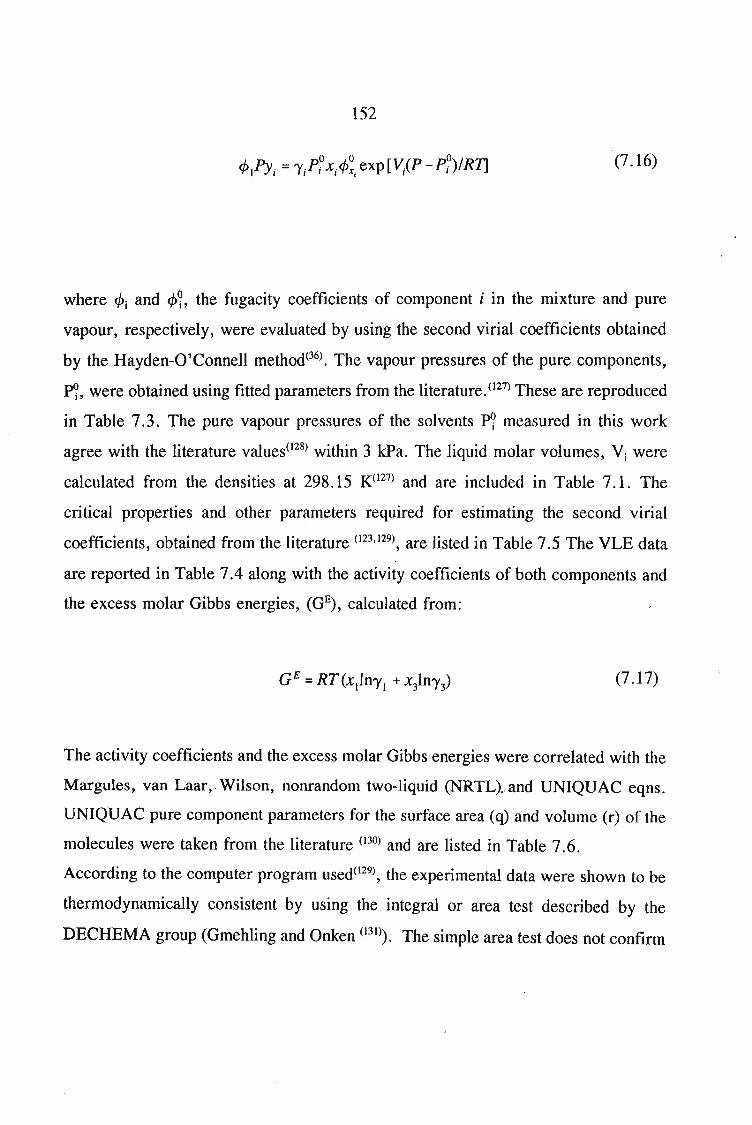
152
(7.16)
where 4Ji and 4J1, the fugacity coefficients of component i in the mixture and pure
vapour, respectively, were evaluated by using the second virial coefficients obtained
by the Hayden-O'Connell method(36). The vapour pressures of the pure components,
I1, were obtained using fitted parameters from the literature.(l27) These are reproduced
in Table 7.3. The pure vapour pressures of the solvents I1 measured in this work
agree with the literature values(l28) within 3 kPa. The liquid molar volumes, Vi were
calculated from the densities at 298.15 K(l27) and are included in Table 7.1. The
critical properties and other parameters required for estimating the second virial
coefficients, obtained from the literature (123,129), are listed in Table 7.5 The VLE data
are reported in Table 7.4 along with the activity coefficients of both components and
the excess molar Gibbs energies, (GE), calculated from:
(7.17)
The activity coefficients and the excess molar Gibbs energies were correlated with the
Margules, van Laar, Wilson, nonrandom two-liquid (NRTL).. and UNIQUAC eqns.
UNIQUAC pure component parameters for the surface area (q) and volume (r) of the
molecules were taken from the literature (130) and are listed in Table 7.6.
According to the computer program used(129), the experimental data were shown to be
thermodynamically consistent by using the integral or area test described by the
DECHEMA group (Gmehling and Onken (131»). The simple area test does not confirm
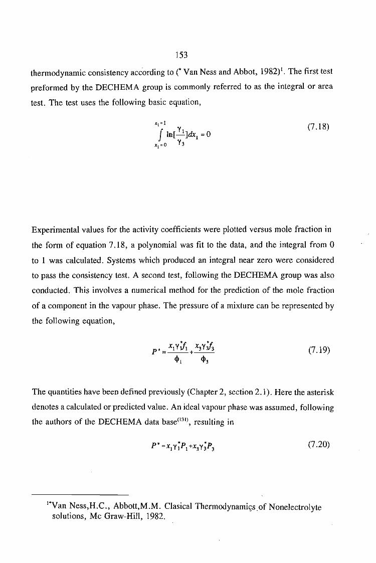
153
thermodynamic consistency acc·ording to (' Van Ness and Abbot, 1982)1. The first test
preformed by the DECHEMA group is commonly referred to as the integral or area
test. The test uses the following basic equation,
~I =1
JIn[~]dxl = 0~l zO y3
(7.18)
Experimental values for the activity coefficients were plotted versus mole fraction in
the form of equation 7.18, a polynomial was fit to the data, and the integral from 0
to 1 was calculated. Systems which produced an integral near zero were considered
to pass the consistency test. A second test, following the DECHEMA group was also
conducted. This involves a numerical method for the prediction of the mole fraction
of a component in the vapour phase. The pressure of a mixture can be represented by
the following equation,
P* = X1YJl + X3Y':J3
~l ~3
(7.19)
The quantities have been defined previously (Chapter 2, section 2.1). Here the asterisk
denotes a calculated or predicted value. An ideal vapour phase was assumed, following
the authors of the DECHEMA data base(I3I), resulting in
(7.20)
I·Van Ness,H.C., Abbott,M.M. Clasical Thermodynami£s,of Nonelectrolytesolutions, Mc Graw-Hill, 1982.
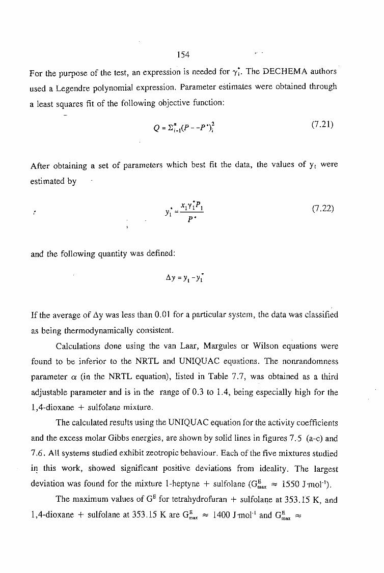
154
For the purpose of the test, an expression is needed for 'Y~. The DECHEMA authors
used a Legendre polynomial expression. Parameter estimates were obtained through
a least squares fit of the following objective function:
(7.21)
After obtaining a set of parameters which best fit the data, the values of y1 were
estimated by
., (7.22)
and the following quantity was defined:
If the average of ~y was less than 0.01 for a particular system, the data was classified
as being thermodynamically consistent.
Calculations done using the van Laar, Margules or Wilson equations were
found to be inferior to the NRTL and UNIQUAC equations. The nonrandomness
parameter a (in the NRTL equation), listed in Table 7.7, was obtained as a third
adjustable parameter and is in the range of 0.3 to lA, being especially high for the
l,4-dioxane + sulfolane mixture.
The calculated results using the UNIQUAC equation for the activity coefficients
and the excess molar Gibbs energies, are shown by solid lines in figures 7.5 (a-c) and
7.6. All systems studied exhibit zeotropic behaviour. Each of the five mixtures studied
it! this work, showed significant positive deviations from ideality. The largest
deviation was found for the mixture I-heptyne + sulfolane (G;ax ~ 1550 J ·mol- I ).
The maximum values of GE for tetrahydrofuran + sulfolaI!e at 353.15 K, and
l,4-dioxane + sulfolane at 353.15 K are G;ax ~ 1400 J 'mol- I and G;ax ~
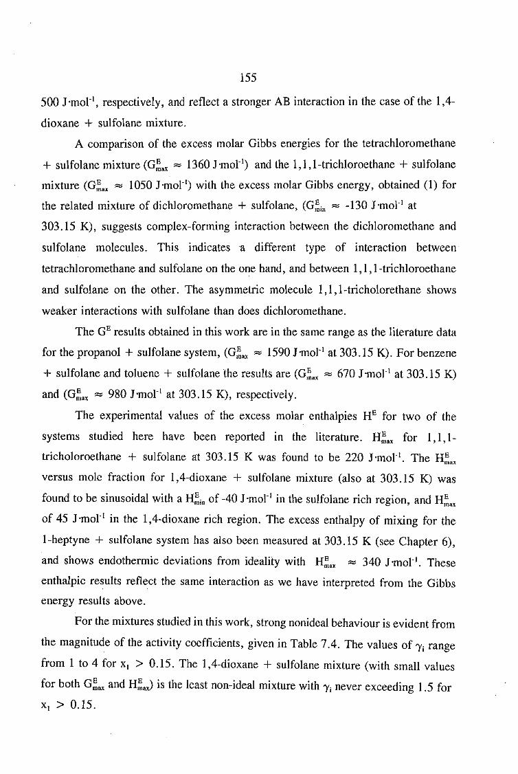
155
500 J 'mol- I, respectively, and reflect a stronger AB interaction in the case of the 1,4
dioxane + sulfolane mixture.
A comparison of the excess molar Gibbs energies for the tetrachloromethane
+ sulfolane mixture (G;ax ~ 1360 J 'mol- I) and the 1,1, l-trichloroethane + sulfolane
mixture (G;ax ~ 1050 J 'mol- I) with the excess molar Gibbs energy, obtained (1) for
the related mixture of dichloromethane + sulfolane, (G;in ~ -130 J 'mol- I at
303.15 K), suggests complex-forming interaction between the dichloromethane and
sulfolane molecules. This indicates a different type of interaction between
tetrachloromethane and sulfolane on the one hand, and between 1,1, I-trichloroethane
and sulfolane on the other. The asymmetric molecule 1,1, I-tricholorethane shows
weaker interactions with sulfolane than does dichloromethane.
The GEresults obtained in this work are in the same range as the literature data
for the propanol + sulfolane system, (G;ax ~ 1590 J 'mol- I at 303.15 K). For benzene
+ sulfolane and toluene + sulfolane the results are (G;ax ~ 670 J 'mot I at 303.15 K)
and (G;ax ~ 980 J 'mol- I at 303 .15K), respectively.
The experimental values of the excess molar enthalpies HE for two of the
systems studied here have been reported in the literature. H;ax for 1,1,1
tricholoroethane + sulfolane at 303.15 K was found to be 220 J ·mot I . The H;ax
versus mole fraction for 1,4-dioxane + sulfolane mixture (also at 303.15 K) was
found to be sinusoidal with a H;in of -40 J 'mol- I in the sulfolane rich region, and H;ax
of 45 J 'mol- I in the l,4-dioxane rich region. The excess enthalpy of mixing for the
I-heptyne + sulfolane system has also been measured at 303.15 K (see Chapter 6),
and shows endothermic deviations from ideality with H;ax ~ 340 J ·mol- I . These
enthalpic results reflect the same interaction as we have interpreted from the Gibbs
energy results above.
For the mixtures studied in this work, strong nonideal behaviour is evident from
the magnitude of the activity coefficients, given in Table 7.4. The values of 'Yi range
from 1 to 4 for Xl > 0.15. The l,4-dioxane + sulfolane mixture (with small values
for both G;ax and H;~ is the least non-ideal mixture with 'Yi never exceeding 1.5 for
Xl > 0.15.
156
The activity coefficient at infinite dilution, 1'7, for each of the solvents in
sulfolane was calculated using UNIQUAC parameters obtained from (VLE) data. 1'7for the mixtures tetrahydrofuran at 338.15 K, I-heptyne + sulfolane at 353.15 K and
tetrahydrofuran + sulfolane at 353.15 K are 2.3,6.2 and 3.8, respectivelyy32.133) 1'7for these two systems were obtained by the G.L.C. technique. The results for the
mixtures I-heptyne + sulfolane at 313.15 K, and 303.15 K (23), and tetrahydrofuran
+ sulfolane at 303.15 K are 7.78,8.10, and 2.24, respectively. A further system 1,4
dioxane + sulfolane at 298.15 K has also been measured by the G.L.C. technique and
the resulting 1'7 obtained is 3.32 whereas the value obtained in this work, is 1.5 at
353.15 K.
7.4. Parameter Optimization
Methods to regress the constants for the various activity coefficients models and
equations of state are discussed here. The recommended method is know as the error
in-variables maximum likelihood technique. (134)
The adjustable parameters, designated as ()j, are included in the expressions for
the activity coefficients, 1';, or the fugacity coefficients, cP;.
(7.24)
(7.25)
Thexj in equations 7.18 and 7.19 refer to the liquid phase mole fraction. The asterisk
indicates a calculated quantity, as opposed to an experimental one. The problem then
becomes one offinding the set of parameters ()h ()2"'" which best fit the data set.
Two approaches are used in this work, the method of least squares, and the more
popular "maximum likelihood method".
157
7.4.1. The Least Squares Regression
The goal of a least squares method is to choose the set of parameter estimates
which minimize the sum of the squares of the error between one or more experimental
and calculated quantities. The objective function, then, is the sum of the squares of
the errors. Four quantities are often measured experimentally, P, T, xj,and Yi' meaning
that the errors of any of these four, or any combination of the four can be part of the
objective function.
7.4.1.2. Least Squares Objective Functions for the Activity Coefficient Models
VLE in a binary system can be described by the following equations
(7.26)
(7.27)
The quantities have been defined earlier.
These are two equations, with four experimental variables. Therefore, two variables
must be considered as independent and the other two as dependent, so as not to over
specify the system.
In addition to the four experimental quantities P, T, ~, and yj, experimental
activity coefficients can be defined as
y.P(j>.'Y; = -'-'
xl:(7.28)
ISH
Two guideline must be used or the selection of the objective function.
First, information from both constraints, equations 7.18, and 7.19, should be
used in the evaluation. For example,
(7.29)
was used in favour of
(7.30)
because equation 7.24 disregards information from the second constraint. Equation
7.23, in which the residual is based on the activity coefficient of both components,
was found to give better results.
A second guideline, was to avoid minimization based solely on the error in the
vapour mole fractions, Yi' Measurements of this quantity are usually the most
inaccurate in comparison to measurements of P, T, and Xi' The large uncertainties
associated with Y1 will be propagated into larger uncertainties in the parameter
estimates. An objective functions used here, which overcomes this problem is
(7.31)
The calculated pressure can be derived from equation 7.27 as
159
P" = Xttf( + X2'Y,J;.cP) cP2
(7.32)
Regression using equation 7.31, require the simultaneously solution of the constraints
for y~ and p... The fugacity coefficients, cPj, are functions of pressure and Yi. the
standard state fugacity, r:, are functions of pressure through the following
approximation
(P" _p~ar)V.j:O _ A..sarpsat [ I i]
Ji -~j j exp RT(7.33)
where cP~at is the fugacity coefficient of pure saturated vapour of component i, Pft is
the vapour pressure of component i at temperature T, and Vi is the molar volume of
the pure liquid.
In the calculation of the fugacity coefficient and standard state fugacities,
experimental values of P and Yi cannot be used. Therefore, equation 7.26 and the
following equation
must be solved simultaneously for p" and y;, where
.. Xj'Y!:y. =--
I cPP"I
(7.34)
(7.35)
the solution can be best achieved by the iteration sequence found in figure 7.4.
160
7.4.2. The Maximum Likelihood Regression
Although the least squares approach produces parameter estimates which fit the
experimental data well, an alternative approach was used. The criterion for the
selection of parameters in the maximum likelihood method is slightly different than
the one for the least squares method. In this procedure, parameters are chosen to
minimize the deviation in all experimental quantities simultaneously.
An important characteristic is the lack of distinction between dependent and
independent variables. In the least squares approach, objective functions and
consequently parameter estimates, differ for each designation of dependent and
independent variables. Only one objective function exists in the maximum likelihood
technique. "Likelihood", in the statistical sense is a measure of the probability of an
event to occur. The event in a VLE application is the simultaneous occurrence of the
values for the pressure, temperature and liquid and vapour concentrations. The
objective function for the maximum likelihood is a measure of this probability. The
regressed _parameters then are those which maximize the "likelihood" or the
probability of the occurrence of the data set. To calculate this probability, the method
takes into account all the experimental data, along with estimates of their errors.1'le
method provides information 6n the degree of accuracy of these parameters. The
accuracy of the maximum likelihood parameters are a function of the accuracy of the
experimental data, since estimates of the variance of the experimental data are variable
of the objective function.
The method employed in this work, follows the error-in-variables method of
Patino-Leal and Reilly(135) and Prausnitz et al(l23). Each variable has associated with it
an error defined as the difference between the estimate of the true value of the variable
and the measured value of the variable. The following symbols are used to distinguish
between the quantities:
161
(7.36)
(7.37)
(7.38)
(7.39)
where t is the estimate of the true value of the variable i, and €j is the error of the
quantity i. Therefore not only do the parameter estimates need to be regressed, but
also the estimates of the true values of the variables. The advantage of this method,. ,,,. -
is that the calculation of the estimates of the true values of the variables is less time
consuming and less complicated than previous methods.
For a system to be in equilibrium in terms of activity coefficients, equations
7.18 and 7.19 must be valid simultaneously. The constraint equations for regressing
the parameters Ob O2, ••• , are then
(7.40)
(7.41)
F I and F2 are the constraints. The error-in-variables method is a maximum likelihood
method, so the likelihood or probability function for the simultaneous occurrence of
162
the experimental observations, P, T, Xl' YI has to be maximized.
The likelihood function can be represented by the proportionality
(7.42)
where n is the number of experimental points, Zj a vector of length four containing the
measured values of the variables (P, T, Xlj, and YI), ~j a vector of length four
containing the true values of the variable and V4 the (4 X 4) error-in-variable matrix.
Values for these quantities should be based on the estimated errors of the experimental
measurements and could be different for each data point. If such information is not
available, the error estimates must be arbitrarily assigned. Superscripts T and -1 refer
to the transpose and inverse, respectively.
The "likelihood It function is subject to the constraints equations 7.24 and 7.25,
which must be linearized to enable regression. The functions are linearized by a
Taylor series expansion about the estimates of the true values of the variables.
(7.43)
where F j is a vector of length two containing the values of the constraints, equations
7.40 and 7.41, Bj is a (2 x 4) matrix containing the derivatives of the constraints with
resPect to the measured variables Bjk = (aF/azJ and ~f is a.. ~ector of length four
containing estimates of the true values of the measured variables.
The ~j are integrated out of the distribution function through a senes of
statistical assumptions. Application of the assumptions reduce the proportionality to
163
(7.44)
where
(7.45)
To maximize the likelihood function, one must minimize the summation inside the
exponential term. In other words, to obtain the error-in-variable parameter estimates,
one must minimize the sum of the Qi values, where Qi is a function of the measured
data, the estimates of the true values of the measured data, the error-covariance
matrix, the constraints, and the derivatives of the constraints. Values for tf can be
obtained through the following algorithm:
(7.46)
where j = 1,2,... . To start the iteration, set tf(l) = z, and continue until the change
in Qi is less than some tolerance.
To simplify the calculation, one can use the experimental data as an estimate
of the true values of the variables, tf = Zi' The iterative solution represented by
equation 7.46, is eliminated and equation 7.45 reduces to
(7.47)
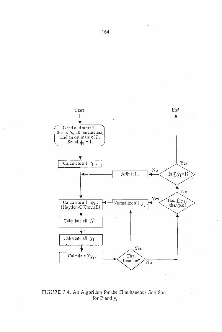
J64
Start End
Read and store Ttthe XI'S, all parnmetcfS,
and an cstlmate ofP.Set all <PI .. 1.
NoAdjust P.
FIGURE 7.4. An Algorithm for the Simultaneous Solutionfor P andYi
165
Because the estimates of the true values of the variables, ~{ are not involved in the
calculations, parameters found using equation 7.47 are called approximate error-in
variable method. The solution to equation 7.45 is referred to as the exact solution.
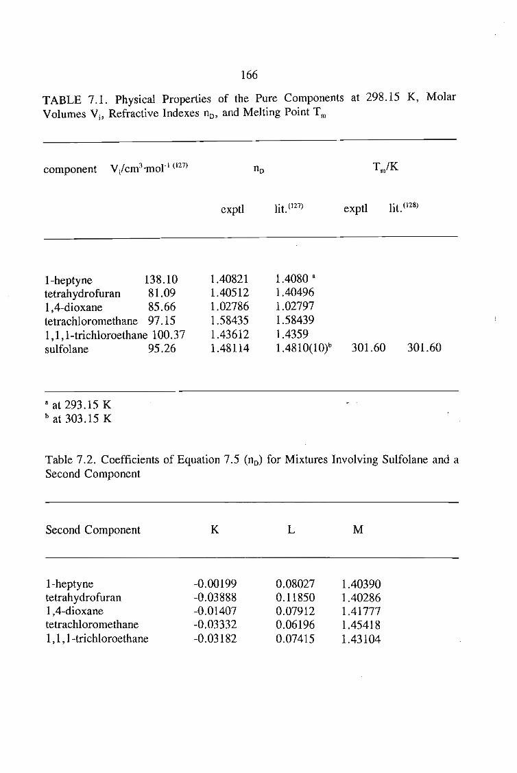
166
TABLE 7.1. Physical Properties of the Pure Components at 298.15 K, MolarVolumes Vi' Refractive Indexes no, and Melting Point Tm
component V/cm3 'mol-1(127)
exptl lit. (127) exptl lit. (128)
I-heptyne 138.10tetrahydrofuran 81.091,4-dioxane 85.66tetrachloromethane 97.151,1,1-trichloroethane 100.37sulfolane 95.26
a at 293.15 Kbat 303.15 K
1.408211.405121.027861.584351.436121.48114
1.4080 a
1.404961.027971.584391.43591.4810(10)b 301.60 301.60
Table 7.2. Coefficients of Equation 7.5 (no) for Mixtures Involving Sulfolane and aSecond Component
Second Component K L M
1-heptyne -0.00199 0.08027 1.40390tetrahydrofuran -0.03888 0.11850 1.402861,4-dioxane -0.01407 0.07912 1.41777tetrachloromethane -0.03332 0.06196 1.454181,1,1-trichloroethane -0.03182 0.07415 1.43104
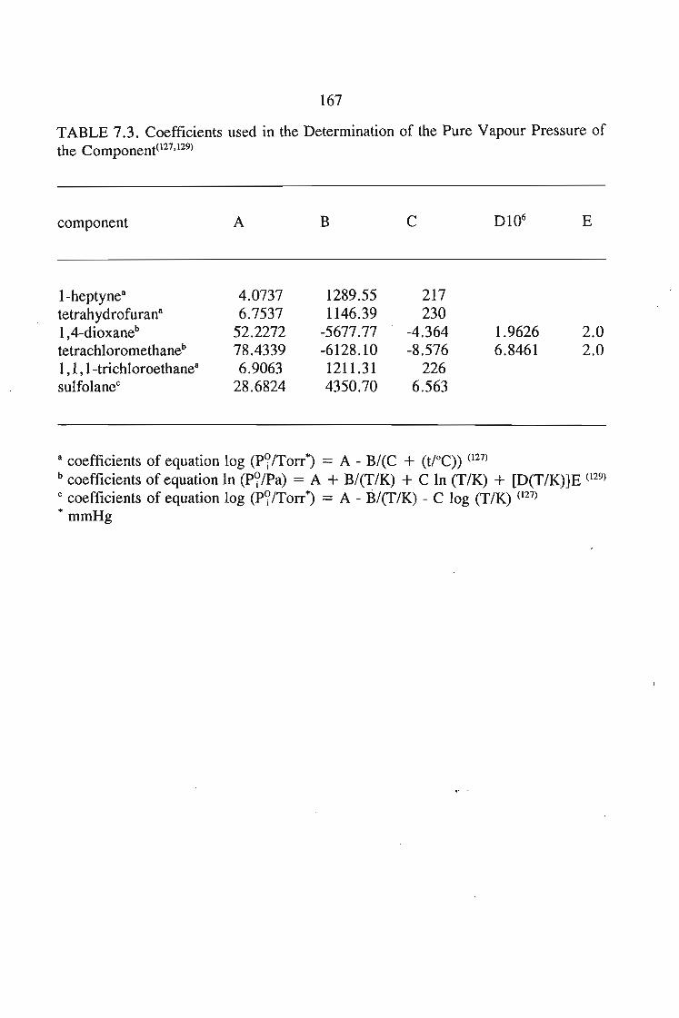
167
TABLE 7.3. Coefficients used in the Determination of the Pure Vapour Pressure ofthe Component(127,129)
component A B C E
I-heptyne8 4.0737 1289.55 217tetrahydrofuran8 6.7537 1146.39 2301,4-dioxaneb 52.2272 -5677.77 -4.364 1.9626 2.0tetrachloromethaneb 78.4339 -6128.10 -8.576 6.8461 2.01,1 , I-trichloroethane8 6.9063 1211.31 226sulfolanec 28.6824 4350.70 6.563
8 coefficients of equation log (P?/Torr+) = A - B/(C + (t/oc» (127)b coefficients of equation In (P?/Pa) = A + B/(T/K) + C In (T/K) + [D(T/K)]E (129)C coefficients of equation log (P?/Torr+) = A - B/(T/K) - Clog (T/K) (127)+mmHg
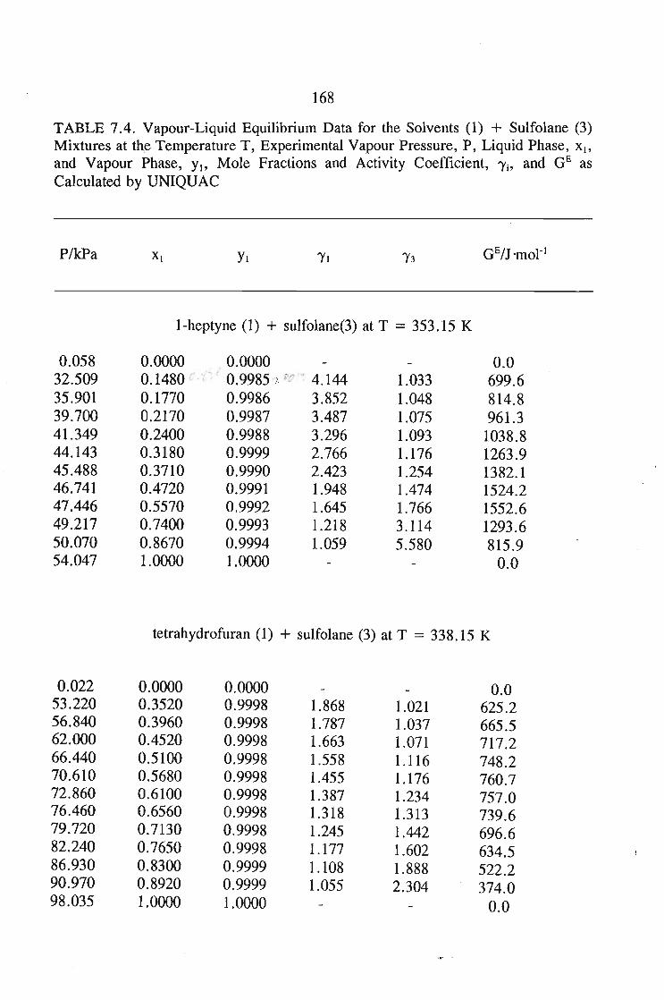
168
TABLE 7.4. Vapour-Liquid Equilibrium Data for the Solvents (1) + Sulfolane (3)Mixtures at th.e Temperature T, Experimental Vapour Pressure, P, Liquid Phase, Xl'
and Vapour Phase, Yt, Mole _Fractions and Activity Coefficient, 'Yj, and GE asCalculated by UNIQUAC
P/kPa Yt
1-heptyne (1) + sulfolane(3) at T = 353.15 K
0.058 0.0000 0.0000 0.032.509 0.1480 ((~ ( 0.9985 -7- 0C"~ 4.144 1.033 699.635.901 0.1770 0.9986 3.852 1.048 814.839.700 0.2170 0.9987 3.487 1.075 961.341.349 0.2400 0.9988 3.296 1.093 1038.844.143 0.3180 0.9999 2.766 1.176 1263.945.488 0.3710 0.9990 2.423 1.254 1382.146.741 0.4720 0.9991 1.948 1.474 1524.247.446 0.5570 0.9992 1.645 1.766 1552.649.217 0.7400 0.9993 1.218 3.114 1293.650.070 0.8670 0.9994 1.059 5.580 815.954.047 ooסס.1 ooסס.1 0.0
tetrahydrofuran (1) + sulfolane (3) at T = 338.15 K
0.022 0.0000 0.0000 0.053.220 0.3520 0.9998 1.868 1.021 625.256.840 0.3960 0.9998 1.787 1.037 665.562.000 0.4520 0.9998 1.663 1.071 717.266.440 0.5100 0.9998 1.558 1.116 748.270.610 0.5680 0.9998 1.455 1.176 760.772.860 0.6100 0.9998 1.387 1.234 757.076.460 0.6560 0.9998 1.318 1.313 739.679.720 0.7130 0.9998 1.245 1.442 696.682.240 0.7650 0.9998 1.177 1.602 634.586.930 0.8300 0.9999 1.108 1.888 522.290.970 0.8920 0.9999 1.055 2.304 374.098.035 ooסס.1 ooסס.1 0.0
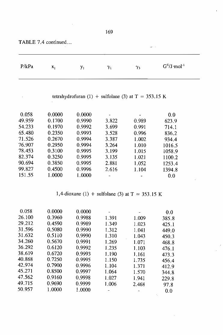
169
TABLE 7.4 continued...
P/kPa
tetrahydrofuran (1) + su1fo1ane (3) at T = 353.15 K
0.058 0.0000 0.0000 0.049.959 0.1700 0.9990 3.822 0.989 623.954.233 0.1970 0.9992 3.699 0.991 714.165.480 0.2350 0.9993 3.528 0.996 836.271.526 0.2670 0.9994 3.387 1.002 934.476.907 0.2950 0.9994 3.264 1.010 1016.578.453 0.3100 0.9995 3.199 1.015 1058.982.374 0.3250 0.9995 3.135 1.021 1100.290.694 0.3850 0.9995 2.881 1.052 1253.499.827 0.4500 0.9996 2.616 1.104 1394.8151.55 1.0000 1.0000 0.0
l,4-dioxane (1) + sulfo1ane (3) at T = 353.15 K
0.058 0.0000 0.0000 0.026.100 0.3960 0.9988 1.391 1.009 385.829.212 0.4590 0.9989 1.349 1.023 425.131.596 0.5080 0.9990 1.312 1.041 449.031.632 0.5110 0.9990 1.310 1.043 450.334.260 0.5670 0.9991 1.269 1.071 468.836.292 0.6120 0.9992 1.235 1.103 476.138.619 0.6720 0.9993 1.190 1.161 473.340.868 0.7250 0.9995 1.150 1.735 456.442.974 0.7900 0.9996 1.104 1.371 412.945.271 0.8500 0.9997 1.064 1.570 344.847.562 0.9160 0.9998 1.027 1.941 229.849.715 0.9690 0.9999 1.006 2.468 97.850.957 1.0000 1.0000 0.0
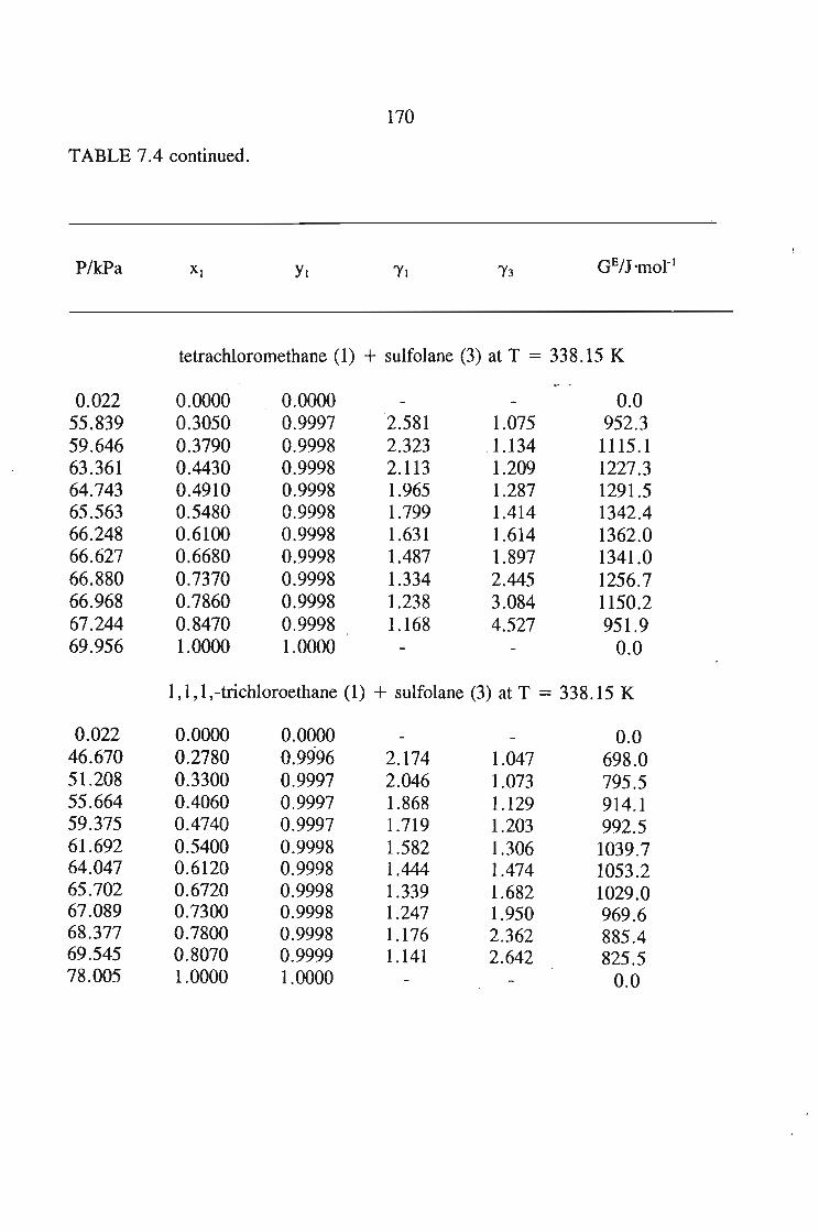
TABLE 7.4 continued.
P/kPa
170
T'J
tetrachloromethane (1) + sulfolane (3) at T = 338.15 K
0.022 0.0000 0.0000 0.055.839 0.3050 0.9997 2.581 1.075 952.359.646 0.3790 0.9998 2.323 1.134 1115.163.361 0.4430 0.9998 2.113 1.209 1227.364.743 0.4910 0.9998 1.965 1.287 1291.565.563 0.5480 0.9998 1.799 1.414 1342.466.248 0.6100 0.9998 1.631 1.614 1362.066.627 0.6680 0.9998 1.487 1.897 1341.066.880 0.7370 0.9998 1.334 2.445 1256.766.968 0.7860 0.9998 1.238 3.084 1150.267.244 0.8470 0.9998 1.168 4.527 951.969.956 1.0000 1.0000 0.0
1,1,1,-trichloroethane (1) + sulfolane (3) at T = 338.15 K
0.022 0.0000 0.0000 0.046.670 0.2780 0.9996 2.174 1.047 698.051.208 0.3300 0.9997 2.046 1.073 795.555.664 0.4060 0.9997 1.868 1.129 914.159.375 0.4740 0.9997 1.719 1.203 992.561.692 0.5400 0.9998 1.582 1.306 1039.764.047 0.6120 0.9998 1.444 1.474 1053.265.702 0.6720 0.9998 1.339 1.682 1029.067.089 0.7300 0.9998 1.247 1.950 969.668.377 0.7800 0.9998 1.176 2.362 885.469.545 0.8070 0.9999 1.141 2.642 825.578.005 1.0000 1.0000 0.0
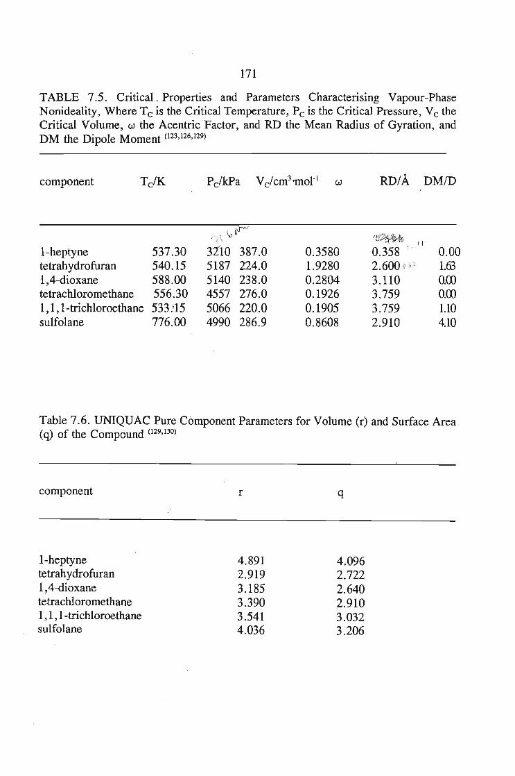
171
TABLE 7.5. Critical. Properties and Parameters Characterising Vapour-PhaseNonideality, Where Tc is the Critical Temperature, Pc is the Critical Pressure, Vc theCritical Volume, w the Acentric Factor, and RD the Mean Radius of Gyration, andDM the Dipole Moment (123,126,129)
component RD/A DM/D
\oF~r \
l-heptyne 537.30 3~10 387.0 0.3580 0.358 1)1 0.00tetrahydrofuran 540.15 5187 224.0 1.9280 2.600 0 p 1.631,4-dioxane 588.00 5140 238.0 0.2804 3.110 0.00tetrachloromethane 556.30 4557 276.0 0.1926 3.759 0.001,1,I-trichloroethane 533:15 5066 220.0 0.1905 3.759 1.10sulfolane 776.00 4990 286.9 0.8608 2.910 4.10
Table 7.6. UNIQUAC Pure Component Parameters for Volume (r) and Surface Area(q) of the Compound (129,130)
component
I-heptynetetrahydrofuran1A-dioxanetetrachloromethane1, 1, I-trichloroethanesulfolane
r
4.8912.9193.1853.3903.5414.036
q
4.0962.7222.6402.9103.0323.206
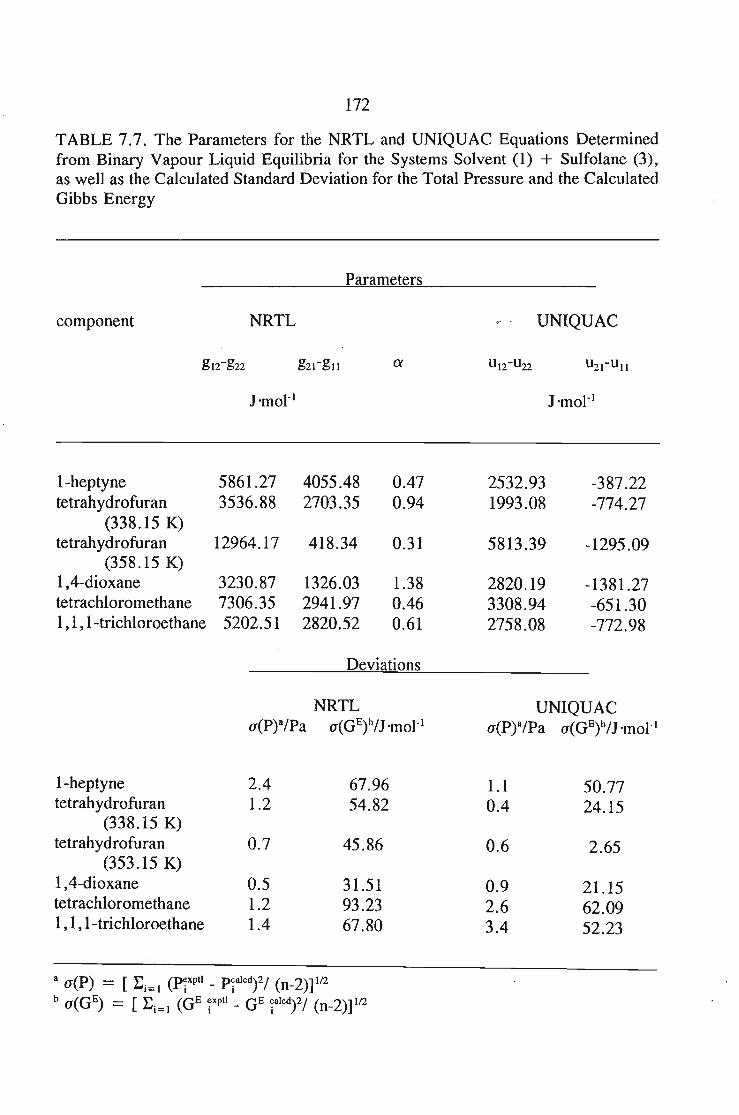
172
TABLE 7.7. The Parameters for the NRTL and UNIQUAC Equations Determinedfrom Binary Vapour Liquid Equilibria for the Systems Solvent (1) + Sulfolane (3),as well as the Calculated Standard Deviation for the Total Pressure and the CalculatedGibbs Energy
Parameters
component NRTL UNIQUAC
I-heptyne 5861.27 4055.48 0.47 2532.93 -387.22tetrahydrofuran 3536.88 2703.35 0.94 1993.08 -774.27
(338.15 K)tetrahydrofuran 12964.17 418.34 0.31 5813.39 -1295.09
(358.15 K)1,4-dioxane 3230.87 1326.03 1.38 2820.19 -1381.27tetrachloromethane 7306.35 2941.97 0.46 3308.94 -651.301, 1, I-trichloroethane 5202.51 2820.52 0.61 2758.08 -772.98
Deviations
NRTL UNIQUACa(P)&/Pa a(GE)b/J "mol-1 a(P)&/Pa a(GE)b/J 'mot l
I-heptyne 2.4 67.96 1.1 50.77tetrahydrofuran 1.2 54.82 0.4 24.15
(338.15 K)tetrahydrofuran 0.7 45.86 0.6 2.65
(353.15 K)1,4-dioxane 0.5 31.51 0.9 21.15tetrachloromethane 1.2 93.23 2.6 62.091, 1, I-trichloroethane 1.4 67.80 3.4 52.23
&a(P) = [ Ej=1 (PiXptl - Pi&ICd?1 (n_2)]1I2b a(GE) = [ Ej=1 (GEixptl _ GE i&Icd)21 (n-2)]1/2
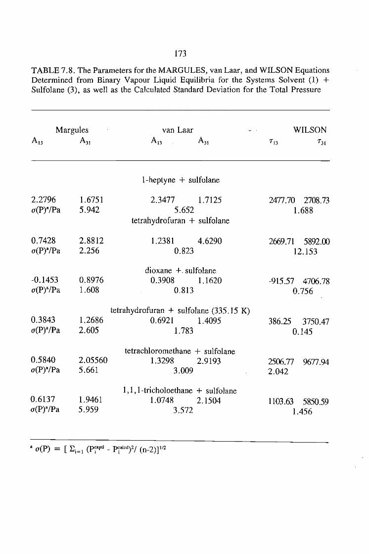
173
TABLE 7.8. The Parameters for the MARGULES, van Laar, and WILSON EquationsDetermined from Binary Vapour Liquid Equilibria for the Systems Solvent (1) +Sulfolane (3), as well as the Calculated Standard Deviation for the Total Pressure
Margu1esA l3 A 31
van LaarA l3 A31
WILSON
I-heptyne + su1fo1ane
2.2796 1.6751 2.3477 1.7125 2477.70 2708.73a(p)8/Pa 5.942 5.652 1.688
tetrahydrofuran + su1fo1ane
0.7428 2.8812 1.2381 4.6290 2669.71 5892.00a(p)8/Pa 2.256 0.823 12.153
dioxane +. sulfolane-0.1453 0.8976 0.3908 1.1620 -915.57 4706.78a(p)8/Pa 1.608 0.813 0.756
tetrahydrofuran + su1fo1ane (335.15 K)0.3843 1.2686 0.6921 1.4095 386.25 3750.47a(p)8/Pa 2.605 1.783 0.145
tetrach1oromethane + su1fo1ane0.5840 2.05560 1.3298 2.9193 2506.77 %77.94a(p)8/Pa 5.661 3.009 2.042
1,1,I-tricholoethane + su1fo1ane0.6137 1.9461 1.0748 2.1504 1103.63 5850.59a(p)8/Pa 5.959 3.572 1.456
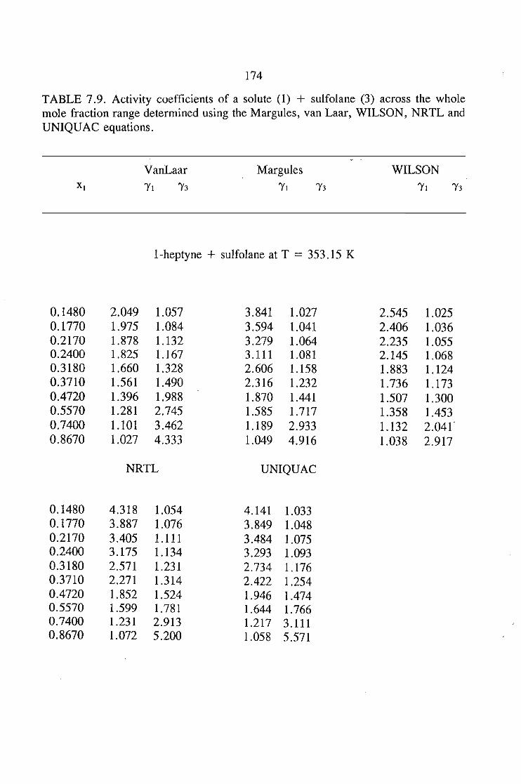
174
TABLE 7.9. Activity coefficients of a solute (1) + sulfolane (3) across the wholemole fraction range determined using the Margules, van Laar, WILSON, NRTL andUNIQUAC equations.
VanLaar1'1 1'3
Margules1'1 1'3
WILSON1'1 1'3
I-heptyne + sulfolane at T = 353.15 K
0.1480 2.049 1.057 3.841 1.027 2.545 1.0250.1770 1.975 1.084 3.594 1.041 2.406 1.0360.2170 1.878 1.132 3.279 1.064 2.235 1.0550.2400 1.825 1.167 3.111 1.081 2.145 1.0680.3180 1.660 1.328 2.606 1.158 1.883 1.1240.3710 1.561 1.490 2.316 1.232 1.736 1.1730.4720 1.396 1.988 1.870 1.441 1.507 1.3000.5570 1.281 2.745 1.585 1.717 1.358 1.4530.7400 1.101 3.462 1.189 2.933 1.132 2.041'0.8670 1.027 4.333 1.049 4.916 1.038 2.917
NRTL UNIQUAC
0.1480 4.318 1.054 4.141 1.0330.1770 3.887 1.076 3.849 1.0480.2170 3.405 1.111 3.484 1.0750.2400 3.175 1.134 3.293 1.0930.3180 2.571 1.231 2.734 1.1760.3710 2.271 1.314 2.422 1.2540.4720 1.852 1.524 1.946 1.4740.5570 1.599 1.781 1.644 1.7660.7400 1.231 2.913 1.217 3.1110.8670 1.072 5.200 1.058 5.571
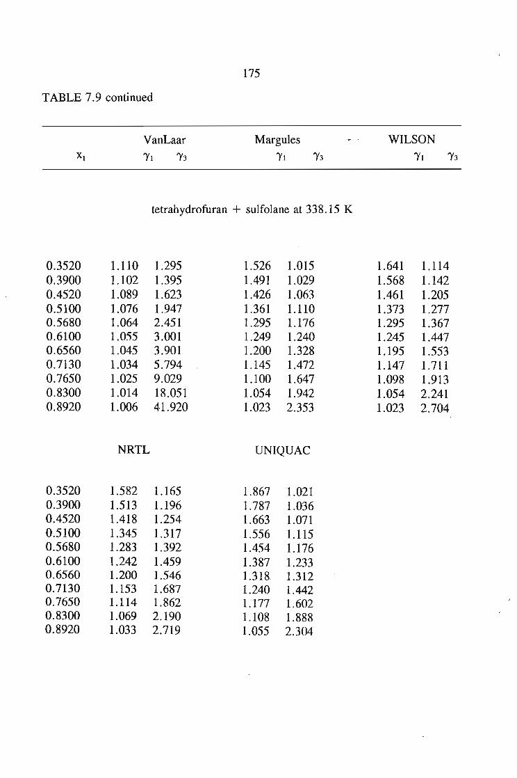
175
TABLE 7.9 continued
VanLaar
1'1 1'3
Margules
1'1 1'3
WILSON
1'1 1'3 .
tetrahydrofuran + sulfolane at 338.15 K
0.3520 1.110 1.295 1.526 1.015 1.641 1.1140.3900 1.102 1.395 1.491 1.029 1.568 1.1420.4520 1.089 1.623 1.426 1.063 1.461 1.2050.5100 1.076 1.947 1.361 1.110 1.373 1.2770.5680 1.064 2.451 1.295 1.176 1.295 1.3670.6100 1.055 3.001 1.249 1.240 1.245 1.4470.6560 1.045 3.901 1.200 1.328 1.195 1.5530.7130 1.034 5.794 1.145 1.472 1.147 1.7110.7650 1.025 9.029 1.100 1.647 1.098 1.9130.8300 1.014 18.051 1.054 1.942 1.054 2.2410.8920 1.006 41.920 1.023 2.353 1.023 2.704
NRTL UNIQUAC
0.3520 1.582 1.165 1.867 1.0210.3900 1.513 1.196 1.787 1.0360.4520 1.418 1.254 1.663 1.0710.5100 1.345 1.317 1.556 1.1150.5680 1.283 1.392 1.454 1.1760.6100 1.242 1.459 1.387 1.2330.6560 1.200 1.546 1.318. 1.3120.7130 1.153 1.687 1.240 1.4420.7650 1.114 1.862 1.177 1.6020.8300 1.069 2.190 1.108 1.8880.8920 1.033 2.719 1.055 2.304
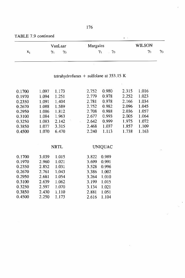
176
TABLE 7.9 continued
VanLaar
1'1 1'3
. Margules
1'1 1'3
WILSON
1'1 1'3
tetrahydrofuran + sulfolane at 353.15 K
0.1700 1.097 1.173 2.752 0.980 2.315 1.0160.1970 1.094 1.251 2.779 0.978 2.252 1.0230.2350 1.091 1.404 2.781 0.978 2.166 1.0340.2670 1.088 1.589 2.752 0.982 2.096 1.0450.2950 1.086 1.812 2.708 0.988 2.036 1.0570.3100 1.084 1.963 2.677 0.993 2.005 1.0640.3250 1.083 2.142 2.642 0.999 1.975 1.0720.3850 1.077 3.315 2.468 1.037 1.857 1.1090.4500 1.070 6.470 2.240 1.113 1.738 1.163
NRTL UNIQUAC
0.1700 3.039 1.015 3.822 0.9890.1970 2.960 1.021 3.699 0.9910.2350 2.852 1.031 3.528 0.9960.2670 2.761 1.043 3.386 1.0020.2950 2.681 1.054 3.264 1.0100.3100 2.639 1.062 3.199 1.0150.3250 2.597 1.070 3.134 1.0210.3850 2.430 1.110 2.881 1.0510.4500 2.250 1.173 2.616 1.104
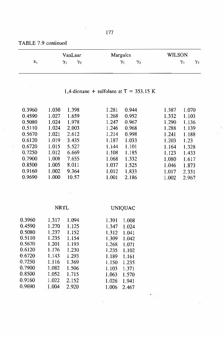
177
TABLE 7.9 continued
VanLaar
'YI 'Y3
Margules
'YI 'Y3
WILSON
'YI 'Y3
l,4-dioxane + sulfolane at T = 353.15 K
0.3960 1.030 1.398 1.281 0.944 1.387 1.0700.4590 1.027 1.659 1.268 0.952 1.332 1.1030.5080 1.024 1.978 1.247 0~967 1.290 1.1360.5110 1.024 2.003 1.246 0.968 1.288 1.1390.5670 1.021 2.612 1.214 0.998 1.241 1.1880.6120 1.019 3.435 1.187 1.033 1.203 1.230.6720 1.015 5.527 1.144 1.101 1.164 1.3280.7250 1.012 6.669 1.108 1.185 1.123 1.4330.7900 1.008 7.655 1.068 1.332 1.080 1.6170.8500 1.005 8.011 1.037 1.525 1.046 1.8730.9160 1.002 9.364 1.012 1.833 1.017 2.3310.9690 1.000 10.57 1.001 2.186 1.002 2.967
NRTL UNIQUAC
0.3960 1.317 1.094 1.391 1.0080.4590 1.270 1.125 1.347 1.0240.5080 1.237 1.152 1.312 1.0410.5110 1.235 1.154 1.309 1.0420.5670 1.201 1.193 1.268 1.0710.6120 1.176 1.230 1.235 1.1020.6720 1.143 1.293 1.189 1.1610.7250 1.116 1.369 1.150 1.2350.7900 1.082 1.506 1.103 1.3710.8500 1.052 1.715 1.063 1.5700.9160 1.022 2.152 1.026 1.9410.9690 1.004 2.920 1.006 2.467
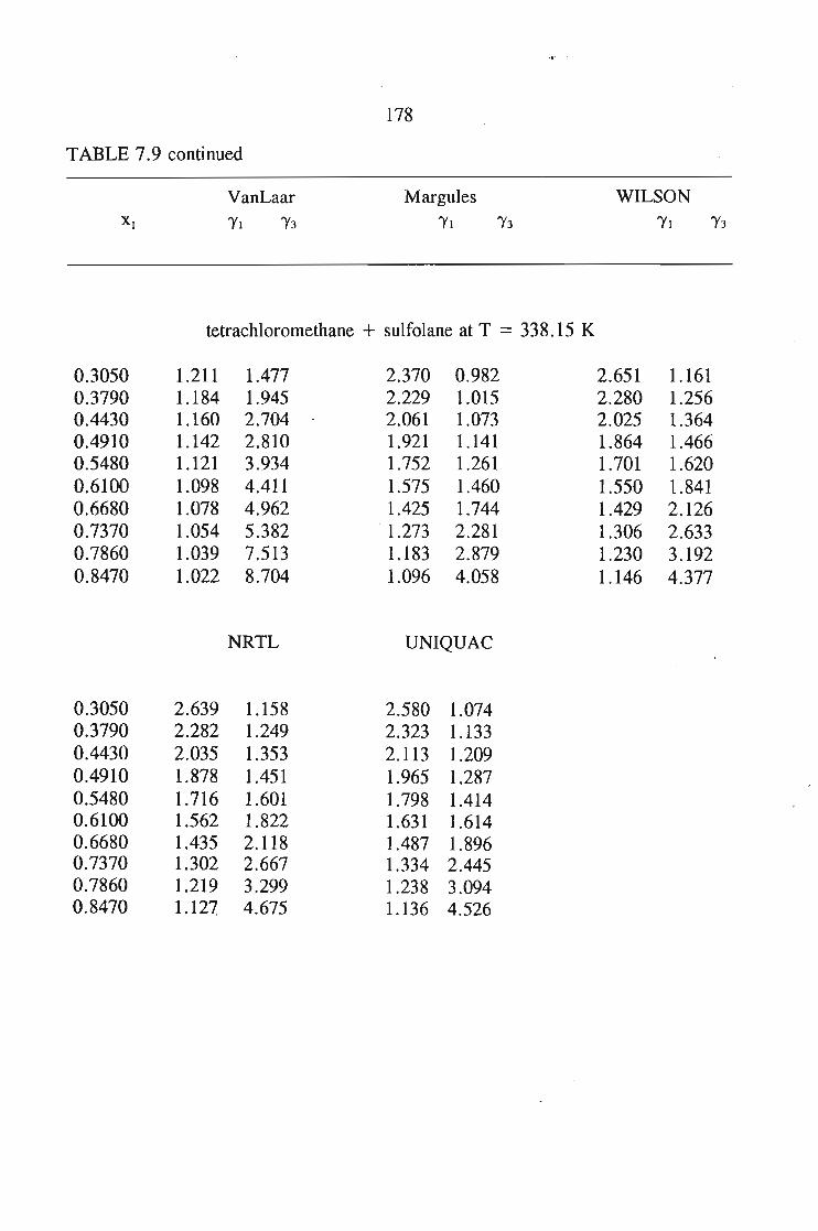
TABLE 7.9 continued
VanLaar
1'1 1'3
178
Margules
1'1 1'3
WILSON
1'1 1'3
tetrachloromethane + sulfolane at T = 338.15 K
0.3050 1.211 1.477 2.370 0.982 2.651 1.1610.3790 1.184 1.945 2.229 1.015 2.280 1.2560.4430 1.160 2.704 2.061 1.073 2.025 1.3640.4910 1.142 2.810 1.921 1.141 1.864 1.4660.5480 1.121 3.934 1.752 1.261 1.701 1.6200.6100 1.098 4.411 1.575 1.460 1.550 1.8410.6680 1.078 4.962 1.425 1.744 1.429 2.1260.7370 1.054 5.382 1.273 2.281 1.306 2.6330.7860 1.039 7.513 1.183 2.879 1.230 3.1920.8470 1.022 8.704 1.096 4.058 1.146 4.377
NRTL UNIQUAC
0.3050 2.639 1.158 2.580 1.0740.3790 2.282 1.249 2.323 1.1330.4430 2.035 1.353 2.113 1.2090.4910 1.878 1.451 1.965 1.2870.5480 1.716 1.601 1.798 1.4140.6100 1.562 1.822 1.631 1.6140.6680 1.435 2.118 1.487 1.8960.7370 1.302 2.667 1.334 2.4450.7860 1.219 3.299 1.238 3.0940.8470 1.127 4.675 1.136 4.526
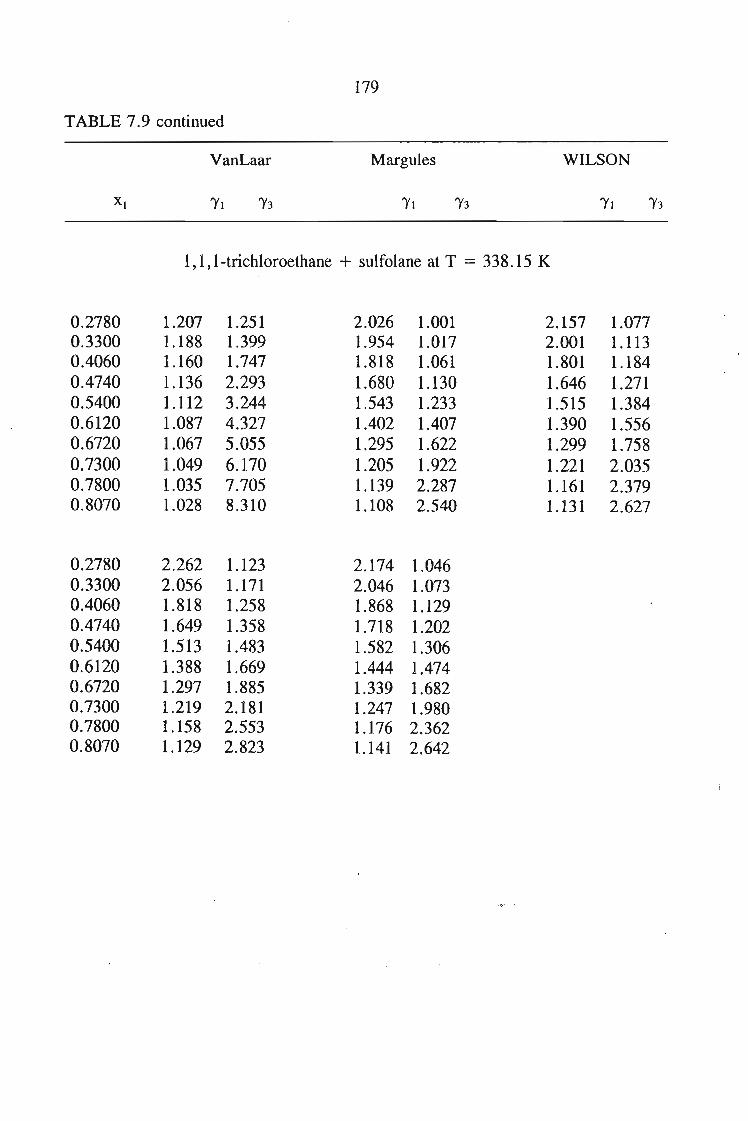
179
TABLE 7.9 continued
VanLaar Margules WILSON
1,1,I-trichloroethane + sulfolane at T = 338.15 K
0.2780 1.207 1.251 2.026 1.001 2.157 1.0770.3300 1.188 1.399 1.954 1.017 2.001 1.1130.4060 1.160 1.747 1.818 1.061 1.801 1.1840.4740 1.136 2.293 1.680 1.130 1.646 1.2710.5400 1.112 3.244 1.543 1.233 1.515 1.3840.6120 1.087 4.327 1.402 1.407 1.390 1.5560.6720 1.067 5.055 1.295 1.622 1.299 1.7580.7300 1.049 6.170 1.205 1.922 1.221 2.0350.7800 1.035 7.705 1.139 2.287 1.161 2.3790.8070 1.028 8.310 1.108 2.540 1.131 2.627
0.2780 2.262 1.123 2.174 1.0460.3300 2.056 1.171 2.046 1.0730.4060 1.818 1.258 1.868 1.1290.4740 1.649 1.358 1.718 1.2020.5400 1.513 1.483 1.582 1.3060.6120 1.388 1.669 1.444 1.4740.6720 1.297 1.885 1.339 1.6820.7300 1.219 2.181 1.247 1.9800.7800 1.158 2.553 1.176 2.3620.8070 1.129 2.823 1.141 2.642
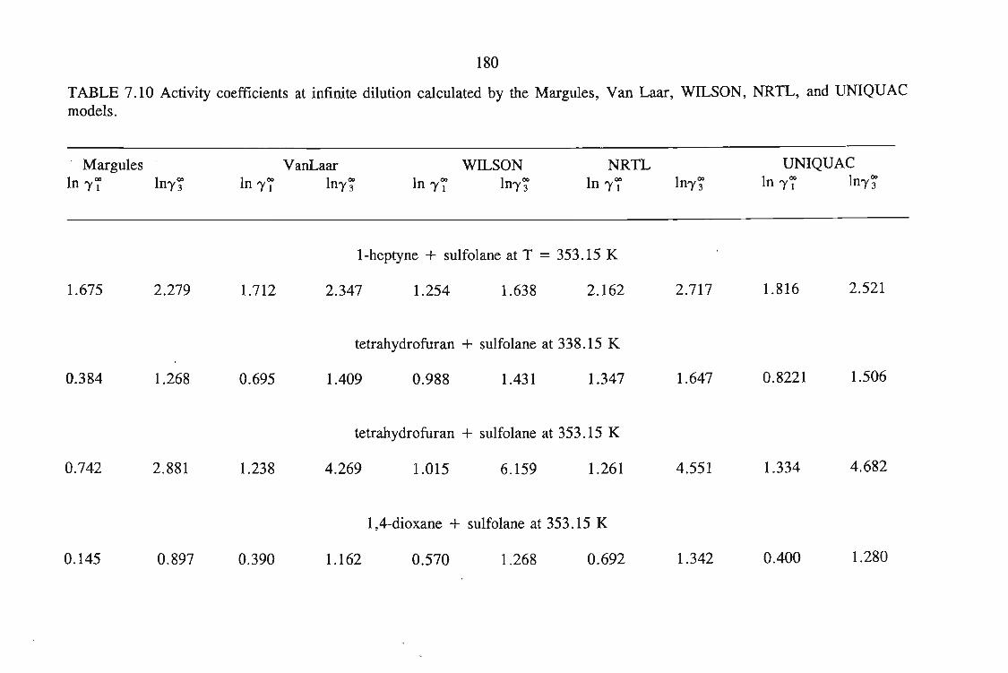
180
TABLE 7.10 Activity coefficients at infinite dilution calculated by the Margules, Van Laar, WILSON, NRTL, and UNIQUACmodels.
MargulesIn ')'7 In1~
VanLaarIn 17 In1~
WILSONIn ')'7 In1~
NRTLIn ')'7 In')'~
UNIQUACIn ')'7 In')'~
I-heptyne + sulfolane at T = 353.15 K
1.675 2.279 1.712 2.347 1.254 1.638 2.162 2.717 1.816 2.521
tetrahydrofuran + sulfolane at 338.15 K
0.384 1.268 0.695 1.409 0.988 1.431 1.347 1.647 0.8221 1.506
tetrahydrofuran + sulfolane at 353.15 K
0.742 2.881 1.238 4.269 1.015 6.159 1.261 4.551 1.334 4.682
1,4-dioxane + sulfolane at 353.15 K
0.145 0.897 0.390 1.162 0.570 1.268 0.692 1.342 0.400 1.280
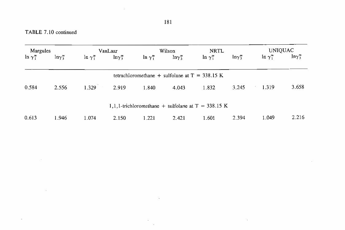
TABLE 7.10 continued
MarguIesIn 'Y~ In'Y~
VanLaarIn '1'7 In'Y~
181
WiIsonIn '1'7 In'Y~
NRTLIn '1'7 In'Y~
UNIQUACIn '1'7 In'Y~
tetrachIoromethane + suIfoIane at T = 338.15 K
0.584 2.556 1.329 2.919 1.840 4.043 1.832 3.245 1.319 3.658
1,1,I-trichIoromethane + suIfoIane at T = 338.15 K
0.613 1.946 1.074 2.150 1.221 2.421 1.601 2.394 1.049 2.216
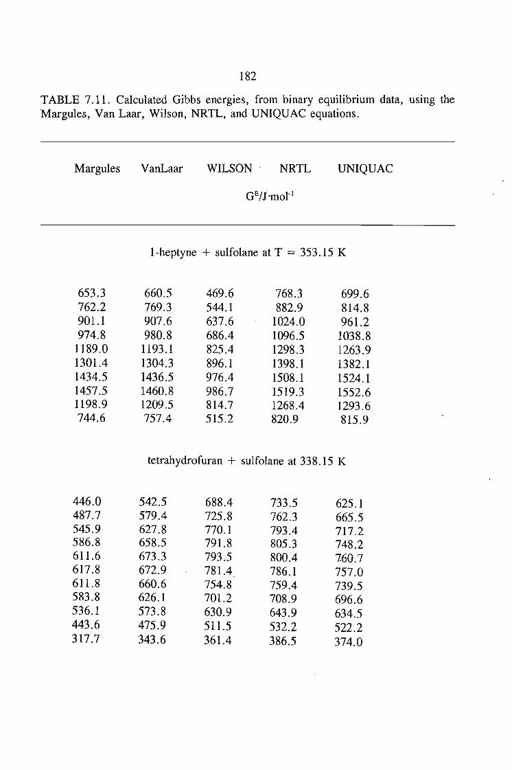
182
TABLE 7.11. Calculated Gibbs energies, from binary equilibrium data, using theMargules, Van Laar, Wilson, NRTL, and UNIQUAC equations.
Margules VanLaar WILSON NRTL UNIQUAC
I-heptyne + sulfolane at T = 353.15 K
653.3 660.5 469.6 768.3 699.6762.2 769.3 544.1 882.9 814.8901.1 907.6 637.6 1024.0 961.2974.8 980.8 686.4 1096.5 1038.8
1189.0 1193.1 825.4 1298.3 1263.91301.4 1304.3 896.1 1398.1 1382.11434.5 1436.5 976.4 1508.1 1524.11457.5 1460.8 986.7 1519.3 1552.61198.9 1209.5 814.7 1268.4 1293.6744.6 757.4 515.2 820.9 815.9
tetrahydrofuran + sulfolane at 338.15 K
446.0 542.5 688.4 733.5 625.1487.7 579.4 725.8 762.3 665.5545.9 627.8 770.1 793.4 717.2586.8 658.5 791.8 805.3 748.2611.6 673.3 793.5 800.4 160.7617.8 672.9 781.4 786.1 757.0611.8 660.6 754.8 759.4 739.5583.8 626.1 701.2 708.9 696.6536.1 573.8 630.9 643.9 634.5443.6 475.9 511.5 532.2 522.2317.7 343.6 361.4 386.5 374.0
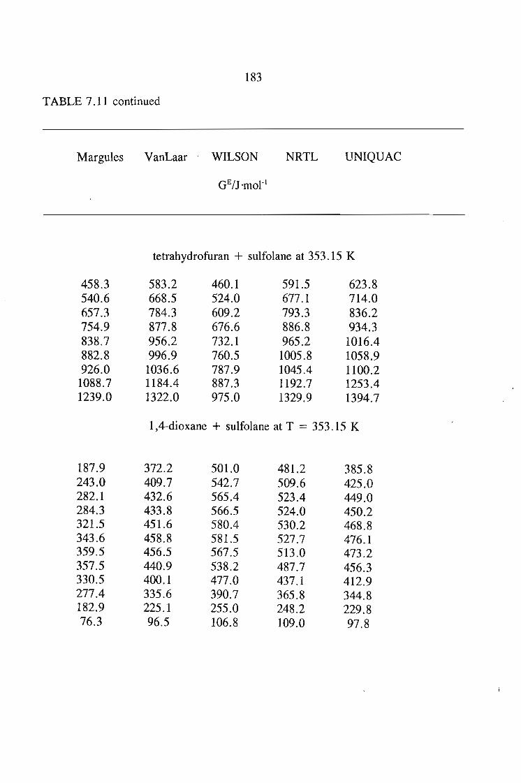
183
TABLE 7.11 continued
Margules VanLaar WILSON NRTL UNIQUAC
tetrahydrofuran +sulfolane at 353.15 K
458.3 583.2 460.1 591.5 623.8540.6 668.5 524.0 677.1 714.0657.3 784.3 609.2 793.3 836.2754.9 877.8 676.6 886.8 934.3838.7 956.2 732.1 965.2 1016.4882.8 996.9 760.5 1005.8 1058.9926.0 1036.6 787.9 1045.4 1100.2
1088.7 1184.4 887.3 1192.7 1253.41239.0 1322.0 975.0 1329.9 1394.7
1,4-dioxane + sulfolane at T = 353.15 K
187.9 372.2 501.0 481.2 385.8243.0 409.7 542.7 509.6 425.0282.1 432.6 565.4 523.4 449.0284.3 433.8 566.5 524.0 450.2321.5 451.6 580.4 530.2 468.8343.6 458.8 581.5 527.7 476.1359.5 456.5 567.5 513.0 473.2357.5 440.9 538.2 487.7 456.3330.5 400.1 477.0 437.1 412.9277.4 335.6 390.7 365.8 344.8182.9 225.1 255.0 248.2· 229.876.3 96.5 106.8 109.0 97.8
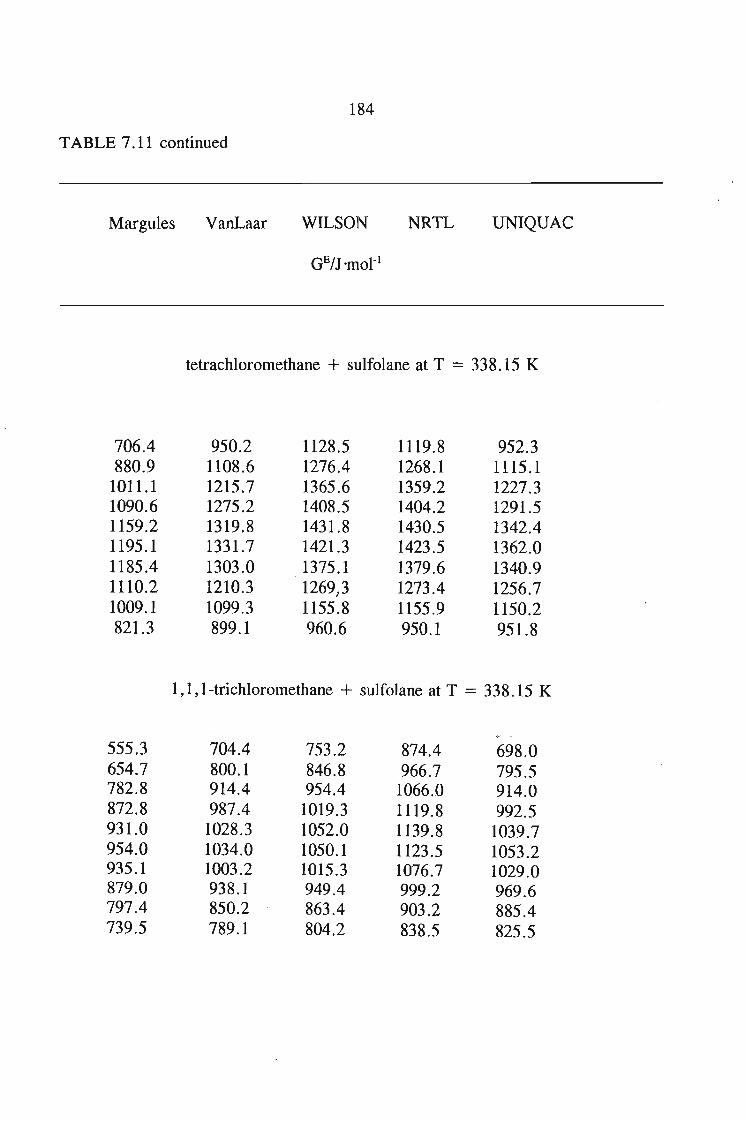
184
TABLE 7.11 continued
Margules VanLaar WILSON NRTL UNIQUAC
tetrachloromethane + sulfolane at T = 338.15 K
706.4 950.2 1128.5 1119.8 952.3880.9 1108.6 1276.4 1268.1 1115.1
1011.1 1215.7 1365.6 1359.2 1227.31090.6 1275.2 1408.5 1404.2 1291.51159.2 1319.8 1431.8 1430.5 1342.41195.1 1331.7 1421.3 1423.5 1362.01185.4 1303.0 1375.1 1379.6 1340.91110.2 1210.3 1269) 1273.4 1256.71009.1 1099.3 1155.8 1155.9 1150.2821.3 899.1 960.6 950.1 951.8
1,1, I-trichloromethane + sulfolane at T = 338.15 K
555.3 704.4 753.2 874.4 698.0654.7 800.1 846.8 966.7 795.5782.8 914.4 954.4 1066.0 914.0872.8 987.4 1019.3 1119.8 992.5931.0 1028.3 1052.0 1139.8 1039.7954.0 1034.0 1050.1 1123.5 1053.2935.1 1003.2 1015.3 1076.7 1029.0879.0 938.1 949.4 999.2 969.6797.4 850.2 863.4 903.2 885.4739.5 789.1 804.2 838.5 825.5
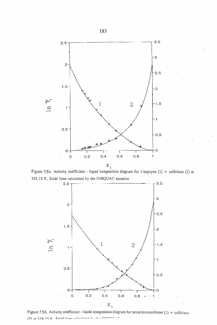
185
2.5 3.5
3
2 --
2.5
1.52
~-1 2 1.5
~ 1I"'--i
0.5
0.5
0.80.60.40.2
o-l----=~:::::::;..------..,r---.,---.....,,,....--=_+_O
o
XlFigure 7Sa. Activity coefficient - liquid composition diagram for l-~eptyne (1) + sulfolane (~) at
353.15 K. Solid lines calculated by the UNIQUAC equation2.5 3.5
3
2
2.5
1.52
~-
J 2~ 1I"'--i
0.5
0.8 '. - 10.60.40.2
o -+-~==r===t:::.':"----.--:"'--r--':"'=:::::::::-+- 0
o
0.5
Xl
Figure 7Sb. Activity coefficient -liquid composition diagram for tetrachloromethane (1) + sulfolane
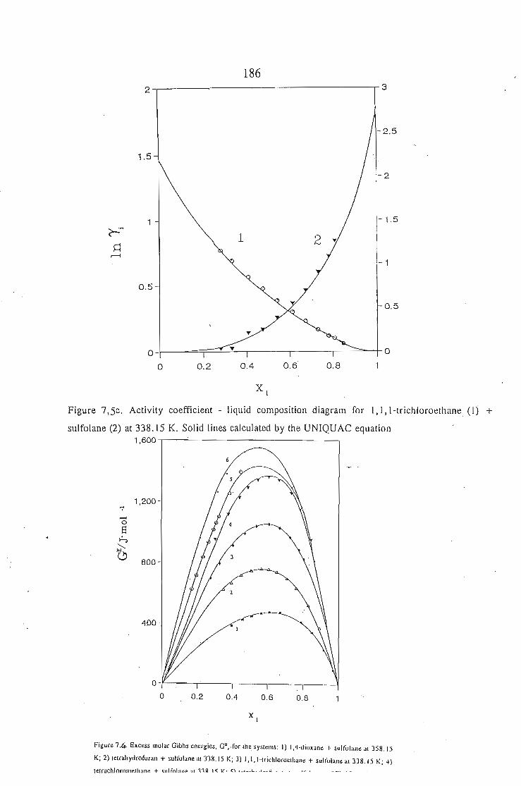
1862-r----~-----------13
0.80.60.40.2
O-+--~==;:====~:!-.-'----,----r----==:::::--t-O
o
1.5
1 -1.5r:~
2 -.:q,.....-l
-1
0.5
0.5
XI
Figure 7,5e. Activity coefficient - liquid composition diagram for 1J 1J I-trichloroethane. (I j +
sulfolane (2) at 338.15 K. Solid lines calculated by the UNIQUAC equation1,600.------'------------_---,
0.6OA0.2
Fil:ur~ 7.G. Exc~ss molar Gibbs ~n~rl:ies. G"•.for Ih~.sysl~IlIS: I) 1.4-<lioxan~ + sultolall~ al 358.15
K; 2) IClraJly<lrofuran + sultolane al 338.15 K; 3) 1.1.l-lricbloro~lhan~ + sult()lan~ al 338.15 K; 4)
lelrachlorolll~lhan~ + <lIlf"I:I""!I' 11R I ~ v· <\ ."".• " ... I __ ~._ .. _ •
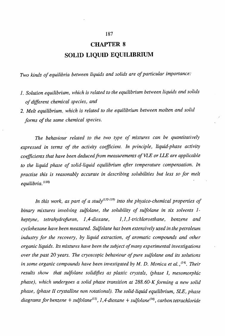
187
CHAPTER 8
SOLID LIQUID EQUILIBRIUM
Two kinds of equilibria between liquids and solids are ofparticular importance:
1. Solution equilibrium, which is related to the equilibrium between liquids and solids
ofdifferent chemical species, and
2. Melt equilibrium, which is related to the equilibrium between molten and solid
forms of the same chemical species.
The behaviour related to the two type of mixtures can be quantitatively
expressed in terms of the activity coefficient. In principle, liquid-phase activity
coefficients that have been deduced from measurements ofVLE or LLE are applicable
to the liquid phase of solid-liquid equilibrium after temperature compensation. In
practise this is reasonably accurate in describing solubilities but less so for melt
equilibria. (130)
In this work, as part of a study{132-133) into the physico-chemical properties of
binary mixtures involving sulfolane, the solubility of sulfolane in six solvents 1
heptyne, tetrahydrofuran, l,4-dioxane, 1,1,1-trichloroethane, benzene and
cyclohexane have been measured. Sulfolane has been extensively used in the petroleum
industry for the recovery, by liquid extraction, of aromatic compounds and other
organic liquids. Its mixtures have been the subject ofmany experimental investigations
over the past 20 years. The cryoscopic behaviour ofpure sulfolane and its solutions
in some organic compounds have been investigated by M. D. Monica et al., (14). Their
results show that sulfolane solidifies as plastic crystals, (phase I, mesomorphic
phase), which undergoes a solid phase transition at 288. 60··K forming a new solid
phase, (phase II crystalline non rotational). The solid-liquid equilibrium, SLE, phase
diagrams for benzene + sulfolane(15), l,4-dioxane + sulfolane(16), carbon tetrachloride
188
+ sulfolane(l7) , 2-methyl-2-propanol + sulfolane and nitrobenzene + sulfolane(l36)
have also been reported in the literature. This data is used together with solubility
measurements conducted in this work, to fully describe (predict) the mixing properties
of sulfolane and various solutes in Chapter 9.
Sulfolane is a dipolar aprotic substance with a low donor number of14.81 (136)
and a large dipole moment in the liquid phase, !J- = 4.8 D (136). The steric hinderance
resulting from the large globular hydrocarbon moiety is responsible for the weakly
structured substance below its melting point (plastic phase 1), and also the large
enthalpy change of transition which considerably exceeds the melting enthalpy (14).
In the publications cited above, little attention has been paid to the analysis of
the (SLE) data using modern theories ofmixing. Only for the nitrobenzene + (TMS)
(8) mixture was the liquidus curve described together with numerical values of
differences between heat capacity of the solute in the solid (plastic phase I) and the
heat capacity of the liquid phase (ACpmzJ, at the melting temperature (ACpm2 = 0).
This assumes that there is no loss of rotational freedom of sulfolane molecules on
solidification. During the phase transition between plastic phase I and crystalline
phase Il, which was assumed as an orientational fusion, the ACprr2 was calculated to
be 45.51 J K-1 moti•
In this work, the results ofthe correlation ofsolubility for sulfolane in various
solvents with respect to the solid-solid phase transition in sulfolane is given in terms
ofthe WILSON(5), NRTL(6), and UNIQUAC') equations, utilizingparameters takenfrom
solid-liquid equilibrium for the simple eutectic mixtures only. The correlations have
been done using the data reported here as well as the data published earlier (14-17).
8.1. Solubility of Solids in Liquids
When the solvent does not enter the solid phase, the fugacity of the solid
remains that of the pure solid, so the condition of equality of partial fugacities at
equilibrium becomes(l30)
189
Asolid =A(solid) =Yr/3(subcooledJil/uid)
Rearranging in simplified notation,
(8.1)
(8.2)
where X3 is the mole fraction of the solute in the solution and h(sc() represents the
fugacity of the pure solid state in a subcooled or hypothetical liquid state below its
melting point.
The ratio h(solid)1.h (scl) of the fugacities of the solid and its subcooled liquid can
be evaluated in terms of conditions at the triple point. When the fundamental equation,
aH aVdlnf= --dt+-dP
RJ'l RT
is applied to each phase and the results subtracted, the conclusion is(l21)
f H -H V-VdIn 3(solid) = L sdT_ L sdP
A(scf) RJ'l RT
(8.3)
(8.4)
For practical purposes the difference in specific volumes of condensed phases
may be independent of pressure, but the enthalpy of fusion, HL - Hs' may vary
appreciably with temperature. The behaviour is described by
190
(8.5)
where the subscript tp designates the triple point. The last form of the equation applies
when the heat capacity difference is relatively insensitive to temperature.
After equation 8.5 is substituted into equation 8.4 and the result is integrated
between (Ttp , Ptp) and the temperature and the pressure of the system (T, P), the ratio
of the fugacities become
f I1H 1 1 I1C T T AVIn_3 '= tp3(_ --)---E(ln tp3 _ tp3 +l) __L.1_(P_P 3) (8.6)h(scl) R Ttp] T R T T RT tp
Substitution of the relations into equation 8.2 results in the General Solubility Equation
1 I1Htp3 1 1 I1Cp3 Ttp3 Ttp3 11 Vx
3=-exp[--(- - ':')---(In---+l)--(P-Ptp]) (8.7)
Y3 R Ttp] T R T T RT
One or more simplifications of the equation are sometime adequate:(130)
1. The pressure may be negligible.
2. Although it is more substantial than the correction for pressure, the contribution
of the heat-capacity difference also is often minor (and difficult to find in the
literature), and when it is neglected the solubility equation becomes
191
1 AB j 1 1 1 AStpj Ttpjx
3= -exp[-tp-(- - ~)] --[--(1--)]
y 3 R Ttp3 T y 1 R T
where ~Slp = Ililq/TIp is the entropy of fusion at the triple point.
(8.8)
3. Since triple-point temperatures usually are very nearly the same at atmospheric
melting points and the latter are more often known, the solubility equation
becomes, with this substitution
, (8.9)
where the subscripts m identifies conditions at the atmospheric melting point.
4. A compact solubility equation that requires knowledge only of properties of the
pure components is obtained in terms of the Scatchard-Hilderbrand(l37) equation 'for
the activity coefficient of the solute
(8.10)
where cPI is the volume fraction of the solvent.
(8.11)
Sometimes the Flory-Huggins(107) correction can give superior results, but neither
192
this nor the basic Scatchard-Hilderbrand equation does a particularly well for the
non-hydrocarbon mixtures and mixtures containing polar compounds.
5. The version of the solubility equation for the ideal solutions, with unit activity
coefficients,
llHm3 1 1 IlSm3 Tm3x = exp[--(---)] = exp[--(l--)]3 R T
m3T R T
is based on the Clausius-Clapeyron equation.
(8.12)
The nature of the solvent and the enthalpy and temperature of fusion are the
main factors influencing solubility. Even chemically similar compounds may differ
substantially in their fusion properties and consequently in their solubilities. The heat
capacity term contributes little to the calculated solubility at modest displacements
from the fusion temperature(l32) and is often neglected.
8.2. Eutectic Compositions
For ideal mixtures, the eutectic temperature and composition can be found when
the enthalpy and temperature of fusion are known. When the following solubility
equations for each component(l30)
llHm3 1 1x3 =exp[--(-- .:.)]
R Tm3 r (8.13)
193
(8.14)
are plotted as T against x, the curves will intersect at the eutectic condition (Te, x).
When the two eutectic conditions are required, the two equations are combined into
one as
/:i.Hm3 1 1 /:i.Hm1 1 1Y3 =exp[--(---)]+exp[--(---)]
R Tm3 Te R Tml Te
(8.15)
from which the Te can be found by an iterative procedure and substituted in the
equation 8.13 or 8.14 to find the composition· of Xe•
When the activity coefficients are known as functions of temperature and
compositions, the following equations can be solved simultaneously for the eutectic
conditions:
AHmj 1 1Y x =exp[--(---)]
3 3 R T Tm3 e
(8.16)
(8.17)
194
In one of the simplest cases the activity coefficients are represented by the equations
lny3=A(l-xlIT
and the equations to be solved by trial for the eutectic conditions are
(8.18)
(8.19)
(8.20)
(8.21)
Since liTe occurs linearly in these equations, it can be eliminated readily, and the
problem becomes one of a solution of an equation in one unknown, Xl'
Although calculations for ideal mixtures are easily performed, the results should
be used with discretion, since many mixtures are significantly non ideal. For instance,
the occurrence of partial miscibility of solid phases is not detected by ideal
calculations, and they do form occasionally in organic mixtures.
195
8.3. Activity Coefficients
In Chapter 9 the activity coefficients are shown to be correlated by several
different kinds of equations, the van Laar,(13) Margules,(12) WILSON(5), NRTL, (6) and
UNIQUAC.(7) Other methods include the NRTL1,(138) NRTL2,(138) and UNIQUAC
ASM. (139) The applicability of these theories to various types of mixtures was studied
extensively by Domanska. (140-142) It was found that for simple paraffins, in mixtures
with hydrocarbons, (140) that the UNIQUAC and NRTL2 equations gave the best
correlations. For the more complicated systems of aliphatic alcohols + long chain
hydrocarbons(l4l), UNIQUAC ASM gave the best solubility correlations, using the
association constant as an either a adjustable or fixed parameter. The Wilson equation
was found to give the best correlation for binary mixtures involving various solvents
in about 500 monocarboxylic acids. (142)
The applicability of the above mentioned solution theories as predictive tools
can only be used for ternary systems, employing binary solubility and VLE data. For
predictions of binary solubility data, the Regular Solution Theory(137), is a model that,
with some modifications, has been used frequently in wax formation predictions. In
its original form, it cannot predict negative deviations to the ideal solution assumption.
In this work, two predictive theories are used to describe the solubility of sulfolane
in various mixtures, ie. DISQUAC(9) and Modified UNIFAC(8).
For binary mixtures both activity coefficients can be evaluated from a
knowledge of the eutectic conditions by solving:
. !
1 boB"'i 1 1Yj =-exp[--(---)]x,. R T.Tnu e
(8.16)
'YI and 'Y3 can then be used to find parameters of a correlating equations such as the
196
NRTL Wilson and UNIQUAC, so that the complete melting curve can be determined.
With the Wilson equation, practical difficulties can arise when the parameters are
found from a limited amount of data such as a eutectic condition, since the process can
lead to negative values of the parameters. This is unacceptable if the equation is to
represent activity coefficients over the whole concentration range.
8.4. Experimental Section
8.4.1. Materials
The solvents were obtained from Aldrich Chemical Co., (with a quoted purity
of 99.9 % w/w) and were purified by fractional distillation through a 30 plate
distillation column. The compounds were dried using activated type 5A molecular
sieves and the water content was found to be less than lOO ppm w/w, as determined
by GLC analysis. Sulfolane was also supplied by Aldrich Chemical Co., (98 %
reagent) and was twice vacuum distilled at a pressure below 20 mmHg to yield a
colourless and odourless product. To minimize the contact of this deliquescent reagent
with moist air, the product was kept in sealed bottles in a desiccator. The physical
properties of the reagents used in this work are listed in Table 8.1 together with
literature values.
8.4.2. Procedure
In this work the solubility of sulfolane in SIX solvents l-heptyne,
tetrahydrofuran, 1,4-dioxane, _1,1, l-trichloroethane, benzene and cyclohexane have
been measured. The solubilities were determined using a dynamic method, described
by Domanska (143). The mixtures of solute and solvent, were prepared by weighing.
The mixture was well stirred using a magnetic stirrer and heated very slowly with a
heating rate, which did not exceed 2 K'h- 1 near the equilibriu'm temperature. The
temperature at which the last crystals disappeared (disappearance of solution
197
cloudiness) was taken as the temperature of the solution-crystal equilibrium.
Measurements were performed in a small range of solute concentration from X3 =
0.16 (l-heptyne, tetrahydrofuran), or 0.6 (l, 1, I-trichloroethane), or 0.5 (1,4-dioxane)
or 0.9 (cyclohexane) to X3 = lover the temperature range from 250 to 310 K. The
temperature was measured using a calibrated platinum resistance thermometer
(Autotherm2 by Gallenkamp), with an accuracy of 0.01 K. Reproducibility of
measurements was better than 0.1 K, which corresponded to a estimated error in
composition of dX3 = 0.001. The experimental results are given in Tables 8.2 and
8.3.
8.S.Results and Discussion
The solute, sulfolane is most soluble in tetrahydrofuran and least soluble in 1,4~
dioxane. The order of solubility of sulfolane is tetrahydrofuran > 1,4-dioxane >
I, I, I-tertachloroethane > benzene > tetrachloromethane > 2-methyl-2-propanol >
I-heptyne. These results indicate that no hydrogen bonds or other strong interactions
exist between sulfolane and I-heptyne, or 2-methyl-2-propanol. This is supported by
work done by M. D. Monica et al.<'4), that no hydrogen bonds exists between benzoic
acid and sulfolane.
In all the solvents used in this work, with the exception of tetrahydrofuran over
a small concentration range, the solubility of sulfolane is lower than ideal. The effect
of the interactions between (TMS) and the .solvents observed in vapour-liquid
equilibria measurements(l4) , was similar to that observed in this work. The solubility
of sulfolane in I-heptyne is much lower than ideal, and the experimental activity
coefficients of the solute (1'3) for X3 > 0.16, are in the range 4.6 - 1.0.
The solubility of sulfolane in 1,4-dioxane for X3 > 0.84 is close to ideal with
experimental activity coefficients 1'3 ::::::: 1.0. This corresponds to the liquidus curve
related to the sulfolane crystal phases I and n. Evidence for the' formation of a solid
molecular compound which largely decomposes on melting was observed in the
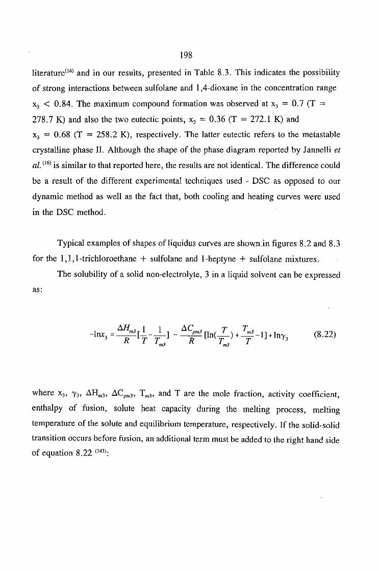
198
literature(l6) and in our results, presented in Table 8.3. This indicates the possibility
of strong interactions between sulfolane and 1,4-dioxane in the concentration range
X3 < 0.84. The maximum compound formation was observed 'at X3 = 0.7 (T =278.7 K) and also the two eutectic points, X3 = 0.36 (T = 272.1 K) and
X3 = 0.68 (T = 258.2 K), respectively. The latter eutectic refers to the metastable
crystalline phase H. Although the shape of the phase diagram reported by Jannelli et
al. (16) is similar to that reported here, the results are not identical. The difference could
be a result of the different experimental techniques used - DSC as opposed to our
dynamic method as well as the fact that, both cooling and heating curves were used
in the DSC method.
Typical examples of shapes ofliquidus curves are shown.in figures 8.2 and 8.3
for the 1,1, I-trichloroethane + sulfolane and I-heptyne + sulfolane mixtures.
The solubility of a solid non-electrolyte, 3 in a liquid solvent can be expressed
as:
AHmJ 1 1-lux3 =--[---]
R T Tm3
AC mJ T TmJ--,-P- [1n(-) + - -1] + In1'3
R TmJ T(8.22)
where x3, 1'3, ARm3 , ACpm3 , Tm3' and T are the mole fraction, activity coefficient,
enthalpy of fusion, solute heat capacity during the melting process, melting
temperature of the solute and equilibrium temperature, respectively. If the solid-solid
transition occurs before fusion, an additional term must be added to the right hand side
of equation 8.22 (143):
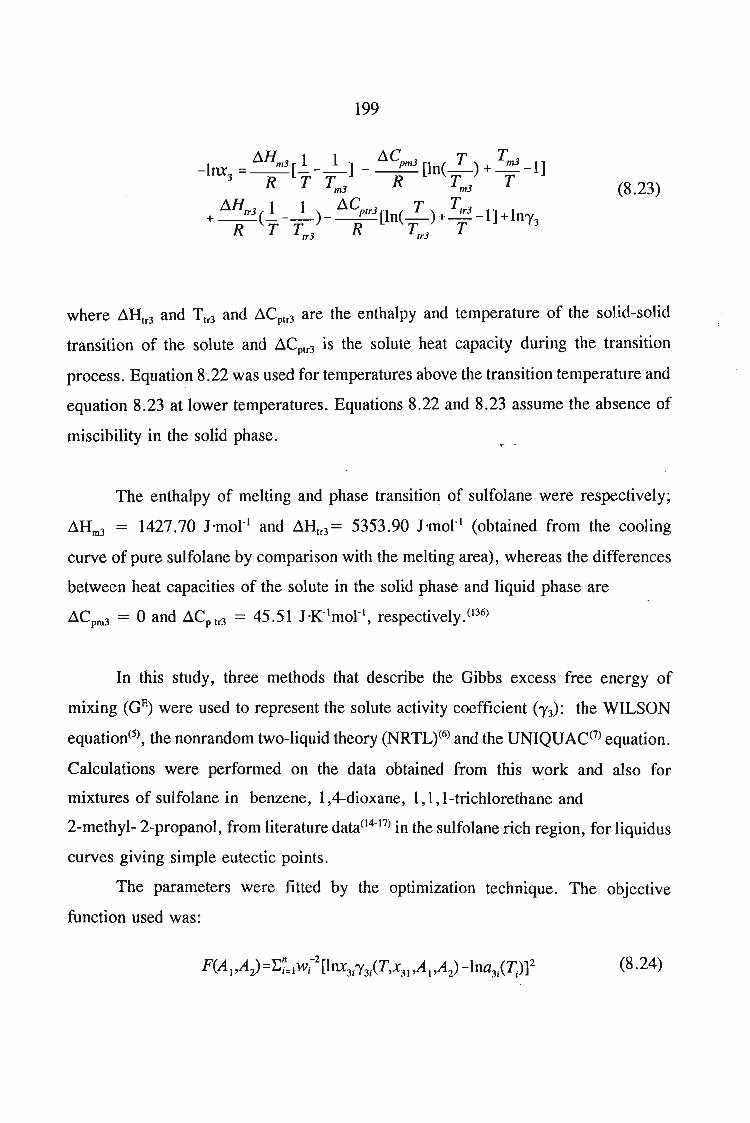
199
(8.23)
where ~Htr3 and Ttr3 and ~Cptr3 are the enthalpy and temperature of the solid-solid
transition of the solute and ~Cptr3 is the solute heat capacity during the transition
process. Equation 8.22 was used for temperatures above the transition temperature and
equation 8.23 at lower temperatures. Equations 8.22 and 8.23 assume the absence of
miscibility in the solid phase.
The enthalpy of melting and phase transition of sulfolane were respectively;
~Hm3 = 1427.70 J'mol-1 and ~Htr3= 5353.90 J'mol-1 (obtained from the cooling
curve of pure sulfolane by comparison with the melting area), whereas the differences
between heat capacities of the solute in the solid phase and liquid phase are
~Cpm3 = 0 and ~Cptr3 = 45.51 J'K-1mol-1, respectively,036)
In this study, three methods that describe the Gibbs excess free energy of
mixing (GE) were used to represent the solute activity coefficient (1'3): the WILSON
equation(5), the nonrandom two-liquid theory (NRTL)C6) and the UNIQUAC(7) equation.
Calculations were performed on the data obtained from this work and also for
mixtures of sulfolane in benzene, l,4-dioxane, 1,1, I-trichlorethane and
2-methyl- 2-propanol, from literature data(l4-17) in the sulfolane rich region, for liquidus
curves giving simple eutectic points.
The parameters were fitted by the optimization technique. The objective
function used was:
(8.24)
200
where In a3i denotes an "experimental" value of the logarithm of solute activity, taken
as the right side of equations 8.22 or 8.33, W i is the weight of an experimental point,
Al and A2 are the two adjustable parameters of the correlation equations, i denotes the
ith experimental point and n is the number of experimental data. The weights were
calculated by means of the error propagation formula:
(8.25)
where LlT and Llx3 are the estimated errors of T and x3, resp.YGtively.
The objective function is consistent with the maximum likelihood principle,
provided that the first order approximation is valid ..
The experimental errors of temperature, and solute mole fraction were fixed for
all cases at LlT = 0.1 K and Llx3 = 0.001.
The root mean square deviation of temperature given below was used as a
measure of the goodness of the fit of the solubility curves - equations 8.22 and 8.23:
(r;al_T)2 I
(J =[E~_ I i]2T I-I (n-2)
(8.26)
where~ and T j are, respectively, the calculated and experimental temperatures of
the ith point and n is the number of experimental points. The calculated values of the
parameters and corresponding root mean square deviations are presented in Table 8.4.
The pure components structural parameters r (volume parameter) and q (surface
parameter) in UNIQUAC were obtained in accordance with the methods suggested by
Vera et al., (144) and relationships (27) and (28);
and
201
Tj =0.029281 ~ (8.27)
(8.28)
where V j is the molar volume of pure component iat 298. 15'K; z is the coordination
number, further assumed equal to 10, lj is the bulk factor; it was accepted that
lj = O.
The solubility of sulfolane in cyc10hexane was only measured in the sulfolane
rich region (x3 > 0.94) as a result the non-miscibility gap in the lower sulfolane
concentrations. The NRTL parameters obtained were: gl3 - g33 = -4151.16 J 'mol- I,
and g31 - gll = 11461.16 J 'motl with a root mean square deviation of 0.26 K.
For the nine solubility curves, (shown in Table 8.4), the results obtained from
the WILSON equation are slightly better than those derived from the NRTL and
UNIQUAC equations. The average deviations are 1.56 K, 1.64 K and 1.65 K, for the
Wilson, NRTL, and UNIQUAC, respectively.
The experimental data of SLE obtained in this work and the VLE (Chapter 7)
have been used to obtain new interaction parameters for the specific solvent groups
with sulfolane using the DISQUAC and Modified UNIFAC models.
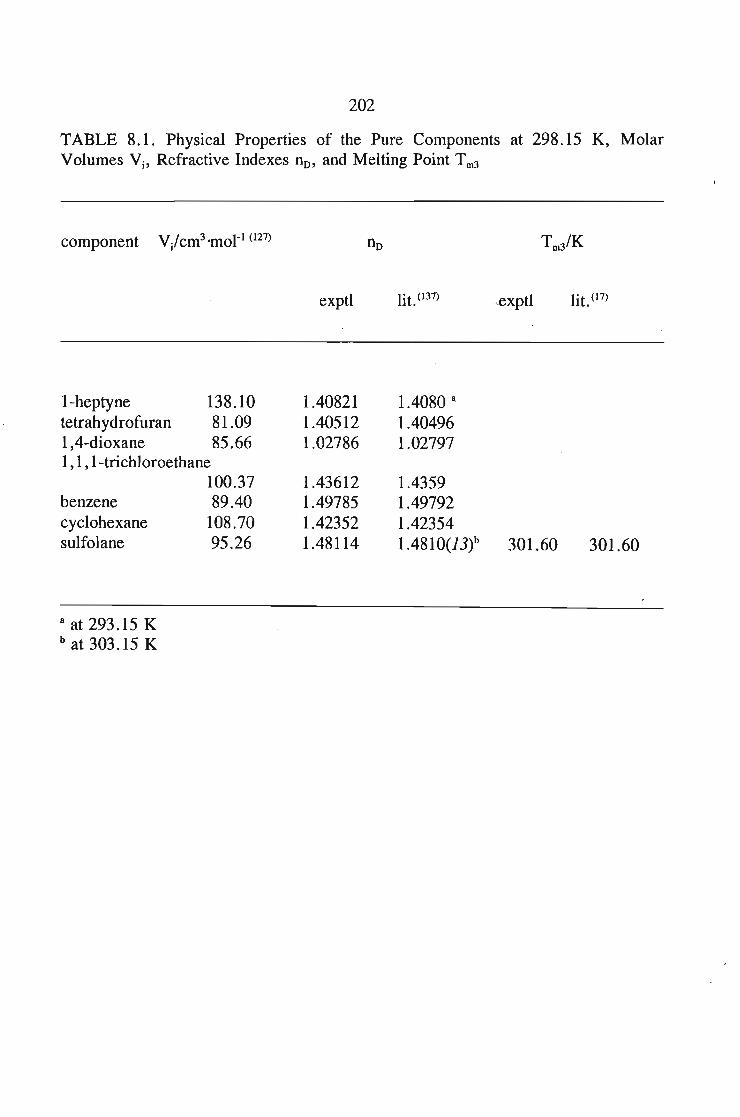
202
TABLE 8.1. Physical Properties of the Pure Components at 298.15 K, MolarVolumes Vi' Refractive Indexes nD, and Melting Point Tm3
component V/cm3 'mol-1 (127)
exptl lit. (137) lit. (17)
1-heptyne 138.10 1.40821 1.4080 8
tetrahydrofuran 81.09 1.40512 1.40496l,4-dioxane 85.66 1.02786 1.027971,1,1-bichloroethane
100.37 1.43612 1.4359benzene 89.40 1.49785 1.49792cyclohexane 108.70 1.42352 1.42354sulfolane 95.26 1.48114 1.481 0(13)b 301.60 301.60
8 at 293.15 Kbat 303.15 K
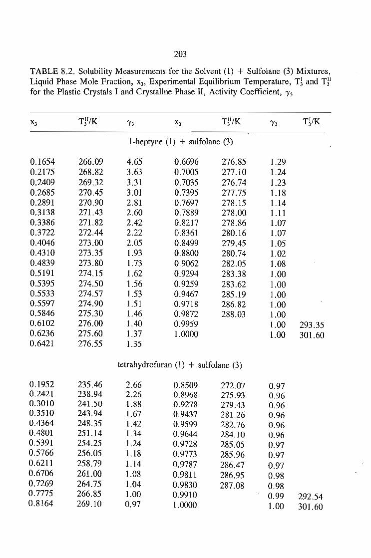
203
TABLE 8.2. Solubility Measurements for the Solvent (1) + Sulfolane (3) Mixtures,Liquid Phase Mole Fraction, x3, Experimental Equilibrium Temperature, T~ and T~I
for the Plastic Crystals I and Crystallne Phase 11, Activity Coefficient, 1'3
x3 T~I/K 1'3 x3 T~I/K 1'3 TVK
I-heptyne (1) + sulfolane (3)
0.1654 266.09 4.65 0.6696 276.85 1.290.2175 268.82 3.63 0.7005 277.10 1.240.2409 269.32 3.31 0.7035 276.74 1.230.2685 270.45 3.01 0.7395 277.75 1.180.2891 270.90 2.81 0.7697 278.15 1.140.3138 271.43 2.60 0.7889 278.00 1.110.3386 271.82 2.42 0.8217 278.86 1.070.3722 272.44 2.22 0.8361 280.16 1.070.4046 273.00 2.05 0.8499 279.45 1.050.4310 273.35 1.93 0.8800 280.74 1.020.4839 273.80 1.73 0.9062 282.05 1.080.5191 274.15 1.62 0.9294 283.38 1.000.5395 274.50 1.56 0.9259 283.62 1.000.5533 274.57 1.53 0.9467 285.19 1.000.5597 274.90 1.51 0.9718 286.82 1.000.5846 275.30 1.46 0.9872 288.03 1.000.6102 276.00 1.40 0.9959 1.00 293.350.6236 275.60 1.37 1.0000 1.00 301.600.6421 276.55 1.35
tetrahydrofuran (1) + sulfolane (3)
0.1952 235.46 2.66 0.8509 272.07 0.970.2421 238.94 2.26 0.8968 275.93 0.960.3010 241.50 1.88 0.9278 279.43 0.960.3510 243.94 1.67 0.9437 281.26 0.960.4364 248.35 1.42 0.9599 282.76 0.960.4801 251.14 1.34 0.9644 284.10 0.960.5391 254.25 1.24 0.9728 285.05 0.970.5766 256.05 1.18 0.9773 285.96 0.970.6211 258.79 1.14 0.9787 286.47 0.970.6706 261.00 1.08 0.9811 286.95 0.980.7269 264.75 1.04 0.9830 287.08 0.980.7775 266.85 1.00 0.9910 0.99 292.540.8164 269.10 0.97 1.0000 1.00 301.60
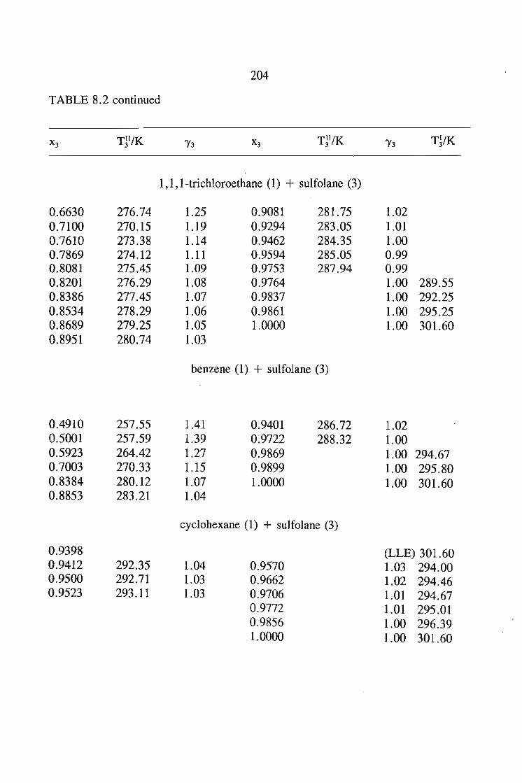
TABLE 8.2 continued
204
1'3 TjlK
1,1,1-trichloroethane (1) + sulfolane (3)
0.6630 276.74 1.25 0.9081 281.75 1.020.7100 270.15 1.19 0.9294 283.05 1.010.7610 273.38 1.14 0.9462 284.35 1.000.7869 274.12 1.11 0.9594 285.05 0.990.8081 275.45 1.09 0.9753 287.94 0.990.8201 276.29 1.08 0.9764 1.00 289.550.8386 277.45 1.07 0.9837 1.00 292.250.8534 278.29 1.06 0.9861 1.00 295.250.8689 279.25 1.05 1.0000 1.00 301.600.8951 280.74 1.03
benzene (1) + sulfolane (3)
0.4910 257.55 1.41 0.9401 286.72 1.020.5001 257.59 1.39 0.9722 288.32 1.000.5923 264.42 1.27 0.9869 1.00 294.670.7003 270.33 1.15 0.9899 1.00 295.800.8384 280.12 1.07 1.0000 1.00 301.600.8853 283.21 1.04
cyclohexane (1) + sulfolane (3)
0.9398 (LLE) 301.600.9412 292.35 1.04 0.9570 1.03 294.000.9500 292.71 1.03 0.9662 1.02 294.460.9523 293.11 1.03 0.9706 1.01 294.67
0.9772 1.01 295.010.9856 1.00 296.391.0000 1.00 301.60
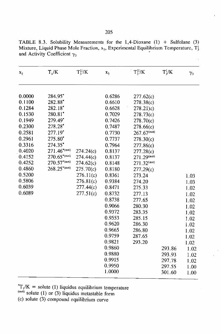
205
TABLE 8.3. Solubility Measurements for the 1,4-Dioxane (1) + Sulfolane (3)Mixture, Liquid Phase Mole Fraction, x3 , Experimental Equilibrium Temperature, T~and Activity Coefficient "13 .~ -
0.00000.11000.12840.15300.19490.23000.25810.29610.33160.40200.41520.42520.48600.52000.58060.60390.6089
T/K Tjl/K
284.95"282.88"282.18"280.81"279.49"278.28"277.19"275.80"274.35"271.46"(met) 274-.24(c)270.65"(met) 274.44(c)270.57"(met) 274.62(c)268.25"(met) 275.70(c)
276.11(c)276.81(c)277.44(c)277.51(c)
0.62860.66100.66280.70290.74260.74870.77300.77370.79640.81370.81370.81480.81800.83610.93840.84710.87320.87380.90660.93720.95530.96200.96650.97590.98210.98600.98800.99150.99501.0000
. Tjl/K
277. 62(c)278.38(c)278.21)c)278.73(c)278.70(c)278.66(c)267. 67(met)
278.30(c)277.86(c)277.28(c)271 .29(met)271. 32(met)
277.29(c)273.24274.20275.33277.13277.65280.30283.35285.15286.30286.80287.65293.20
T1/K3
293.86293.93297.78297.55301.60
1.031.031.021.021.021.021.021.021.021.021.021.021.021.021.021.001.00
"T/K = solute (1) liquidus equilibrium temperature(met) solute (1) or (3) liquidus metastable form(c) solute (3) compound equilibrium curve
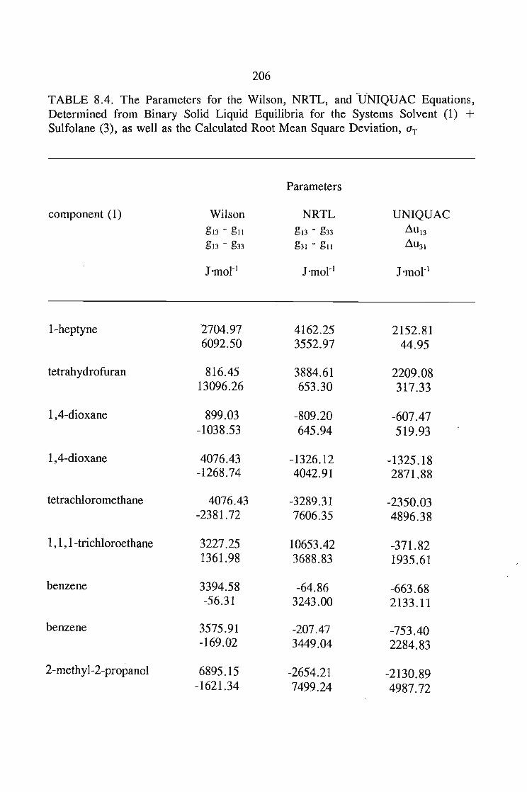
206
TABLE 8.4. The Parameters for the Wilson, NRTL, and~UNIQUAC Equations,Determined from Binary Solid Liquid Equilibria for the Systems Solvent (1) +Sulfolane (3), as well as the Calculated Root Mean Square Deviation, aT
Parameters
component (1) Wilson NRTL UNIQUACgl3 - gll gl3 - g33 dUl3
gl3 - g33 g31 - gll dU31
J 'mol- I J 'mol- I J ·mol- I
I-heptyne 2704.97 4162.25 2152.816092.50 3552.97 44.95
tetrahydrofuran 816.45 3884.61 2209.0813096.26 653.30 317.33
1,4-dioxane 899.03 -809.20 -607.47-1038.53 645.94 519.93
1,4-dioxane 4076.43 -1326.12 -1325.18-1268.74 4042.91 2871.88
tetrachloromethane 4076.43 -3289.31 -2350.03-2381.72 7606.35 4896.38
1,1,I-trichloroethane 3227.25 10653.42 -371.821361.98 3688.83 1935.61
benzene 3394.58 -64.86 -663.68-56.31 3243.00 2133.11
benzene 3575.91 -207.47 -753.40-169.02 3449.04 2284.83
2-methyl-2-propanol 6895.15 -2654.21 -2130.89-1621.34 7499.24 4987.72
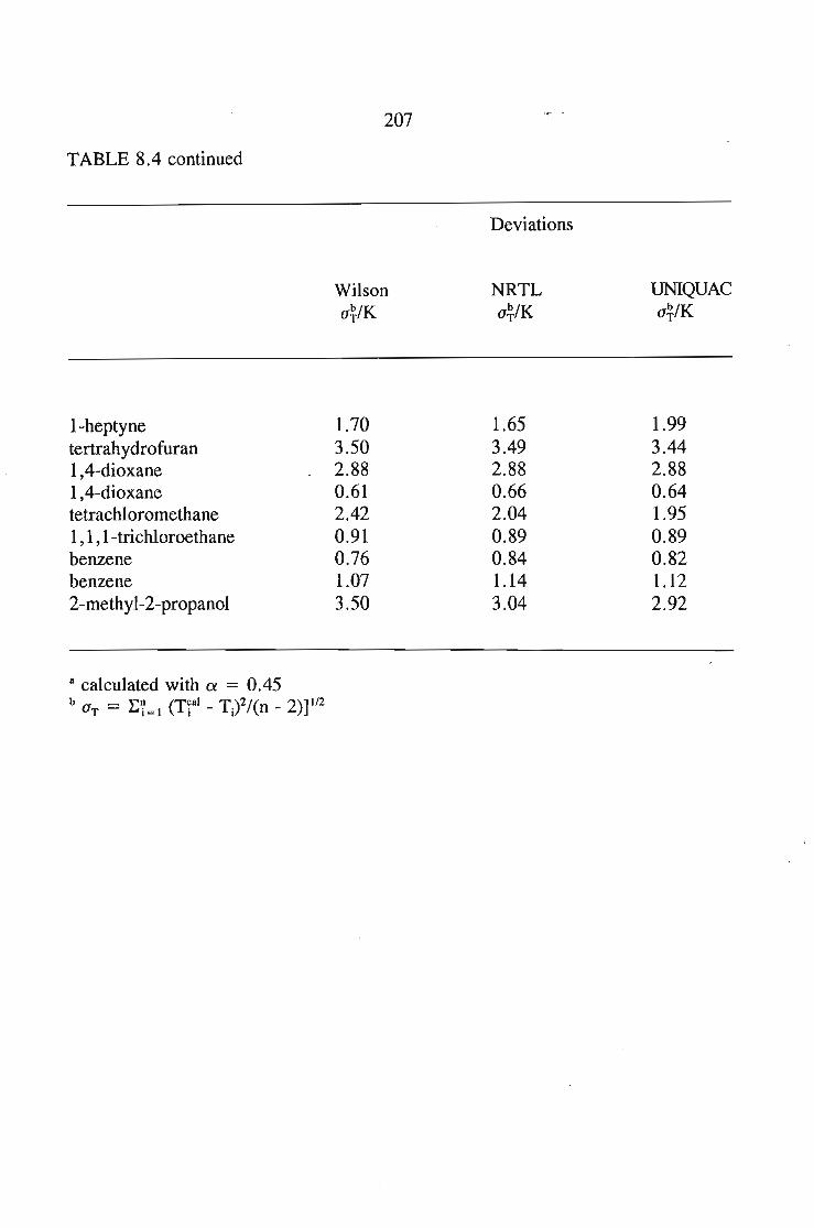
TABLE 8.4 continued
207
Wilsona~/K
Deviations
NRTLa~/K
UNIQUACa~/K
I-heptyne 1.70 1.65 1.99tertrahydrofuran 3.50 3.49 3.441,4-dioxane 2.88 2.88 2.881,4-dioxane 0.61 0.66 0.64tetrachloromethane 2.42 2.04 1.951,1,I-trichloroethane 0.91 0.89 0.89benzene 0.76 0.84 0.82benzene 1.07 1.14 1.122-methyl-2-propanol 3.50 3.04 2.92
a calculated with ex = 0.45b aT = E?=l (T~a' - TY/(n _ 2)]1/2
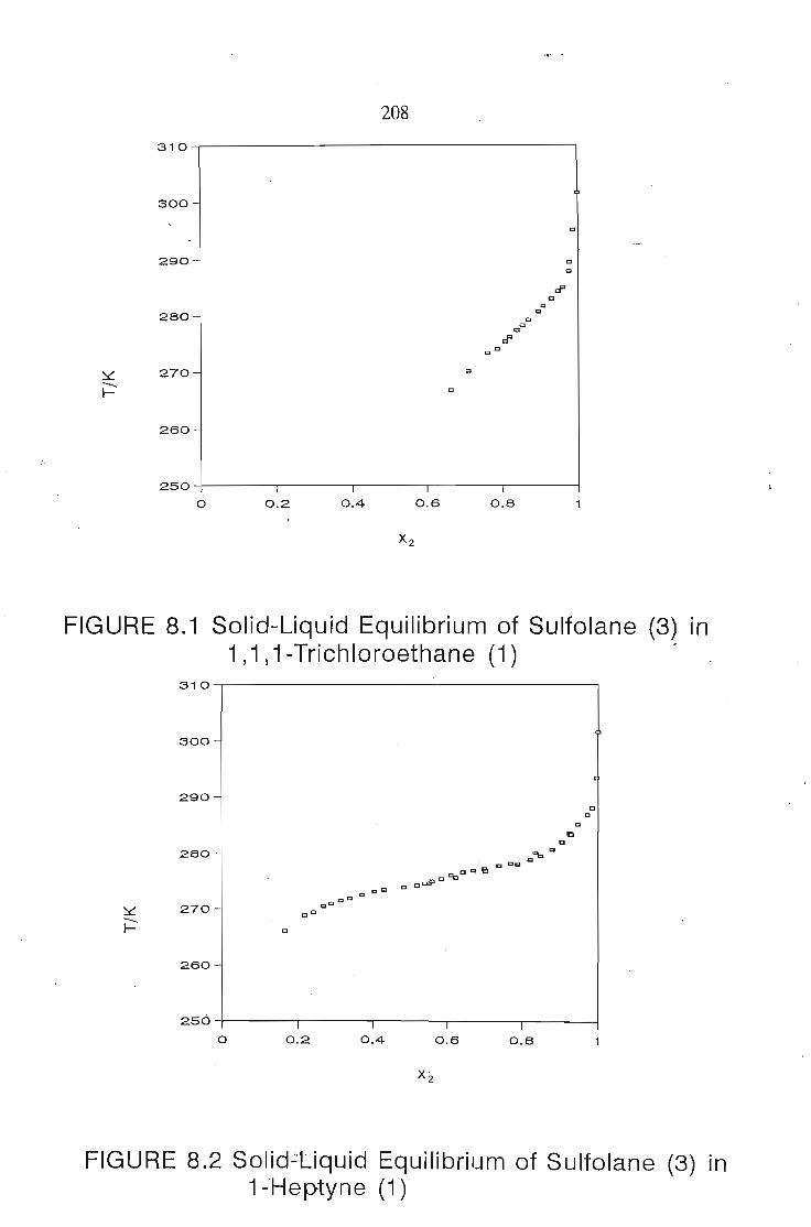
208310.....,.-------------------,
300-
c
290- c
'"rF'
'"'"'"280-C
C
C
cl'C
~ 270- c-f-260-
1o250 ---1-----..1---.--1 --.--1 --.-1 --------1
0.2 0.4 0.6 0.8
FIGURE 8.1 Solid-Liquid Equilibrium of Sulfolane (3) In1,1,1-Trichloroethane (1)
31O~----------------,
300-
,290-
CC
~-f-280-
270-
Ca'"CC
CC
260-
1o250 -I----..I-----,Ir---Ir---.--I---1
0.2 0.4 0.6 0.8
FIGURE 8.2 Solid.::tiquid Equilibrium of Sulfolane (3) In1-'Heptyne (1)
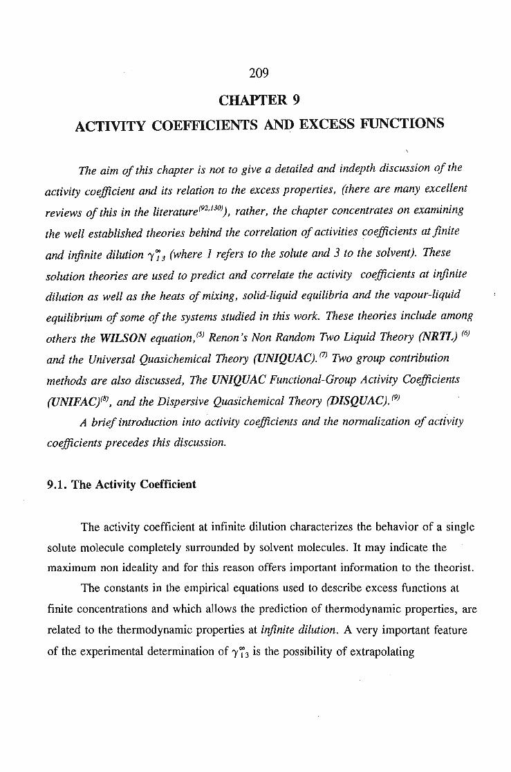
209
CHAPTER 9
ACTIVITY COEFFICIENTS AND EXCESS FUNCTIONS
The aim of this chapter is not to give a detailed and indepth discussion of the
activity coefficient and its relation to the excess properties, (there are many excellent
reviews of this in the literature(92,J30)), rather, the chapter concentrates on examining
the well established theories behind the correlation of activities coefficients at finite
and infinite dilution "173 (where 1 refers to the solute and 3 to the solvent). These
solution theories are used to predict and correlate the activity coefficients at infinite
dilution as well as the heats ofmixing, solid-liquid equilibria and the vapour-liquid
equilibrium of some of the systems studied in this work. These theories include among
others the W/LSON equation, (5) Renon's Non Random Two Liquid Theory (NRTL) (6)
and the Universal Quasichemical Theory (UN/QUAC). (7) Two group contribution
methods are also discussed, The UN/QUAC Functional-Group Activity Coefficients
(UN/FAC/8), and the Dispersive Quasichemical Theory (D/SQUACj. (9)
A brief introduction into activity coefficients and the normalization ofactivity
coefficients precedes this discussion.
9.1. The Activity Coefficient
The activity coefficient at infinite dilution characterizes the behavior of a single
solute molecule completely surrounded by solvent molecules. It may indicate the
maximum non ideality and for this reason offers important information to the theorist.
The constants in the empirical equations used to describe excess functions at
finite concentrations and whicb allows the prediction of thermodynamic properties, are
related to the thermodynamic properties at infinite dilution. A very important feature
of the experimental determination of "I~3 is the possibility of extrapolating
210
measurements to finite concentrations. Once both 'Y73 and 'Ye;' 1 are known, the binary
parameters for any of the two parameter models discussed later, can be determined
and hence the prediction of 'Yl and 'Y3 at any concentration is possible.
Infinitely dilute solutions are also well suited to the application of statistical
mechanical perturbation theory: since solvent-solvent interactions dominate, the solute
solvent interactions can be regarded as perturbation about a pure substance. (130)
The activity coefficient calculated from the experimental work, 'Y73' can be
used for making a preliminary prediction of partial miscibility. (130) An attractive
application of infinite dilution information is the prediction of solubility in dense gases
at supercritical conditions starting from Henry's constants of gases in liquids through
extrapolation in respect to pressure and composition. (130)
Measurements of 'Y73 are now of increasing interest in chemical technology.
These values, which describe highly dilute solutions, can be related to the high-purity
requirements in health-related products in pharmacology and biotechnology and to the
packaging of foods, medicines and other items for human consumption. (146) 'Y73 are
also very important in understanding physical separations as used in most processes to
obtain a desired product, to recover unreacted material, or to remove byproducts. (146)
Quantitative information on phase equilibria and hence 'Y73 data is needed for
the design of various separation units involving techniques such as separation
distillation, extraction, absorption and stripping.
211
9.2 Normalization of Activity Coefficients
It is convenient to define activity coefficients in such a way that for an ideal
solution, the activity is equal to the mole fraction or, equivalently, that the activity
coefficient is equal to unity. Two types of solution ideality (one leading to Raoult's
law, and the other to Henry's law), have been defined. It follows that activity
coefficients may be normalized (ie. become unity) in two different ways.
If defined on the basis of Raoult's law, then for each component i the normalization
definition is(92)
as (9.1)
Since this normalization holds for both the solute and the solvent, eq. (4.9) is called
the symmetric convention for normalization and applies always to liquid mixtures.
However if activity coefficients are defined with reference to an ideal dilute
solution then (Henry's Law)
as Xl -0 1 (solvent)
as x3 -> 0 (solute).(9.2)
Since the solute and the solvent are not normalized in the same way, equation
9.2 gives the unsymmetrical convention for normalization. To distinguish between
symmetrical and unsymmetrical normalization, it is useful to denote with an asterisk
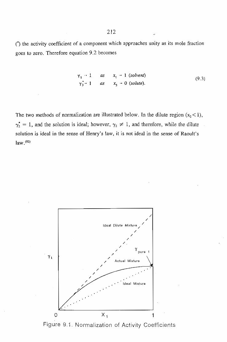
212
() the activity coefficient of a component which approaches unity as its mole fraction
goes to zero. Therefore equation 9.2 becomes
as Xl'" 1 (solvent)
as X3 '" 0 (solute).(9.3)
The two methods of normalization are illustrated below. In the dilute region (x2 < 1),
'Y; = 1, and the solution is ideal; however, 'Y2 ;c 1, and therefore, while the dilute
solution is ideal in the sense of Henry's law, it is not ideal in the sense of Raoult's
law. (92)
ypure 1
Actual Mixture
Ideal Mixture
o X 1 1
Figure 9.1. Normalization of Activity Coefficients
213
9.3. The Relationship Between Activity coefficients and Excess Functions in
Binary Mixtures
Many equations have been proposed for the correlating of activity coefficients
with composition and to a lesser extent with temperature. Some of the have been done
on purely empirical grounds, others on more rational grounds. Usually the
composition is expressed in mole fractions, Xi' (where i refer,s ~o component i in a
mixture) but the use of volume fractions or molecular surface fractions may be
preferable when the molecules differ substantially in size and chemical nature.
At a fixed temperature, the molar excess Gibbs energy GE of a liquid mixture
depends on the composition of the mixture and, to a smaller extent, on pressure.
Considering a binary solution where the excess properties are taken with reference to
an ideal solution wherein the standard state for each component is the pure liquid at
the temperature and pressure of the mixture. In this case, any expression for the molar
excess Gibbs energy must obey the two boundary conditions:
when
when(9.4)
9.3.1. The two sufTlX MARGULES EQUATION
The oldest of the formulas still in common use is that of Margules(l2) (1895)
The simplest non-trivial expression which obeys these boundary conditions is
214
(9.5)
where A is an empirical constant with units of energy, characteristic of component I
and 3, which depend on the temperature but not on composition.
From the relation
we obtain an expression for the activity coefficients
E anpER11ny; = G j = (a )T,P,n
n. 1I
where nj is the number of moles of i and nr is the total number of moles.
remembering that Xl = nl/nT and Xz = '1.J.!nT, we obtain
A 2my! = -x3RT
(9.6)
(9.7)
(9.8)
(9.9)
Equations 9.8 and 9.9 give the two suffix MARGULES EQUATION.(IZ) These
215
simple relationship usually give a good representation for many simple liquids ie., for
mixtures of molecules which are similar in size, shape and chemical nature. The two
equations are symmetrical.
At infinite dilution the activity coefficients of both components are equal:
The excess Gibbs energy can be written as
A= exp(-)
RTA
= exp(R~'
(9.10)
where A and B are two adjustable parameters.
9.3.2. The Redlich-Kister Expansion
(9.11)
Equation 9.11 is a very simple relation. In the general case, a more complex
equation is needed to represent adequately the excess Gibbs energy of a binary
solution.
An expansion similar to that of equation 9.11 is that of Ridlich & Kister(llO) (1948):
(9.12)
216
where the additional parameters B, C, D, ... are temperature dependant parameters
which must be determined from experimental data. Using equation 9.12 we obtain for
the activity coefficients these expressions,
(9.13)
(9.14)
The number of parameters (A, B, C....) which should be used to represent the
experimental data depends on the molecular complexity of the solution, on the quality
of the data, and on the number of experimental points available.
The Ridlich-Kister expansion provides a flexible algebraic expression for
representing the excess Gibbs energy of a liquid mixture.
An equation due to Scathard and Hamer(147) (1935) uses volume fractions as a
measure of composition, ie.
The expression for the Gibbs energy is given by
(9.15)
(9.16)
217
from which the activity coefficients are obtained as
(9.17)
(9.18)
This system takes into account an important difference between molecules and
should possibly have a role to play in the representation of data, but because it is
slightly more complex than other methods, it does not receive much attention
nowadays.
9.3.3. Wohl's Expression for the Excess Gibbs Energy
Wohl's expresses the Gibbs energies(J48) of a binary solution as a power series
in Zl and Z3' the effective volume fraction of the two components:
where
218
(9.20)
Wohl's equation contains two types of parameters, q's and a's. The q's are the
effective volumes, or cross sections, of the molecules: qj is a measure of the size of
the molecule i , or its "sphere of influence "in the solution. A large molecule has a
larger q than a smaller one and, in nonpolar molecules of similar shape, it is often a
good simplifying and important assumption that the ratio of the q's is the same as the
ratio of the pure component liquid molar volumes. The a's are interaction parameters
who physical significance is roughly similar to that of the virial coefficients. The
parameter a l3 is a constant characteristic of the interaction between molecule 1 and
.molecule 3; the parameter all3 is a constant characteristic of the interaction between
three molecules, two of component 1 and one of component 3 and so on.
One of the main advantages of expressing Gibbs energies as proposed by
Wohl(148) is that rough physical significance can be assigned to the parameters w~ich
appear in the equation. Wohl's expansion can be extended systematically to
multicomponent solutions.
9.3.4. The van Laar Equation
The van Laar equation(l3) considers the case of a binary solution of two
components which are not strongly dissimilar chemically, but which have different
molecular sizes. Making the simplifying assumption that the interaction coefficients
a l3 , a ll3 " ..... and higher, from Wohl's expansion, may be neglected; Wohl's
equation becomes
219
(9.21)
which is the van Laar equation. From this equation the expression for the activity
coefficients are given by;
(9.22)
and
(9.23)
Equations 9.22 and 9.23 are the familiar van Laar equations which are
commonly used to represent activity coefficient data. These equations include
empirical constants, AI, and RI; the ratio of AI to RI is the same as the ratio of In 'Y I to
In 1'3'
The derivation of van Laar equations suggest that they should be used for
220
relatively simple, preferably nonpolar liquids but empirically it has been found that
these equations are frequently used to represent activity coefficients of more complex
mixtures. In the special case when the van Laar constants AI and El are equal, the van
Laar equations are identical to the two-suffix Margules equation.
9.3.5. The WILSON, NRTL, and UNIQUAC Equations
Many equations have been proposed for the relation between activity
coefficients and the mole fraction. Some of them can be derived from Wohl's general
method. However three of the most useful of these equations cannot be obtained by
Wohl's formulation.
9.3.5.1. The WILSON Equation
In the development of this equation Wilson(5) (1964) conceived that interactions
between molecules depends primarily on "local concentrations" which he expressed as
volume fractions. Wilson considered the case where the components in a mixture
differ not only in molecular size but also in intermolecular forces. (5) His modifications
are based on a loose semi-theoretical argument's which lack the rigor of the lattice
theory of Guggenheim. (145)
Wilson considered a binary solution of 2 components, component 1, and
component 3. If the central atom is atom 1, the probability of finding a molecule of
type 3, relative to finding a molecule of type 1, around the central molecule 1, is
expressed in terms of the overall mole fraction and two Boltzmann factors:
221
x3exp( - A13/RI)
x1exp( -All/RI)(9.24)
The equation implies that the ratio of number of molecules of type 3 to the ratio
of molecules of type 1 around the central molecule 1 is equal to the ration of the
overall mole fraction of 3 and -1 weighed by the Boltzman's factors exp (-A3l fR1) and
exp (-An fR1). The parameters A3l and An are, respectively, related to the potential
energies (energies of interactions) of 1-3 and a 1-1 pair of molecules.
Wilson now defines local volume fractions using equation 9.24. The local
volume of component 1, designated by ~ I is defined by
(9.25)
where VI and V3 are the molar liquid volumes of components 1 and 3. Substitution
gIves
(9.26)
Similarly, the local volume fraction of component 3 is
(9.27)
The molar excess Gibbs energy of a binary system is given by,
222
(9.28)
In order to introduce simplification Wilson defined two new parameters, A13 and A31
in terms of molar volumes VI and V3 and the energies All' A33 and AI3' (Assuming that
AI3 = A31)'
_ ~I
v A-A__3 exp[ 13 11]
VI RT
v A-A__I exp[ 13 33]
V3 RT
(9.29)
(9.30)
Wilson's equation for the excess Gibbs energy now becomes
(9.31)
According to Wilson's model X 31 + Xli = 1 and X 13 + X 33 = 1. The sum of ~ I and
~3 is not unity except in the limiting case where A 13 = A 11 = A33 = A 31'
The activity coefficients derived from this equation are given by
223
(9.32)
(9.33)
To a fair approximation, the difference in characteristic energies 0'-13 and All) are
independent of temperature, at least over modest temperature intervals. As a result,
Wilson's equation gives not only an expression for the activity- coefficient as a
function of composition but also an estimate of the variation of the activity coefficients
with temperature. (92)
Wilson's equation provides a good representation of excess Gibbs energies for a
variety of miscible mixtures. It is particularly useful for solutions of polar or
associating components (eg. alcohols) in nonpolar solvent.
At infinite dilution the Wilson's equations reduce to
(9.34)
(9.35)
9.3.5.2. Renon's NonRandom Two-Liquid (NRTL) Equation
224
The NRTL (nonrandom two-liquid) equation(6) is based on the two cell
theory. (92) Here it is assumed that the liquid has a structure made up of cells of
molecules of type 1 and 3 in a binary mixture, each surrounded by assortments of the
same molecule, with each of the surrounding molecules in turn surrounded in a similar
manner, and so on. Gibbs energies of interaction between molecules are identified by
gij where the subscript j refers to the central molecule and mol fractions in the
surrounding region, xij' are identified in the same way.
Gibbs energies for the two kinds of cells are
(9.36)
(9.37)
where gll and g33 are the Gibbs energies of the pure substances and the assumptions is
made that g13 = gl3- The excess Gibbs energy for the assemble of cells becomes
(9.38)
The local mole fractions, xij' are given by equations similar to Wilson's Equations
X31 x3exp( -a.l~31/R1)-=Xll Xl exp( -a.l~llIR1) ,
(9.39)
225
X13 XI exp(-a.I~IJR1)-= ,X33 x3exp(-a.l~3JR1)
(9.40)
The significance of gij is similar to that of A ij in Wilson's equation; gij is an energy
parameter characteristic of an i-j interaction. The parameter an is related to the
nonrandomness in the mixture. When a 13 is zero, the mixture is completely random
and reduces to the two suffix MARGULES equation.
Since
(9.41)
the local mole fraction may be solved as
(9.42)
(9.43)
Substituting these into equation 9.38 the final equation for the excess Gibbs energy
226
becomes
't GGE/RT-xx[ 3131
- 1 3 GXl +X3 31
where
(9.44)
The activity coefficients are obtained by differentiation as
(9.45)
(9.46)
(9.47)
(9.48)
(9.49)
227
(9.50)
The NRTL has three parameters, but reduction of experimental data for a large
number of binary systems indicates that an varies from about 0.20 to 0.47. (92)
At infinite dilution, when an can be estimated the equations reduce to
(9.51)
and
(9.52)
9.3.5.3. The Universal Quasi-chemical (UNlQUAC) Equation
Abrams(7) derived an equation which, in sense, extends the quasichemical theory
of Guggenheim(l45) for a nonrandom mixture of solutes containing molecules of
different size. The extension is called the Universal Quasi-Chemical Theory
(UNIQUAC in short). The UNIQUAC equation for the excess Gibbs energy (GE)
consists of two parts, a combinatorial part which attempts to describe the dominant
entropic contribution and a residual part which is due primarily to intermolecular
forces that are responsible for the enthalpy of mixing. The combinatorial part is
determined only by the composition, sizes and shapes of the molecules; it also
requires only pure-component data. The residual part, however, depends also on the
228
intermolecular forces; the two adjustable binary parameters, therefore, appear only in
the residual part. The UNIQUAC equation is(7)
G E = G E(combinatorial) + G E(residual) .
For a binary mixture,
G E( b' . l) ~o ~o e ecom znatorza =X In_I +x In_3 +~(q X In_I +q_r.1n_3)
RT I 3 2 I I 0 Y-3 0
Xl X3 ~l ~3
(9.61)
(9.54)
(9.55)
where z is the coordination number (considering molecules 1 and 3 the nearest number
of touching neighbors is defined as the coordination number). It may have a value
between 6 and 12 depending on the type of packing, ie. the way in which the
molecules are arranged in three dimensional space; empirically, for typica11iquids at
ordinary conditions, z is close to 10. <po is the segment fraction and (J and (Jf are the
area fractions given by(92)
4» 0 = __A._I_'l__1 (9.56)
.4 t(h6t = ----XIql + X3Q3
229
(9.57)
(9.58)
Parameters r, q and q are pure component molecular structure constants depending on
molecular size and external surface areas, where r is the volume of the molecule and q
and q the surface area of the molecule. In the original formulation q = q. To obtain
better agreement for the systems containing water or lower alcohols, the q values for
water or alcohols are adjusted empirically by Anderson(149) to give an optimum fit to a
variety of systems containing these components. For alcohols, the surface of
interaction q is smaller than the geometrical external surface q, suggesting that
intermolecular attraction is dominated by the OH group (ie. hydrogen bonding).
For each binary mixture, there are two adjustable parameters, Tl3 and T 31 •
These, in turn are given by the characteristic energies ~ Un and ~ U31 by
dUI3 at3~13 = exp(------) = exp(----)
RT T(9.59)
230
aU21 aZl't Z1 = exp(---) == exp(--) .
RT T
Activity coefficients 'Yl and 'Y3 are given by
and
where
(9.60)
. (9.61)
(9.62)
(9.63)
231
(9.64)
The advantages of UNIQUAC is that it is easily applicable to multicomponent
mixtures, in terms of binary parameters only. Also it is applicable to liquid-liquid
equilibrium. It has a built in temperature dependence valid over at least moderate
range, and it form the basis for a group contribution method, from properties of the
pure components.
9.4. Group Contribution Methods
Statistical thermodynamics establishes relationship via the partial
function, between the equilibrium properties ofa system and the energy of its
microscopic states. If the system is a mixture, if the property is a thermodynamic
excess function, and if the internal degrees offreedom of the molecule are separable
from the other degrees offreedom and are the same in the pure components and in the
mixture, then the excess properties are related to the energy of intermolecular
interactions via the configurational partition function. (150)
Organic molecules which belong to a given homologous series contain varying
numbers of the same kind of 'segment' or 'groups'. For physical obvious reasons one
may expect that the interaction energy of a given pair of groups will depend less on
the nature of the molecules, than on the nature of the groups themselves. The most
general definition, or assumption, of the group contribution method is that with
conveniently defined groups the configurational energy is given by the sum of group
232
interaction energies. This definitions concerns only the molecular interaction
model. (ISO) If no experimental data are available to fit the required binary pa
rameters, group contribution methods can be said to predict the missing equilibrium
information. In group contribution methods it is assumed that the mixture does not
consist of molecules, but instead, of functional groups. The great advantage of the
11 solution of groups 11 concept is that the number of functional groups is much smaller
than the number of possible compounds. This means that the.behavior of a large
number of systems of interest can be predicted with a limited number of group
interaction parameters. (151)
There are also obvious theoretical shortcomings of these methods. Most cannot
account for induction effects due to neighboring groups (for example a CH2 -OH
interaction is the same whether electron withdrawing or electron supplying groups are
attached next to them on the backbone). (152)
9.4.1. Definition of Groups(150)
The application of a group contribution method require, first of all, a clear
definition of the ensemble of groups taken into consideration. These methods are
useful when the population of 'components' is much larger than the 'groups'. It makes
no sense to apply the method to single-group components which have never been
investigated in mixtures with poly-segmented molecules. However when a defined
group is too large with respect to the average intermolecular distance, then its
interaction potential may become so complex, that no existing theory may describe it
conveniently. (ISO)
The two most widely used group contribution methods at the moment are the
233
UNIFAC (UNIQUAC Function-Group Activity Coefficients) model(8) and DISQUAC
(The Dispersive Quasichemical) model. (9) Both these methods are discussed below.
9.4.2. UNIFAC (UNlQUAC Functional-Group Activity Coefficient Model)
UNIFAC is a functional group technique developed from the UNIQUAC
(UNiversal QuasiChemical) method for the correlation of excess Gibbs energies. As
such, UNIFAC uses the same surface and segment constants for the pure components
as the original UNIQUAC model, but uses group-group interactions to model the
mixing nonidealities rather than regressed parameters.
UNIFAC implies that the activity coefficient consists of two terms:(150)
(9.73)
The combinatorial part (In 'Y7) takes into account the size and the form of the
molecules. In the residual part (in 'Y~) the interactions between the various groups are
considered. Both parts are based on the UNIQUAC equation. In addition the group
interaction parameters anm and ann" group volume parameters, Rk , and surface
parameters, Qk' are involved. The configurational part is the same as the UNIQUAC
equation (see 9.3.5.3).
In UNIFAC the composition of the system is expressed in terms of the groups
and not in terms of the mole fraction of the components, for example, Vki = the
number of atoms other than H (hydrogen) of group k in molecule i. (150)
The total number of groups in the mixture is given by
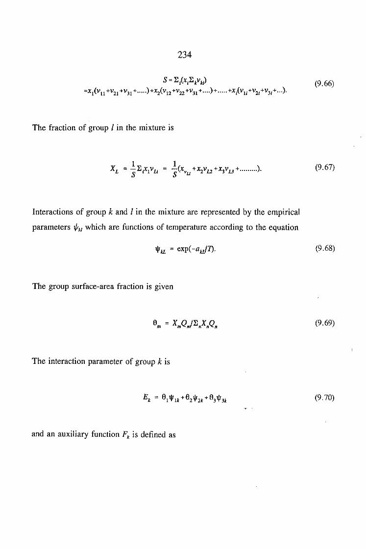
234
s = ~i(Xi~AYki)
=X1(VU
+V21 +V31 +•••••)+X2(V12 +V22 +V31 + ....)+ ..... +Xj(V}j+V2i+V3j+···)·
The fraction of group I in the mixture is
Interactions of group k and I in the mixture are represented by the empirical
parameters t/;kl which are functions of temperature according to the equation
1VkL = exp(-au!1).
The group surface-area fraction is given
The interaction parameter of group k is
and an auxiliary function Fk is defined as
(9.66)
(9.67)
(9.68)
(9.69)
(9.70)
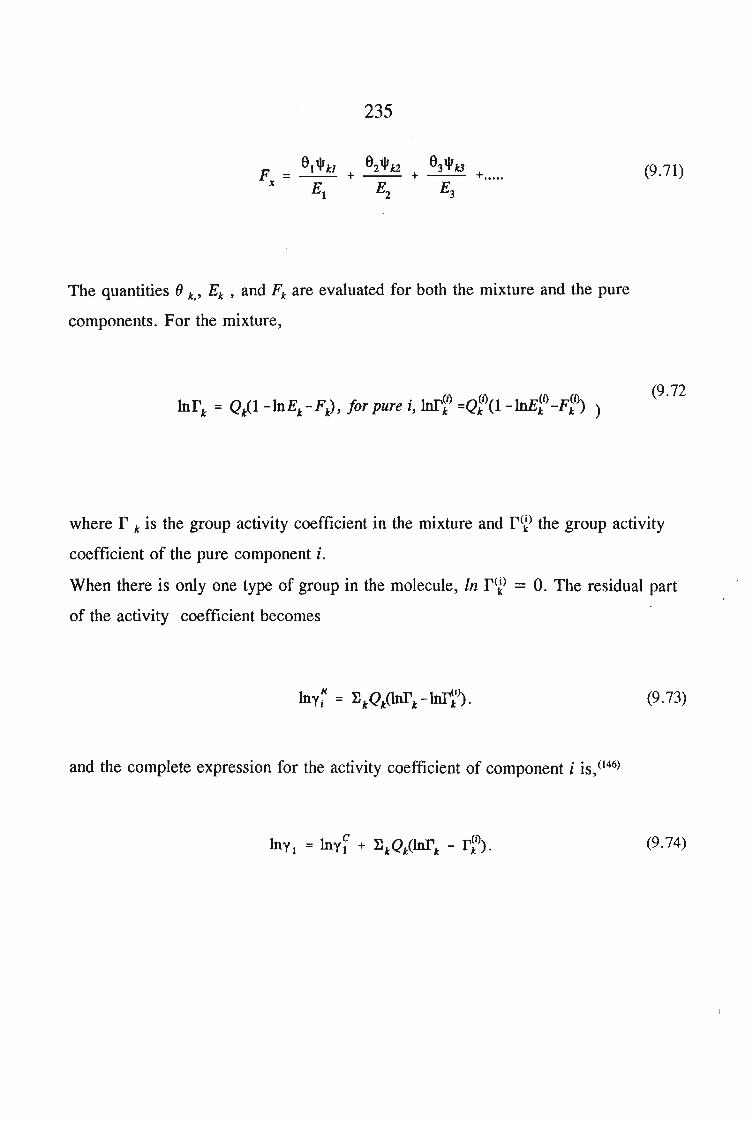
235
F = 8t1JrkJx E
1
(9.71)
The quantities () k,' Ek , and Fk are evaluated for both the mixture and the pure
components. For the mixture,
(9.72
where r k is the group activity coefficient in the mixture and r(~) the group activity
coefficient of the pure component i.
When there is only one type of group in the molecule, In r(~) = O. The residual part
of the activity coefficient becomes
(9.73)
and the complete expression for the activity coefficient of component i is, (146)
(9.74)
236
9.5.3. The Dispersive Quasichemical (DISQUAC) Theory
DISQUAC(9) is a simple extension of the quasi-chemical theory. It resembles
the theory of non-athermal associated solutions. In this theory the 'chemical'
contribution is supplemented by a random-mixing 'physical' contribution. In
DISQUAC the same random-mixing contribution supplements the known qasi
chemical expression. Each contact, either polar or non-polar, is thus characterized by
a dispersive interchange energy, a single parameter, and the polar contacts by two
additional parameters, the quasi-chemical interchange energy and the coordination
number.
The dispersive and the quasi-chemical are calculated independently and simply
added together. Therefore, the contact surfaces are not uniquely defined. There is one
set for the dispersive contribution and one set for the quasichemical contribution.
9.4.3.1. Theory of DISQUAC(145)
9.4.3.1.1. The Configurational Partition Function
In a mixture of c components i in which N; is the molecules of the type i, the total
number N molecules in the system is :
N = "r..N.I I
and the mole fraction of component i is
(i = 1,2,3, ......,c)
Xj = N;lN
(9.75)
(9.76)
237
Each type of molecule is characterized by a characteristic surface q. The total surface
of all the molecules of type i is
(9.77)
and the total surface of all the molecules in the system is
(9.78)
Therefore we can express the surface ratio of component i in the mixture as (9)
(9.79)
and the total surface of all the molecules of type i as
(9.88)
To account for the entropic effect of the mixing process, consider the volume r j of the
molecule i. The volume fraction of the component i is:
Each molecule is composed of different groups, therefore each molecule has
238
(9.81)(i,j = 1,2, ......c)Tf,
<1>,=-~lfj
different types of surfaces, each being characterized by different interaction potentials.
If we concider the area of surface type s on a molecule of type i by
q .=U .q.(s=a,b"....a;i=I,2, .....c)SI SI/
(9.82)
where the total surface of type s on all types of molecules in the system is
A =AuS S
(9.83)
where
(9.84)
is the swface ratio of surface type s in the system, and by definition
~ u = 1S S
(9.85)
Assuming that the molecules in the mixture are in contact with one another over AU
their surface, independent of their relative positions (configuration), then the total
surface of contact is one half of the surface of the molecules. (9)
239
A 1- = - N("T. .q.r..)2 2 I n
(9.86)
However we have to distinguish between different types of contacts; contacts
between surfaces of the same type (ss) and between surface of different types (sI). We
denote the different areas of contact for a particular configuration (c) by Acss and ACSl
respectively. Since a surface of type s can be in contact with either another surface of
type s or a different surface of type 1, the. contact must obey the conservation
equation
2A~ + ~,As~ = Aas (s =a,b, ....0) (9.87)
Thus, the total configurational energy if is the sum of the interactional energies per
unit of contact surface for the two types of contact (ss) and (sI), we now have
(9.88)
where the double sum is take over all contacts between unlik~ pairs of surfaces (si).
After substituting AC
ss by its value from equation 9.86 we get
240
(9.89)
where the quantities
(9.90)
are by definition the Interchange Energies. (9)
In particular homologous molecules, when all the LlE s1 = 0, the configurational
energy no longer depends on the system configuration and at a given composition Ni
has a constant value.
The configurational partition function, 0, of the system is given by
vcn =}J exp(--)C kT
(9.91)
(9.92)
where the sum is taken over all possible configurations of the system, each
configuration being characterized by its configurational energy if. From equation 9.92
we see that [f/kt is a function of the contact surface A\/,
241
(9.93)
With gC denoting the Combinatorial factor for the system (ie. the number of
configurations corresponding to a given value of if., equation 9.89 becomes
(9.94)
where the sum is taken over all possible energies if.
Assuming that there is one energy (ie. the energy at equilibrium) for which the term
gC exp{-if/kt} is large compared to all the other terms and consequently without
introducing any appreciable error we can write eq. 9.92 as
U C UCl = [g Cexp(--)] = gexp(--)kT max kT
(9.95)
The equilibrium values of U and g can be obtained by maximizing the function
gCexp{-UC/kt}. For this we must calculate the partial derivatives of the logarithm of (}
with respect to the variables Acs/' and the solve the system of equations obtained by
putting all the derivatives to zero. However we first have to express the combinatorial
factor gC as a function of Acs/" Here the Quasichemical approximation of the lattice
model used by Guggenheim(l45) is applied. (9)
Secondly, assuming that there are a certain number of different ways of having
contact between two given elements of surface. Let z be this coordination number. It
242
represents the number of possible orientations that can exist between two surfaces in
contact. The total number of orientations is the zA/2 and for each type of contact (ss)
and (st) it is equal to zAss and zAsI. respectively.
If we neglect any interference between different types of orientations of the
various types of contacts, the number of configurations of the system, for a given
energy would be
(zA/2)!(9.96)
where the product 7rsl is extended to all the ordered pairs (st). But the number is
certainly to large because of interferences and therefore we introduce a correction
factor, h, assume to be a function of only the Ni
g C=h (zA/2)!
1ts(zA;)l1tizAsd2)!(9.97)
The value for h is obtained considering the case of mixtures of homologous molecules
for which the combinatorial factor g" can be found. Since all the configurations have
the same energy, the energetic factor does not influence the equilibrium values A "si.
and A"SS" of the contact surfaces. These values depend only on the composition of the
mixture or more exactly on the area of the different types of surfaces (zero
approximation). (9)
The value of surface A"Si. and A"SS" in the zeroth approximation are obtained by
maximizing the logarithm of the function gCexp{-r.t/kt}. Using Stirling's formula (eq.
243
4.98) to approximate the factorials we obtain
inN! = NlnN - N
1ng C _ U*/kT= 1nh + (zA/2)In(zA/2) - 1:s(zA~)In(zA~)
_.!.:E :E (zA c/2) - .!.A:E a e IkT2 s1 sll 2 sssi
(9.98)
(9.99)
To avoid confusion in diffrenciating this relation with respect to the variables ACs/, the
current subscripts in the summation are denoted by ell). In the sum (Es/zAcs/s/)ln(zAcs/s/)
only the derivatives of the terms l =s and l = 1are different from zero and we can
write
_a_[:E(zA C l ..(zA C ) = ~1n(zA c)'"C s'siJU s's' s's'
aAs1 aAs~
+(zAs~)In(zA~)
C aA~ C aA1;=z[l + In(zAs:J]-z[1 + In(zA )]-C ss C
aAs1 aAsl
=-~[2 +In(z2A~f~]2
(9.100)
244
where we have used ACs/AcsI = -1/2, obtained from equation 9.88. Furthermore, since
the term Aesl appear twice in the double sum we have
ale e a CIn _A C12)-[-EsE~zA 1 )n(zA 11/2)] =-[(zAsI) (U1s1
e 2 ss S aA caAsI sI
=z[1 + In(zA;)12]
Thus the required derivatives are
c2Z AsI
= --In.--2 4A CA C
ss' "11
(9.101)
(9.102)
and the equilibrium values in the zero approximation, A"ss' A"sl' A"l/ ,are given by the
equations(9)
" A"A"AsI = 4 ss sI (8,[, =a,b".....a) (9.103)
For a different types of surfaces the number of unknowns A "ss and A "Si is equal to a(a
+ 1)/2. The a(a -1)/2 equations 9.103 and the a equations 9':88 form a system of a(a
+ 1) equations from which all the contact surfaces can be calculated. This system of
equations can easily be reduced to a system of a equations by replacing A"Si by their
245
values given by equation 9.103.
Let
then
On substituting in equation 9.88 we obtain
X;JJ;X,* = as (s=a,b, .... a)
Summing all these equations leads to an expression
which become, because of equation 9.86, (E;X/? = 1, and consequently, from
equation 9.106 .
(9.104)
(9.105)
(9.106)
(9.107)
246
X;=a. s (s=a,b, .... cr) (9.108)
These are the solution of the system of equations 9.106 in the zeroth approximation.
The contact surfaces are given by
(9.109)
Now with these values we can write
g* = h (zA/2) I
1ts(zA~)I1tizA;/2)1
and replace h in the equation 9.97 by it value from equation 9.110. Therefore
(zA/2)I1ts~zA;/2)1gC = g* ~ _
1ts(zA~)I1tizAs,2)1
(9.110)
(9.111)
where A·SS' and A·sl have the values given by equation 9.117.
To determine the equilibrium values of A·sI , of the surface ACsI in the general case
247
where if is given by equation 9.102, we follow the same procedure as before,
Ac2
a(lng C - U C/k1) Z st--'--=------'--'"- = --In---
aA c 24A c..d
csi ~"sl
if we let
A = A(X)2ss 2 s
we have at equilibrium
where
.l\ esi" I = exp[--]
s zkT
On substituting As1 in equation 9.88 we obtain the system of (J equations with (J
unknowns Xs-
(9.112)
(9.113)
(9.114)
(9.115)
(9.116)
248
We see that for ~Esi = 0, or 'YJsi = 1, the solution of the equation 9.116 is the zeroth
approximation A"si and A"SS'
By a process of substitution the equilibrium values Am and AsI we obtain in equations
9.88 and 9.111 the configerational energy at equilibrium is obtained
U 1 1- = -A:E a (e Ik1) + -:E :E A '/1e /k1)kT 2 s s sa 2 s rAs[\. s
and the combinatorial factor at equilibrium
* lt s(zA;) l1ti zA:/2)1g =g lt
s(zAs.J! ltizAsJ2)!
(9.117)
(9.118)
These functions, substituted into equation 9.88, completely define the configurational
partition function of the system, and will be used for calculating the excess
thermodynamic functions.
9.4.3.1.2. Excess Free Energy(9)
The configurational free energy, F, of the system is obtained from the
configurational partition function (} according to the relation:
249
F/kT= -InO
For an ensemble of N; molecules of pure component i;
F/kT= -InO;
and the excess free energy P is given by:
FE/kT = -Inn + ~.Inn. - ~ MInx., , r', I
The excess molar chemical potential J-tE j is defined by:
~/RT= a(FElk1) = _ aInn + Inn; -lnx.
~, aN. aN. N. ', "
where R = NAk, NA being the Avogadro number. From equations .
we can write
(9.119)
(4.120)
(9.121)
(9.122)
250
InO ::; 1ng - U/kT
::; lng* + ~s(zA~)ln(zA~)
+ !~ ~ lzA *)In(zA *)2 s l'ss ss
- ~s(zAss)In(zAss)
-!~s~~zAsl)ln(zAsI2)2
1 1-2A~i1.sf,JkT - 2 ~s~,4s1AEslkT
(9.123)
Differentiation of In n w.r. t Ni can be carried put considering the contact surface A "si
and A"ss to be constant since we know that the partial derivatives w.r.t these variables
lead to the equilibrium conditions and are equal to zero. With equations 9.84, 9.88,
9.109, and 9.113 equation 9.123 becomes
zqj qj--EI.a,.a..J1 + In(zA )] - -E a .eJkT2 ~. ss 2 sS1
alng· zqj • qj::; -- + -~saJn(A ~/A 1) - -~ IX .f, IkTaN. 2 s:/' s 2 s SI d
1
alng" q.::; --+zq,.E.a.;ln(a)X) - -!~ a a .f, IkTaN. ~ ~. of 2 of of SI d
1
For pure components i we will have:
(9.124)
In0 j lngt--=--
Ni Ni
251
(9.125)
where the Xi are the solutions of the systems of equations 9.116 for Xi = 1. Then
~~ ~tE X et. .- =-- +zq.E (X .ln~RT RT I S SI X.(X
SI S
(9.126)
where p/" is the combinatorial molar excess chemical potential. The molar excess free
energy,,t, is given by:
If we choose for pt the simple Flory-Huggins formula
(9.127)
(9.128)
where the volume fraction cPi is given by equation 9.82, the molar excess free energy
can be written as
l E e. X et.- = E.l:.(ln.2 + zq.E et. .1n~)RT n x. I S si'""'" X.
I Slet.S
(9.129)
252
With the Guggenheim combinatorial excess molar chemical potential
the molar excess free energy can be written as
lE 4>; zqi ~; Xscx,sj- = ~ .r.(1n- + -In- + zq.~ cx, .1n _-)RT n x. 2 ..... I 3 ~ x'.a.
I 'f', 31 S
9.4.3.1.3. The Excess Energy(9)
(9.130)
(9.131)
The excess Energy, UE, which can be equal to the energy of mixing, is deduced
from the configurational energy of the system at equilibrium.
(9.132)
253
For Nj
molecules of pure component i the configurational energy is
(9.133)
Thus the excess free energy is:
(9.134)
the molar excess energy is uE = NAUE/N and then
(9.135)
9.4.3.1.4. Application to Real Mixtures(9)
For each contact, (sf) only one interchange parameter exists, Ae equilibrium
remain the same except for the following differences
254
I1wsl
·
n =exp[---]'lsI zkT
The equilibrium configurational free energy, F, can now be written as
F FWe-:: -1ng+-kT kT
The equilibrium configurational energy, U, is given by the relation,
.!!... = _TaCF/k1) = TalnOkT aT aT
(9.136)
(9.137)
(9.138)
where n is expressed by the equation 9.123 with w instead of f.
As before, the partial derivatives of In n with respect to AsI and A "sI are equal
to zero and we can regard the contact surfaces as constants and differentiate only
w.r. t. T. It can be seen the result is identical to equation 9.117 if we put
d(l1w Ik1)I1E IkT = -T s
s dT(9.139)
When real mixtures are considered, the parameters LlwsI and Llfsl are adjusted
255
according to the experimental values of the molar excess Gibbs free energies (GE) and
the molar excess enthalpies, HE, respectively. We call these parameters the
interchange Gibbs energies and the interchange enthalpy respectively, and each contact
(sI) is considered to have two such interchange parameters, gs/ and hs"
The molar interchange Gibbs energies, gsl' in the system of equations
9.116 appear in the exponential factor
[ gSl]"1 =exp--S zRT
(9.140)
The solution Xs and XSi of this system of equations determine the chemical potential
pl, equation 9.133 and the excess molar Gibbs energy
(9.141)
The molar interchange enthalpies, hsz, appear in the expression of the molar excess
enthalpy
(9.142)
The relation between hs1 and gsl is
256
hs1 dgiRT-=-T---RT dT
9.4.3.1.4. The Zeroth Approximation(145)
(9.143)
The formula for the excess functions in the zeroth approximation are obtained
formally from equation and when z-oo. In that case Xs = Cis and XSi = Cisi'
For the molar enthalpy,
(9.144)
Since
(9.155)
and
(9.146)
257
(9.147)
Therefore
(9.148)
Finally
(9.149)
where
(9.150)
The molar excess Gibbs energy, GE*, in the zeroth approximation is the sum of the
258
two terms
The combinatorial term, GE*comb is given by Flory's equation.
E* In <t>jG b = Rn.r.. -..com f"l X.
l
It can be seen that the interfactional term, GE*int is given by similar equations.
where
9.5. Mulitiple Optimization Using DISQUAC and Modified UNIFAC
(9.151)
(9.152)
(9.153)
(9.154)
The design ofphysical processes for liquid mixtures involving the separation of
259
phases requires the knowledge of equilibrium conditions of the phases separated and
the values of the activity coefficients of the components of the mixtures. For this
reason the evaluation of a consistent method to predict values of the thermodynamic
properties is of great interest. Sulfolane, tetrahydrothiophene-l,J-dioxane, (TMS)
represents an industrially important substance. However, owing to its high boiling
temperature, mesomorphic phase below the melting point and large hygroscopic
nature, experimental data concerning the properties of this compound are scarce in the
literature. The application ofpredictive methods to solvent + (TMS) mixtures is
therefore particularly needed. In this work, the liquid - vapour equilibrium, VLE of
six mixtures containing sulfolane, the solid - liquid equilibrium, SLE of six organic
solvent + sulfolane, the activity coefficients at infinite dilution, "17 using a g.l.c of
various solutes in sulfolane, as well as the enthalpy of mixing of few systems have
been measured. These results are examined on the basis of the surface interaction
version of the quasichemical group - contribution theory DISQUAC and Modified
UNIFAC (Dortmund).
New DISQUAC and M"odified UNIFAC interaction parameters between the
aliphatic or triple bond carbons or benzene and toluene or tetrachloromethane or other
chlorocarbon groups or cyclic ethers alcohols or nitriles / sulfolane contacts were
optimized using the experimental results obtained here as well as from all available
literature data. The parameters provided may serve to accurately predict missing
thermodynamic data. Sulfolane is taken as one group, as was suggested in UNIFAC
model tables(130). However, we believe that the present group - contribution analysis
allows us to evaluate, with wider experimental data, the specific interaction parameters
with sulfolane molecule divided for c-CHz and sulfolane group, -SOz in the future.
9.5.l.Results and Discussion
The DISQUAC model
260
As part of a systematic study on thermodynamic properties of sulfolane we have
applied the DISQUAC(9) model (dispersive - quasichemical group contribution method,
to report a complete characterization of the various organic solvents/sulfolane
interactions, together with an extensive comparison between the DISQUAC
calculations and experimental data.
Usually, the model gives a good representation of the equilibrium data,
vapour -liquid, liquid - liquid and solid - liquid{l53-155) as well as of the excess molar
enthalpy, HE orC; data{l55), the latter quantity being rather difficult to reproduce for
any theoretical model{lS6).
The molecules under study, i.e. different solvents and sulfolane are regarded as
possessing few types of surfaces:
- (1) type a: (CH3 or CH2 or CH) group in l-heptyne, toluene, l,l,l-trichloroethane,
propan-2-01 and- nitriles: propionitrile, butyronitrile, valeronitrile, or (C6H6) group in
benzene, or (CCl4) group in CCl4, or (CCl3) group in l, 1, I-frichloroethane, or
(CH2 =) group in dichloromethane, or (c-CH2 ) group in tetrahydrofuran and l,4
dioxane and cyclic hydrocarbons;
- (2) type c:(CH==C) group in I-heptyne, or (A-C6Hs) group in toluene, or (-0-) in
tetrahydrofuran and l,4-dioxane, or (CCI3) group in 1,1, I-trichloroethane, or (Cl)
group in dichloromethane, or (OH) group in alcohols, or (CH3-C == Nand CH2-C == N)
group in nitriles;
- (3) type e: (C) group in 2-methyl-2-propanol;
-(4) type t: sulfolane
The four types of surface generate three pairs of contacts: (a,t), (c,t) and (e,t).
The relative group increments for molecular volumes ra and areas qa, calculated
mainly using Bondi's method(157) and relative volumes rj, relative total surfaces CL , and
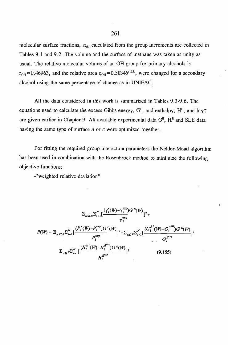
261
molecular surface fractions, asi' calculated from the group increments are collected in
Tables 9.1 and 9.2. The volume and the surface of methane was taken as unity as
usual. The relative molecular volume of an OH group for primary alcohols is
roH =0.46963, and the relative area qOH=O.50345(155), were changed for a secondary
alcohol using the same percentage of change as in UNIFAC.
All the data considered in this work is summarized in Tables 9.3-9.6. The
equations used to calculate the excess Gibbs energy, GE, and enthalpy, HE, and In1'7
are given earlier in Chapter 9. All available experimental data GE, HE and SLE data
having the same type of surface a or c were optimized together.
For fitting the required group interaction parameters the Nelder-Mead algorithm
has been used in combination with the Rosenbrock method to minimize the following
objective functions:
-"weighted relative deviation"
(9.155)
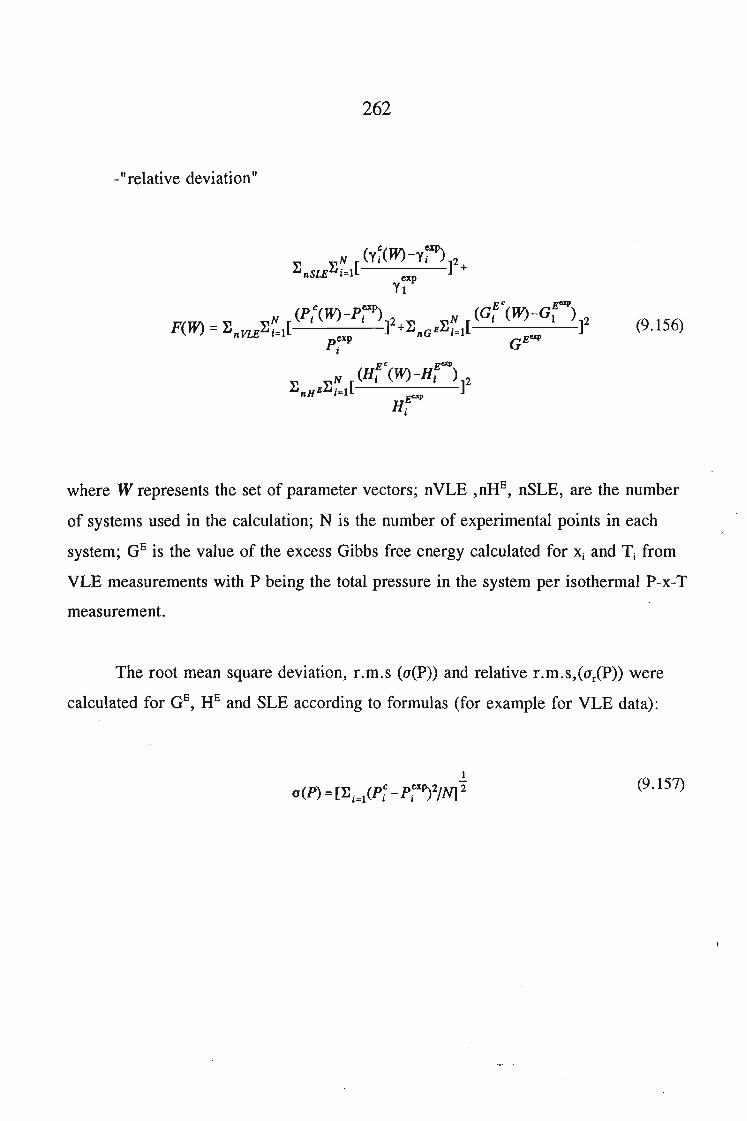
262
-"relative deviation"
(9.156)
where W represents the set of parameter vectors; nVLE ,oRE, nSLE, are the number
of systems used in the calculation; N is the number of experimental points in each
system; GE is the value of the excess Gibbs free energy calculated for Xj and T j from
VLE measurements with P being the total pressure in the system per isothermal P-x-T
measurement.
The root mean square deviation, r.m.s (o{P» and relative r.m.s,(urCP» were
calculated for GE, HE and SLE according to formulas (for example for VLE data):
1
a(P) = [I:i=l(P: _p:x1Y/Nj 2(9.157)
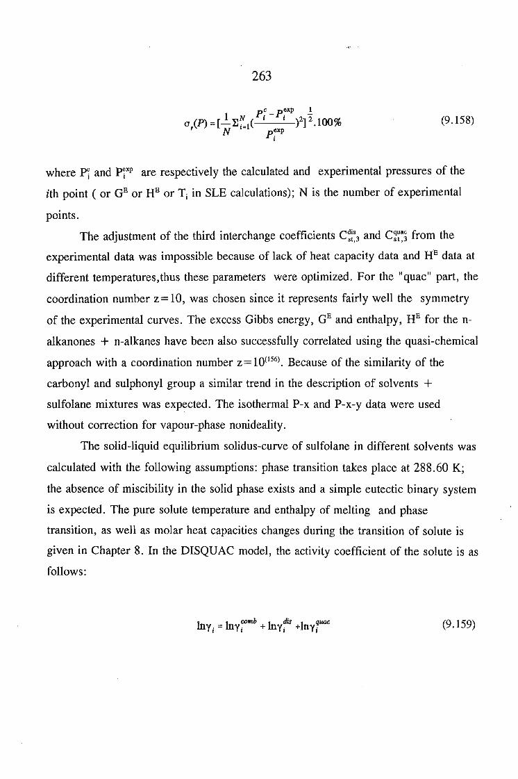
263
(9.158)
where Pi and P~xp are respectively the calculated and experimental pressures of the
ith point ( or GE or HE or T j in SLE calculations); N is the number of experimental
points.
The adjustment of the third interchange coefficients C~~~3 and C;~~~ from the
experimental data was impossible because of lack of heat capacity data and HE data at
different temperatures,thus these parameters were optimized. For the "quac" part, the
coordination number z= 10, was chosen since it represents fairly well the symmetry
of the experimental curves. The excess Gibbs energy, GE and enthalpy, HE for the n
alkanones + n-alkanes have been also successfully correlated using the quasi-chemical
approach with a coordination number z=10(156). Because of the similarity of the
carbonyl and sulphonyl group a similar trend in the description of solvents +sulfolane mixtures was expected. The isothermal P-x and P-x-y data were used
without correction for vapour-phase nonideality.
The solid-liquid equilibrium solidus-curve of sulfolane in different solvents was
calculated with the following assumptions: phase transition takes place at 288.60 K;
the absence of miscibility in the solid phase exists and a simple eutectic binary system
is expected. The pure solute temperature and enthalpy of melting and phase
transition, as well as molar heat capacities changes during the transition of solute is
given in Chapter 8. In the DISQUAC model, the activity coefficient of the solute is as
follows:
In In comb In dis In qU4CYj = Yi + Yi + Yi (9.159)
264
where In-yiomb is the combinatorial term represented by the Flory-Huggins equation,
while In-y1is and In-y?UaC are the dispersive and quasichemical contributions, respectively.
Final interaction parameters are listed in Table 9 i 7. The alkane/sulfolane interactions
(type a) existing in I-heptyne, toluene, 1,1,1-trichloroethane, propan-2-01, and the
nitriles is shown in Table 9.7 as the CH3/sulfolane interaction only for 1-heptyne.
Tables 9.3-9.6 and Figures 9.2-9.6 show numerical and graphical comparisons,
respectively, between our and literature experimental data and predictions. The
equimolar GEand HE values calculated using the new coefficients are presented in .
Tables 9.3 and 9.4. Generally, the agreement is satisfactory except for the sinusoidal
shape of the HE data. The relative r.m.s deviation of pressure alP) calculated for the
entire curve for isothermal P-x or P-x-y data, is less than 7 %. See Figs. 9.2 and 9.3
for 1-heptyne (1) + sulfolane (3), 1,1,1-trichloroethane (1) + sulfolane (3) as well as
the following ethers: tetrahydrofuran (1) + sulfolane (3) at 353.15 K and 338.15 K,
and l,4-dioxane (1) + sulfolane (3) at 353.15 K, mixtures. The GEvalues of benzene
+ sulfolane at 303.15 K(158) are worse than the results of KarvO(91). This is probably
due to experimental error. We expect that the GEvalues predicted using the new
coefficients are accurate to better than 7 % for the following four classes of solvents; I
alkanes/sulfolane, II alkynes/sulfolane; II chlorohydrocarbons/suloflane; IV crown
ethers/sulfolane. Good comparison of the theory with experimental data for the molar
excess Gibbs energy GEis shown in Fig. 9.4 for the mixtures of toluene (1) +sulfolane (3) at 313 .15 K. (126). It should be considered as a success, that the
dependence on temperature of GEis as usual well represented by the model, as GE
increases with temperature (Table 9.3).Caution should be exercised in the case of
alcohol or nitriles + sulfolane mixtures because of the lack of experimental data (HE
and SLE only).
265
The results for HE are shown in Table 9.4. Here, there is fairly good agreement
(Fig. 9.5) for a toluene (1) + sulfolane (3) mixture. However, limitations of
DISQUAC are related to the sinusoidal shape of the HE, which is noted for a large
number of systems in this work: benzene or 1,4-dioxane or acetonitrile. The excess
enthalpies for benzene (1) + sulfolane (3) mixtures measured by KarvO<9I) are more
accurate than those of Pansini and Jannelli(159). The r.m.s. deviation, O"H (for the entire
curve) is 13-18 J·mol-1. On the other hand the prediction of GEis very good and the
r.m.s. deviation is between 20-50 J -motI. In the case of the mixture with
tetrachloromethane (1) + sulfolane (3) the difference of the maximum is about 54
J -mol-I (experimental value HE = 220 J -mot1at X2 = 0.22, calculated value of HE =
166 at X2 = 0.46) and is strongly shifted to the low concentration region of the
sulfolane. With such a shape it is difficult to attribute the difference between
experimental and theory entirely to inadequacies of the model.As a matter of fact one
value of coordination number z= 10 for all systems cannot represent especially HE
over the entire concentration range. This behaviour is quite general for (polar +'.'nonpolar) mixtures(156). The predicted values of HE of 1-heptyne(l) + sulfolane(2)
mixture are much larger than the corresponding experimental results at 303.15 K.
This difference may be explained by short-range orientational changes, termed
"Patterson effect", when 1-alkynes are mixed with globular molecules or the
parameters are not adequately optimized. This discrepancies between experiment and
theory are not observed for VLE and SLE data (see Figs.9.2 and 9.6). The results of
HE for nitriles show r.m.s deviation from 21 to 42 J 'mol-I and underline a problem of
optimizing parameters for CH2CN group for two different shape of equilibrium
curves: sinusoidal for acetonitrile and endothermic for n-nitriles; also only HE data
were available at one temperature.
Sulfolane, because of the steric hindrance of its globular molecule, may play
266
the role of an almost inert diluent and limits its action to a disturbing effect on the
structure of the other component. Solid-liquid equilibrium measurements show weak
interactions or only dipole-dipole interaction between sulfolane and different
solvents(l5-17) The largest interaction is observed with cyclic ethers and
chlorohydrocarbons, the lowest with l-heptyne and 2-methyl-2-propanol. Using the
available interaction parameters for the surface type a and cl type t contacts, the
ability of the DISQUAC model on the prediction of the SLE has been successful. The
r.m.s deviations, <TT and relative r.m.s deviations, <TrT , described by general eqns. (3)
and (4) for the SLE equilibrium temperatures are from 0.9 to 5.5 K and from 0.3 to
2.2 % for all the mixtures investigated. The SLE T-x2 curves are usually well
represented by the model, even at rather low temperatures (see Fig.9.6).The
DISQUAC prediction is somewhat poorer for solubility curve of sulfolane in
tetrahydrofuran, where the experimental curve is shifted to the region of high
sulfolane concentration in liquid component and is higher than the ideal solubility.
Probably, these discrepancies may be due to some experimental inaccuracies, but also
due to the stronger interaction between unlike molecules.
In Table 9.6 the natural logarithms of the activity coefficients at infinite
dilution: In 1"~ = p,foo/RT have been listed. The result show, that structure- and
temperature- dependent conformational effects and inaccuracies in accounting for non
randomness with the quasichemical equations, equally affect the quality of 1"~
predictions. The In 1"7 predictions as a function of temperature may be considered
satisfactory for n-alkanes, l-alkynes and toluene. We were disappointed to see the
disagreement between the calculated values in function of temperature and the
experimentalln1"~ data given in Chapter 4. It seems difficul! to explain other than by
lack of the experimental data at different temperatures (especially LlCp
) and not perfect
values of our optimized interaction parameters. On the other hand, the observed
267
disagreement between the calculated and experimental In'Y~ values for solutions of c
hydrocarbons or crown ethers + sulfolane is probably due to free-volume effects and
to the inadequacy of the Flory-Huggins combinatorial term used in the model.
Moreover, we considered the application of DISQUAC to polar or associated systems
as an empirical extension.
There have been several attempts in the literature to correlate and predict
thermodynamic excess functions using either theoretical lattice-type or other ,more
empirical, group-contribution models. In our opinion, the Modified Unifad8) group
contribution method based on the local composition concept may give GEand HE
results comparable to DISQUAC. This method covers, in principle, all the classes of
solvents considered in this study.
The Modified UN/FA C model
The Modified UNIFAC model has the same expression for the temperatm:e
dependence of the parameters as DISQUAC, needs four parameters per contact (two
for Gibbs energy and two for enthalpy) to reproduce GEand HE; two heat capacity
parameters have been considered also. However, a difference exists between the
definition of the individual groups and values of the relative group increments for
molecular volumes rQand areas qQ' There is also no correlation between the
interchange contact parameters and the structure of particular groups.
Although the Modified UNIFAC method is used world-wide, and the parameter
matrix(I60) is of similar size to that of UNIFAC, the possibility of new parameters for
different solvents + sulfolane mixtures was taken into consideration. The results for
mixtures with sulfolane have been used to fit the group interaction parameters for the
new main group n (sulfolane) and solvents divided into various subgroups m, which
268
have been used by Modified UNIFAC (Dortmund). The temperature dependent
parameters were obtained as far as the required experimental data for the different
thermodynamic properties were available by fitting the parameters simultaneously to
VLE, HE, and SLE data using fitting procedure according to the equations 9.155 and
9.156. For VLE, no consistency test was performed and ideal gas phase was assumed.
The van der Waals properties of the different subgroups were taken from
Gmehling. (160) Sulfolane molecule was described, as before, by the parameters shown
in the Table 9.1.(130) Table 9.8 shows the modified UNIFAC group interaction
parameters between main group n (sulfolane) and different m subgroups existing in the
tested solvents. The prediction of GEand HE is quite satisfactory. The difference
between GE (experimental) and GE (calculated) rarely exceeds 40 J 'mol-1 (Table 9.3),
and this may be well within the limits of experimental error of certain measurements.
There is excellent agreement between the VLE measurements
(Chapter 7) and predicted values for chlorohydrocarbons, where the difference is less
than 10 J 'mol-1 (see Fig. 9.7). A comparsion of Modified UNIFAC with the
experimental work of Karvo(91) is shown for benzene (1) + sulfolane (3) at four·
temperatures in Fig. 9.9. The weakest results were obtained for the prediction of VLE
of THF (1) or propan-l-01 (1) + sulfolane (3), where the relative Lm.S. deviation
(ar(P)) is 9.85 % or11-14%. The calculated excess enthalpies agree for most of the
systems to within 15 J 'mot1 with the available measurements (Table 9.4), except for
mixtures containing I-heptyne + (TMS) where the experimental values, HE, are much
higher. Figure 9.8 shows the comparison of the predicted by Modified UNIFAC
excess enthalpy for the tetrachloromethane (1) + sulfolane (3) mixture at 303.15 K. It
is worth pointing out, that even the maximum is strongly shifted to the sulfolane low
concentration region, the prediction is very good.
As expected the largest deviations appear in the case of the SLE predictions.
For example, the solubility of sulfolane in benzene predicted by Modified UNIFAC is
269
much worse than the prediction by DISQUAC. The r.m.s. increased from 4.2 K to
7.2 K. For I-heptyne the r.m.s increased from 2.0 K to 3.7 K from DISQUAC to
Modified UNIFAC. The predicition of sulfolane solubility in chlorohydrocarbons is
satisfactory; r.m.s. is less than 2 K.
The logarithms of the activity coefficients at infinite dilution In'Y~, have been
determined for sulfolane in various solvents, and are listed in Table 9.6. The
predictions are compared to literature values taken from various authors using a wide
range of experimental techniques. The calculated In 'Y7 for n-hydrocarbons and c
hydrocarbons are much lower than the experimentaly determined values. Unlike
DISQUAC, the proper trend of the change of In 'Y~ with temperature is noted in all
systems. Nevertheless, the predicted values are similar to the measured values ego
benzene + TMS at 303.15 K, the predicted value of In 'Y7 is 0.823, while the
measured value by g.l.c is 0.770 (Chapter 4).
9.5.1. Conclusions
This work, following the series of comperative studies of the thermodynamic
properties and molecular interactions in hundreds of mixtures by DISQUAC and
Modified UNIFAC (Dortmund), illustrates the possibility of applying group
contribution models to prediction of thermodynamic fuctions and phase equilibrium of
certain polar mixtures invloving sulfolane.
Concidering the excess thermodynamic functions, the excess Gibbs energy, GE
and the excess molar enthalpy, HE were mainly better represented by the Modified
UNIFAC model. The optimization by the Modified UNIFAC model is consistently
worse than the DISQUAC model in the prediction of the solid liquid equilibria. The
prediction of activity coefficents at infinite dilution for both the straight chain and
cyclic alkanes by the Modified UNIFAC model does not compare favourably with the
270
experimentally determined values. However the DISQUAC model has reasonable
success with the alkanes t cycloalkanes and the aromatic compounds. Modified
UNIFAC predicts the value In')'7 accurately for the chloroalkanes.
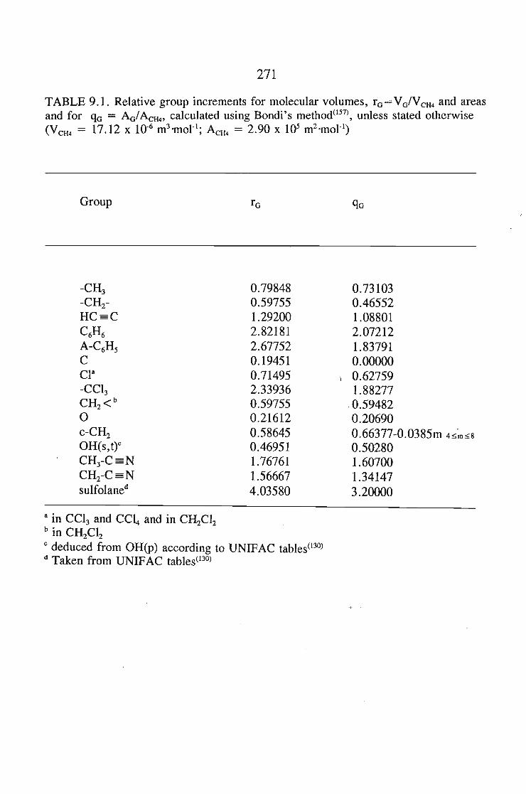
271
TABLE 9.1. Relative group increments for molecular volumes, ra=Va/VCH4 and areasand for qa = AalACH4' calculated using Bondi' s method(157), unless stated otherwise(VCH4 = 17.12 x 10⁻⁶ m]'mol-1; ACH4 = 2.90 X 10⁵ m2 'mol-1
)
Group
-CH]-CHrHC=CC6H6
A-C6HsCCIa-CCl]CH2 <b
oc-CH2
OH(s,tyCH]-C=NCHrC=Nsulfolaned
0.798480.597551.292002.821812.677520.194510.714952.339360.597550.216120.586450.469511.767611.566674.03580
0.731030.465521.088012.072121.837910.00000
\ 0.627591.882770.594820.206900.66377-0.0385m 4~'m~8
0.502801.607001.341473.20000
a in CCl] and CCl4 and in CH2Cl2bin CH2Cl2C deduced from OH(P) according to UNIFAC tables(l30)d Taken from UNIFAC tables(130)
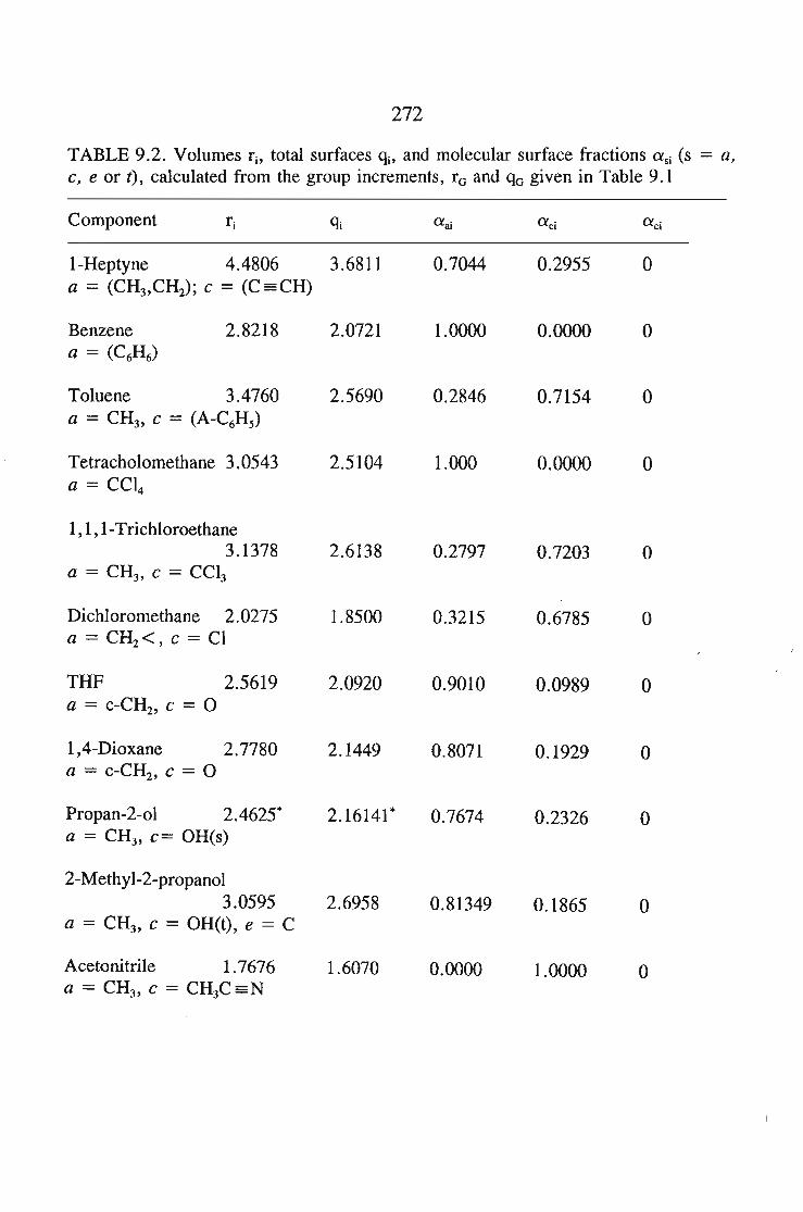
272
TABLE 9.2. Volumes ri' total surfaces <}j, and molecular surface fractions asi (s = a,c, e or t), calculated from the group increments, ra and qa given in Table 9.1
Component r j <}j aai a ci aei
I-Heptyne 4.4806 3.6811 0.7044 0.2955 0a = (CH3,CH2); c = (C =CH)
Benzene 2.8218 2.0721 1.0000 0.0000 0a = (C6H6)
Toluene 3.4760 2.5690 0.2846 0.7154 0a = CH3 , C = (A-C6Hs)
Tetracholomethane 3.0543 2.5104 1.000 0.0000 0a = CCl4
1,1,1-Trichloroethane3.1378 2.6138 0.2797 0.7203 0
a = CH3, C = CCl3
Dichloromethane 2.0275 1.8500 0.3215 0.6785 0a = CH2 <, c = Cl
THF 2.5619 2.0920 0.9010 0.0989 0a = c-CH2 , c = 0
1,4-Dioxane 2.7780 2.1449 0.8071 0.1929 0a = c-CH2 , c = 0
Propan-2-o1 2.4625" 2.16141" 0.7674 0.2326 0a = CH3, c= OH(s)
2-Methyl-2-propanol3.0595 2.6958 0.81349 0.1865 0
a = CH3, c = OH(t), e = C
Acetonitrile 1.7676 1.6070 0.0000 1.0000 0a = CH3, c = CH3C=N
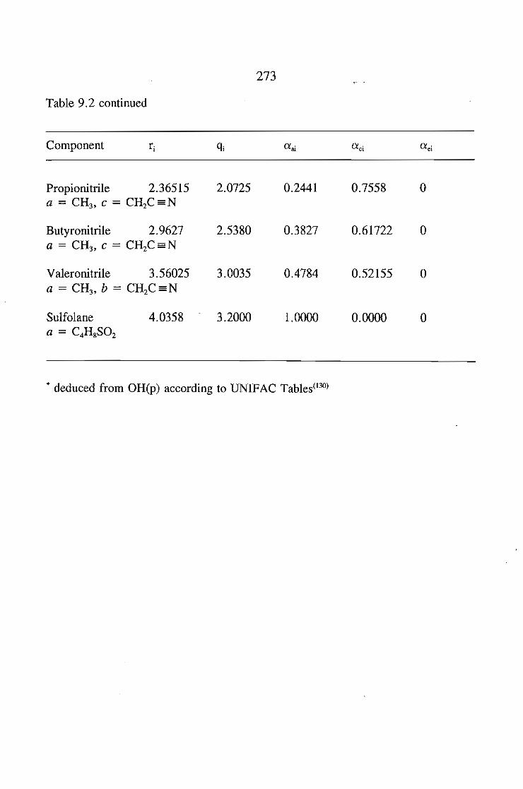
273
Table 9.2 continued
Component r·I
Propionitrile 2.36515 2.0725 0.2441 0.7558 0a = CH3, c = CHzC=N
Butyronitrile 2.9627 2.5380 0.3827 0.61722 0a = CH3, c = CHzC=N
Valeronitrile 3.56025 3.0035 0.4784 0.52155 0a = CH3, b = CHzC=N
Sulfolane 4.0358 3.2000 1.0000 0.0000 0a = C4HgSOz
• deduced from OH(P) according to UNIFAC Tables(l30)
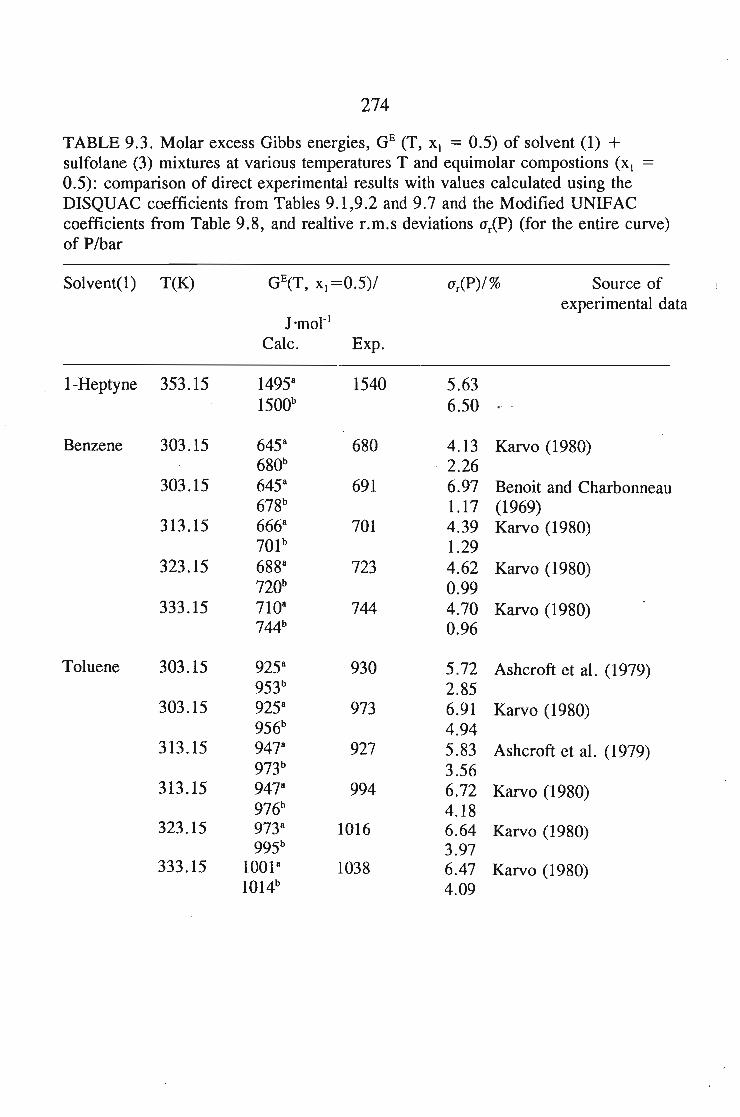
274
TABLE 9.3. Molar excess Gibbs energies, GB (T, Xl = 0.5) of solvent (1) +sulfolane (3) mixtures at various temperatures T and equimolar compostions (Xl =0.5): comparison of direct experimental results with values calculated using theDISQUAC coefficients from Tables 9.1,9.2 and 9.7 and the Modified UNIFACcoefficients from Table 9.8, and realtive r.m.s deviations alP) (for the entire curve)of P/bar
Solvent(1) T(K) GE(T, Xl =0.5)/ arCP)I % Source ofexperimental data
J 'motl
Calc. Exp.
1-Heptyne 353.15 14958 1540 5.631500b 6.50
Benzene 303.15 6458 680 4.13 Karvo (1980)680b . 2.26
303.15 6458 691 6.97 Benoit and Charbonneau678b 1.17 (1969)
313.15 6668 701 4.39 Karvo (1980)701 b 1.29
323.15 6888 723 4.62 Karvo (1980)720b 0.99
333.15 7108 744 4.70 Karvo (1980)744b 0.96
Toluene 303.15 9258 930 5.72 Ashcroft et al. (1979)953b 2.85
303.15 9258 973 6.91 Karvo (1980)956b 4.94
313.15 9478 927 5.83 Ashcroft et al. (1979)973b 3.56
313.15 9478 994 6.72 Karvo (1980)976b 4.18
323.15 9738 1016 6.64 Karvo (1980)995b 3.97
333.15 lOOP 1038 6.47 Karvo (1980)1014b 4.09
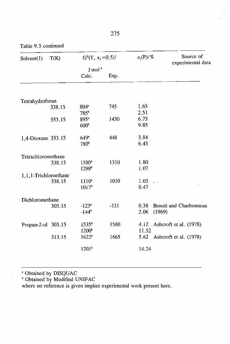
275
Table 9.3 continued
Solvent(1) T(K)
J 'mol-1
Calc. Exp.
<TlP)/% Source ofexperimental data
Tetrahydrofuran338.15 804a 745 1.65
785b 2.51353.15 895a 1430 6.75
600b 9.85
l,4-Dioxane 353.15 649a 448 3.84780b 6.43
Tetrachloromethane338.15 1580a 1310 1.80
1298b 1.071,1,1-Trichloroethane
338.15 1110a 1010 1.031017b 0.47
Dichloromethane303.15 -123a -131 0.38 Benoit and Charbonneau
-144b 2.06 (1969)
Propan-2-ol 303.15 1535a 1580 4.12 Ashcroft et al. (1978)1200b 11.52
313.15 1622a 1665 5.62 Ashcroft et al. (1978)
1201b 14.24
a Obtained by DISQUACb Obtained by Modified UNI~AC
where no reference is given implies experimental work present here.
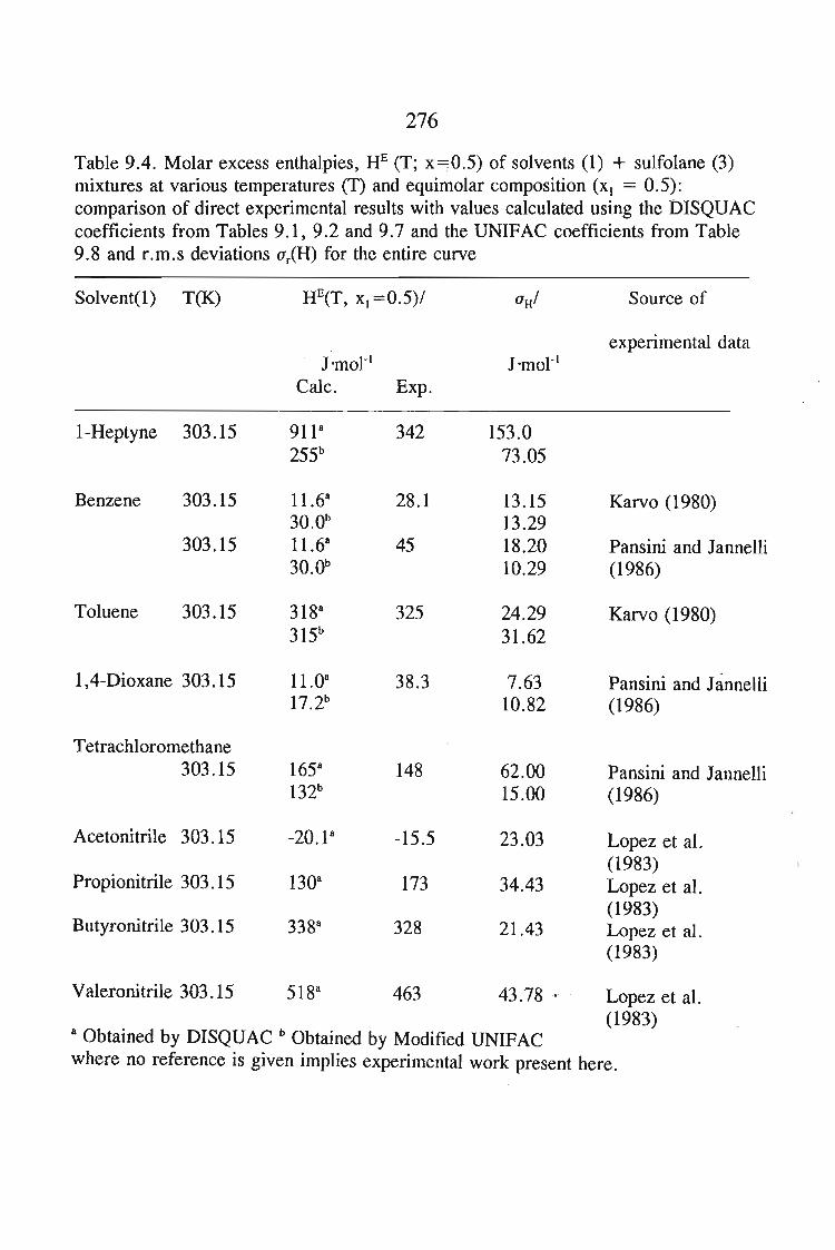
276
Table 9.4. Molar excess enthalpies, RE (T; x-:0.5) of solvents (1) + sulfolane (3)mixtures at various temperatures (T) and equimolar composition (x! = 0.5):comparison of direct experimental results with values calculated using the DISQUACcoefficients from Tables 9.1,9.2 and 9.7 and the UNIFAC coefficients from Table9.8 and r. m. s deviations oiR) for the entire curve
Solvent(1) T(K) HE(T, x! =0.5)1 (JHI Source of
experimental dataJ 'mo!"! J 'mo!"!
Calc. Exp.
I-Heptyne 303.15 91P 342 153.0255b 73.05
Benzene 303.15 11.68 28.1 13.15 Karvo (1980)30.0b 13.29
303.15 11.68 45 18.20 Pansini and Jannelli30.0b 10.29 (1986)
Toluene 303.15 3188 325 24.29 Karvo (1980)315b 31.62
1,4-Dioxane 303.15 11.08 38.3 7.63 Pansini and Jannelli17.2b 10.82 (1986)
Tetrachloromethane303.15 1658 148 62.00 Pansini and Jannelli
132b 15.00 (1986)
Acetonitrile 303.15 -20.1 8 -15.5 23.03 Lopez et al.(1983)
Propionitrile 303.15 1308 173 34.43 Lopez et al.(1983)
Butyronitrile 303.15 3388 328 21.43 Lopez et al.(1983)
Valeronitrile 303.15' 5188 463 43.78 '. Lopez et al.
8 Obtained by DISQUAC b Obtained by Modified UNIFAC(1983)
where no reference is given implies experimental work present here.
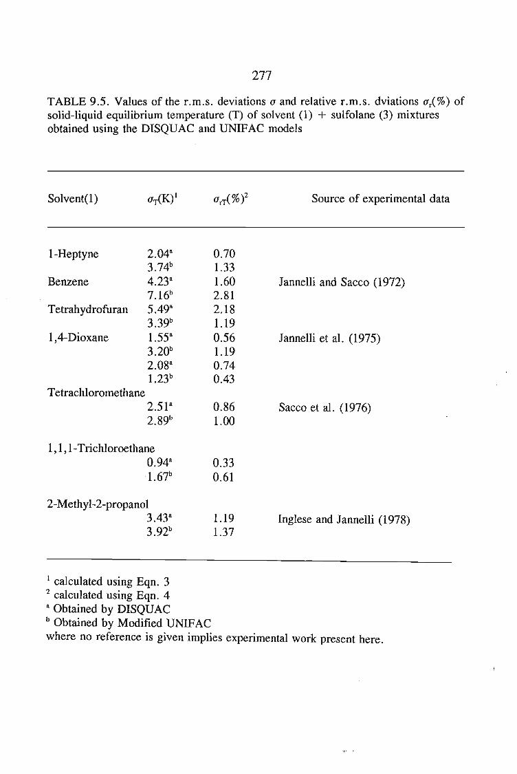
277
TABLE 9.5. Values of the r.m.s. deviations a and relative r.m.s. dviations a r(%) ofsolid-liquid equilibrium temperature (T) of solvent (1) + sulfolane (3) mixturesobtained using the DISQUAC and UNIFAC models
Solvent(l) Source of experimental data
I-Heptyne 2.04a 0.703.74b 1.33
Benzene 4.23a 1.60 Jannelli and Sacco (1972)7.16b 2.81
Tetrahydrofuran 5.49a 2.183039b 1.19
1,4-Dioxane 1.55a 0.56 Jannelli et al. (1975)3.20b 1.192.08a 0.741.23b 0.43
Tetrachloromethane2.51a 0.86 Sacco et al. (1976)2.89b 1.00
1, 1, I-Trichloroethane0.94a 0.33·1.67b 0.61
2-Methyl-2-propanol3.43a 1.19 Inglese and Jannelli (1978)3.92b 1.37
1 calculated using Eqn. 32 calculated using Eqn. 4a Obtained by DISQUACb Obtained by Modified UNIFACwhere no reference is given implies experimental work present here.
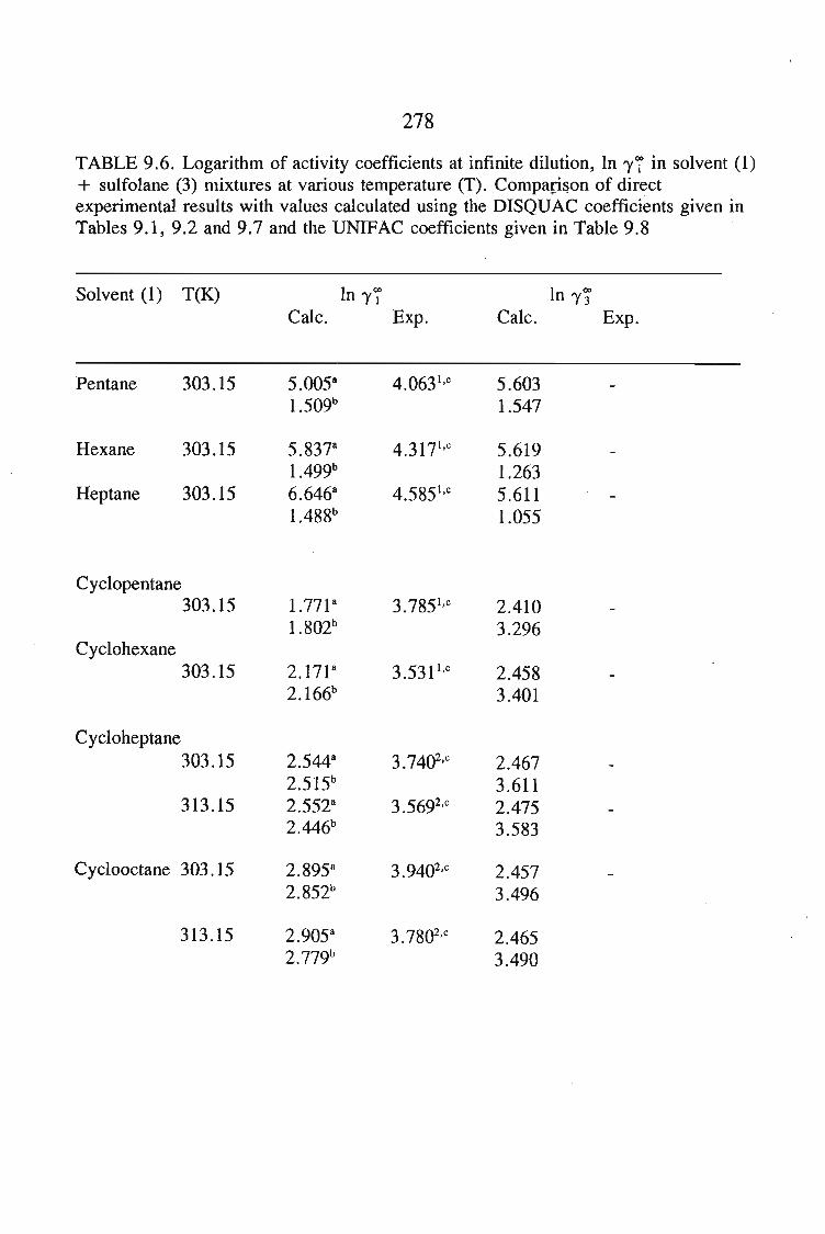
278
TABLE 9.6. Logarithm of activity coefficients at infinite dilution, In 1'7 in solvent (1)+ sulfolane (3) mixtures at various temperature (T). Compapson of directexperimental results with values calculated using the DISQUAC coefficients given inTables 9.1, 9.2 and 9.7 and the UNIFAC coefficients given in Table 9.8
Solvent (1) T(K)Calc. Exp. Calc.
In 1'~
Exp.
Pentane 303.15 5.0058 4.063 1,c 5.6031.509b 1.547
Hexane 303.15 5.8378 4.3171,c 5.6191.499b 1.263
Heptane 303.15 6.6468 4.585 1,c 5.6111.488b 1.055
Cydopentane303.15 1.77P 3.7851,c 2.410
1.802b 3.296Cydohexane
303.15 2.171 8 3.531 1,c 2.4582.166b 3.401
Cydoheptane303.15 2.5448 3.74(f,c 2.467
2.515b 3.611313.15 2.5528 3.5692,c 2.475
2.446b 3.583
Cydooctane 303.15 2.89Y 3.94(f,c 2.4572.852b 3.496
313.15 2.90Y 3.78(f'c 2.4652.779b 3.490
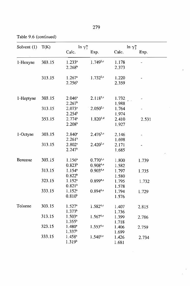
279
Table 9.6 (continued)
Solvent (1) T(K) In 'Y7 In 'Y~
Calc. Exp. Calc. Exp.
I-Hexyne 303.15 1.2338 1.7492,c 1.1782.268b 2.373
313.15 1.2678 1.7322,c 1.2202.256b 2.359
I-Heptyne 303.15 2.0468 2. 11 82,c 1.7322.267b 1.988
313.15 2.0738 . 2.05Q2,c 1.7642.254b 1.974
353.15 2.7748 1.8203,d 2.410 2.5312.208b 1.927
I-Octyne 303.15 2.8408 2.4762,c 2.1462.261 b 1.698
313.15 2.8028 2.42Q2,c 2.1712.247b 1.685
Benzene 303.15 1.1568 0.7701,c 1.800 1.7390.823b 0.9084,e 1.582
313.15 1.1548 0.9034,e 1.797 1.7350.822b 1.580
323.15 1.1528 0.8994,e 1.795 1.7320.821b 1.578
333.15 1.1528 0.8944,e 1.794 1.7290.810b 1.576
Toluene 303.15 1.5278 1.5824,e 1.407 2.8151.373b 1.736
313.15 1.5038 1.5674,e 1.399 2.7861.355b 1.718
323.15 1.4808 1.5534,e 1.406 2.7591.337b 1.699
333.15 1.4588 1.5404,e 1.426 2.7341.319b 1.681
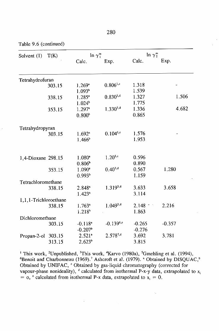
Table 9.6 (continued)
280
Solvent (1) T(K)Calc.
In 'Y~
Exp.In 'Y~
Calc. Exp.
Tetrahydrofuran0.8061,c303.15 1.2698 1.318
1.093b 1.539338.15 1.28SS 0.8303,d 1.327 1.506
1.024b 1.775353.15 1.2978 1.3303,d 1.336 4.682
0.800b 0.865
Tetrahydropyran303.15 1.6928 0.1041,c 1.576
1.466b 1.953
1,4-Dioxane 298.15 1.0808
0.806b
353.15 1.0908
0.993b
Tetrachloromethane338.15 2.8488
1.4238
1,1,1-Trichloroethane338.15 1.7638
1.218b
Dichloromethane303.15 -0.1188
-0.207b
Propan-2-01 303.15 2.521 8
313.15 2.623b
1.3193,d
1.0493,d
-0. 1396,e
2.5787,d
0.5960.8900.5671.159
3.6333.114
2.148'1.863
-0.265-0.2763.6923.815
1.280
3.658
2.216
-0.357
3.781
I This work, 2Unpublished, 3This work, 4Karvo (1980a), 5Gmehling et al. (1994),6Benoit and Charbonneau (1969).7 Ashcroft et al. (1979). 8 Obtained by DISQUAC,bObtained by UNIFAC, C Obtained by gas-liquid chromatography (corrected forvapour-phase nonideality), d calculated from isothermal P-x-y data, extrapolated to Xi
= 0, e calculated from isothermal P-x data, extrapolated to Xi = O.
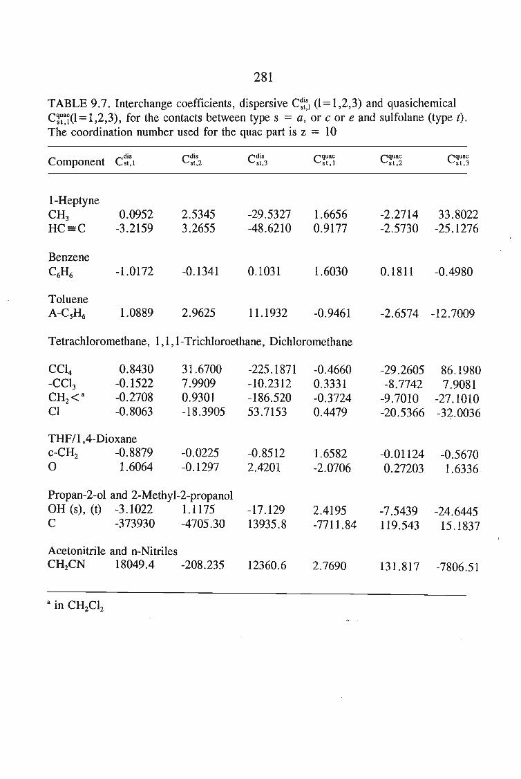
281
TABLE 9.7. Interchange coefficients, dispersive C~:~l (l = 1,2,3) and quasichemicalC~~~I(I=I,2,3), for the contacts between type s = G, or c or e and sulfolane (type t).The coordination number used for the quac part is z = 10
Componentdis Cdis Cdis cquac cquac cquacCst,1 st,2 st,3 st,1 st,2 st ,3
1-HeptyneCH3 0.0952 2.5345 -29.5327 1.6656 -2.2714 33.8022HC=C -3.2159 3.2655 -48.6210 0.9177 -2.5730 -25.1276
BenzeneC6H6 -1.0172 -0.1341 0.1031 1.6030 0.1811 -0.4980
TolueneA-CsH6 1.0889 2.9625 11.1932 -0.9461 -2.6574 -12.7009
Tetrachloromethane, 1,1,1-Trichloroethane, Dichloromethane
CCl4 0.8430 31.6700 -225.1871 -0.4660 -29.2605 86.1980-CCI3 -0.1522 7.9909 -10.2312 0.3331 -8.7742 7.9081CH2 <8 -0.2708 0.9301 -186.520 -0.3724 -9.7010 -27.1010Cl -0.8063 -18.3905 53.7153 0.4479 -20.5366 -32.0036
THF/l,4-Dioxanec-CH2 -0.8879 -0.0225 -0.8512 1.6582 -0.01124 -0.56700 1.6064 -0.1297 2.4201 -2.0706 0.27203 1.6336
Propan-2-o1 and 2-Methyl-2-propanolOH (s), (t) -3.1022 1.1175 -17.129 2.4195 -7.5439 -24.6445C -373930 -4705.30 13935.8 -7711.84 119.543 15.1837
Acetonitrile and n-NitrilesCH2CN 18049.4 -208.235 12360.6 2.7690 131.817 -7806.51
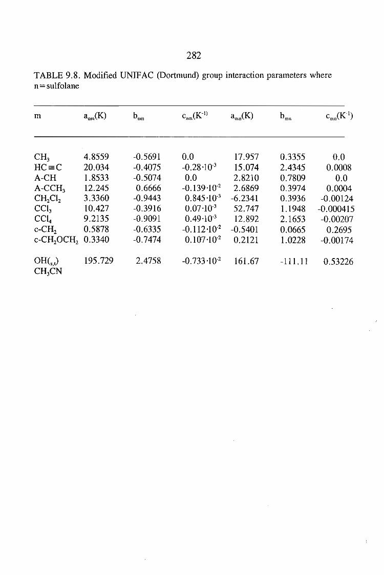
282
TABLE 9.8. Modified UNIFAC (Dortmund) group interaction parameters wheren= sulfolane
m bnmc (K-l)
om
CH3 4.8559 -0.5691 0.0 17.957 0.3355 0.0HC=C 20.034 -0.4075 -0.28'10-3 15.074 2.4345 0.0008A-CH 1.8533 -0.5074 0.0 2.8210 0.7809 0.0A-CCH3 12.245 0.6666 -0.139'10-2 2.6869 0.3974 0.0004CH2C12 3.3360 -0.9443 0.845 '10-3 -6.2341 0.3936 -0.00124CC13 10.427 -0.3916 0.07.10-3 52.747 1.1948 -0.000415CC14 9.2135 -0.9091 0.49.10-3 12.892 2.1653 -0.00207c-CH2 0.5878 -0.6335 -0.112.10-2 -0.5401 0.0665 0.2695c-CH20CH2 0.3340 -0.7474 0.107 ,10-2 0.2121 1.0228 -0.00174
OH(s,J 195.729 2.4758 -0.733,10-2 161.67 -111.11 0.53226CH3CN
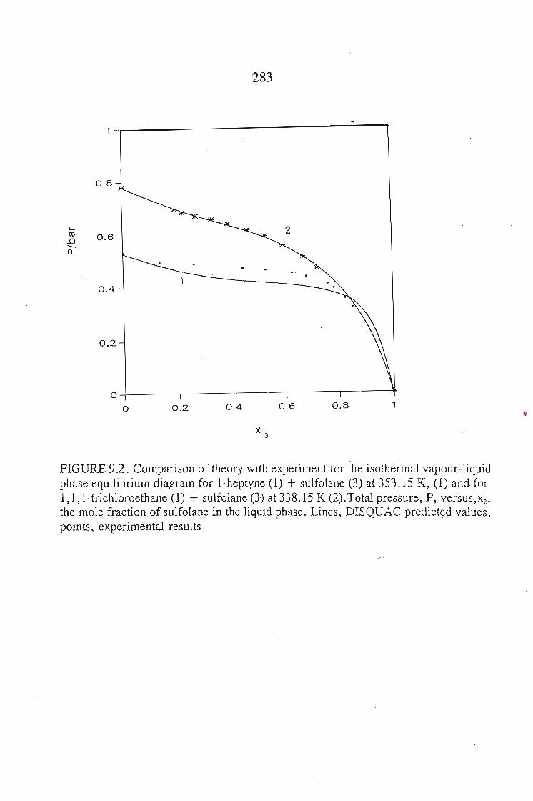
283
1-.--:..------------..:...----,
'-ro.0-Cl.
0.8
0.6
0.4
0.2
o--+----.----r---~--_r--~o 0.2 0.4
X3
0.6 0.8 1
FIGURE 9.2. Comparison of theory with experiment for the isothermal vapour-liquidphase equilibrium diagram for I-heptyne (1) + sulfolane (3) at 353.15 K, (1) and for1,1, I-trichloroethane (1) + sulfolane (3) at 338.15 K (2).Total pressure, P, versus,x
2,
the mole fraction of sulfolane in the liquid phase. Lines, DISQUAC predict~d values,points, experimental results
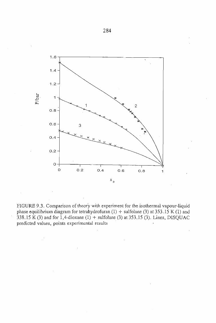
284
1.6
1.4
1.2
~. 1.0-...f.l..
20.8
0.6 3
0.4
0.2
0
0 0.2 0.4 0.6 0.8 1
X3
FIGURE 9.3. Comparison of theory with exp~riment for the isothermal vapour-liquidphase equilibrium diagram for tetrahydrofuran (1) + sulfolane (3) at 353.15 K (1) and338.15 K (3) and for 1,4-dioxane (1) + sulfolane (3) at 353.15 (3). Lines, DISQUACpredicted values, points experimental results .
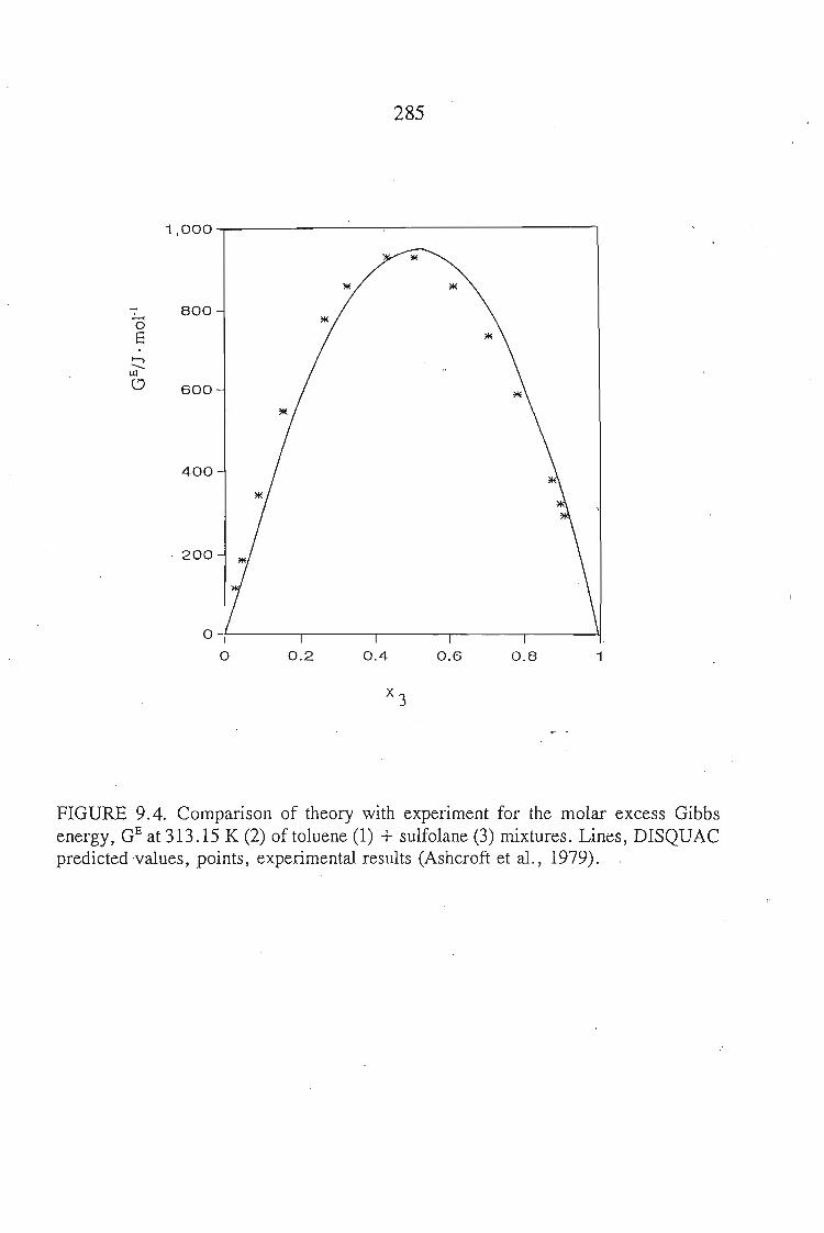
285
1 ,000 -.------------,---------~
10.80.60.40.2
O-f--- .------.----r------.------I.l
o
400
·200
lIE lIE
, 800-0E.
h-Ul
CJ 600
FIGURE 9.4. Comparison of theory with experiment for the molar excess Gibbsenergy, GE at 313.15 K (2) of toluene (1) + sulfolane (3) mixtures. Lines, DISQUACpredicted values, points, experimental results (Ashcroft et al., 1979).
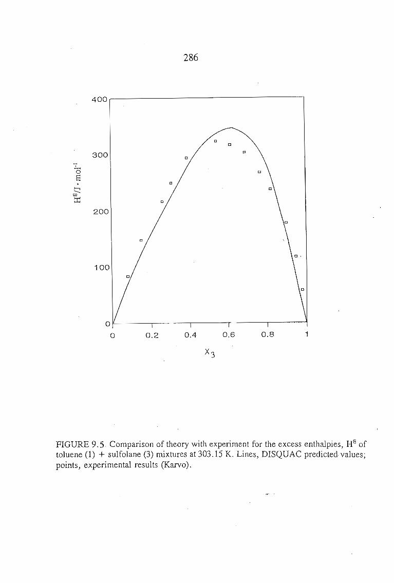
286
400.---------------------,
300 cc
,.-06.
>-,-Ul
~
200
100
10.80.60.40.2
oll----.,----r-----,-----.,.------..,l
o
FIGURE 9.5, Comparison of theory with experiment for the excess enthalpies, HE oftoluene (1) + sulfolane (3) mixtures at 303.15 K. Lines, DISQUAC predicted values;points, experimental results (Karvo).
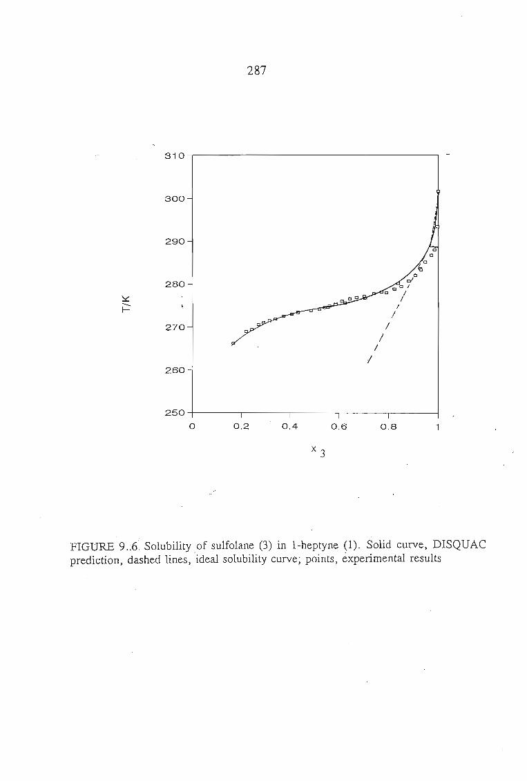
287
310,---------------------,
300
290
~o
6
280cl
001
~/- I
I- /
/270 /
//
I260
10.80.60.40.2
250 +,---,------.-----,.-----r---~
o
x 3
FIGURE 9.:6 Solubility of sulfolane (3) in I-heptyne (1). Solid curve, DISQUACprediction, dashed lines, ideal solubility curve; points, experimental results
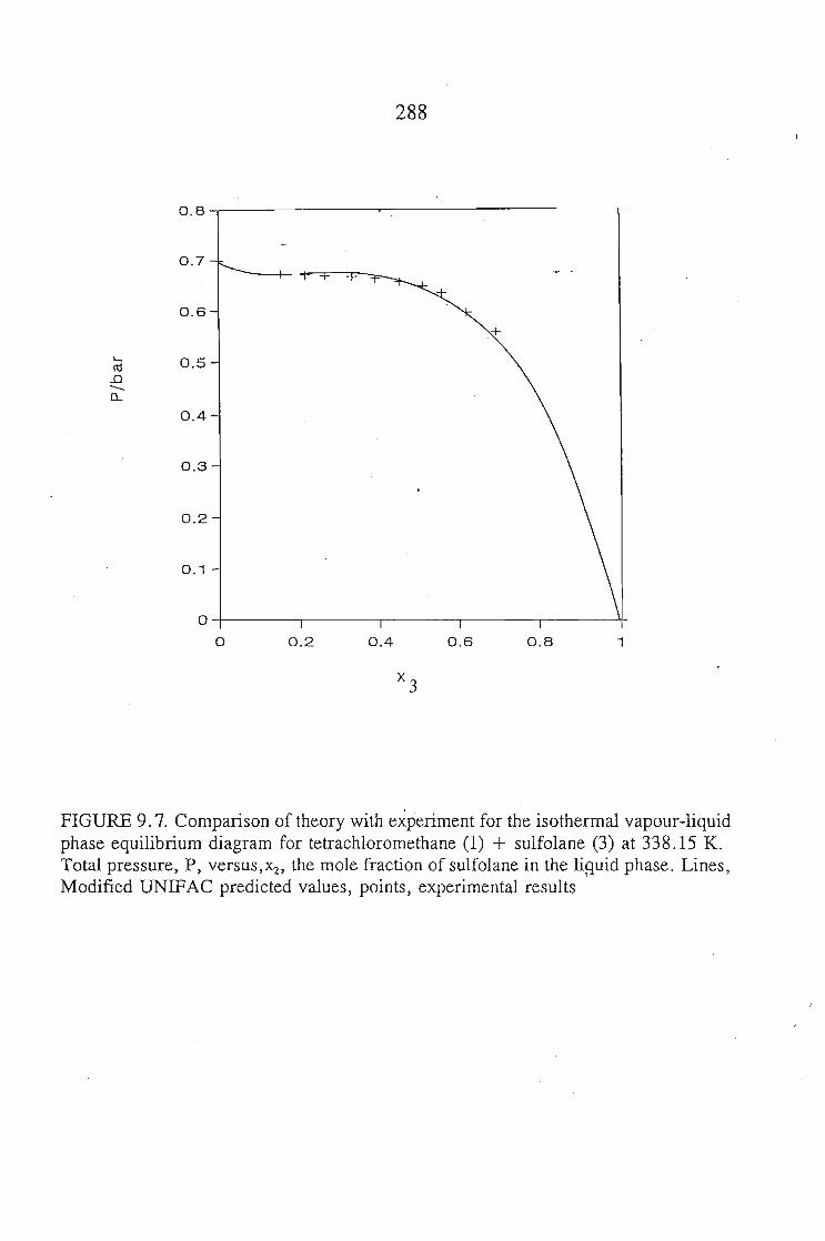
288
0.8
0.7
0.6
L- 0.5co-0-(l-
OA
0.3
0.2
0.1
0
0 0.2 0.4 0.6 0.8 1
X3
FIGURE 9.7. Comparison of theory with experiment for the isothermal vapour-liquidphase equilibrium diagram for tetrachloromethane (1) + sulfolane (3) at 338.15 K.Total pressure, P, versus, x2 , the mole fraction of sulfolane in the lifluid phase. Lines,Modified UNIFAC predicted values, points, experimental results
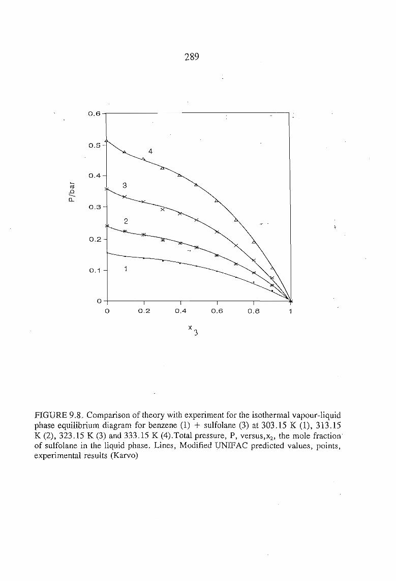
289
0.6-r---------------------,
10.80.60.40.2
O-+----r-----.---.-----...---...:::::k
o
0.1 1
0.5
0.2
0.3
0.4~
ro..Q-0...
FIGURE 9.8. Comparison of theory with experiment for the isothermal vapour-liquidphase equilibrium diagram for benzene (1) + sulfolane (3) at 303.15 K (1), 313 .15K (2), 323.15 K (3) and 333.15 K (4).Total pressure, P, versus,x2 , the mole fractionof sulfolane in the liquid phase. Lines, Modified UNIFAC predicted values, points,experimental results (Karvo)
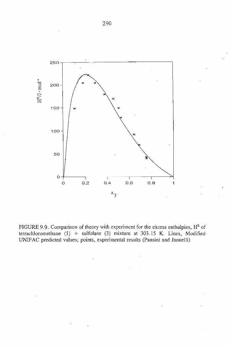
290
10.80.60.40.2
O-¥----...-------r-----.----.,------">i
o
50
100
250 -.---------------------,
,......0 200E.....,
---Ul
~
150
FIGURE 9.9. Comparison of theory with experiment for the exc"ess enthalpies, HE oftetrachloromethane (1) + sulfolane (3) mixture at 303.15 K. Lines, ModifiedUNIFAC predicted values; points, experimental results (Pansini and Jannelli)
291
CHAPTER 10
CONCLUSIONS
The aims of this work, given in Chapter I, have been successfully carried out.
The extension to the Cruickshank and Everett method, for the determination of
')'73 of moderately volatile solvents, has been tested and new data of ')'73 for n
dodecane + various hydrocarbon mixtures have been obtained. These results fill a gap
in the literatur~. The technique is also used to investigate the possibility of determining
the solvent vapour pressure. The results for the vapour pressure obtained from the
modified technique compare favourably with the publi$hed results. The results are an
indication that this new techique may open up a large field of systems which can be
investigated.
New ')'73 for sulfolane and various solutes have been obtained using G.L.C.
One of the reasons for using sulfolane was because of its polar nature. The results
indicate that polar solvents may also be used in the determination of ')'73 by G.L. C.,
without any modification to the existing theory. This is another advance in the
applications that may be investigated by G.L.C. It is important to stress, that ')'73 of
sulfolane and many of the sy'stems studied here could not be obtained by other
methods (exept static cell method), because of the limited solubility in the polar
solvent sulfolane. This once again extends the field of study of ')'73 to a variety of
solutes which are immiscible in partially involatile polar solvents.
New excess volume (YE) data have been obtained for an alkyne + sulfolane.
Other hydrocarbons + sulfolane mixtures could not be investigated because of their
limited miscibility. The results indicate a significant intera,ction between the alkynes
and sulfolane. This supports the evidence obtained from VLE and SLE.
292
The excess enthalpy (HE) was determined for I-heptyne and l-octyne +sulfolane. Other mixtures were not investigated because of the limited solubility of
most hydrocarbons and sulfolane. The results indicate a significant interaction between
the alkynes + sulfolane and support the VE results. The interaction is most likely
between the acidic a proton in the l-alkynes and the available oxygen atoms in
sulfolane. The HE is positive over the whole curve. This is most likely a result of the
dissociation of sulfolane and of the alkyne molecules, which has masked the
association between sulfolane and the alkyne. The association between sulfolane and
the alkynes appears to be stronger than between sulfolane and benzene and smaller
than between sulfolane and the nitriles. The obtained results are used in the "multi
optimization" procedure conducted in chapter 9. Both DISQUAC and UNIFAC is used
to fit the curve. The obtained parameters are given in chapter 9.
Isothermal vapour-liquid equilibria at 338.15 K or 353.15 K for I-heptyne, or
tetrahydrofuran, or 1,4-dioxane, or tetrachloromethane, or 1,1, I-trichloroethane +sulfolane binary mixtures have been determined using an ebulliometric method. The
data reported have been successfully described using the Margules, van Laar,
WILSON, NRTL and UNIQUAC equations. The obtained parameters may be used
to p,redict and correlate phase equilibria in ternary mixtures involving sulfolane.
The experimental data has allowed us to obtain new interaction parameters for
the above mentioned groups with sulfolane (as an individual group) in the DISQUAC
and Modified UNIFAC models.
The Margules, van Laar, WILSON, NRTL and UNIQUAC equations for the
molar excess Gibbs energy, were chosen for the reduction of the VLE data as
'representatives of local composition equations and semi-empirical enthalpic
expressions. The VLE data are the excess molar Gibbs energies, (GE), calculated
from the total pressure data.
The activity coefficients and the excess molar Gibbs energies were correlated
with the same theories. Calculations done using the van Laar, Margules or Wilson
equations were found to be inferior to the NRTL and UNIQUAC equations.
293
Each of the five mixtures studied in this work, showed significant positive
deviations from ideality. The largest deviation was found for the mixture I-heptyne
+ sUlfolane. All systems studied exhibit zeotropic behaviour.
The maximum values of GE are obtained for tetrahydrofuraTl: + sulfolane at
353.15 K, and l,4-dioxane + sulfolane at 353.15 K. A comparison of the excess
molar Gibbs energies for the tetrachloromethane + sulfolane mixture and the
trichloroethane + sulfolane mixture with the excess molar Gibbs energy, obtained for
the related mixture of dichloromethane + sulfolane, at 303.15 K), suggests complex
forming interaction bet)-veen the dichloromethane and sulfolane molecules. This
indicates a different type of interaction between tetrachloromethane and sulfolane on
the one hand, and between trichloroethane and sulfolane on the other. The asymmetric
molecule trichloroethane shows weaker interactions with sulfolane than does
dichloromethane.
The experimental values of the excess molar enthalpies HE for two of the
systems studied here have been reported in the literature. The H; versus mole fraction
for l,4-dioxane + sulfolane mixture (also at 303.15 K) was found to be sinusoidal. (161)
with a H;in in the sulfolane rich region, and H;ax in the l,4-dioxane rich region. The
excess enthalpy of mixing for· the l-heptyne + sulfolane system has also been
measured at 303.15 K (Chapter 6), and shows endothermic deviations from ideality.
These enthalpic results reflect the same interactions we have interpreted from the
Gibbs energy results above.
For the mixtures studied in this work, strong nonideal behaviour is evident from
the magnitude of the activity coefficients. The 1,4-dioxane + sulfolane mixture (with
small values for both G;ax and H;~ is the least non-ideal mixture.
The activity coefficient at infinite dilution, 1'7, for each of the solvents in
sulfolane was calculated using Margules, van Laar, WILSON, NRTL and UNIQUAC
parameters obtained from VLE data. The calculated results for the mixtures·l-Heptyne
+ sulfolane at 313.15 K, and 303.15 K, and tetrahydrofuran + sulfolane at
294
303.15 K compare well with the published data.
The solubilities of sulfolane, have been determined experimentally in six
solvents: I-heptyne, tetrahydrofuran, 1,4-dioxane, 1,1, 1-trichloroethane, benzene and
cyclohexane - by a dynamic method in the temperature range 250 - 301 K. The results
have been correlated by the WILSON, NRTL and UNIQUAC equations, utilizing
parameters taken from solid-liquid equilibrium for the simple eutectic mixtures only.
The correlations have been done using the data reported here as well as the data
published earlier.
The solute, sulfolane is most soluble in tetrahydrofuran and least soluble in 1
heptyne. The order of solubility of sulfolane is tetrahydrofuran > l,4-dioxane >
trichloroethane > benzene> tetrachloromethane > cyclohexane > I-heptyne. These
results indicate that no hydrogen bonds exist between sulfolane and 1-heptyne, or 2
methyl-2-propanol. This is supported by work done by M. D. Monica et al. (4), that no
hydrogen bonds exists between benzoic acid and sulfolane.
In all the solvents used in this work, with the exception of tetrahydrofuran over
a small concentration range, the solubility of sulfolane is lower than ideal. The effect
of the interactions between sulfolane and the solvents .observed in vapour-liquid
equilibria measurements, was similar to that observed in this SLE work. The
solubility of sulfolane in 1-heptyne is much lower than ideal. The solubility of
sulfolane in 1,4-dioxane for X2 > 0.84 is close to ideal with experimental activity
coefficients ')12 ~ 1.0. This corresponds to the liquidus curve related to the sulfolane
crystal phases I and 11.
For l,4-dioxane + sulfolane evidence for the formation of a solid molecular
compound which largely decomposes on melting was observed. This indicates the
possibility of strong interactions between sulfolane and l,4-dioxane. Two eutectic
points, were observed. The latter eutectic refers to the metastable crystalline phase 11.
In this study, three methods that describe the Gibbs excess free energy of
mixing (GE) were used to represent the solute activity coefficient (')12): the WILSON
equation, the nonrandom two-liquid theory (NRTL) and the UNIQUAC equation.
295
Calculations were performed on the data obtained from this work and also for
mixtures of sulfolane in benzene, 1,4-dioxane, tetrachloromethane and cyclohexane,
from literature data in the sulfolane rich region, for liquidus curves giving simple
eutectic points.
The solubility of sulfolane in cydohexane was only measured in the sulfolane
rich region as a result the non~miscibility gap in the lower sulfolane concentrations.
For the nine solubility curves, the results obtained from the WILSON equation
are slightly better than those derived from the NRTL and UNIQUAC equations.
The experimental data of SLE obtained in this work and the VLE data (Chapter
7) have been used to obtain new interaction parameters for the specific solvent groups
with sulfolane using the DlSQUAC and Modified UNIFAC models.
296
APPENDIX I
Calibration of the Hewlett-Packard 2804 A Quartz Thermometer
The thermometer was calibrated against a Tinsley Platinium resistance thermometer,
which had been previously calibrated by the CSIR-South Africa. The platinum
resistance thermometer, T, was measured with an FE Smith difference bridge. The
oftbalance current was amplified using a PYE Galvanometer Photocell preamplifier,
and was fed to a PYE Scalamp galvanometer. A 2 V emf source was used to drive the
circuit.
To eliminate stray emf,s it was necessary to take resistance readings of both
themometers, with the current flowing in both directions in turn.
The resistance, RT , is given by
where x refers to the number of readings. The first term in the equation corresponds
to the average of the resistance of the standara resister, R, with current flowing, while
the second term is with respect to the platinum thermometer.
Resistance reading were converted to temperature values using the iterative
relationship.
T= [(RT-R)/ctRo +0 [(T/lOO)-1)](T/1OO)
where R, ex, Dare constants of the platinum thermometer.
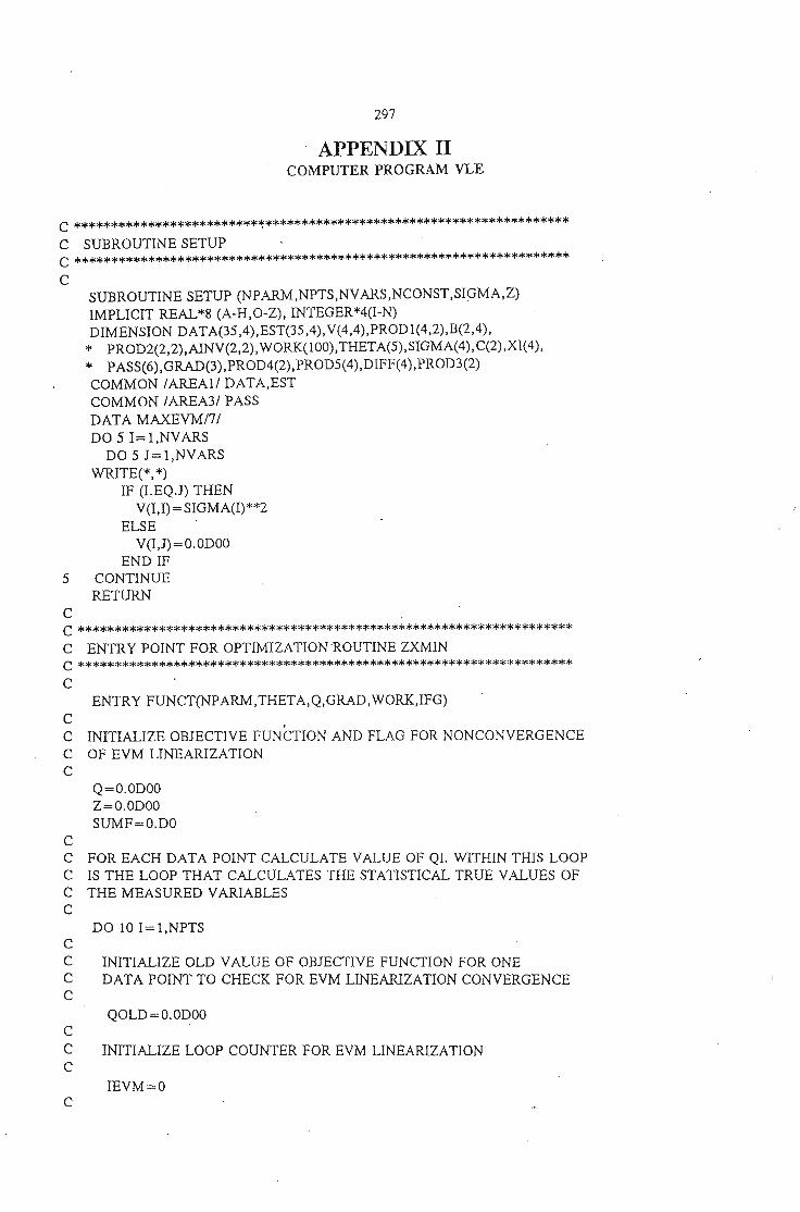
297
APPENDIX IICOMPUTER PROGRAM VLE
C *************************~******************************************
C SUBROUTINE SETUPC ********************************************************************C
SUBROUTINE SETUP (NPARM,NPTS,NVARS,NCONST,SIGMA,Z)IMPLICIT REAL*8 (A-H,O-Z), INTEGER*4(I-N)DIMENSION DATA(35,4),EST(35,4), V(4,4),PRODl(4,2),B(2,4),
* PROD2(2,2),AINV(2,2),WORK(lOO),THETA(5),SIGMA(4),C(2),XI(4),* PASS(6),GRAD(3),PROD4(2),PROD5(4),DIFF(4),PROD3(2)COMMON /AREAl/ DATA,ESTCOMMON /AREA3/ PASSDATA MAXEVMI7/DO 5 I=l,NVARS
DO 5 ]=l,NVARSWRITE(*,*)
IF (I.EQ.J) THENV(I,I) =SIGMA(I)**2
ELSEV(I,J)=O.ODOO
END IF5 CONTINUE
RETURNC
C ********************************************************************C ENTRY POINT FOR OPTIMIZATION·ROUTINE ZXMINC ********************************************************************C
ENTRY FUNCT(NPARM,THETA, Q,GRAD,WORK,IFG)CC INITIALIZE OBJECTIVE FUNCTION AND FLAG FOR NONCONVERGENCEC OF EVM LINEARIZATIONC
Q=O.ODOOZ=O.ODOOSUMF=O.DO
CC FOR EACH DATA POINT CALCULATE VALUE OF QI. WITHIN THIS LOOPC IS THE LOOP THAT CALCULATES THE STATISTICAL TRUE VALUES OFC THE MEASURED VARIABLESC
DO 10 1= 1,NPTSC
C INITIALIZE OLD VALUE OF OBJECTIVE FUNCTION FOR ONEC DATA POINT TO CHECK FOR EVM LINEARIZATION CONVERGENCEC
QOLD=O.ODOOC
C INITIALIZE LOOP COUNTER FOR EVM LINEARIZATIONC
IEVM=OC
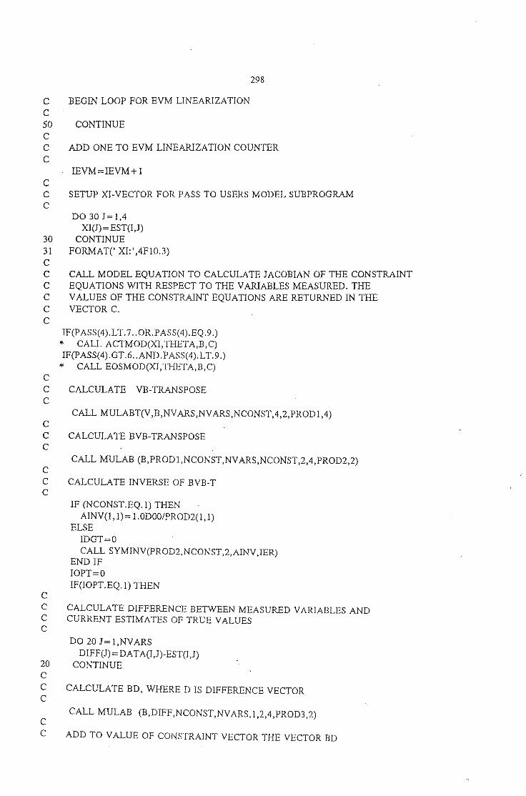
298
C BEGIN LOOP FOR EVM LINEARlZATIONC50 CONTINUECC ADD ONE TO EVM LINEARlZATION COUNTERC
IEVM=IEVM+1CC SETUP XI-VECTOR FOR PASS TO USERS MODEL SUBPROGRAMC
DO 30 J=1,4XI(J)= EST(I,J)
30 CONTINUE31 FORMAT(' XI:',4FlO.3)CC CALL MODEL EQUATION TO CALCULATE JACOBIAN OF THE CONSTRAINTC EQUATIONS WITH RESPECT TO THE VARlABLES MEASURED. THEC VALUES OF THE CONSTRAINT EQUATIONS ARE RETURNED IN THEC VECTOR C.C
IF(PASS(4).LT.7 .. OR.PASS(4). EQ. 9.)* CALL ACTMOD(XI,THETA,B,C)IF(PASS(4).GT.6 .. AND.PASS(4).LT. 9.)* CALL EOSMOD(XI,THETA,B,C)
CC CALCULATE VB-TRANSPOSEC
CALL MULABT(V,B,NVARS,NVARS,NCONST,4,2,PROD1 ,4)CC CALCULATE BVB-TRANSPOSEC
CALL MULAB (B,PROD1,NCONST,NVARS,NCONST,2,4,PROD2,2)CC CALCULATE INVERSE OF BVB-TC
IF (NCONST.EQ.1) THENAINV(1, 1)= 1.0DOO/PROD2(1,1)
ELSEIDGT=OCALL SYMINV(PROD2,NCONST,2,AINV,IER)
END IFIOPT=OIF(IOPT.EQ.1) THEN
CCCC
20CCC
CC
CALCULATE DIFFERENCE BETWEEN MEASURED VARIABLES ANDCURRENT ESTIMATES OF TRUE VALUES
DO 20 J=1,NVARSDIFF(J)=DATA(I,J)-EST(I,J)
CONTINUE
CALCULATE BD, WHERE D IS DIFFERENCE VECTOR
CALL MULAB (B,DIFF,NCONST,NVARS,1,2,4,PROD3,2)
ADD TO VALUE OF CONSTRAINT VECTOR THE VECTOR BD
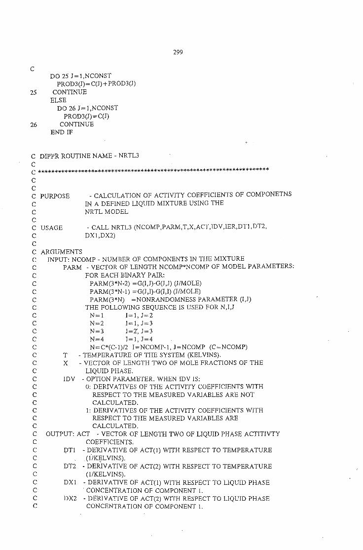
299
CDO 25 J=1,NCONST
PROD3(J) = CCJ) +PROD3(J)25 CONTINUE
ELSEDO 26 J=l,NCONST
PROD3(J)= CCJ)26 CONTINUE
END IF
C DIPPR ROUTINE NAME - NRTUCC **********************************************************************
- CALL NRTU (NCOMP,PARM,T,X,ACT,IDV,IER,DT1,DT2,DX1,DX2)
- CALCULATION OF ACTIVITY COEFFICIENTS OF COMPONETNSIN A DEFINED LIQUID MIXTURE USING THENRTL MODEL
ARGUMENTSINPUT: NCOMP - NUMBER OF COMPONENTS IN THE MIXTURE
PARM - VECTOR OF LENGTH NCOMP*NCOMP OF MODEL PARAMETERS:FOR EACH BINARY PAIR:
PARM(3*N-2) =G(I,J)-G(J,J) (l/MOLE)PARM(3*N-1) =G(J,I)-G(1,I) (l/MOLE)PARM(3*N) =NONRANDOMNESS PARAMETER (1,1)
THE FOLLOWING SEQUENCE IS USED FOR N,I,lN=1 1=1, J=2N=2 1=1, J=3N=3 I=Z, J=3N=4 1=1,1=4N=C*(C-1)/2 I=NCOMP-1, J=NCOMP (C=NCOMP)
T - TEMPERATURE OF THE SYSTEM (KELVINS).X - VECTOR OF LENGTH TWO OF MOLE FRACTIONS OF THE
LIQUID PHASE.IDV - OPTION PARAMETER. WHEN IDV IS:
0: DERIVATIVES OF THE ACTIVITY COEFFICIENTS WITHRESPECT TO THE MEASURED VARIABLES ARE NOTCALCULATED.
1: DERIVATIVES OF THE ACTIVITY COEFFICIENTS WITHRESPECT TO THE MEASURED VARIABLES ARECALCULATED.
OUTPUT: ACT - VECTOR OF LENGTH TWO OF LIQUID PHASE ACTITIVTYCOEFFICIENTS.
DT1 - ~ERIVATIVE OF ACT(1) WITH RESPECT TO TEMPERATURE( l/KJ2:LVINS).
DT2 - DERIVATIVE OF ACT(2) WITH RESPECT TO TEMPERATURE(l/KELVINS).
DX1 - DERIVATIVE OF ACT(1) WITH RESPECT TO LIQUID PHASE. CONCENTRATION OF COMPONENT 1.
DX2 - DERIVATIVE OF ACT(2) WITH RESPECT TO LIQUID PHASECONCENTRATION OF COMPONENT 1.
USAGE
CCC PURPOSECCCCCCCCCCCCCCCCCCCCCCCCCCCCCCCCCCCCCCC
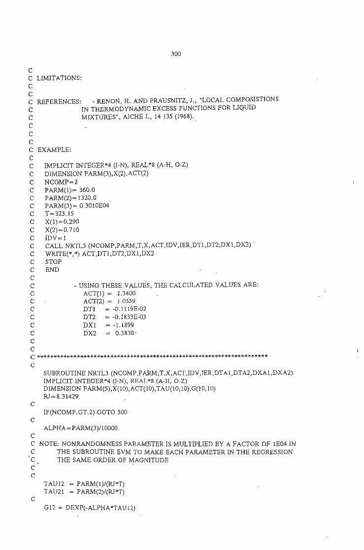
300
- USING THESE VALUES, THE CALCULATED VALUES ARE:ACT(I) = 1.3400ACT(2) = 1.0559DTl = -0.1119E-02DTI = -0.1833E-03DXl = -1.1899DX2 = 0.3830'
IMPLICIT INTEGER*4 (I-N), REAL*8 (A-H, O-Z)DIMENSION PARM(3),X(2),ACT(2)NCOMP=2PARM(I)= 360.0PARM(2)= 1320.0PARM(3)= 0.301OE04T=323.15X(1)=0.290X(2)=O.710IDV=1 .CALL NRTL3 (NCOMP,PARM,T,X,ACT,IDV,IER,DTl,DT2,DX1,DX2)'WRITE(*, *) ACT,DTl,DT2,DX1,DX2STOPEND
EXAMPLE:
REFERENCES: - RENON, H. AND PRAUSNITZ, l., "LOCAL COMPOSISTIONSIN THERMODYNAMIC EXCESS FUNCTIONS FOR LIQUIDMIXTURES", AlCHE J., 14 135 (1968).
CC LIMITATIONS:CCCCCCCCCCCCCCCCCCCCCCCCCCCCCCCCCCC **********************************************************************C
SUBROUTINE NRTL3 (NCOMP,PARM,T,X,ACT,IDV,IER,DTAl,DTA2,DXA1,DXA2)IMPLICIT INTEGER*4 (I-N), REAL*8 (A-H, O-Z)DIMENSION PARM(5),X(1O),ACT(1 0),TAU(1 O,lO),G(l 0,10)RJ=8.31429
CIF(NCOMP.GT.2) GOTO 500
CALPHA = PARM(3)11 0000.
CC NOTE: NONRANDOMNESS PARAMETER IS MULTIPLIED BY A FACTOR OF lE04 INC THE SUBROUTINE EVM TO MAKE EACH PARAMETER IN THE REGRESSIONC THE SAME ORDER OF MAGNITUDECC
TAU12 = PARM(l)/(RJ*T)TAU21 = PARM(2)/(RJ*T)
C
G12 = DEXP(-ALPHA*TAU12)
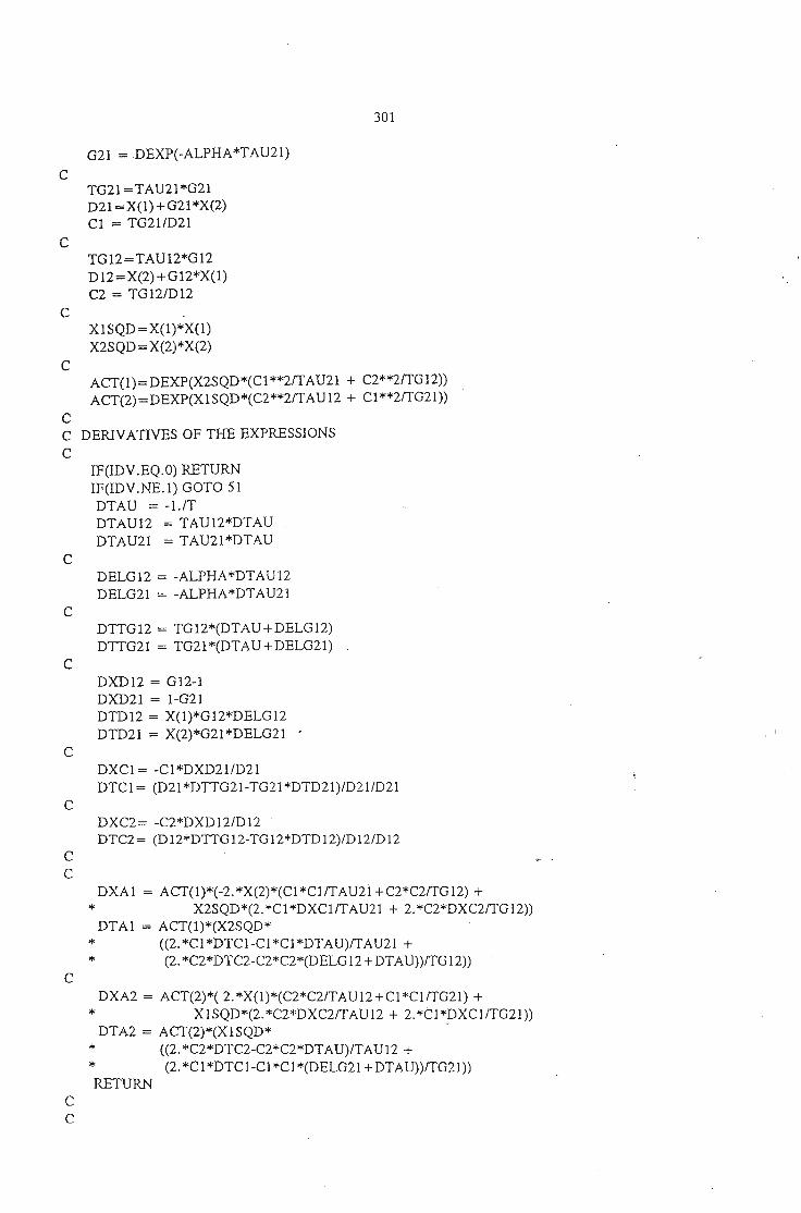
*
301
G21 = DEXP(-ALPHA*TAU2l)
CTG21 =TAU2l *G21D21 =X(1)+G21 *X(2)Cl = TG211D21
CTG12=TAU12*G12D12=X(2)+G12*X(l)C2 = TG121D12
CXlSQD=X(l)*X(l)X2SQD = X(2)*X(2)
CACT(1)=DEXP(X2SQD*(C1 **2/TAU21 + C2**2ITG12»ACT(2)=DEXP(X1SQD*(C2**2/TAU12 + Cl**2ITG21»
CC DERlVATIVES OF THE EXPRESSIONSC
IF(IDV.EQ.O) RETURNIF(IDV.NE.1) GOTO 51
DTAU = -UTDTAU12 = TAU12*DTAUDTAU21 = TAU21*DTAU
CDELG12 = -ALPHA*DTAU12DELG21 = -ALPHA*DTAU2l
CDTTG12 = TG12*(DTAU+DELG12)DTTG21 = TG21*(DTAU+DELG21)
CDXD12 = G12-1DXD21 = I-G21DTD12 = X(l)*G12*DELG12DTD21 = X(2)*G21 *DELG21
CDXCl = -Cl *DXD211D21DTCl = (D2l *DTTG21-TG21 *DTD21)1D211D21
CDXC2= -C2*DXD12/D12DTC2= (D12*DTTG 12-TG 12*DTD 12)/D121D 12
CC
DXA1 = ACT(1)*(-2.*X(2)*(C1*Cl/TAU21+C2*C2ITG12) +* X2SQD*(2. *Cl *DXClITAU2l + 2. *C2*DXC2/TG 12»
DTAl = ACT(1)*(X2SQD** ((2.*Cl*DTCl-Cl*Cl*DTAU)ITAU21 +* (2. *C2*DTC2-C2*C2*(DELG12+ DTAU»/TG12»
CDXA2 = ACT(2)*( 2.*X(l)*(C2*C2ITAU12+Cl*ClITG21) +
* XlSQD*(2. *C2*DXC2/TAU12 + 2. *Cl *DXClITG21»DTA2 = ACT(2)*(XlSQD*'
* ((2.*C2*DTC2-C2*C2*DTAU)/TAU12 +(2. *Cl *DTCl-Cl *Cl *(DELG2l +DTAU»/TG2l»
RETURNCC
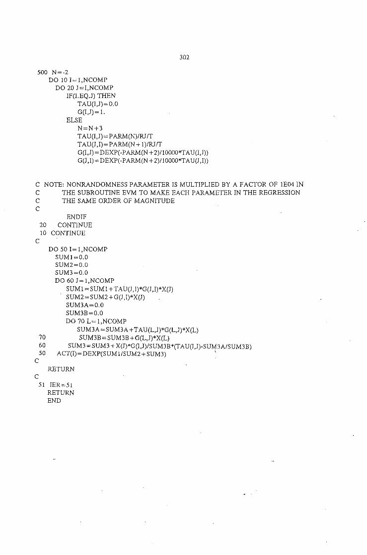
302
500 N=-2DO 10 I=l,NCOMP
DO 20 J=I,NCOMPIF(LEQ.J) THEN
TAU(I,J)=O.OG(I,J) = 1.
ELSEN=N+3TAU(I,J)=PARM(N)/RJITTAU(J,I)=PARM(N + l)/RJ/TG(I,J)=DEXP(-PARM(N + 2)/10000*TAU(I,J))G(J ,I)=DEXP(-PARM(N +2)/l0000*TAU(J ,I))
C NOTE: NONRANDOMNESS PARAMETER IS MULTIPLIED BY A FACTOR OF lE04 INC THE SUBROUTINE EVM TO MAKE EACH PARAMETER IN THE REGRESSIONC THE SAME ORDER OF MAGNITUDEC
ENDIF20 CONTINUE10 CONTINUE
CDO 50 I=l,NCOMP
SUMI=O.OSUM2=0.0SUM3=0.0DO 60 J=l,NCOMP
SUM1= SUM 1+ TAU(J,I)*G(J,I)*X(J)SUM2=SUM2+G(J,I)*X(J)SUM3A=0.OSUM3B=0.0DO 70 L= 1,NCOMP
SUM3A=SUM3A+TAU(L,J)*G(L,J)*X(L)70 SUM3B = SUM3B + G(L,J)*X(L)60 SUM3 =SUM3 + X(J)*G(I,J)/SUM3B*(TAU(I,J)-SUM3A/SUM3B)50 ACT(I)=DEXP(SUMI/SUM2+SUM3) ,
CRETURN
C51 IER=51
RETURNEND
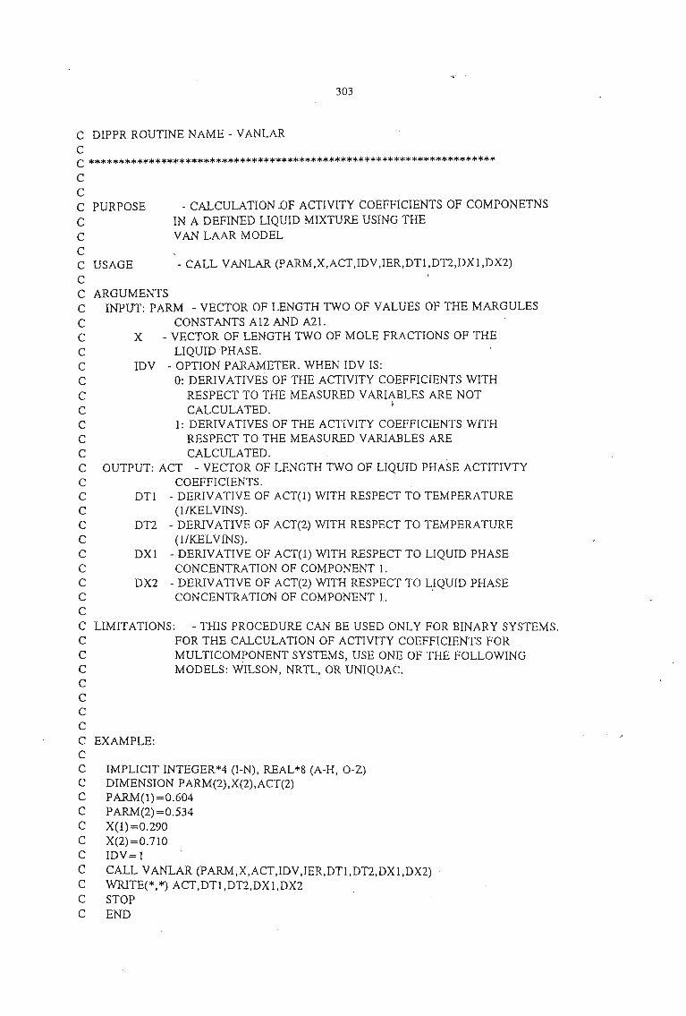
303
C DIPPR ROUTINE NAME - VANLARCC ********************************************************************
- CALL VANLAR (PARM,X,ACT,IDV,IER,DTl,DTI,DXl,DX2)
- CALCULATION OF ACTIVITY COEFFICIENTS OF COMPONETNSIN A DEFINED LIQUID MIXTURE USING THEVAN LAAR MODEL
IMPLICIT INTEGER*4 (I-N), REAL*8 (A-H, O-Z)DIMENSION PARM(2),X(2),ACT(2)PARM(1)=0.604PARM(2) =0.534X(1)=0.290X(2)=0.71OIDV=lCALL VANLAR (PARM,X,ACT,IDV,IER,DTl,DT2,DXI,DX2)WRITE(*.*) ACT,DTl,DTI,DXI,DX2STOPEND
ARGUMENTSINPUT: PARM - VECTOR OF LENGTH TWO OF VALUES OF THE MARGULES
CONSTANTS A12 AND A21.X - VECTOR OF LENGTH TWO OF MOLE FRACTIONS OF THE
LIQUID PHASE.IDV - OPTION PARAMETER. WHEN IDV IS:
0: DERIVATIVES OF THE ACTIVITY COEFFICIENTS WITHRESPECT TO THE MEASURED VARIABLES ARE NOTCALCULATED. ~
1: DERIVATIVES OF THE ACTIVITY COEFFICIENTS WITHRESPECT TO THE MEASURED VARIABLES ARECALCULATED.
OUTPUT: ACT - VECTOR OF LENGTH TWO OF LIQUID PHASE ACTITIVTYCOEFFICIENTS.
DTl - DERIVATIVE OF ACT(l) WITH RESPECT TO TEMPERATURE(lIKELVINS).
DTI - DERIVATIVE OF ACT(2) WITH RESPECT TO TEMPERATURE(l/KELVINS).
DX1 - DERIVATIVE OF ACT(l) WITH RESPECT TO LIQUID PHASECONCENTRATION OF COMPONENT 1.
DX2 - DERIVATIVE OF ACT(2) WITH RESPECT TO L.IQUID PHASECONCENTRATION OF COMPONENT 1.
LIMITATIONS: - THIS PROCEDURE CAN BE USED ONLY FOR BINARY SYSTEMS.FOR THE CALCULATION OF ACTIVITY COEFFICIENTS FORMULTICOMPONENT SYSTEMS, USE ONE OF THE FOLLOWINGMODELS: WILSON, NRTL, OR UNIQUAC.
EXAMPLE:
USAGE
CCC PURPOSECCCCCCCCCCCCCCCCCCCCCCCCCCCCCCCCCCCCCCCCCCCCCCCCC
- USING THESE VALUES, THE CALCULATED VALUES ARE:ACT(1) = 1.3266ACT(2) = 1.0548DT1 = 0.00DTI = 0.00DXl =-1.1506DX2 = 0.3737
304
CCCCCCCCCCC ********************************************************************CC
SUBROUTINE VANLAR (PARM,X,ACT,IDV ,IER,DTACTl,DTACT2,DXACTl,DXACTI)IMPLICIT INTEGER*4 (l-N), REAL*8 (A-H, O-Z)DIMENSION PARM(5),X(10),ACT(10)IER=OA12=PARM(1)A21=PARM(2)DENOM=A12*X(1)+A21 *X(2)IF(DABS(DENOM).LT.1.D-06) GOTO 920TERM 1 = A2l *X(2)/DENOMEXP01 = A12*TERM1 **2IF(DABS(EXPOl).GT.170) GOTO 921ACT(l) = DEXPCEXPOl)TERM2 =A12*X(1)/DENOMEXP02= A2l *TERM2**2IF(DABS(EXP02).GT.170) GOTO 921ACT(2) = DEXP(EXP02)IF(IDV.EQ.O) RETURNIF(IDV.NE.l) GOTO 51DXACTl = ACT(I)*(-2. *(A12*A21)**2*X(2)/DENOM**3)DTACTl = O.DO
DXACT2 = ACT(2)*(2.*(AI2*A2l)**2*X(1)/DENOM**3)DTACTI = O.DO
RETURN920IER=920
GOTO 925921 IER=921925 ACT(l)= 1.0
ACT(2)= 1.0DXACT1 =0.0DXACTI=O.ODTACT1=O.ODTACTI=O.ORETURN
51 IER==51RETURNEND
cC
C
CALCULATE INV(BVB-T)(C+BD)
CALL MULAB (AINV,PR0D3,NCONST,NCONST,I,2,2,PROD4,2)
305
C CALCULATE QI=(C+BD)-T INV(BVB-T) (C+BD)
CCALL MULATB(PROD3,PROD4, l,NCONST,l,2,2,QI,l)
27 FORMATe VALUE OF THE Q; , ,F20.6,1)
IF (IOPT.EQ.l) THENCC IF THE EVM LINEARIZATION HAD PREVIOUSLY FAILED, THENC THE QI JUST CALCULATED WAS BASED ON THE TRUE VALUE BEINGC THE MEASURED DATA POINT. GO ON TO THE NEXT POINT
CIF (IEVM.G1.MAXEVM) GOTO 60
CC CALCULATE NEW DATA VECTOR
CCALL MULAB (PROD 1,PROD4,NVARS,NCONST, l,4,2,PROD5,4)DO 40 J=l,NVARS
EST(I,]) = DATA(I,J)-PROD5(J)40 CONTINUE
IF (QI.EQ.O.ODOO) GOTO 60IF (DABS(QOLD-QI)/QI.LT.1.0D-07) GOTO 60IF (EST(I,3).LT.0.DO.OR.EST(I,3).GT.l.DO) IEVM=MAXEVMIF (EST(I,4).LT.0.DO.OR.EST(I,4).GT.l.DO) IEVM=MAXEVM
CC SAVE RECENTLY CALCULATED QI FOR COMPARISON ON NEXTC LINEARIZATIONC
49 FORMATe Q AND XI:',F15.6,2FI0.3,2F15.5)QOLD=QI
CC EVM LINEARIZATION CONVERGES' IN FOUR TO FIVE ITERATIONSC (IEVM) USU~LY. HOWEVER, SOMETIMES THE LINEARIZATIONC FAILS WHEN THETA IS NOT CLOSE TO THE MAXIMUMC LIKELIHOOD ESTIMATES. IN THIS CASE, SET VARIABLE ESTIMATESC TO THE MEASURED DATA AND CALCULATED QI. THISC IS USUALLY A CLOSE ENOUGH APPROXIMATION TO ALLOW ZXMINC TO GET CLOSER TO THE CORRECT V4UE OF THETA. WHEN THEC TRUE VALU~ OF THETA IS APPROACHED, THE EVM LINEARIZATIONC CONVERGES.C
IF (IEVM.LT.MAXEVM) GOTO 50WRITE (6, *) , EVM DID NOT CONVERGE POINT ',IDO 70 1=I,NVARS
EST(I ,1) = DATA(I ,J)70 CONTINUE
GOTO 5060 CONTINUE
END IFSUMF=SUMF +C(1)+C(2)Q=Q+QIZ=Z"+DSQRT(QI)
10 CONTINUE
2000 FORMATe TH,QI,Q,Fl,F2,SF',F8.3,5FlO.0)RETURNEND
306
C DIPPR ROUTINE NAME - UNIQUACC **********************************************************************
- .CALL UNIQUA CNCOMP,PARM,R,QQ,QP,T,X,ACT,IDV,IER,DTl,DTI,DX1,DX2)
- CALCULATION OF ACTIVITY COEFFICIENTS OF COMPONETNSIN A DEFINED LIQUID MIXTURE USING THEUNIQUAC MODEL
RQQQP
ARGUMENTSINPUT: NCOMP - NUMBER OF COMPONENTS IN THE MIXTURE
PARM ~ VECTOR OF LENGTH NCOMP*CNCOMP-l) OF PARAMETERS:FOR EACH BINARY PAIR:
PARM(2*N-l) =U(I,J) (J/MOLE)PARMC2*N) = U(J,I) (J/MOLE)
WHERE N IS THE BINARY PAIR NUMBER. THE FOLLOWINGSYSTEM IS USED TO NUMBER BINARY PAIRS: PAIRNUMBER ONE IS 1=1, J=2. PAIRS ARE NUMBEREDSUCCESIVELY UNTIL I=l,J=NCOMP. THE NEXT PAIR ISI=2,J=3, AND PAIRS ARE NUMBERED SUCCESSIVELYUNTIL I=2,J=NCOMP. THE NUMBERING CONTINUES UNTIL I=NCOMP-l AND J=NCOMP.
- VOLUME PARAMETER FOR UNIQUAC MODEL.- SURFACE AREA PARAMETER FOR UNIQUAC MODEL.- SURFACE AREA PARAMETER FOR UNIQUAC MODEL ADJUSTED
FOR ALCOHOLS AND WATER.T - TEMPERATURE OF THE SYSTEM (KELVINS).X - VECTOR OF LENGTH TWO OF MOLE FRACTIONS OF THE
LIQUID PHASE:IDV - OPTION PARAMETER. WHEN IDV IS:
0: DERIVATIVES OF THE ACTIVITY COEFFICIENTS WITHRESPECT TO THE MEASURED VARIABLES ARE NOTCAI.;CULATED.
1: DERIVATIVES OF THE ACTIVITY COEFFICIENTS WITHRESPECT TO THE MEASURED VARIABLES ARECALCULATED.
OUTPUT: ACT - VECTOR OF LENGTH TWO OF LIQUID PHASE ACTITIVTYCOEFFICIENTS.
DTl - DERIVATIVE OF ACT(l) WITH RESPECT TO TEMPERATURE(l/KELVINS).
DTI - DERIVATIVE OF ACT(2) WITH RESPECT TO TEMPERATURECl/KELVINS).
DXl - DERIVATIVE OF ACT(l) WITH RESPECT TO LIQUID PHASECONCENTRATION OF COMPONENT 1.
DX2 - DERIVATIVE OF ACT(2) WITH RESPECT TO LIQUID PHASECONCENTRATION OF COMPONENT 1.
USAGE
LIMITATIONS:
REFERENCES: ~ ABRAMS, D. AND PRAUSNITZ, l., "STATISTICALTHERMODYNAMICS OF LIQUID MIXTURES: A NEWEXPRESSION FOR THE EXCESS GIBBS ENERGY OF
CCC PURPOSECCCCCCCCCCCCCCCCCCCCCCCCCCCCCCCCCCCCCCCCCCCCCCCCCC
307
IMPLICIT INTEGER*4 (I-N), REAL*8 (A-H, O-Z)DIMENSION PARM(2),X(2),ACT(2),R(2),QQ(2),QP(2)
NCOMP=2PARM(l)= 1448.0PARM(2)= 1188.0T=323.15X(l)=0.290X(2)=O.710R(1)=2.5735R(2) =1.4311QQ(I)=2.336QQ(2) = 1.432QP(l)=2.336QP(2)=O.96IDV=lCALL UNIQUA (NCOMP,PARM,R,QQ,QP,T,X,ACT,IDV,IER,DTl,DT2,DXI,DX2)WRITE(*, *) ACT,DT1 ,DT2,DX1 ,DX2STOPEND
CCCCCC EXAMPLE:CCCCCCCCCCCCCCCCCCCCCCCCCCCCC
PARTIALLY OR COMPLETELY MISCIBLE SYSTEMS", AICHEl., 21 116 (1975).
- USING THESE VALUES, THE CALCULATED VALUES ARE:ACT(l) = 1.5746ACT(2) = 1.2051DT1 = -0.221OE-02DT2 = -0.6366E-03DX1 = -3.4384DX2 = 1.1543
C ********~*************************************************************
C
SUBROUTINE UNIQUA (NCOMP,PARM,R,QQ,QP,T,X,'" ACT,IDV ,IER,DT1 ,DTI,DX1,DX2)IMPLICIT INTEGER*4 (I-N), REAL*8 (A-H, O-Z)REAL*8 L,Ll,L2DIMENSION ACT(1O),PARM(5),X(lO),R(lO),
* QQ(lO),QP(lO),THP(IO),'" L(IO),TAU(lO, 10)
CX1SQ=X(I)*X(1)X2SQ=X(2)"'X(2)RJ =8.31439Z= 10.DOODX1 =O.DODX2=0.DODTl=O.DODT2=O.DO
C
IF(NCOMP.GT.2) GOTO 500C
SUMXR = X(l)*R(I) + X(2)*R(2)SUMXQ = X(1)*QQ(1)+X(2)*QQ(2)SUMXQP = X(I)*QP(1)+X(2)*QP(2)SUMXR2 ,;" SUMXR*SUMXRSUMXQ2 = SUMXQ*SUMXQSMXQP2 = SUMXQP*SUMXQP
CPHIl = X(1)*~(l)/SUMXR
PHI2 = X(2)*R(2)/SUMXRTHl = X(l)*QQ(l)/SUMXQTH2 = X(2)*QQ(2)/SUMXQTHIP = X(l)*QP(1)/SUMXQPTH2P = X(2)*QP(2)/SUMXQPTAUI2 = DEXP(-PARM(I)/(RJ*T))TAU2I = DEXP(-PARM(l)/(RJ*T))
CDPHIl = R(1)*R(2)/SUMXR2DPHI2 = -R(I)*R(2)/SUMXR2DTHl = QQ(I)*QQ(2)/SUMXQ2DTH2 = -QQ(1)*QQ(2)/SUMXQ2DTHIP = QP(I)*QP(2)/SMXQP2DTH2P = -QP(I)*QP(2)/SMXQP2DTAU12 = TAUI2*PARM(I)/(RJ*T*T)DTAU21 = TAU21*PARM(2)/(RJ*T*T)
CWll= THIP + TH2P*TAU2lW22= THIP*TAUI2 + TH2PLl = Z/2. *(R(1)-QQ(l))-(R(l)-1.DO)L2 = Z/2. *(R(2)-QQ(2))-(R(2)-l.DO)
CIF(X(1).LE.l.D-08) THEN
ACT(1) = l.DOACT(l) = l.DOGOTO 5ENDIF
IF(X(2).LE.l.D-08) THENACT(I)= 1. DO .ACT(2)= 1. DOGOT05ENDIF
GOT065 RETURN
C
6 AI = PHIlIX(l)Bl = (THIIPHIl)**(Z/2.*QQ(1))Dl = PHI2*(Ll-R(1)/R(2)*L2) .Cl = Wll**(-QP(l))El = TH2P*QP(1)1W11Fl = TH2P*QP(1)1W22.
C
A2. = PHI2/X(2)B2 = (TH2/PHI2)**(Z/2. *QQ(2))D2 = PHIl *(L2-R(2)/R(1)*L1)Cl = W22**(-QP(2))
308
C
309
E2 = THIP*QP(2)/W22F2 = THIP*QP(2)1W11
CACT(l) = Al * Bl * Cl * DEXP(Dl + TAU21 *El - TAU12*Fl)ACT(2) = A2 * B2 * C2 * DEXP(D2 + TAU12*E2 - TAU21*F2)
CIF(IDV.EQ.O) RETURNIF(IDV.NE.l) GOTO 51
C WRITE(*.*)'THE VALUES OF ACTl,2:',ACTl.ACT2
CDXAl = (X(l)*DPHII-PHIl)/XISQDXBl = Z/2.*QQ(I)*(THI/PHIl)**(Z/2. *QQ(l)-l.DO)
* *(PHIl *DTHI-DPHIl*THl)/PHIl/PHIlDXCl = -QP(l)*Wll **(-QP(I)-l.DO)*(DTHIP+DTH2P*TAU21)DXDl = DPHI2*(Ll-R(I)/R(2)*L2)DXEl = QP(I)*(Wll*DTH2P-(DTHIP+DTH2P*TAU21)*TH2P)IWHIW1lDXF 1 = QP(1)*(W22*DTH2P-(DTH1P*TAU12 + DTH2P)*TH2P)/W221W22
DXA2 = (X(2)*DPHI2+PHI2)/X2SQDXB2 = Z/2. *QQ(2)*(TH2/PHI2)**(Z/2. *QQ(2)-I.DO)
* *(PHI2*DTH2-DPHI2*TH2)/PHI2/PHI2DXC2 = -QP(2)*W22**(-QP(2)-l.DO)*(DTHIP*TAUI2+DTH2P)DXD2 = DPHIl *(L2-R(2)/R(I)*Ll)DXE2 = QP(2)*(W22*DTHIP-(DTHIP*TAUI2+DTH2P)*THIP)/W221W22DXF2 = QP(2)*(Wll *DTHIP-(DTHIP+ DTH2P*TAU21)*THIP)lWll1Wll
CDXl =ACT(l)*
* (DXAl/Al + DXBl/Bl + DXClICl +(DXDl +TAU21 *DXEI-TAU12*DXFl))DX2=ACT(2)*
* (DXA21A2 + DXB2/B2 + DXC2/C2 + (DXD2 + TAU 12*DXE2-TAU 12*DXF2))C
DTCl = -QP(l)*Wll **(-QP(I)-l.DO)*(TH2P*DTAU21)DTEl = -EIIW1l*(TH2P*DTAU21)DTFl = -FIIW22*(THIP*DTAU12)
CDTC2 = -QP(2)*W22**(-QP(2)-l.DO)*(THIP*DTAUI2)DTE2 = -E2/W22*(THIP*DTAU12)DTF2 = -F21W1l*(THlP*DTAU21)
CDTl =ACT(l)*
* (DTCl/Cl +TAU21 *DTEl + DTAU21 *El-(TAUI2*DTFl + DTAUI2*Fl))DT2=ACT(2)*
* (DTC2/C2+TAU12*DTE2+ DTAU12*E2-(TAU21 *DTF2+ DTAU21 *F2))C
RETURNC500 N=-1
SUMXR= O.DOSUMXQ= O.DO
,SUMXQP=O.DODO 101= l,NCOMP
DO 20 J =I,NCOMPIF(I.EQ.J) THEN
TAU(I,J)= l.DOELSE
N=N+2
. i
310
TAU(I,J)= DEXP(-PARM(N)/RJ/T)TAU(J,I)= DEXP(-PARM(N + 1)/RJ/T)
ENDIF20 CONTINUE
SUMXR= SUMXR + X(I)*R(I)SUMXQ= SUMXQ + X(I)*QQ(I)SUMXQP=SUMXQP+ X(I)*QP(I)L(I) = Z/2. *(R(I)-QQ(I))-(R(I)-l.)
10 CONTINUEC
SUM1=0.DODO 501= l,NCOMP
SUM 1= SUM 1+ X(I)*L(I)50 THP(I)=X(I)*QP(I)/SUMXQP
CDO 1001= I,NCOMP
PHI = X(I)*R(I)/SUMXRTHETA = X(I)*QQ(I)/SUMXQA=PHII,X(I)B = THETA/PHISUM2=0.DOSUM3=0.DODO 110 J= I,NCOMP
SUM2=SUM2+THP(I)*TAU(J,I)SUM3A=0.DODO 120 K= I,NCOMP
120 SUM3A=SUM3A+THP(K)*TAU(K,J)110 SUM3=SUM3+THP(J)*TAU(I,J)/SUM3A100 ACT(I) = A*DEXP(Z/2. *QQ(I)*DLOG(B) +L(I)-A*SUM 1
* -QP(I)*DLOG(SUM2) + QP(I)-QP(I)*SUM3)C
RETURN51 IER=51
RETURNEND
C DIPPR ROUTINE NAME - DELlJCC **********************************************************************
- CALL D?LU (NCOMP,MIX,THETA,XY,K,AU,DEL,DXDEL)
- CALCULATION OF ENERGY PARAMETER A(I,J) AND BINARYINTERACTION PARAMETER DEL(I,J) USING THEGEOMETRIC MEAN MIXING RULE OR COMPOSITIONDEPENDENT INTERACTION PARAMETER MIXING RULE.
USAGE
ARGUMENTSINPUT: NCOMP - NUMBER OF COMPONENTS IN THE MIXTURE
MIX - INDICATOR FOR MIXING RULES. WHEN MIX IS:1: GEOMETRIC MEAN MIXING RULES (REFERENCE #1)2: COMPOSITION DEPENDENT INTERACTION PARAMETER
(REFERENCE #2)
CCC PURPOSECCCCCCCCCCCC
REFERENCES: - SOAVE, G., "EQUILIBRIUM CONSTANTS FROM A MODIFIEDREDLICH-KWONG EQUATION OF STATE," CHEM. ENG.SCL, 27,1197 (1972).
- PANAGIOTOPOLOUS, A. Z. AND REID, R. C., "NEW MIXINGRULES FOR CUBIC EQUATIONS OF STATE FOR HIGHLYPOLAR, ASYMMETRIC SYSTEMS," EQUATIONS OF S:rATETHEORIES AND APPLICATIONS, ACS SYMPOSIUM SERIES,NO. 300, 571 (1986).
THETA - VECTOR OF LENGTH 2*NPARM OF PARAMETERSFOR MIX= I:
THETA(N) = DEL(I,J)FOR MIX=2:
THETA(2*N-l)= K(I,J)THETA(2*N) = K(J,I)
WHERE N IS THE BINARY PAIR NUMBER. THE FOLLOWINGSYSTEM IS USED TO NUMBER BINARY PAIRS: PAIRNUMBER ONE IS 1=1, J=2. PAIRS ARE NUMBEREDSUCCESIVELY UNTIL I;:=1,J=NCOMP. THE NEXT PAIR ISI=2,J=3, AND PAIRS ARE NUMBERED SUCCESSIVELYUNTIL I=2,J=NCOMP. THE NUMBERING CONTINUES INTHIS MANNER UNTIL I=NCOMP-l AND J=NCOMP.
XY - VECTOR OF LENGTH NCOMP OF MOLE FRACTIONS, EITHERVAPOR OR LIQUID.
OUTPUT: K - MATRIX OF DIMENSION (NPARM,NPARM) OF BINARYINTERACTION PARAMETERS.
AD - MATRIX OF DIMENSION (NPARM,NPARM) OF ENERGYPARAMETERS USED IN THE CALCULATION OF THE ENERGYPARAMETER A OF THE MIXTURE.
DEL - MATRIX OF DIMENSION (NPARM,NPARM) OF BINARYINTERACTION PARAMETERS.
DXDEL - DERIVATIVE OF THE BINARY INTERACTION PARAMETERDEL(I,J) WITH RESPECT TO COMPOSITION. USED ONLYBINARY SYSTEMS.
311
CCCCCCCCCCCCCCCCCCCCCCCCCCCC LIMITATIONS: - THE SOAVE EQUATION OF STATE WORKS BEST FOR HIGHC PRESSURE SYSTEMS (REGIONS NEAR THE CRITICAL).C FOR LOW PRESSURE SYSTEMS, ACTIVITY COEFFICIENTC MODELS PERFORM BETTER. THE MATHIAS-COPEMANC MIXING RULES (MIX=4) WORK BEST, BUT GREATLYC INCREASE COMPUTATION TIMES. THE HURON-VIDALC MIXING RULES (MIX=3) ARE THE NEXT BEST AVAILABLEC MIXING RULE. A COMPARISON OF THE MIXING RULESC FOR LOW PRESSURE SYSTEMS CAN BE FOUND IN CHAPTERC 8 OF GESS AND DANNER (1988).CCCCCCCCCCCCC
SUBROUTINE DELI] (NCOMP,MIX,PARM,XY,K,AIJ,DEL,DXDEL)IMPLICIT INTEGER*4 (I-N), REAL*8 (A-H, O-Z)REAL*8 KDIMENSION PARM(5),XY(1O),K(lO,lO),AD(lO,10),
* DEL(lO,10)N=1
312
DO 101= I,NCOMPDO 20J=I,NCOMP
IF(I.EQ.J) GOTO 25IF(MIX.EQ.l) GOTO 30
K(I,J) =PARM(2*N-l )/1 O.K(J ,I) = PARM(2*N)11O.DEL(l,J) = K(l,J)-(K(I,J)-K(J ,I))*XY(I)DEL(J,1) = K(J ,I)-(K(J ,I)-K(I,J))*XY(J)GOTO 40K(l,J)=O.O
K(J,I)=O.ODEL(I,J) = PARM(N)/lO.DEL(J ,I) = DEL(I,J)N=N+l
AIJ(l,J) = DSQRT(AIJ(I,I)*AD(J ,J))*Cl-DEL(I,J))AD(J ,I) = DSQRT(AIJ(I,I)*AD(J ,J))*(l-DEL(J ,I))
WRITE(*, *) 'I,J ,AIJ ,DELIJ' ,1,1 ,AIJ(I,J),DEL(I,J)GOTO 20
K(I,J)=O.DODEL(I,J)=O.O
CONTINUECONTINUE
25
40
30
2010
CC WRITE(*,7) AIJ(l, 1),AIJ(2,2),AIJ(I,2),XY(I)C 7 FORMATe APX:',4D15.5)
DXDEL=-K(l ,2) + K(2, 1)
C
CRETURNEND
SUBROUTINE DATMODIMPLICIT REAL*8 (A-H,O-Z), INTEGER*4 (I-N)REAL*8 LMVINTEGE~*4 VLEIDDIMENSION VAP(5), UNIQ(8),IDREC(500)CHARACTER VLENAM*30,VLEFOR*1O,FMSRCH*10,RC*3,YON*1CHARACTER DISPLl *11 ,DISPL2*1OCHARACTER ENDHCHARACTER*3 BEGCHARACTER BEGX(3)EQUIVALENCE (BEG,BEGX)DATA UNIQ /0.96,0.92,0.89,0.88,1.15,1.78,2.71,1.00/BEGX(I)=CHAR(19)BEGX(2) = CHAR(255)BEGX(3)=CHAR(I)ENDH=CHAR(l)
C
OPEN (20,FILE= 'PUREDAT' ,ACCESS= 'DIRECT' ,FORM= 'FORMATTED' ,RECL= 80)OPEN (25,FILE'= 'PURELST' ,ACCESS= 'DIRECT' ,FORM = 'FORMAlTED' ,RECL= 80)READ (20,I,REC=I) NTOT
1 FORMAT(I4,76X)C
2 WRITE(*, *) BEG, 'USE,MAlI02.AID' ,ENDHWRITE(*,*) BEG,'MENU',ENDH
313
READ(*,5) IOPT5 FORMAT(I2)
IF (IOPT.EQ.4) GO TO 1000
CIF (IOPT.EQ.1) THEN
102 WRITE(*,*) BEG,'USE,DATOOl.AID',ENDHWRITE(*,*) BEG,'MENU',ENDHREAD(*,5) IOPT!IF (IOPTl.EQ.4) GO TO 2IC=OIF (IOPTl.EQ.1) THEN
IC=NTOTDO 1041= 1,IC
IDREC(I) = I + 1104 CONTINUE
ELSE IF (IOPTl.EQ.2) THENWRITE(*, *) BEG,'OPEN,DAT003.AID, 16,25' ,ENDHWRITE(*, *) BEG, 'INPUT,IDSRCH' ,ENDHREAD(*, 105) IDSRCH
105 FORMAT(I4)IF «IDSRCH.LE.O).OR.(IDSRCH.GT.NTOT» THEN
DO 108 I= 1,80WRITE(*, *) BEG, 'MERGE,DAT008.AID,22,25' ,ENDH
108 CONTINUEGO TO 102
END IFIC=1IDREC(IC)=IDSRCH + 1
ELSE IF (IOPTl.EQ.3) THENWRITE(*,*) BEG,'OPEN,DAT004:AID,16,25',ENDHWRITE(*,*) BEG,'INPUT,FMSRCH',ENDHREAD(*,"110) FMSRCH
110 FORMAT(AlO)IF (FMSRCH.EQ.' ') GO TO 112CALL FORM (FMSRCH,IDREC,IC)
;IF (IC.EQ.O) THEN112 DO 1131=1,80
WRITE(*,*) BEG,'MERGE,DAT008.AID,22,25 ' ,ENDH113 CONTINUE
GO TO 102END IF
END IFC
IK=IC/16IF(IC.GT.(IK*16» IK=IK + 111=0
120 WRITE(*,*) BEG,'USE,DAT002.AID' ,ENDHIF(JJ.EQ.O) WRITE(*,*) BEG, 'MERGE,DAT009.AID,24, 12' ,ENDHIF(11.EQ.(IK-1» WRITE(*, *) BEG, 'MERGE,DAT009.AID,24,SI' ,ENDHJJ16=JJ*16DO 1301=1,16
II=I+JJ16IF(II.LE.IC) THEN
READ(25, 125 ,REC=IDREC(II»VLEID, VLENAM, VLEFOR125 FORMAT(I4,5X,A30,AlO,31X)
WRITE(*,*) BEG, 'DISPLAY,VLEID,' ,I,' ,=', VLEID,ENDH
314
WRITE(*, *) BEG , 'DISPLAY, VLEFOR,' ,I,', =',VLEFOR,ENDHWRITE(*,*) BEG,'DISPLAY,VLENAM,',I,', = ',VLENAM,ENDH
END IF130 CONTINUE
WRITE(*,*) BEG, 'MENU' ,ENDHREAD(* ,5) IOPTLIF «JJ.EQ.0).AND.(JJ.EQ.(IK-1))) GO TO 102IF (JJ.EQ.O) THEN
IF (lOPTL.EQ.1) THENGO TO 102
ELSE IF (lOPTL.EQ.2) THEN11=11 + 1GO TO 120
END IFEND IFIF (11.EQ.(lK-1)) THEN
IF (IOPTL.EQ.1) THEN11=11-1GO TO 120
ELSE IF (lOPTL.EQ.2) THENGO TO 102
END IFEND IFIF (IOPTL.EQ.l) THEN
11=11-1GO TO 120
ELSE IF (lOPTL.EQ.2) THENGO TO 102
ELSE IF (IOPTL.EQ.3) THEN11=JJ + 1GO TO 129
END IFEND IF
C
*
*
308
320
IF (IOPT.EQ.3) THENWRITE(*, *) BEG,'USE,DAT007 .AID, 17,23' ,ENDHWRITE(*, *) BEG, 'INPUT,IDEDIT' ,ENDHREAD(*, 105) IDEDITIF «IDEDIT.LE.O). OR. (IDEDIT.GT.NTOT)) THEN
DO 308 1= 1,80WRITE(*, *) BEG, 'MERGE,DAT008.AID,22,25' ,ENDH
CONTINUEGOTO 2
END IFREAD(25 ,125,REC=IDEDIT+ l)VLEID, VLENAM,VLEFORREAD(20,320,REC = 2*IDEDIT)VLEID ,(VAP(I),I= 1,5),LMV,TC,PC,
DPM,RG,ASSOC,UNIQ1,UNIQ2,UNIQ3,ACENFORMAT(l4, lX,5(lPE11.4, 1X),OPF8.6, 1X,F6.2,1,
F8.2,3X,F6.4,3X,F6.4,3X,F4.2,3X,4(F7.4,3X),4X)YON='N'IF (UNIQ3.NE.UNIQ2) YON='Y'
CWRITE(*.. *) BEG, 'VERTICAL, YES' ,ENDHWRITE(*, *) BEG,'EXIT,RET=D,TAB=D,BAT= U,FKl =H,FK3= V,FKO= V' ,ENDHWRITE(*,*) BEG,'USE,DAT005.AID',ENDHWRITE(*,*) BEG, 'DISPLAY,VLEID,=' ,VLEID,ENDH
315
WRITE(*, *) BEG, 'DISPLAY,VLENAM, =' ,VLENAM,ENDHWRITE(*.*) BEG, 'DISPLAY ,VLEFOR,=' .VLEFOR,ENDHWRITE(*,*) BEG,'DISPLAY,TC,=',TC,ENDHWRITE(DISPL2,330)PC*1000.0
330 FORMAT(IPEI0.4)WRITE(*, *) BEG, 'DISPLAY ,PC, =' ,DISPL2,ENDHWRITE(*.*) BEG,'DISPLAY,LMV,=' ,LMV,ENDHWRITE(*.*) BEG. 'DISPLAY,ACEN. =' ,ACEN.ENDHWRITE(DISPL2,330)RG*I.0E-I0WRITE(*,*) BEG,'DISPLAY.RG,=' .DISPL2.ENDHWRITE(DISPL2,330)DPM*3.33564E-30WRITE(*,*) BEG. 'DISPLAY .DPM, =' ,DISPL2,ENDHWRITE(*. *) BEG, 'DISPLAY,ASSOC, =' .ASSOC,ENDHWRITE(*.*) BEG,'DISPLAY,UNIQl,=' .UNIQl,ENDHWRITE(*,*) BEG,'DISPLAY,UNIQ2,=' ,UNIQ2,ENDHWRITE(*, *) BEG, 'DISPLAY, YON, =',YON,ENDHDO 3401=1,5
WRITE(DISPLl ,335)VAP(I)335 FORMAT(IPEl1.4)
WRITE(*.*) BEG,'DISPLAY,VAP,',I,' ,=',DISPLl,ENDH340 CONTINUE
GO TO 440END IF
CVLEID = NTOT+ 1WRITE(*, *) BEG, 'VERTICAL, YES' ,ENDHWRITE(*, *) BEG, 'EXIT,RET=D,TAB = D,BAT= U,FK 1= H,FK3 = V,FKO= V' ,ENDHWRITE(*,*) BEG,'USE,DAT005.AID',ENDHWRITE(*,*) BEG, 'DISPLAY, VLEID, =:= ',VLEID,ENDH
C
440 WRITE(*,*} BEG, 'SCREEN,VERIFY,RC',ENDHREAD(*,450) RC
450 FORMAT(A3)IF (RC.EQ. 'XXX') THEN
WRITE(*,*) BEG,'FIRST,VAP,I,' ,ENDHGO TO 440
END IFWRITE(*, *) BEG, 'EXIT' ,ENDHWRITE(*,*) BEG,'VERTICAL,NO',ENDHIF(RC.EQ. 'FK3') GO TO 2
C
WRITE(*, *) BEG, 'RECOVER, VLENAM' ,ENDHREAD(*,205) VLENAM
205 FORMAT(A30)WRITE(*, *) BEG, 'RECOVER, VLEFOR' ,ENDHREAD(*,21O) VLEFOR
210 FOR1v1AT(AI0)CALL FORM (VLEFOR,IDREC,-l)WRITE(*,*) BEQ,'RECOVER,T9',ENDHREAD(*,215} TC -
215 FORMAT(F6.2)WRITE(*, *) BEG,'RECOVER,PC' ,ENDHREAD(*,220) PC
220 FORMAT(GIO.4)PC=PCIlOOO.OWRITE(*,*) BEG,'RECOVER,LMV',ENDH
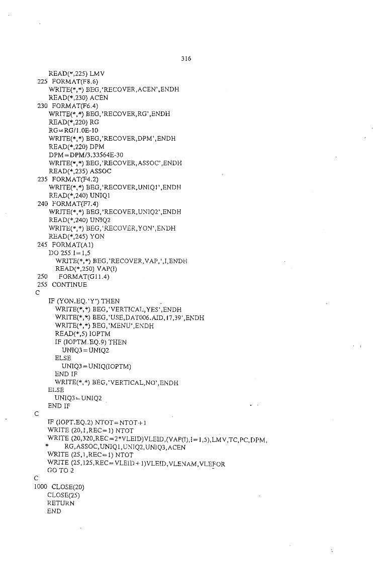
316
READ(*,225) LMV225 FORMAT(F8.6)
WRITE(*, *) BEG, 'RECOVER,ACEN' ,ENDHREAD(*,230) ACEN
230 FORMAT(F6.4)WRlTE(*, *) BEG, 'RECOVER,RG' ,ENDHREAD(*,220) RGRG=RG/1.0E-I0WRlTE(*,*) BEG,'RECOVER,DPM',ENDHREAD(*,220) DPMDPM=DPM/3.33564E-30WRITE(*,*) BEG, 'RECOVER,ASSOC' ,ENDHREAD(*,235) ASSOC
235 FORMAT(F4.2)WRITE(*,*) BEG,'RECOVER,UNIQ1',ENDHREAD(*,240) UNIQ1
240 FORMAT(F7.4)WRITE(*, *) BEG, 'RECOVER, UNIQ2' ,ENDHREAD(*,240) UNIQ2WRITE(*,*) BEG,'RECOVER,YON',ENDHREAD(*,245) YON
245 FORMAT(A1)DO 255 1= 1,5
WRITE(*, *) BEG, 'RECOVER, VAP,' ,I,ENDHREAD(*,250) VAP(I)
250 FORMAT(G11.4)255 CONTINUE
CIF (YON.EQ. 'Y') THEN
WRITE(*,*) BEG,'VERTICAL,YES',ENDHWRITE(*,~)BEG, 'USE,DAT006.AlD, 17,39' ,ENDHWRITE(*,*) BEG,'MENU',ENDHREAD(*,5) IOPTMIF (lOPTM.EQ.9) THEN
UNIQ3 = UNIQ2ELSE
UNIQ3 = UNIQ(lOPTM)END IFWRITE(*, *) BEG, 'VERTICAL, NO' ,ENDH
ELSEUNIQ3 = UNIQ2
END IFC
IF (IOPT.EQ.2) NTOT=NTOT+ 1WRITE (20,l,REC=I) NTOTWRITE (20,320,REC=2*VLEID)VLEID,(VAP(I),I= 1,5),LMV,TC,PC,DPM,
* RG,ASSOC,UNIQ1,UNIQ2,UNIQ3,ACENWRITE (25,l,REC=l) NTOTWRITE (25, 125,REC= VLEID + I)VLEID, VLENAM, VLEFORGO TO ~ -
C1000 CLOSE(20)
CLOSE(25)RETURNEND
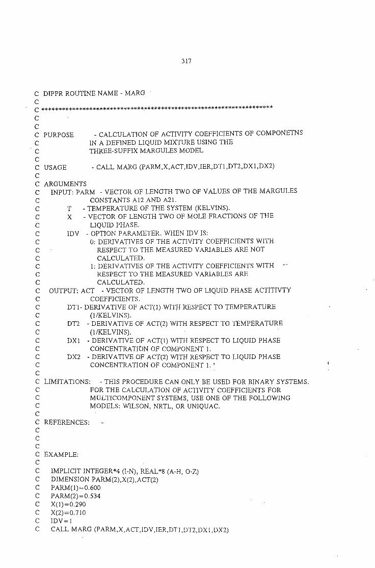
317
C DIPPR ROUTINE NAME - MARGCC ********************************************************************
- CALL MARG (PARM,X,ACT,IDV,IER,DTl,DT2,DXI,DX2)
- CALCULATION OF ACTIVITY COEFFICIENTS OF COMPONETNSIN A DEFINED LIQUID MIXTURE USING THETHREE-SUFFIX MARGULES MODEL
IMPLICIT INTEGER*4 (I-N), REAL*8 (A-H, O-Z)DIMENSIONPARM(2),X(2),ACT(2)PARM(1)=O.600PARM(2) =0.534X(1)=O.290X(2)=O.710IDV=lCALL MARG (PARM,X,ACT,IDV,IER,DTl ,DT2,DXl ,DX2)
LIMITATIONS: - THIS PROCEDURE CAN ONLY BE USED FOR BINARY SYSTEMS.FOR THE CALCULATION OF ACTIVITY COEFFICIENTS FORMULTICOMPONENT SYSTEMS, USE ONE OF THE FOLLOWINGMODELS: WILSON, NRTL, OR UNIQUAC.
C
CC PURPOSEC
·C
CC USAGECC ARGUMENTSC INPUT: PARM - VECTOR OF LENGTH TWO OF VALUES OF THE MARGULESC CONSTANTS AI2 AND A21.C T - TEMPERATURE OF THE SYSTEM (KELVINS).C X - VECTOR OF LENGTH TWO OF MOLE FRACTIONS OF THEC LIQUID PHASE.C IDV - OPTION PARAMETER. WHEN IDV IS:C 0: DERIVATIVES OF THE ACTIVITY COEFFICIENTS WITHC RESPECT TO THE MEASURED VARIABLES ARE NOTC CALCULATED.C 1: DERIVATIVES OF THE ACTIVITY COEFFICIENTS WITHC RESPECT TO THE MEASURED VARIABLES AREC CALCULATED.C OUTPUT: ACT - VECTOR OF LENGTH TWO OF LIQUID PHASE ACTITIVTYC COEFFICIENTS.C DTl- DERIVATIVE OF ACT(I) WITH RESPECT TO TEMPERATUREC (l/KELVINS).C DD - DERIVATIVE OF ACT(2) WITH RESPECT TO TEMPERATUREC (l/KELVINS).C DXI - DERIVATIVE OF ACT(1) WITH RESPECT TO LIQUID PHASEC CONCENTRATION OF COMPONENT 1..C DX2 - DERIVATIVE OF ACT(2) WITH RESPECT TO LIQUID PHASEC CONCENTRATION OF COMPONENT 1. ;CCCCCC
C REFERENCES:CCCC EXAMPLE:CC
CCCCC
CC
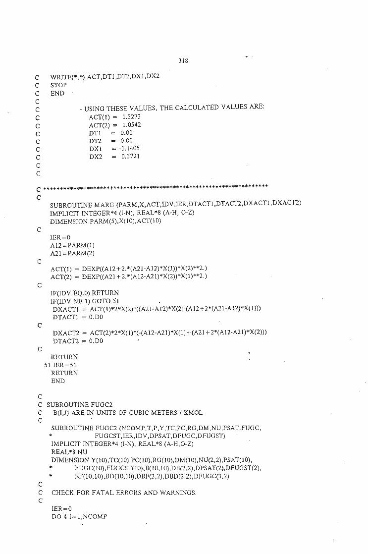
C
C CHECK FOR FATAL ERRORS AND WARNINGS.C
318
C WRITE(*,*) ACT,DT1,DTl,DX1,DX2C STOPC ENDCC - USING THESE VALUES, THE CALCULATED VALUES ARE:C ACT(l) = 1.3273C ACT(2) = 1.0542C DTl = 0.00C DTI = 0.00C DX1 = -1.1405C DX2 = 0.3721CC
C ********************************************************************C
SUBROUTINE MARG (PARM,X,ACT,IDV ,IER,DTACTl,DTACTI,DXACTI ,DXACTI)IMPLICIT INTEGER*4 (I-N) , REAL*8 (A-H, O-Z)DIMENSION PARM(5),X(l0),ACT(IO)
CIER=OA12=PARM(1)A21 =PARM(2)
CACT(l) = DEXP«A12+2. *(A21-A12)*X(l»*X(2)**2.)ACT(2) = DEXP«A21 +2. *(A12-A21)*X(2»*X(1)**2.)
CIF(IDV.EQ.O) RETURNIF(IDV.NE.l) GOTO 51
DXACTI = ACT(l)*2*X(2)*«A21-A12)*X(2)-(A12+ 2*(A21-A12)*X(l»))DTACTI = .O.DO
C
DXACTI = ACT(2)*2*X(l)*(-(A12-A21)*X(l)+(A21 +2*(A12-A21)*X(2»))DTACTI = O.DO
CRETURN
51 IER=51RETURNEND
C
C SUBROUTINE FUGC2C B(I,I) ARE IN UNITS OF CUBIC METERS/ KMOLC
SUBROUTINE FUGC2 (NCOMP,T,P,Y,TC,PC,RG,DM,NU,PSAT,FUGC,* FUGCST,IER,IDV,DPSAT,DFUGC,DFUGST)IMPLICIT INTEGER*4 (I-N), REAL*8 (A-H,O-Z)REAL*8 NU
DIMENSION Y(l 0),TCC1 0),PCC1 0),RG(IO),DM(l0),NU(2,2),PSAT(1 0),* FUGC(10),FUGCST(l0),B(IO,10),DB(2,2),DPSAT(2),DFUGST(2),* BF(lO, 1O),BD(IO, 1O),DBF(2,2),DBD(2,2),DFUGC(3,2)
IER=ODO 41= 1,NCOMP
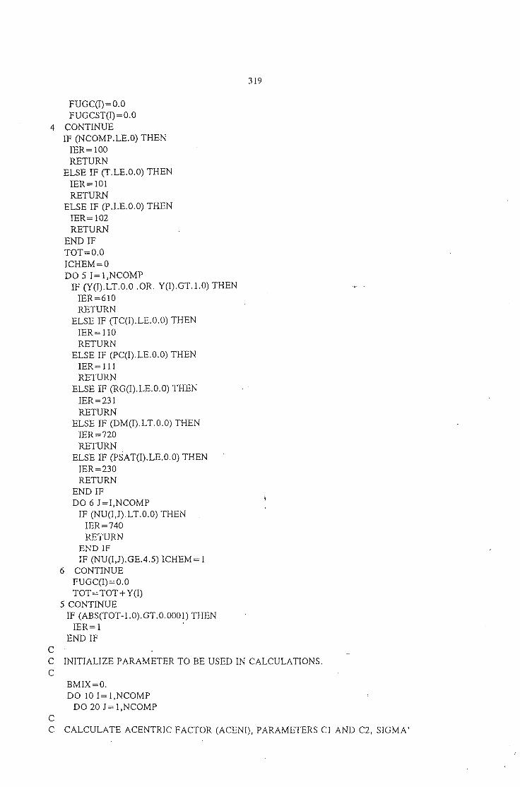
319
FUGC(I)=O.OFUGCST(I)=O.O
4 CONTINUEIF (NCOMP.LE.O) THEN
IER=100RETURN
ELSE IF (T.LE.O.O) THENIER=101RETURN
ELSE IF (P.LE.O.O) THENIER= 102RETURN
END IFTOT=O.OICHEM=ODO 5 1= l,NCOMP
IF (Y(I).LT.O.O .OR. Y(I).GT.l.O) THENIER=61ORETURN
ELSE IF (TC(I).LE.O.O) THENIER= 110RETURN
ELSE IF (PC(I).LE.O.O) THENIER= 111RETURN
ELSE IF (RG(I).LE.O.O) THENIER=231RETURN
ELSE IF (DM(I).LT.O.O) THENIER=720RETURN
ELSE IF (PSAT(I).LE.O.O) THENIER=230RETURN
END IFDO 6 J =I,NCOMP
IF (NU(I,J).LT.O.O) THENIER=740RETURN
END IFIF (NU(I,J).GE.4.5) ICHEM = 1
6 CONTINUEFUGC(I)=O.OTOT=TOT+ Y(I)
5 CONTINUEIF (ABS(TOT-1.0).GT.0.0001) THEN
IER= 1 .END IF
CC INITIALIZE PARAMETER TO BE USED IN CALCULATIONS.C
BMIX=O.DO 101= 1,NCOMP
DO 20 J=l,NCOMPCC CALCULATE ACENTRIC FACTOR (ACENI), PARAMETERS Cl AND C2, SIGMA'
320
C (SIGMAl), AND E/K'(EOKl) FROM EQUATIONS 6C-18, 6C-24, 6C-23, 6C-22,
C AND 6C-2l RESPECTIVELY OF COMPONENT 1.
CACENI=0.006026"'RG(I)+0.02096"'RG(I)"''''2-0.001366'''RG(I)**3Cl =(16. +400. *ACENI)/(lO. +400. *ACENI)
C2=3.1(10. +400. *ACENI)SIGMAl = (2.44-ACENn*(lOl.33*TC(I)/(PC(I)/IOOO.))**(l./3.)EOKl=TC(I)*(0.748+0.9l *ACENI-0.4*NU(l,I)/(2. +20. *ACENI))
CC CALCULATE PARAMETER XI FROM EQUATION 6C-23 OR SET EQUAL TO ZERO,C DEPENDING ON THE VALUE OF THE DIPOLE MOMENT FOR COMPONENT 1.
CIF (DM(I).LT.1.45) THEN
XI=O.OELSE
XI = 1.7941E07*DM(l)**4/«2. 822-1. 882*ACENI/(O.03 + ACENI))** TC(I)*SIGMAl **6*EOK1)
END IFCC CALCULATE MOLECULAR SIZE (SIGMAI) AND CHARACTERISTIC ENERGY (EOKI)
C FOR COMPONENT I FROM EQUATIONS 6C-20 AND 6C-19.
CSIGMAI=SIGMAl *(1. + XI*C2)**(1./3.)EOKI=EOKl *(1.-XI*Cl *(1.-XI*(1. + Cl)/2.))
CC IF I IS NOT EQUAL TO J, CALCULATE ACENTRIC FACTOR (ACENJ), ANDC PARAMETERS Cl, C2, SIGMA1, EOK1, XI, SIGMAJ, AND EOKJ FOR COMPONENTC J FROM SAME EQUATIONS USED FOR COMPONENT 1.
C
*
IF (1.NE.J) THENACENJ=;,0.OO6026*RG(J) + 0.02096*RG(J)**2-0. 001 366*RG(J)**3Cl =(16. +400. *ACENJ)/(lO. +400. *ACENJ)C2=3./(1O. +400. *ACENJ)SIGMAl = (2.44-ACENJ)*(101. 33*TC(J)/(PC(J)11000.))**(l.l3.)EOKl =TC(J)*(0.748 +0.91 *ACENJ-0.4*NU(J,J)/(2. +20. *ACENJ))IF (DM(J).LT.1.4S) THEN
XI=O.OELSE
XI= 1.7941 E07*DM(J)**4/«2. 822-l.882*ACENJ/(0.03 + ACENJ))*TC(J)*SIGMAl **6*EOK1)
END IFSIGMAJ =SIGMAl *(1. + XI*C2)**(I.I3.)EOKJ =EOKl *(I.-XI*Cl *(1.-XI*(l. + Cl)/2.))
CC IF I IS NOT EQUAL TO J, CALCULATE CROSS PARAMETER ACENTRIC FACTORC (ACEN), CROSS PARAMETERS Cl, C2, SIGMA1, EOKl, AND XII, CHARACTERC ISTIC ENERGY FOR THE I-J INTERACTION (EOK), AND CROSS PARAMETERC MOLECULAR SIZE FROM EQUATIONS 6C-26, 6C-32, 6C-33, 6C-30, 6C-29,C 6C-3l, 6C-27, AND 6C-28 RESPECTIVELY.C
ACEN =O.S*(ACENI + ACENJ)Cl =(16. +400. *ACEN)/(lO. +400. "'ACEN)C2=3./(10. +400. *ACEN)SIGMAl =SQRT(SIGMAI*SIGMAJ)EOKl =0.7*SQRT(EOKI*EOKJ) +0.6/(J./EOKI + J./EOKJ)IF (DM(I).GE.2..AND. DM(J).EQ.O.) THEN
321
XII = DM(I)**2*EOKJ**(2./3.)*SIGMAJ**4/(EOK 1*SIGMA 1**6)ELSE IF (DM(J).GE.2..AND. DM(I).EQ.O.) THEN
XIl =DM(1)**2*EOKI**(2./3.)*SIGMAI**4/(EOKI *SIGMAl **6)
ELSEXII =0.0
END IFSIGMA=SIGMAI *(1.-XIl *C2)EOK=EOKI *(1. + XII *CI)
ELSECC IF I EQUALS J, SET ACENTRIC FACTOR (ACEN), MOLECULAR SIZE (SIGMA),C AND CHARACTERISTIC ENERGY FOR THE I-J INTERACTION (EOK) EQUAL TOC PURE COMPONENT PROPERTIES OF COMPONENT 1.C
ACEN=ACENISIGMA=SIGMAIEOK=EOKI
END IFCC CALCULATE PARAMETER E FROM EQUATION 6C-17 DEPENDING ON THE VALUE ORC THE ASSOCIATION OR SOLVATION PARAMETER.C
IF (NU(l,J).LT.4.5) THENE = EXP(NU(I,J)*(650.l(EOK + 300.)-4.27))
ELSEE= EXP(NU(l,J)*(42800. I(EOK + 22400.)-4.27))
END IFC
C CALCULATE PARAMETERS DM* (DMSTAR), DELTAH, AND A FROM EQUATIONSC 6C-16, 6C-15, AND 6C-14 RESPECTIVELY.C
DMSTAR=7243. 8*DM(I)*DM(J)/(EOK*SIGMA**3)DELTAH= 1.99+0.2*DMSTAR**2A=-0.3-0.05*DMSTAR
CC CALCULATE PARAMETER DM*' (DMSTR1) FROM EQUATION 6C-13 DEPENDING ONC THE VALUE OF DM*.C
IF (DMSTAR.LT.0.04) THENDMSTRI = DMSTAR
. ELSE IF (DMSTAR.GE.0.04 .AND. DMSTAR.LT.0.25) THENDMSTRl=O.O
ELSEDMSTRI =DMSTAR-0.25
END IFC
C CALCULATE PARAMETERS BO, T* (TSTAR), AND T*' (TSTAR1) FROM EQUATIONSC 6C-12, 6C-ll, AND 6C-1O RESPECTIVELY.C
BO=0.00126*SIGMA**3TSTAR=T/EOK
TSTARI = l.l(1.1TSTAR-I.6*ACEN)
C
C CALCULATE CHEMICAL (BCHEM), METASTABLE + BOUND (BMETBB), POLARC (BPOLAR), AND NONPOLAR (BNPOLR) CONTRIBUTIONS TO THE SECOND VIRIAL
322
C COEFFICIENT FROM EQUATIONS 6C-9, 6C-8, 6C-7, AND 6C-6 RESPECTIVELY.C
BCHEM = BO*E*(l.-EXP(1500.*NU(I,J)/T))BMETBB = BO*A*EXP(DELTAHITSTAR)BPOLAR=-BO*DMSTRI *(0.74-3.1TSTARI +2. 1ITSTAR 1**2+2.IITSTARI **3)BNPOLR=BO*(0.94-1.47ITSTARI-O. 85ITSTARl **2-1.015ITSTARI **3)
CC CALCULATION OF DERIVATIVESC
IF(IDV.EQ.O) GOTO 9DTSTAR=lIEOKDTSTl = -l./(TSTAR**2. *(1ITSTAR-1.6*ACEN)**2.)*DTSTARDBCHEM =-BO*E*EXP(1500. *NU(I,J)IT)*(-1500. *NU(I,J)/T**2)DBMTBB=BMETBB*(-DELTAH/TSTAR**2.)*DTSTARDBPOLR=-BO*DMSTRI *(3.ITSTARI **2.-2.IITSTARI **3-2.IITSTARI **4)
* *DTSTlDBNPLR= BO*(1.47/TSTAR 1**2. +0. 85ITSTARI **3 + 1.0I51TSTARI **4)
* *DTSTlC
9 IF (ICHEM.EQ.I) GOTO 40C
B(I,J) =BNPOLR+BPOLAR+BMETBB+BCHEMDB(I,J)=DBNPLR + DBPOLR + DBMTBB + DBCHEM
CC CALCULATE MIXTURE SECOND VIRIAL COEFFICIENT FROM EQUATION 6C-2.C
BMIX=BMIX + Y(I)*Y(J)*B(I,J)FUGC(I)= FUGC(I)+ Y(J)*B(I,J)
CC CALCULATE FUGACITY COEFFICIENT FOR PURE SATURATED COMPONENT IC (FUGCST) FROM EQUATION 6C-34.C
*
IF (I.EQ.J) THENFUGCST(I)=EXP(B(I,J)*P6AT(I)/(8314*T))IF(IDV.EQ.O) GOTO 20DFUGST(I) = FUGCST(I)*CT*(DB(I,I)*PSAT(I)-B(I,J)*DPSAT(I))
B(I,J)*PSAT(I))1T1T183 14.END IFGOTO 20
C
40 BF(I,J) = BPOLAR + BNPOLRDBF(I,J) = DBNPLR + DBPOLR
BD(I.J)=BCHEM + BMETBBDBD(I,J)=DBMTBB + DBCHEM
C20 CONTINUE10 CONTINUE
C
._ C CALCULATE FUGACITY COEFFICIENT OF COMPONENT I IN THE VAPOR PHASEC (FUCG) FROM EQUATION 6C-l AND RETURN TO CALLING PROGRAM.C - .
IF (ICHEM.EQ.I) GOTO 50DO 30 1= I.NCOMP
ARG =(2. *FUGC(I)-BMIX)*P/(8314*T)FUGC(I) = EXP(ARG)DFUGC(l ,I) = FUGC(I)*ARG/P
323
30 CONTINUEC
. IF(lDV.EQ.O) GOTO 60DFUGC(2,l) = FUGC(1)*(P/83141T*
* (Y(l)*(2-Y(l))*DB(I, 1) +2*Y(2)**2*DB(I ,2)-Y(2)**2*DB(2,2)).-
* -DLOG(FUGC(l))/T)DFUGC(2,2) = FUGC(2)*(P/83141T*
* (-Y(1)**2*DB(1, 1) +2*Y(l)**2*DB(l,2) + Y(2)*(2-Y(2))*DB(2,2))* -DLOG(FUGC(2))IT)
CDFUGC(3, 1)=FUGC(1)*2*P/8314/T*Y(2)*(-2*B(1 ,2) + B(l, 1)+ B(2,2))DFUGC(3,2)= FUGC(2)*2*P/83141T*Y(1)*( 2*B(1 ,2)-B(l,I)-B(2,2))
C60 RETURN
C50 CALL CHEM (NCOMP,T,P,PSAT,Y,BF,BD,FUGC,FUGCST,IER,
* IDV ,DBF,DBD,DPSAT,DFUGC,DFUGST)RETURNEND
CC DIPPR ROUTINE NAME - ACTMODCC **********************************************************************
- CALL ACTMOD (XI,THETA,C,F)
- CALCULATION OF THE CONSTRAINTS AND DERIVATIVES OFTHE CONSTRAINTS FOR USE IN THE ERROR-IN-VARIABLESREGRESSION TECHNIQUE OF ACTIVITY COEFFICIENTPARAMETERS.
USAGE
ARGUMENTS'INPUT: XI - VECTOR OF LENGTH 4 OF ESTIMATES OF THE TRUE VALUES
OF THE MEASURED QUANTITIES. FOR THE APPROXIMATEEVM METHOD, THE EXPERIMENTAL VALUES ARE USED.XI(l) = PRESSURE (PA)XI(2) = TEMPERATURE (KELVINS)XI(3) = LIQUID MOLE FRACTION OF COMPONENT 1XI(4) ~ VAPOR MOLE FRACTION OF COMPONENT 1
THETA - VECTOR OF LENGTH 3 OF PARAMETERS TO BE REGRESSED.COMMONSTATEMENTS:
COMMON/AREA2/PDPD - MATRIX OF DIMENSION (15,2) OF PARAMETERS. FOR THIS
SUBROUTINE, THE ABOVE COMMON STATEMENT MUST BEINCLl,lDED IN THE CALLING ROUTINE OR ANY PREVIOUSLYCALLED ROUTINE AND THE FOLLOWING VARIABLES MUSTBE DEFINED:
PD(l,I) TO PD(5,I) - DIPPR VAPOR PRESSURECONSTANTS, A THROUGH E, FOR EACH COMPONENT.
THE FOLLOWING IS NEEDED ONLY FOR THE WILSON MODEL:PD(6,I) - LIQUID MOLAR VOLUME OF EACH COMPONENT
(M**3/MOL).
CCC PURPOSECCCCCCCCCCCCCCCCCCCCCCCCCCCC
OUTPUT: C - MATRIX OF DIMENSION (2,4) OF DERIVATIVES OF THECONSTRAINTS WITH RESPECT TO THE MEASUREDVARIABLES.
F - VECTOR OF LENGTH 2 OF CONSTRAINTS
THE FOLLOWING ARE NEEDED ONLY IF FUGACITYCOEFFICIENTS ARE CALCULATED WITH THE METHOD OFHAYDEN-O'CONNELL:
PD(7,I) - CRITICAL TEMPERATURES OF EACH COMPONENT(KELVINS).
PD(8,I) - CRITICAL PRESSURES OF EACH COMPONENT(KILOPASCALS).
PD(9,I) - DIPOLE MOMENTS OF EACH COMPONENT(DEBYE).
PD(lO,I)- RADIUS OF GYRATION OF EACH COMPONENT(ANGSTROMS).
PD(11,I)- ASSOCIATION PARAMETERS OF EACHCOMPONENT (DIMENSIONLESS).
THE FOLLOWING ARE NEEDED ONLY IF THE UNIQUAC MODELIS CHOSEN:
PD(12,I)- UNIQUAC VOLUME PARAMETER, R, FOR EACHCOMPONENT
PD(13,I)- UNIQUAC AREA PARAMETER, Q, FOR EACHCOMPONENT.
PD(14,I)- UNIQUAC AREA PARAMETER, Q, ADJUSTED FORALCOHOLS AND WATER, FOR EACH COMPONENT.
COMMON/AREA3/EOFSEOFS - VECTOR OF LENGHT 6 OF PARAMETERS. FOR THIS
SUBROUTINE, THE ABOVE COMMON STATEMENT MUST BEINCLUDED IN THE CALLING ROUTINE OR ANY PREVIOUSLYCALLED ROUTINE AND THE FOLLOWING VARIABLES MUSTBE DEFINED:
EOS(3) - INDICATOR FO.R THE INCLUSION OF PURECOMPONENT ENDPOINTS IN THE DATA SET:
. EOS(3) = 1 FOR INCLUSION OF ENDPOINTSEOS(3) = 0 FOR EXCLUSION OF ENDPOINTS
EOS(1) - PRESSURE OF SYSTEM AT X(1)=O.O. (NEEDEDONLY IF,EOS(3)= 1).
EOS(2) - PRESSURE OF SYSTEM AT X(1)= 1.0. (NEEDEDONLY IF EOS(3)= 1).
EOS(4) -' INDICATOR FOR ACTIVITY COEFFICIENT MODEL1: THREE-SUFFIX MARGULES2: VAN LAAR3: WILSON (TWO-PARAMETER)4: UNIQUAC5: NRTL6: WILSON (THREE-PARAMETER)
THE FOLLOWING ARE NEEDED ONLY IF FUGACITYCOEFFICIENTS ARE CALCULATED WITH THE METHOD OFHAYDEN-O'CONNELL:
EOS(5) - SOLVATION PARAMETER BETWEEN COMPONENTS ONEAND TWO (DIMENSIONLESS).
324
CCCCCCCCCCCCCCCCCCCCCCCCCCCCCCCCCCCCCCCCC
CCCCCCCCCCCCCC
C SUBROUTINES REQ.- MARG (THREE-SUFFIX MARGULES MODEL)
325
VANLAR (VAN LAAR MODEL)WILSON (TWO-PARAMETER WILSON MODEL)UNIQUA (UNIQUAC MODEL)NRTL (NRTL MODEL)WIL3 (THREE-PARAMETER WILSON MODEL)FUGC (HAYDEN-O'CONNELL FUGACITY COEFF ROUTINE)
- ABRAMS, D. S. AND PRAUSNITZ, J. M., "STATISTICALTHERMODYNAMICS OF LIQUID MIXTURES: A NEWEXPRESSION FOR THE EXCESS GIBBS ENERGY OFPARTIALLY OR COMPLETELY MISCIBLE SYSTEMS," AICHEJ., 21,116 (1975).
- RENON, H. AND PRAUSNITZ, J. M., "LOCAL COMPOSITIONSIN THERMODYNAMIC EXCESS FUNCTIONS FOR LIQUIDMIXTURES," AICHE J., J4, 135 (1968).
- USING THESE VALUES, THE CALCULATED VALUES ARE:F(1) = F(2) =C(I,I) = CC2,1) =
C(1,2) = CC2,2) =C(I,3) = CC2,3) =CCl,4) = CC2,4) =
LIMITATIONS: - THE ACTIVITY COEFFICIENT APPROACH SHOULD ONLY BEUSED FOR LOW PRESSURE SYSTEMS. THE REGRESSIONMETHOD CAN ONLY BE USED FOR BINARY SYSTEMS.
REFERENCES: - WILSON, G. M., "VAPOR-LIQUID EQUILIBRIUM. XI. A NEWEXPRESSION FOR THE EXCESS FREE ENERGY OF MIXING,"J. AMER. CHEM. SOC. 86, 127 (1964).
IMPLICIT INTEGER*4 (I-N),REAL*8 (A-H, O-Z)DIMENSION XI(4),THETA(3),CC2,4),F(2),PD(15,2),
* FUGCC2,2),DPFCC2,2),DTFCC2,2),DXFCC2,2),EOFS(6)COMMON IAREA21 PDCOMMON IAREA31 EOFSXI(1) = 90.446E03XI(2) = 323.15XI(3) = 0.290XI(4) = 0.423EOFS(4) = 5THETA(I) = 1000.0THETA(2) = 700.0THETA(3) = 0.3CALL EOSMOD (XI,THETA,C,F)WRITE(*, IO) F, C
10 FORMATe F:', 2DI5.5,!,' CI:',4EI5.5,1,' C2:',4EI5.5)STOPEND
CCCCCCCCCCCCCCCCCCCCCCCCCCCC
··C EXAMPLE:CCCCCCCCCCCCCCCCCCC.CC ,C .C
CCCC
326
CC **********************************************************************C
SUBROUTINE ACTMOD(XI,THETA,B,F)IMPLICIT INTEGER*4 (I-N), REAL*8 (A-H, O-Z)REAL*8 NUDIMENSION XI(4),THETA(5),B(2,4),F(2),R(10),QQ(10), VOL(10),
* X(1O), Y(1O),DM(10),RG(1O),TC(1O),PD(15,10),PC(10),* NU(2,2),FUGC(10),FUGCST(10),PSAT(10),GAMMA(10),* QP(1O),AM(6),DPSAT(2),DFUGC(3,2),DFUGST(2)COMMON /AREA2/ PDCOMMON /AREA3/ AM
CIDV=1IER=ONCOMP=2RPA=8.31439RKMOL=8314.39
. P= XI(l)T= XI(2)X(I)=XI(3)
X(2)= l.-X(l)Y(l)=XI(4)
Y(2)= l.-Y(l)C
D015N=1,2VOL(N)=PD(6,N)
.TC(N)=PD(7,N)PC(N)=PD(8,N)*l.D03DM(N)=PD(9,N)RG(N)=PD(1O,N)NU(N,N)=PD(ll,N)
15 CONTINUECC ASSIGNMENT OF VAPOR PRESSURESC OPTION TO USE EXPERMENTAL DATA POINTS FOR VAPOR PRESSURESC ** AM(3)= 1 FOR AN ISOTHERMAL SYSTEM WITH ENDPOINTS **C
IF (AM(3).EQ. I.DO) THENPSAT(l)=AM(l)PSAT(2)=AM(2)
ELSEDO 100J=I,2
100 PSAT(J)= DEXP(PD(l ,1) + PD(2,1)/T + PD(3,J)*DLOG(T) +* PD(4,J)*T**PD(5,J»ENDIF
C
IF(X(l).EQ.O.O) PSAT(2)=AM(2)IF(X(l).EQ.l.O) PSAT(I)=AM(l)
C
DTVPl = -PD(2,1)/T**2+ PD(3, 1)/T + PD(4,1)*PD(5,1)*T**(PD(5,1)-I)DTVP2 = -PD(2,2)/T**2 + PD(3 ,2)/T + PD(4,2)*PD(5 ,2)*T**(PD(5,2)-I)DPSAT(l) = PSAT(I)*DTVPlDPSAT(2) = PSAT(2)*DTVP2
C
C CALCULATION OF THE OBJECTIVE FUNCTIONS F(l) AND F(2)
C
C THE OBJECTIVE FUNCTIONSC
327
CC CALLING OF ACTIVITY COEFFICIENT ROUTINESC
IF(AM(4).EQ.1.)* CALL MARG (THETA,X,GAMMA,IDV,IER,DTACTl,DTACTI,DXACTl,DXACTI)IF(AM(4).EQ.2.)
* CALL VANLAR (THETA,X,GAMMA,IDV,IER,DTACTl,DTACTI,DXACTl,DXACTI)IF(AM(4).EQ.3.)
* CALL WILSON (NCOMP,THETA,VOL,T,X,* GAMMA,IDV ,DTACTl ,DTACTI,DXACTl ,DXACTI)IF(AM(4).EQ.4.) THEN
DO 30 J=1,2R(J)=PD(12,J)QQ(J)=PD(13,J)
30 QP(J)=PD(14,J)31 FORMAT(6FlO.3)
CALL UNIQUA (NCOMP,THETA,R,QQ,QP,T,X,* GAMMA,IDV ,IER,DTACTl ,DTACTI,DXACTl ,DXACTI)
ENDIFIF(AM(4).EQ.5.)
*CALL NRTL3 (NCOMP,THETA,T,X,GAMMA,IDV,IER,* DTACTl,DTACT2,DXACTl,DXACTI)·IF(AM(4).EQ.6.)
*CALL WIL3 (THETA,PD(6,1),PD(6,2),T,X,* ACTl ,ACTI,DTACTl ,DTACT2,DXACTl ,DXACTI)IF(AM(4).EQ.9.)
*CALL MARGUL (THETA, X, ACTl, ACT2, DXACTl, DXACT2, DTACTI,DTACTI)IF(AM(4).LT.6.) THEN
ACTl =GAMMA(1)ACTI = GAMMA(2)
ENDIFC
C CALLING OF FUGACITY COEFFICIENT ROUTINEC
NU(1,2)=AM(5)NU(2,1)=NU(1,2)POYNTl = (P-PSAT(l»*PD(6, 1)/RKMOLlTPOYNTI= (P-PSAT(2»*PD(6,2)/RKMOUTDTPYN1= 11T*(-PD(6 ,1)*DPSAT(I)/RKMOL-POYNTl)DTPYN2 = lIT*(-PD(6,2)*DPSAT(2)/RKMOL-POYNT2)
C
IF(AM(4).EQ.9.) GOTO 1000
CALL FUGC2(NCOMP,T,P, Y,TC,PC,RG ,DM,NU,PSAT,FUGC,FUGCST,IER,* IDV,DPSAT,DFUGC,DFUGST)SSFUG 1= FUGCST(1)*PSAT(l)*DEXP(POYNTl)SSFUG2= FUGCST(2)*PSAT(2)*DEXP(POYNTI)
C
89 FORMATC X,PHII ,PHI2,PHllS,PHI2S:' ,F8.3,4FlO.4)91 FORMATC Xl' ,FlO.3)
IF(FUGC(I).LE.O.O) WRITE(*, *) 'ERROR CODE:' ,IERIF(FUGC(2).LE.0.0) WRITE(*,*) 'ERROR CODE:',IER
F(l) = Y(I)*P*FUGC(l) - ACTl *X(l)*SSFUGIF(2) = Y(2)*P*FUGC(2) - ACT2*X(2)*SSFUG2
328
510 FORMATe FUGC 1,2: ',2F15.5,1,* ' SSFUG I1PSATI: ' ,2F15.5,1,* ' SSFUG 2/PSAT2: ',2F15.5,1,* ' ACT 1 IACT 2: ',2F15.5)
CC CALCULATION OF DERIVATIVES WITH RESPECT TO PRESSUREC
DPSSFl = SSFUG 1*PD(6, 1)/RKMOLlTDPSSF2 = SSFUG2*PD(6,2)/RKMOLIT
CB(l,l) = DFUGC(I,I)*Y(1)*P + FUGC(1)*Y(l) - ACTI*X(I)*DPSSFIB(2,1) = DFUGC(I,2)*Y(2)*P + FUGC(2)*Y(2) - ACT2*X(2)*DPSSF2
CC CALCULATION OF DERIVATIVES WITH RESPECT TO TEMPERATUREC
DTSSF1 = SSFUGI *(DTPYNl + DTVP1) + PSAT(1)*DEXP(POYNTI)*DFUGST(l)DTSSF2 = SSFUG2*(DTPYN2 + DTVP2) + PSAT(2)*DEXP(POYNT2)*DFUGST(2)
CB(l,2) = DFUGC(2,1)*Y(l)*P - DTACTl*X(1)*SSFUG1 - ACTI*X(l)*DTSSFlB(2,2) = DFUGC(2,2)*Y(2)*P - DTACT2*X(2)*SSFU'G2 - ACT2*X(2)*DTSSF2
CC CALCULATION OF DERIVATIVES WITH RESPECT TO Xl .C
B(1,3) = (-DXACTl*X(l)*SSFUGl - ACTl*SSFUGl)B(2,3) = (-DXACT2*X(2)*SSFUG2 + ACT2*SSFUG2)
CC CALCULATION OF DERIVATIVES WITH RESPECT TO YlC
B(1,4) = (DFUGC(3,l)*Y(l)*P + FUOCCl)*P)B(2,4) = (DFUGC(3,2)*Y(2)*P - FUGC(2)*P)
C500 FORMATe F(I) AND F(2) :', 2F15~6)
502 FORMATe F(l) AND F(2) :',2FI5.6,1,*' LEFT & RJGHT TERMS :" 4F15.2,/,*'FUGl,FUGSATI - FUG2,FUGSAT2:', 4FlO.6,1,*' B(l,I) AND B(2,1) :', 2F15.6,1, ;*' B(I,2) AND B(2,2) :', 2F15.6,/, .*' B(1,3) AND B(2,3) :', 2F15.6,/,*' B(l,4) AND B(2,4) :', 2F15.6)
501 FORMAT (/,' COMPI: Xl YI ACTlEXP ACTI:',4FI2.4,* I,' COMP2: X2 Y2 ACT2EXP ACT2:',4F12.4,1)RETURN
C
C ENTRY POINT FOR CALCULATION OF CONSTRAINTS FOR CONSISTENCY TESTC
1000 CALL FUGC2(NCOMP,T,P,Y,TC,PC,RG,DM,NU,PSAT,FUGC,FUGCST,IER,* IDV,DPSAT,DFUGC,DFUGST)
345 FORMATe T, Yl,PHIl,PHI2 -REG-' ,FlO.2,3F12.4)IF(IER.GT.O) WRITE(*,*) 'IER=',IER
115 SS.FUGl =FUGCST(l)*PSAT(l)*DEXP(POYNTl)SSFUG2 = FUGCST(2)*PSAT(2)*DEXP(POYNT2)
CC THE OBJECTIVE FUNCTIONSC
PCALC = X(l)*ACTl *SSFUG I1FUGC(l) + X(2)*ACT2*SSFUG2/FUGC(2)F(I) = P - PCALC '
329
C120 FCISQ=FUGC(l)*FUGC(1)
FC2SQ = FUGC(2)*FUGC(2)CC CALCULATION OF DERIVATIVES WITH RESPECT TO PRESSUREC
BO,I) = 1.CC CALCULATION OF DERIVATIVES WITH RESPECT TO TEMPERATUREC
DTSSFl = SSFUGI*(DTPYNl + DTVPI + DFUGST(I)/FUGCST(I))DTSSF2 = SSFUG2*(DTPYN2 + DTVP2 + DFUGST(2)/FUGCST(2»
CB(l,2) = -X(I)*ACTl *(FUGC(I)*DTSSFI - SSFUG I*DFUGC(2, I))/FCI SQ
* -X(2)*ACTI*(FUGC(2)*DTSSF2 - SSFUG2*DFUGC(2,2»/FC2SQCC CALCULATION OF DERIVATIVES WITH RESPECT TO XlC
B(1,3) = -SSFUGlIFUGC(l)*(X(l)*DXACTl + ACTl)* -SSFUG2/FUGC(2)*(X(2)*DXACT2 - ACTI)
CRETURNEND
CC ****************~***************************************************
C SUBROUTINE MARGUL (MARGULES MODEL PARAMETERS) .C ********************************************************************C
SUBROUTINE MARGUL (THETA,X,ACTl,ACT2,LACTI,LACTI,DXACTl,DXACTI)IMPLICIT IN:rEGER*4 (I-N), REAL*8 (A-H, O-Z)REAL*8 LACTl,LACT2DIMENSION X(2),THETA(5)
C
XISQ=X(I)*X(1)X2SQ = X(2)*X(2)A = THETA(I)B = THETA(2)D = THETA(3)
C
LACTl = X2SQ*(A + 2*(B-A-D)*X(1) + 3*D*XISQ)LACTI = XISQ*(B + 2*(A-B-D)*X(2) + 3*D*X2SQ)
CC WRITE(*,9) THETA,LACTl,LACT2
9 FORMATe TH,LACTl,2:',3FlO.5,2F15.5)ACTl = DEXP(LACTl)ACTI = DEXP(LACTI)DXACTl = (-2*A*X(2) + 2*(B-A-D)*(X2SQ - 2*X(2)*X(1» + 3*D
* *(-2*X1SQ*X(2) + 2*X2SQ*X(1»)*AGTlDXACTI = (2*B*X(I) +~*(A-B-D)*(2*X(1)*X(2) - X1SQ) + 3*D
* *( 2*X2SQ*X(1) - 2*XISQ*X(2»)*ACT2RETURN END
330
REFERENCES
1. Cruickshank, A. J. B.; Gainey, B. W.; Hicks, C. P.; Letcher, T. M.; Woods,
R.W. Young, C. L. Trans. Faraday Soc.; 1969,65, 1014
2. Everett, D. H. Trans. Faraday Soc.; 1965, 61, 1-637
3. Young, C. L. PhD. Thesis, Bristol, 1967
4. Shell Technical Bulletine, Sulfo1ane, Shell Chemical Co. 1964
5. Wilson, G. M. J. Am. Chem. Soc. 1964, 86, 127.
6. Renon, H.; Prausnitz, J. M. AIChE J. 1968, 14, 135.
7. Abrams, D. S.; Prausnitz, J. M. AIChE J. 1975,21, 116.
8.Fredens1und, A.; lones, R. L.; Prausnitz, J. M., AIChE J. 21, 1086
. 1098, 1975
9.Kehiaian, H. V.; Gro1ier, J-P.; Benson, G. C. J de Chemie Physique, 1978,75,
44
10. Rogalski, M.; Malanowski, S. Fluid Phase Equi1ibri,a 1980, 5, -97
11. Rogalski, M.; Rybaklewicz, K.; Malanowski, S. Ber. Bunsenges Phys. Chem.
1977, 81, 1070
12. Zemansky, M. W.; Heat and Thermodynamics. Fifth Edition. Ney York:
McGraw-Hill Book Company. 1968
13. van Laar, J. J. Z. Physik,Chem. 1910, 18,57
14. Della Monica, M.; Janelli, L.; Lamanna, U. J. Phys. Chem. 1968,72, 1068.
15. Jannelli, L.; Sacco, A. J. C·hem. Thermodynamics, 1972: 4, 715.
16. Jannelli, L.; Inglese, A.; Saeco, A.; Ciani, P. Z. Naturforsch, 1975, 30a, 87.
17. Sacco, A.; Ing1ese, A.; Ciani, P.; Dell'Atti, A.; Rakshit, A. K. Thermochim.
Acta, 1976, 15, 71.
18. Dal1inger, L.; Schiller, M.; Gmeh1ing, J.; J. Chem. Eng. Data.1993, 38, 147
19. Thomas, E.; Newman, B. A.; Lang, T. C.; Wood, D. A.; Eckert, C. A.; J.
Chem. Eng.Data 1982, 27, 399
20. Eckert, C. A.; Newman, B. A.; NieoladesG. L.; Long, T. C. AIChEJ. 1981,
27, 33 .
21. Sehreiber, L. B.; Eekert, C. A.; Ind. Eng. Chem. Proe. Des. Dev. 1971, 10,
572
331
22. Tassios, D. AIChE J. 1971,17,1367
23. Smith, J. M.; Van Ness, H. C.; Intro. Chem. Engineering Thermodynamics,
McGraw Hill, NY, 1975
24.. Wong, K. F.; Eckert, C. A.; Ind. Eng. Chem. Fund. 1~71, 10,20
25. Chemical Thermodynamics, VoILA Specialist Thermodynamic Report. Ed.:
McG1ashan M. London, 1973
26. Activity Coefficients at Infinite Dilution. Chemistry Data Series Vol 9.
DECHEMA, Germany 1993\
27. Barker, J. A. Aust. J. Chem. 1953, 6,207
28. Letcher T.M. Chemical Thermodynamics Vo1 2. A Specialist Report, Editor:
McG1ashan M. L.; The Chemical Society London. 1978. . ,
29. Leroi, J. C.; Masson, J. C.; Renon, H.; Fabries, J.F.; Sannier, H. lnd. Eng.
Chem. Process. Des. Dev. vo1 16, no. 1. 1977
30. Surovy, J.; Oveckova, J.; Graczova, E. Collect. Czesc. Chem. CDmmun. 1990,
vol55
31. Prividal, K. A.; Britigh, A.; Sandler, S. J. Chem. Eng. Data, 1992,37,484
32. Tramp, D. B.; Eckert, C. A.; AIChE J. 1993,39, 6
33. Null, H. R.; Phase Equilibrium in Process Design, Wi1ey, NY, 1970
34. Gautreaux, M. F.; Coate,s, J. AIChE J. 1955, 1,496
35. Hala, E.; Pick, J.; Fried, V,.; Vilim, O. Vapour Liquid Equilibrium, Pergomaon
Press, London, 1967
36. Hayden, J. G.; O;Connell; J. P.; AIChE J. 1975, 1,496
37. Li, J. J.; Dallas, A. J.; Eigens, D. 1.; Carr, P. W.; Bergman, D. K.; Hait, M.
J.; Eckert, C. A.; Anal. Chem. 1993,65, 3212
38. Shaffer, D. L.; Daubert, T. E. Anal. Chem. 1966,3, 1661
39. Golubkok, Y. V.; Pepneva, T. G.; Raginskaya, L. M.; Promst. Sint. Kauch. Ref.
SB. 1975, 7, 1
40. Hussam, A.; Carr, P. W.; Anal. Chem, 1985,793,57
41. Ray, A. K.; Venkatraman, S.; AIChE J. 1995, 41, 4
42. Conder, J. R.; Young, C. L. Physicochemical measure01ents by Gas
Chromatography, John Wiley and Sons Ltd.; 1979
332
43. Purnell, H. Gas Chromatography, John Wiley and Sons Ltd. U.S.A.; 1962
44. Martin, A. J. P.; Purnell, R. L.; Biochem. J.; 1941,35, 1358
45. James, A. T.; Martin, A. J. P. Biochem. J.; 1952, 50, 679
46. Forter, P. E; Deal, C. H.; Stross, F.H. J. Am. Chem. Soc.; 1956, 78,~999
47. Everett, D. H.; Stoddart, C. T. H.; Trans. Faraday Soc. 1961,57,746
48. Desty, D. H.; Go1dup, A.; Luckhurst, G. R.; Swanton, .W. T. Gas
Chromatography, 1962, Butterworth, 1962
49. Laub R.J.; Pesock R.L. Physicochemical Application of Gas Chromatography,
John Wi1ey and Sons Ltd. U.S.A. 1978
50. Kwantes, A.; Rijnders, G. W. A. Gas Chromatography, 1958
Editor: D. Desty, ;Sutterworth, London, 1958
51. Kurkchi, G. A.; Iogansen, A. V. Proc. Acad. Sci.; USSR, 145,571, 1962
52. Langer, S; H.; Iogansen, A. V.; Conder, J. R. J. Phys. Chem. 72, 4020, 1968
53. Letcher, T. M.; Baxter, R. C.; J. Solution Chem.; 18, 65, 198-9
54. Marsicano, F. Ph. D. Thesis, South Africa, ,1989
55. McGlashan, M.L.; Potter, D.J.B. Proc. Roy. Soc. A, 1962,267,478
56. Hudson, G.H.; McCoubrey, l.C. Trans. Faraday Soc. 1960,56,761
57. Cruickshank, A.J.B.; Windsor, M.L.; Young, C.L. Trans. Faraday Soc. 1966,
2341.
58. Letcher, T.M.; Baxter, R.C,; Bean, A.; Sewry, J.D. J. Chem. Thermodynamics,
1988,20,581'
59. Baonza, V. D.; Caceres,M.; Nunez, J.; Fluid Phase Equilibria. 1992,78,43
60. Selected Values of Properties of Hydrocarbons and Related Compounds. American
Petroleum Institute, Research Project 44, Thermodynamics Research Centre. Texas
A&M University, College Station, Texas. Tables 6k, 20k, and 21k, 1953
61. Selected Values of Properties of Hydrocarbons and Related Compounds. American
Petroleum Institute, Research Project 44, Thermodynamics Research Centre. Texas
A&M University, College Station, Texas. Tables 20d, and 21d, 1975
62. Bayles, I.W.; Letcher, T.M.; Moollan, W.C. J. Chem. Thermody~amics 1993,
27,781 .
333
63. Bayles, J.W.; Letcher, T.M.; Moollan, W.C. J. Chem. Thermodynamics 1994,
26, 571
64. Karol, A. N., Dkr. Khim. Zh. 1966,32, 198
65. Karol, A. N.; Neftkhimiya 1963,5,635
66. Kikic, I; Renon, H.; Sep. Sci. 1076, 11, 45
67. Kwantes, A. Rjinders, G. W. A.; Gas Chromatography, ed. Desty , D. H.
Butterworths, London 1958
68. Young, C. L. Trans. Faraday Soc. 1968, 64, 349
69. Martire, D. E.; Piedle, P.; J. Phys. Chem. 1968, 72, 3473
70. Letcher, T. M.; Marsicano, F.; J. Chem. Thermodynamics 1974, 6, 501
71. Letcher, T. M.; Jerman, P.; J. Chem. Thermodynamics 1976, 8, 127
72. Janini, G. M.; Martire, D. E.; J. Phys. Chem. 1974,78, 1644
73. Letcher, T. M.; J. Chem. Thermodynamics 1975, 7, 969
74. Gainey, B. W.; Young, C. L.; Trans. Faraday Soc. 1968, 64, 348
75. Martire, D. E.; Opllara, L. Z.; J. Chem. Eng. Data 1965, 40, 10
76. Hicks, C. P.; Young, C. L.; Trans. Faraday Soc. 1968, 64, 2675
77. Parcher, J. F.; Yun, K. S.; J. ·Chromatog. 1975, 105,257
78 Tewari, J.-B.; Martire, D. E.; Sheridan, J. P.; J. Phys. Chem. 1970,3263,74
79. Chen, S. S.; Zwolinski"B.; J. Chem. Thermodynamics 1973, 1133
80. Bowden, W. W.; Ataton, J. C.; Smith, B. D.; J. C. Eng. Data 1966, 3, 296,
81. Meyer, H. S.; PetroL Ref. 1957, 13, 175
82. Cummins, L. W. T.; Stones, F. W.; Volante, M. A.; Ind. Eng. Chem. 1933,25,
728
83. Smith, V. C.; Robinson Jf. R. L; J. Chem. Eng. Data 1970, 3, 391
84. Smyth, C. P.; Engel, E. W.; J. Am. Chem. Soc. 1929, 15,2646
85. Ott, J. B.; Marsh, K. N.; Stocks R. H.; J. Chem. Thermodynamics 1981, 13,
371
86. G6mez-Ibanez, J. D.; Sheih, J. J. C.; Thorsteinson, E. M.; J. Phys. Chem. 1966,
70, 1998
87. Messow, D.; Quitzsch, K.; Z Phy. Chem. (Leipzig) 1976, 257, 121
88. Keistler, J.; Winkler, R. Ind. Eng. Chem. 1952,44, 622
334
89. C.R.C. Handbook of Chemistry and Physics. 64th edition. Editor; Weast, R.e.
C.R.C Press Inc.: Boca Ratan. 1994
90. Gajle', A. A.; Pariieva, N. V.; Proskurjokov, V. A.; Zh. Prik. Khim. 1974,47,
191
91. Karvo, M.; J. Chem. Thermodynamics 1980, 12, 1175
92. Prausnitz, J. M.; Lichtenthaler, R. N.; Games de Azevedo, E. Molecular
Thermodynamics of Fluid-Phase equilibria, Prentice-Hall Inc.; Englewood Cliffs,
N. J. 1986
93. Batinno, R. Chem. Reviews, 1971, 5, 71.
94. Letcher, T. M.; Chem. South Africa, 1975, 1, 226.
95. Handa, Y. P.; Benson, G. C.; Fluid Phase Equilibria,: 1976,
185, 3
96. Stokes, R. H.; Marsh, K. N. Ann. Rev; Phy. Chem. 1972, 65,23
97. Marsh, K. N. Ann. Rev. RSC, Sect, C, 1980, 77, 101
98. Marsh, K. N. Ann. Rev. RSC, Sect, C, 1984, 209, 81
99. Scatchard, G.; Wood, S. E.; Muchel, J. M. J. Am. Che, Soc.
1946, 68, 1957
100. Hepler, L. J. Phys. Chem. 1957,61, 1426
101. Battino, R. J. Phys. Ch~m. 1966,3408, 70
102. Kimura, T.; Takagi, S. J. Chem. Thermo. 1979, 11, 119. ~
103. Leopold, H. Electronik, 1970, 19, 297
104. Keyes, D. B.; Hildebrand, J. H. J. Am. Chem. Soc. 1917,39,2126
105. Geffcken, W.; Kruis, A.; Salana, Z.; Z. Phys. Chem. 1937, 35, 317
106. Battino, R. J. Phys. Chem. 1966, 3408, 70
107. F10ry J. A.; J. Am. Chem. Soc. 1965, 87, 1833
108. Heintz, A.; Dolch, E.; Lichtenthaler,R. N.; Fluid Phase Equilib. 1986,27, 61
109. Treszezanowicz, G. C.; Benson, G. C., J. Chem. Thermos. 1977, 4, 1189
1l0. Redlich, 0.; Kister, A. T. Ind. Eng. Chemistry, 40, 345, 1948.
111. Ross, P. D. Biochemica et Biophysica Acta, 1973, 106, 313.
112. Letcher, T. M., Bayles, J. W. J. Chem. Eng. Data 1971, 16, 266
113. Govender, U. P. Masters Thesis, University of Natal, South Africa, 1993.
335
114. Letcher, T. M.; Schoonmbaert, F. E. Z.; Bean, B. Fluid Phase Equilibria, 1990,
61, 111
115. Swi~toslawski, W. Ebulliometric Measurements, Reinhold, New York, 1945
116. Marsh, K. N. Chemical Thermodynamics, Specialist Reports, Vol n. Editor
McGlashen, M. L. Chemicial Society, London. 1978
117. Allen, P. W.; Everett, D. H.; Penney, M. F. Proc. Roy. Soc. 1952, A212, 149
118. Baxendale, J. H.; Enustun, B. V.; Stein, J. Phil. Trans. 1951, A243, 169
119. McG1ashen, M.L.; Williamson, A. G. Trans. Faraday Soc. 1961,57,588
120. Brown, 1. Austral. J: of Sci. Research, 1952, 5A, 530
121. Malanowski, S., ~6wnowagaCiecz-Para, PWN, Warsaw, 1974
122. Rogalski, M., PhD Thesis, Institute of Physical Chemistry, Warsaw, 1974.
123. Prausnitz, J.; Anderson, T.; Grens, E.; Eckert, C.; Hsieh, R.; O'Connell, J.
Computer Calculations for Mu1ticomponent Vapour-Liquid and Liquid-Liquid
Equilibria, Prentice-Hall International Series, Englewood C1ifts, NJ, 1980
124. Benoit, R.L.; Charbonneau, J. Can. J. Chem. 1969,47,4195
125. De Fre, R. M.; Verhoeye, L. A. 1. Appl. Chem. Biotechnol. 1976,26,469
126. Ashcroft, S. J.; Clayton, A. D.; Shearn, R. B. J. Chem. Eng. Data 1979, 24,
195
127. Riddick, J. A.; Bunger, W. B.; Sakano, T. K.; Organic Solvents Physical
Properties and Methods of Purification, Fourth Edition; Wiley-Interscience
Publication, 1986
128. lng1ese, A.; Jannelli, L. Thermoch. Acta, 1978,23,263.16
129. Gess, M. A.; Danner, R.P.; Nagvekar, ThermodynaIJlic Analysis of Vapour
Liquid Equi1ibria: Recommended Models and Standard Data Base Am. lnst. Chem.
Eng.:PA, 1991
130. Walas, S. M. Phase Equi1ibria in Chemical Engineering, Butterworth Publishers,
Boston: 1985
131. Gmeh1ing, J.; Onken, U. Vapor-Liquid Equilibrium Data Collection; Chemistry
Data Series, DECHEMA: Frankfurt, 1977; vo1 1, Part 1
132. Letcher, T. M.; Moollan, W. C. J."Chem. Thermodynamics 1995,27,867 132.
336
133. Domariska, D.; Sporzyrislci, A.; Moollan, W. C.; Letcher T. M., J. Chem.
Eng. Data, 1995 - submitted.
134. Neu, E.;Peneloux, A., Fluid Phase Equilibria, 1981,6, 1
135. Patino-Leal, H.; Reilly, P. AIChE, 1982,28,580
136. Jannelli, L.; Lopez, A.; Jalent, R.; Silvestri, L. J. Chem. Eng. Data, 1982,
27, 28.
137. Hi1debrand, J. J. Chem. Phys. 1947, 15,225
138. Nagata, J.; Nakamiya, Y.; Kotoh, K.; Kogabu, J. Themochim. Acta 1981, 45,
153
139. Nag.ata, J. Fluid Phase Equilibrium, 1985, 19, 153
140. Domariska, D.; Roli.riska, J.; Fluid Phase Equilibria, 1989, 45, 25,
141. Domariska, D.; Rol.inska, J.; Fluid Phase Equilibna, 1993, 86,233
142. Domariska, D.; Rofman, T.; Fluid Phase Equilibria, 1991, 68, 103
143. Domariska, D. Fluid Phase Equilibria, 1986, 26, 201
144. Vera, J. H.; Sayegh, G. S.; Ratcliff, G. M.; Fluid Phase Equilibria, 1977, 1,
113.
145. Guggeriheim, E. A., Mixtures. Oxford: Oxford Press: 1952
146. Alesi, P. Activity coefficients at Infinte Dilution. Determination and Retrieval.
Experimental ThermodY!1amics measurements ans Correlations. Editors:
Malanowski, S.; and And~rko, A. Institute of Physical Chemistry of the Polish
Acadamy of Science. Warsaw. 1990.
147. Scatchard, G.; Ramer, W. J.; 1. Am. Chem. Soc. 57, 1805, 1935.
148 Wohl, K. Tran. AIChE. 42, 215, 1946
149. Orye, R. V.; and Prausnitz, J. M. Ind. Eng. Chem. 57, 18, 1965
150. Anderson, T. F.; and Prausnitz, J. M. Ind. Eng. Chem. 17,552,1978.
151. Kehiaian, H. V.; Fluid Phase Equilibrium, 13,243-253, 1983
152. Christensen, J. J.; Hanks, R. W.; Izatt, M. R. Handbook of Heat of
Mixing, Wiley-Interscience Publication, Ney York, 1988
153. GonzaIez, J. A., Garcia de la Fuente', 1., Cobos, I.C. and Casanova, C., Ber.
Bunsenges. Phys. Chem., 1994,95, 1658
337
154. GonzaIez, J. A., Garcia de la Fuente, 1., Cobos, J.C., Casanova, C. and
Domanska, D., Ber. Bunsenges. Phys. Chem., 1994,98,955
155. Kehiaian, H. V. and Marongiu, B. Fluid Phase Equilibria, 1988, 40,23
156. Kehiaian, H. V., Fluid Phase Equilibria, 1983, 13,243
157. Bondi, A., 1968. Physical Properties of Molecular Crystals, Liquids and
Glasses, Wi1ey, NY, 502 PP" I
158. Benoit, R. L. and Charbonneau, J. Can. J. Chem. 1969,47,4195
159. Lopez, A., Pansini, M. and Jannelli, L., J.Chem. Eng. Data, 1983,28, 173-175
160. Gmeh1ing, J . Results of a modified UNIFAC method for alkane - alcohol
systems. In: H. V. Kehiaian and H. Renon ( Editors ), Measurements, Evaluation
and ~rediction of Phase~quilibria,EIsevier, Amsterdam., ,
161. Pansini, M. and Jannelli, L., 1986. J.Chem. Eng. Data, 1986, 31, 157


