Embed Size (px)
Citation preview
The development of structural mass
spectrometry based techniques for the study of
aggregation-prone proteins.
Owen Cornwell
School of Molecular and Cellular Biology
Astbury Centre for Structural Molecular Biology
University of Leeds
Submitted in accordance with the requirements for the degree of Doctor of
Philosophy
December 2019


i
Declaration
The candidate confirms that the submitted work is his own and that appropriate credit has been given
within the thesis where reference has been made to the work of others.
This copy has been supplied on the understanding that it is copyright material and that no quotation
from this thesis may be published without proper acknowledgement.
© 2019 The University of Leeds and Owen Cornwell

ii
iii
Jointly Authored Publications
Chapters 4 and 5 contain work from the following published manuscript:
Cornwell, O., et al., Comparing Hydrogen Deuterium Exchange and Fast
Photochemical Oxidation of Proteins: a Structural Characterisation of Wild-Type and
ΔN6 β2-Microglobulin. Journal of The American Society for Mass Spectrometry, 2018.
29(12): p. 2413-2426.
In this work, all experimental work and data analysis was performed by OC.
Optimisation of the HDX workflow and associated method development was
performed by OC and JRA. Initial development and coding of the novel processing
algorithm was performed by OC. Final development and coding of the PAVED
software available for download was performed by JRA.
Chapter 6 contains work from the following published manuscript:
Cornwell, O., et al., Long-Range Conformational Changes in Monoclonal Antibodies
Revealed Using FPOP-LC-MS/MS. Analytical Chemistry, 2019. 91(23): p. 15163-
15170.
In this work, all experimental work and data analysis was performed by OC. Data
acquisition was performed at AstraZeneca (Granta Park, Cambridge) by OC under the
supervision of NJB.

iv

v
Acknowledgements
Firstly, I’d like to thank my two academic supervisors, Alison and Sheena, not just for taking
me on as a student when I had nowhere else to go, but for their continued support and
encouragement throughout the four years of my PhD at Leeds. I’d like to recognise James
Ault, our MS facility manager, for his significant contribution to the work in this thesis, and
for not yelling at me when I text him on Sundays in a panic because the HDX robot has
squashed the syringe again. Rachel George, for keeping the lab running smoothly and doing
all the jobs that I really should know how to do but don’t, and all past and present members
of the lab that helped me out along the way (particularly Anton, Hugh, Tom, Patrick, Emma,
Leon and Nasir!).
I’d also like to thank my industrial supervisor Nick Bond, as well as Dan Higazi, and Jim
Scrivens, my two original supervisors. Similarly, an honourable mention is thoroughly
deserved by Sue Slade, for looking after me at several conferences, as well as stocking my
formerly deficient kitchen full of a variety of cooking utensils - and a garlic crusher.
I’d also like to thank my family, and the doctors and nurses at Royal Papworth Hospital. Their
hard work, which makes writing a PhD thesis look unbelievably easy, has given my family
and I more time with my dad, for which I will be forever grateful. With recent events I’ve
come to appreciate the true significance of my family’s guidance in my life, and just how far
away I’d be from getting a PhD, without them. I love you all.
Well…most of you.
Lastly, I’d like to recognise the essential, if less obvious, contributions made from a number
of other people, entities and institutions. I realise I’m running out of space on the page so I’ll
be brief. I’d like to thank Mr Clark (my A-level chemistry teacher), Dr Brandon Reeder (my
undergraduate project supervisor), the quality control department for KP's dry roasted
peanuts, Dr Malcolm Finney and his wife Kathy, Spam, laser pointers, the 'Find and Replace'
function in Microsoft Excel, John Cleese, Lemsip Cold & Flu, Chinese takeaway restaurants
(especially the one on Town Street), scientific calculators, the complaints department at
British Telecom, Robert Palmer, large USB sticks, most small and medium sized USB sticks,
the cast and crew of Stargate: SG1, Oxo cubes, VAX essentials vacuum cleaners, pot noodle
sandwiches, and last, but by no means least, my dragon tree houseplant - Steve.

vi

vii
Oh and my girlfriend Sophie.
She was great too…
Un-acknowledgements
I would also like to not gratefully thank my former landlord, and the staff at the Wakefield
branch of Linely & Simpson letting agents, for refusing to fix my leaky bedroom window for
two years until I got fed up with it and moved out, somewhere about a third of the way
through Chapter 5.

viii
ix
Table of Contents
JOINTLY AUTHORED PUBLICATIONS ................................................................... III
ACKNOWLEDGEMENTS ........................................................................................... V
TABLE OF CONTENTS .............................................................................................. IX
LIST OF FIGURES ................................................................................................... XIV
LIST OF TABLES ...................................................................................................... XIX
LIST OF EQUATIONS .............................................................................................. XX
LIST OF ABBREVIATIONS ..................................................................................... XXI
ABSTRACT ............................................................................................................ XXV
1 INTRODUCTION I: MASS SPECTROMETRY THEORY ..................................... 2
1.1 Overview and history of mass spectrometry ....................................................... 2
1.2 Ionisation ............................................................................................................... 3
1.2.1 Electrospray ionisation .............................................................................. 4
1.3 Mass analysers ....................................................................................................... 7
1.3.1 Quadrupole analysers ................................................................................. 8
1.3.2 Linear ion traps ........................................................................................ 13
1.3.3 Time-of-flight (ToF) analysers ................................................................ 16
1.3.4 Orbital trapping analysers ....................................................................... 20
1.4 Ion Detectors ....................................................................................................... 25
1.4.1 Electron multipliers ................................................................................. 25
1.4.2 Image current detection .......................................................................... 26
1.5 Analysis of mass spectrometry data ................................................................... 27
1.5.1 Mass error and mass accuracy ................................................................. 29
1.6 Tandem mass spectrometry (MS/MS) ................................................................ 29
x
1.7 Liquid chromatography – mass spectrometry (LC-MS) .................................... 31
1.8 LC-MS/MS data acquisition methods................................................................. 33
1.8.1 Data dependent acquisition (DDA) ......................................................... 33
1.8.2 Data independent acquisition (DIA) ....................................................... 35
1.9 Ion mobility spectrometry – mass spectrometry (IMS-MS) ............................. 36
1.9.1 Drift tube IMS (DTIMS) .......................................................................... 37
1.9.2 Travelling wave IMS (TWIMS) ............................................................... 38
1.10 Commercial instruments used in this thesis ...................................................... 40
1.10.1 Waters Synapt high definition mass spectrometer ................................ 40
1.10.2 Thermo Q Exactive hybrid quadrupole – orbitrap mass spectrometer . 41
1.10.3 Thermo orbitrap fusion tribrid mass spectrometer ................................ 42
2 INTRODUCTION II: PROTEIN AGGREGATION, STRUCTURE AND
DYNAMICS STUDIED BY MASS SPECTROMETRY ................................................ 46
2.1 Protein folding, misfolding and aggregation ..................................................... 49
2.1.1 Protein folding ......................................................................................... 49
2.1.2 Misfolding, aggregation and disease ....................................................... 52
2.1.3 Structure and formation of amyloid ....................................................... 53
2.2 Beta-2 microglobulin (β2m) ................................................................................ 56
2.2.1 Normal function and dialysis related amyloidosis ................................. 56
2.2.2 β2m aggregation in vitro .......................................................................... 59
2.2.3 β2m folding pathway and the IT state ...................................................... 60
2.2.4 ΔN6 β2-microglobulin .............................................................................. 62
2.2.5 D76N β2-microglobulin ............................................................................ 63
2.3 Protein aggregation in biopharmaceuticals ....................................................... 65
xi
2.3.1 MEDI1912 and MEDI1912_STT ............................................................. 68
2.4 Mass spectrometry in structural biology ........................................................... 69
2.4.1 Accurate mass determination, native MS and ion mobility .................. 70
2.4.2 Fragmentation and peptide sequencing .................................................. 72
2.4.3 Hydrogen deuterium exchange (HDX) ................................................... 74
2.4.4 Fast photochemical oxidation of proteins (FPOP) ................................. 79
2.5 Aim of the thesis ................................................................................................. 83
3 MATERIALS AND METHODS ........................................................................... 86
3.1 Protein preparation and purification ................................................................. 86
3.1.1 Wild-type, D76N and ΔN6 ...................................................................... 86
3.1.2 WFL and STT ........................................................................................... 90
3.2 Native MS ............................................................................................................ 90
3.2.1 Sample preparation .................................................................................. 90
3.2.2 Waters Synapt G1 HDMS ........................................................................ 90
3.2.3 Calculation of in silico CCS ..................................................................... 93
3.3 Intact mass analysis ............................................................................................. 94
3.4 Hydrogen Deuterium Exchange ......................................................................... 94
3.4.1 Experimental ............................................................................................ 94
3.4.2 Data processing and analysis ................................................................... 95
3.5 Fast Photochemical Oxidation of Proteins ........................................................ 96
3.5.1 Experimental procedures for the analysis of β2m ................................... 96
3.5.2 Experimental procedures for the analysis of WFL and STT .................. 97
3.5.3 Data processing and analysis ................................................................... 97
3.5.4 Calculation of solvent accessible surface area ........................................ 98
xii
3.6 Homology modelling of mAbs ........................................................................... 98
4 IMS-MS AND HDX-LC-IMS-MS/MS COMPARING Β2M VARIANTS ............. 100
4.1 Protein preparation and initial characterisation ............................................. 101
4.2 Native IMS-MS .................................................................................................. 104
4.3 HDX-LC-IMS-MS ............................................................................................. 113
4.4 Development of a new HDX-MS processing algorithm ................................. 117
4.5 Evaluating the PAVED algorithm .................................................................... 123
4.6 Deuterium uptake behaviour of the D76N variant of β2m ............................. 129
4.7 Discussion .......................................................................................................... 132
4.7.1 The PAVED algorithm .......................................................................... 132
4.7.2 HDX behaviour of the D76N variant .................................................... 134
4.7.3 Insights on the aggregation propensity of the D76N variant .............. 135
4.7.4 Attempted HDX-ETD single residue experiments ............................... 136
5 FPOP-LC-MS/MS COMPARING Β2M VARIANTS ........................................... 144
5.1 FPOP method validation .................................................................................. 144
5.2 FPOP LC-MS/MS of wild-type, D76N and ΔN6 β2m ...................................... 154
5.2.1 Wild-type Vs ΔN6 .................................................................................. 160
5.2.2 Positional isomers in FPOP experiments ............................................. 165
5.2.3 FPOP behaviour of the D76N variant of β2m ....................................... 176
5.3 Discussion .......................................................................................................... 178
5.3.1 Interpretation of FPOP data .................................................................. 178
5.3.2 FPOP method development .................................................................. 180
5.3.3 FPOP of the ΔN6 truncation variant of β2m ......................................... 183
5.3.4 FPOP of the D76N variant of β2m ......................................................... 184
xiii
6 FPOP-LC-MS/MS OF WFL AND STT ............................................................... 186
6.1 Initial characterisation and overview .............................................................. 186
6.2 Regions surrounding the W30S and F31T mutations ..................................... 190
6.3 Constant domains and the CL-CH1 interface .................................................... 195
6.4 Analysis of retention time data ........................................................................ 200
6.5 Discussion .......................................................................................................... 205
6.5.1 Retention time analysis ......................................................................... 206
7 CONCLUDING REMARKS ............................................................................... 208
7.1 A new understanding of FPOP ........................................................................ 208
7.1.1 How do HDX and FPOP compare? ....................................................... 209
7.2 The D76N variant .............................................................................................. 210
7.3 What did we learn from studying biopharmaceuticals? ................................. 212
7.4 Final thoughts.................................................................................................... 215
8 APPENDICES.................................................................................................... 218
8.1 Related information for Chapter 4 ................................................................... 218
8.2 Related information for Chapter 5 ................................................................... 241
8.3 Related information for Chapter 6 ................................................................... 246
9 REFERENCES ................................................................................................... 260
xiv
List of Figures
Figure 1.1 Overview of a mass spectrometer. .............................................................................................3
Figure 1.2 Overview of the Electrospray ionisation (ESI) source. ............................................................5
Figure 1.3 ESI ionisation mechanisms. .......................................................................................................6
Figure 1.4 Different definitions of m/z resolution. ....................................................................................8
Figure 1.5 Schematic diagram of a quadrupole mass analyser. ..................................................................9
Figure 1.6 The m/z separation of ions in the two lateral planes of a quadrupole. .................................. 11
Figure 1.7 Stability diagrams for ions in a quadrupole. ........................................................................... 12
Figure 1.8 Basic design of the linear ion trap. .......................................................................................... 13
Figure 1.9 Dipolar resonance ejection in linear ion traps. ....................................................................... 15
Figure 1.10 The relationship between dipolar resonance ejection frequency and applied AC
amplitude. .................................................................................................................................................. 16
Figure 1.11 m/z separation by time-of-flight mass spectrometry (ToF-MS). ......................................... 18
Figure 1.12 Schematic diagram of an orthogonal acceleration time-of-flight mass spectrometer (oa-
ToF). ........................................................................................................................................................... 19
Figure 1.13 Schematic diagram of an electrostatic reflector. ................................................................... 20
Figure 1.14 The Kingdon trap and the Knight trap: early orbital ion traps. ........................................... 21
Figure 1.15 The orbitrap mass analyser: an ‘ideal’ Kingdon trap. ........................................................... 23
Figure 1.16 Excitation by injection, and radial de-phasing of ions in an orbitrap. ................................ 24
Figure 1.17 Schematic diagram of a microchannel plate continuous dynode electron multiplier. ....... 26
Figure 1.18 Image current detection in orbitrap mass analysers. ............................................................ 27
Figure 1.19 Determination of charge states in a mass spectrum. ............................................................ 28
Figure 1.20 The workflow of a product ion scan. .................................................................................... 30
Figure 1.21 Separating and analysing complex mixtures by liquid chromatography-mass spectrometry
(LC-MS). ..................................................................................................................................................... 32
Figure 1.22 Operating procedure of data dependent acquisition (DDA) in LC-MS experiments. ......... 34
Figure 1.23 Operating procedure for data independent acquisition (DIA) in LC-MS experiments. ..... 35
Figure 1.24 Data analysis in DIA-MSE. ..................................................................................................... 36
Figure 1.25 The principle of drift cell ion mobility spectrometry. ......................................................... 37
Figure 1.26 Schematic diagram of a stacked ring ion guide..................................................................... 38
Figure 1.27 Separation of ions by travelling wave ion mobility spectrometry (TWIMS). ..................... 39
Figure 1.28 Schematic diagram of a Waters Synapt G2Si HDMS. ........................................................... 41
Figure 1.29 Schematic diagram of a Thermo Q Exactive mass spectrometer. ........................................ 42
xv
Figure 1.30 Schematic diagram of a Thermo orbitrap fusion tribrid mass spectrometer. ..................... 43
Figure 2.1 Transcribing, translating and folding polypeptide chains. .................................................... 47
Figure 2.2 Idealised folding funnel/energy landscape for protein folding. ............................................ 51
Figure 2.3 Generalised mechanism of protein aggregation. .................................................................... 53
Figure 2.4 Structure of an amyloid fibril. ................................................................................................. 54
Figure 2.5 Energy landscape for protein folding, misfolding and aggregation....................................... 55
Figure 2.6 The structures of β2m and the class 1 major histocompatibility protein complex................ 57
Figure 2.7 β2m amyloid deposits in dialysis related amyloidosis (DRA). ................................................ 58
Figure 2.8 The folding pathway of β2m. ................................................................................................... 61
Figure 2.9 Wild-type, and aggregation-prone variants of β2m. .............................................................. 65
Figure 2.10 The structure of an IgG1 antibody. ...................................................................................... 66
Figure 2.11 A summary of structural MS methods. ................................................................................. 69
Figure 2.12 Idealised native and non-native charge state distributions. ................................................ 71
Figure 2.13 Peptide sequencing by product ion scan MS/MS. ................................................................ 73
Figure 2.14 Fragment ions generated from peptide ion dissociation. ..................................................... 73
Figure 2.15 General HDX-MS experimental workflow. ......................................................................... 75
Figure 2.16 Mechanisms of acid and base catalysed deuterium exchange. ............................................ 78
Figure 2.17 General theory of FPOP labelling. ....................................................................................... 81
Figure 2.18 Aims of this thesis. ................................................................................................................. 84
Figure 3.1 The pINK plasmid containing the gene of one of three variants of β2m. .............................. 86
Figure 4.1 Size exclusion purification of wild-type β2m. ...................................................................... 102
Figure 4.2 CD spectra for three variants of β2m..................................................................................... 103
Figure 4.3 Denatured ESI-MS analysis of three variants of β2m. .......................................................... 104
Figure 4.4 Native ESI-MS analysis of three variants of β2m. ................................................................. 106
Figure 4.5 3D IMS-MS plots of three variants of β2m............................................................................ 107
Figure 4.6 Arrival time distributions from ESI-IMS-MS analysis of the 6+ charge state of three variants
of β2m. ...................................................................................................................................................... 108
Figure 4.7 Linear calibration plot for native ESI-IMS-MS CCS values. ............................................... 109
Figure 4.8 Gas-phase molecular dynamics and CCS values for three variants of β2m. ........................ 112
Figure 4.9 Automated HDX-LC-IMS-MS/MS workflow using a Synapt G2Si. .................................... 113
Figure 4.10 Sequence coverage of wild-type, D76N and ΔN6 β2m from online pepsin digestion. ..... 114
Figure 4.11 Generating deuterium uptake plots for peptides of β2m variants. ..................................... 115
Figure 4.12 Example deuterium uptake plots highlighting increases in uptake in the ΔN6 truncation
variant. ..................................................................................................................................................... 117
Figure 4.13 PAVED graphical user interface. ........................................................................................ 123
xvi
Figure 4.14 Consolidation of HDX-MS data using positional averaging. .............................................. 125
Figure 4.15 Comparing HDX-MS between three β2m variants data after 30 seconds deuteration. ..... 126
Figure 4.16 PAVED difference plots of HDX-MS data for wild-type, D76N and ΔN6 β2m. ................ 127
Figure 4.17 Visualising differences in deuterium uptake relative to wild-type β2m. ........................... 128
Figure 4.18 Deuterium uptake plots for peptides covering the D76N substitution. ............................. 130
Figure 4.19 Back exchange correction for peptides covering the D76N substitution. ......................... 131
Figure 4.20 A-B loop hydrogen exchange uptake plots. ........................................................................ 132
Figure 4.21 Hydrogen bonding in the E-F loop of wild-type β2m. ....................................................... 135
Figure 4.22 ETD fragmentation of peptide P1........................................................................................ 137
Figure 4.23 Deuterium scrambling analysis on peptide P1. .................................................................. 138
Figure 4.24 Online HDX-LC-ETD-MS of the N-terminal peptide of β2m. ........................................... 139
Figure 4.25 ETD fragmentation of the E-F loop of wild-type β2m. ....................................................... 140
Figure 4.26 Alternative acid protease digests of wild-type β2m. ........................................................... 141
Figure 5.1 Schematic diagram of a typical FPOP experimental setup. ................................................. 146
Figure 5.2 Visualising laminar flow in capillaries. ................................................................................. 148
Figure 5.3 Velocities and time spent in the irradiation zone calculated for different flow regimes in
the FPOP capillary................................................................................................................................... 149
Figure 5.4 Exposure events per protein in the current FPOP experimental arrangement. ................. 151
Figure 5.5 Native MS of FPOP oxidised wild-type β2m. ........................................................................ 152
Figure 5.6 The effect of FPOP oxidation on native IMS ATDs and sequence coverage in proteolytic
digests of wild-type β2m. ......................................................................................................................... 153
Figure 5.7 Denatured ESI-MS of three β2m variants following FPOP. ................................................. 155
Figure 5.8 Peptide coverage of three variants of β2m following chymotrpyptic digest. ...................... 156
Figure 5.9 Residues modified by FPOP in wild-type, D76N and ΔN6 β2m mapped onto the β2m
structure. .................................................................................................................................................. 157
Figure 5.10 Analysis workflow for FPOP-LC-MS/MS experiments. .................................................... 158
Figure 5.11 Residue level quantification of FPOP oxidations in three variants of β2m. ...................... 159
Figure 5.12 Differences in FPOP oxidation between wild-type and ΔN6 β2m. .................................... 160
Figure 5.13 Minor side chain rearrangements detected by FPOP between wild-type and ΔN6 β2m.. 161
Figure 5.14 FPOP oxidation compared with SASA calculated from NMR structures. ........................ 162
Figure 5.15 The rotation of the Phe 30 side chain in the ΔN6 truncation variant of β2m. .................. 164
Figure 5.16 Identification of positional isomers in FPOP modified peptides. ...................................... 166
Figure 5.17 Positional isomers of +16 Da hydroxyl radical-mediated phenylalanine oxidation. ........ 168
Figure 5.18 Quantification of positional isomers identified from Phe30. ............................................. 170
Figure 5.19 Quantification of positional isomers identified from Trp 60. ............................................ 171
xvii
Figure 5.20 Overlaid states in the NMR structures of wild-type and ΔN6 β2m. .................................. 172
Figure 5.21 Common oxidation products of the hydroxyl radical-mediated oxidation of tryptophan.
.................................................................................................................................................................. 174
Figure 5.22 Full and tandem MS scans of the 2-hydroxytryptophan oxidation product of Trp 60. ... 175
Figure 5.23 Structural differences between wild-type and D76N β2m observed by FPOP. ................ 176
Figure 5.24 Positional isomers of oxidised Tyr 78 in three variants of β2m. ........................................ 177
Figure 5.25 Proximity of the Trp 60 side chain to nearby Phe side chains. ......................................... 178
Figure 5.26 Chimeric MS/MS data from co-isolation of overlapping oxidised peptides. ..................... 182
Figure 5.27 A schematic representation of DDA vs DIA MS/MS workflows for FPOP data acquisition.
.................................................................................................................................................................. 183
Figure 6.1 Example peptide coverage map of mAbs WFL and STT following FPOP and tryptic
digestion. ................................................................................................................................................. 188
Figure 6.2 Modified residues identified following FPOP-LC-MS/MS of WFL and STT. .................... 190
Figure 6.3 XICs for modified and unmodified peptides covering the W30S and F31T mutations. .... 191
Figure 6.4 Representative MS/MS for peptide 24-38 of WFL. .............................................................. 193
Figure 6.5 Quantification of FPOP modifications identified in WFL and STT.................................... 194
Figure 6.6 Differences in FPOP oxidation between WFL and STT. ..................................................... 197
Figure 6.7 Identifying and quantifying positional isomers of oxidised Trp 152. ................................. 198
Figure 6.8 Analysis of the effect of FPOP oxidations on peptide retention time in RP-LC. ............... 201
Figure 6.9 Chemical structures of histidine and 2-oxo histidine. ......................................................... 202
Figure 6.10 Histidine oxidations in peptides show charge state biases towards lower charge states. . 203
Figure 6.11 Possible in-source oxidations observed during FPOP-LC-MS/MS experiments. ............. 204
Figure 8.1 R code for the original PAVED algorithm. .......................................................................... 235
Figure 8.2 XIC of peptide 79-87. ............................................................................................................ 241
Figure 8.3 XIC of peptide 88-95. ............................................................................................................ 242
Figure 8.4 XIC of peptide 53-67 from the heavy chain of STT. ............................................................ 246
Figure 8.5 XIC of peptide 53-67 from the heavy chain of WFL. .......................................................... 246
Figure 8.6 XIC of peptide 68-87 from the heavy chain. ........................................................................ 247
Figure 8.7 XIC of peptide 117-132 from the heavy chain. .................................................................... 247
Figure 8.8 XIC of peptide 133-144 from the heavy chain. .................................................................... 248
Figure 8.9 XIC of peptide 145-158 from the heavy chain. .................................................................... 248
Figure 8.10 XIC of peptide 286-289 from the heavy chain. .................................................................. 249
Figure 8.11 XIC of peptide 313-328 from the heavy chain. .................................................................. 249
Figure 8.12 XIC of peptide 367-381 from the heavy chain. .................................................................. 250
Figure 8.13 XIC of peptide 372-381 from the heavy chain. .................................................................. 250

xviii
Figure 8.14 XIC of peptide 404-420 from the heavy chain. .................................................................. 251
Figure 8.15 XIC of peptide 428-450 from the heavy chain. .................................................................. 251
Figure 8.16 XIC of peptide 18-46 from the light chain. ......................................................................... 252
Figure 8.17 XIC of peptide 68-106 from the light chain. ....................................................................... 252
Figure 8.18 XIC for peptide 107-114 from the light chain. ................................................................... 253
Figure 8.19 XIC for peptide 154-170 from the light chain. ................................................................... 253
Figure 8.20 XIC for peptide 176-190 from the light chain. ................................................................... 254
Figure 8.21 XIC for peptide 194-208 from the light chain. ................................................................... 254
xix
List of Tables
Table 2.1 Summary of the twenty different naturally occurring amino acid structures, masses and
abbreviations. ............................................................................................................................................ 48
Table 2.2 Reactivities and common mass additions in hydroxyl radical oxidation of amino acid side
chains. ........................................................................................................................................................ 80
Table 3.1 Solution components of Tris-tricine buffered SDS-PAGE gels used for analysis of β2m. ...... 89
Table 3.2 Summary of instrument source and IMS conditions used in native IMS-MS experiments. . 91
Table 4.1 Calculated CCS values for wild-type, D76N, and ΔN6 β2m. ................................................. 110
Table 5.1 Determining the number of irradiation events under different flow regimes of a laminar
flow model in FPOP experiments. ......................................................................................................... 150
Table 5.2 Residues modified by FPOP in wild-type, D76N and ΔN6 β2m. .......................................... 157
Table 5.3 A summary of residues to which multiple mono-oxidised XIC peaks could be assigned. .. 167
Table 5.4 A summary of Phenylalanine positional isomer ratios calculated from FPOP quantification
data for Phe 22, Phe 30 and Phe 70 in the β2m protein sequence. ....................................................... 169
Table 6.1 A summary of modifications observed following FPOP of the mAbs WFL and STT. ........ 189
Table 8.1 Raw state data (as exported from DynamX) for HDX-MS experiments. .............................. 218
Table 8.2 PAVED processed data for D76N β2m.................................................................................... 229
Table 8.3 Paved processed data for wild-type β2m. ............................................................................... 231
Table 8.4 Paved processed data for ΔN6 β2m. ........................................................................................ 233
Table 8.5 Quantification and assignment data for FPOP of wild-type, D76N and ΔN6 β2m. ............. 243
Table 8.6 Raw data table for WFL and STT FPOP data. ....................................................................... 255
xx
List of Equations
Equation 1.1 Definition of resolution. ........................................................................................................7
Equation 1.2 Dynamic potential on quadrupolar rods generated by superimposed AC and DC
potentials. .....................................................................................................................................................9
Equation 1.3 The relationship between potential and kinetic energy for ions accelerated in ToF-MS.
.................................................................................................................................................................... 17
Equation 1.4 The relationship between flight time and m/z for ions accelerated in ToF-MS. .............. 17
Equation 1.5 The relationship between z axis oscillation frequency and m/z in an orbitrap mass
analyser. ..................................................................................................................................................... 24
Equation 1.6 Calculating mass from a mass spectrum. ............................................................................ 27
Equation 1.7 Determination of charge states in non-isotopically resolved mass spectra. ...................... 29
Equation 1.8 The definition of mass accuracy. ......................................................................................... 29
Equation 1.9 The Mason-Schamp equation. ............................................................................................. 38
Equation 3.1 Conversion of measured ellipticity to mean residue ellipticity. ........................................ 89
Equation 3.2 Correcting literature CCS for mass, charge and buffer gas mass. ...................................... 92
Equation 3.3 Correcting drift time for m/z dependent flight time. ........................................................ 92
Equation 3.4 Linear calibration curve used to determine unknown CCS values from analyte proteins.
.................................................................................................................................................................... 92
Equation 3.5 Calculation of CCS values for analyte proteins based on a linear calibration plot. .......... 93
Equation 3.6 Quantifying FPOP oxidations at residue level resolution. ................................................ 98
Equation 4.1 Simplified Rayleigh equation to model charges on the surface of globular, natively
folded proteins. ........................................................................................................................................ 105
Equation 4.2 Previously published HDX-MS peptide level data consolidation approaches. ............... 120
Equation 4.3 PAVED algorithm: calculating combined mean relative fractional uptake per residue.
.................................................................................................................................................................. 121
Equation 4.4 PAVED algorithm: calculating combined standard deviation per residue. .................... 121
Equation 4.5 Proposed modelling of HDX data based on PAVED processing. ..................................... 133
Equation 5.1 Calculating irradiation volumes in FPOP capillary experimental setups assuming a plug
flow model. .............................................................................................................................................. 147
Equation 5.2 Calculating the velocity of solvent at different radii from the capillary centre in laminar
flow. .......................................................................................................................................................... 147
Equation 5.3 Simultaneous equations calculating the maximum and minimum number of irradiation
events for different flow regimes in FPOP. ............................................................................................ 150
xxi
List of Abbreviations
AC = Alternating current
ATD = Arrival time distribution
BEH = Ethylene bridged hybrid
BSA = Bovine serum albumin
BSE = Bovine spongiform encephalopathy
CCS = Collision cross section
CD = Circular dichroism
CDR = Complementarity determining region
CEM = Chain ejection model
CI = Chemical ionisation
CID = Collision induced dissociation
CRM = Charge residue model
DC = Direct current
DTIMS = Drift tube ion mobility spectrometry
DDA = Data dependent acquisition
DIA = Data independent acquisition
DNA = Deoxyribonucleic acid
DRA = Dialysis related amyloidosis
DTT = Dithiothreitol
ECD = Electron capture dissociation
EDC = Enhanced duty cycle
xxii
EDTA = Ethylenediaminetetraacetic
EI = Electron ionisation
ESI = Electrospray ionisation
ETD = Electron transfer dissociation
FPOP = Fast photochemical oxidation of proteins
FWHM = Full width half maximum
GAG = Glycosaminoglycan
HCD = High energy collision induced dissociation
HDMS = High definition mass spectrometer
HDX = Hydrogen deuterium exchange
HNSB = Dimethyl(2-hydroxy-5-nitrobenzyl)sulfonium bromide
HPLC = High performance liquid chromatography
IEM = Ion ejection model
Ig = Immunoglobulin
IMS = Ion mobility spectrometry
IPTG = Isopropyl β- d-1-thiogalactopyranoside
IRM = Ion routing multipole
LB = Lysogeny broth
LC = Liquid chromatography
LIT = Linear ion trap
m/z = Mass to charge ratio
mAb = Monoclonal antibody
xxiii
MCP = Micro channel plate
MD = Molecular dynamics
MeCN = Acetonitrile
MHC1 = Class 1 major histocompatibility complex
MS = Mass spectrometry
MWCO = Molecular weight cut off
nESI = Nano electrospray ionisation
NGF = Nerve growth factor
NMR = Nuclear magnetic resonance
oa-ToF = Orthogonal acceleration time-of-flight
PAVED = Positional averaging for visualising exchange data
PDB = Protein data bank
PLGS = ProteinLynx global server
PMSF = Phenylmethylsulfonyl fluoride
Ppm = Parts per million
RF = Radio frequency
RP-LC = Reverse phase liquid chromatography
RT = Retention time
SAP =Serum amyloid P
SASA = Solvent accessible surface area
SDS-PAGE = Sodium dodecyl sulphate polyacrylamide gel electrophoresis
SEC = Size exclusion chromatography
xxiv
SRIG = Stacked ring ion guide
ssNMR = Solid state nuclear magnetic resonance
TEMED = Tetramethylethylenediamine
ToF = Time-of-flight
TWIMS = Travelling wave ion mobility spectrometry
UPLC = Ultra performance liquid chromatography
XIC = Extracted ion chromatogram
Β2m = β2 – microglobulin
xxv
Abstract
The structural characterisation of aggregation-prone proteins, and the development
of methods which allow such investigations, is of paramount importance to the
prevention and treatment of illnesses such as Alzheimer’s disease, and to the
development of the next generation of biotherapeutic medicines.
This thesis outlines the development of several structural mass spectrometry based
techniques, including hydrogen deuterium exchange (HDX) and fast photochemical
oxidation of proteins (FPOP) to study the structure and dynamics of two protein
systems: β2 – microglobulin (β2m), along with two of its variants (ΔN6 and D76N), as
well as WFL and STT, two biotherapeutic antibody variants.
The first aggregation-prone variant of β2m studied, missing the six N-terminal residues
(ΔN6), showed significant structural changes compared with the wild-type protein
close to the truncation site when examined by FPOP-LC-MS/MS, consistent with
experiments performed using more well-established structural MS methods, such as
HDX. A thorough examination of the data revealed the presence of positional isomers,
generated from the oxidation of aromatic amino acids within peptides, which showed
oxidation patterns consistent with known structural changes observed by NMR,
indicating sub-amino acid level resolution may be achievable using FPOP. The second
aggregation-prone variant, D76N, showed significant structural changes proximal to
the site of the amino acid substitution when using HDX, but only minimal changes
when analysed by FPOP-LC-MS/MS. We hypothesise that these changes may be due
to a disruption of hydrogen bonding networks within the loop containing the amino
acid substitution, and that these differences may lead, or contribute, to the increased
aggregation propensity of the D76N variant, relative to the wild-type protein.
FPOP-LC-MS/MS analysis of the antibody variants WFL and STT, so called due to
their different amino acid sequences in the heavy chain complementarity determining
regions (CDRs), revealed long-range conformational changes at the interface between
the two constant domains of the Fab arm, a considerable distance from the site of the
xxvi
amino acid substitutions. Although the relationship between these observed changes
and the propensity of WFL to undergo reversible self-association cannot be
determined from these data, these experiments strongly indicate that conformational
changes can be transmitted between the antigen binding region and the constant
domains of the Fab arm – two regions often considered to be functionally
independent. The large data set obtained from these experiments allowed further
development of the FPOP experimental technique, where trends in the altered
hydrophobicity of modified peptides, probed by relative retention time shifts of
peptides following separation by reverse-phase chromatography, highlight the
possibility of using such analyses to aid in the assignment of modified species, when
coupled to tandem MS analysis.
Overall, the data presented in this thesis shed new light on the changes in protein
structure and dynamics associated with the two aggregation-prone variants of β2m, as
well as the aggregation-prone mAb, WFL which may provide key insights into the
causes of aggregation or reversible self-association in these proteins. Similarly, the
work presented here contributes significantly to a greater understanding of FPOP, the
application of both FPOP and HDX towards the study of aggregation-prone proteins,
and provides a foundation for the further advancement of these methods in future
research.
1
Chapter 1:
Introduction I: Mass
spectrometry theory
Introduction I: Mass spectrometry theory
2
1 Introduction I: Mass Spectrometry Theory
“I feel sure that there are many problems in chemistry which could be solved with
far greater ease by this than any other method.”
- J.J Thomson, from the Preface of “Rays of positive electricity and their
application to chemical analysis”, 1913, [1].
1.1 Overview and history of mass spectrometry
Mass spectrometry (MS) is an analytical technique used to determine molecular mass
by measuring the mass to charge ratio (m/z) of ions in the gas phase. The earliest work
in the field of mass spectrometry was done by J.J Thomson in 1897, where he observed
that cathode rays under vacuum could be deflected by electromagnetic fields [2]. This
lead to the discovery of the electron, and determination of its mass to charge ratio,
winning Thomson the Nobel Prize in physics in 1906. Later, in April 1912, Thomson,
along with his assistant F.W. Aston, constructed the first mass spectrometer, called a
parabola ion spectrograph at the time, using the same principle of deflecting ion beams
with electromagnetic fields to study ions of neon. They discovered that the neon ion
beam generated two different parabolas when deflected by the magnetic field,
suggesting the presence of two different atomic masses, 20Ne and 22Ne – the first
evidence of isotopes in a stable element [3]. Aston would later go on to study isotopes
of other stable elements using a refined version of the spectrograph instrument, an
early version of what would later be called a magnetic sector mass spectrometer,
winning his own Nobel Prize in chemistry in 1922.
Since then, MS has advanced from the electromagnets and photographic detector
plates used by Thomson and Aston, to a diverse range of intricate mass analysers and
detector systems. New ionisation methods, as well as advances in MS instrument
technology and chemical labelling techniques, have allowed MS to evolve from the
Introduction I: Mass spectrometry theory
3
study of elementary particles, to the investigation of complex biological systems such
as proteins - the structure, dynamics and aggregation of which will be the main focus
of this thesis.
Although many of today’s modern mass spectrometers, and the analysis methods used,
would be unrecognisable to Thomson and Aston, the essential principle of
determining the m/z of a gas phase ion, by manipulating electric or magnetic fields
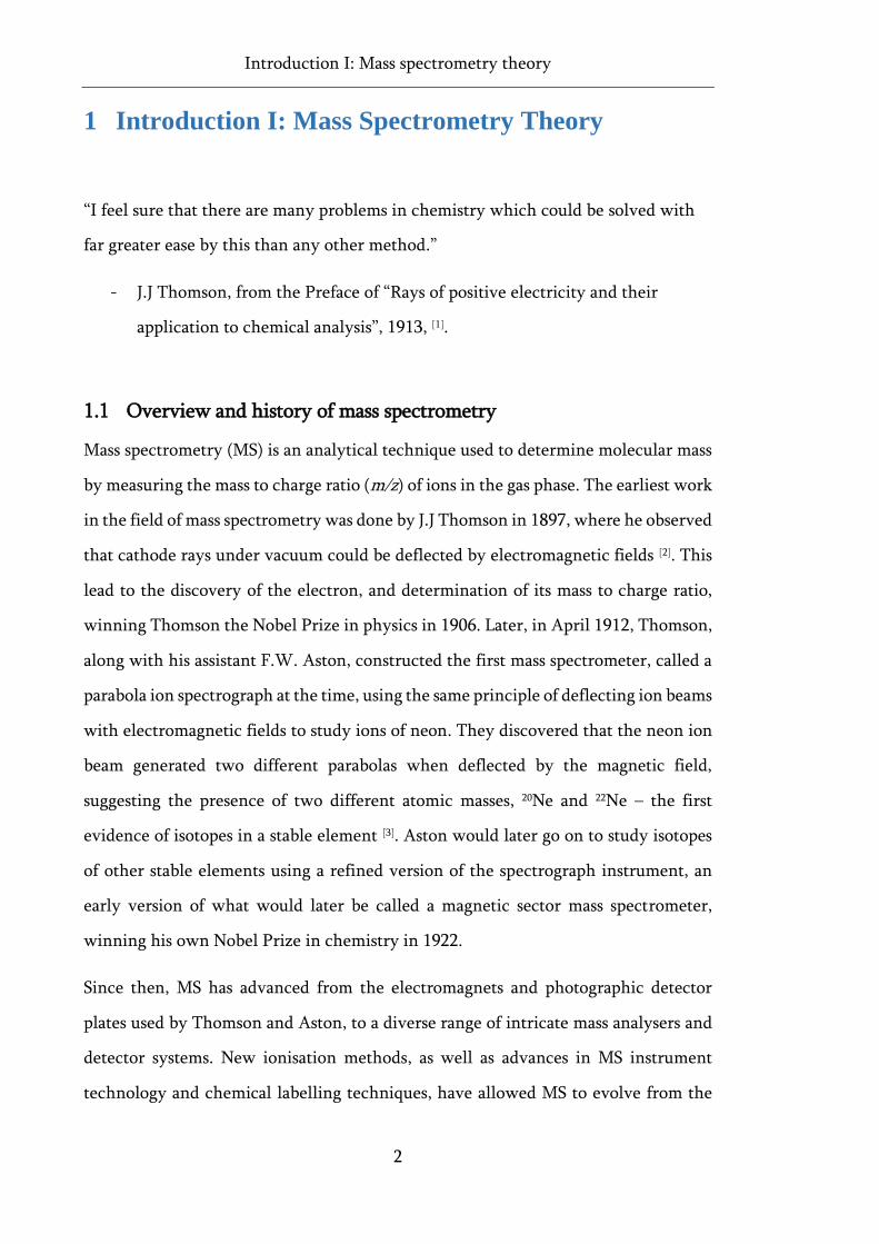
has remained the same. As such, MS can be broken down into three fundamental
components: ionisation, m/z separation, and detection (Figure 1.1).
Figure 1.1 Overview of a mass spectrometer. Samples are ionised and introduced into the gas phase
before m/z separation by a mass analyser. This is followed by detection of the ions and data analysis.
1.2 Ionisation
For a molecule to be analysed by MS, it must first be ionised. Although dozens of
ionisation methods have been developed to suit specific experiments or types of
analyte, historically, one of the most practical, and thus widely used, ionisation
methods was electron ionisation (EI) [4]. In an EI source, a heated filament is used to
generate electrons which are then accelerated towards an orthogonal path of gaseous
molecules. With the appropriate wavelength and kinetic energy, these electrons can
Introduction I: Mass spectrometry theory
4
ionise the nearby gaseous sample, before the product ions are directed towards a mass
analyser. However, EI frequently induces fragmentation of the analyte, a property not
always experimentally useful, so complementary ionisation methods, such as chemical
ionisation (CI) were developed to reduce fragmentation and study intact molecular
ions [5]. Chemical ionisation uses EI to ionise gas reagents in the source region, such as
methane or isobutane, which in turn undergo ion-molecule collisions with the
gaseous analyte, ionising the sample by proton transfer.
These, and other similar ionisation methods are, however, limiting in the sense that
they require the analyte to be in the gas phase prior to ionisation. For years, this made
MS analysis of large biomolecules, such as proteins, problematic, effectively limiting
MS to the analysis of thermally stable, volatile compounds that could be introduced
into the gas phase by heating.
1.2.1 Electrospray ionisation
The development of electrospray ionisation-MS (ESI-MS) in 1984 by John Fenn
revolutionised the study of large biomolecules by mass spectrometry [6, 7]. During ESI,
an atmospheric pressure ionisation technique, a voltage is applied across a thin, metal
coated glass capillary containing a low µM concentration of analyte in a volatile buffer
solution. The applied voltage forms a unique solvent formation at the capillary tip
know as a Taylor cone, which generates a fine spray of charged droplets containing
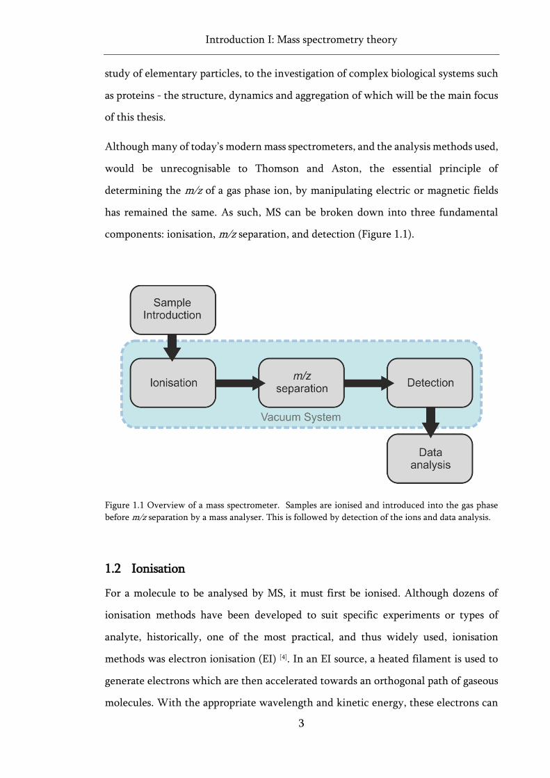
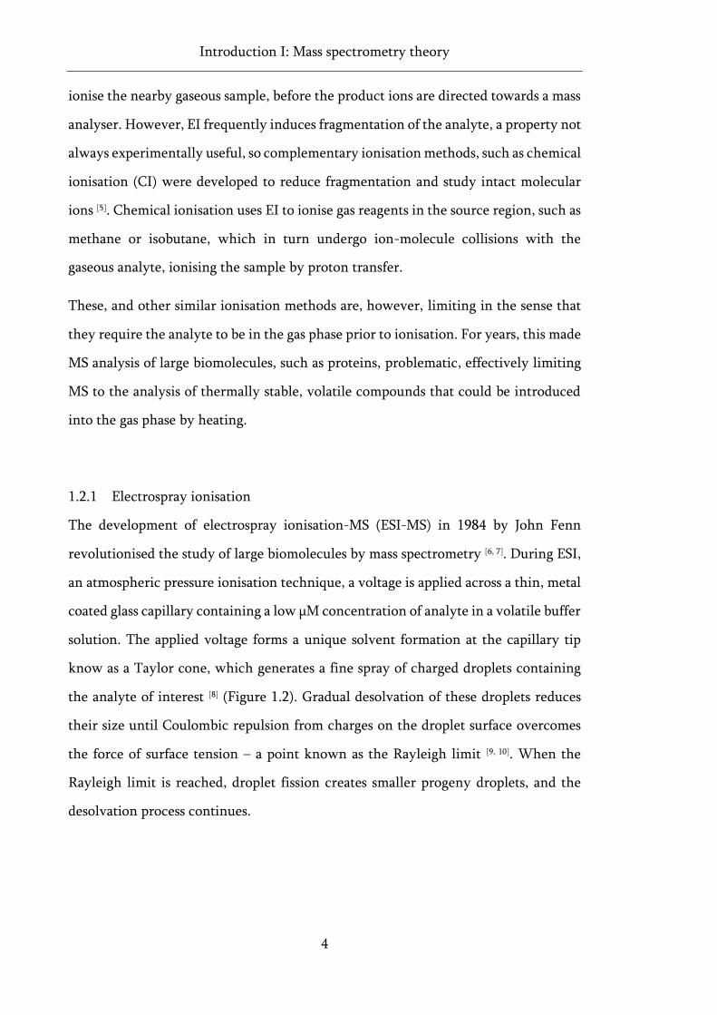
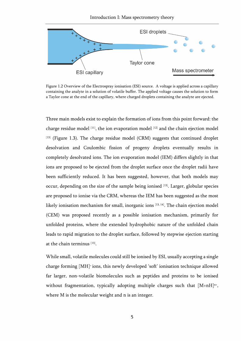
the analyte of interest [8] (Figure 1.2). Gradual desolvation of these droplets reduces
their size until Coulombic repulsion from charges on the droplet surface overcomes
the force of surface tension – a point known as the Rayleigh limit [9, 10]. When the
Rayleigh limit is reached, droplet fission creates smaller progeny droplets, and the
desolvation process continues.
Introduction I: Mass spectrometry theory
5
Figure 1.2 Overview of the Electrospray ionisation (ESI) source. A voltage is applied across a capillary
containing the analyte in a solution of volatile buffer. The applied voltage causes the solution to form
a Taylor cone at the end of the capillary, where charged droplets containing the analyte are ejected.
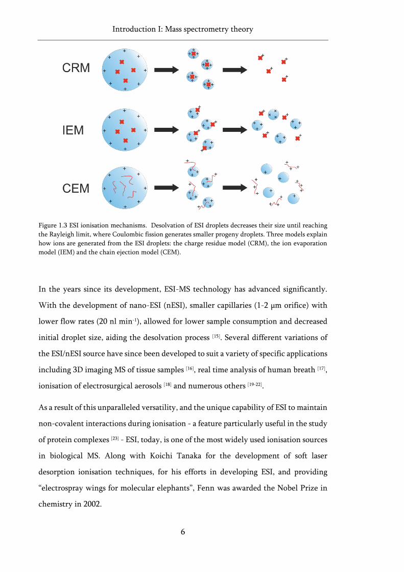
Three main models exist to explain the formation of ions from this point forward: the
charge residue model [11], the ion evaporation model [12] and the chain ejection model
[13] (Figure 1.3). The charge residue model (CRM) suggests that continued droplet
desolvation and Coulombic fission of progeny droplets eventually results in
completely desolvated ions. The ion evaporation model (IEM) differs slightly in that
ions are proposed to be ejected from the droplet surface once the droplet radii have
been sufficiently reduced. It has been suggested, however, that both models may
occur, depending on the size of the sample being ionised [13]. Larger, globular species
are proposed to ionise via the CRM, whereas the IEM has been suggested as the most
likely ionisation mechanism for small, inorganic ions [13, 14]. The chain ejection model
(CEM) was proposed recently as a possible ionisation mechanism, primarily for
unfolded proteins, where the extended hydrophobic nature of the unfolded chain
leads to rapid migration to the droplet surface, followed by stepwise ejection starting
at the chain terminus [13].
While small, volatile molecules could still be ionised by ESI, usually accepting a single
charge forming [MH]+ ions, this newly developed ‘soft’ ionisation technique allowed
far larger, non-volatile biomolecules such as peptides and proteins to be ionised
without fragmentation, typically adopting multiple charges such that [M+nH]n+,
where M is the molecular weight and n is an integer.
Introduction I: Mass spectrometry theory
6
Figure 1.3 ESI ionisation mechanisms. Desolvation of ESI droplets decreases their size until reaching
the Rayleigh limit, where Coulombic fission generates smaller progeny droplets. Three models explain
how ions are generated from the ESI droplets: the charge residue model (CRM), the ion evaporation
model (IEM) and the chain ejection model (CEM).
In the years since its development, ESI-MS technology has advanced significantly.
With the development of nano-ESI (nESI), smaller capillaries (1-2 µm orifice) with
lower flow rates (20 nl min-1), allowed for lower sample consumption and decreased
initial droplet size, aiding the desolvation process [15]. Several different variations of
the ESI/nESI source have since been developed to suit a variety of specific applications
including 3D imaging MS of tissue samples [16], real time analysis of human breath [17],
ionisation of electrosurgical aerosols [18] and numerous others [19-22].
As a result of this unparalleled versatility, and the unique capability of ESI to maintain
non-covalent interactions during ionisation - a feature particularly useful in the study
of protein complexes [23] - ESI, today, is one of the most widely used ionisation sources
in biological MS. Along with Koichi Tanaka for the development of soft laser
desorption ionisation techniques, for his efforts in developing ESI, and providing
“electrospray wings for molecular elephants”, Fenn was awarded the Nobel Prize in
chemistry in 2002.
Introduction I: Mass spectrometry theory
7
1.3 Mass analysers
After ionisation, ions are separated according to their m/z using a mass analyser. Like
most other regions of the mass spectrometer, mass analysers are kept at a constant
high vacuum (low pressure) to prevent unwanted ion-molecule collisions and increase
ion transmission and resolution. While all mass analysers use some combination of
static or dynamic electric fields to achieve m/z separation, the basic difference
between different analysers is the manner in which these fields are applied. There are
three main features by which different mass analysers are often characterised: mass
range limit (the m/z range over which an analyser can measure ions), scan speed (the
rate at which mass spectra can be acquired) and resolution. Although different
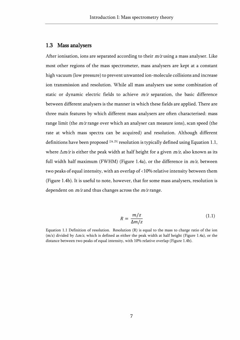
definitions have been proposed [24, 25] resolution is typically defined using Equation 1.1,
where Δm/z is either the peak width at half height for a given m/z, also known as its
full width half maximum (FWHM) (Figure 1.4a), or the difference in m/z, between
two peaks of equal intensity, with an overlap of <10% relative intensity between them
(Figure 1.4b). It is useful to note, however, that for some mass analysers, resolution is
dependent on m/z and thus changes across the m/z range.
𝑅 =
𝑚/𝑧
∆𝑚/𝑧
(1.1)
Equation 1.1 Definition of resolution. Resolution (R) is equal to the mass to charge ratio of the ion
(m/z) divided by Δm/z, which is defined as either the peak width at half height (Figure 1.4a), or the
distance between two peaks of equal intensity, with 10% relative overlap (Figure 1.4b).
Introduction I: Mass spectrometry theory
8
Figure 1.4 Different definitions of m/z resolution. a) Resolution defined by the peak width at half
height (FWHM) and b) the difference in m/z between two peaks that overlap at 10% relative intensity.
Although an extensive review of mass analysers is beyond the scope of this thesis,
certain types of mass analyser have been shown to be particularly useful in the field
of biological mass spectrometry.
1.3.1 Quadrupole analysers
First described by Wolfgang Paul and co-workers in 1953 [26], a quadrupole mass
analyser is a tuneable m/z filter, frequently used in combination with other mass
analysers, where ions of different m/z are separated by the differential stability of their
trajectories as they pass through the instrument. Ions with a stable trajectory are able
to pass through the length of the quadrupole and reach the detector, where ions with
unstable trajectories are filtered out. The quadrupole itself is made from two pairs of
parallel metal rods arranged perpendicular to one another, where opposite direct
current (DC) polarities are applied to each rod pair, such that opposite rods have the
same charge, and adjacent rods have opposite charge (Figure 1.5).
Introduction I: Mass spectrometry theory
9
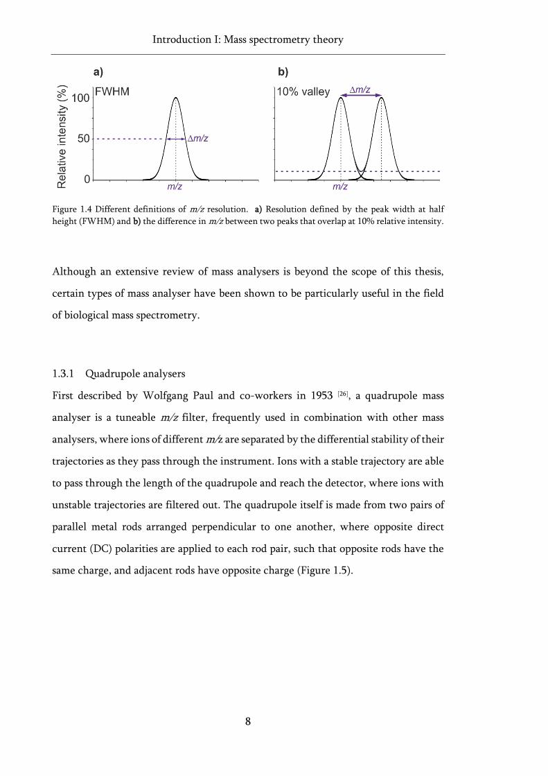
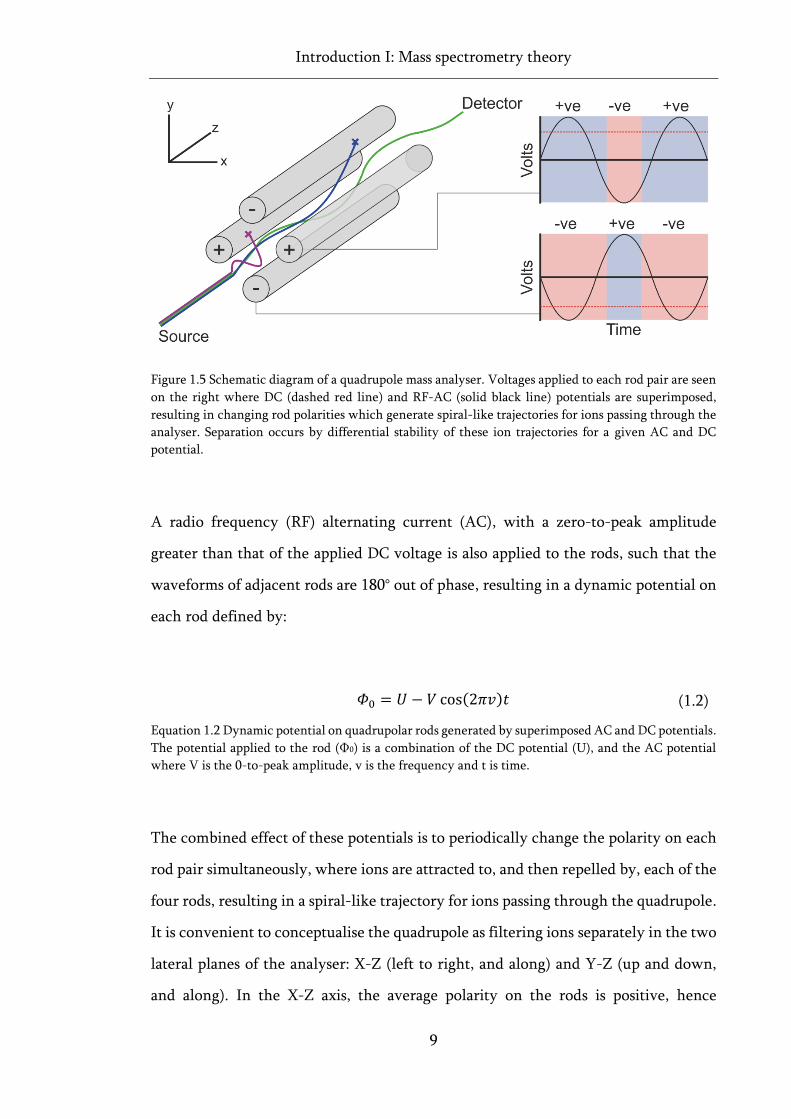
Figure 1.5 Schematic diagram of a quadrupole mass analyser. Voltages applied to each rod pair are seen
on the right where DC (dashed red line) and RF-AC (solid black line) potentials are superimposed,
resulting in changing rod polarities which generate spiral-like trajectories for ions passing through the
analyser. Separation occurs by differential stability of these ion trajectories for a given AC and DC
potential.
A radio frequency (RF) alternating current (AC), with a zero-to-peak amplitude
greater than that of the applied DC voltage is also applied to the rods, such that the
waveforms of adjacent rods are 180° out of phase, resulting in a dynamic potential on
each rod defined by:
𝛷0 = 𝑈 − 𝑉 cos(2𝜋𝑣)𝑡 (1.2)
Equation 1.2 Dynamic potential on quadrupolar rods generated by superimposed AC and DC potentials.
The potential applied to the rod (Φ0) is a combination of the DC potential (U), and the AC potential
where V is the 0-to-peak amplitude, v is the frequency and t is time.
The combined effect of these potentials is to periodically change the polarity on each
rod pair simultaneously, where ions are attracted to, and then repelled by, each of the
four rods, resulting in a spiral-like trajectory for ions passing through the quadrupole.
It is convenient to conceptualise the quadrupole as filtering ions separately in the two
lateral planes of the analyser: X-Z (left to right, and along) and Y-Z (up and down,
and along). In the X-Z axis, the average polarity on the rods is positive, hence
Introduction I: Mass spectrometry theory
10
positively charged ions will be repelled by the rods and focused into the centre of the
analyser. The brief change to negative polarity in the X-Z plane will have a negligible
effect on the trajectory of higher m/z ions, as they respond less significantly to the
polarity change than to the average polarity on the rod, allowing these ions to pass
through to the detector unhindered. Conversely, the trajectories of lower m/z ions,
which respond more significantly to the polarity change, are more likely to be
destabilised, and therefore less likely to reach the detector. Thus the X-Z plane of the
quadrupole acts as a ‘high pass m/z filter’ allowing only high m/z ions to pass through
to the analyser (Figure 1.6) [27, 28]. In the Y-Z axis, the average polarity on the electrodes
is negative, hence positively charged ions are pulled from a stable trajectory in the
centre of the analyser, towards the rods. Lower m/z ions, responding more
significantly to the temporary change to positive polarity, are repelled back towards
the centre of the analyser and are able to pass through to the detector with stable
trajectories. Higher m/z ions, being more affected by the average polarity on the rod,
have unstable trajectories in this plane, and depolarise on the rods before exiting the
quadrupole. The Y-Z plane, then, acts as a ‘low pass m/z filter’ (Figure 1.6).
For an ion to be able to pass through the quadrupole and reach the detector, it must
lie in the overlapped stability region between the two planes of the quadrupole, where
the m/z of the ion is high enough to be stable in the X-Z plane, but low enough to be
stable in the Y-Z plane. The main determinants of an ion’s stability through the
quadrupole are the frequency of the polarity changes (i.e. AC frequency – typically
maintained constant) and the magnitude of the applied DC and AC voltages (U and V
as per Equation 1.2) [29]. While a fixed value of U and V can be maintained to allow
consistently only ions of a particular m/z to have stable trajectories through the
analyser, maintaining a fixed ratio of U and V while changing their absolute values,
allows the quadrupole to sequentially stabilise the trajectory of different m/z ions.
Thus, a quadrupole can behave as a scanning mass analyser, building up a mass
spectrum by rapidly ramping up the AC and DC voltages, sequentially allowing ions
of different m/z through to the detector (Figure 1.6).
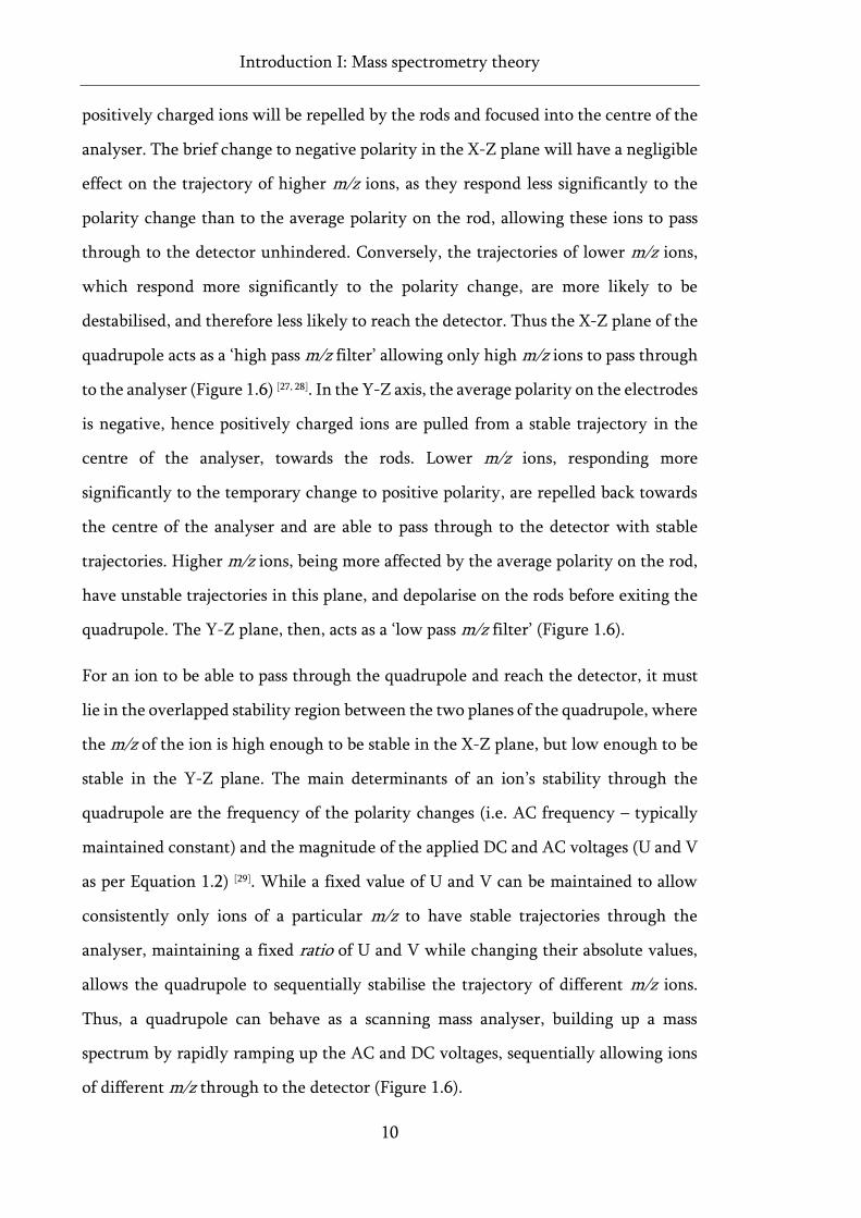
Introduction I: Mass spectrometry theory
11
Figure 1.6 The m/z separation of ions in the two lateral planes of a quadrupole. The low pass m/z filter
(Y-Z) and the high pass m/z filter (X-Z) work together to stabilise the trajectory of ions in the
quadrupole (m/z values with stable trajectories in each plane are in the grey shaded area of each plot).
A mass spectrum is acquired by sequentially stabilising the trajectories of different m/z ions by
increasing U and V.
The effect of U and V on the stability of different m/z ions in the quadrupole can be
readily visualised using stability areas calculated from a complex series of equations
known as the Mathieu and Paul equations [26, 30] (Figure 1.7). The increase in DC and
AC voltage necessary for scanning m/z analysis is visualised as the scan line in Figure
1.7, where an intersection between this line and a stability area highlights conditions
at which an ion will have a stable trajectory in both planes of the quadrupole, and
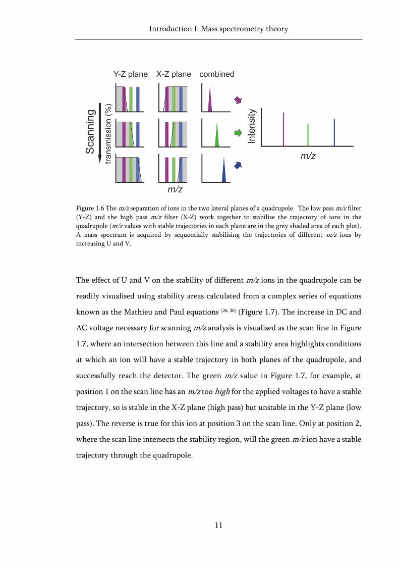
successfully reach the detector. The green m/z value in Figure 1.7, for example, at
position 1 on the scan line has an m/z too high for the applied voltages to have a stable
trajectory, so is stable in the X-Z plane (high pass) but unstable in the Y-Z plane (low
pass). The reverse is true for this ion at position 3 on the scan line. Only at position 2,
where the scan line intersects the stability region, will the green m/z ion have a stable
trajectory through the quadrupole.
Introduction I: Mass spectrometry theory
12
Figure 1.7 Stability diagrams for ions in a quadrupole. Each lateral plane of the quadrupole acts as an
m/z filter, allowing either low m/z ions (Y-Z), or high m/z ions (X-Z) to pass through to the detector.
The combined stability area for both lateral planes as a function of DC and AC voltage for high (blue),
low (purple) and intermediate (green) m/z values is shown, where an ion will have a stable trajectory
in the quadrupole at voltages where the scan line intersects the stability area. The stability of the green
ion is shown, in each plane of the quadrupole, at U:V ratios at positions 1,2 and 3 on the scan line.
The gradient of the scan line (i.e. the ratio of U and V) determines the m/z resolution
of the quadrupole, visually represented in Figure 1.7 as the stability area above the
scan line (the smaller this area, the higher the resolution). Although the resolution
can be increased by adjusting to a higher U/V ratio (steeper scan line gradient),
quadrupoles are inherently low resolution mass analysers, and are usually operated at
unit resolution (two peaks one m/z unit apart) [29]. Similarly, quadrupoles are limited
in their detectable m/z range, which is typically no more than 3000-4000 m/z [29, 31],
although this can be increased by lowering the frequency of the AC potential,
typically at the cost of sensitivity and resolution [31]. Their advantage, however, is their
fast scan speed, and the independence of ion kinetic energy and initial lateral ion
Introduction I: Mass spectrometry theory
13
positioning on m/z separation, allowing ions to be continually infused into the
analyser – a characteristic ideal for coupling to continuous ionisation sources such as
ESI. Additionally, by removing the DC potential entirely, a quadrupole can function
in RF-only mode (Y=0 in Figure 1.7), allowing a very wide range of m/z ions to be
transmitted through the analyser simultaneously, effectively acting solely as an ion
guide – a characteristic ideal for using quadrupoles in conjunction with other mass
analysers.
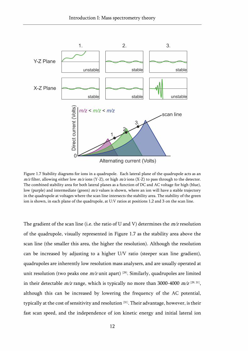
1.3.2 Linear ion traps
Conceptually very similar to a quadrupole mass analyser, the most common variant of
the linear ion trap (LIT), sometimes referred to as the 2D ion trap or Paul trap, after
Wolfgang Paul, consists of four parallel rods, each of which is cut into three separate
sections, usually referred to as a segmented quadrupole. A quadrupolar RF field is
applied (i.e. waveforms of adjacent rods are 180° out of phase) to the centre section,
confining ions in the X and Y dimensions, and DC potentials are applied to the two
end sections, repelling ions back and forth axially along the trap, thus confining ions
to the centre of the device in all three dimensions (Figure 1.8) [32].
Figure 1.8 Basic design of the linear ion trap. DC confinement potentials are applied to the front and
back sections of the segmented quadrupole. RF-AC quadrupolar potentials are applied to the centre
section to radially confine ions. Slots are cut into the x axis centre rods for radial ion ejection.
Introduction I: Mass spectrometry theory
14
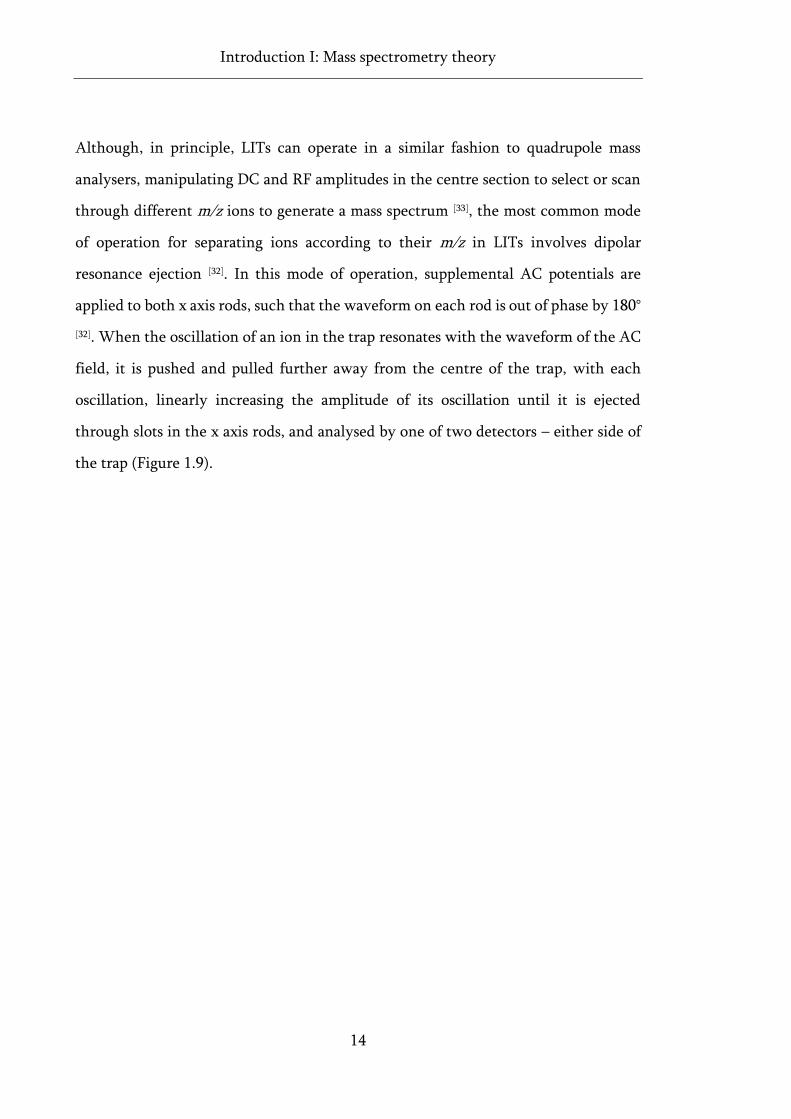
Although, in principle, LITs can operate in a similar fashion to quadrupole mass
analysers, manipulating DC and RF amplitudes in the centre section to select or scan
through different m/z ions to generate a mass spectrum [33], the most common mode
of operation for separating ions according to their m/z in LITs involves dipolar
resonance ejection [32]. In this mode of operation, supplemental AC potentials are
applied to both x axis rods, such that the waveform on each rod is out of phase by 180°
[32]. When the oscillation of an ion in the trap resonates with the waveform of the AC
field, it is pushed and pulled further away from the centre of the trap, with each
oscillation, linearly increasing the amplitude of its oscillation until it is ejected
through slots in the x axis rods, and analysed by one of two detectors – either side of
the trap (Figure 1.9).
Introduction I: Mass spectrometry theory
15
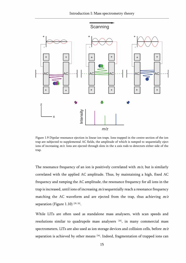
Figure 1.9 Dipolar resonance ejection in linear ion traps. Ions trapped in the centre section of the ion
trap are subjected to supplemental AC fields, the amplitude of which is ramped to sequentially eject
ions of increasing m/z. Ions are ejected through slots in the x axis rods to detectors either side of the
trap.
The resonance frequency of an ion is positively correlated with m/z, but is similarly
correlated with the applied AC amplitude. Thus, by maintaining a high, fixed AC
frequency and ramping the AC amplitude, the resonance frequency for all ions in the
trap is increased, until ions of increasing m/z sequentially reach a resonance frequency
matching the AC waveform and are ejected from the trap, thus achieving m/z
separation (Figure 1.10) [29, 33].
While LITs are often used as standalone mass analysers, with scan speeds and
resolutions similar to quadrupole mass analysers [33], in many commercial mass
spectrometers, LITs are also used as ion storage devices and collision cells, before m/z
separation is achieved by other means [34]. Indeed, fragmentation of trapped ions can
Introduction I: Mass spectrometry theory
16
be readily achieved by filling the device with a collision gas, and exciting ions to
elevated energies, below the energy required for resonance ejection [33]. This
versatility, coupled with the ability to eject ions both axially, and laterally after
storage or fragmentation, makes the 2D ion trap a valuable multi-use component in
many commercial instruments [34]. Indeed, the RF ion confinement technology that
underpins both the quadrupole and the LIT, as well as other mass analysers such as
the 3D ion trap, is now widely considered to be an essential tool in MS instruments
for a wide variety of applications. For his work in the development of the ion trap
technique, Paul was awarded the Nobel Prize in physics in 1989.
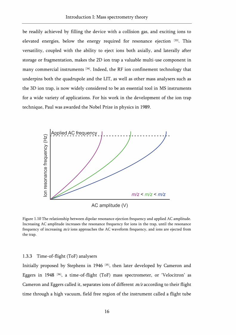
Figure 1.10 The relationship between dipolar resonance ejection frequency and applied AC amplitude.
Increasing AC amplitude increases the resonance frequency for ions in the trap, until the resonance
frequency of increasing m/z ions approaches the AC waveform frequency, and ions are ejected from
the trap.
1.3.3 Time-of-flight (ToF) analysers
Initially proposed by Stephens in 1946 [35], then later developed by Cameron and
Eggers in 1948 [36], a time-of-flight (ToF) mass spectrometer, or ‘Velocitron’ as
Cameron and Eggers called it, separates ions of different m/z according to their flight
time through a high vacuum, field free region of the instrument called a flight tube
Introduction I: Mass spectrometry theory
17
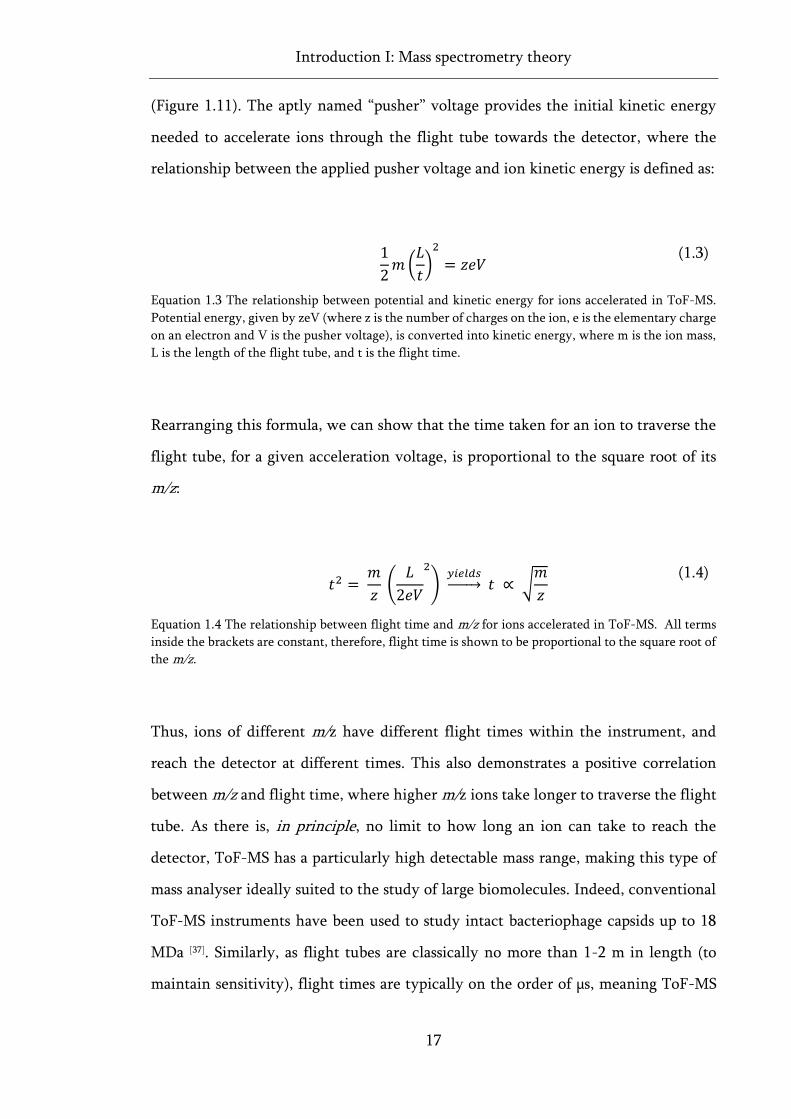
(Figure 1.11). The aptly named “pusher” voltage provides the initial kinetic energy
needed to accelerate ions through the flight tube towards the detector, where the
relationship between the applied pusher voltage and ion kinetic energy is defined as:
1
2𝑚 (𝐿
𝑡)2
= 𝑧𝑒𝑉 (1.3)
Equation 1.3 The relationship between potential and kinetic energy for ions accelerated in ToF-MS.
Potential energy, given by zeV (where z is the number of charges on the ion, e is the elementary charge
on an electron and V is the pusher voltage), is converted into kinetic energy, where m is the ion mass,
L is the length of the flight tube, and t is the flight time.
Rearranging this formula, we can show that the time taken for an ion to traverse the
flight tube, for a given acceleration voltage, is proportional to the square root of its
m/z:
𝑡2 =
𝑚
𝑧 (𝐿
2𝑒𝑉
2
) 𝑦𝑖𝑒𝑙𝑑𝑠→ 𝑡 ∝ √
𝑚
𝑧
(1.4)
Equation 1.4 The relationship between flight time and m/z for ions accelerated in ToF-MS. All terms
inside the brackets are constant, therefore, flight time is shown to be proportional to the square root of
the m/z.
Thus, ions of different m/z have different flight times within the instrument, and
reach the detector at different times. This also demonstrates a positive correlation
between m/z and flight time, where higher m/z ions take longer to traverse the flight
tube. As there is, in principle, no limit to how long an ion can take to reach the
detector, ToF-MS has a particularly high detectable mass range, making this type of
mass analyser ideally suited to the study of large biomolecules. Indeed, conventional
ToF-MS instruments have been used to study intact bacteriophage capsids up to 18
MDa [37]. Similarly, as flight tubes are classically no more than 1-2 m in length (to
maintain sensitivity), flight times are typically on the order of µs, meaning ToF-MS
Introduction I: Mass spectrometry theory
18
instruments are also capable of fast scanning speeds, usually acquiring multiple scans
in order to build up a mass spectrum.
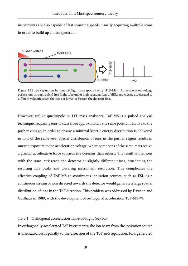
Figure 1.11 m/z separation by time-of-flight mass spectrometry (ToF-MS). An acceleration voltage
pushes ions through a field free flight tube under high vacuum. Ions of different m/z are accelerated to
different velocities such that ions of lower m/z reach the detector first.
However, unlike quadrupole or LIT mass analysers, ToF-MS is a pulsed analysis
technique, requiring ions to start from approximately the same position relative to the
pusher voltage, in order to ensure a minimal kinetic energy distribution is delivered
to ions of the same m/z. Spatial distribution of ions in the pusher region results in
uneven exposure to the acceleration voltage, where some ions of the same m/z receive
a greater accelerative force towards the detector than others. The result is that ions
with the same m/z reach the detector at slightly different times, broadening the
resulting m/z peaks and lowering instrument resolution. This complicates the
effective coupling of ToF-MS to continuous ionisation sources, such as ESI, as a
continuous stream of ions directed towards the detector would generate a large spatial
distribution of ions in the ToF direction. This problem was addressed by Dawson and
Guilhaus in 1989, with the development of orthogonal acceleration ToF-MS [38].
1.3.3.1 Orthogonal acceleration Time-of-flight (oa-ToF)
In orthogonally accelerated ToF instruments, the ion beam from the ionisation source
is orientated orthogonally to the direction of the ToF m/z separation. Ions generated
Introduction I: Mass spectrometry theory
19
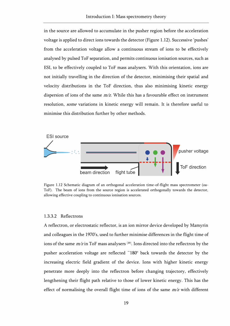
in the source are allowed to accumulate in the pusher region before the acceleration
voltage is applied to direct ions towards the detector (Figure 1.12). Successive ‘pushes’
from the acceleration voltage allow a continuous stream of ions to be effectively
analysed by pulsed ToF separation, and permits continuous ionisation sources, such as
ESI, to be effectively coupled to ToF mass analysers. With this orientation, ions are
not initially travelling in the direction of the detector, minimising their spatial and
velocity distributions in the ToF direction, thus also minimising kinetic energy
dispersion of ions of the same m/z. While this has a favourable effect on instrument
resolution, some variations in kinetic energy will remain. It is therefore useful to
minimise this distribution further by other methods.
Figure 1.12 Schematic diagram of an orthogonal acceleration time-of-flight mass spectrometer (oa-
ToF). The beam of ions from the source region is accelerated orthogonally towards the detector,
allowing effective coupling to continuous ionisation sources.
1.3.3.2 Reflectrons
A reflectron, or electrostatic reflector, is an ion mirror device developed by Mamyrin
and colleagues in the 1970’s, used to further minimise differences in the flight time of
ions of the same m/z in ToF mass analysers [39]. Ions directed into the reflectron by the
pusher acceleration voltage are reflected ~180° back towards the detector by the
increasing electric field gradient of the device. Ions with higher kinetic energy
penetrate more deeply into the reflectron before changing trajectory, effectively
lengthening their flight path relative to those of lower kinetic energy. This has the
effect of normalising the overall flight time of ions of the same m/z with different
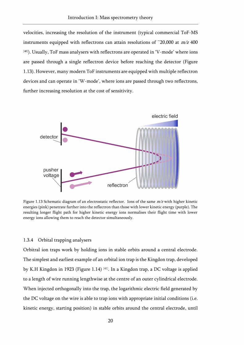
Introduction I: Mass spectrometry theory
20
velocities, increasing the resolution of the instrument (typical commercial ToF-MS
instruments equipped with reflectrons can attain resolutions of ~20,000 at m/z 400
[40]). Usually, ToF mass analysers with reflectrons are operated in ‘V-mode’ where ions
are passed through a single reflectron device before reaching the detector (Figure
1.13). However, many modern ToF instruments are equipped with multiple reflectron
devices and can operate in ‘W-mode’, where ions are passed through two reflectrons,
further increasing resolution at the cost of sensitivity.
Figure 1.13 Schematic diagram of an electrostatic reflector. Ions of the same m/z with higher kinetic
energies (pink) penetrate further into the reflectron than those with lower kinetic energy (purple). The
resulting longer flight path for higher kinetic energy ions normalises their flight time with lower
energy ions allowing them to reach the detector simultaneously.
1.3.4 Orbital trapping analysers
Orbitral ion traps work by holding ions in stable orbits around a central electrode.
The simplest and earliest example of an orbital ion trap is the Kingdon trap, developed
by K.H Kingdon in 1923 (Figure 1.14) [41]. In a Kingdon trap, a DC voltage is applied
to a length of wire running lengthwise at the centre of an outer cylindrical electrode.
When injected orthogonally into the trap, the logarithmic electric field generated by
the DC voltage on the wire is able to trap ions with appropriate initial conditions (i.e.
kinetic energy, starting position) in stable orbits around the central electrode, until
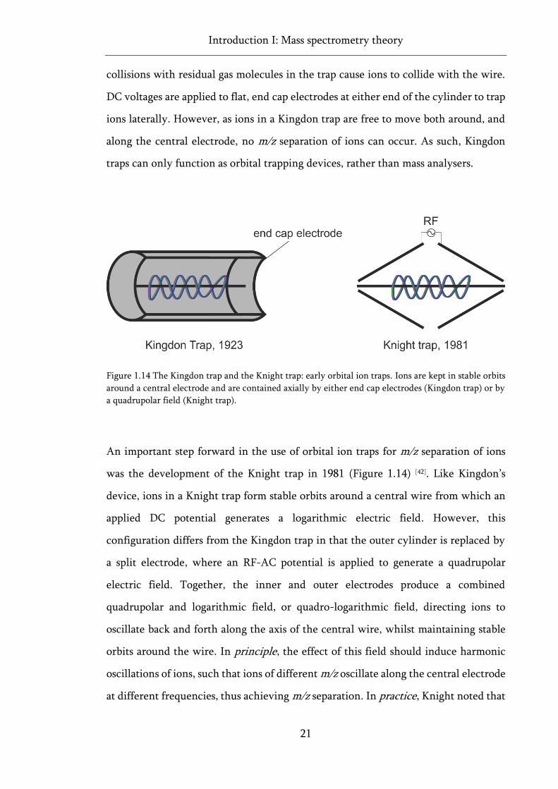
Introduction I: Mass spectrometry theory
21
collisions with residual gas molecules in the trap cause ions to collide with the wire.
DC voltages are applied to flat, end cap electrodes at either end of the cylinder to trap
ions laterally. However, as ions in a Kingdon trap are free to move both around, and
along the central electrode, no m/z separation of ions can occur. As such, Kingdon
traps can only function as orbital trapping devices, rather than mass analysers.
Figure 1.14 The Kingdon trap and the Knight trap: early orbital ion traps. Ions are kept in stable orbits
around a central electrode and are contained axially by either end cap electrodes (Kingdon trap) or by
a quadrupolar field (Knight trap).
An important step forward in the use of orbital ion traps for m/z separation of ions
was the development of the Knight trap in 1981 (Figure 1.14) [42]. Like Kingdon’s
device, ions in a Knight trap form stable orbits around a central wire from which an
applied DC potential generates a logarithmic electric field. However, this
configuration differs from the Kingdon trap in that the outer cylinder is replaced by
a split electrode, where an RF-AC potential is applied to generate a quadrupolar
electric field. Together, the inner and outer electrodes produce a combined
quadrupolar and logarithmic field, or quadro-logarithmic field, directing ions to
oscillate back and forth along the axis of the central wire, whilst maintaining stable
orbits around the wire. In principle, the effect of this field should induce harmonic
oscillations of ions, such that ions of different m/z oscillate along the central electrode
at different frequencies, thus achieving m/z separation. In practice, Knight noted that
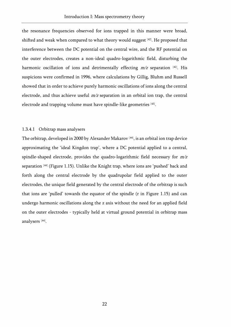
Introduction I: Mass spectrometry theory
22
the resonance frequencies observed for ions trapped in this manner were broad,
shifted and weak when compared to what theory would suggest [42]. He proposed that
interference between the DC potential on the central wire, and the RF potential on
the outer electrodes, creates a non-ideal quadro-logarithmic field, disturbing the
harmonic oscillation of ions and detrimentally effecting m/z separation [42]. His
suspicions were confirmed in 1996, where calculations by Gillig, Bluhm and Russell
showed that in order to achieve purely harmonic oscillations of ions along the central
electrode, and thus achieve useful m/z separation in an orbital ion trap, the central
electrode and trapping volume must have spindle-like geometries [43].
1.3.4.1 Orbitrap mass analysers
The orbitrap, developed in 2000 by Alexander Makarov [44], is an orbital ion trap device
approximating the ‘ideal Kingdon trap’, where a DC potential applied to a central,
spindle-shaped electrode, provides the quadro-logarithmic field necessary for m/z
separation [44] (Figure 1.15). Unlike the Knight trap, where ions are ‘pushed’ back and
forth along the central electrode by the quadrupolar field applied to the outer
electrodes, the unique field generated by the central electrode of the orbitrap is such
that ions are ‘pulled’ towards the equator of the spindle (r in Figure 1.15) and can
undergo harmonic oscillations along the z axis without the need for an applied field
on the outer electrodes - typically held at virtual ground potential in orbitrap mass
analysers [44].
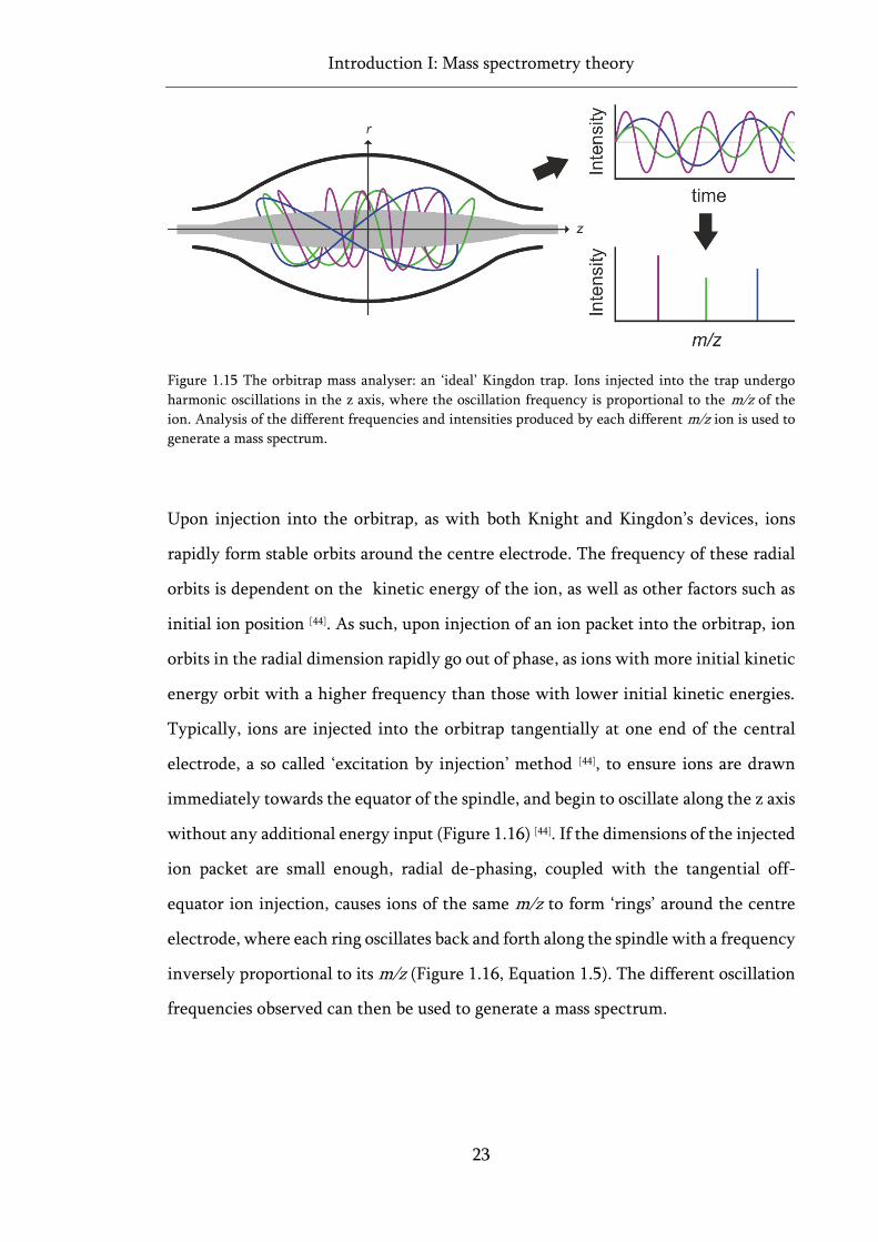
Introduction I: Mass spectrometry theory
23
Figure 1.15 The orbitrap mass analyser: an ‘ideal’ Kingdon trap. Ions injected into the trap undergo
harmonic oscillations in the z axis, where the oscillation frequency is proportional to the m/z of the
ion. Analysis of the different frequencies and intensities produced by each different m/z ion is used to
generate a mass spectrum.
Upon injection into the orbitrap, as with both Knight and Kingdon’s devices, ions
rapidly form stable orbits around the centre electrode. The frequency of these radial
orbits is dependent on the kinetic energy of the ion, as well as other factors such as
initial ion position [44]. As such, upon injection of an ion packet into the orbitrap, ion
orbits in the radial dimension rapidly go out of phase, as ions with more initial kinetic
energy orbit with a higher frequency than those with lower initial kinetic energies.
Typically, ions are injected into the orbitrap tangentially at one end of the central
electrode, a so called ‘excitation by injection’ method [44], to ensure ions are drawn
immediately towards the equator of the spindle, and begin to oscillate along the z axis
without any additional energy input (Figure 1.16) [44]. If the dimensions of the injected
ion packet are small enough, radial de-phasing, coupled with the tangential off-
equator ion injection, causes ions of the same m/z to form ‘rings’ around the centre
electrode, where each ring oscillates back and forth along the spindle with a frequency
inversely proportional to its m/z (Figure 1.16, Equation 1.5). The different oscillation
frequencies observed can then be used to generate a mass spectrum.
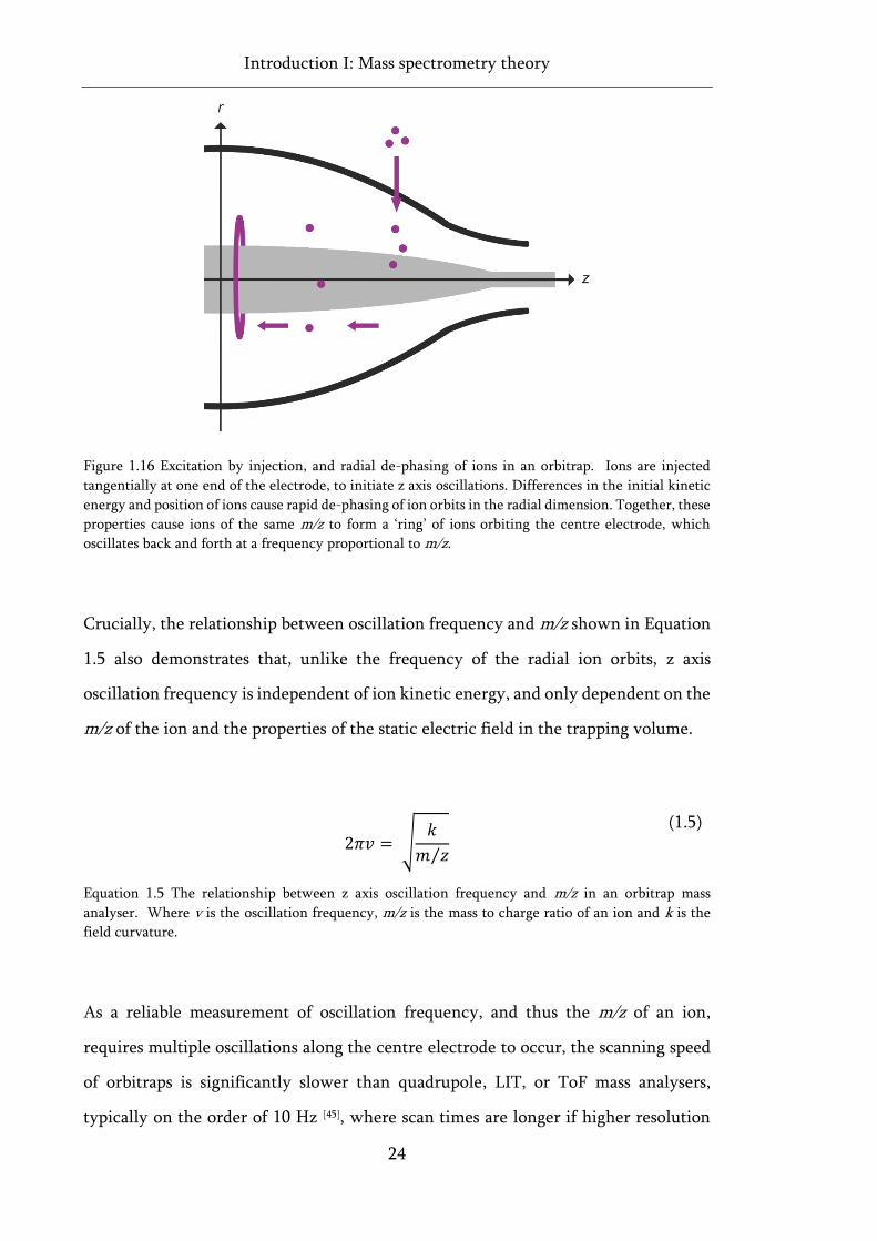
Introduction I: Mass spectrometry theory
24
Figure 1.16 Excitation by injection, and radial de-phasing of ions in an orbitrap. Ions are injected
tangentially at one end of the electrode, to initiate z axis oscillations. Differences in the initial kinetic
energy and position of ions cause rapid de-phasing of ion orbits in the radial dimension. Together, these
properties cause ions of the same m/z to form a ‘ring’ of ions orbiting the centre electrode, which
oscillates back and forth at a frequency proportional to m/z.
Crucially, the relationship between oscillation frequency and m/z shown in Equation
1.5 also demonstrates that, unlike the frequency of the radial ion orbits, z axis
oscillation frequency is independent of ion kinetic energy, and only dependent on the
m/z of the ion and the properties of the static electric field in the trapping volume.
2𝜋𝑣 = √
𝑘
𝑚 𝑧⁄
(1.5)
Equation 1.5 The relationship between z axis oscillation frequency and m/z in an orbitrap mass
analyser. Where v is the oscillation frequency, m/z is the mass to charge ratio of an ion and k is the
field curvature.
As a reliable measurement of oscillation frequency, and thus the m/z of an ion,
requires multiple oscillations along the centre electrode to occur, the scanning speed
of orbitraps is significantly slower than quadrupole, LIT, or ToF mass analysers,
typically on the order of 10 Hz [45], where scan times are longer if higher resolution
Introduction I: Mass spectrometry theory
25
measurements are required. Similarly, unlike quadrupoles where resolution is largely
independent of m/z, the resolution of orbitrap mass analysers decreases as a function
of (m/z)0.5 [46]. Nevertheless, orbitrap mass analysers are, due to the unique ion motions
around the central electrode, inherently high resolution instruments, where
continued development has thus far enabled orbitraps to achieve up to 1,000,000
resolution (FWHM) at m/z 200 [47]. Similar to ToF instruments, orbitrap mass analysers
require pulses of ion packets for analysis, and as such are often coupled to continuous
ionisation sources via a curved linear ion trap, usually called the C-trap. The purpose
of this is twofold: to accumulate and store ions from the ionisation source, cooling
them with collisions with gas molecules, and to rapidly (100-200 ns) inject ion packets
into the orbitrap with minimal spatial and temporal spread [48], crucial for maintaining
the coherence of the harmonic oscillations of ions. This linear ion trap, rather than
the orbitrap itself, is often the limiting factor in the detectable mass range limit [29].
However, recent advances in instrument technology upstream of the mass analyser,
have enabled orbitrap instruments to study high molecular weight intact protein
complexes up to several MDa [49].
1.4 Ion Detectors
Ion detection is the final fundamental component in a mass spectrometer. Far from
the photographic plates used as detectors by Thomson and Aston in the early 20th
century, today, the purpose of an ion detector in mass spectrometry is to produce a
signal from the separated ions, which can interpreted by a computer in order to
generate a mass spectrum.
1.4.1 Electron multipliers
One of the most commonly used detector systems in modern mass spectrometers is
the electron multiplier. In this type of detector, ions collide with a conversion dynode,
causing the emission of secondary particles, including electrons. This sets off a cascade
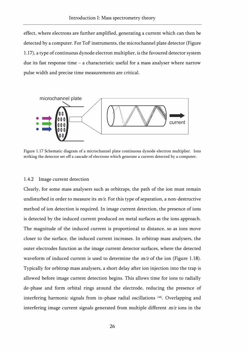
Introduction I: Mass spectrometry theory
26
effect, where electrons are further amplified, generating a current which can then be
detected by a computer. For ToF instruments, the microchannel plate detector (Figure
1.17), a type of continuous dynode electron multiplier, is the favoured detector system
due its fast response time – a characteristic useful for a mass analyser where narrow
pulse width and precise time measurements are critical.
Figure 1.17 Schematic diagram of a microchannel plate continuous dynode electron multiplier. Ions
striking the detector set off a cascade of electrons which generate a current detected by a computer.
1.4.2 Image current detection
Clearly, for some mass analysers such as orbitraps, the path of the ion must remain
undisturbed in order to measure its m/z. For this type of separation, a non-destructive
method of ion detection is required. In image current detection, the presence of ions
is detected by the induced current produced on metal surfaces as the ions approach.
The magnitude of the induced current is proportional to distance, so as ions move
closer to the surface, the induced current increases. In orbitrap mass analysers, the
outer electrodes function as the image current detector surfaces, where the detected
waveform of induced current is used to determine the m/z of the ion (Figure 1.18).
Typically for orbitrap mass analysers, a short delay after ion injection into the trap is
allowed before image current detection begins. This allows time for ions to radially
de-phase and form orbital rings around the electrode, reducing the presence of
interfering harmonic signals from in-phase radial oscillations [44]. Overlapping and
interfering image current signals generated from multiple different m/z ions in the
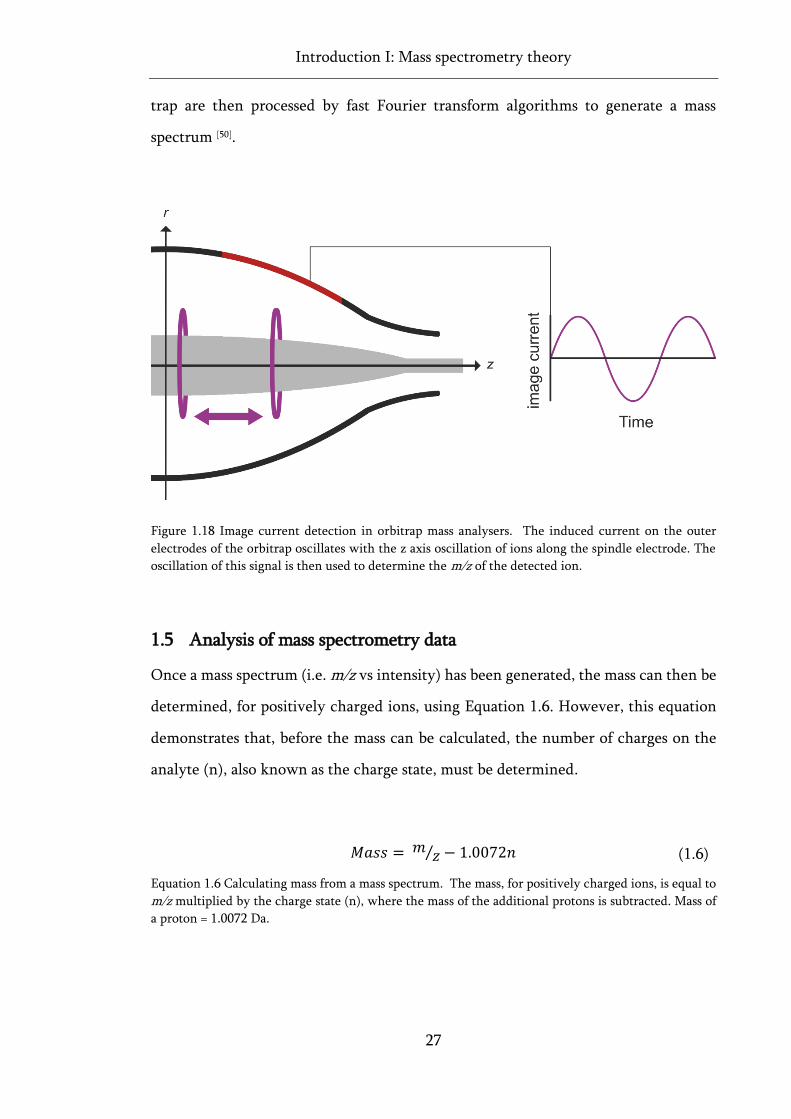
Introduction I: Mass spectrometry theory
27
trap are then processed by fast Fourier transform algorithms to generate a mass
spectrum [50].
Figure 1.18 Image current detection in orbitrap mass analysers. The induced current on the outer
electrodes of the orbitrap oscillates with the z axis oscillation of ions along the spindle electrode. The
oscillation of this signal is then used to determine the m/z of the detected ion.
1.5 Analysis of mass spectrometry data
Once a mass spectrum (i.e. m/z vs intensity) has been generated, the mass can then be
determined, for positively charged ions, using Equation 1.6. However, this equation
demonstrates that, before the mass can be calculated, the number of charges on the
analyte (n), also known as the charge state, must be determined.
𝑀𝑎𝑠𝑠 = 𝑚 𝑧⁄ − 1.0072𝑛 (1.6)
Equation 1.6 Calculating mass from a mass spectrum. The mass, for positively charged ions, is equal to
m/z multiplied by the charge state (n), where the mass of the additional protons is subtracted. Mass of
a proton = 1.0072 Da.
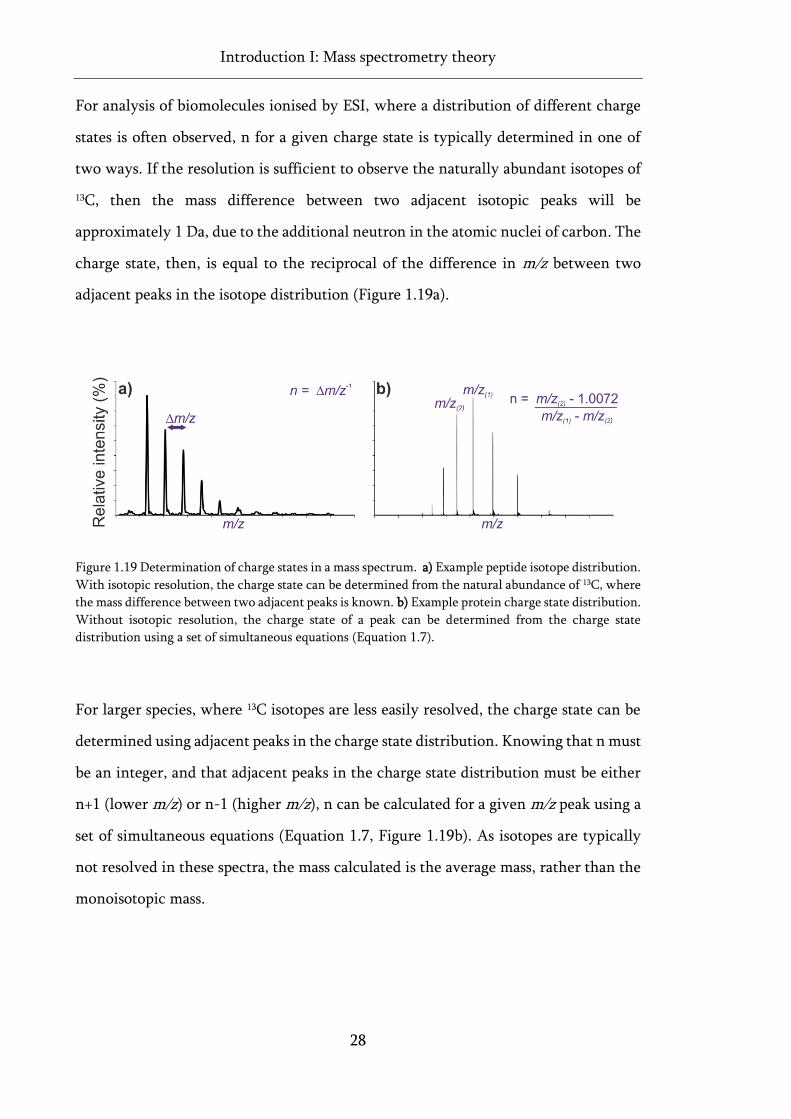
Introduction I: Mass spectrometry theory
28
For analysis of biomolecules ionised by ESI, where a distribution of different charge
states is often observed, n for a given charge state is typically determined in one of
two ways. If the resolution is sufficient to observe the naturally abundant isotopes of
13C, then the mass difference between two adjacent isotopic peaks will be
approximately 1 Da, due to the additional neutron in the atomic nuclei of carbon. The
charge state, then, is equal to the reciprocal of the difference in m/z between two
adjacent peaks in the isotope distribution (Figure 1.19a).
Figure 1.19 Determination of charge states in a mass spectrum. a) Example peptide isotope distribution.
With isotopic resolution, the charge state can be determined from the natural abundance of 13C, where
the mass difference between two adjacent peaks is known. b) Example protein charge state distribution.
Without isotopic resolution, the charge state of a peak can be determined from the charge state
distribution using a set of simultaneous equations (Equation 1.7).
For larger species, where 13C isotopes are less easily resolved, the charge state can be
determined using adjacent peaks in the charge state distribution. Knowing that n must
be an integer, and that adjacent peaks in the charge state distribution must be either
n+1 (lower m/z) or n-1 (higher m/z), n can be calculated for a given m/z peak using a
set of simultaneous equations (Equation 1.7, Figure 1.19b). As isotopes are typically
not resolved in these spectra, the mass calculated is the average mass, rather than the
monoisotopic mass.
Introduction I: Mass spectrometry theory
29
𝑀𝑎𝑠𝑠 = 𝑚 𝑧(1)⁄ 𝑛 − 1.0072𝑛 = 𝑚 𝑧(2)⁄ (𝑛 + 1) − 1.0072(𝑛 + 1) (1.7)
Equation 1.7 Determination of charge states in non-isotopically resolved mass spectra. Adjacent peaks
in a charge state distribution have a different number of charges but are ionised from the same
molecule, and have the same mass, after correcting for the different number of additional protons. This
can be used to calculate n for a given peak and, subsequently, to calculate mass.
1.5.1 Mass error and mass accuracy
Mass accuracy is typically quoted in parts per million (ppm) and is a measure of how
close the calculated mass is to the theoretical mass of the molecule (Equation 1.8) [51].
𝑀𝑎𝑠𝑠 𝑎𝑐𝑐𝑢𝑟𝑎𝑐𝑦 =
𝑇ℎ𝑒𝑜𝑟𝑒𝑡𝑖𝑐𝑎𝑙 𝑚𝑎𝑠𝑠 − 𝑂𝑏𝑠𝑒𝑟𝑣𝑒𝑑 𝑚𝑎𝑠𝑠
𝑇ℎ𝑒𝑜𝑟𝑒𝑡𝑖𝑐𝑎𝑙 𝑚𝑎𝑠𝑠 × 106
(1.8)
Equation 1.8 The definition of mass accuracy. Measured in ppm, mass accuracy is a measure of how
close the calculated mass is to the theoretical mass of the molecule being studied.
1.6 Tandem mass spectrometry (MS/MS)
For many applications in mass spectrometry, such as experiments where
fragmentation of specific ions is required, one stage of mass analysis is not enough.
For this reason, many modern mass spectrometers are equipped with multiple mass
analysers, frequently separated by collision cells for ion fragmentation, enabling m/z
separation to be performed in tandem, usually referred to as MS/MS. While the use of
multiple mass analysers allows a variety of different MS/MS workflows, a commonly
used workflow in biological mass spectrometry, particularly for the structural analysis
of proteins, is the product ion scan (Figure 1.20).
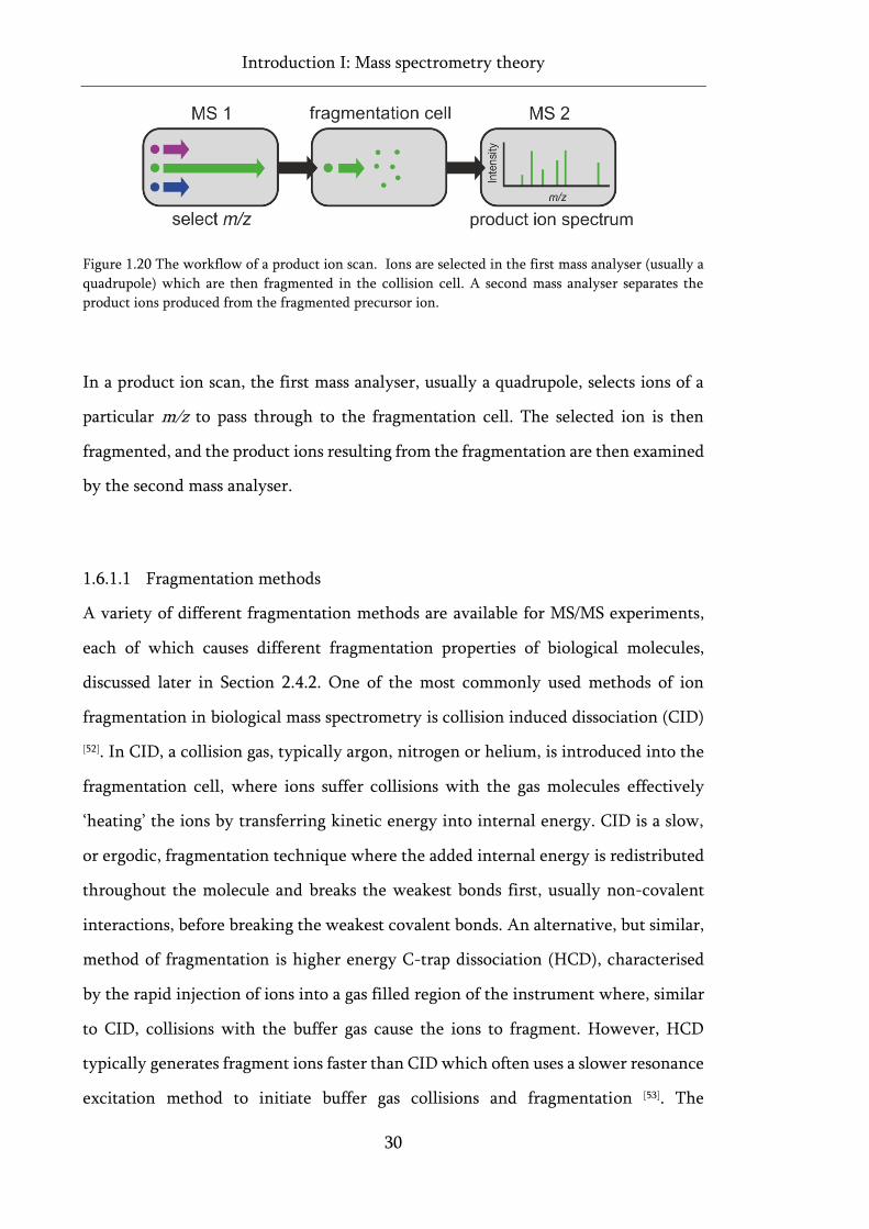
Introduction I: Mass spectrometry theory
30
Figure 1.20 The workflow of a product ion scan. Ions are selected in the first mass analyser (usually a
quadrupole) which are then fragmented in the collision cell. A second mass analyser separates the
product ions produced from the fragmented precursor ion.
In a product ion scan, the first mass analyser, usually a quadrupole, selects ions of a
particular m/z to pass through to the fragmentation cell. The selected ion is then
fragmented, and the product ions resulting from the fragmentation are then examined
by the second mass analyser.
1.6.1.1 Fragmentation methods
A variety of different fragmentation methods are available for MS/MS experiments,
each of which causes different fragmentation properties of biological molecules,
discussed later in Section 2.4.2. One of the most commonly used methods of ion
fragmentation in biological mass spectrometry is collision induced dissociation (CID)
[52]. In CID, a collision gas, typically argon, nitrogen or helium, is introduced into the
fragmentation cell, where ions suffer collisions with the gas molecules effectively
‘heating’ the ions by transferring kinetic energy into internal energy. CID is a slow,
or ergodic, fragmentation technique where the added internal energy is redistributed
throughout the molecule and breaks the weakest bonds first, usually non-covalent
interactions, before breaking the weakest covalent bonds. An alternative, but similar,
method of fragmentation is higher energy C-trap dissociation (HCD), characterised
by the rapid injection of ions into a gas filled region of the instrument where, similar
to CID, collisions with the buffer gas cause the ions to fragment. However, HCD
typically generates fragment ions faster than CID which often uses a slower resonance
excitation method to initiate buffer gas collisions and fragmentation [53]. The
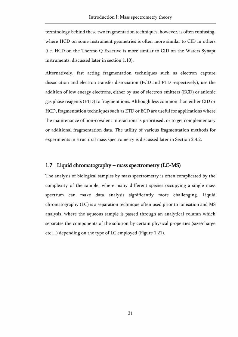
Introduction I: Mass spectrometry theory
31
terminology behind these two fragmentation techniques, however, is often confusing,
where HCD on some instrument geometries is often more similar to CID in others
(i.e. HCD on the Thermo Q Exactive is more similar to CID on the Waters Synapt
instruments, discussed later in section 1.10).
Alternatively, fast acting fragmentation techniques such as electron capture
dissociation and electron transfer dissociation (ECD and ETD respectively), use the
addition of low energy electrons, either by use of electron emitters (ECD) or anionic
gas phase reagents (ETD) to fragment ions. Although less common than either CID or
HCD, fragmentation techniques such as ETD or ECD are useful for applications where
the maintenance of non-covalent interactions is prioritised, or to get complementary
or additional fragmentation data. The utility of various fragmentation methods for
experiments in structural mass spectrometry is discussed later in Section 2.4.2.
1.7 Liquid chromatography – mass spectrometry (LC-MS)
The analysis of biological samples by mass spectrometry is often complicated by the
complexity of the sample, where many different species occupying a single mass
spectrum can make data analysis significantly more challenging. Liquid
chromatography (LC) is a separation technique often used prior to ionisation and MS
analysis, where the aqueous sample is passed through an analytical column which
separates the components of the solution by certain physical properties (size/charge
etc…) depending on the type of LC employed (Figure 1.21).
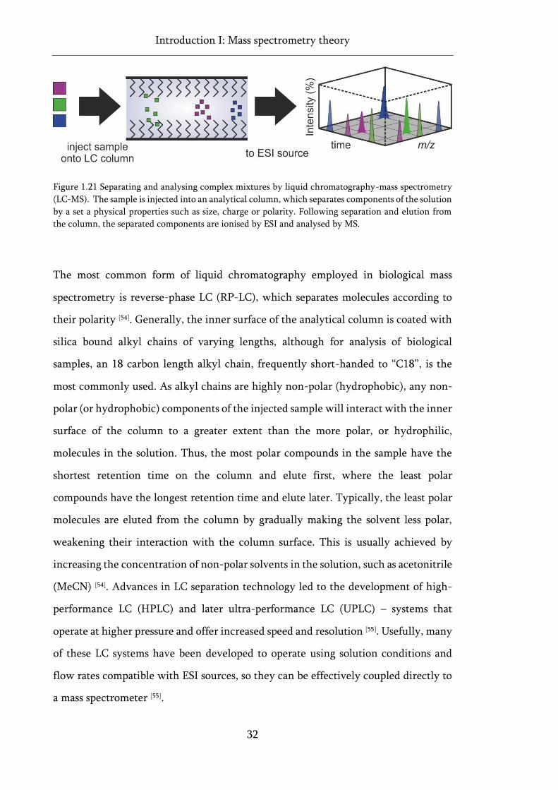
Introduction I: Mass spectrometry theory
32
Figure 1.21 Separating and analysing complex mixtures by liquid chromatography-mass spectrometry
(LC-MS). The sample is injected into an analytical column, which separates components of the solution
by a set a physical properties such as size, charge or polarity. Following separation and elution from
the column, the separated components are ionised by ESI and analysed by MS.
The most common form of liquid chromatography employed in biological mass
spectrometry is reverse-phase LC (RP-LC), which separates molecules according to
their polarity [54]. Generally, the inner surface of the analytical column is coated with
silica bound alkyl chains of varying lengths, although for analysis of biological
samples, an 18 carbon length alkyl chain, frequently short-handed to “C18”, is the
most commonly used. As alkyl chains are highly non-polar (hydrophobic), any non-
polar (or hydrophobic) components of the injected sample will interact with the inner
surface of the column to a greater extent than the more polar, or hydrophilic,
molecules in the solution. Thus, the most polar compounds in the sample have the
shortest retention time on the column and elute first, where the least polar
compounds have the longest retention time and elute later. Typically, the least polar
molecules are eluted from the column by gradually making the solvent less polar,
weakening their interaction with the column surface. This is usually achieved by
increasing the concentration of non-polar solvents in the solution, such as acetonitrile
(MeCN) [54]. Advances in LC separation technology led to the development of high-
performance LC (HPLC) and later ultra-performance LC (UPLC) – systems that
operate at higher pressure and offer increased speed and resolution [55]. Usefully, many
of these LC systems have been developed to operate using solution conditions and
flow rates compatible with ESI sources, so they can be effectively coupled directly to
a mass spectrometer [55].
Introduction I: Mass spectrometry theory
33
1.8 LC-MS/MS data acquisition methods
As discussed earlier in Section 1.6, tandem mass spectrometry experiments are useful
for acquiring fragment ion spectra of the ion of interest which, for biomolecules, is
typically used for peptide sequencing, discussed later in Section 2.4.2. When
continually infusing a pure analyte into the mass spectrometer, the intact and
fragment ion spectra can be easily acquired separately by activating and deactivating
fragmentation in the collision cell, to obtain both the intact mass measurement, and
the fragment ion spectra necessary to analyse the sample. However, when LC is used
to separate complex mixtures prior to MS analysis, the ion is only introduced into the
mass spectrometer for the brief period that it elutes off the LC column, making rapid
acquisition of both the intact, and the fragment ion spectra for each molecule
challenging. To tackle this issue, instrument methods have been developed to allow
rapid automated switching between high and low energies in the collision cell,
allowing acquisition of both MS, and tandem MS data of ions as they are introduced
into the mass spectrometer from online LC separation. Generally, there are two main
acquisition modes that achieve this: data dependent, and data independent,
acquisition.
1.8.1 Data dependent acquisition (DDA)
In data dependent acquisition modes (DDA), the spectra for intact molecular ions are
first acquired by deactivating the fragmentation, and allowing a full m/z scan of all
ions eluting from the LC column at that time. A user-defined number of the most
intense m/z ions from the initial scan, sometimes called the MS1 or precursor ion scan,
are then sequentially selected by the first mass analyser for fragmentation and spectral
analysis by the second mass analyser. When complete, another full m/z scan is
acquired at the new, now longer, LC retention time, and the cycle is repeated for as
long as the LC elution takes place (Figure 1.22). Typically, a dynamic exclusion time
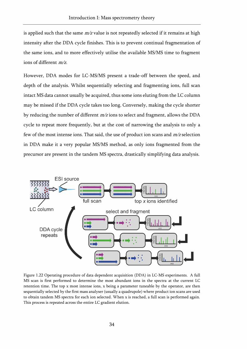
Introduction I: Mass spectrometry theory
34
is applied such that the same m/z value is not repeatedly selected if it remains at high
intensity after the DDA cycle finishes. This is to prevent continual fragmentation of
the same ions, and to more effectively utilise the available MS/MS time to fragment
ions of different m/z.
However, DDA modes for LC-MS/MS present a trade-off between the speed, and
depth of the analysis. Whilst sequentially selecting and fragmenting ions, full scan
intact MS data cannot usually be acquired, thus some ions eluting from the LC column
may be missed if the DDA cycle takes too long. Conversely, making the cycle shorter
by reducing the number of different m/z ions to select and fragment, allows the DDA
cycle to repeat more frequently, but at the cost of narrowing the analysis to only a
few of the most intense ions. That said, the use of product ion scans and m/z selection
in DDA make it a very popular MS/MS method, as only ions fragmented from the
precursor are present in the tandem MS spectra, drastically simplifying data analysis.
Figure 1.22 Operating procedure of data dependent acquisition (DDA) in LC-MS experiments. A full
MS scan is first performed to determine the most abundant ions in the spectra at the current LC
retention time. The top x most intense ions, x being a parameter tuneable by the operator, are then
sequentially selected by the first mass analyser (usually a quadrupole) where product ion scans are used
to obtain tandem MS spectra for each ion selected. When x is reached, a full scan is performed again.
This process is repeated across the entire LC gradient elution.
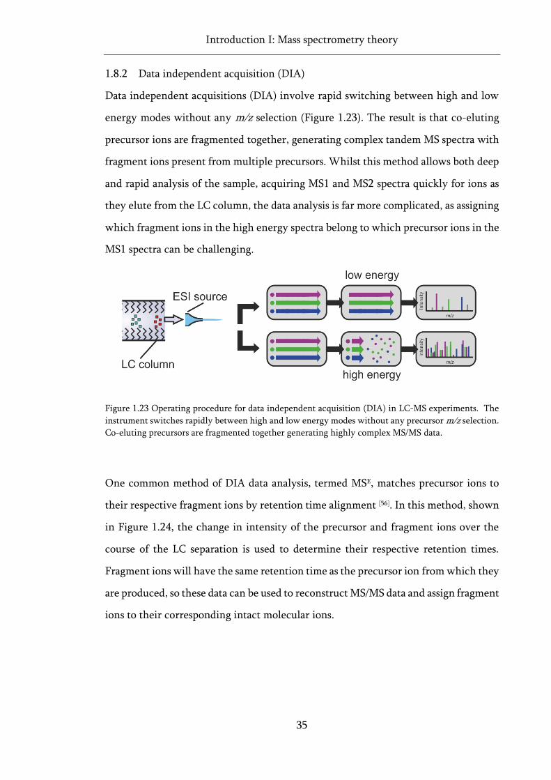
Introduction I: Mass spectrometry theory
35
1.8.2 Data independent acquisition (DIA)
Data independent acquisitions (DIA) involve rapid switching between high and low
energy modes without any m/z selection (Figure 1.23). The result is that co-eluting
precursor ions are fragmented together, generating complex tandem MS spectra with
fragment ions present from multiple precursors. Whilst this method allows both deep
and rapid analysis of the sample, acquiring MS1 and MS2 spectra quickly for ions as
they elute from the LC column, the data analysis is far more complicated, as assigning
which fragment ions in the high energy spectra belong to which precursor ions in the
MS1 spectra can be challenging.
Figure 1.23 Operating procedure for data independent acquisition (DIA) in LC-MS experiments. The
instrument switches rapidly between high and low energy modes without any precursor m/z selection.
Co-eluting precursors are fragmented together generating highly complex MS/MS data.
One common method of DIA data analysis, termed MSE, matches precursor ions to
their respective fragment ions by retention time alignment [56]. In this method, shown
in Figure 1.24, the change in intensity of the precursor and fragment ions over the
course of the LC separation is used to determine their respective retention times.
Fragment ions will have the same retention time as the precursor ion from which they
are produced, so these data can be used to reconstruct MS/MS data and assign fragment
ions to their corresponding intact molecular ions.
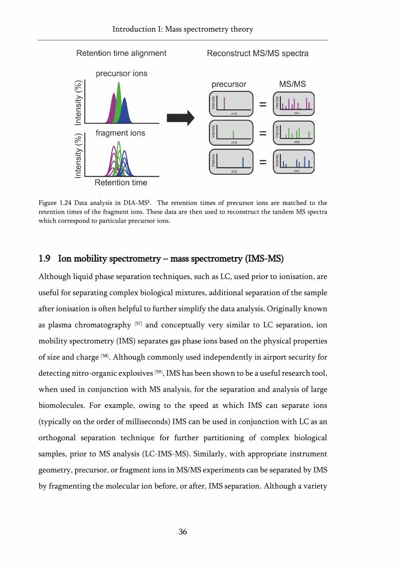
Introduction I: Mass spectrometry theory
36
Figure 1.24 Data analysis in DIA-MSE. The retention times of precursor ions are matched to the
retention times of the fragment ions. These data are then used to reconstruct the tandem MS spectra
which correspond to particular precursor ions.
1.9 Ion mobility spectrometry – mass spectrometry (IMS-MS)
Although liquid phase separation techniques, such as LC, used prior to ionisation, are
useful for separating complex biological mixtures, additional separation of the sample
after ionisation is often helpful to further simplify the data analysis. Originally known
as plasma chromatography [57] and conceptually very similar to LC separation, ion
mobility spectrometry (IMS) separates gas phase ions based on the physical properties
of size and charge [58]. Although commonly used independently in airport security for
detecting nitro-organic explosives [59], IMS has been shown to be a useful research tool,
when used in conjunction with MS analysis, for the separation and analysis of large
biomolecules. For example, owing to the speed at which IMS can separate ions
(typically on the order of milliseconds) IMS can be used in conjunction with LC as an
orthogonal separation technique for further partitioning of complex biological
samples, prior to MS analysis (LC-IMS-MS). Similarly, with appropriate instrument
geometry, precursor, or fragment ions in MS/MS experiments can be separated by IMS
by fragmenting the molecular ion before, or after, IMS separation. Although a variety
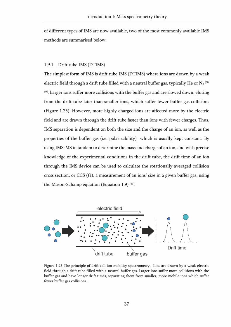
Introduction I: Mass spectrometry theory
37
of different types of IMS are now available, two of the most commonly available IMS
methods are summarised below.
1.9.1 Drift tube IMS (DTIMS)
The simplest form of IMS is drift tube IMS (DTIMS) where ions are drawn by a weak
electric field through a drift tube filled with a neutral buffer gas, typically He or N2 [58,
60]. Larger ions suffer more collisions with the buffer gas and are slowed down, eluting
from the drift tube later than smaller ions, which suffer fewer buffer gas collisions
(Figure 1.25). However, more highly charged ions are affected more by the electric
field and are drawn through the drift tube faster than ions with fewer charges. Thus,
IMS separation is dependent on both the size and the charge of an ion, as well as the
properties of the buffer gas (i.e. polarizability) which is usually kept constant. By
using IMS-MS in tandem to determine the mass and charge of an ion, and with precise
knowledge of the experimental conditions in the drift tube, the drift time of an ion
through the IMS device can be used to calculate the rotationally averaged collision
cross section, or CCS (Ω), a measurement of an ions’ size in a given buffer gas, using
the Mason-Schamp equation (Equation 1.9) [61].
Figure 1.25 The principle of drift cell ion mobility spectrometry. Ions are drawn by a weak electric
field through a drift tube filled with a neutral buffer gas. Larger ions suffer more collisions with the
buffer gas and have longer drift times, separating them from smaller, more mobile ions which suffer
fewer buffer gas collisions.
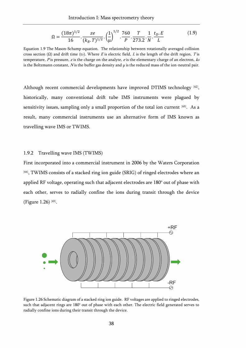
Introduction I: Mass spectrometry theory
38
Ω =
(18𝜋)1/2
16.
𝑧𝑒
(𝑘𝐵. 𝑇)1/2. (1
µ)1/2
.760
𝑃.𝑇
273.2.1
𝑁.𝑡𝐷 . 𝐸
𝐿
(1.9)
Equation 1.9 The Mason-Schamp equation. The relationship between rotationally averaged collision
cross section (Ω) and drift time (tD). Where E is electric field, L is the length of the drift region, T is
temperature, P is pressure, z is the charge on the analyte, e is the elementary charge of an electron, kB
is the Boltzmann constant, N is the buffer gas density and µ is the reduced mass of the ion-neutral pair.
Although recent commercial developments have improved DTIMS technology [62],
historically, many conventional drift tube IMS instruments were plagued by
sensitivity issues, sampling only a small proportion of the total ion current [63]. As a
result, many commercial instruments use an alternative form of IMS known as
travelling wave IMS or TWIMS.
1.9.2 Travelling wave IMS (TWIMS)
First incorporated into a commercial instrument in 2006 by the Waters Corporation
[64], TWIMS consists of a stacked ring ion guide (SRIG) of ringed electrodes where an
applied RF voltage, operating such that adjacent electrodes are 180° out of phase with
each other, serves to radially confine the ions during transit through the device
(Figure 1.26) [65].
Figure 1.26 Schematic diagram of a stacked ring ion guide. RF voltages are applied to ringed electrodes,
such that adjacent rings are 180° out of phase with each other. The electric field generated serves to
radially confine ions during their transit through the device.
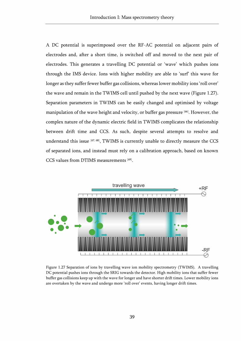
Introduction I: Mass spectrometry theory
39
A DC potential is superimposed over the RF-AC potential on adjacent pairs of
electrodes and, after a short time, is switched off and moved to the next pair of
electrodes. This generates a travelling DC potential or ‘wave’ which pushes ions
through the IMS device. Ions with higher mobility are able to ‘surf’ this wave for
longer as they suffer fewer buffer gas collisions, whereas lower mobility ions ‘roll over’
the wave and remain in the TWIMS cell until pushed by the next wave (Figure 1.27).
Separation parameters in TWIMS can be easily changed and optimised by voltage
manipulation of the wave height and velocity, or buffer gas pressure [66]. However, the
complex nature of the dynamic electric field in TWIMS complicates the relationship
between drift time and CCS. As such, despite several attempts to resolve and
understand this issue [67, 68], TWIMS is currently unable to directly measure the CCS
of separated ions, and instead must rely on a calibration approach, based on known
CCS values from DTIMS measurements [69].
Figure 1.27 Separation of ions by travelling wave ion mobility spectrometry (TWIMS). A travelling
DC potential pushes ions through the SRIG towards the detector. High mobility ions that suffer fewer
buffer gas collisions keep up with the wave for longer and have shorter drift times. Lower mobility ions
are overtaken by the wave and undergo more ‘roll over’ events, having longer drift times.
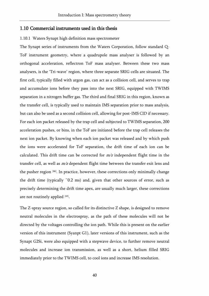
Introduction I: Mass spectrometry theory
40
1.10 Commercial instruments used in this thesis
1.10.1 Waters Synapt high definition mass spectrometer
The Synapt series of instruments from the Waters Corporation, follow standard Q-
ToF instrument geometry, where a quadrupole mass analyser is followed by an
orthogonal acceleration, reflectron ToF mass analyser. Between these two mass
analysers, is the ‘Tri-wave’ region, where three separate SRIG cells are situated. The
first cell, typically filled with argon gas, can act as a collision cell, and serves to trap
and accumulate ions before they pass into the next SRIG, equipped with TWIMS
separation in a nitrogen buffer gas. The third and final SRIG in this region, known as
the transfer cell, is typically used to maintain IMS separation prior to mass analysis,
but can also be used as a second collision cell, allowing for post-IMS CID if necessary.
For each ion packet released by the trap cell and subjected to TWIMS separation, 200
acceleration pushes, or bins, in the ToF are initiated before the trap cell releases the
next ion packet. By knowing when each ion packet was released and by which push
the ions were accelerated for ToF separation, the drift time of each ion can be
calculated. This drift time can be corrected for m/z independent flight time in the
transfer cell, as well as m/z dependent flight time between the transfer exit lens and
the pusher region [66]. In practice, however, these corrections only minimally change
the drift time (typically ~0.2 ms) and, given that other sources of error, such as
precisely determining the drift time apex, are usually much larger, these corrections
are not routinely applied [63].
The Z-spray source region, so called for its distinctive Z shape, is designed to remove
neutral molecules in the electrospray, as the path of these molecules will not be
directed by the voltages controlling the ion path. While this is present on the earlier
version of this instrument (Syanpt G1), later versions of this instrument, such as the
Synapt G2Si, were also equipped with a stepwave device, to further remove neutral
molecules and increase ion transmission, as well as a short, helium filled SRIG
immediately prior to the TWIMS cell, to cool ions and increase IMS resolution.
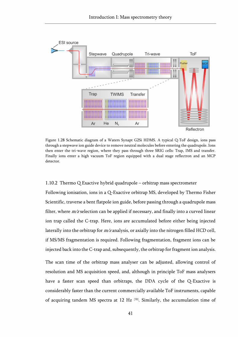
Introduction I: Mass spectrometry theory
41
Figure 1.28 Schematic diagram of a Waters Synapt G2Si HDMS. A typical Q-ToF design, ions pass
through a stepwave ion guide device to remove neutral molecules before entering the quadrupole. Ions
then enter the tri-wave region, where they pass through three SRIG cells: Trap, IMS and transfer.
Finally ions enter a high vacuum ToF region equipped with a dual stage reflectron and an MCP
detector.
1.10.2 Thermo Q Exactive hybrid quadrupole – orbitrap mass spectrometer
Following ionisation, ions in a Q-Exactive orbitrap MS, developed by Thermo Fisher
Scientific, traverse a bent flatpole ion guide, before passing through a quadrupole mass
filter, where m/z selection can be applied if necessary, and finally into a curved linear
ion trap called the C-trap. Here, ions are accumulated before either being injected
laterally into the orbitrap for m/z analysis, or axially into the nitrogen filled HCD cell,
if MS/MS fragmentation is required. Following fragmentation, fragment ions can be
injected back into the C-trap and, subsequently, the orbitrap for fragment ion analysis.
The scan time of the orbitrap mass analyser can be adjusted, allowing control of
resolution and MS acquisition speed, and, although in principle ToF mass analysers
have a faster scan speed than orbitraps, the DDA cycle of the Q-Exactive is
considerably faster than the current commercially available ToF instruments, capable
of acquiring tandem MS spectra at 12 Hz [70]. Similarly, the accumulation time of
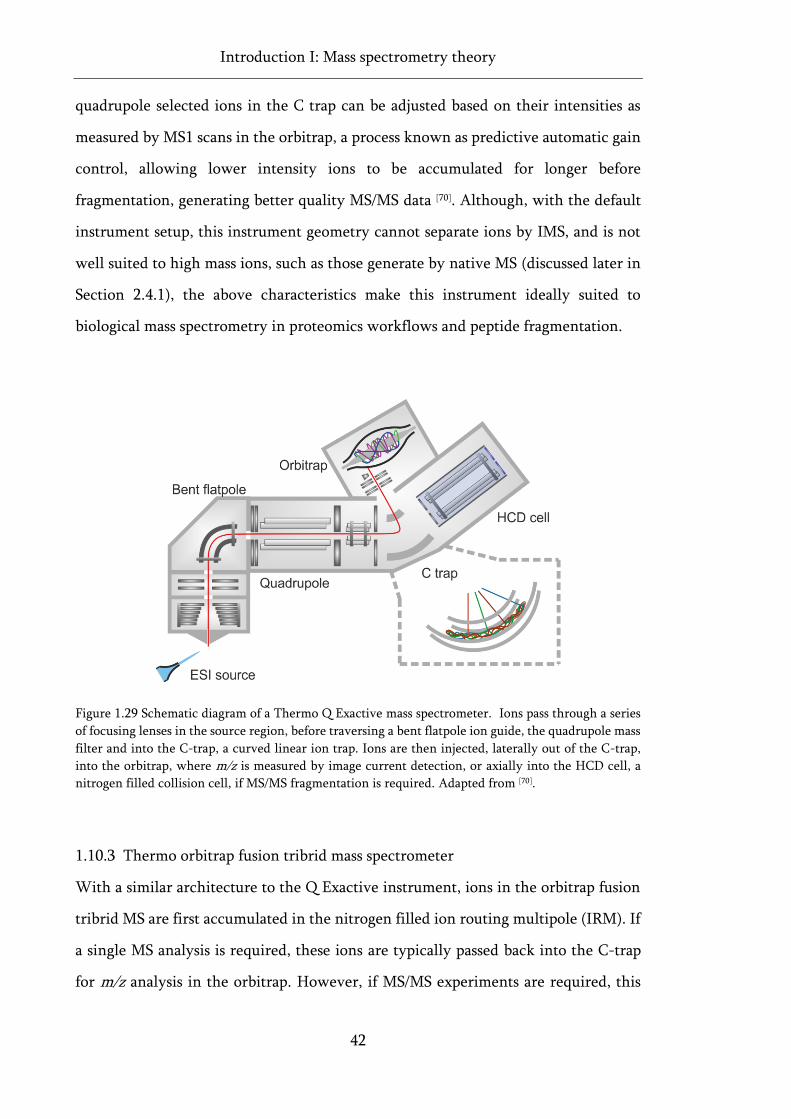
Introduction I: Mass spectrometry theory
42
quadrupole selected ions in the C trap can be adjusted based on their intensities as
measured by MS1 scans in the orbitrap, a process known as predictive automatic gain
control, allowing lower intensity ions to be accumulated for longer before
fragmentation, generating better quality MS/MS data [70]. Although, with the default
instrument setup, this instrument geometry cannot separate ions by IMS, and is not
well suited to high mass ions, such as those generate by native MS (discussed later in
Section 2.4.1), the above characteristics make this instrument ideally suited to
biological mass spectrometry in proteomics workflows and peptide fragmentation.
Figure 1.29 Schematic diagram of a Thermo Q Exactive mass spectrometer. Ions pass through a series
of focusing lenses in the source region, before traversing a bent flatpole ion guide, the quadrupole mass
filter and into the C-trap, a curved linear ion trap. Ions are then injected, laterally out of the C-trap,
into the orbitrap, where m/z is measured by image current detection, or axially into the HCD cell, a
nitrogen filled collision cell, if MS/MS fragmentation is required. Adapted from [70].
1.10.3 Thermo orbitrap fusion tribrid mass spectrometer
With a similar architecture to the Q Exactive instrument, ions in the orbitrap fusion
tribrid MS are first accumulated in the nitrogen filled ion routing multipole (IRM). If
a single MS analysis is required, these ions are typically passed back into the C-trap
for m/z analysis in the orbitrap. However, if MS/MS experiments are required, this
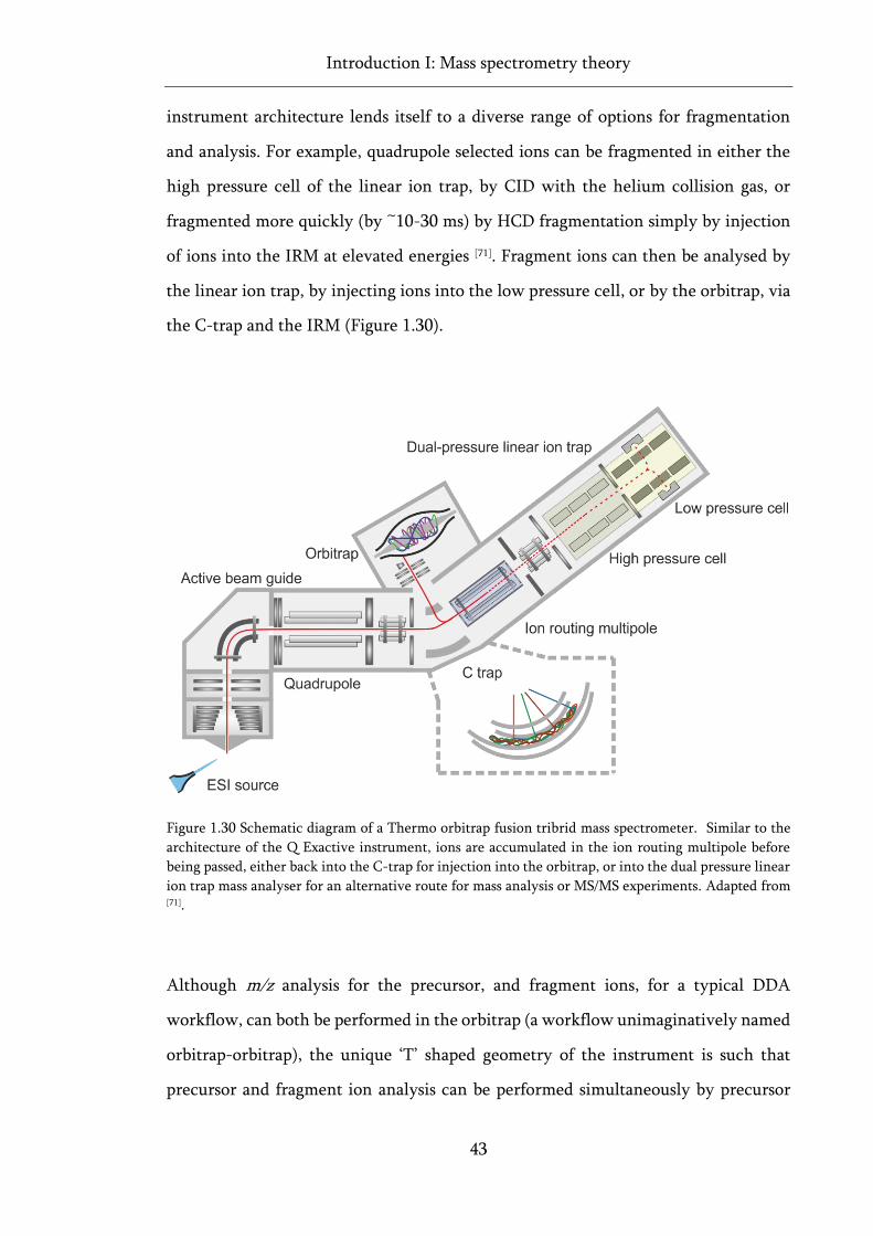
Introduction I: Mass spectrometry theory
43
instrument architecture lends itself to a diverse range of options for fragmentation
and analysis. For example, quadrupole selected ions can be fragmented in either the
high pressure cell of the linear ion trap, by CID with the helium collision gas, or
fragmented more quickly (by ~10-30 ms) by HCD fragmentation simply by injection
of ions into the IRM at elevated energies [71]. Fragment ions can then be analysed by
the linear ion trap, by injecting ions into the low pressure cell, or by the orbitrap, via
the C-trap and the IRM (Figure 1.30).
Figure 1.30 Schematic diagram of a Thermo orbitrap fusion tribrid mass spectrometer. Similar to the
architecture of the Q Exactive instrument, ions are accumulated in the ion routing multipole before
being passed, either back into the C-trap for injection into the orbitrap, or into the dual pressure linear
ion trap mass analyser for an alternative route for mass analysis or MS/MS experiments. Adapted from [71].
Although m/z analysis for the precursor, and fragment ions, for a typical DDA
workflow, can both be performed in the orbitrap (a workflow unimaginatively named
orbitrap-orbitrap), the unique ‘T’ shaped geometry of the instrument is such that
precursor and fragment ion analysis can be performed simultaneously by precursor

Introduction I: Mass spectrometry theory
44
analysis in the orbitrap, and fragment ion analysis in the linear ion trap (orbitrap-
iontrap workflow). This parallelisation streamlines MS/MS acquisition, taking
advantage of both the high resolution of the orbitrap and fast scan speeds of the linear
ion trap, drastically increasing the DDA cycle speed, and allowing the orbitrap fusion
instrument to achieve MS/MS fragmentation frequencies of up to 22 Hz [71].
45
Chapter 2:
Introduction II: Protein
aggregation, structure and
dynamics studied by mass
spectrometry
Introduction II: Protein aggregation, structure and dynamics studied by MS
46
2 Introduction II: Protein aggregation, structure and
dynamics studied by mass spectrometry
“…the most remarkable thing about proteins is that they can do almost anything.”
-Francis Crick, Co-discoverer of the Structure of DNA, 1958 [72].
Essential for nearly all biochemical processes, proteins can be thought of as the
molecular machines that maintain life, where almost everything inside a cell is itself,
or is synthesised by, a protein. Some of the more well-known roles proteins adopt are
enzymes, biological catalysts for a cells’ metabolism, and antibodies, a vital component
of the adaptive immune system. However, proteins have an almost uncountable
number of other functions. Opsin proteins in the retina mediate the conversion of
photons into electrochemical signals to enable sight [73]. Motor proteins like kinesins
‘walk’ through cells moving cellular cargo from one place to another [74]. Even the air
we breathe is transported around our bodies using the oxygen binding protein
haemoglobin.
The remarkable ability of these molecules to function in such a wide variety of roles,
for most proteins, relies on adopting a specific three-dimensional shape, or
conformation. These 3D shapes are formed by the folding of one or more polypeptide
chains - long strings of peptide bond linked amino acids - the main structural
components of proteins (Figure 2.1). In 1961, after demonstrating for the first time
that protein folding could be reversible, work for which he would later be awarded
the Nobel Prize in chemistry, C.B Anfinsen famously concluded that the specific
sequence of amino acids in a polypeptide chain, contains all the information necessary
for the protein to adopt its native fold [75]. Although varying significantly in length
from just ~50 or so amino acids, up to several thousand for larger proteins,
polypeptides are composed of only twenty different types of amino acids, sometimes
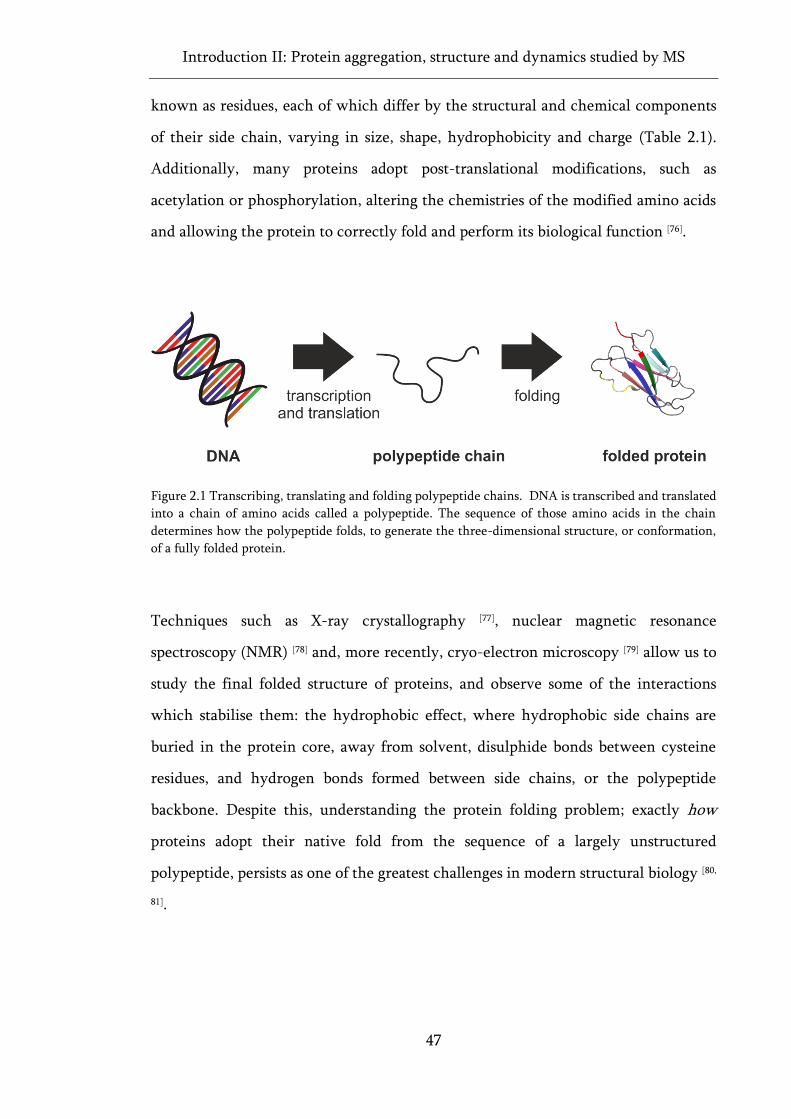
Introduction II: Protein aggregation, structure and dynamics studied by MS
47
known as residues, each of which differ by the structural and chemical components
of their side chain, varying in size, shape, hydrophobicity and charge (Table 2.1).
Additionally, many proteins adopt post-translational modifications, such as
acetylation or phosphorylation, altering the chemistries of the modified amino acids
and allowing the protein to correctly fold and perform its biological function [76].
Figure 2.1 Transcribing, translating and folding polypeptide chains. DNA is transcribed and translated
into a chain of amino acids called a polypeptide. The sequence of those amino acids in the chain
determines how the polypeptide folds, to generate the three-dimensional structure, or conformation,
of a fully folded protein.
Techniques such as X-ray crystallography [77], nuclear magnetic resonance
spectroscopy (NMR) [78] and, more recently, cryo-electron microscopy [79] allow us to
study the final folded structure of proteins, and observe some of the interactions
which stabilise them: the hydrophobic effect, where hydrophobic side chains are
buried in the protein core, away from solvent, disulphide bonds between cysteine
residues, and hydrogen bonds formed between side chains, or the polypeptide
backbone. Despite this, understanding the protein folding problem; exactly how
proteins adopt their native fold from the sequence of a largely unstructured
polypeptide, persists as one of the greatest challenges in modern structural biology [80,
81].
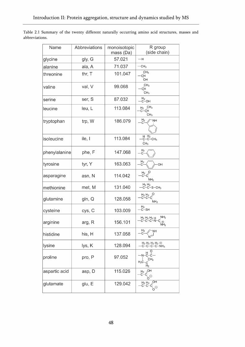
Introduction II: Protein aggregation, structure and dynamics studied by MS
48
Table 2.1 Summary of the twenty different naturally occurring amino acid structures, masses and
abbreviations.
Introduction II: Protein aggregation, structure and dynamics studied by MS
49
2.1 Protein folding, misfolding and aggregation
In 1968, Cyrus Levinthal famously summarised the protein folding problem by
demonstrating that even a relatively small polypeptide of 100 or so residues has such
a large number of possible conformations physically available to it, that an exhaustive
search of all of them, even when sampling at 10 trillion conformations per second,
would take longer than the current lifetime of the universe to complete [82]. Knowing
that proteins can find and adopt their native fold in as little as a few microseconds [80],
this problem, now known as Levinthal’s paradox, effectively illustrated that the native
state of a polypeptide could not possibly be found simply by searching conformations
at random [83].
2.1.1 Protein folding
In the face of Levinthal’s paradox, many models have been proposed to explain how
polypeptides fold into proteins on a biological timescale. The framework model
proposed that smaller secondary structural elements, such as α-helices, folded first
before these pre-formed structural elements dock together to create the overall native
fold [84-87]. Conversely, the hydrophobic collapse model proposed that the need for
hydrophobic side chains in the polypeptide to be free from solvent interaction, leads
to a collapsed molten globule state with hydrophobic side chains at its core. This
collapsed globule was proposed to aid protein folding by compacting the polypeptide
into a confined volume, narrowing the conformational search necessary to find the
native state [88, 89]. The nucleation-condensation model combines these two processes,
suggesting that protein folding occurs by the formation of a small nucleus, that may
involve weak secondary structure, followed by collapse of the polypeptide around it
[90].
Today, protein folding is thought of in the context of energy landscapes or ‘folding
funnels’ [81], where the internal free energy of the polypeptide (y axis) is plotted against
entropy (x axis), a measure of the conformational freedom of the molecule (Figure
Introduction II: Protein aggregation, structure and dynamics studied by MS
50
2.2). Native-like interactions formed by folding polypeptides, perhaps driven by
hydrophobic interactions or partially folded secondary structure, are, on average,
more stable than non-native interactions. These favourable contacts are therefore
more persistent, forming partially folded intermediate structures with lower internal
energy and restricted conformational freedom (i.e. reduced entropy). This further
directs the polypeptide towards ever more stable, lower energy species, eventually
adopting the fully folded native state, usually considered to be the lowest energy, most
thermodynamically stable structure that is kinetically accessible under physiological
conditions [91].
A thought experiment proposed by Dawkins [92] and discussed elsewhere [82] is useful
for understanding this concept. Consider the, now infamous, infinite monkey
theorem: a monkey randomly hitting keys on a typewriter will, given an infinite
amount of time, produce the complete works of Shakespeare. To make it easier for the
monkey, we reduce the number of typewriter keys to just 27, the 26 letters and a space
key, and instead of having to produce the complete works of Shakespeare, the monkey
only has to correctly type a single phrase from Hamlet: ‘Methinks it is like a weasel’.
Randomly typing letters, it would take approximately 1040 key strokes for the monkey
to correctly type out this statement [82]. However, if, with each attempt, the monkey
cannot change those letters already in the correct positions, analogous to the
polypeptide finding a stable native-like interaction, he need only attempt the
statement a few thousand times before correctly reproducing Hamlet’s comment.
This analogy simplifies the problem somewhat. In actuality, protein conformations
are in constant dynamic equilibrium, where changing environmental or solution
conditions (temperature, pH etc…) shifts the equilibrium to populate more unfolded
or native forms of the molecule. Depending on their relative stabilities, partially
folded states can often revert to more unfolded conformations rather than move
towards the native state, analogous to the monkey merely finding it difficult to change
correctly placed letters rather than impossible. Similarly, there is some debate as to
whether folding intermediates are useful, on-pathway structures towards the native
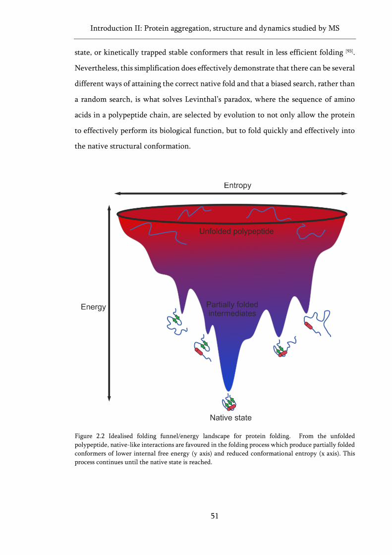
Introduction II: Protein aggregation, structure and dynamics studied by MS
51
state, or kinetically trapped stable conformers that result in less efficient folding [93].
Nevertheless, this simplification does effectively demonstrate that there can be several
different ways of attaining the correct native fold and that a biased search, rather than
a random search, is what solves Levinthal’s paradox, where the sequence of amino
acids in a polypeptide chain, are selected by evolution to not only allow the protein
to effectively perform its biological function, but to fold quickly and effectively into
the native structural conformation.
Figure 2.2 Idealised folding funnel/energy landscape for protein folding. From the unfolded
polypeptide, native-like interactions are favoured in the folding process which produce partially folded
conformers of lower internal free energy (y axis) and reduced conformational entropy (x axis). This
process continues until the native state is reached.
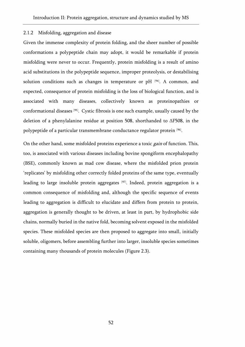
Introduction II: Protein aggregation, structure and dynamics studied by MS
52
2.1.2 Misfolding, aggregation and disease
Given the immense complexity of protein folding, and the sheer number of possible
conformations a polypeptide chain may adopt, it would be remarkable if protein
misfolding were never to occur. Frequently, protein misfolding is a result of amino
acid substitutions in the polypeptide sequence, improper proteolysis, or destabilising
solution conditions such as changes in temperature or pH [94]. A common, and
expected, consequence of protein misfolding is the loss of biological function, and is
associated with many diseases, collectively known as proteinopathies or
conformational diseases [95]. Cystic fibrosis is one such example, usually caused by the
deletion of a phenylalanine residue at position 508, shorthanded to ΔF508, in the
polypeptide of a particular transmembrane conductance regulator protein [96].
On the other hand, some misfolded proteins experience a toxic gain of function. This,
too, is associated with various diseases including bovine spongiform encephalopathy
(BSE), commonly known as mad cow disease, where the misfolded prion protein
‘replicates’ by misfolding other correctly folded proteins of the same type, eventually
leading to large insoluble protein aggregates [97]. Indeed, protein aggregation is a
common consequence of misfolding and, although the specific sequence of events
leading to aggregation is difficult to elucidate and differs from protein to protein,
aggregation is generally thought to be driven, at least in part, by hydrophobic side
chains, normally buried in the native fold, becoming solvent exposed in the misfolded
species. These misfolded species are then proposed to aggregate into small, initially
soluble, oligomers, before assembling further into larger, insoluble species sometimes
containing many thousands of protein molecules (Figure 2.3).
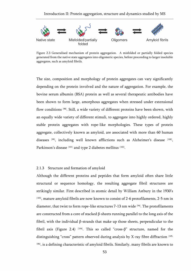
Introduction II: Protein aggregation, structure and dynamics studied by MS
53
Figure 2.3 Generalised mechanism of protein aggregation. A misfolded or partially folded species
generated from the native state aggregates into oligomeric species, before proceeding to larger insoluble
aggregates, such as amyloid fibrils.
The size, composition and morphology of protein aggregates can vary significantly
depending on the protein involved and the nature of aggregation. For example, the
bovine serum albumin (BSA) protein as well as several therapeutic antibodies have
been shown to form large, amorphous aggregates when stressed under extensional
flow conditions [98]. Still, a wide variety of different proteins have been shown, with
an equally wide variety of different stimuli, to aggregate into highly ordered, highly
stable protein aggregates with rope-like morphologies. These types of protein
aggregate, collectively known as amyloid, are associated with more than 60 human
diseases [99], including well known afflictions such as Alzheimer’s disease [100],
Parkinson’s disease [101] and type 2 diabetes mellitus [102].
2.1.3 Structure and formation of amyloid
Although the different proteins and peptides that form amyloid often share little
structural or sequence homology, the resulting aggregate fibril structures are
strikingly similar. First described in atomic detail by William Astbury in the 1930’s
[103], mature amyloid fibrils are now known to consist of 2-6 protofilaments, 2-5 nm in
diameter, that twist to form rope-like structures 7-13 nm wide [94]. The protofilaments
are constructed from a core of stacked β-sheets running parallel to the long axis of the
fibril, with the individual β-strands that make up those sheets, perpendicular to the
fibril axis (Figure 2.4) [104]. This so called “cross-β” structure, named for the
distinguishing “cross” pattern observed during analysis by X-ray fibre diffraction [105,
106], is a defining characteristic of amyloid fibrils. Similarly, many fibrils are known to
Introduction II: Protein aggregation, structure and dynamics studied by MS
54
share common non-amyloid components as part of the overall in vivo structure. Long
unbranched polysaccharides known as glycosaminoglycans (GAGs), various metal
ions and Serum Amyloid P (SAP), a pentameric protein (each subunit ~ 25 kDa)
observed to make up approximately 14% of amyloid deposits by dry mass, are all
known to associate with amyloid deposits in vivo [94].
Figure 2.4 Structure of an amyloid fibril. Twisted protofilaments forming the overall amyloid fibril
consist of stacked β-sheets stabilised by extensive hydrogen bonding between strands, and steric zipper
interactions. PDB: 5OQV [107].
Generally, amyloid fibrils and protofilaments are extraordinarily stable structures,
held together by extensive hydrogen bonding between β-strands, and interdigitated
amino acid side chains in the fibril core that form solvent free ‘steric zipper’ interfaces
[108]. Indeed, it has been suggested that the amyloid fibril state can be more
thermodynamically stable than the native state under certain conditions (Figure 2.5)
[109], where drastic changes in pH, or dissolution in strong organic solvents is often
required to disaggregate fibril structures [110, 111].
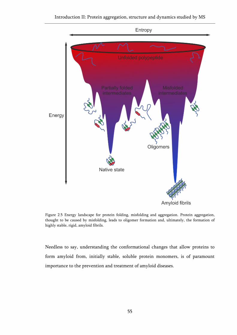
Introduction II: Protein aggregation, structure and dynamics studied by MS
55
Figure 2.5 Energy landscape for protein folding, misfolding and aggregation. Protein aggregation,
thought to be caused by misfolding, leads to oligomer formation and, ultimately, the formation of
highly stable, rigid, amyloid fibrils.
Needless to say, understanding the conformational changes that allow proteins to
form amyloid from, initially stable, soluble protein monomers, is of paramount
importance to the prevention and treatment of amyloid diseases.
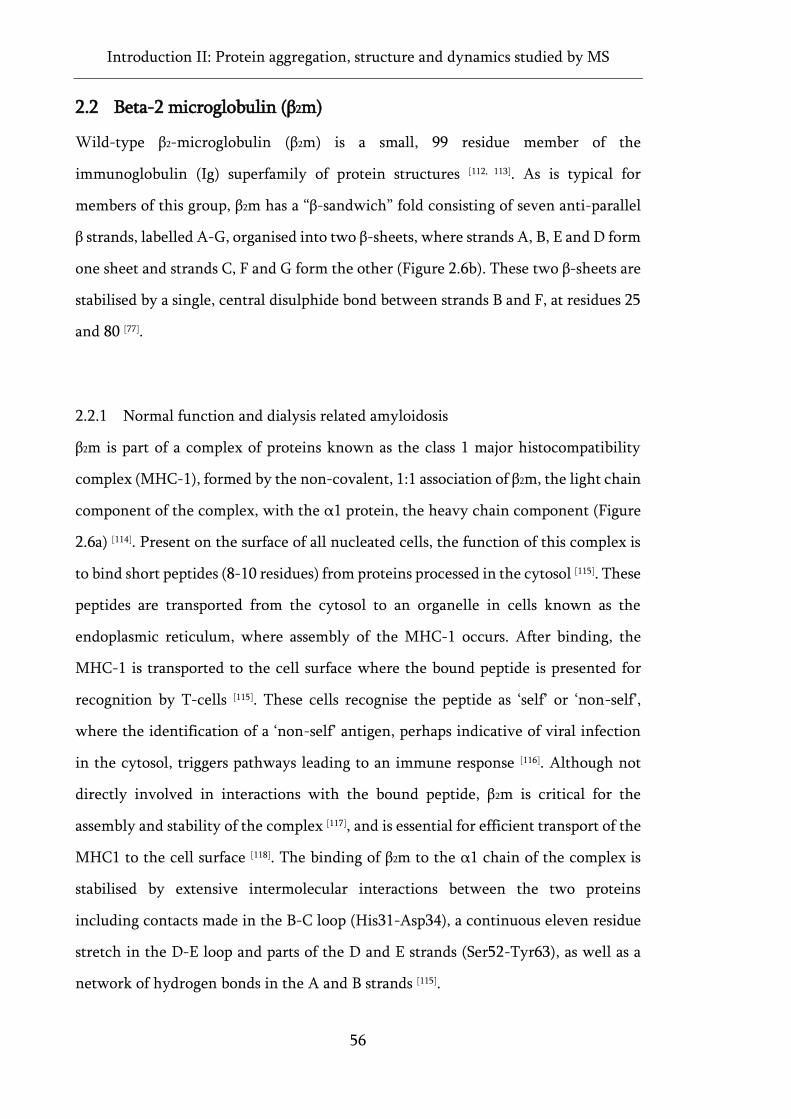
Introduction II: Protein aggregation, structure and dynamics studied by MS
56
2.2 Beta-2 microglobulin (β2m)
Wild-type β2-microglobulin (β2m) is a small, 99 residue member of the
immunoglobulin (Ig) superfamily of protein structures [112, 113]. As is typical for
members of this group, β2m has a “β-sandwich” fold consisting of seven anti-parallel
β strands, labelled A-G, organised into two β-sheets, where strands A, B, E and D form
one sheet and strands C, F and G form the other (Figure 2.6b). These two β-sheets are
stabilised by a single, central disulphide bond between strands B and F, at residues 25
and 80 [77].
2.2.1 Normal function and dialysis related amyloidosis
β2m is part of a complex of proteins known as the class 1 major histocompatibility
complex (MHC-1), formed by the non-covalent, 1:1 association of β2m, the light chain
component of the complex, with the α1 protein, the heavy chain component (Figure
2.6a) [114]. Present on the surface of all nucleated cells, the function of this complex is
to bind short peptides (8-10 residues) from proteins processed in the cytosol [115]. These
peptides are transported from the cytosol to an organelle in cells known as the
endoplasmic reticulum, where assembly of the MHC-1 occurs. After binding, the
MHC-1 is transported to the cell surface where the bound peptide is presented for
recognition by T-cells [115]. These cells recognise the peptide as ‘self’ or ‘non-self’,
where the identification of a ‘non-self’ antigen, perhaps indicative of viral infection
in the cytosol, triggers pathways leading to an immune response [116]. Although not
directly involved in interactions with the bound peptide, β2m is critical for the
assembly and stability of the complex [117], and is essential for efficient transport of the
MHC1 to the cell surface [118]. The binding of β2m to the α1 chain of the complex is
stabilised by extensive intermolecular interactions between the two proteins
including contacts made in the B-C loop (His31-Asp34), a continuous eleven residue
stretch in the D-E loop and parts of the D and E strands (Ser52-Tyr63), as well as a
network of hydrogen bonds in the A and B strands [115].
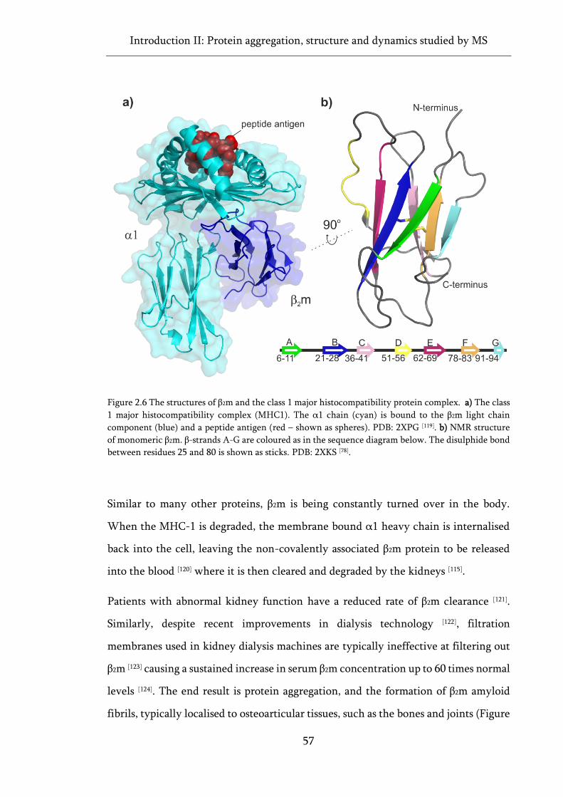
Introduction II: Protein aggregation, structure and dynamics studied by MS
57
Figure 2.6 The structures of β2m and the class 1 major histocompatibility protein complex. a) The class
1 major histocompatibility complex (MHC1). The α1 chain (cyan) is bound to the β2m light chain
component (blue) and a peptide antigen (red – shown as spheres). PDB: 2XPG [119]. b) NMR structure
of monomeric β2m. β-strands A-G are coloured as in the sequence diagram below. The disulphide bond
between residues 25 and 80 is shown as sticks. PDB: 2XKS [78].
Similar to many other proteins, β2m is being constantly turned over in the body.
When the MHC-1 is degraded, the membrane bound α1 heavy chain is internalised
back into the cell, leaving the non-covalently associated β2m protein to be released
into the blood [120] where it is then cleared and degraded by the kidneys [115].
Patients with abnormal kidney function have a reduced rate of β2m clearance [121].
Similarly, despite recent improvements in dialysis technology [122], filtration
membranes used in kidney dialysis machines are typically ineffective at filtering out
β2m [123] causing a sustained increase in serum β2m concentration up to 60 times normal
levels [124]. The end result is protein aggregation, and the formation of β2m amyloid
fibrils, typically localised to osteoarticular tissues, such as the bones and joints (Figure
Introduction II: Protein aggregation, structure and dynamics studied by MS
58
2.7) [123, 124]. Whilst β2m fibril formation has been documented in long surviving non-
dialysed kidney disease patients [121], build-up of amyloid deposits typically takes years,
and is usually beyond the life expectancy of most non-dialysed patients. As such,
amyloid deposits of this kind are more commonly found in patients undergoing long-
term hemodialysis, with an estimated incidence of >95% after 15 years of treatment
[123]. Even with kidney transplantation, this condition, known as dialysis related
amyloidosis (DRA), is difficult to reverse, eventually leading to pathological
destruction of the bones and joints with symptoms including bone cysts, restricted
movement, joint pain and carpal tunnel syndrome [115].
Figure 2.7 β2m amyloid deposits in dialysis related amyloidosis (DRA). Indium labelled β2m amyloid
fibrils are localised to the bones and joints of DRA patients. Zoomed images are shown of the arms (a),
chest (b) and knees (c). Taken, with permission, from [125].
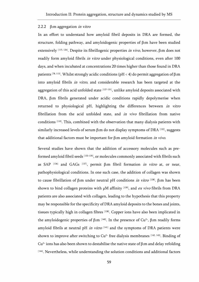
Introduction II: Protein aggregation, structure and dynamics studied by MS
59
2.2.2 β2m aggregation in vitro
In an effort to understand how amyloid fibril deposits in DRA are formed, the
structure, folding pathway, and amyloidogenic properties of β2m have been studied
extensively [115, 126]. Despite its fibrillogenic properties in vivo, however, β2m does not
readily form amyloid fibrils in vitro under physiological conditions, even after 100
days, and when incubated at concentrations 20 times higher than those found in DRA
patients [78, 113]. Whilst strongly acidic conditions (pH < 4) do permit aggregation of β2m
into amyloid fibrils in vitro, and considerable research has been targeted at the
aggregation of this acid unfolded state [127-131], unlike amyloid deposits associated with
DRA, β2m fibrils generated under acidic conditions rapidly depolymerise when
returned to physiological pH, highlighting the differences between in vitro
fibrillation from the acid unfolded state, and in vivo fibrillation from native
conditions [110]. This, combined with the observation that many dialysis patients with
similarly increased levels of serum β2m do not display symptoms of DRA [132], suggests
that additional factors must be important for β2m amyloid formation in vivo.
Several studies have shown that the addition of accessory molecules such as pre-
formed amyloid fibril seeds [133-135], or molecules commonly associated with fibrils such
as SAP [136] and GAGs [137], permit β2m fibril formation in vitro at, or near,
pathophysiological conditions. In one such case, the addition of collagen was shown
to cause fibrillation of β2m under neutral pH conditions in vitro [138]. β2m has been
shown to bind collagen proteins with µM affinity [139], and ex vivo fibrils from DRA
patients are also associated with collagen, leading to the hypothesis that this property
may be responsible for the specificity of DRA amyloid deposits to the bones and joints,
tissues typically high in collagen fibres [138]. Copper ions have also been implicated in
the amyloidogenic properties of β2m [140]. In the presence of Cu2+, β2m readily forms
amyloid fibrils at neutral pH in vitro [141] and the symptoms of DRA patients were
shown to improve after switching to Cu2+ free dialysis membranes [142, 143]. Binding of
Cu2+ ions has also been shown to destabilise the native state of β2m and delay refolding
[144]. Nevertheless, while understanding the solution conditions and additional factors
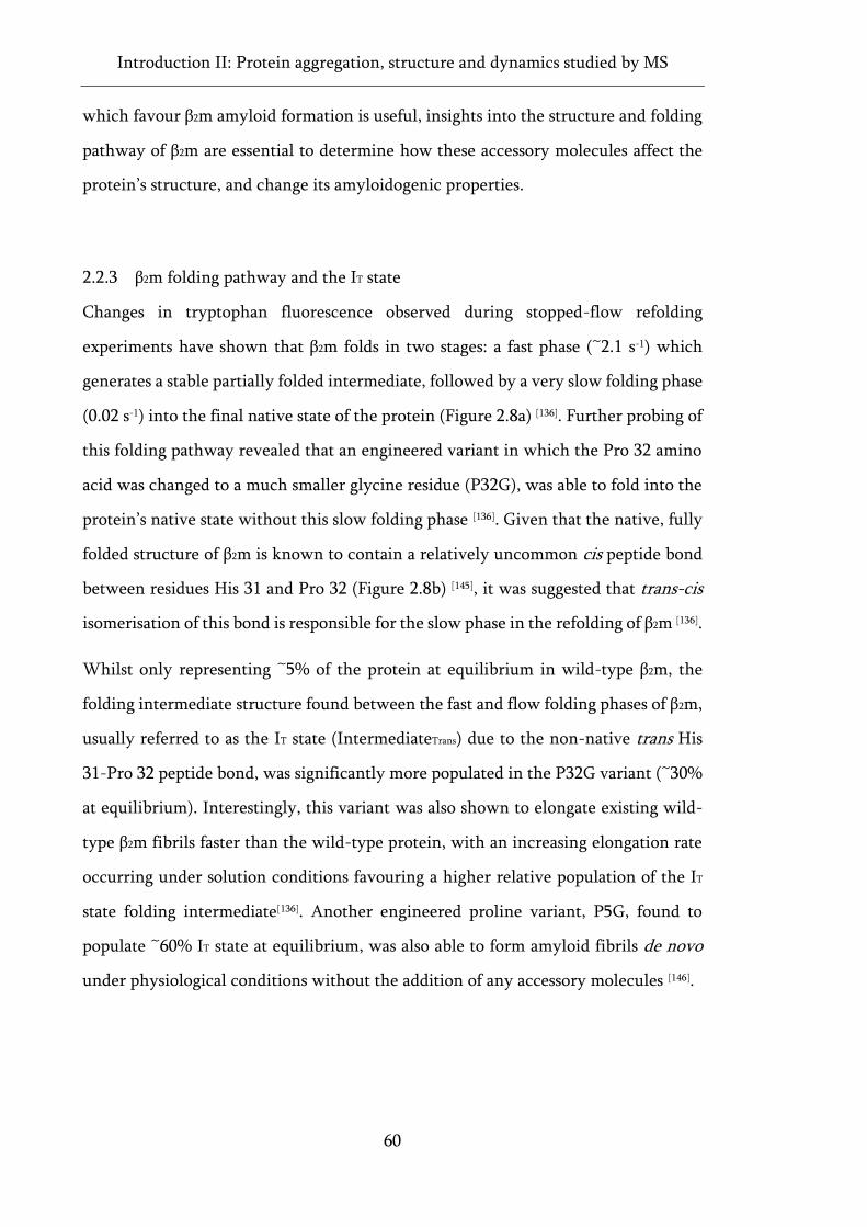
Introduction II: Protein aggregation, structure and dynamics studied by MS
60
which favour β2m amyloid formation is useful, insights into the structure and folding
pathway of β2m are essential to determine how these accessory molecules affect the
protein’s structure, and change its amyloidogenic properties.
2.2.3 β2m folding pathway and the IT state
Changes in tryptophan fluorescence observed during stopped-flow refolding
experiments have shown that β2m folds in two stages: a fast phase (~2.1 s-1) which
generates a stable partially folded intermediate, followed by a very slow folding phase
(0.02 s-1) into the final native state of the protein (Figure 2.8a) [136]. Further probing of
this folding pathway revealed that an engineered variant in which the Pro 32 amino
acid was changed to a much smaller glycine residue (P32G), was able to fold into the
protein’s native state without this slow folding phase [136]. Given that the native, fully
folded structure of β2m is known to contain a relatively uncommon cis peptide bond
between residues His 31 and Pro 32 (Figure 2.8b) [145], it was suggested that trans-cis
isomerisation of this bond is responsible for the slow phase in the refolding of β2m [136].
Whilst only representing ~5% of the protein at equilibrium in wild-type β2m, the
folding intermediate structure found between the fast and flow folding phases of β2m,
usually referred to as the IT state (IntermediateTrans) due to the non-native trans His
31-Pro 32 peptide bond, was significantly more populated in the P32G variant (~30%
at equilibrium). Interestingly, this variant was also shown to elongate existing wild-
type β2m fibrils faster than the wild-type protein, with an increasing elongation rate
occurring under solution conditions favouring a higher relative population of the IT
state folding intermediate[136]. Another engineered proline variant, P5G, found to
populate ~60% IT state at equilibrium, was also able to form amyloid fibrils de novo
under physiological conditions without the addition of any accessory molecules [146].
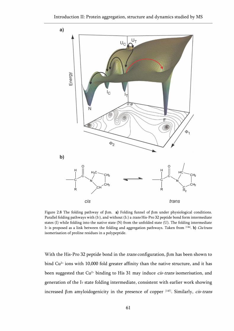
Introduction II: Protein aggregation, structure and dynamics studied by MS
61
Figure 2.8 The folding pathway of β2m. a) Folding funnel of β2m under physiological conditions.
Parallel folding pathways with (IT), and without (IC) a trans His-Pro 32 peptide bond form intermediate
states (I) while folding into the native state (N) from the unfolded state (U). The folding intermediate
IT is proposed as a link between the folding and aggregation pathways. Taken from [136]. b) Cis/trans isomerisation of proline residues in a polypeptide.
With the His-Pro 32 peptide bond in the trans configuration, β2m has been shown to
bind Cu2+ ions with 10,000 fold greater affinity than the native structure, and it has
been suggested that Cu2+ binding to His 31 may induce cis-trans isomerisation, and
generation of the IT state folding intermediate, consistent with earlier work showing
increased β2m amyloidogenicity in the presence of copper [147]. Similarly, cis-trans
Introduction II: Protein aggregation, structure and dynamics studied by MS
62
isomerisation of proline residues has been linked to aggregation in several other Ig
domains [148-150]. As a result, the IT state folding intermediate of β2m has been
highlighted as a leading candidate for the amyloidogenic precursor of β2m fibril
formation.
2.2.4 ΔN6 β2-microglobulin
Considered to be a structural mimic of the IT state, ΔN6 is a proteolytically cleaved
truncation variant of β2m lacking the six N-terminal amino acids. This variant readily
forms amyloid fibrils in vitro under physiological conditions in the absence of
accessory molecules and, at equilibrium, is approximately 90% in the trans His-Pro 32
conformer [78, 146]. ΔN6 has a higher affinity for collagen relative to full length β2m [139]
and has been detected in the amyloid deposits of DRA patients [151, 152] constituting
~30% of protein extracted from ex vivo fibrils [153]. Although not detected in the blood
plasma of DRA patients [154], leading to the inevitable question of whether formation
of ΔN6 is a cause, or result of amyloid formation in DRA, it has been shown that ΔN6
can initiate fibrillation of full length β2m in vitro, even when added at ~1%
concentration relative to the full length protein [78]. This, coupled with their known
association in vivo, led to the suggestion that that ΔN6 promotes aggregation of the
wild-type protein [155]. Some have suggested a prion-like mechanism whereby a ΔN6-
β2m collision initiates amyloidogenesis by triggering cis-trans isomerisation of full
length β2m, causing it to adopt the non-native, IT state precursor to amyloid formation
[78]. Others suggest a secondary nucleation mechanism where formation of ΔN6
amyloid fibrils seed the growth of amyloid fibrils made from the wild-type protein
[156]. In spite of recent efforts, an exact mechanism of how β2m forms amyloid fibrils in
DRA, and indeed how the IT state is involved in amyloid formation, has yet to be
elucidated.
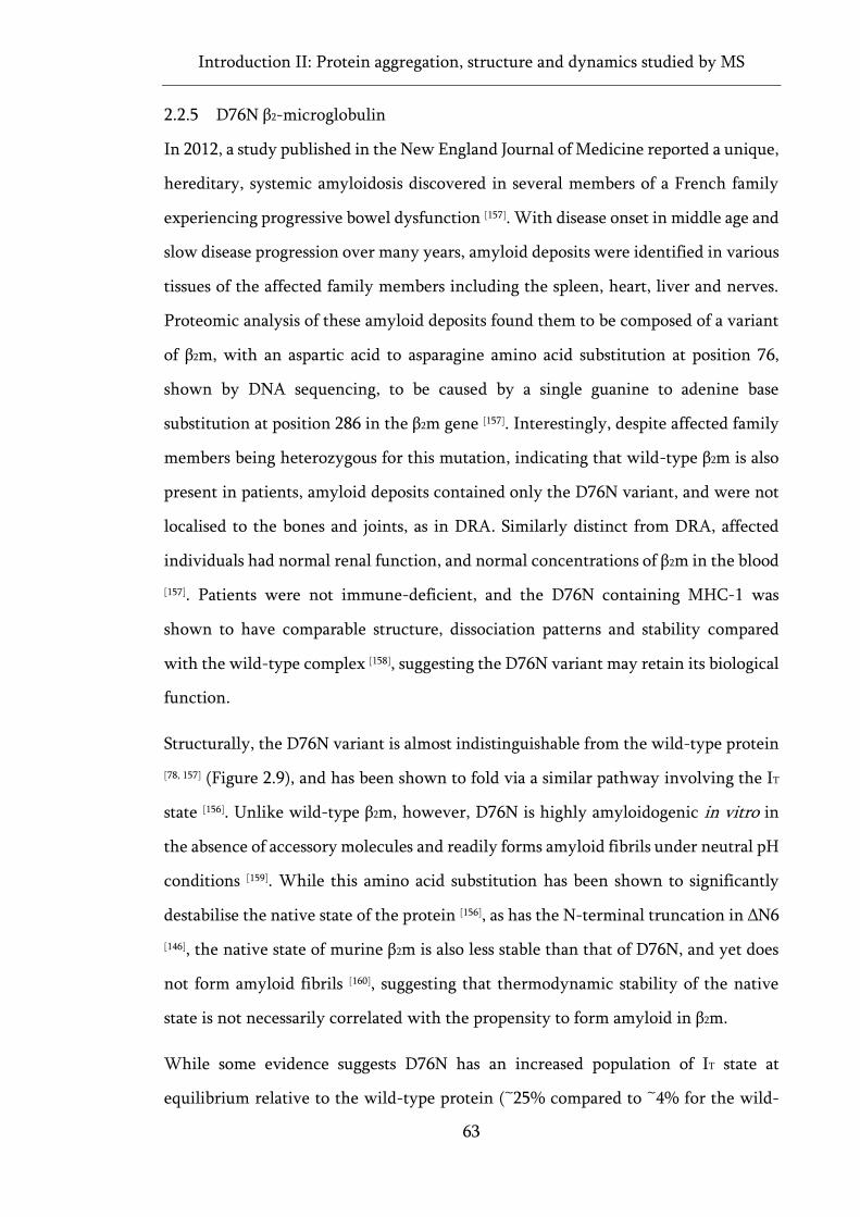
Introduction II: Protein aggregation, structure and dynamics studied by MS
63
2.2.5 D76N β2-microglobulin
In 2012, a study published in the New England Journal of Medicine reported a unique,
hereditary, systemic amyloidosis discovered in several members of a French family
experiencing progressive bowel dysfunction [157]. With disease onset in middle age and
slow disease progression over many years, amyloid deposits were identified in various
tissues of the affected family members including the spleen, heart, liver and nerves.
Proteomic analysis of these amyloid deposits found them to be composed of a variant
of β2m, with an aspartic acid to asparagine amino acid substitution at position 76,
shown by DNA sequencing, to be caused by a single guanine to adenine base
substitution at position 286 in the β2m gene [157]. Interestingly, despite affected family
members being heterozygous for this mutation, indicating that wild-type β2m is also
present in patients, amyloid deposits contained only the D76N variant, and were not
localised to the bones and joints, as in DRA. Similarly distinct from DRA, affected
individuals had normal renal function, and normal concentrations of β2m in the blood
[157]. Patients were not immune-deficient, and the D76N containing MHC-1 was
shown to have comparable structure, dissociation patterns and stability compared
with the wild-type complex [158], suggesting the D76N variant may retain its biological
function.
Structurally, the D76N variant is almost indistinguishable from the wild-type protein
[78, 157] (Figure 2.9), and has been shown to fold via a similar pathway involving the IT
state [156]. Unlike wild-type β2m, however, D76N is highly amyloidogenic in vitro in
the absence of accessory molecules and readily forms amyloid fibrils under neutral pH
conditions [159]. While this amino acid substitution has been shown to significantly
destabilise the native state of the protein [156], as has the N-terminal truncation in ΔN6
[146], the native state of murine β2m is also less stable than that of D76N, and yet does
not form amyloid fibrils [160], suggesting that thermodynamic stability of the native
state is not necessarily correlated with the propensity to form amyloid in β2m.
While some evidence suggests D76N has an increased population of IT state at
equilibrium relative to the wild-type protein (~25% compared to ~4% for the wild-
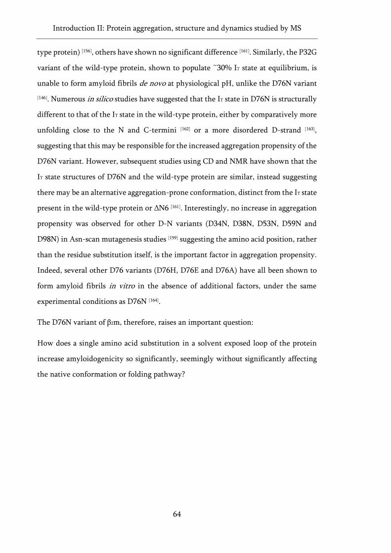
Introduction II: Protein aggregation, structure and dynamics studied by MS
64
type protein) [156], others have shown no significant difference [161]. Similarly, the P32G
variant of the wild-type protein, shown to populate ~30% IT state at equilibrium, is
unable to form amyloid fibrils de novo at physiological pH, unlike the D76N variant
[146]. Numerous in silico studies have suggested that the IT state in D76N is structurally
different to that of the IT state in the wild-type protein, either by comparatively more
unfolding close to the N and C-termini [162] or a more disordered D-strand [163],
suggesting that this may be responsible for the increased aggregation propensity of the
D76N variant. However, subsequent studies using CD and NMR have shown that the
IT state structures of D76N and the wild-type protein are similar, instead suggesting
there may be an alternative aggregation-prone conformation, distinct from the IT state
present in the wild-type protein or ΔN6 [161]. Interestingly, no increase in aggregation
propensity was observed for other D-N variants (D34N, D38N, D53N, D59N and
D98N) in Asn-scan mutagenesis studies [159] suggesting the amino acid position, rather
than the residue substitution itself, is the important factor in aggregation propensity.
Indeed, several other D76 variants (D76H, D76E and D76A) have all been shown to
form amyloid fibrils in vitro in the absence of additional factors, under the same
experimental conditions as D76N [164].
The D76N variant of β2m, therefore, raises an important question:
How does a single amino acid substitution in a solvent exposed loop of the protein
increase amyloidogenicity so significantly, seemingly without significantly affecting
the native conformation or folding pathway?
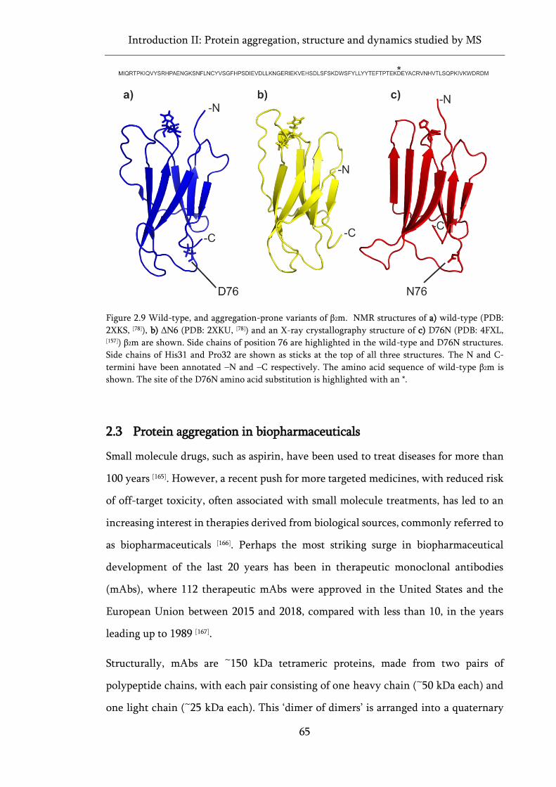
Introduction II: Protein aggregation, structure and dynamics studied by MS
65
Figure 2.9 Wild-type, and aggregation-prone variants of β2m. NMR structures of a) wild-type (PDB:
2XKS, [78]), b) ΔN6 (PDB: 2XKU, [78]) and an X-ray crystallography structure of c) D76N (PDB: 4FXL, [157]) β2m are shown. Side chains of position 76 are highlighted in the wild-type and D76N structures.
Side chains of His31 and Pro32 are shown as sticks at the top of all three structures. The N and C-
termini have been annotated –N and –C respectively. The amino acid sequence of wild-type β2m is
shown. The site of the D76N amino acid substitution is highlighted with an *.
2.3 Protein aggregation in biopharmaceuticals
Small molecule drugs, such as aspirin, have been used to treat diseases for more than
100 years [165]. However, a recent push for more targeted medicines, with reduced risk
of off-target toxicity, often associated with small molecule treatments, has led to an
increasing interest in therapies derived from biological sources, commonly referred to
as biopharmaceuticals [166]. Perhaps the most striking surge in biopharmaceutical
development of the last 20 years has been in therapeutic monoclonal antibodies
(mAbs), where 112 therapeutic mAbs were approved in the United States and the
European Union between 2015 and 2018, compared with less than 10, in the years
leading up to 1989 [167].
Structurally, mAbs are ~150 kDa tetrameric proteins, made from two pairs of
polypeptide chains, with each pair consisting of one heavy chain (~50 kDa each) and
one light chain (~25 kDa each). This ‘dimer of dimers’ is arranged into a quaternary
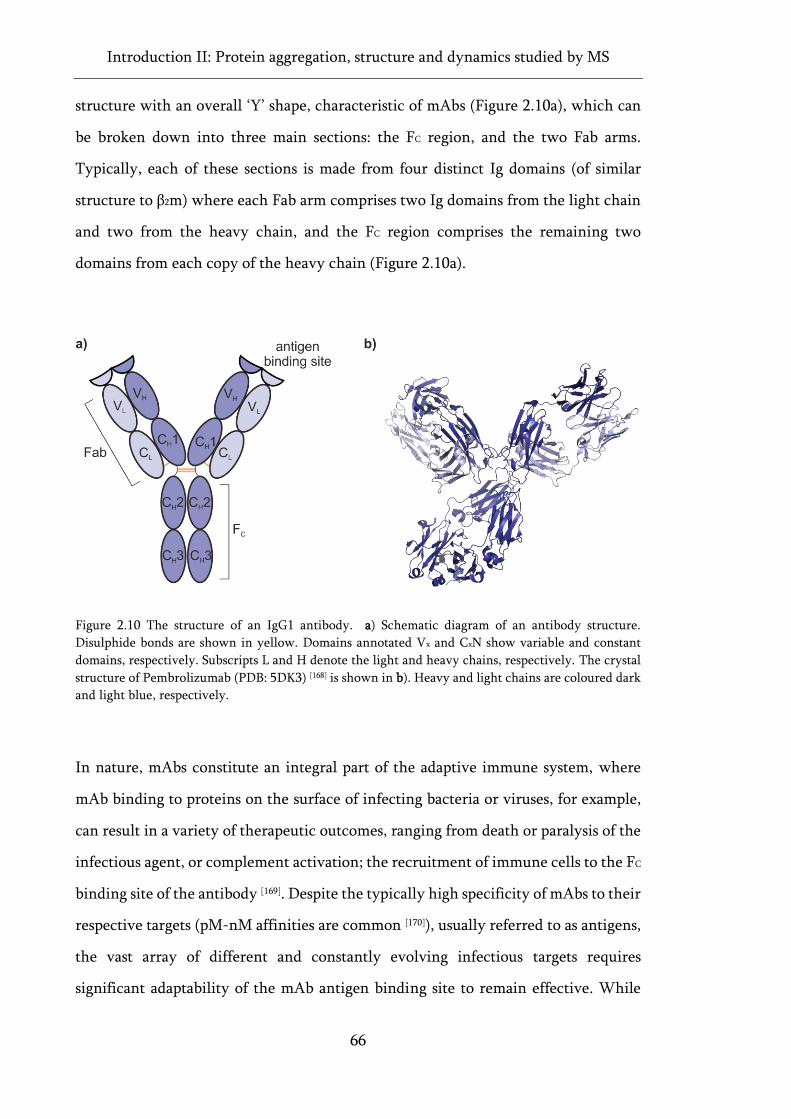
Introduction II: Protein aggregation, structure and dynamics studied by MS
66
structure with an overall ‘Y’ shape, characteristic of mAbs (Figure 2.10a), which can
be broken down into three main sections: the FC region, and the two Fab arms.
Typically, each of these sections is made from four distinct Ig domains (of similar
structure to β2m) where each Fab arm comprises two Ig domains from the light chain
and two from the heavy chain, and the FC region comprises the remaining two
domains from each copy of the heavy chain (Figure 2.10a).
Figure 2.10 The structure of an IgG1 antibody. a) Schematic diagram of an antibody structure.
Disulphide bonds are shown in yellow. Domains annotated Vx and CxN show variable and constant
domains, respectively. Subscripts L and H denote the light and heavy chains, respectively. The crystal
structure of Pembrolizumab (PDB: 5DK3) [168] is shown in b). Heavy and light chains are coloured dark
and light blue, respectively.
In nature, mAbs constitute an integral part of the adaptive immune system, where
mAb binding to proteins on the surface of infecting bacteria or viruses, for example,
can result in a variety of therapeutic outcomes, ranging from death or paralysis of the
infectious agent, or complement activation; the recruitment of immune cells to the FC
binding site of the antibody [169]. Despite the typically high specificity of mAbs to their
respective targets (pM-nM affinities are common [170]), usually referred to as antigens,
the vast array of different and constantly evolving infectious targets requires
significant adaptability of the mAb antigen binding site to remain effective. While
Introduction II: Protein aggregation, structure and dynamics studied by MS
67
most of the mAb structure is comprised of constant domains (denoted CH1-3 or CL in
Figure 2.10a), so called due to their lack of variability among mAb variants, the
capacity for mAbs to adapt to bind a wide range of different antigens arises from
hypervariable loop structures in the antigen binding site in the variable domains of
the Fab arms (denoted VL and VH in Figure 2.10a for the variable domains of the light
and heavy chains, respectively). Typically, there are twelve of these loop structures
for a given mAb protein, three for each of the variable domains, where the amino acid
sequences in these loops, also known as the complementarity determining regions
(CDRs), are readily substituted between antibody variants, adapting the structure,
conformation and microenvironment of the antigen binding site to suit a multitude
of different targets.
In the development of biotherapeutic antibodies, this system is ‘hijacked’, and the
structure and sequence of the CDR regions is purposefully changed to produce mAbs
which bind a target chosen by the developer, typically one the natural immune system
has failed to identify. For example, Pembrolizumab, the structure of which is shown
in Figure 2.10b, is a biotherapeutic used to treat a variety of different cancers by
binding to the PD-1 receptor protein on the surface of activated T cells. Cancerous
cells often highly express the binding partner of this receptor, PD-L1, on their surface,
such that activated immune cells recognise the tumour as ‘self’, hence preventing an
anti-tumour immune response. Pembrolizumab binding to PD-1 receptors interferes
with this interaction, allowing activated T cells and the natural immune system to
attacked the tumour [171].
While the benefits of developing specifically targeted biotherapeutic antibodies are
obvious, the development process for these products harbours numerous
opportunities for protein aggregation. Coupled with the engineered amino acid
sequence of the mAb, itself a possible cause of aggregation, biotherapeutics are
subjected to an array of physical, chemical and mechanical stresses at various stages
of production, storage or even during the administration of the drug to patients. For
example, changes in pH or temperature during protein production in bioreactors [172],
Introduction II: Protein aggregation, structure and dynamics studied by MS
68
or downstream purification [173], freeze-thaw cycles during storage [174], and interaction
with siliconized surfaces on syringes prior to subcutaneous injection of the drug [175],
are all possible causes of protein aggregation in biopharmaceuticals. Not only does
protein aggregation decrease the yield of useful product, passing the increased cost on
to consumers, but can also result in more insidious outcomes, such as reducing the
efficacy of treatment, requiring higher doses to remain effective, or worse, the
triggering of an immune response in patients, compromising patient safety.
Consequently, mitigating protein aggregation in the early stages of biopharmaceutical
development is of paramount importance.
2.3.1 MEDI1912 and MEDI1912_STT
Initially designed to bind the nerve growth factor (NGF) protein for the potential
treatment of chronic pain, MEDI1912, developed by Medimmune (now AstraZeneca),
is an IgG1 class mAb which, despite low pM affinity for its target antigen [170],
displayed significant propensity to reversibly self-associate into protein aggregates
during manufacture. Noting several other undesirable biophysical characteristics,
such as adsorption to filter membranes during purification, resulting in decreased
yield, and significant oligomerisation at low (<1 mg ml-1) concentrations, three surface
exposed hydrophobic amino acids in CDR loops one and two of the VH domain were
highlighted for their involvement in the reversible self-association dimer interface:
W30, F31 and L57 [170]. These amino acids in MEDI1912, hereafter referred to as WFL,
were substituted for three less hydrophobic groups (W30S, F31T, L57T) generating a
triple substitution variant: STT. Despite these CDR substitutions, the STT variant
maintained a low pM affinity for NGF, with significantly improved biophysical
characteristics including significantly reduced self-association, a 2-fold improved
half-life in rat in vivo models, and less non-specific tissue association [170]. Although
WFL and STT have been shown to behave differently under flow induced stress
conditions [176], the exact mechanism of aggregation and the conformational changes
associated with these amino acid substitutions remain unexplored.
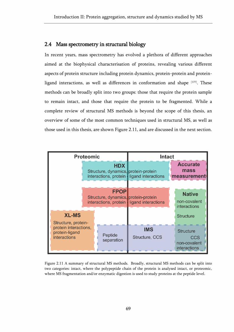
Introduction II: Protein aggregation, structure and dynamics studied by MS
69
2.4 Mass spectrometry in structural biology
In recent years, mass spectrometry has evolved a plethora of different approaches
aimed at the biophysical characterisation of proteins, revealing various different
aspects of protein structure including protein dynamics, protein-protein and protein-
ligand interactions, as well as differences in conformation and shape [177]. These
methods can be broadly split into two groups: those that require the protein sample
to remain intact, and those that require the protein to be fragmented. While a
complete review of structural MS methods is beyond the scope of this thesis, an
overview of some of the most common techniques used in structural MS, as well as
those used in this thesis, are shown Figure 2.11, and are discussed in the next section.
Figure 2.11 A summary of structural MS methods. Broadly, structural MS methods can be split into
two categories: intact, where the polypeptide chain of the protein is analysed intact, or proteomic,
where MS fragmentation and/or enzymatic digestion is used to study proteins at the peptide level.
Introduction II: Protein aggregation, structure and dynamics studied by MS
70
2.4.1 Accurate mass determination, native MS and ion mobility
As discussed earlier in Section 1.2.1, the advent of ESI has allowed large molecules
such as proteins to be ionised and analysed intact by use of MS. By using volatile, but
non-denaturing, solution conditions, such as ammonium acetate solutions, proteins
can be ionised and introduced into the instrument from their native solution phase
conformation. Typically, folded proteins have a lower solvent accessible surface area
(SASA) than unfolded proteins and, as such, have fewer accessible ionisable groups,
resulting in native proteins adopting narrower charge state distributions, with fewer
charges on average (i.e. higher m/z) when ionised by ESI (Figure 2.12b). Conversely,
unfolded proteins, with a larger SASA and more accessible ionisable groups, adopt
more charges from ESI (lower m/z) and have wider charge state distributions (Figure
2.12a). Thus analysis of charge state distributions can yield information on the
conformation of proteins [178-180].
Typically for native MS experiments, considerable effort is made to optimise
instrument conditions, aimed at striking a balance between effective transmission of
high m/z ions, maintaining the intact molecule and any non-covalent interactions
(particularly important for protein complexes), and aiding the desolvation process,
usually achieved by voltage and pressure manipulation within the instrument [181-183].
That said, complete desolvation of native ions, particularly for larger complexes,
remains challenging, and broader, less resolved, solvated charge state peaks are
frequently observed in native MS spectra, decreasing the mass accuracy. This, coupled
with the fewer charge states observed for native charge state distributions, equating
to fewer data points from which to calculate a mass, means that denatured MS is the
preferred technique to calculate an average mass of a protein, whilst native MS is more
typically used for structural characterisation of the folded protein or native protein
complex.
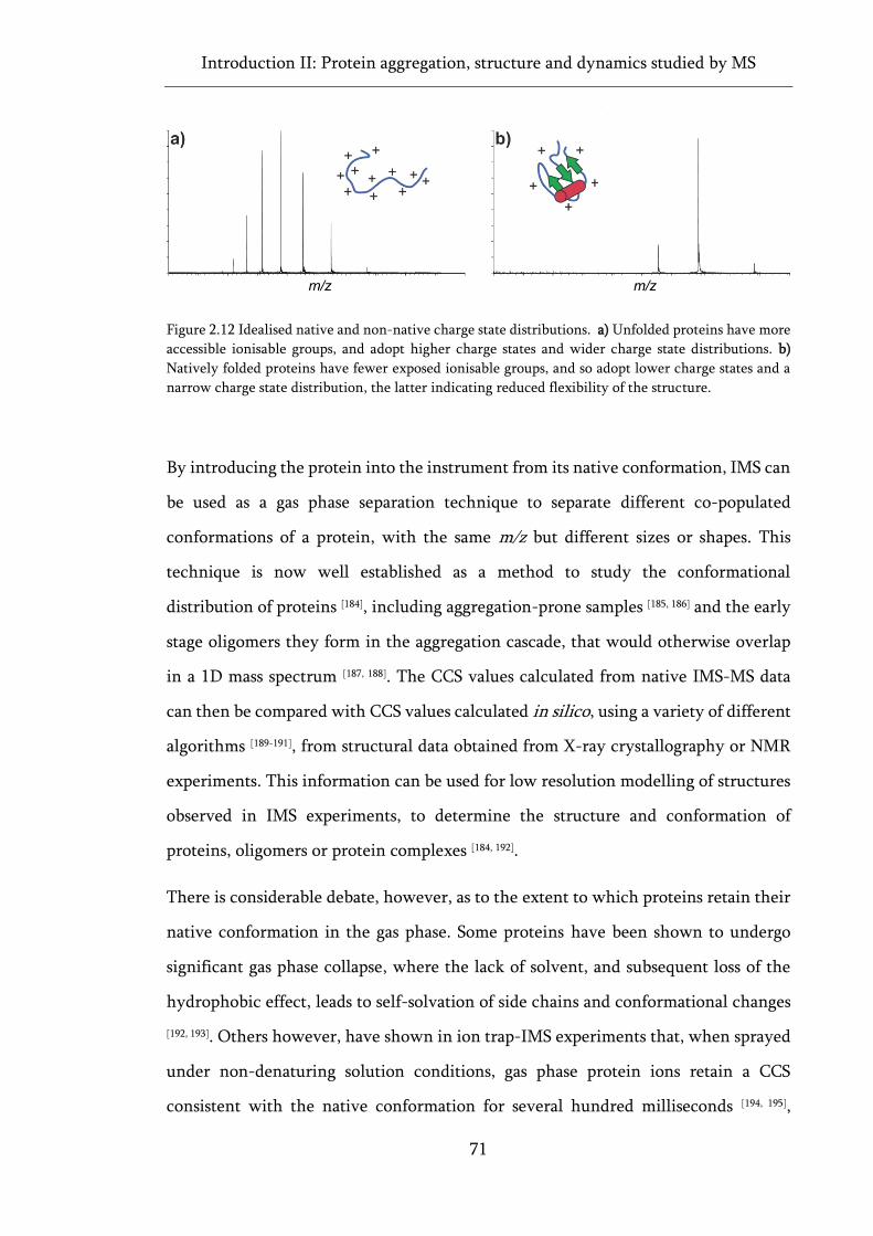
Introduction II: Protein aggregation, structure and dynamics studied by MS
71
Figure 2.12 Idealised native and non-native charge state distributions. a) Unfolded proteins have more
accessible ionisable groups, and adopt higher charge states and wider charge state distributions. b)
Natively folded proteins have fewer exposed ionisable groups, and so adopt lower charge states and a
narrow charge state distribution, the latter indicating reduced flexibility of the structure.
By introducing the protein into the instrument from its native conformation, IMS can
be used as a gas phase separation technique to separate different co-populated
conformations of a protein, with the same m/z but different sizes or shapes. This
technique is now well established as a method to study the conformational
distribution of proteins [184], including aggregation-prone samples [185, 186] and the early
stage oligomers they form in the aggregation cascade, that would otherwise overlap
in a 1D mass spectrum [187, 188]. The CCS values calculated from native IMS-MS data
can then be compared with CCS values calculated in silico, using a variety of different
algorithms [189-191], from structural data obtained from X-ray crystallography or NMR
experiments. This information can be used for low resolution modelling of structures
observed in IMS experiments, to determine the structure and conformation of
proteins, oligomers or protein complexes [184, 192].
There is considerable debate, however, as to the extent to which proteins retain their
native conformation in the gas phase. Some proteins have been shown to undergo
significant gas phase collapse, where the lack of solvent, and subsequent loss of the
hydrophobic effect, leads to self-solvation of side chains and conformational changes
[192, 193]. Others however, have shown in ion trap-IMS experiments that, when sprayed
under non-denaturing solution conditions, gas phase protein ions retain a CCS
consistent with the native conformation for several hundred milliseconds [194, 195],
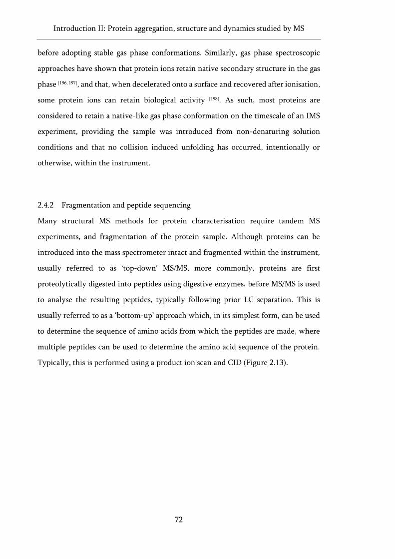
Introduction II: Protein aggregation, structure and dynamics studied by MS
72
before adopting stable gas phase conformations. Similarly, gas phase spectroscopic
approaches have shown that protein ions retain native secondary structure in the gas
phase [196, 197], and that, when decelerated onto a surface and recovered after ionisation,
some protein ions can retain biological activity [198]. As such, most proteins are
considered to retain a native-like gas phase conformation on the timescale of an IMS
experiment, providing the sample was introduced from non-denaturing solution
conditions and that no collision induced unfolding has occurred, intentionally or
otherwise, within the instrument.
2.4.2 Fragmentation and peptide sequencing
Many structural MS methods for protein characterisation require tandem MS
experiments, and fragmentation of the protein sample. Although proteins can be
introduced into the mass spectrometer intact and fragmented within the instrument,
usually referred to as ‘top-down’ MS/MS, more commonly, proteins are first
proteolytically digested into peptides using digestive enzymes, before MS/MS is used
to analyse the resulting peptides, typically following prior LC separation. This is
usually referred to as a ‘bottom-up’ approach which, in its simplest form, can be used
to determine the sequence of amino acids from which the peptides are made, where
multiple peptides can be used to determine the amino acid sequence of the protein.
Typically, this is performed using a product ion scan and CID (Figure 2.13).
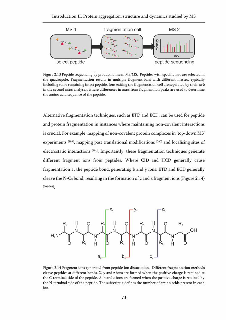
Introduction II: Protein aggregation, structure and dynamics studied by MS
73
Figure 2.13 Peptide sequencing by product ion scan MS/MS. Peptides with specific m/z are selected in
the quadrupole. Fragmentation results in multiple fragment ions with different masses, typically
including some remaining intact peptide. Ions exiting the fragmentation cell are separated by their m/z
in the second mass analyser, where differences in mass from fragment ion peaks are used to determine
the amino acid sequence of the peptide.
Alternative fragmentation techniques, such as ETD and ECD, can be used for peptide
and protein fragmentation in instances where maintaining non-covalent interactions
is crucial. For example, mapping of non-covalent protein complexes in ‘top-down MS’
experiments [199], mapping post translational modifications [200] and localising sites of
electrostatic interactions [201]. Importantly, these fragmentation techniques generate
different fragment ions from peptides. Where CID and HCD generally cause
fragmentation at the peptide bond, generating b and y ions, ETD and ECD generally
cleave the N-Cα bond, resulting in the formation of c and z fragment ions (Figure 2.14)
[202-204].
Figure 2.14 Fragment ions generated from peptide ion dissociation. Different fragmentation methods
cleave peptides at different bonds. X, y and z ions are formed when the positive charge is retained at
the C-terminal side of the peptide. A, b and c ions are formed when the positive charge is retained by
the N-terminal side of the peptide. The subscript x defines the number of amino acids present in each
ion.
Introduction II: Protein aggregation, structure and dynamics studied by MS
74
2.4.3 Hydrogen deuterium exchange (HDX)
Developed at the Carlsberg laboratory in the late 1950’s [205] (yes, that Carlsberg),
hydrogen deuterium exchange (HDX) is a non-covalent labelling technique where
labile protons, such as those involved in N-H, O-H or S-H bonds [206], are exchanged
for deuterium, a heavy isotope of hydrogen with an additional neutron (+1 Da).
Although deuterium exchange is detectable by other methods [207-209], the mass
difference resulting from deuterium incorporation is readily detectable by MS, which
has the advantage of lower sample requirements, and the ability to study larger
proteins or protein complexes when compared with other analytical techniques used
to measure HDX, such as NMR. Although many variations on this method exist, such
as ‘exchange-out’ reactions (D→H exchange) [210], or rapid pulsed labelling techniques
[211], HDX in structural MS is typically performed using the forward exchange reaction
(H→D, ‘exchange-in’) in a continuous labelling approach, where the sample is first
diluted into a deuterated buffer solution, and left to equilibrate for a fixed period of
time, before quenching the reaction to limit further exchange (Figure 2.15). The
deuterated protein sample is then either analysed at the intact level [212], or, more
commonly, proteolytically cleaved into peptide fragments before LC-MS analysis is
used to separate the labelled peptides, and localise differences in deuterium uptake to
peptide level resolution [213].
Although any labile proton in a protein can exchange for deuterium, in practice,
many, such as those on amino acid side chains, undergo rapid back-exchange to the
protonated form when the reaction is quenched [214], typically leaving only the
deuterium incorporated at the amide nitrogen on the peptide backbone. As such,
HDX-MS largely only probes deuterium uptake observed at these positions on the
protein – with one backbone amide group for each amino acid in the sequence, except
proline residues, which have no exchangeable amide group (Table 2.1).
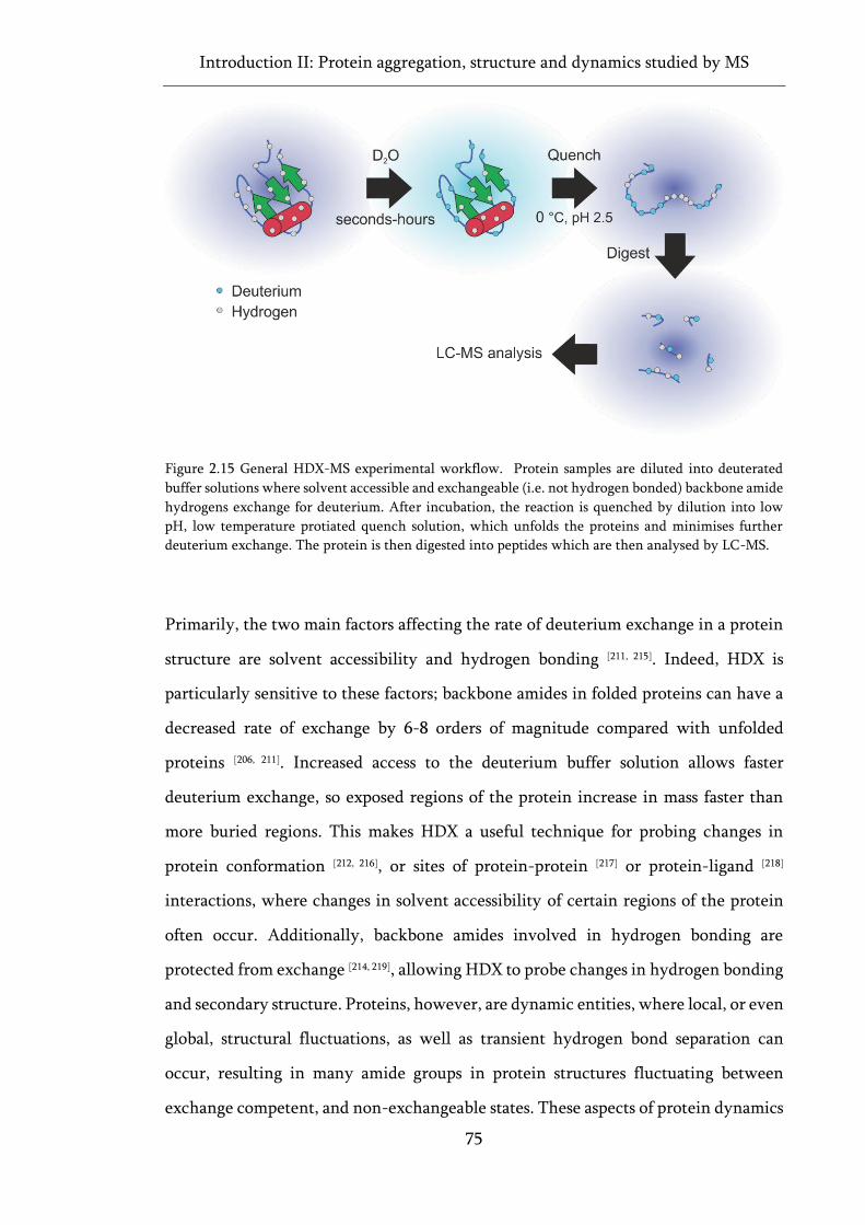
Introduction II: Protein aggregation, structure and dynamics studied by MS
75
Figure 2.15 General HDX-MS experimental workflow. Protein samples are diluted into deuterated
buffer solutions where solvent accessible and exchangeable (i.e. not hydrogen bonded) backbone amide
hydrogens exchange for deuterium. After incubation, the reaction is quenched by dilution into low
pH, low temperature protiated quench solution, which unfolds the proteins and minimises further
deuterium exchange. The protein is then digested into peptides which are then analysed by LC-MS.
Primarily, the two main factors affecting the rate of deuterium exchange in a protein
structure are solvent accessibility and hydrogen bonding [211, 215]. Indeed, HDX is
particularly sensitive to these factors; backbone amides in folded proteins can have a
decreased rate of exchange by 6-8 orders of magnitude compared with unfolded
proteins [206, 211]. Increased access to the deuterium buffer solution allows faster
deuterium exchange, so exposed regions of the protein increase in mass faster than
more buried regions. This makes HDX a useful technique for probing changes in
protein conformation [212, 216], or sites of protein-protein [217] or protein-ligand [218]
interactions, where changes in solvent accessibility of certain regions of the protein
often occur. Additionally, backbone amides involved in hydrogen bonding are
protected from exchange [214, 219], allowing HDX to probe changes in hydrogen bonding
and secondary structure. Proteins, however, are dynamic entities, where local, or even
global, structural fluctuations, as well as transient hydrogen bond separation can
occur, resulting in many amide groups in protein structures fluctuating between
exchange competent, and non-exchangeable states. These aspects of protein dynamics
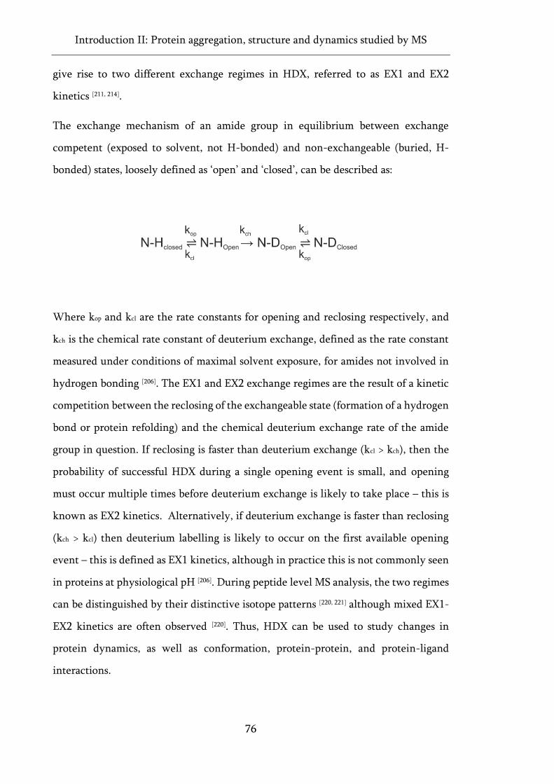
Introduction II: Protein aggregation, structure and dynamics studied by MS
76
give rise to two different exchange regimes in HDX, referred to as EX1 and EX2
kinetics [211, 214].
The exchange mechanism of an amide group in equilibrium between exchange
competent (exposed to solvent, not H-bonded) and non-exchangeable (buried, H-
bonded) states, loosely defined as ‘open’ and ‘closed’, can be described as:
Where kop and kcl are the rate constants for opening and reclosing respectively, and
kch is the chemical rate constant of deuterium exchange, defined as the rate constant
measured under conditions of maximal solvent exposure, for amides not involved in
hydrogen bonding [206]. The EX1 and EX2 exchange regimes are the result of a kinetic
competition between the reclosing of the exchangeable state (formation of a hydrogen
bond or protein refolding) and the chemical deuterium exchange rate of the amide
group in question. If reclosing is faster than deuterium exchange (kcl > kch), then the
probability of successful HDX during a single opening event is small, and opening
must occur multiple times before deuterium exchange is likely to take place – this is
known as EX2 kinetics. Alternatively, if deuterium exchange is faster than reclosing
(kch > kcl) then deuterium labelling is likely to occur on the first available opening
event – this is defined as EX1 kinetics, although in practice this is not commonly seen
in proteins at physiological pH [206]. During peptide level MS analysis, the two regimes
can be distinguished by their distinctive isotope patterns [220, 221] although mixed EX1-
EX2 kinetics are often observed [220]. Thus, HDX can be used to study changes in
protein dynamics, as well as conformation, protein-protein, and protein-ligand
interactions.
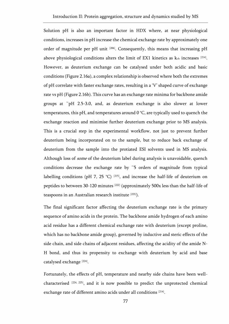
Introduction II: Protein aggregation, structure and dynamics studied by MS
77
Solution pH is also an important factor in HDX where, at near physiological
conditions, increases in pH increase the chemical exchange rate by approximately one
order of magnitude per pH unit [206]. Consequently, this means that increasing pH
above physiological conditions alters the limit of EX1 kinetics as kch increases [214].
However, as deuterium exchange can be catalysed under both acidic and basic
conditions (Figure 2.16a), a complex relationship is observed where both the extremes
of pH correlate with faster exchange rates, resulting in a ‘V’ shaped curve of exchange
rate vs pH (Figure 2.16b). This curve has an exchange rate minima for backbone amide
groups at ~pH 2.5-3.0, and, as deuterium exchange is also slower at lower
temperatures, this pH, and temperatures around 0 °C, are typically used to quench the
exchange reaction and minimise further deuterium exchange prior to MS analysis.
This is a crucial step in the experimental workflow, not just to prevent further
deuterium being incorporated on to the sample, but to reduce back exchange of
deuterium from the sample into the protiated ESI solvents used in MS analysis.
Although loss of some of the deuterium label during analysis is unavoidable, quench
conditions decrease the exchange rate by ~5 orders of magnitude from typical
labelling conditions (pH 7, 25 °C) [215], and increase the half-life of deuterium on
peptides to between 30-120 minutes [222] (approximately 500x less than the half-life of
teaspoons in an Australian research institute [223]).
The final significant factor affecting the deuterium exchange rate is the primary
sequence of amino acids in the protein. The backbone amide hydrogen of each amino
acid residue has a different chemical exchange rate with deuterium (except proline,
which has no backbone amide group), governed by inductive and steric effects of the
side chain, and side chains of adjacent residues, affecting the acidity of the amide N-
H bond, and thus its propensity to exchange with deuterium by acid and base
catalysed exchange [224].
Fortunately, the effects of pH, temperature and nearby side chains have been well-
characterised [224, 225], and it is now possible to predict the unprotected chemical
exchange rate of different amino acids under all conditions [214].
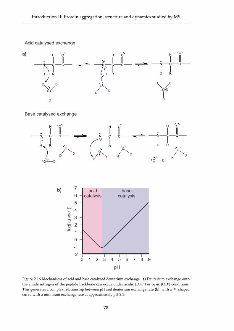
Introduction II: Protein aggregation, structure and dynamics studied by MS
78
Figure 2.16 Mechanisms of acid and base catalysed deuterium exchange. a) Deuterium exchange onto
the amide nitrogen of the peptide backbone can occur under acidic (D3O+) or basic (OD-) conditions.
This generates a complex relationship between pH and deuterium exchange rate (b), with a ‘V’ shaped
curve with a minimum exchange rate at approximately pH 2.5.
Introduction II: Protein aggregation, structure and dynamics studied by MS
79
2.4.4 Fast photochemical oxidation of proteins (FPOP)
Developed in the early 2000’s [226, 227], Fast Photochemical Oxidation of Proteins
(FPOP) is a covalent labelling technique where hydroxyl radicals liberated from
photolysis of hydrogen peroxide covalently label solvent accessible regions of the
protein. Although hydroxyl radicals can attack almost any region of a protein, where
attack on certain residues, or the α-carbon itself can result in fragmentation of the
polypeptide backbone [228], more commonly, steric inaccessibility of the backbone
leads to hydroxyl radical attack primarily on amino acid side chains, preferentially
labelling large hydrophobic residues, or side chains containing sulfur atoms [228]. This
hydroxyl radical labelling results in a variety of different covalent modifications of
different masses. By far, the most common of these are +16 Da hydroxylations
(addition of OH and abstraction of H), although many others are possible, including
the formation of carbonyl groups (+14 Da, addition of O and abstraction of 2H),
decarboxylation (-30 Da) and deguanidination (-43 Da). A summary of common
oxidative modifications, and the side chains on which they are typically observed, are
shown in Table 2.2.
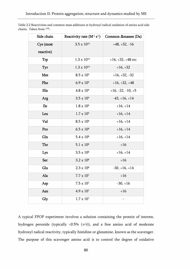
Introduction II: Protein aggregation, structure and dynamics studied by MS
80
Table 2.2 Reactivities and common mass additions in hydroxyl radical oxidation of amino acid side
chains. Taken from [228].
Side chain Reactivity rate (M-1 s-1) Common Δmasses (Da)
Cys (most
reactive)
3.5 x 10¹⁰ +48, +32, -16
Trp 1.3 x 10¹⁰ +16, +32, +48 etc
Tyr 1.3 x 10¹⁰ +16, +32
Met 8.5 x 10⁹ +16, +32, -32
Phe 6.9 x 10⁹ +16, +32, +48
His 4.8 x 10⁹ +16, -22, -10, +5
Arg 3.5 x 10⁹ -43, +16, +14
Ile 1.8 x 10⁹ +16, +14
Leu 1.7 x 10⁹ +16, +14
Val 8.5 x 10⁸ +16, +14
Pro 6.5 x 10⁸ +16, +14
Gln 5.4 x 10⁸ +16, +14
Thr 5.1 x 10⁸ +16
Lys 3.5 x 10⁸ +16, +14
Ser 3.2 x 10⁸ +16
Glu 2.3 x 10⁸ -30, +16, +14
Ala 7.7 x 10⁷ +16
Asp 7.5 x 10⁷ -30, +16
Asn 4.9 x 10⁷ +16
Gly 1.7 x 10⁷ -
A typical FPOP experiment involves a solution containing the protein of interest,
hydrogen peroxide (typically <0.5% (v/v)), and a free amino acid of moderate
hydroxyl radical reactivity, typically histidine or glutamine, known as the scavenger.
The purpose of this scavenger amino acid is to control the degree of oxidative
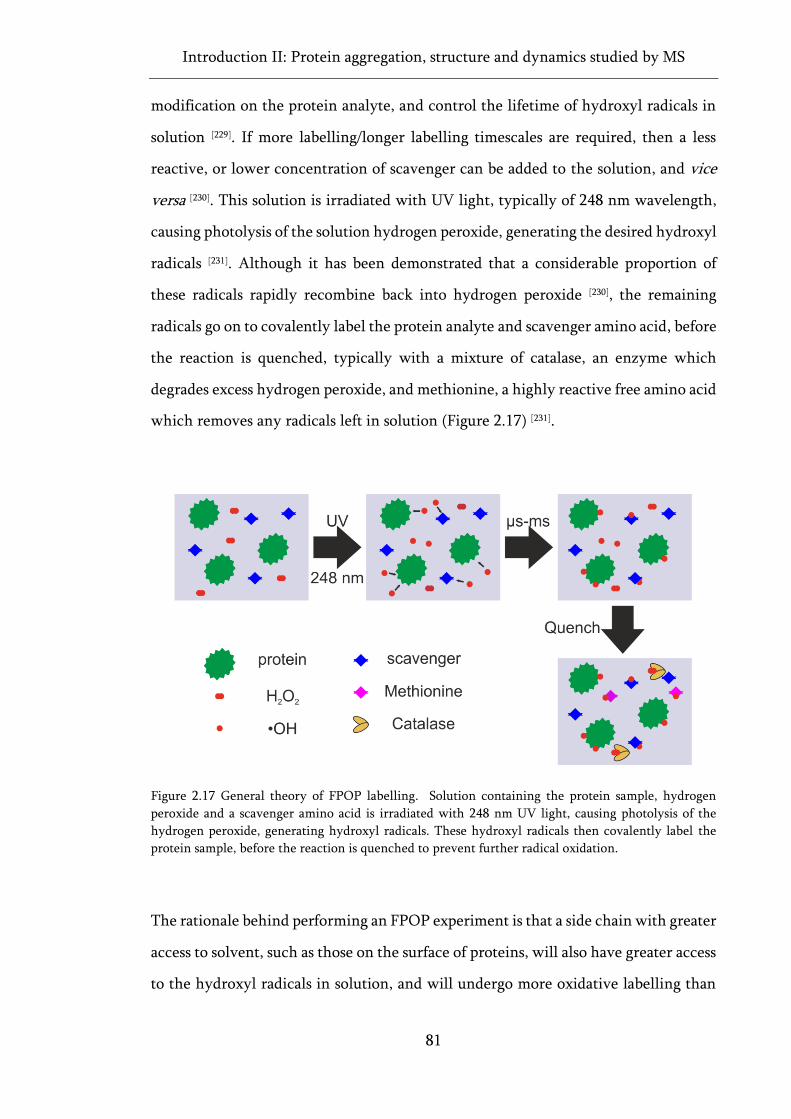
Introduction II: Protein aggregation, structure and dynamics studied by MS
81
modification on the protein analyte, and control the lifetime of hydroxyl radicals in
solution [229]. If more labelling/longer labelling timescales are required, then a less
reactive, or lower concentration of scavenger can be added to the solution, and vice
versa [230]. This solution is irradiated with UV light, typically of 248 nm wavelength,
causing photolysis of the solution hydrogen peroxide, generating the desired hydroxyl
radicals [231]. Although it has been demonstrated that a considerable proportion of
these radicals rapidly recombine back into hydrogen peroxide [230], the remaining
radicals go on to covalently label the protein analyte and scavenger amino acid, before
the reaction is quenched, typically with a mixture of catalase, an enzyme which
degrades excess hydrogen peroxide, and methionine, a highly reactive free amino acid
which removes any radicals left in solution (Figure 2.17) [231].
Figure 2.17 General theory of FPOP labelling. Solution containing the protein sample, hydrogen
peroxide and a scavenger amino acid is irradiated with 248 nm UV light, causing photolysis of the
hydrogen peroxide, generating hydroxyl radicals. These hydroxyl radicals then covalently label the
protein sample, before the reaction is quenched to prevent further radical oxidation.
The rationale behind performing an FPOP experiment is that a side chain with greater
access to solvent, such as those on the surface of proteins, will also have greater access
to the hydroxyl radicals in solution, and will undergo more oxidative labelling than
Introduction II: Protein aggregation, structure and dynamics studied by MS
82
side chains with less solvent accessible surface area. Although the target, and nature
of the labelling is very different, these characteristics mean FPOP can be used to probe
many of the same changes as HDX; changes in protein structure, conformation and
dynamics, as well as protein-protein or protein ligand interactions, all of which can
change a side chain’s accessibility to solvent, and thus its degree of oxidative
modification in FPOP. Again similar to HDX, changes in FPOP oxidative labelling can
be observed by introducing the protein sample into the mass spectrometer intact, and
quantifying the observed distributions of different mass modifications. However,
unlike HDX, quenching can be performed under neutral pH conditions, and the
covalent nature of the label means that no back exchange occurs during the
experiment. Combined, these properties make proteolytic digestion and LC-MS/MS
analysis of the oxidised peptides a more attractive option, as choice of digestive
enzyme is not restricted to acid proteases as in HDX, and lengthy analytical
procedures can be used to analyse the resulting peptides, without the concern of losing
the label.
However, unlike the wealth of knowledge available concerning solution conditions
and protein structure on deuterium labelling in HDX [224, 225], these parameters are not
well understood with regards to oxidative labelling in FPOP. Work by Xie et al., has
shown a positive correlation between the fraction of the side chain that is exposed to
solvent and the extent of modification observed, normalised for the reactivity of each
side chain [232]. However, this relationship was only observed for the most reactive side
chains, while the correlation was less clear or absent for less reactive residues. The
authors proposed that highly reactive side chains compete for hydroxyl radicals with
nearby side chains that are less reactive, highlighting possible effects of sequence or
local environment on the extent of oxidative modification, in addition to solvent
accessible surface area [232]. Similarly, although it is not currently disputed that the
primary radical generated by FPOP, the hydroxyl radical, labels the protein sample
on the timescale of µs under typical FPOP solution conditions [230], Vahidi et al., have
demonstrated that radicals in FPOP experiments can exist in such solutions for up to
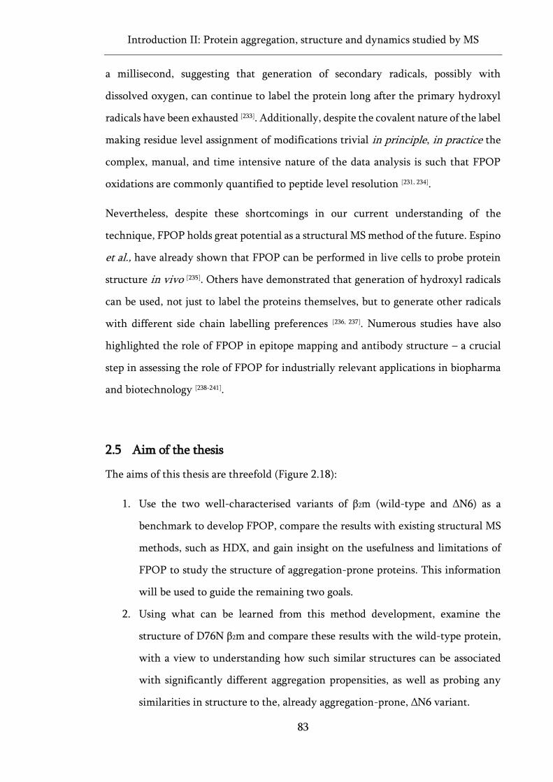
Introduction II: Protein aggregation, structure and dynamics studied by MS
83
a millisecond, suggesting that generation of secondary radicals, possibly with
dissolved oxygen, can continue to label the protein long after the primary hydroxyl
radicals have been exhausted [233]. Additionally, despite the covalent nature of the label
making residue level assignment of modifications trivial in principle, in practice the
complex, manual, and time intensive nature of the data analysis is such that FPOP
oxidations are commonly quantified to peptide level resolution [231, 234].
Nevertheless, despite these shortcomings in our current understanding of the
technique, FPOP holds great potential as a structural MS method of the future. Espino
et al., have already shown that FPOP can be performed in live cells to probe protein
structure in vivo [235]. Others have demonstrated that generation of hydroxyl radicals
can be used, not just to label the proteins themselves, but to generate other radicals
with different side chain labelling preferences [236, 237]. Numerous studies have also
highlighted the role of FPOP in epitope mapping and antibody structure – a crucial
step in assessing the role of FPOP for industrially relevant applications in biopharma
and biotechnology [238-241].
2.5 Aim of the thesis
The aims of this thesis are threefold (Figure 2.18):
1. Use the two well-characterised variants of β2m (wild-type and ΔN6) as a
benchmark to develop FPOP, compare the results with existing structural MS
methods, such as HDX, and gain insight on the usefulness and limitations of
FPOP to study the structure of aggregation-prone proteins. This information
will be used to guide the remaining two goals.
2. Using what can be learned from this method development, examine the
structure of D76N β2m and compare these results with the wild-type protein,
with a view to understanding how such similar structures can be associated
with significantly different aggregation propensities, as well as probing any
similarities in structure to the, already aggregation-prone, ΔN6 variant.
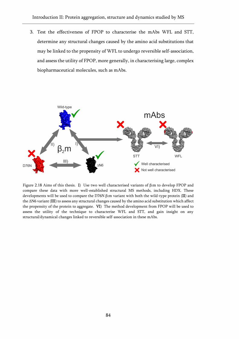
Introduction II: Protein aggregation, structure and dynamics studied by MS
84
3. Test the effectiveness of FPOP to characterise the mAbs WFL and STT,
determine any structural changes caused by the amino acid substitutions that
may be linked to the propensity of WFL to undergo reversible self-association,
and assess the utility of FPOP, more generally, in characterising large, complex
biopharmaceutical molecules, such as mAbs.
Figure 2.18 Aims of this thesis. I) Use two well characterised variants of β2m to develop FPOP and
compare these data with more well-established structural MS methods, including HDX. These
developments will be used to compare the D76N β2m variant with both the wild-type protein (II) and
the ΔN6 variant (III) to assess any structural changes caused by the amino acid substitution which affect
the propensity of the protein to aggregate. VI) The method development from FPOP will be used to
assess the utility of the technique to characterise WFL and STT, and gain insight on any
structural/dynamical changes linked to reversible self-association in these mAbs.

85
Chapter 3:
Materials and methods
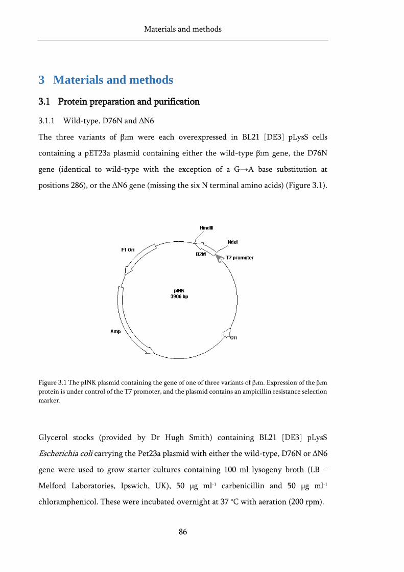
Materials and methods
86
3 Materials and methods
3.1 Protein preparation and purification
3.1.1 Wild-type, D76N and ΔN6
The three variants of β2m were each overexpressed in BL21 [DE3] pLysS cells
containing a pET23a plasmid containing either the wild-type β2m gene, the D76N
gene (identical to wild-type with the exception of a G→A base substitution at
positions 286), or the ΔN6 gene (missing the six N terminal amino acids) (Figure 3.1).
Figure 3.1 The pINK plasmid containing the gene of one of three variants of β2m. Expression of the β2m
protein is under control of the T7 promoter, and the plasmid contains an ampicillin resistance selection
marker.
Glycerol stocks (provided by Dr Hugh Smith) containing BL21 [DE3] pLysS
Escherichia coli carrying the Pet23a plasmid with either the wild-type, D76N or ΔN6
gene were used to grow starter cultures containing 100 ml lysogeny broth (LB –
Melford Laboratories, Ipswich, UK), 50 µg ml-1 carbenicillin and 50 µg ml-1
chloramphenicol. These were incubated overnight at 37 °C with aeration (200 rpm).
Materials and methods
87
Large scale 1 L cultures were then set up containing 25 g LB, 5 ml of starter culture
and 50 µg ml-1 carbenicillin. These were incubated at 37 °C with aeration (200 rpm)
to an OD600 of 0.6 and then induced with 1 mM isopropyl β-D-1-
thiogalactopyranoside (IPTG) before overnight incubation (37 °C, 200 rpm).
After 16 hours, cells were harvested by centrifugation at 15,000 rpm for 20 minutes
using a Beckman JLA 16.250 rotor (approximately 33,700 G) (4 °C). The cell pellets
were incubated in 200 ml lysis buffer (100 µg ml-1 lysozyme, 50 µg ml-1
phenylmethylsulfonyl fluoride (PMSF), 20 µg ml-1 DNase, 1 mM
ethylenediaminetetraacetic acid (EDTA) in 25 mM Tris.HCl pH 8.0) for 30 min at
room temperature before being further lysed using a cell disrupter (constant cell
disruptor systems, Northhants, UK) at a pressure of 30 kpsi.
This cell lysate was then centrifuged as above for 30 min. The resulting pellet
(containing the inclusion bodies) was then washed with 200 ml, 25 mM Tris.HCl pH
8.0 and any dark material on the pellet surface was removed. The pellet was then
resuspended in 200 ml 25 mM Tris.HCl pH 8.0 and centrifuged again (as above). This
process was repeated three times to remove any dark material left on the pellet surface
following centrifugation.
The resulting clean pellet was then solubilised in 200 ml, 25 mM Tris.HCl pH 8.0
containing 8 M urea and incubated at room temperature overnight with gentle
stirring, before a final centrifugation step (15,000 rpm for 1 hour) was used to remove
any precipitate.
The protein was then allowed to refold by dialysis into 5 L, 25 mM Tris.HCl pH 8.0,
using 3500 molecular weight cut off (MWCO) dialysis tubing (Thermo Scientific,
Hemel Hempstead, UK). The dialysis buffer was changed a total of 6 times with a two
hour equilibration period between changes.
Refolded protein was then purified by anion exchange chromatography using an
XK50 fast-flow Q-Sepharose column (GE Healthcare, Buckinghamshire, UK). The
column was equilibrated with 2 column volumes of buffer (25 mM Tris.HCl pH 8.0)
Materials and methods
88
before the refolded protein was added. The bound protein was then eluted with a 0-
125 mM NaCl gradient at room temperature in 25 mM Tris.HCl pH 8.0 buffer. Eluted
fractions containing the protein were then dialysed into purite 18 MΩ water using the
above dialysis protocol, before being concentrated to ≈ 1 mM using Sartorius vivaspin
2, 3,000 MWCO spin columns.
The refolded, concentrated ion exchange product was then filtered (0.22 µm filter
units, Fischer Scientific) and further purified by size exclusion chromatography using
a Superdex 75 prep grade XK 26/60 column (Amersham Biosciences,
Buckinghamshire, UK) equilibrated with 150 mM ammonium acetate (pH 7.4) at
room temperature. The eluted fractions containing monomeric protein were collected
and analysed by SDS-PAGE to confirm the presence of monomeric β2m (or
D76N/ΔN6). These fractions were then pooled, and stored at ≈400 µM at -80 °C.
Protein preparation and purification of all three variants of β2m was carried out with
the help and supervision of Dr Hugh Smith (Radford research laboratory).
3.1.1.1 SDS-PAGE
Tris-tricine buffered SDS-PAGE gels were used to confirm the presence of β2m in the
eluted gel filtration fractions. Samples were diluted 1:1 with 2X loading buffer (50
mM Tris.HCl pH 6.8, 100 mM dithiotheritol (DTT), 2% w/v sodium dodecyl sulphate
(SDS), 0.1% w/v bromophenol blue, 10% v/v glycerol) and boiled for 5 min prior to
being loaded onto the gel. A 60 mA current was applied until the samples had entered
the resolving gel, at which point the current was increased to 100 mA. The completed
gels were then stained with Instant Blue (Expedeon protein solutions,
Cambridgeshire, UK) overnight and then imaged using the Genesnap software
(Syngene bioimaging). Molecular weight markers used for SDS-PAGE analysis were
2-250 kDa precision plus protein standard ladders (Bio Rad, Hertfordshire, UK).
Components of the resolving and stacking gels are listed in Table 3.1. The cathode
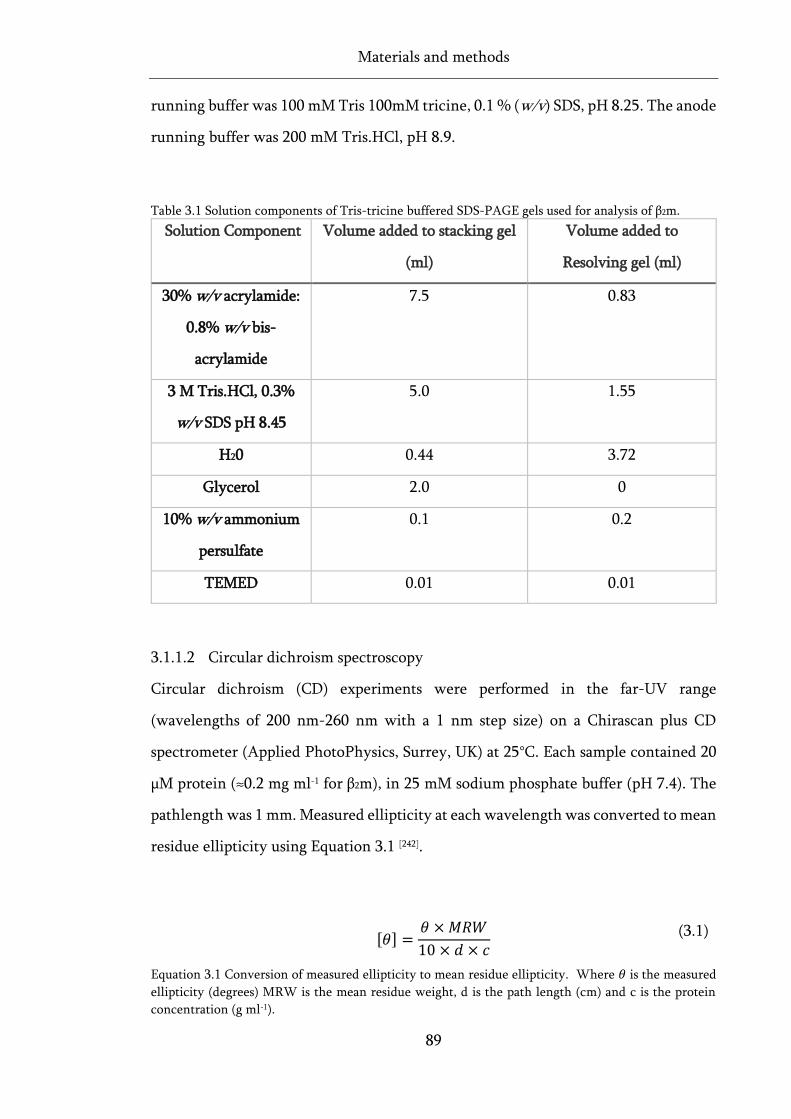
Materials and methods
89
running buffer was 100 mM Tris 100mM tricine, 0.1 % (w/v) SDS, pH 8.25. The anode
running buffer was 200 mM Tris.HCl, pH 8.9.
Table 3.1 Solution components of Tris-tricine buffered SDS-PAGE gels used for analysis of β2m.
Solution Component Volume added to stacking gel
(ml)
Volume added to
Resolving gel (ml)
30% w/v acrylamide:
0.8% w/v bis-
acrylamide
7.5 0.83
3 M Tris.HCl, 0.3%
w/v SDS pH 8.45
5.0 1.55
H20 0.44 3.72
Glycerol 2.0 0
10% w/v ammonium
persulfate
0.1 0.2
TEMED 0.01 0.01
3.1.1.2 Circular dichroism spectroscopy
Circular dichroism (CD) experiments were performed in the far-UV range
(wavelengths of 200 nm-260 nm with a 1 nm step size) on a Chirascan plus CD
spectrometer (Applied PhotoPhysics, Surrey, UK) at 25°C. Each sample contained 20
µM protein (≈0.2 mg ml-1 for β2m), in 25 mM sodium phosphate buffer (pH 7.4). The
pathlength was 1 mm. Measured ellipticity at each wavelength was converted to mean
residue ellipticity using Equation 3.1 [242].
[𝜃] =
𝜃 ×𝑀𝑅𝑊
10 × 𝑑 × 𝑐
(3.1)
Equation 3.1 Conversion of measured ellipticity to mean residue ellipticity. Where 𝜃 is the measured
ellipticity (degrees) MRW is the mean residue weight, d is the path length (cm) and c is the protein
concentration (g ml-1).
Materials and methods
90
CD experiments were carried out by Dr Hugh Smith (Radford research laboratory).
3.1.2 WFL and STT
The two mAb variants MEDI1912_WFL and MEDI1912_STT were provided by
AstraZeneca (formerly Medimmune) in formulation buffer (125 mM L- arginine, 20
mM sodium succinate, pH 6.0).
3.2 Native MS
3.2.1 Sample preparation
Samples prepared for native MS were 2x buffer exchanged into 150 mM ammonium
acetate (pH 7.4) using 7k MWCO zeba spin desalting columns (Thermo Scientific,
Hemel Hempstead, UK). The final sample was diluted to a concentration of 10 µM,
calculated based on the absorbance at 280 nm and the Beer-Lambert law, using an
extinction coefficient of 20065 M-1 cm-1 for all β2m variants.
Samples were then loaded into borosilicate glass capillaries pulled in-house (Sutter
Intrument Company, Novato, CA, USA) and coated with palladium using a sputter
coater (Polaron SC7620, Quorum Technologies Ltd, Kent, UK).
3.2.2 Waters Synapt G1 HDMS
The instrument was first calibrated using ~10 mg ml-1 caesium iodide clusters across
the m/z acquisition range (usually 500-8000 m/z) before data were analysed using
MassLynx v4.1 and Driftscope v3.0 (Waters, Wilmslow, UK), if IMS acquisition mode
was active. All samples were analysed in positive ionisation mode.
Ion mobility experiments were performed under two different sets of T-wave
conditions. Source and T-wave conditions for the instrument in each case are listed
in Table 3.2.
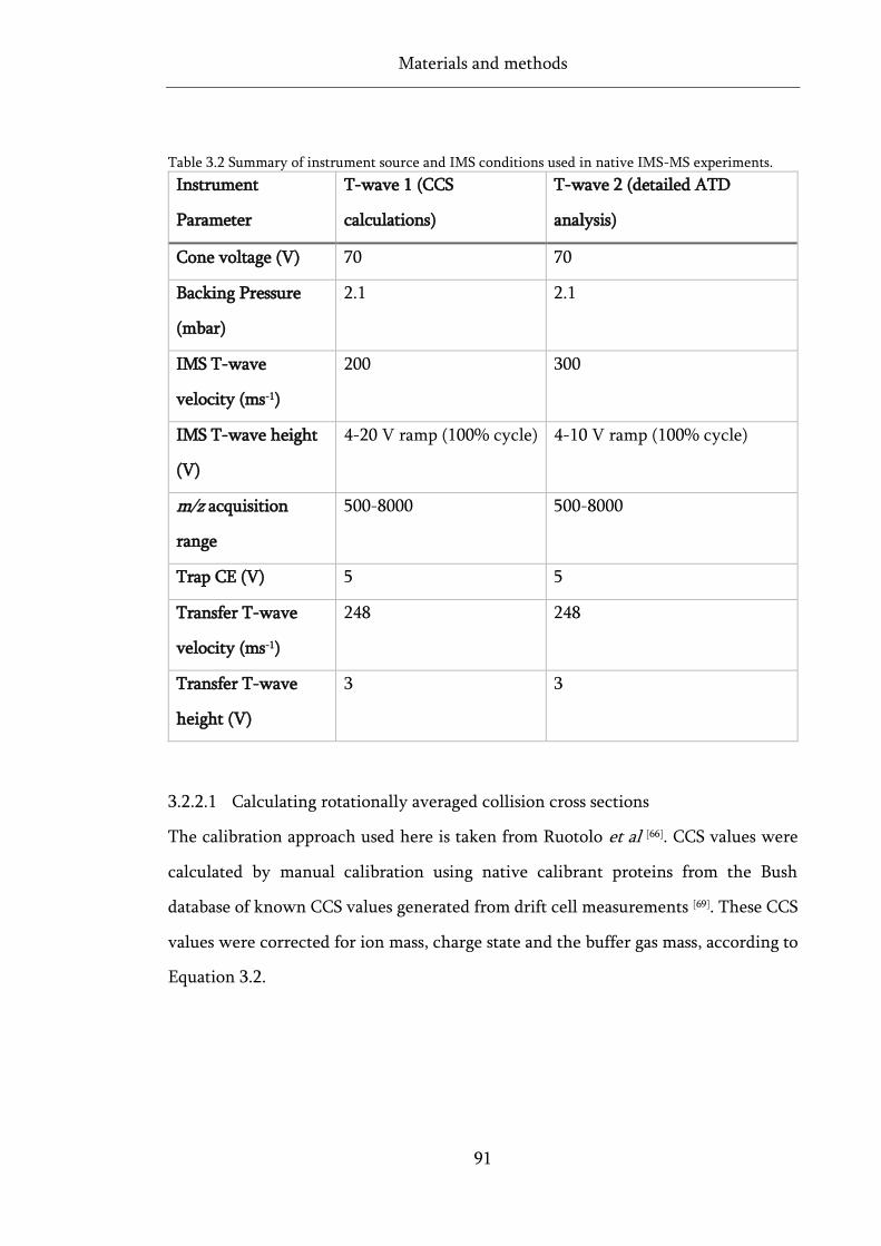
Materials and methods
91
Table 3.2 Summary of instrument source and IMS conditions used in native IMS-MS experiments.
Instrument
Parameter
T-wave 1 (CCS
calculations)
T-wave 2 (detailed ATD
analysis)
Cone voltage (V) 70 70
Backing Pressure
(mbar)
2.1 2.1
IMS T-wave
velocity (ms-1)
200 300
IMS T-wave height
(V)
4-20 V ramp (100% cycle) 4-10 V ramp (100% cycle)
m/z acquisition
range
500-8000 500-8000
Trap CE (V) 5 5
Transfer T-wave
velocity (ms-1)
248 248
Transfer T-wave
height (V)
3 3
3.2.2.1 Calculating rotationally averaged collision cross sections
The calibration approach used here is taken from Ruotolo et al [66]. CCS values were
calculated by manual calibration using native calibrant proteins from the Bush
database of known CCS values generated from drift cell measurements [69]. These CCS
values were corrected for ion mass, charge state and the buffer gas mass, according to
Equation 3.2.
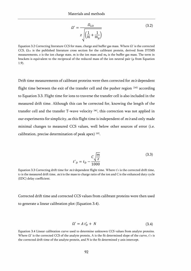
Materials and methods
92
𝛺′ =
𝛺𝐿𝑖𝑡
𝑧√(1𝑚 +
1𝑚𝑔)
(3.2)
Equation 3.2 Correcting literature CCS for mass, charge and buffer gas mass. Where Ω’ is the corrected
CCS, ΩLit is the published literature cross section for the calibrant protein, derived from DTIMS
measurements, z is the ion charge state, m is the ion mass and mg is the buffer gas mass. The term in
brackets is equivalent to the reciprocal of the reduced mass of the ion neutral pair (µ from Equation
1.9).
Drift time measurements of calibrant proteins were then corrected for m/z dependent
flight time between the exit of the transfer cell and the pusher region [243] according
to Equation 3.3. Flight time for ions to traverse the transfer cell is also included in the
measured drift time. Although this can be corrected for, knowing the length of the
transfer cell and the transfer T-wave velocity [66], this correction was not applied in
our experiments for simplicity, as this flight time is independent of m/z and only made
minimal changes to measured CCS values, well below other sources of error (i.e.
calibration, precise determination of peak apex) [63].
𝑡′𝐷 = 𝑡𝐷 −𝐶√𝑚𝑧
1000
(3.3)
Equation 3.3 Correcting drift time for m/z dependent flight time. Where t’D is the corrected drift time,
tD is the measured drift time, m/z is the mass to charge ratio of the ion and C is the enhanced duty cycle
(EDC) delay coefficient.
Corrected drift time and corrected CCS values from calibrant proteins were then used
to generate a linear calibration plot (Equation 3.4).
Ω′ = 𝐴 𝑡𝐷′ + 𝑁 (3.4)
Equation 3.4 Linear calibration curve used to determine unknown CCS values from analyte proteins.
Where Ω’ is the corrected CCS of the analyte protein, A is the fit determined slope of the curve, t’D is
the corrected drift time of the analyte protein, and N is the fit determined y axis intercept.
Materials and methods
93
Fit determined constants from the calibration plot were used to determine CCS
values of analyte proteins, by combining Equation 3.2 and Equation 3.4 (Equation
3.5).
Ω = 𝐴 𝑡𝐷
′ + 𝑁 𝑧 √(1
𝑚+1
𝑚𝑔)
(3.5)
Equation 3.5 Calculation of CCS values for analyte proteins based on a linear calibration plot. Where
Ω is the calculated CCS of the analyte protein, A and N are fit determined constants from the calibration
curve (Equation 3.4), t’D is the corrected drift time of the analyte protein, z is the charge state of the
analyte protein, m is the ion mass and mg is the buffer gas mass.
IMS data for calibrant proteins and analyte proteins were acquired on the same day
under identical IMS conditions. Literature CCS values were taken from a database of
published cross sections [69]. Although N2 was used as a separation gas in the IMS cell
of the Synapt instrument, CCS values acquired in He separation gas were used for
calibration [69] as these allow comparison to computationally derived CCS values,
where He is the most commonly used in silico buffer gas [190]. Annotation for CCS
values in this thesis follows recommendations by Gabelica et al., [244] and will be shown
as: TWCCSN2>He.
Peak top times from IMS arrival time distributions (ATDs) were determined by
Gaussian curves fitted to ATD data using the multiple peak fit function from Origin
2017 (Origin Lab Corporation).
3.2.3 Calculation of in silico CCS
To calculate CCS values from protein structures derived from X-ray crystallography
or NMR data, gas phase molecular dynamics (MD) simulations (i.e. absent of solvent)
were first performed on the analyte PDB structures using NAMD (v2.9) [245] and the
Materials and methods
94
CHARMM force field [246]. A radial cut-off of 12 Å around each atom was used with a
time-step of 2 fs. Simulations were run for 2 ps and kept at a constant temperature of
300 K.
The resulting post-MD structures were used as input data for IMPACT, a software
developed by the Robinson group to determine in silico CCS values from protein
structures [190].
3.3 Intact mass analysis
Intact mass analysis for accurate mass determination was performed using a Waters
Xevo G2-XS Q-TOF MS operating in MS mode. Prior to introduction into the mass
spectrometer, protein samples at a concentration of 5 µM, were loaded onto a
MassPREP micro desalting column (Waters corporation, Wilmslow, Manchester, UK)
before being eluted with an MeCN gradient containing 0.1% v/v formic acid.
3.4 Hydrogen Deuterium Exchange
3.4.1 Experimental
HDX-MS experiments were carried out using an automated sample handling robot
(LEAP technologies, Fort Lauderdale, FL, USA) coupled to an M-Class Acquity LC
system and HDX manager (Waters Ltd., Wilmslow, UK). 30 µl of protein stock
solution containing 8 µM of either wild-type β2m, D76N or ΔN6 in equilibration buffer
(10 mM potassium phosphate, pH 7.4) was added to 135 µl of deuterated label buffer
(10 mM potassium phosphate, pD 7.4). This was incubated at 4 °C for 30, 60, 120, 1800
or 7200 seconds, before 50 µl of the labelled solution was quenched by dilution into
100 µl quench buffer (10 mM potassium phosphate, 2 M guanidine HCl, 200 mM
tris(2-carboxyethyl)phosphine pH 2.2) at 1 °C, giving a final quench pH ~ 2.5. 50 µl of
quenched sample (~ 24 pmol) was passed through an immobilised ethylene bridged
hybrid (BEH) pepsin column (Waters Ltd., Wilmslow, UK) at 20 °C at a flow rate of
Materials and methods
95
500 µl min-1 before the resulting peptides were trapped using a VanGuard pre-column
Acquity UPLC BEH C18 trap column (1.7 µm, 2.1 µm x 5 µm, Waters Ltd., Wilmslow,
UK). After valve switching, the resulting peptic peptides were transferred to a C18
column (75 µm x 150 mm, Waters Ltd., Wilmslow, UK) and separated by gradient
elution of 0-40% MeCN (0.1% v/v formic acid) in H20 (0.3% v/v formic acid) over 7
minutes at 40 µl min-1. Peptides were analysed using a Synapt G2Si mass spectrometer
(Waters Ltd., Wilmslow, UK) operating in DIA mode. Dynamic range extension, with
an HDMSE workflow (with ion mobility separation) was used to separate peptides
prior to fragmentation in the transfer cell (exact details of this type of workflow are
described in [247].
3.4.2 Data processing and analysis
HDX data were processed using Protein Lynx Global Server (PLGS v3.0.2) and
DynamX (v3.0.0) software supplied with the mass spectrometer. Criteria for
confidently identified peptides were as follows: min intensity = 1000, min products
per amino acid = 0.3, max sequence length = 25, max ppm error = 5, file threshold =
4/5 replicates.
To visualise data and generate difference plots, data were further processed using an
in-house developed algorithm originally written in R by the author, and later
developed by Dr James Ault (MS facility manager) using R and Java. This processing
method, named PAVED (positional averaging for visualising exchange data),
combines the mean relative fractional uptake values per residue, along with their
standard deviations from replicate measurements, per time point, for all peptides
covering a given residue.
Further details on the development and functioning of this algorithm can be found in
Section 4.4. The original R code developed by the author for the first version of this
algorithm (not the final version in PAVED) can be found in Section 8.1.
Materials and methods
96
3.5 Fast Photochemical Oxidation of Proteins
3.5.1 Experimental procedures for the analysis of β2m
Immediately prior to UV irradiation, 1 µl of 5% v/v H2O2 was added to 100 µl of
protein solution containing 10 µM of protein (either wild-type β2m, D76N or ΔN6)
and 20 mM L-histidine in 10 mM potassium phosphate pH 7.4, to give a final H2O2
concentration of 0.05 % v/v. The sample was then passed at a flowrate of 20 µl min-1,
through a fused silica capillary (inner diameter: 100 µm) and exposed to UV
irradiation (beam width ~3 mm) using a Compex 50 Pro KrF excimer laser operating
at 248 nm (Coherent Inc., Ely, UK) with a firing frequency of 15 Hz and a pulse
duration of 20 ns. Laser power was kept constant at 110 mJ. The outflow from the
capillary was collected in an Eppendorf tube containing 20 µl quench solution (100
mM L-methionine, 1 µM catalase in 10 mM potassium phosphate pH 7.4) and placed
immediately on ice.
Following UV irradiation and quenching, the single disulphide bond in β2m was
reduced by incubation with 10 mM DTT for 1 hr at 55 °C, shaking at 500 rpm. The
resulting free thiols were alkylated (incubation with 55 mM iodoacetamide for 45
min, 20 °C at 500 rpm in the dark). A 1:50 w/w ratio of chymotrypsin:protein was
then added, and left for 18 hours at 37 °C, shaking at 500 rpm, to digest the samples
into peptides.
The resulting chymotryptic peptides (1 µl at 0.5 µM peptide concentration) were
injected onto a UPLC M-Class Acquity system equipped with a C18 column (75 µm x
150 mm, Waters Ltd., Wilmslow, UK) and separated by gradient elution of 1-50%
MeCN in H2O, over 60 min at 0.3 µl min-1, where both mobile phases contained 0.1%
v/v formic acid. Peptides eluting from the UPLC were analysed using a Q-Exactive
Plus orbitrap mass spectrometer (ThermoFisher, Bremen, Germany) operating in
DDA mode with the following acquisition parameters: TopN = 5, max injection time
= 300 ms, dynamic exclusion = 3 s.
Materials and methods
97
3.5.2 Experimental procedures for the analysis of WFL and STT
Immediately prior to UV irradiation, 3 µl of 5% v/v H2O2 was added to 100 µl of
protein solution containing 0.1 mg ml-1 of either WFL or STT and 10 mM L-histidine
in formulation buffer (125 mM L- arginine, 20 mM sodium succinate, pH 6.0), to give
a final H2O2 concentration of 0.15 % v/v. The sample was then passed at a flowrate of
20 µl min-1, through the FPOP experimental setup and quenched as described in
Section 3.5.1.
Following UV irradiation and quenching, disulphide bonds were reduced by
incubation with 10 mM DTT for 1 hr at 65 °C, shaking at 500 rpm. The resulting free
thiols were alkylated (incubation with 55 mM iodoacetamide for 45 min, 20 °C at 500
rpm in the dark). A 1:50 w/w ratio of trypsin:protein was then added, and left for 18
hours at 37 °C, shaking at 500 rpm, to digest the samples in to peptides.
The resulting tryptic peptides (1 µl at 0.5 µM peptide concentration) were injected
onto a UPLC M-Class Acquity system equipped with a C18 column (75 µm x 150 mm,
Waters Ltd., Wilmslow, UK) and separated by gradient elution of 1-60% MeCN in
H2O, over 90 min at 0.3 µl min-1, where both mobile phases contained 0.1% v/v formic
acid. Peptides eluting from the UPLC were analysed using an Orbitrap Fusion mass
spectrometer (ThermoFisher, Bremen, Germany) operating in orbitrap-iontrap mode
where the orbitrap was operated at 240,000 resolution and the linear ion trap was
operated in rapid mode. The following DDA acquisition parameters were used: TopN
= 7, max injection time = 200 ms, dynamic exclusion = 3 s.
3.5.3 Data processing and analysis
Peptides were identified using PEAKS v8.5 (Bioinformatics Solution Inc., Waterloo,
ON, Canada). Variable mass additions of +16 Da, +32 Da, +14 Da, +73 Da and +89 Da
were searched to identify FPOP oxidations (the latter two being singly and doubly
oxidised cys side chains following carbamidomethylation). MS/MS data were
manually curated to identify and assign genuine FPOP oxidations. Data were then
Materials and methods
98
quantified manually at the residue level using Xcalibur software (v4.0.27.19,
ThermoFisher, Bremen, Germany) by integrating peaks in the extracted ion
chromatograms (XICs) of each peptide ion, generated by extracting the m/z of the base
peak of each peptide isotope distribution, for each charge state, for the modified and
unmodified versions of each peptide using Equation 3.6.
% 𝑀𝑜𝑑𝑖𝑓𝑖𝑒𝑑 =
∑𝑀𝑜𝑑𝑖𝑓𝑖𝑒𝑑𝑃𝑒𝑎𝑘𝑈𝑛𝑚𝑜𝑑𝑖𝑓𝑖𝑒𝑑 + ∑𝑀𝑜𝑑𝑖𝑓𝑖𝑒𝑑
𝐴𝑙𝑙 𝑃𝑒𝑎𝑘𝑠
(3.6)
Equation 3.6 Quantifying FPOP oxidations at residue level resolution. The modified peak of interest,
generated from using XIC analysis, is quantified against the ion counts of all other identifiable versions
of the peptide, both modified and unmodified.
3.5.4 Calculation of solvent accessible surface area
Calculation of the solvent accessible surface area of side chains in the NMR structures
of wild-type and ΔN6 was performed in Pymol using the “get_area” command.
Dot_solvent was set to on. Dot_density was set to 4.
3.6 Homology modelling of mAbs
Homology models of the Fab and Fc domains of MEDI19129-WFL were generated
using SWISS-MODEL [248]. The homology model for the Fab domain was generated
using PDB: 5WKZ [249] and the homology model for the Fc domain was generated using
PDB: 5K65 [250] which had sequence identities to WFL of 95.23% and 89.81%
respectively. These homology models were then roughly aligned into the canonical
‘Y’ shape of an IgG using PDB: 1IGY [251].
99
Chapter 4:
IMS-MS and HDX-LC-IMS-
MS/MS comparing β2m variants
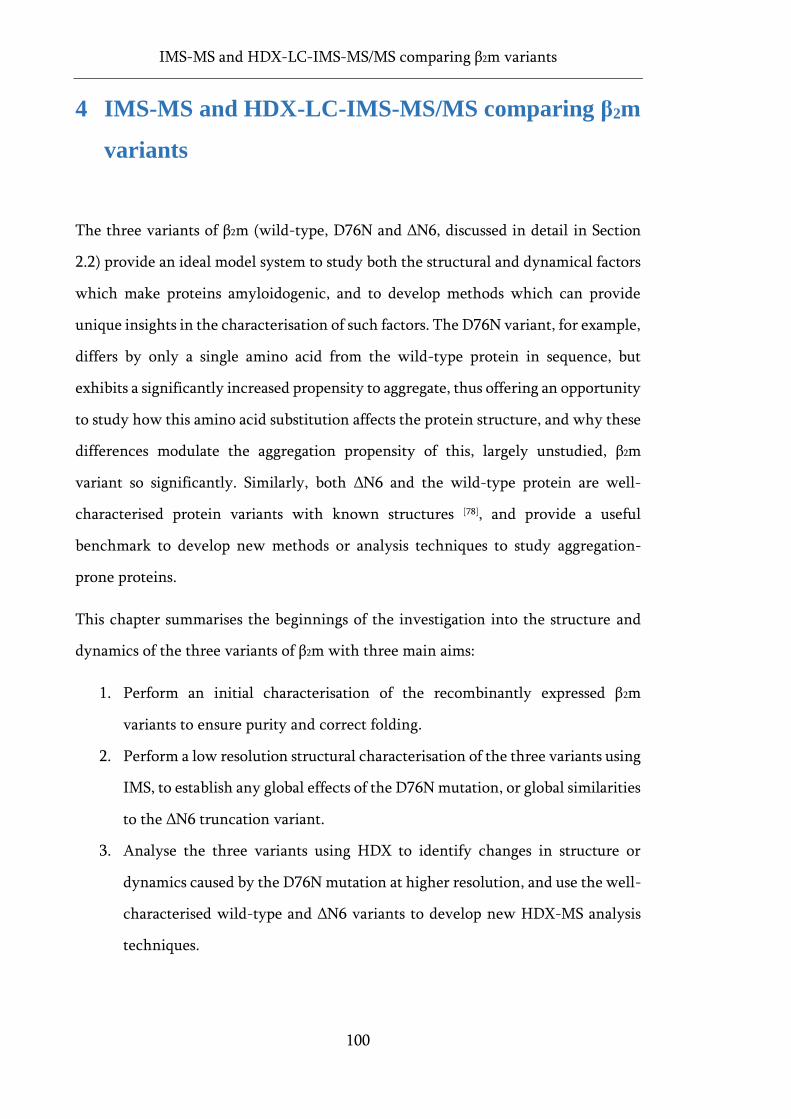
IMS-MS and HDX-LC-IMS-MS/MS comparing β2m variants
100
4 IMS-MS and HDX-LC-IMS-MS/MS comparing β2m
variants
The three variants of β2m (wild-type, D76N and ΔN6, discussed in detail in Section
2.2) provide an ideal model system to study both the structural and dynamical factors
which make proteins amyloidogenic, and to develop methods which can provide
unique insights in the characterisation of such factors. The D76N variant, for example,
differs by only a single amino acid from the wild-type protein in sequence, but
exhibits a significantly increased propensity to aggregate, thus offering an opportunity
to study how this amino acid substitution affects the protein structure, and why these
differences modulate the aggregation propensity of this, largely unstudied, β2m
variant so significantly. Similarly, both ΔN6 and the wild-type protein are well-
characterised protein variants with known structures [78], and provide a useful
benchmark to develop new methods or analysis techniques to study aggregation-
prone proteins.
This chapter summarises the beginnings of the investigation into the structure and
dynamics of the three variants of β2m with three main aims:
1. Perform an initial characterisation of the recombinantly expressed β2m
variants to ensure purity and correct folding.
2. Perform a low resolution structural characterisation of the three variants using
IMS, to establish any global effects of the D76N mutation, or global similarities
to the ΔN6 truncation variant.
3. Analyse the three variants using HDX to identify changes in structure or
dynamics caused by the D76N mutation at higher resolution, and use the well-
characterised wild-type and ΔN6 variants to develop new HDX-MS analysis
techniques.
IMS-MS and HDX-LC-IMS-MS/MS comparing β2m variants
101
Data for the wild-type protein and for the ΔN6 truncation variant shown in the HDX
section of this chapter were subsequently published in Cornwell., et al., JASMS, 2019
[252].
4.1 Protein preparation and initial characterisation
Wild-type, D76N, and ΔN6 β2m were expressed recombinantly and purified as
described in Section 3.1. The final gel filtration purification step showed all three
proteins eluting as a single peak from the size exclusion column (an example of wild-
type β2m is shown in Figure 4.1). SDS-PAGE analysis of fractions collected from the
gel filtration eluate show the elution peak to consist of pure protein with a band at
approximately 12 kDa consistent with the mass of monomeric β2m (Figure 4.1b). For
the wild-type protein, pooling fractions 4-7 (Figure 4.1b) generated a final yield of
~40 mg L-1 (10 L total prepared volume), which was approximately consistent across
all three variants.
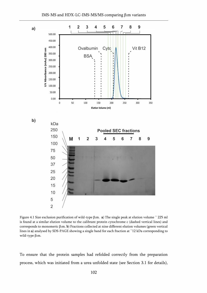
IMS-MS and HDX-LC-IMS-MS/MS comparing β2m variants
102
Figure 4.1 Size exclusion purification of wild-type β2m. a) The single peak at elution volume ~ 225 ml
is found at a similar elution volume to the calibrant protein cytochrome c (dashed vertical lines) and
corresponds to monomeric β2m. b) Fractions collected at nine different elution volumes (green vertical
lines in a) analysed by SDS-PAGE showing a single band for each fraction at ~12 kDa corresponding to
wild-type β2m.
To ensure that the protein samples had refolded correctly from the preparation
process, which was initiated from a urea unfolded state (see Section 3.1 for details),
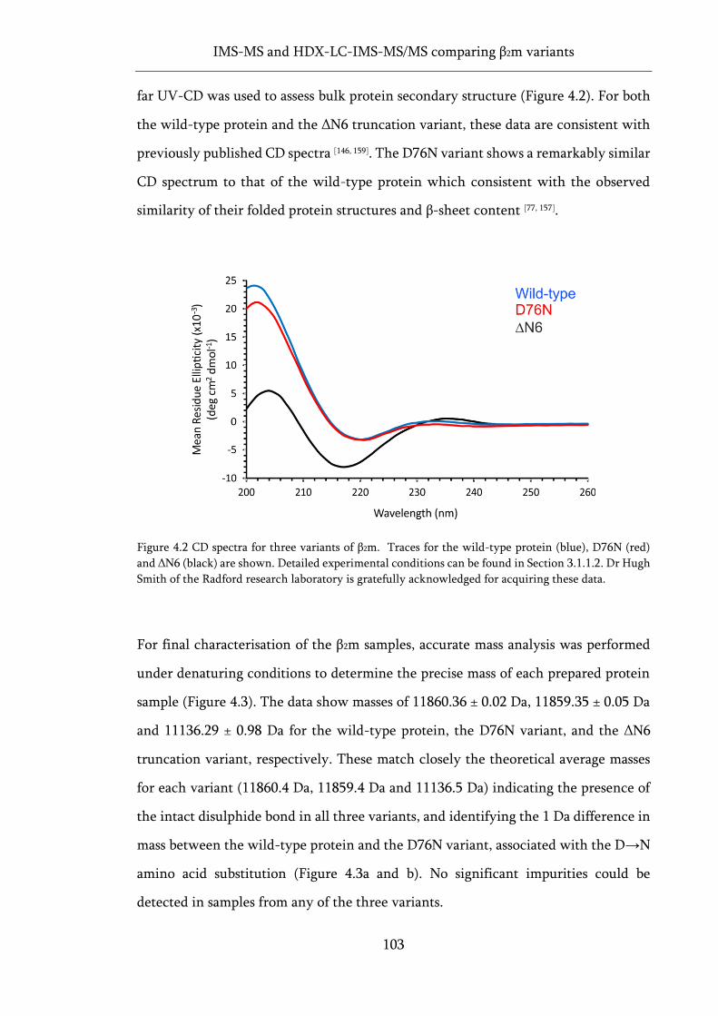
IMS-MS and HDX-LC-IMS-MS/MS comparing β2m variants
103
far UV-CD was used to assess bulk protein secondary structure (Figure 4.2). For both
the wild-type protein and the ΔN6 truncation variant, these data are consistent with
previously published CD spectra [146, 159]. The D76N variant shows a remarkably similar
CD spectrum to that of the wild-type protein which consistent with the observed
similarity of their folded protein structures and β-sheet content [77, 157].
Figure 4.2 CD spectra for three variants of β2m. Traces for the wild-type protein (blue), D76N (red)
and ΔN6 (black) are shown. Detailed experimental conditions can be found in Section 3.1.1.2. Dr Hugh
Smith of the Radford research laboratory is gratefully acknowledged for acquiring these data.
For final characterisation of the β2m samples, accurate mass analysis was performed
under denaturing conditions to determine the precise mass of each prepared protein
sample (Figure 4.3). The data show masses of 11860.36 ± 0.02 Da, 11859.35 ± 0.05 Da
and 11136.29 ± 0.98 Da for the wild-type protein, the D76N variant, and the ΔN6
truncation variant, respectively. These match closely the theoretical average masses
for each variant (11860.4 Da, 11859.4 Da and 11136.5 Da) indicating the presence of
the intact disulphide bond in all three variants, and identifying the 1 Da difference in
mass between the wild-type protein and the D76N variant, associated with the D→N
amino acid substitution (Figure 4.3a and b). No significant impurities could be
detected in samples from any of the three variants.
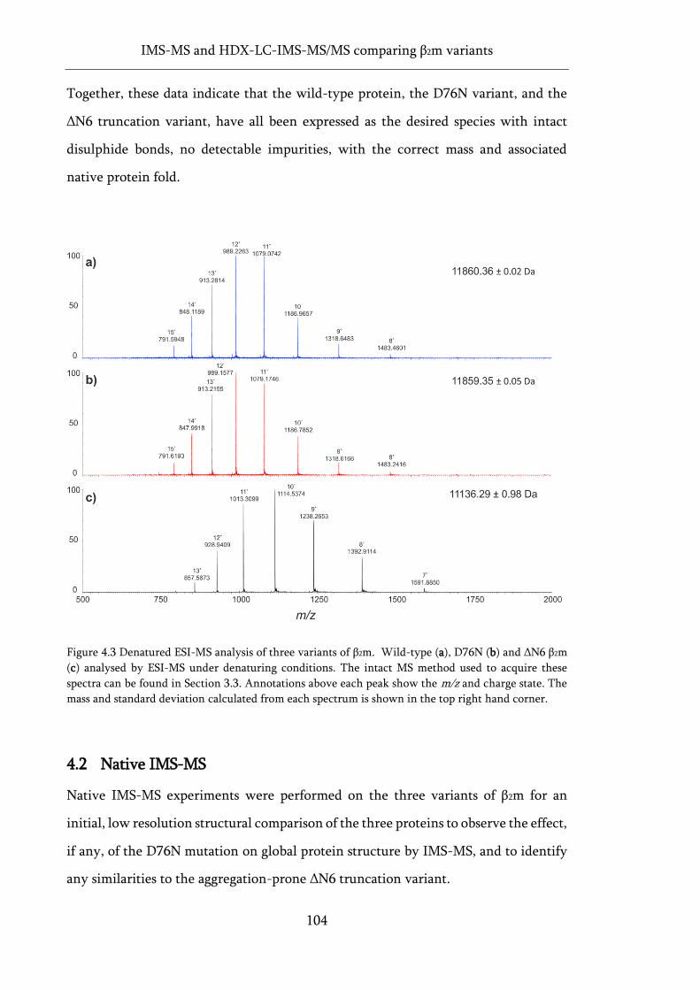
IMS-MS and HDX-LC-IMS-MS/MS comparing β2m variants
104
Together, these data indicate that the wild-type protein, the D76N variant, and the
ΔN6 truncation variant, have all been expressed as the desired species with intact
disulphide bonds, no detectable impurities, with the correct mass and associated
native protein fold.
Figure 4.3 Denatured ESI-MS analysis of three variants of β2m. Wild-type (a), D76N (b) and ΔN6 β2m
(c) analysed by ESI-MS under denaturing conditions. The intact MS method used to acquire these
spectra can be found in Section 3.3. Annotations above each peak show the m/z and charge state. The
mass and standard deviation calculated from each spectrum is shown in the top right hand corner.
4.2 Native IMS-MS
Native IMS-MS experiments were performed on the three variants of β2m for an
initial, low resolution structural comparison of the three proteins to observe the effect,
if any, of the D76N mutation on global protein structure by IMS-MS, and to identify
any similarities to the aggregation-prone ΔN6 truncation variant.
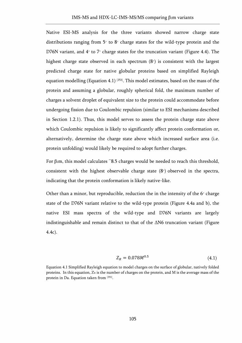
IMS-MS and HDX-LC-IMS-MS/MS comparing β2m variants
105
Native ESI-MS analysis for the three variants showed narrow charge state
distributions ranging from 5+ to 8+ charge states for the wild-type protein and the
D76N variant, and 4+ to 7+ charge states for the truncation variant (Figure 4.4). The
highest charge state observed in each spectrum (8+) is consistent with the largest
predicted charge state for native globular proteins based on simplified Rayleigh
equation modelling (Equation 4.1) [253]. This model estimates, based on the mass of the
protein and assuming a globular, roughly spherical fold, the maximum number of
charges a solvent droplet of equivalent size to the protein could accommodate before
undergoing fission due to Coulombic repulsion (similar to ESI mechanisms described
in Section 1.2.1). Thus, this model serves to assess the protein charge state above
which Coulombic repulsion is likely to significantly affect protein conformation or,
alternatively, determine the charge state above which increased surface area (i.e.
protein unfolding) would likely be required to adopt further charges.
For β2m, this model calculates ~8.5 charges would be needed to reach this threshold,
consistent with the highest observable charge state (8+) observed in the spectra,
indicating that the protein conformation is likely native-like.
Other than a minor, but reproducible, reduction the in the intensity of the 6+ charge
state of the D76N variant relative to the wild-type protein (Figure 4.4a and b), the
native ESI mass spectra of the wild-type and D76N variants are largely
indistinguishable and remain distinct to that of the ΔN6 truncation variant (Figure
4.4c).
𝑍𝑅 = 0.078𝑀0.5 (4.1)
Equation 4.1 Simplified Rayleigh equation to model charges on the surface of globular, natively folded
proteins. In this equation, ZR is the number of charges on the protein, and M is the average mass of the
protein in Da. Equation taken from [253].
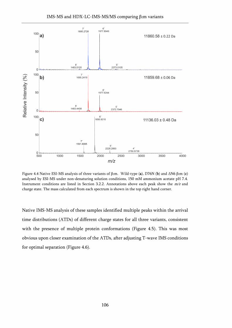
IMS-MS and HDX-LC-IMS-MS/MS comparing β2m variants
106
Figure 4.4 Native ESI-MS analysis of three variants of β2m. Wild-type (a), D76N (b) and ΔN6 β2m (c)
analysed by ESI-MS under non-denaturing solution conditions, 150 mM ammonium acetate pH 7.4.
Instrument conditions are listed in Section 3.2.2. Annotations above each peak show the m/z and
charge state. The mass calculated from each spectrum is shown in the top right hand corner.
Native IMS-MS analysis of these samples identified multiple peaks within the arrival
time distributions (ATDs) of different charge states for all three variants, consistent
with the presence of multiple protein conformations (Figure 4.5). This was most
obvious upon closer examination of the ATDs, after adjusting T-wave IMS conditions
for optimal separation (Figure 4.6).
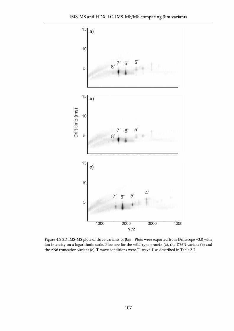
IMS-MS and HDX-LC-IMS-MS/MS comparing β2m variants
107
Figure 4.5 3D IMS-MS plots of three variants of β2m. Plots were exported from Driftscope v3.0 with
ion intensity on a logarithmic scale. Plots are for the wild-type protein (a), the D76N variant (b) and
the ΔN6 truncation variant (c). T-wave conditions were ‘T-wave 1’ as described in Table 3.2.
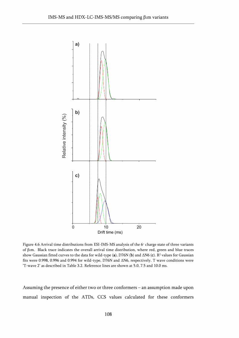
IMS-MS and HDX-LC-IMS-MS/MS comparing β2m variants
108
Figure 4.6 Arrival time distributions from ESI-IMS-MS analysis of the 6+ charge state of three variants
of β2m. Black trace indicates the overall arrival time distribution, where red, green and blue traces
show Gaussian fitted curves to the data for wild-type (a), D76N (b) and ΔN6 (c). R2 values for Gaussian
fits were 0.998, 0.996 and 0.994 for wild-type, D76N and ΔN6, respectively. T wave conditions were
‘T-wave 2’ as described in Table 3.2. Reference lines are shown at 5.0, 7.5 and 10.0 ms.
Assuming the presence of either two or three conformers – an assumption made upon
manual inspection of the ATDs, CCS values calculated for these conformers
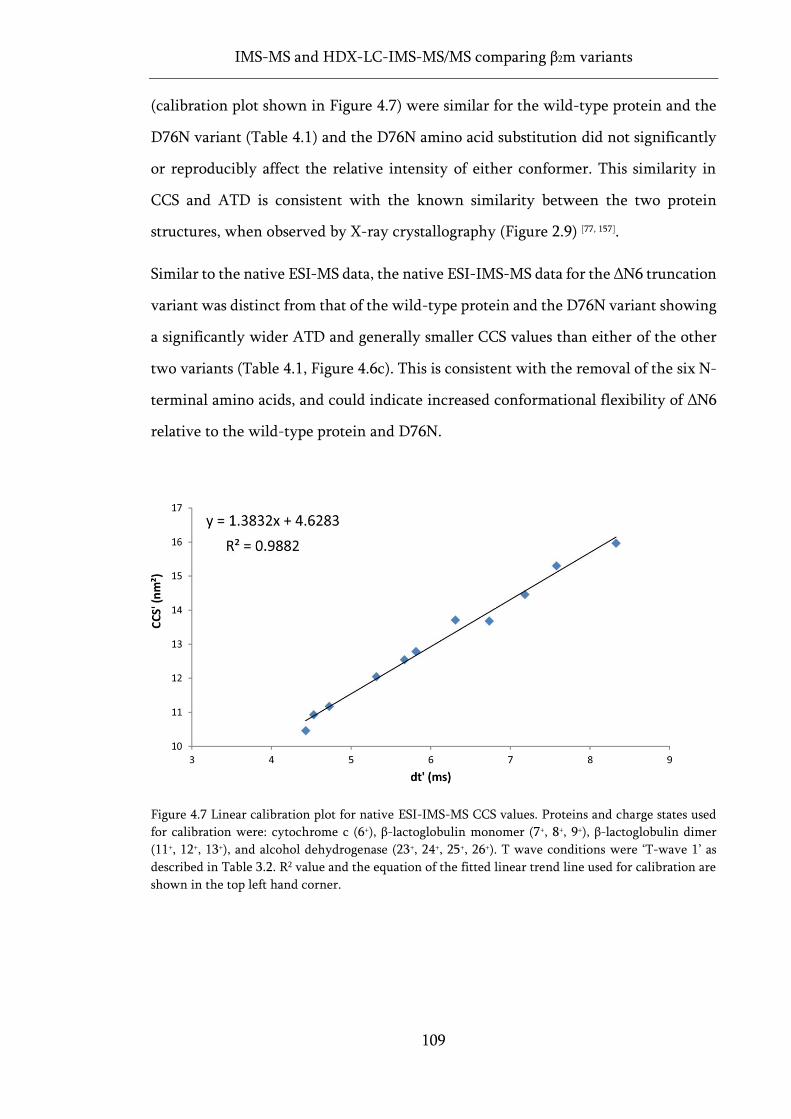
IMS-MS and HDX-LC-IMS-MS/MS comparing β2m variants
109
(calibration plot shown in Figure 4.7) were similar for the wild-type protein and the
D76N variant (Table 4.1) and the D76N amino acid substitution did not significantly
or reproducibly affect the relative intensity of either conformer. This similarity in
CCS and ATD is consistent with the known similarity between the two protein
structures, when observed by X-ray crystallography (Figure 2.9) [77, 157].
Similar to the native ESI-MS data, the native ESI-IMS-MS data for the ΔN6 truncation
variant was distinct from that of the wild-type protein and the D76N variant showing
a significantly wider ATD and generally smaller CCS values than either of the other
two variants (Table 4.1, Figure 4.6c). This is consistent with the removal of the six N-
terminal amino acids, and could indicate increased conformational flexibility of ΔN6
relative to the wild-type protein and D76N.
Figure 4.7 Linear calibration plot for native ESI-IMS-MS CCS values. Proteins and charge states used
for calibration were: cytochrome c (6+), β-lactoglobulin monomer (7+, 8+, 9+), β-lactoglobulin dimer
(11+, 12+, 13+), and alcohol dehydrogenase (23+, 24+, 25+, 26+). T wave conditions were ‘T-wave 1’ as
described in Table 3.2. R2 value and the equation of the fitted linear trend line used for calibration are
shown in the top left hand corner.
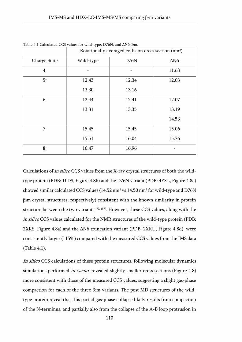
IMS-MS and HDX-LC-IMS-MS/MS comparing β2m variants
110
Table 4.1 Calculated CCS values for wild-type, D76N, and ΔN6 β2m.
Rotationally averaged collision cross section (nm2)
Charge State Wild-type D76N ΔN6
4+ - - 11.63
5+ 12.43
13.30
12.34
13.16
12.03
6+ 12.44
13.31
12.41
13.35
12.07
13.19
14.53
7+ 15.45
15.51
15.45
16.04
15.06
15.76
8+ 16.47 16.96 -
Calculations of in silico CCS values from the X-ray crystal structures of both the wild-
type protein (PDB: 1LDS, Figure 4.8b) and the D76N variant (PDB: 4FXL, Figure 4.8c)
showed similar calculated CCS values (14.52 nm2 vs 14.50 nm2 for wild-type and D76N
β2m crystal structures, respectively) consistent with the known similarity in protein
structure between the two variants [77, 157]. However, these CCS values, along with the
in silico CCS values calculated for the NMR structures of the wild-type protein (PDB:
2XKS, Figure 4.8a) and the ΔN6 truncation variant (PDB: 2XKU, Figure 4.8d), were
consistently larger (~15%) compared with the measured CCS values from the IMS data
(Table 4.1).
In silico CCS calculations of these protein structures, following molecular dynamics
simulations performed in vacuo, revealed slightly smaller cross sections (Figure 4.8)
more consistent with those of the measured CCS values, suggesting a slight gas-phase
compaction for each of the three β2m variants. The post MD structures of the wild-
type protein reveal that this partial gas-phase collapse likely results from compaction
of the N-terminus, and partially also from the collapse of the A-B loop protrusion in
IMS-MS and HDX-LC-IMS-MS/MS comparing β2m variants
111
the crystal structure, a feature absent in the NMR structure (Figure 4.8a and b).
Interestingly, despite this large protrusion that is absent in the NMR structure of the
wild-type protein, the NMR structure of wild-type β2m undergoes significantly more
gas phase reduction in CCS than the crystal structure (~14.5 % compared to 10%),
with a much lower endpoint CCS value. This likely results from the significant shift
in conformation of the flexible D-strand, a rigid element in the crystal structure, the
collapse of which is the likely cause of the difference in CCS between the two post-
MD conformations.
Interestingly, the measured CCS values for the compact and extended conformations
observed for the lowest discernible charge state of the wild-type protein (5+) were
found to be consistent with the post-MD CCS values of the NMR and crystal
structures, respectively. Although curious, the data presented here are insufficient to
determine the identity of the two conformations, and the CCS and relative abundance
of neither is significantly affected by the D76N amino acid substitution.
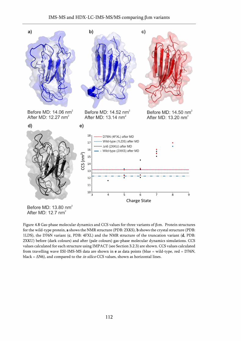
IMS-MS and HDX-LC-IMS-MS/MS comparing β2m variants
112
Figure 4.8 Gas-phase molecular dynamics and CCS values for three variants of β2m. Protein structures
for the wild-type protein, a shows the NMR structure (PDB: 2XKS), b shows the crystal structure (PDB:
1LDS), the D76N variant (c, PDB: 4FXL) and the NMR structure of the truncation variant (d, PDB:
2XKU) before (dark colours) and after (pale colours) gas-phase molecular dynamics simulations. CCS
values calculated for each structure using IMPACT (see Section 3.2.3) are shown. CCS values calculated
from travelling wave ESI-IMS-MS data are shown in e as data points (blue = wild-type, red = D76N,
black = ΔN6), and compared to the in silico CCS values, shown as horizontal lines.
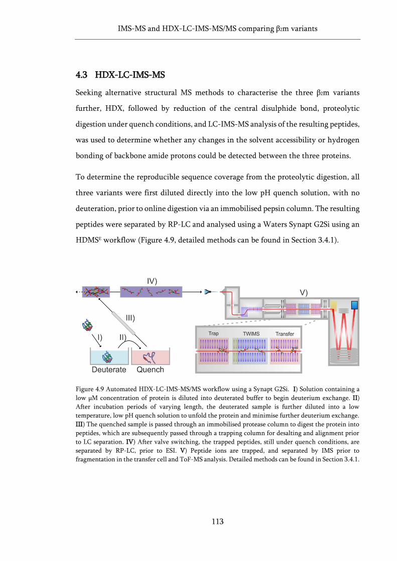
IMS-MS and HDX-LC-IMS-MS/MS comparing β2m variants
113
4.3 HDX-LC-IMS-MS
Seeking alternative structural MS methods to characterise the three β2m variants
further, HDX, followed by reduction of the central disulphide bond, proteolytic
digestion under quench conditions, and LC-IMS-MS analysis of the resulting peptides,
was used to determine whether any changes in the solvent accessibility or hydrogen
bonding of backbone amide protons could be detected between the three proteins.
To determine the reproducible sequence coverage from the proteolytic digestion, all
three variants were first diluted directly into the low pH quench solution, with no
deuteration, prior to online digestion via an immobilised pepsin column. The resulting
peptides were separated by RP-LC and analysed using a Waters Synapt G2Si using an
HDMSE workflow (Figure 4.9, detailed methods can be found in Section 3.4.1).
Figure 4.9 Automated HDX-LC-IMS-MS/MS workflow using a Synapt G2Si. I) Solution containing a
low µM concentration of protein is diluted into deuterated buffer to begin deuterium exchange. II)
After incubation periods of varying length, the deuterated sample is further diluted into a low
temperature, low pH quench solution to unfold the protein and minimise further deuterium exchange.
III) The quenched sample is passed through an immobilised protease column to digest the protein into
peptides, which are subsequently passed through a trapping column for desalting and alignment prior
to LC separation. IV) After valve switching, the trapped peptides, still under quench conditions, are
separated by RP-LC, prior to ESI. V) Peptide ions are trapped, and separated by IMS prior to
fragmentation in the transfer cell and ToF-MS analysis. Detailed methods can be found in Section 3.4.1.
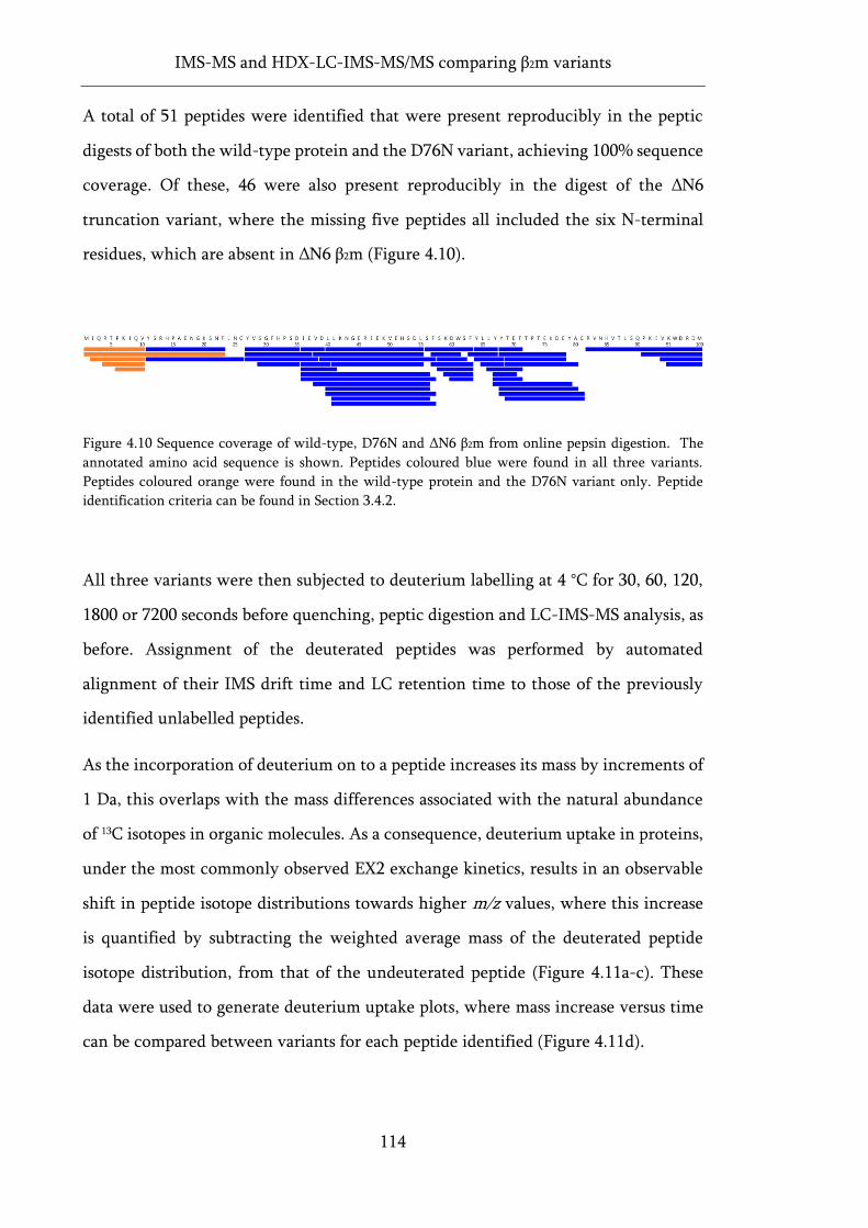
IMS-MS and HDX-LC-IMS-MS/MS comparing β2m variants
114
A total of 51 peptides were identified that were present reproducibly in the peptic
digests of both the wild-type protein and the D76N variant, achieving 100% sequence
coverage. Of these, 46 were also present reproducibly in the digest of the ΔN6
truncation variant, where the missing five peptides all included the six N-terminal
residues, which are absent in ΔN6 β2m (Figure 4.10).
Figure 4.10 Sequence coverage of wild-type, D76N and ΔN6 β2m from online pepsin digestion. The
annotated amino acid sequence is shown. Peptides coloured blue were found in all three variants.
Peptides coloured orange were found in the wild-type protein and the D76N variant only. Peptide
identification criteria can be found in Section 3.4.2.
All three variants were then subjected to deuterium labelling at 4 °C for 30, 60, 120,
1800 or 7200 seconds before quenching, peptic digestion and LC-IMS-MS analysis, as
before. Assignment of the deuterated peptides was performed by automated
alignment of their IMS drift time and LC retention time to those of the previously
identified unlabelled peptides.
As the incorporation of deuterium on to a peptide increases its mass by increments of
1 Da, this overlaps with the mass differences associated with the natural abundance
of 13C isotopes in organic molecules. As a consequence, deuterium uptake in proteins,
under the most commonly observed EX2 exchange kinetics, results in an observable
shift in peptide isotope distributions towards higher m/z values, where this increase
is quantified by subtracting the weighted average mass of the deuterated peptide
isotope distribution, from that of the undeuterated peptide (Figure 4.11a-c). These
data were used to generate deuterium uptake plots, where mass increase versus time
can be compared between variants for each peptide identified (Figure 4.11d).
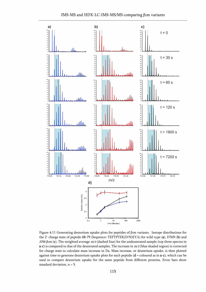
IMS-MS and HDX-LC-IMS-MS/MS comparing β2m variants
115
Figure 4.11 Generating deuterium uptake plots for peptides of β2m variants. Isotope distributions for
the 2+ charge state of peptide 68-79 (Sequence: TEFTPTEK(D/N)EYA) for wild-type (a), D76N (b) and
ΔN6 β2m (c). The weighted average m/z (dashed line) for the undeuterated sample (top three spectra in
a-c) is compared to that of the deuterated samples. The increase in m/z (blue shaded region) is corrected
for charge state to calculate mass increase in Da. Mass increase, or deuterium uptake, is then plotted
against time to generate deuterium uptake plots for each peptide (d – coloured as in a-c), which can be
used to compare deuterium uptake for the same peptide from different proteins. Error bars show
standard deviation, n = 5.
IMS-MS and HDX-LC-IMS-MS/MS comparing β2m variants
116
The most obvious identifiable differences between the three variants were
significantly increased deuterium uptake in the ΔN6 truncation variant, relative to the
wild-type protein and the D76N variant, on peptides surrounding the D-E loop
(residues 56-60), B-C loop (28-34) and the C-terminus (81-99), regions where
deuterium uptake in the wild-type and D76N proteins were remarkably similar to
each other (Figure 4.12). Multiple overlapping peptides covering the same regions
were also identified, most of which showed similar trends of increased deuterium
uptake in ΔN6. However, in some instances the overlapping peptides showed differing
trends. For example, although peptide 81-99, covering the C-terminus of β2m, showed
higher deuterium incorporation in the truncation variant relative to the other two
proteins, peptides covering the final six residues in the C-terminus (94-99) showed no
significant difference in uptake between any of the variants (Figure 4.12). Instances
of this nature make data interpretation challenging, as multiple, sometimes
contradictory, uptake plots of overlapping peptides covering the same region, with
varying degrees of overlap, need to be interpreted simultaneously, across multiple
different proteins, as well as multiple different time points, to determine the regions
of most significant difference.
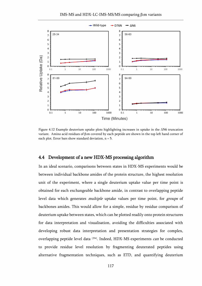
IMS-MS and HDX-LC-IMS-MS/MS comparing β2m variants
117
Figure 4.12 Example deuterium uptake plots highlighting increases in uptake in the ΔN6 truncation
variant. Amino acid residues of β2m covered by each peptide are shown in the top left hand corner of
each plot. Error bars show standard deviation, n = 5.
4.4 Development of a new HDX-MS processing algorithm
In an ideal scenario, comparisons between states in HDX-MS experiments would be
between individual backbone amides of the protein structure, the highest resolution
unit of the experiment, where a single deuterium uptake value per time point is
obtained for each exchangeable backbone amide, in contrast to overlapping peptide
level data which generates multiple uptake values per time point, for groups of
backbones amides. This would allow for a simple, residue by residue comparison of
deuterium uptake between states, which can be plotted readily onto protein structures
for data interpretation and visualisation, avoiding the difficulties associated with
developing robust data interpretation and presentation strategies for complex,
overlapping peptide level data [254]. Indeed, HDX-MS experiments can be conducted
to provide residue level resolution by fragmenting deuterated peptides using
alternative fragmentation techniques, such as ETD, and quantifying deuterium
IMS-MS and HDX-LC-IMS-MS/MS comparing β2m variants
118
incorporation at each backbone amide by analysing the isotope distributions of the
resulting fragment ions [216, 255]. However, these experiments are plagued by poor,
charge dependent fragmentation efficiency, often requiring the addition of non-
volatile supercharging reagents to achieve adequate peptide fragmentation [255].
Similarly, MS source conditions must be carefully tuned to avoid transferring excess
internal energy to peptide ions, and minimise gas phase scrambling of the non-
covalent and labile, deuterium label [216, 256]. This additional experimental complexity
is such that, despite the problematic interpretation and visualisation, HDX-MS
experiments are typically performed to peptide level resolution [206, 257].
Numerous efforts have been made to consolidate peptide level deuterium uptake data
to attain a single uptake value per amino acid, and simplify comparisons between
states. One popular approach is a subtraction analysis, whereby the deuterium content
of the overlapped region between peptides is calculated from the difference in
deuterium content of the two peptides which overlap [258]. In the example presented
in Figure 4.12, this would mean the deuterium content, and any differences in uptake
between the three variants of β2m, between residues 81-93 could be assessed by
subtracting the deuterium content of peptide 94-99 from peptide 81-99. While
conceptually appealing, there are several problems with this approach. Firstly, in cases
where more than two peptides cover the same overlapped region, multiple subtraction
analyses are possible, which can still result in multiple uptake values per exchangeable
amide. For example, two additional peptides, that cover the C-terminal ~10 amino
acids of β2m (other than the two listed above) were also identified (Figure 4.10), so a
simple subtraction of peptides 81-99 and 94-99 would discard these, otherwise valid,
data. Secondly, recent evidence suggests that, excepting cases where almost complete
deuterium retention on the overlapped peptides can be achieved (i.e. no back
exchange), subtraction analyses often provide unreliable results, as peptides of
different lengths but similar sequence, can form different secondary structures, such
as alpha helices, under quench conditions [257]. The resulting differential hydrogen
bonds that form can change the back exchange behaviour of the peptide and, as such,

IMS-MS and HDX-LC-IMS-MS/MS comparing β2m variants
119
the deuterium uptake values for identical amide groups present on different peptides
cannot be considered equivalent [257].
Many commercial HDX-MS processing methods, such as those in the Waters DynamX
software used in our studies, circumvent this issue entirely by plotting data for all
observed peptides, ordered by amino acid starting position, next to one another on the
x axis, against change in absolute mass on the y axis, for each time point [259]. These so
called ‘butterfly plots’, have an advantage in that they present the raw data in a
minimally processed form. However, as a result, they can be challenging to interpret
and visualise, as peptide lengths, and the regions of the protein each peptides covers,
are not readily identifiable. Similarly, a threshold for differences in absolute mass
between peptides of different states is typically set as the determinant of statistically
significant difference [260, 261]. This can be misleading, however, as the biological
significance of that mass change is somewhat dependent on the length of the peptide,
which is not typically taken into account when measuring only changes in absolute
mass. For instance, a difference of 0.5 Da in the weighted average mass of a 20 amino
acid long peptide between two states, would appear, on a butterfly plot, to be of equal
significance to the same mass difference on a five amino acid long peptide, despite
being four times more concentrated, in terms of mass increase per exchangeable site,
in the latter example.
One novel approach however, designed to consolidate peptide level data across
multiple time points into a single plot, sums the mass increase for a given peptide
across all measured time points, before correcting for the number of exchangeable
sites in the peptide, generating a single, fractional mass increase value for each peptide
observed [170, 262]. These values are then averaged across all peptides covering a
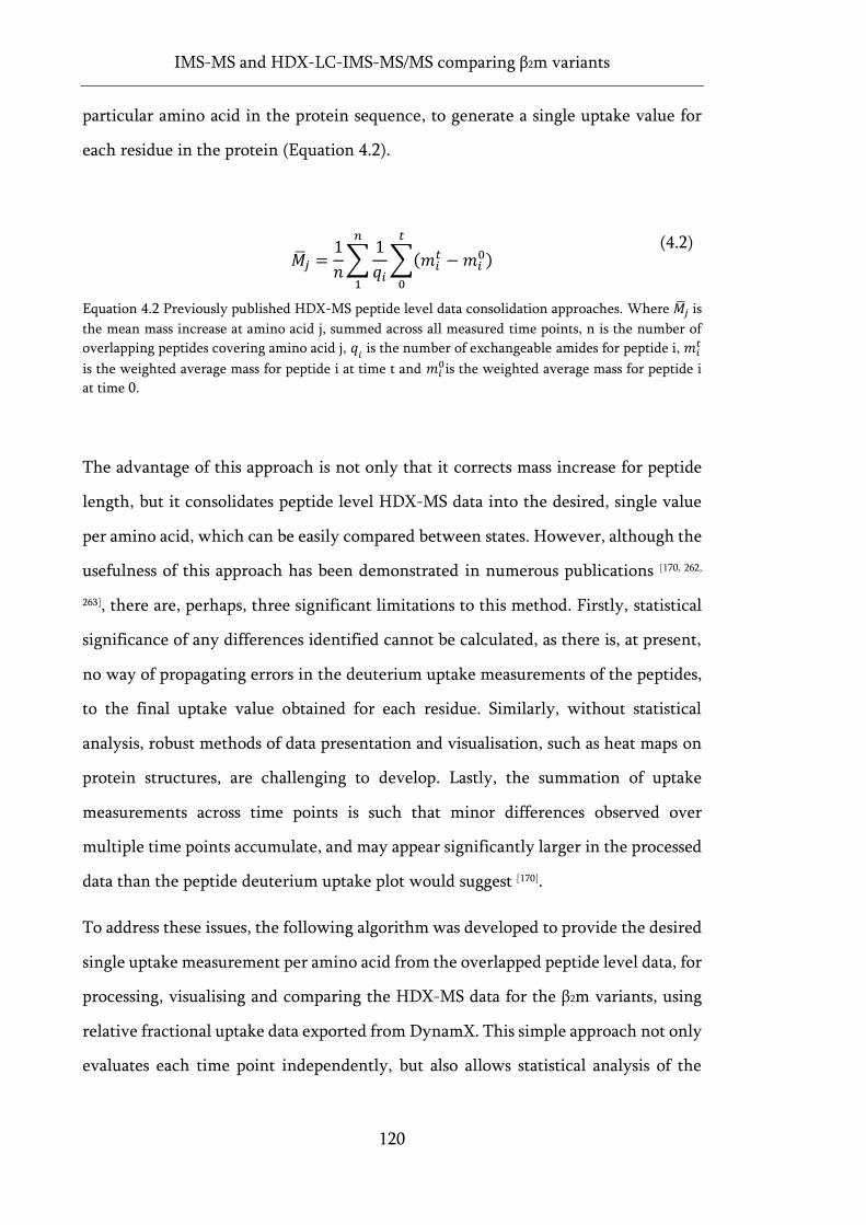
IMS-MS and HDX-LC-IMS-MS/MS comparing β2m variants
120
particular amino acid in the protein sequence, to generate a single uptake value for
each residue in the protein (Equation 4.2).
𝑗 =
1
𝑛∑
1
𝑞𝑖∑(𝑚𝑖
𝑡 −𝑚𝑖0)
𝑡
0
𝑛
1
(4.2)
Equation 4.2 Previously published HDX-MS peptide level data consolidation approaches. Where 𝑗 is
the mean mass increase at amino acid j, summed across all measured time points, n is the number of
overlapping peptides covering amino acid j, 𝑞𝑖 is the number of exchangeable amides for peptide i, 𝑚𝑖
𝑡
is the weighted average mass for peptide i at time t and 𝑚𝑖0is the weighted average mass for peptide i
at time 0.
The advantage of this approach is not only that it corrects mass increase for peptide
length, but it consolidates peptide level HDX-MS data into the desired, single value
per amino acid, which can be easily compared between states. However, although the
usefulness of this approach has been demonstrated in numerous publications [170, 262,
263], there are, perhaps, three significant limitations to this method. Firstly, statistical
significance of any differences identified cannot be calculated, as there is, at present,
no way of propagating errors in the deuterium uptake measurements of the peptides,
to the final uptake value obtained for each residue. Similarly, without statistical
analysis, robust methods of data presentation and visualisation, such as heat maps on
protein structures, are challenging to develop. Lastly, the summation of uptake
measurements across time points is such that minor differences observed over
multiple time points accumulate, and may appear significantly larger in the processed
data than the peptide deuterium uptake plot would suggest [170].
To address these issues, the following algorithm was developed to provide the desired
single uptake measurement per amino acid from the overlapped peptide level data, for
processing, visualising and comparing the HDX-MS data for the β2m variants, using
relative fractional uptake data exported from DynamX. This simple approach not only
evaluates each time point independently, but also allows statistical analysis of the
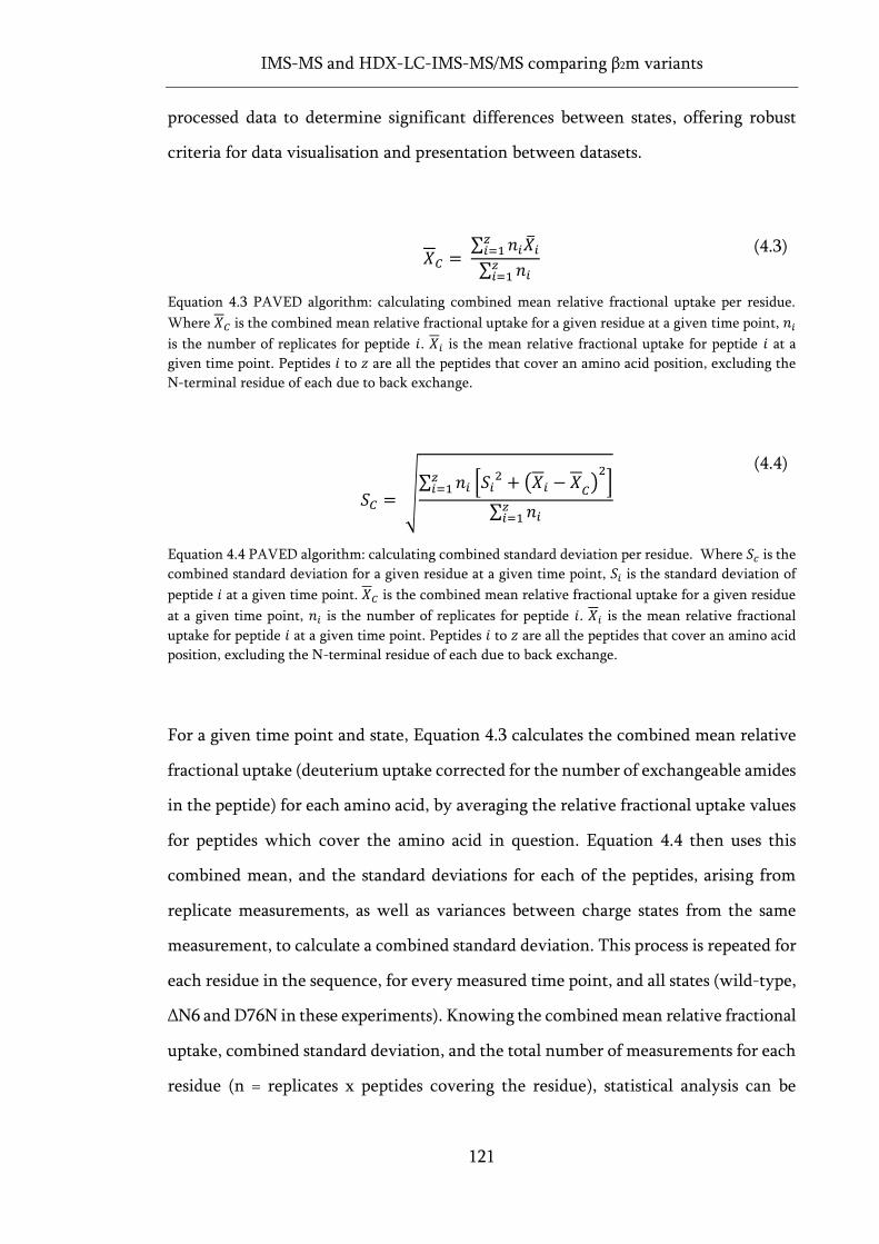
IMS-MS and HDX-LC-IMS-MS/MS comparing β2m variants
121
processed data to determine significant differences between states, offering robust
criteria for data visualisation and presentation between datasets.
𝑋𝐶 =
∑ 𝑛𝑖𝑖𝑧𝑖=1
∑ 𝑛𝑖𝑧𝑖=1
(4.3)
Equation 4.3 PAVED algorithm: calculating combined mean relative fractional uptake per residue.
Where 𝑋𝐶 is the combined mean relative fractional uptake for a given residue at a given time point, 𝑛𝑖
is the number of replicates for peptide 𝑖. 𝑋𝑖 is the mean relative fractional uptake for peptide 𝑖 at a
given time point. Peptides 𝑖 to 𝑧 are all the peptides that cover an amino acid position, excluding the
N-terminal residue of each due to back exchange.
𝑆𝐶 = √∑ 𝑛𝑖𝑧𝑖=1 [𝑆𝑖
2 + (𝑋𝑖 − 𝑋𝐶)2]
∑ 𝑛𝑖𝑧𝑖=1
(4.4)
Equation 4.4 PAVED algorithm: calculating combined standard deviation per residue. Where 𝑆𝑐 is the
combined standard deviation for a given residue at a given time point, 𝑆𝑖 is the standard deviation of
peptide 𝑖 at a given time point. 𝑋𝐶 is the combined mean relative fractional uptake for a given residue
at a given time point, 𝑛𝑖 is the number of replicates for peptide 𝑖. 𝑋𝑖 is the mean relative fractional
uptake for peptide 𝑖 at a given time point. Peptides 𝑖 to 𝑧 are all the peptides that cover an amino acid
position, excluding the N-terminal residue of each due to back exchange.
For a given time point and state, Equation 4.3 calculates the combined mean relative
fractional uptake (deuterium uptake corrected for the number of exchangeable amides
in the peptide) for each amino acid, by averaging the relative fractional uptake values
for peptides which cover the amino acid in question. Equation 4.4 then uses this
combined mean, and the standard deviations for each of the peptides, arising from
replicate measurements, as well as variances between charge states from the same
measurement, to calculate a combined standard deviation. This process is repeated for
each residue in the sequence, for every measured time point, and all states (wild-type,
ΔN6 and D76N in these experiments). Knowing the combined mean relative fractional
uptake, combined standard deviation, and the total number of measurements for each
residue (n = replicates x peptides covering the residue), statistical analysis can be
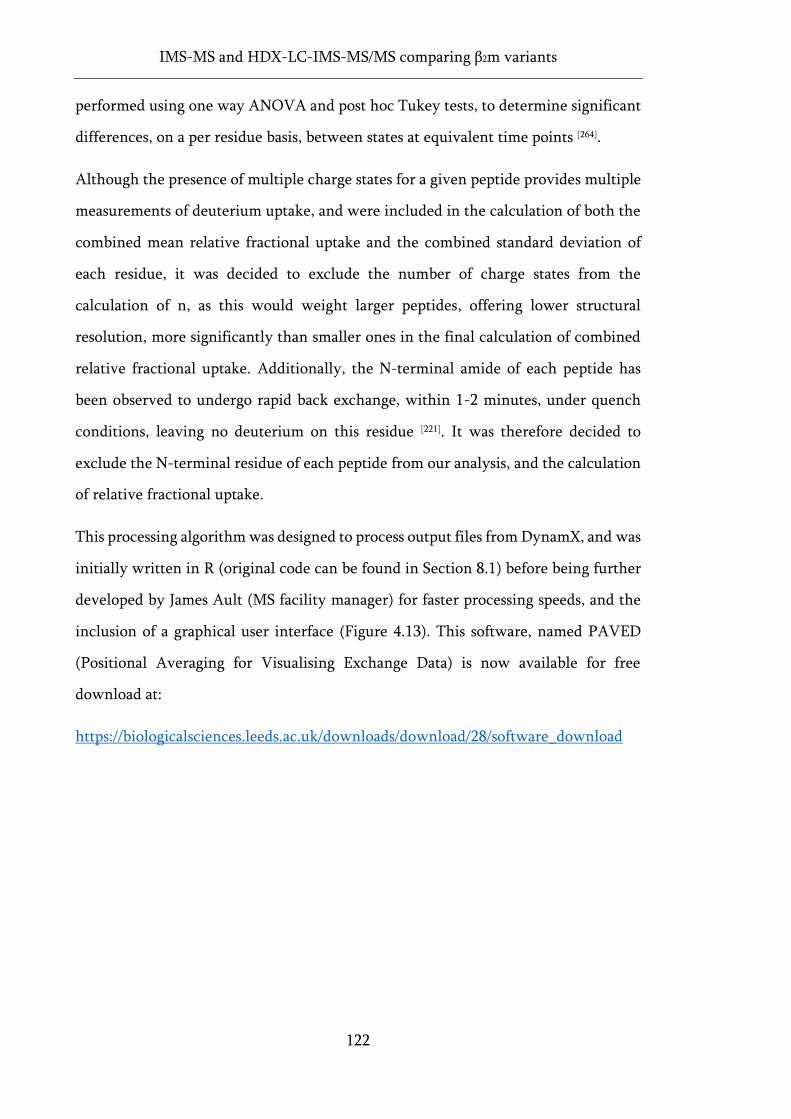
IMS-MS and HDX-LC-IMS-MS/MS comparing β2m variants
122
performed using one way ANOVA and post hoc Tukey tests, to determine significant
differences, on a per residue basis, between states at equivalent time points [264].
Although the presence of multiple charge states for a given peptide provides multiple
measurements of deuterium uptake, and were included in the calculation of both the
combined mean relative fractional uptake and the combined standard deviation of
each residue, it was decided to exclude the number of charge states from the
calculation of n, as this would weight larger peptides, offering lower structural
resolution, more significantly than smaller ones in the final calculation of combined
relative fractional uptake. Additionally, the N-terminal amide of each peptide has
been observed to undergo rapid back exchange, within 1-2 minutes, under quench
conditions, leaving no deuterium on this residue [221]. It was therefore decided to
exclude the N-terminal residue of each peptide from our analysis, and the calculation
of relative fractional uptake.
This processing algorithm was designed to process output files from DynamX, and was
initially written in R (original code can be found in Section 8.1) before being further
developed by James Ault (MS facility manager) for faster processing speeds, and the
inclusion of a graphical user interface (Figure 4.13). This software, named PAVED
(Positional Averaging for Visualising Exchange Data) is now available for free
download at:
https://biologicalsciences.leeds.ac.uk/downloads/download/28/software_download
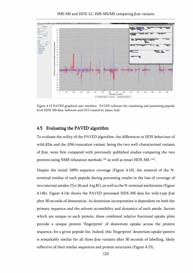
IMS-MS and HDX-LC-IMS-MS/MS comparing β2m variants
123
Figure 4.13 PAVED graphical user interface. PAVED software for visualising and presenting peptide
level HDX-MS data. Software and GUI created by James Ault.
4.5 Evaluating the PAVED algorithm
To evaluate the utility of the PAVED algorithm, the differences in HDX behaviour of
wild-β2m and the ΔN6 truncation variant, being the two well-characterised variants
of β2m, were first compared with previously published studies comparing the two
proteins using NMR relaxation methods [78] as well as intact HDX-MS [134].
Despite the initial 100% sequence coverage (Figure 4.10), the removal of the N-
terminal residue of each peptide during processing results in the loss of coverage of
two internal amides (Tyr 26 and Arg 81), as well as the N-terminal methionine (Figure
4.14b). Figure 4.14c shows the PAVED processed HDX-MS data for wild-type β2m
after 30 seconds of deuteration. As deuterium incorporation is dependent on both the
primary sequence and the solvent accessibility and dynamics of each amide, factors
which are unique to each protein, these combined relative fractional uptake plots
provide a unique protein ‘fingerprint’ of deuterium uptake across the protein
sequence, for a given peptide list. Indeed, this ‘fingerprint’ deuterium uptake pattern
is remarkably similar for all three β2m variants after 30 seconds of labelling, likely
reflective of their similar sequences and protein structures (Figure 4.15).
IMS-MS and HDX-LC-IMS-MS/MS comparing β2m variants
124
After processing, significant errors in the combined mean relative fractional uptake
values are observed across all three variants between residues 35-40 and 65-70 (Figure
4.14c, Figure 4.15). This is due to the positional averaging of peptides with minimal
overlap, covering different regions of the protein, which have significantly different
relative fractional uptake values, and accurately reflects the uncertainty of the
deuterium uptake measurements in these regions (Figure 4.14a and b). The same effect
is observed in ΔN6 at the C-terminal region (residues 90-99) where overlapping
peptides discussed earlier (peptides 81-99 and 94-99, Figure 4.12) showed differing
trends with regards to the deuterium uptake differences relative to the wild-type
protein. Here, the positional averaging algorithm has reduced the combined mean
relative fractional uptake at the extreme C-terminus to show no statistical significance
to the wild-type protein, but significant differences are shown between residues 82-
90 (F-G loop), accurately reflecting the complex overlapping peptide level data for
this region (Figure 4.12, Figure 4.15, Figure 4.17).
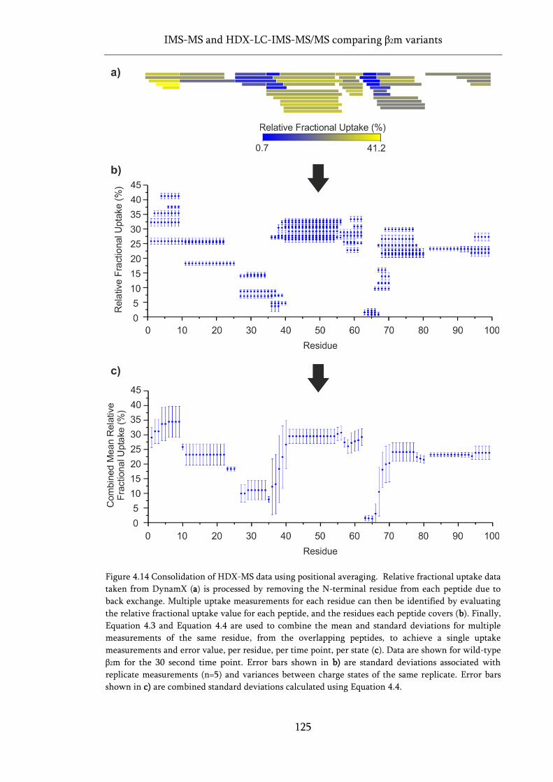
IMS-MS and HDX-LC-IMS-MS/MS comparing β2m variants
125
Figure 4.14 Consolidation of HDX-MS data using positional averaging. Relative fractional uptake data
taken from DynamX (a) is processed by removing the N-terminal residue from each peptide due to
back exchange. Multiple uptake measurements for each residue can then be identified by evaluating
the relative fractional uptake value for each peptide, and the residues each peptide covers (b). Finally,
Equation 4.3 and Equation 4.4 are used to combine the mean and standard deviations for multiple
measurements of the same residue, from the overlapping peptides, to achieve a single uptake
measurements and error value, per residue, per time point, per state (c). Data are shown for wild-type
β2m for the 30 second time point. Error bars shown in b) are standard deviations associated with
replicate measurements (n=5) and variances between charge states of the same replicate. Error bars
shown in c) are combined standard deviations calculated using Equation 4.4.
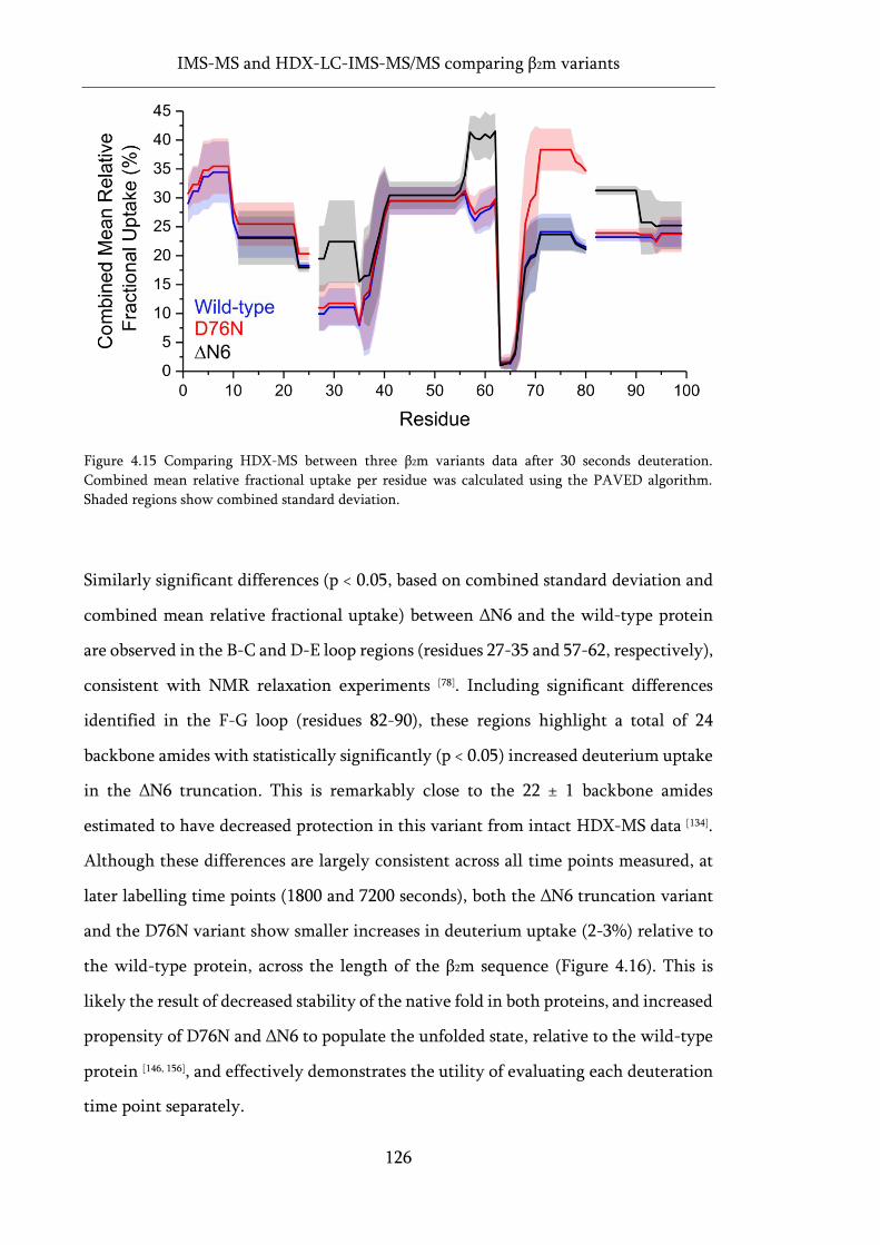
IMS-MS and HDX-LC-IMS-MS/MS comparing β2m variants
126
Figure 4.15 Comparing HDX-MS between three β2m variants data after 30 seconds deuteration.
Combined mean relative fractional uptake per residue was calculated using the PAVED algorithm.
Shaded regions show combined standard deviation.
Similarly significant differences (p < 0.05, based on combined standard deviation and
combined mean relative fractional uptake) between ΔN6 and the wild-type protein
are observed in the B-C and D-E loop regions (residues 27-35 and 57-62, respectively),
consistent with NMR relaxation experiments [78]. Including significant differences
identified in the F-G loop (residues 82-90), these regions highlight a total of 24
backbone amides with statistically significantly (p < 0.05) increased deuterium uptake
in the ΔN6 truncation. This is remarkably close to the 22 ± 1 backbone amides
estimated to have decreased protection in this variant from intact HDX-MS data [134].
Although these differences are largely consistent across all time points measured, at
later labelling time points (1800 and 7200 seconds), both the ΔN6 truncation variant
and the D76N variant show smaller increases in deuterium uptake (2-3%) relative to
the wild-type protein, across the length of the β2m sequence (Figure 4.16). This is
likely the result of decreased stability of the native fold in both proteins, and increased
propensity of D76N and ΔN6 to populate the unfolded state, relative to the wild-type
protein [146, 156], and effectively demonstrates the utility of evaluating each deuteration
time point separately.
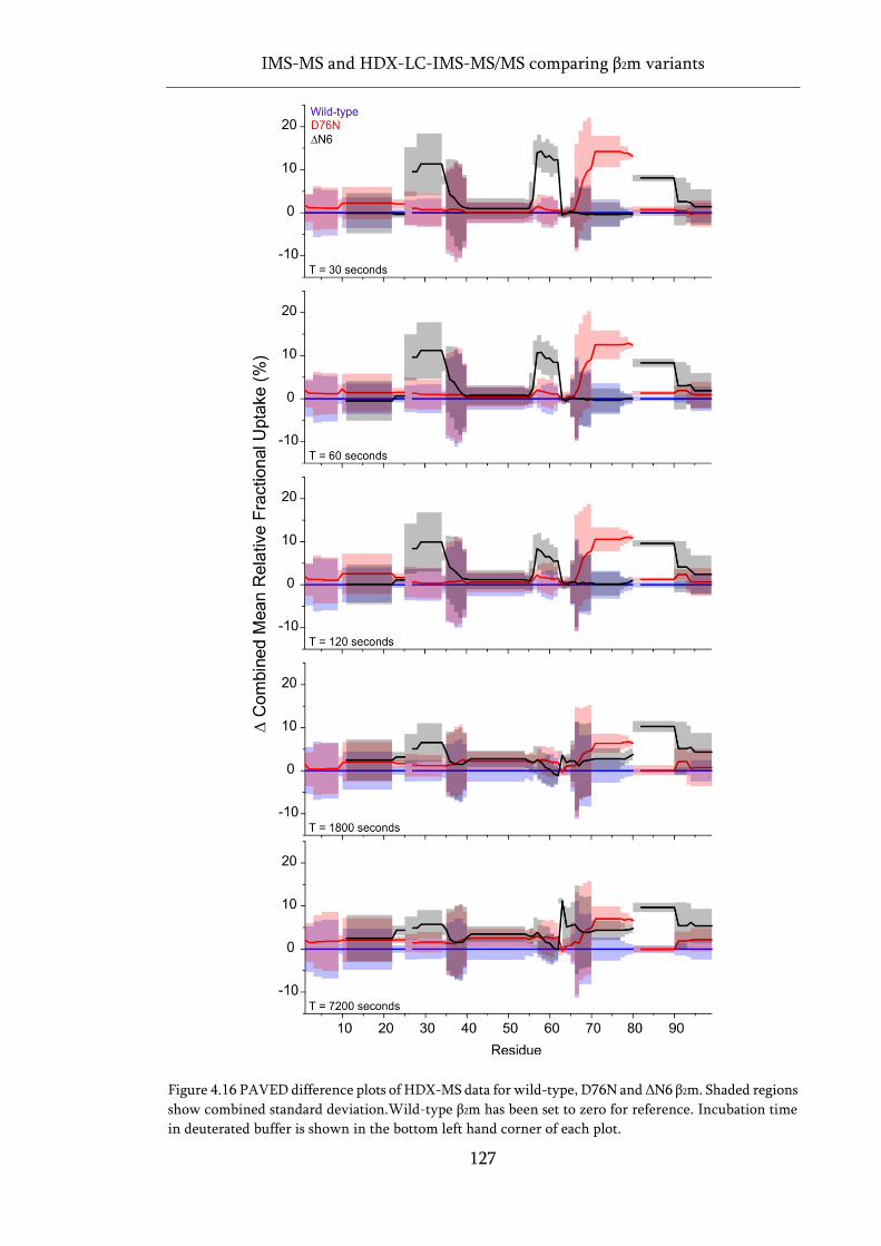
IMS-MS and HDX-LC-IMS-MS/MS comparing β2m variants
127
Figure 4.16 PAVED difference plots of HDX-MS data for wild-type, D76N and ΔN6 β2m. Shaded regions
show combined standard deviation.Wild-type β2m has been set to zero for reference. Incubation time
in deuterated buffer is shown in the bottom left hand corner of each plot.
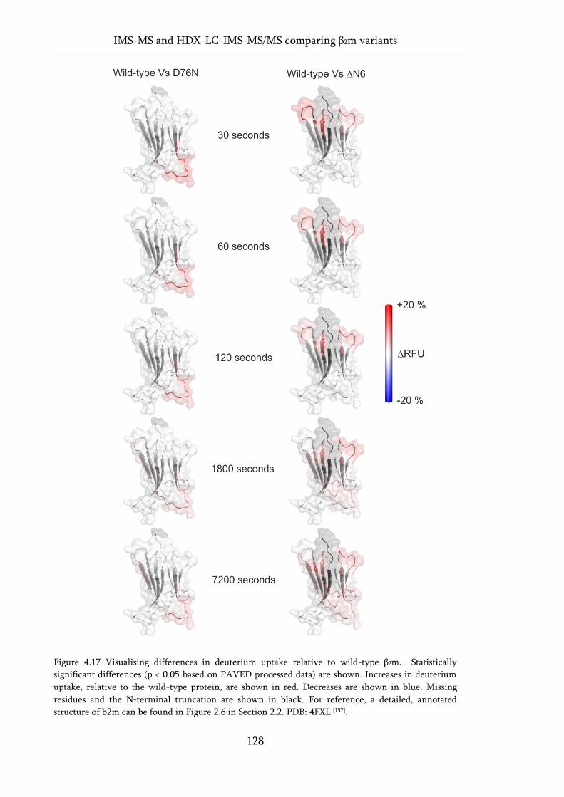
IMS-MS and HDX-LC-IMS-MS/MS comparing β2m variants
128
Figure 4.17 Visualising differences in deuterium uptake relative to wild-type β2m. Statistically
significant differences (p < 0.05 based on PAVED processed data) are shown. Increases in deuterium
uptake, relative to the wild-type protein, are shown in red. Decreases are shown in blue. Missing
residues and the N-terminal truncation are shown in black. For reference, a detailed, annotated
structure of b2m can be found in Figure 2.6 in Section 2.2. PDB: 4FXL [157].
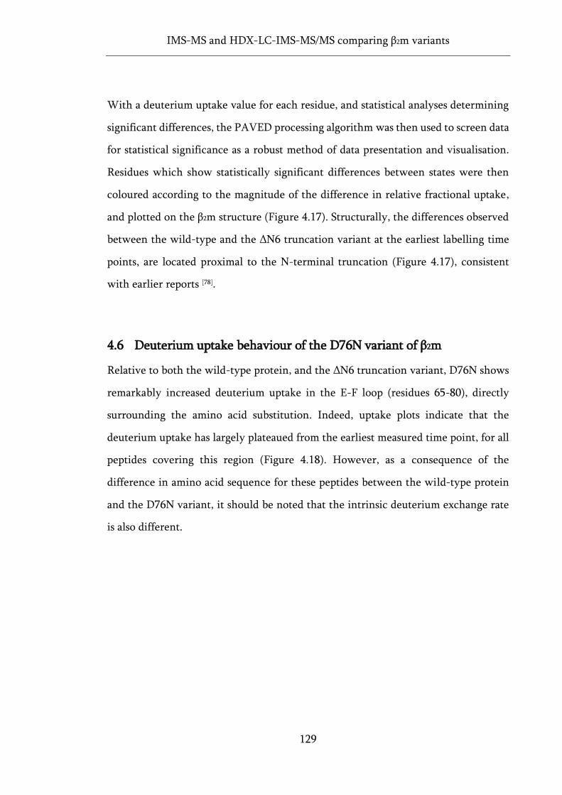
IMS-MS and HDX-LC-IMS-MS/MS comparing β2m variants
129
With a deuterium uptake value for each residue, and statistical analyses determining
significant differences, the PAVED processing algorithm was then used to screen data
for statistical significance as a robust method of data presentation and visualisation.
Residues which show statistically significant differences between states were then
coloured according to the magnitude of the difference in relative fractional uptake,
and plotted on the β2m structure (Figure 4.17). Structurally, the differences observed
between the wild-type and the ΔN6 truncation variant at the earliest labelling time
points, are located proximal to the N-terminal truncation (Figure 4.17), consistent
with earlier reports [78].
4.6 Deuterium uptake behaviour of the D76N variant of β2m
Relative to both the wild-type protein, and the ΔN6 truncation variant, D76N shows
remarkably increased deuterium uptake in the E-F loop (residues 65-80), directly
surrounding the amino acid substitution. Indeed, uptake plots indicate that the
deuterium uptake has largely plateaued from the earliest measured time point, for all
peptides covering this region (Figure 4.18). However, as a consequence of the
difference in amino acid sequence for these peptides between the wild-type protein
and the D76N variant, it should be noted that the intrinsic deuterium exchange rate
is also different.
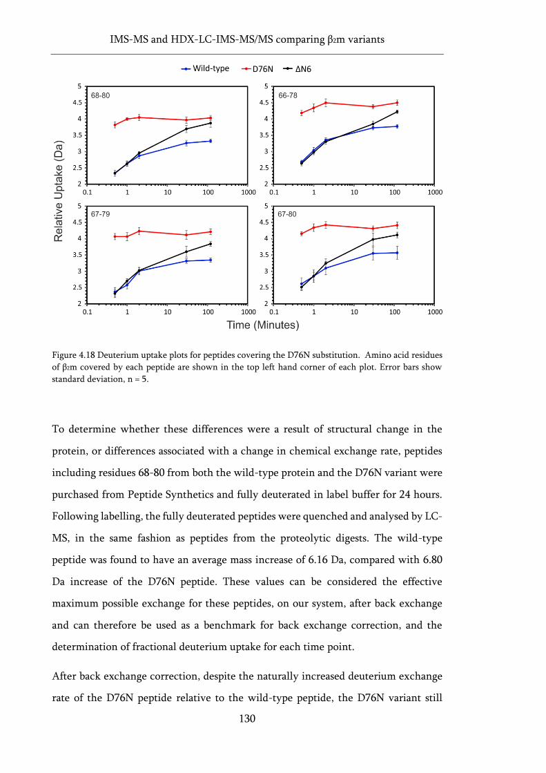
IMS-MS and HDX-LC-IMS-MS/MS comparing β2m variants
130
Figure 4.18 Deuterium uptake plots for peptides covering the D76N substitution. Amino acid residues
of β2m covered by each peptide are shown in the top left hand corner of each plot. Error bars show
standard deviation, n = 5.
To determine whether these differences were a result of structural change in the
protein, or differences associated with a change in chemical exchange rate, peptides
including residues 68-80 from both the wild-type protein and the D76N variant were
purchased from Peptide Synthetics and fully deuterated in label buffer for 24 hours.
Following labelling, the fully deuterated peptides were quenched and analysed by LC-
MS, in the same fashion as peptides from the proteolytic digests. The wild-type
peptide was found to have an average mass increase of 6.16 Da, compared with 6.80
Da increase of the D76N peptide. These values can be considered the effective
maximum possible exchange for these peptides, on our system, after back exchange
and can therefore be used as a benchmark for back exchange correction, and the
determination of fractional deuterium uptake for each time point.
After back exchange correction, despite the naturally increased deuterium exchange
rate of the D76N peptide relative to the wild-type peptide, the D76N variant still
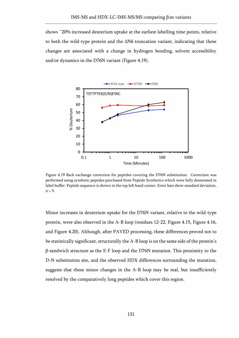
IMS-MS and HDX-LC-IMS-MS/MS comparing β2m variants
131
shows ~20% increased deuterium uptake at the earliest labelling time points, relative
to both the wild-type protein and the ΔN6 truncation variant, indicating that these
changes are associated with a change in hydrogen bonding, solvent accessibility
and/or dynamics in the D76N variant (Figure 4.19).
Figure 4.19 Back exchange correction for peptides covering the D76N substitution. Correction was
performed using synthetic peptides purchased from Peptide Synthetics which were fully deuterated in
label buffer. Peptide sequence is shown in the top left hand corner. Error bars show standard deviation,
n = 5.
Minor increases in deuterium uptake for the D76N variant, relative to the wild-type
protein, were also observed in the A-B loop (residues 12-22, Figure 4.15, Figure 4.16,
and Figure 4.20). Although, after PAVED processing, these differences proved not to
be statistically significant, structurally the A-B loop is on the same side of the protein’s
β-sandwich structure as the E-F loop and the D76N mutation. This proximity to the
D-N substitution site, and the observed HDX differences surrounding the mutation,
suggests that these minor changes in the A-B loop may be real, but insufficiently
resolved by the comparatively long peptides which cover this region.
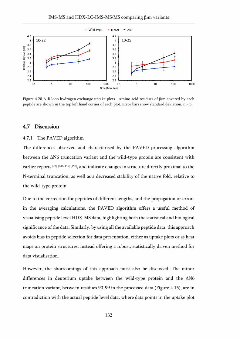
IMS-MS and HDX-LC-IMS-MS/MS comparing β2m variants
132
Figure 4.20 A-B loop hydrogen exchange uptake plots. Amino acid residues of β2m covered by each
peptide are shown in the top left hand corner of each plot. Error bars show standard deviation, n = 5.
4.7 Discussion
4.7.1 The PAVED algorithm
The differences observed and characterised by the PAVED processing algorithm
between the ΔN6 truncation variant and the wild-type protein are consistent with
earlier reports [78] [134, 146] [156], and indicate changes in structure directly proximal to the
N-terminal truncation, as well as a decreased stability of the native fold, relative to
the wild-type protein.
Due to the correction for peptides of different lengths, and the propagation or errors
in the averaging calculations, the PAVED algorithm offers a useful method of
visualising peptide level HDX-MS data, highlighting both the statistical and biological
significance of the data. Similarly, by using all the available peptide data, this approach
avoids bias in peptide selection for data presentation, either as uptake plots or as heat
maps on protein structures, instead offering a robust, statistically driven method for
data visualisation.
However, the shortcomings of this approach must also be discussed. The minor
differences in deuterium uptake between the wild-type protein and the ΔN6
truncation variant, between residues 90-99 in the processed data (Figure 4.15), are in
contradiction with the actual peptide level data, where data points in the uptake plot
IMS-MS and HDX-LC-IMS-MS/MS comparing β2m variants
133
overlay (Figure 4.12). Although processing with PAVED has correctly assigned
differences in this region as not statistically significant, the combined average
deuterium uptake in the processed data is higher in the ΔN6 variant than in the wild-
type protein in this region, as a result of a much longer, overlapping peptide where
deuterium uptake in ΔN6 is increased relative to the wild-type protein. This
‘smoothing’ effect on the data is to some extent unavoidable with this approach, and
is a similar issue for the alternative processing method described in Equation 4.2.
Clearly, shorter peptides provide higher structural resolution on changes in deuterium
uptake, where overlap with longer peptides exacerbates the smoothing effect on the
data during processing. The PAVED algorithm developed here lends itself to further
development in this regard as, currently, peptides of all lengths are weighted equally
in the calculation of the relative fractional uptake for each residue. In reality, the
relative fractional uptake for a given residue is more likely to be represented
accurately by shorter peptides than by longer peptides as, in the former case, an
individual amide makes a larger relative contribution to the measured peptide level
data.
As such, a modelling approach, based on the PAVED processing algorithm, could be
conceived whereby shorter peptides are weighted more heavily in the calculation of
relative fractional uptake:
𝑋𝐶 =
∑ 𝑛𝑖𝑖𝑙𝑖−1𝑧
𝑖=1
∑ 𝑛𝑖𝑧𝑖=1 𝑙𝑖
−1 (4.5)
Equation 4.5 Proposed modelling of HDX data based on PAVED processing. Where 𝑋𝐶 is the combined
mean relative fractional uptake for a given residue at a given time point, 𝑛𝑖 is the number of replicates
for peptide 𝑖. 𝑋𝑖 is the mean relative fractional uptake for peptide 𝑖 at a given time point. 𝑙𝑖 is the
number of exchangeable amides in peptide 𝑖 , excluding the N-terminal residue. Peptides 𝑖 to 𝑧 are all
the peptides that cover an amino acid position, excluding the N-terminal residue of each.
Although such a modelling approach would need to be tested on control proteins with
precisely known deuterium uptake behaviour, weighting shorter peptides more
IMS-MS and HDX-LC-IMS-MS/MS comparing β2m variants
134
heavily may mitigate the smoothing effect of the algorithm, thus further simplifying
data interpretation.
4.7.2 HDX behaviour of the D76N variant
The markedly increased deuterium uptake of the E-F loop in the D76N variant,
observed here for the first time, is suggestive of a significant structural or dynamical
change in this region. These observations are consistent with ssNMR experiments
which identified structural changes between wild-type β2m and D76N at both the E-
F loop, and more minor differences at residues Arg 12 and His 13 in the A-B loop [164].
These findings could be consistent with the minor differences in deuterium exchange
of the A-B loop observed by HDX-MS, where such minor differences are expectedly
unresolved, both dynamically and spatially, by the comparatively long (> 11 residues)
peptides identified which cover this region (Figure 4.10).
Although increased solvent accessibility in the E-F loop of the D76N variant, relative
to the wild-type protein, could account for the observed relative increase in
deuterium uptake, this explanation seems unlikely, as the E-F loop extends out into
bulk solvent, and is largely solvent exposed in both variants (Figure 2.9). In the NMR
structure of wild-type β2m, Asp 76 is involved in an extensive hydrogen bonding
network in the E-F loop involving residues Tyr 78, Thr 73 and Lys 75 (Figure 4.21).
Three of these contacts are main-chain hydrogen bonds involving backbone amide
protons, changes in which would be visible by HDX-MS experiments (Figure 4.21).
While many of these hydrogen bonds are also present in the crystal structure of the
D76N variant [157], static crystallographic structures are not necessarily representative
of the solution phase conformational distribution of the protein. Indeed, MD
simulations of the D76N variant have indicated that the D-N substitution disrupts
hydrogen bonding in the E-F loop, causing the loss of molecular contact between
hydrogen bonded residues [265]. These simulations are consistent with the observed de-
protection of backbone amides in the E-F loop of D76N and, given the central role
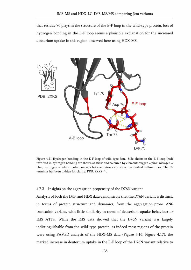
IMS-MS and HDX-LC-IMS-MS/MS comparing β2m variants
135
that residue 76 plays in the structure of the E-F loop in the wild-type protein, loss of
hydrogen bonding in the E-F loop seems a plausible explanation for the increased
deuterium uptake in this region observed here using HDX-MS.
Figure 4.21 Hydrogen bonding in the E-F loop of wild-type β2m. Side chains in the E-F loop (red)
involved in hydrogen bonding are shown as sticks and coloured by element: oxygen = pink, nitrogen =
blue, hydrogen = white. Polar contacts between atoms are shown as dashed yellow lines. The C-
terminus has been hidden for clarity. PDB: 2XKS [78].
4.7.3 Insights on the aggregation propensity of the D76N variant
Analysis of both the IMS, and HDX data demonstrate that the D76N variant is distinct,
in terms of protein structure and dynamics, from the aggregation-prone ΔN6
truncation variant, with little similarity in terms of deuterium uptake behaviour or
IMS ATDs. While the IMS data showed that the D76N variant was largely
indistinguishable from the wild-type protein, as indeed most regions of the protein
were using PAVED analysis of the HDX-MS data (Figure 4.16, Figure 4.17), the
marked increase in deuterium uptake in the E-F loop of the D76N variant relative to
IMS-MS and HDX-LC-IMS-MS/MS comparing β2m variants
136
the wild-type protein, and hypothesised loss of hydrogen bonding, is an important
observation regarding the increased aggregation propensity of this variant. The
hydrogen bonding analysis in Section 4.7.2, coupled with previous studies
demonstrating the critical nature of the D76 residue in preventing the aggregation of
β2m [159] is highly suggestive that the structure of the E-F loop is a key factor in
preventing oligomerisation and amyloid formation in β2m. Although considerably
more research is needed before any firm conclusions can be drawn from these data,
the clear distinction between D76N and the ΔN6 truncation variant, considered to be
a structural mimic of the amyloidogenic IT state [78, 146], shown by these data and by
others [161] could indicate an alternative, or additional route, to amyloid formation in
β2m, not involving the IT state folding intermediate. If true, further analysis of the β2m
model protein system could prove invaluable in studying the potential multiplicity of
pathways available to amyloid formation from the native state of a protein structure.
4.7.4 Attempted HDX-ETD single residue experiments
In an effort to gain higher resolution structural information on the HDX behaviour of
the E-F loop in D76N, and ascertain precisely which residues were responsible for the
increased deuterium uptake in this region, single residue HDX-MS experiments using
ETD peptide fragmentation were attempted. Although problems with method
development meant these experiments ultimately failed to yield any useful results,
the discussion of these data may help future research and, for the interested reader,
are presented (briefly) in this section.
With help from Malcolm Anderson (Principal applications chemist, Waters
Corporation, Wilmslow, UK) the Synapt G2Si instrument was tuned to optimise ETD
fragmentation and minimise deuterium scrambling, using the peptide P1 standard
similar to earlier reports [266]. Good sequence coverage was obtained (Figure 4.22), and
minimal deuterium scrambling was observed after incorporation of the peptide with
deuterated buffer, as evidenced by the retention of deuterium at the C-terminal end
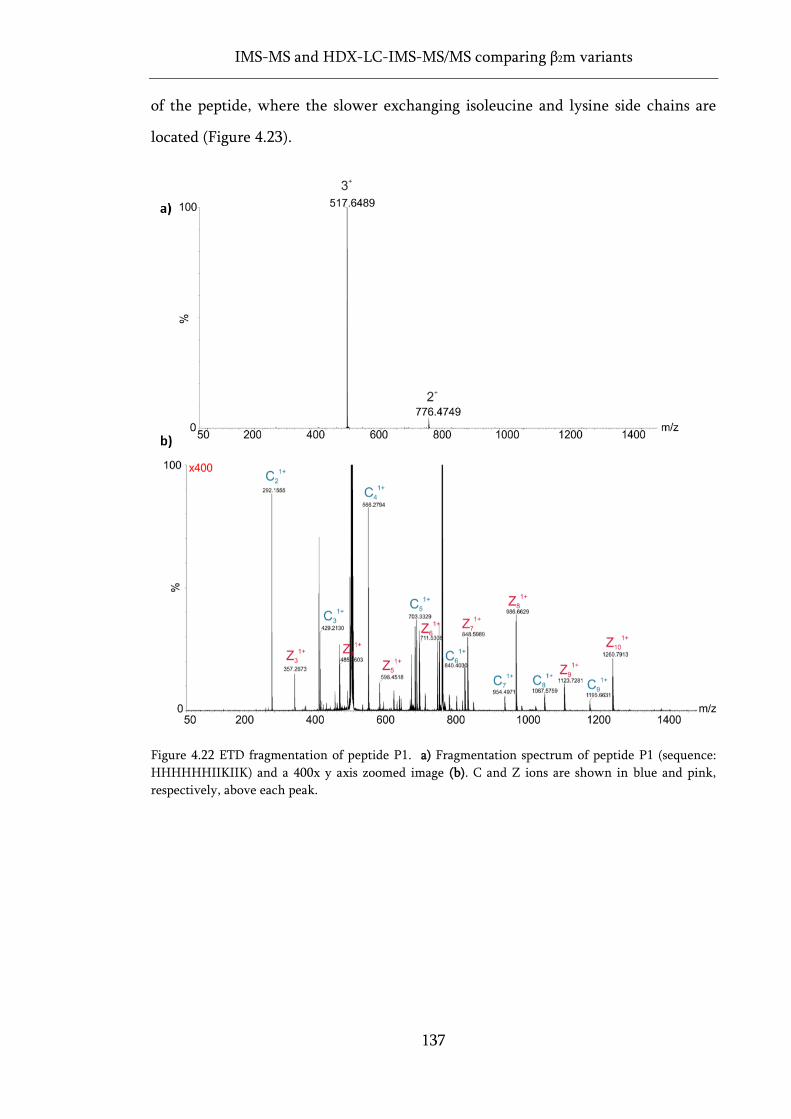
IMS-MS and HDX-LC-IMS-MS/MS comparing β2m variants
137
of the peptide, where the slower exchanging isoleucine and lysine side chains are
located (Figure 4.23).
Figure 4.22 ETD fragmentation of peptide P1. a) Fragmentation spectrum of peptide P1 (sequence:
HHHHHHIIKIIK) and a 400x y axis zoomed image (b). C and Z ions are shown in blue and pink,
respectively, above each peak.
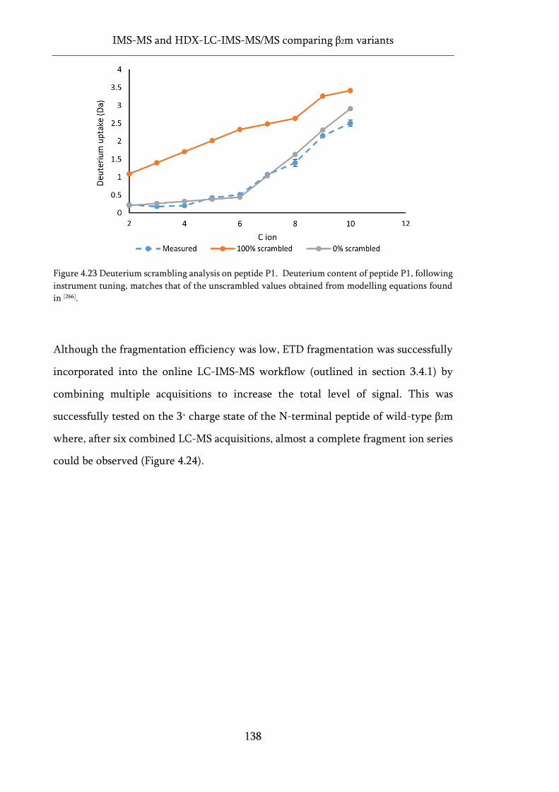
IMS-MS and HDX-LC-IMS-MS/MS comparing β2m variants
138
Figure 4.23 Deuterium scrambling analysis on peptide P1. Deuterium content of peptide P1, following
instrument tuning, matches that of the unscrambled values obtained from modelling equations found
in [266].
Although the fragmentation efficiency was low, ETD fragmentation was successfully
incorporated into the online LC-IMS-MS workflow (outlined in section 3.4.1) by
combining multiple acquisitions to increase the total level of signal. This was
successfully tested on the 3+ charge state of the N-terminal peptide of wild-type β2m
where, after six combined LC-MS acquisitions, almost a complete fragment ion series
could be observed (Figure 4.24).
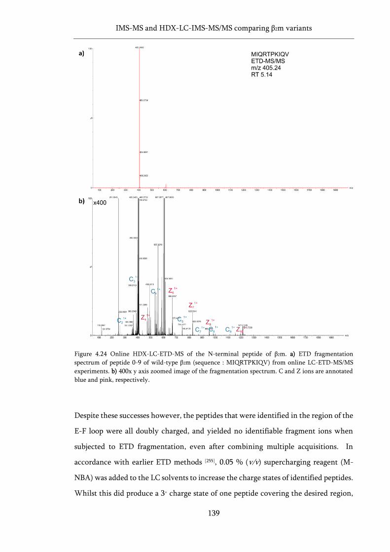
IMS-MS and HDX-LC-IMS-MS/MS comparing β2m variants
139
Figure 4.24 Online HDX-LC-ETD-MS of the N-terminal peptide of β2m. a) ETD fragmentation
spectrum of peptide 0-9 of wild-type β2m (sequence : MIQRTPKIQV) from online LC-ETD-MS/MS
experiments. b) 400x y axis zoomed image of the fragmentation spectrum. C and Z ions are annotated
blue and pink, respectively.
Despite these successes however, the peptides that were identified in the region of the
E-F loop were all doubly charged, and yielded no identifiable fragment ions when
subjected to ETD fragmentation, even after combining multiple acquisitions. In
accordance with earlier ETD methods [255], 0.05 % (v/v) supercharging reagent (M-
NBA) was added to the LC solvents to increase the charge states of identified peptides.
Whilst this did produce a 3+ charge state of one peptide covering the desired region,
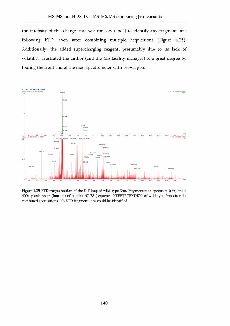
IMS-MS and HDX-LC-IMS-MS/MS comparing β2m variants
140
the intensity of this charge state was too low (~5e4) to identify any fragment ions
following ETD, even after combining multiple acquisitions (Figure 4.25).
Additionally, the added supercharging reagent, presumably due to its lack of
volatility, frustrated the author (and the MS facility manager) to a great degree by
fouling the front end of the mass spectrometer with brown goo.
Figure 4.25 ETD fragmentation of the E-F loop of wild-type β2m. Fragmentation spectrum (top) and a
400x y axis zoom (bottom) of peptide 67-78 (sequence YTEFTPTEKDEY) of wild-type β2m after six
combined acquisitions. No ETD fragment ions could be identified.
FULL ETD run wild-type b2m t=0
m/z100 200 300 400 500 600 700 800 900 1000 1100 1200 1300 1400 1500 1600 1700 1800 1900
%
0
100
m/z100 200 300 400 500 600 700 800 900 1000 1100 1200 1300 1400 1500 1600 1700 1800 1900
%
0
100
wil-type t=0 v2 24 (5.760) Cm (21:27) 4: TOF MSMS 508.20ES+ 5.59e4508.2256
505.2191
508.5602
508.8949
761.8333509.2298
511.1917
762.8336
763.3400
wil-type t=0 v2 24 (5.760) Cm (17:29) 4: TOF MSMS 508.20ES+ 814508.2256
469.8646
467.8137
251.0715
131.1003
365.1955
405.1697
508.5602 761.8333682.0223
681.6918
668.0061
762.3394
1002.0049
887.7979
887.4338
767.2763
768.9820
826.7335
1001.5214
942.7509
1011.5192
1012.1857
1022.5017
1023.0461
1395.49981136.5590
1669.2717
1396.7229 1851.2004
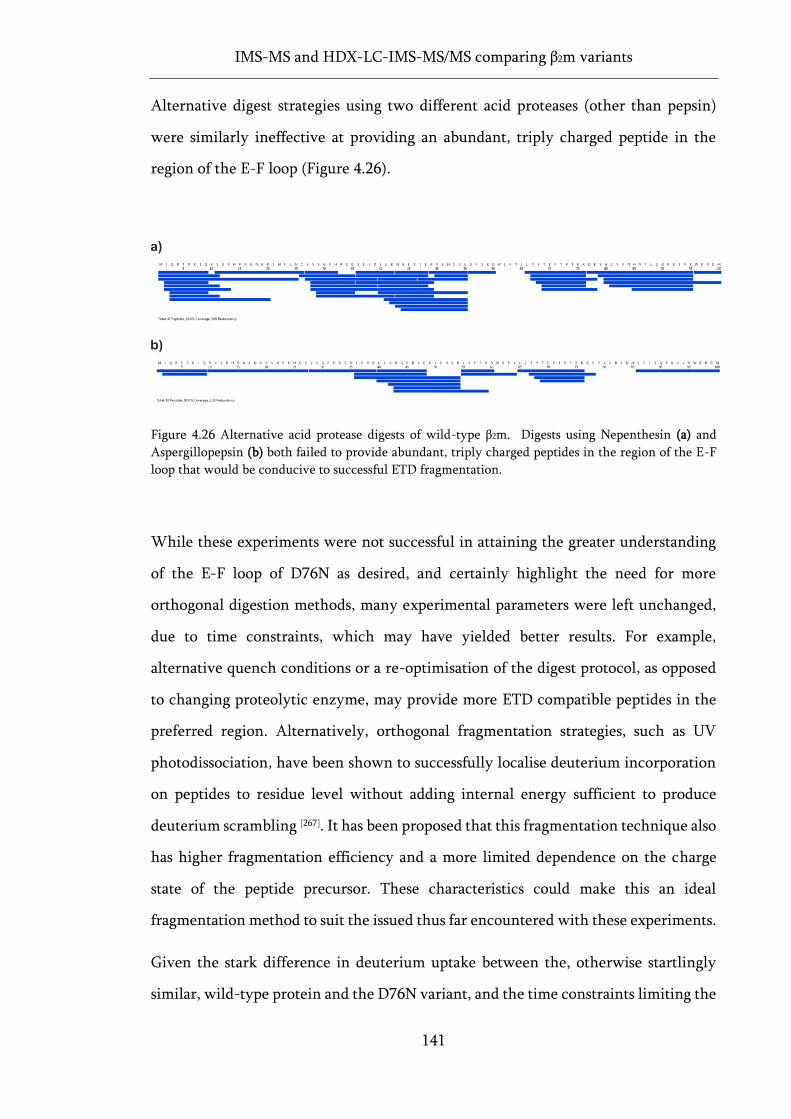
IMS-MS and HDX-LC-IMS-MS/MS comparing β2m variants
141
Alternative digest strategies using two different acid proteases (other than pepsin)
were similarly ineffective at providing an abundant, triply charged peptide in the
region of the E-F loop (Figure 4.26).
Figure 4.26 Alternative acid protease digests of wild-type β2m. Digests using Nepenthesin (a) and
Aspergillopepsin (b) both failed to provide abundant, triply charged peptides in the region of the E-F
loop that would be conducive to successful ETD fragmentation.
While these experiments were not successful in attaining the greater understanding
of the E-F loop of D76N as desired, and certainly highlight the need for more
orthogonal digestion methods, many experimental parameters were left unchanged,
due to time constraints, which may have yielded better results. For example,
alternative quench conditions or a re-optimisation of the digest protocol, as opposed
to changing proteolytic enzyme, may provide more ETD compatible peptides in the
preferred region. Alternatively, orthogonal fragmentation strategies, such as UV
photodissociation, have been shown to successfully localise deuterium incorporation
on peptides to residue level without adding internal energy sufficient to produce
deuterium scrambling [267]. It has been proposed that this fragmentation technique also
has higher fragmentation efficiency and a more limited dependence on the charge
state of the peptide precursor. These characteristics could make this an ideal
fragmentation method to suit the issued thus far encountered with these experiments.
Given the stark difference in deuterium uptake between the, otherwise startlingly
similar, wild-type protein and the D76N variant, and the time constraints limiting the

IMS-MS and HDX-LC-IMS-MS/MS comparing β2m variants
142
development time that was available for the above method, the importance of the
continuation and further development of this, or similar, methods to further
understand the E-F loop of D76N cannot be overstated. The implications of this are
discussed further in section 7.2.
143
Chapter 5:
FPOP-LC-MS/MS comparing β2m
variants
FPOP-LC-MS/MS comparing β2m variants
144
5 FPOP-LC-MS/MS comparing β2m variants
As discussed earlier in Section 2.4.4, fast photochemical oxidation of proteins (FPOP)
is an emerging technique frequently used in conjunction with MS analysis, used for
the characterisation and understanding of protein structures, although the method
itself, and the intricacies of how to analyse and interpret the resulting data, are poorly
understood. This chapter aims to address some of these issues, with the following aims:
1. Evaluate the current FPOP method used in our laboratory and determine the
significance, and incidence, of structural artefacts created by FPOP labelling
in these experiments.
2. Use the well-characterised wild-type and ΔN6 truncation variants of β2m to
develop the FPOP method, and gain a greater understanding of how to
interpret and analyse FPOP-LC-MS/MS data.
3. Use FPOP-LC-MS/MS to characterise the, poorly understood, D76N variant of
β2m and identify any changes that may be associated with the increased
propensity of this variant to aggregate.
FPOP data for wild-type β2m and the ΔN6 truncation variant from this chapter were
subsequently published in Cornwell., et al., JASMS, 2019 [252].
5.1 FPOP method validation
In an ideal FPOP experiment, each protein, and the solution immediately surrounding
it, would be irradiated no more than once. This is because once a protein has been
irradiated, it has the possibility, although not certainty, of being labelled by a nearby
hydroxyl radical, and the introduction of such non-native oxidations may shift the
protein structure into a non-native conformation. As a result, continued oxidative
labelling of the protein increases the chance of probing non-native structures
generated as artefacts of FPOP labelling, rather than the protein in its native state.
FPOP-LC-MS/MS comparing β2m variants
145
However, the experimental setup typically used in FPOP, both in the literature and
our laboratory (described in detail in Section 3.5), makes the determination of exactly
how many irradiation events, or ‘shots’, a protein has undergone quite challenging.
The FPOP analyte solution is passed, at a fixed flow rate, through a capillary that
intersects orthogonally the beam of a UV excimer laser, necessary to liberate hydroxyl
radicals from hydrogen peroxide. Due to the nature of the laser itself, this beam is not
constant and is instead pulsed at a constant frequency, for a fixed duration of 20 ns
(Figure 5.1). Although this extremely short pulse duration can be assumed as
instantaneous, for most practical purposes, this setup is such that many other
parameters are involved in determining how many times a protein molecule is
irradiated including: laser firing frequency, beam width, diffusion of the protein in
solution, and time spent in the irradiation window, the latter of which is directly
proportional to the flowrate of the solvent in the capillary.
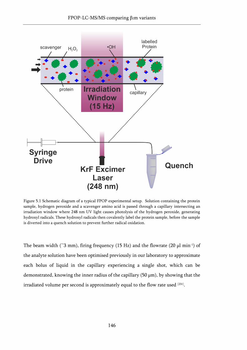
FPOP-LC-MS/MS comparing β2m variants
146
Figure 5.1 Schematic diagram of a typical FPOP experimental setup. Solution containing the protein
sample, hydrogen peroxide and a scavenger amino acid is passed through a capillary intersecting an
irradiation window where 248 nm UV light causes photolysis of the hydrogen peroxide, generating
hydroxyl radicals. These hydroxyl radicals then covalently label the protein sample, before the sample
is diverted into a quench solution to prevent further radical oxidation.
The beam width (~3 mm), firing frequency (15 Hz) and the flowrate (20 µl min-1) of
the analyte solution have been optimised previously in our laboratory to approximate
each bolus of liquid in the capillary experiencing a single shot, which can be
demonstrated, knowing the inner radius of the capillary (50 µm), by showing that the
irradiated volume per second is approximately equal to the flow rate used [231].
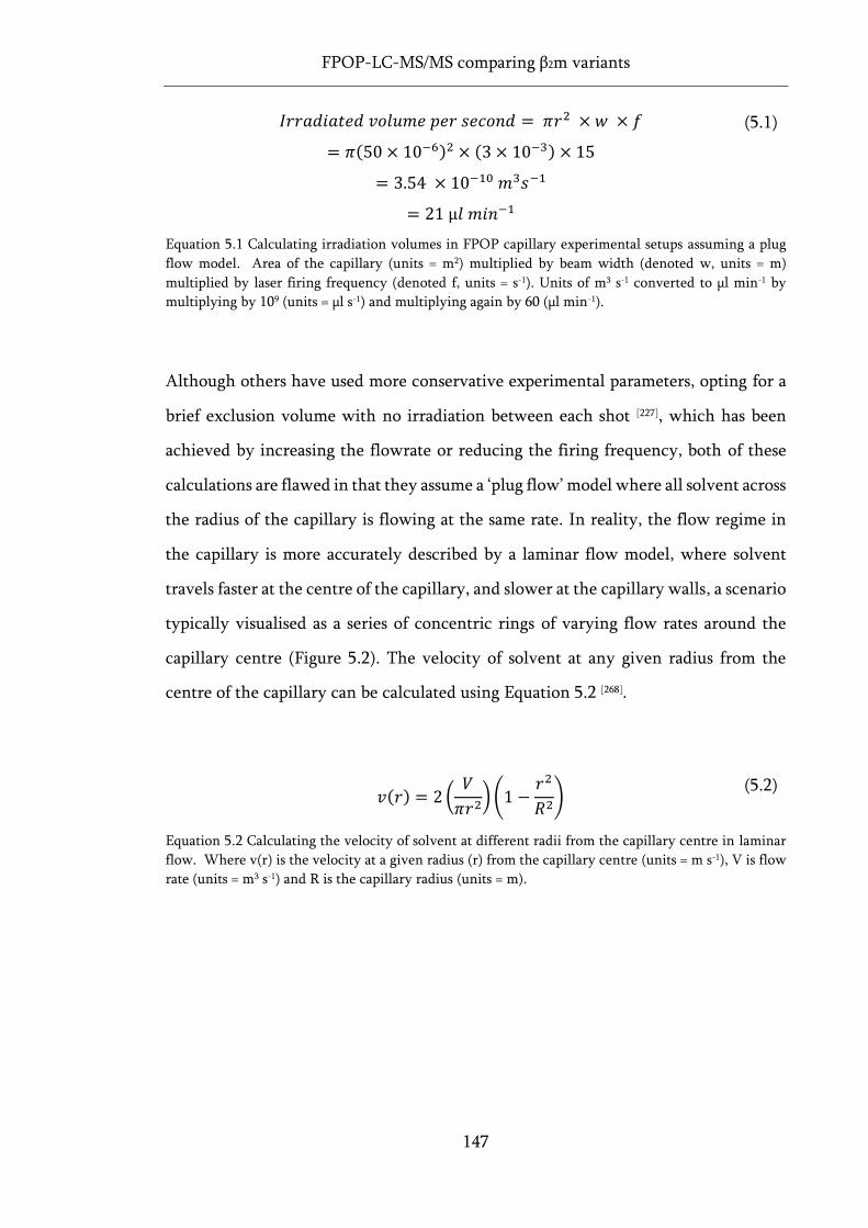
FPOP-LC-MS/MS comparing β2m variants
147
𝐼𝑟𝑟𝑎𝑑𝑖𝑎𝑡𝑒𝑑 𝑣𝑜𝑙𝑢𝑚𝑒 𝑝𝑒𝑟 𝑠𝑒𝑐𝑜𝑛𝑑 = 𝜋𝑟2 × 𝑤 × 𝑓
= 𝜋(50 × 10−6)2 × (3 × 10−3) × 15
= 3.54 × 10⁻¹⁰ 𝑚3𝑠−1
= 21 µ𝑙 𝑚𝑖𝑛−1
(5.1)
Equation 5.1 Calculating irradiation volumes in FPOP capillary experimental setups assuming a plug
flow model. Area of the capillary (units = m2) multiplied by beam width (denoted w, units = m)
multiplied by laser firing frequency (denoted f, units = s-1). Units of m3 s-1 converted to µl min-1 by
multiplying by 109 (units = µl s-1) and multiplying again by 60 (µl min-1).
Although others have used more conservative experimental parameters, opting for a
brief exclusion volume with no irradiation between each shot [227], which has been
achieved by increasing the flowrate or reducing the firing frequency, both of these
calculations are flawed in that they assume a ‘plug flow’ model where all solvent across
the radius of the capillary is flowing at the same rate. In reality, the flow regime in
the capillary is more accurately described by a laminar flow model, where solvent
travels faster at the centre of the capillary, and slower at the capillary walls, a scenario
typically visualised as a series of concentric rings of varying flow rates around the
capillary centre (Figure 5.2). The velocity of solvent at any given radius from the
centre of the capillary can be calculated using Equation 5.2 [268].
𝑣(𝑟) = 2 (
𝑉
𝜋𝑟2)(1 −
𝑟2
𝑅2)
(5.2)
Equation 5.2 Calculating the velocity of solvent at different radii from the capillary centre in laminar
flow. Where v(r) is the velocity at a given radius (r) from the capillary centre (units = m s-1), V is flow
rate (units = m3 s-1) and R is the capillary radius (units = m).
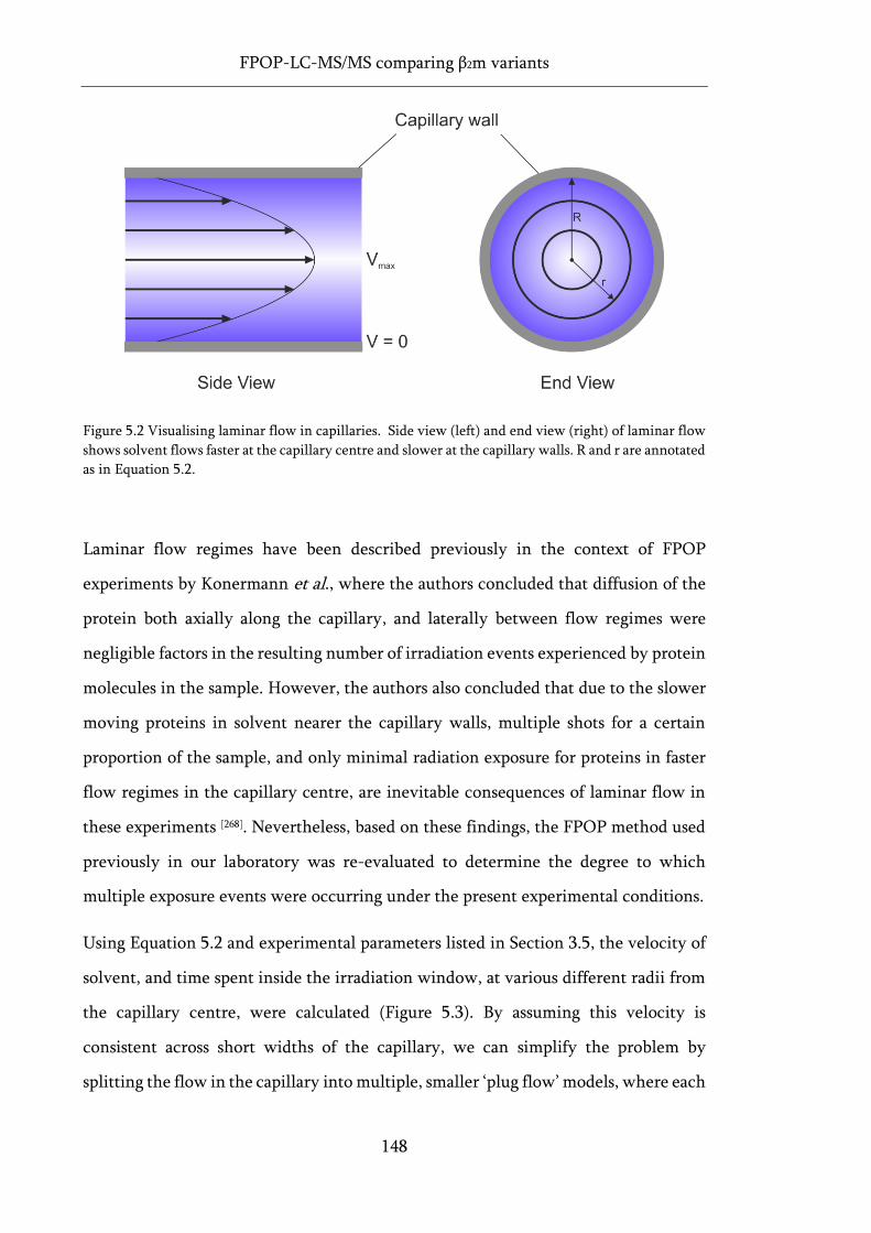
FPOP-LC-MS/MS comparing β2m variants
148
Figure 5.2 Visualising laminar flow in capillaries. Side view (left) and end view (right) of laminar flow
shows solvent flows faster at the capillary centre and slower at the capillary walls. R and r are annotated
as in Equation 5.2.
Laminar flow regimes have been described previously in the context of FPOP
experiments by Konermann et al., where the authors concluded that diffusion of the
protein both axially along the capillary, and laterally between flow regimes were
negligible factors in the resulting number of irradiation events experienced by protein
molecules in the sample. However, the authors also concluded that due to the slower
moving proteins in solvent nearer the capillary walls, multiple shots for a certain
proportion of the sample, and only minimal radiation exposure for proteins in faster
flow regimes in the capillary centre, are inevitable consequences of laminar flow in
these experiments [268]. Nevertheless, based on these findings, the FPOP method used
previously in our laboratory was re-evaluated to determine the degree to which
multiple exposure events were occurring under the present experimental conditions.
Using Equation 5.2 and experimental parameters listed in Section 3.5, the velocity of
solvent, and time spent inside the irradiation window, at various different radii from
the capillary centre, were calculated (Figure 5.3). By assuming this velocity is
consistent across short widths of the capillary, we can simplify the problem by
splitting the flow in the capillary into multiple, smaller ‘plug flow’ models, where each
FPOP-LC-MS/MS comparing β2m variants
149
concentric ring of flow, of arbitrary width, is approximated to have the same average
velocity. This approximation is most accurate closest to the capillary centre, where
the dependence of velocity on radial position is the lowest (Figure 5.3). As such, the
calculation was split into multiple 5 µm wide rings from the capillary centre (0-5 µm,
5-10 µm etc…) where, smaller, 1 µm intervals were used after 45 µm from the
capillary centre, where radial position affects velocity most significantly.
Figure 5.3 Velocities and time spent in the irradiation zone calculated for different flow regimes in the
FPOP capillary. Calculated using Equation 5.2 and experimental parameters listed in Section 3.5. A
radius of 0 on the x axis is the capillary centre. The work of Prof. Nik Kapur (Applied Fluid Mechanics,
School of Mechanical Engineering, University of Leeds) is gratefully acknowledged for his help in these
calculations.
Knowing the firing frequency of the laser (15 Hz) and the time spent in the irradiation
window for each concentric ring of flow, or flow regime, we can determine the
average number of shots and, consequently, the maximum and minimum number of
shots, a protein could experience under each flow regime, maximum being a scenario
where a protein is irradiated the instant it enters the beam width, and the minimum
being a protein that follows one that was instantly irradiated (equivalent to one fewer
than the maximum number of hits). As the proportion of protein receiving the
maximum and minimum number of shots under each flow regime must sum to 1, we
can determine the fraction of protein, under each flow regime, that receives the
maximum and minimum number of shots (Equation 5.3, Table 5.1).
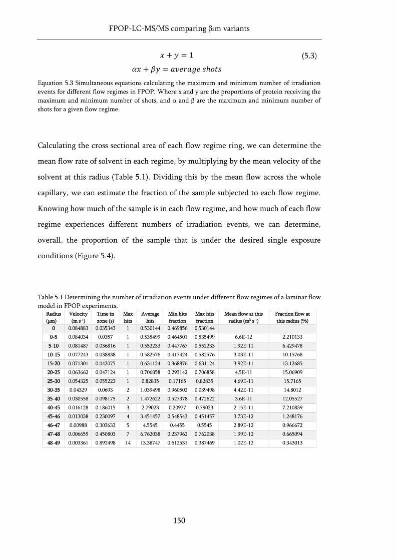
FPOP-LC-MS/MS comparing β2m variants
150
𝑥 + 𝑦 = 1
𝛼𝑥 + 𝛽𝑦 = 𝑎𝑣𝑒𝑟𝑎𝑔𝑒 𝑠ℎ𝑜𝑡𝑠
(5.3)
Equation 5.3 Simultaneous equations calculating the maximum and minimum number of irradiation
events for different flow regimes in FPOP. Where x and y are the proportions of protein receiving the
maximum and minimum number of shots, and α and β are the maximum and minimum number of
shots for a given flow regime.
Calculating the cross sectional area of each flow regime ring, we can determine the
mean flow rate of solvent in each regime, by multiplying by the mean velocity of the
solvent at this radius (Table 5.1). Dividing this by the mean flow across the whole
capillary, we can estimate the fraction of the sample subjected to each flow regime.
Knowing how much of the sample is in each flow regime, and how much of each flow
regime experiences different numbers of irradiation events, we can determine,
overall, the proportion of the sample that is under the desired single exposure
conditions (Figure 5.4).
Table 5.1 Determining the number of irradiation events under different flow regimes of a laminar flow
model in FPOP experiments. Radius
(µm)
Velocity
(m s-1)
Time in
zone (s)
Max
hits
Average
hits
Min hits
fraction
Max hits
fraction
Mean flow at this
radius (m3 s-1)
Fraction flow at
this radius (%)
0 0.084883 0.035343 1 0.530144 0.469856 0.530144
0-5 0.084034 0.0357 1 0.535499 0.464501 0.535499 6.6E-12 2.210133
5-10 0.081487 0.036816 1 0.552233 0.447767 0.552233 1.92E-11 6.429478
10-15 0.077243 0.038838 1 0.582576 0.417424 0.582576 3.03E-11 10.15768
15-20 0.071301 0.042075 1 0.631124 0.368876 0.631124 3.92E-11 13.12685
20-25 0.063662 0.047124 1 0.706858 0.293142 0.706858 4.5E-11 15.06909
25-30 0.054325 0.055223 1 0.82835 0.17165 0.82835 4.69E-11 15.7165
30-35 0.04329 0.0693 2 1.039498 0.960502 0.039498 4.42E-11 14.8012
35-40 0.030558 0.098175 2 1.472622 0.527378 0.472622 3.6E-11 12.05527
40-45 0.016128 0.186015 3 2.79023 0.20977 0.79023 2.15E-11 7.210839
45-46 0.013038 0.230097 4 3.451457 0.548543 0.451457 3.73E-12 1.248176
46-47 0.00988 0.303633 5 4.5545 0.4455 0.5545 2.89E-12 0.966672
47-48 0.006655 0.450803 7 6.762038 0.237962 0.762038 1.99E-12 0.665094
48-49 0.003361 0.892498 14 13.38747 0.612531 0.387469 1.02E-12 0.343013
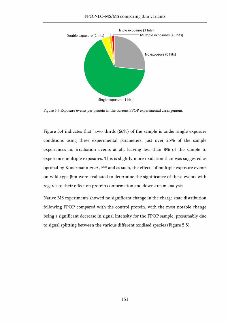
FPOP-LC-MS/MS comparing β2m variants
151
Figure 5.4 Exposure events per protein in the current FPOP experimental arrangement.
Figure 5.4 indicates that ~two thirds (66%) of the sample is under single exposure
conditions using these experimental parameters, just over 25% of the sample
experiences no irradiation events at all, leaving less than 8% of the sample to
experience multiple exposures. This is slightly more oxidation than was suggested as
optimal by Konermann et al., [268] and as such, the effects of multiple exposure events
on wild-type β2m were evaluated to determine the significance of these events with
regards to their effect on protein conformation and downstream analysis.
Native MS experiments showed no significant change in the charge state distribution
following FPOP compared with the control protein, with the most notable change
being a significant decrease in signal intensity for the FPOP sample, presumably due
to signal splitting between the various different oxidised species (Figure 5.5).
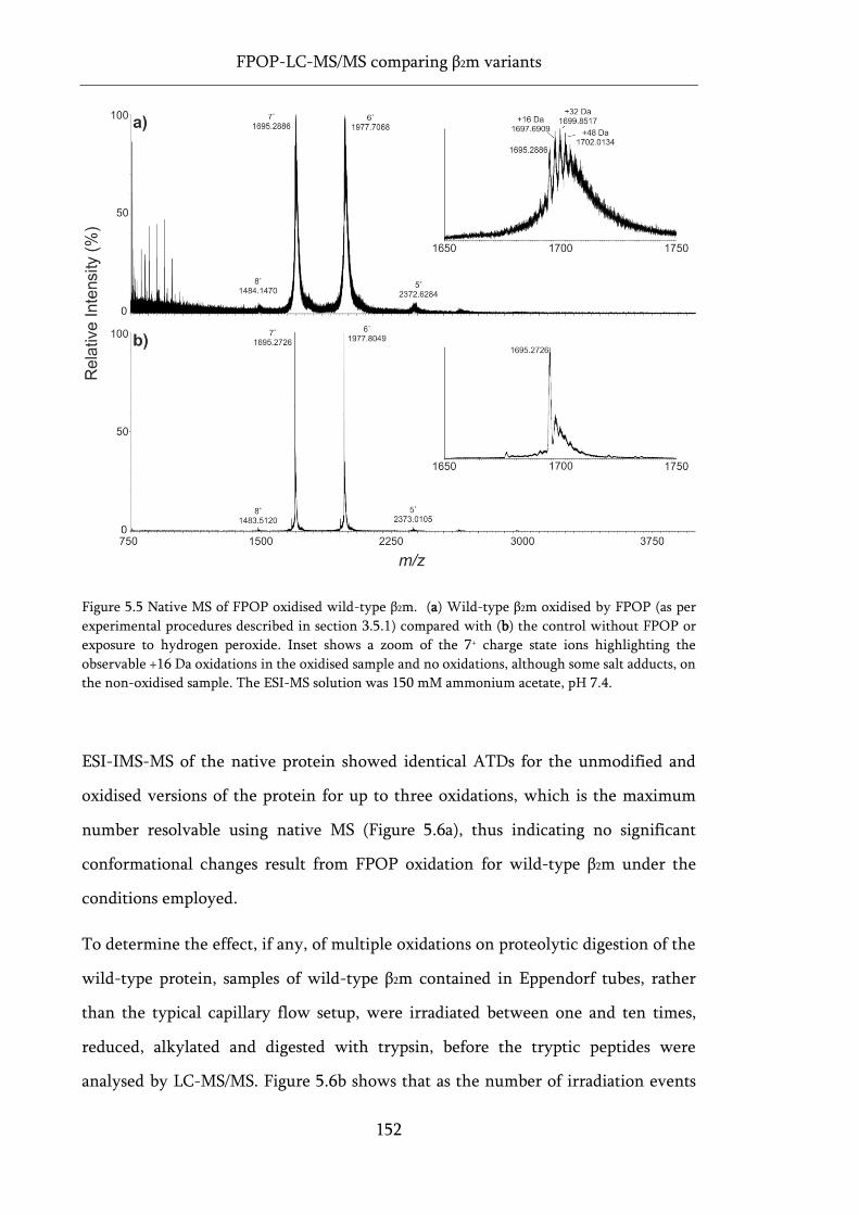
FPOP-LC-MS/MS comparing β2m variants
152
Figure 5.5 Native MS of FPOP oxidised wild-type β2m. (a) Wild-type β2m oxidised by FPOP (as per
experimental procedures described in section 3.5.1) compared with (b) the control without FPOP or
exposure to hydrogen peroxide. Inset shows a zoom of the 7+ charge state ions highlighting the
observable +16 Da oxidations in the oxidised sample and no oxidations, although some salt adducts, on
the non-oxidised sample. The ESI-MS solution was 150 mM ammonium acetate, pH 7.4.
ESI-IMS-MS of the native protein showed identical ATDs for the unmodified and
oxidised versions of the protein for up to three oxidations, which is the maximum
number resolvable using native MS (Figure 5.6a), thus indicating no significant
conformational changes result from FPOP oxidation for wild-type β2m under the
conditions employed.
To determine the effect, if any, of multiple oxidations on proteolytic digestion of the
wild-type protein, samples of wild-type β2m contained in Eppendorf tubes, rather
than the typical capillary flow setup, were irradiated between one and ten times,
reduced, alkylated and digested with trypsin, before the tryptic peptides were
analysed by LC-MS/MS. Figure 5.6b shows that as the number of irradiation events
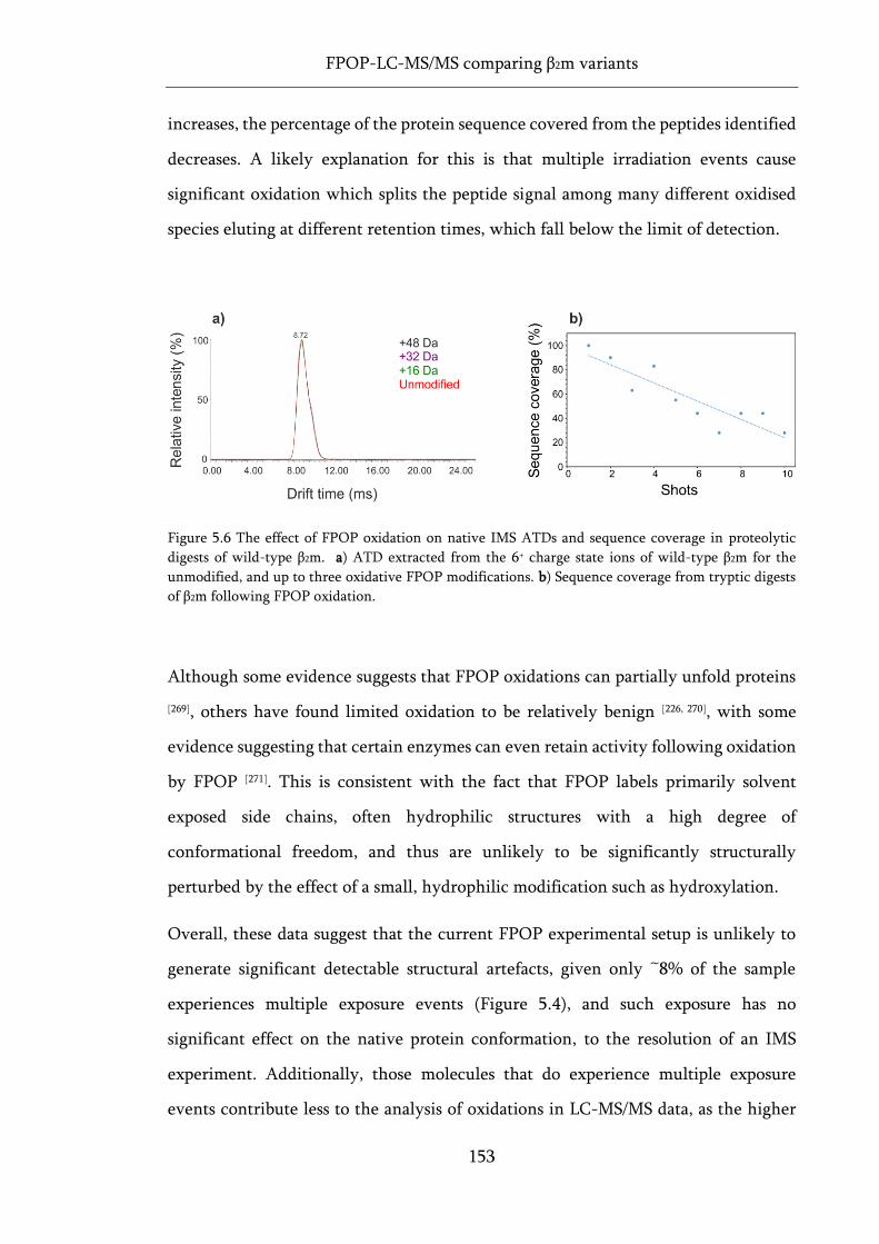
FPOP-LC-MS/MS comparing β2m variants
153
increases, the percentage of the protein sequence covered from the peptides identified
decreases. A likely explanation for this is that multiple irradiation events cause
significant oxidation which splits the peptide signal among many different oxidised
species eluting at different retention times, which fall below the limit of detection.
Figure 5.6 The effect of FPOP oxidation on native IMS ATDs and sequence coverage in proteolytic
digests of wild-type β2m. a) ATD extracted from the 6+ charge state ions of wild-type β2m for the
unmodified, and up to three oxidative FPOP modifications. b) Sequence coverage from tryptic digests
of β2m following FPOP oxidation.
Although some evidence suggests that FPOP oxidations can partially unfold proteins
[269], others have found limited oxidation to be relatively benign [226, 270], with some
evidence suggesting that certain enzymes can even retain activity following oxidation
by FPOP [271]. This is consistent with the fact that FPOP labels primarily solvent
exposed side chains, often hydrophilic structures with a high degree of
conformational freedom, and thus are unlikely to be significantly structurally
perturbed by the effect of a small, hydrophilic modification such as hydroxylation.
Overall, these data suggest that the current FPOP experimental setup is unlikely to
generate significant detectable structural artefacts, given only ~8% of the sample
experiences multiple exposure events (Figure 5.4), and such exposure has no
significant effect on the native protein conformation, to the resolution of an IMS
experiment. Additionally, those molecules that do experience multiple exposure
events contribute less to the analysis of oxidations in LC-MS/MS data, as the higher
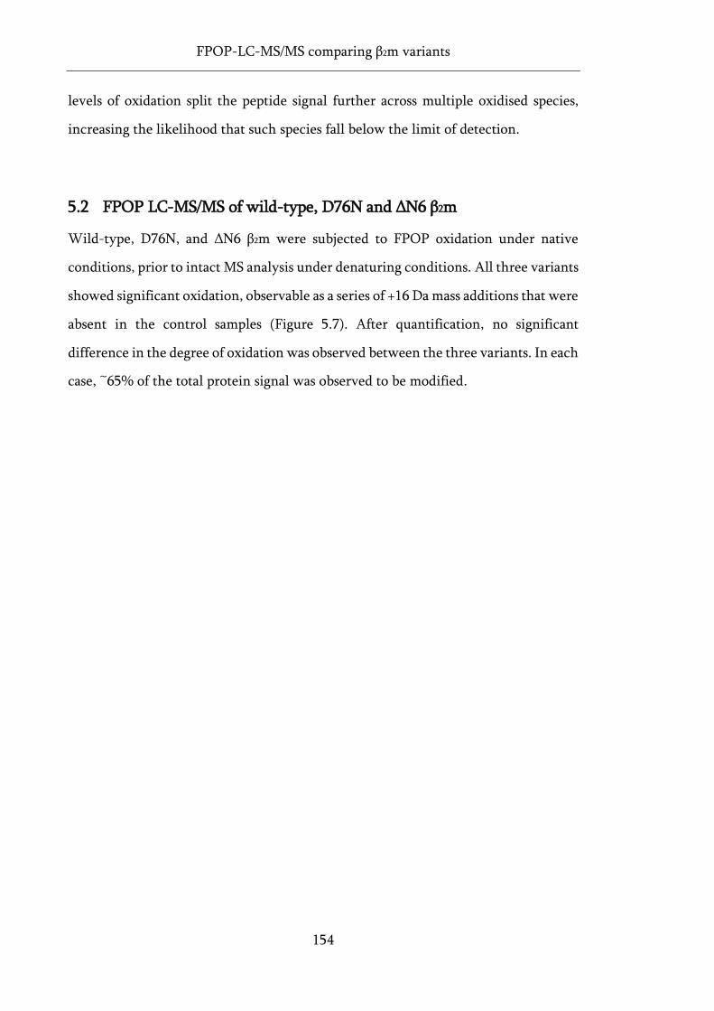
FPOP-LC-MS/MS comparing β2m variants
154
levels of oxidation split the peptide signal further across multiple oxidised species,
increasing the likelihood that such species fall below the limit of detection.
5.2 FPOP LC-MS/MS of wild-type, D76N and ΔN6 β2m
Wild-type, D76N, and ΔN6 β2m were subjected to FPOP oxidation under native
conditions, prior to intact MS analysis under denaturing conditions. All three variants
showed significant oxidation, observable as a series of +16 Da mass additions that were
absent in the control samples (Figure 5.7). After quantification, no significant
difference in the degree of oxidation was observed between the three variants. In each
case, ~65% of the total protein signal was observed to be modified.
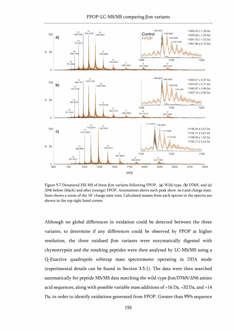
FPOP-LC-MS/MS comparing β2m variants
155
Figure 5.7 Denatured ESI-MS of three β2m variants following FPOP. (a) Wild-type, (b) D76N, and (c)
ΔN6 before (black) and after (orange) FPOP. Annotations above each peak show m/z and charge state.
Inset shows a zoom of the 10+ charge state ions. Calculated masses from each species in the spectra are
shown in the top right hand corner.
Although no global differences in oxidation could be detected between the three
variants, to determine if any differences could be observed by FPOP at higher
resolution, the three oxidised β2m variants were enzymatically digested with
chymotrypsin and the resulting peptides were then analysed by LC-MS/MS using a
Q-Exactive quadrupole orbitrap mass spectrometer operating in DDA mode
(experimental details can be found in Section 3.5.1). The data were then searched
automatically for peptide MS/MS data matching the wild-type β2m/D76N/ΔN6 amino
acid sequences, along with possible variable mass additions of +16 Da, +32 Da, and +14
Da, in order to identify oxidations generated from FPOP. Greater than 95% sequence
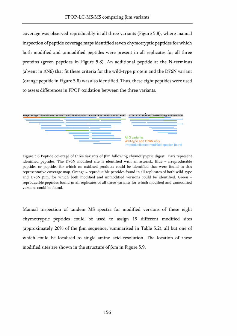
FPOP-LC-MS/MS comparing β2m variants
156
coverage was observed reproducibly in all three variants (Figure 5.8), where manual
inspection of peptide coverage maps identified seven chymotryptic peptides for which
both modified and unmodified peptides were present in all replicates for all three
proteins (green peptides in Figure 5.8). An additional peptide at the N-terminus
(absent in ΔN6) that fit these criteria for the wild-type protein and the D76N variant
(orange peptide in Figure 5.8) was also identified. Thus, these eight peptides were used
to assess differences in FPOP oxidation between the three variants.
Figure 5.8 Peptide coverage of three variants of β2m following chymotrpyptic digest. Bars represent
identified peptides. The D76N modified site is identified with an asterisk. Blue = irreproducible
peptides or peptides for which no oxidised products could be identified that were found in this
representative coverage map. Orange = reproducible peptides found in all replicates of both wild-type
and D76N β2m, for which both modified and unmodified versions could be identified. Green =
reproducible peptides found in all replicates of all three variants for which modified and unmodified
versions could be found.
Manual inspection of tandem MS spectra for modified versions of these eight
chymotryptic peptides could be used to assign 19 different modified sites
(approximately 20% of the β2m sequence, summarised in Table 5.2), all but one of
which could be localised to single amino acid resolution. The location of these
modified sites are shown in the structure of β2m in Figure 5.9.
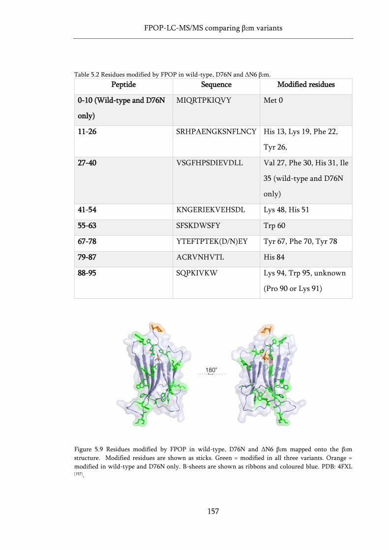
FPOP-LC-MS/MS comparing β2m variants
157
Table 5.2 Residues modified by FPOP in wild-type, D76N and ΔN6 β2m.
Peptide Sequence Modified residues
0-10 (Wild-type and D76N
only)
MIQRTPKIQVY Met 0
11-26 SRHPAENGKSNFLNCY His 13, Lys 19, Phe 22,
Tyr 26,
27-40 VSGFHPSDIEVDLL Val 27, Phe 30, His 31, Ile
35 (wild-type and D76N
only)
41-54 KNGERIEKVEHSDL Lys 48, His 51
55-63 SFSKDWSFY Trp 60
67-78 YTEFTPTEK(D/N)EY Tyr 67, Phe 70, Tyr 78
79-87 ACRVNHVTL His 84
88-95 SQPKIVKW Lys 94, Trp 95, unknown
(Pro 90 or Lys 91)
Figure 5.9 Residues modified by FPOP in wild-type, D76N and ΔN6 β2m mapped onto the β2m
structure. Modified residues are shown as sticks. Green = modified in all three variants. Orange =
modified in wild-type and D76N only. Β-sheets are shown as ribbons and coloured blue. PDB: 4FXL [157].
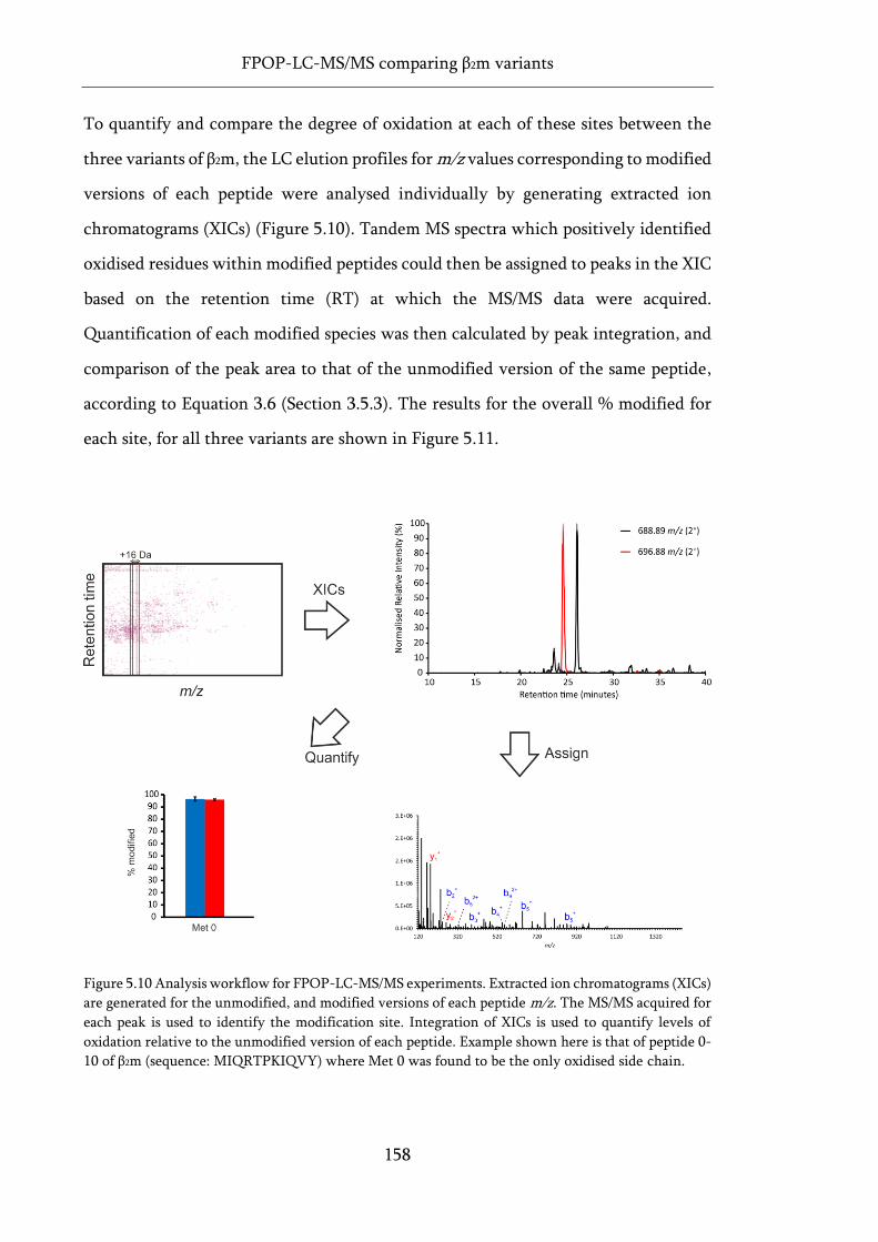
FPOP-LC-MS/MS comparing β2m variants
158
To quantify and compare the degree of oxidation at each of these sites between the
three variants of β2m, the LC elution profiles for m/z values corresponding to modified
versions of each peptide were analysed individually by generating extracted ion
chromatograms (XICs) (Figure 5.10). Tandem MS spectra which positively identified
oxidised residues within modified peptides could then be assigned to peaks in the XIC
based on the retention time (RT) at which the MS/MS data were acquired.
Quantification of each modified species was then calculated by peak integration, and
comparison of the peak area to that of the unmodified version of the same peptide,
according to Equation 3.6 (Section 3.5.3). The results for the overall % modified for
each site, for all three variants are shown in Figure 5.11.
Figure 5.10 Analysis workflow for FPOP-LC-MS/MS experiments. Extracted ion chromatograms (XICs)
are generated for the unmodified, and modified versions of each peptide m/z. The MS/MS acquired for
each peak is used to identify the modification site. Integration of XICs is used to quantify levels of
oxidation relative to the unmodified version of each peptide. Example shown here is that of peptide 0-
10 of β2m (sequence: MIQRTPKIQVY) where Met 0 was found to be the only oxidised side chain.
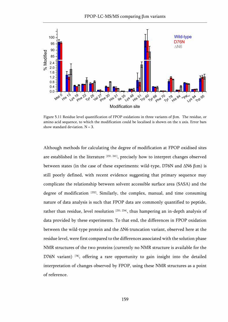
FPOP-LC-MS/MS comparing β2m variants
159
Figure 5.11 Residue level quantification of FPOP oxidations in three variants of β2m. The residue, or
amino acid sequence, to which the modification could be localised is shown on the x axis. Error bars
show standard deviation. N = 3.
Although methods for calculating the degree of modification at FPOP oxidised sites
are established in the literature [231, 241], precisely how to interpret changes observed
between states (in the case of these experiments: wild-type, D76N and ΔN6 β2m) is
still poorly defined, with recent evidence suggesting that primary sequence may
complicate the relationship between solvent accessible surface area (SASA) and the
degree of modification [232]. Similarly, the complex, manual, and time consuming
nature of data analysis is such that FPOP data are commonly quantified to peptide,
rather than residue, level resolution [231, 234], thus hampering an in-depth analysis of
data provided by these experiments. To that end, the differences in FPOP oxidation
between the wild-type protein and the ΔN6 truncation variant, observed here at the
residue level, were first compared to the differences associated with the solution phase
NMR structures of the two proteins (currently no NMR structure is available for the
D76N variant) [78], offering a rare opportunity to gain insight into the detailed
interpretation of changes observed by FPOP, using these NMR structures as a point
of reference.
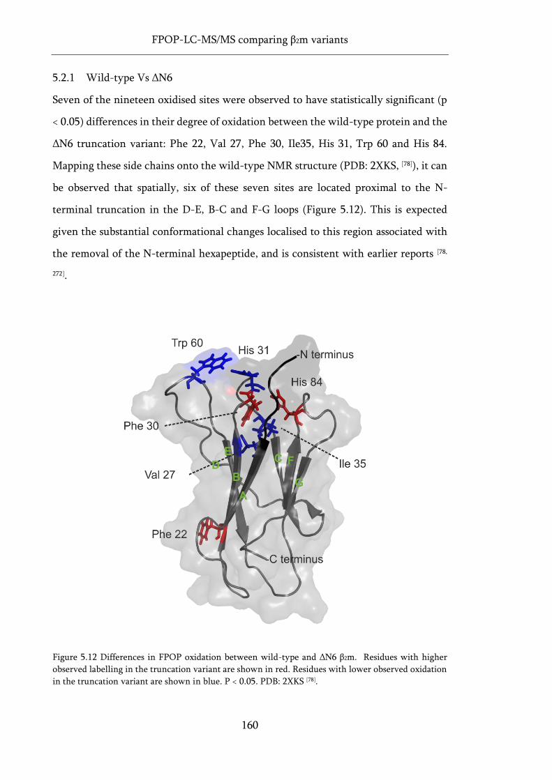
FPOP-LC-MS/MS comparing β2m variants
160
5.2.1 Wild-type Vs ΔN6
Seven of the nineteen oxidised sites were observed to have statistically significant (p
< 0.05) differences in their degree of oxidation between the wild-type protein and the
ΔN6 truncation variant: Phe 22, Val 27, Phe 30, Ile35, His 31, Trp 60 and His 84.
Mapping these side chains onto the wild-type NMR structure (PDB: 2XKS, [78]), it can
be observed that spatially, six of these seven sites are located proximal to the N-
terminal truncation in the D-E, B-C and F-G loops (Figure 5.12). This is expected
given the substantial conformational changes localised to this region associated with
the removal of the N-terminal hexapeptide, and is consistent with earlier reports [78,
272].
Figure 5.12 Differences in FPOP oxidation between wild-type and ΔN6 β2m. Residues with higher
observed labelling in the truncation variant are shown in red. Residues with lower observed oxidation
in the truncation variant are shown in blue. P < 0.05. PDB: 2XKS [78].
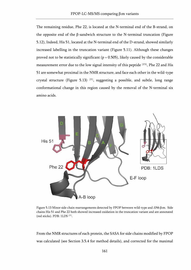
FPOP-LC-MS/MS comparing β2m variants
161
The remaining residue, Phe 22, is located at the N-terminal end of the B-strand, on
the opposite end of the β-sandwich structure to the N-terminal truncation (Figure
5.12), Indeed, His 51, located at the N-terminal end of the D-strand, showed similarly
increased labelling in the truncation variant (Figure 5.11). Although these changes
proved not to be statistically significant (p = 0.505), likely caused by the considerable
measurement error due to the low signal intensity of this peptide [273], Phe 22 and His
51 are somewhat proximal in the NMR structure, and face each other in the wild-type
crystal structure (Figure 5.13) [77], suggesting a possible, and subtle, long range
conformational change in this region caused by the removal of the N-terminal six
amino acids.
Figure 5.13 Minor side chain rearrangements detected by FPOP between wild-type and ΔN6 β2m. Side
chains His 51 and Phe 22 both showed increased oxidation in the truncation variant and are annotated
(red sticks). PDB: 1LDS [77].
From the NMR structures of each protein, the SASA for side chains modified by FPOP
was calculated (see Section 3.5.4 for method details), and corrected for the maximal
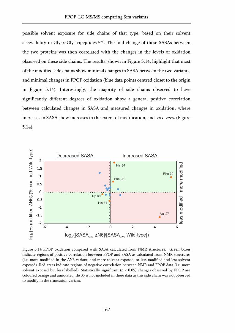
FPOP-LC-MS/MS comparing β2m variants
162
possible solvent exposure for side chains of that type, based on their solvent
accessibility in Gly-x-Gly tripeptides [274]. The fold change of these SASAs between
the two proteins was then correlated with the changes in the levels of oxidation
observed on these side chains. The results, shown in Figure 5.14, highlight that most
of the modified side chains show minimal changes in SASA between the two variants,
and minimal changes in FPOP oxidation (blue data points centred closet to the origin
in Figure 5.14). Interestingly, the majority of side chains observed to have
significantly different degrees of oxidation show a general positive correlation
between calculated changes in SASA and measured changes in oxidation, where
increases in SASA show increases in the extent of modification, and vice versa (Figure
5.14).
Figure 5.14 FPOP oxidation compared with SASA calculated from NMR structures. Green boxes
indicate regions of positive correlation between FPOP and SASA as calculated from NMR structures
(i.e. more modified in the ΔN6 variant, and more solvent exposed, or less modified and less solvent
exposed). Red areas indicate regions of negative correlation between NMR and FPOP data (i.e. more
solvent exposed but less labelled). Statistically significant (p < 0.05) changes observed by FPOP are
coloured orange and annotated. Ile 35 is not included in these data as this side chain was not observed
to modify in the truncation variant.
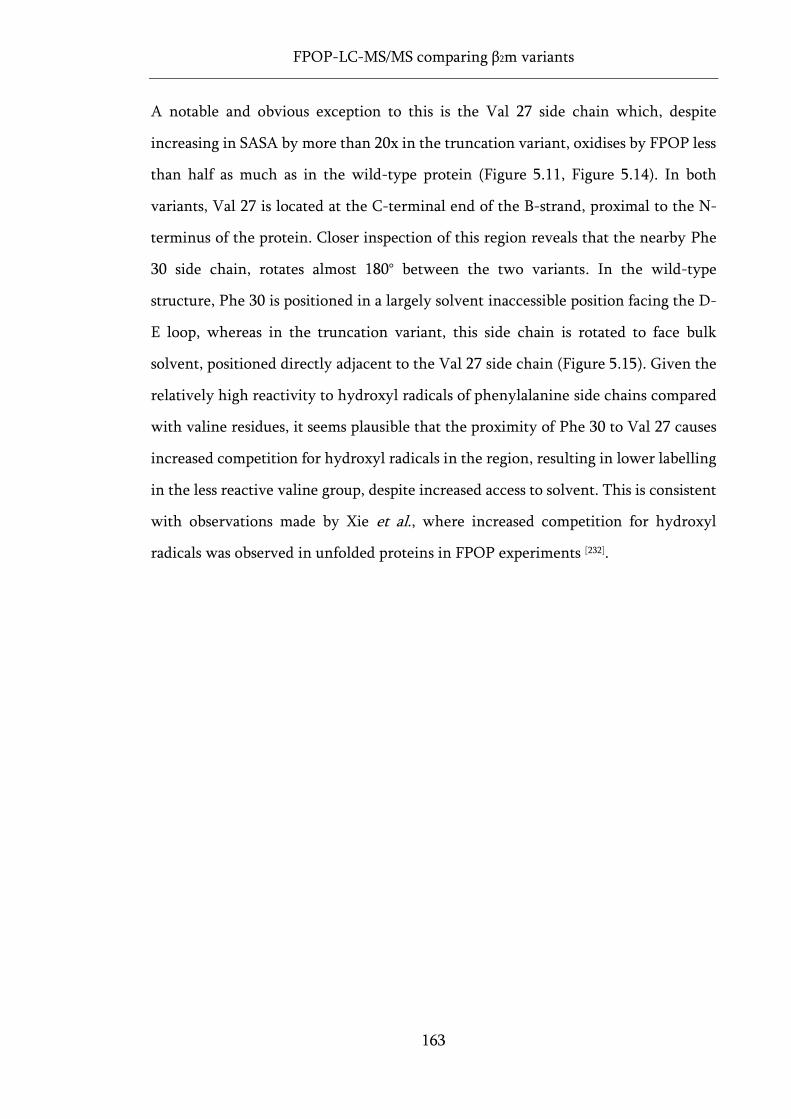
FPOP-LC-MS/MS comparing β2m variants
163
A notable and obvious exception to this is the Val 27 side chain which, despite
increasing in SASA by more than 20x in the truncation variant, oxidises by FPOP less
than half as much as in the wild-type protein (Figure 5.11, Figure 5.14). In both
variants, Val 27 is located at the C-terminal end of the B-strand, proximal to the N-
terminus of the protein. Closer inspection of this region reveals that the nearby Phe
30 side chain, rotates almost 180° between the two variants. In the wild-type
structure, Phe 30 is positioned in a largely solvent inaccessible position facing the D-
E loop, whereas in the truncation variant, this side chain is rotated to face bulk
solvent, positioned directly adjacent to the Val 27 side chain (Figure 5.15). Given the
relatively high reactivity to hydroxyl radicals of phenylalanine side chains compared
with valine residues, it seems plausible that the proximity of Phe 30 to Val 27 causes
increased competition for hydroxyl radicals in the region, resulting in lower labelling
in the less reactive valine group, despite increased access to solvent. This is consistent
with observations made by Xie et al., where increased competition for hydroxyl
radicals was observed in unfolded proteins in FPOP experiments [232].
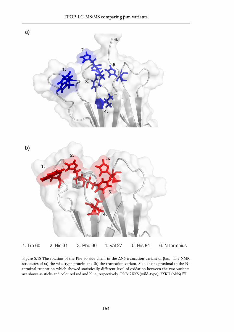
FPOP-LC-MS/MS comparing β2m variants
164
Figure 5.15 The rotation of the Phe 30 side chain in the ΔN6 truncation variant of β2m. The NMR
structures of (a) the wild-type protein and (b) the truncation variant. Side chains proximal to the N-
terminal truncation which showed statistically different level of oxidation between the two variants
are shows as sticks and coloured red and blue, respectively. PDB: 2XKS (wild-type), 2XKU (ΔN6) [78].
FPOP-LC-MS/MS comparing β2m variants
165
5.2.2 Positional isomers in FPOP experiments
When examining the XIC profiles of modified peptides, several species of the same
m/z are observed frequently as different peaks in the XIC. Each peak corresponds to a
different version of the modified peptide, where hydroxyl radical labelling has
occurred on a different side chain in the peptide sequence. An example of this is
shown in Figure 5.16a, where seven differently modified species of peptide 11-26 of
the β2m sequence could be identified by use of MS/MS. However, certain residue
types, when modified, appeared more than once in the XIC, with multiple peaks at
different retention times. In the example shown in Figure 5.16a, both Phe 22 and Tyr
26 were identified as the modified residue within the peptide, at multiple different
retention times.
Across all the modified residues in the experiment, peptides containing modified Phe
side chains were observed to elute at three different retention times, peptides
containing modified Tyr residues were observed to elute at two different retention
times, and peptides which contained modified Trp side chains, were observed to elute
at up to nine different retention times (summarised in Table 5.3). These peaks
correspond to positional isomers formed by hydroxyl radical attack at different
positions on the same aromatic side chain, based on well-established oxidation
chemistries of aromatic amino acids, such as Trp [275], Phe [276, 277] and Tyr [228].
However, despite the fact that these positional isomers are a known and expected
consequence of the hydroxyl radical-mediated oxidation of aromatic side chains, these
products are, to date, seldom mentioned in the FPOP literature [241, 278]. To that end,
the NMR structures of wild-type and ΔN6 β2m were again used to assess the properties
of positional isomers in FPOP experiments, and to determine their utility in detecting
conformational changes in proteins at higher structural resolution.
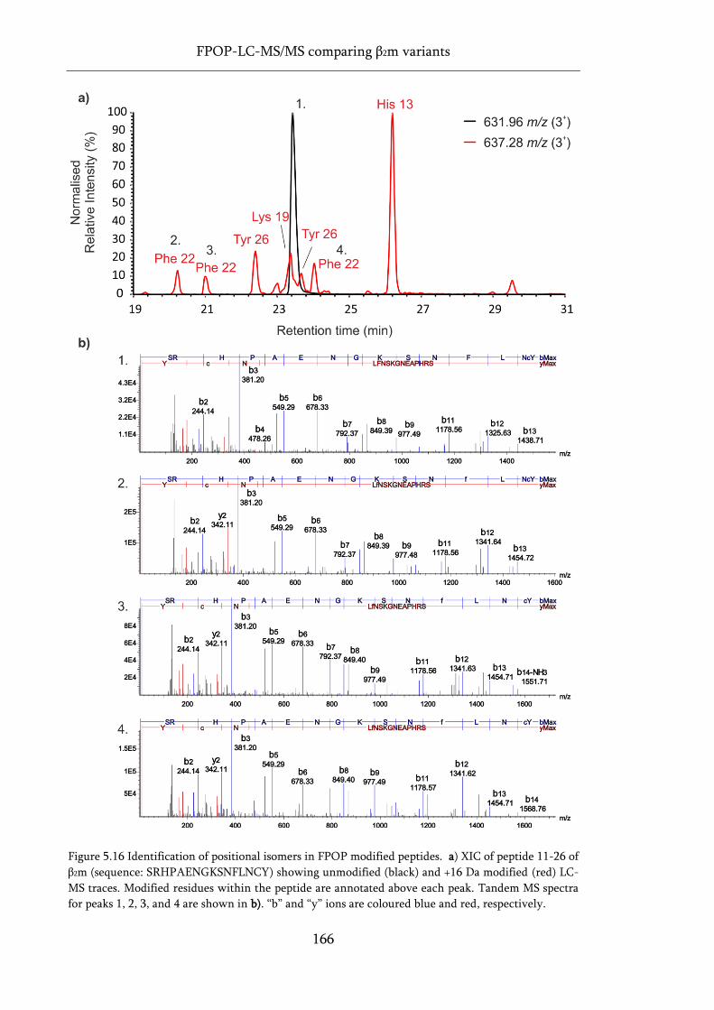
FPOP-LC-MS/MS comparing β2m variants
166
Figure 5.16 Identification of positional isomers in FPOP modified peptides. a) XIC of peptide 11-26 of
β2m (sequence: SRHPAENGKSNFLNCY) showing unmodified (black) and +16 Da modified (red) LC-
MS traces. Modified residues within the peptide are annotated above each peak. Tandem MS spectra
for peaks 1, 2, 3, and 4 are shown in b). “b” and “y” ions are coloured blue and red, respectively.
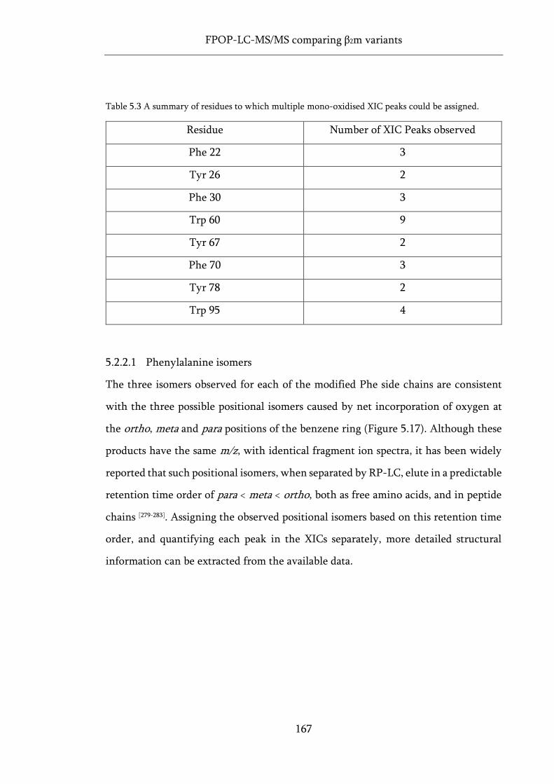
FPOP-LC-MS/MS comparing β2m variants
167
Table 5.3 A summary of residues to which multiple mono-oxidised XIC peaks could be assigned.
Residue Number of XIC Peaks observed
Phe 22 3
Tyr 26 2
Phe 30 3
Trp 60 9
Tyr 67 2
Phe 70 3
Tyr 78 2
Trp 95 4
5.2.2.1 Phenylalanine isomers
The three isomers observed for each of the modified Phe side chains are consistent
with the three possible positional isomers caused by net incorporation of oxygen at
the ortho, meta and para positions of the benzene ring (Figure 5.17). Although these
products have the same m/z, with identical fragment ion spectra, it has been widely
reported that such positional isomers, when separated by RP-LC, elute in a predictable
retention time order of para < meta < ortho, both as free amino acids, and in peptide
chains [279-283]. Assigning the observed positional isomers based on this retention time
order, and quantifying each peak in the XICs separately, more detailed structural
information can be extracted from the available data.
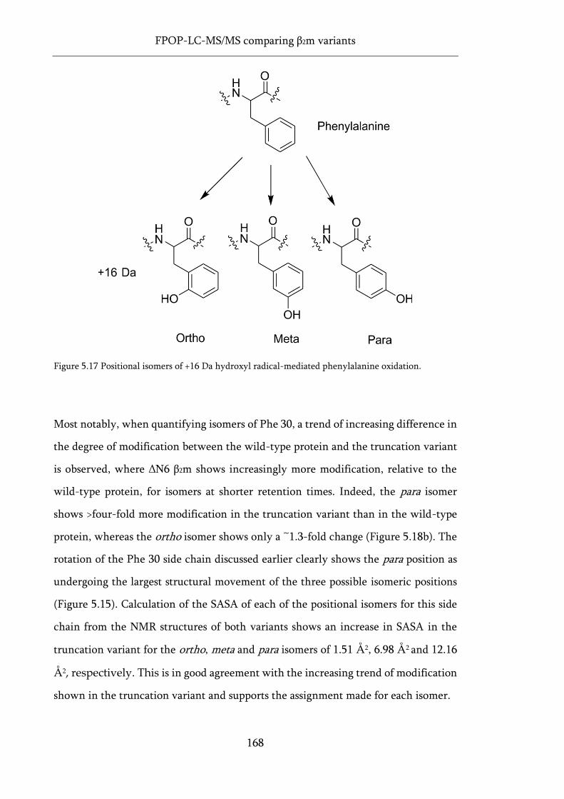
FPOP-LC-MS/MS comparing β2m variants
168
Figure 5.17 Positional isomers of +16 Da hydroxyl radical-mediated phenylalanine oxidation.
Most notably, when quantifying isomers of Phe 30, a trend of increasing difference in
the degree of modification between the wild-type protein and the truncation variant
is observed, where ΔN6 β2m shows increasingly more modification, relative to the
wild-type protein, for isomers at shorter retention times. Indeed, the para isomer
shows >four-fold more modification in the truncation variant than in the wild-type
protein, whereas the ortho isomer shows only a ~1.3-fold change (Figure 5.18b). The
rotation of the Phe 30 side chain discussed earlier clearly shows the para position as
undergoing the largest structural movement of the three possible isomeric positions
(Figure 5.15). Calculation of the SASA of each of the positional isomers for this side
chain from the NMR structures of both variants shows an increase in SASA in the
truncation variant for the ortho, meta and para isomers of 1.51 Å2, 6.98 Å2 and 12.16
Å2, respectively. This is in good agreement with the increasing trend of modification
shown in the truncation variant and supports the assignment made for each isomer.
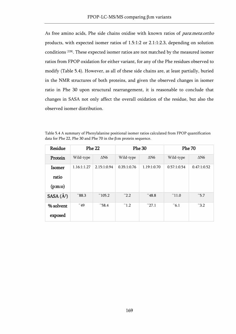
FPOP-LC-MS/MS comparing β2m variants
169
As free amino acids, Phe side chains oxidise with known ratios of para:meta:ortho
products, with expected isomer ratios of 1.5:1:2 or 2.1:1:2.3, depending on solution
conditions [228]. These expected isomer ratios are not matched by the measured isomer
ratios from FPOP oxidation for either variant, for any of the Phe residues observed to
modify (Table 5.4). However, as all of these side chains are, at least partially, buried
in the NMR structures of both proteins, and given the observed changes in isomer
ratio in Phe 30 upon structural rearrangement, it is reasonable to conclude that
changes in SASA not only affect the overall oxidation of the residue, but also the
observed isomer distribution.
Table 5.4 A summary of Phenylalanine positional isomer ratios calculated from FPOP quantification
data for Phe 22, Phe 30 and Phe 70 in the β2m protein sequence.
Residue Phe 22 Phe 30 Phe 70
Protein Wild-type ΔN6 Wild-type ΔN6 Wild-type ΔN6
Isomer
ratio
(p:m:o)
1.16:1:1.27 2.15:1:0.94 0.35:1:0.76 1.19:1:0.70 0.57:1:0.54 0.47:1:0.52
SASA (Å2) ~88.3 ~105.2 ~2.2 ~48.8 ~11.0 ~5.7
% solvent
exposed
~49 ~58.4 ~1.2 ~27.1 ~6.1 ~3.2
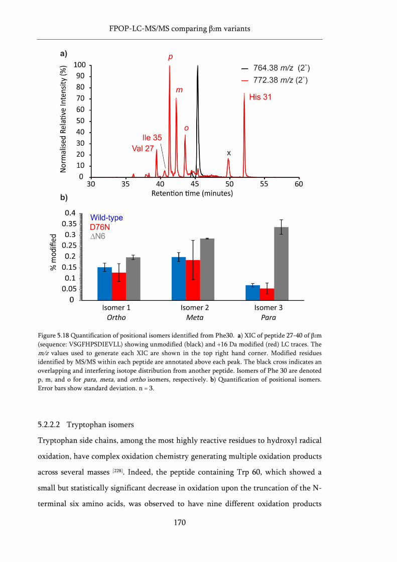
FPOP-LC-MS/MS comparing β2m variants
170
Figure 5.18 Quantification of positional isomers identified from Phe30. a) XIC of peptide 27-40 of β2m
(sequence: VSGFHPSDIEVLL) showing unmodified (black) and +16 Da modified (red) LC traces. The
m/z values used to generate each XIC are shown in the top right hand corner. Modified residues
identified by MS/MS within each peptide are annotated above each peak. The black cross indicates an
overlapping and interfering isotope distribution from another peptide. Isomers of Phe 30 are denoted
p, m, and o for para, meta, and ortho isomers, respectively. b) Quantification of positional isomers.
Error bars show standard deviation. n = 3.
5.2.2.2 Tryptophan isomers
Tryptophan side chains, among the most highly reactive residues to hydroxyl radical
oxidation, have complex oxidation chemistry generating multiple oxidation products
across several masses [228]. Indeed, the peptide containing Trp 60, which showed a
small but statistically significant decrease in oxidation upon the truncation of the N-
terminal six amino acids, was observed to have nine different oxidation products
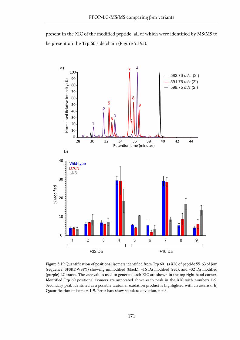
FPOP-LC-MS/MS comparing β2m variants
171
present in the XIC of the modified peptide, all of which were identified by MS/MS to
be present on the Trp 60 side chain (Figure 5.19a).
Figure 5.19 Quantification of positional isomers identified from Trp 60. a) XIC of peptide 55-63 of β2m
(sequence: SFSKDWSFY) showing unmodified (black), +16 Da modified (red), and +32 Da modified
(purple) LC traces. The m/z values used to generate each XIC are shown in the top right hand corner.
Identified Trp 60 positional isomers are annotated above each peak in the XIC with numbers 1-9.
Secondary peak identified as a possible tautomer oxidation product is highlighted with an asterisk. b)
Quantification of isomers 1-9. Error bars show standard deviation. n = 3.
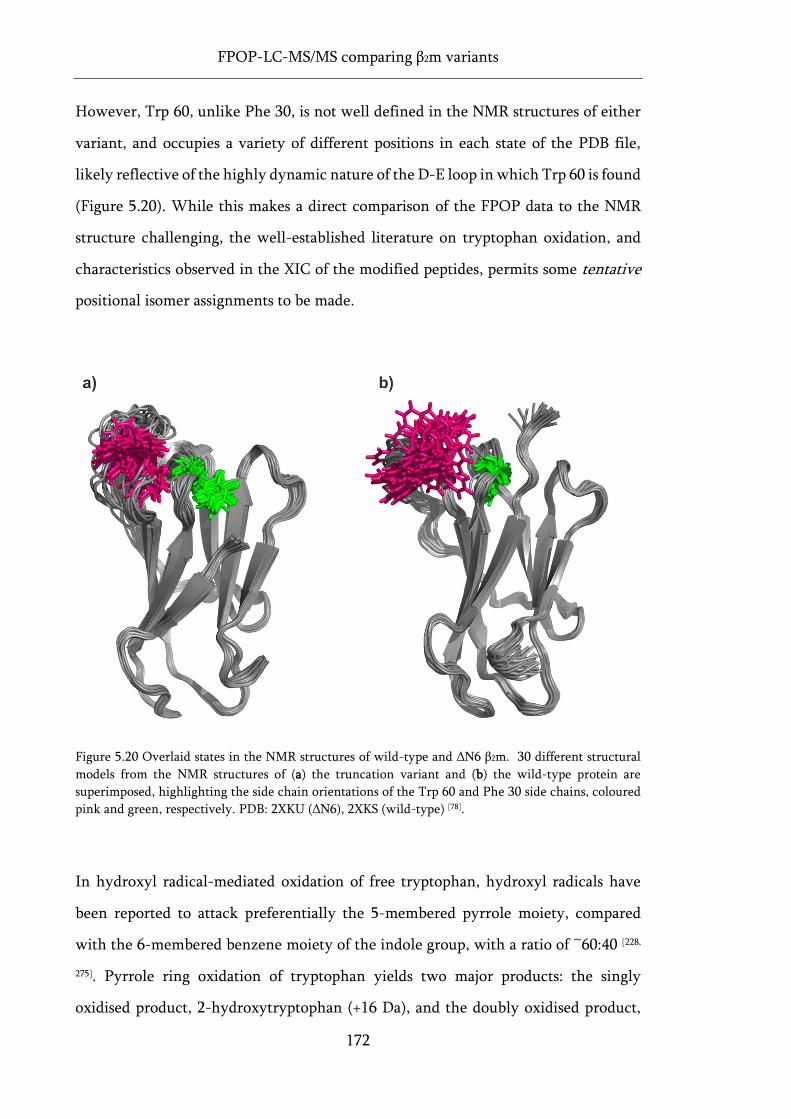
FPOP-LC-MS/MS comparing β2m variants
172
However, Trp 60, unlike Phe 30, is not well defined in the NMR structures of either
variant, and occupies a variety of different positions in each state of the PDB file,
likely reflective of the highly dynamic nature of the D-E loop in which Trp 60 is found
(Figure 5.20). While this makes a direct comparison of the FPOP data to the NMR
structure challenging, the well-established literature on tryptophan oxidation, and
characteristics observed in the XIC of the modified peptides, permits some tentative
positional isomer assignments to be made.
Figure 5.20 Overlaid states in the NMR structures of wild-type and ΔN6 β2m. 30 different structural
models from the NMR structures of (a) the truncation variant and (b) the wild-type protein are
superimposed, highlighting the side chain orientations of the Trp 60 and Phe 30 side chains, coloured
pink and green, respectively. PDB: 2XKU (ΔN6), 2XKS (wild-type) [78].
In hydroxyl radical-mediated oxidation of free tryptophan, hydroxyl radicals have
been reported to attack preferentially the 5-membered pyrrole moiety, compared
with the 6-membered benzene moiety of the indole group, with a ratio of ~60:40 [228,
275]. Pyrrole ring oxidation of tryptophan yields two major products: the singly
oxidised product, 2-hydroxytryptophan (+16 Da), and the doubly oxidised product,
FPOP-LC-MS/MS comparing β2m variants
173
N-formylkynurenine (+32 Da) (Figure 5.21). This is consistent with the two dominant
oxidation products of Trp 60 for the wild-type protein (peaks 7 and 4, respectively in
Figure 5.19a). Strikingly, comparing the ratio of modification for these two oxidation
products with that of the remaining oxidation products observed for Trp 60, a ratio of
60.4:39.6 is observed in favour of the dominant +16 Da and +32 Da products –
remarkably close to that of the expected ratio for free tryptophan in solution [228, 275].
This can be rationalised by closer inspection of the wild-type NMR structure, which
shows the Trp 60 side chain is, on average, ~80% solvent exposed and thus, can be
expected to behave similarly to the free amino acid in solution. Similarly, the 2-
hydroxytryptophan product, tentatively assigned to peak 7 in Figure 5.19a, is known
to undergo keto-enol tautomerism [284]. These tautomers interconvert during
separation by RP-LC, and can be observed as a double peak [285]. A smaller shoulder
peak is observed on peak 7 at ~30% relative intensity (denoted with an * in Figure
5.19a). Examination of the full MS scan for this retention time revealed no interfering
isotope distributions from other peptides (Figure 5.22a). Similarly, examination of the
tandem MS spectra did not show any evidence of multiple species (Figure 5.22b),
indicating that the shoulder peak is the same modified residue as the main peak. As
the four other possible +16 Da positional isomers, caused by oxidation on the benzene
ring of the indole group, can be reasonably assigned to the four other +16 Da oxidation
products observed (peaks 5, 6, 8 and 9), this shoulder peak could be the alternative
tautomer for the 2-hydroxytryptophan product, reinforcing the assignment made for
this XIC peak. The remaining three +32 Da oxidised species are likely
dihydroxytryptophan, where both aromatic rings of the indole group are oxidised
(Figure 5.21).
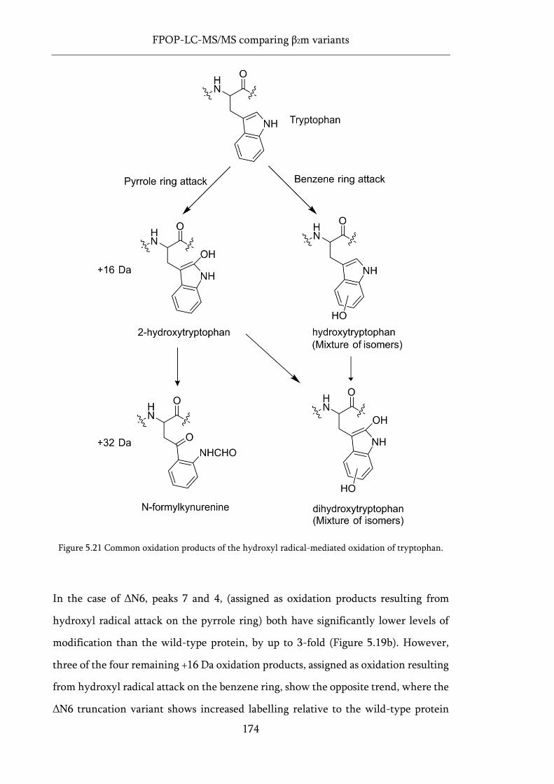
FPOP-LC-MS/MS comparing β2m variants
174
Figure 5.21 Common oxidation products of the hydroxyl radical-mediated oxidation of tryptophan.
In the case of ΔN6, peaks 7 and 4, (assigned as oxidation products resulting from
hydroxyl radical attack on the pyrrole ring) both have significantly lower levels of
modification than the wild-type protein, by up to 3-fold (Figure 5.19b). However,
three of the four remaining +16 Da oxidation products, assigned as oxidation resulting
from hydroxyl radical attack on the benzene ring, show the opposite trend, where the
ΔN6 truncation variant shows increased labelling relative to the wild-type protein
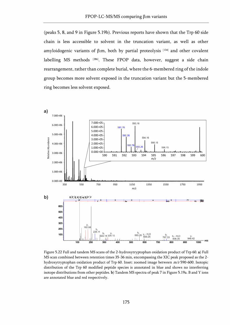
FPOP-LC-MS/MS comparing β2m variants
175
(peaks 5, 8, and 9 in Figure 5.19b). Previous reports have shown that the Trp 60 side
chain is less accessible to solvent in the truncation variant, as well as other
amyloidogenic variants of β2m, both by partial proteolysis [134] and other covalent
labelling MS methods [286]. These FPOP data, however, suggest a side chain
rearrangement, rather than complete burial, where the 6-membered ring of the indole
group becomes more solvent exposed in the truncation variant but the 5-membered
ring becomes less solvent exposed.
Figure 5.22 Full and tandem MS scans of the 2-hydroxytryptophan oxidation product of Trp 60. a) Full
MS scan combined between retention times 35-36 min, encompassing the XIC peak proposed as the 2-
hydroxytryptophan oxidation product of Trp 60. Inset: zoomed image between m/z 590-600. Isotopic
distribution of the Trp 60 modified peptide species is annotated in blue and shows no interferring
isotope distributions from other peptides. b) Tandem MS spectra of peak 7 in Figure 5.19a. B and Y ions
are annotated blue and red respectively.
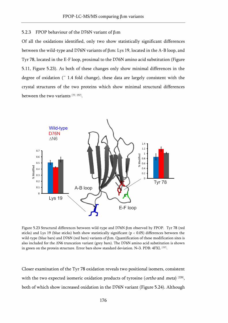
FPOP-LC-MS/MS comparing β2m variants
176
5.2.3 FPOP behaviour of the D76N variant of β2m
Of all the oxidations identified, only two show statistically significant differences
between the wild-type and D76N variants of β2m: Lys 19, located in the A-B loop, and
Tyr 78, located in the E-F loop, proximal to the D76N amino acid substitution (Figure
5.11, Figure 5.23). As both of these changes only show minimal differences in the
degree of oxidation (~ 1.4 fold change), these data are largely consistent with the
crystal structures of the two proteins which show minimal structural differences
between the two variants [77, 157].
Figure 5.23 Structural differences between wild-type and D76N β2m observed by FPOP. Tyr 78 (red
sticks) and Lys 19 (blue sticks) both show statistically significant (p < 0.05) differences between the
wild-type (blue bars) and D76N (red bars) variants of β2m. Quantification of these modification sites is
also included for the ΔN6 truncation variant (grey bars). The D76N amino acid substitution is shown
in green on the protein structure. Error bars show standard deviation. N=3. PDB: 4FXL [157].
Closer examination of the Tyr 78 oxidation reveals two positional isomers, consistent
with the two expected isomeric oxidation products of tyrosine (ortho and meta) [228],
both of which show increased oxidation in the D76N variant (Figure 5.24). Although
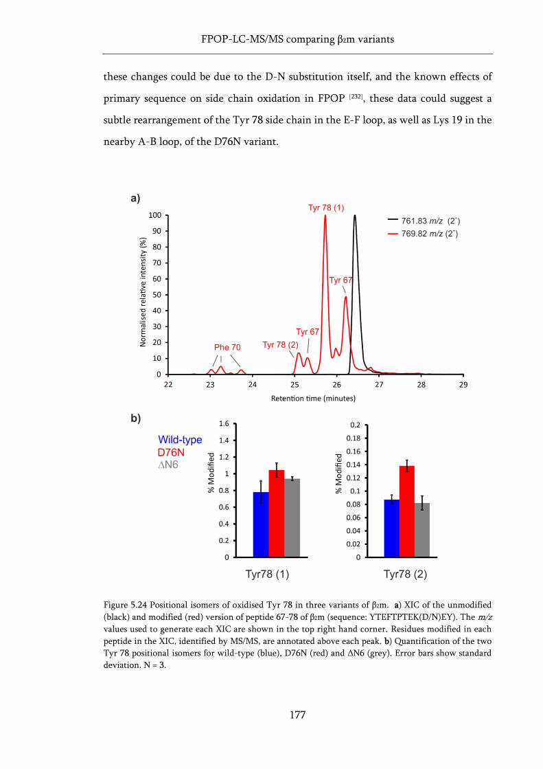
FPOP-LC-MS/MS comparing β2m variants
177
these changes could be due to the D-N substitution itself, and the known effects of
primary sequence on side chain oxidation in FPOP [232], these data could suggest a
subtle rearrangement of the Tyr 78 side chain in the E-F loop, as well as Lys 19 in the
nearby A-B loop, of the D76N variant.
Figure 5.24 Positional isomers of oxidised Tyr 78 in three variants of β2m. a) XIC of the unmodified
(black) and modified (red) version of peptide 67-78 of β2m (sequence: YTEFTPTEK(D/N)EY). The m/z
values used to generate each XIC are shown in the top right hand corner. Residues modified in each
peptide in the XIC, identified by MS/MS, are annotated above each peak. b) Quantification of the two
Tyr 78 positional isomers for wild-type (blue), D76N (red) and ΔN6 (grey). Error bars show standard
deviation. N = 3.
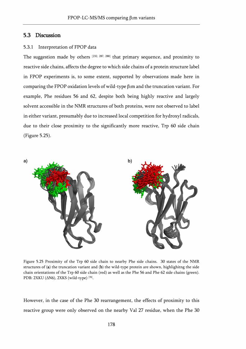
FPOP-LC-MS/MS comparing β2m variants
178
5.3 Discussion
5.3.1 Interpretation of FPOP data
The suggestion made by others [232, 287, 288] that primary sequence, and proximity to
reactive side chains, affects the degree to which side chains of a protein structure label
in FPOP experiments is, to some extent, supported by observations made here in
comparing the FPOP oxidation levels of wild-type β2m and the truncation variant. For
example, Phe residues 56 and 62, despite both being highly reactive and largely
solvent accessible in the NMR structures of both proteins, were not observed to label
in either variant, presumably due to increased local competition for hydroxyl radicals,
due to their close proximity to the significantly more reactive, Trp 60 side chain
(Figure 5.25).
Figure 5.25 Proximity of the Trp 60 side chain to nearby Phe side chains. 30 states of the NMR
structures of (a) the truncation variant and (b) the wild-type protein are shown, highlighitng the side
chain orientations of the Trp 60 side chain (red) as well as the Phe 56 and Phe 62 side chains (green).
PDB: 2XKU (ΔN6), 2XKS (wild-type) [78].
However, in the case of the Phe 30 rearrangement, the effects of proximity to this
reactive group were only observed on the nearby Val 27 residue, when the Phe 30
FPOP-LC-MS/MS comparing β2m variants
179
side chain rotated to the solvent exposed position, in place of the truncated N-
terminus. Given that, in both variants, Phe 30 and Val 27 are the same distance apart
in sequence, these data could suggest an effect of nearby, reactive solvent accessible
side chains on the degree of labelling of other groups, in space. Although this
phenomenon requires further exploration, if true it raises a number of important
questions regarding the interpretation of FPOP data:
1. Over what distance, in 3D space, are the effects of nearby reactive side chains
significant?
2. Does this distance change for side chains of different reactivities?
3. Does the solvent accessibility of either group, or the presence of multiple
reactive side chains, change the significance of this effect?
Indeed, the detailed comparison of FPOP data with calculated SASAs from the NMR
structures in Figure 5.14, although finding a general positive correlation between
SASA and the degree of oxidation for most of the changes which showed statistical
significance, no definitive correlation was observed between the magnitude of
changes in SASA and the magnitude of changes in FPOP oxidation, for equivalent side
chains. This may be due to the complication of microenvironment factors discussed
above, but could similarly be affected by differential sensitivity to changes in SASA
for side chains of varying reactivities. That is to say, is a tryptophan side chain, for
example, more or less sensitive to changes in SASA than a phenylalanine side chain?
To the author’s knowledge, this factor has yet to be explored in the FPOP literature
but, given the known and well-established differences in reactivity to hydroxyl
radical oxidation of the different side chains, is certainly a plausible scenario which
requires further study, before detailed interpretations of unknown protein structures
can be made from FPOP data.
That said, the examination of positional isomers following these FPOP experiments
highlights the potential for achieving sub-amino acid level resolution on changes in
protein structure using this technique. Although further study is required to
FPOP-LC-MS/MS comparing β2m variants
180
determine the usefulness of positional isomers in FPOP, which would no doubt
benefit from a greater understanding of the effects of local microenvironment, it is
important to note that side chain movements, at this level of detail, are largely
invisible to other structural MS methods, such as HDX. Moreover, the propensity of
FPOP to label large hydrophobic side chains, coupled with the immense detail
provided by separate quantification of positional isomers, is of great significance in
the study of aggregation-prone proteins, where solvent exposure of typically buried,
hydrophobic groups is often implicated in the aggregation mechanism [170].
5.3.2 FPOP method development
Being a new method, multiple stages of the FPOP experiment lend themselves
towards further development, including the oxidation process itself, as well as the
associated LC-MS/MS workflows and data processing/analysis.
5.3.2.1 Internal standards
During sample oxidation, the inclusion of internal standards, or dosimetry
experiments to assess the hydroxyl radical dose given to each sample, would be a
useful tool to develop the robustness and reproducibility of the technique, and has
been implemented successfully into the FPOP workflow elsewhere [289-291]. Although
not used in the experiments described here due to the identical solution conditions
between samples, internal standards such as leu-enkephalin have been used in FPOP
to correct for changes in hydroxyl radical dose, thus allowing comparisons of samples
at different concentration, or under different buffer conditions where the •OH
scavenging ability of the solution may vary [291]. However, as discussed earlier, a deeper
understanding of the reactivities of different side chains, and the effects of their
relative solvent accessibilities, would be needed before the corrections applied from
the oxidation of internal standards could be relied upon for detailed analyses. Namely,
does side chain reactivity affect the sensitivity of side chains to change in •OH dose
FPOP-LC-MS/MS comparing β2m variants
181
(i.e. is a tryptophan side chain more or less sensitive to change in •OH dose than a
phenylalanine?), and does the solvent accessibility of each side chain affect that
sensitivity (is a buried tryptophan more or less sensitive to changes in •OH dose than
an exposed tryptophan?). Considering the sensitivity to oxidation of the internal
standard itself is of critical importance, such effects require further study before an
optimal choice of internal standard can be made.
5.3.2.2 LC-MS/MS development
Although the assignments of FPOP isomers identified for the two β2m variants are
consistent with the existing literature regarding known oxidation chemistries [228] and
the affirmed elution orders of positional isomers by RP-LC [279-283], these assignments
cannot be made with certainty, without retention time alignment of identical oxidised
peptides with known, unique, positional isomers. Not only would this be prohibitively
expensive, but the low throughput of this method makes this approach largely
impractical. However, positional isomers of both Phe [292] and Trp [293] are
distinguishable by differential UV absorbance spectra, and UV detectors are routinely
implemented for online analysis in LC-MS/MS workflows. Indeed, Trp oxidation in
heat stressed antibodies has been characterised previously in precisely this manner [294]
and thus, make this an appealing development opportunity for the routine
characterisation of positional isomers in FPOP experiments.
With regards to MS/MS procedures, the DDA approach used in our experiments and
most commonly in the literature, while effective, requires instrumentation capable of
fast MS/MS acquisition and, due to the oxidised products frequently having the same
m/z, partial or incomplete LC separation of different versions of a modified peptide,
results in co-selection of the different modified peptides by the quadrupole, and the
generation of difficult to interpret, chimeric MS/MS data (Figure 5.26).
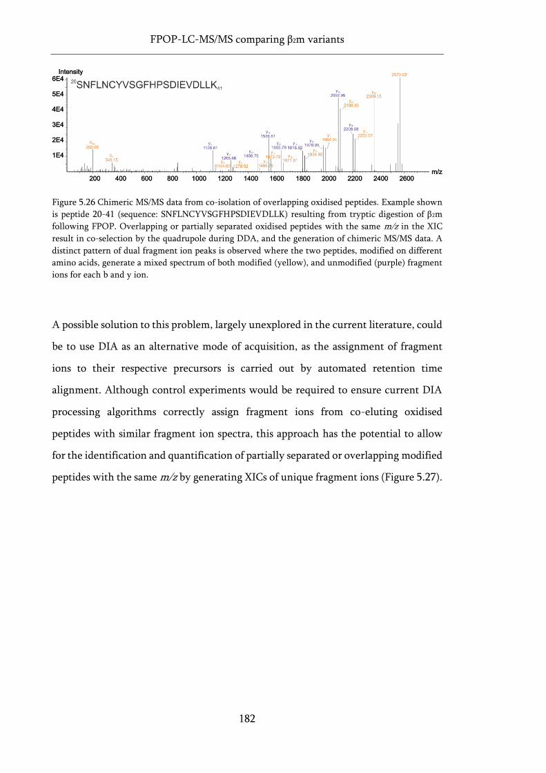
FPOP-LC-MS/MS comparing β2m variants
182
Figure 5.26 Chimeric MS/MS data from co-isolation of overlapping oxidised peptides. Example shown
is peptide 20-41 (sequence: SNFLNCYVSGFHPSDIEVDLLK) resulting from tryptic digestion of β2m
following FPOP. Overlapping or partially separated oxidised peptides with the same m/z in the XIC
result in co-selection by the quadrupole during DDA, and the generation of chimeric MS/MS data. A
distinct pattern of dual fragment ion peaks is observed where the two peptides, modified on different
amino acids, generate a mixed spectrum of both modified (yellow), and unmodified (purple) fragment
ions for each b and y ion.
A possible solution to this problem, largely unexplored in the current literature, could
be to use DIA as an alternative mode of acquisition, as the assignment of fragment
ions to their respective precursors is carried out by automated retention time
alignment. Although control experiments would be required to ensure current DIA
processing algorithms correctly assign fragment ions from co-eluting oxidised
peptides with similar fragment ion spectra, this approach has the potential to allow
for the identification and quantification of partially separated or overlapping modified
peptides with the same m/z by generating XICs of unique fragment ions (Figure 5.27).
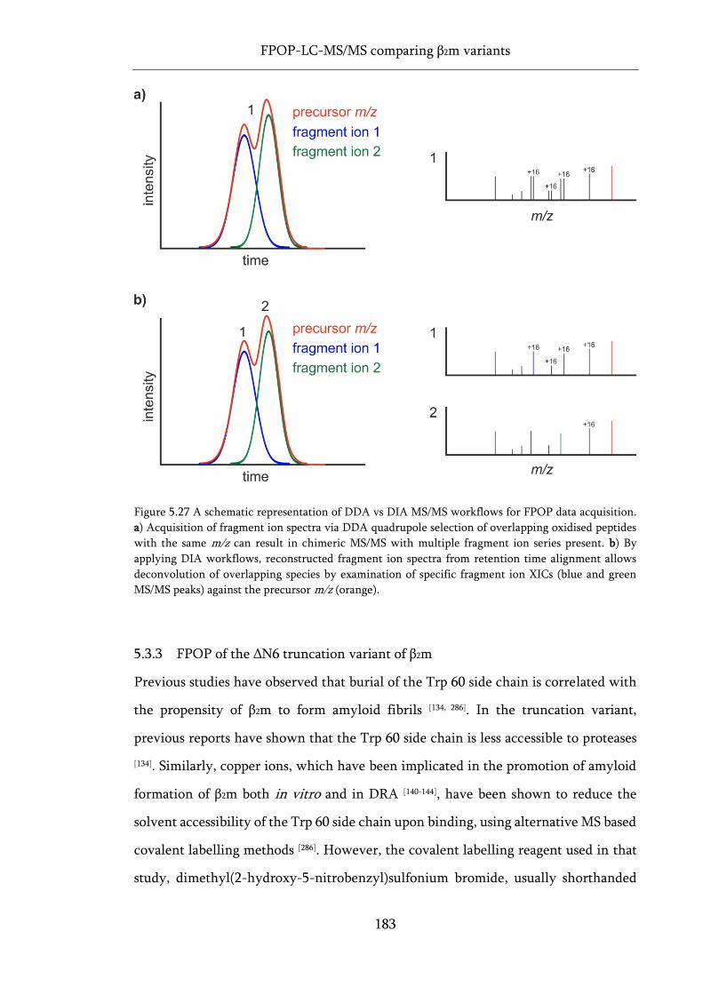
FPOP-LC-MS/MS comparing β2m variants
183
Figure 5.27 A schematic representation of DDA vs DIA MS/MS workflows for FPOP data acquisition.
a) Acquisition of fragment ion spectra via DDA quadrupole selection of overlapping oxidised peptides
with the same m/z can result in chimeric MS/MS with multiple fragment ion series present. b) By
applying DIA workflows, reconstructed fragment ion spectra from retention time alignment allows
deconvolution of overlapping species by examination of specific fragment ion XICs (blue and green
MS/MS peaks) against the precursor m/z (orange).
5.3.3 FPOP of the ΔN6 truncation variant of β2m
Previous studies have observed that burial of the Trp 60 side chain is correlated with
the propensity of β2m to form amyloid fibrils [134, 286]. In the truncation variant,
previous reports have shown that the Trp 60 side chain is less accessible to proteases
[134]. Similarly, copper ions, which have been implicated in the promotion of amyloid
formation of β2m both in vitro and in DRA [140-144], have been shown to reduce the
solvent accessibility of the Trp 60 side chain upon binding, using alternative MS based
covalent labelling methods [286]. However, the covalent labelling reagent used in that
study, dimethyl(2-hydroxy-5-nitrobenzyl)sulfonium bromide, usually shorthanded
FPOP-LC-MS/MS comparing β2m variants
184
to HNSB, is comparatively large, giving rise to a 151 Da mass addition upon
modification of the tryptophan side chain [286]. The smaller size of the hydroxyl radical
in FPOP labelling, and the identification of positional isomers has allowed
experiments performed here to obtain a higher resolution analysis of Trp 60,
suggesting only partial burial of this residue in the amyloidogenic truncation variant.
The minor conformational changes observed for Phe 22 and His 51 are intriguing, as
these are distant from the site of the N-terminal truncation. While the significance of
these changes, with regards to the aggregation propensity of the truncation variant,
are difficult to ascertain from these data without further study, the conformation of
the D-strand in which His 51 is located has been implicated numerous times in the
aggregation of β2m [295, 296], and could provide additional insight into the aggregation of
the ΔN6 truncation variant.
5.3.4 FPOP of the D76N variant of β2m
For the most part, the wild-type protein and the D76N variant were largely
indistinguishable by FPOP, exhibiting only minor differences in labelling on two side
chains: Tyr 76 and Lys 19. While these changes are both located nearby to the D76N
substitution, indicating the amino acid change has some effect on the solvent
accessibility of nearby side chains, these data are largely consistent with the known
similarity between the crystal structures of the two variants [77, 157], and suggest only
minimal changes in protein structure caused by the D76N substitution. These data
are, perhaps, unsurprising, as even considerable side chain movements nearby to the
D-N substitution could easily remain undetectable by FPOP, assuming the residue
adopts a similarly solvent exposed position in the D76N variant, a likely scenario given
the solvent exposed nature of the E-F loop in which the D76N substitution is found.
Curiously, these data are in contrast to the deuterium exchange behaviour of the E-F
loop in this variant, relative to the wild-type protein, discussed earlier in Section 4.6
and 4.7.2. These differences will be discussed in detail later in Section 7.2.
185
Chapter 6:
FPOP-LC-MS/MS of WFL and
STT
FPOP-LC-MS/MS of WFL and STT
186
6 FPOP-LC-MS/MS of WFL and STT
As discussed earlier in Section 2.3, protein aggregation in biopharmaceutical
development is of critical importance to patient safety, and the future development of
biopharmaceutical products. Given the minor, triple amino acid substitution made in
the heavy chain CDRs (W30S, F31T, L57T), and subsequent drastic changes in the
propensity to undergo reversible self-association, the two mAbs WFL and STT
developed by Medimmune (discussed in detail in Section 2.3.1), provide an ideal
model system by which to study aggregation in pharmaceutically relevant mAbs.
Similarly, these proteins offer an opportunity to develop further the FPOP
methodology for the study of larger, more complex protein systems, and assess the
potential utility of this technique for probing conformational changes associated with
aggregation propensity in mAbs. As such, the two mAb variants, WFL and STT, were
subjected to FPOP-LC-MS/MS analysis, with the following aims:
1. Identify differences in conformation and structure which may be associated
with the propensity of WFL to undergo reversible self-association
2. Develop the FPOP-LC-MS/MS methodology for more complex protein
systems, and assess the utility of FPOP in the study of biopharmaceutical
protein structure.
Data in this chapter were subsequently published in Cornwell et al., Analytical
Chemistry, 2019 [297].
6.1 Initial characterisation and overview
Both WFL and STT were subjected to oxidation by FPOP as described in Section 3.5.2.
Both proteins were oxidised in their formulation buffer (20 mM sodium succinate,
125 mM L-arginine, pH 6.0 – optimised by Medimmune) at 0.1 mg ml-1, conditions at
which both proteins are known to be predominantly monomeric [170]. 10 mM L-
histidine was added as a scavenger amino acid, and 3 µl of 5 % v/v H2O2 was added
FPOP-LC-MS/MS of WFL and STT
187
immediately prior to oxidation. This is 3x the hydrogen peroxide used in the FPOP
experiments performed with β2m (Section 5) and was necessary to overcome the •OH
scavenging effect of the arginine excipient in the formulation buffer.
Following FPOP, reduction of disulphide bonds, alkylation and proteolytic digestion
using trypsin (detailed methods described in Section 3.5.2) yielded good sequence
coverage for the heavy and light chains for both WFL and STT (an example coverage
map is shown in Figure 6.1). A total of 19 peptides were used for quantification of
identified FPOP oxidations (green lines in Figure 6.1), as these were found to be
present in all replicates of both proteins, and had both modified, and unmodified
versions. Of these 19 peptides, MS/MS data were used to identify 50 different modified
sites (28 identified on the heavy chain, and 22 on the light chain), the majority of
which could be localised to residue level resolution, and were observed in both
variants (Table 6.1, Figure 6.2).
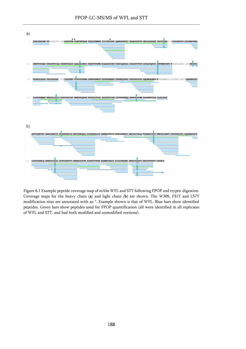
FPOP-LC-MS/MS of WFL and STT
188
Figure 6.1 Example peptide coverage map of mAbs WFL and STT following FPOP and tryptic digestion.
Coverage maps for the heavy chain (a) and light chain (b) are shown. The W30S, F31T and L57T
modification sites are annotated with an *. Example shown is that of WFL. Blue bars show identified
peptides. Green bars show peptides used for FPOP quantification (all were identified in all replicates
of WFL and STT, and had both modified and unmodified versions).
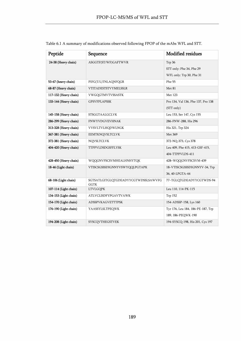
FPOP-LC-MS/MS of WFL and STT
189
Table 6.1 A summary of modifications observed following FPOP of the mAbs WFL and STT.
Peptide Sequence Modified residues
24-38 (Heavy chain) ASGGTF(ST/WF)GAFTWVR Trp 36
STT only: Phe 34, Phe 29
WFL only: Trp 30, Phe 31
53-67 (heavy chain) PIFG(T/L)TNLAQNFQGR Phe 55
68-87 (Heavy chain) VTITADESTSTVYMELSSLR Met 81
117-132 (Heavy chain) VWGQGTMVTVSSASTK Met 123
133-144 (Heavy chain) GPSVFPLAPSSK Pro 134, Val 136, Phe 137, Pro 138
(STT only)
145-158 (Heavy chain) STSGGTAALGCLVK Leu 153, Ser 147, Cys 155
286-299 (Heavy chain) FNWYVDGVEVHNAK 286-FNW-288, His 296
313-328 (Heavy chain) VVSVLTVLHQDWLNGK His 321, Trp 324
367-381 (Heavy chain) EEMTKNQVSLTCLVK Met 369
372-381 (Heavy chain) NQVSLTCLVK 372-NQ-373, Cys 378
404-420 (Heavy chain) TTPPVLDSDGSFFLYSK Leu 409, Phe 415, 413-GSF-415,
404-TTPPVLDS-411
428-450 (Heavy chain) WQQGNVFSCSVMHEALHNHYTQK 428–WQQGNVFSCSVM-439
18-46 (Light chain) VTISCSGSSSDIGNNYVSWYQQLPGTAPK 18–VTISCSGSSSDIGNNYV-34, Trp
36, 40-LPGTA-44
68-106 (Light chain) SGTSATLGITGLQTGDEADYYCGTWDSSLSAWVFG
GGTK
77–TGLQTGDEADYYCGTWDS-94
107-114 (Light chain) LTVLGQPK Leu 110, 114-PK-115
134-153 (Light chain) ATLVCLISDFYPGAVTVAWK Trp 152
154-170 (Light chain) ADSSPVKAGVETTTPSK 154-ADSSP-158, Lys 160
176-190 (Light chain) YAASSYLSLTPEQWK Tyr 176, Leu 184, 186-PE-187, Trp
189, 186-PEQWK-190
194-208 (Light chain) SYSCQVTHEGSTVEK 194-SYSCQ-198, His 201, Cys 197
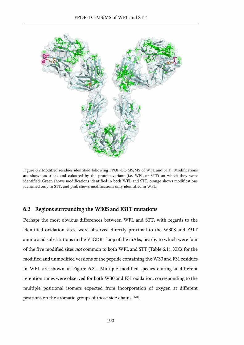
FPOP-LC-MS/MS of WFL and STT
190
Figure 6.2 Modified residues identified following FPOP-LC-MS/MS of WFL and STT. Modifications
are shown as sticks and coloured by the protein variant (i.e. WFL or STT) on which they were
identified. Green shows modifications identified in both WFL and STT, orange shows modifications
identified only in STT, and pink shows modifications only idenitified in WFL.
6.2 Regions surrounding the W30S and F31T mutations
Perhaps the most obvious differences between WFL and STT, with regards to the
identified oxidation sites, were observed directly proximal to the W30S and F31T
amino acid substitutions in the VHCDR1 loop of the mAbs, nearby to which were four
of the five modified sites not common to both WFL and STT (Table 6.1). XICs for the
modified and unmodified versions of the peptide containing the W30 and F31 residues
in WFL are shown in Figure 6.3a. Multiple modified species eluting at different
retention times were observed for both W30 and F31 oxidation, corresponding to the
multiple positional isomers expected from incorporation of oxygen at different
positions on the aromatic groups of those side chains [228].
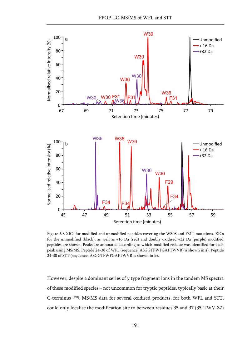
FPOP-LC-MS/MS of WFL and STT
191
Figure 6.3 XICs for modified and unmodified peptides covering the W30S and F31T mutations. XICs
for the unmodified (black), as well as +16 Da (red) and doubly oxidised +32 Da (purple) modified
peptides are shown. Peaks are annotated according to which modified residue was identified for each
peak using MS/MS. Peptide 24-38 of WFL (sequence: ASGGTFWFGAFTWVR) is shown in a). Peptide
24-38 of STT (sequence: ASGGTFWFGAFTWVR is shown in b).
However, despite a dominant series of y type fragment ions in the tandem MS spectra
of these modified species – not uncommon for tryptic peptides, typically basic at their
C-terminus [298], MS/MS data for several oxidised products, for both WFL and STT,
could only localise the modification site to between residues 35 and 37 (35-TWV-37)
FPOP-LC-MS/MS of WFL and STT
192
(Figure 6.4). This can be further narrowed down to Trp 36 or Val 37, if water loss ions
are used for assignment [299]. Given the significantly higher reactivity to hydroxyl
radical oxidation of tryptophan than either threonine or valine, as well as the presence
of multiple oxidation products and double (+32 Da) oxidations in this region, these
modifications are most likely present on the Trp 36 side chain. Although this residue
is present in the core of the VH domain, surprisingly, following quantification, Trp 36
was found to be ~6-fold more oxidised in the WFL variant than in the STT variant
(Figure 6.5a). This could suggest a marked difference in the conformation and solvent
accessibility of side chains in the region of the VH domain caused by the WFL-STT
substitutions.

FPOP-LC-MS/MS of WFL and STT
193
Figure 6.4 Representative MS/MS for peptide 24-38 of WFL. The region, or residue, to which MS/MS
could localise the +16 Da modification are shown underlined on the sequence of each peptide, shown
in the top right hand corner of each spectrum. The assignment made for the modification site is shown
in bold. The top spectrum shows the unmodified version of the peptide.
This hypothesis is supported by a closer examination of other oxidised products in the
region. The Phe 29 and Phe 34 side chains, located either side of the W30S and F31T
substitutions, were only observed to modify in the STT variant (Figure 6.3b, Figure
6.5a). Similarly, the Phe 55 side chain in the VHCDR2 loop, adjacent to the L57T
substitution site and spatially proximal to the W30S and F31T substitutions, was
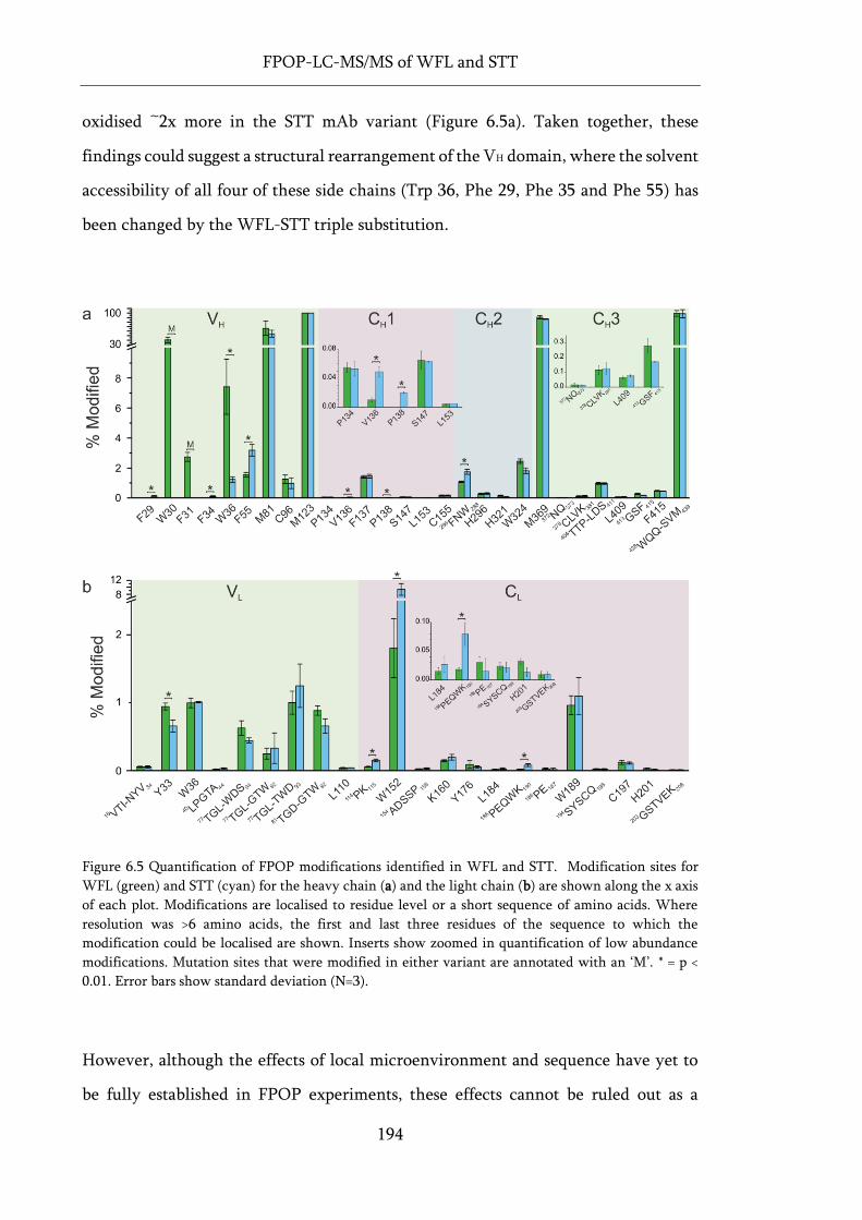
FPOP-LC-MS/MS of WFL and STT
194
oxidised ~2x more in the STT mAb variant (Figure 6.5a). Taken together, these
findings could suggest a structural rearrangement of the VH domain, where the solvent
accessibility of all four of these side chains (Trp 36, Phe 29, Phe 35 and Phe 55) has
been changed by the WFL-STT triple substitution.
Figure 6.5 Quantification of FPOP modifications identified in WFL and STT. Modification sites for
WFL (green) and STT (cyan) for the heavy chain (a) and the light chain (b) are shown along the x axis
of each plot. Modifications are localised to residue level or a short sequence of amino acids. Where
resolution was >6 amino acids, the first and last three residues of the sequence to which the
modification could be localised are shown. Inserts show zoomed in quantification of low abundance
modifications. Mutation sites that were modified in either variant are annotated with an ‘M’. * = p <
0.01. Error bars show standard deviation (N=3).
However, although the effects of local microenvironment and sequence have yet to
be fully established in FPOP experiments, these effects cannot be ruled out as a
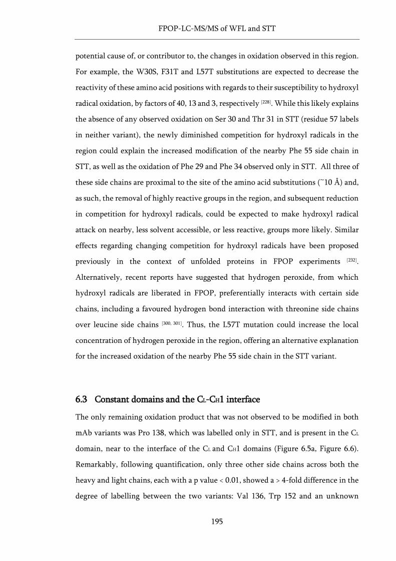
FPOP-LC-MS/MS of WFL and STT
195
potential cause of, or contributor to, the changes in oxidation observed in this region.
For example, the W30S, F31T and L57T substitutions are expected to decrease the
reactivity of these amino acid positions with regards to their susceptibility to hydroxyl
radical oxidation, by factors of 40, 13 and 3, respectively [228]. While this likely explains
the absence of any observed oxidation on Ser 30 and Thr 31 in STT (residue 57 labels
in neither variant), the newly diminished competition for hydroxyl radicals in the
region could explain the increased modification of the nearby Phe 55 side chain in
STT, as well as the oxidation of Phe 29 and Phe 34 observed only in STT. All three of
these side chains are proximal to the site of the amino acid substitutions (~10 Å) and,
as such, the removal of highly reactive groups in the region, and subsequent reduction
in competition for hydroxyl radicals, could be expected to make hydroxyl radical
attack on nearby, less solvent accessible, or less reactive, groups more likely. Similar
effects regarding changing competition for hydroxyl radicals have been proposed
previously in the context of unfolded proteins in FPOP experiments [232].
Alternatively, recent reports have suggested that hydrogen peroxide, from which
hydroxyl radicals are liberated in FPOP, preferentially interacts with certain side
chains, including a favoured hydrogen bond interaction with threonine side chains
over leucine side chains [300, 301]. Thus, the L57T mutation could increase the local
concentration of hydrogen peroxide in the region, offering an alternative explanation
for the increased oxidation of the nearby Phe 55 side chain in the STT variant.
6.3 Constant domains and the CL-CH1 interface
The only remaining oxidation product that was not observed to be modified in both
mAb variants was Pro 138, which was labelled only in STT, and is present in the CL
domain, near to the interface of the CL and CH1 domains (Figure 6.5a, Figure 6.6).
Remarkably, following quantification, only three other side chains across both the
heavy and light chains, each with a p value < 0.01, showed a > 4-fold difference in the
degree of labelling between the two variants: Val 136, Trp 152 and an unknown
FPOP-LC-MS/MS of WFL and STT
196
modification between residues Pro 186 and Lys 190 (Figure 6.5a and b). All three of
these side chains are similarly located proximal to the CL-CH1 interface and all show
significantly lower levels of oxidation in the WFL variant (Figure 6.6). Minor (< 2-
fold), although statistically significant, changes in oxidation were also observed at the
top of the nearby CH2 domain, with similarly decreased labelling in the WFL variant
(Figure 6.6). These results are surprising, as these changes are a distance of > 60 Å from
the WFL-STT triple substitution, and suggest a conformational change of the constant
domains, or a change in orientation of the constant domains, particularly the CL and
CH1 domains, relative to one another.
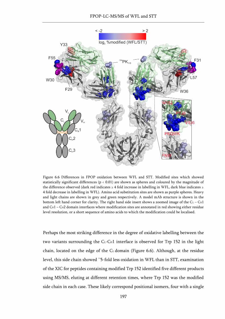
FPOP-LC-MS/MS of WFL and STT
197
Figure 6.6 Differences in FPOP oxidation between WFL and STT. Modified sites which showed
statistically significant differences (p < 0.01) are shown as spheres and coloured by the magnitude of
the difference observed (dark red indicates ≥ 4 fold increase in labelling in WFL, dark blue indicates ≥
4 fold decrease in labelling in WFL). Amino acid substitution sites are shown as purple spheres. Heavy
and light chains are shown in grey and green respectively. A model mAb structure is shown in the
bottom left hand corner for clarity. The right hand side insert shows a zoomed image of the CL – CH1
and CH1 – CH2 domain interfaces where modification sites are annotated in red showing either residue
level resolution, or a short sequence of amino acids to which the modification could be localised.
Perhaps the most striking difference in the degree of oxidative labelling between the
two variants surrounding the CL-CH1 interface is observed for Trp 152 in the light
chain, located on the edge of the CL domain (Figure 6.6). Although, at the residue
level, this side chain showed ~5-fold less oxidation in WFL than in STT, examination
of the XIC for peptides containing modified Trp 152 identified five different products
using MS/MS, eluting at different retention times, where Trp 152 was the modified
side chain in each case. These likely correspond positional isomers, four with a single
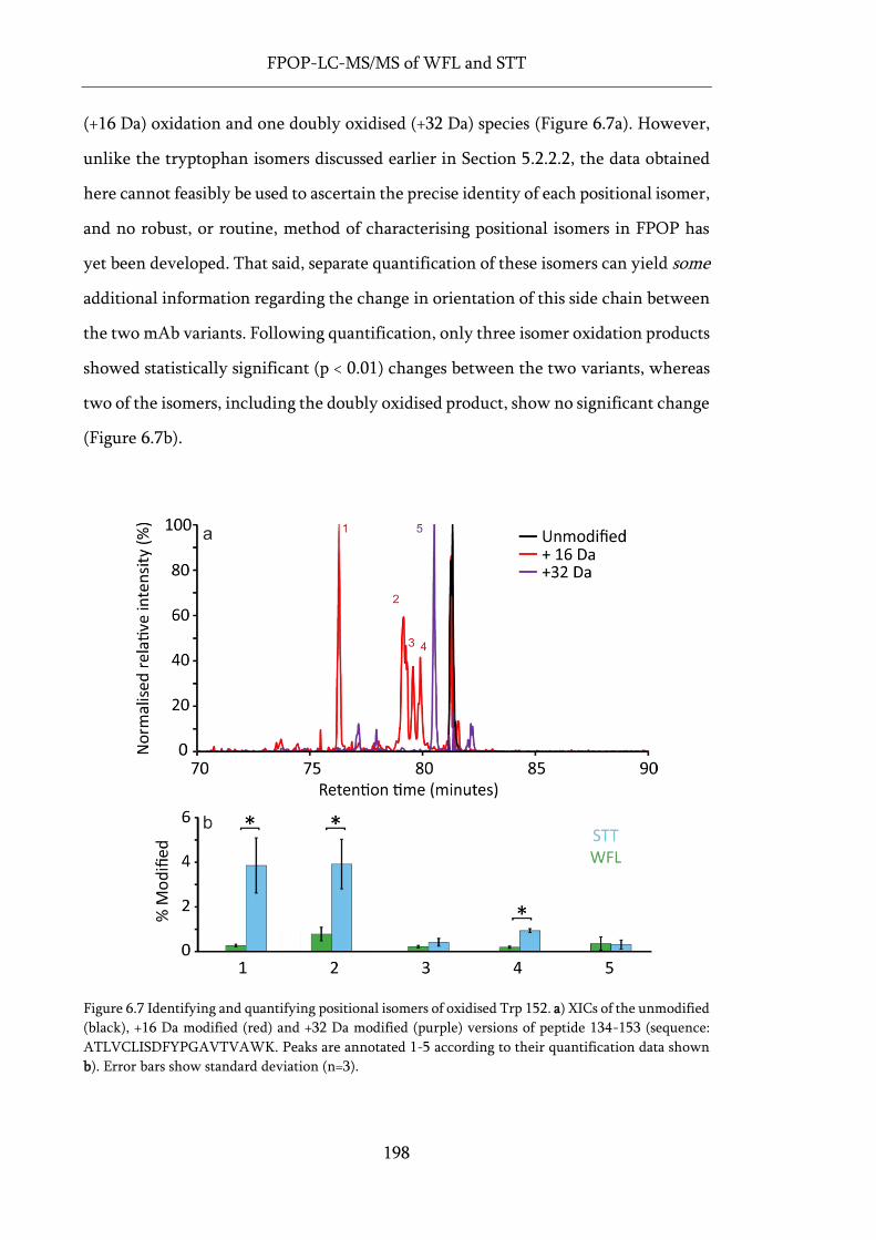
FPOP-LC-MS/MS of WFL and STT
198
(+16 Da) oxidation and one doubly oxidised (+32 Da) species (Figure 6.7a). However,
unlike the tryptophan isomers discussed earlier in Section 5.2.2.2, the data obtained
here cannot feasibly be used to ascertain the precise identity of each positional isomer,
and no robust, or routine, method of characterising positional isomers in FPOP has
yet been developed. That said, separate quantification of these isomers can yield some
additional information regarding the change in orientation of this side chain between
the two mAb variants. Following quantification, only three isomer oxidation products
showed statistically significant (p < 0.01) changes between the two variants, whereas
two of the isomers, including the doubly oxidised product, show no significant change
(Figure 6.7b).
Figure 6.7 Identifying and quantifying positional isomers of oxidised Trp 152. a) XICs of the unmodified
(black), +16 Da modified (red) and +32 Da modified (purple) versions of peptide 134-153 (sequence:
ATLVCLISDFYPGAVTVAWK. Peaks are annotated 1-5 according to their quantification data shown
b). Error bars show standard deviation (n=3).
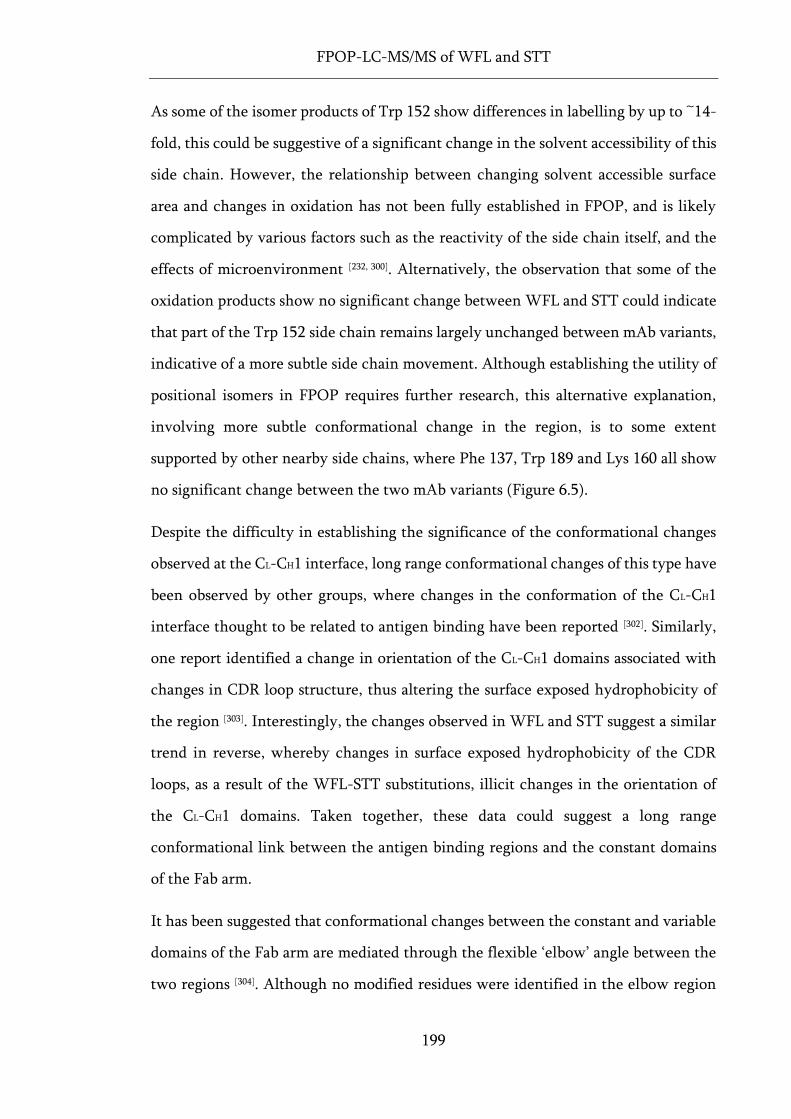
FPOP-LC-MS/MS of WFL and STT
199
As some of the isomer products of Trp 152 show differences in labelling by up to ~14-
fold, this could be suggestive of a significant change in the solvent accessibility of this
side chain. However, the relationship between changing solvent accessible surface
area and changes in oxidation has not been fully established in FPOP, and is likely
complicated by various factors such as the reactivity of the side chain itself, and the
effects of microenvironment [232, 300]. Alternatively, the observation that some of the
oxidation products show no significant change between WFL and STT could indicate
that part of the Trp 152 side chain remains largely unchanged between mAb variants,
indicative of a more subtle side chain movement. Although establishing the utility of
positional isomers in FPOP requires further research, this alternative explanation,
involving more subtle conformational change in the region, is to some extent
supported by other nearby side chains, where Phe 137, Trp 189 and Lys 160 all show
no significant change between the two mAb variants (Figure 6.5).
Despite the difficulty in establishing the significance of the conformational changes
observed at the CL-CH1 interface, long range conformational changes of this type have
been observed by other groups, where changes in the conformation of the CL-CH1
interface thought to be related to antigen binding have been reported [302]. Similarly,
one report identified a change in orientation of the CL-CH1 domains associated with
changes in CDR loop structure, thus altering the surface exposed hydrophobicity of
the region [303]. Interestingly, the changes observed in WFL and STT suggest a similar
trend in reverse, whereby changes in surface exposed hydrophobicity of the CDR
loops, as a result of the WFL-STT substitutions, illicit changes in the orientation of
the CL-CH1 domains. Taken together, these data could suggest a long range
conformational link between the antigen binding regions and the constant domains
of the Fab arm.
It has been suggested that conformational changes between the constant and variable
domains of the Fab arm are mediated through the flexible ‘elbow’ angle between the
two regions [304]. Although no modified residues were identified in the elbow region
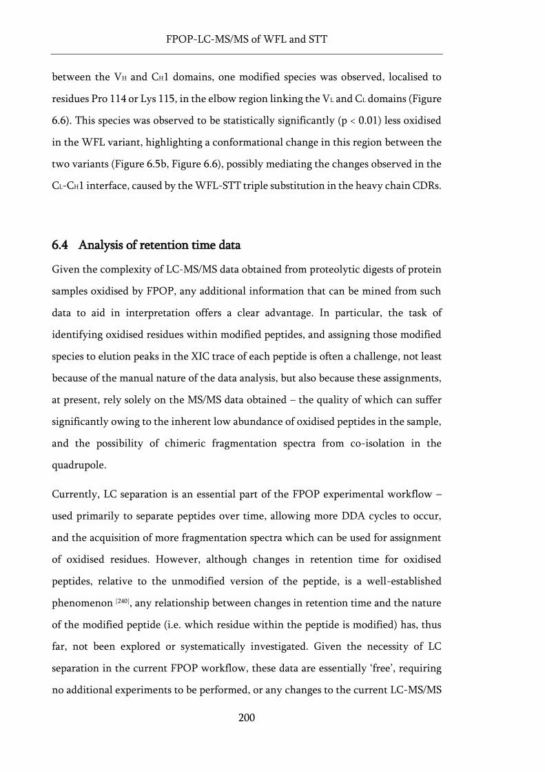
FPOP-LC-MS/MS of WFL and STT
200
between the VH and CH1 domains, one modified species was observed, localised to
residues Pro 114 or Lys 115, in the elbow region linking the VL and CL domains (Figure
6.6). This species was observed to be statistically significantly (p < 0.01) less oxidised
in the WFL variant, highlighting a conformational change in this region between the
two variants (Figure 6.5b, Figure 6.6), possibly mediating the changes observed in the
CL-CH1 interface, caused by the WFL-STT triple substitution in the heavy chain CDRs.
6.4 Analysis of retention time data
Given the complexity of LC-MS/MS data obtained from proteolytic digests of protein
samples oxidised by FPOP, any additional information that can be mined from such
data to aid in interpretation offers a clear advantage. In particular, the task of
identifying oxidised residues within modified peptides, and assigning those modified
species to elution peaks in the XIC trace of each peptide is often a challenge, not least
because of the manual nature of the data analysis, but also because these assignments,
at present, rely solely on the MS/MS data obtained – the quality of which can suffer
significantly owing to the inherent low abundance of oxidised peptides in the sample,
and the possibility of chimeric fragmentation spectra from co-isolation in the
quadrupole.
Currently, LC separation is an essential part of the FPOP experimental workflow –
used primarily to separate peptides over time, allowing more DDA cycles to occur,
and the acquisition of more fragmentation spectra which can be used for assignment
of oxidised residues. However, although changes in retention time for oxidised
peptides, relative to the unmodified version of the peptide, is a well-established
phenomenon [240], any relationship between changes in retention time and the nature
of the modified peptide (i.e. which residue within the peptide is modified) has, thus
far, not been explored or systematically investigated. Given the necessity of LC
separation in the current FPOP workflow, these data are essentially ‘free’, requiring
no additional experiments to be performed, or any changes to the current LC-MS/MS
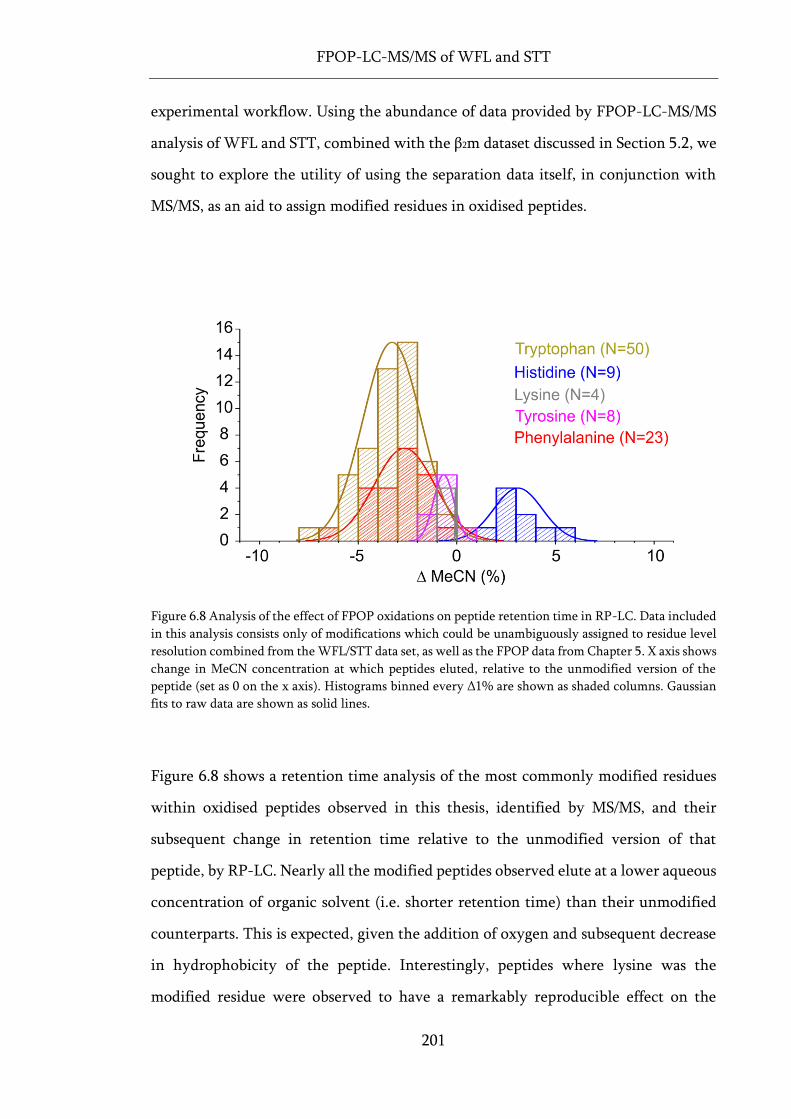
FPOP-LC-MS/MS of WFL and STT
201
experimental workflow. Using the abundance of data provided by FPOP-LC-MS/MS
analysis of WFL and STT, combined with the β2m dataset discussed in Section 5.2, we
sought to explore the utility of using the separation data itself, in conjunction with
MS/MS, as an aid to assign modified residues in oxidised peptides.
Figure 6.8 Analysis of the effect of FPOP oxidations on peptide retention time in RP-LC. Data included
in this analysis consists only of modifications which could be unambiguously assigned to residue level
resolution combined from the WFL/STT data set, as well as the FPOP data from Chapter 5. X axis shows
change in MeCN concentration at which peptides eluted, relative to the unmodified version of the
peptide (set as 0 on the x axis). Histograms binned every Δ1% are shown as shaded columns. Gaussian
fits to raw data are shown as solid lines.
Figure 6.8 shows a retention time analysis of the most commonly modified residues
within oxidised peptides observed in this thesis, identified by MS/MS, and their
subsequent change in retention time relative to the unmodified version of that
peptide, by RP-LC. Nearly all the modified peptides observed elute at a lower aqueous
concentration of organic solvent (i.e. shorter retention time) than their unmodified
counterparts. This is expected, given the addition of oxygen and subsequent decrease
in hydrophobicity of the peptide. Interestingly, peptides where lysine was the
modified residue were observed to have a remarkably reproducible effect on the
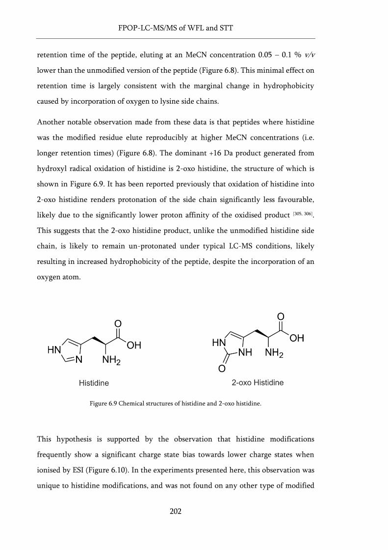
FPOP-LC-MS/MS of WFL and STT
202
retention time of the peptide, eluting at an MeCN concentration 0.05 – 0.1 % v/v
lower than the unmodified version of the peptide (Figure 6.8). This minimal effect on
retention time is largely consistent with the marginal change in hydrophobicity
caused by incorporation of oxygen to lysine side chains.
Another notable observation made from these data is that peptides where histidine
was the modified residue elute reproducibly at higher MeCN concentrations (i.e.
longer retention times) (Figure 6.8). The dominant +16 Da product generated from
hydroxyl radical oxidation of histidine is 2-oxo histidine, the structure of which is
shown in Figure 6.9. It has been reported previously that oxidation of histidine into
2-oxo histidine renders protonation of the side chain significantly less favourable,
likely due to the significantly lower proton affinity of the oxidised product [305, 306].
This suggests that the 2-oxo histidine product, unlike the unmodified histidine side
chain, is likely to remain un-protonated under typical LC-MS conditions, likely
resulting in increased hydrophobicity of the peptide, despite the incorporation of an
oxygen atom.
Figure 6.9 Chemical structures of histidine and 2-oxo histidine.
This hypothesis is supported by the observation that histidine modifications
frequently show a significant charge state bias towards lower charge states when
ionised by ESI (Figure 6.10). In the experiments presented here, this observation was
unique to histidine modifications, and was not found on any other type of modified
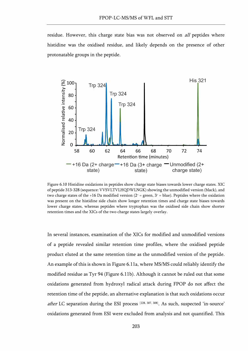
FPOP-LC-MS/MS of WFL and STT
203
residue. However, this charge state bias was not observed on all peptides where
histidine was the oxidised residue, and likely depends on the presence of other
protonatable groups in the peptide.
Figure 6.10 Histidine oxidations in peptides show charge state biases towards lower charge states. XIC
of peptide 313-328 (sequence: VVSVLTVLHQDWLNGK) showing the unmodified version (black), and
two charge states of the +16 Da modified version (2+ = green, 3+ = blue). Peptides where the oxidation
was present on the histidine side chain show longer retention times and charge state biases towards
lower charge states, whereas peptides where tryptophan was the oxidised side chain show shorter
retention times and the XICs of the two charge states largely overlay.
In several instances, examination of the XICs for modified and unmodified versions
of a peptide revealed similar retention time profiles, where the oxidised peptide
product eluted at the same retention time as the unmodified version of the peptide.
An example of this is shown in Figure 6.11a, where MS/MS could reliably identify the
modified residue as Tyr 94 (Figure 6.11b). Although it cannot be ruled out that some
oxidations generated from hydroxyl radical attack during FPOP do not affect the
retention time of the peptide, an alternative explanation is that such oxidations occur
after LC separation during the ESI process [228, 307, 308]. As such, suspected ‘in-source’
oxidations generated from ESI were excluded from analysis and not quantified. This
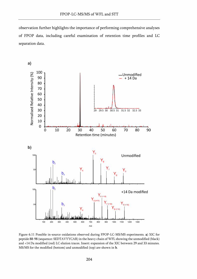
FPOP-LC-MS/MS of WFL and STT
204
observation further highlights the importance of performing comprehensive analyses
of FPOP data, including careful examination of retention time profiles and LC
separation data.
Figure 6.11 Possible in-source oxidations observed during FPOP-LC-MS/MS experiments. a) XIC for
peptide 88-98 (sequence: SEDTAVYYCAR) in the heavy chain of WFL showing the unmodified (black)
and +14 Da modified (red) LC elution traces. Insert: expansion of the XIC between 29 and 33 minutes.
MS/MS for the modified (bottom) and unmodified (top) are shown in b.

FPOP-LC-MS/MS of WFL and STT
205
6.5 Discussion
The changes in conformation observed between WFL and STT at the CL-CH1 interface
support the view that long range changes in conformation can occur between the
constant and variable domains of the Fab arm in mAbs. However, the significance of
this conformational change, and indeed the changes in oxidation observed
surrounding the WFL-STT substitutions in the CDR regions, cannot be reliably
determined from these data. Interpretation of FPOP data in this regard would benefit
greatly from a greater understanding of positional isomers, the effects of changing
solvent accessibility for different side chains as well as changes in local
microenvironment.
Similarly, the significance of the observed changes in conformation between the two
mAb variants, with regards to the poor pharmacological properties of WFL [170] cannot
be established from these data. However, a recent report demonstrated that, for light
chain dimers, structurally similar to that of the Fab domain [309], the CL domains were
observed to modulate protein aggregation, and the interface between constant
domains was suggested as a potential target for mitigating protein aggregation [310].
This could suggest a possible role of the CL domain in the aggregation of WFL, where
the conformational changes observed, caused by the WFL-STT substitution, play a
role in the reversible self-association of the WFL mAb variant.
Critically, however, these data definitively show that amino acid substitutions in the
variable domain of the Fab arm, can affect the conformation and positioning of side
chains in the constant domains of the Fab arm. Typically, these two distinct regions
are often assumed to be functionally independent [311, 312]. While the functionality of
this conformational link cannot be established from these data, the observation itself
may prove critical in the identification of aggregation-prone sites, or undesirable
conformational changes, generated distal from the site of amino acid substitutions that
may otherwise go overlooked.
FPOP-LC-MS/MS of WFL and STT
206
6.5.1 Retention time analysis
The retention time analysis of peptides oxidised by FPOP, from both the mAb data
discussed here, and the β2m data discussed in Section 5, highlight the potential utility
of using the LC separation data as an aid, not only to assign modified residues within
oxidised peptides, but to avoid erroneous assignments of in-source oxidations
generated from the ESI process. Undoubtedly, MS/MS remains the gold standard in
determining oxidation sites in FPOP. However, as peptides in FPOP experiments
often have the same m/z, are typically low abundance and sometimes only partially
separated by LC, the resulting chimeric, or poor quality, tandem MS spectra, are such
that finding alternative, or complementary methods of assignment offers a distinct
advantage. Given the current necessity of using LC in FPOP experimental workflows,
the LC separation data seems an obvious place to start, in looking for such alternatives.
Although considerably more data would be needed to establish whether changes in
retention time could be used as a predictive tool in FPOP assignments, even the small
data set collated here demonstrates the potential utility of using changes in retention
time to assign lysine and histidine oxidations within oxidised peptides, given their
unique, and reproducible effect on the elution of the peptide. Indeed, retention time
prediction tools have long been established in other peptide LC-MS workflows [313],
and may prove to be a useful future tool in characterising positional isomers in FPOP.

207
Chapter 7:
Concluding remarks
Concluding remarks
208
7 Concluding remarks
The work presented here has outlined several novel findings and advances that are of
crucial importance to the field of structural MS, particularly with regards to the use
of FPOP and other structural MS techniques in the study of aggregation-prone
proteins.
In this last section, the overall findings of this thesis are discussed in a broader
scientific context, with regards to the thesis aims laid out in Section 2.5.
7.1 A new understanding of FPOP
The detailed comparison of FPOP data between wild-type β2m and the ΔN6
truncation variant, outlined in Section 5.2.1, and subsequently published in 2018 [252],
allowed for the first time a detailed characterisation of positional isomers in FPOP
experiments. These data highlight the possibility, with further study, of utilising
positional isomers in FPOP for more detailed analyses of protein structures. However,
the well-characterised variants studied in these experiments also revealed a complex
relationship between SASA, or change in SASA, and the degree to which side chains
label in FPOP. While these data are in line with those of other studies [232, 287, 288], these
combined observations begin to illustrate the true complexity of using FPOP to
analyse protein structures, where nearby side chains in sequence or space, changing
solution conditions, and the reactivity of the side chain itself, all likely play a role in
the degree to which amino acid groups oxidise, and the sensitivity of the oxidation on
these side chains to changes in protein structure and local microenvironment.
Efforts to understand these effects in FPOP experiments should be considered
amongst the highest priority tasks for future work in this field. In the immediate
future, disentanglement of these factors would allow optimal design of internal
standards in FPOP experiments [289-291], greatly improving the robustness and
reproducibility of the technique, but would also widen the range of possible
Concluding remarks
209
experiments available to FPOP users. Similarly, a greater understanding of the
interplay between different side chains, SASA and amino acid reactivity on the degree
to which side chains label in FPOP would also release this technique from its current
limitations with regards to data interpretation.
These efforts would also likely benefit from a more detailed understanding of the
precise reactivities of the different amino acids, specifically for oxidation induced by
FPOP. Indeed, the general observations made from the FPOP data presented here
show that tyrosine side chains modify considerably less, on average, than tryptophan
side chains, even when similarly solvent exposed (section 5.2). Given that the
reactivities of these two residue types are predicted to be precisely the same, from
reactivity data produced by electron pulse radiolysis (Table 2.2), we must entertain
the possibility that the reactivity of the amino acids in FPOP differs slightly from
these data.
In much the same way that the effects of pH, temperature and sequence have been
largely unravelled with regards to deuterium incorporation in HDX, in the long term,
achieving a near complete understanding of the factors described above in FPOP,
particularly in the age of machine learning, seems largely feasible. Although
challenging, the prize for such an endeavour: a known relationship between absolute
SASA and the degree of labelling for a given amino acid type, under a given set of
conditions, promises the establishment of low resolution protein structural models,
derived de novo from MS data alone. With the already recognised possibility of
expanding the FPOP platform to include alternative radical based labelling reactions
[236, 237], as well as in vivo work [235], adding FPOP to the suite of well-established
structural MS techniques already available, could yet prove to be a critical step
forward in the advancement of structural MS as a field.
7.1.1 How do HDX and FPOP compare?
In addition to the findings outlined above, the comparison of wild-type β2m to the
truncation variant using both FPOP and HDX highlights the similarity regarding the
Concluding remarks
210
identified regions of difference between the two proteins, where both techniques
identified the region directly proximal to the N-terminal truncation as the site of most
significant structural change. However, the closest agreement between the two
methods was observed at the earliest labelling time points of the HDX experiment,
prior to larger scale increases in deuterium uptake across the length of the protein,
likely associated with the decreased stability of the native fold of the truncation
variant, relative to the wild-type protein. These large scale changes were not observed
by FPOP, and could indicate a time dependence of the agreement between the two
methods, where faster HDX labelling time points show better correlation with FPOP
data, than longer deuterium incubation times. Similarly, the trend in labelling
between the two methods was not observed to be consistent, where, upon truncation
of the N-terminus, both increased and decreased labelling of sites was observed using
FPOP, but only increased labelling was observed using HDX. This is not entirely
unexpected, given the different labelling targets (i.e. side chain vs backbone) of the
two methods. Similarly, although the precise timescale of FPOP labelling is still
currently disputed [233], the differing labelling timescales of the two methods, along
with the broad/low resolution vs narrow/high resolution coverage of structural
changes for HDX and FPOP, respectively, grant these two methods a high degree of
complementarity when used together. Indeed, an increasing number of studies have
utilised both HDX and FPOP in the characterisation of protein structural changes or
binding events [217, 278, 314], further demonstrating the useful structural MS niche FPOP
is beginning to occupy.
7.2 The D76N variant
Given its overwhelming structural similarity to the wild-type protein, the observation
that the D76N variant of β2m has significantly increased deuterium uptake in the E-F
loop surrounding the D-N amino acid substitution, is of notable importance. These
changes could not be described solely by the changes in intrinsic exchange rate caused
Concluding remarks
211
by the change in amino acid sequence, and demonstrate a significant structural change
in the D76N variant, with some evidence supporting minor changes in deuterium
uptake in the nearby A-B loop as well. Although the differences between the wild-
type protein and D76N shown by FPOP were also in these regions, supporting both
the minor changes observed by HDX in the A-B loop, and the observation that HDX
and FPOP, as structural MS techniques, highlight similar regions of structural change,
the differences in oxidation observed were minor, compared with the substantial
differences in deuterium uptake between the two proteins.
There are several possible explanations for this observation. One is that the differences
are observed more significantly at timescales appropriate for HDX (sec – hours) than
for FPOP (µs-ms). However, the most significant changes in deuterium uptake were
observed at the earliest labelling time points of the HDX experiment and, as such, one
might expect to observe larger differences with faster labelling techniques such as
FPOP, as opposed to the minimal changes in oxidation which these data show.
Alternatively, the difference in resolution and coverage between FPOP and HDX
could explain the discrepancy, whereby residues in the E-F loop which significantly
change in SASA are covered by the peptide level HDX data, but were not labelled in
the FPOP experiment. Lastly, both the HDX and FPOP data could be explained by
the difference in the protein structural factors each technique probes. For example, a
significant loss of hydrogen bonding in residues of the E-F loop, a hypothesis outlined
in Section 4.7.2, would likely dramatically increase the deuterium uptake of the
region, in line with the observed uptake behaviour. However, such H-bond losses
would not necessarily cause significant movement of the amino acid side chains
involved and, indeed, given the largely solvent accessible nature of the E-F loop in
both proteins, would likely only make minimal changes to the SASA of side chains in
this region. Hydrogen bonding is not currently believed to significantly affect
oxidation of amino acid side chains by FPOP. Therefore, the fact that oxidation by
FPOP remained largely similar between the wild-type protein and the D76N variant,
could support, or at least does not contradict, the hypothesis that the D76N
Concluding remarks
212
substitution has disturbed hydrogen bonding in the E-F loop, as opposed to having
caused a wholesale structural rearrangement of the region.
Although considerably more work is needed before a determination of how, or even
if, the stability and structure of the E-F loop factor in to the increased aggregation
propensity of this variant, given the stark similarity between the structure and
dynamics of D76N and the wild-type protein when studied by other methods [157, 161],
these large scale changes in HDX surrounding the D-N substitution are encouraging
and worthy of further investigation. It would be wise for future work to be directed
towards establishing precisely which residues cause the increase in deuterium uptake
by, for example, continuing to develop the single residue HDX-MS experiments using
ETD peptide fragmentation outlined in section 4.7.4. Additionally, utilising site
directed mutagenesis to disrupt hydrogen bonding in this region by other means, will
be useful to establish the significance of the E-F or A-B loops on aggregation
propensity, before an aggregation mechanism can be elucidated. The observation by
FPOP, HDX and IMS that the D76N variant is largely distinct from the aggregation-
prone ΔN6 truncation variant, considered to be a structural mimic of the
amyloidogenic IT state folding intermediate, is consistent with the results of others
[161]. Although this research is certainly in the early stages, these data could suggest an
alternative, or additional, aggregation pathway for the D76N variant not involving the
amyloidogenic IT state. If true, this would offer a remarkable opportunity to study the
common factors which direct both the IT state, and the D76N variant towards amyloid
formation and, more generally, gain insight into which factors lead proteins to form
amyloid – an essential step in future disease prevention and treatment.
7.3 What did we learn from studying biopharmaceuticals?
The detailed characterisation of the mAbs WFL and STT by FPOP, subsequently
published in 2019 [297], gave a unique insight into the effect of the triple CDR
substitutions on the structure of these proteins. Although some studies have suggested
Concluding remarks
213
a functional allosteric link between the constant and variable domains of mAbs [315], it
is generally considered that these two domains are functionally independent [311, 312].
Although the existence of a functional link between the constant and variable
domains of the Fab arms in WFL/STT cannot be established from these data, the FPOP
data clearly demonstrate that the structural features of the heavy chain CDR in these
proteins significantly affect the structure of the interface between the CH1 and CL
domains. Although these conformational changes are likely minor, as discussed in
Section 6.3, these data highlight three key findings:
1. Long range conformational changes in mAbs can be transmitted between the
constant and variable domains of the Fab arm.
2. FPOP, as a technique, is capable of distinguishing these minor conformational
changes, which could be important for protein aggregation and reversible self-
association.
3. FPOP could be a useful method for screening new biopharmaceuticals for long
range interactions which may/may not be beneficial.
Indeed, despite the significantly increased complexity of the sample compared with
the FPOP study of the three variants of β2m (Section 5), sub-amino acid level
resolution on some of the oxidised products identified was still achievable, and could
be used to gain additional insight on the long range conformational changes observed.
Similarly, the large data set obtained from LC-MS/MS analysis of the oxidised mAb
samples provided a useful starting point for the comprehensive analysis of RT data
from oxidised peptides. Although limited, the LC RT data obtained here demonstrate,
for the first time, that changes in RT may be useful as an aid in determining the
oxidised site within the peptide. Given that LC separation is, at present, an essential
part of the FPOP experimental workflow, the utility of analysing and compiling these
data cannot be overstated, and future work should continue to compile LC RT data
from FPOP experiments in an effort to expand and assess the predictability of RT
changes for specific types of oxidation.
Concluding remarks
214
However, the limitations of this work must also be discussed. Firstly, the difficulty in
the interpretation of changes surrounding the site of the amino acid substitutions
would greatly benefit from an increased understanding of the effects of local
microenvironment and sequence, discussed earlier in Section 7.1. Secondly, following
FPOP-LC-MS/MS analysis, only ~2.5x the number of oxidised sites were identified in
WFL and STT (50 in total) than in the FPOP data for the β2m variants (19 in total),
despite WFL and STT being ~12x larger. Although, the interfaces between domains
of the antibody reduce the available surface area per Ig subunit, when compared with
monomeric β2m, this is considerably lower than one might expect, for a protein
consisting of multiple Ig domains of similar structure to β2m. Undoubtedly, further
optimisation of the LC-MS/MS method used would yield more confidently identified
modifications. However, a comprehensive analysis of such large proteins following
FPOP oxidation and ‘bottom-up’ LC-MS sample prep, with hundreds, if not
thousands, of low abundance, modified peptides with the same m/z and similar
fragmentation spectra, may be asking too much of even the most capable MS/MS
instrumentation.
Although the current experimental workflow is largely effective and provides an
enormous quantity of data for each sample, with regards to optimising FPOP for larger
molecules such as biopharmaceuticals, it would be unwise to rule out alternative
experimental strategies to that of the traditional LC-MS/MS workflow, especially
given the early stage of method development FPOP currently occupies.
For example, could a ‘top-down’ approach be considered? Modern orbitrap MS
instruments are capable of utilising multiple ion activation techniques, and have been
used successfully for top-down sequencing of mAbs previously [316]. While this may
complicate quantification of oxidised sites and likely remove the possibility of
characterising positional isomers, this method would subvert other issues with the
traditional bottom-up LC-MS/MS approach. For example, issues with failing
enzymatic digestion at oxidised lysine residues, and signal splitting from multiple
Concluding remarks
215
oxidised species eluting at different retention times. Alternatively, a ‘Middle-down’
approach could be used, using enzymatic digestion or reduction of disulphide bonds
to generate smaller subunits of the protein for subsequent top-down analysis [317, 318].
Regardless, these data demonstrate that, although significantly more work is required
to optimise FPOP for the study of larger, more complex molecules, this method has
the potential to characterise the structure of mAbs, in great detail, and may prove to
be a useful additional tool to study the reversible self-association of biotherapeutics.
7.4 Final thoughts
The study of aggregation-prone proteins, and the development of methods which
make their characterisation possible, is of critical importance to the prevention and
treatment of disease in the modern era. The work presented in this thesis
demonstrates a modest step forward in the understanding and development of several
MS based techniques ideally suited to this purpose, as well as an increased
understanding of the protein systems studied.
The lessons learned during this project however, stretch much further than those
outlined above. With each research project, the subtleties of each obstacle stumbled
across provide a valuable insight to those involved, as to how future work might be
streamlined for faster research progression. While many of the issues encountered
during the course of this PhD project could easily be attributed to any eager young
scientist with a limited experience pool, most others could be attributed to challenges
in appropriate data interpretation, usually arising from a multitude of different,
plausible explanations. Hindered by a fledgling scientific career, or perhaps because
of it, the author has often resorted to searching for answers to these problems from
outside of the scientific realm.
During his time in the military, the famous comic, writer and poet, Spike Milligan,
was once asked by a fellow serviceman where, in the UK, he was from. Although he
had been born in India, Spike responded by saying that he was from London, where
he had lived from the age of twelve, having moved there with his parents in 1931.
Concluding remarks
216
“Which part?” remarked the serviceman - London being a rather large place.
“… Well, all of me.” Said Spike.
Although likely not the intention of either man, this exchange demonstrates, quite
effectively, that such difficulties in the interpretation of data can arise, even when not
really asking the wrong question, by asking the right question, imprecisely.
Given that protein aggregation and FPOP are both, independently, incredibly
complex, multi-faceted subjects for study, moving forward, a high degree of precision
in the research questions posited will undoubtedly prove beneficial in the further
implementation and development of FPOP, as well as other methods in the structural
MS toolbox, to study the aggregation of amyloidogenic proteins like D76N, or
biopharmaceuticals like WFL and STT. While this thesis outlines some of the
questions, and suggests some new avenues of research to begin this effort, there is,
unquestionably, a long way to go, where - to paraphrase the great, Douglas Adams -
making progress will require us to think the unthinkable, to do the undoable, and to
“grapple with the ineffable itself, and see if we may not eff it after all.”

217
Chapter 8:
Appendices
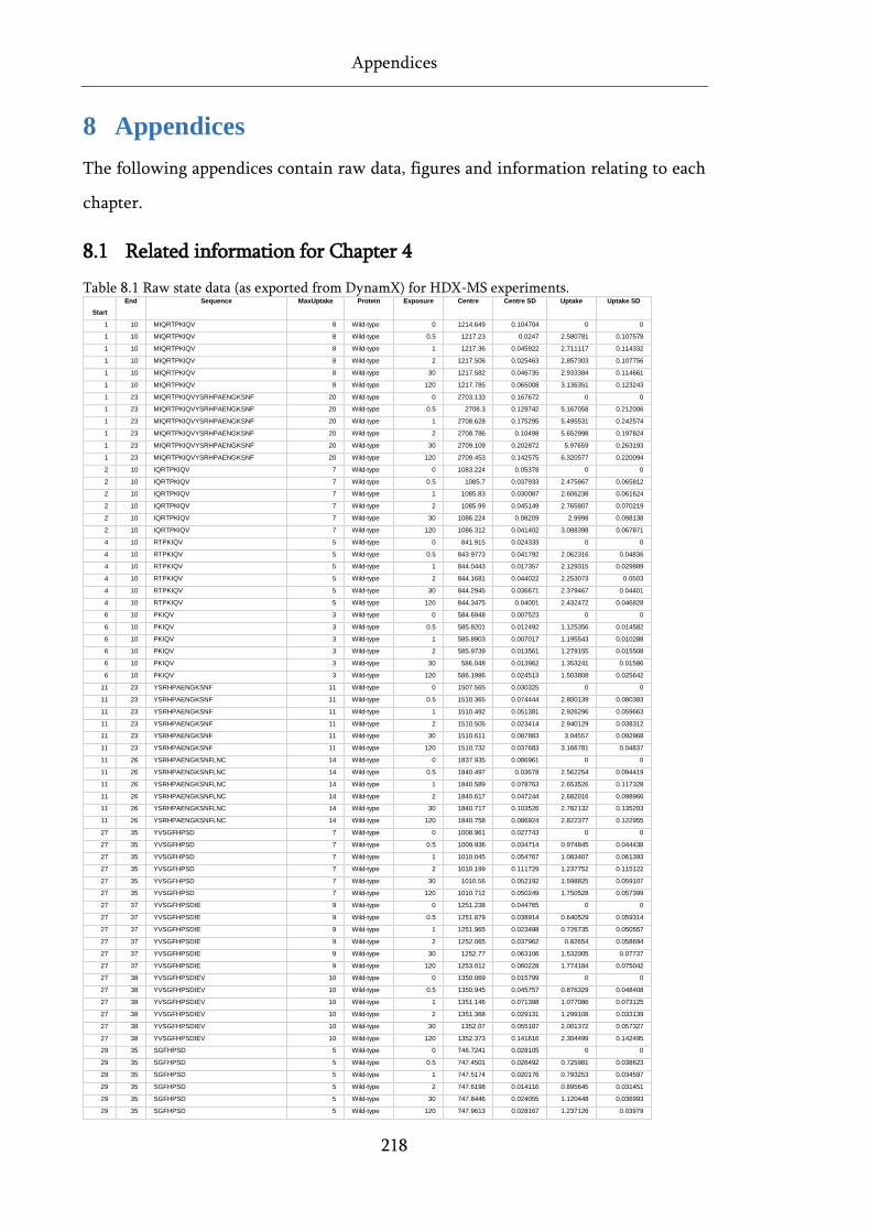
Appendices
218
8 Appendices
The following appendices contain raw data, figures and information relating to each
chapter.
8.1 Related information for Chapter 4
Table 8.1 Raw state data (as exported from DynamX) for HDX-MS experiments.
Start
End Sequence MaxUptake Protein Exposure Centre Centre SD Uptake Uptake SD
1 10 MIQRTPKIQV 8 Wild-type 0 1214.649 0.104704 0 0
1 10 MIQRTPKIQV 8 Wild-type 0.5 1217.23 0.0247 2.580781 0.107578
1 10 MIQRTPKIQV 8 Wild-type 1 1217.36 0.045922 2.711117 0.114332
1 10 MIQRTPKIQV 8 Wild-type 2 1217.506 0.025463 2.857303 0.107756
1 10 MIQRTPKIQV 8 Wild-type 30 1217.582 0.046735 2.933384 0.114661
1 10 MIQRTPKIQV 8 Wild-type 120 1217.785 0.065008 3.136351 0.123243
1 23 MIQRTPKIQVYSRHPAENGKSNF 20 Wild-type 0 2703.133 0.167672 0 0
1 23 MIQRTPKIQVYSRHPAENGKSNF 20 Wild-type 0.5 2708.3 0.129742 5.167058 0.212006
1 23 MIQRTPKIQVYSRHPAENGKSNF 20 Wild-type 1 2708.628 0.175295 5.495531 0.242574
1 23 MIQRTPKIQVYSRHPAENGKSNF 20 Wild-type 2 2708.786 0.10498 5.652998 0.197824
1 23 MIQRTPKIQVYSRHPAENGKSNF 20 Wild-type 30 2709.109 0.202872 5.97659 0.263193
1 23 MIQRTPKIQVYSRHPAENGKSNF 20 Wild-type 120 2709.453 0.142575 6.320577 0.220094
2 10 IQRTPKIQV 7 Wild-type 0 1083.224 0.05378 0 0
2 10 IQRTPKIQV 7 Wild-type 0.5 1085.7 0.037933 2.475867 0.065812
2 10 IQRTPKIQV 7 Wild-type 1 1085.83 0.030087 2.606238 0.061624
2 10 IQRTPKIQV 7 Wild-type 2 1085.99 0.045149 2.765807 0.070219
2 10 IQRTPKIQV 7 Wild-type 30 1086.224 0.08209 2.9998 0.098138
2 10 IQRTPKIQV 7 Wild-type 120 1086.312 0.041402 3.088398 0.067871
4 10 RTPKIQV 5 Wild-type 0 841.915 0.024333 0 0
4 10 RTPKIQV 5 Wild-type 0.5 843.9773 0.041792 2.062316 0.04836
4 10 RTPKIQV 5 Wild-type 1 844.0443 0.017357 2.129315 0.029889
4 10 RTPKIQV 5 Wild-type 2 844.1681 0.044022 2.253073 0.0503
4 10 RTPKIQV 5 Wild-type 30 844.2945 0.036671 2.379467 0.04401
4 10 RTPKIQV 5 Wild-type 120 844.3475 0.04001 2.432472 0.046828
6 10 PKIQV 3 Wild-type 0 584.6948 0.007523 0 0
6 10 PKIQV 3 Wild-type 0.5 585.8201 0.012492 1.125356 0.014582
6 10 PKIQV 3 Wild-type 1 585.8903 0.007017 1.195543 0.010288
6 10 PKIQV 3 Wild-type 2 585.9739 0.013561 1.279155 0.015508
6 10 PKIQV 3 Wild-type 30 586.048 0.013962 1.353241 0.01586
6 10 PKIQV 3 Wild-type 120 586.1986 0.024513 1.503808 0.025642
11 23 YSRHPAENGKSNF 11 Wild-type 0 1507.565 0.030325 0 0
11 23 YSRHPAENGKSNF 11 Wild-type 0.5 1510.365 0.074444 2.800139 0.080383
11 23 YSRHPAENGKSNF 11 Wild-type 1 1510.492 0.051381 2.926296 0.059663
11 23 YSRHPAENGKSNF 11 Wild-type 2 1510.505 0.023414 2.940129 0.038312
11 23 YSRHPAENGKSNF 11 Wild-type 30 1510.611 0.087883 3.04557 0.092968
11 23 YSRHPAENGKSNF 11 Wild-type 120 1510.732 0.037683 3.166781 0.04837
11 26 YSRHPAENGKSNFLNC 14 Wild-type 0 1837.935 0.086961 0 0
11 26 YSRHPAENGKSNFLNC 14 Wild-type 0.5 1840.497 0.03678 2.562254 0.094419
11 26 YSRHPAENGKSNFLNC 14 Wild-type 1 1840.589 0.078763 2.653526 0.117328
11 26 YSRHPAENGKSNFLNC 14 Wild-type 2 1840.617 0.047244 2.682016 0.098966
11 26 YSRHPAENGKSNFLNC 14 Wild-type 30 1840.717 0.103526 2.782132 0.135203
11 26 YSRHPAENGKSNFLNC 14 Wild-type 120 1840.758 0.086924 2.822377 0.122955
27 35 YVSGFHPSD 7 Wild-type 0 1008.961 0.027743 0 0
27 35 YVSGFHPSD 7 Wild-type 0.5 1009.936 0.034714 0.974845 0.044438
27 35 YVSGFHPSD 7 Wild-type 1 1010.045 0.054767 1.083407 0.061393
27 35 YVSGFHPSD 7 Wild-type 2 1010.199 0.111729 1.237752 0.115122
27 35 YVSGFHPSD 7 Wild-type 30 1010.56 0.052192 1.598825 0.059107
27 35 YVSGFHPSD 7 Wild-type 120 1010.712 0.050249 1.750528 0.057399
27 37 YVSGFHPSDIE 9 Wild-type 0 1251.238 0.044765 0 0
27 37 YVSGFHPSDIE 9 Wild-type 0.5 1251.879 0.038914 0.640529 0.059314
27 37 YVSGFHPSDIE 9 Wild-type 1 1251.965 0.023498 0.726735 0.050557
27 37 YVSGFHPSDIE 9 Wild-type 2 1252.065 0.037962 0.82654 0.058694
27 37 YVSGFHPSDIE 9 Wild-type 30 1252.77 0.063106 1.532005 0.07737
27 37 YVSGFHPSDIE 9 Wild-type 120 1253.012 0.060228 1.774184 0.075042
27 38 YVSGFHPSDIEV 10 Wild-type 0 1350.069 0.015799 0 0
27 38 YVSGFHPSDIEV 10 Wild-type 0.5 1350.945 0.045757 0.876329 0.048408
27 38 YVSGFHPSDIEV 10 Wild-type 1 1351.146 0.071398 1.077086 0.073125
27 38 YVSGFHPSDIEV 10 Wild-type 2 1351.368 0.029131 1.299108 0.033139
27 38 YVSGFHPSDIEV 10 Wild-type 30 1352.07 0.055107 2.001372 0.057327
27 38 YVSGFHPSDIEV 10 Wild-type 120 1352.373 0.141616 2.304499 0.142495
29 35 SGFHPSD 5 Wild-type 0 746.7241 0.028105 0 0
29 35 SGFHPSD 5 Wild-type 0.5 747.4501 0.026492 0.725981 0.038623
29 35 SGFHPSD 5 Wild-type 1 747.5174 0.020176 0.793253 0.034597
29 35 SGFHPSD 5 Wild-type 2 747.6198 0.014116 0.895645 0.031451
29 35 SGFHPSD 5 Wild-type 30 747.8446 0.024055 1.120448 0.036993
29 35 SGFHPSD 5 Wild-type 120 747.9613 0.028167 1.237126 0.03979
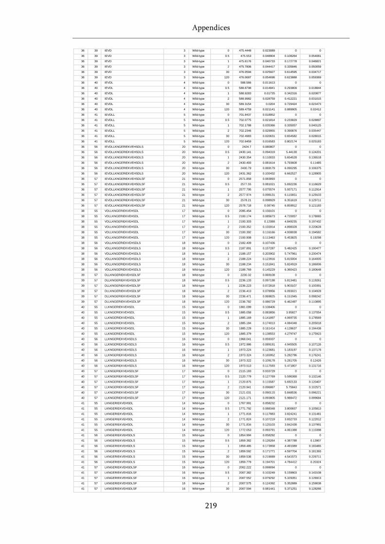
Appendices
219
36 39 IEVD 3 Wild-type 0 475.4448 0.023089 0 0
36 39 IEVD 3 Wild-type 0.5 475.553 0.048904 0.108264 0.054081
36 39 IEVD 3 Wild-type 1 475.6176 0.040733 0.172778 0.046821
36 39 IEVD 3 Wild-type 2 475.7806 0.044417 0.335846 0.050059
36 39 IEVD 3 Wild-type 30 476.0594 0.025927 0.614595 0.034717
36 39 IEVD 3 Wild-type 120 476.0687 0.054696 0.623888 0.059369
36 40 IEVDL 4 Wild-type 0 588.586 0.011613 0 0
36 40 IEVDL 4 Wild-type 0.5 588.8798 0.014841 0.293809 0.018844
36 40 IEVDL 4 Wild-type 1 588.9283 0.01735 0.342316 0.020877
36 40 IEVDL 4 Wild-type 2 588.9982 0.028759 0.412221 0.031015
36 40 IEVDL 4 Wild-type 30 589.3154 0.0204 0.729424 0.023473
36 40 IEVDL 4 Wild-type 120 589.4759 0.021141 0.889905 0.02412
36 41 IEVDLL 5 Wild-type 0 701.8437 0.018952 0 0
36 41 IEVDLL 5 Wild-type 0.5 702.0775 0.021814 0.233829 0.028897
36 41 IEVDLL 5 Wild-type 1 702.1788 0.035366 0.335057 0.040125
36 41 IEVDLL 5 Wild-type 2 702.2346 0.029955 0.390876 0.035447
36 41 IEVDLL 5 Wild-type 30 702.4983 0.020631 0.654582 0.028015
36 41 IEVDLL 5 Wild-type 120 702.6459 0.016583 0.802174 0.025183
36 56 IEVDLLKNGERIEKVEHSDLS 20 Wild-type 0 2424.7 0.080807 0 0
36 56 IEVDLLKNGERIEKVEHSDLS 20 Wild-type 0.5 2430.141 0.094319 5.44138 0.124201
36 56 IEVDLLKNGERIEKVEHSDLS 20 Wild-type 1 2430.354 0.110033 5.654528 0.136518
36 56 IEVDLLKNGERIEKVEHSDLS 20 Wild-type 2 2430.493 0.081614 5.793608 0.11485
36 56 IEVDLLKNGERIEKVEHSDLS 20 Wild-type 30 2430.79 0.069179 6.090295 0.106375
36 56 IEVDLLKNGERIEKVEHSDLS 20 Wild-type 120 2431.362 0.100432 6.662527 0.128905
36 57 IEVDLLKNGERIEKVEHSDLSF 21 Wild-type 0 2571.858 0.083893 0 0
36 57 IEVDLLKNGERIEKVEHSDLSF 21 Wild-type 0.5 2577.55 0.081021 5.692236 0.116629
36 57 IEVDLLKNGERIEKVEHSDLSF 21 Wild-type 1 2577.795 0.075574 5.937171 0.112914
36 57 IEVDLLKNGERIEKVEHSDLSF 21 Wild-type 2 2577.974 0.098131 6.115651 0.129103
36 57 IEVDLLKNGERIEKVEHSDLSF 21 Wild-type 30 2578.21 0.098929 6.351619 0.129711
36 57 IEVDLLKNGERIEKVEHSDLSF 21 Wild-type 120 2578.718 0.08745 6.859912 0.121183
38 55 VDLLKNGERIEKVEHSDL 17 Wild-type 0 2095.454 0.156101 0 0
38 55 VDLLKNGERIEKVEHSDL 17 Wild-type 0.5 2100.174 0.085673 4.720057 0.178065
38 55 VDLLKNGERIEKVEHSDL 17 Wild-type 1 2100.303 0.12088 4.849235 0.197432
38 55 VDLLKNGERIEKVEHSDL 17 Wild-type 2 2100.352 0.155914 4.898328 0.220628
38 55 VDLLKNGERIEKVEHSDL 17 Wild-type 30 2100.392 0.116166 4.938038 0.194582
38 55 VDLLKNGERIEKVEHSDL 17 Wild-type 120 2100.908 0.113463 5.453825 0.19298
38 56 VDLLKNGERIEKVEHSDLS 18 Wild-type 0 2182.409 0.107436 0 0
38 56 VDLLKNGERIEKVEHSDLS 18 Wild-type 0.5 2187.891 0.157287 5.482425 0.190477
38 56 VDLLKNGERIEKVEHSDLS 18 Wild-type 1 2188.157 0.203902 5.747961 0.230474
38 56 VDLLKNGERIEKVEHSDLS 18 Wild-type 2 2188.224 0.123916 5.815004 0.164005
38 56 VDLLKNGERIEKVEHSDLS 18 Wild-type 30 2188.234 0.151841 5.824919 0.186006
38 56 VDLLKNGERIEKVEHSDLS 18 Wild-type 120 2188.769 0.145229 6.360423 0.180648
39 57 DLLKNGERIEKVEHSDLSF 18 Wild-type 0 2230.32 0.069108 0 0
39 57 DLLKNGERIEKVEHSDLSF 18 Wild-type 0.5 2236.133 0.097198 5.813481 0.119261
39 57 DLLKNGERIEKVEHSDLSF 18 Wild-type 1 2236.223 0.072818 5.903107 0.100391
39 57 DLLKNGERIEKVEHSDLSF 18 Wild-type 2 2236.413 0.078956 6.093021 0.104928
39 57 DLLKNGERIEKVEHSDLSF 18 Wild-type 30 2236.471 0.069825 6.151945 0.098242
39 57 DLLKNGERIEKVEHSDLSF 18 Wild-type 120 2236.782 0.086729 6.462497 0.110895
40 55 LLKNGERIEKVEHSDL 15 Wild-type 0 1881.099 0.108406 0 0
40 55 LLKNGERIEKVEHSDL 15 Wild-type 0.5 1885.058 0.083856 3.95827 0.137054
40 55 LLKNGERIEKVEHSDL 15 Wild-type 1 1885.169 0.141897 4.069735 0.178569
40 55 LLKNGERIEKVEHSDL 15 Wild-type 2 1885.184 0.174013 4.084348 0.205018
40 55 LLKNGERIEKVEHSDL 15 Wild-type 30 1885.228 0.161414 4.128637 0.194438
40 55 LLKNGERIEKVEHSDL 15 Wild-type 120 1885.379 0.138553 4.279747 0.175923
40 56 LLKNGERIEKVEHSDLS 16 Wild-type 0 1968.041 0.059337 0 0
40 56 LLKNGERIEKVEHSDLS 16 Wild-type 0.5 1972.986 0.089191 4.945505 0.107126
40 56 LLKNGERIEKVEHSDLS 16 Wild-type 1 1973.224 0.123681 5.183197 0.137178
40 56 LLKNGERIEKVEHSDLS 16 Wild-type 2 1973.324 0.165952 5.282796 0.176241
40 56 LLKNGERIEKVEHSDLS 16 Wild-type 30 1973.322 0.109178 5.281705 0.12426
40 56 LLKNGERIEKVEHSDLS 16 Wild-type 120 1973.513 0.117593 5.471807 0.131716
40 57 LLKNGERIEKVEHSDLSF 17 Wild-type 0 2115.183 0.033729 0 0
40 57 LLKNGERIEKVEHSDLSF 17 Wild-type 0.5 2120.779 0.127769 5.596368 0.132146
40 57 LLKNGERIEKVEHSDLSF 17 Wild-type 1 2120.875 0.115587 5.692133 0.120407
40 57 LLKNGERIEKVEHSDLSF 17 Wild-type 2 2120.941 0.096867 5.75843 0.102571
40 57 LLKNGERIEKVEHSDLSF 17 Wild-type 30 2121.031 0.090115 5.848536 0.096221
40 57 LLKNGERIEKVEHSDLSF 17 Wild-type 120 2121.171 0.093805 5.988472 0.099684
41 55 LKNGERIEKVEHSDL 14 Wild-type 0 1767.991 0.058232 0 0
41 55 LKNGERIEKVEHSDL 14 Wild-type 0.5 1771.792 0.088348 3.800837 0.105813
41 55 LKNGERIEKVEHSDL 14 Wild-type 1 1771.816 0.117883 3.824241 0.131481
41 55 LKNGERIEKVEHSDL 14 Wild-type 2 1771.824 0.107219 3.832733 0.122012
41 55 LKNGERIEKVEHSDL 14 Wild-type 30 1771.834 0.125103 3.842438 0.137991
41 55 LKNGERIEKVEHSDL 14 Wild-type 120 1772.053 0.093791 4.061388 0.110398
41 56 LKNGERIEKVEHSDLS 15 Wild-type 0 1854.994 0.058292 0 0
41 56 LKNGERIEKVEHSDLS 15 Wild-type 0.5 1859.382 0.126264 4.387788 0.13907
41 56 LKNGERIEKVEHSDLS 15 Wild-type 1 1859.485 0.173958 4.491089 0.183465
41 56 LKNGERIEKVEHSDLS 15 Wild-type 2 1859.592 0.171771 4.597704 0.181393
41 56 LKNGERIEKVEHSDLS 15 Wild-type 30 1859.536 0.219089 4.541573 0.226711
41 56 LKNGERIEKVEHSDLS 15 Wild-type 120 1859.779 0.194701 4.784412 0.20324
41 57 LKNGERIEKVEHSDLSF 16 Wild-type 0 2002.222 0.099094 0 0
41 57 LKNGERIEKVEHSDLSF 16 Wild-type 0.5 2007.382 0.103249 5.159903 0.143108
41 57 LKNGERIEKVEHSDLSF 16 Wild-type 1 2007.552 0.079292 5.329351 0.126913
41 57 LKNGERIEKVEHSDLSF 16 Wild-type 2 2007.575 0.124392 5.352889 0.159038
41 57 LKNGERIEKVEHSDLSF 16 Wild-type 30 2007.594 0.081441 5.371251 0.128266
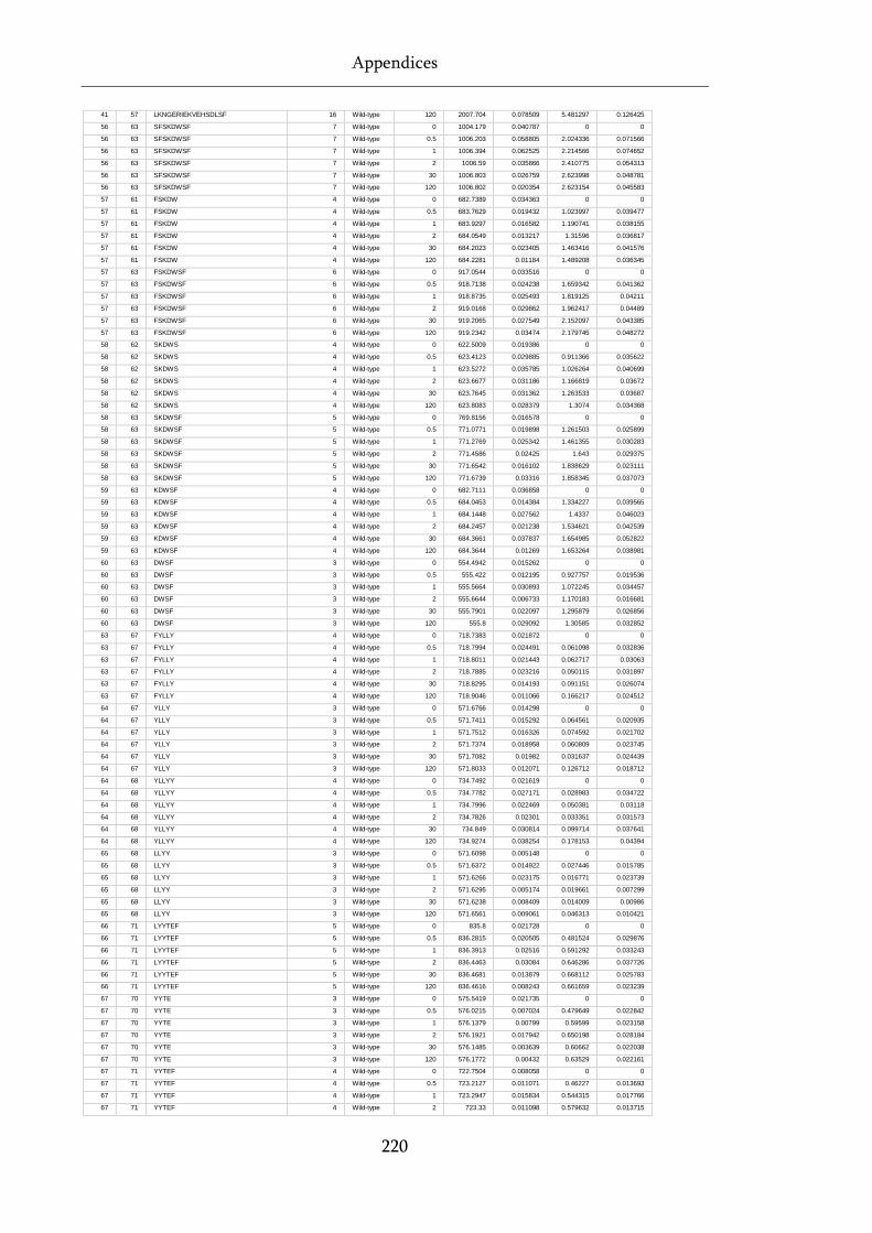
Appendices
220
41 57 LKNGERIEKVEHSDLSF 16 Wild-type 120 2007.704 0.078509 5.481297 0.126425
56 63 SFSKDWSF 7 Wild-type 0 1004.179 0.040787 0 0
56 63 SFSKDWSF 7 Wild-type 0.5 1006.203 0.058805 2.024336 0.071566
56 63 SFSKDWSF 7 Wild-type 1 1006.394 0.062525 2.214566 0.074652
56 63 SFSKDWSF 7 Wild-type 2 1006.59 0.035866 2.410775 0.054313
56 63 SFSKDWSF 7 Wild-type 30 1006.803 0.026759 2.623998 0.048781
56 63 SFSKDWSF 7 Wild-type 120 1006.802 0.020354 2.623154 0.045583
57 61 FSKDW 4 Wild-type 0 682.7389 0.034363 0 0
57 61 FSKDW 4 Wild-type 0.5 683.7629 0.019432 1.023997 0.039477
57 61 FSKDW 4 Wild-type 1 683.9297 0.016582 1.190741 0.038155
57 61 FSKDW 4 Wild-type 2 684.0549 0.013217 1.31596 0.036817
57 61 FSKDW 4 Wild-type 30 684.2023 0.023405 1.463416 0.041576
57 61 FSKDW 4 Wild-type 120 684.2281 0.01184 1.489208 0.036345
57 63 FSKDWSF 6 Wild-type 0 917.0544 0.033516 0 0
57 63 FSKDWSF 6 Wild-type 0.5 918.7138 0.024238 1.659342 0.041362
57 63 FSKDWSF 6 Wild-type 1 918.8735 0.025493 1.819125 0.04211
57 63 FSKDWSF 6 Wild-type 2 919.0168 0.029862 1.962417 0.04489
57 63 FSKDWSF 6 Wild-type 30 919.2065 0.027549 2.152097 0.043385
57 63 FSKDWSF 6 Wild-type 120 919.2342 0.03474 2.179745 0.048272
58 62 SKDWS 4 Wild-type 0 622.5009 0.019386 0 0
58 62 SKDWS 4 Wild-type 0.5 623.4123 0.029885 0.911366 0.035622
58 62 SKDWS 4 Wild-type 1 623.5272 0.035785 1.026264 0.040699
58 62 SKDWS 4 Wild-type 2 623.6677 0.031186 1.166819 0.03672
58 62 SKDWS 4 Wild-type 30 623.7645 0.031362 1.263533 0.03687
58 62 SKDWS 4 Wild-type 120 623.8083 0.028379 1.3074 0.034368
58 63 SKDWSF 5 Wild-type 0 769.8156 0.016578 0 0
58 63 SKDWSF 5 Wild-type 0.5 771.0771 0.019898 1.261503 0.025899
58 63 SKDWSF 5 Wild-type 1 771.2769 0.025342 1.461355 0.030283
58 63 SKDWSF 5 Wild-type 2 771.4586 0.02425 1.643 0.029375
58 63 SKDWSF 5 Wild-type 30 771.6542 0.016102 1.838629 0.023111
58 63 SKDWSF 5 Wild-type 120 771.6739 0.03316 1.858345 0.037073
59 63 KDWSF 4 Wild-type 0 682.7111 0.036858 0 0
59 63 KDWSF 4 Wild-type 0.5 684.0453 0.014384 1.334227 0.039565
59 63 KDWSF 4 Wild-type 1 684.1448 0.027562 1.4337 0.046023
59 63 KDWSF 4 Wild-type 2 684.2457 0.021238 1.534621 0.042539
59 63 KDWSF 4 Wild-type 30 684.3661 0.037837 1.654985 0.052822
59 63 KDWSF 4 Wild-type 120 684.3644 0.01269 1.653264 0.038981
60 63 DWSF 3 Wild-type 0 554.4942 0.015262 0 0
60 63 DWSF 3 Wild-type 0.5 555.422 0.012195 0.927757 0.019536
60 63 DWSF 3 Wild-type 1 555.5664 0.030893 1.072245 0.034457
60 63 DWSF 3 Wild-type 2 555.6644 0.006733 1.170183 0.016681
60 63 DWSF 3 Wild-type 30 555.7901 0.022097 1.295879 0.026856
60 63 DWSF 3 Wild-type 120 555.8 0.029092 1.30585 0.032852
63 67 FYLLY 4 Wild-type 0 718.7383 0.021872 0 0
63 67 FYLLY 4 Wild-type 0.5 718.7994 0.024491 0.061098 0.032836
63 67 FYLLY 4 Wild-type 1 718.8011 0.021443 0.062717 0.03063
63 67 FYLLY 4 Wild-type 2 718.7885 0.023216 0.050115 0.031897
63 67 FYLLY 4 Wild-type 30 718.8295 0.014193 0.091151 0.026074
63 67 FYLLY 4 Wild-type 120 718.9046 0.011066 0.166217 0.024512
64 67 YLLY 3 Wild-type 0 571.6766 0.014298 0 0
64 67 YLLY 3 Wild-type 0.5 571.7411 0.015292 0.064561 0.020935
64 67 YLLY 3 Wild-type 1 571.7512 0.016326 0.074592 0.021702
64 67 YLLY 3 Wild-type 2 571.7374 0.018958 0.060809 0.023745
64 67 YLLY 3 Wild-type 30 571.7082 0.01982 0.031637 0.024439
64 67 YLLY 3 Wild-type 120 571.8033 0.012071 0.126712 0.018712
64 68 YLLYY 4 Wild-type 0 734.7492 0.021619 0 0
64 68 YLLYY 4 Wild-type 0.5 734.7782 0.027171 0.028983 0.034722
64 68 YLLYY 4 Wild-type 1 734.7996 0.022469 0.050381 0.03118
64 68 YLLYY 4 Wild-type 2 734.7826 0.02301 0.033351 0.031573
64 68 YLLYY 4 Wild-type 30 734.849 0.030814 0.099714 0.037641
64 68 YLLYY 4 Wild-type 120 734.9274 0.038254 0.178153 0.04394
65 68 LLYY 3 Wild-type 0 571.6098 0.005148 0 0
65 68 LLYY 3 Wild-type 0.5 571.6372 0.014922 0.027446 0.015785
65 68 LLYY 3 Wild-type 1 571.6266 0.023175 0.016771 0.023739
65 68 LLYY 3 Wild-type 2 571.6295 0.005174 0.019661 0.007299
65 68 LLYY 3 Wild-type 30 571.6238 0.008409 0.014009 0.00986
65 68 LLYY 3 Wild-type 120 571.6561 0.009061 0.046313 0.010421
66 71 LYYTEF 5 Wild-type 0 835.8 0.021728 0 0
66 71 LYYTEF 5 Wild-type 0.5 836.2815 0.020505 0.481524 0.029876
66 71 LYYTEF 5 Wild-type 1 836.3913 0.02516 0.591292 0.033243
66 71 LYYTEF 5 Wild-type 2 836.4463 0.03084 0.646286 0.037726
66 71 LYYTEF 5 Wild-type 30 836.4681 0.013879 0.668112 0.025783
66 71 LYYTEF 5 Wild-type 120 836.4616 0.008243 0.661659 0.023239
67 70 YYTE 3 Wild-type 0 575.5419 0.021735 0 0
67 70 YYTE 3 Wild-type 0.5 576.0215 0.007024 0.479649 0.022842
67 70 YYTE 3 Wild-type 1 576.1379 0.00799 0.59599 0.023158
67 70 YYTE 3 Wild-type 2 576.1921 0.017942 0.650198 0.028184
67 70 YYTE 3 Wild-type 30 576.1485 0.003639 0.60662 0.022038
67 70 YYTE 3 Wild-type 120 576.1772 0.00432 0.63529 0.022161
67 71 YYTEF 4 Wild-type 0 722.7504 0.008058 0 0
67 71 YYTEF 4 Wild-type 0.5 723.2127 0.011071 0.46227 0.013693
67 71 YYTEF 4 Wild-type 1 723.2947 0.015834 0.544315 0.017766
67 71 YYTEF 4 Wild-type 2 723.33 0.011098 0.579632 0.013715
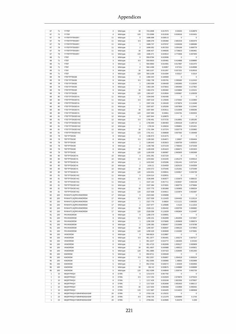
Appendices
221
67 71 YYTEF 4 Wild-type 30 723.2908 0.017073 0.54043 0.018879
67 71 YYTEF 4 Wild-type 120 723.3096 0.013159 0.559216 0.015431
67 79 YYTEFTPTEKDEY 11 Wild-type 0 1686.698 0.038113 0 0
67 79 YYTEFTPTEKDEY 11 Wild-type 0.5 1689.379 0.035484 2.681019 0.052074
67 79 YYTEFTPTEKDEY 11 Wild-type 1 1689.737 0.079747 3.039339 0.088386
67 79 YYTEFTPTEKDEY 11 Wild-type 2 1690.052 0.057253 3.354169 0.068779
67 79 YYTEFTPTEKDEY 11 Wild-type 30 1690.427 0.046935 3.728623 0.060461
67 79 YYTEFTPTEKDEY 11 Wild-type 120 1690.471 0.043514 3.772836 0.057845
68 71 YTEF 3 Wild-type 0 559.5784 0.015936 0 0
68 71 YTEF 3 Wild-type 0.5 559.9933 0.035481 0.414868 0.038895
68 71 YTEF 3 Wild-type 1 560.0963 0.014391 0.517897 0.021472
68 71 YTEF 3 Wild-type 2 560.1499 0.00957 0.57151 0.018588
68 71 YTEF 3 Wild-type 30 560.1157 0.011267 0.537321 0.019516
68 71 YTEF 3 Wild-type 120 560.1106 0.014284 0.53217 0.0214
68 78 YTEFTPTEKDE 9 Wild-type 0 1360.344 0.106569 0 0
68 78 YTEFTPTEKDE 9 Wild-type 0.5 1362.739 0.035781 2.395582 0.112415
68 78 YTEFTPTEKDE 9 Wild-type 1 1363.006 0.046428 2.662683 0.116243
68 78 YTEFTPTEKDE 9 Wild-type 2 1363.184 0.070815 2.840493 0.127952
68 78 YTEFTPTEKDE 9 Wild-type 30 1363.374 0.055382 3.029884 0.120101
68 78 YTEFTPTEKDE 9 Wild-type 120 1363.437 0.019504 3.093667 0.108339
68 80 YTEFTPTEKDEYA 11 Wild-type 0 1594.649 0.042436 0 0
68 80 YTEFTPTEKDEYA 11 Wild-type 0.5 1597.019 0.125935 2.370042 0.132893
68 80 YTEFTPTEKDEYA 11 Wild-type 1 1597.226 0.106183 2.576974 0.114349
68 80 YTEFTPTEKDEYA 11 Wild-type 2 1597.657 0.105206 3.007809 0.113442
68 80 YTEFTPTEKDEYA 11 Wild-type 30 1597.964 0.053511 3.315008 0.068296
68 80 YTEFTPTEKDEYA 11 Wild-type 120 1597.994 0.04661 3.344791 0.063034
68 81 YTEFTPTEKDEYAC 12 Wild-type 0 1697.844 0.169876 0 0
68 81 YTEFTPTEKDEYAC 12 Wild-type 0.5 1700.461 0.073725 2.616891 0.185185
68 81 YTEFTPTEKDEYAC 12 Wild-type 1 1700.694 0.084463 2.850218 0.189716
68 81 YTEFTPTEKDEYAC 12 Wild-type 2 1700.94 0.108224 3.096801 0.201421
68 81 YTEFTPTEKDEYAC 12 Wild-type 30 1701.394 0.107374 3.550778 0.200965
68 81 YTEFTPTEKDEYAC 12 Wild-type 120 1701.411 0.098699 3.567592 0.196468
69 78 TEFTPTEKDE 8 Wild-type 0 1196.973 0.013275 0 0
69 78 TEFTPTEKDE 8 Wild-type 0.5 1199.363 0.054871 2.39007 0.056454
69 78 TEFTPTEKDE 8 Wild-type 1 1199.643 0.053923 2.669759 0.055533
69 78 TEFTPTEKDE 8 Wild-type 2 1199.768 0.072229 2.795043 0.073439
69 78 TEFTPTEKDE 8 Wild-type 30 1199.939 0.051623 2.966071 0.053303
69 78 TEFTPTEKDE 8 Wild-type 120 1199.939 0.080987 2.965905 0.082068
69 80 TEFTPTEKDEYA 10 Wild-type 0 1431.381 0.027154 0 0
69 80 TEFTPTEKDEYA 10 Wild-type 0.5 1433.662 0.041045 2.281274 0.049214
69 80 TEFTPTEKDEYA 10 Wild-type 1 1433.942 0.025286 2.561441 0.037104
69 80 TEFTPTEKDEYA 10 Wild-type 2 1434.21 0.034059 2.829133 0.043558
69 80 TEFTPTEKDEYA 10 Wild-type 30 1434.572 0.070446 3.191361 0.075499
69 80 TEFTPTEKDEYA 10 Wild-type 120 1434.631 0.038041 3.250817 0.046738
69 81 TEFTPTEKDEYAC 11 Wild-type 0 1534.514 0.028031 0 0
69 81 TEFTPTEKDEYAC 11 Wild-type 0.5 1536.848 0.083577 2.333675 0.088152
69 81 TEFTPTEKDEYAC 11 Wild-type 1 1537.142 0.057711 2.628267 0.064158
69 81 TEFTPTEKDEYAC 11 Wild-type 2 1537.384 0.074591 2.869776 0.079684
69 81 TEFTPTEKDEYAC 11 Wild-type 30 1537.775 0.081868 3.260855 0.086534
69 81 TEFTPTEKDEYAC 11 Wild-type 120 1537.838 0.044611 3.323974 0.052687
82 100 RVNHVTLSQPKIVKWDRDM 17 Wild-type 0 2323.565 0.035898 0 0
82 100 RVNHVTLSQPKIVKWDRDM 17 Wild-type 0.5 2327.509 0.110425 3.944402 0.116114
82 100 RVNHVTLSQPKIVKWDRDM 17 Wild-type 1 2327.776 0.08834 4.211121 0.095355
82 100 RVNHVTLSQPKIVKWDRDM 17 Wild-type 2 2327.977 0.105686 4.4125 0.111616
82 100 RVNHVTLSQPKIVKWDRDM 17 Wild-type 30 2328.121 0.056432 4.555759 0.066882
82 100 RVNHVTLSQPKIVKWDRDM 17 Wild-type 120 2328.558 0.119209 4.992804 0.124497
91 100 PKIVKWDRDM 8 Wild-type 0 1288.379 0.039091 0 0
91 100 PKIVKWDRDM 8 Wild-type 0.5 1290.231 0.062899 1.852006 0.074057
91 100 PKIVKWDRDM 8 Wild-type 1 1290.339 0.076685 1.959608 0.086074
91 100 PKIVKWDRDM 8 Wild-type 2 1290.395 0.068407 2.015696 0.078788
91 100 PKIVKWDRDM 8 Wild-type 30 1290.467 0.068597 2.088125 0.078953
91 100 PKIVKWDRDM 8 Wild-type 120 1290.529 0.069089 2.150282 0.079381
94 100 VKWDRDM 6 Wild-type 0 949.9624 0.019987 0 0
94 100 VKWDRDM 6 Wild-type 0.5 951.2677 0.064491 1.305274 0.067517
94 100 VKWDRDM 6 Wild-type 1 951.3227 0.024772 1.360305 0.03183
94 100 VKWDRDM 6 Wild-type 2 951.4715 0.062699 1.509127 0.065808
94 100 VKWDRDM 6 Wild-type 30 951.4607 0.040988 1.498313 0.045601
94 100 VKWDRDM 6 Wild-type 120 951.4885 0.047423 1.526095 0.051463
95 100 KWDRDM 5 Wild-type 0 850.8711 0.039349 0 0
95 100 KWDRDM 5 Wild-type 0.5 852.2357 0.056807 1.364618 0.069104
95 100 KWDRDM 5 Wild-type 1 852.3595 0.036966 1.48835 0.053989
95 100 KWDRDM 5 Wild-type 2 852.3744 0.049272 1.50328 0.063056
95 100 KWDRDM 5 Wild-type 30 852.42 0.028675 1.548889 0.048689
95 100 KWDRDM 5 Wild-type 120 852.4299 0.048849 1.558744 0.062726
1 10 MIQRTPKIQV 8 D76N 0 1214.573 0.067792 0 0
1 10 MIQRTPKIQV 8 D76N 0.5 1217.253 0.032829 2.679976 0.075323
1 10 MIQRTPKIQV 8 D76N 1 1217.426 0.033249 2.852556 0.075507
1 10 MIQRTPKIQV 8 D76N 2 1217.525 0.053099 2.952003 0.086112
1 10 MIQRTPKIQV 8 D76N 30 1217.603 0.068468 3.02958 0.096352
1 10 MIQRTPKIQV 8 D76N 120 1217.887 0.043425 3.314023 0.080508
1 23 MIQRTPKIQVYSRHPAENGKSNF 20 D76N 0 2703.118 0.125231 0 0
1 23 MIQRTPKIQVYSRHPAENGKSNF 20 D76N 0.5 2708.725 0.121379 5.606965 0.1744
1 23 MIQRTPKIQVYSRHPAENGKSNF 20 D76N 1 2709.061 0.163565 5.94378 0.206
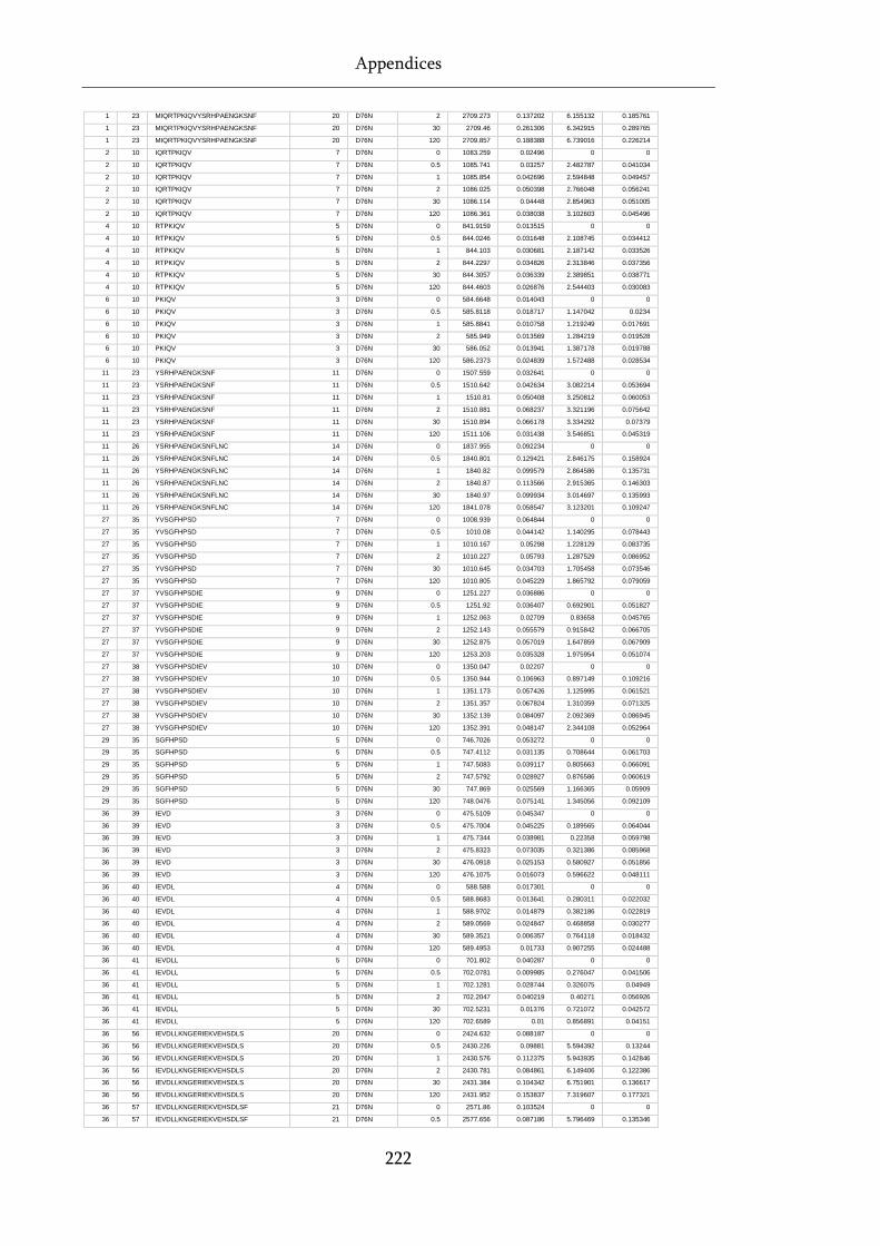
Appendices
222
1 23 MIQRTPKIQVYSRHPAENGKSNF 20 D76N 2 2709.273 0.137202 6.155132 0.185761
1 23 MIQRTPKIQVYSRHPAENGKSNF 20 D76N 30 2709.46 0.261306 6.342915 0.289765
1 23 MIQRTPKIQVYSRHPAENGKSNF 20 D76N 120 2709.857 0.188388 6.739016 0.226214
2 10 IQRTPKIQV 7 D76N 0 1083.259 0.02496 0 0
2 10 IQRTPKIQV 7 D76N 0.5 1085.741 0.03257 2.482787 0.041034
2 10 IQRTPKIQV 7 D76N 1 1085.854 0.042696 2.594848 0.049457
2 10 IQRTPKIQV 7 D76N 2 1086.025 0.050398 2.766048 0.056241
2 10 IQRTPKIQV 7 D76N 30 1086.114 0.04448 2.854963 0.051005
2 10 IQRTPKIQV 7 D76N 120 1086.361 0.038038 3.102603 0.045496
4 10 RTPKIQV 5 D76N 0 841.9159 0.013515 0 0
4 10 RTPKIQV 5 D76N 0.5 844.0246 0.031648 2.108745 0.034412
4 10 RTPKIQV 5 D76N 1 844.103 0.030681 2.187142 0.033526
4 10 RTPKIQV 5 D76N 2 844.2297 0.034826 2.313846 0.037356
4 10 RTPKIQV 5 D76N 30 844.3057 0.036339 2.389851 0.038771
4 10 RTPKIQV 5 D76N 120 844.4603 0.026876 2.544403 0.030083
6 10 PKIQV 3 D76N 0 584.6648 0.014043 0 0
6 10 PKIQV 3 D76N 0.5 585.8118 0.018717 1.147042 0.0234
6 10 PKIQV 3 D76N 1 585.8841 0.010758 1.219249 0.017691
6 10 PKIQV 3 D76N 2 585.949 0.013569 1.284219 0.019528
6 10 PKIQV 3 D76N 30 586.052 0.013941 1.387178 0.019788
6 10 PKIQV 3 D76N 120 586.2373 0.024839 1.572488 0.028534
11 23 YSRHPAENGKSNF 11 D76N 0 1507.559 0.032641 0 0
11 23 YSRHPAENGKSNF 11 D76N 0.5 1510.642 0.042634 3.082214 0.053694
11 23 YSRHPAENGKSNF 11 D76N 1 1510.81 0.050408 3.250812 0.060053
11 23 YSRHPAENGKSNF 11 D76N 2 1510.881 0.068237 3.321196 0.075642
11 23 YSRHPAENGKSNF 11 D76N 30 1510.894 0.066178 3.334292 0.07379
11 23 YSRHPAENGKSNF 11 D76N 120 1511.106 0.031438 3.546851 0.045319
11 26 YSRHPAENGKSNFLNC 14 D76N 0 1837.955 0.092234 0 0
11 26 YSRHPAENGKSNFLNC 14 D76N 0.5 1840.801 0.129421 2.846175 0.158924
11 26 YSRHPAENGKSNFLNC 14 D76N 1 1840.82 0.099579 2.864586 0.135731
11 26 YSRHPAENGKSNFLNC 14 D76N 2 1840.87 0.113566 2.915365 0.146303
11 26 YSRHPAENGKSNFLNC 14 D76N 30 1840.97 0.099934 3.014697 0.135993
11 26 YSRHPAENGKSNFLNC 14 D76N 120 1841.078 0.058547 3.123201 0.109247
27 35 YVSGFHPSD 7 D76N 0 1008.939 0.064844 0 0
27 35 YVSGFHPSD 7 D76N 0.5 1010.08 0.044142 1.140295 0.078443
27 35 YVSGFHPSD 7 D76N 1 1010.167 0.05298 1.228129 0.083735
27 35 YVSGFHPSD 7 D76N 2 1010.227 0.05793 1.287529 0.086952
27 35 YVSGFHPSD 7 D76N 30 1010.645 0.034703 1.705458 0.073546
27 35 YVSGFHPSD 7 D76N 120 1010.805 0.045229 1.865792 0.079059
27 37 YVSGFHPSDIE 9 D76N 0 1251.227 0.036886 0 0
27 37 YVSGFHPSDIE 9 D76N 0.5 1251.92 0.036407 0.692901 0.051827
27 37 YVSGFHPSDIE 9 D76N 1 1252.063 0.02709 0.83658 0.045765
27 37 YVSGFHPSDIE 9 D76N 2 1252.143 0.055579 0.915842 0.066705
27 37 YVSGFHPSDIE 9 D76N 30 1252.875 0.057019 1.647859 0.067909
27 37 YVSGFHPSDIE 9 D76N 120 1253.203 0.035328 1.975954 0.051074
27 38 YVSGFHPSDIEV 10 D76N 0 1350.047 0.02207 0 0
27 38 YVSGFHPSDIEV 10 D76N 0.5 1350.944 0.106963 0.897149 0.109216
27 38 YVSGFHPSDIEV 10 D76N 1 1351.173 0.057426 1.125995 0.061521
27 38 YVSGFHPSDIEV 10 D76N 2 1351.357 0.067824 1.310359 0.071325
27 38 YVSGFHPSDIEV 10 D76N 30 1352.139 0.084097 2.092369 0.086945
27 38 YVSGFHPSDIEV 10 D76N 120 1352.391 0.048147 2.344108 0.052964
29 35 SGFHPSD 5 D76N 0 746.7026 0.053272 0 0
29 35 SGFHPSD 5 D76N 0.5 747.4112 0.031135 0.708644 0.061703
29 35 SGFHPSD 5 D76N 1 747.5083 0.039117 0.805663 0.066091
29 35 SGFHPSD 5 D76N 2 747.5792 0.028927 0.876586 0.060619
29 35 SGFHPSD 5 D76N 30 747.869 0.025569 1.166365 0.05909
29 35 SGFHPSD 5 D76N 120 748.0476 0.075141 1.345056 0.092109
36 39 IEVD 3 D76N 0 475.5109 0.045347 0 0
36 39 IEVD 3 D76N 0.5 475.7004 0.045225 0.189565 0.064044
36 39 IEVD 3 D76N 1 475.7344 0.038981 0.22358 0.059798
36 39 IEVD 3 D76N 2 475.8323 0.073035 0.321386 0.085968
36 39 IEVD 3 D76N 30 476.0918 0.025153 0.580927 0.051856
36 39 IEVD 3 D76N 120 476.1075 0.016073 0.596622 0.048111
36 40 IEVDL 4 D76N 0 588.588 0.017301 0 0
36 40 IEVDL 4 D76N 0.5 588.8683 0.013641 0.280311 0.022032
36 40 IEVDL 4 D76N 1 588.9702 0.014879 0.382186 0.022819
36 40 IEVDL 4 D76N 2 589.0569 0.024847 0.468858 0.030277
36 40 IEVDL 4 D76N 30 589.3521 0.006357 0.764118 0.018432
36 40 IEVDL 4 D76N 120 589.4953 0.01733 0.907255 0.024488
36 41 IEVDLL 5 D76N 0 701.802 0.040287 0 0
36 41 IEVDLL 5 D76N 0.5 702.0781 0.009985 0.276047 0.041506
36 41 IEVDLL 5 D76N 1 702.1281 0.028744 0.326075 0.04949
36 41 IEVDLL 5 D76N 2 702.2047 0.040219 0.40271 0.056926
36 41 IEVDLL 5 D76N 30 702.5231 0.01376 0.721072 0.042572
36 41 IEVDLL 5 D76N 120 702.6589 0.01 0.856891 0.04151
36 56 IEVDLLKNGERIEKVEHSDLS 20 D76N 0 2424.632 0.088187 0 0
36 56 IEVDLLKNGERIEKVEHSDLS 20 D76N 0.5 2430.226 0.09881 5.594392 0.13244
36 56 IEVDLLKNGERIEKVEHSDLS 20 D76N 1 2430.576 0.112375 5.943935 0.142846
36 56 IEVDLLKNGERIEKVEHSDLS 20 D76N 2 2430.781 0.084861 6.149406 0.122386
36 56 IEVDLLKNGERIEKVEHSDLS 20 D76N 30 2431.384 0.104342 6.751901 0.136617
36 56 IEVDLLKNGERIEKVEHSDLS 20 D76N 120 2431.952 0.153837 7.319607 0.177321
36 57 IEVDLLKNGERIEKVEHSDLSF 21 D76N 0 2571.86 0.103524 0 0
36 57 IEVDLLKNGERIEKVEHSDLSF 21 D76N 0.5 2577.656 0.087186 5.796469 0.135346
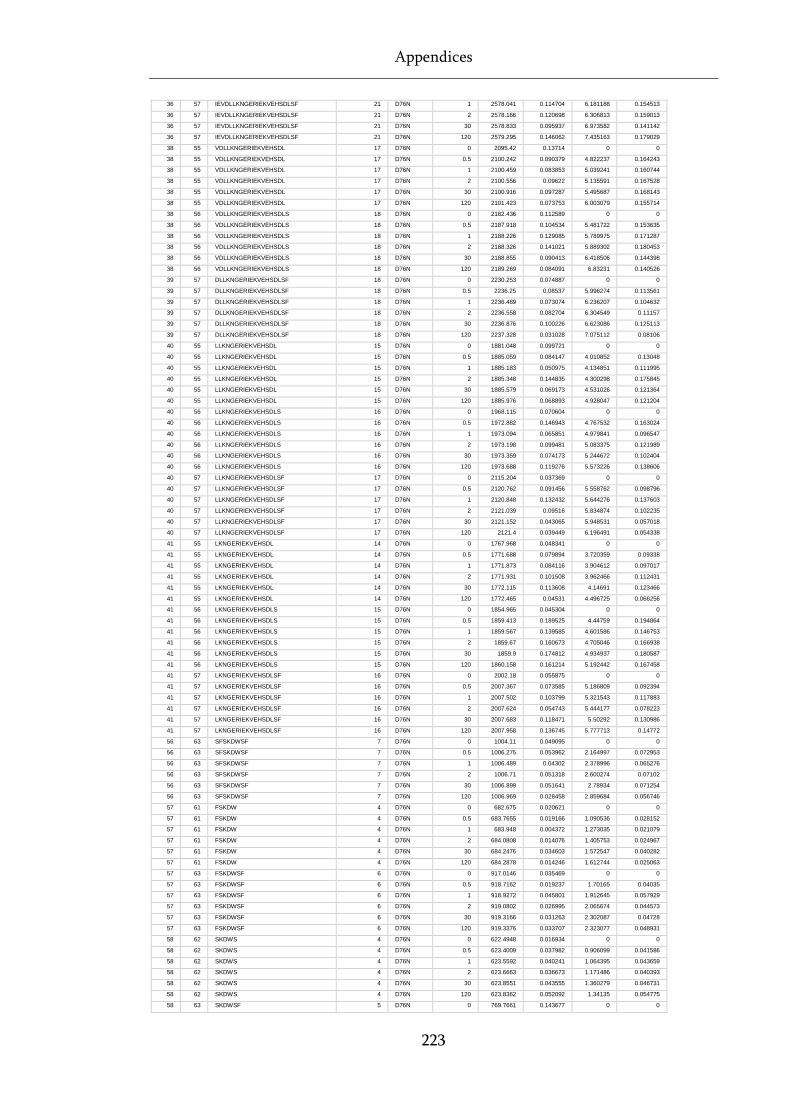
Appendices
223
36 57 IEVDLLKNGERIEKVEHSDLSF 21 D76N 1 2578.041 0.114704 6.181188 0.154513
36 57 IEVDLLKNGERIEKVEHSDLSF 21 D76N 2 2578.166 0.120698 6.306813 0.159013
36 57 IEVDLLKNGERIEKVEHSDLSF 21 D76N 30 2578.833 0.095937 6.973582 0.141142
36 57 IEVDLLKNGERIEKVEHSDLSF 21 D76N 120 2579.295 0.146062 7.435163 0.179029
38 55 VDLLKNGERIEKVEHSDL 17 D76N 0 2095.42 0.13714 0 0
38 55 VDLLKNGERIEKVEHSDL 17 D76N 0.5 2100.242 0.090379 4.822237 0.164243
38 55 VDLLKNGERIEKVEHSDL 17 D76N 1 2100.459 0.083853 5.039241 0.160744
38 55 VDLLKNGERIEKVEHSDL 17 D76N 2 2100.556 0.09622 5.135591 0.167528
38 55 VDLLKNGERIEKVEHSDL 17 D76N 30 2100.916 0.097287 5.495687 0.168143
38 55 VDLLKNGERIEKVEHSDL 17 D76N 120 2101.423 0.073753 6.003079 0.155714
38 56 VDLLKNGERIEKVEHSDLS 18 D76N 0 2182.436 0.112589 0 0
38 56 VDLLKNGERIEKVEHSDLS 18 D76N 0.5 2187.918 0.104534 5.481722 0.153635
38 56 VDLLKNGERIEKVEHSDLS 18 D76N 1 2188.226 0.129085 5.789975 0.171287
38 56 VDLLKNGERIEKVEHSDLS 18 D76N 2 2188.326 0.141021 5.889302 0.180453
38 56 VDLLKNGERIEKVEHSDLS 18 D76N 30 2188.855 0.090413 6.418506 0.144398
38 56 VDLLKNGERIEKVEHSDLS 18 D76N 120 2189.269 0.084091 6.83231 0.140526
39 57 DLLKNGERIEKVEHSDLSF 18 D76N 0 2230.253 0.074887 0 0
39 57 DLLKNGERIEKVEHSDLSF 18 D76N 0.5 2236.25 0.08537 5.996274 0.113561
39 57 DLLKNGERIEKVEHSDLSF 18 D76N 1 2236.489 0.073074 6.236207 0.104632
39 57 DLLKNGERIEKVEHSDLSF 18 D76N 2 2236.558 0.082704 6.304549 0.11157
39 57 DLLKNGERIEKVEHSDLSF 18 D76N 30 2236.876 0.100226 6.623086 0.125113
39 57 DLLKNGERIEKVEHSDLSF 18 D76N 120 2237.328 0.031028 7.075112 0.08106
40 55 LLKNGERIEKVEHSDL 15 D76N 0 1881.048 0.099721 0 0
40 55 LLKNGERIEKVEHSDL 15 D76N 0.5 1885.059 0.084147 4.010852 0.13048
40 55 LLKNGERIEKVEHSDL 15 D76N 1 1885.183 0.050975 4.134851 0.111995
40 55 LLKNGERIEKVEHSDL 15 D76N 2 1885.348 0.144835 4.300298 0.175845
40 55 LLKNGERIEKVEHSDL 15 D76N 30 1885.579 0.069173 4.531026 0.121364
40 55 LLKNGERIEKVEHSDL 15 D76N 120 1885.976 0.068893 4.928047 0.121204
40 56 LLKNGERIEKVEHSDLS 16 D76N 0 1968.115 0.070604 0 0
40 56 LLKNGERIEKVEHSDLS 16 D76N 0.5 1972.882 0.146943 4.767532 0.163024
40 56 LLKNGERIEKVEHSDLS 16 D76N 1 1973.094 0.065851 4.979841 0.096547
40 56 LLKNGERIEKVEHSDLS 16 D76N 2 1973.198 0.099481 5.083375 0.121989
40 56 LLKNGERIEKVEHSDLS 16 D76N 30 1973.359 0.074173 5.244672 0.102404
40 56 LLKNGERIEKVEHSDLS 16 D76N 120 1973.688 0.119276 5.573226 0.138606
40 57 LLKNGERIEKVEHSDLSF 17 D76N 0 2115.204 0.037369 0 0
40 57 LLKNGERIEKVEHSDLSF 17 D76N 0.5 2120.762 0.091456 5.558762 0.098796
40 57 LLKNGERIEKVEHSDLSF 17 D76N 1 2120.848 0.132432 5.644276 0.137603
40 57 LLKNGERIEKVEHSDLSF 17 D76N 2 2121.039 0.09516 5.834874 0.102235
40 57 LLKNGERIEKVEHSDLSF 17 D76N 30 2121.152 0.043065 5.948531 0.057018
40 57 LLKNGERIEKVEHSDLSF 17 D76N 120 2121.4 0.039449 6.196491 0.054338
41 55 LKNGERIEKVEHSDL 14 D76N 0 1767.968 0.048341 0 0
41 55 LKNGERIEKVEHSDL 14 D76N 0.5 1771.688 0.079894 3.720359 0.09338
41 55 LKNGERIEKVEHSDL 14 D76N 1 1771.873 0.084116 3.904612 0.097017
41 55 LKNGERIEKVEHSDL 14 D76N 2 1771.931 0.101508 3.962466 0.112431
41 55 LKNGERIEKVEHSDL 14 D76N 30 1772.115 0.113608 4.14691 0.123466
41 55 LKNGERIEKVEHSDL 14 D76N 120 1772.465 0.04531 4.496725 0.066256
41 56 LKNGERIEKVEHSDLS 15 D76N 0 1854.965 0.045304 0 0
41 56 LKNGERIEKVEHSDLS 15 D76N 0.5 1859.413 0.189525 4.44759 0.194864
41 56 LKNGERIEKVEHSDLS 15 D76N 1 1859.567 0.139585 4.601586 0.146753
41 56 LKNGERIEKVEHSDLS 15 D76N 2 1859.67 0.160673 4.705046 0.166938
41 56 LKNGERIEKVEHSDLS 15 D76N 30 1859.9 0.174812 4.934937 0.180587
41 56 LKNGERIEKVEHSDLS 15 D76N 120 1860.158 0.161214 5.192442 0.167458
41 57 LKNGERIEKVEHSDLSF 16 D76N 0 2002.18 0.055875 0 0
41 57 LKNGERIEKVEHSDLSF 16 D76N 0.5 2007.367 0.073585 5.186809 0.092394
41 57 LKNGERIEKVEHSDLSF 16 D76N 1 2007.502 0.103799 5.321543 0.117883
41 57 LKNGERIEKVEHSDLSF 16 D76N 2 2007.624 0.054743 5.444177 0.078223
41 57 LKNGERIEKVEHSDLSF 16 D76N 30 2007.683 0.118471 5.50292 0.130986
41 57 LKNGERIEKVEHSDLSF 16 D76N 120 2007.958 0.136745 5.777713 0.14772
56 63 SFSKDWSF 7 D76N 0 1004.11 0.049095 0 0
56 63 SFSKDWSF 7 D76N 0.5 1006.275 0.053962 2.164997 0.072953
56 63 SFSKDWSF 7 D76N 1 1006.489 0.04302 2.378996 0.065276
56 63 SFSKDWSF 7 D76N 2 1006.71 0.051318 2.600274 0.07102
56 63 SFSKDWSF 7 D76N 30 1006.899 0.051641 2.78934 0.071254
56 63 SFSKDWSF 7 D76N 120 1006.969 0.028458 2.859684 0.056746
57 61 FSKDW 4 D76N 0 682.675 0.020621 0 0
57 61 FSKDW 4 D76N 0.5 683.7655 0.019166 1.090536 0.028152
57 61 FSKDW 4 D76N 1 683.948 0.004372 1.273035 0.021079
57 61 FSKDW 4 D76N 2 684.0808 0.014076 1.405753 0.024967
57 61 FSKDW 4 D76N 30 684.2476 0.034603 1.572547 0.040282
57 61 FSKDW 4 D76N 120 684.2878 0.014246 1.612744 0.025063
57 63 FSKDWSF 6 D76N 0 917.0146 0.035469 0 0
57 63 FSKDWSF 6 D76N 0.5 918.7162 0.019237 1.70165 0.04035
57 63 FSKDWSF 6 D76N 1 918.9272 0.045801 1.912645 0.057929
57 63 FSKDWSF 6 D76N 2 919.0802 0.026995 2.065674 0.044573
57 63 FSKDWSF 6 D76N 30 919.3166 0.031263 2.302087 0.04728
57 63 FSKDWSF 6 D76N 120 919.3376 0.033707 2.323077 0.048931
58 62 SKDWS 4 D76N 0 622.4948 0.016934 0 0
58 62 SKDWS 4 D76N 0.5 623.4009 0.037982 0.906099 0.041586
58 62 SKDWS 4 D76N 1 623.5592 0.040241 1.064395 0.043659
58 62 SKDWS 4 D76N 2 623.6663 0.036673 1.171486 0.040393
58 62 SKDWS 4 D76N 30 623.8551 0.043555 1.360279 0.046731
58 62 SKDWS 4 D76N 120 623.8362 0.052092 1.34135 0.054775
58 63 SKDWSF 5 D76N 0 769.7661 0.143677 0 0
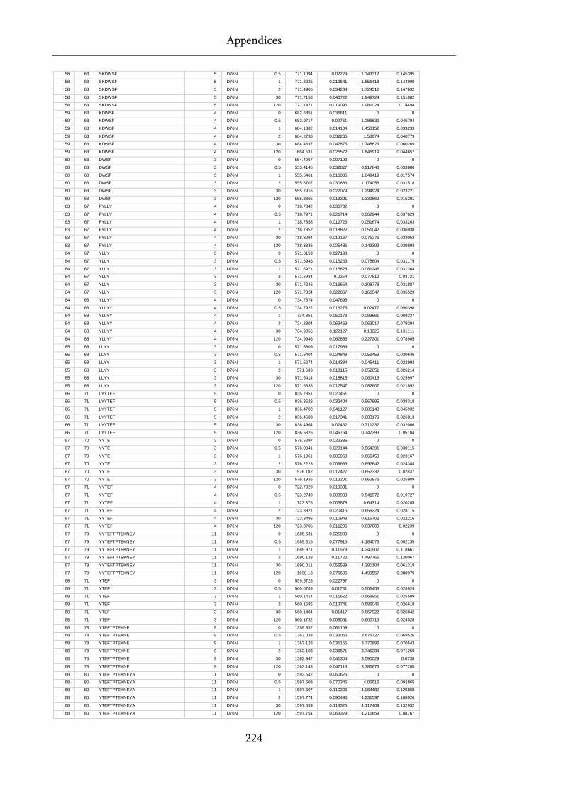
Appendices
224
58 63 SKDWSF 5 D76N 0.5 771.1094 0.02229 1.343312 0.145395
58 63 SKDWSF 5 D76N 1 771.3225 0.019541 1.556418 0.144999
58 63 SKDWSF 5 D76N 2 771.4906 0.034204 1.724512 0.147692
58 63 SKDWSF 5 D76N 30 771.7158 0.046722 1.949724 0.151082
58 63 SKDWSF 5 D76N 120 771.7471 0.019096 1.981024 0.14494
59 63 KDWSF 4 D76N 0 682.6851 0.036611 0 0
59 63 KDWSF 4 D76N 0.5 683.9717 0.02751 1.286639 0.045794
59 63 KDWSF 4 D76N 1 684.1382 0.014104 1.453152 0.039233
59 63 KDWSF 4 D76N 2 684.2738 0.032235 1.58874 0.048779
59 63 KDWSF 4 D76N 30 684.4337 0.047875 1.748623 0.060269
59 63 KDWSF 4 D76N 120 684.531 0.025572 1.845919 0.044657
60 63 DWSF 3 D76N 0 554.4967 0.007193 0 0
60 63 DWSF 3 D76N 0.5 555.4145 0.032827 0.917848 0.033606
60 63 DWSF 3 D76N 1 555.5461 0.016035 1.049419 0.017574
60 63 DWSF 3 D76N 2 555.6707 0.030686 1.174058 0.031518
60 63 DWSF 3 D76N 30 555.7916 0.022079 1.294924 0.023221
60 63 DWSF 3 D76N 120 555.8365 0.013391 1.339862 0.015201
63 67 FYLLY 4 D76N 0 718.7342 0.030732 0 0
63 67 FYLLY 4 D76N 0.5 718.7971 0.021714 0.062944 0.037629
63 67 FYLLY 4 D76N 1 718.7858 0.012726 0.051674 0.033263
63 67 FYLLY 4 D76N 2 718.7852 0.018822 0.051042 0.036038
63 67 FYLLY 4 D76N 30 718.8094 0.012167 0.075276 0.033053
63 67 FYLLY 4 D76N 120 718.8836 0.025436 0.149393 0.039893
64 67 YLLY 3 D76N 0 571.6159 0.027193 0 0
64 67 YLLY 3 D76N 0.5 571.6945 0.015253 0.078604 0.031179
64 67 YLLY 3 D76N 1 571.6971 0.015628 0.081246 0.031364
64 67 YLLY 3 D76N 2 571.6934 0.0254 0.077512 0.03721
64 67 YLLY 3 D76N 30 571.7246 0.016654 0.108778 0.031887
64 67 YLLY 3 D76N 120 571.7824 0.022867 0.166547 0.035529
64 68 YLLYY 4 D76N 0 734.7674 0.047698 0 0
64 68 YLLYY 4 D76N 0.5 734.7922 0.016275 0.02477 0.050398
64 68 YLLYY 4 D76N 1 734.851 0.050173 0.083661 0.069227
64 68 YLLYY 4 D76N 2 734.8304 0.063469 0.063017 0.079394
64 68 YLLYY 4 D76N 30 734.9056 0.122127 0.13825 0.131111
64 68 YLLYY 4 D76N 120 734.9946 0.062856 0.227201 0.078905
65 68 LLYY 3 D76N 0 571.5809 0.017939 0 0
65 68 LLYY 3 D76N 0.5 571.6404 0.024848 0.059453 0.030646
65 68 LLYY 3 D76N 1 571.6274 0.014384 0.046411 0.022993
65 68 LLYY 3 D76N 2 571.633 0.019115 0.052051 0.026214
65 68 LLYY 3 D76N 30 571.6414 0.018816 0.060413 0.025997
65 68 LLYY 3 D76N 120 571.6635 0.012547 0.082607 0.021892
66 71 LYYTEF 5 D76N 0 835.7851 0.020451 0 0
66 71 LYYTEF 5 D76N 0.5 836.3528 0.032404 0.567695 0.038318
66 71 LYYTEF 5 D76N 1 836.4703 0.041127 0.685143 0.045932
66 71 LYYTEF 5 D76N 2 836.4683 0.017341 0.683179 0.026813
66 71 LYYTEF 5 D76N 30 836.4964 0.02462 0.711232 0.032006
66 71 LYYTEF 5 D76N 120 836.5325 0.046764 0.747393 0.05104
67 70 YYTE 3 D76N 0 575.5297 0.022386 0 0
67 70 YYTE 3 D76N 0.5 576.0941 0.020144 0.564391 0.030115
67 70 YYTE 3 D76N 1 576.1961 0.005963 0.666453 0.023167
67 70 YYTE 3 D76N 2 576.2223 0.009666 0.692642 0.024384
67 70 YYTE 3 D76N 30 576.182 0.017427 0.652332 0.02837
67 70 YYTE 3 D76N 120 576.1926 0.013201 0.662876 0.025989
67 71 YYTEF 4 D76N 0 722.7329 0.019331 0 0
67 71 YYTEF 4 D76N 0.5 723.2749 0.003933 0.541972 0.019727
67 71 YYTEF 4 D76N 1 723.376 0.005878 0.64314 0.020205
67 71 YYTEF 4 D76N 2 723.3921 0.020415 0.659224 0.028115
67 71 YYTEF 4 D76N 30 723.3496 0.010948 0.616702 0.022216
67 71 YYTEF 4 D76N 120 723.3705 0.011296 0.637609 0.02239
67 79 YYTEFTPTEKNEY 11 D76N 0 1685.631 0.025989 0 0
67 79 YYTEFTPTEKNEY 11 D76N 0.5 1689.815 0.077915 4.184076 0.082135
67 79 YYTEFTPTEKNEY 11 D76N 1 1689.971 0.11578 4.340902 0.118661
67 79 YYTEFTPTEKNEY 11 D76N 2 1690.128 0.11722 4.497766 0.120067
67 79 YYTEFTPTEKNEY 11 D76N 30 1690.011 0.055539 4.380104 0.061319
67 79 YYTEFTPTEKNEY 11 D76N 120 1690.13 0.076695 4.499557 0.080979
68 71 YTEF 3 D76N 0 559.5725 0.022797 0 0
68 71 YTEF 3 D76N 0.5 560.0789 0.01781 0.506453 0.028929
68 71 YTEF 3 D76N 1 560.1414 0.011622 0.568951 0.025589
68 71 YTEF 3 D76N 2 560.1585 0.013741 0.586045 0.026618
68 71 YTEF 3 D76N 30 560.1404 0.01417 0.567922 0.026842
68 71 YTEF 3 D76N 120 560.1732 0.009051 0.600715 0.024528
68 78 YTEFTPTEKNE 9 D76N 0 1359.357 0.061159 0 0
68 78 YTEFTPTEKNE 9 D76N 0.5 1363.033 0.033066 3.675727 0.069526
68 78 YTEFTPTEKNE 9 D76N 1 1363.128 0.035155 3.770896 0.070543
68 78 YTEFTPTEKNE 9 D76N 2 1363.103 0.036571 3.746284 0.071259
68 78 YTEFTPTEKNE 9 D76N 30 1362.947 0.041304 3.590029 0.0738
68 78 YTEFTPTEKNE 9 D76N 120 1363.143 0.047118 3.785875 0.077205
68 80 YTEFTPTEKNEYA 11 D76N 0 1593.542 0.060625 0 0
68 80 YTEFTPTEKNEYA 11 D76N 0.5 1597.608 0.070345 4.06616 0.092865
68 80 YTEFTPTEKNEYA 11 D76N 1 1597.607 0.110306 4.064482 0.125868
68 80 YTEFTPTEKNEYA 11 D76N 2 1597.774 0.090496 4.231597 0.108926
68 80 YTEFTPTEKNEYA 11 D76N 30 1597.659 0.118325 4.117409 0.132952
68 80 YTEFTPTEKNEYA 11 D76N 120 1597.754 0.063329 4.211859 0.08767

Appendices
225
68 81 YTEFTPTEKNEYAC 12 D76N 0 1696.717 0.030187 0 0
68 81 YTEFTPTEKNEYAC 12 D76N 0.5 1700.871 0.052499 4.154027 0.060559
68 81 YTEFTPTEKNEYAC 12 D76N 1 1701.057 0.112346 4.3396 0.116331
68 81 YTEFTPTEKNEYAC 12 D76N 2 1701.141 0.095837 4.423755 0.100479
68 81 YTEFTPTEKNEYAC 12 D76N 30 1701.028 0.073206 4.310272 0.079185
68 81 YTEFTPTEKNEYAC 12 D76N 120 1701.129 0.098385 4.411646 0.102912
69 78 TEFTPTEKNE 8 D76N 0 1196.023 0.012761 0 0
69 78 TEFTPTEKNE 8 D76N 0.5 1199.633 0.034685 3.610346 0.036958
69 78 TEFTPTEKNE 8 D76N 1 1199.663 0.037894 3.64014 0.039985
69 78 TEFTPTEKNE 8 D76N 2 1199.592 0.091284 3.569292 0.092171
69 78 TEFTPTEKNE 8 D76N 30 1199.393 0.071473 3.369751 0.072603
69 78 TEFTPTEKNE 8 D76N 120 1199.606 0.057044 3.58259 0.058454
69 80 TEFTPTEKNEYA 10 D76N 0 1430.322 0.042827 0 0
69 80 TEFTPTEKNEYA 10 D76N 0.5 1434.048 0.129707 3.726412 0.136594
69 80 TEFTPTEKNEYA 10 D76N 1 1434.223 0.091209 3.900798 0.100763
69 80 TEFTPTEKNEYA 10 D76N 2 1434.276 0.131614 3.954575 0.138407
69 80 TEFTPTEKNEYA 10 D76N 30 1434.186 0.058812 3.863939 0.072754
69 80 TEFTPTEKNEYA 10 D76N 120 1434.245 0.088715 3.923276 0.098512
69 81 TEFTPTEKNEYAC 11 D76N 0 1533.436 0.027766 0 0
69 81 TEFTPTEKNEYAC 11 D76N 0.5 1537.255 0.084483 3.819046 0.088928
69 81 TEFTPTEKNEYAC 11 D76N 1 1537.435 0.027826 3.998879 0.039309
69 81 TEFTPTEKNEYAC 11 D76N 2 1537.482 0.085727 4.045802 0.090111
69 81 TEFTPTEKNEYAC 11 D76N 30 1537.405 0.092964 3.968517 0.097022
69 81 TEFTPTEKNEYAC 11 D76N 120 1537.47 0.071504 4.033793 0.076706
82 100 RVNHVTLSQPKIVKWDRDM 17 D76N 0 2323.559 0.036512 0 0
82 100 RVNHVTLSQPKIVKWDRDM 17 D76N 0.5 2327.626 0.117442 4.066652 0.122987
82 100 RVNHVTLSQPKIVKWDRDM 17 D76N 1 2327.992 0.081892 4.432753 0.089663
82 100 RVNHVTLSQPKIVKWDRDM 17 D76N 2 2328.183 0.063839 4.62351 0.073543
82 100 RVNHVTLSQPKIVKWDRDM 17 D76N 30 2328.129 0.196082 4.56983 0.199452
82 100 RVNHVTLSQPKIVKWDRDM 17 D76N 120 2328.539 0.141636 4.98007 0.146267
91 100 PKIVKWDRDM 8 D76N 0 1288.393 0.037954 0 0
91 100 PKIVKWDRDM 8 D76N 0.5 1290.255 0.116675 1.861692 0.122693
91 100 PKIVKWDRDM 8 D76N 1 1290.558 0.115179 2.164236 0.121271
91 100 PKIVKWDRDM 8 D76N 2 1290.703 0.094827 2.309773 0.102141
91 100 PKIVKWDRDM 8 D76N 30 1290.808 0.265519 2.414757 0.268218
91 100 PKIVKWDRDM 8 D76N 120 1290.891 0.222585 2.497556 0.225797
94 100 VKWDRDM 6 D76N 0 949.958 0.029286 0 0
94 100 VKWDRDM 6 D76N 0.5 951.1507 0.066865 1.192707 0.072997
94 100 VKWDRDM 6 D76N 1 951.3044 0.067611 1.346384 0.073681
94 100 VKWDRDM 6 D76N 2 951.3407 0.095715 1.382741 0.100095
94 100 VKWDRDM 6 D76N 30 951.3046 0.019364 1.346591 0.035109
94 100 VKWDRDM 6 D76N 120 951.6492 0.023426 1.69123 0.037502
95 100 KWDRDM 5 D76N 0 850.8568 0.064341 0 0
95 100 KWDRDM 5 D76N 0.5 852.2432 0.040685 1.386415 0.076125
95 100 KWDRDM 5 D76N 1 852.3555 0.067351 1.498793 0.093145
95 100 KWDRDM 5 D76N 2 852.3943 0.04514 1.537557 0.078596
95 100 KWDRDM 5 D76N 30 852.4941 0.042827 1.637341 0.077291
95 100 KWDRDM 5 D76N 120 852.5511 0.023912 1.694373 0.068641
11 23 YSRHPAENGKSNF 11 ΔN6 0 1507.495 0.037201 0 0
11 23 YSRHPAENGKSNF 11 ΔN6 0.5 1510.484 0.095233 2.989718 0.102241
11 23 YSRHPAENGKSNF 11 ΔN6 1 1510.659 0.075175 3.164558 0.083876
11 23 YSRHPAENGKSNF 11 ΔN6 2 1510.72 0.070509 3.224995 0.079721
11 23 YSRHPAENGKSNF 11 ΔN6 30 1511.07 0.045306 3.575224 0.058622
11 23 YSRHPAENGKSNF 11 ΔN6 120 1511.364 0.05075 3.869537 0.062925
11 26 YSRHPAENGKSNFLNC 14 ΔN6 0 1837.884 0.057194 0 0
11 26 YSRHPAENGKSNFLNC 14 ΔN6 0.5 1840.399 0.094384 2.514222 0.110361
11 26 YSRHPAENGKSNFLNC 14 ΔN6 1 1840.624 0.051517 2.739648 0.076975
11 26 YSRHPAENGKSNFLNC 14 ΔN6 2 1840.72 0.075712 2.835142 0.094886
11 26 YSRHPAENGKSNFLNC 14 ΔN6 30 1841.11 0.15855 3.225593 0.16855
11 26 YSRHPAENGKSNFLNC 14 ΔN6 120 1841.317 0.14138 3.432686 0.152511
27 35 YVSGFHPSD 7 ΔN6 0 1008.995 0.058462 0 0
27 35 YVSGFHPSD 7 ΔN6 0.5 1010.913 0.032352 1.917408 0.066817
27 35 YVSGFHPSD 7 ΔN6 1 1010.978 0.062263 1.982236 0.085408
27 35 YVSGFHPSD 7 ΔN6 2 1011.081 0.042597 2.085801 0.072335
27 35 YVSGFHPSD 7 ΔN6 30 1011.075 0.005145 2.080008 0.058688
27 35 YVSGFHPSD 7 ΔN6 120 1011.144 0.087233 2.14811 0.105011
27 37 YVSGFHPSDIE 9 ΔN6 0 1251.252 0.031903 0 0
27 37 YVSGFHPSDIE 9 ΔN6 0.5 1252.663 0.030503 1.411797 0.044139
27 37 YVSGFHPSDIE 9 ΔN6 1 1252.729 0.056784 1.476987 0.065133
27 37 YVSGFHPSDIE 9 ΔN6 2 1252.821 0.039326 1.569772 0.050639
27 37 YVSGFHPSDIE 9 ΔN6 30 1253.211 0.091449 1.959106 0.096854
27 37 YVSGFHPSDIE 9 ΔN6 120 1253.527 0.045852 2.275289 0.055859
27 38 YVSGFHPSDIEV 10 ΔN6 0 1350.364 0.08177 0 0
27 38 YVSGFHPSDIEV 10 ΔN6 0.5 1351.898 0.096883 1.533954 0.126778
27 38 YVSGFHPSDIEV 10 ΔN6 1 1352.214 0.134442 1.849836 0.157357
27 38 YVSGFHPSDIEV 10 ΔN6 2 1352.145 0.086814 1.780851 0.11926
27 38 YVSGFHPSDIEV 10 ΔN6 30 1352.811 0.064228 2.447229 0.103979
27 38 YVSGFHPSDIEV 10 ΔN6 120 1353.015 0.108172 2.650374 0.1356
29 35 SGFHPSD 5 ΔN6 0 746.7365 0.027362 0 0
29 35 SGFHPSD 5 ΔN6 0.5 748.3017 0.020828 1.565132 0.034387
29 35 SGFHPSD 5 ΔN6 1 748.3254 0.033508 1.588852 0.043261
29 35 SGFHPSD 5 ΔN6 2 748.3577 0.012021 1.621219 0.029887
29 35 SGFHPSD 5 ΔN6 30 748.3617 0.048549 1.625206 0.055729
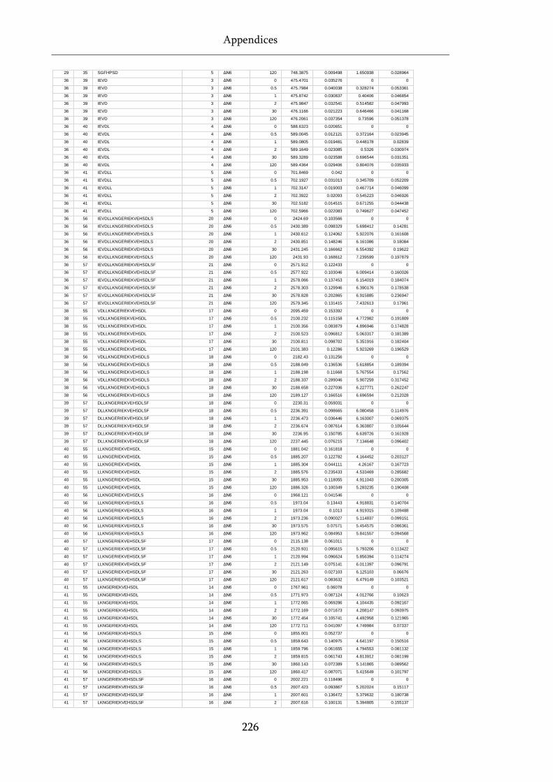
Appendices
226
29 35 SGFHPSD 5 ΔN6 120 748.3875 0.009498 1.650938 0.028964
36 39 IEVD 3 ΔN6 0 475.4701 0.035276 0 0
36 39 IEVD 3 ΔN6 0.5 475.7984 0.040038 0.328274 0.053361
36 39 IEVD 3 ΔN6 1 475.8742 0.030837 0.40406 0.046854
36 39 IEVD 3 ΔN6 2 475.9847 0.032541 0.514582 0.047993
36 39 IEVD 3 ΔN6 30 476.1166 0.021223 0.646466 0.041168
36 39 IEVD 3 ΔN6 120 476.2061 0.037354 0.73596 0.051378
36 40 IEVDL 4 ΔN6 0 588.6323 0.020651 0 0
36 40 IEVDL 4 ΔN6 0.5 589.0045 0.012121 0.372164 0.023945
36 40 IEVDL 4 ΔN6 1 589.0805 0.019481 0.448178 0.02839
36 40 IEVDL 4 ΔN6 2 589.1649 0.023085 0.5326 0.030974
36 40 IEVDL 4 ΔN6 30 589.3289 0.023588 0.696544 0.031351
36 40 IEVDL 4 ΔN6 120 589.4364 0.029406 0.804076 0.035933
36 41 IEVDLL 5 ΔN6 0 701.8469 0.042 0 0
36 41 IEVDLL 5 ΔN6 0.5 702.1927 0.031013 0.345709 0.052209
36 41 IEVDLL 5 ΔN6 1 702.3147 0.019003 0.467714 0.046099
36 41 IEVDLL 5 ΔN6 2 702.3922 0.02093 0.545223 0.046926
36 41 IEVDLL 5 ΔN6 30 702.5182 0.014515 0.671255 0.044438
36 41 IEVDLL 5 ΔN6 120 702.5966 0.022083 0.749627 0.047452
36 56 IEVDLLKNGERIEKVEHSDLS 20 ΔN6 0 2424.69 0.103566 0 0
36 56 IEVDLLKNGERIEKVEHSDLS 20 ΔN6 0.5 2430.389 0.098329 5.698412 0.14281
36 56 IEVDLLKNGERIEKVEHSDLS 20 ΔN6 1 2430.612 0.124062 5.922076 0.161608
36 56 IEVDLLKNGERIEKVEHSDLS 20 ΔN6 2 2430.851 0.148246 6.161086 0.18084
36 56 IEVDLLKNGERIEKVEHSDLS 20 ΔN6 30 2431.245 0.166662 6.554392 0.19622
36 56 IEVDLLKNGERIEKVEHSDLS 20 ΔN6 120 2431.93 0.168612 7.239599 0.197879
36 57 IEVDLLKNGERIEKVEHSDLSF 21 ΔN6 0 2571.912 0.122433 0 0
36 57 IEVDLLKNGERIEKVEHSDLSF 21 ΔN6 0.5 2577.922 0.103046 6.009414 0.160026
36 57 IEVDLLKNGERIEKVEHSDLSF 21 ΔN6 1 2578.066 0.137453 6.154019 0.184074
36 57 IEVDLLKNGERIEKVEHSDLSF 21 ΔN6 2 2578.303 0.129946 6.390176 0.178538
36 57 IEVDLLKNGERIEKVEHSDLSF 21 ΔN6 30 2578.828 0.202865 6.915885 0.236947
36 57 IEVDLLKNGERIEKVEHSDLSF 21 ΔN6 120 2579.345 0.131415 7.432613 0.17961
38 55 VDLLKNGERIEKVEHSDL 17 ΔN6 0 2095.459 0.153392 0 0
38 55 VDLLKNGERIEKVEHSDL 17 ΔN6 0.5 2100.232 0.115158 4.772982 0.191809
38 55 VDLLKNGERIEKVEHSDL 17 ΔN6 1 2100.356 0.083879 4.896946 0.174828
38 55 VDLLKNGERIEKVEHSDL 17 ΔN6 2 2100.523 0.096812 5.063317 0.181389
38 55 VDLLKNGERIEKVEHSDL 17 ΔN6 30 2100.811 0.098702 5.351916 0.182404
38 55 VDLLKNGERIEKVEHSDL 17 ΔN6 120 2101.383 0.12286 5.923269 0.196529
38 56 VDLLKNGERIEKVEHSDLS 18 ΔN6 0 2182.43 0.131256 0 0
38 56 VDLLKNGERIEKVEHSDLS 18 ΔN6 0.5 2188.049 0.136536 5.618854 0.189394
38 56 VDLLKNGERIEKVEHSDLS 18 ΔN6 1 2188.198 0.11668 5.767554 0.17562
38 56 VDLLKNGERIEKVEHSDLS 18 ΔN6 2 2188.337 0.289046 5.907259 0.317452
38 56 VDLLKNGERIEKVEHSDLS 18 ΔN6 30 2188.658 0.227036 6.227771 0.262247
38 56 VDLLKNGERIEKVEHSDLS 18 ΔN6 120 2189.127 0.166516 6.696594 0.212028
39 57 DLLKNGERIEKVEHSDLSF 18 ΔN6 0 2230.31 0.059031 0 0
39 57 DLLKNGERIEKVEHSDLSF 18 ΔN6 0.5 2236.391 0.098665 6.080458 0.114976
39 57 DLLKNGERIEKVEHSDLSF 18 ΔN6 1 2236.473 0.036446 6.163007 0.069375
39 57 DLLKNGERIEKVEHSDLSF 18 ΔN6 2 2236.674 0.087614 6.363807 0.105644
39 57 DLLKNGERIEKVEHSDLSF 18 ΔN6 30 2236.95 0.150785 6.639726 0.161928
39 57 DLLKNGERIEKVEHSDLSF 18 ΔN6 120 2237.445 0.076215 7.134648 0.096402
40 55 LLKNGERIEKVEHSDL 15 ΔN6 0 1881.042 0.161818 0 0
40 55 LLKNGERIEKVEHSDL 15 ΔN6 0.5 1885.207 0.122782 4.164452 0.203127
40 55 LLKNGERIEKVEHSDL 15 ΔN6 1 1885.304 0.044111 4.26167 0.167723
40 55 LLKNGERIEKVEHSDL 15 ΔN6 2 1885.576 0.235433 4.533469 0.285682
40 55 LLKNGERIEKVEHSDL 15 ΔN6 30 1885.953 0.118055 4.911043 0.200305
40 55 LLKNGERIEKVEHSDL 15 ΔN6 120 1886.326 0.100349 5.283235 0.190408
40 56 LLKNGERIEKVEHSDLS 16 ΔN6 0 1968.121 0.041546 0 0
40 56 LLKNGERIEKVEHSDLS 16 ΔN6 0.5 1973.04 0.13443 4.918831 0.140704
40 56 LLKNGERIEKVEHSDLS 16 ΔN6 1 1973.04 0.1013 4.919315 0.109488
40 56 LLKNGERIEKVEHSDLS 16 ΔN6 2 1973.236 0.090027 5.114837 0.099151
40 56 LLKNGERIEKVEHSDLS 16 ΔN6 30 1973.575 0.07571 5.454575 0.086361
40 56 LLKNGERIEKVEHSDLS 16 ΔN6 120 1973.962 0.084953 5.841557 0.094568
40 57 LLKNGERIEKVEHSDLSF 17 ΔN6 0 2115.138 0.061011 0 0
40 57 LLKNGERIEKVEHSDLSF 17 ΔN6 0.5 2120.931 0.095615 5.793206 0.113422
40 57 LLKNGERIEKVEHSDLSF 17 ΔN6 1 2120.994 0.096624 5.856394 0.114274
40 57 LLKNGERIEKVEHSDLSF 17 ΔN6 2 2121.149 0.075141 6.011397 0.096791
40 57 LLKNGERIEKVEHSDLSF 17 ΔN6 30 2121.263 0.027103 6.125103 0.06676
40 57 LLKNGERIEKVEHSDLSF 17 ΔN6 120 2121.617 0.083632 6.479149 0.103521
41 55 LKNGERIEKVEHSDL 14 ΔN6 0 1767.961 0.06078 0 0
41 55 LKNGERIEKVEHSDL 14 ΔN6 0.5 1771.973 0.087124 4.012766 0.10623
41 55 LKNGERIEKVEHSDL 14 ΔN6 1 1772.065 0.069286 4.104435 0.092167
41 55 LKNGERIEKVEHSDL 14 ΔN6 2 1772.169 0.071673 4.208147 0.093975
41 55 LKNGERIEKVEHSDL 14 ΔN6 30 1772.454 0.105741 4.492958 0.121965
41 55 LKNGERIEKVEHSDL 14 ΔN6 120 1772.711 0.041097 4.749984 0.07337
41 56 LKNGERIEKVEHSDLS 15 ΔN6 0 1855.001 0.052737 0 0
41 56 LKNGERIEKVEHSDLS 15 ΔN6 0.5 1859.643 0.140975 4.641197 0.150516
41 56 LKNGERIEKVEHSDLS 15 ΔN6 1 1859.796 0.061655 4.794553 0.081132
41 56 LKNGERIEKVEHSDLS 15 ΔN6 2 1859.815 0.061743 4.813912 0.081199
41 56 LKNGERIEKVEHSDLS 15 ΔN6 30 1860.143 0.072389 5.141865 0.089562
41 56 LKNGERIEKVEHSDLS 15 ΔN6 120 1860.417 0.087071 5.415649 0.101797
41 57 LKNGERIEKVEHSDLSF 16 ΔN6 0 2002.221 0.118496 0 0
41 57 LKNGERIEKVEHSDLSF 16 ΔN6 0.5 2007.423 0.093867 5.202024 0.15117
41 57 LKNGERIEKVEHSDLSF 16 ΔN6 1 2007.601 0.136472 5.379632 0.180738
41 57 LKNGERIEKVEHSDLSF 16 ΔN6 2 2007.616 0.100131 5.394805 0.155137
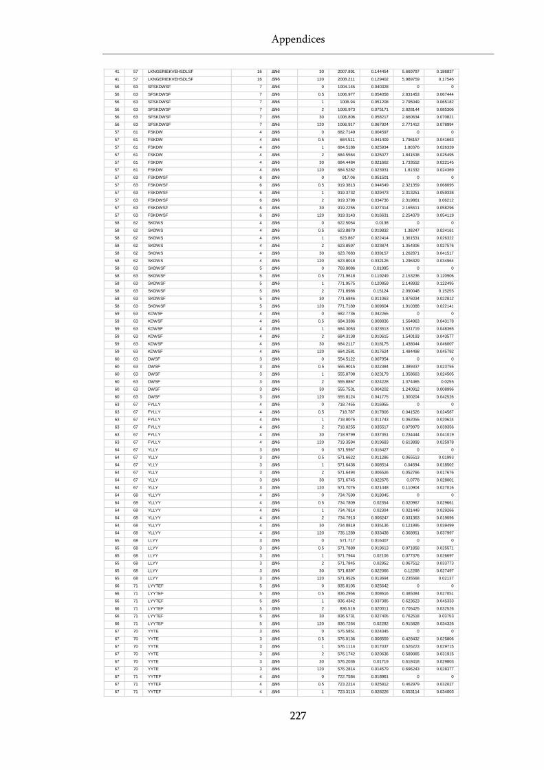
Appendices
227
41 57 LKNGERIEKVEHSDLSF 16 ΔN6 30 2007.891 0.144454 5.669797 0.186837
41 57 LKNGERIEKVEHSDLSF 16 ΔN6 120 2008.211 0.129402 5.989759 0.17546
56 63 SFSKDWSF 7 ΔN6 0 1004.145 0.040328 0 0
56 63 SFSKDWSF 7 ΔN6 0.5 1006.977 0.054058 2.831453 0.067444
56 63 SFSKDWSF 7 ΔN6 1 1006.94 0.051208 2.795049 0.065182
56 63 SFSKDWSF 7 ΔN6 2 1006.973 0.075171 2.828144 0.085306
56 63 SFSKDWSF 7 ΔN6 30 1006.806 0.058217 2.660634 0.070821
56 63 SFSKDWSF 7 ΔN6 120 1006.917 0.067924 2.771412 0.078994
57 61 FSKDW 4 ΔN6 0 682.7149 0.004597 0 0
57 61 FSKDW 4 ΔN6 0.5 684.511 0.041409 1.796157 0.041663
57 61 FSKDW 4 ΔN6 1 684.5186 0.025934 1.80376 0.026339
57 61 FSKDW 4 ΔN6 2 684.5564 0.025077 1.841538 0.025495
57 61 FSKDW 4 ΔN6 30 684.4484 0.021662 1.733552 0.022145
57 61 FSKDW 4 ΔN6 120 684.5282 0.023931 1.81332 0.024369
57 63 FSKDWSF 6 ΔN6 0 917.06 0.051501 0 0
57 63 FSKDWSF 6 ΔN6 0.5 919.3813 0.044549 2.321359 0.068095
57 63 FSKDWSF 6 ΔN6 1 919.3732 0.029473 2.313251 0.059338
57 63 FSKDWSF 6 ΔN6 2 919.3798 0.034736 2.319861 0.06212
57 63 FSKDWSF 6 ΔN6 30 919.2255 0.027314 2.165511 0.058296
57 63 FSKDWSF 6 ΔN6 120 919.3143 0.016631 2.254379 0.054119
58 62 SKDWS 4 ΔN6 0 622.5054 0.0138 0 0
58 62 SKDWS 4 ΔN6 0.5 623.8879 0.019832 1.38247 0.024161
58 62 SKDWS 4 ΔN6 1 623.867 0.022414 1.361531 0.026322
58 62 SKDWS 4 ΔN6 2 623.8597 0.023874 1.354306 0.027576
58 62 SKDWS 4 ΔN6 30 623.7683 0.039157 1.262871 0.041517
58 62 SKDWS 4 ΔN6 120 623.8018 0.032126 1.296329 0.034964
58 63 SKDWSF 5 ΔN6 0 769.8086 0.01995 0 0
58 63 SKDWSF 5 ΔN6 0.5 771.9618 0.119249 2.153236 0.120906
58 63 SKDWSF 5 ΔN6 1 771.9575 0.120859 2.148932 0.122495
58 63 SKDWSF 5 ΔN6 2 771.8986 0.15124 2.090048 0.15255
58 63 SKDWSF 5 ΔN6 30 771.6846 0.011063 1.876034 0.022812
58 63 SKDWSF 5 ΔN6 120 771.7189 0.009604 1.910388 0.022141
59 63 KDWSF 4 ΔN6 0 682.7736 0.042265 0 0
59 63 KDWSF 4 ΔN6 0.5 684.3386 0.008836 1.564963 0.043178
59 63 KDWSF 4 ΔN6 1 684.3053 0.023513 1.531719 0.048365
59 63 KDWSF 4 ΔN6 2 684.3138 0.010615 1.540193 0.043577
59 63 KDWSF 4 ΔN6 30 684.2117 0.018175 1.438044 0.046007
59 63 KDWSF 4 ΔN6 120 684.2581 0.017624 1.484498 0.045792
60 63 DWSF 3 ΔN6 0 554.5122 0.007954 0 0
60 63 DWSF 3 ΔN6 0.5 555.9015 0.022384 1.389337 0.023755
60 63 DWSF 3 ΔN6 1 555.8708 0.023179 1.358663 0.024505
60 63 DWSF 3 ΔN6 2 555.8867 0.024228 1.374465 0.0255
60 63 DWSF 3 ΔN6 30 555.7531 0.004202 1.240912 0.008996
60 63 DWSF 3 ΔN6 120 555.8124 0.041775 1.300204 0.042526
63 67 FYLLY 4 ΔN6 0 718.7455 0.016955 0 0
63 67 FYLLY 4 ΔN6 0.5 718.787 0.017806 0.041526 0.024587
63 67 FYLLY 4 ΔN6 1 718.8076 0.011743 0.062055 0.020624
63 67 FYLLY 4 ΔN6 2 718.8255 0.035517 0.079979 0.039356
63 67 FYLLY 4 ΔN6 30 718.9799 0.037351 0.234444 0.041019
63 67 FYLLY 4 ΔN6 120 719.3594 0.019683 0.613899 0.025978
64 67 YLLY 3 ΔN6 0 571.5967 0.016427 0 0
64 67 YLLY 3 ΔN6 0.5 571.6622 0.011286 0.065513 0.01993
64 67 YLLY 3 ΔN6 1 571.6436 0.008514 0.04694 0.018502
64 67 YLLY 3 ΔN6 2 571.6494 0.006526 0.052766 0.017676
64 67 YLLY 3 ΔN6 30 571.6745 0.022676 0.0778 0.028001
64 67 YLLY 3 ΔN6 120 571.7076 0.021448 0.110904 0.027016
64 68 YLLYY 4 ΔN6 0 734.7599 0.018045 0 0
64 68 YLLYY 4 ΔN6 0.5 734.7809 0.02354 0.020967 0.029661
64 68 YLLYY 4 ΔN6 1 734.7814 0.02304 0.021449 0.029266
64 68 YLLYY 4 ΔN6 2 734.7913 0.006247 0.031363 0.019096
64 68 YLLYY 4 ΔN6 30 734.8819 0.035136 0.121995 0.039499
64 68 YLLYY 4 ΔN6 120 735.1289 0.033438 0.368951 0.037997
65 68 LLYY 3 ΔN6 0 571.717 0.016407 0 0
65 68 LLYY 3 ΔN6 0.5 571.7889 0.019613 0.071858 0.025571
65 68 LLYY 3 ΔN6 1 571.7944 0.02106 0.077376 0.026697
65 68 LLYY 3 ΔN6 2 571.7845 0.02952 0.067512 0.033773
65 68 LLYY 3 ΔN6 30 571.8397 0.022066 0.12268 0.027497
65 68 LLYY 3 ΔN6 120 571.9526 0.013694 0.235568 0.02137
66 71 LYYTEF 5 ΔN6 0 835.8105 0.025642 0 0
66 71 LYYTEF 5 ΔN6 0.5 836.2956 0.008616 0.485084 0.027051
66 71 LYYTEF 5 ΔN6 1 836.4342 0.037385 0.623623 0.045333
66 71 LYYTEF 5 ΔN6 2 836.516 0.020011 0.705425 0.032526
66 71 LYYTEF 5 ΔN6 30 836.5731 0.027405 0.762518 0.03753
66 71 LYYTEF 5 ΔN6 120 836.7264 0.02282 0.915828 0.034326
67 70 YYTE 3 ΔN6 0 575.5851 0.024345 0 0
67 70 YYTE 3 ΔN6 0.5 576.0136 0.008559 0.428432 0.025806
67 70 YYTE 3 ΔN6 1 576.1114 0.017037 0.526223 0.029715
67 70 YYTE 3 ΔN6 2 576.1742 0.020636 0.589065 0.031915
67 70 YYTE 3 ΔN6 30 576.2036 0.01719 0.618418 0.029803
67 70 YYTE 3 ΔN6 120 576.2814 0.014579 0.696243 0.028377
67 71 YYTEF 4 ΔN6 0 722.7584 0.018961 0 0
67 71 YYTEF 4 ΔN6 0.5 723.2214 0.025812 0.462979 0.032027
67 71 YYTEF 4 ΔN6 1 723.3115 0.028226 0.553114 0.034003
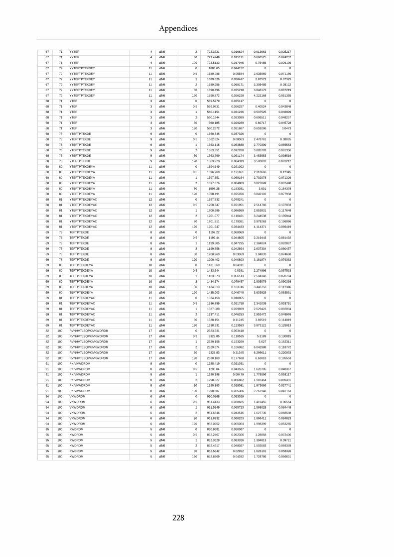
Appendices
228
67 71 YYTEF 4 ΔN6 2 723.3721 0.016624 0.613663 0.025217
67 71 YYTEF 4 ΔN6 30 723.4249 0.015121 0.666525 0.024252
67 71 YYTEF 4 ΔN6 120 723.5133 0.017945 0.75485 0.026106
67 79 YYTEFTPTEKDEY 11 ΔN6 0 1686.65 0.044152 0 0
67 79 YYTEFTPTEKDEY 11 ΔN6 0.5 1689.286 0.05584 2.635969 0.071186
67 79 YYTEFTPTEKDEY 11 ΔN6 1 1689.626 0.058447 2.97572 0.07325
67 79 YYTEFTPTEKDEY 11 ΔN6 2 1689.956 0.068171 3.305485 0.08122
67 79 YYTEFTPTEKDEY 11 ΔN6 30 1690.496 0.075218 3.846173 0.087219
67 79 YYTEFTPTEKDEY 11 ΔN6 120 1690.872 0.026228 4.222168 0.051355
68 71 YTEF 3 ΔN6 0 559.5779 0.035117 0 0
68 71 YTEF 3 ΔN6 0.5 559.9831 0.026257 0.40524 0.043848
68 71 YTEF 3 ΔN6 1 560.1154 0.031236 0.537525 0.046999
68 71 YTEF 3 ΔN6 2 560.1844 0.033099 0.606511 0.048257
68 71 YTEF 3 ΔN6 30 560.185 0.029289 0.60717 0.045728
68 71 YTEF 3 ΔN6 120 560.2372 0.031687 0.659286 0.0473
68 78 YTEFTPTEKDE 9 ΔN6 0 1360.345 0.037326 0 0
68 78 YTEFTPTEKDE 9 ΔN6 0.5 1362.824 0.08063 2.478761 0.08885
68 78 YTEFTPTEKDE 9 ΔN6 1 1363.115 0.053888 2.770399 0.065553
68 78 YTEFTPTEKDE 9 ΔN6 2 1363.351 0.072288 3.005703 0.081356
68 78 YTEFTPTEKDE 9 ΔN6 30 1363.799 0.091174 3.453553 0.098519
68 78 YTEFTPTEKDE 9 ΔN6 120 1363.928 0.084319 3.583091 0.092212
68 80 YTEFTPTEKDEYA 11 ΔN6 0 1594.649 0.021002 0 0
68 80 YTEFTPTEKDEYA 11 ΔN6 0.5 1596.968 0.121651 2.318666 0.12345
68 80 YTEFTPTEKDEYA 11 ΔN6 1 1597.351 0.068164 2.702078 0.071326
68 80 YTEFTPTEKDEYA 11 ΔN6 2 1597.676 0.084889 3.027049 0.087448
68 80 YTEFTPTEKDEYA 11 ΔN6 30 1598.25 0.163031 3.601 0.164378
68 80 YTEFTPTEKDEYA 11 ΔN6 120 1598.491 0.075076 3.842102 0.077958
68 81 YTEFTPTEKDEYAC 12 ΔN6 0 1697.832 0.079241 0 0
68 81 YTEFTPTEKDEYAC 12 ΔN6 0.5 1700.347 0.071951 2.514766 0.107033
68 81 YTEFTPTEKDEYAC 12 ΔN6 1 1700.686 0.086959 2.853831 0.117648
68 81 YTEFTPTEKDEYAC 12 ΔN6 2 1701.077 0.110461 3.244538 0.135944
68 81 YTEFTPTEKDEYAC 12 ΔN6 30 1701.811 0.179361 3.978263 0.196086
68 81 YTEFTPTEKDEYAC 12 ΔN6 120 1701.947 0.034483 4.114371 0.086419
69 78 TEFTPTEKDE 8 ΔN6 0 1197.22 0.068069 0 0
69 78 TEFTPTEKDE 8 ΔN6 0.5 1199.44 0.044805 2.219443 0.081492
69 78 TEFTPTEKDE 8 ΔN6 1 1199.605 0.047295 2.384024 0.082887
69 78 TEFTPTEKDE 8 ΔN6 2 1199.858 0.042894 2.637304 0.080457
69 78 TEFTPTEKDE 8 ΔN6 30 1200.269 0.03069 3.04833 0.074668
69 78 TEFTPTEKDE 8 ΔN6 120 1200.402 0.040803 3.181874 0.079362
69 80 TEFTPTEKDEYA 10 ΔN6 0 1431.369 0.04311 0 0
69 80 TEFTPTEKDEYA 10 ΔN6 0.5 1433.644 0.0381 2.274996 0.057533
69 80 TEFTPTEKDEYA 10 ΔN6 1 1433.873 0.056143 2.504343 0.070784
69 80 TEFTPTEKDEYA 10 ΔN6 2 1434.174 0.079457 2.805079 0.090398
69 80 TEFTPTEKDEYA 10 ΔN6 30 1434.813 0.103746 3.443753 0.112346
69 80 TEFTPTEKDEYA 10 ΔN6 120 1435.003 0.046748 3.633929 0.063591
69 81 TEFTPTEKDEYAC 11 ΔN6 0 1534.458 0.018855 0 0
69 81 TEFTPTEKDEYAC 11 ΔN6 0.5 1536.799 0.021758 2.341039 0.028791
69 81 TEFTPTEKDEYAC 11 ΔN6 1 1537.088 0.079899 2.629423 0.082094
69 81 TEFTPTEKDEYAC 11 ΔN6 2 1537.411 0.046283 2.952472 0.049976
69 81 TEFTPTEKDEYAC 11 ΔN6 30 1538.154 0.11245 3.69519 0.114019
69 81 TEFTPTEKDEYAC 11 ΔN6 120 1538.331 0.123583 3.873121 0.125013
82 100 RVNHVTLSQPKIVKWDRDM 17 ΔN6 0 2323.531 0.053418 0 0
82 100 RVNHVTLSQPKIVKWDRDM 17 ΔN6 0.5 2328.85 0.118535 5.3189 0.130015
82 100 RVNHVTLSQPKIVKWDRDM 17 ΔN6 1 2329.158 0.153269 5.627 0.162311
82 100 RVNHVTLSQPKIVKWDRDM 17 ΔN6 2 2329.574 0.106082 6.042988 0.118772
82 100 RVNHVTLSQPKIVKWDRDM 17 ΔN6 30 2329.83 0.21345 6.299611 0.220033
82 100 RVNHVTLSQPKIVKWDRDM 17 ΔN6 120 2330.169 0.177698 6.63818 0.185553
91 100 PKIVKWDRDM 8 ΔN6 0 1288.419 0.021031 0 0
91 100 PKIVKWDRDM 8 ΔN6 0.5 1290.04 0.043555 1.620705 0.048367
91 100 PKIVKWDRDM 8 ΔN6 1 1290.198 0.06479 1.778596 0.068117
91 100 PKIVKWDRDM 8 ΔN6 2 1290.327 0.086882 1.907464 0.089391
91 100 PKIVKWDRDM 8 ΔN6 30 1290.393 0.018091 1.973686 0.027741
91 100 PKIVKWDRDM 8 ΔN6 120 1290.687 0.035386 2.267943 0.041163
94 100 VKWDRDM 6 ΔN6 0 950.0268 0.053029 0 0
94 100 VKWDRDM 6 ΔN6 0.5 951.4433 0.038685 1.416455 0.06564
94 100 VKWDRDM 6 ΔN6 1 951.5949 0.065723 1.568028 0.084448
94 100 VKWDRDM 6 ΔN6 2 951.6546 0.043516 1.627736 0.068598
94 100 VKWDRDM 6 ΔN6 30 951.8932 0.066203 1.866411 0.084823
94 100 VKWDRDM 6 ΔN6 120 952.0252 0.005004 1.998399 0.053265
95 100 KWDRDM 5 ΔN6 0 850.9581 0.050067 0 0
95 100 KWDRDM 5 ΔN6 0.5 852.2467 0.052306 1.28858 0.072406
95 100 KWDRDM 5 ΔN6 1 852.3529 0.083326 1.394813 0.09721
95 100 KWDRDM 5 ΔN6 2 852.4617 0.048027 1.503583 0.069378
95 100 KWDRDM 5 ΔN6 30 852.5842 0.02992 1.626101 0.058326
95 100 KWDRDM 5 ΔN6 120 852.6869 0.04392 1.728786 0.066601
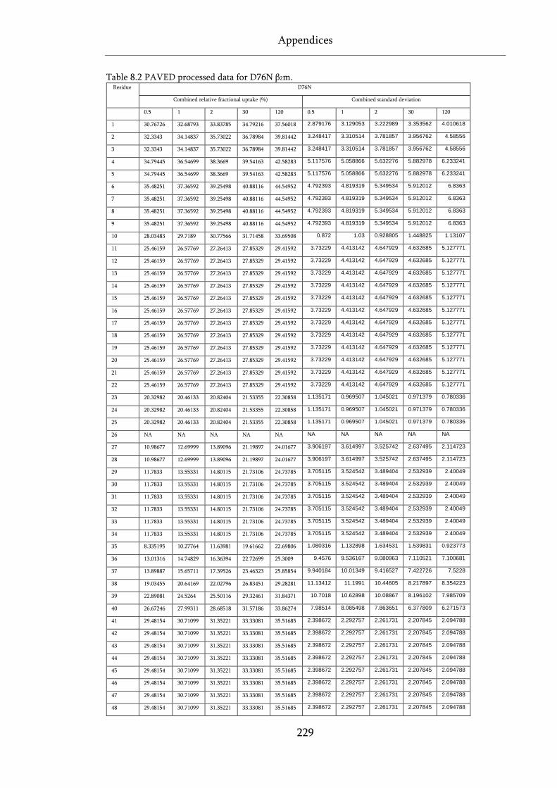
Appendices
229
Table 8.2 PAVED processed data for D76N β2m. Residue D76N
Combined relative fractional uptake (%) Combined standard deviation
0.5 1 2 30 120 0.5 1 2 30 120
1 30.76726 32.68793 33.83785 34.79216 37.56018 2.879176 3.129053 3.222989 3.353562 4.010618
2 32.3343 34.14837 35.73022 36.78984 39.81442 3.248417 3.310514 3.781857 3.956762 4.58556
3 32.3343 34.14837 35.73022 36.78984 39.81442 3.248417 3.310514 3.781857 3.956762 4.58556
4 34.79445 36.54699 38.3669 39.54163 42.58283 5.117576 5.058866 5.632276 5.882978 6.233241
5 34.79445 36.54699 38.3669 39.54163 42.58283 5.117576 5.058866 5.632276 5.882978 6.233241
6 35.48251 37.36592 39.25498 40.88116 44.54952 4.792393 4.819319 5.349534 5.912012 6.8363
7 35.48251 37.36592 39.25498 40.88116 44.54952 4.792393 4.819319 5.349534 5.912012 6.8363
8 35.48251 37.36592 39.25498 40.88116 44.54952 4.792393 4.819319 5.349534 5.912012 6.8363
9 35.48251 37.36592 39.25498 40.88116 44.54952 4.792393 4.819319 5.349534 5.912012 6.8363
10 28.03483 29.7189 30.77566 31.71458 33.69508 0.872 1.03 0.928805 1.448825 1.13107
11 25.46159 26.57769 27.26413 27.85329 29.41592 3.73229 4.413142 4.647929 4.632685 5.127771
12 25.46159 26.57769 27.26413 27.85329 29.41592 3.73229 4.413142 4.647929 4.632685 5.127771
13 25.46159 26.57769 27.26413 27.85329 29.41592 3.73229 4.413142 4.647929 4.632685 5.127771
14 25.46159 26.57769 27.26413 27.85329 29.41592 3.73229 4.413142 4.647929 4.632685 5.127771
15 25.46159 26.57769 27.26413 27.85329 29.41592 3.73229 4.413142 4.647929 4.632685 5.127771
16 25.46159 26.57769 27.26413 27.85329 29.41592 3.73229 4.413142 4.647929 4.632685 5.127771
17 25.46159 26.57769 27.26413 27.85329 29.41592 3.73229 4.413142 4.647929 4.632685 5.127771
18 25.46159 26.57769 27.26413 27.85329 29.41592 3.73229 4.413142 4.647929 4.632685 5.127771
19 25.46159 26.57769 27.26413 27.85329 29.41592 3.73229 4.413142 4.647929 4.632685 5.127771
20 25.46159 26.57769 27.26413 27.85329 29.41592 3.73229 4.413142 4.647929 4.632685 5.127771
21 25.46159 26.57769 27.26413 27.85329 29.41592 3.73229 4.413142 4.647929 4.632685 5.127771
22 25.46159 26.57769 27.26413 27.85329 29.41592 3.73229 4.413142 4.647929 4.632685 5.127771
23 20.32982 20.46133 20.82404 21.53355 22.30858 1.135171 0.969507 1.045021 0.971379 0.780336
24 20.32982 20.46133 20.82404 21.53355 22.30858 1.135171 0.969507 1.045021 0.971379 0.780336
25 20.32982 20.46133 20.82404 21.53355 22.30858 1.135171 0.969507 1.045021 0.971379 0.780336
26 NA NA NA NA NA NA NA NA NA NA
27 10.98677 12.69999 13.89096 21.19897 24.01677 3.906197 3.614997 3.525742 2.637495 2.114723
28 10.98677 12.69999 13.89096 21.19897 24.01677 3.906197 3.614997 3.525742 2.637495 2.114723
29 11.7833 13.55331 14.80115 21.73106 24.73785 3.705115 3.524542 3.489404 2.532939 2.40049
30 11.7833 13.55331 14.80115 21.73106 24.73785 3.705115 3.524542 3.489404 2.532939 2.40049
31 11.7833 13.55331 14.80115 21.73106 24.73785 3.705115 3.524542 3.489404 2.532939 2.40049
32 11.7833 13.55331 14.80115 21.73106 24.73785 3.705115 3.524542 3.489404 2.532939 2.40049
33 11.7833 13.55331 14.80115 21.73106 24.73785 3.705115 3.524542 3.489404 2.532939 2.40049
34 11.7833 13.55331 14.80115 21.73106 24.73785 3.705115 3.524542 3.489404 2.532939 2.40049
35 8.335195 10.27764 11.63981 19.61662 22.69806 1.080316 1.132898 1.634531 1.539831 0.923773
36 13.01316 14.74829 16.36394 22.72699 25.3009 9.4576 9.536167 9.080963 7.110521 7.100681
37 13.89887 15.65711 17.39526 23.46323 25.85854 9.940184 10.01349 9.416527 7.422726 7.5228
38 19.03455 20.64169 22.02796 26.83451 29.28281 11.13412 11.1991 10.44605 8.217897 8.354223
39 22.89081 24.5264 25.50116 29.32461 31.84371 10.7018 10.62898 10.08867 8.196102 7.985709
40 26.67246 27.99311 28.68518 31.57186 33.86274 7.98514 8.085498 7.863651 6.377809 6.271573
41 29.48154 30.71099 31.35221 33.33081 35.51685 2.398672 2.292757 2.261731 2.207845 2.094788
42 29.48154 30.71099 31.35221 33.33081 35.51685 2.398672 2.292757 2.261731 2.207845 2.094788
43 29.48154 30.71099 31.35221 33.33081 35.51685 2.398672 2.292757 2.261731 2.207845 2.094788
44 29.48154 30.71099 31.35221 33.33081 35.51685 2.398672 2.292757 2.261731 2.207845 2.094788
45 29.48154 30.71099 31.35221 33.33081 35.51685 2.398672 2.292757 2.261731 2.207845 2.094788
46 29.48154 30.71099 31.35221 33.33081 35.51685 2.398672 2.292757 2.261731 2.207845 2.094788
47 29.48154 30.71099 31.35221 33.33081 35.51685 2.398672 2.292757 2.261731 2.207845 2.094788
48 29.48154 30.71099 31.35221 33.33081 35.51685 2.398672 2.292757 2.261731 2.207845 2.094788
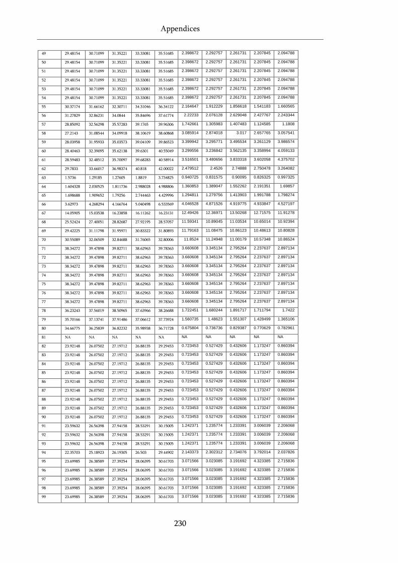
Appendices
230
49 29.48154 30.71099 31.35221 33.33081 35.51685 2.398672 2.292757 2.261731 2.207845 2.094788
50 29.48154 30.71099 31.35221 33.33081 35.51685 2.398672 2.292757 2.261731 2.207845 2.094788
51 29.48154 30.71099 31.35221 33.33081 35.51685 2.398672 2.292757 2.261731 2.207845 2.094788
52 29.48154 30.71099 31.35221 33.33081 35.51685 2.398672 2.292757 2.261731 2.207845 2.094788
53 29.48154 30.71099 31.35221 33.33081 35.51685 2.398672 2.292757 2.261731 2.207845 2.094788
54 29.48154 30.71099 31.35221 33.33081 35.51685 2.398672 2.292757 2.261731 2.207845 2.094788
55 30.37174 31.66162 32.30711 34.31046 36.34122 2.164647 1.912229 1.856618 1.541183 1.660565
56 31.27829 32.86231 34.0844 35.84696 37.61774 2.22233 2.076128 2.629048 2.427767 2.243344
57 28.85092 32.56298 35.57283 39.1765 39.96306 1.742661 1.305983 1.407483 1.124585 1.1808
58 27.2143 31.08544 34.09918 38.10619 38.60868 3.085914 2.874018 3.017 2.657765 3.057541
59 28.03958 31.95933 35.03573 39.04109 39.86523 3.399942 3.295771 3.495534 3.261129 3.986574
60 28.40463 32.39095 35.62138 39.6301 40.55049 3.299556 3.236842 3.562135 3.358994 4.059133
61 28.59483 32.48512 35.70097 39.68283 40.58914 3.516501 3.480656 3.833318 3.602058 4.375702
62 29.7833 33.66017 36.98374 40.818 42.00022 2.479512 2.4526 2.74888 2.750478 3.264082
63 1.5736 1.29185 1.27605 1.8819 3.734825 0.940725 0.831575 0.90095 0.826325 0.997325
64 1.604328 2.030525 1.811736 2.988028 4.988806 1.360853 1.389047 1.552262 2.191351 1.69857
65 1.698688 1.909652 1.79256 2.744463 4.429996 1.294811 1.279756 1.413903 1.991788 1.798274
66 3.62973 4.268294 4.166764 5.040498 6.533569 4.046528 4.871526 4.919775 4.933847 4.527197
67 14.05905 15.03538 16.23858 16.11262 16.23131 12.49426 12.36971 13.50268 12.71575 11.91278
68 25.52424 27.40051 28.82687 27.92195 28.57057 11.59341 10.89045 11.03534 10.65014 10.92394
69 29.42225 31.11798 31.95971 30.83322 31.80893 11.79163 11.08475 10.86123 10.48613 10.80828
70 30.55089 32.06509 32.84688 31.76065 32.80006 11.8524 11.24948 11.00179 10.57348 10.86524
71 38.34272 39.47898 39.82711 38.62963 39.78363 3.660608 3.345134 2.795264 2.237637 2.897134
72 38.34272 39.47898 39.82711 38.62963 39.78363 3.660608 3.345134 2.795264 2.237637 2.897134
73 38.34272 39.47898 39.82711 38.62963 39.78363 3.660608 3.345134 2.795264 2.237637 2.897134
74 38.34272 39.47898 39.82711 38.62963 39.78363 3.660608 3.345134 2.795264 2.237637 2.897134
75 38.34272 39.47898 39.82711 38.62963 39.78363 3.660608 3.345134 2.795264 2.237637 2.897134
76 38.34272 39.47898 39.82711 38.62963 39.78363 3.660608 3.345134 2.795264 2.237637 2.897134
77 38.34272 39.47898 39.82711 38.62963 39.78363 3.660608 3.345134 2.795264 2.237637 2.897134
78 36.23243 37.56019 38.50965 37.63966 38.26688 1.722451 1.680244 1.891717 1.711794 1.7422
79 35.70166 37.13741 37.91486 37.06612 37.73924 1.560735 1.48623 1.551307 1.428499 1.365106
80 34.66775 36.25839 36.82232 35.98938 36.71728 0.675804 0.736736 0.829387 0.770629 0.782961
81 NA NA NA NA NA NA NA NA NA NA
82 23.92148 26.07502 27.19712 26.88135 29.29453 0.723453 0.527429 0.432606 1.173247 0.860394
83 23.92148 26.07502 27.19712 26.88135 29.29453 0.723453 0.527429 0.432606 1.173247 0.860394
84 23.92148 26.07502 27.19712 26.88135 29.29453 0.723453 0.527429 0.432606 1.173247 0.860394
85 23.92148 26.07502 27.19712 26.88135 29.29453 0.723453 0.527429 0.432606 1.173247 0.860394
86 23.92148 26.07502 27.19712 26.88135 29.29453 0.723453 0.527429 0.432606 1.173247 0.860394
87 23.92148 26.07502 27.19712 26.88135 29.29453 0.723453 0.527429 0.432606 1.173247 0.860394
88 23.92148 26.07502 27.19712 26.88135 29.29453 0.723453 0.527429 0.432606 1.173247 0.860394
89 23.92148 26.07502 27.19712 26.88135 29.29453 0.723453 0.527429 0.432606 1.173247 0.860394
90 23.92148 26.07502 27.19712 26.88135 29.29453 0.723453 0.527429 0.432606 1.173247 0.860394
91 23.59632 26.56398 27.94158 28.53291 30.15005 1.242371 1.235774 1.233391 3.006039 2.206068
92 23.59632 26.56398 27.94158 28.53291 30.15005 1.242371 1.235774 1.233391 3.006039 2.206068
93 23.59632 26.56398 27.94158 28.53291 30.15005 1.242371 1.235774 1.233391 3.006039 2.206068
94 22.35703 25.18923 26.19305 26.503 29.44902 2.143373 2.302312 2.734076 3.792014 2.037826
95 23.69985 26.38589 27.39254 28.06395 30.61703 3.071566 3.023085 3.191692 4.323385 2.715836
96 23.69985 26.38589 27.39254 28.06395 30.61703 3.071566 3.023085 3.191692 4.323385 2.715836
97 23.69985 26.38589 27.39254 28.06395 30.61703 3.071566 3.023085 3.191692 4.323385 2.715836
98 23.69985 26.38589 27.39254 28.06395 30.61703 3.071566 3.023085 3.191692 4.323385 2.715836
99 23.69985 26.38589 27.39254 28.06395 30.61703 3.071566 3.023085 3.191692 4.323385 2.715836
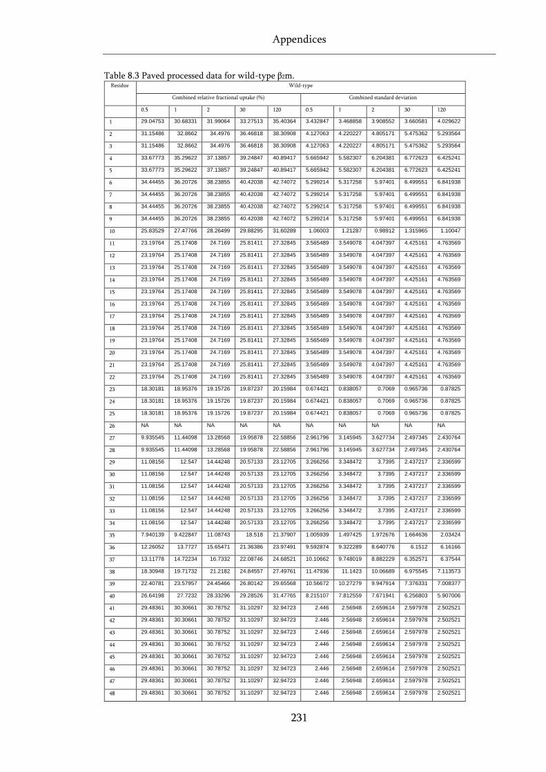
Appendices
231
Table 8.3 Paved processed data for wild-type β2m. Residue Wild-type
Combined relative fractional uptake (%) Combined standard deviation
0.5 1 2 30 120 0.5 1 2 30 120
1 29.04753 30.68331 31.99064 33.27513 35.40364 3.432847 3.468858 3.908552 3.660581 4.029622
2 31.15486 32.8662 34.4976 36.46818 38.30908 4.127063 4.220227 4.805171 5.475362 5.293564
3 31.15486 32.8662 34.4976 36.46818 38.30908 4.127063 4.220227 4.805171 5.475362 5.293564
4 33.67773 35.29622 37.13857 39.24847 40.89417 5.665942 5.582307 6.204381 6.772623 6.425241
5 33.67773 35.29622 37.13857 39.24847 40.89417 5.665942 5.582307 6.204381 6.772623 6.425241
6 34.44455 36.20726 38.23855 40.42038 42.74072 5.299214 5.317258 5.97401 6.499551 6.841938
7 34.44455 36.20726 38.23855 40.42038 42.74072 5.299214 5.317258 5.97401 6.499551 6.841938
8 34.44455 36.20726 38.23855 40.42038 42.74072 5.299214 5.317258 5.97401 6.499551 6.841938
9 34.44455 36.20726 38.23855 40.42038 42.74072 5.299214 5.317258 5.97401 6.499551 6.841938
10 25.83529 27.47766 28.26499 29.88295 31.60289 1.06003 1.21287 0.98912 1.315965 1.10047
11 23.19764 25.17408 24.7169 25.81411 27.32845 3.565489 3.549078 4.047397 4.425161 4.763569
12 23.19764 25.17408 24.7169 25.81411 27.32845 3.565489 3.549078 4.047397 4.425161 4.763569
13 23.19764 25.17408 24.7169 25.81411 27.32845 3.565489 3.549078 4.047397 4.425161 4.763569
14 23.19764 25.17408 24.7169 25.81411 27.32845 3.565489 3.549078 4.047397 4.425161 4.763569
15 23.19764 25.17408 24.7169 25.81411 27.32845 3.565489 3.549078 4.047397 4.425161 4.763569
16 23.19764 25.17408 24.7169 25.81411 27.32845 3.565489 3.549078 4.047397 4.425161 4.763569
17 23.19764 25.17408 24.7169 25.81411 27.32845 3.565489 3.549078 4.047397 4.425161 4.763569
18 23.19764 25.17408 24.7169 25.81411 27.32845 3.565489 3.549078 4.047397 4.425161 4.763569
19 23.19764 25.17408 24.7169 25.81411 27.32845 3.565489 3.549078 4.047397 4.425161 4.763569
20 23.19764 25.17408 24.7169 25.81411 27.32845 3.565489 3.549078 4.047397 4.425161 4.763569
21 23.19764 25.17408 24.7169 25.81411 27.32845 3.565489 3.549078 4.047397 4.425161 4.763569
22 23.19764 25.17408 24.7169 25.81411 27.32845 3.565489 3.549078 4.047397 4.425161 4.763569
23 18.30181 18.95376 19.15726 19.87237 20.15984 0.674421 0.838057 0.7069 0.965736 0.87825
24 18.30181 18.95376 19.15726 19.87237 20.15984 0.674421 0.838057 0.7069 0.965736 0.87825
25 18.30181 18.95376 19.15726 19.87237 20.15984 0.674421 0.838057 0.7069 0.965736 0.87825
26 NA NA NA NA NA NA NA NA NA NA
27 9.935545 11.44098 13.28568 19.95878 22.58856 2.961796 3.145945 3.627734 2.497345 2.430764
28 9.935545 11.44098 13.28568 19.95878 22.58856 2.961796 3.145945 3.627734 2.497345 2.430764
29 11.08156 12.547 14.44248 20.57133 23.12705 3.266256 3.348472 3.7395 2.437217 2.336599
30 11.08156 12.547 14.44248 20.57133 23.12705 3.266256 3.348472 3.7395 2.437217 2.336599
31 11.08156 12.547 14.44248 20.57133 23.12705 3.266256 3.348472 3.7395 2.437217 2.336599
32 11.08156 12.547 14.44248 20.57133 23.12705 3.266256 3.348472 3.7395 2.437217 2.336599
33 11.08156 12.547 14.44248 20.57133 23.12705 3.266256 3.348472 3.7395 2.437217 2.336599
34 11.08156 12.547 14.44248 20.57133 23.12705 3.266256 3.348472 3.7395 2.437217 2.336599
35 7.940139 9.422847 11.08743 18.518 21.37907 1.005939 1.497425 1.972676 1.664636 2.03424
36 12.26052 13.7727 15.65471 21.36386 23.97491 9.592874 9.322289 8.640776 6.1512 6.16166
37 13.11778 14.72234 16.7332 22.08746 24.68521 10.10662 9.748019 8.882229 6.352571 6.37544
38 18.30948 19.71732 21.2182 24.84557 27.49761 11.47936 11.1423 10.06689 6.975545 7.113573
39 22.40781 23.57957 24.45466 26.80142 29.65568 10.56672 10.27279 9.947914 7.376331 7.008377
40 26.64198 27.7232 28.33296 29.28526 31.47765 8.215107 7.812559 7.671941 6.256803 5.907006
41 29.48361 30.30661 30.78752 31.10297 32.94723 2.446 2.56948 2.659614 2.597978 2.502521
42 29.48361 30.30661 30.78752 31.10297 32.94723 2.446 2.56948 2.659614 2.597978 2.502521
43 29.48361 30.30661 30.78752 31.10297 32.94723 2.446 2.56948 2.659614 2.597978 2.502521
44 29.48361 30.30661 30.78752 31.10297 32.94723 2.446 2.56948 2.659614 2.597978 2.502521
45 29.48361 30.30661 30.78752 31.10297 32.94723 2.446 2.56948 2.659614 2.597978 2.502521
46 29.48361 30.30661 30.78752 31.10297 32.94723 2.446 2.56948 2.659614 2.597978 2.502521
47 29.48361 30.30661 30.78752 31.10297 32.94723 2.446 2.56948 2.659614 2.597978 2.502521
48 29.48361 30.30661 30.78752 31.10297 32.94723 2.446 2.56948 2.659614 2.597978 2.502521
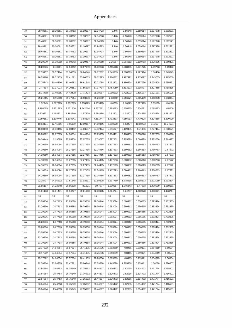
Appendices
232
49 29.48361 30.30661 30.78752 31.10297 32.94723 2.446 2.56948 2.659614 2.597978 2.502521
50 29.48361 30.30661 30.78752 31.10297 32.94723 2.446 2.56948 2.659614 2.597978 2.502521
51 29.48361 30.30661 30.78752 31.10297 32.94723 2.446 2.56948 2.659614 2.597978 2.502521
52 29.48361 30.30661 30.78752 31.10297 32.94723 2.446 2.56948 2.659614 2.597978 2.502521
53 29.48361 30.30661 30.78752 31.10297 32.94723 2.446 2.56948 2.659614 2.597978 2.502521
54 29.48361 30.30661 30.78752 31.10297 32.94723 2.446 2.56948 2.659614 2.597978 2.502521
55 30.29979 31.30002 31.90542 32.29417 34.09958 2.26057 2.204612 2.100783 1.876235 1.550401
56 30.69826 31.8991 32.94812 33.97649 35.00673 2.415168 2.068305 2.071775 2.39783 1.69422
57 27.39157 30.57464 33.34853 36.64646 36.97792 1.643933 1.208713 1.127414 1.06496 0.943649
58 26.03778 29.32153 32.41521 35.66005 36.12293 2.276212 2.187992 1.915227 2.245055 1.975759
59 27.25743 30.40836 33.40693 36.61248 37.02098 3.452302 3.180574 2.857056 3.004408 2.695451
60 27.7814 31.17023 34.20681 37.55298 37.97794 3.453059 3.513133 3.298437 3.627488 3.418315
61 28.14498 31.40385 34.42478 37.71424 38.10687 3.580952 3.723632 3.495597 3.871651 3.666626
62 29.21715 32.5533 35.47564 38.93943 39.23642 2.88652 2.916171 2.805109 2.968373 2.948054
63 1.52745 1.567925 1.252875 2.278775 4.155425 0.8209 0.76575 0.797425 0.65185 0.6128
64 1.468019 1.771283 1.371206 1.942064 4.277661 0.989693 0.918685 0.934211 1.029313 0.8206
65 1.329731 1.468221 1.192246 1.57329 3.594188 0.92801 1.03202 0.874895 1.108874 1.391622
66 2.989881 3.539745 3.538941 3.93108 4.851447 3.432893 4.255033 4.770128 4.824268 3.500029
67 10.53131 12.45816 13.5119 13.99167 14.89156 8.308508 9.63424 10.68423 11.2034 11.24521
68 18.08193 20.80416 22.80452 24.03657 24.82424 5.996327 6.109455 6.71196 8.227444 8.208621
69 19.90212 22.67675 24.74014 26.44784 27.25955 6.216411 6.468965 6.808228 8.217053 8.066016
70 20.30149 22.9695 25.05308 27.07055 27.9067 6.387902 6.725779 7.066399 8.363758 8.219997
71 24.10859 26.94094 29.27255 32.27455 32.74465 3.137593 3.580982 3.266313 2.760763 2.67572
72 24.10859 26.94094 29.27255 32.27455 32.74465 3.137593 3.580982 3.266313 2.760763 2.67572
73 24.10859 26.94094 29.27255 32.27455 32.74465 3.137593 3.580982 3.266313 2.760763 2.67572
74 24.10859 26.94094 29.27255 32.27455 32.74465 3.137593 3.580982 3.266313 2.760763 2.67572
75 24.10859 26.94094 29.27255 32.27455 32.74465 3.137593 3.580982 3.266313 2.760763 2.67572
76 24.10859 26.94094 29.27255 32.27455 32.74465 3.137593 3.580982 3.266313 2.760763 2.67572
77 24.10859 26.94094 29.27255 32.27455 32.74465 3.137593 3.580982 3.266313 2.760763 2.67572
78 22.38437 24.96802 27.61548 31.03611 31.50328 1.517789 1.878255 1.998373 1.922089 1.903374
79 21.86107 24.22848 26.85838 30.321 30.7677 1.239557 1.346343 1.47993 1.409099 1.380661
80 21.51133 23.81471 25.94777 29.61698 30.00105 1.264724 1.24287 1.300378 1.308621 1.173714
81 NA NA NA NA NA NA NA NA NA NA
82 23.20236 24.7713 25.95588 26.79858 29.36944 0.683024 0.560912 0.656565 0.393424 0.732335
83 23.20236 24.7713 25.95588 26.79858 29.36944 0.683024 0.560912 0.656565 0.393424 0.732335
84 23.20236 24.7713 25.95588 26.79858 29.36944 0.683024 0.560912 0.656565 0.393424 0.732335
85 23.20236 24.7713 25.95588 26.79858 29.36944 0.683024 0.560912 0.656565 0.393424 0.732335
86 23.20236 24.7713 25.95588 26.79858 29.36944 0.683024 0.560912 0.656565 0.393424 0.732335
87 23.20236 24.7713 25.95588 26.79858 29.36944 0.683024 0.560912 0.656565 0.393424 0.732335
88 23.20236 24.7713 25.95588 26.79858 29.36944 0.683024 0.560912 0.656565 0.393424 0.732335
89 23.20236 24.7713 25.95588 26.79858 29.36944 0.683024 0.560912 0.656565 0.393424 0.732335
90 23.20236 24.7713 25.95588 26.79858 29.36944 0.683024 0.560912 0.656565 0.393424 0.732335
91 23.17622 24.64854 25.57604 26.41135 28.26236 0.813889 0.8415 0.919121 0.854319 1.50584
92 23.17622 24.64854 25.57604 26.41135 28.26236 0.813889 0.8415 0.919121 0.854319 1.50584
93 23.17622 24.64854 25.57604 26.41135 28.26236 0.813889 0.8415 0.919121 0.854319 1.50584
94 22.70234 23.94255 25.47821 25.96844 27.39238 1.145788 1.205368 0.979461 1.06038 1.870607
95 23.84984 25.4753 26.75249 27.35992 28.44307 2.326472 2.82055 2.314402 2.471774 2.415501
96 23.84984 25.4753 26.75249 27.35992 28.44307 2.326472 2.82055 2.314402 2.471774 2.415501
97 23.84984 25.4753 26.75249 27.35992 28.44307 2.326472 2.82055 2.314402 2.471774 2.415501
98 23.84984 25.4753 26.75249 27.35992 28.44307 2.326472 2.82055 2.314402 2.471774 2.415501
99 23.84984 25.4753 26.75249 27.35992 28.44307 2.326472 2.82055 2.314402 2.471774 2.415501
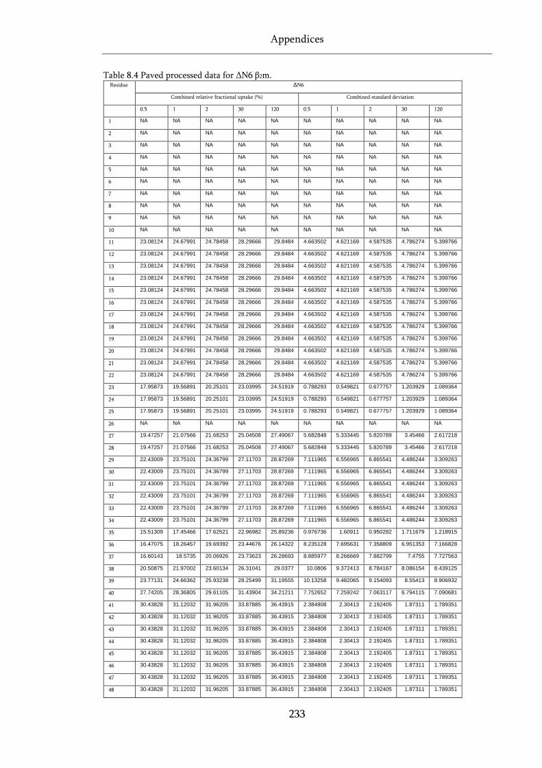
Appendices
233
Table 8.4 Paved processed data for ΔN6 β2m. Residue ΔN6
Combined relative fractional uptake (%) Combined standard deviation
0.5 1 2 30 120 0.5 1 2 30 120
1 NA NA NA NA NA NA NA NA NA NA
2 NA NA NA NA NA NA NA NA NA NA
3 NA NA NA NA NA NA NA NA NA NA
4 NA NA NA NA NA NA NA NA NA NA
5 NA NA NA NA NA NA NA NA NA NA
6 NA NA NA NA NA NA NA NA NA NA
7 NA NA NA NA NA NA NA NA NA NA
8 NA NA NA NA NA NA NA NA NA NA
9 NA NA NA NA NA NA NA NA NA NA
10 NA NA NA NA NA NA NA NA NA NA
11 23.08124 24.67991 24.78458 28.29666 29.8484 4.663502 4.621169 4.587535 4.786274 5.399766
12 23.08124 24.67991 24.78458 28.29666 29.8484 4.663502 4.621169 4.587535 4.786274 5.399766
13 23.08124 24.67991 24.78458 28.29666 29.8484 4.663502 4.621169 4.587535 4.786274 5.399766
14 23.08124 24.67991 24.78458 28.29666 29.8484 4.663502 4.621169 4.587535 4.786274 5.399766
15 23.08124 24.67991 24.78458 28.29666 29.8484 4.663502 4.621169 4.587535 4.786274 5.399766
16 23.08124 24.67991 24.78458 28.29666 29.8484 4.663502 4.621169 4.587535 4.786274 5.399766
17 23.08124 24.67991 24.78458 28.29666 29.8484 4.663502 4.621169 4.587535 4.786274 5.399766
18 23.08124 24.67991 24.78458 28.29666 29.8484 4.663502 4.621169 4.587535 4.786274 5.399766
19 23.08124 24.67991 24.78458 28.29666 29.8484 4.663502 4.621169 4.587535 4.786274 5.399766
20 23.08124 24.67991 24.78458 28.29666 29.8484 4.663502 4.621169 4.587535 4.786274 5.399766
21 23.08124 24.67991 24.78458 28.29666 29.8484 4.663502 4.621169 4.587535 4.786274 5.399766
22 23.08124 24.67991 24.78458 28.29666 29.8484 4.663502 4.621169 4.587535 4.786274 5.399766
23 17.95873 19.56891 20.25101 23.03995 24.51919 0.788293 0.549821 0.677757 1.203929 1.089364
24 17.95873 19.56891 20.25101 23.03995 24.51919 0.788293 0.549821 0.677757 1.203929 1.089364
25 17.95873 19.56891 20.25101 23.03995 24.51919 0.788293 0.549821 0.677757 1.203929 1.089364
26 NA NA NA NA NA NA NA NA NA NA
27 19.47257 21.07566 21.68253 25.04508 27.49067 5.682848 5.333445 5.820789 3.45466 2.617218
28 19.47257 21.07566 21.68253 25.04508 27.49067 5.682848 5.333445 5.820789 3.45466 2.617218
29 22.43009 23.75101 24.36799 27.11703 28.87269 7.111965 6.556965 6.865541 4.486244 3.309263
30 22.43009 23.75101 24.36799 27.11703 28.87269 7.111965 6.556965 6.865541 4.486244 3.309263
31 22.43009 23.75101 24.36799 27.11703 28.87269 7.111965 6.556965 6.865541 4.486244 3.309263
32 22.43009 23.75101 24.36799 27.11703 28.87269 7.111965 6.556965 6.865541 4.486244 3.309263
33 22.43009 23.75101 24.36799 27.11703 28.87269 7.111965 6.556965 6.865541 4.486244 3.309263
34 22.43009 23.75101 24.36799 27.11703 28.87269 7.111965 6.556965 6.865541 4.486244 3.309263
35 15.51309 17.45466 17.62521 22.96982 25.89236 0.976736 1.60911 0.950282 1.711679 1.218915
36 16.47075 18.26457 19.69392 23.44676 26.14322 8.235128 7.695631 7.358809 6.951353 7.166828
37 16.60143 18.5735 20.06926 23.73623 26.28693 8.885977 8.266669 7.882799 7.4755 7.727563
38 20.50875 21.97002 23.60134 26.31041 29.0377 10.0806 9.372413 8.784167 8.086154 8.439125
39 23.77131 24.66362 25.93238 28.25499 31.19555 10.13258 9.482065 9.154093 8.55413 8.906932
40 27.74205 28.36805 29.61105 31.43904 34.21211 7.752652 7.259242 7.063117 6.794115 7.090681
41 30.43828 31.12032 31.96205 33.87885 36.43915 2.384808 2.30413 2.192405 1.87311 1.789351
42 30.43828 31.12032 31.96205 33.87885 36.43915 2.384808 2.30413 2.192405 1.87311 1.789351
43 30.43828 31.12032 31.96205 33.87885 36.43915 2.384808 2.30413 2.192405 1.87311 1.789351
44 30.43828 31.12032 31.96205 33.87885 36.43915 2.384808 2.30413 2.192405 1.87311 1.789351
45 30.43828 31.12032 31.96205 33.87885 36.43915 2.384808 2.30413 2.192405 1.87311 1.789351
46 30.43828 31.12032 31.96205 33.87885 36.43915 2.384808 2.30413 2.192405 1.87311 1.789351
47 30.43828 31.12032 31.96205 33.87885 36.43915 2.384808 2.30413 2.192405 1.87311 1.789351
48 30.43828 31.12032 31.96205 33.87885 36.43915 2.384808 2.30413 2.192405 1.87311 1.789351
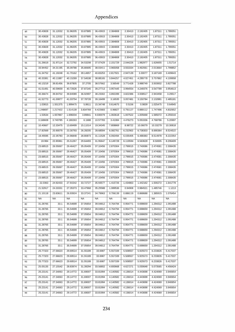
Appendices
234
49 30.43828 31.12032 31.96205 33.87885 36.43915 2.384808 2.30413 2.192405 1.87311 1.789351
50 30.43828 31.12032 31.96205 33.87885 36.43915 2.384808 2.30413 2.192405 1.87311 1.789351
51 30.43828 31.12032 31.96205 33.87885 36.43915 2.384808 2.30413 2.192405 1.87311 1.789351
52 30.43828 31.12032 31.96205 33.87885 36.43915 2.384808 2.30413 2.192405 1.87311 1.789351
53 30.43828 31.12032 31.96205 33.87885 36.43915 2.384808 2.30413 2.192405 1.87311 1.789351
54 30.43828 31.12032 31.96205 33.87885 36.43915 2.384808 2.30413 2.192405 1.87311 1.789351
55 31.26619 31.97114 32.72792 34.53208 37.07429 2.151729 2.044226 1.982977 1.626655 1.51714
56 33.94452 34.31195 35.09788 35.80695 38.03411 3.965058 3.553334 3.462061 2.013664 1.799852
57 41.34752 41.19248 41.70162 39.14657 40.83253 2.817921 2.947139 3.30077 3.187169 3.409643
58 40.33381 40.11887 40.15269 37.54538 38.88165 3.844257 4.027451 4.289778 3.757862 4.109958
59 40.13219 39.81456 39.87805 37.2705 38.57662 3.56549 3.771428 3.988749 3.503932 3.827788
60 41.01491 40.59659 40.72626 37.87245 39.27713 3.957445 3.994554 4.249376 3.547789 3.954613
61 40.36674 39.84702 39.84089 36.92997 38.23302 3.892289 3.822386 3.938517 2.943458 3.29517
62 41.52773 41.00877 41.03754 37.78728 39.16499 3.16535 3.057481 3.150784 2.132881 2.485181
63 1.03815 1.551375 1.999475 5.8611 15.34748 0.614675 0.5156 0.9839 1.025475 0.64945
64 1.248697 1.217422 1.514139 3.834769 9.422683 0.96827 0.791127 0.889112 1.747486 4.832652
65 1.53534 1.557867 1.698204 3.89841 9.030079 1.063618 1.007522 1.005668 1.585072 4.255016
66 3.168608 3.740785 4.180263 6.1688 10.57783 3.41084 4.476273 5.053336 4.768786 5.20997
67 10.40667 12.33475 13.69499 15.11014 19.34345 7.808869 8.98722 10.06079 10.33279 10.30818
68 17.82569 20.90079 23.30793 26.28205 28.68594 6.082761 6.232902 6.738303 8.690364 8.524522
69 19.45595 22.35783 24.96848 28.80873 31.11528 6.092494 6.035405 6.488383 8.514978 8.222354
70 19.984 22.85961 25.51267 29.64493 31.95647 6.149728 6.119594 6.563628 8.50005 8.206409
71 23.68515 26.55067 29.46427 35.05409 37.10456 2.870304 2.799015 2.740086 2.474581 2.308435
72 23.68515 26.55067 29.46427 35.05409 37.10456 2.870304 2.799015 2.740086 2.474581 2.308435
73 23.68515 26.55067 29.46427 35.05409 37.10456 2.870304 2.799015 2.740086 2.474581 2.308435
74 23.68515 26.55067 29.46427 35.05409 37.10456 2.870304 2.799015 2.740086 2.474581 2.308435
75 23.68515 26.55067 29.46427 35.05409 37.10456 2.870304 2.799015 2.740086 2.474581 2.308435
76 23.68515 26.55067 29.46427 35.05409 37.10456 2.870304 2.799015 2.740086 2.474581 2.308435
77 23.68515 26.55067 29.46427 35.05409 37.10456 2.870304 2.799015 2.740086 2.474581 2.308435
78 22.0363 24.92433 27.91542 33.72727 35.93577 1.415726 1.434863 1.442162 1.500272 1.641778
79 21.52917 24.33331 27.35373 33.47968 35.25588 1.089536 0.94908 0.984521 1.485746 1.1213
80 21.10118 23.83611 26.93924 33.37241 34.79963 0.706139 0.886119 0.868688 1.385915 1.076454
81 NA NA NA NA NA NA NA NA NA NA
82 31.28765 33.1 35.54699 37.05654 39.04812 0.764794 0.954771 0.698659 1.294312 1.091488
83 31.28765 33.1 35.54699 37.05654 39.04812 0.764794 0.954771 0.698659 1.294312 1.091488
84 31.28765 33.1 35.54699 37.05654 39.04812 0.764794 0.954771 0.698659 1.294312 1.091488
85 31.28765 33.1 35.54699 37.05654 39.04812 0.764794 0.954771 0.698659 1.294312 1.091488
86 31.28765 33.1 35.54699 37.05654 39.04812 0.764794 0.954771 0.698659 1.294312 1.091488
87 31.28765 33.1 35.54699 37.05654 39.04812 0.764794 0.954771 0.698659 1.294312 1.091488
88 31.28765 33.1 35.54699 37.05654 39.04812 0.764794 0.954771 0.698659 1.294312 1.091488
89 31.28765 33.1 35.54699 37.05654 39.04812 0.764794 0.954771 0.698659 1.294312 1.091488
90 31.28765 33.1 35.54699 37.05654 39.04812 0.764794 0.954771 0.698659 1.294312 1.091488
91 25.77323 27.66623 29.69514 31.55189 33.6987 5.557339 5.508557 5.925573 6.233826 5.417037
92 25.77323 27.66623 29.69514 31.55189 33.6987 5.557339 5.508557 5.925573 6.233826 5.417037
93 25.77323 27.66623 29.69514 31.55189 33.6987 5.557339 5.508557 5.925573 6.233826 5.417037
94 25.05135 27.15542 28.83974 31.39294 33.56802 4.693668 4.627271 5.030648 5.073565 4.456424
95 25.23141 27.34063 29.14772 31.69007 33.81994 4.140582 4.136014 4.443698 4.424069 3.940654
96 25.23141 27.34063 29.14772 31.69007 33.81994 4.140582 4.136014 4.443698 4.424069 3.940654
97 25.23141 27.34063 29.14772 31.69007 33.81994 4.140582 4.136014 4.443698 4.424069 3.940654
98 25.23141 27.34063 29.14772 31.69007 33.81994 4.140582 4.136014 4.443698 4.424069 3.940654
99 25.23141 27.34063 29.14772 31.69007 33.81994 4.140582 4.136014 4.443698 4.424069 3.940654
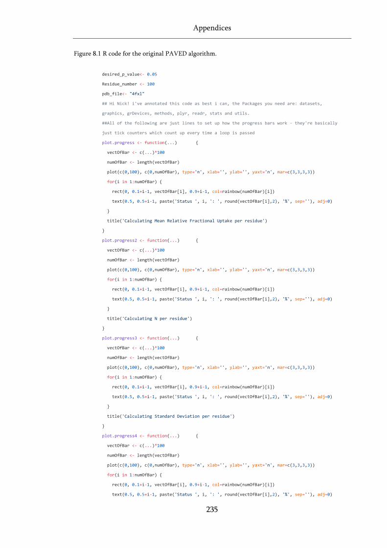
Appendices
235
Figure 8.1 R code for the original PAVED algorithm.
desired_p_value<- 0.05
Residue_number <- 100
pdb_file<- "4fxl"
## Hi Nick! i've annotated this code as best i can, the Packages you need are: datasets,
graphics, grDevices, methods, plyr, readr, stats and utils.
##All of the following are just lines to set up how the progress bars work - they're basically
just tick counters which count up every time a loop is passed
plot.progress <- function(...)
vectOfBar <- c(...)*100
numOfBar <- length(vectOfBar)
plot(c(0,100), c(0,numOfBar), type='n', xlab='', ylab='', yaxt='n', mar=c(3,3,3,3))
for(i in 1:numOfBar)
rect(0, 0.1+i-1, vectOfBar[i], 0.9+i-1, col=rainbow(numOfBar)[i])
text(0.5, 0.5+i-1, paste('Status ', i, ': ', round(vectOfBar[i],2), '%', sep=''), adj=0)
title('Calculating Mean Relative Fractional Uptake per residue')
plot.progress2 <- function(...)
vectOfBar <- c(...)*100
numOfBar <- length(vectOfBar)
plot(c(0,100), c(0,numOfBar), type='n', xlab='', ylab='', yaxt='n', mar=c(3,3,3,3))
for(i in 1:numOfBar)
rect(0, 0.1+i-1, vectOfBar[i], 0.9+i-1, col=rainbow(numOfBar)[i])
text(0.5, 0.5+i-1, paste('Status ', i, ': ', round(vectOfBar[i],2), '%', sep=''), adj=0)
title('Calculating N per residue')
plot.progress3 <- function(...)
vectOfBar <- c(...)*100
numOfBar <- length(vectOfBar)
plot(c(0,100), c(0,numOfBar), type='n', xlab='', ylab='', yaxt='n', mar=c(3,3,3,3))
for(i in 1:numOfBar)
rect(0, 0.1+i-1, vectOfBar[i], 0.9+i-1, col=rainbow(numOfBar)[i])
text(0.5, 0.5+i-1, paste('Status ', i, ': ', round(vectOfBar[i],2), '%', sep=''), adj=0)
title('Calculating Standard Deviation per residue')
plot.progress4 <- function(...)
vectOfBar <- c(...)*100
numOfBar <- length(vectOfBar)
plot(c(0,100), c(0,numOfBar), type='n', xlab='', ylab='', yaxt='n', mar=c(3,3,3,3))
for(i in 1:numOfBar)
rect(0, 0.1+i-1, vectOfBar[i], 0.9+i-1, col=rainbow(numOfBar)[i])
text(0.5, 0.5+i-1, paste('Status ', i, ': ', round(vectOfBar[i],2), '%', sep=''), adj=0)
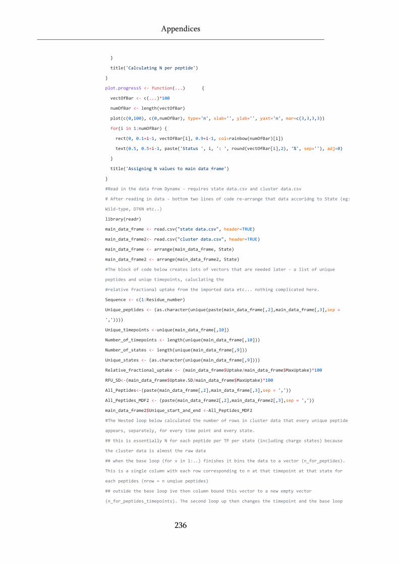
Appendices
236
title('Calculating N per peptide')
plot.progress5 <- function(...)
vectOfBar <- c(...)*100
numOfBar <- length(vectOfBar)
plot(c(0,100), c(0,numOfBar), type='n', xlab='', ylab='', yaxt='n', mar=c(3,3,3,3))
for(i in 1:numOfBar)
rect(0, 0.1+i-1, vectOfBar[i], 0.9+i-1, col=rainbow(numOfBar)[i])
text(0.5, 0.5+i-1, paste('Status ', i, ': ', round(vectOfBar[i],2), '%', sep=''), adj=0)
title('Assigning N values to main data frame')
#Read in the data from Dynamx - requires state data.csv and cluster data.csv
# After reading in data - bottom two lines of code re-arrange that data accoridng to State (eg:
Wild-type, D76N etc..)
library(readr)
main_data_frame <- read.csv("state data.csv", header=TRUE)
main_data_frame2<- read.csv("cluster data.csv", header=TRUE)
main_data_frame <- arrange(main_data_frame, State)
main_data_frame2 <- arrange(main_data_frame2, State)
#The block of code below creates lots of vectors that are needed later - a list of unique
peptides and uniqe timepoints, caluclating the
#relative fractional uptake from the imported data etc... nothing complicated here.
Sequence <- c(1:Residue_number)
Unique_peptides <- (as.character(unique(paste(main_data_frame[,2],main_data_frame[,3],sep =
','))))
Unique_timepoints <-unique(main_data_frame[,10])
Number_of_timepoints <- length(unique(main_data_frame[,10]))
Number_of_states <- length(unique(main_data_frame[,9]))
Unique_states <- (as.character(unique(main_data_frame[,9])))
Relative_fractional_uptake <- (main_data_frame$Uptake/main_data_frame$MaxUptake)*100
RFU_SD<-(main_data_frame$Uptake.SD/main_data_frame$MaxUptake)*100
All_Peptides<-(paste(main_data_frame[,2],main_data_frame[,3],sep = ','))
All_Peptides_MDF2 <- (paste(main_data_frame2[,2],main_data_frame2[,3],sep = ','))
main_data_frame2$Unique_start_and_end <-All_Peptides_MDF2
#The Nested loop below calculated the number of rows in cluster data that every unique peptide
appears, separately, for every time point and every state.
## this is essentially N for each peptide per TP per state (including charge states) because
the cluster data is almost the raw data
## when the base loop (for v in 1:..) finishes it bins the data to a vector (n_for_peptides).
This is a single column with each row corresponding to n at that timepoint at that state for
each peptides (nrow = n unqiue peptides)
## outside the base loop ive then column bound this vector to a new empty vector
(n_for_peptides_timepoints). The second loop up then changes the timepoint and the base loop
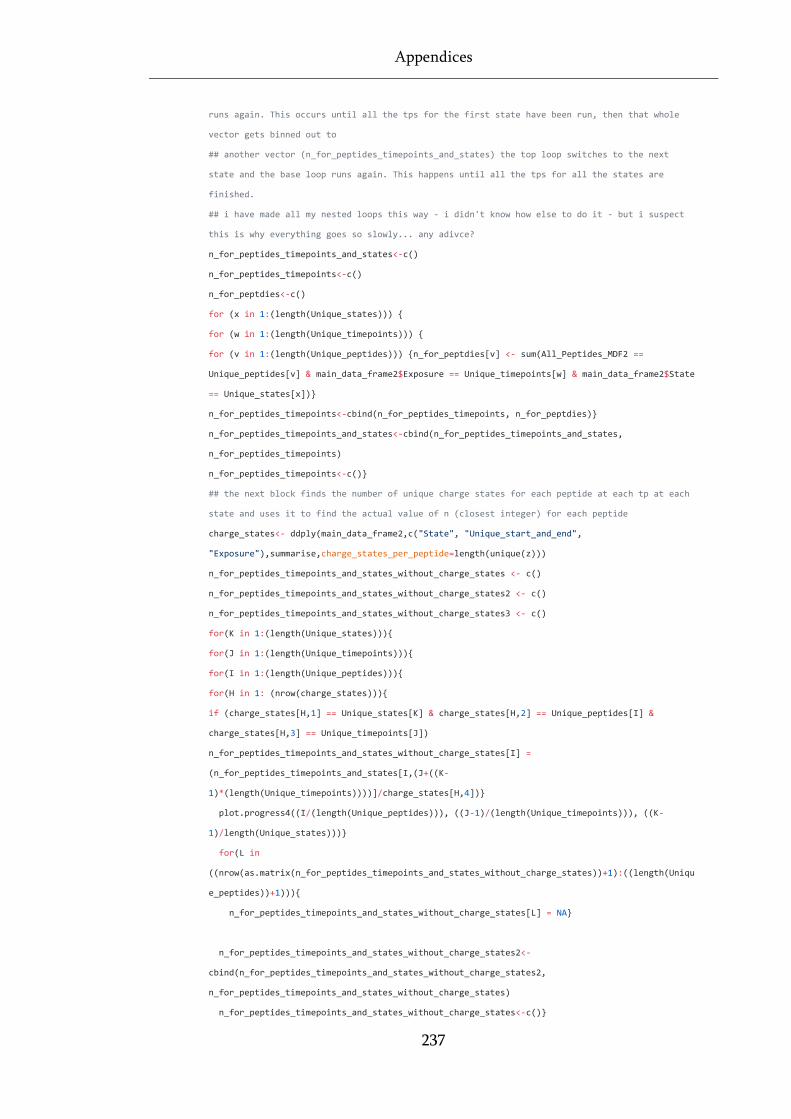
Appendices
237
runs again. This occurs until all the tps for the first state have been run, then that whole
vector gets binned out to
## another vector (n_for_peptides_timepoints_and_states) the top loop switches to the next
state and the base loop runs again. This happens until all the tps for all the states are
finished.
## i have made all my nested loops this way - i didn't know how else to do it - but i suspect
this is why everything goes so slowly... any adivce?
n_for_peptides_timepoints_and_states<-c()
n_for_peptides_timepoints<-c()
n_for_peptdies<-c()
for (x in 1:(length(Unique_states)))
for (w in 1:(length(Unique_timepoints)))
for (v in 1:(length(Unique_peptides))) n_for_peptdies[v] <- sum(All_Peptides_MDF2 ==
Unique_peptides[v] & main_data_frame2$Exposure == Unique_timepoints[w] & main_data_frame2$State
== Unique_states[x])
n_for_peptides_timepoints<-cbind(n_for_peptides_timepoints, n_for_peptdies)
n_for_peptides_timepoints_and_states<-cbind(n_for_peptides_timepoints_and_states,
n_for_peptides_timepoints)
n_for_peptides_timepoints<-c()
## the next block finds the number of unique charge states for each peptide at each tp at each
state and uses it to find the actual value of n (closest integer) for each peptide
charge_states<- ddply(main_data_frame2,c("State", "Unique_start_and_end",
"Exposure"),summarise,charge_states_per_peptide=length(unique(z)))
n_for_peptides_timepoints_and_states_without_charge_states <- c()
n_for_peptides_timepoints_and_states_without_charge_states2 <- c()
n_for_peptides_timepoints_and_states_without_charge_states3 <- c()
for(K in 1:(length(Unique_states)))
for(J in 1:(length(Unique_timepoints)))
for(I in 1:(length(Unique_peptides)))
for(H in 1: (nrow(charge_states)))
if (charge_states[H,1] == Unique_states[K] & charge_states[H,2] == Unique_peptides[I] &
charge_states[H,3] == Unique_timepoints[J])
n_for_peptides_timepoints_and_states_without_charge_states[I] =
(n_for_peptides_timepoints_and_states[I,(J+((K-
1)*(length(Unique_timepoints))))]/charge_states[H,4])
plot.progress4((I/(length(Unique_peptides))), ((J-1)/(length(Unique_timepoints))), ((K-
1)/length(Unique_states)))
for(L in
((nrow(as.matrix(n_for_peptides_timepoints_and_states_without_charge_states))+1):((length(Uniqu
e_peptides))+1)))
n_for_peptides_timepoints_and_states_without_charge_states[L] = NA
n_for_peptides_timepoints_and_states_without_charge_states2<-
cbind(n_for_peptides_timepoints_and_states_without_charge_states2,
n_for_peptides_timepoints_and_states_without_charge_states)
n_for_peptides_timepoints_and_states_without_charge_states<-c()
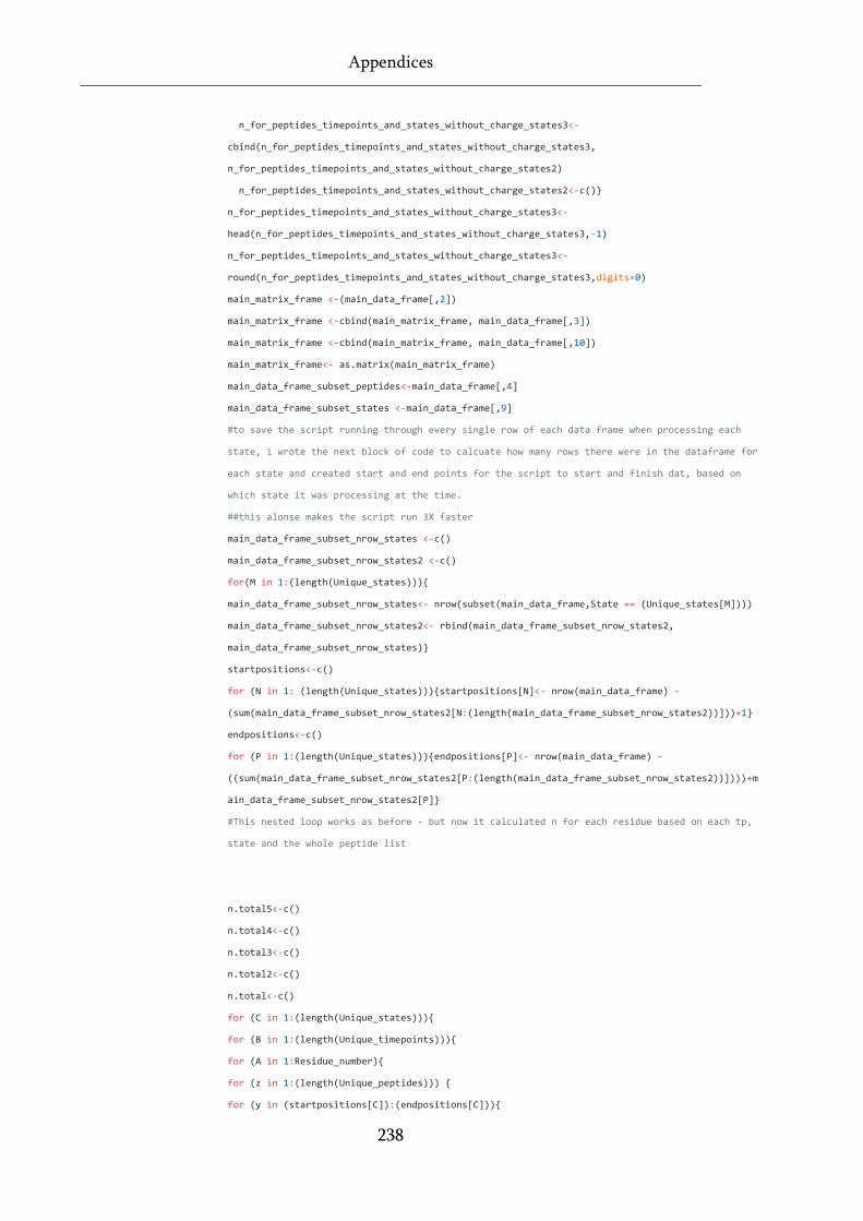
Appendices
238
n_for_peptides_timepoints_and_states_without_charge_states3<-
cbind(n_for_peptides_timepoints_and_states_without_charge_states3,
n_for_peptides_timepoints_and_states_without_charge_states2)
n_for_peptides_timepoints_and_states_without_charge_states2<-c()
n_for_peptides_timepoints_and_states_without_charge_states3<-
head(n_for_peptides_timepoints_and_states_without_charge_states3,-1)
n_for_peptides_timepoints_and_states_without_charge_states3<-
round(n_for_peptides_timepoints_and_states_without_charge_states3,digits=0)
main_matrix_frame <-(main_data_frame[,2])
main_matrix_frame <-cbind(main_matrix_frame, main_data_frame[,3])
main_matrix_frame <-cbind(main_matrix_frame, main_data_frame[,10])
main_matrix_frame<- as.matrix(main_matrix_frame)
main_data_frame_subset_peptides<-main_data_frame[,4]
main_data_frame_subset_states <-main_data_frame[,9]
#to save the script running through every single row of each data frame when processing each
state, i wrote the next block of code to calcuate how many rows there were in the dataframe for
each state and created start and end points for the script to start and finish dat, based on
which state it was processing at the time.
##this alonse makes the script run 3X faster
main_data_frame_subset_nrow_states <-c()
main_data_frame_subset_nrow_states2 <-c()
for(M in 1:(length(Unique_states)))
main_data_frame_subset_nrow_states<- nrow(subset(main_data_frame,State == (Unique_states[M])))
main_data_frame_subset_nrow_states2<- rbind(main_data_frame_subset_nrow_states2,
main_data_frame_subset_nrow_states)
startpositions<-c()
for (N in 1: (length(Unique_states)))startpositions[N]<- nrow(main_data_frame) -
(sum(main_data_frame_subset_nrow_states2[N:(length(main_data_frame_subset_nrow_states2))]))+1
endpositions<-c()
for (P in 1:(length(Unique_states)))endpositions[P]<- nrow(main_data_frame) -
((sum(main_data_frame_subset_nrow_states2[P:(length(main_data_frame_subset_nrow_states2))])))+m
ain_data_frame_subset_nrow_states2[P]
#This nested loop works as before - but now it calculated n for each residue based on each tp,
state and the whole peptide list
n.total5<-c()
n.total4<-c()
n.total3<-c()
n.total2<-c()
n.total<-c()
for (C in 1:(length(Unique_states)))
for (B in 1:(length(Unique_timepoints)))
for (A in 1:Residue_number)
for (z in 1:(length(Unique_peptides)))
for (y in (startpositions[C]):(endpositions[C]))
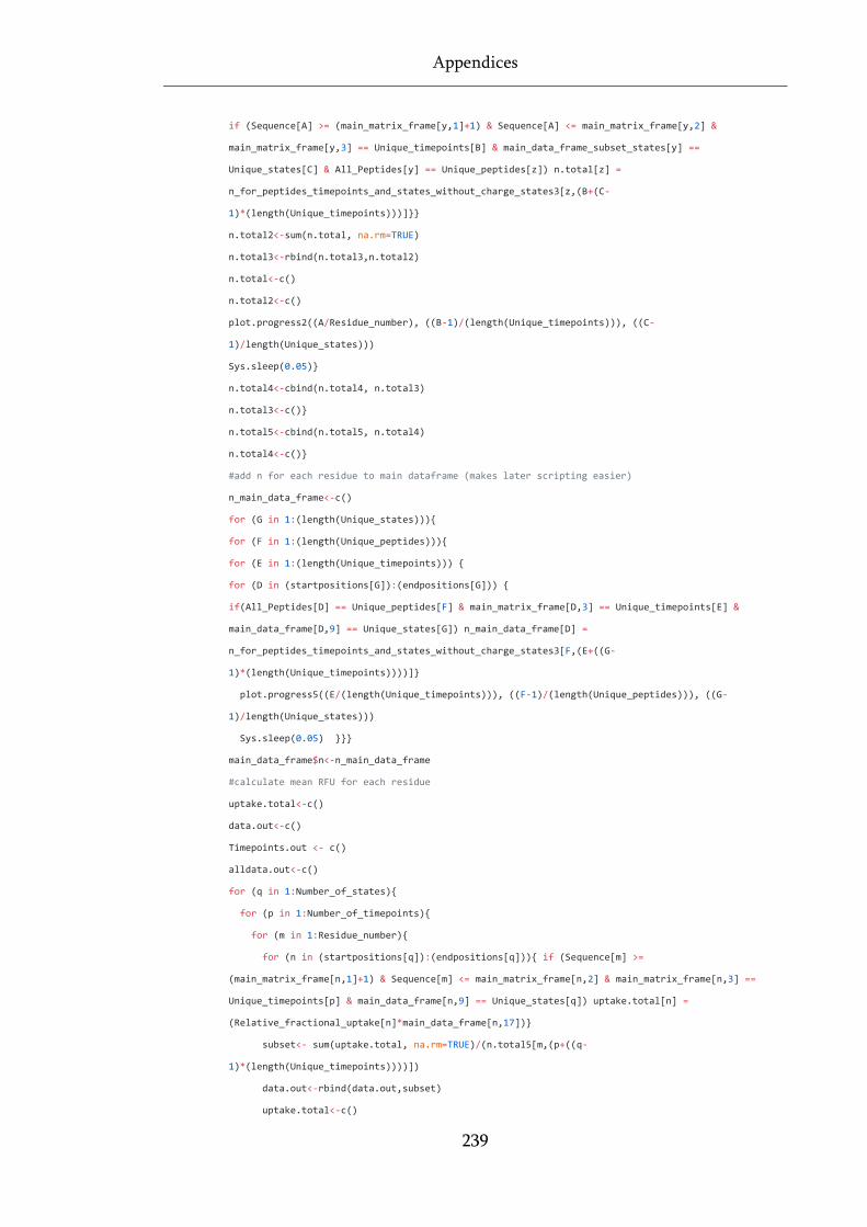
Appendices
239
if (Sequence[A] >= (main_matrix_frame[y,1]+1) & Sequence[A] <= main_matrix_frame[y,2] &
main_matrix_frame[y,3] == Unique_timepoints[B] & main_data_frame_subset_states[y] ==
Unique_states[C] & All_Peptides[y] == Unique_peptides[z]) n.total[z] =
n_for_peptides_timepoints_and_states_without_charge_states3[z,(B+(C-
1)*(length(Unique_timepoints)))]
n.total2<-sum(n.total, na.rm=TRUE)
n.total3<-rbind(n.total3,n.total2)
n.total<-c()
n.total2<-c()
plot.progress2((A/Residue_number), ((B-1)/(length(Unique_timepoints))), ((C-
1)/length(Unique_states)))
Sys.sleep(0.05)
n.total4<-cbind(n.total4, n.total3)
n.total3<-c()
n.total5<-cbind(n.total5, n.total4)
n.total4<-c()
#add n for each residue to main dataframe (makes later scripting easier)
n_main_data_frame<-c()
for (G in 1:(length(Unique_states)))
for (F in 1:(length(Unique_peptides)))
for (E in 1:(length(Unique_timepoints)))
for (D in (startpositions[G]):(endpositions[G]))
if(All_Peptides[D] == Unique_peptides[F] & main_matrix_frame[D,3] == Unique_timepoints[E] &
main_data_frame[D,9] == Unique_states[G]) n_main_data_frame[D] =
n_for_peptides_timepoints_and_states_without_charge_states3[F,(E+((G-
1)*(length(Unique_timepoints))))]
plot.progress5((E/(length(Unique_timepoints))), ((F-1)/(length(Unique_peptides))), ((G-
1)/length(Unique_states)))
Sys.sleep(0.05)
main_data_frame$n<-n_main_data_frame
#calculate mean RFU for each residue
uptake.total<-c()
data.out<-c()
Timepoints.out <- c()
alldata.out<-c()
for (q in 1:Number_of_states)
for (p in 1:Number_of_timepoints)
for (m in 1:Residue_number)
for (n in (startpositions[q]):(endpositions[q])) if (Sequence[m] >=
(main_matrix_frame[n,1]+1) & Sequence[m] <= main_matrix_frame[n,2] & main_matrix_frame[n,3] ==
Unique_timepoints[p] & main_data_frame[n,9] == Unique_states[q]) uptake.total[n] =
(Relative_fractional_uptake[n]*main_data_frame[n,17])
subset<- sum(uptake.total, na.rm=TRUE)/(n.total5[m,(p+((q-
1)*(length(Unique_timepoints))))])
data.out<-rbind(data.out,subset)
uptake.total<-c()
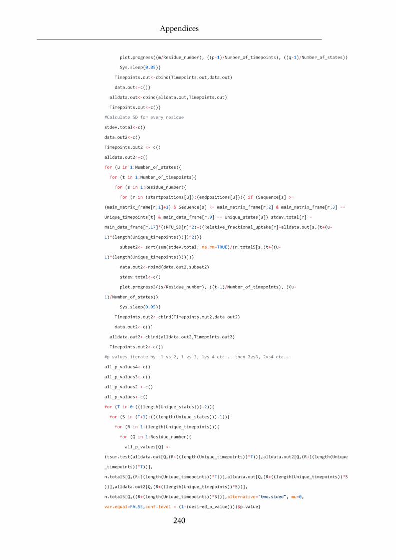
Appendices
240
plot.progress((m/Residue_number), ((p-1)/Number_of_timepoints), ((q-1)/Number_of_states))
Sys.sleep(0.05)
Timepoints.out<-cbind(Timepoints.out,data.out)
data.out<-c()
alldata.out<-cbind(alldata.out,Timepoints.out)
Timepoints.out<-c()
#Calculate SD for every residue
stdev.total<-c()
data.out2<-c()
Timepoints.out2 <- c()
alldata.out2<-c()
for (u in 1:Number_of_states)
for (t in 1:Number_of_timepoints)
for (s in 1:Residue_number)
for (r in (startpositions[u]):(endpositions[u])) if (Sequence[s] >=
(main_matrix_frame[r,1]+1) & Sequence[s] <= main_matrix_frame[r,2] & main_matrix_frame[r,3] ==
Unique_timepoints[t] & main_data_frame[r,9] == Unique_states[u]) stdev.total[r] =
main_data_frame[r,17]*((RFU_SD[r]^2)+((Relative_fractional_uptake[r]-alldata.out[s,(t+(u-
1)*(length(Unique_timepoints)))])^2))
subset2<- sqrt(sum(stdev.total, na.rm=TRUE)/(n.total5[s,(t+((u-
1)*(length(Unique_timepoints))))]))
data.out2<-rbind(data.out2,subset2)
stdev.total<-c()
plot.progress3((s/Residue_number), ((t-1)/Number_of_timepoints), ((u-
1)/Number_of_states))
Sys.sleep(0.05)
Timepoints.out2<-cbind(Timepoints.out2,data.out2)
data.out2<-c()
alldata.out2<-cbind(alldata.out2,Timepoints.out2)
Timepoints.out2<-c()
#p values iterate by: 1 vs 2, 1 vs 3, 1vs 4 etc... then 2vs3, 2vs4 etc...
all_p_values4<-c()
all_p_values3<-c()
all_p_values2 <-c()
all_p_values<-c()
for (T in 0:(((length(Unique_states)))-2))
for (S in (T+1):(((length(Unique_states)))-1))
for (R in 1:(length(Unique_timepoints)))
for (Q in 1:Residue_number)
all_p_values[Q] <-
(tsum.test(alldata.out[Q,(R+((length(Unique_timepoints))*T))],alldata.out2[Q,(R+((length(Unique
_timepoints))*T))],
n.total5[Q,(R+((length(Unique_timepoints))*T))],alldata.out[Q,(R+((length(Unique_timepoints))*S
))],alldata.out2[Q,(R+((length(Unique_timepoints))*S))],
n.total5[Q,((R+(length(Unique_timepoints))*S))],alternative="two.sided", mu=0,
var.equal=FALSE,conf.level = (1-(desired_p_value))))$p.value
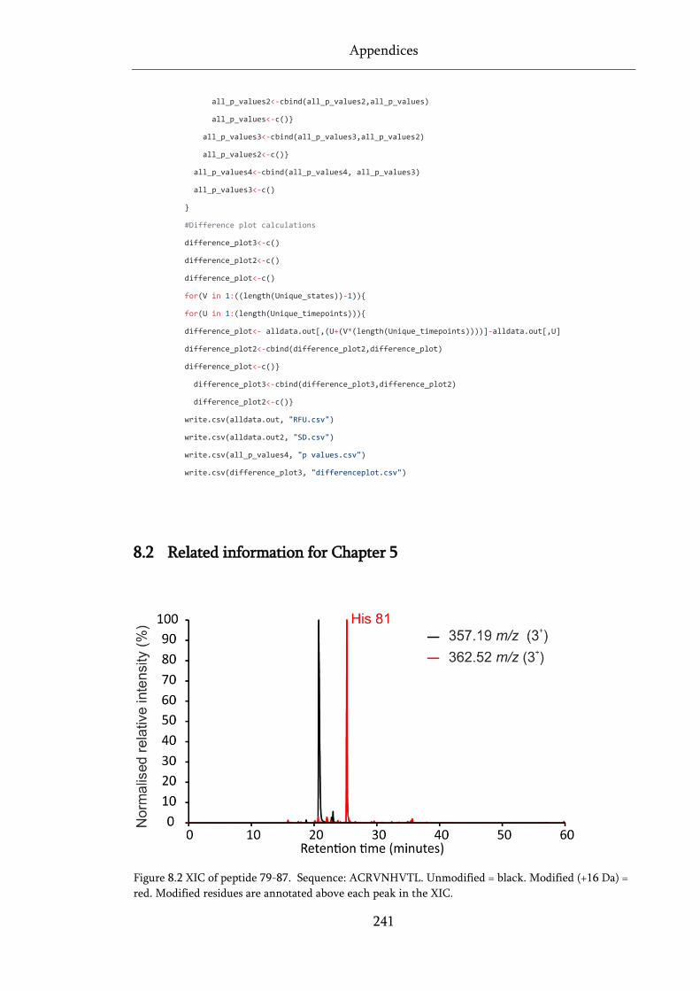
Appendices
241
8.2 Related information for Chapter 5
Figure 8.2 XIC of peptide 79-87. Sequence: ACRVNHVTL. Unmodified = black. Modified (+16 Da) =
red. Modified residues are annotated above each peak in the XIC.
all_p_values2<-cbind(all_p_values2,all_p_values)
all_p_values<-c()
all_p_values3<-cbind(all_p_values3,all_p_values2)
all_p_values2<-c()
all_p_values4<-cbind(all_p_values4, all_p_values3)
all_p_values3<-c()
#Difference plot calculations
difference_plot3<-c()
difference_plot2<-c()
difference_plot<-c()
for(V in 1:((length(Unique_states))-1))
for(U in 1:(length(Unique_timepoints)))
difference_plot<- alldata.out[,(U+(V*(length(Unique_timepoints))))]-alldata.out[,U]
difference_plot2<-cbind(difference_plot2,difference_plot)
difference_plot<-c()
difference_plot3<-cbind(difference_plot3,difference_plot2)
difference_plot2<-c()
write.csv(alldata.out, "RFU.csv")
write.csv(alldata.out2, "SD.csv")
write.csv(all_p_values4, "p values.csv")
write.csv(difference_plot3, "differenceplot.csv")
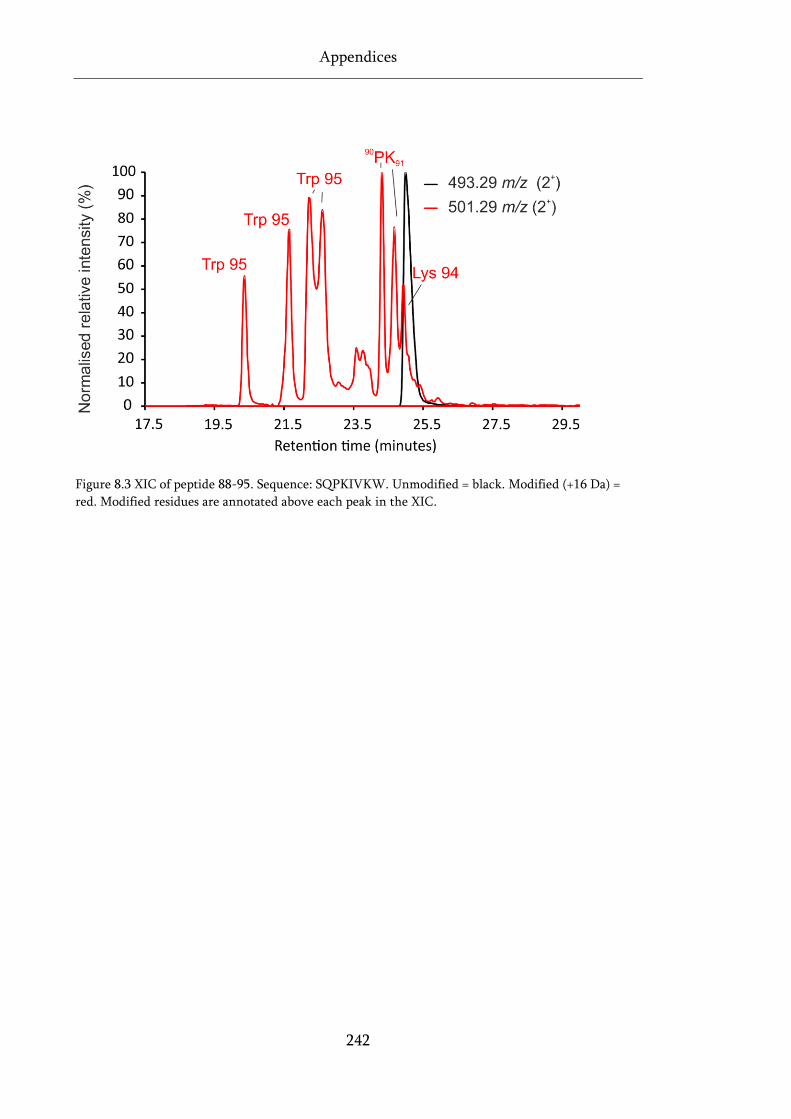
Appendices
242
Figure 8.3 XIC of peptide 88-95. Sequence: SQPKIVKW. Unmodified = black. Modified (+16 Da) =
red. Modified residues are annotated above each peak in the XIC.
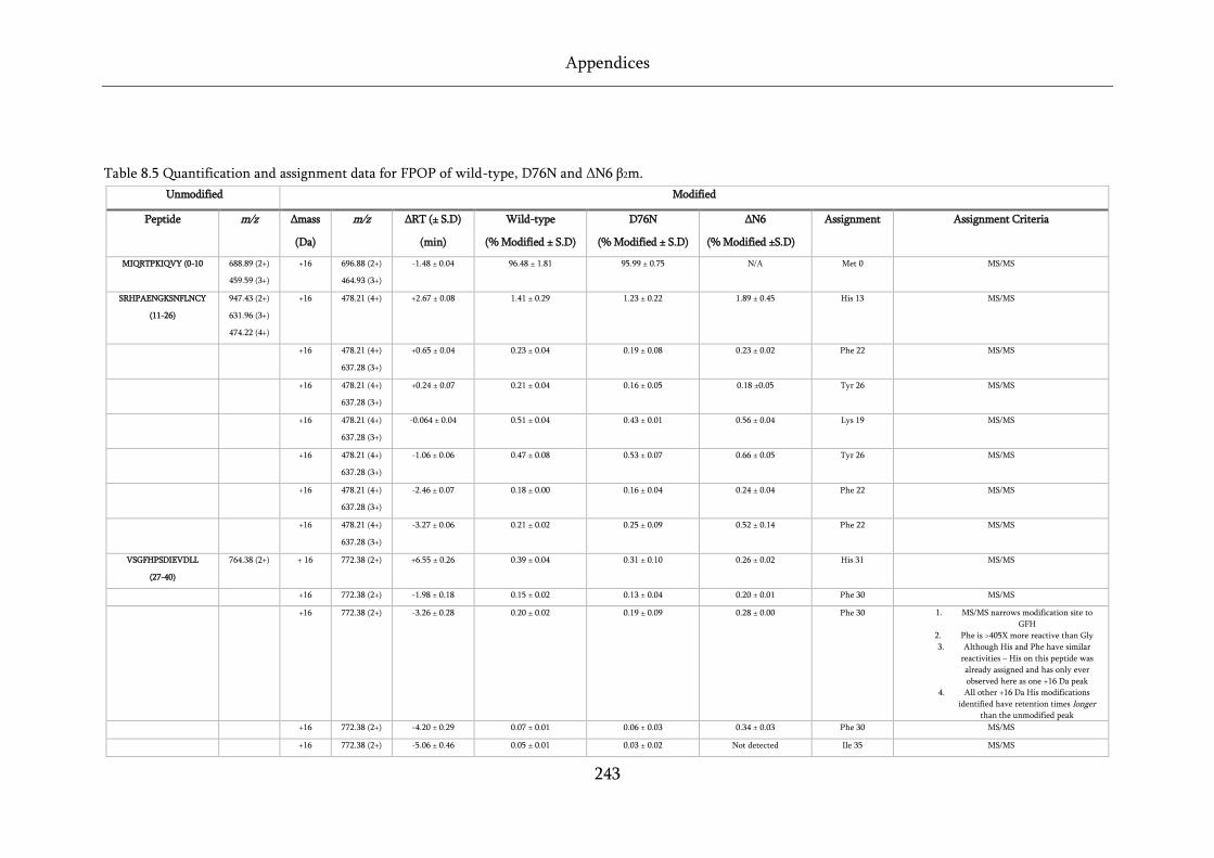
Appendices
243
Table 8.5 Quantification and assignment data for FPOP of wild-type, D76N and ΔN6 β2m.
Unmodified Modified
Peptide m/z Δmass
(Da)
m/z ΔRT (± S.D)
(min)
Wild-type
(% Modified ± S.D)
D76N
(% Modified ± S.D)
ΔN6
(% Modified ±S.D)
Assignment Assignment Criteria
MIQRTPKIQVY (0-10 688.89 (2+)
459.59 (3+)
+16 696.88 (2+)
464.93 (3+)
-1.48 ± 0.04 96.48 ± 1.81 95.99 ± 0.75 N/A Met 0 MS/MS
SRHPAENGKSNFLNCY
(11-26)
947.43 (2+)
631.96 (3+)
474.22 (4+)
+16 478.21 (4+) +2.67 ± 0.08 1.41 ± 0.29 1.23 ± 0.22 1.89 ± 0.45 His 13 MS/MS
+16 478.21 (4+)
637.28 (3+)
+0.65 ± 0.04 0.23 ± 0.04 0.19 ± 0.08 0.23 ± 0.02 Phe 22 MS/MS
+16 478.21 (4+)
637.28 (3+)
+0.24 ± 0.07 0.21 ± 0.04 0.16 ± 0.05 0.18 ±0.05 Tyr 26 MS/MS
+16 478.21 (4+)
637.28 (3+)
-0.064 ± 0.04 0.51 ± 0.04 0.43 ± 0.01 0.56 ± 0.04 Lys 19 MS/MS
+16 478.21 (4+)
637.28 (3+)
-1.06 ± 0.06 0.47 ± 0.08 0.53 ± 0.07 0.66 ± 0.05 Tyr 26 MS/MS
+16 478.21 (4+)
637.28 (3+)
-2.46 ± 0.07 0.18 ± 0.00 0.16 ± 0.04 0.24 ± 0.04 Phe 22 MS/MS
+16 478.21 (4+)
637.28 (3+)
-3.27 ± 0.06 0.21 ± 0.02 0.25 ± 0.09 0.52 ± 0.14 Phe 22 MS/MS
VSGFHPSDIEVDLL
(27-40)
764.38 (2+) + 16 772.38 (2+) +6.55 ± 0.26 0.39 ± 0.04 0.31 ± 0.10 0.26 ± 0.02 His 31 MS/MS
+16 772.38 (2+) -1.98 ± 0.18 0.15 ± 0.02 0.13 ± 0.04 0.20 ± 0.01 Phe 30 MS/MS
+16 772.38 (2+) -3.26 ± 0.28 0.20 ± 0.02 0.19 ± 0.09 0.28 ± 0.00 Phe 30 1. MS/MS narrows modification site to
GFH
2. Phe is >405X more reactive than Gly
3. Although His and Phe have similar
reactivities – His on this peptide was
already assigned and has only ever
observed here as one +16 Da peak
4. All other +16 Da His modifications
identified have retention times longer
than the unmodified peak
+16 772.38 (2+) -4.20 ± 0.29 0.07 ± 0.01 0.06 ± 0.03 0.34 ± 0.03 Phe 30 MS/MS
+16 772.38 (2+) -5.06 ± 0.46 0.05 ± 0.01 0.03 ± 0.02 Not detected Ile 35 MS/MS
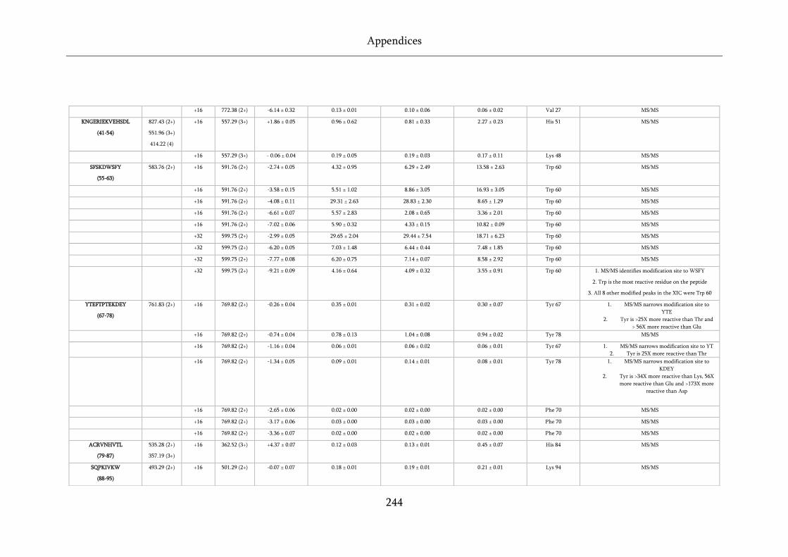
Appendices
244
+16 772.38 (2+) -6.14 ± 0.32 0.13 ± 0.01 0.10 ± 0.06 0.06 ± 0.02 Val 27 MS/MS
KNGERIEKVEHSDL
(41-54)
827.43 (2+)
551.96 (3+)
414.22 (4)
+16 557.29 (3+) +1.86 ± 0.05 0.96 ± 0.62 0.81 ± 0.33 2.27 ± 0.23 His 51 MS/MS
+16 557.29 (3+) - 0.06 ± 0.04 0.19 ± 0.05 0.19 ± 0.03 0.17 ± 0.11 Lys 48 MS/MS
SFSKDWSFY
(55-63)
583.76 (2+) +16 591.76 (2+) -2.74 ± 0.05 4.32 ± 0.95 6.29 ± 2.49 13.58 ± 2.63 Trp 60 MS/MS
+16 591.76 (2+) -3.58 ± 0.15 5.51 ± 1.02 8.86 ± 3.05 16.93 ± 3.05 Trp 60 MS/MS
+16 591.76 (2+) -4.08 ± 0.11 29.31 ± 2.63 28.83 ± 2.30 8.65 ± 1.29 Trp 60 MS/MS
+16 591.76 (2+) -6.61 ± 0.07 5.57 ± 2.83 2.08 ± 0.65 3.36 ± 2.01 Trp 60 MS/MS
+16 591.76 (2+) -7.02 ± 0.06 5.90 ± 0.32 4.33 ± 0.15 10.82 ± 0.09 Trp 60 MS/MS
+32 599.75 (2+) -2.99 ± 0.05 29.65 ± 2.04 29.44 ± 7.54 18.71 ± 6.23 Trp 60 MS/MS
+32 599.75 (2+) -6.20 ± 0.05 7.03 ± 1.48 6.44 ± 0.44 7.48 ± 1.85 Trp 60 MS/MS
+32 599.75 (2+) -7.77 ± 0.08 6.20 ± 0.75 7.14 ± 0.07 8.58 ± 2.92 Trp 60 MS/MS
+32 599.75 (2+) -9.21 ± 0.09 4.16 ± 0.64 4.09 ± 0.32 3.55 ± 0.91 Trp 60 1. MS/MS identifies modification site to WSFY
2. Trp is the most reactive residue on the peptide
3. All 8 other modified peaks in the XIC were Trp 60
YTEFTPTEKDEY
(67-78)
761.83 (2+) +16 769.82 (2+) -0.26 ± 0.04 0.35 ± 0.01 0.31 ± 0.02 0.30 ± 0.07 Tyr 67 1. MS/MS narrows modification site to
YTE
2. Tyr is >25X more reactive than Thr and
> 56X more reactive than Glu
+16 769.82 (2+) -0.74 ± 0.04 0.78 ± 0.13 1.04 ± 0.08 0.94 ± 0.02 Tyr 78 MS/MS
+16 769.82 (2+) -1.16 ± 0.04 0.06 ± 0.01 0.06 ± 0.02 0.06 ± 0.01 Tyr 67 1. MS/MS narrows modification site to YT
2. Tyr is 25X more reactive than Thr
+16 769.82 (2+) -1.34 ± 0.05 0.09 ± 0.01 0.14 ± 0.01 0.08 ± 0.01 Tyr 78 1. MS/MS narrows modification site to
KDEY
2. Tyr is >34X more reactive than Lys, 56X
more reactive than Glu and >173X more
reactive than Asp
+16 769.82 (2+) -2.65 ± 0.06 0.02 ± 0.00 0.02 ± 0.00 0.02 ± 0.00 Phe 70 MS/MS
+16 769.82 (2+) -3.17 ± 0.06 0.03 ± 0.00 0.03 ± 0.00 0.03 ± 0.00 Phe 70 MS/MS
+16 769.82 (2+) -3.36 ± 0.07 0.02 ± 0.00 0.02 ± 0.00 0.02 ± 0.00 Phe 70 MS/MS
ACRVNHVTL
(79-87)
535.28 (2+)
357.19 (3+)
+16 362.52 (3+) +4.37 ± 0.07 0.12 ± 0.03 0.13 ± 0.01 0.45 ± 0.07 His 84 MS/MS
SQPKIVKW
(88-95)
493.29 (2+) +16 501.29 (2+) -0.07 ± 0.07 0.18 ± 0.01 0.19 ± 0.01 0.21 ± 0.01 Lys 94 MS/MS

Appendices
245
+16 501.29 (2+) -0.44 ± 0.12 0.39 ± 0.01 0.37 ± 0.04 0.32 ± 0.03 Unassigned 1. MS/MS narrows modification to Pro 90
or Lys 91
2. Both have similar reactivities (approx. 2
fold difference)
3. Pro can have >1 structural isomer
+16 501.29 (2+) -0.79 ± 0.11 0.35 ± 0.03 0.31 ± 0.02 0.32 ± 0.01 Unassigned 1. MS/MS narrows modification to Pro 90
or Lys 91
2. Both have similar reactivities (approx. 2
fold difference)
3. Pro can have >1 structural isomer
+16 501.29 (2+) -2.54 ± 0.14 0.35 ± 0.01 0.40 ± 0.04 0.35 ± 0.11 Trp 95 MS/MS
+16 501.29 (2+) -2.94 ± 0.14 0.43 ± 0.07 0.44 ± 0.12 0.39 ± 0.08 Trp 95 MS/MS
+16 501.29 (2+) -3.46 ± 0.14 0.17 ± 0.07 0.25 ± 0.05 0.36 ± 0.02 Trp 95 MS/MS
+16 501.29 (2+) -4.73 ± 0.13 0.15 ± 0.08 0.15 ± 0.03 0.16 ± 0.04 Trp 95 MS/MS
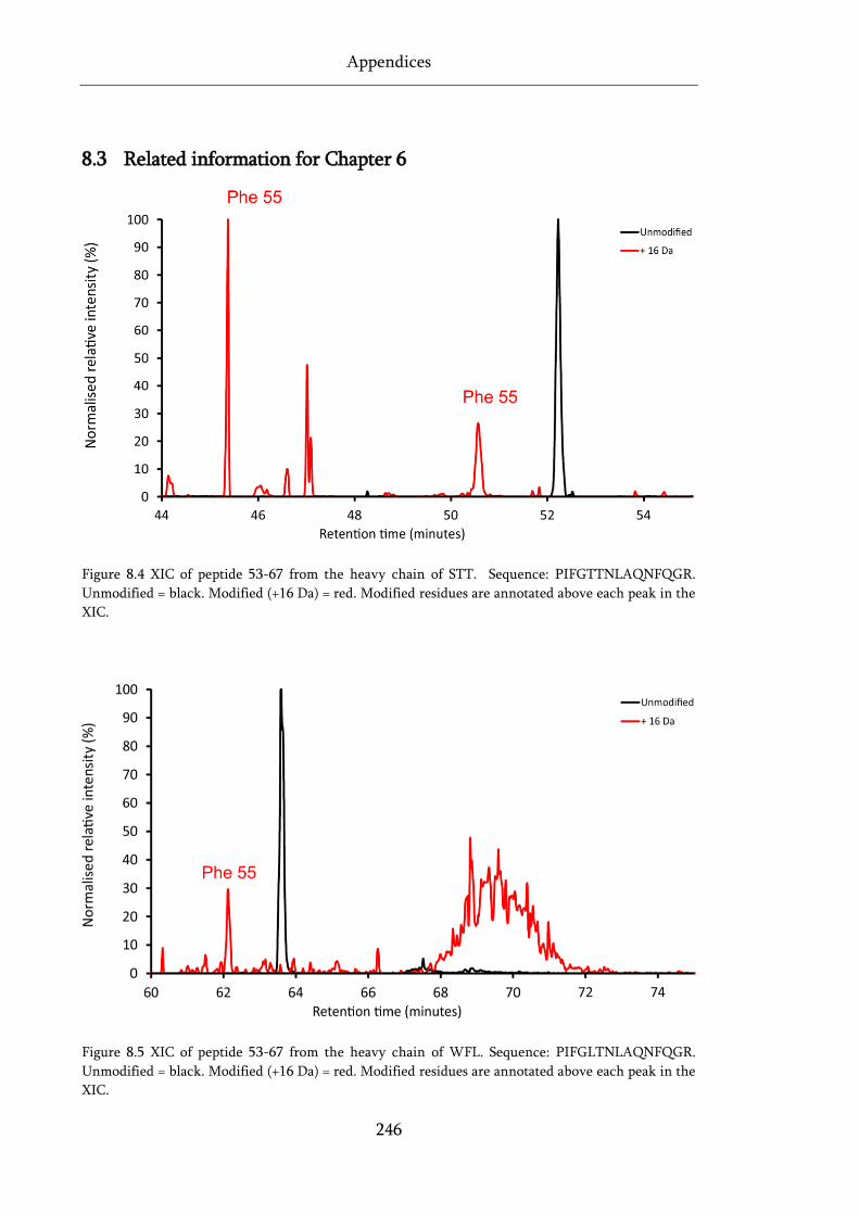
Appendices
246
8.3 Related information for Chapter 6
Figure 8.4 XIC of peptide 53-67 from the heavy chain of STT. Sequence: PIFGTTNLAQNFQGR.
Unmodified = black. Modified (+16 Da) = red. Modified residues are annotated above each peak in the
XIC.
Figure 8.5 XIC of peptide 53-67 from the heavy chain of WFL. Sequence: PIFGLTNLAQNFQGR.
Unmodified = black. Modified (+16 Da) = red. Modified residues are annotated above each peak in the
XIC.
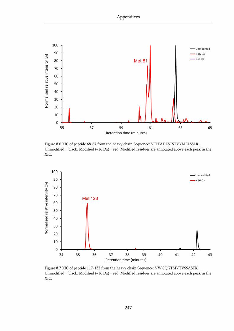
Appendices
247
Figure 8.6 XIC of peptide 68-87 from the heavy chain.Sequence: VTITADESTSTVYMELSSLR.
Unmodified = black. Modified (+16 Da) = red. Modified residues are annotated above each peak in the
XIC.
Figure 8.7 XIC of peptide 117-132 from the heavy chain.Sequence: VWGQGTMVTVSSASTK.
Unmodified = black. Modified (+16 Da) = red. Modified residues are annotated above each peak in the
XIC.
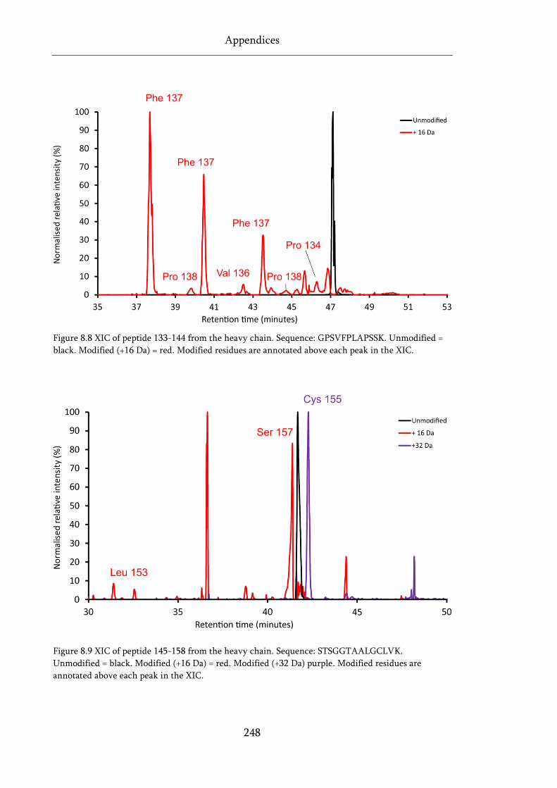
Appendices
248
Figure 8.8 XIC of peptide 133-144 from the heavy chain. Sequence: GPSVFPLAPSSK. Unmodified =
black. Modified (+16 Da) = red. Modified residues are annotated above each peak in the XIC.
Figure 8.9 XIC of peptide 145-158 from the heavy chain. Sequence: STSGGTAALGCLVK.
Unmodified = black. Modified (+16 Da) = red. Modified (+32 Da) purple. Modified residues are
annotated above each peak in the XIC.
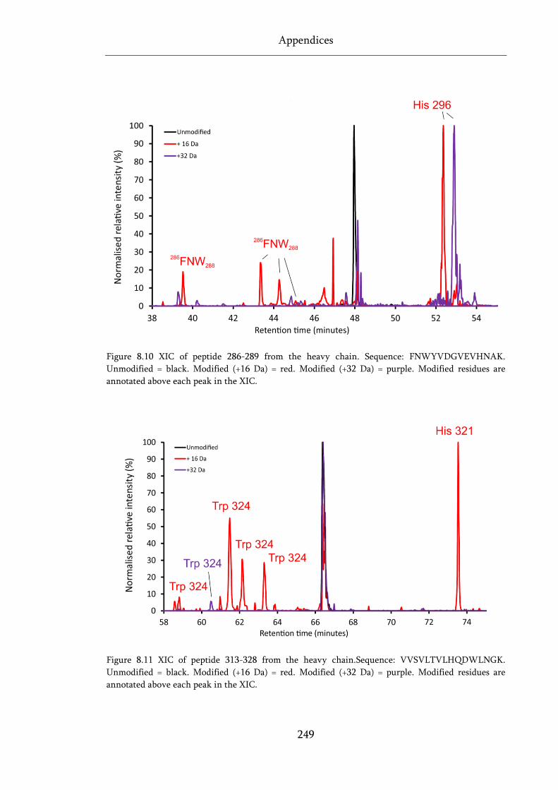
Appendices
249
Figure 8.10 XIC of peptide 286-289 from the heavy chain. Sequence: FNWYVDGVEVHNAK.
Unmodified = black. Modified (+16 Da) = red. Modified (+32 Da) = purple. Modified residues are
annotated above each peak in the XIC.
Figure 8.11 XIC of peptide 313-328 from the heavy chain.Sequence: VVSVLTVLHQDWLNGK.
Unmodified = black. Modified (+16 Da) = red. Modified (+32 Da) = purple. Modified residues are
annotated above each peak in the XIC.
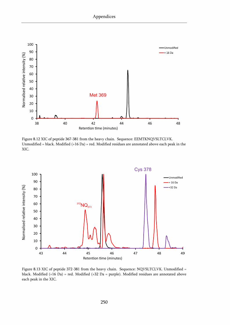
Appendices
250
Figure 8.12 XIC of peptide 367-381 from the heavy chain. Sequence: EEMTKNQVSLTCLVK.
Unmodified = black. Modified (+16 Da) = red. Modified residues are annotated above each peak in the
XIC.
Figure 8.13 XIC of peptide 372-381 from the heavy chain. Sequence: NQVSLTCLVK. Unmodified =
black. Modified (+16 Da) = red. Modified (+32 Da = purple). Modified residues are annotated above
each peak in the XIC.
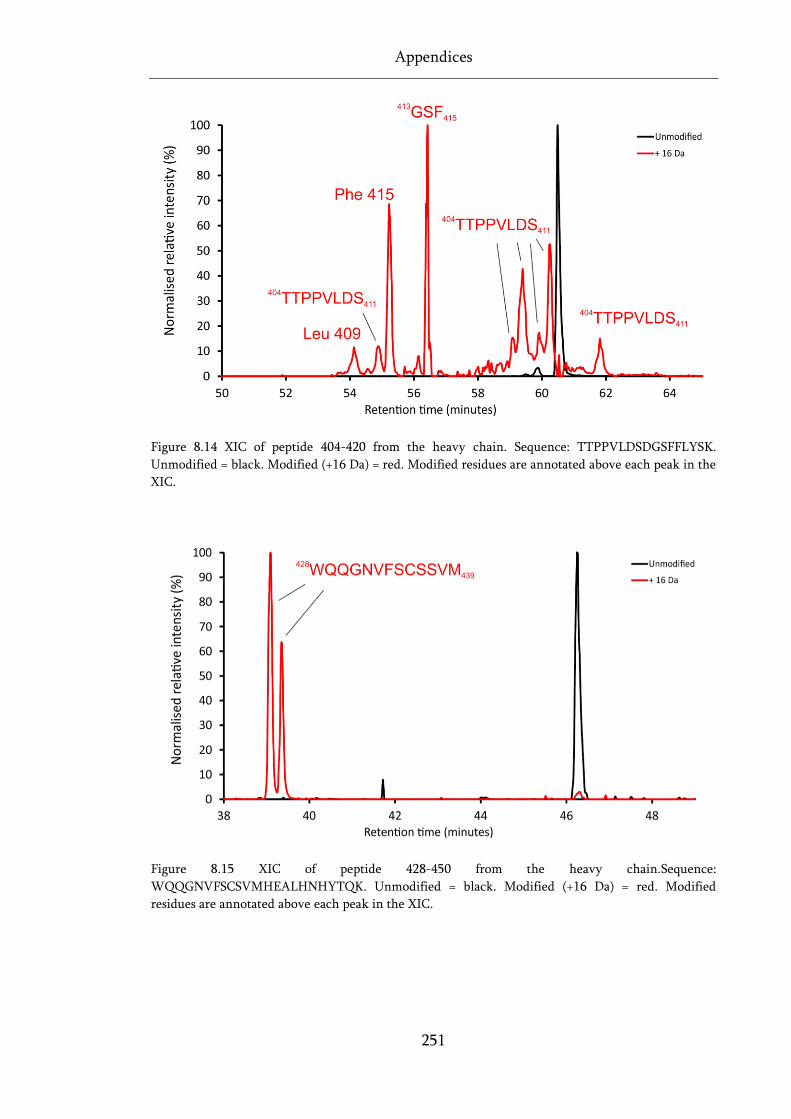
Appendices
251
Figure 8.14 XIC of peptide 404-420 from the heavy chain. Sequence: TTPPVLDSDGSFFLYSK.
Unmodified = black. Modified (+16 Da) = red. Modified residues are annotated above each peak in the
XIC.
Figure 8.15 XIC of peptide 428-450 from the heavy chain.Sequence:
WQQGNVFSCSVMHEALHNHYTQK. Unmodified = black. Modified (+16 Da) = red. Modified
residues are annotated above each peak in the XIC.
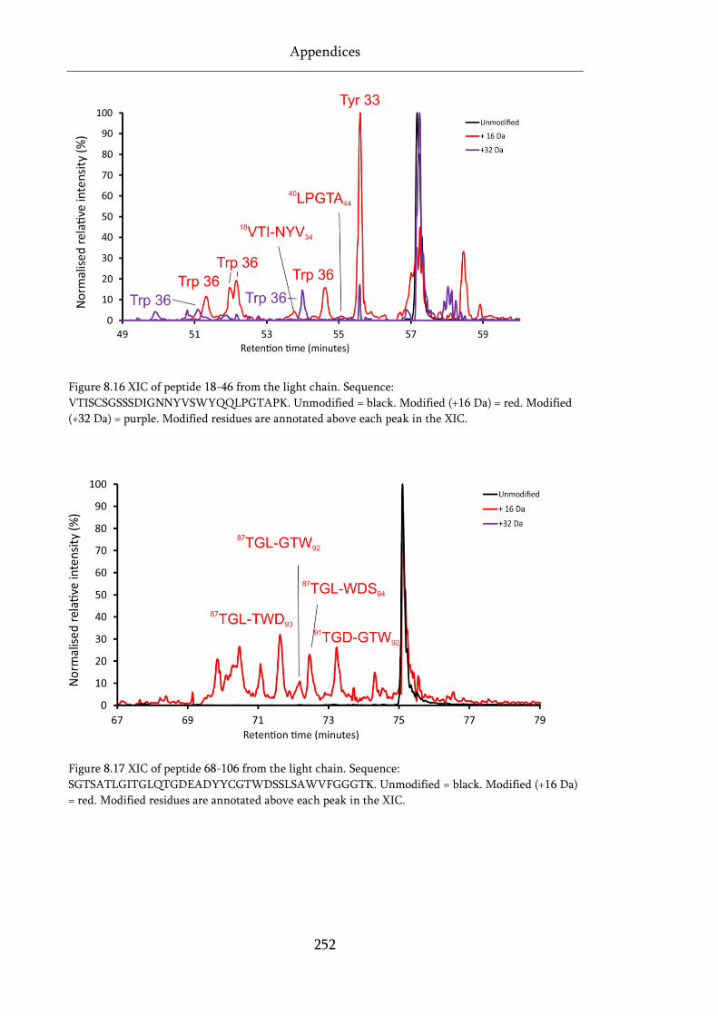
Appendices
252
Figure 8.16 XIC of peptide 18-46 from the light chain. Sequence:
VTISCSGSSSDIGNNYVSWYQQLPGTAPK. Unmodified = black. Modified (+16 Da) = red. Modified
(+32 Da) = purple. Modified residues are annotated above each peak in the XIC.
Figure 8.17 XIC of peptide 68-106 from the light chain. Sequence:
SGTSATLGITGLQTGDEADYYCGTWDSSLSAWVFGGGTK. Unmodified = black. Modified (+16 Da)
= red. Modified residues are annotated above each peak in the XIC.
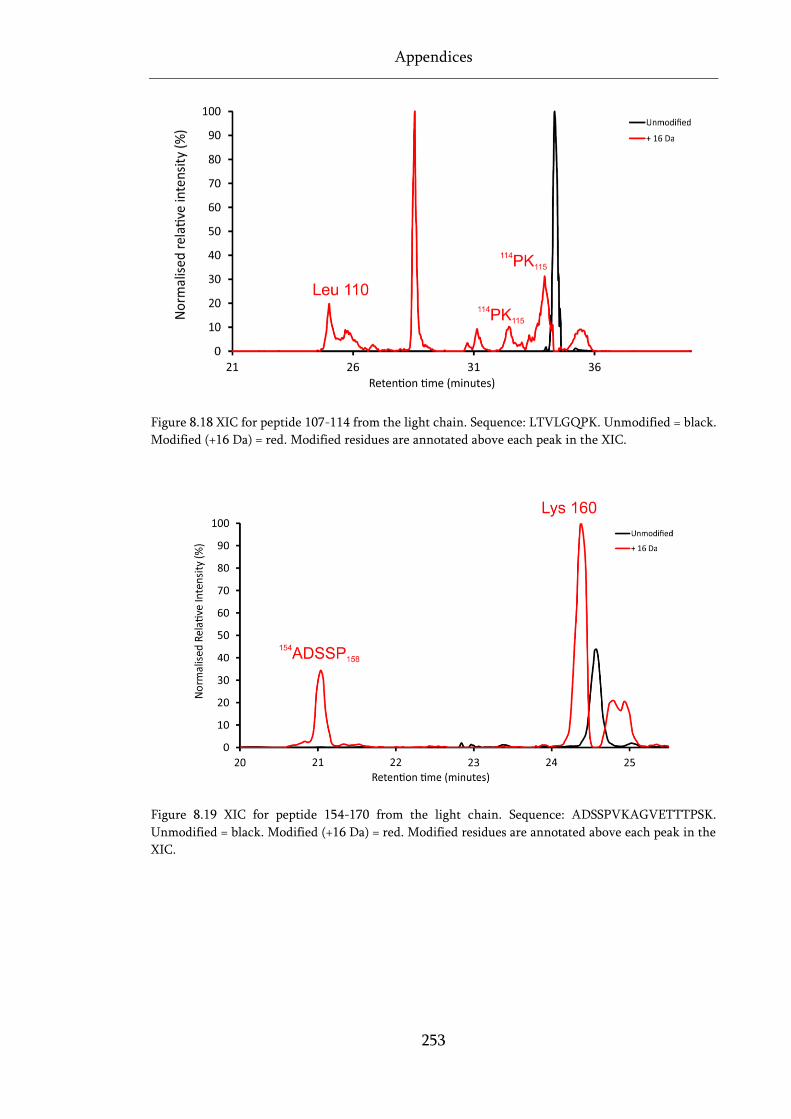
Appendices
253
Figure 8.18 XIC for peptide 107-114 from the light chain. Sequence: LTVLGQPK. Unmodified = black.
Modified (+16 Da) = red. Modified residues are annotated above each peak in the XIC.
Figure 8.19 XIC for peptide 154-170 from the light chain. Sequence: ADSSPVKAGVETTTPSK.
Unmodified = black. Modified (+16 Da) = red. Modified residues are annotated above each peak in the
XIC.
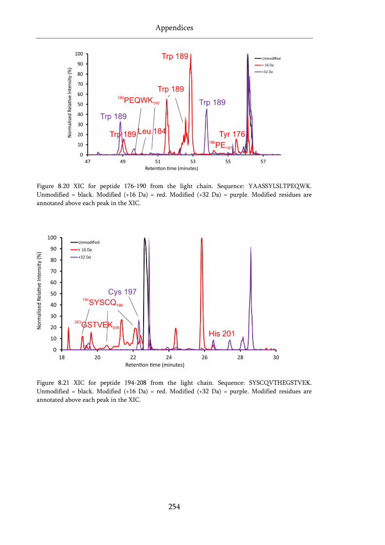
Appendices
254
Figure 8.20 XIC for peptide 176-190 from the light chain. Sequence: YAASSYLSLTPEQWK.
Unmodified = black. Modified (+16 Da) = red. Modified (+32 Da) = purple. Modified residues are
annotated above each peak in the XIC.
Figure 8.21 XIC for peptide 194-208 from the light chain. Sequence: SYSCQVTHEGSTVEK.
Unmodified = black. Modified (+16 Da) = red. Modified (+32 Da) = purple. Modified residues are
annotated above each peak in the XIC.
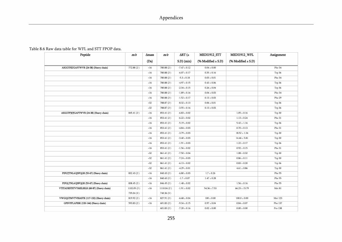
Appendices
255
Table 8.6 Raw data table for WFL and STT FPOP data.
Peptide m/z Δmass
(Da)
m/z ΔRT (±
S.D) (min)
MEDI1912_STT
(% Modified ± S.D)
MEDI1912_WFL
(% Modified ± S.D)
Assignment
ASGGTFSTGAFTWVR (24-38) (Heavy chain) 772.88 (2+) +16 780.88 (2+) -7.47 ± 0.12 0.04 ± 0.00 Phe 34
+16 780.88 (2+) -6.07 ± 0.17 0.35 ± 0.16 Trp 36
+16 780.88 (2+) -5.3 ± 0.18 0.03 ± 0.01 Phe 34
+16 780.88 (2+) -4.97 ± 0.15 0.43 ± 0.06 Trp 36
+16 780.88 (2+) -2.34 ± 0.15 0.26 ± 0.04 Trp 36
+16 780.88 (2+) -1.89 ± 0.16 0.04 ± 0.03 Phe 34
+16 780.88 (2+) -1.52 ± 0.17 0.13 ± 0.03 Phe 29
+32 788.87 (2+) -8.32 ± 0.13 0.06 ± 0.01 Trp 36
+32 788.87 (2+) -3.55 ± 0.16 0.13 ± 0.03 Trp 36
ASGGTFWFGAFTWVR (24-38) (Heavy chain) 845.41 (2+) +16 853.41 (2+) -6.83 ± 0.02 1.05 ± 0.16 Trp 30
+16 853.41 (2+) -6.22 ± 0.02 1.13 ± 0.24 Phe 31
+16 853.41 (2+) -5.19 ± 0.02 5.42 ± 1.16 Trp 36
+16 853.41 (2+) -4.84 ± 0.03 0.70 ± 0.13 Phe 31
+16 853.41 (2+) -3.79 ± 0.03 18.52 ± 1.34 Trp 30
+16 853.41 (2+) -3.40 ± 0.03 14.46 ± 5.81 Trp 30
+16 853.41 (2+) -1.91 ± 0.03 1.22 ± 0.17 Trp 36
+16 853.41 (2+) -1.56 ± 0.02 0.92 ± 0.15 Phe 31
+32 861.41 (2+) -7.50 ± 0.04 1.08 ± 0.32 Trp 30
+32 861.41 (2+) -7.24 ± 0.03 0.86 ± 0.11 Trp 30
+32 861.41 (2+) -6.13 ± 0.02 0.83 ± 0.20 Trp 36
+32 861.41 (2+) -4.29 ± 0.01 4.61 ± 0.86 Trp 30
PIFGTTNLAQNFQGR (53-67) (Heavy chain) 832.43 (2+) +16 840.43 (2+) -6.80 ± 0.03 1.7 ± 0.26 Phe 55
+16 840.43 (2+) -1.7 ± 0.07 1.47 ± 0.28 Phe 55
PIFGLTNLAQNFQGR (53-67) (Heavy chain) 838.45 (2+) +16 846.45 (2+) -1.48 ± 0.02 1.56 ± 0.16 Phe 55
VTITADESTSTVYMELSSLR (68-87) (Heavy chain) 1102.05 (2+)
735.04 (3+)
+16 1110.04 (2+)
740.36 (3+)
-1.91 ± 0.02 54.36 ± 7.53 66.23 ± 15.79 Met 81
VWGQGTMVTVSSASTK (117-132) (Heavy chain) 819.92 (2+) +16 827.91 (2+) -6.68 ± 0.04 100 ± 0.00 100.0 ± 0.00 Met 123
GPSVFPLAPSSK (133-144) (Heavy chain) 593.83 (2+) +16 601.83 (2+) -9.34 ± 0.15 0.97 ± 0.04 0.84 ± 0.07 Phe 137
601.83 (2+) -7.20 ± 0.16 0.02 ± 0.00 0.00 ± 0.00 Pro 138
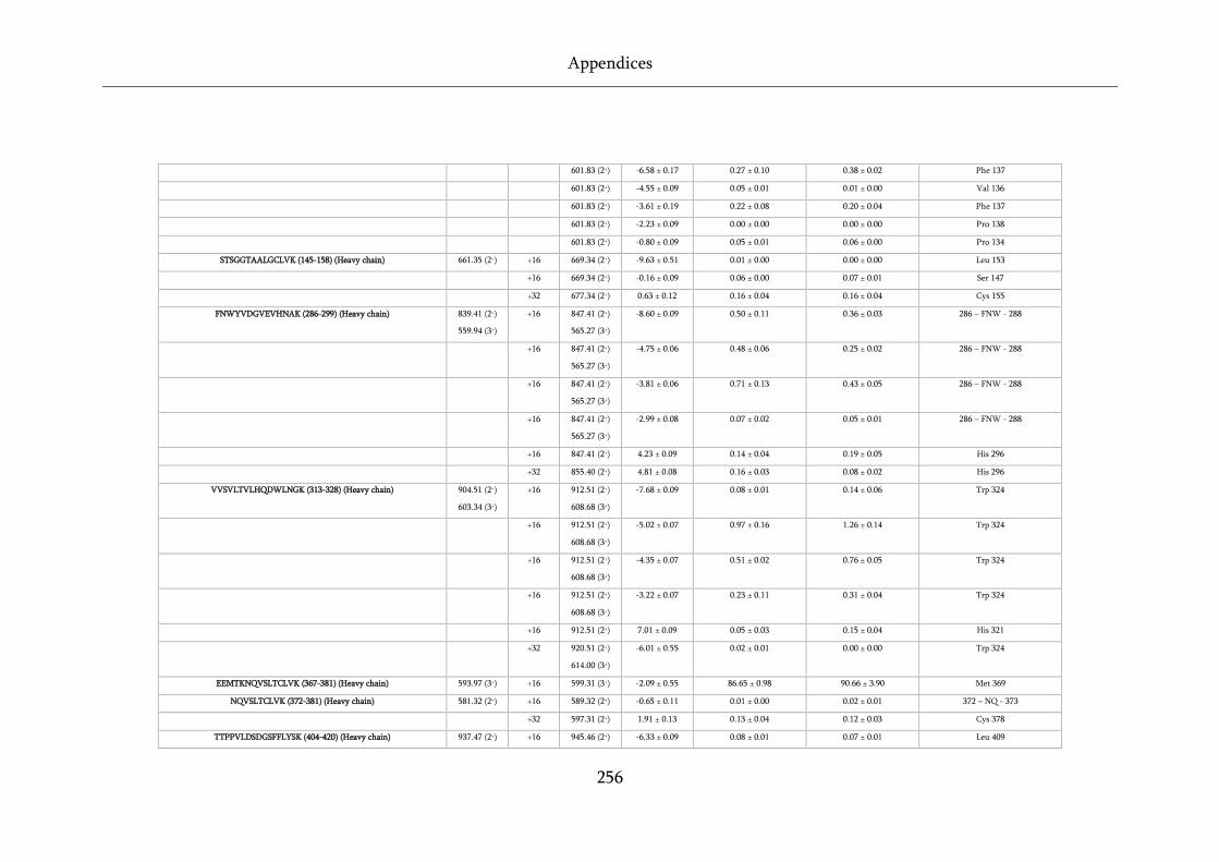
Appendices
256
601.83 (2+) -6.58 ± 0.17 0.27 ± 0.10 0.38 ± 0.02 Phe 137
601.83 (2+) -4.55 ± 0.09 0.05 ± 0.01 0.01 ± 0.00 Val 136
601.83 (2+) -3.61 ± 0.19 0.22 ± 0.08 0.20 ± 0.04 Phe 137
601.83 (2+) -2.23 ± 0.09 0.00 ± 0.00 0.00 ± 0.00 Pro 138
601.83 (2+) -0.80 ± 0.09 0.05 ± 0.01 0.06 ± 0.00 Pro 134
STSGGTAALGCLVK (145-158) (Heavy chain) 661.35 (2+) +16 669.34 (2+) -9.63 ± 0.51 0.01 ± 0.00 0.00 ± 0.00 Leu 153
+16 669.34 (2+) -0.16 ± 0.09 0.06 ± 0.00 0.07 ± 0.01 Ser 147
+32 677.34 (2+) 0.63 ± 0.12 0.16 ± 0.04 0.16 ± 0.04 Cys 155
FNWYVDGVEVHNAK (286-299) (Heavy chain) 839.41 (2+)
559.94 (3+)
+16 847.41 (2+)
565.27 (3+)
-8.60 ± 0.09 0.50 ± 0.11 0.36 ± 0.03 286 – FNW - 288
+16 847.41 (2+)
565.27 (3+)
-4.75 ± 0.06 0.48 ± 0.06 0.25 ± 0.02 286 – FNW - 288
+16 847.41 (2+)
565.27 (3+)
-3.81 ± 0.06 0.71 ± 0.13 0.43 ± 0.05 286 – FNW - 288
+16 847.41 (2+)
565.27 (3+)
-2.99 ± 0.08 0.07 ± 0.02 0.05 ± 0.01 286 – FNW - 288
+16 847.41 (2+) 4.23 ± 0.09 0.14 ± 0.04 0.19 ± 0.05 His 296
+32 855.40 (2+) 4.81 ± 0.08 0.16 ± 0.03 0.08 ± 0.02 His 296
VVSVLTVLHQDWLNGK (313-328) (Heavy chain) 904.51 (2+) 603.34 (3+)
+16 912.51 (2+)
608.68 (3+) -7.68 ± 0.09 0.08 ± 0.01 0.14 ± 0.06 Trp 324
+16 912.51 (2+)
608.68 (3+)
-5.02 ± 0.07 0.97 ± 0.16 1.26 ± 0.14 Trp 324
+16 912.51 (2+)
608.68 (3+)
-4.35 ± 0.07 0.51 ± 0.02 0.76 ± 0.05 Trp 324
+16 912.51 (2+)
608.68 (3+)
-3.22 ± 0.07 0.23 ± 0.11 0.31 ± 0.04 Trp 324
+16 912.51 (2+) 7.01 ± 0.09 0.05 ± 0.03 0.15 ± 0.04 His 321
+32 920.51 (2+)
614.00 (3+) -6.01 ± 0.55 0.02 ± 0.01 0.00 ± 0.00 Trp 324
EEMTKNQVSLTCLVK (367-381) (Heavy chain) 593.97 (3+) +16 599.31 (3+) -2.09 ± 0.55 86.65 ± 0.98 90.66 ± 3.90 Met 369
NQVSLTCLVK (372-381) (Heavy chain) 581.32 (2+) +16 589.32 (2+) -0.65 ± 0.11 0.01 ± 0.00 0.02 ± 0.01 372 – NQ - 373
+32 597.31 (2+) 1.91 ± 0.13 0.13 ± 0.04 0.12 ± 0.03 Cys 378
TTPPVLDSDGSFFLYSK (404-420) (Heavy chain) 937.47 (2+) +16 945.46 (2+) -6.33 ± 0.09 0.08 ± 0.01 0.07 ± 0.01 Leu 409
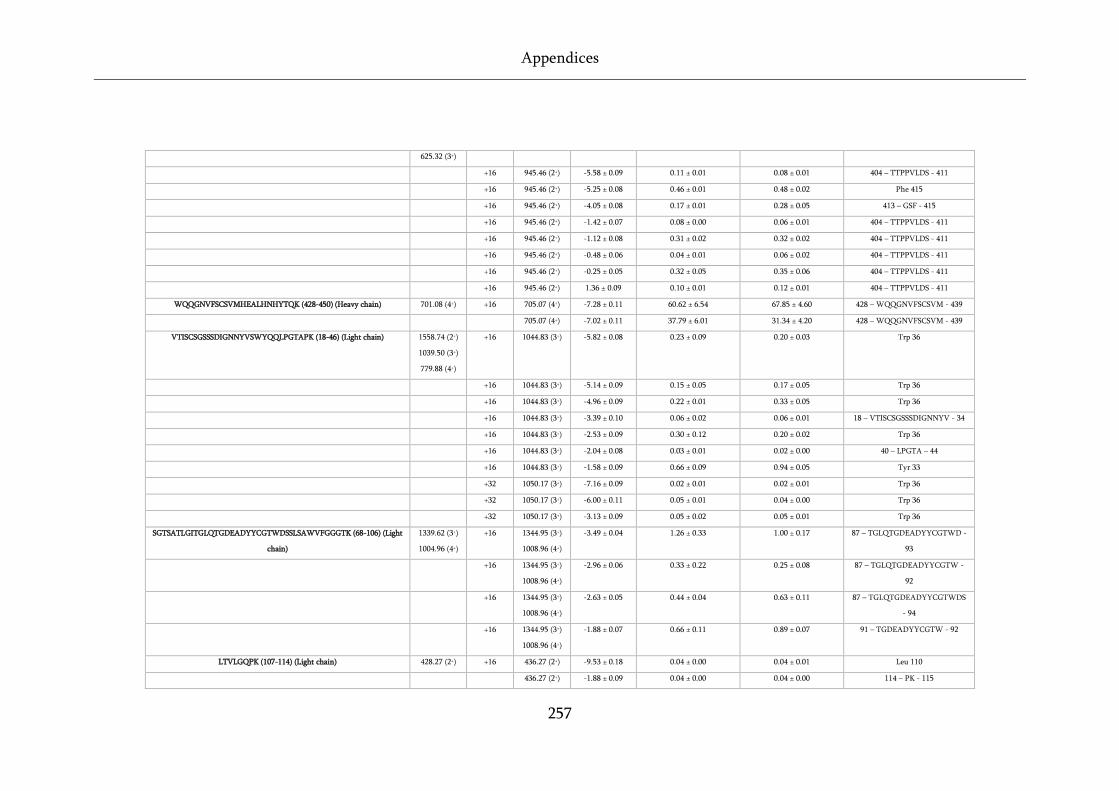
Appendices
257
625.32 (3+)
+16 945.46 (2+) -5.58 ± 0.09 0.11 ± 0.01 0.08 ± 0.01 404 – TTPPVLDS - 411
+16 945.46 (2+) -5.25 ± 0.08 0.46 ± 0.01 0.48 ± 0.02 Phe 415
+16 945.46 (2+) -4.05 ± 0.08 0.17 ± 0.01 0.28 ± 0.05 413 – GSF - 415
+16 945.46 (2+) -1.42 ± 0.07 0.08 ± 0.00 0.06 ± 0.01 404 – TTPPVLDS - 411
+16 945.46 (2+) -1.12 ± 0.08 0.31 ± 0.02 0.32 ± 0.02 404 – TTPPVLDS - 411
+16 945.46 (2+) -0.48 ± 0.06 0.04 ± 0.01 0.06 ± 0.02 404 – TTPPVLDS - 411
+16 945.46 (2+) -0.25 ± 0.05 0.32 ± 0.05 0.35 ± 0.06 404 – TTPPVLDS - 411
+16 945.46 (2+) 1.36 ± 0.09 0.10 ± 0.01 0.12 ± 0.01 404 – TTPPVLDS - 411
WQQGNVFSCSVMHEALHNHYTQK (428-450) (Heavy chain) 701.08 (4+) +16 705.07 (4+) -7.28 ± 0.11 60.62 ± 6.54 67.85 ± 4.60 428 – WQQGNVFSCSVM - 439
705.07 (4+) -7.02 ± 0.11 37.79 ± 6.01 31.34 ± 4.20 428 – WQQGNVFSCSVM - 439
VTISCSGSSSDIGNNYVSWYQQLPGTAPK (18-46) (Light chain) 1558.74 (2+)
1039.50 (3+)
779.88 (4+)
+16 1044.83 (3+) -5.82 ± 0.08 0.23 ± 0.09 0.20 ± 0.03 Trp 36
+16 1044.83 (3+) -5.14 ± 0.09 0.15 ± 0.05 0.17 ± 0.05 Trp 36
+16 1044.83 (3+) -4.96 ± 0.09 0.22 ± 0.01 0.33 ± 0.05 Trp 36
+16 1044.83 (3+) -3.39 ± 0.10 0.06 ± 0.02 0.06 ± 0.01 18 – VTISCSGSSSDIGNNYV - 34
+16 1044.83 (3+) -2.53 ± 0.09 0.30 ± 0.12 0.20 ± 0.02 Trp 36
+16 1044.83 (3+) -2.04 ± 0.08 0.03 ± 0.01 0.02 ± 0.00 40 – LPGTA – 44
+16 1044.83 (3+) -1.58 ± 0.09 0.66 ± 0.09 0.94 ± 0.05 Tyr 33
+32 1050.17 (3+) -7.16 ± 0.09 0.02 ± 0.01 0.02 ± 0.01 Trp 36
+32 1050.17 (3+) -6.00 ± 0.11 0.05 ± 0.01 0.04 ± 0.00 Trp 36
+32 1050.17 (3+) -3.13 ± 0.09 0.05 ± 0.02 0.05 ± 0.01 Trp 36
SGTSATLGITGLQTGDEADYYCGTWDSSLSAWVFGGGTK (68-106) (Light
chain)
1339.62 (3+)
1004.96 (4+)
+16 1344.95 (3+)
1008.96 (4+)
-3.49 ± 0.04 1.26 ± 0.33 1.00 ± 0.17 87 – TGLQTGDEADYYCGTWD -
93
+16 1344.95 (3+)
1008.96 (4+)
-2.96 ± 0.06 0.33 ± 0.22 0.25 ± 0.08 87 – TGLQTGDEADYYCGTW -
92
+16 1344.95 (3+)
1008.96 (4+)
-2.63 ± 0.05 0.44 ± 0.04 0.63 ± 0.11 87 – TGLQTGDEADYYCGTWDS
- 94
+16 1344.95 (3+)
1008.96 (4+)
-1.88 ± 0.07 0.66 ± 0.11 0.89 ± 0.07 91 – TGDEADYYCGTW - 92
LTVLGQPK (107-114) (Light chain) 428.27 (2+) +16 436.27 (2+) -9.53 ± 0.18 0.04 ± 0.00 0.04 ± 0.01 Leu 110
436.27 (2+) -1.88 ± 0.09 0.04 ± 0.00 0.04 ± 0.00 114 – PK - 115
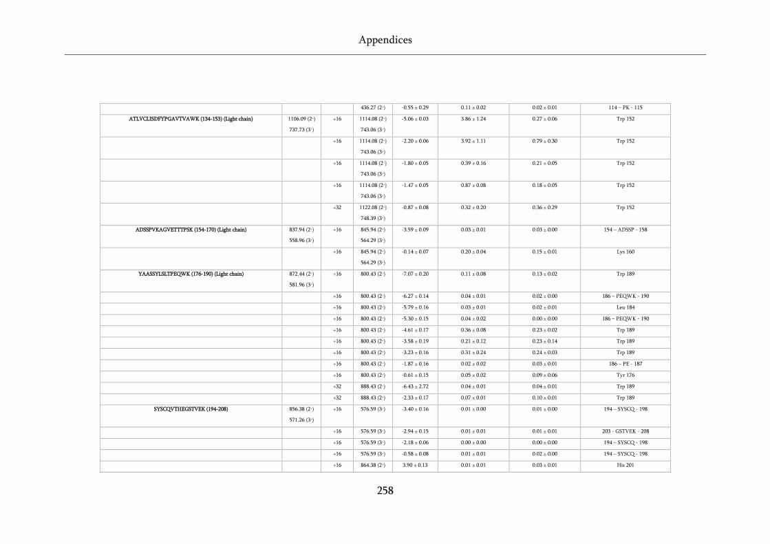
Appendices
258
436.27 (2+) -0.55 ± 0.29 0.11 ± 0.02 0.02 ± 0.01 114 – PK - 115
ATLVCLISDFYPGAVTVAWK (134-153) (Light chain) 1106.09 (2+)
737.73 (3+)
+16 1114.08 (2+)
743.06 (3+)
-5.06 ± 0.03 3.86 ± 1.24 0.27 ± 0.06 Trp 152
+16 1114.08 (2+)
743.06 (3+)
-2.20 ± 0.06 3.92 ± 1.11 0.79 ± 0.30 Trp 152
+16 1114.08 (2+)
743.06 (3+)
-1.80 ± 0.05 0.39 ± 0.16 0.21 ± 0.05 Trp 152
+16 1114.08 (2+)
743.06 (3+)
-1.47 ± 0.05 0.87 ± 0.08 0.18 ± 0.05 Trp 152
+32 1122.08 (2+)
748.39 (3+)
-0.87 ± 0.08 0.32 ± 0.20 0.36 ± 0.29 Trp 152
ADSSPVKAGVETTTPSK (154-170) (Light chain) 837.94 (2+)
558.96 (3+)
+16 845.94 (2+)
564.29 (3+)
-3.59 ± 0.09 0.03 ± 0.01 0.03 ± 0.00 154 – ADSSP - 158
+16 845.94 (2+)
564.29 (3+)
-0.14 ± 0.07 0.20 ± 0.04 0.15 ± 0.01 Lys 160
YAASSYLSLTPEQWK (176-190) (Light chain) 872.44 (2+)
581.96 (3+)
+16 800.43 (2+) -7.07 ± 0.20 0.11 ± 0.08 0.13 ± 0.02 Trp 189
+16 800.43 (2+) -6.27 ± 0.14 0.04 ± 0.01 0.02 ± 0.00 186 – PEQWK - 190
+16 800.43 (2+) -5.79 ± 0.16 0.03 ± 0.01 0.02 ± 0.01 Leu 184
+16 800.43 (2+) -5.30 ± 0.15 0.04 ± 0.02 0.00 ± 0.00 186 – PEQWK - 190
+16 800.43 (2+) -4.61 ± 0.17 0.36 ± 0.08 0.23 ± 0.02 Trp 189
+16 800.43 (2+) -3.58 ± 0.19 0.21 ± 0.12 0.23 ± 0.14 Trp 189
+16 800.43 (2+) -3.23 ± 0.16 0.31 ± 0.24 0.24 ± 0.03 Trp 189
+16 800.43 (2+) -1.87 ± 0.16 0.02 ± 0.02 0.03 ± 0.01 186 – PE - 187
+16 800.43 (2+) -0.61 ± 0.15 0.05 ± 0.02 0.09 ± 0.06 Tyr 176
+32 888.43 (2+) -6.43 ± 2.72 0.04 ± 0.01 0.04 ± 0.01 Trp 189
+32 888.43 (2+) -2.33 ± 0.17 0.07 ± 0.01 0.10 ± 0.01 Trp 189
SYSCQVTHEGSTVEK (194-208) 856.38 (2+)
571.26 (3+)
+16 576.59 (3+) -3.40 ± 0.16 0.01 ± 0.00 0.01 ± 0.00 194 – SYSCQ - 198
+16 576.59 (3+) -2.94 ± 0.15 0.01 ± 0.01 0.01 ± 0.01 203 - GSTVEK - 208
+16 576.59 (3+) -2.18 ± 0.06 0.00 ± 0.00 0.00 ± 0.00 194 – SYSCQ - 198
+16 576.59 (3+) -0.58 ± 0.08 0.01 ± 0.01 0.02 ± 0.00 194 – SYSCQ - 198
+16 864.38 (2+) 3.90 ± 0.13 0.01 ± 0.01 0.03 ± 0.01 His 201

Appendices
259
576.59 (3+)
+32 872.38 (2+)
581.92 (3+)
-0.38 ± 0.08 0.11 ± 0.02 0.12 ± 0.04 Cys 197
References
260
9 References
1. Thomson, J.J., Rays of positive electricity and their application to chemical analyses. Vol. 1. 1921: Longmans, Green and Company.
2. Thomson, J.J., XL. Cathode Rays. The London, Edinburgh, and Dublin Philosophical
Magazine and Journal of Science, 1897. 44(269): p. 293-316.
3. Thomson, J.J., Bakerian Lecture:—rays of positive electricity. Proc. R. Soc. Lond. A,
1913. 89(607): p. 1-20.
4. Bleakney, W., A New Method of Positive Ray Analysis and Its Application to the Measurement of Ionization Potentials in Mercury Vapor. Physical Review, 1929.
34(1): p. 157-160.
5. Harrison, A.G., Chemical ionization mass spectrometry. 2018: Routledge.
6. Fenn, J., M. Mann, C. Meng, S. Wong, and C. Whitehouse, Electrospray ionization for mass spectrometry of large biomolecules. Science, 1989. 246(4926): p. 64-71.
7. Yamashita, M. and J.B. Fenn, Electrospray ion source. Another variation on the free-jet theme. The Journal of Physical Chemistry, 1984. 88(20): p. 4451-4459.
8. Sir Geoffrey Taylor, F.R.S., Disintegration of water drops in an electric field. Proceedings of the Royal Society of London. Series A. Mathematical and Physical
Sciences, 1964. 280(1382): p. 383.
9. Kebarle, P. and L. Tang, From ions in solution to ions in the gas phase - the mechanism of electrospray mass spectrometry. Analytical Chemistry, 1993. 65(22):
p. 972A-986A.
10. Rayleigh, L., XX. On the equilibrium of liquid conducting masses charged with electricity. The London, Edinburgh, and Dublin Philosophical Magazine and Journal
of Science, 1882. 14(87): p. 184-186.
11. Dole, M., L.L. Mack, R.L. Hines, R.C. Mobley, L.D. Ferguson, and M.B. Alice,
Molecular Beams of Macroions. The Journal of Chemical Physics, 1968. 49(5): p.
2240-2249.
12. Iribarne, J.V. and B.A. Thomson, On the evaporation of small ions from charged droplets. The Journal of Chemical Physics, 1976. 64(6): p. 2287-2294.
13. Konermann, L., E. Ahadi, A.D. Rodriguez, and S. Vahidi, Unraveling the Mechanism of Electrospray Ionization. Analytical Chemistry, 2013. 85(1): p. 2-9.
14. Kebarle, P. and U.H. Verkerk, Electrospray: from ions in solution to ions in the gas phase, what we know now. Mass Spectrometry Reviews, 2009. 28(6): p. 898-917.
15. Wilm, M. and M. Mann, Analytical Properties of the Nanoelectrospray Ion Source. Analytical Chemistry, 1996. 68(1): p. 1-8.
16. Nemes, P., A.A. Barton, and A. Vertes, Three-dimensional imaging of metabolites in tissues under ambient conditions by laser ablation electrospray ionization mass spectrometry. Analytical Chemistry, 2009. 81(16): p. 6668-6675.
17. García-Gómez, D., L. Bregy, C. Barrios-Collado, G. Vidal-de-Miguel, and R. Zenobi,
Real-Time High-Resolution Tandem Mass Spectrometry Identifies Furan Derivatives in Exhaled Breath. Analytical Chemistry, 2015. 87(13): p. 6919-6924.
18. Guenther, S., K.-C. Schäfer, J. Balog, J. Dénes, T. Majoros, K. Albrecht, M. Tóth, B.
Spengler, and Z. Takáts, Electrospray Post-Ionization Mass Spectrometry of Electrosurgical Aerosols. Journal of The American Society for Mass Spectrometry,
2011. 22(11): p. 2082.
References
261
19. Chang, D.-Y., C.-C. Lee, and J. Shiea, Detecting Large Biomolecules from High-Salt Solutions by Fused-Droplet Electrospray Ionization Mass Spectrometry. Analytical
Chemistry, 2002. 74(11): p. 2465-2469.
20. Cheng, S.-C., T.-L. Cheng, H.-C. Chang, and J. Shiea, Using Laser-Induced Acoustic Desorption/Electrospray Ionization Mass Spectrometry To Characterize Small Organic and Large Biological Compounds in the Solid State and in Solution Under Ambient Conditions. Analytical Chemistry, 2009. 81(3): p. 868-874.
21. Shiea, J., M.-Z. Huang, H.S. Hsiu-Jung, C.-Y. Lee, C.-H. Yuan, I. Beech, and J.
Sunner, Electrospray-assisted laser desorption/ionization mass spectrometry for direct ambient analysis of solids. Rapid Communications in Mass Spectrometry,
2005. 19(24): p. 3701-3704.
22. Gong, X., Y. Zhao, S. Cai, S. Fu, C. Yang, S. Zhang, and X. Zhang, Single Cell Analysis with Probe ESI-Mass Spectrometry: Detection of Metabolites at Cellular and Subcellular Levels. Analytical Chemistry, 2014. 86(8): p. 3809-3816.
23. Loo, J.A., Electrospray ionization mass spectrometry: a technology for studying noncovalent macromolecular complexes. International Journal of Mass
Spectrometry, 2000. 200(1–3): p. 175-186.
24. Sparkman, O.D., Mass Spec Desk Reference. Global View, Pittsburgh, 2000.
25. Marshall, A.G., C.L. Hendrickson, and S.D.H. Shi, Scaling MS plateaus with high-resolution FT-ICRMS. 2002, ACS Publications.
26. Paul, W. and H. Steinwedel, Quadrupole mass filter. Z. Naturforsch. A, 1953. 8: p.
448.
27. Miller, P.E. and M.B. Denton, The quadrupole mass filter: Basic operating concepts. Journal of Chemical Education, 1986. 63(7): p. 617.
28. Savaryn, J.P., T.K. Toby, and N.L. Kelleher, A Researcher's Guide to Mass Spectrometry-Based Proteomics. Proteomics, 2016. 16(18): p. 2435-2443.
29. Hoffmann, E.d. and V. Stroobant, Mass Spectrometry; Principles and applications, Third edition. 2007.
30. Mathieu, É., Mémoire sur le mouvement vibratoire d'une membrane de forme elliptique. Journal de Mathématiques Pures et Appliquées, 1868. 13: p. 137.
31. Collings, B.A. and D.J. Douglas, An extended mass range quadrupole for electrospray mass spectrometry. International Journal of Mass Spectrometry and Ion Processes,
1997. 162(1): p. 121-127.
32. Schwartz, J.C., M.W. Senko, and J.E.P. Syka, A two-dimensional quadrupole ion trap mass spectrometer. Journal of the American Society for Mass Spectrometry,
2002. 13(6): p. 659-669.
33. Douglas, D.J., A.J. Frank, and D. Mao, Linear ion traps in mass spectrometry. Mass
Spectrometry Reviews, 2005. 24(1): p. 1-29.
34. Makarov, A., E. Denisov, A. Kholomeev, W. Balschun, O. Lange, K. Strupat, and S.
Horning, Performance Evaluation of a Hybrid Linear Ion Trap/Orbitrap Mass Spectrometer. Analytical Chemistry, 2006. 78(7): p. 2113-2120.
35. Stephens, W.E., A Pulsed Mass Spectrometer with Time Dispersion. Phys. Rev.,
1946. 69: p. 691.
36. Cameron, A.E. and D.F. Eggers Jr, An Ion``Velocitron''. Review of Scientific
Instruments, 1948. 19(9): p. 605-607.
37. Snijder, J., R.J. Rose, D. Veesler, J.E. Johnson, and A.J.R. Heck, Studying 18 Mega Dalton Virus Assemblies with Native Mass Spectrometry(). Angewandte Chemie
(International ed. in English), 2013. 52(14): p. 4020-4023.
References
262
38. Dawson, J.H.J. and M. Guilhaus, Orthogonal-acceleration time-of-flight mass spectrometer. Rapid Communications in Mass Spectrometry, 1989. 3(5): p. 155-159.
39. Mamyrin, B.A., V.I. Karataev, D.V. Shmikk, and V.A. Zagulin, The massreflectron, a new non-magnetic time-of-flight mass spectrometer with high resolution. Zh. Eksp.
Teor. Fiz, 1973. 64: p. 82-89.
40. Helm, D., J.P.C. Vissers, C.J. Hughes, H. Hahne, B. Ruprecht, F. Pachl, A. Grzyb, K.
Richardson, J. Wildgoose, S.K. Maier, H. Marx, M. Wilhelm, I. Becher, S. Lemeer,
M. Bantscheff, J.I. Langridge, and B. Kuster, Ion Mobility Tandem Mass Spectrometry Enhances Performance of Bottom-up Proteomics. Molecular &
Cellular Proteomics, 2014. 13(12): p. 3709.
41. Kingdon, K.H., A Method for the Neutralization of Electron Space Charge by Positive Ionization at Very Low Gas Pressures. Physical Review, 1923. 21(4): p. 408-
418.
42. Knight, R.D., Storage of ions from laser‐produced plasmas. Applied Physics Letters,
1981. 38(4): p. 221-223.
43. Gillig, K.J., B.K. Bluhm, and D.H. Russell, Ion motion in a Fourier transform ion cyclotron resonance wire ion guide cell. International Journal of Mass Spectrometry
and Ion Processes, 1996. 157-158: p. 129-147.
44. Makarov, A., Electrostatic Axially Harmonic Orbital Trapping: A High-Performance Technique of Mass Analysis. Analytical Chemistry, 2000. 72(6): p.
1156-1162.
45. Olsen, J.V., J.C. Schwartz, J. Griep-Raming, M.L. Nielsen, E. Damoc, E. Denisov, O.
Lange, P. Remes, D. Taylor, M. Splendore, E.R. Wouters, M. Senko, A. Makarov, M.
Mann, and S. Horning, A Dual Pressure Linear Ion Trap Orbitrap Instrument with Very High Sequencing Speed. Molecular & Cellular Proteomics, 2009. 8(12): p. 2759.
46. Perry, R.H., R.G. Cooks, and R.J. Noll, Orbitrap mass spectrometry: instrumentation, ion motion and applications. Mass spectrometry Reviews, 2008. 27(6): p. 661-699.
47. Schmidt, E.M., M.A. Pudenzi, J.M. Santos, C.F.F. Angolini, R.C.L. Pereira, Y.S.
Rocha, E. Denisov, E. Damoc, A. Makarov, and M.N. Eberlin, Petroleomics via Orbitrap mass spectrometry with resolving power above 1000000 at m/z 200. RSC
Advances, 2018. 8(11): p. 6183-6191.
48. Hu, Q., R.J. Noll, H. Li, A. Makarov, M. Hardman, and R. Graham Cooks, The Orbitrap: a new mass spectrometer. Journal of Mass Spectrometry, 2005. 40(4): p.
430-443.
49. Fort, K.L., M. van de Waterbeemd, D. Boll, M. Reinhardt-Szyba, M.E. Belov, E.
Sasaki, R. Zschoche, D. Hilvert, A.A. Makarov, and A.J.R. Heck, Expanding the structural analysis capabilities on an Orbitrap-based mass spectrometer for large macromolecular complexes. Analyst, 2018. 143(1): p. 100-105.
50. Bracewell, R.N. and R.N. Bracewell, The Fourier transform and its applications. Vol.
31999. 1986: McGraw-Hill New York, USA.
51. Brenton, A.G. and A.R. Godfrey, Accurate mass measurement: Terminology and treatment of data. Journal of the American Society for Mass Spectrometry, 2010.
21(11): p. 1821-1835.
52. Jennings, K.R., Collision-induced decompositions of aromatic molecular ions. International Journal of Mass Spectrometry and Ion Physics, 1968. 1(3): p. 227-235.
53. Olsen, J.V., B. Macek, O. Lange, A. Makarov, S. Horning, and M. Mann, Higher-energy C-trap dissociation for peptide modification analysis. Nature Methods, 2007.
4: p. 709.
References
263
54. Molnar, I. and C. Horváth, Reverse-phase chromatography of polar biological substances: separation of catechol compounds by high-performance liquid chromatography. Clinical chemistry, 1976. 22(9): p. 1497-1502.
55. Swartz, M.E., UPLC™: An Introduction and Review. Journal of Liquid
Chromatography & Related Technologies, 2005. 28(7-8): p. 1253-1263.
56. Plumb, R.S., K.A. Johnson, P. Rainville, B.W. Smith, I.D. Wilson, J.M. Castro-Perez,
and J.K. Nicholson, UPLC/MSE; a new approach for generating molecular fragment information for biomarker structure elucidation. Rapid Communications in Mass
Spectrometry, 2006. 20(13): p. 1989-1994.
57. Cohen, M.J. and F.W. Karasek, Plasma chromatography™—a new dimension for gas chromatography and mass spectrometry. Journal of Chromatographic Science, 1970.
8(6): p. 330-337.
58. Kanu, A.B., P. Dwivedi, M. Tam, L. Matz, and H.H. Hill, Jr., Ion mobility-mass spectrometry. J Mass Spectrom, 2008. 43(1): p. 1-22.
59. Ewing, R.G., D.A. Atkinson, G.A. Eiceman, and G.J. Ewing, A critical review of ion mobility spectrometry for the detection of explosives and explosive related compounds. Talanta, 2001. 54(3): p. 515-529.
60. Uetrecht, C., R.J. Rose, E. van Duijn, K. Lorenzen, and A.J. Heck, Ion mobility mass spectrometry of proteins and protein assemblies. Chemical Society Reviews, 2010.
39(5): p. 1633-55.
61. Mason, E.A. and H.W. Schamp, Mobility of gaseous lons in weak electric fields. Annals of Physics, 1958. 4(3): p. 233-270.
62. Mordehai, A., L. Howard, M.H. Werlich, R.T. Kurulugama, and T.A. Knotts, Ion mobility spectrometry-mass spectrometry (IMS-MS) with improved ion transmission and IMS resolution. 2016.
63. Smith, D.P., T.W. Knapman, I. Campuzano, R.W. Malham, J.T. Berryman, S.E.
Radforda, and A.E. Ashcrofta, Deciphering drift time measurements from travelling wave ion mobility spectrometry-mass spectrometry studies. European Journal of
Mass Spectrometry, 2009. 12(13): p. 13.
64. Pringle, S.D., K. Giles, J.L. Wildgoose, J.P. Williams, S.E. Slade, K. Thalassinos, R.H.
Bateman, M.T. Bowers, and J.H. Scrivens, An investigation of the mobility separation of some peptide and protein ions using a new hybrid quadrupole/travelling wave IMS/oa-ToF instrument. International Journal of Mass
Spectrometry, 2007. 261(1): p. 1-12.
65. Giles, K., S.D. Pringle, K.R. Worthington, D. Little, J.L. Wildgoose, and R.H.
Bateman, Applications of a travelling wave-based radio-frequency-only stacked ring ion guide. Rapid Commun Mass Spectrom, 2004. 18(20): p. 2401-14.
66. Ruotolo, B.T., J.L.P. Benesch, A.M. Sandercock, S.-J. Hyung, and C.V. Robinson, Ion mobility-mass spectrometry analysis of large protein complexes. Nat. Protocols,
2008. 3(7): p. 1139-1152.
67. Giles, K., J.L. Wildgoose, D.J. Langridge, and I. Campuzano, A method for direct measurement of ion mobilities using a travelling wave ion guide. International
Journal of Mass Spectrometry, 2010. 298(1–3): p. 10-16.
68. Shvartsburg, A.A. and R.D. Smith, Fundamentals of Traveling Wave Ion Mobility Spectrometry. Analytical Chemistry, 2008. 80(24): p. 9689-9699.
69. Bush, M.F., Z. Hall, K. Giles, J. Hoyes, C.V. Robinson, and B.T. Ruotolo, Collision cross sections of proteins and their complexes: A calibration framework and
References
264
database for gas-phase structural biology. Analytical Chemistry, 2010. 82(22): p.
9557-9565.
70. Michalski, A., E. Damoc, J.-P. Hauschild, O. Lange, A. Wieghaus, A. Makarov, N.
Nagaraj, J. Cox, M. Mann, and S. Horning, Mass Spectrometry-based Proteomics Using Q Exactive, a High-performance Benchtop Quadrupole Orbitrap Mass Spectrometer. Molecular & Cellular Proteomics, 2011. 10(9): p. M111.011015.
71. Senko, M.W., P.M. Remes, J.D. Canterbury, R. Mathur, Q. Song, S.M. Eliuk, C.
Mullen, L. Earley, M. Hardman, J.D. Blethrow, H. Bui, A. Specht, O. Lange, E.
Denisov, A. Makarov, S. Horning, and V. Zabrouskov, Novel Parallelized Quadrupole/Linear Ion Trap/Orbitrap Tribrid Mass Spectrometer Improving Proteome Coverage and Peptide Identification Rates. Analytical Chemistry, 2013.
85(24): p. 11710-11714.
72. Crick, F.H.C. On protein Synthesis. in Symposia for the Society of Experimental Biology. 1958.
73. Björn, L.O., Photobiology: The science of light and life. 2015: Springer.
74. Hirokawa, N. and Y. Tanaka, Kinesin superfamily proteins (KIFs): Various functions and their relevance for important phenomena in life and diseases. Experimental Cell
Research, 2015. 334(1): p. 16-25.
75. Anfinsen, C.B., E. Haber, M. Sela, and F.H. White, The kinetics of formation of native ribonuclease during oxidation of the reduced polypeptide chain. Proceedings
of the National Academy of Sciences of the United States of America, 1961. 47(9): p.
1309-1314.
76. Witze, E.S., W.M. Old, K.A. Resing, and N.G. Ahn, Mapping protein post-translational modifications with mass spectrometry. Nature Methods, 2007. 4(10): p.
798-806.
77. Trinh, C.H., D.P. Smith, A.P. Kalverda, S.E.V. Phillips, and S.E. Radford, Crystal structure of monomeric human β-2-microglobulin reveals clues to its amyloidogenic properties. Proceedings of the National Academy of Sciences of the USA, 2002.
99(15): p. 9771-9776.
78. Eichner, T., A.P. Kalverda, G.S. Thompson, S.W. Homans, and S.E. Radford,
Conformational Conversion during Amyloid Formation at Atomic Resolution. Molecular Cell, 2011. 41(2): p. 161-172.
79. Frauenfeld, J., J. Gumbart, E.O. Van Der Sluis, S. Funes, M. Gartmann, B. Beatrix, T.
Mielke, O. Berninghausen, T. Becker, and K. Schulten, Cryo-EM structure of the ribosome–SecYE complex in the membrane environment. Nature Structural &
Molecular Biology, 2011. 18(5): p. 614.
80. Dill, K.A. and J.L. MacCallum, The Protein-Folding Problem, 50 Years On. Science,
2012. 338(6110): p. 1042.
81. Dill, K.A. and H.S. Chan, From Levinthal to pathways to funnels. Nature Structural
and Molecular Biology, 1997. 4(1): p. 10.
82. Zwanzig, R., A. Szabo, and B. Bagchi, Levinthal's paradox. Proceedings of the
National Academy of Sciences of the United States of America, 1992. 89(1): p. 20-22.
83. Levinthal, C., Are there pathways for protein folding? Journal de Chimie Physique,
1968. 65: p. 44-45.
84. Kim, P.S. and R.L. Baldwin, Specific Intermediates in the Folding Reactions of Small Proteins and the Mechanism of Protein Folding. Annual Review of Biochemistry,
1982. 51(1): p. 459-489.
References
265
85. Ptitsyn, O.B., Protein folding: Hypotheses and experiments. Journal of Protein
Chemistry, 1987. 6(4): p. 273-293.
86. Ptitsyn, O.B. and A.A. Rashin, A model of myoglobin self-organization. Biophysical
Chemistry, 1975. 3(1): p. 1-20.
87. Kim, P.S. and R.L. Baldwin, Intermediates in the Folding Reactions of Small Proteins. Annual Review of Biochemistry, 1990. 59(1): p. 631-660.
88. Baldwin, R.L., How does protein folding get started? Trends in Biochemical
Sciences, 1989. 14(7): p. 291-294.
89. Tanford, C., Contribution of Hydrophobic Interactions to the Stability of the Globular Conformation of Proteins. Journal of the American Chemical Society,
1962. 84(22): p. 4240-4247.
90. Daggett, V. and A.R. Fersht, Is there a unifying mechanism for protein folding?
Trends in Biochemical Sciences, 2003. 28(1): p. 18-25.
91. Dobson, C.M., A. Šali, and M. Karplus, Protein folding: a perspective from theory and experiment. Angewandte Chemie International Edition, 1998. 37(7): p. 868-893.
92. Dawkins, R., The blind watchmaker: Why the evidence of evolution reveals a universe without design. 1996: WW Norton & Company, New York, USA.
93. Tsytlonok, M. and L.S. Itzhaki, The how’s and why’s of protein folding intermediates. Archives of Biochemistry and Biophysics, 2013. 531(1): p. 14-23.
94. Chiti, F. and C.M. Dobson, Protein misfolding, functional amyloid, and human disease. Annual review of Biochemistry, 2006. 75(0066-4154): p. 333-366.
95. Carrell, R.W. and D.A. Lomas, Conformational disease. The Lancet, 1997. 350(9071):
p. 134-138.
96. Davies, J.C., E.W.F.W. Alton, and A. Bush, Cystic fibrosis. BMJ : British Medical
Journal, 2007. 335(7632): p. 1255-1259.
97. Zanusso, G. and S. Monaco, Bovine Spongiform Encephalopathy, in Prions and diseases. 2013, Springer: New York, USA. p. 1-13.
98. Dobson, J., A. Kumar, L.F. Willis, R. Tuma, D.R. Higazi, R. Turner, D.C. Lowe, A.E.
Ashcroft, S.E. Radford, N. Kapur, and D.J. Brockwell, Inducing protein aggregation by extensional flow. Proceedings of the National Academy of Sciences of the USA,
2017.
99. Chiti, F. and C.M. Dobson, Protein Misfolding, Amyloid Formation, and Human Disease: A Summary of Progress Over the Last Decade. Annual Review of
Biochemistry, 2017. 86(1): p. 27-68.
100. Takata, K. and Y. Kitamura, Molecular Approaches to the Treatment, Prophylaxis, and Diagnosis of Alzheimer's Disease: Tangle Formation, Amyloid-β, and Microglia in Alzheimer's Disease. Journal of Pharmacological Sciences, 2012. 118(3): p. 331-
337.
101. Jain, S., Nicholas W. Wood, and Daniel G. Healy, Molecular genetic pathways in Parkinson's disease: a review. Clinical Science, 2005. 109(4): p. 355-364.
102. Westermark, P., A. Andersson, and G.T. Westermark, Islet Amyloid Polypeptide, Islet Amyloid, and Diabetes Mellitus. Physiological Reviews, 2011. 91(3): p. 795-826.
103. Astbury, W.T., S. Dickinson, and K. Bailey, The X-ray interpretation of denaturation and the structure of the seed globulins. The Biochemical Journal, 1935. 29(10): p.
2351-2360.1.
104. Sunde, M., L.C. Serpell, M. Bartlam, P.E. Fraser, M.B. Pepys, and C.C.F. Blake,
Common core structure of amyloid fibrils by synchrotron X-ray diffraction1. Journal
of Molecular Biology, 1997. 273(3): p. 729-739.
References
266
105. Eanes, E.D. and G.G. Glenner, X-Ray Diffraction studies on amyloid filaments. Journal of Histochemistry & Cytochemistry, 1968. 16(11): p. 673-677.
106. Geddes, A.J., K.D. Parker, E.D.T. Atkins, and E. Beighton, “Cross-β” conformation in proteins. Journal of Molecular Biology, 1968. 32(2): p. 343-358.
107. Gremer, L., D. Schölzel, C. Schenk, E. Reinartz, J. Labahn, R.B.G. Ravelli, M.
Tusche, C. Lopez-Iglesias, W. Hoyer, H. Heise, D. Willbold, and G.F. Schröder,
Fibril structure of amyloid-β(1–42) by cryo–electron microscopy. Science, 2017.
358(6359): p. 116.
108. Schmidt, A., K. Annamalai, M. Schmidt, N. Grigorieff, and M. Fändrich, Cryo-EM reveals the steric zipper structure of a light chain-derived amyloid fibril. Proceedings of the National Academy of Sciences of the United States of America,
2016. 113(22): p. 6200-6205.
109. Shammas, S.L., T.P.J. Knowles, A.J. Baldwin, C.E. Macphee, M.E. Welland, C.M.
Dobson, and G.L. Devlin, Perturbation of the stability of amyloid fibrils through alteration of electrostatic interactions. Biophysical Journal, 2011. 100(11): p. 2783-
2791.
110. Myers, S.L., S. Jones, T.R. Jahn, I.J. Morten, G.A. Tennent, E.W. Hewitt, and S.E.
Radford, A Systematic Study of the Effect of Physiological Factors on β2-Microglobulin Amyloid Formation at Neutral pH. Biochemistry, 2006. 45(7): p.
2311-2321.
111. Yanagi, K., M. Ashizaki, H. Yagi, K. Sakurai, Y.-H. Lee, and Y. Goto,
Hexafluoroisopropanol induces amyloid fibrils of islet amyloid polypeptide by enhancing both hydrophobic and electrostatic interactions. The Journal of Biological
Chemistry, 2011. 286(27): p. 23959-23966.
112. Becker, J.W. and G.N. Reeke, Three-dimensional structure of beta 2-microglobulin. Proceedings of the National Academy of Sciences of the United States of America,
1985. 82(12): p. 4225-4229.
113. Eichner, T. and S.E. Radford, Understanding the complex mechanisms of β(2)-microglobulin amyloid assembly. The Febs Journal, 2011. 278(20): p. 3868-3883.
114. Androlewicz, M.J., B. Ortmann, P.M. van Endert, T. Spies, and P. Cresswell,
Characteristics of peptide and major histocompatibility complex class I/beta 2-microglobulin binding to the transporters associated with antigen processing (TAP1 and TAP2). Proceedings of the National Academy of Sciences of the United States of
America, 1994. 91(26): p. 12716-12720.
115. Heegaard, N.H.H., β2-microglobulin: from physiology to amyloidosis. Amyloid,
2009. 16(3): p. 151-173.
116. Campbell, E.C., A.N. Antoniou, and S.J. Powis, The multi-faceted nature of HLA class I dimer molecules. Immunology, 2012. 136(4): p. 380-384.
117. Otten, G.R., E. Bikoff, R.K. Ribaudo, S. Kozlowski, D.H. Margulies, and R.N.
Germain, Peptide and beta 2-microglobulin regulation of cell surface MHC class I conformation and expression. The Journal of Immunology, 1992. 148(12): p. 3723.
118. Williams, D.B., B.H. Barber, R.A. Flavell, and H. Allen, Role of beta 2-microglobulin in the intracellular transport and surface expression of murine class I histocompatibility molecules. The Journal of Immunology, 1989. 142(8): p. 2796.
119. McMahon, R.M., L. Friis, C. Siebold, M.A. Friese, L. Fugger, and E.Y. Jones,
Structure of HLA-A*0301 in complex with a peptide of proteolipid protein: insights into the role of HLA-A alleles in susceptibility to multiple sclerosis. Acta
Crystallographica Section D, 2011. 67(5): p. 447-454.
References
267
120. Cresswell, P., T. Springer, J.L. Strominger, M.J. Turner, H.M. Grey, and R.T. Kubo,
Immunological Identity of the Small Subunit of HL-A Antigens and β(2)-Microglobulin and Its Turnover on the Cell Membrane. Proceedings of the National
Academy of Sciences of the United States of America, 1974. 71(5): p. 2123-2127.
121. Moriniere, P., A. Marie, N. El Esper, P. Fardellone, H. Deramond, A. Remond, J.
Sebert, and A. Fournier, Destructive spondyloarthropathy with β2-microglobulin amyloid deposits in a uremic patient before chronic hemodialysis. Nephron, 1991.
59(4): p. 654-657.
122. Lonnemann, G. and K.M. Koch, β2-microglobulin amyloidosis: effects of ultrapure dialysate and type of dialyzer membrane. Journal of the American Society of
Nephrology, 2002. 13(suppl 1): p. S72-S77.
123. Scarpioni, R., M. Ricardi, V. Albertazzi, S. De Amicis, F. Rastelli, and L. Zerbini,
Dialysis-related amyloidosis: challenges and solutions. International Journal of
Nephrology and Renovascular Disease, 2016. 9: p. 319-328.
124. Koch, K.M., Dialysis-related amyloidosis. Kidney International, 1992. 41(5): p. 1416-
1429.
125. Linke, R.P., J. Schäeffer, P. Gielow, P. Lindner, F. Lottspeich, A. Plückthun, and
E.H. Weiss, Production of recombinant human β2‐microglobulin for scintigraphic diagnosis of amyloidosis in uremia and hemodialysis. European Journal of
Biochemistry, 2000. 267(3): p. 627-633.
126. Kameda, A., M. Hoshino, T. Higurashi, S. Takahashi, H. Naiki, and Y. Goto, Nuclear Magnetic Resonance Characterization of the Refolding Intermediate of β2-Microglobulin Trapped by Non-native Prolyl Peptide Bond. Journal of Molecular
Biology, 2005. 348(2): p. 383-397.
127. Iadanza, M.G., R. Silvers, J. Boardman, H.I. Smith, T.K. Karamanos, G.T.
Debelouchina, Y. Su, R.G. Griffin, N.A. Ranson, and S.E. Radford, The structure of a β2-microglobulin fibril suggests a molecular basis for its amyloid polymorphism. Nature Communications, 2018. 9(1): p. 4517.
128. McParland, V.J., N.M. Kad, A.P. Kalverda, A. Brown, P. Kirwin-Jones, M.G. Hunter,
M. Sunde, and S.E. Radford, Partially Unfolded States of β2-Microglobulin and Amyloid Formation in Vitro. Biochemistry, 2000. 39(30): p. 8735-8746.
129. Gosal, W.S., I.J. Morten, E.W. Hewitt, D.A. Smith, N.H. Thomson, and S.E. Radford,
Competing pathways determine fibril morphology in the self-assembly of beta2-microglobulin into amyloid. Journal of Molecular Biology, 2005. 351(4): p. 850-864.
130. Smith, D.P., S. Jones, L.C. Serpell, M. Sunde, and S.E. Radford, A systematic investigation into the effect of protein destabilisation on beta 2-microglobulin amyloid formation. Journal of Molecular Biology, 2003. 330(5): p. 943-954.
131. Platt, G.W., K.E. Routledge, S.W. Homans, and S.E. Radford, Fibril Growth Kinetics Reveal a Region of β(2)-microglobulin Important for Nucleation and Elongation of Aggregation. Journal of Molecular Biology, 2008. 378(1): p. 251-263.
132. Gejyo, F., S. Odani, T. Yamada, N. Honma, H. Saito, Y. Suzuki, Y. Nakagawa, H.
Kobayashi, Y. Maruyama, Y. Hirasawa, M. Suzuki, and M. Arakawa, β2-microglobulin: A new form of amyloid protein associated with chronic hemodialysis. Kidney International, 1986. 30(3): p. 385-390.
133. Naiki, H., N. Hashimoto, S. Suzuki, H. Kimura, K. Nakakuki, and F. Gejyo,
Establishment of a kinetic model of dialysis-related amyloid fibril extension in vitro. Amyloid, 1997. 4(4): p. 223-232.
References
268
134. Esposito, G., R. Michelutti, G. Verdone, P. Viglino, H. Hernández, C.V. Robinson,
A. Amoresano, F. Dal Piaz, M. Monti, P. Pucci, P. Mangione, M. Stoppini, G.
Merlini, G. Ferri, and V. Bellotti, Removal of the N-terminal hexapeptide from human beta2-microglobulin facilitates protein aggregation and fibril formation. Protein Science, 2000. 9(5): p. 831-845.
135. Chiti, F., E. De Lorenzi, S. Grossi, P. Mangione, S. Giorgetti, G. Caccialanza, C.M.
Dobson, G. Merlini, G. Ramponi, and V. Bellotti, A Partially Structured Species of β2-Microglobulin Is Significantly Populated under Physiological Conditions and Involved in Fibrillogenesis. Journal of Biological Chemistry, 2001. 276(50): p. 46714-
46721.
136. Jahn, T.R., M.J. Parker, S.W. Homans, and S.E. Radford, Amyloid formation under physiological conditions proceeds via a native-like folding intermediate. Nature
Structural and Molecular Biology, 2006. 13(3): p. 195-201.
137. Borysik, A.J., I.J. Morten, S.E. Radford, and E.W. Hewitt, Specific glycosaminoglycans promote unseeded amyloid formation from beta2-microglobulin under physiological conditions. Kidney Int, 2007. 72(2): p. 174-81.
138. Relini, A., C. Canale, S. De Stefano, R. Rolandi, S. Giorgetti, M. Stoppini, A. Rossi, F.
Fogolari, A. Corazza, G. Esposito, A. Gliozzi, and V. Bellotti, Collagen Plays an Active Role in the Aggregation of β2-Microglobulin under Physiopathological Conditions of Dialysis-related Amyloidosis. Journal of Biological Chemistry, 2006.
281(24): p. 16521-16529.
139. Giorgetti, S., A. Rossi, P. Mangione, S. Raimondi, S. Marini, M. Stoppini, A. Corazza,
P. Viglino, G. Esposito, G. Cetta, G. Merlini, and V. Bellotti, β2-Microglobulin isoforms display an heterogeneous affinity for type I collagen. Protein Science, 2005.
14(3): p. 696-702.
140. Morgan, C.J., M. Gelfand, C. Atreya, and A.D. Miranker, Kidney dialysis-associated amyloidosis: a molecular role for copper in fiber formation1. Journal of Molecular
Biology, 2001. 309(2): p. 339-345.
141. Eakin, C.M., F.J. Attenello, C.J. Morgan, and A.D. Miranker, Oligomeric assembly of native-like precursors precedes amyloid formation by β-2 microglobulin. Biochemistry, 2004. 43(24): p. 7808-7815.
142. Barbour, B.H., M. Bischel, and D.E. Abrams, Copper accumulation in patients undergoing chronic hemodialysis. The role of cuprophan. Nephron, 1971. 8(5): p.
455-462.
143. Hardouin, P., R.M. Flipo, P. Foissac-Gegoux, A. Dumont, B. Duquesnoy, and B.
Delcambre, Dialysis—relatedβ2 microglobulin—Amyloid arthropathy Improvement of clinical symptoms after a switch of dialysis membranes. Clinical Rheumatology,
1988. 7(1): p. 41-45.
144. De Lorenzi, E., R. Colombo, S. Sabella, D.B. Corlin, and N.H.H. Heegaard, The influence of Cu2+ on the unfolding and refolding of intact and proteolytically processed β2‐microglobulin. Electrophoresis, 2008. 29(8): p. 1734-1740.
145. Verdone, G., A. Corazza, P. Viglino, F. Pettirossi, S. Giorgetti, P. Mangione, A.
Andreola, M. Stoppini, V. Bellotti, and G. Esposito, The solution structure of human β2-microglobulin reveals the prodromes of its amyloid transition. Protein Science,
2002. 11(3): p. 487-499.
146. Eichner, T. and S.E. Radford, A generic mechanism of beta2-microglobulin amyloid assembly at neutral pH involving a specific proline switch. Journal of Molecular
Biology, 2009. 386(5): p. 1312-1326.
References
269
147. Eakin, C.M., A.J. Berman, and A.D. Miranker, A native to amyloidogenic transition regulated by a backbone trigger. Nature Structural and Molecular Biology, 2006. 13:
p. 202.
148. Feige, M.J., F. Hagn, J. Esser, H. Kessler, and J. Buchner, Influence of the Internal Disulfide Bridge on the Folding Pathway of the CL Antibody Domain. Journal of
Molecular Biology, 2007. 365(4): p. 1232-1244.
149. Feige, M.J., S. Walter, and J. Buchner, Folding Mechanism of the CH2 Antibody Domain. Journal of Molecular Biology, 2004. 344(1): p. 107-118.
150. Thies, M.J.W., J. Mayer, J.G. Augustine, C.A. Frederick, H. Lilie, and J. Buchner,
Folding and association of the antibody domain CH3: prolyl isomerization preceeds dimerization11Edited by A. R. Fersht. Journal of Molecular Biology, 1999. 293(1): p.
67-79.
151. Linke, R.P., H. Hampl, H. Lobeck, E. Ritz, J. Bommer, R. Waldherr, and M. Eulitz,
Lysine-specific cleavage of β<sub>2</sub>-microglobulin in amyloid deposits associated with hemodialysis. Kidney International, 1989. 36(4): p. 675-681.
152. Stoppini, M., P. Arcidiaco, P. Mangione, S. Giorgetti, D. Brancaccio, and V. Bellotti,
Detection of fragments of β<sub>2</sub>-microglobulin in amyloid fibrils. Kidney International, 2000. 57(1): p. 349-350.
153. Bellotti, V., M. Stoppini, P. Mangione, M. Sunde, C. Robinson, L. Asti, D.
Brancaccio, and G. Ferri, β 2-microglobulin can be refolded into a native state from ex vivo amyloid fibrils. European Journal of Biochemistry, 1998. 258(1): p. 61-67.
154. Stoppini, M., P. Mangione, M. Monti, S. Giorgetti, L. Marchese, P. Arcidiaco, L.
Verga, S. Segagni, P. Pucci, G. Merlini, and V. Bellotti, Proteomics of β2-microglobulin amyloid fibrils. Biochimica et Biophysica Acta (BBA) - Proteins and
Proteomics, 2005. 1753(1): p. 23-33.
155. Piazza, R., M. Pierno, S. Iacopini, P. Mangione, G. Esposito, and V. Bellotti, Micro-heterogeneity and aggregation in β 2-microglobulin solutions: effects of temperature, pH, and conformational variant addition. European Biophysics Journal,
2006. 35(5): p. 439.
156. Mangione, P.P., G. Esposito, A. Relini, S. Raimondi, R. Porcari, S. Giorgetti, A.
Corazza, F. Fogolari, A. Penco, Y. Goto, Y.-H. Lee, H. Yagi, C. Cecconi, M.M. Naqvi,
J.D. Gillmore, P.N. Hawkins, F. Chiti, R. Rolandi, G.W. Taylor, M.B. Pepys, M.
Stoppini, and V. Bellotti, Structure, Folding Dynamics, and Amyloidogenesis of D76N β(2)-Microglobulin: Roles of shear flow, hydrophobic surfaces, and α-crystallin. The Journal of Biological Chemistry, 2013. 288(43): p. 30917-30930.
157. Valleix, S., J.D. Gillmore, F. Bridoux, P.P. Mangione, A. Dogan, B. Nedelec, M.
Boimard, G. Touchard, J.-M. Goujon, C. Lacombe, P. Lozeron, D. Adams, C. Lacroix,
T. Maisonobe, V. Planté-Bordeneuve, J.A. Vrana, J.D. Theis, S. Giorgetti, R. Porcari,
S. Ricagno, M. Bolognesi, M. Stoppini, M. Delpech, M.B. Pepys, P.N. Hawkins, and
V. Bellotti, Hereditary Systemic Amyloidosis Due to Asp76Asn Variant β2-Microglobulin. New England Journal of Medicine, 2012. 366(24): p. 2276-2283.
158. Halabelian, L., S. Ricagno, S. Giorgetti, C. Santambrogio, A. Barbiroli, S. Pellegrino,
A. Achour, R. Grandori, L. Marchese, S. Raimondi, P.P. Mangione, G. Esposito, R.
Al-Shawi, J.P. Simons, I. Speck, M. Stoppini, M. Bolognesi, and V. Bellotti, Class I Major Histocompatibility Complex, the Trojan Horse for Secretion of Amyloidogenic β2-Microglobulin. Journal of Biological Chemistry, 2014. 289(6): p.
3318-3327.
References
270
159. de Rosa, M., A. Barbiroli, S. Giorgetti, P.P. Mangione, M. Bolognesi, and S. Ricagno,
Decoding the Structural Bases of D76N ß2-Microglobulin High Amyloidogenicity through Crystallography and Asn-Scan Mutagenesis. PLoS ONE, 2015. 10(12): p.
e0144061.
160. Karamanos, T.K., C.L. Pashley, A.P. Kalverda, G.S. Thompson, M. Mayzel, V.Y.
Orekhov, and S.E. Radford, A Population Shift between Sparsely Populated Folding Intermediates Determines Amyloidogenicity. Journal of the American Chemical
Society, 2016. 138(19): p. 6271-6280.
161. Smith, H.I., Dynamic structures of rare conformations involved in amyloid formation, in School of Molecular and Cellular Biology. 2018, University of Leeds.
162. Loureiro Rui, J.S., D. Vila‐Viçosa, M. Machuqueiro, I. Shakhnovich Eugene, and
F.N. Faísca Patricia, A tale of two tails: The importance of unstructured termini in the aggregation pathway of β2‐microglobulin. Proteins: Structure, Function, and
Bioinformatics, 2017. 85(11): p. 2045-2057.
163. Chong, S.-H., J. Hong, S. Lim, S. Cho, J. Lee, and S. Ham, Structural and Thermodynamic Characteristics of Amyloidogenic Intermediates of β-2-Microglobulin. Scientific Reports, 2015. 5: p. 13631.
164. Le Marchand, T., M. de Rosa, N. Salvi, B.M. Sala, L.B. Andreas, E. Barbet-Massin, P.
Sormanni, A. Barbiroli, R. Porcari, C. Sousa Mota, D. de Sanctis, M. Bolognesi, L.
Emsley, V. Bellotti, M. Blackledge, C. Camilloni, G. Pintacuda, and S. Ricagno,
Conformational dynamics in crystals reveal the molecular bases for D76N beta-2 microglobulin aggregation propensity. Nature Communications, 2018. 9(1): p. 1658.
165. Sneader, W., The discovery of aspirin: a reappraisal. British Medical Journal, 2000.
321(7276): p. 1591-1594.
166. Jozala, A.F., D.C. Geraldes, L.L. Tundisi, V.d.A. Feitosa, C.A. Breyer, S.L. Cardoso,
P.G. Mazzola, L.d. Oliveira-Nascimento, C.d.O. Rangel-Yagui, P.d.O. Magalhães,
M.A.d. Oliveira, and A. Pessoa, Jr., Biopharmaceuticals from microorganisms: from production to purification. Brazilian journal of microbiology, 2016. 47 Suppl 1(Suppl
1): p. 51-63.
167. Walsh, G., Biopharmaceutical benchmarks 2018. Nat. Biotechnol, 2018. 36: p. 1136-
1145.
168. Scapin, G., X. Yang, W.W. Prosise, M. McCoy, P. Reichert, J.M. Johnston, R.S.
Kashi, and C. Strickland, Structure of full-length human anti-PD1 therapeutic IgG4 antibody pembrolizumab. Nature Structural and Molecular Biology, 2015. 22(12): p.
953.
169. Forthal, D.N., Functions of Antibodies. Microbiology Spectrum, 2014. 2(4): p. 1-17.
170. Dobson, C.L., P.W.A. Devine, J.J. Phillips, D.R. Higazi, C. Lloyd, B. Popovic, J.
Arnold, A. Buchanan, A. Lewis, J. Goodman, C.F. van der Walle, P. Thornton, L.
Vinall, D. Lowne, A. Aagaard, L.-L. Olsson, A. Ridderstad Wollberg, F. Welsh, T.K.
Karamanos, C.L. Pashley, M.G. Iadanza, N.A. Ranson, A.E. Ashcroft, A.D. Kippen,
T.J. Vaughan, S.E. Radford, and D.C. Lowe, Engineering the surface properties of a human monoclonal antibody prevents self-association and rapid clearance in vivo. Scientific Reports, 2016. 6: p. 38644.
171. Garon, E.B., N.A. Rizvi, R. Hui, N. Leighl, A.S. Balmanoukian, J.P. Eder, A. Patnaik,
C. Aggarwal, M. Gubens, L. Horn, E. Carcereny, M.-J. Ahn, E. Felip, J.-S. Lee, M.D.
Hellmann, O. Hamid, J.W. Goldman, J.-C. Soria, M. Dolled-Filhart, R.Z. Rutledge, J.
Zhang, J.K. Lunceford, R. Rangwala, G.M. Lubiniecki, C. Roach, K. Emancipator,
References
271
and L. Gandhi, Pembrolizumab for the Treatment of Non–Small-Cell Lung Cancer. New England Journal of Medicine, 2015. 372(21): p. 2018-2028.
172. Jing, Y., M. Borys, S. Nayak, S. Egan, Y. Qian, S.-H. Pan, and Z.J. Li, Identification of cell culture conditions to control protein aggregation of IgG fusion proteins expressed in Chinese hamster ovary cells. Process Biochemistry, 2012. 47(1): p. 69-
75.
173. Mazzer, A.R., X. Perraud, J. Halley, J. O’Hara, and D.G. Bracewell, Protein A chromatography increases monoclonal antibody aggregation rate during subsequent low pH virus inactivation hold. Journal of Chromatography A, 2015. 1415: p. 83-90.
174. Hawe, A., J.C. Kasper, W. Friess, and W. Jiskoot, Structural properties of monoclonal antibody aggregates induced by freeze–thawing and thermal stress. European journal of Pharmaceutical Sciences, 2009. 38(2): p. 79-87.
175. Teska, B.M., J.M. Brake, G.S. Tronto, and J.F. Carpenter, Aggregation and Particle Formation of Therapeutic Proteins in Contact With a Novel Fluoropolymer Surface Versus Siliconized Surfaces: Effects of Agitation in Vials and in Prefilled Syringes. Journal of Pharmaceutical Sciences, 2016. 105(7): p. 2053-2065.
176. Willis, L.F., A. Kumar, J. Dobson, N.J. Bond, D. Lowe, R. Turner, S.E. Radford, N.
Kapur, and D.J. Brockwell, Using extensional flow to reveal diverse aggregation landscapes for three IgG1 molecules. Biotechnology and Bioengineering, 2018.
115(5): p. 1216-1225.
177. Tian, Y. and B.T. Ruotolo, The growing role of structural mass spectrometry in the discovery and development of therapeutic antibodies. Analyst, 2018. 143(11): p.
2459-2468.
178. Chowdhury, S.K., V. Katta, and B.T. Chait, Probing conformational changes in proteins by mass spectrometry. Journal of the American Chemical Society, 1990.
112(24): p. 9012-9013.
179. Mirza, U.A. and B.T. Chait, Do proteins denature during droplet evolution in electrospray ionization? International Journal of Mass Spectrometry and Ion
Processes, 1997. 162(1–3): p. 173-181.
180. Li, J., C. Santambrogio, S. Brocca, G. Rossetti, P. Carloni, and R. Grandori,
Conformational effects in protein electrospray-ionization mass spectrometry. Mass
Spectrometry Reviews, 2016. 35(1): p. 111-122.
181. Chernushevich, I.V. and B.A. Thomson, Collisional Cooling of Large Ions in Electrospray Mass Spectrometry. Analytical Chemistry, 2004. 76(6): p. 1754-1760.
182. Douglas, D.J. and J.B. French, Collisional focusing effects in radio frequency quadrupoles. Journal of the American Society for Mass Spectrometry, 1992. 3(4): p.
398-408.
183. Kirshenbaum, N., I. Michaelevski, and M. Sharon, Analyzing Large Protein Complexes by Structural Mass Spectrometry. Journal of Visualized Experiments :
JoVE, 2010(40): p. 1954.
184. Wyttenbach, T., M. Grabenauer, K. Thalassinos, J.H. Scrivens, and M.T. Bowers,
The Effect of Calcium Ions and Peptide Ligands on the Relative Stabilities of the Calmodulin Dumbbell and Compact Structures. The Journal of Physical Chemistry,
2009. 114(1): p. 437-447.
185. Bernstein, S.L., D. Liu, T. Wyttenbach, M.T. Bowers, J.C. Lee, H.B. Gray, and J.R.
Winkler, α-Synuclein: Stable compact and extended monomeric structures and pH dependence of dimer formation. Journal of the American Society for Mass
Spectrometry, 2004. 15(10): p. 1435-1443.
References
272
186. Woods, L.A., G.W. Platt, A.L. Hellewell, E.W. Hewitt, S.W. Homans, A.E. Ashcroft,
and S.E. Radford, Ligand binding to distinct states diverts aggregation of an amyloid-forming protein. Nature Chemical Biology, 2011. 7(10): p. 730-739.
187. Bernstein, S.L., N.F. Dupuis, N.D. Lazo, T. Wyttenbach, M.M. Condron, G. Bitan,
D.B. Teplow, J.-E. Shea, B.T. Ruotolo, C.V. Robinson, and M.T. Bowers, Amyloid-β protein oligomerization and the importance of tetramers and dodecamers in the aetiology of Alzheimer's disease. Nat Chem, 2009. 1(4): p. 326-331.
188. Smith, D.P., S.E. Radford, and A.E. Ashcroft, Elongated oligomers in β(2)-microglobulin amyloid assembly revealed by ion mobility spectrometry-mass spectrometry. Proceedings of the National Academy of Sciences of the United States
of America, 2010. 107(15): p. 6794-6798.
189. Mesleh, M.F., J.M. Hunter, A.A. Shvartsburg, G.C. Schatz, and M.F. Jarrold,
Structural Information from Ion Mobility Measurements: Effects of the Long-Range Potential. The Journal of Physical Chemistry, 1996. 100(40): p. 16082-16086.
190. Marklund, E.G., M.T. Degiacomi, C.V. Robinson, A.J. Baldwin, and J.L. Benesch,
Collision cross sections for structural proteomics. Structure, 2015(1878-4186): p.
791-9.
191. Ewing, S.A., M.T. Donor, J.W. Wilson, and J.S. Prell, Collidoscope: An Improved Tool for Computing Collisional Cross-Sections with the Trajectory Method. Journal
of The American Society for Mass Spectrometry, 2017: p. 1-10.
192. Devine, P.W.A., H.C. Fisher, A.N. Calabrese, F. Whelan, D.R. Higazi, J.R. Potts,
D.C. Lowe, S.E. Radford, and A.E. Ashcroft, Investigating the Structural Compaction of Biomolecules Upon Transition to the Gas-Phase Using ESI-TWIMS-MS. Journal
of The American Society for Mass Spectrometry, 2017. 28(9): p. 1855-1862.
193. Hogan, C.J., B.T. Ruotolo, C.V. Robinson, and J. Fernandez de la Mora, Tandem Differential Mobility Analysis-Mass Spectrometry Reveals Partial Gas-Phase Collapse of the GroEL Complex. The Journal of Physical Chemistry B, 2011. 115(13):
p. 3614-3621.
194. Myung, S., E.R. Badman, Y.J. Lee, and D.E. Clemmer, Structural Transitions of Electrosprayed Ubiquitin Ions Stored in an Ion Trap over ∼10 ms to 30 s. The
Journal of Physical Chemistry A, 2002. 106(42): p. 9976-9982.
195. Badman, E.R., C.S. Hoaglund-Hyzer, and D.E. Clemmer, Monitoring Structural Changes of Proteins in an Ion Trap over ∼10−200 ms: Unfolding Transitions in Cytochrome c Ions. Analytical Chemistry, 2001. 73(24): p. 6000-6007.
196. Seo, J., W. Hoffmann, S. Warnke, M.T. Bowers, K. Pagel, and G. von Helden,
Retention of Native Protein Structures in the Absence of Solvent: A Coupled Ion Mobility and Spectroscopic Study. Angewandte Chemie International Edition, 2016.
55(45): p. 14173-14176.
197. Ruotolo, B.T. and C.V. Robinson, Aspects of native proteins are retained in vacuum. Curr Opin Chem Biol, 2006. 10(5): p. 402-8.
198. Ouyang, Z., Z. Takáts, T.A. Blake, B. Gologan, A.J. Guymon, J.M. Wiseman, J.C.
Oliver, V.J. Davisson, and R.G. Cooks, Preparing Protein Microarrays by Soft-Landing of Mass-Selected Ions. Science, 2003. 301(5638): p. 1351.
199. Lermyte, F., A. Konijnenberg, J.P. Williams, J.M. Brown, D. Valkenborg, and F.
Sobott, ETD Allows for Native Surface Mapping of a 150 kDa Noncovalent Complex on a Commercial Q-TWIMS-TOF Instrument. Journal of The American Society for
Mass Spectrometry, 2014. 25(3): p. 343-350.
References
273
200. Chi, A., C. Huttenhower, L.Y. Geer, J.J. Coon, J.E.P. Syka, D.L. Bai, J. Shabanowitz,
D.J. Burke, O.G. Troyanskaya, and D.F. Hunt, Analysis of phosphorylation sites on proteins from Saccharomyces cerevisiae by electron transfer dissociation (ETD) mass spectrometry. Proceedings of the National Academy of Sciences of the USA, 2007.
104(7): p. 2193.
201. Jackson, S.N., S. Dutta, and A.S. Woods, The Use of ECD/ETD to Identify the Site of Electrostatic Interaction in Noncovalent Complexes. Journal of the American
Society for Mass Spectrometry, 2009. 20(2): p. 176-179.
202. Simons, J., Mechanisms for S–S and N–Cα bond cleavage in peptide ECD and ETD mass spectrometry. Chemical Physics Letters, 2010. 484(4): p. 81-95.
203. Syrstad, E.A. and F. Turecček, Toward a general mechanism of electron capture dissociation. Journal of the American Society for Mass Spectrometry, 2005. 16(2): p.
208-224.
204. Roepstorff, P. and J. Fohlman, Proposal for a common nomenclature for sequence ions in mass spectra of peptides. Biomedical mass spectrometry, 1984. 11(11): p. 601-
601.
205. Schellman, J.A. and C.G. Schellman, Kaj Ulrik Linderstrøm-Lang (1896–1959). Protein Science, 1997. 6(5): p. 1092-1100.
206. Konermann, L., J. Pan, and Y.-H. Liu, Hydrogen exchange mass spectrometry for studying protein structure and dynamics. Chemical Society Reviews, 2011. 40(3): p.
1224-1234.
207. Englander, S.W., T.R. Sosnick, J.J. Englander, and L. Mayne, Mechanisms and uses of hydrogen exchange. Current Opinion in Structural Biology, 1996. 6(1): p. 18-23.
208. Kossiakoff, A.A., Protein dynamics investigated by the neutron diffraction–hydrogen exchange technique. Nature, 1982. 296(5859): p. 713.
209. Englander, J.J., D.B. Calhoun, and S.W. Englander, Measurement and calibration of peptide group hydrogen-deuterium exchange by ultraviolet spectrophotometry. Analytical Biochemistry, 1979. 92(2): p. 517-524.
210. Xiao, H., J.K. Hoerner, S.J. Eyles, A. Dobo, E. Voigtman, A.I. Mel'čuk, and I.A.
Kaltashov, Mapping protein energy landscapes with amide hydrogen exchange and mass spectrometry: I. A generalized model for a two-state protein and comparison with experiment. Protein Science, 2005. 14(2): p. 543-557.
211. Wales, T.E. and J.R. Engen, Hydrogen exchange mass spectrometry for the analysis of protein dynamics. Mass Spectrometry Reviews, 2006. 25(1): p. 158-170.
212. Hodkinson, J.P., T.R. Jahn, S.E. Radford, and A.E. Ashcroft, HDX-ESI-MS Reveals Enhanced Conformational Dynamics of the Amyloidogenic Protein β(2)-Microglobulin upon Release from the MHC-1. Journal of the American Society for
Mass Spectrometry, 2009. 20(2): p. 278-286.
213. Kan, Z.-Y., B.T. Walters, L. Mayne, and S.W. Englander, Protein hydrogen exchange at residue resolution by proteolytic fragmentation mass spectrometry analysis. Proceedings of the National Academy of Sciences of the USA, 2013.
110(41): p. 16438-16443.
214. Englander, S.W., Hydrogen exchange and mass spectrometry: A historical perspective. Journal of The American Society for Mass Spectrometry, 2006. 17(11):
p. 1481-1489.
215. Zhang, Z. and D.L. Smith, Determination of amide hydrogen exchange by mass spectrometry: a new tool for protein structure elucidation. Protein science : a
publication of the Protein Society, 1993. 2(4): p. 522-531.
References
274
216. Phillips, J.J., A. Buchanan, J. Andrews, M. Chodorge, S. Sridharan, L. Mitchell, N.
Burmeister, A.D. Kippen, T.J. Vaughan, D.R. Higazi, and D. Lowe, Rate of Asparagine Deamidation in a Monoclonal Antibody Correlating with Hydrogen Exchange Rate at Adjacent Downstream Residues. Analytical Chemistry, 2017. 89: p.
2361-2368.
217. Li, J., H. Wei, S.R. Krystek, D. Bond, T.M. Brender, D. Cohen, J. Feiner, N.
Hamacher, J. Harshman, R.Y.C. Huang, S.H. Julien, Z. Lin, K. Moore, L. Mueller, C.
Noriega, P. Sejwal, P. Sheppard, B. Stevens, G. Chen, A.A. Tymiak, M.L. Gross, and
L.A. Schneeweis, Mapping the Energetic Epitope of an Antibody/Interleukin-23 Interaction with Hydrogen/Deuterium Exchange, Fast Photochemical Oxidation of Proteins Mass Spectrometry, and Alanine Shave Mutagenesis. Analytical Chemistry,
2017. 89(4): p. 2250-2258.
218. Chalmers, M.J., S.A. Busby, B.D. Pascal, G.M. West, and P.R. Griffin, Differential hydrogen/deuterium exchange mass spectrometry analysis of protein–ligand interactions. Expert Review of Proteomics, 2011. 8(1): p. 43-59.
219. Trabjerg, E., Z.E. Nazari, and K.D. Rand, Conformational analysis of complex protein states by hydrogen/deuterium exchange mass spectrometry (HDX-MS): Challenges and emerging solutions. TrAC Trends in Analytical Chemistry, 2018.
106: p. 125-138.
220. Duc, N.M., Y. Du, T.S. Thorsen, S.Y. Lee, C. Zhang, H. Kato, B.K. Kobilka, and K.Y.
Chung, Effective Application of Bicelles for Conformational Analysis of G Protein-Coupled Receptors by Hydrogen/Deuterium Exchange Mass Spectrometry. Journal
of The American Society for Mass Spectrometry, 2015. 26(5): p. 808-817.
221. Hentze, N. and M.P. Mayer, Analyzing Protein Dynamics Using Hydrogen Exchange Mass Spectrometry. Journal of Visualized Experiments : JoVE, 2013(81): p.
50839.
222. Wales, T.E., K.E. Fadgen, G.C. Gerhardt, and J.R. Engen, High-Speed and High-Resolution UPLC Separation at Zero Degrees Celsius. Analytical Chemistry, 2008.
80(17): p. 6815-6820.
223. Lim, M.S.C., M.E. Hellard, and C.K. Aitken, The case of the disappearing teaspoons: longitudinal cohort study of the displacement of teaspoons in an Australian research institute. BMJ, 2005. 331(7531): p. 1498-1500.
224. Bai, Y., S. Milne John, L. Mayne, and S.W. Englander, Primary structure effects on peptide group hydrogen exchange. Proteins: Structure, Function, and
Bioinformatics, 1993. 17(1): p. 75-86.
225. Molday, R.S., S.W. Englander, and R.G. Kallen, Primary structure effects on peptide group hydrogen exchange. Biochemistry, 1972. 11(2): p. 150-158.
226. Aye, T.T., T.Y. Low, and S.K. Sze, Nanosecond Laser-Induced Photochemical Oxidation Method for Protein Surface Mapping with Mass Spectrometry. Analytical
Chemistry, 2005. 77(18): p. 5814-5822.
227. Hambly, D.M. and M.L. Gross, Laser Flash Photolysis of Hydrogen Peroxide to Oxidize Protein Solvent-Accessible Residues on the Microsecond Timescale. Journal
of the American Society for Mass Spectrometry, 2005. 16(12): p. 2057-2063.
228. Xu, G. and M.R. Chance, Hydroxyl Radical-Mediated Modification of Proteins as Probes for Structural Proteomics. Chemical Reviews, 2007. 107(8): p. 3514-3543.
229. Zhang, B., M. Cheng, D. Rempel, and M.L. Gross, Implementing fast photochemical oxidation of proteins (FPOP) as a footprinting approach to solve diverse problems in structural biology. Methods, 2018. 144: p. 94-103.
References
275
230. Niu, B., H. Zhang, D. Giblin, D.L. Rempel, and M.L. Gross, Dosimetry Determines the Initial OH Radical Concentration in Fast Photochemical Oxidation of Proteins (FPOP). Journal of The American Society for Mass Spectrometry, 2015. 26(5): p.
843-846.
231. Calabrese, A.N., J.R. Ault, S.E. Radford, and A.E. Ashcroft, Using hydroxyl radical footprinting to explore the free energy landscape of protein folding. Methods, 2015.
89: p. 38-44.
232. Xie, B., A. Sood, R.J. Woods, and J.S. Sharp, Quantitative Protein Topography Measurements by High Resolution Hydroxyl Radical Protein Footprinting Enable Accurate Molecular Model Selection. Scientific Reports, 2017. 7(1): p. 4552.
233. Vahidi, S. and L. Konermann, Probing the Time Scale of FPOP (Fast Photochemical Oxidation of Proteins): Radical Reactions Extend Over Tens of Milliseconds. Journal
of The American Society for Mass Spectrometry, 2016. 27(7): p. 1156-1164.
234. Watkinson, T.G., A.N. Calabrese, J.R. Ault, S.E. Radford, and A.E. Ashcroft, FPOP-LC-MS/MS Suggests Differences in Interaction Sites of Amphipols and Detergents with Outer Membrane Proteins. Journal of The American Society for Mass
Spectrometry, 2017. 28(1): p. 50-55.
235. Espino, J.A., V.S. Mali, and L.M. Jones, In Cell Footprinting Coupled with Mass Spectrometry for the Structural Analysis of Proteins in Live Cells. Analytical
Chemistry, 2015. 87(15): p. 7971-7978.
236. Gau, B.C., H. Chen, Y. Zhang, and M.L. Gross, Sulfate Radical Anion as a New Reagent for Fast Photochemical Oxidation of Proteins. Analytical Chemistry, 2010.
82(18): p. 7821-7827.
237. Cheng, M., B. Zhang, W. Cui, and M.L. Gross, Laser-Initiated Radical Trifluoromethylation of Peptides and Proteins: Application to Mass-Spectrometry-Based Protein Footprinting. Angewandte Chemie International Edition, 2017.
56(45): p. 14007-14010.
238. Shi, L.R., T. Liu, M.L. Gross, and Y. Huang, Recognition of Human IgG1 by Fcγ Receptors: Structural Insights from Hydrogen-Deuterium Exchange and Fast Photochemical Oxidation of Proteins Coupled with Mass Spectrometry. Biochemistry, 2019. 58: p. 1074-1080.
239. Jones, L.M., J. B. Sperry, J. A. Carroll, and M.L. Gross, Fast Photochemical Oxidation of Proteins for Epitope Mapping. Analytical Chemistry, 2011. 83(20): p. 7657-7661.
240. Zhang, Y., A.T. Wecksler, P. Molina, G. Deperalta, and M.L. Gross, Mapping the Binding Interface of VEGF and a Monoclonal Antibody Fab-1 Fragment with Fast Photochemical Oxidation of Proteins (FPOP) and Mass Spectrometry. Journal of The
American Society for Mass Spectrometry, 2017: p. 1-9.
241. Yan, Y., G. Chen, H. Wei, R.Y.C. Huang, J. Mo, D.L. Rempel, A.A. Tymiak, and
M.L. Gross, Fast Photochemical Oxidation of Proteins (FPOP) Maps the Epitope of EGFR Binding to Adnectin. Journal of The American Society for Mass Spectrometry,
2014. 25(12): p. 2084-2092.
242. Adler, A.J., N.J. Greenfield, and G.D. Fasman, [27] Circular dichroism and optical rotatory dispersion of proteins and polypeptides, in Methods in Enzymology. 1973,
Academic Press. p. 675-735.
243. Michaelevski, I., N. Kirshenbaum, and M. Sharon, T-wave ion mobility-mass spectrometry: basic experimental procedures for protein complex analysis. J Vis Exp,
2010(41).
References
276
244. Gabelica, V., A.A. Shvartsburg, C. Afonso, P. Barran, J.L.P. Benesch, C. Bleiholder,
M.T. Bowers, A. Bilbao, M.F. Bush, J.L. Campbell, I.D.G. Campuzano, T. Causon,
B.H. Clowers, C.S. Creaser, E. De Pauw, J. Far, F. Fernandez-Lima, J.C. Fjeldsted, K.
Giles, M. Groessl, C.J. Hogan Jr, S. Hann, H.I. Kim, R.T. Kurulugama, J.C. May, J.A.
McLean, K. Pagel, K. Richardson, M.E. Ridgeway, F. Rosu, F. Sobott, K. Thalassinos,
S.J. Valentine, and T. Wyttenbach, Recommendations for reporting ion mobility Mass Spectrometry measurements. Mass Spectrometry Reviews, 2019. 38(3): p. 291-
320.
245. Phillips, J.C., R. Braun, W. Wang, J. Gumbart, E. Tajkhorshid, E. Villa, C. Chipot,
R.D. Skeel, L. Kalé, and K. Schulten, Scalable molecular dynamics with NAMD. Journal of Computational Chemistry, 2005. 26(16): p. 1781-1802.
246. Brooks, B.R., R.E. Bruccoleri, B.D. Olafson, D.J. States, S. Swaminathan, and M.
Karplus, CHARMM: A program for macromolecular energy, minimization, and dynamics calculations. Journal of Computational Chemistry, 1983. 4(2): p. 187-217.
247. Cryar, A., K. Groves, and M. Quaglia, Online Hydrogen-Deuterium Exchange Traveling Wave Ion Mobility Mass Spectrometry (HDX-IM-MS): a Systematic Evaluation. Journal of the American Society for Mass Spectrometry, 2017. 28(6): p.
1192-1202.
248. Waterhouse, A., M. Bertoni, S. Bienert, G. Studer, G. Tauriello, R. Gumienny, F.T.
Heer, T.A P. de Beer, C. Rempfer, L. Bordoli, R. Lepore, and T. Schwede, SWISS-MODEL: homology modelling of protein structures and complexes. Nucleic Acids
Research, 2018. 46(W1): p. W296-W303.
249. Wilson, I.A., Lang, S., Kurosawa, Y., Ohshima, N., Ota, T., Abadejos, J., Lee, P.S.,
Nemazee, D., VH1-69 germline antibody predicted from CR6261. 2017.
250. Lobner, E., A.-S. Humm, G. Mlynek, K. Kubinger, M. Kitzmüller, M.W. Traxlmayr,
K. Djinović-Carugo, and C. Obinger. Two-faced Fcab prevents polymerization with VEGF and reveals thermodynamics and the 2.15 Å crystal structure of the complex.
Taylor & Francis.
251. Harris, L.J., E. Skaletsky, and A. McPherson, Crystallographic structure of an intact IgG1 monoclonal antibody. Journal of Molecular Biology, 1998. 275(5): p. 861-872.
252. Cornwell, O., S.E. Radford, A.E. Ashcroft, and J.R. Ault, Comparing Hydrogen Deuterium Exchange and Fast Photochemical Oxidation of Proteins: a Structural Characterisation of Wild-Type and ΔN6 β2-Microglobulin. Journal of The American
Society for Mass Spectrometry, 2018. 29(12): p. 2413-2426.
253. Heck, A.J.R. and R.H.H. van den Heuvel, Investigation of intact protein complexes by mass spectrometry. Mass Spectrometry Reviews, 2004. 23(5): p. 368-389.
254. Masson, G.R., J.E. Burke, N.G. Ahn, G.S. Anand, C. Borchers, S. Brier, G.M. Bou-
Assaf, J.R. Engen, S.W. Englander, J. Faber, R. Garlish, P.R. Griffin, M.L. Gross, M.
Guttman, Y. Hamuro, A.J.R. Heck, D. Houde, R.E. Iacob, T.J.D. Jørgensen, I.A.
Kaltashov, J.P. Klinman, L. Konermann, P. Man, L. Mayne, B.D. Pascal, D.
Reichmann, M. Skehel, J. Snijder, T.S. Strutzenberg, E.S. Underbakke, C. Wagner,
T.E. Wales, B.T. Walters, D.D. Weis, D.J. Wilson, P.L. Wintrode, Z. Zhang, J.
Zheng, D.C. Schriemer, and K.D. Rand, Recommendations for performing, interpreting and reporting hydrogen deuterium exchange mass spectrometry (HDX-MS) experiments. Nature Methods, 2019. 16(7): p. 595-602.
255. Rand, K.D., M. Zehl, O.N. Jensen, and T.J.D. Jørgensen, Protein Hydrogen Exchange Measured at Single-Residue Resolution by Electron Transfer Dissociation Mass Spectrometry. Analytical Chemistry, 2009. 81(14): p. 5577-5584.
References
277
256. Rand, K.D., M. Zehl, and T.J.D. Jørgensen, Measuring the Hydrogen/Deuterium Exchange of Proteins at High Spatial Resolution by Mass Spectrometry: Overcoming Gas-Phase Hydrogen/Deuterium Scrambling. Accounts of Chemical Research, 2014.
47(10): p. 3018-3027.
257. Sheff, J.G., M. Rey, and D.C. Schriemer, Peptide–Column Interactions and Their Influence on Back Exchange Rates in Hydrogen/Deuterium Exchange-MS. Journal
of the American Society for Mass Spectrometry, 2013. 24(7): p. 1006-1015.
258. Pascal, B.D., M.J. Chalmers, S.A. Busby, and P.R. Griffin, HD Desktop: An Integrated Platform for the Analysis and Visualization of H/D Exchange Data. Journal of the American Society for Mass Spectrometry, 2009. 20(4): p. 601-610.
259. Wei, H., J. Ahn, Y.Q. Yu, A. Tymiak, J.R. Engen, and G. Chen, Using hydrogen/deuterium exchange mass spectrometry to study conformational changes in granulocyte colony stimulating factor upon PEGylation. Journal of the American
Society for Mass Spectrometry, 2012. 23(3): p. 498-504.
260. Lim, X.-X., A. Chandramohan, X.-Y.E. Lim, J.E. Crowe Jr, S.-M. Lok, and G.S.
Anand, Epitope and paratope mapping reveals temperature-dependent alterations in the dengue-antibody interface. Structure, 2017. 25(9): p. 1391-1402.
261. Houde, D., S.A. Berkowitz, and J.R. Engen, The Utility of Hydrogen/Deuterium Exchange Mass Spectrometry in Biopharmaceutical Comparability Studies. Journal
of Pharmaceutical Sciences, 2011. 100(6): p. 2071-2086.
262. Stephens, A.D., N. Nespovitaya, M. Zacharopoulou, C.F. Kaminski, J.J. Phillips, and
G.S. Kaminski Schierle, Different Structural Conformers of Monomeric α-Synuclein Identified after Lyophilizing and Freezing. Analytical Chemistry, 2018. 90(11): p.
6975-6983.
263. Klein, T., N. Vajpai, J.J. Phillips, G. Davies, G.A. Holdgate, C. Phillips, J.A. Tucker,
R.A. Norman, A.D. Scott, D.R. Higazi, D. Lowe, G.S. Thompson, and A.L. Breeze,
Structural and dynamic insights into the energetics of activation loop rearrangement in FGFR1 kinase. Nature Communications, 2015. 6: p. 7877.
264. Tukey, J.W., Comparing Individual Means in the Analysis of Variance. Biometrics,
1949. 5(2): p. 99-114.
265. P, C. and R. R, A systematic molecular dynamics approach to the structural characterization of amyloid aggregation propensity of [small beta]2-microglobulin mutant D76N. Molecular BioSystems, 2016. 12(3): p. 850-859.
266. Zehl, M., K.D. Rand, O.N. Jensen, and T.J.D. Jørgensen, Electron Transfer Dissociation Facilitates the Measurement of Deuterium Incorporation into Selectively Labeled Peptides with Single Residue Resolution. Journal of the
American Chemical Society, 2008. 130(51): p. 17453-17459.
267. Mistarz, U.H., B. Bellina, P.F. Jensen, J.M. Brown, P.E. Barran, and K.D. Rand, UV Photodissociation Mass Spectrometry Accurately Localize Sites of Backbone Deuteration in Peptides. Analytical Chemistry, 2018. 90(2): p. 1077-1080.
268. Konermann, L., B.B. Stocks, and T. Czarny, Laminar Flow Effects During Laser-Induced Oxidative Labeling for Protein Structural Studies by Mass Spectrometry. Analytical Chemistry, 2010. 82(15): p. 6667-6674.
269. Gau, B.C., J.S. Sharp, D.L. Rempel, and M.L. Gross, Fast Photochemical Oxidation of Protein Footprints Faster than Protein Unfolding. Analytical Chemistry, 2009.
81(16): p. 6563-6571.
References
278
270. Maleknia, S.D. and K.M. Downard, Radical approaches to probe protein structure, folding, and interactions by mass spectrometry. Mass Spectrometry Reviews, 2001.
20(6): p. 388-401.
271. Chea Emily, E. and M. Jones Lisa, Modifications generated by fast photochemical oxidation of proteins reflect the native conformations of proteins. Protein Science,
2018. 27(6): p. 1047-1056.
272. Rennella, E., T. Cutuil, P. Schanda, I. Ayala, V. Forge, and B. Brutscher, Real-Time NMR Characterization of Structure and Dynamics in a Transiently Populated Protein Folding Intermediate. Journal of the American Chemical Society, 2012.
134(19): p. 8066-8069.
273. Abolhasani Khaje, N., C.K. Mobley, S.K. Misra, L. Miller, Z. Li, E. Nudler, and J.S.
Sharp, Variation in FPOP Measurements Is Primarily Caused by Poor Peptide Signal Intensity. Journal of The American Society for Mass Spectrometry, 2018.
274. Miller, S., J. Janin, A.M. Lesk, and C. Chothia, Interior and surface of monomeric proteins. Journal of Molecular Biology, 1987. 196(3): p. 641-656.
275. Solar, S., W. Solar, and N. Getoff, Resolved multisite OH-attack on aqueous tryptophan studied by pulse radiolysis. Radiation Physics and Chemistry (1977),
1984. 23(4): p. 371-376.
276. Solar, S., Reaction of OH with phenylalanine in neutral aqueous solution. Radiation
Physics and Chemistry (1977), 1985. 26(1): p. 103-108.
277. Fonseca, C., P. Domingues, A. Reis, and M.R.M. Domingues, Identification of leucine‐enkephalin radical oxidation products by liquid chromatography tandem mass spectrometry. Biomedical Chromatography, 2008. 22(9): p. 947-959.
278. Li, K.S., G. Chen, J. Mo, R.Y.C. Huang, E.G. Deyanova, B.R. Beno, S.R. O’Neil, A.A.
Tymiak, and M.L. Gross, Orthogonal Mass Spectrometry-Based Footprinting for Epitope Mapping and Structural Characterization: The IL-6 Receptor upon Binding of Protein Therapeutics. Analytical Chemistry, 2017. 89(14): p. 7742-7749.
279. Du, M., W. Wu, N. Ercal, and Y. Ma, Simultaneous determination of 3-nitro tyrosine, o-, m-, and p-tyrosine in urine samples by liquid chromatography–ultraviolet absorbance detection with pre-column cloud point extraction. Journal of
Chromatography B, 2004. 803(2): p. 321-329.
280. Hensley, K., S. Williamson Kelly, L. Maidt Michael, S. Prasad Gabbita, P. Grammas,
and A. Floyd Robert, Determination of Biological Oxidative Stress Using High Performance Liquid Chromatography with Electrochemical Detection (HPLC‐ECD). Journal of High Resolution Chromatography, 1999. 22(8): p. 429-437.
281. Ishimitsu, S., S. Fujimoto, and A. Ohara, Tyrosine Formation from Phenylalanine by Ultraviolet Irradiation. Chemical & Pharmaceutical Bulletin, 1990. 38(5): p. 1417-
1418.
282. van der Vliet, A., A. O'Neill Charles, B. Halliwell, E. Cross Carroll, and H. Kaur,
Aromatic hydroxylation and nitration of phenylalanine and tyrosine by peroxynitrite. FEBS Letters, 2001. 339(1-2): p. 89-92.
283. Greifenhagen, U., A. Frolov, and R. Hoffmann, Oxidative degradation of N ε-fructosylamine-substituted peptides in heated aqueous systems. Amino Acids, 2015.
47(5): p. 1065-1076.
284. Labroo, R.B. and L.A. Cohen, Preparative separation of the diastereoisomers of dioxindolyl-L-alanine and assignment of stereochemistry at C-3. The Journal of
Organic Chemistry, 1990. 55(16): p. 4901-4904.
References
279
285. Simat, T.J. and H. Steinhart, Oxidation of Free Tryptophan and Tryptophan Residues in Peptides and Proteins. Journal of Agricultural and Food Chemistry,
1998. 46(2): p. 490-498.
286. Borotto, N.B., Z. Zhang, J. Dong, B. Burant, and R.W. Vachet, Increased β-Sheet Dynamics and D–E Loop Repositioning Are Necessary for Cu(II)-Induced Amyloid Formation by β-2-Microglobulin. Biochemistry, 2017. 56(8): p. 1095-1104.
287. Sharp, J.S. and K.B. Tomer, Effects of anion proximity in peptide primary sequence on the rate and mechanism of leucine oxidation. Analytical Chemistry, 2006. 78(14):
p. 4885-4893.
288. Reis, A., C. Fonseca, E. Maciel, P. Domingues, and M.R.M. Domingues, Influence of amino acid relative position on the oxidative modification of histidine and glycine peptides. Analytical and Bioanalytical Chemistry, 2011. 399(8): p. 2779-2794.
289. Misra, S.K., R. Orlando, S.R. Weinberger, and J.S. Sharp, Compensated Hydroxyl Radical Protein Footprinting Measures Buffer and Excipient Effects on Conformation and Aggregation in an Adalimumab Biosimilar. The AAPS Journal,
2019. 21(5): p. 87.
290. Sharp, J.S., S.K. Misra, J.J. Persoff, R.W. Egan, and S.R. Weinberger, Real Time Normalization of Fast Photochemical Oxidation of Proteins Experiments by Inline Adenine Radical Dosimetry. Analytical Chemistry, 2018.
291. Niu, B., B.C. Mackness, D.L. Rempel, H. Zhang, W. Cui, C.R. Matthews, J.A.
Zitzewitz, and M.L. Gross, Incorporation of a Reporter Peptide in FPOP Compensates for Adventitious Scavengers and Permits Time-Dependent Measurements. Journal of The American Society for Mass Spectrometry, 2017. 28(2):
p. 389-392.
292. Hallwell, B. and H. Kaur, Hydroxylation of Salicylate and Phenylalanine as Assays for Hydroxyl Radicals: a Cautionary Note Visited for the Third Time. Free Radical
Research, 1997. 27(3): p. 239-244.
293. Maskos, Z., J.D. Rush, and W.H. Koppenol, The hydroxylation of tryptophan. Archives of Biochemistry and Biophysics, 1992. 296(2): p. 514-520.
294. Li, Y., A. Polozova, F. Gruia, and J. Feng, Characterization of the Degradation Products of a Color-Changed Monoclonal Antibody: Tryptophan-Derived Chromophores. Analytical Chemistry, 2014. 86(14): p. 6850-6857.
295. Leney, A.C., C.L. Pashley, C.A. Scarff, S.E. Radford, and A.E. Ashcroft, Insights into the role of the beta-2 microglobulin D-strand in amyloid propensity revealed by mass spectrometry. Molecular BioSystems, 2014. 10(3): p. 412-420.
296. Azinas, S., M. Colombo, A. Barbiroli, C. Santambrogio, S. Giorgetti, S. Raimondi, F.
Bonomi, R. Grandori, V. Bellotti, S. Ricagno, and M. Bolognesi, D-strand perturbation and amyloid propensity in beta-2 microglobulin. The FEBS Journal,
2011. 278(13): p. 2349-2358.
297. Cornwell, O., N.J. Bond, S.E. Radford, and A.E. Ashcroft, Long-Range Conformational Changes in Monoclonal Antibodies Revealed Using FPOP-LC-MS/MS. Analytical Chemistry, 2019. 91(23): p. 15163-15170.
298. Brodbelt, J.S., Ion Activation Methods for Peptides and Proteins. Analytical
chemistry, 2016. 88(1): p. 30-51.
299. Ballard, K.D. and S.J. Gaskell, Dehydration of peptide [M + H]+ ions in the gas phase. Journal of the American Society for Mass Spectrometry, 1993. 4(6): p. 477-
481.
References
280
300. Liu, X.R., M.M. Zhang, B. Zhang, D.L. Rempel, and M.L. Gross, Hydroxyl-Radical Reaction Pathways for the Fast Photochemical Oxidation of Proteins Platform As Revealed by 18O Isotopic Labeling. Analytical Chemistry, 2019. 91(14): p. 9238-
9245.
301. Karmakar, T. and S. Balasubramanian, Elucidating the interaction of H2O2 with polar amino acids – Quantum chemical calculations. Chemical Physics Letters, 2014.
613: p. 5-9.
302. Sela-Culang, I., S. Alon, and Y. Ofran, A systematic comparison of free and bound antibodies reveals binding-related conformational changes. The Journal of
Immunology, 2012. 189(10): p. 4890-4899.
303. Ponomarenko, N., S.D. Chatziefthimiou, I. Kurkova, Y. Mokrushina, Y. Mokrushina,
A. Stepanova, I. Smirnov, M. Avakyan, T. Bobik, and A. Mamedov, Role of κ→ λ light-chain constant-domain switch in the structure and functionality of A17 reactibody. Acta Crystallographica Section D: Biological Crystallography, 2014.
70(3): p. 708-719.
304. Pritsch, O., C. Magnac, G. Dumas, J.-P. Bouvet, P. Alzari, and G. Dighiero, Can isotype switch modulate antigen-binding affinity and influence clonal selection?
European Journal of Immunology, 2000. 30(12): p. 3387-3395.
305. Bridgewater, J.D., R. Srikanth, J. Lim, and R.W. Vachet, The Effect of Histidine Oxidation on the Dissociation Patterns of Peptide Ions. Journal of the American
Society for Mass Spectrometry, 2007. 18(3): p. 553-562.
306. Perrin, D.D., Dissociation constants of organic acids and bases. 1965, Butterworths:
London.
307. Boys, B.L., M.C. Kuprowski, J.J. Noël, and L. Konermann, Protein Oxidative Modifications During Electrospray Ionization: Solution Phase Electrochemistry or Corona Discharge-Induced Radical Attack? Analytical Chemistry, 2009. 81(10): p.
4027-4034.
308. Maleknia, S.D., M.R. Chance, and K.M. Downard, Electrospray-assisted modification of proteins: a radical probe of protein structure. Rapid Communications in Mass
Spectrometry, 1999. 13(23): p. 2352-2358.
309. Brumshtein, B., S.R. Esswein, M. Landau, C.M. Ryan, J.P. Whitelegge, M.L. Phillips,
D. Cascio, M.R. Sawaya, and D.S. Eisenberg, Formation of amyloid fibers by monomeric light chain variable domains. The Journal of Biological Chemistry, 2014.
289(40): p. 27513-27525.
310. Rennella, E., G.J. Morgan, J.W. Kelly, and L.E. Kay, Role of domain interactions in the aggregation of full-length immunoglobulin light chains. PNAS, 2019. 116(3): p.
854.
311. Kiyoshi, M., J.M.M. Caaveiro, T. Kawai, S. Tashiro, T. Ide, Y. Asaoka, K. Hatayama,
and K. Tsumoto, Structural basis for binding of human IgG1 to its high-affinity human receptor FcγRI. Nature Communications, 2015. 6: p. 6866.
312. Wright, J.K. and J. Engel, Independence of the binding of domain‐specific ligands to Fab and Fc suggests that antigen‐induced effects in IgG antibodies are not allosteric. FEBS letters, 1978. 90(1): p. 79-83.
313. Petritis, K., L.J. Kangas, B. Yan, M.E. Monroe, E.F. Strittmatter, W.-J. Qian, J.N.
Adkins, R.J. Moore, Y. Xu, M.S. Lipton, D.G. Camp, and R.D. Smith, Improved Peptide Elution Time Prediction for Reversed-Phase Liquid Chromatography-MS by Incorporating Peptide Sequence Information. Analytical Chemistry, 2006. 78(14): p.
5026-5039.
References
281
314. Li, K.S., L. Shi, and M.L. Gross, Mass Spectrometry-Based Fast Photochemical Oxidation of Proteins (FPOP) for Higher Order Structure Characterization. Accounts of Chemical Research, 2018. 51(3): p. 736-744.
315. Bowen, A. and A. Casadevall, Revisiting the immunoglobulin intramolecular signaling hypothesis. Trends in Immunology, 2016. 37(11): p. 721-723.
316. Fornelli, L., K. Srzentić, R. Huguet, C. Mullen, S. Sharma, V. Zabrouskov, R.T.
Fellers, K.R. Durbin, P.D. Compton, and N.L. Kelleher, Accurate Sequence Analysis of a Monoclonal Antibody by Top-Down and Middle-Down Orbitrap Mass Spectrometry Applying Multiple Ion Activation Techniques. Analytical Chemistry,
2018. 90(14): p. 8421-8429.
317. Wu, C., J.C. Tran, L. Zamdborg, K.R. Durbin, M. Li, D.R. Ahlf, B.P. Early, P.M.
Thomas, J.V. Sweedler, and N.L. Kelleher, A protease for 'middle-down' proteomics. Nature Methods, 2012. 9(8): p. 822-824.
318. Zhao, Y., L. Sun, M.D. Knierman, and N.J. Dovichi, Fast separation and analysis of reduced monoclonal antibodies with capillary zone electrophoresis coupled to mass spectrometry. Talanta, 2016. 148: p. 529-533.


