The galaxy counts-in-cells distribution from the SDSS

ApJ, Accepted: 13 January 2011Preprint typeset using LATEX style emulateapj v. 11/10/09

THE GALAXY COUNTS-IN-CELLS DISTRIBUTION FROM THE SDSS

Abel YangDepartment of Astronomy, University of Virginia, Charlottesville, VA 22904

William C. SaslawInstitute of Astronomy, Madingley Road, Cambridge CB3 0HA, UK; and Department of Astronomy, University of Virginia,

Charlottesville, VA 22904ApJ, Accepted: 13 January 2011

ABSTRACT

We determine the galaxy counts-in-cells distribution from the Sloan Digital Sky Survey (SDSS) for3D spherical cells in redshift space as well as for 2D projected cells. We find that cosmic variance inthe SDSS causes the counts-in-cells distributions in different quadrants to differ from each other by upto 20%. We also find that within this cosmic variance, the overall galaxy counts-in-cells? distributionagrees with both the gravitational quasi-equilibrium distribution and the negative binomial distri-bution. We also find that brighter galaxies are more strongly clustered than if they were randomlyselected from a larger complete sample that includes galaxies of all luminosities. The results suggestthat bright galaxies could be in dark matter haloes separated by less than ∼ 10h−1 Mpc.Subject headings: galaxies: statistics — cosmology: theory — large-scale structure of universe —

gravitation

1. INTRODUCTION

The galaxy counts-in-cells distribution is a simple butpowerful statistic which characterizes the locations ofgalaxies in space. It includes statistical information onvoids and other underdense regions, on clusters of allshapes and sizes, on filaments, on the probability of find-ing an arbitrary number of neighbors around randomlylocated positions, on counts of galaxies in cells of arbi-trary shapes and sizes randomly located, and on galaxycorrelation functions of all orders. These are just some ofits representations (Saslaw 2000; Saslaw & Yang 2010).Moreover it is also closely related to the distributionfunction of the peculiar velocities of galaxies around theHubble flow (Saslaw et al. 1990; Leong & Saslaw 2004).

Although the counts-in-cells distribution contains alarge amount of information about galaxy clustering, ithas not received as much attention as more common sta-tistical descriptions of clustering such as the two-pointcorrelation function. In addition, most earlier studieshave focused on the counts-in-cells distribution for amagnitude-limited sample in projection (e.g. Sivakoff &Saslaw 2005 and references within). While there havebeen studies that have used redshift-limited samples (e.g.Saslaw & Haque-Copilah 1998; Rahmani et al. 2009),their samples were generally smaller and their statisticswere less precise.

Other studies have also examined the void probabilityfunction, which is a special case of the counts-in-cells dis-tribution that describes the distribution of the volumesof voids, or regions with no galaxies. However, stud-ies (Saslaw & Hamilton 1984; Fry 1986) have shown thatthe void probability function can be entirely described bythe volume integral of the two-point correlation functionξ2 and the mean number of galaxies in a cell N . Thissuggests that the void probability function alone is insuf-ficient to completely describe the clustering of galaxies.To do so we would have to consider more than just voids.

Various statistical descriptions for the distributionfunction have been developed (for an early review seeFry 1986) with the gravitational quasi-equilibrum dis-tribution (GQED, Saslaw & Hamilton 1984; Ahmadet al. 2002) and the negative binomial distribution (NBD,Elizalde & Gaztanaga 1992; Sheth 1995) in common use.While the GQED can be derived from thermodynam-ics (Saslaw & Hamilton 1984) and statistical mechan-ics (Ahmad et al. 2002), the NBD has been shown toviolate the second law of thermodynamics by Saslaw &Fang (1996).

Observations however show a more complex picture.While the counts-in-cells distribution for the 2MASScatalog in projection shows a good agreement with theGQED (Sivakoff & Saslaw 2005), an analysis of the voidprobability function for the SDSS and DEEP2 catalogsin redshift space by Conroy et al. (2005) suggests acloser agreement with the NBD. This disagreement be-tween projection and redshift space complicates our un-derstanding of the theory behind the clustering of galax-ies and raises a number of questions. Why does the ob-served counts-in-cells distribution agree with the NBDin some cases and the GQED in others? What are theconditions under which the counts-in-cells distributionagrees more closely with the GQED or NBD? Moreover,should the universe be allowed to violate the second lawof thermodynamics?

In section 2 we describe the distribution functions andthe information they contain. In particular, we describethe derivation and some aspects of the GQED and NBD.In section 3, we describe the procedure used to measurethe counts in cells distribution from the SDSS NYU-VAGC catalog (Blanton et al. 2005). In section 4 wepresent our results for the 2-point correlation functionand fV (N). In section 5 we summarize our findings. Fol-lowing Blanton et al. (2005), we use Ωm = 0.3, Ωk = 0.0,ΩΛ = 0.7 and H0 = 100h km s−1 Mpc−1.

arX

iv:1

009.

0013

v2 [

astr

o-ph

.CO

] 2

7 Ja

n 20

11

2

2. DISTRIBUTION FUNCTIONS

The most general form of the counts-in-cells distribu-tion is denoted by f(N,V ) which gives the probabilityof finding N galaxies in a region of space with volumeV . There are two approaches to studying this distribu-tion. The first approach is to let V be constant resultingin fV (N) which gives the distribution of the number ofgalaxies N for cells of a given volume V . This method issimple to use, yet powerful. The measurement of fV (N)generally involves examining cells in 3D space or in pro-jection and counting the number of galaxies in each cell.

In addition, the moments of fV (N) are closely relatedto the volume integrals of the correlation functions of allorders (e.g. Peebles 1980; Fry 1985; Saslaw 2000) andthe correlation functions can be measured from the mo-ments of fV (N) (Fry & Gaztanaga 1994). For examplethe relation between the volume integrals of the 2-pointand 3-point correlation functions and the moments of thecounts-in-cells distribution are given by

〈(∆N)2〉=N2ξ2 +N (1)

〈(∆N)3〉=N3ξ3 + 3N

2ξ2 +N (2)

where N is the mean number of galaxies in a cell and thevolume integral of the N -point correlation function

ξN (V ) =1

V N

∫V

ξN (r1, . . . , rN )d3r1 . . . d3rN (3)

with ξ1 = 1 depends on the cell volume V . This prop-erty allows us to compare the counts-in-cells results withobservations of the two-point correlation function.

To get the measured value of the two-point correlationfunction ξ2(r) we rewrite equation (3) for the 2-galaxycase as

ξ2(r) =1

V (r)

∫ r

0

dV

drξ2(r)dr. (4)

This is a conditional average correlation where onegalaxy is located at the center of the volume so one powerof V in the denominator is removed by using polar co-ordinates relative to the central galaxy of the arbitraryvolume.

We can invert the integral using a finite differencescheme with an interval of ∆r to approximate the valueof ξ2(r) such that

ξ2(r) =ξ2(r + ∆r)V (r + ∆r)− ξ2(r)V (r)

V (r + ∆r)− V (r)(5)

where from equation (1)

ξ2 =〈(∆N)2〉 −N

N2 (6)

and V is the volume of the cell which depends on theshape of the cell. This gives us a means of determin-ing the two-point correlation function from a series ofmeasurements of fV (N) over a range of scales.

The other approach to studying f(V,N) is to let Nbe constant resulting in fN (V ) which gives the distribu-tion of the volume V occupied by N galaxies of whichthe void probability function (VPF), where N = 0, isa special case (e.g. Crane & Saslaw 1986). A theoret-ical approach to fN (V ) is complicated by the fact that

the distribution depends on the correlation function atall scales rather than a scale determined by a particularvalue of V . This scale dependence can be found eitherempirically from the dependence of the variance of thefV (N) distribution on V , or from a model assumptionof the form of ξ2(V ). These give the analytic form offN (V ). To avoid these complications, most attempts tostudy fN (V ) have focused on the VPF because use of thereduced void probability (Fry 1986) considerably simpli-fies the analysis by expressing f0(V ) in terms of Nξ2.

The reduced void probability, given by

χ(Nξ2) ≡ − ln(f0(V ))

N, (7)

provides a means of isolating the scale-dependence of thevoid probability function because χ is a function that de-pends only on Nξ2, and Nξ2 is easily derived from thevariance of fV (N). However, this simplification is onlypossible for voids in the GQED and NBD because, forN ≥ 1, fN (V ) depends on N and ξ2 separately. More-over, the void distribution is relatively insensitive to in-formation on large cell sizes because large cells are un-likely to be completely empty. For these reasons we focuson the simpler fV (N) approach in this paper and in-troduce the statistical descriptions of the counts-in-cellsdistribution.

2.1. The GQED

The gravitational quasi-equilibrium distribution wasfirst derived from thermodynamics (Saslaw & Hamilton1984) and subsequently from statistical mechanics (Ah-mad et al. 2002) by assuming that galaxy clusteringevolves through a sequence of quasi-equilibrium states.The resulting distribution is given by

fV,GQED(N) =N(1− b)

N !

(N(1− b) +Nb

)N−1e−N(1−b)−Nb

(8)where N = nV is the average expected number of galax-ies in a cell of volume V and n is the average numberdensity of galaxies. Here b = −W/2K is the ratio of thegravitational correlation energy W to twice the kineticenergy K of peculiar velocities relative to the Hubbleflow and it represents a measure of clustering.

A physical description of b is given by Ahmad et al.(2002) to be

b =3/2(Gm2)3nT−3

1 + 3/2(Gm2)3nT−3(9)

which relates b to the mass of a galaxy m, the numberdensity of galaxies n and the kinetic temperature of thegalaxies T . Here G is the gravitational constant. Origi-nally an ansatz proposed by Saslaw & Hamilton (1984),the physical origin of b was only later understood throughwork done by Saslaw & Fang (1996) on the first and sec-ond laws of thermodynamics, and through the statisti-cal mechanical derivation of the GQED by Ahmad et al.(2002).

We can relate the clustering parameter b to the vari-ance of the counts-in-cells distribution through

〈(∆N)2〉 =N

(1− b)2. (10)

3

which allows us to describe the clustering of galaxies withthe GQED in a self-consistent manner with no free pa-rameters. This also allows us to relate b to the volumeintegral of the two-point correlation function such that

b = 1−(Nξ2(V ) + 1

)−1/2(11)

which indicates that b depends on ξ2 and varies with cellvolume V .

Although the derivation of equation (8) by Ahmadet al. (2002) was done assuming that all galaxies havethe same mass, theoretical work by Ahmad et al. (2006)showed that the statistical mechanical framework can beextended to take into account population componentsof differing masses. In addition, N -body simulations byItoh et al. (1993) also showed that the GQED for thecase where galaxies are of the same mass is often a goodfit to N -body simulations where galaxies are allowed totake a range of masses. This suggests that the GQEDgiven in equation (8) is a reasonable approximation tothe counts-in-cells distribution. Together with the phys-ical motivation behind its derivation, the GQED can beused to gain further insights into the physics behind thecounts-in-cells distribution.

2.2. The NBD

The negative binomial distribution was proposed in thecosmological context by Carruthers & Minh (1983) andsubsequently derived by Elizalde & Gaztanaga (1992) bydescribing the distribution as a statistical random pro-cess where N galaxies are introduced in m spatially dis-connected boxes. In this model, the probability that agalaxy is introduced in a particular box is proportionalto the number of galaxies already inside the box. Theresulting distribution is

fV,NBD(N) =Γ(N + 1

g

)Γ(

1g

)N !

NN(

1g

) 1g

(N + 1

g

)N+ 1g

(12)

where

g = ξ2(V ) =〈(∆N)2〉 −N

N2 (13)

is a clustering parameter that depends on cell volumeand Γ is the standard gamma function. Similar to theGQED, the NBD can also describe the counts-in-cells dis-tribution self-consistently with no free parameters, andthe clustering parameter g is just ξ2.

An alternative derivation of the NBD in the thermody-namic framework of Saslaw & Hamilton (1984) is givenby Sheth (1995). In this case, the equivalent of b is givenby

b = 1− ln(1 + b0nT3)

b0nT 3. (14)

Although this form fulfils 0 ≤ b ≤ 1, it was found toviolate the second law of thermodynamics by Saslaw &Fang (1996) which suggests that the NBD is not physi-cally motivated. A closer look at the statistical randomprocess from which the NBD was derived suggests thatthe NBD assumes galaxies form where there is alreadya cluster of galaxies. This process does not take infall

into account, and hence the depletion of regions outsidea cluster that occur in the process of infall is not takeninto account.

From the derivation of the NBD by Elizalde & Gaz-tanaga (1992), we note that the NBD can describe thecase where galaxies form from the merger of less massiveobjects. In this description, the less massive objects canbe expected to follow the GQED, but not all of them canbe observed. These objects may merge to form objectsbright enough to be observed, and their locations arelikely to be in denser regions that contain a higher den-sity of fainter objects. N -body simulations by Conroyet al. (2005) show that while the VPF for galaxies fol-lows the NBD, the VPF for dark matter particles followsthe GQED. While this qualitative explanation may seemplausible, a detailed quantitative analysis will depend onthe physics of the more complicated halo occupation dis-tribution.

3. DATA AND PROCEDURE

3.1. Catalog data

The New York University value-added galaxy cata-log (NYU-VAGC, Blanton et al. 2005) is a compositecatalog with the Sloan Digital Sky Survey (SDSS) data asits primary component. It contains over 550,000 galaxieswith their redshifts and positions on the sky. The cat-alog also contains extinction corrected and K-correctedabsolute magnitudes for 8 bands, of which the u, g, r, iand z bands come from the SDSS and the J , H and Ks

bands come from the 2-Micron All-Sky Survey (2MASS)although for this study we use only the data from theSDSS. The galaxies in the catalog are also corrected forfiber collisions using the “nearest” method described inBlanton et al. (2005). Less that 10% of the galaxies areaffected by this correction which allows for a more com-plete sample in crowded regions.

In addition to the galaxy catalog, the NYU-VAGC alsocontains a survey geometry catalog that describes thesurvey footprint in terms of spherical polygons (describedin Blanton et al. 2005). Since the SDSS is not an all-skysurvey, the survey footprint determines the positions ofcells and allows us to lay down cells where there is validdata.

For this work, we use the large scale structure samplesin the version of the catalog corresponding to the seventhdata release of the SDSS (Abazajian et al. 2009, DR7).We use the subsample with a flux limit of r < 17.6 andperform further selection cuts based on the properties ofthe sample. In particular, we choose absolute magnitudecuts to obtain a complete sample within a given redshiftrange.

We consider two redshift ranges in the g, r and i bandsat 0.04 ≤ z ≤ 0.12 and 0.12 ≤ z ≤ 0.20. The low red-shift limit of z ≥ 0.04 ensures that the sample is withinthe Hubble flow, and excludes the Coma and Virgo clus-ters. Since the SDSS “great wall” spans a redshift rangeof 0.065 ≤ z ≤ 0.09 (Gott et al. 2005), it is fully con-tained within the low redshift range. This allows us toisolate the effect of the “great wall” by comparing thelow redshift range to the high redshift range.

To determine a suitable absolute magnitude cut, we de-fine the faint limit Mf as the absolute magnitude wherethe observed luminosity function begins to turn over be-

4

-3.5

-3

-2.5

-2log(φ

(M))

(log(h

3M

pc−3))

-4.5

-4

-3.5

-3

-24 -23 -22 -21 -20 -19M − 5 log(h)

i bandr bandg band

Figure 1. Observed luminosity function for the NYU-VAGC at0.04 ≤ z ≤ 0.12 (top panel) and 0.12 ≤ z ≤ 0.20 (bottom panel).The vertical lines indicate the absolute magnitude cuts we haveadopted.

cause the limiting magnitude has been reached. Thismeans that for a faint limit Mf and limiting redshiftzmax, the comoving number density of galaxies n(Mf )brighter than Mf should be the approximately the samefor any limiting redshift z < zmax.

We obtainMf by comparing n(Mf ) for a redshift rangewith a lower redshift subset of the same range. For thelow range, we compare the range 0.04 ≤ z ≤ 0.12 withthe range 0.04 ≤ z ≤ 0.10 and for the high redshift rangewe compare the range 0.12 ≤ z ≤ 0.20 with the range0.12 ≤ z ≤ 0.18. The optimal faint limit Mf whichgives us the largest complete sample occurs where thecompared values of n(Mf ) are approximately equal.

We find that the lower redshift range is complete forMg < −19.5, Mr < −20.2 and Mi < −20.6 whilethe higher redshift range is complete for Mg < −20.7,Mr < −21.5 and Mi < −21.9. We plot these limits onthe observed luminosity function at 0.04 ≤ z ≤ 0.12 and0.12 ≤ z ≤ 0.20 in figure 1 and summarize the subsam-ples we use in table 1.

Here we note that the 1a(g), 1a(r) and 1a(i) sampleshave similar spatial densities, and likewise the 1b(g),1b(r) and 1b(i), and 2b(g), 2b(r) and 2b(i) samples alsohave similar spatial densities. Hence any large differ-ences in clustering between the samples of different colorshould arise from selection effects that depend on color.

3.2. Cosmic Variance

An analysis by Sylos Labini et al. (2009) found system-atic variations between different subvolumes of the SDSScatalog on scales larger than 30h−1 Mpc such that thesesubvolumes are not statistically similar. These variations

Table 1Selected subsamples

Sample Redshift Magnitude Density n GalaxiesM − 5 log(h) h−3 Mpc3

1a(g) 0.04 – 0.12 Mg < −19.5 4.22 × 10−3 1329771a(r) 0.04 – 0.12 Mr < −20.2 4.65 × 10−3 1464131a(i) 0.04 – 0.12 Mi < −20.6 4.41 × 10−3 138754

1b(g) 0.04 – 0.12 Mg < −20.7 2.38 × 10−4 74831b(r) 0.04 – 0.12 Mr < −21.5 2.78 × 10−4 87371b(i) 0.04 – 0.12 Mi < −21.9 2.63 × 10−4 8263

2b(g) 0.12 – 0.20 Mg < −20.7 3.61 × 10−4 397722b(r) 0.12 – 0.20 Mr < −21.5 3.97 × 10−4 437252b(i) 0.12 – 0.20 Mi < −21.9 3.68 × 10−4 40521

are likely to be caused by cosmic variance that our anal-ysis should take into account. We use two approaches toanalyze the effect of cosmic variance on our results.

The first is simply to consider independent subfields ofthe survey footprint. To ensure that effects of galacticlatitude, distance and lookback time are constant acrossall subsamples, we compute and compare the counts-in-cells distribution for cells in non-overlapping quadrantsin galactic longitude. The size of quadrants is also com-parable with the size of the SDSS “great wall” whichspans ∼ 70 (Deng et al. 2006). In this approach, all cellsthat belong to a quadrant are fully-contained within theselected quadrant. This gives us a picture of the varia-tions among widely separated areas of the sky. We con-sider subsamples in four quadrants such that for galacticlongitude l, quadrant 1 (q1) covers 0.0 ≤ l ≤ 90.0,quadrant 2 (q2) covers 90.0 ≤ l ≤ 180.0, quadrant3 (q3) covers 180.0 ≤ l ≤ 270.0 and quadrant 4 (q4)covers 270.0 ≤ l ≤ 360.0. For some samples, we alsoexamine the quadrant to quadrant variations where thequadrant boundaries boundaries have been shifted by30, 45 and 60 in galactic longitude to check that anyvariation between quadrants is not caused by our choiceof quadrant boundaries.

Moreover, we have varied the size of subsamples andfound that for smaller subsamples, e.g. sixths ratherthan quadrants, the subsample to subsample variationsare smaller than for larger subsamples. However, sub-samples that are too large will not be independent, andthere will be too few of them to provide an accurate es-timate of the cosmic variance between disconnected re-gions of the sky. Therefore quadrants are a reasonablesubsample size to use.

The second approach is a jackknife-style approachwhere we leave out cells that fall within a region of thesky, selected based on a quasi-random sequence fromBratley et al. (1994)1 such that each part of the sur-vey region is equally likely to be chosen for exclusion.For our analysis, we use 1000 different exclusion regionswhich are circular with a radius of 15. This correspondsto a transverse distance of about 60h−1 Mpc at z ∼ 0.04and an area of approximately 10% of the SDSS footprintfor a “leave 10% out” jackknife procedure from which we

1 Implemented in the GNU Scientific Library (http://www.gnu.org/software/gsl/)

http://www.gnu.org/software/gsl/

http://www.gnu.org/software/gsl/

5

can determine the 1-σ error.Here we wish to stress that the jackknife errors are only

valid in the case where the SDSS catalog is a represen-tative sample of the universe. This condition essentiallyrequires the universe to be statistically homogenous atscales larger than the SDSS footprint. If this requirementis not met, the errors will not be meaningful because thesample is not a representative sample of the universe.

3.3. Counts-in-cells strategy

To obtain the counts-in-cells distribution, we take asample of cells whose positions are evenly distributedover the survey footprint. To sample the galaxies effi-ciently, we use a number of cells approximately equal tothe number of galaxies, so based on table 1 we use asample of approximately 130, 000 ∼ 140, 000 cells.

To ensure that the entire survey footprint is sampledwithout bias to any particular region of space, we use thefollowing procedure. We first define an “instance” as aset of cells that tile the entire survey region with a con-sistent amount of overlap. For small cell sizes, a singleinstance provides enough cells for reliable statistics. Forlarger cell sizes, we use multiple instances for efficientsampling. To do so, we displace the origin of each subse-quent instance by a quasi-random sequence from Bratleyet al. (1994)1 so that cells from no two instances exactlyline up with each other. Because we may be dealingwith cells on small scales and because cells are allowedto overlap, adjacent cells are generally not independentand hence we cannot use statistical tests which assumesamples are independent.

Since the SDSS is not an all-sky survey, we also checkeach cell against the survey coverage area. We expressthe projected extent of each cell in terms of sphericalpolygons and check these against the survey geometryof the NYU-VAGC. We use the mangle software pack-age (Hamilton & Tegmark 2004; Swanson et al. 2008) tocombine the survey geometry and the bright star maskinto a combined exclusion mask that removes areas thatare either not in the SDSS or are obscured by a fore-ground object. In addition, we also discard regions witha galactic latitude below 20 to further minimize fore-ground contamination from the galaxy.

To accept or reject a cell, we use mangle to computethe overlap between the combined exclusion mask andthe cell. Since cells may be partly obscured by foregroundobjects even if they are well within the contiguous regionof the survey, we accept cells that have less than 5% oftheir area masked out. This allows cells to have smallregions that may be obscured by foreground objects whilehaving a minor effect of less than 5% on our statistics.

The counts-in-cells distribution fV (N) is then obtainedby taking the histogram of the number of galaxies withina cell. For this study, we consider 2-dimensional circularcells projected on the sky and 3-dimensional sphericalcells in redshift space.

3.3.1. 2-dimensional cells projected on the sky

For the study of the 2-dimensional projected cells, weuse circular cells because their areas and membershipare simple to calculate. Such cells can be represented byonly two parameters, the cell radius θ and the positionof the cell center. This allows the cell to be described

as a spherical polygon with only one cap which is easilyprocessed by mangle. The area of a circular cell insteradians is given by 2π(1 − cos θ), and a galaxy is amember of a cell if the great circle distance between thegalaxy and the cell center is less than θ.

With a redshift limited sample defined such that theredshift z falls in the range z1 ≤ z ≤ z2, we can alsodetermine the comoving volume of the cell with angularradius θ using

V (θ; z1, z2) =2(1− cos θ)

3

[D(z2)3 −D(z1)3

](15)

where the comoving distance D(z) is given by integratingthe Friedmann equation

D(z) =

∫ z

0

cz′

H0

(Ωm(1 + z′)3 + Ωk(1 + z′)2 + ΩΛ

)−1/2dz′.

(16)To obtain the 2D projected counts-in-cells distribution,

we first map the celestial sphere onto an equal-area sinu-soidal projection using

x0 =α cos(δ)

x1 = δ (17)

where α and δ refer to the J2000.0 right ascension anddeclination respectively. For each instance, we place cellcenters on a square grid overlaid on this projection atintervals of

√2θ. Subsequent projections will have x0

and x1 shuffled by an amount less than√

2θ. For the 2Dsample we consider cells with radii between 0.05 and6.0 in steps of 0.05.

3.3.2. 3-dimensional cells in redshift space

For 3-dimensional cells in redshift space, we use spher-ical cells because they are simple to analyse. For exam-ple, the simplest form of equation (3) applies to sphericalcells, and such cells can be described by just their loca-tion and radius r.

To obtain the 3D counts-in-cells distribution in red-shift space, we first convert redshift space into Cartesiancoordinates using (c.f. Blanton et al. 2005)

x0 =D cos δ cosα

x1 =D cos δ sinα

x2 =D sin δ (18)

where α and δ refer to the J2000.0 right ascension anddeclination respectively, and D is the comoving distancegiven by equation (16). For each instance, we place cell

centers on a cartesian grid with spacings of√

2r. Subse-quent instances will have the origin of the grid shuffledby an amount less than

√2r. For the 3D sample we con-

sider cells with radii between 2.0h−1 Mpc and 36.0h−1

Mpc in steps of 0.2h−1 Mpc.Since we work in comoving coordinates, the resulting

projected area of a cell is a circle about the cell center ofangular radius θ = sin−1(r/D) where r is the radius ofthe cell in comoving coordinates. The cell center is alsoeasily obtained from x0, x1 and x2. Hence, we can definea spherical polygon that represents the footprint of thecell on the sky in a manner similar to what we have usedfor the case of 2D cells.

6

To get the positions of galaxies in redshift space, weapply the transformation in equation (18). Then a galaxyis a member of a cell if the distance between the galaxyand cell center is less than r.

4. RESULTS

4.1. The Two-Point Correlation Function

Since the two-point correlation function is a well-studied description of clustering, we first compute thetwo-point correlation functions ξ2(r) from the counts-in-cells distribution using equation (6) and compare our re-sults with earlier works. This allows us to check the va-lidity of our data and method by comparing our resultsto results from previous studies.

For this study, we focus on the power law approxima-tion of the two-point correlation function since we aredealing with small scales. The power law approxima-tion of the two-point correlation function at small scalesis (e.g. Totsuji & Kihara 1969)

ξ2,3D(r) =

(r

r0

)−γ(19)

for 3D cells and

ξ2,2D(θ) =

(θ

θ0

)−γ+1

(20)

for 2D cells. We obtain the parameters r0 and γ by fittinga linear relation between log(ξ2(r)) and log(r).

Since previous studies (e.g. Hawkins et al. 2003; Con-nolly et al. 2002) have shown that the two-point correla-tion function deviates from a power law at large scales,we use datapoints from scales smaller than 10.0h−1 Mpcfor 3D cells or scales smaller than 1.25 for 2D cells todetermine a power law fit. Because ξ2(r) depends onthe gradient of V ξ2(r), we use a 5-point moving averageof V ξ2(r) to obtain the overall shape of V ξ2(r) for ouranalysis. We summarize our results in tables 2 and 3.

We find that the value of γ for the 3D two-point cor-relation function is about 1.5 ∼ 1.6 and ξ2,3D(r) beginsto deviate from a power law at scales of r = 11 ∼ 12h−1

Mpc, in agreement with earlier work such as Hawkinset al. (2003). The value of γ for the 2D two-point corre-lation function is about 1.7 ∼ 1.8 and is close to the valueobtained by Connolly et al. (2002). We note that ξ2,2D(θ)shows a break from the power law fit at θ ≈ 1.75 for the1a and 2b samples, and θ ≈ 2.4 ∼ 2.6 for the 1b sam-ples.

To compare the 2D and 3D samples, we first note thatthe 2D samples measure the projected correlation func-tion while the 3D samples measure the redshift space cor-relation function. The 3D samples are affected by distor-tions in redshift space caused by peculiar velocities whilethe 2D samples, which ignore the detailed distance in-formation, are not affected by redshift space distortions.Therefore the comparison between 2D and 3D samplescan help quantify the effect of these distortions.

Totsuji & Kihara (1969) and Davis & Peebles (1983)relate the projected correlation function ξ2,2D(rp) to thereal space corelation function ξ2(rreal) by

ξ2(rreal) = − 1

rr

∫ ∞rreal

dξ2,2Ddrp

(r2p − r2

real

)−1/2drp (21)

Table 2Two-point correlation function ξ2,2D(θ) for 2D cells

Sample Quadrant θ0() γ

1a(g) All 0.053+0.002−0.001 1.68+0.02

−0.02

1a(g) 0 ≤ l ≤ 90 0.046+0.006−0.004 1.56+0.04

−0.02

1a(g) 90 ≤ l ≤ 180 0.064+0.007−0.003 1.78+0.09

−0.05

1a(g) 180 ≤ l ≤ 270 0.057+0.007−0.004 1.81+0.08

−0.05

1a(g) 270 ≤ l ≤ 360 0.056+0.008−0.006 1.79+0.15

−0.11

1a(r) All 0.066+0.002−0.001 1.71+0.02

−0.02

1a(r) 0 ≤ l ≤ 90 0.063+0.007−0.006 1.59+0.04

−0.02

1a(r) 90 ≤ l ≤ 180 0.075+0.009−0.003 1.80+0.09

−0.05

1a(r) 180 ≤ l ≤ 270 0.065+0.007−0.004 1.83+0.08

−0.05

1a(r) 270 ≤ l ≤ 360 0.069+0.007−0.007 1.82+0.15

−0.11

1a(i) All 0.068+0.002−0.001 1.72+0.02

−0.02

1a(i) 0 ≤ l ≤ 90 0.066+0.007−0.007 1.60+0.04

−0.02

1a(i) 90 ≤ l ≤ 180 0.078+0.009−0.002 1.81+0.09

−0.04

1a(i) 180 ≤ l ≤ 270 0.068+0.006−0.004 1.84+0.08

−0.05

1a(i) 270 ≤ l ≤ 360 0.074+0.007−0.006 1.83+0.15

−0.11

1b(g) All 0.140+0.005−0.002 1.74+0.02

−0.02

1b(g) 0 ≤ l ≤ 90 0.159+0.025−0.015 1.62+0.07

−0.02

1b(g) 90 ≤ l ≤ 180 0.174+0.034−0.005 1.95+0.11

−0.06

1b(g) 180 ≤ l ≤ 270 0.113+0.005−0.016 1.81+0.04

−0.06

1b(g) 270 ≤ l ≤ 360 0.113+0.023−0.015 1.75+0.17

−0.13

1b(r) All 0.169+0.005−0.003 1.76+0.02

−0.03

1b(r) 0 ≤ l ≤ 90 0.172+0.032−0.020 1.61+0.04

−0.02

1b(r) 90 ≤ l ≤ 180 0.212+0.030−0.005 2.07+0.08

−0.05

1b(r) 180 ≤ l ≤ 270 0.141+0.007−0.019 1.87+0.04

−0.08

1b(r) 270 ≤ l ≤ 360 0.148+0.026−0.013 1.73+0.18

−0.14

1b(i) All 0.168+0.005−0.003 1.78+0.02

−0.02

1b(i) 0 ≤ l ≤ 90 0.173+0.026−0.015 1.66+0.04

−0.02

1b(i) 90 ≤ l ≤ 180 0.200+0.036−0.007 1.98+0.09

−0.05

1b(i) 180 ≤ l ≤ 270 0.147+0.008−0.018 1.90+0.05

−0.08

1b(i) 270 ≤ l ≤ 360 0.146+0.020−0.012 1.73+0.17

−0.14

2b(g) All 0.051+0.004−0.002 1.85+0.05

−0.02

2b(g) 0 ≤ l ≤ 90 0.052+0.004−0.008 1.92+0.07

−0.07

2b(g) 90 ≤ l ≤ 180 0.051+0.012−0.006 1.92+0.14

−0.07

2b(g) 180 ≤ l ≤ 270 0.044+0.016−0.005 1.70+0.24

−0.05

2b(g) 270 ≤ l ≤ 360 0.070+0.017−0.011 2.05+0.15

−0.09

2b(r) All 0.063+0.004−0.002 1.86+0.05

−0.03

2b(r) 0 ≤ l ≤ 90 0.060+0.004−0.006 1.95+0.06

−0.06

2b(r) 90 ≤ l ≤ 180 0.063+0.019−0.008 1.94+0.20

−0.09

2b(r) 180 ≤ l ≤ 270 0.057+0.016−0.010 1.72+0.19

−0.06

2b(r) 270 ≤ l ≤ 360 0.080+0.019−0.009 2.02+0.11

−0.03

2b(i) All 0.066+0.004−0.002 1.87+0.05

−0.03

2b(i) 0 ≤ l ≤ 90 0.063+0.004−0.007 1.96+0.06

−0.07

2b(i) 90 ≤ l ≤ 180 0.068+0.019−0.007 1.93+0.20

−0.08

2b(i) 180 ≤ l ≤ 270 0.058+0.017−0.009 1.73+0.19

−0.06

2b(i) 270 ≤ l ≤ 360 0.088+0.020−0.012 2.06+0.12

−0.07

7

Table 3Two-point correlation function ξ2,3D(r) for 3D cells

Sample Quadrant r0(h−1 Mpc) γ

1a(g) All 5.64+0.05−0.02 1.51+0.01

−0.01

1a(g) 0 ≤ l ≤ 90 5.74+0.24−0.12 1.53+0.04

−0.07

1a(g) 90 ≤ l ≤ 180 5.72+0.17−0.32 1.49+0.12

−0.05

1a(g) 180 ≤ l ≤ 270 5.27+0.04−0.12 1.53+0.06

−0.02

1a(g) 270 ≤ l ≤ 360 6.14+0.51−0.41 1.37+0.09

−0.12

1a(r) All 5.95+0.05−0.03 1.51+0.01

−0.01

1a(r) 0 ≤ l ≤ 90 6.07+0.24−0.12 1.54+0.04

−0.07

1a(r) 90 ≤ l ≤ 180 6.09+0.18−0.38 1.49+0.12

−0.05

1a(r) 180 ≤ l ≤ 270 5.48+0.04−0.13 1.54+0.06

−0.02

1a(r) 270 ≤ l ≤ 360 6.57+0.55−0.45 1.38+0.09

−0.10

1a(i) All 6.05+0.06−0.03 1.51+0.01

−0.01

1a(i) 0 ≤ l ≤ 90 6.19+0.25−0.13 1.53+0.03

−0.07

1a(i) 90 ≤ l ≤ 180 6.16+0.19−0.39 1.50+0.13

−0.04

1a(i) 180 ≤ l ≤ 270 5.55+0.04−0.14 1.54+0.06

−0.02

1a(i) 270 ≤ l ≤ 360 6.73+0.56−0.45 1.38+0.09

−0.10

1b(g) All 7.78+0.12−0.10 1.51+0.02

−0.01

1b(g) 0 ≤ l ≤ 90 8.19+0.68−0.45 1.47+0.09

−0.10

1b(g) 90 ≤ l ≤ 180 7.19+0.47−0.64 1.63+0.27

−0.11

1b(g) 180 ≤ l ≤ 270 7.25+0.17−0.54 1.52+0.10

−0.04

1b(g) 270 ≤ l ≤ 360 7.75+0.56−0.83 1.38+0.11

−0.11

1b(r) All 8.44+0.13−0.10 1.57+0.01

−0.01

1b(r) 0 ≤ l ≤ 90 8.76+0.84−0.47 1.53+0.06

−0.10

1b(r) 90 ≤ l ≤ 180 8.28+0.67−0.88 1.61+0.16

−0.08

1b(r) 180 ≤ l ≤ 270 7.44+0.19−0.40 1.63+0.07

−0.03

1b(r) 270 ≤ l ≤ 360 8.85+1.17−0.72 1.49+0.16

−0.22

1b(i) All 8.44+0.12−0.10 1.59+0.01

−0.01

1b(i) 0 ≤ l ≤ 90 8.38+0.76−0.42 1.60+0.07

−0.11

1b(i) 90 ≤ l ≤ 180 8.38+0.53−0.73 1.63+0.13

−0.07

1b(i) 180 ≤ l ≤ 270 7.70+0.28−0.48 1.60+0.07

−0.03

1b(i) 270 ≤ l ≤ 360 9.09+1.21−0.75 1.48+0.14

−0.23

2b(g) All 7.23+0.06−0.05 1.53+0.01

−0.01

2b(g) 0 ≤ l ≤ 90 7.07+0.22−0.22 1.53+0.04

−0.04

2b(g) 90 ≤ l ≤ 180 7.02+0.09−0.10 1.60+0.02

−0.01

2b(g) 180 ≤ l ≤ 270 7.32+0.10−0.18 1.51+0.04

−0.01

2b(g) 270 ≤ l ≤ 360 7.34+0.71−0.61 1.53+0.11

−0.08

2b(r) All 7.83+0.06−0.06 1.54+0.01

−0.01

2b(r) 0 ≤ l ≤ 90 7.60+0.23−0.23 1.54+0.04

−0.04

2b(r) 90 ≤ l ≤ 180 7.71+0.13−0.16 1.59+0.02

−0.01

2b(r) 180 ≤ l ≤ 270 7.89+0.08−0.19 1.55+0.05

−0.01

2b(r) 270 ≤ l ≤ 360 7.94+0.76−0.76 1.53+0.12

−0.08

2b(i) All 7.98+0.06−0.06 1.55+0.01

−0.01

2b(i) 0 ≤ l ≤ 90 7.73+0.23−0.22 1.54+0.03

−0.04

2b(i) 90 ≤ l ≤ 180 7.92+0.13−0.16 1.58+0.02

−0.01

2b(i) 180 ≤ l ≤ 270 8.02+0.06−0.18 1.56+0.05

−0.01

2b(i) 270 ≤ l ≤ 360 8.14+0.86−0.85 1.53+0.16

−0.11

where rreal is the real space position, rr is the radialposition along the line of sight and rp is the position inthe direction perpendicular to the line of sight. Becausewe write the projected two-point correlation function interms of angles on the sky, equation (21) does not di-rectly apply to the comparison between the 2D and 3Dsamples in this study without a conversion factor be-tween θ and rp. However, a detailed analysis of equation(21) by Totsuji & Kihara (1969) shows that for a powerlaw where ξ2,2D(θ) ∝ θ−γ+1, the real space correlation

function follows ξ2(rreal) ∝ r−γreal. This means that thevalue of γ for the 2D projected samples follows the valueof γ for the correlation function in real space. Hence wecan simply compare the value of γ between the 2D pro-jected samples and 3D redshift space samples to quantifythe redshift space distortions.

Comparisons of tables 2 and 3 shows that the value ofγ for the 2D samples (projection) is consistently higherthan the value of γ for the 3D samples (redshift space)with a difference of about 0.2 ∼ 0.3, agreeing with ear-lier work by Fry & Gaztanaga (1994) and Hawkins et al.(2003). These agreements with earlier work show thatthe counts-in-cells method used in this study correctlydescribes galaxy clustering and distortions in redshiftspace. However, because distortions in redshift spacewill affect an analysis of large-scale structure using the3D samples, we note that results from the 3D samplesmay be less reliable than the results from the 2D sam-ples.

Comparing samples with different color selection cri-teria, we note that there is generally no significant dif-ference in the value of γ between samples selected usingdifferent colors within the same redshift range althoughin some cases there is a difference in r0 and θ0 which canbe attributed to the fact that samples selected using dif-ferent colors have slightly different spatial densities (c.f.table 1). This means that samples selected using differ-ent colors cluster similarly. For this reason, we will focusour subsequent analysis on the r-band selected samplesbecause they have the highest spatial density. We illus-trate the comparison between the selection criteria fordifferent colors in figure 2 and note in particular that theslopes of the power law fits for samples selected usingdifferent colors are close to each other.

Comparing the power law fit parameters r0, θ0 and γbetween quadrants, we note the presence of differencesthat are significant at the 1-σ level. In particular, thesedifferences are consistent across different color and mag-nitude cuts but not across redshift ranges. For example,the value of γ in the q2 subsample for 2D cells is signifi-cantly lower than the other quadrants for the low redshiftrange, but this is not the case in the high redshift range.We see similar behavior for the q3 subsample in the 2Dhigh redshift range, and for the q4 subsample in the 3Dlow redshift range. For more insight into the differencesbetween quadrants, we look at the counts-in-cells distri-bution fV (N).

4.2. Counts-in-cells distribution fV (N)

Using measurements of the two-point correlation func-tion, we can define 3 regimes to examine in detail. Sincethe two-point correlation function exhibits a break atabout 12h−1 Mpc for 3D cells and at about 2 for 2D

8

0.01

0.1

1

0.1 1

ξ 2,2D(θ)

Projected cell radius θ ()

0.04 ≤ z ≤ 0.12Mi < −20.6Mr < −20.2Mg < −19.5

0.01

0.1

110

10

ξ 2,3D(r)

Spherical cell radius r (h−1 Mpc)

0.04 ≤ z ≤ 0.12Mi < −20.6Mr < −20.2Mg < −19.5

0.01

0.1

1

0.1 1

ξ 2,2D(θ)


0.04 ≤ z ≤ 0.12Mi < −21.9Mr < −21.5Mg < −20.7

0.01

0.1

110

10

ξ 2,3D(r)


0.04 ≤ z ≤ 0.12Mi < −21.9Mr < −21.5Mg < −20.7

0.01

0.1

1

0.1 1

ξ 2,2D(θ)


0.12 ≤ z ≤ 0.20Mi < −21.9Mr < −21.5Mg < −20.7

0.01

0.1

110

10

ξ 2,3D(r)


0.12 ≤ z ≤ 0.20Mi < −21.9Mr < −21.5Mg < −20.7

Figure 2. Two-point correlation functions of different samples. Top left: 2D cells, 1a samples. Middle left: 2D cells, 1b samples. Bottomleft: 2D cells, 2b samples. Top right: 3D cells, 1a samples. Middle right: 3D cells,1b samples. Bottom right: 3D cells, 2b samples.

9

Table 4Cells used for counts-in-cells analysis

Size Redshift Comoving Volume(104h−3 Mpc)

θ () 2D Projected Cells1.00 0.04 ≤ z ≤ 0.12 1.312.00 0.04 ≤ z ≤ 0.12 5.254.00 0.04 ≤ z ≤ 0.12 20.98

1.00 0.12 ≤ z ≤ 0.20 4.602.00 0.12 ≤ z ≤ 0.20 18.384.00 0.12 ≤ z ≤ 0.20 73.49r (h−1 Mpc) 3D Spherical Cells6.0 0.04 ≤ z ≤ 0.12 0.09012.0 0.04 ≤ z ≤ 0.12 0.72424.0 0.04 ≤ z ≤ 0.12 5.79

6.0 0.12 ≤ z ≤ 0.20 0.09012.0 0.12 ≤ z ≤ 0.20 0.72424.0 0.12 ≤ z ≤ 0.20 5.79

cells, we look at fV (N) for the cell sizes of 6.0h−1 Mpc,12.0h−1 Mpc and 24.0h−1 Mpc for 3D cells, and 1.00,2.00 and 4.00 for 2D cells. Because the analysis ofthe two-point correlation has shown samples selected us-ing different colors are similarly clustered, we focus oursubsequent analysis of the counts-in-cells distribution onthe r-band samples because they have the highest spa-tial density for a given redshift and magnitude cut. Wesummarize the cells we use in table 4.

From the analysis of the two-point correlation function,we note that there may be considerable variation betweenquadrants and hence the sample we have used might notbe homogenous. A simple test to show that the full sam-ple is homogenous is to show that different quadrants,being disjoint subsamples of the full sample, are identi-cally distributed. To compare quadrants, we use a ran-dom permutation test (Dwass 1957) with 100, 000 permu-tations to compare the equivalence of N and 〈(∆N)2〉across quadrants. This gives a necessary condition forthe distribution of two samples to be equivalent.

To compare N , we define the observed test statis-tic TN (obs) = |NA − NB | as the difference in N be-tween two given quadrants A and B, the test statisticTN = |NAp−NBp| as the difference in N for a given per-mutation p, and the null hypothesis that both quadrantshave the same N . Each permutation is constructed byshuffling cells at random across quadrants. The p-valueis given by the frequency of sampled permutations wherethe TN ≥ TN (obs). We can define a similar test statisticand procedure T∆ = |〈(∆N)2〉Ap − 〈(∆N)2〉Bp| for thevariance.

We find that at the 95% level, in the 3D 1a(r) 6.0h−1

Mpc sample, q1 and q4 have the same mean and vari-ance. In the 2b(r) 6.0h−1 Mpc sample, the q1-q2, q1-q3and q3-q4 pairs have the same mean and variance, andin the 2b(r) 12.0h−1 Mpc sample, the q1-q2 and q2-q3pairs have the same mean and variance. In all othersamples, we find that we can reject the null hypothe-sis that N and 〈(∆N)2〉 are equal in the samples at the95% level. Here we note that the q1-q4 and q2-q4 pairsin the 2b(r) 6.0h−1 Mpc sample and the q2-q3 pair in

the 2b(r) 12.0h−1 Mpc sample was not found to havethe same mean and variance, suggesting that althoughthere are quadrant pairs that seem to be similar, thereis still enough variation between 3 quadrants such thatnot every pair of quadrants is identically distributed.

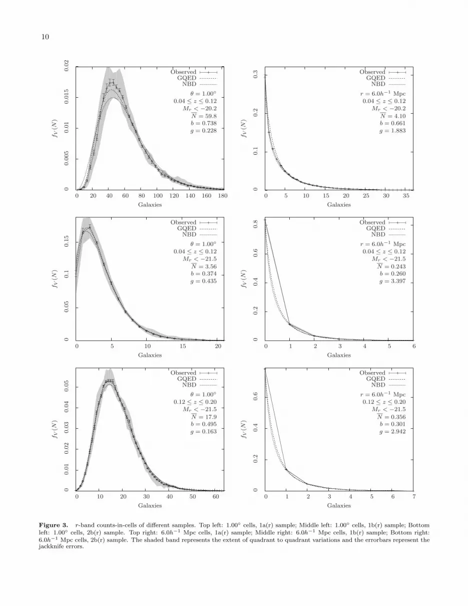
The result that quadrants are generally not identicallydistributed suggests that the jackknife errors underes-timate the true range of variability in the data. Forthis reason, a better and simpler estimate of variabilitywould be to compare fV (N) across quadrants. Hence weuse the quadrant to quadrant variations in fV (N) as ameasure of the variability of the counts-in-cells statistic.We plot the observed counts-in-cells distribution fV (N),the minimum and maximum values of fV (N) from eachquadrant as a shaded band, and the GQED and NBDwith the same mean and variance as the observed fV (N)in figures 3, 4 and 5. We also plot the jackknife errorsas errorbars to illustrate the difference between the jack-knife errors and the quadrant to quadrant variations.

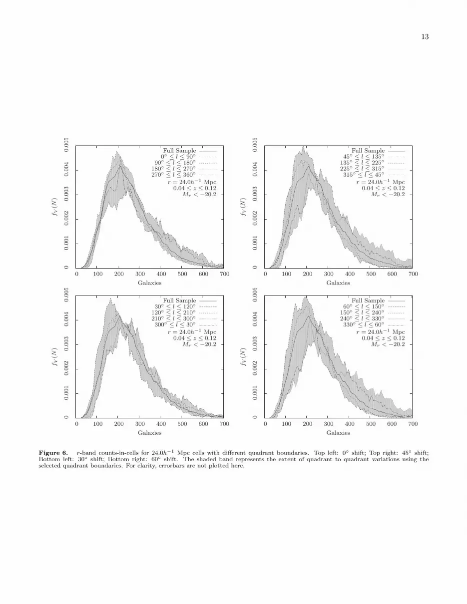
We also repeat the analysis for different quadrantboundaries shifted by 30, 45 and 60 in galactic longi-tude. In all cases, we see a similar amount of variationwhich suggests that in general, the amount of variationbetween quadrants is not coincidental with the choiceof quadrant boundaries. To illustrate, we plot the vari-ation between quadrants for different quadrant bound-aries in figure 6. We note from figure 6 that althoughthe variation between quadrants is different for differentquadrant boundaries, the amount of variation is approx-imately the same. This means that these variations areprobably caused by fluctuations in the number densityof galaxies on scales that are about as large as the quad-rants themselves, suggesting a significant amount of cos-mic variance.

4.2.1. Comparison with models

To study the parameters b and g and compare the ob-served fV (N) to models, we use equations (11) and (13)to obtain b and g in a self-consistent manner from themean N and variance 〈(∆N)2〉 such that the theoreticaldistributions have the same mean and variance as theobserved fV (N). Since the populations of nearby cellsare often strongly correlated, the cells are in general notindependent and a χ2 fit cannot be used. Instead, wecompute the least squares distance

x =

Nmax∑N=0

(fV (N)obs − fV (N))2

(22)

between the observed distribution and the theoreticaldistribution as a qualitative measure of goodness of fitwhere Nmax is the largest number of galaxies in a cell.We use this goodness-of-fit measure to determine whichmodel is closer to the observed data.

We summarize our results in tables 5 and 6. As ex-pected, our results show large differences in N , b and gbetween quadrants. Comparing the observed counts-in-cells distribution between the GQED and NBD, basedon the least squares distance alone, fV (N) for 2D pro-jected cells tend to follow the GQED while fV (N) for 3Dspherical cells tend to follow the NBD. However, in mostcases, the GQED and NBD both fall within the mea-sured quadrant to quadrant variations, and we note that

10

00.

005

0.01

0.01

50.

02

0 20 40 60 80 100 120 140 160 180

fV(N

)

Galaxies

θ = 1.00

0.04 ≤ z ≤ 0.12Mr < −20.2

N = 59.8b = 0.738g = 0.228

ObservedGQED

NBD

00.

10.

20.

3

0 5 10 15 20 25 30 35

fV(N

)

Galaxies

r = 6.0h−1 Mpc0.04 ≤ z ≤ 0.12

Mr < −20.2

N = 4.10b = 0.661g = 1.883

ObservedGQED

NBD

00.

050.

10.

15

0 5 10 15 20

fV(N

)

Galaxies

θ = 1.00

0.04 ≤ z ≤ 0.12Mr < −21.5

N = 3.56b = 0.374g = 0.435

ObservedGQED

NBD

00.

20.

40.

60.

8

0 1 2 3 4 5 6

fV(N

)

Galaxies

r = 6.0h−1 Mpc0.04 ≤ z ≤ 0.12

Mr < −21.5

N = 0.243b = 0.260g = 3.397

ObservedGQED

NBD

00.

010.

020.

030.

040.

05

0 10 20 30 40 50 60

fV(N

)

Galaxies

θ = 1.00

0.12 ≤ z ≤ 0.20Mr < −21.5

N = 17.9b = 0.495g = 0.163

ObservedGQED

NBD

00.

20.

40.

6

0 1 2 3 4 5 6 7

fV(N

)

Galaxies

r = 6.0h−1 Mpc0.12 ≤ z ≤ 0.20

Mr < −21.5

N = 0.356b = 0.301g = 2.942

ObservedGQED

NBD

Figure 3. r-band counts-in-cells of different samples. Top left: 1.00 cells, 1a(r) sample; Middle left: 1.00 cells, 1b(r) sample; Bottomleft: 1.00 cells, 2b(r) sample. Top right: 6.0h−1 Mpc cells, 1a(r) sample; Middle right: 6.0h−1 Mpc cells, 1b(r) sample; Bottom right:6.0h−1 Mpc cells, 2b(r) sample. The shaded band represents the extent of quadrant to quadrant variations and the errorbars represent thejackknife errors.

11

00.

002

0.00

40.

006

0 100 200 300 400 500

fV(N

)

Galaxies

θ = 2.00

0.04 ≤ z ≤ 0.12Mr < −20.2

N = 236.b = 0.823g = 0.131

ObservedGQED

NBD

0.00

50.

010.

015

0.02

0.02

5

0 20 40 60 80 100 120 140

fV(N

)

Galaxies

r = 12.0h−1 Mpc0.04 ≤ z ≤ 0.12

Mr < −20.2

N = 32.5b = 0.790g = 0.668

ObservedGQED

NBD

00.

010.

020.

030.

040.

050.

06

0 10 20 30 40 50

fV(N

)

Galaxies

θ = 2.00

0.04 ≤ z ≤ 0.12Mr < −21.5

N = 14.0b = 0.525g = 0.245

ObservedGQED

NBD

00.

10.

20.

3

0 2 4 6 8 10 12 14 16

fV(N

)

Galaxies

r = 12.0h−1 Mpc0.04 ≤ z ≤ 0.12

Mr < −21.5

N = 1.90b = 0.441g = 1.160

ObservedGQED

NBD

00.

005

0.01

0.01

50.

02

0 20 40 60 80 100 120 140 160

fV(N

)

Galaxies

θ = 2.00

0.12 ≤ z ≤ 0.20Mr < −21.5

N = 71.6b = 0.626g = 0.086

ObservedGQED

NBD

00.

050.

10.

150.

20.

25

0 5 10 15 20

fV(N

)

Galaxies

r = 12.0h−1 Mpc0.12 ≤ z ≤ 0.20

Mr < −21.5

N = 2.86b = 0.497g = 1.030

ObservedGQED

NBD

Figure 4. r-band counts-in-cells of different samples. Top left: 2.00 cells, 1a(r) sample; Middle left: 2.00 cells, 1b(r) sample; Bottomleft: 2.00 cells, 2b(r) sample. Top right: 12.0h−1 Mpc cells, 1a(r) sample; Middle right: 12.0h−1 Mpc cells, 1b(r) sample; Bottom right:12.0h−1 Mpc cells, 2b(r) sample. The shaded band represents the extent of quadrant to quadrant variations and the errorbars representthe jackknife errors.

12

00.

001

0.00

20.

003

0 200 400 600 800 1000 1200 1400 1600 1800

fV(N

)

Galaxies

θ = 4.00

0.04 ≤ z ≤ 0.12Mr < −20.2

N = 945.b = 0.879g = 0.071

ObservedGQED

NBD

00.

001

0.00

20.

003

0.00

4

0 100 200 300 400 500 600 700

fV(N

)

Galaxies

r = 24.0h−1 Mpc0.04 ≤ z ≤ 0.12

Mr < −20.2

N = 259.b = 0.860g = 0.194

ObservedGQED

NBD

00.

010.

020.

03

0 20 40 60 80 100 120 140

fV(N

)

Galaxies

θ = 4.00

0.04 ≤ z ≤ 0.12Mr < −21.5

N = 56.2b = 0.648g = 0.126

ObservedGQED

NBD

00.

010.

020.

030.

040.

050.

06

0 10 20 30 40 50 60

fV(N

)

Galaxies

r = 24.0h−1 Mpc0.04 ≤ z ≤ 0.12

Mr < −21.5

N = 14.9b = 0.588g = 0.328

ObservedGQED

NBD

00.

005

0.01

0 100 200 300 400 500

fV(N

)

Galaxies

θ = 4.00

0.12 ≤ z ≤ 0.20Mr < −21.5

N = 287.b = 0.716g = 0.040

ObservedGQED

NBD

00.

010.

020.

030.

04

0 10 20 30 40 50 60 70 80 90

fV(N

)

Galaxies

r = 24.0h−1 Mpc0.12 ≤ z ≤ 0.20

Mr < −21.5

N = 23.0b = 0.643g = 0.298

ObservedGQED

NBD

Figure 5. r-band counts-in-cells of different samples. Top left: 4.00 cells, 1a(r) sample; Middle left: 4.00 cells, 1b(r) sample; Bottomleft: 4.00 cells, 2b(r) sample. Top right: 24.0h−1 Mpc cells, 1a(r) sample; Middle right: 24.0h−1 Mpc cells, 1b(r) sample; Bottom right:24.0h−1 Mpc cells, 2b(r) sample. The shaded band represents the extent of quadrant to quadrant variations and the errorbars representthe jackknife errors.

13

00.

001

0.00

20.

003

0.00

40.

005

0 100 200 300 400 500 600 700

fV(N

)

Galaxies

r = 24.0h−1 Mpc0.04 ≤ z ≤ 0.12

Mr < −20.2

Full Sample0 ≤ l ≤ 90

90 ≤ l ≤ 180180 ≤ l ≤ 270270 ≤ l ≤ 360

00.

001

0.00

20.

003

0.00

40.

005

0 100 200 300 400 500 600 700

fV(N

)

Galaxies

r = 24.0h−1 Mpc0.04 ≤ z ≤ 0.12

Mr < −20.2


135 ≤ l ≤ 225225 ≤ l ≤ 315315 ≤ l ≤ 45

00.

001

0.00

20.

003

0.00

40.

005

0 100 200 300 400 500 600 700

fV(N

)

Galaxies

r = 24.0h−1 Mpc0.04 ≤ z ≤ 0.12

Mr < −20.2


120 ≤ l ≤ 210210 ≤ l ≤ 300300 ≤ l ≤ 30

00.

001

0.00

20.

003

0.00

40.

005

0 100 200 300 400 500 600 700

fV(N

)

Galaxies

r = 24.0h−1 Mpc0.04 ≤ z ≤ 0.12

Mr < −20.2


150 ≤ l ≤ 240240 ≤ l ≤ 330330 ≤ l ≤ 60

Figure 6. r-band counts-in-cells for 24.0h−1 Mpc cells with different quadrant boundaries. Top left: 0 shift; Top right: 45 shift;Bottom left: 30 shift; Bottom right: 60 shift. The shaded band represents the extent of quadrant to quadrant variations using theselected quadrant boundaries. For clarity, errorbars are not plotted here.

14

Table 5r-band 2D Counts-in-cells fV (N)

Sample Quadrant Cells N b g x× 10−5 x× 10−5

(GQED) (NBD)

θ = 1.001a(r) All 135995 59.8 0.738 0.228 5.68 19.41a(r) 0 ≤ l ≤ 90 35174 64.8 0.773 0.285 10.3 27.41a(r) 90 ≤ l ≤ 180 31916 54.2 0.718 0.213 9.94 21.31a(r) 180 ≤ l ≤ 270 45518 59.0 0.706 0.179 6.60 16.91a(r) 270 ≤ l ≤ 360 15710 64.7 0.728 0.193 32.6 51.4

1b(r) All 135995 3.56 0.374 0.435 6.44 40.41b(r) 0 ≤ l ≤ 90 35174 3.92 0.426 0.519 21.6 84.01b(r) 90 ≤ l ≤ 180 31916 3.13 0.333 0.399 31.3 33.01b(r) 180 ≤ l ≤ 270 45518 3.47 0.321 0.336 8.97 23.91b(r) 270 ≤ l ≤ 360 15710 4.06 0.384 0.403 73.8 137

2b(r) All 135995 17.9 0.495 0.163 2.47 4.652b(r) 0 ≤ l ≤ 90 35174 18.4 0.460 0.132 10.4 9.172b(r) 90 ≤ l ≤ 180 31916 18.4 0.476 0.143 7.61 4.152b(r) 180 ≤ l ≤ 270 45518 17.8 0.534 0.202 9.71 23.82b(r) 270 ≤ l ≤ 360 15710 16.7 0.468 0.152 11.0 16.9

θ = 2.001a(r) All 131804 236 0.823 0.131 2.51 6.241a(r) 0 ≤ l ≤ 90 31218 258 0.852 0.173 8.49 13.71a(r) 90 ≤ l ≤ 180 29022 217 0.805 0.117 12.6 14.01a(r) 180 ≤ l ≤ 270 44054 234 0.796 0.099 15.2 19.71a(r) 270 ≤ l ≤ 360 13105 258 0.803 0.096 17.9 18.5



θ = 4.001a(r) All 131467 945 0.879 0.071 3.62 4.431a(r) 0 ≤ l ≤ 90 24923 1083 0.906 0.103 11.3 11.01a(r) 90 ≤ l ≤ 180 24505 888 0.863 0.059 8.63 8.881a(r) 180 ≤ l ≤ 270 42890 929 0.843 0.043 18.9 19.71a(r) 270 ≤ l ≤ 360 9743 1024 0.806 0.025 25.8 26.8

1b(r) All 131467 56.2 0.648 0.126 27.1 25.41b(r) 0 ≤ l ≤ 90 24923 66.2 0.726 0.186 62.8 64.01b(r) 90 ≤ l ≤ 180 24505 50.7 0.548 0.077 106 91.71b(r) 180 ≤ l ≤ 270 42890 55.2 0.545 0.069 49.1 43.51b(r) 270 ≤ l ≤ 360 9743 65.6 0.516 0.050 90.6 96.0

2b(r) All 131467 287 0.716 0.0396 11.2 10.62b(r) 0 ≤ l ≤ 90 24923 296 0.659 0.0257 39.1 35.42b(r) 90 ≤ l ≤ 180 24505 297 0.650 0.0242 38.6 42.52b(r) 180 ≤ l ≤ 270 42890 287 0.780 0.0682 19.6 22.52b(r) 270 ≤ l ≤ 360 9743 249 0.611 0.0225 35.3 37.5

the observed fV (N) for individual quadrants within asample may be closer to the GQED or NBD. This showsthat the SDSS catalog is unable to distinguish betweenthe GQED and NBD because the difference between theGQED and NBD is smaller than the quadrant to quad-rant variations. Since the NBD has been shown to beunphysical (Saslaw & Fang 1996), on physical groundswe use the GQED for further analysis.

4.2.2. Comparison between redshift ranges

Comparing the values of N and b, between redshiftranges, we note that the values of N and correspondingly

b are lower in the low redshift range than in the highredshift range for the same magnitude cutoff (samples1b and 2b). This is despite the presence of the SDSS“great wall” in the low redshift range.

On a closer look, we note that the “great wall” spansthe region between 0.065 ≤ z ≤ 0.09, 140 ≤ α ≤ 210

and −3 ≤ δ ≤ 6 (Deng et al. 2006) which is a smallfraction of the SDSS footprint. The observed quadrantto quadrant variations of fV (N) do not seem to departmuch from the GQED, so the presence of a large su-percluster probably does not affect the observed form offV (N). This result is in agreement with an earlier anal-

15

Table 6r-band 3D Counts-in-cells fV (N)

Sample Quadrant Cells N b g x× 10−5 x× 10−5

(GQED) (NBD)

r = 6.0h−1 Mpc1a(r) All 141612 4.10 0.661 1.88 338 54.91a(r) 0 ≤ l ≤ 90 35560 4.46 0.679 1.95 295 1151a(r) 90 ≤ l ≤ 180 32542 3.70 0.650 1.94 343 38.81a(r) 180 ≤ l ≤ 270 47263 4.06 0.644 1.70 433 7.941a(r) 270 ≤ l ≤ 360 15545 4.53 0.686 2.02 241 193



r = 12.0h−1 Mpc1a(r) All 134349 32.5 0.790 0.668 30.9 8.721a(r) 0 ≤ l ≤ 90 29558 35.5 0.802 0.693 38.0 11.31a(r) 90 ≤ l ≤ 180 28014 29.4 0.784 0.694 35.1 12.71a(r) 180 ≤ l ≤ 270 44707 32.3 0.777 0.590 32.4 6.671a(r) 270 ≤ l ≤ 360 12145 36.9 0.817 0.780 23.1 47.3


2b(r) All 130665 2.86 0.497 1.03 78.1 5.252b(r) 0 ≤ l ≤ 90 32557 2.93 0.494 0.99 182 8.412b(r) 90 ≤ l ≤ 180 29872 2.92 0.494 0.99 114 5.852b(r) 180 ≤ l ≤ 270 43578 2.87 0.501 1.05 33.7 36.22b(r) 270 ≤ l ≤ 360 14037 2.70 0.486 1.03 26.1 39.1

r = 24.0h−1 Mpc1a(r) All 131132 259 0.860 0.194 1.48 1.541a(r) 0 ≤ l ≤ 90 19301 292 0.871 0.201 13.4 7.791a(r) 90 ≤ l ≤ 180 21734 240 0.856 0.198 5.76 7.241a(r) 180 ≤ l ≤ 270 40900 251 0.845 0.162 3.01 3.491a(r) 270 ≤ l ≤ 360 9179 293 0.881 0.236 16.2 19.6

1b(r) All 131132 14.9 0.588 0.328 4.69 10.81b(r) 0 ≤ l ≤ 90 19301 17.7 0.632 0.359 35.5 10.21b(r) 90 ≤ l ≤ 180 21734 13.1 0.551 0.301 55.4 60.81b(r) 180 ≤ l ≤ 270 40900 14.4 0.547 0.270 23.8 21.81b(r) 270 ≤ l ≤ 360 9179 18.8 0.612 0.300 99.1 115


ysis of the 2MASS catalog by Sivakoff & Saslaw (2005)where it was found that the inclusion of the Shapley su-percluster did not make a large difference on the agree-ment with the GQED. Therefore these large superclus-ters may be natural consequences of gravitational inter-actions among galaxies.

Since the “great wall” probably does not make a largecontribution to the counts-in-cells statistics, the differ-ence in N and b between the high and low redshift rangescould be due to evolution or selection. Further pursuitof these possibilities requires more detailed models. Here

we note that the difference is consistent across quadrantswhich rules out cosmic variance as a dominant cause. Wealso note that the difference in lookback time between themiddle of the low and high redshift ranges is about 0.7Gyr, which is close to the amount of time a merging pairof galaxies takes to merge (Conselice 2009) so we canexpect that the effect of galaxy mergers might make adifference between the low and high redshift range.

4.2.3. Comparison between magnitude cufoffs

As expected from different magnitude cutoffs, the val-ues of N and b are lower for the brighter 1b sample than

16

Table 7Examples of observed and expected values of b for bright

randomly selected subsamples

2D cells 3D cellsθ () b (obs.) b (exp.) r (h−1 Mpc) b (obs.) b (exp.)

1.0 0.374 0.256 6.0 0.260 0.1712.0 0.525 0.406 12.0 0.441 0.3364.0 0.648 0.553 24.0 0.588 0.492

00.

20.

40.

60.

81

b

00.

050.

1

0 5 10 15 20 25 30 35 40

∆b

Cell Radius (h−1 Mpc)

Mr < −20.2 (Observed)Mr < −21.5 (Observed)Mr < −21.5 (Expected)

Figure 7. The value of b as a function of cell radius for bright andfaint galaxies. The bottom plot is the difference between the ob-served and expected value of b for randomly selected bright galax-ies. For a given size cell, the variations between quadrants rangeover 2.5% for the complete sample and 10% for the brighter sample.

the fainter 1a sample. We can compare the value of bfor the brighter sample with the expected value of b ifthe brighter sample is a randomly selected sample froma fainter parent sample using (Lahav & Saslaw 1992):

(1− bsample)2

=(1− bparent)

2

1−(

1− Nsample

Nparent

)(2− bparent) bparent

.

(23)This allows us to compare the clustering of the brighter1a sample with the fainter 1b sample. We find that for allsamples, the brighter galaxies from the 1b samples havea higher value of b than would be expected if they werea random subsample of the 1a sample. This means thatbright galaxies are more strongly clustered than faintergalaxies which may be a result of brighter galaxies beingconcentrated around cluster centers, or in dark matterhaloes. If so, it suggests an upper limit of about 10h−1

Mpc for the size of these haloes. We summarize the com-parisons in table 7 and plot the comparison of b for 3Dcells over a range of cell sizes in figure 7.

5. DISCUSSION AND CONCLUSION

In this paper we have compared the counts-in-cells dis-tribution of galaxies fV (N) with two theoretical models

and found that the observed distribution has large fieldto field variations which may be as great as 20% acrossquadrants. These large variations essentially mean thatthere is a considerable amount of cosmic variance in thedata, and that the galaxies in different quadrants arenot identically distributed. This also means that errorsdetermined using the jackknife procedure will underesti-mate the true range of variation in the data because dif-ferent subsets of the data are not identically distributed.We see the existence of these subregions of different localdensity from the bumps in the counts-in-cells distributionfor large cells. We note that as shown by Coleman &Saslaw (1990), these bumps may be the result of regionsof different local density.

As suggested by Sylos Labini et al. (2009), a largersurvey volume will show less effects of cosmic variance,and an earlier analysis of the 2MASS catalog by Sivakoff& Saslaw (2005) provides a hint that this may be thecase. In the 2MASS analysis, Sivakoff & Saslaw (2005)found less variation between quadrants, on the order of5% instead of the 20% we have found in the SDSS. Wenote that after excluding regions close to the galacticplane using |l| < 20, the 2MASS catalog covers two-thirds of the sky, a coverage that is more than threetimes that of the SDSS.

Although the SDSS “great wall” is contained withinthe low redshift range, it covers only a small fraction ofthe SDSS footprint in a stripe within 6 of the celes-tial equator. For this reason we do not see much differ-ence between the low redshift range and the high redshiftrange beyond differences in N because the overdensityin the “great wall” is not large enough to dominate overthe rest of the survey. Indeed, because the “great wall”is most likely porous in three dimensions, it is not clearthat “great wall” is an accurate description.

Our comparison of γ for 2D projected cells and 3Dspherical cells in redshift space shows that there is a dif-ference in the exponent γ of the two-point correlationfunction between the 2D and 3D sample. The 3D sam-ples have a value of γ that is lower than that for the 2Dsamples because the 3D samples in redshift space are af-fected by peculiar velocity distortions which change theapparent clustering in redshift space. Using the well-known relation between the projected correlation func-tion and the real space correlation function we find thatthe difference in γ between the 2D and 3D samples is ameasure of the redshift space distortions. Our findingsfor the value of γ suggest that the difference betweenthe projected sample and redshift space sample is about0.2 ∼ 0.3 in agreement with work by Fry & Gaztanaga(1994) and Hawkins et al. (2003) using earlier catalogs.

Comparing the low redshift and high redshift range,we find that there is a large difference in N between thelow and high redshift range for samples with the samemagnitude cutoff which may be caused by galaxy merg-ers. We also find that brighter galaxies are more stronglyclustered than a random subset of all galaxies in the lowredshift range, which may be a result of bright galaxiesclustering around cluster centers or dark matter haloes.

The analysis of the counts-in-cells distribution showsthat the observed fV (N) may follow the GQED or NBD,and 2D projected cells generally prefer the GQED while3D spherical cells often prefer the NBD. However, both

17

distributions are generally within the range of quadrantto quadrant variations so we can conclude that both theGQED or NBD are in agreement with observations.

Since the GQED is physically motivated while theNBD was found to be unphysical, we can reject the NBDas a physically complete description of galaxy clustering.This conclusion is not at odds with the results of Conroyet al. (2005) because although the error bars in Conroyet al. (2005) excludes the GQED, jackknife errors wereused which, as our results suggest, underestimate thetrue range of variability in the data.

We conclude that while the SDSS is an excellent sam-ple, there remains a considerable amount of cosmic vari-ance that will probably require an all-sky survey to re-solve. Nevertheless, the counts-in-cells analysis of theSDSS data has shown that observations of fV (N) agreewith the GQED within cosmic variance.

We thank Matt Malkan and Gerry Gilmore for veryhelpful discussions on this subject.

Funding for the creation and distribution of the SDSSArchive is provided by the Alfred P. Sloan Foundation,the Participating Institutions, the National Aeronauticsand Space Administration, the National Science Founda-tion, the US Department of Energy, the Japanese Mon-bukagakusho, and the Max Planck Society. The SDSSWeb site is at http://www.sdss.org.

The SDSS is managed by the Astrophysical ResearchConsortium (ARC) for the Participating Institutions.The Participating Institutions are the University ofChicago, Fermilab, the Institute for Advanced Study,the Japan Participation Group, Johns Hopkins Uni-versity, the Korean Scientist Group, Los Alamos Na-tional Laboratory, the Max-Planck-Institute for Astron-omy (MPIA), the Max-Planck-Institute for Astrophysics(MPA), New Mexico State University, University ofPittsburgh, Princeton University, the US Naval Obser-vatory, and the University of Washington.

REFERENCES

Abazajian, K. N. et al. 2009, ApJS, 182, 543Ahmad, F., Malik, M. A., and Masood, S. 2006, International

Journal of Modern Physics D, 15, 1267Ahmad, F., Saslaw, W. C., and Bhat, N. I. 2002, ApJ, 571, 576Blanton, M. R. et al. 2005, AJ, 129, 2562Bratley, P., Fox, B. L., and Niederreiter, H. 1994, ACM Trans.

Math. Softw., 20, 494Carruthers, P. and Minh, D.-v. 1983, Physics Letters B, 131, 116Coleman, P. H. and Saslaw, W. C. 1990, ApJ, 353, 354Connolly, A. J. et al. 2002, ApJ, 579, 42Conroy, C. et al. 2005, ApJ, 635, 990Conselice, C. J. 2009, MNRAS, 399, L16Crane, P. and Saslaw, W. C. 1986, ApJ, 301, 1Davis, M. and Peebles, P. J. E. 1983, ApJ, 267, 465Deng, X., Chen, Y., Zhang, Q., and He, J. 2006, Chinese Journal

of Astronomy and Astrophysics, 6, 35Dwass, M. 1957, The Annals of Mathematical Statistics, 28, 181Elizalde, E. and Gaztanaga, E. 1992, MNRAS, 254, 247Fry, J. N. 1985, ApJ, 289, 10—. 1986, ApJ, 306, 358Fry, J. N. and Gaztanaga, E. 1994, ApJ, 425, 1Gott, III, J. R., Juric, M., Schlegel, D., Hoyle, F., Vogeley, M.,

Tegmark, M., Bahcall, N., and Brinkmann, J. 2005, ApJ, 624,463

Hamilton, A. J. S. and Tegmark, M. 2004, MNRAS, 349, 115Hawkins, E. et al. 2003, MNRAS, 346, 78Itoh, M., Inagaki, S., and Saslaw, W. C. 1993, ApJ, 403, 476Lahav, O. and Saslaw, W. C. 1992, ApJ, 396, 430Leong, B. and Saslaw, W. C. 2004, ApJ, 608, 636Peebles, P. J. E. 1980, The large-scale structure of the universe

(Princeton, NJ: Princeton University Press)

Rahmani, H., Saslaw, W. C., and Tavasoli, S. 2009, ApJ, 695,1121

Saslaw, W. C. 2000, The distribution of the galaxies :gravitational clustering in cosmology (Cambridge, UK:Cambridge University Press)

Saslaw, W. C., Chitre, S. M., Itoh, M., and Inagaki, S. 1990, ApJ,365, 419

Saslaw, W. C. and Fang, F. 1996, ApJ, 460, 16Saslaw, W. C. and Hamilton, A. J. S. 1984, ApJ, 276, 13Saslaw, W. C. and Haque-Copilah, S. 1998, ApJ, 509, 595Saslaw, W. C. and Yang, A. 2010, in Lecture Notes of the Les

Houches Summer School: Long-Range Interacting Systems, ed.T. Dauxois, S. Ruffo, & L. F. Cugliandolo, Vol. XC (Oxford,UK: Oxford University Press), 377–398

Sheth, R. K. 1995, MNRAS, 274, 213Sivakoff, G. R. and Saslaw, W. C. 2005, ApJ, 626, 795Swanson, M. E. C., Tegmark, M., Hamilton, A. J. S., and Hill,

J. C. 2008, MNRAS, 387, 1391Sylos Labini, F., Vasilyev, N. L., and Baryshev, Y. V. 2009,

A&A, 508, 17Totsuji, H. and Kihara, T. 1969, PASJ, 21, 221

http://www.sdss.org

Documents

The galaxy counts-in-cells distribution from the SDSS