Faculty of Behavioral, Management and Social Sciences

Master of Science in Business Administrations

The Impact of Green Innovation

on Firm Financial Performance

24 April 2020

Full name: Martijn Arjan Hogeslag

Student number: s2032392

E-mail address: m.a.hogeslag@student.utwente.nl

Supervisors: Dr. X. Huang

Prof. Dr. M.R. Kabir

ABSTRACT

This study investigates the relationship between green innovation and firm performance. The

hypothesis that goes with this is: “green innovation affects firm financial performance

positively”. To substantiate this hypothesis the study uses an unbalanced panel dataset and a

sample consisting of 450 unique firms with at least one European granted green patent in one

of the total 1,314 firm year observations between the years 2007 and 2014. These firms have a

combined number of 7,700 new European green patents granted by EPO with its 9,087 citations.

In the OLS regression analysis for the full sample, both the number of patents and citations,

proxies for green innovation, are positively related to ROE as the firm performance measure.

For the number of citations this relationship is also statistically significant at the 1% level.

However, looking at ROA as the performance measure, the number of citations still shows a

positive and significant sign, but for the number of patents it becomes negative and even

significant at the 5% level for some models. For ROS and Profit Margin as the performance

measures the regression reports extremely weak results and almost no significance at all for

both proxies of green innovation. With these mixed results the hypothesis only receives partial

support.

TABLE OF CONTENTS

1 INTRODUCTION 1

2 LITERATURE REVIEW & HYPOTHESIS DEVELOPMENT 4

2.1 Introduction to Green Innovation 4

2.1.1 Four types of Green Innovation 7

2.2 Theories on innovation 9

2.2.1 Innovation Theory 9

2.2.2 Contingency Theory 10

2.2.3 Institutional Theory 11

2.2.4 Resource-based Theory 12

2.3 Empirical Evidence 12

2.3.1 Antecedents of Green Innovation 13

2.3.2 Impact of Green Innovation on Competitive Advantage 15

2.3.3 Impact of Green Innovation on Firm Performance 19

2.3.4 Moderating impacts on the relationship of Green Innovation and performance factors 23

2.3.5 Overview field of study 25

2.4 Hypothesis Development 29

3 METHODOLOGY 31

3.1 Research Methods 31

3.1.1 Structural Equation Modeling 31

3.1.2 Ordinary Least Squares regression analysis 36

3.1.3 Fixed/random effects model 40

3.2 Model used in this study 43

3.3 Variables 45

3.3.1 Dependent variables 45

3.3.2 Independent variables 48

3.3.3 Control variables 51

4 DATA & SAMPLE 57

4.1 Data Collection 57

4.2 Final Full Sample 60

4.3 Distributions 62

4.3.1 Industry Distribution 62

4.3.2 Country Distribution 64

5 RESULTS 65

5.1 Descriptive Statistics 65

5.2 Correlation Matrix 67

5.2.1 Pearson’s Correlation Matrix 67

5.2.2 Multicollinearity 68

5.3 OLS Regression Results 70

5.3.1 Full Sample Results 70

6 ROBUSTNESS CHECKS 75

6.1 Fixed/Random Effects model 75

6.2 Sample split by variable Size 78

6.3 2-Year lag 83

6.4 Patent-sensitive industries 85

6.5 Firms with at least one citation 88

6.6 2-Year and 3-year lag for Firm Performance Improvement 92

6.7 Citation Dummy 96

7 CONCLUSION 98

7.1 Conclusion 98

7.2 Limitations and further research 101

8 REFERENCES 102

9 APPENDIX 109

9.1 Appendix A – Overview of factors within the field of study 109

9.2 Appendix B – Examples of patents with the Y02 classification 118

9.3 Appendix C – List of new European Green Patents granted in 2014 120

9.4 Appendix D – OLS results full sample 121

9.5 Appendix E – Fixed Effects results full sample 124

9.6 Appendix F – Results split samples 127

9.7 Appendix G – Results 2-year lag 135

9.8 Appendix H – Results patent-sensitive industries 139

9.9 Appendix I – Results firms with at least one citation 143

9.10 Appendix J – Results firm performance improvement 147

9.11 Appendix K – Results citation dummy 155

1

1 INTRODUCTION

The world is changing and it is changing tremendously fast. The consequences of global

warming are affecting the world. For the last 45 years, the earth's average temperature rose

0.17°C per decade. That is double the 0.07°C per decade increase that occurred during the entire

period of recorded observations between 1880 and 2015 (Dahlman, 2017). On the other side of

the timeline, looking into the future, it can be seen that the sea levels will rise by 18 to almost

60 centimeter by the end of this century (IPCC, 2007). The latter is a result of the strong

decrease of 7% of the sea ice in the Arctic Ocean since 1979 (Soyez & Grassl, 2008). These

facts and many others indicate that the world and in particular firms need to deal with the

consequences of the changing environment. For firms, in order to change their way of operating

and be sustainable for the future, one of the most logical ways to do this is by investing in green

innovation.

The world became aware of the environmental problems after 1972 when there was a

United Nations conference on the human environment (Dangelico, 2016). However, two

decades ago the world was still dealing with firms that were inexperienced in environmental

solutions. Also, customers did not know that resource inefficiency meant that they had to pay

for the cost of pollution (Porter & van der Linde, 1995). Schiederig, Tietze and Herstatt (2012)

show that one possible reason could be that until 1990 there was hardly any research about

green innovation. In the seven years thereafter the field of study became more popular with

using environmental innovation as the main term. Since 2000, the term sustainable innovation

became more popular and from 2005 until now the concepts of green and eco innovation were

used increasingly. The different terms of describing green innovation are of interchangeable

usage. This study follows the definition of green innovation introduced by Schiederig et al.

(2012), namely: “The innovation object may be a product, process, service or method and it

should satisfy a user’s need or solve a problem and therefore be competitive on the market.

Regarding the environmental aspect it should reduce negative impact, and a full life cycle

analysis and a thorough analysis of all input- and output factors must be done with the aim of a

reduction of resource consumption and with an economical or ecological intention. This all is

for setting a new innovation/green standard to the firm”.

Corporate environmental management was already of real importance two decades ago

(Russo & Fouts, 1997). The rise of strict international regulation and conventions of

environmental protection was because of the fact of growing attention towards the environment

nowadays, which led to a change of the strategies and industries. Chen, Lai and Wen (2006)

2

add to this that in general many businesses have had a negative view of green innovation with

the thought that investing in the protection of the environment would be harmful to their

businesses. However, the study concluded that environmental pressure is something all

businesses have to deal with these days and this asks for a professional attitude towards

managing it. Businesses do not have to avoid these pressures, because by carrying out green

innovation they could be turned into unique competitive advantages. Global competition

demands environmental innovations to raise resource productivity (Porter & van der Linde,

1995). Next to that, proactive strategies in green innovation also prevent firms from facing

environmental protests or penalties and it helps them developing new market opportunities. So,

overall, green innovation improves the performance of a firm.

The field of innovation is already widely studied1. However, the green part of innovation

is still quite a new subject of research. Although, some studies already investigated green

innovation, almost all of them used a survey to gather their data. Performing a survey could

bring disadvantages like data error due to non-responses or questions could be interpreted

differently by different respondents. The study of Aguilera-Caracuel and Ortiz-de-Mandojana

(2013) is the only study of green innovation that does not use a survey to gather their data. This

study will use the same patent database and Y02 classification for green patents they use.

However, the Y02 classification has been available for public as part of the classification

scheme since 2010 and therefore during the time of research of their study there were not many

green patents yet2. Next to that, it is difficult to measure all four parts of green innovation3 with

using a survey and that is why almost all green innovation studies only focus on green product

innovation. By using patent data, like this study, it is able to not only use green product

innovation, but also include the other parts. So, the intention of this paper is to investigate the

impact of green innovation on firm performance while using an unbalanced panel dataset and

to provide concrete suggestions for the field of study. Therefore, this study contributes to the

literature of innovation by going deeper into the green part of it, by adding new empirical

evidence to green innovation based on the use of panel data instead of survey data, and by not

making a distinction between the four parts of innovation and thus not focusing on green

product innovation alone. Formulated into a research question: “To what extent does green

1 Supporting literature: Griliches et al., 1986; Hall et al., 1986; DeCarolis & Deeds, 1999; Hall et al., 2001;

Melvin, 2002; Feeny & Rogers, 2003; Hall et al., 2005; Frietsch & Grupp, 2006; Arora et al., 2008; Harhoff &

Wagner, 2009; Artz et al., 2010; Czarnitzki & Kraft, 2012; Choi & Williams, 2013; Santos et al., 2014; Seru,

2014; Chen et al., 2018; Huang & Hou, 2019; Zhou & Sadeghi, 2019. 2 EPO. “Y02 – E-learning module”. e-courses.epo.org

https://e-courses.epo.org/wbts/y02/index.html (accessed April 24, 2020) 3 These four parts are green product, process, service, and method innovation.

3

innovation influence firm financial performance?”. With using a sample only consisting of

firms with at least one granted green patent an answer will be given to this question. The patent

data is gathered from the EPO database for the period of 2007-2014 and the financial data is

gathered from the ORBIS database for the period of 2010-2017. The full sample consists of a

total of 450 unique firms with 1,314 firm year observations and with a total of 7,700 newly

granted green patents and 9,087 citations. An OLS regression analysis with an unbalanced panel

dataset is performed to test the hypothesis. Additively, robustness checks will be performed to

examine if the results of the main analysis are consistent, robust and provide reliable outcomes.

The first chapter of this study concerns an introduction to green innovation, a literature

review on theories and empirical evidence within this field of study, and with this a hypothesis

will be formed. Thereafter, a methodology will be substantiated wherein the scope of research

methods and variables will be explained. The next chapter described the data collection method

and the final full sample used in this study. After this, the results of the main analysis and

robustness checks will be reported with a thorough substantiation. Lastly, a conclusion will be

made and limitations of this study and avenues for further research will be given.

4

2 LITERATURE REVIEW & HYPOTHESIS DEVELOPMENT

2.1 Introduction to Green Innovation

To understand what innovation means, one must first understand the definition of an invention.

In the study of Artz, Norman, Hatfield, & Cardinal (2010) invention is defined as the creation

of new products and processes through the development of new knowledge or the combination

of existing knowledge. Innovation is a process of transforming an idea or invention into a good

or service that will create value or for which the customers will pay a price. This will further

satisfy the needs and expectations of the customers. Innovation is a popular field of study,

looking at the fact that it has many different interpretable definitions. Many studies already

studied the field of the changing industries and innovations. So, looking at innovation studies

in general, it is known that innovations raise productivity and profitability, improve efficiency

and reduce costs of investments of firms (Hsu, 2009). Rogers (1995) stated decades ago that

innovations with greater advantages when compared to current products will lead to faster and

more widespread adoption.

However, in that time there was not much attention for the impact of innovations on the

environment. Most firms did not think about the positive impacts green innovations could bring,

such as the advantage of lower emission that comes with a higher selling price. Russo and Fouts

(1997) were one of the first that studied the environmental impacts. They state that corporate

environmental management is of real importance. The rise of strict international regulation and

conventions of environmental protection was because of the fact of growing attention towards

the impact on the environment nowadays. Due to the upcoming awareness this led to a change

of strategies and industries (Chen, Lai, & Wen, 2006). Lin, Tan, and Geng (2013) agree and

state that innovation became important for increasing market shares and surviving the long run.

Recently, Gürlek and Tuna (2018) found that successful green innovations improve market

position, attract possible customers and gains competitive advantages.

Same as for innovation, the definition of the green innovation is also interpreted

differently among studies. Due to the rise of awareness for the green part of innovation, the

interest of studies that wanted to define green innovation also increased. For example, the

definition of green innovation from the ISO 14031 standards, as stated by Chen et al. (2006),

defines green innovation as hardware or software innovation that is related to green products or

processes. This includes the technology innovations that are involved in energy-saving,

pollution-prevention, recycling of waste, green product designs, or corporate environmental

management. Although this description is sufficient, this study uses the quantitative literature

5

review of Schiederig et al. (2012) to define green innovation, because this study compares and

summarizes a diversity of definitions of green innovation used by the majority of studies within

this field. They conclude that there are four interchangeable usable notions of green innovation

and they find only minor conceptual differences between the definitions and therefore come up

with a summarized definition, namely: “The innovation object may be a product, process,

service or method and it should satisfy a user’s need or solve a problem and therefore be

competitive on the market. Regarding the environmental aspect it should reduce negative

impact, and a full life cycle analysis and a thorough analysis of all input- and output factors

must be done with the aim of a reduction of resource consumption and with an economical or

ecological intention. This all is for setting a new innovation/green standard to the firm”. To

conclude, this allows dividing green innovation into green product innovation, green process

innovation, green service innovation and green method innovation. These four parts will be

described in more details in the next paragraph.

In today’s society environmental awareness is becoming increasingly important. Many

governments and thus firms have to deal with the impact of their operations on the environment.

Firms could use green innovation to deal with the changing environment and at the same time

increase their performance. Porter and Reinhardt (2007) state that the change of the

environment has two ways of affecting firms. The first and most obvious one is through

changing temperature and weather patterns. But, secondly, regulations also effects firms when,

for example, the cost of emissions increase. Both have an influence on business inputs, access

to related industries, and rules and incentives of rivalry. Of course, managers have to look after

their firm by evaluating the effects of their operations on the environment. Tseng, Wang, Chiu,

Geng, and Lin (2013) state that improving environmental performance and obeying

environmental regulations contributes to the competitiveness of a firm. Firms must improve

their green innovations, otherwise they weaken their competitiveness due to the rapidly

changing green technology and the short life cycle of products. Aguilera-Caracuel and Ortiz-

de-Mandojana (2013) acknowledge this as well and describe two different reasons why green

innovation could help firms to be profitable, but also why it improves the quality of life. Firstly,

green innovation can enhance preventive pollution. Firms could recycle and reuse materials and

this will help a firm to save on operating costs. Next to that, environmental protection is a hot

topic nowadays. So, firms could acquire a better ecological reputation if they show their green

initiatives. A consequence is that such a firm could ask for premium prices and this greater

social approval could also increase their sales. This allows firms to differentiate their products.

Both reasons show a source of valuable opportunities.

6

So, green innovative studies agree that firms must introduce green innovation for having

a sustainable future. The expectation of reputation improvement and of opportunities for

innovation are the most important internal factors that drive the development of green

innovation. The external factors concern environmental regulations, market demand and market

stakeholder pressure, and networking activities (Dangelico, 2016). So, managers should know

the importance of these factors. Porter and van der Linde (1995) name a few things managers

could do to change their operations in order to reach that sustainable future. Firstly, they could

measure direct and indirect environmental impacts instead of ignoring them. Secondly, they

could learn to recognize opportunity cost of underutilized resources. Thirdly, they should create

a positive bias towards innovation-based, productivity-enhancing solutions. And finally, they

should be more proactive towards new types of relationships with regulators and

environmentalists to get a new (greener) mind-set. Unruh and Ettenson (2010) also provide

strategies to align a firm’s green goal with their capabilities, namely accentuate, acquire, and

architect. The first one involves playing up existing or latent green attributes in their portfolio.

The second regards buying someone else’s green brand. However, one needs to keep in mind

the culture clash and the strategic fit. The third one contains the innovation of new green

products. This is slower and more costly than the other two, but at the end it will be the best

strategy, because it leads to valuable competencies.

Although different strategies exist to reach a sustainable future, all firms generally have

the same goal, namely earning profits and surviving in the marketplace. To reach this goal,

firms have to add value to the customers through the core business processes. One way to do

this is by incorporating environmental concerns. Ultimately, this could lead to an improvement

of a firm’s overall efficiency and thus an increase in the performance and reduce in costs of the

firm. However, every firm needs to tackle climate change differently and on their own way, as

long as it reduces climate-related costs and risks. These approaches are mostly operational

effective, but can also become strategic. But, for both they need to realize that carbon emissions

are costly in order to reduce this. Implementing the best practices for reducing these costs is

necessary to remain competitive. Firms could, for example, create environmentally friendly

products, such as the reusable coffee cups4, but could also restructure industries to cope with

environmental impacts, or innovate activities that are sensitive to climate change. These

4 Barrett, Clear. “What’s the return on investing in a reusable coffee cup?” ft.com

https://www.ft.com/content/edddb47c-0b22-11e8-839d-41ca06376bf2 (accessed November 28, 2018)

7

examples are forms of green innovation and this will lead to a better performance of the firm

(Porter & Reinhardt, 2007).

2.1.1 Four types of Green Innovation

Because of the definition used in this study, green innovation can be divided into four types;

green product, process, service, and method innovation. These four types will be used to

describe green innovation on itself in more detail. Although, this study will make no further

distinction between these types. It is also necessarily to mention that green product innovation

completely dominates the other three types of green innovation for incorporating environmental

concerns into corporate operations (Chan, Yee, Dai, & Lim, 2016). But in this section, for the

sake of completeness, the four different types of green innovation will be substantiated

consecutively.

First of all, starting with green product innovation, literature struggled with defining it.

Yet several studies did try to come up with a definition or assumption. Back in 2004 the

European Economic Interest Grouping (EEIG) concludes that product innovation has the largest

impact on the environment. Poor product design and environmental regulations of developing

countries could have negative impacts like waste issues (EEIG, 2004). Oke et al. (2007) agree

and they provide a general definition of product innovation that matches the distribution used

by the quantitative literature review of Schiederig et al. (2012). They describe product

innovation as the offering of new products or improvements of existing products.

Regarding the green part, Reinhardt (1998) was one of the first to describe this

definition. He simplistically expresses it as the kind of innovation that not only protects the

environment, but also provides environmental benefits higher than conventional products.

Moreover, Tseng et al. (2013) also look at the green aspect and go a step further. They divide

green product innovation into five aspects, namely; the degree of new green product

competitiveness understands customer needs, the evaluation of technical, economic and

commercial feasibility of green products, the recovery of firm’s end-of-life products and

recycling, the use of eco-labeling, environment management system and ISO 14000, and the

innovation of green products and design measures. Furthermore, to specify towards green

product innovation, The Commission of the European Communities (2001) defines it as

products that reduce the negative impacts and risks to the environment, utilize less resources

and prevent waste generation during the phase of product’s disposal.

Moreover, as most of the green innovative studies use a survey to measure green

innovation, they name different classifications that could identify a green innovation. Chen et

8

al. (2006) name a few items to measure green product innovation, namely; the firm chooses

materials with the least amount of pollution, energy consumption, and resources for conducting

the product development or design, the firm uses the fewest amount of materials, and the firm

would use products that are easy to recycle, reuse, and decompose. Chiou, Chan, Lettice, and

Chung (2011), Ar (2012) and Lin et al. (2013) state that whenever product innovation uses

environmentally friendly materials, improves and designs environmentally friendly packaging

for existing and new products, recovers a firm’s end-of-life products and recycling, and uses

eco-labeling, it could be called green product innovation.

Furthermore, less study has been done to green process, service, and method innovation,

Oke, Burke, and Myers (2007) study process and service innovation and define process

innovation as creating or improving methods of production, service or administrative operations

as well as developments in the processes, systems and reengineering activities undertaken to

develop new products. They describe service innovation as new developments in activities to

deliver the core product and make it more attractive to consumers. They acknowledge the study

of Klassen and Whybank (1999) as they state that green process innovation is any adaptation

to the manufacturing process that reduces the negative impact on the environment during

material acquisition, production, and delivery. Moreover, Chen et al. (2006) use ISO 14031

standards to define green process innovation as the performance in process innovation that is

related to energy-saving, pollution-prevention, waste recycling, or no toxicity (Lai et al., 2003).

Green process innovation is used to increase the performance of environmental management

and this helps protecting the environment. Similarly, Chiou et al. (2011) also operationalize

green process innovation. They state that whenever an process innovation has a low energy

consumption during production, use, and disposal; recycle, reuse, and remanufacture material;

and use cleaner technology to make savings and prevent pollution, it could be labeled as green

process innovation.

Regarding green method innovation, Schiederig et al. (2012) describe that, for example,

green business models or marketing methods are meant by this. Chiou et al. (2011) have made

an effort to operationalize green managerial innovation, which is comparable with green

method innovation described by Schiederig et al. (2012). They name redefining operation and

production processes to ensure internal efficiency and re-designing and improving product or

service to obtain new environmental criteria or directives as measurements of green managerial

innovation (Chiou et al., 2011). Unfortunately, other studies did not study this type of green

innovation due to the fact that it is tremendously difficult to measure the impact of it.

9

In summary, it can be stated that the main type of green innovation is green product

innovation. Many previous studies were interested in only this type of green innovation and its

impact on the performance of a firm and used a survey to gather their data. However, this study

will use an unbalanced panel dataset that unfortunately cannot make a distinction between these

types. So, this study will look at green innovation in general and therefore contributes to

literature as most previous studies only look at green product innovation.

2.2 Theories on innovation

The field of green innovation is quite new, so there have not been many theories on the green

part of innovation yet. However, of course the field of innovation itself is been widely studied

and many theoreticians have already described their theories on innovation. This study will

substantiate them and will make a link to the green part of innovation.

2.2.1 Innovation Theory

Back in the 30’s of previous century, far ahead of the awareness of climate change, Schumpeter

(1934) defined an innovation theory where many innovation studies are based on. He was the

first to explicitly research innovation (Santos, Basso, Kimura, & Kayo, 2014). In his study, he

describes innovation as the creation of new knowledge, or the transformation of new

combinations of existing knowledge into innovation within the organization. This perspective

could be explained by five types of innovation: new product, new process, new markets, new

input sources and new industrial structures. These five types have two sides of innovation;

radical and incremental innovation. The first are innovations originating from the process of

creative destruction, such as technological discoveries, shifting to something completely new

that could be associated with a product or process. The latter is the continuous improvement

process that aims to consolidate radical changes and to strengthen the market position (Santos

et al., 2014). The innovation theory of Schumpeter explains that adaptable firms that try new

creative ways of operating are more likely to outperform firms that do not, especially in a

competitive environment. He states that trying new ways of using a firm’s knowledge,

technology and resources brings new opportunities that ultimately could lead to a stronger

market position. Schumpeter describes these changes as a dynamic process of ‘creative

accumulation’. Therefore, innovation brings new levels of economic performance for all

industries and this could be explained by the inputs to and outputs of innovation, namely R&D

intensity and patent intensity respectively (Choi & Williams, 2013).

10

2.2.2 Contingency Theory

Next to Schumpeter’s theory as the foundation of innovation theories, many studies also use

the contingency theory (Sousa & Voss, 2008). The theory explains the firm as a complex

organization of individuals and focuses on analyzing the firm its internal structure and the

relationship among departments and units (DeCarolis & Deeds, 1999). This theory helps

explaining the behavior of organizations, because it states that organizations adapt their

structures in order to keep up with the changing contextual factors, so that it reach high

performance. There is no best way to organize or lead a firm. The process of decision making

differs across firms, but the impact of the same decisions also differ across firms. For a

contingent manager or leader it is all about applying their own style to the right situation.

Morgan (1998) describes that organizations are open systems. These systems need thoughtful

management for internal needs and to be able to adapt to environmental elements, without

having a best way of tackling this. However, there are three theoretical and practical

contributions of this theory. Firstly, one needs to identify important contingency factors that

distinguish between contexts. Secondly, one needs to group different contexts based on the

contingency factors. Thirdly, one needs to determine the most effective internal organization

designs or responses in all of the different contexts groups.

So, this theory defines three types of factors, namely contextual, response and

performance factors. These will be substantiated by linking this to the field of green innovation.

The first refers to the exogenous situational characteristics that could influence the organization.

In most of the cases, these factors are hard to control or manipulate, but a manager with enough

effort could change the impact of it in the long-term (Sousa & Voss, 2008). Examples of a

contextual factor are environmental dynamism or market demand (Lin et al., 2013). But, the

most interesting contextual factor is the pressure of environmental regulations (Chan et al.,

2016). These regulations are rapidly changing. So, if firms are not constantly adapting to these

regulations, they will weaken their competitiveness (Tseng et al., 2013). One way of adapting

to this is by investing in green innovation. This is an example of the second factor, which refers

to the actions taken by the organizations in response to the contextual factors. Chan et al. (2016)

argue that green innovation and environmental regulations cannot be separated. The latter are

unstable and uncertain yet inevitable in today’s society. So, they consider green product

innovation as a positively associated consequence of the pressure of environmental regulations

and policies. Regulatory pressure is one of key drivers for firms to develop a sustainable future.

Regulatory pressure itself does not lead to an increase in firm performance. Therefore,

managers have to convert these pressures by using (e.g.) green innovation. Many studies within

11

this field are interested in at least green innovation as the response to these contextual factors.

Although, most of the studies do not test for the relationship between them, but only between

the response and the third factor; the performance factor. The performance measures the

effectiveness of the response factor subject to the contextual factor. Most of the studies within

this field are mostly interested in firm performance or competitive advantage as the

performance factor.

Sousa and Voss (2008) state that according to the contingency arguments, an

organization should use practices that are both effective to a high degree and ineffective to a

low degree. This is in line with the perspective of practices being adopted due to efficiency

factors to directly improve performance. However, this does not explain when a firm has non-

efficiency drivers of adoption or when it focuses on building capabilities as the alternative

source of performance. Therefore, they name the institutional theory and resource-based theory

respectively as promising theories that address the limitations of the contingency theory.

2.2.3 Institutional Theory

The institutional theory considers the structures of an organization as authoritative guidelines

for social behavior. The institutional theory argues that practices could also be adopted due to

non-efficiency instead of efficiency like the constitutional theory describes. In this way, a firm

could gain legitimacy whether or not the practices may lead to a performance increase (Sousa

& Voss, 2008). Aguilera-Caracuel and Ortiz-de-Mandojana (2013) describe that studies use the

institutional theory to study the adoption and diffusion of organizational practices among

organizations. Organizations with the same environment will have similar practices and

motives and will thus correspondent with each other. These practices become institutionalized

and thereby the society will adopt them and see them as legitimate. This means that countries

will regard and respond differently to environmental issues based on the two dimensions

described by the institutional theory (Hoffman, 1999). The first dimension is called the

regulatory dimension and refers to the existing laws and rules in a particular national

environment that promote certain types of behavior and restrict others (Kostova, 1999). The

second is called normative dimension and refers to the cultural values, beliefs, and goals of the

society regarding organizational behavior (Kostova & Roth, 2002). Linking this to the study

means that one could expect differences between countries for the effect of green innovation

on firm performance.

12

2.2.4 Resource-based Theory

The resource-based theory defines that not all resources are of the same importance and not all

of them will become a source of a sustainable competitive advantage. Because, it depends on

whether the resources could be imitated or substituted. So, the performance of a firm results

from valuable resources that are difficult to obtain and hard to imitate or trade. This explains

why firms not always adopt efficient practices from other firms, but rather invest in other

sources of performance advantage (Sousa & Voss, 2008).

So, a manager or leader of an organization must identify the potential key resources of

a firm and find out whether these resources are valuable, rare, not imitable and not substitutable.

Examples of these intangible resources are brand names, skilled employees, machinery, and

capital (Cho & Pucik, 2005). The resource-based theory substantiates that the unique resources

and capabilities of a firm are the key drivers of competitive advantage and business

performance. The manager of the firm must cultivate these capabilities and deploy them in

product-market strategies to strive for this advantage (DeCarolis & Deeds, 1999). Green

innovation is such a unique capability and thus a key driver of firm performance within this

study. Hart (1995) is one of the key theoreticians of this theory and he states that capabilities

that avoid pollution, ensure sustainable development and generate environmental solutions

provide competitive advantage to a firm. The theory defines that competitive advantage leads a

firm to perform better than its competitors, because a firm could have relatively lower operating

costs or could differentiate itself. When green innovation is successful it could make imitation

more difficult, which allows firms to sustain their competitive advantage longer and thus

increase their firm performance (Chang, 2016).

2.3 Empirical Evidence

Previous studies already studied the field of green innovation. Overall, these studies stimulate

the strategic approaches a firm could take to reduce emissions by stating that it will, next to

helping the environment, increase the performance of the firm (Olson, 2014). It will provide

them social, environmental and economic benefits. Kim, Moon and Yin (2016) partly agree

with Olson by stating that on the one hand environmental management leads to become

competitive and gain legitimacy, which leads to a better performance of a firm. But on the other

hand, it could create additional costs, such as the costs of solid waste disposal, which have a

negative influence on firm performance (Palmer, Oates, & Portney, 1995). Multinational firms

have a hard time developing sustainable green strategies to meet the demands of stakeholders,

which makes it an interesting field of study.

13

This section will be based on the factors described by the contingency theory to fully

describe green innovation as the center of research. Firstly, the antecedents of green innovation

will be described. These are similar to the contextual factors defined by the contingency theory.

Of course, there are many different ways for a manager or leader to make a decision to respond

to these factors and there is no best way. One could, for example, move the headquarter of the

firm to another country when national regulations are too strict. But, this study only focuses on

green innovation as the response action. Although firm performance will be the performance

factor of this study, competitive advantage will also be outlined for the sake of completeness.

2.3.1 Antecedents of Green Innovation

Antecedents, or as the contingency theory calls them; contextual factors, should not be

overlooked. The most interesting antecedent is the pressure of environmental regulations (Chan

et al., 2016). Porter and van der Linde (1995) were one of the first to describe that many firms

could open up new market segments and determine higher prices for green products by carrying

out the opportunities that reduce pollution through innovations that redesign products,

processes, and operations. Firms that succeed in becoming green will be distinguished by their

commitment to being environmental sustainable and to the performance of their green products

(Unruh & Ettenson, 2010). However, firms will more often not go for these opportunities

without environmental regulation that pushes them. This is because of the fact that managers

often do not have complete information and unlimited time and attention. There are too many

barriers to change into a more environmentally friendly business. This means that these kinds

of regulations play an important part in green innovation. Bad regulation could damage

competitiveness, while good regulation could enhance it. Environmental regulations provide

opportunities for firms to increase their green product innovation as it is the most important

external driver for the development of green innovation (Chan et al., 2016; Dangelico, 2016).

So, policies regarding environmental regulations should become stricter to encourage greener

innovations.

Moreover, Chan et al. (2016) describe that the pressure of environmental

regulations/policies pushes firms into a more sustainable development. These pressures may

not directly lead to a better firm performance. However, they are directly related to green

innovation, because these pressures are inevitable. Therefore, they hypothesize whether the

pressure of environmental regulations/policies is positively associated with green product

innovation. These regulations include national and regional regulations on the environment, on

resource saving and conservation, but also on products that potentially conflict with laws. Their

14

sample consists of 250 operations managers from the operating industry in China that who have

completed the survey between April 24 and May 8 in 2015. They find a positive relation that is

significant at the 1% level between the pressure of environmental regulations and green product

innovation. This means that the managers of these firms use green product innovation as a

response to these regulations as it converts these pressures into a better environmental

performance.

Furthermore, Chiou et al. (2011) use another antecedent of green innovation, namely

greening the supplier. This is in line with the argumentation of environmental regulations and

policies described by Chan et al. (2016), because customers and buyers require their suppliers

to also have environmentally friendly products and materials. Firms need to cooperate with

suppliers early in the product development process, because in this way they could reduce the

negative impacts on the environment. So, they test whether greening the supplier is positively

associated with green product, process, and even managerial innovation. Chiou et al. (2011)

state that a firm could do a few things to encourage their suppliers to go green. They could

encourage them by requiring and assisting suppliers to obtain a third-party certification of

environmental management system, by providing environmental awareness seminars and

training for suppliers, by providing environmental technical advice to suppliers and contractors

in order to help them to meet the environmental criteria, by inviting suppliers to join in the

development and design stage, and/or by sending in-house auditor to appraise the

environmental performance of the supplier. Their sample consists of 124 respondents from the

purchasing department of firms in Taiwan. The results report that greening the supplier is

positively related and significant at the 1% level to all three parts of green innovation. So, the

results show that if firms have used at least one of the ways to encourage their suppliers to go

green, it has led to internal green product, process and method innovations. So, firms should

work together with their suppliers to become more environmentally friendly.

Another antecedent of green innovation is market demand. Lin et al. (2013) state that

especially green product innovation is being adopted to meet market demand and to gain a

competitive advantage. The key elements of market demand are customer benefit and price,

and customer preference can be influenced by the price of the product. However, although many

customers want firms to produce green products, they do not align their actual purchasing

behavior with these requirements. Finding balance between these factors in order to meet

market demand is still difficult for many firms. When firms notice a gap between supply and

demand in the market, they could respond to this by having successful green innovations,

meaning that these innovations are critical to survive and improve market position. Therefore

15

they hypothesize that market demand is positively associated with the three types of green

product innovation performance. They define market demand by the segmentation of the

market, by the requirements about green products of the customers, by the price flexibility of

demand for green products, and by the customer benefits for these green products. The study

uses a sample of 208 respondents that are a CEO, director, or manager of a Vietnamese firm

operating in the motorcycle industry and filled out the survey between January and July 2011.

They indeed find a positive relationship between market demand and the three types of green

product innovation performance. Unfortunately, they do not report the level of significance. So,

manufactures should understand the market demand. Because, if a firm manages its market

demand well, then its green product innovation performance will improve.

Lastly, Gürlek and Tuna (2018) are interested in the antecedent factor green

organizational culture, because firms with a green organizational culture could contribute to

further protection of the environment. Environmental regulations and policies alone are not

sufficient enough. A firm also has to develop a green organizational culture to make green

innovations into a success. Therefore they hypothesize the positive effect of green

organizational culture on green innovation. They define green organizational culture as a set of

shared mental assumptions that guide interpretation and action in organizations by describing

appropriate behavior in different kind of situations. Their sample consists of 545 employees or

managers of four- and five-star hotel companies in Antalya that filled out the survey in August

2016. The results reveal that green organizational culture has a positive on green innovation as

this relationship is significant at the 1% level. This means that a green organizational culture is

an important antecedent of green innovation as it shapes the actions regarding the environment.

The antecedents of green innovation have a positive effect on green innovation when a

firm uses it as a response to them. So, many firms will do well by going green. Although, some

have a more proactive attitude by greening the supplier and others need the push of inevitable

environmental regulations to go green.

2.3.2 Impact of Green Innovation on Competitive Advantage

Competitive advantage is one of the two main performance factors green innovation has. This

section will introduce the performance factor first and then describe the empirical evidence of

the link between green innovation and competitive advantage done by other studies.

Back in the days many businesses had a general negative view of green innovation. They

thought that investing in the protection of the environment was harmful to their businesses.

Because, the inefficiently use of resources results in unnecessary waste, defects, and stored

16

materials. This can be seen from scrap, harmful substances, or pollution. Firms may think that

helping the environment will bring additional activities that add costs but create no value for

customers, such as the handling, storage and disposal of waste. The bottom line is that managers

should not focus on these actual additional costs, but focus on including the opportunity costs

of pollution. Environmental improvement and competitiveness come together and managers

must recognize environmental improvement as economic and competitive opportunities instead

of additional cost or inevitable threats. The early movers will have the major benefits. So,

environmental innovation has two sides of the trade-off, namely the side of the social benefits

arising from environmental standards and the side of industry’s private costs for prevention and

cleanup, which means higher prices and lower competitiveness. However, properly designed

environmental standards could trigger innovations that lower these costs and therefore improve

the value of the product. Firms could use inputs more effectively and productively for

improving environmental impact and this makes firms more competitive (Porter & van der

Linde, 1995).

Yet, the study of Chen et al. (2006) states that environmental pressure is something all

businesses have to deal with these days and this asks for a professional attitude towards

managing this. Businesses do not have to avoid this, because these pressures could be turned

into unique competitive advantages by carrying out green innovation. Next to that, proactive

strategies in green innovation also prevent firms from facing environmental protests or penalties

and it helps them developing new market opportunities. They define this corporate competitive

advantage as “the firm occupies some positions where the competitors cannot copy its

successful strategy and the firm can gain the sustainable benefits from this successful strategy”.

So, Chen et al. (2006) declare that green innovation increases resource productivity to

make up with the environmental costs. Besides, businesses will also have first-mover

advantages, so they could ask for higher prices for green products. This will lead to a better

image, selling their green technologies and services and the creation of new markets (Porter &

van der Linde, 1995). Chang (2016) also points out that a firm’s resources could provide

competitive advantage when these are valuable, unique, and imperfectly imitable. Having a

better capability of using these resources could decrease the difficulty of adjusting to future

changes. The environmentally impact on the economy is increasing, so firms should have an

environmental vision and management. The latter takes care of conveying the environmental

goals. However, Li, Su and Lin (2010) argue that many fail to recognize the fact that many

competitors and imitators actually have profited more from the innovation. Both studies have a

17

fair point, but green innovation will only lead to competitive advantage when it could not be

imitated.

Regarding empirical evidence, Chen et al. (2006) study green innovation for firms

operating in information and electronics industries in Taiwan and their sample consists of 203

managers in manufacturing, marketing, R&D, or environmental protection departments that

filled in the survey. They divide green innovation into green product innovation and green

process innovation and hypothesize that the performance of green product and process

innovation is positively associated with corporate competitive advantage. They state that a firm

has competitive advantage when a firm occupies some positions where competitors cannot copy

their strategies while this strategy brings the firm benefits. Their measurement of competitive

advantage contains of eight strategies in which a firm could score relatively better than

competitors to (partly) have competitive advantage over their competitors, namely; lower costs,

higher quality of products or services, more capable of R&D and innovation, better managerial

capabilities, better profitability, exceeding growth of the firm, being a first mover and

occupying important positions, or a better corporate image. They find a positive relation

between green innovation and competitive advantage for both green product and process

innovation. This relationship is significant at the 5% level for green product innovation and at

the 1% level for green process innovation. The study did not found any general significant

differences between green product and process innovation. Although, it had some industrial

differences. Thus, increasing green product and process innovation will lead to stronger

corporate competitive advantage and this performance is helpful to businesses.

Moreover, Chiou et al. (2011) follow and broaden the definition of green innovation as

used in Chen et al. (2006) and also test whether it is positively related to competitive advantage.

This study also uses firms in Taiwan as a sample, but this study aimed to extend their study

beyond a single sector in Taiwan. They state that customers are becoming more

environmentally conscious and firms have to respond to this by introducing green innovation

to meet market demand and gain competitive advantage. They measure competitive advantage

by a firm its customer response, product design and innovation, quality of products and services,

and low production costs. While using the sample of 124 respondents from the purchasing

department of firms in Taiwan they find positive relations between green product, process, and

method innovation and competitive advantage as well. These three relationships are all

significant at the 1% level, concluding that firms could gain competitive advantage by

implementing green innovation. This means that by implementing green innovation firms have

lower production costs, increased productivity and efficiency, better product and service

18

quality, and a better response from customers that leads to an improvement of competitive

advantage.

Furthermore, Gürlek and Tuna (2018) also describe the conflict that environmental

protection activities could have a negative effect on firms. The solution that was often used was

abandoning the green or green washing. However, green innovation could be a better solution,

because these innovations give the opportunity to both protect the environment and increase

competitive advantage. The study substantiates that high green innovation creates competitive

advantage for the organization, because it provides a strategy that many competitors cannot

take over, which provides them more financial benefits. These organizations gain the advantage

of differentiation and the advantage of cost savings. A win-win solution which increase product

value and decreases the costs of environmental effects (Porter & van der Linde, 1995; Chang,

2016). They study four- and five-star hotel firms in Antalya and test whether green innovation

has a positive effect on competitive advantage. They use the same items used by Chen et al.

(2006) to measure competitive advantage and they find that green innovation has a positive

effect on competitive advantage as well. This relationship is significant at the 1% level. This

means that green innovation provides a strategy competitors cannot perfectly imitate and this

leads to more financial benefits compared to their competitors.

Moreover, Frenken and Faber (2009) state that environmental innovation is of great

importance regarding being sustainable. Ar (2012) agrees and adds to this that green innovation

is increasingly important for firms to show they are aware of the environmental impacts by

producing non-hazardous and non-toxic products. He studies the largest 1000 exporters

explained by Turkish Exporters Assembly for 2010 and checks whether green product

innovation has a positive influence on competitive capability. Although he names it competitive

capability instead of competitive advantage, he means the same. Because, he measures it by

similar items, such as if the products could not be easily substituted, the arrival of new

competing products, and the time of products becoming obsolete, which correspondents to the

imitability of products. He finds a positive relationship between green product innovation and

competitive capability and this relationship is significant at the 1% level. Ar checked if this

relationship is stronger for managers with high environmental concerns as well, but that was

not the case.

Pujari (2006) also agrees by stating that green innovation is portrayed as an opportunity

and more and more firms are going to see that. However, the study argues that it is uncertain

whether green innovation truly achieves market success. Lin et al. (2013) take away this

uncertainty and state that firms need green innovation as an opportunity to reduce the negative

19

influences of production on the environment. They acknowledge that this will lead to

competitive advantage which ensures a larger market share (Dangelico & Pontrandolfo, 2010).

Olson (2014) adds that green product innovation has the advantage of not relying on system

redundancy for reliability compared to conventional innovations. Widely adopted green

innovations also provide non-green user benefits. Successful green innovations will compensate

conventional innovations which makes it financial attractive and only these innovations can

have significant positive impacts on the environment. Improving product design and quality

leads to higher prices and higher profit margins. Green product innovation increases resource

productivity by saving on materials, lowering energy consumption, increasing the recycling of

waste and reducing the use of the resources. That is why environmentalists and government

policy makers promote green innovation and they usually use three main reasons. Firstly, they

state that non-green innovation have unfair advantages, because of the failure to pay for dealing

with greenhouse gases. Secondly, new green innovations require start-up subsidies, otherwise

it could not compete with older non-green innovations. Thirdly, green subsidies lead to high

value green industries and jobs (Olson, 2014).

To summarize, green innovation could turn environmental pressures into competitive

advantages, but only when these are valuable, unique, and imperfectly imitable. Otherwise, the

competition could just copy it and profit more from it. Previous studies indeed find a positive

relationship between green innovation and competitive advantage and most of these

relationships are significant at the 1% level. These studies name being the first-mover and

demanding higher prices as the main reasons for this positive effect.

2.3.3 Impact of Green Innovation on Firm Performance

Other studies name firm performance instead of competitive advantage as the most important

performance factor, because some doubt whether competitive advantage is a real performance

factor at all as it may lead to firm performance. Meaning that firm performance could be seen

as a consequence of competitive advantage and thus a more fitting performance factor (Ar,

2012; Gürlek & Tuna, 2018). Although, many studies use a different name for firm

performance, they almost all mean practically the same. Again, this section will describe the

performance factor and the empirical evidence of the link between green innovation and firm

performance done by other studies.

Some studies only studied the impact of green product innovation on firm performance,

because this type of green innovation has the largest part in green innovation and is therefore

easier to measure. Lin et al. (2013), for example, studied green product innovation in the

20

Vietnamese motorcycle industry. They state that with green product innovation firms could

gain sustainable development and achieve their business targets. So, they emphasize that green

product innovation and firm performance should incorporate considerations related to the

knowledge of market demand. The study divides green product innovation performance into

three main aspects, namely environmental performance, products, and economic performance

and hypothesizes that all three kinds are positively associated with firm performance. Because

of using a survey, they measure firm performance by checking if a firm’s market position

improves and if a firm’s sale volume, profit rate, or reputations enhances (Li et al. 2010). They

indeed find that all three kinds are positively associated with firm performance. Unfortunately,

as already stated, they do not report the level of significance. So, if a firm manages the market

demands well, then the performance of the green product innovation and thus the performance

of the firm will improve, which leads to a better market position and reputation.

Moreover, Ar (2012) also substantiates why there is a relationship between green

product innovation and firm performance, because he finds that a change in a regulatory policy

may affect green product innovation and thus firm performance. He hypothesizes that there is

a positive relationship between green product innovation and firm performance. Because, this

type of innovation encourages using raw materials efficiently and this results in lower costs for

these materials what eventually leads to new ways of converting waste into saleable products

to increase cash flow, competitive advantage and thus firm performance. He measures firm

performance by sales growth, market share, and return on investment. With his sample of the

largest 1000 exporters explained by Turkish Exporters Assembly for 2010 he finds a positive

relationship between green product innovation and firm performance for all three measurements

of firm performance and all significant at the 1% level. Combining this results with his

antecedent factor shows that firms should take into account changes in regulatory policies that

may affect green product innovation, because this may result in a better firm performance. The

positive relation between green product innovation and firm performance demonstrates the

strong influence of green product innovation and this confirms previous literature (Pujari, 2006;

Chen et al., 2006; Chiou et al., 2011).

Similar to Lin et al. (2013) and Ar (2012), Chan et al. (2016) also study green product

innovation. However, they divide firm performance in firm profitability and cost efficiency.

These two represent the major visions of firms, because most of the firms are either pursuing

premium prices or cost-oriented. They name green product innovation a direct consequence of

the pressure of environmental regulations and policies and hypothesize whether green product

innovation is positively associated with firm profitability and cost efficiency. They measure

21

profitability with profit/loss, return on assets, profit margin, and return on equity. Regarding

cost efficiency, they name products with low costs, low inventory costs, low overhead costs,

and an offer price as low or lower than competitors as items that measure it. With their sample

of operation managers from the industry operating in China they find a positive relationship for

both firm performance indicators and both are also significant at the 1% level. These results in

combination with the positive significant relationship between the pressure of environmental

regulations/policies and green product innovation prove that, because of environmental

pressure, firms could develop green product innovations, which is a key capability for

competitiveness that will increase firm performance (Porter & van der Linde, 1995). So,

managers have to align their firm’s activities with (e.g.) green product innovation to cope with

these pressures in order to increase their firm performance. But, policy makers could also learn

from these results. They need to consider the practical implications when setting up

environmental regulations, because otherwise the responsibility would only blindly shift to the

manufacturers. In the future, many firms that are unable to innovate will not survive and this

affects the economy of the whole country.

Next, Aguilera-Caracuel and Ortiz-de-Mandojana (2013) study green innovative firms

that have registered a higher percentage of green patents at EPO for the past 20 years and use a

matched-pairs sample of pairs of 88 green innovative and 70 non–green innovative firms with

green patents granted by EPO. They state that green innovation is one of the most proactive

ways of achieving the benefits of environmental development. Green innovative firms could

enhance their firm performance by using two complementary mechanisms. Firstly, by

implementing green innovation firms could improve their reputation and legitimacy through

external agents. This will lead to an increase in their revenues. Secondly, green innovative firms

are always looking for improvements in green management processes to improve the

performance and reduce the operating costs. Therefore, they hypothesize that green innovative

firms experience a greater improvement in financial performance than non-green innovative

firms. They measure the improvement of firm performance by the change of return on assets

for two consecutive years. They analyzed the improvement of firm performance during the

period of 2008-2010 and find that firm performance is indeed higher for green innovative firms

than for non-green innovative firms. This is significant at the 10% level. Although, the

improvement of firm performance is not higher for green innovative firms than non-green

innovative firms as they find no significant relationship. They give some reasons why this could

be the case. For example, it takes time before green innovative firms could potentially improve

22

their firm performance, not all green innovative firms have the necessary conditions to improve

their firm performance.

Same as Aguilera-Caracuel and Ortiz-de-Mandojana, Li et al. (2010) also study Chinese

firms and the field of innovation and firm performance, but not the green aspect. So, logically,

their variable product innovation is a combined variable of green product innovation and non-

green product innovation. They state that product innovation improves market position

compared to competitors, creates entry barriers, establishes a leadership position, creates new

distribution channels and customers and therefore increases the performance of a firm.

Therefore, they hypothesize that there is a positive relationship between product innovation and

firm performance. In this study firm performance is measured by market position, sales volume,

profit rate, and reputation. Their results support this relationship significantly at the 1% level,

which means that product innovation is beneficial for the performance of a firm. So, top

managers should include product innovation in their strategies.

Lastly, Chiou et al. (2011) study firms in Taiwan, but call it environmental performance

and hypothesize whether the three forms of green innovation, namely

product/process/managerial, have a positive relationship with environmental performance.

They measure this performance by the level of hazardous waste and emission reduction, the

level of water, electricity, gas, and petrol consumption, and the improvement of environmental

compliance. They find support for the positive relationship between green product/process

innovation and environmental performance significant at the 1% level, but not with green

method innovation and environmental performance as this relationship is not significant and

even shows a slightly negative sign. The reason could be that green managerial innovation has

a more indirect effect on a performance variable. This makes it interesting to check whether

this variable have an indirect impact on the relationship between green innovation and a

performance factor. This will be further explained in paragraph 2.3.4.

So, overall studies find a positive relationship between green innovation and firm

performance significant at the 1% level. This concludes that green innovation ensures lower

material costs, improves the position in the market compared to competitors, creates new

channels of distribution and attracts new customers. This all leads to an improvement of the

performance of a firm.

23

2.3.4 Moderating impacts on the relationship of Green Innovation and

performance factors

There could also be indirect impacts on the relationship between green innovation and a

performance factor, the so called moderation effect. It could occur when the relationship

between green innovation and the performance factor depends on a third factor, the moderator.

This factor changes the strength or direction of the effect of the relationship.

Most of the studies within the field of innovation that test for other impacts on the

relationship between green innovation and performance factors test for the effect of moderators.

For example, Aguilera-Caracuel and Ortiz-de-Mandojana (2013) study whether there is a

moderating effect on the relationship between green innovation and the financial performance

improvement of green innovative firms and test for two moderators, namely stringent

environmental regulations and environmental normative level. The first includes the challenges

environmental regulations contain, because these regulations are difficult to implement, are

inefficient, and differ in stringency for each country. This could cause disadvantages for the

profitability of firms. Thus, they hypothesize that the more stringent the environmental

regulations are in a country, the lower the positive relationship will be between green innovation

intensity and the financial performance improvement of green innovative firms. The stringency

of environmental regulations is measured by the regulation levels of air pollution, toxic waste

disposal, water pollution, chemical waste, clarity and stability, flexibility, and innovation, but

also by leadership in environmental policies and the consistency of regulation enforcements.

They find a negative moderating effect significant at the 10% level. This means that the greater

the stringency of environmental regulations in a country, the lower is the probability that green

innovation will lead to better financial performance improvement. The second includes that

countries where environmental issues are relevant will appreciate environmental improvements

in firms. Because they did not find that the improvement of firm performance is significantly

higher for green innovative firms than non-green innovative firms, they concluded that not all

green innovative firms have the necessary conditions to improve their firm performance. Thus,

they hypothesize that the higher the level of environmental norms in a country, the greater the

positive relationship between green innovation intensity and financial performance

improvement of green innovative firms. They indicate this by the level of contribution of the

public sector to international and bilateral funding for environmental projects and development

aid. However, they do not find a significant moderating effect. This could be because the

majority of societies are still too concerned with environmental regulations.

24

Next to that, Chan et al. (2016) also test for the effect of a moderator, environmental

dynamism, on the relationship between green product innovation and the two measurements of

firm profitability. They describe this moderator as frequent and rapid changes induced by

technology, customers, and suppliers. The significant moderating effect of environmental

dynamism makes clear that managers should consider these changes when designing green

innovative products in a dynamic environment, because it could increase firm performance.

They find this positive relationship significant at the 1% level for the first measurement of firm

performance, namely cost efficiency, and conclude that this relationship is stronger in an

environment characterized by high dynamism. For the second measurement, firm profitability,

they only find marginal support as the significant level is 10%, but still enough to confirm the

relationship. So, firms could better improve their firm performance under a dynamic

circumstance, but the improvement is found to be more for cost efficiency than for firm

profitability. However, they also note that these results might be influenced, because cost

efficiency is easier to measure than firm profitability.

More interestingly for this study is the study of Ar (2012). He uses managerial

environmental concern as a moderator variable on the relationship between green product

innovation and firm performance and between green product innovation and competitive

capability. The study states that the more the commitment of management towards innovation,

the more the willingness of the implementation of green innovations as it is one of the most

important factors of innovation. He measures it by checking whether the environmental

innovation is not necessary to achieve high levels and an important and effective component of

strategy, and whether most environmental innovations are worthwhile. He finds a stronger

relationship between green product innovation and firm performance in high managerial

environmental concern than in low managerial environmental concern as this relationship is

positively significant at the 5% level. However, this result was not found in the relationship of

green product innovation on competitive capability from the level of managerial environmental

concern. A possible explanation could be that product innovation activities may not lead to

competitive capability although firms seek competitive advantage firstly through product

innovation. Sectorial differences and competition level in the sector could be possible reasons.

Unfortunately, the results of the study of Ar (2012) do not focus on these sectorial differences

(Friar, 1999). He also does make a statement that further research should include other

moderator variables such as environmental regulation or environmental policy.

There are many other impacts on the relationship between green innovation and a

performance factor that could be examined. However, almost none of the impacts that have

25

already been tested has good substantiated or strong significant empirical evidence. Next to

that, all of these other impacts are measured by using a questionnaire, because there is no data

available to measure it. So, therefore investigating such an impact on the aforementioned

relationship will be left out of this study.

2.3.5 Overview field of study

To summarize, the majority of studies with empirical evidence of a relationship between green

innovation and firm performance or similar performance factors conclude that there is in fact a

positive significant relationship between green innovation and these performance factors. Some

studies divide firm performance in more specific firm performance factors and environmental

performance is one of them (Chiou et al., 2011; Lin et al., 2013). However, this study focuses

on the financial part of firm performance: economic performance. Therefore, it is important to

mention that this study will express economic/financial firm performance as firm performance.

Table I and Figure I give an overview of the most used factors and relationships that have to do

with green innovation. Of course, there are many more and most of the factors could also be

split into more specific factors. Appendix A gives an overview of these factors. Next to that,

table II gives an overview of the costs and benefits of green innovation.

Moreover, most of the studies within the field of green innovation use a survey to gather

their data, because green innovation is difficult to measure. A problem that arises when one

uses a survey is the non-response bias between the groups of respondents, although this could

be solved easily. However, a limitation it brings is the limited choice of research methods one

can use to test the hypothesis, because of the fact that green innovation will not be directly

observable while using a survey. This will be explained in paragraph 3.2. Next to that, many of

the surveys done by other studies only focus on green product innovation as this is the easiest

one to measure with this method of data gathering. By using patent data, like this study, it is

able to not only use green product innovation, but also include green process, service, and

method innovation. Therefore, this study contributes to the literature.

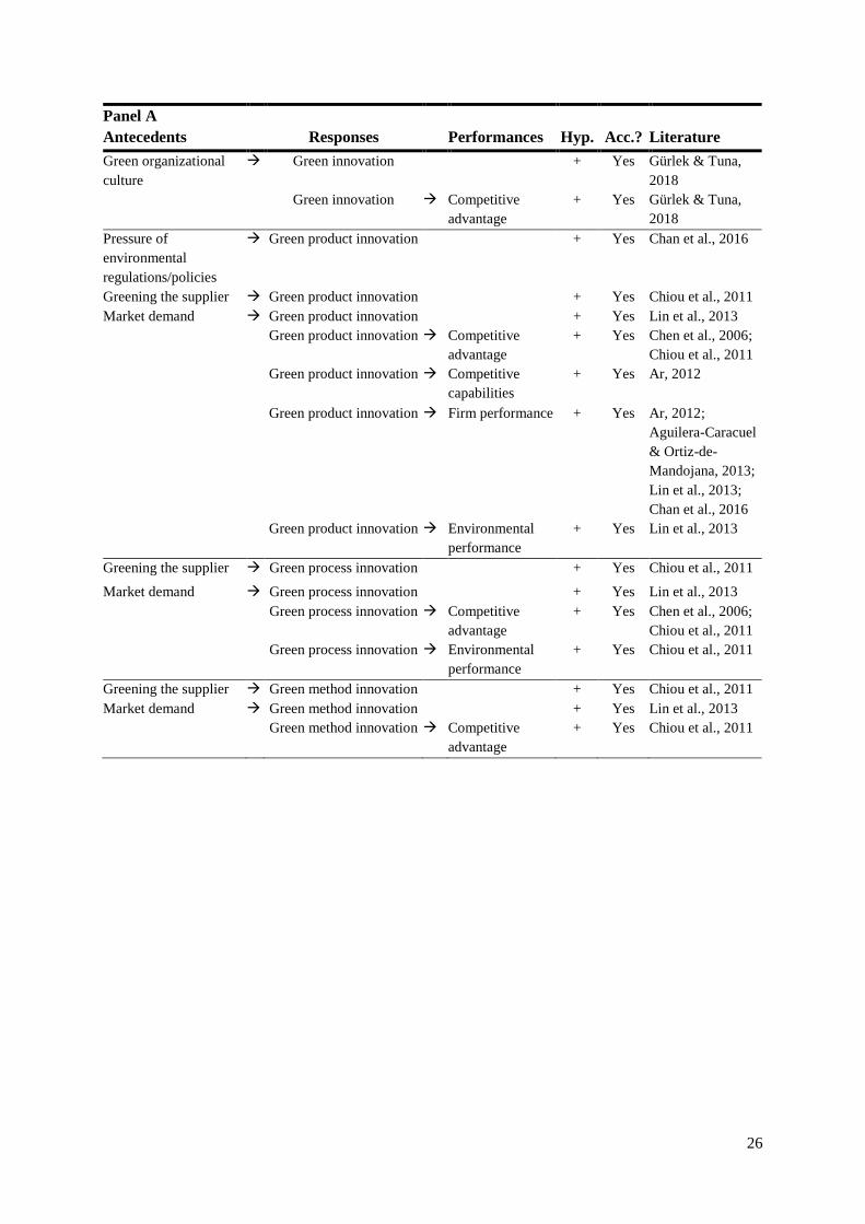
26

Panel A

Antecedents Responses Performances Hyp. Acc.? Literature

Green organizational

culture

Green innovation

+ Yes Gürlek & Tuna,

2018

Green innovation Competitive

advantage

+ Yes Gürlek & Tuna,

2018

Pressure of

environmental

regulations/policies

Green product innovation + Yes Chan et al., 2016

Greening the supplier Green product innovation + Yes Chiou et al., 2011

Market demand Green product innovation + Yes Lin et al., 2013

Green product innovation Competitive

advantage

+ Yes Chen et al., 2006;

Chiou et al., 2011

Green product innovation Competitive

capabilities

+ Yes Ar, 2012

Green product innovation Firm performance + Yes Ar, 2012;

Aguilera-Caracuel

& Ortiz-de-

Mandojana, 2013;

Lin et al., 2013;

Chan et al., 2016

Green product innovation Environmental

performance

+ Yes Lin et al., 2013

Greening the supplier Green process innovation + Yes Chiou et al., 2011

Market demand Green process innovation + Yes Lin et al., 2013

Green process innovation Competitive

advantage

+ Yes Chen et al., 2006;

Chiou et al., 2011

Green process innovation Environmental

performance

+ Yes Chiou et al., 2011

Greening the supplier Green method innovation + Yes Chiou et al., 2011

Market demand Green method innovation + Yes Lin et al., 2013

Green method innovation Competitive

advantage

+ Yes Chiou et al., 2011

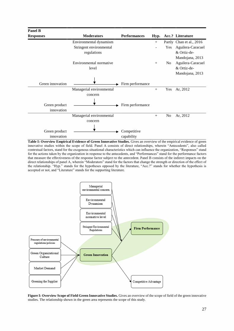
27

Panel B

Responses Moderators Performances Hyp. Acc.? Literature

Environmental dynamism + Partly Chan et al., 2016

Stringent environmental

regulations

-

Yes Aguilera-Caracuel

& Ortiz-de-

Mandojana, 2013

Environmental normative

level

+ No Aguilera-Caracuel

& Ortiz-de-

Mandojana, 2013

Green innovation Firm performance

Managerial environmental

concern

+ Yes Ar, 2012

Green product

innovation

Firm performance

Managerial environmental

concern

+ No Ar, 2012

Green product

innovation

Competitive

capability

Table I: Overview Empirical Evidence of Green Innovative Studies. Gives an overview of the empirical evidence of green

innovative studies within the scope of field. Panel A consists of direct relationships, wherein “Antecedents”, also called

contextual factors, stand for the exogenous situational characteristics which can influence the organization, “Responses” stand

for the actions taken by the organization in response to the antecedents, and “Performances” stand for the performance factors

that measure the effectiveness of the response factor subject to the antecedent. Panel B consists of the indirect impacts on the

direct relationships of panel A, wherein “Moderators” stand for the factors that change the strength or direction of the effect of

the relationship. “Hyp.” stands for the hypotheses opposed by the literature, “Acc.?” stands for whether the hypothesis is

accepted or not, and “Literature” stands for the supporting literature.

Figure I: Overview Scope of Field Green Innovative Studies. Gives an overview of the scope of field of the green innovative

studies. The relationship shown in the green area represents the scope of this study.

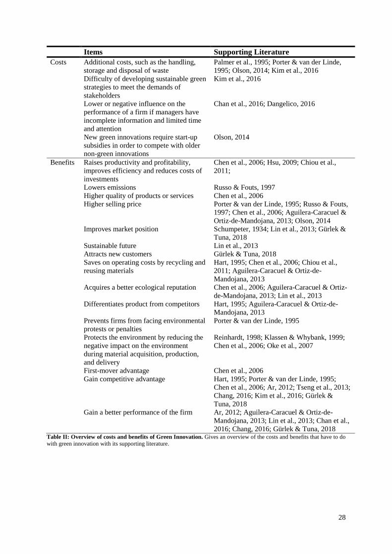
28

Items Supporting Literature

Costs Additional costs, such as the handling,

storage and disposal of waste

Palmer et al., 1995; Porter & van der Linde,

1995; Olson, 2014; Kim et al., 2016

Difficulty of developing sustainable green

strategies to meet the demands of

stakeholders

Kim et al., 2016

Lower or negative influence on the

performance of a firm if managers have

incomplete information and limited time

and attention

Chan et al., 2016; Dangelico, 2016

New green innovations require start-up

subsidies in order to compete with older

non-green innovations

Olson, 2014

Benefits Raises productivity and profitability,

improves efficiency and reduces costs of

investments

Chen et al., 2006; Hsu, 2009; Chiou et al.,

2011;

Lowers emissions Russo & Fouts, 1997

Higher quality of products or services Chen et al., 2006

Higher selling price Porter & van der Linde, 1995; Russo & Fouts,

1997; Chen et al., 2006; Aguilera-Caracuel &

Ortiz-de-Mandojana, 2013; Olson, 2014

Improves market position

Schumpeter, 1934; Lin et al., 2013; Gürlek &

Tuna, 2018

Sustainable future Lin et al., 2013

Attracts new customers Gürlek & Tuna, 2018

Saves on operating costs by recycling and

reusing materials

Hart, 1995; Chen et al., 2006; Chiou et al.,

2011; Aguilera-Caracuel & Ortiz-de-

Mandojana, 2013

Acquires a better ecological reputation Chen et al., 2006; Aguilera-Caracuel & Ortiz-

de-Mandojana, 2013; Lin et al., 2013

Differentiates product from competitors Hart, 1995; Aguilera-Caracuel & Ortiz-de-

Mandojana, 2013

Prevents firms from facing environmental

protests or penalties

Porter & van der Linde, 1995

Protects the environment by reducing the

negative impact on the environment

during material acquisition, production,

and delivery

Reinhardt, 1998; Klassen & Whybank, 1999;

Chen et al., 2006; Oke et al., 2007

First-mover advantage Chen et al., 2006

Gain competitive advantage Hart, 1995; Porter & van der Linde, 1995;

Chen et al., 2006; Ar, 2012; Tseng et al., 2013;

Chang, 2016; Kim et al., 2016; Gürlek &

Tuna, 2018

Gain a better performance of the firm Ar, 2012; Aguilera-Caracuel & Ortiz-de-

Mandojana, 2013; Lin et al., 2013; Chan et al.,

2016; Chang, 2016; Gürlek & Tuna, 2018 Table II: Overview of costs and benefits of Green Innovation. Gives an overview of the costs and benefits that have to do

with green innovation with its supporting literature.

29

2.4 Hypothesis Development

In this section, the arguments used to explain the positive relationship between the types of

green innovation and firm performance will be described.

It all started with the change in regulatory policies that affected firms. Although, it was

understood that innovation could improve market position compared to competitors, create

entry barriers, establish a leadership position, create new distribution channels and customers

(li et al., 2010), many firms still saw green innovation as an obstacle towards a better financial

future (Ar, 2012). Fortunately, previous studies did prove the opposite, namely that investing

in green innovation does contribute towards a better world, but also a better performance of the

firm. Ar (2012) finds that green product innovation encourages the use of raw materials

efficiently and this results in lower costs and new ways of converting waste into saleable

products. This could increase cash flow and thus increase the performance of a firm. Lin et al.

(2013) agree and state that with this type of green innovation firms could gain sustainable

development. Moreover, Chan et al. (2016) add that firms could use these regulations in their

advantage by developing green innovations as it is a key capability for competitiveness that

will increase the performance of a firm. Many firms that are unable to cope with the changing

industries will not survive. Literature states that green innovation converts the increasing

pressure of environmental regulation into a better performance of the firm. Something all firms

have to deal with, so managers should have a proactive attitude towards it (Chen et al., 2006;

Chiou et al., 2011; Chan et al., 2016; Chang et al., 2016).

Furthermore, Artz, Norman, Hatfield, and Cardinal (2010) state that firms being able to

develop and exploit their innovative capabilities is known as one of the most critical

determinants of firm performance. A continuous stream of innovations allows a firm to develop

or maintain a better market position. So, a relatively rapid stream of innovations could enable

a firm to constantly generate high profits. Choi and Williams (2013) describe three ways of

how all kinds of innovation could impact firm performance. They firstly explain that technical

knowledge is hard to imitate within a short period. So, the firm could have a competitive

advantage in this period and therefore the firm could gain a better market position to see its

sales increase. Secondly, firms that continuously use their technical knowledge and experience

to create new opportunities within their competitive field will be more adaptable to changing

environments and thus are more likely to identify profitable opportunities. And thirdly, this

exceptional knowledge and experience could provide better resources that are necessarily for

executing the profitable innovations.

30

Additionally, the theories already argue the positive impact of green innovation as

Schumpeter (1934) explains that adaptable firms that try new creative ways of operating are

more likely to outperform firms that do not, especially in a competitive environment. Green

innovation is one of these creative ways nowadays, because in order to invest in green

innovation a firm has to try new ways of using its knowledge, technology and resources. By

using the capabilities of a firm and its valuable resources that are difficult to obtain and hard to

imitate or trade a firm could gain a better performance of the firm. Therefore, the firm has to

identify these potential key resources as it is a key driver of firm performance. Although the

institutional theory describes that firms within the same environment will have similar

institutionalized and legitimate practices and motives, it is expected that countries will regard

and respond differently. Furthermore, looking at the three types of factors described by the

contingency theory this study focuses on the direct relationship between the response factor and

performance factor, because there are many contextual factors that could trigger a firm to

innovate in way that also takes into account the environment. Of course, based on the factors

described by the contingency theory, green innovation will be used as the response factor.

Regarding the performance factor, as already stated, studies name firm performance instead of

competitive advantage as the most important performance factor (Ar, 2012; Gürlek & Tuna,

2018).

So, empirical evidence regarding the relationship between green innovation and firm

performance generally describe a positive and significant outcome. However, most of the green

studies only focus on green product innovation, because this type of green innovation is the

easiest to measure. Next to that, most of them use a survey to measure it. Therefore, this study

will take into account all parts of green innovation and will use an unbalanced panel dataset to

try to confirm the evidence of previous literature. The named arguments based on the empirical

evidence and theories described in this chapter lead to the following hypotheses:

H1 Green innovation affects firm financial performance positively.

31

3 METHODOLOGY

3.1 Research Methods

Previous studies with similar hypotheses as this study are analyzed to determine which method

to use. This section mentions the different methods that are used by others to test the impact of

an independent/contextual factor on a dependent/performance factor. These methods are

Structural Equation Modeling (SEM), the Ordinary Least Squares (OLS) regression analysis

and the fixed/random effects model (FE/RE). OLS and a fixed/random effects model will be

used in this study, although SEM seems more appropriate at first sight. This will be explained

in paragraph 3.2, but first each method will be described in this section.

3.1.1 Structural Equation Modeling

Structural Equation Modeling (SEM) is a statistical technique for testing and estimating causal

relations using a combination of statistical data and qualitative causal assumptions. It models

causal relationships within their nomological net, takes measurement error into account at the

item level, and shows an intuitive graphical representation of the theory. There are two SEM

techniques, namely the covariance-based SEM and the variance based SEM. SEM has some

requirements for data and samples that apply to both techniques. The data must be metric, quasi-

metric and/or dichotomous. It is striking that most of the studies within the field of green

innovation use SEM to test their hypotheses, because they gather their data by using surveys

(Chen et al., 2006; Li et al., 2010; Chiou et al., 2011; Ar, 2012; Chan et al., 2016, Chang, 2016;

Gürlek & Tuna, 2018). The Likert scales data used by these surveys are examples of quasi-

metric and dummy variables are examples of dichotomous. One advantage of SEM is that there

are no distributional assumptions, which means that data may be non-normal, skewed, and

kurtotic. However, it does have requirements regarding sample size, because the recommended

sample size is ten times the number of maximum arrowheads pointing on a latent variable. Also,

technically, the number of observations could be smaller than the number of variables and the

number of parameters. So, exceeding the recommended sample size makes convergence likely.

But, this will be too small to even identify moderate effects (Henseler, 2017).

In SEM the model of the relationship between the variables will be displayed as shown

in Figure II, where x stands for the indicators, also called the observed variables, ξ stands for

the latent variable, the unobserved variable, ε stands for the error terms, λ stands for loading

factors, and the arrow reflects a linear relationship. The latent variable in this study would be

green innovation and examples of indicators are; using less or non-polluting/toxic materials,

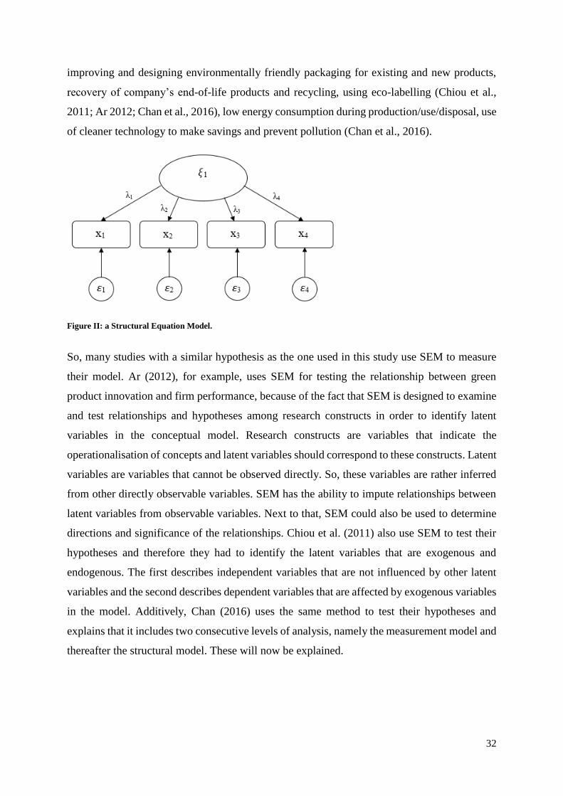
32

improving and designing environmentally friendly packaging for existing and new products,

recovery of company’s end-of-life products and recycling, using eco-labelling (Chiou et al.,

2011; Ar 2012; Chan et al., 2016), low energy consumption during production/use/disposal, use

of cleaner technology to make savings and prevent pollution (Chan et al., 2016).

Figure II: a Structural Equation Model.

So, many studies with a similar hypothesis as the one used in this study use SEM to measure

their model. Ar (2012), for example, uses SEM for testing the relationship between green

product innovation and firm performance, because of the fact that SEM is designed to examine

and test relationships and hypotheses among research constructs in order to identify latent

variables in the conceptual model. Research constructs are variables that indicate the

operationalisation of concepts and latent variables should correspond to these constructs. Latent

variables are variables that cannot be observed directly. So, these variables are rather inferred

from other directly observable variables. SEM has the ability to impute relationships between

latent variables from observable variables. Next to that, SEM could also be used to determine

directions and significance of the relationships. Chiou et al. (2011) also use SEM to test their

hypotheses and therefore they had to identify the latent variables that are exogenous and

endogenous. The first describes independent variables that are not influenced by other latent

variables and the second describes dependent variables that are affected by exogenous variables

in the model. Additively, Chan (2016) uses the same method to test their hypotheses and

explains that it includes two consecutive levels of analysis, namely the measurement model and

thereafter the structural model. These will now be explained.

33

3.1.1.1 Measurement Model

The measurement model contains an evaluation of the reliability and the validity. In this model

the latent variables will be defined by using observable variables (Henseler, 2017). Chiou et al.

(2011) add that the measurement model, next to evaluating the reliability and validity of the

model, also defines relationships between the observed and unobserved variables.

Firstly, before analysing the two levels of analysis, the sample size must be taken into

account. Chiou et al. (2011) state that sample size is one important issue in SEM, because it

affects the degrees of freedom of the model and the model fitting process. A sample size must

be between 100 and 200 and below 100 is not stable. When using a survey, one must also use

a test to verify non-response bias between the groups of respondents. A t-test and Chi-Square

test could be used as a test. The t-test evaluates the differences in means between two groups

and the Chi-Square test examines the two groups based on control variables, such as industry

level, firm size, and firm age. Insignificancy in these tests mean there are no significant

differences between the two groups. So, when the sample size requirement is satisfied and the

global fit indices of the measurement model are accepted, the measurement model could be

examined.

So, thereafter, one could perform an exploratory or a confirmatory factor analysis and

should check the global fit indices. A factor analysis itself is a method used to reduce a large

number of variables into fewer factors. An exploratory factor analysis is a method to detect the

underlying structure of a large set of variables. A confirmatory factor analysis is used to test

how well the measured variables represent the number of constructs. So, it allows for the

assessment of fit between observed data and an a priori conceptualized, theoretically grounded

model (Hooper, Coughlan, & Mullen, 2008). Ar (2012), for example, started with an

exploratory factor analysis to determine the measurement scales and thereafter a confirmatory

factor analysis was conducted to validate the data. The latter is used to verify unidimensionality,

discriminant and convergent validity. But, before testing unidimensionality, reliability and

validity, Ar tests the global fit indices of his model. Regarding unidimensionality, he deleted

items that loaded on multiple constructs and with too low item-to-construct loadings. In this

way, it is possible to check whether the requirements arising from measurement issues are

satisfied or not to start with SEM. Gürlek & Tuna (2018) also perform a confirmatory factory

analysis and then test their structural model. To do this, they used the two-stage approach of

Anderson and Gerbing (1988) wherein firstly the measurement model is examined separately

from the structural equation model to test whether the measurement model has acceptable fit

indices. Secondly, confirmatory factor analysis is performed. The maximum likelihood method

34

was used to test the measurement model and structural model. However, one can only use this

method if the assumption of normal distribution is achieved. Li et al. (2010) and Chang (2016)

also use a confirmatory factor analyses for all constructs to further test the composite reliability

and construct validity. Moreover, Chiou et al. (2011) used confirmatory factor analysis as a pre-

test analysis to validate the sample size and non-response bias between the two groups. The

first is of great importance, because it affects the degrees of freedom of the model and the model

fitting process. So, firstly a confirmatory factor analysis must be performed to verify reliability

and validity and to check the global fit indices of the measurement model.

So, these factor analyses are necessary to assess the reliability and validity of the

reflective measurement models within this kind of research. Therefore, reliability and validity

will be discussed in more detail. Reliability refers to the overall consistency of the model and

validity refers to the extent that the model measures what is was designed to measure. Henseler

(2017) describes two types of reliability, namely construct reliability and indicator reliability

and two types of validity, namely discriminant validity and convergence validity. However, no

study within this field of study mention any measure of indicator reliability, so that one will be

left out. Examples of construct reliability are Dillon-Goldstein‘s rho, Dijkstra-Henseler‘s rho,

and the most popular and therefore most used one is Cronbach’s alpha coefficient. Although,

previous studies refer to the term composite reliability when they test construct reliability

measures. These different types of reliability and validity will now be described.

Firstly, regarding construct or composite reliability, many studies use Cronbach’s alpha

to test composite reliability of each construct and items established in their study (Chen et al.,

2006; Oke et al., 2007; Li et al., 2010; Chiou et al., 2011; Ar, 2012; Lin et al., 2013; Chan et

al., 2016; Chang, 2016; Gürlek & Tuna, 2018). The value is between 0.00 and 1.00 and the

larger the value, the better is the consistency in the measurement (Vogt, 1999). Hair, Anderson,

Tatham and Black (1998) state that the minimum requirement must be 0.70. Nunnally (1978)

adds that in early phases of research, a value of 0.70 is regarded as acceptable. In later phases,

the threshold should be higher, for instance 0.80 or 0.90. However, newer scales have a less

strictly threshold, because the value must be higher than 0.60. Next to Cronbach's Alpha, Chiou

et al. (2011) also used Corrected Item-Total Correlation (ITC). ITC sums up each item

correlation and then excludes items with ITC values below 0.40. This makes it possible to check

if excluding them increases the value of Cronbach’s alpha (Nunnally, 1978). Unfortunately, as

already stated, no study mention any measure of indicator reliability.

So, secondly and thirdly, the validity will be tested. Chang (2016) describes three ways

to verify the validity of the measurement model. Firstly, when a study uses a survey it must

35

refer to previous research to design questionnaire items to achieve a high level of content

validity. Thereafter, the study must measure the average variance extracted (AVE) to access the

discriminant validity of the measurement model. Thirdly, the value of AVE of all constructs

must be more than 0.5, so that the convergent validity is acceptable. The majority of studies use

AVE to test for discriminant and convergent validity, which measures the internal consistency

of the model (Li et al., 2010; Chiou et al., 2011; Ar, 2012; Chan et al., 2016; Chang, 2016;

Gürlek & Tuna, 2018). Fornell and Larcker (1981) state that the value of AVE of each construct

should exceed the squared correlation among other constructs in that model. Li et al. (2010)

add that the value of AVE should be higher than 0.50 (Fornell & Larcker 1981; Henseler, 2017).

Chan et al. (2016) and Chang (2016) also acknowledge that the AVE of each construct should

be compared with the square of the correlation between all possible pairs of constructs to test

for discriminant validity. Discriminant validity is acceptable if the AVE values are greater than

the square of the correlation between all possible pairs of constructs. Li et al. (2010) take a

different approach and use Chi-square difference for all constructs in pairs to assess the

discriminant validity of the measures. They take their two moderator variables as two variances

and together to see if the two moderator variables should be used as two separate factors or one

combined factor. They also used an F-test to check whether there is an increment in R2 and

used the variance inflation factor (VIF) of the regression model to check whether the condition

of no collinearity is met. Chen et al. (2006) agree and also use the VIF value.

Lastly, after checking for reliability and validity, one must also take into account the

possibility of common method bias when the study relies upon the assessments of respondents

to conduct the measures of variables (Li et al., 2010). Chan et al. (2016) also check for the

impact of common method variance by using Harman’s single factor test and the lowest bi-

variate correlation among the manifest variable as the marker variable. For this the adjusted

correlation matrix must be composed and must be tested with the significance of the adjusted

correlations. Common method bias does not exist when the correlations are still significant after

the adjustments and when the reliability and validity tests are acceptable.

3.1.1.2 Structural Model

The structural model contains explanatory power and the assessment of effects wherein the

validation of the measurement models is a requirement for assessing the structural model. This

model shows potential causal dependencies between endogenous and exogenous variables

(Henseler, 2017). This second level of analysis defines the relationships among the unobserved

variables and tests the hypotheses of the research (Chiou et al., 2011).

36

If the measurement model is acceptable, the structural model could be tested wherein

the good fit of the measurement model is tested first. Chiou et al. (2011) carry out the goodness

of fit test and used different indices to negate bias related to the use of a single index. Therefore,

they used the goodness of fit index (GFI), Chi-Square (χ2)/degrees of freedom (df), the

comparative fit index (CFI), the Tucker Lewis index (TLI), the normed fit index (NFI) and the

incremental fit index (IFI). A value of 0.90 is acceptable for the GFI, CFI, TLI, NFI and IFI

tests and GFI and AGFI is acceptable between 0.80 and 0.89 (Hu & Bentler, 1999). χ2/df must

be below 3.0, but this measure is only used when the sample size is limited and therefore it

replaces Chi-Square (χ2). So, a final structural model could still be acceptable if the values of

all these tests are acceptable, even if the sample size is limited.

Chan et al. (2016) also test the good fit of the model by using χ2, CFI, TLI. Additively,

they also check for the root mean square error of approximation (RMSEA) and (SRMR).

RMSEA avoids issues of sample size, because it analyses the discrepancy between the

hypothesized model and the population covariance matrix. The value is between 0 and 1 and

the lower the better model fit. SRMR is an absolute measure of fit and is the standardized

difference between the observed and predicted correlation. A value of 0 means a perfect fit, but

a value of less than 0.08 is acceptable (Hu & Bentler, 1999). Chang (2016) uses GFI, NFI, CFI

and RMSEA to test for the good fit of the model.

When the good fit of the model is accepted, the hypotheses could be tested. The

hypotheses are supported when the path coefficients between the constructs are significant and

show the hypothesized sign (Henseler, 2017).

3.1.2 Ordinary Least Squares regression analysis

Ordinary Least Squares (OLS) regression analysis is an econometric methodology used to

estimate the unknown parameters in a linear regression model. Least squares means that the

analysis minimizes the sum of the squares of the differences between observed and predicted

dependent variables. The OLS regression analysis is consistent when the independent variables

are exogenous, meaning that the independent variable is not being influenced within the model.

Furthermore, OLS regression analysis is most efficient when errors are normally distributed

and are not heteroscedastic and autocorrelated. When the OLS estimator is normally distributed,

it is similar to the maximum likelihood estimator. Furthermore, the regression analysis has two

hypothesis that will be tested. The first one tests whether the estimated regression is better than

just predicting that all values of the dependent variable equal its sample mean. The null

hypothesis states that there is no explanatory value of the estimated regression. The alternative

37

hypothesis states that the regression does have explanatory power. An F-test is used to test the

sign and significance of the regression. The second one tests whether its estimated coefficient

differs from zero. The null hypothesis states that the true coefficient is zero and the alternative

hypothesis states otherwise, meaning that the variable does have explanatory power. A T-

statistic is used to test the sign and significance of the regression (Goldberger, 1964).

Moreover, the OLS regression analysis has some assumptions it has to fulfil in order to

produce the best estimates of the coefficients. Firstly, the errors in the regression must have a

conditional expected value of zero, because in this way the OLS regression is exogenous and

thus the independent variables are as well. The independent variables are endogenous when this

assumption is not met. A solution to this problem is to perform an Instrumental Variables (IV)

regression analysis. This test is used to control for confounding and measurement errors

(Hayashi, 2000). Next to the OLS regression analysis, Chen, Leung and Evans (2018) perform

this IV regression to extract the exogenous component of their independent variable and this

helps explaining the outcomes of innovation. Their results conclude that the magnitudes of the

IV estimates are larger than those of the OLS regression analysis, however both are positive

and significant. So, this suggests that the OLS regression analysis may have some bias of

omitted variables. Huang and Hou (2019) also thought of using the IV regression analysis to

examine the marginal effect of innovative activities on the profitability of a firm, because of

the endogenous causality that exists between a firm’s innovative activities and its profitability.

They used the Wu-Hausman test to analyse this problem and identify no endogeneity.

Therefore, they use the fixed effects regression model, but more about this model later.

However, if the endogeneity problem was indeed identified, they would have used the panel IV

technique.

Secondly, the independent and control variables must all be linearly independent. There

does not exist linear dependence if this is the case. But, if this does exist, then the independent

and/or control variables are multicollinear. For instance, Abuhommous (2017) tests whether

investment in trade credit is positively related with firm’s profitability. This kind of relationship

is similar to the one used in this study, only he studies trade credit. He uses panel data, controls

for unobservable heterogeneity and performs a regression to test their hypothesis. He describes

that their correlation matrix does not show any high correlation between the independent

variables, so he concludes that multicollinearity does not exist. Pramod, Krishnan and Puja

(2012), Gui-long, Yi, Kai-hua and Jiang (2017) and Zhou and Sadeghi (2019) also state that the

Pearson correlation matrix could be used to see if there exists multicolinearity among the

regressors. Vithessonthi and Racela (2016) analyze the correlation coefficients between key

38

variables before performing the OLS regression analysis as well. Multicollinearity will not be

a great problem when the correlation coefficients between the explanatory variables are below

0.30. But, when the correlation coefficient between two measures is above 0.30 and statistically

significant, the variables will be added separately in the regressions. Next to that, Ehie & Olibe

(2010) test the influence of R&D investment on the market value of a firm. They have a pooled

cross-sectional sample and use the OLS regression analysis to test this. But, before performing

this analysis, they also test for multicollinearity by examining the VIF values of the independent

variables as well. Moreover, Li et al. (2010) mean-centered all the variables to minimize the

threat of multicollinearity.

Thirdly, there must not be any spherical errors. Splitting this into two parts, the data

must not be heteroscedastic and there must not exists autocorrelation. To test for

heteroscedasticity, one can perform White’s Heteroscedasticity-Consistent Standard Errors and

Covariance method. The study of Pramod et al. (2012), Ortega-Argilés, Piva, Potters and

Vivarelli (2009), Ortega-Argilés et al. (2011) and Aggelopoulos, Eriotis, Georgopoulos, and

Tsamis (2016) are one of many that corrected their OLS panel data model for potential

heteroscedasticity by using the White’s method. Anagnostopoulou and Levis (2008) have a

balanced panel dataset and used the OLS regression method to test the impact of R&D on firm

performance and also use White’s heteroscedasticity robust standard errors to correct their OLS

panel data for heteroscedasiticity. Moreover, Aggelopoulos et al. (2016) also tested the

stationarity of the panel by performing a Fisher unit-root test. The ideal outcome of this test is

to be able to reject the null hypothesis of non-stationarity at the 1% level for both dependent

and independent variables. Next to that, they also run a basis F-test for joint parameter

insignificance. Here the outcome must be to be able to reject the null hypothesis that coefficients

are jointly insignificant at the 1% level. This ensures the robustness of the OLS panel data

model. However, when the presence of heteroscedasticity exists, a solution would be to perform

a Weighted Least Squares (WLS) regression analysis instead of an OLS regression analysis.

For example, Chen, Lai and Chang (2017) investigate the long-term stock market performance

of firms following announcements of new product introductions and they use Carhart’s four-

factor model to test this (Carhart, 1997). Within this model they use the OLS regression analysis

and the weighted-least-square (WLS) regression analysis to correct for misevaluations of

abnormal returns, also called event-bunching bias. Their results show the same sign and

significance, but stronger in the WLS regression analysis.

Furthermore, there exist no autocorrelation when the errors are uncorrelated between

the observations. One benefit of using panel data, like this study, is the fact that this assumption

39

may be violated. Aggelopoulos et al. (2016) hypothesize whether R&D investment is likely to

have a positive effect on operating performance of SMEs in a small open economy. They

perform an OLS regression using panel data for their sample period and describe that it can

provide more information on the variability and efficiency as an advantage of using panel data

over conventional cross sectional and time series data. Next, Gui-long et al. (2017) have a novel

unbalanced panel data set. They construct a longitudinal sample consisting of time series cross-

sectional data. The reasons for this are that it prevents bias caused by unobserved heterogeneity

and it may reveal dynamics that are difficult for simple cross-sectional data to detect. The

difference between panel data and cross-sectional or time series data is that panel data usually

have significantly more observations and panel data also decreases the multicollinearity

between variables, which improves the estimates. However, when there is autocorrelation, it is

better to use a Generalized Least Squares (GLS) regression analysis as this analysis is more

efficient than OLS and WLS when there is a certain degree of correlation between the residuals.

For example, Andras and Srinivasan (2003) hypothesize whether advertising intensity and/or

R&D intensity of the firm are positively related to the profit margin of the firm. They use an

OLS regression analysis to test this relationship. However, their OLS regression revealed that

errors have a higher variance at higher levels of R&D intensity. Therefore, they also use a GLS

regression analysis with the inverse of R&D intensity as the weighting factor. In this way they

could correct for heteroscedasticity.

Fourthly, although it is not needed for the validity of the OLS regression analysis, the

errors terms must have a normal distribution. This does not apply to the dependent variable.

And fifthly, when using cross-sectional data, the observations must also be independent and

identically distributed. Meaning that all observations are taken from a random sample. Cross-

sectional data is a type of data that is collected through the observation of many subjects at the

one point or period of time. The difference between cross-sectional data and time series data is

that time series data is a set of observations collected at usually discrete and equally spaced

time intervals and not at one point or period of time. Another type of data, panel/longitudinal

data, is a combination of these two and looks at how the subjects change over a time series

(Goldberger, 1964).

Moreover, the general equation of the OLS regression analysis will be described in

order to better understand this analysis. The multiple linear model equation for the OLS

regression analysis is described to predict the value of the dependent variable:

Yi,t = β1Xi,t,1 + β2Xi,t,2 + ... + εi,t

40

where Yi,t represents the dependent variable, X represents the independent variables, β

represents the regression coefficient of the independent variables for firm i at time t and ε

represents the unobserved random errors that could have an influence on the dependent variable.

In these kind of models a lag is also possible, meaning that variables could be measured at

different times. For example, a variable measured three years before the other variables will be

indicated by t - 3.

Many studies use the OLS regression analysis to test their independent variable on their

performance variable (Andras & Srinivasan, 2003; Chen et al., 2006; Anagnostopoulou &

Levis, 2008; Kale, Reis, & Venkateswaran, 2009; Loughran & Shive, 2011; Feeny & Rogers,

2013; Lin et al., 2013; Ilyukhin, 2015; Aggelopoulos et al., 2016; Frijns, Dodd, & Cimerova,

2016; Abuhommous, 2017; Zhou & Sadeghi, 2019). For example, Vithessonthi and Racela

(2016) hypothesize whether R&D intensity and the level of internationalization of a firm has a

negative effect on operating performance and a positive effect on firm value and perform an

OLS regression analysis. They also include firm-fixed in their panel OLS regressions in order

to control for unobservable time invariant firm-specific effects and include period-fixed effects

in order to control for unobservable time-varying macro-level effects. Chen et al. (2006) use

the regression analysis to test the relationship between green product innovation and corporate

competitive advantage. Lin et al. (2013) also use it to test whether market demand is positively

associated with green product innovation performance, whether green product innovation

performance is positively associated with firm performance, and whether market demand is

positively associated with firm performance.

3.1.3 Fixed/random effects model

Next, some studies use a combination of the OLS regression analysis with a

fixed/random effects model analysis. Pramod et al. (2012), for example, test the R&D intensity

and market valuation of a firm with an unbalanced panel dataset. They begin with the pooled

OLS regression method. However, they mention that when using the OLS regression method

one ignores the panel structure of the data. The OLS regression method assumes that

observations are serially uncorrelated and that the errors across individual and time are

homoskedastic. This is not always the case. The estimates of OLS are consistent, but inefficient

when these errors are not homoskedastic. Next to that, omitted variable bias could also be

present. That is why they also use another regression, namely fixed/random effects regression

analysis. Ortega-Argilés et al. (2011) investigate the relationship between R&D expenditures

41

and the productivity of a firm and use an unbalanced longitudinal dataset. They agree with the

method of Pramod et al. (2012) and used OLS regression analysis and fixed/random effects

models as well to test their relationship. In this way, they are able to control for possible

idiosyncratic sectoral effects. Kumbhakar, Ortega-Argilés, Potters, Vivarelli and Voigt (2011)

investigate the impact of corporate R&D activities on firm performance and used an unbalanced

longitudinal dataset. They state that choosing the most appropriate parametric or non-

parametric method is a judgment call, because both have strengths and limitations. They also

use the OLS regression analysis method and a random effects panel model to test their

hypothesis.

The two models are both statistical models, but for the fixed effects model the

parameters are non-random quantities and in a random fixed effects model they all or some are,

of course, random. Furthermore, in a fixed effects model the group means are fixed and in a

random effects model the group means are a random sample of a population. The random effects

model is a special case of the fixed effects model and these models control for unobserved

heterogeneity when it is constant over time and not correlated with independent variables. Panel

data could be estimated using either random or fixed effects model. So, random effects includes

between effects and this explores cross-sectional dimension by using the firm means over time.

Fixed effects includes within effects and here the focus is on time series data (Greene, 2011).

Both models have assumptions. The assumption regarding the fixed effects model states

that individual-specific effects must be correlated with the independent variables. The random

effects model assumption states that the individual specific effects are uncorrelated with the

independent variables. One could use the Durbin-Wu-Hausman test, also called the Hausman

test, to test this assumption. The test checks if there is a correlation between the unique errors

and the regressors in the model, wherein the null hypothesis states that there is no correlation.

If the null hypothesis is accepted, one could use either fixed or random effects model, because

both will be consistent. However, only the random effects model will be efficient. If the null

hypothesis is rejected, the fixed effects model will be consistent and the random effects model

would not. Ortega-Argilés et al. (2009) name various reasons why to choose the random effects

model over the fixed effects model. Firstly, the nature of their unbalanced short panel dataset

affects the within-firm variability component of the data. Secondly, it is better to use the random

effects model when the within-firm component of the variability of the dependent variable turns

out to be overwhelmed by the between-firms component. Lastly, in the fixed effects model it is

not possible to estimate the coefficient of any time-invariant regressor, because it is absorbed

into the individual-specific effect. But, of course, the outcome of the Hausman test must also

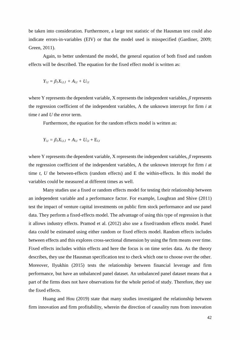
42

be taken into consideration. Furthermore, a large test statistic of the Hausman test could also

indicate errors-in-variables (EIV) or that the model used is misspecified (Gardiner, 2009;

Green, 2011).

Again, to better understand the model, the general equation of both fixed and random

effects will be described. The equation for the fixed effect model is written as:

Yi,t = β1Xi,t,1 + Ai,t + Ui,t

where Y represents the dependent variable, X represents the independent variables, β represents

the regression coefficient of the independent variables, A the unknown intercept for firm i at

time t and U the error term.

Furthermore, the equation for the random effects model is written as:

Yi,t = β1Xi,t,1 + Ai,t + Ui,t + Ei,t

where Y represents the dependent variable, X represents the independent variables, β represents

the regression coefficient of the independent variables, A the unknown intercept for firm i at

time t, U the between-effects (random effects) and E the within-effects. In this model the

variables could be measured at different times as well.

Many studies use a fixed or random effects model for testing their relationship between

an independent variable and a performance factor. For example, Loughran and Shive (2011)

test the impact of venture capital investments on public firm stock performance and use panel

data. They perform a fixed-effects model. The advantage of using this type of regression is that

it allows industry effects. Pramod et al. (2012) also use a fixed/random effects model. Panel

data could be estimated using either random or fixed effects model. Random effects includes

between effects and this explores cross-sectional dimension by using the firm means over time.

Fixed effects includes within effects and here the focus is on time series data. As the theory

describes, they use the Hausman specification test to check which one to choose over the other.

Moreover, Ilyukhin (2015) tests the relationship between financial leverage and firm

performance, but have an unbalanced panel dataset. An unbalanced panel dataset means that a

part of the firms does not have observations for the whole period of study. Therefore, they use

the fixed effects.

Huang and Hou (2019) state that many studies investigated the relationship between

firm innovation and firm profitability, wherein the direction of causality runs from innovation

43

to profitability. This is because of the perception that firms invest in R&D to continue growing

through product development and to stay competitive. They use an unbalanced panel dataset to

study the causal relationship between firm profitability and innovative activities and analysed

the determinants of firm profitability. They used Granger causality to examine the direction

between firm profitability and innovative activities. The null hypothesis states that a firm’s

innovative activities does not Granger-cause firm profitability. After that, they used both

random effect and fixed effect panel data models. However, they state that they choose fixed

effects estimators over random effects estimators, but they did not know whether they could

assume that the individual effect was uncorrelated with other explanatory variables. They did

use the Hausman test to explore which model to use, but the problem that goes with this is the

endogenous causality between a firm’s innovative activities and the firm profitability.

Therefore, they used GMM regression analysis. This is the most used method when panels have

small T-value and large N-values. The results indicate that there is a one-way causality from a

firm’s innovative activities to its profitability. However, they also find some weak evidence

regarding the direction of causality from a firm’s profitability to its innovative activities.

3.2 Model used in this study

As stated, the majority of studies within the field of green innovation choose SEM as their

method. So, it seems logical to use this model as well. However, all these studies use a survey

to gather their data, because green innovation is difficult to measure. Unfortunately, this implies

that green innovation is not directly observable and thus a latent variable. SEM is one of most

obvious methods to use for testing relationships when one only has latent variables. However,

in this study an unbalanced panel dataset will be used. Therefore, looking at the studies with a

similar relationship between an independent variable and a performance factor, it is more

appropriate to use OLS regression. Although performing a fixed/random effects model could

also be possible.

The hypothesis posits that green innovation positively influences firm performance. To

test if this is indeed the case, the following OLS regression estimation will be run.

PERFi,t = β1 (GI)i,t-3 + β2 (SIZE)i,t + β3 (AGE)i,t + β4 (LEV)i,t + β5 (IND)i,t + β6 (COU)i,t + εi,t.

Where PERFi,t represents the different measures of firm performance, namely ROA, ROE,

ROS, and Profit Margin. GIi,t-3 represents the independent variable Green Innovation, measured

by the number of patents and citations for a 3-year time lag. Meaning that a patent granted in

44

2010 shows its impact in 2013. It happens more often that a lag is used in the analysis and many

still argue about how many years this lag must be (Artz et al., 2010). However, based on

previous literature, this study will use a 3-year lag and this will be described in paragraph 3.3.2.

Furthermore, SIZEi,t represents the control variable firm size, AGEi,t represents the control

variable firm age, LEVi,t represents the control variable firm leverage, INDi,t represents the

dummy variable industry control, and COUi,t represents the dummy variable country control.

Furthermore, β1 represents the regression coefficient of the independent variable for firm i at

time t and ε represents the unobserved random errors that could have an influence on firm

performance.

A variety of models will be constructed on the different measures of the dependent

variables with the execution of the OLS regression analysis. In order to establish a benchmark,

the first model will only consists of all control variables and the independent variables will be

left out. Thereafter, different combinations of variables will tested and lastly the full model will

be tested. In this way, one could find changes in variability when the measures of green

innovation are added to the model. So, the impact of green innovation will then become clear

and this will be done for all the performance measures separately. The variables will be tested

for the alpha significance level of 10%, 5%, and 1%.

Moreover, this study has an unbalanced panel dataset, because using a balanced dataset

would have the consequence of not having enough observations. So, an unbalanced dataset

brings more observations and thus the sample will be larger. This could cause some bias,

because some firms could be represented more in the sample and this is not favourable when

using the OLS regression analysis. In panel data the behaviour of entities are observed across

time. Examples of these entities are companies, countries or individuals. Panel data allows to

control for unobservable variables across firms or variables that change over time but not across

entities. Panel data is much more informative than either cross-sectional or time series data, but

the problem that could arise is that one may find insufficient observations for a particular period

of time. For example, firms could have 50 granted green patents in year 2010 and only 20

granted green patents in 2011, but still have a higher firm performance in 2014 compared to

2013. The 50 granted green patents could still have an influence on the firm performance of

2014, while the analysis only looks at the 20 granted green patents, because of the time lag of

3-years. This problem could be prevented by performing a fixed/random effects model as a

robustness check (Vithessonthi & Racela, 2016; Chen et al., 2018). Therefore, a fixed/random

effects model will be used as such a check. This is in line with the study of Pramod et al. (2012)

who describe that omitted variable bias could be present when using the OLS regression

45

analysis. Ortega-Argilés et al. (2011) also perform both the OLS regression analysis and the

fixed/random effects model, because it checks for individual firms’ unobservables.

Studies also perform other robustness checks to strengthen their results. For example,

Vithessonthi and Racela (2016) divide their sample into low and high based on the cross-

sectional median value of R&D intensity as a robustness check. The dummy variable takes a

value of 1 for innovations larger than the cross-sectional median, and zero otherwise.

Subsequently, they divide their sample into small and large firms based on the cross-sectional

median value of firm size. Again, the dummy variable takes a value of one for an observation

with a firm size larger than the median, and zero otherwise. Loughran and Shive (2011) also

split their sample, but into small, medium, and large firms. They also make sure the test is not

driven by one industry or an omitted industry-level variable. For this, they use an individual

industry-level OLS regression test on the five largest industries within their study. Furthermore,

Vithessonthi and Racela (2016) use an alternative proxy for their independent variable. In this

study citation count will used as a second measure of green innovation and not just as a

robustness check. This will be explained in paragraph 3.3.2.

The robustness checks that will be performed in this study are a fixed/random effects

model for the full sample, and extra OLS regression checks for: the full sample split by the

median of size, a 2-year lag sample, a sample consisting of firms operating only in patent-

sensitive industries, a sample consisting of firms with at least one citation, a 2010-2014 sample

with using a 2-year and 3-year lag for firm performance improvement as the replacement of the

dependent variable, and a sample using a citation dummy as the replacement of the number of

citations.

3.3 Variables

3.3.1 Dependent variables

Based on previous literature and regarding the hypothesis, this study will use different measures

of firm performance as the dependent variable. The literature is divided when it comes to the

measurement of firm performance. Firm performance measures can be divided into accounting

performance measures, such as Return On Assets (ROA), Return On Equity (ROE) and Return

On Sales (ROS), market performance measures, such as stock returns, and hybrid performance

measures, such as Tobin’s Q.

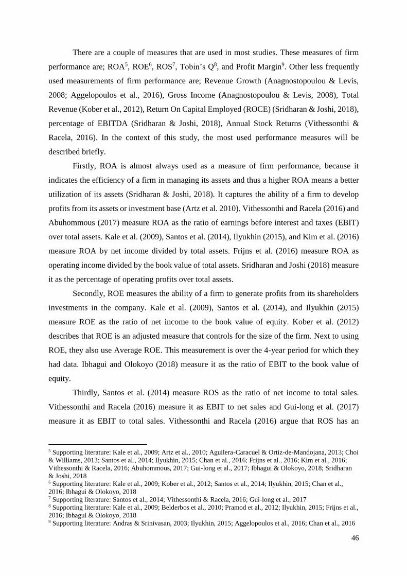
46

There are a couple of measures that are used in most studies. These measures of firm

performance are; ROA5, ROE6, ROS7, Tobin’s Q8, and Profit Margin9. Other less frequently

used measurements of firm performance are; Revenue Growth (Anagnostopoulou & Levis,

2008; Aggelopoulos et al., 2016), Gross Income (Anagnostopoulou & Levis, 2008), Total

Revenue (Kober et al., 2012), Return On Capital Employed (ROCE) (Sridharan & Joshi, 2018),

percentage of EBITDA (Sridharan & Joshi, 2018), Annual Stock Returns (Vithessonthi &

Racela, 2016). In the context of this study, the most used performance measures will be

described briefly.

Firstly, ROA is almost always used as a measure of firm performance, because it

indicates the efficiency of a firm in managing its assets and thus a higher ROA means a better

utilization of its assets (Sridharan & Joshi, 2018). It captures the ability of a firm to develop

profits from its assets or investment base (Artz et al. 2010). Vithessonthi and Racela (2016) and

Abuhommous (2017) measure ROA as the ratio of earnings before interest and taxes (EBIT)

over total assets. Kale et al. (2009), Santos et al. (2014), Ilyukhin (2015), and Kim et al. (2016)

measure ROA by net income divided by total assets. Frijns et al. (2016) measure ROA as

operating income divided by the book value of total assets. Sridharan and Joshi (2018) measure

it as the percentage of operating profits over total assets.

Secondly, ROE measures the ability of a firm to generate profits from its shareholders

investments in the company. Kale et al. (2009), Santos et al. (2014), and Ilyukhin (2015)

measure ROE as the ratio of net income to the book value of equity. Kober et al. (2012)

describes that ROE is an adjusted measure that controls for the size of the firm. Next to using

ROE, they also use Average ROE. This measurement is over the 4-year period for which they

had data. Ibhagui and Olokoyo (2018) measure it as the ratio of EBIT to the book value of

equity.

Thirdly, Santos et al. (2014) measure ROS as the ratio of net income to total sales.

Vithessonthi and Racela (2016) measure it as EBIT to net sales and Gui-long et al. (2017)

measure it as EBIT to total sales. Vithessonthi and Racela (2016) argue that ROS has an

5 Supporting literature: Kale et al., 2009; Artz et al., 2010; Aguilera-Caracuel & Ortiz-de-Mandojana, 2013; Choi

& Williams, 2013; Santos et al., 2014; Ilyukhin, 2015; Chan et al., 2016; Frijns et al., 2016; Kim et al., 2016;

Vithessonthi & Racela, 2016; Abuhommous, 2017; Gui-long et al., 2017; Ibhagui & Olokoyo, 2018; Sridharan

& Joshi, 2018 6 Supporting literature: Kale et al., 2009; Kober et al., 2012; Santos et al., 2014; Ilyukhin, 2015; Chan et al.,

2016; Ibhagui & Olokoyo, 2018 7 Supporting literature: Santos et al., 2014; Vithessonthi & Racela, 2016; Gui-long et al., 2017 8 Supporting literature: Kale et al., 2009; Belderbos et al., 2010; Pramod et al., 2012; Ilyukhin, 2015; Frijns et al.,

2016; Ibhagui & Olokoyo, 2018 9 Supporting literature: Andras & Srinivasan, 2003; Ilyukhin, 2015; Aggelopoulos et al., 2016; Chan et al., 2016

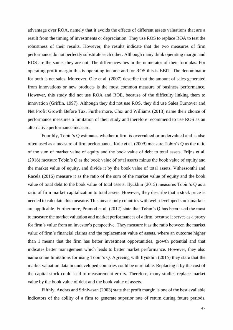
47

advantage over ROA, namely that it avoids the effects of different assets valuations that are a

result from the timing of investments or depreciation. They use ROS to replace ROA to test the

robustness of their results. However, the results indicate that the two measures of firm

performance do not perfectly substitute each other. Although many think operating margin and

ROS are the same, they are not. The differences lies in the numerator of their formulas. For

operating profit margin this is operating income and for ROS this is EBIT. The denominator

for both is net sales. Moreover, Oke et al. (2007) describe that the amount of sales generated

from innovations or new products is the most common measure of business performance.

However, this study did not use ROA and ROE, because of the difficulty linking them to

innovation (Griffin, 1997). Although they did not use ROS, they did use Sales Turnover and

Net Profit Growth Before Tax. Furthermore, Choi and Williams (2013) name their choice of

performance measures a limitation of their study and therefore recommend to use ROS as an

alternative performance measure.

Fourthly, Tobin’s Q estimates whether a firm is overvalued or undervalued and is also

often used as a measure of firm performance. Kale et al. (2009) measure Tobin’s Q as the ratio

of the sum of market value of equity and the book value of debt to total assets. Frijns et al.

(2016) measure Tobin’s Q as the book value of total assets minus the book value of equity and

the market value of equity, and divide it by the book value of total assets. Vithessonthi and

Racela (2016) measure it as the ratio of the sum of the market value of equity and the book

value of total debt to the book value of total assets. Ilyukhin (2015) measures Tobin’s Q as a

ratio of firm market capitalization to total assets. However, they describe that a stock price is

needed to calculate this measure. This means only countries with well-developed stock markets

are applicable. Furthermore, Pramod et al. (2012) state that Tobin’s Q has been used the most

to measure the market valuation and market performances of a firm, because it serves as a proxy

for firm’s value from an investor’s perspective. They measure it as the ratio between the market

value of firm’s financial claims and the replacement value of assets, where an outcome higher

than 1 means that the firm has better investment opportunities, growth potential and that

indicates better management which leads to better market performance. However, they also

name some limitations for using Tobin’s Q. Agreeing with Ilyukhin (2015) they state that the

market valuation data in undeveloped countries could be unreliable. Replacing it by the cost of

the capital stock could lead to measurement errors. Therefore, many studies replace market

value by the book value of debt and the book value of assets.

Fifthly, Andras and Srinivasan (2003) state that profit margin is one of the best available

indicators of the ability of a firm to generate superior rate of return during future periods.

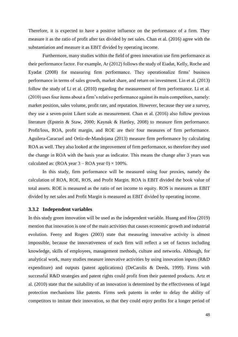
48

Therefore, it is expected to have a positive influence on the performance of a firm. They

measure it as the ratio of profit after tax divided by net sales. Chan et al. (2016) agree with the

substantiation and measure it as EBIT divided by operating income.

Furthermore, many studies within the field of green innovation use firm performance as

their performance factor. For example, Ar (2012) follows the study of Eiadat, Kelly, Roche and

Eyadat (2008) for measuring firm performance. They operationalize firms’ business

performance in terms of sales growth, market share, and return on investment. Lin et al. (2013)

follow the study of Li et al. (2010) regarding the measurement of firm performance. Li et al.

(2010) uses four items about a firm’s relative performance against its main competitors, namely:

market position, sales volume, profit rate, and reputation. However, because they use a survey,

they use a seven-point Likert scale as measurement. Chan et al. (2016) also follow previous

literature (Epstein & Staw, 2000; Kaynak & Hartley, 2008) to measure firm performance.

Profit/loss, ROA, profit margin, and ROE are their four measures of firm performance.

Aguilera-Caracuel and Ortiz-de-Mandojana (2013) measure firm performance by calculating

ROA as well. They also looked at the improvement of firm performance, so therefore they used

the change in ROA with the basis year as indicator. This means the change after 3 years was

calculated as: (ROA year 3 – ROA year 0) × 100%.

In this study, firm performance will be measured using four proxies, namely the

calculation of ROA, ROE, ROS, and Profit Margin. ROA is EBIT divided the book value of

total assets. ROE is measured as the ratio of net income to equity. ROS is measures as EBIT

divided by net sales and Profit Margin is measured as EBIT divided by operating income.

3.3.2 Independent variables

In this study green innovation will be used as the independent variable. Huang and Hou (2019)

mention that innovation is one of the main activities that causes economic growth and industrial

evolution. Feeny and Rogers (2003) state that measuring innovative activity is almost

impossible, because the innovativeness of each firm will reflect a set of factors including

knowledge, skills of employees, management methods, culture and networks. Although, for

analytical work, many studies measure innovative activities by using innovation inputs (R&D

expenditure) and outputs (patent applications) (DeCarolis & Deeds, 1999). Firms with

successful R&D strategies and patent rights could profit from their patented products. Artz et

al. (2010) state that the suitability of an innovation is determined by the effectiveness of legal

protection mechanisms like patents. Firms seek patents in order to delay the ability of

competitors to imitate their innovation, so that they could enjoy profits for a longer period of

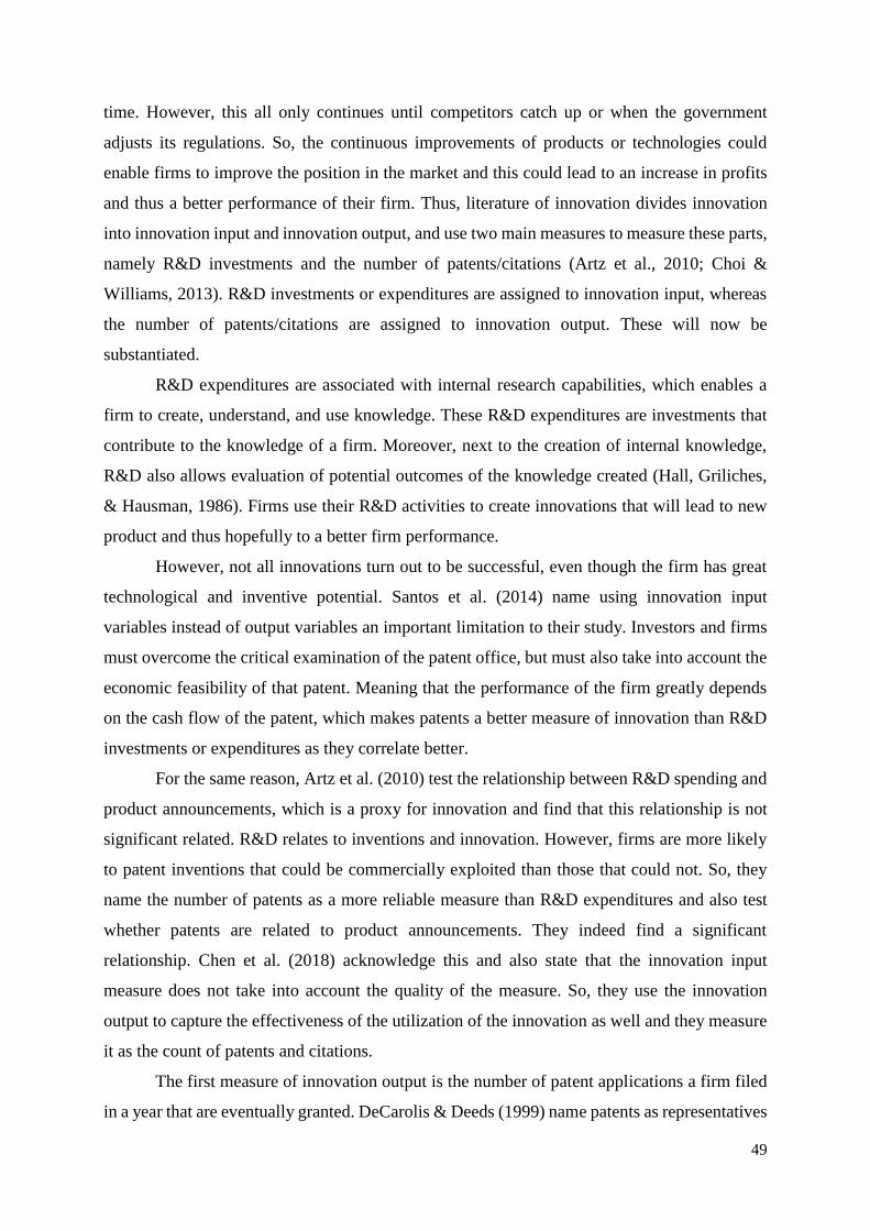
49

time. However, this all only continues until competitors catch up or when the government

adjusts its regulations. So, the continuous improvements of products or technologies could

enable firms to improve the position in the market and this could lead to an increase in profits

and thus a better performance of their firm. Thus, literature of innovation divides innovation

into innovation input and innovation output, and use two main measures to measure these parts,

namely R&D investments and the number of patents/citations (Artz et al., 2010; Choi &

Williams, 2013). R&D investments or expenditures are assigned to innovation input, whereas

the number of patents/citations are assigned to innovation output. These will now be

substantiated.

R&D expenditures are associated with internal research capabilities, which enables a

firm to create, understand, and use knowledge. These R&D expenditures are investments that

contribute to the knowledge of a firm. Moreover, next to the creation of internal knowledge,

R&D also allows evaluation of potential outcomes of the knowledge created (Hall, Griliches,

& Hausman, 1986). Firms use their R&D activities to create innovations that will lead to new

product and thus hopefully to a better firm performance.

However, not all innovations turn out to be successful, even though the firm has great

technological and inventive potential. Santos et al. (2014) name using innovation input

variables instead of output variables an important limitation to their study. Investors and firms

must overcome the critical examination of the patent office, but must also take into account the

economic feasibility of that patent. Meaning that the performance of the firm greatly depends

on the cash flow of the patent, which makes patents a better measure of innovation than R&D

investments or expenditures as they correlate better.

For the same reason, Artz et al. (2010) test the relationship between R&D spending and

product announcements, which is a proxy for innovation and find that this relationship is not

significant related. R&D relates to inventions and innovation. However, firms are more likely

to patent inventions that could be commercially exploited than those that could not. So, they

name the number of patents as a more reliable measure than R&D expenditures and also test

whether patents are related to product announcements. They indeed find a significant

relationship. Chen et al. (2018) acknowledge this and also state that the innovation input

measure does not take into account the quality of the measure. So, they use the innovation

output to capture the effectiveness of the utilization of the innovation as well and they measure

it as the count of patents and citations.

The first measure of innovation output is the number of patent applications a firm filed

in a year that are eventually granted. DeCarolis & Deeds (1999) name patents as representatives

50

of stocks of organizational knowledge as patents are physical, codifiable manifestations of

innovative ideas, techniques, and products that embody the knowledge of one or more

employees of the firm. An innovation is patented if the net benefits of doing so exceed the costs.

These costs can include the tangible costs of filing and defending patents, or the less tangible

costs of information disclosure associated with patenting (Arora, Ceccagnoli, & Cohen, 2008).

Many inventions ultimately result in marketable innovations, because patents ensure protection

(Artz et al., 2010). However, DeCarolis and Deeds (1999) also name limitations to simply using

patent count. First, simple patent count do not reflect the value of knowledge, which is better

captured by citations. Second, firms tend to differ in their policies toward patents as some firms

patent more than other firms. The estimated minimum costs of an issued patent are $ 12,000.

This is small for a big firm, but big for a small firm.

So, next to the number of patents, the number of citations will also be used in this study.

Griliches, Pakes and Hall (1986) use this second measure to capture innovation productivity,

because the patent count vary in their technological and economic importance and therefore are

not sufficient enough to capture innovation productivity. This second measure assesses the

importance of a patent, because it is related to the social and economic value that is created by

the innovation (Hall, Jaffe, & Trajtenberg, 2005). Citation count is measured as the total number

of non-self citations ultimately received by the patents applied for in a given year. Thus,

citations are how many times a firm’s patents are cited by subsequent issued patents (DeCarolis

& Deeds, 1999). Meaning that others want to use that specific document for further research

purposes. So, green innovation will be based on the intensity of green innovations and it will

be calculated by the total number of patents that could be attributed to green patents (Melvin,

2002; Harhoff & Wagner, 2009) and citation count (Hall et al., 2005).

Other studies also use at least one of the innovations measures described above. Frietsch

and Grupp (2006), for example, named patents as the most important proxy to define

innovation. Zhou & Sadeghi (2019) agree and also mention that patents are an output of

innovation capital during the process of the production of a firm. Therefore, they use the natural

logarithm of the number of patent applications and acquired patents as well to define

innovation. Czarnitzki and Kraft (2012) use both R&D investments and patent count as a

measure of innovation to test the impact on firm performance and their results conclude that

patents have a more significant impact on firm performance than R&D investments. Choi &

Williams acknowledge the inputs and outputs of innovation and also use R&D intensity and

patent intensity as their independent variables. However, they find that R&D intensity is not

statistically significant for both their two firm performance measures. For ROA it even shows

51

a negative sign. On the other hand, patent intensity does have a statistically significant and

positive effect on firm performance for both the performance measures. This provides support

to the Schumpeterian view of innovation based on accumulated knowledge.

So, previous studies agree with each other that patents and citations counts are the most

reliable way of measuring innovation. Unfortunately, patents and citations suffer from several

imperfections (Chen et al., 2018) that has to be taken care of first. Firstly, it takes some time

for a patent to be granted. This causes a truncation bias in the number of patents for the end of

the sample period. Secondly, patents created at the end of the year of the sample could have

fewer citations. Thirdly, the intensity of patenting and citations vary across industries. Hall,

Jaffe and Trajtenberg (2001) and Seru (2014) name strategies to take care of these

imperfections. So, this study follows these studies to adjust both patent and citation count. The

first and partly the third imperfection is taken care of by dividing the number of patents for each

firm by the average patent count of all firms in the industry classification and year. This variable

is called Patent. To adjust for the second and third implication, the patent’s non-self citation

count will be scaled by the mean of the non-self citation count of all patents in the same industry

classification and year. This variable is called Citation and is measured as the sum of the non-

self citation counts across all patents applied for by a firm in a given year.

Next, it is also expected that the number of patents and citations will be highly skewed,

because most of the firms will have only one granted green patent and no citations. Following

the approach of Artz et al. (2010) the green innovation measures will transformed because of

error term skewness problems if this will indeed be the case. So, to deal with the imperfections

of patents and citations this study uses two measures of green innovation, namely the natural

logarithm of the number of patents, in this study called; Log(PAT), and the natural logarithm

of the number of non-self citations, in this study called; Log(CIT). All the firms in the sample

have at least one granted green patent. However, this is not the case for citations as firms could

have no citations on their granted green patents in a given year. This is a problem when using

a natural logarithm and therefore the natural logarithm the number of citations plus 0.01 is used

to deal with this problem (Artz et al., 2010). The difference between what is a green patent and

what is not will be explained in chapter 4.

3.3.3 Control variables

Investing in green innovation most likely influences firm performance, but there are other

factors that could also have a significant influence on the performance of a firm. The so called

52

control variables related to firm characteristics could isolate the effects of the predictable

influence of green innovation on firm performance (Gui-long et al., 2017).

The firm characteristics that are used the most in previous studies are: firm size10, firm

age11, firm leverage12 and an industry dummy13. Other less frequently used firm characteristics

are for example: industry concentration (Ho et al., 2005; Ehie & Olibe, 2010; Loughran &

Shive, 2011) and earnings per share (EPS) (Anagnostopoulou & Levis, 2008). In the context of

this study, the most used control variables will be briefly described.

Firstly, firm size affects firm performance directly, because of the funds available, the

diversification in operations, and controlling for more skilled managers specific to larger firms

(Pramod, 2012; Ilyukhin, 2015). Abuhommous (2017) adds that a larger firm has the advantage

of producing in larger quantities. So, large firms could be more efficient and this gives the firm

the opportunity to take advantage of economies of scale (Gui-long et al., 2017; Huang & Hou,

2019). Zhou and Sadeghi (2019) agree and state that larger firms generally have less

information asymmetry. Regarding patents, previous studies state that there may be economies

of scales in generating them. This is due to the fixed costs of maintaining a legal department

that manages patent-related issues and this suggests a positive influence of firm size on firm

performance (Chen et al., 2018). Next to that, firm size also measures a firm’s market power or

the level of concentration in the industries in which the firm operates. This makes

implementation of operations more effective, allows large firms to generate greater returns on

assets and sales, and allows to capture more value as a proportion of the value of the production

and this leads to a higher firm performance. However, on the other hand, strategic and

operational activities of larger firms could also be less efficient than those of smaller firms when

larger firms lose the control of top managers regarding these activities (Pramod et al., 2012).

Huang and Hou (2019) agree and add that inefficient management activities could increase

manufacturing costs when entering new markets and this negatively affects firm performance.

10 Supporting literature: Mansfield, 1986; DeCarolis & Deeds, 1999; Ho et al., 2005; Chen et al., 2006; Oke et

al., 2007; Rehfeld et al., 2007; Anagnostopoulou & Levis, 2008; Arora et al., 2008; Kale et al., 2009; Artz et al.,

2010; Belderos et al., 2010; Ehie & Olibe, 2010; Li et al., 2010; Kumbhakar et al., 2011; Kober et al., 2012;

Pramod et al., 2012; Aguilera-Caracuel & Ortiz-de-Mandojana, 2013; Leonidou et al., 2013; Choi & Williams,

2013; Seru, 2014; Ilyukhin, 2015; Frijns et al., 2016; Kim et al., 2016; Vithessonthi & Racela, 2016;

Abuhommous, 2017; Gui-long et al., 2017; Chen et al., 2018; Ibhagui & Olokoyo, 2018; Sridharan & Joshi,

2018; Huang & Hou, 2019; Zhou & Sadeghi, 2019 11 Supporting literature: Chen et al., 2006; Oke et al., 2007; Anagnostopoulou & Levis, 2008; Pramod et al.,

2012; Choi & Williams, 2013; Seru, 2014; Frijns et al., 2016; Gui-long et al., 2017; Ibhagui & Olokoyo, 2018;

Huang & Hou, 2019; Zhou & Sadeghi, 2019 12 Supporting literature: Ehie & Olibe, 2010; Pramod et al., 2012; Choi & Williams, 2013; Seru, 2014; Frijns et

al., 2016; Vithessonthi & Racela, 2016; Abuhommous, 2017; Chen et al., 2018; Sridharan & Joshi, 2018 13 Supporting literature: Artz et al., 2010; Choi & Williams, 2013; Feeny & Rogers, 2013

53

Oke et al. (2007) state that there is an important link between innovation and business and

economic growth. SMEs operating in high technology industries are more capable of adjusting

to rapidly changing innovations than large firms. However, although these SMEs may have

high intensity of R&D, larger firms with more slack can dedicate more resources to R&D.

Therefore, the control variable firm size was used in this study, because it could have a

significant effect on firm performance.

Firm size is measured differently among the studies investigating firm performance.

Although, when studies are based on operating, accounting- and market-based measures, many

studies use total assets to define the size of a firm (Anagnostopoulou and Levis, 2008; Kober et

al., 2012). Next to total assets, when studies investigate productivity gains, studies use the

number of employees as well to define the size of the firm (Chen et al., 2006; Arora et al., 2008;

Kumbhakar et al., 2011; Kober et al., 2012). Kober et al. (2012) also uses total revenue to

determine the size of the firm. Aguilera-Caracuel & Ortiz-de-Mandojana (2013) measure firm

size using the total net revenues reported on each firm’s balance sheet. But, there are also other

ways of determining firm size. A couple of other studies measure firm size by the natural

logarithm of total assets (DeCarolis & Deeds, 1999; Choi & Williams, 2013; Feeny & Rogers,

2013; Vithessonthi & Racela, 2016; Abuhommous, 2017; Sridharan & Joshi, 2018; Zhou &

Sadeghi, 2019), the natural logarithm of market capitalization (Chen et al., 2018), the natural

logarithm of the number of employees of the firm (Arora et al., 2008), or the natural logarithm

of a firm’s total or net sales (Ehie & Olibe, 2010; Pramod et al., 2012; Gui-long et al., 2017;

Huang & Hou, 2019). The difference between total sales and net sales is that total sales includes

inventories. Ehie and Olibe state that this avoids any compounding effects of firm size on firm

performance by controlling for (dis)economies of scale. Using log transformations makes it

easier to interpret the results, because changes in the logarithm domain represent relative

changes in the original metric. Also, log transformations make the distribution of the data closer

to a normal distribution. Frijns et al. (2016) also use a log-transformed measure, but they use

the log-transformed market value in millions of GBP measured at the end of the calendar year

to determine firm size. Next, Mansfield (1986) and Kale et al. (2009) use the natural log of the

firm’s net sales for the year. Ho et al. (2005) measure firm size by the natural logarithm of

market capitalization of a firm at fiscal year-end. They state that market capitalization has the

advantage of being an unbiased market measure of the size of a firm. They argue that the use

of net sales or total assets could be affected by the accounting policies of a firm.

Secondly, firm age is associated with the production experience of a firm and therefore

it is expected to have a positive influence on firm performance (Gui-long et al., 2017). Pramod

54

et al. (2012) state that older firms with an established history could be expected to fare better in

the stock market, because they can enjoy superior performance compared to newcomers and

they could also avoid the liabilities of newness. Huang and Hou (2019) state that the cumulative

learning approach of firms with experience tends to facilitate their operational approach and

this leads to an increase in their firm performance. However, on the other hand, older firms are

prone to inertia, and have less efficient adaptability and this could lead to a lower firm

performance (Pramod et al. 2012). This makes the relationship between firm age and firm

performance ambiguous. Many studies use the number of years since firm was established to

determine the age of a firm (Frijns et al., 2016; Huang & Hou, 2019). Loughran & Shive (2011),

however, use the number of years the firm has been listed on CRSP. Other studies also use the

natural logarithm of the number of years since the firm was founded (Choi & Williams, 2013;

Gui-long et al., 2017). Pramod et al. (2012) uses two measures of firm age, namely as the

number of years since inception to the date of observation and the number of years since the

incorporation of the firm.

Thirdly, firms use debt to decrease taxes paid. Leverage allows greater potential returns

for investors that otherwise would have been unavailable. On the other hand, debt could also

lead to potential losses if the investment becomes worthless, because then the firm still needs

to pay the loan principal and all accrued interest on the loan. This increase in risk could

decreases the performance of a firm (Pramod et al., 2012). Because, a high debt to equity ratio

affects investments decisions on innovation resources and firm performance by increasing the

likelihood of going bankrupt (Choi & Williams, 2013). However, Feng and Rong (2007) state

that leverage should promote the market value of a firm when taxes shields are valuable or debt

reduce agency problem. The results of other studies regarding leverage show that the

performance of a firm is negatively affected by firms’ leverage (Feng & Rong, 2007; Chadha

& Oriani, 2009). Most studies calculate firm leverage as a firms’ long-term debt divided by

total assets (Ehie & Olibe, 2010; Pramod et al., 2012; Choi & Williams, 2013; Frijns et al.,

2016; Vithessonthi & Racela, 2016; Abuhommous, 2017; Chen et al., 2018). However,

Sridharan and Joshi (2018) measure firm leverage as total term liabilities divided by tangible

net worth.

Fourthly, although less used, industry control and country control will also be used in

this study. Studies that use the OLS regression analysis as their method also include an industry

dummy and/or country dummy to control resp. for the distinction between industries and/or

countries (Ho et al., 2005; Ehie & Olibe, 2010; Loughran & Shive, 2011; Aggelopoulos et al.,

2016).

55

The control variables used in this study are firm size, firm age, firm leverage, and an

industry and a country control dummy. Gui-long et al. (2017) state that using too many control

variables could trouble statistical examination and therefore only these will be included in this

study. Most studies that investigate any impact on firm performance consider at least the size,

the age, and the leverage of a firm. Firstly, firm size will be measured as the natural logarithm

of the net sales of the firm (Log(SIZE)). Firm size could have a positive or negative influence

on firm performance. Larger firms have more resources and thus have operating advantages

and are more efficient in using them. But, on the other side, strategic and operational activities

of larger firms could also be less efficient than those of smaller firms when larger firms lose the

control of top managers regarding these activities. Secondly, firm age will be measured as the

natural logarithm of the number of years since the firm was incorporated (Log(AGE)). Since

firm age is associated with production experience and an established history, it is expected that

firm age could have a positive influence on firm performance. Thirdly, firm leverage will be

used as a measure of firm risk and will be measured as long-term debt divided by total assets

(LEV). An increase in risk of possible worthless investments could lead to a decrease in the

performance of a firm and therefore it is expected to have a negative influence on firm

performance. Fourthly, as already stated and regarding the institutional theory, the analysis will

be controlled for industry and country fixed effects. These dummies will be based on the

comparison of industries and countries with the most patents and the other industries and

countries in the sample. A broader description of the industries and countries will be explained

in chapter 4. Table III shows the definitions of the variables that will be used in this study and

its supporting literature.

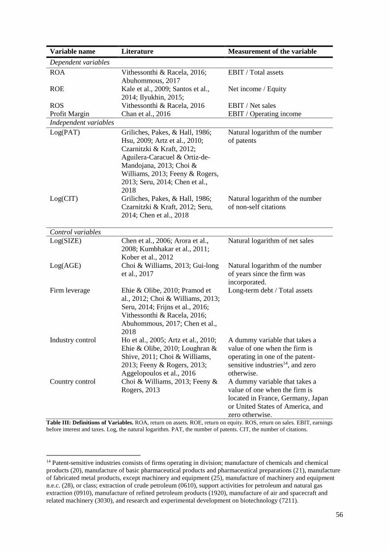
56

Variable name Literature Measurement of the variable

Dependent variables

ROA Vithessonthi & Racela, 2016;

Abuhommous, 2017

EBIT / Total assets

ROE Kale et al., 2009; Santos et al.,

2014; Ilyukhin, 2015;

Net income / Equity

ROS Vithessonthi & Racela, 2016 EBIT / Net sales

Profit Margin Chan et al., 2016 EBIT / Operating income

Independent variables

Log(PAT) Griliches, Pakes, & Hall, 1986;

Hsu, 2009; Artz et al., 2010;

Czarnitzki & Kraft, 2012;

Aguilera-Caracuel & Ortiz-de-

Mandojana, 2013; Choi &

Williams, 2013; Feeny & Rogers,

2013; Seru, 2014; Chen et al.,

2018

Natural logarithm of the number

of patents

Log(CIT) Griliches, Pakes, & Hall, 1986;

Czarnitzki & Kraft, 2012; Seru,

2014; Chen et al., 2018

Natural logarithm of the number

of non-self citations

Control variables

Log(SIZE) Chen et al., 2006; Arora et al.,

2008; Kumbhakar et al., 2011;

Kober et al., 2012

Natural logarithm of net sales

Log(AGE) Choi & Williams, 2013; Gui-long

et al., 2017

Natural logarithm of the number

of years since the firm was

incorporated.

Firm leverage Ehie & Olibe, 2010; Pramod et

al., 2012; Choi & Williams, 2013;

Seru, 2014; Frijns et al., 2016;

Vithessonthi & Racela, 2016;

Abuhommous, 2017; Chen et al.,

2018

Long-term debt / Total assets

Industry control Ho et al., 2005; Artz et al., 2010;

Ehie & Olibe, 2010; Loughran &

Shive, 2011; Choi & Williams,

2013; Feeny & Rogers, 2013;

Aggelopoulos et al., 2016

A dummy variable that takes a

value of one when the firm is

operating in one of the patent-

sensitive industries14, and zero

otherwise.

Country control Choi & Williams, 2013; Feeny &

Rogers, 2013

A dummy variable that takes a

value of one when the firm is

located in France, Germany, Japan

or United States of America, and

zero otherwise. Table III: Definitions of Variables. ROA, return on assets. ROE, return on equity. ROS, return on sales. EBIT, earnings

before interest and taxes. Log, the natural logarithm. PAT, the number of patents. CIT, the number of citations.

14 Patent-sensitive industries consists of firms operating in division; manufacture of chemicals and chemical

products (20), manufacture of basic pharmaceutical products and pharmaceutical preparations (21), manufacture

of fabricated metal products, except machinery and equipment (25), manufacture of machinery and equipment

n.e.c. (28), or class; extraction of crude petroleum (0610), support activities for petroleum and natural gas

extraction (0910), manufacture of refined petroleum products (1920), manufacture of air and spacecraft and

related machinery (3030), and research and experimental development on biotechnology (7211).

57

4 DATA & SAMPLE

4.1 Data Collection

The two main parts of data firms must have to be included in the sample are patent data and

accounting and financial data, such as data on the balance sheet and profit and loss accounts of

the firms. The gathering of the data will now be substantiated.

As already stated, many studies within the field of green innovation use a survey to

gather their data. For example, Chen et al. (2006) used a survey to investigate their research

wherein the managers of manufacturing, marketing, R&D, or environmental protection

departments were the respondents. Gürlek and Tuna (2018) also used a survey to answer the

question regarding green innovation. Their respondents were employees and junior, middle and

senior-level managers. Lin et al. (2013) likewise used a survey to investigate the relationship

between green product innovation performance and firm performance. This data was collected

using a field study and the respondents were executives in charge of the manufacturing function

from the selected firms. Ar (2012) also used a questionnaire for their study.

However, for this study patent data will be used to test the hypothesis. The study of Hsu

(2009) uses R&D data and patent data as proxies for technological innovations. He states that

patents are realized innovations, are more precise because of the territorial principle in patent

laws, and are the intangible assets that are most actively traded in intellectual property markets.

This makes patent data more reliable and informative than R&D data. Belderbos, Faems, Leten

and Van Looy (2010) use this type of data as well, because they study the impact of

technological activities on firm performance. Although this study is not completely in line with

this green innovative study, it does have some overlap. It has the same types of hypotheses and

they also investigate their independent variable by using patent data to construct indicators of

this independent variable. They state numerous advantages of using patent indicators, namely

documents of patents contain highly detailed information, patent data are objective, and patent

data are publicly available. However, a small downside is that not all activities are patented, but

no other indicator has the same level of detail as do patents. The studies of Belderbos et al.

(2010), and Aguilera-Caracuel and Ortiz-de-Mandojana (2013) both use the European Patent

Office (EPO) to gather their patent data. EPO is one of the two parts of the European Patent

Organisation, wherein EPO executes and the Administrative Council supervises. EPO studies

the European patent applications and decide whether or not a patent will be granted. The granted

58

patents are called European patents. However, this does not mean that the owner of this patent

must be European15.

So, for testing the hypothesis, this study uses patent data as a proxy for green innovation.

Patent data are better indicators than patent application data, but the latter has a broader

indicator of the variety of the innovations of the firm. This means that patent application data

will result in a more complete picture. Griliches, Pakes and Hall (1986) state that the year of

application of the patent is preferred over the grant year, because the application year better

represents the actual timing of the innovation. However, EPO its patent-granting decisions take

some years. EPO states that its patent-granting process takes on average 20 months16. In 2014

they launched an initiative to accelerate the delivery of search results and thus to improve

timeliness in substantive examination and opposition in order to streamline these stages of the

patenting process with the goal of reaching an average of 12 months in 202017. This means that

firms who apply for a patent will not start to use the patented technology right away. Therefore,

the publication date will be taken into account.

Following the study of Belderbos et al. (2010) and Aguilera-Caracuel and Ortiz-de-

Mandojana (2013), this study will also use the database of EPO. As already stated, the number

of patents and citations will be used as measures of green innovation. Regarding the green part,

The Cooperative Patent Classification (CPC) uses the Y02 code as the classification of green

patents18. CPC is an extension of the International Patent Classification (IPC) that is managed

by EPO and the US Patent and Trademark Office19. Generally speaking, the Y02 code stands

for “technologies or applications for mitigation or adaption against climate change”. This code

is divided into subcategories, wherein Y02A stands for “Technologies for adaptation to climate

change”, Y02B stands for “Climate change mitigation technologies related to buildings”, Y02C

stands for “Capture, storage, sequestration or disposal of greenhouse gases”, Y02D stands for

“Climate change mitigation technologies in information and communication technologies

15 European Patent Office. “About us” epo.org

https://www.epo.org/about-us.html (accessed January 4, 2020) 16 European Patent Office. “EPO Quality Report 2017” documents.epo.org

http://www. documents.epo.org (accessed November 28, 2019) 17 European Patent Office. “Improving Timeliness” epo.org

https://www.epo.org/about-us/annual-reports-statistics/annual-report/2016/highlights/improving-timeliness

(accessed November 28, 2019) 18 Cooperative Patent Classification. “Technologies or applications for mitigation or adaptation against climate

change” cooperativepatentclassification.org

http://www.cooperativepatentclassification.org/cpc/scheme/Y/scheme-Y02A.pdf (accessed November 29, 2018) 19 European Patent Office. “Cooperative Patent Classification (CPC)” epo.org

https://www.epo.org/searching-for-patents/helpful-resources/first-time-here/classification/cpc.html (accessed

November 29, 2018)

59

(ICT)”, Y02E stands for “Reduction of greenhouse gas emissions, related to energy generation,

transmission or distribution”, Y02P stands for “Climate change mitigation technologies in the

production or processing of goods”, Y02T stands for “Climate change mitigation technologies

related to transportation”, and Y02W stands for “Climate change mitigation technologies

related to wastewater treatment or waste management” 20 . In Appendix B an overview of

examples for each of these codes will be provided. So, the number of granted patents with the

Y02 code and its citations will be used to define the total number of green innovations of a firm

for each year (Aguilera-Caracuel & Ortiz-de-Mandojana, 2013).

Next to having at least one patent with the Y02 code granted and published by EPO,

firms must also have accounting and financial data available to be included in the sample. The

patent database EPO has a collaboration with the financial database ORBIS, which makes it the

perfect database to use for this study. ORBIS is a database that consists of detailed financial

information of 300 million private firms worldwide. The database contains information on over

83 million patents worldwide. So, within ORBIS the patents of the EPO database will be

collected. The data will consist of a sample of firms of green innovative firms who are the

owners of a European patent granted and published by EPO. As aforementioned, this does not

mean that all firms within the sample are European firms.

So, generally speaking, firms must have green patent data and accounting and financial

data available to be included in the sample. Firstly, to go into more detail, the patents that will

be selected are based on the criteria that these patents must be granted, published by EPO,

indicated by CPC’s Y02 code. Next to that, to be included in the sample the firms must also

include data such as: the number of citations, the name of the current owner, the country code

of the current owner, the NACE Rev. 2 Core industry code, the date of incorporation, and most

importantly; the current owner’s BvD ID number (Bureau van Dijk ID number). Because, the

latter is a personalized identification number used by ORBIS to link, for example, the

accounting and financial data of ORBIS itself with the patent data of EPO. ORBIS then

automatically uses these BvD ID numbers to search for all the firms that hold these patents.

Unfortunately, the matching process is currently not exhaustive, because not all applicants for

patents are reported through the database of EPO and patents could also be applied for by

individuals. Therefore, not all patents that will meet the criteria of the patents could be linked

to a BvD ID number.

20 European Patent Office. “CPC Scheme and Definitions” cooperativepatentclassification.org

https://www.cooperativepatentclassification.org/cpcSchemeAndDefinitions/table (accessed December 12, 2019)

60

Secondly, it is needed to have an extended period of time (on average two to three years),

beyond the announcement period, to investigate the full impact of the green innovation on the

value of the firm (Artz et al., 2010; Chen et al., 2017). Because, most innovative activities are

subject to information asymmetry between managers and external investors. For example,

investors could be slow to recognize opportunities of increases in R&D expenditures. Therefore

the data on these green patents of a firm will be gathered at time t - 3 to check the firm

performance at time t. So, secondly, the patent data will run from 2007 to 2014 in order to

calculate a 3-year lag for firm performance using accounting and financial data for the period

of 2010 to 2017. These years are chosen based on the fact that ORBIS only has financial data

on the latest 10 years (2010-2019) and the time-lag of 3 years for patents. The year 2018 and

2019 will be excluded from the sample, because of the bias towards the fact that newer patents

have fewer citations and incomplete financial data.

Thirdly, for these firms to be included in the final sample they also must be listed and

include accounting and financial data as: Operating P/L21, total assets22, P/L for Period23,

shareholders funds24, net sales, operating revenue25, and long term debt26. All firms must have

a known value available for all accounting and financial data after three years of the granted

green patent. These will be used to calculate the four measurements of firm performance and

the control variables. For some robustness checks other samples will be used, but these firms

have the same criteria.

4.2 Final Full Sample

Gathering all granted Y02 patents published between 2007 and 2014 gives a total of 54,652

green patents. With the BvD ID numbers ORBIS could link these patents to a total of 3,224

unique firms. After gathering the accounting and financial data of these firms, a total of 520

unique firms remain in the sample. These firms have data for at least one to a maximum of eight

21 ORBIS definition: EBIT; all operating revenues - all operating expenses (gross profit-other operating

expenses) 22 ORBIS definition: fixed assets + current assets 23 ORBIS definition: net income for the year. Before deduction of minority interests if any (profit after taxation +

extraordinary and other profit). 24 ORBIS definition: total equity (capital + other shareholders funds) 25 ORBIS definition: total operating revenues; net sales + other operating revenues + stock variations. The

figures do not include VAT. Local differences may occur regarding excises taxes and similar obligatory

payments for specific market of tobacco and alcoholic beverage industries. 26 ORBIS definition: long term financial debts (e.g. to credit institutions (loans and credits), bonds)

61

years. Of course, the same firm will not have the same data for different years. The criteria that

reduced the number of unique firms the most was the criteria that the firms must be listed. This

deletes all subsidiary firms, such as holdings. This is necessary, because in this way all firms

within the sample could be checked for by using factual data represented in the annual reports

to see if the data from ORBIS is reliable. 25 firms of the sample are randomly selected to check

whether the accounting and financial figures correspondent with the annual reports. All prove

to be accurate and reliable.

After analyzing these 520 firms, five industries were removed, because of the difficulty

of comparing these industries with others27. These industries are represented below 1% in the

sample as their contribution to the total sample was 0.60%. The same applies to countries. A

total of eight countries with a contribution to the sample of 1.34% are removed28.

Furthermore, all measures of variables are winsorized at 1% at each end of the

distribution to minimize outlier effects and potential data errors (Kale et al., 2009; Ehie & Olibe,

2010; Frijns et al., 2016; Aggelopoulos et al., 2016; Vithessonthi & Racela, 2016). This gives

a total of 450 unique firms with 1,314 firm year observations between 2007 and 2014, and with

a total of 7,700 granted green patents and 9,087 citations. Table IV gives a more detailed

overview of the total sample used in this study. In this table it can be seen that, for example,

180 of the 450 unique firms have at least one newly granted green patent in 2007. So, in 2007

all 180 firms together have a total of 1,290 newly granted green patents and these patents have

received a total of 1,147 citations. Overall, the 450 unique firms appear a total of 1,314 times

in the sample. Meaning that on average each firm is included in almost three of the eight years

in the sample. In these eight years, these 450 unique firms have a total of 7,700 new green

patents granted by EPO and these patents have received a total of 9,087 citations.

Year Number of Firms Number of Patents Number of Citations

2007 180 1290 1147

2008 160 917 1096

2009 156 741 884

2010 147 771 1021

2011 182 975 862

2012 185 1094 1276

2013 153 891 1325

2014 151 1021 1476

1314 7700 9087 Table IV: Overview sample. The table represents each year with the total number of firm year observations, patents, and

citations included in the sample.

27 Removed industries: Real estate activities, Education, Arts, entertainment and recreation, other service

activities, and water supply; sewerage, waste management and remediation activities. 28 Removed countries: Brazil, Canada, China, Greece, New Zealand, Poland, Singapore, and Slovenia.

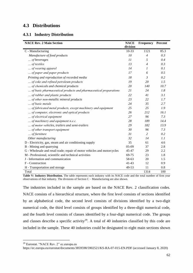
62

4.3 Distributions

4.3.1 Industry Distribution

Table V: Industry Distribution. The table represents each industry with its NACE code and the total number of firm year

observations of that industry. The divisions of Section C – Manufacturing are also shown.

The industries included in the sample are based on the NACE Rev. 2 classification codes.

NACE consists of a hierarchical structure, where the first level consists of sections identified

by an alphabetical code, the second level consists of divisions identified by a two-digit

numerical code, the third level consists of groups identified by a three-digit numerical code,

and the fourth level consists of classes identified by a four-digit numerical code. The groups

and classes describe a specific activity29. A total of 40 industries classified by this code are

included in the sample. These 40 industries could be designated to eight main sections shown

29 Eurostat. “NACE Rev. 2” ec.europa.eu

https://ec.europa.eu/eurostat/documents/3859598/5902521/KS-RA-07-015-EN.PDF (accessed January 8, 2020)

NACE Rev. 2 Main Section NACE

division

Frequency Percent

C - Manufacturing 10-33 1121 85.3

Manufacture of food products 10 4 0.3

… of beverages 11 5 0.4

… of textiles 13 4 0.3

… of wearing apparel 14 1 0.1

… of paper and paper products 17 6 0.5

Printing and reproduction of recorded media 18 3 0.2

… of coke and refined petroleum products 19 20 1.5

… of chemicals and chemical products 20 140 10.7

… of basic pharmaceutical products and pharmaceutical preparations 21 24 1.8

… of rubber and plastic products 22 41 3.1

… of other non-metallic mineral products 23 22 1.7

… of basic metals 24 35 2.7

… of fabricated metal products, except machinery and equipment 25 25 1.9

… of computer, electronic and optical products 26 212 16.1

… of electrical equipment 27 96 7.3

… of machinery and equipment n.e.c. 28 189 14.4

… of motor vehicles, trailers and semi-trailers 29 182 13.9

… of other transport equipment 30 96 7.3

… of furniture 31 2 0.2

Other manufacturing 32 14 1.1

D - Electricity, gas, steam and air conditioning supply 35 61 4.6

B - Mining and quarrying 05-09 37 2.8

G - Wholesale and retail trade; repair of motor vehicles and motorcycles 45-47 29 2.2

M - Professional, scientific and technical activities 69-75 23 1.8

J - Information and communication 58-63 20 1.5

F - Construction 41-43 12 0.9

H - Transportation and storage 49-53 11 0.8

Total 1314 100

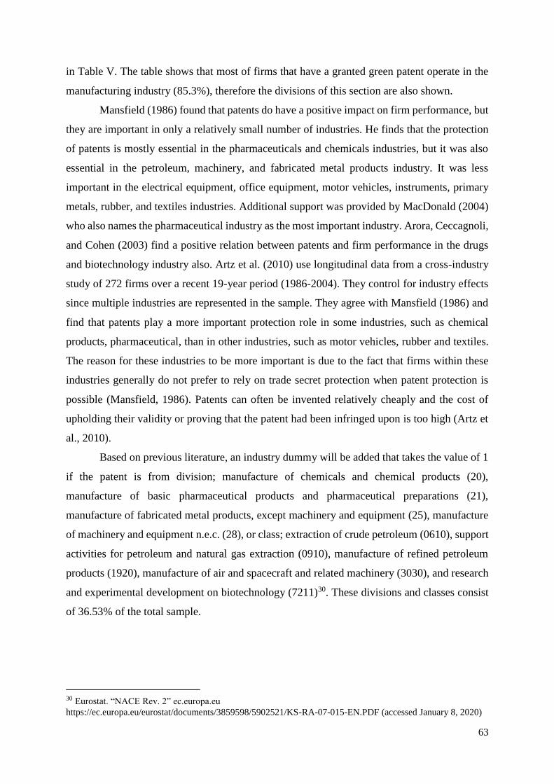
63

in Table V. The table shows that most of firms that have a granted green patent operate in the

manufacturing industry (85.3%), therefore the divisions of this section are also shown.

Mansfield (1986) found that patents do have a positive impact on firm performance, but

they are important in only a relatively small number of industries. He finds that the protection

of patents is mostly essential in the pharmaceuticals and chemicals industries, but it was also

essential in the petroleum, machinery, and fabricated metal products industry. It was less

important in the electrical equipment, office equipment, motor vehicles, instruments, primary

metals, rubber, and textiles industries. Additional support was provided by MacDonald (2004)

who also names the pharmaceutical industry as the most important industry. Arora, Ceccagnoli,

and Cohen (2003) find a positive relation between patents and firm performance in the drugs

and biotechnology industry also. Artz et al. (2010) use longitudinal data from a cross-industry

study of 272 firms over a recent 19-year period (1986-2004). They control for industry effects

since multiple industries are represented in the sample. They agree with Mansfield (1986) and

find that patents play a more important protection role in some industries, such as chemical

products, pharmaceutical, than in other industries, such as motor vehicles, rubber and textiles.

The reason for these industries to be more important is due to the fact that firms within these

industries generally do not prefer to rely on trade secret protection when patent protection is

possible (Mansfield, 1986). Patents can often be invented relatively cheaply and the cost of

upholding their validity or proving that the patent had been infringed upon is too high (Artz et

al., 2010).

Based on previous literature, an industry dummy will be added that takes the value of 1

if the patent is from division; manufacture of chemicals and chemical products (20),

manufacture of basic pharmaceutical products and pharmaceutical preparations (21),

manufacture of fabricated metal products, except machinery and equipment (25), manufacture

of machinery and equipment n.e.c. (28), or class; extraction of crude petroleum (0610), support

activities for petroleum and natural gas extraction (0910), manufacture of refined petroleum

products (1920), manufacture of air and spacecraft and related machinery (3030), and research

and experimental development on biotechnology (7211)30. These divisions and classes consist

of 36.53% of the total sample.

30 Eurostat. “NACE Rev. 2” ec.europa.eu

https://ec.europa.eu/eurostat/documents/3859598/5902521/KS-RA-07-015-EN.PDF (accessed January 8, 2020)

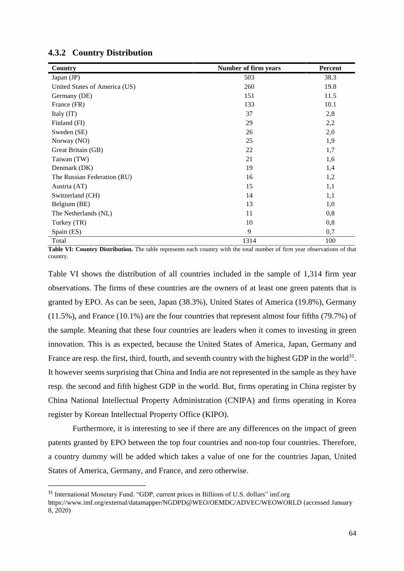
64

4.3.2 Country Distribution

Country Number of firm years Percent

Japan (JP) 503 38.3

United States of America (US) 260 19.8

Germany (DE) 151 11.5

France (FR) 133 10.1

Italy (IT) 37 2,8

Finland (FI) 29 2,2

Sweden (SE) 26 2,0

Norway (NO) 25 1,9

Great Britain (GB) 22 1,7

Taiwan (TW) 21 1,6

Denmark (DK) 19 1,4

The Russian Federation (RU) 16 1,2

Austria (AT) 15 1,1

Switzerland (CH) 14 1,1

Belgium (BE) 13 1,0

The Netherlands (NL) 11 0,8

Turkey (TR) 10 0,8

Spain (ES) 9 0,7

Total 1314 100

Table VI: Country Distribution. The table represents each country with the total number of firm year observations of that

country.

Table VI shows the distribution of all countries included in the sample of 1,314 firm year

observations. The firms of these countries are the owners of at least one green patents that is

granted by EPO. As can be seen, Japan (38.3%), United States of America (19.8%), Germany

(11.5%), and France (10.1%) are the four countries that represent almost four fifths (79.7%) of

the sample. Meaning that these four countries are leaders when it comes to investing in green

innovation. This is as expected, because the United States of America, Japan, Germany and

France are resp. the first, third, fourth, and seventh country with the highest GDP in the world31.

It however seems surprising that China and India are not represented in the sample as they have

resp. the second and fifth highest GDP in the world. But, firms operating in China register by

China National Intellectual Property Administration (CNIPA) and firms operating in Korea

register by Korean Intellectual Property Office (KIPO).

Furthermore, it is interesting to see if there are any differences on the impact of green

patents granted by EPO between the top four countries and non-top four countries. Therefore,

a country dummy will be added which takes a value of one for the countries Japan, United

States of America, Germany, and France, and zero otherwise.

31 International Monetary Fund. “GDP, current prices in Billions of U.S. dollars” imf.org

https://www.imf.org/external/datamapper/NGDPD@WEO/OEMDC/ADVEC/WEOWORLD (accessed January

8, 2020)

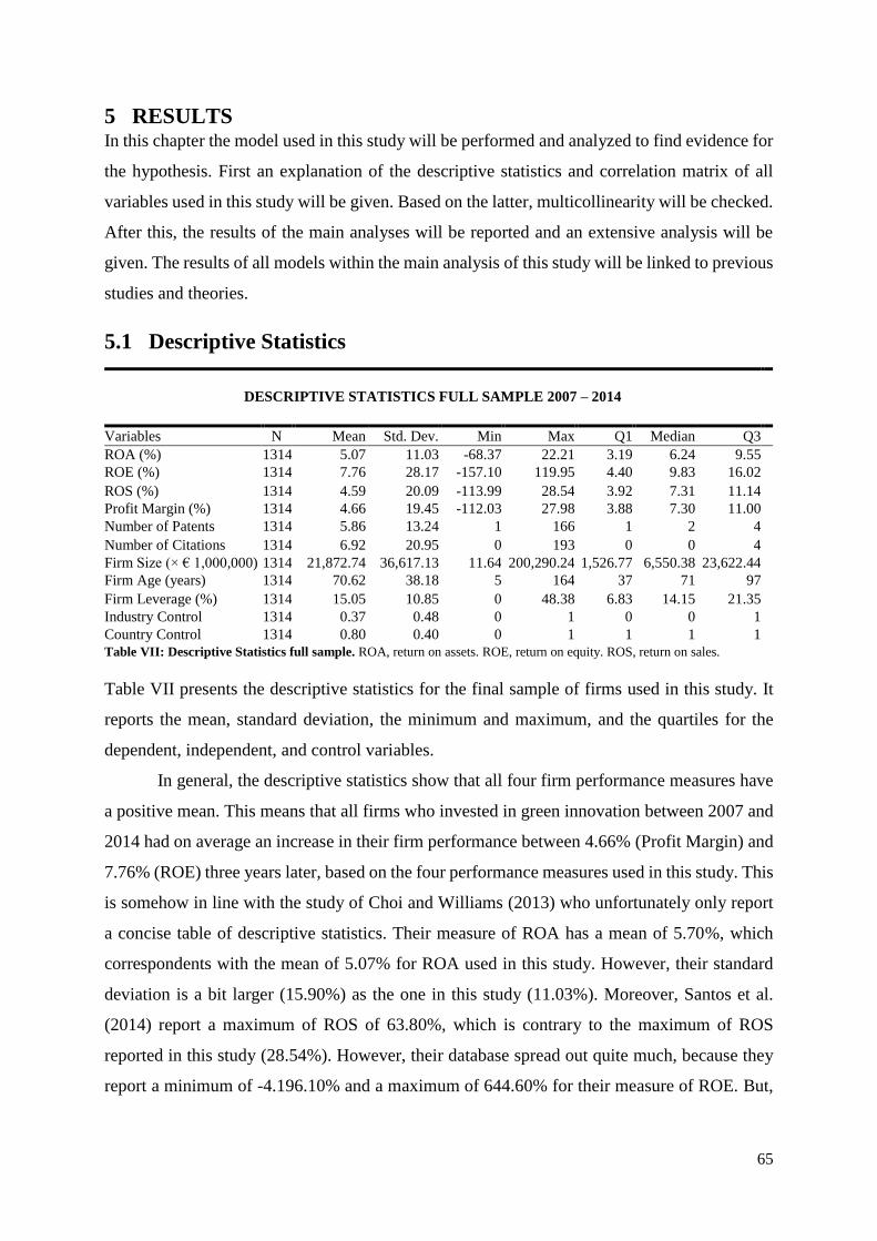
65

5 RESULTS In this chapter the model used in this study will be performed and analyzed to find evidence for

the hypothesis. First an explanation of the descriptive statistics and correlation matrix of all

variables used in this study will be given. Based on the latter, multicollinearity will be checked.

After this, the results of the main analyses will be reported and an extensive analysis will be

given. The results of all models within the main analysis of this study will be linked to previous

studies and theories.

5.1 Descriptive Statistics

Table VII: Descriptive Statistics full sample. ROA, return on assets. ROE, return on equity. ROS, return on sales.

Table VII presents the descriptive statistics for the final sample of firms used in this study. It

reports the mean, standard deviation, the minimum and maximum, and the quartiles for the

dependent, independent, and control variables.

In general, the descriptive statistics show that all four firm performance measures have

a positive mean. This means that all firms who invested in green innovation between 2007 and

2014 had on average an increase in their firm performance between 4.66% (Profit Margin) and

7.76% (ROE) three years later, based on the four performance measures used in this study. This

is somehow in line with the study of Choi and Williams (2013) who unfortunately only report

a concise table of descriptive statistics. Their measure of ROA has a mean of 5.70%, which

correspondents with the mean of 5.07% for ROA used in this study. However, their standard

deviation is a bit larger (15.90%) as the one in this study (11.03%). Moreover, Santos et al.

(2014) report a maximum of ROS of 63.80%, which is contrary to the maximum of ROS

reported in this study (28.54%). However, their database spread out quite much, because they

report a minimum of -4.196.10% and a maximum of 644.60% for their measure of ROE. But,

DESCRIPTIVE STATISTICS FULL SAMPLE 2007 – 2014

Variables N Mean Std. Dev. Min Max Q1 Median Q3

ROA (%) 1314 5.07 11.03 -68.37 22.21 3.19 6.24 9.55

ROE (%) 1314 7.76 28.17 -157.10 119.95 4.40 9.83 16.02

ROS (%) 1314 4.59 20.09 -113.99 28.54 3.92 7.31 11.14

Profit Margin (%) 1314 4.66 19.45 -112.03 27.98 3.88 7.30 11.00

Number of Patents 1314 5.86 13.24 1 166 1 2 4

Number of Citations 1314 6.92 20.95 0 193 0 0 4

Firm Size (× € 1,000,000) 1314 21,872.74 36,617.13 11.64 200,290.24 1,526.77 6,550.38 23,622.44

Firm Age (years) 1314 70.62 38.18 5 164 37 71 97

Firm Leverage (%) 1314 15.05 10.85 0 48.38 6.83 14.15 21.35

Industry Control 1314 0.37 0.48 0 1 0 0 1

Country Control 1314 0.80 0.40 0 1 1 1 1

66

this is not a problem for them as they use SEM as their method, which has no distributional

assumptions. So that means that data may be non-normal, skewed, and kurtotic.

Moreover, the table reports that all firms have at least one granted green patent and the

firm with the most has 166 of them. The firm who reports the most granted green patents

between 2007 and 2014 is Siemens Aktiengesellschaft (AG) from Germany, the largest

industrial manufacturing firm of Europe. They offer a variety of electrical engineering- and

electronics-related products and services32 . Examples of their granted green patents are a

method and device for conversion of carbon monoxide, a device to accumulate electric energy

comprising battery, a device for controlling energy transmission between transmission units in

e.g. electric cars, a power plant running on organic fuel with a carbon dioxide separator, and a

windmill generator. So, it is safe to say that Siemens AG contributes to an environmental

friendly society. A few other new European green patents granted by EPO in 2014 with its

number of citations are listed in Appendix C.

Next to that, the 1,314 firm year observations included in the sample have an average

of 5.86 granted European green patents each year with a standard deviation of 13.24, which

equates to the total of 7,700 granted European green patents. However, most of the firms do not

have that many as the median is two and the third-quartile is only four. In the study of Aquilera-

Caracuel and Ortiz-de-Mandojana (2013) the maximum of granted green patents a firm has in

a given year is almost twice as this study, namely a total of 320. They also report a much higher

median and standard deviation of granted green patents, namely 23.33 and 52.75 respectively.

However, this is due the fact that this study only include firms that have registered a higher

percentage of granted green patents for their period of time, because they are interested in firms

that consistently have developed green innovative behaviour.

Additionally, these granted green patents could also cited by others. The number of

citations range from zero to 193. The descriptive statistics show that each granted green patent

has an average of 6.92 citations with a standard deviation of 20.95, which equates to the total

of 9,087 citations. Although, most of them have none, as the median is zero and the third-

quartile is only four citations. Meaning that at least half of the firms in the sample did not have

a citation for any of the green patents granted that specific year. Therefore, a subsample analysis

for only firms that report at least one citation will be performed as a robustness check to see if

the results will differ or not. Next to that, given the non-normal distributions of the number of

32 Siemens. “Consumer products” new.siemens.com

https://new.siemens.com/global/en/products/consumer.html (accessed January 9, 2020)

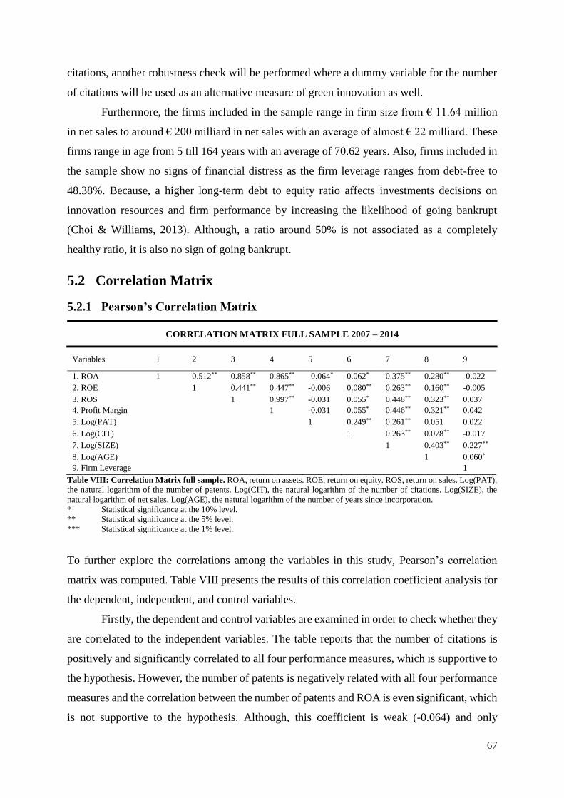
67

citations, another robustness check will be performed where a dummy variable for the number

of citations will be used as an alternative measure of green innovation as well.

Furthermore, the firms included in the sample range in firm size from € 11.64 million

in net sales to around € 200 milliard in net sales with an average of almost € 22 milliard. These

firms range in age from 5 till 164 years with an average of 70.62 years. Also, firms included in

the sample show no signs of financial distress as the firm leverage ranges from debt-free to

48.38%. Because, a higher long-term debt to equity ratio affects investments decisions on

innovation resources and firm performance by increasing the likelihood of going bankrupt

(Choi & Williams, 2013). Although, a ratio around 50% is not associated as a completely

healthy ratio, it is also no sign of going bankrupt.

5.2 Correlation Matrix

5.2.1 Pearson’s Correlation Matrix

CORRELATION MATRIX FULL SAMPLE 2007 – 2014

Variables 1 2 3 4 5 6 7 8 9

1. ROA 1 0.512** 0.858** 0.865** -0.064* 0.062* 0.375** 0.280** -0.022

2. ROE 1 0.441** 0.447** -0.006 0.080** 0.263** 0.160** -0.005

3. ROS 1 0.997** -0.031 0.055* 0.448** 0.323** 0.037

4. Profit Margin 1 -0.031 0.055* 0.446** 0.321** 0.042

5. Log(PAT) 1 0.249** 0.261** 0.051 0.022

6. Log(CIT) 1 0.263** 0.078** -0.017

7. Log(SIZE) 1 0.403** 0.227**

8. Log(AGE) 1 0.060*

9. Firm Leverage 1

Table VIII: Correlation Matrix full sample. ROA, return on assets. ROE, return on equity. ROS, return on sales. Log(PAT),

the natural logarithm of the number of patents. Log(CIT), the natural logarithm of the number of citations. Log(SIZE), the

natural logarithm of net sales. Log(AGE), the natural logarithm of the number of years since incorporation.

* Statistical significance at the 10% level.

** Statistical significance at the 5% level.

*** Statistical significance at the 1% level.

To further explore the correlations among the variables in this study, Pearson’s correlation

matrix was computed. Table VIII presents the results of this correlation coefficient analysis for

the dependent, independent, and control variables.

Firstly, the dependent and control variables are examined in order to check whether they

are correlated to the independent variables. The table reports that the number of citations is

positively and significantly correlated to all four performance measures, which is supportive to

the hypothesis. However, the number of patents is negatively related with all four performance

measures and the correlation between the number of patents and ROA is even significant, which

is not supportive to the hypothesis. Although, this coefficient is weak (-0.064) and only

68

significant at the 10% level. Next to that, not surprisingly, ROA, ROE, ROS and Profit Margin

all have significant positive correlations with each other. They are all measures of firm

performance and therefore correlate with each other. Profit Margin even shows a correlation

coefficient of 0.997 with ROS33. Moreover, both the number of patents and citations show

positive and significant correlation coefficients with firm size. With firm age as well, only the

correlation between the number of patents and firm size is not significant. Meaning that, based

on these correlation analysis, larger and older firms could have more resources and experience

to devote to generating green innovative activity. The control variable firm leverage also shows

a positive correlation with the number of patents, but a negative correlation with the number of

citations, but these correlations are not significant.

Secondly, the control variables are examined. Both firm size and firm age correlate

significantly and positively with all firm performance measures, with each other, and with firm

leverage at the 5% level. Only the correlation between firm age and firm leverage is not

significant at the 5% level, but at the 10% level. The correlation between these two control

variables and the four dependent variables is as expected, because larger and older firms, and

thus more mature and established, are on average better able to efficiently make profit that

increases firm performance. Moreover, the positive significant correlation between firm size

and firm age was to be expected as well as older firms have on average more time to acquire

more total assets compared to younger firms. Although, instead of a positive correlation a

negative correlation between firm size and firm leverage would have been more likely as larger

firms with more total assets are on average more mature and more established and thus have to

depend less on debt. Lastly, it was also more likely that firm leverage was negatively correlated

with the dependent variables as the cost of debt lowers the ability of generating more profits

and thus a better firm performance. Firm leverage only shows a negative correlation with ROA

and ROE. However, the correlation for all four dependent variables are not significant.

5.2.2 Multicollinearity

One of the main problems that could arise in statistics is the problem of multicollinearity.

Multicollinearity is present when two or more independent variables in a multiple regression

model are highly linearly related. Meaning that there is a strong correlation between the

independent variables. This statistical problem makes it hard to estimate the coefficients

33 This is because of the fact that both have EBIT as the numerator and the difference in the denominator is that

ROS is divided by net sales and Profit Margin by net sales + other operating revenues + stock variations. So, if a

firms lacks the last two, the calculation of ROS and Profit Margin have the same result.

69

accurately. It could also affect the standard errors and because of that variables could be

incorrectly displayed as (in)significant.

There are some ways to detect multicollinearity. Firstly, the simplest and most reliable

one is by checking the correlation matrix (Pramod et al., 2012; Abuhommous, 2017; Gui-long

et al., 2017; Zhou & Sadeghi, 2019). Multicollinearity will not be a great problem when the

correlation coefficients between the independent variables are below 0.30 (Vithessonthi &

Racela, 2016). But, when the correlation coefficient between two measures is above 0.30 and

statistically significant, the variables will be added separately in the regressions. Secondly,

multicollinearity could also be tested by examining the VIF values of the independent variables

as well. This provides an index that measures how much the variance of an estimated regression

coefficient is increased because of the multicollinearity. A value of 1 means that there is no

correlation between the independent variables. A value above 3 means that there probably exists

some multicollinearity, a value above 5 means that it is very likely there is a multicollinearity

problem, and a value above 10 definitely indicates multicollinearity that causes inevitable

problems (Ehie & Olibe, 2010).

Both these two approaches are used in this study. Looking at the correlation matrix one

might expect multicollinearity as the correlation between the two independent variables is

0.249, which is not above the threshold of 0.30, but still close to it. However, the VIF approach

gives a value of 1, meaning that there is no multicollinearity between the two independent

variables used in this study. The value of 0.249 is lower than expected, because both are

measures of the same. However, Hall et al. (2005) report a correlation of 0.220 as well and

DeCarolis and Deeds (1999) report an even lower correlation (0.070) between the number of

patents and citations.

Furthermore, the control variable firm size has high correlations with all other variables

and even has a correlation of 0.261 with the number of patents and a correlation of 0.263 with

the number of citations. Both are also not above the threshold of 0.30, but are also really close.

This means that firm size most likely strongly affects the number of patents and citations. So,

this could lead to incorrectly displaying these two as positively or negatively (in)significant

when firm size is included in the regression as well. Therefore, firm size will be monitored

closely to see whether this control variable indeed has too much influence. Artz et al. (2010)

also report that their control variable firm size was significantly correlated with their

independent variable. However, their approach was by removing the control variable from the

analysis and this study will not follow that approach.

70

5.3 OLS Regression Results

5.3.1 Full Sample Results

To test the hypothesis of this study an OLS regression analysis will be performed. This section

reports the results of the independent variables number of patents/citations with its control

variables on the four measures of firm performance as the dependent variables for the full

sample. Only the results of ROE as the firm performance measure will be reported in this section

Appendix D reports the results of the other three firm performance measures. Any differences

between these three measures and ROE will be explicitly described.

Furthermore, the tables report a couple of models wherein the first model (1) will be

used as a benchmark model in order to see the impact of the independent variable in the other

models. The last model (5) will be the full model and shows how all variables are related to the

dependent variable and the other models (2), (3), and (4), the so called specific models, show

how specific combinations of variables are related to the dependent variable. Panel A (B)

reports the results of the regression for the number of patents (citations) as the independent

variable.

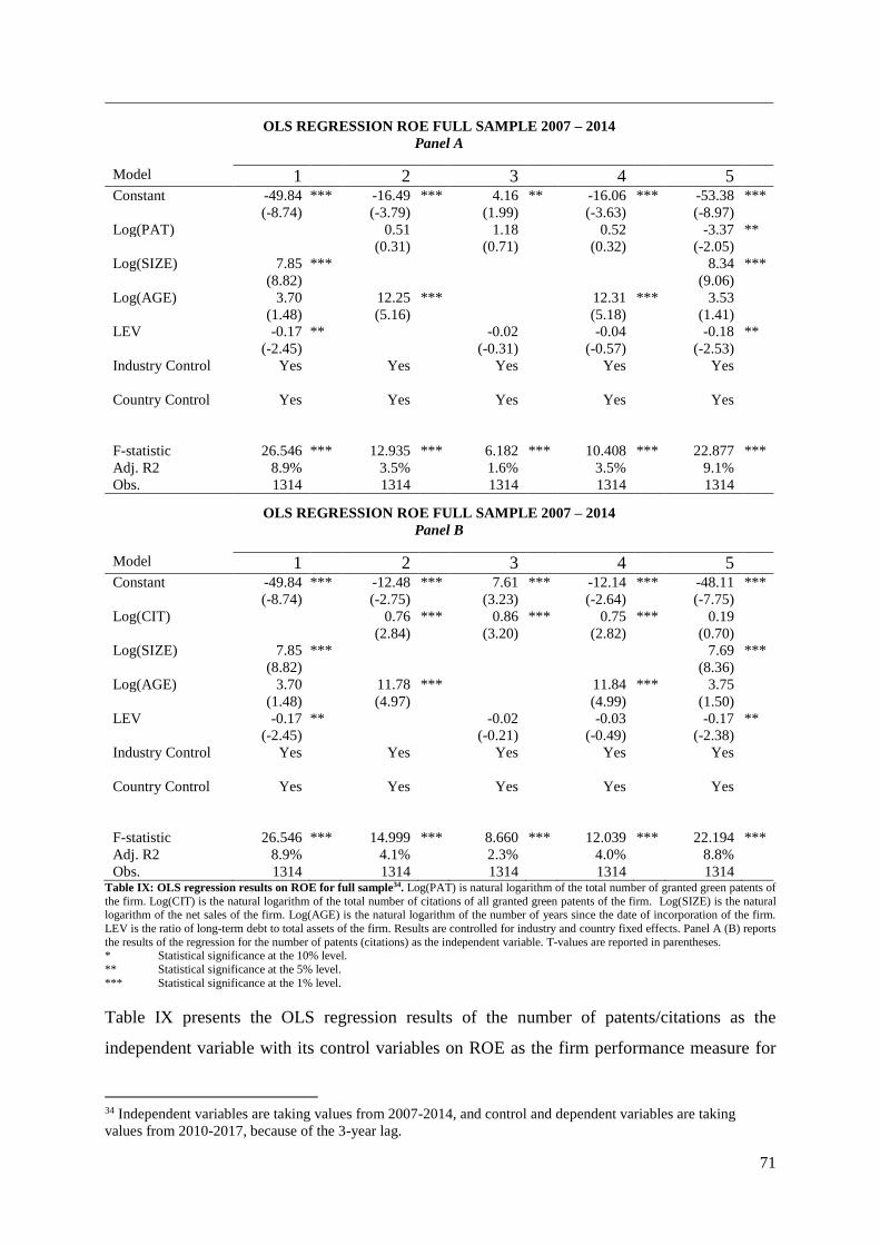
71

OLS REGRESSION ROE FULL SAMPLE 2007 – 2014

Panel A

Model 1 2 3 4 5 Constant -49.84 *** -16.49 *** 4.16 ** -16.06 *** -53.38 ***

(-8.74) (-3.79) (1.99) (-3.63) (-8.97)

Log(PAT) 0.51 1.18 0.52 -3.37 **

(0.31) (0.71) (0.32) (-2.05)

Log(SIZE) 7.85 *** 8.34 ***

(8.82) (9.06)

Log(AGE) 3.70 12.25 *** 12.31 *** 3.53

(1.48) (5.16) (5.18) (1.41)

LEV -0.17 ** -0.02 -0.04 -0.18 **

(-2.45) (-0.31) (-0.57) (-2.53)

Industry Control Yes Yes Yes Yes Yes

Country Control Yes Yes Yes Yes Yes

F-statistic 26.546 *** 12.935 *** 6.182 *** 10.408 *** 22.877 ***

Adj. R2 8.9% 3.5% 1.6% 3.5% 9.1%

Obs. 1314 1314 1314 1314 1314

OLS REGRESSION ROE FULL SAMPLE 2007 – 2014

Panel B

Model 1 2 3 4 5 Constant -49.84 *** -12.48 *** 7.61 *** -12.14 *** -48.11 ***

(-8.74) (-2.75) (3.23) (-2.64) (-7.75)

Log(CIT) 0.76 *** 0.86 *** 0.75 *** 0.19

(2.84) (3.20) (2.82) (0.70)

Log(SIZE) 7.85 *** 7.69 ***

(8.82) (8.36)

Log(AGE) 3.70 11.78 *** 11.84 *** 3.75

(1.48) (4.97) (4.99) (1.50)

LEV -0.17 ** -0.02 -0.03 -0.17 **

(-2.45) (-0.21) (-0.49) (-2.38)

Industry Control Yes Yes Yes Yes Yes

Country Control Yes Yes Yes Yes Yes

F-statistic 26.546 *** 14.999 *** 8.660 *** 12.039 *** 22.194 ***

Adj. R2 8.9% 4.1% 2.3% 4.0% 8.8%

Obs. 1314 1314 1314 1314 1314 Table IX: OLS regression results on ROE for full sample34. Log(PAT) is natural logarithm of the total number of granted green patents of

the firm. Log(CIT) is the natural logarithm of the total number of citations of all granted green patents of the firm. Log(SIZE) is the natural logarithm of the net sales of the firm. Log(AGE) is the natural logarithm of the number of years since the date of incorporation of the firm.

LEV is the ratio of long-term debt to total assets of the firm. Results are controlled for industry and country fixed effects. Panel A (B) reports

the results of the regression for the number of patents (citations) as the independent variable. T-values are reported in parentheses. * Statistical significance at the 10% level.

** Statistical significance at the 5% level.

*** Statistical significance at the 1% level.

Table IX presents the OLS regression results of the number of patents/citations as the

independent variable with its control variables on ROE as the firm performance measure for

34 Independent variables are taking values from 2007-2014, and control and dependent variables are taking

values from 2010-2017, because of the 3-year lag.

72

the full sample. Firstly the benchmark models (1) will be described and thereafter the specific

models (2), (3), and (4), and finally the full model (5).

The benchmark models (1) show that control variables firm size and firm age are

positively related with all four performance measures. These relationships are also significant

at the 1% level in almost all benchmark models, meaning that larger and older firms have on

average a higher firm performance. The control variable firm leverage is negatively and

significantly related to the performance measures, meaning that firms with a higher debt issue

have a lower firm performance.

Furthermore, the results of the specific models (2), (3), and (4) show that there is no

relationship between the number of patents and ROE as the coefficients are not statistically

significant. However, the number of citations is positively related to ROE and this relationship

is statistically significant at the 1% level. This concludes that investing in green innovation,

measured by the number of citations, does have a positive influence on the performance of the

firm, which confirms the hypothesis. These results are somehow in line with the innovation

studies of Li et al. (2010), Choi and Williams (2013), Feeny and Rogers (2013), and Huang and

Hou (2019), because they all find that the number of patents as the innovation indicator is also

positively related to the performance of the firm as their coefficients are statistically significant.

Although the results do not show a statically relationship between the number of patents and

ROE, this relationship still shows the positive sign. Regarding green innovation studies, this

result confirms the study of Chiou et al. (2011), Ar (2012), Lin et al. (2013), and Chan et al.

(2016), who all find that green innovation is significantly and positively related to firm

performance. This proves that the positive effects of green innovation, namely reducing

pollution and limiting hazardous and toxic waste and thus reducing the cost of disposal and

improving the green efficiency and response to external environmental pressure from

customers, all ultimately contribute to a better firm performance (Chiou et al., 2011).

Appendix D reports the results of the other three performance measures. Interestingly,

looking at ROA as the performance measure, the number of citations still shows a positive and

significant relationship with ROA in model (2), (3), and (4), but the number of patents shows a

negative and significant relationship with ROA in model (2) and (4). Artz et al. (2010) find the

same result for the relationship between patents and ROA. This could be due to the fact that the

sample consists of all firms that have at least one granted green patent. So, it is possible that

having only one granted green patent as a firm does not have that big of an impact on the

performance of a firm. Because, in model (2), (3), and (4) three out of four performance

measures show no significant relationship between the number of patents and the performance

73

measure, and is only negative and significant related to ROA. The performance measure ROA

may turn out negative, while that is not due to only that one granted green patent. However, the

negative sign still calls into question the value of patents as protect mechanisms. Artz et al.

(2010) argue that it is possible that patents may only boost firm performance indirectly through

their positive effect on product innovations. They also argue that not all patented technologies

are actually converted into products. In this way, a patent could decrease the competitive

position of a firm, because managers think they are invincible against competitors and thus do

not develop other complementarities and skills that are needed to compete, like management,

production, and marketing. Also, the granting procedure of patents is expensive and this

combined with low returns directly from those patents could explain the negative relationship.

Therefore, regarding to green innovation, the number of citations is probably a better measure

of green innovation than the number of granted green patents. Because, the more citations a

granted green patent has, the more firms have used that particular granted green patent to file

for a green patent themselves. And of course, other firms only continue to embroider on

successful granted patents. So, one could argue that the more citations a granted green patent

has, the more it turned out to be successful. Making citation count a measure of success.

Moreover, firm age shows a positive relation with all four performance measures for all

models and this relationship is also significant at the 1% level in most of the models, which is

in line with previous literature (Pramod et al., 2012; Gui-long et al., 2017; Huang & Hou. 2019).

Firm age is often associated with production experience, which could have a positive influence

on the performance of a firm. Pramod et al. (2012) state that older firms are expected to fare

better on their market. They can avoid the liabilities newcomers have. Furthermore, firm

leverage shows a negative relationship with the four performance measures in all full models

(5) and is significant at the 5% level. Which is in line with previous literature as well as they

find a negative and significant relationship with the performance measure (Feng & Rong, 2007;

Chadha & Oriani, 2009). Pramod et al. (2012) state that debt could lead to potential losses if

the green innovation investment becomes worthless, because then the firm still needs to pay the

loan principal and all accrued interest on the loan. This increase in risk decreases the

performance of a firm. So, a high leverage level affects investments decisions on innovation

resources and firm performance by increasing the likelihood of going bankrupt (Choi &

Williams, 2013).

Furthermore, the results of using ROS and Profit Margin as the dependent variable show

extremely weak results and almost no significance at all for both the independent variables in

models (2), (3), and (4). Only the relationship between the number of citations and the two

74

performance measures is positive and significant at the 5% level in model (3) when only

leverage is included as a control variable. However, only resp. 0.8% and 0.9% of the variance

of the dependent variable is explained by the independent variables in this model.

Lastly, in the full model (5) the control variable firm size is also included in the

regression and expectedly the regression reports completely different results. Using ROE as the

dependent variable, the number of citations as the independent variable still shows a positive

sign, but loses all its significance. The number of patents is even negatively and significantly

related to ROE at the 5% level. Almost the same applies to the regression wherein ROA is used

as the dependent variable, but here the number of citations also shows a negative but weak sign.

For ROS and Profit Margin this relationship suddenly becomes significant at the 5% level.

Meaning that for larger firms the more patents/citations, the lower its performance. Mansfield

(1986) states that many economists seem to believe that for smaller firms patent protection

tends to be more important than for larger firms. Although, Mansfield does not find evidence

regarding this statement, but this could be due to the fact that his study is not concerned with

very small firms (sales below $ 25 million). Therefore, it is interestingly to split the sample by

the median of firm size as a robustness check (Loughran & Shive, 2011; Vithessonthi & Racela,

2016).

In conclusion, the results partly support the hypothesis that green innovation affects firm

performance positively as the number of citations indeed show the positive and significant sign

with ROE and ROA and partly for ROS and Profit Margin when firm size is not included, but

the number of patents does not. Regarding citations, this is in line with the resource-based

theory as the theory states that unique resources and capabilities of a firm are the key drivers of

competitive advantage and a better performance of a firm. Green innovation is one example of

such a unique resource, because a firm could use it to differentiate itself from others. Therefore,

the positive and significant relationship between green innovation and firm performance was

as expected. This result is also consistent with the innovation theory of Schumpeter (1934) as

he stated almost a century ago that adaptable firms that try new creative ways of operating are

more likely to outperform firms that do not, especially in a competitive environment. This is

still the case nowadays as the more successful granted green patents show a higher firm

performance. Because, the number of citations clarifies the number of other firms that are trying

to copy or improve that granted green patent and could thus arguably be a measure of its

success. These firms could on average have a stronger market position, because the new ways

of using the knowledge, technology and resources of the firm could bring new opportunities.

75

6 ROBUSTNESS CHECKS Robustness checks are performed to examine if the results of the main analysis are consistent,

robust and provide reliable outcomes. If the coefficients are plausible and robust, this is

commonly interpreted as evidence of structural validity (Lu & White, 2014). The robustness

checks that are performed to test the hypothesis of this study as well are a fixed/random effects

model for the full sample, and extra OLS regression checks for: the full sample split by the

median of size, a 2-year lag sample, a sample consisting of firms operating only in patent-

sensitive industries, a sample consisting of firms with at least one citation, a 2010-2014 sample

with using a 2-year and 3-year lag for firm performance improvement as the replacement of the

dependent variable, and a sample using a citation dummy as the replacement of the number of

citations. The sections firstly describes the descriptive statistics and correlation matrices that

are reported in appendix E till K. Any differences with the full model of the main analysis will

be described. Thereafter, the results of the robustness test will be reported. Again, only the

results of ROE as the firm performance measure will be reported in this section. Appendix E

till K report the results of the other three firm performance measures as well. Any differences

between the results of the main analysis and robustness tests will be substantiated.

Same as before, the tables report a couple of models wherein the first model (1) will be

used as a benchmark model in order to see the impact of the independent variable in the other

models. The last model (5) will be the full model and shows how all variables are related to the

dependent variable and the other models (2), (3), and (4) show how specific combinations of

variables are related to the dependent variable. Panel A (B) reports the results of the regression

for the number of patents (citations) as the independent variable.

6.1 Fixed/Random Effects model The first robustness check is the fixed/random effects model. Previous studies with similar

hypothesis use a combination of the OLS regression with this model as well (Kumbhakar et al.,

2011; Loughran and Shive 2011; Ortega-Argilés et al., 2011; Vivarelli and Voigt, 2011; Pramod

et al., 2012; Ilyukhin, 2015; Huang and Hou, 2019). The reason for this is the disadvantage of

using an OLS regression for this sample as it ignores the panel structure of the data. An OLS

regression thus assumes that observations are serially uncorrelated and that the errors across

individual and time are homoskedastic, meaning that the estimates of the regression are

inefficient when these errors are not homoskedastic. However, the measures of green innovation

change a lot over time for particular firms. No firm has the same number of patents and citations

over all eight years. Table X, which is an extension of Table IV, shows that the number of

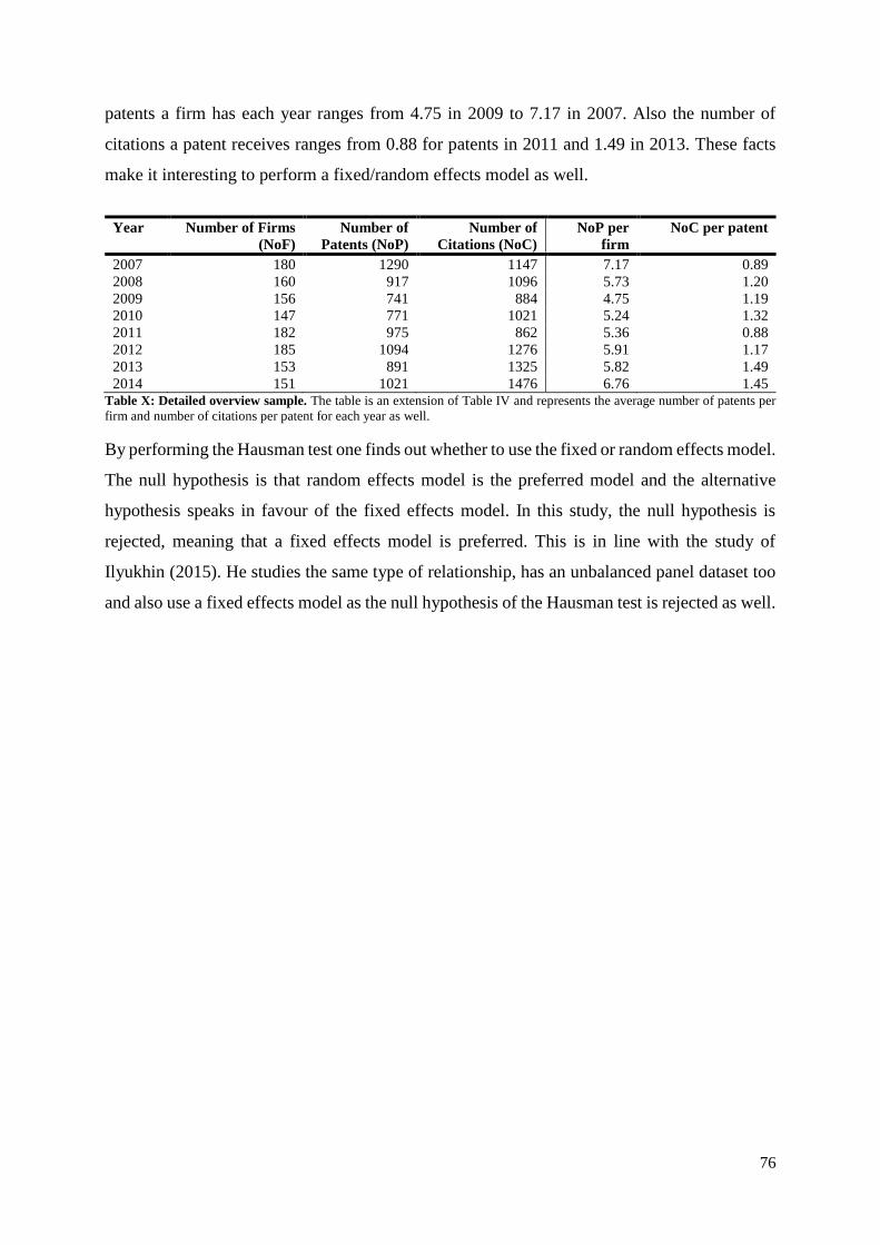
76

patents a firm has each year ranges from 4.75 in 2009 to 7.17 in 2007. Also the number of

citations a patent receives ranges from 0.88 for patents in 2011 and 1.49 in 2013. These facts

make it interesting to perform a fixed/random effects model as well.

Year Number of Firms

(NoF)

Number of

Patents (NoP)

Number of

Citations (NoC)

NoP per

firm

NoC per patent

2007 180 1290 1147 7.17 0.89

2008 160 917 1096 5.73 1.20

2009 156 741 884 4.75 1.19

2010 147 771 1021 5.24 1.32

2011 182 975 862 5.36 0.88

2012 185 1094 1276 5.91 1.17

2013 153 891 1325 5.82 1.49

2014 151 1021 1476 6.76 1.45 Table X: Detailed overview sample. The table is an extension of Table IV and represents the average number of patents per

firm and number of citations per patent for each year as well.

By performing the Hausman test one finds out whether to use the fixed or random effects model.

The null hypothesis is that random effects model is the preferred model and the alternative

hypothesis speaks in favour of the fixed effects model. In this study, the null hypothesis is

rejected, meaning that a fixed effects model is preferred. This is in line with the study of

Ilyukhin (2015). He studies the same type of relationship, has an unbalanced panel dataset too

and also use a fixed effects model as the null hypothesis of the Hausman test is rejected as well.

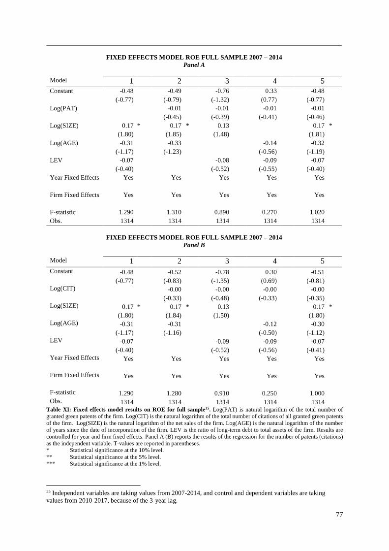
77

FIXED EFFECTS MODEL ROE FULL SAMPLE 2007 – 2014

Panel A

Model 1 2 3 4 5

Constant -0.48 -0.49 -0.76 0.33 -0.48

(-0.77) (-0.79) (-1.32) (0.77) (-0.77)

Log(PAT) -0.01 -0.01 -0.01 -0.01

(-0.45) (-0.39) (-0.41) (-0.46)

Log(SIZE) 0.17 * 0.17 * 0.13 0.17 *

(1.80) (1.85) (1.48) (1.81)

Log(AGE) -0.31 -0.33 -0.14 -0.32

(-1.17) (-1.23) (-0.56) (-1.19)

LEV -0.07 -0.08 -0.09 -0.07

(-0.40) (-0.52) (-0.55) (-0.40)

Year Fixed Effects Yes Yes Yes Yes Yes

Firm Fixed Effects Yes Yes Yes Yes Yes

F-statistic 1.290 1.310 0.890 0.270 1.020

Obs. 1314 1314 1314 1314 1314

FIXED EFFECTS MODEL ROE FULL SAMPLE 2007 – 2014

Panel B

Model 1 2 3 4 5

Constant -0.48 -0.52 -0.78 0.30 -0.51

(-0.77) (-0.83) (-1.35) (0.69) (-0.81)

Log(CIT) -0.00 -0.00 -0.00 -0.00

(-0.33) (-0.48) (-0.33) (-0.35)

Log(SIZE) 0.17 * 0.17 * 0.13 0.17 *

(1.80) (1.84) (1.50) (1.80)

Log(AGE) -0.31 -0.31 -0.12 -0.30

(-1.17) (-1.16) (-0.50) (-1.12)

LEV -0.07 -0.09 -0.09 -0.07

(-0.40) (-0.52) (-0.56) (-0.41)

Year Fixed Effects Yes Yes Yes Yes Yes

Firm Fixed Effects Yes Yes Yes Yes Yes

F-statistic 1.290 1.280 0.910 0.250 1.000

Obs. 1314 1314 1314 1314 1314 Table XI: Fixed effects model results on ROE for full sample35. Log(PAT) is natural logarithm of the total number of

granted green patents of the firm. Log(CIT) is the natural logarithm of the total number of citations of all granted green patents

of the firm. Log(SIZE) is the natural logarithm of the net sales of the firm. Log(AGE) is the natural logarithm of the number

of years since the date of incorporation of the firm. LEV is the ratio of long-term debt to total assets of the firm. Results are

controlled for year and firm fixed effects. Panel A (B) reports the results of the regression for the number of patents (citations)

as the independent variable. T-values are reported in parentheses.

* Statistical significance at the 10% level.

** Statistical significance at the 5% level.

*** Statistical significance at the 1% level.

35 Independent variables are taking values from 2007-2014, and control and dependent variables are taking

values from 2010-2017, because of the 3-year lag.

78

Table XI reports the fixed effects model results of the number of patents/citations as the

independent variable with its control variables on ROE as the firm performance measure for

the full sample. As this model uses the same sample as the OLS regression for the full sample,

the descriptive statistics are the same as reported in Table VII. The results of the other three

performance measures are reported in Appendix E. The industry and country dummy variable

are omitted due to the fact that dummy variables do not change over time. Year and firm fixed

effects are taken into account.

Surprisingly, results of the fixed effects model show that both measures of green

innovation are insignificant and extremely weak related to all four performance measures. ROS

and Profit Margin show the highest t-values (1.19), but these still do not indicate a significant

relationship. This is in line with previous studies as some studies argue that patents do not work

in practice as well as they do in theory. Griliches, Hall, and Pakes (1991) and Arora et al. (2008),

for example, find that patents have no influence on firm performance. A reason for this could

be that patents could often be invented relatively cheaply, but the costs of holding on to these

patents could be too high. Another reason could be that the goal of intention of patenting for

many firms has evolved. Meaning that for a firm it is no longer the goal to protect their own

innovation efforts to get a temporary monopoly to make abnormal profits, but rather to play a

more strategic role in competitiveness. Firms could for example patent their innovations to

block a competitor’s innovation efforts (MacDonald, 2004). This means that many patents

could have a defensive approach and therefore this forces many firms to patent inventions they

normally would not and has no to almost no impact on firm performance.

These results doubt the value a patent has as a protection mechanism. They do repay

some of the R&D expenditures, but the results indicate that there is no direct increase in the

performance of the firm. The impact of a patent can vary greatly, with only a relative small

number of patents having a significant impact on the performance of a firm.

6.2 Sample split by variable Size The next robustness check is an OLS regression where the sample is split by the median of the

variable size. Meaning that the full sample are now split into small and large firms. As described

for the main analysis, the control variable size has strong correlations with all variables. But

most importantly, the strong correlations with both measures of green innovation could affect

the standard errors and thus the results could be incorrectly displayed as (in)significant.

Therefore, it is interesting to check if there are any differences in results for both split samples.

79

Appendix F reports the descriptive statistics and correlation matrices of the split

samples. The large firms show much higher means for all performance measures as they range

for large firms from 6.73% for ROA to 12.20% for ROE and for small firms this range is only

-2.62% for ROS to 3.83% for ROE. Also, the minima of the performance measures for large

firms are around -5.00% and only for ROE this is -71.53%. These minima for small firms range

from -146.85% for ROA to -260.37% for ROS. The maxima show similar results. Furthermore,

there are also differences between the number of patents and citations between small and large

firms. Large firms have an average of about 10 patents (12 citations) per firm year and this

average for small firms is only 2.24 (1.49). The most patents (citations) in a firm year a small

firm has is only 24 (26) and for large firms this is 166 (193). More than three-quarters of small

firms does not have one citation. For large firms this is at least half of the firms. Moreover, of

course the split samples differ in size as the mean for large firms is almost € 42 billion and for

small firms this is only € 2 billion. Larger firms also are on average 20 years older and have a

slightly higher average of leverage ratio.

The correlation matrices show that for small firms the proxy for the number of citations

is not significant related to the four performance measures anymore. It also shows that for small

firms the control variable firm size is not highly correlated with the measures of green

innovation. However, this still is the case for large firms as it reports even stronger correlations

between firm size and the green innovation measures compared to the main analysis.

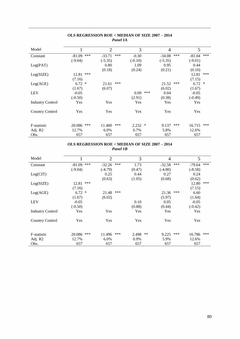
80

OLS REGRESSION ROE < MEDIAN OF SIZE 2007 – 2014

Panel 1A

Model 1 2 3 4 5

Constant -81.09 *** -33.71 *** -0.30 -34.08 *** -81.04 ***

(-9.04) (-5.35) (-0.10) (-5.35) (-9.01)

Log(PAT) 0.80 1.09 0.95 0.44

(0.18) (0.24) (0.21) (0.10)

Log(SIZE) 12.81 *** 12.81 ***

(7.16) (7.15)

Log(AGE) 6.72 * 21.61 *** 21.52 *** 6.72 *

(1.67) (6.07) (6.02) (1.67)

LEV -0.05 0.09 *** 0.04 -0.05

(-0.50) (2.91) (0.38) (-0.49)

Industry Control Yes Yes Yes Yes Yes

Country Control Yes Yes Yes Yes Yes

F-statistic 20.086 *** 11.400 *** 2.232 * 9.137 *** 16.715 ***

Adj. R2 12.7% 6.0% 0.7% 5.8% 12.6%

Obs. 657 657 657 657 657

OLS REGRESSION ROE < MEDIAN OF SIZE 2007 – 2014

Panel 1B

Model 1 2 3 4 5

Constant -81.09 *** -32.26 *** 1.73 -32.58 *** -79.64 ***

(-9.04) (-4.79) (0.47) (-4.80) (-8.58)

Log(CIT) 0.25 0.44 0.27 0.24

(0.63) (1.05) (0.68) (0.62)

Log(SIZE) 12.81 *** 12.80 ***

(7.16) (7.15)

Log(AGE) 6.72 * 21.48 *** 21.36 *** 6.60

(1.67) (6.02) (5.97) (1.64)

LEV -0.05 0.10 0.05 -0.05

(-0.50) (0.88) (0.44) (-0.42)

Industry Control Yes Yes Yes Yes Yes

Country Control Yes Yes Yes Yes Yes

F-statistic 20.086 *** 11.496 *** 2.498 ** 9.225 *** 16.786 ***

Adj. R2 12.7% 6.0% 0.9% 5.9% 12.6%

Obs. 657 657 657 657 657

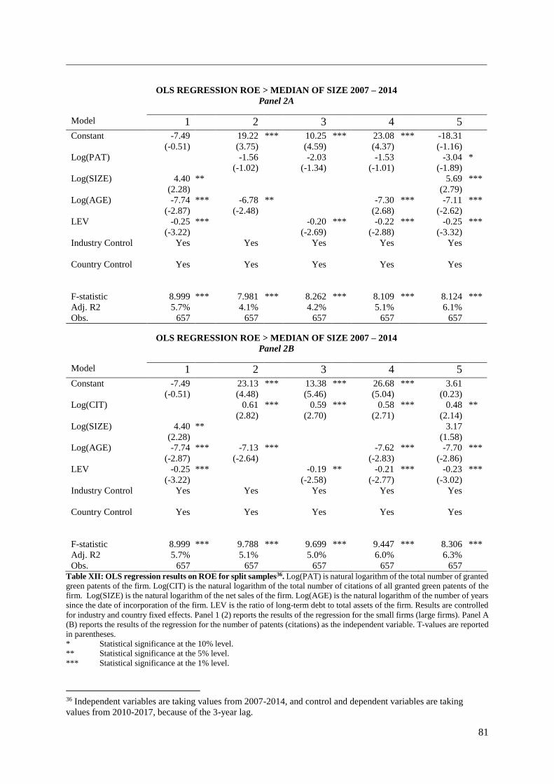
81

OLS REGRESSION ROE > MEDIAN OF SIZE 2007 – 2014

Panel 2A

Model 1 2 3 4 5

Constant -7.49 19.22 *** 10.25 *** 23.08 *** -18.31

(-0.51) (3.75) (4.59) (4.37) (-1.16)

Log(PAT) -1.56 -2.03 -1.53 -3.04 *

(-1.02) (-1.34) (-1.01) (-1.89)

Log(SIZE) 4.40 ** 5.69 ***

(2.28) (2.79)

Log(AGE) -7.74 *** -6.78 ** -7.30 *** -7.11 ***

(-2.87) (-2.48) (2.68) (-2.62)

LEV -0.25 *** -0.20 *** -0.22 *** -0.25 ***

(-3.22) (-2.69) (-2.88) (-3.32)

Industry Control Yes Yes Yes Yes Yes

Country Control Yes Yes Yes Yes Yes

F-statistic 8.999 *** 7.981 *** 8.262 *** 8.109 *** 8.124 ***

Adj. R2 5.7% 4.1% 4.2% 5.1% 6.1%

Obs. 657 657 657 657 657

OLS REGRESSION ROE > MEDIAN OF SIZE 2007 – 2014

Panel 2B

Model 1 2 3 4 5

Constant -7.49 23.13 *** 13.38 *** 26.68 *** 3.61

(-0.51) (4.48) (5.46) (5.04) (0.23)

Log(CIT) 0.61 *** 0.59 *** 0.58 *** 0.48 **

(2.82) (2.70) (2.71) (2.14)

Log(SIZE) 4.40 ** 3.17

(2.28) (1.58)

Log(AGE) -7.74 *** -7.13 *** -7.62 *** -7.70 ***

(-2.87) (-2.64) (-2.83) (-2.86)

LEV -0.25 *** -0.19 ** -0.21 *** -0.23 ***

(-3.22) (-2.58) (-2.77) (-3.02)

Industry Control Yes Yes Yes Yes Yes

Country Control Yes Yes Yes Yes Yes

F-statistic 8.999 *** 9.788 *** 9.699 *** 9.447 *** 8.306 ***

Adj. R2 5.7% 5.1% 5.0% 6.0% 6.3%

Obs. 657 657 657 657 657 Table XII: OLS regression results on ROE for split samples36. Log(PAT) is natural logarithm of the total number of granted

green patents of the firm. Log(CIT) is the natural logarithm of the total number of citations of all granted green patents of the

firm. Log(SIZE) is the natural logarithm of the net sales of the firm. Log(AGE) is the natural logarithm of the number of years

since the date of incorporation of the firm. LEV is the ratio of long-term debt to total assets of the firm. Results are controlled

for industry and country fixed effects. Panel 1 (2) reports the results of the regression for the small firms (large firms). Panel A

(B) reports the results of the regression for the number of patents (citations) as the independent variable. T-values are reported

in parentheses.

* Statistical significance at the 10% level.

** Statistical significance at the 5% level.

*** Statistical significance at the 1% level.

36 Independent variables are taking values from 2007-2014, and control and dependent variables are taking

values from 2010-2017, because of the 3-year lag.

82

Table XII reports the OLS regression results of the number of patents/citations as the

independent variable with its control variables on ROE as the firm performance measure for

the split samples. The results of the other three performance measures are reported in Appendix

F.

For small firms the results report that both green innovation measures show positive

signs with ROE, but these are insignificant in all models. Meaning that there is no relationship.

For large firms the sign between the numbers of patents and ROE are negative but weak as only

the full model is significant at 10%. However, using the number of citations as a measure of

green innovation shows positive and significant relationships with ROE in all models at the 1%

level for large firms, except for the full model (5). Although, the full model is significant at the

5% level. The results regarding the relationship between the number of patents and ROE for

both small and large firms are similar to the results of the main analysis as it shows weak signs

as well. For the number of citations only large firms match the results of the main analysis.

Regarding the other three measures of firm performance, small firms show the same

signs as the results of the main analysis, only weaker. The most important difference for small

firms is that the control variables firm size does not influence the relationship between the

measures of green innovation and firm performance anymore. Meaning that the full models (5)

show similar results as the other specific models (2, 3, and 4). For the main analysis the results

of the relationship between green innovation and firm performance became negative and highly

significant when the control variable firm size was taken into account. For small firms, the

relationship between the number of patents and ROA, ROS, and Profit Margin is insignificant

in all models, meaning that there is no relationship. Almost the same applies to the number of

citations as it is insignificant in all models for all three performance measures except one.

Although, this positive relationship between the number of citations and ROA is only

significant at the 10% level. Mansfield (1986) finds that, although many economists believe

that the protection a patent could bring tends to be more important to smaller firms, this

proposition has little support as seven out of ten industries show no significance at all. This is

in line with this study. However, the firms in the study of Mansfield (1986) are not that small

as firms with sales below $ 25 million are not included in the sample.

Furthermore, the results of the sample consisting of large firms also show similar signs

as the full sample, but also weaker and a bit more negative. For large firms, the relationship

between the number of patents and ROA is still negative, but more significant. And for the

relationship between the number of citations and ROA it is still positive, but no longer

83

significant. The relationship between the number of patents and citations with both ROS and

Profit Margin are negative in all models, but none of them show any significance.

To conclude, the results of the split samples show similar signs as the main analysis,

only it lacks in significance. Both small and large firms show weaker signs than the main

analysis, especially in the full models. However, for small firms the control variable firm size

does not influence the relationship between green innovation and firm performance anymore,

confirming that the control variable indeed has a huge impact on the sign and significance level

of the relationship between green innovation and firm performance. Meaning that both the

number of patents and citations do not have that much of an influence on the performance of a

firm, but are influenced by the control variable firm size, which corresponds to the results of

the fixed effects model.

6.3 2-Year lag In this section, an OLS regression analysis with a 2-year lag sample is performed as the

robustness check. Ernst (2001), for example, finds that national patents applications lead to a

sales increase with a time-lag of two to three years after the priority year. As the main analysis

already takes into account a 3-year lag, this test checks if the results of the sample with a 2-year

lag are consistent or not. Based on the available data, the patents in the sample are from 2008

to 2014 as financial data from ORBIS is available for 2010-2017.

Appendix G reports the descriptive statistics and correlation matrix for the 2-year lag

sample. The descriptive statistics for all variables of the 2-year lag sample are similar to the 3-

year lag full sample. The only noteworthy difference between them is the decrease of

observations from 1,314 to 1,134 firm years for the 2-year lag sample. This is due to the absence

of the 180 firm years in 2007 that showed their impact in 2010 in the full sample. ORBIS has

only financial data available from the year 2010, so the year 2007 is excluded from the sample.

The correlation matrix for the 2-year lag sample only shows a small difference with the 3-year

lag sample as the number of citations and ROE are not significant correlated anymore.

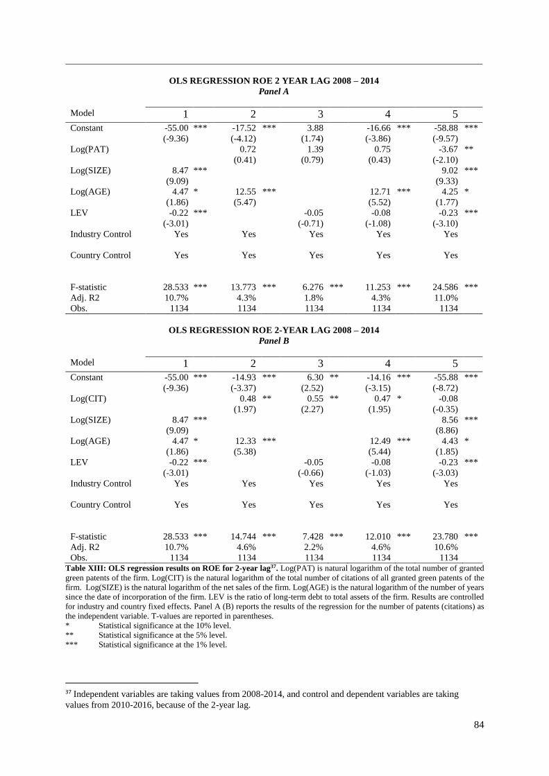
84

OLS REGRESSION ROE 2 YEAR LAG 2008 – 2014

Panel A

Model 1 2 3 4 5

Constant -55.00 *** -17.52 *** 3.88 -16.66 *** -58.88 ***

(-9.36) (-4.12) (1.74) (-3.86) (-9.57)

Log(PAT) 0.72 1.39 0.75 -3.67 **

(0.41) (0.79) (0.43) (-2.10)

Log(SIZE) 8.47 *** 9.02 ***

(9.09) (9.33)

Log(AGE) 4.47 * 12.55 *** 12.71 *** 4.25 *

(1.86) (5.47) (5.52) (1.77)

LEV -0.22 *** -0.05 -0.08 -0.23 ***

(-3.01) (-0.71) (-1.08) (-3.10)

Industry Control Yes Yes Yes Yes Yes

Country Control Yes Yes Yes Yes Yes

F-statistic 28.533 *** 13.773 *** 6.276 *** 11.253 *** 24.586 ***

Adj. R2 10.7% 4.3% 1.8% 4.3% 11.0%

Obs. 1134 1134 1134 1134 1134

OLS REGRESSION ROE 2-YEAR LAG 2008 – 2014

Panel B

Model 1 2 3 4 5

Constant -55.00 *** -14.93 *** 6.30 ** -14.16 *** -55.88 ***

(-9.36) (-3.37) (2.52) (-3.15) (-8.72)

Log(CIT) 0.48 ** 0.55 ** 0.47 * -0.08

(1.97) (2.27) (1.95) (-0.35)

Log(SIZE) 8.47 *** 8.56 ***

(9.09) (8.86)

Log(AGE) 4.47 * 12.33 *** 12.49 *** 4.43 *

(1.86) (5.38) (5.44) (1.85)

LEV -0.22 *** -0.05 -0.08 -0.23 ***

(-3.01) (-0.66) (-1.03) (-3.03)

Industry Control Yes Yes Yes Yes Yes

Country Control Yes Yes Yes Yes Yes

F-statistic 28.533 *** 14.744 *** 7.428 *** 12.010 *** 23.780 ***

Adj. R2 10.7% 4.6% 2.2% 4.6% 10.6%

Obs. 1134 1134 1134 1134 1134 Table XIII: OLS regression results on ROE for 2-year lag37. Log(PAT) is natural logarithm of the total number of granted

green patents of the firm. Log(CIT) is the natural logarithm of the total number of citations of all granted green patents of the

firm. Log(SIZE) is the natural logarithm of the net sales of the firm. Log(AGE) is the natural logarithm of the number of years

since the date of incorporation of the firm. LEV is the ratio of long-term debt to total assets of the firm. Results are controlled

for industry and country fixed effects. Panel A (B) reports the results of the regression for the number of patents (citations) as

the independent variable. T-values are reported in parentheses.

* Statistical significance at the 10% level.

** Statistical significance at the 5% level.

*** Statistical significance at the 1% level.

37 Independent variables are taking values from 2008-2014, and control and dependent variables are taking

values from 2010-2016, because of the 2-year lag.

85

Table XIII reports the OLS regression results of the number of patents/citations as the

independent variable with its control variables on ROE as the firm performance measure for

the 2-year lag sample. The results of the other three performance measures are reported in

Appendix G.

As expected, the results show that the signs of the relationship between green innovation

and ROE are similar to the main analysis in all models. Only, these signs are weaker for the 2-

year lag results. The number of citations are now positive and significant at the 5% level in

model (2) and (3) and only 10% in model (4) where this was significant at the 1% level for all

three measures in the main analysis.

Regarding the other three firm performance measures, it also shows the same signs as

the main analysis. For the relationship between the number of patents and ROA this negative

sign is weaker and for the relationship between the number of citations and ROA this positive

sign is stronger. Almost the same applies to ROS and Profit Margin. The relationship between

number of patents and both performance measures show the same sign and significance. And

the relationship between the number of citations and both performance measures show the same

positive sign as well, but then more significant.

To conclude, the 2-year lag sample on the one hand shows slightly weaker results, but

on the other hand shows slightly stronger results. Meaning that patents and its citations indeed

show the same impact after 2 or 3 years and that there is no difference between these years,

confirming previous literature (Ernst, 2001; Artz et al. 2010). However, one has to keep in mind

that it is possible that patents and its citations do not have that big of an impact on the

performance of a firm as the performances do not differ between the second and third year after

introducing the patent.

6.4 Patent-sensitive industries Because of the questionable impact of patents and its citations an OLS regression robustness

check for a sample consisting of firms operating in only the patent-sensitive industries is

performed. These industries are the industries described in paragraph 4.3.2. Therefore, the

dummy variable Industry Control will not be added in the OLS regression analysis as all firms

included in the sample are operating in patent-sensitive industries.

Previous studies find evidence for industries where the number of patents do have a

significant impact on firm performance where other industries do not report any significance

(Mansfield, 1986; Arora et al., 2003; MacDonald, 2004; Artz et al., 2010). Meaning that these

industries are more sensitive towards granted patents. To repeat briefly, the firms in these

86

patent-sensitive industries are operating in petroleum, machinery, fabricated metal products,

pharmaceuticals, drugs and biotechnology, or chemical products.

Appendix H reports the descriptive statistics and correlation matrix for the sample

consisting of only patent-sensitive industries. The means for the four performance measures are

higher for the patent-sensitive industries compared to the full sample. Also, the patent-sensitive

industries have on average more patents and citations than the other industries in the full sample.

Moreover, regarding the correlation matrix, for patent-sensitive industries the number of

citations is not significant correlated to all four performance measures anymore. This is not as

expected, because it would have been more likely that the number of patents/citations of firms

operating in these industries did indeed show a significant sign with the performance measures.

However, for the main analysis the number of patents is negative correlated with all

performance measures and for the patent-sensitive industry this correlation is positive for three

out of four.

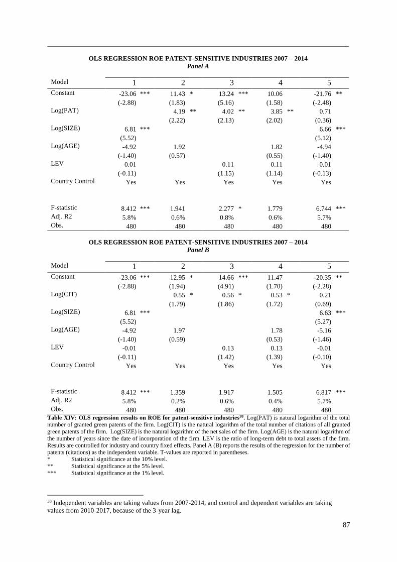
87

OLS REGRESSION ROE PATENT-SENSITIVE INDUSTRIES 2007 – 2014

Panel A

Model 1 2 3 4 5

Constant -23.06 *** 11.43 * 13.24 *** 10.06 -21.76 **

(-2.88) (1.83) (5.16) (1.58) (-2.48)

Log(PAT) 4.19 ** 4.02 ** 3.85 ** 0.71

(2.22) (2.13) (2.02) (0.36)

Log(SIZE) 6.81 *** 6.66 ***

(5.52) (5.12)

Log(AGE) -4.92 1.92 1.82 -4.94

(-1.40) (0.57) (0.55) (-1.40)

LEV -0.01 0.11 0.11 -0.01

(-0.11) (1.15) (1.14) (-0.13)

Country Control Yes Yes Yes Yes Yes

F-statistic 8.412 *** 1.941 2.277 * 1.779 6.744 ***

Adj. R2 5.8% 0.6% 0.8% 0.6% 5.7%

Obs. 480 480 480 480 480

OLS REGRESSION ROE PATENT-SENSITIVE INDUSTRIES 2007 – 2014

Panel B

Model 1 2 3 4 5

Constant -23.06 *** 12.95 * 14.66 *** 11.47 -20.35 **

(-2.88) (1.94) (4.91) (1.70) (-2.28)

Log(CIT) 0.55 * 0.56 * 0.53 * 0.21

(1.79) (1.86) (1.72) (0.69)

Log(SIZE) 6.81 *** 6.63 ***

(5.52) (5.27)

Log(AGE) -4.92 1.97 1.78 -5.16

(-1.40) (0.59) (0.53) (-1.46)

LEV -0.01 0.13 0.13 -0.01

(-0.11) (1.42) (1.39) (-0.10)

Country Control Yes Yes Yes Yes Yes

F-statistic 8.412 *** 1.359 1.917 1.505 6.817 ***

Adj. R2 5.8% 0.2% 0.6% 0.4% 5.7%

Obs. 480 480 480 480 480 Table XIV: OLS regression results on ROE for patent-sensitive industries38. Log(PAT) is natural logarithm of the total

number of granted green patents of the firm. Log(CIT) is the natural logarithm of the total number of citations of all granted

green patents of the firm. Log(SIZE) is the natural logarithm of the net sales of the firm. Log(AGE) is the natural logarithm of

the number of years since the date of incorporation of the firm. LEV is the ratio of long-term debt to total assets of the firm.

Results are controlled for industry and country fixed effects. Panel A (B) reports the results of the regression for the number of

patents (citations) as the independent variable. T-values are reported in parentheses.

* Statistical significance at the 10% level.

** Statistical significance at the 5% level.

*** Statistical significance at the 1% level.

38 Independent variables are taking values from 2007-2014, and control and dependent variables are taking

values from 2010-2017, because of the 3-year lag.

88

Table XIV reports the OLS regression results of the number of patents/citations as the

independent variable with its control variables on ROE as the firm performance measure for

the sample consisting of patent-sensitive industries. The results of the other three performance

measures are reported in Appendix H.

As expected, the relationship between the number of patents and ROE is positive and

significant at the 5% level for all models except the full model (5). The positive sign of the

relationship between the number of citations and ROE still remains, but is only significant at

the 10% level instead of the 1% level the main analysis reports. Although, this could be due to

the sample size. The positive and significant relationship between the number of patents and

ROE confirms previous literature (Mansfield, 1986; Arora et al., 2003; MacDonald, 2004; Artz

et al., 2010). The reason for these industries to be more important is due to the fact that firms

within these industries generally do not prefer to rely on trade secret protection when patent

protection is possible (Mansfield, 1986). Patents can often be invented relatively cheaply and

the cost of upholding their validity or proving that the patent had been infringed upon is too

high (Artz et al., 2010).

The other three performance measures show no significance at all for all models except

the full model (5). In this model both the number of patents and citations is negatively and

significantly related to ROA, ROS, and Profit Margin. However, probably the strong influence

of control variable size on this relationship causes these results as this also happened with the

main analysis.

To conclude, looking at the models (2), (3), and (4) that report specific combinations of

variables, the relationship between the number of patents and firm performance is still positive,

but stronger than the main analysis as it reports higher significance. This confirms previous

literature that patents in these patent-sensitive industries indeed have a bigger impact on the

performance of a firm than other industries (Mansfield, 1986; Arora et al., 2003; MacDonald,

2004; Artz et al., 2010). For citations this cannot be concluded as it shows similar results as the

main analysis.

6.5 Firms with at least one citation Another robustness check is an OLS regression with a sample consisting of firms that have

granted green patents with at least one citation. It is arguable that the citations are a better

indicator of green innovation than patents, because firms only continue to embroider on

successful granted green patents.

89

Appendix I reports the descriptive statistics and correlation matrix for the sample

consisting of firms with at least one citation. Again, the means of the performance measures of

these firms lay higher than the full sample. Not surprisingly, the mean of the number of patents

and citation are higher as well as the average number of patents a firm has that year almost

doubled and the number of citations almost tripled compared to the full model. The firms with

at least one citations are on average larger and older as well and report a slightly lower leverage

ratio. Furthermore, looking at the correlation matrix, both measures of green innovation are

now negative correlated with all four performance measures. For the number of patents the

correlation with ROA, ROS, and Profit Margin is also significant.

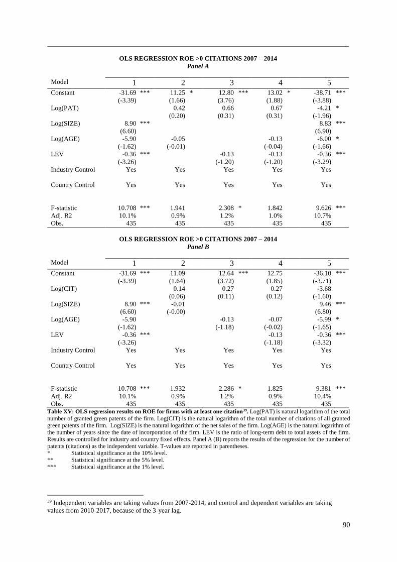
90

OLS REGRESSION ROE >0 CITATIONS 2007 – 2014

Panel A

Model 1 2 3 4 5

Constant -31.69 *** 11.25 * 12.80 *** 13.02 * -38.71 ***

(-3.39) (1.66) (3.76) (1.88) (-3.88)

Log(PAT) 0.42 0.66 0.67 -4.21 *

(0.20) (0.31) (0.31) (-1.96)

Log(SIZE) 8.90 *** 8.83 ***

(6.60) (6.90)

Log(AGE) -5.90 -0.05 -0.13 -6.00 *

(-1.62) (-0.01) (-0.04) (-1.66)

LEV -0.36 *** -0.13 -0.13 -0.36 ***

(-3.26) (-1.20) (-1.20) (-3.29)

Industry Control Yes Yes Yes Yes Yes

Country Control Yes Yes Yes Yes Yes

F-statistic 10.708 *** 1.941 2.308 * 1.842 9.626 ***

Adj. R2 10.1% 0.9% 1.2% 1.0% 10.7%

Obs. 435 435 435 435 435

OLS REGRESSION ROE >0 CITATIONS 2007 – 2014

Panel B

Model 1 2 3 4 5

Constant -31.69 *** 11.09 12.64 *** 12.75 -36.10 ***

(-3.39) (1.64) (3.72) (1.85) (-3.71)

Log(CIT) 0.14 0.27 0.27 -3.68

(0.06) (0.11) (0.12) (-1.60)

Log(SIZE) 8.90 *** -0.01 9.46 ***

(6.60) (-0.00) (6.80)

Log(AGE) -5.90 -0.13 -0.07 -5.99 *

(-1.62) (-1.18) (-0.02) (-1.65)

LEV -0.36 *** -0.13 -0.36 ***

(-3.26) (-1.18) (-3.32)

Industry Control Yes Yes Yes Yes Yes

Country Control Yes Yes Yes Yes Yes

F-statistic 10.708 *** 1.932 2.286 * 1.825 9.381 ***

Adj. R2 10.1% 0.9% 1.2% 0.9% 10.4%

Obs. 435 435 435 435 435 Table XV: OLS regression results on ROE for firms with at least one citation39. Log(PAT) is natural logarithm of the total

number of granted green patents of the firm. Log(CIT) is the natural logarithm of the total number of citations of all granted

green patents of the firm. Log(SIZE) is the natural logarithm of the net sales of the firm. Log(AGE) is the natural logarithm of

the number of years since the date of incorporation of the firm. LEV is the ratio of long-term debt to total assets of the firm.

Results are controlled for industry and country fixed effects. Panel A (B) reports the results of the regression for the number of

patents (citations) as the independent variable. T-values are reported in parentheses.

* Statistical significance at the 10% level.

** Statistical significance at the 5% level.

*** Statistical significance at the 1% level.

39 Independent variables are taking values from 2007-2014, and control and dependent variables are taking

values from 2010-2017, because of the 3-year lag.

91

Table XV reports the OLS regression results of the number of patents/citations as the

independent variable with its control variables on ROE as the firm performance measure for

the sample consisting of firms with at least one citation. The results of the other three

performance measures are reported in Appendix I.

The relationship between green innovation and ROE as the performance measure is

weak as it shows insignificant results in all but one model. Only the full model (5) of the

relationship between the number of patents and ROE reports a negative sign that is significant

at the 10% level. For this relationship these results are similar to the main analysis. However,

for the relationship between the number of citations and ROE this is not as expected, because

the main analysis reports positive signs that are significant at the 1% levels for the specific

models (2), (3), and (4). For this robustness check there exist no relationship between the

number of citations and ROE as all models show no significance.

Looking at the other three performance measures, the number of patents is negatively

related to ROA, ROS, and Profit Margin in all models. Meaning that firms that have a granted

green patent with at least one citation have a significant lower firm performance three years

later, based on these three performance measures. This is somehow in contrast to the main

analysis. Although, this positive impact the number of patents has on the performance measures

in the full model could be influenced by firms having zero citations. Because, the 329 firm year

observations of the quarter of the sample with the most granted green patents in a given year

consists of 139 firm year observations with no citations. 82 out of the 139 report a higher mean

than the mean of the full model for at least three out of four performance. However, regarding

the negative relationship, DeCarolis and Deeds (1999) also find that patents are negatively and

significantly related to firm performance. They argue that patent counts are an ambiguous

measure subject to firm specific variations in the propensity of firms to patent given the resource

expenditure required by the patent process. They name three arguments why the number of

patents could be negatively related to firm performance. Firstly, although it is generally an

accepted measure of innovation, the number of patents does not reflect the quality of it. Also,

in some industries extensive patenting may be cost prohibitive. And lastly, some firms may be

too young to have developed an extensive and reliable collection of patents to other firms.

Patents do represent a stock of knowledge, but it seems that just simply using the number of

patents is not a valid predictor of firm performance for all industries. Moreover, for the number

of citations there exist no relationship with the other three performance measures in almost all

models. For the specific models, the relationship between the number of citations and ROA is

only significant at the 10% level in model (2). Although, in the full model (5) the relationship

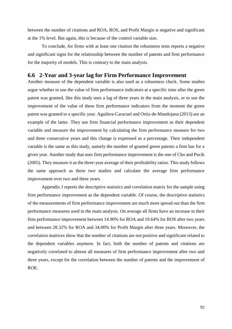
92

between the number of citations and ROA, ROS, and Profit Margin is negative and significant

at the 1% level. But again, this is because of the control variable size.

To conclude, for firms with at least one citation the robustness tests reports a negative

and significant signs for the relationship between the number of patents and firm performance

for the majority of models. This is contrary to the main analysis.

6.6 2-Year and 3-year lag for Firm Performance Improvement Another measure of the dependent variable is also used as a robustness check. Some studies

argue whether to use the value of firm performance indicators at a specific time after the green

patent was granted, like this study uses a lag of three years in the main analysis, or to use the

improvement of the value of these firm performance indicators from the moment the green

patent was granted to a specific year. Aguilera-Caracuel and Ortiz-de-Mandojana (2013) are an

example of the latter. They use firm financial performance improvement as their dependent

variable and measure the improvement by calculating the firm performance measure for two

and three consecutive years and this change is expressed as a percentage. Their independent

variable is the same as this study, namely the number of granted green patents a firm has for a

given year. Another study that uses firm performance improvement is the one of Cho and Pucik

(2005). They measure it as the three-year average of their profitability ratios. This study follows

the same approach as these two studies and calculate the average firm performance

improvement over two and three years.

Appendix J reports the descriptive statistics and correlation matrix for the sample using

firm performance improvement as the dependent variable. Of course, the descriptive statistics

of the measurements of firm performance improvement are much more spread out than the firm

performance measures used in the main analysis. On average all firms have an increase in their

firm performance improvement between 14.90% for ROA and 19.64% for ROS after two years

and between 28.32% for ROA and 34.00% for Profit Margin after three years. Moreover, the

correlation matrices show that the number of citations are not positive and significant related to

the dependent variables anymore. In fact, both the number of patents and citations are

negatively correlated to almost all measures of firm performance improvement after two and

three years, except for the correlation between the number of patents and the improvement of

ROE.

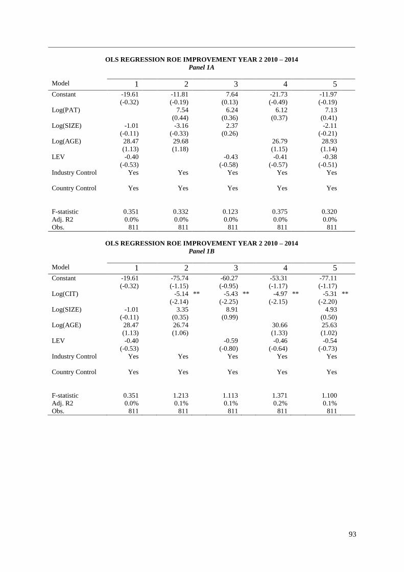
93

OLS REGRESSION ROE IMPROVEMENT YEAR 2 2010 – 2014

Panel 1A

Model 1 2 3 4 5

Constant -19.61 -11.81 7.64 -21.73 -11.97

(-0.32) (-0.19) (0.13) (-0.49) (-0.19)

Log(PAT) 7.54 6.24 6.12 7.13

(0.44) (0.36) (0.37) (0.41)

Log(SIZE) -1.01 -3.16 2.37 -2.11

(-0.11) (-0.33) (0.26) (-0.21)

Log(AGE) 28.47 29.68 26.79 28.93

(1.13) (1.18) (1.15) (1.14)

LEV -0.40 -0.43 -0.41 -0.38

(-0.53) (-0.58) (-0.57) (-0.51)

Industry Control Yes Yes Yes Yes Yes

Country Control Yes Yes Yes Yes Yes

F-statistic 0.351 0.332 0.123 0.375 0.320

Adj. R2 0.0% 0.0% 0.0% 0.0% 0.0%

Obs. 811 811 811 811 811

OLS REGRESSION ROE IMPROVEMENT YEAR 2 2010 – 2014

Panel 1B

Model 1 2 3 4 5

Constant -19.61 -75.74 -60.27 -53.31 -77.11

(-0.32) (-1.15) (-0.95) (-1.17) (-1.17)

Log(CIT) -5.14 ** -5.43 ** -4.97 ** -5.31 **

(-2.14) (-2.25) (-2.15) (-2.20)

Log(SIZE) -1.01 3.35 8.91 4.93

(-0.11) (0.35) (0.99) (0.50)

Log(AGE) 28.47 26.74 30.66 25.63

(1.13) (1.06) (1.33) (1.02)

LEV -0.40 -0.59 -0.46 -0.54

(-0.53) (-0.80) (-0.64) (-0.73)

Industry Control Yes Yes Yes Yes Yes

Country Control Yes Yes Yes Yes Yes

F-statistic 0.351 1.213 1.113 1.371 1.100

Adj. R2 0.0% 0.1% 0.1% 0.2% 0.1%

Obs. 811 811 811 811 811

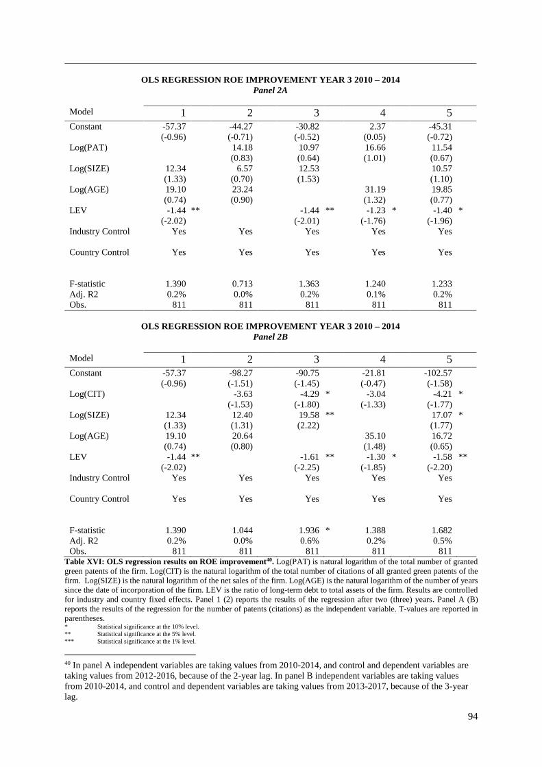
94

OLS REGRESSION ROE IMPROVEMENT YEAR 3 2010 – 2014

Panel 2A

Model 1 2 3 4 5

Constant -57.37 -44.27 -30.82 2.37 -45.31

(-0.96) (-0.71) (-0.52) (0.05) (-0.72)

Log(PAT) 14.18 10.97 16.66 11.54

(0.83) (0.64) (1.01) (0.67)

Log(SIZE) 12.34 6.57 12.53 10.57

(1.33) (0.70) (1.53) (1.10)

Log(AGE) 19.10 23.24 31.19 19.85

(0.74) (0.90) (1.32) (0.77)

LEV -1.44 ** -1.44 ** -1.23 * -1.40 *

(-2.02) (-2.01) (-1.76) (-1.96)

Industry Control Yes Yes Yes Yes Yes

Country Control Yes Yes Yes Yes Yes

F-statistic 1.390 0.713 1.363 1.240 1.233

Adj. R2 0.2% 0.0% 0.2% 0.1% 0.2%

Obs. 811 811 811 811 811

OLS REGRESSION ROE IMPROVEMENT YEAR 3 2010 – 2014

Panel 2B

Model 1 2 3 4 5

Constant -57.37 -98.27 -90.75 -21.81 -102.57

(-0.96) (-1.51) (-1.45) (-0.47) (-1.58)

Log(CIT) -3.63 -4.29 * -3.04 -4.21 *

(-1.53) (-1.80) (-1.33) (-1.77)

Log(SIZE) 12.34 12.40 19.58 ** 17.07 *

(1.33) (1.31) (2.22) (1.77)

Log(AGE) 19.10 20.64 35.10 16.72

(0.74) (0.80) (1.48) (0.65)

LEV -1.44 ** -1.61 ** -1.30 * -1.58 **

(-2.02) (-2.25) (-1.85) (-2.20)

Industry Control Yes Yes Yes Yes Yes

Country Control Yes Yes Yes Yes Yes

F-statistic 1.390 1.044 1.936 * 1.388 1.682

Adj. R2 0.2% 0.0% 0.6% 0.2% 0.5%

Obs. 811 811 811 811 811 Table XVI: OLS regression results on ROE improvement40. Log(PAT) is natural logarithm of the total number of granted

green patents of the firm. Log(CIT) is the natural logarithm of the total number of citations of all granted green patents of the

firm. Log(SIZE) is the natural logarithm of the net sales of the firm. Log(AGE) is the natural logarithm of the number of years

since the date of incorporation of the firm. LEV is the ratio of long-term debt to total assets of the firm. Results are controlled

for industry and country fixed effects. Panel 1 (2) reports the results of the regression after two (three) years. Panel A (B)

reports the results of the regression for the number of patents (citations) as the independent variable. T-values are reported in

parentheses. * Statistical significance at the 10% level.

** Statistical significance at the 5% level.

*** Statistical significance at the 1% level.

40 In panel A independent variables are taking values from 2010-2014, and control and dependent variables are

taking values from 2012-2016, because of the 2-year lag. In panel B independent variables are taking values

from 2010-2014, and control and dependent variables are taking values from 2013-2017, because of the 3-year

lag.

95

Table XVI reports the OLS regression results of the number of patents/citations as the

independent variable with its control variables on the improvement of ROE after two and three

years. The results of the other three performance measures are reported in Appendix J.

The relationship between the number of patents and the improvement of ROE is positive

in all models, only it lacks of any significance. For the relationship between the number of

citations and the improvement of ROE this is negative and significant at the 5% level after two

years and only significant at the 10% level for model (3) and (5) after three years. For the first

relationship this is similar to the main analysis, but for the second this is not as it showed

positive and significant signs.

Regarding the other three firm performance improvement measures, the relationship

between the number of patents and the improvement of ROA, ROS, and Profit Margin after two

and three years is negative in all models, but again it does not show any significance, meaning

that there exist no relationship. After two years, the relationship between the number of citations

and the improvement of ROA, ROS, and Profit Margin is negative in all models at the 10%, but

after three years this relationship becomes insignificant for ROA, significant at the 5% for ROS

in model (2), (3), and (5) and Profit Margin for model (2) and (5). Aguilera-Caracuel and Ortiz-

de-Mandojana (2013) also come to this conclusion as they fail to find any evidence of the

improvement of firm performance. They find that after two years the improvement of firm

performance is negatively related with green innovation, which is significant at the 10% level.

After three years this relationship is positive, but lacks significance. However, this could

indicate a turnaround. They name two reasons why it could be that green firms do not

experience a higher improvement of firm performance. Firstly, the impact of green innovations

could require time to materialize and secondly, all green innovative firms cannot have the

necessary conditions to obtain an improvement in their performance.

To conclude, using firm performance improvement as the dependent variable does not

change that much for the number of patents. However, the number of citations as the green

innovation indicator has a negative impact on the improvement of firm performance after both

two and three years.

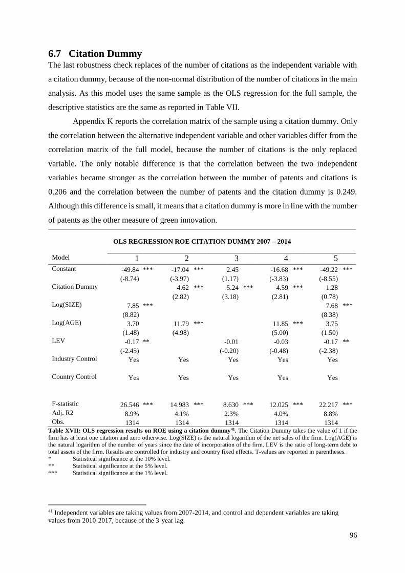
96

6.7 Citation Dummy The last robustness check replaces of the number of citations as the independent variable with

a citation dummy, because of the non-normal distribution of the number of citations in the main

analysis. As this model uses the same sample as the OLS regression for the full sample, the

descriptive statistics are the same as reported in Table VII.

Appendix K reports the correlation matrix of the sample using a citation dummy. Only

the correlation between the alternative independent variable and other variables differ from the

correlation matrix of the full model, because the number of citations is the only replaced

variable. The only notable difference is that the correlation between the two independent

variables became stronger as the correlation between the number of patents and citations is

0.206 and the correlation between the number of patents and the citation dummy is 0.249.

Although this difference is small, it means that a citation dummy is more in line with the number

of patents as the other measure of green innovation.

OLS REGRESSION ROE CITATION DUMMY 2007 – 2014

Model 1 2 3 4 5

Constant -49.84 *** -17.04 *** 2.45 -16.68 *** -49.22 ***

(-8.74) (-3.97) (1.17) (-3.83) (-8.55)

Citation Dummy 4.62 *** 5.24 *** 4.59 *** 1.28

(2.82) (3.18) (2.81) (0.78)

Log(SIZE) 7.85 *** 7.68 ***

(8.82) (8.38)

Log(AGE) 3.70 11.79 *** 11.85 *** 3.75

(1.48) (4.98) (5.00) (1.50)

LEV -0.17 ** -0.01 -0.03 -0.17 **

(-2.45) (-0.20) (-0.48) (-2.38)

Industry Control Yes Yes Yes Yes Yes

Country Control Yes Yes Yes Yes Yes

F-statistic 26.546 *** 14.983 *** 8.630 *** 12.025 *** 22.217 ***

Adj. R2 8.9% 4.1% 2.3% 4.0% 8.8%

Obs. 1314 1314 1314 1314 1314 Table XVII: OLS regression results on ROE using a citation dummy41. The Citation Dummy takes the value of 1 if the

firm has at least one citation and zero otherwise. Log(SIZE) is the natural logarithm of the net sales of the firm. Log(AGE) is

the natural logarithm of the number of years since the date of incorporation of the firm. LEV is the ratio of long-term debt to

total assets of the firm. Results are controlled for industry and country fixed effects. T-values are reported in parentheses.

* Statistical significance at the 10% level.

** Statistical significance at the 5% level.

*** Statistical significance at the 1% level.

41 Independent variables are taking values from 2007-2014, and control and dependent variables are taking

values from 2010-2017, because of the 3-year lag.

97

Table XVII reports the OLS regression results with a sample using a citation dummy as the

replacement of the number of citations with its control variables on ROE as the firm

performance measure. The results of the other three performance measures are reported in

Appendix K.

The results of this robustness check show the same results as the main analysis. Even

the same signs with the same level of significance are founded in almost all models. The only

small difference is that the relationship between the citation dummy and ROA is more

significant in model (2), (3), and (4) as it shows a significance level of 5%, 10%, and 5%

respectively. To conclude, a citation dummy has a higher correlation to the number of patents

than the number of citations, but the results of this robustness check are not different from the

main analysis.

98

7 CONCLUSION

7.1 Conclusion The intention of this study is to investigate the impact of green innovation on firm performance

and to provide concrete suggestions for the field of study. It uses an unbalanced panel dataset

and the sample consists of 450 unique firms with at least one European granted green patent in

one of the total 1,314 firm year observations between the years 2007 and 2014. These firms

have a combined number of 7,700 newly European green patents granted by EPO with its 9,087

citations. In this chapter an answer will be given to the research question: “To what extent does

green innovation influence firm financial performance?”. An OLS regression analysis is used

to find supporting evidence for the hypothesis: “green innovation affects firm financial

performance positively”. This regression uses the number of patents and citations as proxies of

green innovation, ROE, ROA, ROS, and Profit Margin as measures of firm performance, and

firm size, firm age, firm leverage, and two industry and country dummies as control variables.

This study contributes to the literature of innovation by going deeper into the green part of it,

by adding new empirical evidence to green innovation based on the use of panel data instead of

survey data, and by not making a distinction between the four parts of innovation and thus not

focusing on green product innovation alone. The hypothesis only receives partial support.

Literature elaborates four theories that explain the relationship between (green)

innovation and the performance of a firm. The innovation theory of Schumpeter describes that

firms that try new ways of using its knowledge, technology and resources bring more

opportunities that could lead to a stronger market position. These relatively more adaptable

firms are more likely to outperform firms that do not. The resource-based view is based on this

as it defines that firms must identify its potential key resources that are valuable, rare, not

imitable and not substitutable, because the performance of a firm results from these kind of

resources. Green innovation is such a unique capability and thus a key driver of firm

performance. Although, there is no best way to organize or lead a firm. The process of decision

making differs across firms, but the impact of the same decisions also differ across firms, which

is described by the contingency theory. This theory names three types of factors and this study

focuses on the response and performance factor, because a firm can influence these two. Firms

use green innovation to increase the performance of their firm. However, the institutional theory

argues that practices could also be adopted due to non-efficiency to gain legitimacy whether or

not the practices may lead to a performance increase. Based on these theories and on empirical

99

evidence, the hypothesis of this study predicts a positive relationship between green innovation

and firm performance.

The OLS regression for the main analysis shows that both proxies for green innovation

indeed show the positive sign with ROE as the firm performance measure. For the number of

citations there is also a relationship with ROE as this sign is statistically significant at the 1%

level. However, looking at ROA as the performance measure, the number of citations still

shows a positive and significant sign, but for the number of patents it becomes negative and

even significant at the 5% level for some models. For ROS and Profit Margin as the

performance measures the regression reports extremely weak results and almost no significance

at all for both proxies of green innovation, meaning that there is no relationship. This given and

the different results could indicate that having only one does not have that big of an impact on

the performance of a firm. Furthermore, looking at the regression models where the control

variable firm size is included as well, the regression analysis mostly reports negative and

significant results. Meaning that for larger firms the more European granted green

patents/citations a firm has, the lower its performance. Although, the high correlation between

firm size and the two proxies of green innovation could influence this relationship strongly and

incorrectly. With these mixed results the hypothesis only receives partial support.

Robustness checks also report mixed results. The fixed effects model regression report

insignificant and extremely weak results for the hypothesis in all models. The OLS regression

using two samples split by the median of firm size show similar results as the main analysis,

only it lacks in significance as well. This is especially the case in the full models, implying that

the control variable firm size indeed has a huge impact on the relationship between green

innovation and firm performance. Using a 2-year lag instead of a 3-year lag also reports similar

results. However, using a sample consisting of firms only operating in patent-sensitive

industries, the results are still positive, but stronger than the main analysis. And using a sample

consisting of firms with at least one citation the relationship between the number of patents and

firm performance seems to be more negative than the main analysis. This is also the case when

firm performance improvement is used as the measurement of firm performance, but then for

the relationship between the number of citations and firm performance. Moreover, the results

of using a citation dummy to replace the number of citations as the measure of green innovation

show no differences with the main analysis. These mixed results indicate that the results of the

main analysis are not consistent, not robust and do not provide reliable outcomes.

The positive findings prove that the positive effects green innovation, such as reducing

pollution and limiting hazardous and toxic waste and thus reducing the cost of disposal and

100

improving the green efficiency and response to external environmental pressure from

customers, all ultimately contribute to a better firm performance. This is in line with the four

theories. Green innovation is one of the creative ways described by Schumpeter (1934) to

outperform their competitive environment. Because, green innovations needs valuable

resources that are difficult to obtain and hard to imitate or trade and this could lead to a relatively

better performance of a firm compared to its competitors. This is still the case nowadays as the

more successful granted green patents show a higher firm performance. Because, the number

of citations clarifies the number of other firms that are trying to copy or improve that granted

green patent and could thus arguably be a measure of its success. Green innovation encourages

the use of raw materials efficiently and this could results in lower costs and new ways of

converting waste into saleable products.

However, the insignificant results of some robustness checks indicate that patents do

not work in practice as well as they do in theory. Reasons are that patents could often be

invented relatively cheaply, but the costs of holding on to these could be too high or firms could

have evolved patenting goals as some firms do not apply for a patent to protect their own

innovation efforts to get a temporary monopoly to make abnormal profits, but rather to play a

more strategic role in competitiveness. This means that firms will not protect all of its invented

patents, because the protection could be too costly and therefore they keep on filing new patents

without safeguarding old ones. These results doubt the value a patent has as a protection

mechanism. They do repay some of the R&D expenditures, but the insignificant results indicate

that there is no direct increase in the performance of the firm. Firms could for example patent

their innovations to block a competitor’s innovation efforts (MacDonald, 2004). This means

that many patents could have a defensive approach and therefore this forces many firms to

patent inventions they normally would not and has no to almost no impact on firm performance.

Although, this is not the case for all industries. Patents do still have a positive impact on the

performance of a firm for firms operating in patent-sensitive industries. In such industries the

protection of patents is more essential than in other industries, because firms within these

industries generally do not prefer to rely on trade secret protection when patent protection is

possible (Mansfield, 1986).

Contrary, the negative results indicate that the number of patents does not reflect the

quality of it, that extensive patenting may be cost prohibitive and that some firms may be too

young to have developed an extensive and reliable collection of patents to other firms. Patents

do represent a stock of knowledge, but it seems that just simply using the number of patents is

not a valid predictor of firm performance for all industries.

101

7.2 Limitations and further research Overall, these mixed results make it hard to make any reliable and substantiated suggestions for

the field of study. So, this study has some limitations that need to be considered. Both the main

analysis and robustness checks have mixed results, indicating that using the number of patents

and citations are not sufficient measures of green innovation. Thus, the first limitation of this

study is that it simply uses the number of patents and citations as proxies of green innovation.

Although, using patent and citation counts are generally accepted as one of the most appropriate

indicators of innovation, this measure only indicates the quantity of patenting activity and not

the impact of these patents. Other studies already mention the inability of distinguishing

between high and low-impact patents (Trajtenberg, 1990; Hall et al., 2001). Looking at the

positive results of the robustness check using a sample consisting of firms operating in patent-

sensitive industries, further research should examine the role of green patent impact in these

industries as higher patent impact could mitigate some of the negative effects found in other

analyses in this study. Also, a recommendation for another measure of green innovation is an

average or cumulative patent growth over a couple of years and taking the average of firm

performance over two and/or three years as the measure of firm performance. This study tried

to look into this measure, but the sample size decreased to a total of 64 unique firms, which is

not enough to perform a reliable analysis.

Another limitation is that this study only looks at the direct relationship between green

innovation and firm performance. However, there could also be an indirect impact on this

relationship. This third factor could be a moderator or mediator and it changes the strength or

direction of the effect of the direct relationship. A recommendation for a moderator in this field

of study is environmental dynamism. This third factor refers to frequent and rapid changes

induces by technology, customers, and suppliers. Managers should consider these changes

when designing green innovations in a dynamic environment (Lin et al., 2013). Another

recommendation for a mediator is product announcements. Artz et al. (2010) do not found any

significant evidence for the direct relationship between the number of patents and firm

performance. However, they do find positive and significant relationships between the number

of patents and product announcements and between product announcements and firm

performance. Indicating that product announcement indeed mediates the direct relationship.

This mediator represents product innovation efforts by a firm. These announcements could be

introductions, reviews, previews, or announcements of a new product or service. Although it

does not represent all four parts of innovation, it does represent the largest part.

102

8 REFERENCES

Abuhommous, A. A. (2017). The impact of offering trade credit on firms' profitability. The Journal of

Corporate Accounting & Finance, 28(6), 29-40.

Aggelopoulos, E., Eriotis, N., Georgopoulos, A., & Tsamis, A. (2016). R&D activity and operating

performance of small and medium-sized enterprises (SMEs): The case of a small open

economy. Journal of Accounting and Taxation, 8(4), 40-50.

Aguilera-Caracuel, J., & Ortiz-de-Mandojana, N. (2013). Green innovation and financial performance:

An institutional approach. Organization and Environment, 26(4), 365-385.

Anagnostopoulou, S. C., & Levis, M. (2008). R&D and performance persistence: Evidence from the

United Kingdom. The International Journal of Accounting, 43, 293-320.

Anderson, J. C., & Gerbing, D. W. (1988). Structural equation modeling in practice: A review and

recommended two-step approach. Psychological Bulletin, 103(3), 411-423.

Andras, T. L., & Srinivasan, S. S. (2003). Advertising intensity and R&D intensity: Differences across

industries and their impact on firm's performance. International Journal of Business and

Economics, 2(2), 81-90.

Ar, I. M. (2012). The impact of green product innovation on firm performance and competitive

capability: The moderating role of managerial environmental concern. Social and Behavioral

Sciences, 62, 854-864.

Arora, A., Ceccagnoli, M., & Cohen, W. M. (2008). R&D and the patent premium. International

Journal of Industrial Organization, 26(5), 1153-1179.

Artz, K. W., Norman, P. M., Hatfield, D. E., & Cardinal, L. B. (2010). A longitudinal study of the

impact of R&D, patents, and product innovation on firm performance. Product Development

& Management Association, 27(1), 725-740.

Belderbos, R., Faems, D., Leten, B., & van Looy, B. (2010). Technological activities and their impact

on the financial performance of the firm: Exploitation and exploration within and between

firms. Journal of Product Innovation Management, 27, 869-882.

Carhart, M. M. (1997). On persistence in mutual fund performance. The Journal of Finance, 52(1), 57-

82.

Chadha, A., & Oriani, R. (2009). R&D market value under weak intellectual property rights

protection: The case of India. Scientometrics, 82(1), 59-74.

Chan, H. K., Yee, R. W., Dai, J., & Lim, M. K. (2016). The moderating effect of environmental

dynamism on green product innovation and performance. International Journal of Production

Economics, 181, 384-391.

Chang, C. H. (2016). The determinants of green product innovation performance. Corporate Social

Responsibility and Environmental Management, 23(2), 65-76.

Chen, J., Leung, W. S., & Evans, K. P. (2018). Female board representation, corporate innovation and

firm performance. Journal of Empirical Finance, 48, 236-254.

103

Chen, L.-Y., Lai, J.-H., & Chang, S.-C. (2017). The long-term performance of new product

introductions. Finance Research letters, 20, 162-169.

Chen, Y.-S., Lai, S.-B., & Wen, C.-T. (2006). The influence of green innovation performance on

corporate advantage in Taiwan. Journal of Business Ethics, 67(4), 331-339.

Chiou, T. Y., Chan, H. K., Lettice, F., & Chung, S. H. (2011). The influence of greening the suppliers

and green innovation on environmental performance and competitive advantage in Taiwan.

Tansportation Research Part E: Logistics and Transportation Review, 47(6), 822-836.

Cho, H.-J., & Pucik, V. (2005). Relationship between innovativeness, quality, growth, profitability,

and market value. Strategic Management Journal, 26(6), 555-575.

Choi, S. B., & Williams, C. (2013). Innovation and firm performance in Korea and China: A cross-

context test of mainstream theories. Technology Analysis & Strategic Management, 25(4),

423-444.

Cohen, M. A., & Cohen, P. (1983). Applied multiple regression/correlation analysis for behavorial

science,. Hillsdale: Laurence Erlbraum.

Czarnitzki, D., & Kraft, K. (2012). Spillovers of innovation activates and their profitability. Oxford

Economic Papers, 64(2), 302-322.

Dahlman, L. (2017, September 11). www.climate.gov. Retrieved from Climate:

https://www.climate.gov/news-features/understanding-climate/climate-change-global-

temperature

Dangelico, R. M. (2016). Green product innovation: Where we are and where we are going. Business

Strategy and the Environment, 25(8), 560-576.

Dangelico, R. M., & Pontrandolfo, P. (2010). From green product definitions and classifications to the

green option matrix. Journal of Cleaner Production, 18, 1608-1628.

DeCarolis, D. M., & Deeds, D. L. (1999). The impact of stocks and flows of organizational knowledge

on firm performance: An empirical investigation of the biotechnology industry. Strategic

Management Journal, 20(10), 953-968.

Douma, S., George, R., & Kabir, R. (2006). Foreign and domestic ownership, business groups, and

firm performance: Evidence from a large emerging market. Strategic Management Journal,

27(7), 637-657.

EEIG. (2004). Convergence and the digital world. Frankfurt: European Information Technology

Observatory.

Ehie, I. C., & Olibe, K. (2010). The effect of R&D investment on firm value: An examination of US

manufacturing and service industries. International Journal of Production Economics, 128,

127-135.

Eiadat, Y., Kelly, A., Roche, F., & Eyadat, H. (2008). Green and competitive?: An empirical test of

the mediating role of environmental strategy. Journal of World Business, 43(2), 131-145.

Ernst, H. (2001). Patent applications and subsequent changes of performance: Evidence from time-

series cross-section analyses on the firm level. Research Policy, 30(1), 143-157.

104

Feeny, S., & Rogers, M. (2003). Innovation and performance: Benchmarking Australian firms. The

Australian Economic Review, 36(3), 253-264.

Feng, H., & Rong, C. (2007). Innovation, firm efficiency and firm value: Firm-level evidence in

Japanese electricity machinery industry. International Conference on Wireless

Communications, Networking and Mobile Computing, 4217-4220.

Fornell, C., & Larcker, D. F. (1981). Evaluating structural equation models with unobservable

variables and measurement error. Journal of Marketing Research, 18(1), 39-50.

Frenken, K., & Faber, A. (2009). Introduction: Evolutionary methodologies for analyzing

environmental innovations and the implications for environmental policy. Technological

Forecasting and Social Change, 76, 449-452.

Friar, J. H. (1999). Competitive advantage through product performance innovation in a competitive

market. Journal of Product Innovation, 12(1), 33-42.

Frietsch, R., & Grupp, H. (2006). There’s a new man in town: The paradigm shift in optical

technology. Technovation, 26, 13-29.

Frijns, B., Dodd, O., & Cimerova, H. (2016). The impact of cultural diversity in corporate boards on

firm performance. Journal of Corporate Finance, 41, 521-541.

Gardiner, J. C., Luo, Z., & Roman, L. A. (2009). Fixed effects, random effects and GEE: What are the

differences? Statistics in Medicine, 28, 221-239.

Goldberger, A. S. (1964). Classical linear regression. New York: John Wiley & Sons.

Green paper on integrated product policy. (2001). Commission of the European Communities.

Greene, W. H. (2011). Econometric Analysis (7th ed.). New Jersey: Prentice Hall.

Grewal, R., & Tansuhaj, P. (2001). Building organizational capabilities for managing economic crisis:

The role of market orientation and strategic flexibility. Journal of Marketing, 65(2), 67-80.

Griffin, A. (1997). PDMA research on new product development practices: Updating trends and

benchmarking best practices. Journal of Product Innovation Management, 14, 429-458.

Griliches, Z., Pakes, A., & Hall, B. H. (1986). The value of patents as indicators of inventive activity.

NBER Working Paper, 1-43.

Gui-long, Z., Yi, Z., Kai-hua, C., & Jiang, Y. (2017). The impact of R&D intensity on firm

performance in an emerging market: Evidence from China's electronics manufacturing firms.

Asian Journal of Technology Innovation, 25(1), 41-60.

Guoyou, Q., Saixing, Z., Chiming, T., Haitao, Y., & Hailiang, Z. (2013). Stakeholders’ influences on

corporate green innovation strategy: A case study of manufacturing firms in China. Corporate

Social Responsibility and Environmental Management, 20, 1-14.

Gürlek, M., & Tuna, M. (2018). Reinforcing competitive advantage through green organizational

culture and green innovation. The Service Industries Journal, 38(7-8), 467-491.

Hair, J. F., Anderson, R. E., Tatham, R., & Black, W. (1998). Multivariate data analysis with

readings. Englewood Cliffs: Prentice Hall.

105

Hall, B. H., & Ziedonis, R. H. (2001). The patent paradox revisited: An empirical study of patenting in

the U.S. semiconductor industry. Journal of Economics, 32(1), 101-128.

Hall, B. H., Jaffe, A., & Trajtenberg, M. (2001). Market value and patent citations. Journal of

Economics, 36(1), 16-38.

Hall, B. H., Jaffe, A., & Trajtenberg, M. (2001). The NBER patent citations data file: Lessons, insights

and methodological tools. National Bureau of Economic Research, 1-74.

Hall, B. H., Jaffe, A., & Trajtenberg, M. (2005). Market value and patent citations. RAND Journal of

Economics, 16-38.

Hall, B. J., Griliches, Z., & Hausman, J. A. (1986). Patents and R&D: Is there a lag? International

Economic Review, 27(2), 265-283.

Harhoff, D., & Wagner, S. (2009). The Duration of Patent Examination at. Management Science,

55(12), 1969-1984.

Hart, S. L. (1995). A natural‐resource‐based view of the firm. Academy of Management Review, 20(4),

986-1014.

Hayashi, F. (2000). Econometrics. Princeton: Princeton University Press.

Henseler, J. (2017). Bridging design and behavioral research with variance-based structural equation

modeling. Journal of Advertising, 46(1), 178-192.

Ho, Y., Keh, H. T., & Ong, J. M. (2005). The effects of R&D and advertising on firm value: An

examination of manufacturing and nonmanufacturing firms. IEEE Transactions on

Engineering Management, 52(1), 3-14.

Hoffman, A. J. (1999). Institutional evolution and change: Environmentalism and the U.S. chemical

industry. Academy of Management Journal, 42, 351-371.

Hooper, D., Coughlan, J., & Mullen, M. R. (2008). Structural equation modelling: Guidelines for

determining model fit. Electronic Journal of Business Research Methods, 6(1), 53-60.

Hsu, P.-H. (2009). Technological innovations and aggregate risk premiums. Journal of Financial

Economics, 94(2), 264-279.

Hu, L.-t., & Bentler, P. M. (1999). Cutoff criteria for fit indexes in covariance structures analysis:

Coventional criteria versus new alternatives. Structural Equation Model: A Multidisciplinary

Journal, 6(1), 1-55.

Huang, C.-H., & Hou, T. C. (2019). Innovation, research and development, and firm profitability in

Taiwan: Causality and determinants. International Review of Economics and Finance, 59,

385-394.

Ibhagui, O. W., & Olokoyo, F. O. (2018). Leverage and firm performance: New evidence on the role

of firm size. North American Journal of Economics and Finance, 45, 57-82.

Ilyukhin, E. (2015). The impact of financial leverage on firm performance: Evidence from Russia.

Journal of Corporate Finance Research, 2(34), 24-36.

IPCC. (2007). Climate change 2007: Mitigation of climate change. Cambridge: IPCC.

106

Kale, J. R., Reis, E., & Venkateswaran, A. (2009). Rank-order tournaments and incentive alignment:

The effect on firm performance. The Journal of Finance, 64(3), 1479-1512.

Kaynak, H., & Hartley, J. L. (2008). A replication and extension of quality management into the

supply chain. Journal of Operations Management, 26(4), 468-489.

Kim, N., Moon, J. J., & Yin, H. (2016). Environmental pressure and the performance of foreign firms

in an emerging economy. Journal of business ethics, 137(3), 475-490.

Klassen, R. D., & Whybark, D. C. (1999). The impact of environmental technologies on

manufacturing performance. Academy of Management Journal, 42(6), 599-615.

Kober, R., Subraamanniam, T., & Watson, J. (2012). The impact of total quality management adoption

on small and medium enterprises' financial performance. Accounting and Finance, 52(2), 421-

438.

Koellinger, P. (2008). The relationship between technology, innovation, and firm performance:

Emprical evidence from e-business in Europe. Research Policy, 37, 1317-1328.

Kostova, T. (1999). Transnational transfer of strategic organizational practices: A contextual

perspective. Academy of Management Review, 24, 308-324.

Kostova, T., & Roth, K. (2002). Adoption of an organizational practice by subsidiaries of

multinational corporations: Institutional and relational effects. Academy of Management

Journal, 24, 215-233.

Kumbhakar, S. C., Ortega-Argilés, R., Potters, L., Vivarelli, M., & Voigt, P. (2011). Corporate R&D

and firm efficiency: Evidence from Europe's top R&D investors. Journal of Productivity

Analysis, 37, 125-140.

Leonidou, C., Katsikeas, C., & Morgan, N. (2013). Greening’ the marketing mix: do firms do it and

does it pay off? Journal of the Academy of Marketing Science, 41, 151-170.

Li, Y., Su, Z., & Liu, Y. (2010). Can strategic flexibility help firms profit from product innovation?

Technovation, 30(5-6), 300-309.

Lin, R.-J., Tan, K.-H., & Geng, Y. (2013). Market demand, green product innovation, and firm

performance: Evidence from Vietnam motorcycle industry. Journal of Cleaner Production,

40, 101-107.

Loughran, T., & Shive, S. (2011). The impact of venture capital investments on public firm stock

performance. Journal of Behavioral Finance, 12(4), 233-246.

Lu, X., & White, H. (2014). Robustness checks and robustness tests in applied economics. Journal of

Economics, 178(1), 194-206.

MacDonald, S. (2004). When means become ends: Considering the impact of patent strategy on

innovation. Information Economics and Policy, 16(1), 135-158.

Mansfield, E. (1986). Patents and innovation: An empirical study. Management Science, 32(2), 173-

181.

Melvin, T. C. (2002). European patent office. Journal of Business & Finance Librarianship, 8(1), 55-

62.

107

Morgan, G. (1998). Images of organization: The executive edition. Thousand Oaks: Better-Koehler

Publishers and SAGE Publications.

Nunnally, J. C. (1978). PsychometricTheory, second ed. New York: McGraw-Hill.

Oke, A., Burke, G., & Myers, A. (2007). Innovation types and performance in growing UK SMEs.

International Journal of Operations & Production Management, 27(7), 735-753.

Olson, E. L. (2014). Green innovation value chain analysis of PV solar power. Journal of Cleaner

Production, 64, 73-80.

Ortega-Argilés, R., Piva, M., & Vivarelli, M. (2011). Productivity gains from R&D investment: Are

high-tech sectors still ahead? Economics of Innovation and New Technology, 24(3), 204-222.

Ortega-Argilés, R., Piva, M., Potters, L., & Vivarelli, M. (2009). Is corporate R&D investment in

high-tech sectors more effective? Contemporary Economic Policy, 28(3), 353-365.

Palmer, K., Oates, W. E., & Portney, P. R. (1995). Tightening environmental standards: The benefit-

cost or the no-cost paradigm? Journal of Economics Perspectives, 9(4), 119-132.

Penner-Hahn, J., & Myles-Shaver, J. (2005). Does international research and development increase

patent output? An analysis of Japanese pharmaceutical firms. Strategic Management Journal,

26, 121-140.

Porter, M. E., & Reinhardt, F. L. (2007). A Strategic Approach to Climate. Harvard Business Review,

85(10), 22-25.

Porter, M. E., & van der Linde, C. (1995). Green and competitive: Ending the stalemate. Harvard

Business Review, 73(5), 120-134.

Pramod, K. N., Krishnan, N., & Puja, P. (2012). R&D intensity and market valuation of firm: A study

of R&D incurring manufacturing firms in India. Indian Institute of Technology Bombay, 295-

308.

Pujari, D. (2006). Eco-innovation and new product development: Understanding the influences on

market performance. Technovation, 26(1), 76-85.

Reinhardt, F. L. (1998). Environmental product differentiation: Implications for corporate strategy.

California Management Review, 40(4), 43-73.

Rogers, E. (1995). Diffusion of Innovations. New York: Free Press.

Russo, M. V., & Fouts, P. A. (1997). A resource-based perspective on corporate environmental

performance and profitability. The Academy of Management Journal, 40(3), 534-559.

Santos, D. F., Basso, L. F., Kimura, H., & Kayo, E. K. (2014). Innovation efforts and performances of

Brazilian firms. Journal of Business Research, 30(6), 527-535.

Schiederig, T., Tietze, F., & Herstatt, C. (2012). Green innovation in technology and innovation

management: An exploratory literature review. R and D Management, 42(2), pp. 180-192.

Schumpeter, J. A. (1934). The theory of economic development: an inquiry into profits, capital, credit,

interest, and the business cycle. Cambridge: Harvard University Press.

Seru, A. (2014). Firm boundaries matter: Evidence from conglomerates and R&D activity. Journal of

Financial Economics, 111(2), 381-405.

108

Sousa, R., & Voss, C. A. (2008). Contingency research in operations management practices. Journal

of Operations Management, 26, 697-713.

Soyez, K., & Grassl, H. (2008). Climate change and technological options: Basic facts, evaluation

and practical solutions. Wien: Springer.

Sridharan, S., & Joshi, M. (2018). Impact of ownership patterns and firm life-cycle stages on firm

performance: Evidence from India. The Journal of Corporate Accounting & Finance, 29(1),

117-136.

Trajtenberg, M. (1990). A penny for your quotes: Patent Citations and the value of information.

Journal of Economics, 21(1), 325-342.

Tseng, M. L., Lin, Y. H., Chiu, A. S., & Liao, C. H. (2008). Using FANP approach on selection of

competitive priorities based on cleaner production implementation: A case study in PCB

manufacturer, Taiwan. Clean Technology and Environmental Policy, 10(1), 17-29.

Tseng, M. L., Wang, R., Chiu, A. S., Geng, Y., & Lin, Y. H. (2013). Improving performance of green

innovation practices under uncertainty. Journal of Cleaner Production, 40, 71-82.

Unruh, G., & Ettenson, R. (2010). Growing green: Three smart paths to developing sustainable

products. Harvard Business Review, 88(6), 94-100.

Vithessonthi, C., & Racela, O. C. (2016). Short- and long-run effects of internationalization and R&D

intensity of firm performance. Journal of Multinational Financial Management, 34, 28-45.

Vogt, W. P. (1999). Dictionary of statistics and methodology: A non-technical guide for the social

sciences (2nd ed.). London: Sage Publications.

Zhou, L. J., & Sadeghi, M. (2019). The impact of innovation on IPO short-term performance:

Evidence from the Chinese markets. Pacific-Basin Finance Journal, 53, 208-235.

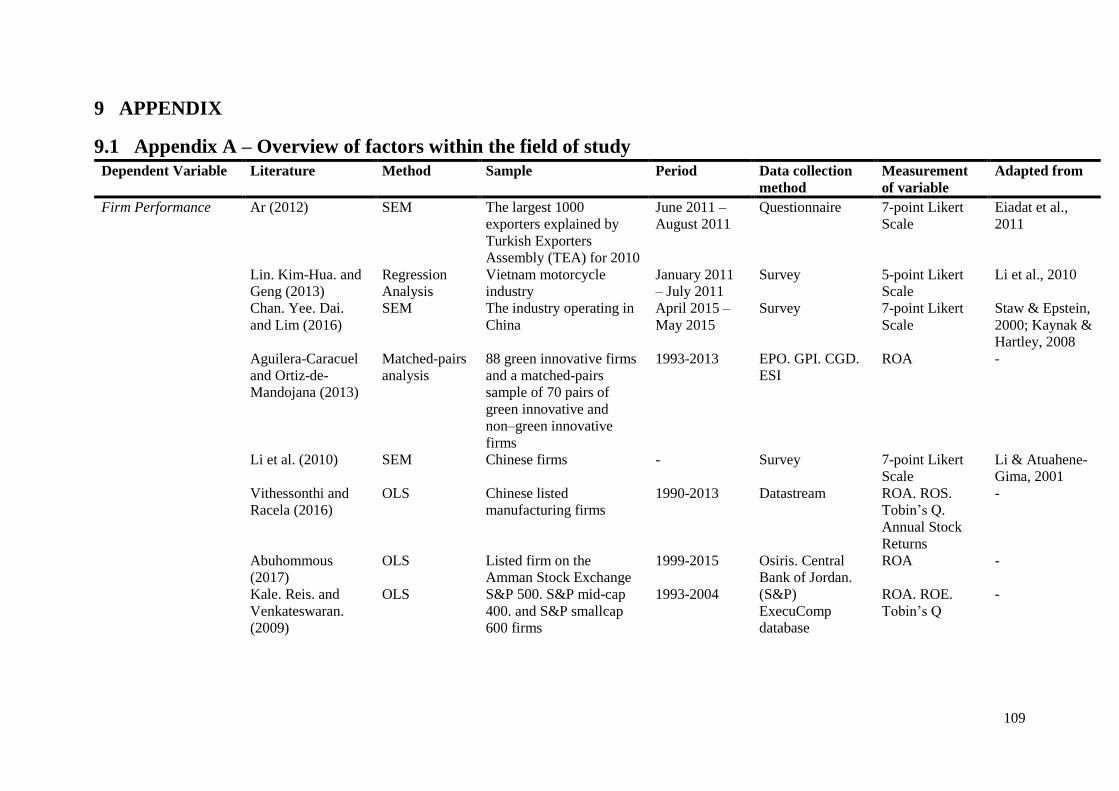
109

9 APPENDIX

9.1 Appendix A – Overview of factors within the field of study

Dependent Variable Literature Method Sample Period Data collection

method

Measurement

of variable

Adapted from

Firm Performance

Ar (2012) SEM The largest 1000

exporters explained by

Turkish Exporters

Assembly (TEA) for 2010

June 2011 –

August 2011

Questionnaire 7-point Likert

Scale

Eiadat et al.,

2011

Lin. Kim-Hua. and

Geng (2013)

Regression

Analysis

Vietnam motorcycle

industry

January 2011

– July 2011

Survey 5-point Likert

Scale

Li et al., 2010

Chan. Yee. Dai.

and Lim (2016)

SEM The industry operating in

China

April 2015 –

May 2015

Survey 7-point Likert

Scale

Staw & Epstein,

2000; Kaynak &

Hartley, 2008

Aguilera-Caracuel

and Ortiz-de-

Mandojana (2013)

Matched-pairs

analysis

88 green innovative firms

and a matched-pairs

sample of 70 pairs of

green innovative and

non–green innovative

firms

1993-2013 EPO. GPI. CGD.

ESI

ROA -

Li et al. (2010) SEM Chinese firms - Survey 7-point Likert

Scale

Li & Atuahene-

Gima, 2001

Vithessonthi and

Racela (2016)

OLS Chinese listed

manufacturing firms

1990-2013 Datastream ROA. ROS.

Tobin’s Q.

Annual Stock

Returns

-

Abuhommous

(2017)

OLS Listed firm on the

Amman Stock Exchange

1999-2015 Osiris. Central

Bank of Jordan.

ROA -

Kale. Reis. and

Venkateswaran.

(2009)

OLS S&P 500. S&P mid-cap

400. and S&P smallcap

600 firms

1993-2004 (S&P)

ExecuComp

database

ROA. ROE.

Tobin’s Q

-

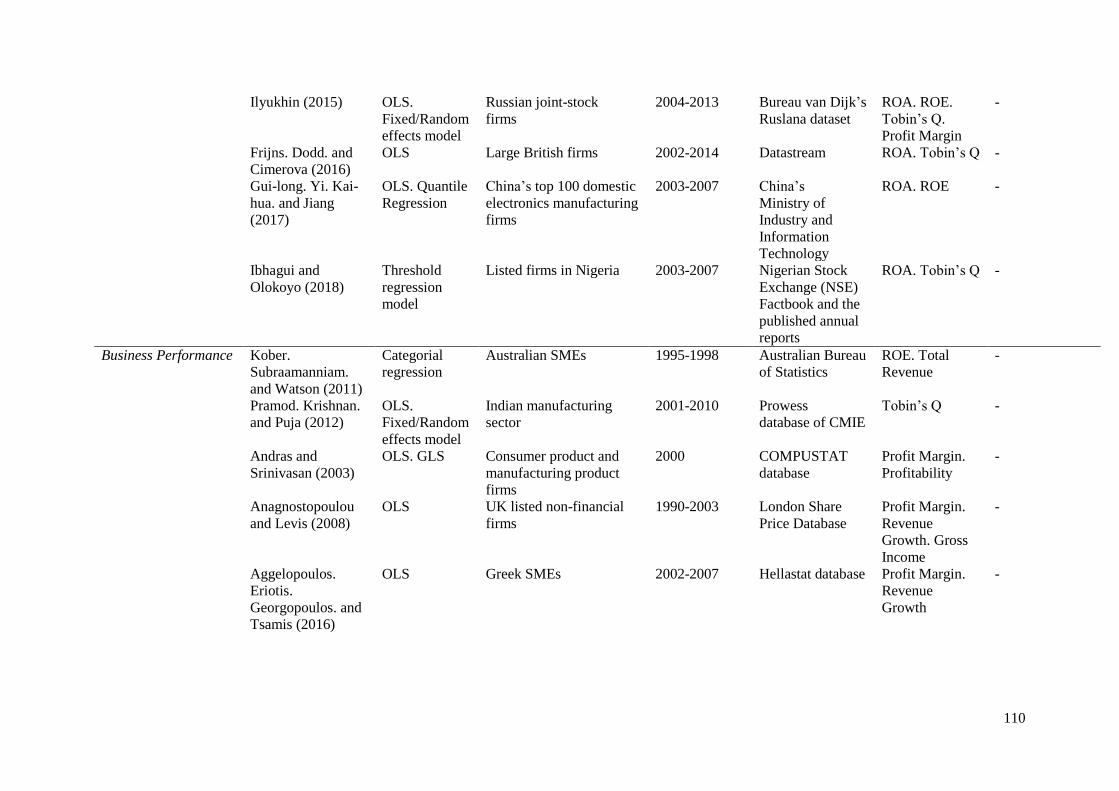
110

Ilyukhin (2015) OLS.

Fixed/Random

effects model

Russian joint-stock

firms

2004-2013 Bureau van Dijk’s

Ruslana dataset

ROA. ROE.

Tobin’s Q.

Profit Margin

-

Frijns. Dodd. and

Cimerova (2016)

OLS Large British firms 2002-2014 Datastream ROA. Tobin’s Q -

Gui-long. Yi. Kai-

hua. and Jiang

(2017)

OLS. Quantile

Regression

China’s top 100 domestic

electronics manufacturing

firms

2003-2007 China’s

Ministry of

Industry and

Information

Technology

ROA. ROE -

Ibhagui and

Olokoyo (2018)

Threshold

regression

model

Listed firms in Nigeria 2003-2007 Nigerian Stock

Exchange (NSE)

Factbook and the

published annual

reports

ROA. Tobin’s Q -

Business Performance Kober.

Subraamanniam.

and Watson (2011)

Categorial

regression

Australian SMEs 1995-1998 Australian Bureau

of Statistics

ROE. Total

Revenue

-

Pramod. Krishnan.

and Puja (2012)

OLS.

Fixed/Random

effects model

Indian manufacturing

sector

2001-2010 Prowess

database of CMIE

Tobin’s Q -

Andras and

Srinivasan (2003)

OLS. GLS Consumer product and

manufacturing product

firms

2000 COMPUSTAT

database Profit Margin.

Profitability

-

Anagnostopoulou

and Levis (2008)

OLS UK listed non-financial

firms

1990-2003 London Share

Price Database

Profit Margin.

Revenue

Growth. Gross

Income

-

Aggelopoulos.

Eriotis.

Georgopoulos. and

Tsamis (2016)

OLS Greek SMEs 2002-2007 Hellastat database Profit Margin.

Revenue

Growth

-

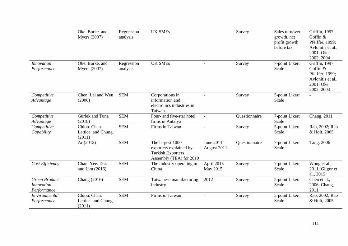
111

Oke. Burke. and

Myers (2007)

Regression

analysis

UK SMEs - Survey Sales turnover

growth. net

profit growth

before tax

Griffin, 1997;

Goffin &

Pfeiffer, 1999;

Avlonitis et al.,

2001; Oke,

2002; 2004

Innovation

Performance

Oke. Burke. and

Myers (2007)

Regression

analysis

UK SMEs - Survey 7-point Likert

Scale

Griffin, 1997;

Goffin &

Pfeiffer, 1999;

Avlonitis et al.,

2001; Oke,

2002; 2004

Competitive

Advantage

Chen. Lai and Wen

(2006)

SEM Corporations in

information and

electronics industries in

Taiwan

- Survey 5-point Likert

Scale

-

Competitive

Advantage

Gürlek and Tuna

(2018)

SEM Four- and five-star hotel

firms in Antalya

- Questionnaire 7-point Likert

Scale

Chang, 2011

Competitive

Capability

Chiou. Chan.

Lettice. and Chung

(2011)

SEM Firms in Taiwan - Survey 5-point Likert

Scale

Rao, 2002; Rao

& Holt, 2005

Ar (2012) SEM The largest 1000

exporters explained by

Turkish Exporters

Assembly (TEA) for 2010

June 2011 –

August 2011

Questionnaire 7-point Likert

Scale

Tang, 2006

Cost Efficiency Chan. Yee. Dai.

and Lim (2016)

SEM The industry operating in

China

April 2015 –

May 2015

Survey 7-point Likert

Scale

Wong et al.,

2011; Gligor et

al., 2015

Green Product

Innovation

Performance

Chang (2016) SEM Taiwanese manufacturing

industry

2012 Survey 5-point Likert

Scale

Chen et al.,

2006; Chang,

2011

Environmental

Performance

Chiou. Chan.

Lettice. and Chung

(2011)

SEM Firms in Taiwan - Survey 5-point Likert

Scale

Rao, 2002; Rao

& Holt, 2005

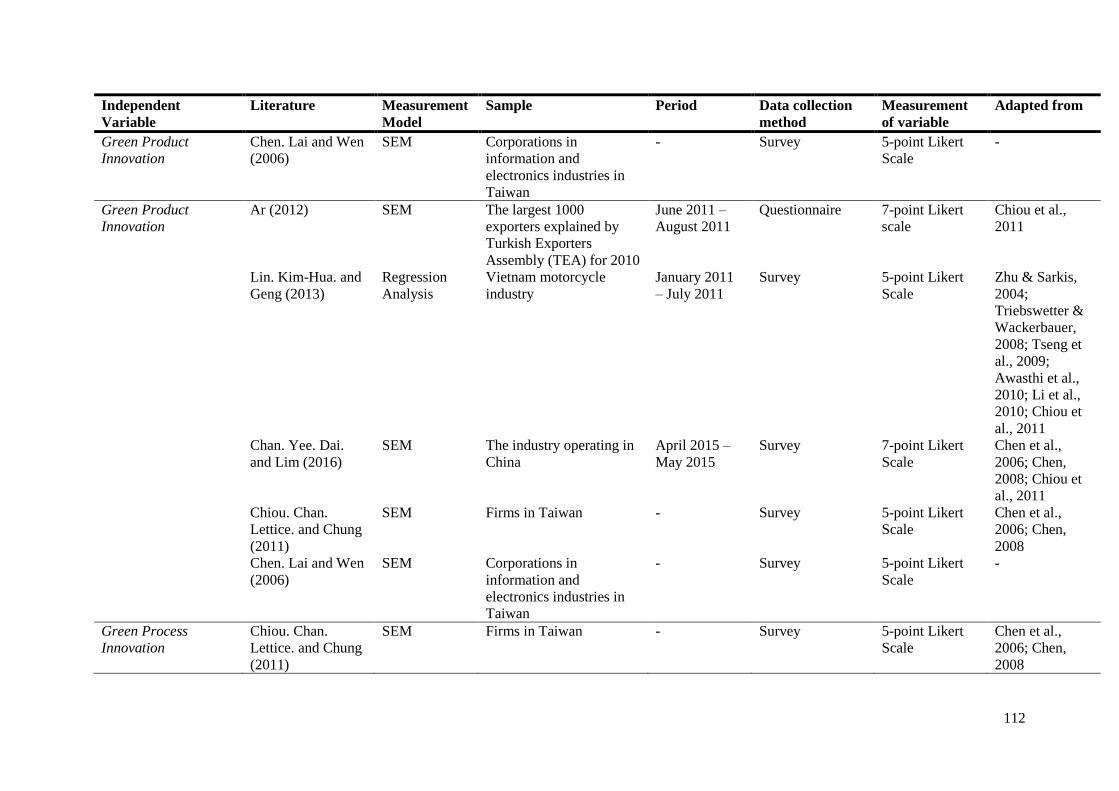
112

Independent

Variable

Literature Measurement

Model

Sample Period Data collection

method

Measurement

of variable

Adapted from

Green Product

Innovation

Chen. Lai and Wen

(2006)

SEM Corporations in

information and

electronics industries in

Taiwan

- Survey 5-point Likert

Scale

-

Green Product

Innovation

Ar (2012) SEM The largest 1000

exporters explained by

Turkish Exporters

Assembly (TEA) for 2010

June 2011 –

August 2011

Questionnaire 7-point Likert

scale

Chiou et al.,

2011

Lin. Kim-Hua. and

Geng (2013)

Regression

Analysis

Vietnam motorcycle

industry

January 2011

– July 2011

Survey 5-point Likert

Scale

Zhu & Sarkis,

2004;

Triebswetter &

Wackerbauer,

2008; Tseng et

al., 2009;

Awasthi et al.,

2010; Li et al.,

2010; Chiou et

al., 2011

Chan. Yee. Dai.

and Lim (2016)

SEM The industry operating in

China

April 2015 –

May 2015

Survey 7-point Likert

Scale

Chen et al.,

2006; Chen,

2008; Chiou et

al., 2011

Chiou. Chan.

Lettice. and Chung

(2011)

SEM Firms in Taiwan - Survey 5-point Likert

Scale

Chen et al.,

2006; Chen,

2008

Chen. Lai and Wen

(2006)

SEM Corporations in

information and

electronics industries in

Taiwan

- Survey 5-point Likert

Scale

-

Green Process

Innovation

Chiou. Chan.

Lettice. and Chung

(2011)

SEM Firms in Taiwan - Survey 5-point Likert

Scale

Chen et al.,

2006; Chen,

2008

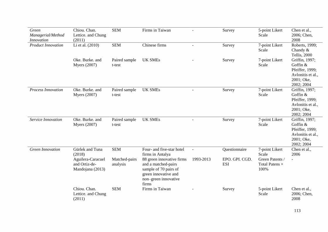
113

Green

Managerial/Method

Innovation

Chiou. Chan.

Lettice. and Chung

(2011)

SEM Firms in Taiwan - Survey 5-point Likert

Scale

Chen et al.,

2006; Chen,

2008

Product Innovation Li et al. (2010) SEM Chinese firms - Survey 7-point Likert

Scale

Roberts, 1999;

Chandy &

Tellis, 2000

Oke. Burke. and

Myers (2007)

Paired sample

t-test

UK SMEs - Survey 7-point Likert

Scale

Griffin, 1997;

Goffin &

Pfeiffer, 1999;

Avlonitis et al.,

2001; Oke,

2002; 2004

Process Innovation Oke. Burke. and

Myers (2007)

Paired sample

t-test

UK SMEs - Survey 7-point Likert

Scale

Griffin, 1997;

Goffin &

Pfeiffer, 1999;

Avlonitis et al.,

2001; Oke,

2002; 2004

Service Innovation Oke. Burke. and

Myers (2007)

Paired sample

t-test

UK SMEs - Survey 7-point Likert

Scale

Griffin, 1997;

Goffin &

Pfeiffer, 1999;

Avlonitis et al.,

2001; Oke,

2002; 2004

Green Innovation Gürlek and Tuna

(2018)

SEM Four- and five-star hotel

firms in Antalya

- Questionnaire 7-point Likert

Scale

Chen et al.,

2006

Aguilera-Caracuel

and Ortiz-de-

Mandojana (2013)

Matched-pairs

analysis

88 green innovative firms

and a matched-pairs

sample of 70 pairs of

green innovative and

non–green innovative

firms

1993-2013 EPO. GPI. CGD.

ESI

Green Patents /

Total Patens ×

100%

-

Chiou. Chan.

Lettice. and Chung

(2011)

SEM Firms in Taiwan - Survey 5-point Likert

Scale

Chen et al.,

2006; Chen,

2008

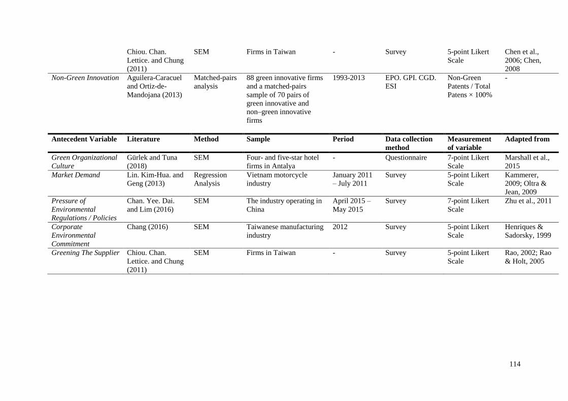
114

Chiou. Chan.

Lettice. and Chung

(2011)

SEM Firms in Taiwan - Survey 5-point Likert

Scale

Chen et al.,

2006; Chen,

2008

Non-Green Innovation Aguilera-Caracuel

and Ortiz-de-

Mandojana (2013)

Matched-pairs

analysis

88 green innovative firms

and a matched-pairs

sample of 70 pairs of

green innovative and

non–green innovative

firms

1993-2013 EPO. GPI. CGD.

ESI

Non-Green

Patents / Total

Patens × 100%

-

Antecedent Variable Literature Method Sample Period Data collection

method

Measurement

of variable

Adapted from

Green Organizational

Culture

Gürlek and Tuna

(2018)

SEM Four- and five-star hotel

firms in Antalya

- Questionnaire 7-point Likert

Scale

Marshall et al.,

2015

Market Demand Lin. Kim-Hua. and

Geng (2013)

Regression

Analysis

Vietnam motorcycle

industry

January 2011

– July 2011

Survey 5-point Likert

Scale

Kammerer,

2009; Oltra &

Jean, 2009

Pressure of

Environmental

Regulations / Policies

Chan. Yee. Dai.

and Lim (2016)

SEM The industry operating in

China

April 2015 –

May 2015

Survey 7-point Likert

Scale

Zhu et al., 2011

Corporate

Environmental

Commitment

Chang (2016) SEM Taiwanese manufacturing

industry

2012 Survey 5-point Likert

Scale

Henriques &

Sadorsky, 1999

Greening The Supplier Chiou. Chan.

Lettice. and Chung

(2011)

SEM Firms in Taiwan - Survey 5-point Likert

Scale

Rao, 2002; Rao

& Holt, 2005

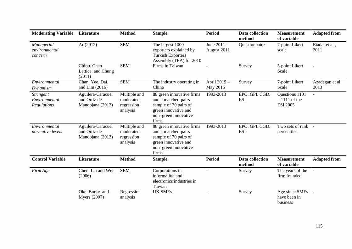
115

Moderating Variable Literature Method Sample Period Data collection

method

Measurement

of variable

Adapted from

Managerial

environmental

concern

Ar (2012) SEM The largest 1000

exporters explained by

Turkish Exporters

Assembly (TEA) for 2010

June 2011 –

August 2011

Questionnaire 7-point Likert

scale

Eiadat et al.,

2011

Chiou. Chan.

Lettice. and Chung

(2011)

SEM Firms in Taiwan - Survey 5-point Likert

Scale

-

Environmental

Dynamism

Chan. Yee. Dai.

and Lim (2016)

SEM The industry operating in

China

April 2015 –

May 2015

Survey 7-point Likert

Scale

Azadegan et al.,

2013

Stringent

Environmental

Regulations

Aguilera-Caracuel

and Ortiz-de-

Mandojana (2013)

Multiple and

moderated

regression

analysis

88 green innovative firms

and a matched-pairs

sample of 70 pairs of

green innovative and

non–green innovative

firms

1993-2013 EPO. GPI. CGD.

ESI

Questions 1101

– 1111 of the

ESI 2005

-

Environmental

normative levels

Aguilera-Caracuel

and Ortiz-de-

Mandojana (2013)

Multiple and

moderated

regression

analysis

88 green innovative firms

and a matched-pairs

sample of 70 pairs of

green innovative and

non–green innovative

firms

1993-2013 EPO. GPI. CGD.

ESI

Two sets of rank

percentiles

-

Control Variable Literature Method Sample Period Data collection

method

Measurement

of variable

Adapted from

Firm Age Chen. Lai and Wen

(2006)

SEM Corporations in

information and

electronics industries in

Taiwan

- Survey The years of the

firm founded

-

Oke. Burke. and

Myers (2007)

Regression

analysis

UK SMEs - Survey Age since SMEs

have been in

business

-

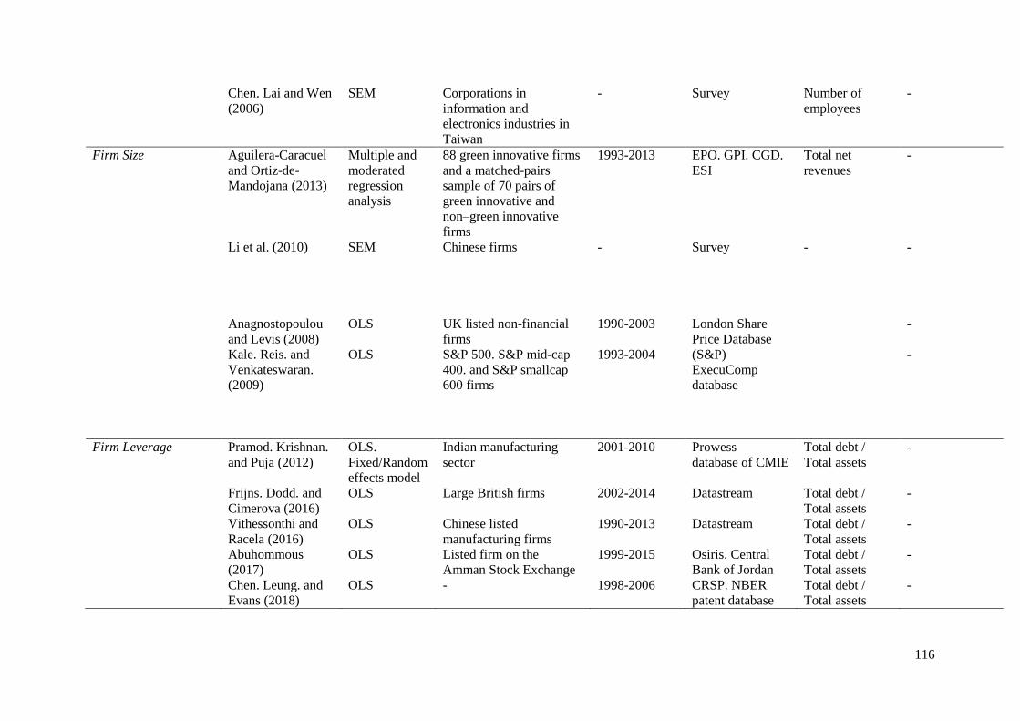
116

Chen. Lai and Wen

(2006)

SEM Corporations in

information and

electronics industries in

Taiwan

- Survey Number of

employees

-

Firm Size

Aguilera-Caracuel

and Ortiz-de-

Mandojana (2013)

Multiple and

moderated

regression

analysis

88 green innovative firms

and a matched-pairs

sample of 70 pairs of

green innovative and

non–green innovative

firms

1993-2013 EPO. GPI. CGD.

ESI

Total net

revenues

-

Li et al. (2010) SEM Chinese firms - Survey - -

Anagnostopoulou

and Levis (2008)

OLS UK listed non-financial

firms

1990-2003 London Share

Price Database

-

Kale. Reis. and

Venkateswaran.

(2009)

OLS S&P 500. S&P mid-cap

400. and S&P smallcap

600 firms

1993-2004 (S&P)

ExecuComp

database

-

Firm Leverage Pramod. Krishnan.

and Puja (2012)

OLS.

Fixed/Random

effects model

Indian manufacturing

sector

2001-2010 Prowess

database of CMIE

Total debt /

Total assets

-

Frijns. Dodd. and

Cimerova (2016)

OLS Large British firms 2002-2014 Datastream Total debt /

Total assets

-

Vithessonthi and

Racela (2016)

OLS Chinese listed

manufacturing firms

1990-2013 Datastream Total debt /

Total assets

-

Abuhommous

(2017)

OLS Listed firm on the

Amman Stock Exchange

1999-2015 Osiris. Central

Bank of Jordan

Total debt /

Total assets

-

Chen. Leung. and

Evans (2018)

OLS - 1998-2006 CRSP. NBER

patent database

Total debt /

Total assets

-

117

Type of Industry Aguilera-Caracuel

and Ortiz-de-

Mandojana (2013)

Multiple and

moderated

regression

analysis

88 green innovative firms

and a matched-pairs

sample of 70 pairs of

green innovative and

non–green innovative

firms

1993-2013 EPO. GPI. CGD.

ESI

Four different

industries

-

Firm level of

Innovation

Aguilera-Caracuel

and Ortiz-de-

Mandojana (2013)

Multiple and

moderated

regression

analysis

88 green innovative firms

and a matched-pairs

sample of 70 pairs of

green innovative and

non–green innovative

firms

1993-2013 EPO. GPI. CGD.

ESI

Total number of

patents

registered

-

Prior financial

performance

Aguilera-Caracuel

and Ortiz-de-

Mandojana (2013)

Multiple and

moderated

regression

analysis

88 green innovative firms

and a matched-pairs

sample of 70 pairs of

green innovative and

non–green innovative

firms

1993-2013 EPO. GPI. CGD.

ESI

ROA average

from the 3

previous years

-

118

9.2 Appendix B – Examples of patents with the Y02 classification CPC Code Examples

Y02A Adaption to climate change at coastal zones; at river basins

Water conservation; efficient water supply; efficient water use

Adaption or protecting infrastructure or their operation

Adaption technologies in agriculture. forestry. livestock or agro alimentary production

Adaption to climate change in human health protection

Technologies having an indirect contribution to adaptation to climate change Y02B Integration of renewable energy sources in buildings

Energy efficient lighting technologies

Energy efficient heating. ventilation or air conditioning

Technologies aiming at improving the efficiency of home appliances

Energy efficient technologies in elevators. escalators and moving walkways

Y02B Technologies for an efficient end-user side electric power management and

consumption

Architectural or constructional elements improving the thermal performance of

buildings

Enabling technologies or technologies with a potential or indirect contribution to

greenhouse gas emissions mitigation

Y02C CO2 capture or storage

Capture or disposal of greenhouse gases other than CO2

Y02D Energy efficient computing

High level techniques for reducing energy consumption in communication networks

Techniques for reducing energy consumption in wire-line communication networks

Techniques for reducing energy consumption in wireless communication networks

Y02E Energy generation through renewable energy sources

Combustion technologies with mitigation potential

Energy generation of nuclear origin

Technologies for an efficient electrical power generation. transmission or distribution

Technologies for the production of fuel of non-fossil origin

Enabling technologies or technologies with a potential or indirect contribution to

greenhouse gas emissions mitigation

Other energy conversion or management systems reducing greenhouse gas emissions

Y02P Climate change mitigation technologies related to metal processing

Climate change mitigation technologies relating to chemical industry

Climate change mitigation technologies relating to oil refining and petrochemical

industry

Climate change mitigation technologies relating to the processing of minerals

Climate change mitigation technologies relating to agriculture. livestock or agro

alimentary industries

Climate change mitigation technologies in the production process for final industrial or

consumer products

Climate change mitigation technologies for sector wide applications

Enabling technologies with a potential contribution to greenhouse gas emissions

mitigation

119

CPC Code Examples

Y02T Climate change mitigation technologies related to road transport of goods or passengers

Climate change mitigation technologies related to transportation of goods or passengers

via railways

Climate change mitigation technologies related to aeronautics or air transport

Climate change mitigation technologies related to maritime or waterways transport

Y02W Enabling technologies or technologies with a potential or indirect contribution to

greenhouse gas emissions mitigation

Climate change mitigation technologies for wastewater treatment

Climate change mitigation technologies for solid waste management

Enabling technologies or technologies with a potential or indirect contribution to

greenhouse gas emissions mitigation

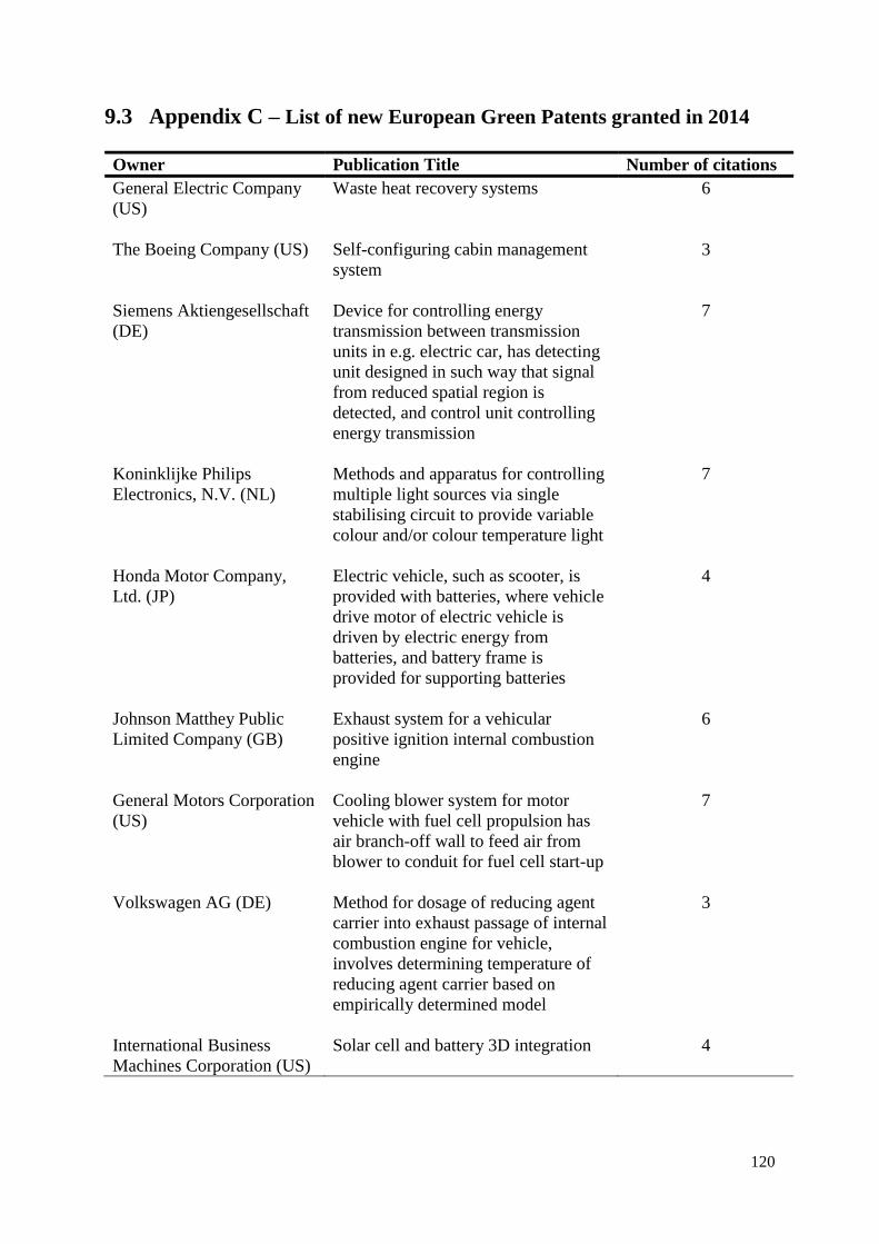
120

9.3 Appendix C – List of new European Green Patents granted in 2014

Owner Publication Title Number of citations

General Electric Company

(US)

Waste heat recovery systems

6

The Boeing Company (US) Self-configuring cabin management

system

3

Siemens Aktiengesellschaft

(DE)

Device for controlling energy

transmission between transmission

units in e.g. electric car, has detecting

unit designed in such way that signal

from reduced spatial region is

detected, and control unit controlling

energy transmission

7

Koninklijke Philips

Electronics, N.V. (NL)

Methods and apparatus for controlling

multiple light sources via single

stabilising circuit to provide variable

colour and/or colour temperature light

7

Honda Motor Company,

Ltd. (JP)

Electric vehicle, such as scooter, is

provided with batteries, where vehicle

drive motor of electric vehicle is

driven by electric energy from

batteries, and battery frame is

provided for supporting batteries

4

Johnson Matthey Public

Limited Company (GB)

Exhaust system for a vehicular

positive ignition internal combustion

engine

6

General Motors Corporation

(US)

Cooling blower system for motor

vehicle with fuel cell propulsion has

air branch-off wall to feed air from

blower to conduit for fuel cell start-up

7

Volkswagen AG (DE) Method for dosage of reducing agent

carrier into exhaust passage of internal

combustion engine for vehicle,

involves determining temperature of

reducing agent carrier based on

empirically determined model

3

International Business

Machines Corporation (US)

Solar cell and battery 3D integration 4

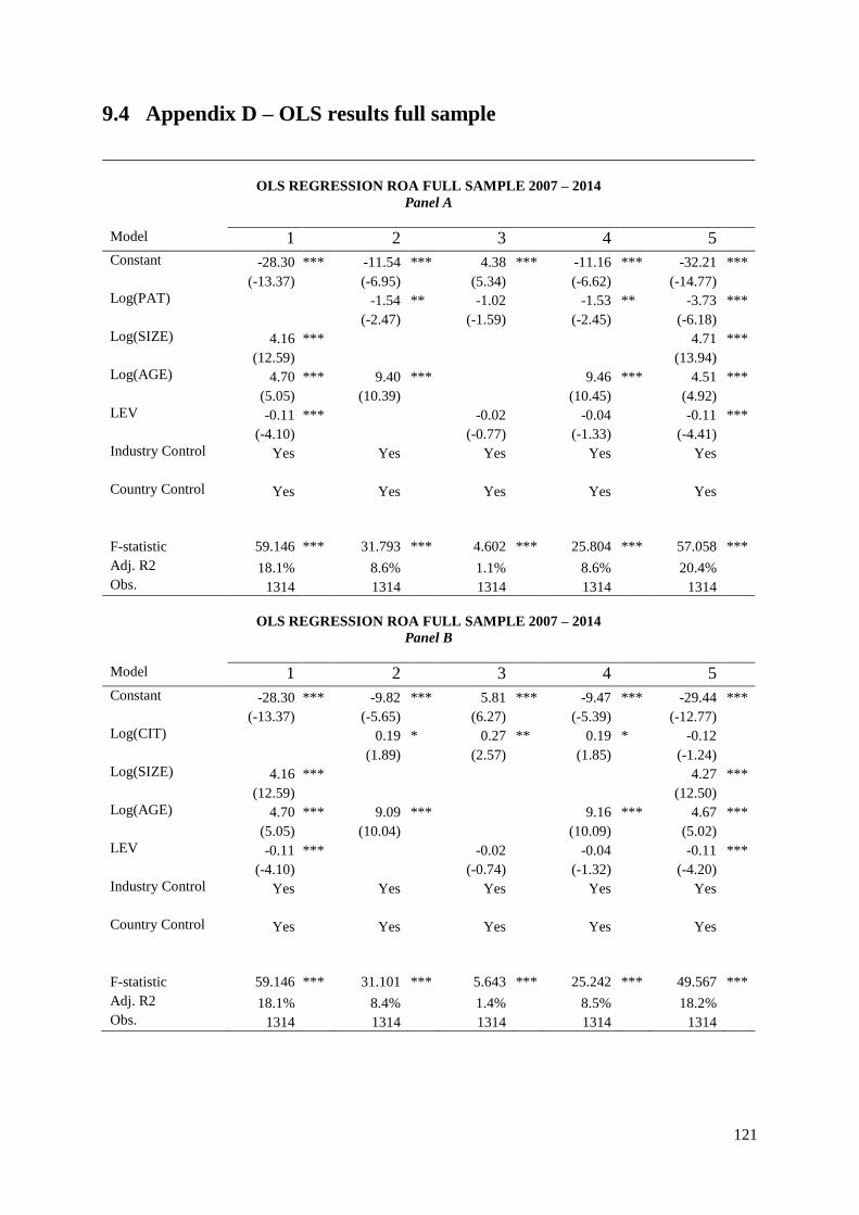
121

9.4 Appendix D – OLS results full sample

OLS REGRESSION ROA FULL SAMPLE 2007 – 2014

Panel A

Model 1 2 3 4 5

Constant -28.30 *** -11.54 *** 4.38 *** -11.16 *** -32.21 ***

(-13.37) (-6.95) (5.34) (-6.62) (-14.77)

Log(PAT) -1.54 ** -1.02 -1.53 ** -3.73 ***

(-2.47) (-1.59) (-2.45) (-6.18)

Log(SIZE) 4.16 *** 4.71 ***

(12.59) (13.94)

Log(AGE) 4.70 *** 9.40 *** 9.46 *** 4.51 ***

(5.05) (10.39) (10.45) (4.92)

LEV -0.11 *** -0.02 -0.04 -0.11 ***

(-4.10) (-0.77) (-1.33) (-4.41)

Industry Control Yes Yes Yes Yes Yes

Country Control Yes Yes Yes Yes Yes

F-statistic 59.146 *** 31.793 *** 4.602 *** 25.804 *** 57.058 ***

Adj. R2 18.1% 8.6% 1.1% 8.6% 20.4%

Obs. 1314 1314 1314 1314 1314

OLS REGRESSION ROA FULL SAMPLE 2007 – 2014

Panel B

Model 1 2 3 4 5

Constant -28.30 *** -9.82 *** 5.81 *** -9.47 *** -29.44 ***

(-13.37) (-5.65) (6.27) (-5.39) (-12.77)

Log(CIT) 0.19 * 0.27 ** 0.19 * -0.12

(1.89) (2.57) (1.85) (-1.24)

Log(SIZE) 4.16 *** 4.27 ***

(12.59) (12.50)

Log(AGE) 4.70 *** 9.09 *** 9.16 *** 4.67 ***

(5.05) (10.04) (10.09) (5.02)

LEV -0.11 *** -0.02 -0.04 -0.11 ***

(-4.10) (-0.74) (-1.32) (-4.20)

Industry Control Yes Yes Yes Yes Yes

Country Control Yes Yes Yes Yes Yes

F-statistic 59.146 *** 31.101 *** 5.643 *** 25.242 *** 49.567 ***

Adj. R2 18.1% 8.4% 1.4% 8.5% 18.2%

Obs. 1314 1314 1314 1314 1314

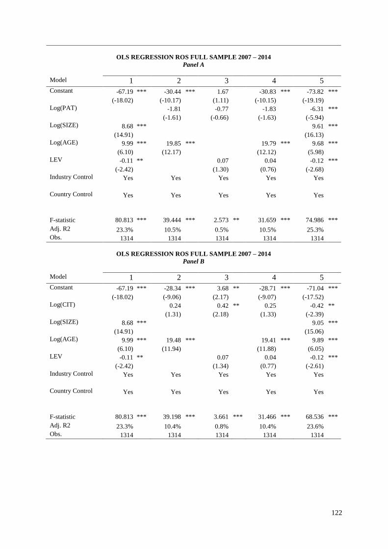
122

OLS REGRESSION ROS FULL SAMPLE 2007 – 2014

Panel A

Model 1 2 3 4 5

Constant -67.19 *** -30.44 *** 1.67 -30.83 *** -73.82 ***

(-18.02) (-10.17) (1.11) (-10.15) (-19.19)

Log(PAT) -1.81 -0.77 -1.83 -6.31 ***

(-1.61) (-0.66) (-1.63) (-5.94)

Log(SIZE) 8.68 *** 9.61 ***

(14.91) (16.13)

Log(AGE) 9.99 *** 19.85 *** 19.79 *** 9.68 ***

(6.10) (12.17) (12.12) (5.98)

LEV -0.11 ** 0.07 0.04 -0.12 ***

(-2.42) (1.30) (0.76) (-2.68)

Industry Control Yes Yes Yes Yes Yes

Country Control Yes Yes Yes Yes Yes

F-statistic 80.813 *** 39.444 *** 2.573 ** 31.659 *** 74.986 ***

Adj. R2 23.3% 10.5% 0.5% 10.5% 25.3%

Obs. 1314 1314 1314 1314 1314

OLS REGRESSION ROS FULL SAMPLE 2007 – 2014

Panel B

Model 1 2 3 4 5

Constant -67.19 *** -28.34 *** 3.68 ** -28.71 *** -71.04 ***

(-18.02) (-9.06) (2.17) (-9.07) (-17.52)

Log(CIT) 0.24 0.42 ** 0.25 -0.42 **

(1.31) (2.18) (1.33) (-2.39)

Log(SIZE) 8.68 *** 9.05 ***

(14.91) (15.06)

Log(AGE) 9.99 *** 19.48 *** 19.41 *** 9.89 ***

(6.10) (11.94) (11.88) (6.05)

LEV -0.11 ** 0.07 0.04 -0.12 ***

(-2.42) (1.34) (0.77) (-2.61)

Industry Control Yes Yes Yes Yes Yes

Country Control Yes Yes Yes Yes Yes

F-statistic 80.813 *** 39.198 *** 3.661 *** 31.466 *** 68.536 ***

Adj. R2 23.3% 10.4% 0.8% 10.4% 23.6%

Obs. 1314 1314 1314 1314 1314

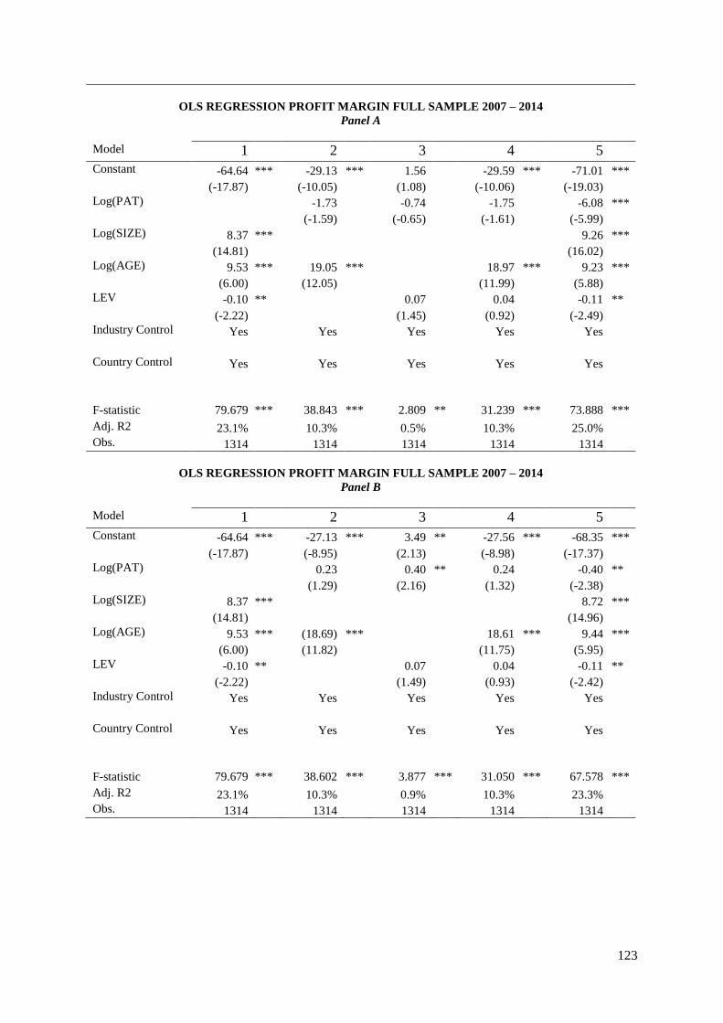
123

OLS REGRESSION PROFIT MARGIN FULL SAMPLE 2007 – 2014

Panel A

Model 1 2 3 4 5

Constant -64.64 *** -29.13 *** 1.56 -29.59 *** -71.01 ***

(-17.87) (-10.05) (1.08) (-10.06) (-19.03)

Log(PAT) -1.73 -0.74 -1.75 -6.08 ***

(-1.59) (-0.65) (-1.61) (-5.99)

Log(SIZE) 8.37 *** 9.26 ***

(14.81) (16.02)

Log(AGE) 9.53 *** 19.05 *** 18.97 *** 9.23 ***

(6.00) (12.05) (11.99) (5.88)

LEV -0.10 ** 0.07 0.04 -0.11 **

(-2.22) (1.45) (0.92) (-2.49)

Industry Control Yes Yes Yes Yes Yes

Country Control Yes Yes Yes Yes Yes

F-statistic 79.679 *** 38.843 *** 2.809 ** 31.239 *** 73.888 ***

Adj. R2 23.1% 10.3% 0.5% 10.3% 25.0%

Obs. 1314 1314 1314 1314 1314

OLS REGRESSION PROFIT MARGIN FULL SAMPLE 2007 – 2014

Panel B

Model 1 2 3 4 5

Constant -64.64 *** -27.13 *** 3.49 ** -27.56 *** -68.35 ***

(-17.87) (-8.95) (2.13) (-8.98) (-17.37)

Log(PAT) 0.23 0.40 ** 0.24 -0.40 **

(1.29) (2.16) (1.32) (-2.38)

Log(SIZE) 8.37 *** 8.72 ***

(14.81) (14.96)

Log(AGE) 9.53 *** (18.69) *** 18.61 *** 9.44 ***

(6.00) (11.82) (11.75) (5.95)

LEV -0.10 ** 0.07 0.04 -0.11 **

(-2.22) (1.49) (0.93) (-2.42)

Industry Control Yes Yes Yes Yes Yes

Country Control Yes Yes Yes Yes Yes

F-statistic 79.679 *** 38.602 *** 3.877 *** 31.050 *** 67.578 ***

Adj. R2 23.1% 10.3% 0.9% 10.3% 23.3%

Obs. 1314 1314 1314 1314 1314

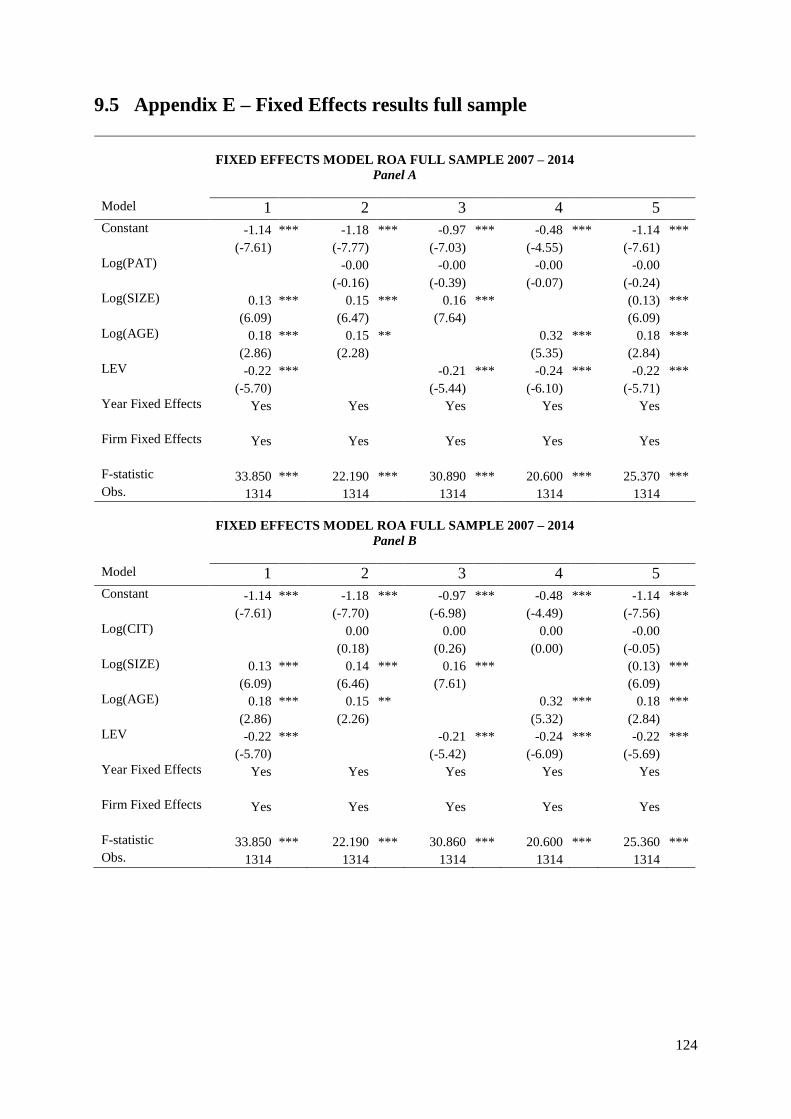
124

9.5 Appendix E – Fixed Effects results full sample

FIXED EFFECTS MODEL ROA FULL SAMPLE 2007 – 2014

Panel A

Model 1 2 3 4 5

Constant -1.14 *** -1.18 *** -0.97 *** -0.48 *** -1.14 ***

(-7.61) (-7.77) (-7.03) (-4.55) (-7.61)

Log(PAT) -0.00 -0.00 -0.00 -0.00

(-0.16) (-0.39) (-0.07) (-0.24)

Log(SIZE) 0.13 *** 0.15 *** 0.16 *** (0.13) ***

(6.09) (6.47) (7.64) (6.09)

Log(AGE) 0.18 *** 0.15 ** 0.32 *** 0.18 ***

(2.86) (2.28) (5.35) (2.84)

LEV -0.22 *** -0.21 *** -0.24 *** -0.22 ***

(-5.70) (-5.44) (-6.10) (-5.71)

Year Fixed Effects Yes Yes Yes Yes Yes

Firm Fixed Effects Yes Yes Yes Yes Yes

F-statistic 33.850 *** 22.190 *** 30.890 *** 20.600 *** 25.370 ***

Obs. 1314 1314 1314 1314 1314

FIXED EFFECTS MODEL ROA FULL SAMPLE 2007 – 2014

Panel B

Model 1 2 3 4 5

Constant -1.14 *** -1.18 *** -0.97 *** -0.48 *** -1.14 ***

(-7.61) (-7.70) (-6.98) (-4.49) (-7.56)

Log(CIT) 0.00 0.00 0.00 -0.00

(0.18) (0.26) (0.00) (-0.05)

Log(SIZE) 0.13 *** 0.14 *** 0.16 *** (0.13) ***

(6.09) (6.46) (7.61) (6.09)

Log(AGE) 0.18 *** 0.15 ** 0.32 *** 0.18 ***

(2.86) (2.26) (5.32) (2.84)

LEV -0.22 *** -0.21 *** -0.24 *** -0.22 ***

(-5.70) (-5.42) (-6.09) (-5.69)

Year Fixed Effects Yes Yes Yes Yes Yes

Firm Fixed Effects Yes Yes Yes Yes Yes

F-statistic 33.850 *** 22.190 *** 30.860 *** 20.600 *** 25.360 ***

Obs. 1314 1314 1314 1314 1314

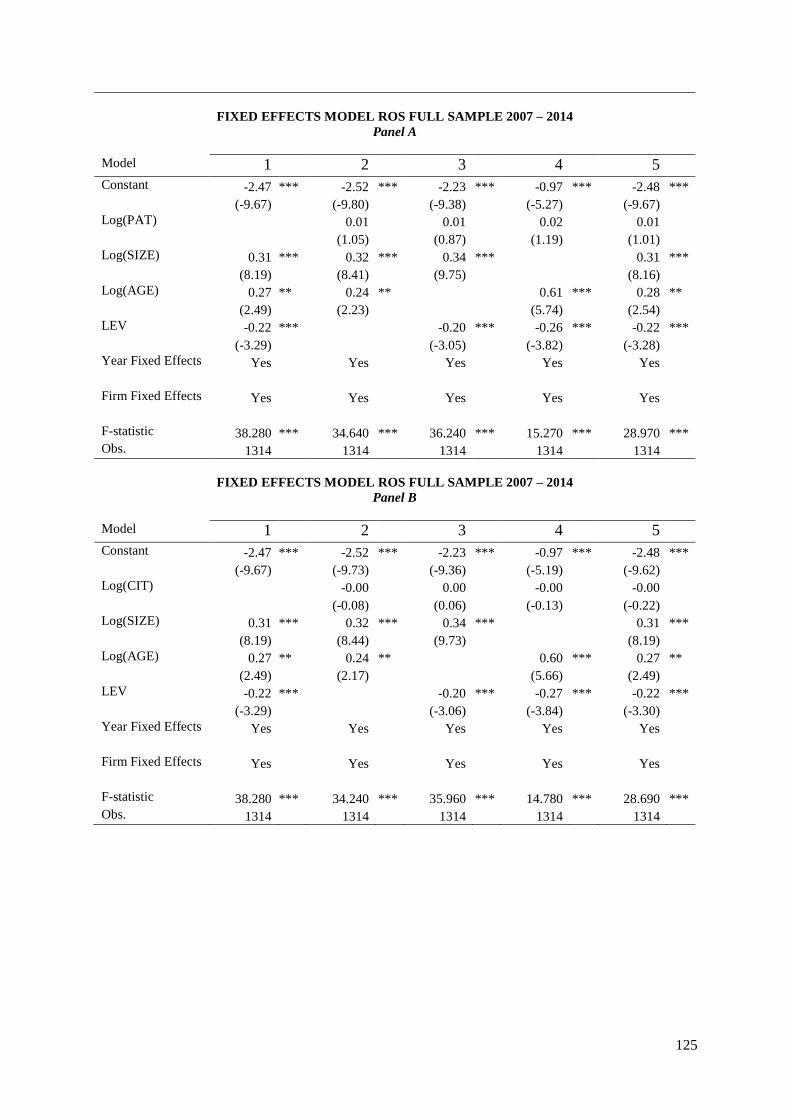
125

FIXED EFFECTS MODEL ROS FULL SAMPLE 2007 – 2014

Panel A

Model 1 2 3 4 5

Constant -2.47 *** -2.52 *** -2.23 *** -0.97 *** -2.48 ***

(-9.67) (-9.80) (-9.38) (-5.27) (-9.67)

Log(PAT) 0.01 0.01 0.02 0.01

(1.05) (0.87) (1.19) (1.01)

Log(SIZE) 0.31 *** 0.32 *** 0.34 *** 0.31 ***

(8.19) (8.41) (9.75) (8.16)

Log(AGE) 0.27 ** 0.24 ** 0.61 *** 0.28 **

(2.49) (2.23) (5.74) (2.54)

LEV -0.22 *** -0.20 *** -0.26 *** -0.22 ***

(-3.29) (-3.05) (-3.82) (-3.28)

Year Fixed Effects Yes Yes Yes Yes Yes

Firm Fixed Effects Yes Yes Yes Yes Yes

F-statistic 38.280 *** 34.640 *** 36.240 *** 15.270 *** 28.970 ***

Obs. 1314 1314 1314 1314 1314

FIXED EFFECTS MODEL ROS FULL SAMPLE 2007 – 2014

Panel B

Model 1 2 3 4 5

Constant -2.47 *** -2.52 *** -2.23 *** -0.97 *** -2.48 ***

(-9.67) (-9.73) (-9.36) (-5.19) (-9.62)

Log(CIT) -0.00 0.00 -0.00 -0.00

(-0.08) (0.06) (-0.13) (-0.22)

Log(SIZE) 0.31 *** 0.32 *** 0.34 *** 0.31 ***

(8.19) (8.44) (9.73) (8.19)

Log(AGE) 0.27 ** 0.24 ** 0.60 *** 0.27 **

(2.49) (2.17) (5.66) (2.49)

LEV -0.22 *** -0.20 *** -0.27 *** -0.22 ***

(-3.29) (-3.06) (-3.84) (-3.30)

Year Fixed Effects Yes Yes Yes Yes Yes

Firm Fixed Effects Yes Yes Yes Yes Yes

F-statistic 38.280 *** 34.240 *** 35.960 *** 14.780 *** 28.690 ***

Obs. 1314 1314 1314 1314 1314

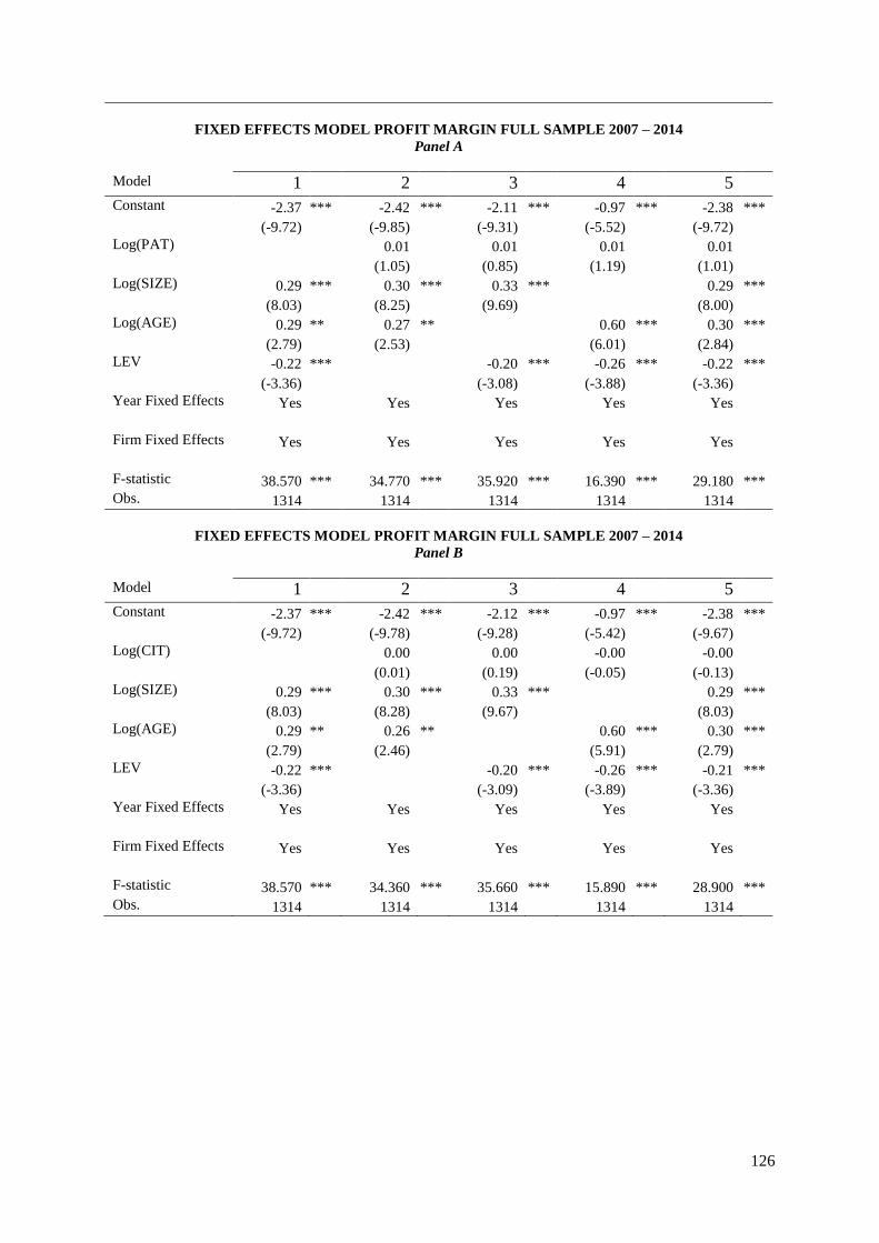
126

FIXED EFFECTS MODEL PROFIT MARGIN FULL SAMPLE 2007 – 2014

Panel A

Model 1 2 3 4 5

Constant -2.37 *** -2.42 *** -2.11 *** -0.97 *** -2.38 ***

(-9.72) (-9.85) (-9.31) (-5.52) (-9.72)

Log(PAT) 0.01 0.01 0.01 0.01

(1.05) (0.85) (1.19) (1.01)

Log(SIZE) 0.29 *** 0.30 *** 0.33 *** 0.29 ***

(8.03) (8.25) (9.69) (8.00)

Log(AGE) 0.29 ** 0.27 ** 0.60 *** 0.30 ***

(2.79) (2.53) (6.01) (2.84)

LEV -0.22 *** -0.20 *** -0.26 *** -0.22 ***

(-3.36) (-3.08) (-3.88) (-3.36)

Year Fixed Effects Yes Yes Yes Yes Yes

Firm Fixed Effects Yes Yes Yes Yes Yes

F-statistic 38.570 *** 34.770 *** 35.920 *** 16.390 *** 29.180 ***

Obs. 1314 1314 1314 1314 1314

FIXED EFFECTS MODEL PROFIT MARGIN FULL SAMPLE 2007 – 2014

Panel B

Model 1 2 3 4 5

Constant -2.37 *** -2.42 *** -2.12 *** -0.97 *** -2.38 ***

(-9.72) (-9.78) (-9.28) (-5.42) (-9.67)

Log(CIT) 0.00 0.00 -0.00 -0.00

(0.01) (0.19) (-0.05) (-0.13)

Log(SIZE) 0.29 *** 0.30 *** 0.33 *** 0.29 ***

(8.03) (8.28) (9.67) (8.03)

Log(AGE) 0.29 ** 0.26 ** 0.60 *** 0.30 ***

(2.79) (2.46) (5.91) (2.79)

LEV -0.22 *** -0.20 *** -0.26 *** -0.21 ***

(-3.36) (-3.09) (-3.89) (-3.36)

Year Fixed Effects Yes Yes Yes Yes Yes

Firm Fixed Effects Yes Yes Yes Yes Yes

F-statistic 38.570 *** 34.360 *** 35.660 *** 15.890 *** 28.900 ***

Obs. 1314 1314 1314 1314 1314

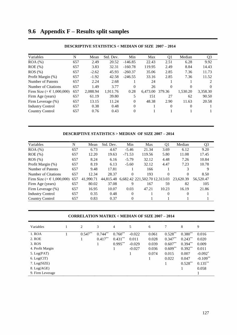
127

9.6 Appendix F – Results split samples

CORRELATION MATRIX < MEDIAN OF SIZE 2007 – 2014

Variables 1 2 3 4 5 6 7 8 9

1. ROA 1 0.547** 0.744** 0.760** -0.022 0.061 0.528** 0.380** 0.016

2. ROE 1 0.417** 0.431** 0.011 0.028 0.347** 0.243** 0.020

3. ROS 1 0.995** -0.029 0.039 0.607** 0.394** 0.009 4. Profit Margin 1 -0.027 0.036 0.609** 0.392** 0.011

5. Log(PAT) 1 0.074 0.015 0.007 -0.092*

6. Log(CIT) 1 0.022 0.047 -0.109**

7. Log(SIZE) 1 0.528** 0.135**

8. Log(AGE) 1 0.058 9. Firm Leverage 1

DESCRIPTIVE STATISTICS < MEDIAN OF SIZE 2007 – 2014

Variables N Mean Std. Dev. Min Max Q1 Median Q3

ROA (%) 657 2.49 20.52 -146.85 22.43 2.51 6.28 9.92

ROE (%) 657 3.83 32.31 -160.78 119.95 2.49 8.84 14.43

ROS (%) 657 -2.62 45.93 -260.37 35.06 2.85 7.36 11.73

Profit Margin (%) 657 -1.92 42.58 -246.55 33.16 2.85 7.36 11.52

Number of Patents 657 2.24 2.68 1 24 1 1 2

Number of Citations 657 1.49 3.77 0 26 0 0 0

Firm Size (× € 1,000,000) 657 2,088.94 1,911.76 0.28 6,473.00 379.36 1,530.20 3,358.30

Firm Age (years) 657 61.19 39.80 5 151 27 62 90.50

Firm Leverage (%) 657 13.15 11.24 0 48.38 2.90 11.63 20.58

Industry Control 657 0.38 0.48 0 1 0 0 1

Country Control 657 0.76 0.43 0 1 1 1 1

DESCRIPTIVE STATISTICS > MEDIAN OF SIZE 2007 – 2014

Variables N Mean Std. Dev. Min Max Q1 Median Q3

ROA (%) 657 6.73 4.67 -5.46 21.34 3.69 6.12 9.20

ROE (%) 657 12.20 19.63 -71.53 119.56 5.80 11.08 17.45

ROS (%) 657 8.24 6.16 -5.79 32.12 4.48 7.26 10.84

Profit Margin (%) 657 8.19 6.13 -5.60 32.12 4.47 7.23 10.78

Number of Patents 657 9.48 17.81 1 166 1 3 9

Number of Citations 657 12.34 28.37 0 193 0 0 8.50

Firm Size (× € 1,000,000) 657 41,990.71 44,815.48 6,682.42 221,502.70 12,313.03 23,620.39 56,520.47

Firm Age (years) 657 80.02 37.08 9 167 59 82 105

Firm Leverage (%) 657 16.95 10.07 0.03 47.21 10.23 16.19 21.86

Industry Control 657 0.35 0.48 0 1 0 0 1

Country Control 657 0.83 0.37 0 1 1 1 1

128

CORRELATION MATRIX > MEDIAN OF SIZE 2007 – 2014

Variables 1 2 3 4 5 6 7 8 9

1. ROA 1 0.426** 0.791** 0.794** -0.167** 0.008 -0.173** -0.181** -0.154**

2. ROE 1 0.360** 0.360** -0.087* 0.102** 0.061 -0.064 -0.075

3. ROS 1 1.000** -0.097* -0.037 -0.019 -0.203** 0.065

4. Profit Margin 1 -0.099* -0.034 -0.022 -0.204** 0.066

5. Log(PAT) 1 0.251** 0.325** 0.082* -0.028

6. Log(CIT) 1 0.301** 0.012 -0.034

7. Log(SIZE) 1 0.020 0.169**

8. Log(AGE) 1 -0.032

9. Firm Leverage 1

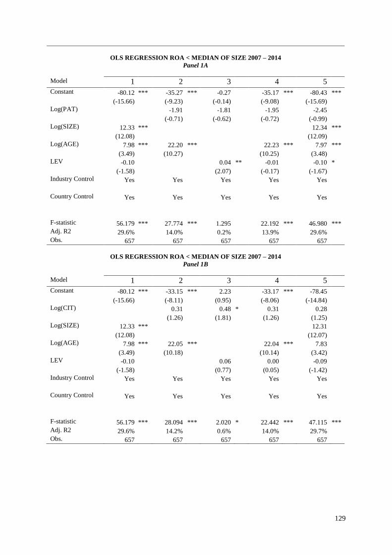
129

OLS REGRESSION ROA < MEDIAN OF SIZE 2007 – 2014

Panel 1A

Model 1 2 3 4 5

Constant -80.12 *** -35.27 *** -0.27 -35.17 *** -80.43 ***

(-15.66) (-9.23) (-0.14) (-9.08) (-15.69)

Log(PAT) -1.91 -1.81 -1.95 -2.45

(-0.71) (-0.62) (-0.72) (-0.99)

Log(SIZE) 12.33 *** 12.34 ***

(12.08) (12.09)

Log(AGE) 7.98 *** 22.20 *** 22.23 *** 7.97 ***

(3.49) (10.27) (10.25) (3.48)

LEV -0.10 0.04 ** -0.01 -0.10 *

(-1.58) (2.07) (-0.17) (-1.67)

Industry Control Yes Yes Yes Yes Yes

Country Control Yes Yes Yes Yes Yes

F-statistic 56.179 *** 27.774 *** 1.295 22.192 *** 46.980 ***

Adj. R2 29.6% 14.0% 0.2% 13.9% 29.6%

Obs. 657 657 657 657 657

OLS REGRESSION ROA < MEDIAN OF SIZE 2007 – 2014

Panel 1B

Model 1 2 3 4 5

Constant -80.12 *** -33.15 *** 2.23 -33.17 *** -78.45

(-15.66) (-8.11) (0.95) (-8.06) (-14.84)

Log(CIT) 0.31 0.48 * 0.31 0.28

(1.26) (1.81) (1.26) (1.25)

Log(SIZE) 12.33 *** 12.31

(12.08) (12.07)

Log(AGE) 7.98 *** 22.05 *** 22.04 *** 7.83

(3.49) (10.18) (10.14) (3.42)

LEV -0.10 0.06 0.00 -0.09

(-1.58) (0.77) (0.05) (-1.42)

Industry Control Yes Yes Yes Yes Yes

Country Control Yes Yes Yes Yes Yes

F-statistic 56.179 *** 28.094 *** 2.020 * 22.442 *** 47.115 ***

Adj. R2 29.6% 14.2% 0.6% 14.0% 29.7%

Obs. 657 657 657 657 657

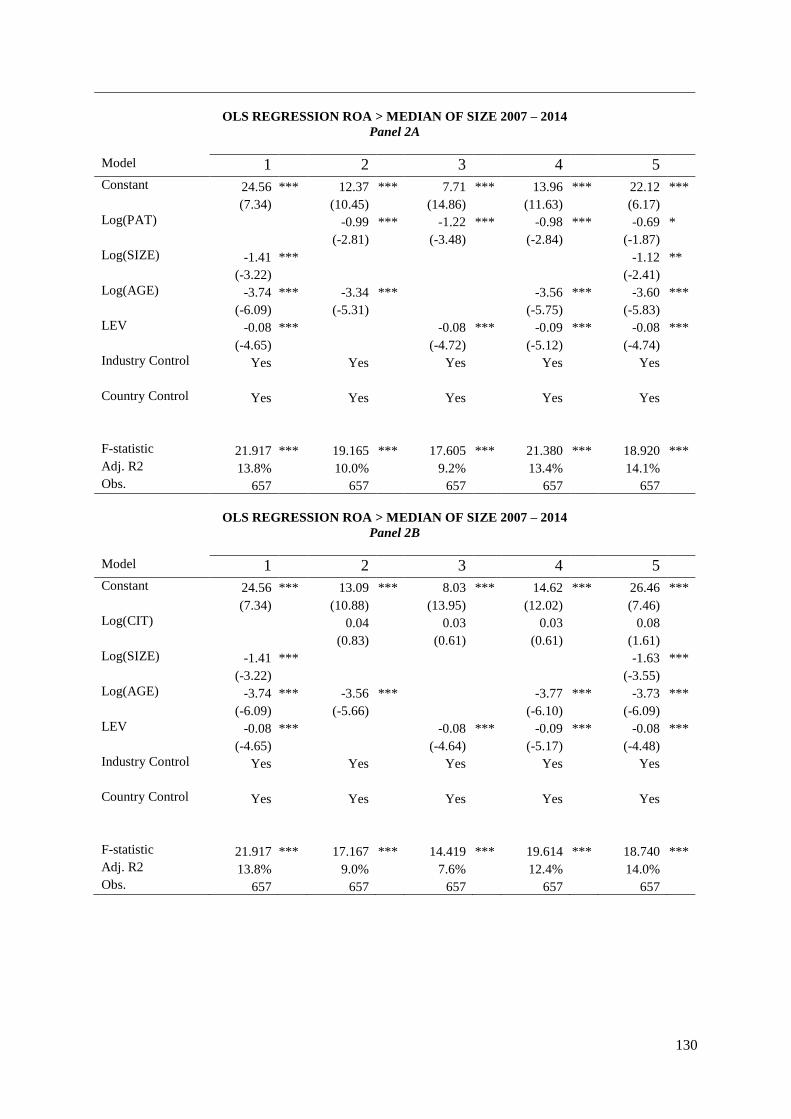
130

OLS REGRESSION ROA > MEDIAN OF SIZE 2007 – 2014

Panel 2A

Model 1 2 3 4 5

Constant 24.56 *** 12.37 *** 7.71 *** 13.96 *** 22.12 ***

(7.34) (10.45) (14.86) (11.63) (6.17)

Log(PAT) -0.99 *** -1.22 *** -0.98 *** -0.69 *

(-2.81) (-3.48) (-2.84) (-1.87)

Log(SIZE) -1.41 *** -1.12 **

(-3.22) (-2.41)

Log(AGE) -3.74 *** -3.34 *** -3.56 *** -3.60 ***

(-6.09) (-5.31) (-5.75) (-5.83)

LEV -0.08 *** -0.08 *** -0.09 *** -0.08 ***

(-4.65) (-4.72) (-5.12) (-4.74)

Industry Control Yes Yes Yes Yes Yes

Country Control Yes Yes Yes Yes Yes

F-statistic 21.917 *** 19.165 *** 17.605 *** 21.380 *** 18.920 ***

Adj. R2 13.8% 10.0% 9.2% 13.4% 14.1%

Obs. 657 657 657 657 657

OLS REGRESSION ROA > MEDIAN OF SIZE 2007 – 2014

Panel 2B

Model 1 2 3 4 5

Constant 24.56 *** 13.09 *** 8.03 *** 14.62 *** 26.46 ***

(7.34) (10.88) (13.95) (12.02) (7.46)

Log(CIT) 0.04 0.03 0.03 0.08

(0.83) (0.61) (0.61) (1.61)

Log(SIZE) -1.41 *** -1.63 ***

(-3.22) (-3.55)

Log(AGE) -3.74 *** -3.56 *** -3.77 *** -3.73 ***

(-6.09) (-5.66) (-6.10) (-6.09)

LEV -0.08 *** -0.08 *** -0.09 *** -0.08 ***

(-4.65) (-4.64) (-5.17) (-4.48)

Industry Control Yes Yes Yes Yes Yes

Country Control Yes Yes Yes Yes Yes

F-statistic 21.917 *** 17.167 *** 14.419 *** 19.614 *** 18.740 ***

Adj. R2 13.8% 9.0% 7.6% 12.4% 14.0%

Obs. 657 657 657 657 657

131

OLS REGRESSION ROS < MEDIAN OF SIZE 2007 – 2014

Panel 1A

Model 1 2 3 4 5

Constant -213.02 *** -90.32 *** -7.66 * -89.67 *** -213.88 ***

(-19.92) (-10.62) (-1.72) (-10.41) (-19.97)

Log(PAT) -5.32 -5.25 -5.58 -6.94

(-0.88) (-0.80) (-0.92) (-1.35)

Log(SIZE) 33.83 *** 33.88 ***

(15.85) (15.88)

Log(AGE) 13.13 *** 52.08 *** 52.24 *** 13.10 ***

(2.74) (10.82) (10.83) (2.74)

LEV -0.31 ** 0.04 -0.07 -0.32 **

(-2.40) (0.24) (-0.49) (-2.52)

Industry Control Yes Yes Yes Yes Yes

Country Control Yes Yes Yes Yes Yes

F-statistic 83.465 *** 30.177 *** 0.769 24.162 *** 69.946 ***

Adj. R2 38.6% 15.1% 0.0% 15.0% 38.7% Obs. 657 657 657 657 657

OLS REGRESSION ROS < MEDIAN OF SIZE 2007 – 2014

Panel 1B

Model 1 2 3 4 5

Constant -213.02 *** -87.83 *** -3.87 -87.49 *** -211.86 ***

(-19.92) (-9.64) (-0.74) (-9.54) (-19.15)

Log(CIT) 0.30 0.67 0.28 0.19

(0.56) (1.14) (0.51) (0.41)

Log(SIZE) 33.83 *** 33.82 ***

(15.85) (15.84)

Log(AGE) 13.13 *** 51.92 *** 52.05 *** 13.03 ***

(2.74) (10.77) (10.76) (2.72)

LEV -0.31 ** 0.07 -0.05 -0.30 **

(-2.40) (0.44) (-0.34) (-2.33)

Industry Control Yes Yes Yes Yes Yes

Country Control Yes Yes Yes Yes Yes

F-statistic 83.465 *** 30.038 *** 0.933 24.021 *** 69.493 ***

Adj. R2 38.6% 15.0% 0.0% 14.9% 38.5%

Obs. 657 657 657 657 657

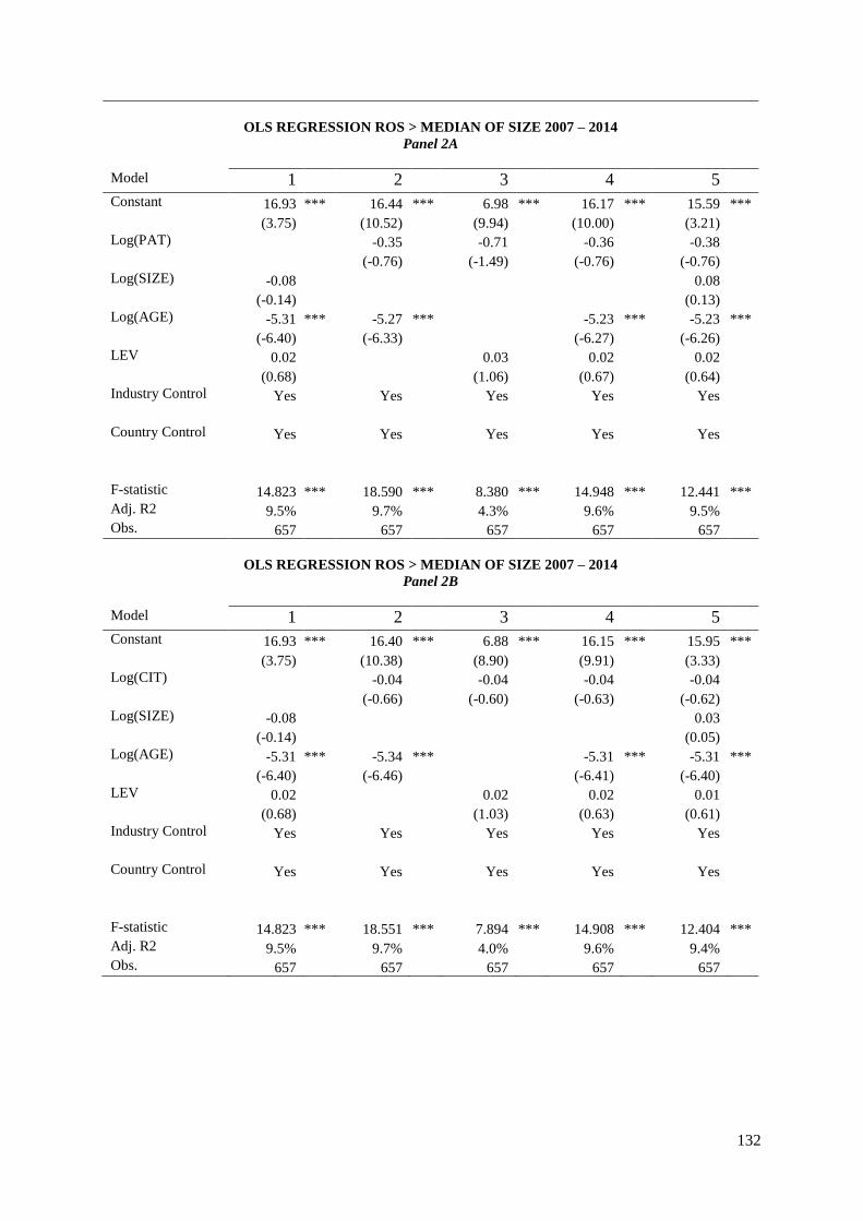
132

OLS REGRESSION ROS > MEDIAN OF SIZE 2007 – 2014

Panel 2A

Model 1 2 3 4 5

Constant 16.93 *** 16.44 *** 6.98 *** 16.17 *** 15.59 ***

(3.75) (10.52) (9.94) (10.00) (3.21)

Log(PAT) -0.35 -0.71 -0.36 -0.38

(-0.76) (-1.49) (-0.76) (-0.76)

Log(SIZE) -0.08 0.08

(-0.14) (0.13)

Log(AGE) -5.31 *** -5.27 *** -5.23 *** -5.23 ***

(-6.40) (-6.33) (-6.27) (-6.26)

LEV 0.02 0.03 0.02 0.02

(0.68) (1.06) (0.67) (0.64)

Industry Control Yes Yes Yes Yes Yes

Country Control Yes Yes Yes Yes Yes

F-statistic 14.823 *** 18.590 *** 8.380 *** 14.948 *** 12.441 ***

Adj. R2 9.5% 9.7% 4.3% 9.6% 9.5%

Obs. 657 657 657 657 657

OLS REGRESSION ROS > MEDIAN OF SIZE 2007 – 2014

Panel 2B

Model 1 2 3 4 5

Constant 16.93 *** 16.40 *** 6.88 *** 16.15 *** 15.95 ***

(3.75) (10.38) (8.90) (9.91) (3.33)

Log(CIT) -0.04 -0.04 -0.04 -0.04

(-0.66) (-0.60) (-0.63) (-0.62)

Log(SIZE) -0.08 0.03

(-0.14) (0.05)

Log(AGE) -5.31 *** -5.34 *** -5.31 *** -5.31 ***

(-6.40) (-6.46) (-6.41) (-6.40)

LEV 0.02 0.02 0.02 0.01

(0.68) (1.03) (0.63) (0.61)

Industry Control Yes Yes Yes Yes Yes

Country Control Yes Yes Yes Yes Yes

F-statistic 14.823 *** 18.551 *** 7.894 *** 14.908 *** 12.404 ***

Adj. R2 9.5% 9.7% 4.0% 9.6% 9.4%

Obs. 657 657 657 657 657

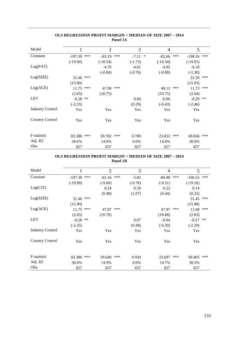
133

OLS REGRESSION PROFIT MARGIN < MEDIAN OF SIZE 2007 – 2014

Panel 1A

Model 1 2 3 4 5

Constant -197.39 *** -83.19 *** -7.11 * -82.66 *** -198.16 ***

(-19.90) (-10.54) (-1.73) (-10.34) (-19.95)

Log(PAT) -4.70 -4.61 -4.92 -6.18

(-0.84) (-0.76) (-0.88) (-1.30)

Log(SIZE) 31.46 *** 31.50 ***

(15.90) (15.93)

Log(AGE) 11.75 *** 47.99 *** 48.12 *** 11.73 ***

(2.65) (10.75) (10.75) (2.64)

LEV -0.28 ** 0.04 -0.06 -0.29 **

(-2.35) (0.29) (-0.43) (-2.46)

Industry Control Yes Yes Yes Yes Yes

Country Control Yes Yes Yes Yes Yes

F-statistic 83.380 *** 29.782 *** 0.789 23.833 *** 69.836 ***

Adj. R2 38.6% 14.9% 0.0% 14.8% 38.6%

Obs. 657 657 657 657 657

OLS REGRESSION PROFIT MARGIN < MEDIAN OF SIZE 2007 – 2014

Panel 1B

Model 1 2 3 4 5

Constant -197.39 *** -81.16 *** -3.82 -80.88 *** -196.55 ***

(-19.90) (-9.60) (-0.78) (-9.51) (-19.16)

Log(CIT) 0.24 0.59 0.22 0.14

(0.48) (1.07) (0.44) (0.32)

Log(SIZE) 31.46 *** 31.45 ***

(15.90) (15.88)

Log(AGE) 11.75 *** 47.87 *** 47.97 *** 11.68 ***

(2.65) (10.70) (10.68) (2.63)

LEV -0.28 ** 0.07 -0.04 -0.27 **

(-2.35) (0.48) (-0.30) (-2.29)

Industry Control Yes Yes Yes Yes Yes

Country Control Yes Yes Yes Yes Yes

F-statistic 83.380 *** 29.640 *** 0.930 23.697 *** 69.405 ***

Adj. R2 38.6% 14.9% 0.0% 14.7% 38.5%

Obs. 657 657 657 657 657

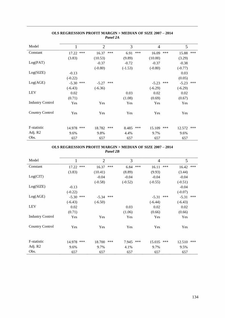
134

OLS REGRESSION PROFIT MARGIN > MEDIAN OF SIZE 2007 – 2014

Panel 2A

Model 1 2 3 4 5

Constant 17.22 *** 16.37 *** 6.91 *** 16.09 *** 15.88 ***

(3.83) (10.53) (9.89) (10.00) (3.29)

Log(PAT) -0.37 -0.72 -0.37 -0.38

(-0.80) (-1.53) (-0.80) (-0.77)

Log(SIZE) -0.13 0.03

(-0.22) (0.05)

Log(AGE) -5.30 *** -5.27 *** -5.23 *** -5.23 ***

(-6.43) (-6.36) (-6.29) (-6.29)

LEV 0.02 0.03 0.02 0.02

(0.71) (1.08) (0.69) (0.67)

Industry Control Yes Yes Yes Yes Yes

Country Control Yes Yes Yes Yes Yes

F-statistic 14.978 *** 18.782 *** 8.485 *** 15.109 *** 12.572 ***

Adj. R2 9.6% 9.8% 4.4% 9.7% 9.6%

Obs. 657 657 657 657 657

OLS REGRESSION PROFIT MARGIN > MEDIAN OF SIZE 2007 – 2014

Panel 2B

Model 1 2 3 4 5

Constant 17.22 *** 16.37 *** 6.84 *** 16.11 *** 16.42 ***

(3.83) (10.41) (8.89) (9.93) (3.44)

Log(CIT) -0.04 -0.04 -0.04 -0.04

(-0.58) (-0.52) (-0.55) (-0.51)

Log(SIZE) -0.13 -0.04

(-0.22) (-0.07)

Log(AGE) -5.30 *** -5.34 *** -5.31 *** -5.31 ***

(-6.43) (-6.50) (-6.44) (-6.43)

LEV 0.02 0.03 0.02 0.02

(0.71) (1.06) (0.66) (0.66)

Industry Control Yes Yes Yes Yes Yes

Country Control Yes Yes Yes Yes Yes

F-statistic 14.978 *** 18.700 *** 7.945 *** 15.035 *** 12.510 ***

Adj. R2 9.6% 9.7% 4.1% 9.7% 9.5%

Obs. 657 657 657 657 657

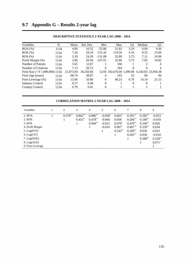
135

9.7 Appendix G – Results 2-year lag

CORRELATION MATRIX 2-YEAR LAG 2008 – 2014

Variables 1 2 3 4 5 6 7 8 9

1. ROA 1 0.578** 0.862** 0.886** -0.058* 0.065* 0.391** 0.285** -0.053

2. ROE 1 0.453** 0.478** -0.004 0.058 0.284** 0.180** -0.018

3. ROS 1 0.994** -0.012 0.070* 0.470** 0.340** 0.036 4. Profit Margin 1 -0.016 0.067* 0.467** 0.339** 0.034

5. Log(PAT) 1 0.243** 0.269** 0.039 0.023

6. Log(CIT) 1 0.265** 0.056 -0.010

7. Log(SIZE) 1 0.388** 0.228**

8. Log(AGE) 1 0.071* 9. Firm Leverage 1

DESCRIPTIVE STATISTICS 2-YEAR LAG 2008 – 2014

Variables N Mean Std. Dev. Min Max Q1 Median Q3

ROA (%) 1134 4.90 10.52 -55.86 21.83 3.19 6.08 9.44

ROE (%) 1134 7.26 28.10 -151.42 119.56 4.16 9.55 15.60

ROS (%) 1134 3.39 24.20 -131.89 32.80 3.75 7.11 10.98

Profit Margin (%) 1134 3.96 20.94 -107.01 32.80 3.73 7.05 10.82

Number of Patents 1134 5.65 12.67 1 166 1 2 4

Number of Citations 1134 7.13 20.72 0 184 0 0 4

Firm Size (× € 1,000,000) 1134 21,873.04 36,350.84 12.85 192,676.00 1,490.08 6,343.83 23,956.38

Firm Age (years) 1134 68.74 38.87 4 163 32 69 96

Firm Leverage (%) 1134 15.06 10.86 0 48.23 6.76 14.14 21.13

Industry Control 1134 0.37 0.48 0 1 0 0 1

Country Control 1134 0.79 0.41 0 1 1 1 1

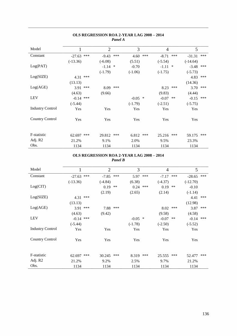
136

OLS REGRESSION ROA 2-YEAR LAG 2008 – 2014

Panel A

Model 1 2 3 4 5

Constant -27.63 *** -9.43 *** 4.60 *** -8.71 *** -31.31 ***

(-13.36) (-6.08) (5.51) (-5.54) (-14.64)

Log(PAT) -1.14 * -0.70 -1.11 * -3.48 ***

(-1.79) (-1.06) (-1.75) (-5.73)

Log(SIZE) 4.31 *** 4.83 ***

(13.13) (14.36)

Log(AGE) 3.91 *** 8.09 *** 8.23 *** 3.70 ***

(4.63) (9.66) (9.83) (4.44)

LEV -0.14 *** -0.05 * -0.07 ** -0.15 ***

(-5.44) (-1.79) (-2.51) (-5.75)

Industry Control Yes Yes Yes Yes Yes

Country Control Yes Yes Yes Yes Yes

F-statistic 62.697 *** 29.812 *** 6.812 *** 25.216 *** 59.175 ***

Adj. R2 21.2% 9.1% 2.0% 9.5% 23.3%

Obs. 1134 1134 1134 1134 1134

OLS REGRESSION ROA 2-YEAR LAG 2008 – 2014

Panel B

Model 1 2 3 4 5

Constant -27.63 *** -7.85 *** 5.97 *** -7.17 *** -28.65 ***

(-13.36) (-4.84) (6.38) (-4.37) (-12.70)

Log(CIT) 0.19 ** 0.24 *** 0.19 ** -0.10

(2.19) (2.65) (2.14) (-1.14)

Log(SIZE) 4.31 *** 4.41 ***

(13.13) (12.98)

Log(AGE) 3.91 *** 7.88 *** 8.02 *** 3.87 ***

(4.63) (9.42) (9.58) (4.58)

LEV -0.14 *** -0.05 * -0.07 ** -0.14 ***

(-5.44) (-1.78) (-2.50) (-5.52)

Industry Control Yes Yes Yes Yes Yes

Country Control Yes Yes Yes Yes Yes

F-statistic 62.697 *** 30.245 *** 8.319 *** 25.555 *** 52.477 ***

Adj. R2 21.2% 9.2% 2.5% 9.7% 21.2%

Obs. 1134 1134 1134 1134 1134

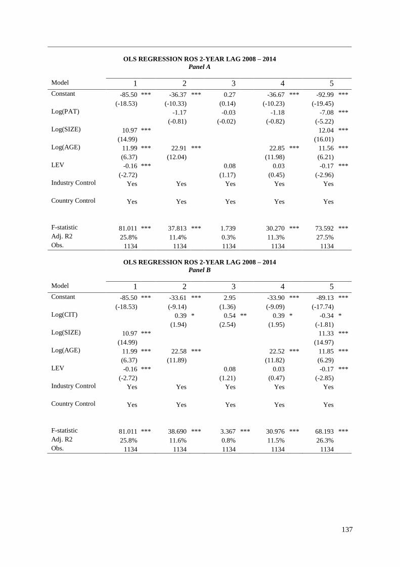
137

OLS REGRESSION ROS 2-YEAR LAG 2008 – 2014

Panel A

Model 1 2 3 4 5

Constant -85.50 *** -36.37 *** 0.27 -36.67 *** -92.99 ***

(-18.53) (-10.33) (0.14) (-10.23) (-19.45)

Log(PAT) -1.17 -0.03 -1.18 -7.08 ***

(-0.81) (-0.02) (-0.82) (-5.22)

Log(SIZE) 10.97 *** 12.04 ***

(14.99) (16.01)

Log(AGE) 11.99 *** 22.91 *** 22.85 *** 11.56 ***

(6.37) (12.04) (11.98) (6.21)

LEV -0.16 *** 0.08 0.03 -0.17 ***

(-2.72) (1.17) (0.45) (-2.96)

Industry Control Yes Yes Yes Yes Yes

Country Control Yes Yes Yes Yes Yes

F-statistic 81.011 *** 37.813 *** 1.739 30.270 *** 73.592 ***

Adj. R2 25.8% 11.4% 0.3% 11.3% 27.5%

Obs. 1134 1134 1134 1134 1134

OLS REGRESSION ROS 2-YEAR LAG 2008 – 2014

Panel B

Model 1 2 3 4 5

Constant -85.50 *** -33.61 *** 2.95 -33.90 *** -89.13 ***

(-18.53) (-9.14) (1.36) (-9.09) (-17.74)

Log(CIT) 0.39 * 0.54 ** 0.39 * -0.34 *

(1.94) (2.54) (1.95) (-1.81)

Log(SIZE) 10.97 *** 11.33 ***

(14.99) (14.97)

Log(AGE) 11.99 *** 22.58 *** 22.52 *** 11.85 ***

(6.37) (11.89) (11.82) (6.29)

LEV -0.16 *** 0.08 0.03 -0.17 ***

(-2.72) (1.21) (0.47) (-2.85)

Industry Control Yes Yes Yes Yes Yes

Country Control Yes Yes Yes Yes Yes

F-statistic 81.011 *** 38.690 *** 3.367 *** 30.976 *** 68.193 ***

Adj. R2 25.8% 11.6% 0.8% 11.5% 26.3%

Obs. 1134 1134 1134 1134 1134

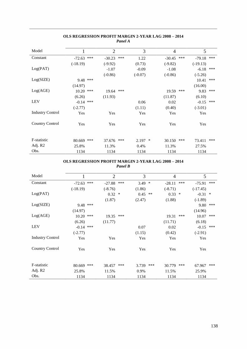
138

OLS REGRESSION PROFIT MARGIN 2-YEAR LAG 2008 – 2014

Panel A

Model 1 2 3 4 5

Constant -72.63 *** -30.23 *** 1.22 -30.45 *** -79.18 ***

(-18.19) (-9.92) (0.73) (-9.82) (-19.13)

Log(PAT) -1.07 -0.09 -1.08 -6.18 ***

(-0.86) (-0.07) (-0.86) (-5.26)

Log(SIZE) 9.48 *** 10.41 ***

(14.97) (16.00)

Log(AGE) 10.20 *** 19.64 *** 19.59 *** 9.83 ***

(6.26) (11.93) (11.87) (6.10)

LEV -0.14 *** 0.06 0.02 -0.15 ***

(-2.77) (1.11) (0.40) (-3.01)

Industry Control Yes Yes Yes Yes Yes

Country Control Yes Yes Yes Yes Yes

F-statistic 80.669 *** 37.676 *** 2.197 * 30.150 *** 73.411 ***

Adj. R2 25.8% 11.3% 0.4% 11.3% 27.5%

Obs. 1134 1134 1134 1134 1134

OLS REGRESSION PROFIT MARGIN 2-YEAR LAG 2008 – 2014

Panel B

Model 1 2 3 4 5

Constant -72.63 *** -27.88 *** 3.49 * -28.11 *** -75.91 ***

(-18.19) (-8.76) (1.86) (-8.71) (-17.45)

Log(PAT) 0.32 * 0.45 ** 0.33 * -0.31 *

(1.87) (2.47) (1.88) (-1.89)

Log(SIZE) 9.48 *** 9.80 ***

(14.97) (14.96)

Log(AGE) 10.20 *** 19.35 *** 19.31 *** 10.07 ***

(6.26) (11.77) (11.71) (6.18)

LEV -0.14 *** 0.07 0.02 -0.15 ***

(-2.77) (1.15) (0.42) (-2.91)

Industry Control Yes Yes Yes Yes Yes

Country Control Yes Yes Yes Yes Yes

F-statistic 80.669 *** 38.457 *** 3.739 *** 30.779 *** 67.967 ***

Adj. R2 25.8% 11.5% 0.9% 11.5% 25.9%

Obs. 1134 1134 1134 1134 1134

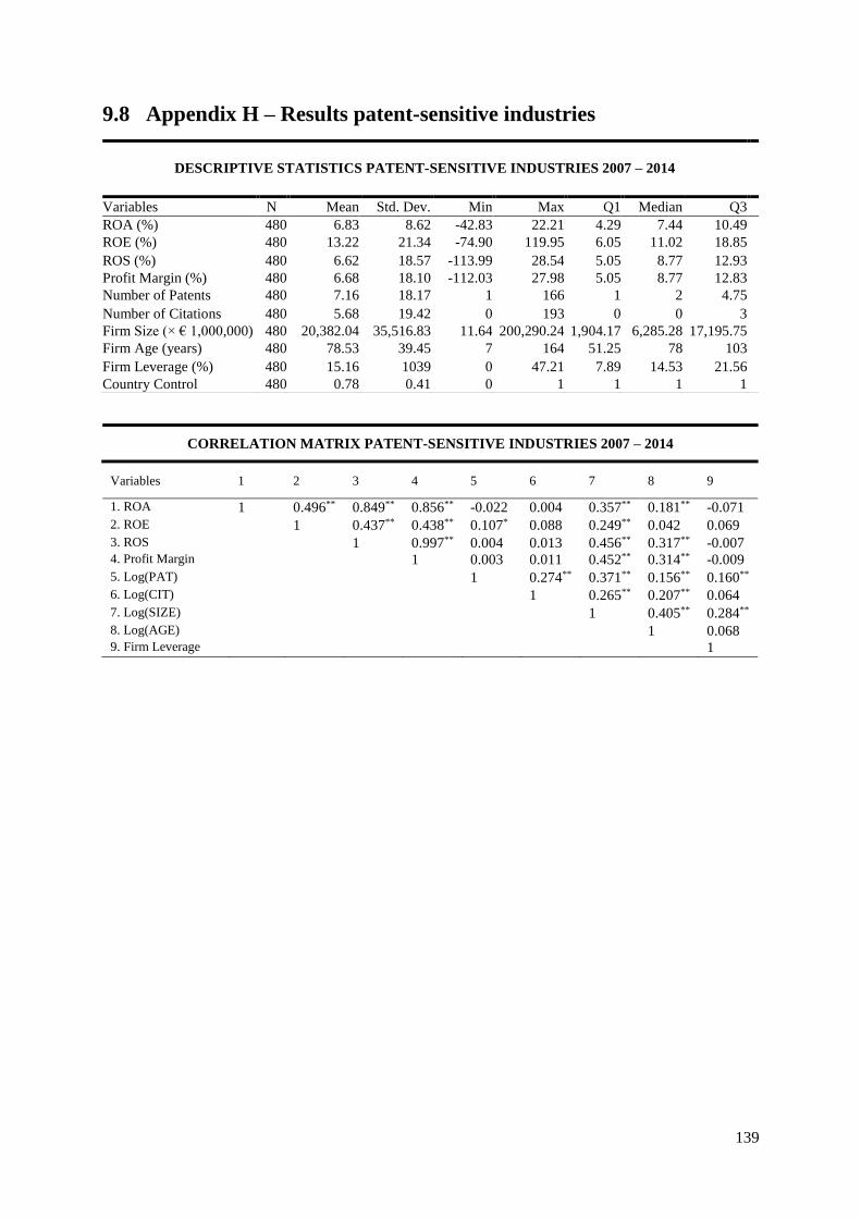
139

9.8 Appendix H – Results patent-sensitive industries

CORRELATION MATRIX PATENT-SENSITIVE INDUSTRIES 2007 – 2014

Variables 1 2 3 4 5 6 7 8 9

1. ROA 1 0.496** 0.849** 0.856** -0.022 0.004 0.357** 0.181** -0.071

2. ROE 1 0.437** 0.438** 0.107* 0.088 0.249** 0.042 0.069

3. ROS 1 0.997** 0.004 0.013 0.456** 0.317** -0.007 4. Profit Margin 1 0.003 0.011 0.452** 0.314** -0.009

5. Log(PAT) 1 0.274** 0.371** 0.156** 0.160**

6. Log(CIT) 1 0.265** 0.207** 0.064

7. Log(SIZE) 1 0.405** 0.284**

8. Log(AGE) 1 0.068 9. Firm Leverage 1

DESCRIPTIVE STATISTICS PATENT-SENSITIVE INDUSTRIES 2007 – 2014

Variables N Mean Std. Dev. Min Max Q1 Median Q3

ROA (%) 480 6.83 8.62 -42.83 22.21 4.29 7.44 10.49

ROE (%) 480 13.22 21.34 -74.90 119.95 6.05 11.02 18.85

ROS (%) 480 6.62 18.57 -113.99 28.54 5.05 8.77 12.93

Profit Margin (%) 480 6.68 18.10 -112.03 27.98 5.05 8.77 12.83

Number of Patents 480 7.16 18.17 1 166 1 2 4.75

Number of Citations 480 5.68 19.42 0 193 0 0 3

Firm Size (× € 1,000,000) 480 20,382.04 35,516.83 11.64 200,290.24 1,904.17 6,285.28 17,195.75

Firm Age (years) 480 78.53 39.45 7 164 51.25 78 103

Firm Leverage (%) 480 15.16 1039 0 47.21 7.89 14.53 21.56

Country Control 480 0.78 0.41 0 1 1 1 1

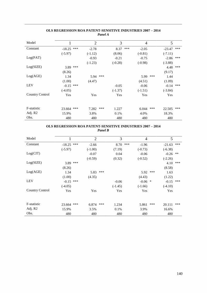
140

OLS REGRESSION ROA PATENT-SENSITIVE INDUSTRIES 2007 – 2014

Panel A

Model 1 2 3 4 5

Constant -18.25 *** -2.78 8.37 *** -2.05 -23.47 ***

(-5.97) (-1.12) (8.06) (-0.81) (-7.11)

Log(PAT) -0.93 -0.21 -0.75 -2.86 ***

(-1.23) (-0.28) (-0.98) (-3.88)

Log(SIZE) 3.89 *** 4.48 ***

(8.26) (9.17)

Log(AGE) 1.34 5.94 *** 5.99 *** 1.44

(1.00) (4.47) (4.51) (1.09)

LEV -0.15 *** -0.05 -0.06 -0.14 ***

(-4.05) (-1.37) (-1.51) (-3.84)

Country Control Yes Yes Yes Yes Yes

F-statistic 23.664 *** 7.282 *** 1.227 6.044 *** 22.505 ***

Adj. R2 15.9% 3.8% 0.1% 4.0% 18.3%

Obs. 480 480 480 480 480

OLS REGRESSION ROA PATENT-SENSITIVE INDUSTRIES 2007 – 2014

Panel B

Model 1 2 3 4 5

Constant -18.25 *** -2.66 8.70 *** -1.96 -21.63 ***

(-5.97) (-1.00) (7.19) (-0.73) (-6.38)

Log(CIT) -0.07 0.04 -0.06 -0.26 **

(-0.59) (0.32) (-0.52) (-2.26)

Log(SIZE) 3.89 *** 4.10 ***

(8.26) (8.58)

Log(AGE) 1.34 5.83 *** 5.92 *** 1.63

(1.00) (4.35) (4.43) (1.22)

LEV -0.15 *** -0.06 -0.06 * -0.15 ***

(-4.05) (-1.45) (-1.66) (-4.10)

Country Control Yes Yes Yes Yes Yes

F-statistic 23.664 *** 6.874 *** 1.234 5.861 *** 20.111 ***

Adj. R2 15.9% 3.5% 0.1% 3.9% 16.6%

Obs. 480 480 480 480 480

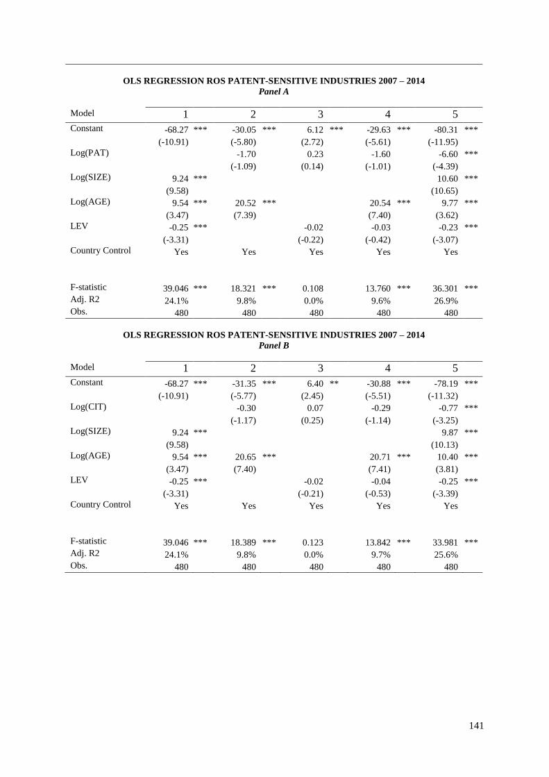
141

OLS REGRESSION ROS PATENT-SENSITIVE INDUSTRIES 2007 – 2014

Panel A

Model 1 2 3 4 5

Constant -68.27 *** -30.05 *** 6.12 *** -29.63 *** -80.31 ***

(-10.91) (-5.80) (2.72) (-5.61) (-11.95)

Log(PAT) -1.70 0.23 -1.60 -6.60 ***

(-1.09) (0.14) (-1.01) (-4.39)

Log(SIZE) 9.24 *** 10.60 ***

(9.58) (10.65)

Log(AGE) 9.54 *** 20.52 *** 20.54 *** 9.77 ***

(3.47) (7.39) (7.40) (3.62)

LEV -0.25 *** -0.02 -0.03 -0.23 ***

(-3.31) (-0.22) (-0.42) (-3.07)

Country Control Yes Yes Yes Yes Yes

F-statistic 39.046 *** 18.321 *** 0.108 13.760 *** 36.301 ***

Adj. R2 24.1% 9.8% 0.0% 9.6% 26.9%

Obs. 480 480 480 480 480

OLS REGRESSION ROS PATENT-SENSITIVE INDUSTRIES 2007 – 2014

Panel B

Model 1 2 3 4 5

Constant -68.27 *** -31.35 *** 6.40 ** -30.88 *** -78.19 ***

(-10.91) (-5.77) (2.45) (-5.51) (-11.32)

Log(CIT) -0.30 0.07 -0.29 -0.77 ***

(-1.17) (0.25) (-1.14) (-3.25)

Log(SIZE) 9.24 *** 9.87 ***

(9.58) (10.13)

Log(AGE) 9.54 *** 20.65 *** 20.71 *** 10.40 ***

(3.47) (7.40) (7.41) (3.81)

LEV -0.25 *** -0.02 -0.04 -0.25 ***

(-3.31) (-0.21) (-0.53) (-3.39)

Country Control Yes Yes Yes Yes Yes

F-statistic 39.046 *** 18.389 *** 0.123 13.842 *** 33.981 ***

Adj. R2 24.1% 9.8% 0.0% 9.7% 25.6%

Obs. 480 480 480 480 480

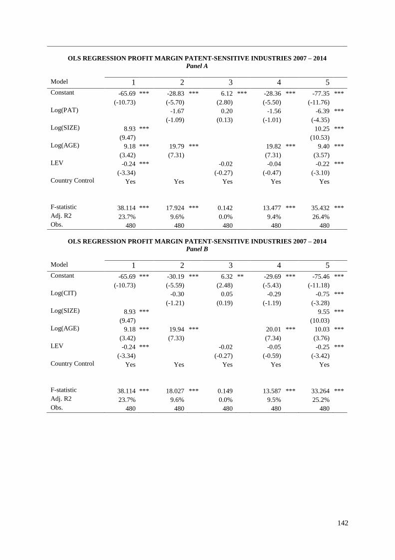
142

OLS REGRESSION PROFIT MARGIN PATENT-SENSITIVE INDUSTRIES 2007 – 2014

Panel A

Model 1 2 3 4 5

Constant -65.69 *** -28.83 *** 6.12 *** -28.36 *** -77.35 ***

(-10.73) (-5.70) (2.80) (-5.50) (-11.76)

Log(PAT) -1.67 0.20 -1.56 -6.39 ***

(-1.09) (0.13) (-1.01) (-4.35)

Log(SIZE) 8.93 *** 10.25 ***

(9.47) (10.53)

Log(AGE) 9.18 *** 19.79 *** 19.82 *** 9.40 ***

(3.42) (7.31) (7.31) (3.57)

LEV -0.24 *** -0.02 -0.04 -0.22 ***

(-3.34) (-0.27) (-0.47) (-3.10)

Country Control Yes Yes Yes Yes Yes

F-statistic 38.114 *** 17.924 *** 0.142 13.477 *** 35.432 ***

Adj. R2 23.7% 9.6% 0.0% 9.4% 26.4%

Obs. 480 480 480 480 480

OLS REGRESSION PROFIT MARGIN PATENT-SENSITIVE INDUSTRIES 2007 – 2014

Panel B

Model 1 2 3 4 5

Constant -65.69 *** -30.19 *** 6.32 ** -29.69 *** -75.46 ***

(-10.73) (-5.59) (2.48) (-5.43) (-11.18)

Log(CIT) -0.30 0.05 -0.29 -0.75 ***

(-1.21) (0.19) (-1.19) (-3.28)

Log(SIZE) 8.93 *** 9.55 ***

(9.47) (10.03)

Log(AGE) 9.18 *** 19.94 *** 20.01 *** 10.03 ***

(3.42) (7.33) (7.34) (3.76)

LEV -0.24 *** -0.02 -0.05 -0.25 ***

(-3.34) (-0.27) (-0.59) (-3.42)

Country Control Yes Yes Yes Yes Yes

F-statistic 38.114 *** 18.027 *** 0.149 13.587 *** 33.264 ***

Adj. R2 23.7% 9.6% 0.0% 9.5% 25.2%

Obs. 480 480 480 480 480

143

9.9 Appendix I – Results firms with at least one citation

CORRELATION MATRIX >0 CITATIONS 2007 – 2014

Variables 1 2 3 4 5 6 7 8 9

1. ROA 1 0.450** 0.786** 0.786** -0.174** -0.094 0.158** 0.066 -0.171**

2. ROE 1 0.333** 0.337** -0.018 -0.011 0.241** 0.029 -0.047

3. ROS 1 1.000** -0.104* -0.044 0.299** 0.126** -0.042 4. Profit Margin 1 -0.105* -0.045 0.304** 0.127** -0.038

5. Log(PAT) 1 0.739** 0.348** 0.031 0.084

6. Log(CIT) 1 0.265** 0.035 0.046

7. Log(SIZE) 1 0.264** 0.317**

8. Log(AGE) 1 0.025 9. Firm Leverage 1

DESCRIPTIVE STATISTICS >0 CITATIONS 2007 – 2014

Variables N Mean Std. Dev. Min Max Q1 Median Q3

ROA (%) 435 6.28 6.67 -26.20 22.21 3.76 6.46 9.30

ROE (%) 435 11.56 23.36 -79.30 119.95 5.69 10.81 17.55

ROS (%) 435 6.43 14.48 -88.14 28.54 4.51 7.42 11.14

Profit Margin (%) 435 6.39 14.34 -88.14 27.98 4.47 7.42 11.11

Number of Patents 435 11.43 20.93 1 166 1 3 11

Number of Citations 435 20.89 32.17 1 193 4 8 22

Firm Size (× € 1,000,000) 435 37,151.25 47,372.40 22.88 200,290.24 3,133.00 16,610.39 57,334.00

Firm Age (years) 435 75.92 39.83 8 164 38 81 101

Firm Leverage (%) 435 14.73 10.35 0 45.10 7.06 13.70 20.79

Industry Control 435 0.32 0.47 0 1 0 0 1

Country Control 435 0.86 0.35 0 1 1 1 1

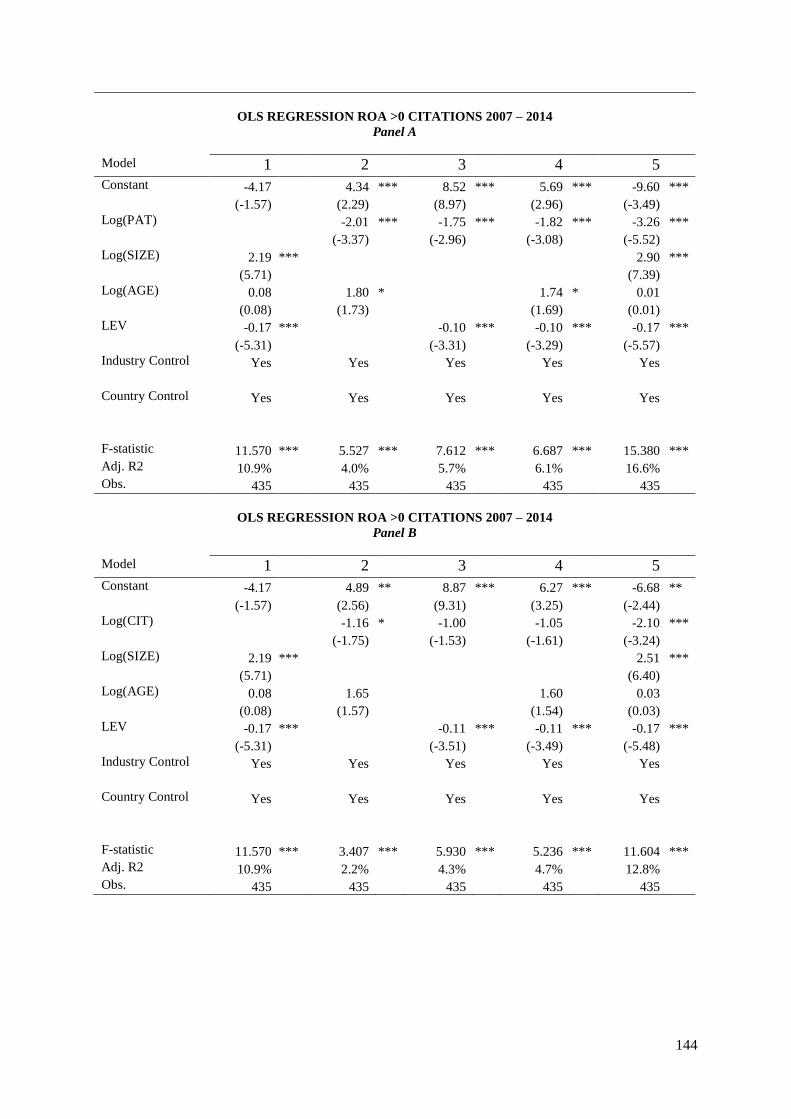
144

OLS REGRESSION ROA >0 CITATIONS 2007 – 2014

Panel A

Model 1 2 3 4 5

Constant -4.17 4.34 *** 8.52 *** 5.69 *** -9.60 ***

(-1.57) (2.29) (8.97) (2.96) (-3.49)

Log(PAT) -2.01 *** -1.75 *** -1.82 *** -3.26 ***

(-3.37) (-2.96) (-3.08) (-5.52)

Log(SIZE) 2.19 *** 2.90 ***

(5.71) (7.39)

Log(AGE) 0.08 1.80 * 1.74 * 0.01

(0.08) (1.73) (1.69) (0.01)

LEV -0.17 *** -0.10 *** -0.10 *** -0.17 ***

(-5.31) (-3.31) (-3.29) (-5.57)

Industry Control Yes Yes Yes Yes Yes

Country Control Yes Yes Yes Yes Yes

F-statistic 11.570 *** 5.527 *** 7.612 *** 6.687 *** 15.380 ***

Adj. R2 10.9% 4.0% 5.7% 6.1% 16.6%

Obs. 435 435 435 435 435

OLS REGRESSION ROA >0 CITATIONS 2007 – 2014

Panel B

Model 1 2 3 4 5

Constant -4.17 4.89 ** 8.87 *** 6.27 *** -6.68 **

(-1.57) (2.56) (9.31) (3.25) (-2.44)

Log(CIT) -1.16 * -1.00 -1.05 -2.10 ***

(-1.75) (-1.53) (-1.61) (-3.24)

Log(SIZE) 2.19 *** 2.51 ***

(5.71) (6.40)

Log(AGE) 0.08 1.65 1.60 0.03

(0.08) (1.57) (1.54) (0.03)

LEV -0.17 *** -0.11 *** -0.11 *** -0.17 ***

(-5.31) (-3.51) (-3.49) (-5.48)

Industry Control Yes Yes Yes Yes Yes

Country Control Yes Yes Yes Yes Yes

F-statistic 11.570 *** 3.407 *** 5.930 *** 5.236 *** 11.604 ***

Adj. R2 10.9% 2.2% 4.3% 4.7% 12.8%

Obs. 435 435 435 435 435

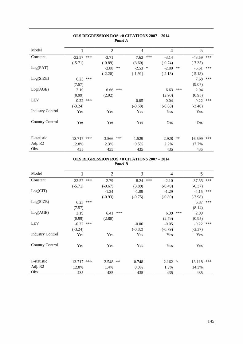
145

OLS REGRESSION ROS >0 CITATIONS 2007 – 2014

Panel A

Model 1 2 3 4 5

Constant -32.57 *** -3.71 7.63 *** -3.14 -43.59 ***

(-5.71) (-0.89) (3.60) (-0.74) (-7.35)

Log(PAT) -2.88 ** -2.53 * -2.80 ** -6.61 ***

(-2.20) (-1.91) (-2.13) (-5.18)

Log(SIZE) 6.23 *** 7.68 ***

(7.57) (9.07)

Log(AGE) 2.19 6.66 *** 6.63 *** 2.04

(0.99) (2.92) (2.90) (0.95)

LEV -0.22 *** -0.05 -0.04 -0.22 ***

(-3.24) (-0.68) (-0.63) (-3.40)

Industry Control Yes Yes Yes Yes Yes

Country Control Yes Yes Yes Yes Yes

F-statistic 13.717 *** 3.566 *** 1.529 2.928 ** 16.599 ***

Adj. R2 12.8% 2.3% 0.5% 2.2% 17.7%

Obs. 435 435 435 435 435

OLS REGRESSION ROS >0 CITATIONS 2007 – 2014

Panel B

Model 1 2 3 4 5

Constant -32.57 *** -2.79 8.24 *** -2.10 -37.55 ***

(-5.71) (-0.67) (3.89) (-0.49) (-6.37)

Log(CIT) -1.34 -1.09 -1.29 -4.15 ***

(-0.93) (-0.75) (-0.89) (-2.98)

Log(SIZE) 6.23 *** 6.87 ***

(7.57) (8.14)

Log(AGE) 2.19 6.41 *** 6.39 *** 2.09

(0.99) (2.80) (2.79) (0.95)

LEV -0.22 *** -0.06 -0.05 -0.22 ***

(-3.24) (-0.82) (-0.79) (-3.37)

Industry Control Yes Yes Yes Yes Yes

Country Control Yes Yes Yes Yes Yes

F-statistic 13.717 *** 2.548 ** 0.748 2.162 * 13.118 ***

Adj. R2 12.8% 1.4% 0.0% 1.3% 14.3%

Obs. 435 435 435 435 435

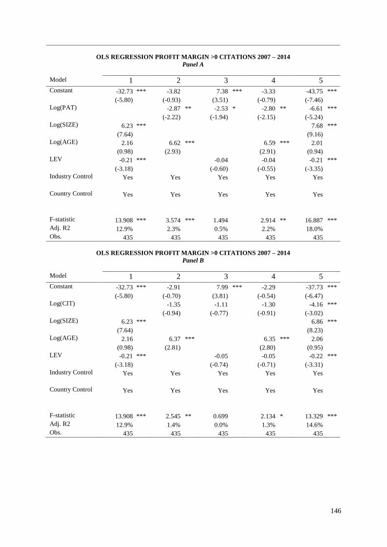
146

OLS REGRESSION PROFIT MARGIN >0 CITATIONS 2007 – 2014

Panel A

Model 1 2 3 4 5

Constant -32.73 *** -3.82 7.38 *** -3.33 -43.75 ***

(-5.80) (-0.93) (3.51) (-0.79) (-7.46)

Log(PAT) -2.87 ** -2.53 * -2.80 ** -6.61 ***

(-2.22) (-1.94) (-2.15) (-5.24)

Log(SIZE) 6.23 *** 7.68 ***

(7.64) (9.16)

Log(AGE) 2.16 6.62 *** 6.59 *** 2.01

(0.98) (2.93) (2.91) (0.94)

LEV -0.21 *** -0.04 -0.04 -0.21 ***

(-3.18) (-0.60) (-0.55) (-3.35)

Industry Control Yes Yes Yes Yes Yes

Country Control Yes Yes Yes Yes Yes

F-statistic 13.908 *** 3.574 *** 1.494 2.914 ** 16.887 ***

Adj. R2 12.9% 2.3% 0.5% 2.2% 18.0%

Obs. 435 435 435 435 435

OLS REGRESSION PROFIT MARGIN >0 CITATIONS 2007 – 2014

Panel B

Model 1 2 3 4 5

Constant -32.73 *** -2.91 7.99 *** -2.29 -37.73 ***

(-5.80) (-0.70) (3.81) (-0.54) (-6.47)

Log(CIT) -1.35 -1.11 -1.30 -4.16 ***

(-0.94) (-0.77) (-0.91) (-3.02)

Log(SIZE) 6.23 *** 6.86 ***

(7.64) (8.23)

Log(AGE) 2.16 6.37 *** 6.35 *** 2.06

(0.98) (2.81) (2.80) (0.95)

LEV -0.21 *** -0.05 -0.05 -0.22 ***

(-3.18) (-0.74) (-0.71) (-3.31)

Industry Control Yes Yes Yes Yes Yes

Country Control Yes Yes Yes Yes Yes

F-statistic 13.908 *** 2.545 ** 0.699 2.134 * 13.329 ***

Adj. R2 12.9% 1.4% 0.0% 1.3% 14.6%

Obs. 435 435 435 435 435

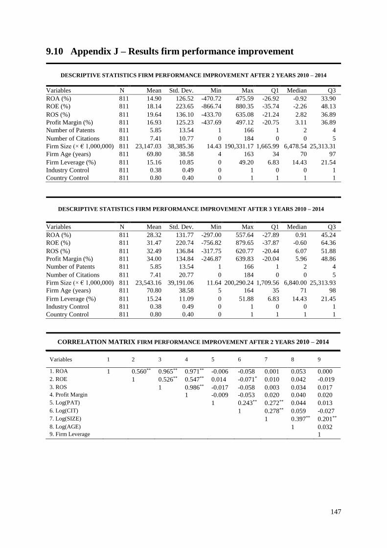
147

9.10 Appendix J – Results firm performance improvement

CORRELATION MATRIX FIRM PERFORMANCE IMPROVEMENT AFTER 2 YEARS 2010 – 2014

Variables 1 2 3 4 5 6 7 8 9

1. ROA 1 0.560** 0.965** 0.971** -0.006 -0.058 0.001 0.053 0.000

2. ROE 1 0.526** 0.547** 0.014 -0.071* 0.010 0.042 -0.019

3. ROS 1 0.986** -0.017 -0.058 0.003 0.034 0.017 4. Profit Margin 1 -0.009 -0.053 0.020 0.040 0.020

5. Log(PAT) 1 0.243** 0.272** 0.044 0.013

6. Log(CIT) 1 0.278** 0.059 -0.027

7. Log(SIZE) 1 0.397** 0.201**

8. Log(AGE) 1 0.032 9. Firm Leverage 1

DESCRIPTIVE STATISTICS FIRM PERFORMANCE IMPROVEMENT AFTER 2 YEARS 2010 – 2014

Variables N Mean Std. Dev. Min Max Q1 Median Q3

ROA (%) 811 14.90 126.52 -470.72 475.59 -26.92 -0.92 33.90

ROE (%) 811 18.14 223.65 -866.74 880.35 -35.74 -2.26 48.13

ROS (%) 811 19.64 136.10 -433.70 635.08 -21.24 2.82 36.89

Profit Margin (%) 811 16.93 125.23 -437.69 497.12 -20.75 3.11 36.89

Number of Patents 811 5.85 13.54 1 166 1 2 4

Number of Citations 811 7.41 10.77 0 184 0 0 5

Firm Size (× € 1,000,000) 811 23,147.03 38,385.36 14.43 190,331.17 1,665.99 6,478.54 25,313.31

Firm Age (years) 811 69.80 38.58 4 163 34 70 97

Firm Leverage (%) 811 15.16 10.85 0 49.20 6.83 14.43 21.54

Industry Control 811 0.38 0.49 0 1 0 0 1

Country Control 811 0.80 0.40 0 1 1 1 1

DESCRIPTIVE STATISTICS FIRM PERFORMANCE IMPROVEMENT AFTER 3 YEARS 2010 – 2014

Variables N Mean Std. Dev. Min Max Q1 Median Q3

ROA (%) 811 28.32 131.77 -297.00 557.64 -27.89 0.91 45.24

ROE (%) 811 31.47 220.74 -756.82 879.65 -37.87 -0.60 64.36

ROS (%) 811 32.49 136.84 -317.75 620.77 -20.44 6.07 51.88

Profit Margin (%) 811 34.00 134.84 -246.87 639.83 -20.04 5.96 48.86

Number of Patents 811 5.85 13.54 1 166 1 2 4

Number of Citations 811 7.41 20.77 0 184 0 0 5

Firm Size (× € 1,000,000) 811 23,543.16 39,191.06 11.64 200,290.24 1,709.56 6,840.00 25,313.93

Firm Age (years) 811 70.80 38.58 5 164 35 71 98

Firm Leverage (%) 811 15.24 11.09 0 51.88 6.83 14.43 21.45

Industry Control 811 0.38 0.49 0 1 0 0 1

Country Control 811 0.80 0.40 0 1 1 1 1

148

CORRELATION MATRIX FIRM PERFORMANCE IMPROVEMENT AFTER 3 YEARS 2010 – 2014

Variables 1 2 3 4 5 6 7 8 9

1. ROA 1 0.541** 0.969** 0.971** -0.021 -0.064 -0.001 0.009 -0.051

2. ROE 1 0.535** 0.525** 0.038 -0.041 0.047 0.048 -0.062

3. ROS 1 0.993** -0.020 -0.058 0.021 -0.002 -0.043 4. Profit Margin 1 -0.023 -0.059 0.009 -0.012 -0.039

5. Log(PAT) 1 0.243** 0.268** 0.046 -0.021

6. Log(CIT) 1 0.278** 0.061 -0.046

7. Log(SIZE) 1 0.399** 0.195**

8. Log(AGE) 1 0.023 9. Firm Leverage 1

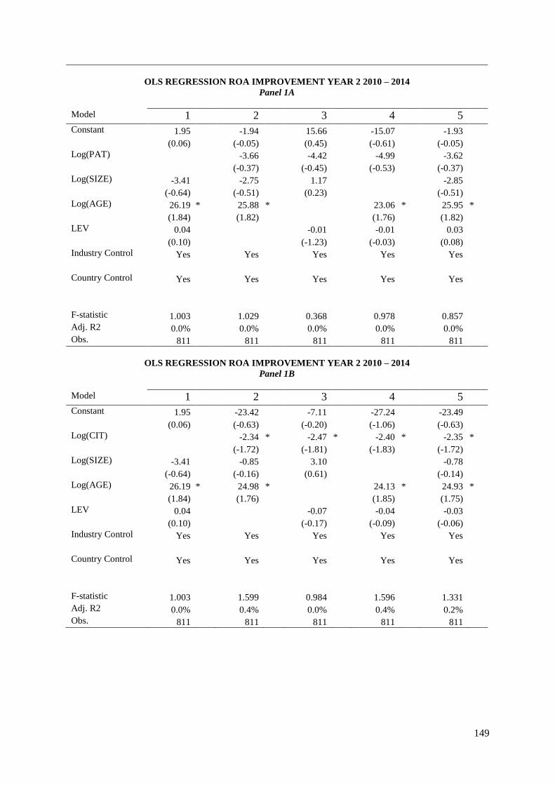
149

OLS REGRESSION ROA IMPROVEMENT YEAR 2 2010 – 2014

Panel 1A

Model 1 2 3 4 5

Constant 1.95 -1.94 15.66 -15.07 -1.93

(0.06) (-0.05) (0.45) (-0.61) (-0.05)

Log(PAT) -3.66 -4.42 -4.99 -3.62

(-0.37) (-0.45) (-0.53) (-0.37)

Log(SIZE) -3.41 -2.75 1.17 -2.85

(-0.64) (-0.51) (0.23) (-0.51)

Log(AGE) 26.19 * 25.88 * 23.06 * 25.95 *

(1.84) (1.82) (1.76) (1.82)

LEV 0.04 -0.01 -0.01 0.03

(0.10) (-1.23) (-0.03) (0.08)

Industry Control Yes Yes Yes Yes Yes

Country Control Yes Yes Yes Yes Yes

F-statistic 1.003 1.029 0.368 0.978 0.857

Adj. R2 0.0% 0.0% 0.0% 0.0% 0.0%

Obs. 811 811 811 811 811

OLS REGRESSION ROA IMPROVEMENT YEAR 2 2010 – 2014

Panel 1B

Model 1 2 3 4 5

Constant 1.95 -23.42 -7.11 -27.24 -23.49

(0.06) (-0.63) (-0.20) (-1.06) (-0.63)

Log(CIT) -2.34 * -2.47 * -2.40 * -2.35 *

(-1.72) (-1.81) (-1.83) (-1.72)

Log(SIZE) -3.41 -0.85 3.10 -0.78

(-0.64) (-0.16) (0.61) (-0.14)

Log(AGE) 26.19 * 24.98 * 24.13 * 24.93 *

(1.84) (1.76) (1.85) (1.75)

LEV 0.04 -0.07 -0.04 -0.03

(0.10) (-0.17) (-0.09) (-0.06)

Industry Control Yes Yes Yes Yes Yes

Country Control Yes Yes Yes Yes Yes

F-statistic 1.003 1.599 0.984 1.596 1.331

Adj. R2 0.0% 0.4% 0.0% 0.4% 0.2%

Obs. 811 811 811 811 811

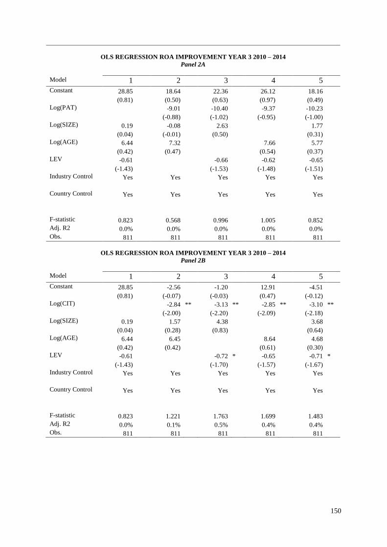
150

OLS REGRESSION ROA IMPROVEMENT YEAR 3 2010 – 2014

Panel 2A

Model 1 2 3 4 5

Constant 28.85 18.64 22.36 26.12 18.16

(0.81) (0.50) (0.63) (0.97) (0.49)

Log(PAT) -9.01 -10.40 -9.37 -10.23

(-0.88) (-1.02) (-0.95) (-1.00)

Log(SIZE) 0.19 -0.08 2.63 1.77

(0.04) (-0.01) (0.50) (0.31)

Log(AGE) 6.44 7.32 7.66 5.77

(0.42) (0.47) (0.54) (0.37)

LEV -0.61 -0.66 -0.62 -0.65

(-1.43) (-1.53) (-1.48) (-1.51)

Industry Control Yes Yes Yes Yes Yes

Country Control Yes Yes Yes Yes Yes

F-statistic 0.823 0.568 0.996 1.005 0.852

Adj. R2 0.0% 0.0% 0.0% 0.0% 0.0%

Obs. 811 811 811 811 811

OLS REGRESSION ROA IMPROVEMENT YEAR 3 2010 – 2014

Panel 2B

Model 1 2 3 4 5

Constant 28.85 -2.56 -1.20 12.91 -4.51

(0.81) (-0.07) (-0.03) (0.47) (-0.12)

Log(CIT) -2.84 ** -3.13 ** -2.85 ** -3.10 **

(-2.00) (-2.20) (-2.09) (-2.18)

Log(SIZE) 0.19 1.57 4.38 3.68

(0.04) (0.28) (0.83) (0.64)

Log(AGE) 6.44 6.45 8.64 4.68

(0.42) (0.42) (0.61) (0.30)

LEV -0.61 -0.72 * -0.65 -0.71 *

(-1.43) (-1.70) (-1.57) (-1.67)

Industry Control Yes Yes Yes Yes Yes

Country Control Yes Yes Yes Yes Yes

F-statistic 0.823 1.221 1.763 1.699 1.483

Adj. R2 0.0% 0.1% 0.5% 0.4% 0.4%

Obs. 811 811 811 811 811

151

OLS REGRESSION ROS IMPROVEMENT YEAR 2 2010 – 2014

Panel 1A

Model 1 2 3 4 5

Constant 9.19 1.53 13.89 -5.92 1.63

(0.25) (0.04) (0.37) (-0.22) (0.04)

Log(PAT) -7.31 -7.60 -7.83 -7.05

(-0.69) (-0.72) (-0.77) (-0.67)

Log(SIZE) -2.73 -0.97 1.16 -1.64

(-0.47) (-0.17) (0.21) (-0.27)

Log(AGE) 18.55 17.62 16.43 18.09

(1.21) (1.15) (1.16) (1.18)

LEV 0.26 0.21 0.22 0.24

(0.56) (0.47) (-1.26) (0.53)

Industry Control Yes Yes Yes Yes Yes

Country Control Yes Yes Yes Yes Yes

F-statistic 0.543 0.575 0.355 0.617 0.526

Adj. R2 0.0% 0.0% 0.0% 0.0% 0.0%

Obs. 811 811 811 811 811

OLS REGRESSION ROS IMPROVEMENT YEAR 2 2010 – 2014

Panel 1B

Model 1 2 3 4 5

Constant 9.19 -18.67 -6.91 -17.71 -18.21

(0.25) (-0.47) (-0.18) (-0.64) (-0.45)

Log(CIT) -2.58 * -2.61 * -2.52 * -2.53 *

(-1.77) (-1.78) (-1.79) (-1.72)

Log(SIZE) -2.73 0.64 2.77 0.10

(-0.47) (0.11) (0.50) (0.02

Log(AGE) 18.55 16.82 17.30 17.19

(1.21) (1.10) (1.23) (1.12)

LEV 0.26 0.15 0.19 0.18

(0.56) (0.34) (0.42) (0.41)

Industry Control Yes Yes Yes Yes Yes

Country Control Yes Yes Yes Yes Yes

F-statistic 0.543 1.105 0.886 1.138 0.947

Adj. R2 0.0% 0.1% 0.0% 0.1% 0.0%

Obs. 811 811 811 811 811

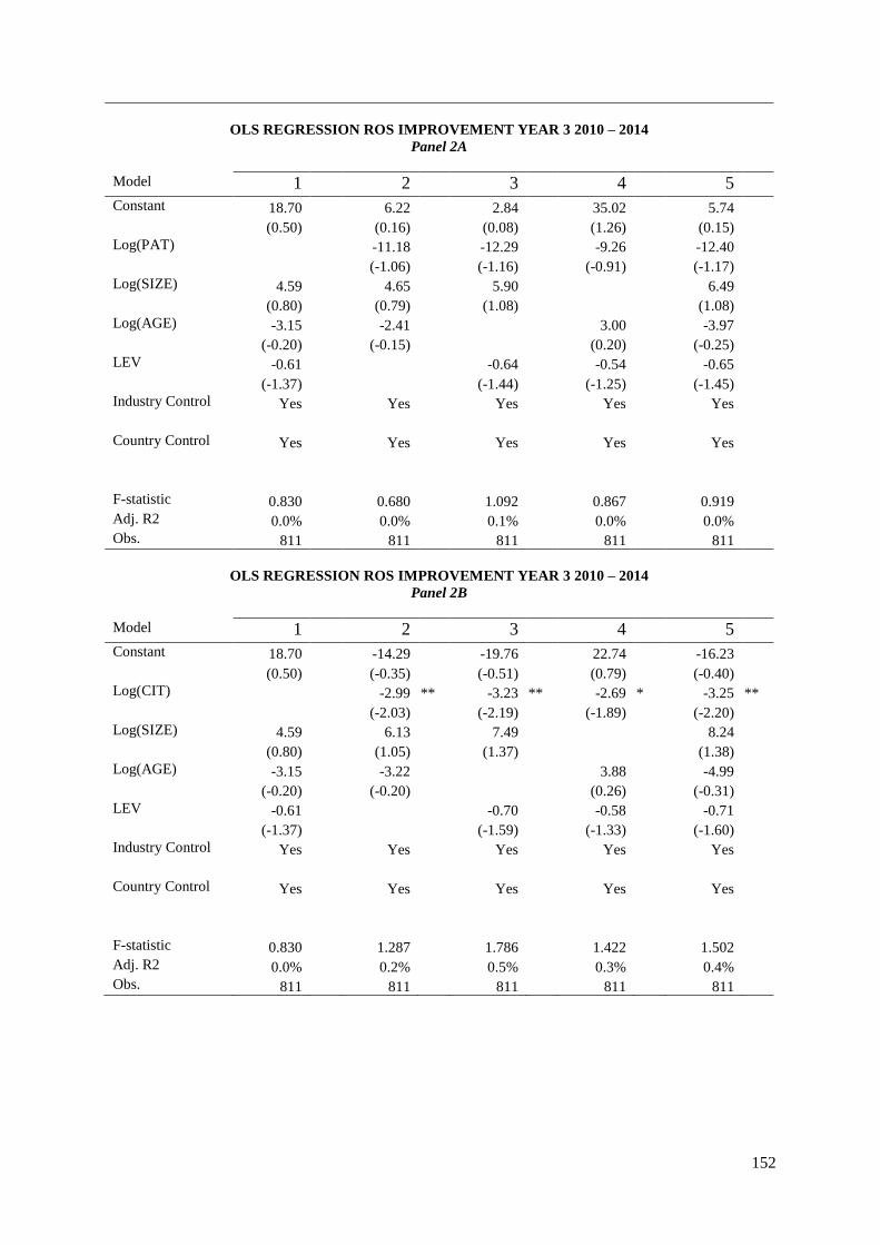
152

OLS REGRESSION ROS IMPROVEMENT YEAR 3 2010 – 2014

Panel 2A

Model 1 2 3 4 5

Constant 18.70 6.22 2.84 35.02 5.74

(0.50) (0.16) (0.08) (1.26) (0.15)

Log(PAT) -11.18 -12.29 -9.26 -12.40

(-1.06) (-1.16) (-0.91) (-1.17)

Log(SIZE) 4.59 4.65 5.90 6.49

(0.80) (0.79) (1.08) (1.08)

Log(AGE) -3.15 -2.41 3.00 -3.97

(-0.20) (-0.15) (0.20) (-0.25)

LEV -0.61 -0.64 -0.54 -0.65

(-1.37) (-1.44) (-1.25) (-1.45)

Industry Control Yes Yes Yes Yes Yes

Country Control Yes Yes Yes Yes Yes

F-statistic 0.830 0.680 1.092 0.867 0.919

Adj. R2 0.0% 0.0% 0.1% 0.0% 0.0%

Obs. 811 811 811 811 811

OLS REGRESSION ROS IMPROVEMENT YEAR 3 2010 – 2014

Panel 2B

Model 1 2 3 4 5

Constant 18.70 -14.29 -19.76 22.74 -16.23

(0.50) (-0.35) (-0.51) (0.79) (-0.40)

Log(CIT) -2.99 ** -3.23 ** -2.69 * -3.25 **

(-2.03) (-2.19) (-1.89) (-2.20)

Log(SIZE) 4.59 6.13 7.49 8.24

(0.80) (1.05) (1.37) (1.38)

Log(AGE) -3.15 -3.22 3.88 -4.99

(-0.20) (-0.20) (0.26) (-0.31)

LEV -0.61 -0.70 -0.58 -0.71

(-1.37) (-1.59) (-1.33) (-1.60)

Industry Control Yes Yes Yes Yes Yes

Country Control Yes Yes Yes Yes Yes

F-statistic 0.830 1.287 1.786 1.422 1.502

Adj. R2 0.0% 0.2% 0.5% 0.3% 0.4%

Obs. 811 811 811 811 811

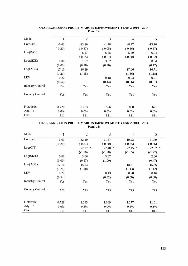
153

OLS REGRESSION PROFIT MARGIN IMPROVEMENT YEAR 2 2010 – 2014

Panel 1A

Model 1 2 3 4 5

Constant -6.63 -13.20 -1.78 -8.77 -13.10

(-0.20) (-0.37) (-0.05) (-0.36) (-0.37)

Log(PAT) -6.27 -6.55 -5.59 -6.04

(-0.65) (-0.67) (-0.60) (-0.62)

Log(SIZE) 0.00 1.52 3.52 0.94

(0.00) (0.28) (0.70) (0.17)

Log(AGE) 17.10 16.29 17.66 16.71

(1.21) (1.15) (1.36) (1.18)

LEV 0.22 0.18 0.23 0.21

(0.54) (0.44) (0.56) (0.51)

Industry Control Yes Yes Yes Yes Yes

Country Control Yes Yes Yes Yes Yes

F-statistic 0.728 0.753 0.526 0.800 0.671

Adj. R2 0.0% 0.0% 0.0% 0.0% 0.0%

Obs. 811 811 811 811 811

OLS REGRESSION PROFIT MARGIN IMPROVEMENT YEAR 2 2010 – 2014

Panel 1B

Model 1 2 3 4 5

Constant -6.63 -32.19 -21.37 -19.23 -31.79

(-0.20) (-0.87) (-0.60) (-0.75) (-0.86)

Log(CIT) -2.37 * -2.40 * -2.15 * -2.32 *

(-1.76) (-1.78) (-1.65) (-1.72)

Log(SIZE) 0.00 3.06 5.07 2.60

(0.00) (0.57) (1.00) (0.47)

Log(AGE) 17.10 15.53 18.51 15.86

(1.21) (1.10) (1.43) (1.12)

LEV 0.22 0.13 0.20 0.16

(0.54) (0.32) (0.50) (0.38)

Industry Control Yes Yes Yes Yes Yes

Country Control Yes Yes Yes Yes Yes

F-statistic 0.728 1.293 1.069 1.277 1.101

Adj. R2 0.0% 0.2% 0.0% 0.2% 0.1%

Obs. 811 811 811 811 811

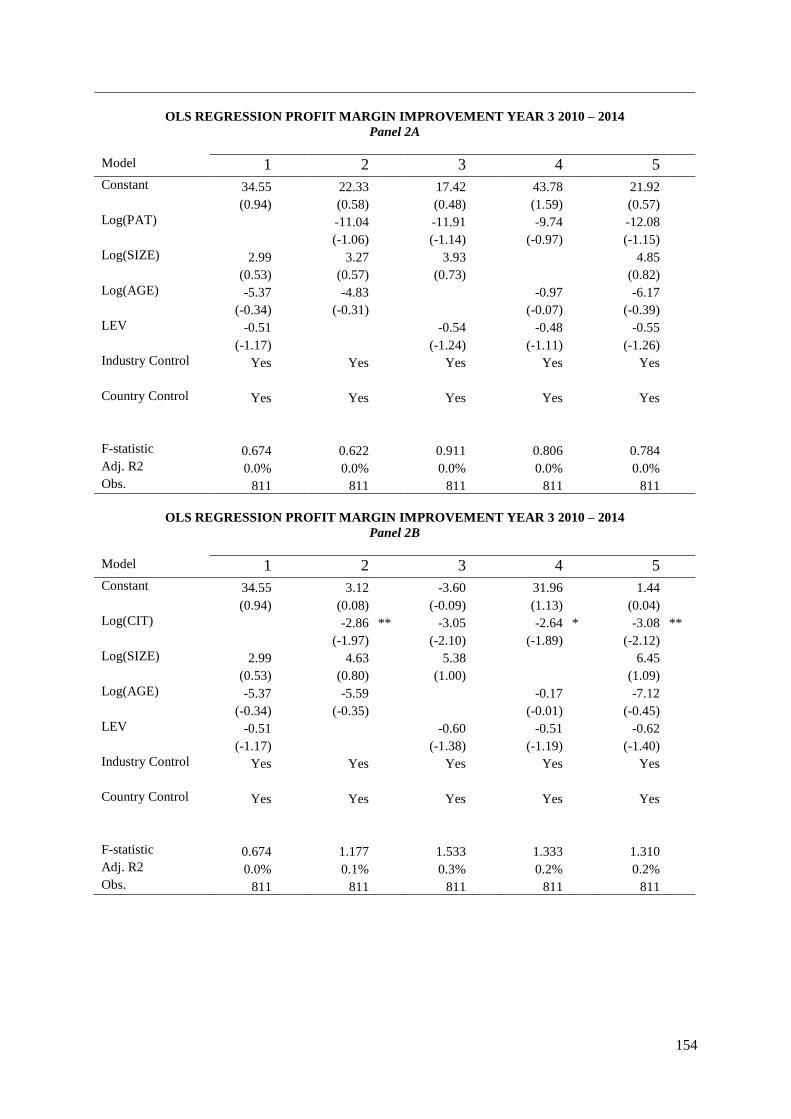
154

OLS REGRESSION PROFIT MARGIN IMPROVEMENT YEAR 3 2010 – 2014

Panel 2A

Model 1 2 3 4 5

Constant 34.55 22.33 17.42 43.78 21.92

(0.94) (0.58) (0.48) (1.59) (0.57)

Log(PAT) -11.04 -11.91 -9.74 -12.08

(-1.06) (-1.14) (-0.97) (-1.15)

Log(SIZE) 2.99 3.27 3.93 4.85

(0.53) (0.57) (0.73) (0.82)

Log(AGE) -5.37 -4.83 -0.97 -6.17

(-0.34) (-0.31) (-0.07) (-0.39)

LEV -0.51 -0.54 -0.48 -0.55

(-1.17) (-1.24) (-1.11) (-1.26)

Industry Control Yes Yes Yes Yes Yes

Country Control Yes Yes Yes Yes Yes

F-statistic 0.674 0.622 0.911 0.806 0.784

Adj. R2 0.0% 0.0% 0.0% 0.0% 0.0%

Obs. 811 811 811 811 811

OLS REGRESSION PROFIT MARGIN IMPROVEMENT YEAR 3 2010 – 2014

Panel 2B

Model 1 2 3 4 5

Constant 34.55 3.12 -3.60 31.96 1.44

(0.94) (0.08) (-0.09) (1.13) (0.04)

Log(CIT) -2.86 ** -3.05 -2.64 * -3.08 **

(-1.97) (-2.10) (-1.89) (-2.12)

Log(SIZE) 2.99 4.63 5.38 6.45

(0.53) (0.80) (1.00) (1.09)

Log(AGE) -5.37 -5.59 -0.17 -7.12

(-0.34) (-0.35) (-0.01) (-0.45)

LEV -0.51 -0.60 -0.51 -0.62

(-1.17) (-1.38) (-1.19) (-1.40)

Industry Control Yes Yes Yes Yes Yes

Country Control Yes Yes Yes Yes Yes

F-statistic 0.674 1.177 1.533 1.333 1.310

Adj. R2 0.0% 0.1% 0.3% 0.2% 0.2%

Obs. 811 811 811 811 811

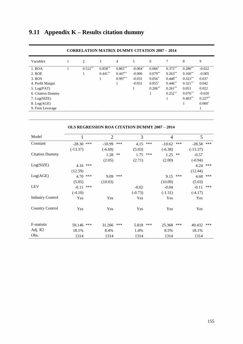
155

9.11 Appendix K – Results citation dummy

CORRELATION MATRIX DUMMY CITATION 2007 – 2014

Variables 1 2 3 4 5 6 7 8 9

1. ROA 1 0.512** 0.858** 0.865** -0.064* 0.066* 0.375** 0.280** -0.022

2. ROE 1 0.441** 0.447** -0.006 0.079** 0.263** 0.160** -0.005

3. ROS 1 0.997** -0.031 0.056* 0.448** 0.323** 0.037

4. Profit Margin 1 -0.031 0.055* 0.446** 0.321** 0.042

5. Log(PAT) 1 0.206** 0.261** 0.051 0.022

6. Citation Dummy 1 0.252** 0.076** -0.020

7. Log(SIZE) 1 0.403** 0.227**

8. Log(AGE) 1 0.060*

9. Firm Leverage 1

OLS REGRESSION ROA CITATION DUMMY 2007 – 2014

Model 1 2 3 4 5

Constant -28.30 *** -10.99 *** 4.15 *** -10.62 *** -28.58 ***

(-13.37) (-6.69) (5.03) (-6.38) (-13.37)

Citation Dummy 1.28 ** 1.75 *** 1.25 ** -0.57

(2.05) (2.71) (2.00) (-0.94)

Log(SIZE) 4.16 *** 4.24 ***

(12.59) (12.44)

Log(AGE) 4.70 *** 9.09 *** 9.15 *** 4.68 ***

(5.05) (10.03) (10.09) (5.03)

LEV -0.11 *** -0.02 -0.04 -0.11 ***

(-4.10) (-0.73) (-1.31) (-4.17)

Industry Control Yes Yes Yes Yes Yes

Country Control Yes Yes Yes Yes Yes

F-statistic 59.146 *** 31.266 *** 5.818 *** 25.368 *** 49.432 ***

Adj. R2 18.1% 8.4% 1.4% 8.5% 18.1%

Obs. 1314 1314 1314 1314 1314

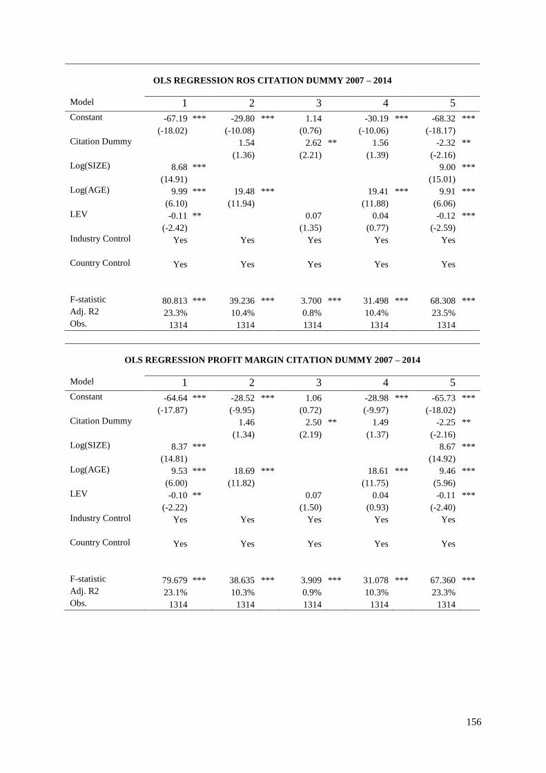
156

OLS REGRESSION ROS CITATION DUMMY 2007 – 2014

Model 1 2 3 4 5

Constant -67.19 *** -29.80 *** 1.14 -30.19 *** -68.32 ***

(-18.02) (-10.08) (0.76) (-10.06) (-18.17)

Citation Dummy 1.54 2.62 ** 1.56 -2.32 **

(1.36) (2.21) (1.39) (-2.16)

Log(SIZE) 8.68 *** 9.00 ***

(14.91) (15.01)

Log(AGE) 9.99 *** 19.48 *** 19.41 *** 9.91 ***

(6.10) (11.94) (11.88) (6.06)

LEV -0.11 ** 0.07 0.04 -0.12 ***

(-2.42) (1.35) (0.77) (-2.59)

Industry Control Yes Yes Yes Yes Yes

Country Control Yes Yes Yes Yes Yes

F-statistic 80.813 *** 39.236 *** 3.700 *** 31.498 *** 68.308 ***

Adj. R2 23.3% 10.4% 0.8% 10.4% 23.5%

Obs. 1314 1314 1314 1314 1314

OLS REGRESSION PROFIT MARGIN CITATION DUMMY 2007 – 2014

Model 1 2 3 4 5

Constant -64.64 *** -28.52 *** 1.06 -28.98 *** -65.73 ***

(-17.87) (-9.95) (0.72) (-9.97) (-18.02)

Citation Dummy 1.46 2.50 ** 1.49 -2.25 **

(1.34) (2.19) (1.37) (-2.16)

Log(SIZE) 8.37 *** 8.67 ***

(14.81) (14.92)

Log(AGE) 9.53 *** 18.69 *** 18.61 *** 9.46 ***

(6.00) (11.82) (11.75) (5.96)

LEV -0.10 ** 0.07 0.04 -0.11 ***

(-2.22) (1.50) (0.93) (-2.40)

Industry Control Yes Yes Yes Yes Yes

Country Control Yes Yes Yes Yes Yes

F-statistic 79.679 *** 38.635 *** 3.909 *** 31.078 *** 67.360 ***

Adj. R2 23.1% 10.3% 0.9% 10.3% 23.3%

Obs. 1314 1314 1314 1314 1314