the isotropy representations of the rosenfeld planes

THE ISOTROPY REPRESENTATIONS OF THEROSENFELD PLANES

Dissertation

zur Erlangung des akademischen Grades

Dr. rer. nat.

eingereicht an der

Mathematisch-Naturwissenschaftlich-Technischen Fakultat

der Universitat Augsburg

von

Erich Dorner

Augsburg, Februar 2018

1

2 THE ISOTROPY REPRESENTATIONS OF THE ROSENFELD PLANES

Erstgutachter: Prof. Dr. Jost-Hinrich EschenburgZweitgutachter: PD Dr. sc. math. Peter Quast

Tag der mundlichen Prufung: 20. 2. 2018

THE ISOTROPY REPRESENTATIONS OF THE ROSENFELD PLANES 3

Dedicated to Jost-Hinrich Eschenburg


Contents

Introduction 51. Division Algebras and Tensor Products 72. Representations for Clk+l−1 103. Representations for Spink+l 114. The Lie Algebras of the Spin Groups 125. The Rosenfeld Planes 146. The Classical Spaces 167. The Rosenfeld Lines 188. The Jacobi Identity 219. The Root Space Decomposition 2410. Conclusion 27Appendix 30References 31


Introduction

In addition to the infinite series of the classical symmetric spacesthere are twelve of exceptional type. Among these twelve are fourwith the dimensions 16, 32, 64 and 128 which are called Rosenfeldplanes after an idea from B. Rosenfeld (see [Fr2], [Be], [Ba]). Thespace with dimension 16 is the well known Cayley plane, a projectiveplane over the octonions. As a homogeneous symmetric space it isdefined as OP2 = F4/Spin9. The 52-dimensional exceptional Lie groupF4 = Aut(H3(O)) is the automorphism group of the Jordan algebraH3(O) (the hermitian 3× 3 matrices over the octonions together withthe Jordan product A ◦B = 1

2(AB+BA)). OP2 can also be defined as

the set {P ∈ H3(O) : P 2 = P, trace P = 1}. With this definition OP2

becomes an extrinsic symmetric space (or symmetric R-space) withequivariant isometric embedding in the 26-dimensional representationmodule H3(O) with fixed trace (H3(O) has dimension 27 = 3 · 8 + 3and can be reduced by one dimension since the trace is an invariant ofthe automorphism group F4, see [Fr1], [Es2]).

Rosenfeld’s idea was to construct the other three spaces as projectiveplanes over the algebras O⊗C, O⊗H (H denoting the quaternions) andO⊗O. But this does not work out properly. Still the idea seems to bepartially correct, in a vague sense. Motivated by it we use the followingnotations for these symmetric spaces with the dimensions 32, 64 and128: (O ⊗ C)P2 := E6/(Spin10 · U1), (O ⊗ H)P2 := E7/(Spin12 · Sp1),(O ⊗ O)P2 := E8/Spin16 with the exceptional Lie groups E6, E7, E8

(with dimensions 78, 133 and 248) and the unitary resp. symplecticgroups U1, Sp1.

If we would try to construct (O⊗C)P2 in a similar way as OP2 above(as a subset of H3(O ⊗ C)), then the following problem arises: Everyelement in O⊗C can be written uniquely as x+y⊗i with x, y ∈ O. Firstwe have to define a conjugation for O⊗C for which the only reasonablechoice is to claim the condition y ⊗ i = y ⊗ i. Then the space of self-conjugated elements x+ y ⊗ i = x + y ⊗ i = x − y ⊗ i = x + y ⊗ ihas dimension 8 (since x is real and y an imaginary octonion in thiscase) and then H3(O ⊗ C) has dimension 72 = 3 · 16 + 3 · 8. But itis known from representation theory that the fundamental irreduciblerepresentation modules for E6 have dimensions 27, 78, 351 and 2925(see [Ti]). Therefore there is no such embedding in the space of thehermitian matrices over O⊗C. For the remaining two Rosenfeld planeswe have the same difficulties. And in addition these two spaces are noteven symmetric R-spaces after the results from Ferus (cf. [Fe] or also[BCO]). Since (O ⊗ C)P2 is hermitian symmetric, it is an extrinsic


symmetric space and can be embedded in the Lie algebra e6 of its ownisometry group with the adjoint representation.

In the following approach an elementary construction of the Rosen-feld planes is given at the level of their Lie algebras. This constructionis based on simple properties of the four division algebras R,C,H andO. The starting point is the known representation for Spin9 operatingon O2 (cf. [Es2], [Ha]), derived from a representation for the Cliffordalgebra Cl8. Then generators for Spin10, Spin12 and Spin16 can befound acting on (O⊗ C)2, (O⊗H)2 and (O⊗O)2 in a natural exten-sion of Spin9. These special representation modules have exactly thesame dimensions as the Rosenfeld planes. Generally, all groups Spink+l

can be represented on (K⊗L)2 where k = dimK and l = dimL. In thespecial case K = O we get the isotropy groups of the Rosenfeld planesand for L = R the ones for the classical projective planes KP2 (to-gether with additional factors U1 or Sp1). Altogether we get ten spacesin this way which all can be viewed as generalized Rosenfeld planes(K ⊗ L)P2 in a certain sense. Furthermore each of these ten spaceshas a symmetric subspace with half the dimension and the same max-imal abelian subalgebra. This is the space with the Lie triple system(K⊗L)1 ⊂ (K⊗L)2 and called Rosenfeld line (K⊗L)P1 (as a general-ization of a projective line). Up to coverings, it is the real Grassmannmanifold Gl(Rk+l). However, only for the proper projective planes anytwo Rosenfeld lines intersect transversally. In the other cases (i.e. forK ⊗ L with both K,L 6= R) the Rosenfeld planes and lines share amaximal torus of rank > 1, and thus the intersection of two lines maycontain a (singular) subtorus (see also [N] - [NT-V]).

Next, we use the definitions given in [EH1] (which goes back to[Wi]) to construct the Lie algebras and Cartan decompositions. Inthe associative cases it can be seen that the given representations forthe spin groups are actually the isotropy representations of symmetricspaces. Since we can show the validity of the Jacobi identity, thisis also true in the exceptional cases. Using a maximal abelian Liesubalgebra, the root space decompositions can be determined and sothe root systems of the corresponding symmetric spaces can be seen.

In this context we should mention the calculations from J. F. Adamsand E. Witt. Adams ([Ad]) constructs the Lie algebra e8 in a similarway (as the Cartan decomposition), where the Jacobi identity is proveddirectly with methods from representation theory, but without usingconcrete representations for spin groups. Furthermore the Lie groupE8 is constructed as the automorphism group of its own Lie algebra:E8 = Aut(e8). Then the other exceptional Lie groups can be found assubgroups of E8.


Witt ([Wi]) uses a more direct and elementary approach. He definesthe Lie algebra (called Liescher Ring in his work) over orthogonal skewsymmetric matrices with the help of the properties of a Clifford algebra(called Cliffordsches Zahlsystem). The construction principle for thisLie algebra is essentially the same as that used in [Ad] and [EH1]. ThenWitt develops a simple formula (using the trace of the representationmatrices) which makes it possible to decide whether the constructedsystem satisfies the Jacobi identity or not.

But Adams and Witt are mainly interested in the exceptional Liegroups (resp. their Lie algebras). In contrast to them, the focus of thepresent work lies on the investigation of the Rosenfeld planes as sym-metric spaces with the explicit construction of their isotropy represen-tations. The key objects for all these calculations are tensor productsof the division algebras. With them we can avoid long and involvedcomputations (as used by Adams and Witt).

Here a short overview of the individual sections: Section 1 lists some el-ementary properties of the division algebras and their tensor products.In Sections 2 and 3 the representations for certain Clifford algebras(associated with the division algebras) and their corresponding spingroups are constructed. Section 4 determines the Lie Algebras of thesegroups. Section 5 introduces the Rosenfeld planes as symmetric spacesand their isotropy groups. Section 6 proves that in the classical casesthe representations derived from the spin groups actually coincide withthe correct isotropy representations of these spaces. Section 7 describesthe Rosenfeld lines together with their maximal abelian Lie subalgebrasand root space decompositions. Section 8 gives a construction of theLie algebras for the exceptional spaces and proves the Jacobi identitywith the help of the classical cases. In Section 9 the root space de-compositions for all Rosenfeld planes is computed, and (together withthe Appendix) the correspondence with the standard root systems isshown. Section 10 is a summary of the preceding sections.

Finally, at this point I would like to express many thanks to my su-pervisor Jost-Hinrich Eschenburg for his extensive support, discussionsand ideas over the whole time. Also I would like to thank Peter Quastfor his work as second advisor.

1. Division Algebras and Tensor Products

There are four normed division algebras K, which are the real num-bers R, the complex numbers C, the quaternions H, and the octonionsO. As (real) vector spaces they have dimensions dimR = 1, dimC =


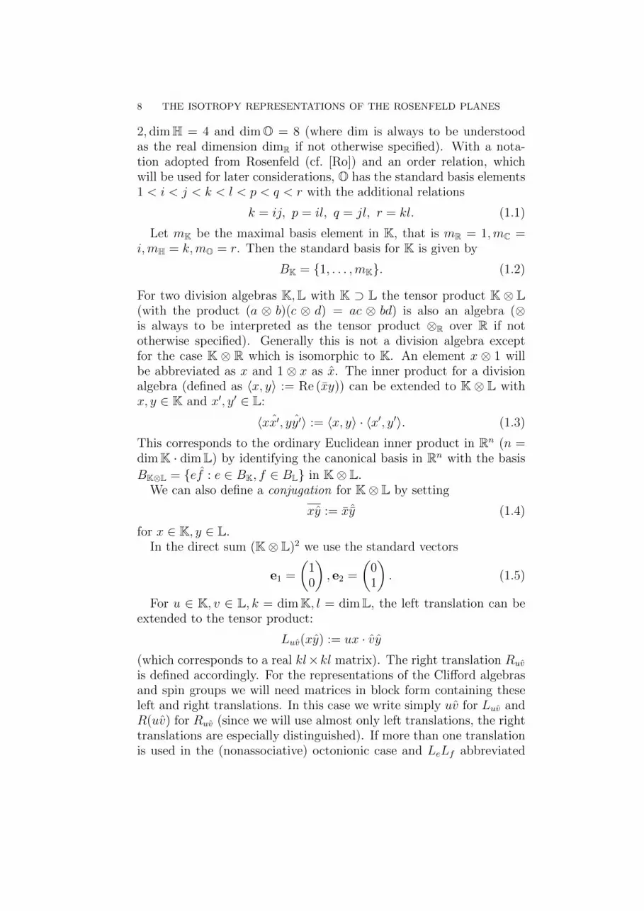
2, dimH = 4 and dimO = 8 (where dim is always to be understoodas the real dimension dimR if not otherwise specified). With a nota-tion adopted from Rosenfeld (cf. [Ro]) and an order relation, whichwill be used for later considerations, O has the standard basis elements1 < i < j < k < l < p < q < r with the additional relations

k = ij, p = il, q = jl, r = kl. (1.1)

Let mK be the maximal basis element in K, that is mR = 1,mC =i,mH = k,mO = r. Then the standard basis for K is given by

BK = {1, . . . ,mK}. (1.2)

For two division algebras K,L with K ⊃ L the tensor product K ⊗ L(with the product (a ⊗ b)(c ⊗ d) = ac ⊗ bd) is also an algebra (⊗is always to be interpreted as the tensor product ⊗R over R if nototherwise specified). Generally this is not a division algebra exceptfor the case K ⊗ R which is isomorphic to K. An element x ⊗ 1 willbe abbreviated as x and 1 ⊗ x as x. The inner product for a divisionalgebra (defined as 〈x, y〉 := Re (xy)) can be extended to K ⊗ L withx, y ∈ K and x′, y′ ∈ L:

〈xx′, yy′〉 := 〈x, y〉 · 〈x′, y′〉. (1.3)

This corresponds to the ordinary Euclidean inner product in Rn (n =dimK · dimL) by identifying the canonical basis in Rn with the basis

BK⊗L = {ef : e ∈ BK, f ∈ BL} in K⊗ L.We can also define a conjugation for K⊗ L by setting

xy := xˆy (1.4)

for x ∈ K, y ∈ L.In the direct sum (K⊗ L)2 we use the standard vectors

e1 =

(10

), e2 =

(01

). (1.5)

For u ∈ K, v ∈ L, k = dimK, l = dimL, the left translation can beextended to the tensor product:

Luv(xy) := ux · vy(which corresponds to a real kl×kl matrix). The right translation Ruv

is defined accordingly. For the representations of the Clifford algebrasand spin groups we will need matrices in block form containing theseleft and right translations. In this case we write simply uv for Luv andR(uv) for Ruv (since we will use almost only left translations, the righttranslations are especially distinguished). If more than one translationis used in the (nonassociative) octonionic case and LeLf abbreviated


as ef , one has to apply them in the appropriate order: Le(Lfx) =(LeLf )x as real matrices, but generally LeLf 6= Lef , e(fx) 6= (ef)x fore, f, x ∈ O.

We note a few known elementary properties for division algebras whichwill play a key role for all later considerations ([Es4], Section 10, p.

111). Set K′ := Im K := 1⊥ and let H ⊂ K be a quaternionic subalge-bra (i.e. a subalgebra isomorphic to the standard quaternions H).

a ∈ K′, |a| = 1, x ∈ K⇒ a(ax) = −x. (1.6)

b ∈ K′, x ∈ K⇒ b(bx) = −|b|2x, b2 = −|b|2. (1.7)

a, b ∈ K′, a ⊥ b⇒ ab ∈ K′, ab ⊥ a, b. (1.8)

a, b ∈ K′, a ⊥ b⇒ ab = −ba (anticommutativity). (1.9)

Two orthonormal a, b ∈ K′ generate H. (1.10)

c ⊥ H⇒ cH = Hc ⊥ H. (1.11)

a, b, c ∈ K′ orthogonal in pairs and c ⊥ ab⇒ (ab)c = −a(bc). (1.12)

This antiassociative triple (a, b, c) is also called a Cayley triple if inaddition a, b, c are unit vectors. Now let x, y, z ∈ BK and set

syx :=

{1 if x and y commute,

−1 else.(1.13)

Then

x(yz) = ±(xy)z with - if it is a Cayley triple and + if not. (1.14)

xy = syxyx. (1.15)

x(yz) = syxy(xz). (1.16)

(xy)z = szy(xz)y. (1.17)

LxxLyyzz = LyyLxxzz = Lxy·xyzz = Lyx·yxzz. (1.18)

RxxRyyzz = RyyRxxzz = Rxy·xyzz = Ryx·yxzz. (1.19)

Proof. (1.6): (1 + a)((1 − a)x) = (1 − a)x + a(x − ax) = x − a(ax)and |1 + a||1 − a||x| = 2|x|. Because of |a(ax)| = |x|, the equation|x − a(ax)| = 2|x| can only be valid if the vectors x and −a(ax) havethe same direction, that is a(ax) = −x.

(1.7): Apply (1.6) to a = b/|b| for b 6= 0.

(1.8): Assume |a| = 1. We have the implications b ⊥ a ⇒ ab ⊥ a2 =−1, b ⊥ 1⇒ ab ⊥ a and a ⊥ 1⇒ ab ⊥ b.

(1.9): Assume |a| = |b| = 1. Then (a + b)2 = a2 + b2 + ab + ba =−2 + (ab+ ba) and also (a+ b)2 = −|a+ b|2 = −2 from (1.7). It followsab+ ba = 0.


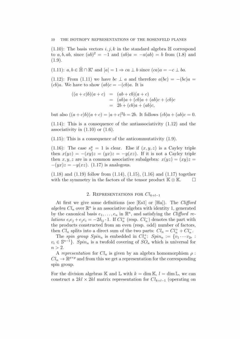
(1.10): The basis vectors i, j, k in the standard algebra H correspondto a, b, ab, since (ab)2 = −1 and (ab)a = −a(ab) = b from (1.8) and(1.9).

(1.11): a, b ∈ H ∩K′ and |a| = 1⇒ ca ⊥ b since (ca)a = −c ⊥ ba.

(1.12): From (1.11) we have bc ⊥ a and therefore a(bc) = −(bc)a =(cb)a. We have to show (ab)c = −(cb)a. It is

((a+ c)b)(a+ c) = (ab+ cb)(a+ c)= (ab)a+ (cb)a+ (ab)c+ (cb)c= 2b+ (cb)a+ (ab)c,

but also ((a+ c)b)(a+ c) = |a+ c|2b = 2b. It follows (cb)a+ (ab)c = 0.

(1.14): This is a consequence of the antiassociativity (1.12) and theassociativity in (1.10) or (1.6).

(1.15): This is a consequence of the anticommutativity (1.9).

(1.16): The case syx = 1 is clear. Else if (x, y, z) is a Cayley triplethen x(yz) = −(xy)z = (yx)z = −y(xz). If it is not a Cayley triplethen x, y, z are in a common associative subalgebra: x(yz) = (xy)z =−(yx)z = −y(xz). (1.17) is analogous.

(1.18) and (1.19) follow from (1.14), (1.15), (1.16) and (1.17) togetherwith the symmetry in the factors of the tensor product K⊗K. �

2. Representations for Clk+l−1

At first we give some definitions (see [Es1] or [Ha]). The Cliffordalgebra Cln over Rn is an associative algebra with identity 1, generatedby the canonical basis e1, . . . , en in Rn, and satisfying the Clifford re-lations eiej + ejei = −2δij · 1. If Cl+n (resp. Cl−n ) denotes the part withthe products constructed from an even (resp. odd) number of factors,then Cln splits into a direct sum of the two parts: Cln = Cl+n + Cl−n .

The spin group Spinn is embedded in Cl+n : Spinn := {v1 · · · v2r :vi ∈ Sn−1}. Spinn is a twofold covering of SOn which is universal forn > 2.

A representation for Cln is given by an algebra homomorphism ρ :Cln → Rp×p and from this we get a representation for the correspondingspin group.

For the division algebras K and L with k = dimK, l = dimL, we canconstruct a 2kl × 2kl matrix representation for Clk+l−1 (operating on


(K⊗ L)2) with the following basis elements:

Ee =

(−e

e

)(1 ≤ e ≤ mK), Ef =

(−f

f

)(1 < f ≤ mL). (2.1)

With the imaginary part Im L = 1⊥ we can write (where the subscriptat the right bracket denotes that the elements generate an algebra)

Clk+l−1 =

⟨(−w −uu w

): (u,w) ∈ K× Im L

⟩alg

. (2.2)

Here we use the same notation Cln for the image ρ(Cln) of the corre-sponding representation ρ.

The Clifford relations are valid since Ee and Ef anticommute. Therepresentations for Cl8+4−1 and Cl8+8−1 are not faithful, we have theadditional relations E1 · · ·Er·Ei · · ·Ek = I resp. E1 · · ·Er·Ei · · ·Er = Iin these cases.

Except for the cases (k, l) = (2, 2), (4, 2), (4, 4), the representationsin (2.2) correspond to the standard representations for the Cliffordalgebras.

The single basis element ( −11 ) in Cl1 is a complex structure (i.e.

J2 = −1) commuting with itself, and therefore the representation ofCl1 is complex linear. For Cl2+1−1 and Cl2+2−1 the elements in (2.1)commute with J = ( i i ) and K = ( κ

−κ ) (with the real 2 × 2 ma-trix κ = ( 1

−1 ) corresponding to the complex conjugation). J and Kform a quaternionic structure (two complex structures anticommutingwith each other), and therefore these representations are quaternioniclinear. Cl4+1−1, Cl4+2−1 and Cl4+4−1 have the quaternionic structure

J =(R(j)

R(j)

), K =

(R(k)

R(k)

). In this case it is essential to use

right translations which commute with the left translations. Cl8+2−1 is

complex linear with J =(ii

), and Cl8+4−1 is quaternionic linear with

J =(R(j)

R(j)

), K =

(R(k)

R(k)

).

3. Representations for Spink+l

The Clifford representations in Section 2 can now be used to con-struct representations for the spin groups. To reach this, one can pro-ceed similarly as in [Es2], Section 11. The generating element usedthere is vω (ω = e1 · · · en is the volume element and v ∈ Sn−1). Itcan be used only if n is odd. But with [Ha], p. 198, it is possible togenerate Spinn by ev in all cases (e, v ∈ Sn−1 and e fixed).


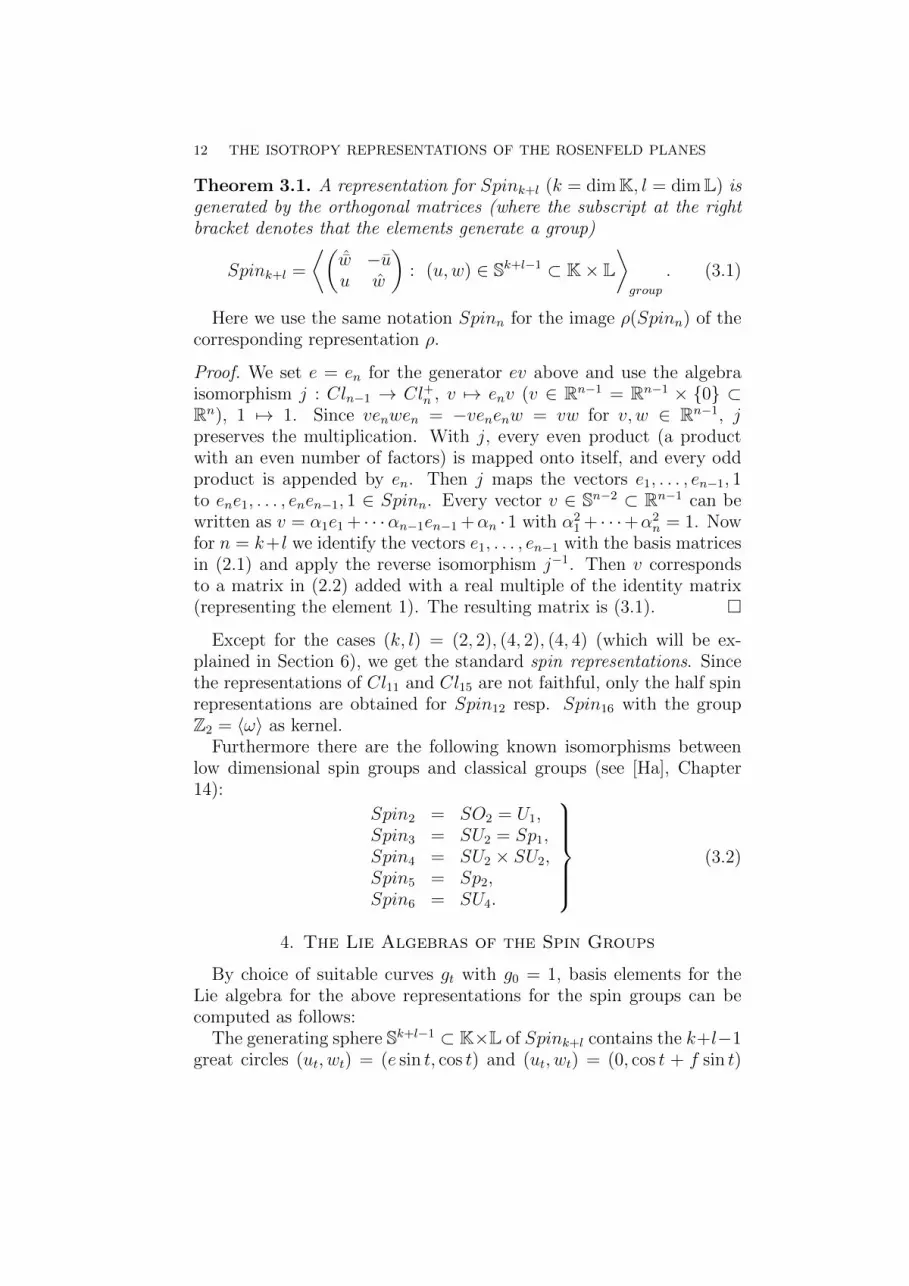
Theorem 3.1. A representation for Spink+l (k = dimK, l = dimL) isgenerated by the orthogonal matrices (where the subscript at the rightbracket denotes that the elements generate a group)

Spink+l =

⟨(ˆw −uu w

): (u,w) ∈ Sk+l−1 ⊂ K× L

⟩group

. (3.1)

Here we use the same notation Spinn for the image ρ(Spinn) of thecorresponding representation ρ.

Proof. We set e = en for the generator ev above and use the algebraisomorphism j : Cln−1 → Cl+n , v 7→ env (v ∈ Rn−1 = Rn−1 × {0} ⊂Rn), 1 7→ 1. Since venwen = −venenw = vw for v, w ∈ Rn−1, jpreserves the multiplication. With j, every even product (a productwith an even number of factors) is mapped onto itself, and every oddproduct is appended by en. Then j maps the vectors e1, . . . , en−1, 1to ene1, . . . , enen−1, 1 ∈ Spinn. Every vector v ∈ Sn−2 ⊂ Rn−1 can bewritten as v = α1e1 + · · ·αn−1en−1 +αn · 1 with α2

1 + · · ·+α2n = 1. Now

for n = k+ l we identify the vectors e1, . . . , en−1 with the basis matricesin (2.1) and apply the reverse isomorphism j−1. Then v correspondsto a matrix in (2.2) added with a real multiple of the identity matrix(representing the element 1). The resulting matrix is (3.1). �

Except for the cases (k, l) = (2, 2), (4, 2), (4, 4) (which will be ex-plained in Section 6), we get the standard spin representations. Sincethe representations of Cl11 and Cl15 are not faithful, only the half spinrepresentations are obtained for Spin12 resp. Spin16 with the groupZ2 = 〈ω〉 as kernel.

Furthermore there are the following known isomorphisms betweenlow dimensional spin groups and classical groups (see [Ha], Chapter14):

Spin2 = SO2 = U1,Spin3 = SU2 = Sp1,Spin4 = SU2 × SU2,Spin5 = Sp2,Spin6 = SU4.

(3.2)

4. The Lie Algebras of the Spin Groups

By choice of suitable curves gt with g0 = 1, basis elements for theLie algebra for the above representations for the spin groups can becomputed as follows:

The generating sphere Sk+l−1 ⊂ K×L of Spink+l contains the k+l−1great circles (ut, wt) = (e sin t, cos t) and (ut, wt) = (0, cos t + f sin t)


(with e ∈ BK, f ∈ Im BL) which intersect each other perpendicularlyat the point (0, 1) for t = 0. Inserting in (3.1) and differentiatingat t = 0 yields the following k + l − 1 elements of the Lie algebraspink+l = L(Spink+l): (

−ee

),

(−f

f

). (4.1)

These are exactly the generators of Clk+l−1 in (2.1).The matrices in (4.1) anticommute with each other according to the

anticommutativity of the left translations (LeLf + LfLe = 0 for e, f ∈Im BO and e < f). Applying the Lie brackets [A,B] = AB − BA =2AB to these matrices, the remaining

(k+l−1

2

)basis elements of spink+l

are obtained (with the factor 2 omitted):(ef−ef

)(1 ≤ e < f ≤ mK),(

ef

ef

)(1 ≤ e ≤ mK, 1 < f ≤ mL),(

ef

ef

)(1 < e < f ≤ mL).

(4.2)

If we change the sign of the matrix(−I

I

)in (4.1), we can combine

(4.1) and (4.2) and have only three classes of(k2

)+ kl +

(l2

)=(k+l

2

)basis matrices:

Aef =

(ef−ef

)(1 ≤ e < f ≤ mK),

Bef =

(ef

−e ˆf

)(1 ≤ e ≤ mK, 1 ≤ f ≤ mL),

Cef =

(−ˆef

ef

)(1 ≤ e < f ≤ mL).

(4.3)

Lemma 4.1. The matrices (4.3) form an orthogonal basis of spink+l

with respect to the trace metric 〈X, Y 〉 = trace X tY .

Proof. The trace metric can be computed as

trace X tY =∑〈X tY ( uv ) , ( uv )〉 (4.4)

where the sum runs over all basis vectors ( uv ) ∈ B(K⊗L)2 .Since spinn+1 = son+1 is a simple Lie algebra (except for n = 3),

there is only one Ad-invariant metric (up to a scaling factor). Nowson+1 = s + [s, s] with s = {V = ( −vt

v ) : v ∈ Rn}. The matrices


Ei and [Ei, Ej] for the standard basis ei in Rn are orthogonal. Thematrices in (4.1) correspond to the Ei and are also orthogonal withrespect to the metric (4.4) and the assertion follows.

�

5. The Rosenfeld Planes

As we will see, the groups Spink+l are essentially (up to a factorwhich will be explained presently) the isotropy groups K of the sym-metric spaces G/K with rank l and Cartan decomposition g = k + Vwhere g, k are the Lie algebras g = L(G), k = L(K) and the representa-tion module V = (K⊗ L)2 for K. These spaces will be defined as the(generalized) Rosenfeld planes (K⊗L)P2. The precise isotropy groupsare K = Spink+l · Sk+l (the dot denoting the usual matrix product)where the Sk+l are defined as

Sk+l := {Ruv : |u| = |v| = 1, u ∈ K, v ∈ L} (5.1)

but with u = 1 if k = 1 or k = 8, and v = 1 if l = 1 or l = 8.Depending on k and l, Sk+l is a representation of a product of one or

two groups of type U1 or Sp1, and it commutes with Spink+l (which canbe achieved by using right instead of left multiplication). As matrixgroups they have a finite intersection. That means, the (surjective)homomorphism Spink+l × Sk+l → Spink+l · Sk+l has a finite kernel(and therefore their Lie algebras are isomorphic).

Lemma 5.1. Spink+l · Sk+l is contained in Spin16.

Proof. The inclusion Spink+l ⊂ Spin16 is clear. It suffices to showSp1 ⊂ Spin16 ( ˆSp1 ⊂ Spin16 follows similarly). We show that an ele-ment from Sp1 can be represented by a combination of two generatorsfrom Spin9:(

R(h)R(h)

)(xy

)=

(−l

−l

)(hl

lh

)(xy

),

where l is the standard basis element from BO and x, y, h ∈ H with|h| = 1. This means xh = −l((lh)x) (resp. the equivalent equationyh = −l((hl)y) since lh = hl). By linearity it is sufficient to prove thisfor x, h ∈ BH: The cases x = 1 or h = 1 are clear. For h = x 6= 1 wehave −l((lh)x) = −l(l(hx)) = −1 = xh. Else (l, h, x) is a Cayley tripleand −l((lh)x) = l(l(hx)) = −hx = xh. �

Basis elements for the Lie algebras u1, u1 are(ii

),

(i

i

)(5.2)


and for sp1, sp1

(R(e)

R(e)

),

(R(e)

R(e)

)(e = i, j, k). (5.3)

Lemma 5.2. The matrices (4.3) with (5.2) or respectively (5.3) forman orthogonal basis of the direct sum spink+l + sk+l with respect to thetrace metric 〈X, Y 〉 = trace X tY . The square of the norm is 〈X,X〉 =2kl.

Proof. We have to look at the possibilities in (5.1). Clearly the matricesin (5.3) are orthogonal to each other and the same holds for matricesfrom a Lie algebra with and without “hat”. Further, ( i i ) ∈ u1 isorthogonal to A1i = ( i −i ) because of the negative sign. The sameis true for u1 and C1i. It remains to show the orthogonality of sp1

and Aef for 1 ≤ e < f ≤ k (the case sp1 and Cef is analogous). Aefconsists of the matrices ( e e ) and ( e −e ) for e = i, j, k. It suffices to seethat a right and a left translation Re and Le are orthogonal. We haveLeReu = −1 for u = 1, e and LeReu = 1 for u 6= 1, e and the tracevanishes.

Since X t = −X and X2 = −I (I the identity matrix) for all matrices(5.2), (5.3) and (4.3), the expression 〈X,X〉 = 2kl follows from (4.4).

�

The definitions in (5.1) can be summarized in the following way: Inthe tensor product K ⊗ L, a quaternionic factor K = H correspondsto a factor Sp1, a factor L = H to ˆSp1, a complex factor K = Cto U1, and L = C to U1. The list (5.4) shows which spaces can beconstructed in this way (with the corresponding root system given aftereach space, see Appendix). If K,L ∈ {R,C,H} we get certain classicalspaces which will be explained in Section 6. For L = R we have thefour classical projective planes KP2 with rank one. The cases K = Orepresent the four Rosenfeld planes with the exceptional Lie groupsG = F4, E6, E7, E8 and Lie algebras f4, e6, e7, e8 (where the Cayley planeOP2 coincides with the first Rosenfeld plane). The construction of theseexceptional spaces (resp. their Cartan decompositions) will be seen inSection 8 together with the root space decomposition in Section 9.


(R⊗ R)P2 = SO3/O2 (b1),(C⊗ R)P2 = SU3/S(U2 × U1) (bc1),(H⊗ R)P2 = Sp3/Sp2 × Sp1 (bc1),(O⊗ R)P2 = F4/Spin9 (bc1),

(C⊗ C)P2 = CP2 × CP2 (bc1 × bc1),(H⊗ C)P2 = SU6/S(U4 × U2) (bc2),

(O⊗ C)P2 = E6/Spin10 · U1 (bc2),

(H⊗H)P2 = SO12/SO8 × SO4 (b4),

(O⊗H)P2 = E7/Spin12 · ˆSp1 (f4),

(O⊗O)P2 = E8/Spin16 (e8).

(5.4)

6. The Classical Spaces

In this Section we will see that in the cases K,L ∈ {R,C,H} therepresentations (3.1), (5.1) for Spink+l ·Sk+l are the isotropy represen-tations (see [EH2]) for the classical spaces in (5.4).

The next Lemma shows the reducibility for the representations (3.1)if l > 1.

Lemma 6.1. If K,L ∈ {R,C,H}, the representation module (K ⊗L)2 for Spink+l in (3.1) has an orthogonal decomposition with the linvariant subspaces of the form

V = K2 · v, v :=m∑g=1

sggg, m := mL, sg = ±1

with the setting s1 = +1 and an even number of negative signs sg inthe case l = 4 (so that we have l different vectors v for a fixed K).

Proof. First we observe the following relation for a basis element e ∈BL: eev = sev. If l = 4 this multiplication with ee corresponds to aproduct of two disjoint transpositions applied to the summands sggg ofv (possibilities for the signs in v are: ++++,++−−,+−+−,+−−+).We get the equivalent condition ev = seev, and therefore for a givenelement w ∈ L there is a w′ ∈ L with wv = w′v. The invariance of Vfollows with a generating matrix from (3.1):(

ˆw −uu w

)(xvyv

)=

(x ˆwv − uyvuxv + ywv

)=

(xw′v − uyvuxv + yw′v

)∈ V.


For the orthogonality of two different spaces U = K2·u and V = K2·vwe have to show for x, y, x′, y′ ∈ K:⟨(

xuyu

),

(x′vy′v

)⟩= (〈x, x′〉+ 〈y, y′〉)

m∑g=1

sgs′g = 0

where the sg are the signs for u and the s′g the signs for v. The sumwith the products of the signs vanishes since one half of the summandsis +1 and the other is −1. �

Theorem 6.1. If K,L ∈ {R,C,H}, the representation for Spink+l ·Sk+l is equivalent to the isotropy representation of the correspondingclassical space in (5.4).

Proof. With v1 :=∑m

g=1 gg and m := mL, we have v1ff = v1 for

f ∈ BL which is equivalent to v1f = v1ˆf . By linearity we get v1q = v1 ˆq

for any q ∈ L. Set V := K2v1 (which is one of the invariant spaces inLemma 6.1).

First the case K = L = H: Define the (real) vector space isomor-phism F : V ⊗ H → (H ⊗ H)2 by v ⊗ q 7→ vq = v ˆq (with kernel zeroand equal dimension of both spaces). Spin8 operates only on the left

factor V of V ⊗ H after Lemma 6.1. The operation of S = Sp1 · ˆSp1

on (H ⊗ H)2 is defined as a.vq := vqa resp. b.vq := vqˆb = vˆbq = vbqfor a, b ∈ S3 ⊂ H. Then S operates (after applying F ) only on theright factor H of V ⊗ H as left resp. right multiplication Lb, Ra, thatis as SO4. It follows the equivariance of F and the equivalence of theisotropy representation SO8⊗SO4 with the representation for Spin8 ·S.

Second the case K = H,L = C: Define the map F : V ⊗C H →(H ⊗ C)2 by v ⊗C q 7→ vq. V and H are complex vector spaces withthe complex structure Ri on V and −Li on H. Note that Ri = −Ri

on V . Therefore V ⊗C H is a complex vector space with both com-plex structures. (H ⊗ C)2 is a complex vector space with the com-plex structure Ri. The map F is a complex vector space isomorphismresp. both structures on V ⊗C H and the structure on (H⊗ C)2 sinceF (−Ri(vq)) = RiF (vq) and F (−Li(vq)) = RiF (vq).

Since Spin6 operates only on the left factor V of V ⊗C H and com-mutes with Ri, it is complex linear on V and belongs to the uni-tary group U4 of V , that is Spin6 = SU4. Define the operation of

S = Sp1 · U1 on (H ⊗ C)2 as (a, b).vq := vqaˆb = vbqa (since vˆb = vb)for a ∈ S3 ⊂ H, b ∈ S1 ⊂ C. Then S operates only on the right factorH = C2 of V ⊗C H as U2 since the operation (a, b; q) 7→ bqa commuteswith the complex structure −Li on H. It follows the equivariance of F


and the equivalence of the isotropy representation SU4 ⊗ U2 with therepresentation for Spin6 · S.

Third the case K = L = C: Here we have V +W = (C⊗C)2 whereV and W are the orthogonal vector spaces from Lemma 6.1 (the mapF in the above cases is simply the identity). Spin4 operates on both

spaces V and W as SU2 = Spin3. Together with U1 and U1 we get theisotropy representation U2 × U2 corresponding to the symmetric spaceCP2 × CP2.

The cases L = R correspond to the classical projective planes KP2.The isotropy representations are the standard ones. �

Remark 6.1. The following observation will be important in Section 8:The generators of spin8 = so8 corresponding to the matrices in (4.3)have squared trace norm 8 on R8 and hence 32 = 8 · 4 on R8 ⊗ R4.Likewise, the generators of so4 corresponding to R(e) and R(e) havesquared norm 4 on R4 and 32 = 4 · 8 on R4 ⊗ R8. Thus both sortsof generators have the same length in the isotropy representation ofG4(R12) and as a Lie subalgebra of spin16, see Lemma 5.1 and 5.2.Thus the two metrics on k are proportional.

7. The Rosenfeld Lines

The upper left block of the diagonal matrices Aef in (4.3) spansthe Lie subalgebra spink with one exception: If K = H we have onlythree linearly independent matrices Aef because of the associativity ofH (that means LeLf = Lef in this case). To get the full Lie algebraspin4 we need the three additional basis matrices from sp1 in (5.3).Therefore Spink (together with Sp1 if k = 4) acts on the subspace(K⊗1)e1 ⊂ (K⊗L)2 as SOk (SO4 is generated by Lp and Rq with unitquaternions p, q, and SO8 is generated by LuLv with unit octonionsu, v). Equivalently, the matrices Cef in (4.3), together with sp1 in thecase l = 4, span spinl and Spinl acts on (1⊗ L)e1 as SOl.

We get the isotropy representation SOk ⊗ SOl of the Grassmannmanifold Gl(Rk+l) (see [EH2]). As a generalization of a projective linewe define the Rosenfeld line (K⊗L)P1 as the totally geodesic subspaceof (K⊗L)P2 with the tangent space V = (K⊗L)e1, which is Gl(Rk+l)up to coverings. This tangent space V is a Lie triple system, that is[V, [V, V ]] ⊂ V (this can be seen with the definitions of the Lie brackets(8.1) and (8.2) in Section 8).

Now we compute the Lie triple used for the root space decomposition.Essentially this is only a translation from the standard representationfor Gl(Rk+l) into the division algebra context. The standard Cartan


decomposition of the Lie algebra is g = k+ p with g = ok+l, k = ok + oland the tangent space p consisting of matrices

(−Xt

X

)with the real

l × k matrices X. Let Xab be the basis matrix with 1 at row a andcolumn b and 0 else. By identifying Xab with a basis element c · ab ∈K⊗L, p can be identified with K⊗L. Here we are free in the choice ofthe constant factor c. For c := 2 the Lie triples in Lemmas 7.1 and 8.2will be compatible with each other. This will become clear in Section8.

Lemma 7.1. Let a ∈ BK, g, h, b ∈ BL. Then

[gg, [hh, ab]] =

4ba if (g, h) ∈ {(a, b), (b, a)}, a 6= b,

−4ab if (g, h) ∈ {(a, a), (b, b)}, a 6= b,

0 else.

(7.1)

Proof. With the notations above we have[(−X t

hh

Xhh

),

(−X t

ab

Xab

)]=

[(At − A

Bt −B

)]where A = X t

hhXab is a k × k matrix. We get A = Xhb for h = a andA = 0 for h 6= a. Similarly, B = XhhX

tab is a l× l matrix with B = Xha

for h = b and B = 0 for h 6= b. Abbreviating(

−Xtab

Xab

)simply with

ab, we get for the Lie triple

[gg, [hh, ab]] =

(−Ct

C

)with C = Xgg(A

t − A) − (Bt − B)Xgg. Computing C we get (7.1) by

the above identification of Xab with 2ab. �

Theorem 7.1. The elements 1, ii, . . . ,mLmL span a maximal abelianLie subalgebra Σ in p = K⊗L, which is a commutative and associativesubalgebra in K⊗ L (viewed as a tensor product algebra).

Proof. The first statement follows immediately from the known factthat the maximal abelian Lie subalgebra consists of all l×k matrices X(as introduced above) with diagonal entries. The commutativity andassociativity follows from the symmetry in the factors of the tensorproduct algebra and (1.15), (1.14). �

The common (i.e simultaneous) eigenspace decomposition for the en-domorphisms ad(x) (see [Es3], p. 21) for a (compact) symmetric spaceG/K with the Cartan decomposition g = k + V (with the Lie algebrasg = L(G), k = L(K) and the tangent space V ) can be determined as


follows. That is to solve

ad(x)xα = [x, xα] = α(x)yα, ad(x)yα = [x, yα] = −α(x)xα (7.2)

with x ∈ Σ ⊂ V (a maximal abelian Lie subalgebra), xα ∈ V, yα ∈ kand the real roots α(x) (with the minus sign for the compact type inthe second equation). By combining the two equations we have

ad(x)2xα = [x, [x, xα]] = −α(x)2xα. (7.3)

Applying this for Gl(Rk+l) we get the root space decomposition forV = K⊗ L:

Theorem 7.2. Let x =∑m

g=1 αggg (αg ∈ R,m := mL) be a general el-ement in the maximal abelian subalgebra Σ. Then we have the followingroots and common eigenspaces:

1) The abelian Lie subalgebra Σ for α(x) = 0,

2)(l2

)one-dimensional spaces ab+ ba, a < b ∈ BL, α(x) = 2(αa−αb),

3)(l2

)one-dimensional spaces ab− ba, a < b ∈ BL, α(x) = 2(αa +αb),

4) l spaces with dimension k − l spanned by ab with all a ∈ BK BLand fixed b ∈ BL for each space, and for α(x) = 2αb.

Proof. The case 1) is clear since [gg, hh] = 0 for g, h ∈ BL. Now leta, b ∈ BL. Applying (7.1) yields

ad(x)2ab =∑

1≤µ,ν≤m

αµαν ad(µµ) ad(νν)ab

= αaαb ad(aa) ad(bb)ab+ αaαb ad(bb) ad(aa)ab

+ α2a ad(aa) ad(aa)ab+ α2

b ad(bb) ad(bb)ab

= 8αaαbba− 4(α2a + α2

b)ab.

By interchanging a and b in this equation and then adding or subtract-ing these two, we get 2) and 3):

ad(x)2(ab± ba) = −4(αa ∓ αb)2(ab± ba).

If a ∈ BK − BL and b ∈ BL, the above sum ad(x)2ab has only onesummand (with (g, h) = (b, b) in (7.1)) and 4) follows:

ad(x)2ab = −4α2bab.

�

The root systems obtained in Theorem 7.2 are isomorphic to thestandard root systems bl for k 6= l and dl for k = l (see Appendix).The difference lies in the factor 2 according to the same constant factorintroduced before Lemma 7.1.


8. The Jacobi Identity

For the Lie algebra k of K = Spink+l · Sk+l we define an extensionfor the Lie bracket on the vector space g := k + V with V = (K⊗ L)2

in the following way for A ∈ k and v, w ∈ V , where the [v, w] ∈ k isdetermined by inserting all A ∈ k in (8.2):

[A, v] := Av = −[v, A], (8.1)

〈A, [v, w]〉k := 〈Av,w〉, (8.2)

where 〈 , 〉k must be an invariant inner product on k under the adjointaction of K and such that at the end it is the restriction of an Ad(G)-invariant inner product on g (e.g, it can be the trace metric for therepresentation of K on g).

If we have an orthogonal basis for k with respect to the metric 〈 , 〉k,the bracket in (8.2) can be explicitly computed as

[v, w] =∑X

αXX, αX =〈Xv,w〉〈X,X〉k

, (8.3)

where the sum runs over all the basis elements X ∈ k.This bracket (for which we have to show that is actually a Lie bracket

on g) is invariant under K:

Lemma 8.1.

[gv, gw] = g[v, w]g−1 for v, w ∈ V, g ∈ K. (8.4)

Proof. The scalar product 〈 , 〉 is invariant under g ∈ K and 〈 , 〉k isinvariant under AdgX = gXg−1, X ∈ k. Then we get

〈A, [gv, gw]〉k = 〈Agv, gw〉 = 〈g−1Agv, w〉 = 〈g−1Ag, [v, w]〉k= 〈A, g[v, w]g−1〉k.

�

It follows the equivariance

g[u, [v, w]] = [gu, [gv, gw]] for u, v, w ∈ V, g ∈ K. (8.5)

The construction with the brackets defined above works for everyrepresentation. But the essential point is to show the Jacobi identity:

J(x, y, z) = [x, [y, z]] + [y, [z, x]] + [z, [x, y]] = 0, x, y, z ∈ V. (8.6)

The exceptional cases will follow easily from subrepresentations of theclassical cases. These are already known to be s-representations fromSection 6 (see also Lemma 4.1 in [EH1]). From Remark 6.1 we makethe following observation: Since spin16 is a simple Lie algebra, there isonly one Ad-invariant metric on it (up to a scaling factor), the bracket


(8.2) on V = (O⊗O)2 depends only on the representation of K and theinvariant metric on k, it is a true Lie triple system for G4(R12) whenrestricted to V ′ = (H⊗H)2.

Theorem 8.1. J = 0 for all x, y, z ∈ V = (O⊗O)2.

Proof. It is sufficient to prove the Jacobi identity only for basis elementsin V . Then x, y, z are of the form abe1 or abe2 with a, b ∈ BO. Wemake use of the equivariance (8.5): With three or two generators ofthe form (3.1) we can transform x into ( 1

0 ) if we set u = a and w = b:Choose g =

(u ˆw

uw

)= ( −1

1 ) ( u−u )

(ˆww

)resp. g =

(u ˆw

−uw)

=

( u−u )

(w

ˆw

). Applying such an element g to y and z, they remain

basis elements (up to a sign). We assume y = abe1 (or abe2) and

z = cde1 (or cde2). But the two elements a, c lie in a quaternionicsubalgebra of O and also b, d (independently of each other) and we arein the classical case H⊗H. Therefore the Jacobi identity must be truealso in the octonionic case. �

Remark 1 In the proof of Theorem 8.1 we may use the group K =Spin16 to carry the elements y and z into the standard subspace (H⊗H)2 (in fact we use G2 × G2 ⊂ Spin7 × Spin7 ⊂ Spin16 where G2 =Aut(O)). According to (3.1), the group K contains the matrix

(N−N)

where N = LuLvLvu for any two distinct orthonormal u, v ∈ Im O.These span a quaternionic subalgebra H1, and N is the involution onO with eigenvalues 1 on H1 and −1 on H⊥1 since H⊥1 = LwH1 for somew ∈ O such that Lw anticommutes with Lu, Lv, Lvu.

Remark 2 Given two quaternionic subalgebras H2 and H spanned byelements of BO, we can use such N to map H2 on H as follows. The twosubalgebras correspond to two lines in the projective plane over the fieldF2 = {0, 1} (Fano plane), whose “points” are the seven basis elementsof Im O, thus H and H2 have precisely one basis element in common,say i. Then H = span {1, i, j, ij} and H2 = span {1, i, p, ip} for somep ∈ BO∩Im O. We claim that i, j+p, ij+ip span another quaternionicsubalgebra H1. In fact, (j+ p)(ij+ ip) = jij+ p(ij) + j(ip) + pip = 2i,note that (p, i, j) is a Cayley triple and hence p(ij) = −(pi)j = j(pi) =−j(ip). Using the map N for this quaternionic subalgebra H1 we obtainN(j+p) = j+p while N(j−p) = −(j−p) since j−p ⊥ H1. Subtractingthe two equations we see N(p) = j, and similarly we obtain N(ip) = ij.Moreover, N fixes i ∈ H1. Thus N(H2) = H.


Remark 3 Another proof for the Jacobi identity would be using Witt’sequation (Theorem 17 in [Wi]):

trace∑i,j

(DiDj)2 =

1

2f 2r. (8.7)

Here we have to sum over all pairs of the(k+l

2

)basis matricesDi in (4.3),

f denotes the dimension of the corresponding representation module,and r the dimension (called rank by Witt) of the Lie algebra. ThenWitt’s Theorem says that the Jacobi identity is valid for a given repre-sentation if and only if the above equation is valid. For the matrices in(4.3) we have the relations DiDj = ±DjDi, D

2i = −I and trace I = f

(with the identity matrix I). To verify the formula, we have to countthe number of matrices with which a given matrix Di commutes oranticommutes. It can be shown that Di commutes with 1 +

(k+l−2

2

)and anticommutes with the remaining

(k+l

2

)−1−

(k+l−2

2

)= 2(k+ l)−4

matrices. Then with f = 2kl and r =(k+l

2

)equation (8.7) can be

reduced to

k2 + l2 − 9(k + l) + 16 = 0. (8.8)

The formula does not work with additional factors Sk+l, only for purespin groups (presumably it can be adapted to this case). Inserting(k, l) = (8, 1) for Spin9 or (k, l) = (8, 8) for Spin16 we see that (8.8) isvalid in these cases.

The next lemma determines the Lie triple where the first two elementsare in (K⊗L)e1 and the third in (K⊗L)e2. Together with Lemma 7.1this will be used for the root space decomposition in Section 9. As inLemma 7.1 we are also free in choosing a constant factor (which mustnot be the same for all spaces, but only fixed within a given space).Here we simply omit the denominator 〈X,X〉k in (8.3).

Lemma 8.2. Let u, v, w, z ∈ BK⊗L and Ru the right translation. Then

[ue1, [ve1, we2]] = −RuRvwe2. (8.9)

Proof. We apply (8.3), where we have to consider only the antidiagonalmatrices of type X = Bz = ( z

−z ) in (4.3) with the inner product

〈X · ve1, we2〉 = −〈zv, w〉.

Since there is only one such X where this inner product does not vanish,namely for z = ±wv, we get (by choosing the inner product such thatthe denominator 〈X,X〉k is 1 in (8.3))

[ve1, we2] = −〈zv, w〉X (8.10)


and

[ue1, [ve1, we2]] = 〈zv, w〉X · ue1 = −〈zv, w〉zue2 = −RuRvwe2.

�

For x ∈ Σ, w ∈ BK⊗L (with the algebra Σ from Theorem 7.1) we get

Corollary 8.1.

ad(xe1)2we2 = −(R(x)2w)e2. (8.11)

Now we can explain the factor 4 connecting the Lie triple in Lemma7.1 with that in 8.2, resulting from the special choice of the constantfactors in the Lie triples.

First we compute [e1, e2] from (8.2) and (8.3). We have to look for allbasis matrices A ∈ spin16 from (4.3) where 〈A, [e1, e2]〉 = 〈Ae1, e2〉 6= 0.There is only one such matrix, namely A = B11 = ( 1

−1 ) and we get[e1, e2] = −B11 and therefore [e1, [e1, e2]] = −e2.

Next we compute [e1, ie1]. In (4.3) there are the four matrices A =A1i, Ajk, Alp, Aqr ∈ spin16 where 〈Ae1, ie1〉 6= 0, and [e1, ie1] is thesum of these matrices (with certain signs ±1). In this case we get[e1, [e1, ie1]] = −4ie1.

Thus the operator − ad(e1)2 has eigenvalues 1 and 4 which are theextreme values of the curvature in CP2.

In the next theorem we see that the Rosenfeld plane (K⊗L)P2 and theRosenfeld line (K⊗ L)P1 have the same maximal abelian subalgebra.

Theorem 8.2. The vectors e1, . . . ,mme1 with m := mL span a maxi-mal abelian Lie subalgebra Σ ⊂ V = (K⊗ L)2.

Proof. That these vectors span an abelian Lie subalgebra in V followsalready from Theorem 7.1. For the same reason this algebra can notbe extended within (K ⊗ L)e1. That this is also true for the othercomponent (K ⊗ L)e2 can be seen from (8.10): This bracket nevervanishes, even if we use a general element instead of only a basis elementabe2. �

9. The Root Space Decomposition

Theorem 9.1. For the Cartan decomposition g = k+V with V = (K⊗L)2, the equation (7.3) has the following roots and common eigenspaces:

The component (K ⊗ L)e1 ⊂ V is decomposed into eigenspaces statedin Theorem 7.2 corresponding to the Grassmann manifold Gl(Rk+l).

For the decomposition of the component (K ⊗ L)e2 ⊂ V we use thenotations: Σ is the maximal abelian subalgebra from Theorem 8.2, x =

THE ISOTROPY REPRESENTATIONS OF THE ROSENFELD PLANES 25∑mg=1 αggge1 ∈ Σ with m := mL, g ∈ BL, αg ∈ R, and the linear form

α(x) =∑m

g=1 sgαg with the signs sg = ±1. For e, f ∈ BK sef is defined

as in (1.13) (that is sef = 1 if e, f commute, and sef = −1 if e, fanticommute) and Re denotes the right translation. A vector ye2 ∈ Vis abbreviated as y (since we are working only in this component fromnow on). Then we distinguish the following four cases:

K⊗R: Set s1 := 1. There is one root and the k-dimensional eigenspacespanned by the vectors Re1 for e ∈ BK.

K ⊗ C: Set s1 := 1 and si arbitrary. There are two roots where eachof them has the k-dimensional eigenspace spanned by the vectors Revewith ve := 1 + sis

ei ii for e ∈ BK.

H ⊗ H: Set s1 := 1, sk := sisj and si, sj arbitrary. There are fourroots (all with an even number of negative signs) where each of themhas the four-dimensional eigenspace spanned by the vectors Reve withve := (1 + sis

ei ii)(1 + sjs

ej jj) for e ∈ BH.

O ⊗ H: Set s1 := 1, sk := −sisj and si, sj arbitrary. There are fourroots (all with an odd number of negative signs) where each of themhas the four-dimensional eigenspace spanned by the vectors Reve withve := (1 − sisei ii)(1 − sjsej jj) for e ∈ BH⊥. In addition we have theroots and eigenspaces from H⊗H.

O⊗O: Set s1 := 1, sef := sesf , s−e := se and si, sj, sl arbitrary. Thereare 64 roots (all with an even number of negative signs) where each ofthem has the one-dimensional eigenspace spanned by the vector Revewith ve := (1 + sis

ei ii)(1 + sjs

ej jj)(1 + sls

el ll) for e ∈ BO.

Proof. K⊗R: With x = ( α10 ) this is clear from the eigenspace equation

(7.3) and Corollary 8.1: ad(x)2e = −α21e. The operator ad(x)2 leaves

all vectors e invariant up to the sign.

K⊗ C: With ab ∈ K⊗ C and x =(α1+αi ii

0

)we get

ad(x)2ab = −(α1 + αiRii)2ab = −(α2

1 + 2α1αiRii + α2i )ab. (9.1)

The operator Rii leaves ve invariant up to the sign: Riive = ii+ sisei =

siseive. Also Rgg commutes with Re up to the sign: For e ∈ BK, a, g ∈

BL we have RggReaa = segReRggaa. We see that our eigenvectors mustbe of the form Reve to be invariant: RiiReve = seiReRiive = siReve.Inserting Reve in (9.1), the proof is finished for K⊗ C:

ad(x)2Reve = −(α1 + siαi)2Reve = −(α2

1 + 2siα1αi + α2i )Reve.


H ⊗ H: Here we follow the same pattern. First we note that ve = xyis a product of two elements x = 1 + sis

ei ii and y = 1 + sjs

ej jj in the

commutative and associative subalgebra Σ (Theorem 7.1). Thereforewe can apply Rgg in any order: Rgg(xy) = (Rggx)y = Rgg(yx) =(Rggy)x. Then Rggve = sgs

egve and RggReve = sgReve for g = i, j as in

the case K⊗ C. For g = k we get with (1.19)

Rkkve = RiiRjjve = sisjseisejve = sijs

eijve = sks

ekve (9.2)

and RggReve = sgReve is also valid for g = k. For two arbitraryoperators Rgg and Rhh for g, h ∈ BH we have

RggRhhReve = RhhRggReve = sgshReve.

Now multiplying this equation with αgαh, we see that the left sidecorresponds to a summand at the left side of the eigenspace equation(7.3) and the right side to a summand at the right side of (7.3) (withthe factor α(x)2 = (α1 + siαi + sjαj + skαk)

2).

O ⊗ H: There is no difference to H ⊗ H up to a slight deviation, butthe result is the same: Since sij = sk = −sisj and sei = sej = −1 for alle ∈ BH⊥ we have in (9.2): sisjs

eisej = −sij(−seij) = sijs

eij = sks

ek.

O ⊗ O: The method is exactly as in H ⊗ H. Analogous to k = ij,every element e ∈ BO, except 1 and r, can be written as a productof two elements in {i, j, l} (see (1.1)). Only for r we need all three:r = (ij)l and we have to apply three right translations in this case.Again the order and setting of parentheses is not relevant because ofthe commutativity and associativity in Σ:

Rrrve = RiiRjjRllve = sisjslseisejsel ve = sijls

eijlve = srs

erve.

�

Writing ve(K) instead of ve for the eigenvectors, denoting their cor-responding division algebra, we see a recursive structure:

ve(R) = 1,

ve(C) = 1± ii,ve(H) = (1± ii)(1± jj),ve(O) = (1± ii)(1± jj)(1± ll).

This can be written as

ve(K) = ve(K′)± ve(K′) nKnK, (9.3)

where K′ denotes the division algebra with half the dimension of K,and nK denotes the “smallest” element in BK′⊥ ⊂ BK. Here the or-thogonality of the eigenvectors can be seen inductively.


Now we can explain the connection between the roots obtained fromTheorems 7.2 and 9.1 and the standard root systems (see Appendix)for the symmetric spaces in (5.4).

K ⊗ R: From Theorem 7.2 we have the roots ±2e1 and from 9.1 theroots ±e1. Together they form the nonreduced root system bc1 (exceptfor K = R with the root system b1 corresponding to the real projectiveplane RP2).

K⊗C: First the case K = C: Multiplying bc1 with√

2 and rotating itwith 45 degree clockwise and also anticlockwise, we get a root systemisomorphic to the direct sum bc1 +bc1. In complex notation this corre-sponds to the left translations L1−i and L1+i (with basis e1 = 1, e2 = i).This isomorphic root system consists of the roots from Theorem 7.2 to-gether with the roots in 9.1. Therefore the resulting symmetric spaceis CP2 × CP2.

For the other two cases K = H,O we apply the left translation L1+i

to bc2 and get the roots in 7.2 and 9.1.

K ⊗ H: For K = H we use quaternionic notation (with basis e1 =1, e2 = i, e3 = j, e4 = k) and apply the left translation L1+i+j+k to b4

and get the roots from 7.2 and 9.1. For K = O there is only a factor2 between the standard root system f4 and the roots from 7.2 and 9.1.Therefore these two root systems are also isomorphic.

O ⊗ O: Here we have also a factor 2 between e8 and the roots in 7.2and 9.1.

10. Conclusion

Every Clifford algebra Cln−1 contains Rn = R · 1 ⊕ Rn−1. The unitsphere Sn−1 ⊂ Rn consists of invertible elements since (t+ v)(t− v) =t2 − v2 = t2 + |v|2 for any (t, v) ∈ R × Rn−1. The group generatedby Sn−1 is the spin group Spinn ⊂ Cln−1. A representation of Cln−1

restricts to a representation of Spinn. In our context, two particularcases for n are important, n = k and n = k + l for k, l ∈ {1, 2, 4, 8}:

(a) n = k = dimK where K is one of the normed division algebrasR,C,H,O. Then Rk = K acts by left (or right) multiplicationon K itself. The action of Sk−1 ⊂ Spink commutes with theright translations R(SK) with SC = S1 ⊂ C, SH = S3 ⊂ H andSK = {1} for K = R and K = O. Then the group

Spin′k := Spink · SK (10.1)

acts on K as SOk.


(b) n = k + l where k, l are the dimensions of K,L ∈ {R,C,H,O}.Then Rk+l = K⊕ L acts on (K⊗ L)2 by

(u,w) 7→(

ˆw −uu w

). (10.2)

This action by matrices whose entries are left translations com-mutes with right multiplications by SK ⊗ SL, and we put

Spin′k+l := Spink+l ·R(SK ⊗ SL). (10.3)

The subgroup of Spin′k+l preserving K⊗ L ⊂ (K⊗ L)2 acts onK ⊗ L as the tensor product representation of Spin′k × Spin′lwhere Spin′k, Spin

′l act on K, L as in (a). This is the isotropy

representation of the Grassmannian Gl(Rk+l).

For any skew adjoint linear action of a Lie algebra k on a euclidean vec-tor space V and for a suitable ad(k)-invariant metric on k, the trilinearmap

k× V × V → R, (A, v, w) 7→ 〈Av,w〉 = −〈Aw, v〉 (10.4)

defines a linear map

Λ2V → k, v ∧ w 7→ [v, w] with 〈A, [v, w]〉 = 〈Av,w〉 (10.5)

for all A ∈ k.This map is equivariant with respect to the linear action of the group

K = exp k on V and (by the adjoint representation) on k. Further, theconstruction is compatible with subrepresentations of Lie subalgebras.It defines a Lie triple on V if and only if the Jacobi identity is satisfied,

[[u, v], w] + [[v, w], u] + [[w, u], v] = 0. (10.6)

Clearly, (10.6) holds if (k, V ) is an “s-representation”, which is theisotropy representation of a symmetric space. It holds also if a sub-representation (k′, V ′) is an s-representation provided that there is abasis of V such that any three basis elements can be mapped into V ′

by some k ∈ K. We apply this for V = (O ⊗ O)2 with its standardbasis

B = {(p⊗ q)ei : i ∈ {1, 2}, p, q ∈ BO} (10.7)

where e1 = ( 10 ) and e2 = ( 0

1 ) and BO = {1, i, j, k, l, il, jl, kl}, and welet V ′ = (H ⊗ H)2. Clearly, using antidiagonal and diagonal matricesof type (10.2) and their products, we can map any (p⊗ q)ei to e1 whilekeeping B invariant. Thus we may assume u = e1, v = (p ⊗ q)ei,w = (r⊗ s)ej with i, j ∈ {1, 2}. But the two octonions p, r lie in somequaternionic subalgebra, and the same is true for q, s. Thus u, v, w lie ina copy of (H⊗H)2 ⊂ (O⊗O)2 (which can be mapped to the standard


subspace V ′ = (H ⊗ H)2 by some element of Aut(O) × Aut(O) ⊂Spin16). On the other hand, (H ⊗ H)2 is the Lie triple system of theGrassmannian G4(R12) since Spin′8 × Spin′4 acts on it as the tensorproduct representation of SO8 × SO4 on R8 ⊗ R4 ∼= (H⊗H)2. To seethis (cf. Section 6), we use the common eigenspace decomposition forthe commuting linear maps R(q ⊗ q) on (H ⊗ H)2 for q ∈ {1, i, j, k}.The eigenspaces are preserved by Spin8 × Spin4 and interchanged bySH ⊗ SH (recall from (10.3) that Spin′4 = Spin4 · SH).

These arguments suffice to show that (K⊗L)2 is a Lie triple system,hence it defines a symmetric space X. In order to identify the type ofX we need to compute the Lie triple [u, [v, w]] for u, v in a maximalabelian subspace Σ ⊂ V = (K⊗ L)2 and w ∈ V , which yields the rootsystem of X. In fact, Σ can be chosen as a maximal abelian subspacein (K ⊗ L)1 ⊂ (K ⊗ L)2, since [αe1, βe2] is nonzero for all α ∈ BK⊗Land nonzero β ∈ K⊗ L, see (10.8) below. Because K⊗ L correspondsto the Grassmannian Gl(Rk+l), we know its maximal abelian subspace;it is spanned by the p⊗ p where p runs through the basis BL ⊂ BO ofL (we may assume L ⊂ K). Since the Lie triple product is known onthe subspace V ′ = (K ⊗ L)1, it suffices to compute [βe1, ωe2] for anyβ, ω ∈ BK⊗L, using (10.5)

[βe1, ωe2] =

(−βω

ωβ

)(10.8)

where the conjugation on K⊗ L is defined by p⊗ q := p⊗ q. Hence

[αe1, [βe1, ωe2]] = −(ωβ)αe2 = −R(α)R(β)ωe2. (10.9)

Thus we only have to determine the common eigenvalues of R(α)R(β)on K⊗L for α, β ∈ Σ (cf. Section 9). Since Σ ⊂ K⊗L is commutativeand fixed under the conjugation, at the end we only need the commoneigenvalues of R(α), α ∈ Σ. These are easy to compute since Rα justpermutes ±BK⊗L. The result is the table in the appendix.

We have seen in this work how the very peculiar properties of thenormed division algebras generate the ten generalized Rosenfeld planes.In particular we have used the representation (10.2) of Clk+l−1 and thefact that any two octonions lie in a common quaternionic subalgebra.


Appendix

In the table below we list the roots (with multiplicities) obtained inTheorems 7.2 and 9.1 and their standard root systems (see also [He],Table V, p. 518, and Table VI, pp. 532-534).

The eigenvalues of ad(x)2 with x =∑mL

g=1 αggge1 ∈ Σ are of the type

−α(x)2 where α : Σ→ R is a linear form (root). By m we denote themultiplicity of α, by R the root system, and by r = dim Σ the rank.e, f are indices with 1 ≤ e < f ≤ mL. We look separately at the rootsystems for each K⊗ L,

(a) first for the corresponding Rosenfeld line,(b) then the extension for the Rosenfeld plane.

(a) (a) (a) (b) (b) (b)No K⊗ L r α m R α m R

1 R⊗ R 1 none 0 ∅ α1 1 b1

2 C⊗ R 1 2α1 1 b1 α1 2 bc1

3 H⊗ R 1 2α1 3 b1 α1 4 bc1

4 O⊗ R 1 2α1 7 b1 α1 8 bc1

5 C⊗ C 2 2(α1 ± αi) 1 d2 α1 ± αi 2 bc1 + bc1

6 H⊗ C 2 2(α1 ± αi) 12αe 2 b2 α1 ± αi 4 bc2

7 O⊗ C 2 2(α1 ± αi) 12αe 6 b2 α1 ± αi 8 bc2

8 H⊗H 4 2(αe ± αf ) 1 d4

∑seαe,

∏se=1 4 b4

9 O⊗H 4 2(αe ± αf ) 12αe 4 b4

∑seαe 4 f4

10 O⊗O 8 2(αe ± αf ) 1 d8

∑seαe,

∏se=1 1 e8

The following standard root systems were used (see [He], pp. 462-464,472-475):

bl (l ≥ 1) : R = {±ei (1 ≤ i ≤ l), ±ei ± ej (1 ≤ i < j ≤ l)},dl (l ≥ 2) : R = {±ei ± ej (1 ≤ i < j ≤ l)},f4 : R = {±ei, ±ei± ej (i < j), 1

2(±e1± e2± e3± e4)}, the cardinality

of R is 2 · 4 +(

42

)· 4 + 24 = 48,

e8 : R = {±ei ± ej (i < j), 12

∑8i=1(−1)ν(i)ei (

∑8i=1 ν(i) even)}, the

cardinality of R is(

82

)· 4 + 27 = 240,

bcl (l ≥ 1) : R = {±ei±ej (1 ≤ i < j ≤ l), ±ei (1 ≤ i ≤ l), ±2ei (1 ≤i ≤ l)}.


References

[Ad] J. F. Adams: Lectures on exceptional Lie Groups, University of ChicagoPress 1996

[Ba] J. Baez: The Octonions, Bulletin AMS 39 (2001), 145-205[BCO] J. Berndt, S. Console, C. Olmos: Submanifolds and holonomy, Chapman

& Hall 2003[Be] A. L. Besse: Einstein Manifolds, Springer 1987[Es1] J.-H. Eschenburg: Quaternionen und Oktaven[Es2] J.-H. Eschenburg: Quaternionen und Oktaven (2)[Es3] J.-H. Eschenburg: Lecture Notes on Symmetric Spaces[Es4] J.-H. Eschenburg: Sternstunden der Mathematik, Springer Spektrum 2017[EH1] J.-H. Eschenburg, E. Heintze: Polar Representations and Symmetric

Spaces, J. Reine und Ang. Math. 507 (1999), 93-106[EH2] J.-H. Eschenburg, E. Heintze: On the classification of polar representa-

tions, Math. Z. 323 (1999), 391-398[Fe] D. Ferus: Symmetric submanifolds of Euclidean Space, Math. Ann. 247

(1980), 81-93[Fr1] H. Freudenthal: Oktaven, Ausnahmegruppen und Oktavengeometrie,

Notes Utrecht 1951, 1960[Fr2] H. Freudenthal: Bericht uber die Theorie der Rosenfeldschen elliptischen

Ebenen, Proc. Coll. Algebraical and Topological Foundations of Geometry,Pergamon Press 1962, 35-37

[Ha] F. R. Harvey: Spinors and Calibrations, Academic Press 1990[He] S. Helgason: Differential Geometry, Lie Groups, and Symmetric Spaces,

AMS 2001[N] T. Nagano: The Involutions of Compact Symmetric Spaces, Tokyo J.

Math. 11 (1988), 57-79[N-II] T. Nagano: The Involutions of Compact Symmetric Spaces II, Tokyo J.

Math. 15 (1992), 39-82[NT-III] T. Nagano, M. S. Tanaka: The Involutions of Compact Symmetric Spaces

III, Tokyo J. Math. 18 (1995), 139-212[NT-IV] T. Nagano, M. S. Tanaka: The Involutions of Compact Symmetric Spaces

IV, Tokyo J. Math. 22 (1999), 139-211[NT-V] T. Nagano, M. S. Tanaka: The Involutions of Compact Symmetric Spaces

V, Tokyo J. Math. 23 (2000), 403-416[Ro] B. Rosenfeld: Geometry of Lie Groups, Kluwer 1997[Ti] J. Tits: Tabellen zu den einfachen Lie Gruppen und ihren Darstellungen,

Springer 1967[Wi] E. Witt: Spiegelungsgruppen und Aufzahlung halbeinfacher Liescher

Ringe, Abh. Math. Sem. Univ. Hamburg 14 (1941), 289-322

Documents

the isotropy representations of the rosenfeld planes