Report 7-01-117-8 THE MULTIAXIAL TEST

ISSN 0169-9288 Asphalt Concrete Response (ACRe)

December 2001 ir. S.M.J.G. Erkens and ing. M.R. Poot

Report 7-00-117-8 THE MULTIAXIAL TEST

ISSN 0169-9288 Asphalt Concrete Response (ACRe)

May 2001 ir. S.M.J.G. Erkens and ing. M.R. Poot

This project was carried out as an assignment for the Technology Foundation STW, Applied Science Division of NWO and the Technology Programme of the Ministry of Economic Affairs as part of the NWO Priority Programme for Materials Research, co-financed by the Shell Research Laboratory in Rouen and the Road and Hydraulics Department of the Dutch Ministry of Transportation. Assignment number: DCT 4090-5

TU Delft ACRe 3

ACKNOWLEDGEMENTS

I would like to thank all my colleagues from the Road and Railroad Research Laboratory for their advice and support. Special thanks are due to J.A.M. Kalf for his careful preparation and storage of the specimens. Furthermore, I want to express my appreciation for the support provided by M.R. Poot and J. Moraal. They were indefatigable in providing ideas and solutions to adapt the set-up in simple ways. Without their help, it would not have been possible to do the tests in the intended way in the available time span. The financial support from the Technology Foundation STW, Applied Science Division of NWO via the Technology Programme of the Ministry of Economic Affairs, the Road and Hydraulics Division of the Dutch Ministry of Transportation and the Shell Research and Technology in Rouen, France, is also gratefully acknowledged. Sandra Erkens

Lab W&S ACRe 4

SUMMARY

In the Asphalt Concrete Response (ACRe) project, a three dimensional, non-linear material model for Asphalt Concrete is being developed. This model, which is based on the flow surface proposed by Desai, describes three types of material response, namely: elasticity, visco-plasticity and cracking. In the ACRe project also the test set-ups and procedures necessary for the model parameter determination are being developed. This requires an extensive test program, in which firstly the uniaxial compression test and secondly the uniaxial tension set-up were developed. Finally, the confinement sensitivity of the material needs to be investigated and for that purpose the multiaxial test set-up described in this report was developed. The idea behind the four point shear test, establishing a high shear area without the disturbing effect of bending, is discussed. On the basis of the set-up that existed in the laboratory, the necessary adaptations for the application intended for the ACRe project are discussed. The resulting set-up is then presented in detail. Also, some further adaptations with respect to the set-up, modifications that were too time-consuming in the current time frame, are mentioned and recommended for future tests on the set-up. A series of tests at three temperatures and two strain rates were carried out on the set-up. For each of these conditions, first of all unconfined tests were carried out. On the basis of this unconfined shear strength (0) the confinement for each set of conditions was determined as a percentage of 0. At each condition two confinement levels were tested. The unconfined shear strength was expressed as a function temperature and strain rate, using the same general relation as for the tensile and compressive strength in earlier stages of the project. As expected the shear strength increased with the applied confinement, but this increase proved to be independent of the temperature and strain rate.

TU Delft ACRe 5

SAMENVATTING

In het Asphalt Concrete Response (ACRe) project wordt een drie-dimensionaal, niet-lineair materiaalmodel voor asfalt ontwikkeld. Dit model is gebaseerd op de faalomhullende die werd ontwikkeld door Desai en beschrijft drie typen materiaalgedrag, namelijk: elasticiteit, visco-plasticiteit en scheurvorming. In het project zijn ook de proefopstellingen en methoden die nodig zijn voor de modelparameter bepaling ontwikkeld. Hiervoor is een uitgebreid proevenprogramma nodig, waarin eerst de uniaxiale drukopstelling en daarna de uniaxiale trekoptelling zijn ontwikkeld. Doormiddel van deze proeven kan het model grotendeels gekarakteriseerd worden. Tenslotte dient de steundrukgevoeligheid van het material in kaart gebracht te worden en dat gebeurd door middle van de in dit rapport beschreven meerassige proefsopstelling. Het idee achter deze vierpuntsschuifopstelling, het creeren van een smalle zone met hoge schuifspanningen zonder het verstorende effect van buiging, wordt besproken. Vervolgens worden op basis van de bestaande opstelling stap voor stap de aanpassingen besproken die nodig zijn om aan de deolstellingen binnen dit project te voldoen. De daaruit ontstane opstelling wordt vervolgens in detail besproken en een aan tal verder aanpassingen die binnen het voor dit project geldende tijdschema niet mogelijk waren worden ook besproken. De opstelling is vervolgens gebruikt voor een serie proeven bij drie temperaturen en twee reksnelheden. Voor elke conditie is eerst de schuifspanning zonder steundruk bepaald en op de basis van die waarde zijn per conditie twee steundruknivo’s bepaald. De schuifsterkte zonder steundruk is uitgedrukt als een functie van temperatuur en reksnelheid door middle van dezelfde algemene formule als gebruikt voor de trek- en druksterktes in eerdere stadia van dit project. Zoals werd verwacht, blijkt de schuifsterkte toe te nemen bij toenemende steundruk, en de mate waarin bleek onafhankelijk te zijn van de temperatuur en reksnelheid.

Lab W&S ACRe 6

CONTENTS

1. INTRODUCTION .............................................................................................................. 7

2. SPECIMEN COMPOSITION, PRODUCTION AND PREPARATION ..................... 9

2.1 MIX COMPOSITION IN MASS PERCENTAGES AND MIX DENSITY (MIX) ..................................... 9 2.2 SPECIMEN PRODUCTION PROCEDURE ................................................................................... 10

2.2.1 Plate production............................................................................................................. 10 2.2.2 Specimen production ...................................................................................................... 10

3. TEST SET-UP ................................................................................................................. 14

3.1 INTRODUCTION ................................................................................................................... 14 3.2 DEVELOPING THE TEST SET-UP ............................................................................................ 14

3.2.1 Ideas behind the four point shear test ............................................................................ 14 3.2.2 The existing set-up ......................................................................................................... 15 3.2.3 Changes to facilitate the ACRe tests .............................................................................. 16

3.2.3.1 Temperature control ............................................................................................... 16 3.2.3.2 Vertical tension using pendulum bars .................................................................... 17 3.2.3.3 Width of the shear zone ......................................................................................... 18

3.2.4 Connection of the horizontal actuator ........................................................................... 19 3.3 THE MULTIAXIAL TESTS ...................................................................................................... 19

3.3.1 ACRe four point shear test set-up in detail ...................... Error! Bookmark not defined. 3.3.2 Test procedures and conditions ..................................................................................... 23

3.3.2.1 Test procedures ...................................................................................................... 23 3.3.2.2 Test conditions ....................................................................................................... 24 3.3.2.3 Force or displacement control? .............................................................................. 26

4. TEST PROCEDURES, CONDITIONS AND RESULTS ............................................ 23

4.1.1 Test results ..................................................................................................................... 27 4.1.2 General relations for the test results ............................................................................. 32

5. CONCLUSIONS AND RECOMMENDATIONS ......................................................... 34

5.1 CONCLUSIONS ..................................................................................................................... 34 5.2 RECOMMENDATIONS ........................................................................................................... 34 APPENDIX 1:FILLER COMPOSITION ................................................................................................ 36 APPENDIX 2: SIEVE CURVE CRUSHED ROCK 0/5 AND FILLER ........................................................... 37 APPENDIX 3: BITUMEN CHARACTERISTICS ...................................................................................... 38 APPENDIX 4: CALIBRATION DATA LOADCELLS ................................................................................ 39 APPENDIX 5: SLAB PRODUCTION PROCEDURE (IN DUTCH)_ ............................................................ 45

TU Delft ACRe 7

1. INTRODUCTION

In the Asphalt Concrete Response (ACRe) project, a three dimensional, non-linear material model for asphalt concrete (A.C.) is being developed. Such a model describes the material response, from virgin till failed, to any three dimensional state of stress. The ACRe model is based on Desai’s flow surface, combined with relations that govern the different types of response (elasticity, cracking, plastic deformation) exhibited by asphalt concrete. These types of response and the flow surface are expressed in mathematical expressions. These are generally applicable, since they characterise a type of behaviour, the exact characteristics (strength, stiffness, rate of degradation) are controlled by parameters in these expressions. These parameters are material-specific and have to be determined through a series of tests. The parameters are determined from the response of the material to a given state of stress, it does not really matter what state of stress this is, as long as it is the same state of stress throughout the specimen. Tests that result in such a uniform state of stress usually require sophisticated set-ups and test procedures. In the ACRe projects a series of such test are being developed to facilitate the parameter determination for the model development. This requires an extensive test programme, in which firstly the uniaxial monotonic compression test was developed and used. Secondly, the uniaxial tension set-up was developed. On the basis of the results from these two tests four out of five model parameters can be determined for a material. To determine the confinement sensitivity, to which the final model parameter is related, a third test is needed. Since damage in asphalt concrete is caused predominantly by tension-compression states of stress, the effect of confinement on the response to these states of stress is of particular interest. Shear can be decomposed into tension and compression, which makes a shear set-up an interesting tool to use for this part of the investigation. As a result, a set-up developed during a previous project on reinforcement in Asphalt Concrete was adapted to be used in this final part of the ACRe project. This test, the four point shear test, facialitates testing under multi-axial states of stress. In this report this final ACRe test set-up is presented. In Chapter 2 the material used in the ACRe project, a down-scaled Dense Asphalt Concrete, is discussed. Also, the specimen preparation is presented. Because of time restraints the adaptations to the set-up were limited to those that were not too time consuming. This meant that the existing hole patterns in the bottom plate and such were used. As a result, rather long beams (500 mm) were used. The facilities necessary to produce slabs large enough to obtain such long beams are not available in the Road and Railway Laboratory, so the slabs were produced at KOAC-WMD. The procedure used to produce the slabs as well as the method used to cut the beams from he slabs are discussed in this Chapter, as well as the preparation of the beams for testing. The four point shear set-up itself is described in Chapter 3. The basic principle of the four point shear test is discussed and the adaptations to the existing set-up as well as the reasons for them are presented. The adaptations result in a different set-up, which is shown in detail. In this chapter also the set-up as it would have been without the time restrictions is presented. Since this set-up allows the use of much smaller (less length) specimens, it leads to easier specimen production, preparation and handling during the tests. Apart from the fact that this is more convenient, it also requires less material and saves time, so adapting the set-up will pay for itself if the time us available.

Lab W&S ACRe 8

The test conditions, data-analysis and test results are presented in Chapter 4. On the basis of the data-analysis some inherent problems in the data-interpretation are discussed and solutions are suggested. On the basis of the results, a general expression for the shear strength as a function of temperature and strain rate is developed, along with an expression for the shear strength as a function of the confinement. Together, these relations describe the strain rate sensitivity of the material.

TU Delft ACRe 9

2. SPECIMEN COMPOSITION, PRODUCTION AND PREPARATION

2.1 MIX COMPOSITION IN MASS PERCENTAGES AND MIX DENSITY (MIX) The asphalt mixture used in the experiments is the standard ACRe-mixture, which was previously discussed in Erkens et al. 1998 and 2000. This mixture is a down-scaled Dense Asphalt Concrete (DAC) with a maximum aggregate size of 5 mm. The mixture consists of 3 components: 1. Filler: The filler was a weak filler of 100 % calcium powder with a density of 2770 kg/m3 for

the first batch and 2760 kg/m3 for the second batch (Appendix 1). 2. Crushed rock: used in the mix was a crushed rock with a maximum grain size of 5 mm and a

density of 2675 kg/m3. The sieve curve of this crushed rock and that of the aggregate (rock+filler) is shown in Appendix 2.

3. Bitumen: The bitumen was 45/60 bitumen with a density of 1020 kg/m3. From the binder two batches were used, the first had a penetration of 47 x 0.1 mm and TRK= 51 C ( PI = -1.10) and the second had a penetration of 47x0.1 mm and TR&K = 52 C ( PI = -0.83; see Appendix 3). The samples were obtained directly from stock.

The specific densities of the components are summarised in table 2.1. More information about the uncertainties in table 2.1 is presented in Erkens et al. 1998 and 2000. Component Density [kg/m3] Sand 2675 ± 15 Filler 2770 resp. 2760 ± 10 Bitumen 1025 ± 5

Table 2.1: Density of the mix components For the production of the slabs the mass percentages were: ms = 77.1 % mf = 14.3 % mb = 8.6 % The density of the mix can be calculated using the above mass percentages (mj) and the specific density of each component, according to Test 67: Specimen Density (C.R.O.W. 1990):

(2.1)

Where: mj = mass percentage of component j [%] j = density of component j [kg/m3] index s = crushed sand index f = filler index b = bitumen

Lab W&S ACRe 10

This yields a mix density of mix = 2360 10 kg/m3. The uncertainty in this density is calculated from the uncertainties of its components (Erkens and Poot 1998).

2.2 SPECIMEN PRODUCTION PROCEDURE Because rather long beams (500 mm) were used for the tests, large slabs were needed. These slabs had to be at least 520 mm in one direction and 70 mm in thickness. This would facilitate the production of beams that are 500 mm in length and 50 mm in width, while allowing 10 mm of the edges to be cut-off to prevent edge effects. The facilities necessary to produce such large slabs were not available in the Road and Railway Laboratory, so the slabs were produced at KOAC-WMD. The procedure used to produce the slabs is presented in this chapter as well as the method used to cut the beams from the slabs and the preparation of the beams for testing.

2.2.1 PLATE PRODUCTION

Because of the size of the slabs, the necessary material was prepared in several batches. After mixing, each batch was placed in an oven at the compaction temperature until enough material was obtained. Once all the material for a slab was available, first some material was placed along the edges of the mould (which was coated with silicone paper) to try to obtain a better compaction near the edges. This material was manually pre-compacted and the remainder of the material was put in the centre of the mould in several charges (each charge as prepared and stored in a bucket). After adding a charge, the material was flatted. Once the necessary quantity of material was placed in the mould (determined by weight, on the basis of the intended degree of compaction) it is spread evenly using a filling knife. After this, a sheet of silicone paper was placed on top of the material and the first phase of compaction was started, using a multiplex plate of 20 mm thickness. A manual roller is used on top of the plate, to ensure an even compaction. In the second phase of compaction a larger roller is applied directly on top of the asphalt layer, using metal strips of 3 mm thickness on the edges of the mould to facilitate the large volume of material. Starting from four strips, this is reduced gradually to ensure that compaction occurs evenly, without pushing the material to one side of the mould. During compaction the roller is sprinkled with water to prevent it from sticking to the mixture surface. Once all the metal strips are removed, the final compaction phase starts and it lasts until the roller is rolling over the edges of the mould. A more detailed description of this procedure is provided in Appendix 5 (in Dutch).

2.2.2 SPECIMEN PRODUCTION

The coded slabs were delivered to the Road & Railway Laboratory where they were cut into beams for the test. The edges and top and bottom were cut-off and discarded to prevent edge effects and the remaining material was cut into specimens. The specimens were beams of 500x70x50 mm (lxhxw). The specimen height was taken higher than its width to agree as much as possible with the classical shear beam in which it is assumed that the width of the beam is small compared to its height. Specimens of this size and geometry are usually cut from asphalt concrete plates. The facilities to prepare such plates are not available in the Road & Railway Research Laboratory. For this reason, the plate preparation was done at KOAC WMD. They produced 8 slabs of 750x600x70 mm from which 9 specimens of 500x70x50 were cut at the Concrete Laboratory of the Delft University of Technology. Although the specimens would fail locally, as was the case in the tension tests, there was no reason to expect a large variety in specimen composition in this case. The specimen composition was therefore determined prior to testing. At that time, the dimensions of the specimens were also determined. The width and height were determined at three positions over the specimen length and the reported values are the average of these three measurements. The specimens are coded with respect to the plates from which they were cut: S (for shear) plate number – specimen number, e.g. S1-4. After this, the specimens were put in wooden boxes filled with sand,

TU Delft ACRe 11

which were stored in temperature controlled storage rooms. An overview of the specimen geometry and composition is shown in Table 2.2a and b.

Code h [mm] w [mm] l [mm] [kg/m3] v%

S1-1 71.2 50.0 499 2233 4.7S1-2 70.6 49.9 499 2257 3.7S1-3 71.1 50.0 499 2258 3.6S1-4 71.1 49.8 499 2258 3.6S1-5 70.9 50.0 499 2258 3.6S1-6 70.7 50.0 499 2256 3.7S1-7 70.9 49.9 499 2257 3.7S1-8 71.1 49.9 499 2259 3.6S1-9 71.0 50.0 499 2256 3.7S2-1 70.8 49.9 500 2250 4.0S2-2 70.4 50.1 500 2258 3.6S2-3 70.6 50.1 500 2260 3.6S2-4 70.9 50.0 500 2257 3.7S2-5 71.0 50.0 500 2257 3.7S2-6 70.9 50.1 500 2257 3.7S2-7 70.8 50.0 500 2256 3.7S2-8 70.7 50.1 500 2259 3.6S2-9 71.0 49.6 500 2264 3.4S3-1 70.1 51.8 498 2260 3.6S3-2 70.0 51.9 498 2257 3.7S3-3 70.3 51.7 498 2259 3.6S3-4 70.3 51.0 498 2260 3.6S3-5 70.0 51.0 498 2271 3.1S3-6 70.3 51.2 498 2244 4.2S3-7 70.5 51.2 498 2257 3.7S3-8 70.4 51.1 498 2259 3.6S3-9 70.7 50.7 498 2261 3.5S4-1 70.8 51.0 498 2258 3.6S4-2 70.6 51.1 498 2262 3.5S4-3 70.5 51.0 498 2259 3.6S4-4 70.5 50.9 498 2258 3.6S4-5 70.2 51.0 498 2256 3.7S4-6 70.5 51.0 498 2255 3.7S4-7 70.5 50.9 498 2257 3.7S4-8 70.3 51.2 498 2258 3.6S4-9 70.6 51.4 498 2260 3.5

Table 2.2a: Specimen geometry and composition (part 1)

Lab W&S ACRe 12

Code h [mm] w [mm] l [mm] [kg/m3] v%

S5-1 70.9 50.4 500 2252 3.9S5-2 70.8 50.5 500 2265 3.3S5-3 70.7 50.6 500 2266 3.3S5-4 70.7 50.2 500 2268 3.2S5-5 70.8 50.3 500 2269 3.2S5-6 70.7 50.2 500 2268 3.2S5-7 70.6 50.4 500 2265 3.3S5-8 70.4 50.5 500 2262 3.5S5-9 70.7 50.4 500 2257 3.6S6-1 70.1 51.3 501 2258 3.6S6-2 69.9 51.1 501 2257 3.7S6-3 69.9 51.0 501 2256 3.7S6-4 69.8 50.9 501 2254 3.8S6-5 69.9 50.9 501 2255 3.8S6-6 69.9 50.7 501 2255 3.8S6-7 69.9 50.9 501 2257 3.7S6-8 70.2 50.2 501 2258 3.6S6-9 70.3 50.6 501 2261 3.5S7-1 70.6 51.0 499 2241 4.4S7-2 70.8 50.9 499 2256 3.7S7-3 70.7 50.9 499 2257 3.7S7-4 70.8 51.0 499 2259 3.6S7-5 70.7 50.8 499 2260 3.6S7-6 70.9 50.8 499 2259 3.6S7-7 70.9 51.0 499 2257 3.7S7-8 70.7 50.8 499 2255 3.7S7-9 70.7 50.9 499 2255 3.8S8-1 70.7 50.5 500 2251 3.9S8-2 70.7 50.5 500 2259 3.6S8-3 70.6 50.5 500 2256 3.7S8-4 70.5 50.3 500 2255 3.7S8-5 70.4 50.2 500 2256 3.7S8-6 70.4 50.1 500 2256 3.7S8-7 70.5 50.4 500 2258 3.6S8-8 70.8 50.3 500 2258 3.6S8-9 70.9 50.3 500 2255 3.8

Table 2.2b: Specimen geometry and composition (continued)

At least 12 hours prior to testing, the specimens were taken from the storage room and placed in a wooden box filled with sand in a temperature-controlled cabinet that stood directly beside the set-up. This cabinet was set to the test temperature and the temperature in the storage cabinet and that in the temperature controlled cabinet around the set-up were checked with a reference temperature sensor to make sure that the temperatures were the same. Before the specimens were placed in the cabinet, the loading plates were glued onto them. These loading plates were slightly bended aluminum plates that kept the pendulum bars in place on the specimen and prevented the rolls from indenting the specimen and causing local failure. A simple plastic strip marked with the positions of the supports at top and bottom of the specimen was used to mark the appropriate positions on the specimen. A fairly brittle two-component glue (X-60) was used to glue the plates on the specimen. This glue was selected because it can relatively easy be removed from plates after the tests, so the plates can be re-used. The specimens that would also be loaded in the horizontal direction were outfitted with loading plates on their end surfaces as well. These plates were made from 5 mm thick stainless steel instead of 2mm of aluminum, since they had to spread the load over a much larger area. These loading

TU Delft ACRe 13

plates were also glued to the specimen with X-60 and recovered after the test. In Figure 2.1 both the loading plates for the vertical and horizontal forces are shown. Underneath it, in Figure 2.2 a specimen with the loading plates in place is shown.

Figure 2.1: The loading plates used to spread the vertical (curved aluminium plates) and horizontal forces (flat steel plates) respectively

Figure 2.2: Specimen out-fitted with loading plates (picture taken after the test)

Lab W&S ACRe 14

3. TEST SET-UP

3.1 INTRODUCTION The tests in the ACRe project are meant to provide the information necessary to determine the model parameters used in the ACRe material model. On the basis of the uniaxial tension (Erkens et al. 2001) and compression tests (Erkens et al. 1998 and 2000), four out of the five model parameters can be determined. The fifth parameter is related to the influence of multiaxiality on the response. To determine this parameter the influence of confinement on the material strength needs to be known. Since damage in asphalt concrete is caused predominantly by tension-compression states of stress, the effect of confinement on the response to these states of stress is of particular interest. Shear can be decomposed into tension and compression, which makes a shear set-up an interesting tool to use for this part of the investigation. As a result, a set-up developed during a previous project on reinforcement in Asphalt Concrete (Bondt 1999) was adapted to be used in this final part of the ACRe project.

3.2 DEVELOPING THE TEST SET-UP Shear tests have been used in many forms, such as the shear boxes used in soil mechanics, the Leutner test used in road engineering and the constant height shear test developed in the Strategic Highway Research Program. It is not surprising that there exist so many different shear tests. Shear is a combination of tension and compression and as such it is an interesting loading case for many materials. It is, however, difficult to impose a pure shear load, in most shear tests the specimen is subjected to a combination of shear and bending stresses (Bondt et al. 1993). As a result it is very difficult to interpret the results.

Figure 3.1: There are many different shear tests, such as the Leutner (right) and shear box (left)

3.2.1 IDEAS BEHIND THE FOUR POINT SHEAR TEST

In the four point shear test it is attempted to circumvent this problem of combined shear and bending stresses. Four point shear tests have been used to study shear failure in concrete, rock and metal. The idea is to load a beam in such a way that, according to linear elastic beam theory, a region of uniform high shear stresses is created while at the centre of that region the bending moment is zero. This state of stress is achieved by an appropriate test geometry. Although the actual construction of the set-ups can vary considerably, the basic principle remains the same. In

TU Delft ACRe 15

this section it is explained on the basis of the geometry of the four point shear set-up developed in the Road & Railway Research Laboratory. First of all, a hinge between the actuator and the loading block ensures that the forces applied to the specimen are a function of their respective distance to the actuator (Figure 3.2).

Factuator

a2=195 mm a1= 30 mm

F2 F1

Loading block

specimen

Bottom plate

• Factuator=F1+F2

• F2a2-F1a1=0 F2=F1a1/a2=2/13 F1

F1 (1+a1/a2)=Factuator

F1=Factuator/(1+a1/a2) = 13/15 Factuator

F2=Factuator a1/(a2(1+a1/a2)) = 2/15 Factuator

Figure 3.2: A hinge between actuator and loading block ensures the proper load distribution

Secondly, the supports are placed in such a way that a zone of high shear stresses develops between the middle supports while the bending moment at the centre of the span between these supports is zero. As a result, in this cross section a combination of high shear stresses exists without the disturbance of a bending moment.

H orizontalactuator

H orizonta l support

supports

supports

specim en

2 /1 5 F ac tu ato r

1 1 /1 5 F ac tu ato r

2 /1 5 F ac tu a to r

Figure 3.3: Shear and moment distribution in a four point shear test

3.2.2 THE EXISTING SET-UP

The set-up in the Road & Railway Research Laboratory was initially developed to study the effect of reinforcement in asphalt concrete. For these tests, large pre-cracked specimens with and without reinforcement were tested in the four-point shear set-up (Bondt 1999). The test was meant to determine the shear load that a specimen could carry as well as the deformations over the crack at different levels of confinement. The response to both monotonic and cyclic loading was investigated in this project. The cyclic loading required a stable connection system for the specimens and the fact that the specimen was pre-cracked meant that the centre zone (the high shear

Lab W&S ACRe 16

area) could not be too small because otherwise the material near the support might fail. These considerations resulted in the set-up shown in Figure 3.4. Supports were realised by drilling holes trough the specimens and placing steel bars through them. This provides a stable connection that can take both tension and compression. The hearth-to-hearth distance between the middle supports was 65 mm. The specimen sizes tested were either (lxhxw): 450x125x110 (non-reinforced) or 450x125x250 mm (reinforced).

Figure 3.4: The four point shear set-up in its original configuration

3.2.3 CHANGES TO FACILITATE THE ACRe TESTS

For the tension and compression tests, the set-ups were developed in an iterative approach. The initial design was made on the basis of the intended test and a series of preliminary tests was used to determine whether the set-up functioned the way it was intended to. If this was not the case, or if other problems were encountered, the set-up, instrumentation or data-acquisition was modified to solve this. In case of the four point shear test this approach was not feasible because of time restraints. For this reason, only those adaptations that could be thought out beforehand and carried out relatively easily were done. Basically, this meant that the adaptations to the massive parts of the set-up, such as loading block, actuators, frame and bottom plate were circumvented. These changes are left as recommendations for later, using temporary solutions for the current series of tests. In the following sections the changes are discussed where temporary solutions were used, this is mentioned along with the suggested final solution.

3.2.3.1 Temperature control Like the tension and compression tests, the shear tests are used to determine material parameters. For implementation in the finite elements package CAPA-3D these parameters will have to be expressed as a function of temperature and strain rate. In order to do that, the tests must be performed for different temperatures and strain rates as well. To facilitate the former, the shear set-up was equipped with a temperature control cabinet similar to the one used for the compression test (Erkens et al. 1998 and 2000). The cabinet consists of an insulated, demountable cabinet of wood and roofmate (an insulating material) and the same external temperature control unit as used for the

TU Delft ACRe 17

compression tests was attached to the cabinet to maintain the temperature during testing. At high temperatures ambient (outside temperatures of 25oC, due to the hydraulics it was above 27oC in the laboratory room) the capacity of this unit turned out to be insufficient to run tests at 0oC. Eventually, a thick plastic foil was used to construct a tent around the set-up, which was cooled to 18-20oC with a moveable air conditioner.

3.2.3.2 Vertical tension using pendulum bars Since the kind of tests for the ACRe project differed from those performed on the set-up before, the set-up had to be adjusted accordingly. First of all, in this set up only montonic tests would be performed. As a result, the specimen did not have to be completely fixed in the set-up. Second, the specimens were not pre-cracked or notched but would be loaded until failure in the set-up. This meant that, rather than deforming as two halves the specimen would initially deform as a single entity. Pendulum bars were used to provide the necessary freedom of movement and minimise the influence of the rigidity of the set-up on the test. In order to use pendulum bars, the vertical load had to be a tension rather than a compression load. Since both the actuator and the connection to the loading block (a hinge) could facilitate tension loading, this did not pose a problem.

Since the specimens would actually be broken in the set-up, their cross section was kept small (50x70 mm) to limit the necessary load levels. This smaller size in combination with additional space available in the frame of the set-up provided enough space for the use of pendulum bars of 150 mm in length. These pendulum bars were connected to either the bottom plate or the loading block at the top, via hinges. At each support, two pendulum bars were placed, connected by a frame in which the specimen could be positioned. Initially, the frames could rotate with respect to the pendulum bars and the whole thickness of the frame (35 mm) was used as support for the specimen. This did not work because first of all the axis of rotation was not placed correctly, it was located at half the specimen height instead of underneath or on top of it, which led to a different loading pattern than intended. Second of all, the wide, flat support areas restrained the specimen deformations. These wide supports were used initially to prevent local damage due to load introduction, but the specimen must be able to rotate about the supports and that was not possible. To solve these problems, the frames were fixed with respect to the pendulum bars and inside the frames small rolls were placed, which were the actual supports for the specimen (Figure 3.5). The combination of pendulum bars and roll supports ensured freedom of movement for the specimen throughout the test. Local damage due to load introduction at the rolls was prevented by small aluminium plates that were glued onto the specimen at the locations of the supports.

Lab W&S ACRe 18

Figure 3.5: Inside the frames, small rolls provide the actual supports

3.2.3.3 Width of the shear zone Because the ACRe specimens are not pre-cracked or notched the high shear area could be smaller than was the case in the original set-up. The smaller this zone gets, the closer it matches the central plane in which the bending moment is zero. Ideally in this test failure should occur in that plane, so the smaller the shear zone, the better. The closest distance between the centre supports was dictated by the width of the pendulum bars. This resulted in a shear zone of 17 mm only. Initially, it seemed that the cracks were growing from loading plate to loading plate. This is not illogical, since stress concentrations occur at these places and they can easily be crack-initiators. Eventually, during slow tests it was possible to arrest the test before the specimens was broken in two and from the crack pattern observed, it could be concluded that there definitely developed a shear zone in the area between the middle support. In the region over the height of the specimen small shear cracks developed (Figure 3.6). These grow together eventually to form one large crack.

Figure 3.6: Small shear cracks in the centre zone eventually grow together in a large crack (complete specimen above and close-up underneath)

Pendulum bars

frame

Rolling support (D=8 mm)

TU Delft ACRe 19

3.2.3.4 Connection of the horizontal actuator The existing connection of the horizontal actuator consisted of an angle steel at the base of the actuator and an additional guidance clamp with roller bearings around the piston.

Hydraulic Actuator

Specimen

Hydraulic Actuator

cell

Loa

dc

Temperature Cabinet

Figure 3.7: Existing connection of the horizontal actuator

The angle steel provided a good connection of the actuator to the bottom plate but, because it is a hinge, it leaves much freedom of movement. The guidance clamp was intended to provide additional stability. However, the position of this clamp at the piston resulted in high lateral forces on the piston during testing. Besides the damage to piston itself, this can cause damage to the actuator. For this reason, the clamp was removed. Eventually, it should be replaced by a steel frame that connects the actuator housing to the bottom plate. Such a construction requires additional holes with thread in the bottom plate and to save time, during this first series of tests instead a stretching rope was used to clamp the horizontal actuator to the bottom plate.

In the next section the four-point shear test set-up that was the result of all these modifications is shown and discussed in detail.

3.3 THE MULTIAXIAL TESTS The four point shear set-up is build in a 3D space frame that is constructed on an elastically supported concrete block. A series of steel profiles are mounted on this block. The steel bottom plate (2400x400x30mm) for the set-up is connected to these profiles. The horizontal actuator is connected to the bottom plate on one side of the bottom plate. Around the other side of the bottom plate a portal of steel profiles is constructed, with a cross connection at approximately two-thirds of its height. The vertical actuator is connected to the top of this portal and the cross-connection is used to guide the actuator and to connect the top of the insulated cabinet, which allows temperature controlled testing. A schematic representation of the set-up is shown in Figure 3.8.

Angle steel Guidance clamp

Stretching rope

Lab W&S ACRe 20

Lo

ad

c

Temperature Cabinet

isolated hoses, part of the temperature controll system

Figure 3.8: Schematic drawing of the shear set-up

Inside the temperature cabinet a loading block, a steel HE 220 B profile of 500 mm in length is connected to the vertical actuator via a hinge. This hinge ensures the appropriate distribution of the forces, as a function of the respective distances of the loading frames (pendulum bars plus frames) to the actuator (Section 3.2 Figure 3.2). The loading frames are connected to the bottom of the loading block. Two similar loading frames are connected to the bottom plate. The pendulum bars rotate around an axis at the connection with either the loading block or the bottom plate. They do not rotate with respect to the frames, but the specimen can because it is placed on rolls in the frame. In Figure 3.9 a picture of the inside of the set-up is shown.

Figure 3.9: Specimen in the adapted four point shear set-up

An MTS 111 kN (25000 pound) hydraulic actuator (MTS model 204.25, serial nr. 662) is mounted in the vertical portal. The force that is applied with this actuator is measured with a 100 kN LeBow loadcell (model 3116-106, serial number 3576) that can be used in different ranges if an

portal

Concrete block

Steel profiles

Bottom plate Actuator Support block

Pendulum bars

Pendulum bars Horizontal support

Loading block

frames

TU Delft ACRe 21

appropriate cartridge is used in the MTS test controller. On the bottom plate a 25 kN MTS actuator (model 204.52, serial nr. 467) is mounted horizontally. The force applied with this actuator is registered via an MTS 50 kN loadcell (model 661.20 B-02, serial nr. 553). The test is performed with a displacement-controlled vertical signal that is generated by a programmable function generator (MTS microprofiler model 418.91). The vertical actuator is controlled through an MTS 258.20 Micro Console, using a 458.13 AC controller for the displacement transducer and a 458.11 DC controller for the force. The strain rates are similar to those used in tension and compression, but since those rates were related to axial deformation over the whole specimen while here the strain is related to the vertical deformation over the narrow shear zone, the corresponding deformation rates are much smaller. As a result, no special high-response valves were used in this system. The horizontal signal that is applied in some of the tests, is a constant force. The horizontal actuator is controlled through a 458.30 Station Control unit, the controllers used for the displacement and force are the same types as for the vertical actuator. These controllers allow the selection of the appropriate force and displacement ranges for the test conditions by inserting a calibrated cartridge for that system. For the vertical displacement a ± 50mm cartridge was used, the horizontal displacement was registered with an external Solartron displacement transducer with a range of ± 10 mm, the force range for the horizontal actuator was ± 10 kN and for the vertical force two cartridges were used: ± 50 kN for the tests at low temperatures and ± 20 kN for those at higher temperatures. An insulated cabinet with dimensions 1000x700x400 (hxlxw) is placed around the specimen. It is a sandwich structure of wood and roofmate. A PT 100 temperature sensor that is connected to a temperature control unit that maintains the temperature with an accuracy of 1 C is used to control the temperature in the set-up. The unit circulates air in the temperature cabinet between an input channel and an output channel. With simple valves the ratio in airflow can be varied. The unit is capable to maintain the temperature in a range of -5 C till 35C.

3.4 FINAL REMARKS As stated at the beginning of this chapter, the adaptations to the shear set-up were limited by time-restraints. In several cases a temporary, less time consuming solution was used to facilitate the necessary adaptations. In this section, these temporary solutions are recalled and suggestions for more permanent solutions are given. The support system was changed to a set of pendulum bars, which was the most time consuming adaptation that was carried out. The placement of these supports, however, was dictated by the existing hole pattern in the loading block and bottom plate. Changing these patterns would have taken too much time, as well as requiring the complete dismantling of the set-up and therefore it was omitted. However, the required stress distribution in the specimen could also be obtained with much smaller distances between the supports and because this would allow the use of smaller (less length) specimens it would reduce the costs of specimen production (because less material is needed and more specimens can be cut from a single slab) and result in specimens which are easier to handle. At this point, most of the 500 mm length of the specimens is not used. For this reason, it is recommended to change the support positions for future applications. A drawing of the suggested support distances is shown in Figure 3.10.

Also, the connection of the horizontal actuator to the bottom plate must be changed. At the moment this is not truly fixed, except for the angle steel at the basis. The actuator housing is more or less fixed by a stretching rope. This should be replaced by a steel band which is bolted to the bottom plate and connected to the actuator housing. This also requires the drilling of new holes in the bottom plate and for that reason it was postponed.

Lab W&S ACRe 22

Figure 3.10: Side view of the four point shear set-up with smaller specimens

TU Delft ACRe 23

4. TEST PROCEDURES, CONDITIONS AND RESULTS

4.1.1 TEST PROCEDURES AND CONDITIONS

4.1.1.1 Test procedures The specimen is only locally supported after it is placed in the set-up, so it can not be left for longer periods of time to regain its temperature or for elaborate instrumentation, because that would lead to (plastic) deformations and damage. Since this test was only meant to provide information about the changes in strength as function of the applied confinement, instrumentation could be kept simple. Next to the force and displacement information of the actuators only a single external displacement transducer was used to provide information about the movements of the horizontal actuator. This transducer was mounted in a frame and placed in contact with the load cell of the actuator. As a result, no instrumentation had to be placed on the specimen. By placing the storage cabinet next to the set-up, the specimen could be moved from the storage to the set-up quickly, minimising the changes in temperature.

Before the specimen was placed in the set-up, the set-up was allowed to settle on a pair of wooden blocks by removing the pressure from the hydraulic system. These blocks ensure that there was enough room to easily place the specimen in the set-up and because the pressure was off, this could be done safely. Two of the four supports are placed above the specimen and due to the gravity these supports are active only if a load is applied on the specimen. Especially at higher temperatures, the lack of support at these places may lead to deformations of the specimen. To prevent this, the frames at these positions were fitted with spring-plates at the bottom part. These spring-plates, thin aluminium plates connected by two springs, supported the specimen at those points prior to testing. Once the test is running, they hardly influence the test because spring have an axial stiffness but are very flexible in the transverse direction. This system worked very well and after placing it the specimen is resting on the bottom supports and the spring-plates.

Lab W&S ACRe 24

plates

springs

bolt

Axial stiffness:spring supports specimen

Transverse flexibility:spring doesnot effect test

Figure 4.1: Plates supported by springs are used to support the specimen prior to testing at those places where the supports are placed above the specimen

Once the specimen was placed in the set-up the hydraulic pressure was put and the vertical actuator was moved upward until the specimen touched the supports placed above it. With a small pre-load, the system was stable and the safety pins (used to immobilize the pendulum bars) were removed. If confinement was used, as a final step the appropriate horizontal force was applied to the specimen and the test was started.

4.1.1.2 Test conditions As stated before, the conditions of the test were chosen in line with those for the tension and compression tests. As a result, the same temperatures (0, 15 and 30 oC) were used and strain rates that corresponded to those used in the tension test. In the previous tests, the strain applied was a normal strain while in this test it is a shear strain. Using the relation shown in Figure 4.2, the shear strain rate (dxy/dt) is kept equal to the strain rates used in the compression and tension tests (dxx/dt). The strain rate in the shear tests is then found by dividing the displacement rate of the vertical actuator by the width of the shear zone (17 mm). This is the so-called “engineering shear strain” there is another definition of shear strain, where xy=xy/2. In this case the engineering definition was used because of the analogy with the axial case, where =E and in shear it is =G where E is the modulus of elasticity and, the normal stress, the shear stress and G the shear modulus.

support

Spring plate

TU Delft ACRe 25

x x

y0

x*y

xx=x/xo ; yy=y/yo xy=y/xo + x/yo

=[xx yy zz xy yz xz]

x

x0

y

y/2y/2

y0

y0

x

yx0

y

x*= x+y0 y/x0

Figure 4.2: Shear strain (rate) compared to strain in tension and compression

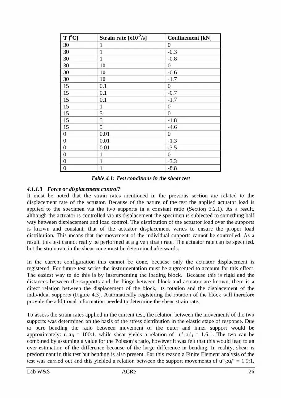
For each temperature, two strain rates were selected in such a way that a difference in strength was observed in the tests without horizontal confinement. The tests with horizontal force were performed under the same conditions (temperature and strain rate), but with a horizontal confinement equal to 15 and 40% of the maximum applied vertical force during the test with zero horizontal confinement (Table 4.1). For each condition, three repetitions were carried out. Initially the second strain rate at 15oC was 1x10-2/s, but this rate did not lead to a significantly different shear strength compared to the slower rate at this temperature. For this reason, the tests without support were repeated at a higher rate (5x10-2/s) and that rate was used in the remainder of the test program.

Lab W&S ACRe 26

T [oC] Strain rate [x10-2/s] Confinement [kN] 30 1 0 30 1 -0.3 30 1 -0.8 30 10 0 30 10 -0.6 30 10 -1.7 15 0.1 0 15 0.1 -0.7 15 0.1 -1.7 15 1 0 15 5 0 15 5 -1.8 15 5 -4.6 0 0.01 0 0 0.01 -1.3 0 0.01 -3.5 0 1 0 0 1 -3.3 0 1 -8.8

Table 4.1: Test conditions in the shear test

4.1.1.3 Force or displacement control? It must be noted that the strain rates mentioned in the previous section are related to the displacement rate of the actuator. Because of the nature of the test the applied actuator load is applied to the specimen via the two supports in a constant ratio (Section 3.2.1). As a result, although the actuator is controlled via its displacement the specimen is subjected to something half way between displacement and load control. The distribution of the actuator load over the supports is known and constant, that of the actuator displacement varies to ensure the proper load distribution. This means that the movement of the individual supports cannot be controlled. As a result, this test cannot really be performed at a given strain rate. The actuator rate can be specified, but the strain rate in the shear zone must be determined afterwards. In the current configuration this cannot be done, because only the actuator displacement is registered. For future test series the instrumentation must be augmented to account for this effect. The easiest way to do this is by instrumenting the loading block. Because this is rigid and the distances between the supports and the hinge between block and actuator are known, there is a direct relation between the displacement of the block, its rotation and the displacement of the individual supports (Figure 4.3). Automatically registering the rotation of the block will therefore provide the additional information needed to determine the shear strain rate. To assess the strain rates applied in the current test, the relation between the movements of the two supports was determined on the basis of the stress distribution in the elastic stage of response. Due to pure bending the ratio between movement of the outer and inner support would be approximately: uo:ui = 100:1, while shear yields a relation of u’o:u’i = 1.6:1. The two can be combined by assuming a value for the Poisson’s ratio, however it was felt that this would lead to an over-estimation of the difference because of the large difference in bending. In reality, shear is predominant in this test but bending is also present. For this reason a Finite Element analysis of the test was carried out and this yielded a relation between the support movements of u”o:ui” = 1.9:1.

TU Delft ACRe 27

This means that initially the deformation rate in the shear zone is approximately 90% of the actuator displacement rate. This value is used as the shear strain rate in the analysis of the test results.

a1 a2

u

ui=u*(1-*a2)uo=u*(1-*a1)

ui:uo ui uo

1:1.6 0.93u 1.48u1:2 0.88u 1.76u1:4 0.71u 2.86u1:10 0.45u 4.54u

Figure 4.3: The relation between the support displacements depends on the rotation of the loading block and the distances between supports and actuator

4.1.2 TEST RESULTS

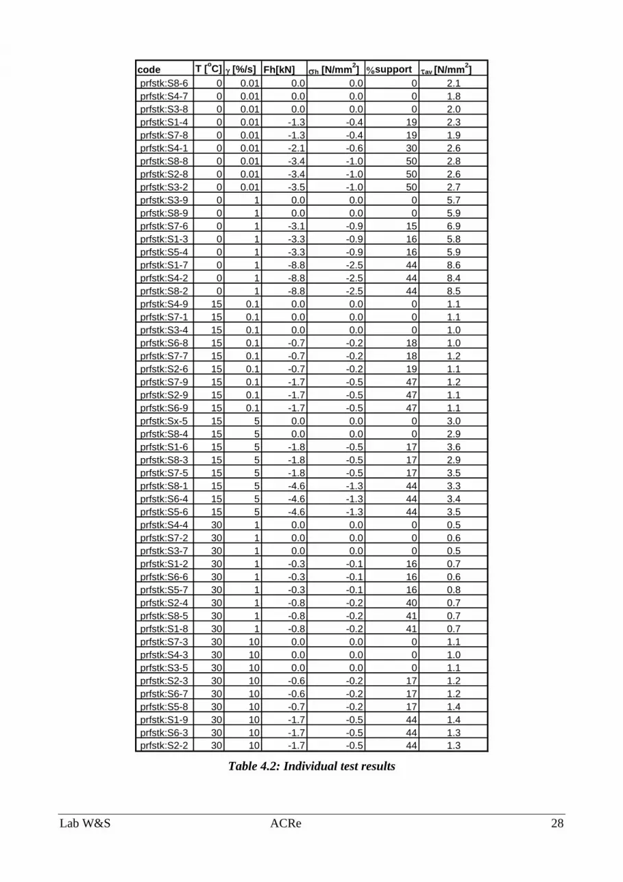
During the tests, the applied vertical and horizontal load and the corresponding actuator movements were registered. From the vertical load the shear strength was determined. On the basis of the strength found without horizontal confinement the confinement levels for that combination of strain rate and temperature were determine, which were as stated previously, 15 and 40% of the maximum vertical force applied in the unconfined shear test, respectively. The test results are presented numerically in Table 4.2 and graphically in Figure 4.4 through Figure 4.9. In legend of the graphs, 0%, 15% and 40% refers to the applied horizontal confinement. In the graphs the vertically applied force and, for the tests with horizontal confinement, the horizontal deformation are plotted as a function of time. The results are plotted as a function of time rather than shear strain because of the uncertainties in the shear strain that were discussed in the previous section. From Table 4.2 it can be seen that for a few conditions the third test was not completed. In these cases a test went wrong (computer malfunction, a support (pendulum bar) that did not stay in place) because of a lack of specimens, these tests could not be repeated but this was not considered a problem because of the availability of two results and the satisfactory repeatability.

Lab W&S ACRe 28

code T [oC] [%/s] Fh[kN] h [N/mm

2] support av [N/mm

2]

prfstk:S8-6 0 0.01 0.0 0.0 0 2.1 prfstk:S4-7 0 0.01 0.0 0.0 0 1.8 prfstk:S3-8 0 0.01 0.0 0.0 0 2.0 prfstk:S1-4 0 0.01 -1.3 -0.4 19 2.3 prfstk:S7-8 0 0.01 -1.3 -0.4 19 1.9 prfstk:S4-1 0 0.01 -2.1 -0.6 30 2.6 prfstk:S8-8 0 0.01 -3.4 -1.0 50 2.8 prfstk:S2-8 0 0.01 -3.4 -1.0 50 2.6 prfstk:S3-2 0 0.01 -3.5 -1.0 50 2.7 prfstk:S3-9 0 1 0.0 0.0 0 5.7 prfstk:S8-9 0 1 0.0 0.0 0 5.9 prfstk:S7-6 0 1 -3.1 -0.9 15 6.9 prfstk:S1-3 0 1 -3.3 -0.9 16 5.8 prfstk:S5-4 0 1 -3.3 -0.9 16 5.9 prfstk:S1-7 0 1 -8.8 -2.5 44 8.6 prfstk:S4-2 0 1 -8.8 -2.5 44 8.4 prfstk:S8-2 0 1 -8.8 -2.5 44 8.5 prfstk:S4-9 15 0.1 0.0 0.0 0 1.1 prfstk:S7-1 15 0.1 0.0 0.0 0 1.1 prfstk:S3-4 15 0.1 0.0 0.0 0 1.0 prfstk:S6-8 15 0.1 -0.7 -0.2 18 1.0 prfstk:S7-7 15 0.1 -0.7 -0.2 18 1.2 prfstk:S2-6 15 0.1 -0.7 -0.2 19 1.1 prfstk:S7-9 15 0.1 -1.7 -0.5 47 1.2 prfstk:S2-9 15 0.1 -1.7 -0.5 47 1.1 prfstk:S6-9 15 0.1 -1.7 -0.5 47 1.1 prfstk:Sx-5 15 5 0.0 0.0 0 3.0 prfstk:S8-4 15 5 0.0 0.0 0 2.9 prfstk:S1-6 15 5 -1.8 -0.5 17 3.6 prfstk:S8-3 15 5 -1.8 -0.5 17 2.9 prfstk:S7-5 15 5 -1.8 -0.5 17 3.5 prfstk:S8-1 15 5 -4.6 -1.3 44 3.3 prfstk:S6-4 15 5 -4.6 -1.3 44 3.4 prfstk:S5-6 15 5 -4.6 -1.3 44 3.5 prfstk:S4-4 30 1 0.0 0.0 0 0.5 prfstk:S7-2 30 1 0.0 0.0 0 0.6 prfstk:S3-7 30 1 0.0 0.0 0 0.5 prfstk:S1-2 30 1 -0.3 -0.1 16 0.7 prfstk:S6-6 30 1 -0.3 -0.1 16 0.6 prfstk:S5-7 30 1 -0.3 -0.1 16 0.8 prfstk:S2-4 30 1 -0.8 -0.2 40 0.7 prfstk:S8-5 30 1 -0.8 -0.2 41 0.7 prfstk:S1-8 30 1 -0.8 -0.2 41 0.7 prfstk:S7-3 30 10 0.0 0.0 0 1.1 prfstk:S4-3 30 10 0.0 0.0 0 1.0 prfstk:S3-5 30 10 0.0 0.0 0 1.1 prfstk:S2-3 30 10 -0.6 -0.2 17 1.2 prfstk:S6-7 30 10 -0.6 -0.2 17 1.2 prfstk:S5-8 30 10 -0.7 -0.2 17 1.4 prfstk:S1-9 30 10 -1.7 -0.5 44 1.4 prfstk:S6-3 30 10 -1.7 -0.5 44 1.3 prfstk:S2-2 30 10 -1.7 -0.5 44 1.3

Table 4.2: Individual test results

TU Delft ACRe 29

30oC & 10 %/s

0

0.5

1

1.5

2

2.5

3

3.5

4

4.5

5

0 2 4 6 8 10 12 14

time [s]

Fv [kN]

40%15%

0%

Figure 4.4: Average response curves for three levels of confinement at 30oC and 10%/s

30oC & 1 %/s

-2

-1.5

-1

-0.5

0

0.5

1

1.5

2

2.5

3

0 10 20 30 40 50 60 70 80

time [s]

Fv [kN]

-0.1

-0.05

0

0.05

0.1

0.15uh [mm]

40%

0%

40%

15%

15%

Figure 4.5: Average response curves for three levels of confinement at 30oC and 1%/s

Applied vertical force versus time

Horizontal deformation

Vertical force

Lab W&S ACRe 30

15oC & 0.1 %/s

-3

-2

-1

0

1

2

3

4

5

0 100 200 300 400 500 600 700 800

time [s]

Fv [kN]

-0.15

-0.1

-0.05

0

0.05

0.1

0.15

0.2

0.25uh [mm]

40%

15%

0%

40%

15%

Figure 4.6: Average response curves for three levels of confinement at 15oC and 0.1%/s

15oC & 5 %/s

-1

1

3

5

7

9

11

13

15

17

19

0 2 4 6 8 10 12 14 16

time [s]

Fv [kN]

-0.01

0.01

0.03

0.05

0.07

0.09

0.11

0.13

0.15

0.17

0.19uh [mm]

40%

15%

0%

40%

15%

Figure 4.7: Average response curves for three levels of confinement at 15oC and 5%/s

Vertical force

Vertical force

Horizontal deformation

Horizontal deformation

TU Delft ACRe 31

0oC & 0.01 %/s

0

2

4

6

8

10

12

0 1000 2000 3000 4000 5000 6000 7000 8000

time [s]

Fv [kN]

-0.15

-0.05

0.05

0.15

0.25

0.35

0.45uh [mm]

40%

15%

0% 40%

15%

Figure 4.8: Average response curves for three levels of confinement at 0oC and 0.01%/s

0oC & 1 %/s

-15

-10

-5

0

5

10

15

20

25

30

35

0 10 20 30 40 50 60

time [s]

Fv [kN]

-0.03

-0.02

-0.01

0

0.01

0.02

0.03

0.04

0.05

0.06

0.07

uh [mm]

40%

15%

0%

40%

15%

Figure 4.9: Average response curves for three levels of confinement at 0oC and 1%/s

From the response curves it can be seen that asphalt concrete is indeed confinement sensitive. As expected, the strength of the material increases with the applied confinement. Whether this confinement sensitivity is temperature and strain rate sensitive is investigated in the next section.

Vertical force

Vertical force

Horizontal deformation

Horizontal deformation

Lab W&S ACRe 32

4.1.3 GENERAL RELATIONS FOR THE TEST RESULTS

A similar trend as observed for the tensile and compressive strength as functions of temperature and strain rate is apparent in the shear strength, despite the different notions (elongation versus shear) that underlie the tests. The general relation that was used to describe all strength-related properties (Equation (4.1)) also enabled the expression of the shear strength as a function of temperature and strain rate. In Figure 4.10 this relation is plotted along with the test results. The shear stress used in this graph is the average shear stress, which is the shear in the centre zone divided by the specimen cross section. The shear strain rate is based on the engineering strain as shown in Section 4.1.1.2, Figure 4.2. The strain rate values are based on 90% of the applied actuator deformation rate for the reasons mentioned in Section 4.1.1.3.

0 0.3126200

93

1 11 17.5 1

1 1

dc

bT T

a

e e

(4.1)

Where: t0=shear strength without confinement in N/mm2

=shear strain rate in mm/mm T= temperature in Kelvin a,b,c,d= regression constants

0

2.5

5

7.5

10

12.5

15

0 1 2 3 4 5 6 7 8 9 10 11 12 13 14 15

[%/s]

0 [N/mm

2]

Eq.6.1 Eq.6.1 Eq.6.10 15 30

Figure 4.10: General expression for the shear strength compared to the test results

In Figure 4.11 the shear strength values normalised with respect to the shear strength without confinement are plotted against the confinement level. The confinement levels plotted in this graph are determined, for every combination of temperature and strain rate, by dividing the applied normal stress by the shear stress at failure if no confinement is applied. These confinement levels are somewhat higher than the 15% and 40% mentioned before because the shear in the failure zone is not equal to the applied actuator load (Section 3.2.1) and the levels mentioned earlier were based on the ratio of the applied horizontal and vertical actuator forces. Since the data are used to develop a relation between the shear strength and the confinement level, which is a material characteristic, it must be represented in a test set-up independent way. Hence the adapted definition of the

TU Delft ACRe 33

confinement level, which now uses the stresses as they occur in the specimen. The earlier definition is more convenient during testing since it is based on quantities that are actually registered and used to control the test.

The increase in shear strength with confinement appears to be independent of temperature and strain rate (Figure 4.11). For this reason a relation between shear strength and confinement level is developed. This relation has to yield the unconfined shear strength for zero confinement and it should go to a limit strength, since the shear strength will not increase indefinitely with increasing confinement. These considerations resulted in Equation 4.2, which is also plotted through the data points in Figure 4.11. A can be seen it describes the trend rather well. This relation basically expresses the confinement sensitivity of the ACRe mixture.

0 0

* 100% 0.005* 100%

0 0( 1)exp 2.5 1.5expN Nb x x

a a

(4.2)

Where: =shear strength at that confinement level

0=shear strength at zero confinement

N=applied confinement (normal stress)

a,b=regression constants

0

0.2

0.4

0.6

0.8

1

1.2

1.4

1.6

1.8

2

0 10 20 30 40 50 60 70 80 90 100

confinement [N/0x100]

0

0.01&0

1&0

0.1&15

5&15

1&30

10&30

Eq. 6.2

Figure 4.11: Normalised shear stress as a function of the applied confinement

Lab W&S ACRe 34

5. CONCLUSIONS AND RECOMMENDATIONS

5.1 CONCLUSIONS As expected, the material proved to be confinement sensitive. This sensitivity proved independent of temperature and strain rate. On the basis of the test results general expressions were developed for the shear strength without confinement and the increase with confinement. This completely covers the confinement sensitivity of the material. The set-up functioned quite well, resulting in shear failure in a narrow band at the centre of the specimen. As a result, most of the specimen does not really contribute to the test, except to allow the establishment of the proper stress state. This stress state is obtained for a particular ratio between the support distances. At the moment the options were limited because of the existing hole-pattern in the bottom plate and loading block. If these are adapted, much smaller specimens can be used. This will simplify the specimen production and the handling of specimens during testing. Although the applied actuator signal is controlled in displacement mode, the specimen loaded in a combination of force and displacement mode. The hinges between specimen and loading block ensure a fixed ration between the two applied forces and the displacements of the supports are adapted correspondingly. As a result, neither the applied shear strain rate nor the force that occur in the shear zone are truly controlled during the test.

5.2 RECOMMENDATIONS To facilitate the use of smaller specimens it is recommended to adapt the hole patterns in the bottom plate and the loading block. This simplifies testing and makes specimen production much cheaper since smaller specimens require less material. Eventually this adaptation will therefore pay for itself. During data-analysis it was realised that this test is really performed in a mixed force and displacement control. As a result, the applied strain rate had to be determined in a rather roundabout way. It is recommended to add a sensor that will register the rotation of the loading block during the tests. Due to time restraints there had not been a series of preliminary tests and as a result this problem was not encountered until after the tests were finished. It can therefore be concluded that it is important to run a series of tests and anaylse the results before starting to use a newly developed set-up. Although it takes up time at that moment, it saves time and prevents errors in a later stage.

TU Delft ACRe 35

References Bondt, A.H. and Scarpas, A., (1993), Shear Interface Test Set-Ups, Delft University of Technology

Report nr.7-93-203-12 Bondt, A.H., (1999), Anti-Reflective Cracking Design of (Reinforced) Asphaltic Overlays, PhD.

Thesis Delft University of Technology, Ponsen & Looijen, ISBN 90-6464-097-1 Erkens, S.M.J.G. and Poot, M.R., (1998), The Uniaxial Compression Test – Asphalt Concrete

Response (ACRe), Delft University of Technology Report nr. 7-98-117-4 Erkens, S.M.J.G. and Poot, M.R., (2001), Additonal Compression Tests – Asphalt Concrete

Response (ACRe), Delft University of Technology Report nr. 7-00-117-5 Erkens, S.M.J.G. and Poot, M.R., (2001), The Uniaxial Tension Test – Asphalt Concrete Response

(ACRe), Delft University of Technology Report nr. 7-01-117-7

Lab W&S ACRe 36

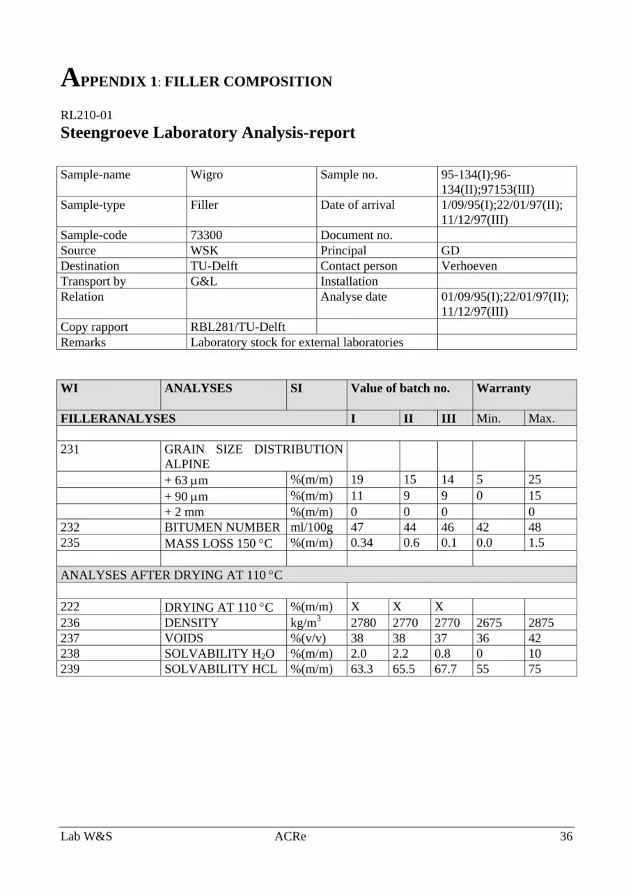
APPENDIX 1: FILLER COMPOSITION

RL210-01

Steengroeve Laboratory Analysis-report Sample-name Wigro Sample no. 95-134(I);96-

134(II);97153(III) Sample-type Filler Date of arrival 1/09/95(I);22/01/97(II);

11/12/97(III) Sample-code 73300 Document no. Source WSK Principal GD Destination TU-Delft Contact person Verhoeven Transport by G&L Installation Relation Analyse date 01/09/95(I);22/01/97(II);

11/12/97(III) Copy rapport RBL281/TU-Delft Remarks Laboratory stock for external laboratories WI

ANALYSES SI Value of batch no. Warranty

FILLERANALYSES I II III Min. Max. 231 GRAIN SIZE DISTRIBUTION

ALPINE

+ 63 m %(m/m) 19 15 14 5 25 + 90 m %(m/m) 11 9 9 0 15 + 2 mm %(m/m) 0 0 0 0 232 BITUMEN NUMBER ml/100g 47 44 46 42 48 235 MASS LOSS 150 C %(m/m) 0.34 0.6 0.1 0.0 1.5 ANALYSES AFTER DRYING AT 110 C 222 DRYING AT 110 C %(m/m) X X X 236 DENSITY kg/m3 2780 2770 2770 2675 2875 237 VOIDS %(v/v) 38 38 37 36 42 238 SOLVABILITY H2O %(m/m) 2.0 2.2 0.8 0 10 239 SOLVABILITY HCL %(m/m) 63.3 65.5 67.7 55 75

TU Delft ACRe 37

APPENDIX 2: SIEVE CURVE CRUSHED ROCK 0/5 AND FILLER 00

0

10

20

30

40

50

60

70

80

90

100

0.01 0.1 1 10

Sieve size [mm]per

cen

tag

e p

assi

ng

[%

]

crushed rock

aggregate (crushedrock + filler)

Dry sieving Crushed rock 0/5 Aggregate (sand + filler) Sieve [mm] Percentage passing

[% m/m] Percentage passing [% m/m]

4 97.5 96.8 2.8 94.9 94.4 2 90.6 90.8 1 60.4 65.3 0.5 34.5 43.4 0.355 26.4 36.6 0.25 18.1 29.6 0.18 11.3 25.2 0.125 5.9 20.6 0.063 1.8 14.6

From the previous Appendix it is known that the filler was sieved on the 63 m, 90 m and 2 mm sieves. It is assumed that the material that remained on the 90 m sieve and passed through the 2 mm sieve would have passed the 125 m sieve used to analyse the sand. The combined sieve data is found by computing the mass percentage on each sieve (difference between two adjacent values) and expressing that as a percentage of the combined mass (m%*=m% * Ms/(Ms+Mf). Where necessary, the percentages for the filler and crushed rock are combined. For example: Sieve 63 m: 1.8% x 2.7/3.2+ 84% x0.5/3.2=14.6% (2.7 kg rock+ 0.5 kg filler=3.2 kg aggregate) Sieve 125 m: (5.9%-1.8%)x2.7/3.2+16%x0.5/3.2+14.6%=20.6% Sieve 180 m: (11.3%-5.9%)x2.7/3.2+20.6%=25.2%, etc.

Lab W&S ACRe 38

APPENDIX 3: BITUMEN CHARACTERISTICS 00 1. Penetration test

Pen.45/60 (batch I) Pen.45/60 (batch II)

1e 2e 3e average 1e 2e 3e average

47 46 48 47 47 48 47 47.3

2. Ring & Ball

R&B (batch I) R&B (batch II)

Level thermostat

Level boiling ring

Starting temperature

Result Level thermostat

Level boiling ring

Starting temperature

Result

45 9 8.6 51/51 45 9 7.2 52/52.1

120)log(50)&(

1952)log(500)&(20

penBRT

penBRTPI (A3.1)

Result batch I: PI = -1.10 Result batch II: PI = -0.83 Density bitumen: b= (1020 5) kg/m3

TU Delft ACRe 39

APPENDIX 4: CALIBRATION DATA LOADCELLS 00

Lab W&S ACRe 40

TU Delft ACRe 41

Lab W&S ACRe 42

TU Delft ACRe 43

Lab W&S ACRe 44

TU Delft ACRe 45

APPENDIX 5: SLAB PRODUCTION PROCEDURE (IN DUTCH)

Lab W&S ACRe 46

TU Delft ACRe 47

Lab W&S ACRe 48