Acta Informatica 23, 621-642 (1986)

�9 Springer-Verlag 1986

The Reliability of Life-Critical Computer Systems*

Robert Geist 1, Mark Smotherman 1, Kishor Trivedi 2, and Joanne Bechta Dugan2

1 Department of Computer Science, Clemson University, Clemson, SC 29631, USA 2 Department of Computer Science, Duke University, Durham, NC 27706, USA

Summary. In order to aid the designers of life-critical, fault-tolerant com- puting systems, accurate and efficient methods for reliability prediction are needed. The accuracy requirement implies the need to model the system in great detail, and hence the need to address the problems of large state space, non-exponential distributions, and error analysis. The efficiency re- quirement implies the need for new model solution techniques, in particular the use of decomposition/aggregation in the context of a hybrid model. We describe a model for reliability prediction which meets both requirements. Specifically, our model is partitioned into fault occurrence and fault/error handling submodels, which are represented by non-homogeneous Markov processes and extended stochastic Petri nets, respectively. The overall ag- gregated model is a stochastic process that is solved by numerical tech- niques. Methods to analyze the effects of variations in input parameters on the resulting reliability predictions are also provided.

1. Introduction

Fault-tolerant computer systems, that is, systems capable of continued correct operation in the presence of either operational or design faults, are experienc- ing an ever-increasing range of important applications [2]. When these appli- cations are life-critical, such as in flight control, fault-tolerance becomes the vehicle used to enhance system reliability, that is, the probability that the system will remain operational throughout the mission time.

Nevertheless, the extensive reliability demands placed upon these life-criti- cal systems (reliability >1 -10 -9 ) preclude simple procedures by which we might verify that the systems possess the level of reliability for which they were designed. As the probability of system failure approaches 0, lifetesting and

* This work was supported in part by NASA grant NAGI-70 and by an equipment grant from the Concurrent Computer Corp

622 R. Geist et al.

simulation techniques become too expensive to remain feasible [18, 25]. More- over, standard stochastic models (e.g., Markov, semi-Markov) sufficiently com- prehensive to include details of fault/error-handling behavior, as well as details of the fault processes and system structure, are generally intractable. In such models a massive state space (typically 105 states [24]) is often coupled with a collection of state transitions having rate variations of several orders of magni- tude. A fault process may exhibit a rate on the order of 10-4/h, whereas a recovery process within the same model could have a rate of 106/h. Standard modeling then yields a massive system of stiff differential or integral equations with the attendant solution difficulties.

As a result, most models used to predict ultra-high reliability (reliability >1-10-9) , including the one described herein, resort to a behavioral decom- position of the system along temporal lines into nearly disjoint fault-occurrence and fault/error-handling submodels [-11, 12, 26, 27]. The fault/error-handling model is solved in isolation and the resulting effectiveness measures, which are termed coverage factors, are then aggregated with the fault occurrence behavior to obtain the prediction of system reliability as a function of mission time. Of course, this behavioral decomposition leads to certain approximations, and the effects of these approximations, as well as the potential ill-effects from other possible sources of modeling error, must be identified and bounded.

The remainder of the paper is organized as follows. In Section 2 we discuss our fault-occurrence model, which describes the fault processes and system structure, as well as the aggregation technique through which we capture the effectiveness measures produced by the fault/error-handling submodel. The latter model is described in Section 3, where we use a framework of Extended Stochastic Petri Nets [5, 6] to capture the process concurrency inherent in fault/error-handling techniques. In Section 4 we discuss error analysis, and in Section 5 we give examples of the implementation of our techniques in H A R P (Hybrid Automated Reliability Predictor), now in development jointly at Clemson University and Duke University under the sponsorship of NASA Langley Research Center.

2. The Fault-Occurrence Model

A fault is an erroneous state of hardware or software resulting from physical interference from the environment, failures of components, operator error, or incorrect design [22]. An error is the manifestation of a fault within the system output. Thus a fault may or may not cause an error. Undetected errors, or detected errors from which we cannot effect recovery, may propagate through the system and cause system failure.

The state of a fault-tolerant system will be a vector whose integer coor- dinates indicate the number of failed components of each type, and whose single binary coordinate indicates whether the system is operational (function- ing properly) or failed. We will find it convenient to identify all failed states with a single, absorbing state, which we hereafter term the system failure state. Note that transition to the system failure state may result from either an

Reliability of Life-Critical Computer Systems 623

exhaustion of component redundancy or an inability to recover from the effects of a fault.

Consider now the general non-homogeneous Markov process which, sui- tably restricted, has been the basis for virtually all of the recent efforts to develop useful reliability prediction packages [3, 4, 11, 19, 26]. If we let P(t) =(Po(t) . . . . , P,(t)) denote the time-dependent probability vector for operational (non-system-failure) states 0 . . . . ,n, and let A(t)=(a~j(t)) denote the associated matrix of state transition rates (where a~j denotes the rate of transition from state i to state j), then the Markovian assumption yields the set of differential equations

P'(t) = P(t) A(t)

with equivalent integral formulation t

t

P (t) = E P,(x)%(x) e x dx (1) i * j O

whose solution gives the system reliability R(t)= ~ Pi(t). Without loss of gener- i

ality, we hereafter assume that the operational state i is merely a non-negative integer, and that the only state transitions are those to the state i+ 1 (one more covered fault) and to the system failure state (one more uncovered fault). We then have

t t

p/+ a(t) = [.Pi(x)ai, i+l(x)e -Iax ....... i>O_ (2) (u) dU d x 0

where t

- [aoo(x)dx Po(t) = e 0

Extensions to the general case will always be straightforward. Now the term al, i§ ) in (2) represents the "instantaneous probability" of

a covered fault from state i to state i + 1 at time x. It is, accordingly, a product, ai.i+l(x)=2i, i+l(x)ci, i+l(x), where 2i, i+l(x ) is the fault rate from state i, and ci,~+l(x) is the probability that the fault is covered. Now it is entirely reason- able to assume that fault processes commence at the beginning of the mission, and hence that state and global time dependence are sufficient to capture the total fault occurrence information. On the other hand, the total information from the fault/error-handling submodel must be passed to the fault-occurrence model (2) through the instantaneous coverage probability cg,i+~(x ). This is clearly a limitation on the adequacy of the Markovian approach. Fault cover- age, or the lack thereof, is not instantaneous. Rather, faults typically exhibit a nonzero latency period during which the system will attempt detection, isol- ation, and reconfiguration procedures. In the use of an instantaneous coverage probability, ci,~+~(x), we are assuming that the total time spent in these fault/ error-handling procedures, which commence at global time x, is relatively insignificant, and that the use of a steady-state rather than transient probability of coverage from the fault/error-handling submodel will suffice. In [21] it is shown that the effects of this approximation are conservative, that is, the

624 R. Geist et al.

approximation will cause an underestimation of system reliability. Thus the Markovian technique remains viable, since the lower bound itself will often meet design specifications (see Section 5).

Consider next the determination of appropriate values for the cl.i+l's from the information supplied by the fault/error-handling submodel. For this pur- pose we will make use of a general, single-entry, four-exit model which sub- sumes those fault/error-handling submodels available in the major reliability prediction packages currently in use [-10]. Fault/error-handling begins (the submodel is entered) when a fault occurs in the system. This does not imply that the fault has been detected. A fault may exist for some time without either producing an error or being detected by self-diagnostic circuity. The entry point of the coverage submodel is labeled I. There are four mutually exclusive exits from the submodel, labeled R, C, S and N. Fault/error-handling com- pletes (the submodel is exited) when the fault is handled (exits R and C) or when the system fails (exits S and N). Exit R represents the correct recognition of and recovery from a transient fault (called transient restoration), while exit C represents the reconfiguration of the system to tolerate a permanent or "leaky" transient fault (traditionally called coverage). System failure can arise from one of two causes, single-point failure (exit S) or a near-coincident fault (exit N). A single-point failure occurs when a single fault is catastrophic to the system, while a near-coincident failure is caused by the occurrence of a second fault while attempting recovery from the first.

Thus, we assume that there is a classification of fault dependencies, leading to two sources of coverage failures:

1. A single fault may cause system failures (i.e., a single point failure), even in the absence of any subsequent fault.

2. Both independent and dependent near-coincident faults are allowed. Two or more independent near-coincident faults do not necessarily result in system failure. However, two or more dependent near-coincident faults will cause system failure. For the sake of simplicity, we assume only dependent near- coincident faults in this paper.

Let P~c(Z) denote the probability of reaching the coverage exit C in an amount of time <z from the occurrence of the fault. We assume this to be independent of the (global) time of occurrence of the fault. Denote by P~c(+ oo) the limit, lim Pxc(Z). If we were to have no near-coincident faults, then clearly

we could set instantaneous coverage c = P / c ( + oe). However, when we include these faults, it is no longer sufficient to know that the system would eventually recover. Recovery must take place prior to the occurrence of the next fault, so we must take into account the distribution of times to reconfiguration recovery (coverage), Tc, given by

e~c(t) Fro(t) = P1c( + oo)"

Let the random variable N~+l(x) denote the time to next fault, given that the system is in the process of handling the i + 1-st fault (i > 0), which occurred at (global) time x. Then

- i ; t~+~a+z(x+u)du Fs, +,(x)(z) = 1 - e o

Reliability of Life-Critical Computer Systems 625

Instantaneous coverage can then be given by

Ci, i +1 (X ) = e I c ( "~- o o ) Prob I T c < N i +1 (x)]

+oo +oo _ i2~+la+2(x+u)d u

= P ~ c ( + ~ ) ~ I 2i+l,i+2(x+z)e o dFTc(y)d z 0 y

+ oo _ i2~+L~+2(x+u)d u =Pgc(+ oo) ~ e 0 dFre(y). (3)

0

Note that the fault/error-handling model can be solved independently of (2) to obtain appropriate expressions for Frc(Y ) and Pw(+ oo). Further, in certain cases, this expression for coverage (3) simplifies considerably. For instance, suppose the fault processes have Weibull distributions, that is, hazard rates of the form 2(x+u)=2oO~(x+u) ~-1, where 20>0 and ~>0. At present, this is the most widely used parametric family of fault distributions [29]. In this case,

+ oo _ i 2 ( x + u ) d u + oo

I e o dFrc(Y)= I e-Z~ (4) 0 0

+oo

=e~~ S e-~~ 0

+ oo + oo y i = e a ~ 5 E g(/)(x)

o o i ~ d F r c ( Y )

- g ( x ) g(x)+E[Tc]g'(x)+E[r~] +"" (5)

where g(x)=e -a~ In the case that recovery times are deterministic, that is, T c = 1/# with probability 1, (5) becomes the Taylor expansion of g (x+ 1/#) about x, so that

. g (x+ 1/#) _ . e - a ~

c(x)= P~c( + Oo ) - g ~ = qc( + oo) e -a~ (6)

Should recovery times be exponentially distributed with mean 1/#, then E[T~] =n!/#" and we obtain

c(x)=Ptc(+ oo) g@x ) [ (x,+g'(x) +g"(x)+g"'(x)+ ] [g ) # #2 #3 ""_]"

[ ] If we now let K(x)= g(x)+g'(x)+g"(x)+ then K ' = p K - # g , which is # #2 "'"

easily solved for K, giving us

# e_ ~O:_ US d s

c(x)=P~c(+ m) x e - z ~ (7)

Of course, both (6) and (7) can be obtained from (4) by inserting the appropri- ate distribution function and, in the latter case, making a change of variables, but (5) directly illustrates the dependence of coverage on the moments of T c.

626 R. Geist et al.

If we compare (6) and (7) in the case a = 1 (constant fault rate), we obtain

c(x) =Pic (+ ~ ) e - ~o/~ ~ Pic( + ~ ) /~ - 2~ for deterministic recovery times and //

c ( x ) = p i c ( + ~ ) ~ , slightly larger, for exponential. In the case a = 2 we can

generalize to the linear hazard rate, 2 ( x + u ) = a . ( x + u ) + b , e > 0 , and, if re- covery times are uniformly distributed over an interval [-0, T], still obtain a considerable simplification

(mx)2 + (b/m)2 + b x

c ( x ) = p i c ( + ~ ) e 2 [ , E z ( m ( x + T ) + b / m ) - F z ( m x + b / m ) ]

where m = l f a and F~ denotes the standard normal distribution function. The use of this instantaneous coverage, Markovian model provides both

computational simplicity and provably conservative estimates of reliability [,21]. On the other hand, to obtain greater accfiracy, we must return to (2) and withdraw the approximation that is (3). In order to reach state i+ 1 at time t, we must recover prior to time t, not just prior to the next fault. Thus, to obtain an exact expression, we must replace Prob(Tc<Ni+l(x)) in (3) with Prob(Tc<t -x). We obtain

t t -~,~,+,.,+2(u)du

e~+,(t)= ~ e,(x).~,,i+l(x)pic( + ~ ) I % ( t - x ) e . dx (8) 0

which no longer represents a non-homogeneous Markov process, since cover- age, c i . i+ l=P1c(+m)FTc( t - - x ) , depends on local, rather than global time. Note, however, that the fault/error-handling model may still be solved in isolation to provide the appropriate information. A special case of (8), with time-independent fault rates, appears in [28].

Equation (8) alone will not suffice to compute system reliability. The state i in (8) represents a system which has sustained i faults, none of which is latent. Since a system may function properly in the presence of a single latent fault, we must, in computing reliability, extend the state i to a state, El, representing a system which has sustained i faults, one of which is perhaps latent. We then let Pis(Z)=pis(+ oO)FTs(Z ) denote the probability that a single fault will cause us to reach a system failure state in time < r from the occurrence of the fault, and use

t - j21+l . i+2(u)du

PE(i+ 1)(t) = ~ P/(x)/~i, i+1 (x) (1 - - PIs ( + ~ ) FTs(t - - X ) ) e x dx 0

in conjunction with (8) to compute system reliability R(t)= ~ PEi(t). i

When we consider transient faults, we find that the fault/error-handling model and the fault-occurrence model do not separate as cleanly as in (8), since, upon recovery from a transient, the "next-fault" process changes. More specifically, if we let Pig(Z)=Pig( + 0(3)FTR(Z ) denote the probability that tran- sient recovery occurs in time < z from occurrence of the fault (and let y denote the latency interval), then the contribution to P~+x(t) from transient restoration

Reliability of Life-Critical Computer Systems 627

is given by

y+x i t t - x - J 2,+a,i+s(u)du - 2i+l,,+=(u)du 5 P i + l ( X ) 2 i + l , i + 2 (X) I PIR(+m)dFrR(Y) e x e ,+~ dx. 0 0

In order to maintain tractability, we resort to an approximation obtained by replacing the fault rate )ti+z,i+3(u ) above by the larger 2i+a,~+2(u). Under the assumption that increased component fault rates will not improve system reliability, we may declare this approximation conservative. We then obtain an expression analogous to (8):

t t - J,~,+,,,+2(u)du

P/+l(t) = I I~I+ I(X) ~i+ I, i+ 2 (x ) PIR(-~- m) F r , ( t - x ) e = dx 0

t t -J2~+L~+2(u)au

+ jPi(x)Xi, i+a(x)Pxc(+ m ) F r c ( t - x ) e ~ dx. (9) 0

We can obtain additional insight into the nature of the approximation of (8) afforded by (3) in (2) through a consideration of recovery time distributions in the transform domain. If Fr~ is continuous and we fix t > 0, then there exists a z* >0 such that P~+l(t), as defined by (8), is also given exactly by

t

i - J,~,+~ ,+~(u)du Pi+l(t)= Pi(x)2i, i+ l (x )P~c(+~)Frc (Z*)e~ ' dx. 0

~* + oo Now Frc(z*)= ~dFr~(y)< J dFrc(y)= 1, and thus there is some s* >0 such that

0 0

Lr~(S*)= j e-Y~*dFr~(y)=Fr~(r*), and hence for which 0

t t -S,~i+l,i+2(u)du

Pi+ 1 (15) = I Pi(x) ~i, i+ 1 (x) PIc( -]- oo) Lrc(S* ) e .~ dx 0

is also exact. Further, since recovery times in ultra-reliable systems are relative- ly small, Fro approaches 1 rather quickly. In particular, for reasonable mission times t, e.g. 10h, F r c ( t - x ) in (8) will be near 1 over most of its range of integration, and thus Frc(Z* ) will be near 1. Hence s* >0 will be quite small for such systems. In the case of constant fault rates, the approximation of (8) given by using (3) in (2) is an approximation of s* by 21+1,i+ 2, which, for the systems of which we speak, is on the order of 10 -4 [16, 30].

The only remaining issue concerning the fault-occurrence model is the solution method of (9), which is a Volterra equation of the second kind, that is, of the form t

y(t) =f( t ) + 5 K(t, x) y(x) dx (10) 0

where K(t ,x) is known as the kernel of the equation, and f ( t ) represents the solution to the permanent (non-transient) fault model.

628 R. G e i s t et al.

Now this solution, f(t), is itself a convolution integral involving several integrands, one of which is FTc, the distribution function of permanent fault recovery times. This distribution function differs from other integrands, in that it can vary significantly over a relatively short time interval [a, b]. Thus, we can regard FTc a s a weight function, w ( t - x ) , so that f ( t ) is of the form

bi

S g(x) w( t - -x ) dx (11) i ai

where, over suitably chosen sub-intervals [ai, bi], of [O,t], g will not vary a great deal.

We can then apply weighted interpolatory quadrature [14] to each of the integrals of (11), in which the interpolation polynomial need not have high

b

degree. In particular, we approximate S g ( x ) w ( t - x ) d x by a

3

qjg(xj) (12) j = l

4)(x) w(t- x) where 6 1 x ) = / x - x l ) ( x - x 2 ) ( x - x 3 ) , and xl,x2, x3 are

interpolation points in [a, b], which define a quadratic. The computation of f ( t ) represents a sequence of integrations whose length

is the size of the operational state space. In order to limit the total number of integrations to be linear in the size of the operational state space, we constrain points x~ and x 3 to be the endpoints of the interval in question, [a,b]. If we choose the point x 2 to be the midpoint of the interval, (a+b)/2, we have a quadrature rule similar to that used in the solution of the CARE III reliability model [24].

Greater precision is possible. The error in using (11) is given by

b

E = ~ 4~(x) g [xx, x2, X 3 , X] w(t - - X ) MX (13) a

where g[ ] denotes the third order divided difference. Should g be a poly- nomial of degree <n, then g[x1,Xz,X3,X ] is a polynomial of degree < n - 3 . Thus if we select x 2 to be the zero of

b

G(x2) = ~ (x - a) (x - x2) (x - b) w(t - x) dx (14) a

then we have E = 0 for polynomials of degree < 3, clearly the maximum degree of precision (subject to the other constraints). For w=Frc , the distribution of recovery times, this choice of x 2 will depend upon T c through the fourth truncated moment. Although this maximum precision approach would appear to require more computation and storage space than a midpoint quadrature, a cubic interpolation across adjacent integration panels, which yields function values at points other than the xl, to be provided to the next level, makes it competitive.

Reliability of Life-Critical Computer Systems 629

Returning to the basic Volterra equation (10), we find that, for parameters chosen from typical life-critical computing systems, a Neumann series ap- proach I-9] will provide rapid convergence. In particular, we construct a series of functions y,(t) according to

Yn+l(t)=f(t)+2iK(t,x)y.(x)dx, Yo(t)=O. o

(15)

We use the parameter 2 to represent a scale factor on the fault rate, such that the scaled fault rate within the integral has maximum magnitude 1. For real and continuous f(t) and K(t, x), this series converges [-9], with factor less than or equal to 2t. For reliable flight control applications, the fault rate 2 is typically 10 -4 faults/h and the mission time t is typically 10h. Thus three iterations would capture all terms greater than 10 - 9 .

3. The Fault/Error Handling Model

Since the fault-occurrence model (9) incorporates functional rather than in- stantaneous coverage factors, the analysis of the fault/error-handling model must now generate these functions. To facilitate this analysis and to facilitate the modeler's task of specifying concurrent behavior which is inherent in fault/error-handling processes, we choose to represent our fault/error-handling model as an Extended Stochastic Petri Net (ESPN) [5, 6, 11]. A description of these nets may be found in the Appendix.

The H A R P model calls for the interactive input of an arbitrary ESPN, or for the user specification of parameters associated to a default net. The default net, shown in Fig. 1, models three aspects of a fault recovery process: fault behavior, transient recovery, and permanent recovery. The fault behavior mod- el captures the physical status of the fault, i.e. whether the fault is active or benign (if permanent), and whether the fault still exists (if transient). Once the fault is detected, it is assumed to be transient, and an appropriate recovery procedure (e.g. rollahead or rollback) may commence. If the detection/recovery cycle is repeated k times, the fault is assumed to be permanent and a per- manent recovery procedure (reconfiguration) is invoked. If reconfiguration is successful, the system is again operating correctly, although in a degraded state. The user inputs are the transition firing time distributions and the probabilities of error detection, fault detection, fault isolation, and recon- figuration. (Note that the distributions need not be exponential.) The user must also specify the number of attempts at transient recovery, the percentage of faults which are transient, and a desired confidence level.

The net is then simulated, and statistics gathered to enable estimation of the probability of and conditional time-to-exit for a token reaching places Transient Recovery and Reconfigure Recovery. In this case the coverage factor R is represented by place Transient Recovery and the coverage factor C by Reconfigure Recovery. The incorporation of these statistics into the overall model proceeds as follows: for each of the coverage factors X, P~x(+ oo) will be

630 R. Geist et al.

T 5

T8

T I I

Fig. 1. HARP single fault ESPN model

estimated by the ratio of the number of tokens reaching the corresponding terminal place X from the initial marking I, to the number of trials run.

The estimation of fTx(r ) for each coverage factor X is done by dividing the time axis into small intervals, and associating a counter with each interval. For each simulation trial, the counter for the interval which represents the time to exit is incremented. This series of counter represents a discretized estimate of the density function for time-to-exit.

It is also possible in many cases to solve the ESPN analytically. If all the transition firing times are exponentially distributed, then the net can be con- verted to a Markov chain [-6, 20]. The associated Markov chain can then be solved analytically for P~x(T), where 1 is the initial state (marking), and the X states are absorbing. Further, under certain restrictions on the firing time distributions of concurrently enabled transitions (see [6]), an arbitrary ESPN can be converted to a semi-Markov process, and, again, solved analytically for the necessary coverage functions.

4. Error Analysis

We analyze the effect of parametric and initial condition errors on reliability prediction by studying the system of ordinary differential equations which

Reliability of Life-Critical Computer Systems 631

result from using (3) in (2). The use of the approximation is justified by its provably conservative (lower bound) effect on reliability estimation [21] and the importance of such lower bounds in the design of life-critical systems.

Analysis of errors in this context has been studied by several authors. Frank [8] has shown how the system of differential equations can be expanded to generate the first-order partial derivatives of the state probabilities with respect to parameter and initial condition errors. This approach yields error estimates rather than bounds. Iyer [17] has used the method of doubly sto- chastic processes to derive the moments of the reliability distribution as func- tions of the distribution of a model parameter. Gnedenko [13] also treats this as distributions of mixtures. However, either an analytic expression for re- liability is required or involved numerical integrations must be used. We seek an error analysis for which the required computation is a small fraction of that required for the model solution.

Consider again the basic differential system

P'(t) = P(t) A(t) P(O) = Po.

Let I[ II denote both the l I norm and its associated induced matrix norm [-15]"

Plxll = ~ Lxil i=,

IIAll--max ~ I%1- i j = l

Since P(t) is the vector of operational states, it is clear that

R(t)= IIP(t)ll = ~ P~(t). i = 1

Theorem. Suppose the behavior of our system is given by

P](t) = PA(t) A(t), PA(O) = PA

and that a user-specified model of this system containing parametric errors and initial condition errors is given by

P~(t) = Pv(t) U(t), Pc(O) = Pv I f we define

K(t)= I] V(t)ll and

e(t) = II U ( t ) - A(t)II then , ,

{ ~ _ ~ } , K(x)dx , K(x)dx IIPA(t)--Pv(t)ll < max (eo -- 1)+ IIPu--PAI Ieo

O<_x<_t

Proof. See [26].

Corollary. I f the system and the user model have constant transition rate mat- rices, A and U, then

IIPv(t)-- PA(t)ll < ~ (e x ' - 1)+ Il Pv-- PAll er'. lk

632 R. Geist et al.

Note that for each parameter of the model we need a nominal parameter value and a variation magnitude.

We can also approach the analysis of errors by decomposing the original model into two simple models [-23]. The simple models will allow us to obtain bounds on the probability of system failure due to a lack of spares, P(A), and separately obtain bounds on the probability of system failure due to lack of coverage, P(B). We then obtain bounds on system failure probability by use of the elementary inequalities:

P(A • B) < min { 1, P(A) + P(B)}

P( A ~ B) > max {P(A), P(B)}.

The first inequality will give us the conservative bound on system failure probability, and the second will give us a complementary optimistic bound.

Again we will require upper and lower bounds on the time-dependent failure rates of the different component types over the mission time, Z Consid- er, without loss of generality, a single component type with failure rate )~(t). We require that the user specify a relative difference bound, A2, on the error in the functional representation of the failure rate over the mission time interval. Therefore,

~high( t ) = (1 + A2) 2(0

2,ow(t ) = (1 -- A2) 2(t).

The user must also specify the number of initial operational components, n, and the minimum number of operational components necessary for the system to remain operational, m. The failure probability due to exhaustion of spares is found using the N M R reliability equation 1-29]:

t t

P~xh(2, t ) = l - - e o (1--e o . t = m

Using the upper and lower bounds on the component failure rate, we then calculate the upper and lower bounds on the probability of system failure due to exhaustion of spares.

P e x h . high(T) -~- Pexh (/~high, T)

P~,,h. tow(T) = P~xh(21ow, T).

If there are multiple component types, we use the product of the N M R reliability equations. If transient faults are modeled, then the N M R equations are conservative, since all transient faults are considered leaky but covered. The alternative to the N M R equations is to solve the differential equations of the model with the reconfiguration coverage probabilities set to one.

To determine bounds on the probability of system failure due to lack of coverage, we note that the ESPN simulator provides confidence intervals about exit probabilities (e.g., P~c(+ oo)) and confidence bands about discretized densi- ty functions (e.g., Jrc(Y))" Combining these with bands on the 2i,j(t), we obtain bands on the ci,j(t ) and on the ai.i(t). Denote the upper and lower band boundaries on [ai, i(t)l by ffi, i(t) and _al, i(t ) respectively, and similarly for 21.~(t) and ci,~(t ).

Reliability of Life-Critical Computer Systems 633

1 1

3 5

R(t)

4

2

Fig. 2. Comparison of error analysis techniques at 100h; line 1: upper reliability bound using theorem; line 2: lower reliability bound using theorem; line 3: upper reliability bound using simple model; line4: lower reliability bound using simple model; line 5: exact reliability using nominal parms

We then aggregate the model into two states: operational and failed. If we consider maximum failure rate combined with minimum coverage and mini- mum failure rate combined with maximum coverage, we obtain bounds on the leakage rate from the single, aggregated, operational state, given by

,T(t) = max {di, i ( t ) - ~ C_i,j(t) ~i,j(t)} i j>i

_2(t) = min {_ai, i(t) -- 2 ci,j(t) _2i, J( t)}" i j>i

We then have bounds on the probability of system failure due to lack of coverage r

Peov. high(T) = 1 -- e o T

- ~ _ ~ u ) d u

P ~ o v . Z o w ( T ) = l _ e o

Use of the combining rules gives us the reliability bounds:

Rhigh(T ) = 1 - max {Pexh. low(T), P~ov. tow(T)}

R tow(T) = 1 - min {(P~xh. high(T) + P~ov. high(T)), 1 }.

Variations in the initial conditions of the model can be handled by chang- ing the value of n in the N M R reliability equations, thereby changing the P~xh values, and changing the domain of the index i in the minimum and maximum value calculations for _2 and S., thereby changing the P~ov values.

634 R. Geist et al.

1

4

R(t)

Fig. 3. Comparison of parameter variations at 100 h; line 1: upper rel. bound using simple model, delta lambda; line 2: lower rel. bound using simple model, delta lambda; line 3: upper rel. bound using simple model, delta c; line 4: lower rel. bound using simple model, delta c

We find that the simple models approach gives tighter bounds than the theorem for realistic parameter values.

As an example of the applicability of this analysis, consider a three-unit standby-sparing system with a nominal fault rate of 10 -2 faults/h and a coverage value of 0.95 for the first fault. Assume that modeler uncertainty in both fault rate and coverage value are 10%. Without the computational expense of the model per se, the modeler can obtain the reliability bands shown in Fig. 2. Assume that the width of the band (or the lower bound alone) is unacceptable, and that the modeler does not possess the financial resources necessary to reduce the uncertainty in the specification of both fault rate and coverage. Computing the bounds with uncertainty only in the fault rate and again with uncertainty only in the coverage (Fig. 3), we see that resources are most appropriateiy directed toward a reduction of uncertainty in coverage.

5. Examples

Consider a three-unit system whose perfect coverage model is shown in Fig. 4. This system is operational as long as one unit remains active. The three units each fail at rate 2. If we wish to model imperfect coverage of the first fault, then we must insert a fault/error-handling model as in Fig. 5, where state 1 is now a terminal state in the fault/error-handling model. The dashed arc from the fault/error-handling model back to state 0 represents recovery from a transient fault; the dashed arc from the F E H M to the failure state represents a single-point failure. The arc labeled 22 from the F E H M to the failure state signifies a failure caused by the occurrence of a second fault during the handling of the first fault.

Reliability of Life-Critical Computer Systems 635

Fig. 4. Three unit system perfect coverage model

R

S i 2k

Fig. 5. Three unit system with imperfect coverage of first fault

l--t t

p r 8 ~ J ~-~

l -q

Fig. 6. Reduced ESPN model for analytic calculations

The fau l t / e r ro r -hand l ing mode l used in this example is a reduced vers ion of the default E S P N of the H A R P p r o g r a m (Fig. 1) and is shown in Fig. 6. In o rde r to c o m p a r e wi th analy t ic results, we assume tha t the t r ans i t ion firing t imes are exponen t ia l ly d is t r ibuted , and tha t recovery is comple t e when the fault is detected. The p a r a m e t e r def ini t ions for this r educed mode l are given in Tab le 1.

636 R. Geist et al.

Table 1. Model parameter definitions

Symbol Quantity

Ct

t

P d 6 q

T

Transition rate of intermittent fault from active to benign and benign to active/h Portion of faults transients Transient fault disappearance rate/h Error production rate/h Fault detectability Fault detection rate/h Error detectability Error propagation rate/h Fault rate/h Mission length/h

t;

(l-q),

0

Fig. 7. Markov chain representation of ESPN of Fig. 6

P

( 1 - q ) ~

(5

e-e t p ~ c ( t ) = P o ( t ) = ~ + ~ _ ~ qeP

p+ao p+ao-e (p+d6-e)(p+d6)

p~F(t)=PF(t)=(1--q)p -~ (1--q)pe -a (1--q)ep p+clO p+d6-~ + (p+d6-e)(p+d6)

Fig. 8. Analytic fault/error-handling model

(1 - e -(p+d~)t)

e (p+dJ)t

Since the transition firing times are all exponentially distributed, this net can be converted to a Markov chain, shown in Fig. 7. The initial state of the chain is TL with probability t (t is the percentage of faults which are transient), and AL with probability ( 1 - t ) . In this example we assume ~ = 0 and t = 0 (no transient faults). The resulting chain and its analytic solution are shown in Fig. 8.

Reliability of Life-Critical Computer Systems

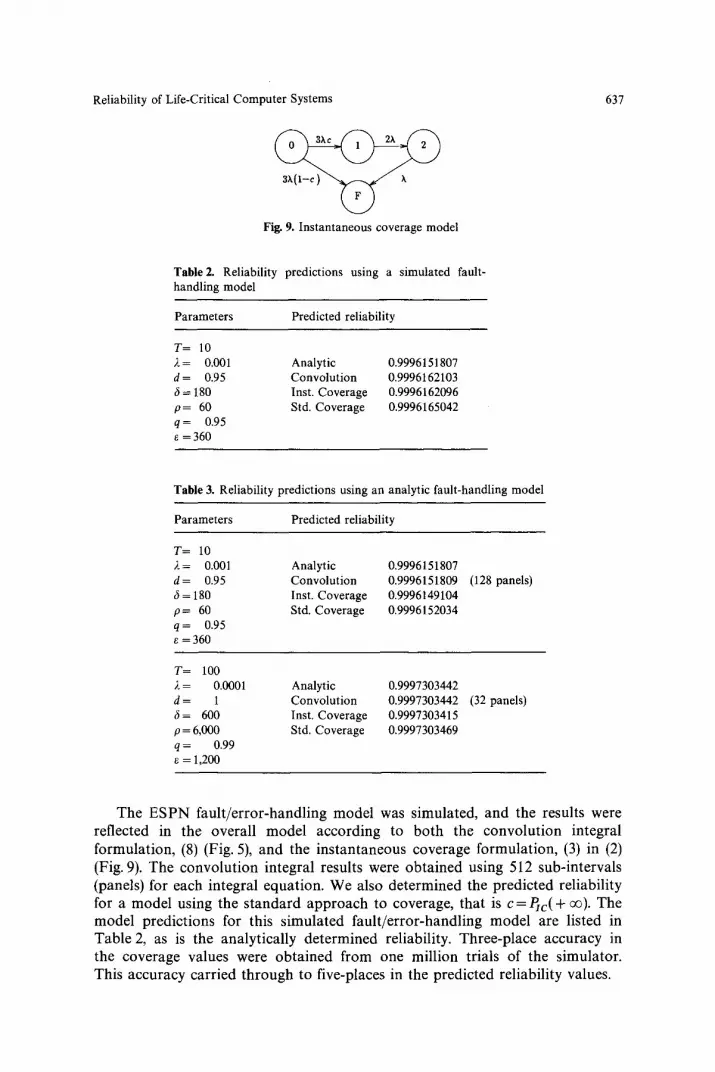
3x(:-c) ~ x

Fig. 9. Instantaneous coverage model

637

Table2. Reliability predictions using a simulated fault- handling model

Parameters Predicted reliability

T= 10 2 = 0.001 d = 0.95 6 = 180 p = 60 q = 0.95 e =360

Analytic 0.9996151807 Convolut ion 0.9996162103 Inst. Coverage 0.9996162096 Std. Coverage 0.9996165042

Table 3. Reliability predictions using an analytic fault-handling model

Parameters Predicted reliability

T= 10 2 = 0.001 d = 0.95 6 = 180 p = 60 q = 0.95

=360

Analytic 0.9996151807 Convolut ion 0.9996151809 Inst. Coverage 0.9996149104 Std. Coverage 0.9996152034

(128 panels)

T= 100 2 = 0.0001 d = 1 6 = 600 p = 6,000 q = 0.99

= 1,200

Analytic 0.9997303442 Convolut ion 0.9997303442 (32 panels) Inst. Coverage 0.9997303415 Std. Coverage 0.9997303469

The ESPN fault/error-handling model was simulated, and the results were reflected in the overall model according to both the convolution integral formulation, (8) (Fig. 5), and the instantaneous coverage formulation, (3) in (2) (Fig. 9). The convolution integral results were obtained using 512 sub-intervals (panels) for each integral equation. We also determined the predicted reliability for a model using the standard approach to coverage, that is c = P~c(+ oo). The model predictions for this simulated fault/error-handling model are listed in Table 2, as is the analytically determined reliability. Three-place accuracy in the coverage values were obtained from one million trials of the simulator. This accuracy carried through to five-places in the predicted reliability values.

638

Table 4. Transient fault iterations

R. Geist et al.

Parameters Failure Convergence 1st fault 2nd fault 3-point RKF45 rate criterion iterations iterations prediction prediction

T= 10 d = 0.95 6 = 180 p = 60 q = 0.95 e =360 z =300 64 panels

10 -4 10 -9 3 2 0.9999697660 0.9999697663 10 -3 10 -9 5 3 0.9996977371 0.9996977726 10 -2 10 -9 7 6 0.9968673403 0.9968703304

2X ~,

2~+(1--q ~ ~ 2 k + ( l - q )~

>Q..~) ' < J

Fig. 10. Three unit model with embedded fault-handling states

Results from the analytic solution to the coverage model were also in- corporated into the aggregate model by the three modeling approaches de- scribed above. The model predictions for two parameter sets using this analytic fault/error-handling model are given in Table 3. We note that for both parame- ter sets the standard approach to coverage yields reliability values that are too optimistic.

Table 4 contains reliability predictions for a three-unit model with coverage submodels defined for both the first and second faults. The state diagram of the model with embedded fault-handling states is given in Fig. 10. The cover- age models are similar to the one used above, but were extended to include transient faults. Solutions were obtained using the Neumann series technique (15). Since no analytic reliability expression is available for the transient case, the convolution integration results are compared with the results of an RKF 45 [7] solution to the defining differential equations.

6. Conclusions

We have shown that the dynamic behavior of a fault-tolerant computer system can be partitioned into fault-occurrence behavior and fault/error-handling be- havior. We utilize this partition, which is based on the several orders of magnitude difference in time constants of the two submodels, in solving an otherwise large and stiff stochastic process. The decomposition also allows us

Reliability of Life-Critical Computer Systems 639

to i n c o r p o r a t e severa l d i f ferent s u b m o d e l types a n d s o l u t i o n t echn iques , as is

d e m o n s t r a t e d in H A R P , w h i c h uses a n u m e r i c a l ana ly t i c s o l u t i o n of the

s tochas t i c p roces s r e p r e s e n t i n g the f a u l t - o c c u r r e n c e b e h a v i o r , a n d a s i m u l a t i v e

so lu t i on o f the E S P N m o d e l r e p r e s e n t i n g the faul t a n d e r ro r h a n d l i n g be- havior . F ina l ly , we h a v e i m p l e m e n t e d m e t h o d s for the eff icient e s t i m a t i o n o f

the effects of v a r i a t i o n (uncer ta in ty ) in the inpu t p a r a m e t e r s on the p r e d i c t e d

re l iabi l i ty .

References

1. Agerwala, T., Flynn, M.: Comments on Capabilities, Limitations and "Correctness" of Petri Nets, Gainesville, FL, pp. 81-86. Proc. First Ann. ACM Symp. Comp. Arch. 1973

2. Bernhard, R.: The "No Downtime" Computer. IEEE Spectrum 17, 33-37 (1980) 3. Conn, R., Merryman, P., Whitelaw, P.: CAST - A Complementary Analytic-Simulative Tech-

nique for Modeling Complex Fault-Tolerant Computer Systems, pp. 6.1-6.27. Proc. AIAA- /NASA/IEEE/ACM Computers in Aerospace Conf., Los Angeles 1977

4. Costes, A., Doucet, J., Landrault, C., Laprie, J.: SURF - A Program for Dependability Evaluation of Complex Fault-Tolerant Computing Systems, pp. 72-78. Proc. 1 lth IEEE Fault- Tolerant Computing Symp., Portland, ME 1981

5. Dugan, J.B.: Extended Stochastic Petri Nets: Applications and Analysis. Dept. Elect. Eng., Duke University, Ph.D. Diss. 1984

6. Dugan, J.B., Trivedi, K., Geist, R., Nicola, V.: Extended Stochastic Petri Nets: Applications and Analysis. Proc. 10th Intl. Syrup. Comput. Perf. (PERFORMANCE '84), Paris, pp. 507-519. Amsterdam: North-Holland 1984

7. Forsythe, G., Malcolm, M., Moler, C.: Computer Methods for Mathematical Computations. Englewood Cliffs, NJ: Prentice-Hall 1977

8. Frank, P.: Introduction to System Sensitivity. New York: Academic Press 1978 9. Froberg, C.-E.: Introduction to Numerical Analysis. Reading, MA: Addison-Wesley 1969

10. Geist, R., Trivedi, K.: Ultra-High Reliability Prediction for Fault-Tolerant Computer Systems. IEEE Trans. Comput. 32, 1118-1127 (1983)

11. Geist, R., Trivedi, K., Dugan, J.B., Smotherman, M.: Design of the Hybrid Automated Reliability Predictor, pp. 16.5.1-16.5.8. Proc. 5th IEEE/AIAA Digital Avionics Systems Conf., Seattle, WA, 1983

12. Geist, R., Trivedi, K., Dugan, J.B., Smotherman, M.: Modeling Imperfect Coverage in Fault- Tolerant Systems, pp. 77-82. Proc. 14th IEEE Intl. Symp. Fault-Tolerant Computing, Orlando, FL 1984

13. Gnedenko, B., Belyayev, Y., Solovyev, A.: Mathematical Methods of Reliability Theory. New York: Academic Press 1969

14. Hildebrand, F.: Introduction to Numerical Analysis. New York, NY: McGraw-Hill 1956 15. Hille, E.: Lectures on Ordinary Differential Equations. Reading, MA: Addison-Wesley 1969 16. Hopkins, A., Smith, T., Lala, J.: FTMP - A Highly Reliable Fault-Tolerant Multiprocessor for

Aircraft. Proc. IEEE 66, 1221-1239 (1978) 17. Iyer, R.: Reliability Evaluation of Fault-Tolerant Systems - Effect of Variability in Failure

Rates. IEEE Trans. Comput. 33, 197-200 (1984) 18. Laprie, J.: Trustable Evaluation of Computer System Dependability. In: Mathematical Comp.

Perf. and Reliability (G. Iazeolla, P. Courtois, A. Hordijk, eds.), pp. 341-360. Amsterdam: North-Holland 1984

19. Macam, S., Avizienis, A.: ARIES 81: A Reliability and Life-Cycle Evaluation Tool for Fault- Tolerant Systems, pp. 267-274. Proc. 12th IEEE Symp. Fault-Tolerant Computing, Los Angeles 1982

20. Marsan, M., Conte, G., Balbo, G.: A Class of Generalized Stochastic Petri Nets for the Performance Evaluation of Multiprocessor Systems. ACM Trans. Comput. Syst. 2, 93-122 (1984)

640 R. Geist et al.

21. McGough, J., Smotherman, M., Trivedi, K.: The Conservativeness of Reliability Estimates Based on Instantaneous Coverage. IEEE Trans. Comput. 34, 6~2-609 (1985)

22. Siewiorek, D., Swarz, R.: The Theory and Practice of Reliable System Design. Bedford, MA: Digital Press 1982

23. Srnotherman, M., Geist, R., Trivedi, K.: Provably Conservative Approximations to Complex Reliability Models. IEEE Trans. Comput. 35, 333-338 (1986)

24. Stiffier, J., Bryant, L.: CARE III Phase III Report - Mathematical Description. NASA Langley Res. Ctr., Langley, VA, Contractor Report 3566, 1982

25. Trivedi, K., Gault, J., Clary, J.: A Validation Prototype of System Reliability in Life Critical Applications, pp. 79-86. Proc. Pathways to System Integrity Symp., National Bureau of Standards, Washington, DC 1980

26. Trivedi, K., Geist, R., Smotherman, M., Dugan, J.B.: Hybrid Reliability Modeling of Fault- Tolerant Computer Systems. Comput. Electr. Eng. 11, 87-108 (1985)

27. Trivedi, K., Geist, R.: Decomposition in Reliability Analysis of Fault-Tolerant Systems. IEEE Trans. Reliab. 32, 463-468 (1983)

28. Trivedi, K.: Reliability Evaluation for Fault-Tolerant Systems. In: Mathematical Comp. Perf. and Reliability (G. Iazeolla, P. Courtois, A. Hordijk, eds.), pp. 403-414. Amsterdam: North- Holland 1984

29. Trivedi, K.: Probability and Statistics with Reliability, Queueing, and Computer Science Applications. Englewood Cliffs, NJ: Prentice-Hall 1982

30. Wensley, J., Lamport, L., Goldberg, J., Green, M., Levitt, K., Melliar-Smith, P., Shostak, R., Weinstock, C.: SIFT: The Design and Analysis of a Fault-Tolerant Computer for Aircraft Control. Proc. IEEE 66, 1240-1255 (1978)

Received February 20, 1986/June 5, 1986

Appendix

Extended Stochastic Petri Nets

A Petri Net is a direct biparti te graph whose two vertex sets are called places and transitions. A marking of a Petri Net is a mapping from the set of places to the non-negat ive integers. The marking is said to assign a number of tokens to each place.

There are certain conventions used in the pictorial representat ion of the vertices of these graphs. Transit ions are typically represented by bars, places by circles, and tokens by small discs within the circles (see Fig. A1). This com- pletes the basic syntax of the Petri Net model ing language.

The semantics of this language consist of a collection of simulation rules. The fundamental rules are as follows: should all arcs into a transit ion emanate f rom places which contain 1 or more tokens, the transit ion is enabled. Enabled transitions may fire, that is, remove 1 token from each input place and add 1 token to each output place. Thus transit ion T in Fig. A1 is enabled and may fire to produce the marking shown in Fig. A2.

Multiple extensions to this basic language have been suggested, each to facilitate the modeling process. In each case, the semantics of the new language (which accompany the change in syntax) are again expressed in terms of rules for simulation. Stochastic Petri Nets represent a modif icat ion of Petri Nets in which exponential firing time distributions are associated to the transitions. When a transit ion is enabled, an amoun t of time determined by a r a n d o m

Reliability of Life-Critical Computer Systems

Fig. A1. Petri net with an enabled transition

641

Fig. A2. Petri net after firing of transition

sample from the associated distribution elapses. If the transition is still enabled at the end of this time period, it fires.

Generalized Stochastic Petri Nets allow both exponentially distributed fir- ing times, as in the Stochastic Petri Net specification, and immediate firing, as in the original Petri Net specification.

Extended Stochastic Petri Nets represent extensions of the Generalized Stochastic Petri Nets in several directions. First, the firing times associated to the transitions may have arbitrary distributions. This includes immediate firing as a special case.

Further, two additional types of arcs are allowed. An inhibitor arc [1] from a place to a transition is syntactically represented by a directed arc whose head has been replaced by a small circle. The associated semantics are as follows: if all standard arcs into a transition emanate from places containing 1 or more tokens, and all inhibitor arcs into this transition emanate from places contain- ing 0 tokens, then the transition is enabled. When such a transition fires, 1 token is removed from each non-inhibitor input place and 1 token is added to each output place.

A probabilistic arc is represented by a bifurcated arc from a transition to a pair of places. One branch of this arc is labeled with a probability, p, and the other with its complement, 1 - p . The associated simulation rule specifies that, upon firing of the transition, a Bernoulli trial (coin-flip) with parameter p is to be performed and the results used to select which output place receives the

642 R. Geist et al.

token. A counter arc from a place to a transition is labeled with an integer value, k. The target transition is enabled when tokens are present in all of its standard input places and at least k tokens are present in the counter input place. When the transition fires, one token is removed from each standard input place, while k tokens are removed from the counter input place. Often associated with the counter arc is a counter-al ternate arc, which enables an alternate transition when the count is between 1 and k - l , inclusive. The alternate transition can fire each time a token is deposited in the counter input place until there are k tokens present. The count remains unchanged by the firing of the alternate transition, as it removes no token from the counter input place. A counter-alternate arc is labeled /~. Neither the counter arc nor the counter-alternate arc represent semantic extensions to Petri Nets, as both can be realized by a cascade of standard places and transitions [-5]. Rather, they are useful syntactic shorthand for such a cascade.

Although these extensions facilitate the modeler's task, with no additional expense in simulative solution, analysis of the dynamic behavior of arbitrary ESPN's can become intractable. On the other hand, our applications to the fault/error-handling behavior of computing systems invariably call for nets which represent stochastic processes having multiple absorbing states, for which our interest is restricted to the probability of reaching each such state and the conditional transition time to each such state. Thus we have sacrificed some traditional Petri Net analyses (e.g. net invariants) to obtain a more flexible modeling tool which can still provide the essential information.