The World of Maps

The Working Group of the International Map Year Editors: F. Ormeling and B. Rystedt © ICA and the authors

The World in your hand. Contribution to Barbara Petchenik Competition 2014 by Anissa Avila (13) Owen Middle School Swannanoa NC (United States). Downloaded from: http://www.explokart.eu/petchenik/

PREFACE Georg Gartner, Austria

Never before so many maps have been produced per day. Maps, especially topographic maps, are used for navigation with the help of satellite systems. Base maps can be used on computers and mobile phones. Indoor navigation, especially in shopping centres, is of increasing interest for the mobile phone industry. More and more decisions are also dependent on maps and the knowledge of geography. The preservation of the environment in a time of climate change is also dependent on maps and geographic information.

Based on a motion from the Swedish Cartographic Society, the General Assembly of the International Cartographic Association (ICA) decided at its Paris conference in 2011 to establish the International Map Year (IMY). The conference of the United Nations Regional Cartographic Conference in Bangkok (Nov 1 2012) asked the ICA in a resolution to organize IMY during the year 2015. In 2014 the United Nations Global Geospatial Information Management (UN-GGIM) body formally endorsed ICA to organize the IMY in 2015 and 2016.

The ICA decided to assign the task of organizing IMY to a working group with Bengt Rystedt as Chairperson and Ferjan Ormeling as Vice Chairperson. Although retired, they are both still involved in shaping the future of cartography. The working group has then been enlarged successively with Aileen Buckley from Esri, Redlands, USA; Ayako Kagawa, UN, New York; Serena Coetzee, University of Pretoria, South Africa; Vit Vozenilek, University of Olomouc, Czech Republic and David Fairbairn, Newcastle, UK.

The objective of IMY is to broaden the knowledge of cartography and geographic information among the general public and especially among schoolchildren. To support this objective, this book has been produced. At schools, the competition between different teaching programs is now heavy, and we hope that the IMY effort will lead to more cartography students in the future.

The book has a broad perspective and covers both production and use of maps and geographic data. Cartography, geographic information, and their adjacent subjects form a broad opportunity for further education and different applications. Cartography and geographic information are to be combined with other disciplines, forming the main subjects of teaching programs. In related fields, we find physical sciences like geoscience including physical geography, geodesy, remote sensing, and photogrammetry. Social sciences like human and economic geography, archaeology and ecology are of interest as well. Knowledge of cartography and geographic information provides many possibilities for interesting jobs. We hope that this book might be useful for many students.

This book has been written by many persons connected to ICA. They did so because of their love of the subject and their interest in cartography. The book is stored as PDF files, chapter by chapter, on the ICA home page. It can be downloaded for free. The copyright of the book belongs to the authors and the ICA. Please respect that. The book has also been translated to French and Spanish. The translation to French has been handled by the French Society of Cartography (CFC) with the help of numerous volunteers co-ordinated by Francois Lecordix. The translation to Spanish has been done in a similar way by a professional translator of the Spanish Society of Cartography (SECFT) co-ordinated by Pilar Sánchez-Ortiz Rodriguez, in collaboration with Antonio F. Rodriquez

and Laura Carrasco, all employee of the National Geographic Institute of Spain. I would like to congratulate the working group and all the authors for their important initiative and work and thank the Swedish Cartographic Society for the initiative. Vienna, October, 2014.

Georg Gartner President of the ICA

Georg Gartner, professor of Cartography at the Vienna University of Technology, President of the ICA and the ICA board liaison with the IMY working group.

Foreword About the Content This book consists of a linked set of chapters which describe a number of aspects of modern cartography. It is possible to read these chapters as separate units, but it is recommended that the book is considered as one publication, which is worth reading through completely.

Activities related to International Map Year (IMY), as promoted by the International Cartographic Association and supported by the United Nations, are diverse in nature and can be directed towards a range of communities, from local groups to international organisations. Similarly, this book (considered as one of these activities) is written to appeal to a broad audience. As there are particular target groups for IMY – school children, the general public, professionals, and government employees and decision makers – it is expected that some chapters will have a stronger interest than others for each reader. This foreword describes each chapter and then suggests ways of reading the book.

Chapter 1 is a general purpose introduction to some of the basic principles of cartography, considering the different types of maps which can be produced along with some of the principles of map making. It also gives a brief overview of how map making developed in previous centuries – but the rest of the book will show that, whilst our heritage is important, maps today are very, very different to maps of the past.

The second chapter considers not the making of maps but their use. Their value as documents and images for a wide range of purposes is presented here. Maps are

used by a large number of individuals, communities, organisations, companies, and governments, in every society on our planet. The nature of maps is appealing, visually, but their main value is in their use for decision making, for navigation, for education, for recreation, for information and for a host of further applications.

Chapter 3 is a more complex description of the type of information that is used to make maps, and also looks at how such information can be managed. The influence of contemporary computing science, in the digital environment within which almost all maps are made today, is widespread. It includes the application of concepts of database management and consideration of how the structure of geographic information can be effectively translated into a graphic map.

The way in which maps are designed has a fundamental effect on how they are used, and how successful they are for the map reader to understand. Maps are graphical objects, whether produced on a computer screen or on a piece of paper, and it is their visual nature that appeals to those who like to look at maps, and those who use maps to help them make decisions. Chapter 4, therefore, looks at this important aspect relatively early on in this book. Covering obvious topics, such as the use of colours, and using words and text effectively on a map, this chapter also considers their layout of maps, their possible uses, and the relationship between the geospatial data and the graphic design of its representation. As always with design, it is by looking at actual examples that we can learn about what is effective and what doesn’t work in a map: this chapter, therefore, has many illustrations.

One common type of map is the ‘topographic map’ – a general purpose map primarily showing the landscape and the environment in which we live and move about. This is the oldest type of map, so there is a brief history about such mapmaking at the end of Chapter 5. The main part of this chapter, however, is a straightforward description of the factors involved in topographic mapping – how to use symbols and present them in a legend, how to determine the scale of the data representation, and how to show the shape of the landscape on a map, through techniques of relief representation.

Chapter 6 also considers design elements: the concentration of this section is on thematic maps, maps which portray a specific topic (e.g. natural vegetation, population statistics, and economic data) on a base map which shows the location of the theme in geographic space. There is an enormous variety of such products and many examples of thematic maps are shown in this chapter. The following chapter, on Atlases, describes the nature of collections of maps and the notable characteristics of this method of presenting geospatial information, particularly appropriate for a classroom setting or as reference works for individual consultation.

The geospatial data which is brought together (‘compiled’) to help the production of maps needs to be assessed for a range of properties before the map can be created. It needs to be timely, appropriately scaled, and, most importantly, accurate. Such accuracy extends to the incorporation of correct and appropriate names. Chapter 8 therefore considers the factors involved in ensuring that the text on a map, particularly that text which attaches names to geographical features, is properly rendered.

Finally, in this section on map creation, the basic spatial framework of every map, its projection, is covered in significant detail, in Chapter 9. This chapter examines the mathematical nature of map projections, but also gives general advice on choosing which projection is most appropriate. It can therefore be read by those who are a bit nervous about mathematical data handling, as well as by those who wish to know the methods by which projections are calculated, and the resultant properties of map projections.

The next section of the book concentrates on the use of maps. One of the main aims of International Map Year is to show the extraordinarily wide range of human activity which can profitably and sensibly use maps. Map use therefore covers numerous possible areas of our everyday life. This part of the book identifies just a few typical examples of organisations and actions using maps. Firstly, the United Nations is examined, to give an indication of how an administrative organisation can use maps for information, for legislation, for operations, and for policy- and decision-making. Then, Chapters 11 and 12 concentrate on a fundamental map use task – navigation – showing how maps and specialist charts can be used to assist with navigation at sea, and then how one can use maps to navigate by foot on the land, notably in the sport of orienteering. The central role of maps in such activities is highlighted.

Maps can be presented in a variety of ways, and the next section of the book outlines the possible methods by which the graphical representation of the environment can be copied and disseminated. Printing of a map is the best way to create multiple, permanent copies of a portable product which can be used in a wide variety of circumstances. Chapter 13 describes printing

technology, whilst Chapter 14 covers the alternative to such output – concentrating instead on ‘temporary’ maps, which are the results of accessing geospatial information on the web, or on mobile devices. The restrictions and the extended possibilities of producing maps using such computer-based technologies are explored. Mobile phones, for example, have small screens which can limit the display of maps; but such devices can display maps which change in real-time and give animated representations of geospatial data.

The fundamental importance and rapidly changing nature of geospatial data in the 21st century, and its impact on the display and distribution of maps is looked at in Chapters 15 and 16. The adoption of standardised flow lines and conventional methods of handling geospatial data is no longer common: there is so much new geospatial data to collect and manipulate; there are so many new ways of doing so; and there is a widening scope for the operations involved in geospatial data management. One particular example, the use of a ‘crowd’ of interested individual amateur map makers to create reliable, extensive, geospatial databases and subsequent maps, is examined in depth in Chapter 17. Currently, much interest is directed to the ways in which those wishing to make their own maps can capture the data in the real world using readily available tools. This approach is a typical example of how mapping is broadening its community of makers and users.

The final section of the book describes how anyone interested in mapping can extend their education in the subject, either formally or informally. Chapter 18 shows the impact of new technologies on the mind-set of a contemporary cartographer, and later there are examples presented of how the subject is tackled in

schools, in colleges, and by individual learners. The possibilities of following courses, or just separate exercises, are presented. This Chapter will be continuously updated with new information.

How to use this book

It is expected that this book will appeal to those who are interested in examining the broad range of products which can be defined as ‘maps’. Thus, school children and the general public, who have a wish to find out what maps can do and how they communicate can profitably follow Chapters 1 and 2 initially. This will give you a sufficient overview of the nature of cartography and the power of maps.

If your wish is to go one step further and actually make your own map, then the practical examples in these chapters will give some ideas. The actual job of compiling data, thinking about map projection, then producing a paper map is followed through Chapters 3 (giving detail about the nature of geospatial data), 4 (the transformation of geospatial data into maps using design procedures), 8 (the handling of geographical names), 9 (the choice and application of an appropriate map projection), and 13 (the way in which maps can be duplicated and printed).

Contemporary methods of mapping using web-based technologies are covered in Chapter 14, although the concepts of accurate data handling outlined in Chapter 3, and expanded upon later in Chapters 15 and 16, still apply. The potential of mapmaking using ‘crowd-sourced’ technologies and systems is outlined in Chapter 17, and this can serve as a template for those wishing to explore such personalised map making themselves.

Administrators and professionals who have a particular interest in the accurate handling and representation of geospatial data should follow Chapters 3 (where data structures and database design are considered), and note the possibilities for mapping specific data types and themes described in Chapters 5, 6 and 7. It should be possible to correctly identify the most effective method of representing geospatial data on a map with reference to the examples given in these chapters, whilst the options available in terms of representing data layers can be understood–symbols, layout and content – can be determined from Chapter 4.

Using maps is the prime concern of those interested in recreational, administrative and scientific applications of geospatial information. Chapters 10, 11, and 12 will be particularly appropriate for those in government, in education, in navigation and in sport, who have the job of communicating geospatial data effectively and using maps in critical situations.

Chapter17 is intended to give advice to young people about how to proceed with an educational programme and a possible future career in cartography. This chapter can be read by itself: it contains a few example exercises to show school children who may not have been exposed to the subject in depth at school, that this is an interesting and worthwhile route to employment in an exciting discipline. Chapter 18 is intended to give further reading tips and is intended to be updated.

Acknowledgement

Specially thanks to all the writers of the chapters and their organisations for their support to allow them to spend time for writing their chapters.

We would also like to thank the ICA commissions and the affiliate members Esri and the UN Cartographic Section for their support to the book.

Olomouc, Czech Republic in February 2014. The IMY Working Group Bengt Rystedt, Ferjan Ormeling, Aileen Buckley, Ayako Kagawa, Serena Coetzee, Vit Vozenilek and David Fairbairn

Bengt Rystedt

Ferjan Ormeling

Serena Coetzee

Aileen Buckley

Vit Vozenilek

David Fairbairn

Table of Content Preface. Georg Gartner, President of ICA Foreword. Working Group Table of Content Introduction and Summary 1. Cartography, Bengt Rystedt, Sweden 2. Use of Maps and Map Reading, Ferjan Ormeling, Netherlands 3. Geographic Information, Bengt Rystedt, Sweden How to Make Maps 4. Map Design, Vit Vozenilek, Czech Republic 5. Topographic maps, Bengt Rystedt, Sweden 6. Thematic Maps, Ferjan Ormeling, Netherlands 7. Atlases, Ferjan Ormeling, Netherlands 8. Geographical Names, Ferjan Ormeling, Netherlands 9. Map Projections and Reference Systems, Miljenko Lapaine, Croatia and Lynn Usery, USA How to Use Maps 10. Map Use at the United Nations, UN Cartographic Section 11. Setting one´s Course with a Nautical Chart, Michel Huét, Monaco 12. Maps for Orienteering and for Finding the Cache, Lazlo Zentai, Hungary How to Present Maps 13. Printing Maps, Bengt Rystedt, Sweden 14. Web and Mobile Mapping, Michael Peterson, USA Geographic Information 15. Geographic Information, Access and Availability, Aileen Buckley, USA and Bengt Rystedt, Sweden 16. Volunteered Geographic Information, Serena Coetzee, Republic of South Africa Education and Further Information 17. Education, David Fairbairn, UK 18. Further Information

1 Cartography

Bengt Rystedt, Sweden

1.1 Introduction Cartography is the science, technique and art of making and using maps. A good cartographer can not only have a good knowledge in science and technique but must also develop the skill in art when choosing types of lines, colour and text.

All maps are intended to be used for either navigation by foot, vehicles, or for describing spatial planning or for finding information in an atlas. Maps are very useful and never before have so many maps been distributed in many different information systems. The map is an efficient interface between a producer and a user, and by using GPS many things can be located on a map.

For a long time paper has been the most common material for maps. Nowadays, most maps are produced by using cartographic software and are distributed via Internet, but the cartographic rules are the same for all types of distribution. In this book we will describe how maps are produced and used, and how they are distributed, and how to get the needed data.

1.2 Different Types of Maps The map deals with two fundamental elements: position and its attributes. Attributes may be occurrence, activity, incident, amount and changes over time. From the position and its attribute many relations may be described such as distance, dissemination, direction and variation, and combinations of different qualities such as income per person and level of education in different places. Different types of maps gives parts of this

spectrum, and maps have the function to present these fact in a feasible manner. Maps have different scales, functions and contents and can be grouped as follows:

1. Topographic maps showing spatial relations between different geographical phenomena such as buildings, roads, boundaries and waters. Official topographic maps are produced by the National Mapping Organization (NMO). Most cities are also producing city plans. Topographic maps are also produced for special use in biking and canoeing. Many car navigation systems and services on Internet also provide topographic maps. Topographic maps are also used as background maps in property mapping and in maps for presenting the geographical aspects in spatial planning.

2. Special maps e.g. Sea Charts and maps for flying. These maps are for professional use and standardized by the UN. There are also specific sea charts for private use and special maps for orienteering, standardized by the International Orienteering Association (See Chapter 12). The Metro Map of London is also a special map.

3. Thematic maps contain descriptions of the geographical phenomena such as in geology (esp. soil and bedrock), and in land use and in vegetation. Statistical maps are also thematic maps. They show the geographical distribution of a statistical variable. See Chapter 7 Atlases for more information on statistical maps.

1.2.1 Thematic Maps The weather map is the most common thematic map. Weather maps are presented every day on the TV for showing the present weather and for prediction of the weather. Weather maps can also be used for showing the movement of hurricanes and snowstorms, and in risk management for showing risks in flooding, draught and landslides. Weather maps are becoming more and more useful in showing the effects of the Climate Change, e.g. the melting of the polar ice. A lot more information can be found on the Internet.

Geological maps are thematic maps and very valid for finding minerals and oil, and the conditions of soil. They include rather complicated information and several geological map sheets are included in the result of doctoral studies in geology.

Atlases, however, have many types of thematic maps. The most common one is the choropleth map (choro for place and pleth for value) for showing the geographical distribution of a statistical variable in a given set of areas. As an example the population density per municipality can be shown in a choropleth map (See Chapter 7, Figures 7.11 -12). Start with making a table with the columns: municipality area identifier, the area, the size of the population, and perhaps also columns for the population divided in different sex and age groups. Open then a mapping or a geographic information system (GIS) software, where the boundaries for the municipalities should be given. The population density must also be given in different classes. It is important to have almost the same amount of objects in each class. Colour should be chosen to get a low intensity for low population density and darker intensity for a higher density. For a detailed information on colour choice see

1

Brewer (2005). It is also possible to use Google Earth for the construction of choropleth maps. The divisions into age groups can be used for construction of diagram maps and maps with pie charts (See Figure 1.1).

Figure 1.1 shows a thematic map with diagram and pie charts. © Diercke International Atlas (p. 48).

1.3 Cartographic Principles 1.3.1 Map Design Maps like all other products must be designed before production. The design process is an iterative process and starts with a demand process telling the theme of the map and how it shall be used. The cartographer takes over and make a proposal that is tested on the criteria that have been given. When the demands are satisfied the map can be produced. The map design process is described in Figure 1.2. See also Chapter 4 and Anson and Ormeling (2002).

Figure 1.2. The design process starts with Map order. When the manuscript satisfies the demands it is time to go to production.

1.3.2 Symbolization Symbolising means to use correct symbols in form and colour for the objects that will be represented. A map has different symbols and text. The symbols are used for describing some part of the reality, while the text is used for a more detailed description of the object that are depicted in the map.

Seen in a geometrical concept there are three types of symbols: point symbols, line symbols and area symbols (Examples of point, line and area symbols are given in the legends of e.g. topographic maps. In Figure 13.1, houses are shown as points, road as lines and land use as areas). The symbols may also vary in abstraction. The simplest symbols are the pure geometric ones. They

represents their reality objects by showing their geometric and geographic attributes; a road is shown by lines and a lake by a polygon and so on. It is also possible to give more information. By giving the symbols different colours and different patterns it is possible to let area symbols represent different types of forest and let line symbols represent roads of different class (See Figure 13.1). Also more abstract symbols, e.g. figurative symbols or icons, may be used as point symbols. These symbols are very useful in city plans and tourist maps (Figure 1.3).

Figure 1.3 shows different icons for drug store, bathing place, camping site, road for biking, golf course, track for jogging with light, remarkable site, historical site and a geological site. © Lantmäteriet Dnr R50160927_130001.

For more information on graphics and symbolization, it is possible to have a detailed study of Bertin´s Semiology of

2

Graphics (Bertin, 2011). The book is rather complex, but it is provides a good opportunity for someone who wants a full description of the graphic issues that cartography deals with.

1.3.3 Text The text is an important part of the map and makes it easier for the user to understand the map. Typographical guidelines must be followed in order to achieve an understandable map. The typography includes dealing with fonts, size, colour and placement.

There are many fonts that can be used, but on the map their number should be limited to a few. The size should never be less than six points in order to be legible. Colour may be used to distinguish between different types of object, e.g. black for place names, blue for waters and green for nature objects. For a river the text should follow the line of the river. The name of an ocean may be curved to indicate that the area of the ocean is big. The placement should also indicate where the object is located. The name of a city should be placed upon land and the name of a lake should be placed in the lake. More information about typography is given in Chapter 13 Printing Maps.

1.4 Visual Hierarchy and Communication 1.4.1 Visual Hierarchy

When studying a map we found different information layers and that one layer is more visual forming the foreground of the map. The background of the map gives the location and orientation to other objects of the map. A topographic map for car driving has the roads in the foreground. In atlases that is more obvious. The

theme of the map is in the foreground and the topography is in the background mostly for orientation.

The best way to handle visual hierarchy is to use colour. More intense colours are used for the foreground that is the theme of the map, and less intense colours for the background. In a map for car navigation the roads would be depicted with stronger colour. Also icons may be used to strengthen the foreground. City plans for visitors have icons to make things such as hotels and restaurants more obvious.

1.4.2 Communication

In many communication processes maps as well as text, diagrams and images are important tools for giving a user important information about geographical aspects of the realty. There are, however, many realities. A topographic map represents the physical landscape, a geological map represents the geological landscape, and a demographic map the demographic landscape. The map is a model of the reality as the cartographer understand it. The cartographer uses a cartographic language to produce the map to be read by a map user. Here we see a problem. The map user may not have the same view of the reality. In Figure 1.4 we see that the realities as seen by the cartographer and as seen by the user of the map are different.

Figure 1.4 shows a model of the communication process and that there are a different view of the reality between the user and the cartographer.

1.5 Scale and Projection 1.5.1 Scale

A map may be seen as a description of the real world into a symbolical form but also in a geometrical form. The chosen scale of the map is a compromise between the amount of object that will be given and the view that will be given in order to give an understandable geographical context. Scale indicates the ratio between the length of a given distance in reality and the length of that distance as represented on the map. If a distance of 8 kilometres is rendered on the map by a length of a line of 4 cm, the scale of that map is 4cm/8km or 4cm/800,000cm = 1:200,000

On a map with a larger scale, such as 1:50,000, that line would be longer 16cm) and on a map with a smaller scale (such as 1:1,000,000), that length would be smaller (0.8cm). It is also obvious that a small scale map (which has less space on the paper or screen for the same area)

3

is more generalised than a large scale map. A meandering river may not be shown in detail in a small scale map. It is the same with shorelines. When measuring the length of a shoreline in a map, the scale must be given. In the real world, the length of a shoreline is unlimited. For any length given it is possible to get a longer length by being more detailed.

Automatic generalisation is difficult, but it is introduced more and more. In some countries, e.g. United States of America, large scale topographic maps are generalised stepwise into smaller and smaller scales.

1.5.2 Projection The Earth is almost a sphere and it is not possible to represent the image of this spherical Earth on a flat paper or screen without distorting it. The systematic way of rendering it two-dimensionally is called a projection. Mercator projection (See Figure 1.5), with Europe and Africa in the middle distorts, as areas with longer distance from the equator are progressively exaggerated. From a map in this projection, it is easy to understand why America is called the West and Japan the Far East. The concept of Western and Eastern countries cannot be understood in any other way.

Projections, fully described in Chapter 9, may be classified into cylindrical, conic and azimuthal ones. Here only the cylindrical one will be described. In that projection the Earth is put into a cylinder with the equator brushing the cylinder. When we project each point on the Earth surface from the centre of the Earth on the cylinder, this projection is called the Mercator projection. If a meridian brushes the cylinder however, we get a transverse Mercator projection. The transverse Mercator projection is often chosen for national

topographic maps. For large countries many such projections must be used with different meridians chosen. There is now a standard, Universal Transverse Mercator (UTM), with 60 zones around the Earth giving each zone a band of 6 degrees in longitude.

A Mercator projection with the equator as reference results in exaggerated areas in the higher latitudes, and the poles even become straight lines. Hence, that projection is not an equal area one. But, on the other hand, it is conformal: angles measured on the map are the same as measured on the Earth. If a compass direction is taken e.g. over the Atlantic from Norway to Rio de Janerio and the compass direction is always followed, the goal will be reached. However, that route is not the shortest one. The shortest line forms a bow as can be seen in Figure 15.13.

The original Mercator projection is not so usable in practice. But if you are very British you may want to see an area-exaggerated image of the Commonwealth, as Canada and Australia are partly located in higher latitudes. For Atlases an equal area projection is wanted such as the Mollweide´s projection (See Figure 1.5).

When mapping it is important to know the location in both latitude and longitude both on Land and Sea. The latitude has for a long time been found by reference to the stars, the Polar star in the Northern hemisphere and the Southern Cross in the Southern hemisphere. The longitude is more difficult to find without a correct time. In mapping, old maps frequently have the wrong distance in a West East direction as compared to the more correct distance in a North South direction. In sailing, many ships were wrecked because the navigator could not measure the longitude in a correct way. With

the use of modern technology such incorrect measurements of latitudes are avoided. A GPS give both location and a correct time.

Figure 1.5 shows the World in two different projections. Above is Mercator´s conformal projection (angle correct) and below is Mollweide´s projection (equal area). Source: Esri.

The next phase in mapping is to determine a coordinate system, where longitudes and latitudes measured on the Earth can be transformed to planar coordinates for drawing the Earth or part of it in two dimensions such as on a paper sheet. That is a rather complicated problem and many decisions must be taken regarding the shape of the Earth in order to get a good mathematical solution. Nowadays, we have a solution called the World

4

Geodetic System, established in 1984 (WGS84). This system is also used in Global Navigation Satellite Systems, of which GPS is the best known one. In order to use the map in navigation the reference frame must be noted on the map in the form of longitudes and latitudes measured in accordance with WGS84.

Land surveyors use the geodetic network to determine positions of points in their measurements. When a new land parcel is going to be created, accurate positions for all corners must be found and their location should be given in the coordinate system. References must also be given so the location of that point can be recalculated.

More information on projections and coordinate systems can be found in Chapter 9 Map Projections and Reference Systems.

1.6 Different Map Media

The oldest maps were made on clay plates and found in Babylon. Maps have also been found graved in stones along the Silk Road to show where the camels of the caravans could get water. In Jordan there are maps in mosaic. Early maps have also been produced on papyrus and rice paper. In a museum in Olomouc, Check Republic, there is a map written on a Mammoth task supposed to be a hunting map. If that is a map it is the oldest map found dated to 25,000 BC.

However, for a long time ordinary paper has been one of the most common map media. But now, the screens on computers and mobiles are the most common ones and the web is the most popular platform for communicating information in map form.

1.7 Historical Maps

1.7.1 Antiquity The first known cartographer was Klaudios Ptolemaios, a Greek who lived in Alexandria, Egypt. He died about AD 165 and he knew that the Earth was round, a fact that later on was denied by the Church. He was a scientist in astronomy, geography, and mathematics. In geography, his most important work was the Geographia, a manual that showed what the Romans knew about the world in his time, combined with a guide how to produce world and regional maps (see figure 1.6), for which he collected the coordinates of some 8000 towns and other geographical objects. Figure 1.7 shows an 11th century manuscript of his Geographia, in the original Greek, preserved in the Vatopedi monastery on Mount Athos in Greece.

Figure 1.6. Ptolemaios´s world map. In the centre, the Arabian peninsula and the Nile are depicted. Source: Wikipedia.

Figure 1.7 shows Ferjan Ormeling studying the Geographia at Mount Athos, Greece, in May 2006. Photo: Bengt Rystedt. Figure 1.8 shows a road map with the military roads used for transportation of soldiers and distribution of messages in the Roman Empire. A series of forts and stations were spread out along the major road systems connecting the regions of the Roman world. The relay points provided horses to dispatch riders for a post service. The distances between the points are also indicated. The map is believed to have been created during the fifth century. The map was forgotten and discovered in a library in Worms and then handed over to Konrad Peutinger in 1508, after whom the map is now called. The map is now conserved at the National Library in Vienna, Austria. Note that the Mediterranean looks like a river, so the scale in the North–South is smaller than in West–East.

5

The whole map can be seen at http://upload.wikimedia.org/wikipedia/commons/5/50 /TabulaPeutingeriana.jpg.

Figure 1.8 shows a part of the Peutinger map. The height of the original map is 0.34 meters, the length is 6.75 meters and it covers the area from Portugal to India. Source: http://en.wikipedia.org /wiki/Tabula_Peutingeriana. In roughly the same period in China, under the Han dynasty, scientist Zheng Hang developed a grid system on which he mapped his country.

1.7.2 The Medieval Time Arabian scholars followed the antique knowledge and took care of the work of Ptolemaios, but the theologians of the Christian church tried for incorporation of cartography into a religious frame. During the period 300 to 1100 AD, cartography declined in Western countries. However, some maps have been produced and several maps are covering the known antique world. A diagram with the letter T in an O, equal to the surrounding ocean, was constructed (see Figure 1.9). If the island Delos earlier had been the centre of the world, it was now Jerusalem.

Figure 1.9 A diagram showing a medieval T-O-map oriented towards the East. The horizontal line is the Don and Nile rivers. The vertical line is the Mediterranean. O represents the surrounding ocean. Source: Ehrensvärd (2006, pp. 26).

Independent from these religious T - O maps, in the 13th century mariners from Italian ports developed highly accurate charts of the Mediterranean, called portolan charts (see figure 1.10). At this moment it is not known from where they derived their knowledge and techniques (Nicolai, 2014).

Figure 1.10 The portolan chart by Diogo Homem (1561). Source ICA, 1995, pp. 93.

6

1.7.3 Renaissance and beyond

In the first half of the 16th century land surveying techniques were developed that enabled surveyors to accurately survey towns, provinces and countries. During the Age of Discovery Europeans were able to establish direct contact with inhabitants of other continents and map their territories, with the help of celestial navigation techniques.. Similtaneously, of an increasing number of towns outside Europe the coordinates were measured enabling cartographers to produce more and more detailed and accurate maps. In the beginning of the Age of Discovery it were the Portuguese, Spanish and Italian cartographers that produced manuscript maps of the new doscoveries. From the second half of the 16th century cartographic publishing houses developed in Flanders and Amsterdam, where Ortelius and Blaeu published lavishly decorated European and world atlases, consisting of small-scale overview maps..

Simultaneously, large-scale property or cadastral mapping also flourished, its results can be found in different archives. The most detailed ones are the property or cadastral maps that can be found in Survey Archives. A paper by Rystedt (2006) shows how the Survey Archive of Sweden has been used to give an overview of the development of property mapping in a village of Sweden. These detailed maps are also of great interest when earlier generations are looked for. The early emigrants, to e.g. the USA, have many descendants that want to find out their forefathers relatives and where these lived. The property maps were called geometric maps and were used to construct geographic maps at a smaller scale. Maps of early defence constructions are also common and can be used for the same purpose.

City Plans can be found in City Archives; they show how cities have been rebuilt at different times, giving a good understanding of the development of the municipality.

1.7.4 Well-known Cartographers

Zhang Heng (AD 78-139) was a Chinese cartographer, living during the Han dynasty, to whom the establishment of the Chinese grid system in cartography is attributed. See: http://en.wikipedia.org/wiki/Zhang_Heng

Abraham Ortelius (1527 –1598) was a Flemish cartographer and geographer, generally recognized as the creator of the first modern atlas, the Theatrum Orbis Terrarum (Theatre of the World). He is also believed to be the first person to imagine that the continents were joined together before drifting to their present positions. See: http://en.wikipedia.org/wiki/Abraham_Ortelius.

Joan Blaeu (1596-1673), a Dutch cartographer, not only produced maps, but he also collected maps, which he redrew and printed in his company. (http://en.wikipedia.org/wiki/Joan_Blaeu).

Another European is Johann Babtist Homann (1664-1724), a German geographer and cartographer. He produced many maps, but also collected maps, which he redrew and published together with his own maps in his own publishing house, (http://en.wikipedia.org/wiki/Johann_Homann).

Ino Tadataka (1745-1818) was a Japanese surveyor and cartographer, the first to produce a complete map of Japan using modern surveying techniques. See: http://en.wikipedia.org/wiki/In%C5%8D_Tadataka

References

Anson, R. W. and Ormeling, F., J., 2002: Basic Cartography for students and technicians (Volume 2). Butterworth & Heinemann, Oxford, England. ISBN 978-0750649964.

Bertin, J., 2011: Semiology of Graphics, Esri Press, Redlands, USA. ISBN 978-1-58948-261-6.

Brewer, C. A., 2005: Designing Better Maps: A Guide for GIS Users. Esri Press, Redlands, USA. ISBN 978-1-58948-089-6. Diercke International Atlas 2010. Westermann, Brunswick, Germany. ISBN 978-3-14-100790-9. Ehrensvärd, Ulla (2006). Nordiska Kartans Historia (The History of the Nordic Map). Art-Print Oy, Helsingfors, Finland. ISBN 951-50-1633-9. ICA, 1995: Portolans de col-leccions espanyoles. Institute of Cartography de Catalonia. Barcelona, Spain. ISBN 84-393-3582-2. Nicolai, Roel (2014) A critical review of the hypothesis of a medieval origin of portolan charts. Thesis, Utrecht University, Netherlands. Rystedt, B., 2006: The Cadastral Heritage of Sweden. http://www.e-perimetron.org/Vol_1_2/Vol1_2.htm

7

Chapter 2 Map Use and Map Reading

Ferjan Ormeling, Netherlands

Maps can have many functions: they are used for instance for orientation and navigation, they can be used for storing information (inventories) for management purposes (such as road maintenance), for education, terrain analysis (is a site suitable for specific purposes?) and decision support (is it wise to build a town extension in a south-westerly direction? Or to build a new supermarket in that low-income area?). This chapter will give some examples of what maps can contribute.

A. The map as a predictive tool (for navigation and orientation)

With a topographic map (which describes the nature of the land and the man-made objects on it, see figure 2.7 and chapter 5)) of an area you are about to visit, you can deduce in advance the nature of the terrain you are going to visit. Most important will be what the route/road will be like: will it be straight or have many bends, will it be steep, uphill or downhill? What kind of human settlements will you be passing on your trip? You can find out their number of inhabitants from the size of their names on the map!). What will the countryside be like? What kind of vegetation, parcellation, crops, will there be? Will you have to cross rivers or pass through forests? What man-made objects will you sees on the way – factories, canals, railways (infrastructure), and what kind of cultural environment or cultural heritage objects (castles, monuments, religious sites) will you find on your way? And will you be able to pass everywhere, or would there be restrictions, such as boundaries, or roads that are open only part of the year? And where

will you have to go if you are in trouble (police stations, municipality offices, fire brigade, hospitals, etc.).

The kind of map you would have to bring with you, on paper or on a display, would depend on your mode of transportation, whether you would be walking, cycling, or going by car. For walking, a map on the scale 1:25,000 would be deemed suitable (if available), for cycling the optimal scale would be 1:50 000, for motoring 1:200,000 (and for planning a long trip a map 1:1,000,000).

From the topographic map one may for instance derive information on distances, directions and slopes. The contour lines on these maps (formed by the intersections between parallel planes and the earth surface, (see figure 2.2), would allow you to find out the height of any point on a map. The slope then can be deduced from the difference in height and distance between two points on the map. First, from the orientation of the height figures with which the contour lines are labelled, one can see whether in a specific direction the slope goes up or down (figure 2.3).

Figure 2.1 Map functions. (Drawing A.Lurvink).

Figure 2.2. The principle of contour lines. (©HLBG).

The procedure to assess the height of a specific point is done by interpolation: In this case point A is located on the 490m contour line, so its height is 490m; point B lies halfway two contour lines with the values 510 and 500 respectively (see figure 2.4). If the scale of the map is 1:6.000 and the distance AB is measured by a ruler to be 5 cm, the actual distance in the terrain between the two points would be 6.000x5cm= 30.000cm=300m. If the two points A and B are 300m apart and their heights are 490 and 505 m, their height difference is 15m.

Figure 2.3. The meaning of contour labels. (©HLBG).

1

Figure 2.4. Assessing a point’s height through interpolation. (©HLBG).

The slope between these two points can be expressed as a fraction (or ratio) between the horizontal distance (rise) and the vertical distance (run), here 15/300 or 1:20. Slopes can also be given in percentages, for which one must assess the number of vertical units for every 100 horizontal units. For 300/3=100m run the rise would be 15m/3=5%. Finally, the slope can be expressed in angles, which are given in degrees. In the triangle in figure 2-5 formed by the horizontal and vertical distances, the angle is expressed as the trigonometric tangent of the slope angle. In a goniometric table, this value can be retrieved and is found to be 3° (degrees). A slope of 100% corresponds to a 45°slope (see also figure 2.5).

Why are slope values relevant? Because they will decide whether you will be able to pass that specific road or track, walking, cycling or motoring. Slopes of 1:40 (or 2,5%) are already almost too steep for trains; slopes of 1:10 (or 10%) are too steep for cycling and one would have to get off one’s bike; slopes of 1:3 (or 33%) would be almost too steep for a 4-wheel drive car (see figure 2.6). From the relative location of the contour lines we

Figure 2.7. Topographic map, with information categories highlighted. (©www.lgl-bw.de).

can deduce the slopes of the terrain: if they are close together it will be steep, if they are further apart the slopes will be more gently.

Figure 2.5. Slope measurement diagram. VD means vertical distance, HD horizontal distcance.(©Muehrcke, Map Use)

Figure 2.6. Slope effects. (©NSW Dept. of Lands).

2

Now that we have found the road to be passable, we can assess what we will encounter or see from the road: the natural and man-made environment, the infrastructure, cultural objects and restrictions like boundaries, off-limits roads or areas, railway crossings, ferries or tunnels. In figure 2.7 we can see what kind of individual objects can be seen from the road, like power lines, motorways, agricultural roads, orchards, vineyards, separate houses, greenhouses, factories or TV towers.

We will be further helped in our navigation by conspicuous buildings or terrain characteristics on the

map that are easy to recognise in the field, such as a fork or crossroads, conspicuous buildings like churches, mansions or towers, rivers or the bridges over them.

The very names on the map provide information as well: different object categories have different letter styles. River names may be blue and tilting backwards, names of small villages black and leaning fore wards, names of cities rendered in capitals, the size of the fonts indicative of the number of inhabitants of the named place.

Some countries denote the land use on their topographic maps by colours, other by repetitive symbols. Forests usually are rendered green on the map, with symbols added to indicate whether they are coniferous, deciduous or mixed. In Eastern European topographic map extra information is added by showing the average height, circumference and inter distance between the trees for every forest patch.

B. Maps as links in information systems Maps in atlases (see chapter 7) also can be regarded as geographic information systems (see chapter 3 for digital

GIS´s). Just compare the kind of information that can be read off different school atlas maps: in order to learn more about a specific area, like the Algarve in Portugal, on an general overview map in a school atlas (figure 2-8), which shows it as a coastal plain with a hilly hinterland up to 900m with the town of Faro as the main centre, we

Figure 2.9.Inset map of the Bos atlas showing agriculture. (Bosatlas 31sr ed., 1927).

Figure 2.10. Inset map shopping climate.(Bosatlas 31st ed.,1927).

Figures 2.8. The Algarve, in the south-western Iberian Peninsula according to the Bos atlas. (47th ed., 1971).

should link it on the basis of its location to other maps that show this area. If we link it to an agricultural map (figure 2.9) that also shows the Algarve, for instance, we would see that its coastal areas have Mediterranean agriculture (cereal growing and vineyards) and the inland hills would have animal husbandry (esp. goats). A map on the occupational structure would show that the Algarve has an exceptionally high percentage of people working in the services sector, which means, considering its seaside location, in Tourism. From a climate map (figure 2-10) we would see that the area is reasonably humid; likewise that the population density is till rather low (110), when compared to the European Union (150) average. From a soil map of the region it can be deduced that there are terra rossa soils. It can all be deduced from various atlas maps, although the process to do so is rather laborious and roundabout.

3

Figure 2.11. The Algarve according to the Alexander Atlas. (©Ernst.Klett Verlag GmbH).

It is conceivable to include more information in the overview map. The Alexander Atlas from Klett publishers would be an example (see figure 2.11). As the map has more detail, it has the advantage that specific terrain forms can directly be associated with specific land use or land cover forms. The map shows that the Algarve coastal plain has citrus growing and fruit trees, that

land irrigated from the Guadiana reservoirs. The forests show a blue tree symbol denoting oak trees. Their bark is a resource from which corks are produced. There is a clear difference between the Portuguese Algarve coast and the neighbouring Spanish coast, which cannot be deduced from figure 2.7, with its height layer zone colouring. The scheme in figure 2.12 shows additional differences in expression and related information density.

The advantage of the Alexander atlas is that it shows local links or connections. It doesn’t teach you, however, to establish links between the various data sets or maps that is to establish the locations or addresses as links. But the maps themselves are little wonders of well- integrated and perfectly legible mapped information.

Figure 2.12. The kind of information different paper atlas information systems might provide on a region.

So we can oppose the analytical approach in the Bosatlas, which shows on each map ‘where is that phenomenon?’, enabled by the fact that phenomena are shown in isolation (either height layer zones or agriculture or climate, etc) and the synthesis-approach by the Alexander atlas (‘what is there?’). The graphical approach by the latter invites one to make a journey of discovery through the area (describe for instance what you will see on a biking trip from Faro northwards). But one should realise the drawbacks of this method as well: in industrialised areas the overlapping symbols used mask land use, and nothing is communicated about the tertiary (services) sector, which in this tourist area is so important. For getting to deal with information systems, the prior approach might be more effective.

4

Figure 2.13. Sugar production atlas spread from Canet’s Atlas de Cuba (1949).

A third approach is to combine all information that is relevant to a specific topic, like sugar in Cuba (figure 2.13). Here on this atlas spread (a double page related to one specific theme) both the actual sugar factories, the transportation network to get the sugar to the ports, and the counrties where it is exported to are shown, with diagrams illustrating which part of the arable land and of the workforce is used for sugar production.

Climate data

If you would like to know what is the best month to visit a country, based on the likelihood of rain occurring during your trip, try the following FAO website: http://www.fao.org/WAICENT/FAOINFO/sustdev/EIdirect/climate/EIsp0022.htm. It is an animated map which shows for every month the amount of rainfall expected, based on thirty years averages. In order to answer the question one would have to identify the country first, and then look at the rainfall patterns changing over time.

Should the animation run too quickly, then it is also possible to look at the individual maps produced for each month, like the one in figure 2.14.

Figure 2.14. FAO world rainfall map for the month of April.

C. Maps as inventories or switch boards

In order to speed up urban renewal, many cities have information services for their citizens on which these can indicate where something is amiss. After entering the website of Rotterdam municipality I asked for the Utrechtsestraat, which then came up, large scale, allowing me to pinpoint the location of a malfunctioning lamp post. For easier reference the house numbers are also given. In figure 2.15 this is shown. On the basis of such reports the municipal maintenance services can better plan their operations.

Figure 2.15. Map for reporting damaged ‘street furniture’. (©Rotterdam municipality).

Another example would be the cadastral map: if I would like to know the current value considered appropriate for my house, I would consult the municipal website where I can log in and find out for what amount my house is assessed by the municipality. It would also show the assessments of similar houses in my neighbourhood. Figure 2.16 is an example of such a cadastral map. The black numbers in the parcels refer to a list, the ledger or land register in which are indicated the names of my wife and me as the owners of the house, any outstanding mortgages and the amount for which we bought it, and the date of the purchase.

5

Figure 2.16. Extract of a cadastral map. Black numbers are cadastral numbers of parcels; red numbers refer to street addresses.(©Kadaster Nederland).

Soil maps2- are another form of inventories in which geospatial knowledge has been stored. Soil maps display soil units, that is areas that have the same soil characteristics, such as depth of the various soil layers, percentage of humus in the soil, chemical composition, permeability, ground water level, etc. The suitability for specific crops such as barley or sunflowers of a given area would depend on these soil characrteristics, combined with climate data such as the amount of rainfall and the length of the growing season (number of consecutive days with a temperature above 5° C). The soil map (see figure 2.17a) won’t give an immediate

answer regarding this suitability, but when you address the characteristics of each soil unit (these would be stored in the codes applied to the soil units on the map or in the dataset on which the map is based) and tick off the requirements for the crop you want to raise, then the system will highlight those areas that would be suitable (figure 2.17b).

Figure 17a - Soil map; all soil units have codes that show its characteristics for a number of parameters. In 17b, those soil units are suitable for the crop we want to raise, that are from the R soil family (so their code starts with a R) and have drainage characteristic d (see second position of the codes).

D. Map use steps

In all these map use cases, the first step was to find the proper map for the assignment: a topographic map (see chapter 5) or thematic map (see chapter 6), a large-or small scale one, etc. The next step would be to find out how the information was visualised (what symbols are used for which information categories or objects), and only then would one be able to find out relationships between relevant objects, to recognise locations and see what their characteristics are. All these steps are a part of map reading.

A step further would be map analysis. That would entail doing measurements (of slopes, distances, directions, surface areas, etc.) or counting objects. Finally, when I would try to explain the situation (why are these objects concentrated there? or Why are the southern slopes of that mountain range forested and the northern slopes not?) my actions would be part of map interpretation, trying to find the reasons for a specific geographical distribution of objects or phenomena. In the case of the southern forested slopes, this might be because of prevailing southern winds that would bring rains to the southern slopes, a higher temperature, or measures against tree-eating animals, etc.

6

In all these cases the map tells you something about the mapped area without the necessity of actually going there yourself.

Figure 18 Maps as a window opening up reality (drawing A.Lurvink).

7

3 GEOGRAPHIC INFORMATION Bengt Rystedt, Sweden

3.1 Introduction

With Geographic Information we mean information that has a geographic location. The location must be given in a mathematical form that can be used in a computer. The most useful one is longitude and latitude. The location is described more in the next chapter. An easy way to describe how geographic information is handled in a computer is to think in layers (see Figure 3.1), where the landscape is seen in different layers. Then you can continue with the topographic layers with one layer each for administrative areas, roads, lakes, rivers and so on. Thematic data describing geology, land use and vegetation may be other layers. In Figure 3.1, you see the principle of a digital landscape model based on different layers. This idea to organize geographic data was first introduced in Canada in the 1960s when the Canada Land Inventory was built as a fundament for all kind of spatial planning and for the management of national resources. The layers give the geographical dimensions but these must also have attribute data, which are stored in relational tables. An area in the layer and its attribute data are connected with a unique identity normally called the identification number. A great step forward in handling geographic information and making geographical analysis in a computer was taken when Jack Dangermond found that geometry could be handled in

Figure 3.1. The figure shows the principle of a digital landscape model. Each layer contains both location data and a set of attribute data stored in the data source. Source: http://education.nationalgeographic.com/education/photo/new-gis/. one database and the attribute data in another database simultaneously. He called the system ARC/INFO – ARC for geometry and INFO for attribute data in a relational database. Later on, many other systems arrived.

3.2 Data modelling

Before geographic information can be used both for analysis and mapping a geographic data model must be built. One is shown in Figure 3.1, where a beginning of a data model is shown by different layers. The next thing is to define all objects that shall be included. The objects are built up by the element´s points, lines and areas.

The most important part of a geographic data model is its topology, which tells how the different elements fit together to form networks and area structures. In a network such as a road system the points are called nodes and the topology tells which roads are connected to the node as shown in Figure 3.2. Figure 3.2 shows the principle of a road structure with a node in the middle and four connected roads. The nodes and the roads must have an identity (e.g., an identity number that is easy to find in a database) and may also have attributes. In an area structure, each area has several neighbour areas. Following a borderline in a direction you always found one area to the left and one area to the right. When the topology for an area structure is calculated each line is given twice, one for each direction, having one area to the left and one area to the right. That may seem un-necessary but it is necessary for getting a system that can be used for geographical analysis in a Geographic Information System (GIS). Figure 3.3 shows an area structure for a municipality with two parishes.

1

Figure 3.3 shows a municipality with two parishes. Following the boundaries clockwise for each parish, we can see that the boundaries “c” has two directions while the outer boundary only has one direction.

Figure 3.4 shows a hierarchical data structure for the two parishes shown in Figure 3.3. It is also shown that boundary “c” is represented twice and that all points are represented twice but the points “3 and 4” are represented 4 times. A full delimitation of administrative areas may be nation, county, municipality, parish and land parcel. That also means that all these areas can have all these areas as boundaries and must be given in the database (e.g., in a hierarchical data structure as shown in Figure 3.4). The Figure also shows that lines and points will be registered

several times in the database and that the size of the database will grow faster than in a linear way. We have now shown a data structure and hinted that the data shall be stored in a database. A most common organization for a database is the relational database. That means that data are handled in tables and that relations show the connection between the tables. A relational database for the example shown above is given in the following table. The number of columns is defined on how many it will be. The coordinates are just an approximation. Table 3.1 shows the tables in a relational database. The X and Y coordinates are just a guess.

Municipality Parish 1 Parish 2

Municipality name

Parish name Parish name

Area Line Line Line Line

Parish 1 a b c d

Parish 2 c e f g

Boundary Point Point Parish 1

Parish 2

a 1 2 1

b 2 3 1

c 3 4 1 2

d 4 1 1

e 3 5 2

f 5 6 2

g 6 4 2

Point X-coord

Y-coord

Line Line Line

1 80 229 a d

2 221 121 a b

3 375 119 b c e

4 372 295 c d g

5 517 127 e f

6 544 228 f g

2

3.3 Finding the Coordinates in a Database

The tables described above are organized in order of the identity of each item. Each table is stored as a file in the database so it will be rather easy to find an object. It is more difficult with the coordinates. The x-coordinate is defined along the distance from the equator to the pole (the North or the South). The y-coordinate gives the distance in East-West from the meridian that has been chosen and which projection that has been adopted (more details are given in Chapter 9). It is obvious that the coordinates cannot be organized in a table. The problem has been solved by organizing quad-trees. First, we divide the area in four squares and then all the four squares into four squares so we have 16 squares, and so on until we have only one pair of coordinates in each square. We use the binary system to give the squares an identity. After the first division, we get the numbers 00, 01, 10 and 11. By using quad-trees it is easy to find the coordinates in a database by just clicking the screen. An example of a quad-tree is not given here. If you want to know more on quad-trees, Worboys and Duckham (2004) is recommended.

3.4 Information modelling

A geographic database must be based on the real world and be specified on a request analysis. As an example we may look at a system for the management of a fibre-optic cable in a neighbourhood. That will include objects like real properties, property owners (or users), location of the cable, management agreements and costs. The request analysis must be discussed with the future user of the system. It is also important to document the whole process. The working steps and the documentation are given in Figure 3.5.

Figure 3.5 shows the working steps in information modelling to the left and the document that should be presented to the right.

Information modelling has been intensively studied during the last years. An ISO Technical Committee (ISO TC 211) has worked out and published many standards

and these have been used by all producers of geographic data. For our example with the fibre cable, some object types were mentioned. These shall be documented in the object catalogue.

3.5 Metadata and Quality

We will not go through all standards for geographic information but only a short description of metadata and quality information. Metadata gives a summary of what kind of data is included in the database and gives a summary of the data that may be useful for a thought application.

Metadata (data about data) give a description of the database and may include:

• The name of the database.

• Management organization.

• Geographic area covered.

• A list of the object catalogue.

• Coordinate system.

• Rules for downloading and applications.

• Costs.

Quality data are also a kind of metadata and may include:

• Origin giving the basic sources for the data, how data have been collected, and which organisation is responsible.

3

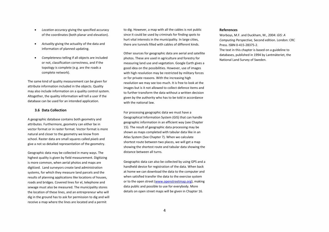
• Location accuracy giving the specified accuracy of the coordinates (both planar and elevation).

• Actuality giving the actuality of the data and information of planned updating.

• Completeness telling if all objects are included or not, classification correctness, and if the topology is complete (e.g. are the roads a complete network).

The same kind of quality measurement can be given for attribute information included in the objects. Quality may also include information on a quality control system. Altogether, the quality information will tell a user if the database can be used for an intended application.

3.6 Data Collection

A geographic database contains both geometry and attributes. Furthermore, geometry can either be in vector format or in raster format. Vector format is more natural and closer to the geometry we know from school. Raster data are small squares called pixels and give a not so detailed representation of the geometry.

Geographic data may be collected in many ways. The highest quality is given by field measurement. Digitizing is more common, when aerial photos and maps are digitized. Land surveyors create land administration systems, for which they measure land parcels and the results of planning applications like locations of houses, roads and bridges. Covered lines for el, telephone and sewage must also be measured. The municipality stores the location of these lines, and an entrepreneur who will dig in the ground has to ask for permission to dig and will receive a map where the lines are located and a permit

to dig. However, a map with all the cables is not public since it could be used by criminals for finding spots to hurt vital interests in the municipality. In large cities, there are tunnels filled with cables of different kinds.

Other sources for geographic data are aerial and satellite photos. These are used in agriculture and forestry for measuring land use and vegetation. Google Earth gives a good idea on the possibilities. However, use of images with high resolution may be restricted by military forces or for private reasons. With the increasing high resolution we may see too much. It is free to look at the images but is it not allowed to collect defence items and to further transform the data without a written decision given by the authority who has to be told in accordance with the national law. For processing geographic data we must have a Geographical Information System (GIS) that can handle geographic information in an efficient way (see Chapter 15). The result of geographic data processing may be shown as maps completed with tabular data like in an Atlas System (See Chapter 7). When we calculate shortest route between two places, we will get a map showing the shortest route and tabular data showing the distance between all turns. Geographic data can also be collected by using GPS and a handheld device for registration of the data. When back at home we can download the data to the computer and when satisfied transfer the data to the exercise system or to the open street (www.openstreetmap.org), making data public and possible to use for everybody. More details on open street maps will be given in Chapter 16.

References Worboys, M.F. and Duckham, M., 2004: GIS: A Computing Perspective, Second edition. London: CRC Press. ISBN 0-415-28375-2. The text in this chapter is based on a guideline to databases, published in 1994 by Lantmäteriet, the National Land Survey of Sweden.

4

4 MAP DESIGN

Vit Vozenilek, Czech Republic

4.1 Introduction

Map making is significantly influenced by current information technology that allows the compilation of maps using different software products as a way of displaying individual data layers. The availability of this software allows the compilation of maps by nonprofessional map makers from different occupations. However, without cartographic knowledge, the final products are often artefacts that do not meet one of the main functions of the map—to provide truthful information.

Nevertheless, maps are unique kind of documents that can convey huge amounts of spatial information quickly and accurately.

Map design is the aggregate of all the thought processes that cartographers go through during the abstraction phase of the cartographic process. Map design is a complex activity involving both intellectual and visual, technological and non-technological, and individual and multidisciplinary aspects (Dent, Torgusin and Hodler, 2009).

For map design, it is necessary be knowledgeable about map projections and reference systems (see Chapter 9), types of maps (see Chapters 5, 6 and 7) and geographical names (see Chapter8).

There are different forms of map design—for topographic maps and for thematic maps. The most complex process of map design is for atlases.

The topographic map is an essential reference map product (see Chapter 5). A fundamental aspect of map design for topographic maps is the most accurate

recording of planimetric (two-dimensional location) and hypsographic (height above sea level) situations on the scale of a map.

Ideally, thematic maps (see Chapter 6) are the result of creative collaboration of experts from two professions. The first is a thematic content expert, the second is a cartographer (a visualization expert). A thematic content expert can be a climatologist, geologist, demographer, urbanist, political scientist, ecologist, botanist, hydrologist, tourist, soldier, economist or other professional who is required to express "his/her thematic information" on a map. A cartographer is responsible for the correct visualization, thus ensuring a process in which the reader gains from the map exactly the same information that the thematic expert was required to insert into the map. Cooperation between the two experts is necessary in most cases—a thematic expert would not display his/her data correctly without a cartographer, and a cartographer would not know without a thematic expert what the map should convey and why.

In order for the map making process to be completed to a high standard (i.e., to produce a map that provides the required information correctly, accurately and quickly), a cartographer must also take into account the process of map use. The beginning of map design must correspond with the end of map use (see Figure 4.1).

Map design passes through three phases—map proposal, map drafting and map compilation (see Figure 4.1).

Figure 4.1 Reciprocal influence of map making and map use.

4.2 Map proposal

A mapping assignment is always the beginning of map design. A map assignment is essentially a special type of order. The execution of such a contract requires professional solutions based on the nature of the map project.

A thematic map assignment is formulated by a customer expressing the intention with which each map is to be compiled and published. The map assignment must include a clearly defined objective and purpose for the map, as well as other requirements, such as the volume of the information or the expected map use.

The objective of the map is a key point of the map assignment. The objective of a topographic map is to provide the most accurate display of a topographic and hypsographic situation on the scale of the map. The objective of a thematic map is defined by a thematic expert (or by a contracting authority) in the form of a

1

statement what is the data provided are about and for whom their visualised portrayal is intended.

According to the map assignment, a cartographer draws up a project map and elaborates important items of map design. It consists of two main parts, namely, the objective specification and the project specification (see Figure 4.2).

When the objective of a map is specified, the target group of users, the way of working with the map and the volume of conveyed information are carefully formulated. There are many possible user groups, characterized by age, education, cartographic literacy and previous experience of working with maps:

• school groups (pupils and students) often use school wall maps and atlases;

• professional groups (experts and officers) often use scientific maps with specialized content, including administrative maps, topographic maps and cadastral maps;

• public groups (the general public, including interest groups) often use tourist maps, road maps, maps of wine regions, maps of fishing grounds, etc.

The manipulation of a map involves specifying the expected time available for viewing the map (a map on the wall permanently or a short map display on TV), the form of the map (paper or digital) and the conditions for viewing the map (for walking, in low light, in a wet environment, etc.).

Figure 4.2 A map assignment and a map project.

4.3 Map drafting

4.3.1 Topographic maps

At the beginning of topographic map compilation, astronomical measurements are necessary for determining the exact position of selected points which are used to define coordinate systems. These are followed up by geodetic measurements generating the network of triangulation points with which all objects on the Earth's surface are mapped in the field—buildings, roads, rivers, forests, borders, etc.

Cartographers compile topographic maps according to the rules and regulations set through which all maps in a topographic map series are identical in projection, content, detail, labelling and symbology. Topographic maps are frequently updated and constantly improved.

Topographic maps usually are compiled under the responsibility of national governments and form one of the most important official documents (see Figure 4.3).

2

Figure 4.3 Topographic maps of the Czech Republic at different map scales.

4.3.2 Thematic maps

Thematic maps are compiled in a different way. Thematic content (geology, climate, population, transportation, etc.) is drawn on a base map, which is most often either a simplified topographic map or a set of data layers. This creates a working map. The results of field surveys or other existing thematic data such as statistical data are added to it. In this working map, the cartographic rules (on colours, labelling, etc.) may not be

strictly observed because the working map is only for the author, not for the end users. The cartographer and thematic expert work together to define its content, methods, symbology, etc. If the map is compiled in GIS, the working map is a simple data view (Voženílek 2005) or visualization of the data.

The cartographer and thematic expert can redraw, refine, supplement or generalize this working map several times. The final working map is called the author's original, which is a master for further cartographic processing (see also figure 6.28).

4.3.3 Map content

The features on a map are the map content. Map content is compiled sequentially to be fully in line with the map objective. Features are displayed in the map content according to one of the following criteria:

• qualitative—the species are expressed (e.g. language map);

• quantitative—the quantifiable properties (e.g. population density map) are displayed;

• topological—the features are represented by their ground nature (the way they relate to the Earth surface) by point, line and areal symbols (e.g. road map);

• developmental—the changes in space and time are displayed (e.g. troop movement map);

• meaning—or significance and the significance of a small settlement in the desert is higher than that of a similar settlement in a well-populated area) and

• structural —the feature as a unit together with its sub-components and interrelationships are represented (e.g. map of the age structure of the population).

In compiling the map contents, the first task is to distinguish primary features (resulting from the map

assignment) from secondary ones (used to supplement the information on the map). A topographic base of the thematic map is created to allow for spatial localization and to find mutual topological relations of the primary features.

4.3.4 Map symbols and cartographic methods

There are a number of methods for map visualization of map contents. The selection of methods is determined by the nature of the displayed features (which can either be related to points, lines or areas) and the objective of the map (see Chapters 4.2 and 4.3.3).

Point map symbols—a simple geometric, figurative or alphanumeric picture (see Figure 4.4)—allow for the expression of feature characteristics at a particular location. Using the shape, size, structure, fill and orientation, both qualitative and quantitative characteristics can be expressed (see Figure 4.5).

Figure 4.4 Types of point map symbols.

3

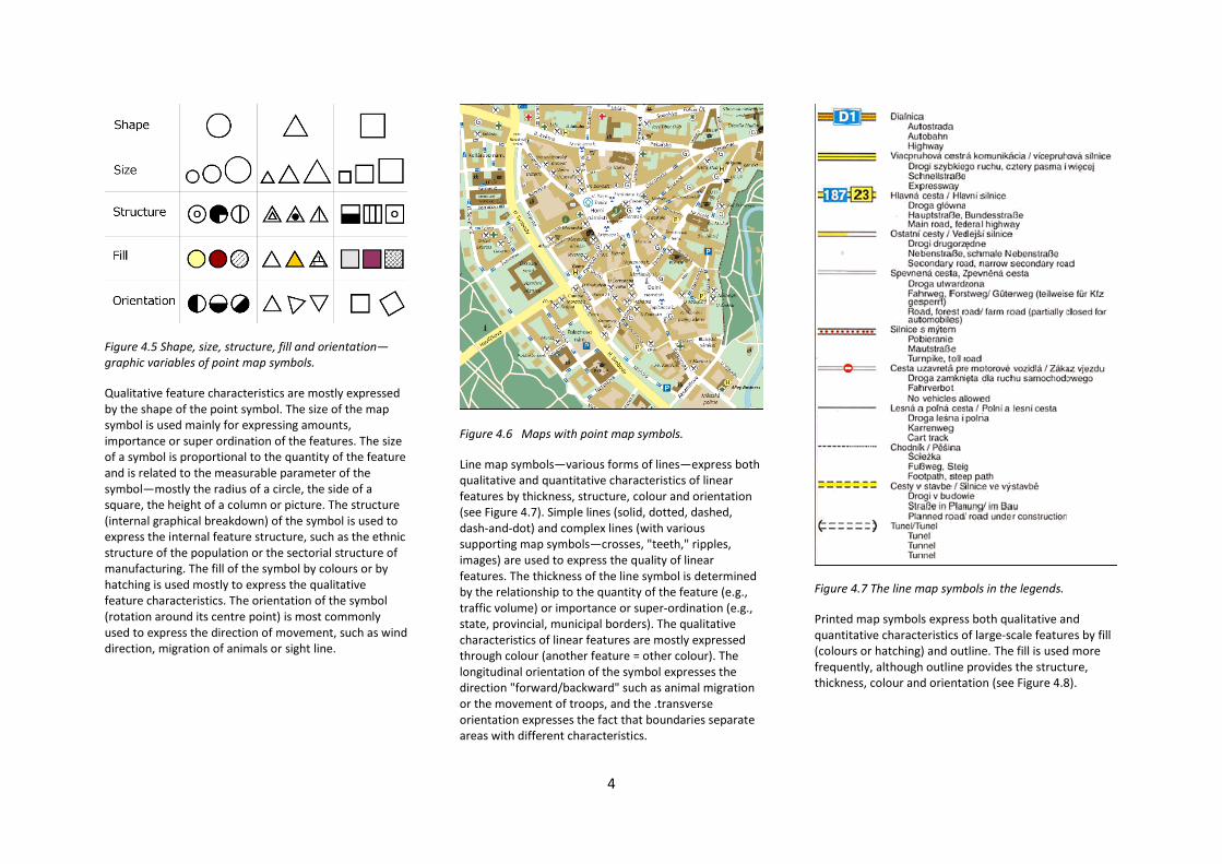
Figure 4.5 Shape, size, structure, fill and orientation—graphic variables of point map symbols.

Qualitative feature characteristics are mostly expressed by the shape of the point symbol. The size of the map symbol is used mainly for expressing amounts, importance or super ordination of the features. The size of a symbol is proportional to the quantity of the feature and is related to the measurable parameter of the symbol—mostly the radius of a circle, the side of a square, the height of a column or picture. The structure (internal graphical breakdown) of the symbol is used to express the internal feature structure, such as the ethnic structure of the population or the sectorial structure of manufacturing. The fill of the symbol by colours or by hatching is used mostly to express the qualitative feature characteristics. The orientation of the symbol (rotation around its centre point) is most commonly used to express the direction of movement, such as wind direction, migration of animals or sight line.

Figure 4.6 Maps with point map symbols.

Line map symbols—various forms of lines—express both qualitative and quantitative characteristics of linear features by thickness, structure, colour and orientation (see Figure 4.7). Simple lines (solid, dotted, dashed, dash-and-dot) and complex lines (with various supporting map symbols—crosses, "teeth," ripples, images) are used to express the quality of linear features. The thickness of the line symbol is determined by the relationship to the quantity of the feature (e.g., traffic volume) or importance or super-ordination (e.g., state, provincial, municipal borders). The qualitative characteristics of linear features are mostly expressed through colour (another feature = other colour). The longitudinal orientation of the symbol expresses the direction "forward/backward" such as animal migration or the movement of troops, and the .transverse orientation expresses the fact that boundaries separate areas with different characteristics.

Figure 4.7 The line map symbols in the legends.

Printed map symbols express both qualitative and quantitative characteristics of large-scale features by fill (colours or hatching) and outline. The fill is used more frequently, although outline provides the structure, thickness, colour and orientation (see Figure 4.8).

4

Figure 4.8 Maps with areal map symbols.

4.3.5 Colour

The colour parameters include hue, value and saturation (see Figure 4.9). Hue can be defined as the various colours we perceive (red, blue, green, yellow, orange, etc.). Millions of hues arise by combining various percentages of the primary hues and altering their value and saturation. Value is the lightness or darkness of a hue and is affected by background: the value looks lighter when surrounded by darker shades of grey colour. Saturation means intensity or purity of a colour and ranges from 0% (neutral grey) to 100% (maximum saturation).

Figure 4.9 Hue, value, saturation.

Finding the right colour combination or colour harmony is not a trivial issue. Colour is used differently for expression of quality (species) and quantity (amount) of the feature characteristics (see Figures 4.10 and 4.11).

When distinguishing the features according to their qualitative characteristics (e.g., countries of the world, soils, language), a cartographer expresses these qualities primarily by differences in hue, then by saturation and value (see Figure 4.10). Lighter colours are applied for larger map areas to be visible and identifiable relative to darker colours. Darker colours appear much more dominant than lighter colours within the same area size. Some colours permit us to perceive less contrast than others (Kraak and Ormeling 2003) because two or more colours interact and influence each other’s appearance.

Figure 4.10 A colour used for distinguishing of qualitative feature characteristics in the map.

When using colour to express feature quantities (see Figure 4.11) in the map, cartographers distinguish amounts of features (more—less; most important—unimportant, etc.) by changing the colour intensity, the combination of colour saturation and brightness according to the following rule: the higher the intensity of the feature, the higher the colour intensity.

The representation of quantitative features on maps involves the use of a single hue or a limited number of hues to unify a feature. For example, with an air temperature map, the hue progression (colour ramp) represents air temperature, and varied values and saturation within the hue creates a graded series from light to dark showing degrees of Celsius. With such a scheme it is easy to associate the feature with the hue and the different quantities with the lightness or darkness of the hue. Lighter hues normally represent lower quantities while darker hues are for higher quantities. The reverse may be applied, however, when it is desirable to emphasize the lower quantities (e.g., to highlight areas of extreme poverty [low income] with the strongest colour in the graded series).

5

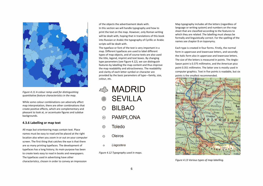
Figure 4.11 A colour ramp used for distinguishing quantitative feature characteristics in the map.

While some colour combinations can adversely affect map interpretation, there are other combinations that create positive effects, which are complementary and pleasant to look at, or accentuate figures and subdue backgrounds.

4.3.6 Labelling or map text

All maps but orienteering maps contain text. Place names must be easy to read and be placed at the right location also when you zoom in or out on your computer screen. The first thing that catches the eye is that there are so many printing typefaces. The development of typefaces has a long history; its main purpose has been to create texts easy to read in books and newspapers. The typefaces used in advertising have other characteristics, chosen in order to convey an impression

of the objects the advertisement deals with. In this section we will handle typography and how to print the text on the map. However, only Roman writing will be dealt with, hoping that in translations of this book into Russian or Arabic the typography of Cyrillic or Arabic scripts will be dealt with. The typeface or font of the text is very important in a map. Different typefaces are used to label different types of map objects, and of course texts are also used the title, legend, imprint and text boxes. By changing type parameters (see Figure 4.12), we can distinguish features by labelling the map content and thus improve the map readability and attractiveness. The readability and clarity of each letter symbol or character are provided by the basic parameters of type—family, size, colour, etc.

Figure 4.12 Typography used in maps.

Map typography includes all the letters (regardless of language or writing system) and numbers on the map sheet that are classified according to the features to which they are related .The labelling must always be formally and linguistically correct. For the spelling of the names see chapter 8 on toponymy.

Each type is created in four forms. Firstly, the normal form in uppercase and lowercase letters, and secondly the italic form also in uppercase and lowercase letters. The size of the letters is measured in points. The Anglo-Saxon point is 0.375 millimetre, and the American pica point 0.351 millimetre. The latter one is mostly used in computer graphics. Text in five points is readable, but six points is the smallest recommended.

Figure 4.13 Various types of map labelling.

6

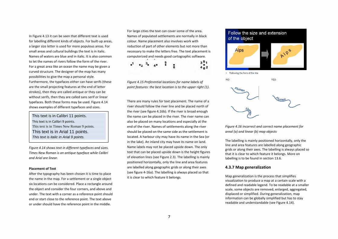
In Figure 4.13 it can be seen that different text is used for labelling different kinds of objects. For built-up areas, a larger size letter is used for more populous areas. For small areas and cultural buildings the text is in italic. Names of waters are blue and in italic. It is also common to let the names of rivers follow the form of the river. For a great area like an ocean the name may be given a curved structure. The designer of the map has many possibilities to give the map a personal style. Furthermore, the typefaces either can have serifs (these are the small projecting features at the end of letter strokes), then they are called antique or they can be without serifs, then they are called sans serif or linear typefaces. Both these forms may be used. Figure 4.14 shows examples of different typefaces and sizes. Figure 4.14 shows text in different typefaces and sizes. Times New Roman is an antique typeface while Calibri and Arial are linear. Placement of Text After the typography has been chosen it is time to place the name in the map. For a settlement or a single object six locations can be considered. Place a rectangle around the object and consider the four corners, and above and under. The text with a corner as a reference point should end or start close to the reference point. The text above or under should have the reference point in the middle.

For large cities the text can cover some of the area. Names of populated settlements are normally in black colour. Name placement also involves work with reduction of part of other elements but not more than necessary to make the letters free. The text placement is computerized and needs good cartographic software.

Figure 4.15 Preferential locations for name labels of point features: the best location is to the upper right (1).

There are many rules for text placement. The name of a river should follow the river line and be placed north of the river (see figure 4.16b). If the river is broad enough the name can be placed in the river. The river name can also be placed on many locations and especially at the end of the river. Names of settlements along the river should be placed on the same side as the settlement is located. A harbour city may have its name in the Sea (or in the lake). An inland city may have its name on land. Name labels may not be placed upside down. The only text that can be placed upside down is the height figures of elevation lines (see Figure 2.3). The labelling is mainly positioned horizontally, only the line and area features are labelled along geographic grids or along their axes (see figure 4-16a). The labelling is always placed so that it is clear to which feature it belongs.

Figure 4.16 incorrect and correct name placement for areal (a) and linear (b) map objects

The labelling is mainly positioned horizontally, only the line and area features are labelled along geographic grids or along their axes. The labelling is always placed so that it is clear to which feature it belongs. More on labelling is to be found in section 13.6.

4.3.7 Map generalization

Map generalization is the process that simplifies visualization to produce a map at a certain scale with a defined and readable legend. To be readable at a smaller scale, some objects are removed, enlarged, aggregated, displaced or simplified. During generalization, map information can be globally simplified but has to stay readable and understandable (see Figure 4.14).

This text is in Calibri 11 points. This text is in Calibri 9 points. This text is in Times New Roman 9 points. This text is in Arial 11 points. This text is italic in Arial 9 points.

7

Figure 4.17 Two maps with different levels of map generalization.

The smaller the scale, the less information is given per square kilometre. Conversely, the larger the scale, the more detailed information is given for the same map size.

Map generalization includes several methods for reducing the complexity of the real world by strategically reducing unnecessary details (see Figure 4.14):

• Selection—the most important features stand out while lesser ones are left out entirely. For example, a directional map between two points may have lesser and untraveled roadways omitted so as not to confuse the map reader. The selection of the most direct and uncomplicated route between the two points is the most important data, and the cartographer may choose to emphasize this;

• Simplification—the shapes of retained features are altered to enhance visibility and reduce complexity. Smaller scale maps have more simplified features than larger scale maps because they simply exhibit more area;

• Combination—the features are combined when their separation is irrelevant to the objective of the map. A mountain chain may be isolated into several smaller ridges and peaks with intermittent forest in the natural environment, but shown as a continuous chain on the map, as determined by scale;

• Smoothing—is reducing the angularity of line work to exhibit it in a much less complicated and less visually disruptive way. An example is the smoothing of a meandering river so that the generalized line of the river contains less bends, is less curved and follows the main flow direction; and

Figure 4.18 The methods of map generalization.

8

• Enhancement—is used to show the primary nature of features and to highlight specific details that would otherwise be left out.

4.3.8 Map composition

Map composition is the first image the reader sees on the map. Map composition means the distribution of the graphic elements on the map sheet. It depends primarily on the objective and scale of the map, map projection, the shape and size of the mapped area and the format of the map sheet. The map composition of the thematic maps is very varied and diverse, unlike the topographic maps with uniform map composition based on official rules and regulations.

Map composition must meet three basic requirements:

• to include all the basic composition elements;

• to be balanced, without empty or overfilled areas; and

• to present aesthetically pleasant conditions for map reading.

The basic elements of composition are:

• map area; • map title; • map legend; • map scale (graphical, verbal); and • imprint.

The map title contains the main textual information on the map. The theme of the map, which the cartographer receives from the map assignment, should be briefly but clearly expressed in the map title. It is then placed on the top of the map legend. The map title must contain

thematic, spatial and temporal determinations of the main theme of the map. If the map title is too long, part of the title is given as the subtitle. The title usually contains the thematic determination of the feature and it is always written in uppercase letters. The subtitle contains the spatial and temporal determinations of the features and it is always written under the title and in lowercase and smaller letters than the title.

The map legend is an overview of the symbology used on the map in easily readable and understandable form, from which the map reader correctly decodes information stored in the map. The map legend is placed near the map area. The map legend must be:

• Complete —"what is in the map is then in the legend." The map legend must contain all map symbols that are in the map. The map legend does not contain information on construction elements (map projection, geographic grid, etc.). The legend of thematic maps does not include the symbols of the topographical base;

• Independent —one feature has only one symbol in the map legend;

• Ordered —the map legend map must be arranged in a logical structure, usually by hierarchy of the features;

• In accordance with the symbol appearance in the map—the symbols in the legend and in the map must be rendered identically (the same shade of colour, the same size, the same thickness, the same width, etc.); and

• Understandable—the explanation of all symbols must be clear and easy to understand.

An imprint always contains the author's name, publisher, place and year of publication. It may also contain

information on the map’s projection, edition, reviewers’ names, copyright, etc.

In addition to basic composition elements, a map can contain other additional composition elements to increase the information value of the map and its attractiveness, such as a north arrow, insets, charts, profiles, explanatory texts, tables, etc.

4.4 Map compilation

Once a cartographer generalizes the map content and interprets it in the map at the scale of issue, this results in an editorial original. The content of the editorial original is drawn with the prescribed graphical accuracy in all details in accordance with a map project.

The thematic content of the editorial original is taken from the authors' originals, which are compiled by thematic experts rather than cartographers. The compilation of the thematic map requires a skilled cartographer, who addresses a number of cartographic tasks in accordance with the map project, especially map composition, generalization, map content maps and symbology. A cartographer is fully responsible for the quality of visualization of the editorial original, which is the final form of the map design.

The editorial original is first elaborated in the areas with the richest map content in order to determine the optimal graphic complexity of these areas and their readability. Symbology and level of generalization are adjusted according to these areas. Other features of the map content are then drawn according to their importance. Finally, the labelling and additional composition elements are drawn. The thematic expert is involved in the compilation of the editorial original primarily as a consultant on the map content and symbology.

9

Printing is the last phase of the map. The result is a perfect map copy, which is then to be faithfully reproduced and published (see Chapter 13). The resultant map must comply in accuracy, completeness and topicality of all features from the map content and all aesthetic demands. Print quality is checked at the first test prints.

4.5 Think before you draw

In map design, all the above knowledge must be respected. In order for a cartographer to work effectively and successfully, everything has to be carefully thought out and plotted. The following principles must be observed:

… each map should be elaborated at least twice

First, a working map should be drawn. On the working map, the thematic expert compiles thematic contents of the map ("the first" map), which does not change during further processing. Then when compiling "the second" map, the cartographer collaborates his/her activities with the thematic expert, in relation to generalization and symbology.

… pay the same attention to each part of the map

All features have to be treated with the same attention on the entire map area. Each map has three aspects—subject (related to content), technical (related to design) and aesthetic (related to appearance)—which need to be processed uniformly and with the same thoroughness.

… from the theme to the legend

It is necessary to follow the sequence: main theme—map title—the most noticeable symbols—map legend. This means that the main theme of the map must be uniquely determined in the map title, then expressed by

the most noticeable symbols and located at the top of the map legend.

… the best legend is an unnecessary legend

The easier it is to read the symbols and the clearer the "map language,” the better the map. The problem is author blindness and branch blindness. In author blindness, the author of the map thinks that if he does understands the map other readers will understand it too. Maps affected by author blindness occur when the thematic expert compiles the map without the cartographer and without cartographic skills. In branch blindness, the members of one branch of science or discipline argue that they all easily understand the map and so everybody will understand it. However, the map will be read by people from other scientific disciplines as well, with varying levels of knowledge of the themes, even with visual impairments or specific colour sense. The map must be understood by all these people.

… a map is read from two distances

From a longer distance, the reader first reads the map composition (especially the map title that tells what the map is about) and the basic spatial pattern of the primary features. All details (particularly map symbols and labelling) are read from a short distance (such as text in book).

… sometimes less is more

A map that is too full graphically is difficult to read and remember.

… no map is useless, the worst-case scenario serves as a deterrent.

References

Brewer, C. A., 2005: Designing Better Maps: A Guide for GIS Users. Esri Press, Redlands, California, USA. ISBN 1-58948-089-9. Christophe, S., Zanin, C. and Roussaffa, H., 2011: Colours Harmony in Cartography. Paris, ICC 2011, Co-084 Dent, B. D., Torguson, J. S., and Hodler, T. W., 2009: Cartography: Thematic Map Design. McGraw-Hill Higher Education, New York, 6th edition. ISBN 9780072943825. Kraak, M-J. and Ormeling, F.J. 2010: Cartography: Visualization of Spatial Data. 3rd edition. Harlow, England: Prentice Hall. Slocum, T. A., McMaster, R. B., Kessler, F. C., Howard, H. H. 2008: Thematic Cartography and Geovisualization. Prentice Hall, 3rd edition, ISBN 9780132298346 Voženílek, V., 2005: Cartography for GIS—Geovisualization and Map Communication. Palacky University, Olomouc, Czech Republic, ISBN 80-244-1047-8.

10

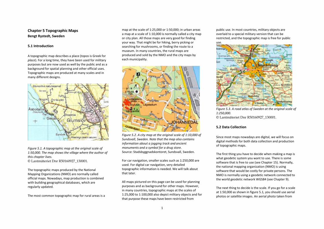
Chapter 5 Topographic Maps Bengt Rystedt, Sweden 5.1 Introduction A topographic map describes a place (topos is Greek for place). For a long time, they have been used for military purposes but are now used as well by the public and as a background for spatial planning and other official uses. Topographic maps are produced at many scales and in many different designs.

Figure 5.1. A topographic map at the original scale of 1:50,000. The map shows the village where the author of this chapter lives. © Lantmäteriet Dnr R50160927_130001. The topographic maps produced by the National Mapping Organizations (NMO) are normally called official maps. Nowadays, map production is combined with building geographical databases, which are regularly updated. The most common topographic map for rural areas is a

map at the scale of 1:25,000 or 1:50,000; in urban areas a map at a scale of 1:10,000 is normally called a city map or city plan. All those maps are very good for finding your way. That might be for hiking, berry picking or searching for mushrooms, or finding the route to a museum. In many countries, the rural maps are produced and sold by the NMO and the city maps by each municipality.

Figure 5.2. A city map at the original scale of 1:10,000 of Sundsvall, Sweden. Note that the map also contains information about a jogging track and ancient monuments and a symbol for a drug store. Source: Stadsbyggnadskontoret, Sundsvall, Sweden. For car navigation, smaller scales such as 1:250,000 are used. For digital car navigation, very detailed topographic information is needed. We will talk about that later. All maps pictured on this page can be used for planning purposes and as background for other maps. However, in many countries, topographic maps at the scales of 1:25,000 to 1:100,000 also depict military objects and for that purpose these maps have been restricted from

public use. In most countries, military objects are overlaid to a special military version that can be restricted, and the topographic map is free for public use.

Figure 5.3. A road atlas of Sweden at the original scale of 1:250,000. © Lantmäteriet Dnr R50160927_130001. 5.2 Data Collection Since most maps nowadays are digital, we will focus on digital methods for both data collection and production of topographic maps. The first thing you have to decide when making a map is what geodetic system you want to use. There is some software that is free to use (see Chapter 15). Normally, the national mapping organization (NMO) is using software that would be costly for private persons. The NMO is normally using a geodetic network connected to the world geodetic network WGS84 (see Chapter 9). The next thing to decide is the scale. If you go for a scale at 1:50,000 as shown in figure 5.1, you should use aerial photos or satellite images. An aerial photo taken from

1

the elevation of 13,000 meters gives a resolution of 1:10,000. Before you can use an aerial photo for mapping, it has to be transformed to an orthophoto map (see Figure 5.4). That is made by each NMO or by companies in the business and implies that photo gets a correct scale over the whole area. You can try to get an orthophoto from your NMO but that is not normally free of charge. You can also go to Google Maps where you can look at topographic maps of all spots of the world.

Figure 5.4 shows an orthophoto of central Stockholm, Sweden, in the year 2009. © Lantmäteriet Dnr R50160927_130001 From an orthophoto map, it is easy to find roads, lakes, rivers, built-up areas and different types of land use. Since all information nowadays is digital, you must also for mapping use a database with geographic data. Designing a database is rather tricky but further information is given in Chapters 3 and 15. One way to collect data is to scan older maps and digitize features, for instance, administrative borders in these maps, but most information can be digitized in the orthophotos. It is also important to classify the information. Roads are of different importance and should be classified with motorways at the highest level

and paths for walking at the lowest level. Since the topographic maps were used by the military, the roads were categorized according to military purposes. A narrow road was a road where it was not possible to turn with a horse and a wagon. It was the same for water streams. A stream that an infantry soldier could cross without problems was depicted with a single line, while a stream that needed a bridge was marked with double lines in blue to indicate the water between the two lines. 5.3 The Legend All maps need a legend (an explanation of the signs and symbols used on the map), and so do topographic maps. It is rather common to start with communications with the group roads, rail and air, followed by power lines for electricity and gas. The next group might be single objects like places for swimming and camping and location of buildings like castles, farms, greenhouses, homes, religious buildings, and so on. In built-up areas, it is not possible to indicate all single houses. Blocks with different construction types must be indicated mostly in accordance with the height of the buildings. Closed blocks in city centres must also be indicated. Administrative borders and lakes and streams are two other groups. Borders shall be indicated with their function and streams with their size. A big and a troublesome group of data to represent on the map is land cover and land use. Some land cover like forest has different definitions in different countries. In Northern Europe, there are not so many trees per area like in a tropical forest, which means that the density of the forest must be compared considering the location. Open spaces in the forest can be shown for some years and will later be changed to young forest. Wetlands are again a different land use type and can be classified by experts. Land use such as arable land changes over time. In the map, it is usually impossible to show different crops, but

in areas with less intensive agriculture, some lands are not continuously used and tend to be bushy. Changes in arable land, forest and road conditions must be checked in the field before printing. There is a standard in topographic mapping to first produce a good copy as soon as possible at the office before going out for field checking. Office work is cheaper than sending out people for fieldwork. 5.4 Relief Representation The most common way to show relief is by contour lines showing the height elevation. Laser-scanning aerial cameras nowadays also can register elevation and give the background for calculation of contour lines and other details in the landscape such as constructions and ditches. Also tracks in wood can be detected. Laser data are collected as point clouds that give possibilities to calculate elevation at a very good accuracy. High resolution laser data have many applications also in climate applications for finding areas with risk for flooding and for land slide. An example of aerial laser-scanning is shown in Figure 5.5.

A special technique for showing elevation is hill shading, where you illuminate the landscape from normally the northwest and get a shadow in the southwest (see Figure 5.6).

2

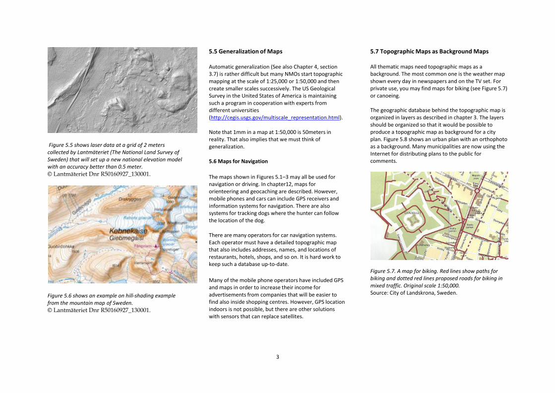
Figure 5.5 shows laser data at a grid of 2 meters collected by Lantmäteriet (The National Land Survey of Sweden) that will set up a new national elevation model with an accuracy better than 0.5 meter. © Lantmäteriet Dnr R50160927_130001.

Figure 5.6 shows an example on hill-shading example from the mountain map of Sweden. © Lantmäteriet Dnr R50160927_130001.

5.5 Generalization of Maps Automatic generalization (See also Chapter 4, section 3.7) is rather difficult but many NMOs start topographic mapping at the scale of 1:25,000 or 1:50,000 and then create smaller scales successively. The US Geological Survey in the United States of America is maintaining such a program in cooperation with experts from different universities (http://cegis.usgs.gov/multiscale_representation.html). Note that 1mm in a map at 1:50,000 is 50meters in reality. That also implies that we must think of generalization. 5.6 Maps for Navigation The maps shown in Figures 5.1–3 may all be used for navigation or driving. In chapter12, maps for orienteering and geocaching are described. However, mobile phones and cars can include GPS receivers and information systems for navigation. There are also systems for tracking dogs where the hunter can follow the location of the dog. There are many operators for car navigation systems. Each operator must have a detailed topographic map that also includes addresses, names, and locations of restaurants, hotels, shops, and so on. It is hard work to keep such a database up-to-date. Many of the mobile phone operators have included GPS and maps in order to increase their income for advertisements from companies that will be easier to find also inside shopping centres. However, GPS location indoors is not possible, but there are other solutions with sensors that can replace satellites.

5.7 Topographic Maps as Background Maps All thematic maps need topographic maps as a background. The most common one is the weather map shown every day in newspapers and on the TV set. For private use, you may find maps for biking (see Figure 5.7) or canoeing. The geographic database behind the topographic map is organized in layers as described in chapter 3. The layers should be organized so that it would be possible to produce a topographic map as background for a city plan. Figure 5.8 shows an urban plan with an orthophoto as a background. Many municipalities are now using the Internet for distributing plans to the public for comments.

Figure 5.7. A map for biking. Red lines show paths for biking and dotted red lines proposed roads for biking in mixed traffic. Original scale 1:50,000. Source: City of Landskrona, Sweden.

3

Figure 5.8 showing a city plan for Kabul—City of Light Development area and concept plan. The blue shows the old city, yellow shows housing and red the commercial district. The background is an orthophoto map. Source: Wikipedia (urban planning).

Property maps can also use topography as a background to property boundaries and administrative boundaries. The reasons for constructing property maps are not only to know the location of the property but also to find out the value of the property for tax purposes. In Sweden, property mapping started in 1628 with an order from the King of Sweden. One person got the task and started to train land surveyors in measuring and mapping. Later on, cartographic rules were developed. The maps were called geometric maps and were produced at the scale of 1:5,000. The maps were used when the division of farm land was reformed to be a more efficient division to allow for new farming techniques. The geometric accuracy of these maps is very good, and they are still valid in questions of land disputes. Most countries have had the same development. For more information, you can contact the NMO in your country. 5.8 Geological Maps Geology maps are thematic maps, generally displayed in Chapter 6. Geology mapping and topographic mapping

are closely related since geological maps must have the correct topography as a background. Geology may also be produced in the form of atlases. An example is the Physical Atlas of China (Ke Liao, 1999). It contains geological and geophysical maps, geomorphological maps, climatic maps, hydrological maps, soil maps, biological maps, maps on natural resources and disasters, and finally maps on nature utilization and conservation including land use. Of public interest is the geological map showing bedrock and the soil map. The topographic map and the bedrock map are good tools for finding minerals, but you need to study a lot before practicing. The soil map can give farmers or farm buyers information on what can be grown and how to fertilize the land. 5.9 Required Map Information All topographic maps must include the following information:

• Title shows the name of the. Further information needed are the area of the map, the map subject and the actuality of the content.

• Legend shows the meaning of the map symbols and the connection to the database.

• Scale shows the scale of the map either by numbers or by a figure showing the length (e.g. of one kilometre).

• Geodetic network showing the position of a point in the map. The network must be included if the map shall be used for navigation.

• Projection shows how points in longitude and latitude are transferred to the plane coordinate system (See Chapter 9).

• Author, publisher and references tell who has made the map, who has published it and what

sources are used and which time the data represents. If some of the data has copyright, it shall also be indicated.

5.10 Historical Topographic Maps The first known maps were found on clay plates in Babylon, but for a long period, the most common media for maps has been paper, until recently when screen maps became the most common ones. Never before have so many unique maps been published. More information on historical maps are given in Chapter 1. 5.10.1 The 19th Century Topographic maps have always had a high military importance. For a long time, it was difficult to measure the distance in West–East. In North–South, you could use the stars and the sun to measure your position, but in West–East, you must know the time in order to get a good position. That means that cartographers also had difficulties in writing correct maps. An efficient clock was most important and the sailors very much needed a correct clock for finding the longitude. That also meant that many maps were not correct in the West-East direction. However, topographical maps were of great importance for military purposes; military brigades were shaped both for geodesy and topographic mapping and the resulting maps became classified not to be used by non-military. Nowadays, most countries have lifted the restriction but some countries still have restrictions for private use. To my knowledge, topographic maps from the 19th

century are of high quality, and they are perfect for studying the development of the society. New versions of the topographic maps are issued regularly. For studying the development of your neighbourhood, you

4

can select different versions of the map at your library. That can be a good exercise in schools. Figure 5.9 shows the present Malmö, the third biggest city in Sweden, located only some 15 kilometres east of Copenhagen in Denmark. The city extends out to the Sound (Öresund in Swedish). The harbour and industrial areas are now located on the landfill. The old industrial buildings in several floors are built such as the 72 floors Turning Torso building in Västra Hamnen (the West Harbour), a special landmark that can be seen from long distances, also from Copenhagen in Denmark. Figure 5.9 shows a map over the city of Malmö, Sweden. Source www,openstreetmap.org visited April 27,2014.

In Figures 5.10–12, you can see the earlier Malmö. The maps have been scanned from an historical atlas produced by a geographer (Lewan, 1985) at Lund University and a land surveyor at the National Land Survey of Sweden.

Figure 5.10 shows an orthophoto from 1985. A new industrial area has been created, and the harbour has been enlarged. Source: National Land Survey of Sweden. © Lantmäteriet Dnr R50160927_130001.

Figure 5.11 shows the topographical map of 1915, produced by the military survey of Sweden. The railroad has now been built and continues through Malmö for a connection ferry to Denmark. The area north of the centre has been filled up, giving place for a harbour and the railroad. © Lantmäteriet Dnr R50160927_130001.

5

Figure 5.12 shows a map from Malmö in the year 1815. The map is a part of the reconnoitre map of the province that was made in a great hurry to be prepared for a possible attack from Napoleon. Source: Lewan, 1985. The original can be found in the Archive of the Military (Krigsarkivet), Stockholm, Sweden.

References Lewan, Nils (1985). Historisk Atlas. Berlings Grafiska AB, Arlöv, Sweden. Liao, Ke, (1999). The National Physical Atlas of China. China Cartographic Publishing House, Beijing, China. ________________

6

Chapter 6 Thematic maps

Ferjan Ormeling, the Netherlands

(see also section 4.3.2, where the production of a thematic map is described from first concept to final map)

6.1 Spatial concepts

In thematic mapping, we visualise data on the basis of spatial concepts, like density, ratio, percentages, index numbers or trends, and of procedures like averaging. To make things comparable, we relate them to standard units like square kilometres, or we convert them to standard situations. In order to compare average temperatures measured at different latitudes, we first assess the height above sea level of the stations where the temperatures were measured, and then we reduce them to sea level (for every 100 metres of height difference with the sea level there is 1⁰C decrease in average temperature).

Figure 6.1 Spatial concepts (drawing A. Lurvink).

6.2 Data analysis

Figure 6.2 Data analysis (drawing A. Lurvink).

Before we can map data, we have to analyse their characteristics. We have to check whether the data represent different qualities (nominal data) or can be ordered (like in cold-tepid-warm-hot, or in hamlet-village-town-city-metropolis), so that they would be called ordinal data. If the data represent different quantities, these quantities can refer to an arbitrary datum, like in temperature (the datum here is the point where water freezes), and then they would be called interval data, or, finally, they have an absolute datum that would allow for ratios to be computed; thence they are called ratio data. The relationships between the data can be visualised with graphical variables (differences in colour, shape, value or size), that would be experienced by map readers as perception of similarities, hierarchies or quantities (see figure 6.3).

Differences in size, be they applied in point, line or area symbols, are experienced as rendering differences in

Figure 6.3 Graphic variables (from Kraak & Ormeling, Cartography, visualization of spatial data, 2010).

quantity (see also section 4.3.4). Differences in tint or value (like the lighter and darker shade of a colour) are experienced in the sense of a hierarchy, with the darker tints representing higher relative amounts and the lighter tints representing lower relative amounts. If we leave out the examples of symbol grain and symbol orientation (see figure 6.3), that are hardly applied in thematic mapping, we find that differences in colour hue (see also section 4.3.5) are experienced as nominal or qualitative differences. The same is valid for differences in shape. When we use shape differences for rendering qualitative data all objects or areas falling in the same class are not recognizable as such. That would be the case when rendered by different colours (see figures 6.4 and 6.5).

6.3 Map types

We discern different map types based on the graphical variables they are using and consequently on the geographical relationships they let map users perceive (see figure 6.6). These are:

1

Figures 6.4 and 6.5 In the upper map all elements belonging to the same class cannot be identified at a glance, while they can when rendered with different colours (maps by B. Köbben).

-chorochromatic maps, showing qualitative differences with the use of colour differences;

-choropleth maps, showing differences in relative quantities with differences in value or tint;

-proportional symbol maps, showing differences in absolute quantities through size differences;

-isoline maps, rendering differences in absolute or relative values on a surface perceived as a continuum;

-diagram maps use diagrams, either for points or areas. Pie graphs are an example;

-flow maps, showing the route, direction (and size) of transportation movements and

-dot maps, representing the distribution of discrete phenomena with point symbols that each denote the same quantity.

6.3.1 Chorochromatic maps

Chorochromatic maps are much used for physical phenomena, like soils, geology and vegetation. We are able to distinguish at a glance the distribution of up to 8 differently coloured classes; if more classes have to be represented, codes should be added as well in order to

(6.6a) Chorochromatic (left) and (6.6b) choropleth maps.

(6.6c) Proportional symbol (left) and (6.6d) isoline map.

(6.6e) Diagram map (left) and (6.6f) flow map (right).

(6.6g) Dot map (left) and (6.6h) combination map.

Figure 6.6 Frequently occurring thematic map types.

2

Figure 6.7 Soil map: too many shades of green are hard to discern on the map (Netherlands Soil Survey).

be able to recognize the relevant phenomena.

When used for socio-economic phenomena, the image they represent frequently has to be corrected. The use of coloured areas gives the map readers the impression that these areas are homogeneous with regard to the phenomenon mapped while in fact there may be enormous differences. Take for instance Figure 6.8: the actual number of Muslims is much smaller than the size of the green-coloured areas on the map would suggest. Therefore diagrams with the correct numbers are added. The actual number of Hindus is much larger than suggested by the relatively small size of brown-coloured area on the map.

6.3.2 Choropleth maps

Chorochromatic maps are mostly used for socio-economic phenomena. They denote relative quantitative data, such as ratios or densities. In figure 6.9 the

Figure 6.8. Distribution of religions. Much of the green-coloured areas (denoting Muslims) consist of sparsely inhabited deserts. See also figure 6.22. (Westermann, Diercke Atlas).

unemployment ratio is rendered, showing the percentage of the labour force out of work. When confronted with this map, the immediate reaction would be that unemployment at the time was highest in the north and the south of the Netherlands, but here again appearances may deceive. The impression that unemployment is highest in those areas is based again on the assumption that the country has a homogeneous population density, which it has not. The population is centred in the lightly-coloured western area, and the north and south generally have a much lower population density. High unemployment percentages therefore would mean much smaller absolute numbers of unemployed as compared to the higher absolute number in the west of the country. That will be obvious when we compare this map to the proportional symbol map of the same phenomenon in figure 6.10.

This distortive effect of choropleth maps does not occur

Figure 6.9 Unemployment percentage of the labour force in the Netherlands, 1980 (Ormeling and Van Elzakker, 1981).

when we deal with density maps. Here, as in maps of population density, the values concerned have already been normalized by dividing them by the surface areas concerned.

6.3.3 Proportional symbol maps. This map type is used for rendering absolute quantitative data. Figurative symbols are not well-suited to be scaled proportionally, so the best option here is to go for simple geometrical symbols like circles and squares. Bars would do as well if it were not the case that they easily pop out of the area they represent. When well-constructed the surface area of the squares or the circles is geometrically proportional to that of the values represented.

3

Figure 6.10 Absolute numbers of the unemployed in 1980 in the Netherlands (Ormeling and Van Elzakker, 1981).

Figure 6.10 shows that the portrayal of relative quantitative data in choropleth maps as in figure 6.9 can indeed be misunderstood by the unwary. The actual largest number of the unemployed can be seen here as located in the western part of the country.

6.3.4 Isoline maps

The construction of isoline maps is an elaborate process, explained here on the basis of temperature maps: at weather stations the average temperature is computed over a period of 30 years. The resulting values would be classified, and the values of the class boundaries would then have to be constructed in between the locations of the weather stations (by interpolation). The next step would be the construction of the isolines, by linking the constructed class boundary points, and the final step would be to make the pattern of isolines clearer by

inserting increasingly darker tints in between them (see figure 6.11).

Figure 6.11 production scheme for an isoline map (from Kraak & Ormeling, Cartography, visualization of spatial data, 2010).

6.3.5 Diagram maps

Figure 6.12 Employment in different types of manufacturing in Hamburg, shown with pie graphs (Deutscher Planuingsatlas, Hamburg, 1970).

Diagram maps are maps that contain diagrams. The latter are primarily meant for being looked at individually or to be compared in pairs, and not so much for being combined in maps, where because of coastlines, boundaries and geographical names such comparisons are difficult to execute. These diagrams can vary from simple pie graphs to elaborate population pyramids. In principle thematic maps are meant to provide global information about the (quantitative) distribution of spatial phenomena at a glance; if one needs more detailed information, one should consult the original data or statistics on which the map was based. That is why diagram maps often are rather disappointing, from a communication point of view.

6.3.6 Flow maps

Figure 6.13 Transportation of mineral resources (green arrows show route, direction and volume of oil exports). (©Westermann Verlag, Diercke Atlas).

Flow maps show the routes and amounts of transports, mostly by arrow symbols. Arrows are most versatile symbols, as they can show the route, the direction and the quantities of the transported volumes. The arrows

4

can be differentiated by colours in order to show the transport of different commodities. In figure 6.13 it is

Minard’s Carte Figurative of Napoleon’s 1812 Russian campaign

Figure 6.14 Minard’s map of Napoleon’s Russian Campaign

One of the best and most captivating flow maps ever produced is the map of Napoleon’s Russian campaign in 1812 by the Frenchman Joseph Minard in 1869 (see figure 6.14). The pink flow line shows Napoleon’s march on Moscow, the black flow line his retreat, when Moscow was set on fire and could not provide any food for his troops in winter. The width of the flow lines is proportional to the number of Napoleon’s troops: he started with 550,000 soldiers when crossing the boundary river with Russia, the Neman, but had already lost most of his soldiers when he arrived in Moscow (with 100,000 soldiers). The real drama struck on the journey back to Poland, when the temperature went below -30⁰C, and when crossing the Berezina River, the bridges collapsed. The stark reduction of Napoleon’s forces during the campaign is manifest in the map, but the message of this grim picture is further strengthened by the combination of a temperature graph below the map, which shows the temperatures on the way back.

20,000 troops returned to cross the Neman westwards.

shown that when this map was produced most oil exported from the Middle East was transported round the Cape of Good Hope to Europe.

6.3.7 Dot maps

Dot maps show distribution patterns by using dots that each represent the same amount or number.. They are not meant for counting the number of dots to assess quantities; instead we would use proportional symbols for showing quantities. The patterns shown by dot maps result from a dot location practice during which one tries to locate the position of the dots as accurately as possible, for the dots to represent the actual geographical distribution of the mapped phenomenon.

In figure 6.15 one black dot shows 1,000 acres' increase in corn cropland per county, and one red dot represents 1,000 acres' decrease in corn acreage per county. The pattern of the map is most eloquent as it shows a decrease in the South-Atlantic states and in the southern Great Plains and an increase in the Corn Belt heartland.

Figure 6.15 Change in acreage of corn, 1978–1982. (©U.S. Bureau of the Census).

6.3.8 Combinations of map types

Of course, map types can be combined: In figure 6.6 we see a combination of diagram, choropleth and flow maps, figure 6.8 is a combination of a chorochromatic map and a diagram map, and figure 6.13 combines a flow map with a proportional symbol map, showing the mineral production. The issue here is that the map should remain legible and that the various information categories should not block the overview of each other.

6.4 Map categories

Opposite to map types (that is maps produced according to specific construction methods), we discern map categories; that is, maps devoted to specific topics, like geology, soil (figure 6.7), demography, vegetation, transportation or elections. We will deal here with a selection of map categories, shortly indicating the specific problems in their construction.

Figure 6.16 Distribution of the population in Slovakia. Red represents Slovak-speaking citizens; green, Hungarian speaking. National Atlas of Slovakia, 1980.

5

Demographic maps show aspects of the population, like its density or distribution and that of minorities (see figure 6.16), and its growth or decrease (chapter 7, figure 7.12), percentages of the young or elderly and their increase or decrease, emigration or immigration, nativity or mortality.

Economic maps try to integrate both agricultural activities, expressed in land use, and manufacturing and service occupations. The problematic aspect is that the manufacturing symbols tend to expand over agricultural areas, masking their land-use types. Figure 6.17 portrays an economic base map of India and Bangladesh, from a German school atlas. The light green land-use symbols refer to irrigated zones, mainly rice and orange zones to non-irrigated crops like wheat. Forests are dark green, the square symbols refer to manufacturing industries and the red town symbols render service industries.

Figure 6.17 Detail of an economic map of India and Bangladesh. ©Ernst Klett Verlag GmbH.

Ethnographic maps show the distribution of linguistic groups. Here, the issues are what colours to assign to which group, whether to assign different shades of colour and even when to assign colours at all. When should an area be shown as inhabited by people

speaking a specific language? When the largest group speaks that language, or when over 50 or 80 % of the population does? Which language groups should be represented by positively perceived colours like red,

Figure 6.18 Ethnographic map of the Balkans in 1877.

and which by more neutral colours? Should mountain areas that are only inhabited in summer by nomadic herdsmen be coloured in or not? In figure 6.18, apart from languages, the various population groups in the Balkans are also differentiated on the basis of religion. Albanians are for instance coloured green, with dark green for Muslims, middle green for Roman Catholics and light green for Greek Orthodox ones.

Environmental maps portray the level of degradation of the environment or the threats the environment is subject to. In figure 6.19, the threats from nuclear power plants in Europe is indicated. The darker the reddish tints, the higher the risk. The dark blue power plants apparently are considered more dangerous than the turquoise ones, which are mainly situated in Western Europe.

Figure 6.19 Risk from nuclear power plants.

In figure 6.20, the darker the areal tints, the stronger the impact of traffic (both marine and terrestrial) on the environment. The same goes for the circles that denote the traffic junctions: the darker they are, the more they pollute. For this kind of map the effects of all kinds of traffic on the environment is assessed, and these effects are added up per areal unit, like cells of 10 x 10 or 50 x 50 km. Then the aggregate values are classified and tints are chosen for each pollution class, and adapted to the audience: instead of giving numeral values, which will only inform the initiated, these are described like very strong, strong, medium, weak or very weak impact on the environment.

6

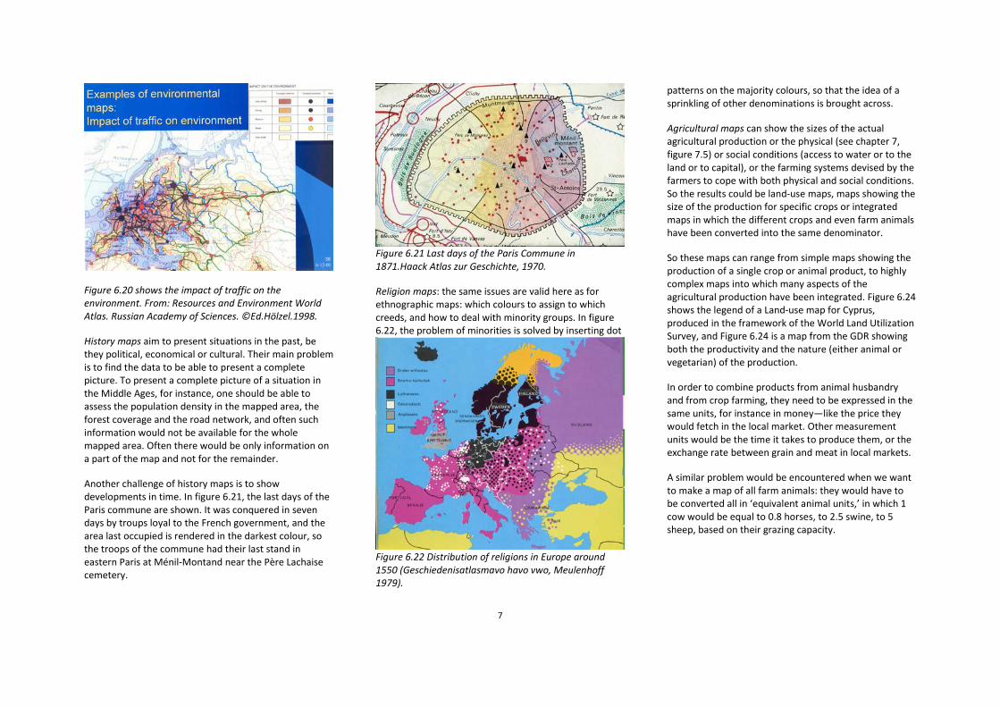
Figure 6.20 shows the impact of traffic on the environment. From: Resources and Environment World Atlas. Russian Academy of Sciences. ©Ed.Hölzel.1998.

History maps aim to present situations in the past, be they political, economical or cultural. Their main problem is to find the data to be able to present a complete picture. To present a complete picture of a situation in the Middle Ages, for instance, one should be able to assess the population density in the mapped area, the forest coverage and the road network, and often such information would not be available for the whole mapped area. Often there would be only information on a part of the map and not for the remainder.

Another challenge of history maps is to show developments in time. In figure 6.21, the last days of the Paris commune are shown. It was conquered in seven days by troups loyal to the French government, and the area last occupied is rendered in the darkest colour, so the troops of the commune had their last stand in eastern Paris at Ménil-Montand near the Père Lachaise cemetery.

Figure 6.21 Last days of the Paris Commune in 1871.Haack Atlas zur Geschichte, 1970.

Religion maps: the same issues are valid here as for ethnographic maps: which colours to assign to which creeds, and how to deal with minority groups. In figure 6.22, the problem of minorities is solved by inserting dot

Figure 6.22 Distribution of religions in Europe around 1550 (Geschiedenisatlasmavo havo vwo, Meulenhoff 1979).

patterns on the majority colours, so that the idea of a sprinkling of other denominations is brought across.

Agricultural maps can show the sizes of the actual agricultural production or the physical (see chapter 7, figure 7.5) or social conditions (access to water or to the land or to capital), or the farming systems devised by the farmers to cope with both physical and social conditions. So the results could be land-use maps, maps showing the size of the production for specific crops or integrated maps in which the different crops and even farm animals have been converted into the same denominator.

So these maps can range from simple maps showing the production of a single crop or animal product, to highly complex maps into which many aspects of the agricultural production have been integrated. Figure 6.24 shows the legend of a Land-use map for Cyprus, produced in the framework of the World Land Utilization Survey, and Figure 6.24 is a map from the GDR showing both the productivity and the nature (either animal or vegetarian) of the production.

In order to combine products from animal husbandry and from crop farming, they need to be expressed in the same units, for instance in money—like the price they would fetch in the local market. Other measurement units would be the time it takes to produce them, or the exchange rate between grain and meat in local markets.

A similar problem would be encountered when we want to make a map of all farm animals: they would have to be converted all in ‘equivalent animal units,’ in which 1 cow would be equal to 0.8 horses, to 2.5 swine, to 5 sheep, based on their grazing capacity.

7

Figure 6.23 Legend of a map of a land-use map of Cyprus.

In figure 6.24 the darker the colours, the higher the value of the overall agricultural production. The more reddish the colour, the more the production is oriented towards animal products; the bluer the more it is oriented towards crop products.

Physical planning maps aim at showing the planning measures that have been taken for the future. Frequently, the exact location of future town extensions, highways or airport has not been defined yet, and that

Figure 6.24 Size and nature of the overall agrarian production in the GDR for the year 1966.

results in these planning maps having a more or less schematic character, so that new roads, plants or town extensions cannot be located exactly, thus diminishing the possible antagonism against these proposed developments. Figure 6.25 is an example.

Figure 6.25 Physical planning map.

Urban maps show the present or future urban land use; in the latter case they would be related to planning maps. They can either portray individual towns and cities or render urbanization phenomena. In figure 6.26 the degree of urbanization of the GDR is shown. What is mapped here is the density of residential buildings that is the number of residential units per km2. The light green squares have less than 3 residential units per km2, while the purple squares have 60–150 and the red squares over 150 per km2.

8

Figure 6.26 Map of residential density for the GDR. The squares measure 10 x 10 km.

Hydrographic maps show the flow or capacity of rivers. They are produced by measuring this flow in all streams over a certain period, in order to be able to compute average flows. These would then be classified, and standard widths would be assigned to each class. In figure 6.27 the intermediate stages in the production of the map are shown, with the manuscript map or author’s original (see chapter 4, section 4.3.2) of the river network, the locations where the river flows were measured and codes that indicate the average

magnitudes of the flow. This document would allow the cartographer to draw the river network with the widths proportionate to the flow. The basis of the map is a precipitation or rainfall map, which is relevant as the river flow, at least in this part of the world, is determined by the amount of rainfall in the river basins. The tints to render the average amounts of rainfall range from yellow (low precipitation) to blue (high).

Figure 6.27 Author’s originals of river flows (above) and rainfall as a basis for the map in figure 6.29.

Figure 6.28 Hydrographic map (produced for ICA textbook).

6.5 Aggregation of enumeration areas

Data for socio-economic maps are available at different levels: usually they are available for postal code areas, for municipalities and combinations of municipalities, for districts, departments or provinces, etc. At every one of these levels the image of the mapped phenomenon will be different. This is caused by the fact that when data are aggregated, the new ratios or densities computed will be less extreme than on lower enumeration area levels: the higher the aggregation level, the more the resulting values will approach the national average.

The large map in figure 6.29 shows the referendum results in Norway regarding joining the European Union in 1994. A majority of 52% voted against joining, a minority of 48% voted for joining (if applicable). On the map reddish colours mean a community with a local majority voting against, blue a community with a local majority for joining. The blue areas are hard to find, but they represent the major urban areas in Norway.

9

Figure 6.29: Result of data aggregation. National atlas of Norway.

The smaller map portrays the same information, but now aggregated for provinces. Much fewer areas are characterised by the bright red colour denoting over 70% against; aggregating the data makes them less extreme.

6.6 Analytical and Synthesis maps

Most thematic maps portray just one aspect of a phenomenon: just soil type or religion or unemployment, population distribution or nuclear risk. We would call them analytical maps. Other maps show a few related aspects, like in figure 6.13, production of minerals and its transportation, or in figure 6.16 land use, manufacturing industries and service industries. When maps would

portray all possible aspects of a topic, we would call it a synthesis map.

Figure 6.30 Synthesis maps: all relevant aspects combined (International Cartographic Yearbook 1967).

Figure 6.30 is an example of a synthesis map. Its topic is wheat growing in Australia. Green isolines show the length of the growing season (when it is humid enough for crops to grow), and blue isolines show critical isohyets, that is lines of equal rainfall. Good soils suitable for wheat growing are rendered in dark brown, lesser soils have lighter colours. As accident terrain might pose problems to mechanical agriculture, hachures indicate such terrain. Finally the current acreage under wheat is shown with red dots, so that people can gauge from the map whether the present acreage could still be extended because there would be other areas still where all positive conditions prevail. The only relevant information not provided on this map is the transport infrastructure: apart from growing and harvesting wheat, it also should be transported to export ports.

Snow’s London Cholera victims map of 1854

Medical doctor John Snow investigated the 1854 cholera outbreak in London. He suspected that cholera outbreaks were related to the contamination of drinking water. He therefore mapped the victims of the cholera epidemic at their home addresses (see figure 6.32). When studying this map (on which he also had indicated the location of the water pumps, because of his suspicion – at that time this part of London did not have a piped water supply), he found out that the victims were located around the pump in Broad Street. He then convinced the local authorities to remove the handle of this pump and as a consequence no further cholera cases developed. Apparently the contaminated water of the Broad Street pump had been the cause of the cholera outbreak.

This is a nice case history of the beneficial role of map analysis. In his later life Snow also researched the statistics of cholera epidemics

10

6.7 References Jacques Bertin (2010) Semiology of Graphics. Esri Press: Redlands, California, USA. Steven Johnson (2006) The Ghost Map. The story of London’s Most terrifying Epidemic – and how it Changed Science, Cities and the Modern World. London: Riverhead Publishers. Arthur Robinson (1967) The Thematic map of Charles Joseph Minard. Imago Mundi vol.21 (1967) pp 95-108.

11

12

Chapter 7 Atlases

Ferjan Ormeling, Netherlands 7.1 Atlas purpose: narrative, scenario and structure Atlases are deliberate and systematic combinations of maps. These maps have been put together in order to put across a specific view or to solve a specific task. That requires the data in the maps to be processed in a specific way in order to solve these tasks. Generally, atlas maps have been combined in an atlas in order to be able to compare these maps, allowing map readers to draw useful and relevant conclusions from these comparisons. The point atlases want to get across can be called a narrative: atlases tell a story. They want to show for instance what the position of your country is in the world

Figure 7.1 Atlases tell a story (Drawing A. Lurvink).

or whether all inhabitants of a region have equal access to the resources (medical, educational, cultural, etc.) of that region. Their intention can be to show whether we

are doing better or worse than our neighbours, or they can be created to allow for a single task, like navigation.

The way in which this narrative has been designed can be called the atlas scenario. This defines the way the geographical information is presented: is it a series of thematic maps, all of the same area, presented in a specific sequence, or is it a digital product where you can set the order in which you view the maps yourself?

Figure 7.2 Atlas scenario. (Drawing A. Lurvink).

For a digital school atlas of Sweden, the scenario could be for instance that a flight of geese from one end of the country to the other is simulated, allowing the atlas users to view the country from above, and touch down or zoom in, whenever they feel like it. By clicking on a specific area, population density, vegetation or climate maps of that same area might pop up next to the overview map, allowing for a better understanding of the characteristics of that region. Issues relevant for that region, like environmental problems, the disappearance of services and medical facilities from the countryside could be highlighted.

Figure 7.3 Example of an atlas scenario (Lagerlöf, 1907).

The narrative of an atlas, like the narrative in a speech, consists of sequence and emphasis. In a speech, different arguments are combined in a specific order, while some arguments get more emphasis than others. The same is valid for an atlas. Here the arguments are the maps with specific themes. Some themes are considered more relevant for the narrative than others, so they would get more emphasis or, in atlas terms, more coverage: the atlas would get more maps on the same topic or maps on that topic would be rendered on a larger scale.

Figure 7.4 shows the structure of a school atlas of Indonesia: the arrows show the sequence in which the various provinces of that country are displayed in the atlas, and the size of the circles are indicative of the scale: larger circles suggest that the provinces represented by them are drawn on a larger scale—for instance because they are considered to be more important areas for the national economy.

1

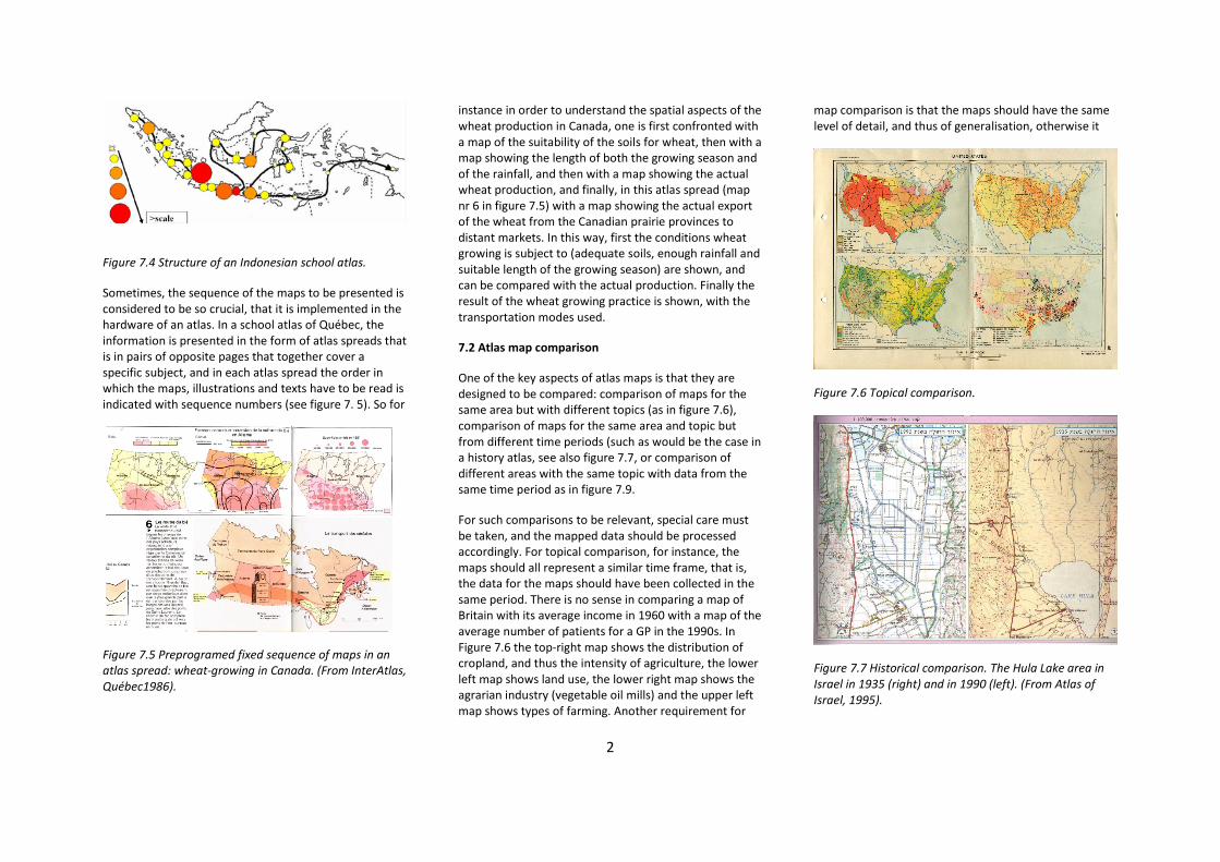
Figure 7.4 Structure of an Indonesian school atlas.

Sometimes, the sequence of the maps to be presented is considered to be so crucial, that it is implemented in the hardware of an atlas. In a school atlas of Québec, the information is presented in the form of atlas spreads that is in pairs of opposite pages that together cover a specific subject, and in each atlas spread the order in which the maps, illustrations and texts have to be read is indicated with sequence numbers (see figure 7. 5). So for

Figure 7.5 Preprogramed fixed sequence of maps in an atlas spread: wheat-growing in Canada. (From InterAtlas, Québec1986).

instance in order to understand the spatial aspects of the wheat production in Canada, one is first confronted with a map of the suitability of the soils for wheat, then with a map showing the length of both the growing season and of the rainfall, and then with a map showing the actual wheat production, and finally, in this atlas spread (map nr 6 in figure 7.5) with a map showing the actual export of the wheat from the Canadian prairie provinces to distant markets. In this way, first the conditions wheat growing is subject to (adequate soils, enough rainfall and suitable length of the growing season) are shown, and can be compared with the actual production. Finally the result of the wheat growing practice is shown, with the transportation modes used.

7.2 Atlas map comparison

One of the key aspects of atlas maps is that they are designed to be compared: comparison of maps for the same area but with different topics (as in figure 7.6), comparison of maps for the same area and topic but from different time periods (such as would be the case in a history atlas, see also figure 7.7, or comparison of different areas with the same topic with data from the same time period as in figure 7.9.

For such comparisons to be relevant, special care must be taken, and the mapped data should be processed accordingly. For topical comparison, for instance, the maps should all represent a similar time frame, that is, the data for the maps should have been collected in the same period. There is no sense in comparing a map of Britain with its average income in 1960 with a map of the average number of patients for a GP in the 1990s. In Figure 7.6 the top-right map shows the distribution of cropland, and thus the intensity of agriculture, the lower left map shows land use, the lower right map shows the agrarian industry (vegetable oil mills) and the upper left map shows types of farming. Another requirement for

map comparison is that the maps should have the same level of detail, and thus of generalisation, otherwise it

Figure 7.6 Topical comparison.

Figure 7.7 Historical comparison. The Hula Lake area in Israel in 1935 (right) and in 1990 (left). (From Atlas of Israel, 1995).

2

would be difficult to compare the respective patterns. A special type of topical comparison are the confrontations between the physical environment and the use mankind has made of this environment. This can be effectuated by putting opposite each other a physical map (showing layer zones or a satellite image) and a land-use map, as has been done in figure 7.8, or by opposing a physical map and an infrared satellite image, in which the vegetation—and thus agricultural enterprise—is highlighted. Both cases would show how humankind has made use of the physical landscape. By comparing such map combinations for areas with different or similar climates it can also be shown how different societies react to the same climatological and physical conditions.

Figure 7.8 physical map and land-use map (right) of Greece opposite each other in an Austrian school atlas. (From Pelzer Atlas, Ed. Hölzel, 1975).

For maps that show the same topic for the same area at different periods, or another area at the same time, of course the symbols in the map legends should be the same. Here as well it is of prime importance that all maps are generalised to the same degree. Take the image in figure 7.9: it is from a digital world reference

atlas that enables its readers to compare different areas. When one selects different areas to be compared, these areas are automatically rendered at the same scale; if one zooms in on one area, the area it is compared with is zoomed in upon at the same time. In this way, the comparisons still make sense. One can still wonder whether the two areas have been generalised to the same degree: the area at left has about 6 million inhabitants, while Greater Calcutta has some 15 million inhabitants; still, because many more names are inserted at the map at left, that map gives the impression of a more densely inhabited area.

Figure 7.9: Geographical comparison between two areas in a digital world reference atlas: here the central area of the Netherlands (left) is compared to the Calcutta or Kolkata area in India. (From Wolters-Noordhoff digital World atlas).

There are some other means we use in order to help readers to get a correct impression from maps. One of them is to render the outline of an area the map reader is familiar with in the margin of a map of an area strange to the map reader. In that way the map reader may get a correct sense of the areal magnitudes involved. This principle is shown in figure 7.10 where, in order to give

users of a Swiss school atlas a correct idea of the relative importance of the American manufacturing industry, an

Figure 7.10 Reference inset map in a Swiss school atlas. (From Schweizerische Weltatlas, 1981).

inset map of the manufacturing industry of Switzerland is shown at the same scale and with the same legend.

A similar procedure is shown in figure 7.12, taken from an Atlas of Maryland, one state of the United States. To all maps of that state in this atlas, whatever their topic, a map of the United States as a whole is added, mapped according to the same legend, so that map users can see to what degree the situation in the state of Maryland is different from that in the country as a whole.

3

Figure 7.11 Average number of children per wife. The lower-left diagram generalises the map. From Atlas de France vol. 2, 1995. GIP Reclus.

In figure 7.11 a small generalised and stylised representation of the main map is added in the lower-left corner, to help map readers remember the image. It shows the highest number of children per wife occurs in the North of France, while fertility is decreasing in the South-West and increasing in the South-East of France.

7.3 Types of atlases and atlas information systems

On the basis of the type of comparison they are intended for, atlases can be divided into different atlas types:

1. National atlases (meant for the comparison of maps with different topics for the same area);

Figure 7.12 Map of the change in population 1960–1970 in the state of Maryland with an inset map of the United States with the same topic and legend. (Atlas of Maryland 1977).

2. Historical atlases (meant for the comparison of maps for the same area and theme from different time periods);

3. Thematic atlases (meant for the comparison of maps for different areas with the same theme from the same time period: world forestry atlas, world petroleum atlas, world atlas of epidemics, etc.);

4. School atlases (introducing students to both physical and socio-economic aspects of world geography);

5. Reference atlases (very detailed atlases allowing their users to find a maximum number of places); and

6. Task-specific atlases (road atlases, yachting atlases, etc.), for instance for finding optimal routes.

All of these atlas types can be in hard copy or in digital form. When speaking of digital atlases, these can be (a) ‘view-only,’ meaning that the design of the map cannot be changed, they can be (b) ‘interactive’ in the sense that colours or class boundaries on the map can be influenced (see figure 7.12), and that data layers can be added to the map (see figure 7.13), and they can be (c) ‘analytical.’ In that last case, on the basis of the underlying datasets available, the information can be visualised and analysed in a way selected by the map user.

Figure 7.13. In an interactive atlas, the same data (World Literacy rate) can be visualised by different colour sets. Electromap World Atlas.

4

Figure 7.14 Selection of map layers for a map in a digital world atlas. Atlas Info Nation.

When digital atlases are presented in a form that allows for access to the data underlying the atlas maps, we speak about atlas information systems. Similar to hard-

copy atlases, atlas information systems can be subdivided into a number of types, such as national atlas information systems, historical atlas information systems, educational atlas information systems, etc. The difference between these atlas information systems and GIS (see chapter 3) is that the first are related to a certain area or theme in connection with a given purpose, with an additional narrative faculty, in which maps play a dominant role. The requirement that the data are pre-processed to allow for comparisons between maps, and that a selection has been made of the data in view of the purpose of the atlas, distinguishes the atlas information systems from ordinary GIS systems.

It should be highlighted here how important it is to be able to change colours (as in figure 7.13), and class boundaries when visualising datasets in map form in an atlas. When we still only had paper atlases, there was only one way in which the data were visualised, dependent on the insight, expertise, bias or taste of the cartographer. In an interactive or analytical, digital atlas, these limitations no longer apply. No map is the only true map, meaning that there is no best solution to visualise a specific dataset—depending on the intended audience for the atlas, the fact whether the map is to be compared with other maps in the atlas, different designs might fulfil the requirements.

Another aspect of interactive and analytical atlases is that they are no longer restricted by the fixed map frames of paper atlases. In a paper atlas, the map frame, the map topic and the time frame are fixed. In a digital environment it has become possible to experiment with the map frame, by panning or zooming (as in figure 7.15), it is possible to change the map topic, and it is possible to change the time frame, even in an animation mode.

Figure 7.15 Fixed map frames in a view only atlas (left) and adjustable frames in an interactive atlas (right). (Drawing A. Lurvink).

7.4 Atlas functionality

Paper atlases have a number of ways of accessing the maps they contain: there are tables of contents showing all the map titles, there are topical indexes showing all maps that portray specific topics, and there would be indexes of geographical names showing the maps with the largest scale where a specific geographical name occurs. There also would be a graphical index, with the outlines of all maps shown on a world map, with a reference page number where those maps can be found (see figure 7.16). A general legend explaining the signs and symbols occurring on the different types of maps would be incorporated as well.

In a digital atlas the access mechanisms are greatly enhanced. Not only would all the tables of contents and indexes all be there, but clicking a specific geographical name would immediately bring up the respective map containing that name, which would be highlighted. Clicking a topic in the topical index would show all the maps answering that description, in sequence.

5

Figure 7.16 Graphical index of the European maps in a paper school atlas. Bosatlas53rd ed., 2007.

A legend would not always be necessary in a digital atlas, as clicking a specific symbol would always result in a pop-up explanation of that symbol. Apart from that, clicking map objects like symbols or areas would result in additional information, such as height above sea level, number of inhabitants or, on economic maps, production figures. This possibility to query all map objects is one of the major benefits of digital maps; it also clears the map image, as all information that is not strictly necessary can be hidden in a pop-up mode. Furthermore, there would be the possibility to hide images or explanations under hot spots. The search engine to find places has already been discussed under the indexes, as have the zoom and scroll functions. In order to allow for zooming in, more detailed datasets need to be available, and will be accessed whenever given scale thresholds have been passed.

7.5 Our school atlases are biased!

Nowadays in many countries it is one of the educational goals of the geography curriculum to make students aware of the usefulness, reliability and representative-ness of the information made available to them—in

textbooks and newspapers or on the Internet. As an example of such an evaluation we will try here to gauge the bias, reliability and representativeness of school atlases.

School atlases introduce pupils and students to the world from a given position or point of view. That position can refer to a geographical position (a school atlas from Sweden will be different from a school atlas from Zambia), to an educational viewpoint (what is the necessary basic knowledge all students should have), or to ideological or political views. Because we are so familiar with the image of the world presented by our own school atlases, we do only recognise their bias when comparing these school atlases with those from other countries. We would also recognise it when comparing our current school atlases with those produced in the past. When we would do so, we would find that society’s ideas of what a country’s characteristics are has changed, as have its ideas of what constitutes the country’s desired development. The amount of geographical information on other countries and the world at large has increased (plate tectonics, climate change) and the world itself has changed as well, with an increasingly complex infrastructure, higher population numbers and environmental problems (desertification, deforestation, etc.). When following the development of atlases over time we would also find the effects of different atlas editors, each with their own view of the geographical information belonging in the atlas, different interests of society at large and changing didactical insights and geography curricula.

a. Style of the atlas and standpoint in the world;

Every school atlas has its own structure, based on choices regarding the sequence of the maps and the emphasis on given areas or topics. It would also have its own particular style, defined by the selection of specific script types, the level of generalisation of the line work

and the use of colour. In the spelling of geographical names, specific choices would have been made, either favouring local official names or exonyms (see Chapter 8). The country’s standpoint in the world would determine which areas of the world are dealt with first, and its global socio-economic position probably would strongly influence the selection of map topics in the atlas. If a country has a prime position in the per capita income, in health care, life expectancy, energy consumption, good governance, political stability and the absence of corruption, that country has more incentive to include maps on these phenomena than other countries that do not. Of course this is also linked to the willingness of a society to also address negative aspects in its educational products like school atlases. Are maps on unemployment, the unequal distribution of wealth, marine pollution, domestic violence or the percentage of smokers also included? Should the attitudes towards capital punishment, gay rights, the part of the gross national product spent on the military, the investment climate and freedom of the press be mapped as well? All these are aspects in which school atlases worldwide differ.

b. Terminology;

School atlases provide schoolchildren with the tools and concepts to find their place in the world. They do so with the special terminology with which we can describe the world, with overall concepts like continents and oceans, countries and seas, deserts and mountain ranges, lowlands or continental shelves. In order to simplify the overview, objects are grouped together. Take the case of Spain: Here mountain ranges have been grouped together for educational purposes and given names no one in the field ever mentions: The Castilian plateau or Meseta Central is divided into two parts by the ‘Sistema Central’ mountain range (see figure 7.17). This is a notional or fictitious object, however; no one in Madrid in winter-time will say that he or she is going to ski in the

6

Sistema Central—they go for the Sierra de Guadarrama, the Sierra de Gredos or the Sierra de Gata (see figure 7.18).

Figure 7.17 Educational names used in Spanish school atlases (Atlas nacional de España, 1991).

Figure 7.18 Composition of the Sistema Central mountairange in Spain. (Atlas nacional de España, 1991).

Examples of similar educational groupings of geographical objects without any local knowledge of them in the terrain are the Greater and Lesser Sunda isles, the Greater and the Lesser Antilles (subdivided again in the Lee-ward and the Windward Isles); Siberia is divided into the Western Siberian Lowlands, the Central Siberian Plateau and some East-Siberian Mountain Ranges. Geography teachers distinguish the Finnish Lakeland and the Central Africa Lakes, as they do with the North and South Equatorial Ridges in Africa and the East African Highlands. All these groupings of mountains, lakes, islands or plains have been effectuated for educational purposes, to simplify teaching the structure of the world. Ideological points of view

Ideological or political points of view can be expressed in the sequence of countries presented in an atlas (for instance, in the past, communist countries, members of the COMECON bloc were dealt with before dealing with the capitalist countries, irrespective of their geographical location. Ideological views were expressed in map titles (see figure 7.19).

The ideological views can also be expressed in the selection of map projections. Some projections are thought to favour Western or capitalist views, the Mercator projection which exaggerated the size of countries in more northerly locations being one of them. As a substitute sometimes the Gall-Peters projection is used, first developed in 1855, which is an equal-area projection, meaning that the size of countries on the map is proportional to their true size. To realise this, the Gall-Peters projection results in rather extreme deformation (see figure 7.20).

Some countries would include the military infrastructure of their country in the school atlas, others would favour

countries where the same language was spoken, for instance French (see figure 7.21).

Elsewhere, geopolitical views, like the division of the world into an economic heartland and its peripheries, surrounded by a number of emerging or threshold countries, are rendered in school atlases, thus visualising theories of global development (figure 7.22).

Figure 7.19 Map from a history atlas produced in 1970 in the German Democratic Republic, with the title The Political Segmentation of Greek Slave-Holding Societies, where the usual title would be Ancient or Classical Greece. Haack Atlas zur Geschichte, 1970.

7

Figure 7.20 World population density map in a Zimbabwean school atlas in the Gall-Peters projection. Harper-Collins Senior Atlas for Zimbabwe, 1992.

Figure 7.21 Distribution of French-speaking countries, from a French school atlas.

Figure 7.22 Geopolitical map dividing the earth in Centre and periphery, with operating systems in world economy from an Austrian school atlas. © Ed.Hölzel.

Sometimes, countries would favour the incorporation of maps in their school atlases that would show that they are particularly good in some fields. In figure 7.23, a map of a school atlas from Sri Lanka is shown. This country does not score particularly high on most economic yardsticks like per capita income, but it does rather well in fighting illiteracy. Thus it is understandable that a map of world literacy is incorporated, the darker the tint, the higher the percentage of those that can read and write, and the position of Sri Lanka in this respect within the South Asia region is certainly remarkable.

Figure 7.23 World literacy rate map from a Sri Lankan school atlas. Sarasavi School atlas, 2004.

c. Basis for overview maps;

Traditionally, the overview maps in our school atlases have either been administrative or physical maps, showing either the administrative subdivision of our countries or their physical characteristics, the latter through the use of isohypses and layer zone tinting. Neither of these two representation nodes is very informative about the country’s landscape diversity. The height above sea level, as portrayed in isohypse and layer tint maps cannot say anything about the country’s vegetation or agricultural potential. That is why some school atlases advocate the use of land-cover tints, combined possibly with symbols for non-agrarian economic activity, as land-cover tints would already inform about agricultural production (see figures 7.24 and 7.25).

8

Figure 7.24 Detail of economic overview map of China. © Ernst Klett Verlag GmbH.

Figure 7.25 Detail of physical overview map of China. © Bertelsmann Weltatlas/wissenmedia mapworks.

7.6 Correcting Eurocentric school atlases

As we saw in section 7.1 an atlas narrative is built on sequence and emphasis. Every country favours the representation of its own territory in its school atlases. Figure 7.26 shows the number of maps in a Dutch school

atlas which covers the home country, as opposed to those for the rest of Europe, the various continents and the world. The home country would also figure first, in the atlas sequence, with neighbouring countries, the home continent, other continents and the world dealt with successively.

Figure 7.26. Proportional number of maps covering the Netherlands, the rest of Europe, other continents and the world (=aarde in Dutch) in a Dutch school atlas in 1877, (top left) and 2010.

While we realise that all countries producing school atlases would favour their home area and home continent, we still should not be blind to the distortive effects of those views. If one is only used to a world map with Europe and Africa in the centre, then there would be many geographical relationships (like in figure 7.27), like those between the Pacific Rim countries, that would stay hidden. That is why it is so important to also look at the viewpoint of atlas producers in other parts of the Earth.

Figure 7.27 shows the view from the United States. Here the central meridian of the world map bisects the United

States, nicely showing its pivotal position between the Atlantic and Pacific world oceans.

Figure 7.27 World map from an American school atlas. (21st ed., Goodes’world atlas, RandMcNally, 2005).

Figure 7.28 is from a school atlas of Sri Lanka, dividing the world in the Eastern and Western Hemispheres, and Sri Lanka is located at the central meridian of the Eastern Hemisphere. Finally, figure 7.29 is from a school atlas of China.

Figure 7.28 World map from Sri Lankan school atlas. Sarasavi school atlas, 2004.

9

Figure 7.29 World map from a Chinese school atlas.

7.7 Web atlases

The current challenge for atlases is to develop atlases for the Internet that do more than just show pre-produced maps, but allow for directly and automatically produced maps, generated case by case from the data available in the database at the website. The system should allow for selecting a visualisation mode, on the basis of the data characteristics for instance: absolute quantitative data to be mapped by proportionate circles, and relative quantitative data to be mapped by choropleth (see Chapter 6). This system should allow for influence by the user, for instance in setting the class boundaries and in selecting the colour tints with the data to be rendered.

Research is now taking place to work out how statistical or environmental data collected from statistical offices can be combined with atlas base maps and atlas metadata, using spatial aggregator services in a data integration and mapping component, allowing for user input regarding classification and visualisation modes, resulting in user-defined atlases maps.

Figure 7.30 Demonstration of a web atlas of the Netherlands, interactively produced.

Figure 7.31. The 20 crown note from Sweden showing Nils Holgersson flying on the goose Mårten over the Swedish landscape (Lagerlöf. 1907). See also Figure 7.3.

References:

Lagerlöf Selma (1907) Nils Holgersson´s wonderful journey through Sweden. Search on www.amazon.com.

For further information on atlas cartography, see the website of the ICA Commission on national and regional atlases: http://www.univie.ac.at/cartography/karto/project/cnra/

The ICA Atlas commission will produce a cookbook for atlas production in 2015.

10

Chapter 8 - Geographical Names

Ferjan Ormeling, Netherlands Maps are superb tools for getting to know our environment, to understand about distances, or to plan a journey. They show us how our location on Earth influences the climate and the possibilities to earn a living. But they only can show us these relationships when they bear geographical names. Look at the map in figure 8.1. It shows (parts of) 5 countries, separated by boundaries, and towns and cities and rivers and canals, but it does not tell us anything because we cannot relate to all these mapped objects as countries, settlements and rivers. They are not named. We can only refer to the objects rendered on the map in an indirect way, like ‘the big city in the southwest of the map,’ or ‘the sea in the northwest corner of the map.’

Figure 8.1 Map without geographical names.

Figure 8.2 shows the difference made by the addition of geographical names. Now every mapped object (except for a few smaller rivers and canals) can be directly referred to. The ‘big city in the southwest corner of the map’ now can be addressed directly as Paris, for instance, and the sea turns out to be the North Sea. Now it is easy to describe the relationships between the mapped objects; for instance, ‘Liège is located in-between Brussels and Aachen,’ or ’Luxembourg is bounded by France in the South, by Germany in the East and by Belgium in the North and the West.’ The characteristics of all mapped objects now can be easily listed, for instance, in a gazetteer. A gazetteer is an alphabetical list of the geographical names within an area, like a country, with an indication of the location of the objects they refer to (expressed, for instance, in geographical coordinates, see Section 9.1), the nature of the named object (is it a town, a river, a canal or a country?) and of their official spelling.

For the official spelling, we have to look first at the way geographical names are collected during the survey of an area in order to produce a topographical map (see Chapter 5). Topographers will visit municipality offices in order to collect the names used locally to refer to the geographical objects. Sometimes they will also go into the countryside and ask the local inhabitants for the names of the lakes, hills, hamlets or forests in their neighbourhoods. All the names collected in this way will be submitted to a names bureau that will check whether the spelling of the name is correct according to the official orthography of the country’s language(s) or whether the spelling reflects the local pronunciation of the name. When everyone agrees what the spelling of the name should be, it is officially defined. We call this process standardization of geographical names. All the

Figure 8.2 Shows the same area as mapped in figure 8.1, but here geographical names have been added.

names of which the spelling has been standardised will then be published in official lists, so that everyone can see how they are to be spelled.

Because their spelling has been standardised, geographi-cal names can also serve as links in geographical information systems. Statistics for municipalities can be linked to boundary files with the boundaries of these same municipalities, allowing for digital mapping of these statistical data. A procedure called ‘parsing’ allows us to retrieve all documents in a database in which a specific geographical name is mentioned. But, again, this only works if everyone agrees about the spelling of that particular name. Here we are frequently confronted with the problem that people from a different language community than ours will use different names for the same geographical objects as we do.

1

Figure 8.3 The same area as mapped in figure 8.1, now with the officially standardized local names (endonyms).

Names like Trèves, Cologne and Dunkirk, used in the English language in order to refer to places that are called officially Trier, Köln and Dunkerque by their local inhabitants, are called exonyms. Exonyms are names used in a particular language for a geographical object outside the area where that language is spoken and differing in their spelling from the names used in the official language(s) of that area where the object is located. Trier, Köln and Dunkerque are examples of endonyms, or locally official standardized names. Exonyms often emerged in a process of adaptation of foreign names to our language, and frequently as such they have become part of our history, and our cultural heritage. In English history, the ‘battle of Jutland’ in the First World War refers to the naval battle off the coast of the Danish peninsula called Jylland in Danish, for which Jutland is the English exonym. The chicken breed called

Leghorn in English refers to the Italian port of Livorno where these chicken were exported from. Leghorn is the English exonym for Livorno. While it is understandable that these exonyms are part of our history, it is also understandable that in view of international name standardization, the use of endonyms is the preferred mode of communication.

Figure 8.4 Finnish exonyms for Western Europe.

The existence of two or more names for one and the same object is called allonyms. A good example is the German town of Cologne: the endonym is Köln; in

English and French it is called Cologne; in Dutch Keulen; in Spanish and Italian Colonia; in Czech Kolín,; and in Polish Kolonia. Opposite of allonyms is the concept of homonyms: the fact that the same name can refer to different geographical objects. The Scottish town of Perth has the same name as the capital of Western Australia. Birmingham in Britain bears the same name as the capital of the American state of Alabama. Stratford upon Avon is the birthplace of William Shakespeare in England, on the banks of the river Avon. But the combination of the place called Stratford and the river Avon also occurs in Australia and in New Zealand. How do we distinguish between them? Here it becomes necessary to add features to these names: Birmingham, Alabama versus Birmingham, England, or Frankfurt am Oder versus Frankfurt am Rhein.

National and International standardisation of geographical names

In an ideal world, every geographical object would be recognised by its unique name, which would only refer to this particular object. In order to get as close as possible to this ideal situation, we first apply the process of national standardization of geographical names: every country decides what should be the spelling of the names of the geographical objects within its borders, and it communicates these spelling decisions to all other countries, by publishing gazetteers, so that inhabitants of those other countries would know what these official spellings are.

The next step would be the process of international standardization. There is a complicating factor here, and that is that we not only speak different languages all over the world, but we also use different writing systems. In order to have ‘univocity’—the existence of one unique standard name for each geographical object in each writing system—it requires that there only be one single, official way to convert names from one

2

writing system, like Arabic, Chinese or Amharic to another writing system like the Roman alphabet. In this way, local names that have been standardized officially in one language and writing system would be converted into standardized names in another writing system.

Figure 8.5 Writing systems used in Southeast Asia: Bengal (Bangladesh), Burmese (Myanmar), Thai (Thailand), Cambodian (Cambodia), Laotian (Laos), Roman (Vietnam) and Chinese (China) writing systems. (© Menno Bolder)

For most of the writing systems displayed in figure 8.5, the United Nations has recognised official conversion systems. The name of a conversion system depends on the writing system it converts into. Conversion into the Roman script is called a romanization system. Pinyin is the name of the romanization system recognised by the UN in order to convert names from the Chinese writing system into the Roman alphabet.

Figure 8.6 Southeast Asia with geographical names converted into the Roman alphabet. (© Menno Bolder)

It can be seen in figure 8.6 that in many names special signs have been added to the letters of the Roman alphabet in order to modify the normal pronunciation of these letters. Some of the letters even have two of these signs added to them (an example is the letter e in Việt Nam), but that is exceptional. Not only do these pronunciation-modifying signs, called diacritical signs, change the sound of the names, they would also influence alphabetization, the sequence of names when arranged or listed alphabetically. In Danish, for instance, geographical names like Amager or Als fall under the first letter of the alphabet, while names like Ålborg or Århus come after the letter Z.

Endonyms can be converted from one language to another in three different ways:

• when both languages use the same alphabet the name can just be copied, including all the diacritical signs used from the first language to the second (e.g., Polish, German, Danish)—

Warszawa (Warsaw), Köln (Cologne), København (Copenhagen). In some countries this procedure is called transposition;

• names can be transferred "letter by letter" according to conversion tables (see also figure 8.7), (e.g.from Cyrillic to Latin, from Greek to Latin, from Arabic script to Latin, etc.)—София (Sofia), Αθήνα (Athens), رصقألا (al-Uqṣur, Luxor). This procedure is called transliteration; and

Figure 8.7. Example of a conversion table, from the Georgian to the Roman alphabet, as proposed by Georgia.

• the sounds of the name can be rendered in the second language according to the pronunciation of the letters in its alphabet For example the Chinese name of the capital of China in Chinese characters: 北京 of China in Chinese) is rendered Beijing in English, Peking in German, Pechino in Italian, Pekín in Spanish, etc. This procedure of phonetic rewriting is called transcription.

3

Functions of geographical names

Geographical names not only serve in relating to our environment or as links in information systems, but they also play a role in brand names. Bordeaux, Beaujolais or Champagne not only are names of French regions, but they also refer to specific wines. And the use of these geographical names for these products can even be protected; it is not allowed to refer to some bubbly wines as Champagne unless they are actually produced in the Champagne region from grapes harvested there. A similar use of geographical names is valid for cheese: Edam and Gouda are names for typical Dutch cheese types, while Gorgonzola and Parmesan refer to Italian cheese types.

Most geographical names, when first given, were transparent. That is, their meaning was clear to those that gave the names. Rio de Janeiro is the name of a river in Brazil that was first sighted by the Portuguese 1 January 1502. Later on, the name of the river was transferred to the settlement that grew up on its bank. Cape Town is the English translation of the Dutch name Kaapstad, given to the settlement built by the Dutch in the 17th century close to the Cape of Good Hope, as a victualing station for the Dutch ships on their route from the Netherlands to the Spice Islands in the Moluccas. Some names lay claim to an area: the name Vladivostok, the Russian main naval port on the Pacific Ocean, means Ruler of the East. ‘Nya Sverige’ (or New Sweden) is the name of a 17th century Swedish colony on the banks of the Delaware River in the present-day United States. Like other European powers, it laid claim to a part of the North American continent. France claimed its ‘Nouvelle France,' England its ‘New England' and the Netherlands its ‘Nieuw Nederland.’ When the Dutch first arrived in the present-day Australia in the 17th century, they called it New Holland, after their principal province of Holland.

When the British at the end of the 18th century claimed it, they were not happy with this Dutch name and they introduced a new, more neutral sounding name, Australia, derived from the Latin word ‘australis’ which means southern. This new name thus referred to the ‘southern’ continent.

Names carry meaning. The name Amsterdam is the present-day version of the mediaeval name Amstelredamme, which means the dam in the river Amstel where the first hamlet of this name was situated in the 13th century. So names describe the original situation of the location or its surrounding area. Dutch names ending in –lo (Almelo, Hengelo) refer to locations in clearings in the forest; names ending in –koop (Nieuwkoop, Boskoop) refer to settlements created when the peat areas were drained and cleared for agriculture; and names ending in –drecht (Sliedrecht, Zwijndrecht) refer to names of settlements built along the dikes in the Middle Ages. Like in personal names, where trends to name children after pop or movie stars alternate with traditional names or fancy French names, there also have been trends in naming towns.– And by studying names it sometimes becomes possible to establish when these names were first given. The study of the meaning of place-names is called etymology.

Name elements

Geographical names sometimes consist of a single word and sometimes of multiple words—examples are London and Newcastle upon Tyne (this addition to the name Newcastle serves to distinguish it from other towns called Newcastle). But even if a name consists of a single word, it may have been constructed from different elements. The name of the Scottish capital Edinburgh consists of two elements, burgh, meaning fort and the personal name Eidyn, so the name would mean the Fort of Eidyn. We call the part that describes the nature of the named object, in this case –burgh, the generic part of

the name, and the part that refers to the person whom the fort was named after, the specific part. Sometimes the generic part is a separate word, like in Mount Everest, Forest of Dean, or Bay of Fundy. Sometimes it is combined with the specific part, like in Newcastle, Blackpool or Plymouth (naming the settlement at the mouth of the river Plym). The distinction of generic and specific elements of names is relevant regarding exonyms. Sometimes when a name is transferred from one language or writing system to another, the generic parts of these names are translated into the new language. So the Greek name Αιγαίο Πέλαγος (Aigaio Pelagos) is converted into English as Aegean Sea, and the Russian name мыс Дежнёва (Mys Dezhnëva, a cape named after the Russian explorer Semyon Dezhnev) is converted to Cape Dezhnev.

Historical names and name planning

Many geographical names used in the past are no longer current and official. This can be caused by changes in the official orthography of a language. It can also be caused by conquest when one country occupies (part of) another country and imposes its own names on the geographical objects in the conquered lands. It can be caused by decolonization as well, when the names used by the former colonial power are exchanged for new names in the language of the newly independent people. In figure 8.8, some examples are given of new names (in black) that emerged in Africa after the decolonization process that happened in the 1960s and replaced former colonial names (in red). These former geographical names that have been replaced by the current new names that are now official locally are called historical names. Examples of these historical names are Batavia, the former Dutch name of the Indonesian capital Jakarta; Leningrad, the former Communist name of the Russian port city on the Baltic Sea called Saint Petersburg (in Russian, Санкт-Петербург, converted into the

4

Roman alphabet as Sankt-Petersburg); and Madras, the former name of the Indian city Chennai, capital of the Indian state Tamil Nadu.

Figure 8.8. Some examples of post-colonial names in Africa.

Whenever names are changed, it is good practice to place the former and the new name side by side for a given time period so that the population can get used to the new name, and foreigners unfamiliar with the new name can still find their way around. This is an aspect of name planning. Name planning can be defined as the deliberate effort to influence the spelling of place-names, primarily in order to improve communication. There can be other reasons; however, for instance, shedding of the toponymic influences regarded as foreign.

Figure 8.9 Detail from Dutch school atlas, 1961, with the names Zuidchinees Bergland and Zuidchinese zee. (Bosatlas, 41th edition, 1961)

Name planning is also needed when the orthographic rules of a language change. Even seemingly small changes, like the introduction of hyphens after cardinal directions instead of joining those words to the main specific name elements, may result in thousands of changes in a reference atlas. In the 1960s, in the Dutch language, the words Zuid (south) and Chinese were

Figure 8.10 Detail from Dutch school atlas, 2006. (Bosatlas, 53rd edition, 2006)

joined while from 2000 onwards these words had to be separated by hyphens, as can be seen when comparing figures8.9 and 8.10. The impact of such spelling measures on cartographical products can necessitate a major overhaul of them.

5

Further references:

For those interested in toponymy and cartography, we refer to the online web course in toponymy, to be accessed from either the website of UNGEGN, the United Nations Group of Experts on Geographical Names (at http://unstats.un.org/unsd/geoinfo/ungegn/default.html) or to the website of the Commission on Education of the International Cartographic Association (http://lazarus.elte.hu/cet/index.html) under Internet Cartography Teaching courses).

The UNGEGN website also provides information on national and international geographical names standardization procedures, addresses of national bureaus in charge of geographical names, and access to national toponymical guidelines. These guidelines inform map editors and other editors on how geographical names in specific language areas are spelled, how countries are dealing with names in multilingual areas, and how names are pronounced.

UNGEGN itself also produces a global gazetteer, which can be accessed at http://unstats.un.org/unsd/geoinfo/geonames/, which presently lists the names of all cities with over 100,000 inhabitants and their pronunciation. It also has all country names in the 6 official UN languages (including Russian, Arabic and Chinese) and the local language.

]

6

1

9 MAP PROJECTIONS AND REFERENCE

SYSTEMS Miljenko Lapaine, Croatia and E. Lynn Usery,

USA

9.1 Introduction A map is a projection of data usually from the real Earth,

celestial body or imagined world to a plane

representation on a piece of paper or on a digital display

such as a computer monitor. Usually, maps are created

by transforming data from the real world to a spherical

or ellipsoidal surface (the generating globe) and then to

a plane. The characteristics of this generating globe are

that angles, distances or surfaces measured on it are

proportional to those measured on the real Earth. The

transformation from the curved surface into a plane is

known as map projection and can take a variety of

forms, all of which involve distortion of areas, angles,

and/or distances. The types of distortion can be

controlled to preserve specific characteristics, but map

projections must distort other characteristics of the

object represented. The main problem in cartography is

that it is not possible to project/transform a spherical or

ellipsoidal surface into a plane without distortions. Only

a spherical or ellipsoidal shaped globe can portray all

round Earth or celestial body characteristics in their true

perspective.

The process of map projection is accomplished in three

specific steps:

1) approximating the size and shape of the object (e.g.,

Earth), by a mathematical figure that is by a sphere or an

ellipsoid;

2) reducing the scale of the mathematical representation

to a generating globe (a reduced model of the Earth

from which map projections are made) with the principal

scale or nominal scale that is the ratio of the radius of

the generating globe to the radius of the mathematical

figure representing the object [Earth]) equivalent to the

scale of the plane map; and

3) transforming the generating globe into the map using

a map projection (Figure 9.1).

Figure 9.1. Map projection from the Earth through a

generating globe to the final map (After Canters, 2002).

Map projections depend first on an assumption of

specific parameters of the object (Earth) itself, such as

spherical or ellipsoidal shape, radius of the sphere (or

lengths of the semi-major and semi-minor axes of the

ellipsoid), and a specific datum or starting point for a

coordinate system representation. These assumptions

form the basis of the science of Geodesy and are

currently accomplished using satellite measurements

usually from the Global Positioning System (GPS),

Glonass, or Galileo (see section 9.2). Once these

measurements are accepted, an ellipsoidal

representation of coordinates is generated as latitude

and longitude coordinates. Those coordinates can then

be transformed through map projection equations to a

plane Cartesian system of x and y coordinates. The

general equations of this transformations have the

following form:

x = f1(φ,λ), y = f2(φ,λ)

where

x is the plane coordinate in the east‐west direction

y is the plane coordinate in the north‐south

direction

φ is the latitude coordinate

λ is the longitude coordinate

The form of the functions f1 and f2 determines the exact

transformation and the characteristics of the ellipsoidal

or spherical representation that will be preserved.

Before addressing the specific types of transformations

and the characteristics preserved, it is necessary to

understand the geodetic characteristics of the ellipsoidal

coordinates and how these are generated with modern

satellite positioning systems.

2

9.2 Geodesy and Global Navigation Satellite

Systems (GNSS)

Map projections have their largest and most frequent

application in producing maps showing a smaller or

bigger part of the Earth's surface. In order to produce

the map of a region, it is necessary to make a geodetic

survey of that region and then to visualise the results of

such a survey. Geodesy is a technology and science

dealing with the survey and representation of the Earth's

surface, the determination of the Earth's shape and

dimensions and its gravity field. Geodesy can be divided

into applied, physical, and satellite geodesy .

Applied geodesy is a part of geodesy encompassing land

surveying, engineering geodesy and management of

geospatial information. Land surveying is a technique for

assessing the relative position of objects on the Earth

surface, when the Earth's curvature is not taken into

account. Engineering geodesy is a part of geodesy

dealing with designing, measuring, and supervising of

constructions and other objects (e.g., roads, tunnels and

bridges).

Physical geodesy is a part of geodesy dealing with the

Earth's gravity field and its implication on geodetic

measurements. The main goal of physical geodesy is the

determination of the dimensions of the geoid, a level

surface modelling Earth, where the potential of the

gravity field is constant. Geometrical geodesy is

concerned with determination of the Earth's shape, size,

and precise location of its parts, including accounting for

the Earth's curvature.

Satellite geodesy is part of geodesy where satellites are

used for measurements. In the past, exact positions of

isolated spots on the Earth were determined in

astronomical geodesy, that is, by taking measurements

on the stars. Measuring techniques in satellite geodesy

are geodetic usage of Global Navigation Satellite Systems

(GNSS) such as GPS, Glonass and Galileo.

A satellite navigation system is a system of satellites that

provides autonomous geospatial positioning with global

coverage. It allows small electronic receivers to

determine their location (longitude, latitude, and

altitude) to within a few metres using time signals

transmitted along a line‐of‐sight by radio from satellites.

Receivers calculate the precise time as well as position. A

satellite navigation system with global coverage may be

termed a global navigation satellite system or GNSS. As

of April 2013, only the United States NAVSTAR Global

Positioning System (GPS) and the Russian GLONASS are

global operational GNSSs. China is in the process of

expanding its regional Beidou navigation system into a

GNSS by 2020. The European Union's Galileo positioning

system is a GNSS in initial deployment phase, scheduled

to be fully operational by 2020 at the earliest. France,

India and Japan are in the process of developing regional

navigation systems. Global coverage for each system is

generally achieved by a satellite constellation of 20–30

medium Earth orbit satellites spread among several

orbital planes. The actual systems vary but use orbital

inclinations of >50° and orbital periods of roughly twelve

hours at an altitude of about 20,000 kilometres.

Photogrammetry is an important technology for

acquiring reliable quantitative information on physical

objects and the environment by using recording,

measurements and interpretation of photographs and

scenes of electromagnetic radiation by using sensor

systems. Remote sensing is a method of collecting and

interpreting data of objects from a distance. The method

is characterized by the fact that the measuring device is

not in contact with the object to be surveyed. Its most

frequent application is from aerial or space platforms.

The study of the transformation from the Earth's surface

model or generating globe to a two‐dimensional

representation requires the use of the following

concepts: ellipsoid, datum, and coordinate system. Each

of these is discussed below.

The Earth's ellipsoid is any ellipsoid approximating the

Earth's figure. Generally, an ellipsoid has three different

axes, but in geodesy and cartography, it is most often a

rotational ellipsoid with small flattening (Figure 9.2).

Figure 9.2. Terminology for rotational ellipsoid: EE' is the

major axis, PP' is the minor axis and the axis of rotation,

where a, is the semi-major axis and b is the semi-minor

axis.

The rotational ellipsoid is a surface resulting from

rotating an ellipse around a straight line passing through

the endpoints of the ellipse. It is used to model the

Earth. Famous Earth ellipsoids include the ones

elaborated by Bessel (1841), and the more recently, WGS84

and GRS80 ellipsoids. Flattening is a parameter used to

determine the difference between the ellipsoid and the

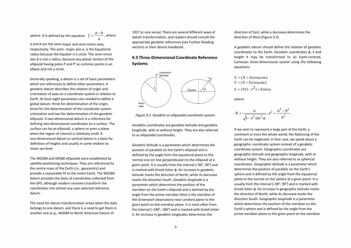
3

sphere. It is defined by the equation a b

fa

, where

a and b are the semi-major and semi-minor axes,

respectively. The semi- major axis a, is the Equatorial

radius because the Equator is a circle. The semi-minor

axis b is not a radius, because any planar section of the

ellipsoid having poles P and P' as common points is an

ellipse and not a circle.

Generally speaking, a datum is a set of basic parameters

which are references to define other parameters. A

geodetic datum describes the relation of origin and

orientation of axes on a coordinate system in relation to

Earth. At least eight parameters are needed to define a

global datum: three for determination of the origin,

three for the determination of the coordinate system

orientation and two for determination of the geodetic

ellipsoid. A two‐dimensional datum is a reference for

defining two‐dimensional coordinates on a surface. The

surface can be an ellipsoid, a sphere or even a plane

when the region of interest is relatively small. A

one‐dimensional datum or vertical datum is a basis for

definition of heights and usually in some relation to

mean sea level.

The WGS84 and GRS80 ellipsoids were established by

satellite positioning techniques. They are referenced to

the centre mass of the Earth (i.e., geocentric) and

provide a reasonable fit to the entire Earth. The WGS84

datum provides the basis of coordinates collected from

the GPS, although modern receivers transform the

coordinates into almost any user selected reference

datum.

The need for datum transformation arises when the data

belongs to one datum, and there is a need to get them in

another one (e.g., WGS84 to North American Datum of

1927 or vice versa). There are several different ways of

datum transformation, and readers should consult the

appropriate geodetic references (see Further Reading

section) or their device handbook.

9.3 Three‐Dimensional Coordinate Reference

Systems

Figure 9.3. Geodetic or ellipsoidal coordinate system.

Geodetic coordinates are geodetic latitude and geodetic

longitude, with or without height. They are also referred

to as ellipsoidal coordinates.

Geodetic latitude is a parameter which determines the

position of parallels on the Earth's ellipsoid and is

defined by the angle from the equatorial plane to the

normal one (or line perpendicular) to the ellipsoid at a

given point. It is usually from the interval [–90°, 90°] and

is marked with Greek letter φ. An increase in geodetic

latitude marks the direction of North, while its decrease

marks the direction South. Geodetic longitude is a

parameter which determines the position of the

meridian on the Earth's ellipsoid and is defined by the

angle from the prime meridian (that is the meridian of

the Greenwich observatory near London) plane to the

given point on the meridian plane. It is most often from

the interval [–180°, 180°] and is marked with Greek letter

λ. An increase in geodetic longitudes determines the

direction of East, while a decrease determines the

direction of West (Figure 9.3).

A geodetic datum should define the relation of geodetic

coordinates to the Earth. Geodetic coordinates φ, λ and

height h may be transformed to an Earth‐centred,

Cartesian three‐dimensional system using the following

equations:

X ( N h) cos cos

Y ( N h) cos sin

Z ( N (1 e2 ) h) sin

where

2 22

22 2,

1 sin

a a bN e

ae

.

If we wish to represent a large part of the Earth, a

continent or even the whole world, the flattening of the

Earth can be neglected. In that case, we speak about a

geographic coordinate system instead of a geodetic

coordinate system. Geographic coordinates are

geographic latitude and geographic longitude, with or

without height. They are also referred to as spherical

coordinates. Geographic latitude is a parameter which

determines the position of parallels on the Earth's

sphere and is defined by the angle from the equatorial

plane to the normal on the sphere at a given point. It is

usually from the interval [–90°, 90°] and is marked with

Greek letter φ. An increase in geographic latitude marks

the direction of North, while its decrease marks the

direction South. Geographic longitude is a parameter

which determines the position of the meridian on the

Earth's sphere and is defined by the angle from the

prime meridian plane to the given point on the meridian

4

plane. It is most often from the interval [–180°, 180°] and

is marked with Greek letter λ. An increase in geographic

longitudes determines the direction of East, while a

decrease determines the direction of West (Figure 9.4).

Figure 9.4. Geographic or spherical coordinate system:

geographic latitude φ, geographic longitude λ.

Geographic coordinates φ, λ and height h=0 may be

transformed to an Earth‐centred, Cartesian

three‐dimensional system using the following equations:

X R cos cos

Y R cos sin

Z R sin

where R is a radius of the spherical Earth.

A spherical coordinate system can be obtained as a

special case of an ellipsoidal coordinate system taking

into account that flattening equals zero, f = 0, or

equivalently stating that the second eccentricity equals

zero, e = 0.

Sometimes, in geodetic and cartographic practice, it is

necessary to transform Cartesian three‐dimensional

coordinates to spherical or even ellipsoidal coordinates.

Furthermore, sometimes there is a need to make a

transformation from one three‐dimensional coordinate

system to another one. The appropriate methods or

equations exist, but the reader should consult the

available literature (see Further Reading chapter).

9.4 Two‐Dimensional Coordinate Reference

Systems Generally, for use of geospatial data, a common frame of

reference is needed and this is usually done in a plane

reference system. Because maps reside in a plane

geometric system, the spherical or ellipsoidal

coordinates, generated from satellite positioning

systems or from any other surveying device, must be

mathematically transformed to the plane geometry

system. The simplest transformation is to assume that

the plane x coordinate is equivalent to φ, and the plane

y coordinate is equivalent to λ. The result is known as

the Plate Carrée projection and although it is simple, it

involves significant distortion of the coordinate positions

and thus presents areas, most distances, and angles that

are distorted or deformed in the plane.

More sophisticated transformations allow preservation

of accurate representations of area or distance or angles,

or other characteristics, but not all can be preserved in

the same transformation. In fact, usually only a single

characteristic, for example preservation of accurate

representation of area, can be maintained, resulting in

distortion of the other characteristics. Thus, many

different map projections have been developed to allow

preservation of the specific characteristics a map user

may require. The following sections provide discussion

and the mathematical basis for transformations that

preserve specific Earth characteristics, specifically area,

angles, and distances.

The Universal Transverse Mercator (UTM) coordinate

system is based on projections of six‐degree zones of

longitude, 80° S to 84° N latitude and the scale factor

0.9996 is specified for the central meridian for each UTM

zone yielding a maximum error of 1 part in 2,500. In the

northern hemisphere, the x coordinate of the central

meridian is offset to have a value of 500,000 meters

instead of zero, normally termed as "False Easting." The

y coordinate is set to zero at the Equator. In the

southern hemisphere, the False Easting is also 500,000

meters with a y offset of the Equator or False Northing

equal to 10,000,000 meters. These offsets force all

coordinates in the system to be positive.

In the Universal Military Grid System (UMGS), the polar

areas, north of 84° N and south of 80° S, are projected to

the Universal Polar Stereographic (UPS) Grid with the

pole as the centre of projection and a scale factor

0.9994. They are termed "North Zone" and "South

Zone."

Map projection also is dependent on the shape of the

country. In the United States of America, the State Plane

Coordinate System is established in which states with an

east‐west long axis, Tennessee, for example, use the

Lambert Conformal Conic projection, whereas states

with a north‐south long axis, Illinois, for example, use

the Transverse Mercator projection.. Not only a map

projection and the map scale, but coordinate

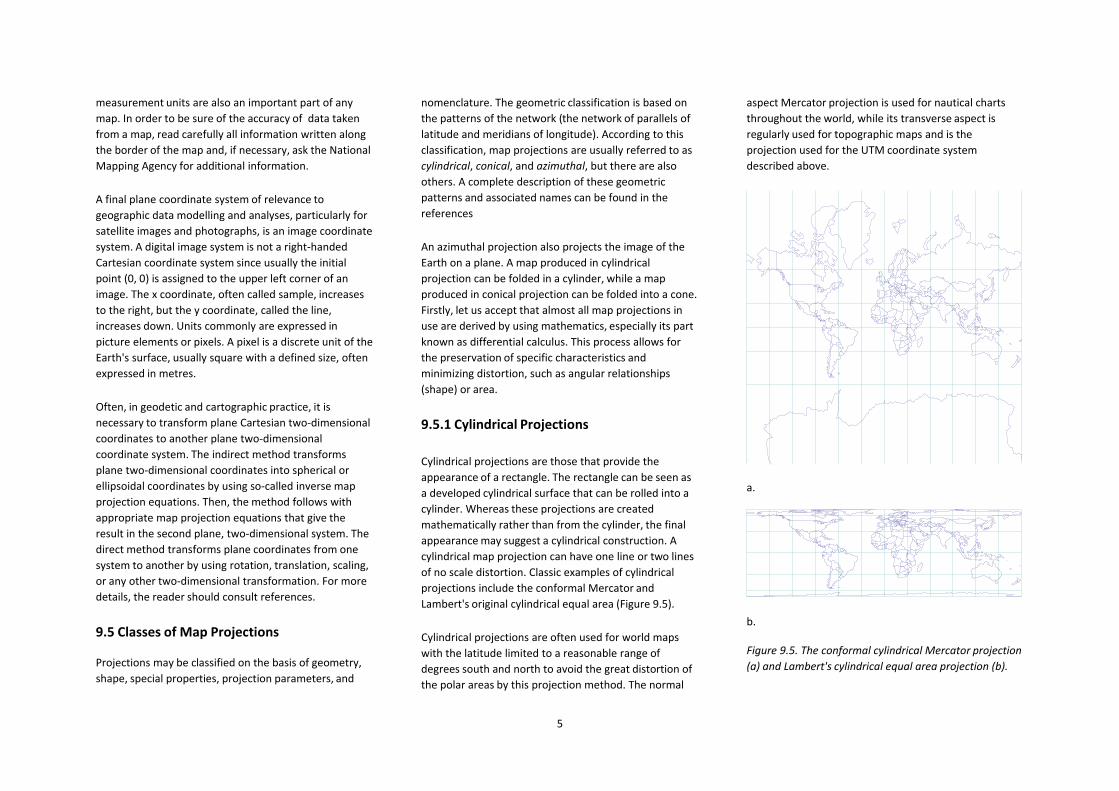
5

measurement units are also an important part of any

map. In order to be sure of the accuracy of data taken

from a map, read carefully all information written along

the border of the map and, if necessary, ask the National

Mapping Agency for additional information.

A final plane coordinate system of relevance to

geographic data modelling and analyses, particularly for

satellite images and photographs, is an image coordinate

system. A digital image system is not a right‐handed

Cartesian coordinate system since usually the initial

point (0, 0) is assigned to the upper left corner of an

image. The x coordinate, often called sample, increases

to the right, but the y coordinate, called the line,

increases down. Units commonly are expressed in

picture elements or pixels. A pixel is a discrete unit of the

Earth's surface, usually square with a defined size, often

expressed in metres.

Often, in geodetic and cartographic practice, it is

necessary to transform plane Cartesian two‐dimensional

coordinates to another plane two‐dimensional

coordinate system. The indirect method transforms

plane two‐dimensional coordinates into spherical or

ellipsoidal coordinates by using so‐called inverse map

projection equations. Then, the method follows with

appropriate map projection equations that give the

result in the second plane, two‐dimensional system. The

direct method transforms plane coordinates from one

system to another by using rotation, translation, scaling,

or any other two‐dimensional transformation. For more

details, the reader should consult references.

9.5 Classes of Map Projections

Projections may be classified on the basis of geometry,

shape, special properties, projection parameters, and

nomenclature. The geometric classification is based on

the patterns of the network (the network of parallels of

latitude and meridians of longitude). According to this

classification, map projections are usually referred to as

cylindrical, conical, and azimuthal, but there are also

others. A complete description of these geometric

patterns and associated names can be found in the

references

An azimuthal projection also projects the image of the

Earth on a plane. A map produced in cylindrical

projection can be folded in a cylinder, while a map

produced in conical projection can be folded into a cone.

Firstly, let us accept that almost all map projections in

use are derived by using mathematics, especially its part

known as differential calculus. This process allows for

the preservation of specific characteristics and

minimizing distortion, such as angular relationships

(shape) or area.

9.5.1 Cylindrical Projections

Cylindrical projections are those that provide the

appearance of a rectangle. The rectangle can be seen as

a developed cylindrical surface that can be rolled into a

cylinder. Whereas these projections are created

mathematically rather than from the cylinder, the final

appearance may suggest a cylindrical construction. A

cylindrical map projection can have one line or two lines

of no scale distortion. Classic examples of cylindrical

projections include the conformal Mercator and

Lambert's original cylindrical equal area (Figure 9.5).

Cylindrical projections are often used for world maps

with the latitude limited to a reasonable range of

degrees south and north to avoid the great distortion of

the polar areas by this projection method. The normal

aspect Mercator projection is used for nautical charts

throughout the world, while its transverse aspect is

regularly used for topographic maps and is the

projection used for the UTM coordinate system

described above.

a.

b.

Figure 9.5. The conformal cylindrical Mercator projection

(a) and Lambert's cylindrical equal area projection (b).

6

a. b.

Figure 9.7. The stereographic (a) and Lambert's azimuthal equal‐area (b) projections.

9.5.2 Conical Projections

Conical projections give the appearance of a developed

cone surface that can be furled into a cone. These

projections are usually created mathematically and not

by projecting onto a conical surface. A single line or two

lines may exist as lines of no scale distortion.

a.

b.

Figure 9.6. Lambert's conformal conic (a) and the Albers

conical equal area (b) projections.

Classic examples of conical projections are Lambert's

conformal conic and the Albers conical equal area

projection (Figure 9.6). Conical projections are

inappropriate for maps of the entire Earth and work best

in areas with a long axis in the east‐west direction. This

makes them ideal for representations of land masses in

the northern hemisphere, such as the United States of

America, Europe, or Russia.

9.5.3 Azimuthal Projections

Azimuthal projections are those preserving azimuths

(i.e., directions related to north in its normal aspect). A

single point or a circle may exist with no scale distortion.

Classic examples of azimuthal projections include the

stereographic and Lambert’s azimuthal equal area

(Figure 9.7).

9.5.4 Other Classifications

Other classifications of map projections are based on the

aspect (i.e., the appearance and position of the graticule,

poles or the equator in the projection). Aspect can be

polar, equatorial, normal, transverse or oblique.

Accordingly, there are polar projections, normal

projections, equatorial projections, transverse projections

and oblique map projections. These are names of

individual sets of map projections and not a systematic

categorization because, for example, a projection can be

polar and normal at the same time. In theory, each

projection can have any aspect. However, many

projections are almost always used in certain aspects in

order to express their characteristics as well as possible.

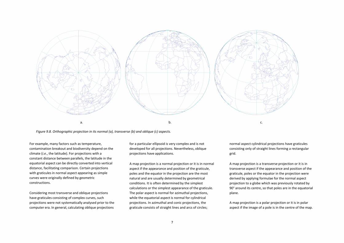
7

a. b. c.

Figure 9.8. Orthographic projection in its normal (a), transverse (b) and oblique (c) aspects.

For example, many factors such as temperature,

contamination breakout and biodiversity depend on the

climate (i.e., the latitude). For projections with a

constant distance between parallels, the latitude in the

equatorial aspect can be directly converted into vertical

distance, facilitating comparison. Certain projections

with graticules in normal aspect appearing as simple

curves were originally defined by geometric

constructions.

Considering most transverse and oblique projections

have graticules consisting of complex curves, such

projections were not systematically analysed prior to the

computer era. In general, calculating oblique projections

for a particular ellipsoid is very complex and is not

developed for all projections. Nevertheless, oblique

projections have applications.

A map projection is a normal projection or it is in normal

aspect if the appearance and position of the graticule,

poles and the equator in the projection are the most

natural and are usually determined by geometrical

conditions. It is often determined by the simplest

calculations or the simplest appearance of the graticule.

The polar aspect is normal for azimuthal projections,

while the equatorial aspect is normal for cylindrical

projections. In azimuthal and conic projections, the

graticule consists of straight lines and arcs of circles;

normal aspect cylindrical projections have graticules

consisting only of straight lines forming a rectangular

grid.

A map projection is a transverse projection or it is in

transverse aspect if the appearance and position of the

graticule, poles or the equator in the projection were

derived by applying formulae for the normal aspect

projection to a globe which was previously rotated by

90° around its centre, so that poles are in the equatorial

plane.

A map projection is a polar projection or it is in polar

aspect if the image of a pole is in the centre of the map.

8

It is often used as a synonym for normal aspect

azimuthal projection.

A map projection is equatorial or it is in equatorial

aspect if the image of the equator is in the centre of the

map. The image of the Equator is placed in the direction

of one of the main axes of the map, mostly horizontally.

Equatorial projection often means normal aspect

cylindrical projection.

A map projection is an oblique projection or it is in

oblique aspect if it is neither polar nor equatorial,

neither normal aspect nor transverse (Figure 9.8).

9.6 Preserving Specific Properties with Map

Projections

Map projections are usually designed to preserve

specific characteristics of the globe, such as areas,

angles, distances, or specific properties such as great

circles (intersections of the Earth and a plane which

passes through the Earth’s center) becoming straight

lines. Maps with angles preserved are called conformal

projections.

Maps with areas preserved are referred to as equal‐area

or equivalent projections

9.6.1 Preserving Angles

Gerardus Mercator in 1569 developed a cylindrical

conformal projection that bears his name. He developed

it to show loxodromes or rhumb lines, which are lines of

constant bearing, as straight lines, making it possible to

navigate a constant course based on drawing a rhumb

line on the chart. The Mercator projection has meridians

as equally spaced parallel lines, with parallels shown as

unequally spaced straight parallel lines, closest near the

Equator and perpendicular to the meridians. The North

and South Poles cannot be shown. Scale is true along the

Equator or along two parallels equidistant from the

Equator. Significant size distortion occurs in the higher

latitudes and that is why the Mercator projection is not

recommended for world maps (Figure 9.5a). The

Mercator projection, a standard for marine charts, was

defined for navigational charts and is best used for

navigational purposes.

Transverse Mercator

The transverse Mercator, also known as a Gauss‐Krüger

projection, is a projection where the line of constant

scale is along a meridian rather than the Equator. The

central meridian and the Equator are straight lines.

Other meridians and parallels are complex curves and

are concave toward the central meridian. The projection

has true scale along the central meridian or along two

lines equidistant from and parallel to the central

meridian. It is commonly used for large‐scale, small area,

presentations. Due to the distribution of distortion, it is

usually used by dividing the region to be mapped in

three‐degree or six‐degree zones limited by meridians.

This projection is widely used for topographic maps from

1:25,000 scale to 1:250,000 scale, and it is the basis of

the UTM coordinate system.

Lambert Conformal Conic

The Lambert Conformal Conic (LCC) projection,

presented by Johann Heinrich Lambert in 1772, shows

meridians as equally spaced straight lines converging at

one of the poles (Figure 9.6a). Angles between the

meridians on the projection are smaller than the

corresponding angles on the globe. Parallels are

unequally spaced concentric circular arcs centred on the

pole, and spacing of the parallels increases away from

the pole. The pole nearest the standard parallel is a point

and the other pole cannot be shown. The scale is true

along the standard parallel or along two standard

parallels and is constant along any given parallel. The

LCC projection is extensively used for large‐scale

mapping of regions with an elongated axis in the East‐

West directions and in mid-latitude regions. It is

standard in many countries for maps at 1:500,000 scale,

as well as for aeronautical charts of a similar scale.

Stereographic

The Stereographic projection, developed by the 2nd

century B.C., is a perspective azimuthal projection that

preserves angles (i.e., is conformal). This projection is

the only projection in which all circles from the globe are

represented as circles in the plane of projection. The

polar, Equatorial and oblique aspects result in different

appearances of the graticule. The polar aspect is

achieved by projecting from one pole to a plane tangent

at the other pole. In this aspect, meridians are equally

spaced straight lines intersecting at the pole with true

angles between them. Parallels are unequally spaced

circles centred on the pole represented as a point.

Spacing of the parallels increases away from the pole.

The Stereographic projection is used in the polar aspect

for topographic maps of Polar Regions. The Universal

Polar Stereographic (UPS) is the sister projection of the

UTM for military mapping. This projection generally is

chosen for regions that are roughly circular in shape. It is

in use in oblique ellipsoidal form in a number of

countries throughout the world, including Canada,

Romania, Poland and the Netherlands. Different

countries have different mathematical developments or

versions of the Stereographic projection.

9

9.6.2 Preserving Areas

Lambert Cylindrical Equal Area.

The Cylindrical Equal Area projection was first presented

by Johann Heinrich Lambert in 1772. It became the basis

for many other similar equal area projections including

the Gall Orthographic, Behrmann, and Trystan‐Edwards

projections. Lambert's original projection uses a single

line of constant scale along the Equator (Figure 9.5b).

Similar equal area projections are constructed using two

parallels as the lines of constant scale. On the Lambert

Cylindrical Equal Area projection, meridians are equally

spaced straight parallel lines and the Equator is π times

as long as the meridians. Lines of latitude are unequally

spaced parallel lines furthest apart near the Equator and

are perpendicular to the meridians. Changing the

spacing of the parallels is the method used to preserve

equal areas. Significant distance and angle distortion,

however, results with the distortion greater in high

latitudes near the poles. This projection is not often used

directly for map construction, but it is a standard to

describe map projection principles in textbooks and has

also served as a prototype for other projections.

Mollweide

In 1805, Carl Brandan Mollweide developed a

pseudocylindrical equal area projection on which the

central meridian is a straight line one‐half as long as the

Equator forming an elliptical area of projection for the

entire globe. The meridians 90° East and West of the

central meridian form a circle on the Mollweide

projection. Other meridians are equally spaced

semiellipses intersecting at the poles and concave

toward the central meridian. Parallels are unequally

spaced straight lines and are perpendicular to the

central meridian. The parallels are farthest apart near

the Equator with spacing changing gradually.

Figure 9.9. Logo of ICA in the Mollweide projection.

The North and South Poles are shown as points, and the

scale is only true along latitudes 40°44' North and South

and constant along any given latitude. The entire globe

projected and centred on the Greenwich meridian is

shown in Figure 9.9. The Mollweide projection has

occasionally been used for world maps, particularly

thematic maps where preservation of area is important.

Different aspects of the Mollweide have been used for

educational purposes, and it was chosen for the logo of

ICA (Figure 9.9).

9.6.3 Compromise Projections

Map projections that are neither conformal nor equal

area are called compromise projections. They are almost

unlimited in variety. Among them are many important

and useful projections.

Orthographic

The Orthographic projection, developed by the 2nd

century B.C., is a perspective azimuthal projection that is

neither conformal nor equal area. It is used in polar,

Equatorial and oblique aspects and results in a view of

an entire hemisphere. The polar aspect of the projection

has meridians that are straight lines and intersect the

central pole with the angles between meridians being

true. The pole is a point and the parallels are unequally

spaced circles centred on the pole. The spacing parallels

decrease away from the pole. Scale is true at the centre

and along the circumference of any circle with its centre

at the projection centre. The projection has a globe‐like

look (Figure 9.8), and is essentially a perspective

projection of the globe onto a plane from an infinite

distance (orthogonally). It is commonly used for pictorial

views of the Earth as if seen from space.

Gnomonic

Figure 9.10. The Gnomonic projection, which maps great

circles to straight lines.

10

The Gnomonic projection is neither conformal nor equal

area. It is a perspective azimuthal projection with the

point of projection at the centre of the Earth, which is

the source of the name (i.e., the centre of the Earth

where the mythical gnomes live). It was developed by

the Greek Thales, possibly around 580 B.C. All great

circles on the projection, including all meridians and the

Equator, are shown as straight lines, a property unique

to this projection (Figure 9.10).

The graticule appearance changes with the aspect, as

with other azimuthal projections. Meridians are equally

spaced straight lines intersecting at the pole with true

angles between them in the polar aspect. Parallels are

unequally spaced circles centred on the pole as a point,

and the spacing of the parallels increases from the pole.

The projection only can show less than a hemisphere.

Scale increases rapidly with distance from the centre. Its

usage results from the special feature of representing

great circles as straight lines, and it thus assists

navigators and aviators in determining the shortest

courses.

Azimuthal Equidistant

In this polar aspect projection, meridians are equally

spaced straight lines intersecting at the central pole.

Angles between them are the true angles. Parallels are

equally spaced circles, centred at the pole, which is a

point. The entire Earth can be shown, but the opposite

pole is a bounding circle having a radius twice that of the

Equator. In its equatorial aspect, meridians are complex

curves, equally spaced along the Equator and

intersecting at each pole. Parallels are complex curves

concave toward the nearest pole and equally spaced

along the central meridian and the meridian 90° from

the central meridian. The scale is true along any straight

line radiating from the centre of projection. It increases

in a direction perpendicular to the radius as the distance

from the centre increases. Distortion is moderate for one

hemisphere but becomes extreme for a map of the

entire Earth. The distance between any two points on a

straight line passing through the centre of projection is

shown at true scale; this feature is especially useful if

one point is the centre.

This projection is commonly used in the polar aspect for

maps of Polar Regions, the Northern and Southern

Hemispheres, and the "aviation‐age" Earth. The oblique

aspect is frequently used for world maps centred on

important cities and occasionally for maps of continents.

The Azimuthal Equidistant projection was recognized by

the UN and used on the UN's flag (Figure 9.11).

Figure 9.11. The azimuthal equidistant projection for

preserving distances on the UN's flag.

Winkel Tripel

The Winkel Tripel projection is neither conformal nor

equal area. It was presented by Oswald Winkel of

Germany in 1921.

Figure 9.12. Winkel Tripel projection.

The projection was obtained by averaging coordinates of

the Equidistant Cylindrical and Aitoff projections. Winkel

applied the name "Tripel," normally meaning triple,

because the Aitoff projection is an equatorial aspect of

one hemisphere of the Azimuthal Equidistant projection,

on which horizontal coordinates have been doubled and

meridians have been given twice their original

longitudes.

The central meridian is straight. Other meridians are

curved, equally spaced along the Equator and concave

toward the central meridian.

The Equator and the poles are straight. Other parallels

are curved, equally spaced along the central meridian

and concave toward the nearest pole. Poles are straight

lines about 0.4 as long as the Equator, depending on the

latitude of the standard parallels. Scale is true along the

central meridian and constant along the Equator.

Distortion is moderate except near outer meridians in

Polar Regions. The Winkel Tripel is used for whole‐world

maps (Figure 9.12).

11

9.7 Modern Approaches to Map Projections

9.7.1 Web Mercator

Many major online street mapping services (Bing Maps,

OpenStreetMap, Google Maps, MapQuest, Yahoo Maps,

and others) use a variant of the Mercator projection for

their map images. Despite its obvious scale variation at

small scales, the projection is well suited as an

interactive world map that can be zoomed into

seamlessly to large‐scale (local) maps, where there is

relatively little distortion due to the variant projection's

near‐conformality.

The scale factor at a point on a conformal map

projection (such as the spherical Mercator or the

ellipsoidal Mercator) is uniform in all directions. This is

not true on a Web Mercator. Let us denote with m the

scale factor in the N/S meridian direction and with n the

scale factor in the E/W parallel direction. Then m = n

because the scale factor at a point is the same in all

directions on the spherical Mercator projection. In other

words, the spherical Mercator is conformal.

The equations for the ellipsoidal Mercator are a little

more complicated, especially in Northing. The

parameters a (semi-major axis) and e (eccentricity) are

given for the selected ellipsoid. Again m = n because the

scale factor at a point is the same in all directions on the

ellipsoidal Mercator projection. In other words, the

ellipsoidal Mercator is conformal.

Web Mercator is the mapping of WGS84 datum (i.e.,

ellipsoidal) latitude/longitude into Easting/Northing

using spherical Mercator equations (where R = a). This

projection was popularized by Google in Google Maps

(not Google Earth). The reference ellipsoid is always

WGS84, and the spherical radius R is equal to the semi-

major axis of the WGS84 ellipsoid a. That's "Web

Mercator."

The scale factor at a point is now different for every

direction. It is a function of the radii of curvature in the

meridian and the prime vertical and the direction alpha.

For the Web Mercator, m and n are not equal. Thus, the

Web Mercator is not a conformal projection.

If somebody uses the Web Mercator for printing out

directions to a new restaurant across town or for

visualization on his/her computer screen or for other

purposes on the web, there will be no problem. But the

Web Mercator is a projection that has jumped from one

domain of use (the web) to another domain of use (GIS)

where it is leading another life. Witnesses are the EPSG,

Esri and FME codes for the Web Mercator. Surveyors and

GIS professionals need to know that the Web Mercator is

not conformal. If distance computations on the Web

Mercator are done simply (as they can be done on a

conformal projection), they will be wrong. If done

correctly, they will be laborious.

For an area the size of the NW quadrisphere (North

America), the differences appear slight. It turns out that

the Eastings are identical. The differences are in the

Northings. There is no Northing difference at the

Equator, but by 70 degrees North, the difference is 40

km. This NS stretching in the Web Mercator is the reason

for its non-conformality.

Mercator projections are useful for navigation because

rhumb lines are straight. These are lines of constant true

heading that navigators used to sail before GPS. So, we

have to have in mind that straight lines on a Web

Mercator are not rhumb lines.

To summarize about the Web Mercator:

The Web Mercator is cylindrical;

Its meridians are equally spaced straight lines;

Its parallels are unequally spaced straight lines

but in a different way than a conformal

Mercator;

Its loxodromes (rhumb lines) are not straight

lines;

It is not perspective;

Its poles are at infinity and

It was not presented by Mercator in 1569, but

by Google recently.

It is not conformal.

9.7.2 Map Projection Transitions

Map Projection Transitions is an example of multiple

applications offered by Jason Davies. The web page

(http://www.jasondavies.com/maps/transition) presents

a world map with graticule and country borders in the

oblique Aitoff projection with the South Pole. The map is

not static, but animated. The South Pole moves toward

the bottom and Earth rotates around its poles. The

animation lasts five seconds, after which the projection

changes and movement continues for five seconds, after

which the projection changes again. Names of

projections appear in a separate window. There are a

total of 56 projections. The South Pole eventually

becomes invisible and the North Pole appears at the top.

Various parts of Earth appear in the centre of the map by

rotating around the poles (Figure 9.13).

By clicking Pause, animation stops and it is possible to

select another projection. By left‐clicking, it is possible to

12

Figure 9.13. From the Map Projection Transitions application (http://www.jasondavies.com/maps/transition)

move the picture around and select projection aspect—

normal, transversal or any of numerous oblique

projections. Differences between two projections can be

seen clearly in such a way. For example, one is able to

select the Ginzburg VI projection and its normal aspect

by moving the mouse. If one wants to see how that

projection's graticule is different from the similar Winkel

Tripel projection, it can be done by clicking on the

Winkel Tripel projection on the drop‐down menu. The

picture on the screen is going to change to the Winkel

projection and differences are going to be clear.

If one clicks on Maps, there is a series of new interesting

applications about interrupted maps, butterfly-shaped

maps, retro-azimuthal projections and other projections.

It is possible to use the mouse to move pictures in many

of those applications. For example, by selecting the

interrupted sinusoidal projection, a world map in three

segments is going to appear. The mouse can be used to

move parts of Earth from one segment to another, and

the slider at the bottom of the screen can be used to

change the number of segments from an uninterrupted

world map to a representation in 24 segments.

A similar option is available for the Berghaus (Snyder and

Voxland, 1989) star projection. The application Azimuth

and Distance from London enables using the mouse to

obtain distances and azimuths from London to any point

on Earth in world maps in oblique equidistant cylindrical

and oblique equidistant azimuthal projection. If an

application's accompanying text mentions a projection,

there is a link to Wikipedia where there is detailed

information on the projection.

9.7.3 Research on New Map Projections

In 2007, inspired by Robinson's method, B. Jenny, T.

Patterson and L. Hurni produced the Flex Projector

interactive program, which enables the user to create

new world map projections with ease. It supports the

normal aspect of cylindrical projections. The program is

free and open source and works under Linux, Mac OS X

and Windows. By executing the program, a world map in

the Robinson projection appears on the screen (Figure

9.14). The right side of the screen includes sliders for

changing lengths of parallels. Clicking the Distance

button brings up sliders for changing distances of

parallels from the Equator. Parallel curvatures (Bending)

and distances between meridians (Meridians) can also

be changed. The Linked Sliders option enables the user

to move each slider separately or several at once. The

next option Move is used to choose the shape of the

curve along which the sliders are moved. The ratio

between the central meridian and the Equator can be

changed with the Proportions (Height/Width) slider.

Instead of modifying the Robinson projection, one can

start from any of a number of provided projections from

the three groups mentioned. If the result is unsatisfying,

one can use the option Reset Projection to go back to

the initial projection. The option can be found in the

upper right corner of the screen.

Clicking Display opens up additional options. The length

of the central meridian can be changed, graticule density

can be chosen, distortion ellipses can be drawn in nodes

of the graticule, and area and maximum angle distortion

isograms can be drawn. The background of newly

created projection can include the graticule and

continent outlines in any activated projection (Show

Second Projection). The bottom left corner of the screen

includes numerical indicators of the summary length,

area and angle distortions for all activated projections

and the projection just created (Figure 9.14).

Figure 9.14. Interface of the Flex Projector program.

13

Flex Projector can import and export vector and raster

data in several formats. The program is recommended to

everyone wanting to try creating a new world map

projection, and it can also be applied in teaching map

projections.

The techniques for combining two source projections to

create a new projection allow for the creation of a large

variety of projections. The mentioned techniques can

also be extended. For example, the Geocart software by

Mapthematics can blend projection parameters, such as

the latitude of standard parallels, between two source

projections. Alternatively, more than two projections can

be combined to form a new one. The extreme case

would be an infinite number of differently

parameterized projections, which is the concept behind

polyconic and poly-cylindric projections. There are

alternative methods for creating a new projection from

scratch, deriving it from existing ones or adjusting

projection parameters to create a new one. Some of

these techniques are used in the adaptive composite

projections for web maps, a new field of map projection

research. The goal of this research is to develop an

alternative to the Web Mercator projection for

small‐scale web maps, where maps automatically use an

optimum projection depending on the map scale, the

map's height‐to‐width ratio, and the central latitude of

the displayed area.

9.8 Suggested Projections

The reason we have so many map projections is because

none serves every need. The selection of an appropriate

map projection for a given application depends on a

variety of factors, including the purpose of the map, the

type of data to be projected, the region of the world to

be projected and scale of the final map. Advice on

selection is available from a variety of print and web

sources (see Further Reading section). In GIS, large‐scale

datasets (small area extent) commonly are projected

with a conformal projection to preserve angles. For such

applications, area distortion is so small over the

geographic extent that it is negligible and an area

preserving projection is not needed. Commonly,

large‐scale data files are used in GIS applications of

limited geographic extent (e.g., a watershed, a county or

a state). The two most commonly used projections for

these scales are the Lambert Conformal Conic and the

Transverse Mercator, which are the basis of the UTM

and most of the USA State Plane coordinate systems. For

general‐purpose world maps, our recommendation is

not using any cylindrical map projection but some of

pseudo-cylindrical (e.g., Robinson or a compromise

projection like the Winkel Tripel).

9.9 Conclusions

Map projections and coordinate transformations are the

basis of achieving a common frame of reference for

geographic information. The requirement of a common

ellipsoid, datum, map projection, and finally plane

coordinate systems make it possible to use plane

geometry for all types of spatial overlay and analysis.

Projection of geographic data from the ellipsoidal Earth

to a plane coordinate system always results in distortion

in area, shape, distance, and other properties. With

appropriate selection of a projection, the user can

preserve desired characteristics at the expense of others.

In this chapter we have briefly examined basic concepts

of the basis of coordinate systems and map projections.

For a more in‐depth treatment, the reader is referred to

the texts and sources referenced in the Further Reading

section.

9.10 Further Reading

Further references and an exercise with questions and

answers are given in Chapter 18.

Google e‐Books on Map Projections

Bureau of Navigation (1869): Projection Tables for the

Use of the United States Navy Comprising A New

Table of Meridional Parts for the Mercator

Projection, Government Printing Office,

Washington.

De Morgan, A. (1836): An Explanation of the Gnomonic

Projection of Sphere, Baldwin and Cradock, London.

Department of the Army (1967): Grids and Grid

References. United States Headquarters,

Department of Army.

Snyder, J. P. (1987): Map Projections Working Manual.

US Geological Survey, Professional paper 1395,

Washington.

Snyder, J. P. and H. Steward (1988): Bibliography of map

projections, US Geological Survey Bulletin 1856.

Spilhaus, A. (1991): Atlas of the World Geophysical

Boundaries—Ocean, Continents and Tectonic Plates

Their Entirety. American Philosophical Society,

Philadelphia.

Books on Map Projections Available on the Internet

Anoni, A., C. Luzet, E. Gubler, and J. Ihde (Eds.) (2003):

Map projections for Europe. Institute for

Environment and Sustainability, European

Communities.

http://www.ec‐gis.org/sdi/publist/pdfs/annoni‐

etal2003eur.pdf

Frankich, K. (1982): Optimization of geographic map

projections for Canadian territory. Simon Fraser

14

University, Vancouver.

http://summit.sfu.ca/item/4135

Hager, J. W., J. F. Behensky, and B.W. Drew (1989): The

universal grids: Universal Transverse Mercator

(UTM) and Universal Polar Stereographic (UPS).

Tech. Rep. TM 8358.2, Defense Mapping Agency.

http://earth‐info.nga.mil/GandG

/publications/tm8358.2/TM8358_2.pdf

Krüger, J. H. L. (1912): Konforme Abbildung des

Erdellipsoids in der Ebene. New Series 52. Royal

Prussian Geodetic Institute, Potsdam.

http://bib.gfz‐potsdam.de/pub/digi/krueger2.pdf

Snyder, J. P. and M. P. Voxland (1989): Album of Map

Projection, US Geological Survey, Professional Paper

1453. http://pubs.usgs.gov/pp/1453/report.pdf

Thomas, P. D. (1952): Conformal projections in geodesy

and cartography. Special Publication 251. US Coast

and Geodetic Survey.

http://docs.lib.noaa.gov/rescue/cgs_specpubs/QB2

75U35no2511952.pdf

Tobler, W. R. (1961): Map transformation of geographic

space. University of Washington, Seattle.

http://www.geog.ucsb.edu/~tobler/publications/pd

f_docs/cartography/projections/cartograms/Transf

ormations.pdf

10 Map use at the United Nations Contributions from the United Nation Cartographic Section 10.1 The Need of Maps in the United Nations This chapter show what functions maps have in the operations by the United Nations, for conflict prevention, food security, health campaigns, and humanitarian operations (See the diagram of the United Nations Family in figure 10.10). The United Nations has been producing and using maps since 1945 to support the needs of the United Nations Secretariat and the countries who are Member States. There were several offices in the United Nations Secretariat who produced maps or supported the mapping needs of all countries. 10.2 Cartographic Section In order to support the requirement by the United Nations Secretariat, there was one Cartographer in the Bureau of Documents of the Conference and General Services in 1946. By 1951, the need for maps increased in its importance in the United Nations and the Cartographic Unit was established in the Department of Conference Services with a team of cartographers. Today, the Cartographic Section of the Department of Field Support continues this tradition and practice and is responsible in providing the United Nations Secretariat different activities including (1) profile maps and deployment map production to be included in the official reports of the United Nations, (2) map clearance and guidance to United Nations Secretariat colleagues to ensure maps produced by the United Nations have one

single cartographic practice, (3) provide map publication permission, (4) customized maps for the Security Council and United Nations Secretariat, (5) programme management of the Geographic Information Services (GIS) of field missions in peace operations, (6) technical assistance to Member States on international boundary issues, and (7) serving as joint Secretariat, together with the United Nations Statistics Division (UNSD) to the United Nations Committee of Experts on Global Geospatial Information Management (UN-GGIM). Maps produced by the United Nations follow the principles of sovereignty and common cartographic practice. In order to ensure that the United Nations produces maps in a consistent manner in its official publications, the Cartographic Section is responsible to provide advice and guidance on maps produced by other offices in the United Nations. This service extends to the larger United Nations family. In order to have a better flow of information and collaboration amongst all United Nations family, specifically in the context of cartography, map production and use of geospatial information, experts from those organizations agreed in 2000 to establish a working group for coordination, sharing of data, products and knowledge. Named as United Nations Geographic Working Group (UNGIWG), it helps experts and their organizations collaborate more closely (http://www.ungiwg.org/). Many academics and organisations around the world use the maps produced by the United Nations for their publications. In order to ensure that copyright issues are cleared, the Cartographic Section also provides

publication permission on behalf of the United Nations Publications Board. In order to provide more focused analysis and understanding of particular issues, the Cartographic Section has been involved in producing customized maps for United Nations Secretariat offices upon request. These maps vary in scope and theme but it allows the United Nations to communicate a message more clearly and effectively to the intended readers, whether it is the Security Council, countries for particular projects or the general public who are interested in the activities of the United Nations.

Figure 10.1 Security Council session on Middle East. Source: UN Image Archive. 10.3 Peace Operations Maps have always been useful for the United Nations peacekeepers, since their earliest operations such as United Nations Truce Supervision Organization (UNTSO) in 1949, but their importance continued to increase as operations on the ground became more and more complex and challenging. Since 2000, the United Nations have been using GIS in the peace operation activities. Today, there are 12 United Nations peacekeeping or

1

special political missions who map important information on the ground. These Geographic Information System (GIS) officers employed in the field missions provide different types of support depending on the mandate or the mission. Some field missions may require electoral support whilst others may require monitoring support and therefore some GIS offices will be preparing electoral maps including the collection of GPS location of polling centres or helicopter landing sites to transport the election ballots, whilst another GIS office would be preparing patrol maps for the military officers and observers to patrol a demilitarized zone.

Figure 10.2. The United Nations Secretary-General inspects a field mission map. Source: UN Image Archive.

A specific example of use of maps in the peacekeeping mission is that of MONUCSO, the United Nations Organization Stabilization Mission in the Democratic Republic of the Congo (DRC). The GIS office in MONUSCO plays a vital role in assisting MONUSCO and other United Nations family in achieving their goals efficiently and in a timely manner. The recent addition of Force Intervention Brigade (FIB) has added a new dimension to the umbrella of United Nations and posed new challenges and requirements. Previously, 1:50,000 topographic maps were the main reference for ground operations for

patrolling, road recognizance survey and logistic transport. In troubled eastern DRC, analysing the threat and environment in a specific geographic area, became more important as FIB had to plan and conduct operations against armed groups. Therefore, the GIS office in MONUSCO generated 1:100,000 maps with greater area coverage allowing mission’s planners and peace keeping troops to have a better understanding of the region and battle field information for better planning. 10.4 The UN Map Collection

Maps produced by the United Nations and maps collected for reference purposes were also collected by the UN Map Collection, co-located with the Cartographic Unit of the Department of Conference Services since its establishment. Today, the UN Reference Collection of the Department of Public Information, continues to take this responsibility to collect maps produced by the United Nations and also of countries for the use of the general public and for the diplomatic community (http://www.un.org/Depts/dhl/). 10.5 Regional Cartographic Conferences One can look back at the history of the Cartographic Section at the United Nations Secretariat Headquarters in New York City for a clearer picture. In order to support the external requirements in assisting Member States, the Cartographic Section of the Resources and Industrial Branch was first established following discussion on “The Question on cartography” by the United Nations Economic and Social Council (ECOSOC) in 1949. This office was responsible for the inter-governmental process amongst countries on cartographic issues including (1) preparation of reports and studies for ECOSOC in the field of cartography, (2) The International Map of the World on the Millionth Scale, (3) technical assistance administration

to Member States, (4) publication of the annual bulletin on World Cartography, and (5) organizing meetings related to cartography.

Figure 10.3. A view from Dag Hammarskjöld Library. Source: UN Image Archive. The Statistics Division (UNSD) of the Department of Economic and Social Affairs continues to be the external face as an inter-governmental secretariat on cartographic issues in the United Nations Secretariat. The first United Nations Regional Cartographic Conference was organized in 1955 in the region of Asia and Pacific, followed by the region of Africa in 1963, and by the region of the Americas in 1976. These United Nations Regional Cartographic Conferences (http://unstats.un.org/UNSD/GEOINFO/RCC/) have continued to-date in their respective regions every three to four years. Today, there are two Regional Cartographic Conferences which convene for the region for Asia and Pacific

2

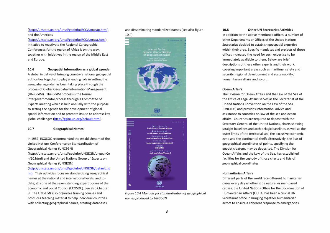
(http://unstats.un.org/unsd/geoinfo/RCC/unrccap.html), and the Americas (http://unstats.un.org/unsd/geoinfo/RCC/unrcca.html). Initiative to reactivate the Regional Cartographic Conferences for the region of Africa is on the way, together with initiatives in the region of the Middle East and Europe. 10.6 Geospatial Information as a global agenda A global initiative of bringing country’s national geospatial authorities together to play a leading role in setting the geospatial agenda has been taking place through the process of Global Geospatial Information Management (UN-GGIM). The GGIM process is the formal intergovernmental process through a Committee of Experts meeting which is held annually with the purpose to setting the agenda for the development of global spatial information and to promote its use to address key global challenges (http://ggim.un.org/default.html). 10.7 Geographical Names In 1959, ECOSOC recommended the establishment of the United Nations Conference on Standardization of Geographical Names (UNCSGN) (http://unstats.un.org/unsd/geoinfo/UNGEGN/ungegnConf10.html) and the United Nations Group of Experts on Geographical Names (UNGEGN) (http://unstats.un.org/unsd/geoinfo/UNGEGN/default.html). Their activities focus on standardizing geographical names at the national and international levels, and to-date, it is one of the seven standing expert bodies of the Economic and Social Council (ECOSOC). See also Chapter 8. The UNGEGN also organizes training courses and produces teaching material to help individual countries with collecting geographical names, creating databases

and disseminating standardized names (see also figure 10.4).

Figure 10.4 Manuals for standardization of geographical names produced by UNGEGN.

10.8 Other UN Secretariat Activities In addition to the above mentioned offices, a number of other Departments or Offices of the United Nations Secretariat decided to establish geospatial expertise within their area. Specific mandates and projects of those offices increased the need for such expertise to be immediately available to them. Below are brief descriptions of these other experts and their work, covering important areas such as maritime, safety and security, regional development and sustainability, humanitarian affairs and so on. Ocean Affairs The Division for Ocean Affairs and the Law of the Sea of the Office of Legal Affairs serves as the Secretariat of the United Nations Convention on the Law of the Sea (UNCLOS) and provides information, advice and assistance to countries on law of the sea and ocean affairs. Countries are required to deposit with the Secretary-General of the United Nations, charts showing straight baselines and archipelagic baselines as well as the outer limits of the territorial sea, the exclusive economic zone and the continental shelf; alternatively, the lists of geographical coordinates of points, specifying the geodetic datum, may be deposited. The Division for Ocean Affairs and the Law of the Sea, has established facilities for the custody of those charts and lists of geographical coordinates. Humanitarian Affairs Different parts of the world face different humanitarian crises every day whether it be natural or man-based causes, the United Nations Office for the Coordination of Humanitarian Affairs (OCHA) has been a crucial UN Secretariat office in bringing together humanitarian actors to ensure a coherent response to emergencies

3

(http://unocha.org/). When disasters occur, one of the sites both the UN and non-UN humanitarian community refer to is OCHA’s information knowledge base of the Relief Web (http://reliefweb.int/), where disaster and crisis updates and analyses are brought together to allow the humanitarian community to make informed decisions and plan effective assistance. Whilst OCHA itself provides maps to show snapshots and hotspots, they also collate and disseminate maps prepared by other UN offices, agencies and non-governmental organisations which can be used in the field. One of the advantages OCHA has is the field level presence represented in over 50 country, regional and headquarters locations in the world where operational maps are also prepared by field based information officers trying to reflect the daily situation on the ground. Safety and Security The United Nations Department of Safety and Security (UNDSS) have a mandate to provide safety and security to personnel working in the United Nations offices and agencies around the world. UNDSS uses maps as a visualisation tool to assist in strategic and operational decision making. The data displayed on the maps is mostly internal confidential security information dealing with security levels of a particular area in a country, for example, an evacuation route planning to ensure safe passage of the UN staff. Outer Space Affairs The United Nations Office for Outer Space Affairs (UNOOSA) is responsible for promoting international cooperation in the peaceful uses of outer space.

Drug and Crime prevention Some substantive offices of the United Nations Secretariat provide support to countries directly through their specific thematic mandate. Thematic maps are produced through these thematic mandates. One notable example is the activities by the United Nations Office on Drugs and Crime (UNODC), which deals with illicit drugs and international crime issues (http://www.unodc.org/unodc/index.html). This office uses satellite images and GIS analysis to produce maps on drug cultivation, drug production and trafficking. Analysis of geospatial data has also guided the implementation of alternative development programmes in areas affected by illicit crop cultivation. The yearly publication, World Drug Report, is an excellent example of how maps are used at UNODC. Maps at UNODC are also used to identify trafficking routes and to pinpoint strategic areas for organized crime. 10.9 Other UN Agencies The United Nations is a huge family of organisations, as mentioned above, and a lot of the needs by the countries cannot be accomplished by the United Nations Secretariat alone. Amongst the United Nations family, many United Nations Specialised Agencies also provide focused support to these countries through projects. Some of the main actors in this context are presented briefly below. UNESCO

The UNESCO Institute for Statistics is the United Nations global repository for international statistics in the fields of education, science and technology, culture, and communication. The Institute is probably most famous

for its education statistics – from the number of children out of school to percentage of schools in Africa with access to electricity and drinking water. With such a rich array of data, the UIS is using maps to help people visualize trends in key areas (http://www.uis.unesco.org/Pages/interactive-content-archive.aspx). For example, the UNESCO eAtlas series (http://www.uis.unesco.org/Education/Pages/unesco-e-atlas-launch.aspx) presents interactive maps on a range of subjects – from girls’ education (see figure 10.5) to the resources devoted to research and development in more than 200 countries and territories. Flow maps let users track the origins and destinations of tertiary students pursuing their education abroad (http://www.uis.unesco.org/education/Pages/international-student-flow-viz.aspx). These are just a few examples of the ways in which the Institute is using maps to encourage people to use data to make a difference in the world.

Figure 10.5 Girls’ enrollment in secondary education. Source: UNESCO. UNICEF

4

The United Nations Children’s Fund (UNICEF) is mandated by the United Nations General Assembly to advocate for the protection of children's rights, to help meet their basic needs and to expand their opportunities to reach their full potential. UNICEF is active in more than 190 countries and territories through country programmes and National Committees. The maps created and provided by UNICEF aim to highlight its activities around the world. When UNICEF staff responds to an emergency in the field, maps become a very useful tool. These maps highlight UNICEF activities, service deliveries and our footprints during our response. Maps can vary, and can show where we are at a certain time and activities we are conducting; where is the highest percentage of undernourished children in the world; how many schools are in an area that UNICEF is managing, or the number of water distribution points or even locations of child friendly recreation centres.

ESCAP and ITU

The Economic and Social Commission of Asia and Pacific (ESCAP) which is a regional commission, and the International Telecommunication Union (ITU) which is a United Nations Specialised Agency for information and communication technologies have jointly worked to develop ESCAP/ITU Information Superhighway maps of fibre optic transmission networks. When we upload or download information from the Internet or send an email, this information travels through different types of networks. In most cases, long distance and high speed internet traffic takes place along fibre optic networks which criss-cross landmasses and oceans floors. While

developed countries have extensive fibre optic networks which allow fast and cheap Internet access, these networks tend to be less extensive in developing countries. Developing countries often rely on just one or two transoceanic fibre cables connecting them to the World Wide Web. Land locked countries use network of neighbouring countries, often at very high prices and as a result, the Internet in developing countries tends to be both more expensive, of lower capacity and more vulnerable to cable cuts. This hinders new opportunities offered by broadband internet, such as online jobs and education, or remote access to medical consultation services. In order to help redress this situation, the United Nations recently developed a set of maps that show the networks of land-based fibre optic cables. These maps are publically available online (http://www.itu.int/itu-d/tnd-map-public/ ). See also figure 10.6. The information provided by these maps will help governments and the private sector to identify the missing links and bottlenecks in the current fibre optic networks. With appropriate investments, Internet should be made more secure from cable cuts, also bring increased competition and therefore lower prices in Internet access.

Figure 10.6 Part of aESCAP/ITU map showing the network of land-based fibre optic cables. Source: ESCAP/ITU. The boundaries and names shown and the designations used on this map do not imply official endorsement or acceptance by the United Nations.

FAO, WFP and UNEP

The Food and Agriculture Organization (FAO) is a Specialised Agency focused on (1) eliminating hunger, food insecurity and malnutrition, (2) making agriculture, forestry and fisheries more productive and sustainable, (3) reducing rural poverty, (4) enabling inclusive and efficient agricultural and food systems and (5) increasing resilience of livelihoods from disasters. FAO’s GeoNetwork (www.fao.org/geonetwork/srv/en/main.home#) is a site where they collate geospatial information by FAO and its partners including United Nations family such as World Food Programme (WFP), United Nations Environment Programme (UNEP) and OCHA.

5

The United Nations Environment Programme (UNEP) is a Specialised Agency focusing on environmental issues. Their areas of focus are in (1) assessing global regional and national environmental conditions, (2) developing international and national environmental instruments and (3) strengthening institutions for management of the environment. UNDP and WHO The United Nations Development Programme (UNDP) is a Specialised Agency which focuses on development issues for countries and focuses on (1) poverty reduction and achievement of the Millennium Development Goals, (2) Democratic Governance, (3) Crisis Prevention and Recovery and (4) Environment and Energy for Sustainable Development. They have different country based projects and in these specific projects, maps can be produced using GIS. The World Health Organisation (WHO) is a Specialised Agency which focuses on health issues in (1) promoting development, (2) fostering health security, (3) strengthening health systems, (4) harnessing research, information and evidence, (5) enhancing partnerships and (6) improving performance. WHO uses GIS to map different themes to communicate different health related issues (http://www.who.int/gho/map_gallery/en/ ).See also figure 10.7.

Figure 10.7. The WHO map shows risks for droughts, flood and landslides in Guatemala based on data from 2008-2012.Source: WHO. UNOSAT The last decade has seen an important development in satellite imagery and space technology offering new perspectives and possibilities for the use of maps in the United Nations. To take full advantage of satellite imagery for mapping, the United Nations Institute for Training and Research (UNITAR), a research and training body of the United Nations family, created the Operational Satellite Applications Programme, known as UNOSAT in 2001. UNOSAT uses satellite imagery to generate geospatial information analysis to support the work of relief and development organisations inside and outside the United Nations family. UNOSAT turns publicly available satellite imagery into solutions to help make a difference in critical areas such as humanitarian relief, human rights, planning, and socio-economic development. Reports and maps of monitoring the extent of flood waters, assessing the

damage caused by earthquakes human rights violations, water resources in remote areas, and many more are prepared within hours of an event. These products assist decision making of the senior management inside and outside the United Nations family. UNOSAT also researches new technological solutions such as collaborative mapping crowd sourcing, and the use of unmanned aerial systems (UAS). UNOSAT ultimately shares its know-how with countries by developing training and capacity development programmes. WMO The World Meteorological Organization (WMO) is a Specialised Agency which focuses on the state and behaviour of the Earth’s atmosphere, its interaction with the oceans, the climate it produces and the resulting distribution of water resources (http://www.wmo.int/pages/about/index_en.html ).

As the world’s climate continues to change, hazards to human health are increasing. The Atlas of Health and Climate (http://library.wmo.int/opac/index.php?lvl=notice_display&id=13572 ), published by the World Health Organization (WHO) and the World Meteorological Organization (WMO), illustrates some of the most pressing current and emerging challenges. Droughts, floods and cyclones affect the health of millions of people each year. Climate variability and extreme conditions such as floods can also trigger epidemics of diseases such as diarrhoea, malaria, dengue and meningitis, which cause death and suffering for many millions more. The Atlas gives practical examples of how the use of weather and climate information can protect public health. For example, in some locations the incidence of infectious

6

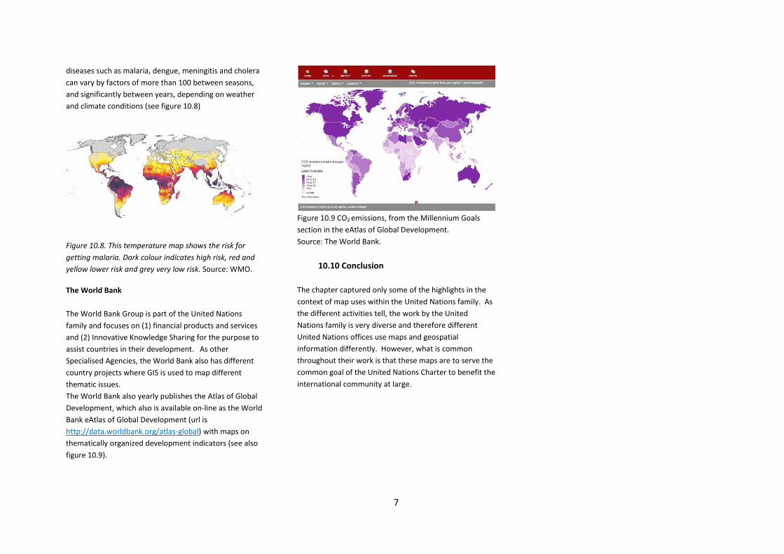
diseases such as malaria, dengue, meningitis and cholera can vary by factors of more than 100 between seasons, and significantly between years, depending on weather and climate conditions (see figure 10.8)

Figure 10.8. This temperature map shows the risk for getting malaria. Dark colour indicates high risk, red and yellow lower risk and grey very low risk. Source: WMO.

The World Bank The World Bank Group is part of the United Nations family and focuses on (1) financial products and services and (2) Innovative Knowledge Sharing for the purpose to assist countries in their development. As other Specialised Agencies, the World Bank also has different country projects where GIS is used to map different thematic issues. The World Bank also yearly publishes the Atlas of Global Development, which also is available on-line as the World Bank eAtlas of Global Development (url is http://data.worldbank.org/atlas-global) with maps on thematically organized development indicators (see also figure 10.9).

Figure 10.9 CO2 emissions, from the Millennium Goals section in the eAtlas of Global Development. Source: The World Bank.

10.10 Conclusion

The chapter captured only some of the highlights in the context of map uses within the United Nations family. As the different activities tell, the work by the United Nations family is very diverse and therefore different United Nations offices use maps and geospatial information differently. However, what is common throughout their work is that these maps are to serve the common goal of the United Nations Charter to benefit the international community at large.

7

. Figure 10.10. The UN family.

Figure 10.10. The UN Family.

8

1

11 Setting one’s course with a nautical chart

Michel Huet, Monaco

11.1 Introduction

On land, even those with a good sense of direction can

get lost in a location with few landmarks or direction

indicators. At sea, you cannot just follow the signs, the

road or the rail track. Unless they remain close to the

shore, mariners may find themselves in the middle of a

body of water with few reference points and no way of

knowing where the safe water lies. To be able to

navigate at sea, mariners need nautical charts, which

show information such as the depth of the water and the

position of known but invisible underwater obstructions.

Being able to use nautical charts is essential to save a

mariner the time and embarrassment of getting lost and

can certainly save lives by avoiding the hazards that lie

under the surface of the sea.

Like a map, a nautical chart is a graphical representation

of part of the earth's surface. Unlike a map, a nautical

chart is a biased representation. It emphasises areas of

water and features that allow mariners to determine

position, to avoid hazards and to find a safe route to a

destination. It is the mariner's road map. Whilst a map

tries to depict as much as possible of the land area,

roads, landmarks, etc., the nautical chart conveys a

selection of information specifically designed to assist in

safely navigating the area that the chart covers. It

identifies navigable areas, shorelines and areas not

suitable for navigation. Such information includes the

depth of the water, the shoreline of adjacent land, rocks

and other hazards, and buoys and beacons. Details about

the land areas are less important on a nautical chart

unless they are useful as reference elements for

navigation and to help the mariner know where he or

she is.

Figure 11.1. Example of a nautical chart: Approaches to Kuching, Sarawak, Malaysia. Source: United Kingdom

Hydrographic Office.

2

Figure 11.2. Officer on a survey ship using a chart for

navigation. Source: Chilean Hydrographic Office.

11.2 Scale

Nautical charts cover the open sea, coastlines, navigable

inland waters and canal systems. They can cover a large

area, for example, the shipping lanes of the North

Atlantic; or provide a detailed representation of a

smaller area, such as a harbour or anchorage. The area

covered by a nautical chart is defined by its scale, which

is the ratio of a given distance on the chart to the actual

distance that it represents on the earth. A scale of 1:10

000 means that the chart is one ten-thousandths of the

size of the area it represents: objects shown as a

centimetre apart on the chart are physically 10,000

centimetres (100 metres) apart on the earth. A chart

covering a relatively large area is called a small-scale

chart, for example, scale 1:500,000 and one covering a

relatively small area is called a large-scale chart, for

example, scale 1:25,000 (See Figure 11.3). The choice of

a chart scale will be determined by the type of

navigation. For example, navigation in harbours and local

waterways will generally require a scale larger than 1:50

000. The same geographic area may be covered by

several charts of differing scales. A golden rule for the

mariner is always to use the largest scale chart available.

This will allow the mariner to see the greatest level of

detail in the area

being covered by the chart.

Figure 11.3 Example of a large-scale chart: Monaco

Harbour. Source: French Hydrographic Office (SHOM).

11.3 Projection

Like a map, a nautical chart represents part of the

spherical earth displayed on a plane surface such as a

sheet of paper or on a video screen (a digital chart). The

process of transferring information from the spherical

earth to a flat surface is known as chart projection. The

projection most commonly used for nautical charts is

called Mercator projection, after Gerhard “Mercator”

Kremer (1512-1594), a Flemish scholar who invented this

projection in 1569. Roughly, it can be described as

projecting the surface of the earth on a cylinder wrapped

around the earth so that it touches the equator, then

cutting open the cylinder to yield the 2-dimensional

chart, (i.e., to make it flat). This results in meridians and

parallels crossing each other at right angles to form a

rectangular grid of latitude and longitude, with lines of

latitude being wider apart further north (See Figure 11.4

and Section 9.5.1). The Mercator projection is popular

among mariners because a straight course through the

water, known as a rhomb line, will appear as a straight

line on the chart, and also directions and distances can

be easily measured directly on the chart. Latitude is

graduated along the sides of the chart and longitude is

shown along the top and bottom of the chart. The

subdivisions are usually in degrees, minutes, and tenths

of minutes. The Mercator projection is not suitable for

charts covering the Polar Regions.

Figure 11.4. The Mercator projection. Source: Harvard

University – Graduate School of Design.

11.4 Datum

Water depths or soundings are vertical distances

depicted on charts by numbers expressed in whole

metres or metres and decimetres if the depth is less than

31m. The depths are supplemented by depth contours or

isobaths similar to the contour lines on land maps. These

are lines connecting points of equal depth

3

Figure 11.5. Datum and depiction of wrecks at various

depths Source: Advanced navigation courses

(www.sailingissues.com/navcourse0.html)

which provide a more intuitive “picture” of the sea-floor.

Depth contours are labelled with numerals in metres. All

depths indicated on nautical charts are measured from a

selected zero point or datum called the chart datum. This

is the calculated level below which the water seldom

falls - in other words, the theoretical lowest low tide in

the area of the chart. The chart datum adopted by the

International Hydrographic Organization (IHO) is known

as Lowest Astronomical Tide (LAT). When navigating or

planning a journey, the mariner will need to add the

current tide height expressed from the chart datum,

which can be predicted or obtained in real time, to the

charted depth in order to know the actual depth.

Coloured areas on the chart emphasise shallow water

and dangerous underwater obstructions. Shoal areas are

often given a blue tint.

The position of places shown on the chart can be

obtained from the longitude and latitude scales on the

borders of the chart. The longitude and latitude of any

Figure 11.6. Use of colours in British Admiralty charts.

Source: United Kingdom Hydrographic Office.

given place depends on the reference frame in which

they are measured, known as the geodetic datum. The

WGS (World Geodetic System) 84 is currently the

geodetic datum most commonly used for nautical charts.

This is the same datum that satellite navigation systems

such as GPS use. This means that GPS positions can be

plotted directly on a chart that uses WGS 84 as its datum

for latitude and longitude.

11.5 Symbols

International regulations require the use of official nautical charts published by government hydrographic offices in accordance with IHO standards. These standards define internationally agreed symbols, abbreviations, and terms to depict chart features, thus allowing mariners from any country around the world to use any charts without confusion. For example, a wreck that is visible at least at low tide will always be shown with the symbol .

11.6 Paper chart versus digital chart

Until the early 1990s, nautical charts were available in

paper form only. Paper charts are usually quite large,

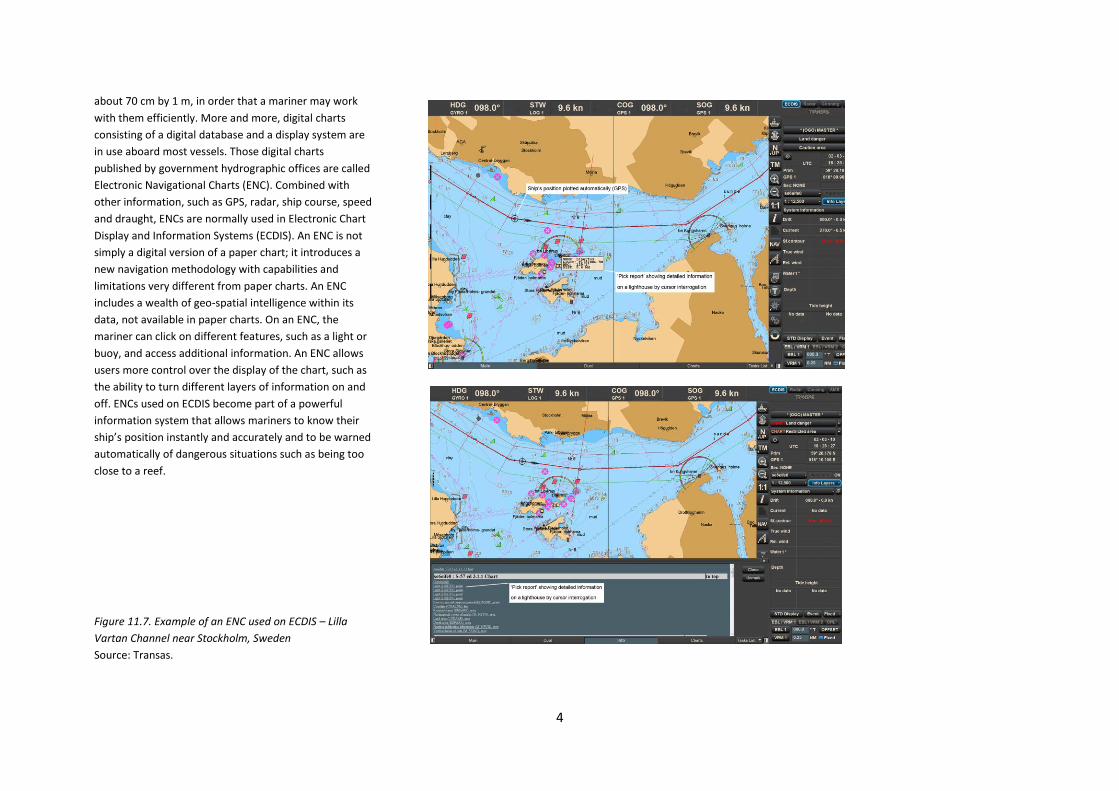
4

about 70 cm by 1 m, in order that a mariner may work

with them efficiently. More and more, digital charts

consisting of a digital database and a display system are

in use aboard most vessels. Those digital charts

published by government hydrographic offices are called

Electronic Navigational Charts (ENC). Combined with

other information, such as GPS, radar, ship course, speed

and draught, ENCs are normally used in Electronic Chart

Display and Information Systems (ECDIS). An ENC is not

simply a digital version of a paper chart; it introduces a

new navigation methodology with capabilities and

limitations very different from paper charts. An ENC

includes a wealth of geo-spatial intelligence within its

data, not available in paper charts. On an ENC, the

mariner can click on different features, such as a light or

buoy, and access additional information. An ENC allows

users more control over the display of the chart, such as

the ability to turn different layers of information on and

off. ENCs used on ECDIS become part of a powerful

information system that allows mariners to know their

ship’s position instantly and accurately and to be warned

automatically of dangerous situations such as being too

close to a reef.

Figure 11.7. Example of an ENC used on ECDIS – Lilla

Vartan Channel near Stockholm, Sweden

Source: Transas.

12 MAPS FOR ORIENTEERING AND FOR FINDING THE CACHE Lazlo Zentai, Hungary What are maps good for? Why do we use maps? How do we use maps? There are several answers to these questions as map users have different ideas and needs regarding map use. However, the most typical and the most classical map use is orientation: to use the maps on the terrain. Of course, not all maps are directly designed for field orientation; for example, thematic maps or small scale maps published in atlases are planned to represent data and give an overview of large (country- or continent-wide) areas. ORIENTEERING MAPS One of the most prominent map types used primarily for navigation is the orienteering map. Although orienteering is a special sport practiced in every continent, it is not a well-known activity in most countries. This sport started as a military navigation test in the second half of the 19th century. The first civil (non-military) event was organized at the very end of the 19th century in Scandinavia. Scandinavia is still the most developed area of orienteering. The main reason is probably its very complicated terrain compared to continental or Mediterranean areas as well as the long tradition of using topographic maps. In every country where orienteering was practiced before the foundation of the International Orienteering Federation (IOF, 1961), local topographic maps were used for the events and training. As large scale topographic maps were allowed to be used for civil purposes from the middle of the 19th century in

Scandinavia, the map use there was a part of the education and culture, much more so than in other countries. The legend of topographic maps was different from country to country. Orienteering was not a part of the Olympic Games (the situation has not changed since then), and international events were rare at that time (these events were organized only in the Nordic countries before the 1960s). Orienteering in Central European countries takes its origins from Scandinavia before the Second World War. In these countries, the sport was based on normal tourist activities and events. Tourist events were widespread especially after 1950, but because of the secret military intention, it was mostly a fieldwork exercise with maps rather than a sport activity. The early period of orienteering maps was the age of homemade maps. In most countries (excluding Scandinavia), there were no suitable maps available for public use. According to the running speed and the course distance, the scale of maps was 1:20,000 to 1:40,000 (or 1:50,000 to 1:100,000 in the early years). In some countries (Eastern Europe), the topographic maps were secret, while the largest available scale of topographic maps was only 1:50,000 in other areas (Germany, Spain). Using tourist maps was a logical alternative, but the accuracy of publicly available tourist maps was not suitable for these events in Eastern Europe. Therefore, these countries tried to find more accurate tourist maps published before the communist era. There was also a problem of copying. The only simple method of making some dozens or hundreds of maps (this was the average number of participants in most events) was the black and white photo in those times.

Figure 12.1. Map and course of the first Estonian championship 1959, 1:50,000, based on an agricultural map. Offset printing (especially in colours) was the most common technique for producing books, journals and any kind of printed product, but it was expensive and technically difficult for the keen organizers of orienteering events. To move one step further, the sport had to reach a higher level: increase the number of participants in events, create international relations, and form regional, national and continental organizations. In those times, there was little sense of speaking about legends, specifications or standardization; in most countries, it was a problem even for local participants to understand maps because the legend was changed from event to event. After the number of users and competitors reached a certain level, orienteers tried to find solutions to make the orienteering maps appropriate, up-to-date, and later, more internationally acknowledged. The Map Committee of the IOF was formed in 1965. The most important and urgent work of the committee was

1

to work out the specifications of World Championship maps, which are as follows:

• The maps have to be new; • The map has to show every detail of the terrain

which can affect the route choice of the competitor;

• Small and unimportant details have to be

omitted (this was most important for the sake of accuracy and legibility); and

• The maps of international events have to use

the same specification. The suggested scale was 1:25,000 or 1:20,000, and the distance between the contour lines was 5 m (10 m or 2.5 m was also allowed depending on the terrain). Later, the scale was increased to 1:15,000, which is now the suggested scale of orienteering maps (they can be magnified to 1:10,000).

The first orienteering map specification specified the colours of the orienteering maps:

• Black, brown and blue for topography; • Yellow for open ground; • Grey or green / black for restricted run ability

(vegetation); • Violet (magenta) for course overprint.

The major differences comparing orienteering maps to other types of maps are:

• There is practically no text on orienteering maps because text information is unnecessary for the competitors during the event, and it would not be fair to use language specific textual information in international events. (Nevertheless, there is certain textual information on orienteering maps, such as title, scale and distance of contour lines, but it does not affect the map use as this information is known in advance.) For the average map user it is quite unusual to prepare a map without text, but one of the most important aspects of orienteering maps is to leave out all unnecessary elements and features which do not help the navigation of competitors, and which are not easily identifiable at running speed;

Figure 12.2. Map of the long distance event of the World Orienteering Championships, Hungary, 2009.

2

• Comparing to other similar scale maps

(topographic maps), orienteering maps have many details, although the map specification contains only a limited number of map symbols (maybe more than 100). The representation of the relief with contour lines is probably the most specific comparing to other similar scale maps;

• On orienteering maps, the representation of

areas is based on the run ability and cross ability. Competitors should be aware of the areas where the vegetation is difficult or impossible to cross or just reduces the running speed. There are some other features too (e.g., cliffs, fences) where it is important to represent the cross ability; and

• These maps are regularly made by amateur orienteers and not by professional mapmakers. Although the users of these maps, the orienteers, are aware of that, their expectations have been increasing as the sport has become more popular. As we have more and more data sources and technologies available (aerial photographs, GPS data, laser scanning), it looks easier to create orienteering maps. However, the excess of data has an unwanted consequence: there will be too much data on the maps, which will make the printed maps less legible.

THE USE OF ORIENTEERING MAPS It is interesting to observe how orienteers use the orienteering maps. According to the competition rules, orienteers can use only the map and compass during the

event. There is not too much sense in using any other tool, although a GPS device could be useful (but they are forbidden). Nevertheless, orienteering maps normally do not show any absolute geographic coordinates, which would be vital for GPS navigation. We will see another sport-like activity, geocaching, in the next subchapter, which is based on the use of GPS.

• Competitors have to measure distances and directions while they are running, as the essence of the orienteering events is that the fastest is the winner. Distances are simply measured, rather than estimated by pace counting. However, orienteers do use this technique only in certain situations during an event. Measuring direction means that orienteers are measuring the angle between the magnetic north (which is provided by their compass) and the direction they want to head. Even the accuracy of distance and direction measuring is not comparable to precise devices, but the method in which orienteers use these techniques is adequate to find the control points on the terrain;

• The general technique of navigation for

orienteers is continuous map reading. It is essential that the competitor should be 100% sure of his/her actual position every second of the event. Due to a large amount of map details, the most difficult task for orienteers is to filter out the most relevant information, to identify the most prominent features in the map and on the terrain; and

• One of the most complex challenges of the

orienteering map is the relief representation, namely, to interpret the contour lines and "translate" them into a real 3-dimensional form in the competitor's mind. It is vital because the relief is a continuous feature

covering the whole terrain. The best competitors are very good at understanding and interpreting contour lines even at running speed.

Orienteering has various official disciplines (foot orienteering is the standard discipline; mountain bike orienteering, ski orienteering and trail orienteering are the newer forms, although ski orienteering was practiced in Nordic countries as early as the foot orienteering). Some other forms (like sprint orienteering) may require different maps. Although these maps are based on the usual orienteering maps, they are specialized:

• Mountain bike and ski orienteering maps are simplified compared to the foot orienteering maps: in both disciplines, the competitors are moving at a much higher speed, and the maps are in a special folder; these conditions do not favour map reading. Small features (knolls, pits) which can be covered by snow or which are not visible from the "bike able" paths and tracks, are not represented, while the road network used by skiers or bikers is exaggerated. The scale of these maps is also slightly smaller (1:20,000) than that of foot orienteering maps because the maps should fit in the map folders;

• Sprint orienteering is a relatively new form of

the sport. The only difference compared to the normal foot orienteering is that the venue of the event is not a forest area but a park or an urban area or their combination. These areas have much more features and objects, so the map scales are much larger (1:4,000 or 1:5,000) in order to show all relevant details. The courses are generally much shorter (the winning time is about 12–15 minutes), which means that the competitors are running as fast as they can. In such a high speed small terrain details are not easily identifiable (or the

3

competitors should reduce their speed), so the mapmakers should represent only the most relevant features. It is easy to create sprint orienteering maps full of details because urban areas usually have very good base maps (e.g., cadastral maps), but it is difficult to create a good sprint orienteering map where only the relevant features are represented; and

• Trail orienteering (sometimes called precision

orienteering) is a discipline of the orienteering sport designed so that people with disabilities could have meaningful orienteering competitions. It eliminates the element of speed over the ground but makes the map interpretation element much harder. Competitors travel along a track or marked route and study clusters of control markers placed on the terrain. They are issued with a very detailed map and control descriptions. With these aids they must decide which (if any) of the markers relate to the feature depicted by the centre of the circle. Movement up and down the track is permitted, but no one may approach the control markers on the terrain. Sprint maps are also used for trail orienteering events. The only specialty is that the trail orienteering competitors are not allowed to approach the control points, so they have to convert the side view of the terrain in their mind to the top view of the map.

Figure 12.3. Map of the first World Mountain Bike Orienteering Championships, France, 2002.

Figure 12.4. World Ski Orienteering Championships, Sweden, 2011. Figure 12.5. Sprint orienteering map, Morocco, 2013.

GEOCACHING Geocaching is a free real-world outdoor activity, which is regularly called treasure hunt. Players try to locate hidden containers called geocaches (most often small plastic boxes) by using a GPS. GPS chips can be built in smartphones or cameras and users can document their treasure hunt experiences. It is more precise to use the general term, Global Navigation Satellite System (GNSS), which is much more neutral than the term GPS (Global Positioning System). The latter was the first available service, but nowadays Russia, China and the European Union are developing their own independent services. Geocaches are hidden outdoors and their location is defined by their geographic coordinates (latitude, longitude; height is also measured, but this is irrelevant in most cases). Theoretically, players do not need maps to find the geocache as its geographic coordinates unambiguously identify the location. Players use traditional paper maps or digital maps in their GPS device or smartphone to find their way to the location of the geocache. Let us imagine you know your actual position and the geocache location. Although this means that you can easily calculate (or rather, the GPS device calculates) the distance and the direction of the geocache, in most areas (especially in an urban environment) it is impossible to go straight. Although clues are given on a geocache website, it is not easy to find the geocache in many cases because the precision of hobby GPS devices is only of the order of 10 meters and the geocache "owners" really hide their boxes on the terrain. There is a global international website of geocache players (http://www.geocaching.com), and there are also independent local (national) community websites. New players can easily join the geocache hunting: they can download the geographic coordinates of selected geocaches to their device and after they have found them on the terrain, the players can also report the

4

successful hunting (password may be hidden in the geocache container), and they can collect scores in this way. There are different variations of geocaching (containers can be virtual, mobile or multi-cache, which can be a collection of several points around the cache). Although similar games were invented before the GPS era (where points had to be found by using written instructions), geocaching started in 2000, when the accuracy of GPS devices improved considerably due to the political decision of the USA. Along with the development of smartphones, the falling price of GPS chips increased the number of users considerably. GPS can identify the geographic location, which is practically useless for ordinary users, but the appearance of online map services (2005) like Google Maps or Bing Maps and the spread of mobile Internet access created a new era, that of the location based services. This service provides automatic information based on the actual location of the user (with the help of the GPS-enabled device). For example, a user can get automatic answers to questions like where it is an open post office nearby or what is this specific building. Young users are keen on using services where they can share their location information with their friends (like Google Latitude or Apple's Find My Friends). All GPS-based applications operate only outdoors, but companies are developing other technologies for a supplementary indoor navigation: users want to use such services without understanding or taking care of the technology. One of the main concerns with these services is similar to social networking concerns: users should be careful to share such information (not only their personal information but also their location) with anybody who they do not know at all. Another similar game or passion of the simple, easily understandable, and a little bit artistic way of GPS usage is the GPS drawing. Tracks of a journey (walking, cycling) can automatically be recorded into the GPS receiver's

memory and can be represented later on a website combined by maps, satellite images or only the track alone. This journey may be on the flat surface (e.g., walking, car driving) or taken in 3D (e.g., while flying or diving).

Figure 12.6. An example of GPS drawing. Source: www.gpsdrawing.com.

5

13 PRINTING MAPS Bengt Rystedt, Sweden

13.1 Introduction By printing we mean all kind of duplication and there are many kind of media, but the most common one nowadays is your own screen. Web mapping on Internet is also common and mapping for mobile telephones is also coming. Web mapping and mobile mapping are described in chapter 14. In this chapter traditional mapping on paper will be described but web and mobile mapping have to use the same principles. Let us first consider how to print a topographic map assuming you have a geographic database where the data are organized in layers such as:

• Administrative borders. • Communications. • Waters (lakes and rivers). • Buildings. • Land use and land cover. • Elevation • Geographical names.

When printing it is best to start with the waters, and land cover and land use. That forms the background of the map. After that you can print the other layers and finish with the geographical names, which are the foreground of the map.

13.2 The Legend The legend describes the content of the map. Setting up the legend is a time consuming work. It is better to look

Figure 13.1 shows a copy of the legend for the Austrian topographic map at the scale of 1:50 000. © Bundesamt für Eich- und Vermessungswesen, 2005, Vienna, Austria. at a map and see how a cartographer has solved the problem (see Figure 13.1).

Legend (continued)

There are many object types that can be included, but where are the swimming pools?

1

13.3 Colour As it is seen in the legend there are colours in a topographic map, but there are more maps like thematic maps and atlases that also have a lot of colour. The sunlight gives no colour but all colours can be seen in the rainbow, where the sunlight is reflected in the rain drops. When we are handling colour on a computer we use only three basic colours: red, green, and blue (RGB). Yellow is a mixture of green and red. This system is called additive and is shown in Figure 13.2.

Figure 13.2 shows additive colour to the left and subtractive colour to the right. Observe that in additive colour yellow is a mixture of red and green and in subtractive colour green is a mixture of blue and yellow. In a simple computerized colour system you may mark each basic colour with eight (0--7) different values which gives 256 different colours at the computer screen. In most computer systems each basic colour is marked with 24 (0-23) intensities which gives 13,824 different colours. That is many, but far from all colours in nature. When we are looking at colour on a paper plane we must use another system. When we add all colours we get a black colour instead of no colour as is shown in Figure 13.2. In the colour system for printing we talk about the basic colours cyan, magenta and yellow. In the printing industry these colours are called process colours. The

intensity is given by percentages. Each combination can also be more white and dark. In a professional printing system one film is produced for each process colour but also one film for black. Since the process colours are given in percentages each film will be given a raster in order to let the required percentages of light pass the film. All these films are then mounted in a printer for printing in what we call a 4-color system CMYK where C stands for cyan, M for magenta, Y for yellow, and K for key colour (black). The same system is used in ink colour printers for private use. It is difficult to choose colours by giving the intensity for each process colour including whiteness and darkness. To make colour selection simpler the company Pantone has developed a help guide that is shown in Figure 13.3.

Figure 13.3 shows a palette developed by Pantone. The palette gives the closest CMYK- code for each colour, which makes it easier to choose colours for printing. Source: Wikipedia.

It is very important that the films fit together exactly when they are mounted for printing. If not there will be blurs in the colours. Earlier the contour lines for elevation that printed in brown colour were a problem since brown contains three basic colours and were represented in three films. The solution was to use a separate film for brown that needed an extra run through a 4-colour printer. Thanks to the digital technique and the way of handling raster on the films that is no longer necessary. The films are no longer produced by the mapping company but sent to the printing office via computer communication techniques. That also eliminates problems with deformation of the films by manual handling or by changes in humidity and temperature. A good colour handling is important for producing good maps. That is more important when printing thematic maps. The colours are very important for understanding the message the map is giving. In choropleth mapping described in chapter 6 on Thematic Maps Figure 10 shows how the colour goes from light yellow to dark green with higher unemployment. The things you want to emphasize should be given with strong colours. More information on colours in thematic mapping is given by Brewer (2005).

13.3.1 Describing colours A simple way to describe colour is to use the colour circle. Figure 12.4 shows such a circle. The extra colour marked in the figure contains 10 % yellow and 90 % red. Orange consists of 50 % yellow and 50 % red. However, the figure shows just some colours. In order to see all colours we need a more complex figure.

2

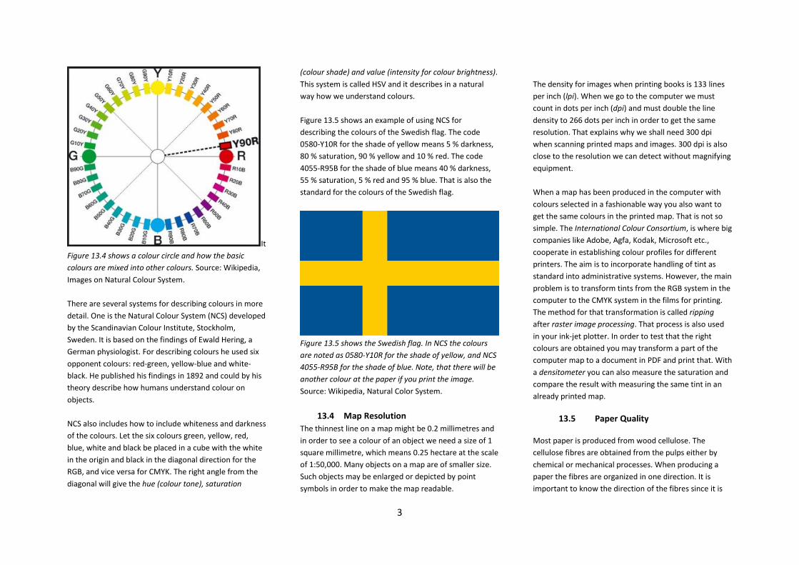
It Figure 13.4 shows a colour circle and how the basic colours are mixed into other colours. Source: Wikipedia, Images on Natural Colour System. There are several systems for describing colours in more detail. One is the Natural Colour System (NCS) developed by the Scandinavian Colour Institute, Stockholm, Sweden. It is based on the findings of Ewald Hering, a German physiologist. For describing colours he used six opponent colours: red-green, yellow-blue and white-black. He published his findings in 1892 and could by his theory describe how humans understand colour on objects. NCS also includes how to include whiteness and darkness of the colours. Let the six colours green, yellow, red, blue, white and black be placed in a cube with the white in the origin and black in the diagonal direction for the RGB, and vice versa for CMYK. The right angle from the diagonal will give the hue (colour tone), saturation

(colour shade) and value (intensity for colour brightness). This system is called HSV and it describes in a natural way how we understand colours. Figure 13.5 shows an example of using NCS for describing the colours of the Swedish flag. The code 0580-Y10R for the shade of yellow means 5 % darkness, 80 % saturation, 90 % yellow and 10 % red. The code 4055-R95B for the shade of blue means 40 % darkness, 55 % saturation, 5 % red and 95 % blue. That is also the standard for the colours of the Swedish flag.

Figure 13.5 shows the Swedish flag. In NCS the colours are noted as 0580-Y10R for the shade of yellow, and NCS 4055-R95B for the shade of blue. Note, that there will be another colour at the paper if you print the image. Source: Wikipedia, Natural Color System.

13.4 Map Resolution The thinnest line on a map might be 0.2 millimetres and in order to see a colour of an object we need a size of 1 square millimetre, which means 0.25 hectare at the scale of 1:50,000. Many objects on a map are of smaller size. Such objects may be enlarged or depicted by point symbols in order to make the map readable.

The density for images when printing books is 133 lines per inch (lpi). When we go to the computer we must count in dots per inch (dpi) and must double the line density to 266 dots per inch in order to get the same resolution. That explains why we shall need 300 dpi when scanning printed maps and images. 300 dpi is also close to the resolution we can detect without magnifying equipment. When a map has been produced in the computer with colours selected in a fashionable way you also want to get the same colours in the printed map. That is not so simple. The International Colour Consortium, is where big companies like Adobe, Agfa, Kodak, Microsoft etc., cooperate in establishing colour profiles for different printers. The aim is to incorporate handling of tint as standard into administrative systems. However, the main problem is to transform tints from the RGB system in the computer to the CMYK system in the films for printing. The method for that transformation is called ripping after raster image processing. That process is also used in your ink-jet plotter. In order to test that the right colours are obtained you may transform a part of the computer map to a document in PDF and print that. With a densitometer you can also measure the saturation and compare the result with measuring the same tint in an already printed map.

13.5 Paper Quality

Most paper is produced from wood cellulose. The cellulose fibres are obtained from the pulps either by chemical or mechanical processes. When producing a paper the fibres are organized in one direction. It is important to know the direction of the fibres since it is

3

easier to bend a paper along the direction than across the direction. That is important if the map shall be folded. One problem with cellulose is that it is not stable over time. Paper from textile, rice and parchment give better possibility for long life. The cellulose paper will over time be destroyed and in the future not possible to read. Unfortunately, there will be not much to read from our time in future archives. The weight of the paper is given in gram per square meter. The most common weight for ordinary writing paper is 80 grams (per square metre, which is not included in the daily talk). For printing maps a paper of 100 -- 150 grams is recommended. The surface of the paper is also important. There are many ways to coat the paper to get it smoother than the raw paper. That is needed for getting the small details of the map visible. If a good result is needed ask a printing office for advice. Printing on waterproof paper is also possible to get maps that can be used in rain and while canoeing. Plastic material is available. For some orienteering events waterproof maps are printed. Such maps are not destroyed by water, but when roughly used they may be heavily wrinkled and some details of the map content may be obliterated.

13.6 Notations The overall description of the map should be given by the person who has designed the map (see Chapter 4). The map image is almost meaningless without a clear

indication of the map’s contents, and that indication should be given in the map title. Preferably, in the map title there is an indication of the topic covered, the area depicted and the year for which the data are valid (for instance: “Population density in the Netherlands in 2010”). A subtitle can further inform on the topic or on the way of presentation. And of course in the map legend all the symbols used on the map need to be explained (see also figure 13.6). But apart from the title, the printer also has to follow the rules for publication, and include a statement regarding the publisher, place of publication and year of publication. When stated in that sequence, this is called the imprint or impressum. It ensures that the printed map can also be retrieved by those that would want to use it. Therefore, in the margin of the map there should be information on the publisher, on the place and date of publication, but preferably also on the map author, and the printer, to show who is responsible for the contents of the map. For more scientific maps the way the geographical data was processed need also to be indicated. . These notations (which can also be called marginal information) shall also include the source and the actuality of the map and its scale. For a topographic map it should also be shown how a bigger area is divided in different map sheets and what the titles of these different sheets would be (in topographic mapping a specific sheet is usually called after the largest inhabited place rendered on that map). It can also show in a small diagram representing the same area as the main map, whether there were any differences in the reliability of the mapped information over the map area. Maps for navigation shall also include the geodetic network and indicate how the coordinates are measured. The legend

and all this marginal information may make it necessary that both sides of the paper are used.

Figure 13.6 Texts on a map. Apart from geographical names or toponyms on the map itself there would be abbreviations, letter symbols (S), and generic terms like Cape, Hospital, Cemetery, etc. The purpose of all this documentation is twofold: a) that this should make it possible to find this specific map when needed, as it allows this kind of information to be stored in catalogues and indexes, and b) as it shows the prospective user whether the map is suitable for the intended use.

4

13.7 Map Folding When the map has been printed it may rest before being handled further for folding or distribution. The best way is to first make a manual folding before using a folding machine. The practical work of folding is an adventure. Trouble may occur very easily and needs some preparation to prevent destroying too many maps. References Brewer, C. A., 2005: Designing Better Maps - A Guide for GIS Users. Esri Press, Redlands, California, USA. ISBN 1-58948-089-9. Granath L. and Elg M.2006: Konsten att framställa kartor – en handledning i kartdesign (The Art of Producing Maps - A Guide for Map Design). Studentlitteratur, Sweden. ISBN 91-44-04560-3.

5

Chapter 14 Web and Mobile Mapping Michael P. Peterson, USA Abstract Mapping has always been dependent on a set of tools, both for measuring the world and for making the map. Since 2005, a new set of online or cloud-based tools has been developed for making maps called Application Programmer Interfaces. These tools provide the additional benefit of being automatically available to anyone with an Internet connection. This chapter examines this new mash-up era in mapping and shows how to make and distribute maps using free mapping tools. 14.1 Introduction It is difficult to overstate the importance of maps as a form of communication about the world. They help us understand both our surroundings and the space beyond our direct perception. Maps influence how we think about the world and how we act within it. They connect us to our environment. Each of us is a mapmaker, or cartographer, in the sense that we all make mental maps. Sometimes, we even need to draw these maps for others to help explain how to find a particular location. The making of maps and the analysis of the underlying information have evolved into a science and are valuable skills for many different types of work. Many of the tools for mapping are now located in the cloud—a sophisticated system of hardware and software accessible through the Internet. Cloud-based mapping tools allow for very advanced forms of mapping. A further advantage of these online maps is that they can be easily made available to others. Making maps in the cloud requires using a server. While it is possible to transform almost any

Figure 14.1a shows in the left panel the signup page for http://000webhost.com. Account information is shown on the right. Choosing a subdomain is free. A charge is incurred for specifying a domain with a specific name, such as http://www.peterson.com but having the site choose a free domain like http://geographyprof.hostei.com is free. (© 2014 First Class Web Hosting) computer into a server, it is easier and more secure to use an online hosting service. Cloud-hosting services such as Amazon Web Services and Microsoft Azure implement scalability in the sense that they can be upgraded to serve millions of simultaneous users. These services charge for disk space usage and server processing cycles. Another option for hosting web pages is web-hosting services that only charge for disk storage. While these services are not as scalable, they are easier to use and offer free subdomain plans with up to

Figure 14.1b shows the Account information. 1,500 MB of disk space. Two such free web-hosting services are 000webhost.com and podserver.info. The following sections describe how to create a website and serve maps using one of these free web-hosting services. 14.2 Servers in the Cloud 14.2.1 Making Space in the Cloud Figure 15.1 depicts the sign-up page for the 000webhost.com provider and the resultant account information. Notice how a free subdomain is being requested under the hostei.com domain. While an address like http://geographyprof.com could be requested in the top line, it would incur a charge because it would represent a new domain. To obtain a free account, it is important to not register your own domain.

1

An e-mail address is needed to register for the free subdomain. The Account Information page shows that the web address that was assigned by the service provider is http://geographyprof.hostei.com (or http://64.120.177.162) and that 1,500 MB of free storage is available. The account information also shows the availability of the Apache web server, and other online tools including PHP and MySQL. Included in most web-hosting services is a graphical interface to the services that are offered. This is called the control panel, or cPanel (see Figure 14.2). The tools handle e-mail, the editing of files, the scheduling of tasks, and account management. All of these tools represent open-source projects that are written and maintained by a small legion of programmers. File Manager is the most useful tool for managing files and building a website. MySQL and phpMyAdmin are used for building a database. Most web-hosting services use a similar cPanel to access server resources. Figure 15.3 shows the File Manager window with access to tools for uploading and creating new files and directories (subfolders). Tools are also available to move, delete, and rename files. The file listing shows the name, type, and size of the file, while the Owner, Group, and Perms fields depict security settings. Mod Time indicates when the file was last modified. The files can be edited directly from this window by clicking “Edit” at the end of each file name. The public_html folder is the directory from which all web files are served. If an html file is to be presented through a web page, it must reside in this folder. Usually, this folder contains a file called index.htm (or index.php) that is the first page that is accessed when the site is referenced. For example, if an address such as http://geographyprof.hostei.com/CloudM_apping/

is entered into a browser, the browser will look for a file called index.htm in a directory (folder) called CloudMapping that is itself located in the public html directory. That means that the following two addresses would display the same file: http://geographyprof.hostei.com/Online_Mapping/ http://geographyprof.hostei.com/Online_Mapping/index.htm

Figure 14.2 shows a standard webHosting control panel, called cPanel, which gives access to different tools. File Manager is the major program for uploading and editing files. (© 2014 First Class Web Hosting)

Figure 14.3 shows the File Manager Window from an online hosting service. This service allows files to be created and edited. All files to be served through the web must be in the public_html directory/folder. (© 2014 First Class Web Hosting) Normally, this index.htm file serves as an entry point to the website and will have links to all other files in the directory. The index.htm file will have a relatively simple structure—a title line followed by links to all of the assignments. This file could have a picture of the website owner and links to the websites of other students, as shown in Figure 14.4. The corresponding code shows how a picture is inserted using the <img src=filename> tag. The links to the student pages are separated by two vertical lines (“||”). The code for the entire index file can be obtained by searching for “Peterson Mapping in the Cloud.”

2

<html> <head></head> <body bgcolor="#CCCCFF"> <h2> Exercises for <i>Mapping in the Cloud</i> </h2> <img src=peterson.jpg height=150><b> Michael Peterson's page </b><p> <p> <b> Student Pages </b><br> <a href=http://victoriaA.site88.net> V. Alapo </a> || <a href=http://mapsarefuntoo.web44.net> K. Edwards </a> || <br> <hr> <ul> <li> Ch 4: <a href=http://maps.unomaha.edu/onlinemapping/ code04.zip> Map Gallery </a><br> <li> Ch 6: <a href=code06.zip> Online Street Map</a><br>

<li> Ch 8: <a href=http://maps.unomaha.edu/onlinemapping/ code08.zip> JavaScript </a><br> </a><br> </ul> <hr> </body> </html> Figure 14.4 shows an example of an index.htm file that includes a picture, links to all other students, and links to the assignments. The code shows how to display a picture using the img tag, links to the pages for the other students, and to the assignments. 14.2.2 HTML HTML is the building block of the web. It is the language that makes it possible to present information through web pages. It is also a container for scripting languages such as JavaScript and PHP. Some knowledge of HTML is necessary for presenting maps through the Internet. HTML consists of tags that define the layout of the page (Willard 2009). It includes simple text codes, surrounded by the “<” and “>” delimiters, that specify how the document will appear in the browser. Other HTML tags also create links to documents or display a graphic file. An ordinary text editor can be used to enter the file (Notepad on Windows or TextEdit with Macintosh, with appropriate settings). Unlike word processors, these programs are intended for entering unformatted text. Once the files are created, they may be opened with a browser such as Explorer, Firefox or Chrome. All HTML files begin with the “<html>” tag and end with the same code prefaced with a slash (e.g., “</html>”). The slash in front of the end code indicates that the HTML coding is finished. Technically, all HTML tags have a beginning and

end, with the end tag indicated with “/.” For example, the <h1> command is used to begin header text—larger text used for titles—and the </h1> code stops the header text format. We can now display a map with the img tag. All file names that are referenced with img must end with GIF, JPG (or JPEG) or PNG as these are the common file types for the different browsers. The img “src” option is used to specify the file's URL address. In the example below, notice the image file designator “.gif” at the end of the URL. The img command also includes a number of options that can be used to alter the size of the image or change its placement on the page. Like hr, img does not have a standard end tag. In strict XHTML formatting, it is written as <img src=map.png /><img src=“http://maps .unomaha.edu/OnlineMapping/Chapter4/MapExample1.gif” width=“500” height=“389”> The <embed> tag is used to display graphic files that are not in the GIF, JPEG, or IMG format. Examples include Adobe’s PDF, Flash, SVG, and QuickTime. The format is identical to that of the <img> option: <embed src=“http://maps.unomaha .edu/Cloud_Mapping/Chapter4/MapExample4.pdf” width=“500” height=“389”> One of the most used tags in HTML is the anchor that is usually used with a text string to create a hypertext link. It can also be used with the img tag to create a hyperimage link. The format of the anchor command is as follows: <a href=http://maps.unomaha .edu/Cloud_Mapping/Chapter4/MapExample4.pdf> Click for PDF file</a>

3

14.2.3 JavaScript By itself, HTML is simply a page formatting language. In combination with JavaScript, an HTML page can execute computer code (W3Schools.com 2011). Once relegated to geeks, programming is now being viewed as a form of expression, as the “amplification of thinking,” and a necessary skill. This “coding as literacy” concept is promoting new ideas about the importance of being able to program. Online programming sites like CodeAcademy are becoming increasingly popular. Khan Academy has introduced a similar suite of free online programming exercises. The following examples provide a brief introduction to JavaScript and how it can be used to call other functions.

Figure 14.5 shows a calculation performed with JavaScript within the body of an HTML file. Functions are the fundamental building blocks of JavaScript. A function is a procedure—a set of statements that performs a specific task. Functions are generally defined in the head section of an HTML document. This assures that all functions are defined before any content is displayed. The example in Figure 15.6 defines a simple function in the head section of an HTML document. The function is then called in the body of the document.

The function square takes one argument, called number, and the function consists of one statement, return number * number, which indicates it should return the argument of the function multiplied by itself. The return statement specifies the value that is returned by the function.

Figure 14.6 shows a function that squares the number passed to it by a call to the function. The external file that contains JavaScript functions can be on the same computer as the HTML file, as implemented in Figure 14.7, or it can be on another computer or server. This is how Application Programming Interface (API) code is distributed. One reference to a library of API code makes it possible for a webpage designer to access thousands of functions. Rather than embed the JavaScript code directly in the HTML file, either in the body or the head, it is possible to place the JavaScript functions within a separate file. The SRC attribute of the <script> tag specifies the external file where the JavaScript code can be found. Figure 14.8 shows the external file

called common.js and how it is referenced in the head section of an HTML document. The external JavaScript file may contain multiple functions but no HTML code.

Figure 14.7 shows a function that is placed into an external document, common.js. The function is then referenced from the HTML file with <script src=“common.js”> Figure 14.8 shows how the Google Maps API code is referenced. To aid in debugging, the Google Maps API code will work locally on a computer without the need to transfer the code to a server. But, in order for others to see the map, the code must reside on a server.

4

Figure 14.8 shows the implementation of a call to the Google Maps API that accesses a large number of mapping-related functions. Here, the sensor is set to “false.” The value of the sensor would be set to “true” if a mobile device is used that can provide the current position. 14.3 Google Maps API Introduced soon after Google Maps in 2005, the Google Maps Application Programming Interface consists of a series of functions that control the appearance of the map, including its scale and location, and any added information in the form of points, lines or areas and associated descriptions. The use of Google Maps API is essentially free, provided the site does not charge for access. Google places a limitation on the number of maps that can be served. A site cannot generate more than 25,000 map loads a day for 90 consecutive days. A map load is one map displayed with the Google Maps API. Once loaded, the degree to which a user interacts with a map has no impact on the map load number. It would be extremely difficult for the average user of the Google Maps API to exceed 25,000 map loads. Even if a site were to go “viral,” it would need to sustain 25,000 map loads per day for 90 consecutive days before the limit would be reached. Usage limits can be placed on a site so that it does not exceed that number. If the site consistently exceeds 25,000 maps a day, Google would require you to register your site and pay US$0.50 for every 1,000 map views beyond this

limit. For example, if your Google mapping page served 100,000 maps a day for 90 consecutive days, you would be charged $37.50 (75,000÷1,000 x 0.5) a month after the initial 90-day period. Specialized Google Maps API web services have additional usage limits, including:

• Directions—provides directions in text form—limited to 2,500 a day;

• Distance Matrix—returns travel distance and time—limited to 100 elements per query and 2,500 a day;

• Elevation—elevation at points—limited to 2,500 requests per day where each request returns up to 512 elevations;

• Geocoding—converts a street address to latitude and longitude—limited to 2,500 a day;

• Places—returns business establishments and other points of interest around a point—requires an API key and is limited to 1,000 requests a day.

A Google Maps API key is a numeric code that registers your site with Google. It is not needed for normal applications and would only be required if the usage limits are exceeded or the Places web service is used. The example in Figure 14.9 shows the JavaScript code and API calls for displaying a simple map that is centered at a specific location. The zoom level, which can range from 0 to 21, is set to 15 under myOptions. The center is defined with a specific latitude and longitude value, and the ROADMAP option is selected to define the map style. All of the API calls are made in the initialize function. This function is called onload within the body of the HTML file.

Figure 14.9 shows a basic Google map request. The center of the map can be changed along with the zoom level and map type. (© 2014 Google) A simple change can be made to this code by substituting new latitude and longitude values. Determining the latitude/longitude for a specific point can be done in a number of different ways:

• In Google Maps with a right-click (control + click on a Mac) and selecting “What’s here?” from the longitude of the point will appear in the top line of the Google Maps window;

5

• A right-click with MapQuest displays the values in a pop-up window;

• In Bing Maps, the latitude and longitude are displayed with a right-click;

• To display the coordinates in the decimal degrees format with Google Earth, select Tools/Options and click on the decimal degrees option;

• Finally, there are a number of online utilities. Searching for “Finding latitude and longitude” will lead you to a site. Most of these sites use Google Maps, including this example: http://findlatituteandlongitude.com.

Another change to the basic Google Map is the type or style of map that is displayed. Google offers four views:

• MapTypeId.ROADMAP displays the default road map view;

• MapTypeId.SATELLITE displays Google Earth satellite images;

• MapTypeId.HYBRID displays a mixture of normal and satellite views;

• MapTypeId.TERRAIN displays a physical map based on terrain information.

The initial zoom level can also be changed. A value of “0” would draw a zoomed-out, small-scale map. As the zoom level number increases, so too does the scale of the map. The upper value varies for different parts of the world. Generally, 20 levels of details are always available. Some parts of the world have more than 20 zoom levels. 14.4 Point, Line, Area, and Layer Mash-ups All maps are composed of points, lines and areas. In addition, multiple maps can be combined as individual layers, a function that is the basis of geographic information systems. The examples in

this section show how these elements can be added to the Google Map. 14.4.1 Points The default Google marker is an upside-down raindrop symbol, but a large number of alternative icons are available. It is even possible to design symbols because they are simply 32x32 pixel images in the PNG format. Markers can be static or interactive. The major interactive type of marker is one that is clickable.

Figure 14.10 shows an example of a clickable marker. The contentString text variable is defined in HTML. (©2014 Google) In the example in Figure 14.10, the variable contentString is defined with text formatted in

HTML. This is associated with an infoWindow variable that is subsequently associated with google.maps.event.addListener. When the user clicks on the marker, the text is displayed in a pop-up bubble. The HTML for this bubble could incorporate a picture or even a video using the img or embed tags. In cases where a large number of points need to be mapped that may be frequently updated, a web format called Really Simple Syndication (RSS) is often used. There are many advantages to RSS. Publishers of RSS feeds benefit by syndicating content automatically while consumers benefit through timely updates of mapped information. A standardized file format allows the information to be published once and viewed using many different programs. KML, Keyhole Markup Language, is a format used for describing two- and three-dimensional space that was originally developed for Google Earth. It is now an open standard officially named the OpenGIS® KML Encoding Standard (OGC KML) and is maintained by the Open Geospatial Consortium (OGC). The format specifies features such as placemarks, images, polygons, and 3D models. Places are always specified with latitude and longitude. A large number of KML files are available through the Internet. The google.maps.KmlLayer function reads a KML-formatted RSS feed specified with an HTTP address. Maps made in this way are usually displayed very fast. The trade-off is that there is less control over the look of the actual map because symbols are defined in the KML file. The example in Figure 14.11 shows an application of an RSS feed for the depiction of earthquakes. This particular KML feed is updated daily and shows earthquakes in the past seven days. Each marker is clickable and provides more information about the

6

earthquake event. The code shows how to make a map for just a certain part of the world.

Figure 14.11 displays an RSS feed defined in KML format from the United States Geological Survey. Each icon pinpoints the earthquake and, when clicked, describes the event. The bottom map is displayed using a basic call to a KML layer that ignores the defined center and zoom level and therefore duplicates most of the world. The top map is displayed with the {preserveViewport: true} option and ctaLayer that applies the user-defined center and zoom level. (© 2014 Google)

14.4.2 Lines The google maps Polyline function is used to draw lines with the Google Maps API. In Figure 14.12, the Polyline function connects points that have been previously defined. Options for controlling the appearance of the line include strokeColor, strokeOpacity, and strokeWeight. As always, an appropriate center and zoom level must also be defined. The center could be the midpoint of the line itself.

Figure 14.12 shows a line made from three elements consisting of four points. (© 2014 Google) The shortest distance between two points on a map because the map has been projected from the spherical earth. On most projections, including the Mercator that is used by all major online mapping services, the shortest distance on the ground is represented as a curve—seemingly a longer distance between two locations. The great circle is defined as the shortest distance between two points that divides the Earth into two equal hemispheres. It is supported in the Google Maps API through the geodesic: true polyline option (see Figure 14.13).

Figure 14.13 shows the geodesic: true polyline option connecting two points through the great circle, the shortest distance between two locations on the sphere. It appears as a longer line on this map because of the projection. (© 2014 Google) 14.4.3 Areas A polygon may be viewed as a line that closes upon itself. It consists of a series of points, with the last point always equal to the first. The two additional attributes that need to be defined for google.maps.Polygon are the shading and opacity of the interior area.

7

Figure 14.14 The Google Polygon function draws a closed shape. Options include strokeColor, strokeOpacity, strokeWeight, fillColor and fillOpacity. (© 2014 Google) Figure 14.14 shows the Bermuda Triangle in the Atlantic Ocean. Four points are defined to depict the triangle. These points are loaded into an array

named triangleCoords. This array is then passed to google.maps.Polygon. Parameters include the strokeColor, strokeOpacity, stroke-Weight, fillColor and fillOpacity. 14.4.4 Layers To this point, we have overlaid points, lines, and areas that were defined as vectors of latitude and longitude. Now, we overlay a raster image or picture that could be an air photo, satellite image and scanned map. The advantage of overlaying an image is that the overlay can be done quickly. No major conversion or drawing is necessary to place the information because the underlying map is in the same format. Raster files can be overlaid as single entities or divided into tiles to precisely match the tiles of the underlying map. The example in Figure 14.15 shows a map that has been scanned and saved in the JPEG format. The latitude and longitude of the southwest and northeast corners have been estimated and are then defined using imageBounds. These coordinates are combined with the address of the image in the oldmap object.

Figure 14.15 shows an overlay of a scanned map in the JPEG format. Map of Newark, NJ, courtesy of the University of Texas Libraries, The University of Texas at Austin. (© 2014 Google) 14.5 Mobile Mapping Location-aware devices are becoming increasingly common. Virtually all mobile phones can now be located within a few meters. Smartphones have the additional ability to display their current location on a map. Tablet computers based on Apple’s iOS and Google’s Android can usually do the same but with the added benefit of displaying a much larger image.

8

There are many different types of mobile devices and many different ways of determining location. To provide a standardized approach, the World Wide Web Consortium (W3C) created a freely available geolocation API. Supported by nearly all browsers, the API uses multiple methods to find the location of the computer or mobile device (Svennerberg 2010, P. 235). The Global Positioning System (GPS) is one method of determining location, but it only works with an unobstructed view of the sky. In urban areas, the most common method of determining location is triangulation based on Wi-Fi and cell tower signals. Location software developed by the Boston-based company, Skyhook, uses a massive reference network comprised of the known locations of over 250 million Wi‐Fi access points and cellular towers. To develop the database, Skyhook deployed drivers to survey every single street, highway, and alley in tens of thousands of cities and towns worldwide, scanning for Wi-Fi access points and cell towers and plotting their precise geographic locations. Mapping the current location of a device through a browser using the W3C API is shown in Figure 14.16. The “navigator.geolocation.getCurrentPosition (function(position)” statement resolves the current position of the device. If the position cannot be determined by GPS, the API uses the triangulation method based on a wireless network. This example presents an infowindow at the current location. The example in Figure 14.16 replaces the infowindow with a clickable marker. The contentString for the bubble text displays the latitude and longitude.

Figure 14.16 shows the text displayed. In the clickable bubble is the latitude and longitude of the current point of the mobile device. The “+” in the contentString statement is used to concatenate the numbers into a text string. (© 2014 Google)

14.6 Conclusions We live in an amazing time for mapping. Within a matter of 20 years, from the 1970s to the 1990s, maps changed from static objects on paper to interactive presentations delivered through an electronic network. In the years since then, maps have become even more interactive in the sense of being able to add information—both thematic information through mash-ups and the editing of the underlying base map. The exercises in this chapter provided an introduction to the new world of mapping through the Internet. The tools that were introduced can be used to make very sophisticated types of maps. References Google Maps JavaScript API V3 Basics (2011). (search: Google Maps JavaScript API V3 Basics). Neumann, A., Winter A. M. (2003). “Web-mapping with Scalable Vector Graphics (SVG): Delivering the promise of high quality and interactive web maps.” In: Peterson, M. P. (ed.) Maps and the Internet. Elsevier, Amsterdam, pp.197–220. Peterson MP (2008) International Perspectives on Maps and the Internet. Springer, Berlin. Svennerberg, Gabriel (2010). Beginning Google Maps API 3. New York, NY: Apress. W3Schools.com (2011). JavaScript Tutorial. [http://www.w3schools.com/js/default.asp]. (search: Learning JavaScript). Willard, Wendy (2009). HTML: A Beginner's Guide. Berkeley, CA: Osborne/McGraw-Hill. Note: The material for this chapter is based on the author’s book entitled Mapping in the Cloud and published by Guilford Press.

9

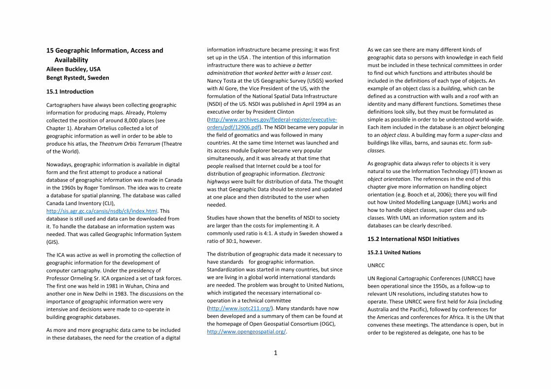
15 Geographic Information, Access and Availability Aileen Buckley, USA Bengt Rystedt, Sweden

15.1 Introduction

Cartographers have always been collecting geographic information for producing maps. Already, Ptolemy collected the position of around 8,000 places (see Chapter 1). Abraham Ortelius collected a lot of geographic information as well in order to be able to produce his atlas, the Theatrum Orbis Terrarum (Theatre of the World).

Nowadays, geographic information is available in digital form and the first attempt to produce a national database of geographic information was made in Canada in the 1960s by Roger Tomlinson. The idea was to create a database for spatial planning. The database was called Canada Land Inventory (CLI), http://sis.agr.gc.ca/cansis/nsdb/cli/index.html. This database is still used and data can be downloaded from it. To handle the database an information system was needed. That was called Geographic Information System (GIS).

The ICA was active as well in promoting the collection of geographic information for the development of computer cartography. Under the presidency of Professor Ormeling Sr. ICA organized a set of task forces. The first one was held in 1981 in Wuhan, China and another one in New Delhi in 1983. The discussions on the importance of geographic information were very intensive and decisions were made to co-operate in building geographic databases.

As more and more geographic data came to be included in these databases, the need for the creation of a digital

information infrastructure became pressing; it was first set up in the USA . The intention of this information infrastructure there was to achieve a better administration that worked better with a lesser cost. Nancy Tosta at the US Geographic Survey (USGS) worked with Al Gore, the Vice President of the US, with the formulation of the National Spatial Data Infrastructure (NSDI) of the US. NSDI was published in April 1994 as an executive order by President Clinton (http://www.archives.gov/f)ederal-register/executive-orders/pdf/12906.pdf). The NSDI became very popular in the field of geomatics and was followed in many countries. At the same time Internet was launched and its access module Explorer became very popular simultaneously, and it was already at that time that people realised that Internet could be a tool for distribution of geographic information. Electronic highways were built for distribution of data. The thought was that Geographic Data should be stored and updated at one place and then distributed to the user when needed.

Studies have shown that the benefits of NSDI to society are larger than the costs for implementing it. A commonly used ratio is 4:1. A study in Sweden showed a ratio of 30:1, however.

The distribution of geographic data made it necessary to have standards for geographic information. Standardization was started in many countries, but since we are living in a global world international standards are needed. The problem was brought to United Nations, which instigated the necessary international co-operation in a technical committee (http://www.isotc211.org/). Many standards have now been developed and a summary of them can be found at the homepage of Open Geospatial Consortium (OGC), http://www.opengeospatial.org/.

As we can see there are many different kinds of geographic data so persons with knowledge in each field must be included in these technical committees in order to find out which functions and attributes should be included in the definitions of each type of objects. An example of an object class is a building, which can be defined as a construction with walls and a roof with an identity and many different functions. Sometimes these definitions look silly, but they must be formulated as simple as possible in order to be understood world-wide. Each item included in the database is an object belonging to an object class. A building may form a super-class and buildings like villas, barns, and saunas etc. form sub-classes.

As geographic data always refer to objects it is very natural to use the Information Technology (IT) known as object orientation. The references in the end of this chapter give more information on handling object orientation (e.g. Booch et al, 2006); there you will find out how United Modelling Language (UML) works and how to handle object classes, super class and sub-classes. With UML an information system and its databases can be clearly described.

15.2 International NSDI Initiatives

15.2.1 United Nations

UNRCC

UN Regional Cartographic Conferences (UNRCC) have been operational since the 1950s, as a follow-up to relevant UN resolutions, including statutes how to operate. These UNRCC were first held for Asia (including Australia and the Pacific), followed by conferences for the Americas and conferences for Africa. It is the UN that convenes these meetings. The attendance is open, but in order to be registered as delegate, one has to be

1

nominated officially by one’s country. Decisions are taken by resolutions. At the UNRCC in Bangkok 2012 a resolution was taken in which ICA was asked to organise the International Map Year in 2015.

UN-GGIM

Figure 15.1.The first GGIM conference in Seoul, South Korea 2011.

In 2011 UN decided to set up Global Geospatial Information Management (GGIM, http://ggim.un.org/) with the focus to make geographic information more accessible to society at large. There is also an intention that UN-GGIM shall take over UNRCC, while simultaneously setting up such conferences for Europe. So far, all National Mapping Organisations in Europe have become members of EuroGeographics; its statutes now are being redrawn to fit the UN-GGIM conditions.

The homepage of GGIM provides rather detailed reports from almost all countries of the World on the situation of geographic information in their own country.

Global Map

In the 1950s the UN accepted a resolution to revive the project of the production of a world map at the scale of 1:1Million. The task was given to the International Geographic Union (IGU). This project petered out, however, in the 1980s, also for Cold War security reasons. To the UN Conference on Environment and Development in Rio de Janeiro in 1992 Japan proposed

to build up a database with a similar purpose. This has now been accepted as a UN activity and the task to build the database is handled by the International Steering Committee for Global Mapping (ISCGM), http://www.iscgm.org. The national dataset in all countries have been built up in the same way and can be downloaded for free. Building the database provides an educational experience for all countries, as they learn how to build geographic datasets. The management costs of the project are paid for by Japan. Of course, it would have been cheaper for Japan to build the whole dataset itself, but then the education benefits would have been lost.

Figure 15.2 shows the different layers of Global Map.

More information on UN activities in cartography and geographic information can be found in Chapter 10.

15.2.2 International Organisations Dealing with Geographic Information

Apart from the International Cartographic Association, the following international organisations are active in this field:

GSDI

Global Spatial Data Infrastructure (GSDI) is an organisation that is promoting the construction of NSDIs globally. Its homepage is handled by OGC (http://www.gsdi.org/) and this shows that GSDI has its main focus on the juridical aspects of building geographic datasets like copyright issues and the costs for downloading and use of geographic data. The homepage also includes links to literature like a Spatial Data Infrastructure Cookbook (GSDI, 2009), that that can be downloaded in different languages for free from the GSDI homepage. It gives detailed instructions on how to build geographic datasets.

Figure 15.3. The front page of the SDI Cookbook.

2

JBGIS

The Joint Board of Geographic Information Societies (JBGIS) is an organisation for co-operation between the international organisations that have an interest in geospatial matters. JBGIS may have ad-hoc committees, such as the committee for Disaster and Risk Management has together with the UN Office for Outer Space Affairs published a booklet that can be downloaded for free (JBGIS and UN, 2010). The different organisations cooperating in JBGIS are described in Chapter 18.

Figure 15.4. The JBGIS publication on Disaster and Risk Management.

Google

As is widely known, Google provides a lot of geographic information for free through its Google Maps and Google Earth. More information on the Google tools will not be given here. Our advice is just to use these tools for discovery.

East View Geospatial

East View Geospatial, EVG (http://www.geospatial.com/). EVG is previously known as East View Cartographic. It now provides not only maps but also geographical information, such as satellite imagery and aerial photos, as well as open source data, further described in Chapter 16. EVG provides a lot of maps and data on Russia and China (this explains the “East” in the name of the company). EVG is an affiliate member of ICA.

Open Street Map (OSM)

Open Street Map (http://www.openstreetmap.org) provides Volunteered Geographic Information (VGI) and is further described in Chapter 16. VGI started as a reaction to the high fees charged by National Mapping Organisations for downloading and using geographic data, especially maps. Often this opposition movement is called either Neo-cartography or Neo-geography; however, one should never call something ‘new’, since new will soon be old if the term is sustainable. VGI is also well described in a position paper for the UN-GGIM produced at the Ordnance Service of Great Britain (GGIM, 2012).

Data for OSM is collected by many persons and can be used for free, but you should follow the rules and refer to OSM whenever you use their data. OSM has now a broad coverage of the World and a mobile availability e.g. in telephones. Some cities are no longer producing city plans in printed versions, as they rely on OSM.

15.2.3 NSDI Initiatives

The main aim of NSDI is to build national geographic datasets and set up Geo-Portals for searching, viewing and downloading geographic data. Searching and viewing should be done without costs for the user, but

downloading and use may have to be paid for by the user. In the following sections, some examples of NSDI initiatives will be given.

USA

Since NSDI was first set up in the United States, it is natural to start here. The US NSDI is handled by the Federal Geographic Data Committee (https://www.fgdc.gov/) with its headquarters at USGS. By using the link Data & Services different kinds of geographic data can be searched for and sometimes also downloaded. Via the Geo-Platform portal it is also possible to download climate data and topographic maps from the US Geological Survey, and census data with street addresses from the US Census Bureau. The street addresses are linked to Census districts and these digital linkages have increased the use of census data tremendously. Through the street addresses it is possible to find both suppliers and users of company products. A lot more information can be found via the homepage.

Figure 15.5 shows the Webpage of the Federal Geographic Data Committee (FGDC).

3

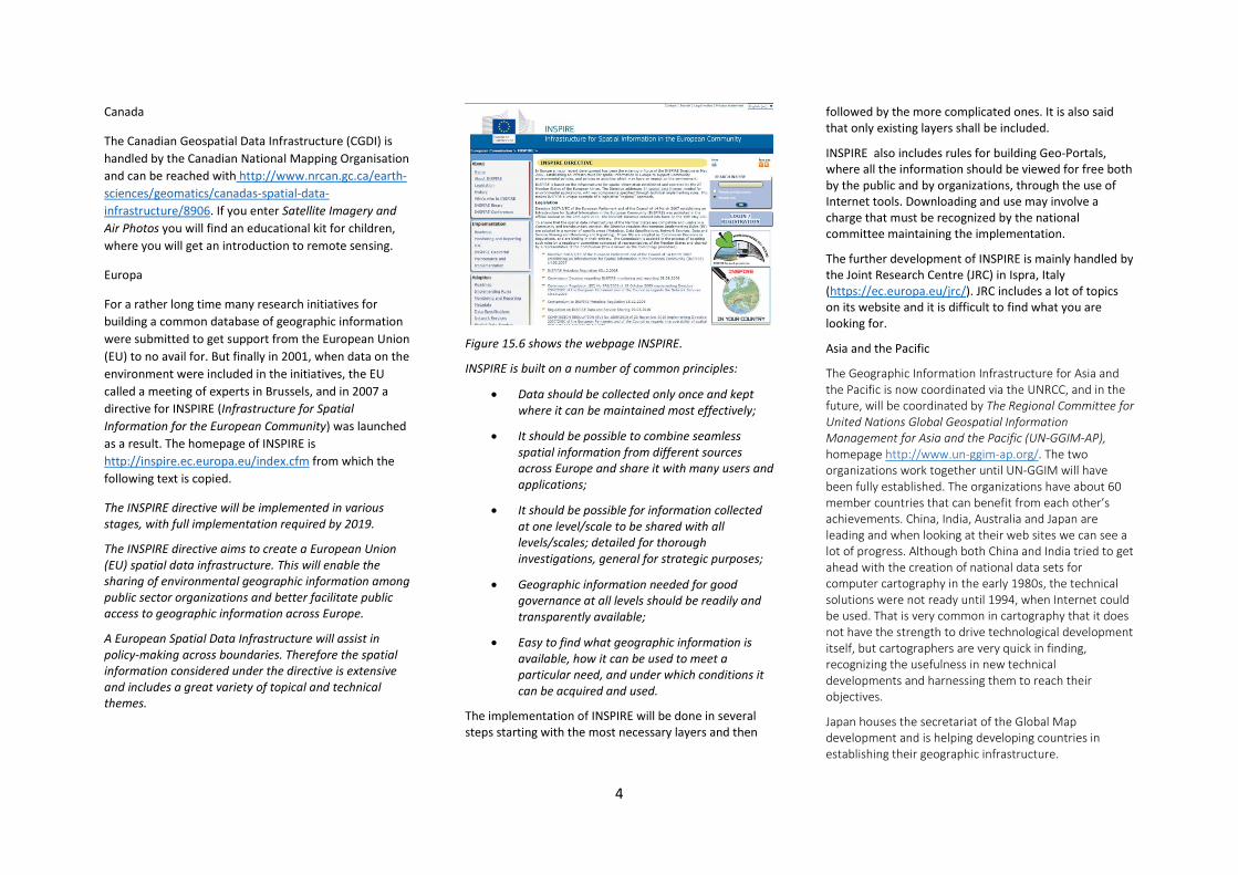
Canada

The Canadian Geospatial Data Infrastructure (CGDI) is handled by the Canadian National Mapping Organisation and can be reached with http://www.nrcan.gc.ca/earth-sciences/geomatics/canadas-spatial-data-infrastructure/8906. If you enter Satellite Imagery and Air Photos you will find an educational kit for children, where you will get an introduction to remote sensing.

Europa

For a rather long time many research initiatives for building a common database of geographic information were submitted to get support from the European Union (EU) to no avail for. But finally in 2001, when data on the environment were included in the initiatives, the EU called a meeting of experts in Brussels, and in 2007 a directive for INSPIRE (Infrastructure for Spatial Information for the European Community) was launched as a result. The homepage of INSPIRE is http://inspire.ec.europa.eu/index.cfm from which the following text is copied.

The INSPIRE directive will be implemented in various stages, with full implementation required by 2019.

The INSPIRE directive aims to create a European Union (EU) spatial data infrastructure. This will enable the sharing of environmental geographic information among public sector organizations and better facilitate public access to geographic information across Europe.

A European Spatial Data Infrastructure will assist in policy-making across boundaries. Therefore the spatial information considered under the directive is extensive and includes a great variety of topical and technical themes.

Figure 15.6 shows the webpage INSPIRE.

INSPIRE is built on a number of common principles:

• Data should be collected only once and kept where it can be maintained most effectively;

• It should be possible to combine seamless spatial information from different sources across Europe and share it with many users and applications;

• It should be possible for information collected at one level/scale to be shared with all levels/scales; detailed for thorough investigations, general for strategic purposes;

• Geographic information needed for good governance at all levels should be readily and transparently available;

• Easy to find what geographic information is available, how it can be used to meet a particular need, and under which conditions it can be acquired and used.

The implementation of INSPIRE will be done in several steps starting with the most necessary layers and then

followed by the more complicated ones. It is also said that only existing layers shall be included.

INSPIRE also includes rules for building Geo-Portals, where all the information should be viewed for free both by the public and by organizations, through the use of Internet tools. Downloading and use may involve a charge that must be recognized by the national committee maintaining the implementation.

The further development of INSPIRE is mainly handled by the Joint Research Centre (JRC) in Ispra, Italy (https://ec.europa.eu/jrc/). JRC includes a lot of topics on its website and it is difficult to find what you are looking for.

Asia and the Pacific

The Geographic Information Infrastructure for Asia and the Pacific is now coordinated via the UNRCC, and in the future, will be coordinated by The Regional Committee for United Nations Global Geospatial Information Management for Asia and the Pacific (UN-GGIM-AP), homepage http://www.un-ggim-ap.org/. The two organizations work together until UN-GGIM will have been fully established. The organizations have about 60 member countries that can benefit from each other’s achievements. China, India, Australia and Japan are leading and when looking at their web sites we can see a lot of progress. Although both China and India tried to get ahead with the creation of national data sets for computer cartography in the early 1980s, the technical solutions were not ready until 1994, when Internet could be used. That is very common in cartography that it does not have the strength to drive technological development itself, but cartographers are very quick in finding, recognizing the usefulness in new technical developments and harnessing them to reach their objectives.

Japan houses the secretariat of the Global Map development and is helping developing countries in establishing their geographic infrastructure.

4

Figure 15.7 shows the ANZLIC website.

Australia works together with New Zealand in the development of their geographic information infrastructure in a committee called the Australian New Zealand Land Information Council (ANZLIC). ‘Foundation spatial data’ describes the basic layers that are needed by users of location-based information. They are the original pieces of spatial information that are created by authoritative sources, like government agencies. Often, this information is collected for core business purposes by these agencies, and not made available in a consistent way, if at all. Governments in New Zealand and Australia have realised that this information needs to be more available. By establishing a common framework for how this information is collected, described and released across Australia and New Zealand, ANZLIC is setting a direction for both countries to aspire.

Africa

Africa has over 50 countries with very different geographic information resources. Since gaining

independence in the 1960s, the production of topographic maps was discontinued and it is now difficult to find updated topographic maps. Now you have to use Google Earth to find large scale maps.

Environmental information and geographic information are important in Africa. The coordination of that is handled by EIS-Africa - a pan-African membership organization working to improve use of geospatial and environmental information to enrich policy debate and support decision-making for the well-being of Africa’s people.

Under the item publications at the homepage of EIS you will find its newsletter and references to reports. The Study of Fundamental Geospatial Datasets in Africa provides a good overview of the situation. The report is a request for tender and will give answers on how to continue with building up a geographic information infrastructure in Africa.

NEPAD, a development organization of the UN Economic Commission for Africa (UNECA) has briefly reviewed the African situation at the beginning of the 21st century and found that: · Africa was the poorest region in the world with not less than half of its total population living on less than $1 per day; · Africa also accounted for only 1 per cent of the global gross domestic product (GDP), while the income distribution was highly skewed against the poor; · Africa was the most marginalized region accounting for only 1.7% of world trade, 2% of world export, and 0.9% of global foreign direct investment (FDI); · 1 out of 5 Africans lived under armed conflict, creating doubt about the region’s future; · African economies were fragmented, structurally shallow and heavily dependent on primary sector – petroleum, mining and agriculture – with little value added; · Africa was the most indebted and most aid dependent region, and

· Africa had the largest population infested with HIV – AIDS. In spite of the above deplorable situation, it is not in doubt that Africa is a well-endowed region. In order to support its sustainable development, Africa needs a geographic information infrastructure, but that is not mentioned in the report from NEPAD.

Figure 15.8 shows a Road Map example. 15.3 Road Data

Road data has always been important. When road databases were first created by national road organizations, they were built for supporting the management of the roads. The network was not often closed so the databases could not be used for calculation of shortest or fasted routes between two places. Later on, companies were set up to build the road databases such as Tomtom and Navtech. For collecting road information, specific cars with measuring instruments and videos are driving over all the roads. The road data are then edited and inserted in the database. After that, street addresses are added as well as petrol stations, restaurants and tourist attractions. With such a system in the car it is easy to find the way. If you have a license to

5

the system you can use the data in the system, but not view and download it. Street addresses are frequently updated and the systems have contacts with many organizations and can report on road work, accidents and other impediments on the road you are driving,

Nokia, a Finnish telecom company, has bought Navtech and implemented its database for free in its mobile phones.

15.4 Statistical Geographic Information

Statistical data are very important for atlas production and for planning purposes. When statistical data are geo-referenced it also constitutes geographic information. Geo-referencing means that data are connected to a geographic location e.g. an administrative area, of which the borders have been digitized. With statistical data geo-referenced to administrative areas we can produce thematic maps that can be included in atlases or be available for decision support in spatial planning.

It is also rather common that street addresses have coordinates of the entrance of each building that is linked to a property that in its turn is linked to an administrative area. Geo-referenced statistical data, both from the census and from administration systems are available in enormous quantities.

Useful statistical data can be accessed from statistical offices and from organizations such as:

• The UN; • The World Bank and • The EU.

All these organizations have large amounts of statistical data related to administrative areas.

Search at http://data.un.org/ for UN data.

Search at http://data.worldbank.org/data-catalog/world-development-indicators for World Bank data.

Search at https://open-data.europa.eu/en/data for European data.

The Global Map also include administrative areas with digital borders. It should be possible to use the Global Map for creation of a world digital population map.15.5 Geo-portals

Geo-portals are built for the exchange of geographic information such as for searching, downloading and use. A geo-portal is built on Internet in a Service Oriented Architecture (SOA). In SOA a service is a specialised process in a computer that is prepared for taking orders from other processes and deliver back the required results. Services can also be linked to other services. In that way more complex services can be built for more demanding tasks.

A geo-portal also has a set of metadata that describes the different object classes. Metadata give data about data and are described in Chapter 3 of the Spatial Data Infrastructure Cookbook (GSDI, 2009).

A geo-portal user must have access to Internet and the geo-portal services that via Internet have access to the organization where the required data are located can be found by using metadata.

Figure 15.9 shows a topographic map achieved with using the Swedish Geo-portal www.geodata.se.

Figure 15.9 shows the topographic map showed in Figure 5.1 achieved by using the Swedish Geo-portal www.geodata.se. The green lines indicate borders for nature reserves. © Lantmäteriet Dnr R50160927_130001.

A geo-portal can also include more advanced services, where the user can order up-dates of data or other services such as transformation between different coordinate systems or handling of licenses or payment systems.

6

References

Booch, G., Rumbaugh, J. and Jacobson, I., 2006 The Unified Modelling Language User Guide, 2nd edition. Reading, MA: Addison Wesley. ISBN 9780321267979.

GGIM, 2012 Future Trends in Geospatial Information Management., Report from the Expert Committee on Global Geospatial Information Management, GGIM Second Session, New York, 2012.http://ggim.un.org/2nd%20Session/Future%20Trends%20Background%20Document.pdf.

GSDI (2009) Spatial Data Infrastructure Cookbook. http://www.gsdi.org/gsdicookbookindex.

JBGIS and UN (2010) Geoinformation for Disaster and Risk Management. http://www.un-spider.org/sites/default/files/VALIDPublication.pdf

7

16 Volunteered Geographic Information

Serena Coetzee, South Africa

16.1 Introduction

In its early days the World Wide Web contained static read-only information. It soon evolved into an interactive platform, known as Web.2.0, where content is added and updated all the time. Blogging, wikis, video sharing and social media are examples of Web.2.0. This type of content is referred to as user-generated content.

Volunteered geographic information (VGI) is a special kind of user-generated content. It refers to geographic information collected and shared voluntarily by the general public. Web.2.0 and associated advances in web mapping technologies have greatly enhanced the abilities to collect, share and interact with geographic information online, leading to VGI.

Crowdsourcing is the method of accomplishing a task, such as problem solving or the collection of information, by an open call for contributions. Instead of appointing a person or company to collect information, contributions from individuals are integrated in order to accomplish the task. Contributions are typically made online through an interactive website.

In the subsequent sub-sections, examples of crowdsourcing and volunteered geographic information are described, namely OpenStreetMap, Tracks4Africa, the Southern African Bird Atlas Project.2 and Wikimapia. In the additional sub-sections a step-by-step guide to contributing to OpenStreetMap is provided.

16.2 OpenStreetMap

OpenStreetMap (www.openstreetmap.org) is a collaborative project to create a free editable map of the world. Two major driving forces behind the

Figure 16.1 The OpenStreetMap map page.

establishment and growth of OpenStreetMap have been restrictions on the use or availability of geospatial information across much of the world and the advent of inexpensive portable satellite navigation devices.

Created by Steve Coast in the UK in 2004, it was inspired by the success of Wikipedia and preponderance of proprietary map data in the UK and elsewhere. Since then, OpenStreetMap has grown to over one million registered users who can contribute data using GPS

devices, aerial photography, and other free sources. This crowdsourced data is then made available under the Open Database License. The site is supported by the OpenStreetMap Foundation, a non-profit organization registered in England.

Rather than the map itself, the data generated by the OpenStreetMap project is considered its primary output. This data is available for use in both traditional applications, such as Craigslist, Geocaching, MapQuest

1

Open, JMP statistical software, and Foursquare to replace Google Maps, and more unusual roles such as replacing default data included with GPS receivers. The OpenStreetMap data has been favourably compared with proprietary data sources, though data quality varies worldwide [Source: Wikipedia].

16.3 Tracks4Africa Tracks4Africa (www.tracks4africa.org) started out as a hobby where like-minded people shared their GPS tracks and waypoints with each other in 2000. In the absence of any useful maps for GPS navigation in Africa, this hobby grew into a community of people sharing their travel

Figure 16.2 The Tracks4Africa map page.

experiences with one another. Tracks4Africa, the company, was established in 2003 to act as the custodian of this vault of community data. Tracks4Africa also started to build a very unique map of Africa using community contributed GPS data exclusively. This map forms the basis of T4A GPS Maps and all their other products. In the year 2005 Tracks4Africa started to sell T4A GPS Maps to people outside the Tracks4Africa community of travellers who contribute to the data. The company aims to strike a balance between crowdsourced data, community driven development of their products and a sustainable commercial model [Source: Tracks4Africa website].

16.4 The Southern African Bird Atlas Project 2

The Southern African Bird Atlas Project 2 (SABAP2) (sabap2.adu.org.za) is the follow-up on the first Southern African Bird Atlas Project (SABAP). The first atlas project took place from 1987–1991. The current project is a joint venture between the Animal Demography Unit at the University of Cape Town in South Africa, Bird Life South Africa and the South African National Biodiversity Institute (SANBI). The project aims to map the distribution and relative abundance of birds in southern Africa. The second atlas project started on 1 July, 2007 and plans to run indefinitely.

The fieldwork for this project is done by more than a thousand volunteers, known as citizen scientists—they collect the data from the field at their own cost and in their own time and as such they make a huge contribution to the conservation of birds and their habitat. The unit of data collection is the pentad, five minutes of latitude by five minutes of longitude, squares with sides of roughly 9 km. There are 17,000 pentads in the original atlas area of South Africa, Lesotho and Swaziland, and a further 10,000 in Namibia [Source: Wikipedia].

16.5 Wikimapia

Wikimapia (www.wikimapia.org) is an open-content collaborative mapping project that aims to mark and describe all geographical objects in the world. It combines an interactive web map with a geographically referenced wiki system. As of early 2013, the project's website claimed that registered users and guests have already marked over 20,000,000 objects.

2

Figure 16.3 Progress map of the Southern African Bird Atlas Project.

The Wikimapia website provides a Google Maps, API-based, interactive web map that consists of a user-generated information layer on top of Google Maps satellite imagery and other resources.

The Wikimapia layer is a collection of 'objects' with polygonal features (such as outlines of buildings, lakes, etc.) and 'linear features' (such as streets, railroads, rivers, etc.). Both kinds of items may have textual descriptions and photos attached to them. Viewers can click on any marked object or street segment to see its description. Facilities are provided to highlight objects by category and to measure distances between objects.

Figure 16.4 The Wikimapia map page.

Anyone can add a new item to the Wikimapia layer. Objects and linear features are supposed to be drawn onto the main window so as to match the satellite photo underneath, using a simple graphical editing tool. When an object is created the user is invited to specify its categories, add a textual description, and upload relevant photos. Only registered users can edit existing items. Editors can set up a 'watchlist' to monitor all changes that are made in one or more rectangular areas on the map.

The editor community is largely self-organized, with users communicating through an internal e-mail-like system and through a public forum. The system automatically assigns 'experience points' to editors for various editing actions, and ranks them in levels according to points earned. Higher levels have increased access to editing tools and fewer restrictions on editing activity.

Editors at the top levels may be invited to become "moderators" or "power users." As such, they receive additional editing rights, access to more map-monitoring facilities, and authority to ban users. Those power users do most of the work of managing other editors, including establishing rules and fighting vandalism [Source: Wikipedia].

16.6 Familiarizing yourself with OpenStreetMap

The tasks described in this section will assist you in familiarizing yourself in OpenStreetMap (i.e., how to search for places, how to move around on the map window and how to share maps from OpenStreetMap with friends).

3

Figure 16.5. Searching for the University of Pretoria (Task 1).

Task 1: Go to the OpenStreetMap page at www.openstreetmap.org and search for the 'University of Pretoria.' Click on the relevant item in Search Results sidebar to position the map around the university. Close the 'Search Results' sidebar when you are done.

The map is navigable with a mouse like any other online map. One can pan or drag the map to a desired location, zoom in and out as required, etc.

Task 2: Close the Search Results window by pressing the X in the top right corner. Zoom the map (use the + and - on the right menu) until the scale bar (in the left bottom corner) displays 50m.

Figure 16.6. Zooming until the scale bar is 50m (Task 2).

4

Task 3: Pan the map to the West (click and hold down the mouse, dragging it right) until the Loftus Versfeld Stadium appears on the left-hand side of the map.

Figure 16.7. Panning to the Loftus Versfeld Stadium (Task 3).

There are different ways to view the OpenStreetMap data on the main map page, depending on one's personal preference or purpose (e.g., hiking, cycling, or tourism). The OpenStreetMap page offers a few alternatives, including a cycling and transport map. Other websites display the OpenStreetMap data for their own specific purpose. Examples include the OpenPisteMap (www.openpistemap.org) showing ski pistes and lifts and a Geocaching Map (www.geocaching.com) showing locations of geocaches.

Task 4: Click on the Layers icon ( ) to open the Map Layers sidebar and use the radio buttons to view the different map styles.

Figure 16.8. Viewing the OpenStreetMap data as a transport map (Task 4).

5

Maps can be shared with friends and colleagues, for example, to communicate the location of a business meeting or birthday party.

Task 5: Click on the Share icon ( ) to open the Share sidebar. Copy the hyperlink in the textbox below 'Link | Short Link | HTML', create a new tab in your browser, paste the text and press Enter. This displays exactly the same map as you had on the first tab. If you check 'Include marker,' a red marker is displayed on the map.

Figure 16.9. The URL for this page was copied and pasted from the Share sidebar. Note the red marker (Task 5).

You will notice that the URL is quite long. Click on 'Short Link' to get a shorter URL that redirects to the same longer URL.You can share this map with friends or clients by sending them either the full or the shortened hyperlink in an e-mail.

Maps can also be embedded into the HTML pages of a website, for example, to show the location of a school or the venue for a sports event (See also Figure 16.11.).

Task 6: Click on the Share icon ( ) to open the Share sidebar and then click on 'HTML.'. Copy the HTML snippet in the textbox to the clipboard (e.g., with Ctrl-C). Use any text editor to create an HTML file and paste the text from the clipboard into the HTML file (e.g., with Ctrl-V). Enclose the text with <html> and <body> tags. See Figure 16.10. Open the HTML file in a browser (e.g., by using File > Open). Alternatively, you can double-click on the HTML file to display it in a browser. See Figure 16.11.

<html><body> This page includes the HTML snippet.<br/> You can zoom and pan the map on this page.<br/> Click on 'Viewing Larger Map' to go to the main OpenStreetMap page. <br/> <iframe width="425" height="350" frameborder="0" scrolling="no" marginheight="0" marginwidth="0" src="http://www.openstreetmap.org/export/embed.html?bbox=28.222439289093018%2C-25.760590307319447%2C28.239691257476807%2C-25.747583759633553&amp; layer=mapnik&amp;marker=-25.7540872115283%2C28.231065273284912" style="border: 1px solid black"> </iframe> <br/> <small><a href=" http://www.openstreetmap.org/?mlat=-25.7541&amp;mlon=28.2311#map=16/-25.7541/28.2311">View Larger Map</a> </small> </body></html>

Figure 16.10. A basic HTML page with an embedded map from OpenStreetMap (Task 6).

6

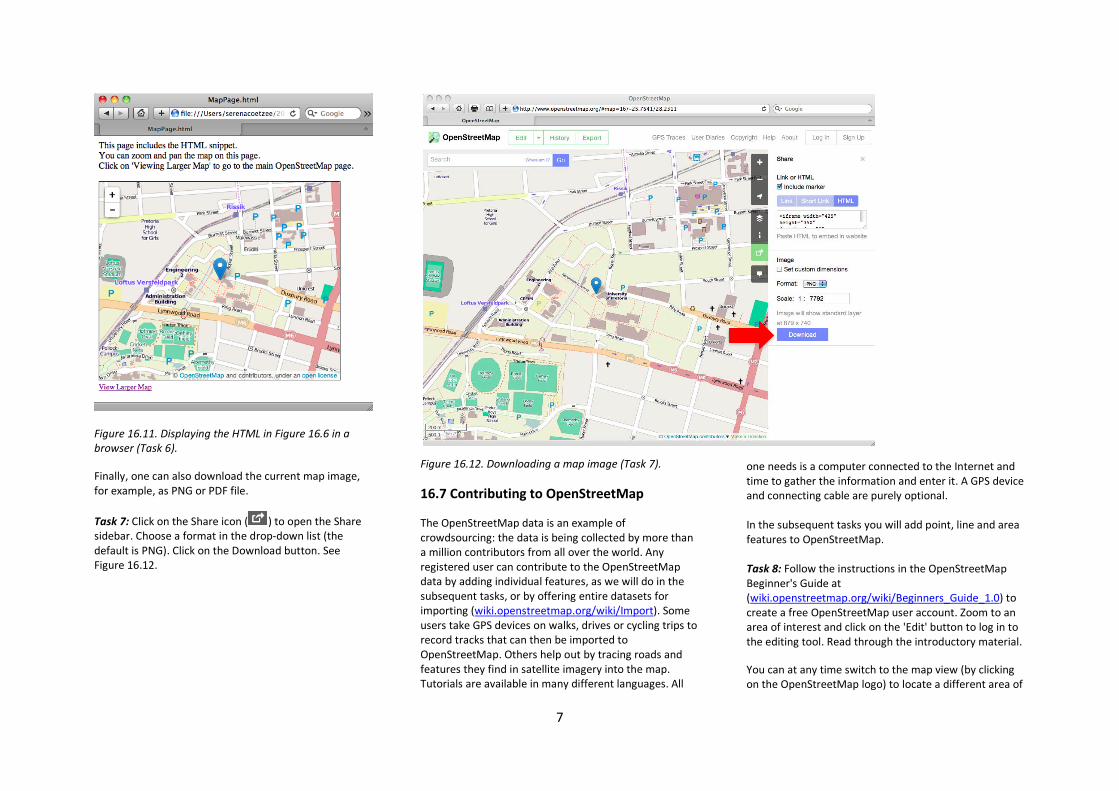
Figure 16.11. Displaying the HTML in Figure 16.6 in a browser (Task 6).

Finally, one can also download the current map image, for example, as PNG or PDF file.

Task 7: Click on the Share icon ( ) to open the Share sidebar. Choose a format in the drop-down list (the default is PNG). Click on the Download button. See Figure 16.12.

Figure 16.12. Downloading a map image (Task 7).

16.7 Contributing to OpenStreetMap

The OpenStreetMap data is an example of crowdsourcing: the data is being collected by more than a million contributors from all over the world. Any registered user can contribute to the OpenStreetMap data by adding individual features, as we will do in the subsequent tasks, or by offering entire datasets for importing (wiki.openstreetmap.org/wiki/Import). Some users take GPS devices on walks, drives or cycling trips to record tracks that can then be imported to OpenStreetMap. Others help out by tracing roads and features they find in satellite imagery into the map. Tutorials are available in many different languages. All

one needs is a computer connected to the Internet and time to gather the information and enter it. A GPS device and connecting cable are purely optional. In the subsequent tasks you will add point, line and area features to OpenStreetMap. Task 8: Follow the instructions in the OpenStreetMap Beginner's Guide at (wiki.openstreetmap.org/wiki/Beginners_Guide_1.0) to create a free OpenStreetMap user account. Zoom to an area of interest and click on the 'Edit' button to log in to the editing tool. Read through the introductory material.

You can at any time switch to the map view (by clicking on the OpenStreetMap logo) to locate a different area of

7

interest on the map. Once you click on the 'Edit' button, the editing map is updated to the current map view.

Figure 16.13. The default OpenStreetMap editing tool (Task 8).

You will now start adding data. First a point of interest, then the outline of a building and finally a footpath.

Task 9: Locate an area you are familiar with and where a point of interest can be added. Click on the 'Edit' button

and click on 'Point' ( ) in the top menu. Click on the map where the point of interest should be added. Select the feature type (see Figure 16.14) and subsequently add the attribute information for the point

of interest (see Figure 16.15). Clicking on the 'i' ( ) next to the attribute name provides a description of the attribute, if available. Additional attributes are available when clicking on the row of icons at the bottom.

Figure 16.14. Indicating the location and selecting the feature type for a point of interest (Task 9).

8

Tags are used to describe a point of interest (or other feature). You can add or remove tags to describe the point of interest you are adding. For example, tags for a restaurant could be amenity, name and cuisine. By default, the values of these tags are set to the values of the attributes.

Figure 16.15. Filling in the attributes for a point of interest (Task 9).

Click 'Save' in the top menu to save the point of interest to OpenStreetMap. You have the opportunity to add a comment before confirming the point of interest by clicking the second 'Save' button. If you now switch to the map view, the point of interest is displayed in OpenStreetMap (see Figure 16.16). You may have to wait a few seconds for the updates to become visible (keep on refreshing the browser window until they are visible).

Figure 16.16. The new point of interest on OpenStreetMap (Task 9).

Click on the History button. A list of changesets is displayed. Click on th e first item in the list. This displays the details of the change to OpenStreetMap (see Figure 16.17).

9

Figure 16.17. The changeset details on the History tab for the new point of interest (Task 9).

Task 10: Familiarize yourself with the OpenStreetMap editing tool by adding additional points of interest, by moving existing points of interest around and by modifying the attributes of an existing point of interest.

Figure 16.18. Adding an area feature (Task 11).

Task 11: On the map view, locate an area you are familiar with. Click on the 'Edit' button and click on 'Area' in the top menu. Indicate the boundary of the area you want to add on the map and press Escape when you are done. Follow the same procedure as Task 8 to specify the feature type and to fill in the attributes.

10

Figure 16.19. Adding a line feature (Task 12).

Task 12: On the map view, locate an area you are familiar with and where a line feature (e.g., a street or footpath) can be added. Click on the 'Edit' button and click on 'Line' in the top menu. Indicate the line feature on the map and press Escape when you are done. Follow the same procedure as Task 8 to specify the feature type and to fill in the attributes.

16.8 Conclusion

VGI and crowdsourcing are becoming an important source of geographic information, particularly for information that is difficult to collect from other sources. However, one should keep in mind that VGI contributions are not necessarily verified and quality checked in the same way as traditional mapping sources.

I would like to encourage you to contribute to OpenStreetMap in the areas where you live!

References

Longley, P.A., M.F. Goodchild, D.J. Maguire, and D.W. Rhind, Geographic Information Systems and Science, Wiley: 2011.

OpenStreetMap, Beginner's Guide to OpenStreetMap, http://wiki.openstreetmap.org/wiki/Beginners_guide.

OpenStreetMap, www.openstreetmap.org.

Southern African Bird Atlas Project 2, sabap2.adu.org.za.

Tracks4Africa, www.tracks4africa.org.

Wikimapia, www.wikimapia.org.

Wikipedia, www.wikipedia.org.

11

Chapter 17 Education in cartography

David Fairbairn, UK

This book which you are reading shows that the world of maps and mapping is an exciting and important place, where a wide range of activities is undertaken to effectively collect, archive and present information about the world in the form of maps. So, how can you learn more about cartography, how can you become a trained cartographer, and what are the possible ways of making cartography your chosen career?

History of education and training in cartography

The United Nations definition of cartography gives some suggestion of the large number of different, but connected, procedures and tasks which are involved in the effective handling of data about the earth and the processes which happen on it (including human activities): “Cartography is considered as the science of preparing all types of maps and charts, and includes every operation from original surveys to final printing of copies.” This definition implies a ‘flowline’ of tasks, from initial surveying and measurement through a range of scientific procedures to the final production of a paper map. These procedures can include manipulation of the measurements, enhancement using other data collection methods such as aerial photography, and drafting the data in graphical form. There is potentially a lot to learn in order to master the flowline and understand what needs to be done to effectively and scientifically prepare the maps which present the data. Education and training in cartography up to very recently did focus on this flowline and taught people at every stage and every level of responsibility about their specific tasks involved.

Whether you were a manager or an apprentice your role was defined by your place in the flowline, and you were taught what was needed to occupy that place.

Therefore, it was possible to be educated in

• techniques of land surveying – how to observe measurements in the field and adjust them to ensure they are as accurate as possible;

• methods of obtaining information from aerial photographs – often using photogrammetry and complex mathematics to geometrically match the photographs to known points on the earth and extract further detail;

• compiling, editing and drafting data for the construction of a map document – using judgement in design and developing content and skill in creating a fair drawing;

• in reproducing the map – which could involve a number of professions such as photography and printing, each of which require significant training to master;

• understanding the economics and marketing of map production;

• the different skills of map reading and using the maps for a number of human activities.

You can see that there was potentially an enormous breadth of education needed to understand the whole flowline. It was no surprise that those interested in cartography specialised only in part of the subject: for example, a national mapping organisation or government map production agency would employ individual surveyors, photogrammetrists, cartographic editors, thematic geographers, photographers, printers, sales representatives, and educational advisers, all

calling themselves cartographers but educated and trained in only a small part of the overall subject. The education and training could be acquired from study in the classroom, or by on-the-job training. The latter predominated as the technologies involved in the flowline were best understood and learned by actually doing and practicing the various tasks: such as survey measurement, plotting from aerial photographs, drafting the original map, or printing the copies. The cartographic profession was hierarchical, with academically trained managers and supervisors, who knew enough about their part of the flowline and how the procedures fitted together, working alongside apprentices who were trained to be skilful in some specific aspects of the cartographic work.

Contemporary cartography and educational possibilities

As cartography has developed so much recently, the flowline described above has changed beyond recognition. No longer is map-making a linear process, and it can now involve an even wider range of procedures and methods to assist in the efficient handling of ‘geo-information’ (information about the earth). And as the range of activities has expanded, so have the ways of learning about them. Where and how you learn about cartography is not limited to the school or college lecture room, or by observing experienced cartographers on-the-job. Today, there is even more to learn, and many different ways of learning it.

How is education and training in cartography reacting to the changing nature of the subject? Perhaps the first point to make is that, for experienced educators and practitioners in cartography, there are still many

1

fundamental concepts and ideas which must be learned. These principles apply whether you are interested in the practical tasks of producing maps, or in thinking about how maps work, or in finding ways of using maps on new devices (such as smartphones). Such basic aspects and issues need to be instilled in apprentice cartographers as they develop knowledge and skills through education and training. For example, it is essential that cartographers

• possess attention to detail; • understand the transformations inherent in the

mapping process; • have a comprehensive view of the world and

the complex processes which occur in it; • are knowledgeable about the datasets which

are sourced from the world to reflect that complexity and the geo-information used to represent it;

• understand the possibilities and limitations of using such datasets for scaling, visualising, archiving, analysis and decision making;

• ensure communication of information through a unique medium (the map);

• show an ability to manipulate and process data whilst retaining accuracy;

• create effective information communication within an aesthetic and well-designed framework.

All these aspects are highlighted in the definition of cartography which is presented by the International Cartographic Association (ICA), the world authoritative body for Cartography and Geographic Information Science: “Cartography is the discipline dealing with the art, science and technology of making and using maps.”

This statement concentrates on the map as the defining element of the job of the cartographer, and it is now acknowledged by most cartographers that some of the other disciplines implied in the United Nations definition of cartography – land surveying, photogrammetry, satellite remote sensing – do not have the map as a core component of their activity, so they are not considered further. However, although the ICA definition of cartography might appear to be now more restricted, in fact it has widened further as it has now embraced the developing topic of geographic information science. The ICA has a definition which enhances its definition of cartography: “Geographic Information Science (GI Science) refers to the scientific context of spatial information processing and management, including associated technology as well as commercial, social and environmental implications. Information processing and management include data analysis and transformations, data management and information visualisation.” Properly educated cartographers need to have learned about the concepts indicated in this definition also.

What should we learn?

There are fundamental topics under the heading of art, science and technology of making and using maps, and there are fundamental principles which are guided by training in GI Science. How, therefore, does contemporary cartographic education address the many objectives which follow from these definitions: objectives such as encouraging innovative flexibility, using the scientific method, developing creativity, and strengthening the basic principles? Educators in cartography are no different to any other cartographers – so along with the fundamentals, modern developments have been embraced with enthusiasm and, as a result,

cartographic education has been re-assessed and changed significantly in recent years.

Cartographic education today can be guided by formal programmes such as the creation of a ‘Body of Knowledge’ relevant to geo-spatial science. This ‘Body of Knowledge’ helps to shape a dynamic syllabus for those studying and those teaching cartography. An initial American attempt to develop a ‘Body of Knowledge’ for geographical science as a whole recognized cartography’s special role by defining a broad knowledge area called ‘Cartography & visualisation’. This knowledge area included the themes ‘History & trends’, ‘Data considerations’, ‘Graphic representation techniques’, ‘Map production’, and ‘Map use & evaluation’, and each theme was further divided into a number of topics. This whole ‘Body of Knowledge’ project has shown that cartography is intimately connected to all other geographical sciences. It also helps teachers by presenting definite learning outcomes and educational objectives which can be assessed; it highlights the large amount of current research in cartography now being undertaken and links it to the taught programmes; and it ensures that the role of the human being is promoted, showing that cartography is not just a series of checkboxes on a technological flowline. The latest additions to the ‘Body of Knowledge’ proposed by ICA have stressed five core areas which have been identified as the subjects which cartographers should be learning about today:

• Data acquisition and Sensor networks (Section 3, Section 8 in this book);

• Internet cartography, Web Mapping and Social Networks (Section 11 in this book);

2

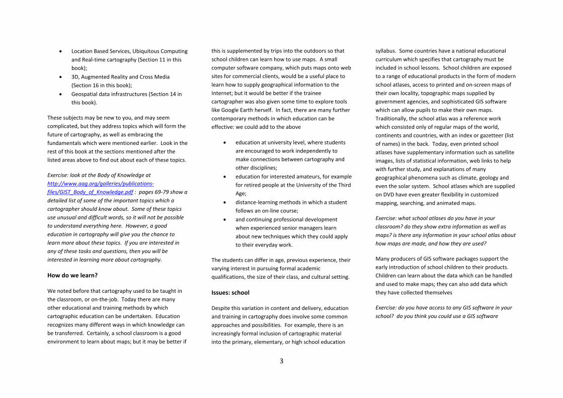
• Location Based Services, Ubiquitous Computing and Real-time cartography (Section 11 in this book);

• 3D, Augmented Reality and Cross Media (Section 16 in this book);

• Geospatial data infrastructures (Section 14 in this book).

These subjects may be new to you, and may seem complicated, but they address topics which will form the future of cartography, as well as embracing the fundamentals which were mentioned earlier. Look in the rest of this book at the sections mentioned after the listed areas above to find out about each of these topics.

Exercise: look at the Body of Knowledge at http://www.aag.org/galleries/publications-files/GIST_Body_of_Knowledge.pdf : pages 69-79 show a detailed list of some of the important topics which a cartographer should know about. Some of these topics use unusual and difficult words, so it will not be possible to understand everything here. However, a good education in cartography will give you the chance to learn more about these topics. If you are interested in any of these tasks and questions, then you will be interested in learning more about cartography.

How do we learn?

We noted before that cartography used to be taught in the classroom, or on-the-job. Today there are many other educational and training methods by which cartographic education can be undertaken. Education recognizes many different ways in which knowledge can be transferred. Certainly, a school classroom is a good environment to learn about maps; but it may be better if

this is supplemented by trips into the outdoors so that school children can learn how to use maps. A small computer software company, which puts maps onto web sites for commercial clients, would be a useful place to learn how to supply geographical information to the Internet; but it would be better if the trainee cartographer was also given some time to explore tools like Google Earth herself. In fact, there are many further contemporary methods in which education can be effective: we could add to the above

• education at university level, where students are encouraged to work independently to make connections between cartography and other disciplines;

• education for interested amateurs, for example for retired people at the University of the Third Age;

• distance-learning methods in which a student follows an on-line course;

• and continuing professional development when experienced senior managers learn about new techniques which they could apply to their everyday work.

The students can differ in age, previous experience, their varying interest in pursuing formal academic qualifications, the size of their class, and cultural setting.

Issues: school

Despite this variation in content and delivery, education and training in cartography does involve some common approaches and possibilities. For example, there is an increasingly formal inclusion of cartographic material into the primary, elementary, or high school education

syllabus. Some countries have a national educational curriculum which specifies that cartography must be included in school lessons. School children are exposed to a range of educational products in the form of modern school atlases, access to printed and on-screen maps of their own locality, topographic maps supplied by government agencies, and sophisticated GIS software which can allow pupils to make their own maps. Traditionally, the school atlas was a reference work which consisted only of regular maps of the world, continents and countries, with an index or gazetteer (list of names) in the back. Today, even printed school atlases have supplementary information such as satellite images, lists of statistical information, web links to help with further study, and explanations of many geographical phenomena such as climate, geology and even the solar system. School atlases which are supplied on DVD have even greater flexibility in customized mapping, searching, and animated maps.

Exercise: what school atlases do you have in your classroom? do they show extra information as well as maps? is there any information in your school atlas about how maps are made, and how they are used?

Many producers of GIS software packages support the early introduction of school children to their products. Children can learn about the data which can be handled and used to make maps; they can also add data which they have collected themselves

Exercise: do you have access to any GIS software in your school? do you think you could use a GIS software

3

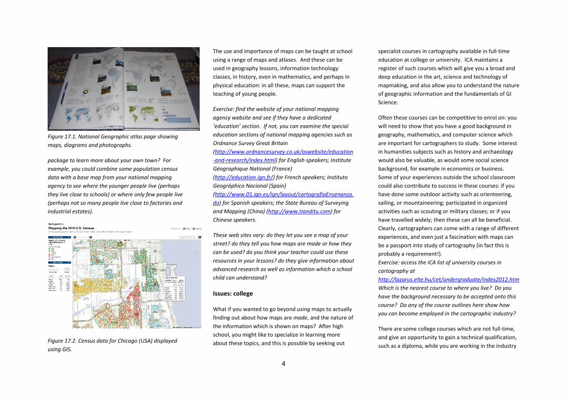
Figure 17.1. National Geographic atlas page showing maps, diagrams and photographs.

package to learn more about your own town? For example, you could combine some population census data with a base map from your national mapping agency to see where the younger people live (perhaps they live close to schools) or where only few people live (perhaps not so many people live close to factories and industrial estates).

Figure 17.2. Census data for Chicago (USA) displayed using GIS.

The use and importance of maps can be taught at school using a range of maps and atlases. And these can be used in geography lessons, information technology classes, in history, even in mathematics, and perhaps in physical education: in all these, maps can support the teaching of young people.

Exercise: find the website of your national mapping agency website and see if they have a dedicated ‘education’ section. If not, you can examine the special education sections of national mapping agencies such as Ordnance Survey Great Britain (http://www.ordnancesurvey.co.uk/oswebsite/education-and-research/index.html) for English speakers; Institute Géographique National (France) (http://education.ign.fr/) for French speakers; Instituto Geográphico Nacional (Spain) (http://www.01.ign.es/ign/layout/cartografiaEnsenanza.do) for Spanish speakers; the State Bureau of Surveying and Mapping (China) (http://www.tianditu.com) for Chinese speakers.

These web sites vary: do they let you see a map of your street? do they tell you how maps are made or how they can be used? do you think your teacher could use these resources in your lessons? do they give information about advanced research as well as information which a school child can understand?

Issues: college

What if you wanted to go beyond using maps to actually finding out about how maps are made, and the nature of the information which is shown on maps? After high school, you might like to specialize in learning more about these topics, and this is possible by seeking out

specialist courses in cartography available in full-time education at college or university. ICA maintains a register of such courses which will give you a broad and deep education in the art, science and technology of mapmaking, and also allow you to understand the nature of geographic information and the fundamentals of GI Science.

Often these courses can be competitive to enrol on: you will need to show that you have a good background in geography, mathematics, and computer science which are important for cartographers to study. Some interest in humanities subjects such as history and archaeology would also be valuable, as would some social science background, for example in economics or business. Some of your experiences outside the school classroom could also contribute to success in these courses: if you have done some outdoor activity such as orienteering, sailing, or mountaineering; participated in organized activities such as scouting or military classes; or if you have travelled widely; then these can all be beneficial. Clearly, cartographers can come with a range of different experiences, and even just a fascination with maps can be a passport into study of cartography (in fact this is probably a requirement!). Exercise: access the ICA list of university courses in cartography at http://lazarus.elte.hu/cet/undergraduate/index2012.htmWhich is the nearest course to where you live? Do you have the background necessary to be accepted onto this course? Do any of the course outlines here show how you can become employed in the cartographic industry?

There are some college courses which are not full-time, and give an opportunity to gain a technical qualification, such as a diploma, while you are working in the industry

4

and given one day off per week to study. Such courses used to be quite numerous, but there are not so many available today, because most cartographic companies or organizations would prefer to teach you about their procedures and methods in-house. Such in-house, on-the-job training has been used for centuries to teach apprentices (for example in printing, or in draftsmanship). It is now a good model for those cartographic companies (the majority) which concentrate on using web technologies and which rely on enthusiastic individuals to help their work, rather than employing large numbers of people doing mechanical and routine work. Whatever the organization, the need for a well-trained workforce is regarded as paramount, and with procedures and possibilities in the revised cartographic flowline changing constantly, it is essential that a well-educated workforce can receive updates in the workplace itself.

Issues: individual learning

A further alternative way of learning about new technologies, which are so central to all contemporary cartographic activity, is for you to follow an informal route of learning yourself. There are numerous opportunities to investigate and master novel web-based tools and systems which could be of benefit to cartography. Perhaps the most valuable new tool for cartography for the next decade is being developed as an ‘app’ at the moment, and you could be the first to demonstrate its value for mapmaking. The age of the individual cartographer is already with us: instead of working for a large traditional mapping agency, there are many cartographers who are self-employed and learning about the subject every day. Such cartographers explore flexible and innovative ways of using map data, creating

exciting graphical maps, serving cartography over the web, and linking maps to an almost infinite range of applications.

As formal courses become more expensive to enrol in, as government investment in higher education is pegged-back, and as more people prefer continuing education rather than the sacrifice of full-time study, informal education including this individualistic approach is becoming more popular.

But formal qualifications are still valuable, as they show that the student has learned about the fundamental concepts. Dedicated, and sometimes open, workshops can be presented in many different ways around the world, and these may offer a certificate of attendance, showing that the student has been exposed to some aspect of cartographic education and training. Such workshops can be and are being offered by learned societies (such as ICA), by pan-governmental outreach programmes (for example, those associated with organisations such as UNECA or the World Bank), by charities (for example, WaterAid in sub-Saharan Africa), and by institutions which have been set up to commit to extension teaching away from their main base (for example, ITC in the Netherlands). Commercial companies can also play a large part in delivering such workshops, concentrating notably on their own products and methods.

Because of the difficulties in gathering people from many different places together for workshops, an increasingly important method for education is by using on-line technologies. Some workshops are presented as ‘webinars’ – on-line seminars with interactive participation by students and engagement with teachers.

Further collaboration between some commercial course suppliers and well-respected educational institutes have led to the development and delivery of extensive education using MOOCs (Massive Open Online Courses), attractive, freely available, authoritative courses which are often at an advanced, university level (for example the course developed by Coursera and Penn State University).

Summary

Whatever your age and level of experience in the subject of cartography, education and training is essential to consider at all times. As cartography develops rapidly, all cartographers need to undertake ‘continuing professional development’ (CPD), keeping their skills up-to-date. The Body of Knowledge can assist in showing what needs to be learned and what needs to be revised, whilst on-line courses, workshops, and CPD modules offered by traditional colleges and universities are all likely to be useful. It is important to recognize the value of cartography as a focused subject addressing many of mankind’s most pressing problems, but at the same time note the value of cartography as an embracing discipline allowing a world-view of sophistication, accuracy and value to be presented to the world: it is educated cartographers who can use their learning and training to fulfil this destiny.

References DiBiase, David, DeMers, M., Johnson, A., Kemp, K., Luck, A.T., Plewe, B., and Wentz, E., 2006. Geographic Information Science & Technology Body of Knowledge, Washington, D.C.: Association of American Geographers. http://www.aag.org/galleries/publications-files/GIST_Body_of_Knowledge.pdf

5

1

Chapter 18. Tactile Cartography: Essential for the Visually Disabled Alejandra Coll Escanilla Chile Jennifer Pinto Soto Chile

1. Introduction Cartography is a science of visual communication that enables the human being to locate him/herself in the geospatial surroundings and to graphically portray that space. In that science, there are various sub-disciplines, which are used and presented through a range of cartographic products, one of these being Tactile Cartography. Tactile Cartography portrays geographic reality through relief and textures on a range of standard objects such as maps, models and boards. These are created on various materials to be sensed by touch. Cartographic products are intended mainly for people with a visual handicap, but may also be used by all those who use their sense of touch. Within the conceptual framework of tactile cartography, the development and production of tactile materials are processes that integrate the self-teaching by blind people with those who desire to learn or to teach this science.

2. The Braille System, fundamental for Tactile Cartography

The Braille system is strongly linked to the development of tactile cartography. “Braille presents information derived from oral language: everything that we talk

Fig 18.1 a. The figure shows some some information for explanation of the cartographic product in figure 18.1 b. about, feel, think, see or touch can be communicated as written language through this system, which enables one to incorporate meaningful communication into the features included in the cartographic products” (T. Barrientos, 2004). This major system of writing and reading for visually handicapped persons enables access to all kinds of text, and, consequently, to knowledge of spelling, punctuation signs, the general structure of the text, also to the information contained in maps, models and adapted hard sheets and boards.

3 Methodologies for tactile cartography For creating the tactile cartographic products, there is a systematic process for achieving an optimum result that is of real, practical use to visually handicapped persons. As follows, the stages of the production process are

Fig 18.1 b shows the population of Chile as a map for blind. outlined, concerning the tactile cartography that is made at the Tactile Cartography Centre – CECAT – of the Metropolitan Technological University – UTEM - in Santiago, Chile.

3.1. Stages in creating tactile cartographic Products

3.1.1 Research in background bibliography: Gathering information about the themes to portray, adapting the material to the available technologies.

3.1.2. Current status: Checking the quality and the relevance of the bibliographic material with is available and of the technological methods for making the cartography.

3.1.3. Objectives - proposals: Define the objectives of the topic to cover, in accordance with the target requirements and context. Adaptation of the base information

2

(territorial data) on which the tactile cartographic products will be established, involving various methodologies and designs for cartographic products.

3.1.4 Design of the base cartography and the symbology: Four fundamental processes are configured at this stage: (1) the geographic space or area to be portrayed, (2) the geographic sources and the search for basic maps, (3) the scale and format of the piece to produce, (4) the tactile symbology studied and designed.

3.1.5 Designing and making the model: The

information and the type of material that the prototype map is to contain are determined. This process involves making the modules, producing the prototype and assessing the material.

3.1.6 Optimizing the tactile cartography: In

this process, the final product is improved and the mock-up is then validated before serving as the model for making the maps by thermoforming.

3.1.7 Making the final cartographic material:

On the basis of the mock-up, thermoform printing is then carried out to make the cartographic sheets in accordance with the requirements established, so that the product can finally be used by blind persons.

3.1.8 Distribution of the tactile cartographic material: Finally the tactile map product is distributed in accordance with the objectives of the visually disabled user, from a business or an institution.

Figure 18.2 shows a prototype or mock-up (left) and a thermos-formed sheet (right).

3.2 Fundamental Features of Tactile Maps. The features that the tactile maps and/or sheets contain are determined by some of the following attributes: the north direction, scale (graphic and numeric), symbology, textures of the materials that portray the concepts, among others. These features are defined in the following sequence:

3

3.2.1 Design and creation of thematic symbols for the moulds: This stage involves designing and setting out in diagrams the information to go in the margins of the maps, also defining and choosing the symbol systems. The base cartographic information is converted to digital media.

3.2.2 Design of the Braille content: When the

information in the tactile product has been defined and confirmed, each one of the texts is designed in Braille form. Normally these take up twice as much space as conventional text printed in ink. This is a major challenge for production, above all when creating tactile cartography, because in most cases the map users find legends that contain not only tactile symbology but also Braille symbology.

3.2.3 Application of a previously evaluated

symbology: In each of the cartographic products and, in some specific cases, in the tactile boards, tactile symbols are used that have already been submitted for assessment at various organizations and have had an acceptance rate of between 80 and 95% in terms of being understood for the various themes being portrayed.

3.2.4 Creation of digital map base and graphic boards: To achieve an optimum result in the creation of tactile cartography and/or images, it is essential to have available a suitable and updated base map, which can be obtained from governmental entities or alternatively created by in-house cartographers.

Figure 18.3. Assessment of tactile maps.

3.2.5 Creation of cartography and its tactile

legend: The cartographic material is configured on the basis of small or large scales, depending on the size of the objects to be portrayed, with textures and colours to represent area, point and line features. For making the mould (to produce the final item), the physical materials and their configuration are studied, in order to ensure its durability over time, thus enabling a commitment to produce a given volume of items over time.

3.2.6 Visual-tactile printing system for

thermoformed plastic: Printing of the cartographic models is generally performed on transparent PVC plastic by means of the thermoforming process, which makes it

possible to add a coloured board with the same information that has been called visual-tactile. The use of colour is important for differentiating aspects that need to be noticed in the case of users with limited vision. For that reason, the study and the application of colour to the thermoformed models and the creation of trial prototypes is a major step towards achieving the final product. Another alternative studied is that of special large-size printing, but due to the high cost relative to small production volumes, this has not yet been implemented. Depending on the location of the tactile cartographic product, the issues of greater durability over time - having a different physical setup if placed within a document, in a closed place or in an outdoor site exposed to the weather - are being researched.

4

Figure 18.4 Visual-tactile map and legend of Chile. 4 Experiences in the world of tactile

cartography, from the viewpoint of the producers.

Currently the Tactile Cartography Centre Program – CECAT – is the only one of its kind in Latin America, thanks to the sponsorship by the OAS through the Pan American Institute for Geography and History - PAIGH. This program has developed research and production projects in the sphere of tactile cartography and multi-sensory material since the year 1994. This Centre was officially set up at the UTEM in 2003. Its products are distributed to both organisations in Chile and internationally. Mainly through the Education Ministry, in Chile they are distributed to schools for the blind and centres for social integration where visually disabled people study.

Figure 18.5 shows the legend of a Chilean tactile map. Over the years, researchers from study centres at Universities and schools in Argentina, Brazil and Peru have joined the program. Its main objective is to study and create multi-sensory cartographic products and teaching material. Production is at the level of academic research with small volumes.

Figure 18.6 Tactile Physical Map of Chile.

Figure 18.7 shows tactile maps in different forms.

5

5 Conclusions The process of creating tactile cartographic products is a fundamental tool for the process of understanding spatial reality by the visually handicapped. The work methodologies for making tactile products are processes that are continually validated and adapted in accordance with the aims of the study or matter being faced. The multidisciplinary research team at a Latin American level that participates in the CECAT has been able to establish the methodological and technical basis for creating tactile cartography for, essentially, blind persons and for those with limited vision. The expertise of each of the researchers in the areas of cartography, geography, special-needs education, design, sociology and other specialisations (depending on the project to perform) has been a decisive factor in the progress made to date. The studies carried out in Chile, in the area of tactile images has made it teaching material where the use of Braille and sound media provide greater benefits to visually disabled people. The earliest research, in Chile, into creating and producing tactile models and maps for blind people was developed at the UTEM, where the lead researcher has stated: “The development of tactile cartography and multi-sensory teaching material to be used by people disabled in the visual aspect, and now also those with

hearing disability, is of use across any thematic area. This has been demonstrated in the projects performed to date, in which the spatial portrayals of geography involving global warming, natural events and now the tourism dimension have served as models for proposing the standardization of tactile symbology and Braille for Latin America.” (A. Coll, 2014). Tactile cartography will be improved when, in the near future, the standardization of its symbology is put into effect in Latin America. The CECAT team is researching this with the purpose of setting up a single language for the tactile portrayal of geographic space. 6 References - Almirón, A. (2004). “Turismo y espacio. Aporte

para otra geografía del turismo” (tourism and space - contributions to another geography of tourism). Sao Paulo, Brazil. Nº 16, 180 pp.

- Barrientos, Teresa. (2004). “Braille and tactile cartography”. 2nd virtual conference about the means of access to communication, education and culture for blind persons.

- CECAT, UTEM. (2006). “Course in Tactile Cartography”. Teaching guide for the OAS Project OEA/SEDI/AE/04, in Santiago, Chile.

- Coll, Alejandra. (2009). “Implementation of a system of cartographic symbols on tactile maps for teaching the impacts associated with global warming”. 24th International Cartographic Confernce of the ICA, hosted by the IGM of Chile.

- Coll, Alejandra; Correa, Pilar. (2011). “Los mapas táctiles y diseño para todos los sentidos” (tactile maps and design for all the senses). Journal ‘Trilogía: Ciencia y Tecnología’. Edited by the UTEM. Pages. 77-87, Vol. 22, Nº 32, ISSN 0716-0356.

- Comar, Alicia; Coronel, Norma. (2011). “diseño, normalizar producir cartografía táctil curricular para ciegos” (design and standardization for producing tactile cartography or the blind). 11th Iberian-American University outreach conference.

- Maestro, I, (2004). “Fomento de la Movilidad de Invidentes Mediante Cartografía Táctil: Criterios de PARTIDA” (Facilitating mobility of blind people through tactile maps: criteria). International Earth Sciences Journal.

- Peréz de Prada, Enrique. (2011). Creating tactile cartography and teaching materials for understanding global warming and its relationship with natural disasters, for blind and deaf persons in Latin America. Presentation in .pdf format.

- Blog of the Tactile Cartography Centre http://cecat.blogutem.cl/

- Convention on the rights of persons with disability, of the United Nations. http://www.un.org/spanish/disabilities/default.asp?id=497

- Metropolitan Technological University http://www.utem.cl/investigacion/centros/centro-de-cartografia-tactil-2/

7 Photographs & translation − http://www.gobiernodelagente.com/nayarit/arti

culos/educacion-para-todos-gobierno-de-la-gente-ofrece-primaria-invidentes-en-sistema

− http://www.utem.cl/2012/05/cartografia-tactil-de-la-utem-en-el-colegio-san-jose-de-lampa/

− http://ielsegundo.blogspot.cl/ − http://www.lr21.com.uy/mundo/1196619-en-

japon-elaboran-sistema-informatico-que-permite-crear-mapas-para-personas-ciegas

Translation to English: Edwin Hunt, Chile.

6

7

1

19 Further Information

19.1 Introduction

In this chapter we will give further information and further references to books and other material. The chapter is intended to be updated more often than other chapters of the book.

19.2 Complements to the Chapters

Chapter 9 Map Projections and Reference Systems The chapter on projections and reference systems is more detailed than the other chapters. That is necessary because so many details had to be provided. The coordinates of geographic data can be stated in different reference systems in different databases. When data are merged, it is important to consider whether a transformation of the coordinates is necessary. If you are insure, ask a person with geodetic knowledge.

Questions and Answers Questions 1. What is a map projection? 2. Is it possible to project/transform a spherical or ellipsoidal surface into a plane without distortions? 3. What is geodesy about? 4. What is a satellite navigation system? 5. Which are the only global operational GNSSs? 6. What is the Earth's ellipsoid? 7. What describes a geodetic datum? 8. Which are geodetic coordinates? 9. Which are geographic coordinates? 10. Describe the Universal Transverse Mercator (UTM) system. 11. Explain geometric classification of map projections. 12. What is the main characteristic of conformal projections?

13. What is preserved on equal‐area or equivalent projections? 14. Why is the Mercator projection not recommended for world maps? 15. Describe the main characteristic of the Stereographic projection. 16. Explain the connection between the logo of the International Cartographic Association (ICA) and the map projections. 17. Which map projection is used to represent the Earth on the UN's flag? 18. What is Web Mercator? 19. Which are the two most commonly used projections for large‐scale maps? 20. Which kind of map projections are recommended for general‐purpose world maps? Answers 1. The transformation from the curved surface into a

plane is known as map projection. 2. It is not possible to project/transform a spherical or

ellipsoidal surface into a plane without distortions. 3. Geodesy is a technology and science dealing with

the survey and representation of the Earth's surface, the determination of the Earth's shape and dimensions and its gravity field.

4. A satellite navigation system is a system of satellites that provide autonomous geospatial positioning with global coverage.

5. As of April 2013, only the United States NAVSTAR Global Positioning System (GPS) and the Russian GLONASS are global operational GNSSs.

6. The Earth's ellipsoid is any ellipsoid approximating Earth.

7. Geodetic datum describes the relation of origin and orientation of axes on a coordinate system in relation to Earth.

8. Geodetic coordinates are geodetic latitude and geodetic longitude, with or without height.

9. Geographic coordinates are geographic latitude and geographic longitude, with or without height.

10. The Universal Transverse Mercator (UTM) system is based on projections of six‐degree zones of longitude, 80° S to 84° N latitude, and the scale factor 0.9996 is specified for the central meridian for each UTM zone yielding a maximum error of 1 part in 2,500. In the northern hemisphere, the x coordinate of the central meridian is offset to have a value of 500,000 meters instead of 0, normally termed as "False Easting." The y coordinate had 0 set at the Equator. In the southern hemisphere, the False Easting is also 500,000 meters with a y offset of the Equator or False Northing equal to 10,000,000 meters.

11. According to the geometric classification, map projections are usually referred to as cylindrical, conical, and azimuthal, but there are also pseudocylindrical, pseudoconic, polyconic and many others.

12. Maps with angles preserved are called conformal projections.

13. Maps with areas preserved are referred to as equal‐area or equivalent projections.

14. Significant size distortion occurs in the higher latitudes and that is why the Mercator projection is not recommended for world maps.

15. The Stereographic projection, developed by the 2nd century BC, is a perspective azimuthal projection that preserves angles (i.e., is conformal). This projection is the only projection in which all circles from the globe are represented as circles in the plane of projection.

16. Logo of the International Cartographic Association (ICA) represents Earth in Mollweide projection.

2

17. The Earth is represented on the UN's flag in azimuthal equidistant projection.

18. Web Mercator is the mapping of WGS84 datum (i.e., ellipsoidal) latitude/longitude into Easting/Northing using spherical Mercator equations (where R = a).

19. The two most commonly used projections for large scale maps are the Lambert Conformal Conic and the Transverse Mercator, which are the basis of the UTM and most of the USA State Plane coordinate systems.

20. For general‐purpose world maps, our recommendation is not using any cylindrical map projection, but some of pseudocylindrical (e.g., Robinson, or compromise like the Winkel Tripel)

Further References

Some literature references were provided already at the end of the chapters. Here comes some more:

Anderson, P. B. and W. R. Tobler (s. d.). Blended map projections are splendid projections, http://www.geog.ucsb.edu/~tobler/publications/pdf_docs/inprog/BlendProj.pdf (accessed 3 August 2011).

Boggs, S. (1929). A new equal‐area projection for world maps, Geographical Journal, 73‐3, 241–245.

Bugayevskiy, L. M. and J. P. Snyder (1995). Map Projections: A Reference Manual, Taylor and Francis, London, 248 p.

Canters, F. (2002). Small‐Scale Map Projection Design, Taylor and Francis, London, 336 p.

Eckert, M. (1906). Neue Entwürfe für Weltkarten. Petermanns Mitteilungen, 52‐5, 97–109.

Érdi‐Krausz, G. (1968). Combined equal‐area projections for world maps, Hungarian Cartographical Studies, 44–49.

Fenna, D. (2007). Cartographic science: a compendium of map projections, with derivations. CRC Press.

Finn, M. P., E. L. Usery, S. T. Posch, and J. C. Seong (2004). "A Decision Support System for Map Projections of Small Scale Data," U. S. Geological Survey Scientific Investigation Report 2004‐5297.

Foucaut, H. C. de Prépetit (1862). Notice sur la construction de nouvelles mappemondes et de nouveaux atlas de géographie, Arras, France.

Gede, M. (2011) Optimising the distortions of sinusoidal‐elliptical composite projections. A. Ruas (ed.), Advances in Cartography and GIScience. Volume 2: Selection from ICC 2011, Paris, Lecture Notes in Geoinformation and Cartography 6, DOI 10.1007/978‐3‐642‐19214‐2_14, Springer‐Verlag Berlin Heidelberg, 209–225.

Goode, J. P. (1925). "The Homolosine Projection: A New Device for Portraying the Earth's Entire Surface," Annals of the Association of American Geographers, 15:119‐125.

Goussinsly, B. (1951). "On the Classification of Map Projections," Empire Survey Review, 11:75‐79.

Hammer, E. (1900). Unechtcylindrische and unechtkonische flächentreue Abbildungen, Petermanns Geographische Mitteilungen, 46, 42–46.

Iliffe, J. C. (2000). Datums and Map Projections, Whittles Publishing, Caithness, Scotland, 150 p.

Jenny, B. (2012). Adaptive composite map projections. IEEE Transactions on Visualization and Computer Graphics (Proceedings Scientific Visualization/Information Visualization 2012) 18(12): 2575–2582.

Jenny, B. and T. Patterson (2007). Flex Projector, http://www.flexprojector.com (accessed 3 August 2011).

Jenny, B. and T. Patterson (2013). Blending world map projections. Cartography and Geographic Information Science, (in print).

Jenny, B., T. Patterson, and L. Hurni (2008). Flex Projector—interactive software for designing world map projections, Cartographic Perspectives, 59, 12–27.

Jenny, B., T. Patterson, and L. Hurni (2010). Graphical design of world map projections. International Journal of Geographic Information Science, 24‐11, 1687–1702.

Maling, D. H. (1968). "The Terminology of Map Projections," International Yearbook of Cartography, 8:11–65.

Maling, D. H. (1992). Coordinate Systems and Map Projections, 2nd Edition, Pergamon Press, Oxford. Maurer, H. (1935). Ebene Kugelbilder, Ein Linnésches System der Kartenentwürfe, Petermanns Mitteilungen, Erg@nzungsheft no. 221.

McBryde, F. W. (1978). A new series of composite equal‐area world maps projections, International Cartographic Association, 9th International Conference on Cartography, College Park, Maryland, Abstracts, 76–77.

Pearson II, F. (1990). Map Projections: Theory and Applications, CRC Press, Boca Raton, FL, 384 p.

Putniņš, R. V. (1934). Jaunas projekci jas pasaules kartēm, Geografiski Raksti, Folia Geographica 3 and 4, p. 180–209. [Latvian with extensive French résumé].

Snyder, J. P. (1977). A comparison of pseudocylindrical map projections, The American Cartographer, 4‐1, 59–81.

Snyder, J. P. (1987). Map Projection: A Working Manual, US Geological Survey Professional Paper 1395, US Government Printing Office, Washington, DC, 383 p.

3

Snyder, J. P. (1993). Flattening the Earth: Two Thousand Years of Map Projections, University of Chicago Press, Chicago, 365 p.

Snyder, J. P. and P. M. Voxland (1989). An Album of Map Projections, US Geological Survey Professional Paper 1453, US Government Printing Office, Washington, DC, 249 p.

Starostin, F. A., L. A. Vakhrameyeva, and L. M. Bugayevskiy (1981). Obobshchennaya klassifikatsiya kartograficheskikh proyektsiy po vidu izobrazheniya meridianov i paralleley, Izvestiya Vysshikh Uchebnykh Zavedeniy, Geodeziya i Aerofotos'emka, 6:111‐116.

Steinwand, D. R., M. P. Finn, J. R. Trent, E. L. Usery, and R. A. Buehler (2005). "Re‐projecting Raster Data of Global Extent," Proceedings, Auto‐Carto 2005: A Research Symposium, Las Vegas, NV. Cartography and Geographic Information Society, Gaithersburg, MD.

Strebe, D. (2010). Mapthematics Geocart 3 User's Manual. Online: http://www.mapthematics.com/Downloads/Geocart_Manual.pdf

Takos, I. K. (1978). "The Azimuthal Equidistant Projection of Hatt," (in Greek), Hellenic Military Geographical Service, Greece, 21‐52.

Tissot, N. A. (1881). Mémoire sur la Représentation des Surfaces et les Projections des Cartes Géographiques, Gauthier Villars, Paris.

Tobler, W. R. (1962). "A Classification of Map Projections," Annals of the Association of American Geographers, 52:167–175.

Tobler, W. R. (1973). The hyperelliptical and other new pseudo cylindrical equal area map projections. Journal of Geophysical Research, 78‐11, 1753–1759.

Tobler, W. R. (1986). Polycylindric map projections, The American Cartographer, 13‐2, 117–120.

USGS (2006). "Cartographic Research," http://carto‐research.er.usgs.gov/, US Geological Survey, Rolla, Missouri (data last accessed, August 2006).

Wagner, K. (1949). Kartographische Netzentwürfe, Leipzig: Bibliographisches Institut.

Welch, R. and A. Homsey (1997). "Datum Shifts for UTM Coordinates," Photogrammetric Engineering & Remote Sensing, 63(4):371–375.

Welch, R. and E. L. Usery (1984). "Cartographic Accuracy of Landsat‐4 MSS and TM Image Data," IEEE Transactions on Geoscience and Remote Sensing, GE‐22(3):281–288.

Winkel, O. (1921). Neue Gradnetzkombinationen, Petermanns Mitteilungen, 67, 248–252.

Yang, Y., J. P. Snyder, and W. R. Tobler (2000). Map Projection Transformation Principles and Applications, Taylor and Francis, London, 367 p.

.

4

Chapter 15 Geographic Information, Access and Availability

Members of the Joint Board of Geospatial Information Societies (JBGIS)

The Joint Board of Geospatial Information Societies (JBGIS) is a coalition of recognised international geospatial organisations involved in the coordination, development, management, standardisation or regulation of geospatial information and related matters, represented by the Presidents, Secretary‐Generals or equivalent office bearers or their nominees that lead those organisations.

The JB GIS is a co‐operation network and there are no obligations to the membership neither does the JB GIS collect any membership fees. The JBGIS was set up in 1999 since there was a need of cooperation between the different organisations that deal with geospatial information and that the organisations needed a common voice for instance in the communications with UN. The current members of the JB GIS are:

Global Spatial Data Infrastructure (GSDI) Association

IEEE Geoscience and Remote Sensing Society (IEEE‐GRSS)

International Association of Geodesy (IAG) International Cartographic Association (ICA) International Federation of Surveyors (FIG) International Geographic Union (IGU) International Hydrographic Organization (IHO) International Map Industry Association (IMIA) International Society of Photogrammetry and

Remote Sensing (ISPRS) International Steering Committee for Global

Mapping (ISCGM)

To get more information on the societies just click the link above. The JB GIS meets normally once a year, in normal case, linked to one of the conferences or other meetings of one or two of the member associations. Chapter 17 Education Masters in Cartography http://learn.org/articles/Cartography_Masters_De

gree_Program_FAQs.html Internet based education