Chemical Engineering Science 59 (2004) 4591–4600www.elsevier.com/locate/ces

Thermal model validation of plate heat exchangers with generalizedconfigurations

Jorge A.W. Guta, Renato Fernandesa, José M. Pintoa,b, Carmen C. Tadinia,∗aDepartment of Chemical Engineering, University of São Paulo, P.O.Box 61548, São Paulo, SP, 05424-970, Brazil

bOthmer Department of Chemical and Biological Sciences and Engineering, Polytechnic University, Six Metrotech Center, Brooklyn, NY 11201, USA

Received 26 September 2003; received in revised form 25 June 2004; accepted 14 July 2004

Abstract

Thermal models of plate heat exchangers rely on correlations for the evaluation of the convective heat transfer coefficients inside thechannels. It is usual to configure the exchanger with one countercurrent single-pass arrangement for acquiring heat transfer experimentaldata. This type of configuration approaches the ideal case of pure countercurrent flow conditions, and therefore a simplified mathematicalmodel can be used for parameter estimation. However, it is known that the results of parameter estimation depend on the selected exchangerconfiguration because the effects of flow maldistribution inside its channels are incorporated into the heat transfer coefficients. This workpresents a parameter estimation procedure for plate heat exchangers that handles experimental data from multiple configurations. Theprocedure is tested with an Armfield FT-43 heat exchanger with flat plates and the parameter estimation results are compared to thoseobtained from the usual method of single-pass arrangements. It can be observed that the heat transfer correlations obtained for plate heatexchangers are intimately associated with the configuration(s) experimentally tested and the corresponding flow distribution pattern(s).� 2004 Elsevier Ltd. All rights reserved.

Keywords:Plate heat exchanger; Parameter identification; Mathematical modeling; Heat transfer; Food processing; Pasteurization

1. Introduction

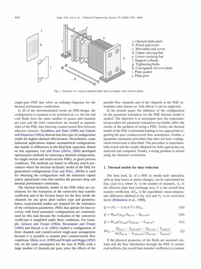
Nowadays, plate heat exchangers (PHEs) are extensivelyused for heating, cooling and heat-regeneration applicationsin the chemical, food and pharmaceutical industries. Thistype of exchanger was originally developed for use in hy-gienic applications such as the pasteurization of liquid foodproducts. However, the range of applications of this type ofexchanger largely expanded in the last decades due to thecontinual design and construction improvements. As shownin Fig. 1, the PHE consists of a pack of corrugated metalplates pressed together into a frame. The gaskets betweenthe plates form a series of thin channels where the hot andcold fluids flow and exchange heat through the metal plates.The flow distribution inside the plate pack is defined by

∗ Corresponding author. Tel.: +55-11-30912258; fax: +55-11-30912255.

E-mail addresses:jpinto@poly.edu (J.M. Pinto), catadini@usp.br(C.C. Tadini).

0009-2509/$ - see front matter� 2004 Elsevier Ltd. All rights reserved.doi:10.1016/j.ces.2004.07.025

the design of the gaskets, the opened and closed ports of theplates and the location of the feed connections at the covers.

Despite the large number of applications, rigorous de-sign methods for the PHEs are still restricted to the equip-ment manufacturers. Simplified methods for the calculationof the required number of plates were presented byLawry(1959), Buonopane et al. (1963), Jackson and Troupe (1966)andRaju and Bansal (1983). Jarzebski and Wardas-Koziel(1985)developed a graphical procedure for determining thenumber of passes and the number of channels per pass thatminimize the annual operational costs. However, a simpli-fied evaluation model of the PHE was used due to the com-plexity of the optimization of the PHE configuration, whichdefines its flow distribution.

A comprehensive step-by-step design method was pre-sented byShah and Focke (1988)for determining the platesize, corrugation type and number of plates. The methodis however restricted to single-pass countercurrent flowconfigurations.Thonon and Mercier (1996)present an it-erative method for determining the number of plates of a

4592 Jorge A.W. Gut et al. / Chemical Engineering Science 59 (2004) 4591–4600

Fig. 1. Structure of a typical gasketed plate heat exchanger with chevron plates.

single-pass PHE that relies on enthalpy-diagrams for thethermal performance verification.

In all of the aforementioned works on PHE-design, theconfiguration is assumed to be symmetrical, i.e. the hot andcold fluids have the same number of passes and channelsper pass and the feed connections are located at oppositesides of the PHE, thus favoring countercurrent flow betweenadjacent channels.Kandlikar and Shah (1989)andZaleskiand Klepacka (1992a)showed that this type of configurationyields the highest thermal effectiveness. Nevertheless, someindustrial applications require asymmetrical configurationsdue mainly to differences in the fluid heat capacities. Basedon this argument,Gut and Pinto (2003a, 2004)developedoptimization methods for selecting a detailed configuration,for single section and multi-section PHEs, at given processconditions. The methods are based on efficient search pro-cedures where the thermal–hydraulic model of the PHE forgeneralized configurations (Gut and Pinto, 2003b) is usedfor obtaining the configuration with the minimum capitaland/or operational costs that satisfies the pressure drop andthermal performance constraints.

The thermal–hydraulic model of the PHE relies on cor-relations for the evaluation of the convective heat transfercoefficient and of the friction factor for the flow inside thechannels for any given plate surface type and geometry;hence, experimental studies are required for the estimationof the correlation parameters. PHEs that operate for heat re-covery with fixed symmetric configurations are commonlyused for this task because the evaluation of the convectivecoefficient is simplified under these conditions. For exam-ple, Jackson and Troupe (1964), Buonopane and Troupe(1969) and Bansal et al. (2001)studied a configuration ofthree channels and countercurrent single-pass arrangementbecause it is possible to assume pure countercurrent flowconditions.Muley et al. (1999)andWright and Heggs (2002)rely on the same assumption for the case of PHEs with alarge number of channels per pass, since the effects of the

parallel flow channels and of the channels at the PHE ex-tremities (also known as “end effects”) can be neglected.

In the present paper, the influence of the configurationon the parameter estimation for the PHE thermal model isstudied. The objective is to investigate how the experimen-tal procedure for parameter estimation can further affect theresults of the problem of sizing a PHE. Firstly, the thermalmodel of the PHE is presented leading to two approaches re-garding the pure countercurrent flow assumption. Further, aparameter estimation procedure that does not have configu-ration restrictions is described. The procedure is experimen-tally tested and the results obtained for both approaches areanalyzed and compared. Finally, a sizing problem is solvedusing the obtained correlations.

2. Thermal models for data reduction

The heat load,Q, of a PHE in steady-state operation,with no heat losses or phase changes, can be represented byEqs. (1a)–(1c), whereNC is the number of channels,AP isthe effective plate heat exchange area,U is the overall heattransfer coefficient,�Tlm is the logarithmic mean tempera-ture difference (defined in Eq. (2)) andFT is its correctionfactor (Rohsenow et al., 1998).

Q= (NC − 1)APUFT�Tlm, (1a)

Q=WhotCphot(Thot,in − Thot,out), (1b)

Q=WcoldCpcold(Tcold,out − Tcold,in), (1c)

�Tlm = (Thot,in − Tcold,out)− (Thot,out − Tcold,in)

ln(Thot,in − Tcold,out)/(Thot,out − Tcold,in). (2)

If the physical properties of the fluids are assumed con-stant and the flow distribution through the PHE is consid-ered uniform, the overall heat transfer coefficient is constant

Jorge A.W. Gut et al. / Chemical Engineering Science 59 (2004) 4591–4600 4593

along the PHE and is obtained from Eq. (3), which repre-sents a series association of thermal resistances.

1

U= 1

hhot+ 1

hcold+ eP

kP+ Rf,hot + Rf,cold. (3)

In order to determineU, correlations for the evaluation ofthe convective coefficients,hhot andhcold, are required forthe selected plate surface type and geometry. For Newtonianfluids under turbulent flow, the correlation whose generalform is presented in Eq. (4) is commonly used, where thedimensionless numbers Nusselt, Reynolds and Prandtl (re-spectivelyNu, ReandPr) are defined in the Nomenclaturefor the PHE geometry anda, b, andc are empirical param-eters (Shah and Focke, 1988).

Nu= aRebP rc. (4)

The system of equations defined by Eqs. (1a)–(1c) and (2)can be solved to obtain the heat load,Q, and the fluid outlettemperatures,Thot,out and Tcold,out, only if the correctionfactorFT is known. This factor is a function of the exchangerconfiguration, of the number of transfer units (NTU definedin Eq. (5)) and of the heat capacity ratio (C∗ defined in Eq.(6)). For the ideal case of pure countercurrent flow,FT = 1.For all other types of flow distribution, 0<FT <1.

NTU = (NC − 1)APU

min(WhotCphot,WcoldCpcold), (5)

C∗ = min(WhotCphot,WcoldCpcold)

max(WhotCphot,WcoldCpcold). (6)

There are no generalized equations in the formFT =FT (configuration, NTU,C∗) for PHEs. The calculation ofFT requires the solution of the differential mathematicalmodeling of the heat exchange between channels, which isnot a trivial task since each configuration corresponds toa unique system (Kandlikar and Shah, 1989; Zaleski andKlepacka, 1992a; Gut and Pinto, 2003b). Various researchershave used PHE simulation models to generate charts andtables in the formFT = FT (NTU, C∗) or ε = ε(NTU, C∗)for the most usual configurations, whereε is the thermaleffectiveness of the exchanger (see definition in Eq. (7)).The relationship betweenFT andε is presented in Eq. (8)(Rohsenow et al., 1998).

ε = Q

Qmax

= Q

min(WhotCphot,WcoldCpcold)(Thot,in − Tcold,in), (7)

FT =

1NTU(1−C∗) ln

(1 − C∗�

1 − �

)if C∗<1,

�NTU(1−�) if C∗ = 1.

(8)

Kandlikar and Shah (1989), for example, published tablesfor obtainingFT andε for PHEs with 1/1, 1/2, 1/3, 1/4,2/2, 2/4, 3/3, and 4/4 pass-arrangements for various

numbers of channels.Zaleski and Klepacka (1992a)pre-sented similar results in the form of chartsε= ε(NTU, C∗).

The main difficulty in obtaining the generalized formFT =FT (configuration, NTU, C∗) resides in the PHE dif-ferential model, which strongly depends on its configuration(note that Eq. (1a) represents the integrated form of the PHEthermal model).Ribeiro and Andrade (2002)used the ex-ponential approximation of the differential model presentedby Zaleski and Klepacka (1992b)to develop an algorithmfor the steady-state simulation of PHEs. However, no detailswere given concerning the construction of the system of dif-ferential equations and of the set of boundary conditions forgeneral configurations.

Gut and Pinto (2003b)presented an “assemblingalgorithm” for the simulation of PHEs with generalizedconfigurations, which are represented by a set of six param-eters:NC , P I , P II , �, Yh andYf (please refer to AppendixAppendix A for definitions). This algorithm guides the con-struction of the mathematical model, its solution throughanalytical or numerical methods and the resulting channeltemperature profiles and exchanger effectiveness. Onceε

is obtained,FT is easily available through Eq. (8). In ad-dition to the six configuration parameters, the assemblingalgorithm also requires two thermal parameters,�hot and�cold, as shown in Eqs. (9), (10a) and (10b). The mathemat-ical model comprises a linear system of first-order ordinarydifferential equations of the boundary value type and anon-linear system of algebraic equations.

ε = ε(NC, P I , P II ,�, Yh, Yf , �hot, �cold), (9)

�hot = APUNhot

WhotCphot, (10a)

�cold = APUNcold

WcoldCpcold. (10b)

3. Parameter estimation procedure for generalizedconfigurations

In order to estimate the model parametersa, b andc ofEq. (4), several heat transfer experimental runs are required,comprising the desired range ofReandPr for a given platetype. For any experimental run of the PHE, where the in-let and outlet temperatures and flow rates are measured, theaverage heat load can be obtained from Eqs. (1b) and (1c),whereas the experimental overall heat transfer coefficient,Uexp, is available through Eq. (1a) if the corresponding cor-rection factorFT is known. Two approaches are used in thiswork for determiningFT :

• Approach 1: pure countercurrent flow is assumed andthereforeFT = 1. This assumption has shown to holdwhen the PHE is configured with a countercurrentsingle-pass arrangement with only two or three chan-nels or with a sufficiently large number of channels

4594 Jorge A.W. Gut et al. / Chemical Engineering Science 59 (2004) 4591–4600

(according toKandlikar and Shah (1989)the end effectscan be neglected forNC >40).

• Approach 2:FT is obtained by solving the PHE differen-tial model for generalized configurations in Eq. (9). Thisapproach does not have configuration restrictions.

The correlation model is presented in Eq. (11), whichcan be fitted to the experimental data by minimizing thequadratic error function,� in Eq. (12), wheren is the num-ber of experimental runs.

Ucalc(a, b, c)= 1De

aRebhotPrchotkhot

+ DeaRebcoldPr

ccoldkcold

+ ePkP

,

(11)

�(a, b, c)=n∑i=1

(Uexp,i − Ucalc,i )2. (12)

4. Experimental procedure

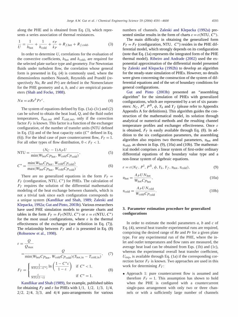
The proposed parameter estimation procedure for gener-alized configurations is tested using an Armfield FT-43 labo-ratory plate heat exchanger (Armfield, Hampshire, UK) withstainless-steel flat plates, as shown inFig. 2, using distilledwater as product and hot service fluids. The main character-istic dimensions of the plate are presented inTable 1.

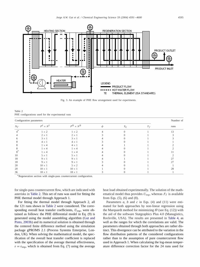
The PHE was assembled with two sections: heating andregeneration, as shown in the example inFig. 3. A data log-ger attached to a personal computer using thermocouplescontinuously recorded inlet and outlet temperatures of eachsection (the monitoring points are represented inFig. 3).The product flow rate was obtained by direct measurementand the hot water flow rate was calculated through the en-ergy balances (Eqs. (1b) and (1c)). To avoid the presence of

Fig. 2. Laboratory plate heat exchanger Armfield FT-43: (a) feed tank, (b) peristaltic pump, (c) PHE with three sections and connected thermocouples,(d) moveable end cover, (e) fixed end cover, (f) a pair of flat plates and (g) a pair of gaskets.

Table 1Main dimensions of the Armfield FT-43 plate

Dimension Value

Plate length, between port centers (mm) 90Plate width, between gaskets (mm) 60Plate thickness (mm) 1.0Mean channel gap (mm) 1.5Mean hydraulic diameter (mm) 3.0Port diameter (mm) 6.5Heat transfer area (m2/plate) 0.0050

fouling, the plates were cleaned by a cleaning out of place(COP) method using intensive brushing after each run. Thehot water flow rates were held constant. The temperaturesof each inlet and outlet streams were recorded at every 10 s.In each run, the system reaches the steady state from whichdata were recorded for at least 2 min. From the recorded data,whenever any temperature standard deviation was larger than0.5◦C, the corresponding run was discarded.

Various configurations were used for the experiments, in-cluding symmetric and asymmetric pass-arrangements withcountercurrent or parallel flows. A total of 121 runs was se-lected, as presented inTable 2.

The physical properties of distillated water (density, vis-cosity, thermal conductivity and specific heat) were obtainedfrom the literature (Bennett and Myers, 1982; Schwier, 1992;Perry et al., 1997). The values of physical properties wereevaluated at the average temperature of the fluid stream.

5. Results and discussion

5.1. Parameter estimation

Table 3presents the experimental results obtained for the24 runs conducted with the regeneration section configured

Jorge A.W. Gut et al. / Chemical Engineering Science 59 (2004) 4591–4600 4595

Fig. 3. An example of PHE flow arrangement used for experiments.

Table 2PHE configurations used for the experimental runs

Configuration parameters Number of

NC P I ×N I P II ×N II � Yh Yf runs

4* 1 × 2 1× 2 4 0 1 134 2× 1 2× 1 3 0 1 36 3× 1 3× 1 4 0 1 38 4× 1 4× 1 3 0 1 18 1× 4 4× 1 4 1 1 28 1× 4 1× 4 4 0 1 28* 1 × 4 1× 4 4 0 1 11

10 5× 1 5× 1 4 0 1 218 9× 1 9× 1 4 1 1 2718 9× 1 9× 1 3 0 1 2720 10× 1 5× 2 4 0 1 120 10× 1 10× 1 1 0 1 2836 18× 1 18× 1 3 0 1 1

∗Regeneration section with single-pass countercurrent configuration.

for single-pass countercurrent flow, which are indicated withasterisks inTable 2. This set of runs was used for fitting thePHE thermal model through Approach 1.

For fitting the thermal model through Approach 2, allthe 121 runs shown inTable 2were considered. The corre-sponding overall heat transfer coefficients,Uexp, were ob-tained as follows: the PHE differential model in Eq. (9) isgenerated using the model assembling algorithm (Gut andPinto, 2003b) and its numerical solution is obtained throughthe centered finite difference method using the simulationpackage gPROMS 2.1 (Process Systems Enterprise, Lon-don, UK). When solving the mathematical model, the spec-ification of the overall heat transfer coefficient is replacedwith the specification of the average thermal effectiveness,ε = εexp, which is obtained from Eq. (7) using the average

heat load obtained experimentally. The solution of the math-ematical model thus providesUexp, whereasFT is availablefrom Eqs. (5), (6) and (8).

Parametersa, b and c in Eqs. (4) and (11) were esti-mated for both approaches by non-linear regression usingthe Marquardt method for minimizing� (see Eq. (12)) withthe aid of the software Statgraphics Plus 4.0 (Manugistics,Rockville, USA). The results are presented inTable 4, aswell as the ranges for which the correlations are valid. Theparameters obtained through both approaches are rather dis-tinct. This divergence can be attributed to the variation in theflow distribution patterns of the considered configurationsrather than to the assumption of pure countercurrent flowused in Approach 1. When calculating the log-mean temper-ature difference correction factor for the 24 runs used for

4596 Jorge A.W. Gut et al. / Chemical Engineering Science 59 (2004) 4591–4600

Table 3Process conditions on the regeneration section for the selected runs of Approach 1

Run NC W Thot,in Thot,out Tcold,in Tcold,out Q

(kg/h) (◦C) (◦C) (◦C) (◦C) (W)

1 4 26.1 74.5 67.4 25.2 32.0 2102 4 32.8 66.0 60.7 25.1 30.2 1983 4 36.3 61.4 56.8 25.1 29.5 1894 4 42.8 56.7 52.8 25.1 28.8 1885 4 49.0 53.3 50.1 25.1 28.2 1806 4 52.6 50.9 48.0 25.1 27.9 1747 4 58.5 48.0 45.3 25.0 27.5 1778 4 63.6 45.8 43.3 25.0 27.3 1769 4 81.2 58.0 56.2 45.6 46.7 133

10 4 94.1 57.3 55.7 45.4 46.5 14911 4 110.1 55.0 53.5 44.5 45.8 17912 4 14.5 84.5 70.1 25.2 37.6 22613 4 19.4 82.8 72.2 25.2 35.0 23114 8 15.51 86.4 72.8 19.8 31.4 22715 8 24.05 81.2 70.6 19.7 29.0 27816 8 4.72 74.6 65.0 19.7 27.9 4917 8 4.72 68.5 60.4 19.7 26.8 4218 8 4.72 62.6 55.7 19.6 25.8 3619 8 4.72 57.9 51.9 19.6 24.9 3120 8 4.72 54.0 48.5 19.6 24.3 2821 8 4.72 50.6 45.7 19.6 23.8 2522 8 4.72 46.9 42.7 19.6 23.3 2223 8 4.72 43.8 40.2 19.5 22.7 1924 8 4.72 67.1 59.5 22.4 29.4 40

Table 4Results of parameter estimation for Approaches 1 and 2

Approach Correlation R2 Range

1 Nu= 0.0188Re0.889Pr0.292 0.98 10�Re�10002.2 <_ Pr <_ 6.8

Nu

Pr1/3= 0.0169Re0.897 0.98

2 Nu= 0.00220Re1.02Pr1.49 0.93 10�Re�24001.8 <_ Pr <_ 6.8

Nu

Pr1/3= 0.0457Re0.771 0.82

Approach 1, it is observed that 0.968�FT�0.990; thus it isacceptable to assume thatFT = 1 for these selected runs.

Since the typical Prandtl number exponent for heat ex-change correlations isc= 1

3, this value was also tested. It wasverified that estimating only parametersa andb did not de-teriorate the quality of the model fitting for Approach 1 (R2

did not change, as can be seen inTable 4). However, a worstfit was obtained for Approach 2 withc = 1

3. The obtainedparameterc = 1.49 suggests an unusual strong dependenceon the Prandtl number. To better detect such dependence, anexperimental study with different fluids would be necessaryto extend the range ofPr. Consequently, both correlationsfitted with constant and fixed parameterc= 1

3 in Table 4aremore consistent and will be considered henceforth.

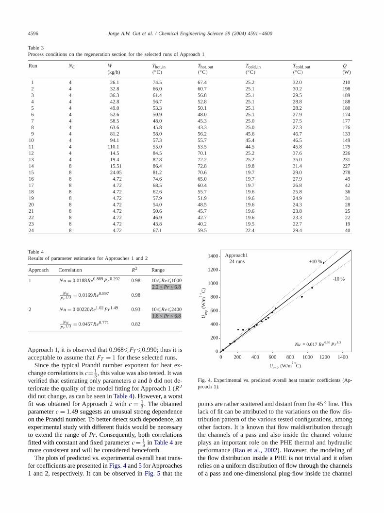
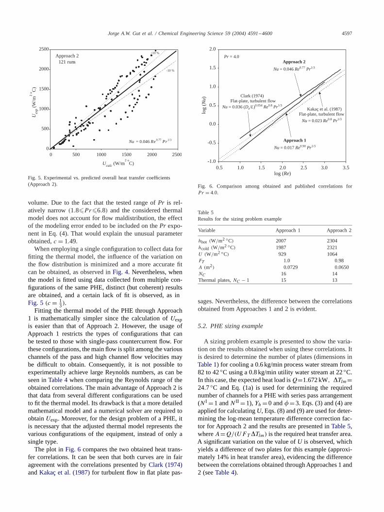
The plots of predicted vs. experimental overall heat trans-fer coefficients are presented inFigs. 4and5 for Approaches1 and 2, respectively. It can be observed inFig. 5 that the

0

200

400

600

800

1000

1200

1400

0 200 400 600 800

Approach124 runs

Nu = 0.017Re0.90Pr1/3

140012001000

+10 %

-10 %

Ucalc (W/m² ºC)

Uexp

(W

/m² º

C)

Fig. 4. Experimental vs. predicted overall heat transfer coefficients (Ap-proach 1).

points are rather scattered and distant from the 45◦ line. Thislack of fit can be attributed to the variations on the flow dis-tribution pattern of the various tested configurations, amongother factors. It is known that flow maldistribution throughthe channels of a pass and also inside the channel volumeplays an important role on the PHE thermal and hydraulicperformance (Rao et al., 2002). However, the modeling ofthe flow distribution inside a PHE is not trivial and it oftenrelies on a uniform distribution of flow through the channelsof a pass and one-dimensional plug-flow inside the channel

Jorge A.W. Gut et al. / Chemical Engineering Science 59 (2004) 4591–4600 4597

0

500

1000

1500

2000

2500

0 500 1000 1500 2000 2500

+10 %

-10 %

Approach 2121 runs

Nu = 0.046 Re0.77Pr1/3

Ucalc (W/m² ºC)

Uexp

(W

/m² º

C)

Fig. 5. Experimental vs. predicted overall heat transfer coefficients(Approach 2).

volume. Due to the fact that the tested range ofPr is rel-atively narrow(1.8�Pr�6.8) and the considered thermalmodel does not account for flow maldistribution, the effectof the modeling error ended to be included on thePr expo-nent in Eq. (4). That would explain the unusual parameterobtained,c = 1.49.

When employing a single configuration to collect data forfitting the thermal model, the influence of the variation onthe flow distribution is minimized and a more accurate fitcan be obtained, as observed inFig. 4. Nevertheless, whenthe model is fitted using data collected from multiple con-figurations of the same PHE, distinct (but coherent) resultsare obtained, and a certain lack of fit is observed, as inFig. 5 (c = 1

3).Fitting the thermal model of the PHE through Approach

1 is mathematically simpler since the calculation ofUexpis easier than that of Approach 2. However, the usage ofApproach 1 restricts the types of configurations that canbe tested to those with single-pass countercurrent flow. Forthese configurations, the main flow is split among the variouschannels of the pass and high channel flow velocities maybe difficult to obtain. Consequently, it is not possible toexperimentally achieve large Reynolds numbers, as can beseen inTable 4when comparing the Reynolds range of theobtained correlations. The main advantage of Approach 2 isthat data from several different configurations can be usedto fit the thermal model. Its drawback is that a more detailedmathematical model and a numerical solver are required toobtainUexp. Moreover, for the design problem of a PHE, itis necessary that the adjusted thermal model represents thevarious configurations of the equipment, instead of only asingle type.

The plot inFig. 6 compares the two obtained heat trans-fer correlations. It can be seen that both curves are in fairagreement with the correlations presented byClark (1974)andKakaç et al. (1987)for turbulent flow in flat plate pas-

-1.0

-0.5

0.0

0.5

1.0

1.5

2.0

0.5 1.0 1.5 2.0 2.5 3.0 3.5

Approach 1

Nu = 0.017 Re0.90 Pr1/3

Approach 2

Nu = 0.046 Re0.77 Pr1/3

Pr = 4.0

Kakaç et al. (1987)Flat-plate, turbulent flow

Nu = 0.023 Re0.8 Pr1/3

Clark (1974)Flat-plate, turbulent flow

Nu = 0.036 (De/L)0.054 Re0.8 Pr1/3

log (Re)

log

(Nu)

Fig. 6. Comparison among obtained and published correlations forPr = 4.0.

Table 5Results for the sizing problem example

Variable Approach 1 Approach 2

hhot (W/m2 ◦C) 2007 2304hcold (W/m2 ◦C) 1987 2321U (W/m2 ◦C) 929 1064FT 1.0 0.98A (m2) 0.0729 0.0650NC 16 14Thermal plates,NC − 1 15 13

sages. Nevertheless, the difference between the correlationsobtained from Approaches 1 and 2 is evident.

5.2. PHE sizing example

A sizing problem example is presented to show the varia-tion on the results obtained when using these correlations. Itis desired to determine the number of plates (dimensions inTable 1) for cooling a 0.6 kg/min process water stream from82 to 42◦C using a 0.8 kg/min utility water stream at 22◦C.In this case, the expected heat load isQ=1.672 kW, �Tlm=24.7◦C and Eq. (1a) is used for determining the requirednumber of channels for a PHE with series pass arrangement(N I =1 andN II =1), Yh=0 and�=3. Eqs. (3) and (4) areapplied for calculatingU, Eqs. (8) and (9) are used for deter-mining the log-mean temperature difference correction fac-tor for Approach 2 and the results are presented inTable 5,whereA=Q/(UFT�Tlm) is the required heat transfer area.A significant variation on the value ofU is observed, whichyields a difference of two plates for this example (approxi-mately 14% in heat transfer area), evidencing the differencebetween the correlations obtained through Approaches 1 and2 (seeTable 4).

4598 Jorge A.W. Gut et al. / Chemical Engineering Science 59 (2004) 4591–4600

6. Conclusions

The thermal modeling of a PHE on steady-state assum-ing constant fluid physical properties and uniform flow dis-tribution inside the PHE was presented, leading to two ap-proaches for obtaining the log-mean temperature differencecorrection factor: Approach 1, that assumes pure counter-current flow conditions and Approach 2, that accounts fordifferent configurations and requires the solution of the dif-ferential thermal model of the PHE. A parameter estimationprocedure for generalized configurations was presented. Themethodology was tested in an Armfield FT-43 PHE withflat plates. Both approaches were used for fitting the ther-mal model. For Approach 1, only single-pass countercurrentarrangements were considered, whereas 12 different config-urations were considered for Approach 2. Since the modeldoes not account for flow maldistribution, a certain lack offit was obtained when using Approach 2. This problem doesnot occur when fitting data collected from a single config-uration type because the variation of the flow distributionpattern among experimental runs is minimal.

The heat transfer correlations obtained for PHEs are inti-mately associated with the configuration(s) experimentallytested and the corresponding flow distribution pattern(s).When sizing a PHE for a given type of configuration, a con-sistent heat transfer correlation must be used for the thermalmodel, otherwise unrealistic results can be obtained. For theproblem of optimizing the configuration of a PHE (Gut andPinto, 2003a, 2004), it is important that the thermal modelcan represent all possible configurations. In this case, a gen-eralized heat transfer correlation should be used, such as oneobtained through Approach 2 using various distinct config-urations. Moreover, efforts have been directed towards im-proving the thermal modeling of the PHEs by taking intoaccount the flow distribution inside the PHE (Bassiouny andMartin, 1984a, b; Thonon and Mercier, 1996; Rao et al.,2002).

Notations

a model parameter, dimensionlessA heat transfer area, m2

AC cross-section area for channel flow, m2

AP effective plate heat transfer area, m2

b model parameter, dimensionlessc model parameter, dimensionlessC∗ heat capacity ratio,C∗�1, dimensionlessCp fluid specific heat at constant pressure, J/kg◦CDe equivalent diameter of the channel, meP thickness of metal plate, mFT log-mean temperature difference correction factor,

0<FT�1, dimensionlessh convective heat transfer coefficient, W/m2 ◦Ck fluid thermal conductivity, W/m ◦C

kP plate thermal conductivity, W/m ◦CL plate length, mn number of experimental runsN number of channels per passNC number of channelsNTU number of heat transfer unitsNu Nusselt number,Nu= hDe/k, dimensionlessP number of passesPr Prandtl number,Pr = Cp �/k, dimensionlessQ heat load, WR2 correlation coefficientRf fluid fouling factor,m2 ◦C/WRe Reynolds number,Re = W De/(�NAC), dimen-

sionlessT temperature,◦CU overall heat transfer coefficient, W/m2 ◦CW fluid mass flow rate, kg/sYf binary parameter for type of channel-flow, dimen-

sionlessYh binary parameter for hot fluid location, dimension-

less

Greek letters

� thermal coefficient defined in Eqs. (10a) and (10b),dimensionless

�Tlm log-mean temperature difference,◦Cε exchanger thermal effectiveness, %� quadratic error function(W/m2 ◦C)2

� fluid viscosity, Pa s� parameter for feed connection relative location,

dimensionless

Subscripts

calc calculatedcold cold fluidexp experimentalhot hot fluidin fluid inletmax maximumout fluid outlet

Acknowledgements

The authors would like to acknowledge financial supportfrom FAPESP (The State of São Paulo Research Founda-tion) and from CNPq (National Council for Scientific andTechnological Development).

Appendix A. Plate heat exchanger configuration param-eters (Gut and Pinto, 2003b)

The configuration of a PHE (plate heat exchanger) canbe characterized by a set of six parameters. These areNC ,P I , P II , �, Yh andYf that are defines as follows:

Jorge A.W. Gut et al. / Chemical Engineering Science 59 (2004) 4591–4600 4599

(a) (b) (c)

(d)

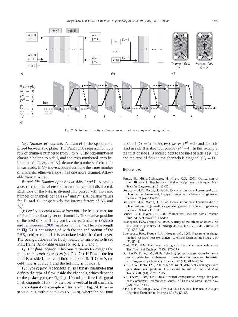
Fig. 7. Definition of configuration parameters and an example of configuration.

NC : Number of channels. A channel is the space com-prised between two plates. The PHE can be represented by arow of channels numbered from 1 toNC . The odd-numberedchannels belong to side I, and the even-numbered ones be-long to side II.N I

C andN IIC denote the numbers of channels

in each side. IfNC is even, both sides have the same numberof channels, otherwise side I has one more channel. Allow-able values:NC�2.P I andP II : Number of passes at sidesI and II. A pass is

a set of channels where the stream is split and distributed.Each side of the PHE is divided into passes with the samenumber of channels per pass (N I andN II ). Allowable valuesfor P I andP II : respectively the integer factors ofN I

C andN IIC .�: Feed connection relative location. The feed connection

of side I is arbitrarily set to channel 1. The relative positionof the feed of side II is given by the parameter� (Pignottiand Tamborenea, 1988), as shown inFig. 7a. The plate lengthin Fig. 7a is not associated with the top and bottom of thePHE, neither channel 1 is associated with the fixed cover.The configuration can be freely rotated or mirrored to fit thePHE frame. Allowable values for�: 1, 2, 3 and 4.Yh: Hot fluid location. This binary parameter assigns the

fluids to the exchanger sides (seeFig. 7b). If Yh=1, the hotfluid is at side I, and cold fluid is at side II. IfYh = 0, thecold fluid is at side I, and the hot fluid is at side II.Yf : Type of flow in channels. Yf is a binary parameter that

defines the type of flow inside the channels, which dependson the gasket type (seeFig. 7c). If Yf=1, the flow is diagonalin all channels. IfYf =0, the flow is vertical in all channels.

A configuration example is illustrated inFig. 7d. It repre-sents a PHE with nine plates(NC = 8), where the hot fluid

in side I (Yh = 1) makes two passes(P I = 2) and the coldfluid in side II makes four passes(P II =4). In this example,the inlet of side II is located next to the inlet of side I(�=1)and the type of flow in the channels is diagonal(Yf = 1).

References

Bansal, B., Müller-Steinhagen, H., Chen, X.D., 2001. Comparison ofcrystallization fouling in plate and double-pipe heat exchangers. HeatTransfer Engineering 22, 13–25.

Bassiouny, M.K., Martin, H., 1984a. Flow distribution and pressure drop inplate heat exchangers—I, U-type arrangement. Chemical EngineeringScience 39 (4), 693–700.

Bassiouny, M.K., Martin, H., 1984b. Flow distribution and pressure drop inplate heat exchangers—II, Z-type arrangement. Chemical EngineeringScience 39 (4), 701–704.

Bennett, C.O., Myers, J.E., 1982. Momentum, Heat and Mass Transfer.third ed. McGraw-Hill, London.

Buonopane, R.A., Troupe, A., 1969. A study of the effects of internal riband channel geometry in rectangular channels. A.I.Ch.E. Journal 15(4), 585–596.

Buonopane, R.A., Troupe, R.A., Morgan, J.C., 1963. Heat transfer designmethod for plate heat exchangers. Chemical Engineering Progress 57(7), 57–61.

Clark, D.F., 1974. Plate heat exchanger design and recent development.The Chemical Engineer (285), 275–279.

Gut, J.A.W., Pinto, J.M., 2003a. Selecting optimal configurations for multi-section plate heat exchangers in pasteurization processes. Industrialand Engineering Chemistry Research 42 (24), 6112–6124.

Gut, J.A.W., Pinto, J.M., 2003b. Modeling of plate heat exchangers withgeneralized configurations. International Journal of Heat and MassTransfer 46 (14), 2571–2585.

Gut, J.A.W., Pinto, J.M., 2004. Optimal configuration design for plateheat exchangers. International Journal of Heat and Mass Transfer 47(22), 4833–4848.

Jackson, B.W., Troupe, R.A., 1964. Laminar flow in a plate heat exchanger.Chemical Engineering Progress 60 (7), 62–65.

4600 Jorge A.W. Gut et al. / Chemical Engineering Science 59 (2004) 4591–4600

Jackson, B.W., Troupe, R.A., 1966. Plate heat exchanger design byε-NTU method. Chemical Engineering Progress Symposium Series 62(64), 185–190.

Jarzebski, A.B., Wardas-Koziel, E., 1985. Dimensioning of plate heat-exchangers to give minimum annual operating costs. ChemicalEngineering Research and Design 63 (4), 211–218.

Kakaç, S., Shah, R.K., Aung, W., 1987. Handbook of Single-PhaseConvective Heat Transfer, Wiley, New York.

Kandlikar, S.G., Shah, R.K., 1989. Multipass plate heatexchangers—effectiveness-NTU results and guidelines for selectingpass arrangements. Journal of Heat Transfer 111, 300–313.

Lawry, F.J., 1959. Plate-type heat exchangers. Chemical Engineering (29),89–94.

Muley, A., Manglik, R.M., Metwally, H.M., 1999. Enhanced heat transfercharacteristics of viscous liquid flows in a chevron plate heat exchanger.Journal of Heat Transfer 121, 1011–1017.

Perry, R.H., Green, D.W., Maloney, J.O., 1997. Perry’s ChemicalEngineers’ Handbook. seventh ed. McGraw-Hill, New York.

Pignotti, A., Tamborenea, P.I., 1988. Thermal effectiveness of multipassplate exchangers. International Journal of Heat and Mass Transfer 31(10), 1983–1991.

Raju, K.S.N., Bansal, J.C., 1983. Design of plate heat exchangers. In:Kakaç, S., Shah, R.K., Bergles, A.E. (Eds.), Low Reynolds NumberFlow Heat Exchangers. Hemisphere, New York.

Rao, B.P., Kumar, P.K., Das, S.K., 2002. Effect of flow distribution tothe channels on the thermal performance of a plate heat exchanger.Chemical Engineering and Processing 41, 49–58.

Ribeiro Jr., C.P., Andrade, M.H.C., 2002. An algorithm for steady-statesimulation of plate heat exchangers. Journal of Food Engineering 53,59–66.

Rohsenow, W.M., Hartnett, J.P., Cho, Y.I. (Eds.) (1998). Handbook ofHeat Transfer. third ed. McGraw-Hill, New York.

Schwier, K., 1992. Properties of liquid water. In: Hewitt, G.F. (Ed.),Handbook of Heat Exchanger Design, s.5.5.3. Begell House, New York.

Shah, R.K., Focke, W.W., 1988. Plate heat exchangers and their designtheory. In: Shah, R.K., Subbarao, E.C., Mashelkar, R.A. (Eds.), HeatTransfer Equipment Design. Hemisphere, New York.

Thonon, B., Mercier, P., 1996. Les Échangeurs à Plaques: Dix Ansde Recherche au GRETh: Partie 2. Dimensionnement et MauvaiseDistribuition. Revue Générale Thermique 35, 561–568.

Wright, A.D., Heggs, P.J., 2002. Rating calculation for plate heat exchangereffectiveness and pressure drop using existing performance data.Chemical Engineering Research and Design 80A, 309–312.

Zaleski, T., Klepacka, K., 1992a. Plate heat-exchangers—method ofcalculation, charts and guidelines for selecting plate heat-exchangersconfigurations. Chemical Engineering and Processing 31 (1), 45–56.

Zaleski, T., Klepacka, K., 1992b. Approximate methods of solving forplate heat-exchangers. International Journal of Heat and Mass Transfer35, 1125–1130.