TP

JS

a

ARRAA

KPCAV

1

thdheao

tcswieit

0h

Fluid Phase Equilibria 330 (2012) 1– 11

Contents lists available at SciVerse ScienceDirect

Fluid Phase Equilibria

j our na l ho me page: www.elsev ier .com/ locate / f lu id

hermodynamic properties and vapor–liquid equilibria of associating fluids,eng–Robinson equation of state coupled with shield-sticky model

un Ma, Jinlong Li, Changchun He, Changjun Peng ∗, Honglai Liu, Ying Hutate Key Laboratory of Chemical Engineering and Department of Chemistry, East China University of Science and Technology, 130 Meilong Road, Shanghai 200237, China

r t i c l e i n f o

rticle history:eceived 22 December 2011eceived in revised form 8 June 2012ccepted 12 June 2012vailable online 19 June 2012

eywords:eng–Robinson equation of stateubic-plus-associationssociating fluidsapor–liquid equilibria

a b s t r a c t

Combining Peng–Robinson (PR) equation of state (EOS) with Liu et al.’s association contribution derivedfrom shield-sticky model (SSM), a new cubic-plus-association (CPA) EOS is proposed to describe thethermodynamic properties of pure associating fluids and their mixtures. The CPA-SSM EOS contains fivemolecular parameters (a0, c1, b, ω and ıε/k) for the pure associating fluids, while for non-associatingfluids it reduces to PR EOS with three molecular parameters (a0, c1, b). The molecular parameters areobtained by fitting the saturated pressures and/or liquid molar volumes at wide temperature ranges. Theoverall average absolute deviations (AADs) of 58 pure associating fluids and 20 non-associating fluidsare 0.74% and 0.54% for saturated vapor pressure, 2.00% and 1.85% for liquid molar volumes respectively.The enthalpies of vaporization for 13 pure associating fluids are well predicted by using these molecularparameters. The molecular parameter b for homologous substances shows a good linear relationship withrespect to their corresponding molecular weights. Using one temperature-independent binary adjustable

parameter kij, satisfactory results of vapor–liquid equilibria (VLE) for both self- and cross-associatingsystems are obtained. The overall AADs of the equilibrium temperatures, pressures and vapor phasemole fractions are 1.46 K, 1.26 kPa and 0.0197 respectively for 25 self-associating systems, and 0.75 K,0.50 kPa and 0.0155 respectively for 29 cross-associating systems. Other caloric properties such as theexcess molar enthalpies of mixing are also successfully computed. The CPA-SSM EOS proposed has beenproved to have comparable accuracy as other models but with much simpler form.

. Introduction

Various theories and/or models have been developed to describehe thermodynamic properties of associating fluids, which haveydrogen-bonding interactions and often exhibit unusual thermo-ynamic behaviors such as high normal boiling point (NBP) andigh enthalpy of vaporization at NBP. In terms of the methodmployed to account for the extent of hydrogen bonding, thosessociation models can be categorized as chemical theory, latticer quasi-chemical theory and perturbation theory.

The premise of the chemical theory lies in the proposition thathe association can be treated as a series of reversible chemi-al reactions resulting in the formation of a series of oligomers,o the corresponding chemical equilibrium equations need to beritten in advance and chemical equilibrium constants are then

ntroduced. Heidemann and Prausnitz [1] successfully combined an

quation of state (EOS) for non-associating substances with a chem-cal approach for the first time and gave the analytical solutionso the chemical equilibrium equations. After that, several models

∗ Corresponding author. Tel.: +86 21 64252767.E-mail address: cjpeng@ecust.edu.cn (C. Peng).

378-3812/$ – see front matter © 2012 Elsevier B.V. All rights reserved.ttp://dx.doi.org/10.1016/j.fluid.2012.06.008

© 2012 Elsevier B.V. All rights reserved.

developed with the same concept, such as the associating perturbedanisotropic chain theory (APACT) [2,3], the perturbed hard-chaintheory (PHCT) [4] and the equation of state with association (AEOS)by Anderko [5,6] in which the Yu–Lu [7] EOS is employed as thephysical contribution.

In contrast to the chemical theory, the lattice or quasi-chemicaltheory assumed that non-idealities in associating fluids can beassigned to the existence of nonrandom mixing at the molecularlevel, thus, large energy parameters are assigned to describe theassociation. The widely used activity coefficient models for liquidmixtures are based on this theory, such as the nonrandom two-liquid model (NRTL) [8], the universal quasi-chemical approach(UNIQUAC) [9], the universal functional activity coefficient model(UNIFAC) [10], the analytical solution of groups (ASOG) [11] and soon. Panayiotou and Sanchez [12] modified the Sanchez–LacombeEOS to account explicitly for hydrogen-bonding interactions. Intheir approach, a specific interaction is introduced between adja-cent sites in a lattice, and the number of bonds determining theextent of hydrogen bonding is based on the Veytsman lattice statis-

tics. They divided the partition function into two contributions,the physical contribution treated with a lattice fluid equation andthe association contribution with an approach similar in spirit tolattice or quasi-chemical theory. Other lattice EOSs based on the

2 se Equ

qfl

imtkitrm[(ipbIsodtodtS[c[slssucr

tipmmSEemEuCthc[iariat

himEaat

J. Ma et al. / Fluid Pha

uasi-chemical approach have also been extended to associatinguids [13–15] in a similar way.

The perturbation theory calculates the total free energy includ-ng the contribution from hydrogen bonding based on statistical

echanics. It has several advantages over the chemical theory andhe lattice or quasi-chemical one. Firstly, it is not necessary tonow the chemical reactions in advance or to introduce the chem-cal equilibrium constants. Secondly, the approximations made inhe theory can be rigorously tested against computer simulationesults because the perturbation theory is based on a well-definedodel for the molecules and their molecular interaction. Wertheim

16–20] presented the famous thermodynamic perturbation theoryTPT) and a sticky-point model for the associating fluids of dimeriz-ng hard spheres from this theory. Chapman and coworkers [21,22]roposed the statistical associating fluids theory (SAFT), which isased on extensions and simplifications of the Wertheim’s TPT.

n Chapman’s SAFT EOS, hydrogen bonding is modeled by using aquare well potential and the association term is calculated basedn a simple material balance. The model requires distinguishing theifferent associating sites with which the association contributiono Helmholtz function can be obtained. Subsequently, various typesf modified SAFT models to describe associating fluids have beeneveloped, such as the perturbed-chain SAFT (PC-SAFT) EOS [23],he SAFT-HR EOS presented by Huang and Radosz [24,25], and theAFT model with attractive potentials of variable range (SAFT-VR)26,27]. All these SAFT models mentioned above use the same asso-iation terms as introduced by Chapman et al. [22]. Stell and Zhou28,29] also generalized Wertheim’s model and yielded the sticky-hield model by introducing a new parameter (associating bondength L) for associating fluids. Liu et al. [30] employed the sticky-hield model to develop a simplified association expression anduccessfully described the VLE of associating systems. He et al. [31]sing Liu’s association expression [30] as association term, and suc-essfully extended the square-well chain molecules with variableange (SWCF-VR) EOS [32] to associating fluids.

The SAFT EOS is one of the most successful models and receivesremendous attention by the academic and industrial researchers,n part because it has been successfully applied to describe thehase behavior of complex fluids and it is a theoretically basedodel and the parameters of these models have explicit physicaleanings. Despite the success, there is a confusion surrounding

AFT because of the complex expressions. In fact, SAFT is not a rigidOS, but rather a method that allows for the incorporation of theffects of association into a given theory. In recent years, more andore attentions have been paid to the cubic-plus-association (CPA)

OS which was firstly proposed by Kontogeorgis [33]. The CPA-EOSses the Soave–Redlich–Kwong (SRK) EOS for the physical part andhapman’s association term [22] as many SAFT models used forhe association contribution. Remarkably, although the CPA EOSas simpler form than complex SAFT, the obtained results of someomplicated associating systems are comparable to that from SAFT34], and it has been widely adopted in the traditional and emerg-ng field including the phase behaviors of associating fluids suchs alkanols [35,36], carboxylic acids [37], amines [38], petroleumeservoir fluids [39], biodiesel [40], and drug-like molecules [41]. Its worth mentioning that there are also other CPA-type EOSs suchs ESD (Elliott–Suresh–Donohue) proposed by Elliott et al. [42] andhe Peng–Robinson (PR) CPA EOS by Wu and Prausnitz [43].

As mentioned above, although a large number of publicationsave focused on the development of models for associating flu-

ds, this subject is still open for further investigation, especiallyore CPA-type EOSs need to be developed. In this work, a CPA

OS is presented by combining the PR-EOS [44] and Liu et al.’sssociation model [30] derived from shield-sticky method (SSM)nd tentatively named as CPA-SSM EOS here. One-site associa-ion scheme is employed by the association term of the CPA-SSM

ilibria 330 (2012) 1– 11

EOS for all associating substances investigated in current work.The rest of paper is organized as follows. A theoretical frameworkof CPA-SSM EOS is given in Section 2. The determination of themolecular parameters for 58 pure associating fluids, the predictedcaloric properties for pure fluids and molecular parameter analysisfor homologues are presented in Section 3. Section 4 shows VLEand excess molar enthalpies of mixing for binary self-associatingand cross-associating mixtures. Finally, conclusions are made inSection 5.

2. CPA-SSM EOS

The compressibility factor of the CPA-SSM EOS can be expressedas

z = zphys + zassoc (1)

where zphys and zassoc represent the physical and association con-tributions, respectively. In this work, the PR EOS [44] is adopted forthe physical contribution.

zphys = Vm

Vm − b− aVm

RT[Vm(Vm + b) + b(Vm − b)](2)

where R is the gas constant, T the temperature, Vm the molar vol-ume, a is a parameter concerning molecular interaction and is afunction of temperature, and b represents the covolume parame-ter. a and b can be calculated by the classical van der Waals one-fluidmixing rule

a =∑

i

∑j

xixjaij, b =∑

i

xibi (3)

with

aij = (1 − kij)√

aiiajj (kii = kjj = 0, kij = kji) (4)

aii = a0,i[1 + c1,i(1 −√

Tr)]2

(5)

where kij is a temperature-independent binary interaction param-eter. Tr is the reduced temperature defined as Tr = T/Tc and Tc is thecritical temperature. The parameters a0,i, c1,i and bi in Eqs. (3)–(5)are the molecular parameters of pure substances in PR EOS and canbe obtained by fitting the experimental data of the saturated vaporpressures and/or liquid densities of pure substance i.

The association contribution to compressibility factor is directlycalculated by Liu et al.’s model [30]

zassoc =∑

i

xi

(1Xi

− 12

)�0

(∂Xi

∂�0

)(6)

here, Xi represents the mole fraction of molecule i not bonded, andxi is the mole fraction of component i. �0 is the total molecularnumber density. It is worth noting that Michelsen and Hendriksever presented a approach to avoid the Xi derivatives, which canmake the calculation simpler [45]. Considering the CPA-SSM EOSitself is a simplified associating model rather than complex one,we calculated the association properties by iteration directly in thiswork. In Eq. (6), Xi and �0(∂Xi/∂�0) are severally calculated by

Xi =

⎛⎝1 +

∑j

Xj˝ij

⎞⎠

−1

(7)

and(�0

∂Xi

∂�0

)= −X2

i

∑j

˝ij

(�0

∂Xj

∂�0

)− X2

i

∑j

�0∂˝ij

∂�0Xj (8)

se Equ

w

�

˝

ba

�

hcfptcc

ω

l

w

cottefiwfap

3

3

pnmtııapvtbs

O

J. Ma et al. / Fluid Pha

here

0∂˝ij

∂�0= ˝ij

(1 + �

∂ ln yref

∂�

)(9)

ij = xj�ijbij

b(10)

In Eq. (10), the interaction covolume parameter bij is defined asij = (bi + bj)/2. �ij is the association strength between molecule ind j and can be expressed as

ij = 2ωij

[exp

(ıεij

kT

)− 1

]yref � (11)

ere, ωij is the surface fraction for association, ıεij/k is the asso-iation energy parameter. If i = j, ωij and ıεij/k are the parametersor pure substances. If i /= j, ωij and ıεij/k are the cross-associationarameters between molecule i and j. For self-associating sys-ems, the cross-association parameters are equal to zero. Forross-associating systems, the cross-association parameters arealculated by the following combining rules [46]

ij =√

ωiiωjj (12)

ıεij

k= ıεii/k + ıεjj/k

2(13)

The cavity-correlation function yref in Eq. (11) is given by

n yref = −0.309095� + 0.097105(1 − �)

+ 0.097105

(1 − �)2

− 2.75503 ln(1 − �) (14)

here the reduced density � is defined as � = b/4Vm.So far, the complete expressions of PR EOS and association

ontribution have been given and the final CPA-SSM EOS can bebtained via Eqs. (2) and (6). For non-associating fluids, zassoc equalso zero, and then the CPA-SSM EOS reduces to PR EOS [44]. If xi = 1,he CPA-SSM EOS reduces to the model for pure fluids, in whichach molecule of pure associating substance is characterized byve molecular parameters: two molecular parameters a0 and c1ere contained in the physical part as shown in Eq. (5), the surface

raction for association ωii and the association energy ıεii/k in thessociation part as shown in Eqs. (12) and (13), and the covolumearameter b in both the physical and the association parts.

. Application to pure associating fluids

.1. Calculations of VLE

The CPA-SSM EOS has been applied to describe thermodynamicroperties such as pVT behavior and phase equilibrium of bothon-associating and associating fluids and their mixtures. In thisodel, each pure associating fluid is fully characterized by five

emperature-independent molecular parameters (a0, c1, b, ω andε/k). For non-associating fluids, the association parameters (ω andε/k) equal to zero, and then the CPA-SSM EOS reduces to PR EOSnd has three molecular parameters (a0, c1 and b). These modelarameters are determined by fitting the experimental saturatedapor pressure and liquid molar volume data of pure fluids usinghe simplex method [47]. In regression, the objective function isased on the minimization of the calculation deviation of both theaturated vapor pressure and liquid molar volume.

⎡ 2 2⎤1/2

F = ⎣ 1Np

Np∑i=1

(pexp − pcal

pexp

)+ 1

NV

NV∑i=1

(VL,exp − VL,cal

VL,exp

) ⎦(15)

ilibria 330 (2012) 1– 11 3

where Np and NV are the number of experimental data points of sat-urated vapor pressure and liquid molar volume, respectively. Thesuperscripts “exp” and “cal” denote experimental and calculatedresults, “L” represents liquid phase.

Table 1 lists the calculated results of 58 associating fluids includ-ing inorganics, alkanols, carboxylic acids, amines, mercaptans fromthe CPA-SSM EOS, in that molecular weight (MW), critical tem-perature (Tc), temperature range, molecular parameters (a0, c1, b,ω and ıε/k), the average absolute deviations (AADs) of saturatedvapor pressures and liquid molar volumes, and experimental datasources are included. The overall AADs of 58 associating fluidsby the CPA-SSM EOS are 0.74% for the saturated vapor pressuresand 2.00% for the liquid molar volumes, respectively. Consider-ing the wide temperature ranges and the simple form of theCPA-SSM EOS, the results of this work are satisfactory. Note thatmercaptan is supposed as an associating fluid in current worksince it has similar molecular structure as alcohol, whose sulfurtakes the place of oxygen in the hydroxyl group of an alcohol.In real solutions, mercaptans might still show weaker associationby hydrogen bonding due to its weak electronegativity althoughthe S H bond is less polar than the hydroxyl group. One cansee from Table 1 that the obtained association parameters ofmercaptans are obviously lower than ones of the correspondingalkanols.

For non-associating fluids, the CPA-SSM EOS directly reduces toPR EOS and contains three molecular parameters (a0, c1 and b). Thetemperature range is set from 0.55Tc to 90Tc for 20 non-associatingfluids involved in this work. Table 2 lists molecular weight (MW),critical properties (Tc and pc), molecular parameters (a0, c1 and b),the AADs of saturated vapor pressures and liquid molar volumes,and experimental data sources of all investigated non-associatingfluids including alkanes, polar substance, aromatic hydrocarbons,esters and so on. The overall AADs of 20 non-associating fluids are0.54% and 1.85% for the saturated vapor pressures and liquid molarvolumes, respectively. By the way, the results in this way are betterthan those of molecular parameters directly obtained from criticalproperties and acentric factor.

For several representative associating substances, the compar-ison of the AADs for vapor pressure and liquid density calculatedfrom the CPA-SSM EOS and other models, i.e., PR EOS [44], SWCF-VR EOS[31], SAFT EOS [24], PC-SAFT EOS [52] and PHSC-AS EOS[53] are given in Table 3. One can see that the CPA-SSM EOS givesmuch better results than PR EOS [44], and the CPA-SSM EOS and theSWCF-VR EOS gives similar results while the physical contributionin the former is simpler than one contained in the latter. Note thatboth the CPA-SSM EOS and the SWCF-VR EOS use the same associ-ation term [30]. For the original SAFT, PC-SAFT and PHSC-AS EOSs,the different associating sites in a molecule are required to be dis-tinguished, with which the association contribution to Helmholtzfunction can then be obtained, and the expressions of these modelsare also more complex than CPA-SSM EOS. As observed above, theCPA-SSM EOS is as accurate as those complex EOSs in calculatingthe saturated vapor pressure and liquid density of pure substances,and moreover, the CPA-SSM EOS shows slightly better results thanthe original SAFT and PHSC-AS EOS.

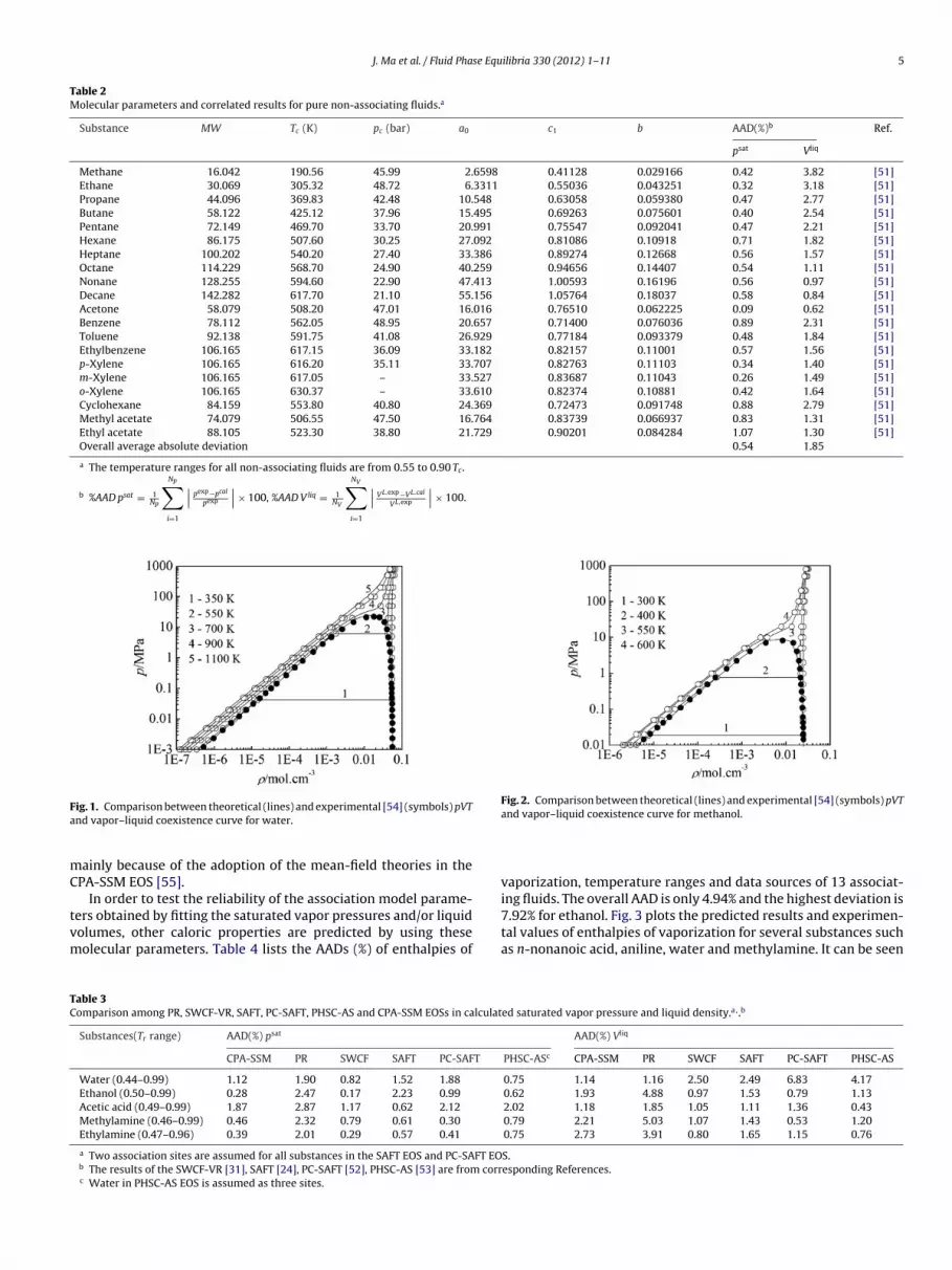
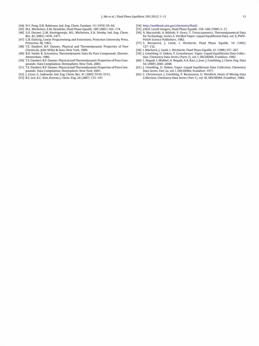
Figs. 1 and 2 give a graphical comparison of complete phase dia-grams for water and methanol at the pressures up to 1000 MPa. As ismentioned above, the molecular parameters of water and methanolare obtained by fitting the experimental vapor–liquid coexistencecurves, then, the isothermal lines at both the supercritical andsubcritical temperatures are predicted by using the molecularparameters. One can see from the figures that the CPA-SSM EOS

can well describe the pVT and vapor–liquid coexistence curvesand be reliably extrapolated except in the vicinity of the criticalpoints. Unfortunately, both the critical pressures and temperaturesare overestimated as those produced by SAFT type models, which

4 J. Ma et al. / Fluid Phase Equilibria 330 (2012) 1– 11

Table 1Molecular parameters and correlated results for pure associating fluids.

Substance MW Tc (K) Tr range a0 c1 b ω × 103 ıε/k (K) AAD (%)a Ref.

psat Vliq

InorganicsWater 18.015 647.13 0.44–0.99 5.3419 0.75490 0.015878 0.57500 1008.76 1.12 1.14 [48]Deuterium oxide 20.031 643.89 0.45–0.99 5.3287 0.79030 0.015915 0.51700 702.730 0.48 1.25 [48]Hydrogen peroxide 34.015 730.15 0.46–0.95 5.8227 0.79320 0.021346 127.00 3153.75 0.58 2.20 [48]Hydrogen sulfide 34.082 373.53 0.55–0.96 4.4562 0.18750 0.027910 14.400 1865.36 0.67 2.69 [48]Ammonia 17.031 405.65 0.48–0.97 3.0906 0.33900 0.019448 20.900 2478.86 0.94 0.54 [48]Hydrogen phosphide 33.998 324.75 0.43–0.95 4.4956 0.00130 0.034407 14.100 1821.23 0.81 1.94 [48]Hydrazine 32.045 653.15 0.44–0.97 7.6558 0.44470 0.027832 7.6900 3917.10 0.48 0.67 [48]

AlkanolsMethanol 32.042 512.58 0.53–0.97 6.6956 0.83486 0.033283 27.4002 3085.02 1.13 2.42 [48]Ethanol 46.069 516.25 0.50–0.99 10.586 0.64856 0.048415 0.75881 4349.86 0.28 1.93 [48]1-Propanol 60.096 536.71 0.50–0.96 16.194 0.75013 0.064666 0.38394 4132.59 0.31 1.83 [48]2-Propanol 60.096 508.30 0.49–0.98 15.561 1.02472 0.065432 2.3625 2932.64 1.10 1.70 [49]1-Butanol 74.123 562.93 0.53–0.96 21.407 0.83532 0.081156 0.37970 4070.22 0.30 2.64 [48]2-Butanol 74.123 536.01 0.52–0.95 20.384 0.91082 0.080605 0.32708 3703.11 0.27 2.48 [48]2-Methyl-1-propanol 74.123 547.78 0.49–0.99 21.034 0.59546 0.079573 0.049588 4987.70 1.19 1.37 [49]2-Methyl-2-propanol 74.123 506.20 0.61–0.95 19.988 0.93964 0.082277 0.17000 3656.39 0.09 2.66 [48]1-Pentanol 88.150 586.15 0.55–0.95 27.778 0.97441 0.098205 0.60161 3495.20 0.40 2.58 [48]2-Pentanol 88.150 552.00 0.52–0.95 25.694 1.14015 0.098887 0.88775 3128.80 0.19 2.38 [48]1-Hexanol 102.177 611.35 0.50–0.95 33.299 1.00710 0.11427 0.80500 3486.44 0.42 2.63 [48]1-Heptanol 116.203 631.90 0.54–0.95 41.313 1.03534 0.13232 0.028246 4527.31 0.34 2.22 [48]1-Octanol 130.230 652.50 0.50–0.96 48.150 1.05647 0.14909 0.032745 4539.53 0.48 2.35 [48]1-Nonanol 144.257 673.00 0.53–0.96 54.490 1.09126 0.16547 0.098290 4274.09 0.96 2.87 [48]1-Decanol 158.284 690.00 0.52–0.96 62.313 1.17048 0.18487 0.043919 4470.79 0.17 2.36 [48]Cyclohexanol 100.161 625.15 0.55–0.99 30.017 0.82397 0.097833 0.20579 4307.10 0.65 1.86 [48]Allyl alcohol 58.050 545.05 0.52–0.99 13.956 0.60198 0.058923 0.84046 4354.95 0.21 1.21 [48]Benzyl alcohol 108.140 677.00 0.54–0.96 33.386 1.17668 0.097169 1.0594 2011.88 1.51 2.34 [48]

Carboxylic acidsFormic acid 46.026 588.00 0.48–0.96 6.5934 0.28598 0.030316 25.166 4855.24 0.28 1.09 [50]Acetic acid 66.053 591.95 0.49–0.99 10.985 0.74292 0.048900 112.10 3129.61 1.87 1.18 [50]Propionic acid 74.079 600.81 0.50–0.99 13.894 0.81701 0.063871 12.750 4472.41 0.64 2.88 [50]n-Butyric acid 88.106 628.00 0.55–0.98 23.798 0.76301 0.084576 2.2760 4262.67 0.13 0.95 [48]n-Pentanoic acid 102.133 651.00 0.50–0.99 31.980 1.06044 0.10313 11.024 2701.16 0.60 1.55 [48]n-Hexanoic acid 116.160 667.00 0.50–0.98 38.661 1.01772 0.11957 0.59721 4232.00 0.41 2.24 [48]n-Heptanoic acid 130.187 680.00 0.55–0.98 46.109 1.18983 0.13926 1.0471 3646.25 0.99 1.64 [48]n-Octanoic acid 144.214 692.00 0.55–0.99 53.140 1.31791 0.15594 0.94048 3383.52 0.26 2.81 [48]n-Nonanoic acid 158.241 703.00 0.58–0.99 57.254 1.12170 0.17501 1.7600 4551.99 1.51 1.65 [48]n-Decanoic acid 172.268 713.00 0.65–0.98 69.513 1.37932 0.19188 0.65173 3373.39 1.67 1.95 [48]Acrylic acid 72.064 615.00 0.51–0.98 14.241 0.78100 0.060560 12.800 4080.31 1.12 1.87 [48]Benzoic acidb 122.123 751.00 0.53–0.70 22.879 1.31670 0.095712 13.100 5424.44 0.64 0.12 [48]

AminesMethylamine 31.057 430.05 0.46–0.99 7.4309 0.68064 0.036406 16.160 1439.06 0.46 2.21 [48]Ethylamine 45.084 456.15 0.47–0.96 11.546 0.73910 0.052825 10.200 1379.85 0.39 2.73 [48]1-Propylamine 59.111 496.95 0.47–0.98 15.429 0.70766 0.068177 41.715 1581.92 0.75 2.54 [48]1-Butylamine 73.138 531.90 0.48–0.95 19.281 0.80740 0.083403 58.500 1761.70 0.76 2.59 [48]2-Butanamine 73.138 514.30 0.45–0.92 20.407 0.74560 0.084864 45.200 1252.40 0.53 1.83 [48]1-Pentylamine 87.165 555.00 0.49–0.97 26.870 0.91970 0.10147 59.800 1026.39 0.28 2.81 [48]1-Hexylamine 101.920 583.00 0.52–0.97 32.419 0.91770 0.11876 53.122 1603.55 1.55 1.70 [48]1-Heptanamine 115.219 607.00 0.49–0.99 36.348 1.11250 0.13583 534.00 977.680 1.39 1.45 [48]1-Octylamine 129.246 627.00 0.50–0.98 47.166 1.05729 0.15450 103.34 1020.30 1.78 1.35 [48]1-Nonylamine 143.272 648.00 0.48–0.95 54.386 1.11949 0.17174 151.34 880.839 1.57 1.72 [48]1-Decylamine 157.299 663.00 0.50–0.99 62.412 1.17523 0.18981 139.46 744.326 2.27 1.64 [48]Ethyleneimine 43.068 537.00 0.46–0.96 11.738 0.49516 0.043831 2.1338 2502.29 0.55 1.09 [48]Dimethylamine 45.084 437.65 0.48–0.92 11.255 0.72520 0.054097 8.9000 1515.93 0.47 2.65 [48]Diethylamine 73.138 496.60 0.47–0.95 20.773 0.83623 0.086069 1.1810 1091.72 0.59 2.87 [50]Ethylenediamine 60.099 593.00 0.49–0.97 15.579 0.85740 0.059525 54.000 2263.06 1.89 0.87 [48]

MercaptansMethanethiol 48.109 469.95 0.46–0.95 9.8838 0.40970 0.043790 4.5300 1968.16 0.80 2.54 [48]Ethanethiol 62.136 499.15 0.44–0.94 14.664 0.65790 0.060548 0.63500 1432.01 0.17 2.90 [48]1-Butanethiol 90.189 569.00 0.47–0.95 25.978 0.77220 0.093521 0.23600 2045.56 0.23 2.80 [48]tert-Butanethiol 90.189 530.00 0.52–0.90 23.532 0.69700 0.094521 0.52200 2029.69 0.33 2.85 [48]1-Pentanethiol 104.216 598.00 0.48–0.96 32.673 0.80090 0.11063 0.19700 2362.31 0.57 2.51 [48]Phenylthiol 110.180 689.00 0.47–0.96 31.869 0.67790 0.095034 1.1500 2986.16 0.60 2.61 [48]Overall average absolute deviation 0.74 2.00

a %AAD psat = 1Np

Np∑i=1

∣∣ pexp−pcal

pexp

∣∣ × 100, %AAD Vliq = 1NV

NV∑i=1

∣∣ VL,exp−VL,cal

VL,exp

∣∣ × 100.

b The temperature range is from 400 K up to normal boiling point.

J. Ma et al. / Fluid Phase Equilibria 330 (2012) 1– 11 5

Table 2Molecular parameters and correlated results for pure non-associating fluids.a

Substance MW Tc (K) pc (bar) a0 c1 b AAD(%)b Ref.

psat Vliq

Methane 16.042 190.56 45.99 2.6598 0.41128 0.029166 0.42 3.82 [51]Ethane 30.069 305.32 48.72 6.3311 0.55036 0.043251 0.32 3.18 [51]Propane 44.096 369.83 42.48 10.548 0.63058 0.059380 0.47 2.77 [51]Butane 58.122 425.12 37.96 15.495 0.69263 0.075601 0.40 2.54 [51]Pentane 72.149 469.70 33.70 20.991 0.75547 0.092041 0.47 2.21 [51]Hexane 86.175 507.60 30.25 27.092 0.81086 0.10918 0.71 1.82 [51]Heptane 100.202 540.20 27.40 33.386 0.89274 0.12668 0.56 1.57 [51]Octane 114.229 568.70 24.90 40.259 0.94656 0.14407 0.54 1.11 [51]Nonane 128.255 594.60 22.90 47.413 1.00593 0.16196 0.56 0.97 [51]Decane 142.282 617.70 21.10 55.156 1.05764 0.18037 0.58 0.84 [51]Acetone 58.079 508.20 47.01 16.016 0.76510 0.062225 0.09 0.62 [51]Benzene 78.112 562.05 48.95 20.657 0.71400 0.076036 0.89 2.31 [51]Toluene 92.138 591.75 41.08 26.929 0.77184 0.093379 0.48 1.84 [51]Ethylbenzene 106.165 617.15 36.09 33.182 0.82157 0.11001 0.57 1.56 [51]p-Xylene 106.165 616.20 35.11 33.707 0.82763 0.11103 0.34 1.40 [51]m-Xylene 106.165 617.05 – 33.527 0.83687 0.11043 0.26 1.49 [51]o-Xylene 106.165 630.37 – 33.610 0.82374 0.10881 0.42 1.64 [51]Cyclohexane 84.159 553.80 40.80 24.369 0.72473 0.091748 0.88 2.79 [51]Methyl acetate 74.079 506.55 47.50 16.764 0.83739 0.066937 0.83 1.31 [51]Ethyl acetate 88.105 523.30 38.80 21.729 0.90201 0.084284 1.07 1.30 [51]Overall average absolute deviation 0.54 1.85

a The temperature ranges for all non-associating fluids are from 0.55 to 0.90 Tc .

b %AAD psat = 1Np

Np∑i=1

∣∣ pexp−pcal

pexp

∣∣ × 100, %AAD Vliq = 1NV

NV∑i=1

∣∣ VL,exp−VL,cal

VL,exp

∣∣ × 100.

Fa

mC

tvm

Fig. 2. Comparison between theoretical (lines) and experimental [54] (symbols) pVT

TC

ig. 1. Comparison between theoretical (lines) and experimental [54] (symbols) pVTnd vapor–liquid coexistence curve for water.

ainly because of the adoption of the mean-field theories in thePA-SSM EOS [55].

In order to test the reliability of the association model parame-ers obtained by fitting the saturated vapor pressures and/or liquidolumes, other caloric properties are predicted by using theseolecular parameters. Table 4 lists the AADs (%) of enthalpies of

able 3omparison among PR, SWCF-VR, SAFT, PC-SAFT, PHSC-AS and CPA-SSM EOSs in calculat

Substances(Tr range) AAD(%) psat

CPA-SSM PR SWCF SAFT PC-SAFT

Water (0.44–0.99) 1.12 1.90 0.82 1.52 1.88

Ethanol (0.50–0.99) 0.28 2.47 0.17 2.23 0.99

Acetic acid (0.49–0.99) 1.87 2.87 1.17 0.62 2.12

Methylamine (0.46–0.99) 0.46 2.32 0.79 0.61 0.30

Ethylamine (0.47–0.96) 0.39 2.01 0.29 0.57 0.41

a Two association sites are assumed for all substances in the SAFT EOS and PC-SAFT EOb The results of the SWCF-VR [31], SAFT [24], PC-SAFT [52], PHSC-AS [53] are from corrc Water in PHSC-AS EOS is assumed as three sites.

and vapor–liquid coexistence curve for methanol.

vaporization, temperature ranges and data sources of 13 associat-ing fluids. The overall AAD is only 4.94% and the highest deviation is7.92% for ethanol. Fig. 3 plots the predicted results and experimen-

tal values of enthalpies of vaporization for several substances suchas n-nonanoic acid, aniline, water and methylamine. It can be seen

ed saturated vapor pressure and liquid density.a, .b

AAD(%) Vliq

PHSC-ASc CPA-SSM PR SWCF SAFT PC-SAFT PHSC-AS

0.75 1.14 1.16 2.50 2.49 6.83 4.170.62 1.93 4.88 0.97 1.53 0.79 1.132.02 1.18 1.85 1.05 1.11 1.36 0.430.79 2.21 5.03 1.07 1.43 0.53 1.200.75 2.73 3.91 0.80 1.65 1.15 0.76

S.esponding References.

6 J. Ma et al. / Fluid Phase Equilibria 330 (2012) 1– 11

Table 4Comparison of the AAD (%) of vaporization heats between CPA-SSM and SWCF-VR EOS.

Substance Tr range AAD �Hvap(%)a Ref.

CPA-SSM SWCF-VR

Water 0.44–0.96 5.32 4.88 [56]Ethanol 0.52–0.94 7.92 4.40 [48]Allyl alcohol 0.51–0.98 5.13 3.00 [48]2-Methyl-1-butanol 0.55–0.94 6.14 4.04 [48]1-Decanol 0.55–0.94 4.59 5.00 [48]Arcrylic acid 0.51–0.98 5.03 1.49 [48]n-Nonanoic acid 0.57–0.95 2.56 3.98 [48]Methylamine 0.46–0.96 2.74 3.21 [48]Ethylamine 0.46–0.95 4.24 3.26 [48]Aniline 0.48–0.94 3.85 5.68 [48]1-Nonylamine 0.54–0.98 5.12 2.73 [48]1-Decylamine 0.55–0.97 5.79 2.69 [48]Methanethiol 0.46–0.93 5.75 4.35 [48]Overall average absolute deviation 4.94 3.75

a %AAD Hvap = 1NH

NH∑i=1

∣∣ Hexp−Hcal

Hexp

∣∣ × 100.

Frw

td

3

untl

Ffn

ig. 3. Comparison between predicted (lines) and experimental [48,54] (symbols)esults of the vaporization heats of n-nonanoic acid (circles), aniline(pentacles),ater (triangles) and methylamine (squares).

hat the predicted results are in good agreement with experimentalata [48,54].

.2. Molecular parameters for homologues

Now we focus on the model parameters with respect to molec-

lar weights (MW). The parameter b for homologous 1-alkanols,-alkanoic acids, 1-alkylamines and n-alkanes has good linear rela-ions with their molecular weights, as illustrated in Fig. 4. Table 5ists the expression and coefficients. The squares of correlation

ig. 4. Linear relation between molecular parameter b and molecular weightsor 1-alkanols (squares), n-alkanoic acids (triangles), 1-alkylamines (circles) and-alkanes (diamonds).

coefficients (R2) are also included in this table. The R2 valuesfor all the relations are above 0.99 suggesting that the expres-sion for the model parameters of the homologous substances arevery satisfactory. The model parameter b of the homologue serieswith larger molar weights can be predicted by using these linearrelations listed in Table 5. Subsequently, the model parameterscan be further reduced effectively. Fig. 5 gives the comparisonbetween experimental data and predicted results of 1-undecanol,1-dodecanol and 1-tridecanol. The model parameter b for thesepredicted results is from linear relations directly. The AADs of 1-undecanol, 1-dodecanol and 1-tridecanol by the CPA-SSM EOS are0.35%, 0.27% and 0.33% for the saturated vapor pressures, and 1.88%,2.85% and 2.32% for the saturated liquid molar volumes, respec-tively. As can be seen in Fig. 5, the predicted results of 1-undecanol,1-dodecanol and 1-tridecanol by the CPA-SSM EOS are in excellentagreement with the experimental data [48].

4. Phase behavior of associating fluid mixtures

In principle, the physicochemical properties of mixtures can beconveniently obtained via a molecular thermodynamic model oncethe model parameters of pure fluids are determined. In addition,VLE require that the pressure, temperature and chemical potentialof each component in vapor and liquid phase are equal, respec-tively, namely

pV = pL; TV = TL; Vi = L

i i = 1, . . . , k (16)

where the superscripts ‘V’ and ‘L’ denote vapor and liquid phase,respectively. i is the chemical potential of component i. Toimprove the calculation precision, the only need is a binary

adjustable parameter kij in Eq. (4), which can be estimated in virtueof experimental properties of a binary mixture with the bubblepoint method. To obtain the adjustable parameter kij, the objective

Table 5Expressions of generalized molecular parameters for different homologouscompounds.a

Homologous k1 k2 R2

1-Alkanols 0.0012 −0.0069 0.9996n-Alkanoic acids 0.0013 −0.0322 0.99831-Alkylamines 0.0012 −0.0033 0.9991n-Alkane 0.0012 0.0069 0.9991

a b = k1 × MW + k2.

J. Ma et al. / Fluid Phase Equilibria 330 (2012) 1– 11 7

F es) of

v

f

O

tfcmatT

4

Bb(kbtaS1ac[sl

Fi

the experimental excess molar enthalpies of mixing for this system

ig. 5. Comparison between experimental (symbols) [48] and predicted results (linapor pressures; (b) saturated liquid densities.

unction is selected as

F = 100

⎡⎣ 1

N�

N�∑i=1

((�cal − �exp)

�exp

)2

i

+ 1Ny

Ny∑i=1

(ycal1 − yexp

1 )2i

⎤⎦

1/2

(17)

Here, N is the number of experimental data points, � representshe equilibrium temperature or pressure, y1 is vapor phase moleraction of component 1. Furthermore, a mixture containing asso-iating substances can be divided into self- and cross-associatingixtures according to the association mechanism, thus we will sep-

rately discuss them in detail. By the way, the model parameters forhe associating and non-associating substances are obtained fromables 1 and 2.

.1. Calculations of VLE for binary systems with self-association

For a binary mixture with self-association composed of A and, there exists only one sort of dimer, i.e., AA or BB. Thus, no com-ining rules are needed for the interaction association parametersωij and ıεij/k), the only need is a binary adjustable parameterij in Eq. (4). Table 6 lists the temperature and pressure ranges,inary interaction parameters kij, the AADs of the equilibriumemperatures, pressures and vapor phase molar fractions, as wells the experimental data sources for 25 self-associating mixtures.atisfactory results are achieved with the overall AADs of 1.46 K,.26 kPa and 0.0197 for the equilibrium temperatures, pressuresnd vapor phase mole fractions, respectively. Fig. 6 gives a graphi-

al comparison between the theoretical and experimental VLE data56] for 1-propanol (1) + p-xylene (2) at 101.3 kPa. In the figure, theolid line represents the result of the CPA-SSM EOS, while the dashine denotes that of the SWCF-VR EOS. It can be seen that both

ig. 6. Comparison of CPA-SSM (solid lines) and SWCF-VR (dashed lines) to exper-mental data [56] (symbols) of VLE for 1-propanol (1) + p-xylene (2) at 101.3 kPa.

1-undecanol (squares), 1-dodecanol (circles), 1-tridecanol (triangles). (a) Saturated

models can satisfactorily reproduce the experimental VLE includ-ing the azeotropic point, although the SWCF-VR EOS shows slightlybetter result than the CPA-SSM EOS. Considering the simpler formof the CPA-SSM EOS, the result is acceptable. Fig. 7 illustrates agraphical comparison between the theoretical and experimentalVLE data [57] for 1-butanol (1) + n-decane (2) at 358.15 K, 373.15 Kand 388.15 K. The results from the SWCF-VR EOS (dashed lines) arealso given. Using a temperature-independent binary adjustableparameter kij = 0.0312, the CPA-SSM EOS gives satisfactory descrip-tion for this self-associating system at temperature ranging from358.15 to 388.15 K and pressure ranging from 5.09 to 92.48 kPa. TheAAD of the equilibrium pressure and vapor phase molar fractionfrom the CPA-SSM EOS are 1.05 kPa and 0.0169, and the results ofthe SWCF-VR EOS [31] are 1.11 kPa and 0.0117, respectively. TheCPA-SSM EOS gives comparative results for this system. Generally,the CPA-SSM EOS can give a satisfactory description of bothisothermal and isobaric self-associating systems at low pressures,and the results from the CPA-SSM EOS are comparable to thosefrom the SWCF-VR EOS [31], but the physical contribution of theCPA-SSM EOS is simpler than one contained in the SWCF-VR EOS.

It is a challenge to calculate the excess molar enthalpies of mix-ing by a model. Figs. 8 and 9 give the examples for predicting theexcess molar enthalpies of mixing by the CPA-SSM EOS. Fig. 8 givesa graphical comparison between the theoretical and experimen-tal [62] excess enthalpies of methanol (1) + methyl acetate (2) at298.15 K. Satisfactory result with kij = 0.0569 are observed. Anothertypical comparison between the theoretical and experimental [62]results for tetrachloromethane (1) + acetic acid (2) at 293.15 K isshown in Fig. 9. It can be seen that the CPA-SSM EOS can calculate

well with kij = 0.0178.

Fig. 7. Comparison of CPA-SSM (solid lines) and SWCF-VR (dashed lines) to exper-imental data (symbols) [57] of VLE for 1-butanol (1) + n-decane (2) at 358.15 K(squares), 373.15 K (triangles) and 388.15 K (circles).

8 J. Ma et al. / Fluid Phase Equilibria 330 (2012) 1– 11

Table 6Correlated results of VLE for binary self-associating systems.

System (1–2) T/K p/kPa kij �T/K (�p/kPa)a,b �ya NP Ref.

Methanol Toluene 336.55–372.65 101.3 0.05188 2.076 0.0211 35 [56]Ethanol Ethylbenzene 351.45–409.33 101.3 0.06221 1.302 0.0171 17 [56]1-Propanol n-Decane 363.15 51.41–74.34 0.01721 (1.58) 0.0118 11 [56]1-Propanol p-Xylene 370.03–411.52 101.3 0.05000 0.765 0.0163 25 [56]1-Butanol n-Decane 358.15–388.15 5.09–92.48 0.03120 (1.05) 0.0169 42 [57]2-Methyl-2-propanol Toluene 333.31–383.75 27.42–101.3 0.04000 0.398 0.0289 59 [56]1-Pentanol Ethylbenzene 402.72–411.11 101.3 0.04600 0.408 0.0305 18 [56]1-Pentanol p-Xylene 404.07–411.52 101.3 0.04050 0.282 0.0304 19 [57]Heptane 1-Pentanol 348.15–368.15 7.32–93.08 0.06410 (2.04) 0.0260 61 [58]1-Hexanol Ethylbenzene 409.24–429.44 101.32 0.05000 0.753 0.0275 23 [56]Cyclohexane 1-Hexanol 298.85–373.15 12.69–98.91 0.08087 (2.16) 0.0127 77 [56]Cyclohexane Cyclohexanol 318.15 19.72–29.72 0.08553 (0.88) 0.0074 12 [56]Benzene Benzyl alcohol 343.15 0.28–70.01 0.02656 (1.67) 0.0007 11 [56]Toluene Benzyl alcohol 383.75–478.65 101.3 0.06913 3.461 0.0131 11 [56]Ethyl acetate Acetic acid 333.11 17.03–53.49 −0.04344 (0.48) 0.0295 9 [59]Methyl acetate Acetic acid 337.75–388.90 101.3 −0.04750 1.954 0.0171 30 [59]Acetic acid Ethylbenzene 333.15–400.15 7.47–97.98 −0.03150 (0.91) 0.0291 25 [59]Acetic acid p-Xylene 388.35–401.65 101.3 0.01725 2.362 0.0064 11 [59]Propionic acid o-Xylene 409.60–416.45 101.3 −0.04444 1.659 0.0252 19 [59]Octane Propionic acid 394.45–414.25 101.3 0.01170 0.874 0.0287 15 [59]p-Xylene Propionic acid 406.15–412.70 101.3 −0.04000 2.466 0.0261 17 [59]Butyric acid Toluene 363.15 6.09–54.42 0.04273 (0.57) 0.0242 12 [60]p-Xylene Butyric acid 410.35–437.65 101.3 0.00800 1.063 0.0299 14 [59]m-Xylene Butyric acid 411.35–434.25 101.3 0.00923 3.274 0.0122 23 [59]Diethylamine Ethyl acetate 328.15–350.25 46.66–101.3 0.01875 0.281 0.0032 39 [59]Overall average absolute deviation 1.46 (1.26) 0.0197

a 1

N∑cal exp = 1

N

N∑i=1

|ycal1 − yexp

1 |.

4

Bissp

eadTaatptt

Fe

Fig. 9. Comparison between theoretical (line) and experimental (circles) [62] excessenthalpies of tetrachloromethane (1) + acetic acid (2) at 293.15 K. kij = 0.0178.

� = N

i=1

|� − � | (� denotes equilibrium temperature or pressure), y1

b The data in parentheses means average deviation of pressures (�p, kPa).

.2. Calculations of VLE for binary systems with cross-association

For a binary mixture with cross-association composed of A and, there are three types of dimmers based on the association model,

.e., AA, AB and BB. The cross-association interaction would betrong when both components A and B are associating components,o the combining rule is needed for the interaction associationarameters as shown in Eqs. (12) and (13).

The temperature and pressure ranges, binary interaction param-ters kij, the AADs of the equilibrium temperatures, pressuresnd vapor phase molar fractions, as well as the experimentalata sources for 29 binary cross-associating mixtures are listed inable 7. These binary cross-associating mixtures mainly containlkanol–alkanol, alkanol–alkanoic acid, alkanoic acid–alkanoic acidnd aqueous solution systems. The overall AADs are 0.75 K for the

emperatures, 0.50 kPa for the pressures and 0.0155 for the vaporhase mole fractions, respectively. It also can be found from Table 7hat the binary interaction parameter kij is zero for several sys-ems, such as methanol + 2-propanol, acetic acid + propionic acid

ig. 8. Comparison between theoretical (line) and experimental (circles) [62] excessnthalpies of methanol (1) + methyl acetate (2) at 298.15 K. kij = 0.0569.

Fig. 10. Comparison of CPA-SSM (solid lines) and SWCF-VR (dashed lines) to exper-imental data (symbols) [61] of VLE for ethanol (1) + 1-propanol (2) at 323.15 K(circles), 343.15 K (triangles) and 353.15 K (squares).

J. Ma et al. / Fluid Phase Equilibria 330 (2012) 1– 11 9

Table 7Correlated results of VLE for binary cross-associating systems.

System (1–2) T/K p/kPa kij �T/K (�p/kPa)a,b �ya NP Ref.

Methanol 2-Propanol 328.15–354.85 32.93–101.3 0 0.66 0.0255 35 [61]Methanol 2-Methyl-1-propanol 337.85–381.05 101.3 0.18375 2.06 0.0301 9 [61]Methanol 2-Methyl-2-propanol 338.45–354.35 101.3 0.01375 0.53 0.0180 10 [61]Methanol Acetic acid 336.05–388.95 94.1 0.10375 0.84 0.0183 22 [61]Methanol 1-Butylamine 340.85–350.65 101.3 −0.12600 1.49 0.0258 9 [61]Methanol Ethylenediamine 337.65–390.35 101.3 −0.08453 0.61 0.0075 31 [61]Ethanol 1-Propanol 323.15–370.31 14.40–104.01 0.03467 (0.27) 0.0166 27 [61]Ethanol 2-Propanol 351.95–355.05 101.3 0 0.21 0.0065 13 [61]Ethanol 1-Butanol 351.45–390.75 101.3 0.02768 0.38 0.0106 14 [61]Ethanol 2-Butanol 352.05–370.65 101.3 0 0.45 0.0122 8 [61]Ethanol 2-Methyl-1-propanol 343.15–379.05 20.93–101.3 0.10375 1.06 0.0151 25 [61]Ethanol 2-Methyl-2-propanol 351.90–355.75 101.3 −0.01313 0.40 0.0084 16 [61]Ethanol 1-Pentanol 353.75–405.55 101.3 0.01800 0.74 0.0110 10 [61]Ethanol 3-Methyl-1-butanol 343.15 7.67–73.06 0.07000 (0.55) 0.0093 11 [61]Ethanol Acetic acid 349.95–388.95 94.1 0.13664 1.19 0.0268 18 [61]1-Propanol 1-Butanol 370.15–390.75 101.3 0.01050 0.28 0.0090 9 [61]1-Propanol 3-Methyl-1-butanol 353.15–404.15 12.93–101.3 0.02300 0.33 0.0107 24 [61]1-Propanol Acrylic acid 373.15–408.95 101.3 0.03200 1.12 0.0035 9 [61]2-Propanol 1-Propanol 356.55–369.25 101.3 0.02450 0.18 0.0099 14 [61]2-Methyl-1-propanol 1-Propanol 369.75–379.95 101.3 0.06112 0.56 0.0169 10 [61]Acetic acid Propinioc acid 391.20–412.10 101.3 0 2.10 0.0127 23 [59]Acetic acid n-Butyric acid 358.20 5.00–34.10 0.09167 (0.69) 0.0224 9 [59]Acetic acid Acrylic acid 390.95–413.55 101.3 0.05063 0.34 0.0107 17 [59]n-Hexanioc acid n-Octanioc acid 406.15–425.45 6.7 0 0.44 0.0088 17 [59]n-Octanioc acid n-Decanioc acid 451.75–473.25 13.3 −0.02271 0.88 0.0088 9 [59]1-Propanamine 1-Propanol 324.35–364.55 101.3 0 1.02 0.0247 10 [61]1-Propanamine Water 324.95–348.25 101.3 −0.43944 0.69 0.0282 8 [59]Diethylamine Methanol 330.55–340.45 97.3 −0.21000 0.66 0.0110 20 [61]Diethylamine Ethanol 330.05–351.15 101.3 −0.10598 0.19 0.0296 18 [61]Overall average absolute deviation 0.75 (0.50) 0.0155

a � = 1N

N∑|�cal − �exp| (� denotes equilibrium temperature or pressure), y1 = 1

N

N∑|ycal

1 − yexp1 |.

athcpokrfpEps

Fe

298.15 K [62]. Satisfactory result with k = −0.126 are observed

i=1b The data in parentheses means average deviation of pressures (�p, kPa).

nd so on. It may be due to the similarity in the molecular struc-ures of alkanol–alkanol or acid–acid mixtures, thus, those mixturesave small binary adjustable parameters, even to zero. Fig. 10ompares the theoretical and experimental VLE of ethanol (1) + 1-ropanol (2) at 323.15 K, 343.15 K and 353.15 K. In this example,nly one temperature-independent binary adjustable parameterij = 0.0347 is used at three temperatures, but the agreement isather good. The AADs are 0.27 kPa for the pressures and 0.0166or the vapor phase mole fractions by the CPA-SSM EOS when theressures are from 14.40 to 104.01 kPa. The result of the SWCF-VROS [31] is 1.162 kPa for the pressures and 0.0055 for the vapor

hase mole fractions with kij = 0.0197. The CPA-SSM EOS showslightly better result than that of the SWCF-VR EOS. Fig. 11 shows a

ig. 11. Comparison between theoretical (line) and experimental (circles) [62]xcess enthalpies of ethanol (1) + 1-butanol (2) at 298.15 K. kij = 0.0277.

i=1

comparison between the predicted and experimental [62] excessmolar enthalpies at 308.15 K for ethanol (1) + 1-butanol (2) mix-ture. In calculations, the binary parameter kij = 0.0277 is directlyobtained from the VLE data, and then the excess molar enthalpiesof mixing can be simultaneously predicted. Fig. 12 gives anothertypical comparison between the theoretical and experimental [62]results for 1-propanol (1) + 1-butanol (2) at 293.15 K. From the fig-ure, the theoretical results from the CPA-SSM EOS are in goodagreement with experiments with kij = 0.0105. Fig. 13 shows thenegative excess enthalpy of methanol (1) + 1-butylamine (2) at

ijfrom the CPA-SSM EOS as well.

Fig. 12. Comparison between theoretical (line) and experimental (circles) [62]excess enthalpies of 1-propanol (1) + 1-butanol (2) at 298.15 K. kij = 0.0105.

10 J. Ma et al. / Fluid Phase Equ

Fe

5

feTaPovoptBeacflss

L

zTTTppVMRRakωXxy�ıy��

N

Se

[[[[

[

[[[[[[[

[

[[[[

[

[[[[

[[

[

[

[

[

[

[

[

ig. 13. Comparison between theoretical (line) and experimental (circles) [62]xcess enthalpies of methanol (1) + 1-butylamine (2) at 298.15 K. kij = −0.126.

. Conclusions

A new cubic-plus-association equation of state (CPA-SSM EOS)or associating fluids is proposed by combining PR EOS with Liut al’s association model derived from shield-sticky model (SSM).he CPA-SSM EOS contains five model parameters for the puressociating fluids. For non-associating fluids, this EOS reduces toR EOS with three model parameters. The model parameters arebtained by fitting the saturated pressures and/or liquid molarolumes at wide temperature ranges, and satisfactory results arebtained for both associating and non-associating fluids. The modelarameter b for homologous substances shows a good linear rela-ionship with respect to their corresponding molecular weights.y using one temperature-independent binary adjustable param-ter kij, satisfactory calculated results for the VLE for both self-nd cross-associating systems are also obtained. In addition, otheraloric properties such as the enthalpies of vaporization for pureuids and the excess molar enthalpies of mixing for mixtures areuccessfully predicted. The merit of the CPA-SSM EOS lies in theimpler form than other models but with comparable accuracy.

ist of symbols

compressibility factor temperature (K)c critical temperature (K)r reduced temperature, defined as Tr = T/Tc

pressure (bar)c critical pressure (bar)m molar volume, L/molW molecular weight (g/mol)

gas constant (J mol−1 K−1)2 square of correlation coefficient0, c1, b pure compound parameters from the physical partij adjustable parameter of physical part

acentric factor, degree of association areai mole fraction of component i NOT bondedi mole fraction of component i

i vapor mole fraction of component i0 number densityε/k association energy parameter (K)ref cavity-correlation function

reduced density chemical potentialij interaction association strength between molecule i and

j

m number of experimental data points

uperscriptsxp experimental results

[

[[

ilibria 330 (2012) 1– 11

cal calculated resultsref formula of reference expressionV vapor phaseL liquid phase

Subscriptsphys contributions due to physical partassoc contributions due to association parti, j pure component indexesij interaction of component i and j

Acknowledgments

Financial support for this work was provided by the NationalNatural Science Foundation of China (Nos. 20876041, 21136004),National Basic Research Program of China (2009CB219902), and the111 Project (Grant B08021) of China.

References

[1] R.A. Heidemann, J.M. Prausnitz, Proc. Natl. Acad. Sci. U.S.A. 73 (1976)1173–1776.

[2] G.D. Ikonomou, M.D. Donohue, Fluid Phase Equilib. 39 (1988) 129–159.[3] I.G. Economou, M.D. Donohue, Ind. Eng. Chem. Res. 31 (1992) 2388–2394.[4] M.D. Donohue, J.M. Prausnitz, AIChE J. 24 (1978) 849–860.[5] A. Anderko, Fluid Phase Equilib. 45 (1989) 39–67.[6] A. Anderko, Fluid Phase Equilib. 50 (1989) 21–52.[7] J.M. Yu, B.C.-Y. Lu, Fluid Phase Equilib. 34 (1987) 1–19.[8] H. Renon, J.M. Prausnitz, AIChE J. 14 (1968) 135–144.[9] D.S. Abrams, J.M. Prausnitz, AIChE J. 21 (1975) 116–128.10] A. Fredenslund, R. Jones, J.M. Prausnitz, AIChE J. 21 (1975) 1086–1099.11] E.L. Derr, C.H. Deal, Int. Symp. Distill. 32 (3) (1969) 40–51.12] C. Panayiotou, I.C. Sanchez, J. Phys. Chem. 95 (1991) 10090–10097.13] M.S. Yeom, K.P. Yoo, B.H. Park, C.S. Lee, Fluid Phase Equilib. 158–160 (1999)

143–149.14] C. Panayiotou, M. Pantoula, E. Stefanis, I. Tsivintzelis, I.G. Economou, Ind. Eng.

Chem. Res. 43 (2004) 6592–6606.15] X.C. Xu, H.L. Liu, C.J. Peng, Y. Hu, Fluid Phase Equilib. 265 (2008) 112–121.16] M.S. Wertheim, J. Stat. Phys. 35 (1984) 19–34.17] M.S. Wertheim, J. Stat. Phys. 35 (1984) 35–47.18] M.S. Wertheim, J. Stat. Phys. 42 (1986) 459–476.19] M.S. Wertheim, J. Stat. Phys. 42 (1986) 477–492.20] M.S. Wertheim, J. Chem. Phys. 85 (1986) 2929–2936.21] W.G. Chapman, K.E. Gubbins, G. Jackson, M. Radosz, Fluid Phase Equilib. 52

(1989) 31–38.22] W.G. Chapman, K.E. Gubbins, G. Jackson, M. Radosz, Ind. Eng. Chem. Res. 29

(1990) 1709–1721.23] J. Gross, G. Sadowski, Ind. Eng. Chem. Res. 40 (2001) 1244–1260.24] S.H. Huang, M. Radosz, Ind. Eng. Chem. Res. 29 (1990) 2284–2294.25] S.H. Huang, M. Radosz, Ind. Eng. Chem. Res. 30 (1991) 1994–2005.26] A. Gil-Villegas, A. Galindo, P.J. Whitehead, S.J. Mills, G. Jackson, A. Burgess, J.

Chem. Phys. 106 (1997) 4168–4186.27] B.H. Patel, H. Docherty, S. Varga, A. Galindo, G.C. Maitland, Mol. Phys. 103 (2005)

129–139.28] G. Stell, Y. Zhou, J. Chem. Phys. 91 (1989) 3618–3623.29] Y. Zhou, G. Stell, J. Chem. Phys. 96 (1991) 1504–1506.30] H.L. Liu, Y. Hu, Ind. Eng. Chem. Res. 37 (1998) 3058–3066.31] C.C. He, J.L. Li, J. Ma, C.J. Peng, H.L. Liu, Y. Hu, Fluid Phase Equilib. 302 (2011)

139–152.32] J.L. Li, H.H. He, C.J. Peng, H.L. Liu, Y. Hu, Fluid Phase Equilib. 276 (2009) 57–68.33] G.M. Kontogeorgis, E.C. Voutsas, I.V. Yakoumis, D.P. Tassios, Ind. Eng. Chem.

Res. 35 (1996) 4310–4318.34] E.C. Voutsas, G.C. Boulougouris, I.G. Economou, D.P. Tassios, Ind. Eng. Chem.

Res. 39 (2000) 797–804.35] I.V. Yakoumis, G.M. Kontogeorgis, E.C. Voutsas, D.P. Tassios, Fluid Phase Equilib.

130 (1997) 31–47.36] E.C. Voutsas, G.M. Kontogeorgis, I.V. Yakoumis, D.P. Tassios, Fluid Phase Equilib.

132 (1997) 61–75.37] S.O. Derawi, J. Zeuthen, M.L. Michelsen, E.H. Stenby, G.M. Kontogeorgis, Fluid

Phase Equilib. 225 (2004) 107–113.38] M. Kaarsholm, S.O. Derawi, M.L. Michelsen, G.M. Kontogeorgis, Ind. Eng. Chem.

Res. 44 (2005) 4406–4413.39] H. Haghighi, A. Chapoy, R. Burgess, S. Mazloum, B. Tohidi, Fluid Phase Equilib.

278 (2009) 109–116.40] M.B. Oliveira, A.J. Queimada, J.A.P. Coutinho, Ind. Eng. Chem. Res. 49 (3) (2010)

1419–1427.41] F.L. Mota, A.J. Queimada, S.P. Pinho, E.A. Macedo, Fluid Phase Equilib. 298 (2010)

75–82.42] J.R. Elliott, S.J. Suresh, M.D. Donohue, Ind. Eng. Chem. Res. 29 (1990) 1476–1485.43] J. Wu, J.M. Prausnitz, Ind. Eng. Chem. Res. 37 (1998) 1634–1643.

se Equ

[[[

[

[

[

[

[

[[

[[[

[

[[

[

J. Ma et al. / Fluid Pha

44] D.Y. Peng, D.B. Robinson, Ind. Eng. Chem. Fundam. 15 (1976) 59–64.45] M.L. Michelsen, E.M. Hendriks, Fluid Phase Equilib. 180 (2001) 165–174.46] S.O. Derawi, G.M. Kontogeorgis, M.L. Michelsen, E.H. Stenby, Ind. Eng. Chem.

Res. 42 (2003) 1470–1477.47] G.B. Dantzig, Linear Programming and Extensions, Princeton University Press,

Princeton, NJ, 1963.48] T.E. Daubert, R.P. Danner, Physical and Thermodynamic Properties of Pure

Chemicals, John Wiley & Sons, New York, 1989.49] B.D. Smith, R. Srivastava, Thermodynamic Data for Pure Compounds, Elsevier,

Amsterdam, 1986.50] T.E. Daubert, R.P. Danner, Physical and Thermodynamic Properties of Pure Com-

pounds: Data Compilation, Hemisphere, New York, 2003.51] T.E. Daubert, R.P. Danner, Physical and Thermodynamic Properties of Pure Com-

pounds: Data Compilation, Hemisphere, New York, 2007.52] J. Gross, G. Sadowski, Ind. Eng. Chem. Res. 41 (2002) 5510–5515.53] B.S. Lee, K.C. Kim, Korean J. Chem. Eng. 24 (2007) 133–147.

[

[

ilibria 330 (2012) 1– 11 11

54] http://webbook.nist.gov/chemistry/fluid/.55] J.M.H. Levelt Sengers, Fluid Phase Equilib. 158–160 (1999) 3–17.56] A. Maczynski, A. Bilinski, P. Oracz, T. Treszczanowicz, Thermodynamical Data

for Technology, Series A, Verified Vapor–Liquid Equilibrium Data, vol. 6, PWN-Polish Science Publishers, 1982.

57] S. Bernatová, J. Linek, I. Wichterle, Fluid Phase Equilib. 74 (1992)127–132.

58] I. Máchová, J. Linek, I. Wichterle, Fluid Phase Equilib. 41 (1988) 257–267.59] J. Gmehling, U. Onken, P. Grenzheuser, Vapor–Liquid Equilibrium Data Collec-

tion, Chemistry Data Series (Parts 5), vol. I, DECHEMA, Frankfurt, 1982.60] L. Negadi, I. Mokbel, A. Negadi, A.A. Kaci, J. Jose, J. Gmehling, J. Chem. Eng. Data

54 (2009) 2045–2048.61] J. Gmehling, U. Onken, Vapor–Liquid Equilibrium Data Collection, Chemistry

Data Series, Part 2a, vol. I, DECHEMA, Frankfurt, 1977.62] C. Christensen, J. Gmehling, P. Rasmussen, U. Weidlich, Heats of Mixing Data

Collection, Chemistry Data Series (Part 1), vol. III, DECHEMA, Frankfurt, 1984.