thesis_ebe_2009_dowling_sl.pdf - University of Cape Town

The copyright of this thesis rests with the University of Cape Town. No

quotation from it or information derived from it is to be published

without full acknowledgement of the source. The thesis is to be used

for private study or non-commercial research purposes only.

Univers

ity of

Cap

e Tow

n

“Energy from waste as a renewable energy

supply to supplement electricity in South

Africa”

by

S.L. Dowling

BSc. (Eng) Chemical, UCT

Thesis presented for the degree of Masters of Science in

Engineering

in the department of Chemical Engineering

University of Cape Town

January

2009

Univers

ity of

Cap

e Tow

n

i

Declaration

I know the meaning of plagiarism and declare that all of the work in the document, save for

that which is properly acknowledged, is my own.

Univers

ity of

Cap

e Tow

n

ii

In memorium

Marquind Jorge Jack - beloved cousin and friend

1979 - 2009

Univers

ity of

Cap

e Tow

n

iii

Acknowledgements

I would like to extend my sincere thanks to the following people and organisations for their

assistance and contributions to this study: the Combustion Group of Cambridge University, in

particular Dr. Stuart Scott, Dr. John Dennis, Prof. John Davidson and Dr. Christof Mueller;

Paul Fountain of Thames Water for providing valuble information on Thames Water

operations and always being available to answer questions; to the following industry experts

for valuble insight: Joe Rawlinson (Tongaat-Hulett), Iain Kerr (PAMSA); Mike Edwards

(FSA), Mike Howard (Fractal Forests), Brian Tait (Sasol), Dr. AJ Liebenberg (ARC), Dr. A

Nel (ARC), Dr. Jan Dreyer (ARC), Thinus Prinsloo (ARC), Peter King (Cape Town Water

and Sanitation Services), Shaun Deacon (Joburg Water), Mohammed Dildar (eThekwini

Water and Sanitation Unit), David Ntsowe (Tshwane Wastewater Treatment), Steve Davis

(SMRI), Rianto Van Antwerpen (SMRI), Jennene Singh (SASA), Adrian Wynne (SA

Canegrowers), Pietman Botha (Grain SA) and Christos Eleftheriades (Carbon and

Environmental Options); to UCT’s Chemical Engineering academic staff in particular, Prof.

K Moller for his encouragement and Prof. H von Blottnitz for technical input; CeBER’s

laboratory manager Fran Pocock for practical lab advice and encouragement; to Anna

Stephenson, Roberta Pacciani and Tamaryn Brown for making my stay in Cambridge such a

good one; to Tyrone Kotze and Alistair Hughes for great company at tea and lunch times,

respectively. Lastly thanks to my fellow UCT ChemEng postgrads for making this postgrad

more than an academic exercise. Special thanks to my supervisor Prof. S.TL. Harrison for

affording me the opportunity of this MSc. Special thanks too, to my family for all their

support.

Univers

ity of

Cap

e Tow

n

iv

Synopsis

The need for renewable energy in South Africa’s energy mix, particularly in the coal-

dominated electricity generation sector, is well recognised. Growing awareness of the

negative impacts of first generation biofuels is driving a move to second generation biofuels

to avoid competition with food crops and turning of virgin lands. Biogenic waste fuels, such

as sewerage sludge, agricultural, forestry and sugar mill residues and organically loaded

wastewater streams, represent potential feedstocks for the generation of heat and renewable

electricity through combustion, gasification and anaerobic digestion. In this study, their

potential is investigated through addressing of the following objectives: identification of

technologies suitable for processing biogenic waste in South Africa; development of energy

yield equations to compare these technologies; validation of these equations using industrial

data; characterisation of biogenic waste fuels and their effect on processing; generation of a

decision-making tool for technology selection based on feedstock characteristics; and, lastly,

determination of the potential energy from biogenic waste streams in South Africa.

Combustion, gasfication and anaerobic digestion were evaluated as technologies to generate

heat and power from distributed waste biogenic feedstocks in South Africa. Three main

criteria were considered in the final recommendation viz., the thermal efficiency with small

scale operation; technology challenges and the operational experience within South Africa.

Gasification (in its current form) was dismissed due to the technical challenges of tar removal

which limit the range of application of the fuel gas (Kiel et al., 2004)) and the limitation of

higher efficiencies to scales greater than 100 MW (Bridgewater, 1995; Wang, et al., 2008).

The use of anaerobic digestion as an energy generating technology, not solely for wastewater

treatment, requires changes in plant control philosophy. For feedstocks resistant to biological

action, pretreatment is required. The clean biogas product can be used directly in

reciprocating gas engines. Combustion is relatively simple and achieves thermal efficiencies

of 20 to 40%. Some operational experience of processing biogenic waste fuels exists within

South Africa.

The application of combustion and anaerobic digestion to processing biogenic waste fuels,

specifically sewerage sludge, are compared through a case study of three Thames Water

wastewater treatment plants. The study showed that anaerobic digestion with thermal

Univers

ity of

Cap

e Tow

n

v

hydrolysis pretreatment gave the highest energy yield. This anaerobic digestion process

achieved a volatile solids destruction of 65%, compared to 45% in the absence of feed

pretreatment. Combustion of a sludge containing 20% dry solids and anaerobic digestion of

sludge to achieve 45% volatile solids destruction resulted in comparable energy recovery.

Plant data suggested that combustion was the inferior option, owing to sensitivity of gross

energy recovery on dry solids content.

Recalcitrant material reduces the maximum attainable volatile solids destruction and

concomitant gas yield on anaerobic digestion. High-temperature, high pressure (HPHT)

pretreatments cause structural changes increasing amenability to hydrolysis and digestion.

High pressure homogenisation breaks recalcitrant cell walls to release the digestible cell

content. The energy requirements of these pretreatments were compared with the energy yield

from anaerobic digestion. With HTHP treatments, a positive nett energy yield is predicted at

dry solids contents above 20% and a volatile solids destruction above 50%, assuming no heat

recovery and a thermal efficency of 40%. With high pressure homogenisation at pressures

greater than 5 MPa, a positive energy yield is not predicted.

The high volatile content of biogenic waste fuels results in similarities to gas combustion in a

bubbling fluidised bed. Higher bed temperatures promote inbed combustion and higher

combustion efficiencies. Underbed feeding allows longer residence time in the bed and hence

higher conversion of volatiles and tar than overbed feeding. Experimental investigations of

the combustion efficiency of woodchip in a bubbling fluidised bed showed little effect of

temperature above ~700°C. The combustion efficiency of sewerage sludge below 750°C was

markedly lower. Combustion efficiency of woodchip decreased from 90% to 65% when the

feed location was changed from underbed feeding to overbed feeding. In this study the

contribution to loss in combustion efficiency from overbed burning was small (less than

10%). It is proposed that a greater loss arose from volatiles or tars passing through the system

unburnt. While the absolute contribution of overbed burning to total energy release is small,

changes in freeboard temperature of up to 50°C were seen, owing to the small thermal mass

of freeboard air compared to the bed.

A methodology to compare the energy yield from combustion and anaerobic digestion based

on feedstock characteristics is presented. Following selection of appropriate technology,

Univers

ity of

Cap

e Tow

n

vi

energy yield models were used to determine the energy recovery. Competing uses for the

residue stream have been highlighted in the study, e.g. nutrient recycling in the case of

agricultural residues, cane trash and forestry residues. Maximum and probable energy

recoveries, viz. 310 and 200 PJ/yr are are similar to those obtained by Williams and Eberhard

(1988) and the DME (2004), and to Lynd et al. (2003) when the contribution from energy

crops is neglected. Assuming a thermal efficiency of 30%, the maximum and probable

electrical output from biogenic waste represents 11% and 7.5% of current demand. It is thus

concluded sourcing 7.5% of current electricity demand from renewable sources of available

biogenic waste is a realistic target.

To summarise, considerable potential energy recovery from biogenic waste fuels exists, both

in South Africa and elsewhere. While potential technologies exist, the technical challenges

resulting from specific characteristics of biogenic waste fuels (eg. recalcitrant matter and high

volatile content) must be recognised. Further, drivers for renewable energy need to address

non-technical issues such as the competing use of the fuel, installation of technology and

infrastructure development.

Univers

ity of

Cap

e Tow

n

vii

Table of contents

Acknowledgements ................................................................................................. iii

Synopsis................................................................................................................... iv

Table of contents .................................................................................................... vii

List of figures ......................................................................................................... xiii

List of tables .......................................................................................................... xvi

Glossary ................................................................................................................. xix

Nomenclature ........................................................................................................ xxii

List of abbreviations ........................................................................................... xxiv

Chapter 1 Introduction ......................................................................................... 1

1.1. Biofuels as a sustainable energy source .................................................................. 1

1.1.1. Definitions and terms ......................................................................................... 1

1.1.2. Retreat from first generation biofuels in first world countries .......................... 1

1.1.2.1. Increased greenhouse gas emission from land use change ........................ 1

1.1.2.2. Food price increase ..................................................................................... 2

1.1.2.3. New biofuel legislature in the EU and the USA ........................................ 4

1.2. Biogenic wastes as second generation renewable fuels ......................................... 4

1.2.1. Types of waste biomass ...................................................................................... 5

1.2.2. Characteristics of biogenic waste streams ......................................................... 5

1.2.2.1. Thermochemical analysis ........................................................................... 5

1.2.2.2. Biological structure of biomass feedstocks ................................................ 6

1.2.2.3. Other ........................................................................................................... 7

1.3. Sustainable energy supply in South Africa ............................................................ 7

1.3.1. Current energy supply situation in South Africa ................................................ 7

1.3.2. Energy efficiency ................................................................................................ 8

1.3.3. Increasing the renewable energy share in South Africa .................................... 9

1.4. Problem statement, key questions and objectives ................................................. 9

1.5. Thesis structure ...................................................................................................... 11

Chapter 2 Technologies suitable for heat and electricity generation from

biogenic waste streams ......................................................................................... 12

2.1. Introduction ............................................................................................................ 12

2.2. Combustion ............................................................................................................. 12

Univers

ity of

Cap

e Tow

n

viii

2.2.1. Process ............................................................................................................. 12

2.2.2. Reactor types and current installations ........................................................... 15

2.2.3. Feedstock preparation ...................................................................................... 18

2.2.3.1. Lignocellulosic feedstock preparation ..................................................... 18

2.2.3.2. Sludge feedstock preparation ................................................................... 18

2.2.4. Summary ........................................................................................................... 20

2.3. Gasification ............................................................................................................. 21

2.3.1. Process ............................................................................................................. 21

2.3.2. Reactor types and application .......................................................................... 24

2.3.3. Challenges ........................................................................................................ 25

2.3.3.1. Tar conversion .......................................................................................... 25

2.3.3.2. Bed agglomeration ................................................................................... 27

2.3.4. Summary ........................................................................................................... 30

2.4. Anaerobic digestion ................................................................................................ 30

2.4.1. Process ............................................................................................................. 30

2.4.2. Reactor types and current installations ........................................................... 34

2.4.2.1. CSTR ........................................................................................................ 35

2.4.2.2. UASB ....................................................................................................... 36

2.4.2.3. Covered lagoons ....................................................................................... 37

2.4.3. Challenges ........................................................................................................ 37

2.4.4. Feedstock pretreatment .................................................................................... 37

2.4.4.1. Pretreatments for lignocellulosic waste .................................................... 38

2.4.4.2. Comparison of lignocellulosic pretreatments ........................................... 41

2.4.4.3. Pretreatment methods for microbial sludges ............................................ 43

2.4.5. Summary ........................................................................................................... 44

2.5. Conclusion ............................................................................................................... 45

Chapter 3 Comparison of combustion and anaerobic digestion for

processing biogenic waste – a case study .......................................................... 46

3.1. Introduction ............................................................................................................ 46

3.1.1. Thames Water company overview .................................................................... 46

3.1.2. EU and UK legislature regarding sewerage sludge disposal .......................... 46

3.1.3. Objectives ......................................................................................................... 47

3.2. Overview of wastewater treatment process ......................................................... 48

Univers

ity of

Cap

e Tow

n

ix

3.2.1. Wastewater treatment process ......................................................................... 48

3.2.2. Sludge treatment options .................................................................................. 50

3.2.2.1. Alkaline stabilisation ................................................................................ 50

3.2.2.2. Composting .............................................................................................. 50

3.2.2.3. Aerobic digestion ..................................................................................... 51

3.2.2.4. Anaerobic digestion .................................................................................. 52

3.2.2.5. Incineration ............................................................................................... 52

3.2.3. Final disposal of sludge to agricultural land ................................................... 53

3.3. Thames Water’ plants investigated ...................................................................... 54

3.3.1. Beckton WWTP, London Docklands ................................................................ 54

3.3.1.1. Process description ................................................................................... 54

3.3.1.2. Challenges to plant operation ................................................................... 55

3.3.2. Reading WWTP ................................................................................................ 58



3.3.3. Chertsey WWTP ............................................................................................... 61



3.4. Energy generation potential and plant-wide energy requirements ................... 65

3.4.1. Energy generation ............................................................................................ 65

3.4.2. Energy requirements ........................................................................................ 66

3.4.2.1. Pumps ....................................................................................................... 66

3.4.2.2. Compressors ............................................................................................. 67

3.5. Comparison of technologies ................................................................................... 68

3.5.1. System definitions and system boundaries ....................................................... 68

3.5.2. Calculations ..................................................................................................... 70

3.5.3. Results and discussion ...................................................................................... 70

3.6. Conclusions ............................................................................................................. 75

Chapter 4 Biogenic waste feedstock characteristics and their effect on

energy recovery ...................................................................................................... 76

4.1. Effect of recalcitrant substances on biogas yield ................................................. 76

4.1.1. Biochemical components affecting digestibility ............................................... 76

4.1.1.1. Lignocellulosic components ..................................................................... 76

Univers

ity of

Cap

e Tow

n

x

4.1.1.2. Microbial cells .......................................................................................... 79

4.1.2. Increasing energy yield from anaerobic digestion ........................................... 82

4.1.2.1. Predicting volatile solids destruction ....................................................... 82

4.1.2.2. Energy requirements of pretreatments ..................................................... 82

4.1.3. Conclusions ...................................................................................................... 87

4.2. The effect of volatile combustion in fluidised beds.............................................. 87

4.2.1. Introduction ...................................................................................................... 87

4.2.2. Factors affecting volatile combustion .............................................................. 88

4.2.2.1. Hydrocarbon gases and coal volatiles ...................................................... 88

4.2.2.2. Biomass fuels ........................................................................................... 90

4.2.3. Experimental materials and methods ............................................................... 91

4.2.3.1. Fuels ......................................................................................................... 91

4.2.3.2. Experimental setup ................................................................................... 92

4.2.3.3. Data acquisition ........................................................................................ 93

4.2.3.4. Experimental procedure ........................................................................... 94

4.2.4. Mass balances .................................................................................................. 96

4.2.4.1. Calculations .............................................................................................. 96

4.2.4.2. Results and discussion .............................................................................. 97

4.2.5. Energy balance model .................................................................................... 100

4.2.5.1. Model development ................................................................................ 100

4.2.5.2. Analysis of experimental data ................................................................ 102

4.2.5.3. Discussion on energy balance model ..................................................... 104

4.2.6. Results ............................................................................................................ 105

4.2.6.1. Underbed and overbed feeding of wood ................................................ 105

4.2.6.2. Underbed feeding of sludge ................................................................... 108

4.2.7. Discussion ...................................................................................................... 111

4.2.8. Conclusions and recommendations ................................................................ 112

Chapter 5 Processing biogenic waste in South Africa: technology selection

and feedstock availability .................................................................................... 113

5.1. Introduction .......................................................................................................... 113

5.1.1. Biogenic waste availability in South Africa: previous studies ....................... 113

5.1.2. Harnessing energy from biogenic wastes ....................................................... 114

5.1.3. Objectives ....................................................................................................... 115

Univers

ity of

Cap

e Tow

n

xi

5.2. Methodology to compare combustion and anaerobic digestion energy yield

from biogenic wastes ........................................................................................................ 116

5.2.1. Development of methodology ......................................................................... 116

5.2.2. Application to South African biogenic waste streams .................................... 120

5.3. Quantifying biogenic waste streams in South Africa ........................................ 122

5.3.1. Domestic wastewater ...................................................................................... 122

5.3.1.1. Industry overview ................................................................................... 122

5.3.1.2. Residue production ................................................................................. 123

5.3.2. Industrial wastewaters ................................................................................... 123

5.3.3. Intensive animal husbandry ........................................................................... 123

5.3.4. Agricultural residues ...................................................................................... 125

5.3.5. Forestry .......................................................................................................... 126



5.3.6. Pulp and paper ............................................................................................... 127



5.3.7. Sawmills ......................................................................................................... 130



5.3.8. Sugar industry ................................................................................................ 131



5.4. Energy recovery from biogenic waste streams .................................................. 133

5.4.1. Results ............................................................................................................ 133

5.4.2. Discussion ...................................................................................................... 133

5.4.2.1. Domestic wastewater .............................................................................. 133

5.4.2.2. Industrial wastewater .............................................................................. 135

5.4.2.3. Animal husbandry .................................................................................. 135

5.4.2.4. Agriculture ............................................................................................. 136

5.4.2.5. Forestry residues .................................................................................... 136

5.4.2.6. Debarking ............................................................................................... 136

5.4.2.7. Pulp and paper industry .......................................................................... 136

Univers

ity of

Cap

e Tow

n

xii

5.4.2.8. Sawmills ................................................................................................. 137

5.4.2.9. Sugar industry ........................................................................................ 137

5.4.2.10. Comments on the use of energy crops in South Africa .......................... 138

5.4.2.11. Comments on using energy recovery from Municipal Solid Waste ...... 140

5.4.3. Conclusions .................................................................................................... 142

Chapter 6 Conclusions ..................................................................................... 143

6.1. Technologies suitable for heat and electricity generation from biogenic waste

fuels 143

6.2. Comparison of combustion and anaerobic digestion for processing biogenic

waste – a case study .......................................................................................................... 144

6.3. Biogenic waste feedstock characteristics and their effect on energy recovery 144

6.4. Energy from biogenic waste in South Africa ..................................................... 145

Reference list ........................................................................................................ 147

Appendix A Experimental work appendix ...................................................... 162

A.1. Run information table .......................................................................................... 162

A.2. Mass balance data ................................................................................................ 162

A.3. Energy balance data ............................................................................................. 166

A.3.1. Thermodynamic data inputs ........................................................................... 166

A.3.2. Heat input calculations .................................................................................. 166

A.3.3. Bed and freeboard temperature raw data ...................................................... 167

A.4. Matlab code for mass balance ............................................................................. 179

A.5. Matlab code for regression analysis ................................................................... 181

Appendix B Waste availability calculations ................................................... 188

B.1. Derivation of biogas yield from COD destruction ............................................. 188

B.2. Energy yields from DME White Paper on renewable energy .......................... 188

B.3. Landfill gas electricity generating potential calculations ................................. 189

Univers

ity of

Cap

e Tow

n

xiii

List of figures

Figure 1-1: Carbon debt repayment times (taken from Fargione et al., 2008) .......................... 2

Figure 1-2: Global bioethanol and biodiesel production (adapted from IEA, 2004 and IFPRI,

2008a) ......................................................................................................................................... 3

Figure 1-3: Global food prices (IFPRI, 2007) ............................................................................ 4

Figure 1-4: Biomass waste sources in South Africa .................................................................. 5

Figure 1-5: Total global energy consumption by feedstock (REN21,2007) .............................. 8

Figure 1-6: Global electricity consumption by feedstock (REN21,2007) ................................. 8

Figure 1-7: Total energy consumption by feedstock in SA (DME, 2005) ................................ 8

Figure 1-8: Total electricity consumption by feedstock in SA (dme.gov.za, 2008) .................. 8

Figure 2-1: Energy conversion routes for biomass .................................................................. 12

Figure 2-2: Boiler configuration (taken from Wienese, 2001) ................................................. 13

Figure 2-3: Measures to improve thermal efficiency (adapted from Beeharry, 1996) ............ 13

Figure 2-4: Process of combustion of biogenic feedstocks ...................................................... 14

Figure 2-5: Van Krevelan diagram for solid fuels (taken from McKendry, 2002b) ................ 14

Figure 2-6: Flow regimes for fluidised beds (Davidson et al., 1977) ...................................... 15

Figure 2-7: Feed preparation for lignocellulosic materials (adapted from Bridgewater, 1995)

.................................................................................................................................................. 18

Figure 2-8 - The process of gasification ................................................................................... 21

Figure 2-9: Efficiencies of thermal processes as a function of installed capacity (Bridgewater,

2003) ......................................................................................................................................... 23

Figure 2-10: BIG-CCGT system (adapted from Rosillo-Calle et al., 2000) ............................ 23

Figure 2-11: Process of bed agglomeration (Ohman and Nordin, 2000) ................................. 27

Figure 2-12: Process of anaerobic digestion ............................................................................ 32

Figure 2-13: Energy consumption of particle size reduction techniques (adapted from Sun and

Cheng, 2002) ............................................................................................................................ 39

Figure 3-1: Composting process used at Goudkoppies WWTP, Johannesburg (Boyd, 2008) 51

Figure 3-2: Process block diagram of Beckton WWTP ........................................................... 57

Figure 3-3: Aerial view of Beckton WWTP (obtained from maps.google.co.uk, 2008) ......... 58

Figure 3-4: Process block diagram of Reading WWTP ........................................................... 60

Figure 3-5: Aerial view of Reading WWTP ............................................................................ 61

Figure 3-6: Process block diagram of Chertsey WWTP .......................................................... 64

Univers

ity of

Cap

e Tow

n

xiv

Figure 3-7: Activated sludge process on which aeration energy calculation based ................. 67

Figure 3-8: Combustion system boundaries ............................................................................. 69

Figure 3-9: Anaerobic digestion system boundary .................................................................. 69

Figure 3-10: Enhanced anaerobic digestion system boundary ................................................. 70

Figure 3-11: Summary of calculated and actual electricity balances and heat balance for the

three processes .......................................................................................................................... 73

Figure 3-12: Sensitivity of gross thermal energy production by combustion on solids content

.................................................................................................................................................. 74

Figure 4-1: Cellulase system of Trichoderma reesei (Bailey and Ollis, 1986) ........................ 77

Figure 4-2: Lignin monomers (Helm, 2000) ............................................................................ 79

Figure 4-3: Gram-negative cell envelope (Middelberg, 1995) ................................................ 81

Figure 4-4: Energy requirement for thermal hydrolysis ........................................................... 84

Figure 4-5: Energy requirements for high pressure homogenisation (high pressure range) .... 86

Figure 4-6: Energy requirement for high pressure homogenisation (low pressure range) ....... 86

Figure 4-7: Diagram of reactor apparatus ............................................................................... 95

Figure 4-8: Sample plot of flue gas analysis (Run 16) ............................................................. 97

Figure 4-9: Carbon balance for wood runs ............................................................................... 98

Figure 4-10: Carbon balance for sludge runs ........................................................................... 99

Figure 4-11: Mass balance for oxygen consumed and carbon released as CO2 and CO for

selected wood runs ................................................................................................................. 100

Figure 4-12: Reactor showing system boundary .................................................................... 101

Figure 4-13: Sample plot of raw data (Run: 1) ...................................................................... 103

Figure 4-14: Determining Qloss ............................................................................................... 104

Figure 4-15: Determining Qin ................................................................................................. 104

Figure 4-16: Partition of heat release between bed and freeboard for wood runs ................. 106

Figure 4-17: Effect of bed temperature on combustion efficiency for wood runs ................. 107

Figure 4-18: Freeboard temperature jump for underbed and overbed feeding of wood ........ 108

Figure 4-19: Partition of heat release between bed and freeboard for sludge runs ................ 109

Figure 4-20: Effect of bed temperature on combustion efficiency for underbed feeding of

sludge ..................................................................................................................................... 110

Figure 4-21: Freeboard temperature jump for underbed sludge runs ..................................... 110

Figure 5-1: Technology selection plot showing feasible and infeasible operating regions for

combustion systems ................................................................................................................ 118

Univers

ity of

Cap

e Tow

n

xv

Figure 5-2: Comparison of specific energy yield from anaerobic digestion and combustion for

three hypothetical fuels described in Table 5.3 ...................................................................... 119

Figure 5-3: South African biogenic waste streams super-imposed on technology selection plot

for combustion ........................................................................................................................ 120

Figure 5-4: Plantation area in Ha for different species (Chamberlain et al.,2005a) .............. 126

Figure 5-5: Jatropha seed yields from dry land and irrigated lands (data from

jatrophabiodiesel.org) ............................................................................................................. 140

Univers

ity of

Cap

e Tow

n

xvi

List of tables

Table 1-1: Proximate and ultimate analysis of fossil and biomass waste fuels ......................... 6

Table 1-2: Specific CO2 emissions from power generating plants ............................................ 8

Table 2-1: Combustion furnace reactor types (adapted from Nussbaumer, 2003) .................. 16

Table 2-2: Types of water found in sludge (adapted from Werther and Ogada, 1999 and

Vesilind, 1994) ......................................................................................................................... 19

Table 2-3: Materal balance and unit operations for increasing dry solids content of sludge ... 19

Table 2-4: Operating and capital expenses of dewatering equipment ..................................... 19

Table 2-5: Important gasification reactions (taken from Scott, 2004) ..................................... 22

Table 2-6: Gasifier reactor types .............................................................................................. 25

Table 2-7: Five classes of tar (adapted from Kiel et al., 2004 and van Paasen and Kiel, 2004)

.................................................................................................................................................. 26

Table 2-8: Comparison of final conversion technologies for biogas (adapted from Chambers

and Potter, 2002) ...................................................................................................................... 31

Table 2-9: Interspecies hydrogen transfer (adapted form Ullmans, 2003a) ............................. 33

Table 2-10: Minimum generation time for microbes involved in anaerobic digestion (adapted

from Speece, 1996) .................................................................................................................. 33

Table 2-11: Types of anaerobic digester reactors .................................................................... 35

Table 2-12: Comparison of xylose and glucose yields for selected lignocellulosic

pretreatments ............................................................................................................................ 41

Table 2-13: Summary of operating conditions for pretreatment technologies ......................... 42

Table 3-1: Properties of Goudkoppies compost (Boyd, 2008) ................................................. 51

Table 3-2: Volatile solids destruction achieved in South African municipal WWTP’s .......... 52

Table 3-3: 1997 WRC sludge classification system ................................................................. 53

Table 3-4: Effect of primary: secondary sludge ratio on combustor performance (Fountain,

2007) ......................................................................................................................................... 58

Table 3-5: Energy requirement to pump wastewater up from sewer ....................................... 66

Table 3-6: Energy requirement to pressurise sludge ................................................................ 67

Table 3-7: Aeration energy requirements for the activated sludge process ............................. 67

Table 3-8: Calculated gross electricity and high grade heat production .................................. 71

Table 3-9: Gross electricty production and parasitic loads from plant data ............................. 71

Table 3-10: Parasitic loads ....................................................................................................... 71

Univers

ity of

Cap

e Tow

n

xvii

Table 3-11: Calculation of high grade heating requirements ................................................... 72

Table 3-12: Relative costs of different sludge disposal options (Fountain, 2008) ................... 74

Table 4-1: Enzymatic hydrolysis of heteroarabinoxylans (Saha, 2003) ................................. 78

Table 4-2: Algal storage products (Barsanti and Gaultieri, 2006) ........................................... 81

Table 4-3: Operating conditions of selected pretreatments ...................................................... 83

Table 4-4: CHNO analysis of wood and sewerage sludge ....................................................... 92

Table 4-5: Bed material composition ....................................................................................... 92

Table 5-1: Energy availability from waste biomass in South Africa ..................................... 114

Table 5-2: Energy available from wastewater streams in South Africa (Burton et al., 2007) 114

Table 5-3: Fuel characteristics of three hypothetical fuels .................................................... 119

Table 5-4: Feedstock characteristics of a number of South African biogenic waste streams 121

Table 5-5: Energy available from industrial wastewaters ...................................................... 124

Table 5-6: Energy recovery from animal husbandry ............................................................. 125

Table 5-7: Agricultural residue production ............................................................................ 125

Table 5-8: Energy recovery calculation for forestry residue based on 2005 plantation data . 127

Table 5-9: Residues from debarking ...................................................................................... 128

Table 5-10: South African pulp and paper mills: pulp production, yields and renewable energy

share (adapted from Chamberlains et al., 2005b) .................................................................. 129

Table 5-11: Energy recovery opportunities from sawmilling operations .............................. 130

Table 5-12: South African bagasse production ...................................................................... 132

Table 5-13: Potential energy generation from biogenic waste streams in South Africa ........ 134

Table 5-14: Cane residue yields for different harvesting techniques (van Antwerpen et al.,

2001) ....................................................................................................................................... 138

Table 5-15: Electricity generation from landfill sites ............................................................ 141

Table 5-16: Summary of energy recovery potential from SA biogenic waste streams .......... 142

Table A-0-1: Run information ................................................................................................ 162

Table A-0-2: Thermodynamic inputs ..................................................................................... 166

Table A-0-3: Calculation of electrical heat input from the furnace ....................................... 167

Table A-0-4: Calculation of furnace element temperature ..................................................... 167

Table A-0-5: Calculation of heat loss through firebricks ....................................................... 167

Table A-0-6: Calculation of Biot number .............................................................................. 167

Table B-0-7: Average South African agriculatural seed yield ............................................... 189

Table B-0-8: Interpolation for areal energy yield .................................................................. 189

Univers

ity of

Cap

e Tow

n

xviii

Table B-0-9: Manipulations of DME data ............................................................................. 189

Univers

ity of

Cap

e Tow

n

xix

Glossary

Archae – the class of micro-organisms, distinctly different from bacteria, to which, inter alia,

methanogens belong

Biofuel – specifically, any renewable fuel derived from biological matter but used colloquially

to refer to liquid renewable fuel

Biogenic – derived from biological (as opposed to fossil) sources

Biomass – lignocellulosic plant material i.e. wood, agricultural residues, energy crops

Chemical Oxygen Demand (COD) – measures the organic fraction of a wastewater sample. A

COD test determines the amount of oxygen required to oxidise the organic fraction in the

sample

Co-generation – a power plant system where the hot flue gases from the gas turbine generator

set are used to raise steam to drive a steam turbine. High thermal efficiencies are achieved in

this system

Colony Forming Units (CFU) – a measure of the number of viable bacteria present in a

sample

Combined Heat and Power (CHP) – the concomitant generation of electricity and high grade

process heat

Dewater – removal of free water in sludge, usually by mechanical means. Typically used in

the wastewater treatment industry.

Energy efficiency – the ratio of actual amount of energy produced to the theoretical amount o

of energy produced

Energy recovery – used loosely as the amount of energy gained from a process

Energy yield – the ratio of the amount of energy produced by a process to that required by the

process

Equivalence ratio – the ratio of the mols of oxygen fed to a combustor or gasifier to the

number of mols of oxygen required for complete combustion

Filter Paper Units (FPU) – a measure of cellulase enzyme activity as determined by the Filter

Paper Assay. Filter paper is digested by the enzyme and the amount of glucose product is

measured. ][

37.0

EnzymeFPU where [Enzyme] is the enzyme concentration required to release 2

mg glucose.

Univers

ity of

Cap

e Tow

n

xx

First generation biofuels – biofuels which are produced from a single storage product of the

plant e.g. seed oil or plant sugar

Generation time – the time it takes for a bacterial population to double in size

Gram-negative bacteria – bacteria with an outer and inner membrane structure which does

not retain the the crystal violet dye applied in the Gram staining test

Greenhouse Gas (GHG) – gaseous emissions to atmosphere from anthropogenic and natural

processes which reflect long wave terrestrial radiation from leaving the atmosphere thus

causing a heating effect. Examples include CO2, CH4 and N2O.

Higher heating value (HHV) – HHV measures the enthalpy change with the water vapour

exiting as a liquid, and is the value measured by bomb calorimetry.

Hot gas efficiency – a measurement of gasifier efficiency calculated from the ratio of the

energy content in the hot gas leaving the gasifier and energy content of the gasifier feed

Lower heating value (LHV) – the amount of heat released on complete combustion of a fuel

where the combustion products are CO2(g) and H2O(g). This value is generally determined in

a bomb calorimeter.

Mesophile – a micro-organism which thrives at temperatures up to 37°C

Million Ton Oil Equivalent – the amount of energy released from burning 1 ton of crude oil.

The IEA defines this as 42 GJ.

Pathogen reduction – a reduction in a pathogenic indicator organism, typically E Coli.

Sludge sterilisation processes often require a log 5 pathogen reduction. i.e. a reduction in E

Coli count from 1010

to 105 organisms.

Scale factor – an engineering index used to relate plant capacity to capital cost based on the

fact that processing plants realise economies of scale. Cost = (Capacity)x where x is the scale

factor.

Second generation renewables – biofuels which are produced from lignocellulosic material,

algae or biogenic waste streams

Sonication – a laboratory method for disrupting the cell wall (generally to release proteins)

which uses ultrasound induced cavitation to break the cell wall

Sustainable energy – an energy source which does not deplete non-renewable sources nor

endanger the long term health of the earth. Renewable energy is generally regarded as a

sustainable energy supply

Thermal efficiency – in furnace design thermal efficiency refers to the ratio of electrical

energy gained from the system to the amount of chemical energy fed to the system

Univers

ity of

Cap

e Tow

n

xxi

Thermophile – a micro-organism which thrives at temperatures higher than 37°C

Thicken – to reduce the moisture content (or increase the dry solids content) of a sludge,

typically not using mechanical means. Typically used in the wastewater treatment industry.

Vector – an organism capable of spreading pathogens either by physically transporting the

pathogens or by playing a positive role in the life cycle of the pathogen

Volatile solids – the organic fraction of a biogenic stream which can be degraded by microbial

action. Typically used in the wastewater treatment industry

Univers

ity of

Cap

e Tow

n

xxii

Nomenclature

Symbol Description

%ash ash content of fuel [%]

%C carbon content of fuel [%]

%K2O K2O content of fuel [%]

%Na2O Na2O content in fuel [%]

%power percentage power input from furnace [%]

[CO] molar concentration of CO in the flue gas [%]

[CO2] molar concentration of CO2 in the flue gas [%]

[O2] molar concentration of CO2 in the flue gas [%]

Ah heat transfer area [m2]

Ahr radiative heat transfer surface [m2]

AI alkali index [kg/GJ]

ash ash content in fuel on dry basis [%]

Cpair heat capacity of gas [kJ/kg.K]

Cpbed heat capacity of bed material [J/kg.K]

Cpgas heat capacity of gas [J/kg.K]

Cpslurry heat capacity of slurry [J/kg.K]

DS dry solids content [%]

E energy consumption [J]

EAD energy yield from anaerobic digestion [MJ/day]

ÊAD energy yield from anaerobic digestion [MJ/kg VS]

Ecombustion energy yield from combustion [MJ/day]

Êcombustion energy yield from combustion [MJ/kg DS]

Êcombustion energy yield from combustion [MJ/kg VS]

ÊHPH energy required for high pressure homogenisation [W/kg]

ÊTH energy required for thermal hydrolysis [W/kg]

h overall furnace to bed heat transfer coefficient [W/m2.K]

HHV higher heating value of the fuel [GJ/kg]

HI harvest index [#]

Hloss harvest loss [#]

I current through furnace heating rods [A]

k conductivity of the firebricks [W/m.K]

l thickness of firebricks [m]

LHVCH4 lower heating value of CH4 at STP [ 35.8 MJ/m3]

LHVfuel,db lower heating value of fuel on dry basis [MJ/kg]

LHVfuel,daf lower heating value of fuel on dry ash-free basis [MJ/kg]

LHVfuel,daf lower heating value of fuel on dry ash-free basis [MJ/kg]

mair mass of gas flowrate through bed [kg/s]

Mbed mass of bed material [kg]

mbiomass mass flowrate of biomass [kg/s]

mDS mass flowrate of dry solids [kg/day]

Mfuel mass of fuel placed in hopper [kg]

mgas mass flowrate of gas [kg/s]

MMC molar mass of carbon [kg/mol]

Mresidue amount of residue available for collection [ton]

Mseed seed harvest [ton]

Univers

ity of

Cap

e Tow

n

xxiii

MWe electrical power output

N number of passes [#]

NC,in carbon fed to the system [mol]

NC,out carbon exiting system in flue gas [mols]

ngas molar flow of gas through the reactor [mol/s]

NO2,out oxygen exiting system in flue gas [mols]

Np number of particles [#]

P operating pressure of homogeniser [Pa]

Q volumetric flowrate [m3/s]

Qexperimental experimentally observed heat release to the bed [W]

Qfb heat lost due to overbed burning [W]

Qfurnace heat input to bed from furnace [W]

Qin heat input to bed from furnace [W]

Qloss heat loss from bed [W]

Qmaximum maximum possible heat release to the bed [W]

Qradiative radiative heat input from furnace [W]

rc rate of combustion [kmol/particle/s]

T* Tbed – Tbed,ss [K]

Telement element temperature [K]

Tbed bed temperature [K]

Tbed,ss steady state bed temperature [K]

Tfurnace furnace temperature [K]

Tinlet inlet air temperature [K]

Twall, outer outer wall temperature [K]

Twall,inner inner wall temperature [K]

U superficial velocity [m/s]

Uh overall heat transfer coefficient [W/m2.K]

Umf minimum fluidisation velocity [m/s]

UR average rise velocity of coal particle in bed [m/s]

V potential difference across heating rods [V]

VSd percentage volatile solids destruction [%]

VSd percentage volatile solids destruction [%]

YCH4 yield of methane STP [0.65 m3/kg VS]

ΔHc heat of combustion [J/kmol]

ΔHc heat of combustion of fuel [J/kg]

ΔHvapwater heat of evaporation of water at 25°C [2.38 MJ/kg]

ΔP operating pressure of unit [Pa]

ΔT temperature change [K]

ΔTfb jump in freeboard temperature [K]

ε emissivity of heating rods

η combustion efficiency

ρslurry slurry density [kg/m3]

σ Stefan Boltzmann constant [5.67·10-8

W/m2/K

4]

Univers

ity of

Cap

e Tow

n

xxiv

List of abbreviations

CDM – Carbon Development Mechanism

CFU – Colony Forming Units

CHP – Combined Heat and Power

COD – Chemical Oxygen Demand

CSTR – Continuous Stirred Tank Reactor

ER – Equivalence ratio

FPU – Filter Paper Units

GHG – Greenhouse Gas

HHV – Higher Heating Value

HRT – Hydraulic Retention Time

LHV – Lower Heating Value

MTOE – Million Ton Oil Equivalent

SRT – Solids Retention Time

UASB – Upflow Anaerobic Sludge Blanket

VS – Volatile solids

Univers

ity of

Cap

e Tow

n

1

Chapter 1 Introduction

1.1. Biofuels as a sustainable energy source

The two tenants of a sustainable energy policy require energy efficiency and increased use of

renewable energy (ACEEE, 2007). Renewable energy sources are classified into two groups:

those which can be replenished in a short timeframe (e.g. biomass), and those which are

inexhaustible in the timeframe of our civilisation (e.g. solar, wind, geothermal and tidal). In

this thesis, the sustainable use of the former is considered in terms of availability and

technology selection.

1.1.1. Definitions and terms

“Biofuel” is the term given to a renewable fuel derived from biological matter, encompassing

a wide range of end products including biodiesel, bioethanol, biogas and dimethyl ether

derived from biomass. Colloquially it refers primarily to the former two fuels. Biofuels may

be further classified as either first or second generation biofuels. First generation biofuels are

those derived from the storage products of the plant only, i.e. seed oils (e.g. soya and canola

biodiesel) or plant sugars (e.g. ethanol from maize or sugarcane), hence much of the plant

matter is not converted to fuel. Second generation biofuels do not use conventional

agricultural crops as feedstock, deriving fuels from lignocellulosic material, algae and

biogenic waste. Essentially, it is a biofuel processed from the entire plant or biomass as

opposed to a single storage product, or it can be viewed as a biofuel which does not compete

with food crops.

1.1.2. Retreat from first generation biofuels in first world countries

Statutory targets for biofuel use were introduced in many first world countries around the turn

of the century. The goal of the legislation was to reduce greenhouse gas emissions. However,

the introduction of these targets has had a number of negative spin-offs, viz., environment

destruction, the use of biofuels with marginal greenhouse gas emission savings and a potential

contribution to the food price increases

1.1.2.1. Increased greenhouse gas emission from land use change

Life Cycle Analysis (LCA) has been used to determine the saving in CO2 emissions users on

switching from fossil fuel to biofuels. Kaltschmitt et al. (1994) determined a CO2 equivalent

Univers

ity of

Cap

e Tow

n

2

emission saving of 58% for Rape Methyl Ester (RME) compared to mineral diesel produced

in Germany. Biodiesel production in the UK realised a CO2 equivalent saving of 26 to 32%

depending on small or large scale production, with small scale production realising the greater

saving. (Stephenson et al., 2008). The difference in CO2 equivalent savings is due to

Stephenson et al. using current IPCC guidelines for N2O soil emissions, which have been

revised upwards since the Kaltschmitt study.

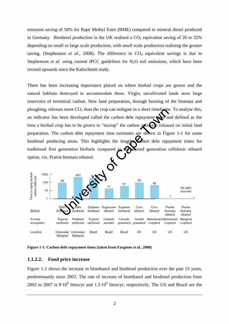
There has been increasing importance placed on where biofuel crops are grown and the

natural habitats destroyed to accommodate them. Virgin, uncultivated lands store large

reservoirs of terrestrial carbon. New land preparation, through burning of the biomass and

ploughing, releases more CO2 than the crop can mitigate in a short timeframe. To analyse this,

an indicator has been developed called the carbon debt repayment time and defined as the

time a biofuel crop has to be grown to “recoup” the carbon emission released on initial land

preparation. The carbon debt repayment time estimates are shown in Figure 1-1 for some

biodiesel producing areas. This highlights the lengthy carbon debt repayment times for

traditional first generation biofuels compared to the second generation cellulosic ethanol

option, viz. Prairie biomass ethanol.

Figure 1-1: Carbon debt repayment times (taken from Fargione et al., 2008)

1.1.2.2. Food price increase

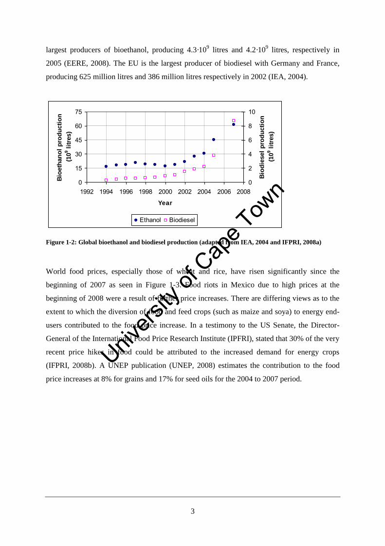
Figure 1-2 shows the increase in bioethanol and biodiesel production over the past 15 years,

predominantly since 2002. The rate of increase of bioethanol and biodiesel production from

2002 to 2007 is 8·109 litres/yr and 1.5·10

9 litres/yr, respectively. The US and Brazil are the

Univers

ity of

Cap

e Tow

n

3

largest producers of bioethanol, producing 4.3·109 litres and 4.2·10

9 litres, respectively in

2005 (EERE, 2008). The EU is the largest producer of biodiesel with Germany and France,

producing 625 million litres and 386 million litres respectively in 2002 (IEA, 2004).

0

15

30

45

60

75

1992 1994 1996 1998 2000 2002 2004 2006 2008

Year

Bio

eth

an

ol

pro

du

cti

on

(10

9 l

itre

s)

0

2

4

6

8

10

Bio

die

sel

pro

du

cti

on

(10

9 l

itre

s)

Ethanol Biodiesel

Figure 1-2: Global bioethanol and biodiesel production (adapted from IEA, 2004 and IFPRI, 2008a)

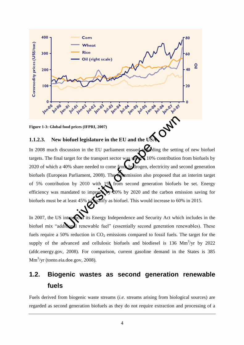
World food prices, especially those of wheat and rice, have risen significantly since the

beginning of 2007 as seen in Figure 1-3. Food riots in Mexico due to high prices at the

beginning of 2008 were a result of further price increases. There are differing views as to the

extent to which the diversion of food and feed crops (such as maize and soya) to energy end-

users contributed to the food price increase. In a testimony to the US Senate, the Director-

General of the International Food Price Research Institute (IPFRI), stated that 30% of the very

recent price hikes in food could be attributed to the increased demand for energy crops

(IFPRI, 2008b). A UNEP publication (UNEP, 2008) estimates the contribution to the food

price increases at 8% for grains and 17% for seed oils for the 2004 to 2007 period.

Univers

ity of

Cap

e Tow

n

4

Figure 1-3: Global food prices (IFPRI, 2007)

1.1.2.3. New biofuel legislature in the EU and the USA

In 2008 much discussion in the EU parliament ensued regarding the setting of new biofuel

targets. The final target for the transport sector was set at a 10% contribution from biofuels by

2020 of which a 40% share needed to come from hydrogen, electricity and second generation

biofuels (European Parliament, 2008). The Commission also proposed that an interim target

of 5% contribution by 2010 with 1% from second generation biofuels be set. Energy

efficiency was mandated to improve by 20% by 2020 and the carbon emission saving for

biofuels must be at least 45% to qualify as biofuel. This would increase to 60% in 2015.

In 2007, the US introduced its Energy Independence and Security Act which includes in the

biofuel mix “additional renewable fuel” (essentially second generation renewables). These

fuels require a 50% reduction in CO2 emissions compared to fossil fuels. The target for the

supply of the advanced and cellulosic biofuels and biodiesel is 136 Mm3/yr by 2022

(afdc.energy.gov, 2008). For comparison, current gasoline demand in the States is 385

Mm3/yr (tonto.eia.doe.gov, 2008).

1.2. Biogenic wastes as second generation renewable

fuels

Fuels derived from biogenic waste streams (i.e. streams arising from biological sources) are

regarded as second generation biofuels as they do not require extraction and processing of a

Univers

ity of

Cap

e Tow

n

5

single plant storage product nor do they compete with food crops. Renewable energy from

biogenic wastes is particularly attractive as the waste avoids additional land use and the

associated emissions from changing land use.

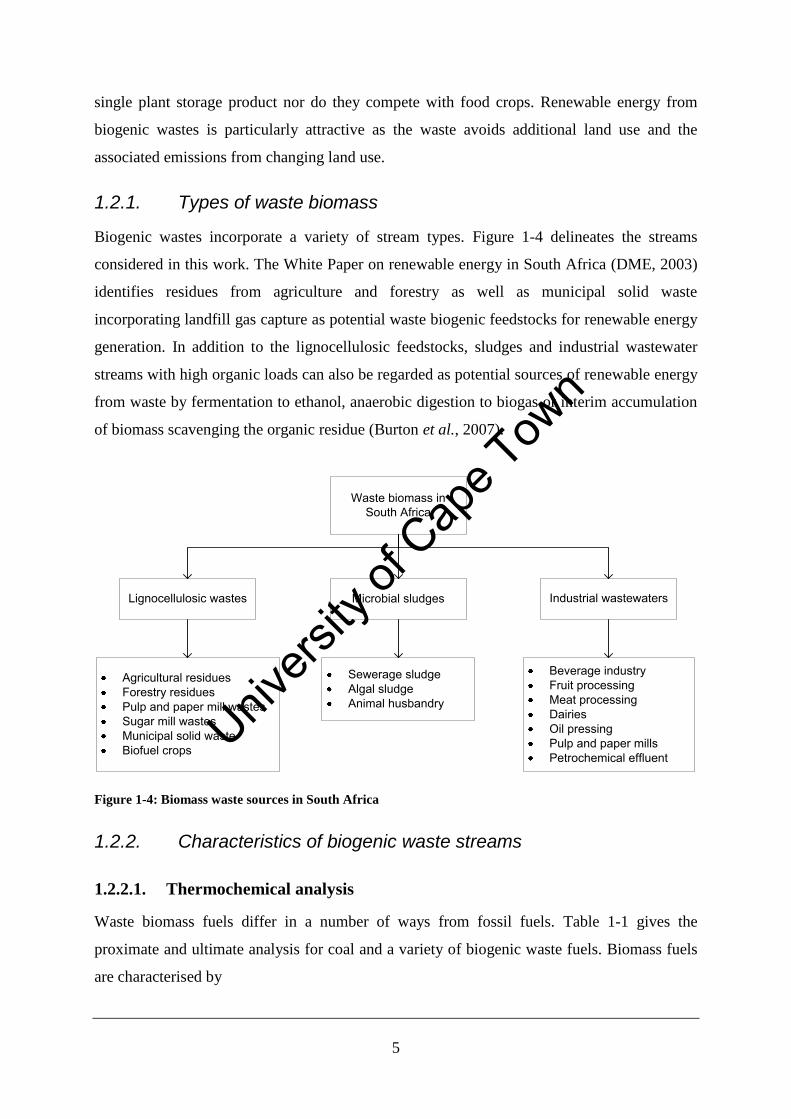
1.2.1. Types of waste biomass

Biogenic wastes incorporate a variety of stream types. Figure 1-4 delineates the streams

considered in this work. The White Paper on renewable energy in South Africa (DME, 2003)

identifies residues from agriculture and forestry as well as municipal solid waste

incorporating landfill gas capture as potential waste biogenic feedstocks for renewable energy

generation. In addition to the lignocellulosic feedstocks, sludges and industrial wastewater

streams with high organic loads can also be regarded as potential sources of renewable energy

from waste by fermentation to ethanol, anaerobic digestion to biogas or interim accumulation

of biomass scavenging the organic residue (Burton et al., 2007).

Waste biomass in South Africa

Lignocellulosic wastes Microbial sludges Industrial wastewaters

Agricultural residuesForestry residuesPulp and paper mill wastesSugar mill wastesMunicipal solid wasteBiofuel crops

Sewerage sludgeAlgal sludgeAnimal husbandry

Beverage industryFruit processingMeat processingDairiesOil pressingPulp and paper millsPetrochemical effluent

Figure 1-4: Biomass waste sources in South Africa

1.2.2. Characteristics of biogenic waste streams

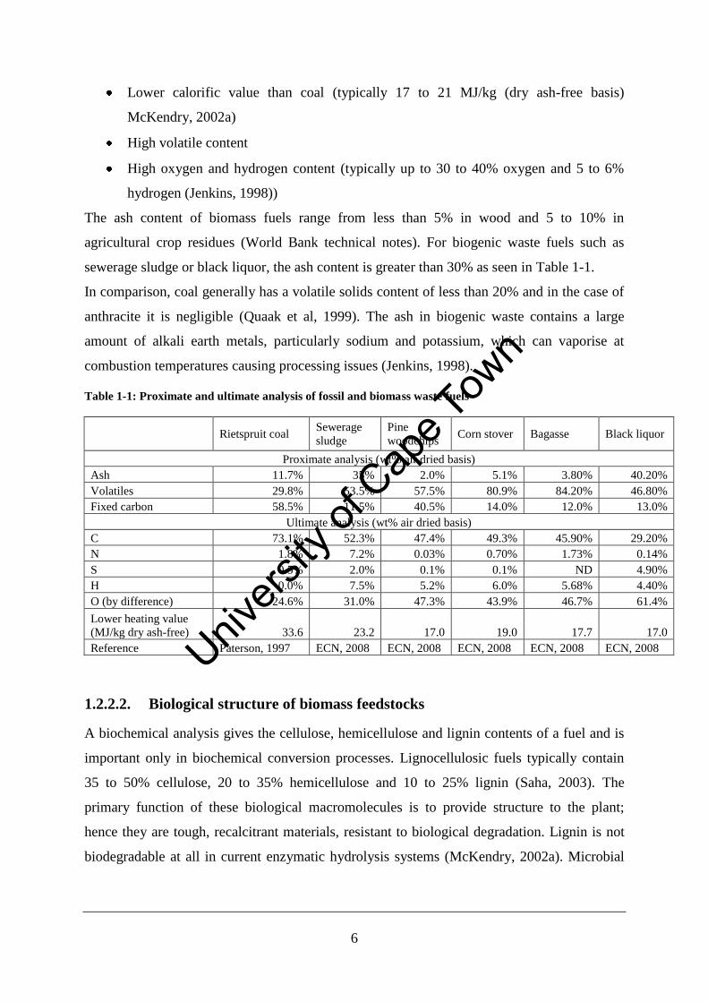
1.2.2.1. Thermochemical analysis

Waste biomass fuels differ in a number of ways from fossil fuels. Table 1-1 gives the

proximate and ultimate analysis for coal and a variety of biogenic waste fuels. Biomass fuels

are characterised by

Univers

ity of

Cap

e Tow

n

6

Lower calorific value than coal (typically 17 to 21 MJ/kg (dry ash-free basis)

McKendry, 2002a)

High volatile content

High oxygen and hydrogen content (typically up to 30 to 40% oxygen and 5 to 6%

hydrogen (Jenkins, 1998))

The ash content of biomass fuels range from less than 5% in wood and 5 to 10% in

agricultural crop residues (World Bank technical notes). For biogenic waste fuels such as

sewerage sludge or black liquor, the ash content is greater than 30% as seen in Table 1-1.

In comparison, coal generally has a volatile solids content of less than 20% and in the case of

anthracite it is negligible (Quaak et al, 1999). The ash in biogenic waste contains a large

amount of alkali earth metals, particularly sodium and potassium, which can vaporise at

combustion temperatures causing processing issues (Jenkins, 1998).

Table 1-1: Proximate and ultimate analysis of fossil and biomass waste fuels

Rietspruit coal

Sewerage

sludge

Pine

woodchips Corn stover Bagasse Black liquor

Proximate analysis (wt% air dried basis)

Ash 11.7% 35% 2.0% 5.1% 3.80% 40.20%

Volatiles 29.8% 53.5% 57.5% 80.9% 84.20% 46.80%

Fixed carbon 58.5% 11.5% 40.5% 14.0% 12.0% 13.0%

Ultimate analysis (wt% air dried basis)

C 73.1% 52.3% 47.4% 49.3% 45.90% 29.20%

N 1.8% 7.2% 0.03% 0.70% 1.73% 0.14%

S 0.5% 2.0% 0.1% 0.1% ND 4.90%

H 0.0% 7.5% 5.2% 6.0% 5.68% 4.40%

O (by difference) 24.6% 31.0% 47.3% 43.9% 46.7% 61.4%

Lower heating value

(MJ/kg dry ash-free) 33.6 23.2 17.0 19.0 17.7 17.0

Reference Paterson, 1997 ECN, 2008 ECN, 2008 ECN, 2008 ECN, 2008 ECN, 2008

1.2.2.2. Biological structure of biomass feedstocks

A biochemical analysis gives the cellulose, hemicellulose and lignin contents of a fuel and is

important only in biochemical conversion processes. Lignocellulosic fuels typically contain

35 to 50% cellulose, 20 to 35% hemicellulose and 10 to 25% lignin (Saha, 2003). The

primary function of these biological macromolecules is to provide structure to the plant;

hence they are tough, recalcitrant materials, resistant to biological degradation. Lignin is not

biodegradable at all in current enzymatic hydrolysis systems (McKendry, 2002a). Microbial

Univers

ity of

Cap

e Tow

n

7

sludges resist biological action due to the complex cellular walls of the microbes which make

up the sludge (e.g. domestic sewerage sludge or algal sludge) (Speece, 1996).

1.2.2.3. Other

Other factors aside, moisture content, or its inverse, dry solids content, is the single

determining factor when choosing an energy conversion process (McKendry, 2002a).

Thermal conversion processes typically require moisture content less than 65% to be

energetically favourable (Jenkins, 1998) whereas biological conversion processes can utilise

high moisture content feedstocks.

The bulk density of waste biogenic fuels affects transport and storage costs and sizing of

material handling systems (McKendry, 2002a). Baling and pelleting or briquetting of biomass

is often necessary to reduce the transport costs and make handling easier. For example, the

bulk density of sawdust is 0.12 ton/m3 compared to wood pellets which are 0.56 ton/m

3.

1.3. Sustainable energy supply in South Africa

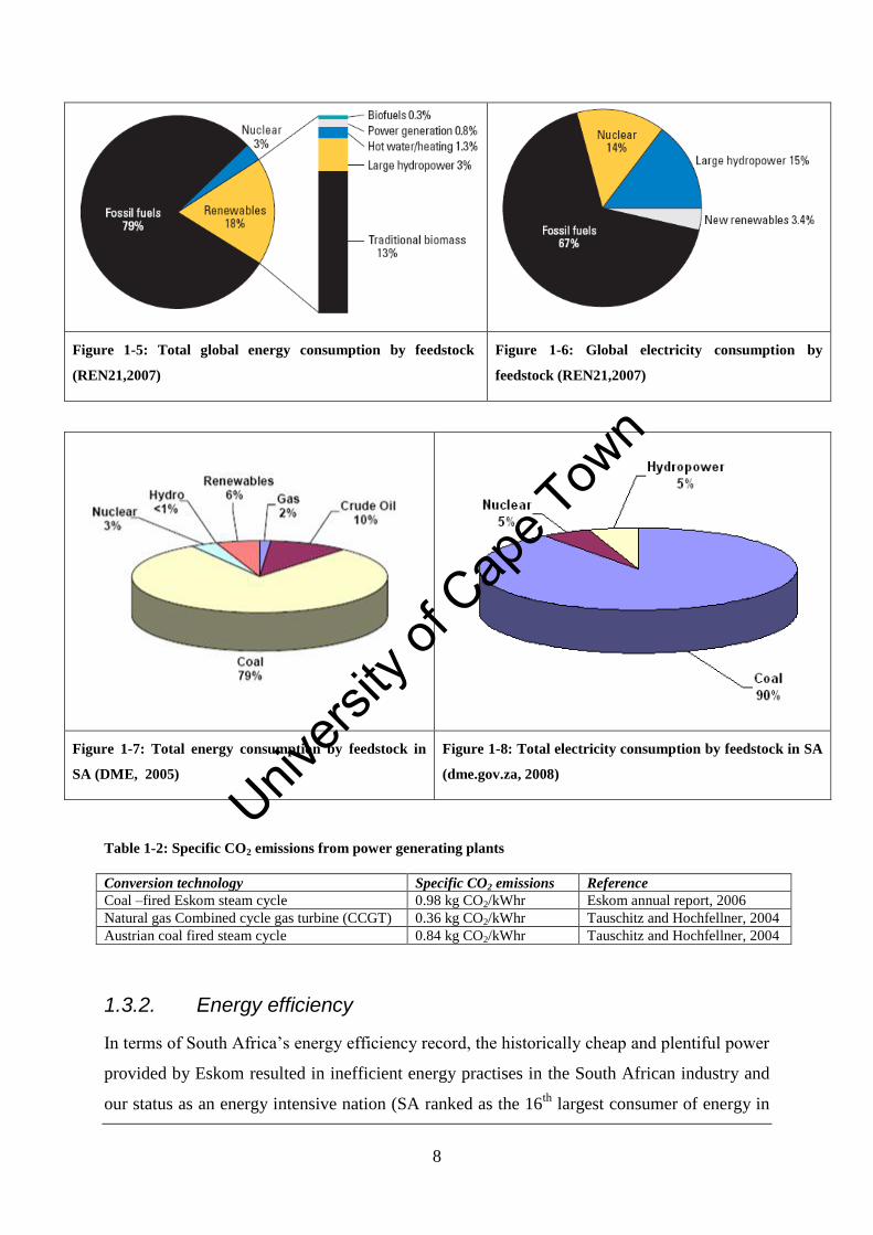
1.3.1. Current energy supply situation in South Africa

Figure 1-5 to Figure 1-8 compare the global primary energy and electricity consumption by

feedstock to South Africa. It is clear that South Africa lags behind world trend towards greater

inclusion of renewables in the energy mix. The 6% contribution of renewables to total energy

consumption in South Africa is primarily from fuelwood and dung for heating in rural areas.

However, the practise is unsustainable as it results in deforestation and soil nutrient depletion

in the surrounding areas (DME, 2003). The legacy of cheap coal to provide liquid fuel and

electricity in South Africa removed the need to diversity our energy mix.

The use of coal as a feedstock to our power plants and their low efficiencies result in high

CO2 emissions per kilowatt-hour of electricity produced. Table 1-2 compares specific CO2

emissions for various power generating plants

Univers

ity of

Cap

e Tow

n

8

Figure 1-5: Total global energy consumption by feedstock

(REN21,2007)

Figure 1-6: Global electricity consumption by

feedstock (REN21,2007)

Figure 1-7: Total energy consumption by feedstock in

SA (DME, 2005)

Figure 1-8: Total electricity consumption by feedstock in SA

(dme.gov.za, 2008)

Table 1-2: Specific CO2 emissions from power generating plants

Conversion technology Specific CO2 emissions Reference

Coal –fired Eskom steam cycle 0.98 kg CO2/kWhr Eskom annual report, 2006

Natural gas Combined cycle gas turbine (CCGT) 0.36 kg CO2/kWhr Tauschitz and Hochfellner, 2004

Austrian coal fired steam cycle 0.84 kg CO2/kWhr Tauschitz and Hochfellner, 2004

1.3.2. Energy efficiency

In terms of South Africa’s energy efficiency record, the historically cheap and plentiful power

provided by Eskom resulted in inefficient energy practises in the South African industry and

our status as an energy intensive nation (SA ranked as the 16th

largest consumer of energy in

Univers

ity of

Cap

e Tow

n

9

2001 and our GDP ranked 26th

(DME, 2005). The recent energy demand exceeding supply

has highlighted the need to revise our energy practises.

Whilst energy efficiency in the EU has been legislated, in South Africa energy efficiency

improvements remain voluntary. The Energy Efficiency Strategy released by the Department

of Minerals and Energy (DME, 2005) sets a national target for an energy efficiency

improvement of 12% by 2015. The improvements are expected to be brought about by

economic and legislative means, efficiency labels and performance standards and energy

audits. In response, the formation of the National Business Initiative brought 24 companies

and 7 industrial associations together to pledge to reduce their energy demand by 15% by

2015 voluntarily. Further business level collaboration has been limited, hence the efficacy of

the Strategy without legislation is in question (NBI, 2008).

1.3.3. Increasing the renewable energy share in South Africa

In the White Paper on renewable energy policy for South Africa (2003) a national target of

sourcing 10 000 GWhr or 0.8 Million Tone Oil Equivalent (MTOE) from renewable resources

by 2013 was set; this equates to 4% of the projected 2013 demand or 4.5% of current demand.

Biomass energy, biofuels (as liquid transport fuels), hydropower, wind, solar, geothermal and

tidal power are cited as potential renewable energy resources. The Paper specifies that the

renewable resources should contribute primarily to electricity supply.

Few estimates of the energy available from biomass energy or biogenic wastes in South

Africa exist in literature. The DME provided some estimates in the White Paper (DME,

2004). Williams and Eberhard (1988) and Lynd et al. (2003) presented data on the energy

potential from lignocellulosic waste streams. Burton et al. (2007) reviewed the potential

contribution of wastewater sources.

1.4. Problem statement, key questions and objectives

Second generation renewables, including those from biogenic waste streams, may be regarded

as a more sustainable energy form than first generation renewables. Further, South Africa

needs to increase its share of renewables in the electricity mix. Electricity generation from

biogenic waste streams is one possibility which warrants further exploration.

Univers

ity of

Cap

e Tow

n

10

To address the potential for electricity production from biogenic waste streams a series of key

questions can be identified:

What established technologies are suitable for generating electricity from second

generation biofuel resources, particularly biogenic waste streams?

What barriers or technical difficulties exist when processing biogenic wastes and what

feedstock pretreatments aid in implementing these technologies to process waste?

From simple energy balances and operational experience, can the energy yield for

different technologies be established, based on intrinsic feedstock characteristics?

Where more than one technology is available to process a feedstock, can a defined

analytical framework assist in technology selection?

What is the energy potential of biogenic waste streams in South Africa?

Would realising this potential infringe on alternate uses of the waste?

To address the potential for electricity generation from biogenic waste streams, a series of key

objecties can be identified:

1. Identify technologies suitable for processing biogenic waste in South Africa.

2. Develop an energy yield model for technologies suitable for the South African context

3. Validate the model using wastewater treatment plant data

4. Consider the trade-off between the energy cost of feedstock pretreatment and

improved energy yield for two commercial microbial sludge pretreatments.

5. Investigate the effect of operational variables on the energy efficiency of combustion

of two biogenic waste fuels.

6. Generate a decision-making tool for selecting a technology based on feedstock

characteristics.

7. Determine the potential energy from biogenic waste in SA using the above tools and

compare these estimates to previous studies.

8. Consider the alternate uses of biogenic waste streams or, if applicable, their current

use and the energy efficiency thereof to enable a realistic estimation of biogenic

electricity potential in South Africa.

Univers

ity of

Cap

e Tow

n

11

1.5. Thesis structure

Chapter 2 considers technologies which may be used to generate electricity from biogenic

waste streams. Specifically the process, reactor types and current installations, challenges and

feedstock preparation techniques for combustion (Section 2.2), gasification (Section 2.3) and

anaerobic digestion (Section 2.4) are considered.

In Chapter 3, case studies of three wastewater treatment plants which feature different

technologies for energy recovery are presented. While these data were sourced from the UK,

they are not regionally dependent and so have relevance to the South African case. The

selection of the UK data resulted as South African data of equivalent detail was not available.

Plant operation observations are presented to highlight the challenges of these systems and

their potential. The ability of the technologies to deliver heat and power are compared. An

energy yield model is derived and is compared to plant data to investigate its ability to assist

decision making.

Chapter 4 considers the effect of characteristics specific to biogenic waste on the processing

of these fuels. Two studies are presented: the effect of recalcitrant material on biogas yield in

anaerobic digestion (Section 4.1) and the effect of high volatile content on combustion in

fluidised beds (Section 4.2).

In Chapter 5 a technology selection methodology is presented to assist in estimating the

potential energy yield from biogenic waste streams in South Africa. Alternate uses and

current practice are compared with best practice, allowing realistic energy estimates to be

prepared. The conclusions and significance of the study are presented in Chapter 6. Univers

ity of

Cap

e Tow

n

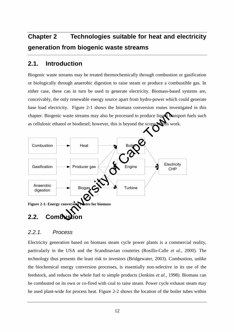
12

Chapter 2 Technologies suitable for heat and electricity

generation from biogenic waste streams

2.1. Introduction

Biogenic waste streams may be treated thermochemically through combustion or gasification

or biologically through anaerobic digestion to raise steam or produce a combustible gas. In

either case, these can in turn be used to generate electricity. Biomass-based systems are,

conceivably, the only renewable energy source apart from hydro-power which could generate

base load electricity. Figure 2-1 shows the biomass conversion routes investigated in this

chapter. Biogenic waste streams may also be processed to produce liquid transport fuels such

as cellulosic ethanol or biodiesel; however, this is beyond the scope of this work.

Combustion

Gasification

Anaerobic digestion

Heat

Producer gas

Biogas

Boiler

Engine

Turbine

ElectricityCHP

Figure 2-1: Energy conversion routes for biomass

2.2. Combustion

2.2.1. Process

Electricity generation based on biomass steam cycle power plants is a commercial reality,

particularly in the USA and the Scandinavian countries (Rosillo-Calle et al., 2000). The

technology thus presents the least risk to investors (Bridgewater, 2003). Combustion, unlike

the biochemical energy conversion processes, is essentially non-selective in its use of the

feedstock, and reduces the whole fuel to simple products (Jenkins et al., 1998). Biomass can

be combusted on its own or co-fired with coal to raise steam. Power cycle exhaust steam may

be used plant-wide for process heat. Figure 2-2 shows the location of the boiler tubes within

Univers

ity of

Cap

e Tow

n

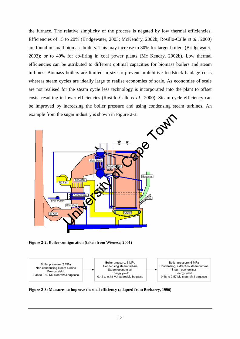
13

the furnace. The relative simplicity of the process is negated by low thermal efficiencies.

Efficiencies of 15 to 20% (Bridgewater, 2003; McKendry, 2002b; Rosillo-Calle et al., 2000)

are found in small biomass boilers. This may increase to 30% for larger boilers (Bridgewater,

2003); or to 40% for co-firing in coal power plants (Mc Kendry, 2002b). Low thermal

efficiencies can be attributed to different optimal capacities for biomass boilers and steam

turbines. Biomass boilers are limited in size to prevent prohibitive feedstock haulage costs

whereas steam cycles are ideally large to realise economies of scale. As economies of scale

are not realised for the steam cycle less technology is incorporated into the plant to offset

costs, resulting in lower efficiencies (Rosillo-Calle et al., 2000). Steam cycle efficiency can

be improved by increasing the boiler pressure and using condensing steam turbines. An

example from the sugar industry is shown in Figure 2-3.

Figure 2-2: Boiler configuration (taken from Wienese, 2001)

Boiler pressure: 2 MPaNon-condensing steam turbine

Energy yield: 0.38 to 0.42 MJ steam/MJ bagasse

Boiler pressure: 3 MPaCondensing steam turbine

Steam economiserEnergy yield:

0.42 to 0.48 MJ steam/MJ bagasse

Boiler pressure: 6 MPaCondensing, extraction steam turbine

Steam economiserEnergy yield:

0.48 to 0.57 MJ steam/MJ bagasse

Figure 2-3: Measures to improve thermal efficiency (adapted from Beeharry, 1996)

Univers

ity of

Cap

e Tow

n

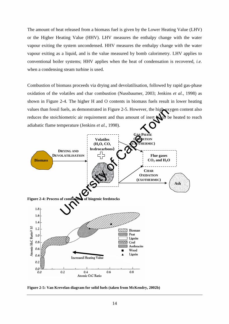
14

The amount of heat released from a biomass fuel is given by the Lower Heating Value (LHV)

or the Higher Heating Value (HHV). LHV measures the enthalpy change with the water

vapour exiting the system uncondensed. HHV measures the enthalpy change with the water

vapour exiting as a liquid, and is the value measured by bomb calorimetry. LHV applies to

conventional boiler systems; HHV applies when the heat of condensation is recovered, i.e.

when a condensing steam turbine is used.

Combustion of biomass proceeds via drying and devolatilisation, followed by rapid gas-phase

oxidation of the volatiles and char combustion (Nussbaumer, 2003; Jenkins et al., 1998) as

shown in Figure 2-4. The higher H and O contents in biomass fuels result in lower heating

values than fossil fuels, as demonstrated in Figure 2-5. However, the high oxygen content also

reduces the stoichiometric air requirement and thus amount of inert N2 to be heated to reach

adiabatic flame temperature (Jenkins et al., 1998).

Figure 2-4: Process of combustion of biogenic feedstocks

Figure 2-5: Van Krevelan diagram for solid fuels (taken from McKendry, 2002b)

Volatiles

(H2O, CO,

hydrocarbons)

GAS PHASE

OXIDATION

(EXOTHERMIC)

Flue gases

CO2 and H2O

Ash

CHAR

OXIDATION

(EXOTHERMIC)

DRYING AND

DEVOLATILISATION

Char

Biomass

Univers

ity of

Cap

e Tow

n

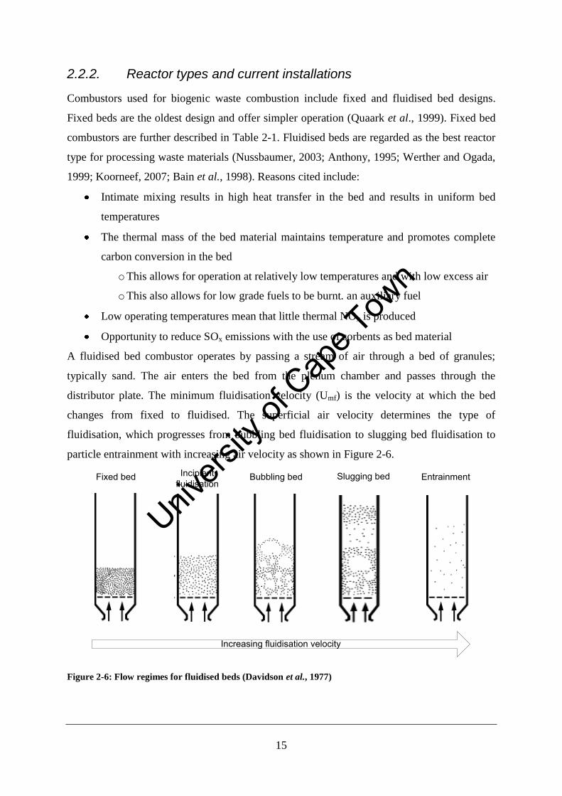
15

2.2.2. Reactor types and current installations

Combustors used for biogenic waste combustion include fixed and fluidised bed designs.

Fixed beds are the oldest design and offer simpler operation (Quaark et al., 1999). Fixed bed

combustors are further described in Table 2-1. Fluidised beds are regarded as the best reactor

type for processing waste materials (Nussbaumer, 2003; Anthony, 1995; Werther and Ogada,

1999; Koorneef, 2007; Bain et al., 1998). Reasons cited include:

Intimate mixing results in high heat transfer in the bed and results in uniform bed

temperatures

The thermal mass of the bed material maintains temperature and promotes complete

carbon conversion in the bed

o This allows for operation at relatively low temperatures and with low excess air

o This also allows for low grade fuels to be burnt. an auxiliary fuel

Low operating temperatures mean that little thermal NOx is produced

Opportunity to reduce SOx emissions with the use of sorbents as bed material

A fluidised bed combustor operates by passing a stream of air through a bed of granules;

typically sand. The air enters the bed from the plenum chamber and passes through the

distributor plate. The minimum fluidisation velocity (Umf) is the velocity at which the bed

changes from fixed to fluidised. The superficial air velocity determines the type of

fluidisation, which progresses from bubbling bed fluidisation to slugging bed fluidisation to

particle entrainment with increasing air velocity as shown in Figure 2-6.

Fixed bed Incipient fluidisation

Bubbling bed Slugging bed Entrainment

Increasing fluidisation velocity

Figure 2-6: Flow regimes for fluidised beds (Davidson et al., 1977)

Univers

ity of

Cap

e Tow

n

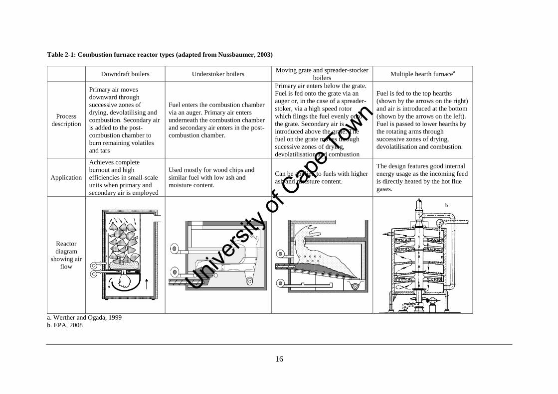
16

Table 2-1: Combustion furnace reactor types (adapted from Nussbaumer, 2003)

Downdraft boilers Understoker boilers Moving grate and spreader-stocker

boilers Multiple hearth furnace

a

Process

description

Primary air moves

downward through

successive zones of

drying, devolatilising and

combustion. Secondary air

is added to the post-

combustion chamber to

burn remaining volatiles

and tars

Fuel enters the combustion chamber

via an auger. Primary air enters

underneath the combustion chamber

and secondary air enters in the post-

combustion chamber.

Primary air enters below the grate.

Fuel is fed onto the grate via an

auger or, in the case of a spreader-

stoker, via a high speed rotor

which flings the fuel evenly onto

the grate. Secondary air is

introduced above the grate. The

fuel on the grate moves through

sucessive zones of drying,

devolatilisation and combustion

Fuel is fed to the top hearths

(shown by the arrows on the right)

and air is introduced at the bottom

(shown by the arrows on the left).

Fuel is passed to lower hearths by

the rotating arms through

successive zones of drying,

devolatilisation and combustion.

Application

Achieves complete

burnout and high

efficiencies in small-scale

units when primary and

secondary air is employed

Used mostly for wood chips and

similar fuel with low ash and

moisture content.

Can be applied to fuels with higher

ash and moisture content.

The design features good internal

energy usage as the incoming feed

is directly heated by the hot flue

gases.

Reactor

diagram

showing air

flow

a. Werther and Ogada, 1999

b. EPA, 2008

b

Univers

ity of

Cap

e Tow

n

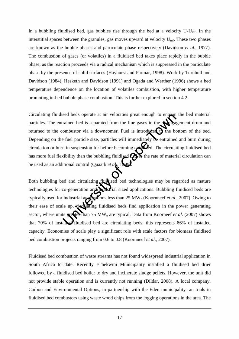
17

In a bubbling fluidised bed, gas bubbles rise through the bed at a velocity U-Umf. In the

interstitial spaces between the granules, gas moves upward at velocity Umf. These two phases

are known as the bubble phases and particulate phase respectively (Davidson et al., 1977).

The combustion of gases (or volatiles) in a fluidised bed takes place rapidly in the bubble

phase, as the reaction proceeds via a radical mechanism which is suppressed in the particulate

phase by the presence of solid surfaces (Hayhurst and Parmar, 1998). Work by Turnbull and

Davidson (1984), Hesketh and Davidson (1991) and Ogada and Werther (1996) shows a bed

temperature dependence on the location of volatiles combustion, with higher temperature

promoting in-bed bubble phase combustion. This is further explored in section 4.2.

Circulating fluidised beds operate at air velocities great enough to entrain the bed material

particles. The entrained bed is separated from the flue gases in the disengagement drum and

returned to the combustor via a downcomer. Fuel is introduced to the bottom of the bed.

Depending on the fuel particle size, particles will immediately be entrained and burn during

circulation or burn in suspension for before becoming entrained. The circulating fluidised bed

has more fuel flexibility than the bubbling fluidised bed as the rate of material circulation can

be used as an additional control (Quaark et al., 1999).

Both bubbling bed and circulating fluidised bed technologies may be regarded as mature

technologies for co-generation and industrial sized applications. Bubbling fluidised beds are

typically used for industrial applications less than 25 MWe (Koornneef et al., 2007). Owing to

their ease of scale up, circulating fluidised beds find application in the power generating

sector, where units greater than 75 MWe are typical. Data from Koorneef et al. (2007) shows

that 70% of installed fluidised bed are circulating beds; this represents 86% of installed

capacity. Economies of scale play a significant role with scale factors for biomass fluidised

bed combustion projects ranging from 0.6 to 0.8 (Koornneef et al., 2007).

Fluidised bed combustion of waste streams has not found widespread industrial application in

South Africa to date. Recently eThekwini Municipality installed a fluidised bed drier

followed by a fluidised bed boiler to dry and incinerate sludge pellets. However, the unit did

not provide stable operation and is currently not running (Dildar, 2008). A local company,

Carbon and Environmental Options, in partnership with the Eden municipality ran trials in

fluidised bed combustors using waste wood chips from the logging operations in the area. The

Univers

ity of

Cap

e Tow

n

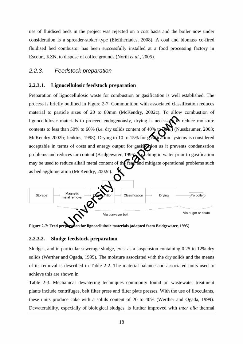
18

use of fluidised beds in the project was rejected on a cost basis and the boiler now under

consideration is a spreader-stoker type (Eleftheriades, 2008). A coal and biomass co-fired

fluidised bed combustor has been successfully installed at a food processing factory in

Escourt, KZN, to dispose of coffee grounds (North et al., 2005).

2.2.3. Feedstock preparation

2.2.3.1. Lignocellulosic feedstock preparation

Preparation of lignocellulosic waste for combustion or gasification is well established. The

process is briefly outlined in Figure 2-7. Communition with associated classification reduces

material to particle sizes of 20 to 80mm (McKendry, 2002c). To allow combustion of

lignocellulosic materials to proceed endogenously, drying is necessary to reduce moisture

contents to less than 50% to 60% (i.e. dry solids content of 40% to 50%) (Nussbaumer, 2003;

McKendry 2002b; Jenkins, 1998). Drying to 10 to 15% for gasification systems is considered

acceptable in terms of costs and energy output for gasification as it prevents condensation

problems and reduces tar content (Bridgewater, 1995). Leaching in water prior to gasification

may be used to reduce alkali metal content of the feed and mitigate operational problems such

as bed agglomeration (McKendry, 2002c).

Communition Classification DryingMagnetic metal removalStorage

Via conveyor belt Via auger or chute

To boiler

Figure 2-7: Feed preparation for lignocellulosic materials (adapted from Bridgewater, 1995)

2.2.3.2. Sludge feedstock preparation

Sludges, and in particular sewerage sludge, exist as a suspension containing 0.25 to 12% dry

solids (Werther and Ogada, 1999). The moisture associated with the dry solids and the means

of its removal is described in Table 2-2. The material balance and associated units used to

achieve this are shown in

Table 2-3. Mechanical dewatering techniques commonly found on wastewater treatment

plants include centrifuges, belt filter press and filter plate presses. With the use of flocculants,

these units produce cake with a solids content of 20 to 40% (Werther and Ogada, 1999).

Dewaterability, especially of biological sludges, is further improved with inter alia thermal

Univers

ity of

Cap

e Tow

n

19

conditioning as this ruptures the cell water and releases the intracellular water. Comparative

capital expense and operating expenses of the dewatering units are given in

Table 2-4.

Table 2-2: Types of water found in sludge (adapted from Werther and Ogada, 1999 and Vesilind, 1994)

Moisture

association

Description Removal technique

Free water Water not associated with or

influenced by solid particles

Thickening

Interstitial or

floc water

Water trapped in the crevices and

interstices of flocs and organisms

Mechanical dewatering

Capillary or

vicinal moisture

Layers of water held to the particle

surface by hydrogen bonding

Mechanical dewatering

with chemical conditioning

Intracellular

water

Water inside the organism Water only released after

cell disruption

Table 2-3: Materal balance and unit operations for increasing dry solids content of sludge

Process Thickening Dewatering

Unit operation Gravity

thickener

Gravity belt

thickener

Belt filter press; filter plate

press; solid bowl centrifuge

Dry solids content of sludge 1% 6% 15% 28%

Total mass (kg/kg dry solids) 100 17 7 4

Table 2-4: Operating and capital expenses of dewatering equipment

Capital expense a

Operating expense a

Energy consumption

Belt press Low Low 30 to 60 MJ/ton dry solids

Filter plate press High High Similar to above

Solid bowl centrifuge Medium Medium 100 to 300 MJ/ton dry solids

a.) Bane, 2000

b.) adapted from Wang et al., 2007

(1) Gravity belt thickeners

Horizontal gravity belt thickeners consist of a continuously rolling belt onto which sludge is

evenly introduced at one end. Thickening occurs by gravity as the water falls through the

porous belt. The thickened sludge is discharged at the other end of the belt. The belts are self-

cleaning as the water dropping through the belt at the top fall onto the belt below. The unit is

good for coarse fast settling solids (McCabe et al., 2005). With the addition of polymer

flocculants, gravity belt thickeners increase the dry solids content from 1% to 6% dry solids

content (Fountain, 2008). Although this unit is strictly speaking a thickener and not a

dewatering unit, it is included here for completeness as it is used upstream of the dewatering

units.

Univers

ity of

Cap

e Tow

n

20

(2) Belt filter press

Belt filter presses comprise of a continuously rolling belt onto which the sludge is fed.

Following a section of gravity thickening, the sludge is then squeezed between two opposing

porous cloth belts. The belts are rolled between successively smaller rollers which increase

the pressure and force the water through the belt. The sludge is scraped off the belt into a

collection bin by scraper blades. Belt filter presses increase the solids content from about 5%

to 15% to 28% depending on the proportion of biological sludge in the feed. The unit is the

preferred dewatering technique in the US. Its main disadvantage is sensitivity to wide

variations in sludge characteristics (Tchobanoglous et al., 2003).

(3) Filter plate press

A filter plate press is operated in batch mode. It consists of a number of plates, recessed on

both sides, supported on a frame. A filter cloth covers each plate. Sludge is introduced to the

compartments between each plate under 3 to 10 bar pressure. Water is forced through the

filter cloth into a discharge pipe. Once sufficient water has been removed the pressure is

released and the plates are separated. The wet cake is dropped into a collection bin (McCabe

et al., 2005). Discharge solids contents of 48 to 70% cited (Tchobanoglous et al., 2003);

however operational difficulties, such as blinded filter cloth, can result in discharge solids

contents of 20 to 25% (Fountain, 2008). Disadvantages of the unit include excessive

downtime for equipment maintenance and high labour costs (Tchobanoglous et al., 2003)

(4) Solid bowl centrifuge

A solid bowl centrifuge consists of a horizontally mounted centrifuge bowl inside which a

helical scroll, rotating slightly slower than the bowl, moves the solids to one end of the bowl.

“Centrate” or liquor is withdrawn from the other end (McCabe et al., 2005). Discharge solids

content ranges from 10 to 30% depending on the amount of biological sludge (Tchobanoglous

et al., 2003). Disadvantages of the unit include high power costs (typically three times more

than belt filter presses (Fountain, 2008)).

2.2.4. Summary

Combustion of biogenic waste fuels, particularly woody biomass and sewerage sludge is well-

established technology. The units involved in the preparation of fuel prior to combustion are

Univers

ity of

Cap

e Tow

n

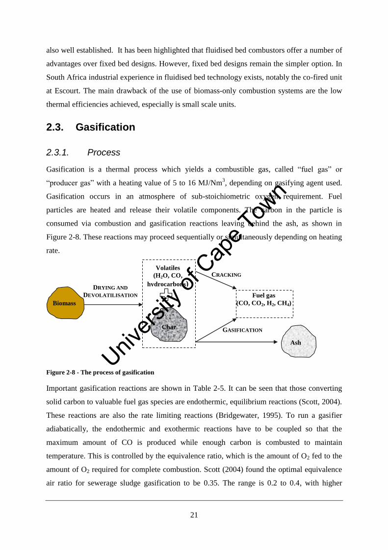
21

also well established. It has been highlighted that fluidised bed combustors offer a number of

advantages over fixed bed designs. However, fixed bed designs remain the simpler option. In

South Africa industrial experience in fluidised bed technology exists, notably the co-fired unit

at Escourt. The main drawback of the use of biomass-only combustion systems are the low

thermal efficiencies achieved, especially is small scale units.

2.3. Gasification

2.3.1. Process

Gasification is a thermal process which yields a combustible gas, called “fuel gas” or

“producer gas” with a heating value of 5 to 16 MJ/Nm3, depending on gasifying agent used.

Gasification occurs in an atmosphere of sub-stoichiometric oxygen requirement. Fuel

particles are heated and release their volatile components. The carbon in the particle is

consumed via combustion and gasification reactions leaving behind the ash, as shown in

Figure 2-8. These reactions may proceed sequentially or simultaneously depending on heating

rate.

Figure 2-8 - The process of gasification

Important gasification reactions are shown in Table 2-5. It can be seen that those converting

solid carbon to valuable fuel gas species are endothermic, equilibrium reactions (Scott, 2004).

These reactions are also the rate limiting reactions (Bridgewater, 1995). To run a gasifier

adiabatically, the endothermic and exothermic reactions have to be coupled so that the

maximum amount of CO is produced while enough carbon is combusted to maintain

temperature. This is controlled by the equivalence ratio, which is the amount of O2 fed to the

amount of O2 required for complete combustion. Scott (2004) found the optimal equivalence

air ratio for sewerage sludge gasification to be 0.35. The range is 0.2 to 0.4, with higher

Volatiles

(H2O, CO,

hydrocarbons)

CRACKING

Fuel gas

(CO, CO2, H2, CH4)

Ash

GASIFICATION

DRYING AND

DEVOLATILISATION

Char

Biomass

Univers

ity of

Cap

e Tow

n

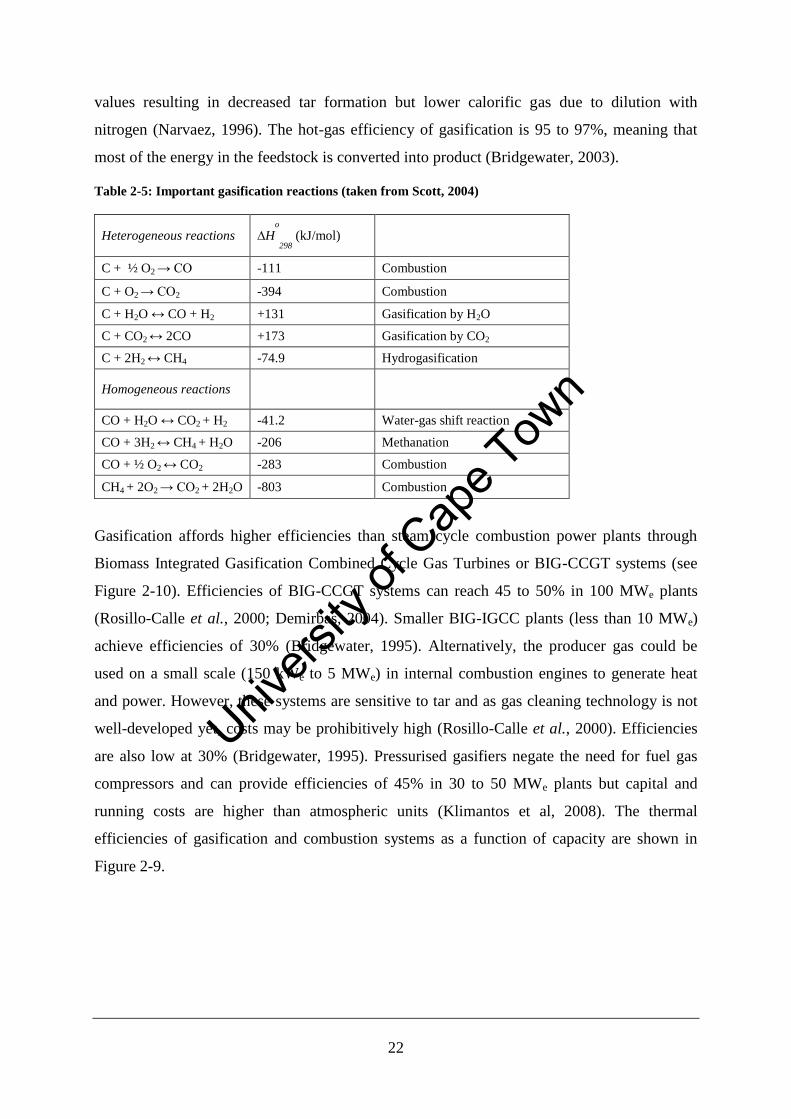
22

values resulting in decreased tar formation but lower calorific gas due to dilution with

nitrogen (Narvaez, 1996). The hot-gas efficiency of gasification is 95 to 97%, meaning that

most of the energy in the feedstock is converted into product (Bridgewater, 2003).

Table 2-5: Important gasification reactions (taken from Scott, 2004)

Heterogeneous reactions ∆Ho

298 (kJ/mol)

C + ½ O2 → CO -111 Combustion

C + O2 → CO2 -394 Combustion

C + H2O ↔ CO + H2 +131 Gasification by H2O

C + CO2 ↔ 2CO +173 Gasification by CO2

C + 2H2 ↔ CH4 -74.9 Hydrogasification

Homogeneous reactions

CO + H2O ↔ CO2 + H2 -41.2 Water-gas shift reaction

CO + 3H2 ↔ CH4 + H2O -206 Methanation

CO + ½ O2 ↔ CO2 -283 Combustion

CH4 + 2O2 → CO2 + 2H2O -803 Combustion

Gasification affords higher efficiencies than steam cycle combustion power plants through

Biomass Integrated Gasification Combined Cycle Gas Turbines or BIG-CCGT systems (see

Figure 2-10). Efficiencies of BIG-CCGT systems can reach 45 to 50% in 100 MWe plants

(Rosillo-Calle et al., 2000; Demirbas, 2004). Smaller BIG-IGCC plants (less than 10 MWe)

achieve efficiencies of 30% (Bridgewater, 1995). Alternatively, the producer gas could be

used on a small scale (150 kWe to 5 MWe) in internal combustion engines to generate heat

and power. However, these systems are sensitive to tar and as gas cleaning technology is not

well-developed yet, costs may be prohibitively high (Rosillo-Calle et al., 2000). Efficiencies

are also low at 30% (Bridgewater, 1995). Pressurised gasifiers negate the need for fuel gas

compressors and can provide efficiencies of 45% in 30 to 50 MWe plants but capital and

running costs are higher than atmospheric units (Klimantos et al, 2008). The thermal

efficiencies of gasification and combustion systems as a function of capacity are shown in

Figure 2-9.

Univers

ity of

Cap

e Tow

n

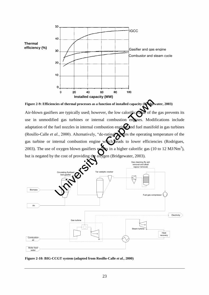
23

Thermal

efficiency (%)

Figure 2-9: Efficiencies of thermal processes as a function of installed capacity (Bridgewater, 2003)

Air-blown gasifiers are typically used; however, the low calorific value of the gas prevents its

use in unmodified gas turbines or internal combustion engines. Modifications include

adaptation of the fuel nozzles in internal combustion engines and fuel manifold in gas turbines

(Rosillo-Calle et al., 2000). Alternatively, “de-rating” lowers the operating temperature of the

gas turbine or internal combustion engine which leads to lower efficiencies (Rodrigues,

2003). The use of oxygen blown gasifiers results in a higher calorific gas (10 to 12 MJ/Nm3),

but is negated by the cost of providing the oxygen (Bridgewater, 2003).

Biomass

Heat recovery

Air

Combustionair

Boiler feedwater

Gas cleaning (fly ash removal and alkali vapour removal)

Tar catalytic crackerCirculating fluidised bed gasifier

Fuel gas compressor

Electricity

Steam turbine

Gas turbine

Figure 2-10: BIG-CCGT system (adapted from Rosillo-Calle et al., 2000)

Installed capacity (MW)

IGCC

Gasifier and gas engine Combustor and steam cycle

Univers

ity of

Cap

e Tow

n

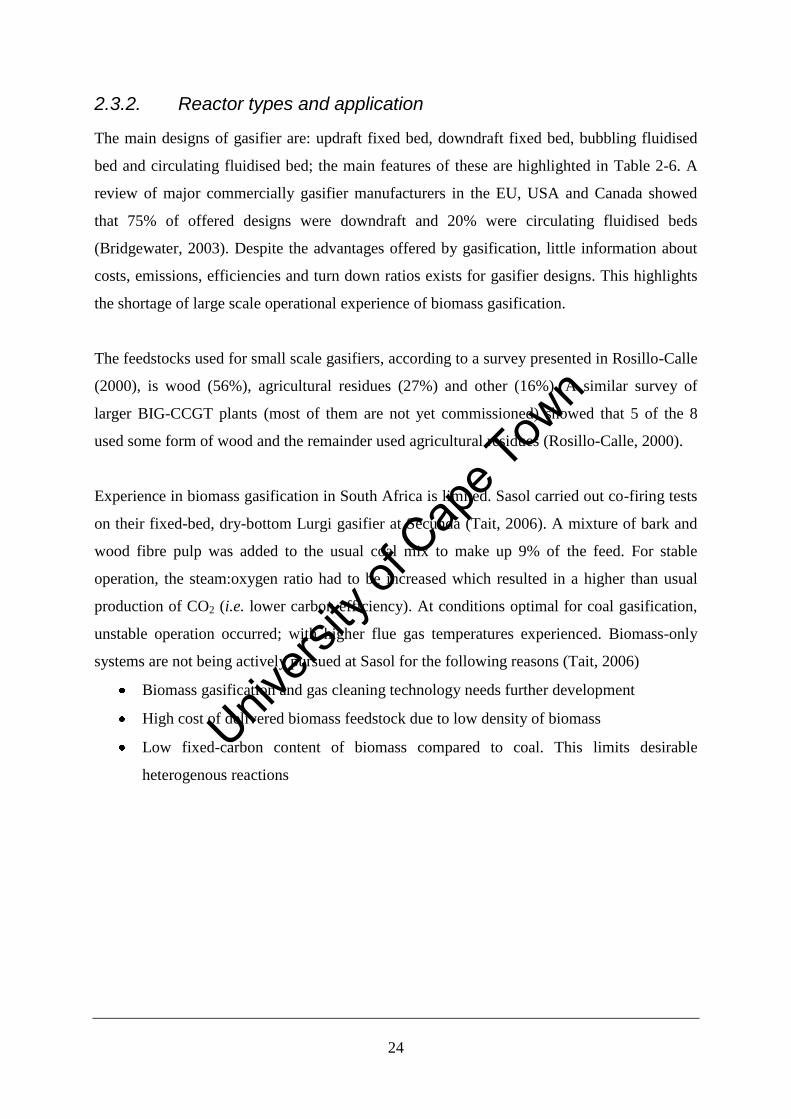
24

2.3.2. Reactor types and application

The main designs of gasifier are: updraft fixed bed, downdraft fixed bed, bubbling fluidised

bed and circulating fluidised bed; the main features of these are highlighted in Table 2-6. A

review of major commercially gasifier manufacturers in the EU, USA and Canada showed

that 75% of offered designs were downdraft and 20% were circulating fluidised beds

(Bridgewater, 2003). Despite the advantages offered by gasification, little information about

costs, emissions, efficiencies and turn down ratios exists for gasifier designs. This highlights

the shortage of large scale operational experience of biomass gasification.

The feedstocks used for small scale gasifiers, according to a survey presented in Rosillo-Calle

(2000), is wood (56%), agricultural residues (27%) and other (16%). A similar survey of

larger BIG-CCGT plants (most of them are not yet commissioned) showed that 5 of the 8

used some form of wood and the remainder used agricultural residues (Rosillo-Calle, 2000).

Experience in biomass gasification in South Africa is limited. Sasol carried out co-firing tests

on their fixed-bed, dry-bottom Lurgi gasifier at Secunda (Tait, 2006). A mixture of bark and

wood fibre pulp was added to the usual coal mix to make up 9% of the feed. For stable

operation, the steam:oxygen ratio had to be increased which resulted in a higher than usual

production of CO2 (i.e. lower carbon efficiency). At conditions optimal for coal gasification,

unstable operation occurred; with higher flue gas temperatures experienced. Biomass-only

systems are not being actively pursued at Sasol for the following reasons (Tait, 2006)

Biomass gasification and gas cleaning technology needs further development

High cost of delivered biomass feedstock due to low density of biomass

Low fixed-carbon content of biomass compared to coal. This limits desirable

heterogenous reactions

Univers

ity of

Cap

e Tow

n

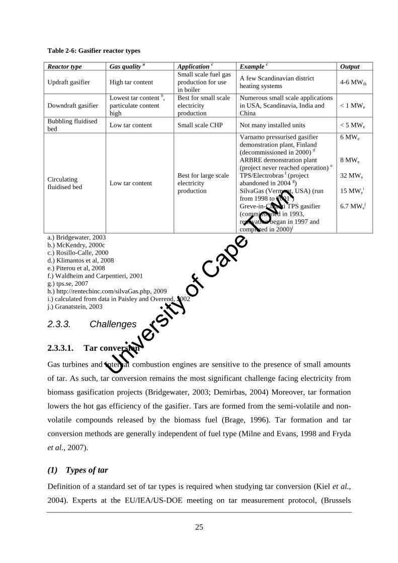
25

Table 2-6: Gasifier reactor types

Reactor type Gas quality a

Application c

Example c

Output

Updraft gasifier High tar content

Small scale fuel gas

production for use

in boiler

A few Scandinavian district

heating systems 4-6 MWth

Downdraft gasifier

Lowest tar content b,

particulate content

high

Best for small scale

electricity

production

Numerous small scale applications

in USA, Scandinavia, India and

China

< 1 MWe

Bubbling fluidised

bed Low tar content Small scale CHP Not many installed units < 5 MWe

Circulating

fluidised bed Low tar content

Best for large scale

electricity

production

Varnamo pressurised gasifier

demonstration plant, Finland

(decommissioned in 2000) d

ARBRE demonstration plant

(project never reached operation) e

TPS/Electrobras f (project

abandoned in 2004 g)

SilvaGas (Vermont, USA) (run

from 1998 to 2001h)

Greve-in-Chianti TPS gasifier

(commissioned in 1993,

renovation began in 1997 and

completed in 2000)j

6 MWe

8 MWe

32 MWe

15 MWei

6.7 MWej

a.) Bridgewater, 2003

b.) McKendry, 2000c

c.) Rosillo-Calle, 2000

d.) Klimantos et al, 2008

e.) Piterou et al, 2008

f.) Waldheim and Carpentieri, 2001

g.) tps.se, 2007

h.) http://rentechinc.com/silvaGas.php, 2009

i.) calculated from data in Paisley and Overend, 2002

j.) Granatstein, 2003

2.3.3. Challenges

2.3.3.1. Tar conversion

Gas turbines and internal combustion engines are sensitive to the presence of small amounts

of tar. As such, tar conversion remains the most significant challenge facing electricity from

biomass gasification projects (Bridgewater, 2003; Demirbas, 2004) Moreover, tar formation

lowers the hot gas efficiency of the gasifier. Tars are formed from the semi-volatile and non-

volatile compounds released by the biomass fuel (Brage, 1996). Tar formation and tar

conversion methods are generally independent of fuel type (Milne and Evans, 1998 and Fryda

et al., 2007).

(1) Types of tar

Definition of a standard set of tar types is required when studying tar conversion (Kiel et al.,

2004). Experts at the EU/IEA/US-DOE meeting on tar measurement protocol, (Brussels

Univers

ity of

Cap

e Tow

n

http://rentechinc.com/silvaGas.php

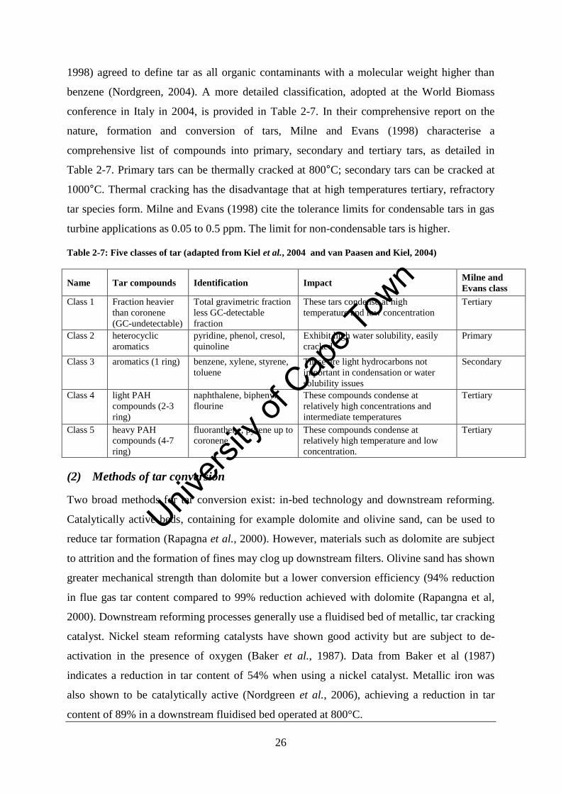
26

1998) agreed to define tar as all organic contaminants with a molecular weight higher than

benzene (Nordgreen, 2004). A more detailed classification, adopted at the World Biomass

conference in Italy in 2004, is provided in Table 2-7. In their comprehensive report on the

nature, formation and conversion of tars, Milne and Evans (1998) characterise a

comprehensive list of compounds into primary, secondary and tertiary tars, as detailed in

Table 2-7. Primary tars can be thermally cracked at 800°C; secondary tars can be cracked at

1000°C. Thermal cracking has the disadvantage that at high temperatures tertiary, refractory

tar species form. Milne and Evans (1998) cite the tolerance limits for condensable tars in gas

turbine applications as 0.05 to 0.5 ppm. The limit for non-condensable tars is higher.

Table 2-7: Five classes of tar (adapted from Kiel et al., 2004 and van Paasen and Kiel, 2004)

Name Tar compounds Identification Impact Milne and

Evans class

Class 1 Fraction heavier

than coronene

(GC-undetectable)

Total gravimetric fraction

less GC-detectable

fraction

These tars condense at high

temperature and low concentration

Tertiary

Class 2 heterocyclic

aromatics

pyridine, phenol, cresol,

quinoline

Exhibit high water solubility, easily

cracked.

Primary

Class 3 aromatics (1 ring) benzene, xylene, styrene,

toluene

These are light hydrocarbons not

important in condensation or water

solubility issues

Secondary

Class 4 light PAH

compounds (2-3

ring)

naphthalene, biphenyl,

flourine

These compounds condense at

relatively high concentrations and

intermediate temperatures

Tertiary

Class 5 heavy PAH

compounds (4-7

ring)

fluoranthene, pyrene up to

coronene

These compounds condense at

relatively high temperature and low

concentration.

Tertiary

(2) Methods of tar conversion

Two broad methods for tar conversion exist: in-bed technology and downstream reforming.

Catalytically active beds, containing for example dolomite and olivine sand, can be used to

reduce tar formation (Rapagna et al., 2000). However, materials such as dolomite are subject

to attrition and the formation of fines may clog up downstream filters. Olivine sand has shown

greater mechanical strength than dolomite but a lower conversion efficiency (94% reduction

in flue gas tar content compared to 99% reduction achieved with dolomite (Rapangna et al,

2000). Downstream reforming processes generally use a fluidised bed of metallic, tar cracking

catalyst. Nickel steam reforming catalysts have shown good activity but are subject to de-

activation in the presence of oxygen (Baker et al., 1987). Data from Baker et al (1987)

indicates a reduction in tar content of 54% when using a nickel catalyst. Metallic iron was

also shown to be catalytically active (Nordgreen et al., 2006), achieving a reduction in tar

content of 89% in a downstream fluidised bed operated at 800°C.

Univers

ity of

Cap

e Tow

n

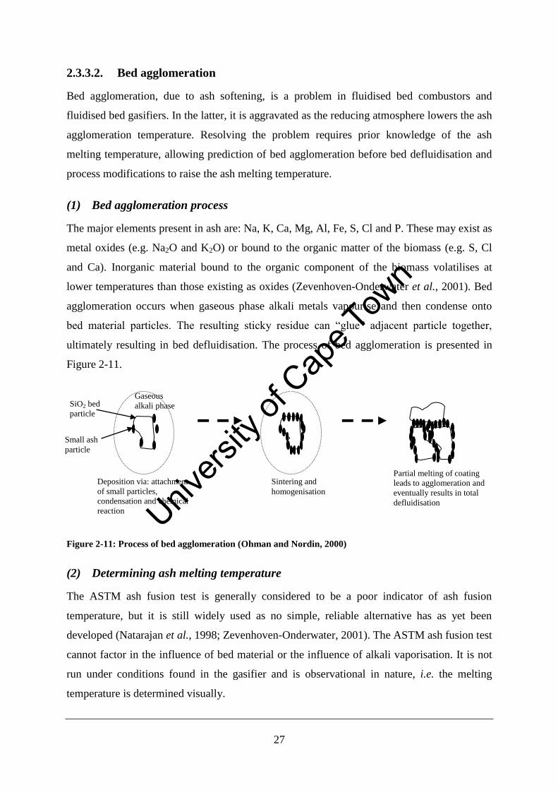
27

2.3.3.2. Bed agglomeration

Bed agglomeration, due to ash softening, is a problem in fluidised bed combustors and

fluidised bed gasifiers. In the latter, it is aggravated as the reducing atmosphere lowers the ash

agglomeration temperature. Resolving the problem requires prior knowledge of the ash

melting temperature, allowing prediction of bed agglomeration before bed defluidisation and

process modifications to raise the ash melting temperature.

(1) Bed agglomeration process

The major elements present in ash are: Na, K, Ca, Mg, Al, Fe, S, Cl and P. These may exist as

metal oxides (e.g. Na2O and K2O) or bound to the organic matter of the biomass (e.g. S, Cl

and Ca). Inorganic material bound to the organic component of the biomass volatilises at

lower temperatures than those existing as oxides (Zevenhoven-Onderwater et al., 2001). Bed

agglomeration occurs when gaseous phase alkali metals vapourise and then condense onto

bed material particles. The resulting sticky residue can “glue” adjacent particle together,

ultimately resulting in bed defluidisation. The process of bed agglomeration is presented in

Figure 2-11.

Figure 2-11: Process of bed agglomeration (Ohman and Nordin, 2000)

(2) Determining ash melting temperature

The ASTM ash fusion test is generally considered to be a poor indicator of ash fusion

temperature, but it is still widely used as no simple, reliable alternative has as yet been

developed (Natarajan et al., 1998; Zevenhoven-Onderwater, 2001). The ASTM ash fusion test

cannot factor in the influence of bed material or the influence of alkali vaporisation. It is not

run under conditions found in the gasifier and is observational in nature, i.e. the melting

temperature is determined visually.

SiO2 bed

particle

Gaseous

alkali phase

Small ash

particle

Deposition via: attachment

of small particles,

condensation and chemical

reaction

Sintering and

homogenisation

Partial melting of coating

leads to agglomeration and

eventually results in total

defluidisation

Univers

ity of

Cap

e Tow

n

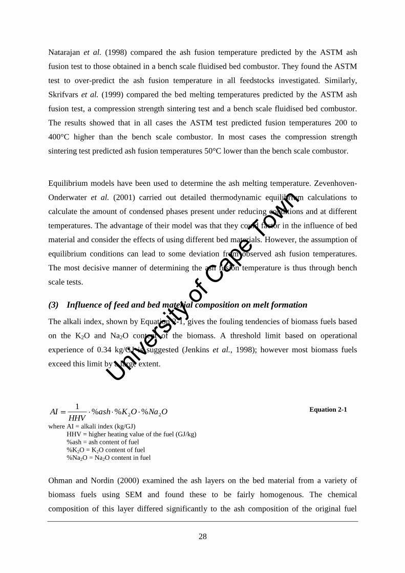
28

Natarajan et al. (1998) compared the ash fusion temperature predicted by the ASTM ash

fusion test to those obtained in a bench scale fluidised bed combustor. They found the ASTM

test to over-predict the ash fusion temperature in all feedstocks investigated. Similarly,

Skrifvars et al. (1999) compared the bed melting temperatures predicted by the ASTM ash

fusion test, a compression strength sintering test and a bench scale fluidised bed combustor.

The results showed that in all cases the ASTM test predicted fusion temperatures 200 to

400°C higher than the bench scale combustor. In most cases the compression strength

sintering test predicted ash fusion temperatures 50°C lower than the bench scale combustor.

Equilibrium models have been used to determine the ash melting temperature. Zevenhoven-

Onderwater et al. (2001) carried out detailed thermodynamic equilibrium calculations to

calculate the amount of condensed phases present under reducing conditions and at different

temperatures. The advantage of their model was that they could factor in the influence of bed

material and consider the effects of using different bed materials. However, the assumption of

equilibrium conditions can lead to some deviation from observed ash fusion temperatures.

The most decisive manner of determining the ash fusion temperature is thus through bench

scale tests.

(3) Influence of feed and bed material composition on melt formation

The alkali index, shown by Equation 2-1, gives the fouling tendencies of biomass fuels based

on the K2O and Na2O content of the biomass. A threshold limit based on operational

experience of 0.34 kg/GJ is suggested (Jenkins et al., 1998); however most biomass fuels

exceed this limit by a large extent.

ONaOKashHHV

AI 22 %%%1

Equation 2-1

where AI = alkali index (kg/GJ)

HHV = higher heating value of the fuel (GJ/kg)

%ash = ash content of fuel

%K2O = K2O content of fuel

%Na2O = Na2O content in fuel

Ohman and Nordin (2000) examined the ash layers on the bed material from a variety of

biomass fuels using SEM and found these to be fairly homogenous. The chemical

composition of this layer differed significantly to the ash composition of the original fuel

Univers

ity of

Cap

e Tow

n

29

indicating a strong influence of bed material. The deposits on the bed particles could be well

represented by the ternary diagram CaO-K2O-SiO2 and were found mostly in the SiO2 rich

region. The first melting temperature in this region is around 720°C, but an addition of

calcium increases this temperature to 1000°C. High potassium content in biomass lowers the

ash melting temperature. Coatings with a relatively high fraction of potassium (e.g. samples

derived from wheat straw and wood) contained a large amount of melt at temperatures below

900 °C, whereas coatings with a smaller fraction of potassium, (e.g. samples derived from

bark, cane trash, and wood residue) did not contain a large amount of melt until temperatures

well above 900 °C. Similarly, Zevenhoven-Onderwater (2001) relates the formation of

potassium silicate melt to lowering the first melting temperature of silica bed material.

A study done by Sasol aimed at increasing the ash fusion temperature of their dry-bottom coal

gasifiers found that adding up to 6% by mass of aluminum oxide to the bed increased the ash

fusion temperature of the ash produced in the bed from 1350°C to 1600°C (van Dyk and

Waanders, 2007). Other bed materials cited as hindering ash fusion by increasing the ash

fusion temperature include kaolin, lime and titanium oxide (van Dyk and Waanders, 2007 and

Fryda et al., 2007).

(4) Predicting bed agglomeration temperature for control purposes

An ideal system for preventing bed agglomeration would incorporate an online monitoring

system to detect the onset of bed agglomeration. Control measures such as changing the bed

temperature, increasing the superficial gas velocity and the bed material make-up rate could

then be used to prevent bed agglomeration (Nijenhuis et al., 2007).

Such a system using high frequency pressure drop measurements over the bed was recently

developed by Nijenhuis et al. (2007) and demonstrated using bench scale fluidised beds.

Previously pressure drop over the bed has been used to identify when agglomeration has

occurred but not for predictive purposes (Fryda et al., 2007; Ohman and Nordin, 2000).

Nijenhuis et al. transformed the high frequency pressure drop measurements to an s-statistic

using chaos theory. The s-values above 3 indicated a significant change while those below 3

were considered normal. Bench scale agglomeration runs using this technique predicted the

bed defluidisation 30 to 45 min before it occurred. Runs to test its control ability were carried

out on petroleum coke beds with agglomeration induced by adding water. The s-value rose to

Univers

ity of

Cap

e Tow

n

30

3, and then returned when the bed had stabilised. Tests carried out on an 80MWth industrial

plant showed that a modified s-statistic could be used successfully.

2.3.4. Summary

Large scale BIG-CCGT units (i.e. 100 MWe) can achieve thermal efficiencies of 45 to 50%.

However, the operation of such a large plant is yet to be achieved. Small scale fixed bed

gasification systems offer simplicity but efficiencies are similar to combustion systems, viz.

30%. Limited experience of biomass gasification in South Africa exists. Notably, Sasol

carried out co-firing tests on their fixed-bed, dry-bottom Lurgi gasifier but found that stable

operation of the co-fired system resulted in higher CO2 emissions. Gasification technology for

biomass-only feedstreams is not considered to be mature. Tar removal from the fuel gas

remains a serious technological hurdle, and in the case of fluidised bed designs, bed

agglomeration poses a serious challenge.

2.4. Anaerobic digestion

2.4.1. Process

Anaerobic digestion is the biological conversion of organic material in the absence of oxygen

to a.) biogas (which consists of roughly 66% methane and 33% CO2 (McKendry, 2002b;

Wilkie, 2008; Speece, 1996)) b.) additional cell matter and c.) inorganics and refractory

material (Wilkie, 2008). The conversion is effected by a complex mixture of bacteria and

archae. Anaerobic digestion is a process effective for both wastewater treatment and

renewable energy production (Wilkie, 2008). Biogas may be converted to electricity in

reciprocating engines or gas turbines or emerging technologies such as micro-turbines or fuel

cells. Biogas conditioning may include particulate removal, water knockout and H2S and

ammonia removal (Chambers and Potter, 2002). A comparison of biogas conversion

technologies is shown in Table 2-8.

Univers

ity of

Cap

e Tow

n

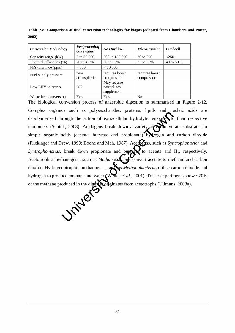
31

Table 2-8: Comparison of final conversion technologies for biogas (adapted from Chambers and Potter,

2002)

Conversion technology Reciprocating

gas engine Gas turbine Micro-turbine Fuel cell

Capacity range (kW) 5 to 50 000 500 to 150 000 30 to 200 <250

Thermal efficiency (%) 20 to 45 % 30 to 50% 25 to 30% 40 to 50%

H2S tolerance (ppm) < 200 < 10 000

Fuel supply pressure near

atmospheric

requires boost

compressor

requires boost

compressor

Low LHV tolerance OK

May require

natural gas

supplement

Waste heat conversion Yes Yes No

The biological conversion process of anaerobic digestion is summarised in Figure 2-12.

Complex organics such as polysaccharides, proteins, lipids and nucleic acids are

depolymerised through the action of extracellular hydrolytic enzymes to their respective

monomers (Schink, 2008). Acidogens break down a variety of carbohydrate substrates to

simple organic acids (acetate, butyrate and propionate) hydrogen and carbon dioxide

(Flickinger and Drew, 1999; Boone and Mah, 1987). Acetogens, such as Syntrophobacter and

Syntrophomonas, break down propionate and butyrate to acetate and H2, respectively.

Acetotrophic methanogens, such as Methanosarcina, convert acetate to methane and carbon

dioxide. Hydrogenotrophic methanogens, such as Methanobacteria, utilise carbon dioxide and

hydrogen to produce methane and water (Waites et al., 2001). Tracer experiments show ~70%

of the methane produced in the digester originates from acetotrophs (Ullmans, 2003a).

Univers

ity of

Cap

e Tow

n

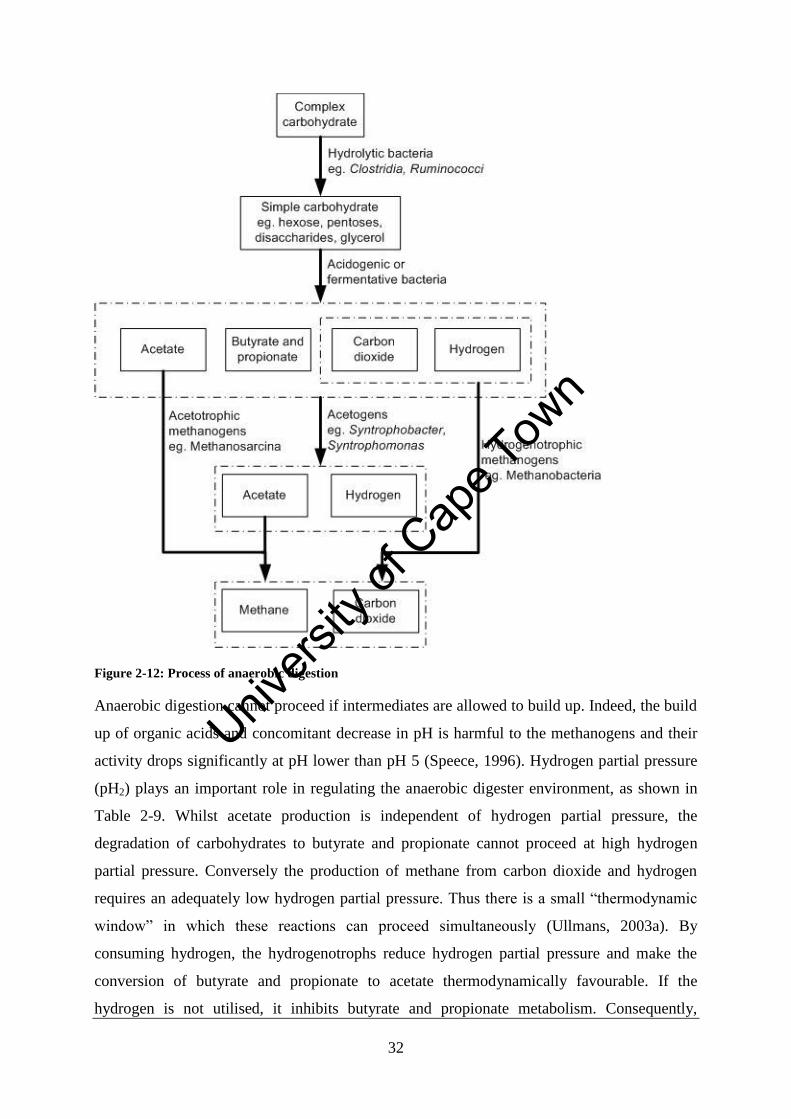
32

Figure 2-12: Process of anaerobic digestion

Anaerobic digestion cannot proceed if intermediates are allowed to build up. Indeed, the build

up of organic acids and concomitant decrease in pH is harmful to the methanogens and their

activity drops significantly at pH lower than pH 5 (Speece, 1996). Hydrogen partial pressure

(pH2) plays an important role in regulating the anaerobic digester environment, as shown in

Table 2-9. Whilst acetate production is independent of hydrogen partial pressure, the

degradation of carbohydrates to butyrate and propionate cannot proceed at high hydrogen

partial pressure. Conversely the production of methane from carbon dioxide and hydrogen

requires an adequately low hydrogen partial pressure. Thus there is a small “thermodynamic

window” in which these reactions can proceed simultaneously (Ullmans, 2003a). By

consuming hydrogen, the hydrogenotrophs reduce hydrogen partial pressure and make the

conversion of butyrate and propionate to acetate thermodynamically favourable. If the

hydrogen is not utilised, it inhibits butyrate and propionate metabolism. Consequently,

Univers

ity of

Cap

e Tow

n

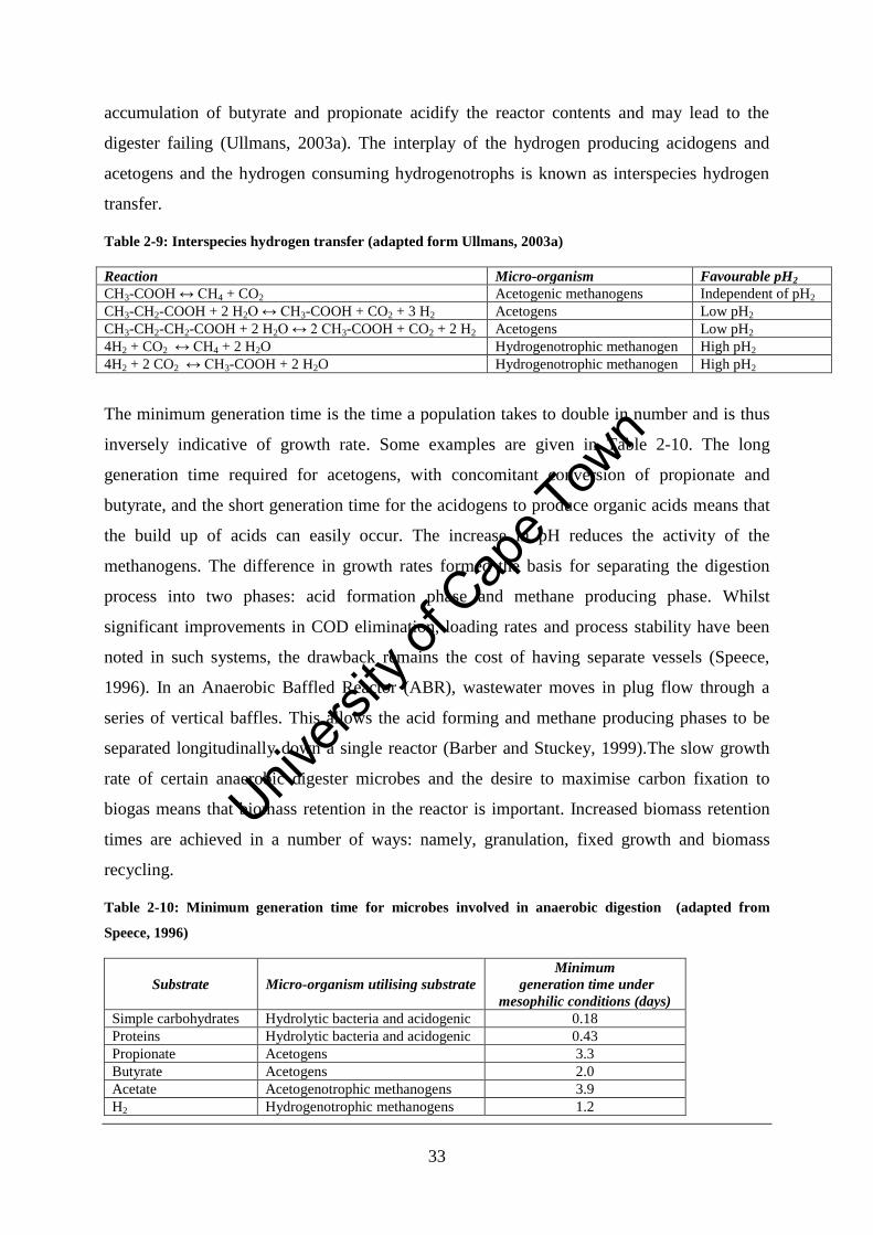
33

accumulation of butyrate and propionate acidify the reactor contents and may lead to the

digester failing (Ullmans, 2003a). The interplay of the hydrogen producing acidogens and

acetogens and the hydrogen consuming hydrogenotrophs is known as interspecies hydrogen

transfer.

Table 2-9: Interspecies hydrogen transfer (adapted form Ullmans, 2003a)

Reaction Micro-organism Favourable pH2

CH3-COOH ↔ CH4 + CO2 Acetogenic methanogens Independent of pH2

CH3-CH2-COOH + 2 H2O ↔ CH3-COOH + CO2 + 3 H2 Acetogens Low pH2

CH3-CH2-CH2-COOH + 2 H2O ↔ 2 CH3-COOH + CO2 + 2 H2 Acetogens Low pH2

4H2 + CO2 ↔ CH4 + 2 H2O Hydrogenotrophic methanogen High pH2

4H2 + 2 CO2 ↔ CH3-COOH + 2 H2O Hydrogenotrophic methanogen High pH2

The minimum generation time is the time a population takes to double in number and is thus

inversely indicative of growth rate. Some examples are given in Table 2-10. The long

generation time required for acetogens, with concomitant conversion of propionate and

butyrate, and the short generation time for the acidogens to produce organic acids means that

the build up of acids can easily occur. The increase in pH reduces the activity of the

methanogens. The difference in growth rates formed the basis for separating the digestion

process into two phases: acid formation phase and methane producing phase. Whilst

significant improvements in COD elimination, loading rates and process stability have been

noted in such systems, the drawback remains the cost of having separate vessels (Speece,

1996). In an Anaerobic Baffled Reactor (ABR), wastewater moves in plug flow through a

series of vertical baffles. This allows the acid forming and methane producing phases to be

separated longitudinally down a single reactor (Barber and Stuckey, 1999).The slow growth

rate of certain anaerobic digester microbes and the desire to maximise carbon fixation to

biogas means that biomass retention in the reactor is important. Increased biomass retention

times are achieved in a number of ways: namely, granulation, fixed growth and biomass

recycling.

Table 2-10: Minimum generation time for microbes involved in anaerobic digestion (adapted from

Speece, 1996)

Substrate Micro-organism utilising substrate

Minimum

generation time under

mesophilic conditions (days)

Simple carbohydrates Hydrolytic bacteria and acidogenic 0.18

Proteins Hydrolytic bacteria and acidogenic 0.43

Propionate Acetogens 3.3

Butyrate Acetogens 2.0

Acetate Acetogenotrophic methanogens 3.9

H2 Hydrogenotrophic methanogens 1.2

Univers

ity of

Cap

e Tow

n

34

Other factors important in the process of anaerobic digestion are temperature and alkalinity.

The optimum temperature for mesophilic operations is 35°C and for thermophilic operations

55°C to 65°C. Methanogen activity is more sensitive to temperature change than the

acidogens and thus temperature fluctuations can give rise to unstable process conditions

(Speece, 1996). Thermophilic operations may achieve metabolic rates that are 50 to 100%

higher than mesophilic operations (Speece, 1996). The operation is practised when the

reduced reactor size justifies the higher energy requirements and the greater attention to

maintaining process stability (Wilke, 2008; Ullmans, 2003a; Tchobanoglous et al., 2003).

The buffering capacity of a digester, as measured by the total alkalinity, is a good indicator of

the process stability. The total alkalinity of a well-established digester is 2000 to 5000 mg/l

(Tchobanoglous et al., 2003). Buffering substances found in a digester include calcium,

magnesium and ammonium bicarbonates and may be supplemented with the addition of

caustic soda, lime, sodium bicarbonate or sodium carbonate. Alkalinity is consumed via the

generation of acids by the acidogens and the dissolution of CO2.

2.4.2. Reactor types and current installations

One of the objectives in anaerobic digester reactor design is to separate the biomass retention

time or solids retention time (SRT) from the hydraulic retention time (HRT). The HRT

defines the time in which the anaerobic microbes can consume the soluble organic load

(Speece, 1996). Thus a higher SRT, relative to HRT, allows for greater organic load

reductions by retention of a high biomass catalyst concentration. In the case of feedstock

containing insoluble complex material, an increased SRT will afford greater opportunity for

biodegradation. Reactor types can be defined according to their method of increasing SRT as

shown in Table 2-11. Three reactor designs will be considered further due to their

applicability in the context of this study, namely, CSTR (Continuous Stirred Tank Reactor);

UASB (Upflow Anaerobic Sludge Blanket) and anaerobic lagoons. Small batch anaerobic

digesters are not considered viable units for industrial energy recovery as control over process

stability is limited (Fannin and Biljetina, 1987). In South Africa, a local company AGAMA

has installed a number of batch digesters primarily for household biogas production. Based on

data presented in Burton et al. (2008) the thermal output of these units is less than 1 kW.

Univers

ity of

Cap

e Tow

n

35

Table 2-11: Types of anaerobic digester reactors

Reactor design Method of increasing SRT

CSTR SRT = HRT

Upflow Anaerobic Sludge Blanket (UASB) Microbial granulation

Fixed bed, expanded bed and fluidised bed reactors Fixed microbial growth

Anaerobic contact process Biomass recycling

Anaerobic covered lagoon Plug flow; insoluble solids settle

2.4.2.1. CSTR

In a completely mixed CSTR, the SRT and the HRT are equivalent. However, the design

remains popular due to lower initial capital cost and the ability to handle high solids content

(Fannin and Biljetina, 1987). The dry solids content of the feed is limited to 7%, after which

mixing may become problematic (Fountain, 2008). Hydraulic retention times for a complex

substrate such as sewerage sludge range from 15 to 30 days and the volumetric organic load

ranges from 1 to 5 kg COD/m3/day (Tchobanoglous et al., 2003). For simpler substrates, the

HRT is less.

Adequate mixing in a CSTR in necessary to prevent the formation of acidified zones. Mixing

is achieved through gas injection, stirring or pumped external reticulation. Tank shape has an

influence on mixing. Egg-shaped digesters have gained popularity for this reason together

with easier sludge withdrawal and better control of the scum layer (Tchobanoglous et al.,

2003). The initial cost of construction, however, exceeds cylindrical tank digesters.

A variant of the single stage CSTR design is two stage digestion where a completely mixed

digester is followed by a second tank which serves as a settling or holding tank. The design is

being phased out due to the capital expense of the second tank with little operational value as

less than 10% of total biogas production comes from the second stage (Tchobanoglous et al.,

2003). Further, digested solids do not settle well due to entrained gas and fine-sized particles

and so the supernatant withdrawn from the second tank may contain high concentrations of

suspended solids (Tchobanoglous et al., 2003). Notwithstanding these drawbacks, two-stage

digestion still finds application in South Africa, (viz. Cape Town and Johannesburg

Wastewater treatment plants (King, 2008 and Deacon, 2008)) illustrating the age of our

wastewater treatment plants.

Univers

ity of

Cap

e Tow

n

36

2.4.2.2. UASB

The UASB consists of 3 zones: a granular sludge bed, a sludge blanket and a gas separation

and settling zone. Liquid feed is introduced to the reactor via a distributor at the bottom of the

reactor. Even distribution is necessary to prevent channelling and bypassing. Some 80 to 90%

of the volatile solid destruction occurs in the dense sludge bed section, which occupies 20%

of the reactor volume (Fannin and Biljetina, 1987). This results in a large portion of reactor

volume which does not contribute to gas production. Gas is collected via internal inverted

cones which also serve as settling surfaces to direct solids back into the bed (Fannin and

Biljetina, 1987). Upflow velocities in UASB’s range from 1 to 3 m/hr (Ullmans, 2003a). This

results in reactors with large footprints.

UASB’s afford efficient biomass retention without the use of costly packing materials or

external solid liquid separation. This allows for high loading rates (Speece, 1996). Good

sludge granulation is ssential to the process and this is achieved with soluble feeds. Feeds

with high suspended solids inhibit the formation of granules (Tchobanoglous et al., 2003).

Whilst the properties of the microbial granules in the dense sludge bed are central to the

process, their formation is still largely empirical (Ullmans, 2003a). Indeed, to start up a

UASB, sludge is generally imported from an operational unit to reduce start up time

(Tchobanoglous et al., 2003).

UASB reactors are considered to be a proven process and more than 500 large scale units

exist (Ullmans, 2003a). One of the earliest installations was the South African “anaerobic

clarigester” for treating winery wastewater (Speece, 1996). UASB’s have been used to treat

sugar wastewaters successfully (Speece, 1996) as well as sugar beet and potato starch

wastewaters (Biljetina, 1987). SAB Durban brewery has used UASB technology since 1996

(Speece, 1996) and SAB Newlands Brewery has treated their wastewater with a UASB

reactor since 2002 (Hoffman, 2008). The use of this technology has subsequently been

extended to 5 other breweries. One of the original drivers for installing the UASB at

Newlands was to mitigate the cost of effluent discharge in the municipal waste water system

(Hofmann, 2008).

Univers

ity of

Cap

e Tow

n

37

2.4.2.3. Covered lagoons

Covered lagoons operate in plug flow with the wastewater introduced at one end of the lagoon

and withdrawn at the other. This digester type has been used to treat manure from animal

husbandry and can also handle fats and grease. HRT ranges from 30-50 days and it is

estimated that the SRT ranges from 50-100 days. Baffles are often installed to prevent the

solids washing out before digestion has occurred. Care must be taken to remove non-

biodegradable material (Tchobanoglous et al., 2003).

2.4.3. Challenges

Whilst significant energy recovery is possible from anaerobic digesters, it is important to bear

in mind that the primary driver in most installations has been wastewater treatment. As such,

energy recovery systems have typically not been installed and it is common to find biogas

being flared. Exceptions in SA include the PetroSA wastewater treatment plant, where the

biogas is currently being used to generate electricity. This project is a registered CDM

(Carbon Development Mechanism) project and hence was only economically feasible with

the sale of Certified Emission Reductions (CER’s or “carbon credits”). In some cases the

economic benefits of energy recovery from biogas is being recognised by industry. However,

this requires adjustment of the process control philosophy. For example, the SAB Newlands

process control philosophy aims to treat the maximum amount of effluent at the expense of a

fluctuating biogas flow. To be able to run a biogas burner, the flow needs to be relatively

constant (Hofmann, 2008).

2.4.4. Feedstock pretreatment

Certain components in biogenic waste streams (e.g. cellulose and microbial cell walls) are

resistant to biological action and unless the feed is pretreated in some manner, these

substances pass unconverted through the system. Various methods of pretreating the feed

exist to make it more amenable to hydrolysis. Work done on pre-treating lignocellulosic

feedstocks for fermentation to ethanol (Sun and Cheng, 2002; Wyman et al., 2005) applies to

pretreating feed for anaerobic digestion as both processes require hydrolysis of the feed before

fermentation or digestion can take place. A number of methods of disrupting the cell wall to

release the intracellular proteins, lipids, nucleic acids and carbohydrates exist e.g. hot water

hydrolysis (with and without chemical additions), high pressure homogenisation and

sonication. Hot water hydrolysis and high pressure homogenisation already exist as patented

Univers

ity of

Cap

e Tow

n

38

processes for pretreating sewerage sludge (Kelly, 2006 and Stephenson et al., 2007).

Sonication has yet to gain industrial application, primarily due to the high energy inputs

required (Weemaes and Verstraete, 1998).

2.4.4.1. Pretreatments for lignocellulosic waste

Lignocellulosic treatments reviewed here are: dilute acid treatment, hot water hydrolysis,

steam hydrolysis, ammonia pretreatment and lime pretreatment. Process conditions and

modes of action of each pretreatment are summarised in Table 2-13. Alkali pretreatments are

excluded from the analysis owing to the reagent cost and waste processing (Wyman et al.,

2005a).

Physical factors which affect the enzymatic hydrolysis of lignocellulosic material are:

cellulose porosity, cellulose fiber crystallinity, lignin content and hemicellulose content.

Cellulose porosity is a measure of surface area accessible to enzymes. Cellulose fiber

crystallinity refers to the ratio of amorphous to crystalline cellulose. A pretreatment process

will thus seek to increase porosity, reduce cellulose crystallinity, remove hemicellulose and

lignin from the microfibril matrix or alter the lignin structure to expose the microfibril matrix

(Sun and Cheng, 2002). Sun and Cheng identify four requirements for successful

pretreatment:

Optimal formation of sugars or the ability for subsequent sugar formation by

enzymatic hydrolysis

Minimal degradation or loss of carbohydrate

Absence of byproducts that inhibit the subsequent hydrolysis and fermentation

processes

Cost-effectiveness

A mechanical pretreatment is usually employed upstream of the pretreatment to produce a

homogenous feedstock of small particles. The energy consumption of knife and hammer mills

is shown in Figure 2-13. It can be seen a feedstocks with high lignin content (e.g. hardwood)

require greater energy input than those with lower lignin content (e.g. corn stover).

Univers

ity of

Cap

e Tow

n

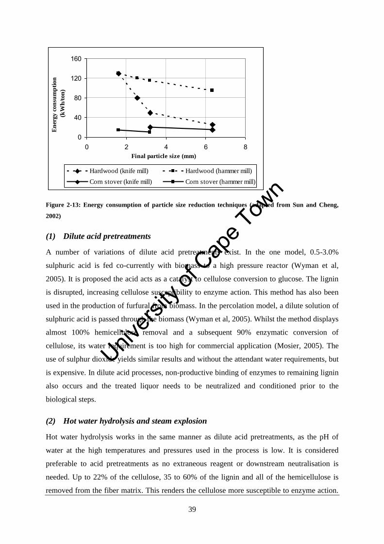
39

0

40

80

120

160

0 2 4 6 8Final particle size (mm)

En

ergy c

on

sum

pti

on

(k

Wh

/ton

)

Hardwood (knife mill) Hardwood (hammer mill)

Corn stover (knife mill) Corn stover (hammer mill)

Figure 2-13: Energy consumption of particle size reduction techniques (adapted from Sun and Cheng,

2002)

(1) Dilute acid pretreatments

A number of variations of dilute acid pretreatments exist. In the one model, 0.5-3.0%

sulphuric acid is fed co-currently with biomass to a high pressure reactor (Wyman et al,

2005). It is proposed the acid acts as a catalyst to cellulose conversion to glucose. The lignin

is disrupted, increasing cellulose susceptibility to enzyme action. This method has also been

used in the production of furfural from biomass. In the percolation model, a dilute solution of

sulphuric acid is passed through the biomass (Wyman et al, 2005). Whilst the method displays

almost 100% hemicellulose removal and a subsequent 90% enzymatic conversion of

cellulose, its water requirement is too high for commercial application (Mosier, 2005). The

use of sulphur dioxide yields similar results and without the attendant water requirements, but

is expensive. In dilute acid processes, non-productive binding of enzymes to remaining lignin

also occurs and the treated liquor needs to be neutralized and conditioned prior to the

biological steps.

(2) Hot water hydrolysis and steam explosion

Hot water hydrolysis works in the same manner as dilute acid pretreatments, as the pH of

water at the high temperatures and pressures used in the process is low. It is considered

preferable to acid pretreatments as no extraneous reagent or downstream neutralisation is

needed. Up to 22% of the cellulose, 35 to 60% of the lignin and all of the hemicellulose is

removed from the fiber matrix. This renders the cellulose more susceptible to enzyme action.

Univers

ity of

Cap

e Tow

n

40

Over 90% of the hemicellulose is recovered as monosaccharides when acid is used to

hydrolyse the resulting liquid (Mosier et al., 2005), although the monosaccharides formed in

the reaction step can be degraded (Wyman et al., 2005).

Steam explosion involves treating coarsely chipped biomass with high-pressure saturated

steam, followed by rapid pressure reduction to make the materials undergo an explosive

decompression (Sun and Cheng, 2002). A large energy saving is realised in avoiding

communition to fine particles as larger particles (5 cm diameter) respond well to this

treatment (Cullis et al., 2004).

(3) Ammonia pretreatments

Ammonia pretreatments include: Ammonia Fibre EXplosion (AFEX), Ammonia Recycle

Percolation (ARP) and Soaking Aqueous Ammonia (SAA). In AFEX the feedstock is

exposed to liquid ammonia at high temperature and pressure. The pressure is then suddenly

released and the material undergoes explosive decompression; the ammonia volatises and can

be recycled (Sun and Cheng, 2002). Very little liquor and soluble products are produced in

the process but it opens the lignin structure and depolymerises the hemicellulose to oligomers.

It is believed that ammonolysis of glucuronic cross-links makes the carbohydrate more

accessible to enzymatic hydrolysis (Wyman et al., 2005b). Whilst oligomers cannot be

fermented to ethanol, they can be digested by digester fermentative bacteria (Tsao, 1987). The

ammonia is not harmful to downstream micro-organisms and can be used on coarse biomass

particles (Wymans et al., 2005a). The process has not demonstrated success with high lignin

containing biomass; the enzymatic cellulose conversion fell from 90% to 50% when the lignin

content increased from 5 to 20% (Sun and Cheng, 2002). In ARP aqueous ammonia is

recycled through the feedstock at elevated temperatures. SAA is a simpler batch process,

where the biomass is soaked in an aqueous ammonia solution at ambient conditions.

(4) Lime pretreatments

Low temperature lime pretreatment is a simple, inexpensive option. Operating temperatures

range from 25 to 130 °C, and the corresponding treatment time ranges from weeks (25 °C) to

hours (130 °C) (Wyman et al., 2005a). The process removes approximately 33% of lignin (in

case of low-lignin content herbaceous materials) and 100% of acetyl groups.

Univers

ity of

Cap

e Tow

n

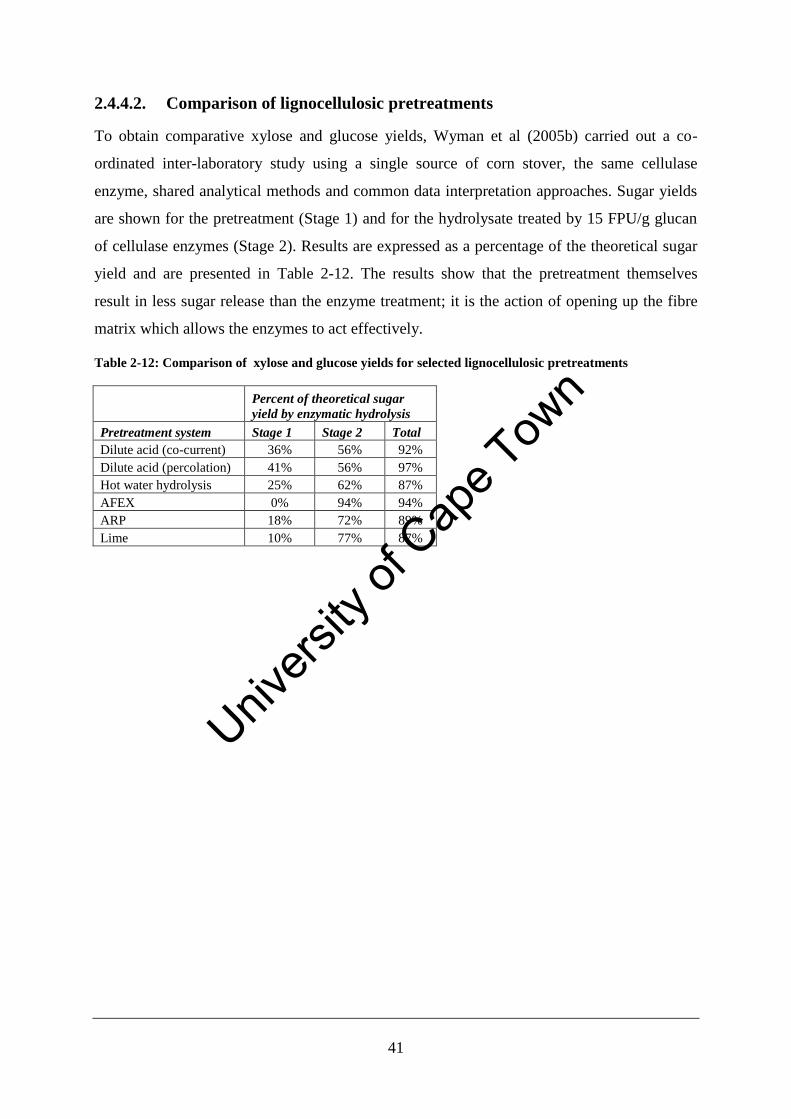
41

2.4.4.2. Comparison of lignocellulosic pretreatments

To obtain comparative xylose and glucose yields, Wyman et al (2005b) carried out a co-

ordinated inter-laboratory study using a single source of corn stover, the same cellulase

enzyme, shared analytical methods and common data interpretation approaches. Sugar yields

are shown for the pretreatment (Stage 1) and for the hydrolysate treated by 15 FPU/g glucan

of cellulase enzymes (Stage 2). Results are expressed as a percentage of the theoretical sugar

yield and are presented in Table 2-12. The results show that the pretreatment themselves

result in less sugar release than the enzyme treatment; it is the action of opening up the fibre

matrix which allows the enzymes to act effectively.

Table 2-12: Comparison of xylose and glucose yields for selected lignocellulosic pretreatments

Percent of theoretical sugar

yield by enzymatic hydrolysis

Pretreatment system Stage 1 Stage 2 Total

Dilute acid (co-current) 36% 56% 92%

Dilute acid (percolation) 41% 56% 97%

Hot water hydrolysis 25% 62% 87%

AFEX 0% 94% 94%

ARP 18% 72% 89%

Lime 10% 77% 87%

Univers

ity of

Cap

e Tow

n

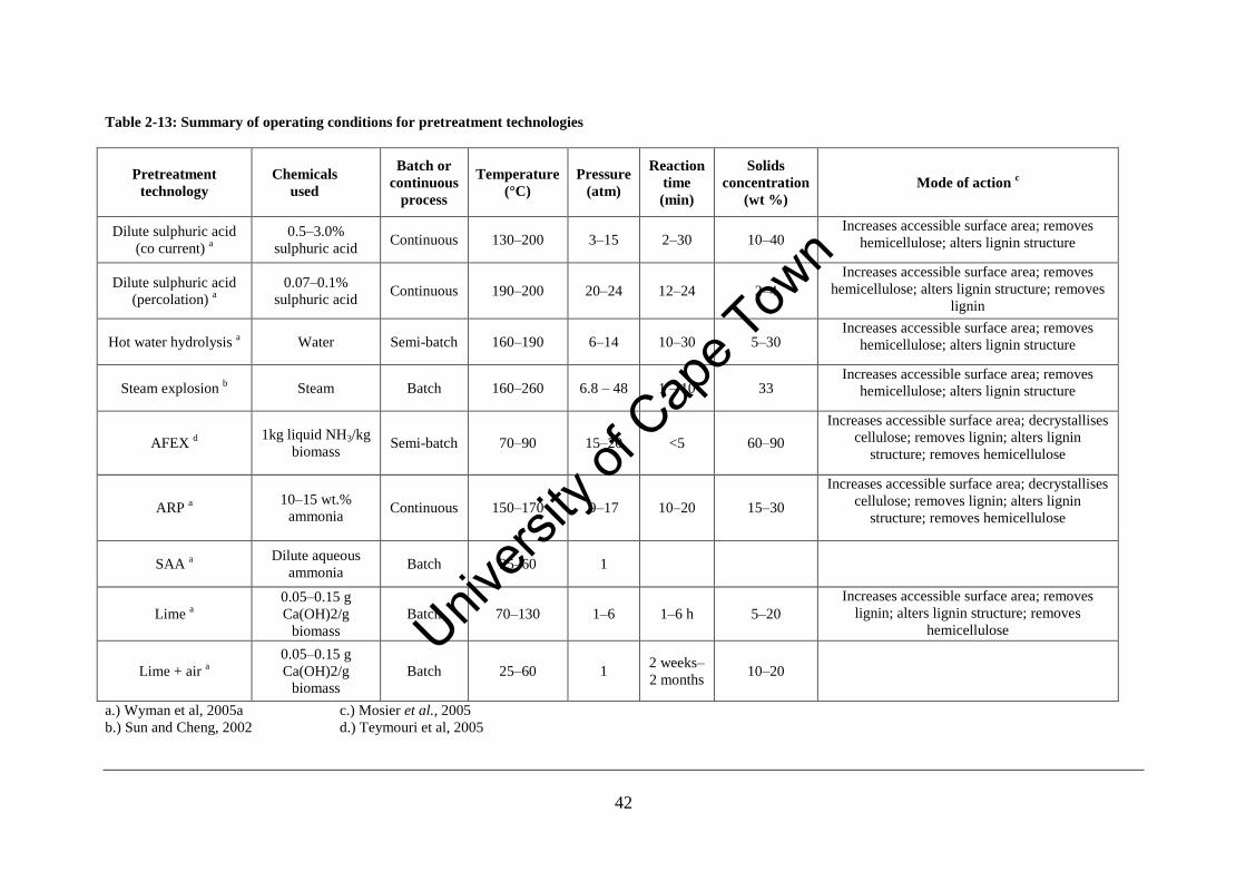
42

Table 2-13: Summary of operating conditions for pretreatment technologies

Pretreatment

technology

Chemicals

used

Batch or

continuous

process

Temperature

(°C)

Pressure

(atm)

Reaction

time

(min)

Solids

concentration

(wt %)

Mode of action c

Dilute sulphuric acid

(co current) a

0.5–3.0%

sulphuric acid Continuous 130–200 3–15 2–30 10–40

Increases accessible surface area; removes

hemicellulose; alters lignin structure


(percolation) a

0.07–0.1%



hemicellulose; alters lignin structure; removes

lignin

Hot water hydrolysis a

Water Semi-batch 160–190 6–14 10–30 5–30 Increases accessible surface area; removes


Steam explosion b

Steam Batch 160–260 6.8 – 48 1 – 10 33 Increases accessible surface area; removes


AFEX d 1kg liquid NH3/kg

biomass Semi-batch 70–90 15–20 <5

60–90

Increases accessible surface area; decrystallises

cellulose; removes lignin; alters lignin

structure; removes hemicellulose

ARP a 10–15 wt.%

ammonia Continuous 150–170 9–17 10–20 15–30

Increases accessible surface area; decrystallises

cellulose; removes lignin; alters lignin

structure; removes hemicellulose

SAA a Dilute aqueous

ammonia Batch 25–60 1

Lime a

0.05–0.15 g

Ca(OH)2/g

biomass

Batch 70–130 1–6 1–6 h 5–20


lignin; alters lignin structure; removes

hemicellulose

Lime + air a

0.05–0.15 g

Ca(OH)2/g

biomass

Batch 25–60 1 2 weeks–

2 months 10–20

a.) Wyman et al, 2005a

b.) Sun and Cheng, 2002

c.) Mosier et al., 2005

d.) Teymouri et al, 2005

Univers

ity of

Cap

e Tow

n

43

2.4.4.3. Pretreatment methods for microbial sludges

(1) Hot water hydrolysis

The initial goal of hot water hydrolysis was to improve the dewaterability of sludge

(Weemaes and Verstraete, 1998) as the breakdown of the cell wall releases the cell bound

water. However, its application to improve digestibility and concomitant biogas production

has been recognised. The patented CAMBITM

process has been employed successfully in a

number of European cities (Kelly, 2006). The CAMBITM

process runs at 165°C and a pressure

of 8 bar for 30 min and does not require the addition of chemicals. Anaerobic digestion of the

treated sludge generally results in an increase from 30% volatile solids reduction to 60%

(Fountain, 2008). Work by Kim et al. (2003) showed that the addition of 7g/l NaOH to a

121°C, 30 min hot water hydrolysis process, resulted in a COD solubilisation of 80%. The

addition of acid also improves COD solubilisation (Neyens and Baeyens, 2003). However, the

hydrolyzate needs to be neutralised before entering the digester (Valo et al., 2004).

The operation of the CAMBITM

thermal hydrolysis pretreatment process has been described in

section 3.3.3. The sludge is pumped into a high pressure “pulper” vessel where it is raised to

near its saturation temperature by the addition of steam. The sludge is held at 165°C and 8 bar

for 30 min. Literature cites the temperature range for thermal hydrolysis processes as 60 to

180°C (Neyens and Baeyens, 2003). Temperatures greater than 150°C showed marked

increase in cell disruption, though temperatures greater than 180°C result in the formation of

refractory compounds. Holding times ranged from 10 to 30 min, with longer holding times

not showing marked increases in cell disruption. Sulphuric acid and bases (KOH, NaOH,

Ca(OH)2) may be added to increase cell disruption.

(2) High pressure homogenisation

High pressure homogenisation is adapted from the food and pharmaceutical industry, where it

is used to create emulsions, to use in cell disruption in the biotechnology field to obtain

intracellular products. It is the preferred method for disrupting non-filamentous cells

(Harrison 1991; Middelberg, 1995). A positive displacement pump in small scale units or a

multiple piston pump in large-scale units provides a pressurised cell suspension at 20 to 120

MPa (Middelberg, 1995). The pressurised cell suspension is forced through the centre of a

Univers

ity of

Cap

e Tow

n

44

valve seat, then radially across the seat face before striking an impact ring. The valve aperture

ranges from 10 to 20µm and radial velocities can reach to 300m/s.

Gram-negative bacteria were found to be easier to disrupt than Gram-positive bacteria;

requiring a 60% increase in pressure to achieve the same amount of cell disruption. Operating

pressures for the disruption of bacteria for protein release ranged from 15 to 24 MPa and

biomass concentrations ranged from 95 to 260 kg dry solids/m3

(Harrison, 1995). The specific

energy requirement for high pressure homogenisation of gram-negative cells is reported to be

0.8 to 1.2 J. The percentage disruption achieved was 90 to 87% (Engler, 1985). Energy

requirements for laboratory batch operations may be calculated from Equation 2-2 (Anand et

al, 2007).

NPQE Equation 2-2

where E = energy consumption (J)

ΔP = operating pressure of unit (Pa)

Q = volumetric flowrate (m3/s)

N = number of passes

The patented Microsludge process, which makes use of high pressure homogenisation, has

been employed in two American wastewater treatment plants (Stephenson et al., 2007).

Operating conditions such as pressure and number of passes are not given in the literature. In

other experimental work on the disruption of waste activate sludge; operating pressures of 30

MPa, (Nah et al.); 50 MPa (Onyeche and Schafer, 2003) and 60 MPa (Weemaes and

Verstaete, 1998) are cited. The Microsludge process involves passing thickened secondary

activated sludge through a coarse filter, after which NaOH is added. The suspension is mixed

by a high shear mixer before being stored in conditioning tank. The conditioned sludge is then

transferred to a gas liquid seperator and through a fine filter before entering the high pressure

homogeniser. The process achieves 80% volatile solids reduction in some cases (Stephenson,

2006), but it would appear that this is variable (Stephenson et al., 2007). The increase of

temperature due to the dissipation of viscous energy benefits the process as it negates the need

for feed preheating.

2.4.5. Summary

Anaerobic digesters are primarily installed for wastewater treatment purposes and the

technology is well-established in this field. However, the advantages of using the biogas from

anaerobic digestion for plant-wide heat and power are being recognised. A wide range of

reactor designs exist; CSTR’s and covered lagoons offer the simplest designs and high rate

Univers

ity of

Cap

e Tow

n

45

digesters such as UASB’s offer higher throughput. There is considerable operational

experience of CSTR and UASB designs in South Africa, particularly at municipal wastewater

treatment plants and breweries, respectively. The application of anaerobic digestion to

lignocellulosic feedstocks requires some form of pretreatment to aid the digester hydrolytic

bacteria. Microbial sludges feedstocks also benefit from pretreatment.

2.5. Conclusion

Of the three technologies reviewed here, combustion and anaerobic digestion offer the most

readily implementable means to process biogenic wastes to heat and electricity in South

Africa. This is due primarily to technology maturity and the operational experience which

exists in South Africa. Biomass gasification requires further advancements in gas cleaning

technology if the gas is to be used in an internal combustion engine or gas turbine.

Preliminary tests at the Sasol Secunda gasifier have shown that even co-firing of biomass is

not without its drawbacks. For example, stable operation was achieved at higher

steam:oxygen ratios which resulted in higher CO2 production. Furthermore, immature gas

cleaning technology, high cost of delivered biomass and low fixed-carbon of biomass were

cited as reasons for not pursuing the project.

Univers

ity of

Cap

e Tow

n

46

Chapter 3 Comparison of combustion and anaerobic

digestion for processing biogenic waste – a case study

3.1. Introduction

In this chapter, the potential of combustion and anaerobic digestion for energy generation

from sewerage sludge is investigated through case studies of three Thames Water sewerage

treatment plants. Strict legislation in the UK regarding the disposal of sewerage sludge to land

has resulted in the wastewater treatment plants processing their sludge further via combustion

or anaerobic digestion to minimise disposal costs and simultaneously generate renewable

electricity. Similar data is not available in South Africa as energy recovery from anaerobic

digestion and combustion is not commonly practised on our wastewater treatment plants.

3.1.1. Thames Water company overview

Thames Water is a UK-based utilities company that supplies clean water to London and the

Southeast of England. In addition to water supply, Thames Water treats domestic and

industrial wastewater in 350 water treatment plants. Thames Water was originally formed to

oversee a number of smaller water boards and to regulate the Thames catchment area. It was

privatised in 1989 and the regulatory responsibilities were taken up by government. In 2001

the company was acquired by a German utility, RWE. In 2006 RWE sold Thames Water to

Kemble Water, a consortium managed by Macquarie Capital Funds (thameswater.co.uk,

2008). Under the new ownership an investment of £1 billion was made in 2007/2008.

Upcoming projects include the construction of a desalination plant in Beckton, London and

construction of tideway tunnels to prevent sewerage outfall into the Thames.

3.1.2. EU and UK legislature regarding sewerage sludge disposal

The UK adopted the EC directive on urban wastewater treatment in 1994 (OPSI, 1994).

Included in this legislature was the banning of sewerage sludge disposal to sea. The EC

directive on sewerage sludge seeks to promote the use of treated sewerage sludge in

agricultural land application provided it complies with applicable requirements of monitoring,

treatment and quality (ec.europa.eu, 2001). In the UK, the application of untreated sewage

sludge to land used to grow food crops ceased at the end of 1999. The application of untreated

sewage on land used to grow industrial crops that may also have had a food use was phased

Univers

ity of

Cap

e Tow

n

47

out at the end of 2001 and the application of untreated sewage sludge on agricultural land

used to grow non-food crops ceased with effect from 31st December 2005 (genesisqa.com,

2008). This legislation resulted in an increased cost of sewerage sludge disposal as essentially

all land disposal options required some form of sludge treatment. Wastewater treatment plants

have thus reviewed their sludge disposal options in terms of benefits gained from the various

treatment options. Thames Water makes use of four sludge disposal methods:

1. Treating the sludge with lime to kill pathogens prior to its application to agricultural

land

2. Anaerobically digesting the sludge, followed by application of the digested sludge to

land.

3. Pasteurising the sludge prior to digestion to increase its range of application, followed

by application of the digested sludge to land

4. Using enhanced anaerobic digestion (i.e. digestion with some form of pretreatment) to

effect greater volatile solids destruction and concomitant volume reduction, followed by

application of the digested sludge to land

5. Incineration (combustion) of the sludge and disposal of the ash to landfill.

The latter four options have potential for energy recovery through electricity generation or

raising process steam either by combined heat and power engines or steam cycle turbines.

3.1.3. Objectives

A number of visits to Thames Water treatment plants were made between November 2007

and February 2008. The plant visits focused on the integration of sludge treatment and energy

generation. The technologies considered are: a.) anaerobic digestion, b.) enhanced anaerobic

digestion and c.) combustion. Much insight into operational and maintenance issues was

obtained from these visits and the presentation of the field notes from these trips is included in

this chapter with a view to exposing the South Africa audience to the energy generation

potential of wastewater treatment plants and associated difficulties. Furthermore, the

objectives of this study are to:

Develop energy yield models for combustion and anaerobic digestion

Compare the predicted results to plant data

Determine which technology gives the highest energy recovery

Univers

ity of

Cap

e Tow

n

48

3.2. Overview of wastewater treatment process

3.2.1. Wastewater treatment process

The main steps in treating the wastewater are: 1.) fat, oil, grit and grease (FOGG) removal, 2.)

primary settling, 3.) biological treatment and 4.) secondary settling. Wastewater is collected

via sewers and pumped to the wastewater treatment plant. Coarse (6 to 24mm) and fine (2 to

6mm) screens at the inflow to the wastewater treatment plant (WWTP) remove large floatable

debris which are disposed of at landfill (Waites et al., 2001). Degritting channels slow the

flow down to allow grit and other remaining solids to settle out. These solids are disposed of

at landfill or used as building material (Waites et al, 2001). The flow may then pass through

comminutors or macerators to break up any remaining solids to fine particles. Rag (toilet

paper) is particularly problematic; if not removed in screening step it can clog the macerators

and is not easily settled in the primary settlers and not easily degraded in the biological

treatment (Fountain, 2008).

While both aerobic and anaerobic treatments of the the wastewater are applicable, aerobic

treatment has found preference owing to lower concentrations of biodegradable COD, higher

effluent quality needs and nutrient removal requirements (Tchobanoglous et al., 2003). Two

classes of aerobic biological treatments will be considered here: a suspended growth process

(activated sludge process) and an attached growth process (trickling bed filters).

Prior to aerobic biological treatment, 50 to 70% of suspended solids are removed in primary

thickeners, giving a 30 to 40% reduction in BOD (Waites et al., 2001). The underflow from

the primary settlers is called primary sludge. The overflow is sent to the biological treatment

plant where soluble, colloidal and suspended biodegradable material is removed

(Tchobanoglous et al., 2003).

In an activated sludge process, vigorous mixing through aeration allows the aerobic bacteria

to metabolise the biodegradable material. Depending on the micro-organism to food ratio, two

modes of metabolism occur:

1. Oxidation and synthesis

CaObHcNdSe + O2 + nutrients CO2 + NH3 + C5H7NO2 + other end products

Univers

ity of

Cap

e Tow

n

49

2. Endogenous respiration

C5H7NO2 + 5O2 5CO2 + 2H2O + NH3 + energy

It is desirable to operate at high micro-organism to food ratio to encourage endogenous

respiration and decrease the sludge volume that must be handled. A decrease in sludge

volume is also achieved by operating at high SRT (Tchobanoglous et al., 2003).

An activated sludge process generally incorporates aerobic as well as anoxic (absence of

oxygen) zones where nitrifying and denitrifying bacteria remove nitrogenous waste by

converting ammonia to nitrate and nitrate to nitrogen respectively. The overflow from the

secondary settlers is generally safe to be released to the environment although some plants

may include tertiary treatment or “polishing”. A portion of the underflow from the secondary

thickeners is returned to the beginning of the process (returned activated sludge (RAS)) to

maintain the microbial culture density. The excess or waste activated sludge (WAS) is sent,

along with the primary sludge, to be dewatered and further treated.

Trickle bed filters are generally circular, sunken tanks filled with a packing on which the

microbial population grows. Pebbles may be used as packing and have the advantage of being

robust but cheaper plastic packing is becoming more common. The water is trickled over the

surface of the vessel by a rotating feed arm. Sludge arises when the microbial colonies slough

off the packing. This is known as humus sludge and significantly smaller amounts are

produced compared to activated sludge process. It is also more amenable to hydrolysis. The

humus sludge is settled in secondary thickeners from where the overflow is released to the

environment and the underflow is sent to be dewatered and further treated.

The underflows from the primary and secondary settling tanks, containing 2% and 1% solids

respectively, are dewatered to around 6% solids, typically using gravity belt thickeners.

Secondary sludge does not dewater as well as primary sludge due to the intra-cellular water of

the bacteria contained in the secondary sludge. Free water (the water in the interstitial spaces)

can be removed in a dewatering process whereas intracellular water, comprising some 70% of

microbial biomass, cannot. In general, fixed film biosolids (i.e. humus sludge) have a higher

specific gravity than WAS and hence higher settling rates which allows for better dewatering.

Univers

ity of

Cap

e Tow

n

50

3.2.2. Sludge treatment options

Owing to the pathogenic nature of the sludge generated in the primary and secondary settlers,

further treatment is needed before disposal. Treatment options prior to final disposal to land

are reviewed below and opportunities for energy recovery are highlighted.

3.2.2.1. Alkaline stabilisation

Alkaline stabilisation requires the addition of hydrated lime (Ca(OH)2) or quicklime (CaO) in

sufficient quantity to raise the pH to 12 or higher. This halts the microbial reactions

responsible for odour formation and vector attraction (Tchobanoglous et al., 2003). If

quicklime is added the hydration reaction releases enough heat to raise the temperature to

50°C which inactivates worm eggs (Tchobanoglous et al., 2003). Hydrated lime can be

applied prior to dewatering, but a number of disadvantages are associated with this method

including: scaling problems in dewatering equipment and as in the case of using hydrated

lime, larger volumes have to be processed. Dosage rates range from 120 g Ca(OH)2/kg dry

solids (primary sludge) to 300 g Ca(OH)2/kg dry solids (waste activated sludge). Quicklime

can be added dry to dewatered sludge. The higher the solids content of the sludge and the

greater the loading rate, the higher the temperature increase, e.g. adding 300 g CaO/kg dry

solids to sludge with a solids content of 20% results in a temperature rise of 18°C; adding the

same amount to 16% dry solids sludge increases the temperature by 15°C (Tchobanoglous et

al., 2003). No energy recovery is possible from alkaline stabilisation.

3.2.2.2. Composting

Composting produces a nuisance-free, humus-like material which can be applied to land. The

sludge undergoes aerobic degradation converting 20 to 30% of the volatile solids to water and

carbon dioxide. The process is aided by aeration; using either a blower system under the pile

or by regular turning of the heap or windrow. Heat release during degradation can result in

compost heap temperatures of 50 to 70°C, allowing pasteurisation to occur (Tchobanoglous et

al., 2003). Goudkoppies WWTP in Johannesburg trialled a composting process, (illustrated in

Figure 3-1), in 2006 with some success (Boyd, 2008). The resulting Class A sludge has an

Na-P-K composition given in Table 3-1, and can be sold as a sludge fertiliser. Class A sludges

must contain less than 1000 CFU of E. Coli per g dry solid and less than 0.25 viable Ascaris

ova per g dry solid as laid out in the 2006 guidelines for application of sludge to land

(Snyman and Herselman, 2006b). Composting does not allow for energy recovery, the

Univers

ity of

Cap

e Tow

n

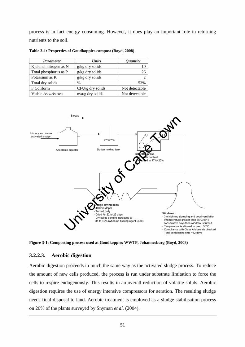
51

process is in fact energy consuming. However, it does play an important role in returning

nutrients to the soil.

Table 3-1: Properties of Goudkoppies compost (Boyd, 2008)

Parameter Units Quantity

Kjeldhal nitrogen as N g/kg dry solids 10

Total phosphorus as P g/kg dry solids 26

Potassium as K g/kg dry solids 2

Total dry solids % 53%

F Coliform CFU/g dry solids Not detectable

Viable Ascaris ova ova/g dry solids Not detectable

Belt filter press

- Dry solids content increased to 17 to 20%

Sludge drying beds- 400mm depth- Turned daily- Dried for 22 to 25 days - Dry solids content increased to 35 to 40% (when no bulking agent used)

Windrow

- 3m high (no slumping and good ventilation- If temperature greater then 55°C for 4 consecutive days then windrow is turned- Temperature is allowed to reach 50°C- Compliance with Class A biosolids checked- Total composting time ~12 days

Primary and waste activated sludge

Biogas

Anaerobic digester Sludge holding tank

Figure 3-1: Composting process used at Goudkoppies WWTP, Johannesburg (Boyd, 2008)

3.2.2.3. Aerobic digestion

Aerobic digestion proceeds in much the same way as the activated sludge process. To reduce

the amount of new cells produced, the process is run under substrate limitation to force the

cells to respire endogenously. This results in an overall reduction of volatile solids. Aerobic

digestion requires the use of energy intensive compressors for aeration. The resulting sludge

needs final disposal to land. Aerobic treatment is employed as a sludge stabilisation process

on 20% of the plants surveyed by Snyman et al. (2004).

Univers

ity of

Cap

e Tow

n

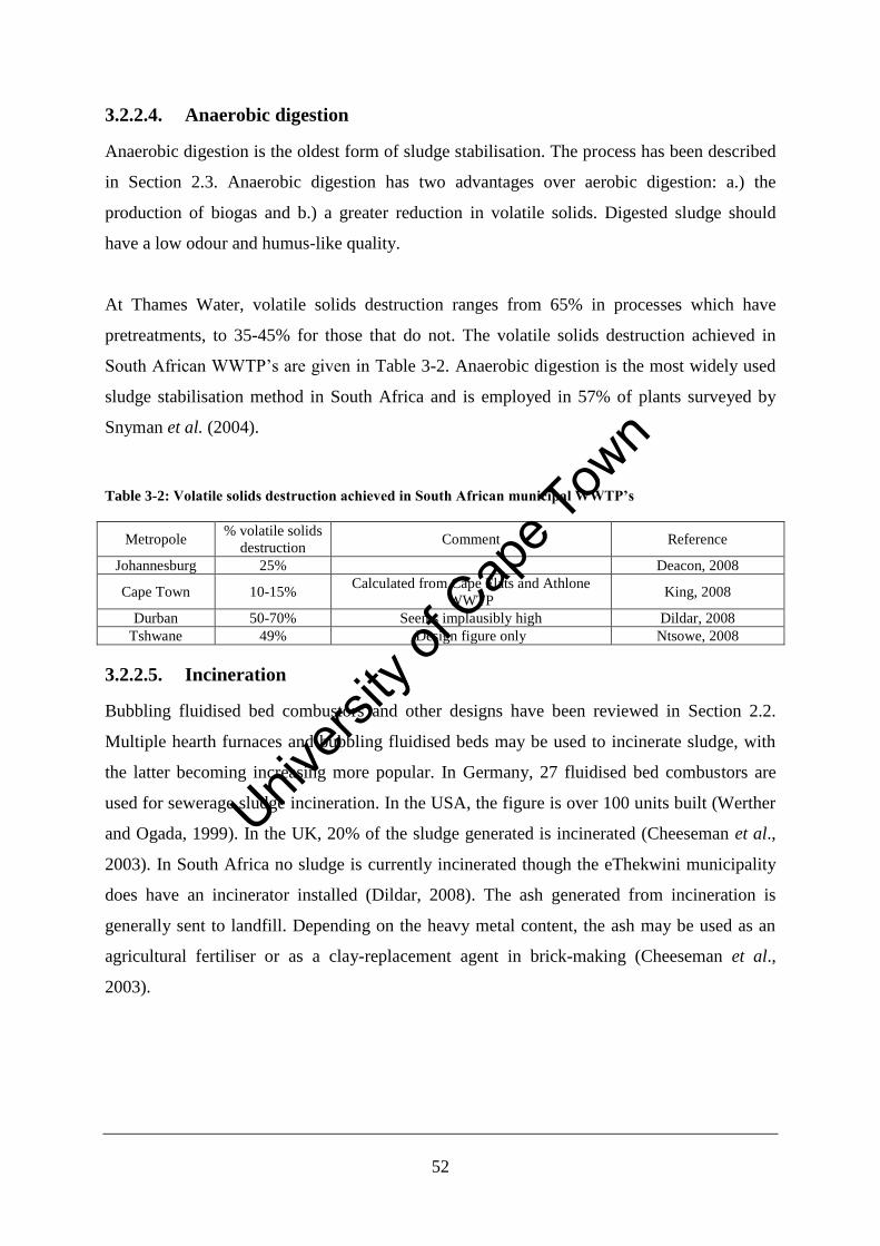
52

3.2.2.4. Anaerobic digestion

Anaerobic digestion is the oldest form of sludge stabilisation. The process has been described

in Section 2.3. Anaerobic digestion has two advantages over aerobic digestion: a.) the

production of biogas and b.) a greater reduction in volatile solids. Digested sludge should

have a low odour and humus-like quality.

At Thames Water, volatile solids destruction ranges from 65% in processes which have

pretreatments, to 35-45% for those that do not. The volatile solids destruction achieved in

South African WWTP’s are given in Table 3-2. Anaerobic digestion is the most widely used

sludge stabilisation method in South Africa and is employed in 57% of plants surveyed by

Snyman et al. (2004).

Table 3-2: Volatile solids destruction achieved in South African municipal WWTP’s

Metropole % volatile solids

destruction Comment Reference

Johannesburg 25% Deacon, 2008

Cape Town 10-15% Calculated from Cape Flats and Athlone

WWTP King, 2008

Durban 50-70% Seems implausibly high Dildar, 2008

Tshwane 49% Design figure only Ntsowe, 2008

3.2.2.5. Incineration

Bubbling fluidised bed combustors and other designs have been reviewed in Section 2.2.

Multiple hearth furnaces and bubbling fluidised beds may be used to incinerate sludge, with

the latter becoming increasing more popular. In Germany, 27 fluidised bed combustors are

used for sewerage sludge incineration. In the USA, the figure is over 100 units built (Werther

and Ogada, 1999). In the UK, 20% of the sludge generated is incinerated (Cheeseman et al.,

2003). In South Africa no sludge is currently incinerated though the eThekwini municipality

does have an incinerator installed (Dildar, 2008). The ash generated from incineration is

generally sent to landfill. Depending on the heavy metal content, the ash may be used as an

agricultural fertiliser or as a clay-replacement agent in brick-making (Cheeseman et al.,

2003).

Univers

ity of

Cap

e Tow

n

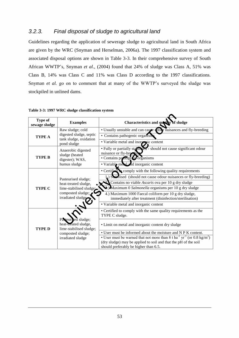
53

3.2.3. Final disposal of sludge to agricultural land

Guidelines regarding the application of sewerage sludge to agricultural land in South Africa

are given by the WRC (Snyman and Herselman, 2006a). The 1997 classification system and

associated disposal options are shown in Table 3-3. In their comprehensive survey of South

African WWTP’s, Snyman et al., (2004) found that 24% of sludge was Class A, 51% was

Class B, 14% was Class C and 11% was Class D according to the 1997 classifications.

Snyman et al. go on to comment that at many of the WWTP’s surveyed the sludge was

stockpiled in unlined dams.

Table 3-3: 1997 WRC sludge classification system

Type of

sewage sludge Examples Characteristics and quality of sludge

TYPE A

Raw sludge; cold

digested sludge, septic

tank sludge, oxidation

pond sludge

• Usually unstable and can cause odour nuisances and fly-breeding

• Contains pathogenic organisms

• Variable metal and inorganic content

TYPE B

Anaerobic digested

sludge (heated

digester); WAS,

humus sludge

• Fully or partially stabilised - should not cause significant odour

nuisance or fly-breeding • Contains pathogenic organisms


TYPE C

Pasteurised sludge;

heat-treated sludge,

lime-stabilised sludge;

composted sludge;

irradiated sludge

• Certified to comply with the following quality requirements 1.) Stabilised (should not cause odour nuisances or fly-breeding)

2.) Contains no viable Ascaris ova per 10 g dry sludge

3.) Maximum 0 Salmonella organisms per 10 g dry sludge

4.) Maximum 1000 Faecal coliform per 10 g dry sludge,

immediately after treatment (disinfection/sterilisation)


TYPE D

Pasteurised sludge;

heat-treated sludge,

lime-stabilised sludge;

composted sludge;

irradiated sludge

• Certified to comply with the same quality requirements as the

TYPE C sludge.

• Limit on metal and inorganic content dry sludge

• User must be informed about the moisture and N P K content.

• User must be warned that not more than 8 t ha-1

yr-1

(or 0.8 kg/m2)

(dry sludge) may be applied to soil and that the pH of the soil

should preferably be higher than 6.5.

Univers

ity of

Cap

e Tow

n

54

3.3. Thames Water’ plants investigated

Three Thames Water wastewater treatment plants in and around London, UK were visited.

The process description, process block diagram and plant operation are described in this

section.

3.3.1. Beckton WWTP, London Docklands

3.3.1.1. Process description

The Beckton wastewater treatment plant (WWTP) located in London Docklands is the largest

in the UK. The plant employs the activated sludge process and incineration is the final sludge

treatment option. Figure 3-3 shows an aerial photograph of Beckton WWTP.

The process at Beckton WWTP is a typical activated sludge process. Refering to Figure 3-2:

water from sewerage lines is channelled through the degritting channels to remove “rag”

(toilet paper) and other large floatable material. The flow is then slowed down, and any sand

from storm water run-off is allowed to settle. The water then passes to the primary settling

tanks, which are rectangular vessels with top skimmers to remove oil and grease and a slanted

bottom to bring the sludge to a central collection drain. The underflow is thickened on

primary gravity belt thickeners and the overflow enters the activated sludge process. The

activated sludge is thickened to 1 to 2% dry solids content in the secondary thickeners. The

overflow from the secondary settlers is returned to the river. Part of the thickened sludge in

the underflow is recycled back (the Return Activated Sludge or RAS) to the top of the

activated sludge process to maintain the culture in the vessel, and the rest (the Surplus

Activated Sludge or SAS) is sent to the secondary gravity belt thickeners. At Beckton WWTP

the ratio of RAS to SAS is 9:1.

Primary and secondary thickened sludge is mixed prior to the sludge holding tanks and is then

pumped to a filter press. The filter press operates up to 10 bar producing a filter cake of ~20%

solids conten which is conveyed to the paddle wheel feeder of the fluidised bed incinerator.

The bed of sand is fluidised by air passing through the distributor plate and the temperature is

maintained at 750°C by the combustion of the sludge. Should the temperature drop due to bad

combustion conditions (e.g. cake too moist); auxiliary gas lances are fired into the bed. The

flue gases leave the bed at 850 to 900°C. The hot gas is used to raise steam for a steam turbine

Univers

ity of

Cap

e Tow

n

55

and is then passed through a heat exchanger to preheat the incoming air stream to 300°C. The

exhausted steam from the turbine is sent to an economiser to further energy recovery. The

cool flue gases pass through bag filters to remove fine particulate matter before being released

to the atmosphere. Ash is collected from the bed and is trucked to a landfill site. shows the

block flow diagram of the Beckton WWTP.

3.3.1.2. Challenges to plant operation

Since commissioning of the fluidised bed incinerator there have been two serious occurrences

of bed agglomeration, which in plant shut-downs, removal of agglomerated material and

refurbishment of the incinerator.

The sequence of events which led to the second incident are:

The overbed feeder system did not distribute the fuel adequately over the bed and did

not break the fuel up into sufficiently small pieces.

The large pieces of fuel combusted on the outside only, resulting in CO release from

the O2 starved core.

The CO combusted above the bed leading to a very high freeboard temperature, but

owing to the lack of oxidation in the bed, the bed temperature was low.

To maintain the bed temperature, the gas lances were switched on. These increased the

bed temperature locally but further starved the large sludge particles of oxygen.

The sludge feeder continued to add more fuel into the bed. This was neither mixed

well nor completely combusted.

The reducing conditions (oxygen starved atmosphere) created in the bed led to the

agglomeration of ash which, in turn, caused the bed to defluidise.

More air could not be introduced into the system as the induced draft and forced draft

fans were under designed and already operating at full capacity.

Water sprays were turned on to reduce the freeboard temperature as the design limit

on the freeboard temperature is 900°C to prevent structural damage,

Refurbishment of the unit included 6 underbed nozzle feeders to distribute the feed evenly

into the bed and ensure smaller feed particles. Underbed feeding is advantageous for fluidised

beds owing to increased devolatilisation of the solid particles in the bed, rather than above it.

When fuel particles devolatilise on the surface of the bed overbed combustion can occur,

leading to the loss in bed temperature and the runaway freeboard temperatures seen above.

Univers

ity of

Cap

e Tow

n

56

The feed to the incinerator is a mixture of primary and secondary sludge. The dewatering

capability of primary sludge is far better the secondary sludge as secondary sludge is

primarily composed of microbial cells which have a high proportion of bound water which

cannot be mechanically removed. Hence primary sludge is a superior fuel. A well running

WWTP should produce more primary sludge than secondary. However, if the primary settlers

are not working properly, then a higher BOD load goes to the activated sludge vessels,

resulting in higher biomass yields. A rough guideline to predicting the performance of the

incinerator based on the relative content of primary and secondary sludge content is shown in

Table 3-4.

Univers

ity of

Cap

e Tow

n

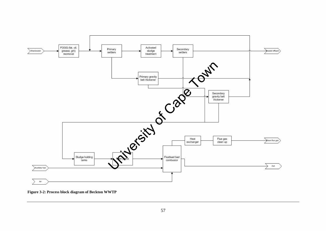
57

Figure 3-2: Process block diagram of Beckton WWTP

Univers

ity of

Cap

e Tow

n

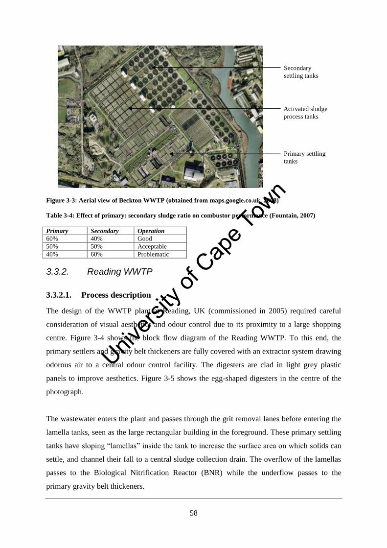
58

Figure 3-3: Aerial view of Beckton WWTP (obtained from maps.google.co.uk, 2008)

Table 3-4: Effect of primary: secondary sludge ratio on combustor performance (Fountain, 2007)

Primary Secondary Operation

60% 40% Good

50% 50% Acceptable

40% 60% Problematic

3.3.2. Reading WWTP


The design of the WWTP plant at Reading, UK (commissioned in 2005) required careful

consideration of visual aesthetics and odour control due to its proximity to a large shopping

centre. Figure 3-4 shows the block flow diagram of the Reading WWTP. To this end, the

primary settlers and gravity belt thickeners are fully covered with an extractor system drawing

odorous air to a central odour control facility. The digesters are clad in light grey plastic

panels to improve aesthetics. Figure 3-5 shows the egg-shaped digesters in the centre of the

photograph.

The wastewater enters the plant and passes through the grit removal lanes before entering the

lamella tanks, seen as the large rectangular building in the foreground. These primary settling

tanks have sloping “lamellas” inside the tank to increase the surface area on which solids can

settle, and channel their fall to a central sludge collection drain. The overflow of the lamellas

passes to the Biological Nitrification Reactor (BNR) while the underflow passes to the

primary gravity belt thickeners.

Secondary

settling tanks

Activated sludge

process tanks

Primary settling

tanks

Univers

ity of

Cap

e Tow

n

59

The BNR’s are long channel reactors with aerobic and anoxic zones which allow nitrifying

and denitrifying bacteria, respectively, to convert ammonia to nitrate and nitrate to nitrogen.

In the aerobic zones, BOD reduction occurs. The flow passes into the secondary settlers at the

end of the channel. The overflow from the thickeners is sent to a tertiary settler before being

released to the river. About 80% of the sludge in the underflow is returned to the BNR’s and

20% passes to the secondary gravity belt thickeners and the overflow is sent to tertiary settlers

before being returned to the river.

The gravity belt thickeners thicken the sludge to 6% dry solids. The thickened sludge is sent

to the pasteurisation unit where it is heated to 55°C for half an hour using a heat exchange

surface inside the vessel. This process kills vegetative pathogens, resulting in a log 5 pathogen

reduction, but does not give any improvement in the digestibility of the sludge (Shana,

2005).This may be due in part to the high content of volatile fatty acids in the primary sludge

which would partially hydrolyse the sludge prior to pasteurisation.

The pasteurised sludge is then pumped to the egg-shaped digesters. The shape of these

concrete vessels aid mixing, as well as ease of sludge withdrawal. The digesters are mixed by

three impellers which have been found to give good radial mixing but limited axial mixing.

The resulting vertical stratification of the digester contents will be minimised by the planned

installation of recirculation pumps.

Biogas collects at the top of the reactor and passes to a double-walled rubber gas collection

“balloon”. The inner balloon collapses and expands as the gas flow fluctuates. The outer

protective balloon, maintained at a pressure slightly above atmospheric, facilitates gas flow

out of the inner balloon. The gas is used in a modularised Combined Heat and Power (CHP)

engines which each produce 0.5 MW of electricity. The exhaust gases from the engine are

used in a heat exchanger to heat the sludge in the pasteurisation unit.

The digester sludge is dewatered to ~20% solids in a centrifuge, whilst the dewatered cake is

stored in silos ready to be taken away to land. The overall volatile solids destruction of the

digesters is 45% compared to the 65% volatile solids reduction at Chertsey WWTP.

Univers

ity of

Cap

e Tow

n

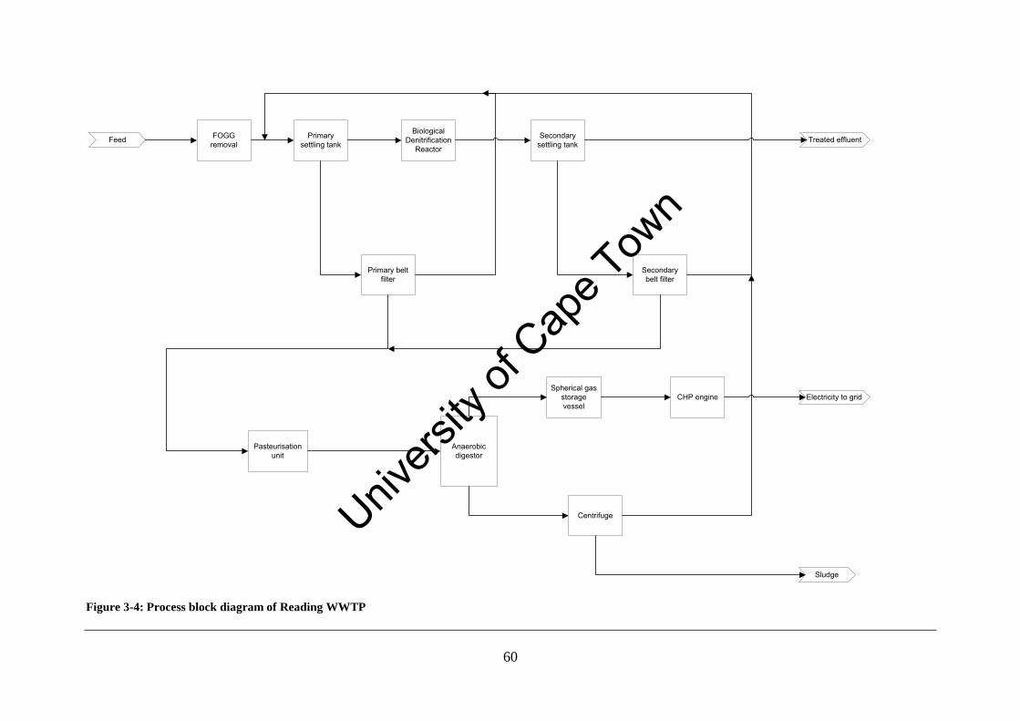
60

FOGG removal

Primary settling tank

Biological Denitrification

Reactor

Secondary settling tank

Primary belt filter

Secondary belt filter

Treated effluent

Anaerobic digestor

Pasteurisation unit

Centrifuge

Sludge

Feed

Spherical gas storage vessel

CHP engine Electricity to grid

Figure 3-4: Process block diagram of Reading WWTP

Univers

ity of

Cap

e Tow

n

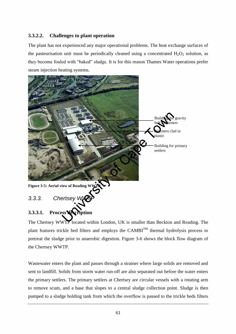
61


The plant has not experienced any major operational problems. The heat exchange surfaces of

the pasteurisation unit must be periodically cleaned using a concentrated H2O2 solution, as

they become fouled with “baked” sludge. It is for this reason Thames Water operations prefer

steam injection heating systems.

Figure 3-5: Aerial view of Reading WWTP

3.3.3. Chertsey WWTP


The Chertsey WWTP located within London, UK is smaller than Beckton and Reading. The

plant features trickle bed filters and employs the CAMBITM

thermal hydrolysis process to

pretreat the sludge prior to anaerobic digestion. Figure 3-6 shows the block flow diagram of

the Chertsey WWTP.

Wastewater enters the plant and passes through a strainer where large solids are removed and

sent to landfill. Solids from storm water run-off are also separated out before the water enters

the primary settlers. The primary settlers at Chertsey are circular vessels with a rotating arm

to remove scum, and a base that slopes to a central sludge collection point. Sludge is then

pumped to a sludge holding tank from which the overflow is passed to the trickle beds filters

Building for gravity

belt thickeners

Digesters clad in

plastic

Building for primary

settlers

Univers

ity of

Cap

e Tow

n

62

and then on to the secondary thickeners. The overflow from the secondary thickeners is

released to the environment and the underflow thickened in gravity belt thickeners before

entering the sludge holding tank. The trickle bed filters at Chertsey WWTP offer a low energy

alternative to the activated sludge process used at the Beckton and Reading WWTP’s.

Chertsey WWTP accepts “import” sludge from other plants which do not have their own

processing capabilities. The “import” sludge is pumped from the tanker into the sludge

holding tank. The sludge from the sludge holding tank is passed through a rag remover to

prevent blockage of the downstream progressive cavity pumps downstream. The sludge is

dewatered to ~15% solids in a belt press. Pumping a 15% dry solids sludge is difficult and

hence the dewatered sludge is re-slurried to 12% to allow for ease of pumping. The sludge is

then passed to the CAMBITM

thermal hydrolysis plant.

The thermal hydrolysis plant consists of three units: a pulper, a reactor and a flash vessel and

operates in sequential batch mode. The sludge is pre-heated to 90°C in the pulper by injecting

recycled steam from the reactor and flash tank. The sludge is then pumped to the reactor at

165°C and 8 bar where it is held under these conditions for 30 minutes, destroying the cell

wall, and making the sludge easier to digest. The severe conditions also destroy pathogens

and the process achieves a pathogen reduction of log 7 (Shana, 2006). The addition of the

steam to the pulper and reactor reduce the solids content further to ~9%.

The pressure on the vessel is then slowly relieved, and the sludge passes to the flash vessel

operated at 105°C by flashing steam back to the pulper. Any vapours from the pulper are

liquefied in a dedicated offgas treatment unit and pumped, with the hydrolysed sludge, to the

digester, thereby eliminating odour.

The digester is operated at a solids content of ~7% and is mixed by sparging the vessel with

the biogas. The digester achieves a high volatile solids destruction of 65% as a result of the

pretreatment process. The digested sludge is dewatered off site, due to capacity constraints,

and the remaining sludge is sent to land.

The biogas is stored in a steel expandable gas storage vessel. Approximately 55% of the gas is

used in a steam boiler to raise steam for the plant and the rest is flared. The reason for not

Univers

ity of

Cap

e Tow

n

63

installing a CHP engine is that the facility to export power onto the grid is not available and

installing it is a large capital expenditure with a long return on investment.


The thermal hydrolysis plant at Chertsey was commissioned in 1999 to increase the

throughput of the existing digesters. The plant initially experienced problems with foul gas

produced from the flash tank. It was re-commissioned in 2005 by CAMBITM

and the

operation of the plant was also out-sourced to CAMBITM

. As CAMBITM

is paid per tonne

solids processed, there is a high incentive for maintaining the plant. Since re-commissioning,

the plant has operated successfully with the overall result that the anaerobic digesters achieve

65% volatile solids destruction compared to the 45% seen at Reading.

Problems with the mixing of the digester at Chertsey WWTP result in acidified regions

forming in the digester. Should the entire digester contents become acidified, the whole

digester the unit may have to be drained and restarted; a process which could up to 3 weeks if

there is no seed culture or 10 days if a seed culture is available. In the case of the Chertsey

WWTP, the problem was diagnosed early, allowing remedial action to be taken viz. diluting

the reactor contents.

This problem occurred due to an under-designed gas sparging system for sludge, which

contained 7% dry solids. The pumps for the system were not able to operate all the nozzles

simultaneously, so a sequential operation of nozzles was introduced such that four out of the

six nozzles would operate sequentially at full capacity at any one time. This modification

improved the overall mixing of the digester.

Univers

ity of

Cap

e Tow

n

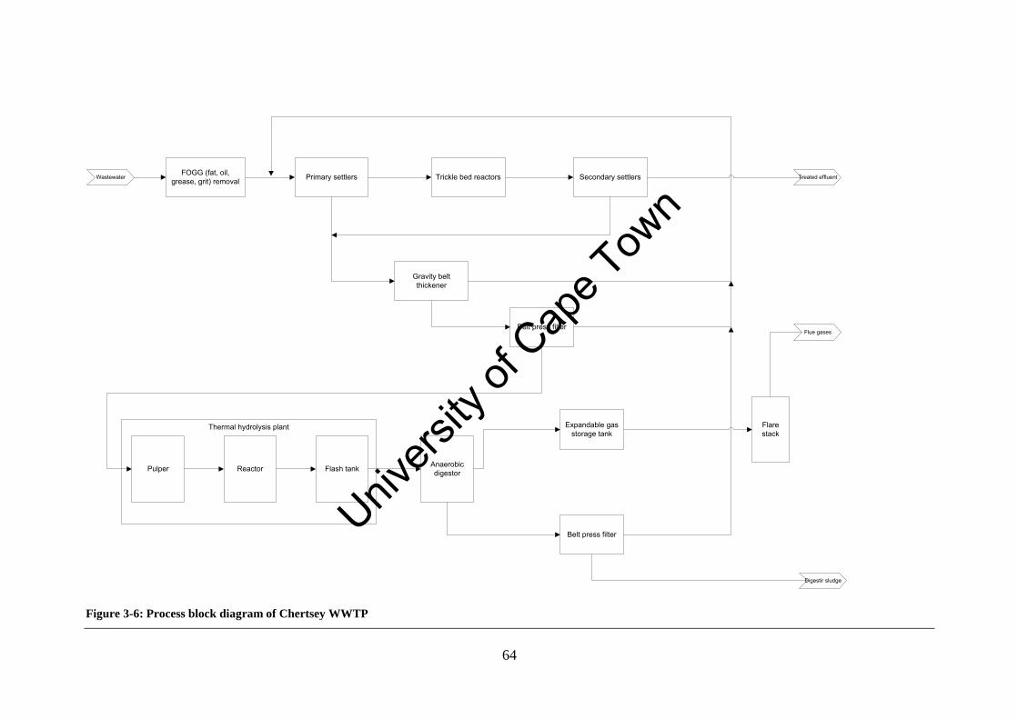
64

FOGG (fat, oil, grease, grit) removal Primary settlers Secondary settlersTrickle bed reactors

Gravity belt thickener

Pulper Reactor Flash tank Anaerobic digestor

Belt press filter

Belt press filter

Expandable gas storage tank

Flare stack

Wastewater

Flue gases

Digestir sludge

Treated effluent

Thermal hydrolysis plant

Figure 3-6: Process block diagram of Chertsey WWTP

Univers

ity of

Cap

e Tow

n

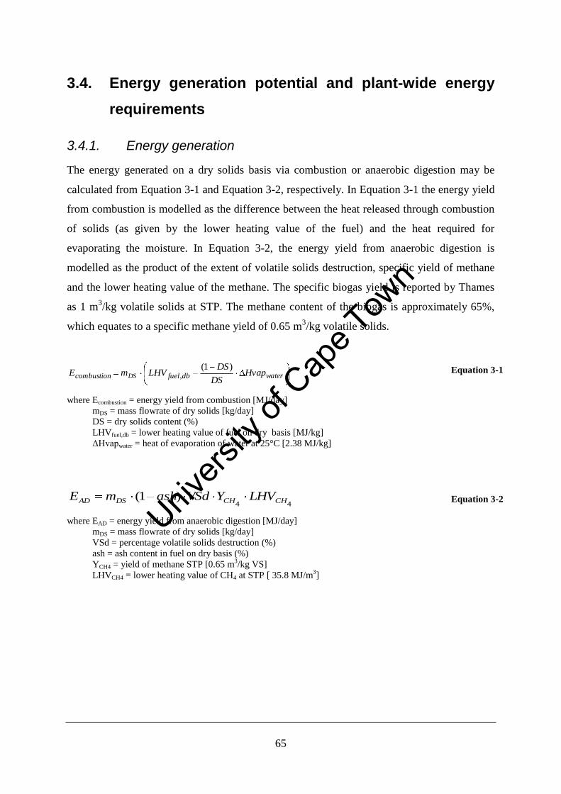
65

3.4. Energy generation potential and plant-wide energy

requirements

3.4.1. Energy generation

The energy generated on a dry solids basis via combustion or anaerobic digestion may be

calculated from Equation 3-1 and Equation 3-2, respectively. In Equation 3-1 the energy yield

from combustion is modelled as the difference between the heat released through combustion

of solids (as given by the lower heating value of the fuel) and the heat required for

evaporating the moisture. In Equation 3-2, the energy yield from anaerobic digestion is

modelled as the product of the extent of volatile solids destruction, specific yield of methane

and the lower heating value of the methane. The specific biogas yield is reported by Thames

as 1 m3/kg volatile solids at STP. The methane content of the biogas is approximately 65%,

which equates to a specific methane yield of 0.65 m3/kg volatile solids.

waterdbfuelcombustion HvapDS

DSLHVmE DS

)1(, Equation 3-1

where Ecombustion = energy yield from combustion [MJ/day]

mDS = mass flowrate of dry solids [kg/day]

DS = dry solids content (%)

LHVfuel,db = lower heating value of fuel on dry basis [MJ/kg]

ΔHvapwater = heat of evaporation of water at 25°C [2.38 MJ/kg]

44)1( CHCHDSAD LHVYVSdashmE Equation 3-2

where EAD = energy yield from anaerobic digestion [MJ/day]


VSd = percentage volatile solids destruction (%)

ash = ash content in fuel on dry basis (%)

YCH4 = yield of methane STP [0.65 m3/kg VS]

LHVCH4 = lower heating value of CH4 at STP [ 35.8 MJ/m3]

Univers

ity of

Cap

e Tow

n

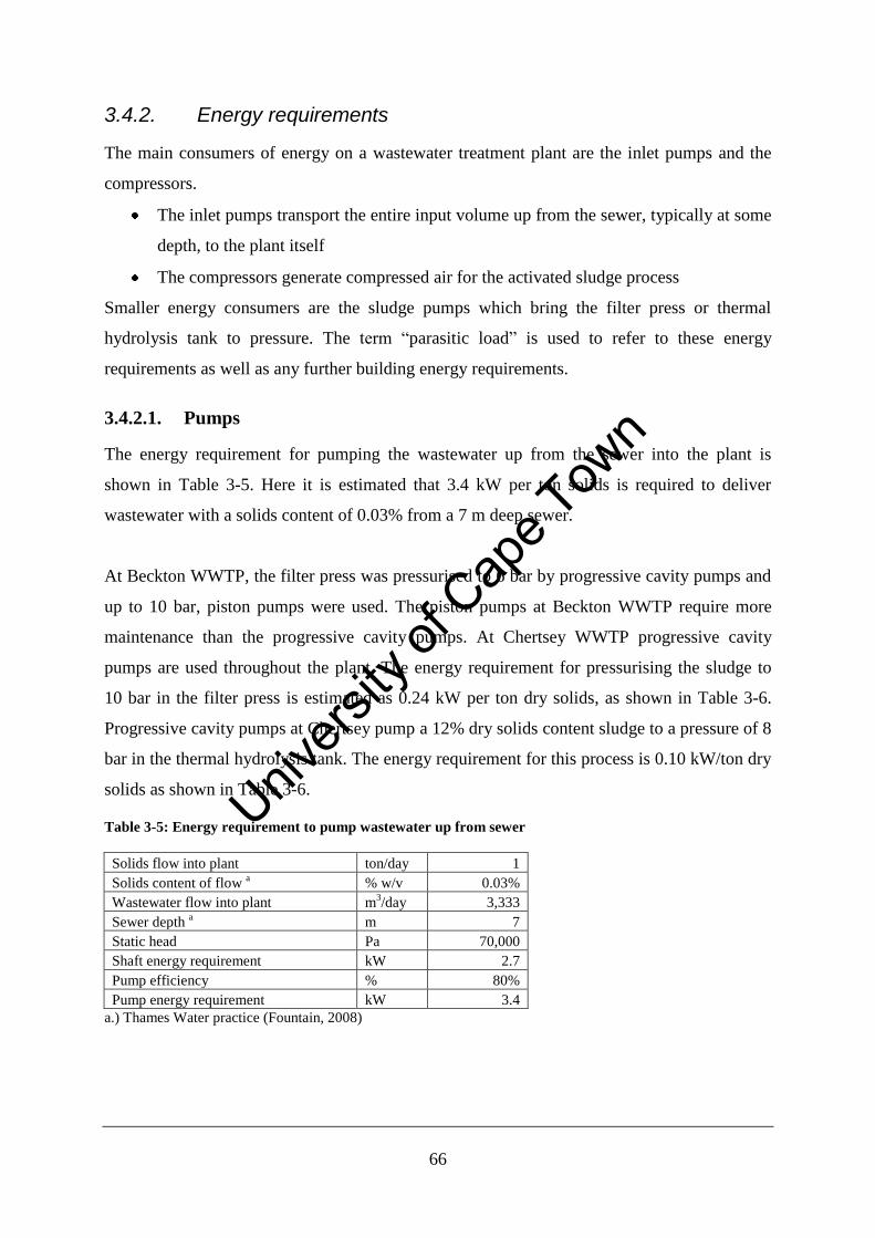
66

3.4.2. Energy requirements

The main consumers of energy on a wastewater treatment plant are the inlet pumps and the

compressors.

The inlet pumps transport the entire input volume up from the sewer, typically at some

depth, to the plant itself

The compressors generate compressed air for the activated sludge process

Smaller energy consumers are the sludge pumps which bring the filter press or thermal

hydrolysis tank to pressure. The term “parasitic load” is used to refer to these energy

requirements as well as any further building energy requirements.

3.4.2.1. Pumps

The energy requirement for pumping the wastewater up from the sewer into the plant is

shown in Table 3-5. Here it is estimated that 3.4 kW per ton solids is required to deliver

wastewater with a solids content of 0.03% from a 7 m deep sewer.

At Beckton WWTP, the filter press was pressurised to 6 bar by progressive cavity pumps and

up to 10 bar, piston pumps were used. The piston pumps at Beckton WWTP require more

maintenance than the progressive cavity pumps. At Chertsey WWTP progressive cavity

pumps are used throughout the plant. The energy requirement for pressurising the sludge to

10 bar in the filter press is estimated as 0.24 kW per ton dry solids, as shown in Table 3-6.

Progressive cavity pumps at Chertsey pump a 12% dry solids content sludge to a pressure of 8

bar in the thermal hydrolysis tank. The energy requirement for this process is 0.10 kW/ton dry

solids as shown in Table 3-6.

Table 3-5: Energy requirement to pump wastewater up from sewer

Solids flow into plant ton/day 1

Solids content of flow a

% w/v 0.03%

Wastewater flow into plant m3/day 3,333

Sewer depth a

m 7

Static head Pa 70,000

Shaft energy requirement kW 2.7

Pump efficiency % 80%

Pump energy requirement kW 3.4

a.) Thames Water practice (Fountain, 2008)

Univers

ity of

Cap

e Tow

n

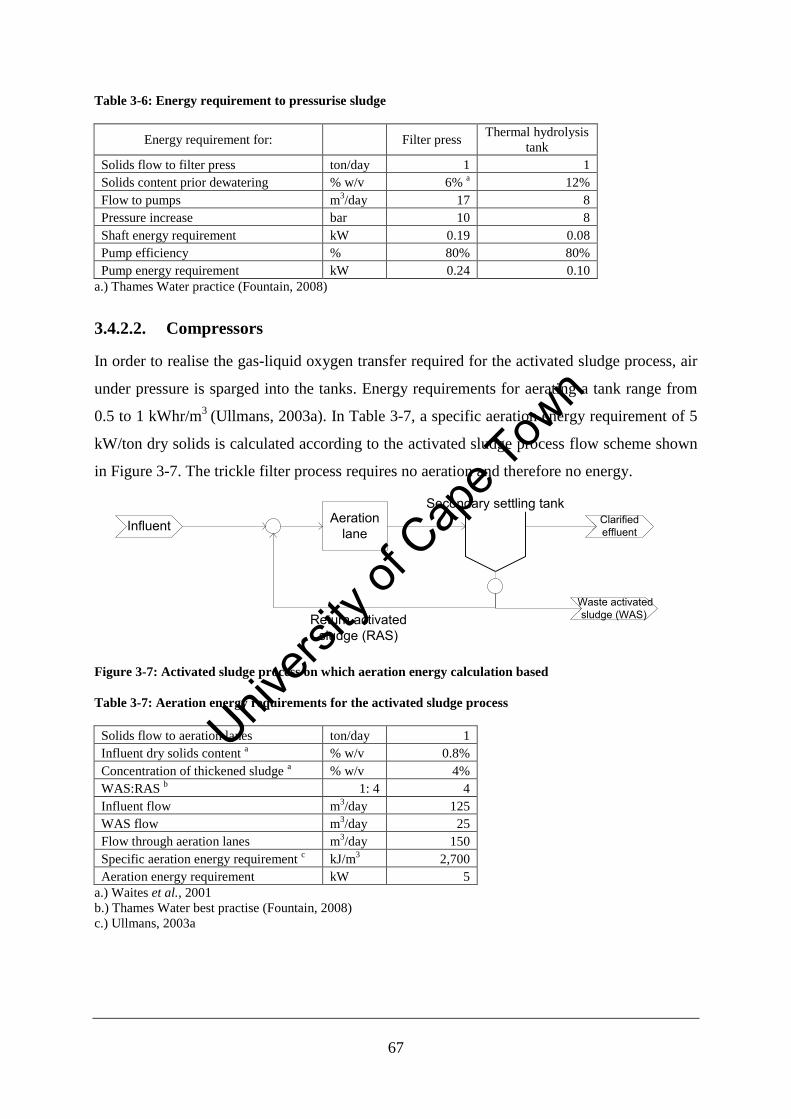
67

Table 3-6: Energy requirement to pressurise sludge

Energy requirement for: Filter press Thermal hydrolysis

tank

Solids flow to filter press ton/day 1 1

Solids content prior dewatering

% w/v 6% a

12%

Flow to pumps m3/day 17 8

Pressure increase bar 10 8

Shaft energy requirement kW 0.19 0.08

Pump efficiency % 80% 80%

Pump energy requirement kW 0.24 0.10

a.) Thames Water practice (Fountain, 2008)

3.4.2.2. Compressors

In order to realise the gas-liquid oxygen transfer required for the activated sludge process, air

under pressure is sparged into the tanks. Energy requirements for aerating a tank range from

0.5 to 1 kWhr/m3

(Ullmans, 2003a). In Table 3-7, a specific aeration energy requirement of 5

kW/ton dry solids is calculated according to the activated sludge process flow scheme shown

in Figure 3-7. The trickle filter process requires no aeration and therefore no energy.

Aeration lane

Secondary settling tankClarifiedeffluent

Waste activatedsludge (WAS)

Influent

Return activated sludge (RAS)

Figure 3-7: Activated sludge process on which aeration energy calculation based

Table 3-7: Aeration energy requirements for the activated sludge process

Solids flow to aeration lanes ton/day 1

Influent dry solids content a

% w/v 0.8%

Concentration of thickened sludge a

% w/v 4%

WAS:RAS b

1: 4 4

Influent flow m3/day 125

WAS flow m3/day 25

Flow through aeration lanes m3/day 150

Specific aeration energy requirement c

kJ/m3 2,700

Aeration energy requirement kW 5

a.) Waites et al., 2001

b.) Thames Water best practise (Fountain, 2008)

c.) Ullmans, 2003a

Univers

ity of

Cap

e Tow

n

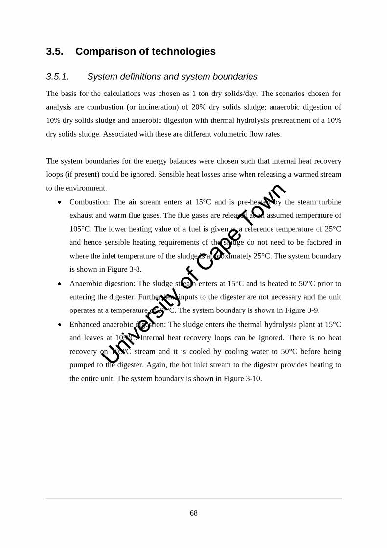
68

3.5. Comparison of technologies

3.5.1. System definitions and system boundaries

The basis for the calculations was chosen as 1 ton dry solids/day. The scenarios chosen for

analysis are combustion (or incineration) of 20% dry solids sludge; anaerobic digestion of

10% dry solids sludge and anaerobic digestion with thermal hydrolysis pretreatment of a 10%

dry solids sludge. Associated with these are different volumetric flow rates.

The system boundaries for the energy balances were chosen such that internal heat recovery

loops (if present) could be ignored. Sensible heat losses arise when releasing a warmed stream

to the environment.

Combustion: The air stream enters at 15°C and is pre-heated by the steam turbine

exhaust and warm flue gases. The flue gases are released at an assumed temperature of

105°C. The lower heating value of a fuel is given at a reference temperature of 25°C

and hence sensible heating requirements of the sludge do not need to be factored in

where the inlet temperature of the sludge is approximately 25°C. The system boundary

is shown in Figure 3-8.

Anaerobic digestion: The sludge stream enters at 15°C and is heated to 50°C prior to

entering the digester. Further heat inputs to the digester are not necessary and the unit

operates at a temperature of 37°C. The system boundary is shown in Figure 3-9.

Enhanced anaerobic digestion: The sludge enters the thermal hydrolysis plant at 15°C

and leaves at 105°C. Internal heat recovery loops can be ignored. There is no heat

recovery on 105°C stream and it is cooled by cooling water to 50°C before being

pumped to the digester. Again, the hot inlet stream to the digester provides heating to

the entire unit. The system boundary is shown in Figure 3-10.

Univers

ity of

Cap

e Tow

n

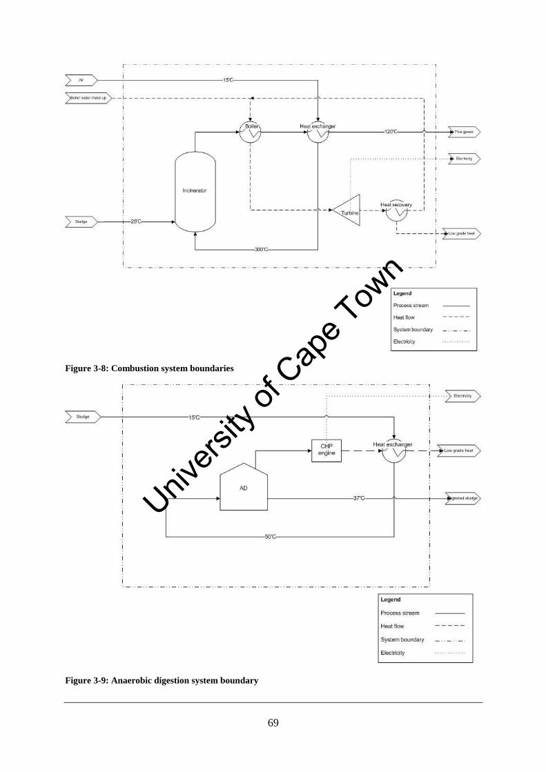
69

Figure 3-8: Combustion system boundaries

Figure 3-9: Anaerobic digestion system boundary

Univers

ity of

Cap

e Tow

n

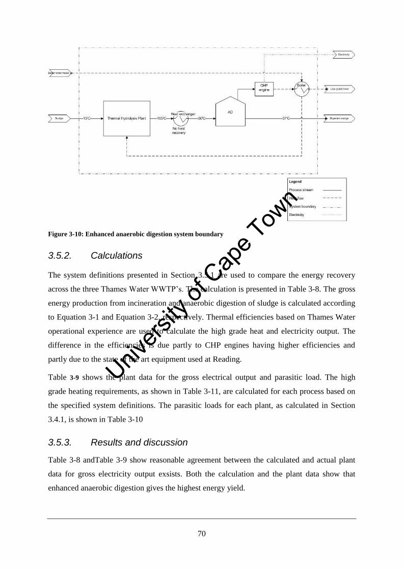
70

Figure 3-10: Enhanced anaerobic digestion system boundary

3.5.2. Calculations

The system definitions presented in Section 3.5.1 are used to compare the energy recovery

across the three Thames Water WWTP’s. The calculation is presented in Table 3-8. The gross

energy production from incineration and anaerobic digestion of sludge is calculated according

to Equation 3-1 and Equation 3-2, respectively. Thermal efficiencies based on Thames Water

operational experience are used to calculate the high grade heat and electricity output. The

difference in the efficiencies is due partly to CHP engines having higher efficiencies and

partly due to the state of the art equipment used at Reading.

Table 3-9 shows the plant data for the gross electrical output and parasitic load. The high

grade heating requirements, as shown in Table 3-11, are calculated for each process based on

the specified system definitions. The parasitic loads for each plant, as calculated in Section

3.4.1, is shown in Table 3-10

3.5.3. Results and discussion

Table 3-8 andTable 3-9 show reasonable agreement between the calculated and actual plant

data for gross electricity output exsists. Both the calculation and the plant data show that

enhanced anaerobic digestion gives the highest energy yield.

Univers

ity of

Cap

e Tow

n

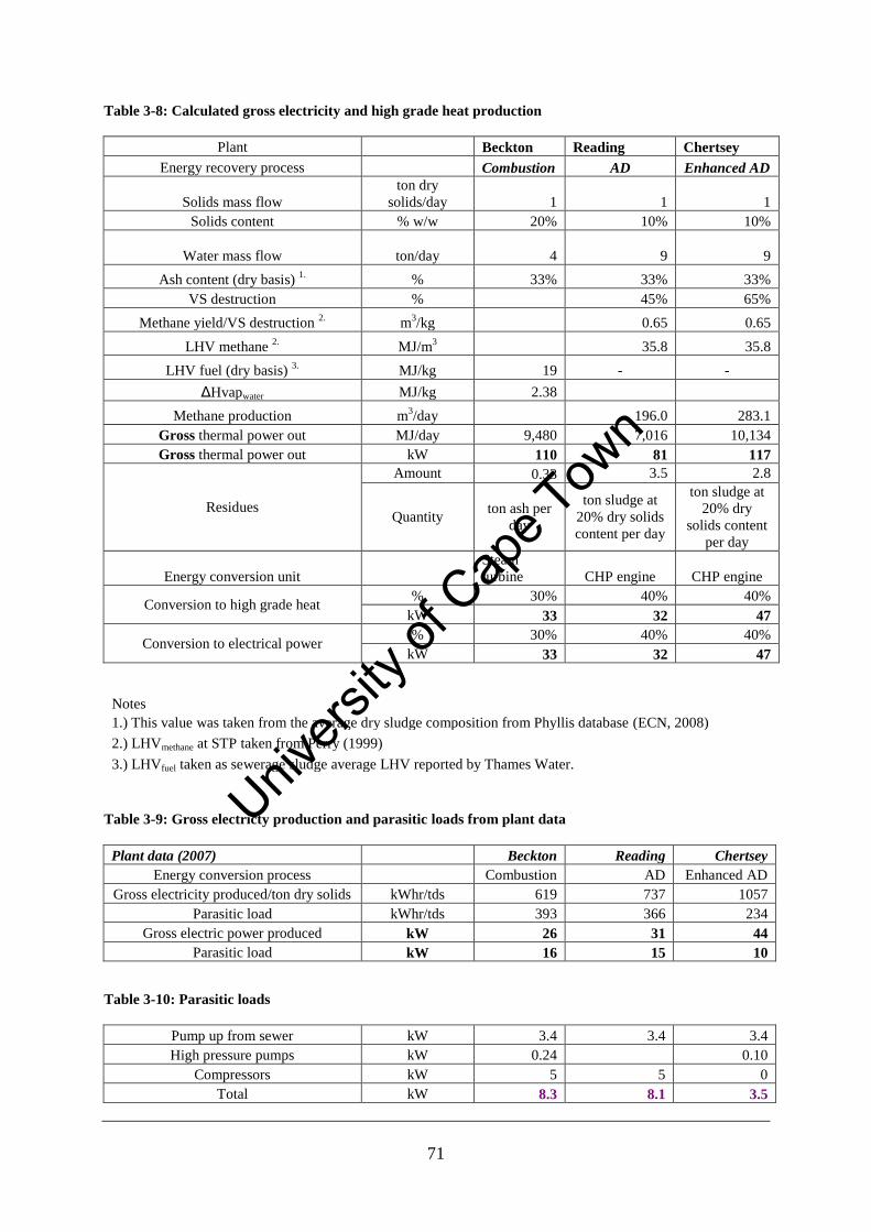
71

Table 3-8: Calculated gross electricity and high grade heat production

Plant Beckton Reading Chertsey

Energy recovery process Combustion AD Enhanced AD

Solids mass flow

ton dry

solids/day 1 1 1

Solids content % w/w 20% 10% 10%

Water mass flow ton/day

4

9

9

Ash content (dry basis) 1. % 33% 33% 33%

VS destruction % 45% 65%

Methane yield/VS destruction 2. m

3/kg 0.65 0.65

LHV methane 2.

MJ/m3 35.8 35.8

LHV fuel (dry basis) 3. MJ/kg 19 - -

ΔHvapwater MJ/kg 2.38

Methane production m3/day 196.0 283.1

Gross thermal power out MJ/day 9,480 7,016 10,134

Gross thermal power out kW 110 81 117

Residues

Amount 0.33 3.5 2.8

Quantity ton ash per

day

ton sludge at

20% dry solids

content per day

ton sludge at

20% dry

solids content

per day

Energy conversion unit

Steam

turbine CHP engine CHP engine

Conversion to high grade heat % 30% 40% 40%

kW 33 32 47

Conversion to electrical power % 30% 40% 40%

kW 33 32 47

Notes

1.) This value was taken from the average dry sludge composition from Phyllis database (ECN, 2008)

2.) LHVmethane at STP taken from Perry (1999)

3.) LHVfuel taken as sewerage sludge average LHV reported by Thames Water.

Table 3-9: Gross electricty production and parasitic loads from plant data

Plant data (2007) Beckton Reading Chertsey

Energy conversion process Combustion AD Enhanced AD

Gross electricity produced/ton dry solids kWhr/tds 619 737 1057

Parasitic load kWhr/tds 393 366 234

Gross electric power produced kW 26 31 44

Parasitic load kW 16 15 10

Table 3-10: Parasitic loads

Pump up from sewer kW 3.4 3.4 3.4

High pressure pumps kW 0.24 0.10

Compressors kW 5 5 0

Total kW 8.3 8.1 3.5

Univers

ity of

Cap

e Tow

n

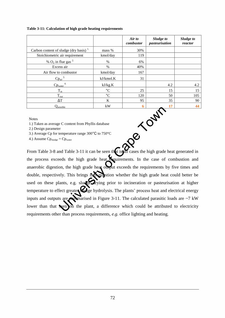
72

Table 3-11: Calculation of high grade heating requirements

Air to

combustor

Sludge to

pasteurisation

Sludge to

reactor

Carbon content of sludge (dry basis) 1. mass % 30%

Stoichiometric air requirement kmol/day 119

% O2 in flue gas 2. % 6%

Excess air % 40%

Air flow to combustor kmol/day 167

Cpair 3. kJ/kmol.K 31

Cpwater 4. kJ/kg.K 4.2 4.2

Tin °C 25 15 15

Tout °C 120 50 105

ΔT K 95 35 90

Qsensible kW 6 17 44

Notes

1.) Taken as average C content from Phyllis database

2.) Design parameter

3.) Average Cp for temperature range 300°C to 750°C

4.) Assume Cpsludge = Cpwater

From Table 3-8 and Table 3-11 it can be seen that is all cases the high grade heat generated in

the process exceeds the high grade heat requirements. In the case of combustion and

anaerobic digestion, the high grade heat output exceeds the requirements by five times and

double, respectively. This brings into question whether the high grade heat could better be

used on these plants, e.g. sludge drying prior to incineration or pasteurisation at higher

temperature to effect greater sludge hydrolysis. The plants’ process heat and electrical energy

inputs and outputs are summarised in Figure 3-11. The calculated parasitic loads are ~7 kW

lower than that seen on the plant, a difference which could be attributed to electricity

requirements other than process requirements, e.g. office lighting and heating.

Univers

ity of

Cap

e Tow

n

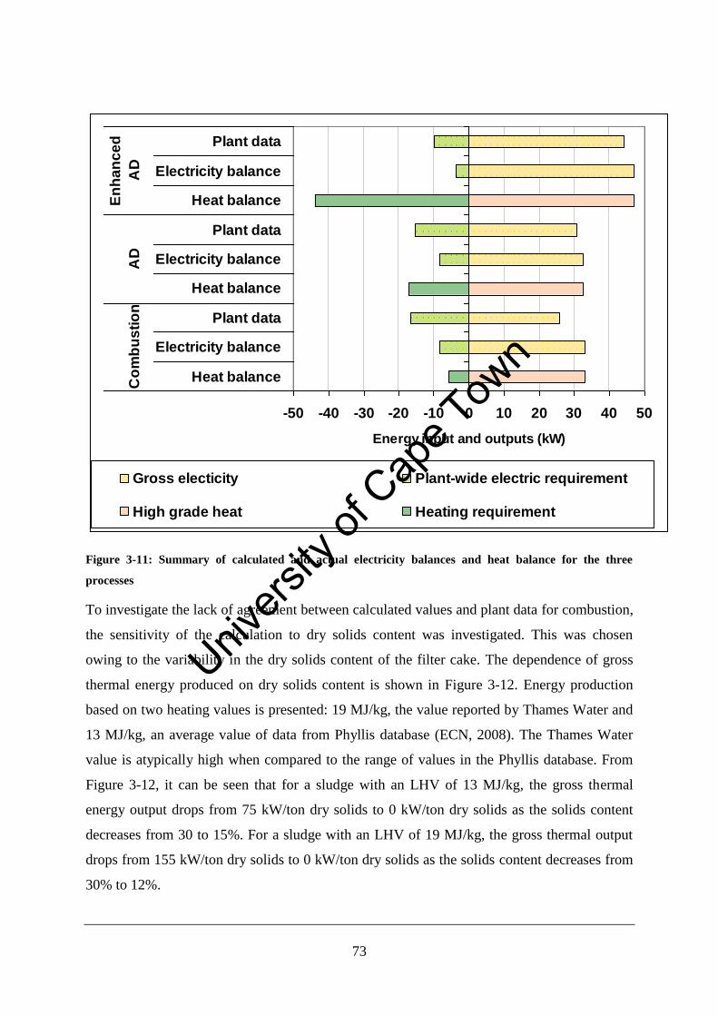
73

-50 -40 -30 -20 -10 0 10 20 30 40 50

Heat balance

Electricity balance

Plant data

Heat balance

Electricity balance

Plant data

Heat balance

Electricity balance

Plant dataC

om

bu

sti

on

AD

En

ha

nc

ed

AD

Energy input and outputs (kW)

Gross electicity Plant-wide electric requirement

High grade heat Heating requirement

Figure 3-11: Summary of calculated and actual electricity balances and heat balance for the three

processes

To investigate the lack of agreement between calculated values and plant data for combustion,

the sensitivity of the calculation to dry solids content was investigated. This was chosen

owing to the variability in the dry solids content of the filter cake. The dependence of gross

thermal energy produced on dry solids content is shown in Figure 3-12. Energy production

based on two heating values is presented: 19 MJ/kg, the value reported by Thames Water and

13 MJ/kg, an average value of data from Phyllis database (ECN, 2008). The Thames Water

value is atypically high when compared to the range of values in the Phyllis database. From

Figure 3-12, it can be seen that for a sludge with an LHV of 13 MJ/kg, the gross thermal

energy output drops from 75 kW/ton dry solids to 0 kW/ton dry solids as the solids content

decreases from 30 to 15%. For a sludge with an LHV of 19 MJ/kg, the gross thermal output

drops from 155 kW/ton dry solids to 0 kW/ton dry solids as the solids content decreases from

30% to 12%.

Univers

ity of

Cap

e Tow

n

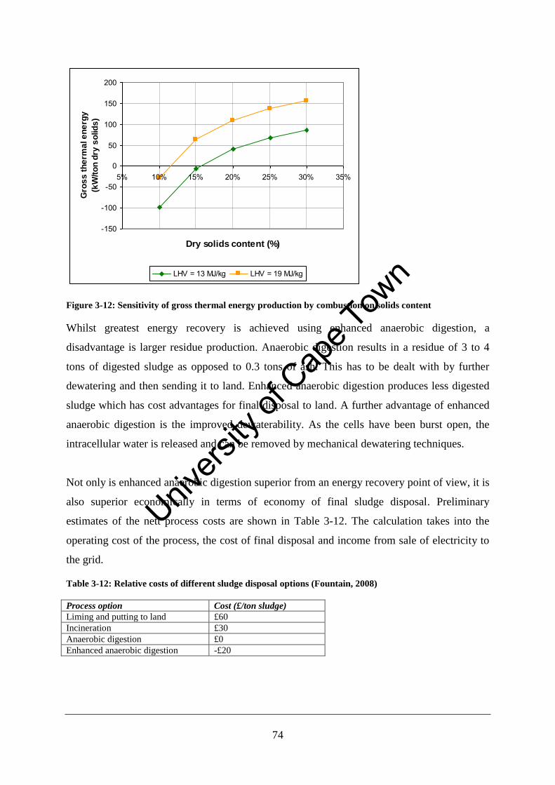
74

-150

-100

-50

0

50

100

150

200

5% 10% 15% 20% 25% 30% 35%

Dry solids content (%)

Gro

ss

th

erm

al e

ne

rgy

(kW

/to

n d

ry s

olid

s)

LHV = 13 MJ/kg LHV = 19 MJ/kg

Figure 3-12: Sensitivity of gross thermal energy production by combustion on solids content

Whilst greatest energy recovery is achieved using enhanced anaerobic digestion, a

disadvantage is larger residue production. Anaerobic digestion results in a residue of 3 to 4

tons of digested sludge as opposed to 0.3 tons of ash. This has to be dealt with by further

dewatering and then sending it to land. Enhanced anaerobic digestion produces less digested

sludge which has cost advantages for final disposal to land. A further advantage of enhanced

anaerobic digestion is the improved dewaterability. As the cells have been burst open, the

intracellular water is released and can be removed by mechanical dewatering techniques.

Not only is enhanced anaerobic digestion superior from an energy recovery point of view, it is

also superior economically in terms of economy of final sludge disposal. Preliminary

estimates of the nett process costs are shown in Table 3-12. The calculation takes into the

operating cost of the process, the cost of final disposal and income from sale of electricity to

the grid.

Table 3-12: Relative costs of different sludge disposal options (Fountain, 2008)

Process option Cost (£/ton sludge)

Liming and putting to land £60

Incineration £30

Anaerobic digestion £0

Enhanced anaerobic digestion -£20

Univers

ity of

Cap

e Tow

n

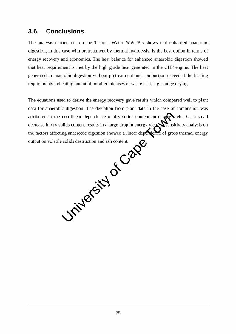
75

3.6. Conclusions

The analysis carried out on the Thames Water WWTP’s shows that enhanced anaerobic

digestion, in this case with pretreatment by thermal hydrolysis, is the best option in terms of

energy recovery and economics. The heat balance for enhanced anaerobic digestion showed

that heat requirement is met by the high grade heat generated in the CHP engine. The heat

generated in anaerobic digestion without pretreatment and combustion exceeded the heating

requirements indicating potential for alternate uses of waste heat, e.g. sludge drying.

The equations used to derive the energy recovery gave results which compared well to plant

data for anaerobic digestion. The deviation from plant data in the case of combustion was

attributed to the non-linear dependence of dry solids content on energy yield, i.e. a small

decrease in dry solids content results in a large drop in energy yield. A sensitivity analysis on

the factors affecting anaerobic digestion showed a linear dependence of gross thermal energy

output on volatile solids destruction and ash content.

Univers

ity of

Cap

e Tow

n

76

Chapter 4 Biogenic waste feedstock characteristics

and their effect on energy recovery

In this Chapter, two studies are carried out in which the effects of biogenic feedstock

characteristics on energy recovery are considered. Section 4.1 considers the effect of

biochemical feedstock characteristics on energy recovery in an anaerobic digester. The energy

costs of anaerobic digestion pretreatments are also considered. Section 4.2 considers the effect

of volatile combustion in bubbling fluidised beds.

4.1. Effect of recalcitrant substances on biogas yield

4.1.1. Biochemical components affecting digestibility

4.1.1.1. Lignocellulosic components

Cellulose, hemicellulose and lignin form the structural components of higher plants. The

biodegradability of agricultural residues, forestry residues and bagasse are affected by these

components. A short review of the structure of cellulose, hemicellulose and lignin and their

enzymatic hydrolysis is presented.

(1) Cellulose

Cellulose consists of up to 10 000 D-glucose molecules linked by β,1-4 glycosidic bonds

(Bailey and Ollis, 1986). Cellulose molecules align to form microfibrils which consist largely

of crystalline cellulose regions broken occasionally by amorphous cellulose regions. The

crystalline cellulose creates an extensive level surface which is difficult for hydrolytic

enzymes to attach to (Schwarz, 2001). Hydrogen bonding between and within the layers

strengthens the microfibril (Schwarz, 2001; Bailey and Ollis, 1986). The microfibrils usually

exist in a matrix of other polymers such as hemicellulose and lignin which further prevent

hydrolytic enzyme binding.

Cellulose degradation is important in terms of feasibly processing lignocellulosic feedstocks.

A number of components must work together to hydrolyse cellulose, as illustrated in Figure

4-1.

Univers

ity of

Cap

e Tow

n

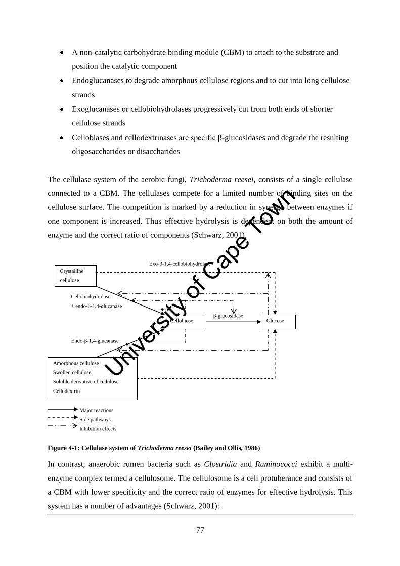
77

A non-catalytic carbohydrate binding module (CBM) to attach to the substrate and

position the catalytic component

Endoglucanases to degrade amorphous cellulose regions and to cut into long cellulose

strands

Exoglucanases or cellobiohydrolases progressively cut from both ends of shorter

cellulose strands

Cellobiases and cellodextrinases are specific β-glucosidases and degrade the resulting

oligosaccharides or disaccharides

The cellulase system of the aerobic fungi, Trichoderma reesei, consists of a single cellulase

connected to a CBM. The cellulases compete for a limited number of binding sites on the

cellulose surface. The competition is marked by a reduction in synergy between enzymes if

one component is increased. Thus effective hydrolysis is dependent on both the amount of

enzyme and the correct ratio of components (Schwarz, 2001).

Figure 4-1: Cellulase system of Trichoderma reesei (Bailey and Ollis, 1986)

In contrast, anaerobic rumen bacteria such as Clostridia and Ruminococci exhibit a multi-

enzyme complex termed a cellulosome. The cellulosome is a cell protuberance and consists of

a CBM with lower specificity and the correct ratio of enzymes for effective hydrolysis. This

system has a number of advantages (Schwarz, 2001):

Major reactions

Side pathways

Inhibition effects

Crystalline

cellulose

Amorphous cellulose

Swollen cellulose

Soluble derivative of cellulose

Cellodextrin

Cellobiose Glucose

Cellobiohydrolase

+ endo-β-1,4-glucanase

Endo-β-1,4-glucanase

β-glucosidase

Exo-β-1,4-cellobiohydrolase

Univers

ity of

Cap

e Tow

n

78

Synergy between the components is optimised by having the correct ratio

Non-productive binding is avoided by optimal spacing of the components

Competition for limited binding sites is reduced as all the components are bound

through a single domain with low specificity

A halt in hydrolysis on depletion of one type of cellulose is prevented by the presence

of other enzymes with different specificity.

(2) Hemicellulose

Hemicellulose consists of short branched polymers of pentoses (xyloses and arabinose) and

hexoses (glucose, galactose and mannose) (Bailey and Ollis, 1986). Most hemicelluloses are

β-1,4 linked except for galactose containing hemicelluloses which are β-1,3 linked. Unlike

cellulose, hemicellulose is not chemically homogenous. Hardwood hemicelluloses contain

mostly xylans, whereas softwood hemicelluloses contain mostly glucomannans (Saha, 2003).

Hemicellulose is hydrogen bonded to cellulose providing structural support to the plant and

protecting the cellulose from enzyme attack (Mosier et al., 2005).

The heterogeneous nature of hemicellulose means that many enzymes are involved in its

hydrolysis. Details of the enzymes involved in the hydrolysis of heteroarabinoxylans are

given in Table 4-1. Whilst many enzymes with different specificities are involved, the

enzymatic hydrolysis of hemicellulose is not as difficult tightly packed crystalline structures

are not present (Saha, 2003). Alternatively, an acid pretreatment may be used to hydrolyse the

hemicellulose to its sugars. Fermentative or acidogenic bacteria can convert the mixed sugars

arising from hemicellulose hydrolysis to organic acids, including acetate, propionate,

succinate and lactate (Saha, 2003).

Table 4-1: Enzymatic hydrolysis of heteroarabinoxylans (Saha, 2003)

Enzyme Mode of action

Endo-xylanase Hydrolyses mainly interior β-1,4-xylose linkages of the xylan backbone

Exo-xylanase Hydrolyses β-1,4-xylose linkages releasing xylobiose

β - Xylosidase Releases xylose from xylobiose and short chain xylo-oligosaccharides

α - Arabinofuranosidase Hydrolyses terminal non-reducing α-arabinofuranose from arabonoxylans

α - Glucuronidase Releases glucuronic acid from glucuronoxylans

Acetylxylan Hydrolyses acetylester bonds in acetyl xylans

Ferulic acid esterase Hydrolyses feruloylester bonds in xylans

ρ - Coumaric acid esterase Hydrolyses ρ-coumaryl ester bonds in xylans

Univers

ity of

Cap

e Tow

n

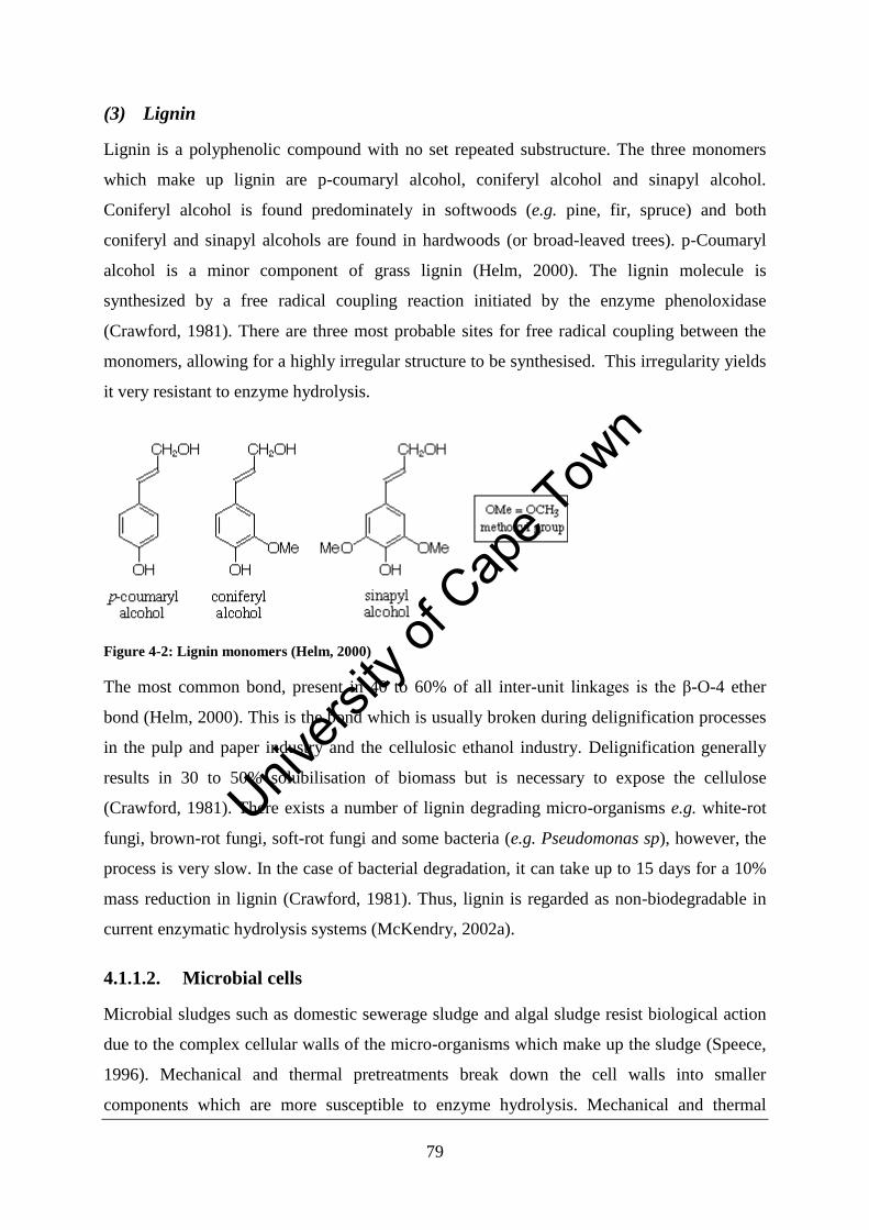
79

(3) Lignin

Lignin is a polyphenolic compound with no set repeated substructure. The three monomers

which make up lignin are p-coumaryl alcohol, coniferyl alcohol and sinapyl alcohol.

Coniferyl alcohol is found predominately in softwoods (e.g. pine, fir, spruce) and both

coniferyl and sinapyl alcohols are found in hardwoods (or broad-leaved trees). p-Coumaryl

alcohol is a minor component of grass lignin (Helm, 2000). The lignin molecule is

synthesized by a free radical coupling reaction initiated by the enzyme phenoloxidase

(Crawford, 1981). There are three most probable sites for free radical coupling between the

monomers, allowing for a highly irregular structure to be synthesised. This irregularity yields

it very resistant to enzyme hydrolysis.

Figure 4-2: Lignin monomers (Helm, 2000)

The most common bond, present in 40 to 60% of all inter-unit linkages is the β-O-4 ether

bond (Helm, 2000). This is the bond which is usually broken during delignification processes

in the pulp and paper industry and the cellulosic ethanol industry. Delignification generally

results in 30 to 50% solubilisation of biomass but is necessary to expose the cellulose

(Crawford, 1981). There exists a number of lignin degrading micro-organisms e.g. white-rot

fungi, brown-rot fungi, soft-rot fungi and some bacteria (e.g. Pseudomonas sp), however, the

process is very slow. In the case of bacterial degradation, it can take up to 15 days for a 10%

mass reduction in lignin (Crawford, 1981). Thus, lignin is regarded as non-biodegradable in

current enzymatic hydrolysis systems (McKendry, 2002a).

4.1.1.2. Microbial cells

Microbial sludges such as domestic sewerage sludge and algal sludge resist biological action

due to the complex cellular walls of the micro-organisms which make up the sludge (Speece,

1996). Mechanical and thermal pretreatments break down the cell walls into smaller

components which are more susceptible to enzyme hydrolysis. Mechanical and thermal

Univers

ity of

Cap

e Tow

n

80

pretreatments also allow the intracellular proteins and carbohydrate storage products to be

released into the bulk liquid to be utilised by the anaerobic digester microbes. Here, the

structure of bacterial cell walls and algal cell walls are considered.

(1) Bacterial cell walls

Bacterial cell walls can be classified according to their structure by Gram staining. The

bacteria retaining the purple iodine Gentian-violet complex even when washed with polar

solvents are termed Gram positive and those not retaining the complex, Gram negative.

Common to both types of cell envelopes is the inner peptidoglycan layer and cytoplasmic

membrane. The peptidoglycan layer consists of alternating β-1,4 linked disaccharides of N-

acetyl-D-glucosamine (NAG) and N-acetyl-muranic acid (NAM) (Bailey and Ollis, 1986;

Middelberg, 1995; Harrison, 1991). NAG comprises a tetrapeptide side chain onto which a

pentapeptide crosslink is attached, allowing crosslinking of the linear saccharide polymers.

The cross-linking provides shape and tensile strength to the cell. The cytoplasmic membrane

consists of a phospholipid bilayer with embedded protein molecules. The proteins regulate the

movement of nutrients through the cell membrane. The cytoplasmic membrane is the

biochemical boundary of the cell, controlling transfer of molecules but providing little

structural strength (Harrison, 1991).

Gram positive cell walls consist of a thick peptidoglycan layer of 15 to 80 nm, compared to 2

nm for Gram negative cells (Bailey and Ollis, 1986). This surrounds the cytoplasmic cell

membrane. Gram negative cell envelopes consist of 4 layers as shown in Figure 4-3. The

outermost layer is a lipid bilayer comprising of transmembrane proteins, phospholipids and

lipopolysaccharides (LPS) and is anchored to the peptidoglycan layer. The lipid bilayer of a

Gram negative cell protects the inner layers from direct chemical attack and the peptidoglycan

layer provides mechanical strength (Harrison, 1991). Although Gram positive cells do not

have a lipid bilayer, their peptidoglycan layer is much thicker and hence yields them less

amenable to mechanical cell disruption techniques, such a high pressure homogenisation or

bead milling. Between the peptidoglygan layer and the cytoplasmic membrane is the

periplasmic space which can contribute up 20 to 40% of the cell mass (Bailey and Ollis,

1986).

Univers

ity of

Cap

e Tow

n

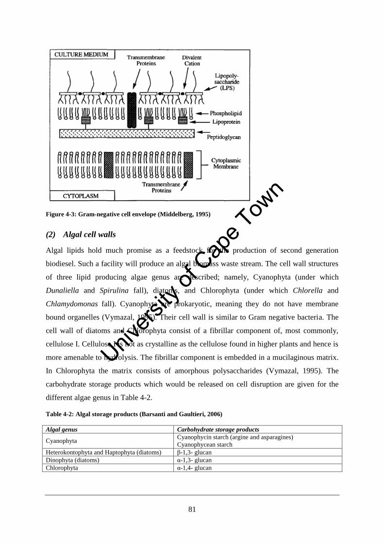
81

Figure 4-3: Gram-negative cell envelope (Middelberg, 1995)

(2) Algal cell walls

Algal lipids hold much promise as a feedstock for the production of second generation

biodiesel. Such a facility will produce an algal biomass waste stream. The cell wall structures

of three lipid producing algae genus are described; namely, Cyanophyta (under which

Dunaliella and Spirulina fall), diatoms, and Chlorophyta (under which Chlorella and

Chlamydomonas fall). Cyanophyta are prokaryotic, meaning they do not have membrane

bound organelles (Vymazal, 1995). Their cell wall is similar to Gram negative bacteria. The

cell wall of diatoms and Chlorophyta consist of a fibrillar component of, most commonly,

cellulose I. Cellulose I is not as crystalline as the cellulose found in higher plants and hence is

more amenable to hydrolysis. The fibrillar component is embedded in a mucilaginous matrix.

In Chlorophyta the matrix consists of amorphous polysaccharides (Vymazal, 1995). The

carbohydrate storage products which would be released on cell disruption are given for the

different algae genus in Table 4-2.

Table 4-2: Algal storage products (Barsanti and Gaultieri, 2006)

Algal genus Carbohydrate storage products

Cyanophyta Cyanophycin starch (argine and asparagines)

Cyanophycean starch

Heterokontophyta and Haptophyta (diatoms) β-1,3- glucan

Dinophyta (diatoms) α-1,3- glucan

Chlorophyta α-1,4- glucan

Univers

ity of

Cap

e Tow

n

82

4.1.2. Increasing energy yield from anaerobic digestion

The energy yield of anaerobic digestion is dependent on the volatile solids (organic solids)

destruction and the ash content of the fuel as seen in Equation 3-2. Anaerobic digestion at a

methane yield of 0.65 m3/kg volatile solids, 100% volatile solids destruction and no ash gives

a maximum energy yield of 23 MJ/kg dry solids.

4.1.2.1. Predicting volatile solids destruction

The volatile solids destruction for sewerage sludge anaerobic digesters ranges from 15 to 45%

depending on the operation. In Chapter 3, it is shown that pretreatment allows greater volatile

solids destruction (up to 65% with thermal hydrolysis). The volatile solids destruction of

simple carbohydrate loaded streams such as those from breweries or fruit processing

operations reaches 95% and higher. Lignin is not considered digestible and hence the

maximum digestibility of lignocellulosic material will only be the non-lignocellulolytic

components. The Biochemical Methane Potential assay was developed to determine the

digestibility of a feedstock experimentally (Speece, 1996; Owen et al, 1979). A small batch

anaerobic digester is inoculated with acclimatised sludge and the cumulative gas production is

monitored. Initial and final COD readings are measured to give the extent of volatile solids

destruction.

4.1.2.2. Energy requirements of pretreatments

The improvement in volatile solids destruction due to the action of a particular pretreatment

should not be offset by the energy requirements of the pretreatment itself. In Section 0 it was

seen that the energy requirement of the CAMBITM

thermal hydrolysis plant at Chertsey

WWTP was less than the high grade heat produced by the CHP engine did not reduce the

gross energy yield; i.e. the improvement in volatile solids destruction due to the pretreatment

was worthwhile. The effects of operational parameters on the energy requirement of two types

of pretreatments are considered, viz. high temperature, high pressure (HTHP) treatments and

high pressure homogenisation. These processes have been described in Chapter 2. The

operating conditions for the processes re-iterated in Table 4-3.

Univers

ity of

Cap

e Tow

n

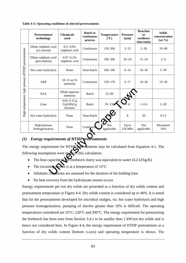
83

Table 4-3: Operating conditions of selected pretreatments

Pretreatment

technology

Chemicals

used

Batch or

continuous

process

Temperature

(°C)

Pressure

(atm)

Reaction

or

residence

time (min)

Solids

concentration

(wt %)

Hig

h t

emp

erat

ure

, h

igh

pre

ssure

(H

TH

P)

pre

trea

tmen

ts Dilute sulphuric acid

(co current)

0.5–3.0%



(percolation)

0.07–0.1%


Hot water hydrolysis

Water Semi-batch 160–190 6–14 10–30 5–30

ARP 10–15 wt.%

ammonia Continuous 150–170 9–17 10–20 15–30

SAA Dilute aqueous

ammonia Batch 25–60 1

Lime

0.05–0.15 g

Ca(OH)2/g

biomass

Batch 70–130 1–6 1–6 h 5–20

Hot water hydrolysis None Semi-batch 165 8 30 8-12

High pressure

homogenisation None Continuous

Not

applicable

Up to

120 MPa

Not

applicable

Maximum

10%

(1) Energy requirements of HTHP pretreatments

The energy requirement for HTHP pretreatments may be calculated from Equation 4-1. The

following assumptions were made in this calculation:

The heat capacity of the feedstock slurry was equivalent to water (4.2 kJ/kg/K)

The incoming stream is at a temperature of 15°C

Adiabatic conditions are assumed for the duration of the holding time

No heat recovery from the hydrolysate stream occurs

Energy requirements per ton dry solids are presented as a function of dry solids content and

pretreatment temperature in Figure 4-4. Dry solids content is considered up to 40%. It is noted

that for the pretreatments developed for microbial sludges, viz. hot water hydrolysis and high

pressure homogenisation, pumping of slurries greater than 10% is difficult. The operating

temperatures considered are 55°C; 120°C and 200°C. The energy requirement for pressurising

the feedstock has been seen from Section 3.4.1 to be smaller than 1 kW/ton dry solids and is

hence not considered here. In Figure 4-4, the energy requirement of HTHP pretreatment as a

function of dry solids content (bottom x-axis) and operating temperature is shown. The

Univers

ity of

Cap

e Tow

n

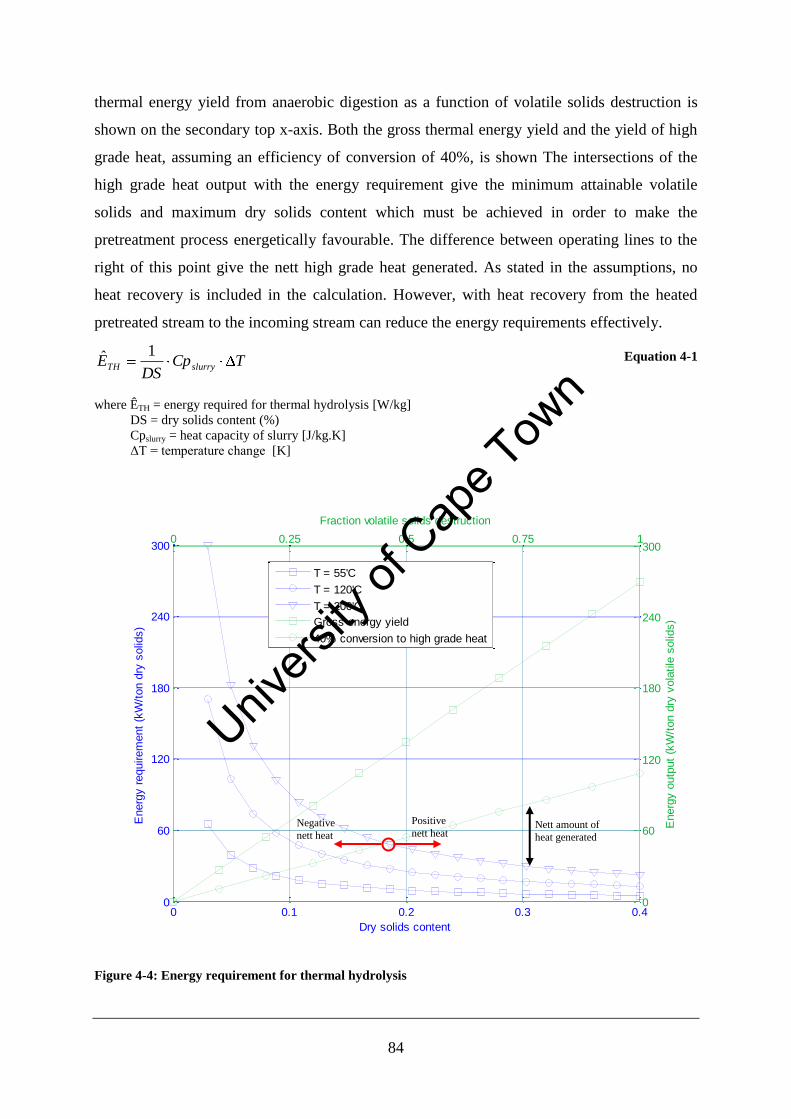
84

thermal energy yield from anaerobic digestion as a function of volatile solids destruction is

shown on the secondary top x-axis. Both the gross thermal energy yield and the yield of high

grade heat, assuming an efficiency of conversion of 40%, is shown The intersections of the

high grade heat output with the energy requirement give the minimum attainable volatile

solids and maximum dry solids content which must be achieved in order to make the

pretreatment process energetically favourable. The difference between operating lines to the

right of this point give the nett high grade heat generated. As stated in the assumptions, no

heat recovery is included in the calculation. However, with heat recovery from the heated

pretreated stream to the incoming stream can reduce the energy requirements effectively.

TCpDS

E slurryTH

1ˆ Equation 4-1

where ÊTH = energy required for thermal hydrolysis [W/kg]


Cpslurry = heat capacity of slurry [J/kg.K]

ΔT = temperature change [K]

0 0.1 0.2 0.3 0.40

60

120

180

240

300

Dry solids content

Energ

y r

equirem

ent

(kW

/ton d

ry s

olid

s)

0 0.25 0.5 0.75 1

0

60

120

180

240

300

Energ

y o

utp

ut

(kW

/ton d

ry v

ola

tile

solid

s)

Fraction volatile solids destruction

T = 55'C

T = 120'C

T = 200'C

Gross energy yield

40% conversion to high grade heat

Figure 4-4: Energy requirement for thermal hydrolysis

Positive

nett heat Negative

nett heat Nett amount of

heat generated

Univers

ity of

Cap

e Tow

n

85

(2) Energy requirements of high pressure homogenisation

The energy requirement from high pressure homogenisation may be calculated from Equation

4-2. The following assumptions were made in the calculation:

The slurry density was assumed to be the same as water (1000 kg/m3)

A single pass through the homogeniser was used

The energy requirement for operating pressures of 30, 50 and 100 MPa are shown in Figure

4-5. It is clear that this is orders of magnitude greater than the energy output of the digester.

Thus, lower operating pressures, viz., 8, 9 and 10 MPa, are shown in Figure 4-6 (blue axis)

with the energy yield from anaerobic digestion given on the secondary axis (green axis).The

same analysis used for thermal hydrolysis can be followed. From this analysis it is clear that

high pressure homogenisation for treating sludge to improve digestibility is not feasible at the

very high pressures used in some studies. Furthermore, these calculations assume only one

pass. The energy requirement will increase proportionally to the number of passes. As the

operating pressure of the Microsludge system is not quoted, it is difficult to tell whether this

system is energy positive. The manufacturers claim so, thus is must operate at a pressure of

less than 10 MPa and a dry solid content of greater than 12% (as highlighted by point A on

Figure 4-6). The process would have to achieve a volatile solids content of greater than 35%,

which according to literature is possible.

PDS

Eslurry

HPH

11ˆ Equation 4-2

where ÊHPH = energy required for high pressure homogenisation [W/kg]


ρslurry = slurry density [kg/m3]

P = operating pressure of homogeniser [Pa]

Univers

ity of

Cap

e Tow

n

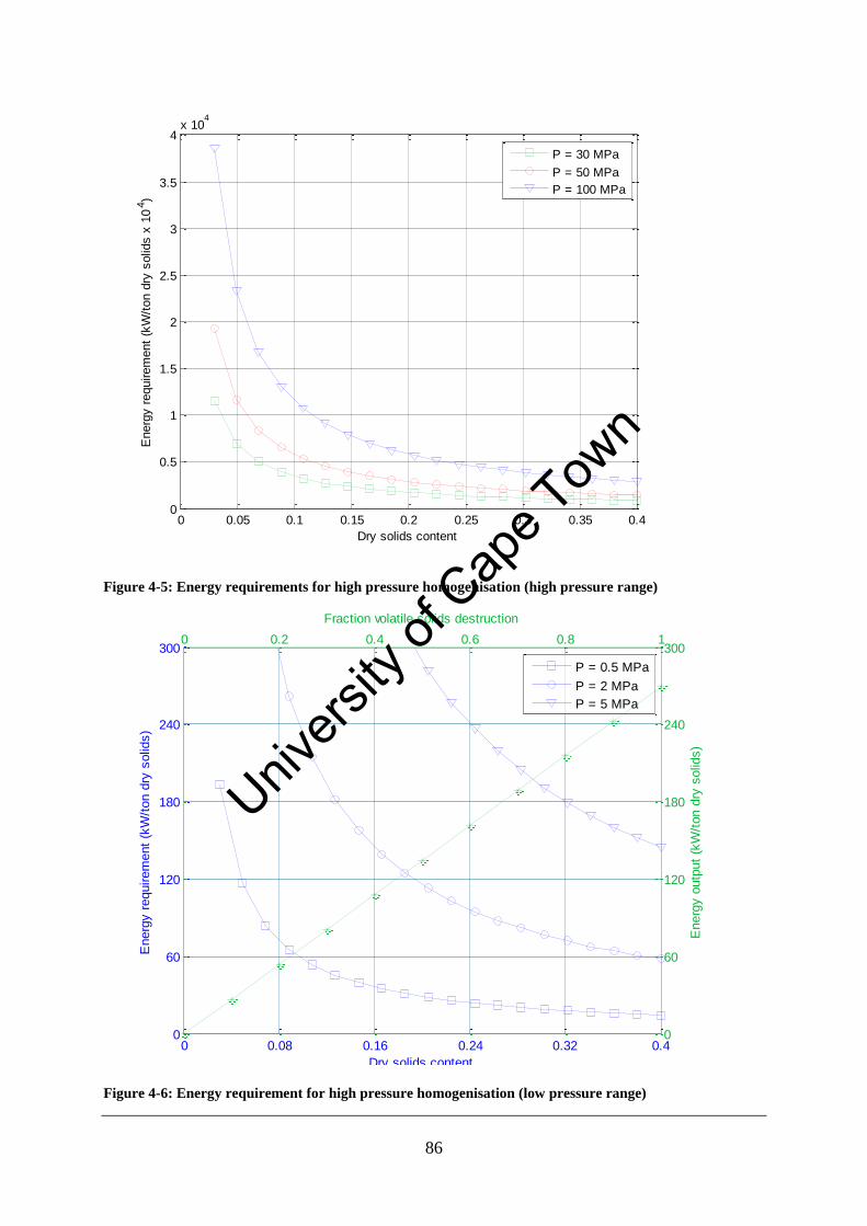
86

0 0.05 0.1 0.15 0.2 0.25 0.3 0.35 0.40

0.5

1

1.5

2

2.5

3

3.5

4x 10

4

Dry solids content

Energ

y r

equirem

ent

(kW

/ton d

ry s

olid

s x

10

4)

P = 30 MPa

P = 50 MPa

P = 100 MPa

Figure 4-5: Energy requirements for high pressure homogenisation (high pressure range)

0 0.08 0.16 0.24 0.32 0.40

60

120

180

240

300

Dry solids content

Energ

y r

equirem

ent

(kW

/ton d

ry s

olid

s)

P = 0.5 MPa

P = 2 MPa

P = 5 MPa

0 0.2 0.4 0.6 0.8 1

0

60

120

180

240

300

Energ

y o

utp

ut

(kW

/ton d

ry s

olid

s)


Figure 4-6: Energy requirement for high pressure homogenisation (low pressure range)

Univers

ity of

Cap

e Tow

n

87

4.1.3. Conclusions

The complex nature of biogenic waste streams means that biodegradability should ideally be

tested experimentally. Some idea about the maximum extent of biodegradability can be

inferred from lignin content of the fuel. Representative volatile solids destruction can be

obtained from the Biochemical Methane Potential assay.

Anaerobic digestion pretreatments such as thermal hydrolysis and high pressure

homogenisation can be used increase the biodegradability of microbial sludges by disrupting

the cell so that the intracellular proteins and carbohydrate storage products are released. The

energy requirements of high pressure homogenisation at pressures of 30 to 50 MPa exclude its

use for improving digestibility, as a positive nett energy yield is not possible. HTHP

pretreatments are the recommended pretreatments as the analysis showed a positive nett

energy yield at dry solids contents greater than 20% and at volatile solids destruction of

greater than 50%, assuming no heat recovery and a thermal efficency of 40%. Heat recovery

from the heated pretreated stream reduces the energy requirements and hence makes the

pretreatments viable at lower volatile solids destruction.

4.2. The effect of volatile combustion in fluidised beds

4.2.1. Introduction

In order to optimise energy recovery from biomass combustion, control of overbed burning is

necessary. The objective of this section is to investigate the effect of temperature on overbed

burning and combustion efficiency experimentally for biogenic materials, using wood chips

and sewerage sludge as examples. Here the combustion efficiency is defined as the actual heat

released into the bed as a fraction of the maximum possible heat generation from the fuel.

A commonly cited industrial problem of combusting biogenic fuels in bubbling fluidised beds

is overbed burning which can lead to runaway freeboard temperatures and difficulties in

maintaining the bed temperature (North, 2005; Fountain, 2008 and Werther and Ogada,

1999). Overbed burning occurs when the volatiles released by the solid fuel burn in the

freeboard above the bed. Biogenic fuels are characterised by their high volatile content and

are hence more susceptible to overbed burning. Previous experimental work on bubbling

Univers

ity of

Cap

e Tow

n

88

fluidised beds by Turnbull and Davidson (1984), Hesketh and Davidson (1991) and Ogada

and Werther (1996) shows that the location of combustion of the gas or volatile component is

dependant on the bed temperature, with higher bed temperatures promoting in-bed bubble

phase combustion. The location of volatile component release and combustion is expected to

be different for overbed and underbed feeding (Werther and Ogada, 1999), as underbed

feeding promotes a longer residence time in the bed.

4.2.2. Factors affecting volatile combustion

4.2.2.1. Hydrocarbon gases and coal volatiles

When fluidising a bed of sand with a stoichiometric mixture of propane and air (used to

model volatiles), the ignition of the fuel and location of combustion is dependent on the bed

temperature. At low bed temperatures (<600°C), an ignition source is needed to burn the gas

in the freeboard. At temperatures around 750°C, ignition is spontaneous in the freeboard. At

bed temperatures higher than some critical temperature (Tcrit1), estimated as 770°C (Turnbull

and Davidson, 1984), the gas burns in the bed (van der Vaart, 1988). Turnbull and Davidson

(1984) presented three regimes of gas combustion to formalise these observations

Regime A, where Tbed < Tcrit1 and gases do no burn in the bed

Regime B, where Tcrit1 < Tbed < Tcrit2 and gases burn only in the bubble phase

Regime C, where Tbed > Tcrit2 where combustion occurs both in the bubble and particulate

phase.

Tcrit1 can be determined by visual inspection of the freeboard or by measuring pressure

fluctuations in the freeboard (van der Vaart, 1988). The difference between Tcrit1 and Tcrit2 is

estimated to be 120 K (Turnbull and Davidson, 1984).

Dennis et al. (cited in Turnbull and Davidson, 1984) proposed that particulate phase

combustion was inhibited by sand particles quenching the radical reaction at the surface of the

bubble and that higher bed temperature promoted the reaction. Van der Vaart (1988)

investigated the effect of bed height and fluidisation velocity on Tcrit, and found that

increasing bed height and lowering fluidisation velocities decreased Tcrit. Both these

conditions permit a longer residence time in the bed. From these observations van der Vaart

(1998) proposed that the combustion reaction was inhibited by an ignition delay. If the gas

residence time was long enough, ignition would occur in the bed. Howevr, later work

Univers

ity of

Cap

e Tow

n

89

supports the theory of the radical reaction being quenched by the presence of solid particles

(Hayhurst and Parmar, 1998).

In models relating to the combustion of coal in a fluidised bed, assumptions must be made

about the location and release of the volatile content. Three modelling approaches have been

developed (LaNauze cited in Werther and Ogada, 1995):

The release and combustion of the volatiles takes place instantaneously at the feed

point, i.e. the rate of devolatilisation is much greater than the rate of mixing and the

rise time of the particle;

The release and combustion of volatiles occur uniformly throughout the bed, i.e. the

rate of devolatilisation is less than the rate of mixing and similar to the rise time of the

particle through the bed;

The volatiles are released as a plume which does not mix with the oxygen and so only

freeboard combustion occurs.

For coal particles, devolatilisation times are of the order of 10 to 20s, and 70% of

devolatilisation occurs within 25 to 30% of the time for total devolatilisation. Thus, 2 to 7s is

the devolatilisation time which should be used when determining the location of release of

volatiles. The average rise velocity of a coal particle in a bed can be calculated from Nienow

(1978) (cited in Turnbull and Davidson, 1984), according to Equation 4-3, with typical values

ranging from 2 to 10 s. Thus the average rise time of the fuel particles is similar to the

devolatilisation time and combustion should occur uniformly throughout the bed.

5.0)(15.0 mfR UUU Equation 4-3

where UR = average rise velocity of coal particle in bed [m/s]

U = superficial velocity [m/s]

Umf = minimum fluidisation velocity [m/s]

An experiment by Hesketh and Davidson (1991) used char and a mixture of propane and air

to model the fixed carbon and volatile content of coal respectively. The burnout time for a

batch of char added to a hot fluidised bed can be calculated by carrying out an energy balance

over the bed, as given by Hesketh and Davidson (1991) and presented in Equation 4-4.

Univers

ity of

Cap

e Tow

n

90

)()( inletbedgasgasbedfurnacehpccbed

bedbed TTCpmTTAhNrHdt

dTCpM Equation 4-4

where Mbed = mass of bed material [kg]

Ah = heat transfer area [m2]

Tfurnace = furnace temperature [K]

mgas = mass flowrate of gas [kg/s]

Cpgas = heat capacity of gas [J/kg.K]

Tinlet = inlet temperature [K]

Np = number of particles

Cpbed = heat capacity of bed material [J/kg.K]

Tbed = bed temperature [K]

ΔHc = heat of combustion [J/kmol]

rc = rate of combustion [kmol/particle/s]

h = overall furnace to bed

heat transfer coefficient [W/m2.K]

After burnout of the char, the bed temperature declines to its previous steady temperature

according to Equation 4-4 with rc set to zero. Identification of the point on the burnout curve

where this relationship holds gives the burnout time of the char. It was found that the burnout

time for the char increased at higher temperatures when the bed was fluidised with the

air/propane mixture as opposed to air alone. The effect was attributed to propane combustion

proceeding in the bed at higher temperatures, thus consuming relatively more oxygen than at

low temperatures. The consumption of oxygen by the volatiles decreased the oxygen available

for combustion of the char and increased the burnout time of the char.

Turnbull (1983) investigated the fluidised bed combustion of volatiles from coal by carrying

out an energy balance over the freeboard. It was found that up to 70% of the energy released

in the freeboard was returned to the bed by the solids falling back into the bed. Turnbull used

Pemberton’s model (1982) to predict the flux of solids into the freeboard. Pemberton assumed

that a single layer of particles carried on the nose of a bursting bubble was projected into the

freeboard. The high heat transfer between bed and freeboard predicted by Turnbull (1983) is

contrary to industrial experience and other experimental work. The anomaly is explained by

“ghost bubbles”, fuel rich bubbles which pass through the splash zone and burn above the

splash zone where the heat released is not returned to the bed (Turnbull, 1983).

4.2.2.2. Biomass fuels

Biomass fuels are characterised by their high volatile content. In the case of the fluidised bed

combustion of sewerage sludge, up to 80% of the sludge carbon is released as volatiles.

Comparisons of the oxygen profile through a fluidised bed combusting sewerage sludge

showed that it was very close to that of a bed combusting hydrocarbon gas (Ogada and

Werther, 1995). Critical issues associated with the combustion of these types of fuel include

separation of volatile and fixed carbon content in the combustor and particle attrition and

fragmentation (Chirone et al., 2008). This can lead to a loss in carbon conversion as the

Univers

ity of

Cap

e Tow

n

91

material is lost from the reactor unconverted, or to high freeboard temperatures where the

volatiles or fines combust in the freeboard.

Conflicting results appear in the literature regarding the location of the release of volatile

components. Ogada and Werther (1996) found that the time for devolatilisation of a single

particle of sewerage sludge was much faster than the solids mixing time, and as a result

uniform combustion should take place in the bed. However, in-bed combustion does not

explain the high freeboard temperatures often seen in industrial units (North et al, 2005;

Fountain, 2008 and Werther and Ogada, 1999). High freeboard temperatures could be due to

volatiles leaving the bed in bubbles and burning only in the freeboard, or lack of segregation

of sludge particles within the bed, which could result in local oxygen deficient regions and

associated release of CO to the freeboard. Ogada and Werther (1996) analysed CxHy profiles

(representative of volatiles) in a reactor, and detected low concentrations just above the feed

point, with higher concentrations seen in the splash zone and freeboard. Regarding particle

segregation, some researchers found that the action of a high velocity jet broke up the fuel

particles into smaller pieces (Ruoss (1991) cited in Werther and Ogada, 1999) whereas others

have seen that the fuel particles retain their shape. Work by Chirone et al. (2008) show an

intact ash skeleton left behind from sludge combustion which indicates a lack of segregation

of particles.

Moisture content and particle size of the fuel also affects the location of release of volatiles

and their combustion. Work done by North et al. (2005) showed that the loss in heat from the

co-firing of a sludge of coffee grounds and coal was approximately 7% of total fuel input,

which they attributed to overbed combustion of the coffee sludge. To overcome this, the fuel

was partially dried by introducing it at a high level in the freeboard. Borodulya (cited in

Werther and Ogada, 1999) noted that sludge particles dropped onto the top of an 800°C bed

remained intact and floated at the top before submerging into the bed for a short period. The

larger, moist particle burnt at the surface of the bed with a long and sooty flame whereas

particles smaller than 10 mm exhibited no flame, indicating combustion within the bed.

4.2.3. Experimental materials and methods

4.2.3.1. Fuels

The following fuels were investigated in this study:

Univers

ity of

Cap

e Tow

n

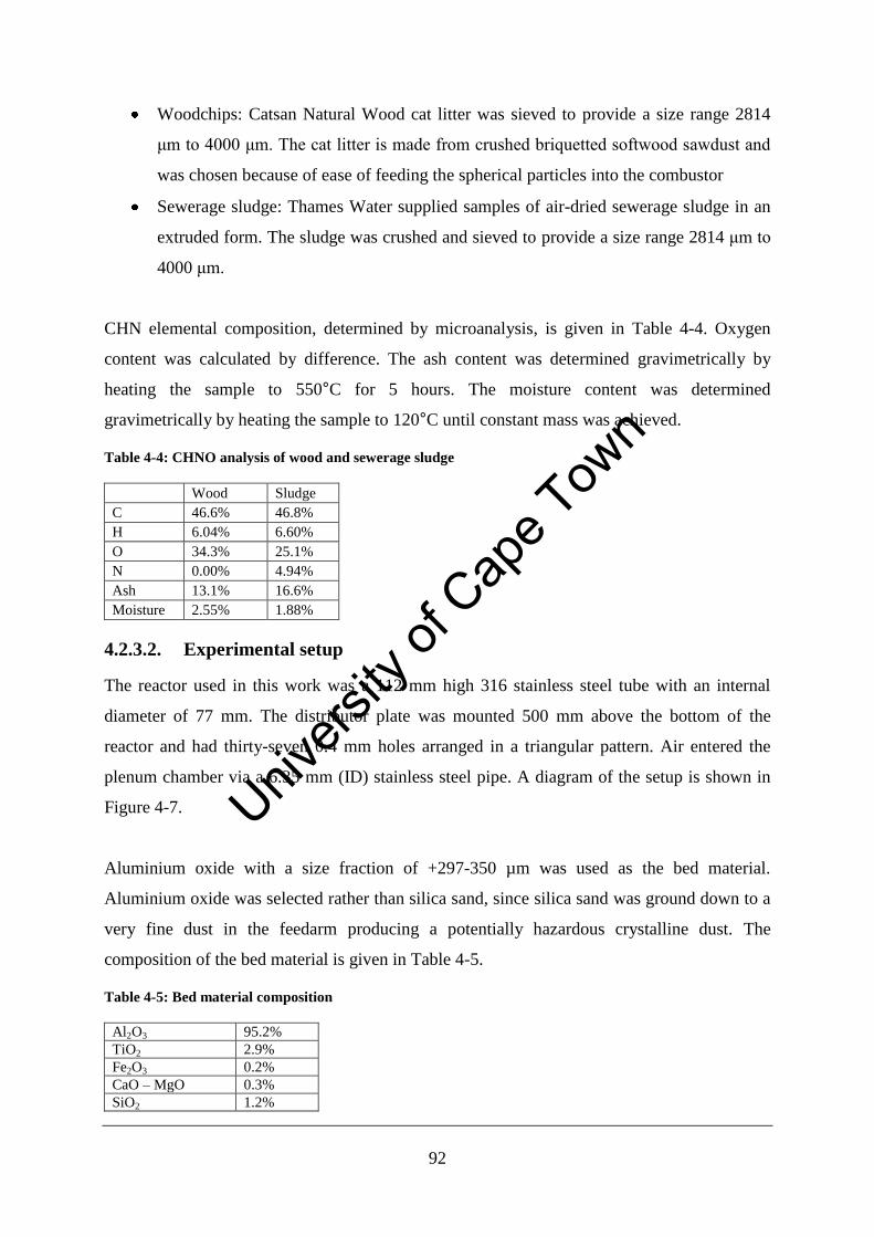
92

Woodchips: Catsan Natural Wood cat litter was sieved to provide a size range 2814

μm to 4000 μm. The cat litter is made from crushed briquetted softwood sawdust and

was chosen because of ease of feeding the spherical particles into the combustor

Sewerage sludge: Thames Water supplied samples of air-dried sewerage sludge in an

extruded form. The sludge was crushed and sieved to provide a size range 2814 μm to

4000 μm.

CHN elemental composition, determined by microanalysis, is given in Table 4-4. Oxygen

content was calculated by difference. The ash content was determined gravimetrically by

heating the sample to 550°C for 5 hours. The moisture content was determined

gravimetrically by heating the sample to 120°C until constant mass was achieved.

Table 4-4: CHNO analysis of wood and sewerage sludge

Wood Sludge

C 46.6% 46.8%

H 6.04% 6.60%

O 34.3% 25.1%

N 0.00% 4.94%

Ash 13.1% 16.6%

Moisture 2.55% 1.88%

4.2.3.2. Experimental setup

The reactor used in this work was a 112 mm high 316 stainless steel tube with an internal

diameter of 77 mm. The distributor plate was mounted 500 mm above the bottom of the

reactor and had thirty-seven 0.4 mm holes arranged in a triangular pattern. Air entered the

plenum chamber via a 6.35 mm (ID) stainless steel pipe. A diagram of the setup is shown in

Figure 4-7.

Aluminium oxide with a size fraction of +297-350 µm was used as the bed material.

Aluminium oxide was selected rather than silica sand, since silica sand was ground down to a

very fine dust in the feedarm producing a potentially hazardous crystalline dust. The

composition of the bed material is given in Table 4-5.

Table 4-5: Bed material composition

Al2O3 95.2%

TiO2 2.9%

Fe2O3 0.2%

CaO – MgO 0.3%

SiO2 1.2%

Univers

ity of

Cap

e Tow

n

93

Heat was provided by six Crusilite silicon carbide heating rods (Kanthal Ltd) placed on either

side of the reactor tube at heights of 250 mm, 480 mm and 710 mm from the reactor base. The

lower two rods provided most of the heat to the bed, whilst the top four rods heated the air

passing through the freeboard to a temperature higher than the bed temperature. The rods

drew a current of 22 A from the mains supply (240 V) to give a range of furnace power of 0

to 5300 W. In these experiments, the power was set to a constant value using a thyristor

controller.

The reactor was insulated by a rectangular wall of firebricks 120 mm thick (JM36, Thermal

Ceramics Ltd). The feed arm and bottom flange were also insulated. (Superwool Thermal

Ceramics). The top of the furnace block was insulated with Superwool and ceramic board.

The bottom feedarm was cooled by running water at ~0°C through copper coils to prevent the

feed from devolatilising or partially combusting before entering the bed. The feedarm and

cooling coils were insulated with Superwool.

The feeding system of the rig consisted of a feed hopper mounted on a brass block. A small

helical doping screw, driven by a stepping motor, controlled the feedrate to the main auger.

The main feed auger was water-cooled to prevent biomass from devolatilising or partially

combusting in the feedarm. A positive pressure was maintained on the hopper at all times to

prevent the backflow of sand into the feedarm or into the hopper.

The reliable operation of the hopper and doping screw system was challenging. Two

operational problems arose regularly: the doping screw jammed or the feed formed a bridge in

the hopper. The solution to the former was to use an optimal particle size of range 2814 μm to

4000 μm. The problem of the biomass bridging was ongoing and also found to have some

dependence on particle size. A number of “anti-bridging” devices were crafted over the

course of this work but no superior design emerged. It was also found that a helical screw

feeder does not move the feed forward satisfactorily. It is suggested for future work that a

machined auger be used.

4.2.3.3. Data acquisition

(1) Temperature measurements

The bed temperature was measured using a 3mm type-K thermocouple. A suction pyrometer

was used to measure the freeboard temperature. A 1.5 mm K-type thermocouple was mounted

Univers

ity of

Cap

e Tow

n

94

in a 6.35 mm steel pipe. A diaphragm pump drew air over the thermocouple at 4 m/s. This

increased the Nusselt number from 2 to 8 and hence increased the convective heat transfer

coefficient. The radiation shield and the high convective heat transfer ensured that the true gas

temperature was measured, free from radiation effects.

(2) Flue gas analysis

The 6.35mm pipe used as the thermocouple radiation shield doubled as the sample line. The

superficial velocity through the pipe was 4 m/s (vs. 0.4 m/s for the reactor). The offgas was

drawn through a 200 μm glass microfibre filter to remove fine dust, tar and char. Two

impinger flasks (one empty and one filled with glass beads) were placed in an ice bath to

condense water vapour. Thereafter the gas was passed through a calcium chloride moisture

trap. The concentrations of CO and CO2 were measured continuously by an infrared gas

analyzer (ABB Easyline I.R.) The O2 concentration was measured by a Universal Exhaust

Gas Oxygen (UEGO) sensor (Horiba MEXA 720). UEGO’s are used primarily for monitoring

air fuel ratios in motor vehicles. The gas stream is passed over a heated element to oxidise any

remaining fuel, including char fines and tar. Hence, the decrease in O2 concentration

measured by the UEGO can be equated directly to the mols of carbon content fed to the

reactor.

4.2.3.4. Experimental procedure

In order to prevent build up of ash in the reactor, 2.1 kg of fresh bed material was placed in

the reactor tube at the start of each run. 30 to 45 g of fuel was placed in the hopper and the

hopper lid was sealed. A purge of nitrogen of 4 l/min was passed through the hopper. The

feed auger, was started to prevent sand flowing back into the feedarm. The air flowrate

through the reactor was set such that U/Umf was 7 to 7.5. An equivalence ratio (i.e. the ratio of

mols fed to mols O2 required for complete combustion) of approximately 2 for wood runs and

1.2 for sludge was used. The bed temperature was increased to the desired temperature by

running the furnace at 50 to 80% power. Once at the desired temperature the power input was

reduced slightly to maintain a constant bed temperature. At this stable temperature the fuel

was fed into the bed by turning on the dosing screw. The offgas compositions, freeboard

temperature and bed temperature were monitored and recorded.

Univers

ity of

Cap

e Tow

n

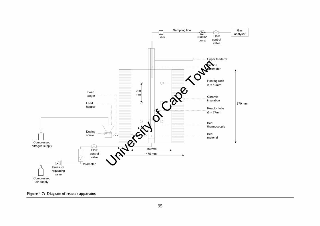
95

Rotameter

Gas analyser

Filter

Sampling line

Suction pump

Ceramic insulation

Heating rods ø = 12mm

Flow control valve

Flow control valve

Compressed air supply

Pressure regulating

valve

Suction pyrometer

Bed thermocouple

Upper feedarm

Bed material

Compressed nitrogen supply

Feed hopper

Feed auger

220 mm

460mm

475 mm

Reactor tubeø = 77mm

Dosing screw

870 mm

Figure 4-7: Diagram of reactor apparatus

Univers

ity of

Cap

e Tow

n

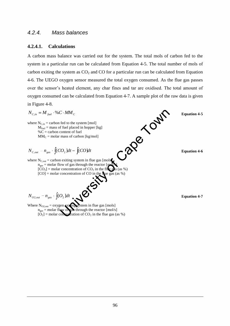
96

4.2.4. Mass balances

4.2.4.1. Calculations

A carbon mass balance was carried out for the system. The total mols of carbon fed to the

system in a particular run can be calculated from Equation 4-5. The total number of mols of

carbon exiting the system as CO2 and CO for a particular run can be calculated from Equation

4-6. The UEGO oxygen sensor measured the total oxygen consumed. As the flue gas passes

over the sensor’s heated element, any char fines and tar are oxidised. The total amount of

oxygen consumed can be calculated from Equation 4-7. A sample plot of the raw data is given

in Figure 4-8.

CfuelinC MMCMN %, Equation 4-5

where NC,in = carbon fed to the system [mol]

Mfuel = mass of fuel placed in hopper [kg]

%C = carbon content of fuel

MMC = molar mass of carbon [kg/mol]

dtCOdtCOnN gasoutC ][][ 2, Equation 4-6

where NC,out = carbon exiting system in flue gas [mols]

ngas = molar flow of gas through the reactor [mol/s]

[CO2] = molar concentration of CO2 in the flue gas (as %)

[CO] = molar concentration of CO in the flue gas (as %)

dtOnN gasoutO ][ 2,2 Equation 4-7

Where NO2,out = oxygen exiting system in flue gas [mols]

ngas = molar flow of gas through the reactor [mol/s]

[O2] = molar concentration of CO2 in the flue gas (as %)

Univ

ersity

of C

ape T

own

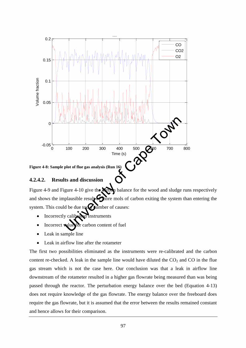
97

0 100 200 300 400 500 600 700 800-0.05

0

0.05

0.1

0.15

0.2

Time (s)

Volu

me f

raction

W__OB850

CO

CO2

O2

Figure 4-8: Sample plot of flue gas analysis (Run 16)

4.2.4.2. Results and discussion

Figure 4-9 and Figure 4-10 give the carbon balance for the wood and sludge runs respectively

and shows the implausible result of more mols of carbon exiting the system than entering the

system. This could be due too a number of causes:

Incorrectly calibrated instruments

Incorrect value for carbon content of fuel

Leak in sample line

Leak in airflow line after the rotameter

The first two possibilities eliminated as the instruments were re-calibrated and the carbon

content re-checked. A leak in the sample line would have diluted the CO2 and CO in the flue

gas stream which is not the case here. Our conclusion was that a leak in airflow line

downstream of the rotameter resulted in a higher gas flowrate being measured than was being

passed through the reactor. The perturbation energy balance over the bed (Equation 4-13)

does not require knowledge of the gas flowrate. The energy balance over the freeboard does

require the gas flowrate, but it is assumed that the error between the results remained constant

and hence allows for their comparison.

Univers

ity of

Cap

e Tow

n

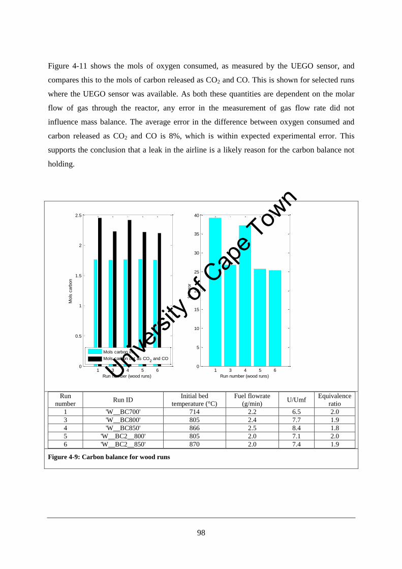
98

Figure 4-11 shows the mols of oxygen consumed, as measured by the UEGO sensor, and

compares this to the mols of carbon released as CO2 and CO. This is shown for selected runs

where the UEGO sensor was available. As both these quantities are dependent on the molar

flow of gas through the reactor, any error in the measurement of gas flow rate did not

influence mass balance. The average error in the difference between oxygen consumed and

carbon released as CO2 and CO is 8%, which is within expected experimental error. This

supports the conclusion that a leak in the airline is a likely reason for the carbon balance not

holding.

1 3 4 5 60

0.5

1

1.5

2

2.5

Run number (wood runs)

Mols

carb

on

Mols carbon in

Mols carbon out as CO2 and CO

1 3 4 5 60

5

10

15

20

25

30

35

40

Run number (wood runs)

% e

rror

Run

number Run ID

Initial bed

temperature (°C)

Fuel flowrate

(g/min) U/Umf

Equivalence

ratio

1 'W__BC700' 714 2.2 6.5 2.0

3 'W__BC800' 805 2.4 7.7 1.9

4 'W__BC850' 866 2.5 8.4 1.8

5 'W__BC2__800' 805 2.0 7.1 2.0

6 'W__BC2__850' 870 2.0 7.4 1.9

Figure 4-9: Carbon balance for wood runs

Univers

ity of

Cap

e Tow

n

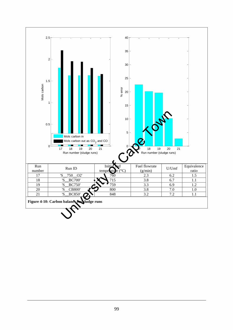
99

17 18 19 20 210

0.5

1

1.5

2

2.5

Run number (sludge runs)

Mols

carb

on

Mols carbon in


17 18 19 20 210

5

10

15

20

25

30

35

40

Run number (sludge runs)

% e

rror

Run

number Run ID

Initial bed

temperature (°C)

Fuel flowrate

(g/min) U/Umf

Equivalence

ratio

17 'S__750__O2' 760 2.3 6.2 1.5

18 'S__BC700' 715 3.8 6.7 1.1

19 'S__BC750' 759 3.3 6.9 1.2

20 'S__CB800' 800 3.8 7.0 1.0

21 'S__BC850' 848 3.2 7.2 1.1

Figure 4-10: Carbon balance for sludge runs

Univers

ity of

Cap

e Tow

n

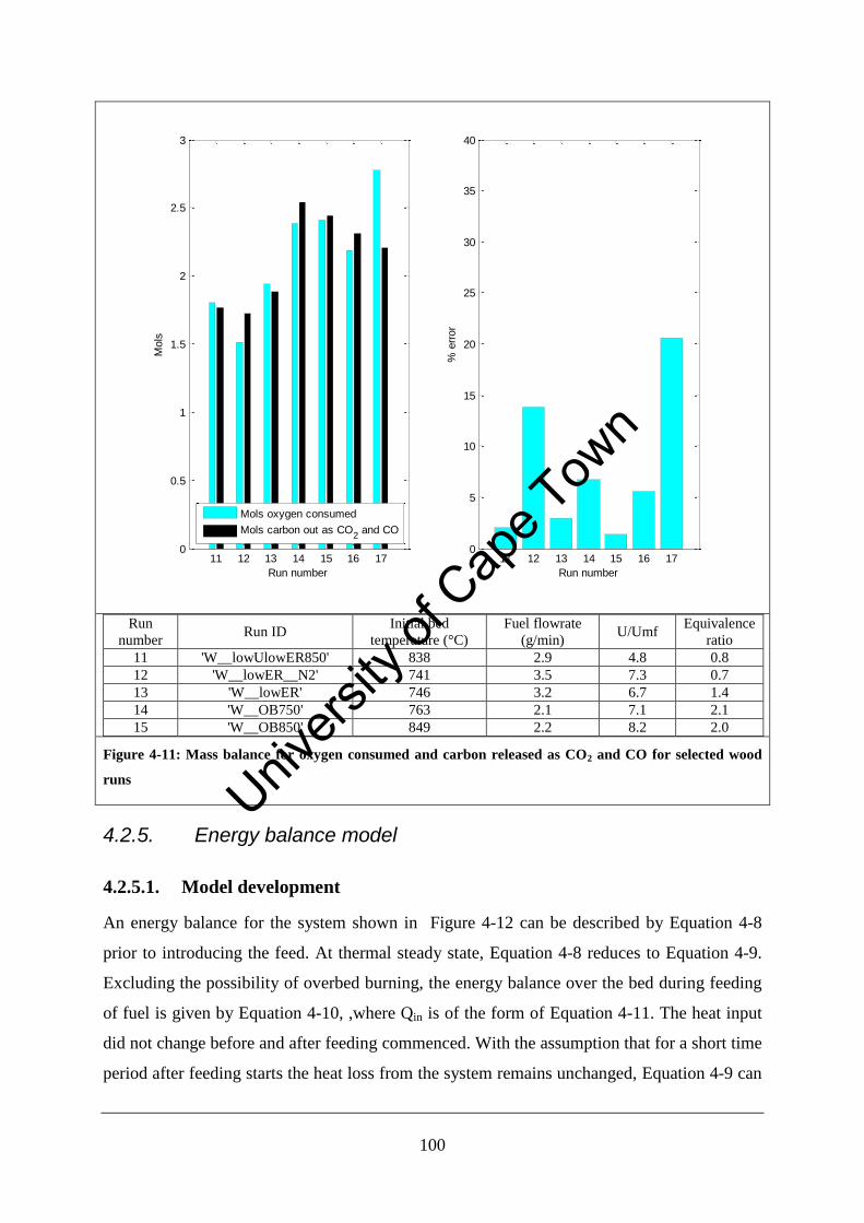
100

11 12 13 14 15 16 170

0.5

1

1.5

2

2.5

3

Run number

Mols

Mols oxygen consumed


11 12 13 14 15 16 170

5

10

15

20

25

30

35

40

Run number

% e

rror

Run

number Run ID

Initial bed

temperature (°C)

Fuel flowrate

(g/min) U/Umf

Equivalence

ratio

11 'W__lowUlowER850' 838 2.9 4.8 0.8

12 'W__lowER__N2' 741 3.5 7.3 0.7

13 'W__lowER' 746 3.2 6.7 1.4

14 'W__OB750' 763 2.1 7.1 2.1

15 'W__OB850' 849 2.2 8.2 2.0

Figure 4-11: Mass balance for oxygen consumed and carbon released as CO2 and CO for selected wood

runs

4.2.5. Energy balance model

4.2.5.1. Model development

An energy balance for the system shown in Figure 4-12 can be described by Equation 4-8

prior to introducing the feed. At thermal steady state, Equation 4-8 reduces to Equation 4-9.

Excluding the possibility of overbed burning, the energy balance over the bed during feeding

of fuel is given by Equation 4-10, ,where Qin is of the form of Equation 4-11. The heat input

did not change before and after feeding commenced. With the assumption that for a short time

period after feeding starts the heat loss from the system remains unchanged, Equation 4-9 can

Univers

ity of

Cap

e Tow

n

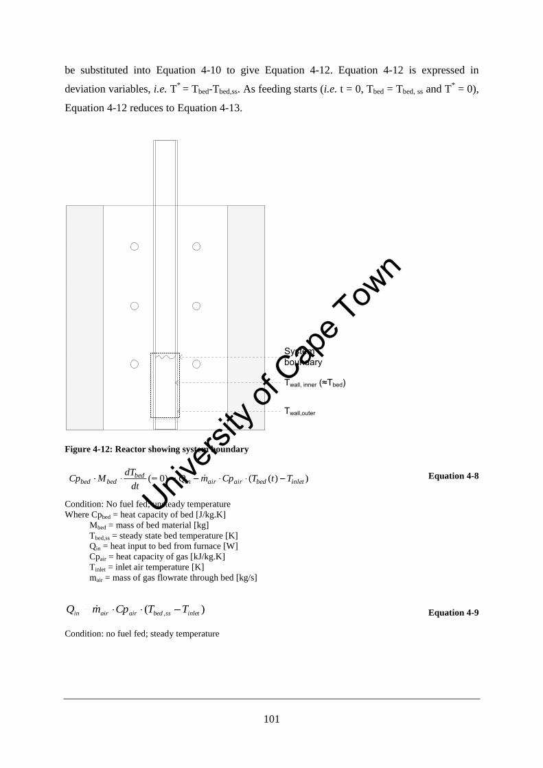
101

be substituted into Equation 4-10 to give Equation 4-12. Equation 4-12 is expressed in

deviation variables, i.e. T* = Tbed-Tbed,ss. As feeding starts (i.e. t = 0, Tbed = Tbed, ss and T

* = 0),

Equation 4-12 reduces to Equation 4-13.

Twall,outer

Twall, inner (≈Tbed)

System boundary

Figure 4-12: Reactor showing system boundary

))(()0( inletbedairairinbed

bedbed TtTCpmQdt

dTMCp Equation 4-8

Condition: No fuel fed; unsteady temperature

Where Cpbed = heat capacity of bed [J/kg.K]

Mbed = mass of bed material [kg]

Tbed,ss = steady state bed temperature [K]

Qin = heat input to bed from furnace [W]

Cpair = heat capacity of gas [kJ/kg.K]

Tinlet = inlet air temperature [K]

mair = mass of gas flowrate through bed [kg/s]

)( , inletssbedairairin TTCpmQ Equation 4-9

Condition: no fuel fed; steady temperature

Univers

ity of

Cap

e Tow

n

102

cbiomassinletbedairairinbed

bedbed HmTtTCpmQdt

dTMCp ))(( Equation 4-10

Condition: Fuel fed; unsteady temperature

Where mbiomass = mass flowrate of biomass [kg/s]

ΔHc = heat of combustion of fuel [J/kg]

Tbed = bed temperature [K]

bedouterwallhhin TTAUQ , Equation 4-11

where Qin = heat input to bed [W]

Uh = overall heat transfer coefficient [W/m2.K]

Ah = heat transfer area [m2]

Twall,outer = outer reactor wall temperature [K]

cbiomassairairbedbed HmtTCpmdt

dTMCp )(*

*

Equation 4-12

Condition: fuel fed; deviation variable used

where T* = Tbed – Tbed,ss [K]

cbiomassbedbed Hmdt

tdTMCp

)0(*

Equation 4-13

Condition: fuel fed; time = 0

4.2.5.2. Analysis of experimental data

The analytical solution to Equation 4-12 given by Equation 4-14. The constants A and α were

found by fitting a curve of the form of Equation 4-14 to the bed temperature experimental

data, using a non-linear regression routine in Matlab. The code is given in Appendix A.5 and

the experimental data with the fitted curves are plotted in Appendix A.3. A sample plot is

shown in Figure 4-13.

As feeding starts (i.e. at t = 0), Equation 4-14 reduces to Error! Reference source not

found..

)1()(* teAtT Equation 4-14

Where T* = Tbed – Tbed,ss

To simplify the analysis, the point of interest is the perturbation point; the point at which

feeding commences i.e. Equation 4-13. The right hand side of Equation 4-13 gives the

potential maximum amount of heat released to the bed. The left hand side of Equation 4-13 is

Univers

ity of

Cap

e Tow

n

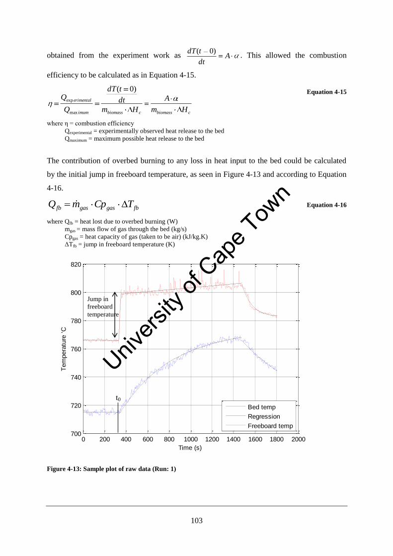
103

obtained from the experiment work as Adt

tdT )0(. This allowed the combustion

efficiency to be calculated as in Equation 4-15.

cbiomasscbiomassimum

erimental

Hm

A

Hm

dt

tdT

Q

Q)0(

max

exp

Equation 4-15

where η = combustion efficiency

Qexperimental = experimentally observed heat release to the bed

Qmaximum = maximum possible heat release to the bed

The contribution of overbed burning to any loss in heat input to the bed could be calculated

by the initial jump in freeboard temperature, as seen in Figure 4-13 and according to Equation

4-16.

fbgasgasfb TCpmQ Equation 4-16

where Qfb = heat lost due to overbed burning (W)

mgas = mass flow of gas through the bed (kg/s)

Cpgas = heat capacity of gas (taken to be air) (kJ/kg.K)

ΔTfb = jump in freeboard temperature (K)

0 200 400 600 800 1000 1200 1400 1600 1800 2000700

720

740

760

780

800

820

Time (s)

Tem

pera

ture

'C

W__BC700

Bed temp

Regression

Freeboard temp

Figure 4-13: Sample plot of raw data (Run: 1)

t0

Jump in

freeboard

temperature

Univers

ity of

Cap

e Tow

n

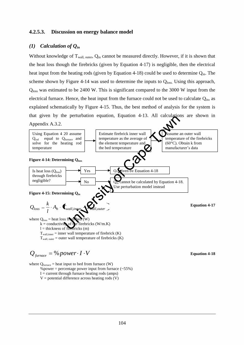
104

4.2.5.3. Discussion on energy balance model

(1) Calculation of Qin

Without knowledge of Twall, outer, Qin cannot be measured directly. However, if it is shown that

the heat loss though the firebricks (given by Equation 4-17) is negligible, then the electrical

heat input from the heating rods (given by Equation 4-18) could be used to determine Qin. The

scheme shown by Figure 4-14 was used to determine the inputs to Qloss. Using this approach,

Qloss was estimated to be 2400 W. This is significant compared to the 3000 W input from the

electrical furnace. Hence, the heat input from the furnace could not be used to calculate Qin, as

explained schematically by Figure 4-15. Thus, the best method of analysis for the system is

that given by the perturbation equation, Equation 4-13. All calculations are shown in

Appendix A.3.2.

Figure 4-14: Determining Qloss

Figure 4-15: Determining Qin

outerwallinnerwallhloss TTAl

kQ ,,

Equation 4-17

where Qloss = heat loss from bed (W)

k = conductivity of the firebricks (W/m.K)

l = thickness of firebricks (m)

Twall,inner = inner wall temperature of firebrick (K)

Twall, outer = outer wall temperature of firebricks (K)

VIpowerQ furnace % Equation 4-18

where Qfurnace = heat input to bed from furnace (W)

%power = percentage power input from furnace (~55%)

I = current through furnace heating rods (amps)

V = potential difference across heating rods (V)

Using Equation 4 20 assume

Qrad equal to Qfurnace and

solve for the heating rod

temperature

Estimate firebrick inner wall

temperature as the average of

the element temperature and

the bed temperature

Assume an outer wall

temperature of the firebricks

(60°C). Obtain k from

manufacturer’s data

Is heat loss (Qloss)

through firebricks

negligible?

Yes

No

Qin given by Equation 4-18

Qin cannot be calculated by Equation 4-18.

Use perturbation model instead

Univers

ity of

Cap

e Tow

n

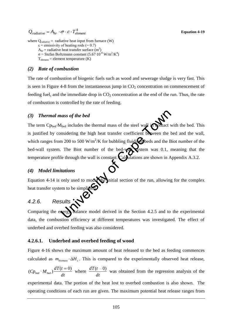
105

4elementhrradiative TAQ Equation 4-19

where Qradiative = radiative heat input from furnace (W)

ε = emissivity of heating rods (= 0.7)

Ahr = radiative heat transfer surface (m2)

σ = Stefan Boltzmann constant (5.67·10-8

W/m2/K

4)

Telement = element temperature (K)

(2) Rate of combustion

The rate of combustion of biogenic fuels such as wood and sewerage sludge is very fast. This

is seen in Figure 4-8 from the instantaneous jump in CO2 concentration on commencement of

feeding fuel, and the immediate drop in CO2 concentration at the end of the run. Thus, the rate

of combustion is controlled by the rate of feeding.

(3) Thermal mass of the bed

The term Cpbed·Mbed includes the thermal mass of the steel wall in contact with the bed. This

is justified by considering the high heat transfer coefficient between the bed and the wall,

which ranges from 200 to 500 W/m2/K for bubbling fluidised beds and the Biot number of the

bed-wall system. The Biot number of the bed-wall system was 0.1, meaning that the

temperature profile through the wall is constant. Calculations are shown in Appendix A.3.2.

(4) Model limitations

Equation 4-14 is only used to model the initial section of the run, allowing for the complex

heat transfer system to be simplified.

4.2.6. Results

Comparing the energy balance model derived in the Section 4.2.5 and to the experimental

data, the combustion efficiency at different temperatures was investigated. The effect of

underbed and overbed feeding was also considered.

4.2.6.1. Underbed and overbed feeding of wood

Figure 4-16 shows the maximum amount of heat released to the bed as feeding commences

calculated as cbiomass Hm . This is compared to the experimentally observed heat release,

dt

tdTMCp bedbed

)0()( where

dt

tdT )0( was obtained from the regression analysis of the

experimental data. The portion of the heat lost to overbed combustion is also shown. The

operating conditions of each run are given. The maximum potential heat release ranges from

Univers

ity of

Cap

e Tow

n

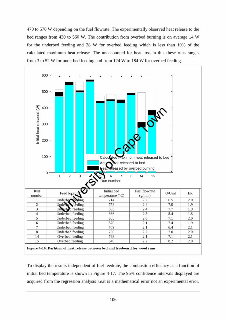
106

470 to 570 W depending on the fuel flowrate. The experimentally observed heat release to the

bed ranges from 430 to 560 W. The contribution from overbed burning is on average 14 W

for the underbed feeding and 28 W for overbed feeding which is less than 10% of the

calculated maximum heat release. The unaccounted for heat loss in this these runs ranges

from 3 to 52 W for underbed feeding and from 124 W to 184 W for overbed feeding.

1 2 3 4 5 6 7 8 9 100

100

200

300

400

500

600

Run number

Initia

l heat

rele

ased (

W)

Calculated maximum heat released to bed

Actual heat released to bed

Heat released by overbed burning

Run

number Feed location

Initial bed

temperature (°C)

Fuel flowrate

(g/min) U/Umf ER

1 Underbed feeding 714 2.2 6.5 2.0








14 Overbed feeding 763 2.1 7.1 2.1

15 Overbed feeding 849 2.2 8.2 2.0

Figure 4-16: Partition of heat release between bed and freeboard for wood runs

To display the results independent of fuel feedrate, the combustion efficency as a function of

initial bed temperature is shown in Figure 4-17. The 95% confidence intervals displayed are

acquired from the regression analysis i.e.it is a mathematical error not an experimental error.

14 15

Univers

ity of

Cap

e Tow

n

107

The experimental error is not shown explicitly but an idea can be gauged from the results

repeated at similar temperatures. Figure 4-17 shows that for all wood underbed-fed runs,

approximately 90% of the heat is released to the bed. There is no clear dependence of

combustion efficiency on temperature for these runs. From Figure 4-17 it can be seen that the

combustion efficiency of overbed feeding is ~65 %. Some dependence on temperature is

evident as the combustion efficiency increases from 57% to 70% as the initial bed

temperature increases from 750° to 850°.

700 720 740 760 780 800 820 840 860 8800

0.1

0.2

0.3

0.4

0.5

0.6

0.7

0.8

0.9

1

Initial bed temperature (oC)

Com

bustion e

ffic

iency

Underbed feeding

Overbed feeding

95% Confidence Interval on regression estimates

Figure 4-17: Effect of bed temperature on combustion efficiency for wood runs

Figure 4-18 shows the jump in freeboard temperature seen in the underbed and overbed wood

runs as feeding commenced. The jump in temperature for the underbed runs is considerably

less than the overbed runs (15°C to 30°C compared to approximately 40°C). The overbed runs

show little dependence on initial bed temperature. The underbed runs show a marked decrease

in freeboard temperature jump as the initial bed temperature increases, dropping from

approximately jump of 30°C at a bed temperature of 715°C to 15°C at 870°C.

Univers

ity of

Cap

e Tow

n

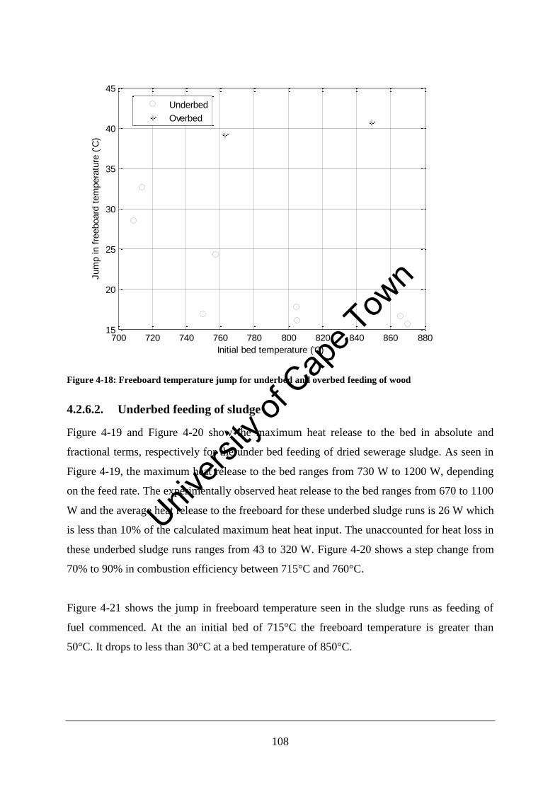
108

700 720 740 760 780 800 820 840 860 88015

20

25

30

35

40

45

Initial bed temperature ('C)

Jum

p in f

reeboard

tem

pera

ture

('C

)

Underbed

Overbed

Figure 4-18: Freeboard temperature jump for underbed and overbed feeding of wood

4.2.6.2. Underbed feeding of sludge

Figure 4-19 and Figure 4-20 show the maximum heat release to the bed in absolute and

fractional terms, respectively for the under bed feeding of dried sewerage sludge. As seen in

Figure 4-19, the maximum heat release to the bed ranges from 730 W to 1200 W, depending

on the feed rate. The experimentally observed heat release to the bed ranges from 670 to 1100

W and the average heat release to the freeboard for these underbed sludge runs is 26 W which

is less than 10% of the calculated maximum heat heat input. The unaccounted for heat loss in

these underbed sludge runs ranges from 43 to 320 W. Figure 4-20 shows a step change from

70% to 90% in combustion efficiency between 715°C and 760°C.

Figure 4-21 shows the jump in freeboard temperature seen in the sludge runs as feeding of

fuel commenced. At the an initial bed of 715°C the freeboard temperature is greater than

50°C. It drops to less than 30°C at a bed temperature of 850°C.

Univers

ity of

Cap

e Tow

n

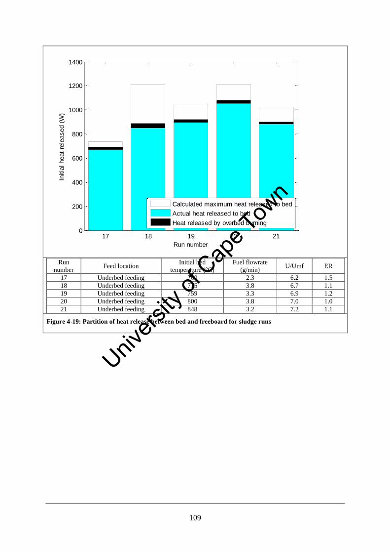
109

17 18 19 20 210

200

400

600

800

1000

1200

1400

Run number

Initia

l heat

rele

ased (

W)

Calculated maximum heat released to bed

Actual heat released to bed

Heat released by overbed burning

Run

number Feed location

Initial bed

temperature (°C)

Fuel flowrate

(g/min) U/Umf ER






Figure 4-19: Partition of heat release between bed and freeboard for sludge runs

Univers

ity of

Cap

e Tow

n

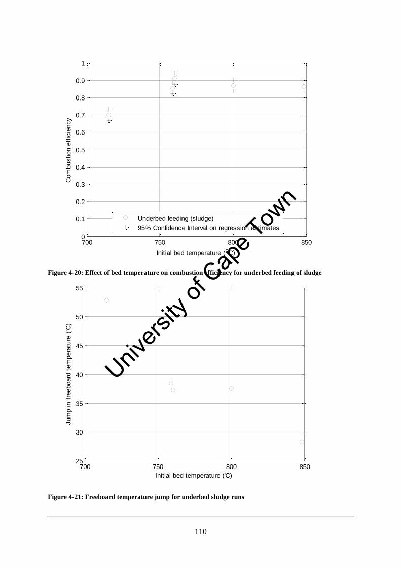
110

700 750 800 8500

0.1

0.2

0.3

0.4

0.5

0.6

0.7

0.8

0.9

1

Initial bed temperature (oC)

Com

bustion e

ffic

iency

Underbed feeding (sludge)

95% Confidence Interval on regression estimates

Figure 4-20: Effect of bed temperature on combustion efficiency for underbed feeding of sludge

700 750 800 85025

30

35

40

45

50

55

Initial bed temperature ('C)

Jum

p in f

reeboard

tem

pera

ture

('C

)

Figure 4-21: Freeboard temperature jump for underbed sludge runs

Univers

ity of

Cap

e Tow

n

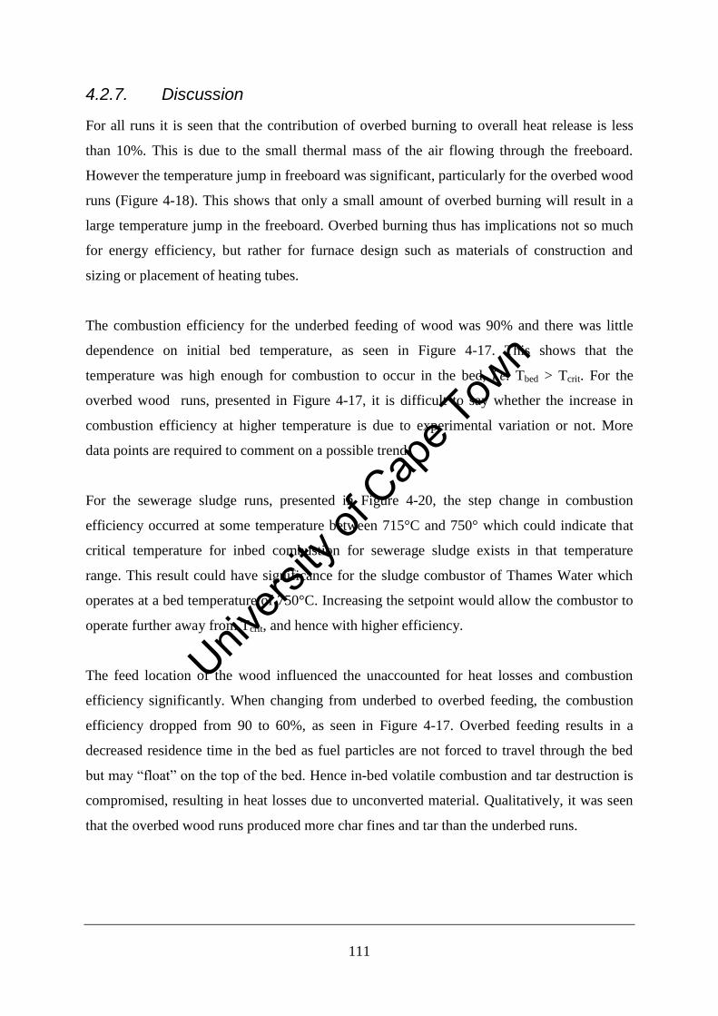
111

4.2.7. Discussion

For all runs it is seen that the contribution of overbed burning to overall heat release is less

than 10%. This is due to the small thermal mass of the air flowing through the freeboard.

However the temperature jump in freeboard was significant, particularly for the overbed wood

runs (Figure 4-18). This shows that only a small amount of overbed burning will result in a

large temperature jump in the freeboard. Overbed burning thus has implications not so much

for energy efficiency, but rather for furnace design such as materials of construction and

sizing or placement of heating tubes.

The combustion efficiency for the underbed feeding of wood was 90% and there was little

dependence on initial bed temperature, as seen in Figure 4-17. This shows that the

temperature was high enough for combustion to occur in the bed, i.e. Tbed > Tcrit. For the

overbed wood runs, presented in Figure 4-17, it is difficult to say whether the increase in

combustion efficiency at higher temperature is due to experimental variation or not. More

data points are required to comment on a possible trend.

For the sewerage sludge runs, presented in Figure 4-20, the step change in combustion

efficiency occurred at some temperature between 715°C and 750° which could indicate that

critical temperature for inbed combustion for sewerage sludge exists in that temperature

range. This result could have significance for the sludge combustor of Thames Water which

operates at a bed temperature of 750°C. Increasing the setpoint would allow the combustor to

operate further away from Tcrit, and hence with higher efficiency.

The feed location of the wood influenced the unaccounted for heat losses and combustion

efficiency significantly. When changing from underbed to overbed feeding, the combustion

efficiency dropped from 90 to 60%, as seen in Figure 4-17. Overbed feeding results in a

decreased residence time in the bed as fuel particles are not forced to travel through the bed

but may “float” on the top of the bed. Hence in-bed volatile combustion and tar destruction is

compromised, resulting in heat losses due to unconverted material. Qualitatively, it was seen

that the overbed wood runs produced more char fines and tar than the underbed runs.

Univers

ity of

Cap

e Tow

n

112

4.2.8. Conclusions and recommendations

An energy balance was used to determine the combustion efficiency as a function of initial

bed temperature and feed location. The simplicity of the model was due to the fast rate of

reaction of the biomass fuel and the fact that the rate of combustion jumped to a steady state

on commencement of feeding. The complex heat transfer of the experimental setup was

ignored by considering only the perturbation point, i.e. the point at which feeding

commenced. It is recommended that for future work on this apparatus, the outer reactor wall

temperature is monitored, or the furnace temperature controlled, to allow Qin to be directly

measured.

This set of experiments has shown that under the conditions of the investigation, significant

overbed burning of the fuels did not occur. In all cases the contribution of overbed burning

was less than 10%. The effect of the freeboard temperature jump needs to be considered, if

not for energy efficiency purposes, then for furnace design,.

In the case of the underbed wood runs, no clear dependence of combustion efficiency on bed

temperature emerged, which could mean that Tcrit for wood is lower than 700°C. For sludge,

the combustion efficiency was ~90%.at temperatures greater than 715°C The step change

could be due to the presence of Tcrit for sewerage sludge in that temperature range. This has

implications for choosing an operating temperature for a sludge combustor, as more stable

operation would be achieved at higher temperature.

Overbed burning of wood resulted in the combustion efficiency dropping from 90% to ~65%.

This is attributed to overbed-fed fuel having a shorter residence time in the bed, resulting in

reduced volatiles and tar conversion. The advantages of underbed feeding have been

recognised at Thames Water, with the re-design of their sludge incinerator including nozzles

to allow for under bed feeding of sludge.

Univers

ity of

Cap

e Tow

n

113

Chapter 5 Processing biogenic waste in South Africa:

technology selection and feedstock availability

5.1. Introduction

The White paper on renewable energy in South Africa (DME, 2004) identifies biogenic waste

streams as one of the sources of renewable energy which should be harnessed to achieve a

target of 10 000 GWhr (1141 MW) by 2013. Biogenic waste streams represent a form of

renewable energy which does not compete with food crops nor does its utilisation require the

clearing of land. The generation of electricity from biogenic waste streams may be achieved

through combustion to raise steam or via anaerobic digestion to produce methane-rich biogas.

This work sets out to compare the energy yield from each process by considering feedstock

characteristics viz. lower heating value, solids content and digestibility. The methodology is

then applied to a range of biogenic waste streams in South Africa and the energy potential

from these streams is estimated.

5.1.1. Biogenic waste availability in South Africa: previous studies

Estimates of the availability of waste biomass resources in South Africa are limited. Four

studies are presented in Table 5-1. Williams and Eberhard (1988) estimated the available

energy from biogenic waste sources at 233 PJ/yr while Lynd et al. (2003) provided a much

higher estimate of 1470 PJ/yr, owing to their proposed role for energy crops. Excluding these

energy crops, their estimate is reduced to 300 PJ/yr. Using the energy yields presented in the

White Paper on Renewable Energy (2004), the amount was estimated as approximately 280

PJ/yr (see Appendix B for details). In a study commissioned by the WRC, Burton et al.

(2007) analysed the potential for energy recovery from wastewater streams and animal

husbandry in South Africa. In this study, a potential energy recovery from industrial and

domestic wastewater of 29 PJ/yr was proposed with the majority harnessed from domestic

wastewater, as shown in Table 5-2. The potential energy recovery from intensive animal

husbandry was calculated to be 76 to 230 PJ/yr.

Univers

ity of

Cap

e Tow

n

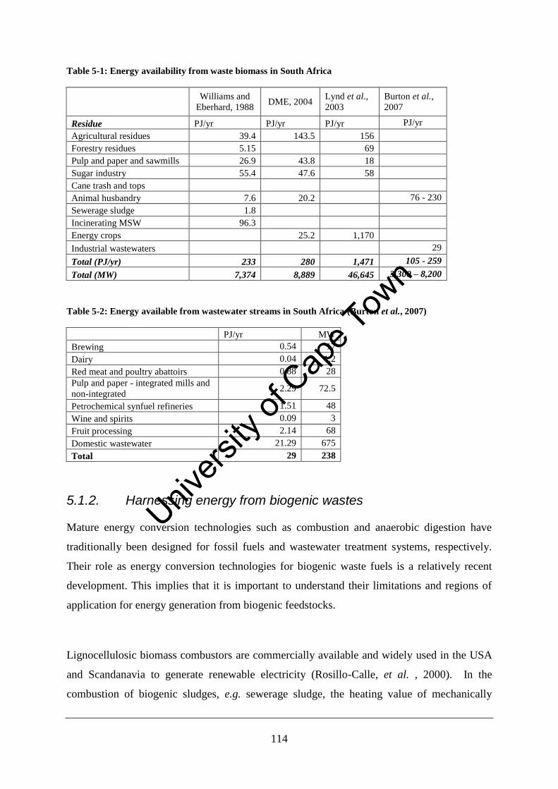
114

Table 5-1: Energy availability from waste biomass in South Africa

Williams and

Eberhard, 1988 DME, 2004

Lynd et al.,

2003

Burton et al.,

2007

Residue PJ/yr PJ/yr PJ/yr PJ/yr

Agricultural residues 39.4 143.5 156

Forestry residues 5.15 69

Pulp and paper and sawmills 26.9 43.8 18

Sugar industry 55.4 47.6 58

Cane trash and tops

Animal husbandry 7.6 20.2 76 - 230

Sewerage sludge 1.8

Incinerating MSW 96.3

Energy crops 25.2 1,170

Industrial wastewaters 29

Total (PJ/yr) 233 280 1,471 105 - 259

Total (MW) 7,374 8,889 46,645 3,300 – 8,200

Table 5-2: Energy available from wastewater streams in South Africa (Burton et al., 2007)

PJ/yr MW

Brewing 0.54 17

Dairy 0.04 1.2

Red meat and poultry abattoirs 0.88 28

Pulp and paper - integrated mills and

non-integrated 2.29 72.5

Petrochemical synfuel refineries 1.51 48

Wine and spirits 0.09 3

Fruit processing 2.14 68

Domestic wastewater 21.29 675

Total 29 238

5.1.2. Harnessing energy from biogenic wastes

Mature energy conversion technologies such as combustion and anaerobic digestion have

traditionally been designed for fossil fuels and wastewater treatment systems, respectively.

Their role as energy conversion technologies for biogenic waste fuels is a relatively recent

development. This implies that it is important to understand their limitations and regions of

application for energy generation from biogenic feedstocks.

Lignocellulosic biomass combustors are commercially available and widely used in the USA

and Scandanavia to generate renewable electricity (Rosillo-Calle, et al. , 2000). In the

combustion of biogenic sludges, e.g. sewerage sludge, the heating value of mechanically

Univers

ity of

Cap

e Tow

n

115

dewatered sludge may not be sufficient for autothermal combustion making an auxiliary fuel

essential (Werther and Ogada, 1999). The relative simplicity of the combustion processes are

negated by low thermal efficiencies of 15 to 20% in small boilers (Bridgewater, 2003;

McKendry, 2002; Rosillo-Calle, 2000), 30% for larger boilers (Bridgewater, 2003) and 40%

for co-firing in coal power plants (Mc Kendry, 2002). Combustion is non-selective in its use

of the feedstock, and reduces the whole fuel to simple products (Jenkins et al., 1998).

Reciprocating engines for CHP production from biogas are commercially available. The

capacity of these units ranges from 5 to 50 000 kW (Chambers and Potter, 2002). The rate

limiting step in the production of biogas is hydrolysis of polymers such as polysaccharides,

lipids and proteins (Noike et al., 1985). Anaerobic digestion of wastewater streams usually

requires hydrolysis of relatively simple sugars and readily digestible material to reduce COD.

However, in energy from waste applications, more recalcitrant feedstocks are processed e.g

.sewerage sludge and manure slurries.

5.1.3. Objectives

In this chapter, a simple methodology is sought, founded on first principles, to guide

determination of the operating region in which combustion and anaerobic digestion can be

utilised for the generation of electricity from biogenic waste materials. The methodology

developed is then used determine whether combustion or anaerobic digestion should be used

to process a variety of biogenic waste streams in South Africa.

The variation in the estimates presented in previous studies highlight the need to further

investigate some of the underlying assumptions on which these estimates are based;

particularly the larger estimates (e.g. the biofuel contribution in Lynd et al. (2003) and the

animal husbandry estimates in Burton et al. (2007)). The objective of this review is thus to

quantify biogenic waste streams in South Africa and calculate the potential energy output.

Furthermore, critical discussion of the availability of the stream for energetic purposes is

included. Where the stream is already used for energetic purposes, comments on the

efficiency are made. Where alternate uses do not preclude energy generation from the

resource, its potential is established.

Univers

ity of

Cap

e Tow

n

116

5.2. Methodology to compare combustion and anaerobic

digestion energy yield from biogenic wastes

5.2.1. Development of methodology

The dry solids content of the feedstock determines if a positive energy balance is possible

over a combustion unit and hence is the first parameter to be considered when comparing

technologies. The energy yield from combustion on a dry solids basis is given by Equation

5-1. As stated in Section 3.4.1, the energy yield from the combustion processes is calculated

as the difference between the heat released through combustion of solids, as given by the

lower heating value of the fuel, and the heat required for evaporating the moisture. Equation

5-2 can be used where it is necessary to account for the ash content of the fuel explicitly.

waterfuelcombustion HvapDS

DSLHVmE DS

)1( Equation 5-1




LHVfuel = lower heating value of fuel on dry basis [MJ/kg]

ΔHvapwater = heat of evaporation of water at 25°C [2.38 MJ/kg] (Perry et al., 1999)

waterfuelcombustion HvapDS

DSashLHVmE DS

)1()1(

Equation 5-2




ash = ash content of fuel (%)

LHVfuel = lower heating value of fuel on dry basis [MJ/kg]

ΔHvapwater = heat of evaporation of water at 25°C [2.38 MJ/kg] (Perry et al., 1999)

The energy yield from anaerobic digestion (Equation 5-3) can be calculated from the product

of the extent of conversion of volatile matter in the feedstock, the specific methane yield and

the heating value of methane. As in Section 3.4.1, a specific methane yield of 0.65 m3/kg

volatile solids is used. Alternatively, if the COD (Chemical Oxygen Demand) and volumetric

flows are known, as is often the case with wastewater streams, Equation 5-4 can be used to

calculate the energy yield.

Univers

ity of

Cap

e Tow

n

117

44)1( CHCHDSAD LHVYVSdashmE Equation 5-3

where EAD = energy yield from anaerobic digestion [MJ/day]


VSd = percentage volatile solids destruction (%)

ash = ash content in fuel on dry basis (%)

YCH4 = yield of methane STP [0.65 m3/kg VS]

LHVCH4 = lower heating value of CH4 at STP [ 35.8 MJ/m3] (Perry et al., 1999)

44][ CHCHAD LHVYCODQE dfd Equation 5-4

where EAD = energy yield from anaerobic digestion [W]

Q = volumetric flow of stream [m3/s]

[COD] = COD load of stream [kg COD/m3]

YCH4 = methane yield at STP [0.35 m3/kg COD]

LHVCH4 = lower heating value of methane at STP [35.8 MJ/m3] (Tchobanoglous et al.,2003)

As seen in Figure 5-1, energy yield from combustion is a non-linear function of dry solids

content and thus positive energy yields (heat generated) and negative energy yields (heat

required) can be defined. In Figure 5-1, positive and negative energy yields are expressed as a

function of dry solids content and LHV for various ash contents. The region above the curve

is the feasible region of operation (i.e. positive energy yield) and region below the curve is an

infeasible region of operation (negative energy yield). It is clear that increasing ash content

reduces the feasible region of operation for combustors. Displayed in Figure 5-1 is a

maximum dry solids content likely to be seen for sludge-type biogenic waste. This is based on

best operation of dewatering units such as belt filter presses, filter presses and centrifuges

(Bane, 2000). When dealing with lignocellulosic wastes, solids contents may reach 80%. An

upper limit on heating value for biogenic waste fuels of 20 MJ/kg (dry, ash-free basis) is

suggested by Quaark et al. (1999).

Univers

ity of

Cap

e Tow

n

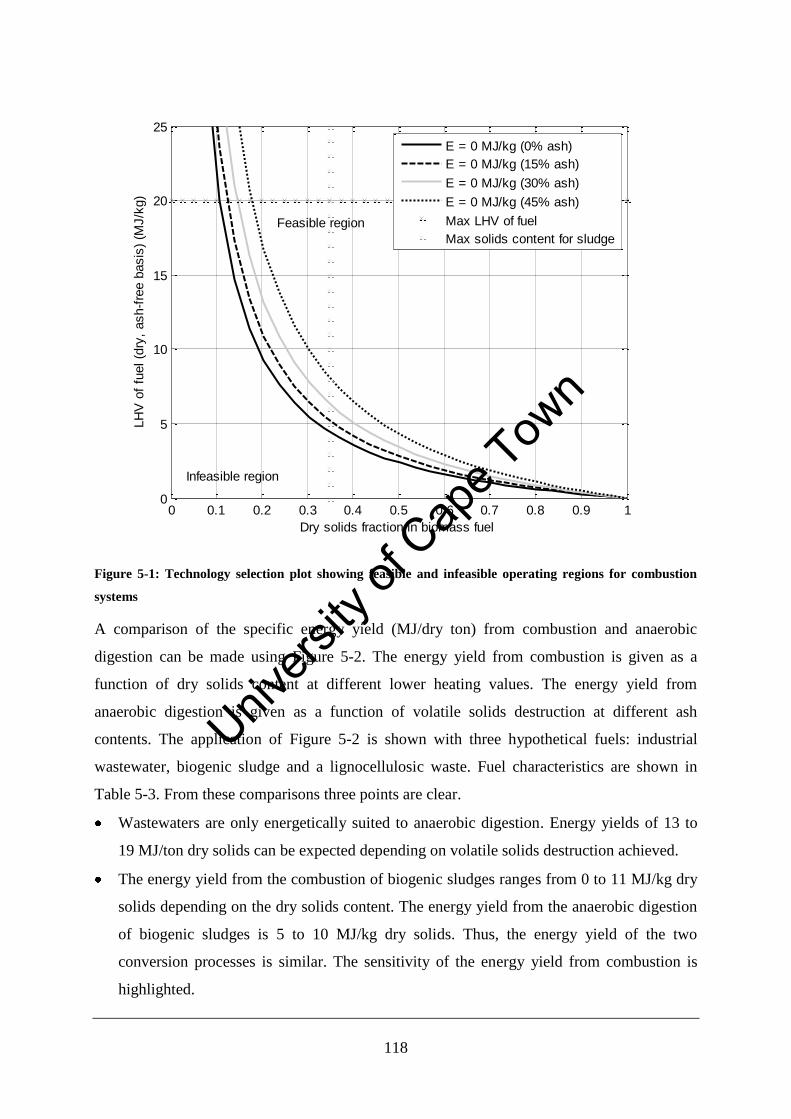
118

0 0.1 0.2 0.3 0.4 0.5 0.6 0.7 0.8 0.9 10

5

10

15

20

25

Dry solids fraction in biomass fuel

LH

V o

f fu

el (d

ry,

ash-f

ree b

asis

) (M

J/k

g)

Infeasible region

Feasible region

E = 0 MJ/kg (0% ash)

E = 0 MJ/kg (15% ash)

E = 0 MJ/kg (30% ash)

E = 0 MJ/kg (45% ash)

Max LHV of fuel

Max solids content for sludge

Figure 5-1: Technology selection plot showing feasible and infeasible operating regions for combustion

systems

A comparison of the specific energy yield (MJ/dry ton) from combustion and anaerobic

digestion can be made using Figure 5-2. The energy yield from combustion is given as a

function of dry solids content at different lower heating values. The energy yield from

anaerobic digestion is given as a function of volatile solids destruction at different ash

contents. The application of Figure 5-2 is shown with three hypothetical fuels: industrial

wastewater, biogenic sludge and a lignocellulosic waste. Fuel characteristics are shown in

Table 5-3. From these comparisons three points are clear.

Wastewaters are only energetically suited to anaerobic digestion. Energy yields of 13 to

19 MJ/ton dry solids can be expected depending on volatile solids destruction achieved.

The energy yield from the combustion of biogenic sludges ranges from 0 to 11 MJ/kg dry

solids depending on the dry solids content. The energy yield from the anaerobic digestion

of biogenic sludges is 5 to 10 MJ/kg dry solids. Thus, the energy yield of the two

conversion processes is similar. The sensitivity of the energy yield from combustion is

highlighted.

Univers

ity of

Cap

e Tow

n

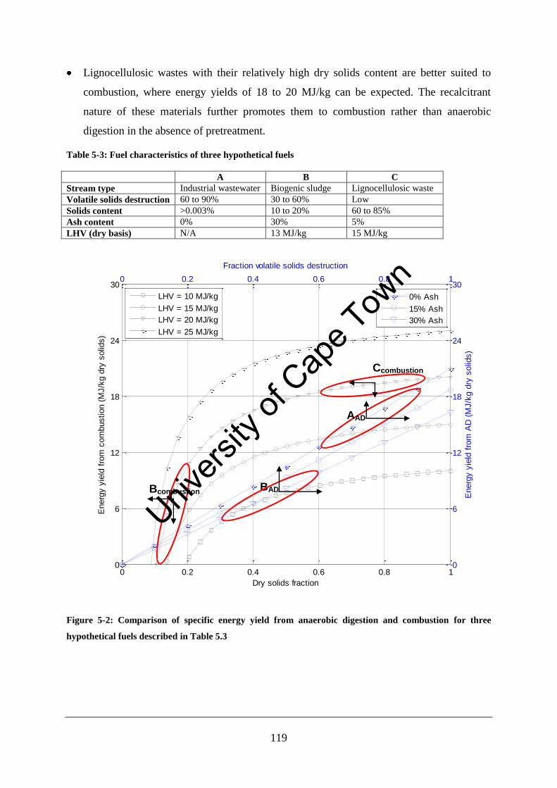
119

Lignocellulosic wastes with their relatively high dry solids content are better suited to

combustion, where energy yields of 18 to 20 MJ/kg can be expected. The recalcitrant

nature of these materials further promotes them to combustion rather than anaerobic

digestion in the absence of pretreatment.

Table 5-3: Fuel characteristics of three hypothetical fuels

A B C

Stream type Industrial wastewater Biogenic sludge Lignocellulosic waste

Volatile solids destruction 60 to 90% 30 to 60% Low

Solids content >0.003% 10 to 20% 60 to 85%

Ash content 0% 30% 5%

LHV (dry basis) N/A 13 MJ/kg 15 MJ/kg

0 0.2 0.4 0.6 0.8 10

6

12

18

24

30

Dry solids fraction

Energ

y y

ield

fro

m c

om

bustion (

MJ/k

g d

ry s

olid

s)

LHV = 10 MJ/kg

LHV = 15 MJ/kg

LHV = 20 MJ/kg

LHV = 25 MJ/kg

0 0.2 0.4 0.6 0.8 1

0

6

12

18

24

30


Energ

y y

ield

fro

m A

D (

MJ/k

g d

ry s

olid

s)

0% Ash

15% Ash

30% Ash

Figure 5-2: Comparison of specific energy yield from anaerobic digestion and combustion for three

hypothetical fuels described in Table 5.3

BAD Bcombustion

Ccombustion

AAD

Univers

ity of

Cap

e Tow

n

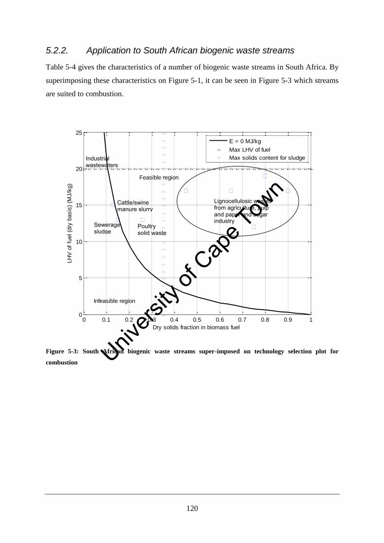
120

5.2.2. Application to South African biogenic waste streams

Table 5-4 gives the characteristics of a number of biogenic waste streams in South Africa. By

superimposing these characteristics on Figure 5-1, it can be seen in Figure 5-3 which streams

are suited to combustion.

0 0.1 0.2 0.3 0.4 0.5 0.6 0.7 0.8 0.9 10

5

10

15

20

25

Dry solids fraction in biomass fuel

LH

V o

f fu

el (d

ry b

asis

) (M

J/k

g)

Infeasible region

Feasible region

E = 0 MJ/kg

Max LHV of fuel

Max solids content for sludge

Figure 5-3: South African biogenic waste streams super-imposed on technology selection plot for

combustion

Industrial wastewaters

Sewerage sludge

Cattle/swine manure slurry

Poultry solid waste

Lignocellulosic wastes from agriculture, pulp and paper and sugar industry

Univers

ity of

Cap

e Tow

n

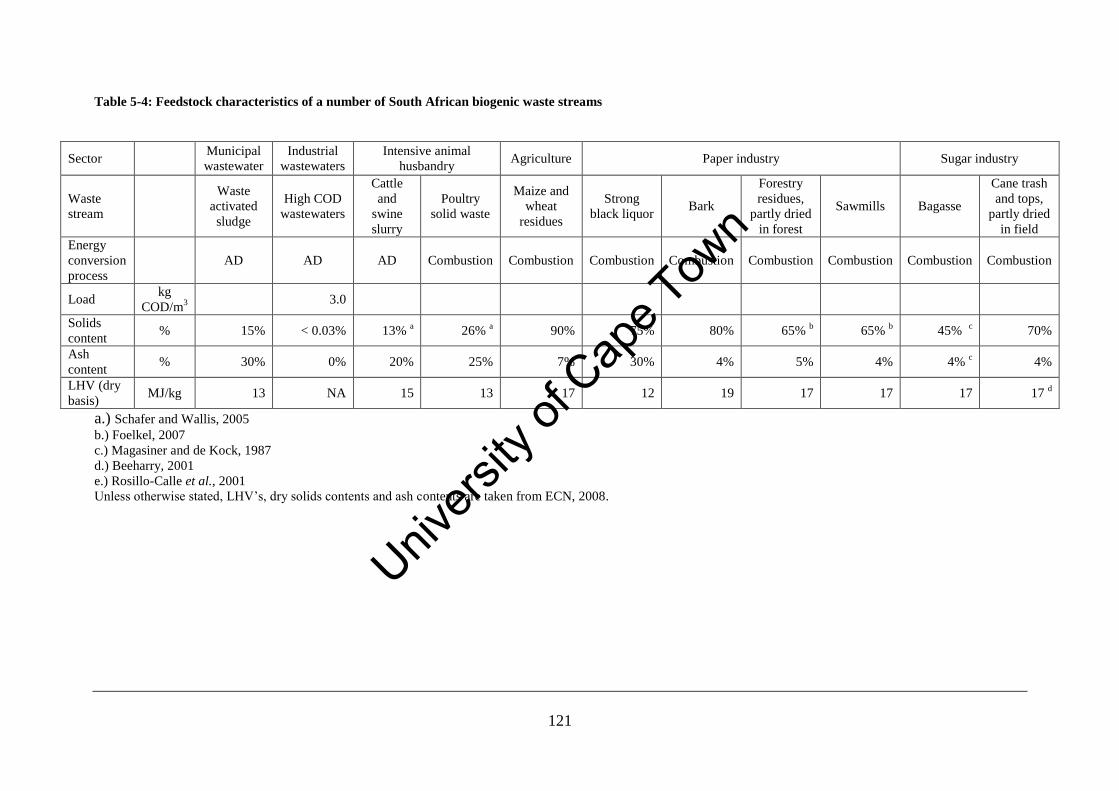
121

Table 5-4: Feedstock characteristics of a number of South African biogenic waste streams

a.) Schafer and Wallis, 2005

b.) Foelkel, 2007

c.) Magasiner and de Kock, 1987

d.) Beeharry, 2001

e.) Rosillo-Calle et al., 2001

Unless otherwise stated, LHV’s, dry solids contents and ash contents are taken from ECN, 2008.

Sector Municipal

wastewater

Industrial

wastewaters

Intensive animal

husbandry Agriculture Paper industry Sugar industry

Waste

stream

Waste

activated

sludge

High COD

wastewaters

Cattle

and

swine

slurry

Poultry

solid waste

Maize and

wheat

residues

Strong

black liquor Bark

Forestry

residues,

partly dried

in forest

Sawmills Bagasse

Cane trash

and tops,

partly dried

in field

Energy

conversion

process

AD AD AD Combustion Combustion Combustion Combustion Combustion Combustion Combustion Combustion

Load kg

COD/m3

3.0

Solids

content % 15% < 0.03% 13%

a 26%

a 90% 75% 80% 65%

b 65%

b 45%

c 70%

Ash

content % 30% 0% 20% 25% 7% 30% 4% 5% 4% 4%

c 4%

LHV (dry

basis) MJ/kg 13 NA 15 13 17 12 19 17 17 17 17

d

Univers

ity of

Cap

e Tow

n

122

5.3. Quantifying biogenic waste streams in South Africa

5.3.1. Domestic wastewater

5.3.1.1. Industry overview

The wastewater treatment process has been covered in detail in Section 3.2. In South Africa,

the municipalities are responsible for the operation of wastewater treatment plants and the

provision of clean water. This is in contrast with the UK where some of the largest water

providers are private companies e.g. Thames Water.

From the study presented in Chapter 3, it is clear that a significant amount of energy is

recoverable from the sewerage sludge generated on a domestic wastewater treatment plant,

either via incineration or anaerobic digestion. In the wastewater treatment process, it is

possible to use anaerobic digestion to treat the influent stream, as opposed to aerobic

processes such as the activated sludge process or trickle bed filters. Indeed, anaerobic

wastewater treatment has a number of advantages over aerobic treatment, viz. less energy

required; less biological sludge produced and production of a useful product, methane

(Tchobanoglous et al., 2003; Waites et al, 2001). However, for domestic wastewaters with

lower concentrations of biodegradable COD, higher effluent quality needs and nutrient

removal requirements, aerobic processes are favoured as present (Tchobanoglous et al., 2003)

and hence, energy recovery from domestic wastewater is not considered in this study.

Approximately 57% of the sludge generated in South Africa WWTP’s is anaerobically

digested (Snyman et al., 2004). In South Africa the use of the biogas varies between

municipalities. Johannesburg and Cape Town do not monitor biogas production and hence it

is unlikely they use it. The Cape Flats wastewater treatment plant in Cape Town, which has a

granulating operation for the anaerobically digested sludge, was set up to use the biogas in the

drying process. Currently this seldom happens and diesel is used instead (Burton et al., 2008).

The Tshwane works use the biogas for raising steam to heat the digesters (Ntsowe, 2008).

South Africa has one installed sludge incinerator at the eThekwini sewerage works. This unit

is currently not operational (Dildar, 2008).

Univers

ity of

Cap

e Tow

n

123

5.3.1.2. Residue production

The total domestic wastewater treated is estimated in Burton et al. (2007) as 7600 Ml/yr. In

their comprehensive field work on metals in South African sewerage sludges, Snyman et al.

(2004) drew up a table of wastewater influent volumes and mass of sludge produced from

some 70 plants. If sludge production was not measured at the plant, an estimate was based on

per capita sludge production. From this data sludge production was calculated to be 282 kg

solids/Ml influent volume. The total sludge production for South Africa was calculated to be

782 000 dry ton/yr.

5.3.2. Industrial wastewaters

Data on the COD load and effluent volumes was collected from a series of projects called

National Survey (Natsurv) (1989 to 2005), carried out by the Water Research Council. The

purpose of Natsurv was to determine current specific water usages and suggest target specific

water usages. As such, effluent flows and pollution loads (COD loads) were available. These

are listed in Table 5-5. Data prior to 1993 were considered outdated and scaled up as shown.

The total quantity of industrial wastewaters is estimated to be 127 Mm3/yr at an average COD

load of 3 kg COD/m3.

5.3.3. Intensive animal husbandry

Intensive animal husbandry refers to the rearing of animals in feedlots. Four classes of animal

husbandry are considered here: cattle, pigs and poultry (layers and broilers). The quantity of

waste generated from animal husbandry is calculated as the product of number of heads,

specific manure production and dry solids content of the manure as shown in Table 5-6. The

number of roaming beef cattle is approximately 12 million (30 times more than those kept in

feedlots), however the energy potential from this manure is not considered due to the

difficulty in collecting it and the fact that in rural areas it is mostly used for floors, fuel or

fertiliser.

Univers

ity of

Cap

e Tow

n

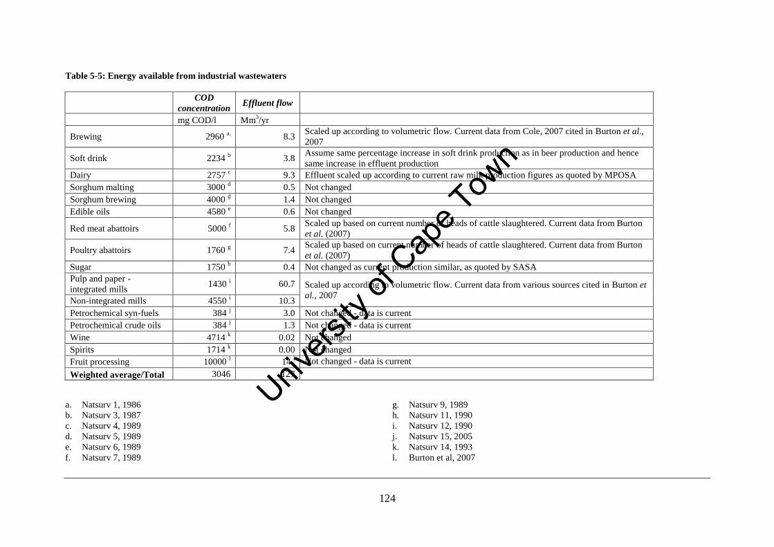
124

Table 5-5: Energy available from industrial wastewaters

COD

concentration Effluent flow

mg COD/l Mm3/yr

Brewing 2960 a.

8.3 Scaled up according to volumetric flow. Current data from Cole, 2007 cited in Burton et al.,

2007

Soft drink 2234 b

3.8 Assume same percentage increase in soft drink production as in beer production and hence

same increase in effluent production

Dairy 2757 c

9.3 Effluent scaled up according to current raw milk production figures as quoted by MPOSA

Sorghum malting 3000 d

0.5 Not changed

Sorghum brewing 4000 d

1.4 Not changed

Edible oils 4580 e

0.6 Not changed

Red meat abattoirs 5000 f

5.8 Scaled up based on current number of heads of cattle slaughtered. Current data from Burton

et al. (2007)

Poultry abattoirs 1760 g

7.4 Scaled up based on current number of heads of cattle slaughtered. Current data from Burton

et al. (2007)

Sugar 1750 h

0.4 Not changed as current production similar, as quoted by SASA

Pulp and paper -

integrated mills 1430

i 60.7 Scaled up according to volumetric flow. Current data from various sources cited in Burton et

al., 2007 Non-integrated mills 4550

i 10.3

Petrochemical syn-fuels 384 j

3.0 Not changed - data is current

Petrochemical crude oils 384 j

1.3 Not changed - data is current

Wine 4714 k

0.02 Not changed

Spirits 1714 k

0.00 Not changed

Fruit processing 10000 l

14 l Not changed - data is current

Weighted average/Total 3046 127

a. Natsurv 1, 1986

b. Natsurv 3, 1987

c. Natsurv 4, 1989

d. Natsurv 5, 1989

e. Natsurv 6, 1989

f. Natsurv 7, 1989

g. Natsurv 9, 1989

h. Natsurv 11, 1990

i. Natsurv 12, 1990

j. Natsurv 15, 2005

k. Natsurv 14, 1993

l. Burton et al, 2007

Univers

ity of

Cap

e Tow

n

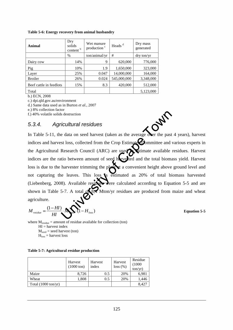
125

Table 5-6: Energy recovery from animal husbandry

Animal

Dry

solids

content b

Wet manure

production c

Heads d

Dry mass

generated

% ton/animal/yr # dry ton/yr

Dairy cow 14% 9 620,000 776,000

Pig 10% 1.9 1,650,000 323,000

Layer 25% 0.047 14,000,000 164,000

Broiler 26% 0.024 545,000,000 3,348,000

Beef cattle in feedlots 15% 8.3 420,000 512,000

Total 5,123,000

b.) ECN, 2008

c.) dpi.qld.gov.au/environment

d.) Same data used as in Burton et al., 2007

e.) 8% collection factor

f.) 40% volatile solids destruction

5.3.4. Agricultural residues

In Table 5-11, the data on seed harvest (taken as the average over the past 4 years), harvest

indices and harvest loss, collected from the Crop Estimates Committee and various experts in

the Agricultural Research Council (ARC) are used to estimate available residues. Harvest

indices are the ratio between amount of seed harvested and the total biomass yield. Harvest

loss is due to the harvester trimming the plant at a convenient height above ground level and

not capturing the leaves. This loss is estimated as 20% of total biomass harvested

(Liebenberg, 2008). Available residues were calculated according to Equation 5-5 and are

shown in Table 5-7. A total of 8,4 Mton/yr residues are produced from maize and wheat

agriculture.

)1()1(

lossseedresidue HMHI

HIM Equation 5-5

where Mresidue = amount of residue available for collection (ton)

HI = harvest index

Mseed = seed harvest (ton)

Hloss = harvest loss

Table 5-7: Agricultural residue production

Harvest

(1000 ton)

Harvest

index

Harvest

loss (%)

Residue

(1000

ton/yr)

Maize 8,726 0.5 20% 6,981

Wheat 1,808 0.5 20% 1,446

Total (1000 ton/yr) 8,427

Univers

ity of

Cap

e Tow

n

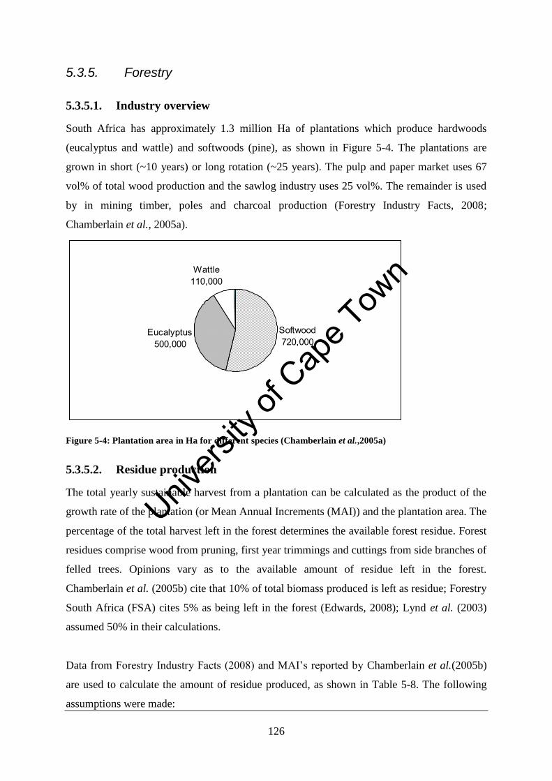
126

5.3.5. Forestry


South Africa has approximately 1.3 million Ha of plantations which produce hardwoods

(eucalyptus and wattle) and softwoods (pine), as shown in Figure 5-4. The plantations are

grown in short (~10 years) or long rotation (~25 years). The pulp and paper market uses 67

vol% of total wood production and the sawlog industry uses 25 vol%. The remainder is used

by in mining timber, poles and charcoal production (Forestry Industry Facts, 2008;

Chamberlain et al., 2005a).

Wattle110,000

Eucalyptus500,000

Softwood720,000

Figure 5-4: Plantation area in Ha for different species (Chamberlain et al.,2005a)


The total yearly sustainable harvest from a plantation can be calculated as the product of the

growth rate of the plantation (or Mean Annual Increments (MAI)) and the plantation area. The

percentage of the total harvest left in the forest determines the available forest residue. Forest

residues comprise wood from pruning, first year trimmings and cuttings from side branches of

felled trees. Opinions vary as to the available amount of residue left in the forest.

Chamberlain et al. (2005b) cite that 10% of total biomass produced is left as residue; Forestry

South Africa (FSA) cites 5% as being left in the forest (Edwards, 2008); Lynd et al. (2003)

assumed 50% in their calculations.

Data from Forestry Industry Facts (2008) and MAI’s reported by Chamberlain et al.(2005b)

are used to calculate the amount of residue produced, as shown in Table 5-8. The following

assumptions were made:

Univers

ity of

Cap

e Tow

n

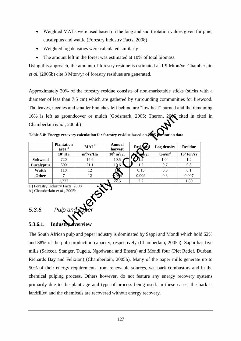
127

Weighted MAI’s were used based on the long and short rotation values given for pine,

eucalyptus and wattle (Forestry Industry Facts, 2008)

Weighted log densities were calculated similarly

The amount left in the forest was estimated at 10% of total biomass

Using this approach, the amount of forestry residue is estimated at 1.9 Mton/yr. Chamberlain

et al. (2005b) cite 3 Mton/yr of forestry residues are generated.

Approximately 20% of the forestry residue consists of non-marketable sticks (sticks with a

diameter of less than 7.5 cm) which are gathered by surrounding communities for firewood.

The leaves, needles and smaller branches left behind are “low heat” burned and the remaining

16% is left as groundcover or mulch (Godsmark, 2005; Theron, 2005 cited in cited in

Chamberlain et al., 2005b)

Table 5-8: Energy recovery calculation for forestry residue based on 2005 plantation data

Plantation

area a MAI

b Annual

harvest Residue Log density Residue

103 Ha m

3/yr/Ha 10

6 m

3/yr 10

6 m3/yr ton/m

3 10

6 ton/yr

Softwood 720 14.6 10.5 1.2 1.04 1.2

Eucalyptus 500 21.1 10.6 1.2 0.7 0.8

Wattle 110 12 1.3 0.15 0.8 0.1

Other 7 12 0.084 0.009 0.8 0.007

1,337 22.5 2.2 1.89

a.) Forestry Industry Facts, 2008

b.) Chamberlain et al., 2005b

5.3.6. Pulp and paper


The South African pulp and paper industry is dominated by Sappi and Mondi which hold 62%

and 38% of the pulp production capacity, respectively (Chamberlain, 2005a). Sappi has five

mills (Saiccor, Stanger, Tugela, Ngodwana and Enstra) and Mondi four (Piet Retief, Durban,

Richards Bay and Felixton) (Chamberlain, 2005b). Many of the paper mills generate up to

50% of their energy requirements from renewable sources, viz. bark combustors and in the

chemical pulping process. Others however, do not feature any energy recovery systems

primarily due to the plant age and type of process being used. In these cases, the bark is

landfilled and the chemicals are recovered without energy recovery.

Univers

ity of

Cap

e Tow

n

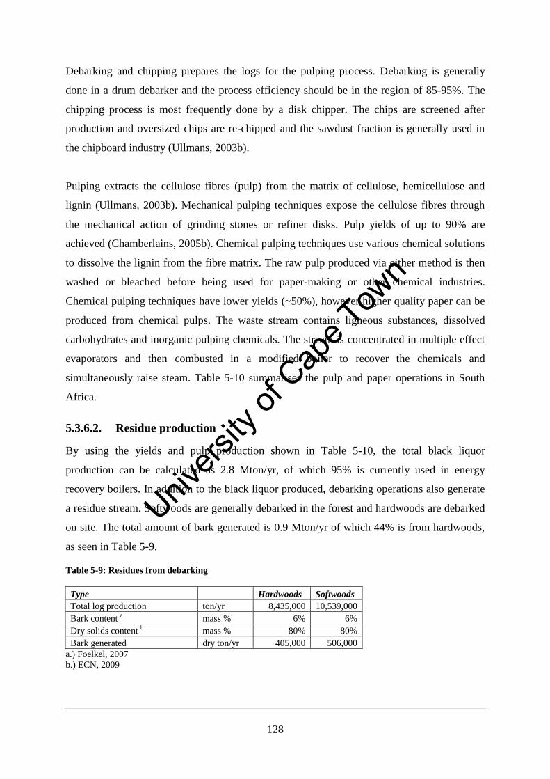
128

Debarking and chipping prepares the logs for the pulping process. Debarking is generally

done in a drum debarker and the process efficiency should be in the region of 85-95%. The

chipping process is most frequently done by a disk chipper. The chips are screened after

production and oversized chips are re-chipped and the sawdust fraction is generally used in

the chipboard industry (Ullmans, 2003b).

Pulping extracts the cellulose fibres (pulp) from the matrix of cellulose, hemicellulose and

lignin (Ullmans, 2003b). Mechanical pulping techniques expose the cellulose fibres through

the mechanical action of grinding stones or refiner disks. Pulp yields of up to 90% are

achieved (Chamberlains, 2005b). Chemical pulping techniques use various chemical solutions

to dissolve the lignin from the fibre matrix. The raw pulp produced via either method is then

washed or bleached before being used for paper-making or other chemical industries.

Chemical pulping techniques have lower yields (~50%), however higher quality paper can be

produced from chemical pulps. The waste stream contains ligneous substances, dissolved

carbohydrates and inorganic pulping chemicals. The stream is concentrated in multiple effect

evaporators and then combusted in a modified boiler to recover the chemicals and

simultaneously raise steam. Table 5-10 summarises the pulp and paper operations in South

Africa.


By using the yields and pulp production shown in Table 5-10, the total black liquor

production can be calculated as 2.8 Mton/yr, of which 95% is currently used in energy

recovery boilers. In addition to the black liquor produced, debarking operations also generate

a residue stream. Softwoods are generally debarked in the forest and hardwoods are debarked

on site. The total amount of bark generated is 0.9 Mton/yr of which 44% is from hardwoods,

as seen in Table 5-9.

Table 5-9: Residues from debarking

Type Hardwoods Softwoods

Total log production ton/yr 8,435,000 10,539,000

Bark content a

mass % 6% 6%

Dry solids content b

mass % 80% 80%

Bark generated dry ton/yr 405,000 506,000

a.) Foelkel, 2007

b.) ECN, 2009

Univers

ity of

Cap

e Tow

n

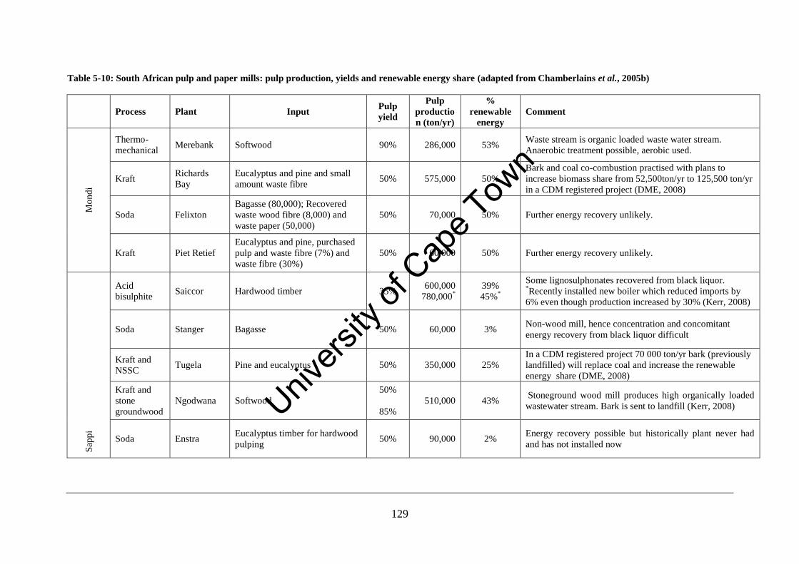
129

Table 5-10: South African pulp and paper mills: pulp production, yields and renewable energy share (adapted from Chamberlains et al., 2005b)

Process Plant Input Pulp

yield

Pulp

productio

n (ton/yr)

%

renewable

energy

Comment

Mo

nd

i

Thermo-

mechanical Merebank Softwood 90% 286,000 53%

Waste stream is organic loaded waste water stream.

Anaerobic treatment possible, aerobic used.

Kraft Richards

Bay

Eucalyptus and pine and small

amount waste fibre 50% 575,000 50%

Bark and coal co-combustion practised with plans to

increase biomass share from 52,500ton/yr to 125,500 ton/yr

in a CDM registered project (DME, 2008)

Soda Felixton

Bagasse (80,000); Recovered

waste wood fibre (8,000) and

waste paper (50,000)

50% 70,000 50% Further energy recovery unlikely.

Kraft Piet Retief

Eucalyptus and pine, purchased

pulp and waste fibre (7%) and

waste fibre (30%)

50% 60,000 50% Further energy recovery unlikely.

Sap

pi

Acid

bisulphite Saiccor Hardwood timber 35%

600,000

780,000*

39%

45%*

Some lignosulphonates recovered from black liquor. *Recently installed new boiler which reduced imports by

6% even though production increased by 30% (Kerr, 2008)

Soda Stanger Bagasse 50% 60,000 3% Non-wood mill, hence concentration and concomitant

energy recovery from black liquor difficult

Kraft and

NSSC Tugela Pine and eucalyptus 50% 350,000 25%

In a CDM registered project 70 000 ton/yr bark (previously

landfilled) will replace coal and increase the renewable

energy share (DME, 2008)

Kraft and

stone

groundwood

Ngodwana Softwood

50%

85%

510,000 43% Stoneground wood mill produces high organically loaded

wastewater stream. Bark is sent to landfill (Kerr, 2008)

Soda Enstra Eucalyptus timber for hardwood

pulping 50% 90,000 2%

Energy recovery possible but historically plant never had

and has not installed now

Univers

ity of

Cap

e Tow

n

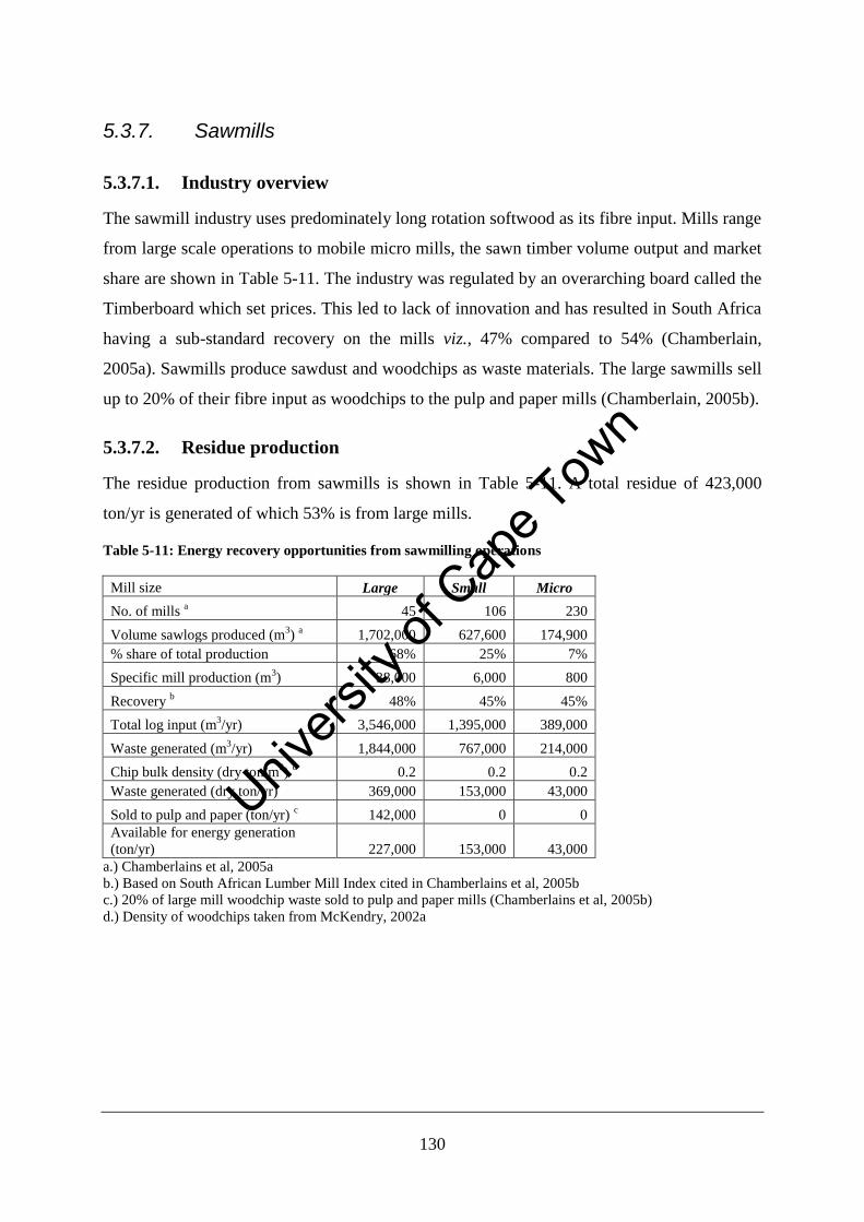
130

5.3.7. Sawmills


The sawmill industry uses predominately long rotation softwood as its fibre input. Mills range

from large scale operations to mobile micro mills, the sawn timber volume output and market

share are shown in Table 5-11. The industry was regulated by an overarching board called the

Timberboard which set prices. This led to lack of innovation and has resulted in South Africa

having a sub-standard recovery on the mills viz., 47% compared to 54% (Chamberlain,

2005a). Sawmills produce sawdust and woodchips as waste materials. The large sawmills sell

up to 20% of their fibre input as woodchips to the pulp and paper mills (Chamberlain, 2005b).


The residue production from sawmills is shown in Table 5-11. A total residue of 423,000

ton/yr is generated of which 53% is from large mills.

Table 5-11: Energy recovery opportunities from sawmilling operations

Mill size Large Small Micro

No. of mills a 45 106 230

Volume sawlogs produced (m3)

a 1,702,000 627,600 174,900

% share of total production 68% 25% 7%

Specific mill production (m3) 38,000 6,000 800

Recovery b 48% 45% 45%

Total log input (m3/yr) 3,546,000 1,395,000 389,000

Waste generated (m3/yr) 1,844,000 767,000 214,000

Chip bulk density (dry ton/m3)

d 0.2 0.2 0.2

Waste generated (dry ton/yr) 369,000 153,000 43,000

Sold to pulp and paper (ton/yr) c 142,000 0 0

Available for energy generation

(ton/yr) 227,000 153,000 43,000

a.) Chamberlains et al, 2005a

b.) Based on South African Lumber Mill Index cited in Chamberlains et al, 2005b

c.) 20% of large mill woodchip waste sold to pulp and paper mills (Chamberlains et al, 2005b)

d.) Density of woodchips taken from McKendry, 2002a

Univers

ity of

Cap

e Tow

n

131

5.3.8. Sugar industry


Cane is grown primarily in Kwa-Zulu Natal and Mpumalanga. The cane producing areas in

KZN are divided into the Coastal Sands and the Northern irrigated areas. Most of the cane in

South Africa is produced under rainfed conditions where the annual precipitation is 800 to

1200 mm/yr, making it one of the driest cane producing areas in the world (van Antwerpen,

2006). The national average cane yield is 65 ton/Ha; lower than other cane producing

countries such as Mauritius (75 ton/Ha (Beeharry, 1996) and Hawaii (200 ton/Ha (Ullmans,

2003c)).

Cane is harvested mechanically or manually depending on the slope of the land. In South

Africa, 90% of cane is harvested dry and prior to harvesting, the trash (dry cane leaves and

cane tops) is burnt to make harvesting easier and to reduce the amount of fibre carried into the

mill (van Antwerpen et al., 2006). If the cane is harvested green, the trash is left on the field

to form a mulch, which returns nutrients to the soil (Singh, 2008). Leaving the trash to dry on

the field for a few days can reduce the moisture content to 30%. It can then be raked into

windrows, baled and transported to the mill for energy recovery (Rosillo-Calle et al., 2000).

After harvesting the cane is transported to the sugar mill. The cane is initially chopped to

pieces 2-10cm by a set of revolving knives and then crushed in a three-roller mill (Ullmans,

2003c). This releases 55-70% of the juice and opens 84-90% of the sucrose-containing

parenchyma cells. The cane juice is extracted from the opened cell by lixiviation and from the

unopened cells by diffusion. To aid this process, the diffuser temperature is 65-75°C which

makes the cells semi-permeable (Baikow, 1982). In the basic operation of a diffuser, bagasse

is moved over perforated plates by chains. A lixiviant or “sweet water” is sprayed onto the

bagasse and is then collected in a trough under the conveyor (Baikow, 1982). Once the

bagasse is exhausted of its sugar, it is dewatered to approximately 50% moisture content

before being fed to the bagasse boilers (Ullmans, 2003c). The cane juice (which has solids

content of 10-25%) is thickened and then liquid is concentrated to 70% solids in a multi-effect

evaporator plant. The resulting cane syrup is then evaporated to supersaturation and seeded to

initiate crystallisation. The sugar leaving the mill is known as raw sugar and is sent to sugar

refineries which further process the sugar to end-consumer products (Ullmans, 2003c).

Univers

ity of

Cap

e Tow

n

132

There are ten sugar mills in South Africa: two owned by TSB (Malelane and Komati) four by

Illovo (Eston, Umzimkulu, Noodsberg and Pongola) and four by Tongaat-Hulett (Maidstone,

Amatikulu, Felixton and Darnell). Currently, the Felixton, Maidstone and Amatikulu mills

export 9 MW (huletts.co.za, 2008) and the go-ahead for a boiler expansion project to export

38 MW in crushing season and 17 MW out of season depends on Eskom price negotiations

(Tongaat-Hulett Annual Report, 2007). The Illovo and TSB operations in South Africa

currently do not export electricity. The Illovo Ubombo mill in Swaziland does export

electricity to the local grid.


Data from SASA (2008) for the period 2003 to 2007 gives an average bagasse production of 6

Mton/yr (wet basis), as seen in Table 5-12. On a dry basis this equates to 2.7 Mton/yr.

Cane trash from cane fields which have not been burnt can be used supplement bagasse.

Purchase et al. (2008) calculate the dry trash yield to be 153 kg/ton wet cane. Using the data

in Table 5-12 the residue from cane trash is calculated as 3 Mton/yr.

Table 5-12: South African bagasse production

Season

Cane processed

(wet tons)

Bagasse produced

(wet tons)

Aug-07 19,724,000 5,954,000

Jul-06 20,279,000 6,144,000

Jun-05 21,052,000 6,247,000

May-04 19,095,000 5,786,000

Apr-03 20,419,000 6,222,000

Average 20,114,000 6,071,000

Univers

ity of

Cap

e Tow

n

133

5.4. Energy recovery from biogenic waste streams

5.4.1. Results

Table 5-13 collates data from Table 5-4, Figure 5-3 and Section 5.3 to summarise the

potential energy generation from biogenic waste streams under a number of scenarios.

“Maximum potential” assumes 100% of the stream is recovered from energetic purposes,

“Probable potential” considers the likely fraction of the stream to be recovered and “Actual”

is the amount of stream which is currently being used for energy generation. The energy

generated via combustion or anaerobic digestion is calculated according to Equation 5-1 or

Equation 5-3 or in the case of the industrial wastewaters via Equation 5-4.

5.4.2. Discussion

5.4.2.1. Domestic wastewater

Two scenarios were prepared: “immediately possible” is the energy recovery from the amount

of biogas currently produced and the “potential” is based on treating all the sludge produced

by anaerobic digestion and assuming a higher destruction of volatile solids is achieved. For

the former scenario, the potential sludge available for energy conversion is the 57% currently

treated by anaerobic digestion (other treatments include aerobic and lagooning) (Snyman et

al, 2004). The former scenario assumes a volatile solids destruction of 25% based on data

obtained from the Johannesburg and Cape Town sewerage works (Section 3.2.2). From this, a

final energy recovery estimate from sludge of 3.2 PJ/yr is found. The potential energy

recovery is 8.3 PJ/yr. Burton et al. (2007) calculate the available energy from sewerage

sludge as 16 to 27 PJ/yr (500 to 850 MW). Simplifying the calculation carried out in Table

5-13 to ignore the inorganic component (ash) of the sludge, assume all sludge is anaerobically

digested and assume 100% volatile solids destruction, the total energy recovery predicted

increases to 550 MW, consistent with the Burton et al. study. However, these simplifications

appear unrealistic.

Univers

ity of

Cap

e Tow

n

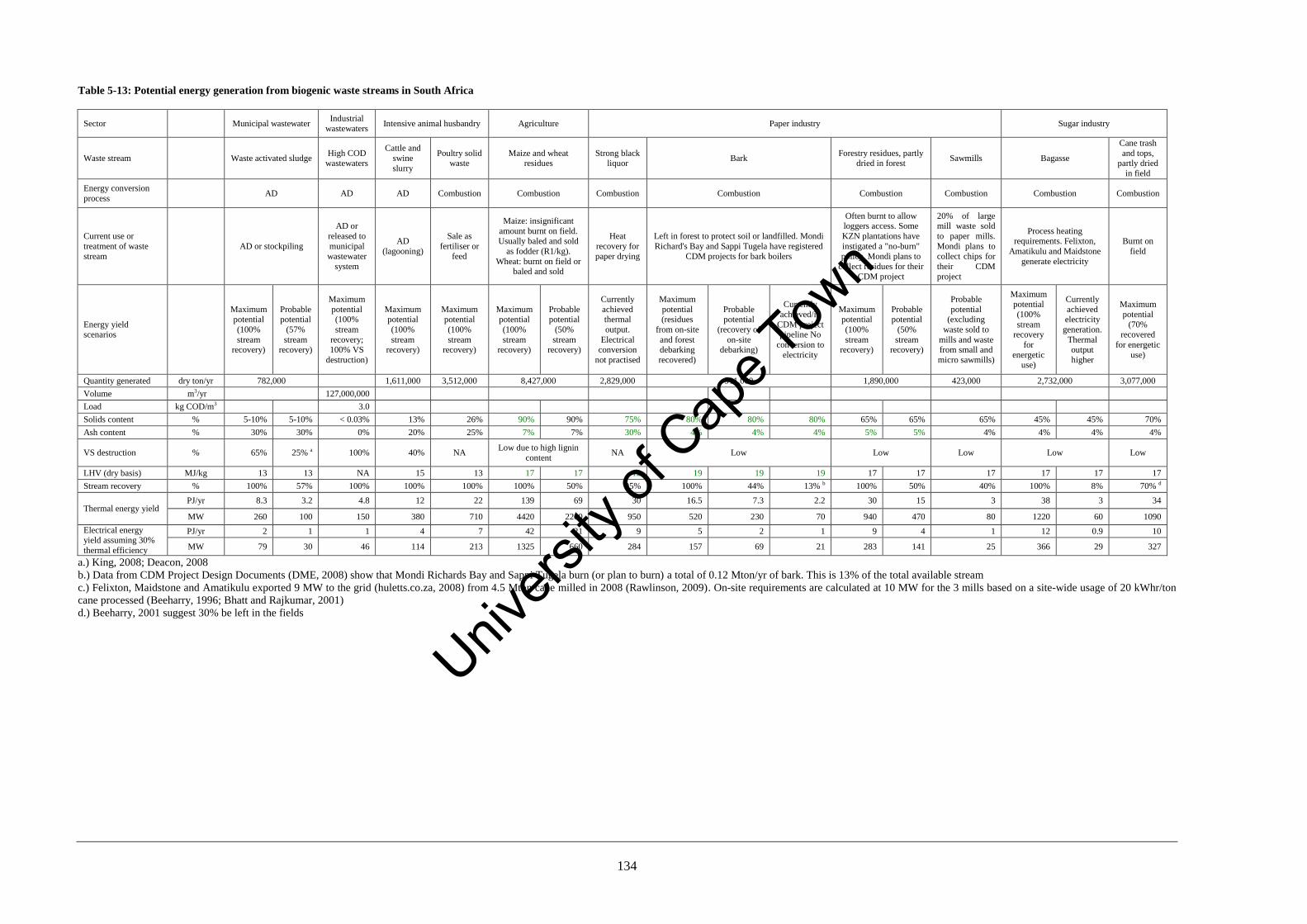
134

Table 5-13: Potential energy generation from biogenic waste streams in South Africa

Sector Municipal wastewater Industrial

wastewaters Intensive animal husbandry Agriculture Paper industry Sugar industry

Waste stream Waste activated sludge High COD

wastewaters

Cattle and

swine

slurry

Poultry solid waste

Maize and wheat residues

Strong black liquor

Bark Forestry residues, partly

dried in forest Sawmills Bagasse

Cane trash

and tops, partly dried

in field

Energy conversion

process AD AD AD Combustion Combustion Combustion Combustion Combustion Combustion Combustion Combustion

Current use or

treatment of waste

stream

AD or stockpiling

AD or

released to

municipal

wastewater

system

AD

(lagooning)

Sale as

fertiliser or

feed

Maize: insignificant

amount burnt on field. Usually baled and sold

as fodder (R1/kg).

Wheat: burnt on field or baled and sold

Heat

recovery for

paper drying

Left in forest to protect soil or landfilled. Mondi

Richard's Bay and Sappi Tugela have registered

CDM projects for bark boilers

Often burnt to allow loggers access. Some

KZN plantations have

instigated a "no-burn"

policy. Mondi plans to

collect residues for their

CDM project

20% of large mill waste sold

to paper mills.

Mondi plans to

collect chips for

their CDM

project

Process heating requirements. Felixton,

Amatikulu and Maidstone

generate electricity

Burnt on

field

Energy yield scenarios

Maximum potential

(100%

stream recovery)

Probable potential

(57%

stream recovery)

Maximum

potential (100%

stream

recovery; 100% VS

destruction)

Maximum potential

(100%

stream recovery)

Maximum potential

(100%

stream recovery)

Maximum potential

(100%

stream recovery)

Probable potential

(50%

stream recovery)

Currently

achieved thermal

output.

Electrical conversion

not practised

Maximum

potential (residues

from on-site

and forest debarking

recovered)

Probable potential

(recovery of

on-site debarking)

Currently

achieved/in

CDM project pipeline No

conversion to

electricity

Maximum potential

(100%

stream recovery)

Probable potential

(50%

stream recovery)

Probable

potential (excluding

waste sold to

mills and waste from small and

micro sawmills)

Maximum potential

(100%

stream recovery

for

energetic use)

Currently

achieved electricity

generation.

Thermal output

higher

Maximum

potential

(70% recovered

for energetic

use)

Quantity generated dry ton/yr 782,000 1,611,000 3,512,000 8,427,000 2,829,000 911,000 1,890,000 423,000 2,732,000 3,077,000

Volume m3/yr 127,000,000

Load kg COD/m3 3.0

Solids content % 5-10% 5-10% < 0.03% 13% 26% 90% 90% 75% 80% 80% 80% 65% 65% 65% 45% 45% 70%

Ash content % 30% 30% 0% 20% 25% 7% 7% 30% 4% 4% 4% 5% 5% 4% 4% 4% 4%

VS destruction % 65% 25% a 100% 40% NA Low due to high lignin

content NA Low Low Low Low Low

LHV (dry basis) MJ/kg 13 13 NA 15 13 17 17 12 19 19 19 17 17 17 17 17 17

Stream recovery % 100% 57% 100% 100% 100% 100% 50% 95% 100% 44% 13% b 100% 50% 40% 100% 8% 70% d

Thermal energy yield PJ/yr 8.3 3.2 4.8 12 22 139 69 30 16.5 7.3 2.2 30 15 3 38 3 34

MW 260 100 150 380 710 4420 2200 950 520 230 70 940 470 80 1220 60 1090

Electrical energy yield assuming 30%

thermal efficiency

PJ/yr 2 1 1 4 7 42 21 9 5 2 1 9 4 1 12 0.9 10

MW 79 30 46 114 213 1325 660 284 157 69 21 283 141 25 366 29 327

a.) King, 2008; Deacon, 2008

b.) Data from CDM Project Design Documents (DME, 2008) show that Mondi Richards Bay and Sappi Tugela burn (or plan to burn) a total of 0.12 Mton/yr of bark. This is 13% of the total available stream

c.) Felixton, Maidstone and Amatikulu exported 9 MW to the grid (huletts.co.za, 2008) from 4.5 Mton cane milled in 2008 (Rawlinson, 2009). On-site requirements are calculated at 10 MW for the 3 mills based on a site-wide usage of 20 kWhr/ton

cane processed (Beeharry, 1996; Bhatt and Rajkumar, 2001)

d.) Beeharry, 2001 suggest 30% be left in the fields

Univers

ity of

Cap

e Tow

n

135

5.4.2.2. Industrial wastewater

The total energy available from wastewater streams was calculated according to Equation 5-4

to be 4.8 PJ/yr (150 MW). This is in the same range as the value of 238 MW calculated by

Burton et al. (2007). The discrepancy between these studies arises partly from the energy

estimated as recoverable from synfuel petrochemical refineries. Burton et al. (2007) attribute

48 MW to synfuel refineries, based on the PetroSA gas-to-liquids refinery energy yield per

barrel of synfuel produced which is being achieved in their CDM project, and scaled up to

total South African synfuel production. The calculation of energy recovery from

petrochemical refineries in this work is based on an influent COD of approximately 400 mg

COD/l (Natsurv 15, 2005). This value is uncharacteristically low for an industrial wastewater

stream and is thus the possible source of error. Indeed, work on anaerobic digestion of the

Sasol coal-to-liquids refinery wastewater gives a wastewater COD of 11 000 mg COD/l (Britz

et al., 1983).

In terms of national consumption, the potential energy from wastewaters is a small

contribution, approximately 0.6% of national demand. Further, to date, the primary goal of the

industries producing the wastewaters has been to reduce COD loading to avoid municipal

fines. This reduction in COD can be achieved via aerobic and mechanical processes, hence

energy recovery from wastewater streams has been further reduced. However, the current

focus on renewable energy and on the reduction of CO2 emissions demands renewed interest

in AD. In terms of reducing COD, anaerobic digestion does hold one distinct advantage,

namely the generation of CER’s under the Kyoto Protocol Emission trading scheme. Projects

registered as CDM projects include the PetroSA biogas to electricity project and the Rosslyn

Brewery fuel switch project (coal to biogas and natural gas) (DME, 2008)

5.4.2.3. Animal husbandry

The energy recovery from animal husbandry activities is calculated to be 12 PJ/yr from

anaerobic digestion of cattle and swine slurry and 22 PJ/yr from combustion of poultry litter

as shown in Table 5-13. This gives a total of 34 PJ/yr (1090 MW); less than half of the lower

estimate of Burton et al. (2007) but much higher than William and Eberhard’s (1988) estimate

of 7.6 PJ/yr. The energy potential of animal husbandry wastes has been realised in some

instances with two piggery waste-to-biogas projects, namely the Kanhym and the Humphries

farm manure projects, awaiting approval from the CDM executive board (DME, 2008).

Univers

ity of

Cap

e Tow

n

136

5.4.2.4. Agriculture

The maximum energy (100% stream recovery) from agricultural residues is calculated as 139

PJ/yr (4420 MW). This compares well to the amount calculated in Lynd et al (2003) of 156

PJ/yr (4900 MW). A probable stream recovery of 50% gives a energy yield of 69 PJ/yr (2200

MW). This is thought to be more realistic as maize stubble is baled as sold as fodder and

wheat residues are still burnt in some areas of the Western Cape.

5.4.2.5. Forestry residues

To calculate the amount of energy recoverable from the forestry residues, it was assumed that

the residues have been allowed to dry to 35% moisture content, which is mid-range of that

suggested by Foelkel (2007). On this basis maximum stream recovery gives 30 PJ/yr and at

50% stream recovery, 15 PJ/yr. Lynd et al. (2003) give an estimate of 69 PJ/yr, however they

assume 50% of forestry residues are left in the forest which is unrealistic.

Forestry residues are in some areas burnt prior to tree felling to allow the loggers easy access

to the trees and to mitigate a fire hazard when the new trees are planted. Mondi initiated a

“no-burn” policy in the KZN coastal sands plantations to prevent soil erosion (Howard, 2008)

and they plan to collect up to 35 000 ton/yr of residues as part of their CDM project (DME,

2008).

5.4.2.6. Debarking

Three scenarios for energy recovery from debarking operations are given: 100% stream

recovery where bark is recovered from both the on-site operations and the in-forest debarking

operations, 44% recovery in which it is assumed that the on-site operations recover the bark

and the in-forest operations leave the bark as a mulch and finally the amount of bark which is

currently being used in bark boiler, viz. 13%. The energy yields from the respective scenarios

are 16.5 PJ/yr, 7.3 PJ/yr and 2.2 PJ/yr.

5.4.2.7. Pulp and paper industry

Pulp mills (non-integrated mills) are generally energy self-sufficient and able to export

electricity and steam to the paper mills; however the paper mills require large quantities of

steam to run their driers. In the States, the pulp mills supply up to 50% of the integrated mill’s

energy requirement (Jeffries, 1997). From Table 5-10 it is seen that four mills reach this

benchmark. This figure increases to six mills, when a greater than 40% renewable energy

Univers

ity of

Cap

e Tow

n

137

share is considered. The remaining three mills do not practise energy recovery and account for

the stream recovery of 93%. The energy recovered from the pulp mills is 30 PJ/yr and is in

line with previous studies, but it is noted that this is directly used in the paper mills to raise

steam for the paper driers.

5.4.2.8. Sawmills

It is assumed that only the waste from the large mills is available for energy production as the

specific mill production of the small and micro mills does not warrant the installation of a

boiler. This accounts for a stream recovery of 40%. The probable energy recovery from

sawmills is thus 3 PJ/yr. In their CDM project, Mondi Richards Bay intends to use 35 000

ton/yr realising some 0.2 PJ.yr energy production from sawmill residues (DME, 2008).

5.4.2.9. Sugar industry

Two scenarios are presented for energy recovery from bagasse: 100% stream recovery which

yields 38 PJ/yr (slightly lower than previous studies) and the currently realised energy

recovery of 2 PJ/yr (8% of total stream). The recovery of cane trash for energetic use is not

currently practised but a maximum potential yield of 34 PJ/yr exists, assuming the cane trash

is allowed to partially dry in the field as suggested by Rosillo-Calle et al. (2000).

Various studies on the sugar industry seek means of improving energy efficiency of the mills.

Reid (2006) suggests reasons as to why South African mills continue to import coal for their

thermal needs:

Increased alternative uses of bagasse (e.g. animal feed production, pulp and paper

feedstock and furfural production)

Increased addition of imbibition water to the diffuser to increase sugar extraction, but

requires increased evaporative duty downstream

The addition of pan movement water to the vacuum crystallisers to maintain control of

the growth of crystals. If the cane syrup quality is bad the amount of water added has

to increase

Not all boilers have an economiser fitted to preheat the boiler water; this represents a

9% loss in steam efficiency (Magasiner, 1987)

Reid (2006) shows that it would be more economical for the mills to add less imbibition water

(and hence achieve less sugar extraction) and make savings on the amount of coal used.

Concerns for the downstream processing of a more concentrated cane syrup solution include:

Univers

ity of

Cap

e Tow

n

138

difficulty in clarification of the syrup and fouling in the evaporator tubes due to low rising

film velocity. The study shows the drawbacks of independent optimisation of process

variables which had clearly taken place on the mill.

Mohee and Beeharry (1996) conducted an LCA to investigate the effect on cane yield if a

fraction of the bagasse was composted. It was found that if 24% of the bagasse was

composted with all the filter cake, the cane yield increased by 50%. However, whilst the mill

could still provide its steam requirements with the remaining bagasse, there was a shortfall in

electricity production. Only if the boiler efficiency and plant steam consumption was

optimised could electricity production be met (Beeharry, 1996).

Cane trash represents a large potential residue stream, however, the effect of trashing (i.e.

leaving the green leaves and tops to form a mulch) on cane yield showed a 9.3 ton cane/Ha/yr

increase compared to burning. The increase in yield is attributed to the higher soil organic

content (van Antwerpen et al., 2001). The trash yields for the various harvesting techniques

are shown in Table 5-14. Cane trashing also reduces the amount of evaporation. Thompson

(1965, 1966) (cited in van Antwerpen, 2006) found that the potential moisture conservation

from trashing was 90 mm/yr, which would have a positive effect on yield, especially in dry

years. It is recommended, to fully consider the effects of replacing fertiliser with the use of

cane trash, an LCA be conducted to calculate the displaced environmental burden.

Table 5-14: Cane residue yields for different harvesting techniques (van Antwerpen et al., 2001)

Yield of residue (ton/Ha/yr)

Treatment With fertiliser Without fertiliser

Cane burnt 0 0

Cane burnt, tops spread 3.2 2.3

Trashed (tops and leaves spread) 20 15

5.4.2.10. Comments on the use of energy crops in South Africa

The contribution of energy crops in the analysis of Lynd et al. (2003) is based on a study done

by Marrison and Larson (1996). These workers calculated an area available for energy crops

by adding up area defined as pasture and “other” by the World Resource Institute, where

“other” included uncultivated land, non-pastoral grassland, built on areas, wetlands,

wastelands, roads and deserts. They excluded deserts but considered everything else to be

available. For South Africa, the pasture and “other” excluding deserts was estimated as 104

Univers

ity of

Cap

e Tow

n

139

MHa available for energy crops. In the analysis of Lynd et al. (2003), 10% (10 MHa) is

assumed to be utilised for energy crops. The figure of 10 MHa does not contain sufficient

local knowledge of SA soil type and current land usage be regarded as an accurate estimate

which can be set aside for energy crop production. The estimate is essentially based on

amount of marginal land. In a submission to the Department of Environment and Tourism,

Laker (2005) considers some factors influencing sustainable soil practice.

South Africa has generally poor quality unstable soils and low rainfall. Only 13% of

the land (14 MHa) is considered arable and only 3% is considered to be high potential

land

Considering that 0.4 Ha of land are required to feed one person, South Africa has

already exceeded the optimal carrying capacity of its soil

Only 35% of land is suitable for dryland farming. There is limited irrigation potential

in South Africa due to either lack of water and unsuitable soil types

Whilst soil ecosystems in SA tend to be robust (i.e., they do not degrade easily), they

shown little resilience (i.e. they cannot recover easily once degraded) and hence policy

should focus on preventing extensive soil degradation

Substantial degradation (up to 25%) of South African soils has been reported. Practices which

could intensify this trend (such as planting crops in marginal land) should be approached with

care.

The issue of land availability much be followed by the considering what to plant. Jatropha

has been much vaunted as a high-yield, drought tolerant species. The oils of Jatropha could

be used in biodiesel production, but equally well, the entire plant could be used in combustion

and gasification systems. Due to limited data on its water requirements, the Department of

Water and Forestry specified that its large scale cultivation be regarded as a Stream Flow

Reduction Activity (SFRA) (Holl et al., 2007). This classification essentially prohibits its

large scale planting. The Water Research Commission funded a study into the hydrological

effects of Jatropha plantations, with the specific aim of determining whether the planting

really should be regarded as a SFRA. The study brought a couple of important points to light

(Holl et al., 2007):

Areas of low and variable rainfall, and areas susceptible to anything more than mild

frost, should be avoided (i.e. Jatropha should not be planted in marginal areas). The

former is illustrated through Figure 5-5.

Univers

ity of

Cap

e Tow

n

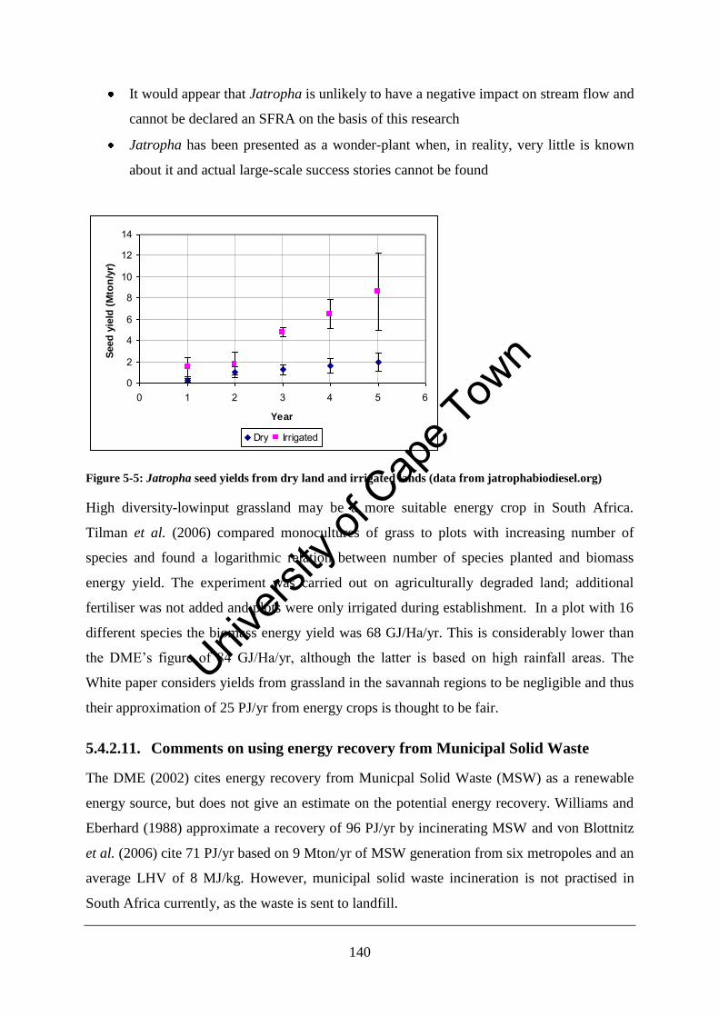
140

It would appear that Jatropha is unlikely to have a negative impact on stream flow and

cannot be declared an SFRA on the basis of this research

Jatropha has been presented as a wonder-plant when, in reality, very little is known

about it and actual large-scale success stories cannot be found

0

2

4

6

8

10

12

14

0 1 2 3 4 5 6

Year

Seed

yie

ld (

Mto

n/y

r)

Dry Irrigated

Figure 5-5: Jatropha seed yields from dry land and irrigated lands (data from jatrophabiodiesel.org)

High diversity-lowinput grassland may be a more suitable energy crop in South Africa.

Tilman et al. (2006) compared monocultures of grass to plots with increasing number of

species and found a logarithmic relation between number of species planted and biomass

energy yield. The experiment was carried out on agriculturally degraded land; additional

fertiliser was not added and plots were only irrigated during establishment. In a plot with 16

different species the biomass energy yield was 68 GJ/Ha/yr. This is considerably lower than

the DME’s figure of 84 GJ/Ha/yr, although the latter is based on high rainfall areas. The

White paper considers yields from grassland in the savannah regions to be negligible and thus

their approximation of 25 PJ/yr from energy crops is thought to be fair.

5.4.2.11. Comments on using energy recovery from Municipal Solid Waste

The DME (2002) cites energy recovery from Municpal Solid Waste (MSW) as a renewable

energy source, but does not give an estimate on the potential energy recovery. Williams and

Eberhard (1988) approximate a recovery of 96 PJ/yr by incinerating MSW and von Blottnitz

et al. (2006) cite 71 PJ/yr based on 9 Mton/yr of MSW generation from six metropoles and an

average LHV of 8 MJ/kg. However, municipal solid waste incineration is not practised in

South Africa currently, as the waste is sent to landfill.

Univers

ity of

Cap

e Tow

n

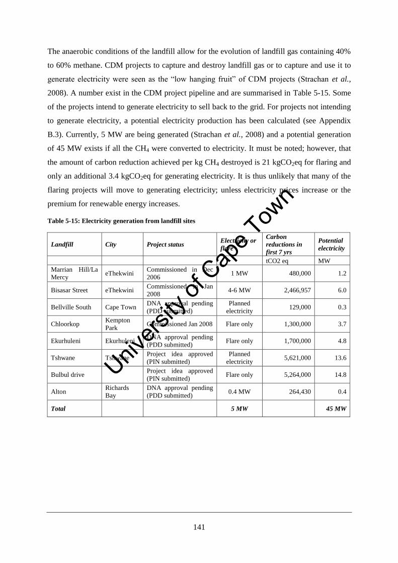
141

The anaerobic conditions of the landfill allow for the evolution of landfill gas containing 40%

to 60% methane. CDM projects to capture and destroy landfill gas or to capture and use it to

generate electricity were seen as the “low hanging fruit” of CDM projects (Strachan et al.,

2008). A number exist in the CDM project pipeline and are summarised in Table 5-15. Some

of the projects intend to generate electricity to sell back to the grid. For projects not intending

to generate electricity, a potential electricity production has been calculated (see Appendix

B.3). Currently, 5 MW are being generated (Strachan et al., 2008) and a potential generation

of 45 MW exists if all the CH4 were converted to electricity. It must be noted; however, that

the amount of carbon reduction achieved per kg CH4 destroyed is 21 kgCO2eq for flaring and

only an additional 3.4 kgCO2eq for generating electricity. It is thus unlikely that many of the

flaring projects will move to generating electricity; unless electricity prices increase or the

premium for renewable energy increases.

Table 5-15: Electricity generation from landfill sites

Landfill City Project status Electricity or

flare

Carbon

reductions in

first 7 yrs

Potential

electricity

tCO2 eq MW

Marrian Hill/La

Mercy eThekwini

Commissioned in Dec

2006 1 MW 480,000 1.2

Bisasar Street eThekwini Commissioned in Jan

2008 4-6 MW 2,466,957 6.0

Bellville South Cape Town DNA approval pending

(PDD submitted)

Planned

electricity 129,000 0.3

Chloorkop Kempton

Park Commissioned Jan 2008 Flare only 1,300,000 3.7

Ekurhuleni Ekurhuleni DNA approval pending

(PDD submitted) Flare only 1,700,000 4.8

Tshwane Tshwane Project idea approved

(PIN submitted)

Planned

electricity 5,621,000 13.6

Bulbul drive Project idea approved

(PIN submitted) Flare only 5,264,000 14.8

Alton Richards

Bay

DNA approval pending

(PDD submitted) 0.4 MW 264,430 0.4

Total 5 MW 45 MW

Univers

ity of

Cap

e Tow

n

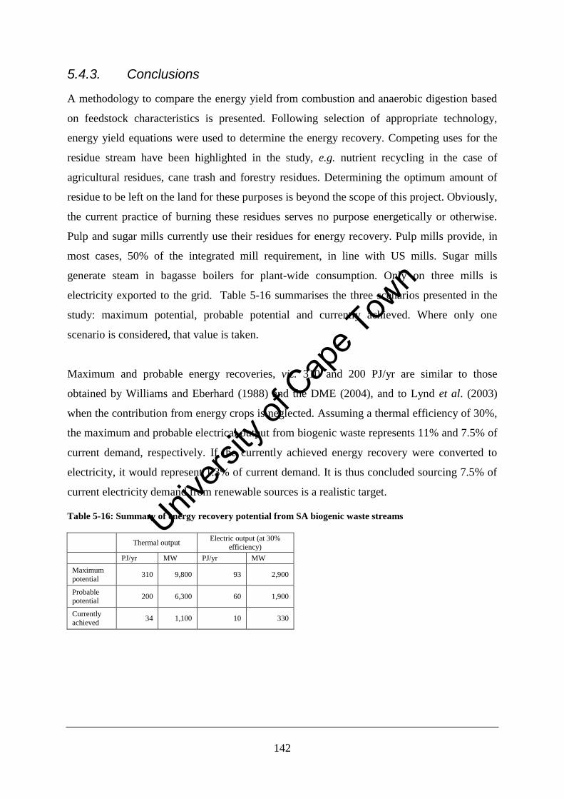
142

5.4.3. Conclusions

A methodology to compare the energy yield from combustion and anaerobic digestion based

on feedstock characteristics is presented. Following selection of appropriate technology,

energy yield equations were used to determine the energy recovery. Competing uses for the

residue stream have been highlighted in the study, e.g. nutrient recycling in the case of

agricultural residues, cane trash and forestry residues. Determining the optimum amount of

residue to be left on the land for these purposes is beyond the scope of this project. Obviously,

the current practice of burning these residues serves no purpose energetically or otherwise.

Pulp and sugar mills currently use their residues for energy recovery. Pulp mills provide, in

most cases, 50% of the integrated mill requirement, in line with US mills. Sugar mills

generate steam in bagasse boilers for plant-wide consumption. Only on three mills is

electricity exported to the grid. Table 5-16 summarises the three scenarios presented in the

study: maximum potential, probable potential and currently achieved. Where only one

scenario is considered, that value is taken.

Maximum and probable energy recoveries, viz. 310 and 200 PJ/yr are similar to those

obtained by Williams and Eberhard (1988) and the DME (2004), and to Lynd et al. (2003)

when the contribution from energy crops is neglected. Assuming a thermal efficiency of 30%,

the maximum and probable electrical output from biogenic waste represents 11% and 7.5% of

current demand, respectively. If the currently achieved energy recovery were converted to

electricity, it would represent 1.3% of current demand. It is thus concluded sourcing 7.5% of

current electricity demand from renewable sources is a realistic target.

Table 5-16: Summary of energy recovery potential from SA biogenic waste streams

Thermal output Electric output (at 30%

efficiency)

PJ/yr MW PJ/yr MW

Maximum

potential 310 9,800 93 2,900

Probable potential

200 6,300 60 1,900

Currently

achieved 34 1,100 10 330

Univers

ity of

Cap

e Tow

n

143

Chapter 6 Conclusions

6.1. Technologies suitable for heat and electricity

generation from biogenic waste fuels

South Africa currently generates ~95% of its electricity from fossil and nuclear sources and

the remainder from large scale hydropower. The White Paper of the DME in South Africa on

renewable energy published in 2003 seeks to increase the share of renewable energy to 4% of

the projected 2013 demand. Electricity from biogenic waste sources is identified as

contributing to renewable energy supply. Technologies suitable for processing biogenic waste

sources to process heat and electricity include combustion, gasification and anaerobic

digestion.

Combustion of biogenic waste sources, particularly woody biomass and sewerage sludge, is a

well established technology. The process is relatively simple but low thermal efficiencies of

15 to 20% are found in small biomass boilers. This may increase to 30% for larger boilers or

to 40% for co-firing in coal power plants. The advantages of fluidised bed combustors for

processing waste biomass fuels are highlighted. In particular, uniform bed temperatures are

easily achieved due to intimate mixing of the bed material and the large thermal mass of the

bed material which maintains temperature and promotes complete carbon conversion.

Gasification offers higher efficiencies, but only at higher capacity (100 MW achieves 45% in

an IGCC system) and greater system complexity. Indeed, successful installation of large scale

biomass gasifiers (greater than 100 MW) is yet to be realised. Technical barriers which exist

include difficulties in tar removal from the fuel gas and agglomeration of the bed in fluidised

bed gasifiers. Biogas production for energy generation has come to the fore recently although

anaerobic digesters are still primarily installed to treat wastewater. Thus, control philosophies

may not be set up to optimise continuous biogas production. Nonetheless, the technology is

well-established in South Africa, particularly as domestic wastewater treatment plants, in the

treatment of synfuel petrochemical waste streams and at the breweries. For the treatment of

recalcitrant substances, such as lignocellulosic materials and microbial sludges, pretreatments

are available to change the structure of the biomass and make it more amenable to digestion.

Of these three technologies reviewed, combustion and anaerobic digestion stand out as

Univers

ity of

Cap

e Tow

n

144

immediately implementable options for South Africa due to the relative simplicity of the

process and the operational experience which exists in the country.

6.2. Comparison of combustion and anaerobic digestion

for processing biogenic waste – a case study

A comparative case study of three wastewater treatment plants, each employing different

technologies to recover energy from waste sewerage sludge was carried out. The technologies

employed were incineration (combustion), anaerobic digestion and enhanced anaerobic

digestion (i.e. anaerobic digestion preceded by a pretreatment, in this case thermal

hydrolysis). Field notes on the operation of these plants were presented to expose the South

Africa audience to the energy generation potential of wastewater treatment plants and

associated difficulties. Energy yield equations for combustion and anaerobic digestion were

used to predict the relative gross electricity output and this was compared to plant data.

Anaerobic digestion with thermal hydrolysis pretreatment gave the highest energy yield. This

was due to the anaerobic digester process achieving a volatile solids destruction of 65% as

opposed to 45% as a result of the feed pretreatment. Combustion of a sludge containing 20%

dry solids and anaerobic digestion of sludge to achieve 45% volatile solids destruction

resulted in comparable energy recovery. However, the plant data showed that combustion was

the inferior option. This was attributed to the sensitivity of gross energy recovery to dry solids

content, i.e. any deviation from 20% dry solids content would have a significant impact on

energy recovery. For all technologies, the process heat requirements were supplied by the

high grade heat generation. Combustion and anaerobic digestion generated up to five times

and double the high grade sensible heat required respectively. This brings into question

possible improvements in heat use, e.g. drying the sludge prior to combustion.

6.3. Biogenic waste feedstock characteristics and their

effect on energy recovery

The effect of characteristics specific to biogenic waste fuels on their processing was explored.

In the case of anaerobic digestion, achieving the maximum biogas yield is prevented by the

presence of recalcitrant compounds e.g. cellulose, hemicellulose, lignin and microbical cells.

The energy requirements of high temperature, high pressure (HTHP) pretreatments as a

function of temperature and dry solids content were measured against the energy yield from

anaerobic digestion. This showed the process conditions necessary for the overall process to

Univers

ity of

Cap

e Tow

n

145

be energy positive. The energy requirements of high pressure homogenisation were seen to be

one order of magnitude greater than the energy yield from anaerobic digestion at operating

pressures cited in literature (30 to 60 MPa). HTHP pretreatments are recommended as the

analysis showed a positive nett energy yield at dry solids contents greater than 20% and at

volatile solids destruction of greater than 50%, assuming no heat recovery and a thermal

efficency of 40%. Heat recovery from the heated pretreated stream reduces the energy

requirements and hence makes the pretreatments viable at lower volatile solids destruction.

The high volatile content of biogenic waste fuels negatively affects combustion efficiency in a

bubbling fluidised bed through increasing the tendency for overbed burning. Higher bed

temperatures can be used to promote inbed combustion. This is desirable as overbed burning

results in unstable operation, viz. runaway freeboard temperatures and difficulties in

maintaining the bed temperature. The feed location also impacts the combustion efficiency,

with under bed feeding promoting a longer residence time of the fuel in the bed. In the

experimental study, wood chips and dried sewerage sludge were fed to a bubbling fluidised

bed combustor at different temperatures and from different feed locations. No effect of initial

bed temperature on combustion efficiency for woodchip was seen. For sewerage sludge, a

step change in combustion efficiency was seen between 715°C and 750°C, indicating a

change from inbed combustion to overbed burning or the escape of unburnt volatiles and tars.

When feeding woodchip overbed, the combustion efficiency dropped dramatically, from 90%

to ~65%. It is proposed this was due to higher amount of unburnt volatiles and tar passing

through the system unburnt. Notably, this study showed that the contribution to loss in

combustion efficiency from overbed burning was small (less than 10%). While the absolute

contribution of overbed burning to total energy release is small, freeboard temperature

increases of up to 50°C were seen. These two phenomena are reconciled by the relatively

small thermal mass of air (compared to the thermal mass of the bed) passing through the

freeboard.

6.4. Energy from biogenic waste in South Africa

A methodology is presented to select the technology which gives the highest energy yield

based on intrinsic feedstock characteristics. The first tool delineates regions of feasible and

infeasible operation for combustion of biogenic feedstocks based on ash content, dry solids

content and heating value. The second tool allows comparison of the specific energy output

Univers

ity of

Cap

e Tow

n

146

from combustion and anaerobic digestion based on dry solids content, heating value, volatile

solids destruction and ash content.

Following selection of appropriate technology, energy yield models were used to determine

the energy recovery. The quantity of residue available was calculated for each waste stream.

Competing uses for the residue stream have been highlighted in the study, e.g. nutrient

recycling in the case of agricultural residues, cane trash and forestry residues. Three scenarios

for energy recovery were presented: maximum, probable and current. The maximum and

probable energy recoveries calculated in this work, viz. 310 and 200 PJ/yr and are similar to

those obtained by Williams and Eberhard (1988) and the DME (2004), and to Lynd et al.

(2003) when the contribution from energy crops is neglected. Assuming a thermal efficiency

of 30%, the electrical output from the maximum and probable scenarios from biogenic waste

represent 11% and 7.5% of current demand, respectively. The thermal output of the current

scenario is 34 PJ/yr (1100 MW). It is thus concluded that sourcing 7.5% of current electricity

demand from renewable sources is a realistic target.

Finally, the incremental improvements in the whiteness of our sugar, the fineness of our paper

and other perceived product qualities are at the energetic expense of the upstream processes of

our industries. The solution may lie not in continuously improved energy efficiency, but in

reduced consumer demand for “perfection”.

Univers

ity of

Cap

e Tow

n

147

Reference list

1. Abrams, LJ, 1996, “Water policy development in South Africa”, presented at the

Cranfield International Water Policy Conference, Cranfield University, Bedford UK,

September 1996, accessed from www.africanwater.org, October 2008

2. ACEEE, 2007, abstract from American Council for an Energy Efficient Economy,

accessed from www.aceee.org, October 2008

3. afdc.energy.gov, 2008, “Alternative fuels and advanced vehicles data centre”, Energy

Efficiency and Renewable Energy, US DOE, accessed from www.afdc.energy.gov/afdc,

December 2008

4. Anand H, Balasundaram B, Pandit AB, Harrison STL, 2007, “The effect of chemical

pretreatment combined with mechanical disruption on the extent of disruption and

release of intracellular protein from E. coli”, Biochemical Engineering Journal, Vol. 35,

pp. 166–173

5. Anthony EJ, 1995, “Fluidised bed combustion of alternative solid fuels: status,

successes and problems of the technology”, Progress in Energy and Combustion

Science, Vol. 21, pp. 239-268.

6. Aracruz Annual and Sustainability report, 2006, accessed from

http://www.aracruz.com/minisites/ra2006/en/home/default.htm

7. aracruz.com, 2007, “Generation and consumption of electrical energy and fuels – 2007”,

accessed from http://www.aracruz.com/minisites/ra2007/, November 2008

8. Baikow VE, 1982, “Sugar series Volume 2: Manufacturing and Refining of Raw Sugar

Cane”, 2nd

completely revised edition, Elsevier, 1982, Amsterdam

9. Bailey JE and Ollis DF, 1986, “Biochemical Engineering Fundamentals”, 2nd

edition,

McGraw-Hill International Editions, Singapore

10. Bain RL, Overend RP, Craig KR, 1998, “Biomass-fired power generation”, Fuel

Processing Technology, Vol 54, pp. 1-16

11. Baker EG, Mudge LK, Brown MD, 1987, “Steam Gasification of Biomass with Nickel

Secondary Catalysts”, Industrial and Engineering Chemical Research, Vol. 26, 1335 –

1339.

12. Bane T, 2000, “Sludge disposal strategies”, presented at Royal Society of Chemistry

sludge treatment seminar, accessed from www.solidstechnology.com, November 2008

Univers

ity of

Cap

e Tow

n

http://www.africanwater.org/

http://www.aceee.org/

http://www.afdc.energy.gov/afdc

http://www.aracruz.com/minisites/ra2006/en/home/default.htm

http://www.aracruz.com/minisites/ra2007/

http://www.solidstechnology.com/

148

13. Barber WP, Stuckey DC, 1999, “The use of the Anaerobic Baffled Reactor (ABR) for

wastewater treatment: a review”, Water Research, Vol. 33, pp. 1559-1578

14. Barsanti L and Gaultieri P, 2006, “Algae: Anatomy, Biochemistry and Biotechnology”,

CRC Taylor and Francis Group, USA

15. Beeharry RP, 1996, “Extended sugarcane biomass utilisation for exported electricity

production in Mauritius”, Biomass and Bioenergy, Vol. 11, pp. 441-449

16. Beeharry RP, 2001, “Strategies for augmenting sugarcane biomass availability for

power production in Mauritius”, Biomass and Bioenergy, Vol. 20, pp. 421-429

17. Bhatt MS and Rajkumar N, 2001, “Mapping of combined heat and power systems in

cane sugar industry, Applied Thermal Engineering, Vol. 21, pp. 1707 - 1719

18. Biljetina R, 1987, “Commercialisation and economics” in Chynoweth DP and Isaacson

R (eds) Anaerobic Digestion of Biomass, Elsevier Applied Science Publisher, England.

19. Boone D, Mah R, 1987, “Transitional bacteria” in Chynoweth DP and Isaacson R (eds)

Anaerobic Digestion of Biomass, Elsevier Applied Science Publisher, England

20. Botnia Environmental Balance Sheet, 2006, accessed from www.botnia.com/en,

November 2008

21. Boyd RJA, Molema J, Deacon SL, van Niekerk AM, 2008, “Advances in sludge

treatment and stabilisation at Johannesburg’s wastewater treatment works”, presented at

the WISA Biennial 2008 Conference, Sun City, South Africa

22. Brage C, Yu Q, Sjostrom K, 1996, “Characteristics of evolution of tar from wood

pyrolysis in a fixed-bed reactor”, Fuel, Vol. 75, pp. 213-219

23. Bridgewater AV, 2003, “Renewable fuels and chemicals by thermal processing of

biomass”, Chemical Engineering Journal, Vol. 91, pp. 87-102

24. Bridgewater, AV, 1995, “The technical and economic feasibility of biomass gasification

for power generation”, Fuel, Vol. 74, pp. 631-653

25. Britz TJ, Meyer LC, Botes PJ, 1983, “Anaerobic digestion of a petrochemical effluent”,

Biotechnology Letter, Vol 5, pp. 113-118

26. Burton SB, Cohen S, Harrison, STL, Pather-Elias S, Stafford W, van Hille R, von

Blottnitz H, 2007, “Energy from wastewater – a feasibility study, Technical report”,

Water Research Commission Report, Project K5/1732

27. Chamberlain D, Essop H, Hougaard C, Malherbe S, Walker R, 2005a, “Economics of

the forestry, timber, pulp and paper industry in South Africa, Part II: Market analysis”,

Univers

ity of

Cap

e Tow

n

http://www.botnia.com/en

149

Genesis market report 29 June 2005, accessed from www.forestry.co.za, November,

2008

28. Chamberlain D, Essop H, Hougaard C, Malherbe S, Walker R, 2005b, “Economics of

the forestry, timber, pulp and paper industry in South Africa, Part III: Technical notes

and appendices”, Genesis market report 29 June 2005, accessed from

www.forestry.co.za, November 2008

29. Chambers AK, Potter I, 2002, “Gas utilisisation from Sewerage Sludge”, Technical

Brochure no. 5, published by Carbon and Energy Management, Alberta Research

Council, accessed from www.aidis.org.br, January 2009

30. Chirone R, Salatino P, Scala F, Solimene R, Urciuolo M, 2008, “Fluidized bed

combustion of pelletized biomass and waste derived fuels”, Combustion and Flame,

Vol. 155, pp. 21-36

31. Crawford RL, 1981, “Lignin Biodegradation and Transformation”, John Wiley and

Sons, Canada.

32. Cullis IF, Saddler JN, Mansfield SD, 2004, “Effect of initial moisture content and chip

size on the bioconversion efficiency of softwood lignocellulosics”, Biotechnology and

Bioengineering, Vol. 85, pp. 413 – 421

33. Davidson JF, Harrison D, Darton RC, LaNauze RD, 1977, “The two-phase theory of

fluidisation and its application to chemical reactors”, in Lapidus L and Amundson NR

Chemical Reactor Theory: A Review, Prentice Hall Inc, New Jersey

34. Davidson JF, Harrison D, Darton RC, LaNauze RD, 1977, “The two-phase theory of

fluidisation and its application to chemical reactors”, in Lapidus L and Amundson NR

Chemical Reactor Theory: A Review, Prentice Hall Inc, New Jersey

35. Davidson JF, Harrison D, Darton RC, LaNauze RD, 1977, “Two-phase theory of

fluidisation and its application to chemical reactors”, in Chemical Reactor Theory: A

Review by Lapidus L and Amundson NR, Prentice Hall Inc, New Jersey

36. Deacon S, 2008, Best Practices Manager, Johannesburg Water, Personal

communication, October 2008

37. Demirbas A, 2004, “Current technologies for the thermo-conversion of biomass into

fuels and chemical”, Energy Sources, Vol. 26, pp. 715 – 730

38. Dennis JS, Hayhurst AN, Mackley, IG, 1982, “The ignition and combustion of propane

air mixtures in a fluidised bed”, International Symposium of Combustion, Combustion

Institute, Haifa, Israel

Univers

ity of

Cap

e Tow

n

http://www.forestry.co.za/


http://www.aidis.org.br/

150

39. Dildar M, 2008, Senior Engineer, eThekwini Water and Sanitation Unit, Personal


40. DME (Department of Minerals and Energy), 2005, Energy efficiency strategy for the

Republic of South Africa, accessed from www.dme.gov.za, October 2008

41. DME, 2003, White paper on the renewable energy policy of the Republic of South

Africa, accessed from www.dme.gov.za, October 2008

42. DME, 2008, “South Africa’s CDM project portfolio”, accessed from www.dme.gov.za,

November 2008.

43. dme.gov.za, 2008, “Electricity”, accessed from www.dme.gov.za , November 2008

44. dpi.qld.gov.au/environment, 2009, “Feedlot waste management series: Manure

production data”, Department of Primary Fisheries and Industry, Queensland

Government, accessed from www2.dpi.qld.gov.au/environment/5166.html, January

2009

45. Draft White Paper on Water Services, 2002, Department of Water Affairs and Forestry,

accessed from www.dwaf.gov.za, October 2008

46. ec.europa.eu, 2001, “Researching the sludge directive”, conference report, EC

Environment DG and UK Water Industry Research, accessed from

www.ec.europa.eu/environment, October 2008

47. ECN 2008, “Phyllis, database for biomass and waste”, published by the Energy

Research Centre of the Netherlands, accessed from http://www.ecn.nl/phyllis, January

2009

48. Edwards M, 2008, Retired director of Forestry South Africa (FSA), Personal


49. EEA, 2008, Final energy consumption by sector page, accessed from

www.dataservice.eea.europa.eu , November 2008

50. EERE, 2008, “Biomass Energy Data Book”, Energy Efficiency and Renewable Energy

(EERE), US Department of Energy, accessed from www.cta.ornl.gov/bedb/biofuels,

November 2008

51. Eleftheriades C, 2008, Carbon and Environmental Options, Personal communication,

November 2008

52. Energy Efficiency and Renewable Energy (EERE), 2008, Biomass feedstock database,

accessed from www.eere.energy.gov , November 2008

Univers

ity of

Cap

e Tow

n

http://www.dme.org.za/

http://www.dme.org.za/

http://www.dme.gov.za/

http://www.dme.gov.za/

http://www2.dpi.qld.gov.au/environment/5166.html

http://www.dwaf.gov.za/

http://www.ec.europa.eu/environment

http://www.ecn.nl/phyllis

http://www.dataservice.eea.europa.eu/

http://www.cta.ornl.gov/bedb/biofuels

http://www.eere.energy.gov/

151

53. Engler CR, 1985, “Disruption of Microbial Cell” in Moo-Young M (ed) Comprehensive

Biotechnology Vol. 2, Pergamon Press

54. EPA, 2008, “Sewerage sludge incineration”, US Environmental Protection Agency

Technology Transfer Network – Clearinghouse for inventories and emissions factors,

accessed from http://www.epa.gov , January 2009

55. Eskom Annual report, 2006, accessed from www.eskom.co.za, December 2008

56. EurActiv.com, 2008, “MEPs seek reduced biofuel commitments”, press release

published on 28 May 2008, accessed from www.euractiv.com, November 2008

57. European Parliament press release, 2008, “More sustainable energy in road transport

targets” published on 11 Spetember 2008, accessed from www.europarl.europa.eu,

November 2008

58. Fannin KF, Biljetina R, 1987, “Reactor designs” in Chynoweth DP and Isaacson R (eds)

Anaerobic Digestion of Biomass, Elsevier Applied Science Publisher, England.

59. Fargione J, Hill J, Tilman D, Polasky S, Hawthorne P, 2008, “Land clearing and the

biofuel carbon debt”, Science, Vol. 319, pp. 1235 – 1238

60. Flickinger MC, Drew SW (eds), 1999, “Encyclopedia of Bioprocess Technology:

Fermentation, Biocatalysis and Bioseperation”, Vol 1, John Wiley and Sons, New York,

pp.137-170

61. Foelkel C, 2007, “Eco-efficient management of the woody forest residues from the

eucalyptus plantation forestry”, online book accessed from www.eucalyptus.com.br,

November 2008

62. Forestry Industry Facts, 2005, published by Forestry South Africa (FSA), accessed from

www.forestry.co.za, November 2008

63. Fountain P, 2008, Senior Consultant, Thames Water, Personal communication,

February, 2008

64. Fryda LE, Panopoulas KD, Kakaras E, 2007, “Agglomeration in fluidised bed

gasification of biomass”, Powder Technology, Vol 179, pp. 108-121

65. Fryda LE, Panopoulos KD, Kakaras E, 2007, “Agglomeration in fluidised bed

gasification of biomass”, Powder Technology, Vol. 179, pp. 108 – 121

66. genesisqa.com, 2008, “Guidelines for the application of sewerage sludge to land”,

accessed from www.genesisqa.com , November 2008

67. Harrison, STLH, 1991, “Bacterial cell disruption: a key unit operation in the recovery of

intracellular products”, Biotechnology Advances, Vol 9, pp. 217-245

Univers

ity of

Cap

e Tow

n

http://www.epa.gov/

http://www.eskom.co.za/

http://www.euractiv.com/

http://www.europarl.europa.eu/

http://www.eucalyptus.com.br/


http://www.genesisqa.com/

152

68. Hayhurst AN, Parmar MS, 1998, “Does solid carbon burn in oxygen to give the gaseous

intermediate CO or produce CO2 directly? Some experiments in a hot bed of sand

fluidized by air”, Chemical Engineering Science. Vol. 53, pp. 427-438

69. Helm R, 2000, “Lignin”, Lecture notes on Wood chemistry, products and processes

(WOOD 3434), Virginia Polytechnic Institute and State University, accessed from

www.woodscience.vt.edu, August 2008

70. Hesketh RP and Davidson JF, 1991, “The effect of volatiles on the combustion of char

in a fluidised bed” Chemical Engineering Science, Vol. 46, No. 12, pp.3101-3113

71. Hoffman P, 2008, Utilities Manager Newlands Brewery, SABMiller, Personal


72. Holl MA, Gush, MB, Hallowes J, Versfeld DB, 2007, “Jatropha curcas in South Africa:

an assessment of its water use and bio-physical potential”, Water Research Commission

report no. 1497/1/07

73. Howard M, 2008, Consultant, Fractal Forests, Personal Communication, December

2008

74. IEA, 2004, “Biofuels for transport – An International Perspective”, International Energy

Agency (IEA), accessed from www.iea.org, November 2008

75. IFPRI, 2007, Food policy report entitled “The world food situation: new driving forces

and required action” by Joachim von Braun, accessed from www.ifpri.org, November

2008

76. IFPRI, 2008b, testimony to US Senate, “Biofuels, international food prices and the

poor”, by Joachim von Braun, accessed from www.ifpri.org, November 2008

77. International Food Price Research Institute (IFPRI), 2008a, presentation entitled “Food

prices, biofuels and climate change”, accessed from www.ifpri.org, November 2008

78. Jeffries T, 1997, “Kraft pulping – Energy Consumption and Production”, lectures notes

accessed from http://calvin.biotech.wisc.edu, January 2009

79. Jenkins BM, Baxter LL, Miles Jr. TR, Miles TR, 1998, “Combustion properties of

biomass”, Fuel Processing Technology, Vol. 54, pp.17–46

80. Kelly H G, 2006, “Emerging processes in biosolids treatment, 2005”, Journal of

Environmental Engineering and Science, Vol. 5, pp. 175 – 186

81. Kerr I, 2008, Senior Research Fellow, Paper Manufacturers Association of South Africa

(PAMSA), Personal communication, October 2008

Univers

ity of

Cap

e Tow

n

http://www.woodscience.vt.edu/

http://www.iea.org/

http://www.ifpri.org/



http://calvin.biotech.wisc.edu/

153

82. Kiel JHA (ed), 2004, “Primary measures to reduce tar formation in fluidised bed

biomass gasifiers”, Final report SDE project P1999-012, ECN

83. Kim J, Park C, Kim T-H, Lee M, 2003, Effects of Various Pretreatments for Enhanced

Anaerobic Digestion with Waste Activated Sludge”, Journal of Bioscience and

Bioengineering, Vol. 95, pp. 271 – 275

84. King P, 2008, Cape Town Water and Sanitation Services, Personal Communication,

September 2008

85. Klimantos P, Koukouzas N, Katsiadakis A, Kakaras E, 2008, “Air-blown biomass

gasification combined cycles (BGCC): System analysis and economic assessment”,

Energy, in press, doi:10.1016/j.energy.2008.04.009

86. Koornneef J, Junginger M and Faaij A, 2007, “Development of fluidized bed

combustion - An overview of trends, performance and cost”, Progress in Energy and

Combustion Science, Vol 33, pp. 19 – 55.

87. La Nauze RD, Duffy GJ, 1985, “Coal rejects – a wasted resource?”, Environmental

Geochemistry and Health, Vol 7, pp. 69 – 79.

88. Liebenberg AJ, 2008, Senior Researcher, Agricultural Research Council, Personal

Communication, September 2008

89. Lynd LR, von Blottnitz H, de Boer J, Tate B, Pretorius IS, Rumbold K, van Zyl WH,

2003, “Plant Biomass Conversion to Fuels and Commodity Chemicals in South Africa:

A Third Chapter?”, South African Journal of Science, Vol. 99, pp. 499-507

90. Magasiner N, 1987, “The effect of fuel moisture content on the performance of a typical

bagasse fired watertube boiler”, Proceedings of the South African Sugar Technologists’

Association, Vol. 60, pp. 86 – 89

91. Magasiner N, Van Alphen C, Inkson MB, Misplon BJ, 2001, Characterising fuels for

biomass-coal co-fired generation, Proceedings of the South African Sugar Association,

Vol. 75, pp. 282 – 291

92. Marrison CI, Larson ED, 1996, “A preliminary analysis of the biomass energy

production potential in Africa in 2025 considering projected land needs for food

production”, Biomass and Bioenergy, Vol. 10, pp. 337-351

93. McCabe W L, Smith J C and Harriott P, 2005, “Unit operations of Chemial

Engineering”, 7th

edition, International edition, McGraw-Hill, Singapore

94. McKendry P, 2000a, “Energy from biomass (part 1): overview of biomass”, Bioresource

Technology Vol. 83, pp. 37–46

Univers

ity of

Cap

e Tow

n

154

95. McKendry P, 2000b, “Energy production from biomass (part 2): conversion

technologies”, Bioresource Technology, Vol. 83, pp.47–54

96. McKendry P, 2002c, “Energy production from biomass (part 3): gasification

technologies”, Bioresource Technology, Vol. 83 pp.55–63

97. Middelberg APJ, 1995, “Process scale disruption of microorganisms”, Biotechnology

Advances, Vol. 13, pp. 491 – 551

98. Milne TA, Evans RJ, 1998, “Biomass Gasifier “Tars”: Their Nature, Formation, and

Conversion”, prepared for National Renewable Energy Laboratory, report reference:

NREL/TP-570-25357

99. Mohee R and Beeharry RP, 1999, “Life cycle analysis of compost incorporated

sugarcane bioenergy systems in Mauritius”, Biomass and Bioenergy, Vol. 17, pp. 73-83

100. Mosier N, Wyman C, Dale B, Elander R, Lee YY, Holtzapple M, Ladisch M, 2005,

“Features of promising technologies for pretreatment of lignocellulosic biomass”,

Bioresource Technology, Vol. 96, pp. 673–686

101. Nah, IW, Kang YW, Hwang K-Y, Woong KS, 2000, “Mechanical Pretreatment of

Waste Activated Sludge for Anaerobic Digestion Process”, Water Research, Vol. 34, pp.

2362-2368

102. Narvaez I, Orio A, Aznar MP, Corella J, 1996, “Biomass Gasification with Air in an

Atmospheric Bubbling Fluidized Bed. Effect of Six Operational Variables on the

Quality of the Produced Raw Gas”, Industry, Engineering and Chemistry Research, Vol.

25. pp. 2110 – 2120.

103. National Business Initiative (NBI), 2008, accessed from www.nbi.org.za, November,

2008

104. Natsurv 1, 1987, Water and Wastewater Management in the Malt Brewing Industry,

Water Research Commision report, report no. TT29/87

105. Natsurv 11, 1990, Water and Wastewater Management in the Sugar Industry, Water

Research Commision report, report no. TT47/90

106. Natsurv 12, 1990, Water and Wastewater Management in the Pulp and Paper Industry,

Water Research Commision report, report no. TT49/90

107. Natsurv 14, 1990, Water and Wastewater Management in the Wine Industry, Water


108. Natsurv 15, 2005, Water and Wastewater Management in the Oil Refining and Re-

refining Industry, Water Research Commision report, report no. TT80/05

Univers

ity of

Cap

e Tow

n

http://www.nbi.org.za/

155

109. Natsurv 3, 1987, Water and Wastewater Management in the Soft Drink Industry, Water


110. Natsurv 4, 1989, Water and Wastewater Management in the Dairy Industry, Water


111. Natsurv 5, 1989, Water and Wastewater Management in the Sorghum Malt Beer

Industry, Water Research Commision report, report no. TT39/89

112. Natsurv 6, 1989, Water and Wastewater Management in the Edible Oil Industry, Water


113. Natsurv 7, 1989, Water and Wastewater Management in the Red Meat Industry, Water


114. Natsurv 9, 1989, Water and Wastewater Management in the Poultry Industry, Water


115. Nel A, 2008, Senior Researcher, Agricultural Research Council, Personal

Communication, September 2008

116. Neyens E, Baeyens J, 2003, A review of thermal sludge pre-treatment processes to

improve dewaterability”, Journal of Hazardous Materials Vol. B98, pp. 51–67

117. Nijenhuis J, Korbee R, Lensselink J, Kiel JHA, van Ommen JR, 2007, “A method for

agglomeration detection and control in full-scale biomass fired fluidized beds”,

Chemical Engineering Science, Vol 62, pp. 644 - 654

118. Noike T, Endo G, Chang J, Yaguchi J, Matsumoto J, 1985, “Characteristics of

carbohydrate degradation and the rate-limiting step in anaerobic digestion”,

Biotechnology and Bioengineering, Vol. 28, pp. 1482 – 1489

119. Nordgreen T, Liliedahl T, Sjostrom K, 2006, “Metallic iron as a tar breakdown catalyst

related to atmospheric, fluidised bed gasification of biomass”, Fuel, Vol. 85, pp. 689–

694

120. North BC, Engelbrecht AD, Hadley TD, 2005, “Co-firing coal and biomass in a

fluidised-bed boiler”, Proceedings of the International Fluidisation South Africa

conference, Johannesburg, South Africa

121. Ntsowe D, 2008, Wastewater Treatment, City of Tshwane, Personal communication,

October 2008

122. Nussbaumer T, 2003, “Combustion and Co-combustion of Biomass: Fundamentals,

Technologies, and Primary Measures for Emission Reduction”, Energy and Fuels, Vol.

17, pp. 1510-1521

Univers

ity of

Cap

e Tow

n

156

123. Ogada T and Werther J, 1996 “Combustion characteristics of wet sludge in a fluidized

bed-Release and combustion of the volatiles”, Fuel, Vol 75, No. 5, pp. 617-626

124. Ohman M, Nordin A, 2000, “Bed Agglomeration Characteristics during Fluidized Bed

Combustion of Biomass Fuels”, Energy and Fuels, Vol. 14, pp.169-178

125. Onyeche TI, Schäfer S, 2003, “Sludge homogenisation as a means to reduce sludge

volume and increase energy production”, Electronic Journal of Environmental,

Agriculture and Food chemistry”, Vol. 2, pp. 291-296

126. OPSI, 1994, “The Urban Waste Water Treatment (England and Wales) Regulations

1994”, accessed from Office of Public Sector Information website, accessed from

www.opsi.gov.uk, November 2008

127. Owen WF, Stuckey DC, Healy Jnr JB, Young LY, McCarty PL, 1979, “Bioassay for

monitoring biochemical methane potential and anaerobic toxicity”, Water Research,

Vol. 13, pp. 485 – 492

128. Paterson, N, 1997, “Fuel behaviour studies in the air-blown gasification cycle”, Fuel,

Vol. 76, pp. 1319 – 1325

129. Perry RH and Green DW, Maloney JO (eds), 1999, “Perry’s Chemical Engineers

Handbook”, 7th

Edition, McGraw-Hill, USA

130. Piterou A, Shackley S, Upham P, 2008, “Project ARBRE: Lessons for bio-energy

developers and policy-makers”, Energy Policy, Vol. 36, pp. 2044– 2050

131. Purchase BS, Wynne AT, Meyer E, Van Antwerpen R, 2008, “Is there profit in cane

trash ? - Another dimension to the assessment of trashing versus burning”. Proceedings

of the South African Sugar Technologists’ Association, Vol. 81, pp. 86-99

132. Quaak P, Knoef H, Stassen H, 1999, “Energy from Biomass – A review of Combustion

and Gasification Technologies”, World Bank Technical Paper No. 422, Energy Series,

Washington DC

133. Rapagna S, Jand N, Kiennemann A, Foscolo PU, 2000, “Steam gasifcation of biomass

in a fuidised-bed of olivine particles”, Biomass and Bioenergy, Vol. 19, pp. 187 -197

134. Rawlinson J, 2008, Engineering manager at Maidstone Sugar mill, Tongaat-Hulett,

Personal communication, October 2008

135. REN21, 2007, “Renewables 2007: global status report”, accessed from www.ren21.net,

November 2008

Univers

ity of

Cap

e Tow

n

http://www.opsi.gov.uk/

http://www.ren21.net/

157

136. Rodrigues M, Walter A, Faaij A, 2003, “Co-firing of natural gas and Biomass gas in

biomass integrated gasification/combined cycle systems”, Energy, Vol. 28 pp.1115–

1131

137. Rosillo-Calle F, Bajay SV, Rothman H (eds.), 2000, “Industrial uses of biomass energy:

The example of Brazil”, Taylor and Francis, Great Britain

138. Saha BC, 2001, “Hemicellulose bioconversion”, Industrial Microbiology and

Biotechnology, 2003, Vol. 30, pp. 279–291

139. SASA, 2008, South African Sugar Association crop data, obtained from SASA

communications officer (Jennene Singh)

140. Schafer KA, Wallis FR, 2005, “Livestock manure production rates and nutrient

content”, 2005 North Carolina Agricultural Chemicals Manual, College of Agricultural

and Life Science, NC State University, accessed from www.lib.clemson.edu/agnic,

October 2008

141. Schink B, 2008, “Energetic aspects of methanogenic feeding webs”, in Wall JD,

Harwood CS, Demain A (eds) Bioenergy, ASM Press, Washington USA

142. Schuster G, Löffer G, Weigl K, Hoffbauer H, 2001, “Biomass steam gasification – an

extensive parametric modeling study”, Bioresource Technology, Vol 77, pp. 71-79.

143. Schwarz WH, 2001, “The cellulosome and cellulose degradation by anaerobic bacteria”,

Applied Microbiology Biotechnology, Vol 56, pp. 634–649

144. Scott SA, 2004, “The Gasification and Combustion of Sewage Sludge in a Fluidised

Bed”, PhD dissertation, Chemical Engineering, University of Cambridge

145. Shana A, 2005, “Reading Sewerage Treatment Works Performance – monitorinig

report”, Thames Water internal report

146. Shana A, 2006, “Performance of the Chertsey Digestion Plant with CAMBITM

thermal

hydrolysis pretreatment”, Thames Water internal report

147. Skrifvars B-J, Ohman M, Nordin M, Hupa M, 1999, “Predicting Bed Agglomeration

Tendencies for Biomass Fuels Fired in FBC Boilers: A Comparison of Three Different

Prediction Methods”, Energy and Fuels, Vol. 13, pp.359-363

148. Skrifvars B-J, Ohman M, Nordin M, Hupa M, 1999, “Predicting Bed Agglomeration

Tendencies for Biomass Fuels Fired in FBC Boilers: A Comparison of Three Different

Prediction Methods”, Energy and Fuels, Vol. 13, pp.359-363

149. Sleat R and Mah R, 1987, “Hydrolytic bacteria” in Chynoweth DP and Isaacson R (eds)


Univers

ity of

Cap

e Tow

n

http://www.lib.clemson.edu/agnic

158

150. Snyman HG and Herselman JE, 2006a, “Guidelines for the Utilisation and Disposal of

Wastewater Sludge Volume 2: Requirements for the agricultural use of wastewater

sludge”, WRC report no. TT 262/06

151. Snyman HG and Herselman JE, 2006b, “Guidelines for the Utilisation and Disposal of

Wastewater Sludge Volume 1: Selection of Management options”, WRC report no. TT

261/06

152. Snyman HG, Herselman JE, Kasselman G, 2004, A metal content survey of South

African sludges and an evaluation of analytical methods for their determination in

sludge”, Water Research Commission report, report no. 1283/1/04

153. Speece RE, 1996, “Anaerobic Biotechnology for Industrial Wastewaters”, Vanderbilt

University, Archae Press, USA

154. Stephenson AL, Dennis JS, Scott SA, 2008, “Improving the sustainability of the

production of biodiesel from oilseed rape in the UK”, Process Safety and Environment

Protection, in press, doi:10.1016/j.psep.2008.06.005

155. Stephenson R, 2006, “Demonstration of the MicroSludge Process to Pre-treat WAS at

Los Angeles County Joint Water Pollution Control Plant”, presented at BC Water and

Waste Association 2006 Conference and Trade Show April 29 – May 3, 2006 Whistler,

BC, accessed from www.bcwwa.org, November 2008

156. Stephenson RJ, Laliberte S, Hoy PM, Britch D, 2007, Full scale and laboratory scale

results from the trial of MicroSludge at the Joint Water Pollution Control Plant at Los

Angeles County”, Water Science, Vol. 1, pp. 1 - 13

157. Strachan LJ, Wright M, Pass J, Couth RJ, Pearson G, Cooke S, 2008, “Great

Expectations: Landfill gas production theory vs. reality”, Proceedings of the 19th

Waste

Management Conference of the IWMSA (WasteCon 2008), 6-10th

October, Durban,

South Africa

158. Sun Y, Cheng J, 2002, “Hydrolysis of lignocellulosic materials for ethanol production: a

review”, Bioresource Technology, Vol 83 pp. 1–11

159. Tait B, 2006, “Sasol’s activities on synthetic fuels”, Proceedings of the 2nd

International

Biomass-to-Gas Congress, 13 October 2006, Berlin, Germany

160. Tauschitz J, Hochfellner M, 2004, “CO2- reduction targets call for applying Best

Available Technology; a new 800MW combined cycle power plant south fo Graz”,

Proceedings of IPCC conference on Energy Efficiency in IPCC installations, Vienna, 21

to 22 October, 2004

Univers

ity of

Cap

e Tow

n

http://www.bcwwa.org/

159

161. Tchobanoglous G, Burton FL, Stensel HD (eds), 2003, “Wastewater engineering,

Treatment and Reuse”, 4th

Edition, Metcalf and Eddy Inc, McGraw-Hill, USA

162. Teymouri F, Laureano-Perez L, Alizadeh H, Dale, BE, 2005, “Optimization of the

ammonia fiber explosion (AFEX) treatment parameters for enzymatic hydrolysis of corn

stover”, Bioresource Technology Vol. 96, pp. 2014–2018

163. thameswater.co.uk, 2008, “Our business: Then and now”, accessed from

www.thameswater.co.uk, November 2008

164. Tongaat-Hulett 2007 Annual report, 21 February 2008, accessed from

www.tongaat.co.za , November 2008

165. tonto.eia.doe.gov, 2008, “Energy Information Administration – official energy statistics

from the US government”, accessed from

http://tonto.eia.doe.gov/oog/info/twip/twip_gasoline.html , December 2008

166. tps.se, 2007, access from www.tps.se, January 2009

167. Tsao, GT, 1987, “Pre-/posttreatments”, in Chynoweth DP and Isaacson R (eds)


168. Turnbull E and Davidson JF, 1984, “Fluidized bed combustion of char and volatiles

from coal”, AIChE Journal, Vol. 30, pp. 881 – 889

169. Turnbull E, 1983, “The fluidized bed combustion of char and volatiles from coal”, PhD

dissertation, Cambridge University.

170. Ullmans’ Encyclopedia of Industrial Chemistry, 2003a, s.v. “Wastewater”, Vol 38, 6th

edition, Wiley-VCH, Weinheim

171. Ullmans’ Encyclopedia of Industrial Chemistry, 2003b, s.v. “Paper and pulp”, Vol 25,

6th edition, Wiley-VCH, Weinheim

172. Ullmans’ Encyclopedia of Industrial Chemistry, 2003c, s.v. “Sugar”, Vol 34, 6th

edition, Wiley-VCH, Weinheim

173. UNEP, 2008, “Global trends in sustainable energy investment 2008”, accessed from

www.unep.fr, November 2008

174. USAID, 2005, “Case studies of bankable water and sewerage utilities Volume 1:

Overview report”, August 2005, accessed from waterwiki.net, November 2008

175. Valo A, Carrere H, Delgenes JP, 2004, “Thermal, chemical and thermo-chemical pre-

treatment of waste activated sludge for anaerobic digestion”, Journal of Chemical

Technology and Biotechnology, Vol. 79, pp. 1197 - 1203

Univers

ity of

Cap

e Tow

n

http://www.thameswater.co.uk/

http://www.tongaat.co.za/

http://tonto.eia.doe.gov/oog/info/twip/twip_gasoline.html

http://www.tps.se/

http://www.unep.fr/

160

176. Van Antwerpen R, Meyer JH, Thompson GD, 2006, “The impact of trashing on yield

response in the South African Sugar Industry: A summary of results from several BT

trials”, Proceedings of the South African Sugar Technologists’ Association, Vol. 80

177. Van Antwerpen R, Meyer, JH, Turner PET, 2001, “The effects of cane trash on yield

and nutrition from the long-term field trial at Mount Edgecombe”, Proceedings of the

South African Sugar Technologists’ Association, Vol. 75, pp. 235 – 241

178. Van der Vaart, DR, 1988 “Freeboard ignition of premixed hydrocarbon gas in a

fluidized bed”, Fuel, Vol 67, pp. 1003

179. Van Dyk JC, Waanders FB, 2007, “Manipulation of gasification coal feed in order to

increase the ash fusion temperature of the coal enabling the gasifiers to operate at higher

temperatures”, Fuel, Vol 86, pp. 2728-2735

180. Vesilind, PA, 1994, “Sludge dewatering: why the water will win every time”,

Proceedings of the 49th

Industrial Waste Conference, Purdue University

181. von Blottnitz H, Austin G, Nissing C, Schmalbein N, Liphoto L, Ncwadi N, Gets A,

Fedorsky C, 2006, “Burn, Gasify, Pyrolyse or Ferment? Making sense of the many

possibilities for energy from waste in South Africa”, Proceedings of the 18th

Waste

Management Conference of the IWMSA (WasteCon 2006), 4th

– 8th

September, Cape

Town, South Africa

182. Vymazal J, 1995, “Algae and Element Cycling in Wetlands”, Lewis Publishers, USA

183. Waites MJ, Morgon NL, Rockey JS, Higton G, 2001, “Industrial biotechnology: An

Introduction”, Blackwell Science, Oxford

184. Waldheim L and Carpentieri, 2001, Update on the Progress of the Brazilian Wood BIG-

GT Demonstration Project”, Journal of Engineering for Gas Turbines and Power,

ASME, Vol 123, pp. 525-536

185. Wang L, Weller C L, Jones D D, Hanna M A, 2008, “Contemporary issues in thermal

gasification of biomass and its application to electricity and fuel production”, Biomass

and Bioenergy, Vol. 32 pp. 573 – 581

186. Wang LK, Shammas NK, Hung Y, 2007, “Handbook of Environmental Engineering Vol

6: Biosolids Treatment Processes”, Humana Press, New Jersey

187. Weesmaes MPJ and Verstaete WH, 1998, “Review: Evaluation of Current Wet Sludge

Disintegration Techniques”, Journal of Chemical Technology and Biotechnology, 1998,

Vol. 73, pp. 83-92

Univers

ity of

Cap

e Tow

n

161

188. Werther J and Ogada T, 1999, “Sewage sludge combustion”, Progress in Energy and

Combustion Science Vol. 25 pp.55–116

189. Werther J, Ogada T, 1999, “Sewage sludge combustion”, Progress in Energy and

Combustion Science, Vol. 25 pp.55–116

190. Wilkie AC, 2008, “Biomethane from biomass, biowaste and biofuels”, in Wall JD,

Harwood CS, Demain A (eds) Bioenergy, ASM Press, Washington USA

191. Winter J (ed), 1999, “Biotechnology, A Multi-Volume Comprehensive Treatise,

Volume 11a, Environmental Processes I”, 2nd

completely revised edition, Wiley VCH,

Germany

192. Wyman CE, Dale BE, Elander RT, Holtzapple M, Ladisch MR, Lee YY, 2005a,

“Coordinated development of leading biomass pretreatment technologies”, Bioresource

Technology Vol. 96, pp. 1959–1966

193. Wyman CE, Dale BE, Elander RT, Holtzapple M, Ladisch MR, Lee YY, 2005b,

“Comparative sugar recovery data from laboratory scale application of leading

pretreatment technologies to corn stover”, Bioresource Technology Vol. 96, pp. 2026–

2032

194. Zevenhoven-Onderwater M, Backman R, Skrifvars B-J, Hupa M, 2001, “The ash

chemistry in fluidised bed combustors of biomass fuels. Part: 1 – Predicting the

chemistry of melting ash and ash-bed material interaction”, Fuel, Vol. 80, pp. 1489 –

1502

Univers

ity of

Cap

e Tow

n

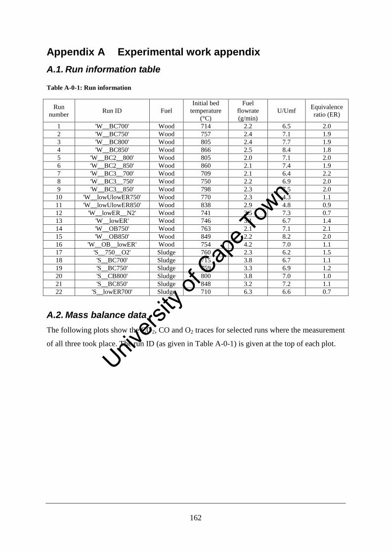
162

Appendix A Experimental work appendix

A.1. Run information table

Table A-0-1: Run information

Run

number Run ID Fuel

Initial bed

temperature

(°C)

Fuel

flowrate

(g/min)

U/Umf Equivalence

ratio (ER)

1 'W__BC700' Wood 714 2.2 6.5 2.0

2 'W__BC750' Wood 757 2.4 7.1 1.9

3 'W__BC800' Wood 805 2.4 7.7 1.9

4 'W__BC850' Wood 866 2.5 8.4 1.8

5 'W__BC2__800' Wood 805 2.0 7.1 2.0

6 'W__BC2__850' Wood 860 2.1 7.4 1.9

7 'W__BC3__700' Wood 709 2.1 6.4 2.2

8 'W__BC3__750' Wood 750 2.2 6.9 2.0

9 'W__BC3__850' Wood 798 2.3 7.5 2.0

10 'W__lowUlowER750' Wood 770 2.3 4.3 1.1

11 'W__lowUlowER850' Wood 838 2.9 4.8 0.9

12 'W__lowER__N2' Wood 741 3.5 7.3 0.7

13 'W__lowER' Wood 746 3.1 6.7 1.4

14 'W__OB750' Wood 763 2.1 7.1 2.1

15 'W__OB850' Wood 849 2.2 8.2 2.0

16 'W__OB__lowER' Wood 754 4.2 7.0 1.1

17 'S__750__O2' Sludge 760 2.3 6.2 1.5

18 'S__BC700' Sludge 715 3.8 6.7 1.1

19 'S__BC750' Sludge 759 3.3 6.9 1.2

20 'S__CB800' Sludge 800 3.8 7.0 1.0

21 'S__BC850' Sludge 848 3.2 7.2 1.1

22 'S__lowER700' Sludge 710 6.3 6.6 0.7

A.2. Mass balance data

The following plots show the CO2, CO and O2 traces for selected runs where the measurement

of all three took place. The run ID (as given in Table A-0-1) is given at the top of each plot.

Univers

ity of

Cap

e Tow

n

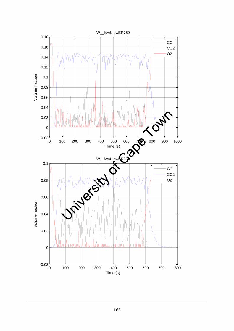
163

0 100 200 300 400 500 600 700 800 900 1000-0.02

0

0.02

0.04

0.06

0.08

0.1

0.12

0.14

0.16

0.18

Time (s)

Volu

me f

raction

W__lowUlowER750

CO

CO2

O2

0 100 200 300 400 500 600 700 800-0.02

0

0.02

0.04

0.06

0.08

0.1

Time (s)

Volu

me f

raction

W__lowUlowER850

CO

CO2

O2

Univers

ity of

Cap

e Tow

n

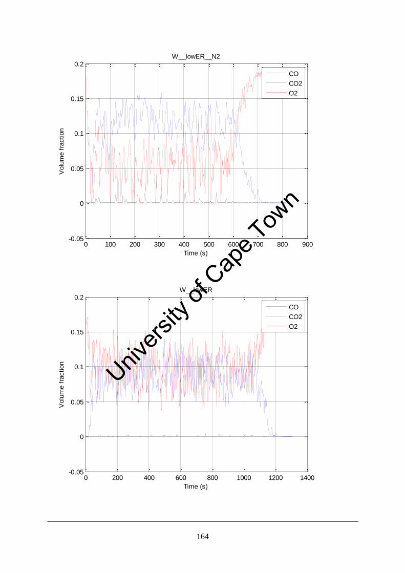
164

0 100 200 300 400 500 600 700 800 900-0.05

0

0.05

0.1

0.15

0.2

Time (s)

Volu

me f

raction

W__lowER__N2

CO

CO2

O2

0 200 400 600 800 1000 1200 1400-0.05

0

0.05

0.1

0.15

0.2

Time (s)

Volu

me f

raction

W__lowER

CO

CO2

O2

Univers

ity of

Cap

e Tow

n

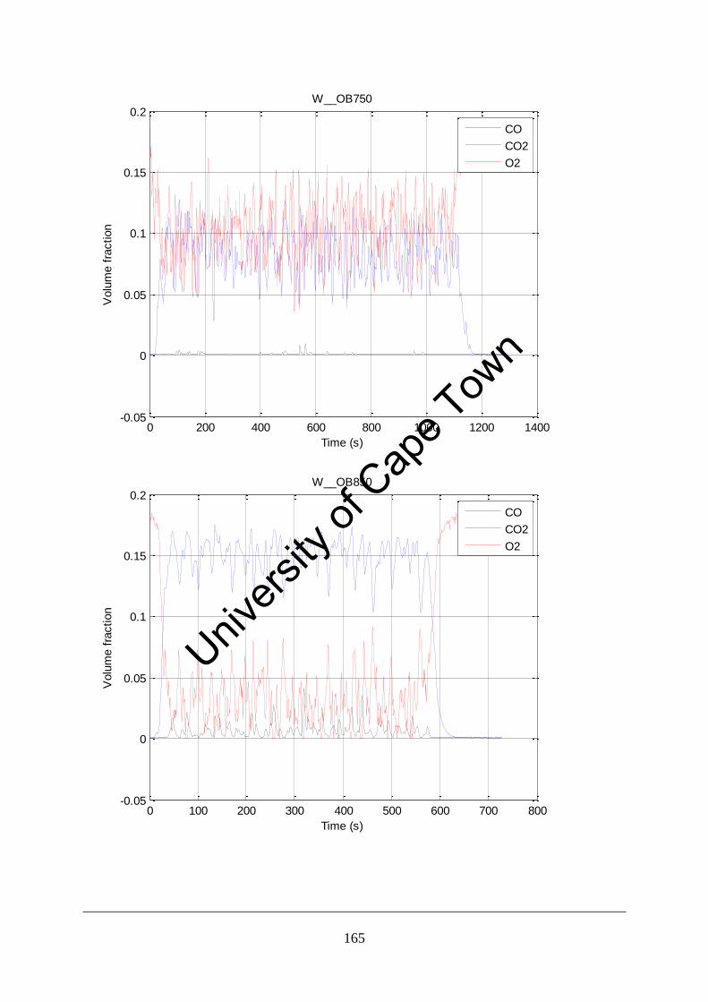
165

0 200 400 600 800 1000 1200 1400-0.05

0

0.05

0.1

0.15

0.2

Time (s)

Volu

me f

raction

W__OB750

CO

CO2

O2

0 100 200 300 400 500 600 700 800-0.05

0

0.05

0.1

0.15

0.2

Time (s)

Volu

me f

raction

W__OB850

CO

CO2

O2

Univers

ity of

Cap

e Tow

n

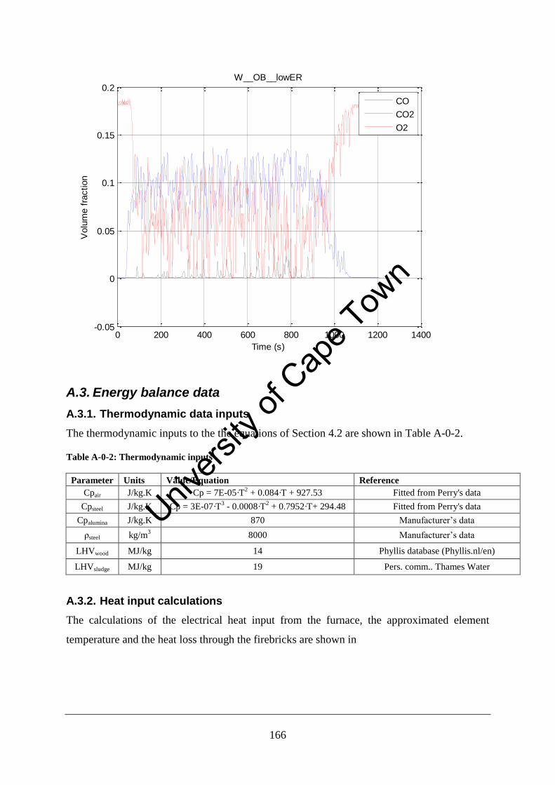
166

0 200 400 600 800 1000 1200 1400-0.05

0

0.05

0.1

0.15

0.2

Time (s)

Volu

me f

raction

W__OB__lowER

CO

CO2

O2

A.3. Energy balance data

A.3.1. Thermodynamic data inputs

The thermodynamic inputs to the the equations of Section 4.2 are shown in Table A-0-2.

Table A-0-2: Thermodynamic inputs

Parameter Units Value/Equation Reference

Cpair J/kg.K Cp = 7E-05·T2 + 0.084·T + 927.53 Fitted from Perry's data

Cpsteel J/kg.K Cp = 3E-07·T3 - 0.0008·T

2 + 0.7952·T+ 294.48 Fitted from Perry's data

Cpalumina J/kg.K 870 Manufacturer’s data

ρsteel kg/m3 8000 Manufacturer’s data

LHVwood MJ/kg 14 Phyllis database (Phyllis.nl/en)

LHVsludge MJ/kg 19 Pers. comm.. Thames Water

A.3.2. Heat input calculations

The calculations of the electrical heat input from the furnace, the approximated element

temperature and the heat loss through the firebricks are shown in

Univers

ity of

Cap

e Tow

n

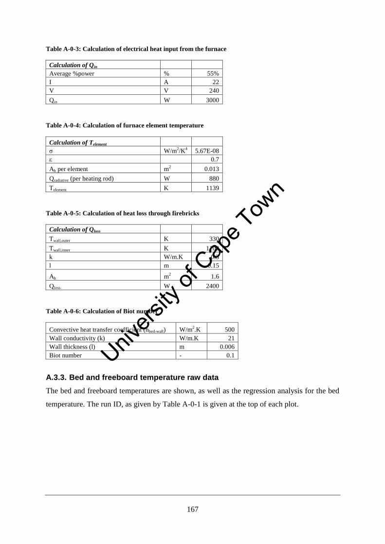
167

Table A-0-3: Calculation of electrical heat input from the furnace

Calculation of Qin

Average %power % 55%

I A 22

V V 240

Qin W 3000

Table A-0-4: Calculation of furnace element temperature

Calculation of Telement

σ W/m2/K

4 5.67E-08

ε 0.7

Ah per element m2 0.013

Qradiative (per heating rod) W 880

Telement K 1139

Table A-0-5: Calculation of heat loss through firebricks

Calculation of Qloss

Twall,outer K 330

Twall,inner K 1100

k W/m.K 0.3

l m 0.15

Ah m2 1.6

Qloss W 2400

Table A-0-6: Calculation of Biot number

Convective heat transfer coefficient (hbed-wall) W/m2.K 500

Wall conductivity (k) W/m.K 21

Wall thickness (l) m 0.006

Biot number - 0.1

A.3.3. Bed and freeboard temperature raw data

The bed and freeboard temperatures are shown, as well as the regression analysis for the bed

temperature. The run ID, as given by Table A-0-1 is given at the top of each plot.

Univers

ity of

Cap

e Tow

n

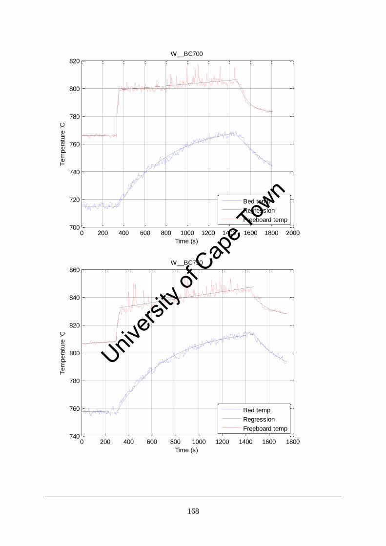
168

0 200 400 600 800 1000 1200 1400 1600 1800 2000700

720

740

760

780

800

820

Time (s)

Tem

pera

ture

'C

W__BC700

Bed temp

Regression

Freeboard temp

0 200 400 600 800 1000 1200 1400 1600 1800740

760

780

800

820

840

860

Time (s)

Tem

pera

ture

'C

W__BC750

Bed temp

Regression

Freeboard temp

Univers

ity of

Cap

e Tow

n

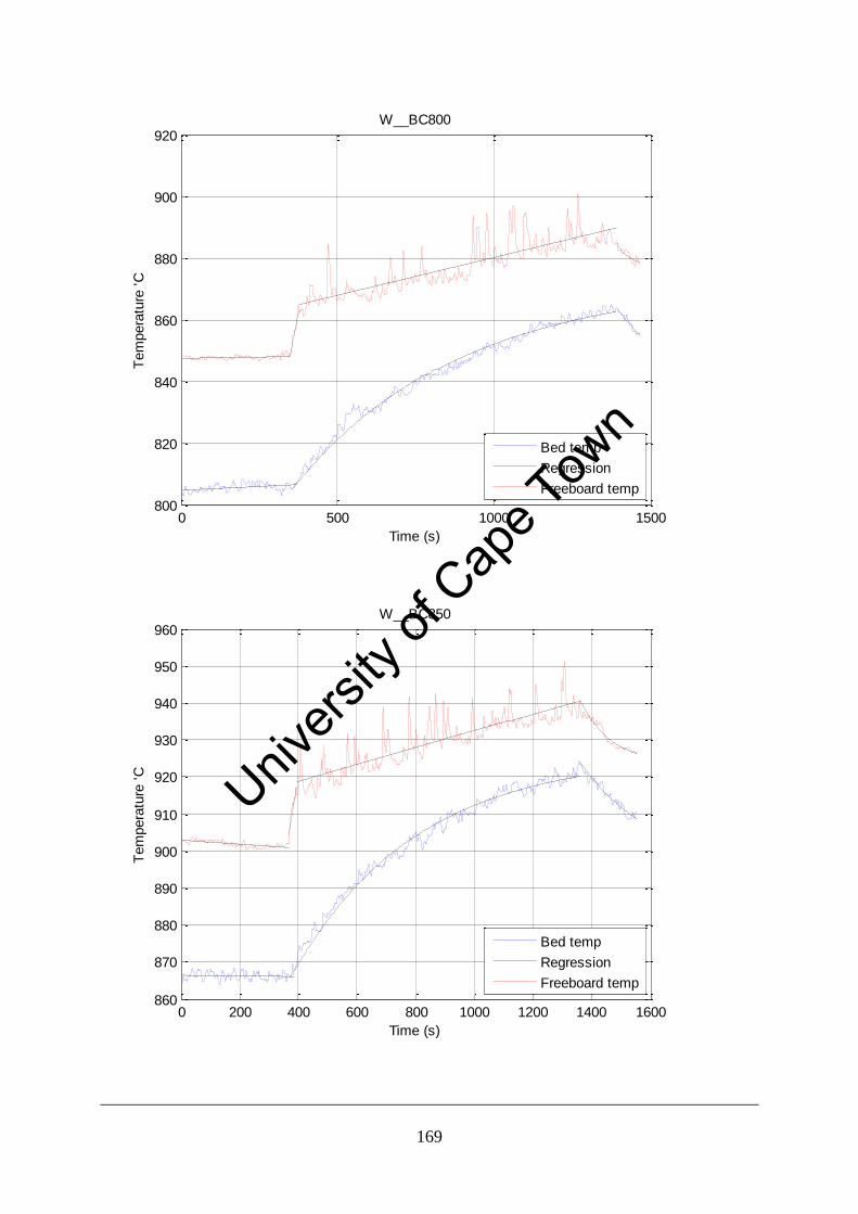
169

0 500 1000 1500800

820

840

860

880

900

920

Time (s)

Tem

pera

ture

'C

W__BC800

Bed temp

Regression

Freeboard temp

0 200 400 600 800 1000 1200 1400 1600860

870

880

890

900

910

920

930

940

950

960

Time (s)

Tem

pera

ture

'C

W__BC850

Bed temp

Regression

Freeboard temp

Univers

ity of

Cap

e Tow

n

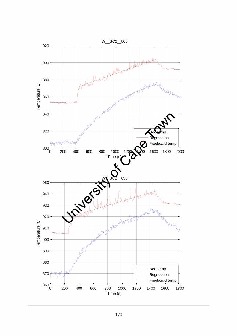
170

0 200 400 600 800 1000 1200 1400 1600 1800 2000800

820

840

860

880

900

920

Time (s)

Tem

pera

ture

'C

W__BC2__800

Bed temp

Regression

Freeboard temp

0 200 400 600 800 1000 1200 1400 1600 1800860

870

880

890

900

910

920

930

940

950

Time (s)

Tem

pera

ture

'C

W__BC2__850

Bed temp

Regression

Freeboard temp

Univers

ity of

Cap

e Tow

n

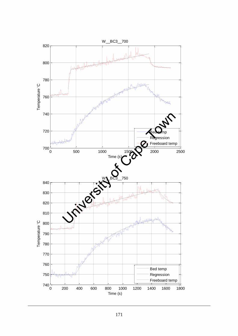
171

0 500 1000 1500 2000 2500700

720

740

760

780

800

820

Time (s)

Tem

pera

ture

'C

W__BC3__700

Bed temp

Regression

Freeboard temp

0 200 400 600 800 1000 1200 1400 1600 1800740

750

760

770

780

790

800

810

820

830

840

Time (s)

Tem

pera

ture

'C

W__BC3__750

Bed temp

Regression

Freeboard temp

Univers

ity of

Cap

e Tow

n

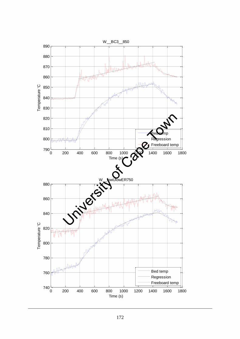
172

0 200 400 600 800 1000 1200 1400 1600 1800790

800

810

820

830

840

850

860

870

880

890

Time (s)

Tem

pera

ture

'C

W__BC3__850

Bed temp

Regression

Freeboard temp

0 200 400 600 800 1000 1200 1400 1600 1800740

760

780

800

820

840

860

880

Time (s)

Tem

pera

ture

'C

W__lowUlowER750

Bed temp

Regression

Freeboard temp

Univers

ity of

Cap

e Tow

n

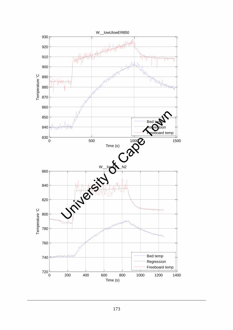
173

0 500 1000 1500830

840

850

860

870

880

890

900

910

920

930

Time (s)

Tem

pera

ture

'C

W__lowUlowER850

Bed temp

Regression

Freeboard temp

0 200 400 600 800 1000 1200 1400720

740

760

780

800

820

840

860

Time (s)

Tem

pera

ture

'C

W__lowER__N2

Bed temp

Regression

Freeboard temp

Univers

ity of

Cap

e Tow

n

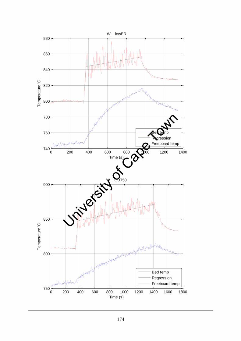
174

0 200 400 600 800 1000 1200 1400740

760

780

800

820

840

860

880

Time (s)

Tem

pera

ture

'C

W__lowER

Bed temp

Regression

Freeboard temp

0 200 400 600 800 1000 1200 1400 1600 1800750

800

850

900

Time (s)

Tem

pera

ture

'C

W__OB750

Bed temp

Regression

Freeboard temp

Univers

ity of

Cap

e Tow

n

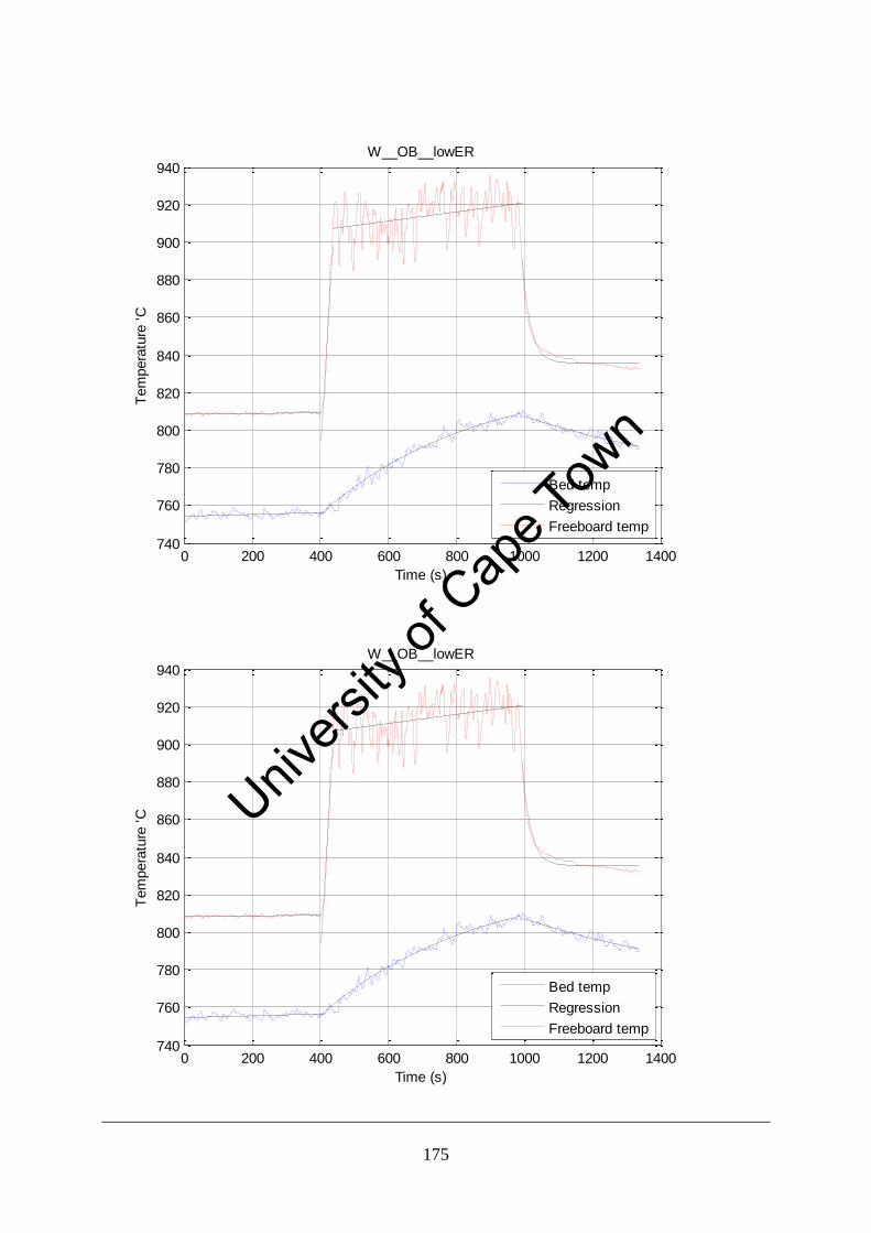
175

0 200 400 600 800 1000 1200 1400740

760

780

800

820

840

860

880

900

920

940

Time (s)

Tem

pera

ture

'C

W__OB__lowER

Bed temp

Regression

Freeboard temp

0 200 400 600 800 1000 1200 1400740

760

780

800

820

840

860

880

900

920

940

Time (s)

Tem

pera

ture

'C

W__OB__lowER

Bed temp

Regression

Freeboard temp

Univers

ity of

Cap

e Tow

n

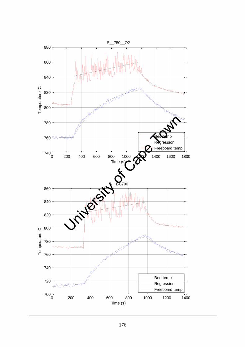
176

0 200 400 600 800 1000 1200 1400 1600 1800740

760

780

800

820

840

860

880

Time (s)

Tem

pera

ture

'C

S__750__O2

Bed temp

Regression

Freeboard temp

0 200 400 600 800 1000 1200 1400700

720

740

760

780

800

820

840

860

Time (s)

Tem

pera

ture

'C

S__BC700

Bed temp

Regression

Freeboard temp

Univers

ity of

Cap

e Tow

n

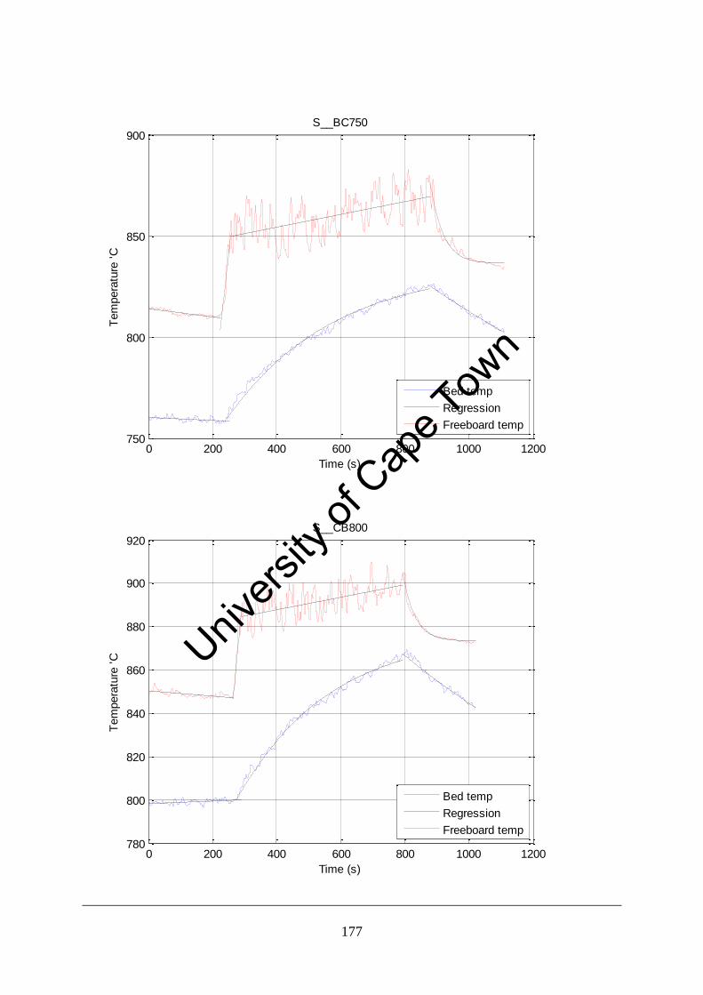
177

0 200 400 600 800 1000 1200750

800

850

900

Time (s)

Tem

pera

ture

'C

S__BC750

Bed temp

Regression

Freeboard temp

0 200 400 600 800 1000 1200780

800

820

840

860

880

900

920

Time (s)

Tem

pera

ture

'C

S__CB800

Bed temp

Regression

Freeboard temp

Univers

ity of

Cap

e Tow

n

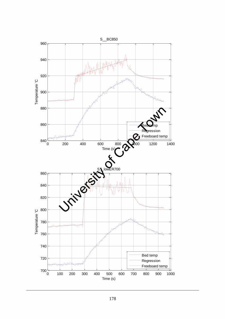
178

0 200 400 600 800 1000 1200 1400840

860

880

900

920

940

960

Time (s)

Tem

pera

ture

'C

S__BC850

Bed temp

Regression

Freeboard temp

0 100 200 300 400 500 600 700 800 900 1000700

720

740

760

780

800

820

840

860

Time (s)

Tem

pera

ture

'C

S__lowER700

Bed temp

Regression

Freeboard temp

Univers

ity of

Cap

e Tow

n

179

A.4. Matlab code for mass balance

% DWLSAR002 26 March 2008 % Mass balancing

close all, clear all, clc

load massbal % "cAll" is NB one for C bal % column 1: time, column 2: CO, column 3: CO2 for runs 1 to 18 as on % 11/12/07 in lab book (and used thru out)

load exceldata2

% t0 and tn used to get average conc over range t0 = [20 0 50 20 20 50 0 0 0 150 50 50 50 40 50 25 70 20]; tn = [1120 0 1000 1000 1200 1200 0 0 0 1170 770 600 600 1100 1100 570 950

600];

for i = 1:22 % need molar flow through reactor RR = values(i,1); RRN2 = values(i,5); % v_air = (0.0001*RR.^2 + ... % 0.0245*RR + 0.0728)*1000; % flow of air in cc/s % / 1.5 to account for operating pressure of 1.5barg v_air = 0.3124*RR^2 + 23.328*RR + 89.933; % new calibration

if RRN2 == 0; % flow of second N2 stream (if present) v_N2 = 0; else v_N2 = (0.0001*RR.^2 + ... 0.0245*RR + 0.0728)*1000; end v_hopper = 4; % N2 hopper flow always 4l/min % n_air = (v_air+v_N2)/1e6*1e5/8.314/(21+273); % n_N2 = v_hopper./1000/60*1e5/8.314/(21+273); % pN2(i) = n_N2/(n_N2+n_air(i)); n_gas = (v_air+v_N2)/1e6*1e5/8.314/(21+273) + ... v_hopper./1000/60*1e5/8.314/(21+273) %mol

% convert V to %CO (column:2) or %CO2 (column:3) (time = column 1) % from excel: % %CO = 0.0222V - 0.0492 % %CO2 = 0.0296V - 0.0566 % %O2 = 0.2489x - 0.0012 cEnd = find(cAll(:,3*i-2)); time = cAll(cEnd,3*i-2); CO = 0.0222*cAll(cEnd,3*i-1) - 0.0492; CO2 = 0.0296*cAll(cEnd,3*i) - 0.0566;

% Plot selected runs % if i ~= 2 & i ~=7 & i ~=8 & i ~=9; % figure(i) % plot(CO,'g'), grid on, hold on % plot(CO2,'b'), grid on, hold on

Univers

ity of

Cap

e Tow

n

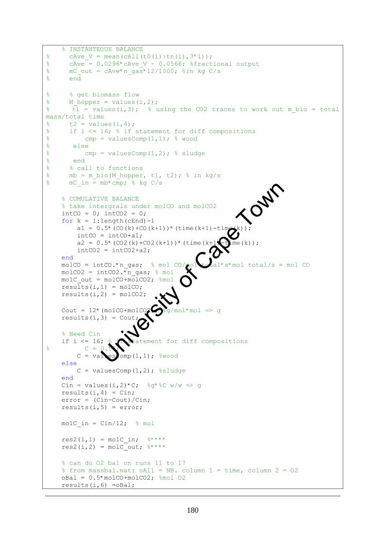
180

% INSTANTEOUS BALANCE % cAve_V = mean(cAll(t0(i):tn(i),3*i)); % cAve = 0.0296*cAve_V - 0.0566; %fractional output % mC_out = cAve*n_gas*12/1000; %in kg C/s % end

% % get biomass flow % M_hopper = values(i,2); % t1 = values(i,3); % using the CO2 traces to work out m_bio = total

mass/total time % t2 = values(i,4); % if i <= 16; % if statement for diff compositions % cmp = valuesComp(1,1); % wood % else % cmp = valuesComp(1,2); % sludge % end % % call to functions % mb = m_bio(M_hopper, t1, t2); % in kg/s % mC_in = mb*cmp; % kg C/s

% CUMULATIVE BALANCE % take intergrals under molCO and molCO2 intCO = 0; intCO2 = 0; for k = 1:length(cEnd)-1 a1 = 0.5*(CO(k)+CO(k+1))*(time(k+1)-time(k)); intCO = intCO+a1; a2 = 0.5*(CO2(k)+CO2(k+1))*(time(k+1)-time(k)); intCO2 = intCO2+a2; end molCO = intCO.*n_gas; % mol CO/mol total*s*mol total/s = mol CO molCO2 = intCO2.*n_gas; % mol molC_out = molCO+molCO2; %mol results(i,1) = molCO; results(i,2) = molCO2;

Cout = 12*(molCO+molCO2); %g/mol*mol => g results(i,3) = Cout;

% Need Cin if i <= 16; % if statement for diff compositions % C = 0.50; C = valuesComp(1,1); %wood else C = valuesComp(1,2); %sludge end Cin = values(i,2)*C; %g*%C w/w => g results(i,4) = Cin; error = (Cin-Cout)/Cin; results(i,5) = error;

molC_in = Cin/12; % mol

res2(i,1) = molC_in; %**** res2(i,2) = molC_out; %****

% can do O2 bal on runs 11 to 17 % from massbal.mat: oAll = NB. column 1 = time, column 2 = O2 oBal = 0.5*molCO+molCO2; %mol O2 results(i,6) =oBal;

Univers

ity of

Cap

e Tow

n

181

if i >= 11 & i <= 17 j = i-10; oEnd = find(oAll(:,2*j-1)); time = oAll(oEnd,2*j-1); O2 = 0.2489*oAll(oEnd,2*j) - 0.0012; % mol/m3 % plot(O2,'r'), grid on, hold on O2 = O2 - O2(1); %"normalise"

%take intergral under curve and make positive intO2 = 0; for k = 1:length(oEnd)-1 a3 = 0.5*(O2(k)+O2(k+1))*(time(k+1)-time(k)); intO2 = intO2+a3; end intO2 = -intO2; molO2 = intO2.*n_gas; % mol O2 results(i,7) = molO2; %**** errorO2 = (molO2 - oBal)/molO2; results(i,8) = errorO2; end

end

wi = 1:1:9; si = 17:21; oi = 11:1:17; figure(1) plot(wi,res2(wi,1),'o k', wi, res2(wi,2),'x k' ), grid on, hold on xlabel('Run number (wood runs)') ylabel('Carbon mol balance (gmol)') legend('Carbon in', 'Carbon out')

figure(2) plot(si,res2(si,1),'o k', si, res2(si,2),'x k' ), grid on, hold on xlabel('Run number (sludge runs)') ylabel('Carbon mol balance (gmol)') legend('Carbon in', 'Carbon out')

figure(3) plot(oi,results(oi,7), '* k', oi, res2(oi,2),'x k', oi, res2(oi,1), 'o k'

), grid on, hold on xlabel('Run number') ylabel('Oxygen mol balance (gmol)') legend('Total oxygen consumed', 'Oxygen out as CO2 and CO', 'Mols carbon

in')

A.5. Matlab code for regression analysis

% Analysis2 on 22 datasets

clc, close all, clear all

Univers

ity of

Cap

e Tow

n

182

load exceldata2 load dataADD2 %in which datatab is NB one

t0s = [341 305 360 377 396 258 380 352 350 372 ... 265 275 350 350 260 400 285 341 245 280 300 286]'; tfs = [1480 1465 1390 1360 1650 1490 1900 1500 1425 1469 ... 1002 865 959 1441 1389 994 1153 973 880 795 909 682]'; % tfb0 = [330 290 350 370 415 254 340 325 330 380 260 255 350 340 235 405

262 332 225 265 300 285; % 360 322 378 395 440 315 400 360 390 405 285 293 375 370 288 450 315

350 260 295 322 302]';

tfb0 = [330 292 350 370 412 254 340 325 335 380 255 250 350 339 234 405 260

332 226 266 300 285; 355 322 378 395 440 315 400 360 390 450 280 290 375 370 288 440 315 350

260 295 322 302]';

% pre-allocate variables TT = zeros(61,22); % EB t = 0:1:60; res = zeros(22,20); % results from first analysis res2 = zeros(22,3); %results from second analysis - looking at slopes res3 = zeros(22,3);

% constants M_bed = 2.15; %kg Cp_bed = 870; % J/K/kg (ref: www.azom.com/details.asp?ArticleID=52 ... for

94% pure Al2O3 (ours was 95.2%)) bedHeight = 0.35; % m (manometer reading) wallThickness = 0.005; % m pSteel = 8000; % kg/m3 (ref:

www.azom.com/details.asp?ArticleID=863#_Physical_Properties) Di = 0.078; % m M_s = (bedHeight*pi*Di*wallThickness)*pSteel;

for i = 1: 22; t0 = t0s(i); tf = tfs(i); Y = datatab(find(datatab(:,2*i-1)),2*i-1); Tb0 = Y(t0); %bed temp as feeding commences Tbf = Y(tf); %bed temp as feeding ends tn = length(Y); % find slope of first portion (ss1)for BED m1 = polyfit([0:1:t0-1]',Y([1:1:t0]'),1); ss1 = polyval(m1,[0:1:t0+10]'); Tss1 = mean(Y([1:1:t0]')); COVss1 = std(Y([1:1:t0]'))/mean(Y([1:1:t0]'))*100;

% find slope of second portion (temp increase) m2 = polyfit((t0:1:t0+45)', Y(t0:1:t0+45,1),1); trans = polyval(m2,(t0-10:1:t0+45)');

% BED ANALYSIS % inputs for minimisation routines xdat = (0:1:tf-t0)'; %for nlinfit ydat = Y(t0:1:tf) - Y(t0); % in deviation variables % nlinfit to get CI on estimates

Univers

ity of

Cap

e Tow

n

183

[beta,resid,J] = nlinfit(xdat,ydat,@expnlinfit,[50 0.0001]); NLF = beta(1)*(1-exp(-beta(2).*xdat))+Tb0; % get CI on estimates ci = nlparci(beta,resid,J); dTdt0 = beta(1)*beta(2); % initial rate from fitted curve (nlinfit) dTdt0_LCI = ci(1,1)*ci(2,1); dTdt0_UCI = ci(1,2)*ci(2,2);

% FREEBOARD ANALYSIS % find slope of ss1 Y2 = datatab(find(datatab(:,2*i)),2*i); TfbF = Y2(tf); mfb1 = polyfit([0:1:tfb0(i,1)-1]',Y2(1:1:tfb0(i,1)'),1); Tfb1_fit = polyval(mfb1,[0:1:tfb0(i,1)]'); Tfbss1 = mean(Y2(1:1:tfb0(i,1))');

% find rate of increase in fb temp Tfb0 = Y2(tfb0(i,1)); % start of fb temp rise Tfb2 = Y2(tfb0(i,2)); % end fb temp rise mfb2 = polyfit(tfb0(i,1):1:tfb0(i,2)',Y2(tfb0(i,1):1:tfb0(i,2))',1); Tfb2_fit = polyval(mfb2, tfb0(i,1):1:tfb0(i,2)');

% find slope of freeboard during feeding % (Over entire period of feeding) mfb3 = polyfit((tfb0(i,2):1:tf)', Y2(tfb0(i,2):1:tf'),1); Tfb3_fit = polyval(mfb3,(tfb0(i,2):1:tf)'); dT_fb = Tfb3_fit(1) - Tfb0;

% END OF RUN ANALYSIS xdatN = [0:1:tn-tf]'; ydatN = Y(tf:1:tn)-Tbf; [betaN] = nlinfit(xdatN,ydatN,@expnlinfit2,[50 0.02]); NLFN = -betaN(1)*(1-exp(-betaN(2).*xdatN))+Tbf; ydatNfb = Y2(tf:1:tn)-TfbF; [betaNfb] = nlinfit(xdatN,ydatNfb,@expnlinfit2,[50 0.02]); NLFNfb = -betaNfb(1)*(1-exp(-betaNfb(2).*xdatN))+TfbF; mN(i) = betaN(1)*betaN(2); mNfb(i) = betaNfb(1)*betaNfb(2);

% dTfb_b analysis dTfb_b0 = Y2 - Y; betaD1 = nlinfit((tfb0(i,2):1:tf)',... dTfb_b0(tfb0(i,2):1:tf)-dTfb_b0(tfb0(i,2)),@expnlinfit2,[20,0.002]) dTfb_b1 = -betaD1(1)*(1-exp(-

betaD1(2).*(tfb0(i,2):1:tf)'))+dTfb_b0(tfb0(i,2));

% EB MODEL % exceldata for EB calc RR = values(i,1); M_hopper = values(i,2); t1 = values(i,3); % using the CO2 traces to work out m_bio = total

mass/total time t2 = values(i,4); RRN2 = values(i,5); if i <= 16 % if statement for diff compositions comp = valuesComp(:,1); LHVar = 14e6; %disp('wood')

Univers

ity of

Cap

e Tow

n

184

else comp = valuesComp(:,2); LHVar = 19e6; %disp('sludge') end % call to functions mb = m_bio(M_hopper, t1, t2); [mg U Umf ER LHV] = EBinputs(RR, RRN2, Tb0,comp,mb); mg_i(i) = mg; %for calculating hA and Te Cpa = Cp_air(Tb0+273); Cpa_i(i) = Cpa; Cps = CpS(Tb0+273);

% Calc Q,fb Cpa_fb(i) = Cp_air(Tfb3_fit(1)); UAfb = 0.4249; %from regression analysis Qc_fb(i) = (mg*Cpa_fb(i))*dT_fb;

%from report: A = (mbiomass*Hc)/(mair*Cpair) [1000 K] %alpha = (mair*Cpair)/(Mbed*Cpbed) [0.0002 s-1] % UA = 0.4468; %from regression analysis of Tele vs Tbed alpha = (mg*Cpa)/(M_bed*Cp_bed+M_s*Cps); % alpha = (mg*Cpa)/(M_bed*Cp_bed); A = (mb.*LHVar)/(mg*Cpa);

% EB model for j = 1:length(t) TT(j,i) = Tb0 + A*(1-exp(-alpha*t(j))); end

% RESULTS TABLE % parameters res(i,1) = Tb0; % initial bed temp res(i,2) = mb*1000*60; %report in g/min res(i,3) = U/Umf; res(i,4) = ER; res(i,5) = RR; % EB model results res(i,6) = dTdt0; % initial slope according to regression res(i,7) = m1(1)/(mb*1000*60); % initial slope: linear fit res(i,8) = A*alpha; % **** initial slope according to EB (normalised to

feedrate) % freeboard results res(i,9) = Tfb0; %initial fb temp res(i,10) = mfb3(1); % slope of fb during feeding res(i,11) = dT_fb; %jump in fb temp res(i,12) = Tfb0 - Tb0; % initial diff betw bed and fb temp % res(i,13) = Tfb2_fit(1) - Tb2; % final diff betw bed and fb temp res(i,14) = mfb2(1); % slope of fb temp jump

% compare regression coeffs and calc'd coeffs res(i,15) = A; % from EB res(i,16) = alpha; % from EB res(i,17) = beta(1); % fitted data from nlinfit res(i,18) = beta(2); % fitted data from nlinfit res(i,19) = dTdt0_LCI/(mb*1000*60); res(i,20) = dTdt0_UCI/(mb*1000*60); res2(i,1) = dTdt0/(A*alpha); %dTdt0 = beta(1)*beta(2) res2(i,2) = dTdt0_LCI/(A*alpha);

Univers

ity of

Cap

e Tow

n

185

res2(i,3) = dTdt0_UCI/(A*alpha);

% Results display: latest % In absolute terms res3(i,1) = mb.*LHVar; %max heat released res3(i,2) = (M_bed*Cp_bed+M_s*Cps)*dTdt0; %actual heat released to bed res3(i,3) = Qc_fb(i); %heat released as overbed burning % As fractions res3(i,4) = (M_bed*Cp_bed+M_s*Cps)*dTdt0/(mb.*LHVar); res3(i,5) = (M_bed*Cp_bed+M_s*Cps)*dTdt0_LCI/(mb.*LHVar); res3(i,6) = (M_bed*Cp_bed+M_s*Cps)*dTdt0_UCI/(mb.*LHVar); res3(i,7) = Qc_fb(i)/(mb.*LHVar);

% PLOTS % figure(i) % % subplot(2,1,1) % h(1) = plot(0:1:tn-1,Y(1:1:tn),'b'),grid on, hold on; % plot(ss1,'k --'), grid on, hold on % % plot((t0-10:1:t0+45)',trans, 'b'), grid on, hold on % h(2) = plot(t+t0,TT(:,i), 'k', 'LineWidth',2 ), grid on, hold on; % % plot(xdat+t0-1,FittedCurve+Tb0, 'k'),grid on, hold on % h(3) = plot(xdat+t0-1,NLF, 'k --'),grid on, hold on; % nlinfit % h(4) = plot((0:1:tn-1)', Y2(1:1:tn)', 'r'), grid on, hold on; % plot((tfb0(i,2):1:tf)', Tfb3_fit, 'k --'), grid on, hold on % plot(Tfb1_fit,'k --'), grid on, hold on % plot(tfb0(i,1):1:tfb0(i,2)',Tfb2_fit, 'k --'), grid on, hold on % plot((tf:1:tn)', NLFN, 'k --'), grid on, hold on % plot((tf:1:tn)', NLFNfb, 'k --'), grid on, hold on % xlabel('time (s)') % ylabel('Temperature ''C') % title(runInfo(i+1)) % legend(h,'Bed temp','Model','Regression','Freeboard

temp','Location','SE')

% subplot(2,1,2) % plot(dTfb_b0), grid on, hold on % plot((tfb0(i,2):1:tf)',dTfb_b1, '-- k'), grid on, hold on % plot(tfb0(i,2), dTfb_b0(tfb0(i,2)), 'o'), grid on , hold on % xlabel('Time (s)') % ylabel('Difference in temperature between bed and freeboard (''C)')

end

figure(23) % wood runs percent heat released h(1) = plot(res([1 2 3 4 5 6 8 ],1),res3([1 2 3 4 5 6 8 ],4),'o k'), hold

on h(2) = plot(res([1 2 3 4 5 6 8 ],1),res3([1 2 3 4 5 6 8 ],5),'+ k'), hold

on plot(res([1 2 3 4 5 6 8 ],1),res3([1 2 3 4 5 6 8 ],6),'+ k'), hold on, grid

on h(3) = plot(res([1 2 3 4 5 6 8 ],1),res3([1 2 3 4 5 6 8 ],7),'* k'), hold

on xlabel('Initial bed temperature (''C)'); ylabel('Fraction of heat released'); legend(h,'Fraction of heat released to bed',... '95% confidence interval from regression estimates',... 'Fraction of heat to freeboard')

Univers

ity of

Cap

e Tow

n

186

figure(24) % sewerage sludge percent heat released h(1) = plot(res([17:21],1),res3([17:21],4),'o k'), hold on h(2) = plot(res([17:21],1),res3([17:21],5),'+ k'), hold on plot(res([17:21],1),res3([17:21],6),'+ k'), hold on, grid on h(3) = plot(res([17:21],1),res3([17:21],7),'* k'), hold on xlabel('Initial bed temperature (''C)'); ylabel('Fraction of heat released'); legend(h,'Fraction of heat released to bed',... '95% confidence interval from regression estimates',... 'Fraction of heat to freeboard')

% Overbed bed runs heat released figure(25) h(1) = plot(res([14:15],1),res3([14:15],4),'o k'), hold on h(2) = plot(res([14:15],1),res3([14:15],5),'+ k'), hold on plot(res([14:15],1),res3([14:15],6),'+ k'), hold on, grid on h(3) = plot(res([14:15],1),res3([14:15],7),'* k'), hold on xlabel('Initial bed temperature (''C)'); ylabel('Fraction of heat released'); legend(h,'Fraction of heat released to bed',... '95% confidence interval from regression estimates',... 'Fraction of heat to freeboard')

figure(26) % wood runs fb temp jump plot(res([1:1:8],1),res([1:1:8],11),'o k'), hold on, grid on xlabel('Initial bed temperature (''C)'); ylabel('Jump in freeboard temperature (''C)'); title('Freeboard temperature jump for wood runs')

figure(27) %sewerage sludge fb temp jump plot(res([17:21],1),res([17:21],11),'o k'), hold on, grid on xlabel('Initial bed temperature (''C)'); ylabel('Jump in freeboard temperature (''C)'); title('Freeboard temperature jump for sludge runs')

% Overbed fb temp jump figure(28) plot(res([14:15],1),res([14:15],11),'o k'), hold on, grid on xlabel('Initial bed temperature (''C)'); ylabel('Jump in freeboard temperature (''C)'); title('Freeboard temperature jump for overbed wood runs')

% Initial slope at end of run figure(29) plot(mN,mNfb, 'o k'), grid on, hold on xlabel('Initial rate of cooling for bed (K/s)') ylabel('Initial rate of cooling for freeboard (K/s)')

% represent as bar chart figure(30) bb(1) = bar([1:8],res3(1:8,1),'w') hold on bb([2:3])= bar([res3(1:8,2) res3(1:1:8,3)],'stack') colormap([0 1 1;0 0 0]); xlabel('Run number') ylabel('Energy flow (W)') legend(bb, 'Maximum heat released to bed',...

Univers

ity of

Cap

e Tow

n

187

'Actual heat released to bed','Heat released by overbed

burning','location','SE')

figure(31) bb(1) = bar([17:21],res3([17:21],1),'w') hold on bb([2:3])= bar([17:21],[res3([17:21],2) res3([17:21],3)],'stack') colormap([0 1 1;0 0 0]); xlabel('Run number') ylabel('Energy flow (W)') legend(bb, 'Maximum heat released to bed',... 'Actual heat released to bed','Heat released by overbed


figure(32) bb(1) = bar([14:15],res3(14:15,1),'w') hold on bb([2:3])= bar([14:15],[res3(14:15,2) res3(14:15,3)],'stack') colormap([0 1 1;0 0 0]); xlabel('Run number') ylabel('Energy flow (W)') legend(bb, 'Maximum heat released to bed',... 'Actual heat released to bed','Heat released by overbed


tableS = cell(23,5); tableS(1,1) = {'Run number'}; tableS(2:23,1) = num2cell([1:1:22]'); tableS(1,2) = {'Run ID'}; tableS(2:23,2) = runInfo(2:23,1); tableS(1,3:6) = {'Initial bed temperature (''C)','Fuel flowrate

(g/min)',... 'U/Umf','ER'}; tableS(2:23,3:6) = num2cell(res(:,[1:4]));

% Find UA for bed ii = [1:1:9 12:1:22]; %select conditions of same gas flowrate I = 22/2; % amps V = 240/3; %volt sigma = 5.67e-8; %W/m2/K^4; eta = 0.7; % pers comm. Kanthal Aele = pi*0.012*0.20; Tele = ((values(ii,6)/100)*I*V/sigma/eta/Aele).^(1/4); % re-arrange Q =

sigma*eta*T,blackbody^4 w2 = polyfit(res(ii,1),Tele,1); aveCpa = mean(Cpa_i(ii)); aveMg = mean(mg_i(ii)); UA = aveMg*aveCpa/(w2(1)+1); UA2 = -aveMg*aveCpa*294/w2(2); U = UA/(Di*pi*0.35);

% Find UA for freeboard % Use mean temp diff of freeboard Tfb_ave = (res(ii,9)-res(ii,1))/2+res(ii,1); w2fb = polyfit(res(ii,9), Tele,1); aveCpa_fb = mean(Cpa_fb(ii)); UAfb = aveMg*aveCpa_fb/(w2fb(1)+1); Ufb = UAfb/pi/Di/0.46; figure(33)

Univers

ity of

Cap

e Tow

n

188

plot(res(ii,1),Tele-273, '* k'), grid on, hold on plot(res(ii,1), polyval(w2,res(ii,1))-273,'k'), grid on, hold on plot(res(ii,1),res(ii,1),'-+'), grid on, hold on plot(Tfb_ave, Tele-273, 'o b'), grid on, hold on % plot(Tfb_ave, polyval(w2fb,res(ii,9))-273, 'b'), grid on, hold on plot(Tfb_ave, Tfb_ave, '-+ r'), grid on, hold on xlabel('Initial bed temperatur ''C') ylabel('Element temperature ''C')

% Plot SS2 presdicted temps % figure(30) % plot(res(:,1), res(:,15), 'o r'), grid on, hold on % plot(res(:,1), res(:,17), 'o k'), grid on, hold on % legend('Tss2 from EB','Tss2 from regression') % ylabel('Predicted Tss2 ''C') % xlabel('Initial bed temp')

Appendix B Waste availability calculations

B.1. Derivation of biogas yield from COD destruction

Biogas yield from volatile solids destruction may be derived from first principles in the

following manner. The COD of methane is the amount of O2 required to completely oxidise 1

mol of methane. From the stoichiometry, it can be seen two mols of O2 are required. Two

mols of O2 are equal to 64 g. Hence the COD equivalent of one mol of methane is 64g

COD/mol (Tchobanoglous et al., 2003).

At STP (0°C, 1 atm), 1 mol of ideal gas occupies 22.4 l, hence

22.4 l/mol CH4 ÷ 64 gCOD/mol CH4 = 0.35 l CH4/g COD = 0.35m3 CH4/kg COD

B.2. Energy yields from DME White Paper on renewable energy

As the data in the DME paper was quoted in terms of ranges of biomass and energy yields,

some further calculations were necessary to obtain a single meaningful value. To relate the

biomass energy yield to the areal energy yield a single representative yield was calculated

from data from the South African Crop Estimates Committee (CEC) as show in Table B-0-7

The weighted average yield was calculated to be 2.7 ton/Ha Assuming that the lowest

biomass yield referred to the lowest areal energy yield, linear interpolation was used to

calculate an energy yield corresponding to the weighted biomass yield. This gave an areal

energy yield of 40.2 GJ/Ha/yr as shown in

Table B-0-8. Other manipulations are shown in Table B-0-9.

Univers

ity of

Cap

e Tow

n

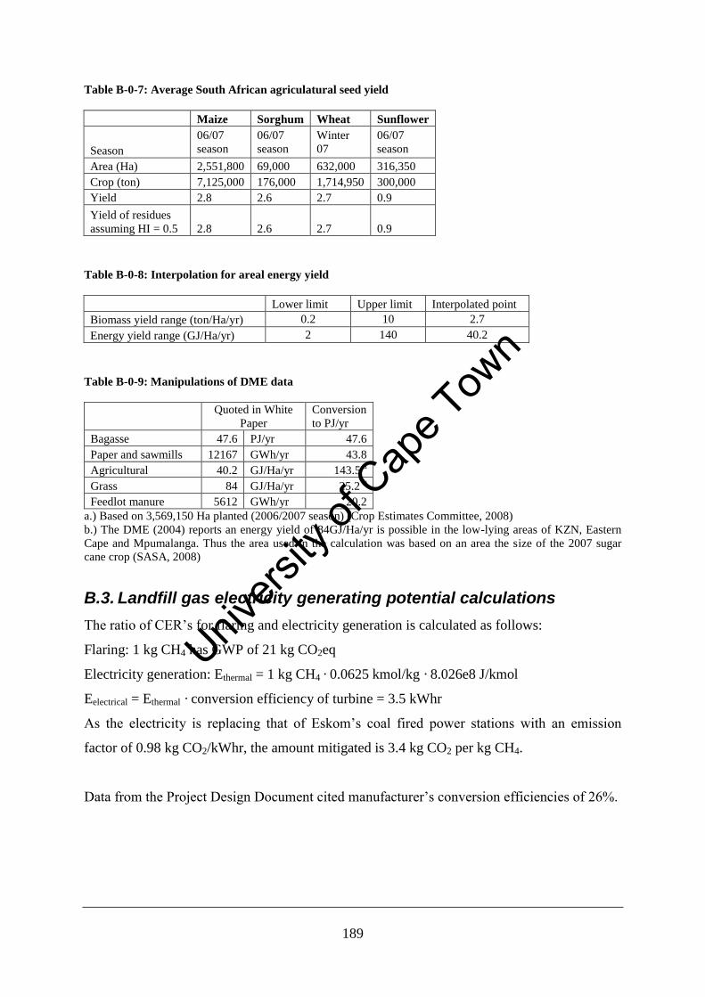
189

Table B-0-7: Average South African agriculatural seed yield

Maize Sorghum Wheat Sunflower

Season

06/07

season

06/07

season

Winter

07

06/07

season

Area (Ha) 2,551,800 69,000 632,000 316,350

Crop (ton) 7,125,000 176,000 1,714,950 300,000

Yield 2.8 2.6 2.7 0.9

Yield of residues

assuming HI = 0.5 2.8 2.6 2.7 0.9

Table B-0-8: Interpolation for areal energy yield

Lower limit Upper limit Interpolated point

Biomass yield range (ton/Ha/yr) 0.2 10 2.7

Energy yield range (GJ/Ha/yr) 2 140 40.2

Table B-0-9: Manipulations of DME data

Quoted in White

Paper

Conversion

to PJ/yr

Bagasse 47.6 PJ/yr 47.6

Paper and sawmills 12167 GWh/yr 43.8

Agricultural 40.2 GJ/Ha/yr 143.5 a

Grass 84 GJ/Ha/yr 25.2 b

Feedlot manure 5612 GWh/yr 20.2

a.) Based on 3,569,150 Ha planted (2006/2007 season) (Crop Estimates Committee, 2008)

b.) The DME (2004) reports an energy yield of 84GJ/Ha/yr is possible in the low-lying areas of KZN, Eastern

Cape and Mpumalanga. Thus the area used in the calculation was based on an area the size of the 2007 sugar

cane crop (SASA, 2008)

B.3. Landfill gas electricity generating potential calculations

The ratio of CER’s for flaring and electricity generation is calculated as follows:

Flaring: 1 kg CH4 has GWP of 21 kg CO2eq

Electricity generation: Ethermal = 1 kg CH4 · 0.0625 kmol/kg · 8.026e8 J/kmol

Eelectrical = Ethermal · conversion efficiency of turbine = 3.5 kWhr

As the electricity is replacing that of Eskom’s coal fired power stations with an emission

factor of 0.98 kg CO2/kWhr, the amount mitigated is 3.4 kg CO2 per kg CH4.

Data from the Project Design Document cited manufacturer’s conversion efficiencies of 26%.

Univers

ity of

Cap

e Tow

n