INEEL/EXT-03-00437

THORsm Bench-Scale Steam Reforming Demonstration

D. W. Marshall N. R. Soelberg K. M. Shaber

May 2003

Idaho National Engineering and Environmental Laboratory Bechtel BWXT Idaho, LLC

INEEL/EXT-03-00437

THORsm Bench-Scale Steam Reforming Demonstration

D. W. Marshall N. R. Soelberg K. M. Shaber

May 2003

Idaho National Engineering and Environmental Laboratory Environmental Research & Development

Idaho Falls, Idaho 83415

Prepared for the U.S. Department of Energy

Assistant Secretary for Environmental Management Under DOE Idaho Operations Office

Contract DE-AC07-99ID13727

iii

ABSTRACT

The Idaho Nuclear Technology and Engineering Center (INTEC) was home to nuclear fuel reprocessing activities for decades at the Idaho National Engineering and Environmental Laboratory. As a result of the reprocessing activities, INTEC has accumulated approximately one million gallons of acidic, radioactive, sodium-bearing waste (SBW). The purpose of this demonstration was to investigate a steam reforming technology, offered by THORsm Treatment Technologies, LLC, for treatment of the SBW into a “road ready” waste form that would meet the waste acceptance criteria for the Waste Isolation Pilot Plant (WIPP). A non-radioactive simulated SBW was used based on the known composition of waste tank WM-180 at INTEC. Rhenium was included as a non-radioactive surrogate for technetium.

Data were collected to determine the nature and characteristics of the product, the operability of the technology, the composition of the off-gases, and the fate of key radionuclides (cesium and technetium) and volatile mercury compounds. The product contained a significant fraction of elemental carbon residues in the cyclone and filter vessel catches. Mercury was quantitatively stripped from the product but cesium, rhenium (Tc surrogate), and the heavy metals were retained. Nitrates were not detected in the product and NOxdestruction exceeded 98%. The demonstration was successful.

iv

v

SUMMARY

THORsm Treatment Technologies, LLC (TTT) was awarded a contract to demonstrate its steam reforming technology on non-radioactive, simulated tank WM-180 sodium-bearing waste using government furnished equipment built and operated by Science Applications International Corporation (SAIC) in Idaho Falls, Idaho. TTT specified the flow sheet conditions and provided additives for the demonstration. Performance dates were January 6 through January 26, 2003 to conduct preliminary optimization tests and execute a successful 100-hour demonstration run.

After a few days of proving and optimizing the flow sheet conditions, the demonstration run was started January 13 and completed January 17, 2003. The 100-hr demonstration run was successfully completed. The sodium-bearing waste simulant was converted into a freely-flowing powder and NOx destruction was excellent. Details of the process flow sheet and data that were collected on product and off-gas characteristics are contained within the report.

vi

vii

ACKNOWLEDGMENTS

The demonstration test is a product of diligent efforts from many persons in several different organizations. Test system design and construction, and test operation, was funded by the U.S. Department of Energy through the Idaho National Engineering and Environmental Laboratory (INEEL) High Level Waste Program Idaho Tank Farm Project. The INEEL designed and fabricated the reformer vessel, provided a high-level design for the complete process, and directed the test system installation at the Science Applications International Corporation’s (SAIC) Science and Technology Application Research (STAR) Center in Idaho Falls, Idaho. SAIC completed the design of the process, coordinated the procurement and receipt of equipment and materials, fabricated and assembled the components, wrote the operating procedures, provided the facility to house the test unit, and operated the unit. Eldredge Engineering provided significant consultation on the fluidized bed design, operation, and calculated the mass balance. Last but not least, the authors thank the contributions of THORsm Treatment Technologies for their technological innovations that were the basis of the demonstration test and their oversight during the performance of the tests.

The coauthors would also like to thank the following persons from the INEEL for their direct contributions to the success of this project:

• Arlin Olson who represented the interests of the Idaho Tank Farm Project and directed the overall technology development effort.

• Wayne Ridgeway who, as the project engineer, managed fiscal and human resources and directed the test facility design and construction.

• Bob Crowton who provided procurement services.

• Curtis St. Michel, Ervin Brubaker, and Paul Petersen who provided the process monitoring, control, and data logging systems.

• Sylvester Losinski who assisted test planning and oversight during operation.

• Kevin Shaber who provided material specifications, and assisted in the procurement, design, and assembly of the reformer vessel, and provided oversight during the execution of the tests.

• Michael Phippen and Wade Waddoups who fabricated the reformer and obtained off-site machining services.

viii

ix

CONTENTS

ABSTRACT................................................................................................................................................. iii

SUMMARY.................................................................................................................................................. v

ACKNOWLEDGMENTS ..........................................................................................................................vii

ACRONYMS.............................................................................................................................................xiii

1. INTRODUCTION.............................................................................................................................. 1

1.1 Purpose and Scope ................................................................................................................... 1

1.2 Test Objectives......................................................................................................................... 2

2. PROCESS DESCRIPTION................................................................................................................ 2

2.1 Theory and Experimental Approach ........................................................................................ 2

2.2 Process Equipment Description ............................................................................................... 4

2.2.1 Feed Systems ................................................................................................................. 52.2.2 Bench-Scale Reformer Description ............................................................................... 52.2.3 Off-Gas Treatment and Waste Collection ..................................................................... 62.2.4 Data Acquisition and Control System ........................................................................... 6

3. CONTINUOUS EMISSIONS MONITORING SYSTEM................................................................. 7

3.1 CEMS Description and Operation ........................................................................................... 7

3.2 Off-gas Measurement Accuracy, Calibrations, and Quality Assurance Checks ...................... 9

3.3 NOx Analyzer Performance, Calibrations, and Quality Control ............................................ 11

3.3.1 Potential Problems and Resolutions ............................................................................ 11

4. EXPERIMENT SETUP.................................................................................................................... 14

4.1 SBW and Feed Compositions ................................................................................................ 14

4.2 Process Optimization ............................................................................................................. 15

4.3 Technology Demonstration Test Parameters ......................................................................... 16

5. OBSERVATIONS AND RESULTS................................................................................................ 16

5.1 Normal Operations................................................................................................................. 16

5.2 Off-Normal Operation and Resolutions ................................................................................. 18

5.3 Off-gas Composition.............................................................................................................. 19

x

5.4 NOx Concentrations and NOx Reduction ............................................................................... 24

5.5 Process Material Balance ....................................................................................................... 25

5.6 Nature and Fate of Mercury ................................................................................................... 26

5.6.1 Mercury Speciation...................................................................................................... 265.6.2 Mercury in the Product ................................................................................................ 275.6.3 Mercury in the Scrub Solution..................................................................................... 285.6.4 Mercury Captured on the Granular Activated Carbon...............................................28``

5.7 Fate of Cesium and Rhenium................................................................................................. 28

5.8 Fate of Cadmium, Chromium, and Lead................................................................................ 29

5.9 Spent Scrub Composition....................................................................................................... 30

5.10 Product Characteristics .......................................................................................................... 30

6. DISCUSSION AND ANALYSIS .................................................................................................... 36

7. CONCLUSIONS .............................................................................................................................. 38

8. REFERENCES................................................................................................................................. 39

9. APPENDIXES.................................................................................................................................. 39

FIGURES

Figure 1. Steam reforming process flow diagram......................................................................................... 4

Figure 2. Continuous emissions monitoring system used during the TTT steam reformer 100-hr test. ....... 8

Figure 3. Changes in feed density with time............................................................................................... 17

Figure 4. Off-gas measurements for the TTT demonstration test. .............................................................. 21

Figure 5. Process flow rates for the TTT demonstration test. ..................................................................... 22

Figure 6. NOx reduction for the TTT steam reformer 100-hr test............................................................... 25

Figure 7. Mass balance variances. .............................................................................................................. 26

Figure 8. Cesium to rhenium mass ratio in the scrub solution.................................................................... 29

Figure 9. TTT steam reformer bed particles with adherent product. .......................................................... 31

Figure 10. Cyclone catch micrograph. ........................................................................................................ 32

Figure 11. Cyclone catch micrograph. ........................................................................................................ 33

xi

Figure 12. Filter catch micrograph – 500X................................................................................................. 34

Figure 13. Filter catch micrograph – 1000X............................................................................................... 34

TABLES

Table 1. Analyzers used in the CEMS. ......................................................................................................... 9

Table 2. WM-180 SBW simulant and blended feed compositions. ............................................................ 14

Table 3. Mass balance................................................................................................................................. 25

Table 4. Mercury speciation from the EPA sample train............................................................................ 27

Table 5. Mercury sorption on the GAC column. ........................................................................................ 28

Table 6. Cesium and rhenium mass distributions. ...................................................................................... 29

Table 7. Product carbon and LOI ash content............................................................................................. 33

Table 8. Average product densities............................................................................................................. 35

Table 9. Waste volume and mass reduction data. ....................................................................................... 35

xii

xiii

ACRONYMS

CAI California Analytical Instruments

CEM continuous emissions monitor(ing)

CEMS continuous emissions monitoring system

COT cumulative operating time

EPA Environmental Protection Agency

GAC granular activated carbon

GUI graphical user interface

HWC hazardous waste combustor

INEEL Idaho National Engineering and Environmental Laboratory

INTEC Idaho Nuclear Technology and Engineering Center

LEL lower explosion limit

MACT Maximum Achievable Control Technology

MTEC Maximum Theoretical Emission Concentration

NAR nozzle atomizing ratio

NDIR nondispersive infrared

RCRA Resource Conservation and Recovery Act

RPD relative percent difference

SAIC Science Applications International Corporation

SBW sodium-bearing waste

SEM scanning electron microscope

STAR Science and Technology Applications Research

TECO Thermo Environmental Instruments, Inc.

THC total hydrocarbons

TTT THORsm Treatment Technologies, LLC.

WIPP Waste Isolation Pilot Plant

xiv

1

THORsm Bench-Scale Steam Reforming Demonstration 1. INTRODUCTION

The Idaho Nuclear Technology and Engineering Center (INTEC) was home to nuclear fuel reprocessing activities for decades until recovery of unspent uranium was halted in the 1990s. As a result of the reprocessing activities, INTEC has accumulated approximately one million gallons of acidic, radioactive, sodium-bearing waste (SBW). To date, the raffinates from reprocessing activities and much of the SBW have been calcined into a powder for storage pending final treatment. Further treatment of the SBW inventory is on hold pending a review and determination of the most appropriate treatment method. Steam reforming is a candidate technology being investigated for treatment of the SBW into a “road ready” waste form that can be shipped to the Waste Isolation Pilot Plant (WIPP) in New Mexico for interment.

Calcination of the SBW, which resulted in visibly brown emissions of nitrogen oxides (NOx),required the recycle of high-mercury scrub solutions to the waste tanks and did not employ Maximum Achievable Control Technology (MACT) to control gaseous emissions. Any alternative technologies that may be deployed for the treatment of SBW must be capable of meeting air quality standards and emission limits, and avoid the generation of secondary wastes that cannot be readily treated and dispositioned with the treated SBW.

1.1 Purpose and Scope

The purpose of this demonstration was to investigate the viability of a steam reforming technology, offered by THORsm Treatment Technologies, LLC. (TTT), as applied to the treatment of a simulated SBW. Data were collected to determine the nature and characteristics of the product, the operability of the technology, the composition of the off-gases, and the fate of key radionuclides (cesium and technetium), semi-volatile heavy metals, and volatile mercury compounds.

For the purpose of this demonstration, a simulant was formulated to represent the SBW contained in waste tank WM-180 at INTEC. All components of the simulated SBW were non-radioactive or naturally occurring isotopes in their natural isotopic distributions. Rhenium was included as a non-radioactive surrogate for technetium.

The scope of this demonstration was to configure and operate a government-furnished test platform in accordance with process conditions/parameters and using the process additives specified/provided by TTT. It should be noted that the test platform equipment did not fully emulate any production-scale systems that TTT would propose for treating SBW, but was constructed to provide an indication of technology feasibility for the treatment of SBW. A production-scale facility that might be proposed by the vendor could be configured significantly different from the test platform, assuming that the technology performs satisfactorily in screening against other treatment technologies and further optimization tests.

TTT was granted one week to ensure equipment, procedures, and materials were staged and ready for the demonstration, followed by a two-week period to execute a successful 100-hr demonstration on the equipment at nominally steady-state conditions. During the first week, the reformer process was operated to validate and, to the extent possible, optimize the TTT flow sheet. TTT observed the operation of the process and requested adjustments to operating parameters, based on the response of the equipment, to establish desired operating conditions and parameters for the demonstration test. The demonstration test was conducted the second week and consisted of 100 cumulative hours of feeding the blended simulated WM-180 solution to the reformer. The demonstration was successfully completed.

2

1.2 Test Objectives

The primary and overriding objective of the bench-scale, fluidized-bed, steam reforming demonstration test was to demonstrate (not develop) the TTT’s steam reforming technology for the treatment of simulated SBW. The configuration of the test platform is not fully representative of any proposed or existing TTT processes, but is suitable for the primary objective. Other primary objectives of the demonstration test were to:

• Show if the fluidized-bed steam reformer can be operated to treat simulated SBW without serious agglomeration of bed particles or de-fluidization

• Characterize the composition, sizes, and behavior of the solid product(s). This includes the absence of free liquids in the product, waste loading, process throughput, and process operability.

• Characterize the composition of the off-gas after filtration

• Determine the fate of cesium, rhenium (Tc surrogate), and mercury speciation

• Quantify nitrate destruction and NOx emissions.

Secondary objectives included determining the effectiveness of granular activated carbon (GAC) for the capture of mercury volatiles from the off-gas and quantifying accumulation of organic carbon in the scrub. The off-gas treatment system was not intended to be fully representative of a treatment system that would be employed on a full-scale steam reforming system. As such, the efficiency of the GAC and scrubber may not be good indicators of the performance expected from a full-scale system.

2. PROCESS DESCRIPTION

2.1 Theory and Experimental Approach

The steam reformer consisted of a fluidized-bed reactor with a starter-bed of alumina and iron oxide catalyst fluidized with a blend of superheated steam and oxygen. Heat was supplied indirectly to the bed by external electric heaters and directly by oxidation of carbonaceous compounds. The steam reformer was operated at negative gage pressure to minimize the potential for harmful substances leaking into the work area. Water and nitric acid in the feed rapidly vaporized in the reactor. Carbonaceous process additives (sucrose and activated carbon) were added to facilitate the decomposition of nitrates in the feed and reduce NOx to elemental nitrogen. Excess sucrose pyrolyzed, at the process temperatures, producing a finely divided carbon char. The activated carbon and the char reacted with the process steam to produce carbon monoxide and hydrogen gas via the water-gas reaction shown below.

22 HCOOHCS +→+

3

Even though carbon monoxide and hydrogen are produced in equimolar quantities by the water-gas reaction, a significant portion of the carbon monoxide reacts with other gaseous species. Examples of this are the water-gas shift reaction that forms hydrogen, the methanation reaction, and reactions with NOx to form nitrogen gas. Of the reactions shown below, the first (water-gas shift) is the most dominant and results in molar hydrogen concentrations that are several times higher than the molar concentration of carbon monoxide.

22

22

242

222

½NCONOCONOCONOCOOHCH3HCO

HCOOHCO

+→++→++→++→+

Hydrogen is believed to be more effective in reducing NOx to elemental nitrogen than CO although reactions with intermediate sugar pyrolysis products may also contribute significantly to NOx destruction. Examples of the hydrogen reactions are as follows:

222

222

½NOHNOHNOOHNOH

+→++→+

A simplified flow schematic of the steam reforming process is shown in Figure 1. The bed material was an attrition resistant spherical alumina, with a nominal diameter of 500 µm and a particle density of about 3.7 g/cc. The bed temperatures ranged from 670 to 695°C within a controlled maximum reactor wall temperature of 750°C; measured on the exterior surface.

Two solid additives (i.e., activated carbon and iron oxide) and one soluble additive (sucrose) were used to promote the reduction of nitrates/nitrites in the simulant, and reduce NOx in the off-gas to elemental nitrogen. Carbon and sucrose provided the carbon source for the water-gas reaction and the iron oxide was added as a catalyst. The sucrose was dissolved in the SBW simulant and reacted directly with the nitrate salts as the feed entered the reactor, resulting in less NOx being evolved than otherwise would have formed and to preclude persistent nitrate salts from agglomerating bed particles together.

4

Figure 1. Steam reforming process flow diagram.

SBW simulant and additives were injected into the bed where they underwent a rapid sequence of vaporization, pyrolysis, and reforming reactions. As the feed coated the bed particles, it dried and denitrated to form anhydrous carbonate and alumina salts that encapsulated the alumina bed particles, thus increasing both bed mass and depth. Salt that attritted from the surface of the bed particles or was spray dried, elutriated from the reactor and was recovered in the cyclone and filter products. As bed particles collided, globules were broken off that provided seed particles for further bed particle growth. Production of seed particles is important for forming a stable particle size distribution in the bed. To compensate for increasing bed depth, product was drawn off periodically by cycling a drain valve on the reformer. Elutriated product was harvested from the process by opening drain valves below the cyclone and filter vessels, allowing collection in 30-gallon drums.

2.2 Process Equipment Description

This section describes the six-inch diameter steam reforming test unit used in the demonstration. A more detailed description is available in the test plan (Marshall 2003). Four general categories of equipment including feed systems, the steam reformer, the product collection and solids management systems, and off-gas treatment and waste collection systems are included. All wetted components were

5

constructed from corrosion resistant materials. Equipment and piping were fabricated from 316 stainless steel except for the reformer vessel, which was fabricated from Inconel 800H and 625.

2.2.1 Feed Systems

Feed systems included a simulant hold/makeup tank and two day-tanks where the simulant was blended with the sucrose, and solid additive feed systems.

The simulant tank was designed to hold 800 liters of solution and the day-tanks were designed for 200 liters to accommodate feed rates up to eight liters/hr. SBW simulant was transferred to the day-tanks, as needed, where sucrose was dissolved in the simulant to formulate the feed for the process. The resultant feed solution had one pound of sucrose for each liter of simulant and a density of approximately 1.33 g/mL.

The feed solution was fed to the reactor by a dual head, peristaltic pump and metered with a coriolis flow meter. During the optimization and demonstration testing, the maximum feed rate was 7.2 kg per hour (5.45 L/hr). The feed was atomized with nitrogen at a nozzle atomizing ratio (NAR) of 400–600 standard liters of gas for each liter of feed.

Activated carbon was augered from Acrison weight-loss feeders into the process. Shuttle valves and inert gas purges provided isolation of the process, which operated under sub-atmospheric conditions, to minimize air encroachment during carbon addition. The activated carbon had too low of a density to reliably feed by gravity and overcome the static hydraulic head of the fluidized bed. Carbon addition was accomplished via a pneumatic injector that included a pressurized chamber between the shuttle valves. The upper shuttle valve would open to allow the activated carbon to fall into the chamber, after which the valve would close, the chamber pressurized with nitrogen, and the lower valve opened to blast the carbon into the bed. Alumina was added through an arrangement of shuttle valves without pneumatic assistance because the alumina is sufficiently dense to overcome the static head of the bed.

2.2.2 Bench-Scale Reformer Description

The reformer vessel has a bed section six inches in diameter and 30 inches tall, mounted below a freeboard section 12 inches in diameter and five feet tall. The two sections were coupled with a concentric 12 × 6-inch reducer. Both the bed and freeboard sections were externally heated with electrical resistance heaters designed to fit the contour of the vessel and fit between the columns of ports and instrument penetrations. The reformer has an open or live bottom distributor to allow bed and agglomerates to be discharged from the reactor as needed. Product fines and process gases exit the freeboard section and pass through a 5-inch cyclone separator to remove most of the particles in excess of 15 µm. The off-gas was subsequently filtered in a vessel with seven 2.5-inch diameter, 24-inch long sintered metal filters with a nominal pore size of 2 µm.

Product collection equipment temperatures were established to minimize carryover of cesium and rhenium while maximizing mercury carryover. The intent was to operate the cyclone at 500°C and the filter vessel at 400°C to encourage mercury to pass on through the system while capturing and retaining semi-volatile metals, such as lead, cesium, rhenium, etc. in the product. Heat losses downstream of the reformer were less than expected, which caused the cyclone and filter vessels to operate at higher temperatures than intended; 558 and 427°C, respectively. Nonetheless, the semi-volatile metals were captured in the product as intended.

6

2.2.3 Off-Gas Treatment and Waste Collection

Off-gas handling equipment was installed to quench the off-gas, sorb acidic gases, and capture volatilized mercury. The equipment was provided to accumulate data on the destiny and speciation of off-gas constituents. A venturi scrubber was used to scrub out acid gases and to quench the off-gas. The scrub temperature (58–62°C) was controlled with an integral heat exchanger to achieve water neutrality (i.e., minimal net water condensation or evaporation).

A continuous emissions monitoring system (CEMS) was installed to measure the concentrations of hydrogen, oxygen, carbon dioxide, carbon monoxide, nitrogen oxide, nitrogen dioxide, and methane in the effluent. Because the CEMS requires a dry gas and because the hydrogen monitor was ranged for 0 to 5% hydrogen, a nitrogen dilution system was installed. The nitrogen dilution was controlled by a critical orifice that maintains a constant flow of nitrogen dilution gas, regardless of the off-gas line pressure. The nitrogen reduced the absolute humidity of the off-gas and ensured that the dry-basis hydrogen concentration was within the range of the instrument. The nitrogen dilution system diluted the entire off-gas and not only a slipstream going to the CEMS.

Following the scrubber, the off-gas is reheated to approximately 120°C before passing through a GAC bed. The GAC column was fabricated from 8-inch diameter schedule 40 pipe and segregated into three sections using internal trays; each holding 1.00 kilograms of GAC. With an average bulk density of the GAC being 0.508 g/cc, the GAC layer was 2.5 inches deep on each tray. The GAC column was externally heated with a heat tape to maintain the column temperature around 115°C. The GAC was impregnated with sulfur to amalgamate with the mercury vapors that were sorbed from the off-gas.

The air eductor jet served as the vacuum and pumping source for the off-gas. It quickly diluted the off-gas to reduce the dew point and flammable gas concentrations without the use of any mechanical parts that could have become an ignition source. The vacuum was controlled by motive air inlet pressure and by drawing bleed air into the vessel off-gas line from the process enclosure.

2.2.4 Data Acquisition and Control System

The process control functions used Rockwell hardware and software to monitor and control operation of the process from two PC-compatible operator workstations, located in the vicinity of the process equipment. An additional process monitoring workstation was located in an office area for non-operational personnel. The process control functions included automated valve and pump sequences for the feed system, automated control of the fluidizing gas flow rate and O2/steam proportions, selectable input temperature control for the reformer vessel, and vacuum control of the system based on the pressure in the reformer. The graphical user interface (GUI) for the system showed the status of the components, provided a control interface for the operator and displayed readings from all the instrumentation in numeric and trend form.

The data acquisition system utilized Rockwell software integrated with the control system and a Sequel database for archiving the data generated. Each record in the database included the tagname for the data-point, the value, and a time-stamp. Analog values from the system were archived once per second, and discrete values were archived on change of state. A workstation with a web interface to the database was provided in the office area for access to the archived data during the tests. The web interface provided data accessed from the database and averaged at user defined intervals in a Microsoft Excel spreadsheet.

7

3. CONTINUOUS EMISSIONS MONITORING SYSTEM

3.1 CEMS Description and Operation

The CEMS is shown in Figure 2. A heated sample probe was used to continuously extract a portion of the off-gas from the off-gas pipe. A heated filter at the back end of the heated probe was used to remove particulate matter from the sample gas. The sample gas flows under negative pressure from the probe through a heated stainless steel sample line to the sample conditioning system. The sample conditioning system includes an ice bath chiller followed by a refrigerated chiller to cool the sample gas, condense water from the sample gas, and separate the condensate from the sample gas. Undesired scrubbing of NO and NO2 in the sample conditioner was minimized by separating the condensate from the sample gas soon after it condenses. The NOx analyzers do not detect any NOx scrubbed from the sample gas.

The sample conditioning system was located in the CEMS upstream of the sample pump so the sample pump (and all valves, flow meters, fittings, and connecting tubing) downstream of the chillers need not be heated. A moisture sensor and backup filter were located immediately downstream of the chillers. The moisture sensor provided alarms (and automatic sample pump shut-off, if the shut-off was enabled) of any liquid water droplets remaining in the sample gas or were formed in the sample lines downstream of the chillers. The backup filter provided added protection for the flow meters and analyzers from particulate matter damage or fouling.

The sample pump, downstream of the backup filter, draws sample gas under negative pressure from the off-gas pipe through the probe, heated filter, sample line, chillers, and backup filter. The sample gas was under positive pressure downstream of the sample pump.

The components of the sample pump, and all other components of the CEMS that contact the sample gas, were constructed of stainless steel, Teflon, glass, or other materials designed to avoid reaction with the sample gas.

Gas analyzers were used to detect O2, CO2, CO, NO, NOx, H2, and CH4. Specifications of these analyzers are shown in Table 1. The sample gas was split and delivered through rotameters and flow control valves to each analyzer. The sample gas for the NOx analyzers was diluted with air at a nominal ratio of four parts air to one part sample gas.

8

Figure 2. Continuous emissions monitoring system used during the TTT steam reformer 100-hr test.

9

Table 1. Analyzers used in the CEMS.

Acceptance limits, % FS Gasspecies Instrument Detection principle

Instrument range Calibration Drift Linearity Bias

Reference method

Servomex 1440 O2

California Analytical

Instruments (CAI)

Paramagnetism 0 to 25%0 to 100%

CO2 Nondispersive infrared (NDIR)

0 to 40%0 to 100%

2 3 4 5 40 CFR 60 App. A

Method 3A

H2

Nova

4230 RM Thermal conductivity 0 to 5% --- --- --- --- ---

CO 0 to 1% 0 to 2%

5 10 2 --- 40 CFR 60 App. A

Method 10

CH4

CAI 200 NDIR

0 to 0.5%0 to 1%

--- --- --- --- ---

Ecophysics CLD 70E

0 to 5 ppm0 to 5,000

ppm

NO, NOx

CAI 400 CLD

Chemiluminescence

0 to 1,000 ppm

2 3 4 5 40 CFR 60 App. A

Method 7E

3.2 Off-gas Measurement Accuracy, Calibrations, and Quality Assurance Checks

The CEMS was operated according to vendor operating instructions and relevant Environmental Protection Agency (EPA) methods. The analyzers were operated in a dry, cool mode rather than a hot, wet mode. The sample conditioning system was operated consistent with guidance in EPA 2002 to minimize acid gas (SO2, NOx, etc) scrubbing. Any higher boiling point compounds like high molecular weight hydrocarbons, if present in the sample gas, may be condensed with water in the chiller system. No separate phases were observed during the 100-hr demonstration and the condensate had the characteristic odor of ammonia, but not that of hydrocarbons.

The analyzers were calibrated with EPA protocol or blended, vendor-certified calibration gases before, during, and after the 100-hr test. The analyzers were calibrated daily during the test. During each calibration, the following activities were generally performed:

• The system was leak-checked two ways (a) by checking the response of the O2 analyzer (a significant O2 response would indicate a significant amount of air inleakage in the CEMS upstream of the sample pump), and (b) by running the sample pump with the CEMS inlet plugged and demonstrating no flow in the rotameters

• Analyzer zero responses were determined using a zero gas (either air for analyzers besides the O2analyzer or N2 for analyzers including the O2 analyzer)

• Analyzer span responses were determined using a calibration gas with the specified gas concentration

10

• Interferences of gas species on the detection of other gas species were determined by recording all analyzer responses for each of the calibration gases

• Calibration data generated prior to any analyzer adjustments applied to CEMS data during the time period prior to the calibration; calibration data generated after analyzer adjustments applied to CEMS data during the time period following that calibration

• For those analyzers which require air dilution for operation (the NOx analyzers) the calibration data were used to generate a composite correction factor for both air dilution and span calibration; all NOx measurements were corrected using the composite correction factor.

The zero and span calibration data are shown in Appendix A. All of the calibrations were within calibration acceptance limits except for the NOx analyzers. The Ecophysics NOx analyzer experienced a positive bias on the zero gas calibration for the NOx measurement during the 100-hr test. The amount of the bias was documented during calibrations. The NOx measurements from this analyzer were adjusted for this bias. The California Analytical Instruments (CAI) NOx analyzer experienced a failure to detect high (~50ppm) NO2 levels, indicated by calibrations with an NO2 calibration gas. NO2 and NOxconcentrations from this analyzer were not valid, and NO2 and NOx levels from only the Ecophysics analyzer were used in data reduction and reporting.

The two O2 analyzers worked well during the test. Prior to the 100-hr test, some questionable calibration results were observed for the Ecophysics analyzer. After a repair by the vendor, this analyzer operated well. Because of the initial uncertainty in how this analyzer would operate, a second rental analyzer was obtained, installed, and calibrated. On average during the 100-hr test, these two analyzers agreed with a zero relative percent difference. The minute-by-minute O2 measurements from these two analyzers were averaged to provide the O2 results used in data reduction and reporting.

The O2 analyzers zero calibrated, span calibrated, and were very stable. As-measured O2 levels decreased from about 0.5% to near zero during the test. Since the analyzers had calibrated well and even the minute-by-minute readings agreed well, this drop in O2 was thought to be due to an increasingly leak-tight steam reformer and CEMS. Since the O2 analyzer was operated in the 0 to 25% range in order to calibrate with air and to provide valid data when the analyzer was measuring sample gas with higher O2 concentrations, all measured O2 concentrations below about 1% (4% of the full-scale value of 25%) were subject to higher (but unquantified) relative error than the EPA-specified calibration error of ±2%. EPA recommends ranging CEMS so that the measured gas concentration is between 30% and 100% of the calibrated instrument range, so that the error in the measured O2 concentration is closer to the specified calibration error limit (EPA 2002). Because of the wide desired measurement range for O2 and other gases for this test, compliance with this recommendation was not possible without multiple analyzers, each calibrated in a different range. Even so, these analyzers provided O2 measurements of sufficient quality for the test objectives.

The CAI CO analyzer worked well. It zero calibrated, span calibrated, and was very stable. CO levels ranged about 0.2%, unavoidably lower on the 0 to 10% instrument range than recommended by EPA. The CO calibration gas concentration, at 5% CO, was adequate for a midrange calibration on the instrument 0–10% scale, but unavoidably too high for accurate CO measurements which averaged about 0.7%. Just like the O2 measurement, the potential error in the CO measurement is not quantified but could be higher than the EPA specified calibration error of ±5%. Even so, this analyzer provided CO measurement data of sufficient quality for the test objectives.

The CAI CO2 analyzer worked well. It zero calibrated, span calibrated, and was very stable. The CO2 calibration gas concentration, at 8%, was an ideal concentration to indicate the quality of

11

as-measured CO2 concentrations that averaged 7.7%. This range is low compared to the analyzer full-scale range of 100% CO2. Like for several other analyzers, the potential error for the CO2 measurements could be higher than the EPA-specified calibration error limit of ±2%. Even so, this analyzer provided CO2 measurement data of sufficient quality for the test objectives.

The H2 analyzer worked well. It zero calibrated, span calibrated, and was very stable. No appreciable interferences were observed. As-measured H2 levels occasionally ranged higher than the analyzer full-scale range of 5%. While the analyzer calibrated well and was accurate at measured H2concentrations up to 5%, the accuracy of as-measured values above 5% are subject to extrapolation inaccuracies beyond the calibrated range. Such errors, if present, were not quantified because H2calibration gas concentrations above 5% were not available. Even so, this analyzer provided H2measurement data of sufficient quality for the test objectives.

There were no EPA-specified acceptance criteria for the CH4 analyzer, but the zero and span calibrations for this analyzer were within even the most restrictive acceptance criteria for any of the other analyzers. The as-measured CH4 levels averaged under 600 ppm, which was under 6% of the analyzer full-scale range of 10,000 ppm. Like for several other analyzers, the potential error for the CH4measurements could be higher than indicated from the calibration data; however, this analyzer provided CH4 measurement data of sufficient quality for the test objectives.

3.3 NOx Analyzer Performance, Calibrations, and Quality Control

The most common off-gas NOx analysis technique used worldwide for several decades is based on chemiluminescence of NO when it forms, with reaction with ozone (O3), NO2. A portion of the NO2formed via this reaction is an unstable radical NO2

* that gives off energy (chemiluminesces) when it converts to NO2. The amount of chemiluminescent discharge is proportional to the concentration of NO in the sample gas, and can be detected and recorded. Chemiluminescent analyzers designed to detect not only NO, but also total NO plus NO2 include a catalytic NOx converter through which the sample gas passes prior to reaction with O3 and chemiluminescent detection. Any NO2 in the sample is converted to NO in the NOx converter, because the NO2 can only be detected if it was first converted to NO, so it can then react with O3 to form the chemiluminescent NO2

* radical. Most chemiluminescent analyzers are now configured to measure NO only, by bypassing the NOx converter, and also measure total NO and NO2 as NOx by flowing sample gas through the NOx converter. Different analyzer models are made to switch either manually or automatically between the NO and total NOx modes. The difference between the NO and NOx signals is the NO2 value.

The NOx analyzers used for the 100-hr test were chemiluminescent analyzers designed in this way. While these analyzers are reliably and commonly used for combustion gas NOx analysis, several quality control checks and modifications were made in order to obtain reliable NOx measurements with these analyzers from the steam reformer gas. Potential problems in using these analyzers to measure NOx in the steam reformer off-gas, and their resolution for the 100-hr test, are summarized below.

3.3.1 Potential Problems and Resolutions

The sample gas to the NOx analyzers was diluted with air to:

• Lower the NOx values for more accurate measurement within the analyzer range

• Dilute levels of gas species such as CO, CH4, and H2 that could interfere with the NO or NOxmeasurements

12

• Lower the heating value of the sample gas to prevent high temperatures from the exothermic reactions in the NOx converter

• Provide an excess of O2 in the sample gas compared to the CO, CH4, and H2 levels to prevent poisoning of the NOx converter catalyst.

The gas species CO2, CO, CH4, and H2 interfere with chemiluminescent NOx analysis in different ways. High levels of CO2 can quench the chemiluminescent signal, causing a negative bias on both NO and NOx measurements. This bias was minimal and within normal analyzer design and operation for the 100-hr test because the as-measured CO2 level, averaging 7.7%, was within the range of the wide variety of combustion processes for which the analyzer was designed.

High levels of reduced gas species including CO, CH4, and H2 will poison the stainless steel NOxconverter catalyst, causing a failure of the analyzer to detect NO2. Without valid NO2 detection, the analyzer can still detect NO, but the NOx measurement would be invalid. Initial tests prior to the 100-hr test showed that, in fact, straight sample gas with essentially no O2 and typical steam reformer off-gas levels of CO, H2, and CH4 rapidly (in 1 hour or less) poisoned the stainless steel NOx converter in the Ecophysics analyzer. This poisoning occurs when the reduced gas species such as CO, H2, and CH4 react with the oxide layer that is the catalyst on the stainless steel NOx converter surface. These reactions readily occur at the normal 600°C operating temperature for stainless steel NOx converters.

These converter-deactivating reactions are prevented when excess O2 is available in the sample gas that flows through the NOx converter. The O2 in the sample gas provides sufficient oxygen for reaction with the CO, H2, and CH4 without involving oxygen in the oxide layer on the surface of the stainless steel converter. After the oxide layer was depleted in the NOx analyzers prior to the 100-hr test, operation of the NOx converters with the air-diluted sample gas flow that included excess O2 readily regenerated the oxide (catalyst) layer.

The NOx analyzers all had a composite span calibration/air dilution correction factor with which all NO and NOx data were adjusted. The exact composite dilution/span calibration factor was determined by calibrations performed through the dilution system. The air dilution factor for the Ecophysics NOxanalyzer averaged 5.1 and 5.3 for the NO and NOx measurements, respectively. The air dilution factor for the CAI analyzer was lower, averaging 3.4 and 3.5 for NO and NOx, respectively. The dilution factors for the two analyzers differed because each analyzer had its own dilution system, set empirically to operate most stably during the test. These dilution factors provided at least 5% O2 in the sample gas to prevent poisoning of the stainless steel NOx converter catalyst.

Even with the air dilution, the Ecophysics analyzer exhibited a short-term positive bias or memory in the NOx mode. The NOx bias was indicated by higher than average NOx values during sampling for the Ecophysics and Thermo Environmental Instruments, Inc. (TECO) analyzers compared to the CAI analyzer. The short-term memory bias was apparent immediately when the sample system was switched from sample gas to zero gas. On zero gas, when the NO response for this analyzer ranged around 0 ppm, the NOx response averaged 96 ppm. Given enough time, the zero gas purged the NOx converter to lower the NOx responses for these analyzers to approximately zero.

This positive bias on the total NOx measurement was due to the presence of other gas species in the steam reformer off-gas detected by these analyzers as total NOx. These gases could include other NxOyspecies such as N2O, HNO3, or NH3, if these species were present in the gas and converted along with NO2 to NO in the NOx converter. Other gas species such as hydrocarbon species can also chemiluminesce and be detected as NOx (Summers 1976) in either the NO or NOx modes. CO, CH4, and other

13

hydrocarbon species can also emit infrared radiation, which can be detected by the detector, after being heated to 600°C in the stainless steel NOx converters.

The NOx bias was not apparent for the CAI NOx analyzer in either the NO or NOx mode. The CAI analyzer differs from the Ecophysics analyzer because it uses:

• A vitreous carbon NOx converter that operates at a much lower temperature of about 80°C (so other side-reactions such as conversion of N2O, HNO3, or NH3 to NO were minimized)

• A narrower bandwidth filter on the chemiluminescence detector that better screens out chemiluminescence and infrared radiation from other gas species.

The short-term memory bias was corrected by subtracting the measured amount of the bias from all of the Ecophysics NOx data.

The NO measurements from both NOx analyzers are valid and accurate enough to provide NO data that meets the test objectives. The NO measurements from the two analyzers agree relatively well with an average relative percent difference of 20%. The minute-by-minute NO measurements from both analyzers were averaged to report the best NO value and to determine the NOx destruction efficiency based on the amount of total nitrate in the feed and the output NO measurements. Both analyzers calibrated well in the NO mode, with zero and span calibration errors well within the acceptance limits. Considering the satisfactory calibrations and the 20% relative percent difference in NO measurements from the two analyzers, the potential error in the average NO measurements for the two analyzers is under 20% and perhaps under 10%.

The NOx measurement was not as high quality as the NO measurement, because of the significant NOx zero bias correction for the Ecophysics analyzer, and because, early in the test, the CAI analyzer failed to accurately detect NO2. Even with the air dilution and the lower temperature, vitreous carbon NOx converter, which is designed to be more impervious to interferences than the stainless steel NOxconverter, the CAI analyzer could not detect NO2. Calibrations showed that by January 15, 2003, the analyzer could detect only 10% or less of the NO2 in the calibration gas. With the inability to detect NO2,the NOx response from this analyzer essentially equaled the NO response; in fact, the NOx response averaged slightly (3.6%) lower than the NO response. Since calibrations showed that it could detect only 10% or less of NO2 if it was present in the sample gas, the NOx response from the CAI analyzer is not valid and not used in subsequent data reduction, reporting, or NOx destruction calculations.

NOx measurements from only the Ecophysics analyzer were used in data reduction, reporting, and total NOx destruction calculations. The as-measured minute-by-minute Ecophysics NOx concentrations averaged 138 ppm, and were corrected by subtracting the zero bias (96 ppm). With such a large correction, propagated errors cause the resulting NOx measurements to be highly variable. The amount of propagated error is indicated in the range of the corrected NOx values. Many of the corrected minute-by-minute NOx measurements were more than 30% lower than the corresponding NO measurements. Many other minute-by-minute NOx measurements were more than two times higher than the corresponding NO measurements. With this amount of variation, the potential error in the NOx measurement is on the order of -30 to +100%.

The difference between the NO and NOx concentrations is the calculated NO2 concentration. Any errors in the measured NO and NOx concentrations were compounded in the difference calculation, causing relatively larger errors in the NO2 concentrations. With potential errors in the NO measurement up to ±20%, and potential errors in the NOx measurements up to -30 to +100%, the propagated error in the NO2 measurement could range between -36 and +102%, based on partial differential analysis of the

14

propagated errors (Holman 1978). The propagated error is dominated by the potential error in the NOxmeasurement.

Frequently, the minute-by-minute NOx values were less than the NO values, and so the NO2 values were frequently negative. NOx values less than the NO values, and negative NO2 values, are not technically possible; however, they were included in the time-averaging calculations in order to avoid biasing the average NO2 values.

Since moisture in the sample gas was removed in the sample conditioning system prior to CEM analysis, the potential existed for scrubbing water-soluble gas species including NOx from the sample gas before it was analyzed. While this potential could have been evaluated by analyzing samples of the condensate for species such as nitrate, no condensate samples were collected for analysis. Instead, the NOx scrubbing potential was evaluated by determining the amount of nitrate in the venturi scrubber water. Analysis of the scrubber water shows that less than 0.1 ppmv of NO2 (wet, N2-diluted basis) was scrubbed into the scrubber water. Although the scrubber water was hotter than the CEMS condensate, the scrubber system was designed for more intimate gas-water contacting than the CEMS condenser. This suggests that NO2 scrubbing in the CEMS condensate was also small.

4. EXPERIMENT SETUP

4.1 SBW and Feed Compositions

For the purposes of this demonstration, a simulated SBW1 was chosen and prepared that is designed to mimic the composition of the waste contained in tank WM-180 at INTEC. Extensive effort has been put into analyzing and characterizing WM-180 SBW and its composition has been the baseline for waste treatment development work in the past. The target and measured simulant compositions are given in Table 2 along with the average composition of the feed after sucrose addition.

Table 2. WM-180 SBW simulant and blended feed compositions.

1 C. M. Barnes 8/27/01 spreadsheet update to a previously issued report (Barnes 2001).

Analyte Target Simulant

Composition (µg/mL)

Measured Simulant Composition

(µg/mL)

Average Feed Composition

(µg/mL)

Acid 1.01 Normal .895 Normal 0.699 Normal

Aluminum 1.79 E4 1.75 E4 1.31 E4

Ammonia - 28.9 77.2

Boron 133 66.3 51.1

Cadmium - 7.5 E-2 5.8 E-2

Calcium 1.89 E3 1.62 E3 1.34 E3

Cesium 332 338 265

Table 2. (continued).

15

Analyte Target Simulant

Composition (µg/mL)

Measured Simulant Composition

(µg/mL)

Average Feed Composition

(µg/mL)

Chloride 1.06 E3 1.23 E3 942

Chromium 174 165 131

Fluoride 901 262 343

Iron 1.21 E3 1.05 E3 870

Lead 271 264 198

Magnesium 292 508 403

Manganese 775 398 303

Mercury 405 429 325

Nickel 86 81.8 62.0

Nitrate 3.27 E5 2.36 E5 2.41 E5

Nitrite - 14.1 14.4

Phosphate 1.30 E3 411 221

Phosphorus 424 419 320

Potassium 7.66 E3 7.80 E3 6.16 E3

Rhenium 166 168 129

Silicon - 5.8 4.1

Sodium 4.74 E4 4.59 E4 3.50 E4

Sulfate 6.72 E3 7.41 E3 5.67 E3

TOC - - 1.40 E4

Zinc 68.6 71.4 54.4

4.2 Process Optimization

TTT was given the week of January 6 through January 10, 2003 to observe the operation of the bench-scale steam-reforming unit and recommend adjustments to the process parameters in order to establish the flow rates and conditions that would satisfactorily demonstrate their technology. Sucrose stoichiometry in the feed solution, activated carbon injection rate, oxygen concentration in the fluidizing steam, and process temperature were the parameters adjusted to optimize the behavior of the reformer.

The initial trial conditions were 200% sucrose stoichiometry, oxygen concentration at 20wt%, and a bed temperature of 720°C. Carbon addition rates were varied in response to the system off-gas measurements. The sweetened feed began after stabilizing the process with water and, subsequently, nitric acid. Off-gas compositions were as expected including a higher than desired NOx concentration during acid feed. Data indicate that the presence of sucrose in the feed suppressed NOx generation, because the NOx levels dropped after switching from acid feed to sweetened feed. Carbon feed was adjusted to attempt to stabilize hydrogen concentrations. Iron oxide additions were infrequent.

16

Feed testing of 100% stoichiometric started and ran for six hours before shutting down due to a concern of bed agglomeration. Carbon feed had been started at 3 kg/hr and reduced to 2 kg/hr. At approximately the six-hour mark, the thermocouple T-2 immediately above the distributor dropped sharply to approximately 70°C below the operational set point. A series of bed drains eventually emptied the reactor and led to a complete cool-down. Small stones observed in the bed samples were presumed to be agglomerates that were forming, but later proved to be gravel present as a contaminant in the activated carbon being fed to the reactor (scanning electron microscope [SEM] analyses showed that the gravel was more than 20wt% silicon and nearly 50wt% oxygen). During the shutdown, the distributor was cleared of deposits observed on the distributor manifold cross, the suspect temperature probe was cleared, and the feed nozzle replaced. Continued problems at 100% stoichiometric feed of probe plugging, possible defluidization at the distributor, and gravel accumulation, prompted a re-evaluation of the test. It was thought that the high temperature was causing some of the product salts to melt, thus forming the gravel-like agglomerates. Although some planar pieces of agglomerated material had been recovered, the gravel was a significant concern, since it was suspected to be agglomerates.

A third test was run at 690°C and 200% stoichiometric feed to correct the problems encountered with the leaner feed. Regular bed drains were used to help remove agglomerates (i.e., gravel). This test set the parameters for the 100-hr demonstration.

4.3 Technology Demonstration Test Parameters

The following operating parameters were selected for the 100-hr technology demonstration conducted from January 13 through January 17, 2003:

• Bed charge was 30 kg of alumina beads with a mean particle size of approximately 500 µm (portable density ~3.7 g/cc)

• Operating temperature of 690°C

• Fluidized with steam and 20% O2 at a superficial gas velocity of 2.0–2.2 ft/s

• NAR of 400 standard liters of atomizing gas (N2) for each liter of feed and a feed nozzle. The feed nozzle was a Spraying Systems Company, No. 60100 liquid cap and No. 180 gas cap.

• Feed comprised of SBW simulant and sucrose in a 200% stoichiometric mix. Feed rate was 7.2 kg/hr (5.5 L/hr).

• Carbon feed rate of 2.25 kg/hr, adjusted as needed, to maintain 4.0–4.6% hydrogen in off-gas, after off-gas dilution, to keep the resultant hydrogen concentration within the range of the instrument

• Iron oxide catalyst initial charge was 3 kg with subsequent additions at 1kg/day.

5. OBSERVATIONS AND RESULTS

5.1 Normal Operations

The reformer, cyclone, and filter were purged with nitrogen and heated in excess of 125°C to ensure that the system was dry before the alumina bed was added. Thirty kilograms of alumina and three kilograms of iron oxide catalyst were charged to the reformer as prescribed by the test plan

17

(Marshall 2003). It took about an hour before the bed was warm enough that the fluidizing gas was switched from nitrogen to steam.

All operating conditions specified in the previous section were achieved. Water was fed to the reformer at 5.5 L/hr, until temperatures had re-stabilized, and feed was switched to the sweetened simulant. The sweetened simulant feed was formulated at a 200% stoichiometric mole ratio of carbon to nitrate (3:1); which was one pound of sucrose for each liter of simulant.

The acid in the simulant begins to react with the sucrose in the feed, after an induction period of several hours. One of the byproducts of the acid hydrolysis reaction is carbon dioxide, which doesn’t dissolve in the feed to any appreciable extent because of the acidity. The progress of the acid hydrolysis reaction is manifested by a decrease in solution density as measured by the coriolis flow meter and shown in Figure 3 below. All but one new feed batch (1/15/03 at 14:05) can be seen as a sudden change in feed density. Although the impact of the acid hydrolysis on the products and reformer operation was immeasurable, it does cause the nature of the feedstock to change with time.

Figure 3. Changes in feed density with time.

In response to what was perceived to be agglomerate formation (but turned out to be mostly gravel introduced with the activated carbon) bed temperature was eventually reduced to 670°C, the oxygen was reduced to 15wt% in the fluidizing gas, and carbon was adjusted to maintain the desired hydrogen concentration (4 to 4.5% as a diluted dry gas).

Although some operational problems were encountered (discussed in the next section), feed was continuously maintained to the reformer for the duration of the demonstration run.

Feed Density

1.30

1.31

1.32

1.33

1.34

1/13/0318:00

1/14/0318:00

1/15/0318:00

1/16/0318:00

1/17/0318:00

Date and Time

Den

sity

(gm

/mL)

18

5.2 Off-Normal Operation and Resolutions

Several challenges presented themselves over the course of the testing period. Pressure and temperature behavior, the carbon feed system, fluidization distribution, and product collection methods were all dynamic throughout the test forcing those involved to adjust their understanding and the equipment set-up.

Pressure tap PT-2 was located immediately above the distributor (1/4 in.). It was responsible for bottom bed temperature, bed differential pressure, in-bed differential pressure (used to calculate the fluidized-bed density), and distributor differential pressure. Difficulties with this probe were associated with distributor problems. As the run progressed, PT-2 temperature continued to slowly diverge away from the temperature of the rest of the bed. Repeated attempts were made to blow the probe clear with pressurized nitrogen. With each attempt, the PT-2 temperature would momentarily jump well above average bed temperature and then return to its previous low value.

The low temperature reading of PT-2 was determined to be a defluidized zone immediately above the distributor in the center near the probe. This insulated the probe and lead to its low temperature readings. It is believed that when the port was purged, the de-fluidized area was blown clear, exposing the probe to process temperatures. Exothermic reactions of the oxygen in the fluidizing steam with combustible gases and activated carbon caused the bed in the immediate vicinity of the distributor to have an elevated temperature, which was sensed whenever the probe was cleared.

Fluidization of the bed presented interesting phenomena on two counts. The first was the defluidized zone around PT-2. Another was the increased fluctuation in bed differential discovered around the 36-hour cumulative operating time (COT) mark. In the morning of January 15, the bed differential pressure reading changed abruptly from reasonably stable to wildly erratic. The standing theory suggests that a transition depth was reached where the rhythmic slugging behavior of the fluidized bed was unstable. It is hypothesized that when screened bed media were re-introduced to the reactor, a secondary fluid-bed flow regime was formed in the concentric reducing section on the bottom of the freeboard section. With the two regimes bubbling/slugging at different characteristic frequencies, the pressure taps recorded erratic fluctuations in bed pressure readings. After several bed draining/sampling operations, the pressure and differential pressure readings stabilized. Once this phenomenon was understood, regular product collection was initiated from the bed drain and no additional bed material was re-introduced into the reformer. System stability improved after several bed draining/sampling operations had been completed. From this point until the conclusion of the test, pressure fluctuations were no longer a problem.

Growth in the mean bed particle size, as observed with an optical microscope, and apparent defluidization in the vicinity of PT-2 warranted a 20% increase in the fluidizing steam flow rate on the fourth day of the demonstration run (~ 90-hr COT), which decreased the problems with PT-2. The oxygen addition rate was held constant to minimize the impact of the increased fluidizing velocity on the in-bed carbon inventory and heat generation. The oxygen fraction was reduced from 15wt% to 12.5wt%.

Product growth on the bed particles was probably influenced by an inadvertent use of an over-sized air cap on the feed nozzle. This resulted in a coarser feed droplet and lower atomizing gas velocities. The coarser droplets would likely reduce the amount of flash-dried fines, increase the mass of product collecting on the bed particles, and could promote agglomerate formation. The reduced atomizing gas velocity reduced the jet-grinding action in the immediate vicinity of the feed nozzle. This probably resulted in a slightly higher product accumulation in the bed and slightly reduced accumulation in the cyclone and filter fractions.

19

The carbon feed system operated with a change-in-weight feeder that controlled feed rate. The process parameters for this test required feed rates at and below the minimum controllable feed rate for the feeder, which caused inconsistency in the feed rate. This inconsistency was noticed with fluctuating hydrogen levels in the off-gas that were seemingly independent of the carbon addition rate. Control of the carbon addition was changed to RPM control, independent of the carbon addition rate set point, to keep the auger speed constant, and a ratio was calculated that gave a consistently accurate feed rate based on motor speed.

After the run was completed, the bed was drained and the distributor was removed from the reformer. It was discovered that the bubble caps were partially restricted, primarily on the sides of the caps nearest the reformer wall. Thin, black “flakes” with white spots had been recovered from the bed during sampling operations. The recovered material is similar in appearance to the accumulations on the distributor. Spectral analysis of the flakes has shown crystalline phases to be predominantly that of mixed iron oxides (Fe3O4 and Fe2O3 [hematite]) and SEM analyses indicate that the sample contained more than 50wt% iron and 30wt% oxygen. The deposits are likely a direct consequence of the iron oxide catalyst additions.

5.3 Off-gas Composition

CEM measurements were performed to determine the off-gas composition of the steam reformer. These measurements were made using an extractive sampling and conditioning system and suite of analyzers to measure for O2, CO2, CO, NO, NOx, H2, and CH4. The sample probe for the CEMS was located downstream of the heated filter vessel, upstream of the venturi scrubber. Nitrogen gas was added to the off-gas just upstream of the CEMS sample probe in order to dilute the off-gas, lowering concentrations of some off-gas species prior to sample extraction and analysis. This dilution lowered the H2 concentration in the sample gas, assuring that the H2 concentration did not pose an explosion or flammability hazard when moisture was removed from the sample gas in the sample conditioner. The steam reformer off-gas composition is shown in Figure 4. These concentrations are reported on a wet, N2-free basis. This basis is unusual, since the off-gas measurements were made on a dry basis with significant N2 and air dilution. The measured sample gas concentrations were normalized to a basis that most reasonably and simply represents the steam reformer off-gas. This normalization facilitates a simplified understanding of the steam reformer off-gas composition without the added dilution from N2added to the steam reformer off-gas. Sources of N2 added to the sample gas are the simulant feed atomizing N2, various N2 purges of pressure sensor ports, “shotgun” N2, heated filter pulse N2, and off-gas dilution N2. The total purge N2 flow rate averaged 4.2 scfm, and the off-gas dilution N2 was about 12 scfm, compared to the wet, N2-free steam reformer flow rate of 10.1 scfm.

The wet, N2-free basis is a simple representation of the steam reformer off-gas, because is it is not diluted with N2 from various sources and amounts that are specific to the test facility. The wet, N2-freeconcentrations are slightly higher than would occur with some reasonable amount of N2 dilution that would occur from reasonably scaled purge and atomization gas, and N2 formed from NOx reduction. The actual steam reformer off-gas has about 2.9% N2 from NOx conversion, based on the calculated average NOx Maximum Theoretical Emission Concentration (MTEC) value of 2.9% (Table A-6 in Appendix A). This small amount of N2 has been subtracted from the off-gas along with all of the dilution N2.

The normalization to convert the as-measured off-gas composition measured on a dry, N2-dilutedbasis to a wet, N2-free basis was done in four steps:

1. Correct the as-measured CEMS data for air dilution, calibration error, and zero bias

20

2. Estimate the level of N2 in the CEMS sample gas by assuming that the difference between the sum of the measured gas species and 100% is the level of N2. This assumption is valid to the extent that:

a. Measurements of the highest concentration gas species (CO2, H2, and CO) are accurate

b. Levels of any other non-N2 gas species that are not measured are relatively low.

Gas species that may be present at low concentrations (under 0.1 to 1%) in the CEMS sample gas include H2O, HCl, SO2, NH3, and total hydrocarbons (THC). Cumulative propagated errors in the N2 concentration estimate are ±10%.

3. Estimate the H2O content of the N2-diluted, wet off-gas based on the gas temperature and pressure at the outlet of the wet scrubber, and assuming that the wet scrubber operates to slightly subcool the off-gas below its adiabatic dew point (using the scrubber water heat exchanger) so that there is no net water evaporation or condensation. This assumption, on average, is accurate because the level of scrubber water in the scrubber varied less than ±5% during the test.

4. Normalize the CEMS data to a wet, N2-free basis by adding the estimated water content (which was removed in the CEMS sample conditioning system) and subtracting the estimated N2 content.

The calibration results, the dry N2-diluted as-measured off-gas composition, and the normalized wet N2-free off-gas composition measurements are summarized in Appendix A. The H2O mass balance closure shows that the off-gas H2O estimate is accurate. The amount of H2O in the off-gas, determined from the off-gas flow rate measurement and the calculation of H2O content of the off-gas, compared to the amount of total H2O from the feeds (fluidizing steam, evaporated water from the simulant feed, and water of oxidation from the sugar in the simulant feed) is 0.94, indicating that the output H2O flow rate is only 6% lower than the input H2O flow rate. This amount of potential error, propagated from several measurements used to calculate the H2O balance, is reasonable given that each individual measurement may have had an error of 1–5%.

The mass balance closure for the H2O balance is similar to the mass balance closure of 0.93 for the total steam reformer process mass flow rate (Appendix A, Table A-7). This consistency suggests that one or more of the input flow rate measurements are slightly too high, or that the off-gas flow rate is slightly too low.

The off-gas composition trends show several notable peaks and valleys, most evident in the H2O,CO2, H2, CO, and CH4 levels. The feed rates of all system inputs (see simulant feed, fluidizing steam, purge N2, and dilution N2 in Figure 5) are relatively constant, but the total and N2-free off-gas flow rate, and the H2O concentration in Figure 5 follow the same trend as the off-gas concentrations. The off-gas composition variations are defined by the scrubber outlet gas temperature (shown in Figure 5). At the test start, the scrubber outlet temperature was about 63°C, but it varied in noticeable step changes during the test between 56°C to 66°C. In that 10°C temperature swing, the off-gas H2O content (on an N2-dilutedbasis) ranged from 22 to 35%. This variation affected the total and wet N2-free off-gas flow rate, and the H2O content on an N2-free basis. The H2O content on a wet N2-free basis ranged from 70 to 83%, and averaged 76%. The wet, N2-free off-gas flow rate affects the concentrations of gas species by changing the degree of dilution of those species, even when the source term of those species based on steam reformer feed rates and operation is unchanged. The distinctive peaks and valleys in the off-gas composition are not due to variations in steam reformer feed rates or operation, but are due to scrubber outlet temperature variations that caused variations in the off-gas moisture content and off-gas flow rate.

21

Figure 4. Off-gas measurements for the TTT demonstration test.

The normalized O2 content averaged about 0.4% (wet, N2-free). In fact, the true steam reformer O2concentration was probably much closer to 0%. The measured O2 concentration was probably biased higher than the true concentration due to a slight zero calibration error, or because of small amounts of air

0

1 0

2 0

3 0

4 0

5 0

6 0

7 0

8 0

9 0C

once

ntra

tion,

%

H 2 O , %

C O 2 , %

0

2

4

6

8

1 0

1 2

Con

cent

ratio

n, %

O 2 , a v g , %

C O , %

H 2 , %

-500

0

500

1,000

1,500

2,000

1/13

/200

3 18

:00

1/14

/200

3 3:

06

1/14

/200

3 11

:26

1/14

/200

3 19

:46

1/15

/200

3 4:

06

1/15

/200

3 12

:26

1/15

/200

3 20

:46

1/16

/200

3 5:

06

1/16

/200

3 13

:26

1/16

/200

3 21

:46

1/17

/200

3 6:

06

1/17

/200

3 14

:26

Tim e

Con

cent

ratio

n, p

pmv

Avg N O , ppmN O 2, Ecophysics, ppmN O x, Ecophys ics , ppmC H 4, ppm

22

inleakage at various locations in the steam reformer system or in the CEMS. The minute-by-minute O2levels decreased from about 1% to 0% during the 100-hr test, suggesting that any small air inleakage became more controlled during the test. If there was indeed some small amount of air inleakage, it was downstream of the fluidized bed, because the measured H2 concentration in the off-gas was high enough that if O2 was present in the high temperature areas, then the H2 would have reacted with and removed it.

Figure 5. Process flow rates for the TTT demonstration test.

0

2

4

6

8

10

12

Simulant feedrate, kg/hr

Fluidizing steam flowrate, kg/hr

0

10

20

30

40

50

60

70

1/13

/200

3 18

:00

1/13

/200

3 23

:19

1/14

/200

3 3:

52

1/14

/200

3 8:

25

1/14

/200

3 12

:58

1/14

/200

3 17

:31

1/14

/200

3 22

:04

1/15

/200

3 2:

37

1/15

/200

3 7:

10

1/15

/200

3 11

:43

1/15

/200

3 16

:16

1/15

/200

3 20

:49

1/16

/200

3 1:

22

1/16

/200

3 5:

55

1/16

/200

3 10

:28

1/16

/200

3 15

:01

1/16

/200

3 19

:34

1/17

/200

3 0:

07

1/17

/200

3 4:

401/

17/2

003

9:13

1/17

/200

3 13

:46

1/17

/200

3 18

:19

Offgas flowrate, kg/hr

Offgas flowrate, wet N2-freebasis, kg/hr

Total N2 purge flowrate, kg/hr

Dilution N2 flowrate, kg/hr

Scrubber outlet gas temp, C

H2O, wet N2 diluted, %

23

The CO2 concentration averaged 14.5% (wet, N2-free basis). The CO2 in the off-gas was produced from oxidation of a portion of the organic feed constituents (sugar blended with the simulant feed and carbon added to the bed). Not all of the carbon in the organic feed constituents was converted to gaseous CO2. Portions of the organic feed constituents partitioned toll CO CH4 in the off-gas, at concentrations that averaged 1.3% and 0.10% (wet, N2-free basis), respectively. A small, uncharacterized amount of carbon may have formed various higher molecular weight gaseous species, indicated in part by a small amount of carbon detected in the scrubber water. The rest of the carbon in organic feed constituents remained as solid elemental carbon, carbon in organic species, or inorganic carbon (i.e., carbonate) in the various products.

Table A-7 in Appendix A shows the carbon mass balance calculations. The overall carbon mass balance closure is 0.90, indicating that the sum of the measured masses of carbon in the gaseous, liquid, and solid steam reformer products is 0.90 of the total measured amount of input carbon. This mass balance closure is reasonable considering that both the input and output carbon mass values depend on several different measurements, each with some amount of potential error that may range between 1–5% or even higher.

Like the H2O balance, the carbon balance is similar to the mass balance closure of 0.93 for the total steam reformer process mass flow rate (Appendix A, Table A-7). This consistency suggests that one or more of the input flow rate measurements are slightly too high, or that the off-gas flow rate is slightly too low.

The carbon mass balance provides the following carbon partitioning results:

Weight % of total output carbon Product

65 CO2

6 CO

0.5 CH4

1 Bed product

22 Cyclone catch

1.5 Filter product

4 Scrubber water

100 Total output C

About 72% of the input carbon was converted to gaseous species, mainly CO2. This value represents the efficiency of carbon utilization in the steam reforming NOx reduction, and oxidation reactions. About 24% remained in the solid products, mainly in the cyclone catch. About 4% was captured in the scrubber water. This amount of carbon may be from a combination of (a) absorbed CO2,(b) various higher molecular weight gaseous or condensable hydrocarbon species captured in scrubber, and (c) solid-phase elemental, organic, or inorganic-phase carbon associated with small-particle-sized particulate matter not completely collected in the cyclone and filter.

The H2 content, as a gasification product of the organic feeds, averaged 8.0% (wet, N2-free basis), almost six times higher than the total CO and CH4.

24

5.4 NOx Concentrations and NOx Reduction

The off-gas NO and NOx concentrations (wet, N2-free basis) averaged about 330 ppm and 352 ppm, respectively. The difference between these average values, attributed to NO2, was 21 ppm. These values were based on measured values, corrected for composite air dilution/span calibration factors and zero bias determined during calibrations, and also normalized to a wet, N2-free basis.

The reduced gas species CO, CH4, H2, intermediate ions including OH, and intermediate free radicals of these species were present in the steam reformer gas to react with nitrates in the feed and NOxgas species that evolved from the feed. These gas species stripped the oxygen from the NOx gas species, progressively converting nitrate, NO2, and NO to N2. Intermediate NOx species, like N2O and more reduced species like NH3, were not measured, but may have been present at trace levels. (NH3 was found in the products and scrub solution in measurable amounts [see Appendixes B and C].)

The degree of NOx reduction was calculated based on the NOx Maximum Theoretical Emission Concentration (MTEC) and the measured NOx concentrations in the steam reformer off-gas. The MTEC was calculated based on the conversion of all nitrate in the feed, regardless of whether the nitrate was in the form of free nitric acid (HNO3) or in the form of a metal nitrate [such as NaNO3 or Al(NO3)3]. The highest possible MTEC from decomposition of nitrate results when 1 mole or total NO and NO2 was formed from 1 mole of nitrate. This may occur via any proportions of the following possible decomposition pathways:

NO3 = NO + O2.

NO3 = NO2 + ½ O2.

For simplicity, the H+ and M+ ions are not shown. The NOx MTEC averaged 2.9% (wet, N2-free basis). The NOx MTEC and NOx reduction calculations are shown in Appendix A Table A-7.

The calculated NOx reduction is shown in Figure 6. Separate values are shown for NO reduction (based only on the NO measurement) and total NOx reduction (based on the total NOx measurement). NO and NOx reduction for the entire 100-hr run both averaged 98.8%, because the average NOx concentration was less than 8% higher than the average NO concentration. After about 30 minutes (January 13, 18:15) from the start of the simulant feed (January 13, 17:45), NOx removal based on the off-gas NO measurement increased to over 98% and ranged between about 98% and almost 100% for the remainder of the test. NOx removal based on the off-gas NOx level responded slower; NOx removal based on the off-gas NOx level consistently exceeded 98% after almost 4 hours from the start of the simulant feed. NOxremoval based on the off-gas NOx level trended slightly lower than the NOx removal based on the off-gas NO measurement, although it still exceeded 98% for most of the test.

More scatter is apparent in NOx removal results based on the off-gas NOx level because of more scatter in the off-gas NOx measurement. Figure 6 shows NOx reduction values based on NOx levels higher than the corresponding values based on the NO levels. This is not possible because the total NOx includes NO; however, these values are included in the time-averaging calculations in order to avoid biasing the average NOx reduction values.

25

Figure 6. NOx reduction for the TTT steam reformer 100-hr test.

5.5 Process Material Balance

A process material balance was performed by Eldredge Engineering on the major cations, toxic heavy metals, radionuclide surrogates, and anions of concern. Data shown in Table 3 and Figure 7 were taken from the masses and concentrations of the bed, additives, feed, products, scrub solution, and GAC. Of the metals, only mercury showed an accumulation on the GAC bed that contributed significantly to the mass balance. Overall, the mass balance closed very well, especially for the more abundant elements. Sulfur recovery in the product and scrub may be under-reported because some of the unaccounted sulfur may have been reduced to sulfides in the product and analyses were only for sulfates. The GAC was not analyzed for sulfur or chlorine, in part because the GAC is sulfur impregnated to amalgamate with mercury and there was no evidence, initially, to suggest that it could be beneficial information.

Table 3. Mass balance.

Component In (grams) Out (grams) %Variance Comments

Aluminum 25,641 22,949 -10.5% Very GoodSodium 19,076 19,241 0.9% ExcellentPotassium 4,612 4,713 2.2% ExcellentCalcium 4,044 4,124 2.0% ExcellentIron 3,741 3,192 -14.7% Very GoodSulfur 1,139 913 -19.9% GoodChloride 512.2 400.2 -21.9% Good

94

95

96

97

98

99

100

1/13

/200

3 18

:00

1/14

/200

3 0:

04

1/14

/200

3 5:

22

1/14

/200

3 10

:40

1/14

/200

3 15

:58

1/14

/200

3 21

:16

1/15

/200

3 2:

34

1/15

/200

3 7:

52

1/15

/200

3 13

:10

1/15

/200

3 18

:28

1/15

/200

3 23

:46

1/16

/200

3 5:

04

1/16

/200

3 10

:22

1/16

/200

3 15

:40

1/16

/200

3 20

:58

1/17

/200

3 2:

16

1/17

/200

3 7:

34

1/17

/200

3 12

:52

1/17

/200

3 18

:10

Time

NOx

rem

oval

effi

cien

cy, %

% removal from avg NO

% removal from avg NOx

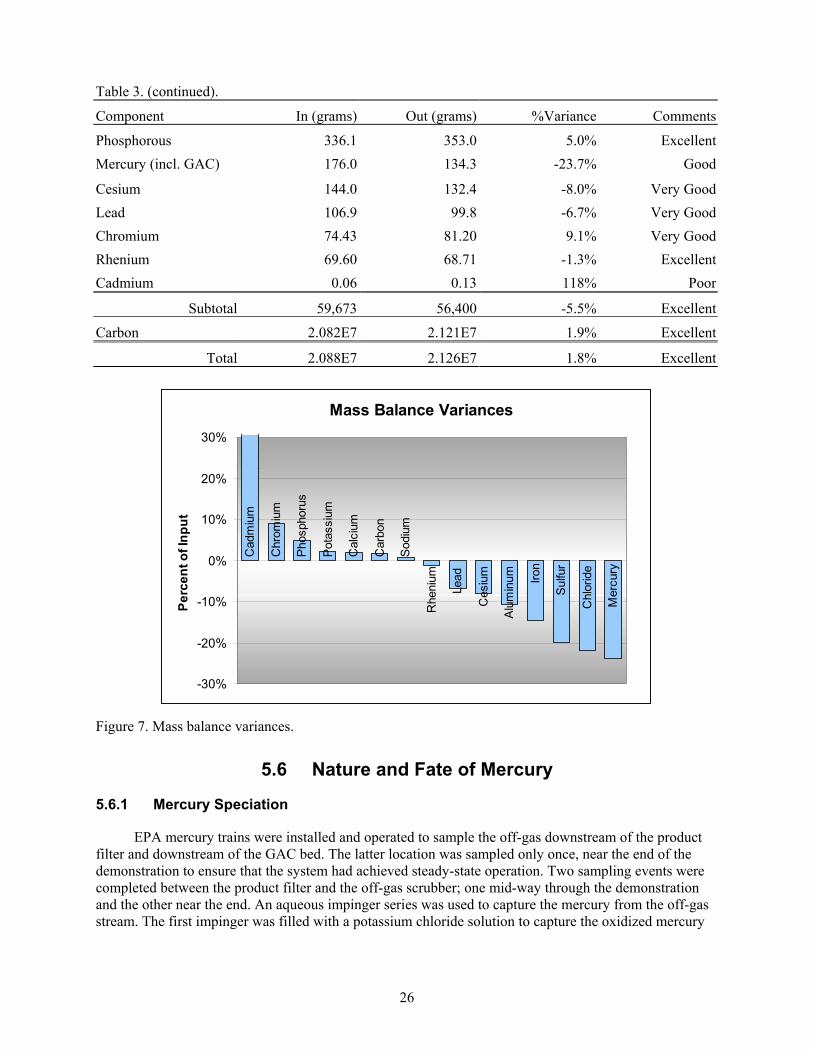
Table 3. (continued).

26

Component In (grams) Out (grams) %Variance Comments

Phosphorous 336.1 353.0 5.0% ExcellentMercury (incl. GAC) 176.0 134.3 -23.7% Good

Cesium 144.0 132.4 -8.0% Very Good Lead 106.9 99.8 -6.7% Very GoodChromium 74.43 81.20 9.1% Very GoodRhenium 69.60 68.71 -1.3% ExcellentCadmium 0.06 0.13 118% Poor

Subtotal 59,673 56,400 -5.5% Excellent

Carbon 2.082E7 2.121E7 1.9% Excellent

Total 2.088E7 2.126E7 1.8% Excellent

Mass Balance Variances

Cad

miu

m

Chr

omiu

m

Pho

spho

rus

Pot

assi

um

Cal

cium

Car

bon

Sod

ium

Rhe

nium

Lead

Ces

ium

Alu

min

um Iron

Sul

fur

Chl

orid

e

Mer

cury

-30%

-20%

-10%

0%

10%

20%

30%

Perc

ent o

f Inp

ut

Figure 7. Mass balance variances.

5.6 Nature and Fate of Mercury

5.6.1 Mercury Speciation

EPA mercury trains were installed and operated to sample the off-gas downstream of the product filter and downstream of the GAC bed. The latter location was sampled only once, near the end of the demonstration to ensure that the system had achieved steady-state operation. Two sampling events were completed between the product filter and the off-gas scrubber; one mid-way through the demonstration and the other near the end. An aqueous impinger series was used to capture the mercury from the off-gas stream. The first impinger was filled with a potassium chloride solution to capture the oxidized mercury

27

in the off-gas. This was followed by impingers designed to remove elemental mercury; namely, potassium permanganate/sulfuric acid and hydrogen peroxide/nitric acid solutions.

One would expect under highly reducing conditions and with the elevated process temperatures, that the mercury would be reduced to the elemental state. This is indeed what was observed with the sampling completed mid-way through the demonstration run. The sampling event at the end of the run, however, showed much more oxidized mercury than elemental mercury upstream of the scrub and almost all elemental mercury passing through the GAC column. This is shown in Table 4. The calculated mass flow rate of mercury passing the sampling probe is about 1% of what would have been expected based on the feed composition and rate (290–295 µg/min.). It is generally accepted that oxidized mercury is readily scrubbed from off-gases by aqueous scrubbers. Given that only a minuscule amount of mercury collected in the scrub, the validity of the anomalous result must be questioned.

Table 4. Mercury speciation from the EPA sample train.

Sample Station Mercury Speciation

ActualConcentration

(µg/acm)

Mass Flow Rate (µg/min)

Percent of Total Mercury

Particle Bound 0.44 0.022 0.0%

Oxidized 24 1.2 0.2%

Elemental 1.2 × 104 580 99.8% Mid-Run

Upstream of Scrubber

Total Hg 1.2 × 104 580 ---

Particle Bound 0.26 0.013 0.0%

Oxidized 3.9 × 103 200 90.9%

Elemental 390 20 9.1% End of Run

Upstream of Scrubber

Total Hg 4.4 × 103 220 ---

Particle Bound 0.22 0.009 0.07%

Oxidized 5.4 0.21 2.4%

Elemental 220 8.4 97.6% End of Run

Downstream of GAC

Total Hg 225 8.6 ---

5.6.2 Mercury in the Product

It is noted that the test platform, used for the demonstration, differed from the process configuration that TTT envisions for a production. Mercury data presented in this section facilitate an understanding of mercury behavior, but may not be representative of a production-scale system.

Mercury concentrations in the cyclone catch were lower than the filter catch, because the product had recently elutriated from the hot reactor and was quickly removed from the off-gas stream. The filter catch, however, operated significantly cooler than the cyclone catch (427°C vs. 558°C) and the filter catch resided as a cake on the filter through which all of the off-gas had to pass. Even though the cyclone catch had a higher elemental carbon content than did the filter catch, the latter had four times as much sorbed mercury (averaging 8.1 mg/kg filter catch vs. 2.0 mg/kg cyclone catch).

28

No mercury was detected in the product recovered from the reactor bed. The cyclone catch contained 0.15 grams of mercury and the filter catch contained 0.22 grams. The total quantity of mercury recovered with the product amounted to less than 0.2% of the mercury fed to the process. That nearly 100% of the mercury would be volatilized was not an unexpected result.

5.6.3 Mercury in the Scrub Solution

Less than 0.002 grams of mercury (<0.001% of input mercury) was detected in the scrub solution, which remained clean and colorless for the entire demonstration run. This would suggest that the mercury was almost entirely elemental. Data in Table 4, above, indicate that this may not have been the case. The average mercury concentration in the scrub was 28 ± 23 µg/ml with one anomalous sample value of 180 µg/ml at the 96-hr COT mark, followed immediately by a more representative result at the 100-hr COT (see Appendix B).

5.6.4 Mercury Captured on the Granular Activated Carbon

The granular activated carbon used in the GAC column for the demonstration was MerSorb, manufactured by NUCON International. It is an extruded carbon that is impregnated with sulfur to amalgamate with sorbed mercury. The GAC column was segmented into three sections, each holding 1.00 kg of virgin GAC. At the conclusion of the 100-hr run, the masses of the three sections within the GAC column increased as shown in Table 5. The total mercury recovered in the GAC was 133.9 grams, or 76.1% of the mercury fed to the process. Mercury recovered in the product and the scrub solution account for less than 1% of the mercury fed to the process.

Table 5. Mercury sorption on the GAC column.

Section 1 Section 2 Section 3

Mass of Section 1.22 kg 1.07 kg 1.03 kg

Mercury Concentration 95.75 gm/kg 13.55 gm/kg 2.50 gm/kg

Sorbed Mercury Mass 116.81 gm 14.50 gm 2.57 gm

Efficiency 66.4% 24.5% 5.8%

5.7 Fate of Cesium and Rhenium

Cesium and technetium are semi-volatile radionuclides that can become problematic in a thermal treatment process because they can be difficult to retain in the product. There has been some indication that both radionuclides may migrate through a system as cesium pertechnetate, which has a cesium to technetium mole ratio of 1:1. To test this mechanism of radionuclide migration, the rhenium was substituted for technetium as a non-radioactive surrogate. Furthermore, the concentrations of cesium and rhenium were artificially inflated to make them more detectable in the product and scrub solutions.

The target cesium and rhenium concentrations in the simulant were 6.41E-3 and 2.29E-3 molar (2.8:1 mole ratio), respectively, which gives cesium to rhenium mass ratio of two. The input streams had a cesium to rhenium mass ratio of 2.07 and the products averaged nearly the same ratio. From Table 6, it can be seen that rhenium had a greater tendency to stay in the bed than did cesium and it was also more likely to be recovered in the filter catch. The cause of the rhenium enrichment in the filter catch is not clear. Cesium perrhenate has a cesium to rhenium mass ratio of 0.71, which could enrich the filter catch in rhenium. Perrhenates are known, however, to be powerful oxidizers that react readily with hydrogen. In industry, elemental rhenium is produced by reducing ammonium perrhenate with hydrogen at elevated

29

temperatures. It is anticipated that the perrhenates are largely reduced to lower oxidation states, possibly even to elemental rhenium, which may explain its greater retention in the bed. The scrub solution (Figure 8) has a mass ratio that is lower than that of cesium perrhenate, which suggests that there are other causes of rhenium enrichment (or cesium depletion) that cannot be attributed to the presence of cesium perrhenate.

Table 6. Cesium and rhenium mass distributions.

Cesium Rhenium

Source Quantity %

Input%

Recovery Quantity %

Input%

Recovery Cs/Re Mass

Ratio

Feed & Additives 144.0 gm 69.9 gm 2.07

Bed Product 0.9 gm 0.6% 0.7% 2.7 gm 3.8% 3.9% 0.34

Cyclone catch 94.9 gm 65.9% 71.7% 41.3 gm 59.4% 60.2% 2.30

Filter catch 36.5 gm 25.4% 27.6% 24.7 gm 35.5% 36.0% 1.48

Scrub Solution 0.004 gm 0.003% 0.003% 0.01 gm 0.01% 0.01% 0.55

Total Recovery 132.4 gm 91.9% 68.7 gm 98.7% 1.93

Scrub Cs/ReMass Ratio

0.0

0.2

0.4

0.6

0.8

12 36 60 84 100COT

(g C

s/g

Re)

Figure 8. Cesium to rhenium mass ratio in the scrub solution.

5.8 Fate of Cadmium, Chromium, and Lead

Cadmium was expressly omitted from the simulant makeup because it is present in the actual WM-180 solution in millimolar concentrations, which doesn’t make it chemically significant for the process, but would pose a significant carcinogenic safety hazard if included in the simulant. Some cadmium was present in small, but measurable, quantities in the blended feed that were below levels considered toxic under the Resource Conservation and Recovery Act (RCRA). Analyses indicate that twice as much cadmium was recovered in the products and scrub solutions than was charged to the process as feed and additives. Of the cadmium recovered, 86% was recovered with the bed product, 9% in

30

the cyclone catch, and 5% in the filter catch. Cadmium concentrations were slightly higher in the filter catch than in the cyclone catch. No cadmium was detected in the scrub solution.

Chromium was added to the simulant as trivalent chromium, which is less hazardous than the hexavalent state. The material balance accounts for 109% of the chromium in the feed, with 61% retained in the bed product, 27% in the cyclone catch, and 12% in the filter catch. Chromium concentrations in the filter catch tended to be slightly higher than in the cyclone catch. Chromium concentrations in the scrub solution were generally below detection levels.

Lead is easily reduced to the elemental state and is fairly volatile. The material balance accounted for 93% of the lead charged to the system with 45% of the recovered lead in the cyclone catch and 55% in the filter catch. Filter catch concentrations were, on average, 3.6 times the cyclone catch concentrations. No lead was detected in the bed product or in the scrub solutions.

5.9 Spent Scrub Composition

The scrub solution used for the demonstration test was a dilute sodium hydroxide solution with an initial pH near 9. The pH remained between 8 and 9 for the duration of the test. No adjustments were made to the scrub composition and no makeup solution was added. The scrub solution level in the scrub tank was controlled by regulating the solution temperature around 59 ± 2°C to maintain a neutral water balance (no net condensation or evaporation of water). The scrub solution level in the tank remained reasonably constant throughout the demonstration run, so changes in composition over time have not been corrected for changes in scrub volume.

Several of the chemical species detected in the scrub solution increased over time while a few others reached a peak value early on and declined as the run continued. Boron, cesium, fluoride, and rhenium are a few of the species that increased in concentration. Magnesium, carbonate, and ammonium seem to have declined in concentration as the run progressed. Graphical representation of the concentrations as a function of time are given in Appendix B.

For the duration of the demonstration, the scrub solution remained colorless, clear, and free of turbidity. No organic carbon was detected in the scrub solution.

5.10 Product Characteristics

In the following discussion of the product characteristics, it is noted that the test platform, used for the demonstration, differed from the process configuration that TTT envisions for a production facility. Product data presented in this section facilitate an understanding of the bed product and gaseous effluents, but may not be representative of product from a production-scale system. Furthermore, no analytical methods were employed in the analysis of the product that were capable of verifying or quantifying the presence of non-crystalline carbonate salts. TTT claims that the majority of the feed salts are converted into carbonate salts in the product. They probably exist as amorphous and/or anhydrous salt compounds.

Two distinct product phases formed on the bed particles. One phase was amber colored spheroids that were “cemented” to the bed particles by the second phase; a white mass that coated the particle substrate and wetted the lower hemisphere of the spheroids. The overall appearance of the particles can be seen in Figure 9. The compositions of the two phases were indistinguishable using the scanning electron microscope.

31

Figure 9. TTT steam reformer bed particles with adherent product.

Some of the spheroidal knobs attritted from the surface of the bed particles, thereby providing seed particles on which additional product was deposited. The actions of attritting and growth can be manipulated to achieve a stable operation within a fluidized bed. It is noteworthy that the particle growth mechanism for the bed product is not like “onion ring” growth observed in the INTEC calciner, where successive feed deposits coat the outer shell and calcine into place, but more that of agglomeration where small particles are captured on the wet surface of larger host particles. This growth mechanism is not indicative of incipient fluidization failure.

As the test progressed, the mean diameter of the bed particles roughly doubled and the particle density decreased from around 3.7 g/cc to between 2.6 and 2.7 g/cc. The net effect of the change in particle parameters is to increase the minimum fluidizing velocity by about a factor of three. Fluidizing gas velocities were several times the minimum fluidizing velocity required for the virgin bed medium and safely above twice the minimum fluidizing velocity for the larger product particles. During the demonstration, no means of obtaining mean particle sizes was provided other than to inspect the product under an optical microscope and no provision was made for measuring particle density. Bed product bulk densities were obtained by weighing a graduated cylinder, which allowed for personnel to monitor the declining trend as alumina was displaced with product in the bed. These parameters would need to be closely monitored in a full-scale facility so that appropriate adjustments to the process could be made to maintain stable operation.

Product elutriated from the bed was collected in the cyclone separator and in the filter vessel. The product was a freely flowing powder with larger pieces of unreacted carbon additive. The Acrison feeder augers abraded some of the activated carbon, producing fines that had a short residence time in the reformer. The soft carbon particles were further abraded by the churning bed and eroded by the steam and

32

oxygen until they elutriated from the bed and were recovered with the cyclone and filter catches. The elemental and organic carbon contents of the products was further augmented by the pyrolysis of the sugar added to the feed in a 200% stoichiometric ratio relative to the nitrates. Micrographs of the cyclone and filter catches can be seen in Figures 10 through 13, which clearly show the remnants of activated carbon among the spongy product particles.

The combined mass of elemental and organic carbon in the products accounted for half of the product weight collected in the cyclone and filter vessels. The cyclone catch had slightly more carbon than the filter catch, but most of the values for the cyclone and filter catches are not statistically different. The data are shown in Table 7. Reported ash values in the table are the inorganic residues from a loss-on-ignition (LOI) analysis. An optimization of the process that either reduced the feed rate of the reductants or improved their residence time in the reformer should result in lower amounts of sugar char and activated carbon in the products.

Data show that several of the metals in the feed were somewhat volatile under the process conditions as evidenced by a disproportionately higher deposition of these metals in the filter catch as compared to the cyclone catch. The most volatile species are lead, mercury, and cadmium. Other species that were enriched in the filter catch include ammonia, chromium, nickel, potassium, rhenium, sodium, and sulfate. Calcium and silicon compounds that elutriated from the bed were more likely found in the cyclone catch. Silicon likely came from the feed makeup water and gravel in the carbon. It is interesting to note, in Table 7, that a portion of the chromium in the feed appears to have become incorporated into the crystalline structure of the alumina substrate. Graphical representations of the product composition are found in Appendix C.

Figure 10. Cyclone catch micrograph.

33

Table 7. Product carbon and LOI ash content.

Analysis Bed Product Cyclone catch Filter catch

Elemental Carbon NA 46 ± 7 wt% 39 ± 5 wt%

Inorganic Carbon 2.2 ± 0.5 wt% 4 ± 3 wt% 3 ± 2 wt%

Organic Carbon 0.2 ± 0.2 wt% 7 ± 6 wt% 11 ± 6 wt%

Total Carbon 2.5 ± 0.7 wt% 57 ± 2 wt% 52 ± 2 wt%

LOI Ash NA 28 ± 2 wt% 29 ± 3 wt%

Number of Samples 6 5 5

Chief Crystalline Phases

-Corundum Cr-doped corundum

(Al1.92Cr0.08O3)

Na1.8(Mg0.9Si1.1O4)CaCO3, and KCl

Na1.8(Mg0.9Si1.1O4)Na2ZnSiO4, and KCl

Figure 11. Cyclone catch micrograph.

34

Figure 12. Filter catch micrograph – 500X.

Figure 13. Filter catch micrograph – 1000X.

The bulk densities were measured for the products as loose, settled (by tapping), and tamped bulk densities. The bed product densities did not change much from the loose bulk density value when settled

35

by rapping the container with a rod. The cyclone and filter catch tamped densities, however, are nearly two and three fold higher than the loose densities. Average density values are given in Table 8.

Table 8. Average product densities.

Product Loose Density Settled Density Tamped Density Particle Density

Bed 1.39 ± 0.09 g/cc 1.43 ± 0.12 g/cc 1.46 ± 0.14 g/cc 2.83 ± 0.15 g/cc

Cyclone 0.24 ± 0.01 g/cc 0.27 ± 0.02 g/cc 0.38 ± 0.02 g/cc 1.50 ± 0.15 g/cc

Filter 0.14 ± 0.02 g/cc 0.16 ± 0.02 g/cc 0.38 ± 0.02 g/cc 1.44 ± 0.17 g/cc

The feed to the process was a solution of WM-180 SBW simulant with a 200% stoichiometric concentration of sucrose (1 lb sucrose for each liter of simulant). Dissolution of the sucrose into the SBW simulant resulted in a 29% volumetric expansion of the solution used for the feed. The average feed rate of 5.45 L/hr corresponds with a simulant feed rate of 4.23 L/hr for a total of 423 L of simulant processed during the demonstration. Detail on the conversion of the feed to product materials are given in Table 9 on the basis of unit volume of unsweetened SBW. A production facility, as envisioned by TTT, would return the cyclone catch to the former and incorporate a secondary reactor to oxidize residual carbon and react with off-gas hydrogen, CO, etc. This would reduce the residual carbon in the product and is expected to reduce overall product volumes relative to these test results.

Table 9. Waste volume and mass reduction data. FEED DATA Feed Processing Rate 5.45 L/hr Equivalent SBW Vol. Rate 4.23 L/hr Equivalent SBW Mass Rate 5.33 kg/hr Total SBW Vol. Processed 423 L Total SBW Mass Processed 533 kg

PRODUCT DATA Recovered Bed Mass 76.2 kg Product Distribution Virgin Bed & Catalyst Mass 38.9 kg Bed 27 wt% Bed Product Inventory 37.3 kg Cyclone 53 wt% Cyclone catch Mass 72.1 kg Filter 20 wt% Filter catch Mass 27.5 kg Total Product 136.9 kg

PRODUCT MASS/SBW MASS PRODUCT VOLUME/SBW VOLUME Settled Product Tamped Product

Bed 0.070 kg/kg 0.06 L/L SBW 0.06 L/L SBW Cyclone 0.135 kg/kg 0.63 L/L SBW 0.45 L/L SBW Filter 0.052 kg/kg 0.41 L/L SBW 0.17 L/L SBW Total Product 0.257 kg/kg 1.10 L/L SBW 0.68 L/L SBW Mass Reduction Volume Reduction 74.3% -10% 32%

36

6. DISCUSSION AND ANALYSIS

CEM measurements were performed to measure for O2, CO2, CO, NO, NOx, H2, and CH4 in the steam reformer off-gas between the heated filter and the venturi scrubber. At this sample location, the off-gas was diluted with some purge N2 and added dilution N2. The dilution N2 lowered the H2concentration in the sample gas, assuring that the H2 concentration did not pose an explosion or flammability hazard when moisture was removed from the sample gas in the sample conditioner. The H2concentration was typically in the 4–4.5% range at the analyzer and is estimated to have averaged near 8% at the outlet of the reformer.

The presence of hydrogen in concentrations exceeding the minimum flammability and explosive values (in air) does not pose a safety threat as long as oxygen and other oxidizing gases are excluded anytime the gas temperatures are below the ignition point. Above the ignition point, the hydrogen will instantaneously react with the gas, thus precluding an accumulation of a flammable or explosive mixture. The system was designed and built to keep air infiltration and inleakage to a minimum, primarily to preserve the integrity and reliability of data collected on the system, but also to prevent oxygen from mixing with hydrogen, carbon monoxide, and methane where gas temperatures are below the ignition temperature. On a production-scale, one would design the process with an oxidizing unit operation to destroy flammable gases before the off-gas is quenched. For the bench-scale system, N2 dilution and an air jet were used to preclude flammable mixtures and ignition sources.

During the optimization tests, an attempt was made to get qualitative assessment on the amount of activated carbon in the bed by halting carbon addition and watching for oxygen breakthrough on the CEM. Instead of observing an increase in oxygen, a rapid increase in temperature was observed at the filter vessel outlet, suggesting oxygen breakthrough had been achieved at the bed and that the filter cake was reacting with the oxygen. The filter pressure drop increased after the temperature excursion had taken place, which caused some concern that the filters may have been damaged or that they may be partially plugged by molten salts formed at the higher temperatures. Repeated attempts to dislodge the filter cake and restore the pressure drop were unsuccessful. A post demonstration inspection of the filters revealed a layer of white powder between the black filter cake and the sintered-metal filter medium. No evidence of a white powder had been observed in the filter catch samples or the product drums. The white powder, however, was easily brushed free from the filters. The interior of the clean gas manifold was discolored from the operating temperatures, but was otherwise in excellent condition. No deposits of particulates were observed on any surfaces downstream of the filter candles, indicating that the filter integrity was sound. A lesson learned is that oxygen sensors will need to be installed between the cyclone and the filter vessel to watch for oxygen breakthrough if this mode of operation is to be used to assess the quantity of carbon in the bed. At no time during the demonstration was a similar oxygen breakthrough test attempted.

Reformer product forms three distinct phases in the THORsm process. The lightest phase has the appearance of shredded sponge and is elutriated from the reformer and captured in the cyclone and filter catch fractions. The other two phases are observed in the bed product particles. These are the amber spheroids and the white phase that acts like a mortar to cement the amber spheroids to the host bed particles. No compositional differences have been observed between the two phases on the bed particles, in spite of their different appearances. The mechanisms for their formation have yet to be explained. The quantities of product forming in the bed relative to that collecting in the cyclone and filter vessels were probably influenced by the inadvertent use of an oversized air cap on the feed nozzle. It is expected that the correctly sized air cap would have caused finer atomization of the feed and greater momentum transfer in the immediate vicinity of the feed nozzle, which would have increased particle grinding action in the jet plume.

37

During the design of a full-scale process, consideration should be given to the types of products that are most desirable. The bed product is denser and contains only a fraction of the carbon found in the cyclone and filter catches, but it represents another product phase that must be handled, packaged, and shipped. Use of a jet grinder to abrade product off the inert bed material could reduce or eliminate the need to routinely drain and collect product off of the bed. The downside of a grinder is that it would not likely discriminate between bed particles and activated carbon (both would be ground) and the increased gas flow rate would shorten the residence time for particles and off-gases in the reformer. The TTT steam reforming system proposes using alumina as a starter bed that would eventually be displaced with product particles. The reformer would be operated with the express intent of removing most of the product from the bed with elutriated carbon and product being treated in a secondary reactor where carbon, CO, H2, and organics will be destroyed.

The activated carbon and sucrose additives did perform admirably well in producing the reducing conditions necessary to destroy NOx. The sugar char and residual activated carbon, however, comprise over half of the mass in the cyclone and filter catch. Recycling the cyclone catch to the reformer will reduce the carbon carryover somewhat, but reducing the carbon inventory in the reformer by increasing the operating temperature would likely have a greater impact on the carbon carryover. The higher temperature would accelerate the production of water-gas and require less of a reformer carbon inventory to achieve a given hydrogen concentration. A denser and less friable carbon source could also reduce carryover, but may have an adverse effect on hydrogen production and NOx reduction. Before the process temperature is elevated, tests should be performed on archived product samples to ensure that molten salt phases would not be encountered.

Rhenium and cesium did not seem to leave the bed in a mass ratio proportionate to that of cesium perrhenate. It is likely that the perrhenate moiety, which is a strong oxidizer, was reduced to rhenium dioxide or rhenium metal. The oxide sublimes at 1,363°C and the metal melts at 3,180°C, so either species would be present only as a solid. It is possible that any rhenium not bound up in the bed product existed as a fume that escaped capture in the cyclone and became trapped by the filter cake. This could explain why rhenium was principally found in the bed and filter catch fractions. The cesium, however, collected preferentially in the cyclone catch fraction. This is possibly due to sorption and condensation of cesium species on the activated carbon fragments.

Volatile toxic metals, such as lead and mercury, are quantitatively removed from the bed product at the operating temperatures. Lead is expected to reduce, under the process conditions, to the elemental metal. Cyclone and filter temperatures are expected to have a strong influence on the quantity of lead captured with cyclone and filter catches. Process temperatures will need to be kept high downstream of the filter to ensure that lead does not foul the piping or perhaps the operating temperature of the filter will need to be reduced so that lead will be captured more efficiently on the filter cake. The off-gas should be maintained either well above the melting point for lead so that lead does not freeze in the filter candles or well enough below the melting point so that lead will be present only as a solid.

The use of an iron oxide catalyst needs to be re-evaluated. The flakes that collected in the bed samples were predominantly iron oxides and unidentified amorphous iron materials. The deposits on and around the distributor bubble caps are believed to be of the same basic composition. The shape of the recovered flakes hint that the iron deposits were forming on the internal surfaces of the reformer and appeared to have a radius of curvature roughly consistent with the internal surfaces of the reformer and 1.5 in. wall penetrations. No dramatic changes in NOx reduction were observed as fresh catalyst was added to the bed during the run. Since catalyst was added before the run started, we cannot discriminate between the catalyst being ineffective and it being overabundant.

38

In response to what was believed to be evidence of agglomerate formation in the bed (gravel in the bed samples and probe plugging) and visual observations of bed product under a microscope, the operating temperature was decreased from 691 to 673°C to avoid large-scale bed agglomeration. Activated carbon addition rate had to be increased to maintain the desired hydrogen concentration in off-gas because the water-gas reaction slowed at the lower temperature. This increased the carbon inventory in the bed and resulted in high bed temperatures near the distributor. As the distributor fouled and gas distribution patterns changed, the temperature probe above the distributor cross registered lower temperatures than expected, except when the probe was blown clear. Blowing the probe cleared defluidized particles away from the probe, thereby exposing the probe to the hot bed material at the bottom of the bed. When this occurred, the registered temperature rose above the average bed temperature by 20 to 40°C and peaked around 700 to 725°C. Had the bed been properly fluidized in the immediate vicinity of the distributor, these temperature extremes would not have been witnessed.

The combination of oxygen being introduced with the fluidizing steam, the presence of iron compounds (i.e., catalyst), and an elevated carbon inventory in the bed worked together to create a condition that promoted the deposition of material on the bubble caps and resulted in the caps being partially blinded off. The deposits were chiefly on the wall-side of the bubble caps with very little on the cross-side of the bubble caps and nothing deposited on the distributor in the vicinity of the T-2 temperature probe that read the temperature extremes.

As expected, the steam reformer off-gas had essentially no O2. Without the purge and dilution N2,the off-gas was mostly (76%) H2O (wet, N2-free basis). CO levels averaged 1.3%, while the measured CH4 levels averaged 0.1%. Neither soluble nor condensable hydrocarbon species were detected in the scrubber solution and were presumably not present in the off-gas at any significant concentration.

7. CONCLUSIONS

The steam reforming process performed well. No serious bed agglomerations were observed and the reactor temperatures remained uniform with the exception of the thermocouple just above the distributor. Nearly three-fourths of the product from the test platform was recovered in the cyclone and filter catches (although half of the mass was carbon).

The sucrose and activated carbon additives produced a reducing environment that resulted in over 98% NOx reduction. The average off-gas NO level was 330 ppm, and the average NO2 concentration was 25 ppm (wet, N2-free basis). The total NOx level was well under the target maximum of 1,000 ppmv. These NOx levels were low enough that they should not cause a visible plume or interfere with performance tests that use manual sampling and analysis. The O2 and H2 levels in the off-gas were low enough that they do not pose a significant threat of forming an explosive mixture. Residual CO, methane, etc. would need to be efficiently destroyed to meet air emission regulations such as the hazardous waste combustor (HWC) MACT standards.

The product was a dry and freely flowing powder that can be densified by settling (e.g., vibratory compaction) or by mechanical compaction to achieve a higher waste loading in storage containers. The product may be hygroscopic, but the residual carbon in the product (~ 50wt%) may prevent the product from forming a crust. Intermediate storage, if required, could be achieved and the product is expected to remain retrievable. Depending on how much compaction is achieved, however, the product volume may be roughly equivalent to the original SBW volume unless the carbon carryover can be reduced. TTT believes that their proposed steam reforming system would harvest mostly bed product and that carbon content would be greatly reduced, which would reduce or eliminate the need for compaction.

39

Volatile metals were recovered in the filter catch except for about one-third of the lead and effectively all of the mercury. Although mercury speciation data have mixed results, it is believed that the mercury exited the reformer as elemental mercury vapors and did not oxidize in the system. The evidence for this is the lack of significant mercury accumulation in the scrub solution and the significant mercury capture in the GAC column. Both lead and mercury were undetectable in the bed product. The process design, however, must accommodate the lead vapors to preclude lead from depositing on surfaces within off-gas handling equipment and piping.

Cesium and rhenium did not escape the process. Only 0.003% of the cesium and 0.01% of the rhenium masses were recovered in the scrub solution. The scrub solution remained clean and clear for the duration of the demonstration run without the necessity to change out the solution or add makeup chemicals. There should be no problem with combining scrubber blowdown with the feed and the volume is expected to be minimal.

The demonstration is considered a success because the specified objectives in Section 1.2 were met and the process had a satisfactory feed rate.

8. REFERENCES

EPA, 2002, Method 6C, “Determination of Sulfur Dioxide Emissions from Stationary Sources (Instrumental Analysis Procedure),” 40 CFR 60, Appendix A.

Holman, J. P., 1978, “Experimental Methods for Engineers,” McGraw-Hill Book Company, New York.

Joyce, Helen, 2003, “Mixed Waste Technology Program Final Report – Sorbents to Capture Volatile Organic Compound Emissions from OASIS Radioactive Sludge 140°F Tests,” MSE Technology Applications.

Marshall, D. W., 2003, “THORsm Steam Reforming Demonstration Test Plan.”

Soelberg, Nick, 2003, “Off-gas Mercury Control for the Idaho Tank Farm Project – Calcination with MACT Upgrade SBW Treatment Alternative,” INEEL EDF-3292, Revision 0.

Summers, R. L., 1976, “NOx Destruction by CO in NOx to NO Converters of Chemiluminescent NO Analyzers,” NASA Technical Memorandum NASA TM X-73480.

9. APPENDIXES

Appendix A—CEMS Calibrations Appendix B—Scrub Solution Composition Appendix C—Product Composition

40

41

Appendix A

CEMS Calibrations

42

43

Tabl

e A

-1. C

EMS

calib

ratio

n da

ta fo

r the

TTT

dem

onst

ratio

n te

st, %

of f

ull s

cale

(FS)

.

Serv

omex

O2

Ecop

hysi

cs N

OEc

ophy

sics

NO

xN

ova

CO

2N

ova

H2

CA

I CO

C

AI C

H4

CA

I O2

CA

I NO

C

AI N

Ox

FS

=25%

FS

=4,0

00 p

pmFS

=4,0

00 p

pmFS

=100

%FS

=5%

FS

=10%

FS

=10,

000

ppm

FS=2

5%

FS=3

,000

ppm

FS=3

,000

ppm

Dat

e Ti

me

Cal

ibra

tion

gas

Zero

Sp

an Z

ero

Span

Ze

ro

Span

Ze

roSp

anZe

roSp

anZe

roSp

anZe

ro

Span

Ze

roSp

anZe

ro

Span

Ze

ro

Span

Com

men

ts

13-J

an-0

3 11

:45

N2

0.0

---

0.0

0.

0 --

- 0.

0 --

- 0.

0--

- 0.

0--

- 0.

0 --

- 0.

0 --

- --

--

- --

--

- C

AI N

Ox n

ot

anal

yzer

read

y ye

t 13

-Jan

-03

11:5

5 6%

CO

/ 0.

8% C

H4 i

n N

2

--

---

--

---

--

---

--

---

--

---

--

0.0

--

0.0

--

---

--

---

--

---

13-J

an-0

3 12

:00

8% C

O2/

1.0%

H2 i

n N

2

--

---

--

---

--

---

--

0.0

--

0.0

--

---

--

---

--

---

--

---

--

---

13-J

an-0

3 12

:05

3% H

2 in

N2

--

---

--

---

--

---

--

---

--

0.0

--

---

--

---

--

---

--

---

--

---

Goo

d H

2 lin

earit

y -

no a

djus

tmen

t ne

eded

13-J

an-0

3 12

:10

air

---

0.0

---

---

---

---

---

---

---

---

---

---

---

---

---

-1.6

---

---

---

---

CA

I O2 m

eter

out

of

span

adj

ustm

ent

13-J

an-0

3 12

:30

zero

-2

.0

---

0.0

---

0.1

---

0.0

---

0.0

---

0.0

-0.1

--

-0.5

-2

.0--

- 0.

0 --

- 0.

0 --

-

13-J

an-0

3 12

:30

zero

0.

0 --

- --

- --

- --

- --

- --

- --

- --

- --

- --

- --

- --

- --

- 0.

0 --

- --

- --

- --

- --

- A

djus

ted

both

O2

met

ers

13-J

an-0

3 12

:30

air

---

2.0

---

---

0.2

---

--

---

--

---

--

---

--

---

--

0.0

--

---

--

---

13

-Jan

-03

12:3

0 ai

r --

- 0.

0 --

- --

- --

- --

- --

--

- --

--

- --

--

- --

--

- --

--

- --

--

- --

--

- A

djus

ted

O2 m

eter

13

-Jan

-03

12:4

5 49

5 N

O/

496

NO

x in

N2

---

---

---

-1.2

--

- --

- --

--

- --

--

- --

--

- --

--

- --

--

- --

1.

8 --

1.

8 D

id n

ot a

djus

t NO

xm

eter

s 13

-Jan

-03

13:0

0 1,

504

NO

/ 1,

508

NO

x in

N2

---

---

---

-4.2

--

- -4

.2

--

---

--

---

--

---

--

---

--

---

--

---

--

---

13-J

an-0

3 13

:00

1,50

4 N

O/

1,50

8 N

Ox i

n N

2

---

---

---

0.0

---

0.0

---

---

---

---

---

---

---

---

---

---

---

---

---

---

Adj

uste

d N

Ox m

eter

s

13-J

an-0

3 13

:15

dilu

ted

200

ppm

NO

2

---

---

0.0

---

---

---

---

---

---

---

---

---

---

---

---

---

1.3

---

---

---

Neg

ligib

le

inte

rfer

ence

from

N

O2 o

n N

O d

etec

tion

13-J

an-0

3 13

:20

air

---

0.0

---

---

0.0

---

---

---

---

---

---

---

---

---

---

0.0

---

---

0.1

---

13

-Jan

-03

13:2

5 di

lute

d 49

5 N

O/

496

NO

x in

N2

0.0

---

---

---

---

---

0.0

---

0.0

---

-0.6

---

-1.9

--

- 0.

0 --

- --

- --

- --

- --

-

Tabl

e A

-1. (

cont

inue

d).

44

Se

rvom

ex O

2 Ec

ophy

sics

NO

Ecop

hysi

cs N

Ox

Nov

a C

O2

Nov

a H

2C

AI C

O

CA

I CH

4 C

AI O

2 C

AI N

O

CA

I NO

x

FS

=25%

FS

=4,0

00 p

pmFS

=4,0

00 p

pmFS

=100

%FS

=5%

FS

=10%

FS

=10,

000

ppm

FS=2

5%

FS=3

,000

ppm

FS=3

,000

ppm

Dat

e Ti

me

Cal

ibra

tion

gas

Zero

Sp

an Z

ero

Span

Ze

ro

Span

Ze

roSp

anZe

roSp

anZe

roSp

anZe

ro

Span

Ze

roSp

anZe

ro

Span

Ze

ro

Span

Com

men

ts

13-J

an-0

3 14

:00

N2

-0.4

--

- 0.

0 --

- 0.

5 --

- 0.

0 --

- 2.

0--

- -0

.4--

- -0

.6

---

-0.8

---

0.0

---

0.0

---

Slow

resp

onse

by

Ecop

hysi

cs in

NO

xm

ode

13-J

an-0

3 14

:44

N2

---

---

0.0

---

0.0

---

---

---

---

---

---

---

---

---

---

---

0.1

---

0.1

---

14

-Jan

-03

15:0

1 A

ir --

- -0

.4

---

---

---

---

---

---

---

---

---

---

---

---

---

0.4

---

---

---

---

14

-Jan

-03

15:0

2 3%

H2 i

n N

2 --

- --

- --

- --

- --

- --

- --

- --

- --

- 0.

0--

- --

- --

- --

- --

- --

- --

- --

- --

- --

-

14-J

an-0

3 15

:05

8% C

O2/

1% H

2 in

N2

---

---

---

---

---

---

---

0.0

---

2.0

---

---

---

---

---

---

---

---

---

---

15-J

an-0

3 19

:38

N2

---

---

---

---

4.0

---

---

---

---

---

---

---

---

---

---

---

---

---

---

---

+160

ppm

NO

x bia

s on

Eco

phys

ics m

eter

15

-Jan

-03

19:4

0 di

lute

d 1,

504

NO

/ 1,

508

NO

x in

N2

1.6

---

---

---

---

---

0.1

---

6.0

---

0.5

---

0.9

---

1.6

---

---

---

---

---

15-J

an-0

3 19

:51

dilu

ted

200

ppm

NO

2

---

---

0.0

---

---

---

---

---

---

---

---

---

---

---

---

---

0.0

---

---

---

15-J

an-0

3 19

:54

N2

0.8

---

0.0

---

1.0

---

0.1

---

4.0

---

-0.5

---

-1.0

--

- 0.

8 --

- --

- --

- 0.

1 --

- 40

ppm

bia

s on

Ecop

hysi

cs N

Ox

16-J

an-0

3 21

:20

N2

---

---

0.0

---

4.3

---

---

---

---

---

---

---

---

---

---

---

0.1

---

0.1

---

172

ppm

Eco

phys

ics

NO

x bia

s 16

-Jan

-03

21:2

6 di

lute

d 20

0 pp

m N

O2

---

---

0.1

---

---

---

---

---

---

---

---

---

---

---

---

---

2.0

---

---

---

16-J

an-0

3 21

:30

N2

0.4

---

0.0

---

---

---

0.1

---

4.0

---

-0.6

---

-0.6

--

- 0.

8 --

- 0.

0 --

- --

- --

-

16-J

an-0

3 21

:30

N2

0.0

---

0.0

---

---

---

0.0

---

0.0

---

0.0

---

---

---

0.0

---

0.0

---

---

---

re-z

eroe

d 16

-Jan

-03

21:3

7 8%

CO

2/ 1%

H2

in N

2

---

---

---

---

---

---

---

-0.3

---

-2.0

---

---

---

---

---

---

---

---

---

---

16-J

an-0

3 21

:37

8% C

O2/

1% H

2in

N2

---

---

---

---

---

---

---

0.0

---

0.0

---

---

---

---

---

---

---

---

---

---

re-s

pann

ed

16-J

an-0

3 21

:39

6% C

O/

0.8%

CH

4 in

N2

---

---

---

---

---

---

---

0.2

---

0.4

---

---

---

---

---

---

---

---

---

---

16-J

an-0

3 21

:39

6% C

O/

0.8%

CH

4 in

N3

---

---

---

---

---

---

---

0.0

---

0.0

---

---

---

---

---

---

---

---

---

---

re-s

pann

ed

16-J

an-0

3 21

:44

air

---

-0.4

--

- --

- --

- --

- --

- --

- --

- --

- --

- --

- --

- --

- --

- 0.

4 --

- --

- --

- --

-

Tabl

e A

-1. (

cont

inue

d).

45

Se

rvom

ex O

2 Ec

ophy

sics

NO

Ecop

hysi

cs N

Ox

Nov

a C

O2

Nov

a H

2C

AI C

O

CA

I CH

4 C

AI O

2 C

AI N

O

CA

I NO

x

FS

=25%

FS

=4,0

00 p

pmFS

=4,0

00 p

pmFS

=100

%FS

=5%

FS

=10%

FS

=10,

000

ppm

FS=2

5%

FS=3

,000

ppm

FS=3

,000

ppm

Dat

e Ti

me

Cal

ibra

tion

gas

Zero

Sp

an Z

ero

Span

Ze

ro

Span

Ze

roSp

anZe

roSp

anZe

roSp

anZe

ro

Span

Ze

roSp

anZe

ro

Span

Ze

ro

Span

Com

men

ts

16-J

an-0

3 21

:44

air

---

0.0

---

---

---

---

---

---

---

---

---

---

---

---

---

0.0

---

---

---

---

re-s

pann

ed

17-J

an-0

3 21

:55

N2

---

---

---

---

0.0

---

---

---

---

---

---

---

---

---

---

---

0.0

---

0.1

---

11 p

pm E

coph

ysic

s N

Ox b

ias

17-J

an-0

3 21

:57

dilu

ted

200

ppm

NO

2

---

---

0.0

---

---

---

---

---

---

---

---

---

---

---

---

---

1.2

---

---

---

17-J

an-0

6 22

:04

N2

0.0

---

0.0

---

0.0

---

0.0

---

0.0

---

0.0

---

0.4

---

0.0

---

0.1

---

0.2

---

17

-Jan

-03

22:0

7 8%

CO

2/1%

H2 i

n N

2

---

---

---

---

---

---

---

0.1

---

0.0

---

---

---

---

---

---

---

---

---

---

17-J

an-0

3 22

:10

6% C

O/

0.8%

CH

4 in

N3

---

---

---

---

---

---

---

---

---

---

---

0.5

---

2.8

---

---

---

---

---

---

17-J

an-0

3 22

:12

3% H

2 in

N2

---

---

---

---

---

---

---

---

---

0.0

---

---

---

---

---

---

---

---

---

---

17

-Jan

-03

22:1

4 ai

r --

- 0.

0 --

- --

- --

- --

- --

- --

- --

- --

- --

- --

- --

- --

- --

- 0.

0 --

- --

- --

- --

-

--

- --

- --

- --

- --

- --

- --

- --

- --

- --

- --

- --

- --

- --

- --

- --

- --

- --

- --

- --

-

Ave

rage

s 0.

0 0.

2 0.

0 --

- 0.

9 --

- 0.

0 0.

0 1.

8 0.

0 -0

.2

0.1

-0.4

0.

8 0.

0 -0

.1

0.4

---

0.1

---

NO

x spa

n/di

lutio

n ca

ls a

re re

porte

d se

para

tely

Acc

epta

nce

limits

2.

0 2.

0 2.

0 2.

0 2.

0 2.

0 2.

0 2.

0 --

- --

- 5.

0 5.

0 --

- --

- 2.

0 2.

0 2.

0 2.

0 2.

0 2.

0

Ref

eren

ce fo

r acc

epta

nce

limits

40

CFR

60

App

. A

Met

hod

3A

40 C

FR 6

0 A

pp. A

M

etho

d 7E

40 C

FR 6

0 A

pp. A

Met

hod

7E

40 C

FR 6

0A

pp. A

Met

hod

3A

Non

e 40

CFR

60

App

. AM

etho

d 10

Non

e 40

CFR

60

App

. A

Met

hod

3A

40 C

FR 6

0 A

pp. A

M

etho

d 7E

40 C

FR 6

0A

pp. A

M

etho

d 7E

Any

cor

rect

ion

base

d on

ca

libra

tions

? no

no

no

ye

s - se

e be

low

yes -

see

belo

w

no

no

no

no

no

no

no

no

no

no

no

yes -

see

belo

wno

ye

s - se

e be

low

All

NO

x dat

a is

co

rrec

ted

for t

he

com

posi

te a

ir di

lutio

n/sp

an

calib

ratio

n fa

ctor

46

Tabl

e A

-2. N

Ox m

eter

cor

rect

ion

fact

ors f

or d

ilutio

n an

d ca

libra

tion.

Serv

omex

O2

Ecop

hysi

cs N

OEc

ophy

sics

NO

xN

ova

CO

2N

ova

H2

CA

I CO

C

AI C

H4

CA

I O2

CA

I NO

C

AI N

Ox

FS

=25%

FS

=4,0

00 p

pmFS

=4,0

00 p

pmFS

=100

%FS

=5%

FS

=10%

FS

=10,

000

ppm

FS=2

5%FS

=3,0

00 p

pmFS

=3,0

00 p

pm

Dat

e Ti

me

Cal

ibra

tion

gas

Zero

Sp

an

Zero

Sp

anZe

ro

Span

Ze

roSp

anZe

roSp

anZe

roSp

an

Zero

Sp

an

Zero

Span

Zero

Sp

an

Zero

Span

C

omm

ents

13-J

an-0

3 13

:05

dilu

ted

1,50

4 N

O/

1,50

8 N

Ox i

n N

2

4.

9

4.8

5.

1

4.9

Rot

amet

er

dilu

tion

for

Ecop

hysi

cs m

eter

is

5×

dilu

tion:

for

CA

I, 5.

2

13-J

an-0

3 13

:15

dilu

ted

200

ppm

NO

2

6.

20

6.

97

Som

e in

abili

ty to

de

tect

NO

2 is

appa

rent

bec

ause

th

e co

rrec

tion

fact

or fo

r hig

h N

O2 i

s hig

her

than

for N

O.

13-J

an-0

3 13

:25

dilu

ted

495

NO

/ 49

6 N

Ox i

n N

2

5.

35

5.

28

4.

42

4.

31

13-J

an-0

3 13

:35

dilu

ted

495

NO

/ 49

6 N

Ox i

n N

2

5.

38

4.

50

13-J

an-0

3 15

:00

dilu

ted

1,50

4 N

O/

1,50

8 N

Ox i

n N

2

4.

87

5.

00

3.

46

3.

57

Cha

nged

dilu

tion

fact

or fo

r CA

I -

0.75

and

3.0

14-J

an-0

3 14

:47

dilu

ted

495

NO

/ 49

6 N

Ox i

n N

2

4.

60

4.

90

3.

20

3.

40

Ave

rage

s fo

r CEM

S pe

riod

1

4.

74

4.

95

3.

33

--

- Fa

ilure

to d

etec

t N

O2

14-J

an-0

3 14

:55

dilu

ted

1,50

4 N

O/

1,50

8 N

Ox i

n N

2

4.

86

5.

31

3.

45

3.

57

15-J

an-0

3 19

:41

dilu

ted

1,50

4 N

O/

1,50

8 N

Ox i

n N

2

4.

90

4.

90

3.

17

3.

20

Tabl

e A

-2. (

cont

inue

d).

47

Se

rvom

ex O

2 Ec

ophy

sics

NO

Ecop

hysi

cs N

Ox

Nov

a C

O2

Nov

a H

2 C

AI C

O

CA

I CH

4 C

AI O

2 C

AI N

O

CA

I NO

x

FS

=25%

FS

=4,0

00 p

pmFS

=4,0

00 p

pmFS

=100

%FS

=5%

FS

=10%

FS

=10,

000

ppm

FS=2

5%FS

=3,0

00 p

pmFS

=3,0

00 p

pm

Dat

e Ti

me

Cal

ibra

tion

gas

Zero

Sp

an

Zero

Sp

anZe

ro

Span

Ze

roSp

anZe

roSp

anZe

roSp

an

Zero

Sp

an

Zero

Span

Zero

Sp

an

Zero

Span

C

omm

ents

15-J

an-0

3 19

:51

dilu

ted

200

ppm

NO

2

5.

00

50

.00

The

CA

I ana

lyze

r fa

iled

to d

etec

t N

O2

Ave

rage

s fo

r CEM

S pe

riod

2

4.

79

5.

04

3.

27

--

- Fa

ilure

to d

etec

t N

O2

16-J

an-0

3 21

:24

dilu

ted

495

NO

/ 49

6 N

Ox i

n N

2

5.

00

5.

00

3.

30

3.

60

16-J

an-0

3 21

:26

dilu

ted

200

ppm

NO

2

5.

40

83

.00

Ave

rage

s fo

r CEM

S pe

riod

3

4.

95

4.

95

3.

24

--

- Fa

ilure

to d

etec

t N

O2

17-J

an-0

3 21

:57

dilu

ted

495

NO

/ 49

6 N

Ox i

n N

2

7.

00

7.

20

4.

10

4.

00

17-J

an-0

3 21

:57

dilu

ted

200

ppm

NO

2

8.

30

40

.00

Ave

rage

s fo

r CEM

S pe

riod

4

6.

00

6.

10

3.

70

--

- Fa

ilure

to d

etec

t N

O2

Ave

rage

s

5.12

5.26

3.38

---

Failu

re to

det

ect

NO

2

Ave

rage

zer

o bi

as

96

48

Tabl

e A

-3. C

orre

cted

dry

, N2-d

ilute

d of

f-ga

s com

posi

tion

for t

he T

TT d

emon

stra

tion

test

.

Tim

e O

2 avg

%

CO

2%

CO

%

NO

Ec

ophy

sics

ppm

NO

2Ec

ophy

sics

ppm

NO

xEc

ophy

sics

pp

m

NO

C

AI p

pmN

O2

CA

I ppm

NO

xC

AI p

pmA

vg

NO

ppm

H2 %

C

H4 p

pmN

2 %

Tota

l %

Ave

rage

s CEM

S Pe

riod

1 (J

an 1

3, 1

8:08

to Ja

n 14

, 13

:53)

0.

41

8.61

0.

839

226

101

328

264

-5

259

245

4.45

51

7 85

.7

100.

0

Ave

rage

s CEM

S Pe

riod

2 (J

an 1

4, 1

5:09

to Ja

n 15

, 19

:39)

0.

33

8.10

0.

726

108

23

131

148

1 14

8 12

8 4.

62

582

86.2

10

0.0

Ave

rage

s CEM

S Pe

riod

3 (J

an 1

5, 2

0:03

to Ja

n 16

, 21

:20)

0.

27

7.60

0.

647

147

27

174

185

-8

178

166

4.25

53

8 87

.2

100.

0

Ave

rage

s CEM

S Pe

riod

4 (J

an 1

6, 2

1:51

to Ja

n 17

, 21

:47)

-0

.02

7.37

0.

698

266

-75

186

306

-21

285

286

3.94

61

1 88

.0

100.

0

Test

ave

rage

s 0.

24

7.89

0.

721

180

13

192

220

-8

212

200

4.32

56

5 86

.8

100.

0

1.

The

mea

sure

men

ts o

f the

two

O2 m

eter

s are

ess

entia

lly id

entic

al; t

he a

vera

ge v

alue

is u

sed

in c

alcu

latio

ns.

2.

The

N2 c

once

ntra

tion

is d

eter

min

ed b

y di

ffer

ence

from

100

% o

f the

%-le

vel g

as sp

ecie

s; p

pm-le

vel g

as sp

ecie

s, le

vels

of a

ny u

nmea

sure

d sp

ecie

s, an

d tra

ce

H2O

are

not

incl

uded

in th

e ca

lcul

atio

n.

3.

No

zero

or s

pan

corr

ectio

ns w

ere

nece

ssar

y fo

r O2,

CO

2, C

O, H

2, or

CH

4.

4.

The

NO

x dat

a ha

s bee

n ad

just

ed fo

r air

dilu

tion

in th

e C

EMS,

and

for c

alib

ratio

n er

ror,

usin

g th

e di

lutio

n/ca

libra

tion

fact

ors d

eter

min

ed d

urin

g ca

libra

tions

.

49

Tabl

e A

-3. (

cont

inue

d).

The

aver

age

dilu

tion/

calib

ratio

n fa

ctor

s are

:

Ec

olog

ic a

naly

zer

CA

I ana

lyze

r

N

O

NO

x N

O

NO

x

CEM

S Pe

riod

1, 1

3 Ja

n, 1

7:00

to 1

4 Ja

n, 1

4:00

4.

74

4.95

3.

33

3.49

CEM

S Pe

riod

2, 1

4 Ja

n, 1

5:07

to 1

5 Ja

n, 1

9:39

4.

79

5.04

3.

27

3.39

CEM

S Pe

riod

3, 1

5 Ja

n, 1

9:59

to 1

6 Ja

n, 2

1:20

4.

95

4.95

3.

24

3.40

CEM

S Pe

riod

4, 1

6 Ja

n, 2

1:51

to 1

7 Ja

n, 2

1:47

6.

00

6.10

3.

70

3.80

The

Test

Per

iod

4 ca

libra

tion

valu

es tr

ende

d hi

gher

than

the

prio

r ca

l per

iods

bec

ause

of a

hig

h po

st-te

st c

alib

ratio

n. A

n ex

act c

ause

of

the

high

cal

ibra

tion

was

not

iden

tifie

d, so

the

high

val

ues w

ere

aver

aged

with

the

othe

rs. T

his i

ncre

ased

the

corr

ecte

d N

O a

nd N

Ox

valu

es b

y ab

out 6

%.

Tes

t ave

rage

s 5.

12

5.26

3.

39

3.52

Th

ese

aver

age

corr

ectio

n fa

ctor

s are

use

d fo

r all

perio

ds

Std

dev

of d

ilutio

n/co

rrec

tion

fact

ors,

% o

f ave

rage

11

.59

10.6

8 6.

30

5.45

The

aver

age

NO

x zer

o bi

as fa

ctor

s are

, in

ppm

: 0

96

0 0

Thes

e va

lues

are

subt

ract

ed fr

om th

e as

-mea

sure

d N

Ox v

alue

s

5.

The

NO

2 val

ues a

re v

ery

sens

itive

to th

e er

rors

in th

e N

O a

nd N

Ox m

easu

rem

ents

. Per

cent

err

or in

the

NO

2 mea

sure

men

ts, b

ased

on

1 st

d de

v of

the

NO

and

N

Ox m

easu

rem

ents

, is:

Ecop

hysi

cs N

O2 %

err

or

= 21

9 C

AI N

O2 %

err

or

= 22

5

6.

Rel

ativ

e %

diff

eren

ce fo

r the

NO

and

NO

x mea

sure

men

ts: R

PD =

Rel

ativ

e Pe

rcen

t Diff

eren

ce b

etw

een

two

valu

es th

at re

pres

ent t

he sa

me

num

ber =

2 ×

(Val

ue 2

- V

alue

1)/(

Val

ue 2

+ V

alue

1) ×

100

%.

NO

: 19

.8

Rel

ativ

e %

diff

eren

ce

NO

x: 10

.0

Rel

ativ

e %

diff

eren

ce

7.

Ave

rage

% o

f tot

al N

Ox t

hat i

s NO

.

Ecop

hysi

cs:

7.0

CA

I: N

ot c

alcu

lata

ble

50

Tabl

e A

-4. C

orre

cted

wet

, N2-d

ilute

d of

f-ga

s com

posi

tion.

Tim

e O

2 avg

%

CO

2 %C

O %

A

vgN

O p

pmN

O2

Ecop

hysi

cs p

pmN

Ox

Ecop

hysi

cs p

pmH

2 %

CH

4pp

m

H2O

%N

2 %To

tal %

D

ilute

d of

f-ga

s mol

e w

t

Ave

rage

s CEM

S Pe

riod

1,

(Jan

13,

18:

08 to

Jan

14, 1

3:53

) 0.

30

6.45

0.

629

170

76

246

3 38

8 25

.0

64.3

10

0.0

25.7

Ave

rage

s CEM

S Pe

riod

2,

(Jan

14,

15:

09 to

Jan

15, 1

9:39

) 0.

25

6.03

0.

540

80

17

97

3 43

3 25

.6

64.2

10

0.0

25.5

Ave

rage

s CEM

S Pe

riod

3,

(Jan

15,

20:

03 to

Jan

16, 2

1:20

) 0.

19

5.39

0.

459

104

19

123

3 38

1 29

.1

61.9

10

0.0

25.2

Ave

rage

s CEM

S Pe

riod

4,

(Jan

16,

21:

51 to

Jan

17, 2

1:47

) -0

.01

5.11

0.

485

184

-51

129

3 42

5 30

.6

61.0

10

0.0

25.0

Test

ave

rage

s 0.

17

5.57

0.

509

127

10

135

3 39

9 29

.4

61.3

10

0.0

25.2

51

Tabl

e A

-5. C

orre

cted

wet

, N2-f

ree

off-

gas c

ompo

sitio

n fo

r the

TTT

dem

onst

ratio

n te

st.

Tim

e O

2 avg

% C

O2 %

CO

%

Avg

NO

ppm

NO

2Ec

ophy

sics

ppm

NO

xEc

ophy

sics

ppm

H2 %

CH

4 ppm

H2O

%N

2 %To

tal %

N2-f

ree

off-

gas m

ole

wt

Ave

rage

s CEM

S Pe

riod

1,

(Jan

13,

18:

08 to

Jan

14, 1

3:53

) 0.

85

18.1

1.

76

475

212

689

9.33

1,

084

70.0

0

100.

0 21

.5

Ave

rage

s CEM

S Pe

riod

2,

(Jan

14,

15:

09 to

Jan

15, 1

9:39

) 0.

69

16.8

1.

51

224

49

272

9.60

1,

209

71.4

0

100.

0 21

.1

Ave

rage

s CEM

S Pe

riod

3,

(Jan

15,

20:

03 to

Jan

16, 2

1:20

) 0.

50

14.1

1.

20

273

51

323

7.90

1,

000

76.3

0

100.

0 20

.6

Ave

rage

s CEM

S Pe

riod

4,

(Jan

16,

21:

51 to

Jan

17, 2

1:47

) -0

.03

13.1

1.

24

473

-131

33

2 7.

01

1,09

0 78

.7

0 10

0.0

20.4

Test

ave

rage

s 0.

44

14.5

1.

33

330

21

352

7.96

1,

040

75.8

0

100.

0 20

.7

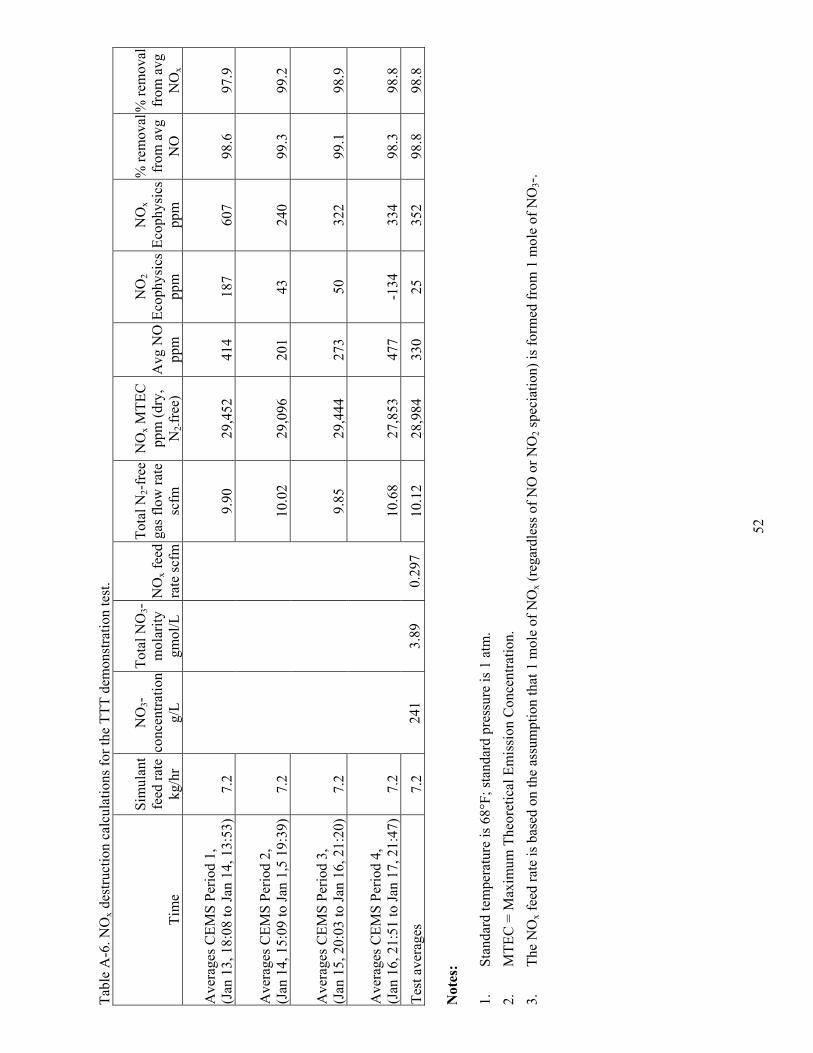
52

Tabl

e A

-6. N

Ox d

estru

ctio

n ca

lcul

atio

ns fo

r the

TTT

dem

onst

ratio

n te

st.

Tim

e

Sim

ulan

t fe

ed ra

te

kg/h

r

NO

3-co

ncen

tratio

ng/

L

Tota

l NO

3-m

olar

ity

gmol

/L

NO

xfe

edra

te sc

fm

Tota

l N2-f

ree

gas f

low

rate

sc

fm

NO

x MTE

C

ppm

(dry

, N

2-fr

ee)

Avg

NO

pp

m

NO

2Ec

ophy

sics

pp

m

NO

xEc

ophy

sics

pp

m

% re

mov

al

from

avg

N

O

% re

mov

al

from

avg

N

Ox

Ave

rage

s CEM

S Pe

riod

1,

(Jan

13,

18:

08 to

Jan

14, 1

3:53

) 7.

2 9.

90

29,4

52

414

187

607

98.6

97

.9

Ave

rage

s CEM

S Pe

riod

2,

(Jan

14,

15:

09 to

Jan

1,5

19:3

9)

7.2

10.0

2 29

,096

20

1 43

24

0 99

.3

99.2

Ave

rage

s CEM

S Pe

riod

3,

(Jan

15,

20:

03 to

Jan

16, 2

1:20

) 7.

2 9.

85

29,4

44

273

50

322

99.1

98

.9

Ave

rage

s CEM

S Pe

riod

4,

(Jan

16,

21:

51 to

Jan

17, 2

1:47

) 7.

2 10

.68

27,8

53

477

-134

33

4 98

.3

98.8

Te

st a

vera

ges

7.2

241

3.89

0.

297

10.1

2 28

,984

33

0 25

35

2 98

.8

98.8

Not

es:

1.

Stan

dard

tem

pera

ture

is 6

8°F;

stan

dard

pre

ssur

e is

1 a

tm.

2.

MTE

C =

Max

imum

The

oret

ical

Em

issi

on C

once

ntra

tion.

3.

Th

e N

Ox f

eed

rate

is b

ased

on

the

assu

mpt

ion

that

1 m

ole

of N

Ox (

rega

rdle

ss o

f NO

or N

O2 s

peci

atio

n) is

form

ed fr

om 1

mol

e of

NO

3-.

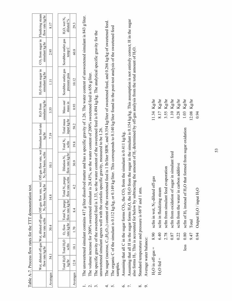
53

Tabl

e A

-7. P

roce

ss fl

ow ra

tes f

or th

e TT

T de

mon

stra

tion

test

.

Wet

, dilu

ted

off-

gas

flow

rate

kg/

hr

Wet

, dilu

ted

off-

gas

flow

rate

scfm

O

ff-g

as fl

ow ra

te, w

et

N2-

free

bas

is, k

g/hr

O

ff-g

as fl

ow ra

te, w

et

N2-

free

bas

is, s

cfm

Si

mul

ant f

eed

rate

kg

/hr

H2O

from

si

mul

ant k

g/hr

H

2O fr

om su

gar i

n si

mul

ant k

g/hr

C

O2 f

rom

suga

r in

sim

ulan

t kg/

hr

Flui

dizi

ng st

eam

flo

w ra

te k

g/hr

Ave

rage

s 54

.1

30.4

14

.8

10.1

7.

19

3.55

1.

11

2.95

8.

17

Tota

l H2O

kg/h

rTo

tal H

2Osc

fm

O2 f

low

ra

te k

g/hr

To

tal N

2 pur

ge

flow

rate

kg/

hrTo

tal N

2 pur

ge

flow

rate

scfm

D

ilutio

n N

2flo

w ra

te k

g/hr

Tota

l N2

scfm

To

tal m

ass

inpu

t kg/

hr

Mas

s out

/ m

ass i

n Sc

rubb

er o

utle

t gas

pr

essu

re p

sia

Scru

bber

out

let g

as

tem

p C

H

2O, w

et N

2di

lute

d %

Ave

rage

s 12

.8

10.1

1.

70

8.4

4.2

30.9

19

.8

58.2

0.

93

10.1

2 60

.8

29.3

1.

The

unsw

eete

ned

sim

ulan

t con

tain

s 417

g/li

ter d

isso

lved

mat

ter a

nd h

as a

spec

ific

grav

ity o

f 1.2

6. T

he w

ater

con

tent

of u

nsw

eete

ned

sim

ulan

t is 8

43 g

/lite

r.

2.

The

volu

me

incr

ease

for 2

00%

swee

tene

d si

mul

ant i

s 28.

43%

, so

the

wat

er c

onte

nt o

f 200

% sw

eete

ned

feed

is 6

56 g

/lite

r. 3.

Th

e sp

ecifi

c gr

avity

of t

he sw

eete

ned

feed

is 1

.33,

so th

e w

ater

con

tent

of t

he sw

eete

ned

feed

is 0

.494

kg/

kg. T

he a

naly

tical

spec

ific

grav

ity fo

r the

un

swee

tene

d si

mul

ant a

gree

s wel

l with

the

corio

lis sp

ecifi

c gr

avity

, mea

sure

d to

be

1.26

. 4.

Th

e su

gar (

sucr

ose,

C12

H22

O11

) con

tent

of t

he sw

eete

ned

feed

is 1

lb/li

ter S

BW

, and

0.3

54 k

g/lit

er o

f sw

eete

ned

feed

, and

0.2

66 k

g/kg

of s

wee

tene

d fe

ed.

5.

The

orga

nic

C o

f the

sim

ulan

t is 0

.112

kg/

kg, o

r 0.1

49 k

g/lit

er. T

his c

orre

spon

ds to

0.1

40 k

g/lit

er fo

und

in th

e po

st-te

st a

naly

sis o

f the

swee

tene

d fe

ed

sam

ples

. 6.

A

ssum

ing

that

all

C in

the

suga

r for

ms C

O2,

the

CO

2 fro

m th

e si

mul

ant i

s 0.4

11 k

g/kg

. 7.

A

ssum

ing

that

all

H in

the

suga

r for

ms H

2O, t

he H

2O fr

om th

e su

gar i

n th

e si

mul

ant i

s 0.1

54 k

g/kg

. Thi

s ass

umpt

ion

is n

ot e

ntire

ly c

orre

ct; H

in th

e su

gar

also

form

s H2.

This

is a

ccou

nted

for b

elow

by

subt

ract

ing

the

amou

nt o

f H2 d

eter

min

ed b

y of

f-ga

s ana

lysi

s fro

m th

e to

tal a

mou

nt o

f H2O

.8.

St

anda

rd te

mpe

ratu

re a

nd p

ress

ure

is 6

8°F

and

1 at

m.

9.

Ave

rage

wat

er b

alan

ce:

H2O

in o

ff-g

as =

8.

90

scfm

in w

et, N

2-dilu

ted

off-

gas

11.3

4K

g/hr

H

2O fe

d =

6.

40

scfm

in fl

uidi

zing

stea

m

8.17

Kg/

hr

2.

78

scfm

from

sim

ulan

t fee

d ev

apor

atio

n 3.

55K

g/hr

0.87

sc

fm fr

om o

xida

tion

of su

gar i

n si

mul

ant f

eed

1.10

Kg/

hr

0.

22

scfm

from

the

wat

er in

car

bon

addi

tive

0.28

Kg/

hr

less

0.

80

scfm

of H

2 ins

tead

of H

2O th

at fo

rmed

from

suga

r oxi

datio

n1.

03K

g/hr

9.47

To

tal

12.0

8K

g/hr

0.94

O

utpu

t H2O

/ in

put H

2O

0.94

54

Tabl

e A

-7. (

cont

inue

d).

10.

The

aver

age

carb

on p

elle

t fee

d ra

te w

as d

eter

min

ed b

y su

mm

ing

all o

f the

car

bon

hopp

er a

dditi

ons a

nd su

btra

ctin

g th

e fin

al h

oppe

r wei

ght f

rom

the

initi

al

hopp

er w

eigh

t:

Hop

per a

dditi

ons =

7 a

t 50

lb e

ach,

2 a

t 25

lb e

ach,

and

1 a

t 1 lb

= 1

82 k

g.

Initi

al h

oppe

r wei

ght –

fina

l hop

per w

eigh

t = 2

.8 k

g To

tal c

arbo

n fe

d =

185

kg

Ave

rage

car

bon

fed

durin

g th

e 10

0 hr

run

= 1.

85 k

g/hr

%

car

bon

in th

e ca

rbon

pel

lets

is 7

4.1%

, so

the

actu

al C

feed

rate

from

the

carb

on fe

ed is

1.3

7 kg

/hr

11.

Ave

rage

car

bon

bala

nce:

Car

bon

in th

e in

put f

eed:

1.

37 k

g/hr

from

car

bon

adde

d to

bed

0.

76 k

g/hr

from

C in

the

suga

r (us

ing

0.14

0 kg

suga

r/lite

r fee

d)

2.13

kg/

hr to

tal i

nput

C fe

ed

Car

bon

in th

e ou

tput

gas

:

Wei

ght %

of t

otal

out

put C

kg

/hr

65

.4

1.25

C

in C

O2

5.97

0.

114

C in

CO

0.

468

0.00

9 C

in C

H4

0.99

8 0.

019

tota

l C in

bed

pro

duct

21

.5

0.41

1 to

tal C

in c

yclo

ne c

atch

1.

47

0.02

8 to

tal C

in fi

lter c

atch

4.

19

0.08

0 to

tal C

in sc

rub

tank

10

0 1.

909

tota

l out

put C

Rou

ghly

0.7

18 o

f the

tota

l out

put C

was

in g

aseo

us p

rodu

cts C

O2,

CO

, and

CH

4C

mas

s bal

ance

clo

sure

is 1

.909

/2.1

3 =

0.90

55

APPENDIX B

Scrub Solution Compositions

56

57

Scrub Solution Composition

AMMONIA

0

300

600

900

1200

1500

1800

0 24 48 72 96

COT

BORON

0.0

0.2

0.4

0.6

0.8

1.0

0 24 48 72 96

COT

CALCIUM

0.0

20.0

40.0

60.0

80.0

100.0

0 24 48 72 96

COT

CARBONATE

0.00

0.01

0.02

0.03

0.04

0.05

0.06

0.07

0 24 48 72 96

COT

CESIUM

0.000

0.005

0.010

0.015

0.020

0.025

0.030

0 24 48 72 96

COT

CHLORIDE

0

5

10

15

20

25

0 24 48 72 96

COT

CHROMIUM

0.0E+0

8.0E-4

1.6E-3

2.4E-3

3.2E-3

4.0E-3

0 24 48 72 96

COT

FLUORIDE

0

5

10

15

20

25

0 24 48 72 96

COT

IRON

0.00

0.03

0.06

0.09

0.12

0.15

0 24 48 72 96

COT

MAGNESIUM

0

5

10

15

20

25

30

0 24 48 72 96

COT

MANGANESE

0.000

0.001

0.002

0.003

0.004

0.005

0.006

0 24 48 72 96

COT

MERCURY

0

50

100

150

200

0 24 48 72 96

COT

mg/

liter

mg/

liter

mg/

liter

Mol

ar

mg/

liter

mg/

liter

mg/

liter

mg/

liter

mg/

liter

mg/

liter

mg/

liter

µg/li

ter

03-GA50602-06

58

03-GA50602-07

NICKEL

0.00

0.01

0.02

0.03

0.04

0.05

0 24 48 72 96

COT

NITRATE

0

3

6

9

12

15

18

0 24 48 72 96

COT

PHOSPHORUS

0.000

0.010

0.020

0.030

0.040

0 24 48 72 96

COT

POTASSIUM

0.0

1.0

2.0

3.0

4.0

5.0

0 24 48 72 96

COT

RHENIUM

0.00

0.01

0.02

0.03

0.04

0.05

0.06

0 24 48 72 96

COT

SILICON

0

3

6

9

12

15

0 24 48 72 96

COT

SODIUM

20

25

30

35

40

0 24 48 72 96

COT

SPGR

0.9980

0.9985

0.9990

0.9995

1.0000

1.0005

0 24 48 72 96

COT

SULFATE

0

15

30

45

60

75

0 24 48 72 96

COT

TDS

0

50

100

150

200

250

300

350

0 24 48 72 96

COT

TIC

0

200

400

600

800

1000

1200

0 24 48 72 96

COT

ZINC

0.0

0.1

0.2

0.3

0.4

0.5

0 24 48 72 96

COT

g/m

L

g/m

L

g/m

L

g/m

L

g/m

L

g/m

L

g/m

L

g/m

L

g/m

L

g/m

L

g/m

L

g/m

L

59

APPENDIX C

Product Compositions

60

61

Product Compositions

03-GA50602-08

AmmoniaNot Detected in Bed

µg/g

µg/g

µg/g

µg/g

µg/g

µg/g

µg/g

µg/g

µg/g

µg/g

µg/g

62

03-GA50602-09

Lead Not Detected in Bed

µg/g

µg/g

µg/g

µg/g

µg/g

µg/g

µg/g

µg/g

µg/g

µg/g

µg/g

63

03-GA50602-10

µg/g

µg/g

µg/g

µg/g

µg/g

µg/g

µg/g

µg/g

µg/g

µg/g

µg/g

64

03-GA50602-11

Bed Bulk Densities Cyclone Product Densities Filter Product Densities

µg/g

µg/g

µg/g

µg/g

µg/g

µg/g

µg/g

g C

s/g

Re

g/cc

g C

s/g

Re

g/cc

g/cc