1

Toward Practical Opportunistic Routing withIntra-session Network Coding for Mesh Networks

Bozidar Radunovic1, Christos Gkantsidis1, Peter Key1, Pablo Rodriguez2

1 Microsoft Research 2 Telefonica ResearchCambridge, UK Barcelona, Spain

{bozidar,chrisgk,peter.key}@microsoft.com pablorr@tid.es

Abstract—We consider opportunistic routing in wireless meshnetworks. We exploit the inherent diversity of the broadcastnature of wireless by making use of multi-path routing. Wepresent a novel optimization framework for opportunistic routingbased on network utility maximization (NUM) that enables usto derive optimal flow control, routing, scheduling, and rateadaptation schemes, where we use network coding to ease therouting problem. All previous work on NUM assumed unicasttransmissions; however, the wireless medium is by its naturebroadcast and a transmission will be received by multiple nodes.The structure of our design is fundamentally different; thisis due to the fact that our link rate constraints are definedper broadcast region instead of links in isolation. We proveoptimality and derive a primal-dual algorithm that lays the basisfor a practical protocol. Optimal MAC scheduling is difficultto implement, and we use 802.11-like random scheduling ratherthan optimal in our comparisons. Under random scheduling, ourprotocol becomes fully decentralized (we assume ideal signaling).The use of network coding introduces additional constraints onscheduling, and we propose a novel scheme to avoid starvation.We simulate realistic topologies and show that we can achieve 20-200% throughput improvement compared to single path routing,and several times compared to a recent related opportunisticprotocol (MORE).

Index Terms—wireless mesh networks, network coding, op-portunistic routing, broadcast, multi-path routing, flow control,fairness, rate adaptation

I. INTRODUCTION

One of the main challenges in building wireless mesh net-works ([1], [2], [3]) is to guarantee high performance despitethe unpredictable and highly-variable nature of the wirelesschannel. In fact the use of wireless channels presents someunique opportunities that can be exploited to improve theperformance. For example, the broadcast nature of the mediumcan be used to provide opportunistic transmissions as sug-gested in [4]. In addition, in wireless mesh networks, thereare typically multiple paths connecting each source destinationpair, hence using some of these paths in parallel can improveperformance [5], [6].

However most of the existing work on optimal wirelessprotocol design (c.f. [7]) ignores the broadcast nature of thechannel. Instead, a transmitter selects a priori the next-hopfor a packet, and if the selected next-hop has not received thepacket, the packet is retransmitted (even though another next-hop neighbor may have received it correctly). The routing isnot opportunistic (as in [4]) and the diversity of the broadcastmedium is ignored.

The main focus of this paper is the optimal use of bothmultiple paths and opportunistic transmission. We use intra-session network coding [8] to simplify the problem of schedul-ing packet transmissions across multiple paths, as others havedone to [5], [6], [9]. We propose a network optimizationframework that optimizes the rate of packet transmissionsbetween source and destination pairs.

In order to use the resources of a wireless mesh networkefficiently, the system needs to take into account: (a) theexistence of multiple paths, (b) the unreliable nature of wire-less links, (c) the existence of multiple transmission powersand rates (which in turn affects the probability of correctpacket reception), (d) the broadcast nature of the channel, (e)competition among many flows, (f) fairness and efficiency.Observe that optimizing across all these parameters impliesoptimizing across multiple layers of the networking stack;for example, the choice of transmission power and rate istypically done at the physical layer, whereas coordinationamong different flows is typically done at the network layer.As we shall see, it is important to perform such cross-layeroptimizations to achieve optimal performance.

We use an optimization framework to design a distributedmaximization algorithm. We account for transport layer con-trols and address questions of fairness by maximizing theaggregate utility of the end-to-end flows, where we associatea utility function U(·) with a flow. Because we use networkcoding, our optimization leverages existing theory [10], [9].Our algorithm is a primal-dual algorithm [11]. The primalformulation expresses the optimization problem as a functionof the rates of the various flows in the network; the dual for-mulation uses as variables the queue lengths (per flow and pernode). The main advantage of using the dual formulation of theoptimization problem is that the dual variables (also referredas shadow prices) relate to queue lengths and can be directlyused by back-pressure algorithms for flow control [12], [7].As a simple example, a large number of queued packets fora particular flow at an internal node can be interpreted thatthe path going through that node is congested and shouldbe avoided. The main advantage of using the primal-dualformulation is that it adapts the primal variables (i.e. flowrates) more slowly, hence, allows TCP-like window-basedrate control modeling (as originally mentioned by Erylimazet al. [12]). We propose a novel algorithm for cross-layeroptimization and prove, using Lyapunov functions, that itconverges to the optimal rate allocation.

2

Despite using similar optimization techniques to prior work(e.g. [12], [7], [13], [14], [11]), the solution to our problemis very different. We define rate constraint for each set ofbroadcast receivers. Consequently, dual variables are relatedto these broadcast sets, and allow us to adjust the level ofopportunism as a function of a congestion in the rest of thenetwork.

The proposed optimization framework is difficult to im-plement; indeed, the joint scheduling, rate and power controlproblem is NP-hard [15]. Additionally, current wireless MACprotocols use uncontrolled randomized channel scheduling.We propose a distributed heuristic based on the optimal algo-rithm. We show that, even in the absence of optimal channelscheduling, the other aspects of the optimization problem(i.e. flow selection and transmission rate selection) still giveperformance advantages. Hence, our heuristic hints toward animplementation in practical systems. The fundamental ideabehind our algorithm (and, of its distributed implementation)is to assign credits to nodes, transfer credits between nodes,and schedule on the basis of credits (see Sec. III for moredetails).

The main contributions of our paper are as follows:

• We propose a network wide optimization algorithm thatmaximizes rate-based global network performance, and ex-tends previous work by incorporating broadcast/opportunisticrouting, multi-path routing, and fairness/rate control (Sec-tions II and III). We introduce a notion of virtual packets,called credits, that enable us to decouple routing and flowcontrol from actual packet transmissions and delivery. Weprove the optimality of the algorithm.

• Based on the optimization algorithm, we give a dis-tributed implementation (assuming ideal signaling) of routing,rate adaptation, and flow control for networks with randomscheduling (Section III-C) that outperforms existing algo-rithms. We prove that our algorithms extends and outperformsa recent proposal, MORE [5]. The distributed algorithm canbe used with the current 802.11 MAC, and indeed is MACindependent.

• Practical network coding schemes use finite generation sizes.We show that a naive approach for scheduling generations maylead to starvation. We propose a novel heuristic and we demon-strate that it circumvents network starvation (Section IV-A).

• We demonstrate that rate selection is important for opti-mizing performance in 802.11a networks (Section IV-B). Weconfirm the findings from [5] that such optimizations are notnecessary for 802.11b networks.

• Using simulation on realistic topologies, we show we canachieve 20-100% throughput improvement with our distributedimplementation compared to single path routing, and 20-300%compared to MORE [5] (Section V).1

The rest of the paper is organized as follows. Section II de-scribes the model we are using. Section III gives the optimiza-tion problem, describes an approximation of the problem that

1Observe that MORE optimizes the number of delivered packets for flowsin isolation, and,when multiple flows are active, may perform worse thansingle path routing w.r.t. rates.

3

1

2

4

p12

p13

p24

p34

C12

C13

y12

y13

C1{2,3}

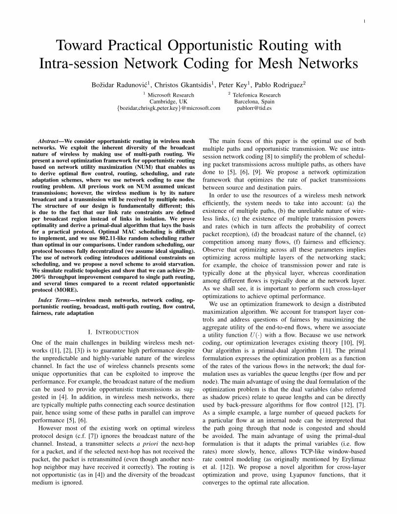
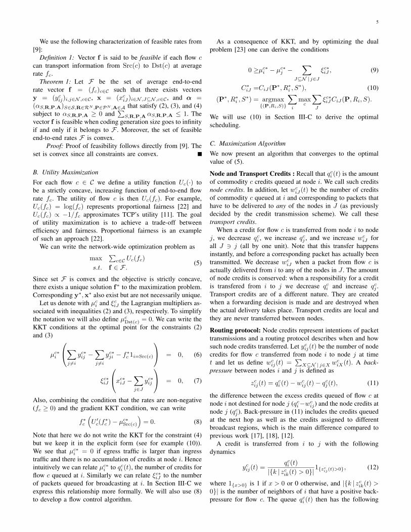
Fig. 1. A network with 4 nodes is shown on the left. For example, anactivation profile {(1, 2), (3, 4)} depicts a profile where nodes 1 and 3 aretransmitting, node 2 is receiving a packet from node 1, while node 4 isreceiving from node 3. Profile {(1, {2, 3})} depicts node 1 transmittingand nodes 2 and 3 receiving (the same) packet from node 1. The feasiblerate region for (y12, y13) is given on the right, described by inequalities:∑

j∈J y1j ≤ C1J for all J ⊆ {2, 3}.

can be computed in a distributed system, and compares witha recent proposal for multi-path routing. Section IV discussessome practical issues, namely the effect of limited generationsizes, and the effect of randomized 802.11-compatible channelscheduling. Section V evaluates the performance of our systemusing simulation. Section VI provides related work.

II. MODEL

In this section we introduce our notation, denoting vectorsin bold typeface. We extend the model of a wireless erasurenetwork developed in [16] to include multiple flows.

A. PHY And MAC Characteristics

We consider a network comprising of a set of nodes N , N =|N |. Whenever a node transmits a packet, several nodes mayreceive it. We model packet transmission from node i to aset of nodes Ki ⊆ N with a hyperarc (i,Ki). We define anactivation profile S = {Sl} to be a set of hyperarcs active atthe same time. There may be several constraints on feasibleactivation profiles. For example, a node may be limited toreceive from but one node, or transmit to only one node at atime. The only condition we shall impose is that a node canbe the source of only one hyperarc in one activation profile.All the other constraints can be expressed through receptionprobabilities and our model is general enough to incorporatethem (in particular, it is possible that a node transmits whilesome information is being sent to it, in which case we shallset the probability of successful reception to 0; see below fordetails). We denote by S the set of feasible activation profilesand let SRC(S) = {i ∈ N | ∃Ki ⊆ N , (i,Ki) ∈ S} be theset of transmitters in activation profile S.

Each transmission has two associated parameters, powerP ∈ P and rate R ∈ R, where P is the set of allowedtransmission powers (e.g. P ∈ [0, PM ], where PM is given byregulations) and R is sets of available PHY transmission rates,defined by supported spreading, coding, and modulations.

Consider an activation profile S in which node i transmitsto set of nodes Ki, and suppose node i is transmitting withpower Pi and rate Ri. We can associate power vector P =(Pi)i∈N rate vector R = (Ri)i∈N to these transmissions. LetTij(P, Ri, S) be an indicator of a random event such thatTij(P, Ri, S) = 1 if a packet is successfully delivered from

3

31

2

5

4

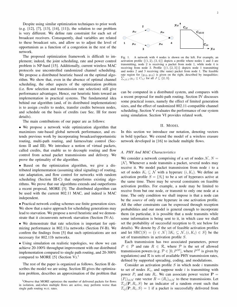
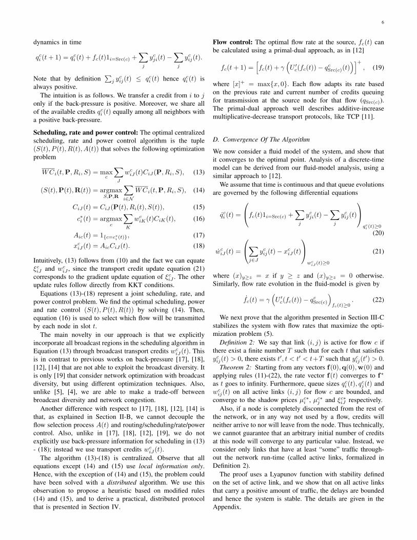
Fig. 2. Forwarding example. Lines connect nodes that can exchange packets.Opportunistic routing implies multiple-paths. Possible paths from 1 to 5 arefor example (1, 2, 3, 4, 5), (1, 2, 3, 5), (1, 2, 4, 5), (1, 3, 4, 5), (1, 3, 5). Path(1, 2, 1, 3, 5) is also possible but will be typically eliminated by a routingprotocol due to suboptimality.

i to j ∈ Ki. It depends on the packet transmission power Pi

and rate Ri, as well as on the interference from concurrenttransmissions described through P and S. We also denote by

TiJ(P, Ri, S) = 1−∏j∈J

(1− Tij(P, Ri, S))

the indicator of the event that at least one of the nodes fromJ , (J ∩Ki 6= ∅) receives a packet. Consequently

piJ(P, Ri, S) = Prob(TiJ = 1).

By convention, we assume piJ(P, Ri, S) = 0 if J ∩Ki = ∅,for (i,Ki) ∈ S. Our model does not require any assumptionson channel conditions; in particular, events Tij and Tik arenot assumed independent.

We can now calculate CiJ(P, Ri, S), the average numberof packets per unit time conveyed from node i to any of thenodes in J ⊆ N . We have

CiJ(P, Ri, S) = Ri piJ(P, Ri, S) (1)

B. Traffic, Forwarding And Flow Scheduling

There is a set of unicast end-to-end flows C in the network,and each flow c ∈ C has a source and a destination nodeSrc(c),Dst(c) ∈ N respectively. We denote by fc the rate offlow c.

Opportunistic routing does not a priori rely on a notionof a path or a route. Consider the example of Figure 2: apacket going from node 1 to node 5 may be relayed by any ofthe nodes 2, 3, 4, depending on which node happens to hearit. Thus implicitly, opportunistic routing implies multi-pathrouting without pre-specifying the path. Formally, a packetfrom node i can reach node j if there exists an activationprofile that allows such a transmission (there exists S ∈ S suchthat (i,Ki) ∈ S and j ∈ Ki). The goal of our optimizationframework is to derive how many packets should be forwardedby each of the nodes.

In practice, an external routing protocol can be combinedwith the opportunistic approach to further improve efficiency.Consider again the example from Figure 2: if a packet isbroadcast by node 2 destined for 5, it may be received andpotentially forwarded by node 1. Our opportunistic routingprotocol will, as described latter, eliminate such events, butwill take some time to discover them. Instead, one mayuse a readily available external routing protocol to promptlyeliminate obviously suboptimal paths (e.g. path (1, 2, 1, 3, 5)

from Figure 2). Our model can be easily extended to includeconstraints imposed by an external routing protocol, but weomit such extensions to simplify the exposition. We do con-strain the set of available paths in the numerical results, asexplained in Section V.

A node that transmits a packet cannot control who willreceive the transmitted packets due to channel randomness.A node that receives a packet has to decide whether itwill forward it or not. This decision is made through creditassignment, described in Section II-D.

Whenever a node is about to transmit, it needs to decidewhich flow it will transmit. This is defined through a flow-scheduling profile matrix A. If node i transmits a packet fromflow c we set Aic = 1, otherwise Aic = 0. We say that a flowscheduling profile is valid if for each i ∈ N there exists onlyone c ∈ C such that Aic = 1. A denotes the set of all validflow scheduling profiles.

To illustrate the use of flow scheduling profile, consider theexample in Figure 1 having two flows C = {1, 2}, both from1 to 4. The number of packets for flow c sent by node 1 andreceived by node 2 depends not only on how often (1, 2)is scheduled, but also on how often (1, {2, 3}) is scheduledto transmit a packet from c. This is why the flow schedulingdecision is assigned to a node instead of a link, which is insharp contrast to [17], [18], [12].

C. Network Coding

We assume network coding per flow is used [16], [5]. The mainbenefit of network coding is that it facilitates scheduling. Ifthe same packet is received by several nodes, a mechanismis needed to prevent two or more nodes forwarding the samepackets [4]. To eliminate this problem, each relay forwards arandom linear combination of all previously received packetsfrom the same flow. It has been show in [9] that the ran-dom linear combinations received at the destination will beindependent with high probability, hence the packets can berestored.

Ideally, network coding should be performed across theentire flow. However, this is not practical. Instead, packetsare divided in generations and only packets from the samegeneration are combined. For more details see [16], [5]. InSection III we analyze the optimal network design assumingvery large generation sizes (as in [16]); we address finitegeneration sizes in Section IV.

D. Credits

As remarked on earlier, whenever a packet is transmitted,it may be received by several nodes, and it is importantto decide which should forward packets, to avoid redundanttransmissions (as explained in [19], [5]).

We introduce the concept of credits, which is similar to thecontrol decision variable of Neely [19]. One credit is createdfor each packet at the source node. Credits are identified witha generation, not a specific packet. They are conserved untilthey arrive at the flow’s destination. In this way we guaranteethat the destination will receive as many linear combinations of

4

the packets as the number of packets generated at the source,and hence will be able to decode the packets.

Credits are interpreted as the number of packets of a specificflow to be forwarded by a node. By controlling the rate ofcredits we control the rate of packets forwarded by next-hoprelays. Consider again the example from Figure 1. Node 1should adapt the rate of packets forwarded through 2 and 3not only as a function of link qualities p12 and p13, but alsoas a function of p24 and p34, the quality of paths from 2 and3 to the destination 4. For example, if p24 � p34 then node 2should not forward any packet, regardless of how many it hasreceived. Node 1 cannot control what nodes 2 and 3 receivedue to randomness of the channel. Instead, node 1 sends acredit to node 2 (or node 3) whenever it wants node 2 (ornode 3) to forward a packet.

The main advantage of the credit scheme is that it simplifiesscheduling. Credits are declarations of intent. The actualpacket transmissions may occur at arbitrary time instants. Dueto the use of network coding, we only need to ensure that thetotal number of packets per generation transmitted betweeneach two nodes corresponds to the number of credits. Thus,scheduling is done at a generation level and not at the packetlevel, incuring significantly smaller overhead (especially whenthe generation size is large).

In practice, credits can be piggybacked with packet trans-missions. The receiving node only updates its credits when asuccessful packet transmission actually occurs. In this workwe assume there is an ideal (no loss and no delay) signalingplane that transmits credits and feedbacks.

As each credit delegates one packet to a node, we mayexpress all the rates in the system in terms of credits. Forexample, yc

ij is the rate of credits of flow c passed fromnode i to node j, and it equals the rate of innovative linearcombinations of packets of flow c delivered from i to j.Theorem 1 shows that the rate of independent packets receivedat a destination of each flow will correspond to the number ofcredits delivered, when the generation size is large.

E. Dynamics And StabilityWe further assume the system is slotted in time. In each slott = 0, 1, . . . a medium access protocol assigns an activationprofile S(t) and a flow-scheduling profile A(t), and to eachtransmitter i ∈ SRC(S(t)) we assign transmit power Pi(t)and rate Ri(t). Let yc

ij(t) be the number of credits for flow ctransmitted from node i to node j during slot t, and let xc

iJ(t)denote the number of packets of flow c actually delivered fromi to any of the nodes in J during slot t (as if all nodes in Jare grouped as a single receiver). Let fc(t) be the number offresh packets/credits generated at the source of flow c.

Note that, because each successful packet delivery is alwaysassociated with a credit transmission, we look at credit queues.Let qc

i (t) be the amount of credits of flow c queued at nodei. The system is stable if every queue size is bounded. Wedefine stability more formally in Section III-D.

F. Constraints Of The Model And Possible GeneralizationsWe make several simplifying assumptions to make the

analysis tractable. Firstly, we assume that the system is slotted.

All operations within a slot occur concurrently and instantly.Secondly, we assume the perfect signaling. There is no lossor delay in signaling messages (credit transfers and acknowl-edgments).

Our results can be extended to consider imperfect signalingand arbitrary but limited delays in the system (see for example[20, Part 2] on a discussion how does a delayed feedback affectthe speed of convergence). Also, see [21] for a practical imple-mentation of a back-pressure based system and its interactionwith TCP.

III. OPTIMAL FLOW CONTROL FOR FAIRNESS

In this Section we introduce the optimization problem(Sec. III-B), propose an algorithm for solving it (Sec. III-C),and prove that the algorithm converges (Sec. III-D). Sec.III-Aintroduces some further notation that is needed for the descrip-tion of the optimization problem. Finally, in Sec. III-E wecompare our algorithm with the MORE algorithm proposedin [5].

A. Feasible Average Rate Set

In this section we define a set of constraints on average ratesin the system. Assume an assignment of average end-to-endrates fc, for each flow c, and denote the average rate vector byf = (fc)c∈C . The vector of rates is valid under the followingthree conditions. First, traffic at node i is stable if the totalingress traffic is smaller than the total egress traffic, which wewrite as ∑

j 6=i

ycji + fc1{i=Src(c)} ≤

∑j 6=i

ycij , (2)

for all i 6= Dst(c), where 1x = 1 if x is true, 0 otherwise, andwhere yij ≥ 0.

Second, traffic at each broadcast region is stable if we donot receive more credits than we can actually forward (seealso Fig. 1): ∑

j∈J

ycij ≤ xc

iJ , for all J ∈ N . (3)

Recall that ycij is the average number of credits of flow c node

i assigns to node j and xciJ is the average number of packets

of flow c actually delivered from i to any of the nodes in J .Finally, we define scheduling constraints. A schedule is a se-

quence {(S(t),R(t),P(t),A(t))}t≥0 which defines schedul-ing profile S(t), routing profile A(t) and power and rateallocations R(t),P(t) in each slot t ≥ 0. Since we areinterested in long-term average rates, we define

αS,R,P,A = limT→∞

1T

∑t≤T

1{S(t)=S,R(t)=R,P(t)=P,A(t)=A}

to be the fraction of time the network uses scheduling profileS, routing profile A and power and rate allocations R,P.By definition, αS,R,P,A ≥ 0 and

∑S,R,P,A αS,R,P,A ≤ 1.

The schedule defined by {αS,R,P,A}S,R,P,A is stable if itcan support broadcast traffic {xc

iJ}i,J,c, and we write thescheduling constraints as

xciJ ≤

∑S,A,R,P

αS,R,P,AAicCiJ(P, Ri, S) (4)

5

We use the following characterization of feasible rates from[9]:

Definition 1: Vector f is said to be feasible if each flow ccan transport information from Src(c) to Dst(c) at averagerate fc.

Theorem 1: Let F be the set of average end-to-endrate vector f = (fc)c∈C such that there exists vectorsy = (yc

ij)i,j∈N ,c∈C , x = (xciJ)i∈N ,J⊆N ,c∈C , and α =

(αS,R,P,A)S∈S,R∈RN ,P∈PN ,A∈A that satisfy (2), (3), and (4)subject to αS,R,P,A ≥ 0 and

∑S,R,P,A αS,R,P,A ≤ 1. The

vector f is feasible when coding generation size goes to infinityif and only if it belongs to F . Moreover, the set of feasibleend-to-end rates F is convex.

Proof: Proof of feasibility follows directly from [9]. Theset is convex since all constraints are convex.

B. Utility Maximization

For each flow c ∈ C we define a utility function Uc(·) tobe a strictly concave, increasing function of end-to-end flowrate fc. The utility of flow c is then Uc(fc). For example,Uc(fc) = log(fc) represents proportional fairness [22] andUc(fc) ∝ −1/fc approximates TCP’s utility [11]. The goalof utility maximization is to achieve a trade-off betweenefficiency and fairness. Proportional fairness is an exampleof such an approach [22].

We can write the network-wide optimization problem as

max∑

c∈C Uc(fc)s.t. f ∈ F .

(5)

Since set F is convex and the objective is strictly concave,there exists a unique solution f∗ to the maximization problem.Corresponding y∗,x∗ also exist but are not necessarily unique.

Let us denote with µci and ξc

iJ the Lagrangian multipliers as-sociated with inequalities (2) and (3), respectively. To simplifythe notation we will also define µc

Dst(c) = 0. We can write theKKT conditions at the optimal point for the constraints (2)and (3)

µc∗i

∑j 6=i

yc∗ij −

∑j 6=i

yc∗ji − f∗c 1i=Src(c)

= 0, (6)

ξc∗iJ

xc∗iJ −

∑j∈J

yc∗ij

= 0, (7)

Also, combining the condition that the rates are non-negative(fc ≥ 0) and the gradient KKT condition, we can write

f∗c

(U ′c(f∗c )− µc∗

Src(c)

)= 0. (8)

Note that here we do not write the KKT for the constraint (4)but we keep it in the explicit form (see for example (10)).We see that µc∗

i = 0 if egress traffic is larger than ingresstraffic and there is no accumulation of credits at node i. Henceintuitively we can relate µc∗

i to qci (t), the number of credits for

flow c queued at i. Similarly we can relate ξc∗iJ to the number

of packets queued for broadcasting at i. In Section III-C weexpress this relationship more formally. We will also use (8)to develop a flow control algorithm.

As a consequence of KKT, and by optimizing the dualproblem [23] one can derive the conditions

0 ≥µc∗i − µc∗

j −∑

J⊆N | j∈J

ξc∗iJ , (9)

C∗iJ =CiJ(P∗, R∗i , S∗), (10)

(P∗, R∗i , S∗) = argmax

{(P,Ri,S)}

∑i

maxc

∑J

ξc∗iJCiJ(P, Ri, S).

We will use (10) in Section III-C to derive the optimalscheduling.

C. Maximization Algorithm

We now present an algorithm that converges to the optimalvalue of (5).

Node and Transport Credits : Recall that qci (t) is the amount

of commodity c credits queued at node i. We call such creditsnode credits. In addition, let wc

iJ(t) be the number of creditsof commodity c queued at i and corresponding to packets thathave to be delivered to any of the nodes in J (as previouslydecided by the credit transmission scheme). We call thesetransport credits.

When a credit for flow c is transferred from node i to nodej, we decrease qc

i , we increase qcj , and we increase wc

iJ forall J 3 j (all by one unit). Note that this transfer happensinstantly, and before a corresponding packet has actually beentransmitted. We decrease wc

iJ when a packet from flow c isactually delivered from i to any of the nodes in J . The amountof node credits is conserved: when a responsibility for a creditis transfered from i to j we decrease qc

i and increase qcj .

Transport credits are of a different nature. They are createdwhen a forwarding decision is made and are destroyed whenthe actual delivery takes place. Transport credits are local andthey are never transferred between nodes.

Routing protocol: Node credits represent intentions of packettransmissions and a routing protocol describes when and howsuch node credits transferred. Let yc

ij(t) be the number of nodecredits for flow c transferred from node i to node j at timet and let us define wc

ij(t) =∑

X⊆N | j∈X wciX(t). A back-

pressure between nodes i and j is defined as

zcij(t) = qc

i (t)− wcij(t)− qc

j(t), (11)

the difference between the excess credits queued of flow c atnode i not destined for node j (qc

i−wcij) and the node credits at

node j (qcj ). Back-pressure in (11) includes the credits queued

at the next hop as well as the credits assigned to differentbroadcast regions, which is the main difference compared toprevious work [17], [18], [12].

A credit is transferred from i to j with the followingdynamics

ycij(t) =

qci (t)

|{k | zcik(t) > 0}|

1{zcij(t)>0}, (12)

where 1{x>0} is 1 if x > 0 or 0 otherwise, and |{k | zcik(t) >

0}| is the number of neighbors of i that have a positive back-pressure for flow c. The queue qc

i (t) then has the following

6

dynamics in time

qci (t+ 1) = qc

i (t) + fc(t)1i=Src(c) +∑

j

ycji(t)−

∑j

ycij(t).

Note that by definition∑

j ycij(t) ≤ qc

i (t) hence qci (t) is

always positive.The intuition is as follows. We transfer a credit from i to j

only if the back-pressure is positive. Moreover, we share allof the available credits qc

i (t) equally among all neighbors witha positive back-pressure.

Scheduling, rate and power control: The optimal centralizedscheduling, rate and power control algorithm is the tuple(S(t), P (t), R(t), A(t)) that solves the following optimizationproblem

WCi(t,P, Ri, S) = maxc

∑J

wciJ(t)CiJ(P, Ri, S), (13)

(S(t),P(t),R(t)) = argmaxS,P,R

∑i∈N

WCi(t,P, Ri, S), (14)

CiJ(t) = CiJ(P(t), Ri(t), S(t)), (15)

c∗i (t) = argmaxc

∑K

wciK(t)CiK(t), (16)

Aic(t) = 1{c=c∗i (t)}, (17)

xciJ(t) = AicCiJ(t). (18)

Intuitively, (13) follows from (10) and the fact we can equateξciJ and wc

iJ , since the transport credit update equation (21)corresponds to the gradient update equation of ξc

iJ . The otherupdate rules follow directly from KKT conditions.

Equations (13)-(18) represent a joint scheduling, rate, andpower control problem. We find the optimal scheduling, powerand rate control (S(t), P (t), R(t)) by solving (14). Then,equation (16) is used to select which flow will be transmittedby each node in slot t.

The main novelty in our approach is that we explicitlyincorporate all broadcast regions in the scheduling algorithm inEquation (13) through broadcast transport credits wc

iJ(t). Thisis in contrast to previous works on back-pressure [17], [18],[12], [14] that are not able to exploit the broadcast diversity. Itis only [19] that consider network optimization with broadcastdiversity, but using different optimization techniques. Also,unlike [5], [4], we are able to make a trade-off betweenbroadcast diversity and network congestion.

Another difference with respect to [17], [18], [12], [14] isthat, as explained in Section II-B, we cannot decouple theflow selection process A(t) and routing/scheduling/rate/powercontrol. Also, unlike in [17], [18], [12], [19], we do notexplicitly use back-pressure information for scheduling in (13)- (18); instead we use transport credits wc

iJ(t).The algorithm (13)-(18) is centralized. Observe that all

equations except (14) and (15) use local information only.Hence, with the exception of (14) and (15), the problem couldhave been solved with a distributed algorithm. We use thisobservation to propose a heuristic based on modified rules(14) and (15), and to derive a practical, distributed protocolthat is presented in Section IV.

Flow control: The optimal flow rate at the source, fc(t) canbe calculated using a primal-dual approach, as in [12]

fc(t+ 1) =[fc(t) + γ

(U ′c(fc(t))− qc

Src(c)(t))]+

, (19)

where [x]+ = max{x, 0}. Each flow adapts its rate basedon the previous rate and current number of credits queuingfor transmission at the source node for that flow (qSrc(c)).The primal-dual approach well describes additive-increasemultiplicative-decrease transport protocols, like TCP [11].

D. Convergence Of The Algorithm

We now consider a fluid model of the system, and show thatit converges to the optimal point. Analysis of a discrete-timemodel can be derived from our fluid-model analysis, using asimilar approach to [12].

We assume that time is continuous and that queue evolutionsare governed by the following differential equations

qci (t) =

fc(t)1i=Src(c) +∑

j

ycji(t)−

∑j

ycij(t)

qc

i (t)≥0

(20)

wciJ(t) =

∑j∈J

ycij(t)− xc

iJ(t)

wc

iJ (t)≥0

(21)

where (x)y≥z = x if y ≥ z and (x)y≥z = 0 otherwise.Similarly, flow rate evolution in the fluid-model is given by

fc(t) = γ(U ′c(fc(t))− qc

Src(c)

)fc(t)≥0

. (22)

We next prove that the algorithm presented in Section III-Cstabilizes the system with flow rates that maximize the opti-mization problem (5).

Definition 2: We say that link (i, j) is active for flow c ifthere exist a finite number T such that for each t that satisfiesyc

ij(t) > 0, there exists t′, t < t′ < t+T such that ycij(t′) > 0.

Theorem 2: Starting from any vectors f(0),q(0),w(0) andapplying rules (11)-(22), the rate vector f(t) converges to f∗

as t goes to infinity. Furthermore, queue sizes qci (t), qc

j(t) andwc

ij(t) on all active links (i, j) for flow c are bounded, andconverge to the shadow prices µc∗

i , µc∗j and ξc∗

iJ respectively.Also, if a node is completely disconnected from the rest of

the network, or in any way not used by a flow, credits willneither arrive to nor will leave from the node. Thus technically,we cannot guarantee that an arbitrary initial number of creditsat this node will converge to any particular value. Instead, weconsider only links that have at least “some” traffic through-out the network run-time (called active links, formalized inDefinition 2).

The proof uses a Lyapunov function with stability definedon the set of active link, and we show that on all active linksthat carry a positive amount of traffic, the delays are boundedand hence the system is stable. The details are given in theAppendix.

7

E. Comparison with MORE

In this section we compare the performance of our algorithmwith the MORE forwarding algorithm described in [5], [24].We summarize it here for sake of completeness. Consider asingle flow and the delivery of a single packet from the sourceof the flow Src to the destination of the flow Dst. Let βi bethe number of transmissions made by node i to successfullydeliver the packet. The goal of MORE is to minimize thenumber of transmissions [24, Eq.(1)-(4)]:

argmin∑i∈N

βi (23)

s.t.∑j∈N

yij −∑j∈N

yji = 1{i=Src} (24)

yij ≥ 0, (25)

βiCiJ ≥∑j∈J

yij . (26)

Note that the MORE forwarding algorithm is designed for asingle flow. As the authors note in [5], [24], its performancedrops as the number of flows increases.

Our algorithm converges to the optimal solution of theoptimization problem (5) (as shown in Theorem 2), henceMORE is at best as good as our algorithm. We first showunder what conditions MORE is guaranteed to give the optimalsolution. We then illustrate by two examples that MORE canyield strictly suboptimal rate allocations.

Theorem 3: If there is only one flow in the system, iftransmission rates and powers of all nodes are fixed and if onlyone node can transmit at a time (that is |SRC(S)| = 1 for allS ∈ S), MORE and our algorithm give the same performance.

Proof: Since only one node can transmit at a time, wehave S = N . Furthermore, transmission powers and rates arefixed, hence (3) and (4) reads as

∑j∈J yij ≤ αiCiJ . We also

omit c as there is only one flow in the system.We start with the MORE optimization problem (23) - (26)

and we introduce f = 1/(∑

i∈N βi

), yij = f yij and αi =

f βi. The optimization (23) - (26) is then equivalent to

min1/f (27)

s.t.∑j∈N

yij −∑j∈N

yji = f1{i=Src} (28)

αiCiJ ≥∑j∈J

yij , (29)∑i∈N

αi = 1, (30)

which is exactly the optimization problem (5).We next give two examples where the performance of

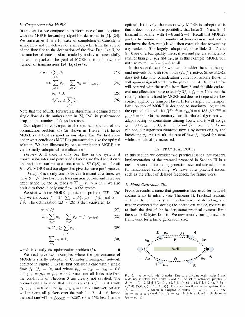
MORE is strictly suboptimal. Consider a hexagonal networkdepicted in Figure 3. Let us first consider a case with a singleflow f1, (f2 = 0), and where p12 = p24 = p46 = 0.8and p13 = p35 = p56 = 0.2. Since not all links interfere,the conditions of Theorem 3 are clearly not satisfied. Theoptimal rate allocation that maximizes (5) is f = 0.313 withy1−2−4−6 = 0.251 and y1−3−5−6 = 0.063. However, MOREwill transmit all packets over the path 1 − 2 − 4 − 6, hencethe total rate will be fMORE = 0.267, some 15% less than the

optimal. Intuitively, the reason why MORE is suboptimal isthat it does not consider possibility that links 3− 5 and 5− 6transmit in parallel with 4−6 and 2−4. (Recall that MORE’sgoal is to minimize the number of transmissions and not tomaximize the flow rate.) It will then conclude that forwardingany packet to 3 is largely suboptimal, since links 3 − 5 and5−6 are of a bad quality. Thus, if p35 and p56 are sufficientlysmaller than p12, p24 and p46, as in this example, MORE willnot use route 1− 3− 5− 6 at all.

In the second example we again consider the same hexag-onal network but with two flows (f1, f2) active. Since MOREdoes not take into consideration contention among flows, itwill again assign all traffic to the path 1−2−4−6. This trafficwill contend with the traffic from flow 2, and feasible end-to-end rate allocations have to satisfy 3f1 +f2 = p. Note that therouting scheme is fixed by MORE and does not depend on flowcontrol applied by transport layer. If for example the transportlayer on top of MORE is designed to maximize log utility,the optimal rates will be fMORE

1 = p12/6 = 0.133, fMORE2 =

p12/2 = 0.4. On the contrary, our distributed algorithm willadapt routing to contentions among flows, and it will assigny1 = 0.12, y2 = 0.03, f1 = 0.15 and f2 = y3 = 0.4. As wecan see, our algorithm balanced flow 1 by decreasing y1 andincreasing y2. As a result, the rate of flow f2 stayed the samewhile the rate of f1 increased.

IV. PRACTICAL ISSUES

In this section we consider two practical issues that concernimplementation of the protocol proposed in Section III in amesh network: finite coding generation size and rate adaptationfor randomized scheduling. We leave other practical issues,such as the effect of delayed feedback, for future work.

A. Finite Generation Size

Previous results assume that generation size used for networkcoding tends to infinity (see Theorem 1). Practical reasons,such as the complexity and performance of decoding, andheader overhead for storing the coefficient vector, require usto limit the size of the header; some practical systems limitthe size to 32 bytes [5], [6]. We now modify our optimizationframework for a finite generation size.

3

1

2

6

5

4

p12

p13

p35

p24

p46

p56

Wall

y2

y1

y3

Fig. 3. A network with 6 nodes. Due to a dividing wall, nodes 2 and4 do not interfere with nodes 3 and 5. The set of activation profiles isS = {{(1, {2, 3})}, {(2, 4)}, {(3, 5)}, {(4, 6)}, {(5, 6)}, {(2, 4), (3, 5)},{(2, 4), (5, 6)}, {(3, 5), (4, 6)}}. There are two flows in the system, flowf1 = y1 + y2 which is assigned 2 routes (y1 = y1−2−4−6 andy2 = y1−3−5−6) and flow f2 = y3 which is assigned a single route(y3 = y2−4).

8

3

1

2

p12

p13

p23

w12(0, 1) = 0,w12(0, 2) = 5,

w1{2,3}(0, 1) = 0,w1{2,3}(0, 2) = 4,

w13(0, 1) = 1,w13(0, 2) = 0

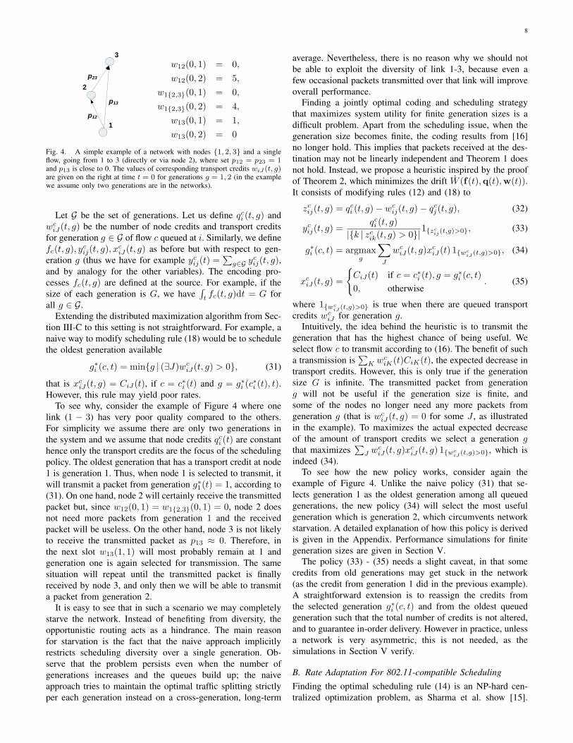
Fig. 4. A simple example of a network with nodes {1, 2, 3} and a singleflow, going from 1 to 3 (directly or via node 2), where set p12 = p23 = 1and p13 is close to 0. The values of corresponding transport credits wiJ (t, g)are given on the right at time t = 0 for generations g = 1, 2 (in the examplewe assume only two generations are in the networks).

Let G be the set of generations. Let us define qci (t, g) and

wciJ(t, g) be the number of node credits and transport credits

for generation g ∈ G of flow c queued at i. Similarly, we definefc(t, g), yc

ij(t, g), xciJ(t, g) as before but with respect to gen-

eration g (thus we have for example ycij(t) =

∑g∈G y

cij(t, g),

and by analogy for the other variables). The encoding pro-cesses fc(t, g) are defined at the source. For example, if thesize of each generation is G, we have

∫tfc(t, g)dt = G for

all g ∈ G.Extending the distributed maximization algorithm from Sec-

tion III-C to this setting is not straightforward. For example, anaive way to modify scheduling rule (18) would be to schedulethe oldest generation available

g∗i (c, t) = min{g | (∃J)wciJ(t, g) > 0}, (31)

that is xciJ(t, g) = CiJ(t), if c = c∗i (t) and g = g∗i (c∗i (t), t).

However, this rule may yield poor rates.To see why, consider the example of Figure 4 where one

link (1 − 3) has very poor quality compared to the others.For simplicity we assume there are only two generations inthe system and we assume that node credits qc

i (t) are constanthence only the transport credits are the focus of the schedulingpolicy. The oldest generation that has a transport credit at node1 is generation 1. Thus, when node 1 is selected to transmit, itwill transmit a packet from generation g∗1(t) = 1, according to(31). On one hand, node 2 will certainly receive the transmittedpacket but, since w12(0, 1) = w1{2,3}(0, 1) = 0, node 2 doesnot need more packets from generation 1 and the receivedpacket will be useless. On the other hand, node 3 is not likelyto receive the transmitted packet as p13 ≈ 0. Therefore, inthe next slot w13(1, 1) will most probably remain at 1 andgeneration one is again selected for transmission. The samesituation will repeat until the transmitted packet is finallyreceived by node 3, and only then we will be able to transmita packet from generation 2.

It is easy to see that in such a scenario we may completelystarve the network. Instead of benefiting from diversity, theopportunistic routing acts as a hindrance. The main reasonfor starvation is the fact that the naive approach implicitlyrestricts scheduling diversity over a single generation. Ob-serve that the problem persists even when the number ofgenerations increases and the queues build up; the naiveapproach tries to maintain the optimal traffic splitting strictlyper each generation instead on a cross-generation, long-term

average. Nevertheless, there is no reason why we should notbe able to exploit the diversity of link 1-3, because even afew occasional packets transmitted over that link will improveoverall performance.

Finding a jointly optimal coding and scheduling strategythat maximizes system utility for finite generation sizes is adifficult problem. Apart from the scheduling issue, when thegeneration size becomes finite, the coding results from [16]no longer hold. This implies that packets received at the des-tination may not be linearly independent and Theorem 1 doesnot hold. Instead, we propose a heuristic inspired by the proofof Theorem 2, which minimizes the drift W (f(t),q(t),w(t)).It consists of modifying rules (12) and (18) to

zcij(t, g) = qc

i (t, g)− wcij(t, g)− qc

j(t, g), (32)

ycij(t, g) =

qci (t, g)

|{k | zcik(t, g) > 0}|

1{zcij(t,g)>0}, (33)

g∗i (c, t) = argmaxg

∑J

wciJ(t, g)xc

iJ(t) 1{wciJ (t,g)>0}, (34)

xciJ(t, g) =

{CiJ(t) if c = c∗i (t), g = g∗i (c, t)0, otherwise

. (35)

where 1{wciJ (t,g)>0} is true when there are queued transport

credits wciJ for generation g.

Intuitively, the idea behind the heuristic is to transmit thegeneration that has the highest chance of being useful. Weselect flow c to transmit according to (16). The benefit of sucha transmission is

∑K wc

iK(t)CiK(t), the expected decrease intransport credits. However, this is only true if the generationsize G is infinite. The transmitted packet from generationg will not be useful if the generation size is finite, andsome of the nodes no longer need any more packets fromgeneration g (that is wc

iJ(t, g) = 0 for some J , as illustratedin the example). To maximizes the actual expected decreaseof the amount of transport credits we select a generation gthat maximizes

∑J w

ciJ(t, g)xc

iJ(t, g) 1{wciJ (t,g)>0}, which is

indeed (34).To see how the new policy works, consider again the

example of Figure 4. Unlike the naive policy (31) that se-lects generation 1 as the oldest generation among all queuedgenerations, the new policy (34) will select the most usefulgeneration which is generation 2, which circumvents networkstarvation. A detailed explanation of how this policy is derivedis given in the Appendix. Performance simulations for finitegeneration sizes are given in Section V.

The policy (33) - (35) needs a slight caveat, in that somecredits from old generations may get stuck in the network(as the credit from generation 1 did in the previous example).A straightforward extension is to reassign the credits fromthe selected generation g∗i (c, t) and from the oldest queuedgeneration such that the total number of credits is not altered,and to guarantee in-order delivery. However in practice, unlessa network is very asymmetric, this is not needed, as thesimulations in Section V verify.

B. Rate Adaptation For 802.11-compatible SchedulingFinding the optimal scheduling rule (14) is an NP-hard cen-tralized optimization problem, as Sharma et al. show [15].

9

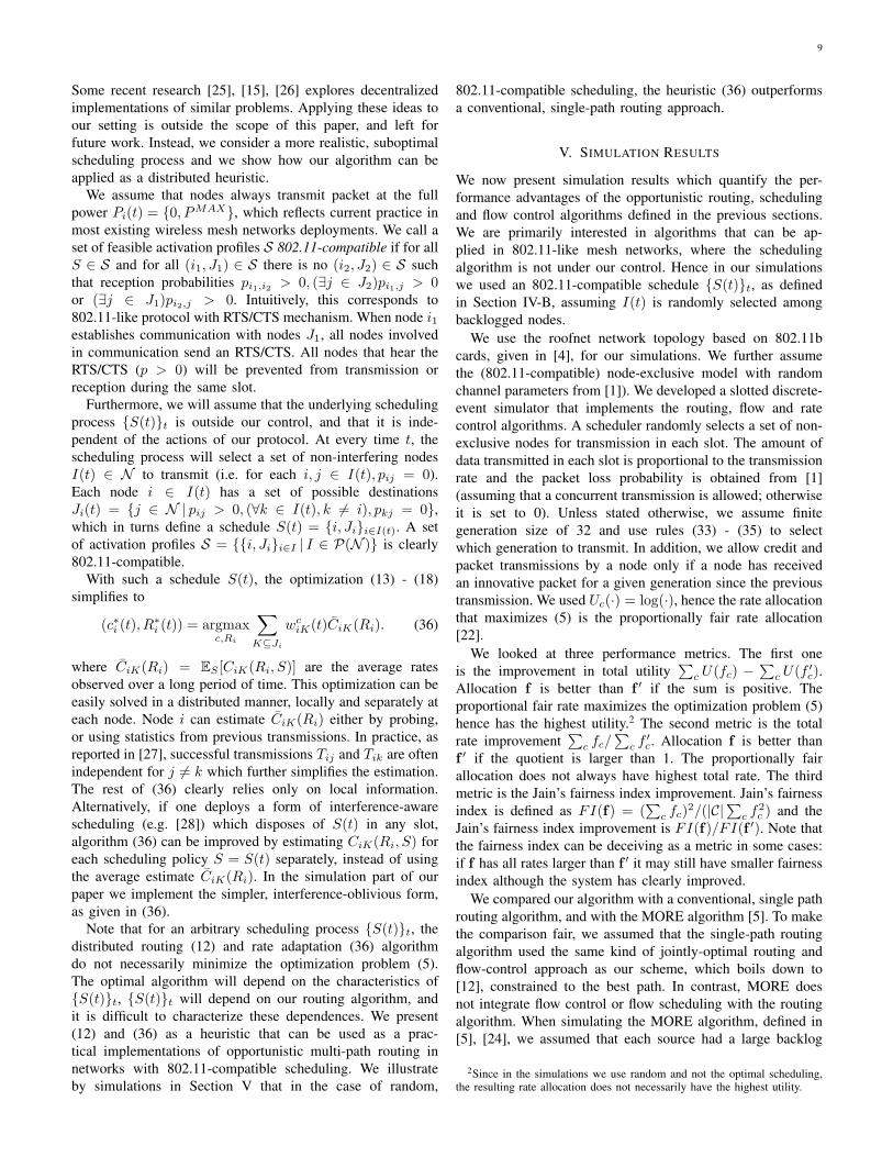
Some recent research [25], [15], [26] explores decentralizedimplementations of similar problems. Applying these ideas toour setting is outside the scope of this paper, and left forfuture work. Instead, we consider a more realistic, suboptimalscheduling process and we show how our algorithm can beapplied as a distributed heuristic.

We assume that nodes always transmit packet at the fullpower Pi(t) = {0, PMAX}, which reflects current practice inmost existing wireless mesh networks deployments. We call aset of feasible activation profiles S 802.11-compatible if for allS ∈ S and for all (i1, J1) ∈ S there is no (i2, J2) ∈ S suchthat reception probabilities pi1,i2 > 0, (∃j ∈ J2)pi1,j > 0or (∃j ∈ J1)pi2,j > 0. Intuitively, this corresponds to802.11-like protocol with RTS/CTS mechanism. When node i1establishes communication with nodes J1, all nodes involvedin communication send an RTS/CTS. All nodes that hear theRTS/CTS (p > 0) will be prevented from transmission orreception during the same slot.

Furthermore, we will assume that the underlying schedulingprocess {S(t)}t is outside our control, and that it is inde-pendent of the actions of our protocol. At every time t, thescheduling process will select a set of non-interfering nodesI(t) ∈ N to transmit (i.e. for each i, j ∈ I(t), pij = 0).Each node i ∈ I(t) has a set of possible destinationsJi(t) = {j ∈ N | pij > 0, (∀k ∈ I(t), k 6= i), pkj = 0},which in turns define a schedule S(t) = {i, Ji}i∈I(t). A setof activation profiles S = {{i, Ji}i∈I | I ∈ P(N )} is clearly802.11-compatible.

With such a schedule S(t), the optimization (13) - (18)simplifies to

(c∗i (t), R∗i (t)) = argmaxc,Ri

∑K⊆Ji

wciK(t)CiK(Ri). (36)

where CiK(Ri) = ES [CiK(Ri, S)] are the average ratesobserved over a long period of time. This optimization can beeasily solved in a distributed manner, locally and separately ateach node. Node i can estimate CiK(Ri) either by probing,or using statistics from previous transmissions. In practice, asreported in [27], successful transmissions Tij and Tik are oftenindependent for j 6= k which further simplifies the estimation.The rest of (36) clearly relies only on local information.Alternatively, if one deploys a form of interference-awarescheduling (e.g. [28]) which disposes of S(t) in any slot,algorithm (36) can be improved by estimating CiK(Ri, S) foreach scheduling policy S = S(t) separately, instead of usingthe average estimate CiK(Ri). In the simulation part of ourpaper we implement the simpler, interference-oblivious form,as given in (36).

Note that for an arbitrary scheduling process {S(t)}t, thedistributed routing (12) and rate adaptation (36) algorithmdo not necessarily minimize the optimization problem (5).The optimal algorithm will depend on the characteristics of{S(t)}t, {S(t)}t will depend on our routing algorithm, andit is difficult to characterize these dependences. We present(12) and (36) as a heuristic that can be used as a prac-tical implementations of opportunistic multi-path routing innetworks with 802.11-compatible scheduling. We illustrateby simulations in Section V that in the case of random,

802.11-compatible scheduling, the heuristic (36) outperformsa conventional, single-path routing approach.

V. SIMULATION RESULTS

We now present simulation results which quantify the per-formance advantages of the opportunistic routing, schedulingand flow control algorithms defined in the previous sections.We are primarily interested in algorithms that can be ap-plied in 802.11-like mesh networks, where the schedulingalgorithm is not under our control. Hence in our simulationswe used an 802.11-compatible schedule {S(t)}t, as definedin Section IV-B, assuming I(t) is randomly selected amongbacklogged nodes.

We use the roofnet network topology based on 802.11bcards, given in [4], for our simulations. We further assumethe (802.11-compatible) node-exclusive model with randomchannel parameters from [1]). We developed a slotted discrete-event simulator that implements the routing, flow and ratecontrol algorithms. A scheduler randomly selects a set of non-exclusive nodes for transmission in each slot. The amount ofdata transmitted in each slot is proportional to the transmissionrate and the packet loss probability is obtained from [1](assuming that a concurrent transmission is allowed; otherwiseit is set to 0). Unless stated otherwise, we assume finitegeneration size of 32 and use rules (33) - (35) to selectwhich generation to transmit. In addition, we allow credit andpacket transmissions by a node only if a node has receivedan innovative packet for a given generation since the previoustransmission. We used Uc(·) = log(·), hence the rate allocationthat maximizes (5) is the proportionally fair rate allocation[22].

We looked at three performance metrics. The first oneis the improvement in total utility

∑c U(fc) −

∑c U(f ′c).

Allocation f is better than f ′ if the sum is positive. Theproportional fair rate maximizes the optimization problem (5)hence has the highest utility.2 The second metric is the totalrate improvement

∑c fc/

∑c f′c. Allocation f is better than

f ′ if the quotient is larger than 1. The proportionally fairallocation does not always have highest total rate. The thirdmetric is the Jain’s fairness index improvement. Jain’s fairnessindex is defined as FI(f) = (

∑c fc)2/(|C|

∑c f

2c ) and the

Jain’s fairness index improvement is FI(f)/FI(f ′). Note thatthe fairness index can be deceiving as a metric in some cases:if f has all rates larger than f ′ it may still have smaller fairnessindex although the system has clearly improved.

We compared our algorithm with a conventional, single pathrouting algorithm, and with the MORE algorithm [5]. To makethe comparison fair, we assumed that the single-path routingalgorithm used the same kind of jointly-optimal routing andflow-control approach as our scheme, which boils down to[12], constrained to the best path. In contrast, MORE doesnot integrate flow control or flow scheduling with the routingalgorithm. When simulating the MORE algorithm, defined in[5], [24], we assumed that each source had a large backlog

2Since in the simulations we use random and not the optimal scheduling,the resulting rate allocation does not necessarily have the highest utility.

10

(a)

0 10 20 30 40−2

0

2

4

6

Run

Abs

olut

e im

prov

emen

t in

utili

ty

4 flows8 flows

(b)

0 20 40 60 800.5

1

1.5

2

2.5

Node pairs

Rel

ativ

e im

prov

emen

t in

tota

l rat

e

4 flows8 flows

(c)

0 20 40 60 80

0.8

1

1.2

1.4

1.6

RunRel

ativ

e im

prov

emen

t in

fairn

ess

inde

x

4 flows8 flows

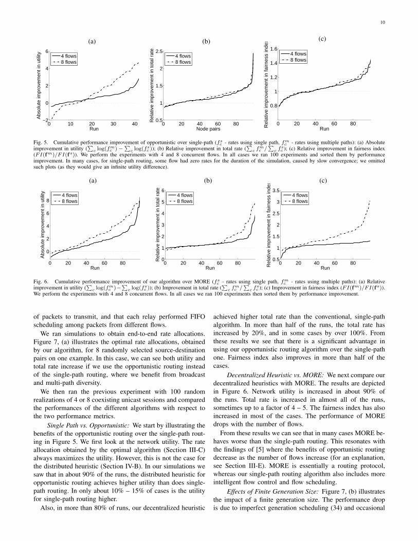
Fig. 5. Cumulative performance improvement of opportunistic over single-path (fsc - rates using single path, fm

c - rates using multiple paths): (a) Absoluteimprovement in utility (

∑c log(fm

c )−∑

c log(fsc )); (b) Relative improvement in total rate (

∑c fm

c /∑

c fsc ); (c) Relative improvement in fairness index

(FI(fm)/FI(fs)). We perform the experiments with 4 and 8 concurrent flows. In all cases we ran 100 experiments and sorted them by performanceimprovement. In many cases, for single-path routing, some flow had zero rates for the duration of the simulation, caused by slow convergence; we omittedsuch plots (as they would give an infinite utility difference).

(a)

0 20 40 60 80

0

2

4

6

8

Run

Abs

olut

e im

prov

emen

t in

utili

ty

4 flows8 flows

(b)

0 20 40 60 800

1

2

3

4

5

6

Run

Rel

ativ

e im

prov

emen

t in

tota

l rat

e

4 flows8 flows

(c)

0 20 40 60 800.5

1

1.5

2

2.5

3

3.5

RunRel

ativ

e im

prov

emen

t in

fairn

ess

inde

x

4 flows8 flows

Fig. 6. Cumulative performance improvement of our algorithm over MORE (fsc - rates using single path, fm

c - rates using multiple paths): (a) Relativeimprovement in utility (

∑c log(fm

c )−∑

c log(fsc )); (b) Improvement in total rate (

∑c fm

c /∑

c fsc ); (c) Improvement in fairness index (FI(fm)/FI(fs)).

We perform the experiments with 4 and 8 concurrent flows. In all cases we ran 100 experiments then sorted them by performance improvement.

of packets to transmit, and that each relay performed FIFOscheduling among packets from different flows.

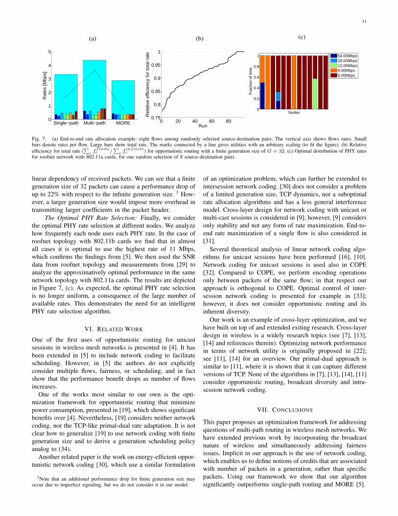
We ran simulations to obtain end-to-end rate allocations.Figure 7, (a) illustrates the optimal rate allocations, obtainedby our algorithm, for 8 randomly selected source-destinationpairs on one example. In this case, we can see both utility andtotal rate increase if we use the opportunistic routing insteadof the single-path routing, where we benefit from broadcastand multi-path diversity.

We then ran the previous experiment with 100 randomrealizations of 4 or 8 coexisting unicast sessions and comparedthe performances of the different algorithms with respect tothe two performance metrics.

Single Path vs. Opportunistic: We start by illustrating thebenefits of the opportunistic routing over the single-path rout-ing in Figure 5. We first look at the network utility. The rateallocation obtained by the optimal algorithm (Section III-C)always maximizes the utility. However, this is not the case forthe distributed heuristic (Section IV-B). In our simulations wesaw that in about 90% of the runs, the distributed heuristic foropportunistic routing achieves higher utility than does single-path routing. In only about 10% – 15% of cases is the utilityfor single-path routing higher.

Also, in more than 80% of runs, our decentralized heuristic

achieved higher total rate than the conventional, single-pathalgorithm. In more than half of the runs, the total rate hasincreased by 20%, and in some cases by over 100%. Fromthese results we see that there is a significant advantage inusing our opportunistic routing algorithm over the single-pathone. Fairness index also improves in more than half of thecases.

Decentralized Heuristic vs. MORE: We next compare ourdecentralized heuristics with MORE. The results are depictedin Figure 6. Network utility is increased in about 90% ofthe runs. Total rate is increased in almost all of the runs,sometimes up to a factor of 4 – 5. The fairness index has alsoincreased in most of the cases. The performance of MOREdrops with the number of flows.

From these results we can see that in many cases MORE be-haves worse than the single-path routing. This resonates withthe findings of [5] where the benefits of opportunistic routingdecrease as the number of flows increase (for an explanation,see Section III-E). MORE is essentially a routing protocol,whereas our single-path routing algorithm also includes moreintelligent flow control and flow scheduling.

Effects of Finite Generation Size: Figure 7, (b) illustratesthe impact of a finite generation size. The performance dropis due to imperfect generation scheduling (34) and occasional

11

(a)

Single−path Multi−path MORE0

1

2

3

4

5

Rat

es [M

bps]

(b)

0 20 40 60 800.75

0.8

0.85

0.9

0.95

1

Run

Rel

ativ

e ef

ficie

ncy

for

tota

l rat

e

(c)

0

0.2

0.4

0.6

0.8

1

Nodes

Fra

ctio

n of

tim

e

54.00Mbps18.00Mbps12.00Mbps9.00Mbps6.00Mbps

Fig. 7. (a) End-to-end rate allocation example: eight flows among randomly selected source-destination pairs. The vertical axis shows flows rates. Smallbars denote rates per flow. Large bars show total rate. The marks connected by a line gives utilities with an arbitrary scaling (to fit the figure). (b) Relativeefficiency for total rate (

∑c ffinite

c /∑

c f infinitec ) for opportunistic routing with a finite generation size of G = 32. (c) Optimal distribution of PHY rates

for roofnet network with 802.11a cards, for one random selection of 8 source-destination pairs.

linear dependency of received packets. We can see that a finitegeneration size of 32 packets can cause a performance drop ofup to 22% with respect to the infinite generation size. 3 How-ever, a larger generation size would impose more overhead intransmitting larger coefficients in the packet header.

The Optimal PHY Rate Selection: Finally, we considerthe optimal PHY rate selection at different nodes. We analyzehow frequently each node uses each PHY rate. In the case ofroofnet topology with 802.11b cards we find that in almostall cases it is optimal to use the highest rate of 11 Mbps,which confirms the findings from [5]. We then used the SNRdata from roofnet topology and measurements from [29] toanalyze the approximatively optimal performance in the samenetwork topology with 802.11a cards. The results are depictedin Figure 7, (c). As expected, the optimal PHY rate selectionis no longer uniform, a consequence of the large number ofavailable rates. This demonstrates the need for an intelligentPHY rate selection algorithm.

VI. RELATED WORK

One of the first uses of opportunistic routing for unicastsessions in wireless mesh networks is presented in [4]. It hasbeen extended in [5] to include network coding to facilitatescheduling. However, in [5] the authors do not explicitlyconsider multiple flows, fairness, or scheduling, and in factshow that the performance benefit drops as number of flowsincreases.

One of the works most similar to our own is the opti-mization framework for opportunistic routing that minimizepower consumption, presented in [19], which shows significantbenefits over [4]. Nevertheless, [19] considers neither networkcoding, nor the TCP-like primal-dual rate adaptation. It is notclear how to generalize [19] to use network coding with finitegeneration size and to derive a generation scheduling policyanalog to (34).

Another related paper is the work on energy-efficient oppor-tunistic network coding [30], which use a similar formulation

3Note that an additional performance drop for finite generation size mayoccur due to imperfect signaling, but we do not consider it in our model.

of an optimization problem, which can further be extended tointersession network coding. [30] does not consider a problemof a limited generation size, TCP dynamics, nor a suboptimalrate allocation algorithms and has a less general interferencemodel. Cross-layer design for network coding with unicast ormulti-cast sessions is considered in [9]; however, [9] considersonly stability and not any form of rate maximization. End-to-end rate maximization of a single flow is also considered in[31].

Several theoretical analysis of linear network coding algo-rithms for unicast sessions have been performed [16], [10].Network coding for unicast sessions is used also in COPE[32]. Compared to COPE, we perform encoding operationsonly between packets of the same flow; in that respect ourapproach is orthogonal to COPE. Optimal control of inter-session network coding is presented for example in [33];however, it does not consider opportunistic routing and itsinherent diversity.

Our work is an example of cross-layer optimization, and wehave built on top of and extended exiting research. Cross-layerdesign in wireless is a widely research topics (see [7], [13],[14] and references therein). Optimizing network performancein terms of network utility is originally proposed in [22];see [11], [14] for an overview. Our primal-dual approach issimilar to [11], where it is shown that it can capture differentversions of TCP. None of the algorithms in [7], [13], [14], [11]consider opportunistic routing, broadcast diversity and intra-session network coding.

VII. CONCLUSIONS

This paper proposes an optimization framework for addressingquestions of multi-path routing in wireless mesh networks. Wehave extended previous work by incorporating the broadcastnature of wireless and simultaneously addressing fairnessissues. Implicit in our approach is the use of network coding,which enables us to define notions of credits that are associatedwith number of packets in a generation, rather than specificpackets. Using our framework we show that our algorithmsignificantly outperforms single-path routing and MORE [5].

12

When scheduling is pre-determined by a MAC protocol,such as by random scheduling or 802.11-like scheduling,we have shown how our approach leads to a distributedheuristic, which still outperforms existing approaches. Usinga simulation results on a realistic topology, we found in ourexamples that for 802.11b, using the maximal rate is optimal,but for 802.11a this was not the case. We have addressedsome of the practical issues associated with having a finitegeneration size for network codes.

Our primal-dual rate adaptation can be used to modelwindow-based flow control schemes, such as TCP. The per-formance of applications that run on top of our system anduse TCP is an interesting open problem. Another interestingdirection is to analyze the performance of our protocol withmore realistic signaling schemes.

REFERENCES

[1] “MIT roofnet - publications and trace data,”http://pdos.csail.mit.edu/roofnet/doku.php?id=publications, 2005.

[2] J. Eriksson, S. Agarwal, P. Bahl, and J. Padhye, “Feasibility study ofmesh networks for all-wireless offices,” in ACM/Usenix MobiSys, 2006.

[3] M. Caesar, M. Castro, E. Nightingale, G. O’Shea, and A. Rowstron,“Virtual ring routing: Network routing inspired by DHTs,” in ACMSigComm, 2006.

[4] S. Biswas and R. Morris, “ExOR: opportunistic multi-hop routing forwireless networks,” in ACM SIGCOMM, 2005.

[5] S. Chachulski, M. Jennings, S. Katti, and D. Katabi, “Trading structurefor randomness in wireless opportunistic routing,” in ACM SigComm,2007.

[6] B. Radunovic, C. Gkantsidis, P. Key, S. Gheorgiu, W. Hu, and P. Ro-driguez, “Multipath code casting for wireless mesh networks,” in MSR-TR-2007-68, March 2007.

[7] L. Georgiadis, M. J. Neely, and L. Tassiulas, “Resource allocation andcross-layer control in wireless networks,” Foundations and Trends inNetworking, vol. 1, no. 1, pp. 1–144, 2006.

[8] R. Ahlswede, N. Cai, S. R. Li, and R. W. Yeung, “Network informationflow,” IEEE Transactions on Information Theory, 2000.

[9] T. Ho and H. Viswanathan, “Dynamic algorithms for multicast withintra-session network coding,” in 43rd Allerton Annual Conference onCommunication, Control, and Computing, 2005.

[10] D. Lun, M. Medard, and R. Koetter, “Network coding for efficient wire-less unicast,” in IEEE International Zurich Seminar on Communications,February 2006.

[11] R. Srikant, The Mathematics of Internet Congestion Control.Birkhauser, 2003.

[12] A. Eryilmaz and R. Srikant, “Joint congestion control, routing and macfor stability and fairness in wireless networks,” IEEE Journal on SelectedAreas in Communications, vol. 24, no. 8, pp. 1514–1524, August 2006.

[13] X. Lin, N. B. Shroff, and R. Srikant, “A tutorial on cross-layer opti-mization in wireless networks,” IEEE J. on Selected Areas in Comm.,vol. 24, no. 8, Aug 2006.

[14] M. Chen, S. Low, M. Chiang, and J. Doyle, “Cross-layer congestioncontrol, routing and scheduling design in ad hoc wireless networks,” inINFOCOM, 2006.

[15] G. Sharma, R. Mazumdar, and N. Shroff, “On the complexity ofscheduling in wireless networks,” in Proc. MOBICOM, 2006.

[16] D. Lun, M. Medard, and M. Effros, “On coding for reliable communi-cation over packet networks,” in Proc. 42nd Allerton Conference, 2004.

[17] L. Tassiulas and A. Ephremides, “Stability properties of constrainedqueueing systems and scheduling policies for maximum throughput inmultihop radio networks,” IEEE Trans. on Automatic Control, vol. 37,no. 12, 1992.

[18] M. Neely, E. Modiano, and C. Rohrs, “Dynamic power allocation androuting for time-varying wireless networks,” IEEE Journal on SelectedAreas in Communications, vol. 23, no. 1, pp. 89–103, January 2005.

[19] M. Neely, “Optimal backpressure routing for wireless networks withmulti-receiver diversity,” in Conference on Information Science andSystems, March 2006.

[20] D. Bertsekas and J. Tsitsiklis, Parallel and Distributed Computation:Numerical Methods. Prentice Hall, 1989.

[21] B. Radunovic, C. Gkantsidis, G. Gunawardena, and P. Key, “Horizon:Balancing tcp over multiple paths in wireless mesh network,” in Proc.MOBICOM, 2008.

[22] F. P. Kelly, A. Maulloo, and D. Tan, “Rate control in communicationnetworks: shadow prices, proportional fairness and stability,” Journal ofthe Operational Research Society, vol. 49, pp. 237–252, 1998.

[23] S. Boyd and L. Vandenberghe, Convex Optimization. CambridgeUniversity Press, 2004.

[24] S. Chachulski, M. Jennings, S. Katti, and D. Katabi, “MORE: A networkcoding approach to opportunistic routing,” in MIT-CSAIL-TR-2006-049,2006.

[25] P. Chaporkar, K. Kar, and S. Sarkar, “Throughput guarantees throughmaximal scheduling in wireless networks,” in Proc. Allerton, 2005.

[26] E. Modiano, D. Shah, and G. Zussman, “Maximizing throughput inwireless networks via gossiping,” in Proc. ACM SIGMETRICS / IFIPPerformance’06, June 2006.

[27] A. K. Miu, H. Balakrishnan, and C. E. Koksal, “Improving LossResilience with Multi-Radio Diversity in Wireless Networks,” in 11thACM MOBICOM Conference, Cologne, Germany, September 2005.

[28] R. Gummadi, R. Patra, H. Balakrishnan, and E. Brewer, “InterferenceAvoidance and Control,” in 7th ACM Workshop on Hot Topics inNetworks (Hotnets-VII), Calgary, Canada, October 2008.

[29] L. Huang, B. Johnson, D. Tadas, and M. Stoler, “802.11a performanceover various channels,” in IEEE 802.11-03/0682-00-000k, 2003.

[30] T. Cui, L. Chen, and T. Ho, “Effcient opportunistic network coding forwireless networks,” in Proc. INFOCOM, 2008.

[31] K. Zeng, W. Lou, and H. Zhai, “On end-to-end throughput of opportunis-tic routing in multirate and multihop wireless networks,” in INFOCOM,2008.

[32] S. Katti, H. Rahul, W. Hu, D. Katabi, M. Medard, and J. Crowcroft,“XORs in the air: Practical wireless network coding,” in ACM SigComm,2006.

[33] A. Eryilmaz and D. Lun, “Control for inter-session network coding,” inNetCod, 2007.

APPENDIX

Before proving Theorem 2 we first introduce the followinglemma

Lemma 1: The following equalities and inequalities holdfor any t:

∑i,j∈N

∑c∈C

yc∗ij (µc∗

i − µc∗j ) =

∑c∈C

f∗c µc∗i , (37)

ξc∗iJx

c∗iJ = ξc∗

iJ

∑j∈J

yc∗ij , (38)∑

i∈N ,J∈P(N )

∑c∈C

ξc∗iJx

ciJ(t) ≤

∑i∈N ,J∈P(N )

∑c∈C

ξc∗iJx

c∗iJ ,

(39)∑i∈N ,J∈P(N )

∑c∈C

ξc∗iJx

ciJ(t) ≤

∑i,j∈N ,c∈C

ξc∗ij y

c∗ij , (40)

∑i,j∈N ,c∈C

yc∗ij (qc

i (t)− qcj(t)) =

∑c∈C

f∗c qcSrc(c)(t), (41)∑

i∈N ,J∈P(N )

wciJ(t)

∑j∈J

ycij(t) =

∑i,j∈N

wcij(t)yc

ij(t), (42)

∑i∈N ,J∈P(N )

∑c∈C

wciJ(t)xc

iJ(t) ≥∑

i,j∈N ,c∈Cwc

ij(t)yc∗ij (43)

Proof: Equalities (37) and (38) follow directly from (6)and (7). From (4) we further have

∑c∈C x

ciJ(t) = CiJ(t);

13

Together with (10) this implies

∑i,J,c

ξc∗iJx

ciJ(t) ≤

∑i,J,c

(∑J

ξc∗iJCiJ(t)

)

≤∑i,J,c

(∑J

ξc∗iJC

∗iJ

)=∑i,J,c

ξc∗iJx

c∗iJ

which proves (39). From (38) and (39) we derive (40). Sinceby definition qc

Dst(c)(t) = 0 we have∑i,j∈N ,c∈C

yc∗ij (t)(qc

i (t)− qcj(t)) =

∑c∈C,j∈N

yc∗Src(c)jq

cSrc(c)(t)

from which we derive (41). Equality (42) follows from thedefinition of wc

ij . Also, by definition of scheduling (13)-(18),we have∑

i,J,c

wciJ(t)xc

iJ(t) ≥∑

i

maxc

∑J

wciJ(t)CiJ(∀CiJ) (44)

≥∑i,J,c

wciJ(t)xc∗

iJ (45)

which yields (43).

A. Proof of Theorem 2

Proof: We will follow the idea of the proof of Theorem2 from [12]. First, let us define Lyapunov function

W (f ,q,w) =1

2γ

∑c∈C

(fc − f∗c )2 +12

∑i∈N ,c∈C

(qci − µc∗

i )2

+12

∑i∈N ,J∈P(N )

∑c∈C

(wciJ − ξc∗

iJ )2. (46)

We want to show that the derivative W ≤ 0. For brevity,we define f c

i (t) = fc(t)1{i=Src(c)}. Using (20), (21) and (22)gives derivative of W as

W (f(t),q(t),w(t))

=∑

c

(fc(t)− f∗c )(U ′c(fc(t))− qcSrc(c)(t))fc(t)≥0

+∑i,c

(qci (t)− µc∗

i )

f ci (t) +

∑j

ycji(t)−

∑k

ycik(t)

qc

i (t)≥0

+∑i,J,c

(wciJ(t)− ξc∗

iJ )

∑j∈J

ycij(t)− xc

iJ(t)

wc

iJ (t)≥0

. (47)

As in (10)-(13) from [12] we have that, when qci (t) < 0 the

derivative qci (t) is by definition positive; also µc∗

i ≥ 0. Thesame holds for wc

iJ(t) and fc(t) and we can upperbound the

derivative

W (f(t),q(t),w(t)) ≤∑

c

(fc(t)− f∗c )(U ′c(fc(t))− qcSrc(c)(t))

+∑i,c

(qci (t)− µc∗

i )

f ci (t) +

∑j

ycji(t)−

∑k

ycik(t)

+∑i,J,c

(wciJ(t)− ξc∗

iJ )

∑j∈J

ycij(t)− xc

iJ(t)

(48)

Let us further add and subtract U ′c(f∗c ) = µc∗Src(c), as in [12],

to obtain

W (f(t),q(t),w(t)) ≤∑

c

(fc(t)− f∗c )(U ′c(fc(t))− U ′c(f∗c ))

+∑i,c

µc∗i

∑k

ycik(t)−

∑j

ycji(t)− f c∗

i

+∑i,c

qci (t)

∑j

ycji(t)−

∑k

ycik(t) + f c∗

i

+∑i,J,c

(wciJ(t)− ξc∗

iJ )

∑j∈J

ycij(t)− xc

iJ(t)

.

Due to concavity of Uc we have (fc(t) − f∗c )(U ′c(fc(t)) −U ′c(f∗c )) ≤ 0. Next, let us pick any set of link rates {yc∗

ij }i,j,cthat correspond to the optimal flow allocation {f∗c }c. Weexpand f∗c using (37) and (41) to obtain

W (f(t),q(t),w(t)) ≤∑i,j,c

(µc∗i − µc∗

j )(ycij(t)− yc∗

ij )

+∑i,j,c

(qci − qc∗

j )(yc∗ij − yc

ij(t))

+∑i,J,c

(wciJ(t)− ξc∗

iJ )

∑j∈J

ycij(t)− xc

iJ(t)

.

Let us denote zc∗ij = µc∗

i − µc∗j − ξc∗

ij . Then, from (40), (42)and (43) we have

W (f(t),q(t),w(t))

≤∑i,j,c

(ycij(t)− yc∗

ij )×[(µc∗

i − µc∗j − ξc∗

ij )− (qci (t)− qc

j(t)− wcij(t))

](49)

=∑i,j,c

(ycij(t)− yc∗

ij )(zc∗ij − zc

ij(t)) (50)

(a)=∑i,j,c

ycij(t)zc∗

ij − (ycij(t)− yc∗

ij )zcij(t) (51)

(b)

≤ −∑i,j,c

(ycij(t)− yc∗

ij )zcij(t)

(c)

≤ 0. (52)

where (a) follows from KKT and the fact that yc∗ij z

c∗ij = 0,

(b) from (9) and (c) from the fact that whenever qci (t) > 0

and zcij(t) > 0 then yc

ij(t) can be made arbitrarily large in thefluid model limit as the slot length goes to zero.

14

Hence we have that W (f(t),q(t),w(t)) ≤ 0 for all f(t) >0,q(t) > 0,w(t) ≥ 0. Let us define

Q(t) =

(q,w) |∑i,j,c

(ycij(t)− yc∗

ij )(zc∗ij − zc

ij(t))

(53)

Let us define E = {(f ,q,w) | W (f ,q,w) = 0}. It is easy tosee from (50) that E ⊆ Q. We can further apply LaSalle’sinvariance principle as in [12] to show that f(t) converges tof∗ and (q(t),w(t)) converges to Q(t).

However, set Q(t) is not bounded in general. If link (i, j) isactive for flow c then for every t, yc

ij(t) > 0 we have qcj(t) +

wcij(t) = qc

i (t)−zc∗ij . If the maximum node degree in a network

is D, we have that qcj(t) +wc

ij(t) ≤ qci (t)− zc∗

ij + 2DT . SinceqcSrc(c) converges to U ′c(f∗c ) we see that queues qc

i (t), qcj(t)

and wcij(t) are bounded for all active links (i, j) of each flow

c.

B. Derivation of (33)-(35)Let us write modified queue evolution equations:

qci (t, g) =

f ci (t, g) +

∑j

ycji(t, g)−

∑j

ycij(t, g)

qc

i (t,g)≥0

wciJ(t, g) =

∑j∈J

ycij(t, g)− xc

iJ(t, g)

wc

iJ (t,g)≥0

.

Note that (20) and (21) do not hold anymore. Consequently,we cannot claim that (48) follows from (47) and the proof ofTheorem 2 cannot be applied.

We first consider qci (t, g). We see from (33) that yc

ik(t, g) >0 only if qc

i (t, g) > 0. Thus, the exact queue evolution is givenby

qci (t, g) = f c

i (t, g) +∑

j

ycji(t)−

∑k

ycik(t).

Next, let us look at the evolution of wciJ(t, g). We have that

wciJ(t, g) = 0 only if wc

iJ(t, g) = 0 and xciJ(t, g) > 0, thus if

g = g∗(c, t). Therefore, we can write

wciJ(t, g) ≥

∑j∈J

ycij(t)− xc

iJ(t, g) 1{wciJ (t,g)≥0},

wciJ(t) ≥

∑j∈J

ycij(t)− xc

iJ(t) 1{wciJ (t,g∗(c,t))≥0}.

and from (47) we can write

W (f(t),q(t),w(t))

≤∑

c

(fc(t)− f∗c )(U ′c(fc(t))− qcSrc(c)(t)) (54)

+∑i,c

(qci (t)− µc∗

i )

f ci (t) +

∑j

ycji(t)−

∑k

ycik(t)

(55)

+∑i,J,c

(wciJ(t)− ξc∗

iJ )

∑j∈J

ycij(t)− xc

iJ(t)

(56)

+∑i,J,c

wciJ(t)xc

iJ(t) 1{wciJ (t,g∗(c,t))<0}. (57)

Intuitively (57) means that if we decide to transmit generationg∗(c, t), we will not remove any credit from queues for whichthere is no such generation queued (that is wc

iJ(t, g∗(c, t)) <0). Note that this cannot happen with infinite generationsizes as wc

iJ(t, g∗(c, t)) < 0 implies wciJ(t) < 0. Since

we have already proven in Theorem 2 that (54) + (55) +(56) ≤ 0, we want to minimize (57), which is equivallentto maximization in (34) and (35) (with a slight caveat thatthe condition wc

iJ(t, g∗(c, t)) < 0 in the fluid model reads aswc

iJ(t, g∗(c, t)) = 0 in the packet model, due to continuity).It is also easy to see from (57) that the naive policy (31) mayyield an unbounded drift.

Bozidar Radunovic is a Researcher in the Systemsand Networking group at Microsoft Research, Cam-bridge. Bozidar received his PhD in technical sci-ences from EPFL, Switzerland, in 2005, and his BScat the School of Electrical Engineering, University ofBelgrade, Serbia, in 1999. He was a PhD student atLCA, EPFL from 2000-2005. Then spent one yearat TREC, at ENS Paris, in 2006. In 2008 he hasbeen awarded IEEE William R. Bennett Prize PaperAward in the Field of Communications Systems.

Christos Gkantsidis is a researcher in the the Sys-tems and Networking Group of Microsoft Researchat Cambridge, UK. Christos did his Ph.D. at theCollege of Computing at Georgia Tech, Atlanta, GA,USA. under the supervision of Prof. Milena Mihail.He did his undergrad at the Computer Engineeringand Informatics Department of the University ofPatras, Rio, Greece. He has also worked at SprintLabs, CA, USA and in the Computer TechnologyInstitute, Patras, Greece.

Peter Key is a principal researcher in the the Sys-tems and Networking Group of Microsoft Researchat Cambridge, UK. Peter graduated in 1978 fromOxford University with a BA in Mathematics. Fol-lowing an Msc in Statistics from University College,London in 1979, he was a Research Assistant inthe Statistics and Computer Science department ofRoyal Holloway College, London University until1982. He was awarded a PhD in 1985 with a thesison Bayesian forecasting. He is a fellow of the RoyalStatistical Society.

Pablo Rodriguez is the Scientific Director of theInternet systems and networking group at the Tele-fonica Research Lab in Barcelona. Prior to Tele-fonica, he was a researcher at Microsoft Research,Cambridge. Pablo have also worked as a Memberof Technical Staff at Bell Labs (NJ, USA) and as asoftware architect for various startups in the SiliconValley including Inktomi (acquired by Yahoo!) andTahoe Networks (now part of Nokia). He receivedhis Ph.D. from the Swiss Federal Institute of Tech-nology (EPFL, Lausanne) while working at Institut

Eurecom, (Sophia Antipolis, France).