Towards an online-coupled chemistry-climate model: evaluation of trace gases and aerosols in COSMO-ART

GMDD4, 1809–1874, 2011

COSMO-ARTevaluation

C. Knote et al.

Title Page

Abstract Introduction

Conclusions References

Tables Figures

J I

J I

Back Close

Full Screen / Esc

Printer-friendly Version

Interactive Discussion

Discussion

Paper

|D

iscussionP

aper|

Discussion

Paper

|D

iscussionP

aper|

Geosci. Model Dev. Discuss., 4, 1809–1874, 2011www.geosci-model-dev-discuss.net/4/1809/2011/doi:10.5194/gmdd-4-1809-2011© Author(s) 2011. CC Attribution 3.0 License.

GeoscientificModel Development

Discussions

This discussion paper is/has been under review for the journal Geoscientific ModelDevelopment (GMD). Please refer to the corresponding final paper in GMD if available.

Towards an online-coupledchemistry-climate model: evaluation ofCOSMO-ARTC. Knote1,2, D. Brunner1,2, H. Vogel3, J. Allan4, A. Asmi5, M. Aijala5, S. Carbone6,H. D. van der Gon7, J. L. Jimenez8, A. Kiendler-Scharr9, C. Mohr10, L. Poulain11,A. S. H. Prevot10, E. Swietlicki12, and B. Vogel3

1Laboratory for Air Pollution/Env. Technology, Empa Materials and Science, 8600 Duebendorf,Switzerland2C2SM Center for Climate Systems Modeling, ETH, Zurich, Switzerland3Institute for Meteorology and Climate Research, Karlsruhe Institute of Technology, Karlsruhe,Germany4School of Earth Atmospheric, and Environmental Sciences, National Centre forAtmospheric Science, University of Manchester, Manchester, UK5Department of Physics, University of Helsinki, Helsinki, Finland6Air Quality Research, Finnish Meteorological Institute, Helsinki, Finland7TNO Princetonlaan 6, 3584 CB Utrecht, The Netherlands8CIRES and Dept. of Chemistry and Biochemistry, Univ. of Colorado, Boulder, CO, USA

1809

http://www.geosci-model-dev-discuss.net

http://www.geosci-model-dev-discuss.net/4/1809/2011/gmdd-4-1809-2011-print.pdf

http://www.geosci-model-dev-discuss.net/4/1809/2011/gmdd-4-1809-2011-discussion.html

http://creativecommons.org/licenses/by/3.0/

GMDD4, 1809–1874, 2011

COSMO-ARTevaluation

C. Knote et al.

Title Page



Tables Figures

J I

J I

Back Close

Full Screen / Esc



Discussion

Paper

|D

iscussionP

aper|

Discussion

Paper

|D

iscussionP

aper|

9Institut IEK-8, Troposphare, Forschungszentrum Julich, Julich, Germany10Laboratory of Atmospheric Chemistry, Paul Scherrer Institute, Villigen, Switzerland11Leibniz Institute for Tropospheric Research, Leipzig, Germany12Division of Nuclear Physics, Department of Physics, Lund University, Lund, Sweden

Received: 9 July 2011 – Accepted: 25 July 2011 – Published: 4 August 2011

Correspondence to: D. Brunner ([email protected])

Published by Copernicus Publications on behalf of the European Geosciences Union.

1810





GMDD4, 1809–1874, 2011

COSMO-ARTevaluation

C. Knote et al.

Title Page



Tables Figures

J I

J I

Back Close

Full Screen / Esc



Discussion

Paper

|D

iscussionP

aper|

Discussion

Paper

|D

iscussionP

aper|

Abstract

The online-coupled, regional chemistry transport model COSMO-ART is evaluated forperiods in all seasons against several measurement datasets to assess its ability to rep-resent gaseous pollutants and ambient aerosol characteristics over the European do-main. Measurements used in the comparison include long-term station observations,5

satellite and ground-based remote sensing products, and complex datasets of aerosolchemical composition and number size distribution from recent field campaigns. This isthe first time these comprehensive measurements of aerosol characteristics in Europeare used to evaluate a regional chemistry transport model. We show a detailed analy-sis of the simulated size-resolved chemical composition under different meteorological10

conditions. The model is able to represent trace gas concentrations with good accu-racy and reproduces bulk aerosol properties rather well though with a clear tendencyto underestimate both total mass (PM10 and PM2.5) and aerosol optical depth. Wefind indications of an overestimation of shipping emissions. Time evolution of aerosolchemical composition is captured, although some biases are found in relative com-15

position. Nitrate aerosol components are on average overestimated, and sulfates un-derestimated. The accuracy of simulated organics depends strongly on season andlocation. While strongly underestimated during summer, organic mass is comparablein spring and autumn. We see indications for an overestimated fractional contributionof primary organic matter in urban areas and an underestimation of SOA at many lo-20

cations. Aerosol number concentrations can be simulated well, size distributions arecomparable. Our work sets the basis for subsequent studies of aerosol characteristicsand climate impacts with COSMO-ART, and highlights areas where improvements arenecessary for current regional modeling systems in general.

1811





GMDD4, 1809–1874, 2011

COSMO-ARTevaluation

C. Knote et al.

Title Page



Tables Figures

J I

J I

Back Close

Full Screen / Esc



Discussion

Paper

|D

iscussionP

aper|

Discussion

Paper

|D

iscussionP

aper|

1 Introduction

Aerosols affect climate through changes in the radiation budget (direct effect), thesubsequent changes in atmospheric stratification (semi-direct effect, Haywood andBoucher, 2000) and through changes in cloud development and lifetime due to thedifferences in available cloud condensation/ice nuclei (indirect effects, Lohmann and5

Feichter, 2005). Aerosols also constitute a health concern if they are small enough totraverse the human respiratory tract (Laden et al., 2006; Dockery et al., 1996). Once inthe lungs their toxicity depends on size (Donaldson et al., 2000) and chemical composi-tion (Aktories et al., 2009; Hoek et al., 2002). Within the climate system, their influenceon the radiation budget depends on their optical properties, and how they affect clouds10

is a function of size and hygroscopicity. Size, chemical composition, and optical prop-erties are therefore indispensable parameters that need to be well represented if anystudy of aerosol effects should be accurate.

Up to now, climate modeling studies including aerosols often lack a comprehensivedescription of aerosol characteristics, due to the high computational demand of such15

a complex effort. Approaches range from simple bulk mass aerosol schemes withonly externally mixed aerosols, up to multi-component, size-resolving aerosol modulesincluding explicit aging of aerosols and interactions with radiation and clouds. Oftenthese modules lack parts (or all) of the interaction between gas- and aerosol-phase.Nucleation of ammonium-sulfate particles is represented in most models, and also20

the condensation of organics onto particles is included in some. Nitrates, which canrepresent up to 50 % of ambient aerosol mass in polluted regions (Putaud et al., 2004),were missing for example in all but two models participating in the Fourth AssessmentReport of the Intergovernmental Panel on Climate Change (IPCC, Meehl et al., 2007).This was probably due to the lack of the necessary, but computationally expensive,25

gas-phase chemistry leading to nitrate formation.Current efforts try to bridge the gap between accurate representation of all aerosol

components while retaining the ability to model climatic timescales. To reach this goal

1812





GMDD4, 1809–1874, 2011

COSMO-ARTevaluation

C. Knote et al.

Title Page



Tables Figures

J I

J I

Back Close

Full Screen / Esc



Discussion

Paper

|D

iscussionP

aper|

Discussion

Paper

|D

iscussionP

aper|

it is necessary to couple climate and air quality models. One such modeling systemwhich focuses on the regional scale combines the numerical weather prediction modelof the Consortium for Small Scale Modeling (COSMO, Baldauf et al., 2011) with anextension for Aerosols and Reactive Trace gases: COSMO-ART (Vogel et al., 2009). Itis based on state-of-the-art components for the description of meteorology, chemistry5

and aerosols and features an integrated approach to couple them. Such an “online”-coupling allows for consistent treatment of all components by the same parameteriza-tion (e.g. advection, diffusion, convection) and avoids unnecessary interpolation steps.Additionally, simulation of feedbacks between chemistry, aerosols and meteorology be-comes possible. Grell and Baklanov (2011) showed the importance of this approach10

and its benefits compared to traditional “offline” models, and Zhang (2008) gave a com-prehensive overview of the available modeling systems. COSMO-ART is in its compo-sition very similar to the Weather Research and Forecasting model (WRF) extendedby chemistry and aerosols: WRF/chem. Grell et al. (2005) presented a comprehensiveevaluation for this modeling system. Most of the components of COSMO-ART are well15

known and tested. However, their interplay and integration into the modeling systemlacks a thorough evaluation.

In this work we analyse COSMO-ART regarding its ability to represent ambient con-centrations of gaseous and particulate matter constituents over Europe under differ-ent meteorological conditions. Particular focus is laid on the accuracy of the repre-20

sentation of climate relevant parameters of aerosols, i.e. their optical properties andability to act as cloud condensation nuclei. We have collected an extensive eval-uation dataset of satellite-derived NO2 and aerosol optical depth (AOD), long-termstation measurements for gas-phase tracers, bulk aerosol mass and optical proper-ties, as well as aerosol mass spectrometer (AMS) measurements of aerosol chemi-25

cal composition and measurements of aerosol size distribution. The comprehensivedatasets of aerosol characteristics have been created during recent field campaignsof the European integrated Project on aerosol cloud climate air quality interactions(EUCAARI, Kulmala et al., 2009), during intensive measurement campaigns of the

1813





GMDD4, 1809–1874, 2011

COSMO-ARTevaluation

C. Knote et al.

Title Page



Tables Figures

J I

J I

Back Close

Full Screen / Esc



Discussion

Paper

|D

iscussionP

aper|

Discussion

Paper

|D

iscussionP

aper|

European Monitoring and Evaluation Programme (EMEP, http://www.emep.int) and incoordinated measurements of the European Supersites for Atmospheric Aerosol Re-search (EUSAAR, http://www.eusaar.net) and the German Ultrafine Aerosol Network(GUAN, Birmili et al., 2009).

Our simulations employ full gas-phase chemistry and aerosol dynamics. Spatial and5

temporal resolution of input data (meteorology, anthropogenic emissions) and modelsetup is on the top end of currently possible simulations. While the modeling systemis currently still too expensive to be used for climate simulations, the results of ourevaluation efforts can be seen as a benchmark for what degree of accuracy can beexpected in future fully-coupled regional chemistry-climate models, and identify model10

deficiencies which would need to be remedied before such simulations can be made.We begin with a description of the system, its setup and the measurement datasets

used in evaluation. The second chapter describes the findings of our evaluation againstthe different datasets and discusses the results. The last chapter provides a more in-depth discussion of simulated aerosol characteristics. We conclude with implications15

for future studies and give directions for further developments of the modeling system.

2 Methods

2.1 Modeling system

COSMO-ART is a regional chemistry transport model, online-coupled to the COSMOregional numerical weather prediction and climate model (Baldauf et al., 2011).20

COSMO is operationally used for numerical weather prediction (NWP) purposes byseveral European national meteorological services and research institutes. In its cli-mate version (Rockel et al., 2008) it has been used in several studies of regional cli-mate impact assessment (e.g. Jaeger and Seneviratne, 2010; Suklitsch et al., 2008;Hohenegger et al., 2008) and participated in the IPCC fourth assessment report mod-25

eling ensemble (Christensen et al., 2007). The extension for Aerosols and Reactive

1814





GMDD4, 1809–1874, 2011

COSMO-ARTevaluation

C. Knote et al.

Title Page



Tables Figures

J I

J I

Back Close

Full Screen / Esc



Discussion

Paper

|D

iscussionP

aper|

Discussion

Paper

|D

iscussionP

aper|

Trace gases (ART) contains a modified version of the Regional Acid Deposition Model,Version 2 (RADM2) gas-phase chemistry mechanism (Stockwell et al., 1990). It hasbeen extended by a more sophisticated isoprene scheme of Geiger et al. (2003) for abetter description of biogenic volatile organic compounds (VOC), but does not includerecent findings regarding formation of secondary organic aerosols and OH recycling5

due to isoprene chemistry (e.g. Paulot et al., 2009). Aerosols are represented by themodal aerosol module MADE (Modal Aerosol Dynamics Model for Europe, Ackermannet al., 1998), improved by explicit treatment of soot aging through condensation of inor-ganic salts (Riemer et al., 2003) and additional modes for mineral dust (Stanelle et al.,2010) and sea salt. Nucleation of new particles is formulated according to Kerminen10

and Wexler (1994) allowing for binary homogeneous nucleation of sulfuric acid. Thecondensation of vapours from biogenic and anthropogenic VOCs is parametrized withthe Secondary Organic Aerosol Model (SORGAM) of Schell et al. (2001). This is stilla commonly used module, although Fast et al. (2009) showed that this scheme under-predicts SOA concentrations up to a factor of 10 in very polluted regions. Biogenic VOC15

emission fluxes, considering isoprene, α-pinene, other monoterpenes and a class ofunidentified compounds, are calculated online with a Guenther-type model presentedin Vogel et al. (1995), using land use data from the Global Land Cover 2000 (GLC2000)dataset (Bartholome and Belward, 2005). Seasalt emissions follow Lundgren (2006),and mineral dust is parameterized as described in Vogel et al. (2006). Dry deposition20

is modeled by a resistance approach (Baer and Nester, 1992). Washout of aerosols isincluded by a parameterization of Rinke (2008). Wet removal of gases and aqueous-phase chemistry are currently not considered. COSMO-ART is fully online-coupled,and currently allows for feedbacks of aerosols on radiation (direct / semi-indirect ef-fects). Cloud feedbacks (indirect effects) have been included in a research version25

(Bangert et al., 2011) but were not used in this work. A complete description of themodeling system can be found in Vogel et al. (2009) and references therein. In ourstudy, COSMO-ART based on COSMO version 4.17 is used.

1815





GMDD4, 1809–1874, 2011

COSMO-ARTevaluation

C. Knote et al.

Title Page



Tables Figures

J I

J I

Back Close

Full Screen / Esc



Discussion

Paper

|D

iscussionP

aper|

Discussion

Paper

|D

iscussionP

aper|

For meteorology we used initial and boundary conditions from the European Cen-tre for Medium-Range Weather Forecasts (ECMWF) Integrated Forecast System (IFS)model, with an update frequency of 3 h. Boundary data for gas-phase species, includ-ing most of the lumped NMVOC compounds, were provided through simulations of theModel for Ozone and Related chemical Tracers (MOZART) driven by meteorological5

data from the National Center for Environmental Prediction (NCEP) presented in Em-mons et al. (2010), with an update frequency of 6 h. No boundary data for aerosolcomponents were available from MOZART or other models that matched our aerosolmechanism. Therefore, we took the output of a previous (otherwise identical) simula-tion of COSMO-ART and chose one point in the Northern Atlantic (8.7◦ W, 47.4◦ N, see10

Fig. 1). We averaged the simulated aerosol characteristics over the complete simula-tion period, and used this vertical column as lateral boundary conditions for all aerosolvariables. While this gives more realistic aerosol concentrations at the boundaries, thetotal inflow will still be underestimated.

The emission inventory for Europe developed by TNO (Netherlands) within the Mon-15

itoring Atmospheric Composition and Climate (MACC) project (TNO/MACC, Kuenenet al., 2011; Denier van der Gon et al., 2010) provides anthropogenic emissions. Thisis a follow-up and improvement of the earlier TNO-GEMS emission database (Viss-chedijk et al., 2007). Therein, emissions from 10 different SNAP (Selected Nomencla-ture for sources of Air Pollution) source categories are represented by a spatial pattern20

of annual emission totals for the years 2003–2007, and statistical time functions forspecies, country and source category dependent monthly, weekly and daily cycles.Our speciation of non-methane volatile organic compounds (NMVOC) mass totals isdone using composition information from Passant (2002) and a translation matrix toRADM2 (J. Keller, PSI, Switzerland, personal communication, 2009). Aerosol emis-25

sions are provided as mass totals of particulate matter below 10 µm (PM10) and below2.5 µm (PM2.5) in diameter. We distribute them onto the different MADE modes follow-ing Elleman and Covert (2010), with a disaggregation into chemical components usinga split table from TNO (Table 1). Emission country totals per SNAP category from the

1816





GMDD4, 1809–1874, 2011

COSMO-ARTevaluation

C. Knote et al.

Title Page



Tables Figures

J I

J I

Back Close

Full Screen / Esc



Discussion

Paper

|D

iscussionP

aper|

Discussion

Paper

|D

iscussionP

aper|

International Institute for Applied Systems Analysis (IIASA, PRIMES09 scenario) serveto extrapolate TNO/MACC emissions to years after 2007. With its spatial resolution ofabout 8 km (0.125×0.0625 ◦), the description of the time evolution of emissions andthe comprehensive set of emitted species this dataset is one of the most detailed cur-rently available emission inventories for Europe. Preparation of all input datasets for5

COSMO-ART is done using INT2COSMO-ART (Appendix A).Our modeling domain (Fig. 1) covers the greater European region, with a horizontal

resolution of 0.17 ◦ and a grid of 200×190 points. Vertically, the model is discretizedinto 40 terrain-following hybrid sigma levels, with the lowest level at 10 m and rangingup to approx. 24 000 m (20 hPa). A Runge-Kutta time integration scheme is employed10

with time steps of 40 s. Tracers are advected horizontally via a semi-lagrangian methodconserving mass over the total domain (“globally mass-conserving”). The overall modelconfiguration closely follows the current operational setup of COSMO-EU of the Ger-man Meteorological Service (DWD).

2.2 Measurement data15

Meteorological parameters have been taken from the operational surface synoptic ob-servations (SYNOP) network, providing measurements for temperature, dew point tem-perature, wind speed and direction at or in the vicinity of most measurement pointsof chemical composition. In the EMEP programme a number of stations through-out Europe report quality-controlled, long-term measurements of gaseous precur-20

sor substances and aerosol variables. AIRBASE (European AIR quality dataBASE,http://airbase.eionet.europa.eu/) data provides measurements at a much larger num-ber of stations, but with heterogeneous quality and mostly at rather polluted locationsnot representative for the model grid size of 0.17 ◦ (approx. 19 km at model domain cen-ter). While AIRBASE, in its recently published version 5, provides data up to the end of25

2009, EMEP data was only available until 2008. As one of our simulation periods is in2009, we settled on the following method to provide a homogeneous dataset of mea-surements for gas-phase species and aerosol mass for all periods: We retrieved data

1817





http://airbase.eionet.europa.eu/

GMDD4, 1809–1874, 2011

COSMO-ARTevaluation

C. Knote et al.

Title Page



Tables Figures

J I

J I

Back Close

Full Screen / Esc



Discussion

Paper

|D

iscussionP

aper|

Discussion

Paper

|D

iscussionP

aper|

from AIRBASE, but restricted the stations used to those which also report to EMEP.As discrepancies between modelled and measured values might be reasoned by thetype and location of a measurement station, we have additionally disaggregated the se-lected stations into categories based on the representativeness study done by Henneet al. (2010), which includes a more comprehensive analysis of the surroundings of5

each station. Therein, stations are classified regarding their pollution burden and us-ability in a model evaluation. We have used the “alternative classification” described inthe Supplement S3 in Henne et al. (2010), which gives classes ranging from very cleanstations (“rural/remote”), via stations with very variable pollution levels (“rural/coastal”)and stations representative for a larger area (“rural”), up to stations with a strong influ-10

ence of large urban areas in their vincinity (“suburban/urban”). Most EMEP stations arefound in the “rural” and “rural/coastal” classes, and are seen as the most representativewhen evaluating model results.

The Aerosol Robotic Network (AERONET) (Holben et al., 1998) provides measure-ments of aerosol optical depth (AOD) for analysis of the optical properties. Aerosol15

mass spectrometer (AMS) measurements give quantitative measurements of thechemical composition of submicron non-refractory aerosol mass (NR−PM1) with hightemporal resolution (Canagaratna et al., 2007). AMS data collected at several sitesthroughout Europe during measurement campaigns of the EMEP/EUCAARI project inOctober 2008 and March 2009 were used, as well as from an EMEP intensive cam-20

paign in June 2006. Homogenized measurements of aerosol size distribution fromscanning mobility particle sizer (SMPS) and differential mobility particle sizer (DMPS)instruments were provided in Asmi et al. (2011) as a result of the EUSAAR projectand data from the GUAN network (Birmili et al., 2009), with 24 measurement sites inEurope. Figure 1 shows the locations of ground-based stations used in our evaluation.25

Finally, satellite-derived datasets provide a vertically integrated view on model per-formance. In our analysis, tropospheric columns of NO2 from the Ozone MonitoringInstrument (OMI) were used for gas-phase comparison. The NO2 columns are basedon the Empa OMI NO2 retrieval (EOMINO) which includes several improvements as

1818





GMDD4, 1809–1874, 2011

COSMO-ARTevaluation

C. Knote et al.

Title Page



Tables Figures

J I

J I

Back Close

Full Screen / Esc



Discussion

Paper

|D

iscussionP

aper|

Discussion

Paper

|D

iscussionP

aper|

compared to operational products in particular regarding a better representation oftopography and surface reflectance using high-resolution data sets (Zhou et al., 2009,2010). To estimate the accuracy of the spatial distribution of simulated aerosol loadingsaerosol optical depth (AOD) retrieved from the Moderate Resolution Imaging Spectrom-eter (MODIS) (Levy et al., 2007, MOD04 L2 product) were used.5

2.3 Investigation periods

The selection of the investigation periods was driven by two goals: to evaluate modelperformance under typical weather conditions and in all seasons, and to have AMSmeasurement data available for comparison. Apart from the campaign measurementdata, AIRBASE and satellite data were available for all simulations. The following peri-10

ods were chosen:

2.3.1 “Winter case”: 23 January–11 February 2006

A stable high pressure system with very low surface temperatures was present overEurope from 23 January onwards, with only minor disturbances on 5–7 February. OverSwitzerland and Eastern Europe, this resulted in an episode with strong temperature15

inversions and exceptionally high particulate matter (PM) concentrations. The Swisslegislative limit for daily mean PM10 (particulate matter below 10 µm in diameter) of50 µg m−3 was exceeded every day between 27 January and 5 February at severalmeasurement stations. This episode represents a typical winter situation where highpollution levels are building up through strong inversions and local emissions are the20

strongest contributors to pollution levels (Holst et al., 2008).

2.3.2 “Summer case”: 10–29 June 2006

This episode was characterized by dry, sunny and warm conditions due to a stable highpressure system from 10–24 June, and a transient low pressure system with embedded

1819





GMDD4, 1809–1874, 2011

COSMO-ARTevaluation

C. Knote et al.

Title Page



Tables Figures

J I

J I

Back Close

Full Screen / Esc



Discussion

Paper

|D

iscussionP

aper|

Discussion

Paper

|D

iscussionP

aper|

thunderstorms on 25 to 29 June. Such a situation is associated with strong photo-chemistry and high O3 levels, representing a typical “summersmog” episode. AMSinstruments were deployed in Payerne (CH), Harwell and Auchencorth (UK) during thisperiod in the context of an EMEP intensive measurement campaign.

2.3.3 “Autumn case”: 1–20 October 20085

A low pressure system over Scandinavia brought polar airmasses towards Europe atthe beginning of the month. From 5–20 October generally mild and sunny conditionsprevailed. On 16 October a low pressure disturbance passed, bringing rain to CentralEurope. Frequent disturbances by mesoscale systems gradually change a summer-time atmosphere towards a wintertime one in this simulation. During this period, an10

EMEP/EUCAARI measurement campaign took place, from which we received AMSdata for Payerne (CH), Melpitz (DE), Vavihill (SE), Hyytiala (FI) and K-Puszta (HU).EUSAAR size distribution data were available for this period.

2.3.4 “Spring case”: 1–20 March 2009

A low pressure system originating over the North Atlantic brought cold weather on15

1 and 2 March. It was followed by spring-like conditions from 13–18 March, anda cold surge from NE on 20 March. We regard this situation as typically spring-like, with first warm days including the initial onset of BVOC emissions, intermittedby “cleansing” periods with clouds, precipitation and strong mesoscale forcing. An-other EMEP/EUCAARI campaign took place during this period, from which we present20

data from AMS instruments deployed in Payerne (CH), Melpitz (DE), Vavihill (SE),Hyytiala (FI), Cabauw (NL), Helsinki (FI), Barcelona (ES), and Montseny (ES). EU-SAAR size distribution data were available for this period.

1820





GMDD4, 1809–1874, 2011

COSMO-ARTevaluation

C. Knote et al.

Title Page



Tables Figures

J I

J I

Back Close

Full Screen / Esc



Discussion

Paper

|D

iscussionP

aper|

Discussion

Paper

|D

iscussionP

aper|

3 Evaluation

3.1 Meteorology

In all periods, the comparison of simulated temperature, dew point temperature, winddirection and wind speed show very good agreement with SYNOP measurement databoth in terms of temporal variability and average values (Fig. 2). Sometimes the (di-5

urnal) variability is underestimated by the simulations (not shown), which is not unex-pected for such coarse grid simulations due to the averaging onto a 0.17 ◦ grid box(e.g. Schlunzen and Katzfey, 2003; Heinemann and Kerschgens, 2005). The meansof temperature, wind speed and direction are well reproduced (Table 2). Except for thesummer 2006 period, where the model shows a negative bias (Fig. 2), also relative10

humidity is realistically represented. The negative bias in summer 2006 might be rea-soned by an unrealistic initialization of soil moisture. Further investigation is needed toremedy this deficiency.

IFS analysis data was used to initialize and force the model at the lateral boundaries.Within the model domain COSMO runs freely, creating its own dynamics. This is not15

the best possible setup. Constant data assimilation from observations like it is done foroperational analysis (e.g. nudging), or a reinitialization of meteorology after one or twodays could further improve meteorology. However, we found no significant loss in ac-curacy of the simulation over the whole integration period when compared against sev-eral SYNOP stations, suggesting that the lateral forcing provides a sufficiently strong20

constraint for the meteorology within the model domain. Some of the underestimated(diurnal) variability found would likely be improved at increased resolution.

The modest deficiencies found such as an underestimated diurnal variability are wellknown to NWP modellers and represent problems such models are currently faced within general. Mean wind speeds simulated by the model, for example, are below 5 %25

biases at nearly all stations in all periods (Table 2), and temperatures show essentiallyno bias. Overall, meteorology is well represented and these findings set the basis for

1821





GMDD4, 1809–1874, 2011

COSMO-ARTevaluation

C. Knote et al.

Title Page



Tables Figures

J I

J I

Back Close

Full Screen / Esc



Discussion

Paper

|D

iscussionP

aper|

Discussion

Paper

|D

iscussionP

aper|

a successful air quality simulation. They also highlight one of the key benefits of thismodeling system: its direct coupling to an operational weather prediction model.

3.2 Gas-phase

3.2.1 Mean concentrations

We have calculated the distribution of median pollutant concentrations at all stations in5

the model domain over each simulation period. Shown in Figure 3 are the distributionsof O3, NO2, NO, SO2, PM10 and PM2.5 for different station classes. They are presentedby boxplots of the distribution of measured and modelled median values during eachseason (afternoon values of hours 12:00–18:00 LT) and allow to evaluate accuracy andpotentially existing biases in our simulations. Table 2 gives a summary of the mean10

biases found.O3 is the measure air quality models often have been “tuned” for. COSMO-ART is

no different from other models in its ability to represent this quantity very well. A smallbut consistent underestimation is visible, but seasonal differences are well captured. Inwinter 2006 largest (negative) biases are observed, while autumn 2008 matches mea-15

surements best (Table 2). Overall biases in the median never exceed 10 ppbv and areoften below 5 ppbv. Variability within the distributions is comparable with observations.Overall, a correlation of 0.7 (r) with hourly station values shows that the performance ofour O3 simulations are in the same range as results from simulations with comparablemodeling systems like WRF/Chem in Grell et al. (2005).20

The O3 precursors NO and NO2 measured within the AIRBASE network show amuch larger variability than O3 itself. The differences between rural and rural/remotestations in concentrations of NO and NO2 are well reproduced by the model. Spring2009, summer 2006 and autumn 2008 concentrations are in a similar range, while val-ues more than twice the median of the other seasons were measured during the high25

pollution episode of winter 2006. The model reproduces this finding very well. NO2concentrations vary strongly between station types and season, which the model also

1822





GMDD4, 1809–1874, 2011

COSMO-ARTevaluation

C. Knote et al.

Title Page



Tables Figures

J I

J I

Back Close

Full Screen / Esc



Discussion

Paper

|D

iscussionP

aper|

Discussion

Paper

|D

iscussionP

aper|

represents. However, a comparably strong underestimation is found in summer 2006.Steinbacher et al. (2007) and Dunlea et al. (2007) showed that the often used molyb-denum converter based NO2 measurements are biased high due to the additional con-version of other oxidized nitrogen compounds. This will influence the comparison es-pecially during this period, which is characterized by the high oxidative capacity of the5

atmosphere due to warm, sunny conditions. “Rural/coastal” stations show an overes-timation throughout all simulation periods (Table 2). In summary we conclude that themodel is able to accurately simulate NOx.

SO2 levels are generally overestimated, especially at coastal stations. Only duringthe summer 2006 period, “rural” stations compare well to modelled results. The in-10

crease in SO2 concentrations during the polluted winter 2006 episode is reproduced,though exaggerated. We argue that a missing parameterization in COSMO-ART forwet scavenging of gases can explain a large part of this SO2 overestimation. Also theassociated removal of SO2 by oxidation to particulate SO2−

4 within cloud droplets is notyet implemented, further contributing to too high SO2 levels. An overestimation of SO215

emissions in the TNO/MACC inventory could also be responsible for the observed mis-match. Uncertainties in emission inventories for SO2 have been shown to be generallylarge (de Meij et al., 2006), and even more so for their strongest contributor, interna-tional shipping (Endresen et al., 2005), consistent with the stronger overestimation atcoastal stations. However, no other species shows a similar overestimation (over land)20

in our simulations.Very few measurements were available for NH3 (3 stations in the Netherlands). At

those points, NH3 levels are on average well represented, but show large variabilitythroughout the simulation period (not shown).

NMVOCs, the components missing to assess the tropospheric chemistry as a whole,25

could not be thoroughly evaluated due to a lack of long-term, European-wide measure-ments. A preliminary comparison with total NMVOC measured at Duebendorf (CH)showed good agreement (not shown), which gave confidence that our NMVOC levelsare in the correct range, but we could not assess the spatial distribution.

1823





GMDD4, 1809–1874, 2011

COSMO-ARTevaluation

C. Knote et al.

Title Page



Tables Figures

J I

J I

Back Close

Full Screen / Esc



Discussion

Paper

|D

iscussionP

aper|

Discussion

Paper

|D

iscussionP

aper|

3.2.2 Spatial distribution

Maps of mean afternoon (hours 12:00–18:00 UTC) concentrations over the whole sim-ulation period were produced, overlaid with point indicators of the same mean concen-trations at each measurement station (Fig. 4 for summer 2006 and in the Supplementfor the other periods).5

The spatial distribution of O3 and NOx concentrations generally corresponds wellwith observed values. Only minor differences are found, as for example a large inter-station variability of measured O3 in Eastern Europe which is not seen in the model,and an underestimation of O3 concentrations over the Iberian Peninsula during thespring 2009 period. NOx values show no region with exceptional biases over land.10

Striking, however, are the high modelled values of NOx, but also of SO2, over water,along shipping routes in the Mediterranean Sea and the English Channel. The generaloverestimation of SO2 concentrations found in evaluation of the mean quantities isclearly visibile throughout Europe for the autumn 2008 period, but less so in the otherperiods. Modelled SO2 concentrations at coastal stations in NE Spain are consistently15

too high. Apart from that no distinct spatial pattern of overestimation could be found.

3.2.3 Diurnal cycles

The representation of the diurnal cycle of atmospheric constituents was evaluated bymeans of ensemble plots. The ensemble consisted of all stations which had measure-ment data for the compound of interest, disaggregated by the classification of Henne20

et al. (2010). The distribution of concentrations was then calculated for each hour ofday, over the whole simulation period. The median and the range covering 70 and 90 %of all stations are shown in Fig. 5 (see Supplement for plots of the other periods).

The simulated daily cycle of O3 is accurate throughout most seasons and stationtypes. The slight underestimation of mean O3 concentrations found is visible as a shift25

of the diurnal cycle to lower values. Only in the autumn 2008 period the modelleddiurnal amplitude is noticeably smaller than the measured one.

1824





GMDD4, 1809–1874, 2011

COSMO-ARTevaluation

C. Knote et al.

Title Page



Tables Figures

J I

J I

Back Close

Full Screen / Esc



Discussion

Paper

|D

iscussionP

aper|

Discussion

Paper

|D

iscussionP

aper|

Simulated NO2 diurnal cycles also correspond well with observations in most cases.Important aspects like the peaks during morning and evening hours (“rush-hour”) vis-ible in the spring 2009 and autumn 2008 periods are reproduced. NO2 levels duringnighttime are overestimated in spring 2009 for rural stations, and in autumn 2008 forrural and rural/remote stations. This overestimation at night could be a consequence5

of the fact that in reality the station is away from emission sources of NO2, though inthe model NO2 is emitted directly into the grid box the station is located in. In spring2009 (rural stations) and summer 2006 (rural and rural/remote), an exaggerated diur-nal amplitude leads to underestimations of NO2 concentrations during daytime. Hereagain, the positive measurement bias will have an influence on our comparison with10

high levels of oxidized nitrogen compounds such as peroxyacetylnitrates (PAN) andHNO3 in the afternoon, leading to positive biases in the measured NO2 concentrations(Steinbacher et al., 2007; Dunlea et al., 2007). Simulated inter-station-type variabilityis comparable with measurements.

Nitric oxide compares well to observations during daytime, but is underestimated at15

night. The relatively high measured concentrations at nighttime could be an indicationfor local sources affecting the measurement sites since NOx is mostly emitted in theform of NO and then rapidly converted to NO2 by reaction with ozone. This interpreta-tion is supported by the comparatively high NO:NO2 ratios of the measurements. Themodel, conversely, shows very low NO values as expected for truly remote sites (Car-20

roll et al., 1992; Brown et al., 2004). Overall the diurnal cycle with low values duringnighttime, a distinct peak during morning hours and a slow reduction towards eveningis captured accurately in all simulated periods.

Only 3 measurement points were available to investigate the simulation quality ofNH3, and all were located in the (highly NH3 loaded) Netherlands, making this compar-25

ison relatively uncertain. While NH3 mean concentrations were comparable to mea-surements, the diurnal cycles were not. The measured cycles were very variablethroughout seasons and stations, and we see a clear deficiency of the modeling sys-tem to account for this variability. The main sources of NH3 emissions are agricultural

1825





GMDD4, 1809–1874, 2011

COSMO-ARTevaluation

C. Knote et al.

Title Page



Tables Figures

J I

J I

Back Close

Full Screen / Esc



Discussion

Paper

|D

iscussionP

aper|

Discussion

Paper

|D

iscussionP

aper|

activities, especially livestock and manure. NH3 concentrations are mostly dominatedby local emissions. It is known that the diurnal cycle of NH3 emissions strongly dependson the emission source (Reidy et al., 2009). Ellis et al. (2011) showed that bi-directionalfluxes between the atmosphere and land surfaces might be needed to accurately sim-ulate NH3 (and associated aerosol) levels. All this makes modeling such emissions a5

major challenge which is currently not accurately addressed in most models (Zhanget al., 2008), as emission inventories based on spatially distributed emission totals andassociated, statistically averaged time functions cannot capture such process-basedemissions.

3.2.4 Satellite observations10

For comparison with OMI satellite information, vertical tropospheric columns (VTCs) ofNO2 were calculated from model output for the hour of the satellite overpass (13:30 LT,approx. 12:30 UTC over Europe). The height of the troposphere was assumed to befixed over all simulations at 10 km geometric height, the exact choice has little influenceon the NO2 columns. The comparison was made only where OMI data were available15

at each overpass and the conditions were nearly cloud-free (cloud radiance fraction re-ported by OMI retrieval <50 %, corresponding to approx. <20 % cloud coverage). Thearithmetic mean over each simulation period was calculated and the results are shownin Fig. 6. The aggregated mean biases for all grid points, land points and sea points canbe found in Table 2. We compared the model simulated NO2 columns directly with the20

respective EOMINO columns without taking into account the averaging kernels whichwould remove the dependency of the result on the a priori NO2 profiles used in theEOMINO retrieval. Not accounting for the averaging kernels might introduce biases ofthe order of 30 % with EOMINO columns tending to be too high over remote locationsand too low over polluted areas (Russell et al., 2011), while differences averaged over25

Europe are likely to be small (Huijnen et al., 2010).Spatial distribution and magnitude of NO2 compares well with our modeling results.

Highly polluted regions over the Netherlands and southern United Kingdom, as well1826





GMDD4, 1809–1874, 2011

COSMO-ARTevaluation

C. Knote et al.

Title Page



Tables Figures

J I

J I

Back Close

Full Screen / Esc



Discussion

Paper

|D

iscussionP

aper|

Discussion

Paper

|D

iscussionP

aper|

as the Po Valley (Italy) are accurately captured. Large urban agglomerations (Paris,Madrid, Berlin, Warszaw) are comparable in extent and magnitude. Also, cleaner re-gions like for example southern France are well represented. Notable differences aremostly found in polluted coastal areas, especially in the Mediterranean Sea, where themodel tends to overestimate NO2 concentrations over water, particularly in the autumn5

2008 and spring 2009 period. This overestimation is also visible in the mean over allgrid points over sea in Table 2. Emission estimates for ship traffic are known to havelarge error margins both in magnitude (Corbett and Koehler, 2003) and spatial alloca-tion (Wang et al., 2008). From the magnitude of the error and the spatial correlationwith main shipping routes an overestimation of ship emissions by the inventory used10

is likely. This would also explain the consistent overestimation of SO2 concentrationsat coastal stations in NE Spain. Seasonal differences are nicely captured for spring,summer and autumn, only the model results for the winter 2006 period overestimateNO2 columns noteably in Northern and Eastern Europe.

3.3 Aerosol characteristics15

All comparisons of measured and modelled particulate matter were made in an asrigorous as possible manner. For PM10 and PM2.5 bulk mass and NR−PM1 AMSmeasurements, the modelled log-normal distribution functions were integrated overthe respective size ranges, and size cut functions were employed to simulate the size-dependent transmission efficiency that is typically found in the measurement instru-20

ments used. See Appendix B for a description of the transmission functions used. Forthe AMS the modelled quantities were additionally converted to vacuum aerodynamicdiameter (DeCarlo et al., 2004). No transmission functions were applied to numbersize distribution measurements, the modelled values are derived from integration overthe exact intervals given: 30 to 50 nm, 50 to 500 nm, 100 to 500 nm and 250 to 500 nm,25

respectively.

1827





GMDD4, 1809–1874, 2011

COSMO-ARTevaluation

C. Knote et al.

Title Page



Tables Figures

J I

J I

Back Close

Full Screen / Esc



Discussion

Paper

|D

iscussionP

aper|

Discussion

Paper

|D

iscussionP

aper|

3.3.1 Bulk mass

Continous bulk aerosol mass measurements are the least available within the measure-ment dataset, making the ensemble of stations for comparison very small (max. 8 sta-tions). When looking at PM10 concentrations (Fig. 3, Table 2), our simulations matchobservations for rural stations in autumn 2008, and underestimate them in the other pe-5

riods. Simulated concentrations for rural/remote stations are almost identical to thoseat rural stations in the model, while in reality large differences are found. In conse-quence, modelled values are above measurements in spring 2009 and autumn 2008,but below in summer and winter 2006. Rural/coastal station concentrations are under-estimated in spring 2009 and summer 2006, match observations in autumn 2008 and10

are above measurements in winter 2006. All this makes autumn 2008 the period inwhich PM10 is simulated best, and worst in summer 2006 (Table 2).

“Rural”-type stations are deemed the most representative for such a model evalu-ation, and they show (except in autumn 2008) an underestimation typical for manyregional models (see e.g. Stern et al., 2008), probably due to missing sources (e.g.15

resuspension, secondary organics, local mineral dust sources, missing aq.-phase con-version of SO2 to SO2−

4 ). Stations of type “rural/coastal”, in contrast, have a ten-dency towards more positive biases, which is reasoned by the high amounts of seasaltaerosols found at these stations in the modeling results. The overestimation could alsobe an artefact of the limited model resolution: coastal stations may be located in grid20

cells partly covered by sea where sea salt aerosols are therefore emitted directly. Fur-ther investigations, e.g. comparisons with filter samples, are needed to assess if theamount of seasalt from the parameterization in COSMO-ART is realistic. The very highPM10 concentrations in winter 2006 are not accurately represented in the model. Thereis in fact no visible increase in PM10 concentrations in the model results compared to25

the other seasons at all.The diurnal cycles for PM10 show that simulated concentrations are often in the same

order as the measured values, both in variability and evolution in time, although overall

1828





GMDD4, 1809–1874, 2011

COSMO-ARTevaluation

C. Knote et al.

Title Page



Tables Figures

J I

J I

Back Close

Full Screen / Esc



Discussion

Paper

|D

iscussionP

aper|

Discussion

Paper

|D

iscussionP

aper|

the simulated values are mostly too low. Winter 2006, the period with very high PMlevels, has no observable diurnal cycle. In spring 2009 and summer 2006, the diurnalcyles at rural stations show a PM10 maximum during night and a minimum at noon,which is – although shifted to lower values – reproduced by the model. The diurnalcycle for rural stations in autumn 2008 is characterized by high but constant PM10 levels5

during nighttime and a drop in concentrations during the day. The model reproducesthis finding to a certain degree, although the amplitude of the drop is underestimated.

Only 7 stations, from 3 different categories, had measurements for PM2.5 for oursimulation periods. From this uncertain data basis we see equally large disagreementsas have been found for PM10.10

The errors are in a similar range as found in other model simulations. Vautard et al.(2007) showed similar performance problems in simulating PM10 in Europe. Stern et al.(2008) saw better performance for PM2.5 simulations than for PM10, which we could notconfirm with the dataset mentioned above.

3.3.2 Aerosol optical depth15

For comparison with MODIS AOD data, a similar procedure was employed as for OMINO2 vertical tropospheric columns, only using grid points for which satellite data wereavailable and which were cloud-free also in the model. The whole vertical column in themodel was used in the calculation of aerosol optical depth with the method describedin Vogel et al. (2009). All aerosol categories (internally and externally mixed Aitken and20

accumulation modes, soot, mineral dust and sea salt modes) contribute to calculatedAOD. Then, the median was calculated over the whole simulation period. We chose themedian instead of the mean to be more robust against outliers. Figure 7 presents theresults. Furthermore, as for the comparison with OMI NO2 VTCs, aggregated biaseshave been calculated and can be found in Table 2.25

For all AERONET stations in the model domain, timelines of AOD at 550 nm werecalculated from model output and compared against measured values. AERONETdata were interpolated (if no direct measurement at 550 nm was available) linearly in

1829





GMDD4, 1809–1874, 2011

COSMO-ARTevaluation

C. Knote et al.

Title Page



Tables Figures

J I

J I

Back Close

Full Screen / Esc



Discussion

Paper

|D

iscussionP

aper|

Discussion

Paper

|D

iscussionP

aper|

log-log space. In case MODIS data was available also this information was addedto the plots. The results for the summer 2006 period are shown in Fig. 8, plots forthe remaining seasons can be found in the Supplement, and Table 2 shows the meanbiases for these comparisons.

The comparison against these two independent sets of AOD measurements leaves5

a mixed picture: compared with MODIS, the model shows consistently lower valuesthan derived from the satellite. We can capture regions with continuously high AODvalues like the Po valley (northern Italy) or Saharan dust events like e.g. in the summer2006 period over the western Mediterranean Sea. The magnitude of the dust eventis underestimated, which might be explained by the fact that modelled “dust” is only10

created within the region of the model domain which covers only a small part of the Sa-hara. Contribution of sea salt to AOD is visible over the Atlantic ocean, but the absolutevalues are much lower than MODIS derived values, except for winter 2006. Some verypolluted regions in south-eastern Europe are captured in location and magnitude (e.g.in Northern Croatia/Southern Hungary), while several other “hot-spots” visible from the15

satellite (e.g. Eastern UK coast) are missed.Comparison with AERONET station data reveals additional details. Although the ab-

solute levels are often too low, which is consistent with our comparison with MODISdata, the temporal evolution is often well represented and most high AOD events visi-ble in station data are also observed in our simulations. Differences between MODIS20

and AERONET derived AOD on the other hand are at several occasions as big as thedifferences between model and AERONET, and non-negligible on average (up to 10 %compared to up to 60 % difference between model and measurements, see Table 2).We suggest that the role of water in the aerosol will play a major role in the differencesfound. Both, MODIS and AERONET data, are “cloud-screened”, i.e. data points con-25

taminated by clouds were removed, as they give erroneously high AOD values. Tocapture the onset of a cloud is difficult to determine, so some increase in AOD due toaerosol water might be left in the dataset. These effects are visible within the satellitedata shown in Fig. 7 (e.g. over Germany in autumn 2008 or west of Ireland in spring

1830





GMDD4, 1809–1874, 2011

COSMO-ARTevaluation

C. Knote et al.

Title Page



Tables Figures

J I

J I

Back Close

Full Screen / Esc



Discussion

Paper

|D

iscussionP

aper|

Discussion

Paper

|D

iscussionP

aper|

2009) near regions with missing (cloud-screened) pixels. Also in several AERONETstations the sudden steep increase of AOD just before measurements are filtered (forclouds) can be found. While we tried to remove this error by using median values in-stead of the arithmetic mean to calculate the MODIS-model comparison, we probablycould not exclude all of those situations. As the effect is non-linear and acts towards5

very high AOD values, this will probably bias AOD results.A clear negative bias in absolute AOD is seen in our model when compared with

two independent measurement datasets which appears to be consistent with the toolow simulated PM10 and PM2.5 levels. Fair correlation of the evolution in time is visiblefrom the AERONET comparison. Performance of our AOD simulations is well in range10

of results for comparable modeling systems (e.g. Zhang et al., 2010; Aan de Brughet al., 2011). We argue that both missing aerosol mass at the lateral boundaries andinaccuracies of simulated aerosols within the domain contribute to the underestimatedAOD. Especially for aerosol components from natural sources (Saharan dust) the miss-ing lateral contribution could be substantial. Although we tried to remedy this by using15

averaged profiles from a previous run, we could not – especially for those categories –represent the absolute mass contributions correctly. The impact of the missing pathwayto form sulfate in clouds and the known too small yield of SOA in the SORGAM modelare additional sources of error that impact the overall accuracy of the comparison.

3.3.3 Chemical composition20

Aerosol chemical composition was evaluated by comparison with AMS data. In sum-mer 2006, AMS measurements were available at Payerne (CH), Harwell (UK) and Bush(UK) (Lanz et al., 2010). Several AMS instruments were deployed during the 2008(autumn) and 2009 (spring) periods at stations throughout Europe. Timelines of thecomposition of NR−PM1 are presented for both measurement and simulation at these25

stations. Shown in Figs. 9, 10, and 10 are the timelines for the autumn 2008 andspring 2009 periods. The comparison for summer 2006 (3 stations) can be found inthe Supplement. In the figures, colors typically used in the AMS community are used to

1831





GMDD4, 1809–1874, 2011

COSMO-ARTevaluation

C. Knote et al.

Title Page



Tables Figures

J I

J I

Back Close

Full Screen / Esc



Discussion

Paper

|D

iscussionP

aper|

Discussion

Paper

|D

iscussionP

aper|

represent each species: ammonium (NH4) in orange, sulfate (SO4) in red, and nitrate(NO3) in blue. Organic aerosols (OA) are represented as shades of green. Chargesare omitted intentionally for the AMS in the figure legends, as also contributions fromorganosulfates, organonitrates are included which are not ions (Farmer et al., 2010). Incase of modelled values, a distinction can be made between anthropogenic primary or-5

ganics (aPOA), secondary organics from anthropogenic (aSOA) and biogenic (bSOA)sources. Table2 presents the mean biases for each species over all stations in eachseason.

At all stations the time evolution of NR−PM1 is represented well by our simulations.Single events with higher aerosol concentrations (e.g. in Vavihill, 2008, Fig. 9) cor-10

respond in time and magnitude with the observations in most cases. Several modeldeficiencies can also be seen throughout the comparison, namely an overestimation ofnitrate components and an underestimation of sulfate and, sometimes, organic mass.In the following we will briefly discuss the result for each station.

In Switzerland, measurements at Payerne were available for three periods. The15

time evolution of total aerosol mass corresponds best in spring 2009, and worst in thesummer 2006 period. The weak correlation in summer 2006 is mostly due to a se-vere underestimation of OA, especially during daytime hours, and an overestimationof nitrate during nighttime. In spring 2009, several abrupt changes in aerosol massconcentrations were observed. Although the timing is not the same each time, the20

model reproduces those changes. A tendency to retain too much nitrate in the aerosolphase during daytime is apparent. Sulfate is underestimated. During autumn 2008,an episode of high aerosol concentrations is observed in the middle of the observationperiod. This is also reported by the model. OA are, however, underestimated, and ni-trate aerosols overestimated. Here also, modelled aerosol nitrate shows a persistence25

to remain in the aerosol phase during daytime that is not found in the observed values.Melpitz in Germany differs from Payerne in a generally higher sulfate content. Other-wise those stations report similar aerosol composition. Striking is the stronger overesti-mation of nitrate aerosols at Melpitz, compared to Payerne, in both periods. Simulated

1832





GMDD4, 1809–1874, 2011

COSMO-ARTevaluation

C. Knote et al.

Title Page



Tables Figures

J I

J I

Back Close

Full Screen / Esc



Discussion

Paper

|D

iscussionP

aper|

Discussion

Paper

|D

iscussionP

aper|

sulfate is in the same range as in Payerne, and therefore even more strongly underes-timated. The concentrations of organics are lower in Melpitz, and simulated values arecomparable here. The third station with more than one period of measurements is Vav-ihill (SE). Generally low aerosol concentrations alternate with bursts in aerosol masswith high contents of inorganic secondary components. This burst pattern is captured5

in our simulations, and also the timing fits mostly well. Especially in spring 2009 themodel lacks, though, the OA mass necessary to fit the measurements. While ammonialevels are comparable in autumn 2008, they are above measured levels in spring 2009.The AMS deployed at Hyytiala reports very low NR−PM1 concentrations, with largecontributions by sulfate and OA, and, in spring 2009, almost no nitrate. The model can10

represent the overall level of aerosol concentration. However, the simulations signifi-cantly underestimate sulfate and overestimate nitrate.

All other stations only report data for one period. In autumn 2008, measurements ofaerosol chemical composition were also available for K-Puszta, Hungary. The stationreported high aerosol concentrations with levels up to 30 µg m−3 total mass. While the15

model represents the build-up of aerosols towards the middle of the observation pe-riod, the overall mass is underestimated. Too high nitrate levels are simulated. Organ-ics and ammonium match observations better, but sulfate tends to be understimatedalso at this location. Four more stations reported data during spring 2009: Cabauw(NL), Helsinki (FI), Barcelona (ES) and Montseny (ES). Cabauw (NL) has lower con-20

centrations than e.g. Payerne or Melpitz, and a big gap in measurements during thefirst half of our simulations. There is some resemblence in the peaks of aerosol massduring the second half of the simulation between model and station values. Nitratesare overestimated while ammonium and sulfate are too low. Organics are well cap-tured. Helsinki (FI), an urban background station is, like Hyytiala (FI) characterized by25

a strong contribution from sulfate. The simulated total aerosol loadings are comparableto the observed concentrations but do not match in composition. We can tentativelyexplain this difference by looking beyond the border of the model domain: both stationsare in the vicinity of large sources of SO2 on the Kola peninsula in Russia (Tuovinen

1833





GMDD4, 1809–1874, 2011

COSMO-ARTevaluation

C. Knote et al.

Title Page



Tables Figures

J I

J I

Back Close

Full Screen / Esc



Discussion

Paper

|D

iscussionP

aper|

Discussion

Paper

|D

iscussionP

aper|

et al., 1993) which are still found to be underestimated in current emission inventories(Prank et al., 2010). Additionally, due to the setup of aerosol boundary conditions inour modeling system, we very likely underestimate direct sulfate inflow in this region.In Barcelona (ES), also an urban background location, a very variable time series isreported, with the highest absolute concentrations of all stations used in this analysis.5

Several peaks of aerosol concentration each day are common, containing relativelyhigh sulfate levels compared to other stations. The model produces a similar variability,although it overestimates nitrate. Sulfate levels are comparable at this site with a largeinfluence from shipping. OA concentrations are, in contrast to most other stations, over-estimated at Barcelona and Helsinki. The largest contributor to simulated total organic10

mass at these stations is primary emitted organics. Statistical analysis of the organicfraction (positive matrix factorization (PMF), Paatero and Tapper, 1994) indicates thatorganics in urban stations are comprised of similar amounts of SOA and POA, while inthe model it is almost exclusively POA. This points towards a strong underestimationof secondary organics in polluted regions as it has been found already by Fast et al.15

(2009). Finally, the AMS in Montseny (ES) measured a time-series with several peri-ods with increased aerosol loadings, and during the first third a period where almost noaerosols were found due to an episode of strong Atlantic advection. The model cap-tures this period well. Total organics are comparable throughout the simulation period,although a PMF analysis gives about 5 % mass contribution from urban primary organ-20

ics (M.C. Minguillon, 2011), instead of about 30 % as given in the model. Nitrates aretoo high, and lacking the diurnal cycle visible in the measurement. Simulated sulfate isbelow measurements.

3.3.4 Number concentrations and size distributions

The dataset compiled by Asmi et al. (2011) provides a homogenized overview of the25

statistical characteristics of aerosol size distributions in Europe during the years 2008and 2009. We evaluate different particle dry size separated subsets of the numberconcentrations, following Asmi et al. (2011). The number of particles from 50 (N50)

1834





GMDD4, 1809–1874, 2011

COSMO-ARTevaluation

C. Knote et al.

Title Page



Tables Figures

J I

J I

Back Close

Full Screen / Esc



Discussion

Paper

|D

iscussionP

aper|

Discussion

Paper

|D

iscussionP

aper|

and 100 (N100) nm up to 500 nm have been chosen as proxies to study climate effects.Health concerns are related to very small particles, which are assessed by comparingnumber concentrations of particles between 30 and 50 nm (N30to50). This concentrationcan also serve as an indicator of new particle formation and emissions from combustionprocesses. Finally, the number of particles with diameters between 250 and 500 nm5

(N250) are given to show the contribution of larger particles to total aerosol numberconcentrations. We have calculated the corresponding model values by integratingthe aerosol modes over the respective intervals. Data were available in up to hourlyresolution, so a direct comparison could be made between modelled and simulatedvalues. Table 3 shows the resulting comparison for the autumn 2008 period, the table10

for 2009 can be found in the Supplement. Table 2 gives a summary overview of themean biases over all stations.

We also studied the histograms (occurence distribution) of logarithms of the num-ber concentrations in the particle size ranges (not shown). The analysis was donein logarithmic concentration space as most of the aerosol number concentrations are15

log-normally distributed (Asmi et al., 2011). It shows the model’s ability to produce sim-ilar distributions of number concentrations as measured and provides a more detailedway to analyze the differences. We also performed a Mann-Whitney U-test (Higgins,2004) on the modelled and measured concentration distributions to see with what p-value they could be considered to be from the same distribution with similar mean and20

distribution shape.The histograms of number concentrations show relatively good agreement between

modelled and measured concentrations. Overall the agreement is better in greaterdiameter size ranges (N100 and N250) in comparison to concentrations in N30to50 sizerange. The model seems to overestimate the number concentrations in the smaller25

size ranges by a factor of two to five, especially in Harwell (UK), Ispra (IT) and the twoSwedish stations (Aspvreten and Vavihill). This overestimation could be explained by arelatively low fraction of new particle formation in the modelled environment. COSMO-ART uses the nucleation parametrization from Kerminen and Wexler (1994), which

1835





GMDD4, 1809–1874, 2011

COSMO-ARTevaluation

C. Knote et al.

Title Page



Tables Figures

J I

J I

Back Close

Full Screen / Esc



Discussion

Paper

|D

iscussionP

aper|

Discussion

Paper

|D

iscussionP

aper|

does not generally produce the observed amounts of nucleated particles in the Eu-ropean boundary layer. Thus the overestimation could be due to a disproportionedamount of emitted sulphur to be considered as primary Aitken particles, which havea much higher lifetime in the atmosphere compared to newly nucleated particles inthese regions. For the larger particle sizes (N100 and N250), the model-measurement5

comparison is more successful. At Central European stations the modelled and mea-sured concentration distributions are generally of similar shape and median, which iswell demonstrated by p-values ranging from 0.31 to 0.66 in the U-test test parameterfor Kosetice and Melpitz. The overall shapes of the concentration histograms are gen-erally similar in all the stations, although some discrepancies in lower-concentration10

regions are visible. The agreement is generally poorer in lower-concentration regionsof Northern Europe, but also in Cabauw (NL) and Harwell (UK) N250 concentrations,where the model overestimated the concentrations by a factor of 2 in 2008.

A second dataset available from Asmi et al. (2011) is seasonal statistics of aerosolnumber size distributions. We have calculated a distribution function as mean over15

all modelled values in each simulation period, and compared it against the measureddistribution statistics of the corresponding season (Fig. 11 for autumn 2008, plots forspring 2009 can be found in the Supplement. Note that there is no exact match be-tween the time periods covered by the measurements and the simulations (3 weeksout of the 3 months). Overall, the modelled size distributions are close to the observed20

ones. At most stations, simulated size distributions were within the central 67 % per-centiles of the values reported by Asmi et al. (2011) when comparing the 20 to 200 nmsize range, for which the instruments were reported to compare the best (Wieden-sohler et al., 2010). Concerning the shape of the size distributions, stations with thebest match between model and measurements were Melpitz (DE), Waldhof (DE) and25

Kosetice (CZ), with only very small deviances in both years. Aerosol number size distri-butions at the rather polluted sites Ispra (IT) and K-Pustza (HU) show distribution func-tions with comparable peak values but opposite skewness. While model values leantowards smaller diameters, measurements have their peak in number concentration at

1836





GMDD4, 1809–1874, 2011

COSMO-ARTevaluation

C. Knote et al.

Title Page



Tables Figures

J I

J I

Back Close

Full Screen / Esc



Discussion

Paper

|D

iscussionP

aper|

Discussion

Paper

|D

iscussionP

aper|

much larger aerosol diameters. For Ispra (IT) this is probably due to the influence ofthe Milan urban agglomeration. Due to the coarse horizontal resolution, fresh emis-sions (with smaller diameter) contribute much more to aerosol composition at Ispra inthe model than in reality, where the aerosol had more time to age. This ageing wouldshift the size distribution towards larger diameters via coagulation as observed in the5

measured distributions. A similar explanation might hold for K-Puszta (HU), which islocated near Budapest, the capital of Hungary. Cloud processing of aerosols is missingin COSMO-ART and might be responsible in general for a bias towards small peak di-ameters. Cabauw (NL) and Vavihill (SE) show comparable shape but model and mea-surements disagree in number concentration. Both, Birkenes (NO) and Harwell (UK)10

show a tendency towards a bimodal size distribution, which is captured by the model in2008, but missed in the 2009 case. Finally, Mace Head (IE), with its large variability innumber concentrations reasoned by the stations setting at the coast in western Ireland,representing mostly clean maritime air masses, occasionally interrupted by continentalinfluences, shows acceptable agreement in terms of total number concentrations, but15

no clear agreement in size distribution.In general we consider the model to have a good representation of the variability of

number concentrations between stations (Table 3). In most cases the model overes-timates number concentrations throughout the size range covered. The station withthe best agreement was Aspvreten (SE) in autumn 2008 and Birkenes (NO) in spring20

2009, while Ispra (IT) compared worst in 2008, K-Pustza in 2009. Several stationsshowed acceptable agreement for number concentrations, for example Melpitz (DE)and Birkenes (NO) in 2008 or Waldhof (DE) and Vavihill (SE) (except for the N30to50range) in 2009. The agreement found was generally better during the autumn 2008than during the spring 2009 period.25

1837





GMDD4, 1809–1874, 2011

COSMO-ARTevaluation

C. Knote et al.

Title Page



Tables Figures

J I

J I

Back Close

Full Screen / Esc



Discussion

Paper

|D

iscussionP

aper|

Discussion

Paper

|D

iscussionP

aper|

4 Discussion of aerosol characteristics

4.1 Sulfate

This aerosol species is virtually always underestimated. Several factors contribute tothis error: Besides some minor direct emissions of sulfate particles, most of the aerosolsulfate is secondary, created from oxidation of SO2 in the gas-phase and within the5

aqueous-phase in cloud droplets. Studies have shown that the amount of sulfate pro-duced in clouds is substantial and even dominating (Walcek and Taylor, 1986; Raschet al., 2000). COSMO-ART currently lacks a parameterization for this pathway. There-fore, especially during periods with cloudy conditions, the underestimation of SO2−

4 is

likely explained by this missing process. The missing conversion of SO2 to SO2−4 is10

also consistent with too high levels of SO2 in our model. In addition to the oxidationissue it was shown that the regional (e.g. Wagstrom and Pandis, 2011) and even in-tercontinental (e.g. Liu and Mauzerall, 2007) contributions to sulfate aerosol mass arehigher than for other aerosol categories like nitrate. Inflow of aerosol concentrationsat the lateral boundaries is realized by a smooth transition to values from a given pro-15

file or a coarser grid model, this is called relaxation. While we do relax our modelat the lateral boundaries against data from a global chemistry transport model (CTM)for gas-phase species, we could not provide similar boundary conditions for aerosolspecies. Instead we relax against a mean profile from a previous run (which is alsolow in sulfate). Therefore, only very little long-range transport of sulfate is simulated20

(approx. 0.2 to 0.4 µg m−3 surface concentration), contributing to this underestimation.A sensitivity study with strongly increased lateral sulfate showed a noticeable but insuf-ficient increase of sulfate at the grid boxes of the AMS measurement stations. Finally,oceanic emissions of dimethyl sulfate (DMS) have also been shown to contribute toaerosol SO2−

4 levels (Gondwe et al., 2003). A parameterization has recently been25

included (Lundgren, 2010) in COSMO-ART but was not yet used in our studies. Sen-sitivity studies showed, though, that sulfate originating from maritime DMS emissions

1838





GMDD4, 1809–1874, 2011

COSMO-ARTevaluation

C. Knote et al.

Title Page



Tables Figures

J I

J I

Back Close

Full Screen / Esc



Discussion

Paper

|D

iscussionP

aper|

Discussion

Paper

|D

iscussionP

aper|

has no substantial influence over continential regions, which again indicates the im-portance of cloud processing of SO2. Oxidation of sulfates in clouds will be includedvia a comprehensive wet scavenging and aqueous-phase chemistry scheme, currentlyunder development at Empa.

4.2 Organics5

Often also organic aerosol contributions are underestimated. This is a well-knownproblem of current CTMs (Volkamer et al., 2006; Hodzic et al., 2009; Hallquist et al.,2009), in our case reasoned by the use of an older parameterization of the conversionof condensable organic vapours to secondary organic aerosols (SOA) (Schell et al.,2001), based on the two-product method by Odum et al. (1996).10

Our total OA underestimations are substantial and reach factors of 2. Underestima-tions for SOA alone by a factor of 10 or more were summarized by Volkamer et al.(2006) and Hodzic et al. (2010) for multiple polluted regions in 3 continents using SOAmodules similar to ours. Compared to the current state of knowledge our SOA pa-rameterization has too low yields, and is lacking the description of semi-volatile and15

intermediate volatility species as implemented in e.g. the volatility basis set approach(Donahue et al., 2006; Murphy et al., 2011). The particular SOA module used in thiswork (MADE/SORGAM) has been shown to underpredict SOA formation by about afactor of 10 in the Mexico City region (Fast et al., 2009). Thus is it very likely that astrong underprediction of pollution-related SOA is compensated by an overprediction20

of anthropogenic POA (De Gouw and Jimenez, 2009), to result in a lower underpredic-tion of total OA. The comparisons with the AMS deployed in Barcelona/Helsinki furthersupport this hypothesis: these two stations were located within an urban area. There,the model overestimates total organics, and attributes the large majority of the mass toprimary organics, while the measurements show a major fraction of secondary organ-25

ics, as is typical of most urban areas (Zhang et al., 2007; Jimenez et al., 2009). Fur-thermore, emissions from forest fires were not included in our simulations, althoughtit is known that they can be a major OA contributor (e.g. Aiken et al., 2010). Finally,

1839





GMDD4, 1809–1874, 2011

COSMO-ARTevaluation

C. Knote et al.

Title Page



Tables Figures

J I

J I

Back Close

Full Screen / Esc



Discussion

Paper

|D

iscussionP

aper|

Discussion

Paper

|D

iscussionP

aper|

domestic wood burning has been shown to release substantial amounts of OA in win-tertime (Alfarra et al., 2007), but also these emissions were not included. Work iscurrently underway to integrate all these recent developments in SOA and emissionsmodeling in COSMO-ART.

4.3 Nitrate5

The most substantial bias found in our simulations is an overestimation of nitrateaerosol components. This is not a new phenomenon and seen also in other modelevaluations (e.g. Stern et al., 2008). Accurately modeling this species is challenging(Dentener and Crutzen, 1994), as it represents the result of a dynamic, coupled systembetween gas- and aerosol-phase, depending on the amount of gas-phase precursors,10

temperature, relative humidity and aerosol composition (cf. Chapter 9 in Seinfeld andPandis, 2006). We have tested several hypotheses to understand this deficiency in ourmodel. We could exclude an erroneous nighttime or daytime chemistry (e.g. providingtoo much HNO3) and emission sources (too high levels of NOx). Evaluation againstnitrate totals (daily averages of gas-phase HNO3 + particulate NO−

3 from impregnated15

filter packs at the station Payerne (CH)) showed some high bias, but the overestimationis much smaller than for nitrate alone. Two hypotheses seem likely: the lack of sulfate,and inaccuracies in the model’s ability to reproduce relative humidity and temperaturewell enough.

In experiments, available ammonia is first neutralized by sulfuric acid and only if no20

more sulfuric acid is available, nitric acid serves as a replacement to form NH4NO3aerosols (Seinfeld and Pandis, 2006). Suppose now that ammonia is limited, then themass of nitrate found in the aerosol depends also on the amount of sulfate substan-tially. As our simulations currently underestimate sulfate, the higher amount of availableNH3 will combine to “excess” NH4NO3. As mentioned earlier, we could not assess the25

accuracy of the modeling system regarding NH3 concentrations due to the lack of mea-surements. If ammonia is overestimated this will strongly influence this system as well.

1840





GMDD4, 1809–1874, 2011

COSMO-ARTevaluation

C. Knote et al.

Title Page



Tables Figures

J I

J I

Back Close

Full Screen / Esc



Discussion

Paper

|D

iscussionP

aper|

Discussion

Paper

|D

iscussionP

aper|

Secondly, the gas-aerosol partitioning for nitrates has a strong temperature depen-dence. If our model cannot represent daytime temperature maxima and minima to ahigh degree of accuracy, this will lead to errors in the partitioning. It is also knownthat the phase-state solid/liquid is a strongly non-linear function of aerosol chemicalcomposition and relative humidity (see Figs. 2, 5 and 7 in Nenes et al., 1998), conse-5

quently changing the partitioning behaviour between gas and aerosol phase. As thelifetime of gas-phase HNO3 is much shorter than for particulate NH4NO3, too strongpartitioning to the aerosol phase results in too strong survival of total HNO3 + nitrate inthe atmosphere, which contributes to overpredictions of nitrate at later times.

In summary: firstly, if the model underestimates sulfate more ammonia is available10

to form nitrate aerosols, which leads to an overestimation. Secondly, even small dif-ferences in modelled temperature and relative humidity compared the situation at theinstrument could change the nitrate gas/aerosol partitioning. Finally, if NH3 concen-trations are overestimated themselves, even more NH3 is available to neutralize NO−

3 ,and even more ammonium-nitrate is formed. We think those three processes together15

explain a large part of our overestimation of nitrate aerosols. Other models experiencesimilar problems in simulating aerosol nitrate, for example the Comprehensive Air qual-ity Model with extensions (CAMx)/particulate matter CAMx (PMCAMx) (e.g. Aksoyogluet al., 2011; Andreani-Aksoyoglu et al., 2007) or WRF/Chem (e.g. Li et al., 2010), oncethe diurnal cycle of aerosol nitrate contributions is looked at, and not only the mean. We20

have seen that there are substantial model deficiencies to accurately describe nitrateaerosols and that this is a general problem also for other, comparable model systems.One straightforward way to improve the situation will be to increase the horizontal res-olution of the simulations to better represent the variability in temperature and relativehumidity. A better knowledge on NH3 emissions and concentrations is needed. The25

impact of the implementation of a comprehensive wet phase chemistry scheme will beinvestigated in a future study.

1841





GMDD4, 1809–1874, 2011

COSMO-ARTevaluation

C. Knote et al.

Title Page



Tables Figures

J I

J I

Back Close

Full Screen / Esc



Discussion

Paper

|D

iscussionP

aper|

Discussion

Paper

|D

iscussionP

aper|

4.4 Number size distributions and concentrations

The evaluation showed a small but consistent high bias of modelled number concen-trations in both periods. As it can be seen from comparison with the number sizedistributions this is often caused by overestimated particle numbers in smaller diame-ter regions, pointing towards either a too high number of particles emitted in the Aitken5

mode, overestimated nucleation rates, or underestimated coagulation.The distribution of emitted particle mass on accumulation and Aitken mode follows a

recent publication of Elleman and Covert (2010), which used a similar aerosol module.They did not find high variability in used emission diameters for different categoriesin North American simulations, and therefore allowed a very simple description of the10

size distribution of emitted particles (a time and emission source category invariantsplit based on total emitted mass). However, their study did not consider modern newparticle formation parametrizations, and could have as result considered at least someof the particle precursors as primary emissions. A study by Spracklen et al. (2010) overEurope came to a different conclusion, indicating substantial variability in emitted num-15

ber size distributions and high importance of adequate representation of new particleformation.

Even though COSMO-ART does not consider some of the more recent findings onnew particle formation or nucleation (e.g. Kerminen et al., 2010), the overall abilityof the model to reproduce the measured size distributions was adequate. We con-20

sider this to be an evidence that using properly derived emission factors, the overalltransformation from emissions to CCN sized particles can be somewhat captured us-ing mostly primary-emission based methodologies. However, the overall agreementbetween modelled and measured values were in general poorer in N30to50 range incomparison to larger size ranges, especially in more remote areas, suggesting a need25

for a better mechanism to account for the differences between primary and secondaryformation. We did not assess, however, the relative contributions of nucleation (andcondensation) versus primary emissions (and condensation) to number concentrations

1842





GMDD4, 1809–1874, 2011

COSMO-ARTevaluation

C. Knote et al.

Title Page



Tables Figures

J I

J I

Back Close

Full Screen / Esc



Discussion

Paper

|D

iscussionP

aper|

Discussion

Paper

|D

iscussionP

aper|

in smaller diameters, so these findings will need further study. Finally, the missing de-scription of cloud processing will influence number size distributions and likely shift thedistribution to larger diameters. This could explain part of the overestimation for smallparticles found.

We conclude for the number size comparison that the approach used is comparable5

with methods currently taken by other modeling groups, but that there is considerableuncertainty that needs to be better understood for future simulations. The overall goodagreement between modelled and measured N100 and N250 concentrations suggestthat the pool of CCN-sized particles simulated in these periods are generally well cap-tured in comparison with measurements.10

5 Conclusions

Our goal has been to thoroughly evaluate the online-coupled, regional-scale chemistry-transport-model COSMO-ART. The evaluation dataset we have collected allows for acomprehensive assessment of model performance throughout Europe. Comparisonwith only recently available measurements of aerosol chemical composition (AMS) and15

aerosol size distribution data was particularly valuable.Meteorological conditions are very well simulated in all periods investigated with-

out any need for tuning. However, there is room left for improvements through dataassimilation and nudging. Results for gas-phase tracer and bulk aerosol mass concen-trations are very encouraging, also for rather difficult periods like winter 2006. Both,20

temporal and spatial distributions of O3 and NOx are in good agreement with obser-vations. The lack of a coordinated, european-wide measurement network for NH3 andNMVOC impairs our ability to wholly evaluate gas-phase chemistry. From the moreadvanced datasets, aerosol chemical composition and size distributions, we can con-clude that the modeling system is also able to represent those quantities with a good25

degree of accuracy, although nitrate aerosols tend to be overestimated and sulfate un-derestimated. Not only is the temporal evolution of aerosol mass correctly reproduced,

1843





GMDD4, 1809–1874, 2011

COSMO-ARTevaluation

C. Knote et al.

Title Page



Tables Figures

J I

J I

Back Close

Full Screen / Esc



Discussion

Paper

|D

iscussionP

aper|

Discussion

Paper

|D

iscussionP

aper|

including distinct peaks seen on several occasions and places, but also the chemicalcomposition is quite comparable to reality. In addition, we could show that the modelingsystem is able to represent these quantities in an accurately size-resolved manner –a quantity that is indispensable for correct quantification of climate and health effects.Some deficiencies have been identified in the model system. Most of them will be5

adressed in the near future by already ongoing developments. These are:

– wet scavenging for gases and wet-phase chemistry/parameterization of in-cloudoxidation of SO2 to SO2−

4 ;

– update of the representation of secondary organic aerosol components;

– realistic lateral boundary conditions for aerosol species;10

– representation of number size distribution and concentrations in primary emis-sions of aerosol particles;

– inclusion of forest fire emissions.

Some discrepancies found are more likely reasoned by the simulation setup ratherthan the model system itself. An increase in horizontal resolution will be key to address15

those issues. Continuous assimilation of meteorological measurement data is anothermethod which will likely result in improvements.

The coupling to a meteorological core that is actively used and developed for bothshort-term weather forecasting as well as climate simulations is regarded as a keybenefit. We conclude that the model is suitable for air-quality assessments as well20

as studies of climate interactions. Only after our evaluation results are known, morecomplex studies of e.g. climate impacts, can be conducted reliably.

1844





GMDD4, 1809–1874, 2011

COSMO-ARTevaluation

C. Knote et al.

Title Page



Tables Figures

J I

J I

Back Close

Full Screen / Esc



Discussion

Paper

|D

iscussionP

aper|

Discussion

Paper

|D

iscussionP

aper|

Appendix A

INT2COSMO-ART

INT2COSMO (formely known as INT2LM, see Schattler, 2009) is the official prepro-cessor for COSMO which, among other tasks, interpolates initial and boundary condi-5

tions (IC/BC) for meteorology to a given COSMO grid. We have extended this prepro-cessor by the ability to interpolate and combine several emission and boundary datasets for gas-phase and aerosol species. Additional boundary conditions for param-eterized emissions can now also be interpolated. The interpolation procedures aremass-conserving on the total domain.10

COSMO-ART thereby gained the ability to be used easily for different domain andgrid setups, with different kinds of chemistry IC/BC and emission datasets. Additionally,operational usage is now made feasible. This addition is called INT2COSMO-ART andis available for other users of COSMO-ART.

Appendix B15

Transmission functions

A correction for the size cut/transmission characteristics of the inlet system for theAIRBASE/EMEP bulk mass and the AMS measurements was performed. For mea-surements within the AIRBASE/EMEP network (PM10, PM2.5 bulk mass) we could not20

determine the inlets used at each measurement station separately. Therefore we set-tled on applying the transmission characteristics of typically used inlets for such in-struments. In case of PM2.5 we used the transmission characteristics of the UnitedStates Environmental Protection Agency (US EPA) PM2.5 Well Impactor Ninety-Six(WINS) as described in Peters et al. (2001). We could not find studies on transmis-25

sion functions for any PM10 inlet used. Instead we applied a function that resembles

1845





GMDD4, 1809–1874, 2011

COSMO-ARTevaluation

C. Knote et al.

Title Page



Tables Figures

J I

J I

Back Close

Full Screen / Esc



Discussion

Paper

|D

iscussionP

aper|

Discussion

Paper

|D

iscussionP

aper|

the maximum allowed tolerances for a PM10 measurement method that would be ac-cepted as US EPA reference method (Table D-3 in 53.43, Part 53, Title 40, ElectronicCode of Federal Regulations, http://www.gpoaccess.gov/ecfr/). For the AMS, addition-ally to the correction for vacuum aerodynamic diameter, whe applied a transmissionfunction which consists of:5

– 0 % transmission below 40 nm dva;

– linear increase in transmission vs log(dva), from 0 % at dva =40 nm to 100 % atdva =100 nm;

– 100 % transmission from dva =100 nm up to dva =550 nm;

– linear decrease in transmission vs log(dva), from 100% at 550 nm to 0 % at10

dva =2 µm.

This transmission function is an average of the transmission curves used in severalAMS studies (DeCarlo et al., 2004; Cross et al., 2007; Vaden et al., 2011; Park et al.,2004).

Supplementary material related to this15

article is available online at:http://www.geosci-model-dev-discuss.net/4/1809/2011/gmdd-4-1809-2011-supplement.pdf.

Acknowledgements. We acknowledge the EBAS team at NILU, Norway, for providing measure-ment data through their web interface. Pirmin Kaufmann, MeteoSuisse, made SYNOP mea-20

surement data available. The Swiss National Supercomputing Center (CSCS) and the Ipazia-team at Empa provided computing ressources for our simulations. We thank the AERONETPI investigators and their staff for establishing and maintaining the 36 sites used in this inves-tigation. Louisa Emmons provided MOZART-NCEP output which we have used as initial andboundary conditions in our simulations, and we are also thankful for advice and help she gave25

1846





http://www.gpoaccess.gov/ecfr/

http://www.geosci-model-dev-discuss.net/4/1809/2011/gmdd-4-1809-2011-supplement.pdf



GMDD4, 1809–1874, 2011

COSMO-ARTevaluation

C. Knote et al.

Title Page



Tables Figures

J I

J I

Back Close

Full Screen / Esc



Discussion

Paper

|D

iscussionP

aper|

Discussion

Paper

|D

iscussionP

aper|

us via email. The work of the AMS measurement group from Manchester has been fundedby ACCENT and the UK Natural Environment Research Council (NERC). The Colorado AMSgroup was supported by NSF ATM-0919189 and NOAA NA08OAR4310565. The AMS mea-surements at Melpitz were supported by the Umweltbundesamt (UBA) grants no. 351 01 031and no. 351 01 038, and UFOPLAN contract 3703 43 200.5

References

Aan de Brugh, J. M. J., Schaap, M., Vignati, E., Dentener, F., Kahnert, M., Sofiev, M., Huijnen,V., and Krol, M. C.: The European aerosol budget in 2006, Atmos. Chem. Phys., 11, 1117–1139, doi:10.5194/acp-11-1117-2011, 2011. 1831

Ackermann, I., Hass, H., Memmesheimer, M., Ebel, A., Binkowski, F., and Shankar, U.: Modal10

aerosol dynamics model for Europe development and first applications, Atmos. Environ., 32,2981–2999, 1998. 1815

Aiken, A. C., de Foy, B., Wiedinmyer, C., DeCarlo, P. F., Ulbrich, I. M., Wehrli, M. N., Szidat,S., Prevot, A. S. H., Noda, J., Wacker, L., Volkamer, R., Fortner, E., Wang, J., Laskin, A.,Shutthanandan, V., Zheng, J., Zhang, R., Paredes-Miranda, G., Arnott, W. P., Molina, L. T.,15

Sosa, G., Querol, X., and Jimenez, J. L.: Mexico city aerosol analysis during MILAGRO usinghigh resolution aerosol mass spectrometry at the urban supersite (T0) – Part 2: Analysis ofthe biomass burning contribution and the non-fossil carbon fraction, Atmos. Chem. Phys.,10, 5315–5341, doi:10.5194/acp-10-5315-2010, 2010. 1839

Aksoyoglu, S., Keller, J., Barmpadimos, I., Oderbolz, D., Lanz, V. A., Prevot, A. S. H., and20

Baltensperger, U.: Aerosol modelling in Europe with a focus on Switzerland during summerand winter episodes, Atmos. Chem. Phys., 11, 7355–7373, doi:10.5194/acp-11-7355-2011,2011. 1841

Aktories, K., Foerstermann, U., Hofmann, F., and Starke, K.: Allgemeine und spezielle Phar-makologie und Toxikologie, 10 Edn., Elsevier GmbH, 2009. 181225

Alfarra, M., Prevot, A., Szidat, S., Sandradewi, J., Weimer, S., Lanz, V., Schreiber, D., Mohr, M.,and Baltensperger, U.: Identification of the mass spectral signature of organic aerosols fromwood burning emissions, Environ. Sci. Technol., 41, 5770–5777, 2007. 1840

Andreani-Aksoyoglu, S., Keller, J., and Prevot, A.: Aerosol Modelling with CAMX4 and PM-

1847





http://dx.doi.org/10.5194/acp-11-1117-2011



GMDD4, 1809–1874, 2011

COSMO-ARTevaluation

C. Knote et al.

Title Page



Tables Figures

J I

J I

Back Close

Full Screen / Esc



Discussion

Paper

|D

iscussionP

aper|

Discussion

Paper

|D

iscussionP

aper|

CAMX: A Comparison Study, Air Pollution Modeling and Its Application XVII, 247–256, 2007.1841

Asmi, A., Wiedensohler, A., Laj, P., Fjaeraa, A.-M., Sellegri, K., Birmili, W., Weingartner, E., Bal-tensperger, U., Zdimal, V., Zikova, N., Putaud, J.-P., Marinoni, A., Tunved, P., Hansson, H.-C.,Fiebig, M., Kivekas, N., Lihavainen, H., Asmi, E., Ulevicius, V., Aalto, P. P., Swietlicki, E., Kris-5

tensson, A., Mihalopoulos, N., Kalivitis, N., Kalapov, I., Kiss, G., de Leeuw, G., Henzing, B.,Harrison, R. M., Beddows, D., O’Dowd, C., Jennings, S. G., Flentje, H., Weinhold, K., Mein-hardt, F., Ries, L., and Kulmala, M.: Number size distributions and seasonality of submicronparticles in Europe 2008–2009, Atmos. Chem. Phys., 11, 5505–5538, doi:10.5194/acp-11-5505-2011, 2011. 1818, 1834, 1835, 1836, 186210

Baer, M. and Nester, K.: Parametrization of trace gas dry deposition velocities for a regionalmesoscale diffusion model, in: Annales Geophysicae, 1992. 1815

Baldauf, M., Seifert, A., Forstner, J., Majewski, D., Raschendorfer, M., and Reinhardt, T.: Oper-ational convective-scale numerical weather prediction with the COSMO model: descriptionand sensitivities, Month. Weather Rev., doi:10.1175/MWR-D-10-05013.1, 2011. 1813, 181415

Bangert, M., Kottmeier, C., Vogel, B., and Vogel, H.: Regional scale effects of the aerosol cloudinteraction simulated with an online coupled comprehensive chemistry model, Atmos. Chem.Phys., 11, 4411–4423, doi:10.5194/acp-11-4411-2011, 2011. 1815

Bartholome, E. and Belward, A.: GLC2000: a new approach to global land cover mapping fromEarth observation data, Int. J. Remote Sens., 26, 1959–1977, 2005. 181520

Birmili, W., Weinhold, K., Nordmann, S., Wiedensohler, A., Spindler, G., Muller, K., Herrmann,H., Gnauk, T., Pitz, M., Cyrys, J., Flentje, H., Nickel, C., Kuhlbusch, T. A. J., Loschau, G.,Haase, D., Meinhardt, F., Schwerin, A., Ries, L., and Wirtz, K.: Atmospheric aerosol mea-surements in the German Ultrafine Aerosol Network (GUAN): Part 1 – soot and particlenumber size distributions, Gefahrst. Reinh. Luft, 69, 137–145, 2009. 1814, 181825

Brown, S., Dibb, J., Stark, H., Aldener, M., Vozella, M., Whitlow, S., Williams, E., Lerner, B., Jak-oubek, R., Middlebrook, A., et al.: Nighttime removal of NOx in the summer marine boundarylayer, Geophys. Res. Lett, 31, 7717, doi:10.1029/2004GL019412, 2004. 1825

Canagaratna, M., Jayne, J., Jimenez, J., Allan, J., Alfarra, M., Zhang, Q., Onasch, T., Drewnick,F., Coe, H., Middlebrook, A., Delia, A., Williams, L. R., Trimborn, A. M., Northway, M. J.,30

DeCarlo, P. F., Kolb, C. E., Davidovits, P., and Worsnop, D. R.: Chemical and microphysicalcharacterization of ambient aerosols with the aerodyne aerosol mass spectrometer, MassSpectrom. Rev., 26, 185–222, 2007. 1818

1848








http://dx.doi.org/10.1175/MWR-D-10-05013.1


http://dx.doi.org/10.1029/2004GL019412

GMDD4, 1809–1874, 2011

COSMO-ARTevaluation

C. Knote et al.

Title Page



Tables Figures

J I

J I

Back Close

Full Screen / Esc



Discussion

Paper

|D

iscussionP

aper|

Discussion

Paper

|D

iscussionP

aper|

Carroll, M., Ridley, B., Montzka, D., Hubler, G., Walega, J., Norton, R., Huebert, B., and Grahek,F.: Measurements of nitric oxide and nitrogen dioxide during the Mauna Loa ObservatoryPhotochemistry Experiment, J. Geophys. Res., 97, 10361–10374, 1992. 1825

Christensen, J., Hewitson, B., Busuioc, A., Chen, A., Gao, X., Held, I., Jones, R., Kolli, R.,Kwon, W.-T., Laprise, R., Magana Rueda, V., Mearns, L., Menendez, C., Raisanen, J.,5

Rinke, A., Sarr, A., and Whetton, P.: Climate Change 2007: The Physical Science Basis.Contribution of Working Group I to the Fourth Assessment Report of the IntergovernmentalPanel on Climate Change, chap. Regional Climate Projections, Cambridge University Press,Cambridge, United Kingdom and New York, NY, USA, 2007. 1814

Corbett, J. and Koehler, H.: Updated emissions from ocean shipping, J. Geophys. Res, 108,10

4650–64, 2003. 1827Cross, E. S., Slowik, J. G., Davidovits, P., Allan, J. D., Worsnop, D. R., Jayne, J. T., Lewis ,

D. K., Canagaratna, M., and Onasch, T. B.: Laboratory and Ambient Particle Density De-terminations using Light Scattering in Conjunction with Aerosol Mass Spectrometry, AerosolSci. Technol., 41, 343–359, doi:10.1080/02786820701199736, 2007. 184615

De Gouw, J. and Jimenez, J.: Organic aerosols in the Earths atmosphere, Environ. Sci. Tech-nol., 43, 7614–7618, 2009. 1839

de Meij, A., Krol, M., Dentener, F., Vignati, E., Cuvelier, C., and Thunis, P.: The sensitivity ofaerosol in Europe to two different emission inventories and temporal distribution of emissions,Atmos. Chem. Phys., 6, 4287–4309, doi:10.5194/acp-6-4287-2006, 2006. 182320

DeCarlo, P., Slowik, J., Worsnop, D., Davidovits, P., and Jimenez, J.: Particle morphology anddensity characterization by combined mobility and aerodynamic diameter measurements,Part 1: Theory, Aerosol Sci. Technol., 38, 1185–1205, 2004. 1827, 1846

Denier van der Gon, H., Visschedijk, A., van der Brugh, H., and Droge, R.: A high resolutionEuropean emission data base for the year 2005, A contribution to UBA- Projekt PAREST:25

Particle Reduction Strategies, TNO-report TNO-034-UT-2010-01895 RPT-ML, 2010. 1816Dentener, F. and Crutzen, P.: A three-dimensional model of the global ammonia cycle, J. Atmos.

Chem., 19, 331–369, 1994. 1840Dockery, D., Cunningham, J., Damokosh, A., Neas, L., Spengler, J., Koutrakis, P., Ware, J.,

Raizenne, M., and Speizer, F.: Health effects of acid aerosols on North American children:30

respiratory symptoms, Environ. Health Perspect., 104(5), 500-505, 1996. 1812Donahue, N., Robinson, A., Stanier, C., and Pandis, S.: Coupled partitioning, dilution, and

chemical aging of semivolatile organics, Environ. Sci. Technol., 40, 2635–2643, 2006. 1839

1849





http://dx.doi.org/10.1080/02786820701199736


GMDD4, 1809–1874, 2011

COSMO-ARTevaluation

C. Knote et al.

Title Page



Tables Figures

J I

J I

Back Close

Full Screen / Esc



Discussion

Paper

|D

iscussionP

aper|

Discussion

Paper

|D

iscussionP

aper|

Donaldson, K., Stone, V., Gilmour, P., Brown, D., and MacNee, W.: Ultrafine particles: mech-anisms of lung injury, Philosophical Transactions of the Royal Society of London, Series A:Mathematical, Phys. Eng. Sci., 358, 2741, doi:10.1098/rsta.2000.0681, 2000. 1812

Dunlea, E. J., Herndon, S. C., Nelson, D. D., Volkamer, R. M., San Martini, F., Sheehy, P. M.,Zahniser, M. S., Shorter, J. H., Wormhoudt, J. C., Lamb, B. K., Allwine, E. J., Gaffney, J.5

S., Marley, N. A., Grutter, M., Marquez, C., Blanco, S., Cardenas, B., Retama, A., RamosVillegas, C. R., Kolb, C. E., Molina, L. T., and Molina, M. J.: Evaluation of nitrogen diox-ide chemiluminescence monitors in a polluted urban environment, Atmos. Chem. Phys., 7,2691–2704, doi:10.5194/acp-7-2691-2007, 2007. 1823, 1825

Elleman, R. and Covert, D.: Aerosol size distribution modeling with the Community Multiscale10

Air Quality modeling system in the Pacific Northwest: 3. Size distribution of particles emit-ted into a mesoscale model, J. Geophys. Res.h, 115, D03204, doi:10.1029/2009JD012401,2010. 1816, 1842

Ellis, R. A., Murphy, J. G., Markovic, M. Z., VandenBoer, T. C., Makar, P. A., Brook, J., andMihele, C.: The influence of gas-particle partitioning and surface-atmosphere exchange on15

ammonia during BAQS-Met, Atmos. Chem. Phys., 11, 133–145, doi:10.5194/acp-11-133-2011, 2011. 1826

Emmons, L. K., Walters, S., Hess, P. G., Lamarque, J.-F., Pfister, G. G., Fillmore, D., Granier,C., Guenther, A., Kinnison, D., Laepple, T., Orlando, J., Tie, X., Tyndall, G., Wiedinmyer,C., Baughcum, S. L., and Kloster, S.: Description and evaluation of the Model for Ozone20

and Related chemical Tracers, version 4 (MOZART-4), Geosci. Model Dev., 3, 43–67,doi:10.5194/gmd-3-43-2010, 2010. 1816

Endresen, O., Bakke, J., Sorgard, E., Flatlandsmo Berglen, T., and Holmvang, P.: Improvedmodelling of ship SO2 emissions–a fuel-based approach, Atmos. Environ.t, 39, 3621–3628,2005. 182325

Farmer, D., Matsunaga, A., Docherty, K., Surratt, J., Seinfeld, J., Ziemann, P., andJimenez, J.: Response of an aerosol mass spectrometer to organonitrates and organosul-fates and implications for atmospheric chemistry, Proc. Nat. Ac. Sci., 107, 6670,doi:10.1073/pnas.0912340107, 2010. 1832

Fast, J., Aiken, A. C., Allan, J., Alexander, L., Campos, T., Canagaratna, M. R., Chapman,30

E., DeCarlo, P. F., de Foy, B., Gaffney, J., de Gouw, J., Doran, J. C., Emmons, L., Hodzic,A., Herndon, S. C., Huey, G., Jayne, J. T., Jimenez, J. L., Kleinman, L., Kuster, W., Marley,N., Russell, L., Ochoa, C., Onasch, T. B., Pekour, M., Song, C., Ulbrich, I. M., Warneke,

1850





http://dx.doi.org/10.1098/rsta.2000.0681


http://dx.doi.org/10.1029/2009JD012401




http://dx.doi.org/10.5194/gmd-3-43-2010

http://dx.doi.org/10.1073/pnas.0912340107

GMDD4, 1809–1874, 2011

COSMO-ARTevaluation

C. Knote et al.

Title Page



Tables Figures

J I

J I

Back Close

Full Screen / Esc



Discussion

Paper

|D

iscussionP

aper|

Discussion

Paper

|D

iscussionP

aper|

C., Welsh-Bon, D., Wiedinmyer, C., Worsnop, D. R., Yu, X.-Y., and Zaveri, R.: Evaluatingsimulated primary anthropogenic and biomass burning organic aerosols during MILAGRO:implications for assessing treatments of secondary organic aerosols, Atmos. Chem. Phys.,9, 6191–6215, doi:10.5194/acp-9-6191-2009, 2009. 1815, 1834, 1839

Geiger, H., Barnes, I., Bejan, I., Benter, T., and Spittler, M.: The tropospheric degradation of5

isoprene: an updated module for the regional atmospheric chemistry mechanism, Atmos.Environ., 37, 1503–1519, 2003. 1815

Gondwe, M., Krol, M., Gieskes, W., Klaassen, W., and De Baar, H.: The contribution of ocean-leaving DMS to the global atmospheric burdens of DMS, MSA, SO2, and NSS SO2−

4 , GlobalBiogeochem. Cy., 17, 1056, doi:10.1029/2002GB001937, 2003. 183810

Grell, G. and Baklanov, A.: Integrated modeling for forecasting weather and air quality: A callfor fully coupled approaches, Atmos. Environ., doi:10.1016/j.atmosenv.2011.01.017,in press,2011. 1813

Grell, G., Peckham, S., Schmitz, R., McKeen, S., Frost, G., Skamarock, W., and Eder, B.: Fullycoupled “online” chemistry within the WRF model, Atmos. Environ., 39, 6957–6975, 2005.15

1813, 1822Hallquist, M., Wenger, J. C., Baltensperger, U., Rudich, Y., Simpson, D., Claeys, M., Dommen,

J., Donahue, N. M., George, C., Goldstein, A. H., Hamilton, J. F., Herrmann, H., Hoffmann,T., Iinuma, Y., Jang, M., Jenkin, M. E., Jimenez, J. L., Kiendler-Scharr, A., Maenhaut, W.,McFiggans, G., Mentel, Th. F., Monod, A., Prevot, A. S. H., Seinfeld, J. H., Surratt, J. D.,20

Szmigielski, R., and Wildt, J.: The formation, properties and impact of secondary organicaerosol: current and emerging issues, Atmos. Chem. Phys., 9, 5155–5236, doi:10.5194/acp-9-5155-2009, 2009. 1839

Haywood, J. and Boucher, O.: Estimates of the direct and indirect radiative forcing due totropospheric aerosols: A review, Rev. Geophys, 38, 513–543, 2000. 181225

Heinemann, G. and Kerschgens, M.: Comparison of methods for area-averaging surface en-ergy fluxes over heterogeneous land surfaces using high-resolution non-hydrostatic simula-tions, Int. J. Climatol., 25, 379–403, 2005. 1821

Henne, S., Brunner, D., Folini, D., Solberg, S., Klausen, J., and Buchmann, B.: Assessmentof parameters describing representativeness of air quality in-situ measurement sites, Atmos.30

Chem. Phys., 10, 3561–3581, doi:10.5194/acp-10-3561-2010, 2010. 1818, 1824, 1865,1867

Higgins, J.: An introduction to modern nonparametric statistics, Brooks/Cole Pacific Grove

1851






http://dx.doi.org/10.1029/2002GB001937

http://dx.doi.org/10.1016/j.atmosenv.2011.01.017





GMDD4, 1809–1874, 2011

COSMO-ARTevaluation

C. Knote et al.

Title Page



Tables Figures

J I

J I

Back Close

Full Screen / Esc



Discussion

Paper

|D

iscussionP

aper|

Discussion

Paper

|D

iscussionP

aper|

(California), 2004. 1835Hodzic, A., Jimenez, J. L., Madronich, S., Aiken, A. C., Bessagnet, B., Curci, G., Fast, J.,

Lamarque, J.-F., Onasch, T. B., Roux, G., Schauer, J. J., Stone, E. A., and Ulbrich, I. M.: Mod-eling organic aerosols during MILAGRO: importance of biogenic secondary organic aerosols,Atmos. Chem. Phys., 9, 6949–6981, doi:10.5194/acp-9-6949-2009, 2009. 18395

Hodzic, A., Jimenez, J. L., Madronich, S., Canagaratna, M. R., DeCarlo, P. F., Kleinman, L., andFast, J.: Modeling organic aerosols in a megacity: potential contribution of semi-volatile andintermediate volatility primary organic compounds to secondary organic aerosol formation,Atmos. Chem. Phys., 10, 5491–5514, doi:10.5194/acp-10-5491-2010, 2010. 1839

Hoek, G., Brunekreef, B., Goldbohm, S., Fischer, P., and van den Brandt, P.: Association10

between mortality and indicators of traffic-related air pollution in the Netherlands: a cohortstudy, The Lancet, 360, 1203–1209, 2002. 1812

Hohenegger, C., Brockhaus, P., and Schar, C.: Towards climate simulations at cloud-resolvingscales, Meteorol. Z., 17, 383–394, 2008. 1814

Holben, B. N., Eck, T. B., Slutsker, I., Tanre, D., Buis, J. P., Setzer, A., Vermote, A., Reagan, J.15

A., Kaufman, Y. J., Nakajima, T., Lavenu, F., Jankowiak, I., and Smirnov, A.: AERONET–Afederated instrument network and data archive for aerosol characterization, Remote Sens.Environ., 66, 1–16, 1998. 1818

Holst, J., Mayer, H., and Holst, T.: Effect of meteorological exchange conditions on PM10 con-centration, Meteorol. Z., 17, 273–282, 2008. 181920

Huijnen, V., Eskes, H. J., Poupkou, A., Elbern, H., Boersma, K. F., Foret, G., Sofiev, M.,Valdebenito, A., Flemming, J., Stein, O., Gross, A., Robertson, L., D’Isidoro, M., Kiout-sioukis, I., Friese, E., Amstrup, B., Bergstrom, R., Strunk, A., Vira, J., Zyryanov, D., Maurizi,A., Melas, D., Peuch, V.-H., and Zerefos, C.: Comparison of OMI NO2 tropospheric columnswith an ensemble of global and European regional air quality models, Atmos. Chem. Phys.,25

10, 3273–3296, doi:10.5194/acp-10-3273-2010, 2010. 1826Jaeger, E. and Seneviratne, S.: Impact of soil moisture–atmosphere coupling on European

climate extremes and trends in a regional climate model, Clim. Dynam., 36, 1–21, 2010.1814

Jimenez, J. L., Canagaratna, M. R., Donahue, N. M., Prevot, A. S. H., Zhang, Q., Kroll, J. H.,30

DeCarlo, P. F., Allan, J. D., Coe, H., Ng, N. L., Aiken, A. C., Docherty, K. S., Ulbrich, I. M.,Grieshop, A. P., Robinson, A. L., Duplissy, J., Smith, J. D., Wilson, K. R., Lanz, V. A., Hueglin,C., Sun, Y. L., Tian, J., Laaksonen, A., Raatikainen, T., Rautiainen, J., Vaattovaara, P., Ehn,

1852








GMDD4, 1809–1874, 2011

COSMO-ARTevaluation

C. Knote et al.

Title Page



Tables Figures

J I

J I

Back Close

Full Screen / Esc



Discussion

Paper

|D

iscussionP

aper|

Discussion

Paper

|D

iscussionP

aper|

M., Kulmala, M., Tomlinson, J. M., Collins, D. R., Cubison, M. J., Dunlea, E. J., Huffman, J.A., Onasch, T. B., Alfarra, M. R., Williams, P. I., Bower, K., Kondo, Y., Schneider, J., Drewnick,F., Borrmann, S., Weimer, S., Demerjian, K., Salcedo, D., Cottrell, L., Griffin, R., Takami, A.,Miyoshi, T., Hatakeyama, S., Shimono, A., Sun, J. Y., Zhang, Y. M., Dzepina, K., Kimmel, J.R., Sueper, D., Jayne, J. T., Herndon, S. C., Trimborn, A. M., Williams, L. R., Wood, E. C.,5

Middlebrook, A. M., Kolb, C. E., Baltensperger, U., and Worsnop, D. R.: Evolution of organicaerosols in the atmosphere, Science, 326, 1525–1529, doi:10.1126/science.1180353, 2009.1839

Kerminen, V. and Wexler, A.: Post-fog nucleation of H2SO2−4 −H2O particles in smog, Atmos.

Environ., 28, 2399–2406, 1994. 1815, 183510

Kerminen, V.-M., Petaja, T., Manninen, H. E., Paasonen, P., Nieminen, T., Sipila, M., Junninen,H., Ehn, M., Gagne, S., Laakso, L., Riipinen, I., Vehkamaki, H., Kurten, T., Ortega, I. K.,Dal Maso, M., Brus, D., Hyvarinen, A., Lihavainen, H., Leppa, J., Lehtinen, K. E. J., Mirme,A., Mirme, S., Horrak, U., Berndt, T., Stratmann, F., Birmili, W., Wiedensohler, A., Metzger,A., Dommen, J., Baltensperger, U., Kiendler-Scharr, A., Mentel, T. F., Wildt, J., Winkler,15

P. M., Wagner, P. E., Petzold, A., Minikin, A., Plass-Dulmer, C., Poschl, U., Laaksonen, A.,and Kulmala, M.: Atmospheric nucleation: highlights of the EUCAARI project and futuredirections, Atmos. Chem. Phys., 10, 10829–10848, doi:10.5194/acp-10-10829-2010, 2010.1842

Kuenen, J., Denier van der Gon, H., Visschedijk, A., and van der Brugh, H.: High resolution Eu-20

ropean emission inventory for the years 2003–2007, TNO-report TNO-060-UT-2011-00588,2011. 1816

Kulmala, M., Asmi, A., Lappalainen, H. K., Carslaw, K. S., Poschl, U., Baltensperger, U., Hov,Ø., Brenquier, J.-L., Pandis, S. N., Facchini, M. C., Hansson, H.-C., Wiedensohler, A., andO’Dowd, C. D.: Introduction: European Integrated Project on Aerosol Cloud Climate and Air25

Quality interactions (EUCAARI) – integrating aerosol research from nano to global scales,Atmos. Chem. Phys., 9, 2825–2841, doi:10.5194/acp-9-2825-2009, 2009. 1813

Laden, F., Schwartz, J., Speizer, F. E., and Dockery, D. W.: Reduction in Fine Particulate AirPollution and Mortality: Extended Follow-up of the Harvard Six Cities Study, Am. J. Respir.Crit. Care Med., 173, 667–672, doi:10.1164/rccm.200503-443OC, 2006. 181230

Lanz, V. A., Prevot, A. S. H., Alfarra, M. R., Weimer, S., Mohr, C., DeCarlo, P. F., Gianini, M.F. D., Hueglin, C., Schneider, J., Favez, O., D’Anna, B., George, C., and Baltensperger, U.:Characterization of aerosol chemical composition with aerosol mass spectrometry in Central

1853





http://dx.doi.org/10.1126/science.1180353



http://dx.doi.org/10.1164/rccm.200503-443OC

GMDD4, 1809–1874, 2011

COSMO-ARTevaluation

C. Knote et al.

Title Page



Tables Figures

J I

J I

Back Close

Full Screen / Esc



Discussion

Paper

|D

iscussionP

aper|

Discussion

Paper

|D

iscussionP

aper|

Europe: an overview, Atmos. Chem. Phys., 10, 10453–10471, doi:10.5194/acp-10-10453-2010, 2010. 1831

Levy, R., Remer, L., Mattoo, S., Vermote, E., and Kaufman, Y.: Second-generation opera-tional algorithm: Retrieval of aerosol properties over land from inversion of Moderate Res-olution Imaging Spectroradiometer spectral reflectance, J. Geophys. Res, 112, D13211,5

doi:10.1029/2006JD007811, 2007. 1819Li, G., Lei, W., Zavala, M., Volkamer, R., Dusanter, S., Stevens, P., and Molina, L. T.: Impacts of

HONO sources on the photochemistry in Mexico City during the MCMA-2006/MILAGO Cam-paign, Atmos. Chem. Phys., 10, 6551–6567, doi:10.5194/acp-10-6551-2010, 2010. 1841

Lipsky, E., Stanier, C., Pandis, S., and Robinson, A.: Effects of sampling conditions on the size10

distribution of fine particulate matter emitted from a pilot-scale pulverized-coal combustor,Energy Fuels, 16, 302–310, 2002. 1860

Liu, J. and Mauzerall, D. L.: Potential influence of inter-continental transport of sulfate aerosolson air quality, Environ. Res. Lett., 2, 045029, doi:10.1088/1748-9326/2/4/045029, 2007. 1838

Lohmann, U. and Feichter, J.: Global indirect aerosol effects: a review, Atmos. Chem. Phys., 5,15

715–737, doi:10.5194/acp-5-715-2005, 2005. 1812Lundgren, K.: Numerical Simulation of the Spatial and Temporal Distribution of Sea Salt Parti-

cles on the Regional Scale, Master’s thesis, Department of Meteorology Stockholm Univer-sity, Stockholm, Sweden, 2006. 1815

Lundgren, K.: Direct Radiative Effects of Sea Salt on the Regional Scale, Ph.D. thesis, Fakultat20

fur Physik des Karlsruher Instituts fur Technologie (KIT), Karlsruhe, Germany, 2010. 1838M.C. Minguillon, N. Perron, X. Q. et al.: Fossil versus contemporary sources of fine elemen-

tal and organic carbonaceous particulate matter during the DAURE campaign in NortheastSpain, Atmos. Chem. Phys. Discuss, in preparation, 2011. 1834

Meehl, G. A., Stocker, T. F., Collins, W. D., Friedlingstein, P., Gaye, A. T., Gregory, J. M., Kitoh,25

A., Knutti, R., Murphy, J. M., Noda, A., Raper, S. C. B., Watterson, I. G., Weaver, A. J.,and Zhao, Z.-C.: Global Climate Projections. Climate Change 2007: The Physical Basis,Contribution of Working Group I to the Fourth Assessment Report of the IntergovernmentalPanel on Climate Change, 2007. 1812

Murphy, B. N., Donahue, N. M., Fountoukis, C., and Pandis, S. N.: Simulating the oxygen30

content of ambient organic aerosol with the 2-D volatility basis set, Atmos. Chem. Phys.Discuss., 11, 8553–8593, doi:10.5194/acpd-11-8553-2011, 2011. 1839

Nenes, A., Pandis, S., and Pilinis, C.: ISORROPIA: A new thermodynamic equilibrium model for

1854








http://dx.doi.org/10.1029/2006JD007811


http://dx.doi.org/10.1088/1748-9326/2/4/045029


http://dx.doi.org/10.5194/acpd-11-8553-2011

GMDD4, 1809–1874, 2011

COSMO-ARTevaluation

C. Knote et al.

Title Page



Tables Figures

J I

J I

Back Close

Full Screen / Esc



Discussion

Paper

|D

iscussionP

aper|

Discussion

Paper

|D

iscussionP

aper|

multiphase multicomponent inorganic aerosols, Aqua. Geochem., 4, 123–152, 1998. 1841Odum, J., Hoffmann, T., Bowman, F., Collins, D., Flagan, R., and Seinfeld, J.: Gas/particle

partitioning and secondary organic aerosol yields, Environ. Sci. Technol., 30, 2580–2585,1996. 1839

Paatero, P. and Tapper, U.: Positive matrix factorization: A non-negative factor model with5

optimal utilization of error estimates of data values, Environmetrics, 5, 111–126, 1994. 1834Park, K., Kittelson, D., Zachariah, M., and McMurry, P.: Measurement of inherent material

density of nanoparticle agglomerates, J. Nanopart. Res., 6, 267–272, 2004. 1846Passant, N.: Speciation of UK emissions of non-methane volatile organic compounds, AEA

Technology Report ENV-0545, Culham, Abingdon, United Kingdom, 2002. 181610

Paulot, F., Crounse, J., Kjaergaard, H., Kurten, A., St Clair, J., Seinfeld, J., and Wennberg, P.:Unexpected epoxide formation in the gas-phase photooxidation of isoprene, Science, 325,730–733, 2009. 1815

Peters, T. M., Vanderpool, R. W., and Wiener, R. W.: Design and Calibration of theEPA PM2.5 Well Impactor Ninety-Six (WINS), Aerosol Sci. Technol., 34, 389–397,15

doi:10.1080/02786820120352, 2001. 1845Prank, M., Sofiev, M., Denier van der Gon, H. A. C., Kaasik, M., Ruuskanen, T. M., and Kukko-

nen, J.: A refinement of the emission data for Kola Peninsula based on inverse dispersionmodelling, Atmos. Chem. Phys., 10, 10849–10865, doi:10.5194/acp-10-10849-2010, 2010.183420

Putaud, J.-P., Raes, F., Van Dingenen, R., Bruggemann, E., Facchini, M.-C., Decesari, S.,Fuzzi, S., Gehrig, R., Huglin, C., Laj, P., Lorbeer, G., Maenhaut, W., Mihalopoulos, N.,Muller, K., Querol, X., Rodriguez, S., Schneider, J., Spindler, G., ten Brink, H., Tørseth,K., and Wiedensohler, A.: A European aerosol phenomenology–2: chemical characteris-tics of particulate matter at kerbside, urban, rural and background sites in Europe, Atmos.25

Environ., 38, 2579–2595, 2004. 1812Rasch, P., Barth, M., Kiehl, J., Schwartz, S., and Benkovitz, C.: A description of the global

sulfur cycle and its controlling processes in the National Center for Atmospheric ResearchCommunity Climate Model, Version 3, J. Geophys. Res., 105, 1367–1385, 2000. 1838

Reidy, B., Webb, J., Misselbrook, T. H., Menzi, H., Luesink, H. H., Hutchings, N. J., Eurich-30

Menden, B., Dohler, H., and Dammgen, U.: Comparison of models used for national agricul-tural ammonia emission inventories in Europe: Litter-based manure systems, Atmos. Envi-ron., 43, 1632–1640, 2009. 1826

1855





http://dx.doi.org/10.1080/02786820120352


GMDD4, 1809–1874, 2011

COSMO-ARTevaluation

C. Knote et al.

Title Page



Tables Figures

J I

J I

Back Close

Full Screen / Esc



Discussion

Paper

|D

iscussionP

aper|

Discussion

Paper

|D

iscussionP

aper|

Riemer, N., Vogel, H., Vogel, B., and Fiedler, F.: Modeling aerosols on the mesoscale-γ: Treatment of soot aerosol and its radiative effects, J. Geophys. Res, 108, 4601,doi:10.1029/2003JD003448, 2003. 1815

Rinke, R.: Parametrisierung des Auswaschens von Aerosolpartikeln durch Niederschlag, Ph.D.thesis, Inst. fur Meteorol. und Klimaforsch. der Univ. Karlsruhe (TH), Karlsruhe, Germany,5

2008. 1815Rockel, B., Will, A., and Hense, A.: The regional climate model COSMO-CLM (CCLM), Meteo-

rol. Z., 17, 347–348, 2008. 1814Russell, A. R., Perring, A. E., Valin, L. C., Bucsela, E., Browne, E. C., Min, K.-E., Wooldridge,

P. J., and Cohen, R. C.: A high spatial resolution retrieval of NO2 column densities from OMI:10

method and evaluation, Atmos. Chem. Phys. Discuss., 11, 12411–12440, doi:10.5194/acpd-11-12411-2011, 2011. 1826

Schattler, U.: A description of the nonhydrostatic regional COSMO-Model Part V., Preprocess-ing: Initial and boundary data for the COSMO-Model, available at: http://www.cosmo-model.org (last access: 28 June 2011), 2009. 184515

Schell, B., Ackermann, I., Hass, H., Binkowski, F., and Ebel, A.: Modeling the formation ofsecondary organic aerosol within a comprehensive air quality model system, J. Geophys.Res., 106, 28275–28294, 2001. 1815, 1839

Schlunzen, K. and Katzfey, J.: Relevance of sub-grid-scale land-use effects for mesoscalemodels, Tellus A, 55, 232–246, 2003. 182120

Seinfeld, J. and Pandis, S.: Atmospheric chemistry and physics: from air pollution to climatechange, A Wiley-Intersciencie publications, Wiley, 2006. 1840

Senior, C., Bool III, L., and Morency, J.: Laboratory study of trace element vaporization fromcombustion of pulverized coal, Fuel Process. Technol., 63, 109–124, 2000. 1860

Spracklen, D. V., Carslaw, K. S., Merikanto, J., Mann, G. W., Reddington, C. L., Pickering, S.,25

Ogren, J. A., Andrews, E., Baltensperger, U., Weingartner, E., Boy, M., Kulmala, M., Laakso,L., Lihavainen, H., Kivekas, N., Komppula, M., Mihalopoulos, N., Kouvarakis, G., Jennings,S. G., O’Dowd, C., Birmili, W., Wiedensohler, A., Weller, R., Gras, J., Laj, P., Sellegri, K.,Bonn, B., Krejci, R., Laaksonen, A., Hamed, A., Minikin, A., Harrison, R. M., Talbot, R.,and Sun, J.: Explaining global surface aerosol number concentrations in terms of primary30

emissions and particle formation, Atmos. Chem. Phys., 10, 4775–4793, doi:10.5194/acp-10-4775-2010, 2010. 1842

Stanelle, T., Vogel, B., Vogel, H., Baumer, D., and Kottmeier, C.: Feedback between dust

1856





http://dx.doi.org/10.1029/2003JD003448




http://www.cosmo-model.org






GMDD4, 1809–1874, 2011

COSMO-ARTevaluation

C. Knote et al.

Title Page



Tables Figures

J I

J I

Back Close

Full Screen / Esc



Discussion

Paper

|D

iscussionP

aper|

Discussion

Paper

|D

iscussionP

aper|

particles and atmospheric processes over West Africa during dust episodes in March 2006and June 2007, Atmos. Chem. Phys., 10, 10771–10788, doi:10.5194/acp-10-10771-2010,2010. 1815

Steinbacher, M., Zellweger, C., Schwarzenbach, B., Bugmann, S., Buchmann, B., Ordonez,C., Prevot, A., and Hueglin, C.: Nitrogen oxide measurements at rural sites in Switzer-5

land: Bias of conventional measurement techniques, J. Geophys. Res., 112, D11307,doi:10.1029/2006JD007971, 2007. 1823, 1825

Stern, R., Builtjes, P., Schaap, M., Timmermans, R., Vautard, R., Hodzic, A., Memmesheimer,M., Feldmann, H., Renner, E., Wolke, R., et al.: A model inter-comparison study focussing onepisodes with elevated PM10 concentrations, Atmos. Environ., 42, 4567–4588, 2008. 1828,10

1829, 1840Stockwell, W., Middleton, P., Chang, J., and Tang, X.: The second generation regional acid

deposition model chemical mechanism for regional air quality modeling, J. Geophys. Res.,95, 16343, doi:10.1029/JD095iD10p16343, 1990. 1815

Suklitsch, M., Gobiet, A., Leuprecht, A., and Frei, C.: High resolution sensitivity studies with the15

regional climate model CCLM in the Alpine Region, Meteorol. Z., 17, 467–476, 2008. 1814Tuovinen, J., Laurila, T., Lattila, H., Ryaboshapko, A., Brukhanov, P., and Korolev, S.: Impact

of the sulphur dioxide sources in the Kola Peninsula on air quality in northernmost Europe,Atmospheric Environment, Part A. General Topics, 27, 1379–1395, 1993. 1833

Vaden, T. D., Imre, D., Beranek, J., Shrivastava, M., and Zelenyuk, A.: Evaporation kinetics20

and phase of laboratory and ambient secondary organic aerosol, Proc. Nat. Ac. Sci., 108,2190–2195, doi:10.1073/pnas.1013391108, 2011. 1846

Vautard, R., Builtjes, P., Thunis, P., Cuvelier, C., Bedogni, M., Bessagnet, B., Honore, C.,Moussiopoulos, N., Pirovano, G., Schaap, M., et al.: Evaluation and intercomparison ofOzone and PM10 simulations by several chemistry transport models over four European25

cities within the CityDelta project, Atmos. Enviro., 41, 173–188, 2007. 1829Visschedijk, A., Zandveld, P., and Denier van der Gon, H.: High resolution gridded European

emission database for the EU Integrate Project GEMS, TNO-report 2007-A-R0233/B, 2007.1816

Vogel, B., Fiedler, F., and Vogel, H.: Influence of topography and biogenic volatile or-30

ganic compounds emission in the state of Baden-Wurttemberg on ozone concentra-tions during episodes of high air temperatures, J. Geophys. Res., 100, 22907–22928,doi:10.1029/95JD01228, 1995. 1815

1857






http://dx.doi.org/10.1029/2006JD007971

http://dx.doi.org/10.1029/JD095iD10p16343

http://dx.doi.org/10.1073/pnas.1013391108

http://dx.doi.org/10.1029/95JD01228

GMDD4, 1809–1874, 2011

COSMO-ARTevaluation

C. Knote et al.

Title Page



Tables Figures

J I

J I

Back Close

Full Screen / Esc



Discussion

Paper

|D

iscussionP

aper|

Discussion

Paper

|D

iscussionP

aper|

Vogel, B., Hoose, C., Vogel, H., and Kottmeier, C.: A model of dust transport applied to theDead Sea area, Meteorol. Z., 15, 611–624, 2006. 1815

Vogel, B., Vogel, H., Baumer, D., Bangert, M., Lundgren, K., Rinke, R., and Stanelle, T.: Thecomprehensive model system COSMO-ART – Radiative impact of aerosol on the state ofthe atmosphere on the regional scale, Atmos. Chem. Phys., 9, 8661–8680, doi:10.5194/acp-5

9-8661-2009, 2009. 1813, 1815, 1829Volkamer, R., Jimenez, J., San Martini, F., Dzepina, K., Zhang, Q., Salcedo, D., Molina,

L., Worsnop, D., and Molina, M.: Secondary organic aerosol formation from anthro-pogenic air pollution: Rapid and higher than expected, Geophys. Res. Lett, 33(17), L17811,doi:10.1029/2006GL026899, 2006. 183910

Wagstrom, K. and Pandis, S.: Contribution of Long Range Transport to Local Fine ParticulateMatter Concerns, Atmos. Environ., 45, 2730–2735, doi:10.1016/j.atmosenv.2011.02.040,2011. 1838

Walcek, C. and Taylor, G.: A theoretical method for computing vertical distributions of acidityand sulfate production within cumulus clouds, J. Atmos. Sci., 43, 339–355, 1986. 183815

Wang, C., Corbett, J. J., and Firestone, J.: Improving Spatial Representation of Global ShipEmissions Inventories, Environ. Sci. Technol., 42, 193–199, doi:10.1021/es0700799, 2008.1827

Wiedensohler, A., Birmili, W., Nowak, A., Sonntag, A., Weinhold, K., Merkel, M., Wehner, B.,Tuch, T., Pfeifer, S., Fiebig, M., Fjaraa, A. M., Asmi, E., Sellegri, K., Depuy, R., Venzac,20

H., Villani, P., Laj, P., Aalto, P., Ogren, J. A., Swietlicki, E., Roldin, P., Williams, P., Quincey,P., Huglin, C., Fierz-Schmidhauser, R., Gysel, M., Weingartner, E., Riccobono, F., Santos,S., Gruning, C., Faloon, K., Beddows, D., Harrison, R. M., Monahan, C., Jennings, S. G.,O’Dowd, C. D., Marinoni, A., Horn, H.-G., Keck, L., Jiang, J., Scheckman, J., McMurry, P.H., Deng, Z., Zhao, C. S., Moerman, M., Henzing, B., and de Leeuw, G.: Particle mobility25

size spectrometers: harmonization of technical standards and data structure to facilitatehigh quality long-term observations of atmospheric particle number size distributions, Atmos.Meas. Tech. Discuss., 3, 5521–5587, doi:10.5194/amtd-3-5521-2010, 2010. 1836, 1874

Zhang, Q., Jimenez, J., Canagaratna, M., Allan, J., Coe, H., Ulbrich, I., Alfarra, M., Takami, A.,Middlebrook, A., Sun, Y., et al.: Ubiquity and dominance of oxygenated species in organic30

aerosols in anthropogenically-influenced Northern Hemisphere midlatitudes, Geophys. Res.Lett, 34, L13801, doi:10.1029/2007GL029979, 2007. 1839

Zhang, Y.: Online-coupled meteorology and chemistry models: history, current status, and

1858








http://dx.doi.org/10.1029/2006GL026899

http://dx.doi.org/10.1016/j.atmosenv.2011.02.040

http://dx.doi.org/10.1021/es0700799

http://dx.doi.org/10.5194/amtd-3-5521-2010

http://dx.doi.org/10.1029/2007GL029979

GMDD4, 1809–1874, 2011

COSMO-ARTevaluation

C. Knote et al.

Title Page



Tables Figures

J I

J I

Back Close

Full Screen / Esc



Discussion

Paper

|D

iscussionP

aper|

Discussion

Paper

|D

iscussionP

aper|

outlook, Atmos. Chem. Phys., 8, 2895–2932, doi:10.5194/acp-8-2895-2008, 2008. 1813Zhang, Y., Wu, S., Krishnan, S., Wang, K., Queen, A., Aneja, V., and Arya, S.: Modeling

agricultural air quality: Current status, major challenges, and outlook, Atmos. Environ., 42,3218–3237, 2008. 1826

Zhang, Y., Pan, Y., Wang, K., Fast, J., and Grell, G.: WRF/Chem-MADRID: Incorporation of5

an aerosol module into WRF/Chem and its initial application to the TexAQS2000 episode, J.Geophys. Res., 115, D18202, doi:10.1029/2009JD013443, 2010. 1831

Zhou, Y., Brunner, D., Boersma, K. F., Dirksen, R., and Wang, P.: An improved troposphericNO2 retrieval for OMI observations in the vicinity of mountainous terrain, Atmos. Meas. Tech.,2, 401–416, doi:10.5194/amt-2-401-2009, 2009. 181910

Zhou, Y., Brunner, D., Spurr, R. J. D., Boersma, K. F., Sneep, M., Popp, C., and Buchmann,B.: Accounting for surface reflectance anisotropy in satellite retrievals of tropospheric NO2,Atmos. Meas. Tech., 3, 1185–1203, doi:10.5194/amt-3-1185-2010, 2010. 1819

1859






http://dx.doi.org/10.1029/2009JD013443

http://dx.doi.org/10.5194/amt-2-401-2009

http://dx.doi.org/10.5194/amt-3-1185-2010

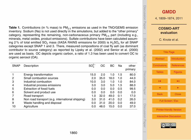
GMDD4, 1809–1874, 2011

COSMO-ARTevaluation

C. Knote et al.

Title Page



Tables Figures

J I

J I

Back Close

Full Screen / Esc



Discussion

Paper

|D

iscussionP

aper|

Discussion

Paper

|D

iscussionP

aper|

Table 1. Contributions (in % mass) to PM2.5 emissions as used in the TNO/GEMS emissioninventory. Sodium (Na) is not used directly in the simulations, but added to the “other primary”category, representing the remaining, non-carbonaceous primary PM2.5 part (including e.g.,minerals, metal oxides, product emissions). Sulfate contributions have been calculated assum-ing 2 % of total emitted SO2 mass (IIASA RAINS emissions for 2000) is H2SO4 for all SNAPcategories except SNAP 1 and 3. There, measured compositions of coal fly ash (as dominantcontributor to source category) as reported by Lipsky et al. (2002) and Senior et al. (2000)are used as basis. OC depicts organic carbon, a ratio of 1.3 has been used to convert OC toorganic aerosol (OA).

SNAP Description SO2−4 OC BC Na other

primary

1 Energy transformation 15.0 2.0 1.0 1.5 80.02 Small combustion sources 2.0 35.0 18.0 1.0 44.03 Industrial combustion 10.0 3.0 1.0 1.0 84.04 Industrial process emissions 3.0 3.0 5.0 1.5 88.05 Extraction of fossil fuels 0.0 0.0 0.0 0.5 99.56 Solvent and product use 0.0 0.0 0.0 0.0 0.07 Road transport 1.0 32.0 49.0 0.1 17.08 Non road transport (e.g. international shipping) 3.0 31.0 41.0 0.2 26.09 Waste handling and disposal 0.0 31.0 20.0 0.0 49.010 Agriculture 0.0 48.0 15.0 0.0 37.0

1860





GMDD4, 1809–1874, 2011

COSMO-ARTevaluation

C. Knote et al.

Title Page



Tables Figures

J I

J I

Back Close

Full Screen / Esc



Discussion

Paper

|D

iscussionP

aper|

Discussion

Paper

|D

iscussionP

aper|

Table 2. Normalized mean biases (%) in spring, summer, autumn and winter (SP,SU,AU,WI) forSYNOP and AIRBASE datasets, satellite comparisons and aerosol datasets. Satellite biasesare the mean over all grid points, only land points and only sea points. AERONET comparisonshows biases model – AERONET (AER), model - MODIS (MOD) at AERONET station, andMODIS – AERONET (DIF). AMS and EUSAAR biases are the mean over all stations presentedin the evaluation, the number of stations in each period is given in the notes.

SP SU AU WI note SP SU AU WI note

Meteorology (SYNOP) Satellite observations

T2m (K) 0 0 0 0 NO2 31 1 56 59 allWS10m 3 3 6 −1 (OMI) 10 −11 38 40 landWD10m 6 3 3 3 66 28 108 121 seaRH 6 −15 −4 10 AOD −58 −56 −55 −49 allGas−phase tracers and aerosol bulk mass (MODIS) −50 −58 −31 −44 land

O3 −12 −15 2 −22 rural −61 −55 −65 −51 sea−16 −3 2 −22 remote AOD at stations (AERONET/MODIS)−17 −13 −1 −23 coastal AOD −22 −61 −14 −46 AER

NO2 −2 −10 18 11 rural −30 −57 −27 −41 MOD7 −39 44 −3 remote 14 19 2 −10 DIF

10 49 44 14 coastal Aerosol chemical compositionNO −2 −14 −21 −40 rural NO−

3 39 −48 47 − 8,3,5,−69 19 75 36 remote NH+

4 −33 −72 −34 − 8,3,5,−−41 −48 −37 −30 coastal SO2−

4 −86 −84 −81 − 8,3,5,−SO2 108 0 49 39 rural OA 1 −61 −17 − 8,2,5,−

60 72 324 −11 remote Aerosol number concentrations155 203 473 75 coastal N30to50 149 − 97 − 9,−,10,−

PM10 −35 −48 3 −43 rural N50 71 − 53 − 9,−,10,−8 −39 15 −25 remote N100 64 − 76 − 9,−,10,−

16 −25 43 −7 coastal N250 139 − 257 − 9,−,10,−PM2.5 −2 −55 −11 1 rural

13 21 43 27 remote−26 −36 101 −2 coastal

1861





GMDD4, 1809–1874, 2011

COSMO-ARTevaluation

C. Knote et al.

Title Page



Tables Figures

J I

J I

Back Close

Full Screen / Esc



Discussion

Paper

|D

iscussionP

aper|

Discussion

Paper

|D

iscussionP

aper|

Table 3. Comparison of different histogram values after Asmi et al. (2011) for number sizedistributions during the autumn 2008 simulation. Note that the N250 parameter has a largeruncertainty than the others due to very low sampling rates.

station name category N30to50 N50 N100 N250

meas. mod. meas. mod. meas. mod. meas. mod.

Birkenes (NO) rural/remote 133 374 250 517 96 171 6 42Cabauw (NL) suburban 2787 2605 4649 4048 1170 1706 63 250Harwell (UK) rural 705 2181 1097 2247 410 713 51 92Ispra (IT) suburban 1732 4915 7172 6293 3829 2632 373 423K-Puszta (HU) rural 597 2698 4626 4247 2609 2013 390 313Mace Head (IE) rural/remote 48 29 158 124 104 95 41 59Melpitz (DE) rural 1031 1377 2386 3447 1306 1650 312 305Kosetice (CZ) rural/remote 508 866 2346 2724 1423 1340 262 265Vavihill (SE) rural 577 1314 1187 2761 365 1010 51 146

1862





GMDD4, 1809–1874, 2011

COSMO-ARTevaluation

C. Knote et al.

Title Page



Tables Figures

J I

J I

Back Close

Full Screen / Esc



Discussion

Paper

|D

iscussionP

aper|

Discussion

Paper

|D

iscussionP

aper|

Fig. 1. Model domain and measurement station positions. AIRBASE/EMEP: gas-phaseand bulk aerosol mass, AMS: aerosol chemical composition (EIMP/EUCAARI/EUSAAR),DMPS/SMPS: aerosol size distribution (EUSAAR/GUAN), AERONET: aerosol optical depth.The position of the column used for aerosol boundary conditions is marked with a red cross(aerosol IC/BC). Stations with AMS and/or DMPS/SMPS measurements: (a) Payerne (CH),(b) Aucencorth/Bush (UK), (c) Harwell (UK), (d) Melpitz (DE), (e) Vavihill (SE), (f) Hyytiala(FI), (g) K-Puszta (HU), (h) Cabauw (NL), (i) Helsinki (FI), (j) Barcelona (ES), (k) Montseny(ES), (l) Kosetice (CZ), (m) Aspvreten (SE), (n) Birkenes (NO), (o) Mace Head (IE), (p) Ispra(IT), (p) Waldhof (DE). Several named stations measured both chemical composition and sizedistribution.

1863





GMDD4, 1809–1874, 2011

COSMO-ARTevaluation

C. Knote et al.

Title Page



Tables Figures

J I

J I

Back Close

Full Screen / Esc



Discussion

Paper

|D

iscussionP

aper|

Discussion

Paper

|D

iscussionP

aper|

Fig. 2. Boxplots of modelled (red) and measured (blue) median values of 2 m temperature (T2m)and relative humidity (RH), and 10 m wind speed (WS). Note that 10 m wind direction (WD) aremean biases (green). Station RH was calculated from T2m and Td2m. Used are measurementsfrom the SYNOP station nearest to each AIRBASE/EMEP station used in Fig. 3. The numberof stations used is shown at the top of each comparison. Simulations are ordered to representan annual cyle: spring 2009, summer 2006, autumn 2008 and winter 2006.

1864





GMDD4, 1809–1874, 2011

COSMO-ARTevaluation

C. Knote et al.

Title Page



Tables Figures

J I

J I

Back Close

Full Screen / Esc



Discussion

Paper

|D

iscussionP

aper|

Discussion

Paper

|D

iscussionP

aper|

Fig. 3. Boxplots of modelled (red) and measured (blue) median concentrations for afternoonhours (12:00–18:00 LT) of several compounds, classified after Henne et al. (2010). The numberof stations used is shown at the top of each comparison. Note that values for NO and NO2 areon a logarithmic scale. Simulations are ordered to represent an annual cyle: spring 2009,summer 2006, autumn 2008 and winter 2006.

1865





GMDD4, 1809–1874, 2011

COSMO-ARTevaluation

C. Knote et al.

Title Page



Tables Figures

J I

J I

Back Close

Full Screen / Esc



Discussion

Paper

|D

iscussionP

aper|

Discussion

Paper

|D

iscussionP

aper|

Fig. 4. Maps of mean afternoon (12–18) NOx, O3 and SO2 concentrations for the summer 2006period. Comparison with AIRBASE station concentrations is shown as points: Modelled meanin the outer ring and measured mean in the center.

1866





GMDD4, 1809–1874, 2011

COSMO-ARTevaluation

C. Knote et al.

Title Page



Tables Figures

J I

J I

Back Close

Full Screen / Esc



Discussion

Paper

|D

iscussionP

aper|

Discussion

Paper

|D

iscussionP

aper|

Fig. 5. Modelled and measured (AIRBASE) mean diurnal cycles of several compounds during the summer 2006period, disaggregated after Henne et al. (2010). Measured values are shown as colored areas, modelled parametersas lines. Light blue areas show 90 % range of station values, the range between dotted lines the same for modelledvalues. Blue colored areas compare to the area between dashed lines (70 % range). The median of measured valuesis a solid, dark blue line, the median of modelled values a solid red line. If less than 5 stations report data, measuredand modelled medians are reported as blue and red line pair per station, with different line styles for each pair.

1867





GMDD4, 1809–1874, 2011

COSMO-ARTevaluation

C. Knote et al.

Title Page



Tables Figures

J I

J I

Back Close

Full Screen / Esc



Discussion

Paper

|D

iscussionP

aper|

Discussion

Paper

|D

iscussionP

aper|

Fig. 6. Comparison of modelled NO2 VTCs against OMI satellite data for (from top) the spring2009, summer 2006, autumn 2008 and winter 2006 periods. Modelled values are found inthe left column, OMI observations in the right one. Not the whole simulation domain could becompared due to missing coverage of the EOMINO dataset.

1868





GMDD4, 1809–1874, 2011

COSMO-ARTevaluation

C. Knote et al.

Title Page



Tables Figures

J I

J I

Back Close

Full Screen / Esc



Discussion

Paper

|D

iscussionP

aper|

Discussion

Paper

|D

iscussionP

aper|

Fig. 7. Comparison of modelled AOD (550 nm) against MODIS satellite data for (from top) thespring 2009, summer 2006, autumn 2008 and winter 2006 periods. Modelled values are foundon the left, MODIS observations on the right hand side.

1869





GMDD4, 1809–1874, 2011

COSMO-ARTevaluation

C. Knote et al.

Title Page



Tables Figures

J I

J I

Back Close

Full Screen / Esc



Discussion

Paper

|D

iscussionP

aper|

Discussion

Paper

|D

iscussionP

aper|

Fig. 8. Timelines of aerosol optical depth (AOD) at several AERONET stations in Europe during the summer 2006period. Shown are AERONET measured values (black circles), MODIS derived AOD (blue asterisks) and the simulatedAOD values (red lines). AERONET data has been cloud-screened by the data provider. MODIS data is also cloudscreened. Modelled values are masked if simulated total cloud cover was above 25 %.

1870





GMDD4, 1809–1874, 2011

COSMO-ARTevaluation

C. Knote et al.

Title Page



Tables Figures

J I

J I

Back Close

Full Screen / Esc



Discussion

Paper

|D

iscussionP

aper|

Discussion

Paper

|D

iscussionP

aper|

Fig. 9. Timeline of chemical composition of NR−PM1 (top: modelled, bottom: measured byAMS) during autumn 2008. Pie charts give mean over time period (size of pie relates totalmass). Measured OA should be compared with the sum of modelled aPOA, aSOA and bSOA.Gray shaded areas mask times without measurement data.

1871





GMDD4, 1809–1874, 2011

COSMO-ARTevaluation

C. Knote et al.

Title Page



Tables Figures

J I

J I

Back Close

Full Screen / Esc



Discussion

Paper

|D

iscussionP

aper|

Discussion

Paper

|D

iscussionP

aper|

Fig. 10a. Timeline of aerosol chemical composition as in Fig. 9 but for stations measuringduring the spring 2009 period (1 of 2).

1872





GMDD4, 1809–1874, 2011

COSMO-ARTevaluation

C. Knote et al.

Title Page



Tables Figures

J I

J I

Back Close

Full Screen / Esc



Discussion

Paper

|D

iscussionP

aper|

Discussion

Paper

|D

iscussionP

aper|

Fig. 10b. Timeline of aerosol chemical composition as done in Fig. 9 but for stations measuringduring the spring 2009 period (2 of 2).

1873





GMDD4, 1809–1874, 2011

COSMO-ARTevaluation

C. Knote et al.

Title Page



Tables Figures

J I

J I

Back Close

Full Screen / Esc



Discussion

Paper

|D

iscussionP

aper|

Discussion

Paper

|D

iscussionP

aper|

Fig. 11. Modelled and measured aerosol size distributions at EUSAAR stations for the au-tumn 2008 period. Modelled distributions are shown as area shaded by mass contributionsof different species, calculated as median over the simulation period. Measured values are astatistical size distribution from data of the whole season and are shown as lines. Solid linesdepict median values, dashed lines the 67 % and dotted lines the 90 % percentile range. Greybackground denotes areas with higher measurement uncertainty (Wiedensohler et al., 2010).

1874





Documents

Towards an online-coupled chemistry-climate model: evaluation of trace gases and aerosols in COSMO-ART